Embed Size (px)
Citation preview
IT 11 061
Examensarbete 45 hpAugusti 2011
Ordered indexing methods for data streaming applications
Sobhan Badiozamany
Institutionen för informationsteknologiDepartment of Information Technology


Teknisk- naturvetenskaplig fakultet UTH-enheten Besöksadress: Ångströmlaboratoriet Lägerhyddsvägen 1 Hus 4, Plan 0 Postadress: Box 536 751 21 Uppsala Telefon: 018 – 471 30 03 Telefax: 018 – 471 30 00 Hemsida: http://www.teknat.uu.se/student
Abstract
Ordered indexing methods for data streamingapplications
Sobhan Badiozamany
Many data streaming applications need ordered indexing techniques in order tomaintain statistics required to answer historical and continuous queries. ConventionalDBMS indexing techniques are not specifically designed for data streamingapplications; this motivates an investigation on comparing the scalability of differentordered indexing techniques in data streaming applications. This master thesiscompares two ordered indexing techniques – tries and B-trees - with each other inthe context of data streaming applications. Indexing data streams also requiressupporting high insertion and deletion rates. Two deletion strategies, bulk deletionand incremental deletion were also compared in this project. The Linear RoadBenchmark, SCSQ-LR and Amos II were comprehensively used to perform thescalability comparisons and draw conclusions.
Tryckt av: Reprocentralen ITC
Sponsor: This project is supported by VINNOVA, grant 2007-02916.IT 11 061Examinator: Anders JanssonÄmnesgranskare: Tore RischHandledare: Tore Risch


Acknowledgments
The idea of this project was suggested by Prof. Tore Risch. Without his continuous valuable
supervision, support, guidance and encouragement it was impossible to perform this study. I
would also like to thank Erik Zeitler and Thanh Truong. Erik helped me in understanding the LRB
and also running the experiments. Thanh generously shared his valuable knowledge on
extending Amos with new indexing structures.
I owe my deepest gratitude to my wife Elham, who has always been supporting me with her
pure love. She went through a lot of lonely moments so that I can finish my studies. I would also
like to show my gratitude to my parents for their dedication and the many years of support
during my whole life that has provided the foundation for this work. I also want to thank our
little Avina who with her beautiful smile gave a new meaning to our family life and provided
relaxation from stressful moments.
My special thanks go to my best friend Karwan Jacksi, who during last two years was always
around for a none-study-related friendly talk. Amanj, Hajar, Salah and other friends, thank you
very much for your support and friendship.
This project is supported by VINNOVA, grant 2007-02916.


Table of Contents
1 Introduction .......................................................................................................................................... 1
2 Background and related work ............................................................................................................... 4
2.1 The Linear Road Benchmark ......................................................................................................... 4
2.1.1 LRB data load ........................................................................................................................ 4
2.1.2 LRB performance requirements ............................................................................................ 5
2.2 Amos II and its extensibility mechanisms ..................................................................................... 6
2.3 SCSQ-LR ......................................................................................................................................... 7
2.3.1 Segment statistics, the SCSQ-LR bottleneck ......................................................................... 8
2.4 Previous applications of tries in data streaming ......................................................................... 10
2.5 Tries and common trie compression techniques ........................................................................ 10
2.5.1 Naïve trie ............................................................................................................................. 11
2.5.2 How to support integer keys in tries ................................................................................... 12
2.5.3 Naïve tries’ sensitivity to key distribution ........................................................................... 12
2.5.4 Using linked lists to reduce memory consumption in tries ................................................ 13
2.5.5 Building a local search tree in every trie node .................................................................... 13
2.5.6 Burst Trie ............................................................................................................................. 14
2.5.7 Judy, a trie based implementation from HP ....................................................................... 14
2.6 A brief evolutionary review on main memory B-trees ............................................................... 18
3 Ordered indexing methods in main memory; Trie vs. B-tree ............................................................. 19
3.1 Insertion ...................................................................................................................................... 20
3.2 Deletion ....................................................................................................................................... 20
3.3 Range Search ............................................................................................................................... 21
3.4 Memory utilization ...................................................................................................................... 22
3.5 B-trees vs. Tries in LRB ................................................................................................................ 24
3.6 Tries vs. B-trees: a more general comparison and analysis ........................................................ 24
4 SCSQ-LR implementation specifics ..................................................................................................... 26
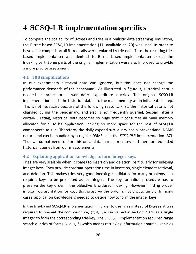
4.1 LRB simplifications ...................................................................................................................... 26
4.2 Exploiting application knowledge to form integer keys ............................................................. 26
4.3 Implementation structure: C, ALisp, AmosQL ............................................................................. 27
4.4 Performance improvements ....................................................................................................... 29
5 Index maintenance strategies ............................................................................................................. 31
5.1 Bulk deletion ............................................................................................................................... 31
5.2 Incremental deletion ................................................................................................................... 32
5.3 Bulk vs. Incremental deletion ..................................................................................................... 33
6 Experimental results ........................................................................................................................... 35
7 Conclusion ........................................................................................................................................... 36
8 Future work ......................................................................................................................................... 37
9 References .......................................................................................................................................... 38
10 Appendixes ...................................................................................................................................... 42
10.1 Appendix A – The original SCSQ-LR segment statistics code ...................................................... 42
10.2 Appendix B – Range-Search-Free segment statistics .................................................................. 43
10.3 Appendix C – Trie-based segment statistics ............................................................................... 47
10.4 Appendix D – Implementation of segment statistics using Incremental deletion ...................... 49
10.5 Appendix E – Sample code for implementing Judy ordered retrieval ........................................ 50
10.6 Appendix F – The Naïve trie data structure ................................................................................ 51
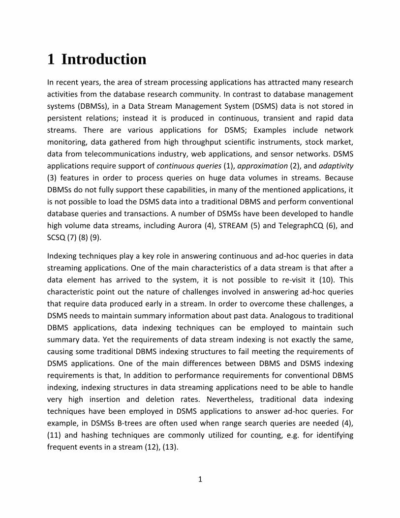
1
1 Introduction
In recent years, the area of stream processing applications has attracted many research
activities from the database research community. In contrast to database management
systems (DBMSs), in a Data Stream Management System (DSMS) data is not stored in
persistent relations; instead it is produced in continuous, transient and rapid data
streams. There are various applications for DSMS; Examples include network
monitoring, data gathered from high throughput scientific instruments, stock market,
data from telecommunications industry, web applications, and sensor networks. DSMS
applications require support of continuous queries (1), approximation (2), and adaptivity
(3) features in order to process queries on huge data volumes in streams. Because
DBMSs do not fully support these capabilities, in many of the mentioned applications, it
is not possible to load the DSMS data into a traditional DBMS and perform conventional
database queries and transactions. A number of DSMSs have been developed to handle
high volume data streams, including Aurora (4), STREAM (5) and TelegraphCQ (6), and
SCSQ (7) (8) (9).
Indexing techniques play a key role in answering continuous and ad-hoc queries in data
streaming applications. One of the main characteristics of a data stream is that after a
data element has arrived to the system, it is not possible to re-visit it (10). This
characteristic point out the nature of challenges involved in answering ad-hoc queries
that require data produced early in a stream. In order to overcome these challenges, a
DSMS needs to maintain summary information about past data. Analogous to traditional
DBMS applications, data indexing techniques can be employed to maintain such
summary data. Yet the requirements of data stream indexing is not exactly the same,
causing some traditional DBMS indexing structures to fail meeting the requirements of
DSMS applications. One of the main differences between DBMS and DSMS indexing
requirements is that, In addition to performance requirements for conventional DBMS
indexing, indexing structures in data streaming applications need to be able to handle
very high insertion and deletion rates. Nevertheless, traditional data indexing
techniques have been employed in DSMS applications to answer ad-hoc queries. For
example, in DSMSs B-trees are often used when range search queries are needed (4),
(11) and hashing techniques are commonly utilized for counting, e.g. for identifying
frequent events in a stream (12), (13).
2
In this project the scalability of two different ordered indexing structures - tries and B-
trees - are compared in data streaming applications. To get a realistic test case for data
streaming application in which we could test different indexing strategies, we used the
Linear Road Benchmark (LRB) (14). LRB is designed to evaluate the performance of a
DSMS. The main goal of the benchmark is evaluating performance of a DSMS under very
high load of input streams and historical queries. According to the benchmark
specifications, in order to pass validation an LRB implementation has to produce
accurate results and meet response time requirements as well.
In comparing scalability of different ordered indexing methods for data streaming
applications, it is important to note that supporting high insertion and deletion rate is
one of the major indexing demands. This supported the initial hypothesis that the
indexing techniques which support higher insertion and deletion rates are better
candidates for data stream indexing. On the other hand, experimental results revealed
that in practice, it is the specific mixture of insertion, deletion and range search in a
particular application that determines which indexing technique provides the most
scalable solution. To get a realistic mixture of insertion, deletion and search queries, we
used LRB to test the scalability of indexing methods. Particular to our benchmark LRB
implementation, the range search was the most demanding operation and therefore B-
trees outperformed tries.
Regarding the indexing maintenance, two deletion alternatives were compared, bulk
deletion and incremental deletion. Again LRB was used as a testing platform. As
anticipated the bulk deletion was a more scalable solution, but since in LRB the range
search was the dominant operation, different deletion alternatives provided minor
improvements which did not affect the final outcome of the benchmark implementation
in terms of the L-rating.
The rest of this report is organized as follows. In Chapter 2 the LRB, SCSQ-LR, tries and B-
trees are reviewed to provide the knowledge that is required to understand the rest of
the report. Chapter 3 presents a general comparison of in-main-memory ordered
indexing structures that are used in this project; Judy and main memory B-tree. Chapter
4 presents the developments activities that were done on SCSQ-LR during this project to
provide fair comparison between Judy and main memory B-tree in the context of a data
streaming application. Chapter 5 compares two different index maintenance strategies
in data streaming applications; bulk deletion and incremental deletion. Finally, the

3
experimental results are presented in chapter 6. Chapter 7 and chapter 8 draw the
conclusion and suggest future work.
4
2 Background and related work
In this chapter first the Linear Road Benchmark (LRB), its specifications and its
performance requirements is reviewed. Then the particular implementation of the LRB -
SCSQ-LR – that we have used in our experiments is reviewed. Next a rather detailed
review of tries and common trie compression techniques are presented. More focus is
given to Judy, a trie implementation that was used in the experiments.
2.1 The Linear Road Benchmark
The Linear Road Benchmark (LRB) (14) is designed to evaluate the performance of a
DSMS. Unlike SQL, used for queries in DBMSs, there is no standard query language for
DSMSs, thus LRB specifies a benchmark without requiring exact queries in any specific
query language. LRB simulates a variable toll system (15) for a number of expressways
(L). Each expressway is 100 miles long and is divided into 100 1-mile-long segments. An
implementation of LRB by a DSMS achieves an L-rating, which is the maximum number
of expressways it can handle. The input stream is generated by the MIT Traffic Simulator
(16) which generates input files for a given L-rating. There are four types of tuples in the
input stream: vehicle position reports, daily expenditure queries, account balance
queries, and estimated travel time queries.
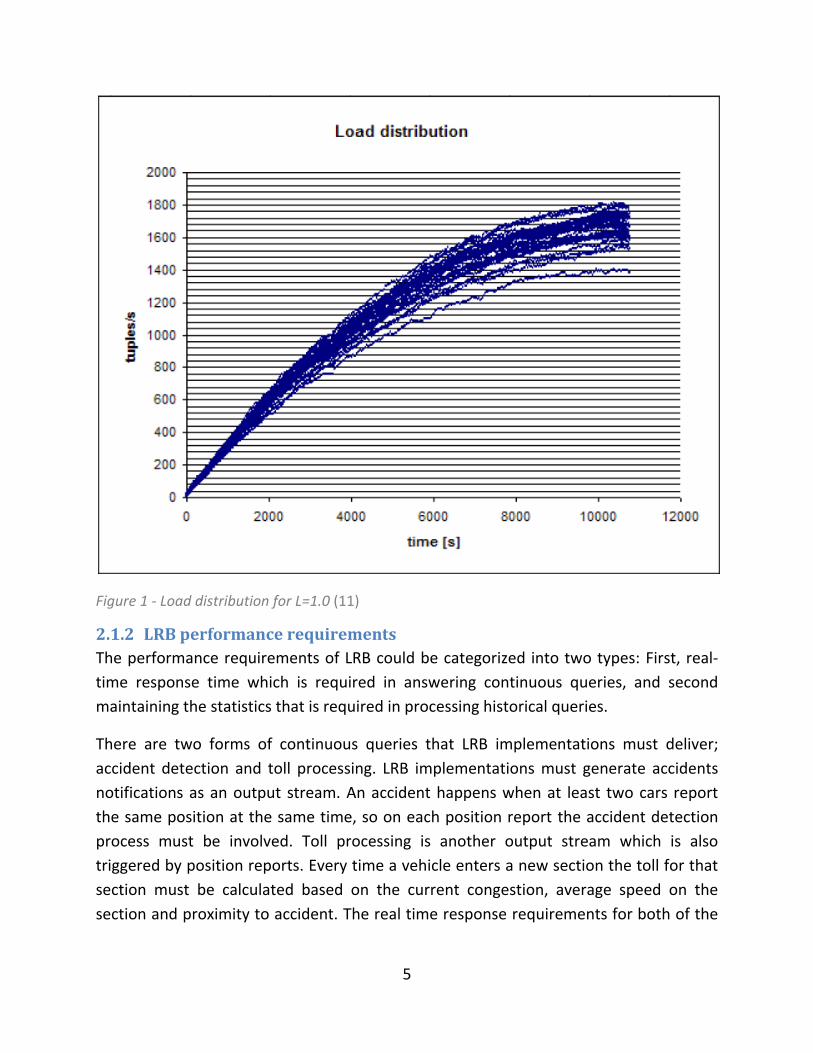
2.1.1 LRB data load
LRB runs for 3 hours. The input stream rate is not constant during the benchmark
implementation. In a single expressway, in the first second there are only 14 events. The
number of events increases as the simulation proceeds; at the end of the simulation it
reaches 1700 events per second. Because the last 13 minutes of the simulation contains
10% of all input events, the major challenge for an LRB implementation is to handle the
load at the end of the simulation. Figure 1 illustrates the load distribution for L=1.0. The
load distribution for higher L ratings is similar, but proportional to L.
5
Figure 1 - Load distribution for L=1.0 (11)
2.1.2 LRB performance requirements
The performance requirements of LRB could be categorized into two types: First, real-
time response time which is required in answering continuous queries, and second
maintaining the statistics that is required in processing historical queries.
There are two forms of continuous queries that LRB implementations must deliver;
accident detection and toll processing. LRB implementations must generate accidents
notifications as an output stream. An accident happens when at least two cars report
the same position at the same time, so on each position report the accident detection
process must be involved. Toll processing is another output stream which is also
triggered by position reports. Every time a vehicle enters a new section the toll for that
section must be calculated based on the current congestion, average speed on the
section and proximity to accident. The real time response requirements for both of the

6
mentioned continuous queries an output event to be delivered not later than 5 seconds
after the respective position report arrives to the system.
LRB specifies three historical queries; account balance, daily expenditure, and travel
time estimation. An answer to an account balance query must accumulate all tolls
charged to a vehicle from the start of the simulation. The daily expenditure query asks
about the toll for a given expressway at a given date. The travel time estimation query
requires the system to predict the time it takes to travel from one section of an
expressway to another one based on the statistics from previous ten weeks. Historical
queries are triggered when the request for them appears in the input stream. The real
time response requirement for historical queries specifies that the output must be ready
not later than 5 seconds after the respective query appears in the input stream.
Responding to continuous and historical queries requires the system to keep statistics
per each section of every expressway in every minute. In other words, statistical data
required to produce average speed and number of cars in each segment have to be
stored in an indexing structure to make fast retrieval possible when answering
continuous queries and also when historical queries arrive. If ordered indexing
structures are used to maintain statistics, like in the SCSQ-LR implementation (11),
calculating statistics becomes the bottleneck of the LRB implementation.
The LRB provided the realistic simulation in which we compared the scalability of
ordered indexing methods.
2.2 Amos II and its extensibility mechanisms
AMOS II (17) is an extensible mediator database system. There are various extensibility
mechanisms provided by Amos II, which provides the possibility of querying
heterogeneous data sources, integrate Amos II with existing systems and functionalities
in other systems, and most interestingly incorporate new indexing structures. In general
there are two methods of extending Amos II to incorporate new indexing structures.
The first method is more general and is commonly used to extend the system with any
component written in other programming languages such as C, Lisp, Java, or Python.
This is done through writing foreign functions described in (18) (19). While this method
provides all required facilities to add a new indexing structure, it takes more
development time and complicated coding. The second method, specifically designed to
add external indexing structures is called Meta External Index Manager (MEXINMA) (still
under development). MEXINMA is designed based on the fact that on an abstract level
7
all indexing methods share some analogous functionality. In MEXINMA most of the
foreign functions to access an index are previously defined and they just need to be
specialized. Furthermore, MEXINMA supports dynamic linking and provides facilities to
define index- specific query rewrite rules that are essential for query optimization.
Extensibility mechanisms of Amos II were used in this project to incorporate new
indexing structures.
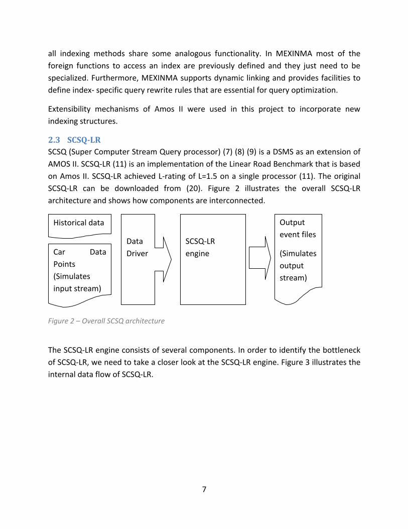
2.3 SCSQ-LR
SCSQ (Super Computer Stream Query processor) (7) (8) (9) is a DSMS as an extension of
AMOS II. SCSQ-LR (11) is an implementation of the Linear Road Benchmark that is based
on Amos II. SCSQ-LR achieved L-rating of L=1.5 on a single processor (11). The original
SCSQ-LR can be downloaded from (20). Figure 2 illustrates the overall SCSQ-LR
architecture and shows how components are interconnected.
Figure 2 – Overall SCSQ architecture
The SCSQ-LR engine consists of several components. In order to identify the bottleneck
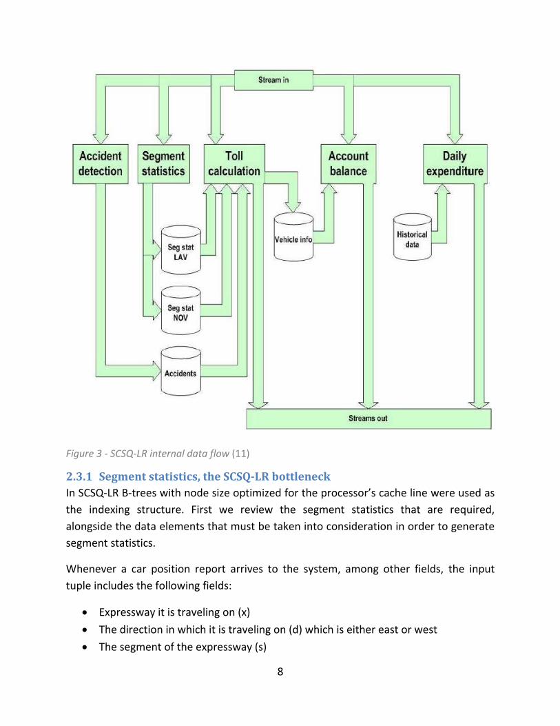
of SCSQ-LR, we need to take a closer look at the SCSQ-LR engine. Figure 3 illustrates the
internal data flow of SCSQ-LR.
Data
Driver
SCSQ-LR
engine
Output
event files
(Simulates
output
stream)
Car Data
Points
(Simulates
input stream)
Historical data
8
Figure 3 - SCSQ-LR internal data flow (11)
2.3.1 Segment statistics, the SCSQ-LR bottleneck
In SCSQ-LR B-trees with node size optimized for the processor’s cache line were used as
the indexing structure. First we review the segment statistics that are required,
alongside the data elements that must be taken into consideration in order to generate
segment statistics.
Whenever a car position report arrives to the system, among other fields, the input
tuple includes the following fields:
Expressway it is traveling on (x)
The direction in which it is traveling on (d) which is either east or west
The segment of the expressway (s)

9
The vehicle id (v).
Segment statistics in a given {x, s, d} consists of two figures LAV and NOV. LAV stands for
Latest Average Velocity and is calculated over the last 5 minutes. NOV stands for
Number Of Vehicles and is calculated over the last minute. In order to have enough
information to generate LAV and NOV per {x, s, d}, the following grain statistics have to
be stored when a position report arrives:
Average velocity of each car in a given {x, s, d}
Number of cars in a given {x, s, d}
The straight forward indexing approach is to maintain last 5 (in case of LAV) and 1 (in
case of NOV) minute of data in two B-trees. In other words, there should be two B-trees
containing the following <key, value> pairs:
<{x, s, d, v}, LAV>
<{x, s, d, v}, 1> (NOV is sum of values for the given key range:{x, s, d,*})
This requires keys to be removed when they are older than 5 (or 1) minutes, so there
will be as many individual deletions from indexing structure as there are insertions into
it. This incremental deletion approach is studied in section 5.2 alongside the bulk
deletion approach. The latter is implemented in the original SQSQ-LR and is as follows.
In the beginning of each new minute, two new B-trees are created, one for LAV and one
for NOV. Since data from last 5 and 1 minutes is required to calculate LAV and NOV
respectively, B-trees older than 5 (and 1) minutes are entirely deleted. This is based on
the fact that removing the whole B-tree is computationally cheaper than incrementally
removing individual elements from it. In total 8 B-trees were used in SCSQ-LR, 6 for
maintaining LAV and 2 for maintaining NOV. The extra B-trees are needed to store
current minute data.
Having data stored per minute as described, calculating NOV and LAV is rather simple.
To calculate NOV for a given {x, s, d}, a count query with pattern {x, s, d, *} is posed to
the NOV B-tree of last minute, this means retrieving the number of vehicles that are in
{x, s, d}. LAV can be calculated by computing the average values in the LAV B-trees of
the last 5 minutes in the {x, s, d, *} key range. To find more details about the original
SCSQ-LR segment statistics code refer to Appendix A (10.1).

10
The bottleneck of SCSQ-LR implementation were identified by profiling. Range search
(avgv) was found to be the bottleneck. The main reason for this is that for each toll
alert, all keys in a given {x, d, s} have to be visited in a range search.
During this project it was also discovered that this expensive range search can be
avoided by incrementally maintaining a moving average (21) to eliminate the necessity
of employing ordered indexing methods and therefore hash indices provide the most
scalable solution. Since the focus of this project was ordered indexing methods, no more
explanation will be provided on the range search free version of SCSQ-LR. However,
readers can refer to Appendix B (10.2) which contains the range search free version of
segment statistics.
2.4 Previous applications of tries in data streaming
Tries are frequently used when prefix sharing is required. One of such applications in
data streaming is filtering of XML streams in publication and subscriptions systems (22)
(23). In filtering of an XML stream, the problem is distributing the incoming XML stream
into several outputs/destination streams by applying respective filters. Tries were used
to implement such filters in (23) and (22). In filtering XML streams tries represent the
filters rather than indexing the incoming data stream. For example in Xtrie (23) when an
XML document appears in the stream, after it is parsed, substrings of the document are
used to probe the trie to find possible matches. In other words, in publication and
subscriptions systems tries were used to index the filters and not the incoming stream.
In contrast to applications of tries in XML stream processing, in this thesis tries were
used in a completely different context. Here we employ tries in a very general indexing
scheme that supports the same applications as other ordered indexing structures like B-
trees support. In this thesis tries were used to maintain statistics of incoming streams
which requires massive insertion and deletion of incoming stream data into the indexing
structure.
2.5 Tries and common trie compression techniques
Digital trees or tries are multi-way tree data structures that store an associative array.
Since their introduction, the most common application of tries has been indexing text.
Tries sequentially partition the key space to form the digital tree, therefore in contrast
to most tree-based indexing structures (like binary trees and spatial partitioning trees),
the position of a node in a trie indicates the keys it holds. Therefore a trie can be
considered as a type of multilevel hashing technique. Digital trees have a key difference
11
to hashing though; they maintain the order of the keys and therefore can answer range
search queries as well. The key positioning model in a trie directly implies another
attractive feature as well. There is no need for balancing the digital tree structure when
keys are added or removed. Some indexing structures like B-trees might suffer from
balancing over-head when keys are massively added or removed as for high volume
streams.
2.5.1 Naïve trie
In the simplest form of tries for indexing text, a trie is a tree structure in which each
node is an array of pointers of size of the alphabet, e.g. 256. In the internal nodes, each
element of this array points to another lower level node. In the leaf nodes, each
element points to data. In a naïve trie implementation, the keys are not stored in the
tree, they are inferred by position. The main advantage of naïve trie is its trivial
implementation. Search/insertion algorithms are simple; start from the root node and
the first character of the string key, decode the first character and follow the respective
pointer from the root node’s pointer array to get to the next node. The search/insertion
then continues by the new node and the next character in the string until we reach the
end of the string or a leaf node.
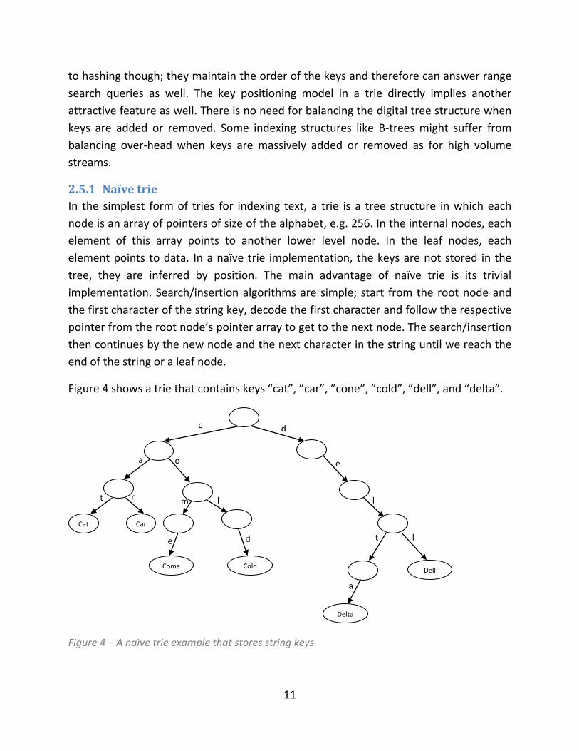
Figure 4 shows a trie that contains keys “cat”, ”car”, ”cone”, ”cold”, ”dell”, and “delta”.
Figure 4 – A naïve trie example that stores string keys
c d
e
l
l t
a
a
t r
o
m
e d
l
Cat Car
Come Cold
Delta
Dell

12
The main advantage of a trie is fast insertion and retrieval. Each string is mapped in a
time proportional to its length. This implies that if the key length is fixed, tries support
constant insertion/search access time. Another advantage is that there is no need to
compare the whole key in each level, only one byte of the key needs to be considered at
each level. In contrast, in balanced trees, the several characters of the key have to be
processed at each level, which possibly becomes expensive if the keys are long.
2.5.2 How to support integer keys in tries
Although tries are initially introduced to index character strings, they can be modified
easily to index integer values. The most straight forward way is breaking the integer into
bytes and introducing these bytes to the trie like characters of a string. In this report for
simplicity reason we always consider integers to be 32 bits. Furthermore, in this report it
is always assumed that 32 bit integer keys are broken to 4 bytes, in order to address
related pointers in different levels within the trie. Nevertheless, tries can be modified to
support longer integers and other forms of breaking integers are also possible.
In a naïve trie implementation for integer keys, the trie is always 4 levels deep. Each
node is a simple array of 256 pointers to nodes in the next level. (Or in case of nodes in
4th level, a data pointer) Refer to Appendix F (10.6) to review naïve trie data structure.
2.5.3 Naïve tries’ sensitivity to key distribution
The naïve trie suffers from poor memory utilization. Depending on data distribution,
there might be many null pointers in the sparse pointer arrays representing the trie
node, which is a waste of memory. For example, naïve tries do not scale well for uniform
distribution in wide ranges. To illustrate this phenomenon, two tests were performed on
naïve tries.
In the first test, random numbers were generated from uniform data distribution from
the full integer range. This means that in this test, each number was randomly picked
from range [0 - 2^32]. This distribution causes naïve tries to run out of memory by a
relatively small key population. This behavior is due to the fact that if the number of
inserted keys is big enough (roughly around 2^32 / 256 ~ around 16 million keys), in a
flat (uniform) distribution, many of those keys share the first 3 bytes, and therefore they
are identical except for the last byte. This results the trie to grow to a full 256ary tree 4
levels deep. This requires (256^4)-1 nodes, which will not fit into the main memory. In
practice naïve tries exhaust the main memory much earlier.
13
The second test, was also a uniform key distribution, but from a narrower integer range.
As expected, it was observed that if the data distribution range is narrower, naïve
implementations don’t waste too much main memory. This can be described using the
same concepts discussed in analyzing the first test results. For example, if the key
distribution is flat from a range that is 10,000,000 keys wide, it needs 10,000,000/256 =
39062 nodes in the lowest level in the worst case(when trie is fully grown) and this
number of nodes can easily be stored in main memory of the modern computers. The
overall utilization of each node depends on the number of keys in the trie and it
increases proportional to the density of keys in the range.
To conclude, naïve trie implementations are sensitive to key distribution. If the
distribution of the keys is random (flat) in a very wide range, naïve tries use too much
memory and do not scale. On the other hand, according to our experiments, a naïve trie
implementation scales reasonably well with normal (Gaussian) data distribution.
When designing indexing structures for streaming data, the main challenge is how to
support fast insertion/retrieval together with reasonable main memory consumption.
Several compression techniques have been introduced to overcome naïve tries weak
memory utilization (24) (25) (26) (27) (28). The main objective in most of them is to
achieve a compact representation that despite its compactness can still support
constant insertion/search time. The main trie compression techniques are reviewed in
the coming sections.
2.5.4 Using linked lists to reduce memory consumption in tries
The simplest compression approach is to use a linked list instead of a fixed size array to
represent sparse pointer array in each node. This approach is optimized good solution
from the memory consumption point of view, but it delivers poor performance.
Insertion and search algorithms need to perform a linear search in each node to find the
proper next pointer to follow. Furthermore since internal node elements are scattered
across the whole main memory, this solution does not exploit CPU caches effectively.
Two linked-list-based compression approaches are introduced in (25) (26).
2.5.5 Building a local search tree in every trie node
Another alternative to reduce memory consumption and achieve relatively good
performance is building a search tree in every node to represent the sparse pointer
array instead of having a fixed size array. This approach delivers better performance in
comparison to a linked list solution. In this approach, a logarithmic time is required to

14
traverse the node’s internal elements to find the proper pointer to follow. This is not an
optimal solution because there is still need for local search in every node which reduces
the performance of original trie implementation. This idea is implemented in ternary
search tries (27). Similar to a linked list solution, this approach does not utilize CPU
caches.
2.5.6 Burst Trie
A burst trie (28) is based on the idea that as long as the population is low, keys that
share same suffix can be stored in the same container (or node). Containers have a
limited capacity and therefore in an attempt to insert more keys into a full container,
depending on the implementation particulars, the container “bursts” into several
containers. Keys will be redistributed to new containers based on deeper suffix
calculations. This is an effective approach in decreasing memory consumption.
However, since the container capacity is fixed in all nodes, memory is still wasted in low
population nodes, and therefore this is not the optimal solution for trie memory
consumption problem.
In burst trie, the CPU cache utilization depends on the representation of the containers.
If the container is stored in consecutive memory cells (i.e. in arrays), the implementation
takes advantage of the CPU cache. Implementing containers using linked lists will result
in poor performance since CPU cache is not utilized.
2.5.7 Judy, a trie based implementation from HP
Developed by Doug Baskins at HP Labs, Judy (24) (29) (30) is a compressed trie
implementation that focuses on CPU cache utilization to improve performance. It could
be categorized as a variation of burst trie, but with an important extension to it; the
node (container) data structure and size is not fixed. To improve memory and CPU cache
utilization, Judy changes node structures according to the current population of each
node. Since Judy was used in our experiments, we review its internal structure here.
The key to an effective compression technique is to design a compact node structure
such that it fits in a single cache block. In this fashion, as soon as the node is accessed,
all of its contents are stored in the CPU cache for fast successive access.
Judy uses arrays to store compact nodes; the sizes of which are decided very carefully so
that they fit in one cache block. This gives Judy a great advantage over most other
compression techniques since it exploits the CPU cache very efficiently. Unlike Judy,
15
most compact tries (27) (28) (26) use linked lists and trees to store contents of the
compact nodes of a trie. Since the elements of a linked list are scattered across the main
memory, they do not take advantage of modern CPU caches.
In its most basic form, Judy indexes keys of the size of a machine word using the JudyL
array structure, therefore several JudyL arrays have to be combined to index longer
strings (30). This structure by definition works well for indexing integers of the size of a
machine word. JudyL is a 256ary trie, thus in 32 bit environments JudyL is always 4 levels
deep. In each level one byte of the key is decoded to locate the next-pointer to follow.
This implies that every key in a JudyL is accessible in (maximum) 4 cache line misses.
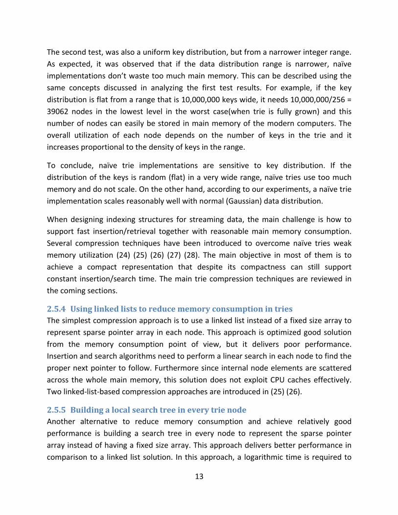
Depending on the population of each node, Judy nodes transform between one of three
node structures: linear, bitmap, and uncompressed (24). Figure 5 shows how a node
transforms from one node type to another. Linear and bitmap nodes are stored in arrays
that fit in a single cache block, but an uncompressed node is flat array of 256 elements.
Judy assumes that cache line size is 64 bits, or 16 words (24).
Figure 5 – How nodes in a Judy array transform from one form to another.
2.5.7.1 Linear nodes
When the number of pointers in a node is very small (up to 7 keys, compared to 256
keys in a fully populated uncompressed node), linear nodes are used. A linear node
consists of three sections: number of pointers, current bytes-to-decode of the keys
present in the node, and next-pointers. One byte is needed to store the number of keys,
and 7 bytes to store the current bytes of the keys. These two consume 8 bytes (2 words)
and assume 16 words cache line size; the 14 remaining words in a linear node are used
to store 7 (sorted list of) pointers (2 words each) to next level nodes. Even if the
population is below 7, the linear node is still 16 words long. This is to simplify
insertion/deletion and faster memory allocation.
Figure 6 illustrates a linear Judy node. JP stands for Judy pointer. The reason JP is longer
than expected is that it contains population data and pointer type information too. Each

16
wide block represents two words; first two narrower blocks are one word each. These
16 words are stored in an array and they altogether compose a linear node.
Figure 6 - Judy linear node (24)
Similar to burst tries, the linear nodes burst into bitmap and/or uncompressed nodes
during key insertion process if they become full.
2.5.7.2 Bitmap nodes
When a linear node becomes full, it bursts into a bitmap node. A bitmap node is a two
layer structure. The first level is the bitmap together with pointers to the second level.
The second level is a linear (packed) list of next level pointers. Bitmap nodes are also
converted to uncompressed nodes when population justifies doing so. The bitmap
needs to cover 256 elements, therefore it requires 256 bits. These bits are packed into 8
bit groups; each followed by a pointer to the list of actual next-pointers. The bitmap is
exactly 16 words long which fit in one cache block. Figure 7 illustrates an example of a
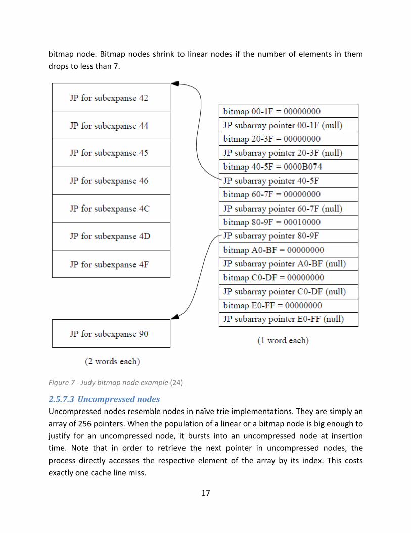
17
bitmap node. Bitmap nodes shrink to linear nodes if the number of elements in them
drops to less than 7.
Figure 7 - Judy bitmap node example (24)
2.5.7.3 Uncompressed nodes
Uncompressed nodes resemble nodes in naïve trie implementations. They are simply an
array of 256 pointers. When the population of a linear or a bitmap node is big enough to
justify for an uncompressed node, it bursts into an uncompressed node at insertion
time. Note that in order to retrieve the next pointer in uncompressed nodes, the
process directly accesses the respective element of the array by its index. This costs
exactly one cache line miss.

18
2.6 A brief evolutionary review on main memory B-trees
First introduced in 1972 by R. Bayer and E. M. McCreight (31), for over three decades,
the B-tree has been the most widely used ordered indexing method in secondary
storage. A B-tree is a generalization of binary search trees with the extension that each
node can have many children. B-trees were originally designed in the context of storing
indexing structures on disks. With ever increasing availability of cheaper and larger main
memory, in many cases it has become possible to load and/or maintain the whole B-tree
in the main memory. Unlike the first generation of B-trees in which they were tuned to
minimize expensive disk access, indexing data in main memory requires a different
optimization and tuning approach.
There were attempts to re-introduce B-tree-like indexing structures that are specifically
designed to be maintained in the main memory; among them is the T tree (32). A T tree
is again a variation of the binary tree data structure in which the nodes have always two
children and they hold an ordered array of data pointers. While T-trees are recurrently
used for main-memory databases such as Datablitz, eXtremeDB, MySQL Cluster, Oracle
TimesTen and KairosMobileLite (33), a recent study suggests that in modern processors,
they actually do not perform better than classical B-trees in the context of in-main-
memory indexing (34). Therefore classical B-trees regained the research focus and there
has been attempts to make B-trees cache conscious (34) (35).
The Main memory B-tree that was used in this project was a classical B-tree
implementation derived from (36), with one key performance improvement for in-main-
memory indexing; the sizes of the nodes were experimentally tuned to minimize cache
misses.
19
3 Ordered indexing methods in main
memory; Trie vs. B-tree
Although LRB provides a practical mixture of insertion, deletion and range search
operations, to have a more precise assessment on individual operations, in the first step
B-trees and tries were compared for pure insertion, deletion, and range search
operations outside the LRB. The data used for all these experiments were LRB data. In
addition, to remove any source of ambiguity in measuring time, all tests were done in
pure C.
In order to make sure that all time measurement of insertion, deletion, and range
search operations are pure operation-specific-time and include least possible amount of
overhead, the tests followed the following procedure:
Remove duplicates: read input tuples from the LRB input file, form the integer
keys, and store them in a unique index.
Form data array: read the unique index and insert all the keys in an array. (to
remove index access time overhead in next step, the insertion)
Insert time measurement: the keys are read from the array and inserted to the
indexing structure.
Range search time measurement: random [low, high] ranges were generated
such that they all have the same selectivity - the ratio of number of keys in [low,
high] over total number of keys in the index. The average time it took to execute
500 range searches were measured for each index structure.
Incremental deletion time measurement: by sequentially accessing the keys in
the data array, delete the keys from the indexing structure.
Given that the intention was to measure scalability, we gradually increased the number
of keys in the indexing structure in a number of steps, and then measured the time it
took to perform insertion, deletion, and range search operations. Moreover, to typify
the measurement, operations were done in batch, i.e. instead of measuring the time of
insertion of a single key in each step, which could be affected by noise, we measure the
time it took to insert e.g. 0.5 million keys.
20
All experiments were run on an Intel (R) Core(TM) i5 760 @2.80GHz 2.93 GHz CPU with
4GB RAM.
3.1 Insertion
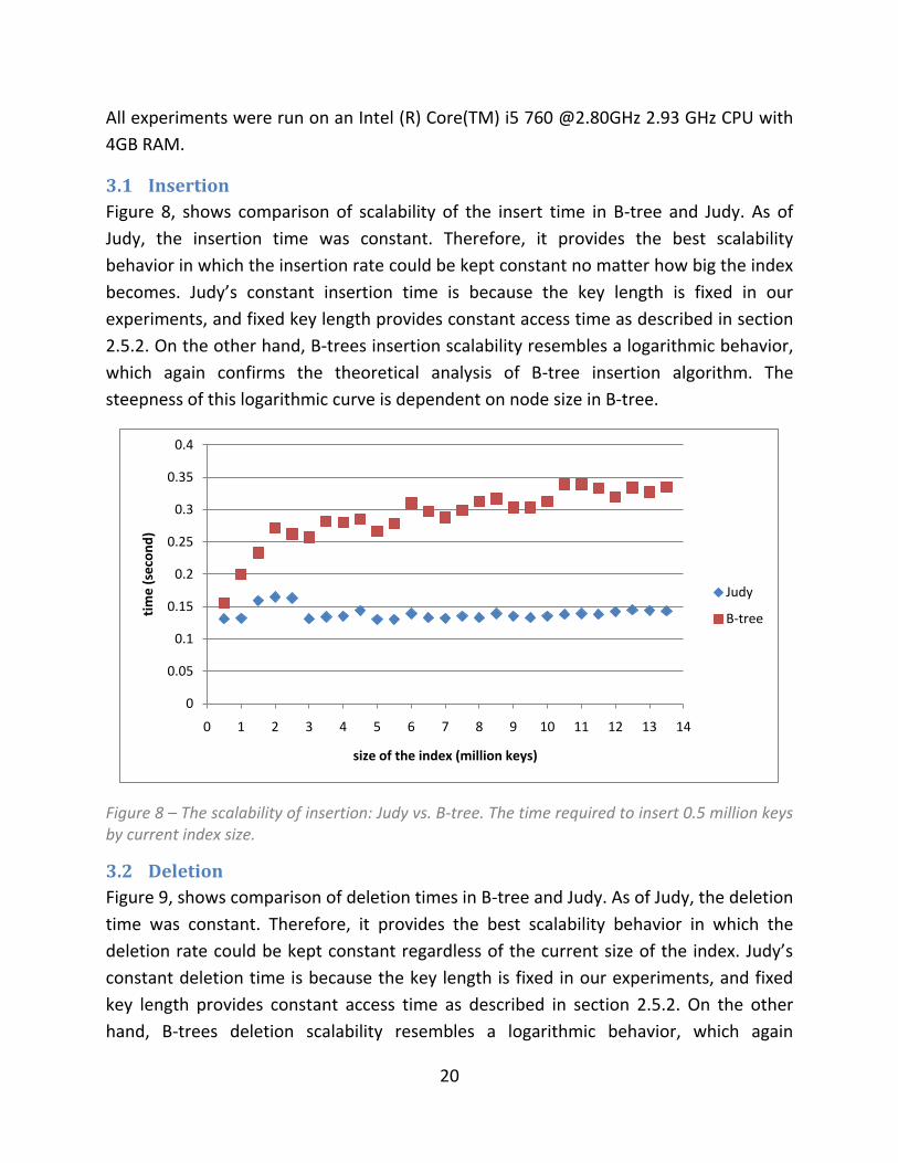
Figure 8, shows comparison of scalability of the insert time in B-tree and Judy. As of
Judy, the insertion time was constant. Therefore, it provides the best scalability
behavior in which the insertion rate could be kept constant no matter how big the index
becomes. Judy’s constant insertion time is because the key length is fixed in our
experiments, and fixed key length provides constant access time as described in section
2.5.2. On the other hand, B-trees insertion scalability resembles a logarithmic behavior,
which again confirms the theoretical analysis of B-tree insertion algorithm. The
steepness of this logarithmic curve is dependent on node size in B-tree.
Figure 8 – The scalability of insertion: Judy vs. B-tree. The time required to insert 0.5 million keys by current index size.
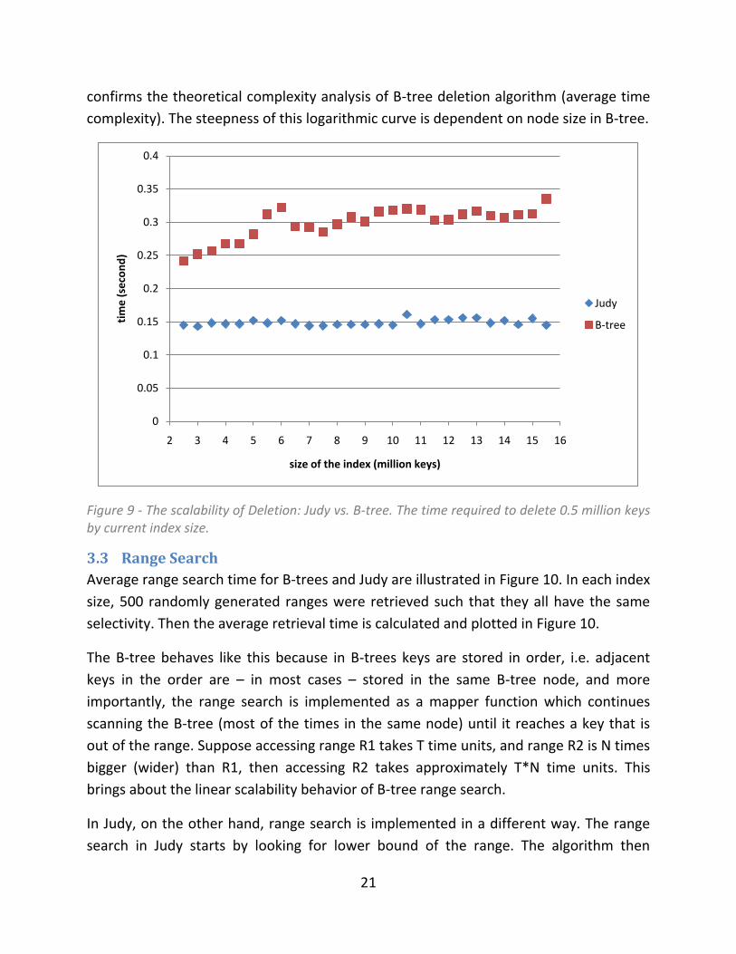
3.2 Deletion
Figure 9, shows comparison of deletion times in B-tree and Judy. As of Judy, the deletion
time was constant. Therefore, it provides the best scalability behavior in which the
deletion rate could be kept constant regardless of the current size of the index. Judy’s
constant deletion time is because the key length is fixed in our experiments, and fixed
key length provides constant access time as described in section 2.5.2. On the other
hand, B-trees deletion scalability resembles a logarithmic behavior, which again
0
0.05
0.1
0.15
0.2
0.25
0.3
0.35
0.4
0 1 2 3 4 5 6 7 8 9 10 11 12 13 14
tim
e (
seco
nd
)
size of the index (million keys)
Judy
B-tree
21
confirms the theoretical complexity analysis of B-tree deletion algorithm (average time
complexity). The steepness of this logarithmic curve is dependent on node size in B-tree.
Figure 9 - The scalability of Deletion: Judy vs. B-tree. The time required to delete 0.5 million keys by current index size.
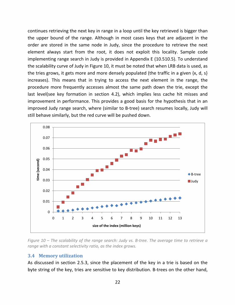
3.3 Range Search
Average range search time for B-trees and Judy are illustrated in Figure 10. In each index
size, 500 randomly generated ranges were retrieved such that they all have the same
selectivity. Then the average retrieval time is calculated and plotted in Figure 10.
The B-tree behaves like this because in B-trees keys are stored in order, i.e. adjacent
keys in the order are – in most cases – stored in the same B-tree node, and more
importantly, the range search is implemented as a mapper function which continues
scanning the B-tree (most of the times in the same node) until it reaches a key that is
out of the range. Suppose accessing range R1 takes T time units, and range R2 is N times
bigger (wider) than R1, then accessing R2 takes approximately T*N time units. This
brings about the linear scalability behavior of B-tree range search.
In Judy, on the other hand, range search is implemented in a different way. The range
search in Judy starts by looking for lower bound of the range. The algorithm then
0
0.05
0.1
0.15
0.2
0.25
0.3
0.35
0.4
2 3 4 5 6 7 8 9 10 11 12 13 14 15 16
tim
e (
seco
nd
)
size of the index (million keys)
Judy
B-tree
22
continues retrieving the next key in range in a loop until the key retrieved is bigger than
the upper bound of the range. Although in most cases keys that are adjacent in the
order are stored in the same node in Judy, since the procedure to retrieve the next
element always start from the root, it does not exploit this locality. Sample code
implementing range search in Judy is provided in Appendix E (10.510.5). To understand
the scalability curve of Judy in Figure 10, it must be noted that when LRB data is used, as
the tries grows, it gets more and more densely populated (the traffic in a given {x, d, s}
increases). This means that in trying to access the next element in the range, the
procedure more frequently accesses almost the same path down the trie, except the
last level(see key formation in section 4.2), which implies less cache hit misses and
improvement in performance. This provides a good basis for the hypothesis that in an
improved Judy range search, where (similar to B-tree) search resumes locally, Judy will
still behave similarly, but the red curve will be pushed down.
Figure 10 – The scalability of the range search: Judy vs. B-tree. The average time to retrieve a range with a constant selectivity ratio, as the index grows.
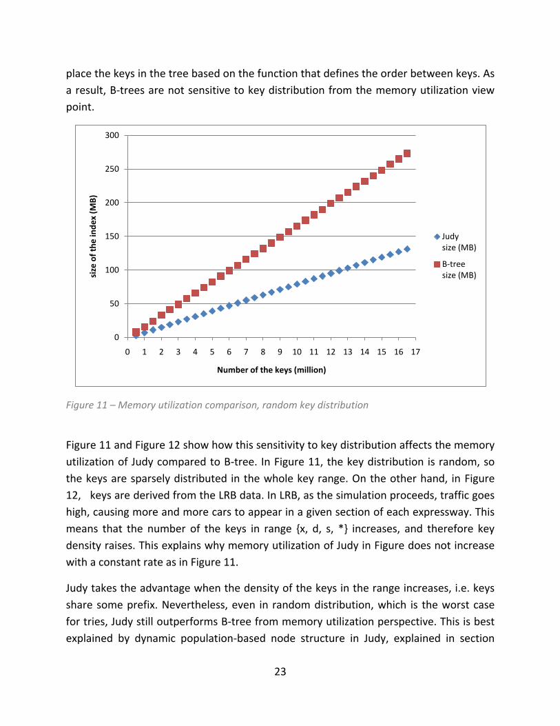
3.4 Memory utilization
As discussed in section 2.5.3, since the placement of the key in a trie is based on the
byte string of the key, tries are sensitive to key distribution. B-trees on the other hand,
0
0.01
0.02
0.03
0.04
0.05
0.06
0.07
0.08
0 1 2 3 4 5 6 7 8 9 10 11 12 13
tim
e (
seco
nd
)
size of the index (million keys)
B-tree
Judy
23
place the keys in the tree based on the function that defines the order between keys. As
a result, B-trees are not sensitive to key distribution from the memory utilization view
point.
Figure 11 – Memory utilization comparison, random key distribution
Figure 11 and Figure 12 show how this sensitivity to key distribution affects the memory
utilization of Judy compared to B-tree. In Figure 11, the key distribution is random, so
the keys are sparsely distributed in the whole key range. On the other hand, in Figure
12, keys are derived from the LRB data. In LRB, as the simulation proceeds, traffic goes
high, causing more and more cars to appear in a given section of each expressway. This
means that the number of the keys in range {x, d, s, *} increases, and therefore key
density raises. This explains why memory utilization of Judy in Figure does not increase
with a constant rate as in Figure 11.
Judy takes the advantage when the density of the keys in the range increases, i.e. keys
share some prefix. Nevertheless, even in random distribution, which is the worst case
for tries, Judy still outperforms B-tree from memory utilization perspective. This is best
explained by dynamic population-based node structure in Judy, explained in section
0
50
100
150
200
250
300
0 1 2 3 4 5 6 7 8 9 10 11 12 13 14 15 16 17
size
of
the
ind
ex
(MB
)
Number of the keys (million)
Judysize (MB)
B-treesize (MB)
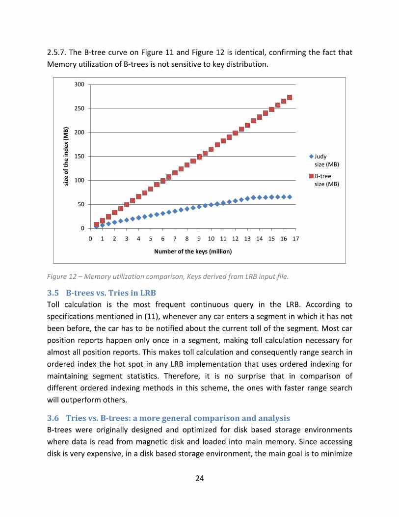
24
2.5.7. The B-tree curve on Figure 11 and Figure 12 is identical, confirming the fact that
Memory utilization of B-trees is not sensitive to key distribution.
Figure 12 – Memory utilization comparison, Keys derived from LRB input file.
3.5 B-trees vs. Tries in LRB
Toll calculation is the most frequent continuous query in the LRB. According to
specifications mentioned in (11), whenever any car enters a segment in which it has not
been before, the car has to be notified about the current toll of the segment. Most car
position reports happen only once in a segment, making toll calculation necessary for
almost all position reports. This makes toll calculation and consequently range search in
ordered index the hot spot in any LRB implementation that uses ordered indexing for
maintaining segment statistics. Therefore, it is no surprise that in comparison of
different ordered indexing methods in this scheme, the ones with faster range search
will outperform others.
3.6 Tries vs. B-trees: a more general comparison and analysis
B-trees were originally designed and optimized for disk based storage environments
where data is read from magnetic disk and loaded into main memory. Since accessing
disk is very expensive, in a disk based storage environment, the main goal is to minimize
0
50
100
150
200
250
300
0 1 2 3 4 5 6 7 8 9 10 11 12 13 14 15 16 17
size
of
the
ind
ex
(MB
)
Number of the keys (million)
Judysize (MB)
B-treesize (MB)
25
the number of accesses to disk. Consequently, the optimal node size for indexing
structures is equal to the size of a disk block. Since the disk block is huge (compared to
64 bytes CPU cache line size), B-tree nodes can contain a very high number of pointers.
More pointers in a node means higher fan out degree and a shallower tree which is the
main advantage of B-tree.
Indexing data in main memory resembles the same challenges as disk based
environments. The roles are different though, main memory is the slow storage and CPU
cache is the fast one. Another difference is that the CPU cache line is much smaller than
a disk block. Similar to disk based environments, in main memory indexing, data
structures must take block size (here, cache-line size) into consideration in order to
provide a fast and scalable indexing technique. Consequently, the optimal node size for
an in-main-memory indexing techniques is equal to the cache line size.
Although the cache line miss optimization is important in indexing data in main memory,
the best way to understand the difference between B-trees and tries is through analysis
of computational complexity of algorithms. B-trees need to maintain a balanced
structure but tries don’t. Keeping the structure balanced adds computation costs to
insertion and deletion procedures. In contrast, tries do not need to balance the
structure and provide constant access time in insertion and deletion. This characteristic
makes tries very good indexing solutions for data stream indexing. But when it comes to
retrieving a range, it is very important how the range search algorithm exploits locality.
As discussed in section 3.33.3, since the range search algorithm in B-trees exploits
locality better than Judy, it scales better in range search retrievals. After all, there is no
free lunch; tries cannot be good at all operations. Trie provides very fast insertion and
single-key-lookup at the cost of slower range search.
As a final point, choosing an ordered indexing structure for a particular application is
very much dependent on the nature of the application, and also its design. In case of
implementing LRB using ordered indexing, the application and design dictates an index-
operation-mixture in which the range search dominates insertion and deletion
operations and as a result B-trees outperform tries. Tries are still good candidates in
other data streaming applications where range search is more seldom than insertion
and deletion.
26
4 SCSQ-LR implementation specifics
To compare the scalability of B-trees and tries in a realistic data streaming simulation,
the B-tree based SCSQ-LR implementation (11) available at (20) was used. In order to
have a fair comparison all B-tree calls were replaced by trie calls. Thus the resulting trie-
based implementation was identical to B-tree based implementation except the
indexing part. Some parts of the original implementation were also improved to provide
a more precise assessment.
4.1 LRB simplifications
In our experiments historical data was ignored, but this does not change the
performance demands of the benchmark. As illustrated in figure 3, Historical data is
needed in order to answer daily expenditure queries. The original SCSQ-LR
implementation loads the historical data into the main memory as an initialization step.
This is not necessary because of the following reasons. First, the historical data is not
changed during the benchmark, and also is not frequently queried. Second, after a
certain L rating, historical data becomes so huge that it consumes all main memory
allocated for a 32 bit application, leaving no more space for the rest of SCSQ-LR
components to run. Therefore, the daily expenditure query has a conventional DBMS
nature and can be handled by a regular DBMS as in the SCSQ-PLR implementation (37).
Thus we do not need to store historical data in main memory and therefore excluded
historical queries from our measurements.
4.2 Exploiting application knowledge to form integer keys
Tries are very scalable when it comes to insertion and deletion, particularly for indexing
integer keys. They provide constant operation time in insertion, single element retrieval,
and deletion. This makes tries very good indexing candidates for many problems, but
requires keys to be presented as an integer. The key formation procedure has to
preserve the key order if the objective is ordered indexing. However, finding proper
integer representation for keys that preserve the order is not always simple. In many
cases, application knowledge is needed to decide how to form the integer keys.
In the trie-based SCSQ-LR implementation, in order to use Tries instead of B-trees, it was
required to present the compound key {x, d, s, v} (explained in section 2.3.1) as a single
integer to form the corresponding trie-key. The SCSQ-LR implementation required range
search queries of forms {x, d, s, *} which means retrieving information about all vehicles

27
travelling at a given {x, d, s}. This provides the required application knowledge about
how to preserve the order of the keys.
To form the ordered key, we put key components of the original compound key into a
single 32 bit integer in this way:
X: [0-3] (4 bits)
D: [4] (1 bit)
S: [5-11] (7 bits)
V: [12-31] (20 bits)
The above key formation poses some obvious limitations on key components; number
of expressways cannot exceed , and the number of vehicles cannot exceed . The
number of bits to present direction (D) and segment (S) are always sufficient though,
since there are only two directions and 100 segments in all cases. There are two possible
ways of overcoming these limitations. The first solution is using 64 bit integers instead
of 32 bits. This solves the problem but results in a deeper trie and therefore a slower
implementation. A second solution is making a trie for each combination of expressway
and direction. This releases 5 more bits to address vehicles. The second solution is faster
because it still needs only 32 bit integers, but it requires the indexing structure to be
redesigned.
4.3 Implementation structure: C, ALisp, AmosQL
SQSQ-LR is implemented using a combination of AmosQL (38) and ALisp (39) functions.
Most of the components that are required for the LRB implementation are written in
AmosQL. Unlike AMOSQL, ALisp is not declarative, hence it provides greater deal of
control over how the program executes. In SCSQ-LR ALisp is used only when high
performance is required. Since segment statistics is the system bottleneck, the functions
to maintain segment statistics are written in ALisp.
The core indexing techniques were done in Alisp, therefore to have a fair comparison,
testing new indexing techniques required development of driver functions that make
them available in ALisp. This crossed out the possibility of using MEXINMA (section 2.2)
and therefore the current design forced us to use the foreign functions instead.
Furthermore, we used Judy to implement a trie-based SCSQ-LR; as a result we needed to
replace B-tree calls in ALisp with Judy-trie calls. Judy is written in C, thus to make Judy
available to ALisp, we needed to write some ALisp foreign functions in C as documented
28
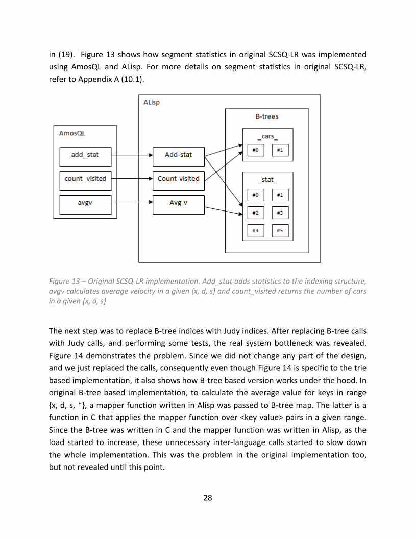
in (19). Figure 13 shows how segment statistics in original SCSQ-LR was implemented
using AmosQL and ALisp. For more details on segment statistics in original SCSQ-LR,
refer to Appendix A (10.1).
Figure 13 – Original SCSQ-LR implementation. Add_stat adds statistics to the indexing structure, avgv calculates average velocity in a given {x, d, s} and count_visited returns the number of cars in a given {x, d, s}
The next step was to replace B-tree indices with Judy indices. After replacing B-tree calls
with Judy calls, and performing some tests, the real system bottleneck was revealed.
Figure 14 demonstrates the problem. Since we did not change any part of the design,
and we just replaced the calls, consequently even though Figure 14 is specific to the trie
based implementation, it also shows how B-tree based version works under the hood. In
original B-tree based implementation, to calculate the average value for keys in range
{x, d, s, *}, a mapper function written in Alisp was passed to B-tree map. The latter is a
function in C that applies the mapper function over <key value> pairs in a given range.
Since the B-tree was written in C and the mapper function was written in Alisp, as the
load started to increase, these unnecessary inter-language calls started to slow down
the whole implementation. This was the problem in the original implementation too,
but not revealed until this point.
29
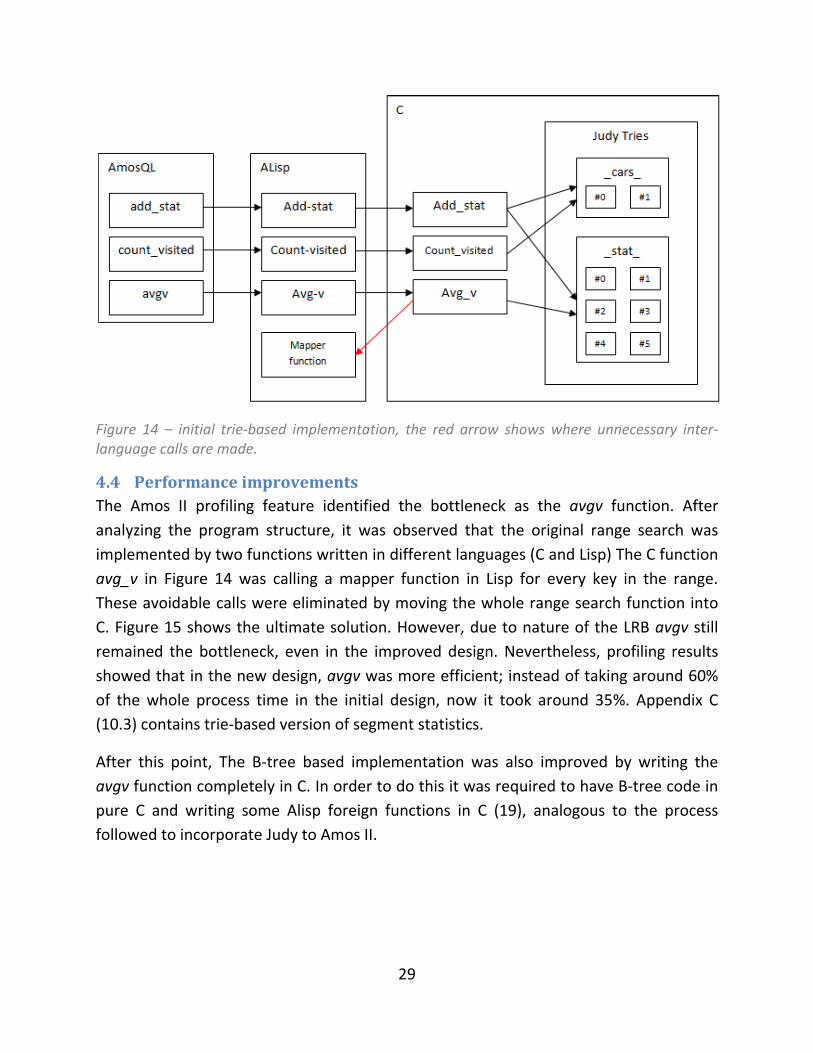
Figure 14 – initial trie-based implementation, the red arrow shows where unnecessary inter-language calls are made.
4.4 Performance improvements
The Amos II profiling feature identified the bottleneck as the avgv function. After
analyzing the program structure, it was observed that the original range search was
implemented by two functions written in different languages (C and Lisp) The C function
avg_v in Figure 14 was calling a mapper function in Lisp for every key in the range.
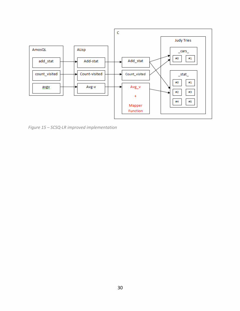
These avoidable calls were eliminated by moving the whole range search function into
C. Figure 15 shows the ultimate solution. However, due to nature of the LRB avgv still
remained the bottleneck, even in the improved design. Nevertheless, profiling results
showed that in the new design, avgv was more efficient; instead of taking around 60%
of the whole process time in the initial design, now it took around 35%. Appendix C
(10.3) contains trie-based version of segment statistics.
After this point, The B-tree based implementation was also improved by writing the
avgv function completely in C. In order to do this it was required to have B-tree code in
pure C and writing some Alisp foreign functions in C (19), analogous to the process
followed to incorporate Judy to Amos II.
30
Figure 15 – SCSQ-LR improved implementation

31
5 Index maintenance strategies
In window based stream processing (40) (41), when the number of elements in a
window grows, linear search becomes costly and an indexing structure is required.
Maintaining an index over a data stream requires high insertion rate together with high
deletion rate. In most cases elements in the stream are time stamped, and when they
reside out of the window (i.e. they expire), they must be deleted to release the memory
allocated for them.
Notice that in any maintenance strategy, after a key is removed from the primary
indexing structure, the associated tuple in database image has to be removed from the
database to release the memory allocated for that object.
In both deletion strategies in the LRB case, the window size is 5 minutes with 1 minute
stride, meaning that in the beginning of each minute M, all keys that have a time stamp
of M-5 have to be deleted. Here we introduce and compare two different deletion
strategies, we name them bulk deletion and incremental deletion.
5.1 Bulk deletion
In bulk deletion one index is maintained per window stride. When the window tumbles,
the index that contains older data has to be wiped out and a new index needs to be
created. Since the whole index structure is removed at once instead of removing
individual keys from it, we call this method bulk deletion. If the index being removed is
the primary index, all data elements that are referred by it have to be released too. This
implies that a full index scan is required.
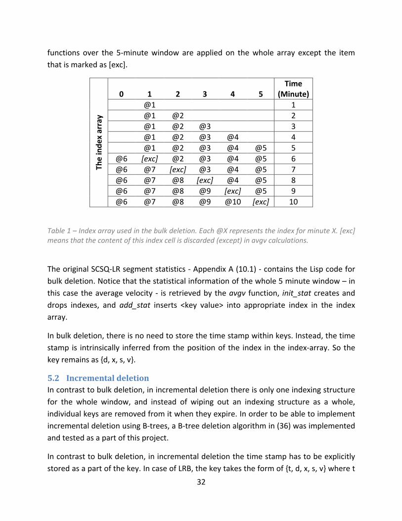
The initial design of SCSQ-LR was based on bulk deletion. In case of the LRB, to maintain
the statistics of last 5 minutes with window stride parameter one, 6 indices are needed.
In the beginning of any minute M, the index associated to minute M-5 needs to be
wiped out. This indexing structure can be implemented by a one dimensional array of
size 6 of indexes each of which containing the data for one minute. When the array
becomes full, the cell containing oldest data is selected to be released and replaced with
the new index. Table 1 shows the content of this index array during minutes 1 to 10
(here the timer starts from 1, and not 0). In each minute incoming data is inserted only
to the index associated with the current minute, tagged as @X in Table 1. The statistical
32
functions over the 5-minute window are applied on the whole array except the item
that is marked as [exc].
The
ind
ex
arra
y
0
1
2
3
4
5
Time (Minute)
@1 1
@1 @2 2
@1 @2 @3 3
@1 @2 @3 @4 4
@1 @2 @3 @4 @5 5
@6 [exc] @2 @3 @4 @5 6
@6 @7 [exc] @3 @4 @5 7
@6 @7 @8 [exc] @4 @5 8
@6 @7 @8 @9 [exc] @5 9
@6 @7 @8 @9 @10 [exc] 10
Table 1 – Index array used in the bulk deletion. Each @X represents the index for minute X. [exc] means that the content of this index cell is discarded (except) in avgv calculations.
The original SCSQ-LR segment statistics - Appendix A (10.1) - contains the Lisp code for
bulk deletion. Notice that the statistical information of the whole 5 minute window – in
this case the average velocity - is retrieved by the avgv function, init_stat creates and
drops indexes, and add_stat inserts <key value> into appropriate index in the index
array.
In bulk deletion, there is no need to store the time stamp within keys. Instead, the time
stamp is intrinsically inferred from the position of the index in the index-array. So the
key remains as {d, x, s, v}.
5.2 Incremental deletion
In contrast to bulk deletion, in incremental deletion there is only one indexing structure
for the whole window, and instead of wiping out an indexing structure as a whole,
individual keys are removed from it when they expire. In order to be able to implement
incremental deletion using B-trees, a B-tree deletion algorithm in (36) was implemented
and tested as a part of this project.
In contrast to bulk deletion, in incremental deletion the time stamp has to be explicitly
stored as a part of the key. In case of LRB, the key takes the form of {t, d, x, s, v} where t
33
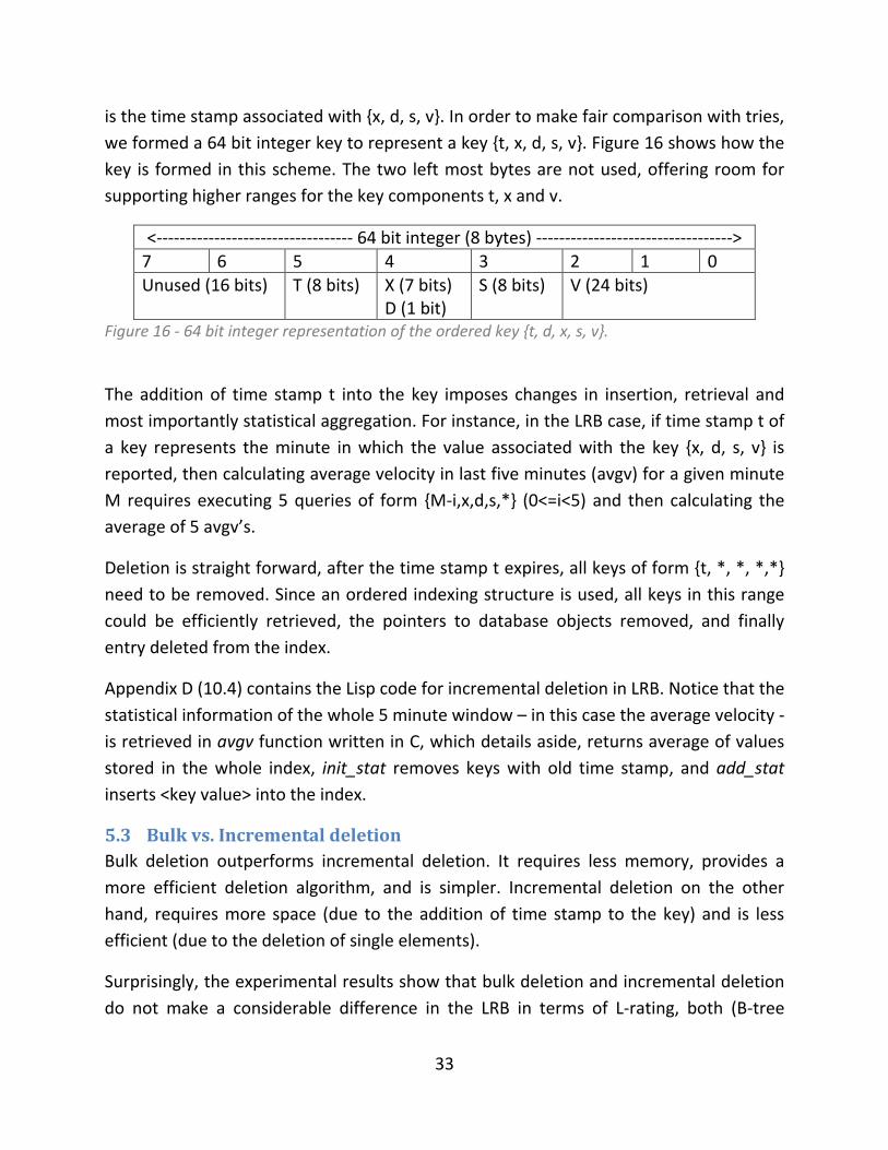
is the time stamp associated with {x, d, s, v}. In order to make fair comparison with tries,
we formed a 64 bit integer key to represent a key {t, x, d, s, v}. Figure 16 shows how the
key is formed in this scheme. The two left most bytes are not used, offering room for
supporting higher ranges for the key components t, x and v.
<---------------------------------- 64 bit integer (8 bytes) ---------------------------------->
7 6 5 4 3 2 1 0
Unused (16 bits) T (8 bits) X (7 bits) D (1 bit)
S (8 bits) V (24 bits)
Figure 16 - 64 bit integer representation of the ordered key {t, d, x, s, v}.
The addition of time stamp t into the key imposes changes in insertion, retrieval and
most importantly statistical aggregation. For instance, in the LRB case, if time stamp t of
a key represents the minute in which the value associated with the key {x, d, s, v} is
reported, then calculating average velocity in last five minutes (avgv) for a given minute
M requires executing 5 queries of form {M-i,x,d,s,*} (0<=i<5) and then calculating the
average of 5 avgv’s.
Deletion is straight forward, after the time stamp t expires, all keys of form {t, *, *, *,*}
need to be removed. Since an ordered indexing structure is used, all keys in this range
could be efficiently retrieved, the pointers to database objects removed, and finally
entry deleted from the index.
Appendix D (10.4) contains the Lisp code for incremental deletion in LRB. Notice that the
statistical information of the whole 5 minute window – in this case the average velocity -
is retrieved in avgv function written in C, which details aside, returns average of values
stored in the whole index, init_stat removes keys with old time stamp, and add_stat
inserts <key value> into the index.
5.3 Bulk vs. Incremental deletion
Bulk deletion outperforms incremental deletion. It requires less memory, provides a
more efficient deletion algorithm, and is simpler. Incremental deletion on the other
hand, requires more space (due to the addition of time stamp to the key) and is less
efficient (due to the deletion of single elements).
Surprisingly, the experimental results show that bulk deletion and incremental deletion
do not make a considerable difference in the LRB in terms of L-rating, both (B-tree

34
based) implementations achieved L=8.0. This is due to the nature of the LRB in which
deletion happens only once in a minute, and therefore its contribution to overall
processing time is insignificant. On the other hand, the range search (avgv) followed by
the insertion (add-stat) are the most demanding parts of LRB execution and they
dominate the whole implementation. Profiling results also support the hypothesis
provided above.

35
6 Experimental results
To compare the scalability of different indexing methods, the Linear Road Benchmark
(explained in section 2.1) was used as a realistic simulation of a data streaming
application. Table 2 contains the L-Rating achieved by each indexing technique.
Original SCSQ-LR (B-tree-based)
B-tree-based (after improvement)
Judy-based (after improvement)
Bulk deletion L=3.0 L=8.0 L=6.0
Incremental deletion Not tested* L=8.0 Not tested*
Table 2- the L-rating achieved by different indexing techniques. * expected to be the same as the L-rating for incremental deletion, but not implemented.
All tests were performed on a HP desktop machine with "Intel (R) Core(TM) i5 760
@2.80GHz 2.93 GHz" CPU and 4GB RAM. Furthermore, only a single CPU was used
during all the experiments.
During this project it was realized that the need for range search in LRB could be
eliminated by maintaining of a moving average (16) (Appendix B 10.2), hence the
ordered indexing was not required in the LRB implementation and hashing methods
would present the most efficient and scalable indexing solution. The range-search-free
based LRB implementation is expected to achieve better results, though investigating its
scalability is out of the scope of this project and therefore has not been fully tested yet.

36
7 Conclusion
In this project, two ordered indexing methods were compared in a practical application,
the Linear Road Benchmark. Some developments in the Linear Road Benchmark were
required to achieve to a platform on top of which we could perform the comparison.
Using ordered indexing methods in the implementation of the Linear Road benchmark
dictates a major bottleneck, the range search. Since the trie data structure we used –
Judy - was not as fast as B-tree in range search retrievals, B-trees outperformed Judy.
More general experiments show that tries are superior in insertion and deletion, a fact
that still keeps tries among good candidates for data streaming applications where
range search is more seldom compared to insertion and deletion.
Two index maintenance strategies were also compared in this project, Bulk deletion and
Incremental Deletion. Although bulk deletion is more efficient and more scalable than
incremental deletion, Experiments based on the Linear road benchmark show that - yet
again - due to dominance of the range search, using bulk deletion does not improve the
final outcome of the benchmark in term of the L-rating.

37
8 Future work
It is worth to investigate the possibility of development of a faster range search in tries.
This is motivated by their scalable insertion and deletion operations, which – if
complemented by a more scalable range search- possible makes them the best ordered
indexing solutions for data streaming applications. The current range search in Judy is
implemented such that the search starts from the root of the trie every time the search
starts. Developing a mapper function that traverses the trie given a [high, low] bound
could potentially improve the support of the range search by tries and perhaps win the
battle against the B-trees. During this investigation, other compact trie variations can
also be tested and compared to Judy and B-trees. Especially simpler burst tries are
worth to try because they provide similar behavior to Judy and it is easier to investigate
possible improvements on range search facilities.
Comparing the performance of Judy to B-trees in other data streaming applications
could reveal different results. It is therefore worth to perform a similar study in
applications where ordered indexing is required, but the fraction of the required range
search is relatively smaller than insertion and deletion.
After studying different deletion strategies and powered by MEXINMA, a window based
indexing structure for data streaming applications could emerge as a package with high
abstraction level. This will improve the declarative nature of SCSQ and eventually makes
it possible to develop a fully declarative implementation of LRB and eliminate the code
currently written in Lisp and/or C.
Another interesting aspect to investigate is effect of running bulk deletion in a separate
thread. At the moment, SCSQ-LR runs in a single thread, and therefore bulk deletion
blocks the whole process. If bulk deletion runs in a separate thread, it could potentially
support a closer-to-real-time behavior which results in a smoother response time curve.
However, because deletion is not the most demanding part of the SCSQ-LR, this is not
expected to make significant improvements in terms of L-rating.
A byproduct of this project was range search free implementation of SCSQ-LR. It opens
the possibility to utilize the state of the art hashing methods and investigate the highest
possible L-rating that could be achieved on a single CPU. This, together with parallel
SCSQ-LR implementation (37) can achieve higher L-rating with lower number of nodes.
38
9 References
1. Continuous queries over append-only databases. Terry, Douglas, et al. 1992, SIGMOD
'92 Proceedings of the 1992 ACM SIGMOD international conference on Management of
data.
2. al, D. B. et. The New Jersey data reduction report. IEEE Data Engineering Bulletin.
1997, pp. 3–45.
3. Continuously adaptive query processing. Eddies, R. Avnur and J. Hellerstein. s.l. :
ACM, 2000. ACM SIGMOD Intl.Conf. on Management of Data. pp. 261–272.
4. Daniel J, Abadi et al. Aurora: a new model and architecture for data. VLDB Journal
12(2). August 2003.
5. The Stanford Stream Data Manager (Demonstration Description). A. Arasu, B.
Babcock, M. Datar, K. Ito, I. Nishizawa,J. Rosenstein, and J. Widom. San Diego, CA :
SIGMOD 2003, 2003. ACM International Con-ference on Management of Data.
6. TelegraphCQ: Continuous data°ow processing for an uncertain world. S.
Chandrasekaran, O. Cooper, A. Deshpande, M. J. Franklin, J. M. Hellerstein, W. Hong,
S. Krishnamurthy, S. Madden, V. Raman, F. Reiss, and M. Shah. Asilomar, CA : (CIDR
2003), 2003. Innovative Data Systems Research .
7. Processing high-volume stream queries on a super-computer. E.Zeitler, T.Risch.
Atlanta, GA : s.n., 2006. ICDE Ph.D. Workshop.
8. Using stream queries to measure communication performance of a parallel computing
environment. Erik Zeitler, Tore Risch. Toronto, Canada : IEEE computer society, 2007.
27th International Conference on Distributed Computing Systems Workshops.
9. Highly scalable trip grouping for large-scale collective transportation systems. Gyozo
Gidofalvi, Torben Bach Pedersen, Tore Risch, Erik Zeitler. s.l. : ACM, 2008. EDBT '08
Proceedings of the 11th international conference on Extending database technology:
Advances in database technology.
10. Models and issues in data stream systems. Brian Babcock, Shivnath Babu, Mayur
Datar, Rajeev Motwani, Jennifer Widom. s.l. : twenty-first ACM SIGMOD-SIGACT-
SIGART symposium on Principles of database systems, 2002.
39
11. Svensson, Mårten. Benchmarking the performance of a data stream management
system. s.l. : Uppsala University, 2007.
12. New directions in traffic measurement and accounting. Cristian Estan, George
Varghese. s.l. : IMW '01 Proceedings of the 1st ACM SIGCOMM Workshop on Internet
Measurement, 2001.
13. Sensor Data Mining: Similarity Search and Pattern Analysis. Faloutsos, C. s.l. :
Tutorial in Proc. Int. Conf. on Very Large Data Bases, 2002.
14. LR Home page. Linear Road Benchmark. [Online] Brandeis University. [Cited: 02 13,
2011.] http://pages.cs.brandeis.edu/~linearroad/.
15. Wikipedia. High occupancy/toll and express toll lanes. Wikipedia. [Online]
Wikipedia. [Cited: 02 13, 2011.]
http://en.wikipedia.org/wiki/High_occupancy/toll_and_express_toll_lanes.
16. MIT. MIT Traffic Simulator. [Online] [Cited: 02 13, 2011.]
http://mit.edu/its/mitsimlab.html.
17. Risch, Tore, Josifovski, Vanja and Katchaounov, Timour. Functional Data Integration
in a Distributed Mediator System. [book auth.] L.Kerschberg, P.King, and A.Poulovassilis
P.Gray. Functional Approach to Data Management - Modeling, Analyzing and
Integrating Heterogeneous Data. s.l. : Springer, 2003.
18. Risch, Tore. Amos II External Interfaces. UDBL. [Online] 01 24, 2001.
http://user.it.uu.se/~torer/publ/external.pdf.
19. —. aStorage. Public UDBL Docs. [Online] 09 03, 2009. [Cited: 8 1, 2011.]
http://user.it.uu.se/~torer/publ/aStorage.pdf.
20. SCSQ-LR Home Page. UDBL. [Online] Uppsala University. [Cited: 02 16, 2011.]
http://user.it.uu.se/~udbl/lr.html.
21. Moving average. Wikipedia. [Online] [Cited: 07 27, 2011.]
http://en.wikipedia.org/wiki/Moving_average.
22. AFilter: Adaptable XML Filtering with Prefix-Caching and SuffixClustering. Candan, K.
Selcuk, et al. Seoul, South Korea : ACM VLDB, 2006.
40
23. Efficient Filtering of XML Documents with XPath Expressions. Chan, Chee-Yong, et al.
s.l. : International Conference on Data Engineering (ICDE’02), 2002.
24. Silverstein, Alan. Judy IV Shop Manual. s.l. : HP, 2002.
25. File searching using variable length keys. Briandais, Rene De La. New York : western
joint computer conference, 1959.
26. Knuth, Donald E. Sorting and Searching. The are of computer programming.
Redwood city, California, US : Addison Wesley Longman, 1998.
27. Fast algorithms for sorting and searching strings. Bentley, Jon L. and Sedgewick,
Robert. New Orleans, Luisiana, USA : SODA '97 Proceedings of the eighth annual ACM-
SIAM symposium on Discrete algorithms , 1997.
28. Burst tries: a fast, efficient data structure for string keys. Heinz, Steffen, Zobel,
Justin and Williams, Hugh E. 2, New York : ACM Transactions on Information Systems
(TOIS), 2002, Vol. 20.
29. Judy web page. [Online] [Cited: 02 25, 2011.]
http://judy.sourceforge.net/glossary/index.html.
30. HP. Programming with Judy. s.l. : HP, 2001.
31. R. Bayer, E. M. McCreight. Organization and maintenance of large ordered indexes.
Acta Informatica. 1972, Vols. 1,#3.
32. A Study of Index Structures for Main Memory Database Management Systems. Tobin
J. Lehman, Michael J. Carey. Kyoto : Proceedings of the Twelfth International
Conference on Very Large Data Bases, 1986.
33. T Tree. Wikipedia. [Online] [Cited: 08 05, 2011.] http://en.wikipedia.org/wiki/T-tree.
34. Cache Conscious Indexing for Decision-Support in Main Memory. Rao, J. Ross, K. s.l. :
PROCEEDINGS OF THE INTERNATIONAL CONFERENCE ON VERY LARGE DATA BASES,
1999.
35. Making B+- trees cache conscious in main memory. Jun Rao, Kenneth A. Ross. s.l. :
Proceedings of the 2000 ACM SIGMOD international conference on Management of
data , 2000.
41
36. Wirth, Niklaus. Dynamic Information Structures. Algorithms and Data Structures.
Englewood Cliffs : Prentice-Hall, 1986.
37. Zeitler, Erik and Risch, Tore. Scalable Splitting of Massive Data Streams. [book auth.]
Yoshiharu Ishikawa, Qing Li and Chiemi Watanabe. Database Systems for Advanced
Applications. Berlin/Heidelberg : Springer, 2010.
38. Flodin, Staffan, et al. Amos II Release 13 User's Manual. UDBL. [Online] 2011. [Cited:
03 08, 2011.] http://user.it.uu.se/~udbl/amos/doc/amos_users_guide.html.
39. Risch, Tore. ALisp v2 User’s Guide. s.l. : Uppsala Database Laboratory, 2006.
40. Query Processing, Resource Management, and Approximation in a Data Stream
Management System. Rajeev Motwani, Jennifer Widom, Arvind Arasu, Brian Babcock,
Shivnath Babu,Mayur Datar, Gurmeet Manku, Chris Olston, Justin Rosenstein, Rohit
Varma. s.l. : Proceedings of the 2003 CIDR Conference, 2003.
41. Lukasz Golab, M. Tamer Ozsu. Issues in Data Stream Management. SIGMOD Record.
2003, Vol. 32.
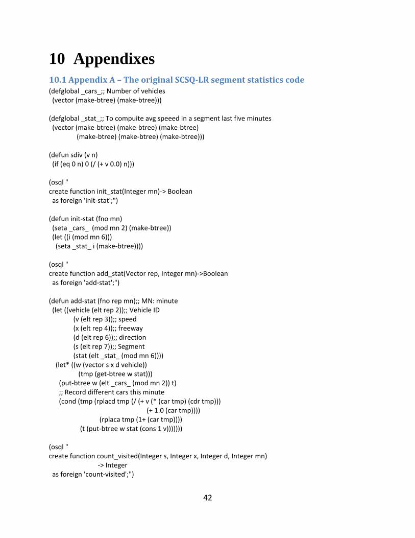
42
10 Appendixes
10.1 Appendix A – The original SCSQ-LR segment statistics code (defglobal _cars_;; Number of vehicles (vector (make-btree) (make-btree))) (defglobal _stat_;; To compuite avg speeed in a segment last five minutes (vector (make-btree) (make-btree) (make-btree) (make-btree) (make-btree) (make-btree))) (defun sdiv (v n) (if (eq 0 n) 0 (/ (+ v 0.0) n))) (osql " create function init_stat(Integer mn)-> Boolean as foreign 'init-stat';") (defun init-stat (fno mn) (seta _cars_ (mod mn 2) (make-btree)) (let ((i (mod mn 6))) (seta _stat_ i (make-btree)))) (osql " create function add_stat(Vector rep, Integer mn)->Boolean as foreign 'add-stat';") (defun add-stat (fno rep mn);; MN: minute (let ((vehicle (elt rep 2));; Vehicle ID (v (elt rep 3));; speed (x (elt rep 4));; freeway (d (elt rep 6));; direction (s (elt rep 7));; Segment (stat (elt _stat_ (mod mn 6)))) (let* ((w (vector s x d vehicle)) (tmp (get-btree w stat))) (put-btree w (elt _cars_ (mod mn 2)) t) ;; Record different cars this minute (cond (tmp (rplacd tmp (/ (+ v (* (car tmp) (cdr tmp))) (+ 1.0 (car tmp)))) (rplaca tmp (1+ (car tmp)))) (t (put-btree w stat (cons 1 v))))))) (osql " create function count_visited(Integer s, Integer x, Integer d, Integer mn) -> Integer as foreign 'count-visited';")
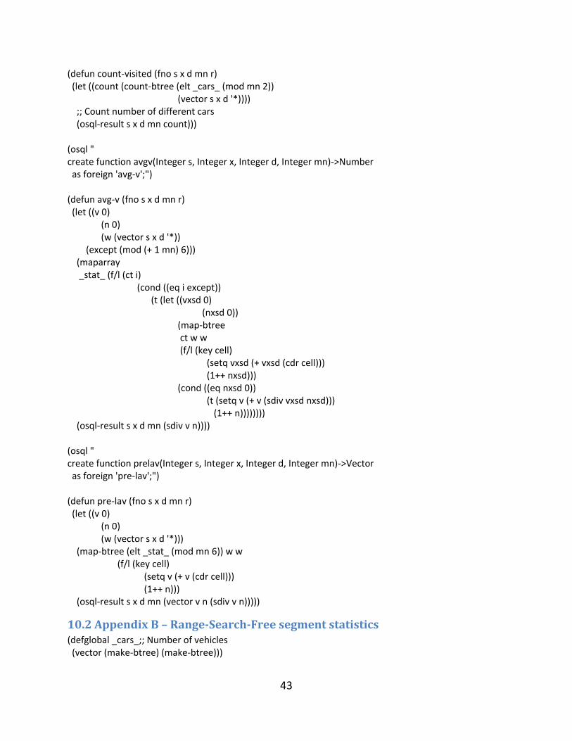
43
(defun count-visited (fno s x d mn r) (let ((count (count-btree (elt _cars_ (mod mn 2)) (vector s x d '*)))) ;; Count number of different cars (osql-result s x d mn count))) (osql " create function avgv(Integer s, Integer x, Integer d, Integer mn)->Number as foreign 'avg-v';") (defun avg-v (fno s x d mn r) (let ((v 0) (n 0) (w (vector s x d '*)) (except (mod (+ 1 mn) 6))) (maparray _stat_ (f/l (ct i) (cond ((eq i except)) (t (let ((vxsd 0) (nxsd 0)) (map-btree ct w w (f/l (key cell) (setq vxsd (+ vxsd (cdr cell))) (1++ nxsd))) (cond ((eq nxsd 0)) (t (setq v (+ v (sdiv vxsd nxsd))) (1++ n)))))))) (osql-result s x d mn (sdiv v n)))) (osql " create function prelav(Integer s, Integer x, Integer d, Integer mn)->Vector as foreign 'pre-lav';") (defun pre-lav (fno s x d mn r) (let ((v 0) (n 0) (w (vector s x d '*))) (map-btree (elt _stat_ (mod mn 6)) w w (f/l (key cell) (setq v (+ v (cdr cell))) (1++ n))) (osql-result s x d mn (vector v n (sdiv v n)))))
10.2 Appendix B – Range-Search-Free segment statistics (defglobal _cars_;; Number of vehicles (vector (make-btree) (make-btree)))
44
(defglobal _stat_;; To compuite avg speeed of a given vehicle in a segment in last five minutes (vector (make-btree) (make-btree) (make-btree) (make-btree) (make-btree) (make-btree))) (defglobal _avgv_;; maintains moving average avgv in a given dxs in last five minutes in form of sum/count (vector (MAKE-HASH-TABLE :TEST (FUNCTION EQUAL)) (MAKE-HASH-TABLE :TEST (FUNCTION EQUAL)) (MAKE-HASH-TABLE :TEST (FUNCTION EQUAL)) (MAKE-HASH-TABLE :TEST (FUNCTION EQUAL)) (MAKE-HASH-TABLE :TEST (FUNCTION EQUAL)) (MAKE-HASH-TABLE :TEST (FUNCTION EQUAL)) ) ) (defun sdiv (v n) (if (eq 0 n) 0 (/ (+ v 0.0) n))) (osql " create function init_stat(Integer mn)-> Boolean as foreign 'init-stat';") (defun init-stat (fno mn) (seta _cars_ (mod mn 2) (make-btree)) (let ((i (mod mn 6))) (seta _stat_ i (make-btree)) (seta _avgv_ i (MAKE-HASH-TABLE :TEST (FUNCTION EQUAL))) ) ) (osql " create function add_stat(Vector rep, Integer mn)->Boolean as foreign 'add-stat';") (defun add-stat (fno rep mn);; MN: minute (let ((vehicle (elt rep 2));; Vehicle ID (v (elt rep 3));; speed (x (elt rep 4));; freeway (d (elt rep 6));; direction (s (elt rep 7));; Segment (stat (elt _stat_ (mod mn 6))) (avgv_ht (elt _avgv_ (mod mn 6))) ) (let* ( (w (vector s x d vehicle)) (tmp (get-btree w stat)) (avgv_key (vector s x d))
45
(avgv_val (gethash avgv_key avgv_ht)) ) (put-btree w (elt _cars_ (mod mn 2)) t) ;; Record different cars this minute (cond (tmp (let ((prev_v (cdr tmp))) (rplacd tmp (/ (+ v (* (car tmp) (cdr tmp))) (+ 1.0 (car tmp))));;update avgv of this car in sxd (rplaca tmp (1+ (car tmp)));;increment number of occurences of this car in sxd ;;adjust avgv in sxd, (no increase in number of cars) (rplacd avgv_val (+ (cdr avgv_val) (/ (- (cdr tmp) prev_v) (car avgv_val)))) ) ) (t;;First time this car apperas in sxd (put-btree w stat (cons 1 v));;add vehicle info to sxdmn stats ;;update avgv in sxd (cond (avgv_val;;in case avgv fo sxd already exists ;;adjust avgv of sxdmn for new vehicle speed (rplacd avgv_val (/ (+ (*(car avgv_val)(cdr avgv_val)) v ) (+ 1.0 (car avgv_val)) )) ;;Increment the number of vehicles involved in this avgv (rplaca avgv_val (+ 1.0 (car avgv_val))) ) (t;;In case avgv fo sxd does not exists yet. (this is the first car that appears in sxdmn) (setf (gethash avgv_key avgv_ht ) (cons 1.0 v)) ) ) ) ) ))) (osql " create function count_visited(Integer s, Integer x, Integer d, Integer mn) -> Integer as foreign 'count-visited';") (defun count-visited (fno s x d mn r) (let ((count (count-btree (elt _cars_ (mod mn 2)) (vector s x d '*)))) ;; Count number of different cars (osql-result s x d mn count))) (osql " create function count_visited_ht(Integer s, Integer x, Integer d, Integer mn) -> Integer as foreign 'count-visited-ht';") (defun count-visited-ht (fno s x d mn r) (let*
46
( (avgv_key (vector s x d)) (avgv_ht (elt _avgv_ (mod mn 6))) (count (car (gethash avgv_key avgv_ht))) ) ;; Count number of different cars (osql-result s x d mn count) ) ) (osql " create function avgv(Integer s, Integer x, Integer d, Integer mn)->Number as foreign 'avg-v-ht';") (defun avg-v-ht (fno s x d mn r) (let ( (v 0) (n 0) (w (vector s x d)) (except (mod (+ 1 mn) 6)) ) ( maparray _avgv_ (f/l (ct i) (cond ((eq i except)) ((gethash w ct) (setq v (+ v (cdr (gethash w ct)))) (1++ n) ) ) ) ) (osql-result s x d mn (sdiv v n)))) (defun avg-v-original (fno s x d mn r) (let ((v 0) (n 0) (w (vector s x d '*)) (except (mod (+ 1 mn) 6))) (maparray _stat_ (f/l (ct i) (cond ((eq i except)) (t (let ((vxsd 0) (nxsd 0)) (map-btree ct w w (f/l (key cell) (setq vxsd (+ vxsd (cdr cell)))
47
(1++ nxsd))) (cond ((eq nxsd 0)) (t (setq v (+ v (sdiv vxsd nxsd))) (1++ n)))))))) (osql-result s x d mn (sdiv v n)))) (osql " create function prelav(Integer s, Integer x, Integer d, Integer mn)->Vector as foreign 'pre-lav';") (defun pre-lav (fno s x d mn r) (let ((v 0) (n 0) (w (vector s x d '*))) (map-btree (elt _stat_ (mod mn 6)) w w (f/l (key cell) (setq v (+ v (cdr cell))) (1++ n))) (osql-result s x d mn (vector v n (sdiv v n)))))
10.3 Appendix C – Trie-based segment statistics (defun add-stat (fno rep mn);; MN: minute (let ((vehicle (elt rep 2));; Vehicle ID (v (elt rep 3));; speed (x (elt rep 4));; freeway (d (elt rep 6));; direction (s (elt rep 7));; Segment (stat (elt _stat_ (mod mn 6)))) (let* ((w (trie-key (vector s x d vehicle))) (tmp (get-trie w stat))) (put-trie w (elt _cars_ (mod mn 2)) t) ;; Record different cars this minute (cond (tmp (rplacd tmp (/ (+ v (* (car tmp) (cdr tmp))) (+ 1.0 (car tmp)))) (rplaca tmp (1+ (car tmp)))) (t (put-trie w stat (cons 1 (+ 0.0 v))))))));; add 0.0 so that v is always a floating point number ;;trie-low-range (x) takes vector of numbers x eg. (s x d *) and returns the trie key representing the buttom of the range ;;trie-high-range (x) takes vector of numbers x eg. (s x d *) and returns the trie key representing the top of the range (osql " create function count_visited(Integer s, Integer x, Integer d, Integer mn) -> Integer as foreign 'count-visited';")
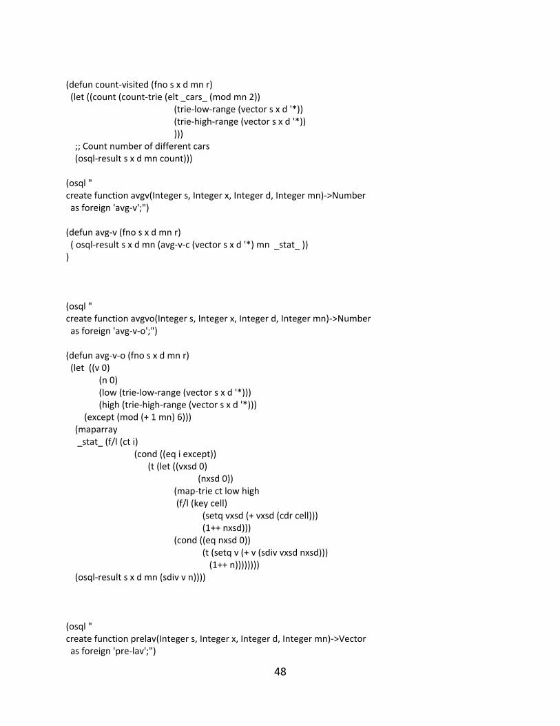
48
(defun count-visited (fno s x d mn r) (let ((count (count-trie (elt _cars_ (mod mn 2)) (trie-low-range (vector s x d '*)) (trie-high-range (vector s x d '*)) ))) ;; Count number of different cars (osql-result s x d mn count))) (osql " create function avgv(Integer s, Integer x, Integer d, Integer mn)->Number as foreign 'avg-v';") (defun avg-v (fno s x d mn r) ( osql-result s x d mn (avg-v-c (vector s x d '*) mn _stat_ )) ) (osql " create function avgvo(Integer s, Integer x, Integer d, Integer mn)->Number as foreign 'avg-v-o';") (defun avg-v-o (fno s x d mn r) (let ((v 0) (n 0) (low (trie-low-range (vector s x d '*))) (high (trie-high-range (vector s x d '*))) (except (mod (+ 1 mn) 6))) (maparray _stat_ (f/l (ct i) (cond ((eq i except)) (t (let ((vxsd 0) (nxsd 0)) (map-trie ct low high (f/l (key cell) (setq vxsd (+ vxsd (cdr cell))) (1++ nxsd))) (cond ((eq nxsd 0)) (t (setq v (+ v (sdiv vxsd nxsd))) (1++ n)))))))) (osql-result s x d mn (sdiv v n)))) (osql " create function prelav(Integer s, Integer x, Integer d, Integer mn)->Vector as foreign 'pre-lav';")
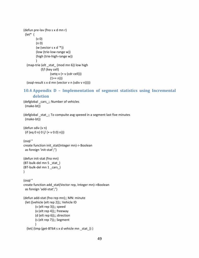
49
(defun pre-lav (fno s x d mn r) (let* ( (v 0) (n 0) (w (vector s x d '*)) (low (trie-low-range w)) (high (trie-high-range w)) ) (map-trie (elt _stat_ (mod mn 6)) low high (f/l (key cell) (setq v (+ v (cdr cell))) (1++ n))) (osql-result s x d mn (vector v n (sdiv v n)))))
10.4 Appendix D – Implementation of segment statistics using Incremental
deletion (defglobal _cars_;; Number of vehicles (make-bt)) (defglobal _stat_;; To compuite avg speeed in a segment last five minutes (make-bt)) (defun sdiv (v n) (if (eq 0 n) 0 (/ (+ v 0.0) n))) (osql " create function init_stat(Integer mn)-> Boolean as foreign 'init-stat';") (defun init-stat (fno mn) (BT-bulk-del mn 5 _stat_) (BT-bulk-del mn 1 _cars_) ) (osql " create function add_stat(Vector rep, Integer mn)->Boolean as foreign 'add-stat';") (defun add-stat (fno rep mn);; MN: minute (let ((vehicle (elt rep 2));; Vehicle ID (v (elt rep 3));; speed (x (elt rep 4));; freeway (d (elt rep 6));; direction (s (elt rep 7));; Segment ) (let( (tmp (get-BT64 s x d vehicle mn _stat_)) )
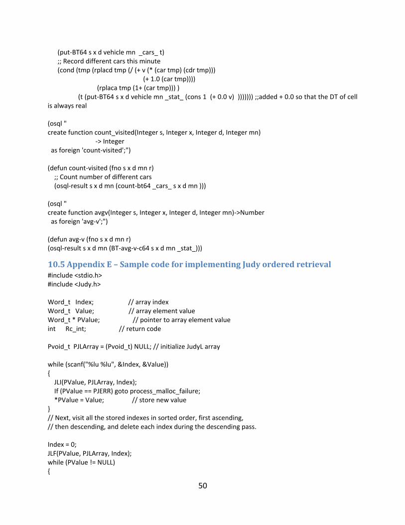
50
(put-BT64 s x d vehicle mn _cars_ t) ;; Record different cars this minute (cond (tmp (rplacd tmp (/ (+ v (* (car tmp) (cdr tmp))) (+ 1.0 (car tmp)))) (rplaca tmp (1+ (car tmp))) ) (t (put-BT64 s x d vehicle mn _stat_ (cons 1 (+ 0.0 v) ))))))) ;;added + 0.0 so that the DT of cell is always real (osql " create function count_visited(Integer s, Integer x, Integer d, Integer mn) -> Integer as foreign 'count-visited';") (defun count-visited (fno s x d mn r) ;; Count number of different cars (osql-result s x d mn (count-bt64 _cars_ s x d mn ))) (osql " create function avgv(Integer s, Integer x, Integer d, Integer mn)->Number as foreign 'avg-v';") (defun avg-v (fno s x d mn r) (osql-result s x d mn (BT-avg-v-c64 s x d mn _stat_)))
10.5 Appendix E – Sample code for implementing Judy ordered retrieval #include <stdio.h> #include <Judy.h> Word_t Index; // array index Word_t Value; // array element value Word_t * PValue; // pointer to array element value int Rc_int; // return code Pvoid_t PJLArray = (Pvoid_t) NULL; // initialize JudyL array while (scanf("%lu %lu", &Index, &Value)) { JLI(PValue, PJLArray, Index); If (PValue == PJERR) goto process_malloc_failure; *PValue = Value; // store new value } // Next, visit all the stored indexes in sorted order, first ascending, // then descending, and delete each index during the descending pass. Index = 0; JLF(PValue, PJLArray, Index); while (PValue != NULL) {
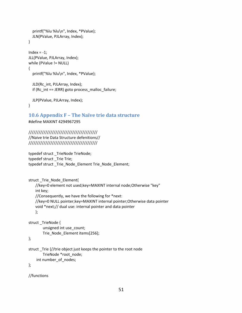
51
printf("%lu %lu\n", Index, *PValue); JLN(PValue, PJLArray, Index); } Index = -1; JLL(PValue, PJLArray, Index); while (PValue != NULL) { printf("%lu %lu\n", Index, *PValue); JLD(Rc_int, PJLArray, Index); if (Rc_int == JERR) goto process_malloc_failure; JLP(PValue, PJLArray, Index); }
10.6 Appendix F – The Naïve trie data structure #define MAXINT 4294967295 ///////////////////////////////////////// //Naive trie Data Structure defenitions// ///////////////////////////////////////// typedef struct _TrieNode TrieNode; typedef struct _Trie Trie; typedef struct _Trie_Node_Element Trie_Node_Element; struct _Trie_Node_Element{ //key=0 element not used;key=MAXINT internal node;Otherwise "key" int key; //Consequently, we have the following for *next: //key=0 NULL pointer;key=MAXINT internal pointer;Otherwise data pointer void *next;// dual use: internal pointer and data pointer }; struct _TrieNode { unsigned int use_count; Trie_Node_Element items[256]; }; struct _Trie {//trie object just keeps the pointer to the root node TrieNode *root_node; int number_of_nodes; }; //functions

52
//creates a naive trie and returns a pointer to it Trie *naive_trie_new(void); //Releases the memory allocated to naive trie node trn //and recursivly, all it's child nodes void naive_trie_free(TrieNode* trn); //Breaks an integer i into 4 bytes //returns the pointer to an array that contains the 4 bytes. unsigned int *BreakInt(unsigned int i); //looks up the trie tri for key ikey. //returns a pointer to the value associated with ikey int* naive_trie_lookup(Trie* tri, int ikey); //removes ikey from trie tri void naive_trie_remove(Trie* tri, int ikey); //inserts iket into trie tri //returns the pointer to the corresponding Trie_Node_Element Trie_Node_Element* naive_trie_insert(Trie* tri, int ikey); //searchj trie tri for next element of ikey //returns Trie_Node_Element that has the key k1 such that //k1 has a value greater than or equal to ikey //this is used in traversing the trie in ascending order Trie_Node_Element naive_trie_next(Trie *tri, int ikey);