UNIVERSITY OF OULU P .O. Box 8000 F I -90014 UNIVERSITY OF OULU FINLAND

A C T A U N I V E R S I T A T I S O U L U E N S I S

University Lecturer Tuomo Glumoff

University Lecturer Santeri Palviainen

Postdoctoral researcher Jani Peräntie

University Lecturer Anne Tuomisto

University Lecturer Veli-Matti Ulvinen

Planning Director Pertti Tikkanen

Professor Jari Juga

University Lecturer Anu Soikkeli

University Lecturer Santeri Palviainen

Publications Editor Kirsti Nurkkala

ISBN 978-952-62-2551-7 (Paperback)ISBN 978-952-62-2552-4 (PDF)ISSN 0355-3221 (Print)ISSN 1796-2234 (Online)

U N I V E R S I TAT I S O U L U E N S I S

MEDICA

ACTAD

D 1562

AC

TAA

leksei Tiulp

in

OULU 2020

D 1562

Aleksei Tiulpin

DEEP LEARNING FORKNEE OSTEOARTHRITIS DIAGNOSIS AND PROGRESSION PREDICTION FROM PLAIN RADIOGRAPHS AND CLINICAL DATA

UNIVERSITY OF OULU GRADUATE SCHOOL;UNIVERSITY OF OULU,FACULTY OF MEDICINE;OULU UNIVERSITY HOSPITAL

ACTA UNIVERS ITAT I S OULUENS I SD M e d i c a 1 5 6 2

ALEKSEI TIULPIN

DEEP LEARNING FOR KNEE OSTEOARTHRITIS DIAGNOSIS AND PROGRESSION PREDICTION FROM PLAIN RADIOGRAPHS AND CLINICAL DATA

Academic dissertation to be presented with the assent ofthe Doctoral Training Committee of Health andBiosciences of the University of Oulu for public defencein Auditorium P117 (Aapistie 5B), on 6 March 2020, at12 noon

UNIVERSITY OF OULU, OULU 2020

Copyright © 2020Acta Univ. Oul. D 1562, 2020

Supervised byProfessor Simo Saarakkala

Reviewed byAssistant Professor Kevin McGuinnessAssociate Professor Jeffrey Duryea

ISBN 978-952-62-2551-7 (Paperback)ISBN 978-952-62-2552-4 (PDF)

ISSN 0355-3221 (Printed)ISSN 1796-2234 (Online)

Cover DesignRaimo Ahonen

PUNAMUSTATAMPERE 2020

OpponentAssistant Professor Valentina Pedoia

Tiulpin, Aleksei, Deep learning for knee osteoarthritis diagnosis and progressionprediction from plain radiographs and clinical data. University of Oulu Graduate School; University of Oulu, Faculty of Medicine; Oulu UniversityHospitalActa Univ. Oul. D 1562, 2020University of Oulu, P.O. Box 8000, FI-90014 University of Oulu, Finland

Abstract

Osteoarthritis (OA) is the most common musculoskeletal disorder in the world, affecting hand,hip, and knee joints. At the final stage, OA leads to joint replacement, causing an immense burdenat the individual and societal levels. Multiple risk factors that can lead to OA are known; however,the etiology of OA and the underlying mechanisms of OA progression are not currently known.

OA is currently diagnosed by a clinical examination and, when necessary, confirmed byimaging – a radiographic evaluation. However, these conventional tools are not sensitive to detectthe early stages of OA, which makes the development of preventive measures for further diseaseprogression difficult. Therefore, there is a need for other methods that could allow for the earlydiagnosis of OA. As such, computer vision-based techniques provide quantitative biomarkers thatallow for an automatic and systematic assessment of OA severity from images.

In recent years, the rapid development of computer vision and machine learning methods havemerged into a new field – deep learning (DL). DL allows for one to formulate the problems ofcomputer vision and other fields in a machine learning fashion. In the medical field, DL has madea tremendous impact and allowed to approach for human-level decision-making accuracy indiagnostic and prognostic tasks compared with the traditional computer vision-based methods.

The focus of this thesis is on the development of DL-based methods for fully automatic kneeOA severity diagnosis and the prediction of its progression. Multiple new methods for localizingthe region of interest, landmark localization, knee OA severity assessment, and OA progressionprediction are proposed. The results exceeded the state-of-the-art or formed completely newbenchmarks for the evaluation of diagnostic and predictive model performance in OA. The mainconclusion is that DL yields excellent performance in the diagnostics of OA and in the predictionof its progression. All the source codes of all the developed methods and the annotations for someof the datasets have been made publicly available.

Keywords: computer vision, deep learning, knee, machine learning, osteoarthritis

Tiulpin, Aleksei, Polven nivelrikon automaattinen diagnostiikka sekä sairaudenetenemisen ennustaminen röntgenkuvan sekä kliinisen tiedon perusteellahyödyntäen syväoppimismalleja. Oulun yliopiston tutkijakoulu; Oulun yliopisto, Lääketieteellinen tiedekunta; Oulunyliopistollinen sairaalaActa Univ. Oul. D 1562, 2020Oulun yliopisto, PL 8000, 90014 Oulun yliopisto

Tiivistelmä

Nivelrikko on maailman yleisin käden, lonkan ja polven niveliin vaikuttava liikuntaelinsairaus.Viimekädessä nivelrikko johtaa tekonivelleikkauksiin, aiheuttaen merkittävää rasitetta niin yksi-lö- kuin yhteiskunnallisella tasolla. Monia nivelrikolle altistavia tekijöitä on jo tunnistettu, mut-ta kaikkia nivelrikon syitä ja vaikutusmekanismeja nivelrikon etenemisessä ei tunneta.

Nivelrikko diagnosoidaan kliinisellä tutkimuksella ja vahvistetaan/varmistetaan tarvittaessatehtävällä kuvantamistutkimuksella – tekemällä radiografinen arviointi. Nämä perinteiset työka-lut eivät kuitenkaan ole riittävän herkkiä nivelrikon varhaisten vaiheiden havaitsemiseen, jatämä hankaloittaa sairauden kehittymistä ehkäisevien toimenpiteiden kehittämistä. Näistä syistäjohtuen tarvitaan muita menetelmiä, jotka mahdollistavat nivelrikon varhaisen diagnosoinnin.Konenäkömenetelmät sellaisenaan tuottavat kvantitatiivisia biologisia indikaattoreita jotka mah-dollistavat automaattisen ja järjestelmällisen nivelrikon vakavuusarvion tekemisen kuvamateri-aalista.

Viime vuosina konenäkö- ja koneoppimismenetelmien nopea kehitys on synnyttänyt uudensyväoppimisen haaran. Syväoppiminen mahdollistaa konenäkö- ja muiden ongelmien määritte-lyn koneoppimisongelman tavoin. Verrattuna perinteisiin lääketieteessä käytettyihin tietokone-näkömenetelmiin, syväoppiminen on mahdollistanut ihmisen suorituskykyä lähestyvät toteutuk-set lääketieteen diagnostisissa ja prognostisissa tehtävissä ja niiden vaikutus alan kehitykselle onollut merkittävä.

Tämän väitöskirja keskittyy kehittämään syväoppimismenetelmiä täysautomaattiseen polvennivelrikon vakavuuden diagnosointiin ja taudin kehittymisen ennustamiseen. Työssä ehdotetaan/esitetään useita uusia menetelmiä kohdealueen paikallistamiseen, maamerkkien paikallistami-seen, polven nivelrikon vakavuuden arviointiin ja nivelrikon etenemisen ennustamiseen. Työntulokset ylittävät viimeisintä tekniikkaa edustavat ratkaisut tai muodostavat täysin uuden mitta-rin diagnostisten ja ennustavien menetelmien suorituskyvyn evaluoinnille nivelrikon kontekstis-sa. Työn keskeisimpänä johtopäätöksenä esitetään, että syväoppimisella on mahdollista saavut-taa erittäin hyvä suorituskyky nivelrikon diagnosoinnissa ja sen etenemisen ennustamisessa.Kaikki työssä kehitetyt menetelmät lähdekoodeineen sekä annotoinnit osalle tutkimuksessa käy-tetyistä aineistoista on saatettu avoimesti saataville.

Asiasanat: konenäkö, koneoppiminen, nivelrikko, polvi, syväoppiminen

Acknowledgements

This doctoral project was carried out from 2017–2019 at the Diagnostics of OsteoarthritisResearch Group of the Research Unit of Medical Imaging, Physics and Technology atthe University of Oulu. I owe my deepest gratitude to my principal supervisor, ProfessorSimo Saarakkala, Ph.D., who let my ambitious ideas see the light of day. Thanks a lotto you Simo for giving me the opportunity to grow as a scientist. Your support andguidance helped me a lot.

My friend, colleague, and co-supervisor Dr. Jérôme Thevenot, Ph.D., is also verymuch acknowledged for teaching me the practical skills of writing and being criticalof myself. Assistant Professor Esa Rahtu, Ph.D., my third supervisor, is also kindlyacknowledged. Thanks a lot to you Esa for providing your feedback from a computervision prospective, especially at the beginning of the thesis, and for bringing me intofruitful collaborations in the side-projects.

The members of my follow-up group also need to acknowledged. I thank AlexeyPopov, Ph.D., Jukka Kortelainen, M.D., Ph.D. and Jukka Komulainen, Ph.D. Thanks fordedicating your time to me and mystery work. I appreciate it very much.

Besides my Ph.D. supervisors and the follow-up group, I would also like toacknowledge Associate Professor Dr. Alexandr Popov, Ph.D., who guided me toward theend of my studies at the Northern (Arctic) Federal University in Russia. Although ourpaths diverged at a certain point, I truly acknowledge your enormous contribution to mydevelopment as an engineer and scientist. Other people from my alma mater, AssociateProfessor Vladimir Berezovsky, Ph.D. and Mr. Alexander Rudalev are also very muchacknowledged for teaching me important skills and providing me with the opportunitiesto grow as an engineer and scientist. Here, I would also like to mention Professor TapioSeppänen, Ph.D., for his initial contribution to my academic career in Finland.

It would not have been possible to finalise this thesis without an external evaluation.Here, I would like to acknowledge Assistant Professor Kevin McGuinness, Ph.D., fromDublin City University, Ireland, and also Associate Professor Jeffrey Duryea, Ph.D.,from Harvard Medical School, USA. Thank you both for your work.

During the Ph.D, I got lucky and was able to meet a lot of people and get to knowmany co-authors in all the different projects I have been involved in. Here, I wouldlike to thank my co-authors from Finland and the Netherlands, from whom I learned

7

a lot. In particular, I thank Associate Professor Stefan Klein, Ph.D., who has madea significant contribution to my Knee Osteoarthritis Progression Prediction Study.Associate Professor Edwin Oei, M.D., Ph.D., Professor Sita Bierma-Zeinstra, Ph.D.,and Associate Professor Joyce Van Meurs, Ph.D., are also very much acknowledged.My friend and co-author Iaroslav Melekhov, with whom I co-authored three papers invarious topics, is also very much acknowledged. I am also giving an apology to all thosenot mentioned in this list, but with whom I co-authored my papers unrelated to the Ph.D.thesis.

Besides the co-authors of my Ph.D. thesis-related publications, I would also like todeeply thank the leader of our research unit – Professor Osmo Tervonen, M.D., Ph.D,.for giving me the opportunities to grow and also giving me the possibility to be a part ofthe Oulu University Hospital staff. Thanks also for being a great boss and colleague.

The medical professionals with whom I had a chance to work with have also asignificant impact on my scientific career during my PhD. These people are ProfessorJaakko Niinimäki, M.D., Ph.D., Professor Petri Lehenkari, M.D., Ph.D., Elias Vaatto-vaara, M.D., Mika Nevalainen, M.D., Ph.D., and Timo Lesonen M.D., with whom I alsoco-authored some of my thesis-unrelated publications.

I would also like to mention all my colleagues from the DIOS group: Egor, Hoang,Mikko, Santeri, Sakari, Sami, Iida and Victor. Thanks for being here and survivingthrough my sometimes arrogant attitude. Getting closer to the end of this section, Iwould also like to mention two of my other friends: Antti and Leo, with whom I canalways share what I think. Antti’s help has also been highly valuable at the final stage ofthe thesis when the manuscript needed to be thoroughly proofread.

At last, but not the least, I have to really thank my family – mom, dad, brother,and grand-dad for helping me throughout my university and PhD years and alwaysbeing here for me. I know that wanting best the is not always the best, however Ibelieve and am happy that me and my parents were eventually able to establish goodrelations. Finally, I also want to thank my brother for finally getting older and becomingreasonable.

I would like to thank the University of Oulu for providing the facilities to conductthe research and the KAUTE foundation for personal grants.

Aleksei Tiulpin,

29th of January, 2020.

8

List of abbreviations

ANN Artificial Neural NetworkAP Average PrecisionAUC Area Under the Receiver Operating Characteristic CurveBMI Body Mass IndexCLM Constrained Local ModelCNN Convolutional Neural NetworkCV Cross-ValidationDL Deep LearningERM Empirical Risk MinimizationFO Femoral OsteophyteGBM Gradient Boosting MachineHoG Histogram of Oriented GradientsJSN Joint-Space NarrowingKL Kellgren-LawrenceLR Logistic RegressionMAP Maximum a-Posteriori PrincipleML MLMOST Multicenter Osteoarthritis StudyOA OsteoarthritisOAI Osteoarthritis InitiativeOARSI Osteoarthritis Research Society InternationalOKOA Oulu Knee OsteoarthritisPR Precision-RecallRFRV Random Forest Regression VotingROC Receiver Operating Characteristic CurveSVM Support Vector MachineTO Tibial OsteophyteWOMAC Western Ontario and McMaster Universities Arthritis Index

9

10

List of original publications

This thesis is based on the following articles, which are referred to in the text by theirRoman numerals (I–V):

I Tiulpin, A., Thevenot, J., Rahtu, E., & Saarakkala, S. (2017, June). A novel method forautomatic localization of joint area on knee plain radiographs. In Scandinavian Conference onImage Analysis (pp. 290-301). Springer, Cham.

II Tiulpin, A., Melekhov, I., & Saarakkala, S. (2019). KNEEL: Knee Anatomical LandmarkLocalization Using Hourglass Networks. In Proceedings of the IEEE International Conferenceon Computer Vision Workshops (pp. 0-0). (to appear in IEEE proceedings)

III Tiulpin, A., Thevenot, J., Rahtu, E., Lehenkari, P., & Saarakkala, S. (2018). Automatic kneeosteoarthritis diagnosis from plain radiographs: A deep learning-based approach. Scientificreports, 8(1), 1727.

IV Tiulpin, A. & Saarakkala, S. (2019). Automatic Grading of Individual Knee OsteoarthritisFeatures in Plain Radiographs using Deep Convolutional Neural Networks (manuscript, underreview).

V Tiulpin, A., Klein, S., Bierma-Zeinstra, S.M.A., Thevenot J., Rahtu E., Van Meurs J.B., Oei E.,& Saarakkala, S. (2019). Multimodal Machine Learning-based Knee Osteoarthritis ProgressionPrediction from Plain Radiographs and Clinical Data. Scientific Reports, 9 (1), 20038

This thesis also contains unpublished data.All the aforementioned sub-studies were designed by the author of this doctoral

thesis. The co-authors of the papers contributed to the conceptualizing and writing ofthe scientific articles. The author of the thesis developed the source codes of all themethods and conducted all the computational experiments.

11

12

Contents

AbstractTiivistelmäAcknowledgements 7List of abbreviations 9List of original publications 11Contents 131 Introduction 172 Knee osteoarthritis 21

2.1 Human knee, articular cartilage, and subchondral bone . . . . . . . . . . . . . . . . . . . 21

2.2 Osteoarthritis: definition, etiology, and risk factors . . . . . . . . . . . . . . . . . . . . . . 23

2.3 Management and treatment . . . . . . . . . . . . . . . . . . . . . . . . . . . . . . . . . . . . . . . . . . . 24

2.4 Societal impact . . . . . . . . . . . . . . . . . . . . . . . . . . . . . . . . . . . . . . . . . . . . . . . . . . . . . . 24

2.5 Diagnosis and prognosis . . . . . . . . . . . . . . . . . . . . . . . . . . . . . . . . . . . . . . . . . . . . . . 25

2.6 Summary . . . . . . . . . . . . . . . . . . . . . . . . . . . . . . . . . . . . . . . . . . . . . . . . . . . . . . . . . . . 25

3 Knee radiography and its quantitative analysis 273.1 Radiographic imaging of knee osteoarthritis . . . . . . . . . . . . . . . . . . . . . . . . . . . . 27

3.2 Kellgren-Lawrence grading . . . . . . . . . . . . . . . . . . . . . . . . . . . . . . . . . . . . . . . . . . . 27

3.3 Osteoarthritis Research Society International (OARSI) grading atlasfor knee radiography . . . . . . . . . . . . . . . . . . . . . . . . . . . . . . . . . . . . . . . . . . . . . . . . . 28

3.4 Computer-aided methods in osteoarthritis . . . . . . . . . . . . . . . . . . . . . . . . . . . . . . 29

3.5 Summary . . . . . . . . . . . . . . . . . . . . . . . . . . . . . . . . . . . . . . . . . . . . . . . . . . . . . . . . . . . 30

4 Deep learning 334.1 The definition of a learning machine . . . . . . . . . . . . . . . . . . . . . . . . . . . . . . . . . . . 33

4.2 The elements of statistical learning theory . . . . . . . . . . . . . . . . . . . . . . . . . . . . . . 34

4.3 Maximum a-posteriori probability . . . . . . . . . . . . . . . . . . . . . . . . . . . . . . . . . . . . . 35

4.4 Overfitting and model selection . . . . . . . . . . . . . . . . . . . . . . . . . . . . . . . . . . . . . . . 36

4.5 Examples of learning machines . . . . . . . . . . . . . . . . . . . . . . . . . . . . . . . . . . . . . . . .36

4.5.1 K-nearest neighbours . . . . . . . . . . . . . . . . . . . . . . . . . . . . . . . . . . . . . . . . . . 36

4.5.2 Logistic and softmax regression . . . . . . . . . . . . . . . . . . . . . . . . . . . . . . . . . 37

4.5.3 Support vector machines . . . . . . . . . . . . . . . . . . . . . . . . . . . . . . . . . . . . . . . 38

4.5.4 Gradient boosting . . . . . . . . . . . . . . . . . . . . . . . . . . . . . . . . . . . . . . . . . . . . . 39

13

4.6 Representation learning. . . . . . . . . . . . . . . . . . . . . . . . . . . . . . . . . . . . . . . . . . . . . . .394.6.1 Feature extraction . . . . . . . . . . . . . . . . . . . . . . . . . . . . . . . . . . . . . . . . . . . . . 394.6.2 Artificial neural networks . . . . . . . . . . . . . . . . . . . . . . . . . . . . . . . . . . . . . . 404.6.3 Deep convolutional neural networks . . . . . . . . . . . . . . . . . . . . . . . . . . . . . 42

4.7 Transfer learning. . . . . . . . . . . . . . . . . . . . . . . . . . . . . . . . . . . . . . . . . . . . . . . . . . . . .444.8 Summary . . . . . . . . . . . . . . . . . . . . . . . . . . . . . . . . . . . . . . . . . . . . . . . . . . . . . . . . . . . 44

5 Aims of the thesis 456 Overview and contributions 477 Materials and methods 51

7.1 Data . . . . . . . . . . . . . . . . . . . . . . . . . . . . . . . . . . . . . . . . . . . . . . . . . . . . . . . . . . . . . . . . 517.2 Knee joint localization . . . . . . . . . . . . . . . . . . . . . . . . . . . . . . . . . . . . . . . . . . . . . . . 547.3 Automatic knee osteoarthritis severity assessment . . . . . . . . . . . . . . . . . . . . . . . 57

7.3.1 Kellgren-Lawrence grading: a Siamese CNN architecture (III) . . . . . 577.3.2 OARSI grading using transfer learning (IV) . . . . . . . . . . . . . . . . . . . . . . 59

7.4 Osteoarthritis progression prediction (V) . . . . . . . . . . . . . . . . . . . . . . . . . . . . . . . 607.5 Performance evaluation and statistical analyses . . . . . . . . . . . . . . . . . . . . . . . . . .61

8 Results 638.1 Knee joint localization . . . . . . . . . . . . . . . . . . . . . . . . . . . . . . . . . . . . . . . . . . . . . . . 63

8.1.1 Proposal-based approach (I) . . . . . . . . . . . . . . . . . . . . . . . . . . . . . . . . . . . . 638.1.2 Landmark-based methods (II) . . . . . . . . . . . . . . . . . . . . . . . . . . . . . . . . . . .64

8.2 Automatic osteoarthritis severity assessment . . . . . . . . . . . . . . . . . . . . . . . . . . . . 648.2.1 Kellgren-Lawrence grading . . . . . . . . . . . . . . . . . . . . . . . . . . . . . . . . . . . . . 648.2.2 OARSI grading (IV) . . . . . . . . . . . . . . . . . . . . . . . . . . . . . . . . . . . . . . . . . . . 68

8.3 Progression prediction (V) . . . . . . . . . . . . . . . . . . . . . . . . . . . . . . . . . . . . . . . . . . . . 718.3.1 Predictive performance . . . . . . . . . . . . . . . . . . . . . . . . . . . . . . . . . . . . . . . . . 71

9 Discussion 759.1 Main outcomes and impact . . . . . . . . . . . . . . . . . . . . . . . . . . . . . . . . . . . . . . . . . . . 759.2 Pre-processing methods (I, II) . . . . . . . . . . . . . . . . . . . . . . . . . . . . . . . . . . . . . . . . . 769.3 Automatic osteoarthritis severity assessment (III, IV, unpublished

work) . . . . . . . . . . . . . . . . . . . . . . . . . . . . . . . . . . . . . . . . . . . . . . . . . . . . . . . . . . . . . . . 779.4 Progression prediction from imaging data (V) . . . . . . . . . . . . . . . . . . . . . . . . . . .789.5 Limitations . . . . . . . . . . . . . . . . . . . . . . . . . . . . . . . . . . . . . . . . . . . . . . . . . . . . . . . . . . 789.6 Directions for the future research . . . . . . . . . . . . . . . . . . . . . . . . . . . . . . . . . . . . . . 79

10 Conclusions 81References 82

14

Appendices 99Original publications 99

15

16

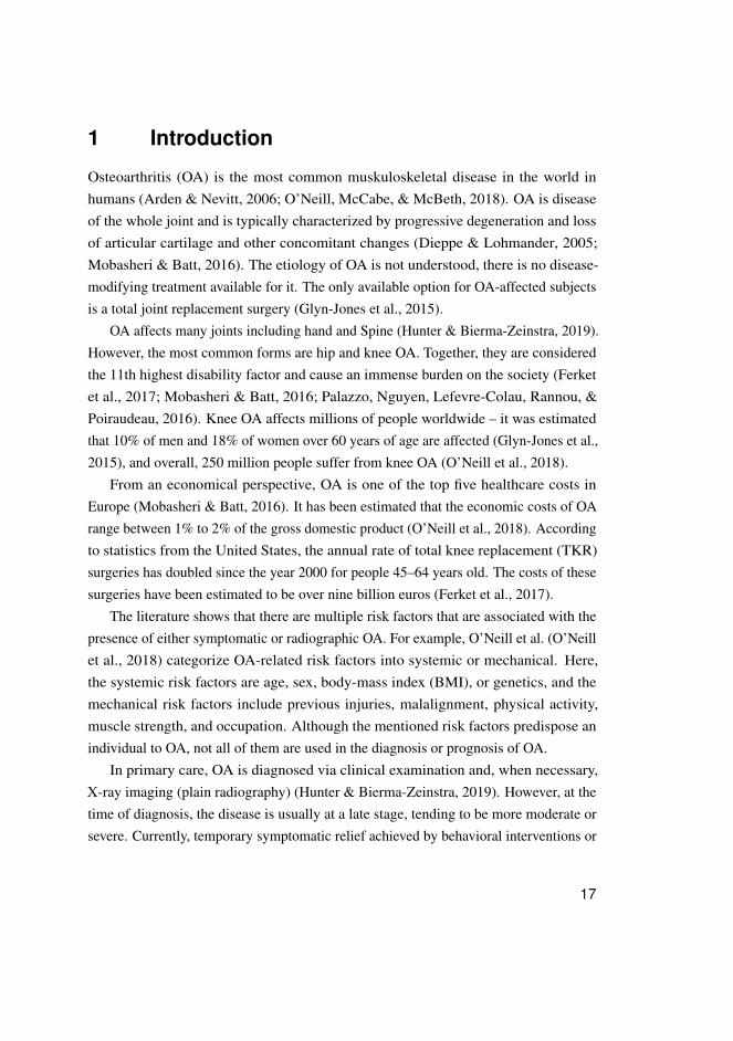
1 Introduction

Osteoarthritis (OA) is the most common muskuloskeletal disease in the world inhumans (Arden & Nevitt, 2006; O’Neill, McCabe, & McBeth, 2018). OA is diseaseof the whole joint and is typically characterized by progressive degeneration and lossof articular cartilage and other concomitant changes (Dieppe & Lohmander, 2005;Mobasheri & Batt, 2016). The etiology of OA is not understood, there is no disease-modifying treatment available for it. The only available option for OA-affected subjectsis a total joint replacement surgery (Glyn-Jones et al., 2015).

OA affects many joints including hand and Spine (Hunter & Bierma-Zeinstra, 2019).However, the most common forms are hip and knee OA. Together, they are consideredthe 11th highest disability factor and cause an immense burden on the society (Ferketet al., 2017; Mobasheri & Batt, 2016; Palazzo, Nguyen, Lefevre-Colau, Rannou, &Poiraudeau, 2016). Knee OA affects millions of people worldwide – it was estimatedthat 10% of men and 18% of women over 60 years of age are affected (Glyn-Jones et al.,2015), and overall, 250 million people suffer from knee OA (O’Neill et al., 2018).

From an economical perspective, OA is one of the top five healthcare costs inEurope (Mobasheri & Batt, 2016). It has been estimated that the economic costs of OArange between 1% to 2% of the gross domestic product (O’Neill et al., 2018). Accordingto statistics from the United States, the annual rate of total knee replacement (TKR)surgeries has doubled since the year 2000 for people 45–64 years old. The costs of thesesurgeries have been estimated to be over nine billion euros (Ferket et al., 2017).

The literature shows that there are multiple risk factors that are associated with thepresence of either symptomatic or radiographic OA. For example, O’Neill et al. (O’Neillet al., 2018) categorize OA-related risk factors into systemic or mechanical. Here,the systemic risk factors are age, sex, body-mass index (BMI), or genetics, and themechanical risk factors include previous injuries, malalignment, physical activity,muscle strength, and occupation. Although the mentioned risk factors predispose anindividual to OA, not all of them are used in the diagnosis or prognosis of OA.

In primary care, OA is diagnosed via clinical examination and, when necessary,X-ray imaging (plain radiography) (Hunter & Bierma-Zeinstra, 2019). However, at thetime of diagnosis, the disease is usually at a late stage, tending to be more moderate orsevere. Currently, temporary symptomatic relief achieved by behavioral interventions or

17

palliative treatment remains the only option before TKR (Glyn-Jones et al., 2015; Hunter& Bierma-Zeinstra, 2019; Jamshidi, Pelletier, & Martel-Pelletier, 2018). The diagnosisof OA at an early stage has the potential to allow for regenerative treatment (Jamshidiet al., 2018; Madry et al., 2016), but the existing diagnostic methods have a limitedsensitivity to early signs of the disease (O’Neill et al., 2018). Furthermore, due to theunknown pathogenesis of OA, a diagnosis of OA does not make it possible to predict thecourse of the disease and design an appropriate treatment. This indicates that there isa high need for an improvement in both the diagnostic and prognostic tools for kneeOA. One possible solution is computer-aided image and general clinical data analysismethods for OA that could enable better early detection of OA in primary care.

Computer-aided image analysis methods in arthritis research have a long history. Inparticular, the first studies of a quantitative analysis of hand radiographs from patientswith hand rheumatoid arthritis were published in the 1980s (Browne et al., 1987;J. Buckland-Wright, Carmichael, & Walker, 1986). Subsequently, knee OA was firstanalyzed using computer-aided methods (Dacre, Coppock, Herbert, Perrett, & Huskisson,1989). Then, in 1991, Lynch et al. introduced the fractal signature analysis (FSA) toassess subchondral bone texture (J. Lynch, Hawkes, & Buckland-Wright, 1991a, 1991b).The FSA approach was used and thoroughly investigated in multiple variations fortwo decades (Brahim et al., 2019; C. Buckland-Wright, 2004; J. Buckland-Wright,Lynch, & Macfarlane, 1996; Chappard et al., 2006; Hirvasniemi, Niinimäki, Thevenot,& Saarakkala, 2019; Hirvasniemi, Thevenot, Guermazi, et al., 2017; Hirvasniemi,Thevenot, Multanen, et al., 2017; Janvier et al., 2017; Jarraya et al., 2015; Kraus et al.,2013; Lespessailles & Jennane, 2012; Messent, Ward, Tonkin, & Buckland-Wright,2006; Podsiadlo, Dahl, Englund, Lohmander, & Stachowiak, 2008; Podsiadlo et al.,2016; Podsiadlo & Stachowiak, 2002; Roemer et al., 2015; Thomson, O’Neill, Felson,& Cootes, 2015; Woloszynski, Podsiadlo, Stachowiak, & Kurzynski, 2010; Wolski,Podsiadlo, & Stachowiak, 2009, 2014; Wolski et al., 2011; Wong et al., 2009).

With the evolution of hardware, methods based on machine learning (ML) started tobecome popular. As such, bone shape modeling was used in multiple studies to assessOA automatically (Minciullo, Bromiley, Felson, & Cootes, 2017; Minciullo & Cootes,2016; Minciullo, Parkes, Felson, & Cootes, 2018; Thomson et al., 2015; Thomson,O’Neill, Felson, & Cootes, 2016). However, the most recent approaches (Abedin et al.,2019; Antony, 2018; Antony, McGuinness, O’Connor, & Moran, 2016; Norman, Pedoia,Noworolski, Link, & Majumdar, 2018) are based on deep learning (DL) – a subfield of

18

ML, studying methods for learning data representations directly from data (LeCun,Bengio, & Hinton, 2015; Schmidhuber, 2015).

The conventional techniques in ML heavily rely on so called feature-engineering

that allows the processing of raw data and turning it into representations (features)used for subsequent predictive modeling or decision making. In contrast, with DL, themanual feature design is bypassed, and the most optimal features are learned directlyfrom the data, yielding drastically better results in image recognition, segmentation,and other image analysis tasks when compared with the methods leveraging manuallydesigned features (LeCun et al., 2015).

The main focus of the current doctoral dissertation is on the development of newmethods for the quantitative data analysis of knee plain radiographs and clinical datausing DL. In particular, three DL-based methods for early diagnosis and the predictionof knee OA are proposed. In addition, two novel methods for knee X-ray imagepre-processing, namely region of interest and landmark localization, are proposed andthoroughly validated.

The present thesis is organized as follows: In Chapter 2, the basic background onknee OA is presented. Chapter 3 focuses on the basics of X-ray data acquisition anddescribes the shortcomings of X-ray imaging. Chapter 4 describes the basics of ML andgives an introduction to DL. In Chapter 5, the aims are described. Chapter 6 providesan overview of the framework built in the thesis. Chapter 7 describes the developedmethods and utilized datasets. Chapter 8 describes the results. Finally, Chapters 9and 10 conclude the thesis by giving a discussion and the conclusions, respectively.

19

20

2 Knee osteoarthritis

2.1 Human knee, articular cartilage, and subchondral bone

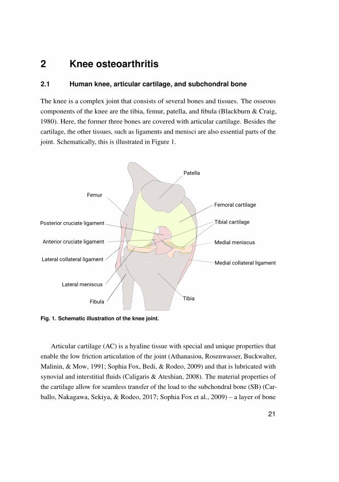
The knee is a complex joint that consists of several bones and tissues. The osseouscomponents of the knee are the tibia, femur, patella, and fibula (Blackburn & Craig,1980). Here, the former three bones are covered with articular cartilage. Besides thecartilage, the other tissues, such as ligaments and menisci are also essential parts of thejoint. Schematically, this is illustrated in Figure 1.

Patella

Femur

TibiaFibula

Femoral cartilage

Lateral meniscus

Medial meniscus

Tibial cartilage

Anterior cruciate ligament

Posterior cruciate ligament

Lateral collateral ligamentMedial collateral ligament

Fig. 1. Schematic illustration of the knee joint.

Articular cartilage (AC) is a hyaline tissue with special and unique properties thatenable the low friction articulation of the joint (Athanasiou, Rosenwasser, Buckwalter,Malinin, & Mow, 1991; Sophia Fox, Bedi, & Rodeo, 2009) and that is lubricated withsynovial and interstitial fluids (Caligaris & Ateshian, 2008). The material properties ofthe cartilage allow for seamless transfer of the load to the subchondral bone (SB) (Car-ballo, Nakagawa, Sekiya, & Rodeo, 2017; Sophia Fox et al., 2009) – a layer of bone

21

Superficial zone (10-20%)

Middle zone (40-60%)

Deep zone (30-50%)

Calcified Cartilage

Subchondral Bone Plate

Subchondral Trabecular Bone

Articular surface

Tidemark

Cement line

Chondrocyte

Fig. 2. Schematic illustration of articular cartilage composition.

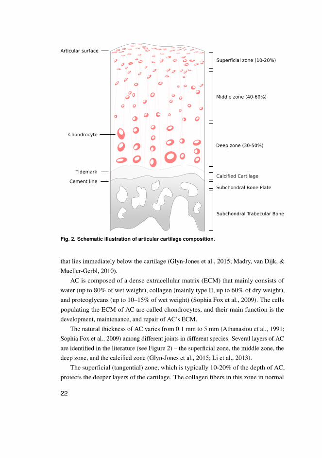
that lies immediately below the cartilage (Glyn-Jones et al., 2015; Madry, van Dijk, &Mueller-Gerbl, 2010).

AC is composed of a dense extracellular matrix (ECM) that mainly consists ofwater (up to 80% of wet weight), collagen (mainly type II, up to 60% of dry weight),and proteoglycans (up to 10–15% of wet weight) (Sophia Fox et al., 2009). The cellspopulating the ECM of AC are called chondrocytes, and their main function is thedevelopment, maintenance, and repair of AC’s ECM.

The natural thickness of AC varies from 0.1 mm to 5 mm (Athanasiou et al., 1991;Sophia Fox et al., 2009) among different joints in different species. Several layers of ACare identified in the literature (see Figure 2) – the superficial zone, the middle zone, thedeep zone, and the calcified zone (Glyn-Jones et al., 2015; Li et al., 2013).

The superficial (tangential) zone, which is typically 10-20% of the depth of AC,protects the deeper layers of the cartilage. The collagen fibers in this zone in normal

22

cartilage are tightly packed and aligned in parallel to the articular surface. Thechondrocytes in this layer are flattened and densely distributed. Together with thesuperficial collagen network, they protect the deeper cartilage layers. The middle(transitional) zone represents 40–60% of the total AC volume. Functionally, it enablesthe first level resistance of AC to compression forces. The collagen fibers in this zoneare aligned chaotically, and the chondrocytes are spherical. The deep zone of ACis responsible for providing the biggest level resistance to compression forces. Thechondrocytes in this zone are arranged in a columnar manner, parallel to the collagenfibers and orthogonal to the joint line. This zone can represent 30-50% of the totalcartilage volume (Brody, 2015; Buckwalter & Mankin, 1997; Madry et al., 2010;Sophia Fox et al., 2009).

The superficial, middle and deep zones of AC are non-calcified and are separatedfrom the calcified (mineralized) zone by a thin interface – the tidemark (see Figure 2).The tidemark provides a gradual transition between two dissimilar tissue regions andrepresents the mineralization front of the calcified cartilage. Calcified cartilage isseparated from SB by a sharp cement line underneath which there lies a subchondralbone plate, followed by a subchondral trabecular bone (Buckwalter & Mankin, 1997; Liet al., 2013; Madry et al., 2010).

2.2 Osteoarthritis: definition, etiology, and risk factors

Osteoarthritis (OA) was long considered a degenerative disease of cartilage; however,now, it is considered a whole-joint disorder that affects multiple structures within theknee (Berenbaum, 2013; Glyn-Jones et al., 2015; Hügle & Geurts, 2016; Hunter &Bierma-Zeinstra, 2019; Li et al., 2013; Yamada, Healey, Amiel, Lotz, & Coutts, 2002).OA is typically characterized by the degradation of AC, but the remodeling of SB andsynovitis (inflammation of synovial membrane) often precedes cartilage damage (Hügle& Geurts, 2016). Furthermore, Arden and Nevitt (2006) defined OA as an "age-related

dynamic reaction pattern of a joint in response to insult or injury", thereby representingOA as a failure of the whole joint. Other studies (Glyn-Jones et al., 2015; Hunter &Bierma-Zeinstra, 2019) also define OA as a disease of the whole joint.

From a biological prospective, AC composition changes in OA and ECM loses itsintegrity (Hunter & Bierma-Zeinstra, 2019; Saarakkala et al., 2010). It has been shownthat OA alters the biomechanical properties of the cartilage (Waldstein et al., 2016).In addition, the structural changes start with erosions of the superficial layer of the

23

cartilage. Subsequently, OA induces more deep fissures in AC, an expansion of calcifiedcartilage, and tidemark duplication (Hunter & Bierma-Zeinstra, 2019). This process isalso accompanied with the aforementioned changes in SB (Aho, Finnilä, Thevenot,Saarakkala, & Lehenkari, 2017; Finnilä et al., 2017; Lories & Luyten, 2011; Yuan et al.,2014).

Multiple factors predispose knee OA, but aging is considered a major risk factor dueto the loss of normal bone and reduced muscle activity (Brody, 2015; Glyn-Jones et al.,2015; Li et al., 2013; Vina & Kwoh, 2018). The prevalence of OA increases with age inall major joints (Allen & Golightly, 2015). Obesity and female sex are also knownmajor risk factors for a predisposition to knee OA. Other risk factors include, but are notlimited to, genetics, occupational load, physical activity, diet and, previous injury (Allen& Golightly, 2015; Brody, 2015; Glyn-Jones et al., 2015; Vina & Kwoh, 2018).

2.3 Management and treatment

The main non-pharmacological treatment option for OA patients is currently behavioralinterventions (Hunter & Bierma-Zeinstra, 2019; Marsh et al., 2016). As such, for obesepatients, exercise, walking, and weight loss have been shown to favorably affect thesymptoms of knee and hip OA (Hunter & Bierma-Zeinstra, 2019).

Pharmacological treatments for OA are largely palliative (pain relieving). Nodisease modifying treatment is approved for OA (Hunter & Bierma-Zeinstra, 2019).Therefore, TKR surgery remains the only option at the end stage of the disease (Hunter& Bierma-Zeinstra, 2019; Lützner, Kasten, Günther, & Kirschner, 2009).

2.4 Societal impact

The incremental healthcare and non-healthcare costs of knee OA per patient in developedcountries range from 528-11,293 e and 2,296-8,772 e, respectively (Puig-Junoy &Zamora, 2015). Considering TKR surgeries, their incidence is growing; therefore, theirtotal cost on healthcare is being increased. As such, in the United States, the total annualnumber of these surgeries already exceeds 640,000 with the total cost over 9.6 billione (Ferket et al., 2017). Regarding the future, an Australian study by Ackerman et al.(2019) estimates that the total burden of OA will reach 3.32 billion e and total numberof TKR would increase by 27.6% from 2013 to 2030.

24

2.5 Diagnosis and prognosis

Currently, OA is diagnosed using clinical examination, and, often, when necessary,radiographic assessment. A clinical examination includes assessment of symptoms anda brief physical evaluation of the joint. The role of imaging is still not clearly definedaccording to the literature; however, the imaging has been shown to be a good predictorof future joint replacement (Hunter & Bierma-Zeinstra, 2019; Sakellariou et al., 2017).

Recent recommendations on the use of imaging in OA diagnostics indicate that itneeds to be used only for cases when a diagnosis needs to be confirmed (Sakellariou et al.,2017). In this case, plain radiography (X-ray imaging) is the first-line imaging modalitythat needs to be utilized (Sakellariou et al., 2017). Although being commonly used,radiography does not offer direct imaging of cartilage, ligaments, meniscii, synovium,and other important structures affected by OA (Hayashi, Roemer, & Guermazi, 2016).Magnetic resonance imaging (MRI) can offer the possibility to image these structures;however, it is costly and not routinely used in clinical practice (Hayashi et al., 2016).Therefore, X-ray imaging remains the main imaging modality in the OA diagnosticchain.

A prognosis, and in particular the course of pain and physical function, is currentlydifficult to predict (de Rooij et al., 2016). This can be explained by the heterogeneityof OA and potential presence of different phenotypes (Vina & Kwoh, 2018). To date,multiple studies have focused on predicting the structural and pain progression ofOA (Bastick, Belo, Runhaar, & Bierma-Zeinstra, 2015; Belo, Berger, Reijman, Koes, &Bierma-Zeinstra, 2007; Bruyere et al., 2003; Bruyère et al., 2007; Collins et al., 2016;Dieppe, Cushnaghan, Young, & Kirwan, 1993; Hafezi-Nejad, Guermazi, Demehri, &Roemer, 2018; Hirvasniemi et al., 2019; Hochberg, 1996; Hunter et al., 2007; Janvier etal., 2017; Kerkhof et al., 2014; Kraus et al., 2009, 2013; LaValley et al., 2017; Miyazakiet al., 2002; Podsiadlo et al., 2016; Reijman et al., 2007; Urish et al., 2013; Yu et al.,2019; W. Zhang et al., 2011). Despite over a decade-long effort, both the mechanismsunderlying OA development and clinically applicable reliable biomarkers are yet to bediscovered.

2.6 Summary

In this chapter, OA, which is a serious disease affecting millions of people worldwide,was broadly discussed. OA of major joints such as the knee and hip is one of the most

25

significant disability factors in the world. Unfortunately, the current treatment optionsfor OA are limited to behavioral intervention, palliative pharmacological treatment,and TKR at the end stage of the disease. The pathogenesis of OA is unknown, so it isdifficult to make any prognosis for OA patients.

The diagnosis of OA is currently done in primary care, yet the main diagnosticmodalities are limited when it comes to the detection of the earliest OA changes.Imaging, while being optional according to the current OA diagnosis guidelines, couldstill be used for detecting and quantifying the earliest changes in the joint. The nextchapter provides details on the main clinical imaging modality – radiography.

26

3 Knee radiography and its quantitativeanalysis

3.1 Radiographic imaging of knee osteoarthritis

OA is commonly imaged using plain radiography, which is done in primary care whennecessary (Hunter & Bierma-Zeinstra, 2019). However, specialized care modalities,such as MRI and ultrasound, can also be used to conduct the imaging of OA.

A knee X-ray is usually performed in the fixed-flexion standing position. When thedata acquisition settings are uncontrolled, for example, when the X-ray beam anglevaries or the knees’ positions are not fixed, radiography lacks reproducibility – that is, theappearance of the knee of the same patient may differ between imaging sessions. Thismay significantly impact the results of image interpretation and especially the assessmentof joint space narrowing (JSN) – the most common radiographic quantitative imagingbiomarker typically considered a surrogate of tibial and femoral AC thickness1. Oneparticular solution to mitigate the reproducibility limitations of radiographic imaging isthe use of a positioning frame (Kothari et al., 2004).

3.2 Kellgren-Lawrence grading

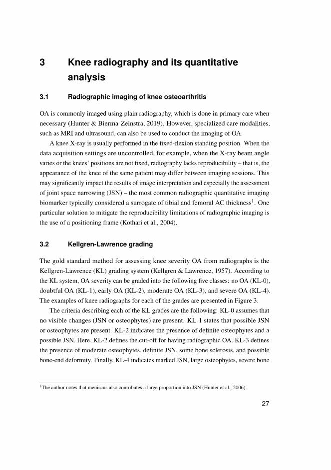
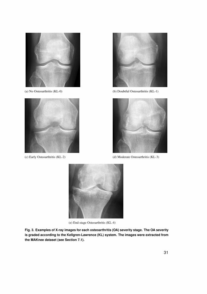
The gold standard method for assessing knee severity OA from radiographs is theKellgren-Lawrence (KL) grading system (Kellgren & Lawrence, 1957). According tothe KL system, OA severity can be graded into the following five classes: no OA (KL-0),doubtful OA (KL-1), early OA (KL-2), moderate OA (KL-3), and severe OA (KL-4).The examples of knee radiographs for each of the grades are presented in Figure 3.

The criteria describing each of the KL grades are the following: KL-0 assumes thatno visible changes (JSN or osteophytes) are present. KL-1 states that possible JSNor osteophytes are present. KL-2 indicates the presence of definite osteophytes and apossible JSN. Here, KL-2 defines the cut-off for having radiographic OA. KL-3 definesthe presence of moderate osteophytes, definite JSN, some bone sclerosis, and possiblebone-end deformity. Finally, KL-4 indicates marked JSN, large osteophytes, severe bone

1The author notes that meniscus also contributes a large proportion into JSN (Hunter et al., 2006).

27

sclerosis, and a definite bone deformity (Culvenor, Engen, Øiestad, Engebretsen, &Risberg, 2015; Kellgren & Lawrence, 1957).

Despite its simplicity, the KL grading system has one major drawback – thesubjectivity of the reader. Various studies have reported Cohen’s weighted kappacoefficients of 0.56 (Gossec et al., 2008), 0.61 (Toivanen et al., 2007), 0.66 (Sheehy etal., 2015), 0.67 (Culvenor et al., 2015), and 0.79 (Guermazi et al., 2015). In addition,the KL system is categorical and not sensitive; thus, it does not allow for fine-grainedassessments of the OA features, which can be a limiting factor in reporting the earlysigns of OA.

3.3 Osteoarthritis Research Society International (OARSI) gradingatlas for knee radiography

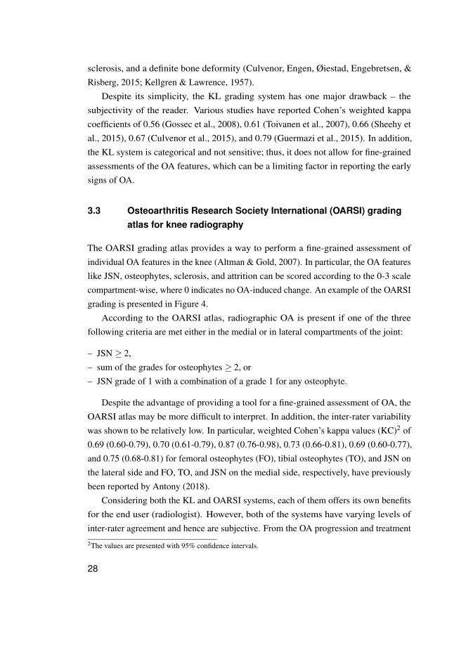
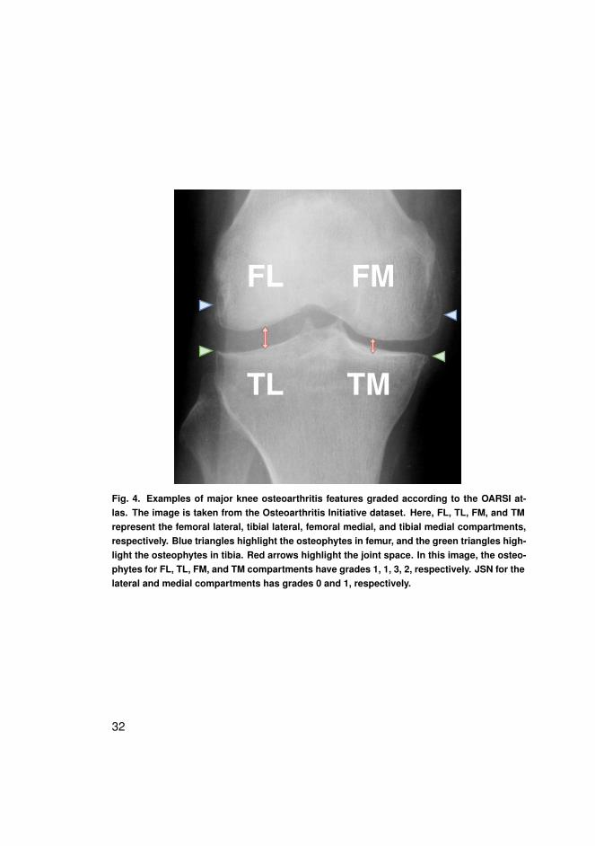
The OARSI grading atlas provides a way to perform a fine-grained assessment ofindividual OA features in the knee (Altman & Gold, 2007). In particular, the OA featureslike JSN, osteophytes, sclerosis, and attrition can be scored according to the 0-3 scalecompartment-wise, where 0 indicates no OA-induced change. An example of the OARSIgrading is presented in Figure 4.

According to the OARSI atlas, radiographic OA is present if one of the threefollowing criteria are met either in the medial or in lateral compartments of the joint:

– JSN ≥ 2,– sum of the grades for osteophytes ≥ 2, or– JSN grade of 1 with a combination of a grade 1 for any osteophyte.

Despite the advantage of providing a tool for a fine-grained assessment of OA, theOARSI atlas may be more difficult to interpret. In addition, the inter-rater variabilitywas shown to be relatively low. In particular, weighted Cohen’s kappa values (KC)2 of0.69 (0.60-0.79), 0.70 (0.61-0.79), 0.87 (0.76-0.98), 0.73 (0.66-0.81), 0.69 (0.60-0.77),and 0.75 (0.68-0.81) for femoral osteophytes (FO), tibial osteophytes (TO), and JSN onthe lateral side and FO, TO, and JSN on the medial side, respectively, have previouslybeen reported by Antony (2018).

Considering both the KL and OARSI systems, each of them offers its own benefitsfor the end user (radiologist). However, both of the systems have varying levels ofinter-rater agreement and hence are subjective. From the OA progression and treatment

2The values are presented with 95% confidence intervals.

28

point of view, the detection of early OA signs is highly important, so more robust andsystematic methods are needed. Computer-aided methods can facilitate this process andreduce ambiguity in OA diagnosis and prognosis. The next section provides a shortreview of several main directions in the computer-aided analysis of knee radiographs.

3.4 Computer-aided methods in osteoarthritis

A bone texture analysis has been under investigation in OA community for two decades,starting in 1989 (Dacre et al., 1989). Later, in 1991, FSA was introduced by Lynchet al. (J. Lynch et al., 1991a, 1991b), and it is still used in various implementations.In particular, FSA was shown to have potential to not only in detect of radiographicOA (Hirvasniemi, Thevenot, Guermazi, et al., 2017), but also predict OA progres-sion (Janvier et al., 2017). Other texture descriptors, such as local binary patternsor gray level co-occurrence matrix-based parameters were also shown useful for OAdetection (Hirvasniemi, Thevenot, Multanen, et al., 2017).

Subchondral bone changes that can be captured by a texture analysis can beconsidered one possible descriptor of OA-induced changes. Another potential approachfor automatic OA detection is based on a shape analysis (Minciullo et al., 2017; Minciullo& Cootes, 2016; Minciullo et al., 2018). In addition, it was shown that a combination ofshape and texture can provide better results in detecting radiographic OA (Thomson etal., 2015).

Shape changes can be considered a generalization of JSW measurements. Gener-ally speaking, JSW measurements of any joint are quantitative and interpretable forpractitioners, but are time-consuming to conduct manually (Platten et al., 2017). Theauthor of the current thesis notes that the research on this topic has been continuingalready since 1989 (Dacree & Huskisson, 1989; Duryea, Jiang, Countryman, & Genant,1999; Duryea, Li, Peterfy, Gordon, & Genant, 2000; Duryea, Zaim, & Genant, 2003;Gordon et al., 2001; Huo et al., 2015; Lukas et al., 2008; J. A. Lynch, Buckland-Wright,& Macfarlane, 1993; Neumann et al., 2009; Platten et al., 2017).

The recently introduced DL approach (LeCun et al., 2015; Schmidhuber, 2015)enables learning of the relevant data representations from data automatically. ThisML method allows practitioners to avoid manual design of feature descriptors anduse the data directly as an input for the model. In contrast, the classic approach, forexample, in OA, is to first extract descriptors as FSA or LBP and use them in themodel (Bayramoglu, Tiulpin, Hirvasniemi, Nieminen, & Saarakkala, 2019; Janvier et al.,

29

2017). Other modeling approaches could also rely on KL-grades or JSN measurementsderived manually or semi-automatically from radiographs.

The pioneering work in applying DL to knee OA was done by Antony et al. (2016)and later on improved (Antony, McGuinness, Moran, & O’Connor, 2017). In particular,in those studies, automatic KL grading was performed. Later, the author of thecurrent thesis developed a method that has been the state-of-the-art since 2018 (Tiulpin,Thevenot, Rahtu, Lehenkari, & Saarakkala, 2018). Concurrent approaches (P. Chen, Gao,Shi, Allen, & Yang, 2019; Norman et al., 2018) were later published, yet a systematiccomparison between all the methods still remains an open issue.

To conclude, more DL studies in the OA research field have been carried out (Chaud-hari et al., 2019; P. Chen et al., 2019; Panfilov, Tiulpin, Klein, Nieminen, & Saarakkala,2019; Pedoia, Lee, Norman, Link, & Majumdar, 2019; Pedoia, Norman, et al., 2019;Tiulpin, Finnilä, Lehenkari, Nieminen, & Saarakkala, 2019; Tiulpin, Klein, et al., 2019;Tiulpin, Melekhov, & Saarakkala, 2019; Tiulpin & Saarakkala, 2019). Many researchgroups have recently contributed to this effort. The author of the present doctoral thesishas also been a part of the first wave of researchers developing DL for OA.

3.5 Summary

This chapter introduced radiographic imaging of the knee joint. Two grading systemsof knee radiographs were described, along with their benefits and limitations. It hasbeen noted that the data acquisition standardization can play an important role in theanalysis of radiographs. Manual grading of the images suffers from inter-rater variability.Quantitative image analysis methods that have the potential to address this limitationwere briefly reviewed at the end of the chapter, and DL was shown to be a promisingapproach for the analysis of knee radiographs.

30

(a) No Osteoarthritis (KL-0) (b) Doubtful Osteoarthritis (KL-1)

(c) Early Osteoarthritis (KL-2) (d) Moderate Osteoarthritis (KL-3)

(e) End-stage Osteoarthritis (KL-4)

Fig. 3. Examples of X-ray images for each osteoarthritis (OA) severity stage. The OA severityis graded according to the Kellgren-Lawrence (KL) system. The images were extracted fromthe MAKnee dataset (see Section 7.1).

31

FL

TL

FM

TM

Fig. 4. Examples of major knee osteoarthritis features graded according to the OARSI at-las. The image is taken from the Osteoarthritis Initiative dataset. Here, FL, TL, FM, and TMrepresent the femoral lateral, tibial lateral, femoral medial, and tibial medial compartments,respectively. Blue triangles highlight the osteophytes in femur, and the green triangles high-light the osteophytes in tibia. Red arrows highlight the joint space. In this image, the osteo-phytes for FL, TL, FM, and TM compartments have grades 1, 1, 3, 2, respectively. JSN for thelateral and medial compartments has grades 0 and 1, respectively.

32

4 Deep learning

DL is a form of ML and is a modern approach to artificial intelligence (AI) (Goodfellow,Bengio, & Courville, 2016). To formulate and explain the idea behind DL, it is importantto first elaborate the basic concepts of learning, specifically starting with the question"What is learning?" Overall, this chapter provides a non-strict mathematical introductionto learning theory, gives a basic background of ML, and briefly explains the foundationsof DL.

4.1 The definition of a learning machine

A sufficient definition of ML is described by Mitchell to include any computer programthat learns through experience (Goodfellow et al., 2016; Mitchell, 1997): "A computerprogram is said to learn from experience E with respect to some class of tasks T andperformance measure P, if its performance at tasks in T, as measured by P, improveswith experience E."

Goodfellow et al. (2016) define several types of tasks T: classification, regression,synthesis, and others. In the current doctoral thesis, learning algorithms performing twotypes of tasks – classification and regression – are explored. Classification indicates theassignment of a label y ∈ {0, . . . ,K−1} to an object x ∈X , where X is a space ofobjects typically considered to be Rd . Here, d – is the size of the data representationspace. A regression here indicates a mapping X −→ Y , where Y is the continuousspace of target variables y. Further, Y = R will be considered.

Strictly speaking, learning algorithms are computer programs that always operatewith representations of objects. For example, a person whose age needs to be determinedcan be represented by a digital photograph, which is an array of numbers stored in thecomputer. In the case of knee OA, an object representation can be a digital X-ray imagethat is also stored as an array of numbers. Numerous other examples can be found inother fields.

The experience E defines the type of learning. Three types of learning are common:supervised, unsupervised, and reinforcement. Mathematically, all types of learningare supervised, but their fundamental difference is in the type of experience E that thelearning machine receives (Goodfellow et al., 2016). In the case of supervised learning,which is utilized in the current thesis, the experience E is derived from the knowledge

33

stored in a dataset D = {x(i),y(i)}N−1i=0 , where N is the size of the dataset and the pair

(x,y) in the dataset D is drawn from a joint distribution p(x,y). Classification andregression are typically performed in a fully supervised fashion, that is having the exactannotations for each training example; however, other forms of learning, for example,semi-supervised or weakly supervised learning, also exist. In particular, semi-supervisedlearning allows us to leverage the unlabeled data, reducing the annotation cost, andweakly-supervised learning allows to use low-cost coarse labeling.

The final part of the definition of learning is a performance measure P that needs toimprove with experience (during learning). Typically, an ML algorithm is designed asa parametric functional f (x;θ) that reconstructs a dependency between sparse noisyobservations x(i) and the corresponding labels y(i),∀i ∈ 0, . . . ,N−1 . Here, θ is theso-called hyperparameters of an algorithm f (·) and directly affects the value of theperformance measure P, θ ∈ Rp. Thereby, the goal of learning is to find a functionalf (·) and hyperparameters θ that maximize P on a dataset D:

θ , f = argmaxf ,θ

P(E,P,T,D). (1)

Non-parametric approaches to ML also exist, but they are omitted due to being outof the scope of the current thesis. Typically, f (·) is chosen in advance, so the goal oflearning becomes an estimation of parameters θ . In the context of DL, f (·) typicallyindicates the architecture of a neural network.

4.2 The elements of statistical learning theory

The learning goal defined in equation (1) is well resembled in statistical learningtheory (Murphy, 2012; Vapnik, 1995). The theory defines the learning process as theminimization of a risk function R(θ):

R(θ) = Ex,y∼p(x,y)[L( f (x;θ),y)]−→minθ

, (2)

where L(·) is a loss function that defines how well a particular algorithm performs.Generally, computing the expectation of the loss is not feasible (the integral over allpossible x,y is not tractable), so the empirical risk is computed:

Remp(θ) =1N

N−1

∑i=0

L(

f (x(i);θ),y(i)). (3)

34

Minimizing the empirical risk is called empirical risk minimization (ERM). Typically,if using the estimator of θ from equation (3), the obtained θ will not allow forgeneralization to the new unseen data besides the dataset D used for ERM. Therefore, aregularization term G(θ) is added to Remp:

θ = argminθ

1N

N−1

∑i=0

L(

f (x(i);θ),y(i))+λG(θ), (4)

where λ is a regularization coefficient that is set before performing ERM. Often, thisproblem cannot be solved analytically; therefore, its approximate solutions are searchedvia gradient based optimization methods, such as a stochastic gradient descent (SGD)and its variations (Murphy, 2012).

4.3 Maximum a-posteriori probability

The process of estimation of the parameters θ for model f (x;θ) can also be viewedfrom a different point of view. As such, two other approaches besides the ERMexist – the maximum likelihood (MLE) and maximum a-posterior probability (MAP)estimation (Bishop, 2006; Murphy, 2012). An MLE allows for one to obtain exactlythe same solution as an ERM without regularization and MAP lets one to obtain aregularized solution, which is important in practical applications.

MAP allows one to perform an inference of parameters given the data. As such, it isdescribed as

θ = argmaxθ

p(θ |D). (5)

From Bayes’ rule

p(θ |D) =p(D|θ)p(θ)

p(D), (6)

andargmax

θ

p(θ |D)≡ argminθ

[− log p(θ |D)] , (7)

so the MAP estimation becomes

θ = argminθ

− log p(D|θ)︸ ︷︷ ︸Empirical Risk

− log p(θ)︸ ︷︷ ︸Regularizer

. (8)

It can be seen that the formulation of a regularized ERM (equation (4)) is equivalentto the one in equation (8).

35

4.4 Overfitting and model selection

The goal of learning, as mentioned in Section 4.1, is to maximize a performance measureP on a dataset D. However, it is also important that the algorithm f (x;θ) is able togeneralize to the unseen data – Dnew, that is the performance of a method should notdecrease when given unseen data. Such decrease can typically happen due to a highdim(θ) (model capacity). Varying dim(θ) can lead to two effects – underfitting (too lowmodel capacity) overfitting. In the case of overfitting, f (x;θ) can fit the training datawell and even memorize it. However, the model can also capture the noise that will leadto poor performance with unseen data.

To prevent overfitting, regularization is typically used. To assess the generalizationperformance, the whole training set D is often split into a new training Dtrain ⊂ Dand a validation set Dval ⊂ D, such that Dtrain∩Dval =∅ and Dtrain∪Dval = D. Thesolution θ (see equation 4) that yields the best performance of the model f (·) on Dval isselected as the final one. It is assumed that having such a model selection process, θ

will generalize to the unseen data – yielding non-random predictions on Dnew.The last element yet to be described for a regularized ERM is the selection of the

hyperparameter λ . To select λ (and any other hyperparameter), a cross-validationprocedure is applied (Murphy, 2012). In particular, instead of splitting the datasetinto the training and validation sets, the data is typically split into K different folds.Subsequently, K− 1 fold is used for training the models and Kth fold is used forperforming the validation of the model. This procedure is repeated K times, each timepicking a different validation set. Eventually, the performance measures for each suchvalidation set are averaged. Finding λ that allows to get the generalizable solution θ iscalled structural risk minimization. In most of ML tasks, instead of solving ERM, thisproblem is solved.

4.5 Examples of learning machines

4.5.1 K-nearest neighbours

One of the simplest examples of an ML algorithm is k-nearest neighbours (Murphy,2012). This particular approach does not employ any learning and simply memorizes

36

the whole training set. At the inference step, the prediction for an object x is made as

y =1k

k−1

∑i=0

y(A[i]), (9)

where A = argsort z(x,x),∀x ∈ D and z(·) – distance measure between the data items.

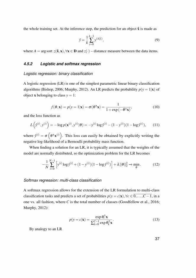
4.5.2 Logistic and softmax regression

Logistic regression: binary classification

A logistic regression (LR) is one of the simplest parametric linear binary classificationalgorithms (Bishop, 2006; Murphy, 2012). An LR predicts the probability p(y = 1|x) ofobject x belonging to class y = 1:

f (θ ,x) = p(y = 1|x) = σ(θᵀx) =1

1+ exp(−θᵀx), (10)

and the loss function as

L(

y(i),y(i))=− log p(x(i),y(i)|θ) =−y(i) log y(i)− (1− y(i))(1− log y(i)), (11)

where y(i) = σ

(θᵀx(i)

). This loss can easily be obtained by explicitly writing the

negative log-likelihood of a Bernoulli probability mass function.When finding a solution for an LR, it is typically assumed that the weights of the

model are normally distributed, so the optimization problem for the LR becomes

− 1N

N−1

∑i=0

[y(i) log y(i)+(1− y(i))(1− log y(i))

]+λ‖θ‖2

2 −→minθ

. (12)

Softmax regression: multi-class classification

A softmax regression allows for the extension of the LR formulation to multi-classclassification tasks and predicts a set of probabilities p(y = c|x),∀c ∈ 0, . . . ,C−1, in aone vs. all fashion, where C is the total number of classes (Goodfellow et al., 2016;Murphy, 2012):

p(y = c|x) = expθᵀc x

∑C−1k=0 expθ

ᵀk x

. (13)

By analogy to an LR

37

− 1N

N−1

∑i=0

C−1

∑k=0

y(i,k) log y(i,k)+λ‖θ‖22 −→min

θ, (14)

where target y(·,k) is one-hot encoded vector. For the case of two classes, this equationbecomes equivalent to equation 10 (Bishop, 2006; Murphy, 2012).

It is worth noting that a softmax regression, in fact, performs a one-vs-all classifica-tion, that is, trains C independent classifiers. Therefore, it is typically written in a matrixform. As such, having S = exp[Θᵀx], one can rewrite equation (13) as

p(y = 0|x)p(y = 1|x)

...p(y =C−1|x)

=exp[Θᵀx]

∑C−1k=0 (Θ

ᵀx)(k). (15)

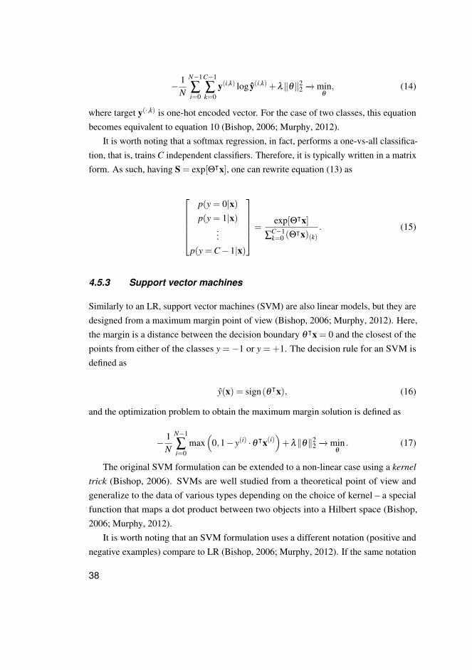
4.5.3 Support vector machines

Similarly to an LR, support vector machines (SVM) are also linear models, but they aredesigned from a maximum margin point of view (Bishop, 2006; Murphy, 2012). Here,the margin is a distance between the decision boundary θᵀx = 0 and the closest of thepoints from either of the classes y =−1 or y =+1. The decision rule for an SVM isdefined as

y(x) = sign(θᵀx), (16)

and the optimization problem to obtain the maximum margin solution is defined as

− 1N

N−1

∑i=0

max(

0,1− y(i) ·θᵀx(i))+λ‖θ‖2

2 −→minθ

. (17)

The original SVM formulation can be extended to a non-linear case using a kernel

trick (Bishop, 2006). SVMs are well studied from a theoretical point of view andgeneralize to the data of various types depending on the choice of kernel – a specialfunction that maps a dot product between two objects into a Hilbert space (Bishop,2006; Murphy, 2012).

It is worth noting that an SVM formulation uses a different notation (positive andnegative examples) compare to LR (Bishop, 2006; Murphy, 2012). If the same notation

38

would be used for an LR, the LR optimization problem would be written as

− 1N

N−1

∑i=0

ln(

1+ exp(−y(i) ·θᵀx(i)))+λ‖θ‖2

2 −→minθ

. (18)

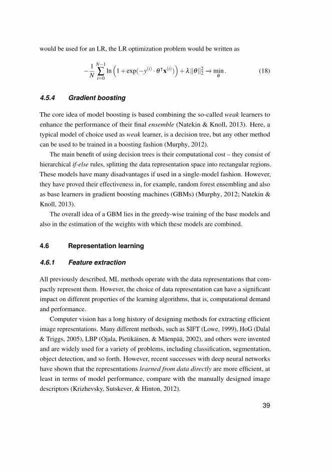
4.5.4 Gradient boosting

The core idea of model boosting is based combining the so-called weak learners toenhance the performance of their final ensemble (Natekin & Knoll, 2013). Here, atypical model of choice used as weak learner, is a decision tree, but any other methodcan be used to be trained in a boosting fashion (Murphy, 2012).

The main benefit of using decision trees is their computational cost – they consist ofhierarchical if-else rules, splitting the data representation space into rectangular regions.These models have many disadvantages if used in a single-model fashion. However,they have proved their effectiveness in, for example, random forest ensembling and alsoas base learners in gradient boosting machines (GBMs) (Murphy, 2012; Natekin &Knoll, 2013).

The overall idea of a GBM lies in the greedy-wise training of the base models andalso in the estimation of the weights with which these models are combined.

4.6 Representation learning

4.6.1 Feature extraction

All previously described, ML methods operate with the data representations that com-pactly represent them. However, the choice of data representation can have a significantimpact on different properties of the learning algorithms, that is, computational demandand performance.

Computer vision has a long history of designing methods for extracting efficientimage representations. Many different methods, such as SIFT (Lowe, 1999), HoG (Dalal& Triggs, 2005), LBP (Ojala, Pietikäinen, & Mäenpää, 2002), and others were inventedand are widely used for a variety of problems, including classification, segmentation,object detection, and so forth. However, recent successes with deep neural networkshave shown that the representations learned from data directly are more efficient, atleast in terms of model performance, compare with the manually designed imagedescriptors (Krizhevsky, Sutskever, & Hinton, 2012).

39

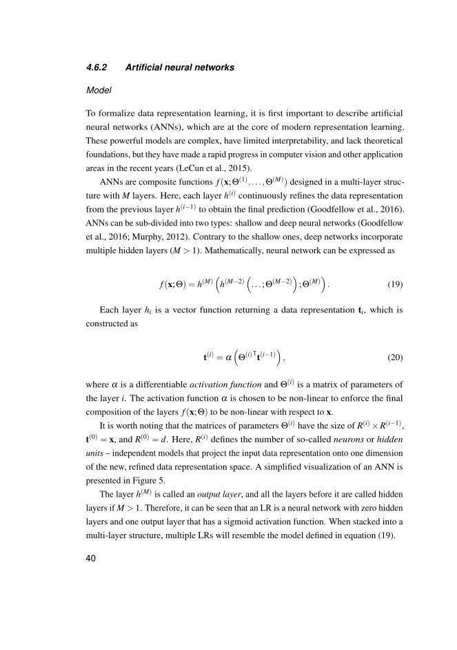
4.6.2 Artificial neural networks

Model

To formalize data representation learning, it is first important to describe artificialneural networks (ANNs), which are at the core of modern representation learning.These powerful models are complex, have limited interpretability, and lack theoreticalfoundations, but they have made a rapid progress in computer vision and other applicationareas in the recent years (LeCun et al., 2015).

ANNs are composite functions f (x;Θ(1), . . . ,Θ(M)) designed in a multi-layer struc-ture with M layers. Here, each layer h(i) continuously refines the data representationfrom the previous layer h(i−1) to obtain the final prediction (Goodfellow et al., 2016).ANNs can be sub-divided into two types: shallow and deep neural networks (Goodfellowet al., 2016; Murphy, 2012). Contrary to the shallow ones, deep networks incorporatemultiple hidden layers (M > 1). Mathematically, neural network can be expressed as

f (x;Θ) = h(M)(

h(M−2)(. . . ;Θ

(M−2))

;Θ(M)). (19)

Each layer hi is a vector function returning a data representation ti, which isconstructed as

t(i) = α

(Θ

(i)ᵀt(i−1)), (20)

where α is a differentiable activation function and Θ(i) is a matrix of parameters ofthe layer i. The activation function α is chosen to be non-linear to enforce the finalcomposition of the layers f (x;Θ) to be non-linear with respect to x.

It is worth noting that the matrices of parameters Θ(i) have the size of R(i)×R(i−1),t(0) = x, and R(0) = d. Here, R(i) defines the number of so-called neurons or hidden

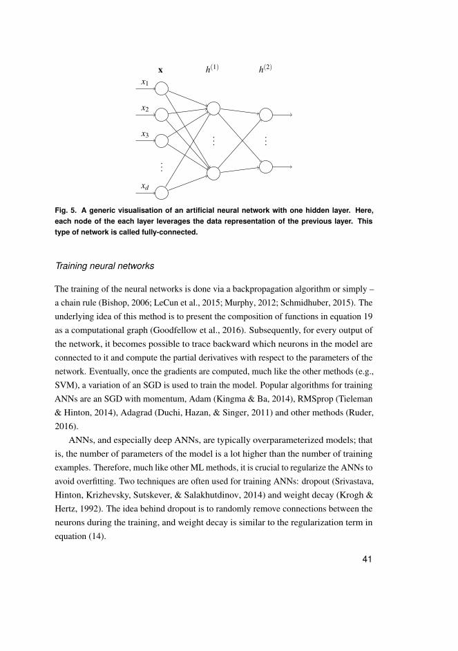
units – independent models that project the input data representation onto one dimensionof the new, refined data representation space. A simplified visualization of an ANN ispresented in Figure 5.

The layer h(M) is called an output layer, and all the layers before it are called hiddenlayers if M > 1. Therefore, it can be seen that an LR is a neural network with zero hiddenlayers and one output layer that has a sigmoid activation function. When stacked into amulti-layer structure, multiple LRs will resemble the model defined in equation (19).

40

...

......

x1

x2

x3

xd

x h(1) h(2)

Fig. 5. A generic visualisation of an artificial neural network with one hidden layer. Here,each node of the each layer leverages the data representation of the previous layer. Thistype of network is called fully-connected.

Training neural networks

The training of the neural networks is done via a backpropagation algorithm or simply –a chain rule (Bishop, 2006; LeCun et al., 2015; Murphy, 2012; Schmidhuber, 2015). Theunderlying idea of this method is to present the composition of functions in equation 19as a computational graph (Goodfellow et al., 2016). Subsequently, for every output ofthe network, it becomes possible to trace backward which neurons in the model areconnected to it and compute the partial derivatives with respect to the parameters of thenetwork. Eventually, once the gradients are computed, much like the other methods (e.g.,SVM), a variation of an SGD is used to train the model. Popular algorithms for trainingANNs are an SGD with momentum, Adam (Kingma & Ba, 2014), RMSprop (Tieleman& Hinton, 2014), Adagrad (Duchi, Hazan, & Singer, 2011) and other methods (Ruder,2016).

ANNs, and especially deep ANNs, are typically overparameterized models; thatis, the number of parameters of the model is a lot higher than the number of trainingexamples. Therefore, much like other ML methods, it is crucial to regularize the ANNs toavoid overfitting. Two techniques are often used for training ANNs: dropout (Srivastava,Hinton, Krizhevsky, Sutskever, & Salakhutdinov, 2014) and weight decay (Krogh &Hertz, 1992). The idea behind dropout is to randomly remove connections between theneurons during the training, and weight decay is similar to the regularization term inequation (14).

41

4.6.3 Deep convolutional neural networks

When working with image data, it is important to consider their dimensionality. Specifi-cally, a grayscale image of 256×256 pixels would have the data dimension of 65536.Therefore, a simple neural network with one hidden layer and one output layer that hasone output unit will have 65536×R(1)+R(2) parameters. However, the images sharemany common features, for example, edges that appear in various parts of an image.

As an example, to learn an edge detector, it is unnecessary to have many parametersin the hidden layer, and furthermore, once a detector of a certain edge is learned, itis likely to be re-usable and that particular edge will also appear in the other parts ofan image. To avoid redundancy in the network’s parameters, the same neuron can beapplied to all spatial locations within an image. Effective low-cost operations that allowthis are convolution and cross-correlation.

Deep convolutional neural networks (CNNs) are the networks that leverage thetranslational invariance of the input. Although they are called convolutional, they usecross-correlation and perform pattern matching at each spatial location of an image. Forsimplicity and alignment with the commonly accepted notation, the author of this thesisuses the term convolution assuming cross-correlation.

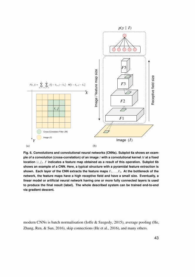
Data representations obtained from one convolutional layer of the network are calledfeature maps. An example of a convolution of an image I and a convolutional kernel M

with the size of 3×3 pixels at a fixed spatial location (i, j) is shown in Figure 6a.Typically, CNNs represent a feature pyramid, where different blocks of layers

learn their own feature representations. Then, before the next representation blocks, amax-pooling operation is typically applied to downscale the current representation. Theidea behind the pooling is to obtain translation invariance and to extract higher levelfeature representations that are eventually used by a classification head of the network.An illustration of pyramidal image data processing by a CNN is shown in Figire 6b.

It is worth noting that deep networks suffer from vanishing gradient problems ifan activation function is chosen incorrectly. As such, deep networks with sigmoidactivation suffer from this problem. To combat this limitation, a rectified linear unit(ReLU) activation has been proposed: ReLU(x) = max(0,x). This activation is widelyapplied in modern CNNs3 (Nair & Hinton, 2010). Another important component of

3Other activation functions, such as LeakyReLU or PReLU, have also been proposed (Xu, Wang, Chen, & Li,2015).

42

�

�

Cross-Correlation Filter ( )�

Image ( )�

� [�, �] = �[� − , � − ] ⋅ �[� − , � − ]∑=−1��

1

∑=−1��

1

�� �� �� ��

�, �

(a)

�1

�2

�3

�5

Image  ( )�

Rec

eptiv

e fie

ld s

ize

Imag

e / f

eatu

re m

ap s

ize

�(� ∣ �)

(b)

Fig. 6. Convolutions and convolutional neural networks (CNNs). Subplot 6a shows an exam-ple of a convolution (cross-correlation) of an image I with a convolutional kernel M at a fixedlocation (i, j). F indicates a feature map obtained as a result of this operation. Subplot 6bshows an example of a CNN. Here, a typical structure with a pyramidal feature extraction isshown. Each layer of the CNN extracts the feature maps F1, . . . ,F4. At the bottleneck of thenetwork, the feature maps have a high receptive field and have a small size. Eventually, alinear model or artificial neural network having one or more fully connected layers is usedto produce the final result (label). The whole described system can be trained end-to-endvia gradient descent.

modern CNNs is batch normalisation (Ioffe & Szegedy, 2015), average pooling (He,Zhang, Ren, & Sun, 2016), skip connections (He et al., 2016), and many others.

43

4.7 Transfer learning

Recent successes with DL methods in many fields, including medicine, can be partlyexplained by the power of transfer learning (Yosinski, Clune, Bengio, & Lipson, 2014).In the context of DL this means training a neural network (often CNN) on a large datasetwith eventual fine-tuning on a target task that has an insufficient number of trainingexamples. Interestingly, most of the models pre-trained on the ImageNet dataset (Denget al., 2009) allow for fine-tuning on a target dataset of a relatively small size and oftenget good performance.

Nowadays, transfer learning is used not only for image classification, but also forimage segmentation (L.-C. Chen, Papandreou, Kokkinos, Murphy, & Yuille, 2017;Iglovikov & Shvets, 2018), object detection (Girshick, 2015), and, interestingly, fornatural language processing (Howard & Ruder, 2018). The author of the currentthesis has also used transfer learning in several of the sub-studies of the present thesis,comparing it with training from scratch.

4.8 Summary

In this chapter, the basics of ML and DL were introduced. Various methods, such as aGBM, LR, and SVM, were introduced, and furthermore, the basics of neural networkshave been covered. Generally speaking, DL offers an end-to-end solution for developingautomatic methods for classification, regression, segmentation or object detection inimages. These tasks have been typically tackled using sophisticated heuristic pipelinesthat have required a significant amount of engineering. However, with DL, thesemethods have become more democratized, allowing for their fast adoption in manyfields, such as medical imaging (Esteva et al., 2017; Ting et al., 2018).

The remaining chapters of the current thesis demonstrate an application of ML andDL in the field of OA and demonstrate multiple methods that advanced the state-of-the-artduring the work on this doctoral dissertation.

44

5 Aims of the thesis

The current doctoral thesis is focused on the development of DL methods for knee OA.Specifically, the exact aims of the current doctoral dissertation are the following:

1. To develop efficient methods for automatic knee radiographic data pre-processingand standardization.

2. To develop an efficient method for automatic Kellgren-Lawrence grading of kneeradiographs.

3. To develop an efficient approach for automatic OARSI grading of knee radiographs.4. To investigate the possibility of the prediction of OA structural progression in an

automatic manner.5. To investigate the added effect of combining the predictions of progression from the

raw image and patient’s clinical data.

45

46

6 Overview and contributions

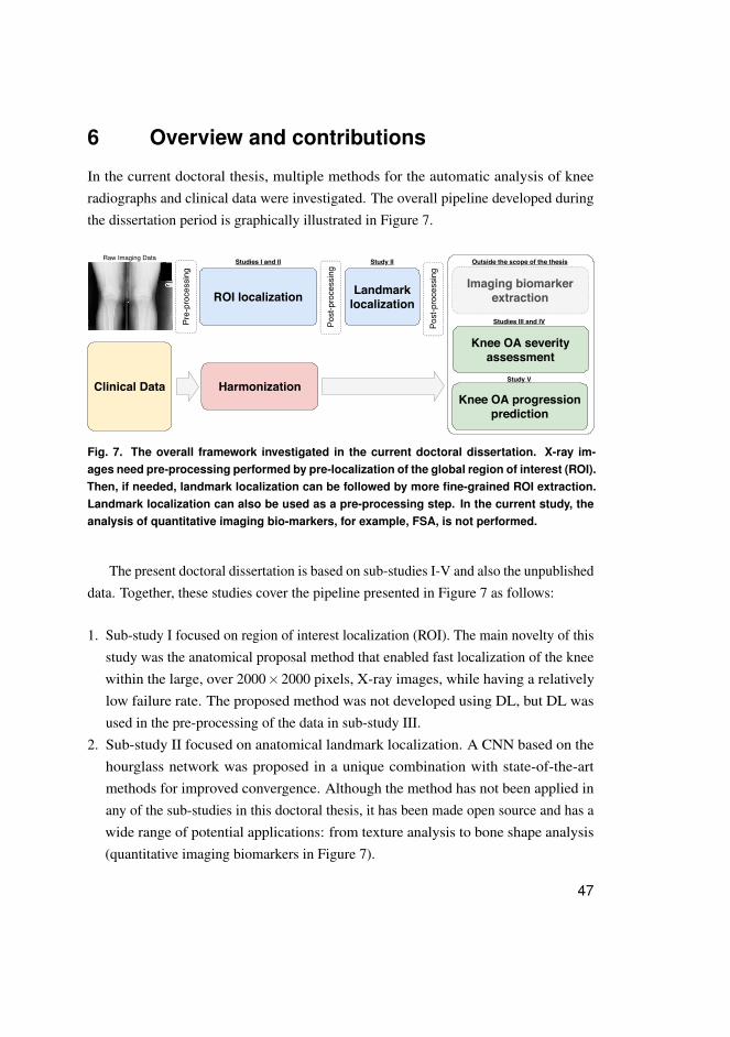
In the current doctoral thesis, multiple methods for the automatic analysis of kneeradiographs and clinical data were investigated. The overall pipeline developed duringthe dissertation period is graphically illustrated in Figure 7.

Landmarklocalization

Pre-processing

Post-processing

Post-processing

Harmonization

Imaging biomarkerextraction

Knee OA severityassessment

Knee OA progressionprediction

ROI localization

Clinical Data

Studies I and II Study II

Studies III and IV

Outside the scope of the thesis

Study V

Raw Imaging Data

Fig. 7. The overall framework investigated in the current doctoral dissertation. X-ray im-ages need pre-processing performed by pre-localization of the global region of interest (ROI).Then, if needed, landmark localization can be followed by more fine-grained ROI extraction.Landmark localization can also be used as a pre-processing step. In the current study, theanalysis of quantitative imaging bio-markers, for example, FSA, is not performed.

The present doctoral dissertation is based on sub-studies I-V and also the unpublisheddata. Together, these studies cover the pipeline presented in Figure 7 as follows:

1. Sub-study I focused on region of interest localization (ROI). The main novelty of thisstudy was the anatomical proposal method that enabled fast localization of the kneewithin the large, over 2000×2000 pixels, X-ray images, while having a relativelylow failure rate. The proposed method was not developed using DL, but DL wasused in the pre-processing of the data in sub-study III.

2. Sub-study II focused on anatomical landmark localization. A CNN based on thehourglass network was proposed in a unique combination with state-of-the-artmethods for improved convergence. Although the method has not been applied inany of the sub-studies in this doctoral thesis, it has been made open source and has awide range of potential applications: from texture analysis to bone shape analysis(quantitative imaging biomarkers in Figure 7).

47

3. Sub-study III leveraged the results of the method developed in sub-study I and wasfocused on fully automatic KL grading of the knee images. The main novelty of thispaper was a new parameter-efficient convolutional neural architecture that leveragedthe symmetry of visual features within the knee. In this thesis, the author alsopresents the unpublished material that shows how the developed method generalizesto data acquired at Oulu University hospital.

4. Sub-study IV leveraged transfer learning and investigated the possibility to performfully-automatic OARSI grading of the knee images. One of the core strengths of thisstudy was in the utilization of two large independent datasets and also state-of-the artperformance.

5. Finally, sub-study V focused on the prediction of OA progression from the dataobtained at a single clinical visit. This is the first study where raw data from asingle X-ray imaging and patient-level characteristics were used for the prediction ofOA progression. This is also the first study where raw imaging data were used forprogression prediction instead of information about the current stage of OA in theknee (e.g., KL grade).

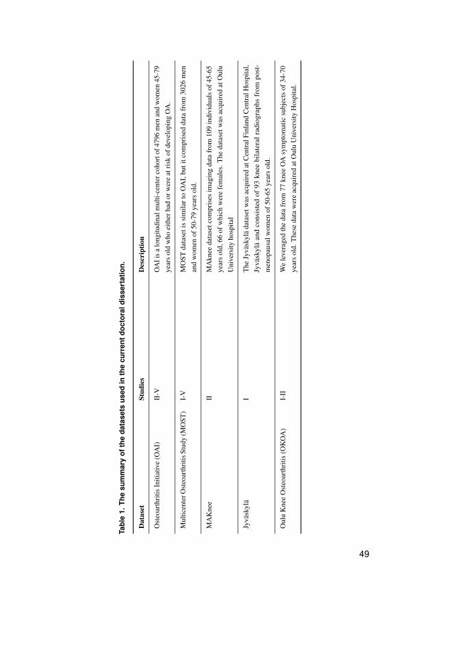
Figure 7 shows that the imaging data underwent various steps of pre-processing andROI localization before the actual predictive modeling. The clinical data and the imageassessments were harmonized across the different datasets to enable the possibility oftraining (developing) the method on one dataset and eventually performing independenttesting on another dataset. The datasets used for each of the sub-studies are presented inTable 1.

The next section provides a more detailed description of the datasets and also theinformation about their use in the sub-studies. In particular, each used dataset was usedeither for training and validation (method development) or for testing. The particular useof the data is indicated in the corresponding sections and tables.

48

Tabl

e1.

The

sum

mar

yof

the

data

sets

used

inth

ecu

rren

tdoc

tora

ldis

sert

atio

n.

Dat

aset

Stud

ies

Des

crip

tion

Ost

eoar

thri

tisIn

itiat

ive

(OA

I)II

-VO

AIi

sa

long

itudi

nalm

ulti-

cent

erco

hort

of47

96m

enan

dw

omen

45-7

9ye

ars

old

who

eith

erha

dor

wer

eat

risk

ofde

velo

ping

OA

.

Mul

ticen

terO

steo

arth

ritis

Stud

y(M

OST

)I-

VM

OST

data

seti

ssi

mila

rto

OA

I,bu

titc

ompr

ised

data

from

3026

men

and

wom

enof

50-7

9ye

ars

old.

MA

Kne

eII

MA

knee

data

setc

ompr

ises

imag

ing

data

from

109

indi

vidu

als

of45

-65

year

sol

d,66

ofw

hich

wer

efe

mal

es.T

heda

tase

twas

acqu

ired

atO

ulu

Uni

vers

ityho

spita

l

Jyvä

skyl

äI

The

Jyvä

skyl

äda

tase

twas

acqu

ired

atC

entr

alFi

nlan

dC

entr

alH

ospi

tal,

Jyvä

skyl

äan

dco

nsis

ted

of93

knee

bila

tera

lrad

iogr

aphs

from

post

-m

enop

ausa

lwom

enof

50-6

5ye

ars

old.

Oul

uK

nee

Ost

eoar

thri

tis(O

KO

A)

I-II

We

leve

rage

dth

eda

tafr

om77

knee

OA

sym

ptom

atic

subj

ects

of34

-70

year

sol

d.T

hese

data

wer

eac

quir

edat

Oul

uU

nive

rsity

Hos

pita

l.

49

50

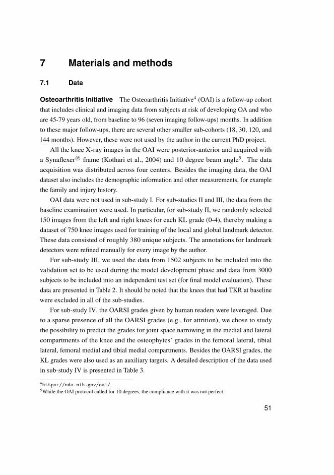
7 Materials and methods

7.1 Data

Osteoarthritis Initiative The Osteoarthritis Initiative4 (OAI) is a follow-up cohortthat includes clinical and imaging data from subjects at risk of developing OA and whoare 45-79 years old, from baseline to 96 (seven imaging follow-ups) months. In additionto these major follow-ups, there are several other smaller sub-cohorts (18, 30, 120, and144 months). However, these were not used by the author in the current PhD project.

All the knee X-ray images in the OAI were posterior-anterior and acquired witha Synaflexer R© frame (Kothari et al., 2004) and 10 degree beam angle5. The dataacquisition was distributed across four centers. Besides the imaging data, the OAIdataset also includes the demographic information and other measurements, for examplethe family and injury history.

OAI data were not used in sub-study I. For sub-studies II and III, the data from thebaseline examination were used. In particular, for sub-study II, we randomly selected150 images from the left and right knees for each KL grade (0-4), thereby making adataset of 750 knee images used for training of the local and global landmark detector.These data consisted of roughly 380 unique subjects. The annotations for landmarkdetectors were refined manually for every image by the author.

For sub-study III, we used the data from 1502 subjects to be included into thevalidation set to be used during the model development phase and data from 3000subjects to be included into an independent test set (for final model evaluation). Thesedata are presented in Table 2. It should be noted that the knees that had TKR at baselinewere excluded in all of the sub-studies.

For sub-study IV, the OARSI grades given by human readers were leveraged. Dueto a sparse presence of all the OARSI grades (e.g., for attrition), we chose to studythe possibility to predict the grades for joint space narrowing in the medial and lateralcompartments of the knee and the osteophytes’ grades in the femoral lateral, tibiallateral, femoral medial and tibial medial compartments. Besides the OARSI grades, theKL grades were also used as an auxiliary targets. A detailed description of the data usedin sub-study IV is presented in Table 3.

4https://nda.nih.gov/oai/5While the OAI protocol called for 10 degrees, the compliance with it was not perfect.

51

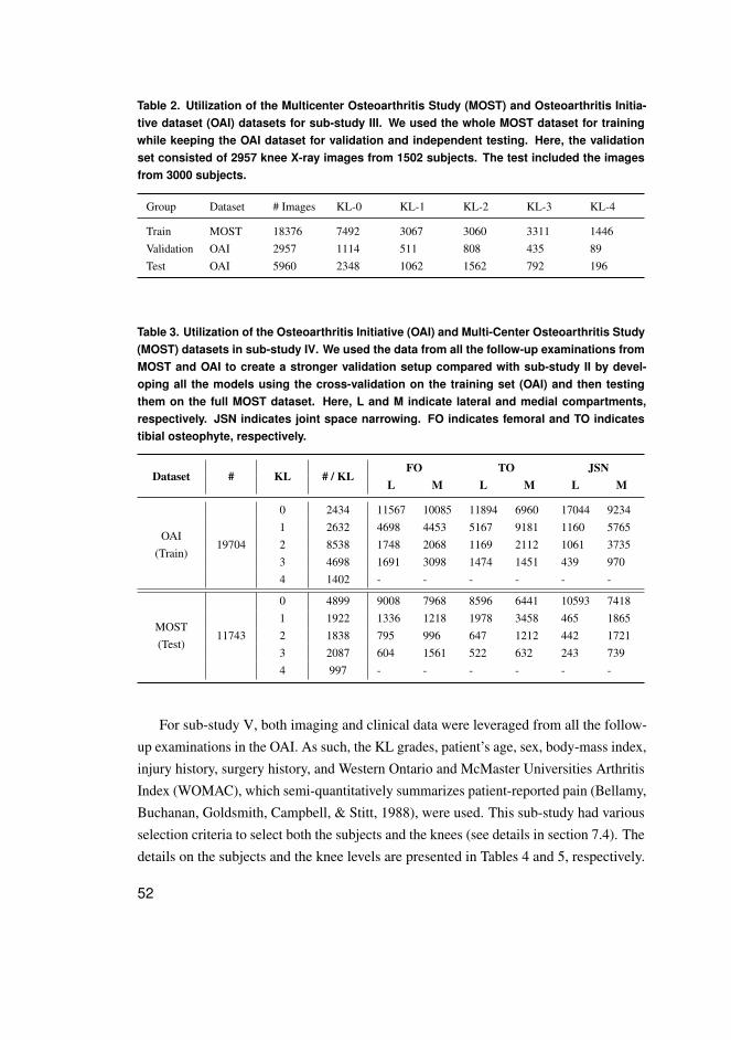
Table 2. Utilization of the Multicenter Osteoarthritis Study (MOST) and Osteoarthritis Initia-tive dataset (OAI) datasets for sub-study III. We used the whole MOST dataset for trainingwhile keeping the OAI dataset for validation and independent testing. Here, the validationset consisted of 2957 knee X-ray images from 1502 subjects. The test included the imagesfrom 3000 subjects.

Group Dataset # Images KL-0 KL-1 KL-2 KL-3 KL-4

Train MOST 18376 7492 3067 3060 3311 1446Validation OAI 2957 1114 511 808 435 89Test OAI 5960 2348 1062 1562 792 196

Table 3. Utilization of the Osteoarthritis Initiative (OAI) and Multi-Center Osteoarthritis Study(MOST) datasets in sub-study IV. We used the data from all the follow-up examinations fromMOST and OAI to create a stronger validation setup compared with sub-study II by devel-oping all the models using the cross-validation on the training set (OAI) and then testingthem on the full MOST dataset. Here, L and M indicate lateral and medial compartments,respectively. JSN indicates joint space narrowing. FO indicates femoral and TO indicatestibial osteophyte, respectively.

Dataset # KL # / KLFO TO JSN

L M L M L M

OAI(Train)

19704

0 2434 11567 10085 11894 6960 17044 92341 2632 4698 4453 5167 9181 1160 57652 8538 1748 2068 1169 2112 1061 37353 4698 1691 3098 1474 1451 439 9704 1402 - - - - - -

MOST(Test)

11743

0 4899 9008 7968 8596 6441 10593 74181 1922 1336 1218 1978 3458 465 18652 1838 795 996 647 1212 442 17213 2087 604 1561 522 632 243 7394 997 - - - - - -

For sub-study V, both imaging and clinical data were leveraged from all the follow-up examinations in the OAI. As such, the KL grades, patient’s age, sex, body-mass index,injury history, surgery history, and Western Ontario and McMaster Universities ArthritisIndex (WOMAC), which semi-quantitatively summarizes patient-reported pain (Bellamy,Buchanan, Goldsmith, Campbell, & Stitt, 1988), were used. This sub-study had variousselection criteria to select both the subjects and the knees (see details in section 7.4). Thedetails on the subjects and the knee levels are presented in Tables 4 and 5, respectively.

52

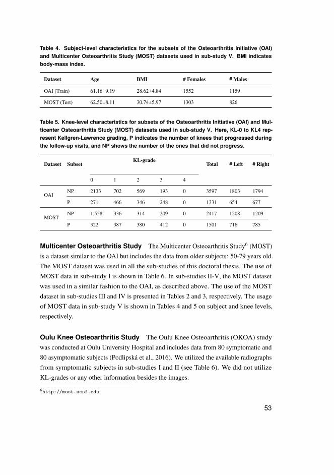
Table 4. Subject-level characteristics for the subsets of the Osteoarthritis Initiative (OAI)and Multicenter Osteoarthritis Study (MOST) datasets used in sub-study V. BMI indicatesbody-mass index.

Dataset Age BMI # Females # Males

OAI (Train) 61.16±9.19 28.62±4.84 1552 1159

MOST (Test) 62.50±8.11 30.74±5.97 1303 826

Table 5. Knee-level characteristics for subsets of the Osteoarthritis Initiative (OAI) and Mul-ticenter Osteoarthritis Study (MOST) datasets used in sub-study V. Here, KL-0 to KL4 rep-resent Kellgren-Lawrence grading, P indicates the number of knees that progressed duringthe follow-up visits, and NP shows the number of the ones that did not progress.

Dataset SubsetKL-grade

Total # Left # Right

0 1 2 3 4

OAINP 2133 702 569 193 0 3597 1803 1794

P 271 466 346 248 0 1331 654 677

MOSTNP 1,558 336 314 209 0 2417 1208 1209

P 322 387 380 412 0 1501 716 785

Multicenter Osteoarthritis Study The Multicenter Osteoarthritis Study6 (MOST)is a dataset similar to the OAI but includes the data from older subjects: 50-79 years old.The MOST dataset was used in all the sub-studies of this doctoral thesis. The use ofMOST data in sub-study I is shown in Table 6. In sub-studies II-V, the MOST datasetwas used in a similar fashion to the OAI, as described above. The use of the MOSTdataset in sub-studies III and IV is presented in Tables 2 and 3, respectively. The usageof MOST data in sub-study V is shown in Tables 4 and 5 on subject and knee levels,respectively.

Oulu Knee Osteoarthritis Study The Oulu Knee Osteoarthritis (OKOA) studywas conducted at Oulu University Hospital and includes data from 80 symptomatic and80 asymptomatic subjects (Podlipská et al., 2016). We utilized the available radiographsfrom symptomatic subjects in sub-studies I and II (see Table 6). We did not utilizeKL-grades or any other information besides the images.

6http://most.ucsf.edu

53

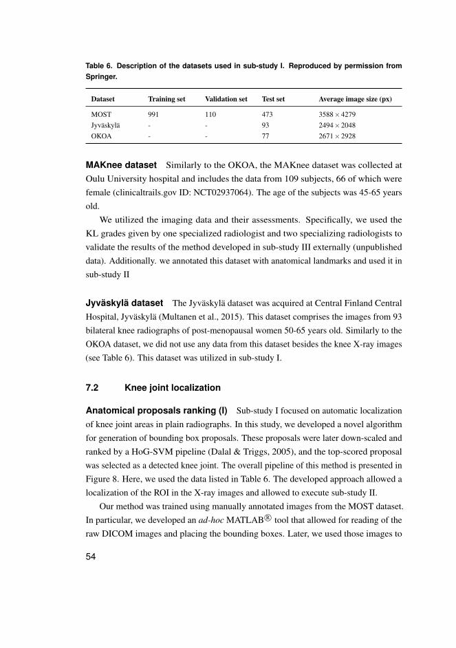
Table 6. Description of the datasets used in sub-study I. Reproduced by permission fromSpringer.

Dataset Training set Validation set Test set Average image size (px)

MOST 991 110 473 3588×4279Jyväskylä - - 93 2494×2048OKOA - - 77 2671×2928

MAKnee dataset Similarly to the OKOA, the MAKnee dataset was collected atOulu University hospital and includes the data from 109 subjects, 66 of which werefemale (clinicaltrails.gov ID: NCT02937064). The age of the subjects was 45-65 yearsold.

We utilized the imaging data and their assessments. Specifically, we used theKL grades given by one specialized radiologist and two specializing radiologists tovalidate the results of the method developed in sub-study III externally (unpublisheddata). Additionally. we annotated this dataset with anatomical landmarks and used it insub-study II

Jyväskylä dataset The Jyväskylä dataset was acquired at Central Finland CentralHospital, Jyväskylä (Multanen et al., 2015). This dataset comprises the images from 93bilateral knee radiographs of post-menopausal women 50-65 years old. Similarly to theOKOA dataset, we did not use any data from this dataset besides the knee X-ray images(see Table 6). This dataset was utilized in sub-study I.

7.2 Knee joint localization

Anatomical proposals ranking (I) Sub-study I focused on automatic localizationof knee joint areas in plain radiographs. In this study, we developed a novel algorithmfor generation of bounding box proposals. These proposals were later down-scaled andranked by a HoG-SVM pipeline (Dalal & Triggs, 2005), and the top-scored proposalwas selected as a detected knee joint. The overall pipeline of this method is presented inFigure 8. Here, we used the data listed in Table 6. The developed approach allowed alocalization of the ROI in the X-ray images and allowed to execute sub-study II.

Our method was trained using manually annotated images from the MOST dataset.In particular, we developed an ad-hoc MATLAB R© tool that allowed for reading of theraw DICOM images and placing the bounding boxes. Later, we used those images to

54

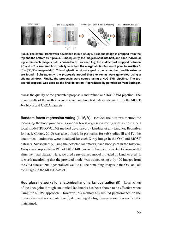
X-ray image ROI centers proposals Proposal generation & HoG-SVM scoring

!

" − !

$%

13(

23(

0

Annotated left joint area

+-

Fig. 8. The overall framework developed in sub-study I. First, the image is cropped from thetop and the bottom by α pixels. Subsequently, the image is split into half, and each individualleg within each image’s half is considered. For each leg, the middle part cropped between13C and 2

3C is summed horizontally to obtain the marginal distribution of pixel intensities Iy

(C = 12W , W – image width). This single-dimensional signal is then smoothed, and its extrema

are found. Subsequently, the proposals around these extremas were generated using asliding window. Finally, the proposals were scored using a HoG-SVM pipeline. The top-scored proposal was used as the final detection. Reproduced by permission from Springer.

assess the quality of the generated proposals and trained our HoG-SVM pipeline. Themain results of the method were assessed on three test datasets derived from the MOST,Jyväskylä and OKOA datasets.

Random forest regression voting (II, IV, V) Besides the our own method forlocalizing the knee joint area, a random forest regression voting with a constrainedlocal model (RFRV-CLM) method developed by Lindner et al. (Lindner, Bromiley,Ionita, & Cootes, 2015) was also utilized. In particular, for sub-studies III and IV, theanatomical landmarks were localized for each X-ray image in the OAI and MOSTdatasets. Subsequently, using the detected landmarks, each knee joint in the bilateralX-rays was cropped to an ROI of 140×140 mm and subsequently rotated to horizontallyalign the tibial plateau. Here, we used a pre-trained model provided by Lindner et al. Itis worth mentioning that the provided model was trained using only 400 images fromthe OAI dataset, but it generalized well to all the remaining images in the OAI and allthe images in the MOST dataset.

Hourglass networks for anatomical landmarks localization (II) Localizationof the knee joint through anatomical landmarks has been shown to be effective whenusing the RFRV approach. However, this method has limited performance on theunseen data and is computationally demanding if a high image resolution needs to bemaintained.

55

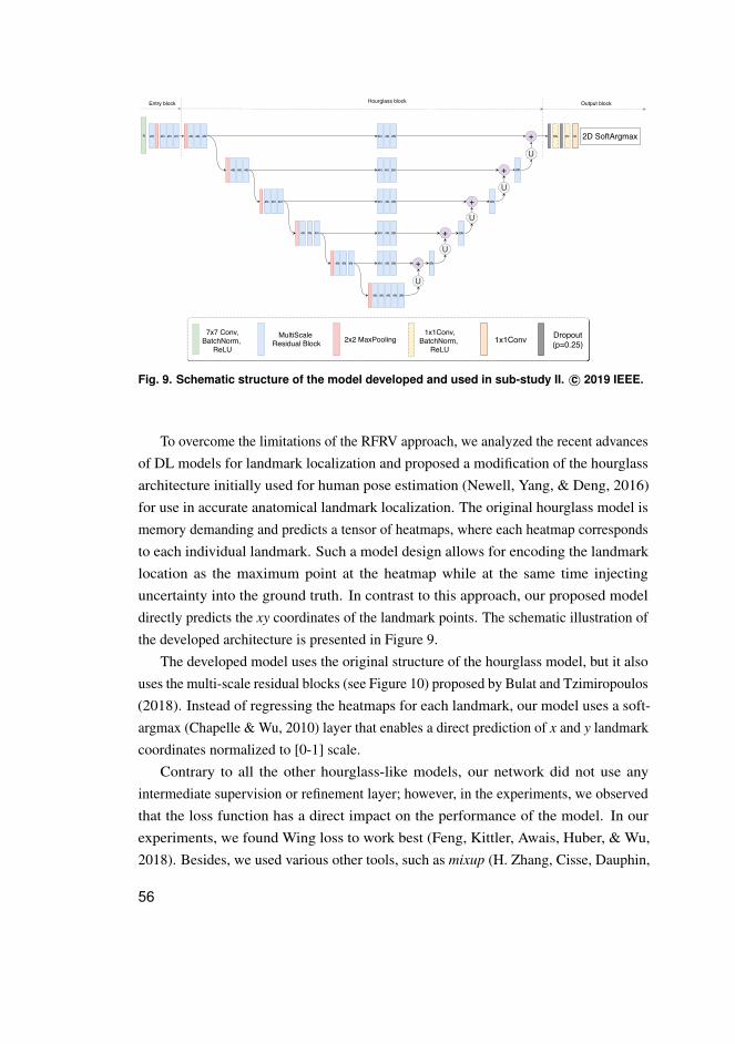
N 2N 2N 2N 4N

U

+U

+

8N

4N 8N4N

4N 8N4N

4N 8N4N 4N 4N

4N 4N 4N

4N 4N 4N

4N 4N 4N

4N 4N 4N

4N 4N 4N

4N 8N4N

U

+

8N

4N 8N4N

U

+

8N

4N 8N4N

U

+

8N

8N 4N M 2D SoftArgmax

7x7 Conv,BatchNorm,

ReLU

MultiScale Residual Block 2x2 MaxPooling

1x1Conv,BatchNorm, 

ReLU1x1Conv Dropout

(p=0.25)

Entry block Hourglass block Output block

Fig. 9. Schematic structure of the model developed and used in sub-study II. c© 2019 IEEE.

To overcome the limitations of the RFRV approach, we analyzed the recent advancesof DL models for landmark localization and proposed a modification of the hourglassarchitecture initially used for human pose estimation (Newell, Yang, & Deng, 2016)for use in accurate anatomical landmark localization. The original hourglass model ismemory demanding and predicts a tensor of heatmaps, where each heatmap correspondsto each individual landmark. Such a model design allows for encoding the landmarklocation as the maximum point at the heatmap while at the same time injectinguncertainty into the ground truth. In contrast to this approach, our proposed modeldirectly predicts the xy coordinates of the landmark points. The schematic illustration ofthe developed architecture is presented in Figure 9.

The developed model uses the original structure of the hourglass model, but it alsouses the multi-scale residual blocks (see Figure 10) proposed by Bulat and Tzimiropoulos(2018). Instead of regressing the heatmaps for each landmark, our model uses a soft-argmax (Chapelle & Wu, 2010) layer that enables a direct prediction of x and y landmarkcoordinates normalized to [0-1] scale.

Contrary to all the other hourglass-like models, our network did not use anyintermediate supervision or refinement layer; however, in the experiments, we observedthat the loss function has a direct impact on the performance of the model. In ourexperiments, we found Wing loss to work best (Feng, Kittler, Awais, Huber, & Wu,2018). Besides, we used various other tools, such as mixup (H. Zhang, Cisse, Dauphin,

56

+

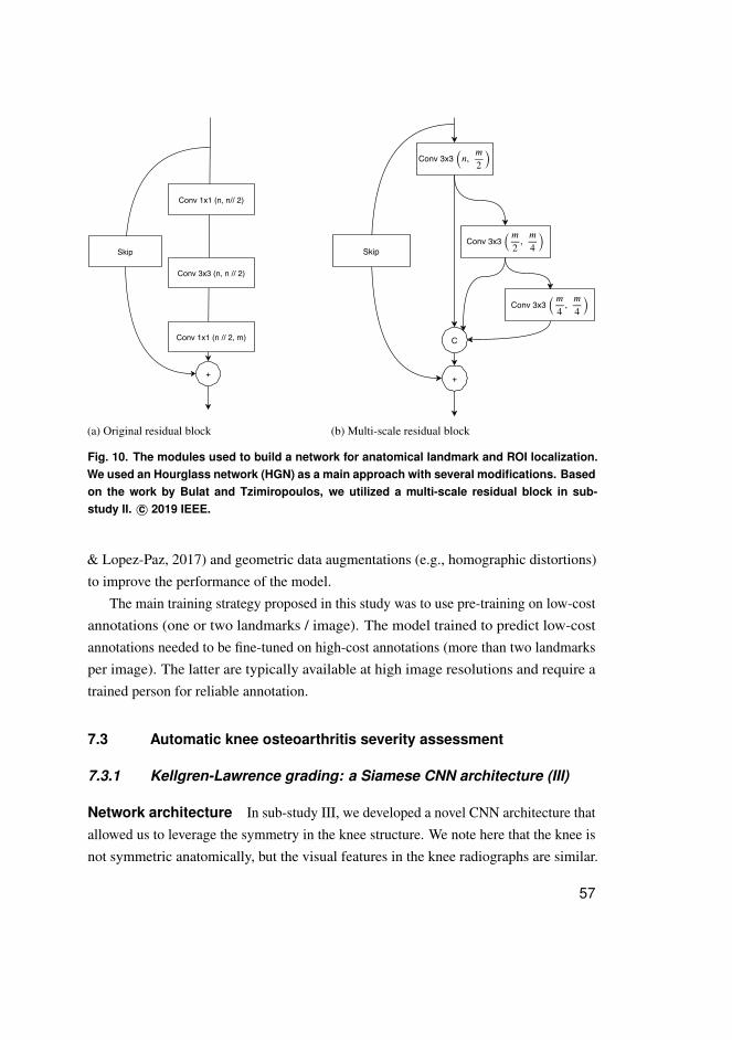
Conv 1x1 (n // 2, m)

Conv 3x3 (n, n // 2)

Conv 1x1 (n, n// 2)

Skip

(a) Original residual block

Conv 3x3 ( ,   )�

2

�

4

Conv 3x3 ( ,   )�

4

�

4

Conv 3x3 (�,   )�

2

С

Skip

+

(b) Multi-scale residual block

Fig. 10. The modules used to build a network for anatomical landmark and ROI localization.We used an Hourglass network (HGN) as a main approach with several modifications. Basedon the work by Bulat and Tzimiropoulos, we utilized a multi-scale residual block in sub-study II. c© 2019 IEEE.

& Lopez-Paz, 2017) and geometric data augmentations (e.g., homographic distortions)to improve the performance of the model.

The main training strategy proposed in this study was to use pre-training on low-costannotations (one or two landmarks / image). The model trained to predict low-costannotations needed to be fine-tuned on high-cost annotations (more than two landmarksper image). The latter are typically available at high image resolutions and require atrained person for reliable annotation.

7.3 Automatic knee osteoarthritis severity assessment

7.3.1 Kellgren-Lawrence grading: a Siamese CNN architecture (III)

Network architecture In sub-study III, we developed a novel CNN architecture thatallowed us to leverage the symmetry in the knee structure. We note here that the knee isnot symmetric anatomically, but the visual features in the knee radiographs are similar.

57

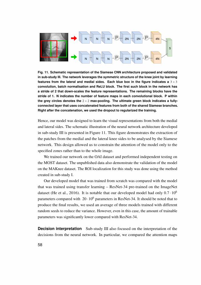
5

4N2N2NPNNN P

4N2N2NPNNN P

Fig. 11. Schematic representation of the Siamese CNN architecture proposed and validatedin sub-study III. The network leverages the symmetric structure of the knee joint by learningfeatures from the lateral and medial sides. Each blue box in the figure indicates a 3× 3convolution, batch normalisation and ReLU block. The first such block in the network hasa stride of 2 that down-scales the feature representations. The remaining blocks have thestride of 1. N indicates the number of feature maps in each convolutional block. P withinthe grey circles denotes the 2× 2 max-pooling. The ultimate green block indicates a fully-connected layer that uses concatenated features from both of the shared Siamese branches.Right after the concatenation, we used the dropout to regularized the training.

Hence, our model was designed to learn the visual representations from both the medialand lateral sides. The schematic illustration of the neural network architecture developedin sub-study III is presented in Figure 11. This figure demonstrates the extraction ofthe patches from the medial and the lateral knee sides to be analysed by the Siamesenetwork. This design allowed us to constrain the attention of the model only to thespecified zones rather than to the whole image.

We trained our network on the OAI dataset and performed independent testing onthe MOST dataset. The unpublished data also demonstrate the validation of the modelon the MAKnee dataset. The ROI localization for this study was done using the methodcreated in sub-study I.

Our developed model that was trained from scratch was compared with the modelthat was trained using transfer learning – ResNet-34 pre-trained on the ImageNetdataset (He et al., 2016). It is notable that our developed model had only 0.7 · 106

parameters compared with 20 ·106 parameters in ResNet-34. It should be noted that toproduce the final results, we used an average of three models trained with differentrandom seeds to reduce the variance. However, even in this case, the amount of trainableparameters was significantly lower compared with ResNet-34.

Decision interpretation Sub-study III also focused on the interpretation of thedecisions from the neural network. In particular, we compared the attention maps

58

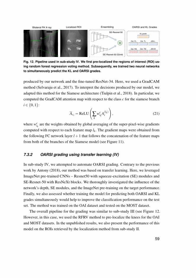
x x

Bilateral PA X-ray Localized ROI

FL

TL TM

FM

Ensembling OARSI and KL Grades

Ost. FMOst. TMOst. FM JSN M

KL-grade

Ost. TL JSN LOst. FL

Ost. FL+

SE-Resnet-50

SE-Resnet-50-32x4d

Fig. 12. Pipeline used in sub-study IV. We first pre-localized the regions of interest (ROI) us-ing random forest regression voting method. Subsequently, we trained two neural networksto simultaneously predict the KL and OARSI grades.

produced by our network and the fine-tuned ResNet-34. Here, we used a GradCAMmethod (Selvaraju et al., 2017). To interpret the decisions produced by our model, weadapted this method for the Siamese architecture (Tiulpin et al., 2018). In particular, wecomputed the GradCAM attention map with respect to the class c for the siamese branchi ∈ {0,1}:

Aci = ReLU

(∑k

wcik A(lk)

i

), (21)

where wcik

are the weights obtained by global averaging of the super-pixel-wise gradientscomputed with respect to each feature map lk. The gradient maps were obtained fromthe following FC network layer l +1 that follows the concatenation of the feature mapsfrom both of the branches of the Siamese model (see Figure 11).

7.3.2 OARSI grading using transfer learning (IV)

In sub-study IV, we attempted to automate OARSI grading. Contrary to the previouswork by Antony (2018), our method was based on transfer learning. Here, we leveragedImageNet pre-trained CNNs – Resnet50 with squeeze-excitation (SE) modules andSE-Resnet-50 with ResNeXt blocks. We thoroughly investigated the influence of thenetwork’s depth, SE modules, and the ImageNet pre-training on the target performance.Finally, we also assessed whether training the model for predicting both OARSI and KLgrades simultaneously would help to improve the classification performance on the testset. The method was trained on the OAI dataset and tested on the MOST dataset.

The overall pipeline for the grading was similar to sub-study III (see Figure 12.However, in this case, we used the RFRV method to pre-localize the knees for the OAIand MOST datasets. In the unpublished results, we also present the performance of thismodel on the ROIs retrieved by the localization method from sub-study II.

59

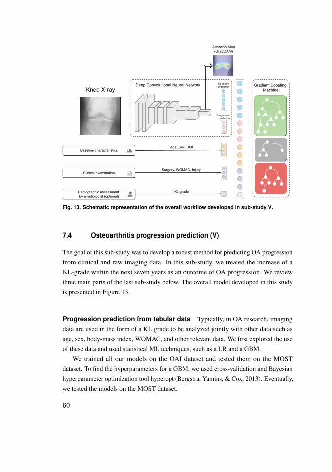
Gradient Boosting Machine

KL-grade prediction

Radiographic assessment by a radiologist (optional)

Attention Map(GradCAM)

Age, Sex, BMI

Surgery, WOMAC, InjuryClinical examination

Baseline characteristics

KL grade

Progression  prediction

Knee X-rayDeep Convolutional Neural Network

Fig. 13. Schematic representation of the overall workflow developed in sub-study V.

7.4 Osteoarthritis progression prediction (V)

The goal of this sub-study was to develop a robust method for predicting OA progressionfrom clinical and raw imaging data. In this sub-study, we treated the increase of aKL-grade within the next seven years as an outcome of OA progression. We reviewthree main parts of the last sub-study below. The overall model developed in this studyis presented in Figure 13.

Progression prediction from tabular data Typically, in OA research, imagingdata are used in the form of a KL grade to be analyzed jointly with other data such asage, sex, body-mass index, WOMAC, and other relevant data. We first explored the useof these data and used statistical ML techniques, such as a LR and a GBM.

We trained all our models on the OAI dataset and tested them on the MOSTdataset. To find the hyperparameters for a GBM, we used cross-validation and Bayesianhyperparameter optimization tool hyperopt (Bergstra, Yamins, & Cox, 2013). Eventually,we tested the models on the MOST dataset.

60

Progression prediction from raw image data Our second approach was todevelop a model that can leverage the whole knee image as an input for the model. Here,we used a CNN pre-trained on the ImageNet to initialize the convolutional layers of themodel. The fully connected layers of this CNN predicted whether the case will progresswithin the next seven years, will progress sooner than 60 months, or will progress after60 months. In addition, we leveraged multi-task learning and forced another FC layerof the model to predict a KL grade that would be assigned to the knee in the inputimage. After the model was trained, we computed the probability of progression as1−P(no progression|x), where x is an input image.

When the model training was finished, we applied GradCAM (Selvaraju et al., 2017)to interpret the decision of the CNN. However, in this case, we considered only theFC-layer predicting the gradients for computation of the feature maps’ weights.

Multi-modal progression prediction In the final part of the study, we combinedthe CNN’s predictions (both progression and KL-grade prediction branches) with thefollowing clinical information: Age, Sex, BMI, WOMAC total score, surgery history,and injury history. In particular, we first trained the CNN in a cross-validation settingand made the predictions for each of the validation folds. Subsequently, we concatenatedthe predictions from the CNN and the aforementioned clinical variables. We also testedadding a KL grade in addition to the clinical variables and our CNN’s predictions. Forthe final stage, we trained a second level model: a GBM. The parameters for the GBMwere selected using the aforementioned hyperopt (Bergstra et al., 2013).

7.5 Performance evaluation and statistical analyses

In the current thesis, the author used various metrics, depending on the task. As such, insub-study I, we developed a proposal method for knee joint localization. We defined thetask in a fuzzy manner and used manual bounding box annotations as a reference. In thatstudy, our main metric was intersection over the union (IoU), whic reflects how muchthe predicted bounding box or mask overlap. Besides the IoU, we also used cumulativeplots that showed the distribution of the IoU in the test set. We also used such plots toanalyze the developed bounding box proposal method.

In sub-study II, we used metrics that reflect landmark localization performanceunder certain distance threshold. In particular, we computed the distances di between thepredicted and ground truth (manual annotations) landmarks using euclidean distance and,

61

subsequently, computed the number of points having di <= t, where t is the distancethreshold. Subsequently, this number was divided by the number of points in the dataset.We refer to this metric as percentage of correct keypoints (PCK).

In sub-studies III-V, we used several metrics to compare the models. In particular,we used receiver operating characteristic (ROC) curves and the areas under them (AUC).Furthermore, in sub-studies IV and V, we leveraged the power of precision-recall (PR)curves and also the areas under them (average precision, AP). Besides, we also used theF1 score to compare the performance of binary classification in sub-study IV. This scoreis a geometric average between the classifier’s recall and precision. In sub-studies IIIand IV, we also used the balanced accuracy (BA), quadratic KC, and the mean squarederror (MSE) to compare the grading results. Finally, these sub-studies also included theuse of confusion matrices for visualization purposes and error analysis. Among thestatistical tests, we used a DeLong’s test (DeLong, DeLong, & Clarke-Pearson, 1988) insub-study V to compare the ROC curves.

62

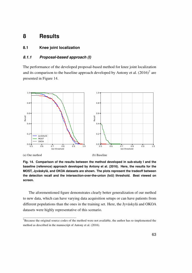
8 Results

8.1 Knee joint localization

8.1.1 Proposal-based approach (I)

The performance of the developed proposal-based method for knee joint localizationand its comparison to the baseline approach developed by Antony et al. (2016)7 arepresented in Figure 14.

0.5 0.6 0.7 0.8 0.9 1.0IoU threshold

0.0

0.2

0.4

0.6

0.8

1.0

Reca

ll

JyväskyläMOSTOKOA

(a) Our method

0.5 0.6 0.7 0.8 0.9 1.0IoU threshold

0.0

0.2

0.4

0.6

0.8

1.0Re

call

(b) Baseline

Fig. 14. Comparison of the results between the method developed in sub-study I and thebaseline (reference) approach developed by Antony et al. (2016). Here, the results for theMOST, Jyväskylä, and OKOA datasets are shown. The plots represent the tradeoff betweenthe detection recall and the intersection-over-the-union (IoU) threshold. Best viewed onscreen.

The aforementioned figure demonstrates clearly better generalization of our methodto new data, which can have varying data acquisition setups or can have patients fromdifferent populations than the ones in the training set. Here, the Jyväskylä and OKOAdatasets were highly representative of this scenario.

7Because the original source codes of the method were not available, the author has re-implemented themethod as described in the manuscript of Antony et al. (2016).

63

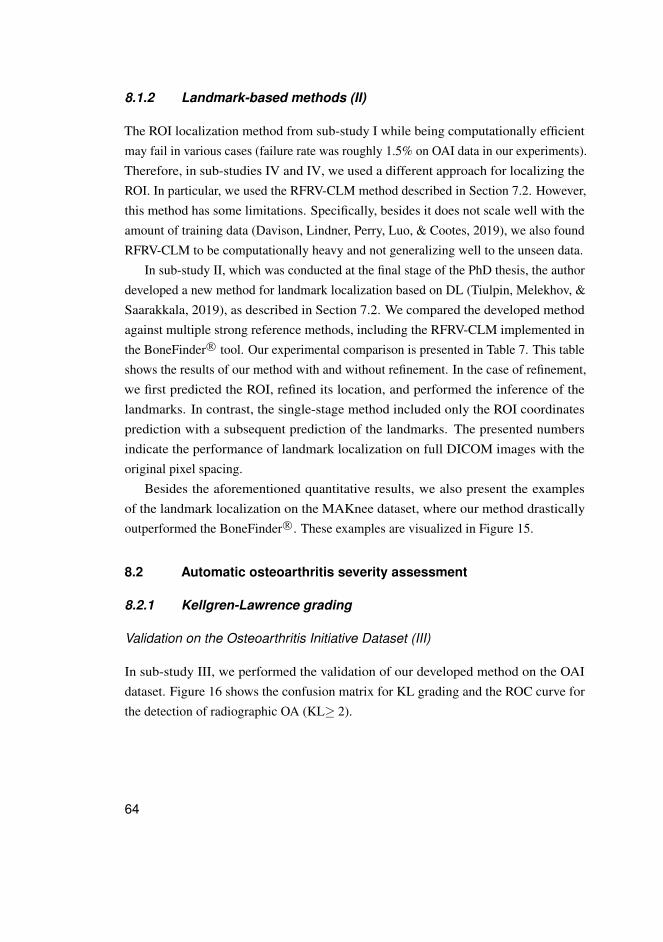
8.1.2 Landmark-based methods (II)

The ROI localization method from sub-study I while being computationally efficientmay fail in various cases (failure rate was roughly 1.5% on OAI data in our experiments).Therefore, in sub-studies IV and IV, we used a different approach for localizing theROI. In particular, we used the RFRV-CLM method described in Section 7.2. However,this method has some limitations. Specifically, besides it does not scale well with theamount of training data (Davison, Lindner, Perry, Luo, & Cootes, 2019), we also foundRFRV-CLM to be computationally heavy and not generalizing well to the unseen data.

In sub-study II, which was conducted at the final stage of the PhD thesis, the authordeveloped a new method for landmark localization based on DL (Tiulpin, Melekhov, &Saarakkala, 2019), as described in Section 7.2. We compared the developed methodagainst multiple strong reference methods, including the RFRV-CLM implemented inthe BoneFinder R© tool. Our experimental comparison is presented in Table 7. This tableshows the results of our method with and without refinement. In the case of refinement,we first predicted the ROI, refined its location, and performed the inference of thelandmarks. In contrast, the single-stage method included only the ROI coordinatesprediction with a subsequent prediction of the landmarks. The presented numbersindicate the performance of landmark localization on full DICOM images with theoriginal pixel spacing.

Besides the aforementioned quantitative results, we also present the examplesof the landmark localization on the MAKnee dataset, where our method drasticallyoutperformed the BoneFinder R©. These examples are visualized in Figure 15.

8.2 Automatic osteoarthritis severity assessment

8.2.1 Kellgren-Lawrence grading

Validation on the Osteoarthritis Initiative Dataset (III)

In sub-study III, we performed the validation of our developed method on the OAIdataset. Figure 16 shows the confusion matrix for KL grading and the ROC curve forthe detection of radiographic OA (KL≥ 2).

64

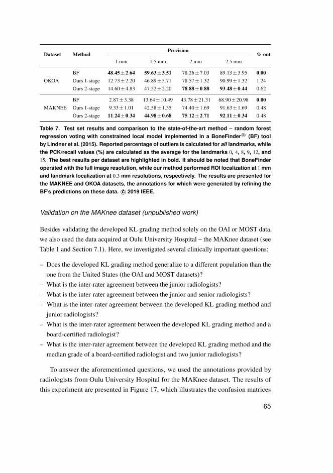
Dataset MethodPrecision

% out1 mm 1.5 mm 2 mm 2.5 mm

OKOABF 48.45±2.64 59.63±3.51 78.26±7.03 89.13±3.95 0.00Ours 1-stage 12.73±2.20 46.89±5.71 78.57±1.32 90.99±1.32 1.24Ours 2-stage 14.60±4.83 47.52±2.20 78.88±0.88 93.48±0.44 0.62

MAKNEEBF 2.87±3.38 13.64±10.49 43.78±21.31 68.90±20.98 0.00Ours 1-stage 9.33±1.01 42.58±1.35 74.40±1.69 91.63±1.69 0.48Ours 2-stage 11.24±0.34 44.98±0.68 75.12±2.71 92.11±0.34 0.48

Table 7. Test set results and comparison to the state-of-the-art method – random forestregression voting with constrained local model implemented in a BoneFinder R© (BF) toolby Lindner et al. (2015). Reported percentage of outliers is calculated for all landmarks, whilethe PCK/recall values (%) are calculated as the average for the landmarks 0, 4, 8, 9, 12, and15. The best results per dataset are highlighted in bold. It should be noted that BoneFinderoperated with the full image resolution, while our method performed ROI localization at 1 mmand landmark localization at 0.3 mm resolutions, respectively. The results are presented forthe MAKNEE and OKOA datasets, the annotations for which were generated by refining theBF’s predictions on these data. c© 2019 IEEE.

Validation on the MAKnee dataset (unpublished work)

Besides validating the developed KL grading method solely on the OAI or MOST data,we also used the data acquired at Oulu University Hospital – the MAKnee dataset (seeTable 1 and Section 7.1). Here, we investigated several clinically important questions:

– Does the developed KL grading method generalize to a different population than theone from the United States (the OAI and MOST datasets)?

– What is the inter-rater agreement between the junior radiologists?– What is the inter-rater agreement between the junior and senior radiologists?– What is the inter-rater agreement between the developed KL grading method and

junior radiologists?– What is the inter-rater agreement between the developed KL grading method and a

board-certified radiologist?– What is the inter-rater agreement between the developed KL grading method and the

median grade of a board-certified radiologist and two junior radiologists?

To answer the aforementioned questions, we used the annotations provided byradiologists from Oulu University Hospital for the MAKnee dataset. The results ofthis experiment are presented in Figure 17, which illustrates the confusion matrices

65

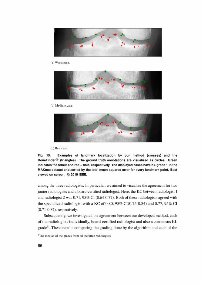
(a) Worst case.

(b) Medium case.

(c) Best case.

Fig. 15. Examples of landmark localization by our method (crosses) and theBoneFinder R© (triangles). The ground truth annotations are visualized as circles. Greenindicates the femur and red – tibia, respectively. The displayed cases have KL grade 1 in theMAKnee dataset and sorted by the total mean-squared error for every landmark point. Bestviewed on screen. c© 2019 IEEE.

among the three radiologists. In particular, we aimed to visualize the agreement for twojunior radiologists and a board-certified radiologist. Here, the KC between radiologist 1and radiologist 2 was 0.71, 95% CI (0.64-0.77). Both of these radiologists agreed withthe specialized radiologist with a KC of 0.80, 95% CI(0.75-0.84) and 0.77, 95% CI(0.71-0.82), respectively.

Subsequently, we investigated the agreement between our developed method, eachof the radiologists individually, board-certified radiologist and also a consensus KLgrade8. These results comparing the grading done by the algorithm and each of the

8The median of the grades from all the three radiologists.

66

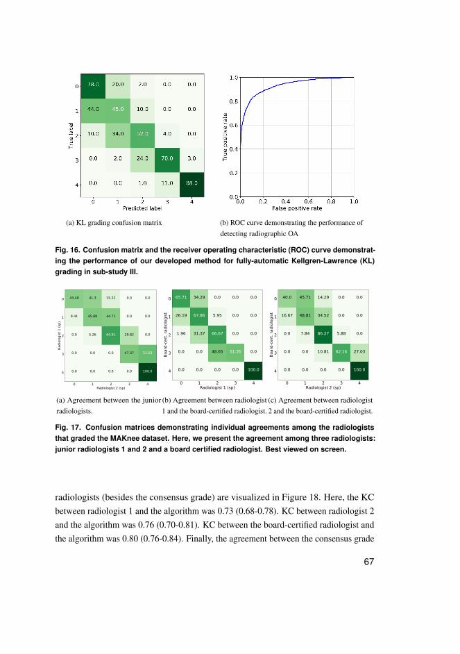
(a) KL grading confusion matrix (b) ROC curve demonstrating the performance ofdetecting radiographic OA

Fig. 16. Confusion matrix and the receiver operating characteristic (ROC) curve demonstrat-ing the performance of our developed method for fully-automatic Kellgren-Lawrence (KL)grading in sub-study III.

0 1 2 3 4Radiologist 2 (sp)

0

1

2

3

4

Radi

olog

ist 1

(sp)

43.48 41.3 15.22 0.0 0.0

9.41 45.88 44.71 0.0 0.0

0.0 5.26 64.91 29.82 0.0

0.0 0.0 0.0 47.37 52.63

0.0 0.0 0.0 0.0 100.0

(a) Agreement between the juniorradiologists.

0 1 2 3 4Radiologist 1 (sp)

0

1

2

3

4

Boar

d-ce

rt. ra

diol

ogist

65.71 34.29 0.0 0.0 0.0

26.19 67.86 5.95 0.0 0.0

1.96 31.37 66.67 0.0 0.0

0.0 0.0 48.65 51.35 0.0

0.0 0.0 0.0 0.0 100.0

(b) Agreement between radiologist1 and the board-certified radiologist.

0 1 2 3 4Radiologist 2 (sp)

0

1

2

3

4

Boar

d-ce

rt. ra

diol

ogist

40.0 45.71 14.29 0.0 0.0

16.67 48.81 34.52 0.0 0.0

0.0 7.84 86.27 5.88 0.0

0.0 0.0 10.81 62.16 27.03

0.0 0.0 0.0 0.0 100.0

(c) Agreement between radiologist2 and the board-certified radiologist.

Fig. 17. Confusion matrices demonstrating individual agreements among the radiologiststhat graded the MAKnee dataset. Here, we present the agreement among three radiologists:junior radiologists 1 and 2 and a board certified radiologist. Best viewed on screen.

radiologists (besides the consensus grade) are visualized in Figure 18. Here, the KCbetween radiologist 1 and the algorithm was 0.73 (0.68-0.78). KC between radiologist 2and the algorithm was 0.76 (0.70-0.81). KC between the board-certified radiologist andthe algorithm was 0.80 (0.76-0.84). Finally, the agreement between the consensus grade

67

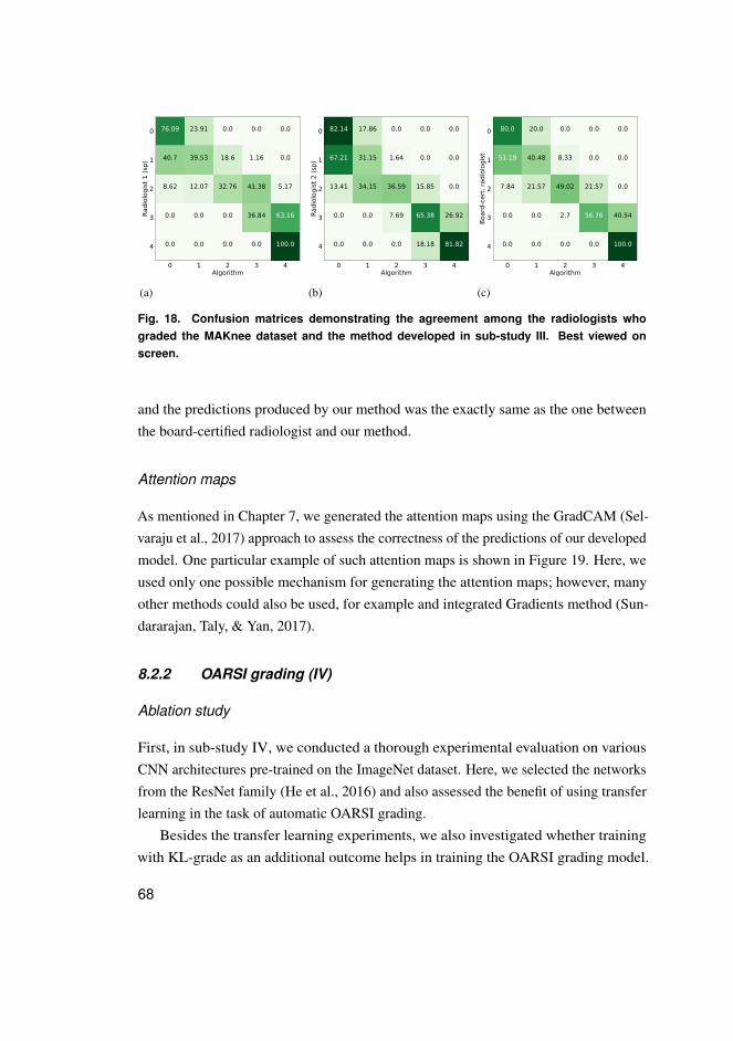
0 1 2 3 4Algorithm

0

1

2

3

4

Radi

olog

ist 1

(sp)

76.09 23.91 0.0 0.0 0.0

40.7 39.53 18.6 1.16 0.0

8.62 12.07 32.76 41.38 5.17

0.0 0.0 0.0 36.84 63.16

0.0 0.0 0.0 0.0 100.0

(a)

0 1 2 3 4Algorithm

0

1

2

3

4

Radi

olog

ist 2

(sp)

82.14 17.86 0.0 0.0 0.0

67.21 31.15 1.64 0.0 0.0

13.41 34.15 36.59 15.85 0.0

0.0 0.0 7.69 65.38 26.92

0.0 0.0 0.0 18.18 81.82

(b)

0 1 2 3 4Algorithm

0

1

2

3

4

Boar

d-ce

rt. ra

diol

ogist

80.0 20.0 0.0 0.0 0.0

51.19 40.48 8.33 0.0 0.0

7.84 21.57 49.02 21.57 0.0

0.0 0.0 2.7 56.76 40.54

0.0 0.0 0.0 0.0 100.0

(c)

Fig. 18. Confusion matrices demonstrating the agreement among the radiologists whograded the MAKnee dataset and the method developed in sub-study III. Best viewed onscreen.

and the predictions produced by our method was the exactly same as the one betweenthe board-certified radiologist and our method.

Attention maps

As mentioned in Chapter 7, we generated the attention maps using the GradCAM (Sel-varaju et al., 2017) approach to assess the correctness of the predictions of our developedmodel. One particular example of such attention maps is shown in Figure 19. Here, weused only one possible mechanism for generating the attention maps; however, manyother methods could also be used, for example and integrated Gradients method (Sun-dararajan, Taly, & Yan, 2017).

8.2.2 OARSI grading (IV)

Ablation study

First, in sub-study IV, we conducted a thorough experimental evaluation on variousCNN architectures pre-trained on the ImageNet dataset. Here, we selected the networksfrom the ResNet family (He et al., 2016) and also assessed the benefit of using transferlearning in the task of automatic OARSI grading.

Besides the transfer learning experiments, we also investigated whether trainingwith KL-grade as an additional outcome helps in training the OARSI grading model.

68

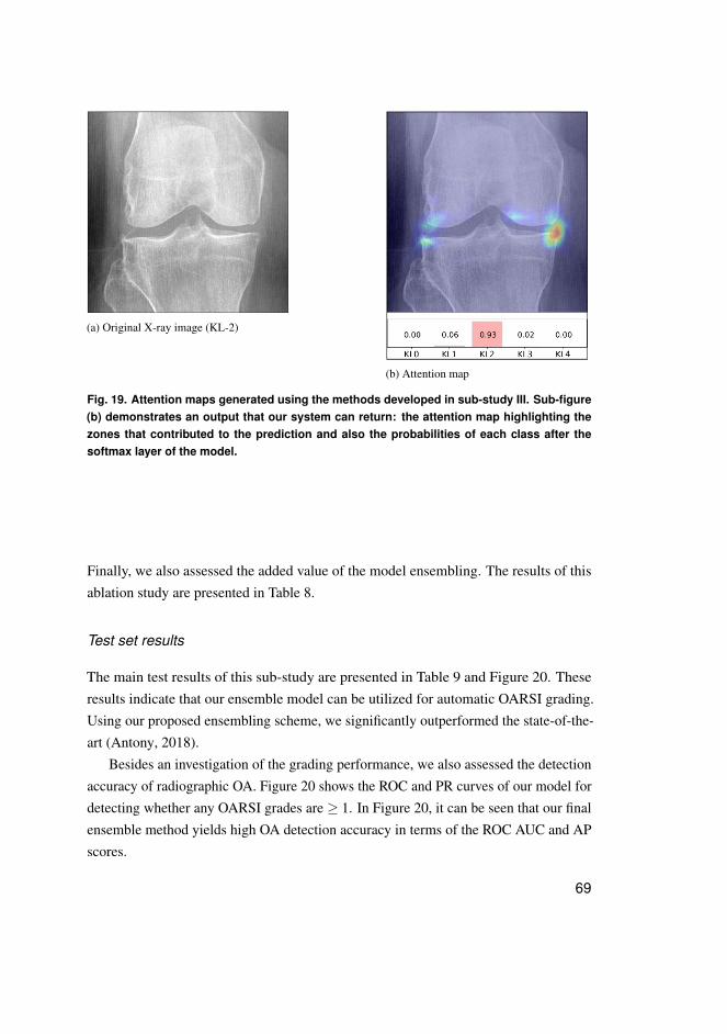
(a) Original X-ray image (KL-2)

(b) Attention map

Fig. 19. Attention maps generated using the methods developed in sub-study III. Sub-figure(b) demonstrates an output that our system can return: the attention map highlighting thezones that contributed to the prediction and also the probabilities of each class after thesoftmax layer of the model.

Finally, we also assessed the added value of the model ensembling. The results of thisablation study are presented in Table 8.

Test set results

The main test results of this sub-study are presented in Table 9 and Figure 20. Theseresults indicate that our ensemble model can be utilized for automatic OARSI grading.Using our proposed ensembling scheme, we significantly outperformed the state-of-the-art (Antony, 2018).

Besides an investigation of the grading performance, we also assessed the detectionaccuracy of radiographic OA. Figure 20 shows the ROC and PR curves of our model fordetecting whether any OARSI grades are ≥ 1. In Figure 20, it can be seen that our finalensemble method yields high OA detection accuracy in terms of the ROC AUC and APscores.

69

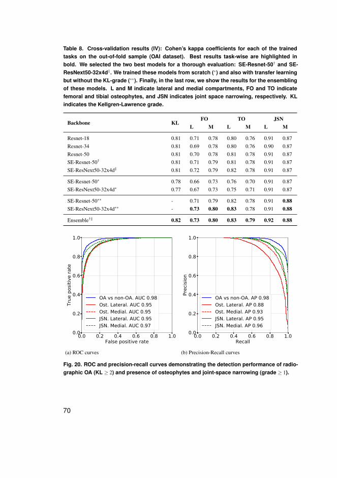
Table 8. Cross-validation results (IV): Cohen’s kappa coefficients for each of the trainedtasks on the out-of-fold sample (OAI dataset). Best results task-wise are highlighted inbold. We selected the two best models for a thorough evaluation: SE-Resnet-50† and SE-ResNext50-32x4d‡. We trained these models from scratch (∗) and also with transfer learningbut without the KL-grade (∗∗). Finally, in the last row, we show the results for the ensemblingof these models. L and M indicate lateral and medial compartments, FO and TO indicatefemoral and tibial osteophytes, and JSN indicates joint space narrowing, respectively. KLindicates the Kellgren-Lawrence grade.

Backbone KLFO TO JSN

L M L M L M

Resnet-18 0.81 0.71 0.78 0.80 0.76 0.91 0.87Resnet-34 0.81 0.69 0.78 0.80 0.76 0.90 0.87Resnet-50 0.81 0.70 0.78 0.81 0.78 0.91 0.87SE-Resnet-50† 0.81 0.71 0.79 0.81 0.78 0.91 0.87SE-ResNext50-32x4d‡ 0.81 0.72 0.79 0.82 0.78 0.91 0.87

SE-Resnet-50∗ 0.78 0.66 0.73 0.76 0.70 0.91 0.87SE-ResNext50-32x4d∗ 0.77 0.67 0.73 0.75 0.71 0.91 0.87

SE-Resnet-50∗∗ - 0.71 0.79 0.82 0.78 0.91 0.88SE-ResNext50-32x4d∗∗ - 0.73 0.80 0.83 0.78 0.91 0.88

Ensemble†‡ 0.82 0.73 0.80 0.83 0.79 0.92 0.88

0.0 0.2 0.4 0.6 0.8 1.0False positive rate

0.0

0.2

0.4

0.6

0.8

1.0

True

pos

itive

rate

OA vs non-OA. AUC 0.98Ost. Lateral. AUC 0.95Ost. Medial. AUC 0.95JSN. Lateral. AUC 0.95JSN. Medial. AUC 0.97

(a) ROC curves

0.0 0.2 0.4 0.6 0.8 1.0Recall

0.0

0.2

0.4

0.6

0.8

1.0

Prec

ision

OA vs non-OA. AP 0.98Ost. Lateral. AP 0.88Ost. Medial. AP 0.93JSN. Lateral. AP 0.95JSN. Medial. AP 0.96

(b) Precision-Recall curves

Fig. 20. ROC and precision-recall curves demonstrating the detection performance of radio-graphic OA (KL ≥ 2) and presence of osteophytes and joint-space narrowing (grade ≥ 1).

70

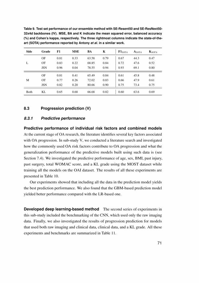
Table 9. Test set performance of our ensemble method with SE-Resent50 and SE-ResNext50-32x4d backbones (IV). MSE, BA and K indicate the mean squared error, balanced accuracy(%) and Cohen’s kappa, respectively. The three rightmost columns indicate the state-of-the-art (SOTA) performance reported by Antony et al. in a similar work.

Side Grade F1 MSE BA K F1SOTA ASOTA KSOTA

LOF 0.81 0.33 63.58 0.79 0.67 44.3 0.47OT 0.83 0.22 68.85 0.84 0.72 47.6 0.52JSN 0.96 0.04 78.55 0.94 0.93 69.1 0.80

MOF 0.81 0.41 65.49 0.84 0.61 45.8 0.48OT 0.77 0.26 72.02 0.83 0.66 47.9 0.61JSN 0.82 0.20 80.66 0.90 0.75 73.4 0.75

Both KL 0.65 0.68 66.68 0.82 0.60 63.6 0.69

8.3 Progression prediction (V)

8.3.1 Predictive performance

Predictive performance of individual risk factors and combined modelsAt the current stage of OA research, the literature identifies several key factors associatedwith OA progression. In sub-study V, we conducted a literature search and investigatedhow the commonly used OA risk factors contribute to OA progression and what thegeneralization performance of the predictive models built using such data is (seeSection 7.4). We investigated the predictive performance of age, sex, BMI, past injury,past surgery, total WOMAC score, and a KL grade using the MOST dataset whiletraining all the models on the OAI dataset. The results of all these experiments arepresented in Table 10.

Our experiments showed that including all the data in the prediction model yieldsthe best prediction performance. We also found that the GBM-based prediction modelyielded better performance compared with the LR-based one.

Developed deep learning-based method The second series of experiments inthis sub-study included the benchmarking of the CNN, which used only the raw imagingdata. Finally, we also investigated the results of progression prediction for modelsthat used both raw imaging and clinical data, clinical data, and a KL grade. All theseexperiments and benchmarks are summarized in Table 11.

71

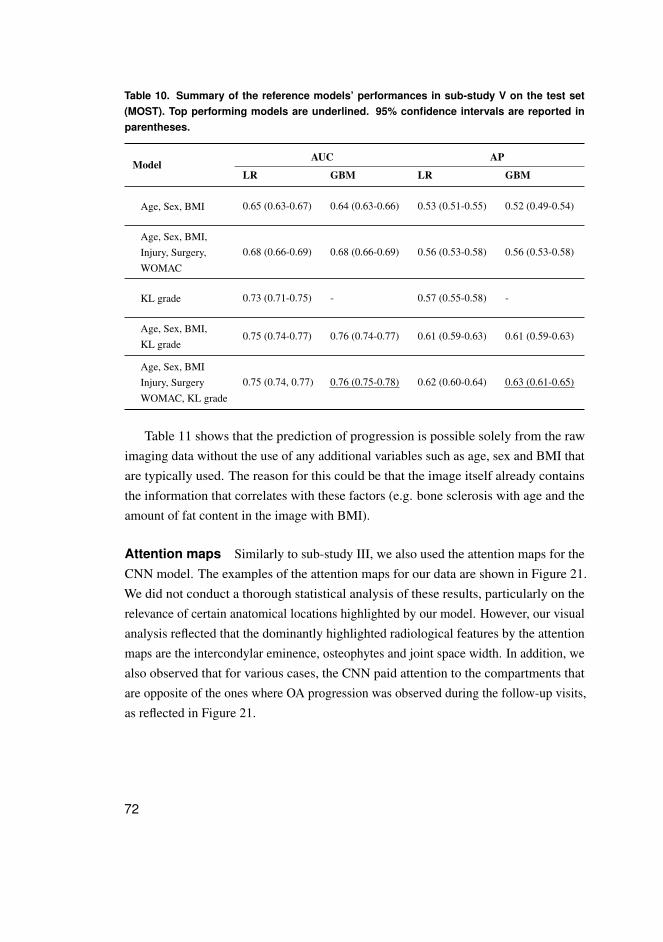
Table 10. Summary of the reference models’ performances in sub-study V on the test set(MOST). Top performing models are underlined. 95% confidence intervals are reported inparentheses.

ModelAUC AP

LR GBM LR GBM

Age, Sex, BMI 0.65 (0.63-0.67) 0.64 (0.63-0.66) 0.53 (0.51-0.55) 0.52 (0.49-0.54)

Age, Sex, BMI,Injury, Surgery,WOMAC

0.68 (0.66-0.69) 0.68 (0.66-0.69) 0.56 (0.53-0.58) 0.56 (0.53-0.58)

KL grade 0.73 (0.71-0.75) - 0.57 (0.55-0.58) -

Age, Sex, BMI,KL grade

0.75 (0.74-0.77) 0.76 (0.74-0.77) 0.61 (0.59-0.63) 0.61 (0.59-0.63)

Age, Sex, BMIInjury, SurgeryWOMAC, KL grade

0.75 (0.74, 0.77) 0.76 (0.75-0.78) 0.62 (0.60-0.64) 0.63 (0.61-0.65)

Table 11 shows that the prediction of progression is possible solely from the rawimaging data without the use of any additional variables such as age, sex and BMI thatare typically used. The reason for this could be that the image itself already containsthe information that correlates with these factors (e.g. bone sclerosis with age and theamount of fat content in the image with BMI).

Attention maps Similarly to sub-study III, we also used the attention maps for theCNN model. The examples of the attention maps for our data are shown in Figure 21.We did not conduct a thorough statistical analysis of these results, particularly on therelevance of certain anatomical locations highlighted by our model. However, our visualanalysis reflected that the dominantly highlighted radiological features by the attentionmaps are the intercondylar eminence, osteophytes and joint space width. In addition, wealso observed that for various cases, the CNN paid attention to the compartments thatare opposite of the ones where OA progression was observed during the follow-up visits,as reflected in Figure 21.

72

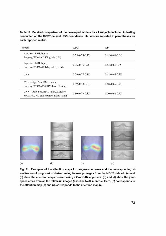
Table 11. Detailed comparison of the developed models for all subjects included in testingconducted on the MOST dataset. 95% confidence intervals are reported in parentheses foreach reported metric.

Model AUC AP

Age, Sex, BMI, Injury,Surgery, WOMAC, KL grade (LR)

0.75 (0.74-0.77) 0.62 (0.60-0.64)

Age, Sex, BMI, Injury,Surgery, WOMAC, KL grade (GBM)

0.76 (0.75-0.78) 0.63 (0.61-0.65)

CNN 0.79 (0.77-0.80) 0.68 (0.66-0.70)

CNN + Age, Sex, BMI, Injury,Surgery, WOMAC (GBM-based fusion)

0.79 (0.78-0.81) 0.68 (0.66-0.71)

CNN + Age, Sex, BMI, Injury, Surgery,WOMAC, KL grade (GBM-based fusion)

0.80 (0.79-0.82) 0.70 (0.68-0.72)

(a) (b) (c) (d)

Fig. 21. Examples of the attention maps for progression cases and the corresponding vi-sualization of progression derived using follow-up images from the MOST dataset. (a) and(c) show the attention maps derived using a GradCAM approach. (b) and (d) show the joint-space areas from all the follow-up images (baseline to 84 months). Here, (b) corresponds tothe attention map (a) and (d) corresponds to the attention map (c).

73

74

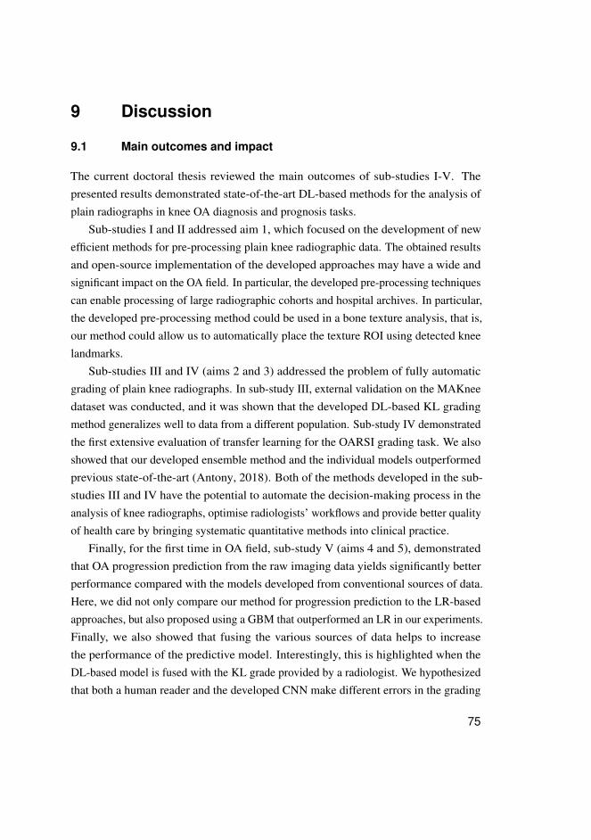
9 Discussion

9.1 Main outcomes and impact

The current doctoral thesis reviewed the main outcomes of sub-studies I-V. Thepresented results demonstrated state-of-the-art DL-based methods for the analysis ofplain radiographs in knee OA diagnosis and prognosis tasks.

Sub-studies I and II addressed aim 1, which focused on the development of newefficient methods for pre-processing plain knee radiographic data. The obtained resultsand open-source implementation of the developed approaches may have a wide andsignificant impact on the OA field. In particular, the developed pre-processing techniquescan enable processing of large radiographic cohorts and hospital archives. In particular,the developed pre-processing method could be used in a bone texture analysis, that is,our method could allow us to automatically place the texture ROI using detected kneelandmarks.

Sub-studies III and IV (aims 2 and 3) addressed the problem of fully automaticgrading of plain knee radiographs. In sub-study III, external validation on the MAKneedataset was conducted, and it was shown that the developed DL-based KL gradingmethod generalizes well to data from a different population. Sub-study IV demonstratedthe first extensive evaluation of transfer learning for the OARSI grading task. We alsoshowed that our developed ensemble method and the individual models outperformedprevious state-of-the-art (Antony, 2018). Both of the methods developed in the sub-studies III and IV have the potential to automate the decision-making process in theanalysis of knee radiographs, optimise radiologists’ workflows and provide better qualityof health care by bringing systematic quantitative methods into clinical practice.

Finally, for the first time in OA field, sub-study V (aims 4 and 5), demonstratedthat OA progression prediction from the raw imaging data yields significantly betterperformance compared with the models developed from conventional sources of data.Here, we did not only compare our method for progression prediction to the LR-basedapproaches, but also proposed using a GBM that outperformed an LR in our experiments.Finally, we also showed that fusing the various sources of data helps to increasethe performance of the predictive model. Interestingly, this is highlighted when theDL-based model is fused with the KL grade provided by a radiologist. We hypothesizedthat both a human reader and the developed CNN make different errors in the grading

75

task, and these are leveraged by a second-level GBM model. Overall, the main impactof this study is providing more sensitive tools for selecting patients into OA clinicaltrials and also for developing behavioral interventions.

To conclude, the sub-studies of this thesis formed a strong basis for the frameworkdescribed in Figure 7. This framework includes all the steps for leveraging the X-rayimaging data for diagnostic and prognostic models and beyond (e.g., measurementof bone sizes, knee alignment and so forth). The next sections will provide a detailedoverview and discuss each of the individual aims of the current doctoral thesis.

9.2 Pre-processing methods (I, II)

The results from sub-study I indicated that with the developed method, it is feasible tolocalize the knee joints fast and accurately. The proposed method included a mechanismfor generating ROI proposals eventually classified as background or foreground. Here,we used the HoG feature descriptor and an SVM to perform such classification. Atthe moment of publication, our results were superior to the state-of-the-art approachpublished by Antony et al. (2016). In our experiments, we observed that there isa trade-off between the recall of the model and speed of computation. Therefore,we adjusted the hyperparameters of the model to tackle this issue and keep the highdetection rate. The open-source implementation of the method developed in sub-study Iis available on GitHub: https://github.com/MIPT-Oulu/KneeLocalizer.

The method developed in sub-study I comprised a HoG-SVM pipeline that allowedfor fast and accurate localization of a knee joint area. However, while performing thepre-processing of the data in sub-study III using this method, we observed the failurecases, especially in the knee images that had high intensity in the patellar region. Thiseventually affected the proposal generation mechanism and the extracted HoG features.To avoid the failure issues in studies IV and V, we used a computationally intensivebut accurate RFRV-CLM (Lindner et al., 2015; Lindner et al., 2013). Besides the ROIlocalization, the RFRV-CLM method allowed us to perform the pre-processing of theimages. In particular, we used knee anatomical landmarks for aligning the tibial plateau.Here, we used the pre-trained model kindly provided by the authors of the methodimplemented in the BoneFinder tool R©.

While being accurate, the RFRV-CLM method was shown to not scale (not improvethe accuracy of localization) with the amount of training data compared with the DL-based counterparts (Davison et al., 2019). In addition, when we tested the RFRV-CLM

76

method on the datasets that had a different data acquisition setup than the OAI (e.g., theMAKnee dataset), we found that this method did not generalize well to these new unseendata. Therefore, we developed a new DL-based method that allowed us to performthe localization of knee landmarks fast and accurately. This method was compared toBoneFinder R©, which is a state-of-the-art approach for this task.

Although the comparison between our method and the RFRV-CLM in sub-study IIwas not absolutely fair due to slightly different training set sizes, it can be seen from a hipstudy by Davison et al. (2019) that the RFRV-CLM method only insignificantly improvesin localization accuracy when more training data are used. Therefore, we considered thedifferences in training set sizes between our model and BoneFinder R© insignificant.Furthermore, we expect our developed method to yield even better results if moretraining data would be used. The open-source implementation of the method developedin sub-study II is available on GitHub: https://github.com/MIPT-Oulu/KNEEL.

9.3 Automatic osteoarthritis severity assessment (III, IV,unpublished work)

The method developed in sub-study III yielded a state-of-the-art performance in theautomatic assessment of osteoarthritis severity. This method had two external validationexperiments – one performed in sub-study III) – and another as unpublished material. Inthe latter experiments, we found that the KL grades predicted by the developed CNNhave high inter-rater agreement with the radiologists from Oulu University Hospital.

The results of sub-study III showed that our model is also parameter-efficient. Inparticular, we used transfer learning and trained a ResNet-34 to solve the same task. Thelatter model had over 20 ·106 million of parameters, while our network had only roughly0.7 ·106 parameters. Such a low amount of parameters was achieved due to the use of aSiamese structure that allowed us to leverage the knee anatomy and exploit the relativesymmetry in the image features9. The open-source implementation of the method devel-oped in sub-study III is available on GitHub: https://github.com/MIPT-Oulu/DeepKnee.Furthermore, the same repository contains an open-source standalone implementation ofthe whole KL grading pipeline.

Sub-study IV formed a basis for research on automatic OARSI grading and proposeda transfer-learning based benchmark for this problem. We investigated what the

9The knee itself is not symmetrical, but the visual features of any knee are the same for a machine learningsystem.

77

impacts of training the OARSI grading model are with and without the KL gradesas an auxiliary outcome and also what the impact of transfer learning and modelensembling is. We found that training a neural network to alone predict the OARSIgrades worked better than when the KL grades were predicted as well. However, theKL grade is a desirable outcome for practitioners. Therefore, we aimed to achieveboth highly accurate KL and OARSI grading. This issue was tackled using theensembling of the two best models that formed a final solution. The open-sourceimplementation of the method developed in sub-study IV is available on GitHub:https://github.com/MIPT-Oulu/KneeOARSIGrading.

9.4 Progression prediction from imaging data (V)

Sub-study V shed the light on several interesting properties of X-ray imaging data. First,we showed that the prediction of progression from the raw images works significantlybetter compared with the conventional models that can be either linear or non-linear(e.g., an LR or a GBM) and use image interpretations (KL grades) as well as theanthropometric data and symptomatic data. Second, we observed that when fusingthe predictions of the model trained using the X-ray images with age, sex, and otherfactors (called tabular data in Section 7.4) using a second-level model, no statisticallysignificant gain was observed. From these two observations, we hypothesized that theknee X-ray images already must contain the information that correlates with the age,sex, or BMI of patients.

It is worth mentioning that sub-study V was the first in the field of OA researchto tackle progression prediction from raw imaging data. Besides this, our study wasthe first that attempted to provide a mechanism for explaining imaging-based OAprogression models, and we showed that the obtained results positively correlate withpreviously published studies, such as the one by Kinds et al. (2013). The open-sourceimplementation of the method developed in sub-study V is available on GitHub:https://github.com/MIPT-Oulu/OAProgression.

9.5 Limitations

The first and most major limitation of the current thesis is that it was conducted usingsolely the data acquired using a positioning frame, and all the analyzed images werePA bilateral radiographs. This can pose some challenges when scaling the developed

78

approaches to clinical settings. Future studies should focus on validation of the developedtechniques in different and non-standardised data acquisition settings. In addition,applying and re-training the developed methods using lateral knee X-rays has also beenleft out of the scope of the current thesis. Future work should consider the use of lateralX-rays for both OA detection and the prediction of structural OA progression.

The second limitation of the current thesis is that it relies on pre-collected large datawith an unknown level of label noise. Therefore, conducting an external validation withadditionally verified labels is highly important for future research. We attempted totackle this challenge when testing our model on the MAKnee dataset.

Other limitations of the thesis are from a clinical point of view. In particular, inthe thesis, the author proposed various imaging methods and concluded with a modelpredicting OA progression. In that study (sub-study V), the outcome was formulated asan increase of the KL grade within the next seven years. Future studies should alsoconsider the inclusion of the symptomatic progression outcomes into the predictivemodels. It is worth adding that the use of the KL grade itself can also be considered alimitation because the inter-rater agreement between the radiologists was shown to beonly moderate when grading knee OA according to the KL system.

9.6 Directions for the future research

In this section, the author would also like to discuss the potential future directions ofML applications in OA. First, all the methods developed in the current dissertationrequire large amounts of annotated data for training. However, they are costly to obtainoutside of a research setting. Consequently, direct industrial applications of the methodsdeveloped in the present thesis are limited.

During recent years, large amounts of data have been accumulated in the imagingarchives of hospitals. In contrast to the open research data used in the current doctoralthesis, the hospital data are typically non-annotated, and their annotation is costly.Future studies can explore directions such as semi-supervised learning (SSL) and fewshot learning to tackle these limitations. In particular, SSL techniques allow for the useof a fraction of annotated data and large amounts of non-annotated data to achieve thesame results as if a large annotated dataset was used for the training.

Another direction of research that has to be further explored in OA is the explainabil-ity of predictions done by an ML model. In the current thesis, the author attemptedto tackle this issue, but the explainability mechanisms only superficially cover the

79

solution. In particular, the leveraged GradCAM approach can highlight only those imagezones that correlate with the prediction of the model; however, the proposed attentionmaps mechanisms do not explain the causal relations in the data. This can be seen inFigure 21, where the attention maps for OA progression are counter-intuitive. Theexisting generation of ML models is incapable of operating with causal relations amongthe concepts reflected in medical images. Therefore, this topic has a lot of potential forinvestigation.

Finally, the author would also like to bring attention to the issue of the model’scertainty in prediction. In particular, the existing DL approaches by default do notallow for an estimation of the model’s uncertainty in predictions. To address suchshortcomings of the existing methods, a new field is emerging – Bayesian DL. Theauthor expects more applications of Bayesian DL in the medical imaging domain inthe near future because in the medical setting, an assessment of uncertainty is vital,especially when building automatic decision-making systems.

80

10 Conclusions

To conclude, the current thesis proposed several state-of-the-art DL-based methodsfor knee joint localization, landmark annotation, grading of OA severity according todifferent atlases, and the prediction of structural progression. The main conclusions ofthe thesis are as follows:

1. Both DL and conventional (e.g., HoG-SVM) methods can be used for ROI localiza-tion.

2. The developed DL-based landmark and ROI localization method yields better resultsthan the state-of-the-art method.

3. The developed KL grading model is parameter-efficient and yields the same or betterperformance compared with the transfer learning reference method.

4. Transfer learning allows to train more accurate joint OARSI and KL-grading models.5. Automatic OARSI grading alone can be conducted with a better accuracy than when

a neural network is trained to predict both KL and OARSI outcomes simultaneously.We showed that averaging the results from several different models trained in such amanner allows to address this issue.

6. Prediction of structural OA progression can be performed from a single X-ray imagewithout the need for any additional co-variate variables. In addition, compared withthe conventional methods that use human-processed image data, such as KL grades,our model that leverages the raw X-ray images yields significantly better results.

81

82

References

Abedin, J., Antony, J., McGuinness, K., Moran, K., O’Connor, N. E., Rebholz-Schuhmann, D., & Newell, J. (2019). Predicting knee osteoarthritis severity:comparative modeling based on patient’s data and plain x-ray images. Scientific

reports, 9(1), 5761.Ackerman, I. N., Bohensky, M. A., Zomer, E., Tacey, M., Gorelik, A., Brand, C. A.,

& de Steiger, R. (2019). The projected burden of primary total knee and hipreplacement for osteoarthritis in australia to the year 2030. BMC musculoskeletal

disorders, 20(1), 90.Aho, O.-M., Finnilä, M., Thevenot, J., Saarakkala, S., & Lehenkari, P. (2017).

Subchondral bone histology and grading in osteoarthritis. PloS one, 12(3),e0173726.

Allen, K. D., & Golightly, Y. M. (2015). Epidemiology of osteoarthritis: state of theevidence. Current opinion in rheumatology, 27(3), 276.

Altman, R. D., & Gold, G. (2007). Atlas of individual radiographic features inosteoarthritis, revised. Osteoarthritis and cartilage, 15, A1–A56.

Antony, J. (2018). Automatic quantification of radiographic knee osteoarthritis severity

and associated diagnostic features using deep convolutional neural networks

(Unpublished doctoral dissertation). Dublin City University.Antony, J., McGuinness, K., Moran, K., & O’Connor, N. E. (2017). Automatic detection

of knee joints and quantification of knee osteoarthritis severity using convolutionalneural networks. In International conference on machine learning and data

mining in pattern recognition (pp. 376–390).Antony, J., McGuinness, K., O’Connor, N. E., & Moran, K. (2016). Quantifying

radiographic knee osteoarthritis severity using deep convolutional neural networks.In 2016 23rd international conference on pattern recognition (icpr) (pp. 1195–1200).

Arden, N., & Nevitt, M. C. (2006). Osteoarthritis: epidemiology. Best practice &

research Clinical rheumatology, 20(1), 3–25.Athanasiou, K., Rosenwasser, M., Buckwalter, J., Malinin, T., & Mow, V. (1991).

Interspecies comparisons of in situ intrinsic mechanical properties of distalfemoral cartilage. Journal of Orthopaedic Research, 9(3), 330–340.

83

Bastick, A. N., Belo, J. N., Runhaar, J., & Bierma-Zeinstra, S. M. (2015). What are theprognostic factors for radiographic progression of knee osteoarthritis? a meta-analysis. Clinical Orthopaedics and Related Research R©, 473(9), 2969–2989.

Bayramoglu, N., Tiulpin, A., Hirvasniemi, J., Nieminen, M. T., & Saarakkala, S. (2019).Adaptive segmentation of knee radiographs for selecting the optimal roi in textureanalysis. arXiv preprint arXiv:1908.07736.

Bellamy, N., Buchanan, W. W., Goldsmith, C. H., Campbell, J., & Stitt, L. W. (1988).Validation study of womac: a health status instrument for measuring clinicallyimportant patient relevant outcomes to antirheumatic drug therapy in patientswith osteoarthritis of the hip or knee. The Journal of rheumatology, 15(12),1833–1840.

Belo, J., Berger, M., Reijman, M., Koes, B., & Bierma-Zeinstra, S. (2007). Prognosticfactors of progression of osteoarthritis of the knee: a systematic review ofobservational studies. Arthritis Care & Research: Official Journal of the American

College of Rheumatology, 57(1), 13–26.Berenbaum, F. (2013). Osteoarthritis as an inflammatory disease (osteoarthritis is not

osteoarthrosis!). Osteoarthritis and cartilage, 21(1), 16–21.Bergstra, J., Yamins, D., & Cox, D. D. (2013). Hyperopt: A python library for

optimizing the hyperparameters of machine learning algorithms. In Proceedings

of the 12th python in science conference (pp. 13–20).Bishop, C. M. (2006). Pattern recognition and machine learning. springer.Blackburn, T. A., & Craig, E. (1980). Knee anatomy: a brief review. Physical therapy,

60(12), 1556–1560.Brahim, A., Jennane, R., Riad, R., Janvier, T., Khedher, L., Toumi, H., & Lespessailles,

E. (2019). A decision support tool for early detection of knee osteoarthritisusing x-ray imaging and machine learning: Data from the osteoarthritis initiative.Computerized Medical Imaging and Graphics, 73, 11–18.

Brody, L. T. (2015). Knee osteoarthritis: Clinical connections to articular cartilagestructure and function. Physical Therapy in Sport, 16(4), 301–316.

Browne, M., Gaydecki, P., Gough, R., Grennan, D., Khalil, S., & Mamtora, H. (1987).Radiographic image analysis in the study of bone morphology. Clinical Physics

and Physiological Measurement, 8(2), 105.Bruyere, O., Collette, J. H., Ethgen, O., Rovati, L. C., Giacovelli, G., Henrotin, Y. E., . . .

Reginster, J.-Y. L. (2003). Biochemical markers of bone and cartilage remodelingin prediction of longterm progression of knee osteoarthritis. The Journal of

84

rheumatology, 30(5), 1043–1050.Bruyère, O., Genant, H., Kothari, M., Zaim, S., White, D., Peterfy, C., . . . others (2007).

Longitudinal study of magnetic resonance imaging and standard x-rays to assessdisease progression in osteoarthritis. Osteoarthritis and cartilage, 15(1), 98–103.

Buckland-Wright, C. (2004). Subchondral bone changes in hand and knee osteoarthritisdetected by radiography. Osteoarthritis and cartilage, 12, 10–19.

Buckland-Wright, J., Carmichael, I., & Walker, S. (1986). Quantitative microfocalradiography accurately detects joint changes in rheumatoid arthritis. Annals of the

rheumatic diseases, 45(5), 379–383.Buckland-Wright, J., Lynch, J., & Macfarlane, D. (1996). Fractal signature analysis

measures cancellous bone organisation in macroradiographs of patients with kneeosteoarthritis. Annals of the rheumatic diseases, 55(10), 749–755.

Buckwalter, J., & Mankin, H. (1997). Articular cartilage: Part i tissue design andchondrocyte-matrix interactions. JBJS, 79(4), 600–611.

Bulat, A., & Tzimiropoulos, Y. (2018). Hierarchical binary cnns for landmarklocalization with limited resources. IEEE Transactions on Pattern Analysis and

Machine Intelligence.Caligaris, M., & Ateshian, G. (2008). Effects of sustained interstitial fluid pressurization

under migrating contact area, and boundary lubrication by synovial fluid, on carti-lage friction. Osteoarthritis and Cartilage, 16(10), 1220 - 1227. Retrieved fromhttp://www.sciencedirect.com/science/article/pii/S1063458408000642

doi: https://doi.org/10.1016/j.joca.2008.02.020Carballo, C. B., Nakagawa, Y., Sekiya, I., & Rodeo, S. A. (2017). Basic science of

articular cartilage. Clinics in sports medicine, 36(3), 413–425.Chapelle, O., & Wu, M. (2010). Gradient descent optimization of smoothed information

retrieval metrics. Information retrieval, 13(3), 216–235.Chappard, D., Pascaretti-Grizon, F., Gallois, Y., Mercier, P., Baslé, M. F., & Audran, M.

(2006). Medullar fat influences texture analysis of trabecular microarchitecture onx-ray radiographs. European journal of radiology, 58(3), 404–410.

Chaudhari, A. S., Stevens, K. J., Wood, J. P., Chakraborty, A. K., Gibbons, E. K., Fang,Z., . . . Hargreaves, B. A. (2019). Utility of deep learning super-resolution inthe context of osteoarthritis mri biomarkers. Journal of Magnetic Resonance

Imaging.Chen, L.-C., Papandreou, G., Kokkinos, I., Murphy, K., & Yuille, A. L. (2017). Deeplab:

Semantic image segmentation with deep convolutional nets, atrous convolution,

85

and fully connected crfs. IEEE transactions on pattern analysis and machine

intelligence, 40(4), 834–848.Chen, P., Gao, L., Shi, X., Allen, K., & Yang, L. (2019). Fully automatic knee

osteoarthritis severity grading using deep neural networks with a novel ordinalloss. Computerized Medical Imaging and Graphics.

Collins, J. E., Losina, E., Nevitt, M. C., Roemer, F. W., Guermazi, A., Lynch, J. A.,. . . Hunter, D. J. (2016). Semi-quantitative imaging biomarkers of knee os-teoarthritis progression: data from the fnih oa biomarkers consortium. Arthritis &

rheumatology (Hoboken, NJ), 68(10), 2422.Culvenor, A. G., Engen, C. N., Øiestad, B. E., Engebretsen, L., & Risberg, M. A. (2015).

Defining the presence of radiographic knee osteoarthritis: a comparison betweenthe kellgren and lawrence system and oarsi atlas criteria. Knee Surgery, Sports

Traumatology, Arthroscopy, 23(12), 3532–3539.Dacre, J., Coppock, J., Herbert, K., Perrett, D., & Huskisson, E. (1989). Development

of a new radiographic scoring system using digital image analysis. Annals of the

rheumatic diseases, 48(3), 194–200.Dacree, J., & Huskisson, E. (1989). The automatic assessment of knee radiographs in

osteoarthritis using digital image analysis. Rheumatology, 28(6), 506–510.Dalal, N., & Triggs, B. (2005). Histograms of oriented gradients for human detection.

In international conference on computer vision & pattern recognition (cvpr’05)

(Vol. 1, pp. 886–893).Davison, A. K., Lindner, C., Perry, D. C., Luo, W., & Cootes, T. F. (2019). Landmark

localisation in radiographs using weighted heatmap displacement voting. InT. Vrtovec, J. Yao, G. Zheng, & J. M. Pozo (Eds.), Computational methods and

clinical applications in musculoskeletal imaging (pp. 73–85). Cham: SpringerInternational Publishing.

DeLong, E. R., DeLong, D. M., & Clarke-Pearson, D. L. (1988). Comparing theareas under two or more correlated receiver operating characteristic curves: anonparametric approach. Biometrics, 44(3), 837–845.

Deng, J., Dong, W., Socher, R., Li, L.-J., Li, K., & Fei-Fei, L. (2009). Imagenet: Alarge-scale hierarchical image database. In 2009 ieee conference on computer

vision and pattern recognition (pp. 248–255).de Rooij, M., van der Leeden, M., Heymans, M. W., Holla, J. F., Häkkinen, A., Lems,

W. F., . . . others (2016). Prognosis of pain and physical functioning in patientswith knee osteoarthritis: a systematic review and meta-analysis. Arthritis care &

86

research, 68(4), 481–492.Dieppe, P., Cushnaghan, J., Young, P., & Kirwan, J. (1993). Prediction of the progression

of joint space narrowing in osteoarthritis of the knee by bone scintigraphy. Annals

of the rheumatic diseases, 52(8), 557–563.Dieppe, P., & Lohmander, S. (2005). Pathogenesis and management of pain in

osteoarthritis. The Lancet, 365(9463), 965–973.Duchi, J., Hazan, E., & Singer, Y. (2011). Adaptive subgradient methods for online

learning and stochastic optimization. Journal of Machine Learning Research,12(Jul), 2121–2159.

Duryea, J., Jiang, Y., Countryman, P., & Genant, H. (1999). Automated algorithm forthe identification of joint space and phalanx margin locations on digitized handradiographs. Medical Physics, 26(3), 453–461.

Duryea, J., Li, J., Peterfy, C., Gordon, C., & Genant, H. (2000). Trainable rule-basedalgorithm for the measurement of joint space width in digital radiographic imagesof the knee. Medical physics, 27(3), 580–591.

Duryea, J., Zaim, S., & Genant, H. (2003). New radiographic-based surrogate outcomemeasures for osteoarthritis of the knee. Osteoarthritis and cartilage, 11(2),102–110.

Esteva, A., Kuprel, B., Novoa, R. A., Ko, J., Swetter, S. M., Blau, H. M., & Thrun,S. (2017). Dermatologist-level classification of skin cancer with deep neuralnetworks. Nature, 542(7639), 115.

Feng, Z.-H., Kittler, J., Awais, M., Huber, P., & Wu, X.-J. (2018). Wing loss for robustfacial landmark localisation with convolutional neural networks. In Proceedings of

the ieee conference on computer vision and pattern recognition (pp. 2235–2245).Ferket, B. S., Feldman, Z., Zhou, J., Oei, E. H., Bierma-Zeinstra, S. M., & Mazumdar,

M. (2017). Impact of total knee replacement practice: cost effectiveness analysisof data from the osteoarthritis initiative. bmj, 356, j1131.

Finnilä, M. A., Thevenot, J., Aho, O.-M., Tiitu, V., Rautiainen, J., Kauppinen, S., . . .others (2017). Association between subchondral bone structure and osteoarthritishistopathological grade. Journal of Orthopaedic Research, 35(4), 785–792.

Girshick, R. (2015). Fast r-cnn. In Proceedings of the ieee international conference on

computer vision (pp. 1440–1448).Glyn-Jones, S., Palmer, A., Agricola, R., Price, A., Vincent, T., Weinans, H., & Carr, A.

(2015). Osteoarthritis. The Lancet, 386(9991), 376–387.Goodfellow, I., Bengio, Y., & Courville, A. (2016). Deep learning. MIT Press.

87

(http://www.deeplearningbook.org)Gordon, C., Wu, C., Peterfy, C., Li, J., Duryea, J., Klifa, C., & Genant, H. (2001).

Automated measurement of radiographic hip joint-space width. Medical physics,28(2), 267–277.

Gossec, L., Jordan, J., Mazzuca, S., Lam, M.-A., Suarez-Almazor, M., Renner, J., . . .others (2008). Comparative evaluation of three semi-quantitative radiographicgrading techniques for knee osteoarthritis in terms of validity and reproducibilityin 1759 x-rays: report of the oarsi–omeract task force. Osteoarthritis and cartilage,16(7), 742–748.

Guermazi, A., Hayashi, D., Roemer, F., Felson, D. T., Wang, K., Lynch, J., . . . Nevitt,M. C. (2015). Severe radiographic knee osteoarthritis–does kellgren and lawrencegrade 4 represent end stage disease?–the most study. Osteoarthritis and cartilage,23(9), 1499–1505.

Hafezi-Nejad, N., Guermazi, A., Demehri, S., & Roemer, F. W. (2018). New imagingmodalities to predict and evaluate osteoarthritis progression. Best Practice &

Research Clinical Rheumatology.Hayashi, D., Roemer, F., & Guermazi, A. (2016). Imaging for osteoarthritis. Annals

of Physical and Rehabilitation Medicine, 59(3), 161 - 169. Retrieved fromhttp://www.sciencedirect.com/science/article/pii/S1877065715005849

(Special Issue: Osteoarthritis / Coordinated by Emmanuel Coudeyre and FrançoisRannou) doi: https://doi.org/10.1016/j.rehab.2015.12.003

He, K., Zhang, X., Ren, S., & Sun, J. (2016). Deep residual learning for imagerecognition. In Proceedings of the ieee conference on computer vision and pattern

recognition (pp. 770–778).Hirvasniemi, J., Niinimäki, J., Thevenot, J., & Saarakkala, S. (2019). Bone density and

texture from minimally post-processed knee radiographs in subjects with kneeosteoarthritis. Annals of biomedical engineering, 1–10.

Hirvasniemi, J., Thevenot, J., Guermazi, A., Podlipská, J., Roemer, F. W., Nieminen,M. T., & Saarakkala, S. (2017). Differences in tibial subchondral bone structureevaluated using plain radiographs between knees with and without cartilagedamage or bone marrow lesions-the oulu knee osteoarthritis study. European

radiology, 27(11), 4874–4882.Hirvasniemi, J., Thevenot, J., Multanen, J., Haapea, M., Heinonen, A., Nieminen, M. T.,

& Saarakkala, S. (2017). Association between radiography-based subchondralbone structure and mri-based cartilage composition in postmenopausal women

88

with mild osteoarthritis. Osteoarthritis and cartilage, 25(12), 2039–2046.Hochberg, M. C. (1996). Prognosis of osteoarthritis. Annals of the rheumatic diseases,

55(9), 685.Howard, J., & Ruder, S. (2018). Universal language model fine-tuning for text

classification. arXiv preprint arXiv:1801.06146.Hügle, T., & Geurts, J. (2016). What drives osteoarthritis?—synovial versus subchondral

bone pathology. Rheumatology, 56(9), 1461–1471.Hunter, D. J., & Bierma-Zeinstra, S. (2019, April). Osteoarthri-

tis. The Lancet, 393(10182), 1745–1759. Retrieved fromhttps://doi.org/10.1016/s0140-6736(19)30417-9 doi: 10.1016/s0140-6736(19)30417-9

Hunter, D. J., Niu, J., Felson, D. T., Harvey, W. F., Gross, K. D., McCree, P., . . .Zhang, Y. (2007). Knee alignment does not predict incident osteoarthritis: theframingham osteoarthritis study. Arthritis & Rheumatism, 56(4), 1212–1218.

Hunter, D. J., Zhang, Y. Q., Tu, X., LaValley, M., Niu, J. B., Amin, S., . . . Felson,D. T. (2006). Change in joint space width: Hyaline articular cartilage loss oralteration in meniscus? Arthritis & Rheumatism, 54(8), 2488-2495. Retrievedfrom https://onlinelibrary.wiley.com/doi/abs/10.1002/art.22016

doi: 10.1002/art.22016Huo, Y., Vincken, K. L., van der Heijde, D., De Hair, M. J., Lafeber, F. P., & Viergever,

M. A. (2015). Automatic quantification of radiographic finger joint space widthof patients with early rheumatoid arthritis. IEEE Transactions on Biomedical

Engineering, 63(10), 2177–2186.Iglovikov, V., & Shvets, A. (2018). Ternausnet: U-net with vgg11 encoder pre-trained

on imagenet for image segmentation. arXiv preprint arXiv:1801.05746.Ioffe, S., & Szegedy, C. (2015). Batch normalization: Accelerating deep network

training by reducing internal covariate shift. arXiv preprint arXiv:1502.03167.Jamshidi, A., Pelletier, J.-P., & Martel-Pelletier, J. (2018). Machine-learning-based

patient-specific prediction models for knee osteoarthritis. Nature Reviews Rheuma-

tology, 1.Janvier, T., Jennane, R., Valery, A., Harrar, K., Delplanque, M., Lelong, C., . . .

Lespessailles, E. (2017). Subchondral tibial bone texture analysis predicts kneeosteoarthritis progression: data from the osteoarthritis initiative: tibial bonetexture & knee oa progression. Osteoarthritis and cartilage, 25(2), 259–266.

Jarraya, M., Guermazi, A., Niu, J., Duryea, J., Lynch, J. A., & Roemer, F. W. (2015).

89

Multi-dimensional reliability assessment of fractal signature analysis in anoutpatient sports medicine population. Annals of Anatomy-Anatomischer Anzeiger,202, 57–60.

Kellgren, J., & Lawrence, J. (1957). Radiological assessment of osteo-arthrosis. Annals

of the rheumatic diseases, 16(4), 494.Kerkhof, H. J., Bierma-Zeinstra, S., Arden, N., Metrustry, S., Castano-Betancourt, M.,

Hart, D., . . . others (2014). Prediction model for knee osteoarthritis incidence,including clinical, genetic and biochemical risk factors. Annals of the rheumatic

diseases, 73(12), 2116–2121.Kinds, M. B., Marijnissen, A. C., Bijlsma, J. W., Boers, M., Lafeber, F. P., & Welsing,

P. M. (2013). Quantitative radiographic features of early knee osteoarthritis:development over 5 years and relationship with symptoms in the check cohort.The Journal of rheumatology, 40(1), 58–65.

Kingma, D. P., & Ba, J. (2014). Adam: A method for stochastic optimization. arXiv

preprint arXiv:1412.6980.Kothari, M., Guermazi, A., von Ingersleben, G., Miaux, Y., Sieffert, M., Block, J. E., . . .

Peterfy, C. G. (2004). Fixed-flexion radiography of the knee provides reproduciblejoint space width measurements in osteoarthritis. European radiology, 14(9),1568–1573.

Kraus, V. B., Feng, S., Wang, S., White, S., Ainslie, M., Brett, A., . . . Charles, H. C.(2009). Trabecular morphometry by fractal signature analysis is a novel markerof osteoarthritis progression. Arthritis & Rheumatism: Official Journal of the

American College of Rheumatology, 60(12), 3711–3722.Kraus, V. B., Feng, S., Wang, S., White, S., Ainslie, M., Le Graverand, M.-P. H.,

. . . others (2013). Subchondral bone trabecular integrity predicts and changesconcurrently with radiographic and magnetic resonance imaging–determinedknee osteoarthritis progression. Arthritis & Rheumatism, 65(7), 1812–1821.

Krizhevsky, A., Sutskever, I., & Hinton, G. E. (2012). Imagenet classification with deepconvolutional neural networks. In Advances in neural information processing

systems (pp. 1097–1105).Krogh, A., & Hertz, J. A. (1992). A simple weight decay can improve generalization. In

Advances in neural information processing systems (pp. 950–957).LaValley, M. P., Lo, G. H., Price, L. L., Driban, J. B., Eaton, C. B., & McAlindon,

T. E. (2017). Development of a clinical prediction algorithm for knee osteoarthri-tis structural progression in a cohort study: value of adding measurement of

90

subchondral bone density. Arthritis research & therapy, 19(1), 95.LeCun, Y., Bengio, Y., & Hinton, G. (2015). Deep learning. nature, 521(7553), 436.Lespessailles, E., & Jennane, R. (2012). Assessment of bone mineral density and

radiographic texture analysis at the tibial subchondral bone. Osteoporosis

International, 23(8), 871–876.Li, G., Yin, J., Gao, J., Cheng, T. S., Pavlos, N. J., Zhang, C., & Zheng, M. H. (2013).

Subchondral bone in osteoarthritis: insight into risk factors and microstructuralchanges. Arthritis research & therapy, 15(6), 223.

Lindner, C., Bromiley, P. A., Ionita, M. C., & Cootes, T. F. (2015). Robust and accurateshape model matching using random forest regression-voting. IEEE transactions

on pattern analysis and machine intelligence, 37(9), 1862–1874.Lindner, C., Thiagarajah, S., Wilkinson, J. M., The arcOGEN Consortium, Wallis, G. A.,

& Cootes, T. F. (2013, Aug). Fully automatic segmentation of the proximal femurusing random forest regression voting. IEEE Transactions on Medical Imaging,32(8), 1462-1472. doi: 10.1109/TMI.2013.2258030

Lories, R. J., & Luyten, F. P. (2011). The bone–cartilage unit in osteoarthritis. Nature

Reviews Rheumatology, 7(1), 43.Lowe, D. G. a. (1999). Object recognition from local scale-invariant features. In

International conference on computer vision (Vol. 99, pp. 1150–1157).Lukas, C., Sharp, J. T., Angwin, J., Boers, M., Duryea, J., Hall, J. R., . . . others (2008).

Automated measurement of joint space width in small joints of patients withrheumatoid arthritis. The Journal of rheumatology, 35(7), 1288–1293.

Lützner, J., Kasten, P., Günther, K.-P., & Kirschner, S. (2009). Surgical options forpatients with osteoarthritis of the knee. Nature Reviews Rheumatology, 5(6), 309.

Lynch, J., Hawkes, D., & Buckland-Wright, J. (1991a). Analysis of texture inmacroradiographs of osteoarthritic knees, using the fractal signature. Physics in

Medicine & Biology, 36(6), 709.Lynch, J., Hawkes, D., & Buckland-Wright, J. (1991b). A robust and accurate method

for calculating the fractal signature of texture in macroradiographs of osteoarthriticknees. Medical Informatics, 16(2), 241–251.

Lynch, J. A., Buckland-Wright, J. C., & Macfarlane, D. G. (1993). Precision of jointspace width measurement in knee osteoarthritis from digital image analysis ofhigh definition macroradiographs. Osteoarthritis and Cartilage, 1(4), 209–218.

Madry, H., Kon, E., Condello, V., Peretti, G. M., Steinwachs, M., Seil, R., . . . Angele,P. (2016). Early osteoarthritis of the knee. Knee Surgery, Sports Traumatology,

91

Arthroscopy, 24(6), 1753–1762.Madry, H., van Dijk, C. N., & Mueller-Gerbl, M. (2010). The basic science of

the subchondral bone. Knee surgery, sports traumatology, arthroscopy, 18(4),419–433.

Marsh, J. D., Birmingham, T. B., Giffin, J. R., Isaranuwatchai, W., Hoch, J. S., Feagan,B. G., . . . Fowler, P. (2016). Cost-effectiveness analysis of arthroscopic surgerycompared with non-operative management for osteoarthritis of the knee. BMJ

open, 6(1), e009949.Messent, E., Ward, R., Tonkin, C., & Buckland-Wright, C. (2006). Differences in

trabecular structure between knees with and without osteoarthritis quantifiedby macro and standard radiography, respectively. Osteoarthritis and cartilage,14(12), 1302–1305.

Minciullo, L., Bromiley, P. A., Felson, D. T., & Cootes, T. F. (2017). Indecisive treesfor classification and prediction of knee osteoarthritis. In International workshop

on machine learning in medical imaging (pp. 283–290).Minciullo, L., & Cootes, T. (2016). Fully automated shape analysis for detection of

osteoarthritis from lateral knee radiographs. In 2016 23rd international conference

on pattern recognition (icpr) (pp. 3787–3791).Minciullo, L., Parkes, M. J., Felson, D. T., & Cootes, T. F. (2018). Comparing image

analysis approaches versus expert readers: the relation of knee radiograph featuresto knee pain. Annals of the rheumatic diseases, 77(11), 1606–1609.

Mitchell, T. (1997). Machine learning. McGraw-Hill Science/Engineering/Math.Miyazaki, T., Wada, M., Kawahara, H., Sato, M., Baba, H., & Shimada, S. (2002).

Dynamic load at baseline can predict radiographic disease progression in medialcompartment knee osteoarthritis. Annals of the rheumatic diseases, 61(7),617–622.

Mobasheri, A., & Batt, M. (2016). An update on the pathophysiology of osteoarthritis.Annals of physical and rehabilitation medicine, 59(5-6), 333–339.

Multanen, J., Heinonen, A., Häkkinen, A., Kautiainen, H., Kujala, U., Lammentausta, E.,. . . Nieminen, M. (2015). Bone and cartilage characteristics in postmenopausalwomen with mild knee radiographic osteoarthritis and those without radiographicosteoarthritis. Journal of musculoskeletal & neuronal interactions, 15(1), 69.

Murphy, K. P. (2012). Machine learning: a probabilistic perspective. MIT press.Nair, V., & Hinton, G. E. (2010). Rectified linear units improve restricted boltzmann

machines. In Proceedings of the 27th international conference on machine

92

learning (icml-10) (pp. 807–814).Natekin, A., & Knoll, A. (2013). Gradient boosting machines, a tutorial. Frontiers in

neurorobotics, 7, 21.Neumann, G., Hunter, D., Nevitt, M., Chibnik, L., Kwoh, K., Chen, H., . . . others (2009).

Location specific radiographic joint space width for osteoarthritis progression.Osteoarthritis and cartilage, 17(6), 761–765.

Newell, A., Yang, K., & Deng, J. (2016). Stacked hourglass networks for human poseestimation. In European conference on computer vision (pp. 483–499).

Norman, B., Pedoia, V., Noworolski, A., Link, T. M., & Majumdar, S. (2018). Applyingdensely connected convolutional neural networks for staging osteoarthritis severityfrom plain radiographs. Journal of digital imaging, 1–7.

Ojala, T., Pietikäinen, M., & Mäenpää, T. (2002). Multiresolution gray-scale and rotationinvariant texture classification with local binary patterns. IEEE Transactions on

Pattern Analysis & Machine Intelligence(7), 971–987.O’Neill, T. W., McCabe, P. S., & McBeth, J. (2018). Update on the epidemiology, risk

factors and disease outcomes of osteoarthritis. Best Practice & Research Clinical

Rheumatology.Palazzo, C., Nguyen, C., Lefevre-Colau, M.-M., Rannou, F., & Poiraudeau, S. (2016).

Risk factors and burden of osteoarthritis. Annals of physical and rehabilitation

medicine, 59(3), 134–138.Panfilov, E., Tiulpin, A., Klein, S., Nieminen, M. T., & Saarakkala, S. (2019). Improving

robustness of deep learning based knee mri segmentation: Mixup and adversarialdomain adaptation. arXiv preprint arXiv:1908.04126.

Pedoia, V., Lee, J., Norman, B., Link, T., & Majumdar, S. (2019). Diagnosing osteoarthri-tis from t2 maps using deep learning: an analysis of the entire osteoarthritisinitiative baseline cohort. Osteoarthritis and cartilage, 27(7), 1002–1010.

Pedoia, V., Norman, B., Mehany, S. N., Bucknor, M. D., Link, T. M., & Majumdar, S.(2019). 3d convolutional neural networks for detection and severity staging ofmeniscus and pfj cartilage morphological degenerative changes in osteoarthritisand anterior cruciate ligament subjects. Journal of Magnetic Resonance Imaging,49(2), 400–410.

Platten, M., Kisten, Y., Kälvesten, J., Arnaud, L., Forslind, K., & van Vollenhoven,R. (2017). Fully automated joint space width measurement and digital x-rayradiogrammetry in early ra. RMD open, 3(1), e000369.

Podlipská, J., Guermazi, A., Lehenkari, P., Niinimäki, J., Roemer, F. W., Arokoski, J. P.,

93

. . . others (2016). Comparison of diagnostic performance of semi-quantitativeknee ultrasound and knee radiography with mri: Oulu knee osteoarthritis study.Scientific reports, 6, 22365.

Podsiadlo, P., Dahl, L., Englund, M., Lohmander, L., & Stachowiak, G. (2008). Differ-ences in trabecular bone texture between knees with and without radiographicosteoarthritis detected by fractal methods. Osteoarthritis and Cartilage, 16(3),323–329.

Podsiadlo, P., Nevitt, M., Wolski, M., Stachowiak, G., Lynch, J., Tolstykh, I., . . .Englund, M. (2016). Baseline trabecular bone and its relation to incidentradiographic knee osteoarthritis and increase in joint space narrowing score:directional fractal signature analysis in the most study. Osteoarthritis and

cartilage, 24(10), 1736–1744.Podsiadlo, P., & Stachowiak, G. (2002). Analysis of trabecular bone texture by modified

hurst orientation transform method. Medical physics, 29(4), 460–474.Puig-Junoy, J., & Zamora, A. R. (2015). Socio-economic costs of osteoarthritis:

a systematic review of cost-of-illness studies. In Seminars in arthritis and

rheumatism (Vol. 44, pp. 531–541).Reijman, M., Pols, H., Bergink, A., Hazes, J., Belo, J., Lievense, A., & Bierma-Zeinstra,

S. (2007). Body mass index associated with onset and progression of osteoarthritisof the knee but not of the hip: the rotterdam study. Annals of the rheumatic

diseases, 66(2), 158–162.Roemer, F., Jarraya, M., Niu, J., Duryea, J., Lynch, J., & Guermazi, A. (2015). Knee

joint subchondral bone structure alterations in active athletes: a cross-sectionalcase–control study. Osteoarthritis and cartilage, 23(12), 2184–2190.

Ruder, S. (2016). An overview of gradient descent optimization algorithms. arXiv

preprint arXiv:1609.04747.Saarakkala, S., Julkunen, P., Kiviranta, P., Mäkitalo, J., Jurvelin, J., & Korhonen, R.

(2010). Depth-wise progression of osteoarthritis in human articular cartilage:investigation of composition, structure and biomechanics. Osteoarthritis and

Cartilage, 18(1), 73–81.Sakellariou, G., Conaghan, P. G., Zhang, W., Bijlsma, J. W., Boyesen, P., D’agostino,

M. A., . . . others (2017). Eular recommendations for the use of imaging in theclinical management of peripheral joint osteoarthritis. Annals of the rheumatic

diseases, 76(9), 1484–1494.Schmidhuber, J. (2015). Deep learning in neural networks: An overview. Neural

94

Networks, 61, 85-117. (Published online 2014; based on TR arXiv:1404.7828[cs.NE]) doi: 10.1016/j.neunet.2014.09.003

Selvaraju, R. R., Cogswell, M., Das, A., Vedantam, R., Parikh, D., & Batra, D.(2017). Grad-cam: Visual explanations from deep networks via gradient-basedlocalization. In Proceedings of the ieee international conference on computer

vision (pp. 618–626).Sheehy, L., Culham, E., McLean, L., Niu, J., Lynch, J., Segal, N. A., . . . Cooke, T. D. V.

(2015). Validity and sensitivity to change of three scales for the radiographicassessment of knee osteoarthritis using images from the multicenter osteoarthritisstudy (most). Osteoarthritis and cartilage, 23(9), 1491–1498.

Sophia Fox, A. J., Bedi, A., & Rodeo, S. A. (2009). The basic science of articularcartilage: structure, composition, and function. Sports health, 1(6), 461–468.

Srivastava, N., Hinton, G., Krizhevsky, A., Sutskever, I., & Salakhutdinov, R. (2014).Dropout: a simple way to prevent neural networks from overfitting. The Journal

of Machine Learning Research, 15(1), 1929–1958.Sundararajan, M., Taly, A., & Yan, Q. (2017). Axiomatic attribution for deep networks.

In Proceedings of the 34th international conference on machine learning-volume

70 (pp. 3319–3328).Thomson, J., O’Neill, T., Felson, D., & Cootes, T. (2015). Automated shape and

texture analysis for detection of osteoarthritis from radiographs of the knee. InInternational conference on medical image computing and computer-assisted

intervention (pp. 127–134).Thomson, J., O’Neill, T., Felson, D., & Cootes, T. (2016). Detecting osteophytes in

radiographs of the knee to diagnose osteoarthritis. In International workshop on

machine learning in medical imaging (pp. 45–52).Tieleman, T., & Hinton, G. (2014). Rmsprop gradient optimization. URL http://www. cs.

toronto. edu/tijmen/csc321/slides/lecture_slides_lec6. pdf .Ting, D. S., Liu, Y., Burlina, P., Xu, X., Bressler, N. M., & Wong, T. Y. (2018). Ai for

medical imaging goes deep. Nature medicine, 24(5), 539.Tiulpin, A., Finnilä, M., Lehenkari, P., Nieminen, H. J., & Saarakkala, S. (2019).

Deep-learning for tidemark segmentation in human osteochondral tissues imagedwith micro-computed tomography. arXiv preprint arXiv:1907.05089.

Tiulpin, A., Klein, S., Bierma-Zeinstra, S., Thevenot, J., Rahtu, E., van Meurs, J., . . .Saarakkala, S. (2019). Multimodal machine learning-based knee osteoarthritisprogression prediction from plain radiographs and clinical data. arXiv preprint

95

arXiv:1904.06236.Tiulpin, A., Melekhov, I., & Saarakkala, S. (2019). Kneel: Knee anatomical landmark

localization using hourglass networks. arXiv preprint arXiv:1907.12237.Tiulpin, A., & Saarakkala, S. (2019). Automatic grading of individual knee osteoarthritis

features in plain radiographs using deep convolutional neural networks. arXiv

preprint arXiv:1907.08020.Tiulpin, A., Thevenot, J., Rahtu, E., Lehenkari, P., & Saarakkala, S. (2018). Automatic

knee osteoarthritis diagnosis from plain radiographs: A deep learning-basedapproach. Scientific reports, 8(1), 1727.

Toivanen, A., Arokoski, J., Manninen, P., Heliövaara, M., Haara, M., Tyrväinen, E., . . .Kröger, H. (2007). Agreement between clinical and radiological methods ofdiagnosing knee osteoarthritis. Scandinavian journal of rheumatology, 36(1),58–63.

Urish, K. L., Keffalas, M. G., Durkin, J. R., Miller, D. J., Chu, C. R., & Mosher,T. J. (2013). T2 texture index of cartilage can predict early symptomatic oaprogression: data from the osteoarthritis initiative. Osteoarthritis and cartilage,21(10), 1550–1557.

Vapnik, V. N. (1995). The nature of statistical learning. Theory. Retrieved fromhttps://ci.nii.ac.jp/naid/10020951890/en/

Vina, E. R., & Kwoh, C. K. (2018). Epidemiology of osteoarthritis: literature update.Current opinion in rheumatology, 30(2), 160–167.

Waldstein, W., Perino, G., Gilbert, S. L., Maher, S. A., Windhager, R., & Boettner,F. (2016). Oarsi osteoarthritis cartilage histopathology assessment system: abiomechanical evaluation in the human knee. Journal of Orthopaedic Research,34(1), 135–140.

Woloszynski, T., Podsiadlo, P., Stachowiak, G., & Kurzynski, M. (2010). A signaturedissimilarity measure for trabecular bone texture in knee radiographs. Medical

physics, 37(5), 2030–2042.Wolski, M., Podsiadlo, P., & Stachowiak, G. (2009). Directional fractal signature

analysis of trabecular bone: evaluation of different methods to detect earlyosteoarthritis in knee radiographs. Proceedings of the Institution of Mechanical

Engineers, Part H: Journal of Engineering in Medicine, 223(2), 211–236.Wolski, M., Podsiadlo, P., & Stachowiak, G. (2014). Directional fractal signature meth-

ods for trabecular bone texture in hand radiographs: data from the osteoarthritisinitiative. Medical physics, 41(8Part1).

96

Wolski, M., Stachowiak, G. W., Dempsey, A. R., Mills, P. M., Cicuttini, F. M., Wang, Y.,. . . Podsiadlo, P. (2011). Trabecular bone texture detected by plain radiographyand variance orientation transform method is different between knees with andwithout cartilage defects. Journal of Orthopaedic Research, 29(8), 1161–1167.

Wong, A., Beattie, K., Emond, P., Inglis, D., Duryea, J., Doan, A., . . . others (2009).Quantitative analysis of subchondral sclerosis of the tibia by bone texture pa-rameters in knee radiographs: site-specific relationships with joint space width.Osteoarthritis and cartilage, 17(11), 1453–1460.

Xu, B., Wang, N., Chen, T., & Li, M. (2015). Empirical evaluation of rectified activationsin convolutional network. arXiv preprint arXiv:1505.00853.

Yamada, K., Healey, R., Amiel, D., Lotz, M., & Coutts, R. (2002). Subchondral bone ofthe human knee joint in aging and osteoarthritis. Osteoarthritis and cartilage,10(5), 360–369.

Yosinski, J., Clune, J., Bengio, Y., & Lipson, H. (2014). How transferable are featuresin deep neural networks? In Advances in neural information processing systems

(pp. 3320–3328).Yu, D., Jordan, K. P., Snell, K. I., Riley, R. D., Bedson, J., Edwards, J. J., . . . others

(2019). Development and validation of prediction models to estimate risk ofprimary total hip and knee replacements using data from the uk: two prospectiveopen cohorts using the uk clinical practice research datalink. Annals of the

rheumatic diseases, 78(1), 91–99.Yuan, X., Meng, H., Wang, Y., Peng, J., Guo, Q., Wang, A., & Lu, S. (2014). Bone–

cartilage interface crosstalk in osteoarthritis: potential pathways and futuretherapeutic strategies. Osteoarthritis and cartilage, 22(8), 1077–1089.

Zhang, H., Cisse, M., Dauphin, Y. N., & Lopez-Paz, D. (2017). mixup: Beyondempirical risk minimization. arXiv preprint arXiv:1710.09412.

Zhang, W., McWilliams, D. F., Ingham, S. L., Doherty, S. A., Muthuri, S., Muir, K. R.,& Doherty, M. (2011). Nottingham knee osteoarthritis risk prediction models.Annals of the rheumatic diseases, 70(9), 1599–1604.

97

98

Original publications

I Tiulpin, A., Thevenot, J., Rahtu, E., & Saarakkala, S. (2017, June). A novel method forautomatic localization of joint area on knee plain radiographs. In Scandinavian Conference onImage Analysis (pp. 290-301). Springer, Cham.

II Tiulpin, A., Melekhov, I., & Saarakkala, S. (2019). KNEEL: Knee Anatomical LandmarkLocalization Using Hourglass Networks. In Proceedings of the IEEE International Conferenceon Computer Vision Workshops (pp. 0-0).

III Tiulpin, A., Thevenot, J., Rahtu, E., Lehenkari, P., & Saarakkala, S. (2018). Automatic kneeosteoarthritis diagnosis from plain radiographs: A deep learning-based approach. Scientificreports, 8(1), 1727.

IV Tiulpin, A. & Saarakkala, S. (2019). Automatic Grading of Individual Knee OsteoarthritisFeatures in Plain Radiographs using Deep Convolutional Neural Networks (manuscript, underreview).

V Tiulpin, A., Klein, S., Bierma-Zeinstra, S.M.A., Thevenot J., Rahtu E., Van Meurs J.B., Oei E.,& Saarakkala, S. (2019). Multimodal Machine Learning-based Knee Osteoarthritis ProgressionPrediction from Plain Radiographs and Clinical Data. Scientific Reports 9 (1), 20038.

Article I was reprinted by permission from Springer Nature. Article II c© IEEE2019. Reprinted, with permission, from Tiulpin, A., Melekhov, I., & Saarakkala, S.(2019). KNEEL: Knee Anatomical Landmark Localization Using Hourglass Networks.In Proceedings of the IEEE International Conference on Computer Vision Workshops(pp. 0-0). Articles III and V have been published under the Creative Commons BY 4.0License (https://creativecommons.org/licenses/by/4.0/).

Original publications are not included in the electronic version of the dissertation.

99

A C T A U N I V E R S I T A T I S O U L U E N S I S

Book orders:Virtual book store

http://verkkokauppa.juvenesprint.fi

S E R I E S D M E D I C A

1545. Karjula, Heikki (2019) Diagnosis, treatment and prophylaxis of pancreatic fistulasin severe necrotizing pancreatitis and the long-term outcome of acutepancreatitis

1546. Huhtakangas, Jaana (2019) Evolution of obstructive sleep apnea after ischemicstroke

1547. Patankar, Madhura (2019) Modeling and histopathological recognition of anoikisresistance in colorectal carcinoma

1548. Pyky, Riitta (2019) Physical activity and sedentary behaviour in young men : thedeterminants and effectiveness of a tailored, mobile, gamified intervention

1549. Kivelä, Kirsi (2019) Terveysvalmennuksen vaikuttavuus paljon terveyspalveluitakäyttäville asiakkaille perusterveydenhuollossa

1550. Vainionpää, Raija (2019) Oral health of Finnish prisoners

1551. Helminen, Heli (2020) Nutritional aspects in perioperative care

1552. Iivanainen, Sanna (2020) Real-world perspectives on cancer patients receivingimmune checkpoint inhibitor therapies

1553. Immonen, Milla (2020) Risk factors for falls and technologies for fall riskassessment in older adults

1554. Männistö, Merja (2020) Hoitotyön opiskelijoiden yhteisöllinen oppiminen jasosiaali- ja terveysalan opettajien osaaminen digitaalisessa oppimisympäristössä

1555. Laatikainen, Outi (2020) Medication-related adverse events in health care

1556. Juujärvi, Sanna (2020) Paracetamol in neonatal intensive care: acute and long-termeffects

1557. Kari, Esa (2020) Clinical impact of antioxidant enzymes Prx6 and Trx and theirregulators Nrf1 and Nrf2 in diffuse Large B-cell lymphoma

1559. Ahonen-Siirtola, Mirella (2020) Surgical treatment of incisional ventral hernia : —with a special reference to laparoscopic techniques

1560. Prusila, Roosa (2020) Clinical studies in adult lymphomas with special emphasison late effects of treatments

1561. Kilpiö, Teemu (2020) Circulating factors in regulation of cardiac function andstress response

UNIVERSITY OF OULU P .O. Box 8000 F I -90014 UNIVERSITY OF OULU FINLAND

A C T A U N I V E R S I T A T I S O U L U E N S I S

University Lecturer Tuomo Glumoff

University Lecturer Santeri Palviainen

Postdoctoral researcher Jani Peräntie

University Lecturer Anne Tuomisto

University Lecturer Veli-Matti Ulvinen

Planning Director Pertti Tikkanen

Professor Jari Juga

University Lecturer Anu Soikkeli

University Lecturer Santeri Palviainen

Publications Editor Kirsti Nurkkala

ISBN 978-952-62-2551-7 (Paperback)ISBN 978-952-62-2552-4 (PDF)ISSN 0355-3221 (Print)ISSN 1796-2234 (Online)

U N I V E R S I TAT I S O U L U E N S I S

MEDICA

ACTAD

D 1562

AC

TAA

leksei Tiulp

in

OULU 2020

D 1562

Aleksei Tiulpin

DEEP LEARNING FORKNEE OSTEOARTHRITIS DIAGNOSIS AND PROGRESSION PREDICTION FROM PLAIN RADIOGRAPHS AND CLINICAL DATA

UNIVERSITY OF OULU GRADUATE SCHOOL;UNIVERSITY OF OULU,FACULTY OF MEDICINE;OULU UNIVERSITY HOSPITAL