OVERVIEW OF TRANSPORTATION DEMAND MODELS

KSG HUT251/GSD 5302 Transportation Policy and Planning, Gomez-Ibanez

OUTLINE OF CLASS:1. Origins and motivations2. The standard five-step model

Often called “UTPS” (Urban Transportation Planning System) model

PassengerFreight

Urban UTPSIntercity

3. Subsequent refinements Disaggregate models and data Simultaneous models Stated vs. revealed preference Virtual or micro simulation

4. “Back of the envelope” assessment

EVOLUTION OF THE MODELS Postwar metropolitan growth planning for major new

expressway systems Early metropolitan studies

1953: Detroit1956: Chicago (CATS)1958: Pittsburgh

1962 Federal Highway Aid Act“3 Cs”: Comprehensive, coordinated and continuing planning

1990 Clean Air Act; 1991 Intermodal Surface Transportation Efficiency (ISTEA) Act

Transportation and air quality improvement plans must be consistent Subsequent refinements

1970s: Disaggregate models: widely adopted1960s and 1980s: Simultaneous models: limited applications1990s: Stated preference: still controversial1990s-2000s: Virtual-micro simulation: still experimental (TRANSIM

program sponsored by DOT, EPA, and DOE)

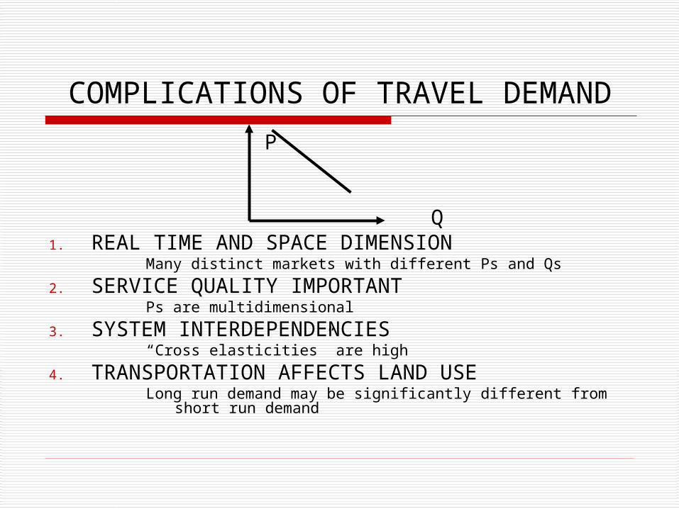
COMPLICATIONS OF TRAVEL DEMAND

P

Q1. REAL TIME AND SPACE DIMENSION

Many distinct markets with different Ps and Qs

2. SERVICE QUALITY IMPORTANTPs are multidimensional

3. SYSTEM INTERDEPENDENCIES“Cross elasticities” are high

4. TRANSPORTATION AFFECTS LAND USELong run demand may be significantly different from short run

demand

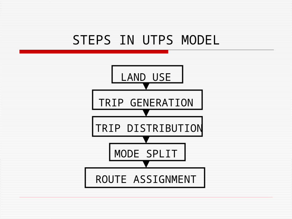
STEPS IN UTPS MODEL

LAND USE

TRIP GENERATION

TRIP DISTRIBUTION

MODE SPLIT

ROUTE ASSIGNMENT

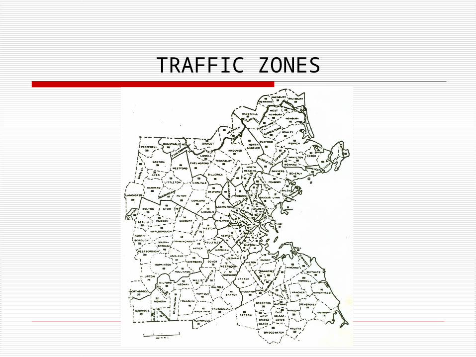
TRAFFIC ZONES

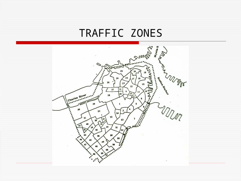
TRAFFIC ZONES

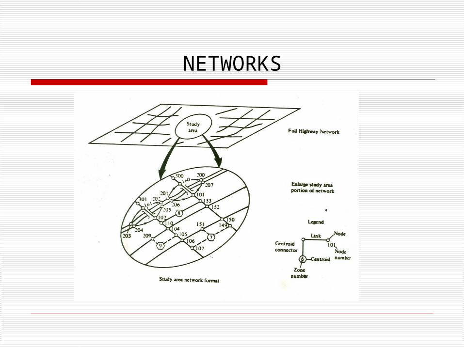
NETWORKS

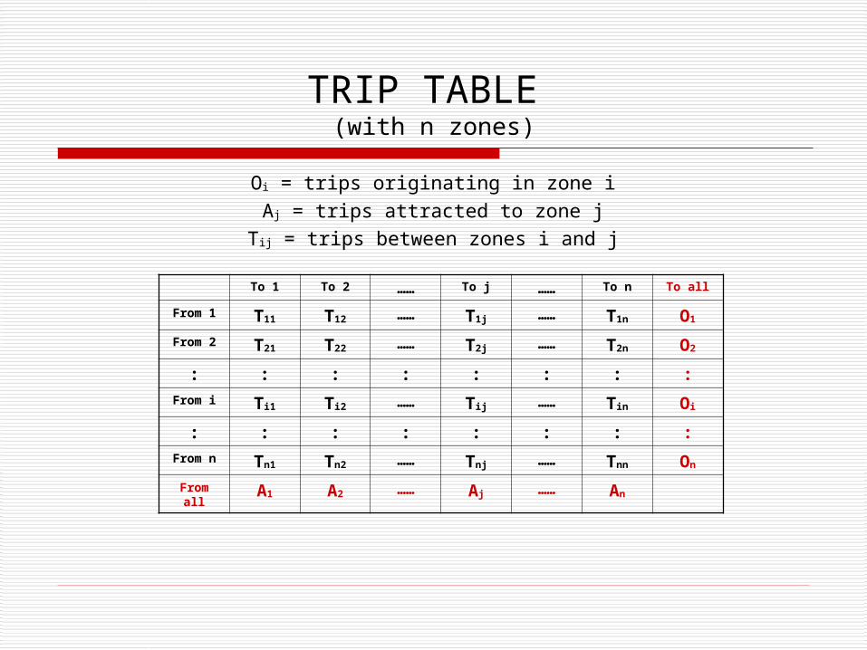
TRIP TABLE (with n zones)

Oi = trips originating in zone iAj = trips attracted to zone j

Tij = trips between zones i and j

To 1 To 2 …… To j …… To n To all

From 1 T11 T12 …… T1j …… T1n O1

From 2 T21 T22 …… T2j …… T2n O2

: : : : : : : :From i Ti1 Ti2 …… Tij …… Tin Oi

: : : : : : : :From n Tn1 Tn2 …… Tnj …… Tnn On

From all

A1 A2 …… Aj …… An

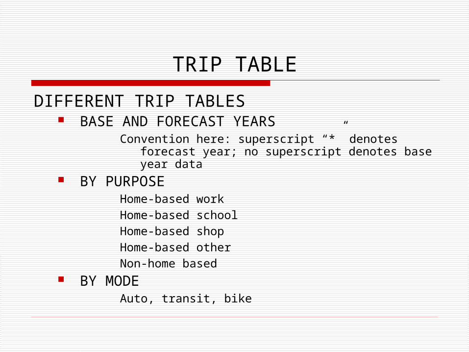
TRIP TABLE

DIFFERENT TRIP TABLES BASE AND FORECAST YEARS

Convention here: superscript “*” denotes forecast year; no superscript denotes base year data

BY PURPOSEHome-based workHome-based schoolHome-based shopHome-based otherNon-home based

BY MODEAuto, transit, bike

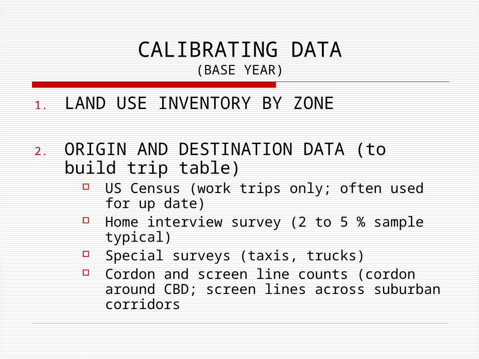
CALIBRATING DATA(BASE YEAR)

1. LAND USE INVENTORY BY ZONE

2. ORIGIN AND DESTINATION DATA (to build trip table)

US Census (work trips only; often used for up date)

Home interview survey (2 to 5 % sample typical)

Special surveys (taxis, trucks) Cordon and screen line counts (cordon around

CBD; screen lines across suburban corridors

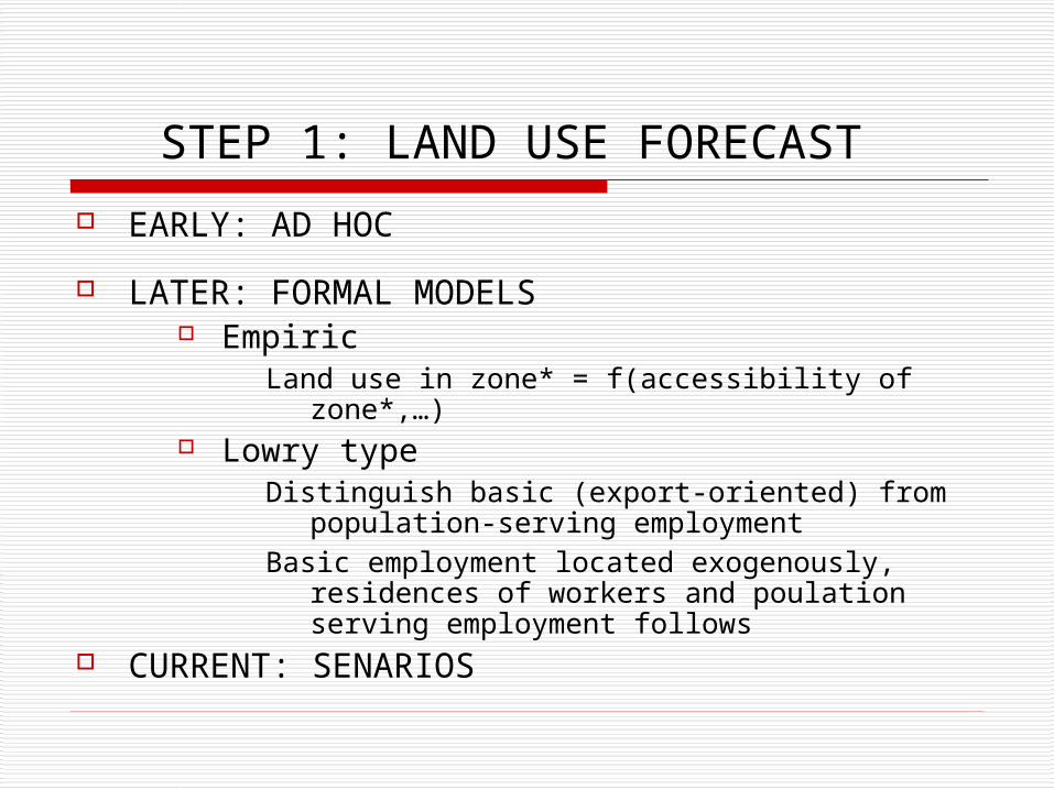
STEP 1: LAND USE FORECAST EARLY: AD HOC

LATER: FORMAL MODELS Empiric

Land use in zone* = f(accessibility of zone*,…) Lowry type

Distinguish basic (export-oriented) from population-serving employment

Basic employment located exogenously, residences of workers and poulation serving employment follows

CURRENT: SENARIOS

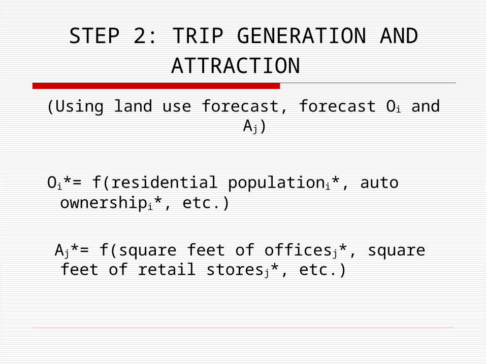
STEP 2: TRIP GENERATION AND ATTRACTION

(Using land use forecast, forecast Oi and Aj)

Oi*= f(residential populationi*, auto ownershipi*, etc.)

Aj*= f(square feet of officesj*, square feet of retail storesj*, etc.)

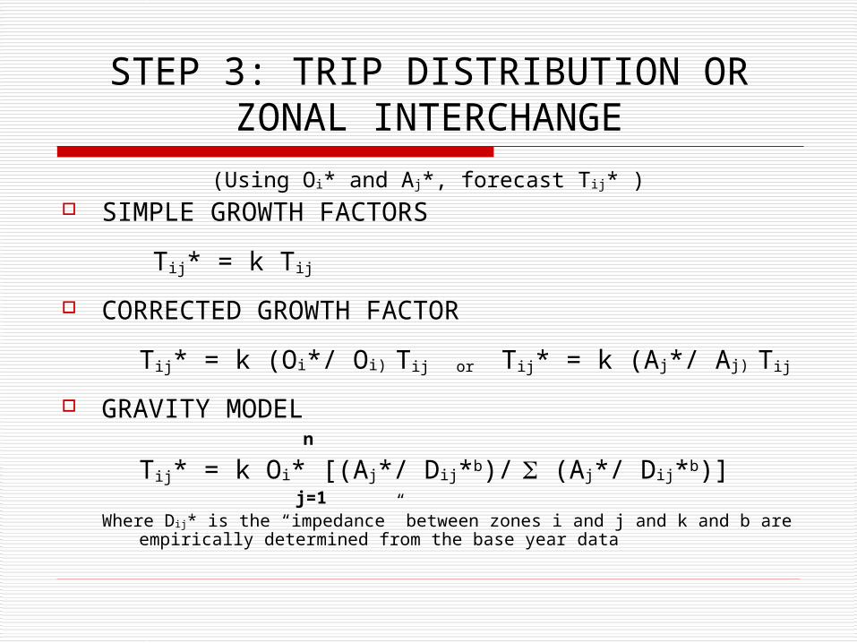
STEP 3: TRIP DISTRIBUTION OR ZONAL INTERCHANGE

(Using Oi* and Aj*, forecast Tij* ) SIMPLE GROWTH FACTORS

Tij* = k Tij

CORRECTED GROWTH FACTOR

Tij* = k (Oi*/ Oi) Tij or Tij* = k (Aj*/ Aj) Tij

GRAVITY MODEL n

Tij* = k Oi* [(Aj*/ Dij*b)/ (Aj*/ Dij*b)] j=1

Where Dij* is the “impedance” between zones i and j and k and b are empirically determined from the base year data

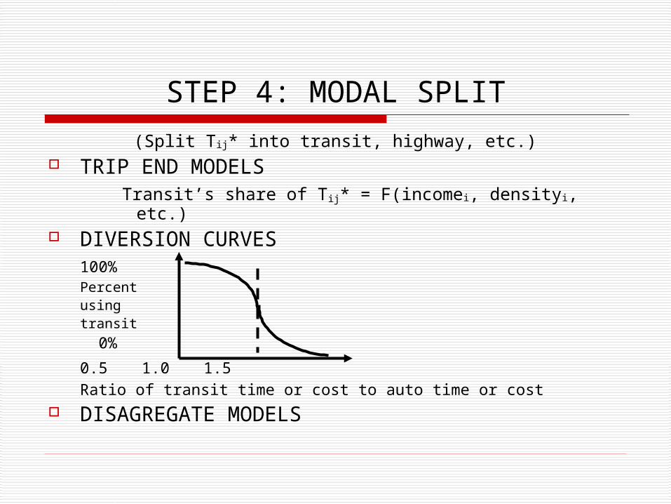
STEP 4: MODAL SPLIT

(Split Tij* into transit, highway, etc.) TRIP END MODELS

Transit’s share of Tij* = F(incomei, densityi, etc.) DIVERSION CURVES

100%Percentusingtransit

0%

0.5 1.0 1.5Ratio of transit time or cost to auto time or cost

DISAGREGATE MODELS

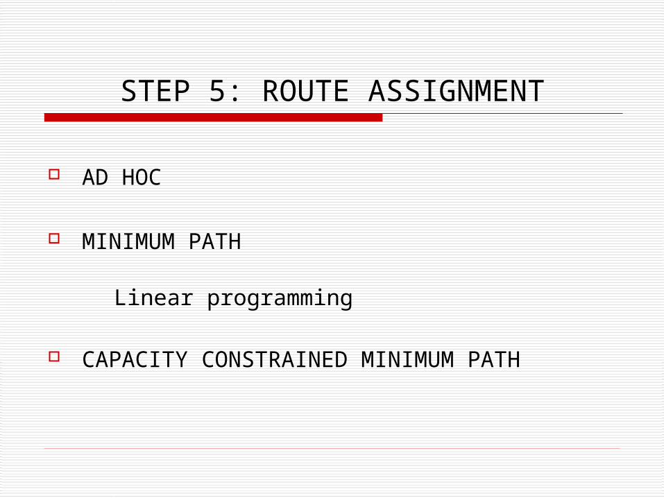
STEP 5: ROUTE ASSIGNMENT

AD HOC

MINIMUM PATH

Linear programming

CAPACITY CONSTRAINED MINIMUM PATH

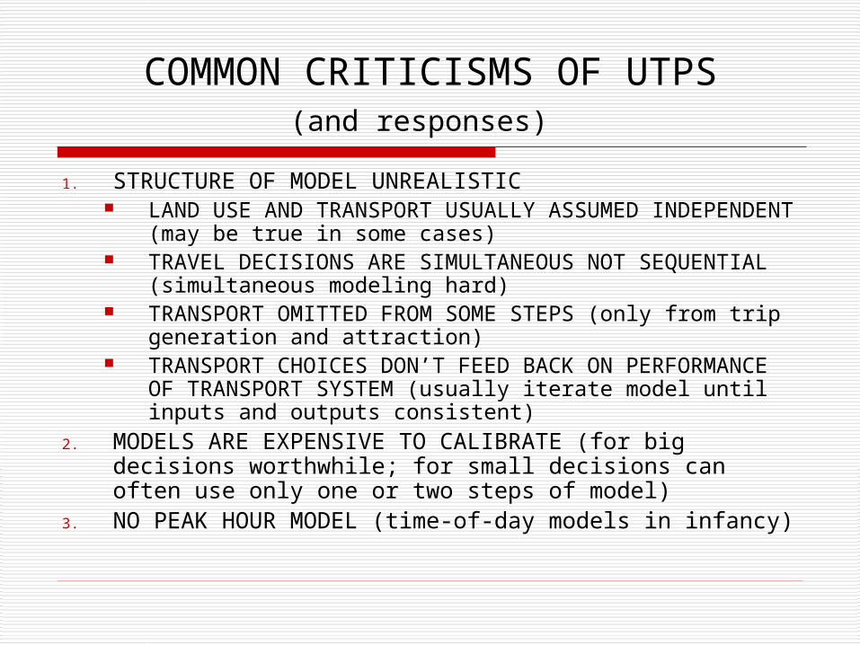
COMMON CRITICISMS OF UTPS(and responses)

1. STRUCTURE OF MODEL UNREALISTIC LAND USE AND TRANSPORT USUALLY ASSUMED

INDEPENDENT (may be true in some cases) TRAVEL DECISIONS ARE SIMULTANEOUS NOT

SEQUENTIAL (simultaneous modeling hard) TRANSPORT OMITTED FROM SOME STEPS (only from trip

generation and attraction) TRANSPORT CHOICES DON’T FEED BACK ON

PERFORMANCE OF TRANSPORT SYSTEM (usually iterate model until inputs and outputs consistent)

2. MODELS ARE EXPENSIVE TO CALIBRATE (for big decisions worthwhile; for small decisions can often use only one or two steps of model)

3. NO PEAK HOUR MODEL (time-of-day models in infancy)

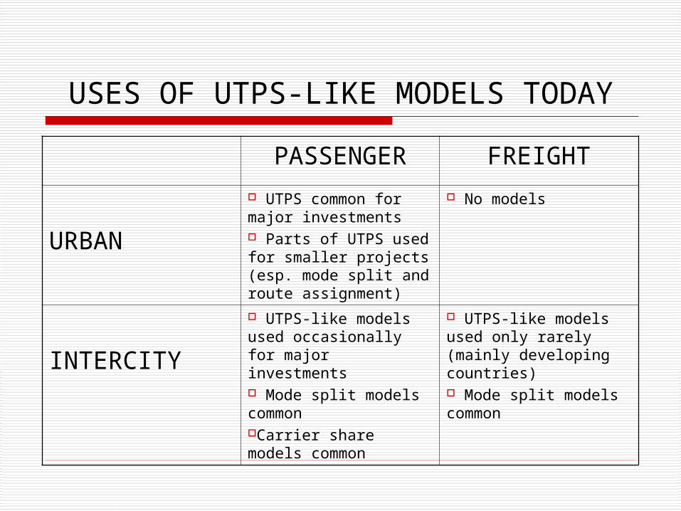
USES OF UTPS-LIKE MODELS TODAY

PASSENGER FREIGHT

URBAN

UTPS common for major investments Parts of UTPS used for smaller projects (esp. mode split and route assignment)

No models

INTERCITY

UTPS-like models used occasionally for major investments Mode split models commonCarrier share models common

UTPS-like models used only rarely (mainly developing countries) Mode split models common

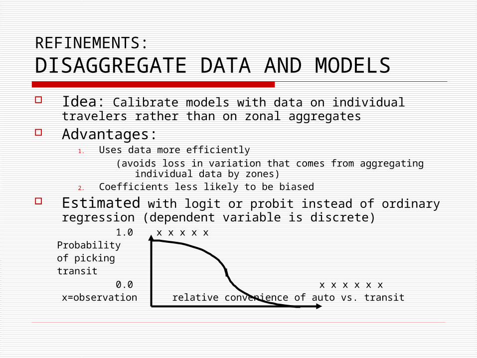
REFINEMENTS:

DISAGGREGATE DATA AND MODELS

Idea: Calibrate models with data on individual travelers rather than on zonal aggregates

Advantages:1. Uses data more efficiently

(avoids loss in variation that comes from aggregating individual data by zones)

2. Coefficients less likely to be biased

Estimated with logit or probit instead of ordinary regression (dependent variable is discrete)

1.0 x x x x xProbabilityof pickingtransit

0.0 x x x x x x x=observation relative convenience of auto vs. transit

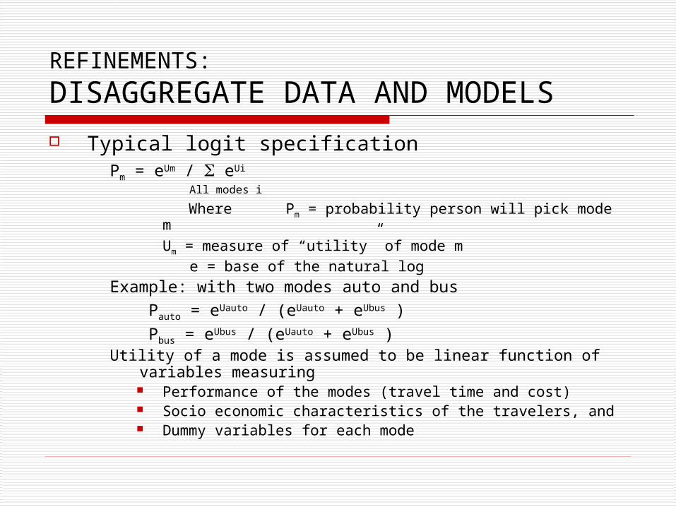
REFINEMENTS:

DISAGGREGATE DATA AND MODELS Typical logit specification

Pm = eUm / eUi

All modes i

Where Pm = probability person will pick mode m

Um = measure of “utility” of mode m

e = base of the natural logExample: with two modes auto and bus

Pauto = eUauto / (eUauto + eUbus )

Pbus = eUbus / (eUauto + eUbus )Utility of a mode is assumed to be linear function of variables

measuring Performance of the modes (travel time and cost) Socio economic characteristics of the travelers, and Dummy variables for each mode

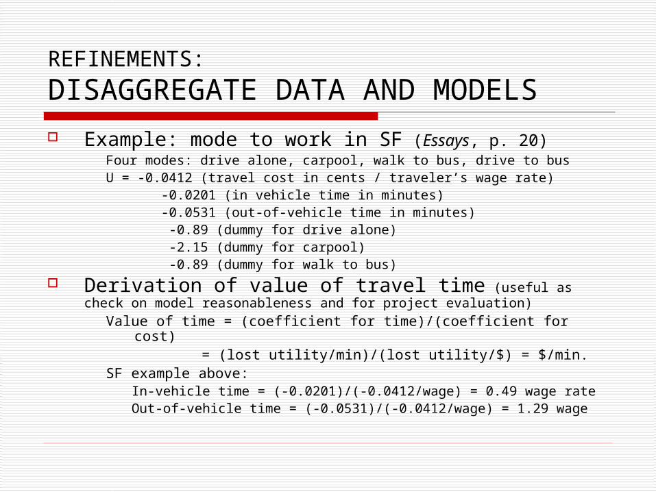
REFINEMENTS:

DISAGGREGATE DATA AND MODELS Example: mode to work in SF (Essays, p. 20)

Four modes: drive alone, carpool, walk to bus, drive to busU = -0.0412 (travel cost in cents / traveler’s wage rate) -0.0201 (in vehicle time in minutes) -0.0531 (out-of-vehicle time in minutes) -0.89 (dummy for drive alone) -2.15 (dummy for carpool) -0.89 (dummy for walk to bus)

Derivation of value of travel time (useful as check on model reasonableness and for project evaluation)

Value of time = (coefficient for time)/(coefficient for cost) = (lost utility/min)/(lost utility/$) = $/min.

SF example above:In-vehicle time = (-0.0201)/(-0.0412/wage) = 0.49 wage rateOut-of-vehicle time = (-0.0531)/(-0.0412/wage) = 1.29 wage

REFINEMENTS:

SIMULTANEUOS MODELS Idea: Eliminate sequential structure

1960s: “Direct” demand models (with aggregated data)Tijpm = Trips from i to j by purpose p and mode m

Tijpm = f(characteristics of zones i and j, service i to j, etc.) 1980s: Nested logit models (with disaggregated data)

Example: vacation destination and mode choice model in U.S. (Essays, p. 22)

DEST 1 DEST 2 DEST 3DEST 4

AUTO AIR RAIL BUS AUTO AIR RAIL BUS

Difficulties1. Relatively data intensive

Many choices and independent variables, so need many observations and much information per observation

2. Results sometimes very sensitive to specification

REFINEMENTS:

STATED PREFERENCE

Distinction REVEALED PREFERENCE: revealed by actual behavior STATED PREFERENCE: revealed by survey

Motivation: New modes of travel (example: high-speed rail in the United States)

Difficulties: Do respondents1. Understand choice?2. Take choice seriously?3. Have incentives to misrepresent preferences?(Same issues as in debate among environmental analysts

over contingent valuation)

REFINEMENTS:

VIRTUAL OR MICRO SIMULATION

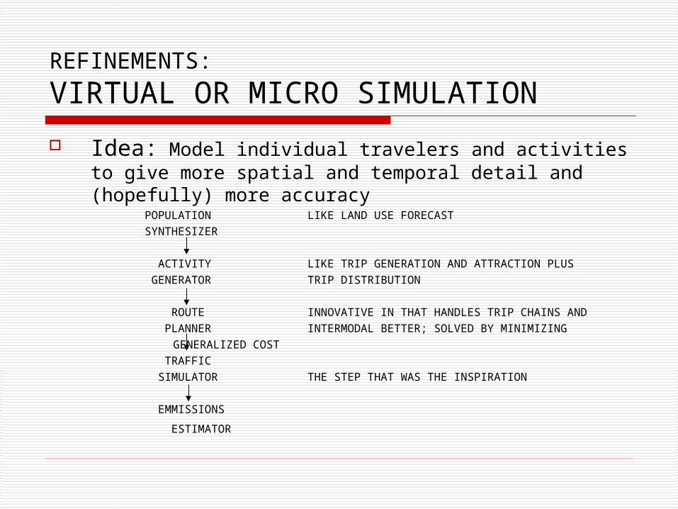
Idea: Model individual travelers and activities to give more spatial and temporal detail and (hopefully) more accuracy

POPULATION LIKE LAND USE FORECASTSYNTHESIZER

ACTIVITY LIKE TRIP GENERATION AND ATTRACTION PLUS GENERATOR TRIP DISTRIBUTION

ROUTE INNOVATIVE IN THAT HANDLES TRIP CHAINS AND PLANNER INTERMODAL BETTER; SOLVED BY MINIMIZING

GENERALIZED COST TRAFFIC SIMULATOR THE STEP THAT WAS THE INSPIRATION

EMMISSIONS

ESTIMATOR

TIPS FOR BACK OF THE ENVELOPE ASSESSMENTS

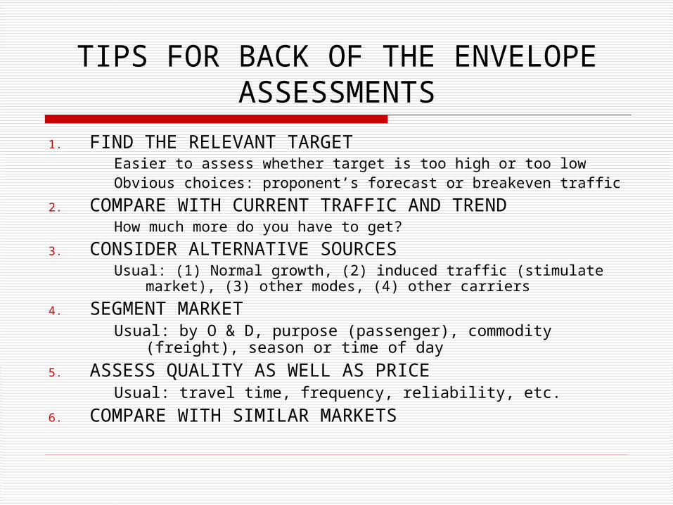
1. FIND THE RELEVANT TARGETEasier to assess whether target is too high or too lowObvious choices: proponent’s forecast or breakeven traffic

2. COMPARE WITH CURRENT TRAFFIC AND TRENDHow much more do you have to get?

3. CONSIDER ALTERNATIVE SOURCESUsual: (1) Normal growth, (2) induced traffic (stimulate market), (3)

other modes, (4) other carriers

4. SEGMENT MARKETUsual: by O & D, purpose (passenger), commodity (freight),

season or time of day

5. ASSESS QUALITY AS WELL AS PRICEUsual: travel time, frequency, reliability, etc.

6. COMPARE WITH SIMILAR MARKETS