Embed Size (px)
Citation preview
Part II Statistical NLP
Advanced Artificial Intelligence
Hidden Markov Models
Wolfram Burgard Luc De Raedt Bernhard Nebel Lars Schmidt-Thieme
Most slides taken (or adapted) from David Meir Blei Figures fromManning and Schuetze and from Rabiner
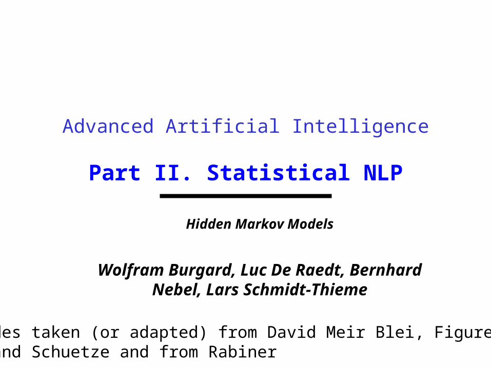
Contents
Markov Models Hidden Markov Models
bull Three problems - three algorithms Decoding Viterbi Baum-Welsch
Next chapter bull Application to part-of-speech-tagging (POS-tagging)
Largely chapter 9 of Statistical NLP Manning and Schuetze or Rabiner A tutorial on HMMs and selected applications in Speech Recognition Proc IEEE
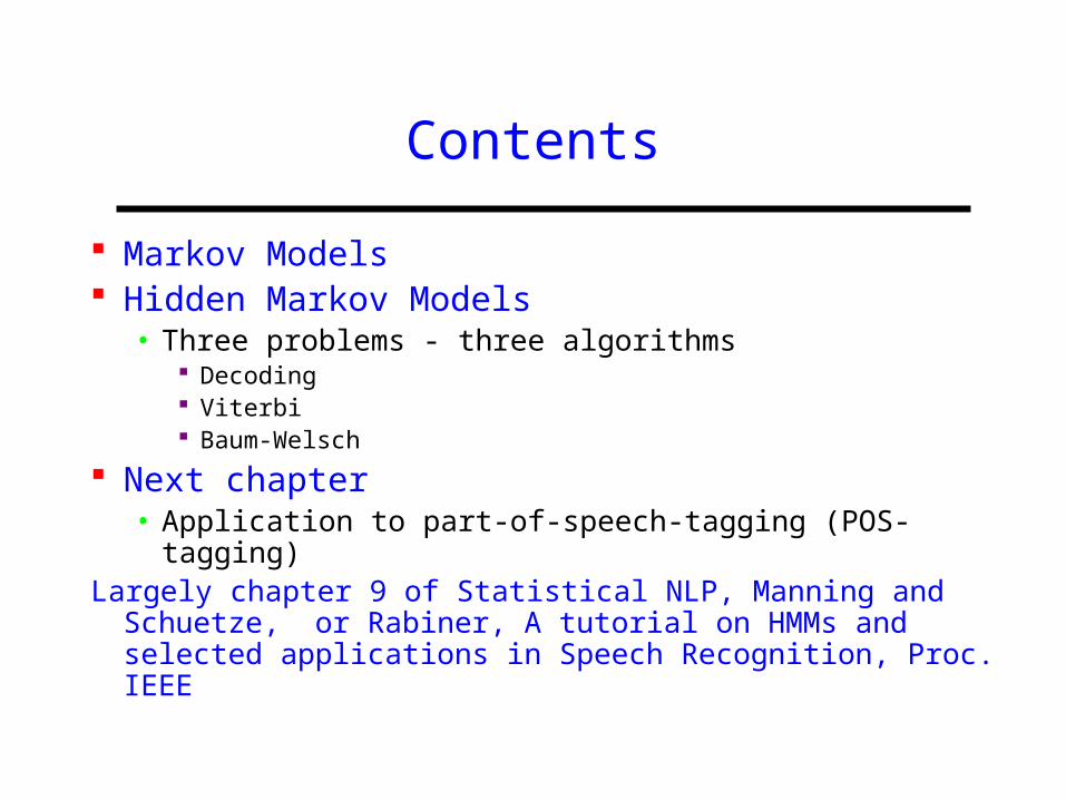
Motivations and Applications
Part-of-speech tagging Sequence taggingbull The representative put chairs on the tablebull AT NN VBD NNS IN AT NNbull AT JJ NN VBZ IN AT NN
Some tags bull AT article NN singular or mass noun VBD verb
past tense NNS plural noun IN preposition JJ adjective
Bioinformatics
Durbin et al Biological Sequence Analysis Cambridge University Press
Several applications eg proteins From primary structure ATCPLELLLD Infer secondary structure HHHBBBBBC
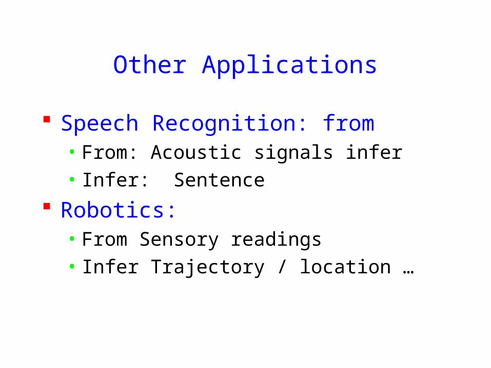
Other Applications
Speech Recognition frombull From Acoustic signals inferbull Infer Sentence
Robotics bull From Sensory readings bull Infer Trajectory location hellip
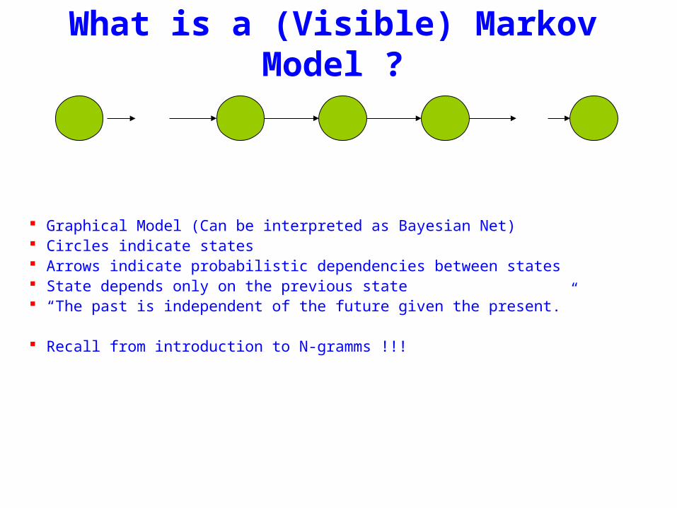
What is a (Visible) Markov Model
Graphical Model (Can be interpreted as Bayesian Net) Circles indicate states Arrows indicate probabilistic dependencies between states State depends only on the previous state ldquoThe past is independent of the future given the presentrdquo
Recall from introduction to N-gramms
Markov Model Formalization
SSS SS
S S s1hellipsN are the values for the hidden states
Limited Horizon (Markov Assumption)
Time Invariant (Stationary)
Transition Matrix A
P(Xt+1 =sk |X1K Xt) =P(Xt+1 =sk |Xt)
=P(X2 = sk | X1)
aij =P(Xt+1 =sj |Xt =si )
Markov Model Formalization
SSS SS
S S s1hellipsN are the values for the hidden states
are the initial state probabilities
A = aij are the state transition probabilities
AAAA
i = P(X1 = si )
What is the probability of a sequence of states
P(X1K XT )
=P(X1)P(X2 |X1)P(X3 |X1X2 )P(XT |X1K XTminus1)=P(X1)P(X2 |X1)P(X3 |X2 )P(XT |XTminus1)
= X1aXtXt+1
t=1
Tminus1
prod
What is an HMM
Graphical Model Circles indicate states Arrows indicate probabilistic dependencies between states
HMM = Hidden Markov Model
What is an HMM
Green circles are hidden states Dependent only on the previous state
What is an HMM
Purple nodes are observed states Dependent only on their corresponding hidden state The past is independent of the future given the
present
HMM Formalism
S K S s1hellipsN are the values for the hidden states
K k1hellipkM are the values for the observations
SSS
KKK
S
K
S
K
HMM Formalism
S K are the initial state probabilities
A = aij are the state transition probabilities
B = bik are the observation state probabilities
Note sometimes one uses B = bijk
output then depends on previous state transition as well
A
B
AAA
BB
SSS
KKK
S
K
S
K
The crazy soft drink machine
Fig 92
B cola iced tea lemonade
CP 06 01 03
IP 01 07 02
Probability of lemice
Sum over all paths taken through HMM Start in CP
bull 1 x 03 x 07 x 01 +bull 1 x 03 x 03 x 07
oTo1 otot-1 ot+1
HMMs and Bayesian Nets (1)
x1 xt-1 xt xt+1 xT
P(x1xT o1oT )=P(x1)P(o1 |x1) P(xi+1 |xii=1
Tminus1
prod )P(oi+1 |xi+1)
= x1bx1o1
t=1
Tminus1
axtxt+1bxt+1ot+1
oTo1 otot-1 ot+1
x1 xt+1 xTxtxt-1
HMM and Bayesian Nets (2)
Conditionally independent of Given
Because of d-separation
ldquoThe past is independent of the future given the presentrdquo
Inference in an HMM
Compute the probability of a given observation sequence
Given an observation sequence compute the most likely hidden state sequence
Given an observation sequence and set of possible models which model most closely fits the data
O =(o1oT )μ =(AB)ComputeP(O |μ)
oTo1 otot-1 ot+1
Given an observation sequence and a model compute the probability of the observation sequence
Decoding
Decoding
TT oxoxox bbbXOP )|(2211
=μ
oTo1 otot-1 ot+1
x1 xt+1 xTxtxt-1
Decoding
TT oxoxox bbbXOP )|(2211
=μ
TT xxxxxxx aaaXP132211
)|(minus
=μ
oTo1 otot-1 ot+1
x1 xt+1 xTxtxt-1
Decoding
)|()|()|( μμμ XPXOPXOP =
TT oxoxox bbbXOP )|(2211
=μ
TT xxxxxxx aaaXP132211
)|(minus
=μ
oTo1 otot-1 ot+1
x1 xt+1 xTxtxt-1
Decoding
)|()|()|( μμμ XPXOPXOP =
TT oxoxox bbbXOP )|(2211
=μ
TT xxxxxxx aaaXP132211
)|(minus
=μ
sum=X
XPXOPOP )|()|()|( μμμ
oTo1 otot-1 ot+1
x1 xt+1 xTxtxt-1
P(O | μ) = x1bx1o1
x1 xT sum
t=1
Tminus1
axtxt+1bxt+1ot+1
Decoding
oTo1 otot-1 ot+1
x1 xt+1 xTxtxt-1
Complexity O(N T 2T )
Eg N =5T =100gives21005100 asymp1072
Dynamic Programming
α i (t) = P(o1ot xt = i | μ )
Forward Procedure
oTo1 otot-1 ot+1
x1 xt+1 xTxtxt-1
bull Special structure gives us an efficient solution using dynamic programming
bull Intuition Probability of the first t observations is the same for all possible t+1 length state sequences
bull Define
α i (1) = P(o1 x1 = i | μ )
= π i bio1
)|()(
)()|()|(
)()|(
)(
1111
11111
1111
111
jxoPjxooP
jxPjxoPjxooP
jxPjxooP
jxooP
tttt
ttttt
ttt
tt
=======
=====
+++
++++
+++
++
oTo1 otot-1 ot+1
x1 xt+1 xTxtxt-1
Forward Procedure
)1( +tjα
oTo1 otot-1 ot+1
x1 xt+1 xTxtxt-1
Forward Procedure
)1( +tjα
)|()(
)()|()|(
)()|(
)(
1111
11111
1111
111
jxoPjxooP
jxPjxoPjxooP
jxPjxooP
jxooP
tttt
ttttt
ttt
tt
=======
=====
+++
++++
+++
++
oTo1 otot-1 ot+1
x1 xt+1 xTxtxt-1
Forward Procedure
)1( +tjα
)|()(
)()|()|(
)()|(
)(
1111
11111
1111
111
jxoPjxooP
jxPjxoPjxooP
jxPjxooP
jxooP
tttt
ttttt
ttt
tt
=======
=====
+++
++++
+++
++
oTo1 otot-1 ot+1
x1 xt+1 xTxtxt-1
Forward Procedure
)1( +tjα
)|()(
)()|()|(
)()|(
)(
1111
11111
1111
111
jxoPjxooP
jxPjxoPjxooP
jxPjxooP
jxooP
tttt
ttttt
ttt
tt
=======
=====
+++
++++
+++
++
sum
sum
sum
sum
=
+++=
++=
+
++=
+
+=
=====
=====
====
Nijoiji
ttttNi
tt
tttNi
ttt
ttNi
ttt
tbat
jxoPixjxPixooP
jxoPixPixjxooP
jxoPjxixooP
1
1111
1
111
11
111
11
1)(
)|()|()(
)|()()|(
)|()(
α
oTo1 otot-1 ot+1
x1 xt+1 xTxtxt-1
Forward Procedure
sum
sum
sum
sum
=
+++=
++=
+
++=
+
+=
=====
=====
====
Nijoiji
ttttNi
tt
tttNi
ttt
ttNi
ttt
tbat
jxoPixjxPixooP
jxoPixPixjxooP
jxoPjxixooP
1
1111
1
111
11
111
11
1)(
)|()|()(
)|()()|(
)|()(
α
oTo1 otot-1 ot+1
x1 xt+1 xTxtxt-1
Forward Procedure
sum
sum
sum
sum
=
+++=
++=
+
++=
+
+=
=====
=====
====
Nijoiji
ttttNi
tt
tttNi
ttt
ttNi
ttt
tbat
jxoPixjxPixooP
jxoPixPixjxooP
jxoPjxixooP
1
1111
1
111
11
111
11
1)(
)|()|()(
)|()()|(
)|()(
α
oTo1 otot-1 ot+1
x1 xt+1 xTxtxt-1
Forward Procedure
= P(o1ot xt = i xt+1 = j)i=1Nsum P(ot+1 | xt+1 = j)
= P(o1ot xt+1 = j | xt = i)i=1Nsum P(xt = i)P(ot+1 | xt+1 = j)
= P(o1ot xt = i)i=1Nsum P(xt+1 = j | xt = i)P(ot+1 | xt+1 = j)
= α i (t)aijb jot +1i=1Nsum
oTo1 otot-1 ot+1
x1 xt+1 xTxtxt-1
Forward Procedure
Dynamic Programming
α j (t +1) = α i (t)aijb jot +1i=1Nsum
Complexity O(N 2 T )
Eg N = 5T = 100 gives asymp 3000
βi (t) = P(ot+1oT | xt = i)
oTo1 otot-1 ot+1
x1 xt+1 xTxtxt-1
Backward Procedure
βi (T ) = 1
βi (t) = aijbiot +1β j (t +1)
j=1Nsum
Probability of the rest of the states given the first state
oTo1 otot-1 ot+1
x1 xt+1 xTxtxt-1
Decoding Solution
sum=
=N
ii TOP
1
)()|( αμ
sum=
=N
iiiOP
1
)1()|( βπμ
)()()|(1
ttOP i
N
ii βαμ sum
=
=
Forward Procedure
Backward Procedure
Combination
P(O Xt =i |μ) =P(o1otXt =iot+1oT |μ)=P(o1otXt =i |μ)P(ot+1oT |o1otXt =i μ)=P(o1otXt =i |μ)P(ot+1oT |Xt =i μ)=α i (t)βi (t)
)()()|(1
ttOP i
N
ii βαμ sum
=
=
oTo1 otot-1 ot+1
Best State Sequence
Find the state sequence that best explains the observations
Two approaches bull Individually most likely statesbull Most likely sequence (Viterbi)
)|(maxarg OXPX
Best State Sequence (1)
γi (t) = P(Xt = i | O μ )
=P(Xt = iO | μ )
P(O | μ )
=α i (t)β i (t)
j=1
n
sum α j (t)β j (t)
Most likely state at each point in time
Xt = arg maxγ i (t)
oTo1 otot-1 ot+1
Best State Sequence (2)
Find the state sequence that best explains the observations
Viterbi algorithm
)|(maxarg OXPX
oTo1 otot-1 ot+1
Viterbi Algorithm
)(max)( 1111 11
ttttxx
j ojxooxxPtt
== minusminusminus
δ
The state sequence which maximizes the probability of seeing the observations to time t-1 landing in state j and seeing the observation at time t
x1 xt-1 j
oTo1 otot-1 ot+1
Viterbi Algorithm
)(max)( 1111 11
ttttxx
j ojxooxxPtt
== minusminusminus
δ
1)(max)1(
+=+
tjoijiij batt δδ
1)(maxarg)1(
+=+
tjoijii
j batt δψRecursive Computation
x1 xt-1 xt xt+1
Initialization
δ1(i) = ibio1
ψ 1(i) =0
oTo1 otot-1 ot+1
Viterbi Algorithm
XT =argmaxi
δi (T )
Xt =ψX^
t+1
(t+1)
P(X)=argmaxi
δi (T )
Compute the most likely state sequence by working backwards
x1 xt-1 xt xt+1 xT
oTo1 otot-1 ot+1
HMMs and Bayesian Nets (1)
x1 xt-1 xt xt+1 xT
P(x1xT o1oT )=P(x1)P(o1 |x1) P(xi+1 |xii=1
Tminus1
prod )P(oi+1 |xi+1)
= x1bx1o1
t=1
Tminus1
axtxt+1bxt+1ot+1
oTo1 otot-1 ot+1
x1 xt+1 xTxtxt-1
HMM and Bayesian Nets (2)
Conditionally independent of Given
Because of d-separation
ldquoThe past is independent of the future given the presentrdquo
Inference in an HMM
Compute the probability of a given observation sequence
Given an observation sequence compute the most likely hidden state sequence
Given an observation sequence and set of possible models which model most closely fits the data
Dynamic Programming
oTo1 otot-1 ot+1
Parameter Estimation
bull Given an observation sequence find the model that is most likely to produce that sequence
bull No analytic methodbull Given a model and observation sequence update
the model parameters to better fit the observations
A
B
AAA
BBB B
arg maxμ
P(Otraining |μ)
α i (t) = P(o1ot xt = i | μ )
βi (t) = P(ot+1oT | xt = i)
)()()|(1
ttOP i
N
ii βαμ sum
=
=
pt (i j)=P(Xt =iXt+1 = j |O μ)
=P(Xt =iXt+1 = jO |μ)
P(O |μ)
oTo1 otot-1 ot+1
Parameter Estimation
A
B
AAA
BBB B
pt (i j)=α i (t)aijbjot+1
β j (t+1)
αm(t)βm(t)m=1Nsum
Probability of traversing an arc
sum=
=Nj
ti jipt1
)()(γ Probability of being in state i
oTo1 otot-1 ot+1
Parameter Estimation
A
B
AAA
BBB B
i =γi(1)
Now we can compute the new estimates of the model parameters
aij =pt(i j)t=1
Tminus1sumγi (t)t=1
Tminus1sum
bik =γi (t) tot=ksum
γi (t)t=1
Tsum
Instance of Expectation Maximization
We have that
We may get stuck in local maximum (or even saddle point)
Nevertheless Baum-Welch usually effective
P(O | μ) geP(O |μ)
Some Variants
So far ergodic modelsbull All states are connectedbull Not always wanted
Epsilon or null-transitionsbull Not all statestransitions emit output symbols
Parameter tyingbull Assuming that certain parameters are shared bull Reduces the number of parameters that have to be estimated
Logical HMMs (Kersting De Raedt Raiko)bull Working with structured states and observation symbols
Working with log probabilities and addition instead of multiplication of probabilities (typically done)
oTo1 otot-1 ot+1
The Most Important Thing
A
B
AAA
BBB B
We can use the special structure of this model to do a lot of neat math and solve problems that are otherwise not solvable
HMMrsquos from an Agent Perspective
AI a modern approachbull AI is the study of rational agentsbull Third part by Wolfram Burgard on
Reinforcement learning
HMMs can also be used herebull Typically one is interested in P(state)
Example
Possible statesbull snow no snow
Observationsbull skis no skis
Questionsbull Was there snow the day before yesterday (given a
sequence of observations) bull Is there now snow (given a sequence of
observations) bull Will there be snow tomorrow given a sequence of
observations Next week
HMM and Agents
Question
bull Case 1 often called smoothing t lt T see last time
Only part of trellis between t and T needed
γi (t) = P(Xt = i | Oμ )
=α i (t)β i (t)
j =1
n
sum α j (t)β j (t)
Most likely state at each point in time
HMM and Agents
bull Case 2 often called filtering t= T last time
Can we make it recursive Ie go from T-1 to T
γi (t) = P(Xt = i | Oμ )
=α i (t)β i (t)
j =1
n
sum α j (t)β j (t)
Most likely state at each point in time
HMM and Agents
bull Case 2 often called filtering t= T last time
λi (T ) = P(XT = i | o1oT μ )
= γ i (T )
=α i (T )β i (T )
j =1
n
sum α j (T )β j (T )
=α i (T )
j =1
n
sum α j (T )
HMM and Agents
bull Case 3 often called prediction t= T+1 (or T+K) not yet seen
Interesting recursive Easily extended towards k gt 1
Extensions
Use Dynamic Bayesian networks instead of HMMsbullOne state corresponds to a Bayesian NetbullObservations can become more complex
Involve actions of the agent as wellbullCf Wolfram Burgardrsquos Part
Contents
Markov Models Hidden Markov Models
bull Three problems - three algorithms Decoding Viterbi Baum-Welsch
Next chapter bull Application to part-of-speech-tagging (POS-tagging)
Largely chapter 9 of Statistical NLP Manning and Schuetze or Rabiner A tutorial on HMMs and selected applications in Speech Recognition Proc IEEE
Motivations and Applications
Part-of-speech tagging Sequence taggingbull The representative put chairs on the tablebull AT NN VBD NNS IN AT NNbull AT JJ NN VBZ IN AT NN
Some tags bull AT article NN singular or mass noun VBD verb
past tense NNS plural noun IN preposition JJ adjective
Bioinformatics
Durbin et al Biological Sequence Analysis Cambridge University Press
Several applications eg proteins From primary structure ATCPLELLLD Infer secondary structure HHHBBBBBC
Other Applications
Speech Recognition frombull From Acoustic signals inferbull Infer Sentence
Robotics bull From Sensory readings bull Infer Trajectory location hellip
What is a (Visible) Markov Model
Graphical Model (Can be interpreted as Bayesian Net) Circles indicate states Arrows indicate probabilistic dependencies between states State depends only on the previous state ldquoThe past is independent of the future given the presentrdquo
Recall from introduction to N-gramms
Markov Model Formalization
SSS SS
S S s1hellipsN are the values for the hidden states
Limited Horizon (Markov Assumption)
Time Invariant (Stationary)
Transition Matrix A
P(Xt+1 =sk |X1K Xt) =P(Xt+1 =sk |Xt)
=P(X2 = sk | X1)
aij =P(Xt+1 =sj |Xt =si )
Markov Model Formalization
SSS SS
S S s1hellipsN are the values for the hidden states
are the initial state probabilities
A = aij are the state transition probabilities
AAAA
i = P(X1 = si )
What is the probability of a sequence of states
P(X1K XT )
=P(X1)P(X2 |X1)P(X3 |X1X2 )P(XT |X1K XTminus1)=P(X1)P(X2 |X1)P(X3 |X2 )P(XT |XTminus1)
= X1aXtXt+1
t=1
Tminus1
prod
What is an HMM
Graphical Model Circles indicate states Arrows indicate probabilistic dependencies between states
HMM = Hidden Markov Model
What is an HMM
Green circles are hidden states Dependent only on the previous state
What is an HMM
Purple nodes are observed states Dependent only on their corresponding hidden state The past is independent of the future given the
present
HMM Formalism
S K S s1hellipsN are the values for the hidden states
K k1hellipkM are the values for the observations
SSS
KKK
S
K
S
K
HMM Formalism
S K are the initial state probabilities
A = aij are the state transition probabilities
B = bik are the observation state probabilities
Note sometimes one uses B = bijk
output then depends on previous state transition as well
A
B
AAA
BB
SSS
KKK
S
K
S
K
The crazy soft drink machine
Fig 92
B cola iced tea lemonade
CP 06 01 03
IP 01 07 02
Probability of lemice
Sum over all paths taken through HMM Start in CP
bull 1 x 03 x 07 x 01 +bull 1 x 03 x 03 x 07
oTo1 otot-1 ot+1
HMMs and Bayesian Nets (1)
x1 xt-1 xt xt+1 xT
P(x1xT o1oT )=P(x1)P(o1 |x1) P(xi+1 |xii=1
Tminus1
prod )P(oi+1 |xi+1)
= x1bx1o1
t=1
Tminus1
axtxt+1bxt+1ot+1
oTo1 otot-1 ot+1
x1 xt+1 xTxtxt-1
HMM and Bayesian Nets (2)
Conditionally independent of Given
Because of d-separation
ldquoThe past is independent of the future given the presentrdquo
Inference in an HMM
Compute the probability of a given observation sequence
Given an observation sequence compute the most likely hidden state sequence
Given an observation sequence and set of possible models which model most closely fits the data
O =(o1oT )μ =(AB)ComputeP(O |μ)
oTo1 otot-1 ot+1
Given an observation sequence and a model compute the probability of the observation sequence
Decoding
Decoding
TT oxoxox bbbXOP )|(2211
=μ
oTo1 otot-1 ot+1
x1 xt+1 xTxtxt-1
Decoding
TT oxoxox bbbXOP )|(2211
=μ
TT xxxxxxx aaaXP132211
)|(minus
=μ
oTo1 otot-1 ot+1
x1 xt+1 xTxtxt-1
Decoding
)|()|()|( μμμ XPXOPXOP =
TT oxoxox bbbXOP )|(2211
=μ
TT xxxxxxx aaaXP132211
)|(minus
=μ
oTo1 otot-1 ot+1
x1 xt+1 xTxtxt-1
Decoding
)|()|()|( μμμ XPXOPXOP =
TT oxoxox bbbXOP )|(2211
=μ
TT xxxxxxx aaaXP132211
)|(minus
=μ
sum=X
XPXOPOP )|()|()|( μμμ
oTo1 otot-1 ot+1
x1 xt+1 xTxtxt-1
P(O | μ) = x1bx1o1
x1 xT sum
t=1
Tminus1
axtxt+1bxt+1ot+1
Decoding
oTo1 otot-1 ot+1
x1 xt+1 xTxtxt-1
Complexity O(N T 2T )
Eg N =5T =100gives21005100 asymp1072
Dynamic Programming
α i (t) = P(o1ot xt = i | μ )
Forward Procedure
oTo1 otot-1 ot+1
x1 xt+1 xTxtxt-1
bull Special structure gives us an efficient solution using dynamic programming
bull Intuition Probability of the first t observations is the same for all possible t+1 length state sequences
bull Define
α i (1) = P(o1 x1 = i | μ )
= π i bio1
)|()(
)()|()|(
)()|(
)(
1111
11111
1111
111
jxoPjxooP
jxPjxoPjxooP
jxPjxooP
jxooP
tttt
ttttt
ttt
tt
=======
=====
+++
++++
+++
++
oTo1 otot-1 ot+1
x1 xt+1 xTxtxt-1
Forward Procedure
)1( +tjα
oTo1 otot-1 ot+1
x1 xt+1 xTxtxt-1
Forward Procedure
)1( +tjα
)|()(
)()|()|(
)()|(
)(
1111
11111
1111
111
jxoPjxooP
jxPjxoPjxooP
jxPjxooP
jxooP
tttt
ttttt
ttt
tt
=======
=====
+++
++++
+++
++
oTo1 otot-1 ot+1
x1 xt+1 xTxtxt-1
Forward Procedure
)1( +tjα
)|()(
)()|()|(
)()|(
)(
1111
11111
1111
111
jxoPjxooP
jxPjxoPjxooP
jxPjxooP
jxooP
tttt
ttttt
ttt
tt
=======
=====
+++
++++
+++
++
oTo1 otot-1 ot+1
x1 xt+1 xTxtxt-1
Forward Procedure
)1( +tjα
)|()(
)()|()|(
)()|(
)(
1111
11111
1111
111
jxoPjxooP
jxPjxoPjxooP
jxPjxooP
jxooP
tttt
ttttt
ttt
tt
=======
=====
+++
++++
+++
++
sum
sum
sum
sum
=
+++=
++=
+
++=
+
+=
=====
=====
====
Nijoiji
ttttNi
tt
tttNi
ttt
ttNi
ttt
tbat
jxoPixjxPixooP
jxoPixPixjxooP
jxoPjxixooP
1
1111
1
111
11
111
11
1)(
)|()|()(
)|()()|(
)|()(
α
oTo1 otot-1 ot+1
x1 xt+1 xTxtxt-1
Forward Procedure
sum
sum
sum
sum
=
+++=
++=
+
++=
+
+=
=====
=====
====
Nijoiji
ttttNi
tt
tttNi
ttt
ttNi
ttt
tbat
jxoPixjxPixooP
jxoPixPixjxooP
jxoPjxixooP
1
1111
1
111
11
111
11
1)(
)|()|()(
)|()()|(
)|()(
α
oTo1 otot-1 ot+1
x1 xt+1 xTxtxt-1
Forward Procedure
sum
sum
sum
sum
=
+++=
++=
+
++=
+
+=
=====
=====
====
Nijoiji
ttttNi
tt
tttNi
ttt
ttNi
ttt
tbat
jxoPixjxPixooP
jxoPixPixjxooP
jxoPjxixooP
1
1111
1
111
11
111
11
1)(
)|()|()(
)|()()|(
)|()(
α
oTo1 otot-1 ot+1
x1 xt+1 xTxtxt-1
Forward Procedure
= P(o1ot xt = i xt+1 = j)i=1Nsum P(ot+1 | xt+1 = j)
= P(o1ot xt+1 = j | xt = i)i=1Nsum P(xt = i)P(ot+1 | xt+1 = j)
= P(o1ot xt = i)i=1Nsum P(xt+1 = j | xt = i)P(ot+1 | xt+1 = j)
= α i (t)aijb jot +1i=1Nsum
oTo1 otot-1 ot+1
x1 xt+1 xTxtxt-1
Forward Procedure
Dynamic Programming
α j (t +1) = α i (t)aijb jot +1i=1Nsum
Complexity O(N 2 T )
Eg N = 5T = 100 gives asymp 3000
βi (t) = P(ot+1oT | xt = i)
oTo1 otot-1 ot+1
x1 xt+1 xTxtxt-1
Backward Procedure
βi (T ) = 1
βi (t) = aijbiot +1β j (t +1)
j=1Nsum
Probability of the rest of the states given the first state
oTo1 otot-1 ot+1
x1 xt+1 xTxtxt-1
Decoding Solution
sum=
=N
ii TOP
1
)()|( αμ
sum=
=N
iiiOP
1
)1()|( βπμ
)()()|(1
ttOP i
N
ii βαμ sum
=
=
Forward Procedure
Backward Procedure
Combination
P(O Xt =i |μ) =P(o1otXt =iot+1oT |μ)=P(o1otXt =i |μ)P(ot+1oT |o1otXt =i μ)=P(o1otXt =i |μ)P(ot+1oT |Xt =i μ)=α i (t)βi (t)
)()()|(1
ttOP i
N
ii βαμ sum
=
=
oTo1 otot-1 ot+1
Best State Sequence
Find the state sequence that best explains the observations
Two approaches bull Individually most likely statesbull Most likely sequence (Viterbi)
)|(maxarg OXPX
Best State Sequence (1)
γi (t) = P(Xt = i | O μ )
=P(Xt = iO | μ )
P(O | μ )
=α i (t)β i (t)
j=1
n
sum α j (t)β j (t)
Most likely state at each point in time
Xt = arg maxγ i (t)
oTo1 otot-1 ot+1
Best State Sequence (2)
Find the state sequence that best explains the observations
Viterbi algorithm
)|(maxarg OXPX
oTo1 otot-1 ot+1
Viterbi Algorithm
)(max)( 1111 11
ttttxx
j ojxooxxPtt
== minusminusminus
δ
The state sequence which maximizes the probability of seeing the observations to time t-1 landing in state j and seeing the observation at time t
x1 xt-1 j
oTo1 otot-1 ot+1
Viterbi Algorithm
)(max)( 1111 11
ttttxx
j ojxooxxPtt
== minusminusminus
δ
1)(max)1(
+=+
tjoijiij batt δδ
1)(maxarg)1(
+=+
tjoijii
j batt δψRecursive Computation
x1 xt-1 xt xt+1
Initialization
δ1(i) = ibio1
ψ 1(i) =0
oTo1 otot-1 ot+1
Viterbi Algorithm
XT =argmaxi
δi (T )
Xt =ψX^
t+1
(t+1)
P(X)=argmaxi
δi (T )
Compute the most likely state sequence by working backwards
x1 xt-1 xt xt+1 xT
oTo1 otot-1 ot+1
HMMs and Bayesian Nets (1)
x1 xt-1 xt xt+1 xT
P(x1xT o1oT )=P(x1)P(o1 |x1) P(xi+1 |xii=1
Tminus1
prod )P(oi+1 |xi+1)
= x1bx1o1
t=1
Tminus1
axtxt+1bxt+1ot+1
oTo1 otot-1 ot+1
x1 xt+1 xTxtxt-1
HMM and Bayesian Nets (2)
Conditionally independent of Given
Because of d-separation
ldquoThe past is independent of the future given the presentrdquo
Inference in an HMM
Compute the probability of a given observation sequence
Given an observation sequence compute the most likely hidden state sequence
Given an observation sequence and set of possible models which model most closely fits the data
Dynamic Programming
oTo1 otot-1 ot+1
Parameter Estimation
bull Given an observation sequence find the model that is most likely to produce that sequence
bull No analytic methodbull Given a model and observation sequence update
the model parameters to better fit the observations
A
B
AAA
BBB B
arg maxμ
P(Otraining |μ)
α i (t) = P(o1ot xt = i | μ )
βi (t) = P(ot+1oT | xt = i)
)()()|(1
ttOP i
N
ii βαμ sum
=
=
pt (i j)=P(Xt =iXt+1 = j |O μ)
=P(Xt =iXt+1 = jO |μ)
P(O |μ)
oTo1 otot-1 ot+1
Parameter Estimation
A
B
AAA
BBB B
pt (i j)=α i (t)aijbjot+1
β j (t+1)
αm(t)βm(t)m=1Nsum
Probability of traversing an arc
sum=
=Nj
ti jipt1
)()(γ Probability of being in state i
oTo1 otot-1 ot+1
Parameter Estimation
A
B
AAA
BBB B
i =γi(1)
Now we can compute the new estimates of the model parameters
aij =pt(i j)t=1
Tminus1sumγi (t)t=1
Tminus1sum
bik =γi (t) tot=ksum
γi (t)t=1
Tsum
Instance of Expectation Maximization
We have that
We may get stuck in local maximum (or even saddle point)
Nevertheless Baum-Welch usually effective
P(O | μ) geP(O |μ)
Some Variants
So far ergodic modelsbull All states are connectedbull Not always wanted
Epsilon or null-transitionsbull Not all statestransitions emit output symbols
Parameter tyingbull Assuming that certain parameters are shared bull Reduces the number of parameters that have to be estimated
Logical HMMs (Kersting De Raedt Raiko)bull Working with structured states and observation symbols
Working with log probabilities and addition instead of multiplication of probabilities (typically done)
oTo1 otot-1 ot+1
The Most Important Thing
A
B
AAA
BBB B
We can use the special structure of this model to do a lot of neat math and solve problems that are otherwise not solvable
HMMrsquos from an Agent Perspective
AI a modern approachbull AI is the study of rational agentsbull Third part by Wolfram Burgard on
Reinforcement learning
HMMs can also be used herebull Typically one is interested in P(state)
Example
Possible statesbull snow no snow
Observationsbull skis no skis
Questionsbull Was there snow the day before yesterday (given a
sequence of observations) bull Is there now snow (given a sequence of
observations) bull Will there be snow tomorrow given a sequence of
observations Next week
HMM and Agents
Question
bull Case 1 often called smoothing t lt T see last time
Only part of trellis between t and T needed
γi (t) = P(Xt = i | Oμ )
=α i (t)β i (t)
j =1
n
sum α j (t)β j (t)
Most likely state at each point in time
HMM and Agents
bull Case 2 often called filtering t= T last time
Can we make it recursive Ie go from T-1 to T
γi (t) = P(Xt = i | Oμ )
=α i (t)β i (t)
j =1
n
sum α j (t)β j (t)
Most likely state at each point in time
HMM and Agents
bull Case 2 often called filtering t= T last time
λi (T ) = P(XT = i | o1oT μ )
= γ i (T )
=α i (T )β i (T )
j =1
n
sum α j (T )β j (T )
=α i (T )
j =1
n
sum α j (T )
HMM and Agents
bull Case 3 often called prediction t= T+1 (or T+K) not yet seen
Interesting recursive Easily extended towards k gt 1
Extensions
Use Dynamic Bayesian networks instead of HMMsbullOne state corresponds to a Bayesian NetbullObservations can become more complex
Involve actions of the agent as wellbullCf Wolfram Burgardrsquos Part
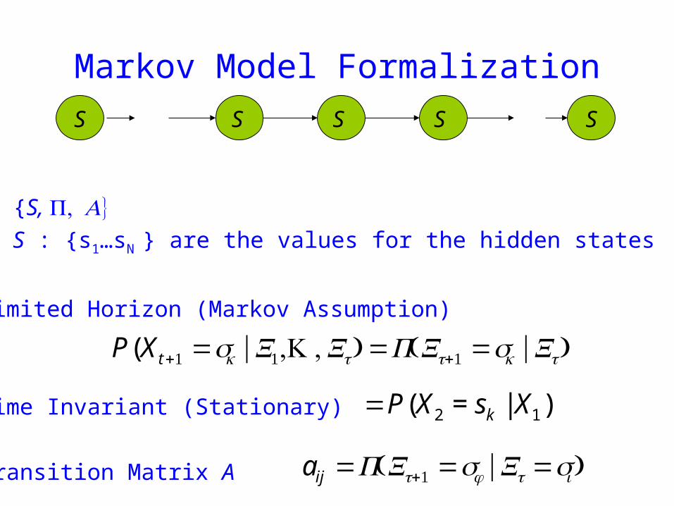
Markov Model Formalization
SSS SS
S S s1hellipsN are the values for the hidden states
Limited Horizon (Markov Assumption)
Time Invariant (Stationary)
Transition Matrix A
P(Xt+1 =sk |X1K Xt) =P(Xt+1 =sk |Xt)
=P(X2 = sk | X1)
aij =P(Xt+1 =sj |Xt =si )
Markov Model Formalization
SSS SS
S S s1hellipsN are the values for the hidden states
are the initial state probabilities
A = aij are the state transition probabilities
AAAA
i = P(X1 = si )
What is the probability of a sequence of states
P(X1K XT )
=P(X1)P(X2 |X1)P(X3 |X1X2 )P(XT |X1K XTminus1)=P(X1)P(X2 |X1)P(X3 |X2 )P(XT |XTminus1)
= X1aXtXt+1
t=1
Tminus1
prod
What is an HMM
Graphical Model Circles indicate states Arrows indicate probabilistic dependencies between states
HMM = Hidden Markov Model
What is an HMM
Green circles are hidden states Dependent only on the previous state
What is an HMM
Purple nodes are observed states Dependent only on their corresponding hidden state The past is independent of the future given the
present
HMM Formalism
S K S s1hellipsN are the values for the hidden states
K k1hellipkM are the values for the observations
SSS
KKK
S
K
S
K
HMM Formalism
S K are the initial state probabilities
A = aij are the state transition probabilities
B = bik are the observation state probabilities
Note sometimes one uses B = bijk
output then depends on previous state transition as well
A
B
AAA
BB
SSS
KKK
S
K
S
K
The crazy soft drink machine
Fig 92
B cola iced tea lemonade
CP 06 01 03
IP 01 07 02
Probability of lemice
Sum over all paths taken through HMM Start in CP
bull 1 x 03 x 07 x 01 +bull 1 x 03 x 03 x 07
oTo1 otot-1 ot+1
HMMs and Bayesian Nets (1)
x1 xt-1 xt xt+1 xT
P(x1xT o1oT )=P(x1)P(o1 |x1) P(xi+1 |xii=1
Tminus1
prod )P(oi+1 |xi+1)
= x1bx1o1
t=1
Tminus1
axtxt+1bxt+1ot+1
oTo1 otot-1 ot+1
x1 xt+1 xTxtxt-1
HMM and Bayesian Nets (2)
Conditionally independent of Given
Because of d-separation
ldquoThe past is independent of the future given the presentrdquo
Inference in an HMM
Compute the probability of a given observation sequence
Given an observation sequence compute the most likely hidden state sequence
Given an observation sequence and set of possible models which model most closely fits the data
O =(o1oT )μ =(AB)ComputeP(O |μ)
oTo1 otot-1 ot+1
Given an observation sequence and a model compute the probability of the observation sequence
Decoding
Decoding
TT oxoxox bbbXOP )|(2211
=μ
oTo1 otot-1 ot+1
x1 xt+1 xTxtxt-1
Decoding
TT oxoxox bbbXOP )|(2211
=μ
TT xxxxxxx aaaXP132211
)|(minus
=μ
oTo1 otot-1 ot+1
x1 xt+1 xTxtxt-1
Decoding
)|()|()|( μμμ XPXOPXOP =
TT oxoxox bbbXOP )|(2211
=μ
TT xxxxxxx aaaXP132211
)|(minus
=μ
oTo1 otot-1 ot+1
x1 xt+1 xTxtxt-1
Decoding
)|()|()|( μμμ XPXOPXOP =
TT oxoxox bbbXOP )|(2211
=μ
TT xxxxxxx aaaXP132211
)|(minus
=μ
sum=X
XPXOPOP )|()|()|( μμμ
oTo1 otot-1 ot+1
x1 xt+1 xTxtxt-1
P(O | μ) = x1bx1o1
x1 xT sum
t=1
Tminus1
axtxt+1bxt+1ot+1
Decoding
oTo1 otot-1 ot+1
x1 xt+1 xTxtxt-1
Complexity O(N T 2T )
Eg N =5T =100gives21005100 asymp1072
Dynamic Programming
α i (t) = P(o1ot xt = i | μ )
Forward Procedure
oTo1 otot-1 ot+1
x1 xt+1 xTxtxt-1
bull Special structure gives us an efficient solution using dynamic programming
bull Intuition Probability of the first t observations is the same for all possible t+1 length state sequences
bull Define
α i (1) = P(o1 x1 = i | μ )
= π i bio1
)|()(
)()|()|(
)()|(
)(
1111
11111
1111
111
jxoPjxooP
jxPjxoPjxooP
jxPjxooP
jxooP
tttt
ttttt
ttt
tt
=======
=====
+++
++++
+++
++
oTo1 otot-1 ot+1
x1 xt+1 xTxtxt-1
Forward Procedure
)1( +tjα
oTo1 otot-1 ot+1
x1 xt+1 xTxtxt-1
Forward Procedure
)1( +tjα
)|()(
)()|()|(
)()|(
)(
1111
11111
1111
111
jxoPjxooP
jxPjxoPjxooP
jxPjxooP
jxooP
tttt
ttttt
ttt
tt
=======
=====
+++
++++
+++
++
oTo1 otot-1 ot+1
x1 xt+1 xTxtxt-1
Forward Procedure
)1( +tjα
)|()(
)()|()|(
)()|(
)(
1111
11111
1111
111
jxoPjxooP
jxPjxoPjxooP
jxPjxooP
jxooP
tttt
ttttt
ttt
tt
=======
=====
+++
++++
+++
++
oTo1 otot-1 ot+1
x1 xt+1 xTxtxt-1
Forward Procedure
)1( +tjα
)|()(
)()|()|(
)()|(
)(
1111
11111
1111
111
jxoPjxooP
jxPjxoPjxooP
jxPjxooP
jxooP
tttt
ttttt
ttt
tt
=======
=====
+++
++++
+++
++
sum
sum
sum
sum
=
+++=
++=
+
++=
+
+=
=====
=====
====
Nijoiji
ttttNi
tt
tttNi
ttt
ttNi
ttt
tbat
jxoPixjxPixooP
jxoPixPixjxooP
jxoPjxixooP
1
1111
1
111
11
111
11
1)(
)|()|()(
)|()()|(
)|()(
α
oTo1 otot-1 ot+1
x1 xt+1 xTxtxt-1
Forward Procedure
sum
sum
sum
sum
=
+++=
++=
+
++=
+
+=
=====
=====
====
Nijoiji
ttttNi
tt
tttNi
ttt
ttNi
ttt
tbat
jxoPixjxPixooP
jxoPixPixjxooP
jxoPjxixooP
1
1111
1
111
11
111
11
1)(
)|()|()(
)|()()|(
)|()(
α
oTo1 otot-1 ot+1
x1 xt+1 xTxtxt-1
Forward Procedure
sum
sum
sum
sum
=
+++=
++=
+
++=
+
+=
=====
=====
====
Nijoiji
ttttNi
tt
tttNi
ttt
ttNi
ttt
tbat
jxoPixjxPixooP
jxoPixPixjxooP
jxoPjxixooP
1
1111
1
111
11
111
11
1)(
)|()|()(
)|()()|(
)|()(
α
oTo1 otot-1 ot+1
x1 xt+1 xTxtxt-1
Forward Procedure
= P(o1ot xt = i xt+1 = j)i=1Nsum P(ot+1 | xt+1 = j)
= P(o1ot xt+1 = j | xt = i)i=1Nsum P(xt = i)P(ot+1 | xt+1 = j)
= P(o1ot xt = i)i=1Nsum P(xt+1 = j | xt = i)P(ot+1 | xt+1 = j)
= α i (t)aijb jot +1i=1Nsum
oTo1 otot-1 ot+1
x1 xt+1 xTxtxt-1
Forward Procedure
Dynamic Programming
α j (t +1) = α i (t)aijb jot +1i=1Nsum
Complexity O(N 2 T )
Eg N = 5T = 100 gives asymp 3000
βi (t) = P(ot+1oT | xt = i)
oTo1 otot-1 ot+1
x1 xt+1 xTxtxt-1
Backward Procedure
βi (T ) = 1
βi (t) = aijbiot +1β j (t +1)
j=1Nsum
Probability of the rest of the states given the first state
oTo1 otot-1 ot+1
x1 xt+1 xTxtxt-1
Decoding Solution
sum=
=N
ii TOP
1
)()|( αμ
sum=
=N
iiiOP
1
)1()|( βπμ
)()()|(1
ttOP i
N
ii βαμ sum
=
=
Forward Procedure
Backward Procedure
Combination
P(O Xt =i |μ) =P(o1otXt =iot+1oT |μ)=P(o1otXt =i |μ)P(ot+1oT |o1otXt =i μ)=P(o1otXt =i |μ)P(ot+1oT |Xt =i μ)=α i (t)βi (t)
)()()|(1
ttOP i
N
ii βαμ sum
=
=
oTo1 otot-1 ot+1
Best State Sequence
Find the state sequence that best explains the observations
Two approaches bull Individually most likely statesbull Most likely sequence (Viterbi)
)|(maxarg OXPX
Best State Sequence (1)
γi (t) = P(Xt = i | O μ )
=P(Xt = iO | μ )
P(O | μ )
=α i (t)β i (t)
j=1
n
sum α j (t)β j (t)
Most likely state at each point in time
Xt = arg maxγ i (t)
oTo1 otot-1 ot+1
Best State Sequence (2)
Find the state sequence that best explains the observations
Viterbi algorithm
)|(maxarg OXPX
oTo1 otot-1 ot+1
Viterbi Algorithm
)(max)( 1111 11
ttttxx
j ojxooxxPtt
== minusminusminus
δ
The state sequence which maximizes the probability of seeing the observations to time t-1 landing in state j and seeing the observation at time t
x1 xt-1 j
oTo1 otot-1 ot+1
Viterbi Algorithm
)(max)( 1111 11
ttttxx
j ojxooxxPtt
== minusminusminus
δ
1)(max)1(
+=+
tjoijiij batt δδ
1)(maxarg)1(
+=+
tjoijii
j batt δψRecursive Computation
x1 xt-1 xt xt+1
Initialization
δ1(i) = ibio1
ψ 1(i) =0
oTo1 otot-1 ot+1
Viterbi Algorithm
XT =argmaxi
δi (T )
Xt =ψX^
t+1
(t+1)
P(X)=argmaxi
δi (T )
Compute the most likely state sequence by working backwards
x1 xt-1 xt xt+1 xT
oTo1 otot-1 ot+1
HMMs and Bayesian Nets (1)
x1 xt-1 xt xt+1 xT
P(x1xT o1oT )=P(x1)P(o1 |x1) P(xi+1 |xii=1
Tminus1
prod )P(oi+1 |xi+1)
= x1bx1o1
t=1
Tminus1
axtxt+1bxt+1ot+1
oTo1 otot-1 ot+1
x1 xt+1 xTxtxt-1
HMM and Bayesian Nets (2)
Conditionally independent of Given
Because of d-separation
ldquoThe past is independent of the future given the presentrdquo
Inference in an HMM
Compute the probability of a given observation sequence
Given an observation sequence compute the most likely hidden state sequence
Given an observation sequence and set of possible models which model most closely fits the data
Dynamic Programming
oTo1 otot-1 ot+1
Parameter Estimation
bull Given an observation sequence find the model that is most likely to produce that sequence
bull No analytic methodbull Given a model and observation sequence update
the model parameters to better fit the observations
A
B
AAA
BBB B
arg maxμ
P(Otraining |μ)
α i (t) = P(o1ot xt = i | μ )
βi (t) = P(ot+1oT | xt = i)
)()()|(1
ttOP i
N
ii βαμ sum
=
=
pt (i j)=P(Xt =iXt+1 = j |O μ)
=P(Xt =iXt+1 = jO |μ)
P(O |μ)
oTo1 otot-1 ot+1
Parameter Estimation
A
B
AAA
BBB B
pt (i j)=α i (t)aijbjot+1
β j (t+1)
αm(t)βm(t)m=1Nsum
Probability of traversing an arc
sum=
=Nj
ti jipt1
)()(γ Probability of being in state i
oTo1 otot-1 ot+1
Parameter Estimation
A
B
AAA
BBB B
i =γi(1)
Now we can compute the new estimates of the model parameters
aij =pt(i j)t=1
Tminus1sumγi (t)t=1
Tminus1sum
bik =γi (t) tot=ksum
γi (t)t=1
Tsum
Instance of Expectation Maximization
We have that
We may get stuck in local maximum (or even saddle point)
Nevertheless Baum-Welch usually effective
P(O | μ) geP(O |μ)
Some Variants
So far ergodic modelsbull All states are connectedbull Not always wanted
Epsilon or null-transitionsbull Not all statestransitions emit output symbols
Parameter tyingbull Assuming that certain parameters are shared bull Reduces the number of parameters that have to be estimated
Logical HMMs (Kersting De Raedt Raiko)bull Working with structured states and observation symbols
Working with log probabilities and addition instead of multiplication of probabilities (typically done)
oTo1 otot-1 ot+1
The Most Important Thing
A
B
AAA
BBB B
We can use the special structure of this model to do a lot of neat math and solve problems that are otherwise not solvable
HMMrsquos from an Agent Perspective
AI a modern approachbull AI is the study of rational agentsbull Third part by Wolfram Burgard on
Reinforcement learning
HMMs can also be used herebull Typically one is interested in P(state)
Example
Possible statesbull snow no snow
Observationsbull skis no skis
Questionsbull Was there snow the day before yesterday (given a
sequence of observations) bull Is there now snow (given a sequence of
observations) bull Will there be snow tomorrow given a sequence of
observations Next week
HMM and Agents
Question
bull Case 1 often called smoothing t lt T see last time
Only part of trellis between t and T needed
γi (t) = P(Xt = i | Oμ )
=α i (t)β i (t)
j =1
n
sum α j (t)β j (t)
Most likely state at each point in time
HMM and Agents
bull Case 2 often called filtering t= T last time
Can we make it recursive Ie go from T-1 to T
γi (t) = P(Xt = i | Oμ )
=α i (t)β i (t)
j =1
n
sum α j (t)β j (t)
Most likely state at each point in time
HMM and Agents
bull Case 2 often called filtering t= T last time
λi (T ) = P(XT = i | o1oT μ )
= γ i (T )
=α i (T )β i (T )
j =1
n
sum α j (T )β j (T )
=α i (T )
j =1
n
sum α j (T )
HMM and Agents
bull Case 3 often called prediction t= T+1 (or T+K) not yet seen
Interesting recursive Easily extended towards k gt 1
Extensions
Use Dynamic Bayesian networks instead of HMMsbullOne state corresponds to a Bayesian NetbullObservations can become more complex
Involve actions of the agent as wellbullCf Wolfram Burgardrsquos Part
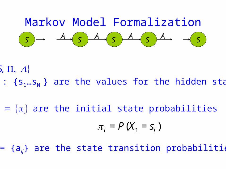
Markov Model Formalization
SSS SS
S S s1hellipsN are the values for the hidden states
are the initial state probabilities
A = aij are the state transition probabilities
AAAA
i = P(X1 = si )
What is the probability of a sequence of states
P(X1K XT )
=P(X1)P(X2 |X1)P(X3 |X1X2 )P(XT |X1K XTminus1)=P(X1)P(X2 |X1)P(X3 |X2 )P(XT |XTminus1)
= X1aXtXt+1
t=1
Tminus1
prod
What is an HMM
Graphical Model Circles indicate states Arrows indicate probabilistic dependencies between states
HMM = Hidden Markov Model
What is an HMM
Green circles are hidden states Dependent only on the previous state
What is an HMM
Purple nodes are observed states Dependent only on their corresponding hidden state The past is independent of the future given the
present
HMM Formalism
S K S s1hellipsN are the values for the hidden states
K k1hellipkM are the values for the observations
SSS
KKK
S
K
S
K
HMM Formalism
S K are the initial state probabilities
A = aij are the state transition probabilities
B = bik are the observation state probabilities
Note sometimes one uses B = bijk
output then depends on previous state transition as well
A
B
AAA
BB
SSS
KKK
S
K
S
K
The crazy soft drink machine
Fig 92
B cola iced tea lemonade
CP 06 01 03
IP 01 07 02
Probability of lemice
Sum over all paths taken through HMM Start in CP
bull 1 x 03 x 07 x 01 +bull 1 x 03 x 03 x 07
oTo1 otot-1 ot+1
HMMs and Bayesian Nets (1)
x1 xt-1 xt xt+1 xT
P(x1xT o1oT )=P(x1)P(o1 |x1) P(xi+1 |xii=1
Tminus1
prod )P(oi+1 |xi+1)
= x1bx1o1
t=1
Tminus1
axtxt+1bxt+1ot+1
oTo1 otot-1 ot+1
x1 xt+1 xTxtxt-1
HMM and Bayesian Nets (2)
Conditionally independent of Given
Because of d-separation
ldquoThe past is independent of the future given the presentrdquo
Inference in an HMM
Compute the probability of a given observation sequence
Given an observation sequence compute the most likely hidden state sequence
Given an observation sequence and set of possible models which model most closely fits the data
O =(o1oT )μ =(AB)ComputeP(O |μ)
oTo1 otot-1 ot+1
Given an observation sequence and a model compute the probability of the observation sequence
Decoding
Decoding
TT oxoxox bbbXOP )|(2211
=μ
oTo1 otot-1 ot+1
x1 xt+1 xTxtxt-1
Decoding
TT oxoxox bbbXOP )|(2211
=μ
TT xxxxxxx aaaXP132211
)|(minus
=μ
oTo1 otot-1 ot+1
x1 xt+1 xTxtxt-1
Decoding
)|()|()|( μμμ XPXOPXOP =
TT oxoxox bbbXOP )|(2211
=μ
TT xxxxxxx aaaXP132211
)|(minus
=μ
oTo1 otot-1 ot+1
x1 xt+1 xTxtxt-1
Decoding
)|()|()|( μμμ XPXOPXOP =
TT oxoxox bbbXOP )|(2211
=μ
TT xxxxxxx aaaXP132211
)|(minus
=μ
sum=X
XPXOPOP )|()|()|( μμμ
oTo1 otot-1 ot+1
x1 xt+1 xTxtxt-1
P(O | μ) = x1bx1o1
x1 xT sum
t=1
Tminus1
axtxt+1bxt+1ot+1
Decoding
oTo1 otot-1 ot+1
x1 xt+1 xTxtxt-1
Complexity O(N T 2T )
Eg N =5T =100gives21005100 asymp1072
Dynamic Programming
α i (t) = P(o1ot xt = i | μ )
Forward Procedure
oTo1 otot-1 ot+1
x1 xt+1 xTxtxt-1
bull Special structure gives us an efficient solution using dynamic programming
bull Intuition Probability of the first t observations is the same for all possible t+1 length state sequences
bull Define
α i (1) = P(o1 x1 = i | μ )
= π i bio1
)|()(
)()|()|(
)()|(
)(
1111
11111
1111
111
jxoPjxooP
jxPjxoPjxooP
jxPjxooP
jxooP
tttt
ttttt
ttt
tt
=======
=====
+++
++++
+++
++
oTo1 otot-1 ot+1
x1 xt+1 xTxtxt-1
Forward Procedure
)1( +tjα
oTo1 otot-1 ot+1
x1 xt+1 xTxtxt-1
Forward Procedure
)1( +tjα
)|()(
)()|()|(
)()|(
)(
1111
11111
1111
111
jxoPjxooP
jxPjxoPjxooP
jxPjxooP
jxooP
tttt
ttttt
ttt
tt
=======
=====
+++
++++
+++
++
oTo1 otot-1 ot+1
x1 xt+1 xTxtxt-1
Forward Procedure
)1( +tjα
)|()(
)()|()|(
)()|(
)(
1111
11111
1111
111
jxoPjxooP
jxPjxoPjxooP
jxPjxooP
jxooP
tttt
ttttt
ttt
tt
=======
=====
+++
++++
+++
++
oTo1 otot-1 ot+1
x1 xt+1 xTxtxt-1
Forward Procedure
)1( +tjα
)|()(
)()|()|(
)()|(
)(
1111
11111
1111
111
jxoPjxooP
jxPjxoPjxooP
jxPjxooP
jxooP
tttt
ttttt
ttt
tt
=======
=====
+++
++++
+++
++
sum
sum
sum
sum
=
+++=
++=
+
++=
+
+=
=====
=====
====
Nijoiji
ttttNi
tt
tttNi
ttt
ttNi
ttt
tbat
jxoPixjxPixooP
jxoPixPixjxooP
jxoPjxixooP
1
1111
1
111
11
111
11
1)(
)|()|()(
)|()()|(
)|()(
α
oTo1 otot-1 ot+1
x1 xt+1 xTxtxt-1
Forward Procedure
sum
sum
sum
sum
=
+++=
++=
+
++=
+
+=
=====
=====
====
Nijoiji
ttttNi
tt
tttNi
ttt
ttNi
ttt
tbat
jxoPixjxPixooP
jxoPixPixjxooP
jxoPjxixooP
1
1111
1
111
11
111
11
1)(
)|()|()(
)|()()|(
)|()(
α
oTo1 otot-1 ot+1
x1 xt+1 xTxtxt-1
Forward Procedure
sum
sum
sum
sum
=
+++=
++=
+
++=
+
+=
=====
=====
====
Nijoiji
ttttNi
tt
tttNi
ttt
ttNi
ttt
tbat
jxoPixjxPixooP
jxoPixPixjxooP
jxoPjxixooP
1
1111
1
111
11
111
11
1)(
)|()|()(
)|()()|(
)|()(
α
oTo1 otot-1 ot+1
x1 xt+1 xTxtxt-1
Forward Procedure
= P(o1ot xt = i xt+1 = j)i=1Nsum P(ot+1 | xt+1 = j)
= P(o1ot xt+1 = j | xt = i)i=1Nsum P(xt = i)P(ot+1 | xt+1 = j)
= P(o1ot xt = i)i=1Nsum P(xt+1 = j | xt = i)P(ot+1 | xt+1 = j)
= α i (t)aijb jot +1i=1Nsum
oTo1 otot-1 ot+1
x1 xt+1 xTxtxt-1
Forward Procedure
Dynamic Programming
α j (t +1) = α i (t)aijb jot +1i=1Nsum
Complexity O(N 2 T )
Eg N = 5T = 100 gives asymp 3000
βi (t) = P(ot+1oT | xt = i)
oTo1 otot-1 ot+1
x1 xt+1 xTxtxt-1
Backward Procedure
βi (T ) = 1
βi (t) = aijbiot +1β j (t +1)
j=1Nsum
Probability of the rest of the states given the first state
oTo1 otot-1 ot+1
x1 xt+1 xTxtxt-1
Decoding Solution
sum=
=N
ii TOP
1
)()|( αμ
sum=
=N
iiiOP
1
)1()|( βπμ
)()()|(1
ttOP i
N
ii βαμ sum
=
=
Forward Procedure
Backward Procedure
Combination
P(O Xt =i |μ) =P(o1otXt =iot+1oT |μ)=P(o1otXt =i |μ)P(ot+1oT |o1otXt =i μ)=P(o1otXt =i |μ)P(ot+1oT |Xt =i μ)=α i (t)βi (t)
)()()|(1
ttOP i
N
ii βαμ sum
=
=
oTo1 otot-1 ot+1
Best State Sequence
Find the state sequence that best explains the observations
Two approaches bull Individually most likely statesbull Most likely sequence (Viterbi)
)|(maxarg OXPX
Best State Sequence (1)
γi (t) = P(Xt = i | O μ )
=P(Xt = iO | μ )
P(O | μ )
=α i (t)β i (t)
j=1
n
sum α j (t)β j (t)
Most likely state at each point in time
Xt = arg maxγ i (t)
oTo1 otot-1 ot+1
Best State Sequence (2)
Find the state sequence that best explains the observations
Viterbi algorithm
)|(maxarg OXPX
oTo1 otot-1 ot+1
Viterbi Algorithm
)(max)( 1111 11
ttttxx
j ojxooxxPtt
== minusminusminus
δ
The state sequence which maximizes the probability of seeing the observations to time t-1 landing in state j and seeing the observation at time t
x1 xt-1 j
oTo1 otot-1 ot+1
Viterbi Algorithm
)(max)( 1111 11
ttttxx
j ojxooxxPtt
== minusminusminus
δ
1)(max)1(
+=+
tjoijiij batt δδ
1)(maxarg)1(
+=+
tjoijii
j batt δψRecursive Computation
x1 xt-1 xt xt+1
Initialization
δ1(i) = ibio1
ψ 1(i) =0
oTo1 otot-1 ot+1
Viterbi Algorithm
XT =argmaxi
δi (T )
Xt =ψX^
t+1
(t+1)
P(X)=argmaxi
δi (T )
Compute the most likely state sequence by working backwards
x1 xt-1 xt xt+1 xT
oTo1 otot-1 ot+1
HMMs and Bayesian Nets (1)
x1 xt-1 xt xt+1 xT
P(x1xT o1oT )=P(x1)P(o1 |x1) P(xi+1 |xii=1
Tminus1
prod )P(oi+1 |xi+1)
= x1bx1o1
t=1
Tminus1
axtxt+1bxt+1ot+1
oTo1 otot-1 ot+1
x1 xt+1 xTxtxt-1
HMM and Bayesian Nets (2)
Conditionally independent of Given
Because of d-separation
ldquoThe past is independent of the future given the presentrdquo
Inference in an HMM
Compute the probability of a given observation sequence
Given an observation sequence compute the most likely hidden state sequence
Given an observation sequence and set of possible models which model most closely fits the data
Dynamic Programming
oTo1 otot-1 ot+1
Parameter Estimation
bull Given an observation sequence find the model that is most likely to produce that sequence
bull No analytic methodbull Given a model and observation sequence update
the model parameters to better fit the observations
A
B
AAA
BBB B
arg maxμ
P(Otraining |μ)
α i (t) = P(o1ot xt = i | μ )
βi (t) = P(ot+1oT | xt = i)
)()()|(1
ttOP i
N
ii βαμ sum
=
=
pt (i j)=P(Xt =iXt+1 = j |O μ)
=P(Xt =iXt+1 = jO |μ)
P(O |μ)
oTo1 otot-1 ot+1
Parameter Estimation
A
B
AAA
BBB B
pt (i j)=α i (t)aijbjot+1
β j (t+1)
αm(t)βm(t)m=1Nsum
Probability of traversing an arc
sum=
=Nj
ti jipt1
)()(γ Probability of being in state i
oTo1 otot-1 ot+1
Parameter Estimation
A
B
AAA
BBB B
i =γi(1)
Now we can compute the new estimates of the model parameters
aij =pt(i j)t=1
Tminus1sumγi (t)t=1
Tminus1sum
bik =γi (t) tot=ksum
γi (t)t=1
Tsum
Instance of Expectation Maximization
We have that
We may get stuck in local maximum (or even saddle point)
Nevertheless Baum-Welch usually effective
P(O | μ) geP(O |μ)
Some Variants
So far ergodic modelsbull All states are connectedbull Not always wanted
Epsilon or null-transitionsbull Not all statestransitions emit output symbols
Parameter tyingbull Assuming that certain parameters are shared bull Reduces the number of parameters that have to be estimated
Logical HMMs (Kersting De Raedt Raiko)bull Working with structured states and observation symbols
Working with log probabilities and addition instead of multiplication of probabilities (typically done)
oTo1 otot-1 ot+1
The Most Important Thing
A
B
AAA
BBB B
We can use the special structure of this model to do a lot of neat math and solve problems that are otherwise not solvable
HMMrsquos from an Agent Perspective
AI a modern approachbull AI is the study of rational agentsbull Third part by Wolfram Burgard on
Reinforcement learning
HMMs can also be used herebull Typically one is interested in P(state)
Example
Possible statesbull snow no snow
Observationsbull skis no skis
Questionsbull Was there snow the day before yesterday (given a
sequence of observations) bull Is there now snow (given a sequence of
observations) bull Will there be snow tomorrow given a sequence of
observations Next week
HMM and Agents
Question
bull Case 1 often called smoothing t lt T see last time
Only part of trellis between t and T needed
γi (t) = P(Xt = i | Oμ )
=α i (t)β i (t)
j =1
n
sum α j (t)β j (t)
Most likely state at each point in time
HMM and Agents
bull Case 2 often called filtering t= T last time
Can we make it recursive Ie go from T-1 to T
γi (t) = P(Xt = i | Oμ )
=α i (t)β i (t)
j =1
n
sum α j (t)β j (t)
Most likely state at each point in time
HMM and Agents
bull Case 2 often called filtering t= T last time
λi (T ) = P(XT = i | o1oT μ )
= γ i (T )
=α i (T )β i (T )
j =1
n
sum α j (T )β j (T )
=α i (T )
j =1
n
sum α j (T )
HMM and Agents
bull Case 3 often called prediction t= T+1 (or T+K) not yet seen
Interesting recursive Easily extended towards k gt 1
Extensions
Use Dynamic Bayesian networks instead of HMMsbullOne state corresponds to a Bayesian NetbullObservations can become more complex
Involve actions of the agent as wellbullCf Wolfram Burgardrsquos Part
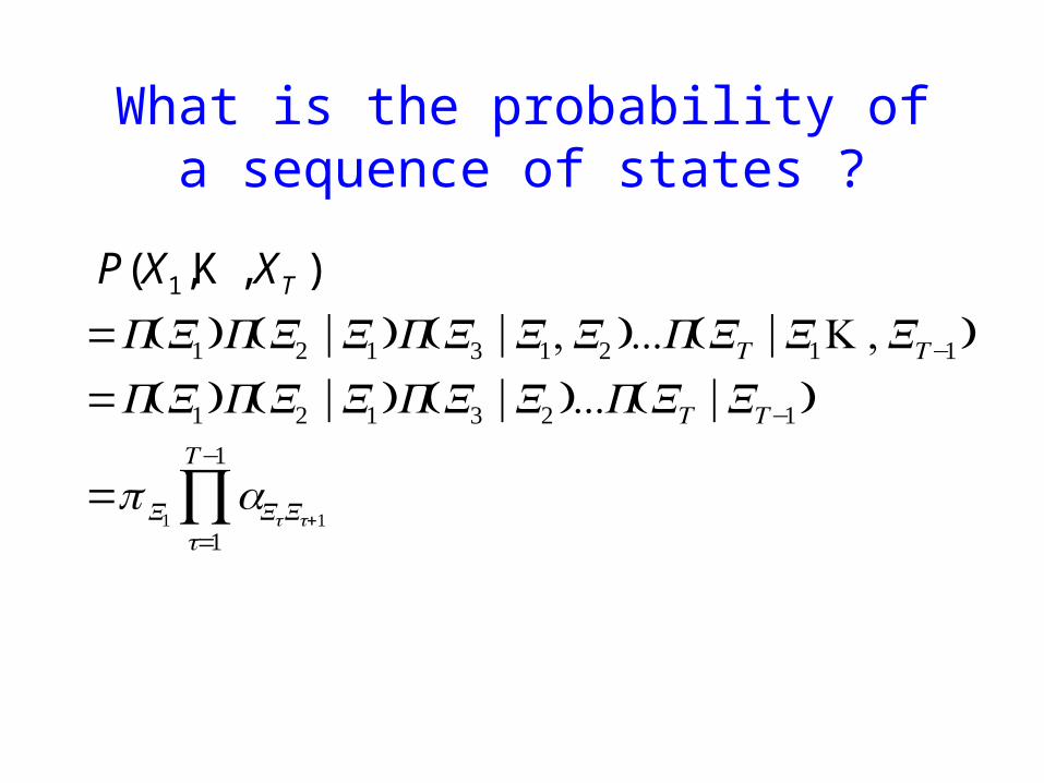
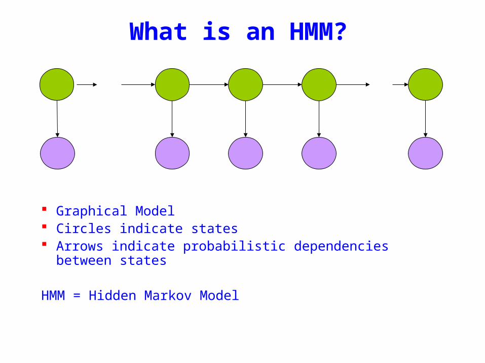
What is an HMM
Graphical Model Circles indicate states Arrows indicate probabilistic dependencies between states
HMM = Hidden Markov Model
What is an HMM
Green circles are hidden states Dependent only on the previous state
What is an HMM
Purple nodes are observed states Dependent only on their corresponding hidden state The past is independent of the future given the
present
HMM Formalism
S K S s1hellipsN are the values for the hidden states
K k1hellipkM are the values for the observations
SSS
KKK
S
K
S
K
HMM Formalism
S K are the initial state probabilities
A = aij are the state transition probabilities
B = bik are the observation state probabilities
Note sometimes one uses B = bijk
output then depends on previous state transition as well
A
B
AAA
BB
SSS
KKK
S
K
S
K
The crazy soft drink machine
Fig 92
B cola iced tea lemonade
CP 06 01 03
IP 01 07 02
Probability of lemice
Sum over all paths taken through HMM Start in CP
bull 1 x 03 x 07 x 01 +bull 1 x 03 x 03 x 07
oTo1 otot-1 ot+1
HMMs and Bayesian Nets (1)
x1 xt-1 xt xt+1 xT
P(x1xT o1oT )=P(x1)P(o1 |x1) P(xi+1 |xii=1
Tminus1
prod )P(oi+1 |xi+1)
= x1bx1o1
t=1
Tminus1
axtxt+1bxt+1ot+1
oTo1 otot-1 ot+1
x1 xt+1 xTxtxt-1
HMM and Bayesian Nets (2)
Conditionally independent of Given
Because of d-separation
ldquoThe past is independent of the future given the presentrdquo
Inference in an HMM
Compute the probability of a given observation sequence
Given an observation sequence compute the most likely hidden state sequence
Given an observation sequence and set of possible models which model most closely fits the data
O =(o1oT )μ =(AB)ComputeP(O |μ)
oTo1 otot-1 ot+1
Given an observation sequence and a model compute the probability of the observation sequence
Decoding
Decoding
TT oxoxox bbbXOP )|(2211
=μ
oTo1 otot-1 ot+1
x1 xt+1 xTxtxt-1
Decoding
TT oxoxox bbbXOP )|(2211
=μ
TT xxxxxxx aaaXP132211
)|(minus
=μ
oTo1 otot-1 ot+1
x1 xt+1 xTxtxt-1
Decoding
)|()|()|( μμμ XPXOPXOP =
TT oxoxox bbbXOP )|(2211
=μ
TT xxxxxxx aaaXP132211
)|(minus
=μ
oTo1 otot-1 ot+1
x1 xt+1 xTxtxt-1
Decoding
)|()|()|( μμμ XPXOPXOP =
TT oxoxox bbbXOP )|(2211
=μ
TT xxxxxxx aaaXP132211
)|(minus
=μ
sum=X
XPXOPOP )|()|()|( μμμ
oTo1 otot-1 ot+1
x1 xt+1 xTxtxt-1
P(O | μ) = x1bx1o1
x1 xT sum
t=1
Tminus1
axtxt+1bxt+1ot+1
Decoding
oTo1 otot-1 ot+1
x1 xt+1 xTxtxt-1
Complexity O(N T 2T )
Eg N =5T =100gives21005100 asymp1072
Dynamic Programming
α i (t) = P(o1ot xt = i | μ )
Forward Procedure
oTo1 otot-1 ot+1
x1 xt+1 xTxtxt-1
bull Special structure gives us an efficient solution using dynamic programming
bull Intuition Probability of the first t observations is the same for all possible t+1 length state sequences
bull Define
α i (1) = P(o1 x1 = i | μ )
= π i bio1
)|()(
)()|()|(
)()|(
)(
1111
11111
1111
111
jxoPjxooP
jxPjxoPjxooP
jxPjxooP
jxooP
tttt
ttttt
ttt
tt
=======
=====
+++
++++
+++
++
oTo1 otot-1 ot+1
x1 xt+1 xTxtxt-1
Forward Procedure
)1( +tjα
oTo1 otot-1 ot+1
x1 xt+1 xTxtxt-1
Forward Procedure
)1( +tjα
)|()(
)()|()|(
)()|(
)(
1111
11111
1111
111
jxoPjxooP
jxPjxoPjxooP
jxPjxooP
jxooP
tttt
ttttt
ttt
tt
=======
=====
+++
++++
+++
++
oTo1 otot-1 ot+1
x1 xt+1 xTxtxt-1
Forward Procedure
)1( +tjα
)|()(
)()|()|(
)()|(
)(
1111
11111
1111
111
jxoPjxooP
jxPjxoPjxooP
jxPjxooP
jxooP
tttt
ttttt
ttt
tt
=======
=====
+++
++++
+++
++
oTo1 otot-1 ot+1
x1 xt+1 xTxtxt-1
Forward Procedure
)1( +tjα
)|()(
)()|()|(
)()|(
)(
1111
11111
1111
111
jxoPjxooP
jxPjxoPjxooP
jxPjxooP
jxooP
tttt
ttttt
ttt
tt
=======
=====
+++
++++
+++
++
sum
sum
sum
sum
=
+++=
++=
+
++=
+
+=
=====
=====
====
Nijoiji
ttttNi
tt
tttNi
ttt
ttNi
ttt
tbat
jxoPixjxPixooP
jxoPixPixjxooP
jxoPjxixooP
1
1111
1
111
11
111
11
1)(
)|()|()(
)|()()|(
)|()(
α
oTo1 otot-1 ot+1
x1 xt+1 xTxtxt-1
Forward Procedure
sum
sum
sum
sum
=
+++=
++=
+
++=
+
+=
=====
=====
====
Nijoiji
ttttNi
tt
tttNi
ttt
ttNi
ttt
tbat
jxoPixjxPixooP
jxoPixPixjxooP
jxoPjxixooP
1
1111
1
111
11
111
11
1)(
)|()|()(
)|()()|(
)|()(
α
oTo1 otot-1 ot+1
x1 xt+1 xTxtxt-1
Forward Procedure
sum
sum
sum
sum
=
+++=
++=
+
++=
+
+=
=====
=====
====
Nijoiji
ttttNi
tt
tttNi
ttt
ttNi
ttt
tbat
jxoPixjxPixooP
jxoPixPixjxooP
jxoPjxixooP
1
1111
1
111
11
111
11
1)(
)|()|()(
)|()()|(
)|()(
α
oTo1 otot-1 ot+1
x1 xt+1 xTxtxt-1
Forward Procedure
= P(o1ot xt = i xt+1 = j)i=1Nsum P(ot+1 | xt+1 = j)
= P(o1ot xt+1 = j | xt = i)i=1Nsum P(xt = i)P(ot+1 | xt+1 = j)
= P(o1ot xt = i)i=1Nsum P(xt+1 = j | xt = i)P(ot+1 | xt+1 = j)
= α i (t)aijb jot +1i=1Nsum
oTo1 otot-1 ot+1
x1 xt+1 xTxtxt-1
Forward Procedure
Dynamic Programming
α j (t +1) = α i (t)aijb jot +1i=1Nsum
Complexity O(N 2 T )
Eg N = 5T = 100 gives asymp 3000
βi (t) = P(ot+1oT | xt = i)
oTo1 otot-1 ot+1
x1 xt+1 xTxtxt-1
Backward Procedure
βi (T ) = 1
βi (t) = aijbiot +1β j (t +1)
j=1Nsum
Probability of the rest of the states given the first state
oTo1 otot-1 ot+1
x1 xt+1 xTxtxt-1
Decoding Solution
sum=
=N
ii TOP
1
)()|( αμ
sum=
=N
iiiOP
1
)1()|( βπμ
)()()|(1
ttOP i
N
ii βαμ sum
=
=
Forward Procedure
Backward Procedure
Combination
P(O Xt =i |μ) =P(o1otXt =iot+1oT |μ)=P(o1otXt =i |μ)P(ot+1oT |o1otXt =i μ)=P(o1otXt =i |μ)P(ot+1oT |Xt =i μ)=α i (t)βi (t)
)()()|(1
ttOP i
N
ii βαμ sum
=
=
oTo1 otot-1 ot+1
Best State Sequence
Find the state sequence that best explains the observations
Two approaches bull Individually most likely statesbull Most likely sequence (Viterbi)
)|(maxarg OXPX
Best State Sequence (1)
γi (t) = P(Xt = i | O μ )
=P(Xt = iO | μ )
P(O | μ )
=α i (t)β i (t)
j=1
n
sum α j (t)β j (t)
Most likely state at each point in time
Xt = arg maxγ i (t)
oTo1 otot-1 ot+1
Best State Sequence (2)
Find the state sequence that best explains the observations
Viterbi algorithm
)|(maxarg OXPX
oTo1 otot-1 ot+1
Viterbi Algorithm
)(max)( 1111 11
ttttxx
j ojxooxxPtt
== minusminusminus
δ
The state sequence which maximizes the probability of seeing the observations to time t-1 landing in state j and seeing the observation at time t
x1 xt-1 j
oTo1 otot-1 ot+1
Viterbi Algorithm
)(max)( 1111 11
ttttxx
j ojxooxxPtt
== minusminusminus
δ
1)(max)1(
+=+
tjoijiij batt δδ
1)(maxarg)1(
+=+
tjoijii
j batt δψRecursive Computation
x1 xt-1 xt xt+1
Initialization
δ1(i) = ibio1
ψ 1(i) =0
oTo1 otot-1 ot+1
Viterbi Algorithm
XT =argmaxi
δi (T )
Xt =ψX^
t+1
(t+1)
P(X)=argmaxi
δi (T )
Compute the most likely state sequence by working backwards
x1 xt-1 xt xt+1 xT
oTo1 otot-1 ot+1
HMMs and Bayesian Nets (1)
x1 xt-1 xt xt+1 xT
P(x1xT o1oT )=P(x1)P(o1 |x1) P(xi+1 |xii=1
Tminus1
prod )P(oi+1 |xi+1)
= x1bx1o1
t=1
Tminus1
axtxt+1bxt+1ot+1
oTo1 otot-1 ot+1
x1 xt+1 xTxtxt-1
HMM and Bayesian Nets (2)
Conditionally independent of Given
Because of d-separation
ldquoThe past is independent of the future given the presentrdquo
Inference in an HMM
Compute the probability of a given observation sequence
Given an observation sequence compute the most likely hidden state sequence
Given an observation sequence and set of possible models which model most closely fits the data
Dynamic Programming
oTo1 otot-1 ot+1
Parameter Estimation
bull Given an observation sequence find the model that is most likely to produce that sequence
bull No analytic methodbull Given a model and observation sequence update
the model parameters to better fit the observations
A
B
AAA
BBB B
arg maxμ
P(Otraining |μ)
α i (t) = P(o1ot xt = i | μ )
βi (t) = P(ot+1oT | xt = i)
)()()|(1
ttOP i
N
ii βαμ sum
=
=
pt (i j)=P(Xt =iXt+1 = j |O μ)
=P(Xt =iXt+1 = jO |μ)
P(O |μ)
oTo1 otot-1 ot+1
Parameter Estimation
A
B
AAA
BBB B
pt (i j)=α i (t)aijbjot+1
β j (t+1)
αm(t)βm(t)m=1Nsum
Probability of traversing an arc
sum=
=Nj
ti jipt1
)()(γ Probability of being in state i
oTo1 otot-1 ot+1
Parameter Estimation
A
B
AAA
BBB B
i =γi(1)
Now we can compute the new estimates of the model parameters
aij =pt(i j)t=1
Tminus1sumγi (t)t=1
Tminus1sum
bik =γi (t) tot=ksum
γi (t)t=1
Tsum
Instance of Expectation Maximization
We have that
We may get stuck in local maximum (or even saddle point)
Nevertheless Baum-Welch usually effective
P(O | μ) geP(O |μ)
Some Variants
So far ergodic modelsbull All states are connectedbull Not always wanted
Epsilon or null-transitionsbull Not all statestransitions emit output symbols
Parameter tyingbull Assuming that certain parameters are shared bull Reduces the number of parameters that have to be estimated
Logical HMMs (Kersting De Raedt Raiko)bull Working with structured states and observation symbols
Working with log probabilities and addition instead of multiplication of probabilities (typically done)
oTo1 otot-1 ot+1
The Most Important Thing
A
B
AAA
BBB B
We can use the special structure of this model to do a lot of neat math and solve problems that are otherwise not solvable
HMMrsquos from an Agent Perspective
AI a modern approachbull AI is the study of rational agentsbull Third part by Wolfram Burgard on
Reinforcement learning
HMMs can also be used herebull Typically one is interested in P(state)
Example
Possible statesbull snow no snow
Observationsbull skis no skis
Questionsbull Was there snow the day before yesterday (given a
sequence of observations) bull Is there now snow (given a sequence of
observations) bull Will there be snow tomorrow given a sequence of
observations Next week
HMM and Agents
Question
bull Case 1 often called smoothing t lt T see last time
Only part of trellis between t and T needed
γi (t) = P(Xt = i | Oμ )
=α i (t)β i (t)
j =1
n
sum α j (t)β j (t)
Most likely state at each point in time
HMM and Agents
bull Case 2 often called filtering t= T last time
Can we make it recursive Ie go from T-1 to T
γi (t) = P(Xt = i | Oμ )
=α i (t)β i (t)
j =1
n
sum α j (t)β j (t)
Most likely state at each point in time
HMM and Agents
bull Case 2 often called filtering t= T last time
λi (T ) = P(XT = i | o1oT μ )
= γ i (T )
=α i (T )β i (T )
j =1
n
sum α j (T )β j (T )
=α i (T )
j =1
n
sum α j (T )
HMM and Agents
bull Case 3 often called prediction t= T+1 (or T+K) not yet seen
Interesting recursive Easily extended towards k gt 1
Extensions
Use Dynamic Bayesian networks instead of HMMsbullOne state corresponds to a Bayesian NetbullObservations can become more complex
Involve actions of the agent as wellbullCf Wolfram Burgardrsquos Part
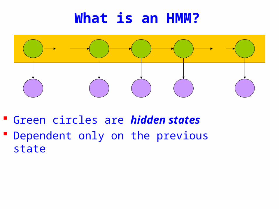
What is an HMM
Green circles are hidden states Dependent only on the previous state
What is an HMM
Purple nodes are observed states Dependent only on their corresponding hidden state The past is independent of the future given the
present
HMM Formalism
S K S s1hellipsN are the values for the hidden states
K k1hellipkM are the values for the observations
SSS
KKK
S
K
S
K
HMM Formalism
S K are the initial state probabilities
A = aij are the state transition probabilities
B = bik are the observation state probabilities
Note sometimes one uses B = bijk
output then depends on previous state transition as well
A
B
AAA
BB
SSS
KKK
S
K
S
K
The crazy soft drink machine
Fig 92
B cola iced tea lemonade
CP 06 01 03
IP 01 07 02
Probability of lemice
Sum over all paths taken through HMM Start in CP
bull 1 x 03 x 07 x 01 +bull 1 x 03 x 03 x 07
oTo1 otot-1 ot+1
HMMs and Bayesian Nets (1)
x1 xt-1 xt xt+1 xT
P(x1xT o1oT )=P(x1)P(o1 |x1) P(xi+1 |xii=1
Tminus1
prod )P(oi+1 |xi+1)
= x1bx1o1
t=1
Tminus1
axtxt+1bxt+1ot+1
oTo1 otot-1 ot+1
x1 xt+1 xTxtxt-1
HMM and Bayesian Nets (2)
Conditionally independent of Given
Because of d-separation
ldquoThe past is independent of the future given the presentrdquo
Inference in an HMM
Compute the probability of a given observation sequence
Given an observation sequence compute the most likely hidden state sequence
Given an observation sequence and set of possible models which model most closely fits the data
O =(o1oT )μ =(AB)ComputeP(O |μ)
oTo1 otot-1 ot+1
Given an observation sequence and a model compute the probability of the observation sequence
Decoding
Decoding
TT oxoxox bbbXOP )|(2211
=μ
oTo1 otot-1 ot+1
x1 xt+1 xTxtxt-1
Decoding
TT oxoxox bbbXOP )|(2211
=μ
TT xxxxxxx aaaXP132211
)|(minus
=μ
oTo1 otot-1 ot+1
x1 xt+1 xTxtxt-1
Decoding
)|()|()|( μμμ XPXOPXOP =
TT oxoxox bbbXOP )|(2211
=μ
TT xxxxxxx aaaXP132211
)|(minus
=μ
oTo1 otot-1 ot+1
x1 xt+1 xTxtxt-1
Decoding
)|()|()|( μμμ XPXOPXOP =
TT oxoxox bbbXOP )|(2211
=μ
TT xxxxxxx aaaXP132211
)|(minus
=μ
sum=X
XPXOPOP )|()|()|( μμμ
oTo1 otot-1 ot+1
x1 xt+1 xTxtxt-1
P(O | μ) = x1bx1o1
x1 xT sum
t=1
Tminus1
axtxt+1bxt+1ot+1
Decoding
oTo1 otot-1 ot+1
x1 xt+1 xTxtxt-1
Complexity O(N T 2T )
Eg N =5T =100gives21005100 asymp1072
Dynamic Programming
α i (t) = P(o1ot xt = i | μ )
Forward Procedure
oTo1 otot-1 ot+1
x1 xt+1 xTxtxt-1
bull Special structure gives us an efficient solution using dynamic programming
bull Intuition Probability of the first t observations is the same for all possible t+1 length state sequences
bull Define
α i (1) = P(o1 x1 = i | μ )
= π i bio1
)|()(
)()|()|(
)()|(
)(
1111
11111
1111
111
jxoPjxooP
jxPjxoPjxooP
jxPjxooP
jxooP
tttt
ttttt
ttt
tt
=======
=====
+++
++++
+++
++
oTo1 otot-1 ot+1
x1 xt+1 xTxtxt-1
Forward Procedure
)1( +tjα
oTo1 otot-1 ot+1
x1 xt+1 xTxtxt-1
Forward Procedure
)1( +tjα
)|()(
)()|()|(
)()|(
)(
1111
11111
1111
111
jxoPjxooP
jxPjxoPjxooP
jxPjxooP
jxooP
tttt
ttttt
ttt
tt
=======
=====
+++
++++
+++
++
oTo1 otot-1 ot+1
x1 xt+1 xTxtxt-1
Forward Procedure
)1( +tjα
)|()(
)()|()|(
)()|(
)(
1111
11111
1111
111
jxoPjxooP
jxPjxoPjxooP
jxPjxooP
jxooP
tttt
ttttt
ttt
tt
=======
=====
+++
++++
+++
++
oTo1 otot-1 ot+1
x1 xt+1 xTxtxt-1
Forward Procedure
)1( +tjα
)|()(
)()|()|(
)()|(
)(
1111
11111
1111
111
jxoPjxooP
jxPjxoPjxooP
jxPjxooP
jxooP
tttt
ttttt
ttt
tt
=======
=====
+++
++++
+++
++
sum
sum
sum
sum
=
+++=
++=
+
++=
+
+=
=====
=====
====
Nijoiji
ttttNi
tt
tttNi
ttt
ttNi
ttt
tbat
jxoPixjxPixooP
jxoPixPixjxooP
jxoPjxixooP
1
1111
1
111
11
111
11
1)(
)|()|()(
)|()()|(
)|()(
α
oTo1 otot-1 ot+1
x1 xt+1 xTxtxt-1
Forward Procedure
sum
sum
sum
sum
=
+++=
++=
+
++=
+
+=
=====
=====
====
Nijoiji
ttttNi
tt
tttNi
ttt
ttNi
ttt
tbat
jxoPixjxPixooP
jxoPixPixjxooP
jxoPjxixooP
1
1111
1
111
11
111
11
1)(
)|()|()(
)|()()|(
)|()(
α
oTo1 otot-1 ot+1
x1 xt+1 xTxtxt-1
Forward Procedure
sum
sum
sum
sum
=
+++=
++=
+
++=
+
+=
=====
=====
====
Nijoiji
ttttNi
tt
tttNi
ttt
ttNi
ttt
tbat
jxoPixjxPixooP
jxoPixPixjxooP
jxoPjxixooP
1
1111
1
111
11
111
11
1)(
)|()|()(
)|()()|(
)|()(
α
oTo1 otot-1 ot+1
x1 xt+1 xTxtxt-1
Forward Procedure
= P(o1ot xt = i xt+1 = j)i=1Nsum P(ot+1 | xt+1 = j)
= P(o1ot xt+1 = j | xt = i)i=1Nsum P(xt = i)P(ot+1 | xt+1 = j)
= P(o1ot xt = i)i=1Nsum P(xt+1 = j | xt = i)P(ot+1 | xt+1 = j)
= α i (t)aijb jot +1i=1Nsum
oTo1 otot-1 ot+1
x1 xt+1 xTxtxt-1
Forward Procedure
Dynamic Programming
α j (t +1) = α i (t)aijb jot +1i=1Nsum
Complexity O(N 2 T )
Eg N = 5T = 100 gives asymp 3000
βi (t) = P(ot+1oT | xt = i)
oTo1 otot-1 ot+1
x1 xt+1 xTxtxt-1
Backward Procedure
βi (T ) = 1
βi (t) = aijbiot +1β j (t +1)
j=1Nsum
Probability of the rest of the states given the first state
oTo1 otot-1 ot+1
x1 xt+1 xTxtxt-1
Decoding Solution
sum=
=N
ii TOP
1
)()|( αμ
sum=
=N
iiiOP
1
)1()|( βπμ
)()()|(1
ttOP i
N
ii βαμ sum
=
=
Forward Procedure
Backward Procedure
Combination
P(O Xt =i |μ) =P(o1otXt =iot+1oT |μ)=P(o1otXt =i |μ)P(ot+1oT |o1otXt =i μ)=P(o1otXt =i |μ)P(ot+1oT |Xt =i μ)=α i (t)βi (t)
)()()|(1
ttOP i
N
ii βαμ sum
=
=
oTo1 otot-1 ot+1
Best State Sequence
Find the state sequence that best explains the observations
Two approaches bull Individually most likely statesbull Most likely sequence (Viterbi)
)|(maxarg OXPX
Best State Sequence (1)
γi (t) = P(Xt = i | O μ )
=P(Xt = iO | μ )
P(O | μ )
=α i (t)β i (t)
j=1
n
sum α j (t)β j (t)
Most likely state at each point in time
Xt = arg maxγ i (t)
oTo1 otot-1 ot+1
Best State Sequence (2)
Find the state sequence that best explains the observations
Viterbi algorithm
)|(maxarg OXPX
oTo1 otot-1 ot+1
Viterbi Algorithm
)(max)( 1111 11
ttttxx
j ojxooxxPtt
== minusminusminus
δ
The state sequence which maximizes the probability of seeing the observations to time t-1 landing in state j and seeing the observation at time t
x1 xt-1 j
oTo1 otot-1 ot+1
Viterbi Algorithm
)(max)( 1111 11
ttttxx
j ojxooxxPtt
== minusminusminus
δ
1)(max)1(
+=+
tjoijiij batt δδ
1)(maxarg)1(
+=+
tjoijii
j batt δψRecursive Computation
x1 xt-1 xt xt+1
Initialization
δ1(i) = ibio1
ψ 1(i) =0
oTo1 otot-1 ot+1
Viterbi Algorithm
XT =argmaxi
δi (T )
Xt =ψX^
t+1
(t+1)
P(X)=argmaxi
δi (T )
Compute the most likely state sequence by working backwards
x1 xt-1 xt xt+1 xT
oTo1 otot-1 ot+1
HMMs and Bayesian Nets (1)
x1 xt-1 xt xt+1 xT
P(x1xT o1oT )=P(x1)P(o1 |x1) P(xi+1 |xii=1
Tminus1
prod )P(oi+1 |xi+1)
= x1bx1o1
t=1
Tminus1
axtxt+1bxt+1ot+1
oTo1 otot-1 ot+1
x1 xt+1 xTxtxt-1
HMM and Bayesian Nets (2)
Conditionally independent of Given
Because of d-separation
ldquoThe past is independent of the future given the presentrdquo
Inference in an HMM
Compute the probability of a given observation sequence
Given an observation sequence compute the most likely hidden state sequence
Given an observation sequence and set of possible models which model most closely fits the data
Dynamic Programming
oTo1 otot-1 ot+1
Parameter Estimation
bull Given an observation sequence find the model that is most likely to produce that sequence
bull No analytic methodbull Given a model and observation sequence update
the model parameters to better fit the observations
A
B
AAA
BBB B
arg maxμ
P(Otraining |μ)
α i (t) = P(o1ot xt = i | μ )
βi (t) = P(ot+1oT | xt = i)
)()()|(1
ttOP i
N
ii βαμ sum
=
=
pt (i j)=P(Xt =iXt+1 = j |O μ)
=P(Xt =iXt+1 = jO |μ)
P(O |μ)
oTo1 otot-1 ot+1
Parameter Estimation
A
B
AAA
BBB B
pt (i j)=α i (t)aijbjot+1
β j (t+1)
αm(t)βm(t)m=1Nsum
Probability of traversing an arc
sum=
=Nj
ti jipt1
)()(γ Probability of being in state i
oTo1 otot-1 ot+1
Parameter Estimation
A
B
AAA
BBB B
i =γi(1)
Now we can compute the new estimates of the model parameters
aij =pt(i j)t=1
Tminus1sumγi (t)t=1
Tminus1sum
bik =γi (t) tot=ksum
γi (t)t=1
Tsum
Instance of Expectation Maximization
We have that
We may get stuck in local maximum (or even saddle point)
Nevertheless Baum-Welch usually effective
P(O | μ) geP(O |μ)
Some Variants
So far ergodic modelsbull All states are connectedbull Not always wanted
Epsilon or null-transitionsbull Not all statestransitions emit output symbols
Parameter tyingbull Assuming that certain parameters are shared bull Reduces the number of parameters that have to be estimated
Logical HMMs (Kersting De Raedt Raiko)bull Working with structured states and observation symbols
Working with log probabilities and addition instead of multiplication of probabilities (typically done)
oTo1 otot-1 ot+1
The Most Important Thing
A
B
AAA
BBB B
We can use the special structure of this model to do a lot of neat math and solve problems that are otherwise not solvable
HMMrsquos from an Agent Perspective
AI a modern approachbull AI is the study of rational agentsbull Third part by Wolfram Burgard on
Reinforcement learning
HMMs can also be used herebull Typically one is interested in P(state)
Example
Possible statesbull snow no snow
Observationsbull skis no skis
Questionsbull Was there snow the day before yesterday (given a
sequence of observations) bull Is there now snow (given a sequence of
observations) bull Will there be snow tomorrow given a sequence of
observations Next week
HMM and Agents
Question
bull Case 1 often called smoothing t lt T see last time
Only part of trellis between t and T needed
γi (t) = P(Xt = i | Oμ )
=α i (t)β i (t)
j =1
n
sum α j (t)β j (t)
Most likely state at each point in time
HMM and Agents
bull Case 2 often called filtering t= T last time
Can we make it recursive Ie go from T-1 to T
γi (t) = P(Xt = i | Oμ )
=α i (t)β i (t)
j =1
n
sum α j (t)β j (t)
Most likely state at each point in time
HMM and Agents
bull Case 2 often called filtering t= T last time
λi (T ) = P(XT = i | o1oT μ )
= γ i (T )
=α i (T )β i (T )
j =1
n
sum α j (T )β j (T )
=α i (T )
j =1
n
sum α j (T )
HMM and Agents
bull Case 3 often called prediction t= T+1 (or T+K) not yet seen
Interesting recursive Easily extended towards k gt 1
Extensions
Use Dynamic Bayesian networks instead of HMMsbullOne state corresponds to a Bayesian NetbullObservations can become more complex
Involve actions of the agent as wellbullCf Wolfram Burgardrsquos Part
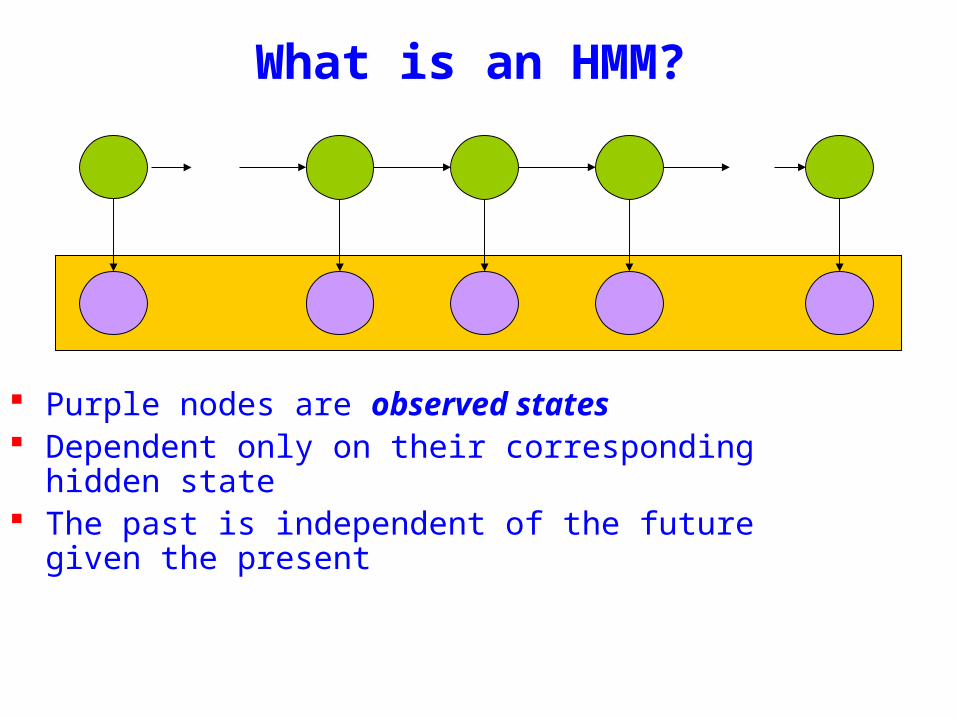
What is an HMM
Purple nodes are observed states Dependent only on their corresponding hidden state The past is independent of the future given the
present
HMM Formalism
S K S s1hellipsN are the values for the hidden states
K k1hellipkM are the values for the observations
SSS
KKK
S
K
S
K
HMM Formalism
S K are the initial state probabilities
A = aij are the state transition probabilities
B = bik are the observation state probabilities
Note sometimes one uses B = bijk
output then depends on previous state transition as well
A
B
AAA
BB
SSS
KKK
S
K
S
K
The crazy soft drink machine
Fig 92
B cola iced tea lemonade
CP 06 01 03
IP 01 07 02
Probability of lemice
Sum over all paths taken through HMM Start in CP
bull 1 x 03 x 07 x 01 +bull 1 x 03 x 03 x 07
oTo1 otot-1 ot+1
HMMs and Bayesian Nets (1)
x1 xt-1 xt xt+1 xT
P(x1xT o1oT )=P(x1)P(o1 |x1) P(xi+1 |xii=1
Tminus1
prod )P(oi+1 |xi+1)
= x1bx1o1
t=1
Tminus1
axtxt+1bxt+1ot+1
oTo1 otot-1 ot+1
x1 xt+1 xTxtxt-1
HMM and Bayesian Nets (2)
Conditionally independent of Given
Because of d-separation
ldquoThe past is independent of the future given the presentrdquo
Inference in an HMM
Compute the probability of a given observation sequence
Given an observation sequence compute the most likely hidden state sequence
Given an observation sequence and set of possible models which model most closely fits the data
O =(o1oT )μ =(AB)ComputeP(O |μ)
oTo1 otot-1 ot+1
Given an observation sequence and a model compute the probability of the observation sequence
Decoding
Decoding
TT oxoxox bbbXOP )|(2211
=μ
oTo1 otot-1 ot+1
x1 xt+1 xTxtxt-1
Decoding
TT oxoxox bbbXOP )|(2211
=μ
TT xxxxxxx aaaXP132211
)|(minus
=μ
oTo1 otot-1 ot+1
x1 xt+1 xTxtxt-1
Decoding
)|()|()|( μμμ XPXOPXOP =
TT oxoxox bbbXOP )|(2211
=μ
TT xxxxxxx aaaXP132211
)|(minus
=μ
oTo1 otot-1 ot+1
x1 xt+1 xTxtxt-1
Decoding
)|()|()|( μμμ XPXOPXOP =
TT oxoxox bbbXOP )|(2211
=μ
TT xxxxxxx aaaXP132211
)|(minus
=μ
sum=X
XPXOPOP )|()|()|( μμμ
oTo1 otot-1 ot+1
x1 xt+1 xTxtxt-1
P(O | μ) = x1bx1o1
x1 xT sum
t=1
Tminus1
axtxt+1bxt+1ot+1
Decoding
oTo1 otot-1 ot+1
x1 xt+1 xTxtxt-1
Complexity O(N T 2T )
Eg N =5T =100gives21005100 asymp1072
Dynamic Programming
α i (t) = P(o1ot xt = i | μ )
Forward Procedure
oTo1 otot-1 ot+1
x1 xt+1 xTxtxt-1
bull Special structure gives us an efficient solution using dynamic programming
bull Intuition Probability of the first t observations is the same for all possible t+1 length state sequences
bull Define
α i (1) = P(o1 x1 = i | μ )
= π i bio1
)|()(
)()|()|(
)()|(
)(
1111
11111
1111
111
jxoPjxooP
jxPjxoPjxooP
jxPjxooP
jxooP
tttt
ttttt
ttt
tt
=======
=====
+++
++++
+++
++
oTo1 otot-1 ot+1
x1 xt+1 xTxtxt-1
Forward Procedure
)1( +tjα
oTo1 otot-1 ot+1
x1 xt+1 xTxtxt-1
Forward Procedure
)1( +tjα
)|()(
)()|()|(
)()|(
)(
1111
11111
1111
111
jxoPjxooP
jxPjxoPjxooP
jxPjxooP
jxooP
tttt
ttttt
ttt
tt
=======
=====
+++
++++
+++
++
oTo1 otot-1 ot+1
x1 xt+1 xTxtxt-1
Forward Procedure
)1( +tjα
)|()(
)()|()|(
)()|(
)(
1111
11111
1111
111
jxoPjxooP
jxPjxoPjxooP
jxPjxooP
jxooP
tttt
ttttt
ttt
tt
=======
=====
+++
++++
+++
++
oTo1 otot-1 ot+1
x1 xt+1 xTxtxt-1
Forward Procedure
)1( +tjα
)|()(
)()|()|(
)()|(
)(
1111
11111
1111
111
jxoPjxooP
jxPjxoPjxooP
jxPjxooP
jxooP
tttt
ttttt
ttt
tt
=======
=====
+++
++++
+++
++
sum
sum
sum
sum
=
+++=
++=
+
++=
+
+=
=====
=====
====
Nijoiji
ttttNi
tt
tttNi
ttt
ttNi
ttt
tbat
jxoPixjxPixooP
jxoPixPixjxooP
jxoPjxixooP
1
1111
1
111
11
111
11
1)(
)|()|()(
)|()()|(
)|()(
α
oTo1 otot-1 ot+1
x1 xt+1 xTxtxt-1
Forward Procedure
sum
sum
sum
sum
=
+++=
++=
+
++=
+
+=
=====
=====
====
Nijoiji
ttttNi
tt
tttNi
ttt
ttNi
ttt
tbat
jxoPixjxPixooP
jxoPixPixjxooP
jxoPjxixooP
1
1111
1
111
11
111
11
1)(
)|()|()(
)|()()|(
)|()(
α
oTo1 otot-1 ot+1
x1 xt+1 xTxtxt-1
Forward Procedure
sum
sum
sum
sum
=
+++=
++=
+
++=
+
+=
=====
=====
====
Nijoiji
ttttNi
tt
tttNi
ttt
ttNi
ttt
tbat
jxoPixjxPixooP
jxoPixPixjxooP
jxoPjxixooP
1
1111
1
111
11
111
11
1)(
)|()|()(
)|()()|(
)|()(
α
oTo1 otot-1 ot+1
x1 xt+1 xTxtxt-1
Forward Procedure
= P(o1ot xt = i xt+1 = j)i=1Nsum P(ot+1 | xt+1 = j)
= P(o1ot xt+1 = j | xt = i)i=1Nsum P(xt = i)P(ot+1 | xt+1 = j)
= P(o1ot xt = i)i=1Nsum P(xt+1 = j | xt = i)P(ot+1 | xt+1 = j)
= α i (t)aijb jot +1i=1Nsum
oTo1 otot-1 ot+1
x1 xt+1 xTxtxt-1
Forward Procedure
Dynamic Programming
α j (t +1) = α i (t)aijb jot +1i=1Nsum
Complexity O(N 2 T )
Eg N = 5T = 100 gives asymp 3000
βi (t) = P(ot+1oT | xt = i)
oTo1 otot-1 ot+1
x1 xt+1 xTxtxt-1
Backward Procedure
βi (T ) = 1
βi (t) = aijbiot +1β j (t +1)
j=1Nsum
Probability of the rest of the states given the first state
oTo1 otot-1 ot+1
x1 xt+1 xTxtxt-1
Decoding Solution
sum=
=N
ii TOP
1
)()|( αμ
sum=
=N
iiiOP
1
)1()|( βπμ
)()()|(1
ttOP i
N
ii βαμ sum
=
=
Forward Procedure
Backward Procedure
Combination
P(O Xt =i |μ) =P(o1otXt =iot+1oT |μ)=P(o1otXt =i |μ)P(ot+1oT |o1otXt =i μ)=P(o1otXt =i |μ)P(ot+1oT |Xt =i μ)=α i (t)βi (t)
)()()|(1
ttOP i
N
ii βαμ sum
=
=
oTo1 otot-1 ot+1
Best State Sequence
Find the state sequence that best explains the observations
Two approaches bull Individually most likely statesbull Most likely sequence (Viterbi)
)|(maxarg OXPX
Best State Sequence (1)
γi (t) = P(Xt = i | O μ )
=P(Xt = iO | μ )
P(O | μ )
=α i (t)β i (t)
j=1
n
sum α j (t)β j (t)
Most likely state at each point in time
Xt = arg maxγ i (t)
oTo1 otot-1 ot+1
Best State Sequence (2)
Find the state sequence that best explains the observations
Viterbi algorithm
)|(maxarg OXPX
oTo1 otot-1 ot+1
Viterbi Algorithm
)(max)( 1111 11
ttttxx
j ojxooxxPtt
== minusminusminus
δ
The state sequence which maximizes the probability of seeing the observations to time t-1 landing in state j and seeing the observation at time t
x1 xt-1 j
oTo1 otot-1 ot+1
Viterbi Algorithm
)(max)( 1111 11
ttttxx
j ojxooxxPtt
== minusminusminus
δ
1)(max)1(
+=+
tjoijiij batt δδ
1)(maxarg)1(
+=+
tjoijii
j batt δψRecursive Computation
x1 xt-1 xt xt+1
Initialization
δ1(i) = ibio1
ψ 1(i) =0
oTo1 otot-1 ot+1
Viterbi Algorithm
XT =argmaxi
δi (T )
Xt =ψX^
t+1
(t+1)
P(X)=argmaxi
δi (T )
Compute the most likely state sequence by working backwards
x1 xt-1 xt xt+1 xT
oTo1 otot-1 ot+1
HMMs and Bayesian Nets (1)
x1 xt-1 xt xt+1 xT
P(x1xT o1oT )=P(x1)P(o1 |x1) P(xi+1 |xii=1
Tminus1
prod )P(oi+1 |xi+1)
= x1bx1o1
t=1
Tminus1
axtxt+1bxt+1ot+1
oTo1 otot-1 ot+1
x1 xt+1 xTxtxt-1
HMM and Bayesian Nets (2)
Conditionally independent of Given
Because of d-separation
ldquoThe past is independent of the future given the presentrdquo
Inference in an HMM
Compute the probability of a given observation sequence
Given an observation sequence compute the most likely hidden state sequence
Given an observation sequence and set of possible models which model most closely fits the data
Dynamic Programming
oTo1 otot-1 ot+1
Parameter Estimation
bull Given an observation sequence find the model that is most likely to produce that sequence
bull No analytic methodbull Given a model and observation sequence update
the model parameters to better fit the observations
A
B
AAA
BBB B
arg maxμ
P(Otraining |μ)
α i (t) = P(o1ot xt = i | μ )
βi (t) = P(ot+1oT | xt = i)
)()()|(1
ttOP i
N
ii βαμ sum
=
=
pt (i j)=P(Xt =iXt+1 = j |O μ)
=P(Xt =iXt+1 = jO |μ)
P(O |μ)
oTo1 otot-1 ot+1
Parameter Estimation
A
B
AAA
BBB B
pt (i j)=α i (t)aijbjot+1
β j (t+1)
αm(t)βm(t)m=1Nsum
Probability of traversing an arc
sum=
=Nj
ti jipt1
)()(γ Probability of being in state i
oTo1 otot-1 ot+1
Parameter Estimation
A
B
AAA
BBB B
i =γi(1)
Now we can compute the new estimates of the model parameters
aij =pt(i j)t=1
Tminus1sumγi (t)t=1
Tminus1sum
bik =γi (t) tot=ksum
γi (t)t=1
Tsum
Instance of Expectation Maximization
We have that
We may get stuck in local maximum (or even saddle point)
Nevertheless Baum-Welch usually effective
P(O | μ) geP(O |μ)
Some Variants
So far ergodic modelsbull All states are connectedbull Not always wanted
Epsilon or null-transitionsbull Not all statestransitions emit output symbols
Parameter tyingbull Assuming that certain parameters are shared bull Reduces the number of parameters that have to be estimated
Logical HMMs (Kersting De Raedt Raiko)bull Working with structured states and observation symbols
Working with log probabilities and addition instead of multiplication of probabilities (typically done)
oTo1 otot-1 ot+1
The Most Important Thing
A
B
AAA
BBB B
We can use the special structure of this model to do a lot of neat math and solve problems that are otherwise not solvable
HMMrsquos from an Agent Perspective
AI a modern approachbull AI is the study of rational agentsbull Third part by Wolfram Burgard on
Reinforcement learning
HMMs can also be used herebull Typically one is interested in P(state)
Example
Possible statesbull snow no snow
Observationsbull skis no skis
Questionsbull Was there snow the day before yesterday (given a
sequence of observations) bull Is there now snow (given a sequence of
observations) bull Will there be snow tomorrow given a sequence of
observations Next week
HMM and Agents
Question
bull Case 1 often called smoothing t lt T see last time
Only part of trellis between t and T needed
γi (t) = P(Xt = i | Oμ )
=α i (t)β i (t)
j =1
n
sum α j (t)β j (t)
Most likely state at each point in time
HMM and Agents
bull Case 2 often called filtering t= T last time
Can we make it recursive Ie go from T-1 to T
γi (t) = P(Xt = i | Oμ )
=α i (t)β i (t)
j =1
n
sum α j (t)β j (t)
Most likely state at each point in time
HMM and Agents
bull Case 2 often called filtering t= T last time
λi (T ) = P(XT = i | o1oT μ )
= γ i (T )
=α i (T )β i (T )
j =1
n
sum α j (T )β j (T )
=α i (T )
j =1
n
sum α j (T )
HMM and Agents
bull Case 3 often called prediction t= T+1 (or T+K) not yet seen
Interesting recursive Easily extended towards k gt 1
Extensions
Use Dynamic Bayesian networks instead of HMMsbullOne state corresponds to a Bayesian NetbullObservations can become more complex
Involve actions of the agent as wellbullCf Wolfram Burgardrsquos Part
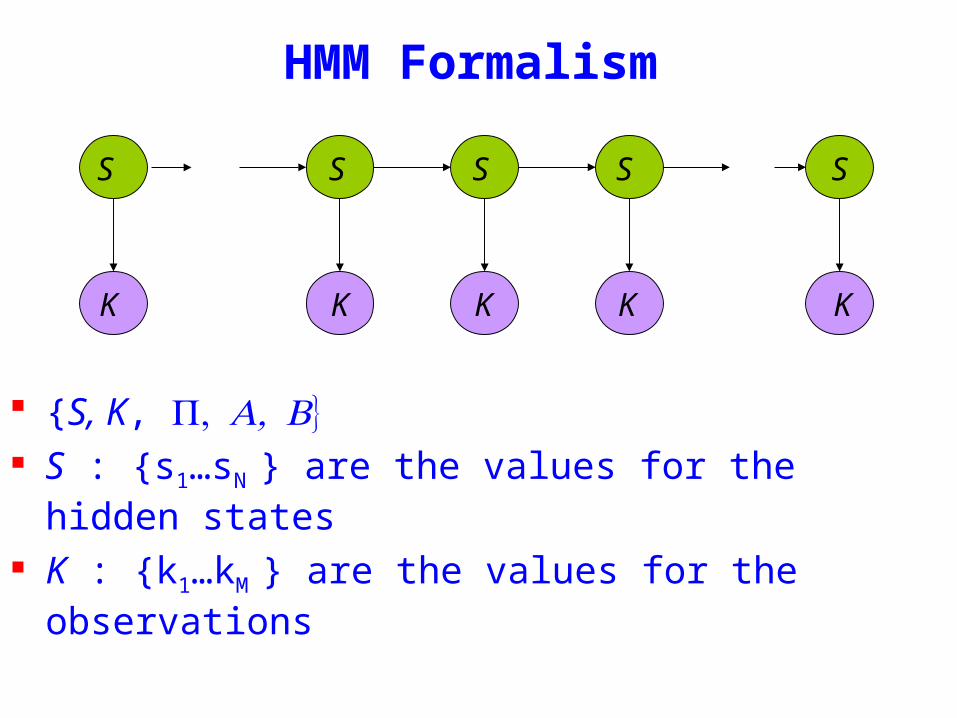
HMM Formalism
S K S s1hellipsN are the values for the hidden states
K k1hellipkM are the values for the observations
SSS
KKK
S
K
S
K
HMM Formalism
S K are the initial state probabilities
A = aij are the state transition probabilities
B = bik are the observation state probabilities
Note sometimes one uses B = bijk
output then depends on previous state transition as well
A
B
AAA
BB
SSS
KKK
S
K
S
K
The crazy soft drink machine
Fig 92
B cola iced tea lemonade
CP 06 01 03
IP 01 07 02
Probability of lemice
Sum over all paths taken through HMM Start in CP
bull 1 x 03 x 07 x 01 +bull 1 x 03 x 03 x 07
oTo1 otot-1 ot+1
HMMs and Bayesian Nets (1)
x1 xt-1 xt xt+1 xT
P(x1xT o1oT )=P(x1)P(o1 |x1) P(xi+1 |xii=1
Tminus1
prod )P(oi+1 |xi+1)
= x1bx1o1
t=1
Tminus1
axtxt+1bxt+1ot+1
oTo1 otot-1 ot+1
x1 xt+1 xTxtxt-1
HMM and Bayesian Nets (2)
Conditionally independent of Given
Because of d-separation
ldquoThe past is independent of the future given the presentrdquo
Inference in an HMM
Compute the probability of a given observation sequence
Given an observation sequence compute the most likely hidden state sequence
Given an observation sequence and set of possible models which model most closely fits the data
O =(o1oT )μ =(AB)ComputeP(O |μ)
oTo1 otot-1 ot+1
Given an observation sequence and a model compute the probability of the observation sequence
Decoding
Decoding
TT oxoxox bbbXOP )|(2211
=μ
oTo1 otot-1 ot+1
x1 xt+1 xTxtxt-1
Decoding
TT oxoxox bbbXOP )|(2211
=μ
TT xxxxxxx aaaXP132211
)|(minus
=μ
oTo1 otot-1 ot+1
x1 xt+1 xTxtxt-1
Decoding
)|()|()|( μμμ XPXOPXOP =
TT oxoxox bbbXOP )|(2211
=μ
TT xxxxxxx aaaXP132211
)|(minus
=μ
oTo1 otot-1 ot+1
x1 xt+1 xTxtxt-1
Decoding
)|()|()|( μμμ XPXOPXOP =
TT oxoxox bbbXOP )|(2211
=μ
TT xxxxxxx aaaXP132211
)|(minus
=μ
sum=X
XPXOPOP )|()|()|( μμμ
oTo1 otot-1 ot+1
x1 xt+1 xTxtxt-1
P(O | μ) = x1bx1o1
x1 xT sum
t=1
Tminus1
axtxt+1bxt+1ot+1
Decoding
oTo1 otot-1 ot+1
x1 xt+1 xTxtxt-1
Complexity O(N T 2T )
Eg N =5T =100gives21005100 asymp1072
Dynamic Programming
α i (t) = P(o1ot xt = i | μ )
Forward Procedure
oTo1 otot-1 ot+1
x1 xt+1 xTxtxt-1
bull Special structure gives us an efficient solution using dynamic programming
bull Intuition Probability of the first t observations is the same for all possible t+1 length state sequences
bull Define
α i (1) = P(o1 x1 = i | μ )
= π i bio1
)|()(
)()|()|(
)()|(
)(
1111
11111
1111
111
jxoPjxooP
jxPjxoPjxooP
jxPjxooP
jxooP
tttt
ttttt
ttt
tt
=======
=====
+++
++++
+++
++
oTo1 otot-1 ot+1
x1 xt+1 xTxtxt-1
Forward Procedure
)1( +tjα
oTo1 otot-1 ot+1
x1 xt+1 xTxtxt-1
Forward Procedure
)1( +tjα
)|()(
)()|()|(
)()|(
)(
1111
11111
1111
111
jxoPjxooP
jxPjxoPjxooP
jxPjxooP
jxooP
tttt
ttttt
ttt
tt
=======
=====
+++
++++
+++
++
oTo1 otot-1 ot+1
x1 xt+1 xTxtxt-1
Forward Procedure
)1( +tjα
)|()(
)()|()|(
)()|(
)(
1111
11111
1111
111
jxoPjxooP
jxPjxoPjxooP
jxPjxooP
jxooP
tttt
ttttt
ttt
tt
=======
=====
+++
++++
+++
++
oTo1 otot-1 ot+1
x1 xt+1 xTxtxt-1
Forward Procedure
)1( +tjα
)|()(
)()|()|(
)()|(
)(
1111
11111
1111
111
jxoPjxooP
jxPjxoPjxooP
jxPjxooP
jxooP
tttt
ttttt
ttt
tt
=======
=====
+++
++++
+++
++
sum
sum
sum
sum
=
+++=
++=
+
++=
+
+=
=====
=====
====
Nijoiji
ttttNi
tt
tttNi
ttt
ttNi
ttt
tbat
jxoPixjxPixooP
jxoPixPixjxooP
jxoPjxixooP
1
1111
1
111
11
111
11
1)(
)|()|()(
)|()()|(
)|()(
α
oTo1 otot-1 ot+1
x1 xt+1 xTxtxt-1
Forward Procedure
sum
sum
sum
sum
=
+++=
++=
+
++=
+
+=
=====
=====
====
Nijoiji
ttttNi
tt
tttNi
ttt
ttNi
ttt
tbat
jxoPixjxPixooP
jxoPixPixjxooP
jxoPjxixooP
1
1111
1
111
11
111
11
1)(
)|()|()(
)|()()|(
)|()(
α
oTo1 otot-1 ot+1
x1 xt+1 xTxtxt-1
Forward Procedure
sum
sum
sum
sum
=
+++=
++=
+
++=
+
+=
=====
=====
====
Nijoiji
ttttNi
tt
tttNi
ttt
ttNi
ttt
tbat
jxoPixjxPixooP
jxoPixPixjxooP
jxoPjxixooP
1
1111
1
111
11
111
11
1)(
)|()|()(
)|()()|(
)|()(
α
oTo1 otot-1 ot+1
x1 xt+1 xTxtxt-1
Forward Procedure
= P(o1ot xt = i xt+1 = j)i=1Nsum P(ot+1 | xt+1 = j)
= P(o1ot xt+1 = j | xt = i)i=1Nsum P(xt = i)P(ot+1 | xt+1 = j)
= P(o1ot xt = i)i=1Nsum P(xt+1 = j | xt = i)P(ot+1 | xt+1 = j)
= α i (t)aijb jot +1i=1Nsum
oTo1 otot-1 ot+1
x1 xt+1 xTxtxt-1
Forward Procedure
Dynamic Programming
α j (t +1) = α i (t)aijb jot +1i=1Nsum
Complexity O(N 2 T )
Eg N = 5T = 100 gives asymp 3000
βi (t) = P(ot+1oT | xt = i)
oTo1 otot-1 ot+1
x1 xt+1 xTxtxt-1
Backward Procedure
βi (T ) = 1
βi (t) = aijbiot +1β j (t +1)
j=1Nsum
Probability of the rest of the states given the first state
oTo1 otot-1 ot+1
x1 xt+1 xTxtxt-1
Decoding Solution
sum=
=N
ii TOP
1
)()|( αμ
sum=
=N
iiiOP
1
)1()|( βπμ
)()()|(1
ttOP i
N
ii βαμ sum
=
=
Forward Procedure
Backward Procedure
Combination
P(O Xt =i |μ) =P(o1otXt =iot+1oT |μ)=P(o1otXt =i |μ)P(ot+1oT |o1otXt =i μ)=P(o1otXt =i |μ)P(ot+1oT |Xt =i μ)=α i (t)βi (t)
)()()|(1
ttOP i
N
ii βαμ sum
=
=
oTo1 otot-1 ot+1
Best State Sequence
Find the state sequence that best explains the observations
Two approaches bull Individually most likely statesbull Most likely sequence (Viterbi)
)|(maxarg OXPX
Best State Sequence (1)
γi (t) = P(Xt = i | O μ )
=P(Xt = iO | μ )
P(O | μ )
=α i (t)β i (t)
j=1
n
sum α j (t)β j (t)
Most likely state at each point in time
Xt = arg maxγ i (t)
oTo1 otot-1 ot+1
Best State Sequence (2)
Find the state sequence that best explains the observations
Viterbi algorithm
)|(maxarg OXPX
oTo1 otot-1 ot+1
Viterbi Algorithm
)(max)( 1111 11
ttttxx
j ojxooxxPtt
== minusminusminus
δ
The state sequence which maximizes the probability of seeing the observations to time t-1 landing in state j and seeing the observation at time t
x1 xt-1 j
oTo1 otot-1 ot+1
Viterbi Algorithm
)(max)( 1111 11
ttttxx
j ojxooxxPtt
== minusminusminus
δ
1)(max)1(
+=+
tjoijiij batt δδ
1)(maxarg)1(
+=+
tjoijii
j batt δψRecursive Computation
x1 xt-1 xt xt+1
Initialization
δ1(i) = ibio1
ψ 1(i) =0
oTo1 otot-1 ot+1
Viterbi Algorithm
XT =argmaxi
δi (T )
Xt =ψX^
t+1
(t+1)
P(X)=argmaxi
δi (T )
Compute the most likely state sequence by working backwards
x1 xt-1 xt xt+1 xT
oTo1 otot-1 ot+1
HMMs and Bayesian Nets (1)
x1 xt-1 xt xt+1 xT
P(x1xT o1oT )=P(x1)P(o1 |x1) P(xi+1 |xii=1
Tminus1
prod )P(oi+1 |xi+1)
= x1bx1o1
t=1
Tminus1
axtxt+1bxt+1ot+1
oTo1 otot-1 ot+1
x1 xt+1 xTxtxt-1
HMM and Bayesian Nets (2)
Conditionally independent of Given
Because of d-separation
ldquoThe past is independent of the future given the presentrdquo
Inference in an HMM
Compute the probability of a given observation sequence
Given an observation sequence compute the most likely hidden state sequence
Given an observation sequence and set of possible models which model most closely fits the data
Dynamic Programming
oTo1 otot-1 ot+1
Parameter Estimation
bull Given an observation sequence find the model that is most likely to produce that sequence
bull No analytic methodbull Given a model and observation sequence update
the model parameters to better fit the observations
A
B
AAA
BBB B
arg maxμ
P(Otraining |μ)
α i (t) = P(o1ot xt = i | μ )
βi (t) = P(ot+1oT | xt = i)
)()()|(1
ttOP i
N
ii βαμ sum
=
=
pt (i j)=P(Xt =iXt+1 = j |O μ)
=P(Xt =iXt+1 = jO |μ)
P(O |μ)
oTo1 otot-1 ot+1
Parameter Estimation
A
B
AAA
BBB B
pt (i j)=α i (t)aijbjot+1
β j (t+1)
αm(t)βm(t)m=1Nsum
Probability of traversing an arc
sum=
=Nj
ti jipt1
)()(γ Probability of being in state i
oTo1 otot-1 ot+1
Parameter Estimation
A
B
AAA
BBB B
i =γi(1)
Now we can compute the new estimates of the model parameters
aij =pt(i j)t=1
Tminus1sumγi (t)t=1
Tminus1sum
bik =γi (t) tot=ksum
γi (t)t=1
Tsum
Instance of Expectation Maximization
We have that
We may get stuck in local maximum (or even saddle point)
Nevertheless Baum-Welch usually effective
P(O | μ) geP(O |μ)
Some Variants
So far ergodic modelsbull All states are connectedbull Not always wanted
Epsilon or null-transitionsbull Not all statestransitions emit output symbols
Parameter tyingbull Assuming that certain parameters are shared bull Reduces the number of parameters that have to be estimated
Logical HMMs (Kersting De Raedt Raiko)bull Working with structured states and observation symbols
Working with log probabilities and addition instead of multiplication of probabilities (typically done)
oTo1 otot-1 ot+1
The Most Important Thing
A
B
AAA
BBB B
We can use the special structure of this model to do a lot of neat math and solve problems that are otherwise not solvable
HMMrsquos from an Agent Perspective
AI a modern approachbull AI is the study of rational agentsbull Third part by Wolfram Burgard on
Reinforcement learning
HMMs can also be used herebull Typically one is interested in P(state)
Example
Possible statesbull snow no snow
Observationsbull skis no skis
Questionsbull Was there snow the day before yesterday (given a
sequence of observations) bull Is there now snow (given a sequence of
observations) bull Will there be snow tomorrow given a sequence of
observations Next week
HMM and Agents
Question
bull Case 1 often called smoothing t lt T see last time
Only part of trellis between t and T needed
γi (t) = P(Xt = i | Oμ )
=α i (t)β i (t)
j =1
n
sum α j (t)β j (t)
Most likely state at each point in time
HMM and Agents
bull Case 2 often called filtering t= T last time
Can we make it recursive Ie go from T-1 to T
γi (t) = P(Xt = i | Oμ )
=α i (t)β i (t)
j =1
n
sum α j (t)β j (t)
Most likely state at each point in time
HMM and Agents
bull Case 2 often called filtering t= T last time
λi (T ) = P(XT = i | o1oT μ )
= γ i (T )
=α i (T )β i (T )
j =1
n
sum α j (T )β j (T )
=α i (T )
j =1
n
sum α j (T )
HMM and Agents
bull Case 3 often called prediction t= T+1 (or T+K) not yet seen
Interesting recursive Easily extended towards k gt 1
Extensions
Use Dynamic Bayesian networks instead of HMMsbullOne state corresponds to a Bayesian NetbullObservations can become more complex
Involve actions of the agent as wellbullCf Wolfram Burgardrsquos Part
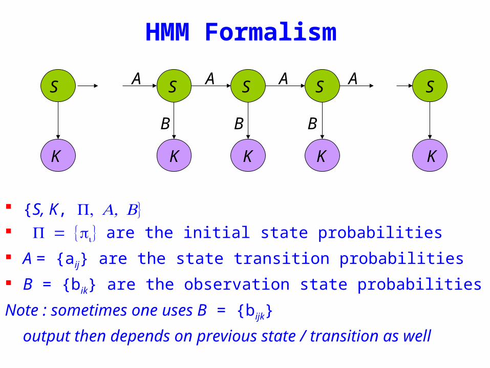
HMM Formalism
S K are the initial state probabilities
A = aij are the state transition probabilities
B = bik are the observation state probabilities
Note sometimes one uses B = bijk
output then depends on previous state transition as well
A
B
AAA
BB
SSS
KKK
S
K
S
K
The crazy soft drink machine
Fig 92
B cola iced tea lemonade
CP 06 01 03
IP 01 07 02
Probability of lemice
Sum over all paths taken through HMM Start in CP
bull 1 x 03 x 07 x 01 +bull 1 x 03 x 03 x 07
oTo1 otot-1 ot+1
HMMs and Bayesian Nets (1)
x1 xt-1 xt xt+1 xT
P(x1xT o1oT )=P(x1)P(o1 |x1) P(xi+1 |xii=1
Tminus1
prod )P(oi+1 |xi+1)
= x1bx1o1
t=1
Tminus1
axtxt+1bxt+1ot+1
oTo1 otot-1 ot+1
x1 xt+1 xTxtxt-1
HMM and Bayesian Nets (2)
Conditionally independent of Given
Because of d-separation
ldquoThe past is independent of the future given the presentrdquo
Inference in an HMM
Compute the probability of a given observation sequence
Given an observation sequence compute the most likely hidden state sequence
Given an observation sequence and set of possible models which model most closely fits the data
O =(o1oT )μ =(AB)ComputeP(O |μ)
oTo1 otot-1 ot+1
Given an observation sequence and a model compute the probability of the observation sequence
Decoding
Decoding
TT oxoxox bbbXOP )|(2211
=μ
oTo1 otot-1 ot+1
x1 xt+1 xTxtxt-1
Decoding
TT oxoxox bbbXOP )|(2211
=μ
TT xxxxxxx aaaXP132211
)|(minus
=μ
oTo1 otot-1 ot+1
x1 xt+1 xTxtxt-1
Decoding
)|()|()|( μμμ XPXOPXOP =
TT oxoxox bbbXOP )|(2211
=μ
TT xxxxxxx aaaXP132211
)|(minus
=μ
oTo1 otot-1 ot+1
x1 xt+1 xTxtxt-1
Decoding
)|()|()|( μμμ XPXOPXOP =
TT oxoxox bbbXOP )|(2211
=μ
TT xxxxxxx aaaXP132211
)|(minus
=μ
sum=X
XPXOPOP )|()|()|( μμμ
oTo1 otot-1 ot+1
x1 xt+1 xTxtxt-1
P(O | μ) = x1bx1o1
x1 xT sum
t=1
Tminus1
axtxt+1bxt+1ot+1
Decoding
oTo1 otot-1 ot+1
x1 xt+1 xTxtxt-1
Complexity O(N T 2T )
Eg N =5T =100gives21005100 asymp1072
Dynamic Programming
α i (t) = P(o1ot xt = i | μ )
Forward Procedure
oTo1 otot-1 ot+1
x1 xt+1 xTxtxt-1
bull Special structure gives us an efficient solution using dynamic programming
bull Intuition Probability of the first t observations is the same for all possible t+1 length state sequences
bull Define
α i (1) = P(o1 x1 = i | μ )
= π i bio1
)|()(
)()|()|(
)()|(
)(
1111
11111
1111
111
jxoPjxooP
jxPjxoPjxooP
jxPjxooP
jxooP
tttt
ttttt
ttt
tt
=======
=====
+++
++++
+++
++
oTo1 otot-1 ot+1
x1 xt+1 xTxtxt-1
Forward Procedure
)1( +tjα
oTo1 otot-1 ot+1
x1 xt+1 xTxtxt-1
Forward Procedure
)1( +tjα
)|()(
)()|()|(
)()|(
)(
1111
11111
1111
111
jxoPjxooP
jxPjxoPjxooP
jxPjxooP
jxooP
tttt
ttttt
ttt
tt
=======
=====
+++
++++
+++
++
oTo1 otot-1 ot+1
x1 xt+1 xTxtxt-1
Forward Procedure
)1( +tjα
)|()(
)()|()|(
)()|(
)(
1111
11111
1111
111
jxoPjxooP
jxPjxoPjxooP
jxPjxooP
jxooP
tttt
ttttt
ttt
tt
=======
=====
+++
++++
+++
++
oTo1 otot-1 ot+1
x1 xt+1 xTxtxt-1
Forward Procedure
)1( +tjα
)|()(
)()|()|(
)()|(
)(
1111
11111
1111
111
jxoPjxooP
jxPjxoPjxooP
jxPjxooP
jxooP
tttt
ttttt
ttt
tt
=======
=====
+++
++++
+++
++
sum
sum
sum
sum
=
+++=
++=
+
++=
+
+=
=====
=====
====
Nijoiji
ttttNi
tt
tttNi
ttt
ttNi
ttt
tbat
jxoPixjxPixooP
jxoPixPixjxooP
jxoPjxixooP
1
1111
1
111
11
111
11
1)(
)|()|()(
)|()()|(
)|()(
α
oTo1 otot-1 ot+1
x1 xt+1 xTxtxt-1
Forward Procedure
sum
sum
sum
sum
=
+++=
++=
+
++=
+
+=
=====
=====
====
Nijoiji
ttttNi
tt
tttNi
ttt
ttNi
ttt
tbat
jxoPixjxPixooP
jxoPixPixjxooP
jxoPjxixooP
1
1111
1
111
11
111
11
1)(
)|()|()(
)|()()|(
)|()(
α
oTo1 otot-1 ot+1
x1 xt+1 xTxtxt-1
Forward Procedure
sum
sum
sum
sum
=
+++=
++=
+
++=
+
+=
=====
=====
====
Nijoiji
ttttNi
tt
tttNi
ttt
ttNi
ttt
tbat
jxoPixjxPixooP
jxoPixPixjxooP
jxoPjxixooP
1
1111
1
111
11
111
11
1)(
)|()|()(
)|()()|(
)|()(
α
oTo1 otot-1 ot+1
x1 xt+1 xTxtxt-1
Forward Procedure
= P(o1ot xt = i xt+1 = j)i=1Nsum P(ot+1 | xt+1 = j)
= P(o1ot xt+1 = j | xt = i)i=1Nsum P(xt = i)P(ot+1 | xt+1 = j)
= P(o1ot xt = i)i=1Nsum P(xt+1 = j | xt = i)P(ot+1 | xt+1 = j)
= α i (t)aijb jot +1i=1Nsum
oTo1 otot-1 ot+1
x1 xt+1 xTxtxt-1
Forward Procedure
Dynamic Programming
α j (t +1) = α i (t)aijb jot +1i=1Nsum
Complexity O(N 2 T )
Eg N = 5T = 100 gives asymp 3000
βi (t) = P(ot+1oT | xt = i)
oTo1 otot-1 ot+1
x1 xt+1 xTxtxt-1
Backward Procedure
βi (T ) = 1
βi (t) = aijbiot +1β j (t +1)
j=1Nsum
Probability of the rest of the states given the first state
oTo1 otot-1 ot+1
x1 xt+1 xTxtxt-1
Decoding Solution
sum=
=N
ii TOP
1
)()|( αμ
sum=
=N
iiiOP
1
)1()|( βπμ
)()()|(1
ttOP i
N
ii βαμ sum
=
=
Forward Procedure
Backward Procedure
Combination
P(O Xt =i |μ) =P(o1otXt =iot+1oT |μ)=P(o1otXt =i |μ)P(ot+1oT |o1otXt =i μ)=P(o1otXt =i |μ)P(ot+1oT |Xt =i μ)=α i (t)βi (t)
)()()|(1
ttOP i
N
ii βαμ sum
=
=
oTo1 otot-1 ot+1
Best State Sequence
Find the state sequence that best explains the observations
Two approaches bull Individually most likely statesbull Most likely sequence (Viterbi)
)|(maxarg OXPX
Best State Sequence (1)
γi (t) = P(Xt = i | O μ )
=P(Xt = iO | μ )
P(O | μ )
=α i (t)β i (t)
j=1
n
sum α j (t)β j (t)
Most likely state at each point in time
Xt = arg maxγ i (t)
oTo1 otot-1 ot+1
Best State Sequence (2)
Find the state sequence that best explains the observations
Viterbi algorithm
)|(maxarg OXPX
oTo1 otot-1 ot+1
Viterbi Algorithm
)(max)( 1111 11
ttttxx
j ojxooxxPtt
== minusminusminus
δ
The state sequence which maximizes the probability of seeing the observations to time t-1 landing in state j and seeing the observation at time t
x1 xt-1 j
oTo1 otot-1 ot+1
Viterbi Algorithm
)(max)( 1111 11
ttttxx
j ojxooxxPtt
== minusminusminus
δ
1)(max)1(
+=+
tjoijiij batt δδ
1)(maxarg)1(
+=+
tjoijii
j batt δψRecursive Computation
x1 xt-1 xt xt+1
Initialization
δ1(i) = ibio1
ψ 1(i) =0
oTo1 otot-1 ot+1
Viterbi Algorithm
XT =argmaxi
δi (T )
Xt =ψX^
t+1
(t+1)
P(X)=argmaxi
δi (T )
Compute the most likely state sequence by working backwards
x1 xt-1 xt xt+1 xT
oTo1 otot-1 ot+1
HMMs and Bayesian Nets (1)
x1 xt-1 xt xt+1 xT
P(x1xT o1oT )=P(x1)P(o1 |x1) P(xi+1 |xii=1
Tminus1
prod )P(oi+1 |xi+1)
= x1bx1o1
t=1
Tminus1
axtxt+1bxt+1ot+1
oTo1 otot-1 ot+1
x1 xt+1 xTxtxt-1
HMM and Bayesian Nets (2)
Conditionally independent of Given
Because of d-separation
ldquoThe past is independent of the future given the presentrdquo
Inference in an HMM
Compute the probability of a given observation sequence
Given an observation sequence compute the most likely hidden state sequence
Given an observation sequence and set of possible models which model most closely fits the data
Dynamic Programming
oTo1 otot-1 ot+1
Parameter Estimation
bull Given an observation sequence find the model that is most likely to produce that sequence
bull No analytic methodbull Given a model and observation sequence update
the model parameters to better fit the observations
A
B
AAA
BBB B
arg maxμ
P(Otraining |μ)
α i (t) = P(o1ot xt = i | μ )
βi (t) = P(ot+1oT | xt = i)
)()()|(1
ttOP i
N
ii βαμ sum
=
=
pt (i j)=P(Xt =iXt+1 = j |O μ)
=P(Xt =iXt+1 = jO |μ)
P(O |μ)
oTo1 otot-1 ot+1
Parameter Estimation
A
B
AAA
BBB B
pt (i j)=α i (t)aijbjot+1
β j (t+1)
αm(t)βm(t)m=1Nsum
Probability of traversing an arc
sum=
=Nj
ti jipt1
)()(γ Probability of being in state i
oTo1 otot-1 ot+1
Parameter Estimation
A
B
AAA
BBB B
i =γi(1)
Now we can compute the new estimates of the model parameters
aij =pt(i j)t=1
Tminus1sumγi (t)t=1
Tminus1sum
bik =γi (t) tot=ksum
γi (t)t=1
Tsum
Instance of Expectation Maximization
We have that
We may get stuck in local maximum (or even saddle point)
Nevertheless Baum-Welch usually effective
P(O | μ) geP(O |μ)
Some Variants
So far ergodic modelsbull All states are connectedbull Not always wanted
Epsilon or null-transitionsbull Not all statestransitions emit output symbols
Parameter tyingbull Assuming that certain parameters are shared bull Reduces the number of parameters that have to be estimated
Logical HMMs (Kersting De Raedt Raiko)bull Working with structured states and observation symbols
Working with log probabilities and addition instead of multiplication of probabilities (typically done)
oTo1 otot-1 ot+1
The Most Important Thing
A
B
AAA
BBB B
We can use the special structure of this model to do a lot of neat math and solve problems that are otherwise not solvable
HMMrsquos from an Agent Perspective
AI a modern approachbull AI is the study of rational agentsbull Third part by Wolfram Burgard on
Reinforcement learning
HMMs can also be used herebull Typically one is interested in P(state)
Example
Possible statesbull snow no snow
Observationsbull skis no skis
Questionsbull Was there snow the day before yesterday (given a
sequence of observations) bull Is there now snow (given a sequence of
observations) bull Will there be snow tomorrow given a sequence of
observations Next week
HMM and Agents
Question
bull Case 1 often called smoothing t lt T see last time
Only part of trellis between t and T needed
γi (t) = P(Xt = i | Oμ )
=α i (t)β i (t)
j =1
n
sum α j (t)β j (t)
Most likely state at each point in time
HMM and Agents
bull Case 2 often called filtering t= T last time
Can we make it recursive Ie go from T-1 to T
γi (t) = P(Xt = i | Oμ )
=α i (t)β i (t)
j =1
n
sum α j (t)β j (t)
Most likely state at each point in time
HMM and Agents
bull Case 2 often called filtering t= T last time
λi (T ) = P(XT = i | o1oT μ )
= γ i (T )
=α i (T )β i (T )
j =1
n
sum α j (T )β j (T )
=α i (T )
j =1
n
sum α j (T )
HMM and Agents
bull Case 3 often called prediction t= T+1 (or T+K) not yet seen
Interesting recursive Easily extended towards k gt 1
Extensions
Use Dynamic Bayesian networks instead of HMMsbullOne state corresponds to a Bayesian NetbullObservations can become more complex
Involve actions of the agent as wellbullCf Wolfram Burgardrsquos Part
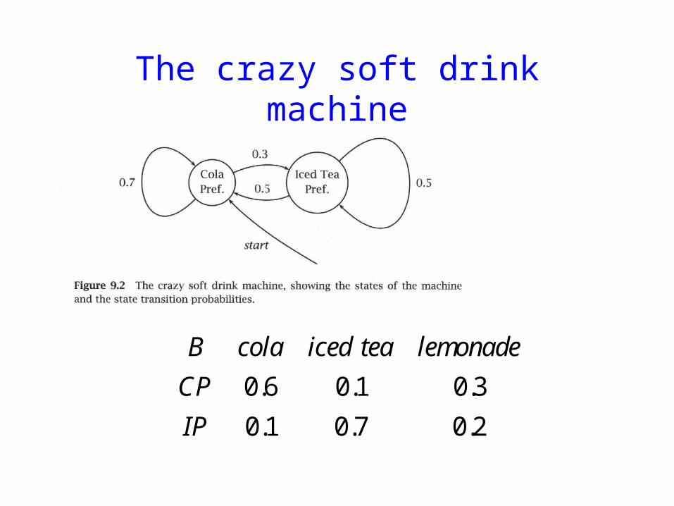
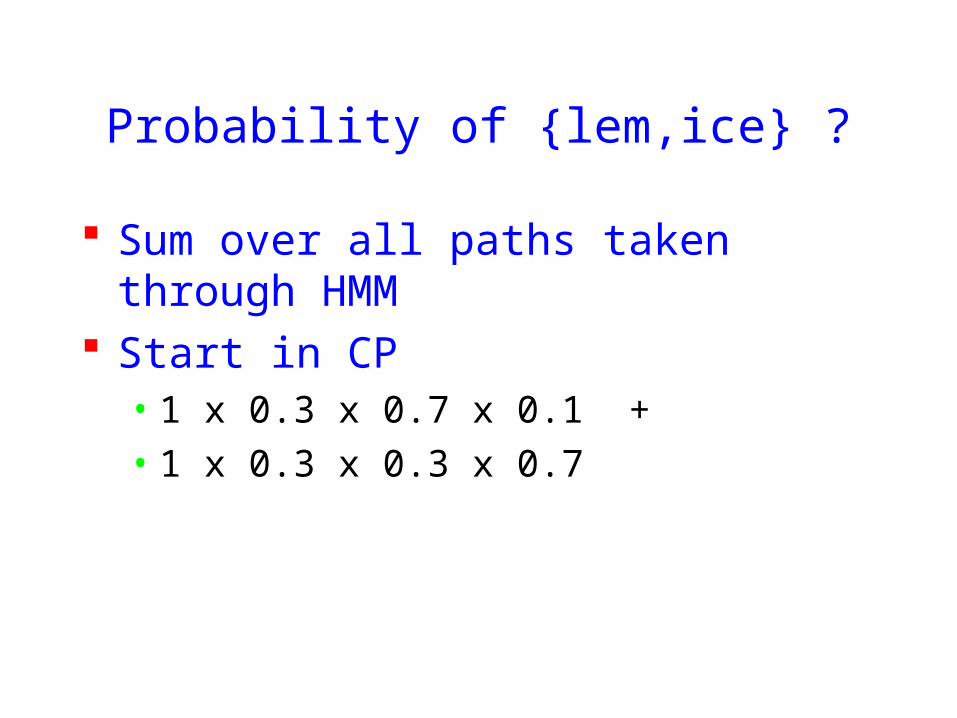
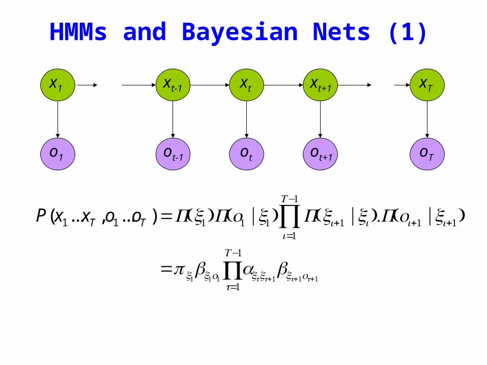
oTo1 otot-1 ot+1
HMMs and Bayesian Nets (1)
x1 xt-1 xt xt+1 xT
P(x1xT o1oT )=P(x1)P(o1 |x1) P(xi+1 |xii=1
Tminus1
prod )P(oi+1 |xi+1)
= x1bx1o1
t=1
Tminus1
axtxt+1bxt+1ot+1
oTo1 otot-1 ot+1
x1 xt+1 xTxtxt-1
HMM and Bayesian Nets (2)
Conditionally independent of Given
Because of d-separation
ldquoThe past is independent of the future given the presentrdquo
Inference in an HMM
Compute the probability of a given observation sequence
Given an observation sequence compute the most likely hidden state sequence
Given an observation sequence and set of possible models which model most closely fits the data
O =(o1oT )μ =(AB)ComputeP(O |μ)
oTo1 otot-1 ot+1
Given an observation sequence and a model compute the probability of the observation sequence
Decoding
Decoding
TT oxoxox bbbXOP )|(2211
=μ
oTo1 otot-1 ot+1
x1 xt+1 xTxtxt-1
Decoding
TT oxoxox bbbXOP )|(2211
=μ
TT xxxxxxx aaaXP132211
)|(minus
=μ
oTo1 otot-1 ot+1
x1 xt+1 xTxtxt-1
Decoding
)|()|()|( μμμ XPXOPXOP =
TT oxoxox bbbXOP )|(2211
=μ
TT xxxxxxx aaaXP132211
)|(minus
=μ
oTo1 otot-1 ot+1
x1 xt+1 xTxtxt-1
Decoding
)|()|()|( μμμ XPXOPXOP =
TT oxoxox bbbXOP )|(2211
=μ
TT xxxxxxx aaaXP132211
)|(minus
=μ
sum=X
XPXOPOP )|()|()|( μμμ
oTo1 otot-1 ot+1
x1 xt+1 xTxtxt-1
P(O | μ) = x1bx1o1
x1 xT sum
t=1
Tminus1
axtxt+1bxt+1ot+1
Decoding
oTo1 otot-1 ot+1
x1 xt+1 xTxtxt-1
Complexity O(N T 2T )
Eg N =5T =100gives21005100 asymp1072
Dynamic Programming
α i (t) = P(o1ot xt = i | μ )
Forward Procedure
oTo1 otot-1 ot+1
x1 xt+1 xTxtxt-1
bull Special structure gives us an efficient solution using dynamic programming
bull Intuition Probability of the first t observations is the same for all possible t+1 length state sequences
bull Define
α i (1) = P(o1 x1 = i | μ )
= π i bio1
)|()(
)()|()|(
)()|(
)(
1111
11111
1111
111
jxoPjxooP
jxPjxoPjxooP
jxPjxooP
jxooP
tttt
ttttt
ttt
tt
=======
=====
+++
++++
+++
++
oTo1 otot-1 ot+1
x1 xt+1 xTxtxt-1
Forward Procedure
)1( +tjα
oTo1 otot-1 ot+1
x1 xt+1 xTxtxt-1
Forward Procedure
)1( +tjα
)|()(
)()|()|(
)()|(
)(
1111
11111
1111
111
jxoPjxooP
jxPjxoPjxooP
jxPjxooP
jxooP
tttt
ttttt
ttt
tt
=======
=====
+++
++++
+++
++
oTo1 otot-1 ot+1
x1 xt+1 xTxtxt-1
Forward Procedure
)1( +tjα
)|()(
)()|()|(
)()|(
)(
1111
11111
1111
111
jxoPjxooP
jxPjxoPjxooP
jxPjxooP
jxooP
tttt
ttttt
ttt
tt
=======
=====
+++
++++
+++
++
oTo1 otot-1 ot+1
x1 xt+1 xTxtxt-1
Forward Procedure
)1( +tjα
)|()(
)()|()|(
)()|(
)(
1111
11111
1111
111
jxoPjxooP
jxPjxoPjxooP
jxPjxooP
jxooP
tttt
ttttt
ttt
tt
=======
=====
+++
++++
+++
++
sum
sum
sum
sum
=
+++=
++=
+
++=
+
+=
=====
=====
====
Nijoiji
ttttNi
tt
tttNi
ttt
ttNi
ttt
tbat
jxoPixjxPixooP
jxoPixPixjxooP
jxoPjxixooP
1
1111
1
111
11
111
11
1)(
)|()|()(
)|()()|(
)|()(
α
oTo1 otot-1 ot+1
x1 xt+1 xTxtxt-1
Forward Procedure
sum
sum
sum
sum
=
+++=
++=
+
++=
+
+=
=====
=====
====
Nijoiji
ttttNi
tt
tttNi
ttt
ttNi
ttt
tbat
jxoPixjxPixooP
jxoPixPixjxooP
jxoPjxixooP
1
1111
1
111
11
111
11
1)(
)|()|()(
)|()()|(
)|()(
α
oTo1 otot-1 ot+1
x1 xt+1 xTxtxt-1
Forward Procedure
sum
sum
sum
sum
=
+++=
++=
+
++=
+
+=
=====
=====
====
Nijoiji
ttttNi
tt
tttNi
ttt
ttNi
ttt
tbat
jxoPixjxPixooP
jxoPixPixjxooP
jxoPjxixooP
1
1111
1
111
11
111
11
1)(
)|()|()(
)|()()|(
)|()(
α
oTo1 otot-1 ot+1
x1 xt+1 xTxtxt-1
Forward Procedure
= P(o1ot xt = i xt+1 = j)i=1Nsum P(ot+1 | xt+1 = j)
= P(o1ot xt+1 = j | xt = i)i=1Nsum P(xt = i)P(ot+1 | xt+1 = j)
= P(o1ot xt = i)i=1Nsum P(xt+1 = j | xt = i)P(ot+1 | xt+1 = j)
= α i (t)aijb jot +1i=1Nsum
oTo1 otot-1 ot+1
x1 xt+1 xTxtxt-1
Forward Procedure
Dynamic Programming
α j (t +1) = α i (t)aijb jot +1i=1Nsum
Complexity O(N 2 T )
Eg N = 5T = 100 gives asymp 3000
βi (t) = P(ot+1oT | xt = i)
oTo1 otot-1 ot+1
x1 xt+1 xTxtxt-1
Backward Procedure
βi (T ) = 1
βi (t) = aijbiot +1β j (t +1)
j=1Nsum
Probability of the rest of the states given the first state
oTo1 otot-1 ot+1
x1 xt+1 xTxtxt-1
Decoding Solution
sum=
=N
ii TOP
1
)()|( αμ
sum=
=N
iiiOP
1
)1()|( βπμ
)()()|(1
ttOP i
N
ii βαμ sum
=
=
Forward Procedure
Backward Procedure
Combination
P(O Xt =i |μ) =P(o1otXt =iot+1oT |μ)=P(o1otXt =i |μ)P(ot+1oT |o1otXt =i μ)=P(o1otXt =i |μ)P(ot+1oT |Xt =i μ)=α i (t)βi (t)
)()()|(1
ttOP i
N
ii βαμ sum
=
=
oTo1 otot-1 ot+1
Best State Sequence
Find the state sequence that best explains the observations
Two approaches bull Individually most likely statesbull Most likely sequence (Viterbi)
)|(maxarg OXPX
Best State Sequence (1)
γi (t) = P(Xt = i | O μ )
=P(Xt = iO | μ )
P(O | μ )
=α i (t)β i (t)
j=1
n
sum α j (t)β j (t)
Most likely state at each point in time
Xt = arg maxγ i (t)
oTo1 otot-1 ot+1
Best State Sequence (2)
Find the state sequence that best explains the observations
Viterbi algorithm
)|(maxarg OXPX
oTo1 otot-1 ot+1
Viterbi Algorithm
)(max)( 1111 11
ttttxx
j ojxooxxPtt
== minusminusminus
δ
The state sequence which maximizes the probability of seeing the observations to time t-1 landing in state j and seeing the observation at time t
x1 xt-1 j
oTo1 otot-1 ot+1
Viterbi Algorithm
)(max)( 1111 11
ttttxx
j ojxooxxPtt
== minusminusminus
δ
1)(max)1(
+=+
tjoijiij batt δδ
1)(maxarg)1(
+=+
tjoijii
j batt δψRecursive Computation
x1 xt-1 xt xt+1
Initialization
δ1(i) = ibio1
ψ 1(i) =0
oTo1 otot-1 ot+1
Viterbi Algorithm
XT =argmaxi
δi (T )
Xt =ψX^
t+1
(t+1)
P(X)=argmaxi
δi (T )
Compute the most likely state sequence by working backwards
x1 xt-1 xt xt+1 xT
oTo1 otot-1 ot+1
HMMs and Bayesian Nets (1)
x1 xt-1 xt xt+1 xT
P(x1xT o1oT )=P(x1)P(o1 |x1) P(xi+1 |xii=1
Tminus1
prod )P(oi+1 |xi+1)
= x1bx1o1
t=1
Tminus1
axtxt+1bxt+1ot+1
oTo1 otot-1 ot+1
x1 xt+1 xTxtxt-1
HMM and Bayesian Nets (2)
Conditionally independent of Given
Because of d-separation
ldquoThe past is independent of the future given the presentrdquo
Inference in an HMM
Compute the probability of a given observation sequence
Given an observation sequence compute the most likely hidden state sequence
Given an observation sequence and set of possible models which model most closely fits the data
Dynamic Programming
oTo1 otot-1 ot+1
Parameter Estimation
bull Given an observation sequence find the model that is most likely to produce that sequence
bull No analytic methodbull Given a model and observation sequence update
the model parameters to better fit the observations
A
B
AAA
BBB B
arg maxμ
P(Otraining |μ)
α i (t) = P(o1ot xt = i | μ )
βi (t) = P(ot+1oT | xt = i)
)()()|(1
ttOP i
N
ii βαμ sum
=
=
pt (i j)=P(Xt =iXt+1 = j |O μ)
=P(Xt =iXt+1 = jO |μ)
P(O |μ)
oTo1 otot-1 ot+1
Parameter Estimation
A
B
AAA
BBB B
pt (i j)=α i (t)aijbjot+1
β j (t+1)
αm(t)βm(t)m=1Nsum
Probability of traversing an arc
sum=
=Nj
ti jipt1
)()(γ Probability of being in state i
oTo1 otot-1 ot+1
Parameter Estimation
A
B
AAA
BBB B
i =γi(1)
Now we can compute the new estimates of the model parameters
aij =pt(i j)t=1
Tminus1sumγi (t)t=1
Tminus1sum
bik =γi (t) tot=ksum
γi (t)t=1
Tsum
Instance of Expectation Maximization
We have that
We may get stuck in local maximum (or even saddle point)
Nevertheless Baum-Welch usually effective
P(O | μ) geP(O |μ)
Some Variants
So far ergodic modelsbull All states are connectedbull Not always wanted
Epsilon or null-transitionsbull Not all statestransitions emit output symbols
Parameter tyingbull Assuming that certain parameters are shared bull Reduces the number of parameters that have to be estimated
Logical HMMs (Kersting De Raedt Raiko)bull Working with structured states and observation symbols
Working with log probabilities and addition instead of multiplication of probabilities (typically done)
oTo1 otot-1 ot+1
The Most Important Thing
A
B
AAA
BBB B
We can use the special structure of this model to do a lot of neat math and solve problems that are otherwise not solvable
HMMrsquos from an Agent Perspective
AI a modern approachbull AI is the study of rational agentsbull Third part by Wolfram Burgard on
Reinforcement learning
HMMs can also be used herebull Typically one is interested in P(state)
Example
Possible statesbull snow no snow
Observationsbull skis no skis
Questionsbull Was there snow the day before yesterday (given a
sequence of observations) bull Is there now snow (given a sequence of
observations) bull Will there be snow tomorrow given a sequence of
observations Next week
HMM and Agents
Question
bull Case 1 often called smoothing t lt T see last time
Only part of trellis between t and T needed
γi (t) = P(Xt = i | Oμ )
=α i (t)β i (t)
j =1
n
sum α j (t)β j (t)
Most likely state at each point in time
HMM and Agents
bull Case 2 often called filtering t= T last time
Can we make it recursive Ie go from T-1 to T
γi (t) = P(Xt = i | Oμ )
=α i (t)β i (t)
j =1
n
sum α j (t)β j (t)
Most likely state at each point in time
HMM and Agents
bull Case 2 often called filtering t= T last time
λi (T ) = P(XT = i | o1oT μ )
= γ i (T )
=α i (T )β i (T )
j =1
n
sum α j (T )β j (T )
=α i (T )
j =1
n
sum α j (T )
HMM and Agents
bull Case 3 often called prediction t= T+1 (or T+K) not yet seen
Interesting recursive Easily extended towards k gt 1
Extensions
Use Dynamic Bayesian networks instead of HMMsbullOne state corresponds to a Bayesian NetbullObservations can become more complex
Involve actions of the agent as wellbullCf Wolfram Burgardrsquos Part

oTo1 otot-1 ot+1
x1 xt+1 xTxtxt-1
HMM and Bayesian Nets (2)
Conditionally independent of Given
Because of d-separation
ldquoThe past is independent of the future given the presentrdquo
Inference in an HMM
Compute the probability of a given observation sequence
Given an observation sequence compute the most likely hidden state sequence
Given an observation sequence and set of possible models which model most closely fits the data
O =(o1oT )μ =(AB)ComputeP(O |μ)
oTo1 otot-1 ot+1
Given an observation sequence and a model compute the probability of the observation sequence
Decoding
Decoding
TT oxoxox bbbXOP )|(2211
=μ
oTo1 otot-1 ot+1
x1 xt+1 xTxtxt-1
Decoding
TT oxoxox bbbXOP )|(2211
=μ
TT xxxxxxx aaaXP132211
)|(minus
=μ
oTo1 otot-1 ot+1
x1 xt+1 xTxtxt-1
Decoding
)|()|()|( μμμ XPXOPXOP =
TT oxoxox bbbXOP )|(2211
=μ
TT xxxxxxx aaaXP132211
)|(minus
=μ
oTo1 otot-1 ot+1
x1 xt+1 xTxtxt-1
Decoding
)|()|()|( μμμ XPXOPXOP =
TT oxoxox bbbXOP )|(2211
=μ
TT xxxxxxx aaaXP132211
)|(minus
=μ
sum=X
XPXOPOP )|()|()|( μμμ
oTo1 otot-1 ot+1
x1 xt+1 xTxtxt-1
P(O | μ) = x1bx1o1
x1 xT sum
t=1
Tminus1
axtxt+1bxt+1ot+1
Decoding
oTo1 otot-1 ot+1
x1 xt+1 xTxtxt-1
Complexity O(N T 2T )
Eg N =5T =100gives21005100 asymp1072
Dynamic Programming
α i (t) = P(o1ot xt = i | μ )
Forward Procedure
oTo1 otot-1 ot+1
x1 xt+1 xTxtxt-1
bull Special structure gives us an efficient solution using dynamic programming
bull Intuition Probability of the first t observations is the same for all possible t+1 length state sequences
bull Define
α i (1) = P(o1 x1 = i | μ )
= π i bio1
)|()(
)()|()|(
)()|(
)(
1111
11111
1111
111
jxoPjxooP
jxPjxoPjxooP
jxPjxooP
jxooP
tttt
ttttt
ttt
tt
=======
=====
+++
++++
+++
++
oTo1 otot-1 ot+1
x1 xt+1 xTxtxt-1
Forward Procedure
)1( +tjα
oTo1 otot-1 ot+1
x1 xt+1 xTxtxt-1
Forward Procedure
)1( +tjα
)|()(
)()|()|(
)()|(
)(
1111
11111
1111
111
jxoPjxooP
jxPjxoPjxooP
jxPjxooP
jxooP
tttt
ttttt
ttt
tt
=======
=====
+++
++++
+++
++
oTo1 otot-1 ot+1
x1 xt+1 xTxtxt-1
Forward Procedure
)1( +tjα
)|()(
)()|()|(
)()|(
)(
1111
11111
1111
111
jxoPjxooP
jxPjxoPjxooP
jxPjxooP
jxooP
tttt
ttttt
ttt
tt
=======
=====
+++
++++
+++
++
oTo1 otot-1 ot+1
x1 xt+1 xTxtxt-1
Forward Procedure
)1( +tjα
)|()(
)()|()|(
)()|(
)(
1111
11111
1111
111
jxoPjxooP
jxPjxoPjxooP
jxPjxooP
jxooP
tttt
ttttt
ttt
tt
=======
=====
+++
++++
+++
++
sum
sum
sum
sum
=
+++=
++=
+
++=
+
+=
=====
=====
====
Nijoiji
ttttNi
tt
tttNi
ttt
ttNi
ttt
tbat
jxoPixjxPixooP
jxoPixPixjxooP
jxoPjxixooP
1
1111
1
111
11
111
11
1)(
)|()|()(
)|()()|(
)|()(
α
oTo1 otot-1 ot+1
x1 xt+1 xTxtxt-1
Forward Procedure
sum
sum
sum
sum
=
+++=
++=
+
++=
+
+=
=====
=====
====
Nijoiji
ttttNi
tt
tttNi
ttt
ttNi
ttt
tbat
jxoPixjxPixooP
jxoPixPixjxooP
jxoPjxixooP
1
1111
1
111
11
111
11
1)(
)|()|()(
)|()()|(
)|()(
α
oTo1 otot-1 ot+1
x1 xt+1 xTxtxt-1
Forward Procedure
sum
sum
sum
sum
=
+++=
++=
+
++=
+
+=
=====
=====
====
Nijoiji
ttttNi
tt
tttNi
ttt
ttNi
ttt
tbat
jxoPixjxPixooP
jxoPixPixjxooP
jxoPjxixooP
1
1111
1
111
11
111
11
1)(
)|()|()(
)|()()|(
)|()(
α
oTo1 otot-1 ot+1
x1 xt+1 xTxtxt-1
Forward Procedure
= P(o1ot xt = i xt+1 = j)i=1Nsum P(ot+1 | xt+1 = j)
= P(o1ot xt+1 = j | xt = i)i=1Nsum P(xt = i)P(ot+1 | xt+1 = j)
= P(o1ot xt = i)i=1Nsum P(xt+1 = j | xt = i)P(ot+1 | xt+1 = j)
= α i (t)aijb jot +1i=1Nsum
oTo1 otot-1 ot+1
x1 xt+1 xTxtxt-1
Forward Procedure
Dynamic Programming
α j (t +1) = α i (t)aijb jot +1i=1Nsum
Complexity O(N 2 T )
Eg N = 5T = 100 gives asymp 3000
βi (t) = P(ot+1oT | xt = i)
oTo1 otot-1 ot+1
x1 xt+1 xTxtxt-1
Backward Procedure
βi (T ) = 1
βi (t) = aijbiot +1β j (t +1)
j=1Nsum
Probability of the rest of the states given the first state
oTo1 otot-1 ot+1
x1 xt+1 xTxtxt-1
Decoding Solution
sum=
=N
ii TOP
1
)()|( αμ
sum=
=N
iiiOP
1
)1()|( βπμ
)()()|(1
ttOP i
N
ii βαμ sum
=
=
Forward Procedure
Backward Procedure
Combination
P(O Xt =i |μ) =P(o1otXt =iot+1oT |μ)=P(o1otXt =i |μ)P(ot+1oT |o1otXt =i μ)=P(o1otXt =i |μ)P(ot+1oT |Xt =i μ)=α i (t)βi (t)
)()()|(1
ttOP i
N
ii βαμ sum
=
=
oTo1 otot-1 ot+1
Best State Sequence
Find the state sequence that best explains the observations
Two approaches bull Individually most likely statesbull Most likely sequence (Viterbi)
)|(maxarg OXPX
Best State Sequence (1)
γi (t) = P(Xt = i | O μ )
=P(Xt = iO | μ )
P(O | μ )
=α i (t)β i (t)
j=1
n
sum α j (t)β j (t)
Most likely state at each point in time
Xt = arg maxγ i (t)
oTo1 otot-1 ot+1
Best State Sequence (2)
Find the state sequence that best explains the observations
Viterbi algorithm
)|(maxarg OXPX
oTo1 otot-1 ot+1
Viterbi Algorithm
)(max)( 1111 11
ttttxx
j ojxooxxPtt
== minusminusminus
δ
The state sequence which maximizes the probability of seeing the observations to time t-1 landing in state j and seeing the observation at time t
x1 xt-1 j
oTo1 otot-1 ot+1
Viterbi Algorithm
)(max)( 1111 11
ttttxx
j ojxooxxPtt
== minusminusminus
δ
1)(max)1(
+=+
tjoijiij batt δδ
1)(maxarg)1(
+=+
tjoijii
j batt δψRecursive Computation
x1 xt-1 xt xt+1
Initialization
δ1(i) = ibio1
ψ 1(i) =0
oTo1 otot-1 ot+1
Viterbi Algorithm
XT =argmaxi
δi (T )
Xt =ψX^
t+1
(t+1)
P(X)=argmaxi
δi (T )
Compute the most likely state sequence by working backwards
x1 xt-1 xt xt+1 xT
oTo1 otot-1 ot+1
HMMs and Bayesian Nets (1)
x1 xt-1 xt xt+1 xT
P(x1xT o1oT )=P(x1)P(o1 |x1) P(xi+1 |xii=1
Tminus1
prod )P(oi+1 |xi+1)
= x1bx1o1
t=1
Tminus1
axtxt+1bxt+1ot+1
oTo1 otot-1 ot+1
x1 xt+1 xTxtxt-1
HMM and Bayesian Nets (2)
Conditionally independent of Given
Because of d-separation
ldquoThe past is independent of the future given the presentrdquo
Inference in an HMM
Compute the probability of a given observation sequence
Given an observation sequence compute the most likely hidden state sequence
Given an observation sequence and set of possible models which model most closely fits the data
Dynamic Programming
oTo1 otot-1 ot+1
Parameter Estimation
bull Given an observation sequence find the model that is most likely to produce that sequence
bull No analytic methodbull Given a model and observation sequence update
the model parameters to better fit the observations
A
B
AAA
BBB B
arg maxμ
P(Otraining |μ)
α i (t) = P(o1ot xt = i | μ )
βi (t) = P(ot+1oT | xt = i)
)()()|(1
ttOP i
N
ii βαμ sum
=
=
pt (i j)=P(Xt =iXt+1 = j |O μ)
=P(Xt =iXt+1 = jO |μ)
P(O |μ)
oTo1 otot-1 ot+1
Parameter Estimation
A
B
AAA
BBB B
pt (i j)=α i (t)aijbjot+1
β j (t+1)
αm(t)βm(t)m=1Nsum
Probability of traversing an arc
sum=
=Nj
ti jipt1
)()(γ Probability of being in state i
oTo1 otot-1 ot+1
Parameter Estimation
A
B
AAA
BBB B
i =γi(1)
Now we can compute the new estimates of the model parameters
aij =pt(i j)t=1
Tminus1sumγi (t)t=1
Tminus1sum
bik =γi (t) tot=ksum
γi (t)t=1
Tsum
Instance of Expectation Maximization
We have that
We may get stuck in local maximum (or even saddle point)
Nevertheless Baum-Welch usually effective
P(O | μ) geP(O |μ)
Some Variants
So far ergodic modelsbull All states are connectedbull Not always wanted
Epsilon or null-transitionsbull Not all statestransitions emit output symbols
Parameter tyingbull Assuming that certain parameters are shared bull Reduces the number of parameters that have to be estimated
Logical HMMs (Kersting De Raedt Raiko)bull Working with structured states and observation symbols
Working with log probabilities and addition instead of multiplication of probabilities (typically done)
oTo1 otot-1 ot+1
The Most Important Thing
A
B
AAA
BBB B
We can use the special structure of this model to do a lot of neat math and solve problems that are otherwise not solvable
HMMrsquos from an Agent Perspective
AI a modern approachbull AI is the study of rational agentsbull Third part by Wolfram Burgard on
Reinforcement learning
HMMs can also be used herebull Typically one is interested in P(state)
Example
Possible statesbull snow no snow
Observationsbull skis no skis
Questionsbull Was there snow the day before yesterday (given a
sequence of observations) bull Is there now snow (given a sequence of
observations) bull Will there be snow tomorrow given a sequence of
observations Next week
HMM and Agents
Question
bull Case 1 often called smoothing t lt T see last time
Only part of trellis between t and T needed
γi (t) = P(Xt = i | Oμ )
=α i (t)β i (t)
j =1
n
sum α j (t)β j (t)
Most likely state at each point in time
HMM and Agents
bull Case 2 often called filtering t= T last time
Can we make it recursive Ie go from T-1 to T
γi (t) = P(Xt = i | Oμ )
=α i (t)β i (t)
j =1
n
sum α j (t)β j (t)
Most likely state at each point in time
HMM and Agents
bull Case 2 often called filtering t= T last time
λi (T ) = P(XT = i | o1oT μ )
= γ i (T )
=α i (T )β i (T )
j =1
n
sum α j (T )β j (T )
=α i (T )
j =1
n
sum α j (T )
HMM and Agents
bull Case 3 often called prediction t= T+1 (or T+K) not yet seen
Interesting recursive Easily extended towards k gt 1
Extensions
Use Dynamic Bayesian networks instead of HMMsbullOne state corresponds to a Bayesian NetbullObservations can become more complex
Involve actions of the agent as wellbullCf Wolfram Burgardrsquos Part
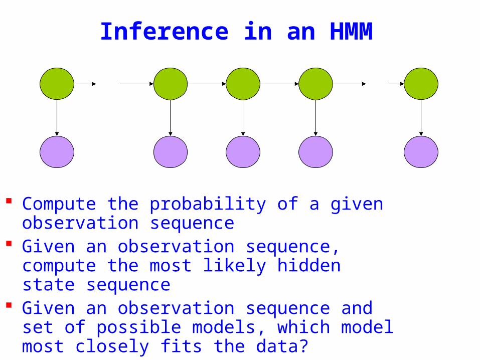
Inference in an HMM
Compute the probability of a given observation sequence
Given an observation sequence compute the most likely hidden state sequence
Given an observation sequence and set of possible models which model most closely fits the data
O =(o1oT )μ =(AB)ComputeP(O |μ)
oTo1 otot-1 ot+1
Given an observation sequence and a model compute the probability of the observation sequence
Decoding
Decoding
TT oxoxox bbbXOP )|(2211
=μ
oTo1 otot-1 ot+1
x1 xt+1 xTxtxt-1
Decoding
TT oxoxox bbbXOP )|(2211
=μ
TT xxxxxxx aaaXP132211
)|(minus
=μ
oTo1 otot-1 ot+1
x1 xt+1 xTxtxt-1
Decoding
)|()|()|( μμμ XPXOPXOP =
TT oxoxox bbbXOP )|(2211
=μ
TT xxxxxxx aaaXP132211
)|(minus
=μ
oTo1 otot-1 ot+1
x1 xt+1 xTxtxt-1
Decoding
)|()|()|( μμμ XPXOPXOP =
TT oxoxox bbbXOP )|(2211
=μ
TT xxxxxxx aaaXP132211
)|(minus
=μ
sum=X
XPXOPOP )|()|()|( μμμ
oTo1 otot-1 ot+1
x1 xt+1 xTxtxt-1
P(O | μ) = x1bx1o1
x1 xT sum
t=1
Tminus1
axtxt+1bxt+1ot+1
Decoding
oTo1 otot-1 ot+1
x1 xt+1 xTxtxt-1
Complexity O(N T 2T )
Eg N =5T =100gives21005100 asymp1072
Dynamic Programming
α i (t) = P(o1ot xt = i | μ )
Forward Procedure
oTo1 otot-1 ot+1
x1 xt+1 xTxtxt-1
bull Special structure gives us an efficient solution using dynamic programming
bull Intuition Probability of the first t observations is the same for all possible t+1 length state sequences
bull Define
α i (1) = P(o1 x1 = i | μ )
= π i bio1
)|()(
)()|()|(
)()|(
)(
1111
11111
1111
111
jxoPjxooP
jxPjxoPjxooP
jxPjxooP
jxooP
tttt
ttttt
ttt
tt
=======
=====
+++
++++
+++
++
oTo1 otot-1 ot+1
x1 xt+1 xTxtxt-1
Forward Procedure
)1( +tjα
oTo1 otot-1 ot+1
x1 xt+1 xTxtxt-1
Forward Procedure
)1( +tjα
)|()(
)()|()|(
)()|(
)(
1111
11111
1111
111
jxoPjxooP
jxPjxoPjxooP
jxPjxooP
jxooP
tttt
ttttt
ttt
tt
=======
=====
+++
++++
+++
++
oTo1 otot-1 ot+1
x1 xt+1 xTxtxt-1
Forward Procedure
)1( +tjα
)|()(
)()|()|(
)()|(
)(
1111
11111
1111
111
jxoPjxooP
jxPjxoPjxooP
jxPjxooP
jxooP
tttt
ttttt
ttt
tt
=======
=====
+++
++++
+++
++
oTo1 otot-1 ot+1
x1 xt+1 xTxtxt-1
Forward Procedure
)1( +tjα
)|()(
)()|()|(
)()|(
)(
1111
11111
1111
111
jxoPjxooP
jxPjxoPjxooP
jxPjxooP
jxooP
tttt
ttttt
ttt
tt
=======
=====
+++
++++
+++
++
sum
sum
sum
sum
=
+++=
++=
+
++=
+
+=
=====
=====
====
Nijoiji
ttttNi
tt
tttNi
ttt
ttNi
ttt
tbat
jxoPixjxPixooP
jxoPixPixjxooP
jxoPjxixooP
1
1111
1
111
11
111
11
1)(
)|()|()(
)|()()|(
)|()(
α
oTo1 otot-1 ot+1
x1 xt+1 xTxtxt-1
Forward Procedure
sum
sum
sum
sum
=
+++=
++=
+
++=
+
+=
=====
=====
====
Nijoiji
ttttNi
tt
tttNi
ttt
ttNi
ttt
tbat
jxoPixjxPixooP
jxoPixPixjxooP
jxoPjxixooP
1
1111
1
111
11
111
11
1)(
)|()|()(
)|()()|(
)|()(
α
oTo1 otot-1 ot+1
x1 xt+1 xTxtxt-1
Forward Procedure
sum
sum
sum
sum
=
+++=
++=
+
++=
+
+=
=====
=====
====
Nijoiji
ttttNi
tt
tttNi
ttt
ttNi
ttt
tbat
jxoPixjxPixooP
jxoPixPixjxooP
jxoPjxixooP
1
1111
1
111
11
111
11
1)(
)|()|()(
)|()()|(
)|()(
α
oTo1 otot-1 ot+1
x1 xt+1 xTxtxt-1
Forward Procedure
= P(o1ot xt = i xt+1 = j)i=1Nsum P(ot+1 | xt+1 = j)
= P(o1ot xt+1 = j | xt = i)i=1Nsum P(xt = i)P(ot+1 | xt+1 = j)
= P(o1ot xt = i)i=1Nsum P(xt+1 = j | xt = i)P(ot+1 | xt+1 = j)
= α i (t)aijb jot +1i=1Nsum
oTo1 otot-1 ot+1
x1 xt+1 xTxtxt-1
Forward Procedure
Dynamic Programming
α j (t +1) = α i (t)aijb jot +1i=1Nsum
Complexity O(N 2 T )
Eg N = 5T = 100 gives asymp 3000
βi (t) = P(ot+1oT | xt = i)
oTo1 otot-1 ot+1
x1 xt+1 xTxtxt-1
Backward Procedure
βi (T ) = 1
βi (t) = aijbiot +1β j (t +1)
j=1Nsum
Probability of the rest of the states given the first state
oTo1 otot-1 ot+1
x1 xt+1 xTxtxt-1
Decoding Solution
sum=
=N
ii TOP
1
)()|( αμ
sum=
=N
iiiOP
1
)1()|( βπμ
)()()|(1
ttOP i
N
ii βαμ sum
=
=
Forward Procedure
Backward Procedure
Combination
P(O Xt =i |μ) =P(o1otXt =iot+1oT |μ)=P(o1otXt =i |μ)P(ot+1oT |o1otXt =i μ)=P(o1otXt =i |μ)P(ot+1oT |Xt =i μ)=α i (t)βi (t)
)()()|(1
ttOP i
N
ii βαμ sum
=
=
oTo1 otot-1 ot+1
Best State Sequence
Find the state sequence that best explains the observations
Two approaches bull Individually most likely statesbull Most likely sequence (Viterbi)
)|(maxarg OXPX
Best State Sequence (1)
γi (t) = P(Xt = i | O μ )
=P(Xt = iO | μ )
P(O | μ )
=α i (t)β i (t)
j=1
n
sum α j (t)β j (t)
Most likely state at each point in time
Xt = arg maxγ i (t)
oTo1 otot-1 ot+1
Best State Sequence (2)
Find the state sequence that best explains the observations
Viterbi algorithm
)|(maxarg OXPX
oTo1 otot-1 ot+1
Viterbi Algorithm
)(max)( 1111 11
ttttxx
j ojxooxxPtt
== minusminusminus
δ
The state sequence which maximizes the probability of seeing the observations to time t-1 landing in state j and seeing the observation at time t
x1 xt-1 j
oTo1 otot-1 ot+1
Viterbi Algorithm
)(max)( 1111 11
ttttxx
j ojxooxxPtt
== minusminusminus
δ
1)(max)1(
+=+
tjoijiij batt δδ
1)(maxarg)1(
+=+
tjoijii
j batt δψRecursive Computation
x1 xt-1 xt xt+1
Initialization
δ1(i) = ibio1
ψ 1(i) =0
oTo1 otot-1 ot+1
Viterbi Algorithm
XT =argmaxi
δi (T )
Xt =ψX^
t+1
(t+1)
P(X)=argmaxi
δi (T )
Compute the most likely state sequence by working backwards
x1 xt-1 xt xt+1 xT
oTo1 otot-1 ot+1
HMMs and Bayesian Nets (1)
x1 xt-1 xt xt+1 xT
P(x1xT o1oT )=P(x1)P(o1 |x1) P(xi+1 |xii=1
Tminus1
prod )P(oi+1 |xi+1)
= x1bx1o1
t=1
Tminus1
axtxt+1bxt+1ot+1
oTo1 otot-1 ot+1
x1 xt+1 xTxtxt-1
HMM and Bayesian Nets (2)
Conditionally independent of Given
Because of d-separation
ldquoThe past is independent of the future given the presentrdquo
Inference in an HMM
Compute the probability of a given observation sequence
Given an observation sequence compute the most likely hidden state sequence
Given an observation sequence and set of possible models which model most closely fits the data
Dynamic Programming
oTo1 otot-1 ot+1
Parameter Estimation
bull Given an observation sequence find the model that is most likely to produce that sequence
bull No analytic methodbull Given a model and observation sequence update
the model parameters to better fit the observations
A
B
AAA
BBB B
arg maxμ
P(Otraining |μ)
α i (t) = P(o1ot xt = i | μ )
βi (t) = P(ot+1oT | xt = i)
)()()|(1
ttOP i
N
ii βαμ sum
=
=
pt (i j)=P(Xt =iXt+1 = j |O μ)
=P(Xt =iXt+1 = jO |μ)
P(O |μ)
oTo1 otot-1 ot+1
Parameter Estimation
A
B
AAA
BBB B
pt (i j)=α i (t)aijbjot+1
β j (t+1)
αm(t)βm(t)m=1Nsum
Probability of traversing an arc
sum=
=Nj
ti jipt1
)()(γ Probability of being in state i
oTo1 otot-1 ot+1
Parameter Estimation
A
B
AAA
BBB B
i =γi(1)
Now we can compute the new estimates of the model parameters
aij =pt(i j)t=1
Tminus1sumγi (t)t=1
Tminus1sum
bik =γi (t) tot=ksum
γi (t)t=1
Tsum
Instance of Expectation Maximization
We have that
We may get stuck in local maximum (or even saddle point)
Nevertheless Baum-Welch usually effective
P(O | μ) geP(O |μ)
Some Variants
So far ergodic modelsbull All states are connectedbull Not always wanted
Epsilon or null-transitionsbull Not all statestransitions emit output symbols
Parameter tyingbull Assuming that certain parameters are shared bull Reduces the number of parameters that have to be estimated
Logical HMMs (Kersting De Raedt Raiko)bull Working with structured states and observation symbols
Working with log probabilities and addition instead of multiplication of probabilities (typically done)
oTo1 otot-1 ot+1
The Most Important Thing
A
B
AAA
BBB B
We can use the special structure of this model to do a lot of neat math and solve problems that are otherwise not solvable
HMMrsquos from an Agent Perspective
AI a modern approachbull AI is the study of rational agentsbull Third part by Wolfram Burgard on
Reinforcement learning
HMMs can also be used herebull Typically one is interested in P(state)
Example
Possible statesbull snow no snow
Observationsbull skis no skis
Questionsbull Was there snow the day before yesterday (given a
sequence of observations) bull Is there now snow (given a sequence of
observations) bull Will there be snow tomorrow given a sequence of
observations Next week
HMM and Agents
Question
bull Case 1 often called smoothing t lt T see last time
Only part of trellis between t and T needed
γi (t) = P(Xt = i | Oμ )
=α i (t)β i (t)
j =1
n
sum α j (t)β j (t)
Most likely state at each point in time
HMM and Agents
bull Case 2 often called filtering t= T last time
Can we make it recursive Ie go from T-1 to T
γi (t) = P(Xt = i | Oμ )
=α i (t)β i (t)
j =1
n
sum α j (t)β j (t)
Most likely state at each point in time
HMM and Agents
bull Case 2 often called filtering t= T last time
λi (T ) = P(XT = i | o1oT μ )
= γ i (T )
=α i (T )β i (T )
j =1
n
sum α j (T )β j (T )
=α i (T )
j =1
n
sum α j (T )
HMM and Agents
bull Case 3 often called prediction t= T+1 (or T+K) not yet seen
Interesting recursive Easily extended towards k gt 1
Extensions
Use Dynamic Bayesian networks instead of HMMsbullOne state corresponds to a Bayesian NetbullObservations can become more complex
Involve actions of the agent as wellbullCf Wolfram Burgardrsquos Part
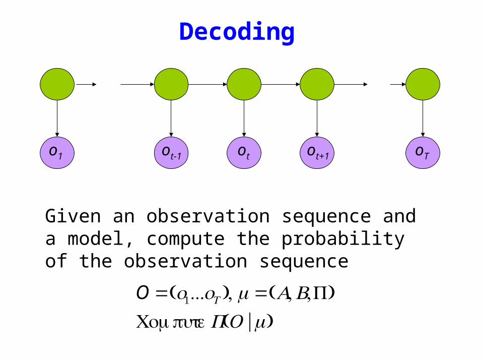
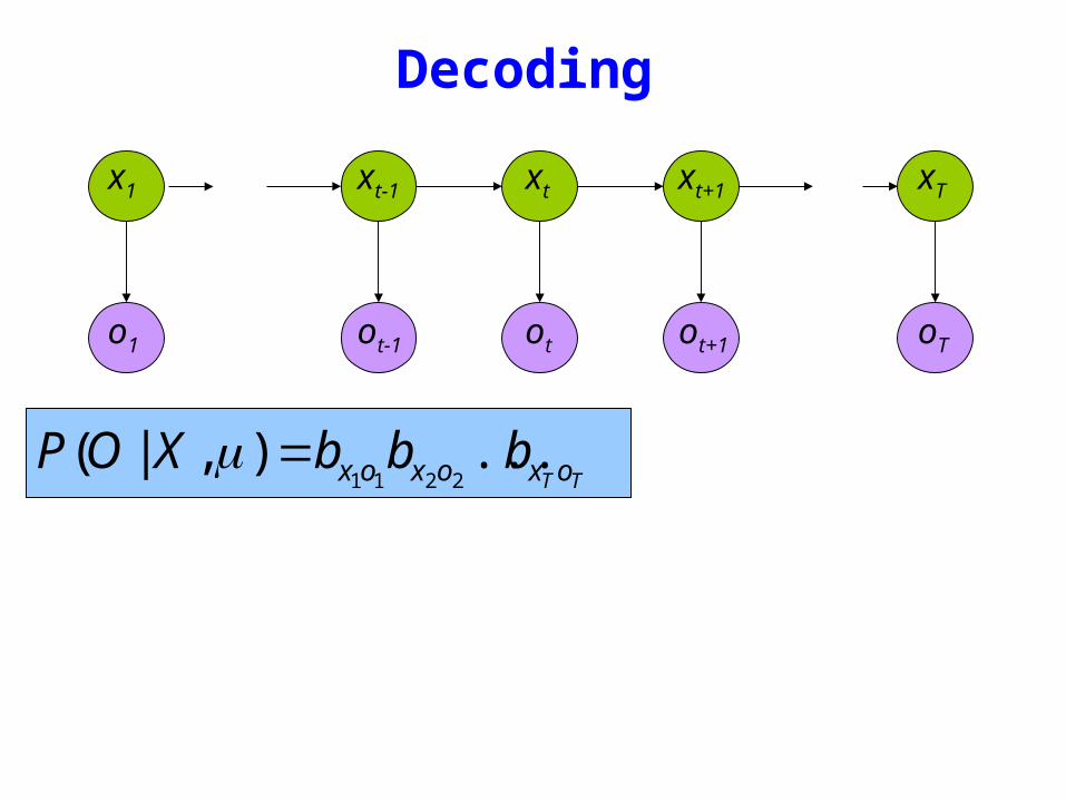
Decoding
TT oxoxox bbbXOP )|(2211
=μ
oTo1 otot-1 ot+1
x1 xt+1 xTxtxt-1
Decoding
TT oxoxox bbbXOP )|(2211
=μ
TT xxxxxxx aaaXP132211
)|(minus
=μ
oTo1 otot-1 ot+1
x1 xt+1 xTxtxt-1
Decoding
)|()|()|( μμμ XPXOPXOP =
TT oxoxox bbbXOP )|(2211
=μ
TT xxxxxxx aaaXP132211
)|(minus
=μ
oTo1 otot-1 ot+1
x1 xt+1 xTxtxt-1
Decoding
)|()|()|( μμμ XPXOPXOP =
TT oxoxox bbbXOP )|(2211
=μ
TT xxxxxxx aaaXP132211
)|(minus
=μ
sum=X
XPXOPOP )|()|()|( μμμ
oTo1 otot-1 ot+1
x1 xt+1 xTxtxt-1
P(O | μ) = x1bx1o1
x1 xT sum
t=1
Tminus1
axtxt+1bxt+1ot+1
Decoding
oTo1 otot-1 ot+1
x1 xt+1 xTxtxt-1
Complexity O(N T 2T )
Eg N =5T =100gives21005100 asymp1072
Dynamic Programming
α i (t) = P(o1ot xt = i | μ )
Forward Procedure
oTo1 otot-1 ot+1
x1 xt+1 xTxtxt-1
bull Special structure gives us an efficient solution using dynamic programming
bull Intuition Probability of the first t observations is the same for all possible t+1 length state sequences
bull Define
α i (1) = P(o1 x1 = i | μ )
= π i bio1
)|()(
)()|()|(
)()|(
)(
1111
11111
1111
111
jxoPjxooP
jxPjxoPjxooP
jxPjxooP
jxooP
tttt
ttttt
ttt
tt
=======
=====
+++
++++
+++
++
oTo1 otot-1 ot+1
x1 xt+1 xTxtxt-1
Forward Procedure
)1( +tjα
oTo1 otot-1 ot+1
x1 xt+1 xTxtxt-1
Forward Procedure
)1( +tjα
)|()(
)()|()|(
)()|(
)(
1111
11111
1111
111
jxoPjxooP
jxPjxoPjxooP
jxPjxooP
jxooP
tttt
ttttt
ttt
tt
=======
=====
+++
++++
+++
++
oTo1 otot-1 ot+1
x1 xt+1 xTxtxt-1
Forward Procedure
)1( +tjα
)|()(
)()|()|(
)()|(
)(
1111
11111
1111
111
jxoPjxooP
jxPjxoPjxooP
jxPjxooP
jxooP
tttt
ttttt
ttt
tt
=======
=====
+++
++++
+++
++
oTo1 otot-1 ot+1
x1 xt+1 xTxtxt-1
Forward Procedure
)1( +tjα
)|()(
)()|()|(
)()|(
)(
1111
11111
1111
111
jxoPjxooP
jxPjxoPjxooP
jxPjxooP
jxooP
tttt
ttttt
ttt
tt
=======
=====
+++
++++
+++
++
sum
sum
sum
sum
=
+++=
++=
+
++=
+
+=
=====
=====
====
Nijoiji
ttttNi
tt
tttNi
ttt
ttNi
ttt
tbat
jxoPixjxPixooP
jxoPixPixjxooP
jxoPjxixooP
1
1111
1
111
11
111
11
1)(
)|()|()(
)|()()|(
)|()(
α
oTo1 otot-1 ot+1
x1 xt+1 xTxtxt-1
Forward Procedure
sum
sum
sum
sum
=
+++=
++=
+
++=
+
+=
=====
=====
====
Nijoiji
ttttNi
tt
tttNi
ttt
ttNi
ttt
tbat
jxoPixjxPixooP
jxoPixPixjxooP
jxoPjxixooP
1
1111
1
111
11
111
11
1)(
)|()|()(
)|()()|(
)|()(
α
oTo1 otot-1 ot+1
x1 xt+1 xTxtxt-1
Forward Procedure
sum
sum
sum
sum
=
+++=
++=
+
++=
+
+=
=====
=====
====
Nijoiji
ttttNi
tt
tttNi
ttt
ttNi
ttt
tbat
jxoPixjxPixooP
jxoPixPixjxooP
jxoPjxixooP
1
1111
1
111
11
111
11
1)(
)|()|()(
)|()()|(
)|()(
α
oTo1 otot-1 ot+1
x1 xt+1 xTxtxt-1
Forward Procedure
= P(o1ot xt = i xt+1 = j)i=1Nsum P(ot+1 | xt+1 = j)
= P(o1ot xt+1 = j | xt = i)i=1Nsum P(xt = i)P(ot+1 | xt+1 = j)
= P(o1ot xt = i)i=1Nsum P(xt+1 = j | xt = i)P(ot+1 | xt+1 = j)
= α i (t)aijb jot +1i=1Nsum
oTo1 otot-1 ot+1
x1 xt+1 xTxtxt-1
Forward Procedure
Dynamic Programming
α j (t +1) = α i (t)aijb jot +1i=1Nsum
Complexity O(N 2 T )
Eg N = 5T = 100 gives asymp 3000
βi (t) = P(ot+1oT | xt = i)
oTo1 otot-1 ot+1
x1 xt+1 xTxtxt-1
Backward Procedure
βi (T ) = 1
βi (t) = aijbiot +1β j (t +1)
j=1Nsum
Probability of the rest of the states given the first state
oTo1 otot-1 ot+1
x1 xt+1 xTxtxt-1
Decoding Solution
sum=
=N
ii TOP
1
)()|( αμ
sum=
=N
iiiOP
1
)1()|( βπμ
)()()|(1
ttOP i
N
ii βαμ sum
=
=
Forward Procedure
Backward Procedure
Combination
P(O Xt =i |μ) =P(o1otXt =iot+1oT |μ)=P(o1otXt =i |μ)P(ot+1oT |o1otXt =i μ)=P(o1otXt =i |μ)P(ot+1oT |Xt =i μ)=α i (t)βi (t)
)()()|(1
ttOP i
N
ii βαμ sum
=
=
oTo1 otot-1 ot+1
Best State Sequence
Find the state sequence that best explains the observations
Two approaches bull Individually most likely statesbull Most likely sequence (Viterbi)
)|(maxarg OXPX
Best State Sequence (1)
γi (t) = P(Xt = i | O μ )
=P(Xt = iO | μ )
P(O | μ )
=α i (t)β i (t)
j=1
n
sum α j (t)β j (t)
Most likely state at each point in time
Xt = arg maxγ i (t)
oTo1 otot-1 ot+1
Best State Sequence (2)
Find the state sequence that best explains the observations
Viterbi algorithm
)|(maxarg OXPX
oTo1 otot-1 ot+1
Viterbi Algorithm
)(max)( 1111 11
ttttxx
j ojxooxxPtt
== minusminusminus
δ
The state sequence which maximizes the probability of seeing the observations to time t-1 landing in state j and seeing the observation at time t
x1 xt-1 j
oTo1 otot-1 ot+1
Viterbi Algorithm
)(max)( 1111 11
ttttxx
j ojxooxxPtt
== minusminusminus
δ
1)(max)1(
+=+
tjoijiij batt δδ
1)(maxarg)1(
+=+
tjoijii
j batt δψRecursive Computation
x1 xt-1 xt xt+1
Initialization
δ1(i) = ibio1
ψ 1(i) =0
oTo1 otot-1 ot+1
Viterbi Algorithm
XT =argmaxi
δi (T )
Xt =ψX^
t+1
(t+1)
P(X)=argmaxi
δi (T )
Compute the most likely state sequence by working backwards
x1 xt-1 xt xt+1 xT
oTo1 otot-1 ot+1
HMMs and Bayesian Nets (1)
x1 xt-1 xt xt+1 xT
P(x1xT o1oT )=P(x1)P(o1 |x1) P(xi+1 |xii=1
Tminus1
prod )P(oi+1 |xi+1)
= x1bx1o1
t=1
Tminus1
axtxt+1bxt+1ot+1
oTo1 otot-1 ot+1
x1 xt+1 xTxtxt-1
HMM and Bayesian Nets (2)
Conditionally independent of Given
Because of d-separation
ldquoThe past is independent of the future given the presentrdquo
Inference in an HMM
Compute the probability of a given observation sequence
Given an observation sequence compute the most likely hidden state sequence
Given an observation sequence and set of possible models which model most closely fits the data
Dynamic Programming
oTo1 otot-1 ot+1
Parameter Estimation
bull Given an observation sequence find the model that is most likely to produce that sequence
bull No analytic methodbull Given a model and observation sequence update
the model parameters to better fit the observations
A
B
AAA
BBB B
arg maxμ
P(Otraining |μ)
α i (t) = P(o1ot xt = i | μ )
βi (t) = P(ot+1oT | xt = i)
)()()|(1
ttOP i
N
ii βαμ sum
=
=
pt (i j)=P(Xt =iXt+1 = j |O μ)
=P(Xt =iXt+1 = jO |μ)
P(O |μ)
oTo1 otot-1 ot+1
Parameter Estimation
A
B
AAA
BBB B
pt (i j)=α i (t)aijbjot+1
β j (t+1)
αm(t)βm(t)m=1Nsum
Probability of traversing an arc
sum=
=Nj
ti jipt1
)()(γ Probability of being in state i
oTo1 otot-1 ot+1
Parameter Estimation
A
B
AAA
BBB B
i =γi(1)
Now we can compute the new estimates of the model parameters
aij =pt(i j)t=1
Tminus1sumγi (t)t=1
Tminus1sum
bik =γi (t) tot=ksum
γi (t)t=1
Tsum
Instance of Expectation Maximization
We have that
We may get stuck in local maximum (or even saddle point)
Nevertheless Baum-Welch usually effective
P(O | μ) geP(O |μ)
Some Variants
So far ergodic modelsbull All states are connectedbull Not always wanted
Epsilon or null-transitionsbull Not all statestransitions emit output symbols
Parameter tyingbull Assuming that certain parameters are shared bull Reduces the number of parameters that have to be estimated
Logical HMMs (Kersting De Raedt Raiko)bull Working with structured states and observation symbols
Working with log probabilities and addition instead of multiplication of probabilities (typically done)
oTo1 otot-1 ot+1
The Most Important Thing
A
B
AAA
BBB B
We can use the special structure of this model to do a lot of neat math and solve problems that are otherwise not solvable
HMMrsquos from an Agent Perspective
AI a modern approachbull AI is the study of rational agentsbull Third part by Wolfram Burgard on
Reinforcement learning
HMMs can also be used herebull Typically one is interested in P(state)
Example
Possible statesbull snow no snow
Observationsbull skis no skis
Questionsbull Was there snow the day before yesterday (given a
sequence of observations) bull Is there now snow (given a sequence of
observations) bull Will there be snow tomorrow given a sequence of
observations Next week
HMM and Agents
Question
bull Case 1 often called smoothing t lt T see last time
Only part of trellis between t and T needed
γi (t) = P(Xt = i | Oμ )
=α i (t)β i (t)
j =1
n
sum α j (t)β j (t)
Most likely state at each point in time
HMM and Agents
bull Case 2 often called filtering t= T last time
Can we make it recursive Ie go from T-1 to T
γi (t) = P(Xt = i | Oμ )
=α i (t)β i (t)
j =1
n
sum α j (t)β j (t)
Most likely state at each point in time
HMM and Agents
bull Case 2 often called filtering t= T last time
λi (T ) = P(XT = i | o1oT μ )
= γ i (T )
=α i (T )β i (T )
j =1
n
sum α j (T )β j (T )
=α i (T )
j =1
n
sum α j (T )
HMM and Agents
bull Case 3 often called prediction t= T+1 (or T+K) not yet seen
Interesting recursive Easily extended towards k gt 1
Extensions
Use Dynamic Bayesian networks instead of HMMsbullOne state corresponds to a Bayesian NetbullObservations can become more complex
Involve actions of the agent as wellbullCf Wolfram Burgardrsquos Part
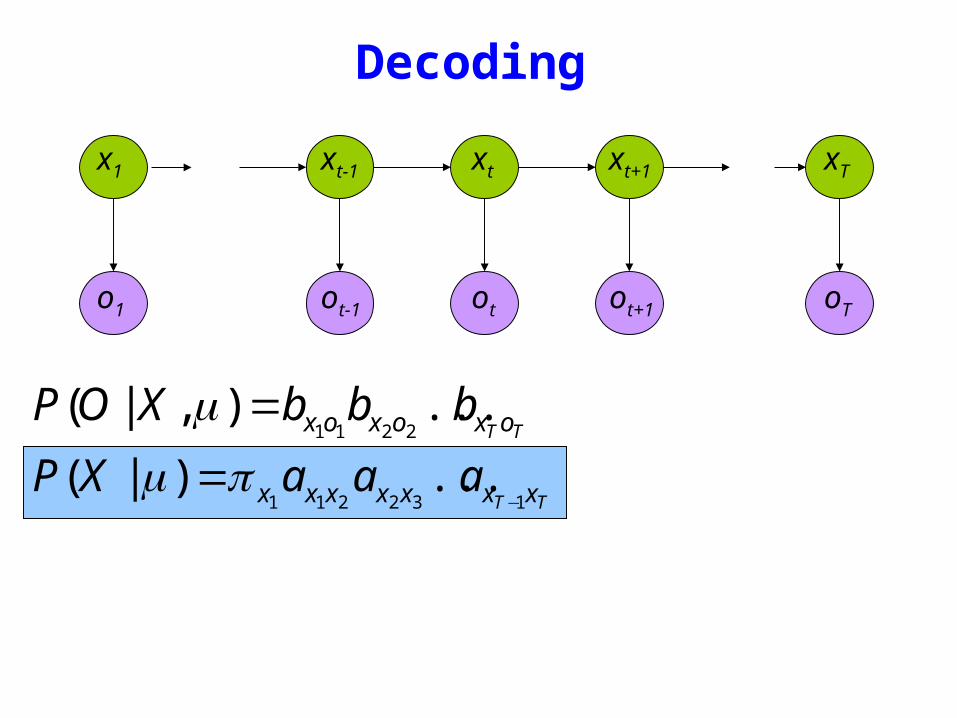
Decoding
TT oxoxox bbbXOP )|(2211
=μ
TT xxxxxxx aaaXP132211
)|(minus
=μ
oTo1 otot-1 ot+1
x1 xt+1 xTxtxt-1
Decoding
)|()|()|( μμμ XPXOPXOP =
TT oxoxox bbbXOP )|(2211
=μ
TT xxxxxxx aaaXP132211
)|(minus
=μ
oTo1 otot-1 ot+1
x1 xt+1 xTxtxt-1
Decoding
)|()|()|( μμμ XPXOPXOP =
TT oxoxox bbbXOP )|(2211
=μ
TT xxxxxxx aaaXP132211
)|(minus
=μ
sum=X
XPXOPOP )|()|()|( μμμ
oTo1 otot-1 ot+1
x1 xt+1 xTxtxt-1
P(O | μ) = x1bx1o1
x1 xT sum
t=1
Tminus1
axtxt+1bxt+1ot+1
Decoding
oTo1 otot-1 ot+1
x1 xt+1 xTxtxt-1
Complexity O(N T 2T )
Eg N =5T =100gives21005100 asymp1072
Dynamic Programming
α i (t) = P(o1ot xt = i | μ )
Forward Procedure
oTo1 otot-1 ot+1
x1 xt+1 xTxtxt-1
bull Special structure gives us an efficient solution using dynamic programming
bull Intuition Probability of the first t observations is the same for all possible t+1 length state sequences
bull Define
α i (1) = P(o1 x1 = i | μ )
= π i bio1
)|()(
)()|()|(
)()|(
)(
1111
11111
1111
111
jxoPjxooP
jxPjxoPjxooP
jxPjxooP
jxooP
tttt
ttttt
ttt
tt
=======
=====
+++
++++
+++
++
oTo1 otot-1 ot+1
x1 xt+1 xTxtxt-1
Forward Procedure
)1( +tjα
oTo1 otot-1 ot+1
x1 xt+1 xTxtxt-1
Forward Procedure
)1( +tjα
)|()(
)()|()|(
)()|(
)(
1111
11111
1111
111
jxoPjxooP
jxPjxoPjxooP
jxPjxooP
jxooP
tttt
ttttt
ttt
tt
=======
=====
+++
++++
+++
++
oTo1 otot-1 ot+1
x1 xt+1 xTxtxt-1
Forward Procedure
)1( +tjα
)|()(
)()|()|(
)()|(
)(
1111
11111
1111
111
jxoPjxooP
jxPjxoPjxooP
jxPjxooP
jxooP
tttt
ttttt
ttt
tt
=======
=====
+++
++++
+++
++
oTo1 otot-1 ot+1
x1 xt+1 xTxtxt-1
Forward Procedure
)1( +tjα
)|()(
)()|()|(
)()|(
)(
1111
11111
1111
111
jxoPjxooP
jxPjxoPjxooP
jxPjxooP
jxooP
tttt
ttttt
ttt
tt
=======
=====
+++
++++
+++
++
sum
sum
sum
sum
=
+++=
++=
+
++=
+
+=
=====
=====
====
Nijoiji
ttttNi
tt
tttNi
ttt
ttNi
ttt
tbat
jxoPixjxPixooP
jxoPixPixjxooP
jxoPjxixooP
1
1111
1
111
11
111
11
1)(
)|()|()(
)|()()|(
)|()(
α
oTo1 otot-1 ot+1
x1 xt+1 xTxtxt-1
Forward Procedure
sum
sum
sum
sum
=
+++=
++=
+
++=
+
+=
=====
=====
====
Nijoiji
ttttNi
tt
tttNi
ttt
ttNi
ttt
tbat
jxoPixjxPixooP
jxoPixPixjxooP
jxoPjxixooP
1
1111
1
111
11
111
11
1)(
)|()|()(
)|()()|(
)|()(
α
oTo1 otot-1 ot+1
x1 xt+1 xTxtxt-1
Forward Procedure
sum
sum
sum
sum
=
+++=
++=
+
++=
+
+=
=====
=====
====
Nijoiji
ttttNi
tt
tttNi
ttt
ttNi
ttt
tbat
jxoPixjxPixooP
jxoPixPixjxooP
jxoPjxixooP
1
1111
1
111
11
111
11
1)(
)|()|()(
)|()()|(
)|()(
α
oTo1 otot-1 ot+1
x1 xt+1 xTxtxt-1
Forward Procedure
= P(o1ot xt = i xt+1 = j)i=1Nsum P(ot+1 | xt+1 = j)
= P(o1ot xt+1 = j | xt = i)i=1Nsum P(xt = i)P(ot+1 | xt+1 = j)
= P(o1ot xt = i)i=1Nsum P(xt+1 = j | xt = i)P(ot+1 | xt+1 = j)
= α i (t)aijb jot +1i=1Nsum
oTo1 otot-1 ot+1
x1 xt+1 xTxtxt-1
Forward Procedure
Dynamic Programming
α j (t +1) = α i (t)aijb jot +1i=1Nsum
Complexity O(N 2 T )
Eg N = 5T = 100 gives asymp 3000
βi (t) = P(ot+1oT | xt = i)
oTo1 otot-1 ot+1
x1 xt+1 xTxtxt-1
Backward Procedure
βi (T ) = 1
βi (t) = aijbiot +1β j (t +1)
j=1Nsum
Probability of the rest of the states given the first state
oTo1 otot-1 ot+1
x1 xt+1 xTxtxt-1
Decoding Solution
sum=
=N
ii TOP
1
)()|( αμ
sum=
=N
iiiOP
1
)1()|( βπμ
)()()|(1
ttOP i
N
ii βαμ sum
=
=
Forward Procedure
Backward Procedure
Combination
P(O Xt =i |μ) =P(o1otXt =iot+1oT |μ)=P(o1otXt =i |μ)P(ot+1oT |o1otXt =i μ)=P(o1otXt =i |μ)P(ot+1oT |Xt =i μ)=α i (t)βi (t)
)()()|(1
ttOP i
N
ii βαμ sum
=
=
oTo1 otot-1 ot+1
Best State Sequence
Find the state sequence that best explains the observations
Two approaches bull Individually most likely statesbull Most likely sequence (Viterbi)
)|(maxarg OXPX
Best State Sequence (1)
γi (t) = P(Xt = i | O μ )
=P(Xt = iO | μ )
P(O | μ )
=α i (t)β i (t)
j=1
n
sum α j (t)β j (t)
Most likely state at each point in time
Xt = arg maxγ i (t)
oTo1 otot-1 ot+1
Best State Sequence (2)
Find the state sequence that best explains the observations
Viterbi algorithm
)|(maxarg OXPX
oTo1 otot-1 ot+1
Viterbi Algorithm
)(max)( 1111 11
ttttxx
j ojxooxxPtt
== minusminusminus
δ
The state sequence which maximizes the probability of seeing the observations to time t-1 landing in state j and seeing the observation at time t
x1 xt-1 j
oTo1 otot-1 ot+1
Viterbi Algorithm
)(max)( 1111 11
ttttxx
j ojxooxxPtt
== minusminusminus
δ
1)(max)1(
+=+
tjoijiij batt δδ
1)(maxarg)1(
+=+
tjoijii
j batt δψRecursive Computation
x1 xt-1 xt xt+1
Initialization
δ1(i) = ibio1
ψ 1(i) =0
oTo1 otot-1 ot+1
Viterbi Algorithm
XT =argmaxi
δi (T )
Xt =ψX^
t+1
(t+1)
P(X)=argmaxi
δi (T )
Compute the most likely state sequence by working backwards
x1 xt-1 xt xt+1 xT
oTo1 otot-1 ot+1
HMMs and Bayesian Nets (1)
x1 xt-1 xt xt+1 xT
P(x1xT o1oT )=P(x1)P(o1 |x1) P(xi+1 |xii=1
Tminus1
prod )P(oi+1 |xi+1)
= x1bx1o1
t=1
Tminus1
axtxt+1bxt+1ot+1
oTo1 otot-1 ot+1
x1 xt+1 xTxtxt-1
HMM and Bayesian Nets (2)
Conditionally independent of Given
Because of d-separation
ldquoThe past is independent of the future given the presentrdquo
Inference in an HMM
Compute the probability of a given observation sequence
Given an observation sequence compute the most likely hidden state sequence
Given an observation sequence and set of possible models which model most closely fits the data
Dynamic Programming
oTo1 otot-1 ot+1
Parameter Estimation
bull Given an observation sequence find the model that is most likely to produce that sequence
bull No analytic methodbull Given a model and observation sequence update
the model parameters to better fit the observations
A
B
AAA
BBB B
arg maxμ
P(Otraining |μ)
α i (t) = P(o1ot xt = i | μ )
βi (t) = P(ot+1oT | xt = i)
)()()|(1
ttOP i
N
ii βαμ sum
=
=
pt (i j)=P(Xt =iXt+1 = j |O μ)
=P(Xt =iXt+1 = jO |μ)
P(O |μ)
oTo1 otot-1 ot+1
Parameter Estimation
A
B
AAA
BBB B
pt (i j)=α i (t)aijbjot+1
β j (t+1)
αm(t)βm(t)m=1Nsum
Probability of traversing an arc
sum=
=Nj
ti jipt1
)()(γ Probability of being in state i
oTo1 otot-1 ot+1
Parameter Estimation
A
B
AAA
BBB B
i =γi(1)
Now we can compute the new estimates of the model parameters
aij =pt(i j)t=1
Tminus1sumγi (t)t=1
Tminus1sum
bik =γi (t) tot=ksum
γi (t)t=1
Tsum
Instance of Expectation Maximization
We have that
We may get stuck in local maximum (or even saddle point)
Nevertheless Baum-Welch usually effective
P(O | μ) geP(O |μ)
Some Variants
So far ergodic modelsbull All states are connectedbull Not always wanted
Epsilon or null-transitionsbull Not all statestransitions emit output symbols
Parameter tyingbull Assuming that certain parameters are shared bull Reduces the number of parameters that have to be estimated
Logical HMMs (Kersting De Raedt Raiko)bull Working with structured states and observation symbols
Working with log probabilities and addition instead of multiplication of probabilities (typically done)
oTo1 otot-1 ot+1
The Most Important Thing
A
B
AAA
BBB B
We can use the special structure of this model to do a lot of neat math and solve problems that are otherwise not solvable
HMMrsquos from an Agent Perspective
AI a modern approachbull AI is the study of rational agentsbull Third part by Wolfram Burgard on
Reinforcement learning
HMMs can also be used herebull Typically one is interested in P(state)
Example
Possible statesbull snow no snow
Observationsbull skis no skis
Questionsbull Was there snow the day before yesterday (given a
sequence of observations) bull Is there now snow (given a sequence of
observations) bull Will there be snow tomorrow given a sequence of
observations Next week
HMM and Agents
Question
bull Case 1 often called smoothing t lt T see last time
Only part of trellis between t and T needed
γi (t) = P(Xt = i | Oμ )
=α i (t)β i (t)
j =1
n
sum α j (t)β j (t)
Most likely state at each point in time
HMM and Agents
bull Case 2 often called filtering t= T last time
Can we make it recursive Ie go from T-1 to T
γi (t) = P(Xt = i | Oμ )
=α i (t)β i (t)
j =1
n
sum α j (t)β j (t)
Most likely state at each point in time
HMM and Agents
bull Case 2 often called filtering t= T last time
λi (T ) = P(XT = i | o1oT μ )
= γ i (T )
=α i (T )β i (T )
j =1
n
sum α j (T )β j (T )
=α i (T )
j =1
n
sum α j (T )
HMM and Agents
bull Case 3 often called prediction t= T+1 (or T+K) not yet seen
Interesting recursive Easily extended towards k gt 1
Extensions
Use Dynamic Bayesian networks instead of HMMsbullOne state corresponds to a Bayesian NetbullObservations can become more complex
Involve actions of the agent as wellbullCf Wolfram Burgardrsquos Part
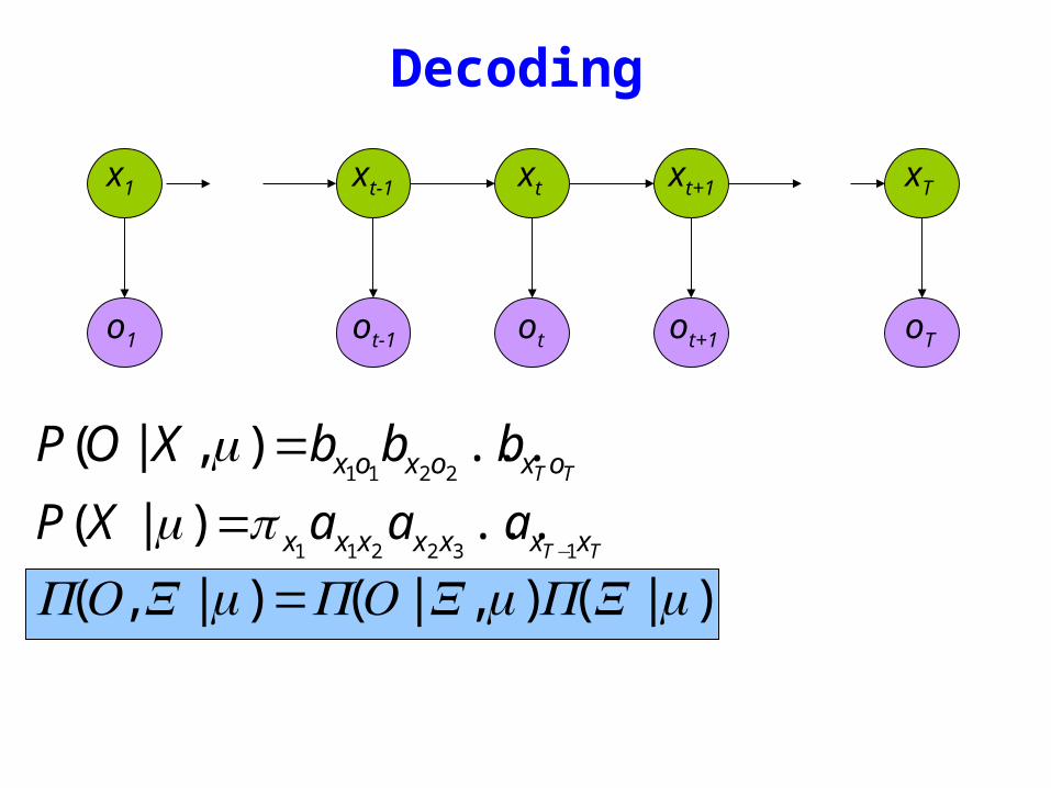
Decoding
)|()|()|( μμμ XPXOPXOP =
TT oxoxox bbbXOP )|(2211
=μ
TT xxxxxxx aaaXP132211
)|(minus
=μ
oTo1 otot-1 ot+1
x1 xt+1 xTxtxt-1
Decoding
)|()|()|( μμμ XPXOPXOP =
TT oxoxox bbbXOP )|(2211
=μ
TT xxxxxxx aaaXP132211
)|(minus
=μ
sum=X
XPXOPOP )|()|()|( μμμ
oTo1 otot-1 ot+1
x1 xt+1 xTxtxt-1
P(O | μ) = x1bx1o1
x1 xT sum
t=1
Tminus1
axtxt+1bxt+1ot+1
Decoding
oTo1 otot-1 ot+1
x1 xt+1 xTxtxt-1
Complexity O(N T 2T )
Eg N =5T =100gives21005100 asymp1072
Dynamic Programming
α i (t) = P(o1ot xt = i | μ )
Forward Procedure
oTo1 otot-1 ot+1
x1 xt+1 xTxtxt-1
bull Special structure gives us an efficient solution using dynamic programming
bull Intuition Probability of the first t observations is the same for all possible t+1 length state sequences
bull Define
α i (1) = P(o1 x1 = i | μ )
= π i bio1
)|()(
)()|()|(
)()|(
)(
1111
11111
1111
111
jxoPjxooP
jxPjxoPjxooP
jxPjxooP
jxooP
tttt
ttttt
ttt
tt
=======
=====
+++
++++
+++
++
oTo1 otot-1 ot+1
x1 xt+1 xTxtxt-1
Forward Procedure
)1( +tjα
oTo1 otot-1 ot+1
x1 xt+1 xTxtxt-1
Forward Procedure
)1( +tjα
)|()(
)()|()|(
)()|(
)(
1111
11111
1111
111
jxoPjxooP
jxPjxoPjxooP
jxPjxooP
jxooP
tttt
ttttt
ttt
tt
=======
=====
+++
++++
+++
++
oTo1 otot-1 ot+1
x1 xt+1 xTxtxt-1
Forward Procedure
)1( +tjα
)|()(
)()|()|(
)()|(
)(
1111
11111
1111
111
jxoPjxooP
jxPjxoPjxooP
jxPjxooP
jxooP
tttt
ttttt
ttt
tt
=======
=====
+++
++++
+++
++
oTo1 otot-1 ot+1
x1 xt+1 xTxtxt-1
Forward Procedure
)1( +tjα
)|()(
)()|()|(
)()|(
)(
1111
11111
1111
111
jxoPjxooP
jxPjxoPjxooP
jxPjxooP
jxooP
tttt
ttttt
ttt
tt
=======
=====
+++
++++
+++
++
sum
sum
sum
sum
=
+++=
++=
+
++=
+
+=
=====
=====
====
Nijoiji
ttttNi
tt
tttNi
ttt
ttNi
ttt
tbat
jxoPixjxPixooP
jxoPixPixjxooP
jxoPjxixooP
1
1111
1
111
11
111
11
1)(
)|()|()(
)|()()|(
)|()(
α
oTo1 otot-1 ot+1
x1 xt+1 xTxtxt-1
Forward Procedure
sum
sum
sum
sum
=
+++=
++=
+
++=
+
+=
=====
=====
====
Nijoiji
ttttNi
tt
tttNi
ttt
ttNi
ttt
tbat
jxoPixjxPixooP
jxoPixPixjxooP
jxoPjxixooP
1
1111
1
111
11
111
11
1)(
)|()|()(
)|()()|(
)|()(
α
oTo1 otot-1 ot+1
x1 xt+1 xTxtxt-1
Forward Procedure
sum
sum
sum
sum
=
+++=
++=
+
++=
+
+=
=====
=====
====
Nijoiji
ttttNi
tt
tttNi
ttt
ttNi
ttt
tbat
jxoPixjxPixooP
jxoPixPixjxooP
jxoPjxixooP
1
1111
1
111
11
111
11
1)(
)|()|()(
)|()()|(
)|()(
α
oTo1 otot-1 ot+1
x1 xt+1 xTxtxt-1
Forward Procedure
= P(o1ot xt = i xt+1 = j)i=1Nsum P(ot+1 | xt+1 = j)
= P(o1ot xt+1 = j | xt = i)i=1Nsum P(xt = i)P(ot+1 | xt+1 = j)
= P(o1ot xt = i)i=1Nsum P(xt+1 = j | xt = i)P(ot+1 | xt+1 = j)
= α i (t)aijb jot +1i=1Nsum
oTo1 otot-1 ot+1
x1 xt+1 xTxtxt-1
Forward Procedure
Dynamic Programming
α j (t +1) = α i (t)aijb jot +1i=1Nsum
Complexity O(N 2 T )
Eg N = 5T = 100 gives asymp 3000
βi (t) = P(ot+1oT | xt = i)
oTo1 otot-1 ot+1
x1 xt+1 xTxtxt-1
Backward Procedure
βi (T ) = 1
βi (t) = aijbiot +1β j (t +1)
j=1Nsum
Probability of the rest of the states given the first state
oTo1 otot-1 ot+1
x1 xt+1 xTxtxt-1
Decoding Solution
sum=
=N
ii TOP
1
)()|( αμ
sum=
=N
iiiOP
1
)1()|( βπμ
)()()|(1
ttOP i
N
ii βαμ sum
=
=
Forward Procedure
Backward Procedure
Combination
P(O Xt =i |μ) =P(o1otXt =iot+1oT |μ)=P(o1otXt =i |μ)P(ot+1oT |o1otXt =i μ)=P(o1otXt =i |μ)P(ot+1oT |Xt =i μ)=α i (t)βi (t)
)()()|(1
ttOP i
N
ii βαμ sum
=
=
oTo1 otot-1 ot+1
Best State Sequence
Find the state sequence that best explains the observations
Two approaches bull Individually most likely statesbull Most likely sequence (Viterbi)
)|(maxarg OXPX
Best State Sequence (1)
γi (t) = P(Xt = i | O μ )
=P(Xt = iO | μ )
P(O | μ )
=α i (t)β i (t)
j=1
n
sum α j (t)β j (t)
Most likely state at each point in time
Xt = arg maxγ i (t)
oTo1 otot-1 ot+1
Best State Sequence (2)
Find the state sequence that best explains the observations
Viterbi algorithm
)|(maxarg OXPX
oTo1 otot-1 ot+1
Viterbi Algorithm
)(max)( 1111 11
ttttxx
j ojxooxxPtt
== minusminusminus
δ
The state sequence which maximizes the probability of seeing the observations to time t-1 landing in state j and seeing the observation at time t
x1 xt-1 j
oTo1 otot-1 ot+1
Viterbi Algorithm
)(max)( 1111 11
ttttxx
j ojxooxxPtt
== minusminusminus
δ
1)(max)1(
+=+
tjoijiij batt δδ
1)(maxarg)1(
+=+
tjoijii
j batt δψRecursive Computation
x1 xt-1 xt xt+1
Initialization
δ1(i) = ibio1
ψ 1(i) =0
oTo1 otot-1 ot+1
Viterbi Algorithm
XT =argmaxi
δi (T )
Xt =ψX^
t+1
(t+1)
P(X)=argmaxi
δi (T )
Compute the most likely state sequence by working backwards
x1 xt-1 xt xt+1 xT
oTo1 otot-1 ot+1
HMMs and Bayesian Nets (1)
x1 xt-1 xt xt+1 xT
P(x1xT o1oT )=P(x1)P(o1 |x1) P(xi+1 |xii=1
Tminus1
prod )P(oi+1 |xi+1)
= x1bx1o1
t=1
Tminus1
axtxt+1bxt+1ot+1
oTo1 otot-1 ot+1
x1 xt+1 xTxtxt-1
HMM and Bayesian Nets (2)
Conditionally independent of Given
Because of d-separation
ldquoThe past is independent of the future given the presentrdquo
Inference in an HMM
Compute the probability of a given observation sequence
Given an observation sequence compute the most likely hidden state sequence
Given an observation sequence and set of possible models which model most closely fits the data
Dynamic Programming
oTo1 otot-1 ot+1
Parameter Estimation
bull Given an observation sequence find the model that is most likely to produce that sequence
bull No analytic methodbull Given a model and observation sequence update
the model parameters to better fit the observations
A
B
AAA
BBB B
arg maxμ
P(Otraining |μ)
α i (t) = P(o1ot xt = i | μ )
βi (t) = P(ot+1oT | xt = i)
)()()|(1
ttOP i
N
ii βαμ sum
=
=
pt (i j)=P(Xt =iXt+1 = j |O μ)
=P(Xt =iXt+1 = jO |μ)
P(O |μ)
oTo1 otot-1 ot+1
Parameter Estimation
A
B
AAA
BBB B
pt (i j)=α i (t)aijbjot+1
β j (t+1)
αm(t)βm(t)m=1Nsum
Probability of traversing an arc
sum=
=Nj
ti jipt1
)()(γ Probability of being in state i
oTo1 otot-1 ot+1
Parameter Estimation
A
B
AAA
BBB B
i =γi(1)
Now we can compute the new estimates of the model parameters
aij =pt(i j)t=1
Tminus1sumγi (t)t=1
Tminus1sum
bik =γi (t) tot=ksum
γi (t)t=1
Tsum
Instance of Expectation Maximization
We have that
We may get stuck in local maximum (or even saddle point)
Nevertheless Baum-Welch usually effective
P(O | μ) geP(O |μ)
Some Variants
So far ergodic modelsbull All states are connectedbull Not always wanted
Epsilon or null-transitionsbull Not all statestransitions emit output symbols
Parameter tyingbull Assuming that certain parameters are shared bull Reduces the number of parameters that have to be estimated
Logical HMMs (Kersting De Raedt Raiko)bull Working with structured states and observation symbols
Working with log probabilities and addition instead of multiplication of probabilities (typically done)
oTo1 otot-1 ot+1
The Most Important Thing
A
B
AAA
BBB B
We can use the special structure of this model to do a lot of neat math and solve problems that are otherwise not solvable
HMMrsquos from an Agent Perspective
AI a modern approachbull AI is the study of rational agentsbull Third part by Wolfram Burgard on
Reinforcement learning
HMMs can also be used herebull Typically one is interested in P(state)
Example
Possible statesbull snow no snow
Observationsbull skis no skis
Questionsbull Was there snow the day before yesterday (given a
sequence of observations) bull Is there now snow (given a sequence of
observations) bull Will there be snow tomorrow given a sequence of
observations Next week
HMM and Agents
Question
bull Case 1 often called smoothing t lt T see last time
Only part of trellis between t and T needed
γi (t) = P(Xt = i | Oμ )
=α i (t)β i (t)
j =1
n
sum α j (t)β j (t)
Most likely state at each point in time
HMM and Agents
bull Case 2 often called filtering t= T last time
Can we make it recursive Ie go from T-1 to T
γi (t) = P(Xt = i | Oμ )
=α i (t)β i (t)
j =1
n
sum α j (t)β j (t)
Most likely state at each point in time
HMM and Agents
bull Case 2 often called filtering t= T last time
λi (T ) = P(XT = i | o1oT μ )
= γ i (T )
=α i (T )β i (T )
j =1
n
sum α j (T )β j (T )
=α i (T )
j =1
n
sum α j (T )
HMM and Agents
bull Case 3 often called prediction t= T+1 (or T+K) not yet seen
Interesting recursive Easily extended towards k gt 1
Extensions
Use Dynamic Bayesian networks instead of HMMsbullOne state corresponds to a Bayesian NetbullObservations can become more complex
Involve actions of the agent as wellbullCf Wolfram Burgardrsquos Part
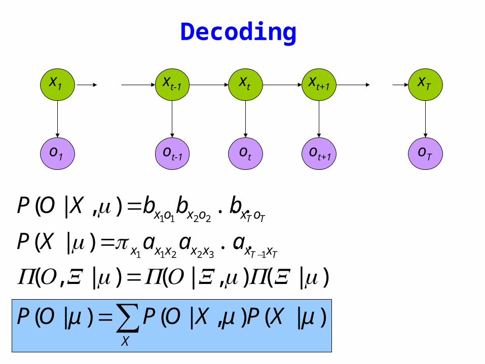
Decoding
)|()|()|( μμμ XPXOPXOP =
TT oxoxox bbbXOP )|(2211
=μ
TT xxxxxxx aaaXP132211
)|(minus
=μ
sum=X
XPXOPOP )|()|()|( μμμ
oTo1 otot-1 ot+1
x1 xt+1 xTxtxt-1
P(O | μ) = x1bx1o1
x1 xT sum
t=1
Tminus1
axtxt+1bxt+1ot+1
Decoding
oTo1 otot-1 ot+1
x1 xt+1 xTxtxt-1
Complexity O(N T 2T )
Eg N =5T =100gives21005100 asymp1072
Dynamic Programming
α i (t) = P(o1ot xt = i | μ )
Forward Procedure
oTo1 otot-1 ot+1
x1 xt+1 xTxtxt-1
bull Special structure gives us an efficient solution using dynamic programming
bull Intuition Probability of the first t observations is the same for all possible t+1 length state sequences
bull Define
α i (1) = P(o1 x1 = i | μ )
= π i bio1
)|()(
)()|()|(
)()|(
)(
1111
11111
1111
111
jxoPjxooP
jxPjxoPjxooP
jxPjxooP
jxooP
tttt
ttttt
ttt
tt
=======
=====
+++
++++
+++
++
oTo1 otot-1 ot+1
x1 xt+1 xTxtxt-1
Forward Procedure
)1( +tjα
oTo1 otot-1 ot+1
x1 xt+1 xTxtxt-1
Forward Procedure
)1( +tjα
)|()(
)()|()|(
)()|(
)(
1111
11111
1111
111
jxoPjxooP
jxPjxoPjxooP
jxPjxooP
jxooP
tttt
ttttt
ttt
tt
=======
=====
+++
++++
+++
++
oTo1 otot-1 ot+1
x1 xt+1 xTxtxt-1
Forward Procedure
)1( +tjα
)|()(
)()|()|(
)()|(
)(
1111
11111
1111
111
jxoPjxooP
jxPjxoPjxooP
jxPjxooP
jxooP
tttt
ttttt
ttt
tt
=======
=====
+++
++++
+++
++
oTo1 otot-1 ot+1
x1 xt+1 xTxtxt-1
Forward Procedure
)1( +tjα
)|()(
)()|()|(
)()|(
)(
1111
11111
1111
111
jxoPjxooP
jxPjxoPjxooP
jxPjxooP
jxooP
tttt
ttttt
ttt
tt
=======
=====
+++
++++
+++
++
sum
sum
sum
sum
=
+++=
++=
+
++=
+
+=
=====
=====
====
Nijoiji
ttttNi
tt
tttNi
ttt
ttNi
ttt
tbat
jxoPixjxPixooP
jxoPixPixjxooP
jxoPjxixooP
1
1111
1
111
11
111
11
1)(
)|()|()(
)|()()|(
)|()(
α
oTo1 otot-1 ot+1
x1 xt+1 xTxtxt-1
Forward Procedure
sum
sum
sum
sum
=
+++=
++=
+
++=
+
+=
=====
=====
====
Nijoiji
ttttNi
tt
tttNi
ttt
ttNi
ttt
tbat
jxoPixjxPixooP
jxoPixPixjxooP
jxoPjxixooP
1
1111
1
111
11
111
11
1)(
)|()|()(
)|()()|(
)|()(
α
oTo1 otot-1 ot+1
x1 xt+1 xTxtxt-1
Forward Procedure
sum
sum
sum
sum
=
+++=
++=
+
++=
+
+=
=====
=====
====
Nijoiji
ttttNi
tt
tttNi
ttt
ttNi
ttt
tbat
jxoPixjxPixooP
jxoPixPixjxooP
jxoPjxixooP
1
1111
1
111
11
111
11
1)(
)|()|()(
)|()()|(
)|()(
α
oTo1 otot-1 ot+1
x1 xt+1 xTxtxt-1
Forward Procedure
= P(o1ot xt = i xt+1 = j)i=1Nsum P(ot+1 | xt+1 = j)
= P(o1ot xt+1 = j | xt = i)i=1Nsum P(xt = i)P(ot+1 | xt+1 = j)
= P(o1ot xt = i)i=1Nsum P(xt+1 = j | xt = i)P(ot+1 | xt+1 = j)
= α i (t)aijb jot +1i=1Nsum
oTo1 otot-1 ot+1
x1 xt+1 xTxtxt-1
Forward Procedure
Dynamic Programming
α j (t +1) = α i (t)aijb jot +1i=1Nsum
Complexity O(N 2 T )
Eg N = 5T = 100 gives asymp 3000
βi (t) = P(ot+1oT | xt = i)
oTo1 otot-1 ot+1
x1 xt+1 xTxtxt-1
Backward Procedure
βi (T ) = 1
βi (t) = aijbiot +1β j (t +1)
j=1Nsum
Probability of the rest of the states given the first state
oTo1 otot-1 ot+1
x1 xt+1 xTxtxt-1
Decoding Solution
sum=
=N
ii TOP
1
)()|( αμ
sum=
=N
iiiOP
1
)1()|( βπμ
)()()|(1
ttOP i
N
ii βαμ sum
=
=
Forward Procedure
Backward Procedure
Combination
P(O Xt =i |μ) =P(o1otXt =iot+1oT |μ)=P(o1otXt =i |μ)P(ot+1oT |o1otXt =i μ)=P(o1otXt =i |μ)P(ot+1oT |Xt =i μ)=α i (t)βi (t)
)()()|(1
ttOP i
N
ii βαμ sum
=
=
oTo1 otot-1 ot+1
Best State Sequence
Find the state sequence that best explains the observations
Two approaches bull Individually most likely statesbull Most likely sequence (Viterbi)
)|(maxarg OXPX
Best State Sequence (1)
γi (t) = P(Xt = i | O μ )
=P(Xt = iO | μ )
P(O | μ )
=α i (t)β i (t)
j=1
n
sum α j (t)β j (t)
Most likely state at each point in time
Xt = arg maxγ i (t)
oTo1 otot-1 ot+1
Best State Sequence (2)
Find the state sequence that best explains the observations
Viterbi algorithm
)|(maxarg OXPX
oTo1 otot-1 ot+1
Viterbi Algorithm
)(max)( 1111 11
ttttxx
j ojxooxxPtt
== minusminusminus
δ
The state sequence which maximizes the probability of seeing the observations to time t-1 landing in state j and seeing the observation at time t
x1 xt-1 j
oTo1 otot-1 ot+1
Viterbi Algorithm
)(max)( 1111 11
ttttxx
j ojxooxxPtt
== minusminusminus
δ
1)(max)1(
+=+
tjoijiij batt δδ
1)(maxarg)1(
+=+
tjoijii
j batt δψRecursive Computation
x1 xt-1 xt xt+1
Initialization
δ1(i) = ibio1
ψ 1(i) =0
oTo1 otot-1 ot+1
Viterbi Algorithm
XT =argmaxi
δi (T )
Xt =ψX^
t+1
(t+1)
P(X)=argmaxi
δi (T )
Compute the most likely state sequence by working backwards
x1 xt-1 xt xt+1 xT
oTo1 otot-1 ot+1
HMMs and Bayesian Nets (1)
x1 xt-1 xt xt+1 xT
P(x1xT o1oT )=P(x1)P(o1 |x1) P(xi+1 |xii=1
Tminus1
prod )P(oi+1 |xi+1)
= x1bx1o1
t=1
Tminus1
axtxt+1bxt+1ot+1
oTo1 otot-1 ot+1
x1 xt+1 xTxtxt-1
HMM and Bayesian Nets (2)
Conditionally independent of Given
Because of d-separation
ldquoThe past is independent of the future given the presentrdquo
Inference in an HMM
Compute the probability of a given observation sequence
Given an observation sequence compute the most likely hidden state sequence
Given an observation sequence and set of possible models which model most closely fits the data
Dynamic Programming
oTo1 otot-1 ot+1
Parameter Estimation
bull Given an observation sequence find the model that is most likely to produce that sequence
bull No analytic methodbull Given a model and observation sequence update
the model parameters to better fit the observations
A
B
AAA
BBB B
arg maxμ
P(Otraining |μ)
α i (t) = P(o1ot xt = i | μ )
βi (t) = P(ot+1oT | xt = i)
)()()|(1
ttOP i
N
ii βαμ sum
=
=
pt (i j)=P(Xt =iXt+1 = j |O μ)
=P(Xt =iXt+1 = jO |μ)
P(O |μ)
oTo1 otot-1 ot+1
Parameter Estimation
A
B
AAA
BBB B
pt (i j)=α i (t)aijbjot+1
β j (t+1)
αm(t)βm(t)m=1Nsum
Probability of traversing an arc
sum=
=Nj
ti jipt1
)()(γ Probability of being in state i
oTo1 otot-1 ot+1
Parameter Estimation
A
B
AAA
BBB B
i =γi(1)
Now we can compute the new estimates of the model parameters
aij =pt(i j)t=1
Tminus1sumγi (t)t=1
Tminus1sum
bik =γi (t) tot=ksum
γi (t)t=1
Tsum
Instance of Expectation Maximization
We have that
We may get stuck in local maximum (or even saddle point)
Nevertheless Baum-Welch usually effective
P(O | μ) geP(O |μ)
Some Variants
So far ergodic modelsbull All states are connectedbull Not always wanted
Epsilon or null-transitionsbull Not all statestransitions emit output symbols
Parameter tyingbull Assuming that certain parameters are shared bull Reduces the number of parameters that have to be estimated
Logical HMMs (Kersting De Raedt Raiko)bull Working with structured states and observation symbols
Working with log probabilities and addition instead of multiplication of probabilities (typically done)
oTo1 otot-1 ot+1
The Most Important Thing
A
B
AAA
BBB B
We can use the special structure of this model to do a lot of neat math and solve problems that are otherwise not solvable
HMMrsquos from an Agent Perspective
AI a modern approachbull AI is the study of rational agentsbull Third part by Wolfram Burgard on
Reinforcement learning
HMMs can also be used herebull Typically one is interested in P(state)
Example
Possible statesbull snow no snow
Observationsbull skis no skis
Questionsbull Was there snow the day before yesterday (given a
sequence of observations) bull Is there now snow (given a sequence of
observations) bull Will there be snow tomorrow given a sequence of
observations Next week
HMM and Agents
Question
bull Case 1 often called smoothing t lt T see last time
Only part of trellis between t and T needed
γi (t) = P(Xt = i | Oμ )
=α i (t)β i (t)
j =1
n
sum α j (t)β j (t)
Most likely state at each point in time
HMM and Agents
bull Case 2 often called filtering t= T last time
Can we make it recursive Ie go from T-1 to T
γi (t) = P(Xt = i | Oμ )
=α i (t)β i (t)
j =1
n
sum α j (t)β j (t)
Most likely state at each point in time
HMM and Agents
bull Case 2 often called filtering t= T last time
λi (T ) = P(XT = i | o1oT μ )
= γ i (T )
=α i (T )β i (T )
j =1
n
sum α j (T )β j (T )
=α i (T )
j =1
n
sum α j (T )
HMM and Agents
bull Case 3 often called prediction t= T+1 (or T+K) not yet seen
Interesting recursive Easily extended towards k gt 1
Extensions
Use Dynamic Bayesian networks instead of HMMsbullOne state corresponds to a Bayesian NetbullObservations can become more complex
Involve actions of the agent as wellbullCf Wolfram Burgardrsquos Part
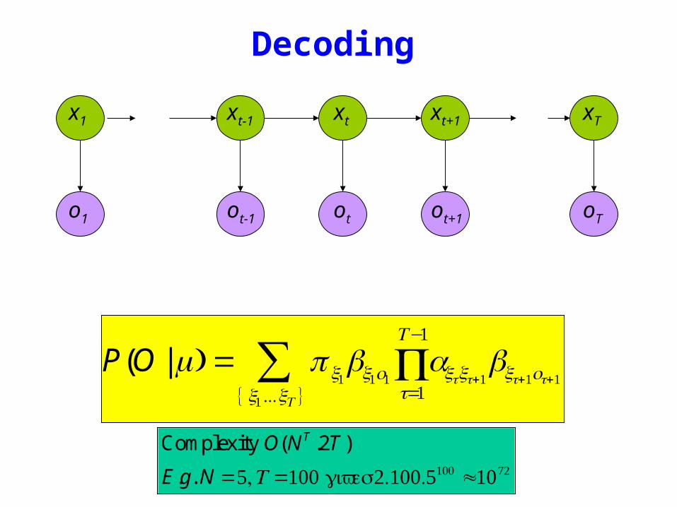
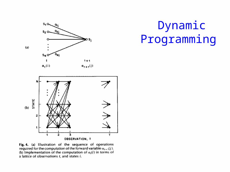
Dynamic Programming
α i (t) = P(o1ot xt = i | μ )
Forward Procedure
oTo1 otot-1 ot+1
x1 xt+1 xTxtxt-1
bull Special structure gives us an efficient solution using dynamic programming
bull Intuition Probability of the first t observations is the same for all possible t+1 length state sequences
bull Define
α i (1) = P(o1 x1 = i | μ )
= π i bio1
)|()(
)()|()|(
)()|(
)(
1111
11111
1111
111
jxoPjxooP
jxPjxoPjxooP
jxPjxooP
jxooP
tttt
ttttt
ttt
tt
=======
=====
+++
++++
+++
++
oTo1 otot-1 ot+1
x1 xt+1 xTxtxt-1
Forward Procedure
)1( +tjα
oTo1 otot-1 ot+1
x1 xt+1 xTxtxt-1
Forward Procedure
)1( +tjα
)|()(
)()|()|(
)()|(
)(
1111
11111
1111
111
jxoPjxooP
jxPjxoPjxooP
jxPjxooP
jxooP
tttt
ttttt
ttt
tt
=======
=====
+++
++++
+++
++
oTo1 otot-1 ot+1
x1 xt+1 xTxtxt-1
Forward Procedure
)1( +tjα
)|()(
)()|()|(
)()|(
)(
1111
11111
1111
111
jxoPjxooP
jxPjxoPjxooP
jxPjxooP
jxooP
tttt
ttttt
ttt
tt
=======
=====
+++
++++
+++
++
oTo1 otot-1 ot+1
x1 xt+1 xTxtxt-1
Forward Procedure
)1( +tjα
)|()(
)()|()|(
)()|(
)(
1111
11111
1111
111
jxoPjxooP
jxPjxoPjxooP
jxPjxooP
jxooP
tttt
ttttt
ttt
tt
=======
=====
+++
++++
+++
++
sum
sum
sum
sum
=
+++=
++=
+
++=
+
+=
=====
=====
====
Nijoiji
ttttNi
tt
tttNi
ttt
ttNi
ttt
tbat
jxoPixjxPixooP
jxoPixPixjxooP
jxoPjxixooP
1
1111
1
111
11
111
11
1)(
)|()|()(
)|()()|(
)|()(
α
oTo1 otot-1 ot+1
x1 xt+1 xTxtxt-1
Forward Procedure
sum
sum
sum
sum
=
+++=
++=
+
++=
+
+=
=====
=====
====
Nijoiji
ttttNi
tt
tttNi
ttt
ttNi
ttt
tbat
jxoPixjxPixooP
jxoPixPixjxooP
jxoPjxixooP
1
1111
1
111
11
111
11
1)(
)|()|()(
)|()()|(
)|()(
α
oTo1 otot-1 ot+1
x1 xt+1 xTxtxt-1
Forward Procedure
sum
sum
sum
sum
=
+++=
++=
+
++=
+
+=
=====
=====
====
Nijoiji
ttttNi
tt
tttNi
ttt
ttNi
ttt
tbat
jxoPixjxPixooP
jxoPixPixjxooP
jxoPjxixooP
1
1111
1
111
11
111
11
1)(
)|()|()(
)|()()|(
)|()(
α
oTo1 otot-1 ot+1
x1 xt+1 xTxtxt-1
Forward Procedure
= P(o1ot xt = i xt+1 = j)i=1Nsum P(ot+1 | xt+1 = j)
= P(o1ot xt+1 = j | xt = i)i=1Nsum P(xt = i)P(ot+1 | xt+1 = j)
= P(o1ot xt = i)i=1Nsum P(xt+1 = j | xt = i)P(ot+1 | xt+1 = j)
= α i (t)aijb jot +1i=1Nsum
oTo1 otot-1 ot+1
x1 xt+1 xTxtxt-1
Forward Procedure
Dynamic Programming
α j (t +1) = α i (t)aijb jot +1i=1Nsum
Complexity O(N 2 T )
Eg N = 5T = 100 gives asymp 3000
βi (t) = P(ot+1oT | xt = i)
oTo1 otot-1 ot+1
x1 xt+1 xTxtxt-1
Backward Procedure
βi (T ) = 1
βi (t) = aijbiot +1β j (t +1)
j=1Nsum
Probability of the rest of the states given the first state
oTo1 otot-1 ot+1
x1 xt+1 xTxtxt-1
Decoding Solution
sum=
=N
ii TOP
1
)()|( αμ
sum=
=N
iiiOP
1
)1()|( βπμ
)()()|(1
ttOP i
N
ii βαμ sum
=
=
Forward Procedure
Backward Procedure
Combination
P(O Xt =i |μ) =P(o1otXt =iot+1oT |μ)=P(o1otXt =i |μ)P(ot+1oT |o1otXt =i μ)=P(o1otXt =i |μ)P(ot+1oT |Xt =i μ)=α i (t)βi (t)
)()()|(1
ttOP i
N
ii βαμ sum
=
=
oTo1 otot-1 ot+1
Best State Sequence
Find the state sequence that best explains the observations
Two approaches bull Individually most likely statesbull Most likely sequence (Viterbi)
)|(maxarg OXPX
Best State Sequence (1)
γi (t) = P(Xt = i | O μ )
=P(Xt = iO | μ )
P(O | μ )
=α i (t)β i (t)
j=1
n
sum α j (t)β j (t)
Most likely state at each point in time
Xt = arg maxγ i (t)
oTo1 otot-1 ot+1
Best State Sequence (2)
Find the state sequence that best explains the observations
Viterbi algorithm
)|(maxarg OXPX
oTo1 otot-1 ot+1
Viterbi Algorithm
)(max)( 1111 11
ttttxx
j ojxooxxPtt
== minusminusminus
δ
The state sequence which maximizes the probability of seeing the observations to time t-1 landing in state j and seeing the observation at time t
x1 xt-1 j
oTo1 otot-1 ot+1
Viterbi Algorithm
)(max)( 1111 11
ttttxx
j ojxooxxPtt
== minusminusminus
δ
1)(max)1(
+=+
tjoijiij batt δδ
1)(maxarg)1(
+=+
tjoijii
j batt δψRecursive Computation
x1 xt-1 xt xt+1
Initialization
δ1(i) = ibio1
ψ 1(i) =0
oTo1 otot-1 ot+1
Viterbi Algorithm
XT =argmaxi
δi (T )
Xt =ψX^
t+1
(t+1)
P(X)=argmaxi
δi (T )
Compute the most likely state sequence by working backwards
x1 xt-1 xt xt+1 xT
oTo1 otot-1 ot+1
HMMs and Bayesian Nets (1)
x1 xt-1 xt xt+1 xT
P(x1xT o1oT )=P(x1)P(o1 |x1) P(xi+1 |xii=1
Tminus1
prod )P(oi+1 |xi+1)
= x1bx1o1
t=1
Tminus1
axtxt+1bxt+1ot+1
oTo1 otot-1 ot+1
x1 xt+1 xTxtxt-1
HMM and Bayesian Nets (2)
Conditionally independent of Given
Because of d-separation
ldquoThe past is independent of the future given the presentrdquo
Inference in an HMM
Compute the probability of a given observation sequence
Given an observation sequence compute the most likely hidden state sequence
Given an observation sequence and set of possible models which model most closely fits the data
Dynamic Programming
oTo1 otot-1 ot+1
Parameter Estimation
bull Given an observation sequence find the model that is most likely to produce that sequence
bull No analytic methodbull Given a model and observation sequence update
the model parameters to better fit the observations
A
B
AAA
BBB B
arg maxμ
P(Otraining |μ)
α i (t) = P(o1ot xt = i | μ )
βi (t) = P(ot+1oT | xt = i)
)()()|(1
ttOP i
N
ii βαμ sum
=
=
pt (i j)=P(Xt =iXt+1 = j |O μ)
=P(Xt =iXt+1 = jO |μ)
P(O |μ)
oTo1 otot-1 ot+1
Parameter Estimation
A
B
AAA
BBB B
pt (i j)=α i (t)aijbjot+1
β j (t+1)
αm(t)βm(t)m=1Nsum
Probability of traversing an arc
sum=
=Nj
ti jipt1
)()(γ Probability of being in state i
oTo1 otot-1 ot+1
Parameter Estimation
A
B
AAA
BBB B
i =γi(1)
Now we can compute the new estimates of the model parameters
aij =pt(i j)t=1
Tminus1sumγi (t)t=1
Tminus1sum
bik =γi (t) tot=ksum
γi (t)t=1
Tsum
Instance of Expectation Maximization
We have that
We may get stuck in local maximum (or even saddle point)
Nevertheless Baum-Welch usually effective
P(O | μ) geP(O |μ)
Some Variants
So far ergodic modelsbull All states are connectedbull Not always wanted
Epsilon or null-transitionsbull Not all statestransitions emit output symbols
Parameter tyingbull Assuming that certain parameters are shared bull Reduces the number of parameters that have to be estimated
Logical HMMs (Kersting De Raedt Raiko)bull Working with structured states and observation symbols
Working with log probabilities and addition instead of multiplication of probabilities (typically done)
oTo1 otot-1 ot+1
The Most Important Thing
A
B
AAA
BBB B
We can use the special structure of this model to do a lot of neat math and solve problems that are otherwise not solvable
HMMrsquos from an Agent Perspective
AI a modern approachbull AI is the study of rational agentsbull Third part by Wolfram Burgard on
Reinforcement learning
HMMs can also be used herebull Typically one is interested in P(state)
Example
Possible statesbull snow no snow
Observationsbull skis no skis
Questionsbull Was there snow the day before yesterday (given a
sequence of observations) bull Is there now snow (given a sequence of
observations) bull Will there be snow tomorrow given a sequence of
observations Next week
HMM and Agents
Question
bull Case 1 often called smoothing t lt T see last time
Only part of trellis between t and T needed
γi (t) = P(Xt = i | Oμ )
=α i (t)β i (t)
j =1
n
sum α j (t)β j (t)
Most likely state at each point in time
HMM and Agents
bull Case 2 often called filtering t= T last time
Can we make it recursive Ie go from T-1 to T
γi (t) = P(Xt = i | Oμ )
=α i (t)β i (t)
j =1
n
sum α j (t)β j (t)
Most likely state at each point in time
HMM and Agents
bull Case 2 often called filtering t= T last time
λi (T ) = P(XT = i | o1oT μ )
= γ i (T )
=α i (T )β i (T )
j =1
n
sum α j (T )β j (T )
=α i (T )
j =1
n
sum α j (T )
HMM and Agents
bull Case 3 often called prediction t= T+1 (or T+K) not yet seen
Interesting recursive Easily extended towards k gt 1
Extensions
Use Dynamic Bayesian networks instead of HMMsbullOne state corresponds to a Bayesian NetbullObservations can become more complex
Involve actions of the agent as wellbullCf Wolfram Burgardrsquos Part
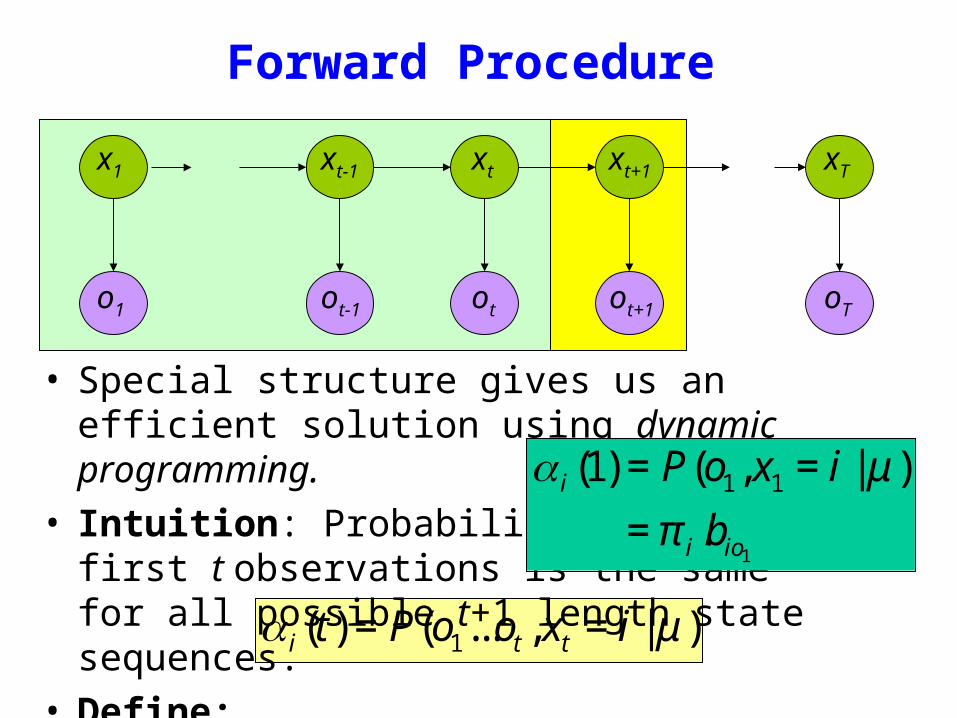
α i (t) = P(o1ot xt = i | μ )
Forward Procedure
oTo1 otot-1 ot+1
x1 xt+1 xTxtxt-1
bull Special structure gives us an efficient solution using dynamic programming
bull Intuition Probability of the first t observations is the same for all possible t+1 length state sequences
bull Define
α i (1) = P(o1 x1 = i | μ )
= π i bio1
)|()(
)()|()|(
)()|(
)(
1111
11111
1111
111
jxoPjxooP
jxPjxoPjxooP
jxPjxooP
jxooP
tttt
ttttt
ttt
tt
=======
=====
+++
++++
+++
++
oTo1 otot-1 ot+1
x1 xt+1 xTxtxt-1
Forward Procedure
)1( +tjα
oTo1 otot-1 ot+1
x1 xt+1 xTxtxt-1
Forward Procedure
)1( +tjα
)|()(
)()|()|(
)()|(
)(
1111
11111
1111
111
jxoPjxooP
jxPjxoPjxooP
jxPjxooP
jxooP
tttt
ttttt
ttt
tt
=======
=====
+++
++++
+++
++
oTo1 otot-1 ot+1
x1 xt+1 xTxtxt-1
Forward Procedure
)1( +tjα
)|()(
)()|()|(
)()|(
)(
1111
11111
1111
111
jxoPjxooP
jxPjxoPjxooP
jxPjxooP
jxooP
tttt
ttttt
ttt
tt
=======
=====
+++
++++
+++
++
oTo1 otot-1 ot+1
x1 xt+1 xTxtxt-1
Forward Procedure
)1( +tjα
)|()(
)()|()|(
)()|(
)(
1111
11111
1111
111
jxoPjxooP
jxPjxoPjxooP
jxPjxooP
jxooP
tttt
ttttt
ttt
tt
=======
=====
+++
++++
+++
++
sum
sum
sum
sum
=
+++=
++=
+
++=
+
+=
=====
=====
====
Nijoiji
ttttNi
tt
tttNi
ttt
ttNi
ttt
tbat
jxoPixjxPixooP
jxoPixPixjxooP
jxoPjxixooP
1
1111
1
111
11
111
11
1)(
)|()|()(
)|()()|(
)|()(
α
oTo1 otot-1 ot+1
x1 xt+1 xTxtxt-1
Forward Procedure
sum
sum
sum
sum
=
+++=
++=
+
++=
+
+=
=====
=====
====
Nijoiji
ttttNi
tt
tttNi
ttt
ttNi
ttt
tbat
jxoPixjxPixooP
jxoPixPixjxooP
jxoPjxixooP
1
1111
1
111
11
111
11
1)(
)|()|()(
)|()()|(
)|()(
α
oTo1 otot-1 ot+1
x1 xt+1 xTxtxt-1
Forward Procedure
sum
sum
sum
sum
=
+++=
++=
+
++=
+
+=
=====
=====
====
Nijoiji
ttttNi
tt
tttNi
ttt
ttNi
ttt
tbat
jxoPixjxPixooP
jxoPixPixjxooP
jxoPjxixooP
1
1111
1
111
11
111
11
1)(
)|()|()(
)|()()|(
)|()(
α
oTo1 otot-1 ot+1
x1 xt+1 xTxtxt-1
Forward Procedure
= P(o1ot xt = i xt+1 = j)i=1Nsum P(ot+1 | xt+1 = j)
= P(o1ot xt+1 = j | xt = i)i=1Nsum P(xt = i)P(ot+1 | xt+1 = j)
= P(o1ot xt = i)i=1Nsum P(xt+1 = j | xt = i)P(ot+1 | xt+1 = j)
= α i (t)aijb jot +1i=1Nsum
oTo1 otot-1 ot+1
x1 xt+1 xTxtxt-1
Forward Procedure
Dynamic Programming
α j (t +1) = α i (t)aijb jot +1i=1Nsum
Complexity O(N 2 T )
Eg N = 5T = 100 gives asymp 3000
βi (t) = P(ot+1oT | xt = i)
oTo1 otot-1 ot+1
x1 xt+1 xTxtxt-1
Backward Procedure
βi (T ) = 1
βi (t) = aijbiot +1β j (t +1)
j=1Nsum
Probability of the rest of the states given the first state
oTo1 otot-1 ot+1
x1 xt+1 xTxtxt-1
Decoding Solution
sum=
=N
ii TOP
1
)()|( αμ
sum=
=N
iiiOP
1
)1()|( βπμ
)()()|(1
ttOP i
N
ii βαμ sum
=
=
Forward Procedure
Backward Procedure
Combination
P(O Xt =i |μ) =P(o1otXt =iot+1oT |μ)=P(o1otXt =i |μ)P(ot+1oT |o1otXt =i μ)=P(o1otXt =i |μ)P(ot+1oT |Xt =i μ)=α i (t)βi (t)
)()()|(1
ttOP i
N
ii βαμ sum
=
=
oTo1 otot-1 ot+1
Best State Sequence
Find the state sequence that best explains the observations
Two approaches bull Individually most likely statesbull Most likely sequence (Viterbi)
)|(maxarg OXPX
Best State Sequence (1)
γi (t) = P(Xt = i | O μ )
=P(Xt = iO | μ )
P(O | μ )
=α i (t)β i (t)
j=1
n
sum α j (t)β j (t)
Most likely state at each point in time
Xt = arg maxγ i (t)
oTo1 otot-1 ot+1
Best State Sequence (2)
Find the state sequence that best explains the observations
Viterbi algorithm
)|(maxarg OXPX
oTo1 otot-1 ot+1
Viterbi Algorithm
)(max)( 1111 11
ttttxx
j ojxooxxPtt
== minusminusminus
δ
The state sequence which maximizes the probability of seeing the observations to time t-1 landing in state j and seeing the observation at time t
x1 xt-1 j
oTo1 otot-1 ot+1
Viterbi Algorithm
)(max)( 1111 11
ttttxx
j ojxooxxPtt
== minusminusminus
δ
1)(max)1(
+=+
tjoijiij batt δδ
1)(maxarg)1(
+=+
tjoijii
j batt δψRecursive Computation
x1 xt-1 xt xt+1
Initialization
δ1(i) = ibio1
ψ 1(i) =0
oTo1 otot-1 ot+1
Viterbi Algorithm
XT =argmaxi
δi (T )
Xt =ψX^
t+1
(t+1)
P(X)=argmaxi
δi (T )
Compute the most likely state sequence by working backwards
x1 xt-1 xt xt+1 xT
oTo1 otot-1 ot+1
HMMs and Bayesian Nets (1)
x1 xt-1 xt xt+1 xT
P(x1xT o1oT )=P(x1)P(o1 |x1) P(xi+1 |xii=1
Tminus1
prod )P(oi+1 |xi+1)
= x1bx1o1
t=1
Tminus1
axtxt+1bxt+1ot+1
oTo1 otot-1 ot+1
x1 xt+1 xTxtxt-1
HMM and Bayesian Nets (2)
Conditionally independent of Given
Because of d-separation
ldquoThe past is independent of the future given the presentrdquo
Inference in an HMM
Compute the probability of a given observation sequence
Given an observation sequence compute the most likely hidden state sequence
Given an observation sequence and set of possible models which model most closely fits the data
Dynamic Programming
oTo1 otot-1 ot+1
Parameter Estimation
bull Given an observation sequence find the model that is most likely to produce that sequence
bull No analytic methodbull Given a model and observation sequence update
the model parameters to better fit the observations
A
B
AAA
BBB B
arg maxμ
P(Otraining |μ)
α i (t) = P(o1ot xt = i | μ )
βi (t) = P(ot+1oT | xt = i)
)()()|(1
ttOP i
N
ii βαμ sum
=
=
pt (i j)=P(Xt =iXt+1 = j |O μ)
=P(Xt =iXt+1 = jO |μ)
P(O |μ)
oTo1 otot-1 ot+1
Parameter Estimation
A
B
AAA
BBB B
pt (i j)=α i (t)aijbjot+1
β j (t+1)
αm(t)βm(t)m=1Nsum
Probability of traversing an arc
sum=
=Nj
ti jipt1
)()(γ Probability of being in state i
oTo1 otot-1 ot+1
Parameter Estimation
A
B
AAA
BBB B
i =γi(1)
Now we can compute the new estimates of the model parameters
aij =pt(i j)t=1
Tminus1sumγi (t)t=1
Tminus1sum
bik =γi (t) tot=ksum
γi (t)t=1
Tsum
Instance of Expectation Maximization
We have that
We may get stuck in local maximum (or even saddle point)
Nevertheless Baum-Welch usually effective
P(O | μ) geP(O |μ)
Some Variants
So far ergodic modelsbull All states are connectedbull Not always wanted
Epsilon or null-transitionsbull Not all statestransitions emit output symbols
Parameter tyingbull Assuming that certain parameters are shared bull Reduces the number of parameters that have to be estimated
Logical HMMs (Kersting De Raedt Raiko)bull Working with structured states and observation symbols
Working with log probabilities and addition instead of multiplication of probabilities (typically done)
oTo1 otot-1 ot+1
The Most Important Thing
A
B
AAA
BBB B
We can use the special structure of this model to do a lot of neat math and solve problems that are otherwise not solvable
HMMrsquos from an Agent Perspective
AI a modern approachbull AI is the study of rational agentsbull Third part by Wolfram Burgard on
Reinforcement learning
HMMs can also be used herebull Typically one is interested in P(state)
Example
Possible statesbull snow no snow
Observationsbull skis no skis
Questionsbull Was there snow the day before yesterday (given a
sequence of observations) bull Is there now snow (given a sequence of
observations) bull Will there be snow tomorrow given a sequence of
observations Next week
HMM and Agents
Question
bull Case 1 often called smoothing t lt T see last time
Only part of trellis between t and T needed
γi (t) = P(Xt = i | Oμ )
=α i (t)β i (t)
j =1
n
sum α j (t)β j (t)
Most likely state at each point in time
HMM and Agents
bull Case 2 often called filtering t= T last time
Can we make it recursive Ie go from T-1 to T
γi (t) = P(Xt = i | Oμ )
=α i (t)β i (t)
j =1
n
sum α j (t)β j (t)
Most likely state at each point in time
HMM and Agents
bull Case 2 often called filtering t= T last time
λi (T ) = P(XT = i | o1oT μ )
= γ i (T )
=α i (T )β i (T )
j =1
n
sum α j (T )β j (T )
=α i (T )
j =1
n
sum α j (T )
HMM and Agents
bull Case 3 often called prediction t= T+1 (or T+K) not yet seen
Interesting recursive Easily extended towards k gt 1
Extensions
Use Dynamic Bayesian networks instead of HMMsbullOne state corresponds to a Bayesian NetbullObservations can become more complex
Involve actions of the agent as wellbullCf Wolfram Burgardrsquos Part
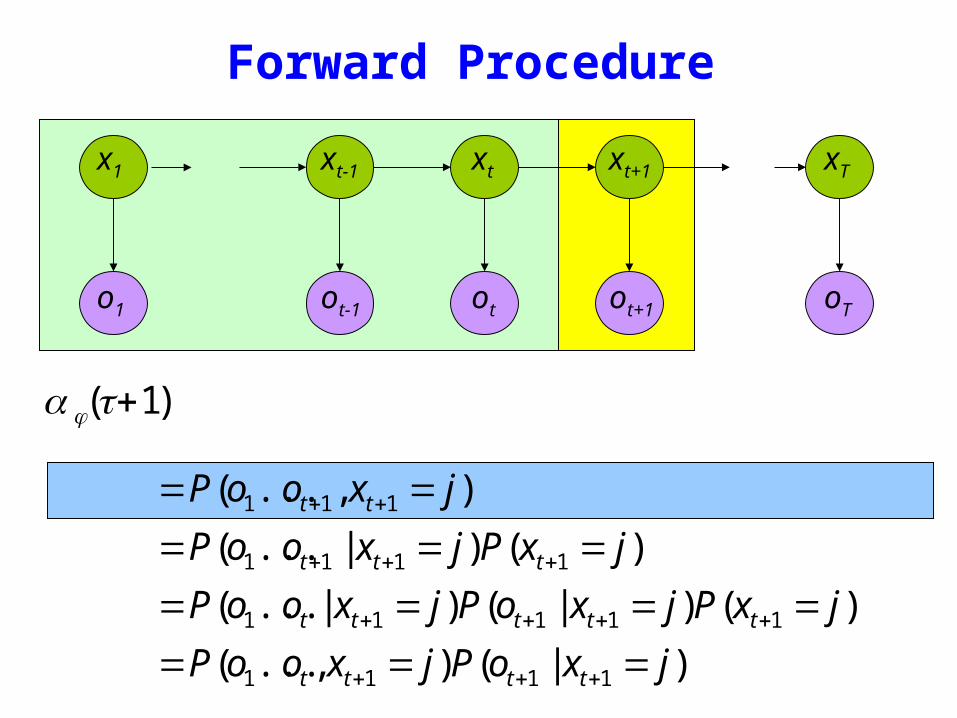
)|()(
)()|()|(
)()|(
)(
1111
11111
1111
111
jxoPjxooP
jxPjxoPjxooP
jxPjxooP
jxooP
tttt
ttttt
ttt
tt
=======
=====
+++
++++
+++
++
oTo1 otot-1 ot+1
x1 xt+1 xTxtxt-1
Forward Procedure
)1( +tjα
oTo1 otot-1 ot+1
x1 xt+1 xTxtxt-1
Forward Procedure
)1( +tjα
)|()(
)()|()|(
)()|(
)(
1111
11111
1111
111
jxoPjxooP
jxPjxoPjxooP
jxPjxooP
jxooP
tttt
ttttt
ttt
tt
=======
=====
+++
++++
+++
++
oTo1 otot-1 ot+1
x1 xt+1 xTxtxt-1
Forward Procedure
)1( +tjα
)|()(
)()|()|(
)()|(
)(
1111
11111
1111
111
jxoPjxooP
jxPjxoPjxooP
jxPjxooP
jxooP
tttt
ttttt
ttt
tt
=======
=====
+++
++++
+++
++
oTo1 otot-1 ot+1
x1 xt+1 xTxtxt-1
Forward Procedure
)1( +tjα
)|()(
)()|()|(
)()|(
)(
1111
11111
1111
111
jxoPjxooP
jxPjxoPjxooP
jxPjxooP
jxooP
tttt
ttttt
ttt
tt
=======
=====
+++
++++
+++
++
sum
sum
sum
sum
=
+++=
++=
+
++=
+
+=
=====
=====
====
Nijoiji
ttttNi
tt
tttNi
ttt
ttNi
ttt
tbat
jxoPixjxPixooP
jxoPixPixjxooP
jxoPjxixooP
1
1111
1
111
11
111
11
1)(
)|()|()(
)|()()|(
)|()(
α
oTo1 otot-1 ot+1
x1 xt+1 xTxtxt-1
Forward Procedure
sum
sum
sum
sum
=
+++=
++=
+
++=
+
+=
=====
=====
====
Nijoiji
ttttNi
tt
tttNi
ttt
ttNi
ttt
tbat
jxoPixjxPixooP
jxoPixPixjxooP
jxoPjxixooP
1
1111
1
111
11
111
11
1)(
)|()|()(
)|()()|(
)|()(
α
oTo1 otot-1 ot+1
x1 xt+1 xTxtxt-1
Forward Procedure
sum
sum
sum
sum
=
+++=
++=
+
++=
+
+=
=====
=====
====
Nijoiji
ttttNi
tt
tttNi
ttt
ttNi
ttt
tbat
jxoPixjxPixooP
jxoPixPixjxooP
jxoPjxixooP
1
1111
1
111
11
111
11
1)(
)|()|()(
)|()()|(
)|()(
α
oTo1 otot-1 ot+1
x1 xt+1 xTxtxt-1
Forward Procedure
= P(o1ot xt = i xt+1 = j)i=1Nsum P(ot+1 | xt+1 = j)
= P(o1ot xt+1 = j | xt = i)i=1Nsum P(xt = i)P(ot+1 | xt+1 = j)
= P(o1ot xt = i)i=1Nsum P(xt+1 = j | xt = i)P(ot+1 | xt+1 = j)
= α i (t)aijb jot +1i=1Nsum
oTo1 otot-1 ot+1
x1 xt+1 xTxtxt-1
Forward Procedure
Dynamic Programming
α j (t +1) = α i (t)aijb jot +1i=1Nsum
Complexity O(N 2 T )
Eg N = 5T = 100 gives asymp 3000
βi (t) = P(ot+1oT | xt = i)
oTo1 otot-1 ot+1
x1 xt+1 xTxtxt-1
Backward Procedure
βi (T ) = 1
βi (t) = aijbiot +1β j (t +1)
j=1Nsum
Probability of the rest of the states given the first state
oTo1 otot-1 ot+1
x1 xt+1 xTxtxt-1
Decoding Solution
sum=
=N
ii TOP
1
)()|( αμ
sum=
=N
iiiOP
1
)1()|( βπμ
)()()|(1
ttOP i
N
ii βαμ sum
=
=
Forward Procedure
Backward Procedure
Combination
P(O Xt =i |μ) =P(o1otXt =iot+1oT |μ)=P(o1otXt =i |μ)P(ot+1oT |o1otXt =i μ)=P(o1otXt =i |μ)P(ot+1oT |Xt =i μ)=α i (t)βi (t)
)()()|(1
ttOP i
N
ii βαμ sum
=
=
oTo1 otot-1 ot+1
Best State Sequence
Find the state sequence that best explains the observations
Two approaches bull Individually most likely statesbull Most likely sequence (Viterbi)
)|(maxarg OXPX
Best State Sequence (1)
γi (t) = P(Xt = i | O μ )
=P(Xt = iO | μ )
P(O | μ )
=α i (t)β i (t)
j=1
n
sum α j (t)β j (t)
Most likely state at each point in time
Xt = arg maxγ i (t)
oTo1 otot-1 ot+1
Best State Sequence (2)
Find the state sequence that best explains the observations
Viterbi algorithm
)|(maxarg OXPX
oTo1 otot-1 ot+1
Viterbi Algorithm
)(max)( 1111 11
ttttxx
j ojxooxxPtt
== minusminusminus
δ
The state sequence which maximizes the probability of seeing the observations to time t-1 landing in state j and seeing the observation at time t
x1 xt-1 j
oTo1 otot-1 ot+1
Viterbi Algorithm
)(max)( 1111 11
ttttxx
j ojxooxxPtt
== minusminusminus
δ
1)(max)1(
+=+
tjoijiij batt δδ
1)(maxarg)1(
+=+
tjoijii
j batt δψRecursive Computation
x1 xt-1 xt xt+1
Initialization
δ1(i) = ibio1
ψ 1(i) =0
oTo1 otot-1 ot+1
Viterbi Algorithm
XT =argmaxi
δi (T )
Xt =ψX^
t+1
(t+1)
P(X)=argmaxi
δi (T )
Compute the most likely state sequence by working backwards
x1 xt-1 xt xt+1 xT
oTo1 otot-1 ot+1
HMMs and Bayesian Nets (1)
x1 xt-1 xt xt+1 xT
P(x1xT o1oT )=P(x1)P(o1 |x1) P(xi+1 |xii=1
Tminus1
prod )P(oi+1 |xi+1)
= x1bx1o1
t=1
Tminus1
axtxt+1bxt+1ot+1
oTo1 otot-1 ot+1
x1 xt+1 xTxtxt-1
HMM and Bayesian Nets (2)
Conditionally independent of Given
Because of d-separation
ldquoThe past is independent of the future given the presentrdquo
Inference in an HMM
Compute the probability of a given observation sequence
Given an observation sequence compute the most likely hidden state sequence
Given an observation sequence and set of possible models which model most closely fits the data
Dynamic Programming
oTo1 otot-1 ot+1
Parameter Estimation
bull Given an observation sequence find the model that is most likely to produce that sequence
bull No analytic methodbull Given a model and observation sequence update
the model parameters to better fit the observations
A
B
AAA
BBB B
arg maxμ
P(Otraining |μ)
α i (t) = P(o1ot xt = i | μ )
βi (t) = P(ot+1oT | xt = i)
)()()|(1
ttOP i
N
ii βαμ sum
=
=
pt (i j)=P(Xt =iXt+1 = j |O μ)
=P(Xt =iXt+1 = jO |μ)
P(O |μ)
oTo1 otot-1 ot+1
Parameter Estimation
A
B
AAA
BBB B
pt (i j)=α i (t)aijbjot+1
β j (t+1)
αm(t)βm(t)m=1Nsum
Probability of traversing an arc
sum=
=Nj
ti jipt1
)()(γ Probability of being in state i
oTo1 otot-1 ot+1
Parameter Estimation
A
B
AAA
BBB B
i =γi(1)
Now we can compute the new estimates of the model parameters
aij =pt(i j)t=1
Tminus1sumγi (t)t=1
Tminus1sum
bik =γi (t) tot=ksum
γi (t)t=1
Tsum
Instance of Expectation Maximization
We have that
We may get stuck in local maximum (or even saddle point)
Nevertheless Baum-Welch usually effective
P(O | μ) geP(O |μ)
Some Variants
So far ergodic modelsbull All states are connectedbull Not always wanted
Epsilon or null-transitionsbull Not all statestransitions emit output symbols
Parameter tyingbull Assuming that certain parameters are shared bull Reduces the number of parameters that have to be estimated
Logical HMMs (Kersting De Raedt Raiko)bull Working with structured states and observation symbols
Working with log probabilities and addition instead of multiplication of probabilities (typically done)
oTo1 otot-1 ot+1
The Most Important Thing
A
B
AAA
BBB B
We can use the special structure of this model to do a lot of neat math and solve problems that are otherwise not solvable
HMMrsquos from an Agent Perspective
AI a modern approachbull AI is the study of rational agentsbull Third part by Wolfram Burgard on
Reinforcement learning
HMMs can also be used herebull Typically one is interested in P(state)
Example
Possible statesbull snow no snow
Observationsbull skis no skis
Questionsbull Was there snow the day before yesterday (given a
sequence of observations) bull Is there now snow (given a sequence of
observations) bull Will there be snow tomorrow given a sequence of
observations Next week
HMM and Agents
Question
bull Case 1 often called smoothing t lt T see last time
Only part of trellis between t and T needed
γi (t) = P(Xt = i | Oμ )
=α i (t)β i (t)
j =1
n
sum α j (t)β j (t)
Most likely state at each point in time
HMM and Agents
bull Case 2 often called filtering t= T last time
Can we make it recursive Ie go from T-1 to T
γi (t) = P(Xt = i | Oμ )
=α i (t)β i (t)
j =1
n
sum α j (t)β j (t)
Most likely state at each point in time
HMM and Agents
bull Case 2 often called filtering t= T last time
λi (T ) = P(XT = i | o1oT μ )
= γ i (T )
=α i (T )β i (T )
j =1
n
sum α j (T )β j (T )
=α i (T )
j =1
n
sum α j (T )
HMM and Agents
bull Case 3 often called prediction t= T+1 (or T+K) not yet seen
Interesting recursive Easily extended towards k gt 1
Extensions
Use Dynamic Bayesian networks instead of HMMsbullOne state corresponds to a Bayesian NetbullObservations can become more complex
Involve actions of the agent as wellbullCf Wolfram Burgardrsquos Part
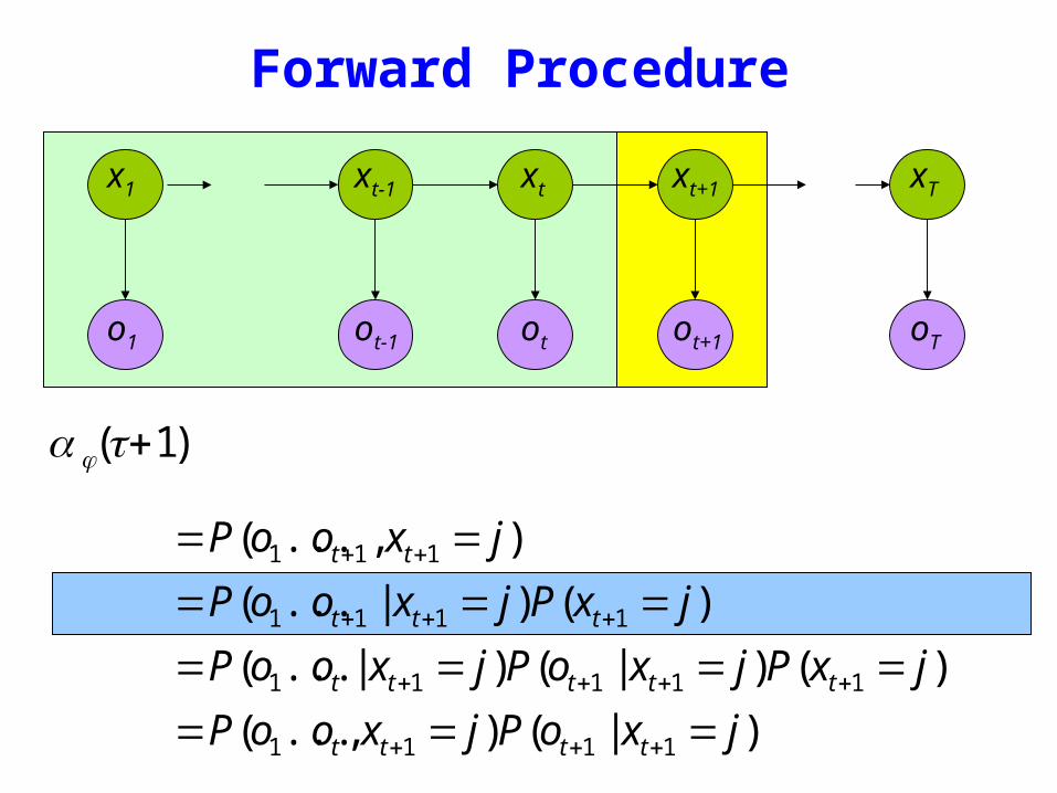
oTo1 otot-1 ot+1
x1 xt+1 xTxtxt-1
Forward Procedure
)1( +tjα
)|()(
)()|()|(
)()|(
)(
1111
11111
1111
111
jxoPjxooP
jxPjxoPjxooP
jxPjxooP
jxooP
tttt
ttttt
ttt
tt
=======
=====
+++
++++
+++
++
oTo1 otot-1 ot+1
x1 xt+1 xTxtxt-1
Forward Procedure
)1( +tjα
)|()(
)()|()|(
)()|(
)(
1111
11111
1111
111
jxoPjxooP
jxPjxoPjxooP
jxPjxooP
jxooP
tttt
ttttt
ttt
tt
=======
=====
+++
++++
+++
++
oTo1 otot-1 ot+1
x1 xt+1 xTxtxt-1
Forward Procedure
)1( +tjα
)|()(
)()|()|(
)()|(
)(
1111
11111
1111
111
jxoPjxooP
jxPjxoPjxooP
jxPjxooP
jxooP
tttt
ttttt
ttt
tt
=======
=====
+++
++++
+++
++
sum
sum
sum
sum
=
+++=
++=
+
++=
+
+=
=====
=====
====
Nijoiji
ttttNi
tt
tttNi
ttt
ttNi
ttt
tbat
jxoPixjxPixooP
jxoPixPixjxooP
jxoPjxixooP
1
1111
1
111
11
111
11
1)(
)|()|()(
)|()()|(
)|()(
α
oTo1 otot-1 ot+1
x1 xt+1 xTxtxt-1
Forward Procedure
sum
sum
sum
sum
=
+++=
++=
+
++=
+
+=
=====
=====
====
Nijoiji
ttttNi
tt
tttNi
ttt
ttNi
ttt
tbat
jxoPixjxPixooP
jxoPixPixjxooP
jxoPjxixooP
1
1111
1
111
11
111
11
1)(
)|()|()(
)|()()|(
)|()(
α
oTo1 otot-1 ot+1
x1 xt+1 xTxtxt-1
Forward Procedure
sum
sum
sum
sum
=
+++=
++=
+
++=
+
+=
=====
=====
====
Nijoiji
ttttNi
tt
tttNi
ttt
ttNi
ttt
tbat
jxoPixjxPixooP
jxoPixPixjxooP
jxoPjxixooP
1
1111
1
111
11
111
11
1)(
)|()|()(
)|()()|(
)|()(
α
oTo1 otot-1 ot+1
x1 xt+1 xTxtxt-1
Forward Procedure
= P(o1ot xt = i xt+1 = j)i=1Nsum P(ot+1 | xt+1 = j)
= P(o1ot xt+1 = j | xt = i)i=1Nsum P(xt = i)P(ot+1 | xt+1 = j)
= P(o1ot xt = i)i=1Nsum P(xt+1 = j | xt = i)P(ot+1 | xt+1 = j)
= α i (t)aijb jot +1i=1Nsum
oTo1 otot-1 ot+1
x1 xt+1 xTxtxt-1
Forward Procedure
Dynamic Programming
α j (t +1) = α i (t)aijb jot +1i=1Nsum
Complexity O(N 2 T )
Eg N = 5T = 100 gives asymp 3000
βi (t) = P(ot+1oT | xt = i)
oTo1 otot-1 ot+1
x1 xt+1 xTxtxt-1
Backward Procedure
βi (T ) = 1
βi (t) = aijbiot +1β j (t +1)
j=1Nsum
Probability of the rest of the states given the first state
oTo1 otot-1 ot+1
x1 xt+1 xTxtxt-1
Decoding Solution
sum=
=N
ii TOP
1
)()|( αμ
sum=
=N
iiiOP
1
)1()|( βπμ
)()()|(1
ttOP i
N
ii βαμ sum
=
=
Forward Procedure
Backward Procedure
Combination
P(O Xt =i |μ) =P(o1otXt =iot+1oT |μ)=P(o1otXt =i |μ)P(ot+1oT |o1otXt =i μ)=P(o1otXt =i |μ)P(ot+1oT |Xt =i μ)=α i (t)βi (t)
)()()|(1
ttOP i
N
ii βαμ sum
=
=
oTo1 otot-1 ot+1
Best State Sequence
Find the state sequence that best explains the observations
Two approaches bull Individually most likely statesbull Most likely sequence (Viterbi)
)|(maxarg OXPX
Best State Sequence (1)
γi (t) = P(Xt = i | O μ )
=P(Xt = iO | μ )
P(O | μ )
=α i (t)β i (t)
j=1
n
sum α j (t)β j (t)
Most likely state at each point in time
Xt = arg maxγ i (t)
oTo1 otot-1 ot+1
Best State Sequence (2)
Find the state sequence that best explains the observations
Viterbi algorithm
)|(maxarg OXPX
oTo1 otot-1 ot+1
Viterbi Algorithm
)(max)( 1111 11
ttttxx
j ojxooxxPtt
== minusminusminus
δ
The state sequence which maximizes the probability of seeing the observations to time t-1 landing in state j and seeing the observation at time t
x1 xt-1 j
oTo1 otot-1 ot+1
Viterbi Algorithm
)(max)( 1111 11
ttttxx
j ojxooxxPtt
== minusminusminus
δ
1)(max)1(
+=+
tjoijiij batt δδ
1)(maxarg)1(
+=+
tjoijii
j batt δψRecursive Computation
x1 xt-1 xt xt+1
Initialization
δ1(i) = ibio1
ψ 1(i) =0
oTo1 otot-1 ot+1
Viterbi Algorithm
XT =argmaxi
δi (T )
Xt =ψX^
t+1
(t+1)
P(X)=argmaxi
δi (T )
Compute the most likely state sequence by working backwards
x1 xt-1 xt xt+1 xT
oTo1 otot-1 ot+1
HMMs and Bayesian Nets (1)
x1 xt-1 xt xt+1 xT
P(x1xT o1oT )=P(x1)P(o1 |x1) P(xi+1 |xii=1
Tminus1
prod )P(oi+1 |xi+1)
= x1bx1o1
t=1
Tminus1
axtxt+1bxt+1ot+1
oTo1 otot-1 ot+1
x1 xt+1 xTxtxt-1
HMM and Bayesian Nets (2)
Conditionally independent of Given
Because of d-separation
ldquoThe past is independent of the future given the presentrdquo
Inference in an HMM
Compute the probability of a given observation sequence
Given an observation sequence compute the most likely hidden state sequence
Given an observation sequence and set of possible models which model most closely fits the data
Dynamic Programming
oTo1 otot-1 ot+1
Parameter Estimation
bull Given an observation sequence find the model that is most likely to produce that sequence
bull No analytic methodbull Given a model and observation sequence update
the model parameters to better fit the observations
A
B
AAA
BBB B
arg maxμ
P(Otraining |μ)
α i (t) = P(o1ot xt = i | μ )
βi (t) = P(ot+1oT | xt = i)
)()()|(1
ttOP i
N
ii βαμ sum
=
=
pt (i j)=P(Xt =iXt+1 = j |O μ)
=P(Xt =iXt+1 = jO |μ)
P(O |μ)
oTo1 otot-1 ot+1
Parameter Estimation
A
B
AAA
BBB B
pt (i j)=α i (t)aijbjot+1
β j (t+1)
αm(t)βm(t)m=1Nsum
Probability of traversing an arc
sum=
=Nj
ti jipt1
)()(γ Probability of being in state i
oTo1 otot-1 ot+1
Parameter Estimation
A
B
AAA
BBB B
i =γi(1)
Now we can compute the new estimates of the model parameters
aij =pt(i j)t=1
Tminus1sumγi (t)t=1
Tminus1sum
bik =γi (t) tot=ksum
γi (t)t=1
Tsum
Instance of Expectation Maximization
We have that
We may get stuck in local maximum (or even saddle point)
Nevertheless Baum-Welch usually effective
P(O | μ) geP(O |μ)
Some Variants
So far ergodic modelsbull All states are connectedbull Not always wanted
Epsilon or null-transitionsbull Not all statestransitions emit output symbols
Parameter tyingbull Assuming that certain parameters are shared bull Reduces the number of parameters that have to be estimated
Logical HMMs (Kersting De Raedt Raiko)bull Working with structured states and observation symbols
Working with log probabilities and addition instead of multiplication of probabilities (typically done)
oTo1 otot-1 ot+1
The Most Important Thing
A
B
AAA
BBB B
We can use the special structure of this model to do a lot of neat math and solve problems that are otherwise not solvable
HMMrsquos from an Agent Perspective
AI a modern approachbull AI is the study of rational agentsbull Third part by Wolfram Burgard on
Reinforcement learning
HMMs can also be used herebull Typically one is interested in P(state)
Example
Possible statesbull snow no snow
Observationsbull skis no skis
Questionsbull Was there snow the day before yesterday (given a
sequence of observations) bull Is there now snow (given a sequence of
observations) bull Will there be snow tomorrow given a sequence of
observations Next week
HMM and Agents
Question
bull Case 1 often called smoothing t lt T see last time
Only part of trellis between t and T needed
γi (t) = P(Xt = i | Oμ )
=α i (t)β i (t)
j =1
n
sum α j (t)β j (t)
Most likely state at each point in time
HMM and Agents
bull Case 2 often called filtering t= T last time
Can we make it recursive Ie go from T-1 to T
γi (t) = P(Xt = i | Oμ )
=α i (t)β i (t)
j =1
n
sum α j (t)β j (t)
Most likely state at each point in time
HMM and Agents
bull Case 2 often called filtering t= T last time
λi (T ) = P(XT = i | o1oT μ )
= γ i (T )
=α i (T )β i (T )
j =1
n
sum α j (T )β j (T )
=α i (T )
j =1
n
sum α j (T )
HMM and Agents
bull Case 3 often called prediction t= T+1 (or T+K) not yet seen
Interesting recursive Easily extended towards k gt 1
Extensions
Use Dynamic Bayesian networks instead of HMMsbullOne state corresponds to a Bayesian NetbullObservations can become more complex
Involve actions of the agent as wellbullCf Wolfram Burgardrsquos Part
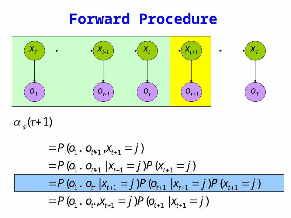
oTo1 otot-1 ot+1
x1 xt+1 xTxtxt-1
Forward Procedure
)1( +tjα
)|()(
)()|()|(
)()|(
)(
1111
11111
1111
111
jxoPjxooP
jxPjxoPjxooP
jxPjxooP
jxooP
tttt
ttttt
ttt
tt
=======
=====
+++
++++
+++
++
oTo1 otot-1 ot+1
x1 xt+1 xTxtxt-1
Forward Procedure
)1( +tjα
)|()(
)()|()|(
)()|(
)(
1111
11111
1111
111
jxoPjxooP
jxPjxoPjxooP
jxPjxooP
jxooP
tttt
ttttt
ttt
tt
=======
=====
+++
++++
+++
++
sum
sum
sum
sum
=
+++=
++=
+
++=
+
+=
=====
=====
====
Nijoiji
ttttNi
tt
tttNi
ttt
ttNi
ttt
tbat
jxoPixjxPixooP
jxoPixPixjxooP
jxoPjxixooP
1
1111
1
111
11
111
11
1)(
)|()|()(
)|()()|(
)|()(
α
oTo1 otot-1 ot+1
x1 xt+1 xTxtxt-1
Forward Procedure
sum
sum
sum
sum
=
+++=
++=
+
++=
+
+=
=====
=====
====
Nijoiji
ttttNi
tt
tttNi
ttt
ttNi
ttt
tbat
jxoPixjxPixooP
jxoPixPixjxooP
jxoPjxixooP
1
1111
1
111
11
111
11
1)(
)|()|()(
)|()()|(
)|()(
α
oTo1 otot-1 ot+1
x1 xt+1 xTxtxt-1
Forward Procedure
sum
sum
sum
sum
=
+++=
++=
+
++=
+
+=
=====
=====
====
Nijoiji
ttttNi
tt
tttNi
ttt
ttNi
ttt
tbat
jxoPixjxPixooP
jxoPixPixjxooP
jxoPjxixooP
1
1111
1
111
11
111
11
1)(
)|()|()(
)|()()|(
)|()(
α
oTo1 otot-1 ot+1
x1 xt+1 xTxtxt-1
Forward Procedure
= P(o1ot xt = i xt+1 = j)i=1Nsum P(ot+1 | xt+1 = j)
= P(o1ot xt+1 = j | xt = i)i=1Nsum P(xt = i)P(ot+1 | xt+1 = j)
= P(o1ot xt = i)i=1Nsum P(xt+1 = j | xt = i)P(ot+1 | xt+1 = j)
= α i (t)aijb jot +1i=1Nsum
oTo1 otot-1 ot+1
x1 xt+1 xTxtxt-1
Forward Procedure
Dynamic Programming
α j (t +1) = α i (t)aijb jot +1i=1Nsum
Complexity O(N 2 T )
Eg N = 5T = 100 gives asymp 3000
βi (t) = P(ot+1oT | xt = i)
oTo1 otot-1 ot+1
x1 xt+1 xTxtxt-1
Backward Procedure
βi (T ) = 1
βi (t) = aijbiot +1β j (t +1)
j=1Nsum
Probability of the rest of the states given the first state
oTo1 otot-1 ot+1
x1 xt+1 xTxtxt-1
Decoding Solution
sum=
=N
ii TOP
1
)()|( αμ
sum=
=N
iiiOP
1
)1()|( βπμ
)()()|(1
ttOP i
N
ii βαμ sum
=
=
Forward Procedure
Backward Procedure
Combination
P(O Xt =i |μ) =P(o1otXt =iot+1oT |μ)=P(o1otXt =i |μ)P(ot+1oT |o1otXt =i μ)=P(o1otXt =i |μ)P(ot+1oT |Xt =i μ)=α i (t)βi (t)
)()()|(1
ttOP i
N
ii βαμ sum
=
=
oTo1 otot-1 ot+1
Best State Sequence
Find the state sequence that best explains the observations
Two approaches bull Individually most likely statesbull Most likely sequence (Viterbi)
)|(maxarg OXPX
Best State Sequence (1)
γi (t) = P(Xt = i | O μ )
=P(Xt = iO | μ )
P(O | μ )
=α i (t)β i (t)
j=1
n
sum α j (t)β j (t)
Most likely state at each point in time
Xt = arg maxγ i (t)
oTo1 otot-1 ot+1
Best State Sequence (2)
Find the state sequence that best explains the observations
Viterbi algorithm
)|(maxarg OXPX
oTo1 otot-1 ot+1
Viterbi Algorithm
)(max)( 1111 11
ttttxx
j ojxooxxPtt
== minusminusminus
δ
The state sequence which maximizes the probability of seeing the observations to time t-1 landing in state j and seeing the observation at time t
x1 xt-1 j
oTo1 otot-1 ot+1
Viterbi Algorithm
)(max)( 1111 11
ttttxx
j ojxooxxPtt
== minusminusminus
δ
1)(max)1(
+=+
tjoijiij batt δδ
1)(maxarg)1(
+=+
tjoijii
j batt δψRecursive Computation
x1 xt-1 xt xt+1
Initialization
δ1(i) = ibio1
ψ 1(i) =0
oTo1 otot-1 ot+1
Viterbi Algorithm
XT =argmaxi
δi (T )
Xt =ψX^
t+1
(t+1)
P(X)=argmaxi
δi (T )
Compute the most likely state sequence by working backwards
x1 xt-1 xt xt+1 xT
oTo1 otot-1 ot+1
HMMs and Bayesian Nets (1)
x1 xt-1 xt xt+1 xT
P(x1xT o1oT )=P(x1)P(o1 |x1) P(xi+1 |xii=1
Tminus1
prod )P(oi+1 |xi+1)
= x1bx1o1
t=1
Tminus1
axtxt+1bxt+1ot+1
oTo1 otot-1 ot+1
x1 xt+1 xTxtxt-1
HMM and Bayesian Nets (2)
Conditionally independent of Given
Because of d-separation
ldquoThe past is independent of the future given the presentrdquo
Inference in an HMM
Compute the probability of a given observation sequence
Given an observation sequence compute the most likely hidden state sequence
Given an observation sequence and set of possible models which model most closely fits the data
Dynamic Programming
oTo1 otot-1 ot+1
Parameter Estimation
bull Given an observation sequence find the model that is most likely to produce that sequence
bull No analytic methodbull Given a model and observation sequence update
the model parameters to better fit the observations
A
B
AAA
BBB B
arg maxμ
P(Otraining |μ)
α i (t) = P(o1ot xt = i | μ )
βi (t) = P(ot+1oT | xt = i)
)()()|(1
ttOP i
N
ii βαμ sum
=
=
pt (i j)=P(Xt =iXt+1 = j |O μ)
=P(Xt =iXt+1 = jO |μ)
P(O |μ)
oTo1 otot-1 ot+1
Parameter Estimation
A
B
AAA
BBB B
pt (i j)=α i (t)aijbjot+1
β j (t+1)
αm(t)βm(t)m=1Nsum
Probability of traversing an arc
sum=
=Nj
ti jipt1
)()(γ Probability of being in state i
oTo1 otot-1 ot+1
Parameter Estimation
A
B
AAA
BBB B
i =γi(1)
Now we can compute the new estimates of the model parameters
aij =pt(i j)t=1
Tminus1sumγi (t)t=1
Tminus1sum
bik =γi (t) tot=ksum
γi (t)t=1
Tsum
Instance of Expectation Maximization
We have that
We may get stuck in local maximum (or even saddle point)
Nevertheless Baum-Welch usually effective
P(O | μ) geP(O |μ)
Some Variants
So far ergodic modelsbull All states are connectedbull Not always wanted
Epsilon or null-transitionsbull Not all statestransitions emit output symbols
Parameter tyingbull Assuming that certain parameters are shared bull Reduces the number of parameters that have to be estimated
Logical HMMs (Kersting De Raedt Raiko)bull Working with structured states and observation symbols
Working with log probabilities and addition instead of multiplication of probabilities (typically done)
oTo1 otot-1 ot+1
The Most Important Thing
A
B
AAA
BBB B
We can use the special structure of this model to do a lot of neat math and solve problems that are otherwise not solvable
HMMrsquos from an Agent Perspective
AI a modern approachbull AI is the study of rational agentsbull Third part by Wolfram Burgard on
Reinforcement learning
HMMs can also be used herebull Typically one is interested in P(state)
Example
Possible statesbull snow no snow
Observationsbull skis no skis
Questionsbull Was there snow the day before yesterday (given a
sequence of observations) bull Is there now snow (given a sequence of
observations) bull Will there be snow tomorrow given a sequence of
observations Next week
HMM and Agents
Question
bull Case 1 often called smoothing t lt T see last time
Only part of trellis between t and T needed
γi (t) = P(Xt = i | Oμ )
=α i (t)β i (t)
j =1
n
sum α j (t)β j (t)
Most likely state at each point in time
HMM and Agents
bull Case 2 often called filtering t= T last time
Can we make it recursive Ie go from T-1 to T
γi (t) = P(Xt = i | Oμ )
=α i (t)β i (t)
j =1
n
sum α j (t)β j (t)
Most likely state at each point in time
HMM and Agents
bull Case 2 often called filtering t= T last time
λi (T ) = P(XT = i | o1oT μ )
= γ i (T )
=α i (T )β i (T )
j =1
n
sum α j (T )β j (T )
=α i (T )
j =1
n
sum α j (T )
HMM and Agents
bull Case 3 often called prediction t= T+1 (or T+K) not yet seen
Interesting recursive Easily extended towards k gt 1
Extensions
Use Dynamic Bayesian networks instead of HMMsbullOne state corresponds to a Bayesian NetbullObservations can become more complex
Involve actions of the agent as wellbullCf Wolfram Burgardrsquos Part
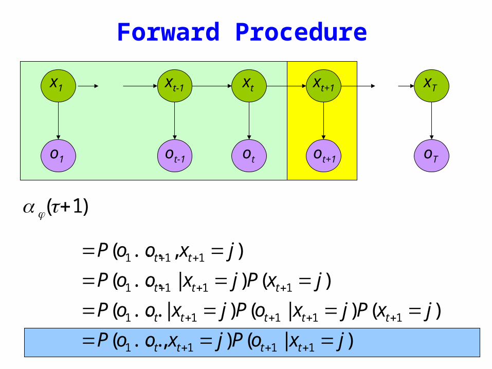
oTo1 otot-1 ot+1
x1 xt+1 xTxtxt-1
Forward Procedure
)1( +tjα
)|()(
)()|()|(
)()|(
)(
1111
11111
1111
111
jxoPjxooP
jxPjxoPjxooP
jxPjxooP
jxooP
tttt
ttttt
ttt
tt
=======
=====
+++
++++
+++
++
sum
sum
sum
sum
=
+++=
++=
+
++=
+
+=
=====
=====
====
Nijoiji
ttttNi
tt
tttNi
ttt
ttNi
ttt
tbat
jxoPixjxPixooP
jxoPixPixjxooP
jxoPjxixooP
1
1111
1
111
11
111
11
1)(
)|()|()(
)|()()|(
)|()(
α
oTo1 otot-1 ot+1
x1 xt+1 xTxtxt-1
Forward Procedure
sum
sum
sum
sum
=
+++=
++=
+
++=
+
+=
=====
=====
====
Nijoiji
ttttNi
tt
tttNi
ttt
ttNi
ttt
tbat
jxoPixjxPixooP
jxoPixPixjxooP
jxoPjxixooP
1
1111
1
111
11
111
11
1)(
)|()|()(
)|()()|(
)|()(
α
oTo1 otot-1 ot+1
x1 xt+1 xTxtxt-1
Forward Procedure
sum
sum
sum
sum
=
+++=
++=
+
++=
+
+=
=====
=====
====
Nijoiji
ttttNi
tt
tttNi
ttt
ttNi
ttt
tbat
jxoPixjxPixooP
jxoPixPixjxooP
jxoPjxixooP
1
1111
1
111
11
111
11
1)(
)|()|()(
)|()()|(
)|()(
α
oTo1 otot-1 ot+1
x1 xt+1 xTxtxt-1
Forward Procedure
= P(o1ot xt = i xt+1 = j)i=1Nsum P(ot+1 | xt+1 = j)
= P(o1ot xt+1 = j | xt = i)i=1Nsum P(xt = i)P(ot+1 | xt+1 = j)
= P(o1ot xt = i)i=1Nsum P(xt+1 = j | xt = i)P(ot+1 | xt+1 = j)
= α i (t)aijb jot +1i=1Nsum
oTo1 otot-1 ot+1
x1 xt+1 xTxtxt-1
Forward Procedure
Dynamic Programming
α j (t +1) = α i (t)aijb jot +1i=1Nsum
Complexity O(N 2 T )
Eg N = 5T = 100 gives asymp 3000
βi (t) = P(ot+1oT | xt = i)
oTo1 otot-1 ot+1
x1 xt+1 xTxtxt-1
Backward Procedure
βi (T ) = 1
βi (t) = aijbiot +1β j (t +1)
j=1Nsum
Probability of the rest of the states given the first state
oTo1 otot-1 ot+1
x1 xt+1 xTxtxt-1
Decoding Solution
sum=
=N
ii TOP
1
)()|( αμ
sum=
=N
iiiOP
1
)1()|( βπμ
)()()|(1
ttOP i
N
ii βαμ sum
=
=
Forward Procedure
Backward Procedure
Combination
P(O Xt =i |μ) =P(o1otXt =iot+1oT |μ)=P(o1otXt =i |μ)P(ot+1oT |o1otXt =i μ)=P(o1otXt =i |μ)P(ot+1oT |Xt =i μ)=α i (t)βi (t)
)()()|(1
ttOP i
N
ii βαμ sum
=
=
oTo1 otot-1 ot+1
Best State Sequence
Find the state sequence that best explains the observations
Two approaches bull Individually most likely statesbull Most likely sequence (Viterbi)
)|(maxarg OXPX
Best State Sequence (1)
γi (t) = P(Xt = i | O μ )
=P(Xt = iO | μ )
P(O | μ )
=α i (t)β i (t)
j=1
n
sum α j (t)β j (t)
Most likely state at each point in time
Xt = arg maxγ i (t)
oTo1 otot-1 ot+1
Best State Sequence (2)
Find the state sequence that best explains the observations
Viterbi algorithm
)|(maxarg OXPX
oTo1 otot-1 ot+1
Viterbi Algorithm
)(max)( 1111 11
ttttxx
j ojxooxxPtt
== minusminusminus
δ
The state sequence which maximizes the probability of seeing the observations to time t-1 landing in state j and seeing the observation at time t
x1 xt-1 j
oTo1 otot-1 ot+1
Viterbi Algorithm
)(max)( 1111 11
ttttxx
j ojxooxxPtt
== minusminusminus
δ
1)(max)1(
+=+
tjoijiij batt δδ
1)(maxarg)1(
+=+
tjoijii
j batt δψRecursive Computation
x1 xt-1 xt xt+1
Initialization
δ1(i) = ibio1
ψ 1(i) =0
oTo1 otot-1 ot+1
Viterbi Algorithm
XT =argmaxi
δi (T )
Xt =ψX^
t+1
(t+1)
P(X)=argmaxi
δi (T )
Compute the most likely state sequence by working backwards
x1 xt-1 xt xt+1 xT
oTo1 otot-1 ot+1
HMMs and Bayesian Nets (1)
x1 xt-1 xt xt+1 xT
P(x1xT o1oT )=P(x1)P(o1 |x1) P(xi+1 |xii=1
Tminus1
prod )P(oi+1 |xi+1)
= x1bx1o1
t=1
Tminus1
axtxt+1bxt+1ot+1
oTo1 otot-1 ot+1
x1 xt+1 xTxtxt-1
HMM and Bayesian Nets (2)
Conditionally independent of Given
Because of d-separation
ldquoThe past is independent of the future given the presentrdquo
Inference in an HMM
Compute the probability of a given observation sequence
Given an observation sequence compute the most likely hidden state sequence
Given an observation sequence and set of possible models which model most closely fits the data
Dynamic Programming
oTo1 otot-1 ot+1
Parameter Estimation
bull Given an observation sequence find the model that is most likely to produce that sequence
bull No analytic methodbull Given a model and observation sequence update
the model parameters to better fit the observations
A
B
AAA
BBB B
arg maxμ
P(Otraining |μ)
α i (t) = P(o1ot xt = i | μ )
βi (t) = P(ot+1oT | xt = i)
)()()|(1
ttOP i
N
ii βαμ sum
=
=
pt (i j)=P(Xt =iXt+1 = j |O μ)
=P(Xt =iXt+1 = jO |μ)
P(O |μ)
oTo1 otot-1 ot+1
Parameter Estimation
A
B
AAA
BBB B
pt (i j)=α i (t)aijbjot+1
β j (t+1)
αm(t)βm(t)m=1Nsum
Probability of traversing an arc
sum=
=Nj
ti jipt1
)()(γ Probability of being in state i
oTo1 otot-1 ot+1
Parameter Estimation
A
B
AAA
BBB B
i =γi(1)
Now we can compute the new estimates of the model parameters
aij =pt(i j)t=1
Tminus1sumγi (t)t=1
Tminus1sum
bik =γi (t) tot=ksum
γi (t)t=1
Tsum
Instance of Expectation Maximization
We have that
We may get stuck in local maximum (or even saddle point)
Nevertheless Baum-Welch usually effective
P(O | μ) geP(O |μ)
Some Variants
So far ergodic modelsbull All states are connectedbull Not always wanted
Epsilon or null-transitionsbull Not all statestransitions emit output symbols
Parameter tyingbull Assuming that certain parameters are shared bull Reduces the number of parameters that have to be estimated
Logical HMMs (Kersting De Raedt Raiko)bull Working with structured states and observation symbols
Working with log probabilities and addition instead of multiplication of probabilities (typically done)
oTo1 otot-1 ot+1
The Most Important Thing
A
B
AAA
BBB B
We can use the special structure of this model to do a lot of neat math and solve problems that are otherwise not solvable
HMMrsquos from an Agent Perspective
AI a modern approachbull AI is the study of rational agentsbull Third part by Wolfram Burgard on
Reinforcement learning
HMMs can also be used herebull Typically one is interested in P(state)
Example
Possible statesbull snow no snow
Observationsbull skis no skis
Questionsbull Was there snow the day before yesterday (given a
sequence of observations) bull Is there now snow (given a sequence of
observations) bull Will there be snow tomorrow given a sequence of
observations Next week
HMM and Agents
Question
bull Case 1 often called smoothing t lt T see last time
Only part of trellis between t and T needed
γi (t) = P(Xt = i | Oμ )
=α i (t)β i (t)
j =1
n
sum α j (t)β j (t)
Most likely state at each point in time
HMM and Agents
bull Case 2 often called filtering t= T last time
Can we make it recursive Ie go from T-1 to T
γi (t) = P(Xt = i | Oμ )
=α i (t)β i (t)
j =1
n
sum α j (t)β j (t)
Most likely state at each point in time
HMM and Agents
bull Case 2 often called filtering t= T last time
λi (T ) = P(XT = i | o1oT μ )
= γ i (T )
=α i (T )β i (T )
j =1
n
sum α j (T )β j (T )
=α i (T )
j =1
n
sum α j (T )
HMM and Agents
bull Case 3 often called prediction t= T+1 (or T+K) not yet seen
Interesting recursive Easily extended towards k gt 1
Extensions
Use Dynamic Bayesian networks instead of HMMsbullOne state corresponds to a Bayesian NetbullObservations can become more complex
Involve actions of the agent as wellbullCf Wolfram Burgardrsquos Part
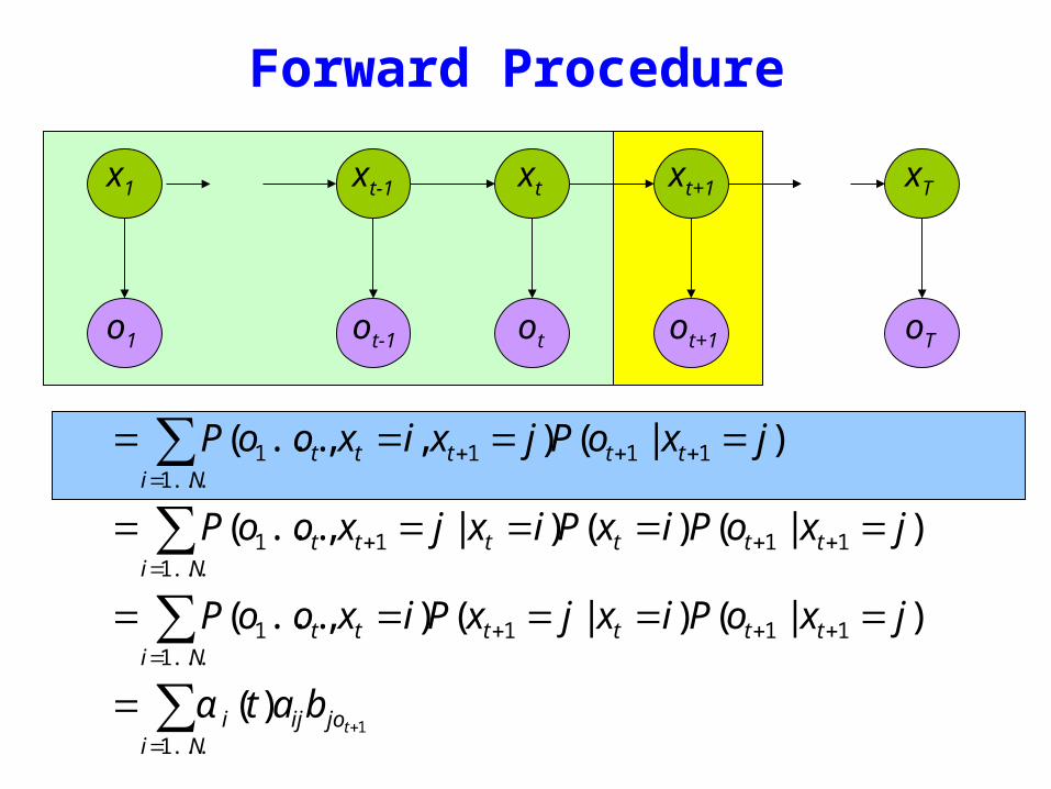
sum
sum
sum
sum
=
+++=
++=
+
++=
+
+=
=====
=====
====
Nijoiji
ttttNi
tt
tttNi
ttt
ttNi
ttt
tbat
jxoPixjxPixooP
jxoPixPixjxooP
jxoPjxixooP
1
1111
1
111
11
111
11
1)(
)|()|()(
)|()()|(
)|()(
α
oTo1 otot-1 ot+1
x1 xt+1 xTxtxt-1
Forward Procedure
sum
sum
sum
sum
=
+++=
++=
+
++=
+
+=
=====
=====
====
Nijoiji
ttttNi
tt
tttNi
ttt
ttNi
ttt
tbat
jxoPixjxPixooP
jxoPixPixjxooP
jxoPjxixooP
1
1111
1
111
11
111
11
1)(
)|()|()(
)|()()|(
)|()(
α
oTo1 otot-1 ot+1
x1 xt+1 xTxtxt-1
Forward Procedure
sum
sum
sum
sum
=
+++=
++=
+
++=
+
+=
=====
=====
====
Nijoiji
ttttNi
tt
tttNi
ttt
ttNi
ttt
tbat
jxoPixjxPixooP
jxoPixPixjxooP
jxoPjxixooP
1
1111
1
111
11
111
11
1)(
)|()|()(
)|()()|(
)|()(
α
oTo1 otot-1 ot+1
x1 xt+1 xTxtxt-1
Forward Procedure
= P(o1ot xt = i xt+1 = j)i=1Nsum P(ot+1 | xt+1 = j)
= P(o1ot xt+1 = j | xt = i)i=1Nsum P(xt = i)P(ot+1 | xt+1 = j)
= P(o1ot xt = i)i=1Nsum P(xt+1 = j | xt = i)P(ot+1 | xt+1 = j)
= α i (t)aijb jot +1i=1Nsum
oTo1 otot-1 ot+1
x1 xt+1 xTxtxt-1
Forward Procedure
Dynamic Programming
α j (t +1) = α i (t)aijb jot +1i=1Nsum
Complexity O(N 2 T )
Eg N = 5T = 100 gives asymp 3000
βi (t) = P(ot+1oT | xt = i)
oTo1 otot-1 ot+1
x1 xt+1 xTxtxt-1
Backward Procedure
βi (T ) = 1
βi (t) = aijbiot +1β j (t +1)
j=1Nsum
Probability of the rest of the states given the first state
oTo1 otot-1 ot+1
x1 xt+1 xTxtxt-1
Decoding Solution
sum=
=N
ii TOP
1
)()|( αμ
sum=
=N
iiiOP
1
)1()|( βπμ
)()()|(1
ttOP i
N
ii βαμ sum
=
=
Forward Procedure
Backward Procedure
Combination
P(O Xt =i |μ) =P(o1otXt =iot+1oT |μ)=P(o1otXt =i |μ)P(ot+1oT |o1otXt =i μ)=P(o1otXt =i |μ)P(ot+1oT |Xt =i μ)=α i (t)βi (t)
)()()|(1
ttOP i
N
ii βαμ sum
=
=
oTo1 otot-1 ot+1
Best State Sequence
Find the state sequence that best explains the observations
Two approaches bull Individually most likely statesbull Most likely sequence (Viterbi)
)|(maxarg OXPX
Best State Sequence (1)
γi (t) = P(Xt = i | O μ )
=P(Xt = iO | μ )
P(O | μ )
=α i (t)β i (t)
j=1
n
sum α j (t)β j (t)
Most likely state at each point in time
Xt = arg maxγ i (t)
oTo1 otot-1 ot+1
Best State Sequence (2)
Find the state sequence that best explains the observations
Viterbi algorithm
)|(maxarg OXPX
oTo1 otot-1 ot+1
Viterbi Algorithm
)(max)( 1111 11
ttttxx
j ojxooxxPtt
== minusminusminus
δ
The state sequence which maximizes the probability of seeing the observations to time t-1 landing in state j and seeing the observation at time t
x1 xt-1 j
oTo1 otot-1 ot+1
Viterbi Algorithm
)(max)( 1111 11
ttttxx
j ojxooxxPtt
== minusminusminus
δ
1)(max)1(
+=+
tjoijiij batt δδ
1)(maxarg)1(
+=+
tjoijii
j batt δψRecursive Computation
x1 xt-1 xt xt+1
Initialization
δ1(i) = ibio1
ψ 1(i) =0
oTo1 otot-1 ot+1
Viterbi Algorithm
XT =argmaxi
δi (T )
Xt =ψX^
t+1
(t+1)
P(X)=argmaxi
δi (T )
Compute the most likely state sequence by working backwards
x1 xt-1 xt xt+1 xT
oTo1 otot-1 ot+1
HMMs and Bayesian Nets (1)
x1 xt-1 xt xt+1 xT
P(x1xT o1oT )=P(x1)P(o1 |x1) P(xi+1 |xii=1
Tminus1
prod )P(oi+1 |xi+1)
= x1bx1o1
t=1
Tminus1
axtxt+1bxt+1ot+1
oTo1 otot-1 ot+1
x1 xt+1 xTxtxt-1
HMM and Bayesian Nets (2)
Conditionally independent of Given
Because of d-separation
ldquoThe past is independent of the future given the presentrdquo
Inference in an HMM
Compute the probability of a given observation sequence
Given an observation sequence compute the most likely hidden state sequence
Given an observation sequence and set of possible models which model most closely fits the data
Dynamic Programming
oTo1 otot-1 ot+1
Parameter Estimation
bull Given an observation sequence find the model that is most likely to produce that sequence
bull No analytic methodbull Given a model and observation sequence update
the model parameters to better fit the observations
A
B
AAA
BBB B
arg maxμ
P(Otraining |μ)
α i (t) = P(o1ot xt = i | μ )
βi (t) = P(ot+1oT | xt = i)
)()()|(1
ttOP i
N
ii βαμ sum
=
=
pt (i j)=P(Xt =iXt+1 = j |O μ)
=P(Xt =iXt+1 = jO |μ)
P(O |μ)
oTo1 otot-1 ot+1
Parameter Estimation
A
B
AAA
BBB B
pt (i j)=α i (t)aijbjot+1
β j (t+1)
αm(t)βm(t)m=1Nsum
Probability of traversing an arc
sum=
=Nj
ti jipt1
)()(γ Probability of being in state i
oTo1 otot-1 ot+1
Parameter Estimation
A
B
AAA
BBB B
i =γi(1)
Now we can compute the new estimates of the model parameters
aij =pt(i j)t=1
Tminus1sumγi (t)t=1
Tminus1sum
bik =γi (t) tot=ksum
γi (t)t=1
Tsum
Instance of Expectation Maximization
We have that
We may get stuck in local maximum (or even saddle point)
Nevertheless Baum-Welch usually effective
P(O | μ) geP(O |μ)
Some Variants
So far ergodic modelsbull All states are connectedbull Not always wanted
Epsilon or null-transitionsbull Not all statestransitions emit output symbols
Parameter tyingbull Assuming that certain parameters are shared bull Reduces the number of parameters that have to be estimated
Logical HMMs (Kersting De Raedt Raiko)bull Working with structured states and observation symbols
Working with log probabilities and addition instead of multiplication of probabilities (typically done)
oTo1 otot-1 ot+1
The Most Important Thing
A
B
AAA
BBB B
We can use the special structure of this model to do a lot of neat math and solve problems that are otherwise not solvable
HMMrsquos from an Agent Perspective
AI a modern approachbull AI is the study of rational agentsbull Third part by Wolfram Burgard on
Reinforcement learning
HMMs can also be used herebull Typically one is interested in P(state)
Example
Possible statesbull snow no snow
Observationsbull skis no skis
Questionsbull Was there snow the day before yesterday (given a
sequence of observations) bull Is there now snow (given a sequence of
observations) bull Will there be snow tomorrow given a sequence of
observations Next week
HMM and Agents
Question
bull Case 1 often called smoothing t lt T see last time
Only part of trellis between t and T needed
γi (t) = P(Xt = i | Oμ )
=α i (t)β i (t)
j =1
n
sum α j (t)β j (t)
Most likely state at each point in time
HMM and Agents
bull Case 2 often called filtering t= T last time
Can we make it recursive Ie go from T-1 to T
γi (t) = P(Xt = i | Oμ )
=α i (t)β i (t)
j =1
n
sum α j (t)β j (t)
Most likely state at each point in time
HMM and Agents
bull Case 2 often called filtering t= T last time
λi (T ) = P(XT = i | o1oT μ )
= γ i (T )
=α i (T )β i (T )
j =1
n
sum α j (T )β j (T )
=α i (T )
j =1
n
sum α j (T )
HMM and Agents
bull Case 3 often called prediction t= T+1 (or T+K) not yet seen
Interesting recursive Easily extended towards k gt 1
Extensions
Use Dynamic Bayesian networks instead of HMMsbullOne state corresponds to a Bayesian NetbullObservations can become more complex
Involve actions of the agent as wellbullCf Wolfram Burgardrsquos Part
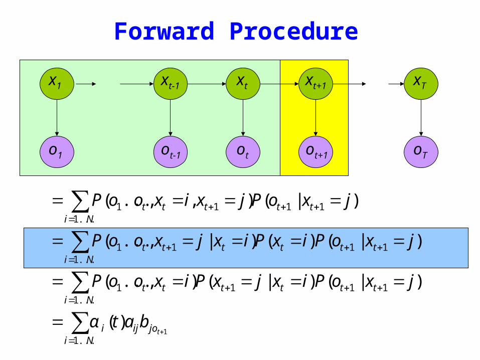
sum
sum
sum
sum
=
+++=
++=
+
++=
+
+=
=====
=====
====
Nijoiji
ttttNi
tt
tttNi
ttt
ttNi
ttt
tbat
jxoPixjxPixooP
jxoPixPixjxooP
jxoPjxixooP
1
1111
1
111
11
111
11
1)(
)|()|()(
)|()()|(
)|()(
α
oTo1 otot-1 ot+1
x1 xt+1 xTxtxt-1
Forward Procedure
sum
sum
sum
sum
=
+++=
++=
+
++=
+
+=
=====
=====
====
Nijoiji
ttttNi
tt
tttNi
ttt
ttNi
ttt
tbat
jxoPixjxPixooP
jxoPixPixjxooP
jxoPjxixooP
1
1111
1
111
11
111
11
1)(
)|()|()(
)|()()|(
)|()(
α
oTo1 otot-1 ot+1
x1 xt+1 xTxtxt-1
Forward Procedure
= P(o1ot xt = i xt+1 = j)i=1Nsum P(ot+1 | xt+1 = j)
= P(o1ot xt+1 = j | xt = i)i=1Nsum P(xt = i)P(ot+1 | xt+1 = j)
= P(o1ot xt = i)i=1Nsum P(xt+1 = j | xt = i)P(ot+1 | xt+1 = j)
= α i (t)aijb jot +1i=1Nsum
oTo1 otot-1 ot+1
x1 xt+1 xTxtxt-1
Forward Procedure
Dynamic Programming
α j (t +1) = α i (t)aijb jot +1i=1Nsum
Complexity O(N 2 T )
Eg N = 5T = 100 gives asymp 3000
βi (t) = P(ot+1oT | xt = i)
oTo1 otot-1 ot+1
x1 xt+1 xTxtxt-1
Backward Procedure
βi (T ) = 1
βi (t) = aijbiot +1β j (t +1)
j=1Nsum
Probability of the rest of the states given the first state
oTo1 otot-1 ot+1
x1 xt+1 xTxtxt-1
Decoding Solution
sum=
=N
ii TOP
1
)()|( αμ
sum=
=N
iiiOP
1
)1()|( βπμ
)()()|(1
ttOP i
N
ii βαμ sum
=
=
Forward Procedure
Backward Procedure
Combination
P(O Xt =i |μ) =P(o1otXt =iot+1oT |μ)=P(o1otXt =i |μ)P(ot+1oT |o1otXt =i μ)=P(o1otXt =i |μ)P(ot+1oT |Xt =i μ)=α i (t)βi (t)
)()()|(1
ttOP i
N
ii βαμ sum
=
=
oTo1 otot-1 ot+1
Best State Sequence
Find the state sequence that best explains the observations
Two approaches bull Individually most likely statesbull Most likely sequence (Viterbi)
)|(maxarg OXPX
Best State Sequence (1)
γi (t) = P(Xt = i | O μ )
=P(Xt = iO | μ )
P(O | μ )
=α i (t)β i (t)
j=1
n
sum α j (t)β j (t)
Most likely state at each point in time
Xt = arg maxγ i (t)
oTo1 otot-1 ot+1
Best State Sequence (2)
Find the state sequence that best explains the observations
Viterbi algorithm
)|(maxarg OXPX
oTo1 otot-1 ot+1
Viterbi Algorithm
)(max)( 1111 11
ttttxx
j ojxooxxPtt
== minusminusminus
δ
The state sequence which maximizes the probability of seeing the observations to time t-1 landing in state j and seeing the observation at time t
x1 xt-1 j
oTo1 otot-1 ot+1
Viterbi Algorithm
)(max)( 1111 11
ttttxx
j ojxooxxPtt
== minusminusminus
δ
1)(max)1(
+=+
tjoijiij batt δδ
1)(maxarg)1(
+=+
tjoijii
j batt δψRecursive Computation
x1 xt-1 xt xt+1
Initialization
δ1(i) = ibio1
ψ 1(i) =0
oTo1 otot-1 ot+1
Viterbi Algorithm
XT =argmaxi
δi (T )
Xt =ψX^
t+1
(t+1)
P(X)=argmaxi
δi (T )
Compute the most likely state sequence by working backwards
x1 xt-1 xt xt+1 xT
oTo1 otot-1 ot+1
HMMs and Bayesian Nets (1)
x1 xt-1 xt xt+1 xT
P(x1xT o1oT )=P(x1)P(o1 |x1) P(xi+1 |xii=1
Tminus1
prod )P(oi+1 |xi+1)
= x1bx1o1
t=1
Tminus1
axtxt+1bxt+1ot+1
oTo1 otot-1 ot+1
x1 xt+1 xTxtxt-1
HMM and Bayesian Nets (2)
Conditionally independent of Given
Because of d-separation
ldquoThe past is independent of the future given the presentrdquo
Inference in an HMM
Compute the probability of a given observation sequence
Given an observation sequence compute the most likely hidden state sequence
Given an observation sequence and set of possible models which model most closely fits the data
Dynamic Programming
oTo1 otot-1 ot+1
Parameter Estimation
bull Given an observation sequence find the model that is most likely to produce that sequence
bull No analytic methodbull Given a model and observation sequence update
the model parameters to better fit the observations
A
B
AAA
BBB B
arg maxμ
P(Otraining |μ)
α i (t) = P(o1ot xt = i | μ )
βi (t) = P(ot+1oT | xt = i)
)()()|(1
ttOP i
N
ii βαμ sum
=
=
pt (i j)=P(Xt =iXt+1 = j |O μ)
=P(Xt =iXt+1 = jO |μ)
P(O |μ)
oTo1 otot-1 ot+1
Parameter Estimation
A
B
AAA
BBB B
pt (i j)=α i (t)aijbjot+1
β j (t+1)
αm(t)βm(t)m=1Nsum
Probability of traversing an arc
sum=
=Nj
ti jipt1
)()(γ Probability of being in state i
oTo1 otot-1 ot+1
Parameter Estimation
A
B
AAA
BBB B
i =γi(1)
Now we can compute the new estimates of the model parameters
aij =pt(i j)t=1
Tminus1sumγi (t)t=1
Tminus1sum
bik =γi (t) tot=ksum
γi (t)t=1
Tsum
Instance of Expectation Maximization
We have that
We may get stuck in local maximum (or even saddle point)
Nevertheless Baum-Welch usually effective
P(O | μ) geP(O |μ)
Some Variants
So far ergodic modelsbull All states are connectedbull Not always wanted
Epsilon or null-transitionsbull Not all statestransitions emit output symbols
Parameter tyingbull Assuming that certain parameters are shared bull Reduces the number of parameters that have to be estimated
Logical HMMs (Kersting De Raedt Raiko)bull Working with structured states and observation symbols
Working with log probabilities and addition instead of multiplication of probabilities (typically done)
oTo1 otot-1 ot+1
The Most Important Thing
A
B
AAA
BBB B
We can use the special structure of this model to do a lot of neat math and solve problems that are otherwise not solvable
HMMrsquos from an Agent Perspective
AI a modern approachbull AI is the study of rational agentsbull Third part by Wolfram Burgard on
Reinforcement learning
HMMs can also be used herebull Typically one is interested in P(state)
Example
Possible statesbull snow no snow
Observationsbull skis no skis
Questionsbull Was there snow the day before yesterday (given a
sequence of observations) bull Is there now snow (given a sequence of
observations) bull Will there be snow tomorrow given a sequence of
observations Next week
HMM and Agents
Question
bull Case 1 often called smoothing t lt T see last time
Only part of trellis between t and T needed
γi (t) = P(Xt = i | Oμ )
=α i (t)β i (t)
j =1
n
sum α j (t)β j (t)
Most likely state at each point in time
HMM and Agents
bull Case 2 often called filtering t= T last time
Can we make it recursive Ie go from T-1 to T
γi (t) = P(Xt = i | Oμ )
=α i (t)β i (t)
j =1
n
sum α j (t)β j (t)
Most likely state at each point in time
HMM and Agents
bull Case 2 often called filtering t= T last time
λi (T ) = P(XT = i | o1oT μ )
= γ i (T )
=α i (T )β i (T )
j =1
n
sum α j (T )β j (T )
=α i (T )
j =1
n
sum α j (T )
HMM and Agents
bull Case 3 often called prediction t= T+1 (or T+K) not yet seen
Interesting recursive Easily extended towards k gt 1
Extensions
Use Dynamic Bayesian networks instead of HMMsbullOne state corresponds to a Bayesian NetbullObservations can become more complex
Involve actions of the agent as wellbullCf Wolfram Burgardrsquos Part
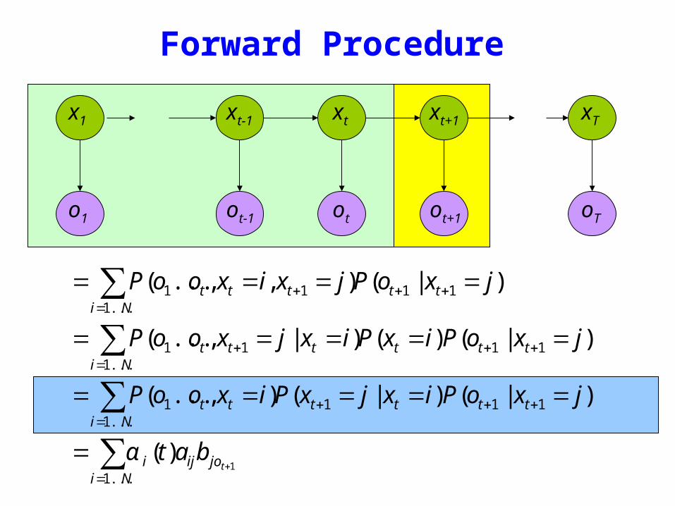
sum
sum
sum
sum
=
+++=
++=
+
++=
+
+=
=====
=====
====
Nijoiji
ttttNi
tt
tttNi
ttt
ttNi
ttt
tbat
jxoPixjxPixooP
jxoPixPixjxooP
jxoPjxixooP
1
1111
1
111
11
111
11
1)(
)|()|()(
)|()()|(
)|()(
α
oTo1 otot-1 ot+1
x1 xt+1 xTxtxt-1
Forward Procedure
= P(o1ot xt = i xt+1 = j)i=1Nsum P(ot+1 | xt+1 = j)
= P(o1ot xt+1 = j | xt = i)i=1Nsum P(xt = i)P(ot+1 | xt+1 = j)
= P(o1ot xt = i)i=1Nsum P(xt+1 = j | xt = i)P(ot+1 | xt+1 = j)
= α i (t)aijb jot +1i=1Nsum
oTo1 otot-1 ot+1
x1 xt+1 xTxtxt-1
Forward Procedure
Dynamic Programming
α j (t +1) = α i (t)aijb jot +1i=1Nsum
Complexity O(N 2 T )
Eg N = 5T = 100 gives asymp 3000
βi (t) = P(ot+1oT | xt = i)
oTo1 otot-1 ot+1
x1 xt+1 xTxtxt-1
Backward Procedure
βi (T ) = 1
βi (t) = aijbiot +1β j (t +1)
j=1Nsum
Probability of the rest of the states given the first state
oTo1 otot-1 ot+1
x1 xt+1 xTxtxt-1
Decoding Solution
sum=
=N
ii TOP
1
)()|( αμ
sum=
=N
iiiOP
1
)1()|( βπμ
)()()|(1
ttOP i
N
ii βαμ sum
=
=
Forward Procedure
Backward Procedure
Combination
P(O Xt =i |μ) =P(o1otXt =iot+1oT |μ)=P(o1otXt =i |μ)P(ot+1oT |o1otXt =i μ)=P(o1otXt =i |μ)P(ot+1oT |Xt =i μ)=α i (t)βi (t)
)()()|(1
ttOP i
N
ii βαμ sum
=
=
oTo1 otot-1 ot+1
Best State Sequence
Find the state sequence that best explains the observations
Two approaches bull Individually most likely statesbull Most likely sequence (Viterbi)
)|(maxarg OXPX
Best State Sequence (1)
γi (t) = P(Xt = i | O μ )
=P(Xt = iO | μ )
P(O | μ )
=α i (t)β i (t)
j=1
n
sum α j (t)β j (t)
Most likely state at each point in time
Xt = arg maxγ i (t)
oTo1 otot-1 ot+1
Best State Sequence (2)
Find the state sequence that best explains the observations
Viterbi algorithm
)|(maxarg OXPX
oTo1 otot-1 ot+1
Viterbi Algorithm
)(max)( 1111 11
ttttxx
j ojxooxxPtt
== minusminusminus
δ
The state sequence which maximizes the probability of seeing the observations to time t-1 landing in state j and seeing the observation at time t
x1 xt-1 j
oTo1 otot-1 ot+1
Viterbi Algorithm
)(max)( 1111 11
ttttxx
j ojxooxxPtt
== minusminusminus
δ
1)(max)1(
+=+
tjoijiij batt δδ
1)(maxarg)1(
+=+
tjoijii
j batt δψRecursive Computation
x1 xt-1 xt xt+1
Initialization
δ1(i) = ibio1
ψ 1(i) =0
oTo1 otot-1 ot+1
Viterbi Algorithm
XT =argmaxi
δi (T )
Xt =ψX^
t+1
(t+1)
P(X)=argmaxi
δi (T )
Compute the most likely state sequence by working backwards
x1 xt-1 xt xt+1 xT
oTo1 otot-1 ot+1
HMMs and Bayesian Nets (1)
x1 xt-1 xt xt+1 xT
P(x1xT o1oT )=P(x1)P(o1 |x1) P(xi+1 |xii=1
Tminus1
prod )P(oi+1 |xi+1)
= x1bx1o1
t=1
Tminus1
axtxt+1bxt+1ot+1
oTo1 otot-1 ot+1
x1 xt+1 xTxtxt-1
HMM and Bayesian Nets (2)
Conditionally independent of Given
Because of d-separation
ldquoThe past is independent of the future given the presentrdquo
Inference in an HMM
Compute the probability of a given observation sequence
Given an observation sequence compute the most likely hidden state sequence
Given an observation sequence and set of possible models which model most closely fits the data
Dynamic Programming
oTo1 otot-1 ot+1
Parameter Estimation
bull Given an observation sequence find the model that is most likely to produce that sequence
bull No analytic methodbull Given a model and observation sequence update
the model parameters to better fit the observations
A
B
AAA
BBB B
arg maxμ
P(Otraining |μ)
α i (t) = P(o1ot xt = i | μ )
βi (t) = P(ot+1oT | xt = i)
)()()|(1
ttOP i
N
ii βαμ sum
=
=
pt (i j)=P(Xt =iXt+1 = j |O μ)
=P(Xt =iXt+1 = jO |μ)
P(O |μ)
oTo1 otot-1 ot+1
Parameter Estimation
A
B
AAA
BBB B
pt (i j)=α i (t)aijbjot+1
β j (t+1)
αm(t)βm(t)m=1Nsum
Probability of traversing an arc
sum=
=Nj
ti jipt1
)()(γ Probability of being in state i
oTo1 otot-1 ot+1
Parameter Estimation
A
B
AAA
BBB B
i =γi(1)
Now we can compute the new estimates of the model parameters
aij =pt(i j)t=1
Tminus1sumγi (t)t=1
Tminus1sum
bik =γi (t) tot=ksum
γi (t)t=1
Tsum
Instance of Expectation Maximization
We have that
We may get stuck in local maximum (or even saddle point)
Nevertheless Baum-Welch usually effective
P(O | μ) geP(O |μ)
Some Variants
So far ergodic modelsbull All states are connectedbull Not always wanted
Epsilon or null-transitionsbull Not all statestransitions emit output symbols
Parameter tyingbull Assuming that certain parameters are shared bull Reduces the number of parameters that have to be estimated
Logical HMMs (Kersting De Raedt Raiko)bull Working with structured states and observation symbols
Working with log probabilities and addition instead of multiplication of probabilities (typically done)
oTo1 otot-1 ot+1
The Most Important Thing
A
B
AAA
BBB B
We can use the special structure of this model to do a lot of neat math and solve problems that are otherwise not solvable
HMMrsquos from an Agent Perspective
AI a modern approachbull AI is the study of rational agentsbull Third part by Wolfram Burgard on
Reinforcement learning
HMMs can also be used herebull Typically one is interested in P(state)
Example
Possible statesbull snow no snow
Observationsbull skis no skis
Questionsbull Was there snow the day before yesterday (given a
sequence of observations) bull Is there now snow (given a sequence of
observations) bull Will there be snow tomorrow given a sequence of
observations Next week
HMM and Agents
Question
bull Case 1 often called smoothing t lt T see last time
Only part of trellis between t and T needed
γi (t) = P(Xt = i | Oμ )
=α i (t)β i (t)
j =1
n
sum α j (t)β j (t)
Most likely state at each point in time
HMM and Agents
bull Case 2 often called filtering t= T last time
Can we make it recursive Ie go from T-1 to T
γi (t) = P(Xt = i | Oμ )
=α i (t)β i (t)
j =1
n
sum α j (t)β j (t)
Most likely state at each point in time
HMM and Agents
bull Case 2 often called filtering t= T last time
λi (T ) = P(XT = i | o1oT μ )
= γ i (T )
=α i (T )β i (T )
j =1
n
sum α j (T )β j (T )
=α i (T )
j =1
n
sum α j (T )
HMM and Agents
bull Case 3 often called prediction t= T+1 (or T+K) not yet seen
Interesting recursive Easily extended towards k gt 1
Extensions
Use Dynamic Bayesian networks instead of HMMsbullOne state corresponds to a Bayesian NetbullObservations can become more complex
Involve actions of the agent as wellbullCf Wolfram Burgardrsquos Part
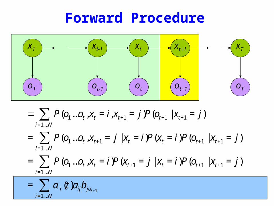
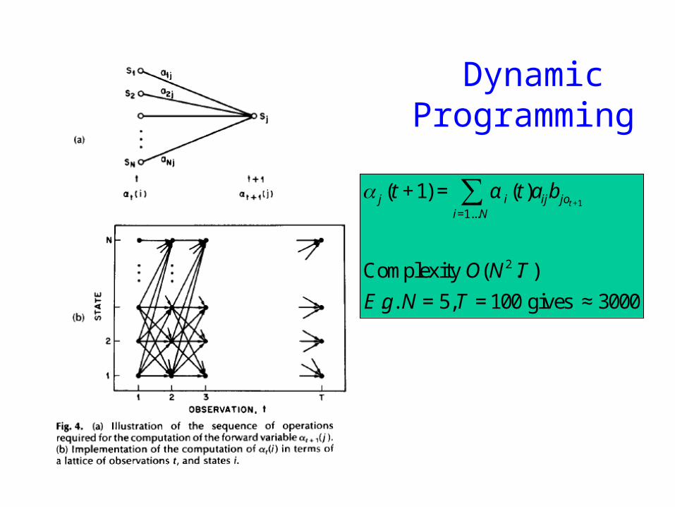
Dynamic Programming
α j (t +1) = α i (t)aijb jot +1i=1Nsum
Complexity O(N 2 T )
Eg N = 5T = 100 gives asymp 3000
βi (t) = P(ot+1oT | xt = i)
oTo1 otot-1 ot+1
x1 xt+1 xTxtxt-1
Backward Procedure
βi (T ) = 1
βi (t) = aijbiot +1β j (t +1)
j=1Nsum
Probability of the rest of the states given the first state
oTo1 otot-1 ot+1
x1 xt+1 xTxtxt-1
Decoding Solution
sum=
=N
ii TOP
1
)()|( αμ
sum=
=N
iiiOP
1
)1()|( βπμ
)()()|(1
ttOP i
N
ii βαμ sum
=
=
Forward Procedure
Backward Procedure
Combination
P(O Xt =i |μ) =P(o1otXt =iot+1oT |μ)=P(o1otXt =i |μ)P(ot+1oT |o1otXt =i μ)=P(o1otXt =i |μ)P(ot+1oT |Xt =i μ)=α i (t)βi (t)
)()()|(1
ttOP i
N
ii βαμ sum
=
=
oTo1 otot-1 ot+1
Best State Sequence
Find the state sequence that best explains the observations
Two approaches bull Individually most likely statesbull Most likely sequence (Viterbi)
)|(maxarg OXPX
Best State Sequence (1)
γi (t) = P(Xt = i | O μ )
=P(Xt = iO | μ )
P(O | μ )
=α i (t)β i (t)
j=1
n
sum α j (t)β j (t)
Most likely state at each point in time
Xt = arg maxγ i (t)
oTo1 otot-1 ot+1
Best State Sequence (2)
Find the state sequence that best explains the observations
Viterbi algorithm
)|(maxarg OXPX
oTo1 otot-1 ot+1
Viterbi Algorithm
)(max)( 1111 11
ttttxx
j ojxooxxPtt
== minusminusminus
δ
The state sequence which maximizes the probability of seeing the observations to time t-1 landing in state j and seeing the observation at time t
x1 xt-1 j
oTo1 otot-1 ot+1
Viterbi Algorithm
)(max)( 1111 11
ttttxx
j ojxooxxPtt
== minusminusminus
δ
1)(max)1(
+=+
tjoijiij batt δδ
1)(maxarg)1(
+=+
tjoijii
j batt δψRecursive Computation
x1 xt-1 xt xt+1
Initialization
δ1(i) = ibio1
ψ 1(i) =0
oTo1 otot-1 ot+1
Viterbi Algorithm
XT =argmaxi
δi (T )
Xt =ψX^
t+1
(t+1)
P(X)=argmaxi
δi (T )
Compute the most likely state sequence by working backwards
x1 xt-1 xt xt+1 xT
oTo1 otot-1 ot+1
HMMs and Bayesian Nets (1)
x1 xt-1 xt xt+1 xT
P(x1xT o1oT )=P(x1)P(o1 |x1) P(xi+1 |xii=1
Tminus1
prod )P(oi+1 |xi+1)
= x1bx1o1
t=1
Tminus1
axtxt+1bxt+1ot+1
oTo1 otot-1 ot+1
x1 xt+1 xTxtxt-1
HMM and Bayesian Nets (2)
Conditionally independent of Given
Because of d-separation
ldquoThe past is independent of the future given the presentrdquo
Inference in an HMM
Compute the probability of a given observation sequence
Given an observation sequence compute the most likely hidden state sequence
Given an observation sequence and set of possible models which model most closely fits the data
Dynamic Programming
oTo1 otot-1 ot+1
Parameter Estimation
bull Given an observation sequence find the model that is most likely to produce that sequence
bull No analytic methodbull Given a model and observation sequence update
the model parameters to better fit the observations
A
B
AAA
BBB B
arg maxμ
P(Otraining |μ)
α i (t) = P(o1ot xt = i | μ )
βi (t) = P(ot+1oT | xt = i)
)()()|(1
ttOP i
N
ii βαμ sum
=
=
pt (i j)=P(Xt =iXt+1 = j |O μ)
=P(Xt =iXt+1 = jO |μ)
P(O |μ)
oTo1 otot-1 ot+1
Parameter Estimation
A
B
AAA
BBB B
pt (i j)=α i (t)aijbjot+1
β j (t+1)
αm(t)βm(t)m=1Nsum
Probability of traversing an arc
sum=
=Nj
ti jipt1
)()(γ Probability of being in state i
oTo1 otot-1 ot+1
Parameter Estimation
A
B
AAA
BBB B
i =γi(1)
Now we can compute the new estimates of the model parameters
aij =pt(i j)t=1
Tminus1sumγi (t)t=1
Tminus1sum
bik =γi (t) tot=ksum
γi (t)t=1
Tsum
Instance of Expectation Maximization
We have that
We may get stuck in local maximum (or even saddle point)
Nevertheless Baum-Welch usually effective
P(O | μ) geP(O |μ)
Some Variants
So far ergodic modelsbull All states are connectedbull Not always wanted
Epsilon or null-transitionsbull Not all statestransitions emit output symbols
Parameter tyingbull Assuming that certain parameters are shared bull Reduces the number of parameters that have to be estimated
Logical HMMs (Kersting De Raedt Raiko)bull Working with structured states and observation symbols
Working with log probabilities and addition instead of multiplication of probabilities (typically done)
oTo1 otot-1 ot+1
The Most Important Thing
A
B
AAA
BBB B
We can use the special structure of this model to do a lot of neat math and solve problems that are otherwise not solvable
HMMrsquos from an Agent Perspective
AI a modern approachbull AI is the study of rational agentsbull Third part by Wolfram Burgard on
Reinforcement learning
HMMs can also be used herebull Typically one is interested in P(state)
Example
Possible statesbull snow no snow
Observationsbull skis no skis
Questionsbull Was there snow the day before yesterday (given a
sequence of observations) bull Is there now snow (given a sequence of
observations) bull Will there be snow tomorrow given a sequence of
observations Next week
HMM and Agents
Question
bull Case 1 often called smoothing t lt T see last time
Only part of trellis between t and T needed
γi (t) = P(Xt = i | Oμ )
=α i (t)β i (t)
j =1
n
sum α j (t)β j (t)
Most likely state at each point in time
HMM and Agents
bull Case 2 often called filtering t= T last time
Can we make it recursive Ie go from T-1 to T
γi (t) = P(Xt = i | Oμ )
=α i (t)β i (t)
j =1
n
sum α j (t)β j (t)
Most likely state at each point in time
HMM and Agents
bull Case 2 often called filtering t= T last time
λi (T ) = P(XT = i | o1oT μ )
= γ i (T )
=α i (T )β i (T )
j =1
n
sum α j (T )β j (T )
=α i (T )
j =1
n
sum α j (T )
HMM and Agents
bull Case 3 often called prediction t= T+1 (or T+K) not yet seen
Interesting recursive Easily extended towards k gt 1
Extensions
Use Dynamic Bayesian networks instead of HMMsbullOne state corresponds to a Bayesian NetbullObservations can become more complex
Involve actions of the agent as wellbullCf Wolfram Burgardrsquos Part
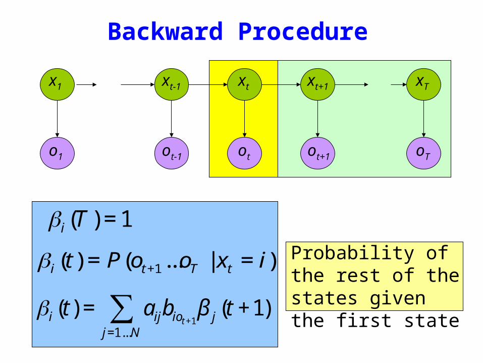
βi (t) = P(ot+1oT | xt = i)
oTo1 otot-1 ot+1
x1 xt+1 xTxtxt-1
Backward Procedure
βi (T ) = 1
βi (t) = aijbiot +1β j (t +1)
j=1Nsum
Probability of the rest of the states given the first state
oTo1 otot-1 ot+1
x1 xt+1 xTxtxt-1
Decoding Solution
sum=
=N
ii TOP
1
)()|( αμ
sum=
=N
iiiOP
1
)1()|( βπμ
)()()|(1
ttOP i
N
ii βαμ sum
=
=
Forward Procedure
Backward Procedure
Combination
P(O Xt =i |μ) =P(o1otXt =iot+1oT |μ)=P(o1otXt =i |μ)P(ot+1oT |o1otXt =i μ)=P(o1otXt =i |μ)P(ot+1oT |Xt =i μ)=α i (t)βi (t)
)()()|(1
ttOP i
N
ii βαμ sum
=
=
oTo1 otot-1 ot+1
Best State Sequence
Find the state sequence that best explains the observations
Two approaches bull Individually most likely statesbull Most likely sequence (Viterbi)
)|(maxarg OXPX
Best State Sequence (1)
γi (t) = P(Xt = i | O μ )
=P(Xt = iO | μ )
P(O | μ )
=α i (t)β i (t)
j=1
n
sum α j (t)β j (t)
Most likely state at each point in time
Xt = arg maxγ i (t)
oTo1 otot-1 ot+1
Best State Sequence (2)
Find the state sequence that best explains the observations
Viterbi algorithm
)|(maxarg OXPX
oTo1 otot-1 ot+1
Viterbi Algorithm
)(max)( 1111 11
ttttxx
j ojxooxxPtt
== minusminusminus
δ
The state sequence which maximizes the probability of seeing the observations to time t-1 landing in state j and seeing the observation at time t
x1 xt-1 j
oTo1 otot-1 ot+1
Viterbi Algorithm
)(max)( 1111 11
ttttxx
j ojxooxxPtt
== minusminusminus
δ
1)(max)1(
+=+
tjoijiij batt δδ
1)(maxarg)1(
+=+
tjoijii
j batt δψRecursive Computation
x1 xt-1 xt xt+1
Initialization
δ1(i) = ibio1
ψ 1(i) =0
oTo1 otot-1 ot+1
Viterbi Algorithm
XT =argmaxi
δi (T )
Xt =ψX^
t+1
(t+1)
P(X)=argmaxi
δi (T )
Compute the most likely state sequence by working backwards
x1 xt-1 xt xt+1 xT
oTo1 otot-1 ot+1
HMMs and Bayesian Nets (1)
x1 xt-1 xt xt+1 xT
P(x1xT o1oT )=P(x1)P(o1 |x1) P(xi+1 |xii=1
Tminus1
prod )P(oi+1 |xi+1)
= x1bx1o1
t=1
Tminus1
axtxt+1bxt+1ot+1
oTo1 otot-1 ot+1
x1 xt+1 xTxtxt-1
HMM and Bayesian Nets (2)
Conditionally independent of Given
Because of d-separation
ldquoThe past is independent of the future given the presentrdquo
Inference in an HMM
Compute the probability of a given observation sequence
Given an observation sequence compute the most likely hidden state sequence
Given an observation sequence and set of possible models which model most closely fits the data
Dynamic Programming
oTo1 otot-1 ot+1
Parameter Estimation
bull Given an observation sequence find the model that is most likely to produce that sequence
bull No analytic methodbull Given a model and observation sequence update
the model parameters to better fit the observations
A
B
AAA
BBB B
arg maxμ
P(Otraining |μ)
α i (t) = P(o1ot xt = i | μ )
βi (t) = P(ot+1oT | xt = i)
)()()|(1
ttOP i
N
ii βαμ sum
=
=
pt (i j)=P(Xt =iXt+1 = j |O μ)
=P(Xt =iXt+1 = jO |μ)
P(O |μ)
oTo1 otot-1 ot+1
Parameter Estimation
A
B
AAA
BBB B
pt (i j)=α i (t)aijbjot+1
β j (t+1)
αm(t)βm(t)m=1Nsum
Probability of traversing an arc
sum=
=Nj
ti jipt1
)()(γ Probability of being in state i
oTo1 otot-1 ot+1
Parameter Estimation
A
B
AAA
BBB B
i =γi(1)
Now we can compute the new estimates of the model parameters
aij =pt(i j)t=1
Tminus1sumγi (t)t=1
Tminus1sum
bik =γi (t) tot=ksum
γi (t)t=1
Tsum
Instance of Expectation Maximization
We have that
We may get stuck in local maximum (or even saddle point)
Nevertheless Baum-Welch usually effective
P(O | μ) geP(O |μ)
Some Variants
So far ergodic modelsbull All states are connectedbull Not always wanted
Epsilon or null-transitionsbull Not all statestransitions emit output symbols
Parameter tyingbull Assuming that certain parameters are shared bull Reduces the number of parameters that have to be estimated
Logical HMMs (Kersting De Raedt Raiko)bull Working with structured states and observation symbols
Working with log probabilities and addition instead of multiplication of probabilities (typically done)
oTo1 otot-1 ot+1
The Most Important Thing
A
B
AAA
BBB B
We can use the special structure of this model to do a lot of neat math and solve problems that are otherwise not solvable
HMMrsquos from an Agent Perspective
AI a modern approachbull AI is the study of rational agentsbull Third part by Wolfram Burgard on
Reinforcement learning
HMMs can also be used herebull Typically one is interested in P(state)
Example
Possible statesbull snow no snow
Observationsbull skis no skis
Questionsbull Was there snow the day before yesterday (given a
sequence of observations) bull Is there now snow (given a sequence of
observations) bull Will there be snow tomorrow given a sequence of
observations Next week
HMM and Agents
Question
bull Case 1 often called smoothing t lt T see last time
Only part of trellis between t and T needed
γi (t) = P(Xt = i | Oμ )
=α i (t)β i (t)
j =1
n
sum α j (t)β j (t)
Most likely state at each point in time
HMM and Agents
bull Case 2 often called filtering t= T last time
Can we make it recursive Ie go from T-1 to T
γi (t) = P(Xt = i | Oμ )
=α i (t)β i (t)
j =1
n
sum α j (t)β j (t)
Most likely state at each point in time
HMM and Agents
bull Case 2 often called filtering t= T last time
λi (T ) = P(XT = i | o1oT μ )
= γ i (T )
=α i (T )β i (T )
j =1
n
sum α j (T )β j (T )
=α i (T )
j =1
n
sum α j (T )
HMM and Agents
bull Case 3 often called prediction t= T+1 (or T+K) not yet seen
Interesting recursive Easily extended towards k gt 1
Extensions
Use Dynamic Bayesian networks instead of HMMsbullOne state corresponds to a Bayesian NetbullObservations can become more complex
Involve actions of the agent as wellbullCf Wolfram Burgardrsquos Part
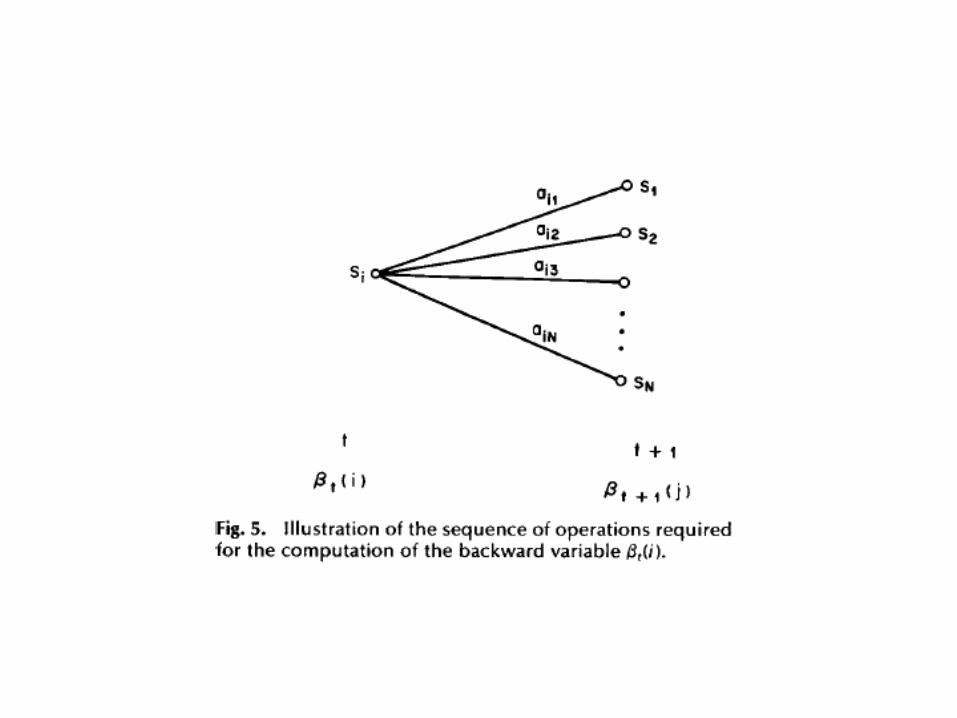
oTo1 otot-1 ot+1
x1 xt+1 xTxtxt-1
Decoding Solution
sum=
=N
ii TOP
1
)()|( αμ
sum=
=N
iiiOP
1
)1()|( βπμ
)()()|(1
ttOP i
N
ii βαμ sum
=
=
Forward Procedure
Backward Procedure
Combination
P(O Xt =i |μ) =P(o1otXt =iot+1oT |μ)=P(o1otXt =i |μ)P(ot+1oT |o1otXt =i μ)=P(o1otXt =i |μ)P(ot+1oT |Xt =i μ)=α i (t)βi (t)
)()()|(1
ttOP i
N
ii βαμ sum
=
=
oTo1 otot-1 ot+1
Best State Sequence
Find the state sequence that best explains the observations
Two approaches bull Individually most likely statesbull Most likely sequence (Viterbi)
)|(maxarg OXPX
Best State Sequence (1)
γi (t) = P(Xt = i | O μ )
=P(Xt = iO | μ )
P(O | μ )
=α i (t)β i (t)
j=1
n
sum α j (t)β j (t)
Most likely state at each point in time
Xt = arg maxγ i (t)
oTo1 otot-1 ot+1
Best State Sequence (2)
Find the state sequence that best explains the observations
Viterbi algorithm
)|(maxarg OXPX
oTo1 otot-1 ot+1
Viterbi Algorithm
)(max)( 1111 11
ttttxx
j ojxooxxPtt
== minusminusminus
δ
The state sequence which maximizes the probability of seeing the observations to time t-1 landing in state j and seeing the observation at time t
x1 xt-1 j
oTo1 otot-1 ot+1
Viterbi Algorithm
)(max)( 1111 11
ttttxx
j ojxooxxPtt
== minusminusminus
δ
1)(max)1(
+=+
tjoijiij batt δδ
1)(maxarg)1(
+=+
tjoijii
j batt δψRecursive Computation
x1 xt-1 xt xt+1
Initialization
δ1(i) = ibio1
ψ 1(i) =0
oTo1 otot-1 ot+1
Viterbi Algorithm
XT =argmaxi
δi (T )
Xt =ψX^
t+1
(t+1)
P(X)=argmaxi
δi (T )
Compute the most likely state sequence by working backwards
x1 xt-1 xt xt+1 xT
oTo1 otot-1 ot+1
HMMs and Bayesian Nets (1)
x1 xt-1 xt xt+1 xT
P(x1xT o1oT )=P(x1)P(o1 |x1) P(xi+1 |xii=1
Tminus1
prod )P(oi+1 |xi+1)
= x1bx1o1
t=1
Tminus1
axtxt+1bxt+1ot+1
oTo1 otot-1 ot+1
x1 xt+1 xTxtxt-1
HMM and Bayesian Nets (2)
Conditionally independent of Given
Because of d-separation
ldquoThe past is independent of the future given the presentrdquo
Inference in an HMM
Compute the probability of a given observation sequence
Given an observation sequence compute the most likely hidden state sequence
Given an observation sequence and set of possible models which model most closely fits the data
Dynamic Programming
oTo1 otot-1 ot+1
Parameter Estimation
bull Given an observation sequence find the model that is most likely to produce that sequence
bull No analytic methodbull Given a model and observation sequence update
the model parameters to better fit the observations
A
B
AAA
BBB B
arg maxμ
P(Otraining |μ)
α i (t) = P(o1ot xt = i | μ )
βi (t) = P(ot+1oT | xt = i)
)()()|(1
ttOP i
N
ii βαμ sum
=
=
pt (i j)=P(Xt =iXt+1 = j |O μ)
=P(Xt =iXt+1 = jO |μ)
P(O |μ)
oTo1 otot-1 ot+1
Parameter Estimation
A
B
AAA
BBB B
pt (i j)=α i (t)aijbjot+1
β j (t+1)
αm(t)βm(t)m=1Nsum
Probability of traversing an arc
sum=
=Nj
ti jipt1
)()(γ Probability of being in state i
oTo1 otot-1 ot+1
Parameter Estimation
A
B
AAA
BBB B
i =γi(1)
Now we can compute the new estimates of the model parameters
aij =pt(i j)t=1
Tminus1sumγi (t)t=1
Tminus1sum
bik =γi (t) tot=ksum
γi (t)t=1
Tsum
Instance of Expectation Maximization
We have that
We may get stuck in local maximum (or even saddle point)
Nevertheless Baum-Welch usually effective
P(O | μ) geP(O |μ)
Some Variants
So far ergodic modelsbull All states are connectedbull Not always wanted
Epsilon or null-transitionsbull Not all statestransitions emit output symbols
Parameter tyingbull Assuming that certain parameters are shared bull Reduces the number of parameters that have to be estimated
Logical HMMs (Kersting De Raedt Raiko)bull Working with structured states and observation symbols
Working with log probabilities and addition instead of multiplication of probabilities (typically done)
oTo1 otot-1 ot+1
The Most Important Thing
A
B
AAA
BBB B
We can use the special structure of this model to do a lot of neat math and solve problems that are otherwise not solvable
HMMrsquos from an Agent Perspective
AI a modern approachbull AI is the study of rational agentsbull Third part by Wolfram Burgard on
Reinforcement learning
HMMs can also be used herebull Typically one is interested in P(state)
Example
Possible statesbull snow no snow
Observationsbull skis no skis
Questionsbull Was there snow the day before yesterday (given a
sequence of observations) bull Is there now snow (given a sequence of
observations) bull Will there be snow tomorrow given a sequence of
observations Next week
HMM and Agents
Question
bull Case 1 often called smoothing t lt T see last time
Only part of trellis between t and T needed
γi (t) = P(Xt = i | Oμ )
=α i (t)β i (t)
j =1
n
sum α j (t)β j (t)
Most likely state at each point in time
HMM and Agents
bull Case 2 often called filtering t= T last time
Can we make it recursive Ie go from T-1 to T
γi (t) = P(Xt = i | Oμ )
=α i (t)β i (t)
j =1
n
sum α j (t)β j (t)
Most likely state at each point in time
HMM and Agents
bull Case 2 often called filtering t= T last time
λi (T ) = P(XT = i | o1oT μ )
= γ i (T )
=α i (T )β i (T )
j =1
n
sum α j (T )β j (T )
=α i (T )
j =1
n
sum α j (T )
HMM and Agents
bull Case 3 often called prediction t= T+1 (or T+K) not yet seen
Interesting recursive Easily extended towards k gt 1
Extensions
Use Dynamic Bayesian networks instead of HMMsbullOne state corresponds to a Bayesian NetbullObservations can become more complex
Involve actions of the agent as wellbullCf Wolfram Burgardrsquos Part
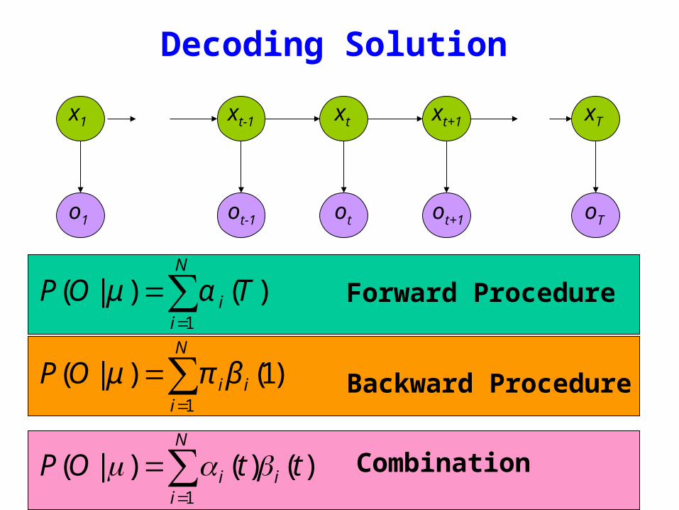
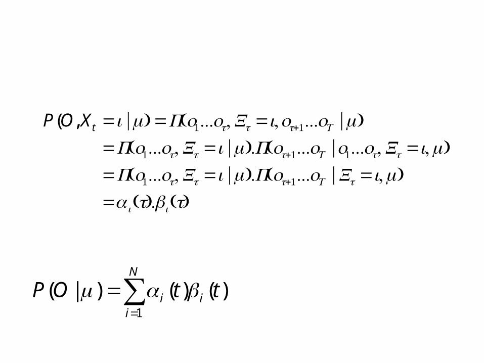
oTo1 otot-1 ot+1
Best State Sequence
Find the state sequence that best explains the observations
Two approaches bull Individually most likely statesbull Most likely sequence (Viterbi)
)|(maxarg OXPX
Best State Sequence (1)
γi (t) = P(Xt = i | O μ )
=P(Xt = iO | μ )
P(O | μ )
=α i (t)β i (t)
j=1
n
sum α j (t)β j (t)
Most likely state at each point in time
Xt = arg maxγ i (t)
oTo1 otot-1 ot+1
Best State Sequence (2)
Find the state sequence that best explains the observations
Viterbi algorithm
)|(maxarg OXPX
oTo1 otot-1 ot+1
Viterbi Algorithm
)(max)( 1111 11
ttttxx
j ojxooxxPtt
== minusminusminus
δ
The state sequence which maximizes the probability of seeing the observations to time t-1 landing in state j and seeing the observation at time t
x1 xt-1 j
oTo1 otot-1 ot+1
Viterbi Algorithm
)(max)( 1111 11
ttttxx
j ojxooxxPtt
== minusminusminus
δ
1)(max)1(
+=+
tjoijiij batt δδ
1)(maxarg)1(
+=+
tjoijii
j batt δψRecursive Computation
x1 xt-1 xt xt+1
Initialization
δ1(i) = ibio1
ψ 1(i) =0
oTo1 otot-1 ot+1
Viterbi Algorithm
XT =argmaxi
δi (T )
Xt =ψX^
t+1
(t+1)
P(X)=argmaxi
δi (T )
Compute the most likely state sequence by working backwards
x1 xt-1 xt xt+1 xT
oTo1 otot-1 ot+1
HMMs and Bayesian Nets (1)
x1 xt-1 xt xt+1 xT
P(x1xT o1oT )=P(x1)P(o1 |x1) P(xi+1 |xii=1
Tminus1
prod )P(oi+1 |xi+1)
= x1bx1o1
t=1
Tminus1
axtxt+1bxt+1ot+1
oTo1 otot-1 ot+1
x1 xt+1 xTxtxt-1
HMM and Bayesian Nets (2)
Conditionally independent of Given
Because of d-separation
ldquoThe past is independent of the future given the presentrdquo
Inference in an HMM
Compute the probability of a given observation sequence
Given an observation sequence compute the most likely hidden state sequence
Given an observation sequence and set of possible models which model most closely fits the data
Dynamic Programming
oTo1 otot-1 ot+1
Parameter Estimation
bull Given an observation sequence find the model that is most likely to produce that sequence
bull No analytic methodbull Given a model and observation sequence update
the model parameters to better fit the observations
A
B
AAA
BBB B
arg maxμ
P(Otraining |μ)
α i (t) = P(o1ot xt = i | μ )
βi (t) = P(ot+1oT | xt = i)
)()()|(1
ttOP i
N
ii βαμ sum
=
=
pt (i j)=P(Xt =iXt+1 = j |O μ)
=P(Xt =iXt+1 = jO |μ)
P(O |μ)
oTo1 otot-1 ot+1
Parameter Estimation
A
B
AAA
BBB B
pt (i j)=α i (t)aijbjot+1
β j (t+1)
αm(t)βm(t)m=1Nsum
Probability of traversing an arc
sum=
=Nj
ti jipt1
)()(γ Probability of being in state i
oTo1 otot-1 ot+1
Parameter Estimation
A
B
AAA
BBB B
i =γi(1)
Now we can compute the new estimates of the model parameters
aij =pt(i j)t=1
Tminus1sumγi (t)t=1
Tminus1sum
bik =γi (t) tot=ksum
γi (t)t=1
Tsum
Instance of Expectation Maximization
We have that
We may get stuck in local maximum (or even saddle point)
Nevertheless Baum-Welch usually effective
P(O | μ) geP(O |μ)
Some Variants
So far ergodic modelsbull All states are connectedbull Not always wanted
Epsilon or null-transitionsbull Not all statestransitions emit output symbols
Parameter tyingbull Assuming that certain parameters are shared bull Reduces the number of parameters that have to be estimated
Logical HMMs (Kersting De Raedt Raiko)bull Working with structured states and observation symbols
Working with log probabilities and addition instead of multiplication of probabilities (typically done)
oTo1 otot-1 ot+1
The Most Important Thing
A
B
AAA
BBB B
We can use the special structure of this model to do a lot of neat math and solve problems that are otherwise not solvable
HMMrsquos from an Agent Perspective
AI a modern approachbull AI is the study of rational agentsbull Third part by Wolfram Burgard on
Reinforcement learning
HMMs can also be used herebull Typically one is interested in P(state)
Example
Possible statesbull snow no snow
Observationsbull skis no skis
Questionsbull Was there snow the day before yesterday (given a
sequence of observations) bull Is there now snow (given a sequence of
observations) bull Will there be snow tomorrow given a sequence of
observations Next week
HMM and Agents
Question
bull Case 1 often called smoothing t lt T see last time
Only part of trellis between t and T needed
γi (t) = P(Xt = i | Oμ )
=α i (t)β i (t)
j =1
n
sum α j (t)β j (t)
Most likely state at each point in time
HMM and Agents
bull Case 2 often called filtering t= T last time
Can we make it recursive Ie go from T-1 to T
γi (t) = P(Xt = i | Oμ )
=α i (t)β i (t)
j =1
n
sum α j (t)β j (t)
Most likely state at each point in time
HMM and Agents
bull Case 2 often called filtering t= T last time
λi (T ) = P(XT = i | o1oT μ )
= γ i (T )
=α i (T )β i (T )
j =1
n
sum α j (T )β j (T )
=α i (T )
j =1
n
sum α j (T )
HMM and Agents
bull Case 3 often called prediction t= T+1 (or T+K) not yet seen
Interesting recursive Easily extended towards k gt 1
Extensions
Use Dynamic Bayesian networks instead of HMMsbullOne state corresponds to a Bayesian NetbullObservations can become more complex
Involve actions of the agent as wellbullCf Wolfram Burgardrsquos Part
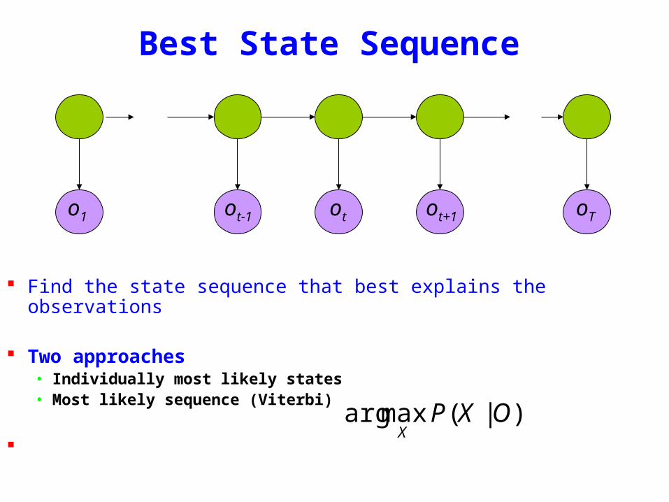
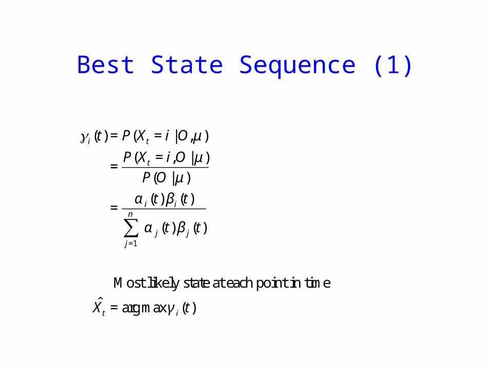
oTo1 otot-1 ot+1
Best State Sequence (2)
Find the state sequence that best explains the observations
Viterbi algorithm
)|(maxarg OXPX
oTo1 otot-1 ot+1
Viterbi Algorithm
)(max)( 1111 11
ttttxx
j ojxooxxPtt
== minusminusminus
δ
The state sequence which maximizes the probability of seeing the observations to time t-1 landing in state j and seeing the observation at time t
x1 xt-1 j
oTo1 otot-1 ot+1
Viterbi Algorithm
)(max)( 1111 11
ttttxx
j ojxooxxPtt
== minusminusminus
δ
1)(max)1(
+=+
tjoijiij batt δδ
1)(maxarg)1(
+=+
tjoijii
j batt δψRecursive Computation
x1 xt-1 xt xt+1
Initialization
δ1(i) = ibio1
ψ 1(i) =0
oTo1 otot-1 ot+1
Viterbi Algorithm
XT =argmaxi
δi (T )
Xt =ψX^
t+1
(t+1)
P(X)=argmaxi
δi (T )
Compute the most likely state sequence by working backwards
x1 xt-1 xt xt+1 xT
oTo1 otot-1 ot+1
HMMs and Bayesian Nets (1)
x1 xt-1 xt xt+1 xT
P(x1xT o1oT )=P(x1)P(o1 |x1) P(xi+1 |xii=1
Tminus1
prod )P(oi+1 |xi+1)
= x1bx1o1
t=1
Tminus1
axtxt+1bxt+1ot+1
oTo1 otot-1 ot+1
x1 xt+1 xTxtxt-1
HMM and Bayesian Nets (2)
Conditionally independent of Given
Because of d-separation
ldquoThe past is independent of the future given the presentrdquo
Inference in an HMM
Compute the probability of a given observation sequence
Given an observation sequence compute the most likely hidden state sequence
Given an observation sequence and set of possible models which model most closely fits the data
Dynamic Programming
oTo1 otot-1 ot+1
Parameter Estimation
bull Given an observation sequence find the model that is most likely to produce that sequence
bull No analytic methodbull Given a model and observation sequence update
the model parameters to better fit the observations
A
B
AAA
BBB B
arg maxμ
P(Otraining |μ)
α i (t) = P(o1ot xt = i | μ )
βi (t) = P(ot+1oT | xt = i)
)()()|(1
ttOP i
N
ii βαμ sum
=
=
pt (i j)=P(Xt =iXt+1 = j |O μ)
=P(Xt =iXt+1 = jO |μ)
P(O |μ)
oTo1 otot-1 ot+1
Parameter Estimation
A
B
AAA
BBB B
pt (i j)=α i (t)aijbjot+1
β j (t+1)
αm(t)βm(t)m=1Nsum
Probability of traversing an arc
sum=
=Nj
ti jipt1
)()(γ Probability of being in state i
oTo1 otot-1 ot+1
Parameter Estimation
A
B
AAA
BBB B
i =γi(1)
Now we can compute the new estimates of the model parameters
aij =pt(i j)t=1
Tminus1sumγi (t)t=1
Tminus1sum
bik =γi (t) tot=ksum
γi (t)t=1
Tsum
Instance of Expectation Maximization
We have that
We may get stuck in local maximum (or even saddle point)
Nevertheless Baum-Welch usually effective
P(O | μ) geP(O |μ)
Some Variants
So far ergodic modelsbull All states are connectedbull Not always wanted
Epsilon or null-transitionsbull Not all statestransitions emit output symbols
Parameter tyingbull Assuming that certain parameters are shared bull Reduces the number of parameters that have to be estimated
Logical HMMs (Kersting De Raedt Raiko)bull Working with structured states and observation symbols
Working with log probabilities and addition instead of multiplication of probabilities (typically done)
oTo1 otot-1 ot+1
The Most Important Thing
A
B
AAA
BBB B
We can use the special structure of this model to do a lot of neat math and solve problems that are otherwise not solvable
HMMrsquos from an Agent Perspective
AI a modern approachbull AI is the study of rational agentsbull Third part by Wolfram Burgard on
Reinforcement learning
HMMs can also be used herebull Typically one is interested in P(state)
Example
Possible statesbull snow no snow
Observationsbull skis no skis
Questionsbull Was there snow the day before yesterday (given a
sequence of observations) bull Is there now snow (given a sequence of
observations) bull Will there be snow tomorrow given a sequence of
observations Next week
HMM and Agents
Question
bull Case 1 often called smoothing t lt T see last time
Only part of trellis between t and T needed
γi (t) = P(Xt = i | Oμ )
=α i (t)β i (t)
j =1
n
sum α j (t)β j (t)
Most likely state at each point in time
HMM and Agents
bull Case 2 often called filtering t= T last time
Can we make it recursive Ie go from T-1 to T
γi (t) = P(Xt = i | Oμ )
=α i (t)β i (t)
j =1
n
sum α j (t)β j (t)
Most likely state at each point in time
HMM and Agents
bull Case 2 often called filtering t= T last time
λi (T ) = P(XT = i | o1oT μ )
= γ i (T )
=α i (T )β i (T )
j =1
n
sum α j (T )β j (T )
=α i (T )
j =1
n
sum α j (T )
HMM and Agents
bull Case 3 often called prediction t= T+1 (or T+K) not yet seen
Interesting recursive Easily extended towards k gt 1
Extensions
Use Dynamic Bayesian networks instead of HMMsbullOne state corresponds to a Bayesian NetbullObservations can become more complex
Involve actions of the agent as wellbullCf Wolfram Burgardrsquos Part
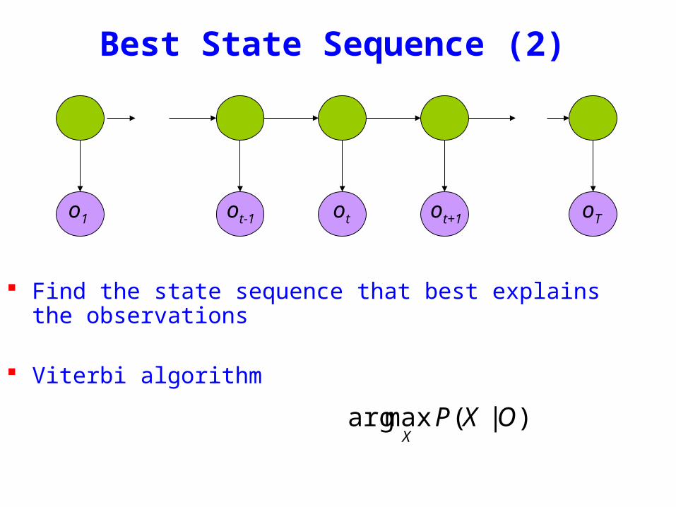
oTo1 otot-1 ot+1
Viterbi Algorithm
)(max)( 1111 11
ttttxx
j ojxooxxPtt
== minusminusminus
δ
The state sequence which maximizes the probability of seeing the observations to time t-1 landing in state j and seeing the observation at time t
x1 xt-1 j
oTo1 otot-1 ot+1
Viterbi Algorithm
)(max)( 1111 11
ttttxx
j ojxooxxPtt
== minusminusminus
δ
1)(max)1(
+=+
tjoijiij batt δδ
1)(maxarg)1(
+=+
tjoijii
j batt δψRecursive Computation
x1 xt-1 xt xt+1
Initialization
δ1(i) = ibio1
ψ 1(i) =0
oTo1 otot-1 ot+1
Viterbi Algorithm
XT =argmaxi
δi (T )
Xt =ψX^
t+1
(t+1)
P(X)=argmaxi
δi (T )
Compute the most likely state sequence by working backwards
x1 xt-1 xt xt+1 xT
oTo1 otot-1 ot+1
HMMs and Bayesian Nets (1)
x1 xt-1 xt xt+1 xT
P(x1xT o1oT )=P(x1)P(o1 |x1) P(xi+1 |xii=1
Tminus1
prod )P(oi+1 |xi+1)
= x1bx1o1
t=1
Tminus1
axtxt+1bxt+1ot+1
oTo1 otot-1 ot+1
x1 xt+1 xTxtxt-1
HMM and Bayesian Nets (2)
Conditionally independent of Given
Because of d-separation
ldquoThe past is independent of the future given the presentrdquo
Inference in an HMM
Compute the probability of a given observation sequence
Given an observation sequence compute the most likely hidden state sequence
Given an observation sequence and set of possible models which model most closely fits the data
Dynamic Programming
oTo1 otot-1 ot+1
Parameter Estimation
bull Given an observation sequence find the model that is most likely to produce that sequence
bull No analytic methodbull Given a model and observation sequence update
the model parameters to better fit the observations
A
B
AAA
BBB B
arg maxμ
P(Otraining |μ)
α i (t) = P(o1ot xt = i | μ )
βi (t) = P(ot+1oT | xt = i)
)()()|(1
ttOP i
N
ii βαμ sum
=
=
pt (i j)=P(Xt =iXt+1 = j |O μ)
=P(Xt =iXt+1 = jO |μ)
P(O |μ)
oTo1 otot-1 ot+1
Parameter Estimation
A
B
AAA
BBB B
pt (i j)=α i (t)aijbjot+1
β j (t+1)
αm(t)βm(t)m=1Nsum
Probability of traversing an arc
sum=
=Nj
ti jipt1
)()(γ Probability of being in state i
oTo1 otot-1 ot+1
Parameter Estimation
A
B
AAA
BBB B
i =γi(1)
Now we can compute the new estimates of the model parameters
aij =pt(i j)t=1
Tminus1sumγi (t)t=1
Tminus1sum
bik =γi (t) tot=ksum
γi (t)t=1
Tsum
Instance of Expectation Maximization
We have that
We may get stuck in local maximum (or even saddle point)
Nevertheless Baum-Welch usually effective
P(O | μ) geP(O |μ)
Some Variants
So far ergodic modelsbull All states are connectedbull Not always wanted
Epsilon or null-transitionsbull Not all statestransitions emit output symbols
Parameter tyingbull Assuming that certain parameters are shared bull Reduces the number of parameters that have to be estimated
Logical HMMs (Kersting De Raedt Raiko)bull Working with structured states and observation symbols
Working with log probabilities and addition instead of multiplication of probabilities (typically done)
oTo1 otot-1 ot+1
The Most Important Thing
A
B
AAA
BBB B
We can use the special structure of this model to do a lot of neat math and solve problems that are otherwise not solvable
HMMrsquos from an Agent Perspective
AI a modern approachbull AI is the study of rational agentsbull Third part by Wolfram Burgard on
Reinforcement learning
HMMs can also be used herebull Typically one is interested in P(state)
Example
Possible statesbull snow no snow
Observationsbull skis no skis
Questionsbull Was there snow the day before yesterday (given a
sequence of observations) bull Is there now snow (given a sequence of
observations) bull Will there be snow tomorrow given a sequence of
observations Next week
HMM and Agents
Question
bull Case 1 often called smoothing t lt T see last time
Only part of trellis between t and T needed
γi (t) = P(Xt = i | Oμ )
=α i (t)β i (t)
j =1
n
sum α j (t)β j (t)
Most likely state at each point in time
HMM and Agents
bull Case 2 often called filtering t= T last time
Can we make it recursive Ie go from T-1 to T
γi (t) = P(Xt = i | Oμ )
=α i (t)β i (t)
j =1
n
sum α j (t)β j (t)
Most likely state at each point in time
HMM and Agents
bull Case 2 often called filtering t= T last time
λi (T ) = P(XT = i | o1oT μ )
= γ i (T )
=α i (T )β i (T )
j =1
n
sum α j (T )β j (T )
=α i (T )
j =1
n
sum α j (T )
HMM and Agents
bull Case 3 often called prediction t= T+1 (or T+K) not yet seen
Interesting recursive Easily extended towards k gt 1
Extensions
Use Dynamic Bayesian networks instead of HMMsbullOne state corresponds to a Bayesian NetbullObservations can become more complex
Involve actions of the agent as wellbullCf Wolfram Burgardrsquos Part
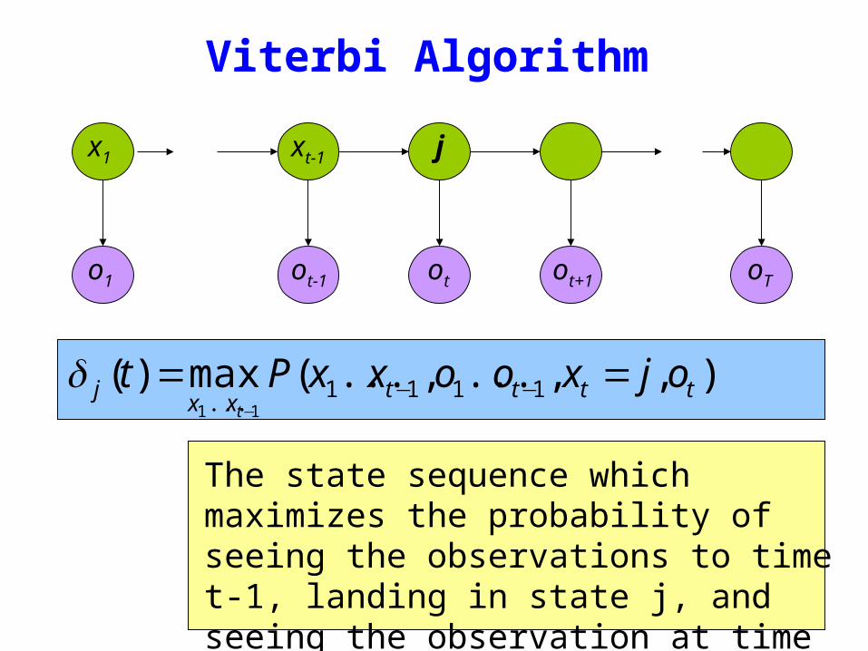
oTo1 otot-1 ot+1
Viterbi Algorithm
)(max)( 1111 11
ttttxx
j ojxooxxPtt
== minusminusminus
δ
1)(max)1(
+=+
tjoijiij batt δδ
1)(maxarg)1(
+=+
tjoijii
j batt δψRecursive Computation
x1 xt-1 xt xt+1
Initialization
δ1(i) = ibio1
ψ 1(i) =0
oTo1 otot-1 ot+1
Viterbi Algorithm
XT =argmaxi
δi (T )
Xt =ψX^
t+1
(t+1)
P(X)=argmaxi
δi (T )
Compute the most likely state sequence by working backwards
x1 xt-1 xt xt+1 xT
oTo1 otot-1 ot+1
HMMs and Bayesian Nets (1)
x1 xt-1 xt xt+1 xT
P(x1xT o1oT )=P(x1)P(o1 |x1) P(xi+1 |xii=1
Tminus1
prod )P(oi+1 |xi+1)
= x1bx1o1
t=1
Tminus1
axtxt+1bxt+1ot+1
oTo1 otot-1 ot+1
x1 xt+1 xTxtxt-1
HMM and Bayesian Nets (2)
Conditionally independent of Given
Because of d-separation
ldquoThe past is independent of the future given the presentrdquo
Inference in an HMM
Compute the probability of a given observation sequence
Given an observation sequence compute the most likely hidden state sequence
Given an observation sequence and set of possible models which model most closely fits the data
Dynamic Programming
oTo1 otot-1 ot+1
Parameter Estimation
bull Given an observation sequence find the model that is most likely to produce that sequence
bull No analytic methodbull Given a model and observation sequence update
the model parameters to better fit the observations
A
B
AAA
BBB B
arg maxμ
P(Otraining |μ)
α i (t) = P(o1ot xt = i | μ )
βi (t) = P(ot+1oT | xt = i)
)()()|(1
ttOP i
N
ii βαμ sum
=
=
pt (i j)=P(Xt =iXt+1 = j |O μ)
=P(Xt =iXt+1 = jO |μ)
P(O |μ)
oTo1 otot-1 ot+1
Parameter Estimation
A
B
AAA
BBB B
pt (i j)=α i (t)aijbjot+1
β j (t+1)
αm(t)βm(t)m=1Nsum
Probability of traversing an arc
sum=
=Nj
ti jipt1
)()(γ Probability of being in state i
oTo1 otot-1 ot+1
Parameter Estimation
A
B
AAA
BBB B
i =γi(1)
Now we can compute the new estimates of the model parameters
aij =pt(i j)t=1
Tminus1sumγi (t)t=1
Tminus1sum
bik =γi (t) tot=ksum
γi (t)t=1
Tsum
Instance of Expectation Maximization
We have that
We may get stuck in local maximum (or even saddle point)
Nevertheless Baum-Welch usually effective
P(O | μ) geP(O |μ)
Some Variants
So far ergodic modelsbull All states are connectedbull Not always wanted
Epsilon or null-transitionsbull Not all statestransitions emit output symbols
Parameter tyingbull Assuming that certain parameters are shared bull Reduces the number of parameters that have to be estimated
Logical HMMs (Kersting De Raedt Raiko)bull Working with structured states and observation symbols
Working with log probabilities and addition instead of multiplication of probabilities (typically done)
oTo1 otot-1 ot+1
The Most Important Thing
A
B
AAA
BBB B
We can use the special structure of this model to do a lot of neat math and solve problems that are otherwise not solvable
HMMrsquos from an Agent Perspective
AI a modern approachbull AI is the study of rational agentsbull Third part by Wolfram Burgard on
Reinforcement learning
HMMs can also be used herebull Typically one is interested in P(state)
Example
Possible statesbull snow no snow
Observationsbull skis no skis
Questionsbull Was there snow the day before yesterday (given a
sequence of observations) bull Is there now snow (given a sequence of
observations) bull Will there be snow tomorrow given a sequence of
observations Next week
HMM and Agents
Question
bull Case 1 often called smoothing t lt T see last time
Only part of trellis between t and T needed
γi (t) = P(Xt = i | Oμ )
=α i (t)β i (t)
j =1
n
sum α j (t)β j (t)
Most likely state at each point in time
HMM and Agents
bull Case 2 often called filtering t= T last time
Can we make it recursive Ie go from T-1 to T
γi (t) = P(Xt = i | Oμ )
=α i (t)β i (t)
j =1
n
sum α j (t)β j (t)
Most likely state at each point in time
HMM and Agents
bull Case 2 often called filtering t= T last time
λi (T ) = P(XT = i | o1oT μ )
= γ i (T )
=α i (T )β i (T )
j =1
n
sum α j (T )β j (T )
=α i (T )
j =1
n
sum α j (T )
HMM and Agents
bull Case 3 often called prediction t= T+1 (or T+K) not yet seen
Interesting recursive Easily extended towards k gt 1
Extensions
Use Dynamic Bayesian networks instead of HMMsbullOne state corresponds to a Bayesian NetbullObservations can become more complex
Involve actions of the agent as wellbullCf Wolfram Burgardrsquos Part
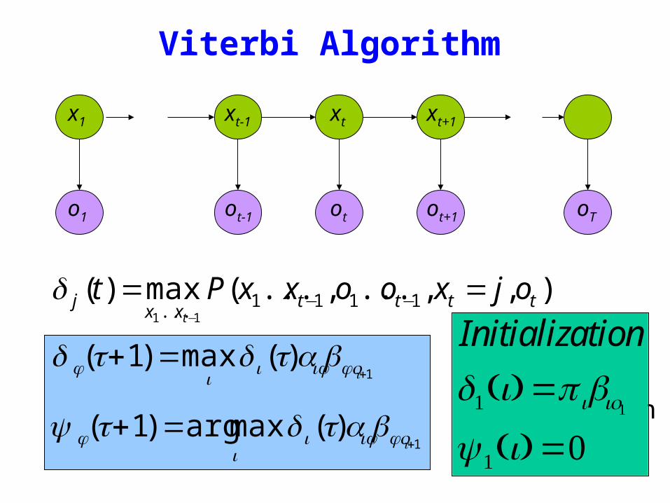
oTo1 otot-1 ot+1
Viterbi Algorithm
XT =argmaxi
δi (T )
Xt =ψX^
t+1
(t+1)
P(X)=argmaxi
δi (T )
Compute the most likely state sequence by working backwards
x1 xt-1 xt xt+1 xT
oTo1 otot-1 ot+1
HMMs and Bayesian Nets (1)
x1 xt-1 xt xt+1 xT
P(x1xT o1oT )=P(x1)P(o1 |x1) P(xi+1 |xii=1
Tminus1
prod )P(oi+1 |xi+1)
= x1bx1o1
t=1
Tminus1
axtxt+1bxt+1ot+1
oTo1 otot-1 ot+1
x1 xt+1 xTxtxt-1
HMM and Bayesian Nets (2)
Conditionally independent of Given
Because of d-separation
ldquoThe past is independent of the future given the presentrdquo
Inference in an HMM
Compute the probability of a given observation sequence
Given an observation sequence compute the most likely hidden state sequence
Given an observation sequence and set of possible models which model most closely fits the data
Dynamic Programming
oTo1 otot-1 ot+1
Parameter Estimation
bull Given an observation sequence find the model that is most likely to produce that sequence
bull No analytic methodbull Given a model and observation sequence update
the model parameters to better fit the observations
A
B
AAA
BBB B
arg maxμ
P(Otraining |μ)
α i (t) = P(o1ot xt = i | μ )
βi (t) = P(ot+1oT | xt = i)
)()()|(1
ttOP i
N
ii βαμ sum
=
=
pt (i j)=P(Xt =iXt+1 = j |O μ)
=P(Xt =iXt+1 = jO |μ)
P(O |μ)
oTo1 otot-1 ot+1
Parameter Estimation
A
B
AAA
BBB B
pt (i j)=α i (t)aijbjot+1
β j (t+1)
αm(t)βm(t)m=1Nsum
Probability of traversing an arc
sum=
=Nj
ti jipt1
)()(γ Probability of being in state i
oTo1 otot-1 ot+1
Parameter Estimation
A
B
AAA
BBB B
i =γi(1)
Now we can compute the new estimates of the model parameters
aij =pt(i j)t=1
Tminus1sumγi (t)t=1
Tminus1sum
bik =γi (t) tot=ksum
γi (t)t=1
Tsum
Instance of Expectation Maximization
We have that
We may get stuck in local maximum (or even saddle point)
Nevertheless Baum-Welch usually effective
P(O | μ) geP(O |μ)
Some Variants
So far ergodic modelsbull All states are connectedbull Not always wanted
Epsilon or null-transitionsbull Not all statestransitions emit output symbols
Parameter tyingbull Assuming that certain parameters are shared bull Reduces the number of parameters that have to be estimated
Logical HMMs (Kersting De Raedt Raiko)bull Working with structured states and observation symbols
Working with log probabilities and addition instead of multiplication of probabilities (typically done)
oTo1 otot-1 ot+1
The Most Important Thing
A
B
AAA
BBB B
We can use the special structure of this model to do a lot of neat math and solve problems that are otherwise not solvable
HMMrsquos from an Agent Perspective
AI a modern approachbull AI is the study of rational agentsbull Third part by Wolfram Burgard on
Reinforcement learning
HMMs can also be used herebull Typically one is interested in P(state)
Example
Possible statesbull snow no snow
Observationsbull skis no skis
Questionsbull Was there snow the day before yesterday (given a
sequence of observations) bull Is there now snow (given a sequence of
observations) bull Will there be snow tomorrow given a sequence of
observations Next week
HMM and Agents
Question
bull Case 1 often called smoothing t lt T see last time
Only part of trellis between t and T needed
γi (t) = P(Xt = i | Oμ )
=α i (t)β i (t)
j =1
n
sum α j (t)β j (t)
Most likely state at each point in time
HMM and Agents
bull Case 2 often called filtering t= T last time
Can we make it recursive Ie go from T-1 to T
γi (t) = P(Xt = i | Oμ )
=α i (t)β i (t)
j =1
n
sum α j (t)β j (t)
Most likely state at each point in time
HMM and Agents
bull Case 2 often called filtering t= T last time
λi (T ) = P(XT = i | o1oT μ )
= γ i (T )
=α i (T )β i (T )
j =1
n
sum α j (T )β j (T )
=α i (T )
j =1
n
sum α j (T )
HMM and Agents
bull Case 3 often called prediction t= T+1 (or T+K) not yet seen
Interesting recursive Easily extended towards k gt 1
Extensions
Use Dynamic Bayesian networks instead of HMMsbullOne state corresponds to a Bayesian NetbullObservations can become more complex
Involve actions of the agent as wellbullCf Wolfram Burgardrsquos Part
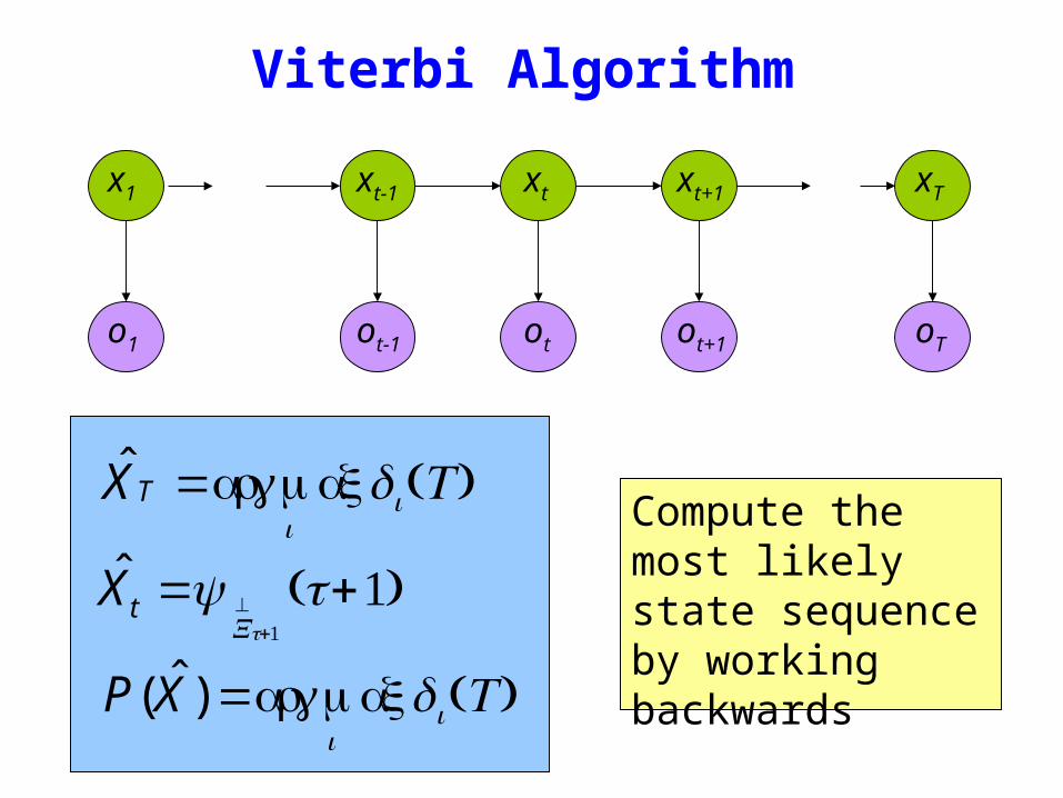
oTo1 otot-1 ot+1
x1 xt+1 xTxtxt-1
HMM and Bayesian Nets (2)
Conditionally independent of Given
Because of d-separation
ldquoThe past is independent of the future given the presentrdquo
Inference in an HMM
Compute the probability of a given observation sequence
Given an observation sequence compute the most likely hidden state sequence
Given an observation sequence and set of possible models which model most closely fits the data
Dynamic Programming
oTo1 otot-1 ot+1
Parameter Estimation
bull Given an observation sequence find the model that is most likely to produce that sequence
bull No analytic methodbull Given a model and observation sequence update
the model parameters to better fit the observations
A
B
AAA
BBB B
arg maxμ
P(Otraining |μ)
α i (t) = P(o1ot xt = i | μ )
βi (t) = P(ot+1oT | xt = i)
)()()|(1
ttOP i
N
ii βαμ sum
=
=
pt (i j)=P(Xt =iXt+1 = j |O μ)
=P(Xt =iXt+1 = jO |μ)
P(O |μ)
oTo1 otot-1 ot+1
Parameter Estimation
A
B
AAA
BBB B
pt (i j)=α i (t)aijbjot+1
β j (t+1)
αm(t)βm(t)m=1Nsum
Probability of traversing an arc
sum=
=Nj
ti jipt1
)()(γ Probability of being in state i
oTo1 otot-1 ot+1
Parameter Estimation
A
B
AAA
BBB B
i =γi(1)
Now we can compute the new estimates of the model parameters
aij =pt(i j)t=1
Tminus1sumγi (t)t=1
Tminus1sum
bik =γi (t) tot=ksum
γi (t)t=1
Tsum
Instance of Expectation Maximization
We have that
We may get stuck in local maximum (or even saddle point)
Nevertheless Baum-Welch usually effective
P(O | μ) geP(O |μ)
Some Variants
So far ergodic modelsbull All states are connectedbull Not always wanted
Epsilon or null-transitionsbull Not all statestransitions emit output symbols
Parameter tyingbull Assuming that certain parameters are shared bull Reduces the number of parameters that have to be estimated
Logical HMMs (Kersting De Raedt Raiko)bull Working with structured states and observation symbols
Working with log probabilities and addition instead of multiplication of probabilities (typically done)
oTo1 otot-1 ot+1
The Most Important Thing
A
B
AAA
BBB B
We can use the special structure of this model to do a lot of neat math and solve problems that are otherwise not solvable
HMMrsquos from an Agent Perspective
AI a modern approachbull AI is the study of rational agentsbull Third part by Wolfram Burgard on
Reinforcement learning
HMMs can also be used herebull Typically one is interested in P(state)
Example
Possible statesbull snow no snow
Observationsbull skis no skis
Questionsbull Was there snow the day before yesterday (given a
sequence of observations) bull Is there now snow (given a sequence of
observations) bull Will there be snow tomorrow given a sequence of
observations Next week
HMM and Agents
Question
bull Case 1 often called smoothing t lt T see last time
Only part of trellis between t and T needed
γi (t) = P(Xt = i | Oμ )
=α i (t)β i (t)
j =1
n
sum α j (t)β j (t)
Most likely state at each point in time
HMM and Agents
bull Case 2 often called filtering t= T last time
Can we make it recursive Ie go from T-1 to T
γi (t) = P(Xt = i | Oμ )
=α i (t)β i (t)
j =1
n
sum α j (t)β j (t)
Most likely state at each point in time
HMM and Agents
bull Case 2 often called filtering t= T last time
λi (T ) = P(XT = i | o1oT μ )
= γ i (T )
=α i (T )β i (T )
j =1
n
sum α j (T )β j (T )
=α i (T )
j =1
n
sum α j (T )
HMM and Agents
bull Case 3 often called prediction t= T+1 (or T+K) not yet seen
Interesting recursive Easily extended towards k gt 1
Extensions
Use Dynamic Bayesian networks instead of HMMsbullOne state corresponds to a Bayesian NetbullObservations can become more complex
Involve actions of the agent as wellbullCf Wolfram Burgardrsquos Part
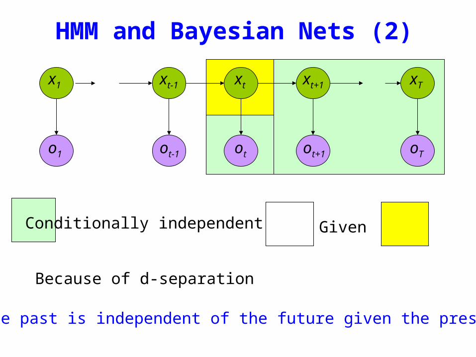

oTo1 otot-1 ot+1
Parameter Estimation
bull Given an observation sequence find the model that is most likely to produce that sequence
bull No analytic methodbull Given a model and observation sequence update
the model parameters to better fit the observations
A
B
AAA
BBB B
arg maxμ
P(Otraining |μ)
α i (t) = P(o1ot xt = i | μ )
βi (t) = P(ot+1oT | xt = i)
)()()|(1
ttOP i
N
ii βαμ sum
=
=
pt (i j)=P(Xt =iXt+1 = j |O μ)
=P(Xt =iXt+1 = jO |μ)
P(O |μ)
oTo1 otot-1 ot+1
Parameter Estimation
A
B
AAA
BBB B
pt (i j)=α i (t)aijbjot+1
β j (t+1)
αm(t)βm(t)m=1Nsum
Probability of traversing an arc
sum=
=Nj
ti jipt1
)()(γ Probability of being in state i
oTo1 otot-1 ot+1
Parameter Estimation
A
B
AAA
BBB B
i =γi(1)
Now we can compute the new estimates of the model parameters
aij =pt(i j)t=1
Tminus1sumγi (t)t=1
Tminus1sum
bik =γi (t) tot=ksum
γi (t)t=1
Tsum
Instance of Expectation Maximization
We have that
We may get stuck in local maximum (or even saddle point)
Nevertheless Baum-Welch usually effective
P(O | μ) geP(O |μ)
Some Variants
So far ergodic modelsbull All states are connectedbull Not always wanted
Epsilon or null-transitionsbull Not all statestransitions emit output symbols
Parameter tyingbull Assuming that certain parameters are shared bull Reduces the number of parameters that have to be estimated
Logical HMMs (Kersting De Raedt Raiko)bull Working with structured states and observation symbols
Working with log probabilities and addition instead of multiplication of probabilities (typically done)
oTo1 otot-1 ot+1
The Most Important Thing
A
B
AAA
BBB B
We can use the special structure of this model to do a lot of neat math and solve problems that are otherwise not solvable
HMMrsquos from an Agent Perspective
AI a modern approachbull AI is the study of rational agentsbull Third part by Wolfram Burgard on
Reinforcement learning
HMMs can also be used herebull Typically one is interested in P(state)
Example
Possible statesbull snow no snow
Observationsbull skis no skis
Questionsbull Was there snow the day before yesterday (given a
sequence of observations) bull Is there now snow (given a sequence of
observations) bull Will there be snow tomorrow given a sequence of
observations Next week
HMM and Agents
Question
bull Case 1 often called smoothing t lt T see last time
Only part of trellis between t and T needed
γi (t) = P(Xt = i | Oμ )
=α i (t)β i (t)
j =1
n
sum α j (t)β j (t)
Most likely state at each point in time
HMM and Agents
bull Case 2 often called filtering t= T last time
Can we make it recursive Ie go from T-1 to T
γi (t) = P(Xt = i | Oμ )
=α i (t)β i (t)
j =1
n
sum α j (t)β j (t)
Most likely state at each point in time
HMM and Agents
bull Case 2 often called filtering t= T last time
λi (T ) = P(XT = i | o1oT μ )
= γ i (T )
=α i (T )β i (T )
j =1
n
sum α j (T )β j (T )
=α i (T )
j =1
n
sum α j (T )
HMM and Agents
bull Case 3 often called prediction t= T+1 (or T+K) not yet seen
Interesting recursive Easily extended towards k gt 1
Extensions
Use Dynamic Bayesian networks instead of HMMsbullOne state corresponds to a Bayesian NetbullObservations can become more complex
Involve actions of the agent as wellbullCf Wolfram Burgardrsquos Part
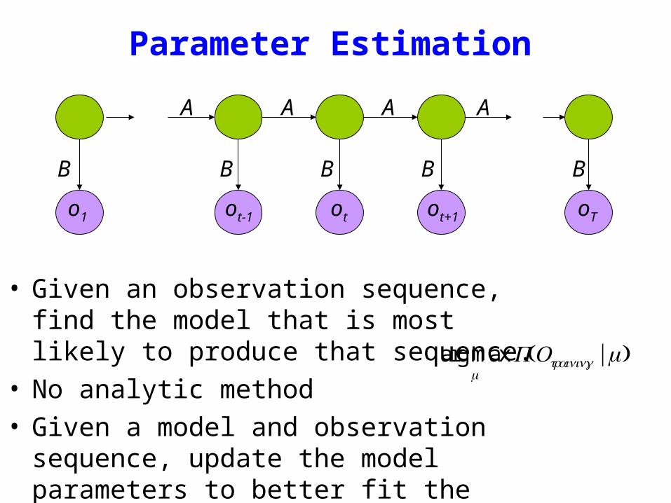
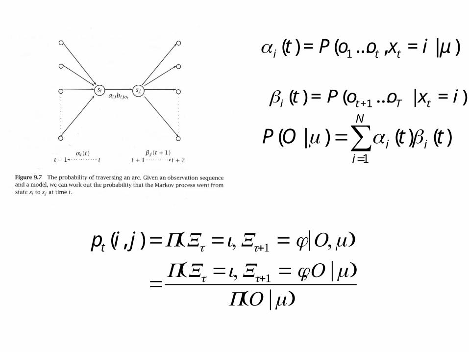
oTo1 otot-1 ot+1
Parameter Estimation
A
B
AAA
BBB B
pt (i j)=α i (t)aijbjot+1
β j (t+1)
αm(t)βm(t)m=1Nsum
Probability of traversing an arc
sum=
=Nj
ti jipt1
)()(γ Probability of being in state i
oTo1 otot-1 ot+1
Parameter Estimation
A
B
AAA
BBB B
i =γi(1)
Now we can compute the new estimates of the model parameters
aij =pt(i j)t=1
Tminus1sumγi (t)t=1
Tminus1sum
bik =γi (t) tot=ksum
γi (t)t=1
Tsum
Instance of Expectation Maximization
We have that
We may get stuck in local maximum (or even saddle point)
Nevertheless Baum-Welch usually effective
P(O | μ) geP(O |μ)
Some Variants
So far ergodic modelsbull All states are connectedbull Not always wanted
Epsilon or null-transitionsbull Not all statestransitions emit output symbols
Parameter tyingbull Assuming that certain parameters are shared bull Reduces the number of parameters that have to be estimated
Logical HMMs (Kersting De Raedt Raiko)bull Working with structured states and observation symbols
Working with log probabilities and addition instead of multiplication of probabilities (typically done)
oTo1 otot-1 ot+1
The Most Important Thing
A
B
AAA
BBB B
We can use the special structure of this model to do a lot of neat math and solve problems that are otherwise not solvable
HMMrsquos from an Agent Perspective
AI a modern approachbull AI is the study of rational agentsbull Third part by Wolfram Burgard on
Reinforcement learning
HMMs can also be used herebull Typically one is interested in P(state)
Example
Possible statesbull snow no snow
Observationsbull skis no skis
Questionsbull Was there snow the day before yesterday (given a
sequence of observations) bull Is there now snow (given a sequence of
observations) bull Will there be snow tomorrow given a sequence of
observations Next week
HMM and Agents
Question
bull Case 1 often called smoothing t lt T see last time
Only part of trellis between t and T needed
γi (t) = P(Xt = i | Oμ )
=α i (t)β i (t)
j =1
n
sum α j (t)β j (t)
Most likely state at each point in time
HMM and Agents
bull Case 2 often called filtering t= T last time
Can we make it recursive Ie go from T-1 to T
γi (t) = P(Xt = i | Oμ )
=α i (t)β i (t)
j =1
n
sum α j (t)β j (t)
Most likely state at each point in time
HMM and Agents
bull Case 2 often called filtering t= T last time
λi (T ) = P(XT = i | o1oT μ )
= γ i (T )
=α i (T )β i (T )
j =1
n
sum α j (T )β j (T )
=α i (T )
j =1
n
sum α j (T )
HMM and Agents
bull Case 3 often called prediction t= T+1 (or T+K) not yet seen
Interesting recursive Easily extended towards k gt 1
Extensions
Use Dynamic Bayesian networks instead of HMMsbullOne state corresponds to a Bayesian NetbullObservations can become more complex
Involve actions of the agent as wellbullCf Wolfram Burgardrsquos Part
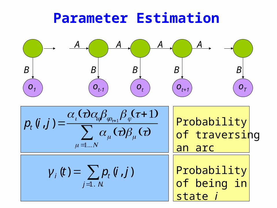
oTo1 otot-1 ot+1
Parameter Estimation
A
B
AAA
BBB B
i =γi(1)
Now we can compute the new estimates of the model parameters
aij =pt(i j)t=1
Tminus1sumγi (t)t=1
Tminus1sum
bik =γi (t) tot=ksum
γi (t)t=1
Tsum
Instance of Expectation Maximization
We have that
We may get stuck in local maximum (or even saddle point)
Nevertheless Baum-Welch usually effective
P(O | μ) geP(O |μ)
Some Variants
So far ergodic modelsbull All states are connectedbull Not always wanted
Epsilon or null-transitionsbull Not all statestransitions emit output symbols
Parameter tyingbull Assuming that certain parameters are shared bull Reduces the number of parameters that have to be estimated
Logical HMMs (Kersting De Raedt Raiko)bull Working with structured states and observation symbols
Working with log probabilities and addition instead of multiplication of probabilities (typically done)
oTo1 otot-1 ot+1
The Most Important Thing
A
B
AAA
BBB B
We can use the special structure of this model to do a lot of neat math and solve problems that are otherwise not solvable
HMMrsquos from an Agent Perspective
AI a modern approachbull AI is the study of rational agentsbull Third part by Wolfram Burgard on
Reinforcement learning
HMMs can also be used herebull Typically one is interested in P(state)
Example
Possible statesbull snow no snow
Observationsbull skis no skis
Questionsbull Was there snow the day before yesterday (given a
sequence of observations) bull Is there now snow (given a sequence of
observations) bull Will there be snow tomorrow given a sequence of
observations Next week
HMM and Agents
Question
bull Case 1 often called smoothing t lt T see last time
Only part of trellis between t and T needed
γi (t) = P(Xt = i | Oμ )
=α i (t)β i (t)
j =1
n
sum α j (t)β j (t)
Most likely state at each point in time
HMM and Agents
bull Case 2 often called filtering t= T last time
Can we make it recursive Ie go from T-1 to T
γi (t) = P(Xt = i | Oμ )
=α i (t)β i (t)
j =1
n
sum α j (t)β j (t)
Most likely state at each point in time
HMM and Agents
bull Case 2 often called filtering t= T last time
λi (T ) = P(XT = i | o1oT μ )
= γ i (T )
=α i (T )β i (T )
j =1
n
sum α j (T )β j (T )
=α i (T )
j =1
n
sum α j (T )
HMM and Agents
bull Case 3 often called prediction t= T+1 (or T+K) not yet seen
Interesting recursive Easily extended towards k gt 1
Extensions
Use Dynamic Bayesian networks instead of HMMsbullOne state corresponds to a Bayesian NetbullObservations can become more complex
Involve actions of the agent as wellbullCf Wolfram Burgardrsquos Part
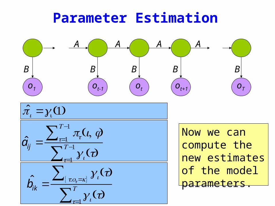
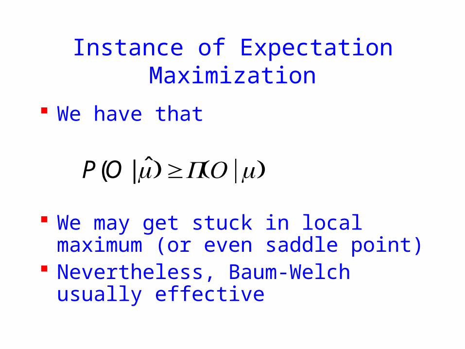
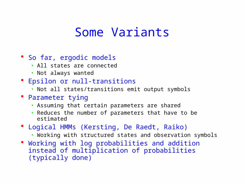
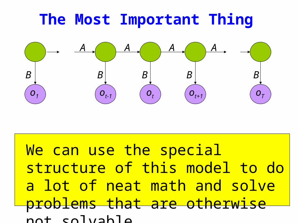
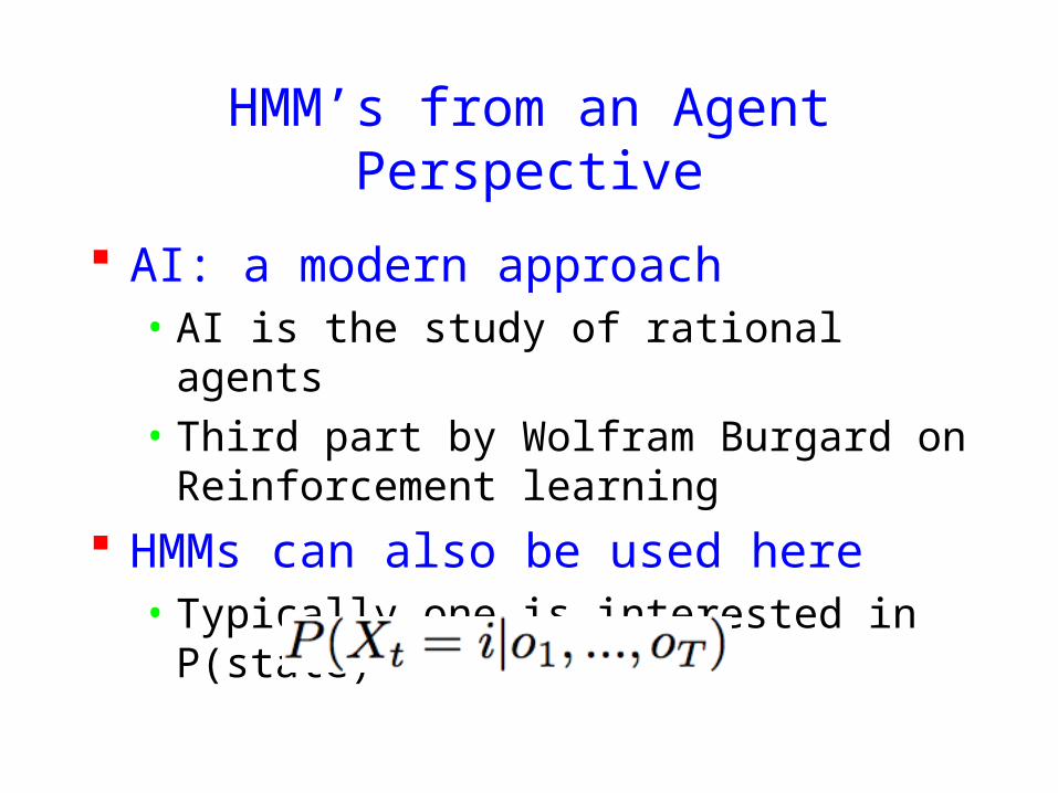
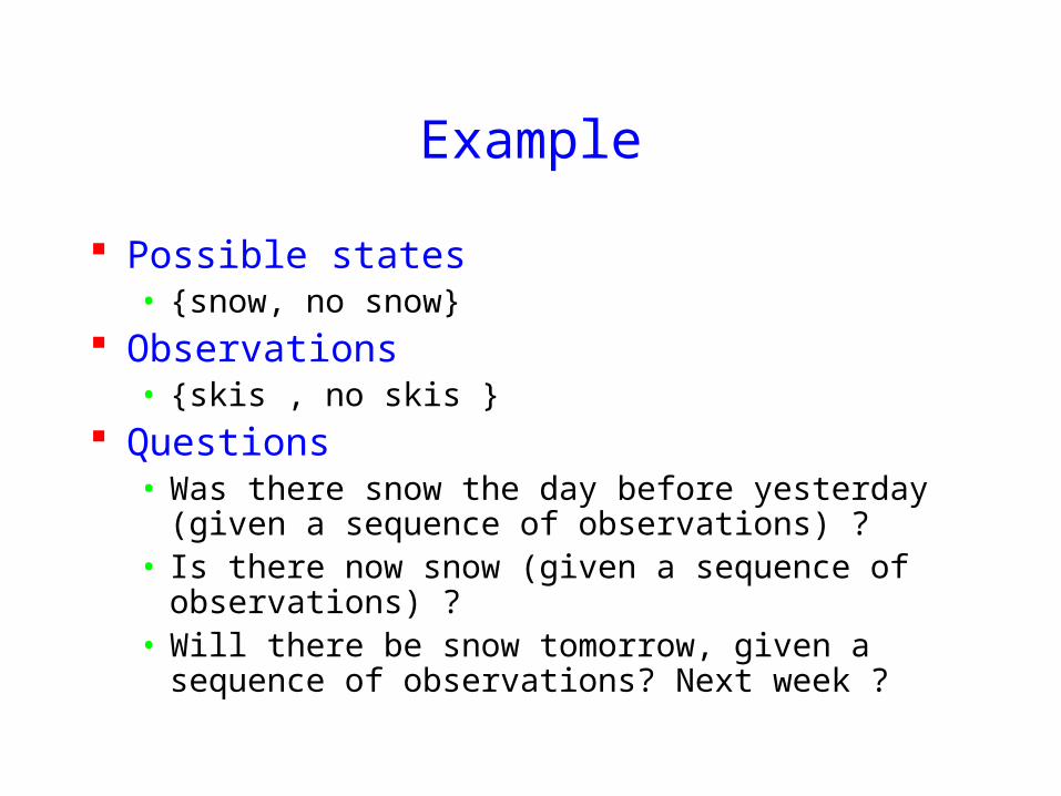
HMM and Agents
Question
bull Case 1 often called smoothing t lt T see last time
Only part of trellis between t and T needed
γi (t) = P(Xt = i | Oμ )
=α i (t)β i (t)
j =1
n
sum α j (t)β j (t)
Most likely state at each point in time
HMM and Agents
bull Case 2 often called filtering t= T last time
Can we make it recursive Ie go from T-1 to T
γi (t) = P(Xt = i | Oμ )
=α i (t)β i (t)
j =1
n
sum α j (t)β j (t)
Most likely state at each point in time
HMM and Agents
bull Case 2 often called filtering t= T last time
λi (T ) = P(XT = i | o1oT μ )
= γ i (T )
=α i (T )β i (T )
j =1
n
sum α j (T )β j (T )
=α i (T )
j =1
n
sum α j (T )
HMM and Agents
bull Case 3 often called prediction t= T+1 (or T+K) not yet seen
Interesting recursive Easily extended towards k gt 1
Extensions
Use Dynamic Bayesian networks instead of HMMsbullOne state corresponds to a Bayesian NetbullObservations can become more complex
Involve actions of the agent as wellbullCf Wolfram Burgardrsquos Part
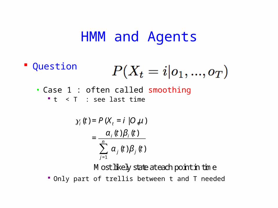
HMM and Agents
bull Case 2 often called filtering t= T last time
Can we make it recursive Ie go from T-1 to T
γi (t) = P(Xt = i | Oμ )
=α i (t)β i (t)
j =1
n
sum α j (t)β j (t)
Most likely state at each point in time
HMM and Agents
bull Case 2 often called filtering t= T last time
λi (T ) = P(XT = i | o1oT μ )
= γ i (T )
=α i (T )β i (T )
j =1
n
sum α j (T )β j (T )
=α i (T )
j =1
n
sum α j (T )
HMM and Agents
bull Case 3 often called prediction t= T+1 (or T+K) not yet seen
Interesting recursive Easily extended towards k gt 1
Extensions
Use Dynamic Bayesian networks instead of HMMsbullOne state corresponds to a Bayesian NetbullObservations can become more complex
Involve actions of the agent as wellbullCf Wolfram Burgardrsquos Part
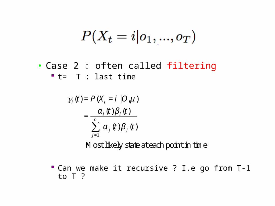
HMM and Agents
bull Case 2 often called filtering t= T last time
λi (T ) = P(XT = i | o1oT μ )
= γ i (T )
=α i (T )β i (T )
j =1
n
sum α j (T )β j (T )
=α i (T )
j =1
n
sum α j (T )
HMM and Agents
bull Case 3 often called prediction t= T+1 (or T+K) not yet seen
Interesting recursive Easily extended towards k gt 1
Extensions
Use Dynamic Bayesian networks instead of HMMsbullOne state corresponds to a Bayesian NetbullObservations can become more complex
Involve actions of the agent as wellbullCf Wolfram Burgardrsquos Part
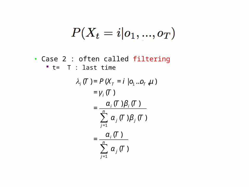
HMM and Agents
bull Case 3 often called prediction t= T+1 (or T+K) not yet seen
Interesting recursive Easily extended towards k gt 1
Extensions
Use Dynamic Bayesian networks instead of HMMsbullOne state corresponds to a Bayesian NetbullObservations can become more complex
Involve actions of the agent as wellbullCf Wolfram Burgardrsquos Part
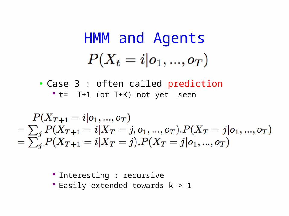
Extensions
Use Dynamic Bayesian networks instead of HMMsbullOne state corresponds to a Bayesian NetbullObservations can become more complex
Involve actions of the agent as wellbullCf Wolfram Burgardrsquos Part