Pathak, S., Ibele, L. M., Boll, R., Callegari, C., Demidovich, A., Erk, B.,Feifel, R., Forbes, R., Di Fraia, M., Giannessi, L., Hansen, C. S.,Holland, D. M. P., Ingle, R. A., Mason, R., Plekan, O., Prince, K. C.,Rouzée, A., Squibb, R. J., Tross, J., ... Rolles, D. (2020). Tracking theUltraviolet Photochemistry of Thiophenone During and After the InitialUltrafast Ring Opening. Nature Chemistry, 12, 795-800.https://doi.org/10.1038/s41557-020-0507-3

Peer reviewed version

Link to published version (if available):10.1038/s41557-020-0507-3

Link to publication record in Explore Bristol ResearchPDF-document

This is the author accepted manuscript (AAM). The final published version (version of record) is available onlinevia Nature Research at https://doi.org/10.1038/s41557-020-0507-3. Please refer to any applicable terms of useof the publisher.

University of Bristol - Explore Bristol ResearchGeneral rights

This document is made available in accordance with publisher policies. Please cite only thepublished version using the reference above. Full terms of use are available:http://www.bristol.ac.uk/red/research-policy/pure/user-guides/ebr-terms/

1

UOB Open

Supplementary Information

Tracking the ultraviolet-induced photochemistry of thiophenone during and after ultrafast

ring opening

Shashank Pathak1+, Lea M. Ibele2+, Rebecca Boll3, Carlo Callegari4, Alexander Demidovich4,

Benjamin Erk5, Raimund Feifel6, Ruaridh Forbes7, Michele Di Fraia4, Luca Giannessi4,8,

Christopher S. Hansen9, David M.P. Holland10, Rebecca A. Ingle11, Robert Mason12, Oksana

Plekan4, Kevin C. Prince4,13, Arnaud Rouzée14, Richard J. Squibb6, Jan Tross1, Michael N.R.

Ashfold15*, Basile F.E. Curchod2*, and Daniel Rolles1*

+both authors have contributed equally *corresponding authors

1J.R. Macdonald Laboratory, Department of Physics, Kansas State University, Manhattan, KS, USA 2Department of Chemistry, Durham University, Durham DH1 3LE, UK

3European XFEL, Schenefeld, Germany 4Elettra - Sincrotrone Trieste S.C.p.A., 34149 Basovizza, Trieste, Italy

5Deutsches Elektronen-Synchrotron, 22607 Hamburg, Germany 6Department of Physics, University of Gothenburg, Gothenburg, Sweden

7Stanford PULSE Institute, SLAC National Accelerator Laboratory, Menlo Park, CA 94025, USA 8Istituto Nazionale di Fisica Nucleare, Laboratori Nazionali di Frascati, 00044 Frascati (Rome),

Italy 9School of Chemistry, University of New South Wales, Sydney NSW 2052, Australia

10Daresbury Laboratory, Daresbury, Warrington, Cheshire WA4 4AD, UK 11 Department of Chemistry, University College London, London, WC1H 0AJ, UK

12Department of Chemistry, University of Oxford, Oxford, OX1 3TA, UK 13Centre for Translational Atomaterials, Swinburne University of Technology, Melbourne,

Australia 14Max-Born-Institut, 12489 Berlin, Germany

15School of Chemistry, University of Bristol, Bristol, BS8 1TS, UK

2

UOB Open

Table of Contents:

1) Experimental details ……………………………………………………………..……… 3

2) Computational details …………………………………………………………………… 7

2.1) Characterization of the excited states ………………………………………………..8

2.2) LIIC pathways – validation of the electronic structure methods …………………… 9

2.3) Selection rules for ionization from S2 to D0 and D1 ………………………………... 13

2.4) Trajectory Surface Hopping dynamics of thiophenone ……………………………. 13

2.5) Validation of the initial conditions for the ab initio molecular dynamics simulations

……………………………………………………………………………………………15

2.6) AIMD trajectories out to t = 2 ps and a trajectory exhibiting interconversion between

different photoproducts…………………………………………………………………..16

2.7) Normal distribution of IPs………………………………………………………….. 18

2.8) Validation of the methodology to compute ionization potentials between S0 and

D0……………………………………………………………………………………….. 18

2.9) Nature of the ionization process……………………………………………………. 20

2.10) AIMD trajectories out to t = 100 ps and trajectories exhibiting dissociation to CO +

thioacrolein……………………………………………………………………………… 22

3) Supplementary References ……………………………………………………………... 23

3

UOB Open

1. Experimental details

2(5H)-thiophenone (Sigma Aldrich, 98%) seeded in a helium carrier gas at 2 bar backing pressure

was introduced into the vacuum chamber through a pulsed Even-Lavie valve heated to 60 ºC. The

FEL pulses were focused to a spot of 40 x 50 μm2 (FWHM) and had an average pulse energy of

18 μJ (measured before the beamline optics). The calculated transmission of the transport optics

at this wavelength is 0.27 [Svetina2015], implying an average pulse energy of 4.9 μJ at the sample.

The UV pump pulses (center wavelength: 264.75 nm, bandwidth: 1.2 nm) were generated as the

third harmonic of a Ti:Sapphire laser and had an average pulse energy of 25 μJ, focused to a

diameter of ~200 μm (FWHM). To investigate the dependence of the observed effects on the pulse

energy of the pump and probe pulses, delay scans were taken at several lower and higher pulse

energies (see Fig. 4). The observed spectral components and time scales were found to be

independent of the pulse energies.

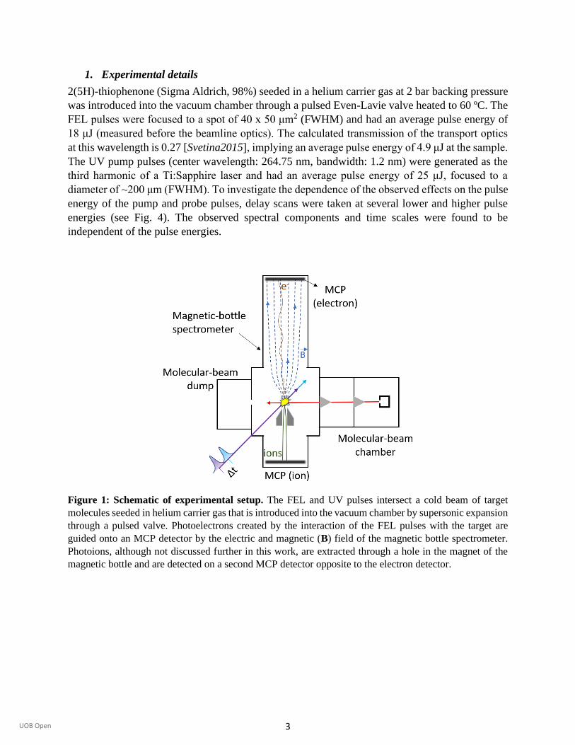
Figure 1: Schematic of experimental setup. The FEL and UV pulses intersect a cold beam of target

molecules seeded in helium carrier gas that is introduced into the vacuum chamber by supersonic expansion

through a pulsed valve. Photoelectrons created by the interaction of the FEL pulses with the target are

guided onto an MCP detector by the electric and magnetic (B) field of the magnetic bottle spectrometer.

Photoions, although not discussed further in this work, are extracted through a hole in the magnet of the

magnetic bottle and are detected on a second MCP detector opposite to the electron detector.

4

UOB Open

Figure 2: Measured photoelectron yield as a function of binding energy and pump-probe delay. Note

the different scaling of the delay axis below and above t = 1 ps, and the larger binding energy range and

different color scale than used in Fig. 2(a) of the main text. The strong contributions at BE ~9.7 and BE

~10.6 eV correspond to ionization to the D0/D1 and the D2 states of the cation, respectively [Chin1998].

Photoelectrons with BE >11 eV were not detected because a retardation voltage of 8 V was used to obtain

better resolution for the electrons with lower binding energies. (b) Photoelectron spectra for the FEL pulse

preceding the UV pulse (t = −500 fs, dashed blue line) and at two delays where the UV pulse precedes the

FEL pulse (orange: t = 0; green: t = 400 fs; each scaled by a factor of 6 and offset by, respectively, 0.04

and 0.3 for better visibility). For the latter two, the contributions from ‘unpumped’ molecules have been

subtracted (see Fig. 3), and the data are integrated over a range of ±40 fs around the indicated t value. The

ionization potential for vertical ionization (in the ground-state equilibrium geometry) from the S2 excited

state to the D0 state of the cation (taken from [Chin1998]) is shown as a dashed line.

5

UOB Open

Table 1: Least-square fits of the delay-dependent photoelectron yields. Fit parameters obtained from

least-square fits to the lineouts of the photoelectron yield in selected binding energy ranges shown in Fig.

2(b) of the main text. The data are fitted by a Gaussian (G(x)), the convolution C(x) = (f*h)(x) of a Gaussian

(h(x)) with an exponential decay (f(x)); or by a cumulative distribution function (CDF(x)), as appropriate

and as defined below.

Energy Range Fit Function x0/fs σ/fs 𝜏/fs

(4.7 – 5.3) eV Gaussian 4 ± 5 76 ± 6 -

(8.3 – 9.1) eV Gaussian * Exponential -2 ± 7 75 (fixed) 72 ± 9

(9.5 – 9.9) eV CDF -15 ± 5 72 ± 8 -

𝐺(𝑥) = 𝐴𝑒−(𝑥−𝑥0)

2

2𝜎2 + 𝑦0

𝐶𝐷𝐹(𝑥) =𝐴

2(1 + erf (

𝑥 − 𝑥0

√2𝜎2)) + 𝐵

Convolution of Gaussian h(x) = 𝑒−

𝑥2

2σ2 and

exponential (for x> x0) f(x) = Heaviside(𝑥 − 𝑥0) {(1 − 𝑒−(𝑥−x0)

𝝉 ) +  𝑏} :

C(x) = σ𝑒−𝑥

𝜏√𝜋

2((𝑎 + 𝑏)𝑒

𝑥

𝜏 (1 + Erf [𝑥

σ√2]) − 𝑎𝑒

2𝜏x0+𝜎2

2𝜏2 Erfc [(−𝜏𝑥+𝜎2)

σ√2𝜏])

6

UOB Open

Figure 3: Subtraction of signal from ‘unpumped’ molecules. To isolate the time-dependent signal

stemming from photoexcited molecules, the photoelectron spectrum measured at negative t (i.e. FEL pulse

arriving before the UV pulse, blue curve, ‘UV late’) is used in order to subtract the signal from unpumped

molecules at positive delays (orange curve, ‘UV early’). For delays t >0.2 ps, the fraction of unpumped

molecules is constant, and a constant scaling factor is chosen. However, in the temporal overlap region, the

subtraction procedure needs to recognize the gradual decrease of this signal caused by the increasing

ground-state depletion. To determine the appropriate scaling factor for a given delay, the ‘UV late’ spectrum

is scaled such that it has the same photoelectron yield in the binding energy range between 9.5 and 9.9 eV

as the spectrum at the given delay. This procedure is repeated for all delay points in the overlap region, and

a cumulative distribution function (CDF) is fitted to obtain a smooth scaling function that is used to generate

the subtracted spectra at all delays. The red line (repeated in the inset on an expanded vertical scale) shows

an example of a subtracted spectrum at t = 1.28 ps). The contribution at BE >9.8 eV in the subtracted

spectrum is due to ionization of S0# molecules to excited cationic states (see also Fig. 15), which are not

included in the calculations presented in this work.

7

UOB Open

Figure 4: Pulse-energy dependence of the pump-probe signal. Dependence of the photoelectron spectra

on the UV (a, b) and FEL (c, d) pulse energies. The latter are measured before the beamline optics and do

not include the beamline transmission [Svetina2015]. The spectra in (a) and (c) are normalized with respect

to the photoelectron signal intensity from unpumped molecules (BE ~9.6 eV). Panels (b) and (d) show the

ratio of the photoelectron yield in the specified binding energy ranges with respect to the yield from

unpumped molecules (BE 9.5-9.9 eV). The data shown in the manuscript were recorded at FEL and UV

pulse energies of 19 μJ and 25 μJ, respectively.

2. Computational details

This section starts by providing additional details for the calculations of ionization potentials and

surface hopping dynamics. We also provide additional benchmarks and supporting discussions

relating to the calculations reported in the main text.

Ionization potentials for potential photoproducts and benchmarking: Ground-state geometry

optimizations for thiophenone and its proposed photoproducts [Murdock2014] were conducted in

vacuo at the MP2/6-311+G** level of theory, and the nature of all located stationary points was

verified by harmonic vibrational frequency calculations. Based on these geometries, single-point

electronic energy calculations were performed using MP2-F12/cc-pVDZ-F12 and CCSD(T)-

F12/cc-pVDZ-F12 [Kong2012, Hattig2012]. Both methods are in good agreement for all the

8

UOB Open

computed ionization potentials of each molecule (see Section 2.8). All calculations were

performed with Molpro 2012.

Trajectory surface hopping dynamics: The excited-state dynamics of thiophenone following

photoexcitation were simulated using the mixed quantum/classical dynamics method trajectory

surface hopping (TSH), employing the fewest-switches algorithm proposed by Tully [Tully1990].

The calculations were performed with the SHARC program package (v2.0) [Mai2018]. 46 initial

conditions for the TSH dynamics were sampled stochastically from a Wigner distribution for

uncoupled harmonic oscillators constructed from a frequency calculation at the ground-state

optimized geometry of thiophenone. All trajectories were initiated in the bright S2 state of

thiophenone (see Section 2.4 for more information). The TSH dynamics employed a time step of

0.5 fs and SA(4)-CASSCF(10/8) for the electronic structure (benchmarking of this method is

discussed more fully in Section 2.2) using Molpro 2012. The energy decoherence correction

scheme by Granucci and Persico [Granucci2007] was applied to the electronic coefficients with

the default constant of 0.1 hartree. Strict total energy conservation was ensured for each trajectory

during the excited-state dynamics. However, the active space showed instabilities within a few

tens of femtoseconds in the S0 state. Such instabilities did not constitute an issue as the TSH

dynamics were sufficiently stable to provide initial conditions for the subsequent ground-state

AIMD calculations.

2.1. Characterization of the excited states

The electronic character of the first two excited singlet states of thiophenone at the Franck-Condon

geometry was determined by natural difference orbitals (NDO), computed with the TheoDORE

program (v 2.0) [Plasser2014].

Figure 5: Electronic character of the S1 state. Pairs of NDOs contributing to the S1 state at the Franck-

Condon geometry, with their respective eigenvalues.

9

UOB Open

Figures 5 and 6 show the NDOs (the eigenvectors of the difference density with respect to the

ground electronic state) for the S1 and S2 states, respectively, with their corresponding eigenvalues;

where negative (positive) eigenvalues describe the detachment (attachment) process. For detailed

information about NDOs we refer to [Plasser2014]. The first pair of NDOs in Fig. 5 shows that

the S1 state is dominated by a n(O)/* transition, with a small contribution of a * transition.

The NDOs for the S2 state (Fig. 6) encourage assignment as a n(S)/* transition, but there is also

a smaller but significant contribution from the n(O)/* transition (highlighting the dissociative

character of this state) and a minor contribution from a * transition (similar to the small

contribution in S1).

Figure 6: Electronic character of the S2 state. Pairs of NDOs contributing to the S2 state at the Franck-

Condon geometry, with their respective eigenvalues.

2.2. LIIC pathways – validation of the electronic structure methods

LIIC pathways allow determination of the most straightforward path from geometry A to geometry

B by interpolating a series of intermediate geometries (ten in the present work), using internal (not

Cartesian) coordinates. It is important to recognize that no reoptimization is performed along these

pathways. As a result, LIIC pathways should not be compared directly with minimum energy

10

UOB Open

paths, as the barriers observed in LIICs are upper estimates of the barriers that would be returned

by locating the true transition states.

The LIIC pathways presented in the main text were derived from critical geometries optimized at

the SA(4)-CASSCF(10/8) level of theory, but their energies were refined with XMS(4)-

CASPT2(10/8). Figure 7 (right half) shows the same LIIC pathway calculated at the SA(4)-

CASSCF(10/8) level. The overall shape of this pathway is in excellent agreement with that

obtained using XMS(4)-CASPT2(10/8) (which is reproduced again in the right-hand part of Fig.

8 below), validating the use of SA-CASSCF for the nonadiabatic molecular dynamics. We note

that the SA-CASSCF S2/S1 MECI point is not perfectly degenerate at the XMS-CASPT2 level of

theory, while the S1/S0 MECI point is. The variations in ionization energy along the LIIC pathway

as given by SA-CASSCF (shown at the top of Fig. 7) are also in excellent agreement with that

returned by XMS-CASPT2.

Figure 7: LIIC pathways. LIIC pathways computed at the SA(4)-CASSCF(10/8) (neutral thiophenone,

solid lines) and SA(4)-CASSCF(9/8) (thiophenone cation, dashed lines) levels of theory. The LIIC pathway

to the right of the FC region is that discussed in the main text, while that shown to the left is discussed

below. Molecular geometries of the critical points located at the SA(4)-CASSCF(10/8) level of theory are

represented beneath the figure.

11

UOB Open

The left part of Fig. 7 presents an alternative LIIC pathway connecting the FC point on the S2 state

to the S0 state. This path differs in that the critical geometries located for the S1 minimum and the

S1/S0 MECI exhibit an out-of-plane configuration and a nonlinear C=C=O moiety (depicted at the

appropriate points at the bottom of Fig. 7). The overall connectivity between S2, S1, and S0 is

nevertheless very similar to that observed for the LIIC pathway shown on the right: direct decay

from the FC point on S2 through conical intersections toward S0. Importantly, the majority (76%)

of the last S1-to-S0 hops observed during the TSH dynamics (discussed below) took place for

molecular configurations similar to the S1/S0 MECI of the LIIC pathway on the right (i.e. the one

presented in the main text). Figure 9 shows this comparison. We note the excellent agreement

between the overall shape of this second LIIC pathway as determined by SA-CASSCF and XMS-

CASPT2 methods (compare Figs. 7 and 8).

Figure 8: LIIC pathways with refined energies. LIICs pathways presented in Fig. 7 with energies refined

at the XMS(4)-CASPT2(10/8) (neutral thiophenone, solid lines) and XMS(4)-CASPT2(9/8) (thiophenone

cation, dashed lines) levels of theory. Molecular geometries of the critical points located at the SA(4)-

CASSCF(10/8) level of theory are represented beneath the figure.

12

UOB Open

Figure 9: Geometries at the end of TSH calculations. Superimposed last S1/S0 hopping geometries from

the TSH dynamics (shown on the left), grouped into two families according to whether the C=C=O angle

corresponds to the bent MECI (76% of the hopping geometries, upper panel) or linear MECI (24% of the

hopping geometries, lower panel).

Table 2 illustrates the influence of the choice of basis set on the XMS-CASPT2 calculations for

the Franck-Condon geometry of thiophenone. At the SA-CASSCF level of theory, use of the larger

cc-pVTZ basis set has negligible difference on the excitation energies for either neutral or charged

thiophenone, and only a small, essentially rigid shift of all transitions energies is observed within

XMS-CASPT2. Interestingly, the energy gap between the neutral and cationic states is increased

when increasing the size of the basis set: for example, XMS-CASPT2/cc-pVTZ returns a IPvert

value for the S0→D0 ionization of 9.38 eV, cf. 8.94 eV for XMS-CASPT2/6-31G*. This accounts

for the difference between the computed and measured BEs highlighted in the main text (inset of

Fig. 3(a) in the main text). Nevertheless, we have used the smaller basis set to explore the PESs of

thiophenone and for the TSH dynamics as a compromise between accuracy and efficiency and

because the benchmarking assures us that this causes only a rigid energy shift.

13

UOB Open

Table 2: Illustration of the effect of the basis set on the electronic energies of thiophenone (at the

Franck-Condon geometry). Energies are given in eV, with respect to the corresponding S0 electronic

energy.

Neutral SA(4)-CASSCF(10/8)

6-31G*

SA4-CASSCF(10/8)

cc-pVTZ

XMS(4)-

CASPT2(10/8)

6-31G*

XMS(4)-

CASPT2(10/8)

cc-pVTZ

S0 0 0 0 0

S1 4.477 4.475 4.199 4.063

S2 5.577 5.505 4.676 4.475

S3 6.800 6.758 5.985 5.747

Cation SA(4)-CASSCF(9/8)

6-31G*

SA4-CASSCF(9/8)

cc-pVTZ

XMS(4)-

CASPT2(9/8)

6-31G*

XMS(4)-

CASPT2(9/8)

cc-pVTZ

D0 8.293 8.276 8.940 9.377

D1 8.827 8.765 9.407 9.757

2.3 Selection rules for ionization from S2 to D0 and D1

A key focus of the present study is the energetic separation between the neutral and cationic states

of thiophenone along the LIIC pathway. Here it may be useful to introduce briefly an electronic

argument for focusing the discussion on ionization to D0 rather than to the D1 state. The S2 state

has dominant n(S)/* character in the Franck-Condon region (see Fig. 6). Importantly, the S atom

lone pair remains the dominant donating orbital along the entire decay pathway, from the Franck-

Condon point on S2, to the S2/S1 MECI, and during the relaxation on S1 towards S1 min, eventually

reaching the S1/S0 MECI. Similarly, the D0 state is always formed by loss of an electron from the

S atom lone pair along this LIIC pathway, whereas the D1 state is initially (i.e. in the Franck-

Condon region) characterized by removal of an electron from the O lone pair, before it too gains

a larger contribution from the n(S) orbital towards the end of the LIIC (when the states get closer

in energy). Simple ionization rules [Arbelo-Gonzalez2016] suggest that ionization should be

allowed from S2 to D0 along the entire LIIC pathway, as the two states differ by just a single spin-

orbital (the accepting orbital in the excitation of the neutral). However, the same logic would imply

that ionization from S2 to D1 is disfavored, as it necessitates (at least in the first part of the LIIC) a

change of more than one spin-orbital in the ionization step.

2.4 Trajectory Surface Hopping dynamics of thiophenone

The electronic-state population trace obtained with TSH for 46 independent trajectories is shown

in Fig. 3 of the main text. The trajectories were all initialized on the S2 state, since the computed

vertical transitions (at the SA(4)-CASSCF(10/8) level of theory) of 100 Wigner sampled structures

indicate that this state is by far the ‘brightest’ when exciting from the S0 state (see Fig. 10) and lies

14

UOB Open

at the appropriate energy for the chosen pump wavelength (when the transition energy is computed

at the XMS-CASPT2 level of theory, see main text).

The populations depicted in the main text are computed as the fraction of trajectories evolving in

a given electronic state at a given time. We note that the displayed population traces match well

with those computed from the squares of the TSH electronic coefficients, averaged over all

trajectories – indicating an internal consistency of the TSH algorithm. In accord with the LIIC

pathways presented above, the nuclear wavepacket created on S2 exhibits an ultrafast (<100 fs)

decay towards the lower electronic states. The growth of the S1 population, if fitted by a single

exponential, is characterized by a waiting period of 19 fs and a growing time of 83 fs.

To shed light on the possible involvement of triplet states, we also investigated the effects of

including two triplet states into the TSH dynamics. The TSH trajectories were initialized on S2, as

in the singlet-only TSH dynamics. The presence of triplet states was found not to influence the

initial ring opening upon excitation. After internal conversion to the S1 state, these triplet states

become almost degenerate with the S1 and S0 states. By opening new decay channels, the presence

of the triplet states could result in a slower decay to the ground state. In these test calculations, the

population transfer to the triplet states was observed to be minor (<20% of the total electronic

population). However, the instability encountered during the dynamics upon addition of triplet

states in the SA-CASSCF calculations prevents us from drawing quantitative conclusions and

these observations need to be regarded with due caution.

Figure 10: Oscillator strength of vertical transitions from the S0 to the S1, S2, and S3 states. Each stick

represents a vertical excitation and corresponding oscillator strength for one of the 100 Wigner sampled

molecular geometries, computed from the ground state to a given excited state (S1, S2, or S3). Note that the

contribution from S1 between 4.5 and 5 eV is so small that it is barely visible in the figure.

15

UOB Open

2.5 Validation of the initial conditions for the ab initio molecular dynamics simulations

The AIMD simulations were initiated from the nuclear coordinates and with the momenta given

by the TSH trajectories once they had reached the S0 state and departed from the region of the

S1/S0 MECI. Figure 11 shows two representative TSH trajectories (grey dots) reaching the ground

state. The energy gap between the S0 and S1 states increases shortly after the TSH trajectory hopped

to S0, offering a validation for the approximation that the subsequent dynamics on S0 will be

considered as adiabatic, i.e., within the Born-Oppenheimer approximation. The percentages in Fig.

11 indicate the contribution of the closed-shell ground-state configuration to the S0 electronic

wavefunction for different molecular geometries selected along each trajectory (each such

geometry is indicated by a cross). This percentage increases rapidly when the TSH trajectory is

driven by the S0 PES. The arrows in Fig. 11 indicate the points selected to initialize the AIMD

simulations – the nuclear coordinates and velocities obtained from the TSH trajectory were used

to initiate the AIMD.

Figure 11: Electronic energies along two different TSH trajectories. The dotted line indicates the

electronic state driving the TSH dynamics at a given time. The percentages give the contribution of the

closed-shell ground-state configuration to the S0 electronic wavefunction (values determined at the SA(4)-

CASSCF(10/8) and XMS(4)-CASPT2(10/8) levels of theory are shown in red and in burgundy (italic),

respectively) at a given geometry (highlighted by a cross). The arrows show the points used to initiate the

subsequent AIMD on S0.

16

UOB Open

2.6 AIMD trajectories out to t = 2 ps and a trajectory exhibiting interconversion between

different photoproducts

One focus of the present work was to determine the distribution of the IPvert values for the S0→D0

transitions of thiophenone and its photoproducts; possible consequences of the energetic proximity

of D1 are considered in section S2.9. Each AIMD trajectory starts from a slightly different time

(defined relative to the initial photoexcitation process), since the TSH trajectories reach the S0 state

at different times. Defining a time-average of the IPvert values over all trajectories is thus

challenging, but this does not preclude investigation of the narrowness of the BE distribution

observed at later t (i.e. following non-radiative decay to the S0 state) as shown in Fig. 4 of the

main text.

Figure 12 shows the IPvert values calculated along an AIMD trajectory in the S0 state, chosen as it

shows interconversion between three photoproducts: 2-(2-thiiranyl)ketene (P3), thiophenone, and

2-(2-sulfanylethyl)ketene (P2); the molecular structures are shown below. The IPvert value is

computed every 10 fs along the trajectory, and the orange line shows a running average of IPvert

over 10 time steps. As with the histograms presented in Fig. 4 of the main text, this plot serves to

highlight the similar IPvert values of the different photoproduct configurations (apart from

thiophenone itself, which exhibits a slightly higher IPvert value). In all AIMD simulations,

compounds were identified based on characteristic atomic connectivities determined by measuring

bond lengths or angles, as depicted in Fig. 13.

Figure 12: Vertical ionization potential value along an example AIMD trajectory on S0.

17

UOB Open

Figure 13: Decision tree for the identification of photoproducts during the AIMD.

18

UOB Open

2.7 Normal distribution of IPs

The histogram of the IP data computed along all AIMD trajectories (without distinguishing the

photoproduct) was fitted to a normal distribution, as shown in Fig. 14. The resulting mean value

was 8.93 eV with a standard deviation σ = 0.41 eV. The FWHM was calculated from the standard

deviation according to 𝐹𝑊𝐻𝑀 = 2√2 ln(2) 𝜎.

Figure 14: Histogram of IPs computed along the AIMD trajectories and their fit to a normal

distribution.

2.8 Validation of the methodology to compute ionization potentials between S0 and D0

Table 3 illustrates the close agreement between the IP values computed with CCSD(T)-F12/cc-

pVDZ-F12 and MP2-F12/cc-pVDZ-F12 for different possible photoproducts of thiophenone. All

geometries for these benchmarking calculations were optimized at the MP2/6-311+G** level of

theory. The table also shows energy differences between the electronic ground state energy of the

photoproduct and the parent thiophenone molecule. Convergence of the CCSD(T)-F12 and MP2-

F12 results with respect to basis set size has been tested by comparing the results obtained with

cc-pVDZ-F12 and cc-pVTZ-F12 for thiophenone and for the P3 isomer. Only minor differences

were observed between the two basis sets: for thiophenone, the variation in IPs between the two

basis sets was 0.05 eV (CCSD(T)-F12) and 0.02 eV (MP2-F12). The level of agreement observed

between CCSD(T)-F12 and MP2-F12 for IPs and the convergence observed for both methods with

the cc-pVDZ-F12 basis validate the use of MP2-F12/cc-pVDZ-F12 for the results presented in the

main text.

Note that the present calculations use a vertical approximation to derive the S0−D0 energy gap,

i.e., we do not use the lowest energy point on the cation PES, but the point of the cationic PES

19

UOB Open

corresponding to the particular nuclear arrangement in the (neutral) ground state. Both the number

of configurations sampled (>4000) and the conformational flexibility of the photoproducts would

challenge an estimation of the vibrational overlap based on the harmonic approximation (as is

commonly employed).

It is also worth commenting on the possible role of other cationic states during the AIMD process,

particularly D1. The analysis presented here was limited to the distribution of the lowest IP band

(i.e. S0# to D0) during the athermal dynamics following the nonadiabatic relaxation to the ground

state. As expected from the LIICs presented above, the D1 cationic state is expected to be only

slightly higher in energy than D0. To gain some estimate of the influence of D1 on the high energy

side of the IP distribution (i.e. of any broadening due to D1), the D1−D0 energy splitting was

computed (using XMS(2)-CASPT2(9/8)) for the three photoproducts observed during the AIMD,

at their optimized ground state energy. The D1−D0 energy gaps derived in this way are only 0.324

eV (for P1), 1.537 eV (for P2) and 0.493 eV (for P3), suggesting that proper inclusion of the D1

state would likely affect the high energy side of the computed IP distributions.

Table 3: Ionization potential of thiophenone and photoproducts. Comparison between CCSD(T)-F12

and MP2-F12 calculated values of the IPs of different photoproducts and of their electronic energies relative

to that of the S0 state of thiophenone.

Finally, the chosen computational strategy for estimating photoelectron spectra was benchmarked

by comparing the measured (He I) photoelectron spectrum of thiophenone with that computed

using configurations extracted from a ground-state AIMD initiated from a set of nuclear

coordinates and momenta sampled from a Wigner distribution (spectrum labelled ‘cold’ in Fig.

15). Figure 15 also compares the photoelectron spectrum computed for this ‘cold’ thiophenone

sample with that obtained for S0# thiophenone molecules (i.e. molecules that have undergone

photoexcitation and subsequent non-adiabatic coupling to the S0 PES, labeled ‘hot’).

20

UOB Open

Figure 15: Comparison of measured (He I) photoelectron spectrum of thiophenone (Chin et al., 1998,

solid black trace) and the distributions of computed S0→D0 IPvert values for ‘cold’ (turquoise) and

‘hot’ (burgundy) thiophenone molecules. The former histogram, obtained from AIMD simulations of S0 molecules with internal energy equal to the zero-point energy only, has been scaled vertically to match the

experimental spectrum and illustrates the good agreement with the experimental IP. The latter histogram,

which shows the distribution of IPvert values associated with closed-ring ‘hot’ thiophenone species

(computed at the MP2/cc-pVDZ-F12 level of theory) produced after photoexcitation and subsequent

relaxation, has been scaled to have the same maximum. Note that the present theory has not attempted to

model the S0→D2 ionization responsible for the BE >10.4 eV peak in the experimental spectrum.

2.9 Nature of the ionization process

For the electrons identified as being involved in the ionization process, spin densities were

computed (at the MP2/cc-pVDZ level of theory) for the optimized structures of the molecules

observed during the AIMD; thiophenone, and the ketene photoproducts P1, P2 and P3 observed in

the AIMD calculations.

Figure 16 shows the spin densities plotted with an isosurface of 0.02. The spin densities are shown

in blue (the green isosurface shows the negative contributions and offers a measure of spin

contamination). The spin densities for thiophenone, P1 and P3 are mainly located on the sulfur

atom, consistent with the previous conclusion that ionization occurs mainly from the n(S) orbital.

In the case of P2 (bottom right structure in Fig. 16), the spin density is mostly on the C=C double

bond, suggesting that ionization occurs from this orbital. However, we note that the optimized

geometry of the P2 structure may not be fully representative of the hot ground-state photoproduct.

For the other photoproducts, the histograms of IPs calculated for the structures observed during

the AIMD are all centered at the IP value calculated for the optimized point. For P2, the calculated

IP at the optimized point is 8.37 eV, whereas the histogram of IPs of the hot photoproduct is

21

UOB Open

centered at ~8.7 eV. Additionally, the distribution of IPs for P2 is broader than that for any of the

other structures. To this end, spin densities were computed for the frames of an AIMD trajectory

showing formation of P2. We observe that, for such S0# geometries, the spin density is localized

not only around the C=C bond but also on the sulfur atom. Thus we conclude that the shift to a

higher IP and the broadening of the IP distribution during the AIMD (cf. the IP obtained from the

ground-state optimized structure) can be understood if we assume that ionization to form D0 occurs

from the and the n(S) orbitals. Finally, we note that the characters of the D0 photoproducts accord

with that observed in the previously discussed XMS(2)-CASPT2(9/8) calculations.

Figure 16: Spin densities of thiophenone and photoproducts. Spin densities (blue) of the optimized

structures of the photoproducts observed, and their negative contributions (green).

22

UOB Open

2.10 AIMD trajectories out to t = 100 ps and trajectories exhibiting dissociation to CO +

thioacrolein

To explore the possible evolution of the ground state photoproducts over longer timescales, 10

AIMD trajectories (out of the initial 22) were propagated until t = 100 ps. Issues of particular

interest here were (i) whether the ‘hot’ S0# thiophenone photoproducts would eventually ring-open,

and (ii) whether the primary photoproducts might undergo further fragmentation. At the start of

the long-time AIMD simulations (i.e., at t = 2 ps), the chosen pool of 10 molecules involved 4 (i.e.

40%) with ‘hot’ thiophenone structures, 4 P1 and 2 P2 structures. We stress that these proportions

were chosen solely for the purpose of investigating the possible fate of some specific

photoproducts (particularly ‘hot’ thiophenone) during the long-time exploratory AIMD; they do

not reflect the relative photoproduct yields after t = 2 ps (recall Fig. 4 in the main paper). Figure

17 shows how these photoproduct proportions evolve over the full length of the AIMD. These

(admittedly small number of) trajectories show the population of thiophenone decreasing and new

dissociation products (thioacrolein + CO) arising from decay of both ‘hot’ thiophenone and

photoproduct P1. The computed S0−D0 IPvert value for thioacrolein (9.04 and 8.99 eV for the Z-

and E-isomers, respectively, at the MP2-F12/cc-pVDZ-F12 level of theory) is in very good

agreement with the experimental value [Bock1982]. Clearly, the present long time AIMD analysis

is statistically limited, but it serves to highlight possible pathways that can alter the composition

of the photoproducts formed on the S0 PES over time in a manner that could account for the long

time variation in the TRPES signal observed in the range 8 BE 9.5 eV (Fig. 4(a) in the main

text).

23

UOB Open

Figure 17: Photoproduct distribution during the long-time AIMD simulations. The dots indicate the

proportion of a given photoproduct sampled every 0.25 ps, while the solid lines show the corresponding

running average (over 15 time steps).

Supplementary References:

Arbelo-Gonzalez, W., Crespo-Otero, R., & Barbatti, M. Steady and time-resolved photoelectron

spectra based on nuclear ensembles. Journal of Chemical Theory and Computation 12,

5037-5049 (2016).

Bock, H., Mohmand, S., Hirabayashi, T. & Semkow, A. Gas-phase reactions. 29. Thioacrolein. J.

Am. Chem. Soc. 104, 312-313 (1982).

Chin, W.S. et al. He I and He II photoelectron spectra of thiophenones. J. Electron Spectroscopy

Related Phenomena 88–91, 97–101 (1998).

Granucci, G. & Persico, M. Critical appraisal of the fewest switches algorithm for surface hopping.

J. Chem. Phys. 126, 134114 (2007).

24

UOB Open

Hattig, C., Klopper, W., Kohn, A. & Tew, D.P. Explicitly Correlated Electrons in Molecules.

Chem. Rev. 112, 4−74 (2012).

Kong, L., Bischoff, F.A. & Valeev, E.F. Explicitly Correlated R12/F12 Methods for Electronic

Structure. Chem. Rev. 112, 75− 107 (2012).

Mai, S., Marquetand, P. & Gonzalez, L. Nonadiabatic dynamics: the SHARC approach. WIREs

Comput. Mol. Sci. 8, 6-e1370 (2018).

Mai, S. et al. SHARC2.0: Surface Hopping Including Arbitrary Couplings — Program Package

for Non-Adiabatic Dynamics, sharc-md.org, 2018.

Plasser, F. TheoDORE 2.0: a package for theoretical density, orbital relaxation, and exciton

analysis. Available from http://theodore-qc.sourceforge.netF.

Plasser, F., Wormit, M., Dreuw, A. New tools for the systematic analysis and visualization of

electronic excitations. I. Formalism. J. Chem. Phys. 141, 024106 (2014).

Svetina, C. et al. The Low Density Matter (LDM) beamline at FERMI: optical layout and first

commissioning. J. Synchrotron Rad. 22, 538–543 (2015).

Tully, J.C. Molecular dynamics with electronic transitions. J. Chem. Phys. 93, 1061–1071 (1990).