Patient flow optimisation of CyberKnife radiotherapy

Frederik Crop

treatmentsPatient flow optimisation of CyberKnife radiotherapy

Academiejaar 2011-2012Faculteit Ingenieurswetenschappen en ArchitectuurVoorzitter: prof. dr. El-Houssaine AghezzafVakgroep Technische Bedrijfsvoering

Master in het industrieel beheer Masterproef ingediend tot het behalen van de academische graad van

Promotoren: prof. dr. ir. Hendrik Van Landeghem, prof. Eric Lartigau

Contents

1 Summary 1

2 Introduction 32.1 Centre Oscar Lambret . . . . . . . . . . . . . . . . . . . . . . . . 32.2 Radiotherapy Department . . . . . . . . . . . . . . . . . . . . . . 4

2.2.1 Staff roles . . . . . . . . . . . . . . . . . . . . . . . . . . . 42.2.2 Machines . . . . . . . . . . . . . . . . . . . . . . . . . . . 42.2.3 Technology in External Beam RadioTherapy . . . . . . . 4

3 Objectives and definition of the problem 73.1 Objectives . . . . . . . . . . . . . . . . . . . . . . . . . . . . . . . 73.2 Definition of the problem . . . . . . . . . . . . . . . . . . . . . . 8

3.2.1 CyberKnife . . . . . . . . . . . . . . . . . . . . . . . . . . 83.3 Current general workflow . . . . . . . . . . . . . . . . . . . . . . 9

3.3.1 Deviations from general workflow . . . . . . . . . . . . . . 113.3.2 Constraints for substeps of the CyberKnife workflow . . . 113.3.3 Annulations and delays . . . . . . . . . . . . . . . . . . . 13

4 Materials and methods 144.1 Data gathering and analysis . . . . . . . . . . . . . . . . . . . . . 14

4.1.1 Process times: pre-treatment . . . . . . . . . . . . . . . . 144.1.2 Process times: treatment . . . . . . . . . . . . . . . . . . . 144.1.3 Technological analysis . . . . . . . . . . . . . . . . . . . . 154.1.4 Distribution fitting . . . . . . . . . . . . . . . . . . . . . . 16

4.2 Process mapping . . . . . . . . . . . . . . . . . . . . . . . . . . . 164.3 Simulations . . . . . . . . . . . . . . . . . . . . . . . . . . . . . . 16

4.3.1 Simulations of classical scheduling . . . . . . . . . . . . . 164.3.2 New workflow simulations . . . . . . . . . . . . . . . . . . 17

4.4 Reunions of the department . . . . . . . . . . . . . . . . . . . . . 174.5 Statistics . . . . . . . . . . . . . . . . . . . . . . . . . . . . . . . 174.6 Evaluation . . . . . . . . . . . . . . . . . . . . . . . . . . . . . . . 18

5 Results: Data and analysis 195.1 Data gathering and analysis . . . . . . . . . . . . . . . . . . . . . 19

5.1.1 Process times: pre-treatment . . . . . . . . . . . . . . . . 195.1.2 Patient arrival . . . . . . . . . . . . . . . . . . . . . . . . 195.1.3 CT/simulation . . . . . . . . . . . . . . . . . . . . . . . . 19

CONTENTS ii

5.1.4 Contouring/prescription time . . . . . . . . . . . . . . . . 205.1.5 Dosimetry time . . . . . . . . . . . . . . . . . . . . . . . . 205.1.6 Treatment time . . . . . . . . . . . . . . . . . . . . . . . . 215.1.7 Technical malfunctioning and repairs . . . . . . . . . . . . 225.1.8 Patient behaviour . . . . . . . . . . . . . . . . . . . . . . 255.1.9 Summary of current issues and analysis: CyberKnife . . . 26

5.2 Analysis: CyberKnife . . . . . . . . . . . . . . . . . . . . . . . . . 275.2.1 Proposed workflows . . . . . . . . . . . . . . . . . . . . . 28

5.3 Simulations . . . . . . . . . . . . . . . . . . . . . . . . . . . . . . 325.3.1 Modelling . . . . . . . . . . . . . . . . . . . . . . . . . . . 325.3.2 Normalised capacity . . . . . . . . . . . . . . . . . . . . . 335.3.3 Simulation Results . . . . . . . . . . . . . . . . . . . . . . 33

5.4 Practical implementation . . . . . . . . . . . . . . . . . . . . . . 35

6 Results: reunions of the department and practical implemen-tation 396.1 Pre-meetings . . . . . . . . . . . . . . . . . . . . . . . . . . . . . 396.2 Department meeting 13/12/2010 . . . . . . . . . . . . . . . . . . 396.3 Department meeting 17/01/2011 . . . . . . . . . . . . . . . . . . 406.4 Department meeting 03/2011 . . . . . . . . . . . . . . . . . . . . 406.5 04/2011 . . . . . . . . . . . . . . . . . . . . . . . . . . . . . . . . 416.6 05/2011: start of change . . . . . . . . . . . . . . . . . . . . . . . 416.7 06/2011 . . . . . . . . . . . . . . . . . . . . . . . . . . . . . . . . 416.8 09/2011 . . . . . . . . . . . . . . . . . . . . . . . . . . . . . . . . 426.9 10/2011 . . . . . . . . . . . . . . . . . . . . . . . . . . . . . . . . 426.10 01-02/2012 . . . . . . . . . . . . . . . . . . . . . . . . . . . . . . 43

7 Conclusions 447.1 Total number of treatments . . . . . . . . . . . . . . . . . . . . . 447.2 Drawbacks . . . . . . . . . . . . . . . . . . . . . . . . . . . . . . . 447.3 Final conclusions: initial objectives . . . . . . . . . . . . . . . . . 467.4 Future improvements . . . . . . . . . . . . . . . . . . . . . . . . . 47

8 List of abbreviations 48

A Tracking methods 49

B Posters 50

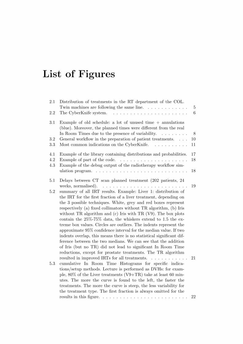
List of Figures

2.1 Distribution of treatments in the RT department of the COL.Twin machines are following the same line. . . . . . . . . . . . . 5

2.2 The CyberKnife system. . . . . . . . . . . . . . . . . . . . . . . 6

3.1 Example of old schedule: a lot of unused time + annulations(blue). Moreover, the planned times were different from the realIn Room Times due to the presence of variability. . . . . . . . . 8

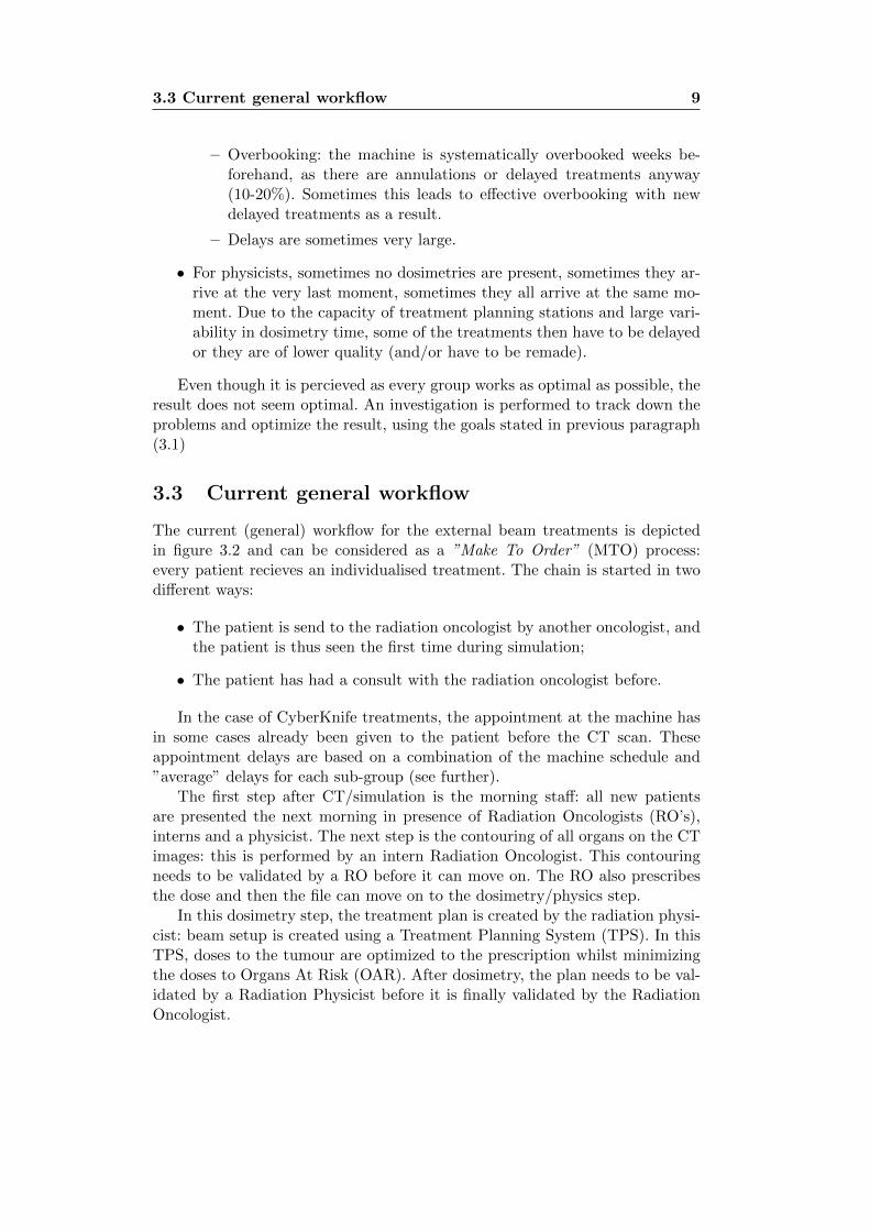
3.2 General workflow in the preparation of patient treatments. . . . 103.3 Most common indications on the CyberKnife. . . . . . . . . . . 11

4.1 Example of the library containing distributions and probabilities. 174.2 Example of part of the code. . . . . . . . . . . . . . . . . . . . . 184.3 Example of the debug output of the radiotherapy workflow sim-

ulation program. . . . . . . . . . . . . . . . . . . . . . . . . . . . 18

5.1 Delays between CT scan planned treatment (202 patients, 24weeks, normalised). . . . . . . . . . . . . . . . . . . . . . . . . . 19

5.2 summary of all IRT results. Example: Liver 1: distribution ofthe IRT for the first fraction of a liver treatment, depending onthe 3 possible techniques. White, grey and red boxes representrespectively (a) fixed collimators without TR algorithm, (b) Iriswithout TR algorithm and (c) Iris with TR (V9). The box plotscontain the 25%-75% data, the whiskers extend to 1.5 the ex-treme box values. Circles are outliers. The indents represent theapproximate 95% confidence interval for the median value. If twoindents overlap, this means there is no statistical significant dif-ference between the two medians. We can see that the additionof Iris (but no TR) did not lead to significant In Room Timereductions, except for prostate treatments. The TR algorithmresulted in improved IRTs for all treatments. . . . . . . . . . . . 21

5.3 cumulative In Room Time Histograms for specific indica-tions/setup methods. Lecture is performed as DVHs: for exam-ple, 80% of the Liver treatments (V9+TR) take at least 60 min-utes. The more the curve is found to the left, the faster thetreatments. The more the curve is steep, the less variability forthe treatment type. The first fraction is always omitted for theresults in this figure. . . . . . . . . . . . . . . . . . . . . . . . . . 22

LIST OF FIGURES iv

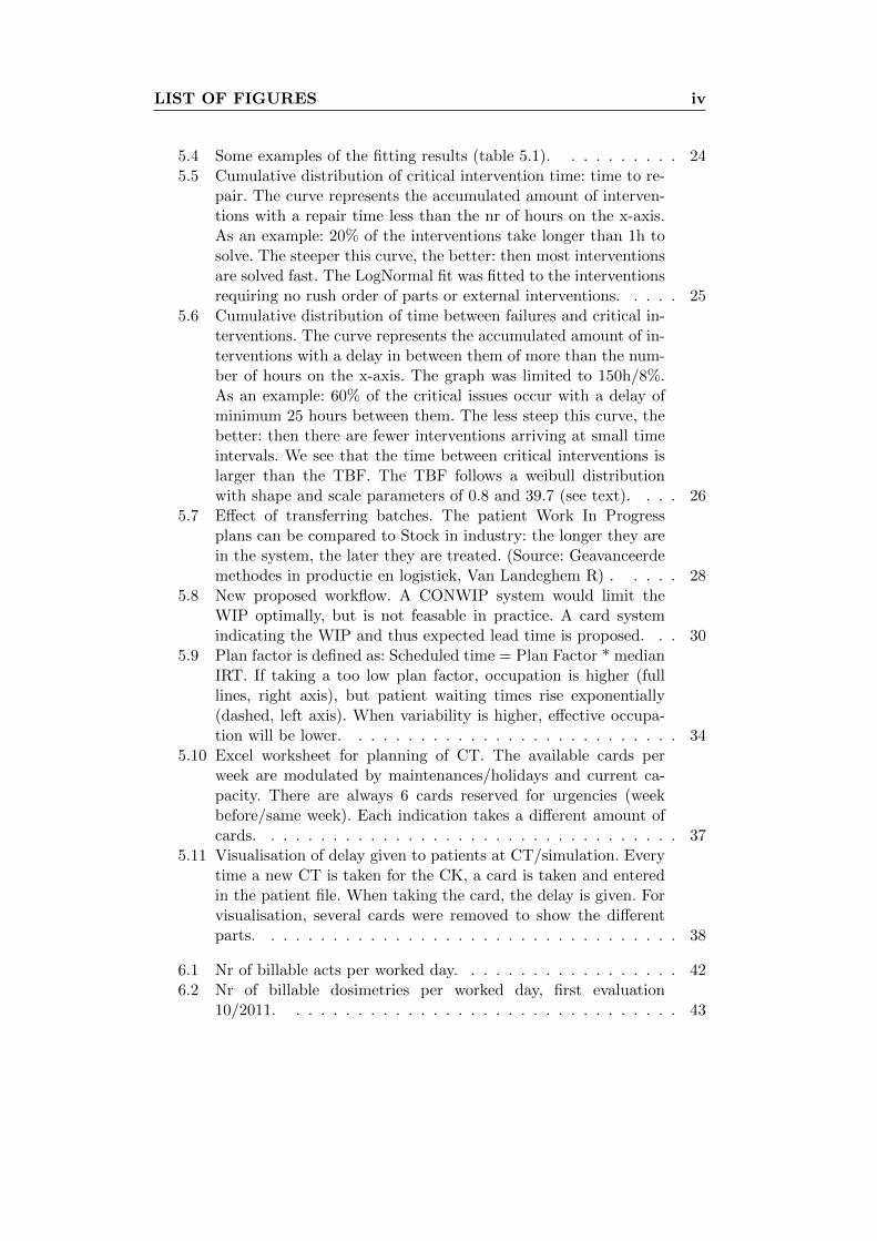
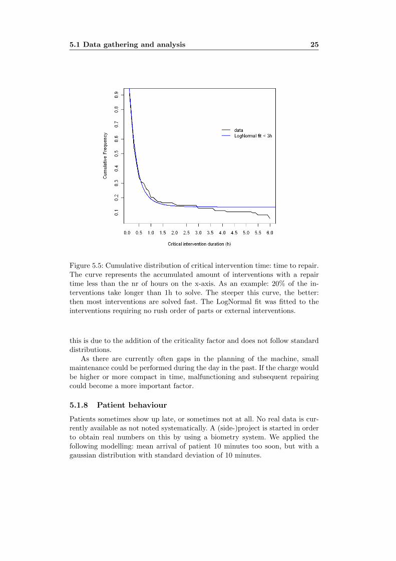
5.4 Some examples of the fitting results (table 5.1). . . . . . . . . . 245.5 Cumulative distribution of critical intervention time: time to re-

pair. The curve represents the accumulated amount of interven-tions with a repair time less than the nr of hours on the x-axis.As an example: 20% of the interventions take longer than 1h tosolve. The steeper this curve, the better: then most interventionsare solved fast. The LogNormal fit was fitted to the interventionsrequiring no rush order of parts or external interventions. . . . . 25

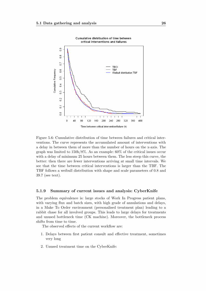
5.6 Cumulative distribution of time between failures and critical in-terventions. The curve represents the accumulated amount of in-terventions with a delay in between them of more than the num-ber of hours on the x-axis. The graph was limited to 150h/8%.As an example: 60% of the critical issues occur with a delay ofminimum 25 hours between them. The less steep this curve, thebetter: then there are fewer interventions arriving at small timeintervals. We see that the time between critical interventions islarger than the TBF. The TBF follows a weibull distributionwith shape and scale parameters of 0.8 and 39.7 (see text). . . . 26

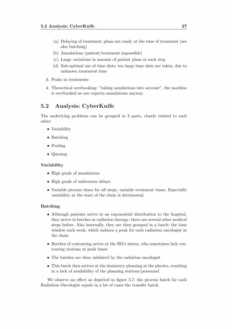
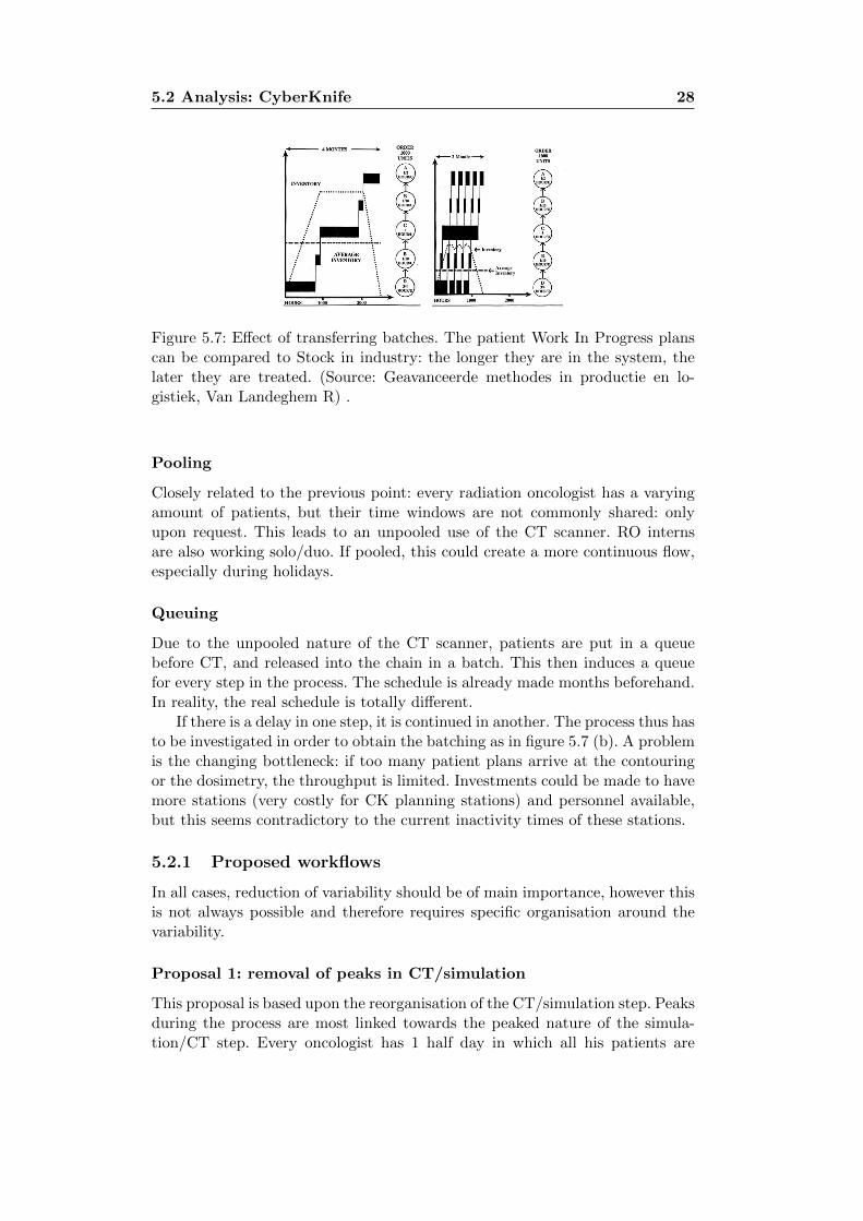
5.7 Effect of transferring batches. The patient Work In Progressplans can be compared to Stock in industry: the longer they arein the system, the later they are treated. (Source: Geavanceerdemethodes in productie en logistiek, Van Landeghem R) . . . . . 28

5.8 New proposed workflow. A CONWIP system would limit theWIP optimally, but is not feasable in practice. A card systemindicating the WIP and thus expected lead time is proposed. . . 30

5.9 Plan factor is defined as: Scheduled time = Plan Factor * medianIRT. If taking a too low plan factor, occupation is higher (fulllines, right axis), but patient waiting times rise exponentially(dashed, left axis). When variability is higher, effective occupa-tion will be lower. . . . . . . . . . . . . . . . . . . . . . . . . . . 34

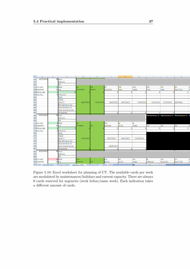
5.10 Excel worksheet for planning of CT. The available cards perweek are modulated by maintenances/holidays and current ca-pacity. There are always 6 cards reserved for urgencies (weekbefore/same week). Each indication takes a different amount ofcards. . . . . . . . . . . . . . . . . . . . . . . . . . . . . . . . . . 37

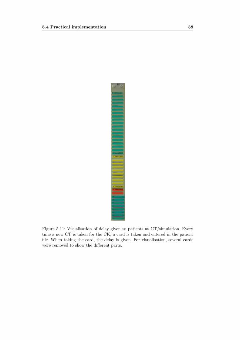
5.11 Visualisation of delay given to patients at CT/simulation. Everytime a new CT is taken for the CK, a card is taken and enteredin the patient file. When taking the card, the delay is given. Forvisualisation, several cards were removed to show the differentparts. . . . . . . . . . . . . . . . . . . . . . . . . . . . . . . . . . 38

6.1 Nr of billable acts per worked day. . . . . . . . . . . . . . . . . . 426.2 Nr of billable dosimetries per worked day, first evaluation

10/2011. . . . . . . . . . . . . . . . . . . . . . . . . . . . . . . . 43

LIST OF FIGURES v

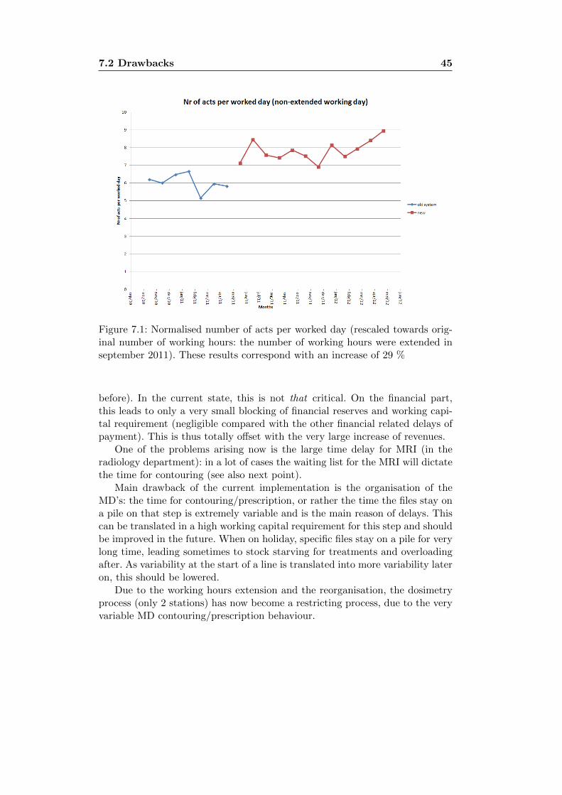
7.1 Normalised number of acts per worked day (rescaled towardsoriginal number of working hours: the number of working hourswere extended in september 2011). These results correspond withan increase of 29 % . . . . . . . . . . . . . . . . . . . . . . . . . 45

Chapter 1

Summary

Cyberknife treatments do not follow the classical conventional radiotherapyschemes. At the COL, utilisation of the CyberKnife treatment machine used tobe very low, whilst waiting lists were growing every day. In aim of this studywas improvement of the workflow. This was performed in several steps:

• Process mapping of the substeps in the process

• Reunions with involved personnel

• Analysis of influencing factors

• Data analysis and model creation of the substeps

• Programming of a Discrete Event Simulation application, simulating theprocess

• Search for different organisational solutions

• Simulations of proposed possibilities and simulations of optimal parame-ters

• Implementation requirements: visualisation and tools

• Implementation

• Follow-up

The main issues were found to be:

• Variability:

– Variable process time for several steps

– Large number of annulations/delays

– Unknown effective treatment time: only at the end the real treatmenttime was known.

• Batching:

2

– Certain steps (CT scan, contouring) were performed in batch, in-creasing process times artificially

The project was started in september 2010 and the first version of the reor-ganisation was implemented in may 2011, later on this was further finetuned.The final version was a hybrid push system with normalised WIP (Work InProgress) follow up/control, combined with lead time indicators for patients.

Inflow of patients at CT scan depends on an amount of normalised work thatcan be released per week, controlled by the current WIP: each patient, depend-ing on indication, requires a certain number of cards. Every week these cardsare modulated depending on the current workload/holidays/breakdowns. . . Thefinal appointment is only given to patients after the dosimetry step: then thereal IRT (In Room Time) can be predicted and correctly scheduled. The numberof cards as WIP are an indicator for the expected delay given to the patients atCT scan. The WIP is not controlled strictly as in a CONWIP (Constant WorkIn Progress) system, but is regulated for. The Nr of cards allowed per week isa critical parameter: too few = starving; too many = delay explosion.

Ideally, a pure CONWIP system would perform better in terms of variabil-ity, slightly better machine occupation and delays. However, that method iscurrently infeasible to implement due to other constraints.

The end results were (1 year of implementation):

• Output: 28% more patients treated = more highest quality treatmentsavailable for patients + leverage for working hours extension. Due tohigher effective capacity, decrease of queuing times before CT.

• Lead Time CT-treatment: only a slight lead time hit: median delayof 9 working days instead of 8 days.

• Personnel: having better control over work

• Quality: no rushing of impossible/hard files

• Patient: no complaints thus far

• Financial: more than 700.000 Euro/year net gain

• Future: faster substeps can automatically lead to faster lead times

Following this work, there were 2 poster presentations delivered at two con-gresses (see appendix):

• EWG-MCTP 3, 15-18 May 2012, Sevilla, SpainCrop F, Lacornerie T, Mirabel X, Vanlandeghem R and Lartigau E 2012Discrete Event Simulation modelling of patient flow for CyberKnife treat-ments

• 31th Annual ESTRO meeting, 9-13 May 2012, Barcelona, SpainCrop F, Lacornerie T, Szymczak H, Mirabel X, Felin A, Bailleux C andLartigau E 2012 Treatment time and technical intervention time analysisof a CyberKnife installation Rad. Ther. Oncol. 103 S1 PO-0775

Chapter 2

Introduction

In the first chapter, a general description of the Centre Oscar Lambret and itsradiotherapy department is given, followed by an explanation of the radiother-apy process.

2.1 Centre Oscar Lambret

The Centre Oscar Lambret (COL) is a so called Centre de Lutte Contre le Can-cer (CLCC). The goal of a CLCC is an integrated multidisciplinary approach oftreatment of cancer: all departments are oriented towards fighting cancer. Theresult is a center covering Radiology, Nuclear Medicine, Radiotherapy, GeneralCancerology. . .

A CLCC is a particular entity in France: the funding is public (budget2010: 87.5 million Euro), but the management is private. CLCC’s are thussemi-organised by the state and are oriented towards the application of newtechniques and act as spearheads in the fight vs cancer. This means that newtechniques are constantly implemented and tested.

The COL employs more than 800 people, of which:

• 150 doctors and scientific staff

• 470 nurses and other paramedical staff

• 200 people in logistics, hotel staff and administration

The RadioTherapy (RT) department of the COL is considered as a verylarge RT department and treats more than 3000 patients yearly, of which:

• 2200 patients by 6 External Beam Radiotherapy machines, with a meanof 20-25 sessions per patient

• 500 patients by Gamma Knife, single session

• 500 Brachy treatments/year (1 HDR, 1 LDR, 3 PDR and prostate im-plants. . . ), hospitalised

2.2 Radiotherapy Department 4

2.2 Radiotherapy Department

2.2.1 Staff roles

The staff of a RT department is a closely collaborating multidisciplinary teamwhich can be divided in the following categories and responsabilities:

• Radiation Oncologists: patient selection; contours; prescription; final ap-proval

• Radiation Physicists: machine and radiation QA/QC + calibration;dosimetry and dosimetry approval1; technical approvals

• Dosimetrists: dosimetry or treatment planning

• Biomedical Engineers: technical maintenance and repairs

• Technologists: operators of simulator, CT, linacs; patient setup

• Nursing : hospitalisation for brachytherapy

• Administrative staff

2.2.2 Machines

The goal of radiotherapy is a curative or palliative treatment of cancer, usingionizing radiation. Depending on the indication, a variety of different methodsare applied in radiotherapy, as there are:

1. Brachytherapy: use of radioactive isotopes, which are inserted in orbrought into contact with the lesion (example: PDR, HDR).

2. External Beam RadioTherapy: (EBRT) use of high energy (+ 1 MeV) ion-izing radiation (photons, electrons or even protons or heavier ions) aimedat the lesion. The radiation is generated by linear accelerators (linac) inthe case of photons or electrons. Indications are subcutaneous or deeplyseated tumors. The CyberKnife is an advanced example.

3. Contact Therapy: use of low energy (50-200 kV) photons, generated byan X-ray tube. Indications are superficial (example: DARPAC machine).

2.2.3 Technology in External Beam RadioTherapy

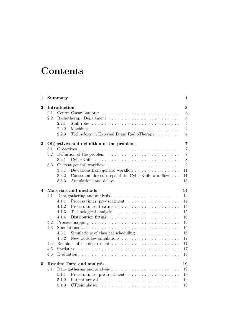
Depending on the indication, different treatment techniques can be applied (seealso figure 2.1 for repartition towards machines). Radiotherapy plans for pa-tients are always highly customized towards the specific patient circomstances.We remark that the terms ”planning” and ”dosimetry” are commonly used asnames of the process of beam setup of the treatment, or the so called ”treatmentplan”.

1dosimetry = treatment planning; Treatment Planning is the process of creating the opti-mal beam setup and delivery. One can say the equivalence of pharmacy of radiation dose.


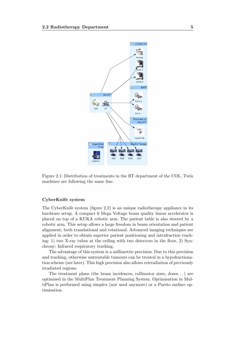
Figure 2.1: Distribution of treatments in the RT department of the COL. Twinmachines are following the same line.

CyberKnife system

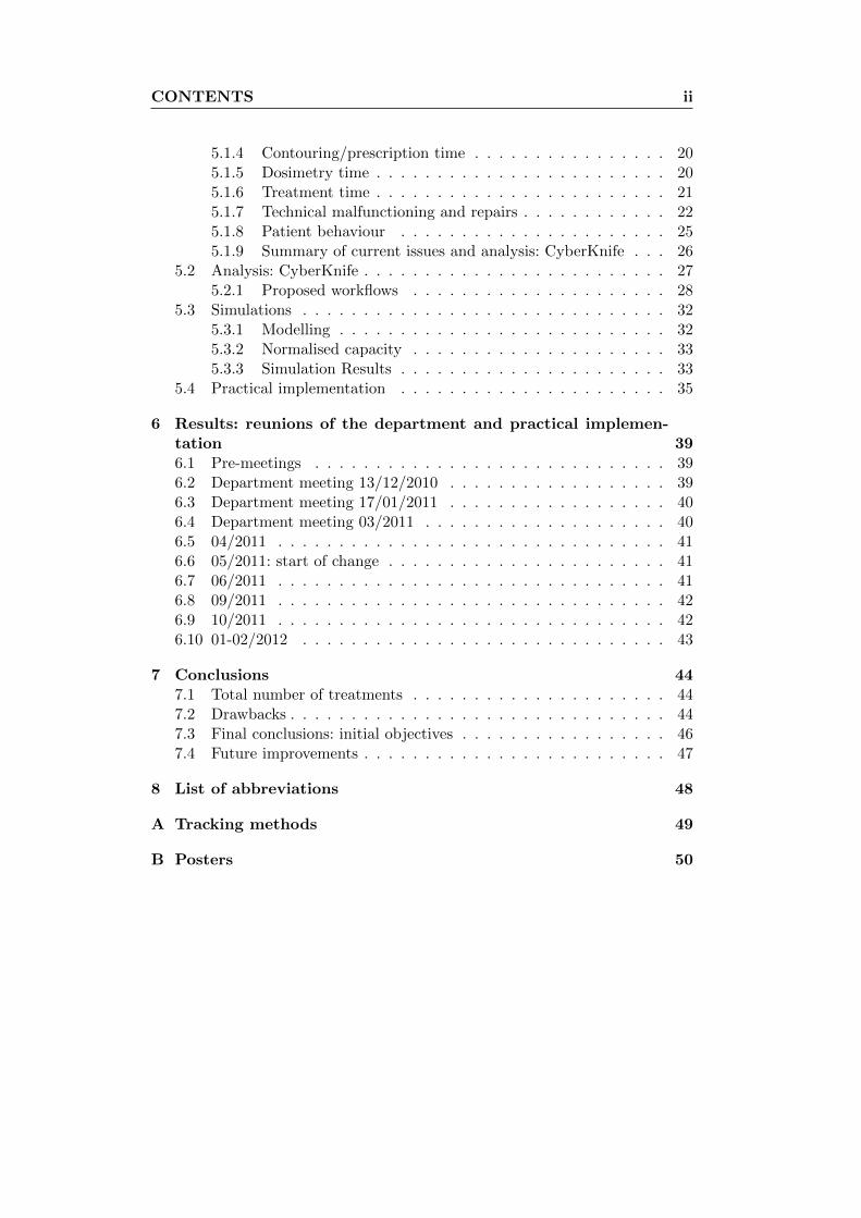
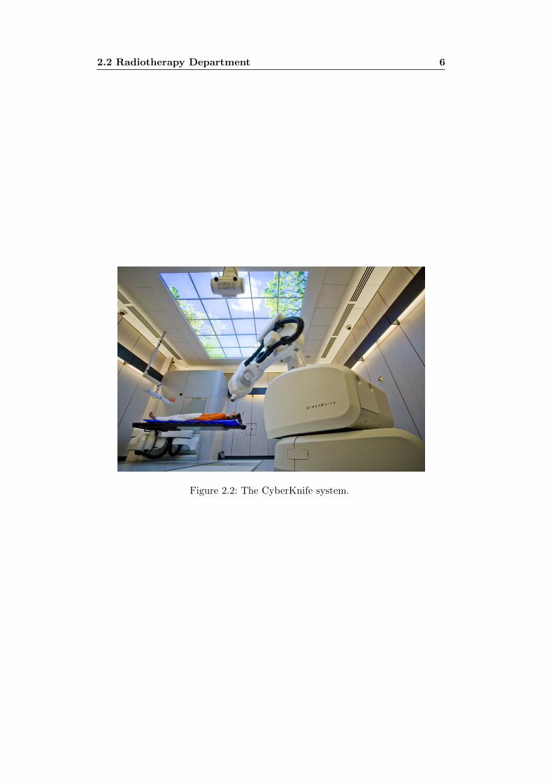
The CyberKnife system (figure 2.2) is an unique radiotherapy appliance in itshardware setup. A compact 6 Mega Voltage beam quality linear accelerator isplaced on top of a KUKA robotic arm. The patient table is also steered by arobotic arm. This setup allows a large freedom in beam orientation and patientalignment, both translational and rotational. Advanced imaging techniques areapplied in order to obtain superior patient positioning and intrafraction track-ing: 1) two X-ray tubes at the ceiling with two detectors in the floor, 2) Syn-chrony: Infrared respiratory tracking.

The advantage of this system is a millimetric precision. Due to this precisionand tracking, otherwise untreatable tumours can be treated in a hypofractiona-tion scheme (see later). This high precision also allows reirradiation of previouslyirradiated regions.

The treatment plans (the beam incidences, collimator sizes, doses. . . ) areoptimised in the MultiPlan Treatment Planning System. Optimisation in Mul-tiPlan is performed using simplex (not used anymore) or a Pareto surface op-timisation.


Figure 2.2: The CyberKnife system.

Chapter 3

Objectives and definition ofthe problem

3.1 Objectives

The goal of this investigation was the optimisation of the following combinationfor the workflow:

• Operational

– Output:

∗ Increasing the nr of patients treated per month

– Delays/Work In Progress:

∗ Keeping CT scan-treatment times as low as possible. This shouldbe below 14 days ideally: CT scan should represent the realpatient anatomy.

∗ By increasing output and capacity, total delay between patientreferral and treatment should be lower as there is currently awaiting list

• Human factors and Quality

– Personnel stress levels

∗ Organisational feasibility for every group: increase control overwork. Decrease the percieved workload of personnel involved.

∗ Quality: Most of the work is manual, quality depends on theavailable time and perception of it

– Patient satisfaction

∗ Patient satisfaction is largely dependent on the fulfillment ofgiven information and promised delays.

• Financial

– Revenues

3.2 Definition of the problem 8

∗ Productivity: more output/capacity

∗ Working capital management: reducing the time between entryof patient and treatment equals lower working capital require-ment

3.2 Definition of the problem

3.2.1 CyberKnife

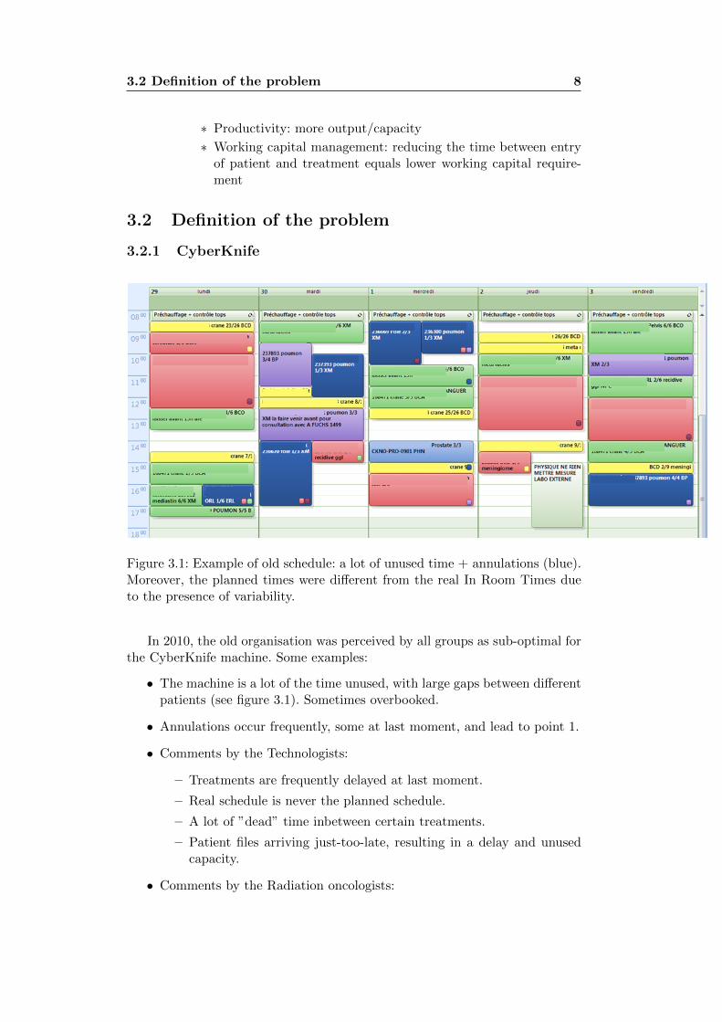
Figure 3.1: Example of old schedule: a lot of unused time + annulations (blue).Moreover, the planned times were different from the real In Room Times dueto the presence of variability.

In 2010, the old organisation was perceived by all groups as sub-optimal forthe CyberKnife machine. Some examples:

• The machine is a lot of the time unused, with large gaps between differentpatients (see figure 3.1). Sometimes overbooked.

• Annulations occur frequently, some at last moment, and lead to point 1.

• Comments by the Technologists:

– Treatments are frequently delayed at last moment.

– Real schedule is never the planned schedule.

– A lot of ”dead” time inbetween certain treatments.

– Patient files arriving just-too-late, resulting in a delay and unusedcapacity.

• Comments by the Radiation oncologists:

3.3 Current general workflow 9

– Overbooking: the machine is systematically overbooked weeks be-forehand, as there are annulations or delayed treatments anyway(10-20%). Sometimes this leads to effective overbooking with newdelayed treatments as a result.

– Delays are sometimes very large.

• For physicists, sometimes no dosimetries are present, sometimes they ar-rive at the very last moment, sometimes they all arrive at the same mo-ment. Due to the capacity of treatment planning stations and large vari-ability in dosimetry time, some of the treatments then have to be delayedor they are of lower quality (and/or have to be remade).

Even though it is percieved as every group works as optimal as possible, theresult does not seem optimal. An investigation is performed to track down theproblems and optimize the result, using the goals stated in previous paragraph(3.1)

3.3 Current general workflow

The current (general) workflow for the external beam treatments is depictedin figure 3.2 and can be considered as a ”Make To Order” (MTO) process:every patient recieves an individualised treatment. The chain is started in twodifferent ways:

• The patient is send to the radiation oncologist by another oncologist, andthe patient is thus seen the first time during simulation;

• The patient has had a consult with the radiation oncologist before.

In the case of CyberKnife treatments, the appointment at the machine hasin some cases already been given to the patient before the CT scan. Theseappointment delays are based on a combination of the machine schedule and”average” delays for each sub-group (see further).

The first step after CT/simulation is the morning staff: all new patientsare presented the next morning in presence of Radiation Oncologists (RO’s),interns and a physicist. The next step is the contouring of all organs on the CTimages: this is performed by an intern Radiation Oncologist. This contouringneeds to be validated by a RO before it can move on. The RO also prescribesthe dose and then the file can move on to the dosimetry/physics step.

In this dosimetry step, the treatment plan is created by the radiation physi-cist: beam setup is created using a Treatment Planning System (TPS). In thisTPS, doses to the tumour are optimized to the prescription whilst minimizingthe doses to Organs At Risk (OAR). After dosimetry, the plan needs to be val-idated by a Radiation Physicist before it is finally validated by the RadiationOncologist.


Fig

ure

3.2

:G

ener

alw

orkfl

owin

the

pre

par

atio

nof

pat

ient

trea

tmen

ts.


3.3.1 Deviations from general workflow

There are quite some situations in which additional steps are added into theworkflow. Some examples are:

• Fiducial implants: fiducials are inserted for tumor motion tracking. Ex-ample: liver, some lung tumours. The CT scan and contouring can onlystart after the fiducials are implanted.

• MRI or PET: an MRI or PET scan is sometimes necessary to performthe contouring of the tumour (example PET FDG scan for lung tumours).Fusion of images is then required during the contouring step. As MRI orPET planning depends on other departments, these are most of the timenot synchronised.

• Urgent treatments: medullar compression requires irradiation within 24hours.

• Boost treatments after external beam treatments. These have to followthe previous treatment (on another machine) immediately.

3.3.2 Constraints for substeps of the CyberKnife workflow

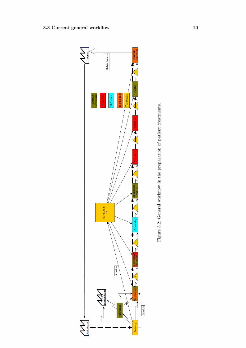
Figure 3.3: Most common indications on the CyberKnife.

Simulation + CT:

1. Seven (1 per oncologist + 1 radiology) time windows of half a day. EachRO has his ”own” half day to perform CT scans.


2. In about half of the cases, the radiation oncologist has to be present duringsimulation: the patient is only seen first time then

Contouring and prescription:

1. Contouring of OAR is performed by the radiation oncologist’s intern

2. Prescription and validation of contours is performed by the RadiationOncologist between other tasks

3. Throughput limitations:

(a) Availability of contouring stations

(b) Availability of RO or RO’s intern

Dosimetry step:

1. Dosimetry for CK is performed by physicists

2. Throughput limitations:

(a) Workstations: 2 workstations

(b) Duration of planning: from 3h to 20h, depending on indication andissues

(c) Returning plans of technical impossible treatments (cf lung track-ing/fiducial tracking)

(d) Crashes

Patient treatment scheduling:

1. Hypofractionation: 1 to 6 fractions are to be delivered. The fractionationhas to be evenly spread, but with a fixed number of days inbetween.Example: 5 fractions, first fraction monday, second fraction wednesday,third friday. . .

2. Normal fractionation: fractions need to be delivered on a day-per-day ba-sis, with almost no interruption (for a 20fx treatment, at most 1 time4fx/week, in extremis 2 times 4fx/week). This factor also has its reper-cussions on maintenances, malfunctions and holidays. These can result ina saturday’s work addition (on a patient case-by-case base, dependent onhistory and indication). Less of a constraint for CK.

3. Urgencies: depending on the indication, some indications need to betreated very quickly, others on a short term (Head and Neck) or morelong term. Generally however, the faster the better.

4. Patients coming from afar: These patients need fixed dates for their treat-ment fractions as they need to book a stay. The appointment at the ma-chine is already given long beforehand.


5. Scheduling: the required schedule time is not straightforward and un-known upfront, as certain treatments use a lot of machine time, whilstothers less (with a large variation intra-indication, between 20 minutesand 200 minutes, see further).

6. Patient transport to the centre: patient transport is organised throughexternal firms.

Technical malfunctions during treatment:

1. Some interruptions can be solved by a physicist, some by biomedical engi-neers. There is a constant permanence of both groups, however they canbe occupied with other machines in the department.

3.3.3 Annulations and delays

Annulations

1. Medical: after simulation/scanner due to medical reasons

2. Physics: after dosimetry: treatment not possible

3. Patient: cancellation of his treatment for personal reasons

Delays during the process:

1. Medical: delays in contouring, fiducials posing, fiducial migration

2. Physics: delay in dosimetry

• before dosimetry: unusable CT, patient in incorrect position, incor-rect reconstruction: CT has to be redone

• after dosimetry: hard/easy dosimetry, amount of files, amount ofother treatment unit ”urgent” files

3. Treatment:

• Technical: machine malfunctioning before/during treatments

• Dosimetry/technical: treatment not executable, file returns tophysics to try to solve

• Patient: showing up late

Chapter 4

Materials and methods

The project can be separated in the following major parts:

• Data gathering and analysis

• Process mapping: future state propositions

• Programming Discrete Event Simulation package in order to simulate pa-tient flow

• Reunions with different groups

• Implementation and follow-up

4.1 Data gathering and analysis

The first problem with the data gathering is the swiss cheese effect: parts of dataare gathered manually in three different databases, of which 2 are in excel (onefrom the start of CK treatments (06/2007), another one was started 05/2010).Entry errors and deviations are thus plenty. Annulations are not really gatheredin a systematic way. The current organisation is analysed regarding busy timeand delays for every step.

In order to perform simulations with these data, distribution fitting wasapplied.

4.1.1 Process times: pre-treatment

Process times were gathered, starting from may 2010, for contouring, dosimetryand validations. These were however gathered in a rough way: the number ofworking days between the different steps. Further detailed measurements werealso performed.

4.1.2 Process times: treatment

Treatment times, or rather In Room Times (IRT), were gathered in a detailedmanner: technologists write down the treatment time for every fraction. Thisdatabase contains information from 06/2007.

4.1 Data gathering and analysis 15

4.1.3 Technological analysis

In room times (IRT) were recorded from 06/2007 up to 11/2011. IRTs aredefined as the time between the patient entering the room and leaving theroom, thus also including setup time. Certain tracking methods require longersetup time and/or treatment time (see appendix A).

In september 2009, an initial version of the Iris collimator and 800 MU linacwere installed. Before, only fixed collimators were used. When using multiplefixed collimators during the treatment, an additional ”changeover” time is re-quired: the robot has to switch collimators and follow new paths around thepatient. The Iris collimator is a collimator with diaphragm, which can changeaperture at any position of the robot arm. An analysis was performed to com-pare treatment times with the Iris collimator. A comparison is also made be-tween ”first fraction” and ”following fraction”, to see if learning factors arepresent (important for scheduling). In september 2010, the time reduction algo-rithm was installed as well as the upgrade to V9.0: new paths and better stophandling. A comparison is made with previous treatment times.

In room time of first fraction-following fraction

Statistical significance between first and following fraction was evaluated usinga one sided paired t-test. Statistical significance between Fixed, Iris and TimeReduction was evaluated using Mann-Whitney U tests. The represented 95%confidence interval of the median in the box-whisker plots is calculated usingthe method of Chambers et al 1983.

Process times: breakdowns and repairs

These are gathered in a detailed manner by the biomedical engineers.Technical interventions of the biomedical engineering department were

recorded and analyzed from 06/2007 up to 10/2011. Interventions were recordedincluding time of call, time of start of intervention, time of end of interventionand criticality. The Time Between Failure (TBF) is the time between failuresof the machine. The Time Between Critical Intervention (TBCI) is the timebetween interventions, interrupting regular CyberKnife operations. Not all in-terventions however are critical: we refer to critical failures when (a) treatmentscannot continue as intervention/repair is needed and (b) the issue cannot besolved by the technologist at the machine. Repairs which can be postponedto the evening/weekend are thus non-critical. This factor is useful for analysison a long time scale to determine normal operation interruptions. Technicalmalfunctions are thus only a part of the TBCI. Other distinctions were madebetween (a) morning failures and failures during the day and (b) between crit-ical interventions requiring external intervention by Accuray. An experimentalversion of the Iris collimator was used during a part of the analyzed time. Theseinterventions are masked, as they did not show normal operations. Distributionfitting is performed using the same methodology of previous paragraph.

4.2 Process mapping 16

4.1.4 Distribution fitting

The obtained results were later on used for distribution fitting, in order toperform simulations easier. If distribution fitting was impossible, then only theavailable probability distribution was used.

Analytical distribution fitting is performed in the R project using the fol-lowing scheme (Law and Kelton 1991):

• Maximum Likelihood Estimation of typical probability distributions forprocess/repair times as Gamma, Weibull and LogNormal distributions

• Graphical comparison of probability density function, frequency distribu-tion and qqplots

• Computation of the Kolmogorov-Smirnov goodness-of-fit statistic. H0 forthis test is: empirical distribution is coming from the hypothesized theo-retical distribution (gamma, Weibull).

These distributions were then applied in the simulations.

4.2 Process mapping

The process was mapped by interviewing the different involved groups. Opinionsare gathered and summarised. These results were given in the previous chapter(section 3.3).

4.3 Simulations

Simulations can be divided in 2 distinct parts: classical scheduling simulationsand the new workflow simulations. All simulations were programmed in python,using the SimPy package: a discrete-event simulation package. The purpose ofthe simulations is to assess (a) future state propositions before implementinganother workflow and (b) optimising parameters.

4.3.1 Simulations of classical scheduling

These simulations were applied to find out the most optimal scheduling time,when the treatment time is still unknown, per indication. The optimal planningparameters were calculated: depending on the ”planning factor” (Scheduledtime = median treatment time(fraction) * PlanFactor) the factors ”machineutilization”, ”average patient wait time”, patients reneged (waiting time longerthan 120 minutes) and personnel OverTime were simulated and calculated.

A schedule is created using the Scheduled times (and thus depends on theplanning factor). We took as standard working day 10 consecutive workinghours. Patient arrival is modeled as 10 minutes too soon, with gaussian distri-bution (σ = 10 minutes). Distinction between first and following fractions weremade (see further). The effective machine load was then simulated using thehistorical distributions. Simulated patients will renege (sent home) when theyhave to wait longer than 2 hours.

4.4 Reunions of the department 17

4.3.2 New workflow simulations

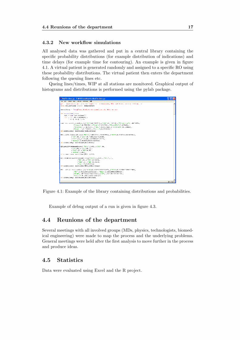
All analysed data was gathered and put in a central library containing thespecific probability distributions (for example distribution of indications) andtime delays (for example time for contouring). An example is given in figure4.1. A virtual patient is generated randomly and assigned to a specific RO usingthese probability distributions. The virtual patient then enters the departmentfollowing the queuing lines etc.

Queing lines/times, WIP at all stations are monitored. Graphical output ofhistograms and distributions is performed using the pylab package.

Figure 4.1: Example of the library containing distributions and probabilities.

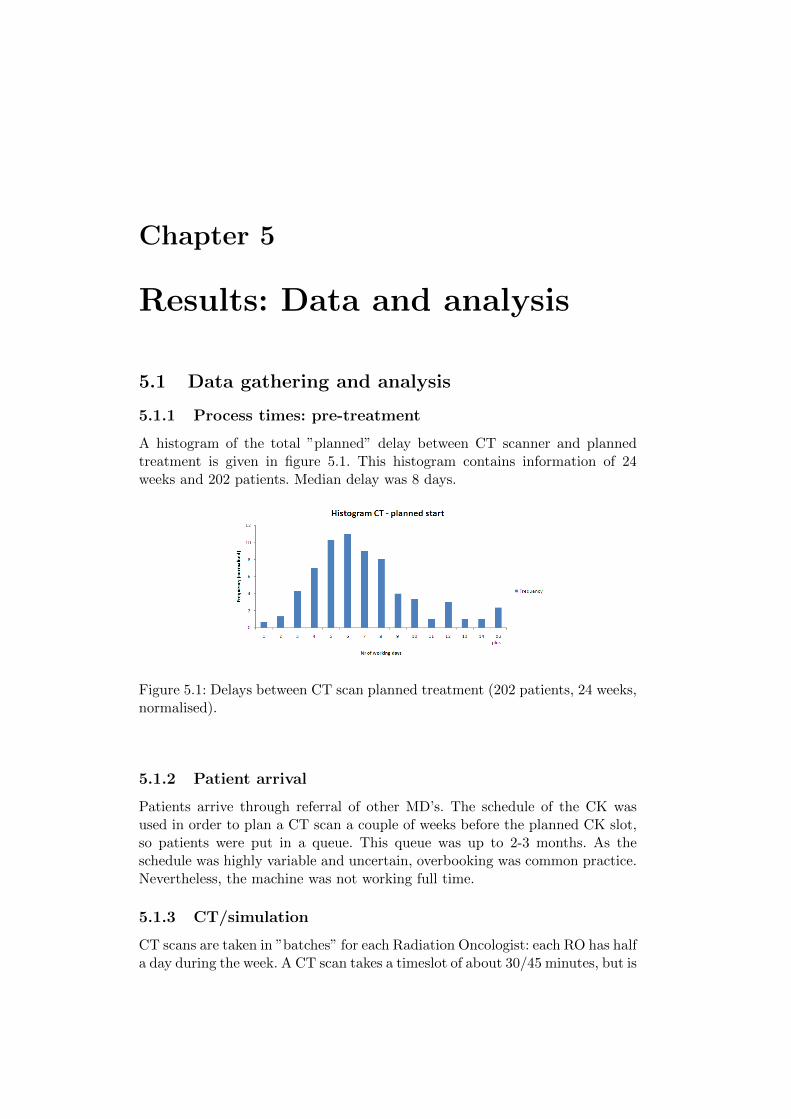
Example of debug output of a run is given in figure 4.3.

4.4 Reunions of the department

Several meetings with all involved groups (MDs, physics, technologists, biomed-ical engineering) were made to map the process and the underlying problems.General meetings were held after the first analysis to move further in the processand produce ideas.

4.5 Statistics

Data were evaluated using Excel and the R project.

4.6 Evaluation 18

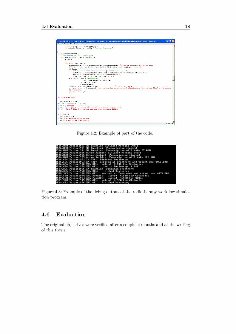
Figure 4.2: Example of part of the code.

Figure 4.3: Example of the debug output of the radiotherapy workflow simula-tion program.

4.6 Evaluation

The original objectives were verified after a couple of months and at the writingof this thesis.

Chapter 5

Results: Data and analysis

5.1 Data gathering and analysis

5.1.1 Process times: pre-treatment

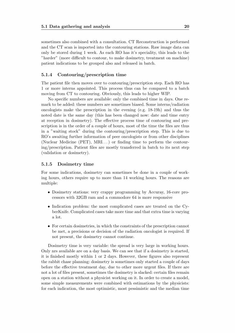
A histogram of the total ”planned” delay between CT scanner and plannedtreatment is given in figure 5.1. This histogram contains information of 24weeks and 202 patients. Median delay was 8 days.

Figure 5.1: Delays between CT scan planned treatment (202 patients, 24 weeks,normalised).

5.1.2 Patient arrival

Patients arrive through referral of other MD’s. The schedule of the CK wasused in order to plan a CT scan a couple of weeks before the planned CK slot,so patients were put in a queue. This queue was up to 2-3 months. As theschedule was highly variable and uncertain, overbooking was common practice.Nevertheless, the machine was not working full time.

5.1.3 CT/simulation

CT scans are taken in ”batches” for each Radiation Oncologist: each RO has halfa day during the week. A CT scan takes a timeslot of about 30/45 minutes, but is


sometimes also combined with a consultation. CT Reconstruction is performedand the CT scan is imported into the contouring stations. Raw image data canonly be stored during 1 week. As each RO has it’s speciality, this leads to the”harder” (more difficult to contour, to make dosimetry, treatment on machine)patient indications to be grouped also and released in batch.

5.1.4 Contouring/prescription time

The patient file then moves over to contouring/prescription step. Each RO has1 or more interns appointed. This process thus can be compared to a batchmoving from CT to contouring. Obviously, this leads to higher WIP.

No specific numbers are available: only the combined time in days. One re-mark to be added: these numbers are sometimes biased. Some interns/radiationoncologists make the prescription in the evening (e.g. 18-19h) and thus thenoted date is the same day (this has been changed now: date and time entryat reception in dosimetry). The effective process time of contouring and pre-scription is in the order of a couple of hours, most of the time the files are thusin a ”waiting stock” during the contouring/prescription step. This is due toRO’s awaiting further information of peer oncologists or from other disciplines(Nuclear Medicine (PET), MRI. . . ) or finding time to perform the contour-ing/prescription. Patient files are mostly transferred in batch to its next step(validation or dosimetry).

5.1.5 Dosimetry time

For some indications, dosimetry can sometimes be done in a couple of work-ing hours, others require up to more than 14 working hours. The reasons aremultiple:

• Dosimetry stations: very crappy programming by Accuray, 16-core pro-cessors with 32GB ram and a commodore 64 is more responsive

• Indication problem: the most complicated cases are treated on the Cy-berKnife. Complicated cases take more time and that extra time is varyinga lot.

• For certain dosimetries, in which the constraints of the prescription cannotbe met, a precisions or decision of the radiation oncologist is required. Ifnot present, the dosimetry cannot continue.

Dosimetry time is very variable: the spread is very large in working hours.Only nrs available are on a day basis. We can see that if a dosimetry is started,it is finished mostly within 1 or 2 days. However, these figures also representthe rabbit chase planning: dosimetry is sometimes only started a couple of daysbefore the effective treatment day, due to other more urgent files. If there arenot a lot of files present, sometimes the dosimetry is slacked: certain files remainopen on a station without a physicist working on it. In order to create a model,some simple measurements were combined with estimations by the physicists:for each indication, the most optimistic, most pessimistic and the median time


was asked and cross-checked with the measurements. Betavariate distributionsare thus created.

5.1.6 Treatment time

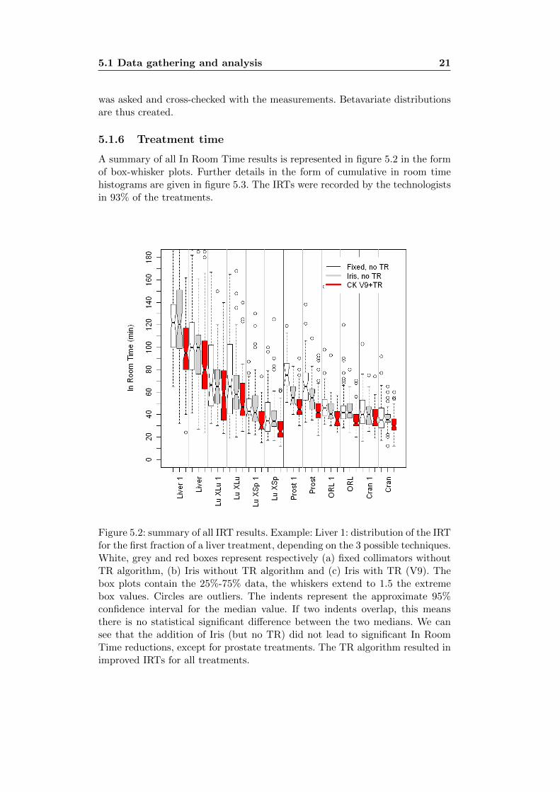
A summary of all In Room Time results is represented in figure 5.2 in the formof box-whisker plots. Further details in the form of cumulative in room timehistograms are given in figure 5.3. The IRTs were recorded by the technologistsin 93% of the treatments.

Figure 5.2: summary of all IRT results. Example: Liver 1: distribution of the IRTfor the first fraction of a liver treatment, depending on the 3 possible techniques.White, grey and red boxes represent respectively (a) fixed collimators withoutTR algorithm, (b) Iris without TR algorithm and (c) Iris with TR (V9). Thebox plots contain the 25%-75% data, the whiskers extend to 1.5 the extremebox values. Circles are outliers. The indents represent the approximate 95%confidence interval for the median value. If two indents overlap, this meansthere is no statistical significant difference between the two medians. We cansee that the addition of Iris (but no TR) did not lead to significant In RoomTime reductions, except for prostate treatments. The TR algorithm resulted inimproved IRTs for all treatments.


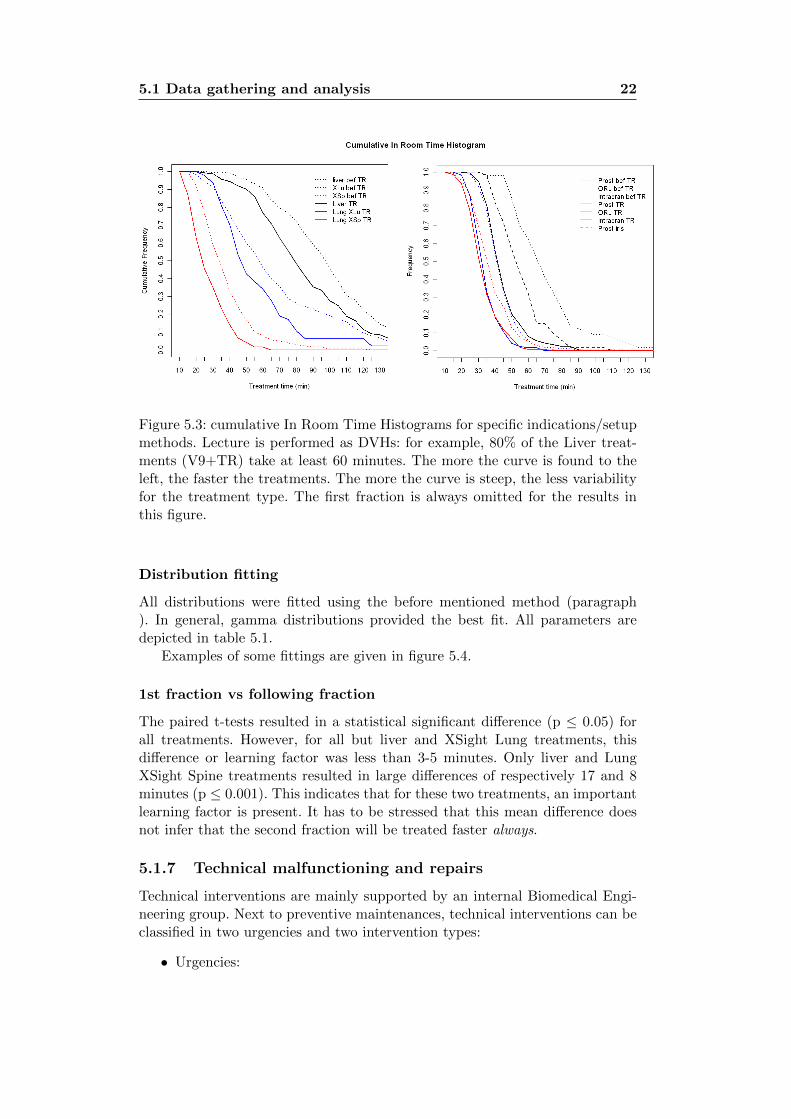
Figure 5.3: cumulative In Room Time Histograms for specific indications/setupmethods. Lecture is performed as DVHs: for example, 80% of the Liver treat-ments (V9+TR) take at least 60 minutes. The more the curve is found to theleft, the faster the treatments. The more the curve is steep, the less variabilityfor the treatment type. The first fraction is always omitted for the results inthis figure.

Distribution fitting

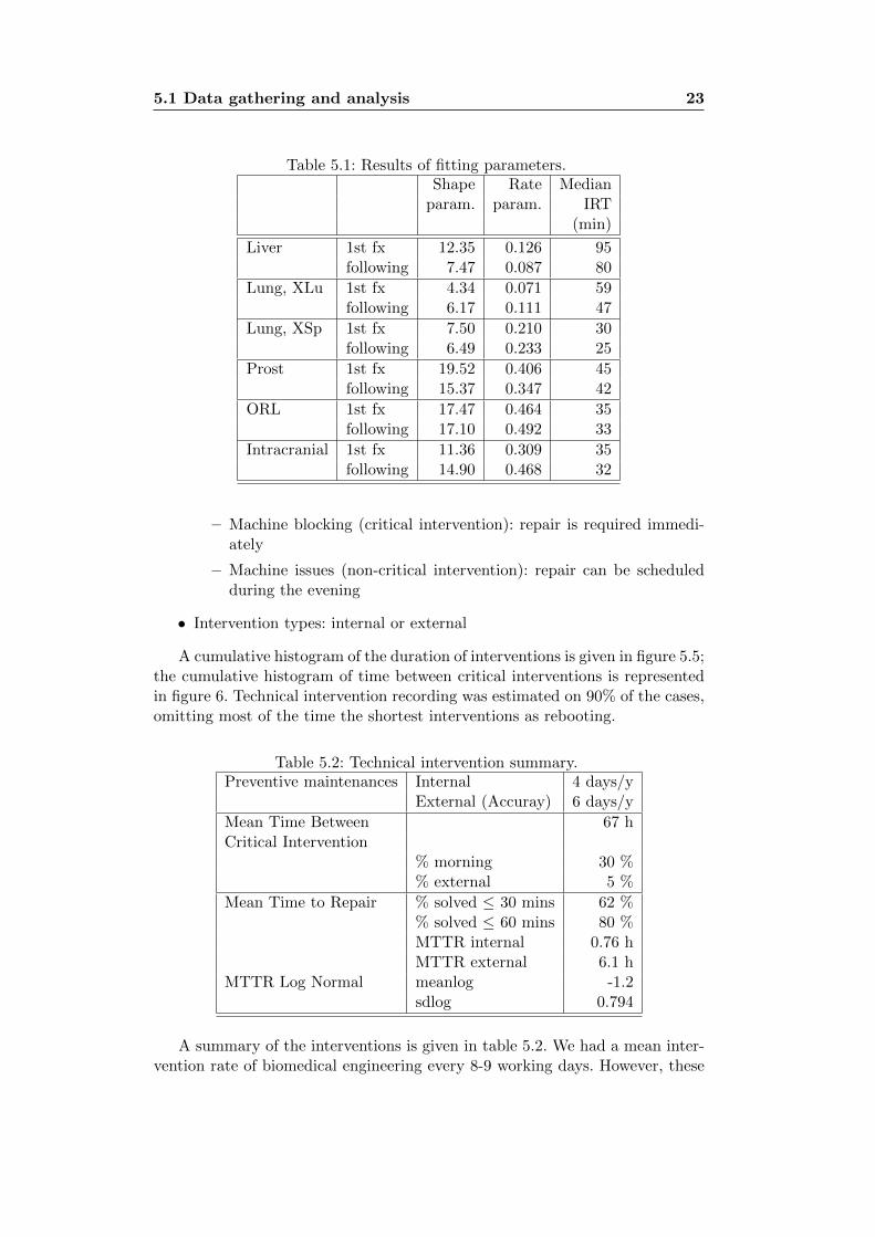
All distributions were fitted using the before mentioned method (paragraph). In general, gamma distributions provided the best fit. All parameters aredepicted in table 5.1.

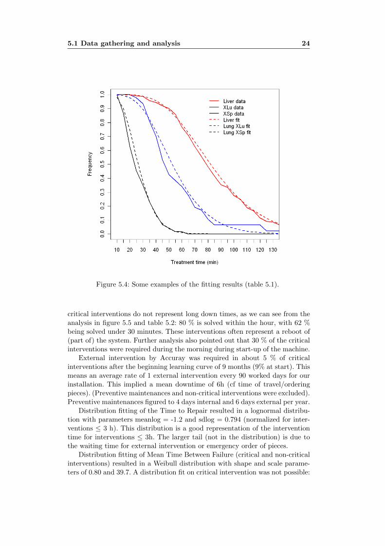
Examples of some fittings are given in figure 5.4.

1st fraction vs following fraction

The paired t-tests resulted in a statistical significant difference (p ≤ 0.05) forall treatments. However, for all but liver and XSight Lung treatments, thisdifference or learning factor was less than 3-5 minutes. Only liver and LungXSight Spine treatments resulted in large differences of respectively 17 and 8minutes (p ≤ 0.001). This indicates that for these two treatments, an importantlearning factor is present. It has to be stressed that this mean difference doesnot infer that the second fraction will be treated faster always.

5.1.7 Technical malfunctioning and repairs

Technical interventions are mainly supported by an internal Biomedical Engi-neering group. Next to preventive maintenances, technical interventions can beclassified in two urgencies and two intervention types:

• Urgencies:


Table 5.1: Results of fitting parameters.Shape Rate Median

param. param. IRT(min)

Liver 1st fx 12.35 0.126 95following 7.47 0.087 80

Lung, XLu 1st fx 4.34 0.071 59following 6.17 0.111 47

Lung, XSp 1st fx 7.50 0.210 30following 6.49 0.233 25

Prost 1st fx 19.52 0.406 45following 15.37 0.347 42

ORL 1st fx 17.47 0.464 35following 17.10 0.492 33

Intracranial 1st fx 11.36 0.309 35following 14.90 0.468 32

– Machine blocking (critical intervention): repair is required immedi-ately

– Machine issues (non-critical intervention): repair can be scheduledduring the evening

• Intervention types: internal or external

A cumulative histogram of the duration of interventions is given in figure 5.5;the cumulative histogram of time between critical interventions is representedin figure 6. Technical intervention recording was estimated on 90% of the cases,omitting most of the time the shortest interventions as rebooting.

Table 5.2: Technical intervention summary.Preventive maintenances Internal 4 days/y

External (Accuray) 6 days/y

Mean Time Between 67 hCritical Intervention

% morning 30 %% external 5 %

Mean Time to Repair % solved ≤ 30 mins 62 %% solved ≤ 60 mins 80 %MTTR internal 0.76 hMTTR external 6.1 h

MTTR Log Normal meanlog -1.2sdlog 0.794

A summary of the interventions is given in table 5.2. We had a mean inter-vention rate of biomedical engineering every 8-9 working days. However, these


Figure 5.4: Some examples of the fitting results (table 5.1).

critical interventions do not represent long down times, as we can see from theanalysis in figure 5.5 and table 5.2: 80 % is solved within the hour, with 62 %being solved under 30 minutes. These interventions often represent a reboot of(part of) the system. Further analysis also pointed out that 30 % of the criticalinterventions were required during the morning during start-up of the machine.

External intervention by Accuray was required in about 5 % of criticalinterventions after the beginning learning curve of 9 months (9% at start). Thismeans an average rate of 1 external intervention every 90 worked days for ourinstallation. This implied a mean downtime of 6h (cf time of travel/orderingpieces). (Preventive maintenances and non-critical interventions were excluded).Preventive maintenances figured to 4 days internal and 6 days external per year.

Distribution fitting of the Time to Repair resulted in a lognormal distribu-tion with parameters meanlog = -1.2 and sdlog = 0.794 (normalized for inter-ventions ≤ 3 h). This distribution is a good representation of the interventiontime for interventions ≤ 3h. The larger tail (not in the distribution) is due tothe waiting time for external intervention or emergency order of pieces.

Distribution fitting of Mean Time Between Failure (critical and non-criticalinterventions) resulted in a Weibull distribution with shape and scale parame-ters of 0.80 and 39.7. A distribution fit on critical intervention was not possible:


Figure 5.5: Cumulative distribution of critical intervention time: time to repair.The curve represents the accumulated amount of interventions with a repairtime less than the nr of hours on the x-axis. As an example: 20% of the in-terventions take longer than 1h to solve. The steeper this curve, the better:then most interventions are solved fast. The LogNormal fit was fitted to theinterventions requiring no rush order of parts or external interventions.

this is due to the addition of the criticality factor and does not follow standarddistributions.

As there are currently often gaps in the planning of the machine, smallmaintenance could be performed during the day in the past. If the charge wouldbe higher or more compact in time, malfunctioning and subsequent repairingcould become a more important factor.

5.1.8 Patient behaviour

Patients sometimes show up late, or sometimes not at all. No real data is cur-rently available as not noted systematically. A (side-)project is started in orderto obtain real numbers on this by using a biometry system. We applied thefollowing modelling: mean arrival of patient 10 minutes too soon, but with agaussian distribution with standard deviation of 10 minutes.


Figure 5.6: Cumulative distribution of time between failures and critical inter-ventions. The curve represents the accumulated amount of interventions witha delay in between them of more than the number of hours on the x-axis. Thegraph was limited to 150h/8%. As an example: 60% of the critical issues occurwith a delay of minimum 25 hours between them. The less steep this curve, thebetter: then there are fewer interventions arriving at small time intervals. Wesee that the time between critical interventions is larger than the TBF. TheTBF follows a weibull distribution with shape and scale parameters of 0.8 and39.7 (see text).

5.1.9 Summary of current issues and analysis: CyberKnife

The problem equivalence is: large stocks of Work In Progress patient plans,with varying flux and batch sizes, with high grade of annulations and delays,in a Make To Order environment (personalised treatment plan) leading to arabbit chase for all involved groups. This leads to large delays for treatmentsand unused bottleneck time (CK machine). Moreover, the bottleneck processshifts from time to time.

The observed effects of the current workflow are:

1. Delays between first patient consult and effective treatment, sometimesvery long

2. Unused treatment time on the CyberKnife:

5.2 Analysis: CyberKnife 27

(a) Delaying of treatment: plans not ready at the time of treatment (seealso batching)

(b) Annulations (patient/treatment impossible)

(c) Large variations in amount of patient plans in each step

(d) Sub-optimal use of time slots: too large time slots are taken, due tounknown treatment time

3. Peaks in treatments

4. Theoretical overbooking: ”taking annulations into account”, the machineis overbooked as one expects annulations anyway.

5.2 Analysis: CyberKnife

The underlying problems can be grouped in 3 parts, closely related to eachother:

• Variability

• Batching

• Pooling

• Queuing

Variability

• High grade of annulations

• High grade of unforeseen delays

• Variable process times for all steps, variable treatment times. Especiallyvariability at the start of the chain is detrimental.

Batching

• Although patients arrive in an exponential distribution to the hospital,they arrive in batches at radiation therapy: there are several other medicalsteps before. Also internally, they are then grouped in a batch: the timewindow each week, which induces a peak for each radiation oncologist inthe chain

• Batches of contouring arrive at the RO’s intern, who sometimes lack con-touring stations at peak times

• The batches are then validated by the radiation oncologist

• This batch then arrives at the dosimetry planning at the physics, resultingin a lack of availability of the planning stations/personnel

We observe an effect as depicted in figure 5.7: the process batch for eachRadiation Oncologist equals in a lot of cases the transfer batch.


Figure 5.7: Effect of transferring batches. The patient Work In Progress planscan be compared to Stock in industry: the longer they are in the system, thelater they are treated. (Source: Geavanceerde methodes in productie en lo-gistiek, Van Landeghem R) .

Pooling

Closely related to the previous point: every radiation oncologist has a varyingamount of patients, but their time windows are not commonly shared: onlyupon request. This leads to an unpooled use of the CT scanner. RO internsare also working solo/duo. If pooled, this could create a more continuous flow,especially during holidays.

Queuing

Due to the unpooled nature of the CT scanner, patients are put in a queuebefore CT, and released into the chain in a batch. This then induces a queuefor every step in the process. The schedule is already made months beforehand.In reality, the real schedule is totally different.

If there is a delay in one step, it is continued in another. The process thus hasto be investigated in order to obtain the batching as in figure 5.7 (b). A problemis the changing bottleneck: if too many patient plans arrive at the contouringor the dosimetry, the throughput is limited. Investments could be made to havemore stations (very costly for CK planning stations) and personnel available,but this seems contradictory to the current inactivity times of these stations.

5.2.1 Proposed workflows

In all cases, reduction of variability should be of main importance, however thisis not always possible and therefore requires specific organisation around thevariability.

Proposal 1: removal of peaks in CT/simulation

This proposal is based upon the reorganisation of the CT/simulation step. Peaksduring the process are most linked towards the peaked nature of the simula-tion/CT step. Every oncologist has 1 half day in which all his patients are


simulated. As the majority of patients for the CK is seen by about 3 oncolo-gists, this results in peaks of contouring and throughout the whole process.

Possibilities:

1. Appointment of oncologist no longer linked with simulation

2. Changing the time window of simulation:

(a) Changing the 3 main oncologists to have their time window evenedout over the week: monday, wednesday and friday

(b) Doubling the time windows and spread over the week, half patientsseen by oncologist, half by his/her assistant

(c) Elimination of the windowed nature of simulation/CT: is it possibleto share the total capacity in a dynamic way?

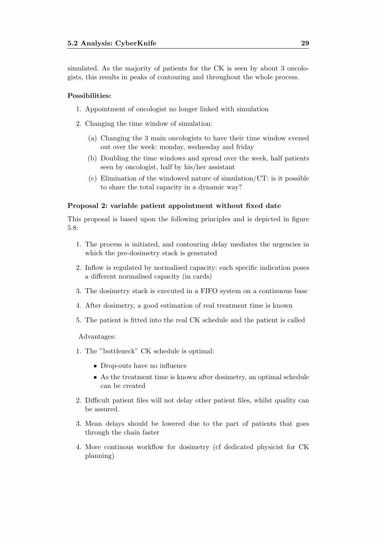
Proposal 2: variable patient appointment without fixed date

This proposal is based upon the following principles and is depicted in figure5.8:

1. The process is initiated, and contouring delay mediates the urgencies inwhich the pre-dosimetry stack is generated

2. Inflow is regulated by normalised capacity: each specific indication posesa different normalised capacity (in cards)

3. The dosimetry stack is executed in a FIFO system on a continuous base

4. After dosimetry, a good estimation of real treatment time is known

5. The patient is fitted into the real CK schedule and the patient is called

Advantages:

1. The ”bottleneck” CK schedule is optimal:

• Drop-outs have no influence

• As the treatment time is known after dosimetry, an optimal schedulecan be created

2. Difficult patient files will not delay other patient files, whilst quality canbe assured.

3. Mean delays should be lowered due to the part of patients that goesthrough the chain faster

4. More continous workflow for dosimetry (cf dedicated physicist for CKplanning)


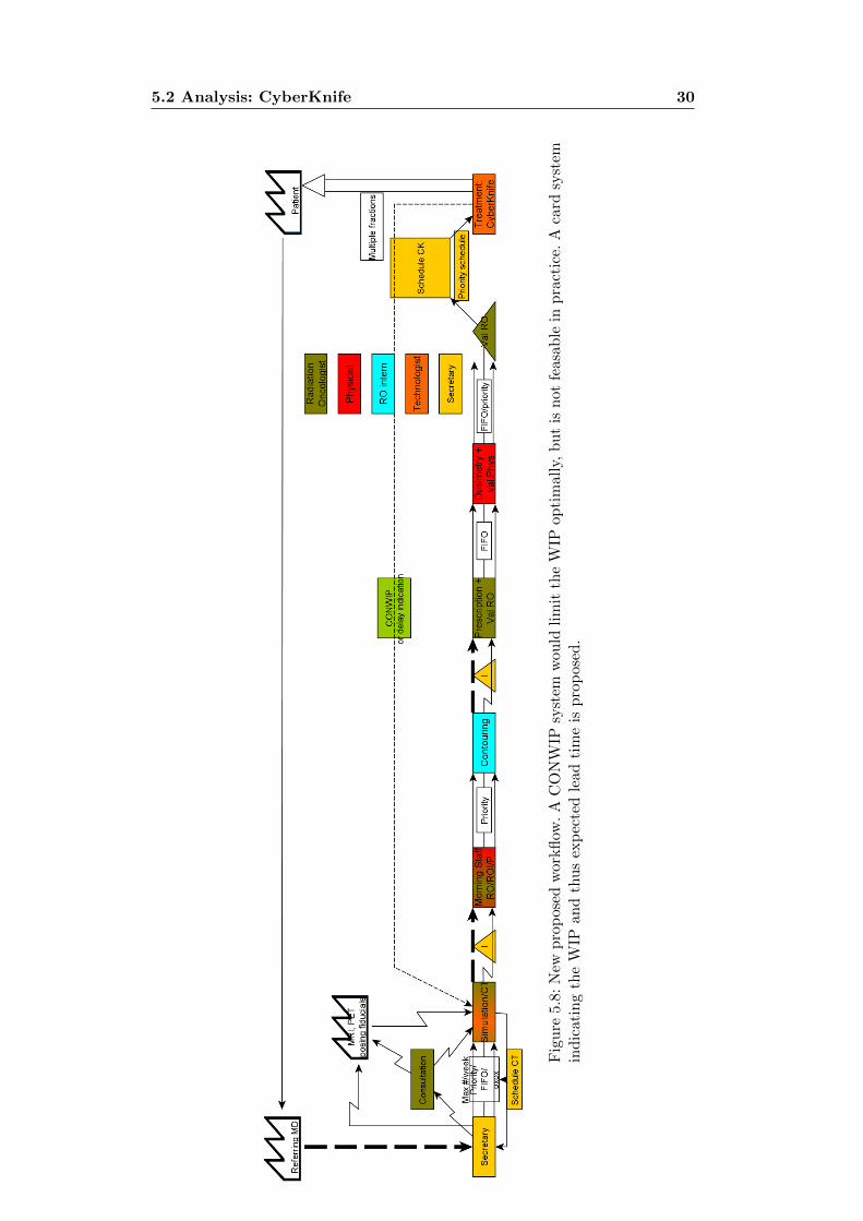
Fig

ure

5.8:

New

pro

pos

edw

orkfl

ow.

AC

ON

WIP

syst

emw

ould

lim

itth

eW

IPop

tim

ally

,b

ut

isnot

feas

able

inp

ract

ice.

Aca

rdsy

stem

ind

icat

ing

the

WIP

and

thu

sex

pec

ted

lead

tim

eis

pro

pos

ed.


5. The FIFO system for the dosimetry allows an auto-organising system: theradiation oncologist decides what patient is more urgent. The more urgentpatients are contoured and prescribed first, and enter the FIFO first andare thus treated first.

6. If in the future any step is executed faster than normally, the flow timecan be shortened.

Constraints and disadvantages:

1. Patient behaviour: is the patient OK with this system? A sort of conwipcard system is proposed: every new CT scan, a card is taken from the wall,indicating the delay to be expected. For example, if there are already 20patients in the system, the delay will be about 3 weeks. The technologistsat the CT scan give this delay to the patient. The card is put in thepatient file and follows the chain.

2. Flow of cases towards dosimetry: if too peaked, delay will be as bad asbefore

3. Influx at the CT scanner has to be limited: simulations are performed toobtain this parameter. If too many, the WIP will increase dramatically.If too few, the CK will not be functioning optimally: simulations need tobe performed to obtain optimal parameter

4. The general rule in variability is: In a line where releases are independentof completions, variability early in a routing increases cycle time morethan equivalent variability later in the routing. Thus the variability shouldbe kept low as possible at the start of the line.

5. In the ideal case, a full CONWIP system would be best, but then ap-pointments for CT scan should not be fixed either.

Proposal 3: variable patient appointment with fixed date

This proposal is a variant of the previous proposal:

1. The patient is given a fixed appointment date of 14 days during simula-tion, of which the first week the patient is not to be called

Proposal 4: dedicated (pooled) assignment of in-ter+dosimetrist/physicist: working cells

This proposal is based on a direct handling of every patient who goes to the CTscanner: the CT is immediately contoured by an assigned intern, immediatelyvalidated and immediately the dosimetry is started by an assigned dosimetristor physicist. The interns, dosimetrists and physicists are assigned from theirrespective pools: not a single dedicated person to a radiation oncologist. Theadvantage of this system is immediate handling with a very short lead time.

Disadvantages:

5.3 Simulations 32

• Patient files requiring additional information: most patient cases requireadditional information from other discipline MD’s. This information isnot readiliy available.

• Annulations in the process leaves empty places on the CK machine.

• Fragile system: due to bottlenecks a large delay can be build up quicklywith varying patient flow: variabilities should be lowered first.

5.3 Simulations

Simulations were programmed in the Simpy 2.1.0 package (Python).

5.3.1 Modelling

All time distributions of process times/step were created, as explained at thestart of this chapter by using distribution fits if possible. If impossible, theactual historical histogram distribution was used.

Patient arrival at consultation

Patient arrivals are modeled as an exponential distribution with user definedarrival rate. Indication and RO are assigned, using the probability distributionsobtained from analysis of historical data. We remark that there is a strong linkbetween indication and RO, following specialisation.

CT scan

The CT scan scheduling is modeled using the time slots for each RO. Further-more, following the proposed new workflow, the nr of scans is limited to a fixednumber per week. A slot is 45 minutes.

Morning staff

Every patient file is presented the day following the CT scan at the morningstaff. This is simply modelled by the file waiting for the next day and stayingin the staff for 1h.

Contouring/prescription

The contouring/prescription time is modelled on a RO basis: the historicaldistribution is used for each RO (variating inbetween RO’s/indication). EachRO/intern is modelled as a resource with capacity 1: sequential execution. Weremark that this is the purpose of the proposed workflow: every file moves onimmediately after contouring or prescription.

5.3 Simulations 33

Dosimetry

Dosimetry time is modelled as a fixed preparation time plus the betavariatedistribution fit, depending on indication. Dosimetry is modelled as a resourcewith capacity 2.

Treatment

Patient arrivals were modelled as on average 10 minutes too soon, with a gaus-sian spread σ = 10 minutes.

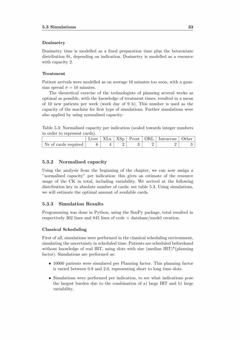
The theoretical exercise of the technologists of planning several weeks asoptimal as possible, with the knowledge of treatment times, resulted in a meanof 10 new patients per week (work day of 9 h). This number is used as thecapacity of the machine for first type of simulations. Further simulations werealso applied by using normalised capacity:

Table 5.3: Normalised capacity per indication (scaled towards integer numbersin order to represent cards).

Liver XLu XSp Prost ORL Intracran Other

Nr of cards required 6 4 2 3 2 2 3

5.3.2 Normalised capacity

Using the analysis from the beginning of the chapter, we can now assign a”normalised capacity” per indication: this gives an estimate of the resourceusage of the CK in total, including variability. We arrived at the followingdistribution key in absolute number of cards: see table 5.3. Using simulations,we will estimate the optimal amount of available cards.

5.3.3 Simulation Results

Programming was done in Python, using the SimPy package, total resulted inrespectively 302 lines and 845 lines of code + database/model creation.

Classical Scheduling

First of all, simulations were performed in the classical scheduling environment,simulating the uncertainty in scheduled time. Patients are scheduled beforehandwithout knowledge of real IRT, using slots with size (median IRT)*(planningfactor). Simulations are performed as:

• 10000 patients were simulated per Planning factor. This planning factoris varied between 0.8 and 2.0, representing short to long time slots.

• Simulations were performed per indication, to see what indications posethe largest burden due to the combination of a) large IRT and b) largevariability.

5.3 Simulations 34

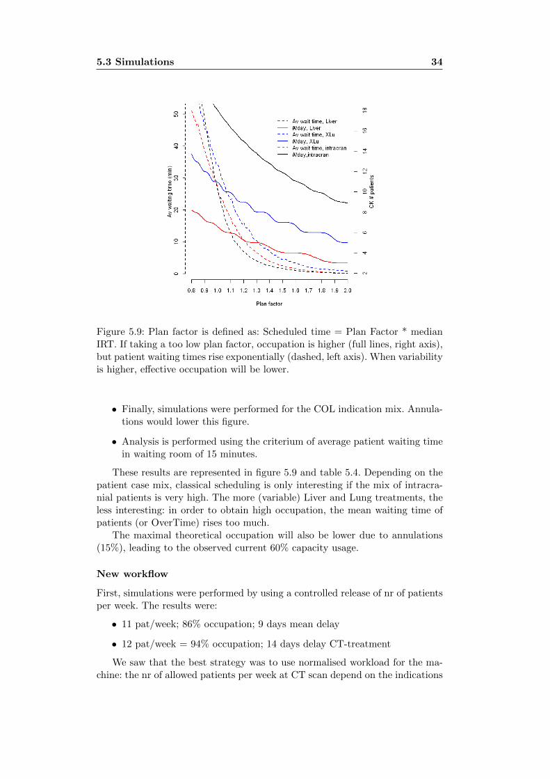
Figure 5.9: Plan factor is defined as: Scheduled time = Plan Factor * medianIRT. If taking a too low plan factor, occupation is higher (full lines, right axis),but patient waiting times rise exponentially (dashed, left axis). When variabilityis higher, effective occupation will be lower.

• Finally, simulations were performed for the COL indication mix. Annula-tions would lower this figure.

• Analysis is performed using the criterium of average patient waiting timein waiting room of 15 minutes.

These results are represented in figure 5.9 and table 5.4. Depending on thepatient case mix, classical scheduling is only interesting if the mix of intracra-nial patients is very high. The more (variable) Liver and Lung treatments, theless interesting: in order to obtain high occupation, the mean waiting time ofpatients (or OverTime) rises too much.

The maximal theoretical occupation will also be lower due to annulations(15%), leading to the observed current 60% capacity usage.

New workflow

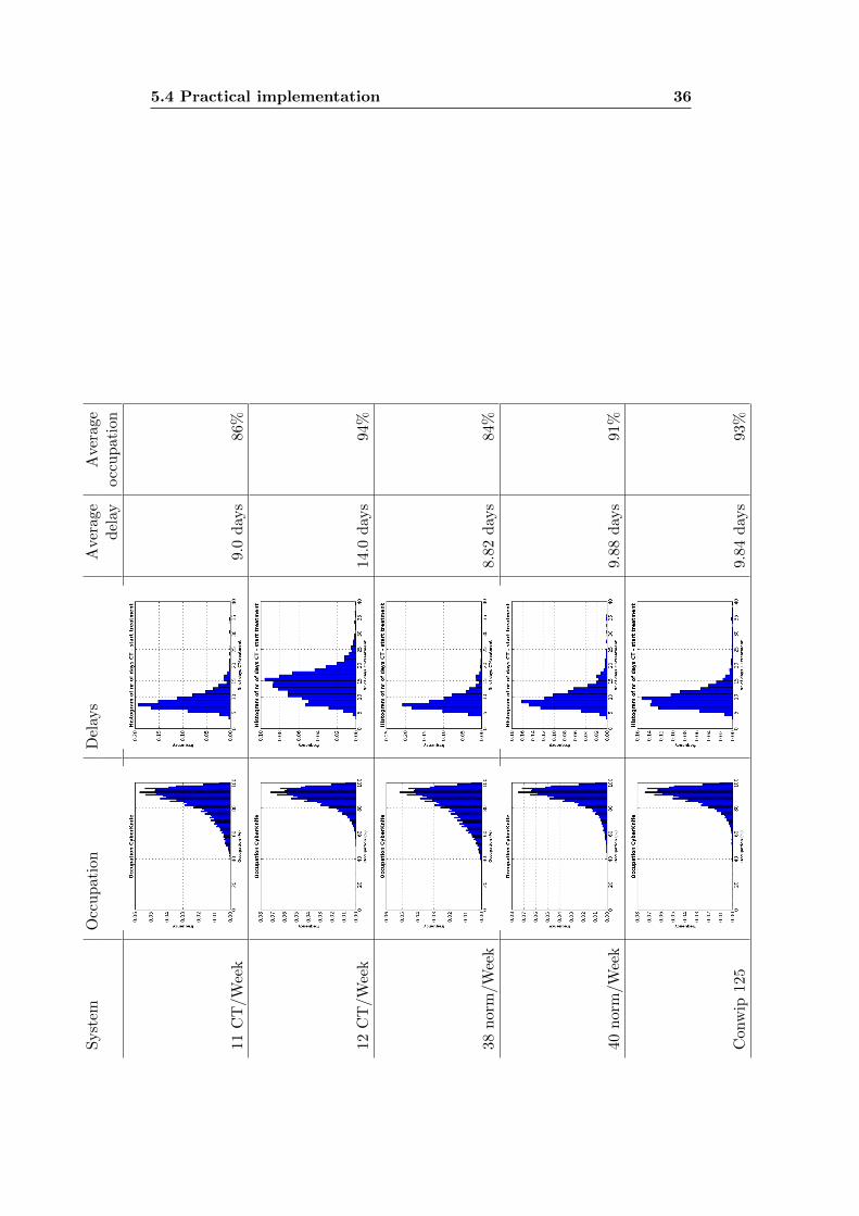
First, simulations were performed by using a controlled release of nr of patientsper week. The results were:

• 11 pat/week; 86% occupation; 9 days mean delay

• 12 pat/week = 94% occupation; 14 days delay CT-treatment

We saw that the best strategy was to use normalised workload for the ma-chine: the nr of allowed patients per week at CT scan depend on the indications

5.4 Practical implementation 35

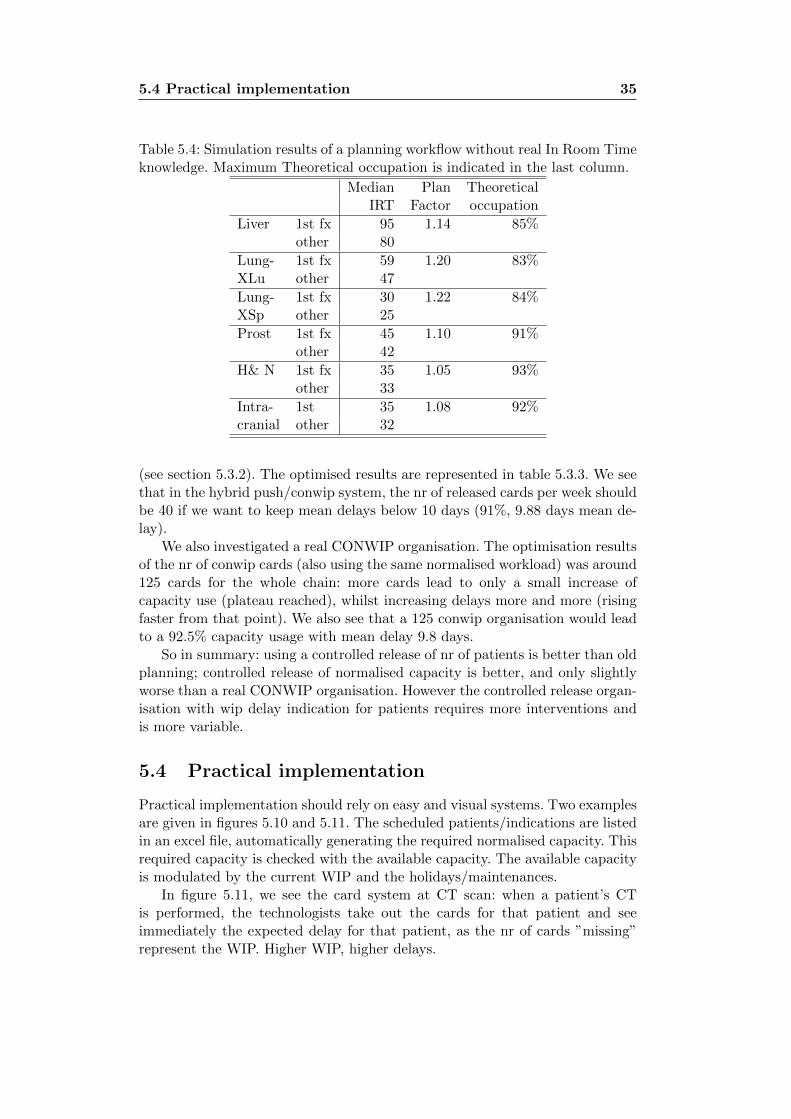
Table 5.4: Simulation results of a planning workflow without real In Room Timeknowledge. Maximum Theoretical occupation is indicated in the last column.

Median Plan TheoreticalIRT Factor occupation

Liver 1st fx 95 1.14 85%other 80

Lung- 1st fx 59 1.20 83%XLu other 47

Lung- 1st fx 30 1.22 84%XSp other 25

Prost 1st fx 45 1.10 91%other 42

H& N 1st fx 35 1.05 93%other 33

Intra- 1st 35 1.08 92%cranial other 32

(see section 5.3.2). The optimised results are represented in table 5.3.3. We seethat in the hybrid push/conwip system, the nr of released cards per week shouldbe 40 if we want to keep mean delays below 10 days (91%, 9.88 days mean de-lay).

We also investigated a real CONWIP organisation. The optimisation resultsof the nr of conwip cards (also using the same normalised workload) was around125 cards for the whole chain: more cards lead to only a small increase ofcapacity use (plateau reached), whilst increasing delays more and more (risingfaster from that point). We also see that a 125 conwip organisation would leadto a 92.5% capacity usage with mean delay 9.8 days.

So in summary: using a controlled release of nr of patients is better than oldplanning; controlled release of normalised capacity is better, and only slightlyworse than a real CONWIP organisation. However the controlled release organ-isation with wip delay indication for patients requires more interventions andis more variable.

5.4 Practical implementation

Practical implementation should rely on easy and visual systems. Two examplesare given in figures 5.10 and 5.11. The scheduled patients/indications are listedin an excel file, automatically generating the required normalised capacity. Thisrequired capacity is checked with the available capacity. The available capacityis modulated by the current WIP and the holidays/maintenances.

In figure 5.11, we see the card system at CT scan: when a patient’s CTis performed, the technologists take out the cards for that patient and seeimmediately the expected delay for that patient, as the nr of cards ”missing”represent the WIP. Higher WIP, higher delays.

5.4 Practical implementation 36S

yst

emO

ccu

pat

ion

Del

ays

Ave

rage

Ave

rage

del

ayocc

up

atio

n

11C

T/W

eek

9.0

day

s86

%

12C

T/W

eek

14.0

day

s94

%

38n

orm

/Wee

k8.

82d

ays

84%

40n

orm

/Wee

k9.

88d

ays

91%

Con

wip

125

9.84

day

s93

%


Figure 5.10: Excel worksheet for planning of CT. The available cards per weekare modulated by maintenances/holidays and current capacity. There are always6 cards reserved for urgencies (week before/same week). Each indication takesa different amount of cards.


Figure 5.11: Visualisation of delay given to patients at CT/simulation. Everytime a new CT is taken for the CK, a card is taken and entered in the patientfile. When taking the card, the delay is given. For visualisation, several cardswere removed to show the different parts.

Chapter 6

Results: reunions of thedepartment and practicalimplementation

Several meetings with all involved groups are made to map the process and theunderlying problems.

6.1 Pre-meetings

Meetings with all involved groups were held and results are given in the earlierchapter 3.

6.2 Department meeting 13/12/2010

A general department meeting with the radiation oncologists and physicistswas done the 13th of december. A presentation was held in order to showexamples of the underlying problems. A discussion over the several possibilitieswas held. During this meeting, the problem of the the unpooled scanner timeslots was recognized, but no immediate solution was found in order to nottotally change organisation for the whole department (not only CK). It wasdecided that starting from january-february a new method would be tested forthe CyberKnife treatments. This would be evaluated and if positive, looked atfor the other treatments, keeping in mind the different constraints for theseother treatments. The method to be implemented was:

• Give a fixed, longer, delay for the appointment at the patient (extremelimit for treatment).

• The patient is at the same time informed of the possibility of an earliertreatment.

• The chain is started as usual, and radiation oncologists and interns areinformed of trying to un-batch as good as possible: validation of contourson a case-by-case basis instead of batch.

6.3 Department meeting 17/01/2011 40

• Physics is reorganised:

– There is ”Physics on duty” for the CK plans

– As soon as a patient file arrives, the dosimetry is started on a FirstCome First Serve basis, but keeping -24h treatments priority.

– If dosimetry is performed succesfully, validation is done immediatelyand the information of treatment time is given to the technologistsat the CK

• Technologists call patients to fill up the planning of the machine as goodas possible, having a good estimation of effective treatment time.

The advantages are as described in section 5.2.1, in short:

1. Improve the patient load for the bottleneck: the CK machine; output

2. Reduce the delays:

• the time between first consult and treatment

• the time between CT scan and treatment: The tail of the histogramshould be cut off

• the time in waiting list

3. Quality: Hard dosimetries should not be rushed

4. Organisational feasibility for every group: no large organisational changes

5. Higher patient satisfaction: doing what is promised should lead to highersatisfaction

6.3 Department meeting 17/01/2011

A presentation was given with the details of the new organisation. General con-sensus was found for the conwip/limited number of files system. Some issuesarised concerning the possibility to put patients in the queue, which were dis-cussed. Therefore, it was proposed to let the marked patient files (CONWIP)enter and follow up the flow. Technologists at the CK were to construct a fic-tional planning with effective treatment times, in order to assess (1) if therewas really to be a gain and (2) if the technologists were comfortable in the neworganisation. Before they didn’t have to deal with all the planning.

The decision to change the organisation would be taken in a later meeting.Discussions with the technologists were to be held also.

6.4 Department meeting 03/2011

Problems with the current organisation of the CyberKnife rise to another level.It was decided that the new system would be entered slowly, especially takingcare to not lose track of certain patients during the shift of systems. Enrollmentwas proposed as followed:

6.5 04/2011 41

• A list of patients was to be made for all patients who had at that momentalready a appointment at the CK. With this list, the nr of additionalpatients that could enter the new system could be defined.

• A new document for the patients, explaining the system very briefly, wouldbe created.

• New patients would be entering this system.

• Total shift to the new system would be done after the maintenance (1week) in the first week of june

6.5 04/2011

New explanation of the system and the migration from old workflow to newworkflow. Further discussions. Sensibilisation of the change from overbookingtowards the system: in the new workflow, the schedule will almost always beempty the weeks to come.

6.6 05/2011: start of change

Some first problems arrived for the planning. In the old system, overbookingwas common practice. It was a mentality change to not do this again for theCT planning. At the start, there was some serious overbooking, leading to toomany patients in the system. The card system however signaled this fast to thetechnologists at the CT, so they told the patients it would take longer than2 weeks. In order to solve this, it was communicated to take temporary lessfor the coming weeks. The planner changed sometimes, and the informationwas not given correctly to the new planner, so this lead to new overbooking.A rectification was in order, so annulations were not replaced in order to getto the correct number again. A third problem arrived (also communication) forthe maintenance: it was communicated in a department meeting that in orderto have a correct transition taking into account a maintenance taking a week, atemporary change had to be made. 2 weeks before, there could only be patientsplanned with a single fraction. 1 week before maintenance, 0 CT’s for the CKwere allowed. This was however not followed (also due to change of planner),with even overbooking. Part of these problems were however solved before themaintenance by an effort of the technologists at the CK and the physicists doingsome overtime.

6.7 06/2011

The system with the limited number of pochettes was somewhat flawed, theplanning was not very clear visual neither. A new system is introduced withcards (see figure 5.11). A new planning file was created, so (1) is was not possibleto overbook, (2) it was more clear. New rule sets were also entered:

6.8 09/2011 42

• If there is a maintenance or holiday: 2 weeks before, there would be prorata 2 patients per day allowed less

• One patient slot would be reserved for urgent patients: if not taken, canbe used for regular patient the same week.

6.8 09/2011

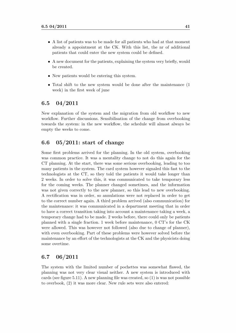
A first analysis was made to asses the new situation now 3 months in place.A remarkable increase of output was noticed (see figure 6.1). The delays CT-treatment however were not really improved, further investigation pointed outthat there are now quite some patient files which take more than 10 days toperform contouring and prescription (17% compared to 6% before: it seems theproblematic files are now left waiting on the MD’s desk).

Figure 6.1: Nr of billable acts per worked day.

6.9 10/2011

A major component failure occured for the CK machine. The whole linac had tobe replaced, recommissioned and measured. This is equal to a new installationand took 1 month. The process was expedited by a lot of night shifts of bothengineers and physics. No dosimetries could be performed, as these could onlybe started after recommissioning of the TPS. Furthermore, all patients undertreatment had to be redone.

6.10 01-02/2012 43

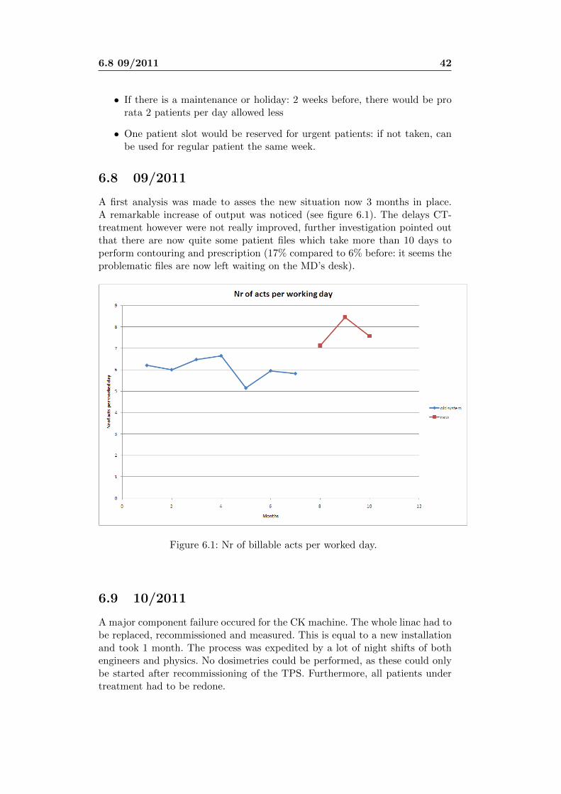
Figure 6.2: Nr of billable dosimetries per worked day, first evaluation 10/2011.

In theory, the proposed system was robust for problems like these: CT scanscould be immediately delayed, so no new patients enter the system and thereare only minor problems (compared with full planning) for the time scheduleof the CK machine. However, there was no consensus among the MD’s forprioritisation of patients, and CT scans were not cancelled. This lead to agigantic overstock of patient files at the dosimetry. After a couple of weeks, theCT scans were however delayed for new patients. Delays of this month and thefollowing are thus very large.

6.10 01-02/2012

MD’s did not follow the rules, about 10 patients were added in the weeks ofjanuary. This lead to an increase of lead times CT-treatment.

Chapter 7

Conclusions

The patient flow was reorganised for CyberKnife treatments, following the pro-cess of analysis-simulations-implementation. The intense collaboration with allinvolved personnel lead to a very high motivated implementation. Simulationsoftware was written, which was applied for tuning the parameters of the neworganisational workflow.

Starting from may-june 2011, the hybrid conwip system with lead time in-dicator was implemented gradually: first using a fixed number of patients perweek: modulated by holidays/maintenances and over-under capacity 2 weekslater. Later on, this was changed towards the system with normalised capacity:each indication takes a specific capacity.

Patients receive always an approximation of their delay at the CT scan,depending on the work in progress. The wip cards are thus used as a weakconwip + delay indication. Urgencies/higher priority patients can still pass byfaster, depending on contouring speed.

7.1 Total number of treatments

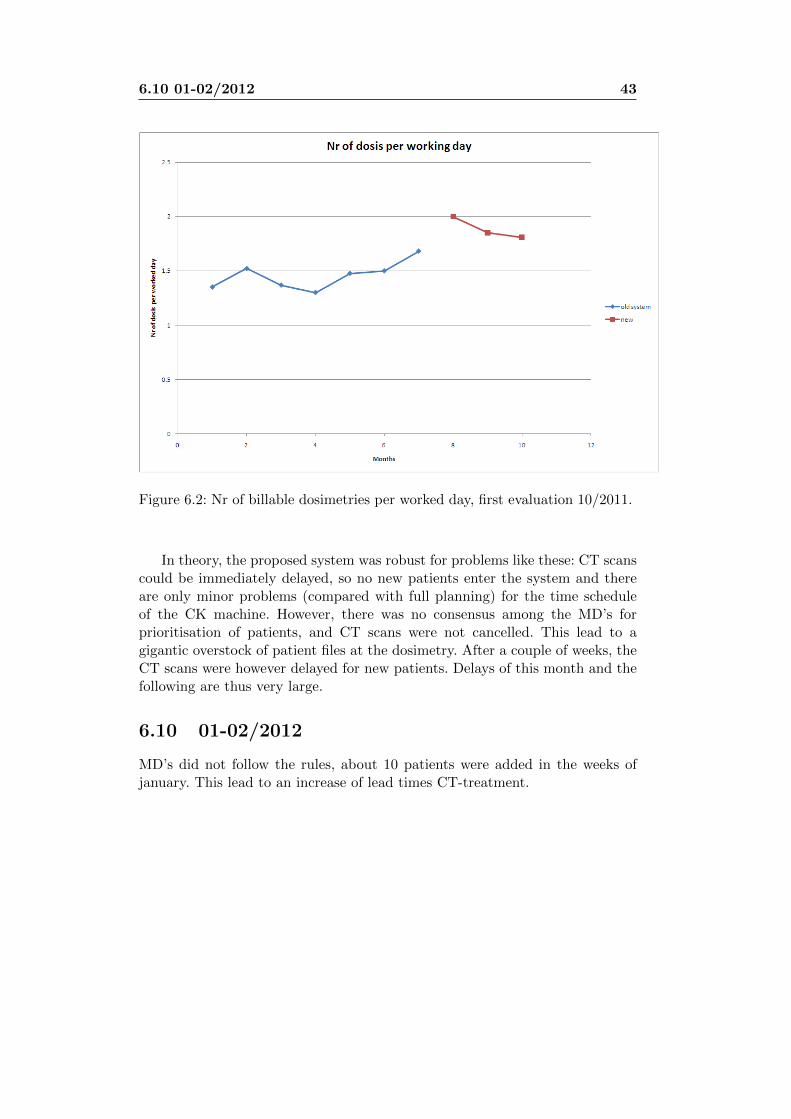
The final results are represented in figure 7.1. For this figure, the billed num-ber of treatment fractions were normalised per worked day in order to removemonth to month specific influence (holidays etc). In order to view the correctinfluence of the reorganisation, the months after september 2011 are also nor-malised towards the months before: working hours were extended at that point.An unpaired 1-sided t-test indicates a 28.7% (95% CI: [20%;38%]) increase ofnumber of fractions. The corresponding number of dosimetries (different fac-turation) increased equivalently. The total (number of fractions + dosimetries)corresponds with a total revenue increase of more than 700.000 Euro/year.However, tarification was lowered in march 2012, lowering the yearly revenueincrease to /year.

7.2 Drawbacks

Following the Pay-Me-Now-or-Pay-me-Later rule, the increase in output comesat the expense of a moderate lead time hit (median 9 days instead of 8 days

7.2 Drawbacks 45

Figure 7.1: Normalised number of acts per worked day (rescaled towards orig-inal number of working hours: the number of working hours were extended inseptember 2011). These results correspond with an increase of 29 %

before). In the current state, this is not that critical. On the financial part,this leads to only a very small blocking of financial reserves and working capi-tal requirement (negligible compared with the other financial related delays ofpayment). This is thus totally offset with the very large increase of revenues.

One of the problems arising now is the large time delay for MRI (in theradiology department): in a lot of cases the waiting list for the MRI will dictatethe time for contouring (see also next point).

Main drawback of the current implementation is the organisation of theMD’s: the time for contouring/prescription, or rather the time the files stay ona pile on that step is extremely variable and is the main reason of delays. Thiscan be translated in a high working capital requirement for this step and shouldbe improved in the future. When on holiday, specific files stay on a pile for verylong time, leading sometimes to stock starving for treatments and overloadingafter. As variability at the start of a line is translated into more variability lateron, this should be lowered.

Due to the working hours extension and the reorganisation, the dosimetryprocess (only 2 stations) has now become a restricting process, due to the veryvariable MD contouring/prescription behaviour.

7.3 Final conclusions: initial objectives 46

7.3 Final conclusions: initial objectives

• Operational

– Output:

∗ Increasing the number of patients treated per month:

· 28% increase

– Delays/Work In Progress:

∗ Keeping CT scan-treatment times as low as possible, should bebelow 14 days ideally: CT scan should represent the real patientanatomy.

· 9 working days median, only a slight increase withbefore

∗ By increasing output and capacity, total delay between patientreferral and treatment should be lower

· Entry in CT schedule is now below 1 month, 1.5years ago: 2 months

• Human factors and Quality

– Personnel stress levels

∗ Organisational feasibility for every group: increase control overwork. Decrease the percieved workload of all personnel involved.

· Percieved better control for all, but the CT planner:a lot of pressure for scheduling from RO’s

∗ Quality: Most of the work is manual, quality depends on theavailable time

· Due to the reduction of the rushing, quality can bet-ter be guarantueed

– Patient satisfaction

∗ Patient satisfaction is largely dependent on the fulfillment ofgiven information and promised delays.

· This far, no complaints are known

· The Work In Progress cards which follow the filesthroughout the service give a good indication to thepatients when they will receive their final appoint-ment.

• Financial

– Revenues

∗ Productivity: more output/capacity

· 28% increase

· Levarage for the working hours extension, increasingthe effective increase to higher than 28%

7.4 Future improvements 47

∗ Working capital management: reducing the time between entryof patient and treatment equals lower working capital require-ment

· Slightly slower, but 1 day does not compare with 2months in facturation.

· The increase of the number of patients increases theworking capital requirement in theory.

· The reduction of the delay between referral andtreatment (from 2 to 1 month) reduces working cap-ital requirement

7.4 Future improvements

• Variability reduction, especially at the start of the line: referrals by otherMD’s, first steps after CT.

• CT/simulation and the subsequent contouring/prescription could be bet-ter organised in order to reduce lead times. For example, a specific timeslot of half a day per intern/RO in their schedule.

• Ideally, a full kanban/conwip system should be implemented for all differ-ent machines. A kanban system could regulate the work charge betweenall different actors and steps. A POLCA system could also be envisaged,especially for the interaction between all different departments (nuclearmedicine, radiology, radiotherapy, surgery. . . ). However, this would bevery very ambitious given the current state of islands in medicine.

• MRI access becomes more and more limiting factor for delays and WorkIn Progress. Moreover, quality could be improved substantially (large un-certainty in contouring) with better MRI access.

Chapter 8

List of abbreviations

CK Cyber KnifeCOL Centre Oscar LambretMD Medical DoctorRO Radiation OncologistTPS Treatment Planning System

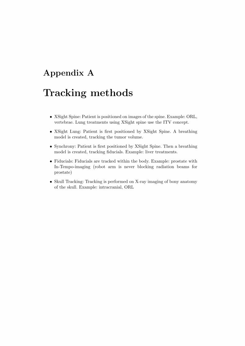
Appendix A

Tracking methods

• XSight Spine: Patient is positioned on images of the spine. Example: ORL,vertebrae. Lung treatments using XSight spine use the ITV concept.

• XSight Lung: Patient is first positioned by XSight Spine. A breathingmodel is created, tracking the tumor volume.

• Synchrony: Patient is first positioned by XSight Spine. Then a breathingmodel is created, tracking fiducials. Example: liver treatments.

• Fiducials: Fiducials are tracked within the body. Example: prostate withIn-Tempo-imaging (robot arm is never blocking radiation beams forprostate)

• Skull Tracking: Tracking is performed on X-ray imaging of bony anatomyof the skull. Example: intracranial, ORL

Appendix B

Posters

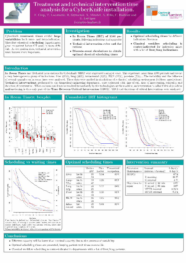
Treatment and technical intervention timeanalysis for aCyberKnife installation.

F. Crop, T. Lacornerie, H. Szymczak, X. Mirabel, A. Felin, C. Bailleux andE. Lartigau

[email protected]

Problem

CyberKnife treatment times exhibit largevariabilities both inter- and intra-indication.Therefore classical scheduling (appointmentgiven to patient before CT scan) is more di�-cult. As occupation rises, technical interventionrates become more important.

Investigation

• In Room Times (IRT) of 1100 pa-tients, following indications and upgrades

• Technical intervention rates and du-rations

• Discrete-event simulations to obtainoptimal classical scheduling times

Results

• Optimal scheduling times for di�erentindications/fractions

• Classical work�ow scheduling iscontra-indicated for indication mixeswith a lot of liver/lung indications.

Introduction

In Room Times and Technical interventions for CyberKnife SBRT were registered during 4 years. This represents more than 1100 patients and coversa very heterogeneous group of indications: liver (21%), lung (29%), intracranial (13%), H&N (11%), prostate (7%). . . The variability and the in�uenceof several upgrades on in room times were analyzed. These data were applied in simulations of a classical scheduling environment (without annulations).Technical interventions, performed by the biomedical engineering department, were registered with time of call, time of intervention, criticality andduration of intervention. When an issue could not be resolved immediately by the technologists at the machine, an intervention is called Critical (machinemalfunctioning is thus only part of the Time Between Critical Intervention (TBCI)). TBCI and durations of critical Interventions were analyzed.

In Room Times: boxplot Cumulative IRT histograms

Scheduling vs waiting times

Plan factor is de�ned as: Scheduled time = Plan Factor *median IRT. If taking a too low plan factor, occupation ishigher (full lines, right axis), but patient waiting times riseexponentially (dashed, left axis).When variability is higher, e�ective occupation will be lower.

Intervention summary

Preventive Internal 4 days/yMaintenances External (Accuray) 6 day/y

MTBCI 67 h% morning 30 %% external 5 %

Mean time to % solved ≤ 30 min 62%repair % solved ≤ 60 min 80%

MTTR internal 0.76 hMTTR external 6.1 h

Optimal scheduling times

Median Plan TheoreticalIRT Factor occupation

Liver 1st fx 95 1.14 85%other 80

Lung- 1st fx 59 1.20 83%XLu other 47

Lung- 1st fx 30 1.22 84%XSp other 25

Prost 1st fx 45 1.10 91%other 42

H& N 1st fx 35 1.05 93%other 33

Intra- 1st 35 1.08 92%cranial other 32

Conclusions

• E�ective capacity will be lower than nominal capacity due to the presence of variability.

• Optimal scheduling times are presented, keeping patient wait times reasonable.

• Classical work�ow scheduling is contra-indicated in departments with a lot of liver/lung patients.

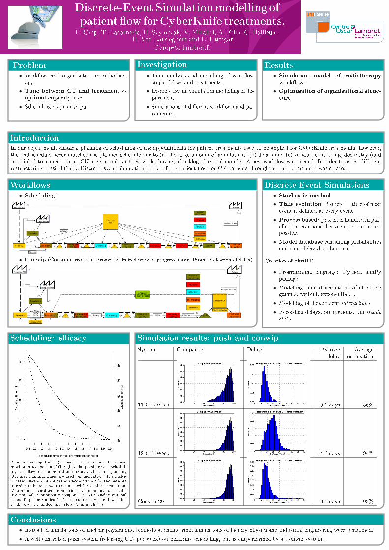
Discrete-Event Simulationmodelling of

patient �ow forCyberKnife treatments.F. Crop, T. Lacornerie, H. Szymczak, X. Mirabel, A. Felin, C. Bailleux,

H. Van Landeghem and E. Lartigau

[email protected]

Problem

• Work�ow and organisation in radiother-apy

• Time between CT and treatment vsoptimal capacity use

• Scheduling vs push vs pull

Investigation

• Time analysis and modelling of work�owsteps, delays and treatments.

• Discrete Event Simulation modelling of de-partment.

• Simulations of di�erent work�ows and pa-rameters.

Results

• Simulation model of radiotherapy

work�ow

• Optimisation of organisational struc-

ture

Introduction

In our department, classical planning or scheduling of the appointments for patient treatments used to be applied for CyberKnife treatments. However,the real schedule never matched the planned schedule due to (a) the large amount of annulations, (b) delays and (c) variable contouring, dosimetry (andespecially) treatment times. CK use was only at 60%, whilst having a backlog of several months. A new work�ow was needed. In order to assess di�erentrestructuring possibilities, a Discrete-Event Simulation model of the patient �ow for CK patients throughout our department was created.

Discrete Event Simulations

• Stochastic method

• Time evolution: discrete = time of nextevent is de�ned at every event

• Process based: processes handled in par-allel, interactions between processes arepossible

• Model database containing probabilitiesand time delay distributions

Creation of simRT

• Programming language: Python, simPypackage

• Modelling time distributions of all steps:gamma, weibull, exponential. . .

• Modelling of department interactions

• Recording delays, occupations. . . in steady

state

Work�ows

• Scheduling:

• Conwip (Constant Work In Progress: limited work in progress ) and Push (indication of delay)

Scheduling: e�cacy

Average waiting times (dashed, left axis) and theoreticalmaximum occupation (full, right axis) possible with schedul-ing work�ow for the indication mix at COL. CorrespondingOptimal planning times are used per indication. The multi-plication factor multiplies the scheduled time for the patientsin order to balance waiting times with machine occupation.Maximum theoretical occupation % for an average wait-ing time of 15 minutes corresponds to 74% (using optimalscheduling time/indication). In reality, it wll be lower dueto the use of rounded time slots (30min, 2h. . . ).

Simulation results: push and conwip

System Occupation Delays Average Averagedelay occupation

11 CT/Week 9.0 days 86%

12 CT/Week 14.0 days 94%

Conwip 29 9.7 days 93%

Conclusions

• Instead of simulations of nuclear physics and biomedical engineering, simulations of factory physics and industrial engineering were performed.

• A well controlled push system (releasing CTs per week) outperforms scheduling, but is outperformed by a Conwip system.

Documents

Patient flow optimisation of CyberKnife radiotherapy