arX

iv:1

503.

0806

3v1

[qu

ant-

ph]

27

Mar

201

5

Spectral properties of a hybrid-qubit model based on a

two-dimensional quantum dot

Alba Y. Ramos∗ and Omar Osenda†

Facultad de Matematica, Astronomıa y Fısica,

Universidad Nacional de Cordoba, and

Instituto de Fısica Enrique Gaviola,

CONICET-UNC, Av. Medina Allende s/n,

Ciudad Universitaria, X5000HUA Cordoba, Argentina

(Dated: April 4, 2018)

Abstract

The design and study of hybrid qubits is driven by their ability to get along the best of charge

qubits and of spin qubits, i.e. the speed of operation of the former and the very slow decoherence

rates of the latter ones. There are several proposals to implement hybrid qubits, this works focuses

on the spectral properties of an one-electron hybrid qubit. By design, the information would be

stored in the electronic spin and the switching between the qubit basis states would be achieved

using an external ac electric field. The electron is confined in a two-dimensional quantum dot, whose

confining potential is given by a quartic potential, features that are typical of GaAS quantum

dots. Besides the confining potential that characterizes the quantum dot there are two static

magnetic fields applied to the system, one is a large constant Zeeman field and the other one has a

constant gradient. We study the spectral properties of the model Hamiltonian, a Scrodinger-Pauli

Hamiltonian with realistic parameters, using the Ritz method. In particular, we look for regions of

the parameter space where the lowest eigenenergies and their eigenfunctions allow to define a qubit

which is stable under perturbations to the design parameters. We put special attention to the

constraints that the design imposes over the magnetic fields, the tuning of the energy gap between

the qubit states and the expectation value of the spin operator where the information would be

stored.

PACS numbers: 73.21.-b,73.21.La,78.67.Hc,31.15.ac

∗Electronic address: aramos@famaf.unc.edu.ar

1

†Electronic address: osenda@famaf.unc.edu.ar

2

I. INTRODUCTION

Semiconductors quantum bits are thought to be one of the most fertile fields to imple-

ment Quantum Information Processing and Computation [1, 2]. The advantages have been

said countless times, from the incredible sophisticated techniques related to semiconductor

technologies - such as integration [3], lithography[4] , ultra-pure sample preparation [4, 5]

and scalability [6]- to the peculiarities of the different kinds of qubits that are offered in

semiconductors such as charge and spin qubits, exciton qubits and hybrid ones [2].

The disadvantages are, of course, a bit less heralded but, nevertheless, they are well

known. One of the leading disadvantages lies in the fact that it is quite difficult to isolate

a truly microscopic system (one electron, its spin, or the spin state of few electrons) from

the semiconductor matrix in which it is embedded. The unavoidable interaction between

the microscopic system chosen to carry the qubit and the environment that surrounds the

systems leads to the loss of the quantum state coherence. Fortunately, the main mechanisms

that produce decoherence are well known so it is possible to design ad hoc strategies to

overcome or palliate their effects.

The term charge qubits was coined to design a qubit where the information is stored in

the spatial degrees of freedom of one (or several) electron(s) [7, 8]. The main mechanism

of decoherence, in this case, is owed to the coupling between the electron and the thermal

phonons present in the semiconductor. For an experimental study of charge relaxation

in Si/SiGe DQD see the work by Wang et al. [9]. A similar study was performed by

Srinivasa et al. [10], in their case they studied the simultaneous spin-charge relaxation

in DQD made of GaAs. As the information is stored in the spatial degrees of freedom,

the quantum gates acting over the qubit take advantage of the strong coupling between

electric (or electromagnetic) fields and the electron charge. The strength of the coupling is

determined by the spatial extent of the electron wave function, this fact led, for instance,

to the development of the exciton qubit [11–13] where the coupling is smaller than in the

electronic case. An exciton, the electron-hole pair produced in a semiconductor when a

valence band electron is promoted to the conduction band, also is coupled to the thermal

phonons but the coupling with the phonons depend on the difference between the electron

and hole states [14]. So, using charge qubits based on states of particles with opposite

charge provides a fairly simple mechanism to attenuate the effects of the phonon-induced

3

decoherence allowing picoseconds gate operation times compared with the characteristic

time scale of the decoherence, around the nanoseconds [2] .

The implementations where the quantum information is stored in the intrinsic angular

momentum of one [15] or more electrons are called spin qubits (for the implementation using

two electrons see [16, 17], and for three electrons [18, 19]). The decoherence mechanism is

owed to the coupling between the electron spin and the nuclear spin of the atoms in the

semiconductor. The maturity and development of this particular implementation is heavily

indebted to the techniques developed in the area of Nuclear Magnetic Resonance (NMR),

from the pulse sequence techniques [20–22] up to dynamic noise suppression techniques

[23, 24]. The double-well quantum dot proposal is a direct application of the NMR ideas to

the implementation of spin qubits [23]. Some quite spectacular advances have been achieved

in dealing with the decoherence mechanisms using qubits based on quantum dots embedded

in ultra-pure Silicon samples very recently [25–27]. Despite that it is possible to obtain very

long coherence times, spin qubits are not (yet) an accomplished answer to the problems of

integration and the interaction between other qubits because their design has become more

and more involved. Of particular concern are the long operation times inherent to the weak

coupling between the magnetic dipole moment of the qubit quantum state and a magnetic

field applied to it.

Hybrid qubits [28–30], those in which the information is stored in the electron spin but

the gate operation is provided by electric fields coupled to the electron charge, seem a

good compromise between the two ways of approaching the problem described above. In

particular, some years ago, Tokura et al. [28] proposed a hybrid qubit, that besides long

coherence and short operation times would take advantage of the very low strength of the

noise spectrum when the energy gap between the qubit states lies in the µeV range. The

design proposed is elegant and sophisticated, employing a nano-wire to confine one electron

in one dimension, a double well potential in this dimension an a pair of magnetic fields, one

applied along the direction of the nano-wire and the other perpendicular to it. The proposal

was aimed to implement single electron spin resonance (SESR) in quantum dots.

Despite some inherent peculiarities of the design in Tokura et al. [28], the hybrid qubit

model has several features that are general enough to make a closer look at it very compelling.

In this work, we study the spectral properties of a hybrid qubit inspired by the one proposed

in [28] but easing some confining requirements, in particular the model considered in this

4

work is not one dimensional so the orbital angular momentum plays a non-trivial role. The

model hybrid qubit and its Hamiltonian, a two-dimensional Schrodinger-Pauli equation, is

presented and analyzed in some detail in Section II. The numerical method employed to

obtain a highly accurate spectrum and eigenfunctions is described in Section III. Since the

model depends on several parameters, a detailed analysis of the lowest lying eigenvalues,

their eigenfunctions and the expectation values that characterize the possibility of using

the system as a qubit is presented in Section IV, paying some attention to the stability

of the system when its parameters are changed. As it will be shown, a thorough analysis

of the model eigenvalues and eigenfunctions is a bit arduous but necessary to study the

dynamics of the system when an external driving is applied. So, despite that it is our goal

to study the performance of the system under time dependent external forcing, we deferred

this investigation for the sake of conciseness. Finally, a discussion about the results and its

implications is the subject of Section V.

II. MODEL AND HAMILTONIAN

Tokura and collaborators [28] proposed an hybrid qubit based on a very particular quan-

tum dot. Actually, their proposal relied heavily on the ability to confine the electron in one

dimension using a nano-wire. Besides, along the direction of the nano-wire, the electron

would be confined in a double well potential. To define the qubit basis states two magnetic

fields were needed, one of them along the nano-wire, and the other perpendicular to it.

Following the work of Tokura we denote the direction along the nano-wire as the z direc-

tion. The field along the z direction is constant in time and spatially uniform, while the

perpendicular one has a constant gradient along the coordinate z. Again, following Tokura,

the perpendicular magnetic field points in the x direction.

The one-dimensional confinement had a twofold purpose, on one hand it allowed to neglect

the contributions owed to the other spatial coordinates and consequently the Hamiltonian

considered by Tokura et al. did not included any term related to the orbital angular mo-

mentum. On the other hand, despite the spatial dependence of one of the magnetic fields

applied to the quantum dot, the spin angular momentum terms could be treated easily and

the qubit basis states were always eigen-states of the spin angular momentum in the x di-

rection. Of course, in the case that the confinement is not strictly one-dimensional, this can

5

z

y

x

B0

b zSL

Vac

FIG. 1: A cartoon showing the geometry of the nano-structure considered. The darker grey stripes

in the light-grey surface point to where the double potential well is located. The two external

magnetic fields, B0 in the z direction and bSLz in the x direction are shown. The white arrows

show the direction in which the spin would point if the system works properly. The electric potential

Vac is used to produce the switching of the electron from one potential well to the other.

not be taken for granted. The swapping between the qubit basis state was achieved applying

an electric external driving.

In this work we analyze a very similar system, that allows to analyze a number of features

that a one-dimensional model can not. Besides, our model does not impose such severe

constraints to a possible actual implementation.

Figure 1 shows a cartoon depicting the geometry, coordinate system and applied fields to

the two-dimensional quantum dot that is under scrutiny in this work. The surface represents

the two-dimensional region where the electron is bound. Along the z direction an external

static slanting magnetic field B0 is applied, also in this direction, the electron is confined by

a double well potential, in this case depicted schematically by the two black stripes that lie

parallel to the y direction. We do not consider the presence of a confining potential in the

y direction anyway, as we will show, the magnetic field B0 effectively bound the electron

in this direction. In any case, this assumption has the same physical implications that to

consider that the characteristic length of the confinement in the y direction is larger than

the radius of the first Landau levels associated to a magnetic field of strength B0. The other

magnetic field that is applied to the system has a constant gradient, bSL, here we follow

6

Tokura et al. [28] that considered a magnetic field of the form (bSLz, 0, bSLx)

Finally, the electron is forced to jump between the two potential wells by the electric

driving provided by the potential Vac.

Despite that the system described above is two-dimensional, the main physical behavior

should be similar to the behavior observed in the system proposed by Tokura et al, i.e when

the electron is in a given potential well the electron magnetic dipole moment should point

in the direction that minimizes the energy, upwards in the rightmost potential well and

downwards in the leftmost potential well. Of course, in a two-dimensional system this is

not equivalent to say that when the electron is “located” in one given potential well it will

be in the corresponding eigenstate of the Pauli operator σx, which is proportional to the

spin angular momentum of the electron.

This last statement remark the elegance of the proposal made by Tokura et al, since the

one dimensional system grants that the eigenstates of the Hamiltonian are also eigenstates

of σx, simplifying the analysis of the spectrum, the eigenstates and their properties.

The electron Hamiltonian, H, can be written as

H =1

2m⋆

[

~σ ·(

−i~~∇−e

c~A(r, t)

)]2

+ V (r), (1)

where A is the vector potential, σ are the Pauli matrices, V (r) the double-well potential

and m⋆ is the electron effective mass. Along this work we use the GaAs effective mass, so

m⋆/m = 0.041.

Since the total magnetic field applied to the QD is given by

B = (bSLz, 0, B0 + bSLx), (2)

then, calling B0 = (0, 0, B0) and B1 = (bSLz, 0, bSLx), we get that

A1 = (0,bSL2

(x2 − z2), 0)

A0 = −B0

2(y,−x, 0), (3)

using the symmetrical gauge for the vector potential.

Replacing the expressions obtained for the vector potentials and magnetic fields, Equa-

tions 2,3, in the Hamiltonian, Equation 1, and assuming a confining potential

V (r) = V (z) =m⋆ω2

0

8b2(z2 − a2)2 − γ

~ω0

az, (4)

7

it can be found that

H = −~2

2m⋆∇2 + V (z) +

i~ e

m⋆c

[

−B0

2

∂

∂x+

(

bSL2

(x2 − z2) +B0

2x

)

∂

∂y

]

+

+e2

2m⋆c2

[

B20y

2

4+b2SL4

(x2 − z2)2 +bSLB0

2(x2 − z2)x+

B20

4x2]

−~ e

2m⋆ c[bSL z σx + (B0 + bSL x) σz] . (5)

The confining potential, Equation 4, is a slight generalization of the well-known quartic

double-well potential, that has two wells centered around ±a, where ω0 sets the energy scale

and the parameter b, that has length units, allows to change the height of the potential in

z = 0. The linear term in Equation 4 plays a double purpose, on one hand it allows the

possibility that an electron confined in it has a non-degenerate ground state and, on the

other, allows to study the quite possible scenario where both potential wells have different

depth. It is clear that the difference in depth between the potential wells in their centers

(±a) is given by ∆pw = 2γ~ω0. If ~ω0 is in the order of 10meV and γ ≈ 10−3, then ∆pw is on

the order of the energy gap between the qubit basis states for which the device is designed

for. We will return latter to the effect of this term over the behavior of the system. Finally,

note that for b = a and a large enough, the ground state energy of the electron is a fraction

of ~ω0.

The spectrum of the Hamiltonian in Equation 5, is quite complicated to calculate because

its lacking of symmetries, and the coupling between the spin degrees of freedom. Moreover,

there are several length and energy scales that characterize the physical behavior. It is

interesting to note that, using matrix notation, the Hamiltonian 5 can be written as

H =

H 0

0 H

+H1 ⊗ σx +H2 ⊗ σz

=

H 0

0 H

+

0 H1

H1 0

+

H2 0

0 −H2

=

H +H2 H1

H1 H −H2

(6)

.

So, neglecting the terms related to the x coordinate and introducing scaled variables

8

y′ = y/a, z′ = z/a, we get

H2d

~ω0= −

(~ωa)

2 (~ω0)

[

∂2

∂z′2+

∂2

∂y′2

]

+(~ω0)

8 (~ωa)(z′

2− 1)2 − γz′ +

−i ~ω∗

c

~ω0

bSL a

2B0

z′2 ∂

∂y′+

(~ω∗c )

2

2 (~ωa)(~ω0)

[

y′2

4+

(

bSL a

2B0

)2

z′4

]

−~ω∗

c

2 ~ω0

[

bSL a z′

B0

σx + σz

]

, (7)

where ω⋆c = eB0

~m⋆cis the Larmor frequency associated to the magnetic field B0, ωa = ~

m⋆a2,

and the subscript 2d stands for “two-dimensional”. The frequency ωa is introduced to make

evident that H2d

~ω0

is effectively dimensionless, which is also true for the ratios bSLa/B0, and

ω⋆c/ω0.

Obtaining accurate numerical approximations to the spectrum and eigenstates of the

Hamiltonian 7 is the subject of the next Sections, but before it is worth to pay some more

attention to the analysis of the Hamiltonian 7.

The different terms in the Hamiltonian are characterized by ratios between four charac-

teristics energies: ~ω0, ~ω⋆c , ~ωa and ~ωSL. The latter frequency is the Larmor frequency of

the magnetic field bSLa. Often, the role of ωa is better understood recalling that ~ω0

~ωa=

(

aℓ0

)2

,

where 2a is the distance between the quartic potential minima, and ℓ0 is the characteristic

length of a quantum harmonic oscillator with ground state energy ~ω0/2. If the electron

is well localized in a given potential well, then ℓ0 < a and ~ω0

~ωa> 1. In this case when a

increases its value, the two wells of the quartic potential become more and more separated

and the spectrum consists in a set of quasi-degenerate levels, at least for small enough val-

ues of γ, which are the ones that we will consider in this work. The situation described

above is where the terms associated to both magnetic fields are relevant to produce a pair of

states suitable to be used as the qubit basis states. In this scenario the energies are ordered,

~ω0 > ~ωa > ~ω⋆c ∼ ~ωSL.

III. THE NUMERICAL METHOD

The Ritz variational method [31] has been used to obtain high accuracy approximations

to the spectrum and eigenstates of many different problems [32–34]. A sensible one-particle

basis set must be chosen to apply the method. From the analysis described in the Section II,

9

it is reasonable to pick a basis set, {χ{i}}Mi=1, such that

χ{i} = Ψpk,nα, (8)

where k = 1, . . . , L, n = 1, . . . , N , p = ±, α is any of the eigenstates of σz, {i} ≡ (k, n, p, α)

and

Ψ±k,n(y, z) = φk(y)ψ

±n (z). (9)

The functions in Equation 9 are given by

φk(y) = NkHk(µy)e−µ2y2/2, (10)

ψ±n (z) = C±

n

(

ψ+an (z)± ψ−a

n (z))

, (11)

with

ψ±an (z) = NnHn(ηz)e

−η2(z∓a)2/2, (12)

where Hm are the Hermite polynomials, and Nm is a normalization constant, as well as C±n .

The functions in Equation 11 are chosen as a combination of functions centered in each

potential well following [35]. It is clear that both kind of functions, φk and ψ±an in Equa-

tions 10 and 12 are harmonic oscillator-like eigenfunctions where the non-linear variational

parameters η and µ are to be chosen to minimize the actual value of the approximate ground

state energy obtained when the Ritz method is applied. It is worth to mention that L and

N is the number of functions φ’s and ψ±’s included in the basis set, so the the basis set has

M = 4. L.N dimension.

The different length scales already mentioned in the preceding Section suggest the election

of a basis set with functions well localized in both potential wells of the quartic potential,

a condition satisfied by the functions in Equation 11. For a large enough the non-linear

variational parameter η should be, roughly speaking, of the same order than 1/ℓ0. While

the functions φk are centered around zero, the functions ψ±an are centered around ±a so,

chosen in this way, the functions ψ±n (z) are able to take into account two length scales, a

and ℓ0.

The variational eigen-functions, Ξvj , can be obtained from the solutions of the generalized

eigenvalue problem

Hcj = Evj Scj, (13)

10

where the elements of the matrix H are given by the matrix elements of the two-dimensional

Hamiltonian, Equation 7

Hij = 〈χi|H2d|χj〉 , (14)

and the overlap matrix elements are given by

Sij = 〈χi|χj〉 . (15)

Once the variational eigenvalues Evj and eigenvectors cj are obtained, the approximate eigen-

functions can be written as

Ξvj =

∑

i

cijχi, (16)

where cij is the i-th element of the column vector cj.

Numerous features characterize the numerical procedure and the calculation of interme-

diate quantities necessary to carry it out. The generalized eigenvalue problem, Equation 13,

can be tackled using the well-known Cholesky method. The matrix elements on Equation 14

can be obtained exactly using the algebraic methods associated to creation and annihilation

operators that are usually employed when dealing with the quantum harmonic oscillator or

related problems, since all the terms in the Hamiltonian, Equation 7, are given in terms of

powers or derivatives of both coordinates, y and z. The analytical expressions are evalu-

ated using MP Fortran algorithms and the generalized eigenvalue problem is solved using

an accuracy of at least sixteen significant figures.

One of the main concerns when the Ritz method is applied has to do with the stability of

the eigenvalues calculated, i.e. the method is unstable if the minimum of the ground state

energy depends on the particular values chosen for the non-linear variational parameters. A

sensible base, with a large enough number of basis functions, should provide stable eigenval-

ues for relatively large intervals of of the non-linear variational parameters. Figure 2 shows

the approximate spectrum calculated using the Ritz method as a function of the parameter

µ, for a QD with ~ω0 = 30meV, a = 30nm, γ = −10−3, B0 = 0.5T, bSLa = 2T, and a

symmetric base with L = 20 and N = 20, η = 4.

From the Figure 2 it is clear that the numerical method is able to provide more than

thirty stabilized eigenvalues for µ ∈ (0.5, 0.75), in particular, for µ ∈ (0.5, 1) the ground state

energy is constant with a relative error smaller that 2×10−5. Of course, if the parameters of

the system are changed too much it is necessary to analyze the behavior of the eigenvalues

11

0 0.5 1 1.5 2µ

0.4

0.5

0.6

E/(

h_ω

0)

FIG. 2: The lowest lying numerical eigenvalues obtained for Hamiltonian 7 using the Ritz method

vs the non-linear variational parameter µ. The spectrum is formed by near degenerate pairs of

eigenvalues. The eigenvalues are stable for an interval, whose width is larger for smaller eigenvalues.

The actual size of the interval can be extended by using increasingly larger basis sets.

as functions of the non-linear variational parameters again, which can be a bit cumbersome.

Anyway, once the values of η and µ are fixed, the matrix elements on Equation 14 must be

calculated only once to analyze different sets of QD parameters.

IV. RESULTS

A. The spectrum of the quartic potential

The quartic potential, Equation 4 without the linear term, has been used numerous times

to model the low energy spectrum of quantum dots. As we are interested in the study of the

quantum dot spectrum described by the Hamiltonian in Equation 7 in the regime where the

dominant (or at least bigger) contribution comes from the QD binding potential, it makes

sense to look at the low energy part of the spectrum of an one-dimensional Hamiltonian

given by

H1d = −~2

2m⋆

[

∂2

∂z2

]

+m⋆ ω2

0

8 a2(z2 − a2)2, (17)

in particular, we look for regions of the (~ω0, a) space where the energy gap between the

ground state and the first excited one is on the order of tens of micro or just micro electron

volts (µeV ).

Figure 3 a) shows the behavior of the energy gap scaled with the factor ~ω0, for different

12

10 15 20 25 30 35a[nm]

0.001

0.01

0.1(E

1-E0)/

(h_ω

0)

10 20 30 40 50h_ ω0

10

20

30

40

50

a[nm

]

0,2000,1700,1200,0700,0200,0170,0120,0070,002

FIG. 3: a) The scaled energy gap vs the potential well distance for different values of ω0. From

top to bottom the lines correspond to ~ω0 = 10 meV, ~ω0 = 15 meV, and so on up to ~ω0 = 50

meV. b) The contour lines of the scaled gap in the (~ω0, a) plane. From top to bottom the different

contour lines correspond to different values of ∆.

strengths of ~ω0. The curves show that the scaled energy gap as a function of a displays

three regions where its behavior is different. For small enough values of a the energy gap

decays accordingly with the quartic potential, for intermediate values the energy gap decays

exponentially, as it is expected for any problem with two potential wells that are being

separated, and for large values of a the energy gap becomes fairly independent of a. The

asymmetry between the potential wells is responsible for this last feature.

From Figure 3 a), it is clear that for a large enough separation a it is possible to obtain

a gap on the order of 10−3~ω0. Besides, with the data in Figure 3 a) it is possible to draw

the contour plot of the scaled gap as shown in Figure 3 b), choosing the minimum value of

a compatible with the corresponding value of the energy gap. Interestingly, the curves in

panel b), that correspond to fixed values of the scaled energy gap, can be accurately fitted

with the function a = A× (~ω0)− 1

2 , where A is a constant that depends on the actual value

of (E1 −E0)/~ω0.

The data in Figure 3 provides enough evidence that there is a scenario, that we call

“well-separated wells”, where the gap between the ground state and the first excited one

can be fairly well tuned to the desired values. For instance, Tokura et al. considered that

a gap in the order of the µeV could be useful to palliate the effects of the environmental

noise over the information stored in the electron spin . Obviously, there is always a distance

13

0.5 1 1.5 2b

sla[T]

0.4

0.45

0.5

0.55

0.6

0.65

E/(

h_ω

0)

FIG. 4: The approximate spectrum vs the magnetic field bSLa. The spectrum mainly consists in

pairs of near degenerate eigenvalues so, at the scale used in the Figure, each line is formed by two

very close energy levels. For the parameters used, see the text, the three first pairs of levels do not

show avoided crossings.

for which the gap is as small as desired, that this distance is within the tens of nano-meters

reinforces the idea that the scenario can be obtained with “realistic” parameters. Note that,

if the potential well are asymmetric, then the minimum value of the energy gap will be on

the order of the difference between the potential well depths.

B. A good qubit

To begin with the study of the physical behavior of the QD system, it is useful to recall

that our search is directed to found QD systems with a pair of states that can be used as

the basis states of a hybrid qubit. In particular, since the information will be stored in the

electron spin but, as the swapping between that pair of states would be done using an electric

driving potential, the pair of states should have spin expectation values easily distinguishable

(ideally they will be two different eigenstates of σx) and be located at different wells of the

quartic potential. This analysis suggests that the we must consider together the behavior of

the spectrum, and the expectation value of the σx and z operators.

Figure 4 shows the behavior of the variational spectrum as a function of the field bSLa.

The other parameters of the system are those used to obtain the data in Figure 2, i.e.

a = 30nm, ~ω0 = 30meV, B0 = 0.5T, γ = −10−3. All the eigenvalues shown are nearly

degenerate pairs, clearly, this corresponds to the regime of “well-separated potential wells”.

14

0 0.5 1 1.5 2b

SLa [T]

-1

-0.5

0

0.5

1

<z/

a>

E0, E

2

E1, E

3

0 0.5 1 1.5 2b

SLa[T]

-1

-0.5

0

0.5

1

<σ x>

E0 , E

2

E1 , E

3

FIG. 5: The expectation value of operators z/a (panel a)) and σx (panel b)) as a function of

the magnetic field bSLa for the first four eigenstates. In each panel, the labels E0, E1, E2 and E3

correspond to the values obtained for the ground, first excited, second and third excited states,

respectively. It is clear that in this regime, the eigenstates are strongly localized around the centers

of the potential wells, the ground state is localized in the leftmost well, the first excited state in

the rightmost and so on.

It is interesting to note that although both, the energy of the fundamental state and the

energy of the first excited state, depend on the applied field and the difference between them

remains basically constant with a value of 2 × 10−3~ω0. So, the gap between these states

belong to the µeV domain, a region of energies where the noise spectrum that affects the

spin degrees of freedom is low enough to allow a coherent manipulation of the state [28].

Anyway, despite all the apparent advantages that show these two states it is necessary to

verify that they are sufficiently distinguishable when a measure of the component x of the

intrinsic angular momentum is performed.

The scenario described in the paragraph above can be better understood by looking at

the behavior of the expectation values of the σx and z operators. Figure 5 shows these

quantities for the first few eigenstates as functions of the field bSLa.

Figure 5 a) shows the expectation value of the position operator z as a function of the

magnetic field bSLa. This Figure clearly shows the confirmation that in this regime the

eigenstates are localized in just one well of the quartic potential, and the fact that the

ground state is localized in the leftmost well, the first excited state in the rightmost, the

second in the leftmost and the third in the rightmost. Besides, from this last argument, we

15

infer that the behavior observed in the spectrum, the eigenvalues are monotone functions

of the magnetic field unless the corresponding eigenstate jumps from one potential well to

the other, as can be observed for large enough eigenvalues , see Figure 4. So, each avoided

crossing observed in Figure 4 is produced when a state that is localized in one well jumps

to the other. Finally, for the set of parameters under analysis here, the expectation value

of the operator z shows that the electron is very close to the minimum of the potential well

where it is localized since 〈z〉 ≈ a. As we will show latter, this is not necessarily so in other

regions of the parameter space.

Figure 5 b) has some more information to give. It shows the behavior of the expectation

value of σx evaluated for the first four eigenstates and as a function of the magnetic field bSLa.

Obviously, for zero magnetic field the expectation value is also zero. When the strength of

the magnetic filed is increased the absolute value of the expectation value also grows, but it

does not reach the unity, i.e. the Hamiltonian eigenstates never become eigenstates of σx.

So the minimum strength of the magnetic field that allow to have a reliable qubit depends

on how well the spin measurement process can distinguish between the two lowest states.

C. Sensitivity to variations in the QD parameters

So far, we have presented almost the best case scenario, i.e. a QD with a set of parameters

that possesses a pair of states with all the desirable properties stated in the work by Tokura,

an energy gap on the order of the µeV, both eigenstates are almost eigenstates of σx for large

enough transversal field, and all the parameters used are “realistic”, at least in the sense

that are compatible with actual QD. Anyway, to gain more physical insight we proceed to

analyze how much those parameters can be changed without spoiling the good features of

the qubit basis states.

Regrettably, the model QD has almost too many parameters to show here a comprehensive

exploration of the parameter space. There are three parameters that define the quantum

dot, the separation between the minima of the quartic potential a, the frequency ω0 and

the height of the barrier between both wells that is regulated by b. As we will show, the

net effect over the spectrum, the energy gap between the ground state and the first excited

state, the expectation value of operators z and σx is pretty similar irrespective of which

specific parameter is changed.

16

0 0,5 1 1,5 2b

sla[T]

0,00

20,

003

0,00

40,

005

(E1-E

0)/(h_

ω0)

20 meV25 meV30 meV35 meV40 meV

a)

0,5 1 1,5 2b

sla[T]

0,00

188

0,00

19

0,00

1920,

0019

40,00

196

(E1-E

0)/(h_

ω0)

25 meV30 meV35 meV40 meV

b)

0 0,5 1 1,5 2b

sla[T]

-1

-0,8

-0,6

-0,4

-0,2

0

<σ x>

20 meV25 meV30 meV35 meV40 meV

c)

0 0,5 1 1,5 2b

sla[T]

-1

-0,9

-0,8

-0,7

-0,6

-0,5

-0,4

<z/

a>

20 meV25 meV30 meV35 meV40 meV

d)

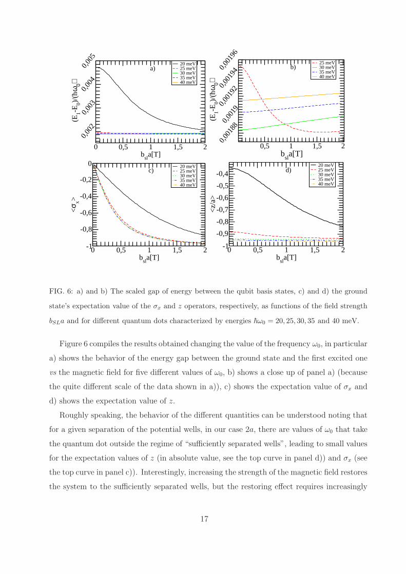
FIG. 6: a) and b) The scaled gap of energy between the qubit basis states, c) and d) the ground

state’s expectation value of the σx and z operators, respectively, as functions of the field strength

bSLa and for different quantum dots characterized by energies ~ω0 = 20, 25, 30, 35 and 40 meV.

Figure 6 compiles the results obtained changing the value of the frequency ω0, in particular

a) shows the behavior of the energy gap between the ground state and the first excited one

vs the magnetic field for five different values of ω0, b) shows a close up of panel a) (because

the quite different scale of the data shown in a)), c) shows the expectation value of σx and

d) shows the expectation value of z.

Roughly speaking, the behavior of the different quantities can be understood noting that

for a given separation of the potential wells, in our case 2a, there are values of ω0 that take

the quantum dot outside the regime of “sufficiently separated wells”, leading to small values

for the expectation values of z (in absolute value, see the top curve in panel d)) and σx (see

the top curve in panel c)). Interestingly, increasing the strength of the magnetic field restores

the system to the sufficiently separated wells, but the restoring effect requires increasingly

17

larger values of the magnetic field as the value ω0 decreases. Anyway, for a design value of

~ω0 = 30meV the system is pretty stable since there will not be appreciable changes in the

behavior of the states associated to the qubit even for deviations of ω0 as large as 20%.

In some sense, the argument above is consistent with the results sketched in Figure 3 b),

i.e. changing the parameters of the QD along a contour-line in the (~ω0, a) plane produces

very much the same quality of qubit basis states or, in other terms for a given a there is

always a “weak-enough” value of ~ω0 that would result in a pair of states well-suited to

be used as qubit basis states. This is clearly to be expected, but Figure 3 and Figure 6

provide the quantitative evidence that this scenario can be achieved for realistic parameters.

Anyway, since the two lowest eigenstates of the Hamiltonian are not eigenstates of the σx

operator, the ability to distinguish between states when a measurement of σx is performed

imposes a certain constraint on the minimum value that can take the field gradient bSL.

Changing the other two parameters that define the confining potential for the electron, b

and γ, has pretty much the same effect over the spectrum and the expectation values that

changing ~ω0 or a, loosely speaking it is fair to say that if the gap between the ground and

the first excited state becomes too large because b becomes smaller and smaller then it is

always possible to separate the wells making a larger and larger in such a way to keep the

energy gap between the desired limits. On the other hand, for larger values of the asymmetry

factor γ it is easier to obtain larger values for the expectation values of σx, anyway, it is

not always easy to design asymmetric double quantum dots and the energy gap between the

qubit basis state can become very large leaving rapidly the domain around the µeV.

The large Zeeman magnetic field B0 is used in NMR to set the energy scale between the

different polarization states of the magnetic nuclei in the sample under scrutiny. Larger

magnetic fields imply a stronger signal since the net polarization, at a given temperature,

depends on the different populations of the “up” and “down” levels. The nuclei are heavy

enough to ignore what happens with the orbital degrees of freedom, but this is not the case

with electrons. The proposal of Tokura et al. [28] was intended to provide a qubit where

single electron spin resonance could be performed. As we will discuss next, what is good for

NMR it is not necessarily so good for SESR in quantum dots.

Figure 7 shows the behavior of the ground state expectation value of the σx operator as a

function of bSL and for different strengths of B0. The data show clearly that if the Zeeman

field becomes larger it is then necessary to resort to increasingly large values of the gradient

18

0 0,5 1 1,5 2b

sla[T]

-1

-0,8

-0,6

-0,4

-0,2

0

<σ x>

B0=0.1[T]

B0=0.5[T]

B0=1.0[T]

B0=1.5[T]

B0=2.0[T]

FIG. 7: The ground state expectation value of the operator σx vs the magnetic field bSLa for

different B0 strengths. From top to bottom, the curves correspond to strengths of 2, 1.5, 1, 05 and

0.1 Tesla.

in order to obtain large enough expectation values of σx. In some sense, is in this Figure

where the two-dimensional character is revealed more plainly. Besides, Figure 7 shows what

was previously enunciated, i.e. that higher values of Zemann field may worsen the qubit

behavior, diminishing the strength of the signal if a measurement of σx is performed.

V. CONCLUSIONS AND DISCUSSION

The results shown in this work do not preclude the possibility of implementing a qubit

suitable to study SESR, up to a point our results just strengthen some of the constraints

already present in the original proposal. Nevertheless, the net effect of considering a two-

dimensional system seems to be the need of stronger field gradients bSL to achieve the same

results than in a one-dimensional system.

On the other hand, the design is pretty robust against perturbations to their design

parameters, even having into account the possible asymmetry between the potential wells

depth. So, there is a broad range of parameters where the qubit can be implemented, but

the controllability, stability and possible probability leakage should be investigated carefully.

Work around this lines is currently in development.

It would be interesting to explore the transition from a two-dimensional system, like the

one studied in this work, to a one-dimensional one, reducing the confinement length in the

y direction from much larger than 2a to smaller than a, but most probably other basis set

19

for the Ritz method must be employed.

Acknowledgments

We would like to acknowledge SECYT-UNC, and CONICET for partial financial support

of this project and to Federico Pont for critical reading of the manuscript.

[1] R. Hanson, L. P. Kouwenhoven, J. R. Petta, S. Tarucha and L. M. K. Vandersypen, Spins in

few-electron quantum dots, Rev. Mod. Phys. 79, 1217 (2007).

[2] O. Benson and F. Henneberger, Semiconductor quantum bits, Pan Stanford Publishing Pte.

Ltd., Singapore ( 2008).

[3] E. Kawakami, P. Scarlino, D. R. Ward, F. R. Braakman, D. E. Savage, M. G. Lagally, M.

Friesen, S. N. Coppersmith, M. A. Eriksson and L. M. K. Vandersypen, Electrical control of

a long-lived spin qubit in a Si/SiGe quantum dot, Nature Nano. 9, 666 (2014).

[4] M. Veldhorst, J. C. C. Hwang, C. H. Yang, A. W. Leenstra, B. de Ronde, J. P. Dehollain, J. T.

Muhonen, F. E. Hudson, K. M. Itoh, A. Morello and A. S. Dzurak, An addressable quantum

dot qubit with fault-tolerant control-fidelity, Nature Nano. 9, 981 (2014).

[5] J. T. Muhonen, Juan P. Dehollain, A. Laucht, F. E. Hudson, R. Kalra, T. Sekiguchi, K.

M. Itoh, D. N. Jamieson, J. C. McCallum, A. S. Dzurak and A. Morello, Storing quantum

information for 30 seconds in a nanoelectronic device, Nature Nano. 9, 986 (2014).

[6] B. E. Kane, A silicon-based nuclear spin quantum computer, Nature (London) 393, 133 (1998).

[7] T. Tanamoto, Quantum gates by coupled asymmetric quantum dots and controlled-NOT-gate

operation, Phys. Rev. A 61, 022305 (2000).

[8] A. Ferron, P. Serra and O. Osenda J., Quantum control of a model qubit based on a multi-

layered quantum dot, Appl. Phys. 113, 134304 (2013).

[9] K. Wang, C. Payette, Y. Dovzhenko, P. W. Deelman and J. R. Petta, Charge Relaxation in a

Single-Electron Si/SiGe Double Quantum Dot, Phys. Rev. Lett. 111, 046801 (2013).

[10] V. Srinivasa, K. C. Nowack, M. Shafiei, L. M. K. Vandersypen and J. M. Taylor, Simultaneous

Spin-Charge Relaxation in Double Quantum Dots, Phys. Rev. Lett. 110, 196803 (2013).

[11] F. Troiani, U. Hohenester and E. Molinari , Exploiting exciton-exciton interactions in semi-

20

conductor quantum dots for quantum-information processing, Phys. Rev. B 62, R2263(R)

(2000).

[12] E. Biolatti, R. C. Iotti, P. Zanardi and F. Rossi, Quantum Information Processing with Semi-

conductor Macroatoms, Phys. Rev. Lett. 85, 5647 (2000).

[13] N. H. Bonadeo, J. Erland, D. Gammon, D. Park, D. S. Katzer, and D. G. Steel, Coherent

Optical Control of the Quantum State of a Single Quantum Dot, Science 282, 1473 (1998).

[14] H. Haug and S. W. Koch, Quantum THeory of the Optical and Electronic Properties of Semi-

conductors, World Scientific Publishing Co. Pte. Ltd., Singapore (2004).

[15] D. Loss and D. P. DiVincenzo, Quantum computation with quantum dots, Phys. Rev. A 57,

120 (1998).

[16] J. Levy, Universal Quantum Computation with Spin-1/2 Pairs and Heisenberg Exchange,

Phys. Rev. Lett. 89, 147902 (2002).

[17] A. W. Holleitner, R. H. Blick, A. K. Huttel, K. Eberl and J. P. Kotthaus, Probing and

Controlling the Bonds of an Artificial Molecule, Science 297, 70 (2002).

[18] L. Gaudreau, S. A. Studenikin, A. S. Sachrajda, P. Zawadzki, A. Kam, J. Lapointe, M.

Korkusinski and P. Hawrylak, Stability Diagram of a Few-Electron Triple Dot, Phys. Rev.

Lett. 97, 036807 (2006).

[19] M. Korkusinski, I. Puerto Gimenez, P. Hawrylak, L. Gaudreau, S. A. Studenikin, and A. S.

Sachrajda, Topological Hunds rules and the electronic properties of a triple lateral quantum

dot molecule, Phys. Rev. B 75, 115301 (2007).

[20] W. M. Witzel and S. Das Sarma, Multiple-Pulse Coherence Enhancement of Solid State Spin

Qubits, Phys. Rev Lett. 98, 077601 (2007).

[21] Zhan Shi, C. B. Simmons, Daniel R. Ward, J. R. Prance, R. T. Mohr, Teck Seng Koh, John

King Gamble, Xian Wu, D. E. Savage, M. G. Lagally, Mark Friesen, S. N. Coppersmith, and

M. A. Eriksson, Coherent quantum oscillations and echo measurements of a Si charge qubit,

Phys. Rev. B 88, 075416 (2013).

[22] G. Burkard and D. Loss, Cancellation of Spin-Orbit Effects in Quantum Gates Based on the

Exchange Coupling in Quantum Dots, Phys. Rev. Lett. 88,047903 (2002).

[23] R. Petta, A. C. Johnson, J. M. Taylor, E. A. Laird, A. Yacoby, M. D. Lukin, C. M. Mar-

cus, M. P. Hanson and A. C. Gossard, Coherent Manipulation of Coupled Electron Spins in

Semiconductor Quantum Dots, Science 309, 2180 (2005).

21

[24] J. M. Taylor, J.R. Petta, A. C. Johnson, A. Yacoby, C. M. Marcus, and M. D. Lukin, Relax-

ation, dephasing, and quantum control of electron spins in double quantum dots, Phys. Rev.

B 76,035315 (2007).

[25] A. Morello , J. Pla, A. Zwanenburg, W. Chan, Y. Tan, H. Huebl, M. Mttnen, D. Nugroho,

C. Yang, A. van Donkelaar, C. Alves, N. Jamieson, C. Escott, L. Hollenberg, G. Clark and S.

Dzurak, Single-shot readout of an electron spin in silicon, Nature (London) 467, 687 (2010).

[26] M. Xiao, M. G. House and H.W. Jiang, Measurement of the Spin Relaxation Time of Single

Electrons in a Silicon Metal-Oxide-Semiconductor-Based Quantum Dot, Phys. Rev. Lett. 104,

096801 (2010).

[27] B. M. Maune, G. Borselli, B. Huang, D. Ladd, W. Deelman, S. Holabird, A. Kiselev, I.

Alvarado-Rodriguez, S. Ross, E. Schmitz, M. Sokolich, A. Watson, F. Gyure and T. Hunter,

Coherent singlet-triplet oscillations in a silicon-based double quantum dot, Nature (London)

481, 344 (2012).

[28] Y. Tokura, G. van der Wield, T. Obata and S. Tarucha, Coherent Single Electron Spin Control

in a Slanting Zeeman Field, Phys. Rev. Lett. 96, 047202 (2006).

[29] Zhan Shi, C. B. Simmons, J. R. Prance, John King Gamble, Teck Seng Koh, Yun-Pil Shim,

Xuedong Hu, D. E. Savage, M. G. Lagally, M. A. Eriksson, Mark Friesen, and S. N. Copper-

smith, Fast Hybrid Silicon Double-Quantum-Dot Qubit, Phys. Rev. Lett. 108, 140503 (2012).

[30] Jun Jing, Peihao Huang, and Xuedong Hu, Decoherence of an electrically driven spin qubit,

Phys. Rev. A 90, 022118 (2014).

[31] See, for example, E. Merzbacher, Quantum Mechanics, 3rd ed., John Wiley, New York (1998).

[32] O. Osenda and P. Serra, Scaling of the von Neumann entropy in a two-electron system near

the ionization threshold, Phys. Rev. A 75, 042331 (2007).

[33] A. Ferron, Omar Osenda and P. Serra, Entanglement in resonances of two-electron quantum

dots, Phys. Rev. A 79, 032509 (2009).

[34] A. Ramos and O. Osenda, Resonance states in a cylindrical quantum dot with an external

magnetic field, J. Phys. B: At. Mol. Opt. Phys. 47, 015502 (2014).

[35] Y. Tokura, T. Kubo, and J. Munro, Power dependence of electric dipole spin resonance , JPS

Conference Proceedings 1, 012022 (2014); arXiv:1308.0071v1 (2013).

22