M/G/1 queue - Tietoverkkolaboratorio - TKK. Virtamo 38.3143 Queueing Theory / The M/G/1/ queue 4 Pollaczek-Khinchin mean formula (continued) From the mean waiting time one immediately

J. Virtamo 38.3143 Queueing Theory / The M/G/1/ queue 1

M/G/1 queue

M (memoryless): Poisson arrival process, intensity λ

G (general): general holding time distribution, mean S = 1/µ

1 : single server, load ρ = λS (in a stable queue one has ρ < 1)

The number of customers in the system, N(t), does not now constitute a Markov process.

• The probability per time unit for a transition from the state {N = n} to the state

{N = n − 1}, i.e. for a departure of a customer, depends also on the time the customer

in service has already spent in the server;

– this information is not contained in the variable N(t)

– only in the case of an exponential service time the amount of service already received

does not have any bearing (memoryless property)

In spite of this, the mean queue length, waiting time, and sojourn time of the M/G/1 queue

can be found. The results (the Pollaczek-Khinchin formulae) will be derived in the following.

It turns out that even the distributions of these quantities can be found. A derivation based

on considering an embedded Markov chain will be presented after the mean formulae.


Pollaczek-Khinchin mean formula

We start with the derivation of the expectation of the waiting time W . W is the time the

customer has to wait for the service (time in the “waiting room”, i.e. in the actual queue).

E[W ] = E[Nq]︸︷︷︸

number of wait-ing customers

· E[S]︸︷︷︸

mean service time

︸︷︷︸

mean time needed to serve thecustomers ahead in the queue

+ E[R]︸︷︷︸

unfinished work

in the server

(R = residual service time)

• R is the remaining service time of the customer in the server (unfinished work expressed

as the time needed to discharge the work).

If the server is idle (i.e. the system is empty), then R = 0.

• In order to calculate the mean waiting time of an arriving customer one needs the expec-

tation of Nq (number of waiting customers) at the instant of arrival.

• Due to the PASTA property of Poison process, the distributions seen by the arriving

• customer are the same as those at an arbitrary instant.

The key observation is that by Little’s result the mean queue length E[Nq] can be expressed

in terms of the waiting time (by considering the waiting room as a black box)

E[Nq] = λE[W ] ⇒ E[W ] =E[R]

1 − ρ

It remains to determine E[R].

ρ = λE[S]


Pollaczek-Khinchin mean formula (continued)

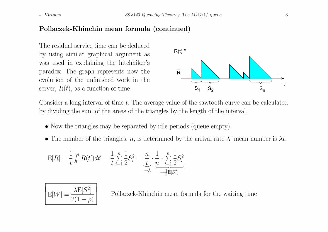
The residual service time can be deduced

by using similar graphical argument as

was used in explaining the hitchhiker’s

paradox. The graph represents now the

evolution of the unfinished work in the

server, R(t), as a function of time.

R(t)

í îì í îì

S1 S2 Sn

t

R

_

í îì

Consider a long interval of time t. The average value of the sawtooth curve can be calculated

by dividing the sum of the areas of the triangles by the length of the interval.

• Now the triangles may be separated by idle periods (queue empty).

• The number of the triangles, n, is determined by the arrival rate λ; mean number is λt.

E[R] =1

t

∫ t

0R(t′)dt′ =

1

t

n∑

i=1

1

2S2

i =n

t︸︷︷︸

→λ

·1

n·

n∑

i=1

1

2S2

i︸︷︷︸

→12E[S2]

E[W ] =λE[S2]

2(1 − ρ)Pollaczek-Khinchin mean formula for the waiting time


Pollaczek-Khinchin mean formula (continued)

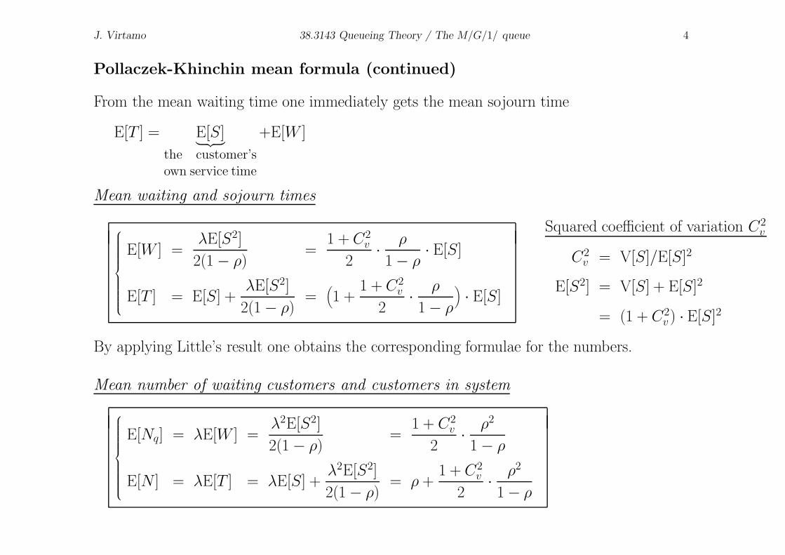
From the mean waiting time one immediately gets the mean sojourn time

E[T ] = E[S]︸︷︷︸

the customer’sown service time

+E[W ]

Mean waiting and sojourn times

E[W ] =λE[S2]

2(1 − ρ)=

1 + C2v

2·

ρ

1 − ρ· E[S]

E[T ] = E[S] +λE[S2]

2(1 − ρ)=

(

1 +1 + C2

v

2·

ρ

1 − ρ

)

· E[S]

Squared coefficient of variation C2v

C2v = V[S]/E[S]2

E[S2] = V[S] + E[S]2

= (1 + C2v ) · E[S]2

By applying Little’s result one obtains the corresponding formulae for the numbers.

Mean number of waiting customers and customers in system

E[Nq] = λE[W ] =λ2E[S2]

2(1 − ρ)=

1 + C2v

2·

ρ2

1 − ρ

E[N ] = λE[T ] = λE[S] +λ2E[S2]

2(1 − ρ)= ρ +

1 + C2v

2·

ρ2

1 − ρ


Remarks on the PK mean formulae

• Mean values depend only on the expectation E[S] and variance V[S] of the service time

distribution but not on higher moments.

• Mean values increase linearly with the variance.

• Randomness, ‘disarray’, leads to an increased waiting time and queue length.

• The formulae are similar to those of the M/M/1 queue; the only difference is the extra

factor (1 + C2v )/2.


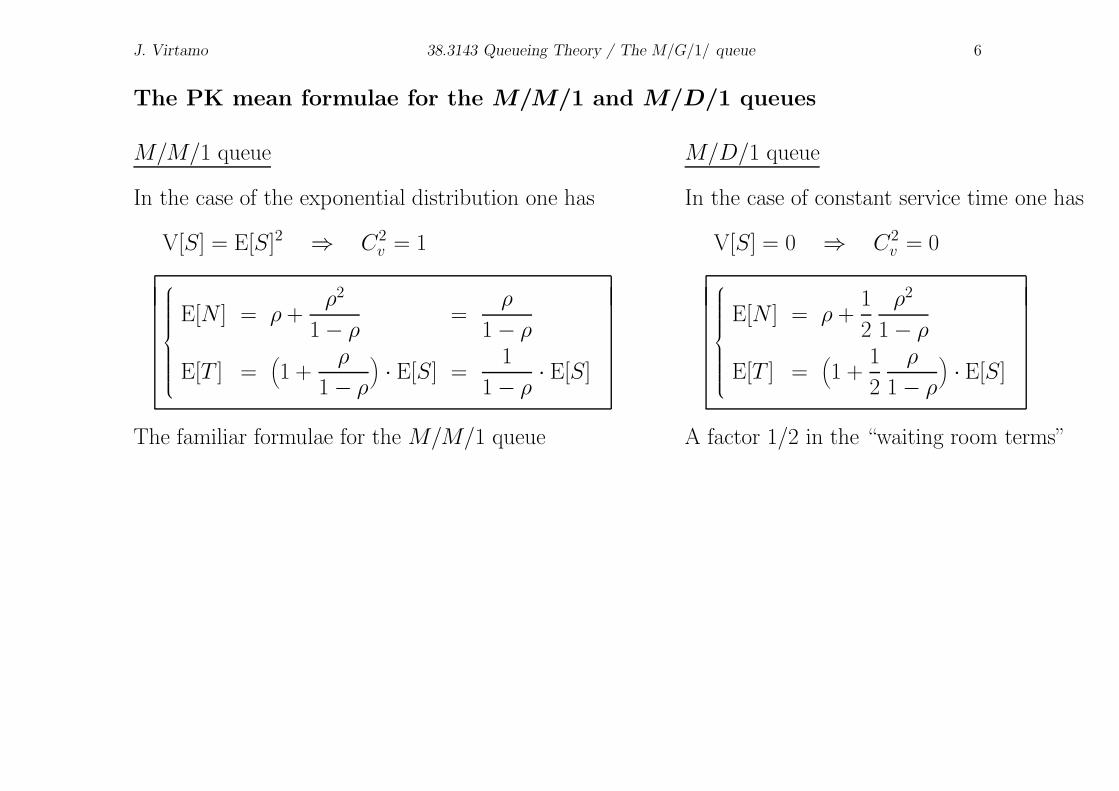
The PK mean formulae for the M/M/1 and M/D/1 queues

M/M/1 queue

In the case of the exponential distribution one has

V[S] = E[S]2 ⇒ C2v = 1

E[N ] = ρ +ρ2

1 − ρ=

ρ

1 − ρ

E[T ] =(

1 +ρ

1 − ρ

)

· E[S] =1

1 − ρ· E[S]

The familiar formulae for the M/M/1 queue

M/D/1 queue

In the case of constant service time one has

V[S] = 0 ⇒ C2v = 0

E[N ] = ρ +1

2

ρ2

1 − ρ

E[T ] =(

1 +1

2

ρ

1 − ρ

)

· E[S]

A factor 1/2 in the “waiting room terms”


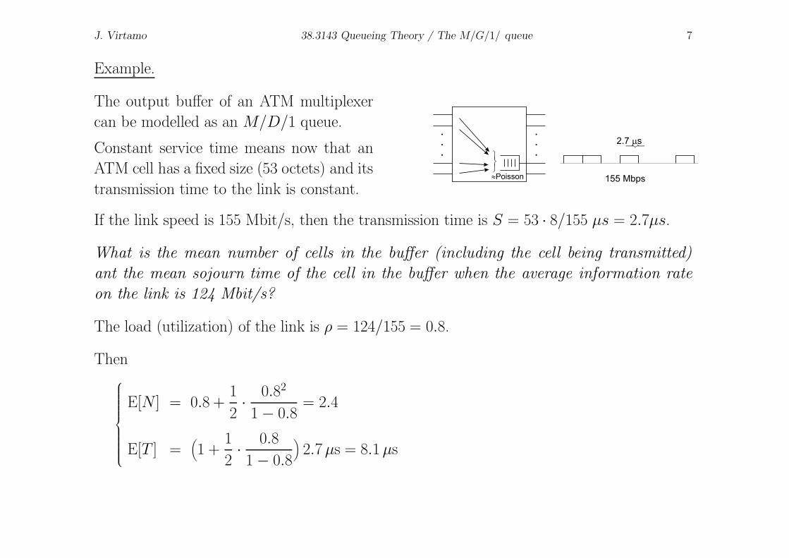
Example.

The output buffer of an ATM multiplexer

can be modelled as an M/D/1 queue.

Constant service time means now that an

ATM cell has a fixed size (53 octets) and its

transmission time to the link is constant.

íî

ì

155 Mbps»Poisson

í îì2.7 sm

.

.

.

.

.

.

If the link speed is 155 Mbit/s, then the transmission time is S = 53 · 8/155 µs = 2.7µs.

What is the mean number of cells in the buffer (including the cell being transmitted)

ant the mean sojourn time of the cell in the buffer when the average information rate

on the link is 124 Mbit/s?

The load (utilization) of the link is ρ = 124/155 = 0.8.

Then

E[N ] = 0.8 +1

2·

0.82

1 − 0.8= 2.4

E[T ] =(

1 +1

2·

0.8

1 − 0.8

)

2.7 µs = 8.1 µs


The queue length distribution in an M/G/1 queue

The queue length Nt in an M/G/1 system does not constitute a Markov process.

• The number in system alone does not tell with which probability (per time) a customer

in service departs, but this probability depends also on the amount of service already

received.

As we saw above, the mean queue length was easy to derive. Also the queue length distribution

can be found. There are two different approaches:

1. The first is based on the observation that the unfinished work in the system, Xt (or

virtual waiting time Vt), does constitute a Markov process. The Markovian property, is a

property of the considered stochastic process, not an intrinsic property of the system.

• The evolution of Xt can be characterized as follows: when there are no arrivals Xt

decreases at a constant rate C (when Xt > 0). In addition, there is a constant

probability per time unit, λ, for a new arrival, bringing to the queue an amount work

having a given distribution. No knowledge about the history of Xt is needed.

• A slight technical difficulty is that Xt is a continuous state (real valued) process.

2. The second approach is based on the observation that there is an embedded Markov chain,

by means of which the distribution can be solved. In the following we use this method.


Embedded Markov chain

The embedded Markov chain is constituted by the queue left by an departing customer (i.e.

number in system at departure epochs). That this indeed is a Markov chain will be justified

later.

Denote

N∗− = the queue length seen by an arriving customer (queue length just before arrival)

N∗+ = the queue length left by a departing customer

N = queue length at an arbitrary time

By the PASTA property of Poisson arrivals we have N∗− ∼ N

In addition, for any system with

single (in contrast to batch) arrivals

and departures, it holds

N∗+ ∼ N∗

−

(so called level crossing property)

Proof:

i

i+1

N*=i- N*=i+

The events {N∗− = i} and {N∗

+ = i} occur pairwise.

P{N∗− = i} = P{N∗

+ = i} ⇒ N∗− ∼ N∗

+


Embedded Markov chain (continued)

We have shown that N∗+ ∼ N∗

− ja N∗− ∼ N . ⇒ N∗

+ ∼ N

Thus to find the distribution of N at an arbitrary time, it is sufficient to find the distribution

at instants immediately after departures.

We focus on the Markov chain N∗+, which in the following will for brevity be denoted just N .

In particular, denote

Nk = queue length after the departure od customer k

Vk = number of new customers arrived during the service time of customer k.

Nk

Nk+1

Nk-1



Claim: The discrete time process Nk constitutes a Markov chain (however, not of a birth-death

type process).

Proof: Given Nk, Nk+1 can be expressed in terms of it and of a random variable Vk+1 which

is independent of Nk and its history:

Nk+1 =

Nk − 1 + Vk+1, Nk ≥ 1

Vk+1, Nk = 0 (= Nk + Vk+1)

• If Nk ≥ 1, then upon the departure of customer k, customer k + 1 is in the queue and

enters the server.

When ultimately customer k + 1 departs, the queue length is decremented by one. Mean-

while (during the service of customer k + 1), there have been Vk+1 arrivals.

• If Nk = 0, customer k leaves an empty queue. Upon the arrival of customer k+1 the queue

length is first incremented and then decremented by one when customer k + 1 departs.

The queue consists of those customers who arrived during the service of customer k + 1.

• As the service times are independent and the arrivals are Poissonian, the Vk are indepen-

dent of each other. Moreover, Vk+1 is independent of the queue length process before the

departure of customer k, i.e. of Nk and its previous values.

The stochastic characterization of Nk+1 depends on Nk but not on the earlier history. QED.



Denote Nk = (Nk − 1)+ =

Nk − 1, Nk ≥ 1

Nk (= 0), Nk = 0

Then Nk+1 = Nk + Vk+1Upward jumps can be arbitrary large.

Downward one step at a time.

• In equilibrium (when the initial information has been wahed out) the random variables

Nk, Nk+1, . . . have the same distribution.

• So are the distributions of the random variables Nk, Nk+1, . . . the same (mutually).

• Random variables Vk, Vk+1, . . . have from the outset the same distributions (mutually).

Denote the random variables obeying the equilibrium distributions without indeces, so that

N = N + V

Since V and N are independent, we have for the generating functions

GN(z) = GN(z) · GV (z) The task now is to determine GN(z) and GV (z).


Expressing the generating function of N in terms of the generating function of N

GN(z) = E[zN ]

= z0 · P{N = 0}︸︷︷︸

P{N=0}+P{N=1}

+∞∑

i=1zi P{N = i}

︸︷︷︸

P{N=i+1}

= P{N = 0} +1

z

∞∑

i=1ziP{N = i}

= P{N = 0}︸︷︷︸

1−ρ

(1 −1

z) +

1

z

∞∑

i=0ziP{N = i}

︸︷︷︸

GN(z)

We have obtained the result

GN(z) =GN(z) − (1 − ρ)(1 − z)

zwhere ρ = λE[S]


The number of arrivals from a Poisson process during a service time

Let X be an arbitrary random variable (representing an interval of time).

We wish to determine the distribution of the number of arrivals, K, from a Poisson process

(intensity λ) occuring in the interval X , and, in particular, its generating function GK(z).

GK(z) = E[zK ] = E[ E[

zK |X]

︸︷︷︸

K∼Poisson(λX)

] = E[e−(1−z)λX ] = X∗((1 − z)λ) | X∗(s) = E[e−sX]

Generally, GK(z) = X∗((1 − z)λ) In particular, GV (z) = S∗((1 − z)λ)

The result can be derived also in a more elementary way

GK(z) =∞∑

i=0ziP{K = i} =

∞∑

i=0zi

∫ ∞

0

(λx)i

i! e−λx

︷︸︸︷

P{K = i |X = x} fX(x)dx

=∫ ∞

0fX(x)e−λx

∞∑

i=0

(λxz)i

i!dx =

∫ ∞

0fX(x)e−λxeλxzdx =

∫ ∞

0fX(x)e−(1−z)λxdx

= X∗((1 − z)λ)


The number of arrivals from a Poisson process during a service time (continued)

The result can be interpreted by the method of collective marks:

• In the method of collective marks GK(z) has the interpretation of the probability that none

of the K arrivals occurring in the interval X is marked, when each arrival is independently

marked with the probability (1 − z).

• The process of marked arrivals is obtained by a random selection of a Poisson process,

and is thus a Poisson process with intensity (1 − z)λ.

• The interpretation of the Laplace transform in terms of collective marks: X∗(s) is the

probability that there are no arrivals in the interval X from a Poisson process with

intensity s:

X∗(s) = E[e−sX ] = E[P{no arrivals in X |X}] = P{no arrivals in X}

• When the intensity of the marking process is (1 − z)λ, the probability of no marks is

X∗((1 − z)λ).


Pollaczek-Khinchin transform formula for the queue length

By collecting the results together,

GN(z) = GN(z) · GV (z) =GN(z) − (1 − ρ)(1 − z)

z· S∗((1 − z)λ)

From this we can solve GN(z)

GN(z) =(1 − ρ)(1 − z)

S∗((1 − z)λ) − z· S∗((1 − z)λ) =

(1 − ρ)(1 − z)

1 − z/S∗((1 − z)λ)

Example. M/M/1 queue

S ∼ Exp(µ) ⇒ S∗(s) =µ

s + µ

S∗((1 − z)λ) =µ

(1 − z)λ + µ=

1

(1 − z)ρ + 1| ρ = λ/µ

GN(z) =(1 − ρ)(1 − z)

1 − z((1 − z)ρ + 1)=

(1 − ρ)(1 − z)

(1 − z)(1 − ρz)=

1 − ρ

1 − ρz

= (1 − ρ)(1 + (ρz) + (ρz)2 + · · ·) (generates the distribution in an M/M/1 queue)


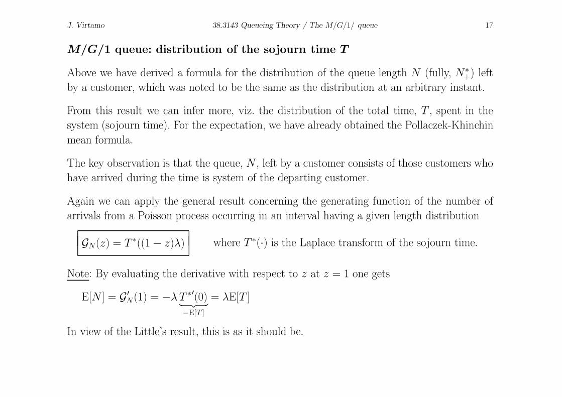
M/G/1 queue: distribution of the sojourn time T

Above we have derived a formula for the distribution of the queue length N (fully, N∗+) left

by a customer, which was noted to be the same as the distribution at an arbitrary instant.

From this result we can infer more, viz. the distribution of the total time, T , spent in the

system (sojourn time). For the expectation, we have already obtained the Pollaczek-Khinchin

mean formula.

The key observation is that the queue, N , left by a customer consists of those customers who

have arrived during the time is system of the departing customer.

Again we can apply the general result concerning the generating function of the number of

arrivals from a Poisson process occurring in an interval having a given length distribution

GN(z) = T ∗((1 − z)λ) where T ∗(·) is the Laplace transform of the sojourn time.

Note: By evaluating the derivative with respect to z at z = 1 one gets

E[N ] = G ′N(1) = −λ T ∗′(0)

︸︷︷︸

−E[T ]

= λE[T ]

In view of the Little’s result, this is as it should be.


M/G/1 queue: distribution of the sojourn time (continued)

We have obtained

T ∗((1 − z)λ) =(1 − ρ)(1 − z)

S∗((1 − z)λ) − zS∗((1 − z)λ)

Here z is a free variable. Denote s = (1 − z)λ, i.e. z = 1 − s/λ, whence

T ∗(s) =(1 − ρ)s

s − λ + λS∗(s)S∗(s)

Pollaczek-Khinchin transform formula

for the sojourn time

Example. M/M/1 queue

S ∼ Exp(µ) ⇒ S∗(s) =µ

s + µ

T ∗(s) =(1 − ρ)s

s − λ + λµ

s + µ

µ

s + µ=

(1 − ρ)s

s − λs

s + µ

µ

s + µ=

µ − λ

s + (µ − λ)

⇒ T ∼ Exp(µ − λ) , in accordance with earlier result.


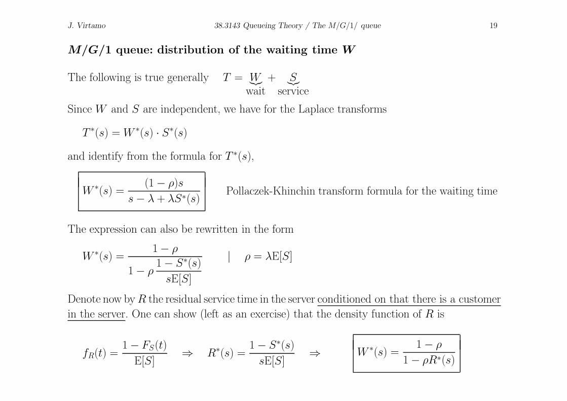
M/G/1 queue: distribution of the waiting time W

The following is true generally T = W︸︷︷︸

wait+ S

︸︷︷︸

service

Since W and S are independent, we have for the Laplace transforms

T ∗(s) = W ∗(s) · S∗(s)

and identify from the formula for T ∗(s),

W ∗(s) =(1 − ρ)s

s − λ + λS∗(s)Pollaczek-Khinchin transform formula for the waiting time

The expression can also be rewritten in the form

W ∗(s) =1 − ρ

1 − ρ1 − S∗(s)

sE[S]

| ρ = λE[S]

Denote now by R the residual service time in the server conditioned on that there is a customer

in the server. One can show (left as an exercise) that the density function of R is

fR(t) =1 − FS(t)

E[S]⇒ R∗(s) =

1 − S∗(s)

sE[S]⇒ W ∗(s) =

1 − ρ

1 − ρR∗(s)


Interpretation of the formula for W ∗(s)

W ∗(s) =1 − ρ

1 − ρR∗(s)=

∞∑

n=0(1 − ρ)ρnR∗(s)n

• The real waiting time W of the customers is, by the PASTA property of Poisson arrivals,

distributed as the virtual waiting time (unfinished work expressed as the time it takes to

recharge the work) at an arbitrary instant.

• Virtual waiting time is independent of the scheduling discipline (justified later) and is in

the ordinary FIFO queue the same as e.g. in a PS queue (Processor Sharing).

• The queue length distribution of an M/M/1-PS queue, πn = (1 − ρ)ρn, is independent

of the service time distribution and applies also for the M/G/1 queue (this does not hold

for the FIFO discipline).

• The unfinished work in a PS queue at an arbitrary instant is composed of the residual

service times of the customers in the system. One can show that, conditioned on the

number of customers in the queue, n, the residual service times are independent and

distribute as R. The total residual service time of the customer thus has the Laplace

transform R∗(s)n.

• By the law of total probability, the above formula gives the Laplace transform of the

virtual waiting time in a PS queue, and thus also that in the FIFO queue.


Virtual waiting time (unfinished work) is independent of the scheduling discipline

• If the discipline is work conserving,

i.e. the server is busy always when

there are customers in the system, the

busy periods are the same no matter

in which order the service is given to

different customers in the system; the

total work is “anonymous work”.

• The scheduling affects Nt but not Xt

or Vt.

jononpituus

jononpituus

virtuaalinenodotusaika

virtuaalinenodotusaika

FIFO

LIFO


Busy period of an M/G/1 queue: waiting time

The server is alternatingly busy and idle. The busy period

is a continuous period where the server is uninterruptedly

busy. Two busy periods are separated by an idle period.

Denote

B = length of busy period

I = length of idle period

í îìí îì

1/l E[B]

In a Poisson process the interarrival times are distributed according to Exp(λ). Because of

the memoryless property, the idle periods (time from the end of an busy period to the start

of the next one) obey the same distribution, I ∼ Exp(λ), thence E[I ] = 1/λ .

By Little’s result, the load of the server ρ = λE[S] is the same as the expected number of

customers in the server. As there can be at most one customer at a time in the server, the

expected number equals the probability that there is a customer in the server, and further,

this equals the proportion of time the server is busy:

λE[S] =E[B]

E[B] + E[I ]=

E[B]

E[B] + 1/λ⇒ E[B] =

ρ

1 − ρ·

1

λ=

E[S]

1 − ρ

In the case of an M/M/1 queue this the same as E[T ], i.e. mean sojourn time!


Mean number of customers served during a busy period

A busy period consists of full service times of a set of customers.

Let the number of customers served during the busy period be Nb. We deduce the expectation

E[Nb].

• The first customer of a busy period finds the system empty, the others find it non-empty.

• Thus an arrving customer finds the system empty with probability 1/E[Nb].

• The probability that the system is empty at an arbitrary instant is 1 − ρ.

• By the PASTA property, these probabilities are equal.

⇒ E[Nb] =1

1 − ρ

Since the mean service time of the customer is E[S], it follows further that

E[B] =E[S]

1 − ρ


Distribution of the length of the busy period in an M/G/1 queue

Denote

B = length of busy period

S = service time of the customer starting the busy period

V = number of customers arriving during this service time

The duration of the busy period is independent

of the scheduling discipline provided this is work

conserving. We can choose scheduling as we wish.

It is easiest to consider a stack, i.e. a LIFO queue. í îì í îì

B1 B2

S

• The first arrival within the busy period interrupts the service of the customer who started

the busy period.

• By considering the period starting from this instant of interruption to the point when

the service of the first customer is resumed, we notice that this period itself forms a busy

period which is distributed in the same way as B, we call it a “mini busy period”.

– It may be paradoxical that inside a busy period there are subperiods with the same

distribution as the busy period itself. However, their expected number is < 1.

• The number of mini busy periods is V : the service of the first customer is executed in

pieces, each of them having a duration ∼ Exp(λ) (except for the last one); thus the

number of mini busy periods is the same as the number of border lines of the pieces,

which equals the number of arrivals from a Poisson(λ) process during the interval S.


Distribution of the length of the busy period (continued)

B = S + B1 + B2 + · · · + BV , V = 0, 1, 2, . . . , B ∼ B1 ∼ B2 ∼ · · · ∼ BV

B∗(s) = E[e−sB] = E[E[

E[

e−sB |V, S]

|S]

] = E[E[

E[

e−s(S+B1+B2+···+BV ) |V, S]

|S]

]

= E[E[

e−sSE[

e−s(B1+B2+···+BV ) |V, S]

|S]

] = E[E[e−sSE[e−sB]︸︷︷︸

B∗(s)

V| S]]

= E[e−sS E[

B∗(s)V |S]

︸︷︷︸

e−(1−B∗(s))λS

] = E[e−(s+λ(1−B∗(s)))S]

B∗(s) = S∗(s + λ − λB∗(s)) Takacs’ equation (functional equation) for B∗(s)

Example: the first moment of B

E[B] = −B∗′(0) = S∗′(0)︸︷︷︸

−E[S]

(1 − λ B∗′(0)︸︷︷︸

−E[B]

)

⇒ E[B] =E[S]

1 − ρ, where ρ = λE[S]

This is in accordance with our earlier results.

In a similar way, one can derive higher moments of B.


M/G/1 queue: algorithmic approach to the queue length distribution

Previously we have derived a result, the Pollaczek-Khinchin transform formula, for the gen-

erating function of the queue length distribution.

• The result is theoretically important.

• It can be used, e.g. to derive moments of the distribution.

• However, the formula is not very practical for computing the distribution itself (proba-

bilities of different queue lengths) because the dependence on z is quite complicated.

The queue length distribution, however, can be determined algorithmically (not as a closed

form formula) quite straight forwardly. We will derive the algorithm in the following.

To this end, consider again the embedded Markov chain Nk, i.e. the queue lengths immediately

after the departure epochs. We have found that this chain evolves as follows:

Nk+1 =

Nk − 1 + V when Nk ≥ 1

V when Nk = 0

where V is the number of arrivals of new customers during the service time of customer k +1.


Distribution of the number of arrivals, V , during the service time

Denote

ki = P{V = i}

fS(x) = the pdf of the service time S

According to the law of the total probability, it holds

ki = P{V = i} =∫ ∞

0P{V = i |S = x}fS(x)dx =

∫ ∞

0

(λx)i

i!e−λxfS(x)dx

ki =∫ ∞

0

(λx)i

i!e−λxfS(x)dx i = 0, 1, . . .

When the arrival intensity λ and the pdf of the service time fS(x) are given, then the proba-

bilities ki can be calculated, at least numerically. In the case of some simple distributions, the

integration can be done analytically.

Example. Exponential service time distribution (M/M/1 queue)

ki =∫ ∞

0

(λx)i

i!e−λxµe−µxdx =

( λ

λ + µ

)i µ

λ + µ

1

i!

∫ ∞

0yie−ydy

︸︷︷︸

i!

=( λ

λ + µ

)i µ

λ + µ

∣∣∣∣∣∣∣∣∣∣

change of variable

y = (λ + µ)x

Geometrical distribution: “λ and µ compete”; “λ wins” i times, until it “loses”, i.e. “µ wins”.


Transition probability matrix of the embedded chain

From the evolution equation of the chain Nk one can identify the transition probabilities

pi,j = P{Nk+1 = j |Nk = i} =

P{V = j − i + 1} = kj−i+1 if i ≥ 1

P{V = j − i} = kj−i if i = 0

The state transition matrix and diagram are thus

P =

k0 k1 k2 k3 · · ·

k0 k1 k2 k3 · · ·

0 k0 k1 k2 · · ·

0 0 k0 k1 · · ·... ... ... ... . . .

0 1 2k0k0k0 k0

3

k0 k1 k1 k1

k1 k2 k2

k2 k3 k3

k3 k4 k4

k4 k5 k5

The method of a cut yields the recursion equations

k0π1 = (k1 + k2 + . . .)π0

k0π2 = (k2 + k3 + . . .)π0 + (k2 + k3 + . . .)π1

k0π3 = (k3 + k4 + . . .)π0 + (k3 + k4 + . . .)π1 + (k2 + k3 + . . .)π2...

k0πi = (ki + ki+1 + . . .)π0 + (ki + ki+1 + . . .)π1 + . . . + (k2 + k3 + . . .)πi−1

from which the πi can be solved consecutively, starting from the known value π0 = 1 − ρ.


Recursion (continued)

Denote: ai = ki+1 + ki+2 + ki+3 + . . . = P{V > i}

i.e. ai is the probability that during the service time S there are at least i + 1 arrivals.

In terms of this, the general recursion step can be written as

πi =1

k0

ai−1π0 +

i−1∑

j=1ai−jπj

Since k0 + k1 + k2 + . . . = 1, we have

k0 = 1 − (k1 + k2 + . . .) = 1 − a0.

The recursion begins from π0 = 1 − ρ.


Recursion (continued)

One need not evaluate the sums of the series in the definition of ai, but we can derive a single

integral expression for these coefficients. Denote by Xj a general interarrival time in a Poisson

process with intensity λ, Xj ∼ Exp(λ). Then, by the definition of ai we have

ai = P{S > X1 + X2 + · · · + Xi+1}

The sum X1 + X2 + · · ·+ Xi+1 is distributed as Erlang(i + 1, λ) with the pdf λe−λx(λx)i/i!.

Given that the sum has the value x, the probability is given by the tail distribution of S,

GS(x) = 1 − FS(x). By the law of the total probability, it then follows that

ai =∫ ∞

0GS(x)

(λx)i

i!λe−λxdx =

∫ ∞

0GS(y/λ)

yi

i!e−ydy

From this the ai can be com-

puted numerically.


Finite M/G/1/K queue

The queue has K system places (server + waiting

places).

The queue length distribution can be derived from

that of the infinite system. To this end, we need a

few deduction steps.

0 1 ....k0k0k0

K-1

k0 k1 k1 k1

k1 k2 k2

k2 k3 k3

k3 k4 k4

k4 k5 k5

Consider again the embedded Markov chain constituted by the queue length, N , left by a

departing customer.

The first observation is that N cannot be grater than K − 1. Before the departure the queue

may have been full, N = K, but after the departure there is one less customer.

The second observation is that up to the state K − 1 the state transition diagram is precisely

the same as in the case of an infinite system. The only difference is that, all the transitions,

which in the infinite system had taken the system to a state N > K − 1, will now imply that

during the service time of the departed customer the queue has become full and overflown. In

all the cases, after the departure, the system will be in state K − 1 as shown in the figure.

The key thing is that the transitions across all the cuts between states lower than K − 1 are

precisely the same as in the infinite system. The ratios of the state probabilities are as before.

The distribution is obtained by normalization.


Finite M/G/1/K queue (continued)

Denote

π(∞)i = probability that a departing customer leaves queue i in an infinite system

π(K)i = probability that a departing customer leaves queue i in a finite system

As said, the finite system probabilities are obtained by simply normalizing

π(K)i =

π(∞)i

K−1∑

j=0π

(∞)j

i = 0, 1, . . . , K−1 The probabilities π(∞)i are computed with

the algorithm given before.

By the level crossing argument, one deduces that π(K)i is also the probability that an arriving

customer accepted into the queue finds the queue length i upon arrival:

- the frequency of transitions from state i to state i + 1 equals the frequency of transitions

from state i + 1 to state i

- now we just have to observe that not all arriving customers are accepted to the queue,

and thus π(K)i is not the state probability as seen by an arriving customer


Finite M/G/1/K queue (continued)

Denote the, thus far unknown, state probabilities as seen by an arriving customer by pi,

i = 0, 1, . . . , K (notice that upon arrival the queue can be full, i.e. in the state K). Due to

the PASTA property pi is also the equilibrium probability at an arbitrary instant.

Denote

X∗ = queue length seen by arriving customer

A = customer is accepted in the queue = {X∗ < K}

A = customer is rejected = {X∗ = K}

For i < K we have

pi = P{X∗ = i} = P{X∗ = i |A}︸︷︷︸

π(K)i

P{A}︸︷︷︸

1−pK

+ P{X∗ = i | A}︸︷︷︸

0

P{A}︸︷︷︸

pK

= (1 − pK)π(K)i , i < K

In order to determine the unknown pK , we make use of the condition which says that, on

average, the frequency at which customers are admitted to the queue equals the frequency

with which customers depart from the system (ρ = λE[S]):

λ(1 − pK) = (1 − p0)/E[S] = (1 − (1 − pK)π(K)0 )/E[S] ⇒ 1 − pK =

1

ρ + π(K)0

pi =π

(K)i

ρ + π(K)0

i = 0, 1, . . . , K − 1 pK = 1 −1

ρ + π(K)0


Finite M/G/1/K queue (summary)

We gather all the results together, skipping the intermediate steps, and modifying the result:

First calculate recursively the queue length distribution in an infinite system:

π(∞)0 = 1 − ρ

π(∞)i =

1

1 − a0

ai−1π

(∞)0 +

i−1∑

j=1ai−jπ

(∞)j

ai =

∫ ∞

0GS(x)

(λx)i

i!λe−λxdx

where GS(x) is the tail distribution of the service time S.

Then compute the tail probability (usually small) of the infinite queue

qK

=∞∑

i=Kπ

(∞)i = 1 −

K−1∑

i=0π

(∞)i

In terms of these, the final result reads

pi =π

(∞)i

1 − qKρ

i = 0, 1, . . . , K − 1 pK =(1 − ρ)q

K

1 − qKρ

Documents

M/G/1 queue - Tietoverkkolaboratorio - TKK. Virtamo 38.3143 Queueing Theory / The M/G/1/ queue 4 Pollaczek-Khinchin mean formula (continued) From the mean waiting time one immediately