PERFORMANCE DEBUGGING FOR DISTRIBUTED SYSTEMS OF BLACK BOXES

Marcos K. Aguilera, Jeffrey C. Mogul, Janet L. Wiener, Patrick Reynolds, Athicha Muthitacharoen

Presented by 김 운태

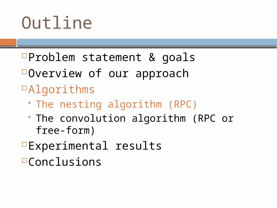
Outline

Problem statement & goalsOverview of our approachAlgorithms

The nesting algorithm (RPC) The convolution algorithm (RPC or free-form)

Experimental resultsConclusions

Motivation

Complex distributed systems Built from black box components Heavy communications traffic Bottlenecks at some specific nodes

These systems may have performance problems High or erratic latency Caused by complex system interactions

Isolating performance bottlenecks is hard We cannot always examine or modify system components

We need tools to infer where bottlenecks are Choose which black boxes to open

Goals

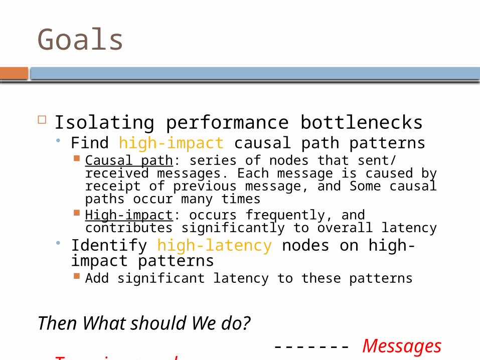
Isolating performance bottlenecks Find high-impact causal path patterns

Causal path: series of nodes that sent/received mes-sages. Each message is caused by receipt of previous message, and Some causal paths occur many times

High-impact: occurs frequently, and contributes signif-icantly to overall latency

Identify high-latency nodes on high-impact pat-terns Add significant latency to these patterns

Then What should We do? ------- Messages Trace is

enough

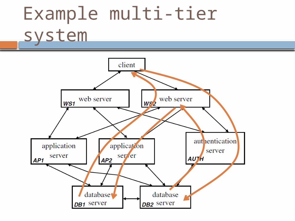
Example multi-tier system

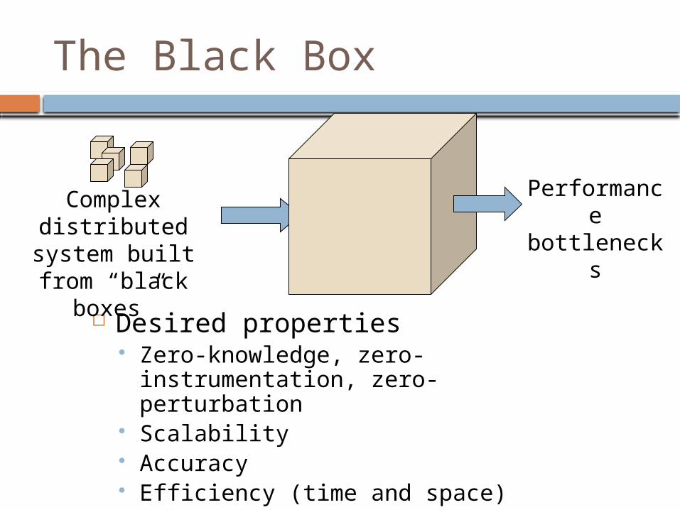
The Black Box

Desired properties Zero-knowledge, zero-instrumenta-

tion, zero-perturbation Scalability Accuracy Efficiency (time and space)

Complex distributed system built from “black

boxes”

Performance bottlenecks

Outline

Problem statement & goalsOverview of our approachAlgorithms

The nesting algorithm (RPC) The convolution algorithm (RPC or free-form)

Experimental resultsConclusions

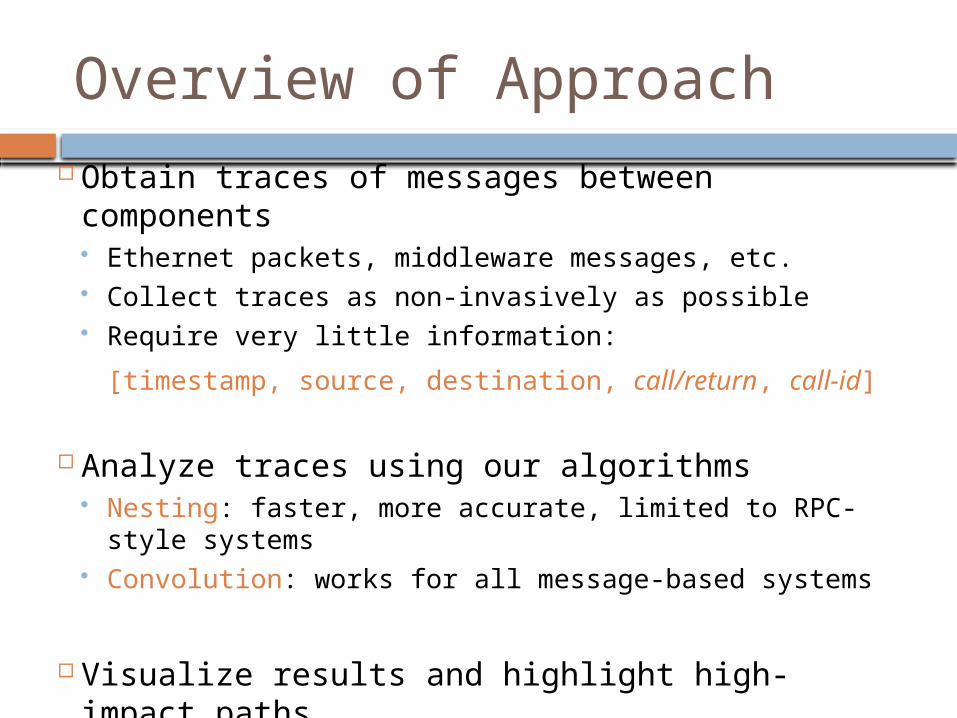
Overview of Approach Obtain traces of messages between components

Ethernet packets, middleware messages, etc. Collect traces as non-invasively as possible Require very little information:

[timestamp, source, destination, call/return, call-id]

Analyze traces using our algorithms Nesting: faster, more accurate, limited to RPC-style sys-

tems Convolution: works for all message-based systems

Visualize results and highlight high-impact paths

Challenges

Trace contain interleaved messages from

many causal paths How to identify causal paths?

Causality trace by Timestamp

Want only statistically significant causal paths How to differentiate significance?

It is easy! They appear repeatedly

Outline

Problem statement & goalsOverview of our approachAlgorithms

The nesting algorithm (RPC) The convolution algorithm (RPC or free-form)

Experimental resultsConclusions

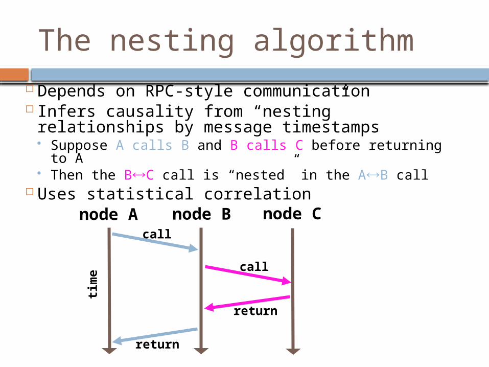
The nesting algorithm Depends on RPC-style communication Infers causality from “nesting” relationships by

message timestamps Suppose A calls B and B calls C before returning to A Then the BC call is “nested” in the AB call

Uses statistical correlation

tim

e

node A node B node C

call

call

return

return

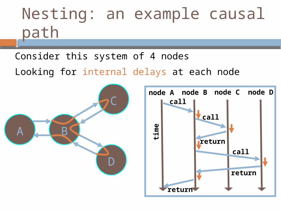
Nesting: an example causal path

A B

C

D

Consider this system of 4 nodes

tim

e

node A node B node Ccall

return

call

call

return

node D

return

Looking for internal delays at each node

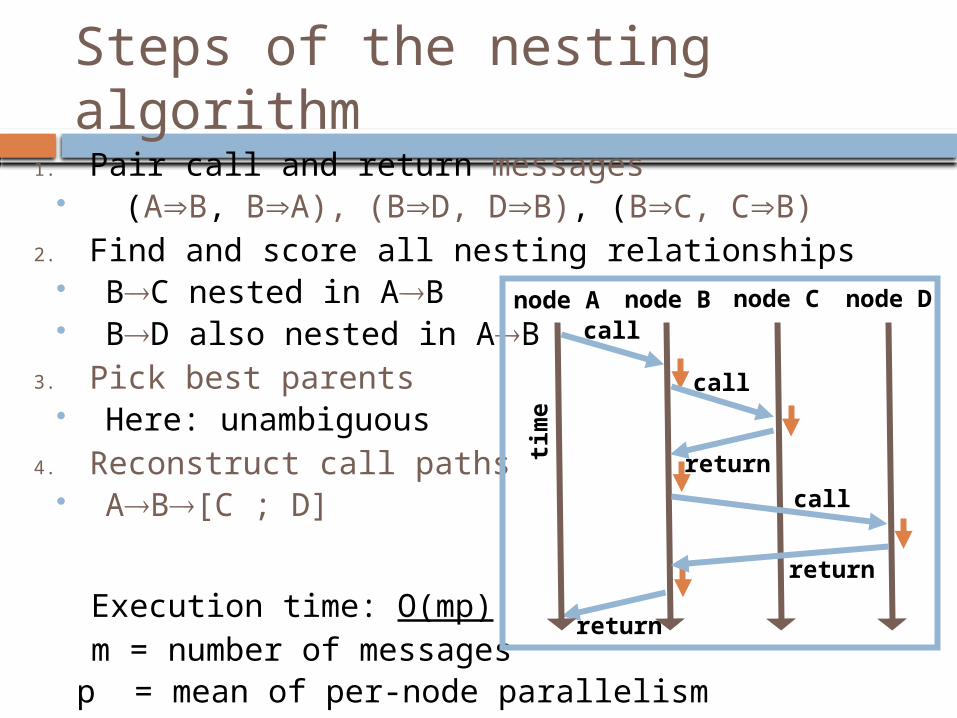
Steps of the nesting algorithm

1. Pair call and return messages (AB, BA), (BD, DB), (BC, CB)

2. Find and score all nesting relationships BC nested in AB BD also nested in AB

3. Pick best parents Here: unambiguous

4. Reconstruct call paths AB[C ; D]

Execution time: O(mp) m = number of messages

p = mean of per-node parallelism

tim

e

node A node B node Ccall

return

call

call

return

node D

return

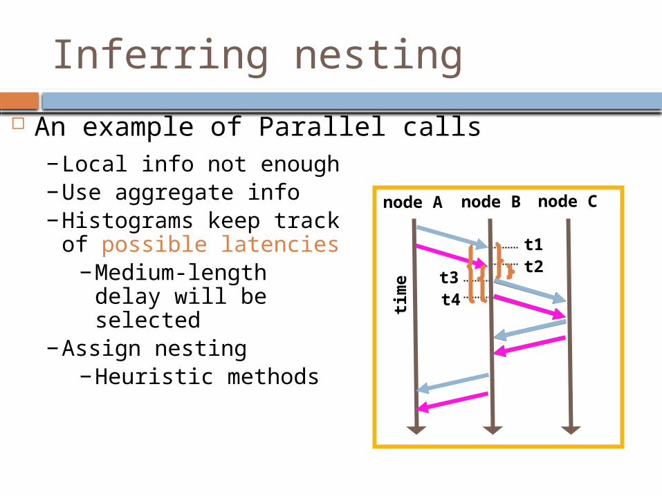
Inferring nesting

An example of Parallel calls−Local info not enough−Use aggregate info−Histograms keep track of

possible latencies−Medium-length delay

will be selected−Assign nesting

−Heuristic methods

tim

e

node A node B node C

t1t2

t3t4

Outline

Problem statement & goalsOverview of our approachAlgorithms

The nesting algorithm The convolution algorithm

Experimental resultsConclusions

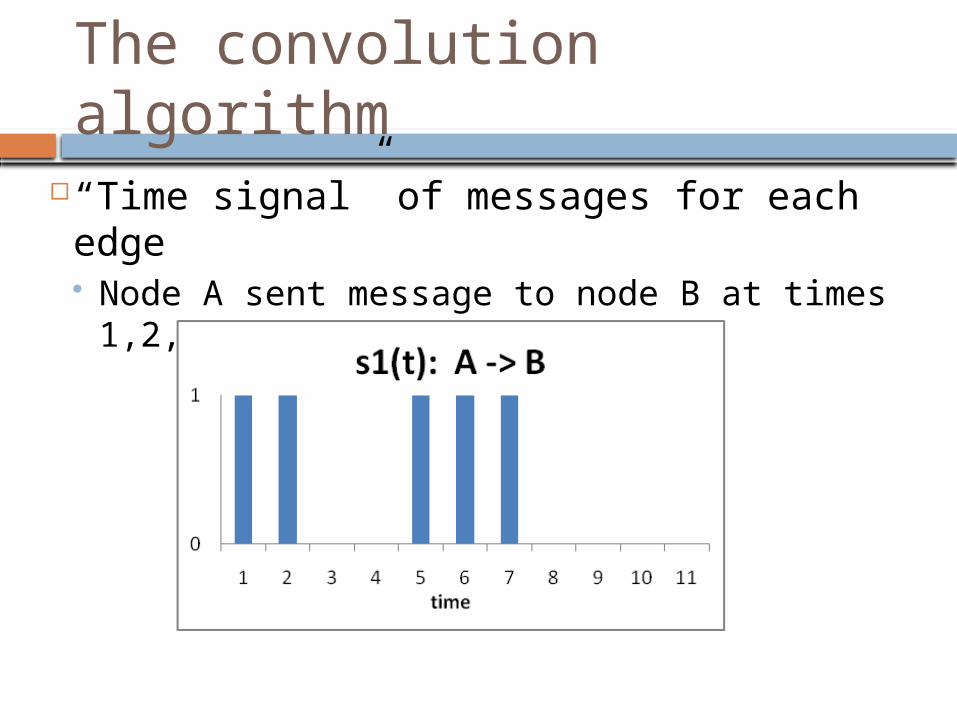
The convolution algorithm

“Time signal” of messages for each edge Node A sent message to node B at times

1,2,5,6,7

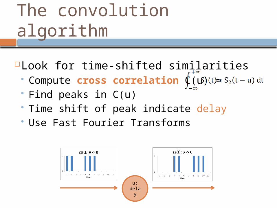
The convolution algorithm

Look for time-shifted similarities Compute cross correlation C(u) = Find peaks in C(u) Time shift of peak indicate delay Use Fast Fourier Transforms

u:dela

y

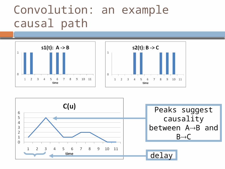
Convolution: an example causal path

Peaks suggest causality between AB

and BC

delay

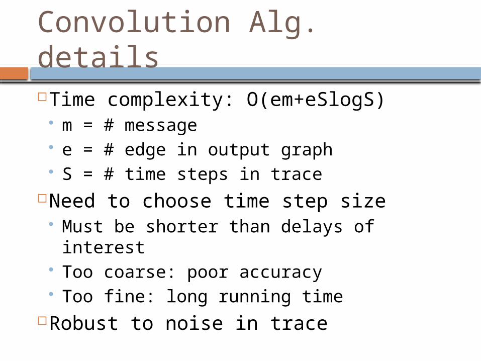
Convolution Alg. details

Time complexity: O(em+eSlogS) m = # message e = # edge in output graph S = # time steps in trace

Need to choose time step size Must be shorter than delays of interest Too coarse: poor accuracy Too fine: long running time

Robust to noise in trace

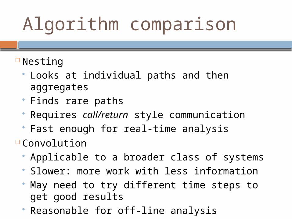
Algorithm comparison

Nesting Looks at individual paths and then aggregates Finds rare paths Requires call/return style communication Fast enough for real-time analysis

Convolution Applicable to a broader class of systems Slower: more work with less information May need to try different time steps to get good

results Reasonable for off-line analysis

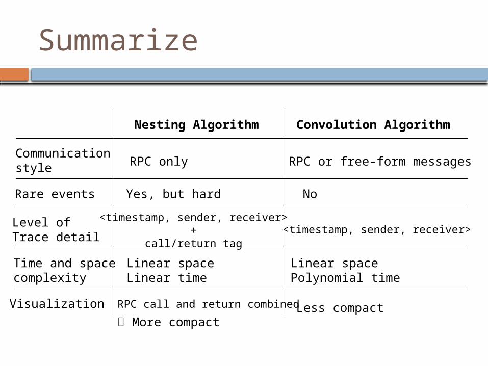
Communicationstyle

Rare events

Level ofTrace detail

Time and spacecomplexity

Visualization

Nesting Algorithm Convolution Algorithm

RPC only RPC or free-form messages

Yes, but hard No

<timestamp, sender, receiver><timestamp, sender, receiver>

+call/return tag

Linear spaceLinear time

Linear spacePolynomial time

RPC call and return combined

More compact Less compact

Summarize

Outline

Problem statement & goals Overview of our approach Algorithms Experimental results

Maketrace: a trace generator Multi-tier configuration Validation of accuracy Execution costs

Conclusions

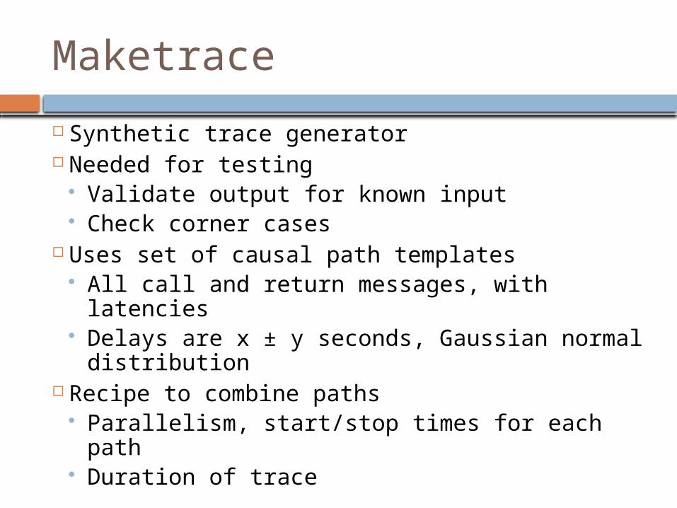
Maketrace

Synthetic trace generator Needed for testing

Validate output for known input Check corner cases

Uses set of causal path templates All call and return messages, with latencies Delays are x ± y seconds, Gaussian normal dis-

tribution Recipe to combine paths

Parallelism, start/stop times for each path Duration of trace

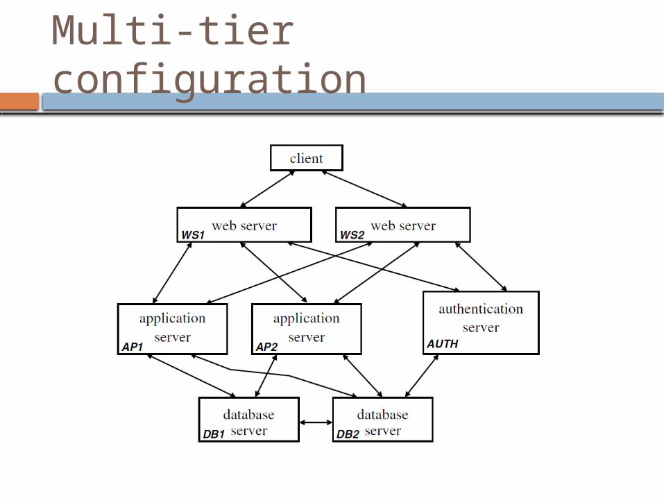
Multi-tier configuration

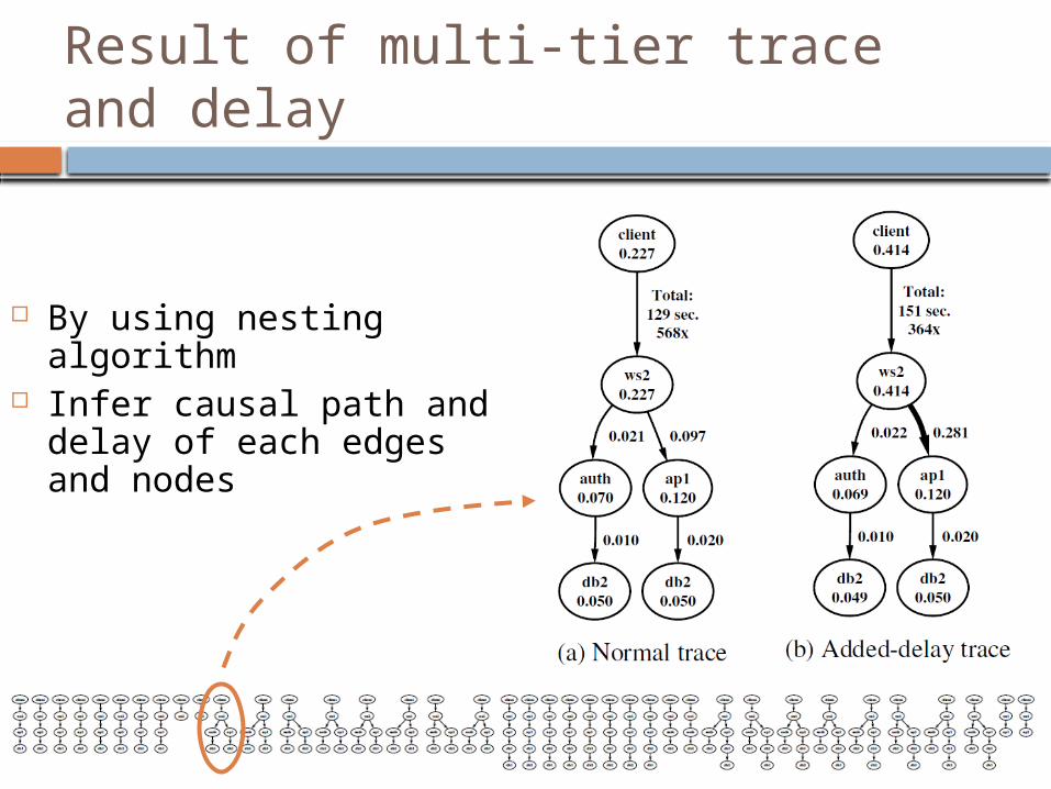
Result of multi-tier trace and de-lay

By using nesting algo-rithm

Infer causal path and de-lay of each edges and nodes

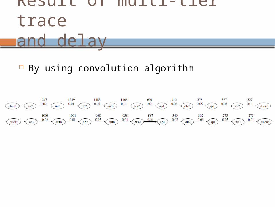
By using convolution algorithm

Result of multi-tier traceand delay

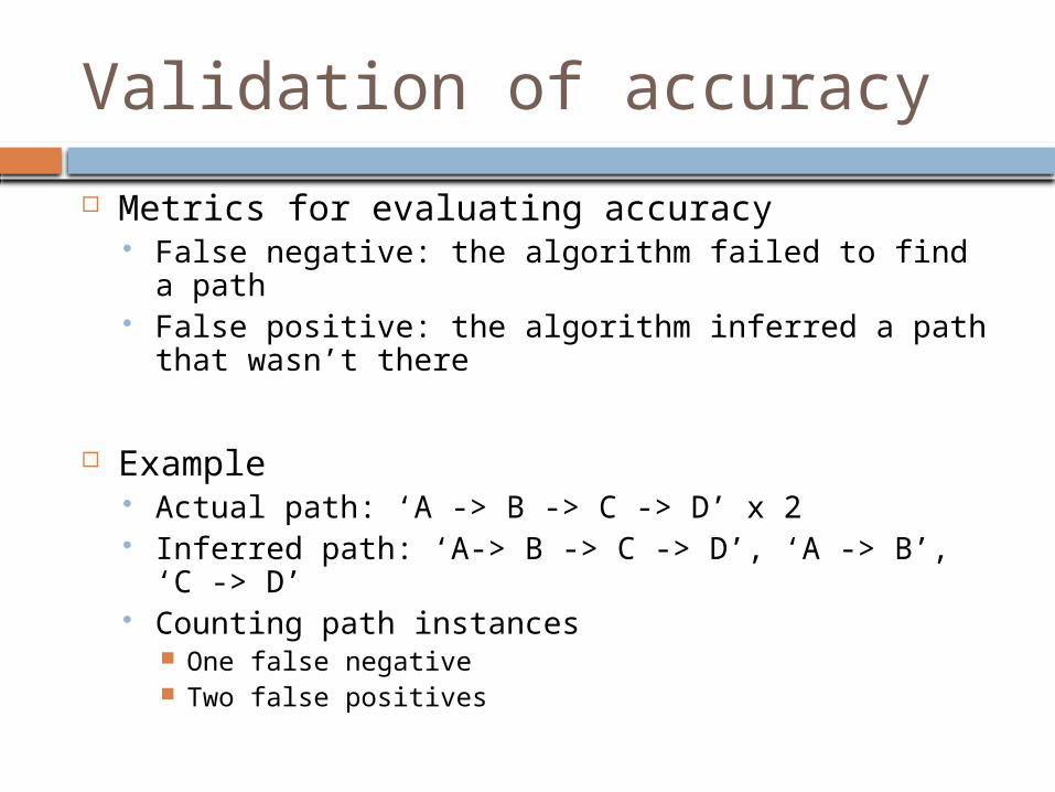
Validation of accuracy

Metrics for evaluating accuracy False negative: the algorithm failed to find a path False positive: the algorithm inferred a path that

wasn’t there

Example Actual path: ‘A -> B -> C -> D’ x 2 Inferred path: ‘A-> B -> C -> D’, ‘A -> B’, ‘C -> D’ Counting path instances

One false negative Two false positives

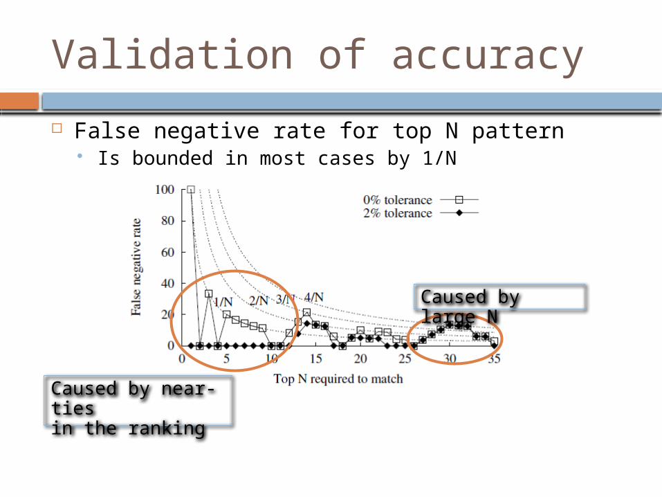
Validation of accuracy

False negative rate for top N pattern Is bounded in most cases by 1/N

Caused by large N

Caused by near-ties in the ranking

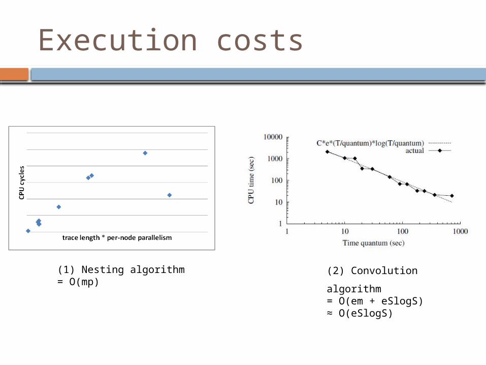
Execution costs

(1) Nesting algorithm= O(mp)

(2) Convolution algorithm= O(em + eSlogS)≈ O(eSlogS)

Conclusions

Looking for bottlenecks in black box sys-tems

Finding causal paths is enough to find bot-tlenecks

Algorithms to find paths in traces really work We find correct latency distributions Two very different algorithms get similar re-

sults Passively collected traces have sufficient in-

formation

THANK YOU!ANY QUESTION?

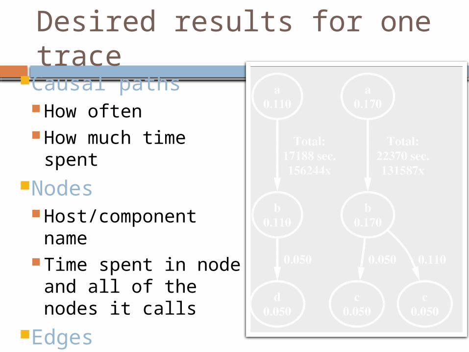
Desired results for one trace

Causal paths How often How much time

spentNodes

Host/component name

Time spent in node and all of the nodes it calls

Edges Time parent waits

before calling child

Related work

Systems that trace end-to-end causality via modified middleware using modified JVM or J2EE layers Magpie (Microsoft Research), aimed at per-

formance debugging Pinpoint (Stanford/Berkeley), aimed at locat-

ing faults Products such as AppAssure, PerformaSure,

OptiBenchSystems that make inferences from traces Intrusion detection (Zhang & Paxson, LBL)

uses traces + statistics to find compromised systems

Future work

Automate trace gathering and con-version

Sliding-window versions of algorithms Find phased behavior Reduce memory usage of nesting al-gorithm

Improve speed of convolution algo-rithm

Validate usefulness on more compli-cated systems

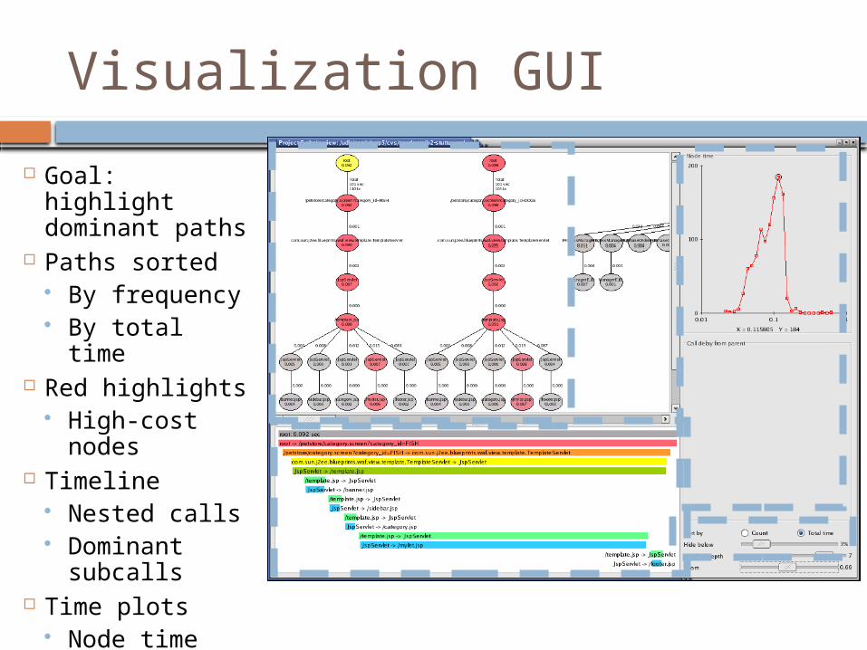
Visualization GUI

Goal: highlight dominant paths

Paths sorted By frequency By total time

Red highlights High-cost

nodes Timeline

Nested calls Dominant sub-

calls Time plots

Node time Call delay

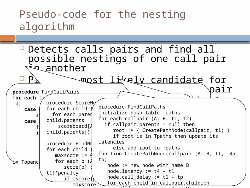
Pseudo-code for the nesting algorithm

Detects calls pairs and find all possible nestings of one call pair in another

Pick the most likely candidate for the caus-ing call for each call pair

Derive call paths from the causal relation-ships

procedure FindCallPairsfor each trace entry (t1, CALL/RET, sender A, receiver B, callid id) case CALL: store (t1,CALL,A,B,id) in Topencalls case RETURN: find matching entry (t2, CALL, B, A, id) in Topencalls if match is found then remove entry from Topencalls update entry with return message timestamp t2 add entry to Tcallpairs entry.parents := {all callpairs (t3, CALL, X, A, id2) in Topencalls with t3 < t2}

procedure ScoreNestingsfor each child (B, C, t2, t3) in Tcallpairs for each parent (A, B, t1, t4) in child.parents scoreboard[A, B, C, t2-t1] += (1/|child.parents|)

procedure FindNestedPairsfor each child (B; C; t2; t3) in call pairs maxscore := 0 for each p (A, B, t1, t4) in child.parents score[p] := scoreboard[A, B, C, t2-t1]*penalty if (score[p] > maxscore) then maxscore := score[p] parent := p parent.children := parent.children U {child}

procedure FindCallPathsinitialize hash table Tpathsfor each callpair (A, B, t1, t2) if callpair.parents = null then root := { CreatePathNode(callpair, t1) } if root is in Tpaths then update its latencies else add root to Tpathsfunction CreatePathNode(callpair (A, B, t1, t4), tp) node := new node with name B node.latency := t4 - t1 node.call_delay := t1 - tp for each child in callpair.children node.edges := node.edges U { CreatePathNode(child, t1)} return node