PERFORMANCE OPTIMIZATION OF SYMMETRIC FACTORIZATIONALGORITHMS

SILVIO TARCA

Abstract. Nonlinear optimization algorithms that use Newton’s method to determine the search directionexhibit quadratic convergence locally. In the predominant case where the Hessian is positive definite, Cholesky fac-torization is a computationally efficient algorithm for evaluating the Newton search direction −∇2f(x(k))−1∇f(x(k)).If the Hessian is indefinite, then modified Cholesky algorithms make use of symmetric indefinite factorization to per-turb the Hessian such that it is sufficiently positive definite and reasonably well-conditioned, while preserving asmuch as possible the information contained in the Hessian. This paper measures and compares the performance ofalgorithms implementing Cholesky factorization, symmetric indefinite factorization and modified Cholesky factoriza-tion. From these performance data we estimate the work (runtime) involved in symmetric pivoting and modifyingthe symmetric indefinite factorization. Furthermore, we evaluate the effect of the degree of indefiniteness of thesymmetric matrix on performance. For each of these matrix factorizations we developed routines that implementa variety of performance optimization techniques including loop reordering, blocking, and the use of tuned BasicLinear Algebra Subroutines.

1. Introduction. Nonlinear optimization algorithms generate a minimizing sequence of it-erates x(k), where x(k+1) = x(k) + t(k)∆x(k). The step length t(k) is positive, and the searchdirection ∆x(k) in a descent method must satisfy ∇f(x(k))T∆x(k) < 0. The sequence of iter-ates x(k) terminates when an optimal point with sufficient accuracy has been found. In movingfrom one iterate to the next, nonlinear optimization algorithms determine a search direction ∆x(k)

and choose a step length t(k). A natural choice for the search direction is the negative gradient,∆x(k) = −∇f(x(k)). The gradient descent method moves in the direction −∇f(x(k)) at every step,which provides a computational advantage since it only requires calculation of the gradient. Ittypically exhibits linear convergence, but can be very slow, even for problems where the Hessianis moderately well-conditioned. By comparison, the Newton method, with search direction givenby ∆x(k) = −∇2f(x(k))−1∇f(x(k)), exhibits quadratic convergence locally [5]. When the Hessian∇2f(x(k)) is positive definite, the Newton direction is guaranteed to be a descent direction; when theHessian is indefinite, the Newton direction may not exist or satisfy the downhill condition. In thelatter case, nonlinear optimization algorithms modify the Hessian to be sufficiently positive definiteand reasonably well-conditioned, while preserving as much as possible the information contained inthe Hessian.

Rearranging the equation for the Newton direction and introducing conventional linear algebranotation, we have Ax = ∇2f(x(k))∆x(k) = −∇f(x(k)) = b. In the predominant case in whichthe Hessian, A = ∇2f(x(k)), is positive definite, nonlinear optimization algorithms make use ofCholesky factorization to efficiently solve for the Newton direction. Cholesky algorithms factors Aby computing the unique lower triangular matrix L with positive diagonal entries, where A = LLT .Given Ax = LLTx = b, the Newton direction is then determined by solving the triangular systemsof equations Ly = b and LTx = y. Cholesky factorization involves 1

3n3 + O(n2) floating point

operations (flops), while solving for the Newton direction adds O(n2) flops to the computation.

If the Hessian is indefinite, nonlinear optimization algorithms make use of modified Choleskyfactorization to efficiently modify the Hessian and solve for the Newton direction. Modified Choleskyalgorithms make use of symmetric indefinite factorization to find a matrix A = A + E, whereA is sufficiently positive definite, so that the Newton direction satisfies the downhill condition.Symmetric indefinite factorization takes the form PAPT = LDLT , where D is diagonal or blockdiagonal, L is unit lower triangular, and P is a permutation matrix for symmetric pivoting. We

1

consider two approaches to modified Cholesky factorization: the method proposed by Gill, Murrayand Wright [14], where D is diagonal, and A is modified as the factorization proceeds; and the

one proposed by Cheng and Higham [8], where D is block diagonal with block order 1 or 2, and Ais found by modifying a computed factorization of A. For both approaches the cost of modifyingthe factorization is a small multiple of n2 flops. For symmetric indefinite factorization, numericalstability comes at the expense of pivoting. Partial pivoting makes only O(n2) comparisons ofmatrix elements but has the worst accuracy; complete pivoting involves O(n3) comparisons; androok pivoting involves between O(n2) and O(n3) comparisons. The Gill-Murray-Wright algorithmuses a form of partial pivoting, while our implementation of the Cheng-Higham algorithm employseither Bunch-Kaufman [6] (partial) or bounded Bunch-Kaufman [2] (rook) pivoting. Given theseestimates of the work (flops) involved in computing a modified Cholesky factorization, we anticipatethat much of the variation in performance between modified Cholesky algorithms will be explainedby the pivoting strategy employed.

This paper measures and compares the performance of algorithms implementing Cholesky fac-torization, symmetric indefinite factorization, and modified Cholesky factorization (Gill-Murray-Wright and Cheng-Higham algorithms). From these performance data we estimate the work (run-time) involved in symmetric pivoting and modifying the symmetric indefinite factorization. Ad-ditionally, for symmetric indefinite and modified Cholesky factorizations, we evaluate the effect ofthe degree of indefiniteness of the symmetric matrix on performance. For each of these matrixfactorizations we implement a variety of performance optimization (tuning) techniques includingloop reordering, blocking, and the use of tuned BLAS (Basic Linear Algebra Subroutines). By com-paring the performance of these algorithms with a benchmark, the corresponding LAPACK (LinearAlgebra PACKage) routine, this paper assesses the efficacy of various performance optimizationtechniques.

Section 2 lists the software developed for this research, and provides technical specificationsfor hardware, compilers and libraries. Section 3 introduces performance optimization techniquessuch as loop reordering and blocking to maximize data locality, and describes the use of efficientlibraries including tuned BLAS and LAPACK. Matrix multiplication is used to demonstrate theseperformance optimization concepts. Unblocked and blocked algorithms for Cholesky factorizationare explained in Section 4. We measure the performance of our implementation of basic and“optimized” algorithms for Cholesky factorization and compare it with that of the correspondingLAPACK routine to assess their efficiency. Section 5 outlines Bunch-Kaufman (partial), boundedBunch-Kaufman (rook) and Bunch-Parlett [7] (complete) pivoting strategies, and discusses un-blocked and blocked algorithms for symmetric indefinite factorization. In addition to measuringthe performance of our implementation of these algorithms, we also evaluate the effect of pivot-ing strategy employed and the degree of indefiniteness of the symmetric matrix on performance.Section 6 builds on the discussion of standard Cholesky and symmetric indefinite factorizationsto explain the Gill-Murray-Wright and Cheng-Higham algorithms for modified Cholesky factoriza-tion. Again, we measure the performance of our implementation of basic and optimized versions ofthese algorithms, and compare the work (runtime) involved in modifying the symmetric indefinitefactorization with the work to perform symmetric pivoting. Finally, Section 7 introduces paral-lel programming using the MPI (Message-Passing Interface) library, and demonstrates concepts ofspeedup and efficiency using Fox’s algorithm for parallel matrix multiplication. This paper focuseson performance optimization of serial algorithms implementing matrix factorizations, so an obviousextension to this research would develop parallel algorithms for these matrix factorizations andmeasure their performance.

2

2. Hardware and Software. Timing experiments to measure the performance of algorithmsanalyzed in this research were conducted primarily on an Intel Xeon 5345 processor, 2.33 GHz, with4 dual-cores, each dual-core sharing 4096 KB of cache. The operating system is Red Hat Linuxrelease 5.1 running kernel 2.6.18.-128.7.1.el5 lustre.1.8.1.1 on CPU architecture x86 64.Software is coded in the C programming language [18], and compiled using Intel C compiler version11.1.046 with -O3 optimization level. Installed on this machine is Intel MKL version 10.2.2, whichis compliant with LAPACK release 3.1. Parallel programming is implemented using MPI libraryfunctions, MVAPICH version 1.1.0. Unless explicitly stated otherwise, performance data presentedin this paper are for routines executed on this machine, and references to BLAS and LAPACK inthe context of this machine should be read as Intel MKL implementations of BLAS and LAPACKlibraries. Timing experiments (jobs) were submitted using a portable batch system script.

In order to provide a comparison of performance across hardware, compilers and libraries, sometiming experiments were also conducted on an alternative machine — AMD Opteron 180, 2.4 GHz,dual-core with 1024 KB of L2 cache per core. The operating system is Red Hat Linux release5.4 running kernel 2.6.18-194.3.1.el5 on CPU architecture x86 64. Programs are compiledusing GNU C compiler version 4.1.2 with -O3 optimization level. Installed on this machine areATLAS (Automatically Tuned Linear Algebra Software) versions of LAPACK and BLAS routines(atlas.x86 64 3.6.0-15.el5). References to BLAS and LAPACK in the context of this machineshould be read as ATLAS implementations of BLAS and LAPACK libraries.

Source code developed for matrix factorization and matrix multiplication algorithms includes:

lufact.c Gaussian elimination (LU factorization)1

cholfact.c Cholesky factorizationldltfact.c symmetric indefinite factorization with Bunch-Kaufman, bounded Bunch-Kaufman

and Bunch-Parlett pivotingmodchol.c modified Cholesky algorithms (Gill-Murray-Wright and Cheng-Higham)matmult.c matrix multiplicationmatmultp.c parallel matrix multiplication

All matrix computations are performed using double-precision arithmetic.

To ensure that algorithms coded for this research perform matrix computations accurately,testing harnesses were developed for matrix factorization (mfactest.c) and serial and parallelmatrix multiplication (mmultest.c and mmultstp.c, respectively). Then to measure the perfor-mance of, and profile these algorithms, timing harnesses were developed for matrix factorization(mfactime.c) and serial and parallel matrix multiplication (mmultime.c and mmultmp.c, respec-tively). Timing harnesses write performance data to an output file. Common matrix operations arecoded in matcom.c, and timing functions used for measuring performance and profiling are codedin timing.c.

The source code, header files and Makefiles [21, 23] developed for this research are listedin the appendix, a separate document (perf optm sym factor appx.pdf) that accompanies thisarticle. These documents, along with a tar archive file containing the source code, header files andMakefiles, are posted on the web pages http://www.cs.cornell.edu/~bindel/students.html

and http://www.cs.nyu.edu/overton/msadvising.html.

1Although not discussed in this paper, LU factorization routines were developed as part of the research effort. LUfactorization is normally used to introduce the concepts of matrix factorization and pivoting before one progressesto standard Cholesky factorization, symmetric indefinite factorization and modified Cholesky factorization.

3

3. Performance Optimization Guidelines. In optimizing the performance of matrix fac-torization code we consider: data locality; the use of efficient libraries; and compiler optimizationlevels. The goal in high performance computing is to keep the functional units of the central pro-cessing unit (CPU), which perform computations on input data, running at their peak capacity.Since moving data between levels of the memory hierarchy to the CPU (memory access) is themajor performance bottleneck, high performance is achieved through data locality. At the top ofa typical memory hierarchy are the registers of the CPU, followed by two levels of cache, thenmain memory, and finally disk storage. As one proceeds down the memory hierarchy, memory sizeincreases but so does access time (latency) of the CPU to data in memory. To provide some ordersof magnitude, approximate access times range from immediate for registers, one clock cycle for L1cache, ten cycles for L2 cache and as many as one-hundred cycles for main memory [15].

There are two basic types of data locality: temporal and spatial. Temporal data locality meansthat if data stored in some memory location is referenced, then it likely will be referenced again in thenear future. Spatial data locality means that if data stored in some memory location is referenced,then it is likely that data stored in nearby memory locations will be referenced in the near future.Efficient algorithms for matrix factorizations, the primary concern of this paper, employ memoryaccess optimization techniques including loop reordering and blocking to maximize data locality. Ingeneral, blocked factorization algorithms iteratively factor a diagonal block, then solve a triangularsystem of equations to yield a column block of a lower triangular matrix or a row block of anupper triangular matrix, and finally update the trailing sub-matrix. Blocked algorithms for matrixfactorization spend the bulk of their time updating the trailing sub-matrix, which is essentiallya matrix multiplication operation. Therefore, we begin by demonstrating the maximization ofdata locality on matrix multiplication, and measuring the performance gains attributable to loopreordering and blocking. The observations we make will inform the performance optimization ofmatrix factorizations discussed in the subsequent sections of this paper.

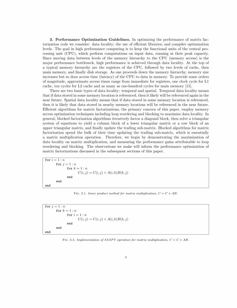
for i = 1 : nfor j = 1 : n

for k = 1 : nC(i, j) = C(i, j) +A(i, k)B(k, j)

end

end

end

Fig. 3.1. Inner product method for matrix multiplication, C = C + AB.

for j = 1 : nfor k = 1 : n

for i = 1 : nC(i, j) = C(i, j) +A(i, k)B(k, j)

end

end

end

Fig. 3.2. Implementation of SAXPY operation for matrix multiplication, C = C + AB.

4

for j = 1 : n : rfor k = 1 : n : r

for i = 1 : n : rC(i : i+r− 1, j :j+r− 1) = C(i : i+r− 1, j :j+r− 1) +

A(i : i+r− 1, k :k+r− 1)B(k :k+r− 1, j :j+r− 1)end

end

end

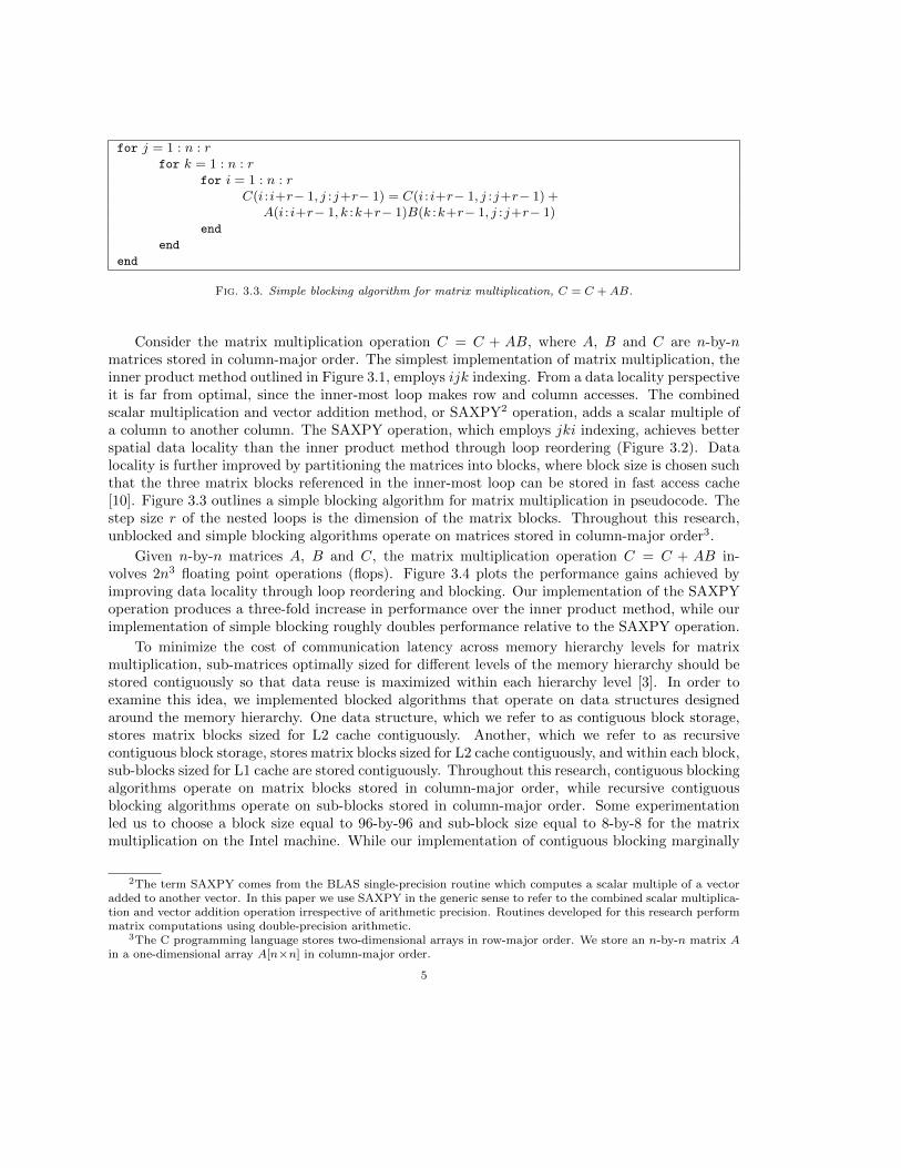
Fig. 3.3. Simple blocking algorithm for matrix multiplication, C = C + AB.

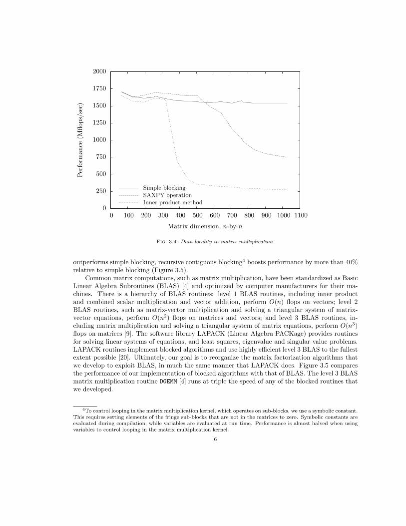
Consider the matrix multiplication operation C = C + AB, where A, B and C are n-by-nmatrices stored in column-major order. The simplest implementation of matrix multiplication, theinner product method outlined in Figure 3.1, employs ijk indexing. From a data locality perspectiveit is far from optimal, since the inner-most loop makes row and column accesses. The combinedscalar multiplication and vector addition method, or SAXPY2 operation, adds a scalar multiple ofa column to another column. The SAXPY operation, which employs jki indexing, achieves betterspatial data locality than the inner product method through loop reordering (Figure 3.2). Datalocality is further improved by partitioning the matrices into blocks, where block size is chosen suchthat the three matrix blocks referenced in the inner-most loop can be stored in fast access cache[10]. Figure 3.3 outlines a simple blocking algorithm for matrix multiplication in pseudocode. Thestep size r of the nested loops is the dimension of the matrix blocks. Throughout this research,unblocked and simple blocking algorithms operate on matrices stored in column-major order3.

Given n-by-n matrices A, B and C, the matrix multiplication operation C = C + AB in-volves 2n3 floating point operations (flops). Figure 3.4 plots the performance gains achieved byimproving data locality through loop reordering and blocking. Our implementation of the SAXPYoperation produces a three-fold increase in performance over the inner product method, while ourimplementation of simple blocking roughly doubles performance relative to the SAXPY operation.

To minimize the cost of communication latency across memory hierarchy levels for matrixmultiplication, sub-matrices optimally sized for different levels of the memory hierarchy should bestored contiguously so that data reuse is maximized within each hierarchy level [3]. In order toexamine this idea, we implemented blocked algorithms that operate on data structures designedaround the memory hierarchy. One data structure, which we refer to as contiguous block storage,stores matrix blocks sized for L2 cache contiguously. Another, which we refer to as recursivecontiguous block storage, stores matrix blocks sized for L2 cache contiguously, and within each block,sub-blocks sized for L1 cache are stored contiguously. Throughout this research, contiguous blockingalgorithms operate on matrix blocks stored in column-major order, while recursive contiguousblocking algorithms operate on sub-blocks stored in column-major order. Some experimentationled us to choose a block size equal to 96-by-96 and sub-block size equal to 8-by-8 for the matrixmultiplication on the Intel machine. While our implementation of contiguous blocking marginally

2The term SAXPY comes from the BLAS single-precision routine which computes a scalar multiple of a vectoradded to another vector. In this paper we use SAXPY in the generic sense to refer to the combined scalar multiplica-tion and vector addition operation irrespective of arithmetic precision. Routines developed for this research performmatrix computations using double-precision arithmetic.

3The C programming language stores two-dimensional arrays in row-major order. We store an n-by-n matrix Ain a one-dimensional array A[n×n] in column-major order.

5

0

250

500

750

1000

1250

1500

1750

2000

0 100 200 300 400 500 600 700 800 900 1000 1100

Per

form

ance

(Mfl

ops/

sec)

Matrix dimension, n-by-n

Simple blockingSAXPY operationInner product method

Fig. 3.4. Data locality in matrix multiplication.

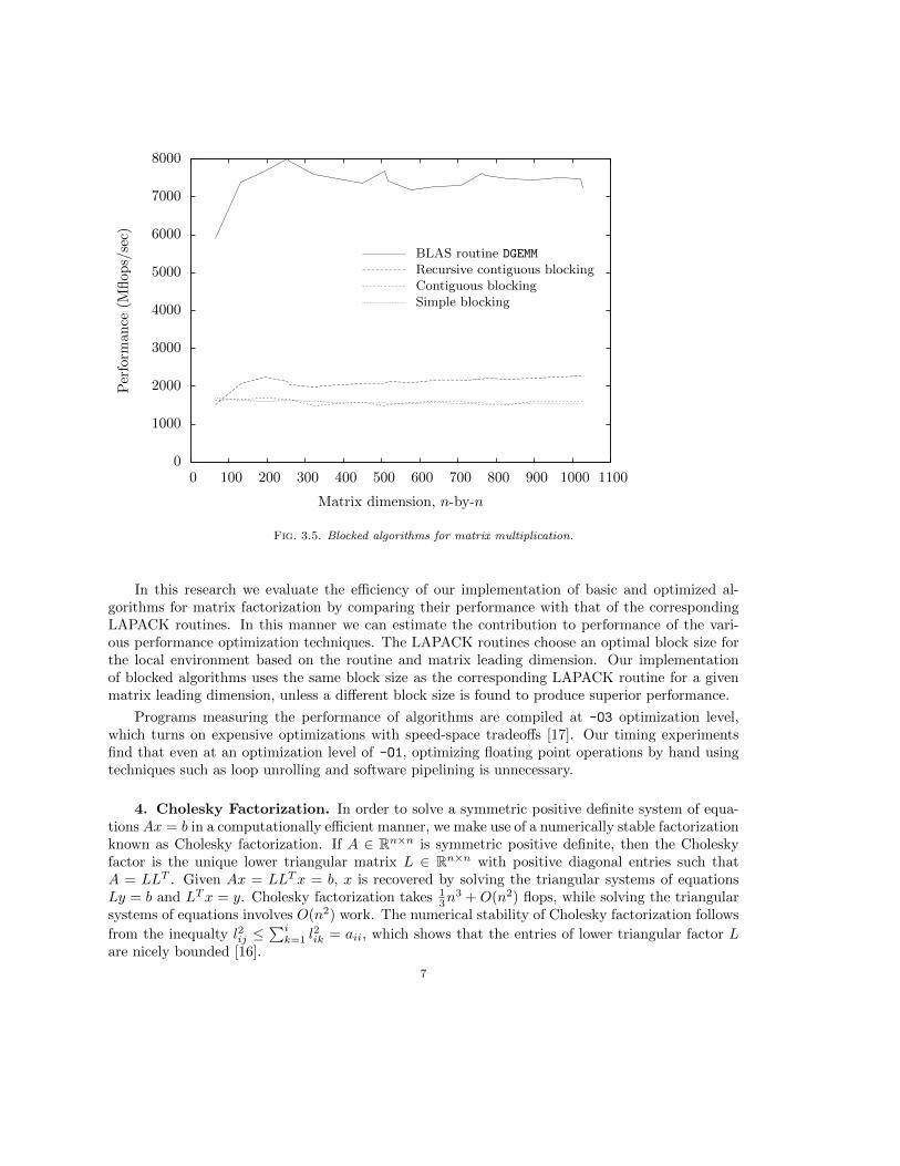
outperforms simple blocking, recursive contiguous blocking4 boosts performance by more than 40%relative to simple blocking (Figure 3.5).

Common matrix computations, such as matrix multiplication, have been standardized as BasicLinear Algebra Subroutines (BLAS) [4] and optimized by computer manufacturers for their ma-chines. There is a hierarchy of BLAS routines: level 1 BLAS routines, including inner productand combined scalar multiplication and vector addition, perform O(n) flops on vectors; level 2BLAS routines, such as matrix-vector multiplication and solving a triangular system of matrix-vector equations, perform O(n2) flops on matrices and vectors; and level 3 BLAS routines, in-cluding matrix multiplication and solving a triangular system of matrix equations, perform O(n3)flops on matrices [9]. The software library LAPACK (Linear Algebra PACKage) provides routinesfor solving linear systems of equations, and least squares, eigenvalue and singular value problems.LAPACK routines implement blocked algorithms and use highly efficient level 3 BLAS to the fullestextent possible [20]. Ultimately, our goal is to reorganize the matrix factorization algorithms thatwe develop to exploit BLAS, in much the same manner that LAPACK does. Figure 3.5 comparesthe performance of our implementation of blocked algorithms with that of BLAS. The level 3 BLASmatrix multiplication routine DGEMM [4] runs at triple the speed of any of the blocked routines thatwe developed.

4To control looping in the matrix multiplication kernel, which operates on sub-blocks, we use a symbolic constant.This requires setting elements of the fringe sub-blocks that are not in the matrices to zero. Symbolic constants areevaluated during compilation, while variables are evaluated at run time. Performance is almost halved when usingvariables to control looping in the matrix multiplication kernel.

6

0

1000

2000

3000

4000

5000

6000

7000

8000

0 100 200 300 400 500 600 700 800 900 1000 1100

Per

form

ance

(Mfl

ops/

sec)

Matrix dimension, n-by-n

BLAS routine DGEMM

Recursive contiguous blockingContiguous blockingSimple blocking

Fig. 3.5. Blocked algorithms for matrix multiplication.

In this research we evaluate the efficiency of our implementation of basic and optimized al-gorithms for matrix factorization by comparing their performance with that of the correspondingLAPACK routines. In this manner we can estimate the contribution to performance of the vari-ous performance optimization techniques. The LAPACK routines choose an optimal block size forthe local environment based on the routine and matrix leading dimension. Our implementationof blocked algorithms uses the same block size as the corresponding LAPACK routine for a givenmatrix leading dimension, unless a different block size is found to produce superior performance.

Programs measuring the performance of algorithms are compiled at -O3 optimization level,which turns on expensive optimizations with speed-space tradeoffs [17]. Our timing experimentsfind that even at an optimization level of -O1, optimizing floating point operations by hand usingtechniques such as loop unrolling and software pipelining is unnecessary.

4. Cholesky Factorization. In order to solve a symmetric positive definite system of equa-tions Ax = b in a computationally efficient manner, we make use of a numerically stable factorizationknown as Cholesky factorization. If A ∈ Rn×n is symmetric positive definite, then the Choleskyfactor is the unique lower triangular matrix L ∈ Rn×n with positive diagonal entries such thatA = LLT . Given Ax = LLTx = b, x is recovered by solving the triangular systems of equationsLy = b and LTx = y. Cholesky factorization takes 1

3n3 +O(n2) flops, while solving the triangular

systems of equations involves O(n2) work. The numerical stability of Cholesky factorization follows

from the inequalty l2ij ≤∑ik=1 l

2ik = aii, which shows that the entries of lower triangular factor L

are nicely bounded [16].

7

For this research, we implemented a number of Cholesky factorization algorithms employing avariety of performance optimization techniques. In the interests of clarity and brevity we identifyeach algorithm by its function name from the source code listings in the appendix when it isintroduced in the discussion. Thereafter, we reference the algorithm by its function name.

for k = 1 : n

A(k, k) =√A(k, k)

for i = k + 1 : nA(i, k) = A(i, k)/A(k, k)

end

for j = k + 1 : nfor i = j : n

A(i, j) = A(i, j)−A(i, k) ∗A(j, k)end

end

end

Fig. 4.1. Outer product method for Cholesky factorization.

for j = 1 : nfor k = 1 : j − 1

for i = j : nA(i, j) = A(i, j)−A(i, k) ∗A(j, k)

end

end

A(j, j) =√A(j, j)

for i = j + 1 : nA(i, j) = A(i, j)/A(j, j)

end

end

Fig. 4.2. Implementation of SAXPY operation for Cholesky factorization.

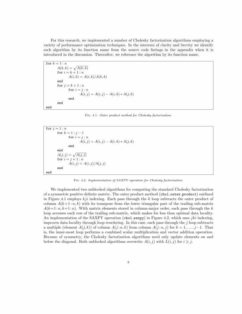
We implemented two unblocked algorithms for computing the standard Cholesky factorizationof a symmetric positive definite matrix. The outer product method (chol outer product) outlinedin Figure 4.1 employs kji indexing. Each pass through the k loop subtracts the outer product ofcolumn A(k+1 : n, k) with its transpose from the lower triangular part of the trailing sub-matrixA(k+1:n, k+1:n). With matrix elements stored in column-major order, each pass through the kloop accesses each row of the trailing sub-matrix, which makes for less than optimal data locality.An implementation of the SAXPY operation (chol saxpy) in Figure 4.2, which uses jki indexing,improves data locality through loop reordering. In this case, each pass through the j loop subtractsa multiple (element A(j, k)) of column A(j :n, k) from column A(j :n, j) for k = 1, . . . , j−1. Thatis, the inner-most loop performs a combined scalar multiplication and vector addition operation.Because of symmetry, the Cholesky factorization algorithms need only update elements on andbelow the diagonal. Both unblocked algorithms overwrite A(i, j) with L(i, j) for i ≥ j.

8

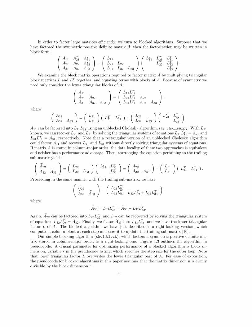
In order to factor large matrices efficiently, we turn to blocked algorithms. Suppose that wehave factored the symmetric positive definite matrix A; then the factorization may be written inblock form: A11 AT21 AT31

A21 A22 AT32A31 A32 A33

=

L11

L21 L22

L31 L32 L33

LT11 LT21 LT31LT22 LT32

LT33

.

We examine the block matrix operations required to factor matrix A by multiplying triangularblock matrices L and LT together, and equating terms with blocks of A. Because of symmetry weneed only consider the lower triangular blocks of A. A11

A21 A22

A31 A32 A33

=

L11LT11

L21LT11 A22

L31LT11 A32 A33

,

where (A22

A32 A33

)=

(L21

L31

)(LT21 LT31

)+

(L22

L32 L33

)(LT22 LT32

LT33

).

A11 can be factored into L11LT11 using an unblocked Cholesky algorithm, say, chol saxpy. With L11

known, we can recover L21 and L31 by solving the triangular systems of equations L21LT11 = A21 and

L31LT11 = A31, respectively. Note that a rectangular version of an unblocked Cholesky algorithm

could factor A11 and recover L21 and L31 without directly solving triangular systems of equations.If matrix A is stored in column-major order, the data locality of these two approaches is equivalentand neither has a performance advantage. Then, rearranging the equation pertaining to the trailingsub-matrix yields(

A22

A32 A33

)=

(L22

L32 L33

)(LT22 LT32

LT33

)=

(A22

A32 A33

)−(L21

L31

)(LT21 LT31

).

Proceeding in the same manner with the trailing sub-matrix, we have(A22

A32 A33

)=

(L22L

T22

L32LT22 L32L

T32 + L33L

T33

),

where

A33 = L33LT33 = A33 − L32L

T32.

Again, A22 can be factored into L22LT22, and L32 can be recovered by solving the triangular system

of equations L32LT22 = A32. Finally, we factor A33 into L33L

T33, and we have the lower triangular

factor L of A. The blocked algorithm we have just described is a right-looking version, whichcomputes a column block at each step and uses it to update the trailing sub-matrix [10].

Our simple blocking algorithm (chol block), which factors a symmetric positive definite ma-trix stored in column-major order, is a right-looking one. Figure 4.3 outlines the algorithm inpseudocode. A crucial parameter for optimizing performance of a blocked algorithm is block di-mension, variable r in the pseudocode listing, which specifies the step size for the outer loop. Notethat lower triangular factor L overwrites the lower triangular part of A. For ease of exposition,the pseudocode for blocked algorithms in this paper assumes that the matrix dimension n is evenlydivisible by the block dimension r.

9

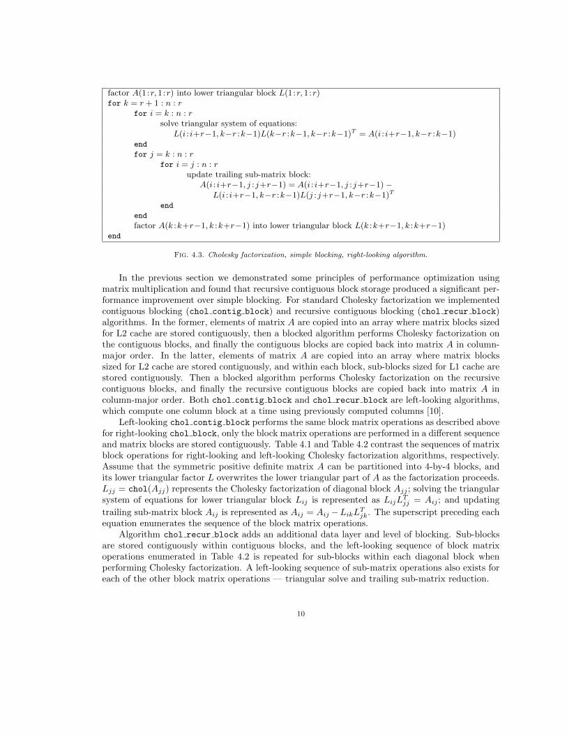
factor A(1 :r, 1:r) into lower triangular block L(1 :r, 1:r)for k = r + 1 : n : r

for i = k : n : rsolve triangular system of equations:

L(i : i+r−1, k−r :k−1)L(k−r :k−1, k−r :k−1)T = A(i : i+r−1, k−r :k−1)end

for j = k : n : rfor i = j : n : r

update trailing sub-matrix block:A(i : i+r−1, j :j+r−1) = A(i : i+r−1, j :j+r−1)−

L(i : i+r−1, k−r :k−1)L(j :j+r−1, k−r :k−1)Tend

end

factor A(k :k+r−1, k :k+r−1) into lower triangular block L(k :k+r−1, k :k+r−1)end

Fig. 4.3. Cholesky factorization, simple blocking, right-looking algorithm.

In the previous section we demonstrated some principles of performance optimization usingmatrix multiplication and found that recursive contiguous block storage produced a significant per-formance improvement over simple blocking. For standard Cholesky factorization we implementedcontiguous blocking (chol contig block) and recursive contiguous blocking (chol recur block)algorithms. In the former, elements of matrix A are copied into an array where matrix blocks sizedfor L2 cache are stored contiguously, then a blocked algorithm performs Cholesky factorization onthe contiguous blocks, and finally the contiguous blocks are copied back into matrix A in column-major order. In the latter, elements of matrix A are copied into an array where matrix blockssized for L2 cache are stored contiguously, and within each block, sub-blocks sized for L1 cache arestored contiguously. Then a blocked algorithm performs Cholesky factorization on the recursivecontiguous blocks, and finally the recursive contiguous blocks are copied back into matrix A incolumn-major order. Both chol contig block and chol recur block are left-looking algorithms,which compute one column block at a time using previously computed columns [10].

Left-looking chol contig block performs the same block matrix operations as described abovefor right-looking chol block, only the block matrix operations are performed in a different sequenceand matrix blocks are stored contiguously. Table 4.1 and Table 4.2 contrast the sequences of matrixblock operations for right-looking and left-looking Cholesky factorization algorithms, respectively.Assume that the symmetric positive definite matrix A can be partitioned into 4-by-4 blocks, andits lower triangular factor L overwrites the lower triangular part of A as the factorization proceeds.Ljj = chol(Ajj) represents the Cholesky factorization of diagonal block Ajj ; solving the triangularsystem of equations for lower triangular block Lij is represented as LijL

Tjj = Aij ; and updating

trailing sub-matrix block Aij is represented as Aij = Aij −LikLTjk. The superscript preceding eachequation enumerates the sequence of the block matrix operations.

Algorithm chol recur block adds an additional data layer and level of blocking. Sub-blocksare stored contiguously within contiguous blocks, and the left-looking sequence of block matrixoperations enumerated in Table 4.2 is repeated for sub-blocks within each diagonal block whenperforming Cholesky factorization. A left-looking sequence of sub-matrix operations also exists foreach of the other block matrix operations — triangular solve and trailing sub-matrix reduction.

10

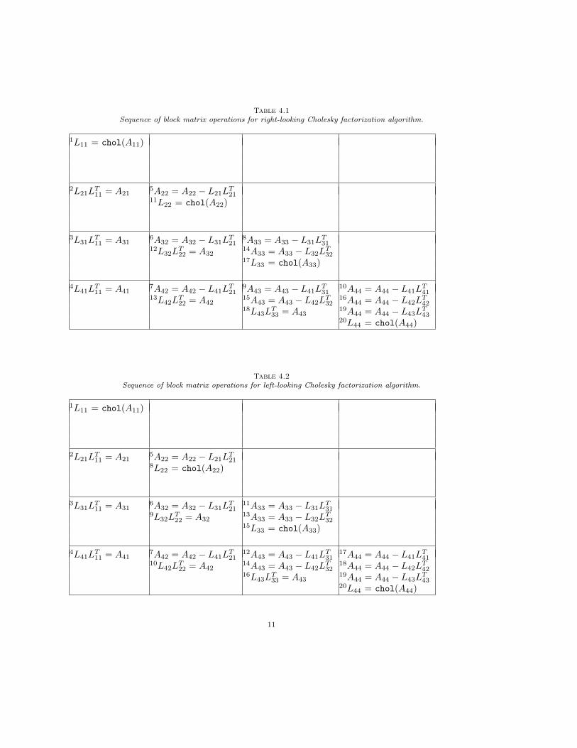
Table 4.1Sequence of block matrix operations for right-looking Cholesky factorization algorithm.

1L11 = chol(A11)

2L21LT11 = A21

5A22 = A22 − L21LT21

11L22 = chol(A22)

3L31LT11 = A31

6A32 = A32 − L31LT21

8A33 = A33 − L31LT31

12L32LT22 = A32

14A33 = A33 − L32LT32

17L33 = chol(A33)

4L41LT11 = A41

7A42 = A42 − L41LT21

9A43 = A43 − L41LT31

10A44 = A44 − L41LT41

13L42LT22 = A42

15A43 = A43 − L42LT32

16A44 = A44 − L42LT42

18L43LT33 = A43

19A44 = A44 − L43LT43

20L44 = chol(A44)

Table 4.2Sequence of block matrix operations for left-looking Cholesky factorization algorithm.

1L11 = chol(A11)

2L21LT11 = A21

5A22 = A22 − L21LT21

8L22 = chol(A22)

3L31LT11 = A31

6A32 = A32 − L31LT21

11A33 = A33 − L31LT31

9L32LT22 = A32

13A33 = A33 − L32LT32

15L33 = chol(A33)

4L41LT11 = A41

7A42 = A42 − L41LT21

12A43 = A43 − L41LT31

17A44 = A44 − L41LT41

10L42LT22 = A42

14A43 = A43 − L42LT32

18A44 = A44 − L42LT42

16L43LT33 = A43

19A44 = A44 − L43LT43

20L44 = chol(A44)

11

32

64

96

128

192

256

320

384

0 200 400 600 800 1000 1200 1400 1600 1800 2000 2200

Blo

ckd

imen

sion

Matrix dimension, n-by-n

Fig. 4.4. Blocking parameter for Cholesky factorization.

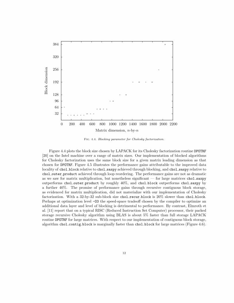
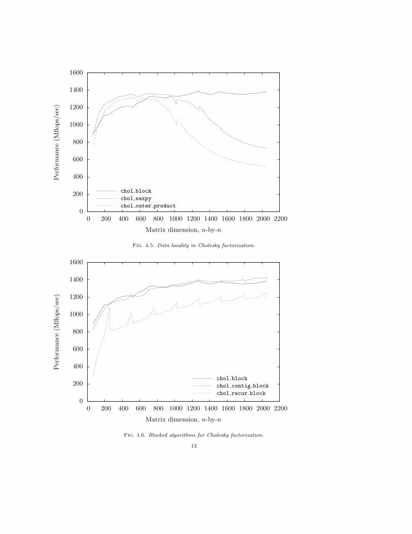
Figure 4.4 plots the block size chosen by LAPACK for its Cholesky factorization routine DPOTRF[20] on the Intel machine over a range of matrix sizes. Our implementation of blocked algorithmsfor Cholesky factorization uses the same block size for a given matrix leading dimension as thatchosen for DPOTRF. Figure 4.5 illustrates the performance gains attributable to the improved datalocality of chol block relative to chol saxpy achieved through blocking, and chol saxpy relative tochol outer product achieved through loop reordering. The performance gains are not as dramaticas we saw for matrix multiplication, but nonetheless significant — for large matrices chol saxpy

outperforms chol outer product by roughly 40%, and chol block outperforms chol saxpy bya further 40%. The promise of performance gains through recursive contiguous block storage,as evidenced for matrix multiplication, did not materialize with our implementation of Choleskyfactorization. With a 32-by-32 sub-block size chol recur block is 20% slower than chol block.Perhaps at optimization level -O3 the speed-space tradeoff chosen by the compiler to optimize anadditional data layer and level of blocking is detrimental to performance. By contrast, Elmroth etal. [11] report that on a typical RISC (Reduced Instruction Set Computer) processor, their packedstorage recursive Cholesky algorithm using BLAS is about 5% faster than full storage LAPACKroutine DPOTRF for large matrices. With respect to our implementation of contiguous block storage,algorithm chol contig block is marginally faster than chol block for large matrices (Figure 4.6).

12

0

200

400

600

800

1000

1200

1400

1600

0 200 400 600 800 1000 1200 1400 1600 1800 2000 2200

Per

form

an

ce(M

flops/

sec)

Matrix dimension, n-by-n

chol block

chol saxpy

chol outer product

Fig. 4.5. Data locality in Cholesky factorization.

0

200

400

600

800

1000

1200

1400

1600

0 200 400 600 800 1000 1200 1400 1600 1800 2000 2200

Per

form

ance

(Mfl

ops/

sec)

Matrix dimension, n-by-n

chol block

chol contig block

chol recur block

Fig. 4.6. Blocked algorithms for Cholesky factorization.

13

0

1000

2000

3000

4000

5000

6000

7000

0 200 400 600 800 1000 1200 1400 1600 1800 2000 2200

Per

form

ance

(Mfl

ops/

sec)

Matrix dimension, n-by-n

LAPACK routine DPOTRF

chol block blas

chol block

Fig. 4.7. Cholesky factorization using BLAS and LAPACK libraries.

0

1000

2000

3000

4000

5000

6000

7000

0 200 400 600 800 1000 1200 1400 1600 1800 2000 2200

Per

form

an

ce(M

flop

s/se

c)

Matrix dimension, n-by-n

Intel Xeon 5345, icc, MKLAMD Opteron 180, gcc, ATLAS

Fig. 4.8. Performance variability across hardware, compilers and libraries.

14

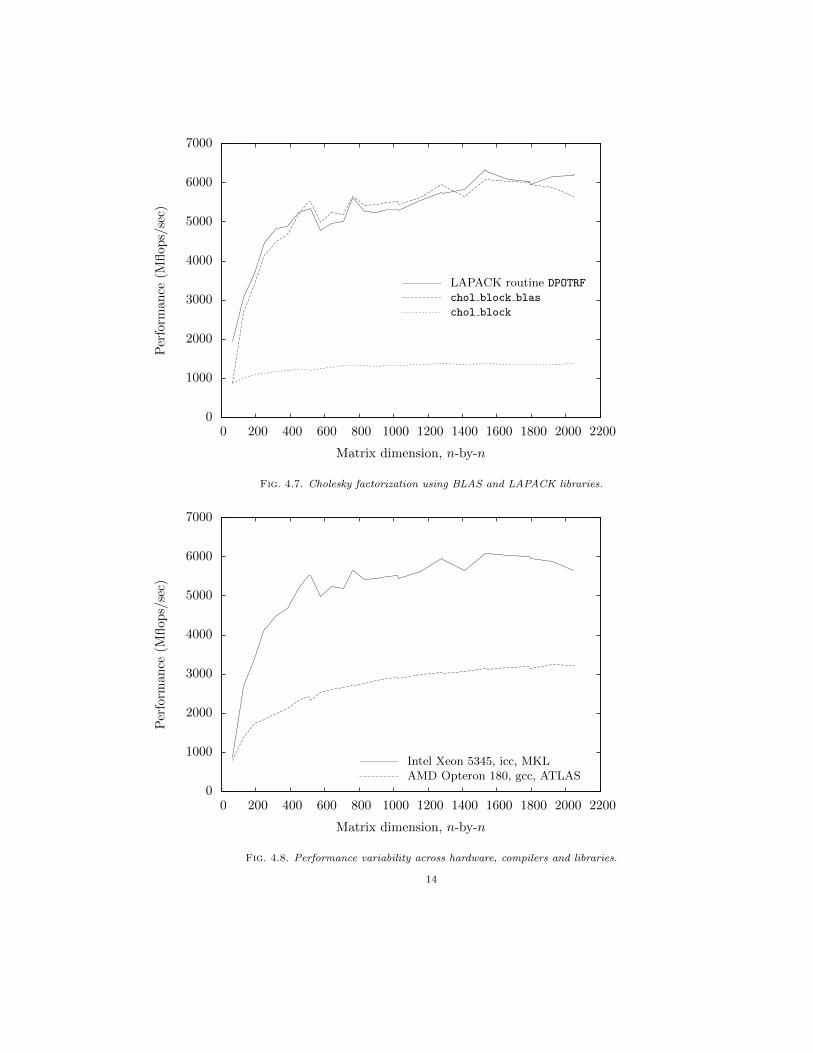
Our implementation of blocked algorithms achieves less than one-quarter of the flop rate at-tained by LAPACK routine DPOTRF, which is a right-looking blocked algorithm. Profile data forchol block factoring 2000-by-2000 symmetric positive definite matrices reveal that the algorithmspends approximately 98% of its time performing block triangular solves (18%) and trailing sub-matrix reductions (80%). If we were to use chol saxpy to perform Cholesky factorization ondiagonal blocks, but call BLAS routines DTRSM and DSYRK [4], respectively, to perform block tri-angular solves and trailing sub-matrix reductions, we would expect a substantial performanceboost. We identify this blocked algorithm as chol block blas. Indeed, Figure 4.7 shows thatchol block blas performs in line with LAPACK routine DPOTRF. The time to factor diagonal blocksis the same for chol block and chol block blas — both algorithms invoke chol saxpy — butlevel 3 BLAS routines DTRSM and DSYRK perform block triangular solves and trailing sub-matrix re-ductions much more efficiently. As a consequence the proportion of time spent by chol block blas

on factoring diagonal blocks rises to 8% and the overall time to perform Cholesky factorization iscut by more than 75%.

Finally, in Figure 4.8 we use chol block blas to demonstrate the variability in performanceacross hardware, compilers and libraries.

5. Symmetric Indefinite Factorization. To solve an n-by-n symmetric, possibly indefinite,system of equations Ax = b in a computationally efficient and numerically stable manner, we makeuse of the factorization PAPT = LDLT , where A ∈ Rn×n is symmetric, L ∈ Rn×n is unit lowertriangular, D is block diagonal with block order 1 or 2, and P ∈ Rn×n is a permutation matrixfor pivoting. Given Ax = PT (LDLT )Px = b, x is recovered by solving the triangular systems ofequations Lw = Pb, Dz = w, LT y = z and Px = y. Although the cost of symmetric indefinitefactorization depends on the pivoting strategy chosen, a lower bound is provided by Choleskyfactorization, which takes 1

3n3 + O(n2) flops. Solving the triangular systems of equations involves

O(n2) work [16].

α = (1 +√17)/8

λ = |ar1| = max{|a21|, . . . , |am1|}if λ > 0

if |a11| ≥ αλuse a11 as 1-by-1 pivot

else

σ = |apr| = max{|a1r|, . . . , |ar−1,r|, |ar+1,r|, . . . , |amr|}if |a11|σ ≥ αλ2

use a11 as 1-by-1 pivotelse if |arr| ≥ ασ

use arr as 1-by-1 pivotelse

use

[a11 ar1ar1 arr

]as 2-by-2 pivot

end

end

end

Fig. 5.1. Bunch-Kaufman (partial) pivoting algorithm.

15

Numerical stability of a matrix factorization is assured when entries in the factors are nicelybounded. For symmetric indefinite factorization, numerical stability comes at the expense of sym-metric pivoting. We outline three pivoting strategies for symmetric indefinite factorization: Bunch-Kaufman [6] (partial pivoting), bounded Bunch-Kaufman [2] (rook pivoting), and Bunch-Parlett [7](complete pivoting). Partial pivoting involves O(n2) comparisons, complete pivoting O(n3) compar-isons, and rook pivoting between O(n2) and O(n3) comparisons. Clearly, Bunch-Kaufman pivotinghas a performance advantage over bounded Bunch-Kaufman and Bunch-Parlett, but unfortunatelyit has the worst accuracy of the three.

Suppose that A is an n-by-n symmetric matrix, and at the kth step of the factorization wehave the reduced symmetric trailing sub-matrix, or Schur complement,

Ak =

a11 · · · am1

.... . .

...am1 · · · amm

where Ak ∈ R(n−k+1)×(n−k+1).

Each of the pivoting strategies compares entries of the Schur complement Ak in making its pivotselection at the kth step.

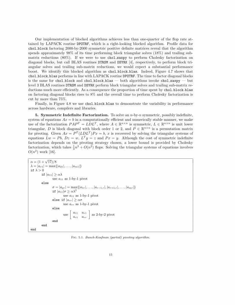
The algorithm for Bunch-Kaufman pivoting is outlined in Figure 5.1. The parameter α boundsthe element growth of the sequence of trailing sub-matrices. With the value of α set to(1 +

√17)/8, the bound on trailing sub-matrix growth for a 2-by-2 pivot equals that for two con-

secutive 1-by-1 pivots, and thereby minimizes the worst case growth for any arbitrary sequence ofpivot selections. Ashcraft, Grimes and Lewis [2] show that in cases where a11 is a 1-by-1 pivot

α = (1 +√17)/8

λ = |ar1| = max{|a21|, . . . , |am1|}if λ > 0

if |a11| ≥ αλuse a11 as 1-by-1 pivot

else

i = 1do

σ = |apr| = max{|a1r|, . . . , |ar−1,r|, |ar+1,r|, . . . , |amr|}if |arr| ≥ ασ

use arr as 1-by-1 pivotelse if λ = σ

use

[aii ariari arr

]as 2-by-2 pivot

else

i = rλ = σr = p

end

until pivot selectedend

end

Fig. 5.2. Bounded Bunch-Kaufman (rook) pivoting algorithm.

16

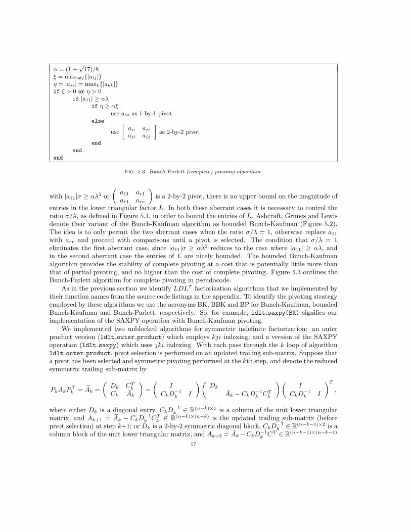
α = (1 +√17)/8

ξ = maxi6=j{|aij |}η = |ass| = maxk{|akk|}if ξ > 0 or η > 0

if |a11| ≥ αλif η ≥ αξ

use ass as 1-by-1 pivotelse

use

[aii ajiaji ajj

]as 2-by-2 pivot

end

end

end

Fig. 5.3. Bunch-Parlett (complete) pivoting algorithm.

with |a11|σ ≥ αλ2 or

(a11 ar1ar1 arr

)is a 2-by-2 pivot, there is no upper bound on the magnitude of

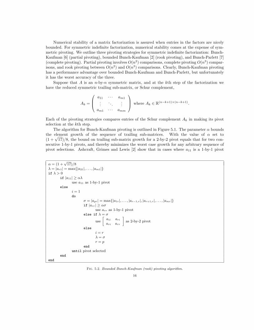
entries in the lower triangular factor L. In both these aberrant cases it is necessary to control theratio σ/λ, as defined in Figure 5.1, in order to bound the entries of L. Ashcraft, Grimes and Lewisdenote their variant of the Bunch-Kaufman algorithm as bounded Bunch-Kaufman (Figure 5.2).The idea is to only permit the two aberrant cases when the ratio σ/λ = 1, otherwise replace a11with arr and proceed with comparisons until a pivot is selected. The condition that σ/λ = 1eliminates the first aberrant case, since |a11|σ ≥ αλ2 reduces to the case where |a11| ≥ αλ, andin the second aberrant case the entries of L are nicely bounded. The bounded Bunch-Kaufmanalgorithm provides the stability of complete pivoting at a cost that is potentially little more thanthat of partial pivoting, and no higher than the cost of complete pivoting. Figure 5.3 outlines theBunch-Parlett algorithm for complete pivoting in pseudocode.

As in the previous section we identify LDLT factorization algorithms that we implemented bytheir function names from the source code listings in the appendix. To identify the pivoting strategyemployed by these algorithms we use the acronyms BK, BBK and BP for Bunch-Kaufman, boundedBunch-Kaufman and Bunch-Parlett, respectively. So, for example, ldlt saxpy(BK) signifies ourimplementation of the SAXPY operation with Bunch-Kaufman pivoting.

We implemented two unblocked algorithms for symmetric indefinite factorization: an outerproduct version (ldlt outer product) which employs kji indexing; and a version of the SAXPYoperation (ldlt saxpy) which uses jki indexing. With each pass through the k loop of algorithmldlt outer product, pivot selection is performed on an updated trailing sub-matrix. Suppose thata pivot has been selected and symmetric pivoting performed at the kth step, and denote the reducedsymmetric trailing sub-matrix by

PkAkPTk = Ak =

(Dk CTkCk Ak

)=

(I

CkD−1k I

)(Dk

Ak − CkD−1k CTk

)(I

CkD−1k I

)T,

where either Dk is a diagonal entry, CkD−1k ∈ R(n−k)×1 is a column of the unit lower triangular

matrix, and Ak+1 = Ak − CkD−1k CTk ∈ R(n−k)×(n−k) is the updated trailing sub-matrix (beforepivot selection) at step k+1; or Dk is a 2-by-2 symmetric diagonal block, CkD

−1k ∈ R(n−k−1)×2 is a

column block of the unit lower triangular matrix, and Ak+2 = Ak−CkD−1k CT ∈ R(n−k−1)×(n−k−1)

17

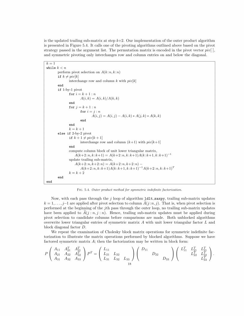
is the updated trailing sub-matrix at step k+2. Our implementation of the outer product algorithmis presented in Figure 5.4. It calls one of the pivoting algorithms outlined above based on the pivotstrategy passed in the argument list. The permutation matrix is encoded in the pivot vector piv[ ],and symmetric pivoting only interchanges row and column entries on and below the diagonal.

k = 1while k < n

perform pivot selection on A(k :n, k :n)if k 6= piv[k]

interchange row and column k with piv[k]end

if 1-by-1 pivotfor i = k + 1 : n

A(i, k) = A(i, k)/A(k, k)end

for j = k + 1 : nfor i = j : n

A(i, j) = A(i, j)−A(i, k) ∗A(j, k) ∗A(k, k)end

end

k = k + 1else if 2-by-2 pivot

if k + 1 6= piv[k + 1]interchange row and column (k+1) with piv[k+1]

end

compute column block of unit lower triangular matrix,A(k+2:n, k :k+1) = A(k+2:n, k :k+1)A(k :k+1, k :k+1)−1

update trailing sub-matrix,A(k+2:n, k+2:n) = A(k+2:n, k+2:n)−

A(k+2:n, k :k+1)A(k :k+1, k :k+1)−1A(k+2:n, k :k+1)T

k = k + 2end

end

Fig. 5.4. Outer product method for symmetric indefinite factorization.

Now, with each pass through the j loop of algorithm ldlt saxpy, trailing sub-matrix updatesk = 1, . . . , j−1 are applied after pivot selection to column A(j :n, j). That is, when pivot selection isperformed at the beginning of the jth pass through the outer loop, no trailing sub-matrix updateshave been applied to A(j : n, j : n). Hence, trailing sub-matrix updates must be applied duringpivot selection to candidate columns before comparisons are made. Both unblocked algorithmsoverwrite lower triangular entries of symmetric matrix A with unit lower triangular factor L andblock diagonal factor D.

We repeat the examination of Cholesky block matrix operations for symmetric indefinite fac-torization to illustrate the matrix operations performed by blocked algorithms. Suppose we havefactored symmetric matrix A; then the factorization may be written in block form:

P

A11 AT21 AT31A21 A22 AT32A31 A32 A33

PT =

L11

L21 L22

L31 L32 L33

D11

D22

D33

LT11 LT21 LT31LT22 LT32

LT33

.

18

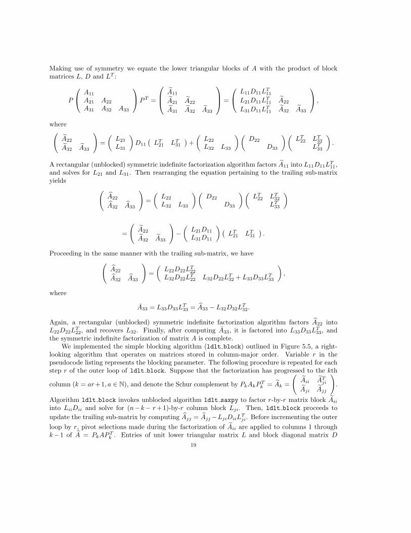
Making use of symmetry we equate the lower triangular blocks of A with the product of blockmatrices L, D and LT :

P

A11

A21 A22

A31 A32 A33

PT =

A11

A21 A22

A31 A32 A33

=

L11D11LT11

L21D11LT11 A22

L31D11LT11 A32 A33

,

where(A22

A32 A33

)=

(L21

L31

)D11

(LT21 LT31

)+

(L22

L32 L33

)(D22

D33

)(LT22 LT32

LT33

).

A rectangular (unblocked) symmetric indefinite factorization algorithm factors A11 into L11D11LT11,

and solves for L21 and L31. Then rearranging the equation pertaining to the trailing sub-matrixyields (

A22

A32 A33

)=

(L22

L32 L33

)(D22

D33

)(LT22 LT32

LT33

)

=

(A22

A32 A33

)−(L21D11

L31D11

)(LT21 LT31

).

Proceeding in the same manner with the trailing sub-matrix, we have(A22

A32 A33

)=

(L22D22L

T22

L32D22LT22 L32D22L

T32 + L33D33L

T33

),

where

A33 = L33D33LT33 = A33 − L32D32L

T32.

Again, a rectangular (unblocked) symmetric indefinite factorization algorithm factors A22 intoL22D22L

T22, and recovers L32. Finally, after computing A33, it is factored into L33D33L

T33, and

the symmetric indefinite factorization of matrix A is complete.We implemented the simple blocking algorithm (ldlt block) outlined in Figure 5.5, a right-

looking algorithm that operates on matrices stored in column-major order. Variable r in thepseudocode listing represents the blocking parameter. The following procedure is repeated for eachstep r of the outer loop of ldlt block. Suppose that the factorization has progressed to the kth

column (k = ar+1, a ∈ N), and denote the Schur complement by PkAkPTk = Ak =

(Aii ATjiAji Ajj

).

Algorithm ldlt block invokes unblocked algorithm ldlt saxpy to factor r-by-r matrix block Aiiinto LiiDii and solve for (n−k− r+1)-by-r column block Lji. Then, ldlt block proceeds to

update the trailing sub-matrix by computing Ajj = Ajj−LjiDiiLTji. Before incrementing the outer

loop by r, pivot selections made during the factorization of Aii are applied to columns 1 throughk−1 of A = PkAP

Tk . Entries of unit lower triangular matrix L and block diagonal matrix D

19

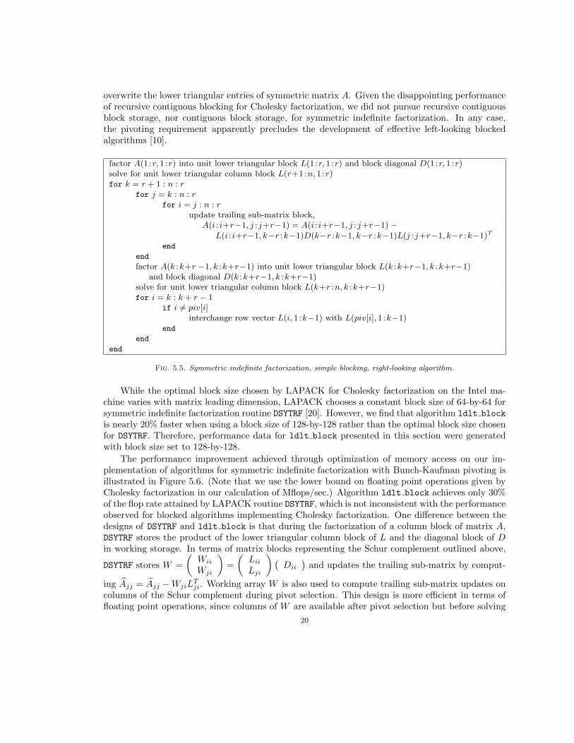
overwrite the lower triangular entries of symmetric matrix A. Given the disappointing performanceof recursive contiguous blocking for Cholesky factorization, we did not pursue recursive contiguousblock storage, nor contiguous block storage, for symmetric indefinite factorization. In any case,the pivoting requirement apparently precludes the development of effective left-looking blockedalgorithms [10].

factor A(1 :r, 1:r) into unit lower triangular block L(1 :r, 1:r) and block diagonal D(1 :r, 1:r)solve for unit lower triangular column block L(r+1:n, 1:r)for k = r + 1 : n : r

for j = k : n : rfor i = j : n : r

update trailing sub-matrix block,A(i : i+r−1, j :j+r−1) = A(i : i+r−1, j :j+r−1)−

L(i : i+r−1, k−r :k−1)D(k−r :k−1, k−r :k−1)L(j :j+r−1, k−r :k−1)Tend

end

factor A(k :k+r −1, k :k+r−1) into unit lower triangular block L(k :k+r−1, k :k+r−1)and block diagonal D(k :k+r−1, k :k+r−1)

solve for unit lower triangular column block L(k+r :n, k :k+r−1)for i = k : k + r − 1

if i 6= piv[i]interchange row vector L(i, 1:k−1) with L(piv[i], 1:k−1)

end

end

end

Fig. 5.5. Symmetric indefinite factorization, simple blocking, right-looking algorithm.

While the optimal block size chosen by LAPACK for Cholesky factorization on the Intel ma-chine varies with matrix leading dimension, LAPACK chooses a constant block size of 64-by-64 forsymmetric indefinite factorization routine DSYTRF [20]. However, we find that algorithm ldlt block

is nearly 20% faster when using a block size of 128-by-128 rather than the optimal block size chosenfor DSYTRF. Therefore, performance data for ldlt block presented in this section were generatedwith block size set to 128-by-128.

The performance improvement achieved through optimization of memory access on our im-plementation of algorithms for symmetric indefinite factorization with Bunch-Kaufman pivoting isillustrated in Figure 5.6. (Note that we use the lower bound on floating point operations given byCholesky factorization in our calculation of Mflops/sec.) Algorithm ldlt block achieves only 30%of the flop rate attained by LAPACK routine DSYTRF, which is not inconsistent with the performanceobserved for blocked algorithms implementing Cholesky factorization. One difference between thedesigns of DSYTRF and ldlt block is that during the factorization of a column block of matrix A,DSYTRF stores the product of the lower triangular column block of L and the diagonal block of Din working storage. In terms of matrix blocks representing the Schur complement outlined above,

DSYTRF stores W =

(Wii

Wji

)=

(LiiLji

)(Dii

)and updates the trailing sub-matrix by comput-

ing Ajj = Ajj −WjiLTji. Working array W is also used to compute trailing sub-matrix updates on

columns of the Schur complement during pivot selection. This design is more efficient in terms offloating point operations, since columns of W are available after pivot selection but before solving

20

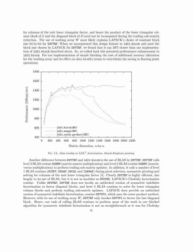
for columns of the unit lower triangular factor, and hence the product of the lower triangular col-umn block of L and the diagonal block of D need not be recomputed during the trailing sub-matrixreduction. The use of working array W most likely explains LAPACK’s choice of constant blocksize 64-by-64 for DSYTRF. When we incorporated this design feature in ldlt block and used theblock size chosen by LAPACK for DSYTRF, we found that it ran 20% slower than our implementa-tion of ldlt block described above. So, we rolled back this potential performance enhancement toldlt block. For our implementation of simple blocking the cost of additional memory allocationfor the working array and its effect on data locality seems to overwhelm the saving in floating pointoperations.

400

600

800

1000

1200

1400

1600

1800

0 200 400 600 800 1000 1200 1400 1600 1800 2000 2200

Per

form

ance

(Mfl

ops/

sec)

Matrix dimension, n-by-n

ldlt block(BK)

ldlt saxpy(BK)

ldlt outer product(BK)

Fig. 5.6. Data locality in LDLT factorization, Bunch-Kaufman pivoting.

Another difference between DSYTRF and ldlt block is the use of BLAS by DSYTRF. DSYTRF callslevel 3 BLAS routine DGEMM (matrix-matrix multiplication) and level 2 BLAS routine DGEMV (matrix-vector multiplication) to perform trailing sub-matrix updates. In addition, it calls a number of level1 BLAS routines (DCOPY, DSWAP, DSCAL and IDAMAX) during pivot selection, symmetric pivoting andsolving for columns of the unit lower triangular factor [4]. Clearly DSYTRF is highly efficient, duelargely to its use of BLAS, but it is not as modular as DPOTRF, LAPACK’s Cholesky factorizationroutine. Unlike DPOTRF, DSYTRF does not invoke an unblocked version of symmetric indefinitefactorization to factor diagonal blocks, and level 3 BLAS routines to solve for lower triangularcolumn blocks and perform trailing sub-matrix updates. LAPACK does provide an unblockedversion of symmetric indefinite factorization, routine DSYTF2, which uses the outer product method.However, with its use of working array W , DSYTRF only invokes DSYTF2 to factor the last diagonalblock. Hence, our task of calling BLAS routines to perform most of the work in our blockedalgorithm for symmetric indefinite factorization is not as straightforward as it was for Cholesky

21

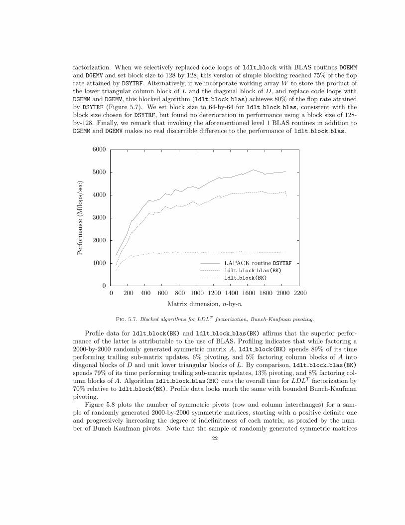
factorization. When we selectively replaced code loops of ldlt block with BLAS routines DGEMM

and DGEMV and set block size to 128-by-128, this version of simple blocking reached 75% of the floprate attained by DSYTRF. Alternatively, if we incorporate working array W to store the product ofthe lower triangular column block of L and the diagonal block of D, and replace code loops withDGEMM and DGEMV, this blocked algorithm (ldlt block blas) achieves 80% of the flop rate attainedby DSYTRF (Figure 5.7). We set block size to 64-by-64 for ldlt block blas, consistent with theblock size chosen for DSYTRF, but found no deterioration in performance using a block size of 128-by-128. Finally, we remark that invoking the aforementioned level 1 BLAS routines in addition toDGEMM and DGEMV makes no real discernible difference to the performance of ldlt block blas.

0

1000

2000

3000

4000

5000

6000

0 200 400 600 800 1000 1200 1400 1600 1800 2000 2200

Per

form

an

ce(M

flop

s/se

c)

Matrix dimension, n-by-n

LAPACK routine DSYTRF

ldlt block blas(BK)

ldlt block(BK)

Fig. 5.7. Blocked algorithms for LDLT factorization, Bunch-Kaufman pivoting.

Profile data for ldlt block(BK) and ldlt block blas(BK) affirms that the superior perfor-mance of the latter is attributable to the use of BLAS. Profiling indicates that while factoring a2000-by-2000 randomly generated symmetric matrix A, ldlt block(BK) spends 89% of its timeperforming trailing sub-matrix updates, 6% pivoting, and 5% factoring column blocks of A intodiagonal blocks of D and unit lower triangular blocks of L. By comparison, ldlt block blas(BK)

spends 79% of its time performing trailing sub-matrix updates, 13% pivoting, and 8% factoring col-umn blocks of A. Algorithm ldlt block blas(BK) cuts the overall time for LDLT factorization by70% relative to ldlt block(BK). Profile data looks much the same with bounded Bunch-Kaufmanpivoting.

Figure 5.8 plots the number of symmetric pivots (row and column interchanges) for a sam-ple of randomly generated 2000-by-2000 symmetric matrices, starting with a positive definite oneand progressively increasing the degree of indefiniteness of each matrix, as proxied by the num-ber of Bunch-Kaufman pivots. Note that the sample of randomly generated symmetric matrices

22

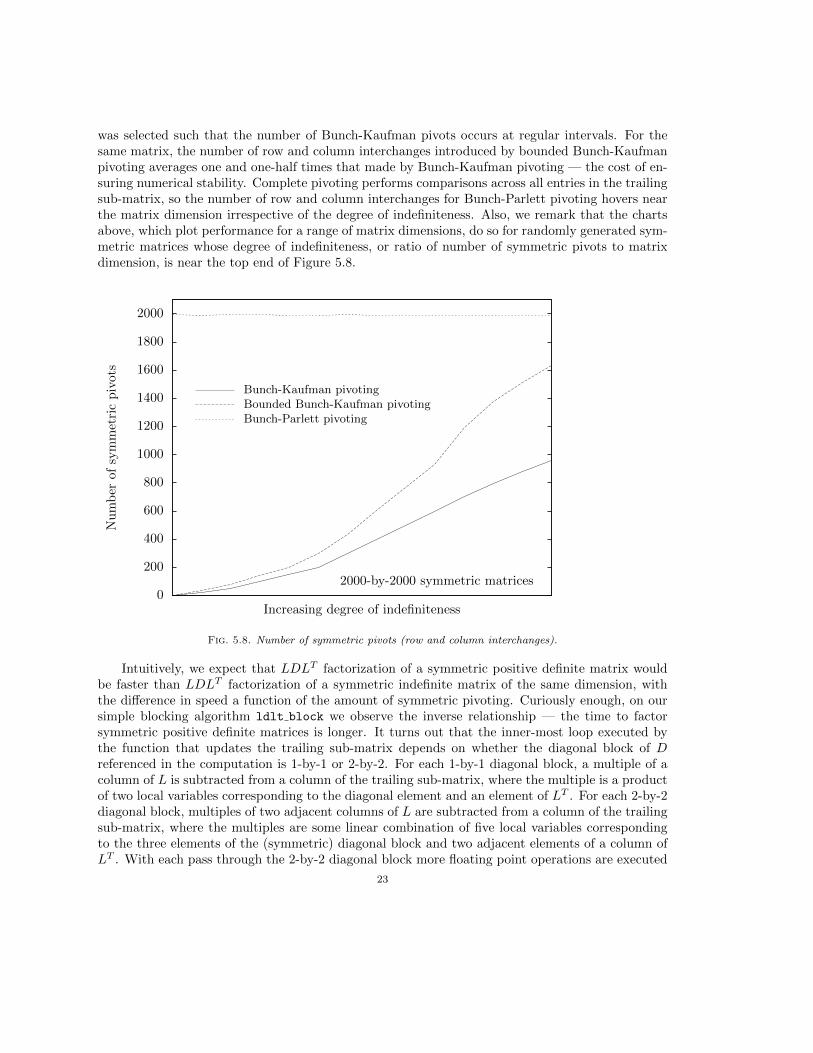
was selected such that the number of Bunch-Kaufman pivots occurs at regular intervals. For thesame matrix, the number of row and column interchanges introduced by bounded Bunch-Kaufmanpivoting averages one and one-half times that made by Bunch-Kaufman pivoting — the cost of en-suring numerical stability. Complete pivoting performs comparisons across all entries in the trailingsub-matrix, so the number of row and column interchanges for Bunch-Parlett pivoting hovers nearthe matrix dimension irrespective of the degree of indefiniteness. Also, we remark that the chartsabove, which plot performance for a range of matrix dimensions, do so for randomly generated sym-metric matrices whose degree of indefiniteness, or ratio of number of symmetric pivots to matrixdimension, is near the top end of Figure 5.8.

0

200

400

600

800

1000

1200

1400

1600

1800

2000

Nu

mb

erof

sym

met

ric

piv

ots

Increasing degree of indefiniteness

2000-by-2000 symmetric matrices

Bunch-Kaufman pivotingBounded Bunch-Kaufman pivotingBunch-Parlett pivoting

Fig. 5.8. Number of symmetric pivots (row and column interchanges).

Intuitively, we expect that LDLT factorization of a symmetric positive definite matrix wouldbe faster than LDLT factorization of a symmetric indefinite matrix of the same dimension, withthe difference in speed a function of the amount of symmetric pivoting. Curiously enough, on oursimple blocking algorithm ldlt block we observe the inverse relationship — the time to factorsymmetric positive definite matrices is longer. It turns out that the inner-most loop executed bythe function that updates the trailing sub-matrix depends on whether the diagonal block of Dreferenced in the computation is 1-by-1 or 2-by-2. For each 1-by-1 diagonal block, a multiple of acolumn of L is subtracted from a column of the trailing sub-matrix, where the multiple is a productof two local variables corresponding to the diagonal element and an element of LT . For each 2-by-2diagonal block, multiples of two adjacent columns of L are subtracted from a column of the trailingsub-matrix, where the multiples are some linear combination of five local variables correspondingto the three elements of the (symmetric) diagonal block and two adjacent elements of a column ofLT . With each pass through the 2-by-2 diagonal block more floating point operations are executed

23

than for every two passes through 1-by-1 diagonal blocks, and in the context of LDLT factorizationof a 2000-by-2000 randomly generated symmetric indefinite matrix (D is block diagonal with blockorder 1 or 2), the total number of floating point operations is a fraction of one percent higherthan that for LDLT factorization of a symmetric positive definite matrix (D is diagonal) of thesame dimension. However, with more local variables in the inner-most loop that processes 2-by-2diagonal blocks, the compiler is able to better exploit on-chip parallelism through optimizationof floating point operations, and as a consequence LDLT factorization of a symmetric indefinitematrix is faster than that of a symmetric positive definite one of the same dimension.

0.30

0.35

0.40

0.45

0.50

0.55

0.60

0.65

0.70

0 100 200 300 400 500 600 700 800 900 1000

Tim

e(s

econ

ds)

Number of symmetric pivots

2000-by-2000 symmetric matrices

LAPACK routine DPOTRF (Cholesky)

LAPACK routine DSYTRF

ldlt block blas(BK)

Fig. 5.9. Cost of Bunch-Kaufman pivoting with increasing indefiniteness, LDLT factorization.

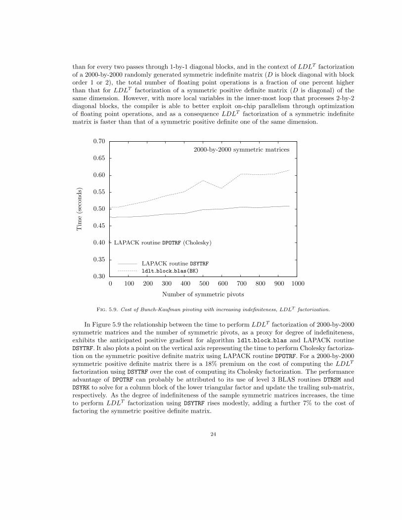
In Figure 5.9 the relationship between the time to perform LDLT factorization of 2000-by-2000symmetric matrices and the number of symmetric pivots, as a proxy for degree of indefiniteness,exhibits the anticipated positive gradient for algorithm ldlt block blas and LAPACK routineDSYTRF. It also plots a point on the vertical axis representing the time to perform Cholesky factoriza-tion on the symmetric positive definite matrix using LAPACK routine DPOTRF. For a 2000-by-2000symmetric positive definite matrix there is a 18% premium on the cost of computing the LDLT

factorization using DSYTRF over the cost of computing its Cholesky factorization. The performanceadvantage of DPOTRF can probably be attributed to its use of level 3 BLAS routines DTRSM andDSYRK to solve for a column block of the lower triangular factor and update the trailing sub-matrix,respectively. As the degree of indefiniteness of the sample symmetric matrices increases, the timeto perform LDLT factorization using DSYTRF rises modestly, adding a further 7% to the cost offactoring the symmetric positive definite matrix.

24

0.35

0.40

0.45

0.50

0.55

0.60

0.65

0.70

0.75

0 200 400 600 800 1000 1200 1400 1600 1800

Tim

e(s

econ

ds)

Number of symmetric pivots

2000-by-2000 symmetric matrices

ldlt block blas(BK)

ldlt block blas(BBK)

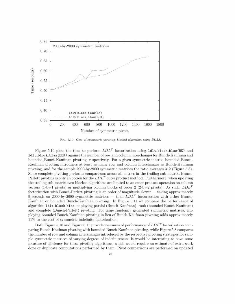
Fig. 5.10. Cost of symmetric pivoting, blocked algorithm using BLAS.

Figure 5.10 plots the time to perform LDLT factorization using ldlt block blas(BK) andldlt block blas(BBK) against the number of row and column interchanges for Bunch-Kaufman andbounded Bunch-Kaufman pivoting, respectively. For a given symmetric matrix, bounded Bunch-Kaufman pivoting introduces at least as many row and column interchanges as Bunch-Kaufmanpivoting, and for the sample 2000-by-2000 symmetric matrices the ratio averages 3 :2 (Figure 5.8).Since complete pivoting performs comparisons across all entries in the trailing sub-matrix, Bunch-Parlett pivoting is only an option for the LDLT outer product method. Furthermore, when updatingthe trailing sub-matrix even blocked algorithms are limited to an outer product operation on columnvectors (1-by-1 pivots) or multiplying column blocks of order 2 (2-by-2 pivots). As such, LDLT

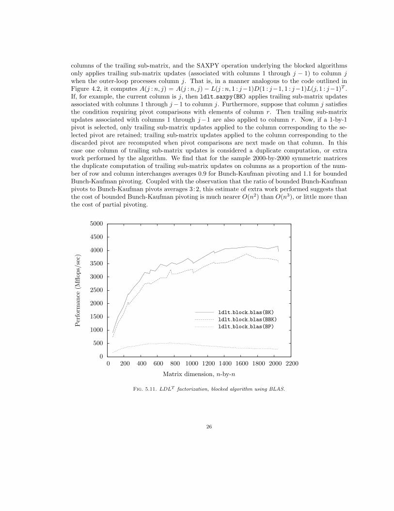
factorization with Bunch-Parlett pivoting is an order of magnitude slower — taking approximately9 seconds on 2000-by-2000 symmetric matrices — than LDLT factorization with either Bunch-Kaufman or bounded Bunch-Kaufman pivoting. In Figure 5.11 we compare the performance ofalgorithm ldlt block blas employing partial (Bunch-Kaufman), rook (bounded Bunch-Kaufman)and complete (Bunch-Parlett) pivoting. For large randomly generated symmetric matrices, em-ploying bounded Bunch-Kaufman pivoting in lieu of Bunch-Kaufman pivoting adds approximately11% to the cost of symmetric indefinite factorization.

Both Figure 5.10 and Figure 5.11 provide measures of performance of LDLT factorization com-paring Bunch-Kaufman pivoting with bounded Bunch-Kaufman pivoting, while Figure 5.8 comparesthe number of row and column interchanges introduced by the respective pivoting strategies for sam-ple symmetric matrices of varying degrees of indefiniteness. It would be interesting to have somemeasure of efficiency for these pivoting algorithms, which would require an estimate of extra workdone or duplicate computations performed by them. Pivot comparisons are performed on updated

25

columns of the trailing sub-matrix, and the SAXPY operation underlying the blocked algorithmsonly applies trailing sub-matrix updates (associated with columns 1 through j − 1) to column jwhen the outer-loop processes column j. That is, in a manner analogous to the code outlined inFigure 4.2, it computes A(j : n, j) = A(j : n, j) − L(j : n, 1 : j−1)D(1 : j−1, 1 : j−1)L(j, 1 : j−1)T .If, for example, the current column is j, then ldlt saxpy(BK) applies trailing sub-matrix updatesassociated with columns 1 through j−1 to column j. Furthermore, suppose that column j satisfiesthe condition requiring pivot comparisons with elements of column r. Then trailing sub-matrixupdates associated with columns 1 through j−1 are also applied to column r. Now, if a 1-by-1pivot is selected, only trailing sub-matrix updates applied to the column corresponding to the se-lected pivot are retained; trailing sub-matrix updates applied to the column corresponding to thediscarded pivot are recomputed when pivot comparisons are next made on that column. In thiscase one column of trailing sub-matrix updates is considered a duplicate computation, or extrawork performed by the algorithm. We find that for the sample 2000-by-2000 symmetric matricesthe duplicate computation of trailing sub-matrix updates on columns as a proportion of the num-ber of row and column interchanges averages 0.9 for Bunch-Kaufman pivoting and 1.1 for boundedBunch-Kaufman pivoting. Coupled with the observation that the ratio of bounded Bunch-Kaufmanpivots to Bunch-Kaufman pivots averages 3:2, this estimate of extra work performed suggests thatthe cost of bounded Bunch-Kaufman pivoting is much nearer O(n2) than O(n3), or little more thanthe cost of partial pivoting.

0

500

1000

1500

2000

2500

3000

3500

4000

4500

5000

0 200 400 600 800 1000 1200 1400 1600 1800 2000 2200

Per

form

an

ce(M

flop

s/se

c)

Matrix dimension, n-by-n

ldlt block blas(BK)

ldlt block blas(BBK)

ldlt block blas(BP)

Fig. 5.11. LDLT factorization, blocked algorithm using BLAS.

26

6. Modified Cholesky Algorithms. Given a symmetric, possibly indefinite, n-by-n matrixA, modified Cholesky algorithms find a matrix A = A+E, where A is sufficiently positive definiteand reasonably well-conditioned, while preserving as much as possible the information of A. Fangand O’Leary catalog modified Cholesky algorithms and analyze the asymptotic cost of the differentapproaches [13]. Their research evaluates how close these different approaches come to achievingthe goal of keeping the cost of the algorithm to a small multiple of n2 higher than that of standardCholesky factorization, which takes 1

3n3 +O(n2) flops.

Fang and O’Leary analyze three factorizations of a symmetric matrix A:1. PAPT = LDLT , where D is diagonal, L is unit lower triangular and P is a permutation

matrix for symmetric pivoting.2. PAPT = LBLT , where B is block diagonal with block order 1 or 2.3. PAPT = LTLT = L(PT LBLT P )LT , where T is tridiagonal with off-diagonal elements in

the first column all zero, and P T PT = LBLT is the LBLT factorization of T .Existing modified Cholesky algorithms typically use either the LDLT or LBLT factorization. Fangand O’Leary propose a new modified Cholesky algorithm, which uses a sandwiched LTLT -LBLT

factorization and modifies a computed factorization. Aasen introduced an algorithm for reducingan n-by-n symmetric matrix to tridiagonal form, which involves 1

3n3 + O(n2) flops and exhibits

numerical stability comparable to that of Gaussian elimination with partial pivoting [1]. Fangand O’Leary show that the LBLT factorization of a symmetric tridiagonal matrix remains sparse,and the cost of symmetric pivoting is no more than O(n2), since pivot selection requires at most

3k comparisons for a k-by-k Schur complement [12]. Finally, the computed L(PT LBLT P )LT

factorization is modified using the method proposed by Cheng and Higham [8]. This new approachto modified Cholesky factorization achieves the objective of keeping the cost of the algorithm to asmall multiple of n2 higher than that of standard Cholesky factorization.

This paper analyzes the performance of modified Cholesky algorithms based on the more typicalLDLT and LBLT factorizations. In particular, we consider the modified LDLT algorithm proposedby Gill, Murray and Wright [14], and the modified LBLT algorithm proposed by Cheng and Higham[8]. Note that the discussion of the previous section on symmetric indefinite factorization is referredto here as LBLT factorization, consistent with the notation used by Fang and O’Leary [13].

The Gill-Murray-Wright algorithm modifies the matrixA as the factorization proceeds. Supposepivot selection and symmetric pivoting have been performed at the kth step of the LDLT factoriza-

tion of an n-by-n symmetric positive definite matrix A = A+E. Let PkAkPTk = Ak =

(ak cTkck Ak

)be the Schur complement, where ak ∈ R, ck ∈ R(n−k)×1 and Ak ∈ R(n−k)×(n−k). Note that if A ispositive definite, so are PkAkP

Tk and its principal sub-matrices, and all diagonal entries are positive.

So, ak = ak + δk > 0. The Gill-Murray-Wright algorithm sets

ak = max

{δ, |ak|,

‖ck‖2∞β2

}where δ = εM (machine epsilon), ‖ck‖∞ = maxk<j≤n |akj |, β2 = max

{η, ξ√

n2−1 , εM

}, and η and ξ

are the maximum magnitude of the diagonal and off-diagonal elements of A, respectively. Then,

D(k, k) = ak, L(k+1:n, k) =ckak, and Ak+1 = Ak −

ckcTk

ak.

27

To ensure numerical stability, the Gill-Murray-Wright algorithm pivots on the maximum mag-nitude diagonal element. That is, at the kth step, rows and columns are symmetrically interchangedsuch that |ak| ≥ |Ak(j, j)| for j = 1, . . . , n−k+1. The cost of this form of partial pivoting is O(n2).

Any symmetric positive definite matrix has an LDLT factorization, where the diagonal elementsof D are positive. The Gill-Murray-Wright algorithm, which modifies the matrix A as the factoriza-tion proceeds, factors a symmetric positive definite matrix A = A+E, such that PAPT = LDLT .For symmetric matrices, in general, an LDLT factorization may fail to exist, but any symmetricmatrix has an LBLT factorization. Therefore, modified Cholesky algorithms that modify a com-puted factorization, including the Cheng-Higham algorithm, use the LBLT factorization.

The Cheng-Higham algorithm first computes PAPT = LBLT , and then perturbs B such thatPAPT = P (A + E)PT = L(B + ∆B)LT = LBLT and A = A + E is symmetric positive definite.Given an LBLT factorization ofA, the Cheng-Higham algorithm modifies each 1-by-1 diagonal blockd in B to be d = max{δ, d}. For each 2-by-2 diagonal block D in B, the algorithm calculates its

spectral decomposition D = U

(λ1

λ2

)UT , sets λk = max{δ, λk} for k = 1, 2, and computes

D = U

(λ1

λ2

)UT . The parameter δ =

√εM/2‖A‖∞ is the preset modification tolerance,

where ‖A‖∞ = max1≤i≤n

{∑nj=1 |aij |

}= max1≤j≤n

{∑ni=1 |aij |

}for a symmetric matrix.

400

600

800

1000

1200

1400

1600

0 200 400 600 800 1000 1200 1400 1600 1800 2000 2200

Per

form

ance

(Mfl

ops/

sec)

Matrix dimension, n-by-n

chol gmw block

chol gmw saxpy

chol gmw outer product

Fig. 6.1. Data locality in modified Cholesky, Gill-Murray-Wright algorithm.

28

We have seen that Cholesky factorization, which provides a lower bound on modified Choleskyfactorization, involves 1

3n3+O(n2) flops, and symmetric pivoting involves between O(n2) and O(n3)

flops. More specifically, the cost of partial pivoting isO(n2) flops, complete pivotingO(n3) flops, androok pivoting between O(n2) and O(n3) flops. The Gill-Murray-Wright algorithm employs partialpivoting, while our implementation of the Cheng-Higham algorithm employs either Bunch-Kaufman(partial) or bounded Bunch-Kaufman (rook) pivoting. In the previous section we estimated thatthe cost of bounded Bunch-Kaufman pivoting is little more than the cost of partial pivoting. Giventhat both the Gill-Murray-Wright and Cheng-Higham modifications to the symmetric indefinitefactorization involve a small multiple of n2 flops, we expect variations in performance betweenmodified Cholesky algorithms to be largely explained by the pivoting strategy employed.

Here, we adopt the same naming convention as used in earlier sections of this paper to referencemodified Cholesky algorithms. Since the Cheng-Higham algorithm modifies a computed symmetricindefinite factorization, our implementation of the outer product method (chol ch outer product),SAXPY operation (chol ch saxpy), simple blocking (chol ch block) and blocked routine usingBLAS (chol ch block blas) invoke the respective symmetric indefinite factorization algorithmsdiscussed in the previous section. On the other hand, the Gill-Murray-Wright algorithm modifiesthe symmetric matrix as the factorization proceeds, so we developed separate and distinct routines:outer product method (chol gmw outer product), SAXPY operation (chol gmw saxpy), simpleblocking (chol gmw block) and blocked routine using BLAS (chol gmw block blas).

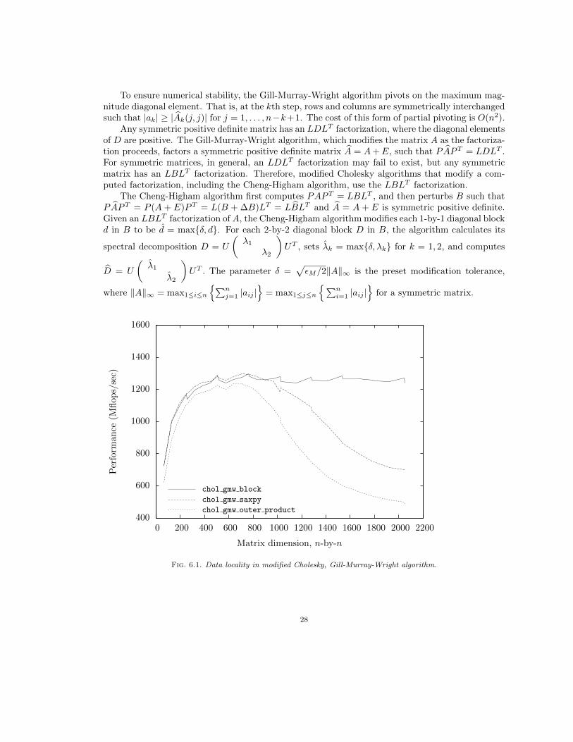
Firstly, to complete the data locality picture, Figure 6.1 plots the effect of loop reordering(chol gmw saxpy) and blocking (chol gmw block) on performance for the Gill-Murray-Wright al-gorithm.

400

600

800

1000

1200

1400

1600

1800

0 200 400 600 800 1000 1200 1400 1600 1800 2000 2200

Per

form

ance

(Mfl

ops/

sec)

Matrix dimension, n-by-n

chol ch block(BK)

chol ch block(BBK)

ldlt block(BK)

ldlt block(BBK)

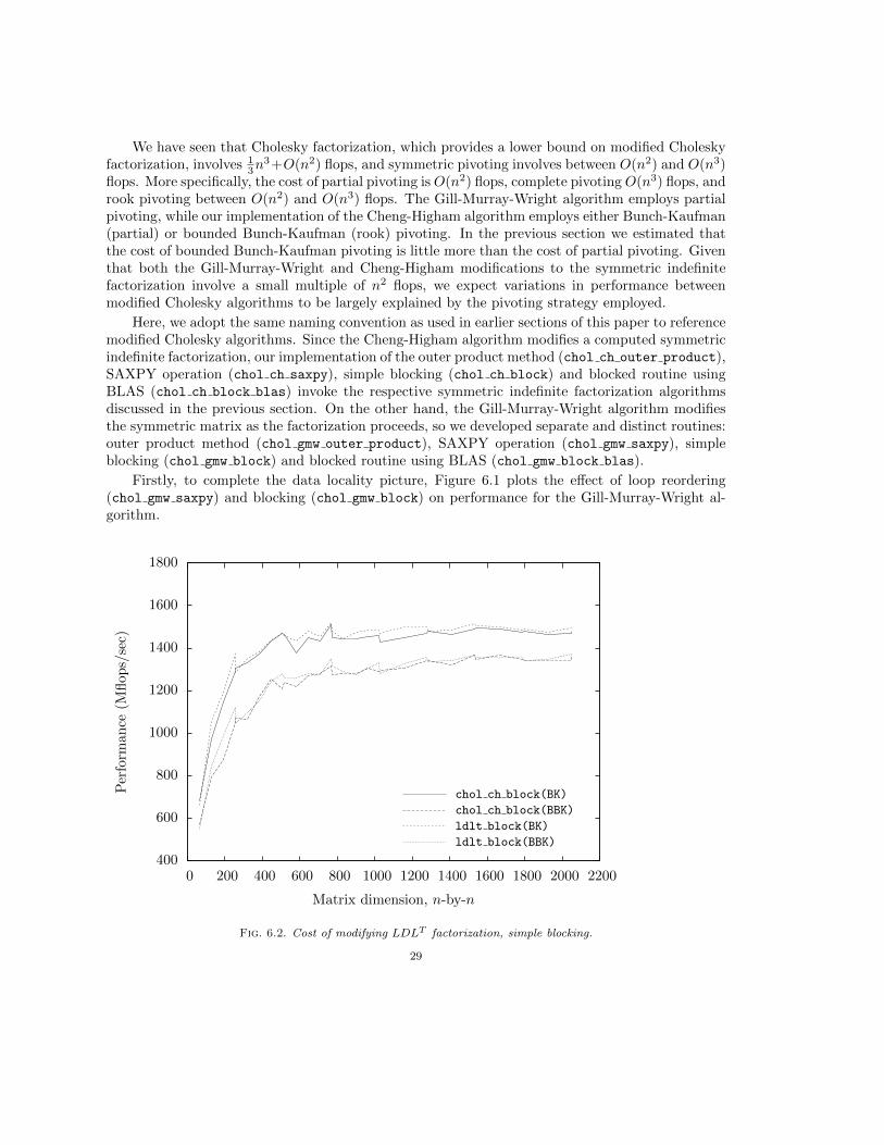
Fig. 6.2. Cost of modifying LDLT factorization, simple blocking.

29

0

500

1000

1500

2000

2500

3000

3500

4000

4500

5000

0 200 400 600 800 1000 1200 1400 1600 1800 2000 2200

Per

form

ance

(Mfl

ops/

sec)

Matrix dimension, n-by-n

chol ch block blas(BK)

chol ch block blas(BBK)

ldlt block blas(BK)

ldlt block blas(BBK)

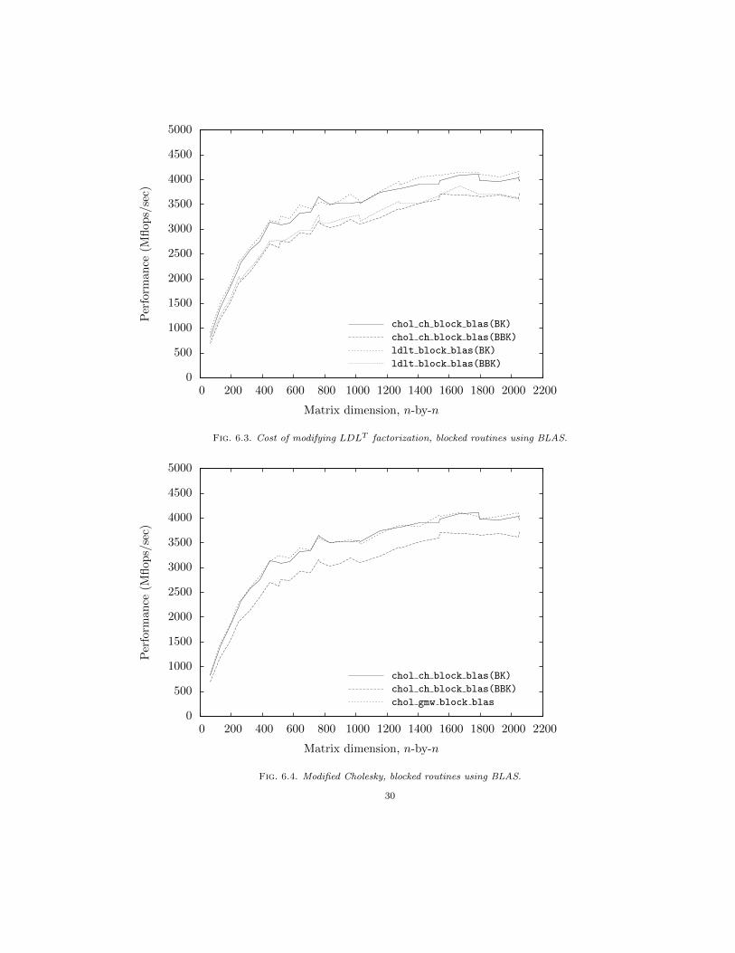
Fig. 6.3. Cost of modifying LDLT factorization, blocked routines using BLAS.

0

500

1000

1500

2000

2500

3000

3500

4000

4500

5000

0 200 400 600 800 1000 1200 1400 1600 1800 2000 2200

Per

form

an

ce(M

flop

s/se

c)

Matrix dimension, n-by-n

chol ch block blas(BK)

chol ch block blas(BBK)

chol gmw block blas

Fig. 6.4. Modified Cholesky, blocked routines using BLAS.

30

One way to measure the cost of modifying a symmetric indefinite factorization is to comparethe performance of modified Cholesky algorithms with the corresponding algorithms implementingsymmetric indefinite factorization. Figure 6.2 plots the performance of our implementation of simpleblocking for the Cheng-Higham algorithm and symmetric indefinite factorization, each employingBunch-Kaufman and bounded Bunch-Kaufman pivoting. Figure 6.3 makes the same performancecomparisons for our blocked routines using BLAS. Both charts reveal that the incremental costof modifying the symmetric indefinite factorization is small relative to the difference in cost be-tween Bunch-Kaufman and bounded Bunch-Kaufman pivoting. Consistent with this observation,Figure 6.4 shows that modified Cholesky algorithms employing partial pivoting perform in linewith one another (chol gmw block blas and chol ch block blas(BK)), while modified Choleskyfactorization with rook pivoting (chol ch block blas(BBK)) is more expensive.

0

200

400

600

800

1000

1200

1400

1600

1800

2000

Nu

mb

erof

sym

met

ric

piv

ots

Increasing degree of indefiniteness

2000-by-2000 symmetric matrices

Bunch-Kaufman pivotingBounded Bunch-Kaufman pivotingGill-Murray-Wright diagonal pivoting

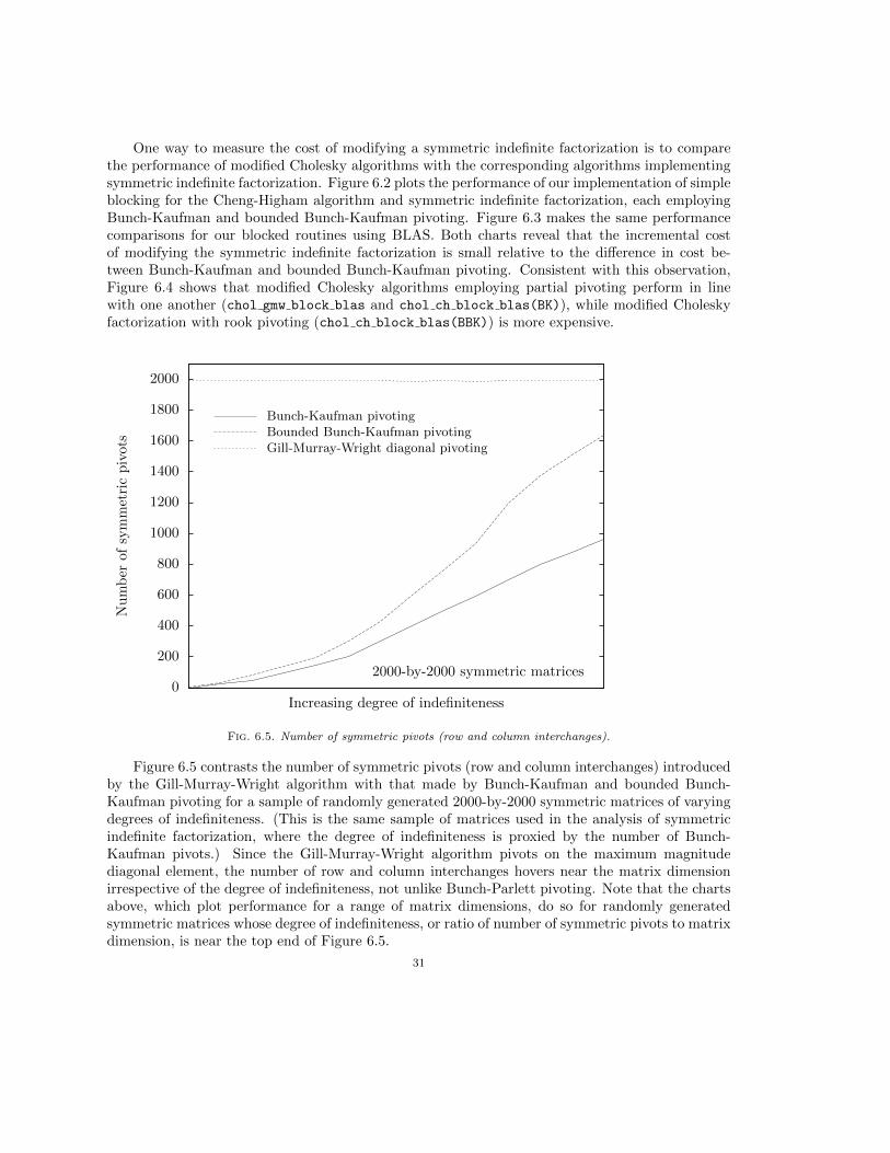
Fig. 6.5. Number of symmetric pivots (row and column interchanges).

Figure 6.5 contrasts the number of symmetric pivots (row and column interchanges) introducedby the Gill-Murray-Wright algorithm with that made by Bunch-Kaufman and bounded Bunch-Kaufman pivoting for a sample of randomly generated 2000-by-2000 symmetric matrices of varyingdegrees of indefiniteness. (This is the same sample of matrices used in the analysis of symmetricindefinite factorization, where the degree of indefiniteness is proxied by the number of Bunch-Kaufman pivots.) Since the Gill-Murray-Wright algorithm pivots on the maximum magnitudediagonal element, the number of row and column interchanges hovers near the matrix dimensionirrespective of the degree of indefiniteness, not unlike Bunch-Parlett pivoting. Note that the chartsabove, which plot performance for a range of matrix dimensions, do so for randomly generatedsymmetric matrices whose degree of indefiniteness, or ratio of number of symmetric pivots to matrixdimension, is near the top end of Figure 6.5.

31

0.40

0.45

0.50

0.55

0.60

0.65

0.70

0.75

0.80

Tim

e(s

econd

s)

Increasing degree of indefiniteness

2000-by-2000 symmetric matrices

chol ch block blas(BK)

chol ch block blas(BBK)

ldlt block blas(BK)

ldlt block blas(BBK)

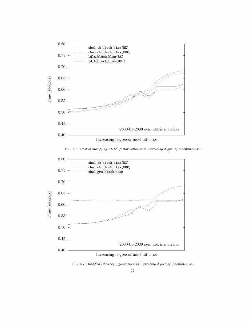
Fig. 6.6. Cost of modifying LDLT factorization with increasing degree of indefiniteness.

0.40

0.45

0.50

0.55

0.60

0.65

0.70

0.75

0.80

Tim

e(s

econd

s)

Increasing degree of indefiniteness

2000-by-2000 symmetric matrices

chol ch block blas(BK)

chol ch block blas(BBK)

chol gmw block blas

Fig. 6.7. Modified Cholesky algorithms with increasing degree of indefiniteness.

32

In Figure 6.6 we provide an alternate measure (runtime) of the cost associated with modifyingthe symmetric indefinite factorization. For the sample of symmetric matrices, the incrementalcost of the Cheng-Higham algorithm employing Bunch-Kaufman and bounded Bunch-Kaufmanpivoting over the corresponding symmetric indefinite factorization algorithms is fairly constantacross the spectrum of indefiniteness. We can explain the observed performance by remarkingthat the computation of the preset modification tolerance by the Cheng-Higham algorithm involvesO(n2) flops, while its modification of 1-by-1 and 2-by-2 diagonal blocks takes only O(n) flops.

The time for algorithms chol ch block blas(BK) and chol ch block blas(BBK) to performmodified Cholesky factorization on the sample of symmetric matrices of varying degrees of indef-initeness tracks that of ldlt block blas(BK) and ldlt block blas(BBK), respectively — timeincreases as the number of symmetric pivots rises, and for Bunch-Kaufman and bounded Bunch-Kaufman pivoting the number of symmetric pivots rises with increasing degree of indefiniteness.As illustrated in Figure 6.5, the number of symmetric pivots for the Gill-Murray-Wright algorithmapproaches the dimension of the matrix irrespective of the degree of indefiniteness, so the time forchol gmw block blas to perform modified Cholesky factorization does not depend on the degreeof indefiniteness of the symmetric matrix (Figure 6.7).

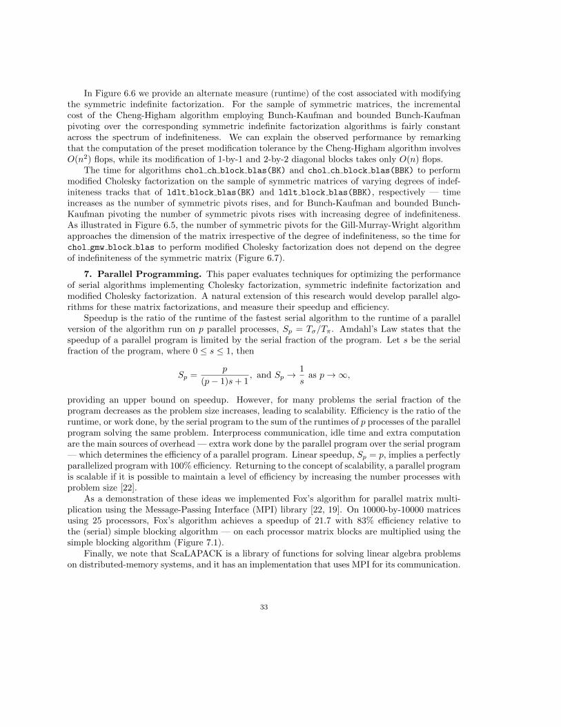
7. Parallel Programming. This paper evaluates techniques for optimizing the performanceof serial algorithms implementing Cholesky factorization, symmetric indefinite factorization andmodified Cholesky factorization. A natural extension of this research would develop parallel algo-rithms for these matrix factorizations, and measure their speedup and efficiency.

Speedup is the ratio of the runtime of the fastest serial algorithm to the runtime of a parallelversion of the algorithm run on p parallel processes, Sp = Tσ/Tπ. Amdahl’s Law states that thespeedup of a parallel program is limited by the serial fraction of the program. Let s be the serialfraction of the program, where 0 ≤ s ≤ 1, then

Sp =p

(p− 1)s+ 1, and Sp →

1

sas p→∞,

providing an upper bound on speedup. However, for many problems the serial fraction of theprogram decreases as the problem size increases, leading to scalability. Efficiency is the ratio of theruntime, or work done, by the serial program to the sum of the runtimes of p processes of the parallelprogram solving the same problem. Interprocess communication, idle time and extra computationare the main sources of overhead — extra work done by the parallel program over the serial program— which determines the efficiency of a parallel program. Linear speedup, Sp = p, implies a perfectlyparallelized program with 100% efficiency. Returning to the concept of scalability, a parallel programis scalable if it is possible to maintain a level of efficiency by increasing the number processes withproblem size [22].

As a demonstration of these ideas we implemented Fox’s algorithm for parallel matrix multi-plication using the Message-Passing Interface (MPI) library [22, 19]. On 10000-by-10000 matricesusing 25 processors, Fox’s algorithm achieves a speedup of 21.7 with 83% efficiency relative tothe (serial) simple blocking algorithm — on each processor matrix blocks are multiplied using thesimple blocking algorithm (Figure 7.1).

Finally, we note that ScaLAPACK is a library of functions for solving linear algebra problemson distributed-memory systems, and it has an implementation that uses MPI for its communication.

33

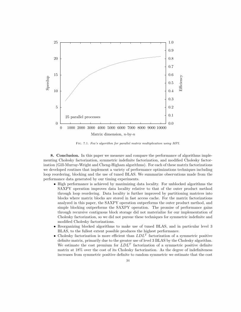
0

5

10

15

20

25

0 1000 2000 3000 4000 5000 6000 7000 8000 9000 100000.0

0.1

0.2

0.3

0.4

0.5

0.6

0.7

0.8

0.9

1.0

Sp

eed

up

Effi

cien

cy

Matrix dimension, n-by-n

25 parallel processes

Fig. 7.1. Fox’s algorithm for parallel matrix multiplication using MPI.

8. Conclusion. In this paper we measure and compare the performance of algorithms imple-menting Cholesky factorization, symmetric indefinite factorization, and modified Cholesky factor-ization (Gill-Murray-Wright and Cheng-Higham algorithms). For each of these matrix factorizationswe developed routines that implement a variety of performance optimizations techniques includingloop reordering, blocking and the use of tuned BLAS. We summarize observations made from theperformance data generated by our timing experiments.

• High performance is achieved by maximizing data locality. For unblocked algorithms theSAXPY operation improves data locality relative to that of the outer product methodthrough loop reordering. Data locality is further improved by partitioning matrices intoblocks where matrix blocks are stored in fast access cache. For the matrix factorizationsanalyzed in this paper, the SAXPY operation outperforms the outer product method, andsimple blocking outperforms the SAXPY operation. The promise of performance gainsthrough recursive contiguous block storage did not materialize for our implementation ofCholesky factorization, so we did not pursue these techniques for symmetric indefinite andmodified Cholesky factorizations.

• Reorganizing blocked algorithms to make use of tuned BLAS, and in particular level 3BLAS, to the fullest extent possible produces the highest performance.

• Cholesky factorization is more efficient than LDLT factorization of a symmetric positivedefinite matrix, primarily due to the greater use of level 3 BLAS by the Cholesky algorithm.We estimate the cost premium for LDLT factorization of a symmetric positive definitematrix at 18% over the cost of its Cholesky factorization. As the degree of indefinitenessincreases from symmetric positive definite to random symmetric we estimate that the cost

34

of LDLT factorization with Bunch-Kaufman pivoting increases by a further 7% due to theincreasing number of row and column interchanges.

• For a given degree of indefiniteness the ratio of bounded Bunch-Kaufman pivots to Bunch-Kaufman pivots averages 3:2. Coupled with estimates of duplicate computations associatedwith trailing sub-matrix updates applied to columns during pivot selection, we contendthat bounded Bunch-Kaufman provides the numerical stability of complete pivoting atlittle more than the cost of partial pivoting. Employing bounded Bunch-Kaufman (rook)pivoting in lieu of Bunch-Kaufman (partial) pivoting adds approximately 11% to the costof symmetric indefinite factorization.

• The cost of modifying a symmetric indefinite factorization is a small multiple of n2 flops, sovariations in performance between modified Cholesky algorithms is largely explained by thepivoting strategy employed. For randomly generated symmetric matrices, the Gill-Murray-Wright algorithm with partial pivoting and the Cheng-Higham algorithm with Bunch-Kaufman pivoting perform in line with one another, while the Cheng-Higham algorithmwith bounded Bunch-Kaufman pivoting is more expensive.

• For the Cheng-Higham algorithm with either Bunch-Kaufman or bounded Bunch-Kaufmanpivoting, the time to perform modified Cholesky factorization increases with increasingdegree of indefiniteness of the symmetric matrix, since the number of symmetric pivots riseswith increasing degree of indefiniteness. By contrast, the Gill-Murray-Wright algorithmpivots on the maximum magnitude diagonal element, so the number of symmetric pivotshovers near the matrix dimension irrespective of the degree of indefiniteness. Hence thetime it takes to perform modified Cholesky factorization does not depend on the degree ofindefiniteness of the symmetric matrix.

In conclusion, we remark that there are possibilities for continuing or extending this researcheffort. Section 6 introduced the modified Cholesky algorithm proposed by Fang and O’Leary, whichuses a sandwiched LTLT -LBLT factorization that performs pivot selection on a (sparse) symmetrictridiagonal matrix. So, one possibility for future research is to develop basic and optimized versionsof the Fang-O’Leary algorithm and compare their performance with that of the Gill-Murray-Wrightand Cheng-Higham algorithms, which perform pivot selection on dense symmetric matrices. An-other possibility, as discussed in the previous section, is to develop parallel algorithms for standardCholesky, symmetric indefinite and modified Cholesky factorizations, and measure their speedupand efficiency. Presently, LAPACK provides unblocked and blocked routines for symmetric indef-inite factorization, which only employ Bunch-Kaufman pivoting. As a final suggestion for futurework, we propose enhancing LAPACK to provide the capability for symmetric indefinite factoriza-tion with bounded Bunch-Kaufman pivoting.

Acknowledgements. We are especially grateful to Professor David Bindel for advising onthis thesis. His guidance on the organization of the research, and his expertise in high performancecomputing and linear algebra were invaluable. Additional thanks to Professor Michael Overtonfor his constructive comments during the review process. The experiments in this research wereconducted on the high performance computing resources at New York University. We wish toacknowledge the technical support provided by the NYU Information Technology Services staff.

35

REFERENCES

[1] Jan O. Aasen, On the reduction of a symmetric matrix to tridiagonal form, BIT, 11 (1971), pp. 233–242.[2] Cleve Ashcraft, Roger G. Grimes, and John G. Lewis, Accurate symmetric indefinite linear equation

solvers, SIAM Journal on Matrix Analysis and Applications, 20 (1998), pp. 513–561.[3] Grey Ballard, James Demmel, Olga Holtz, and Oded Schwartz, Communication-optimal parallel and

sequential cholesky decomposition, Tech. Report UCB/EECS-2009-29, University of California at Berkeley,2009.

[4] BLAS – Basic Linear Algebra Subroutines. http://www.netlib.org/blas/, 2005.[5] Stephen Boyd and Lieven Vandenberghe, Convex Optimization, Cambridge University Press, Cambridge,

United Kingdom, 2004.[6] James R. Bunch and Linda Kaufman, Some stable methods for calculating inertia and solving symmetric

linear systems, Mathematics of Computation, 31 (1977), pp. 163–179.[7] James R. Bunch and Beresford N. Parlett, Direct methods for solving symmetric indefinite systems of

linear equations, SIAM Journal on Numerical Analysis, 8 (1971), pp. 639–655.[8] Sheung Hun Cheng and Nicholas J. Higham, A modified Cholesky algorithm based on a symmetric indefinite

factorization, SIAM Journal on Matrix Analysis and Applications, 19 (1998), pp. 1097–1110.[9] James W. Demmel, Applied Numerical Linear Algebra, Society for Industrial and Applied Mathematics,

Philadelphia, PA, 1997.[10] Jack J. Dongarra, Iain S. Duff, Danny C. Sorensen, and Henk A. van der Vorst, Numerical Linear

Algebra for High-Performance Computers, Society for Industrial and Applied Mathematics, Philadelphia,PA, 1998.

[11] Erik Elmroth, Fred Gustavson, Isak Jonsson, and Bo Kagstrom, Recursive blocked algorithms and hybriddata structures for dense matrix library software, SIAM Review, 46 (2004), pp. 3–45.

[12] Haw-ren Fang and Dianne P. O’Leary, Stable factorizations of symmetric tridiagonal and triadic matrices,SIAM Journal on Matrix Analysis and Applications, 28 (2006), pp. 576–595.

[13] , Modified Cholesky algorithms: a catalog with new approaches, Mathematical Programming (Series A),115 (2008), pp. 319–349.

[14] Philip E. Gill, Walter Murray, and Margaret H. Wright, Practical Optimization, Academic Press, NewYork, NY, 1981.

[15] Stephan Goedecker and Adolfy Hoisie, Performance Optimization of Numerically Intensive Codes, Societyfor Industrial and Applied Mathematics, Philadelphia, PA, 2001.

[16] Gene H. Golub and Charles F. van Loan, Matrix Computations, The John Hopkins University Press,Baltimore, MD, third edition ed., 1996.

[17] Brian Gough, An Introduction to GCC, Network Theory Limited, Bristol, United Kingdom, 2004.[18] Brian W. Kernighan and Dennis M. Ritchie, The C Programming Language, Prentice Hall, Upper Saddle

River, NJ, second edition ed., 1988.[19] Salman Khalid, Fox’s algorithm for matrix multiplication in a parallel environment. Seminar on parallel

algorithms, Center for Solid State Physics, Lahore, Pakistan, 2001.[20] LAPACK – Linear Algebra PACKage. http://www.netlib.org/lapack/, June 2010. Version 3.2.2.[21] Robert Mecklenburg, Managing Projects with GNU Make, O’Reilly, Cambridge, MA, third edition ed., 2005.[22] Peter S. Pacheco, Parallel Programming with MPI, Morgan Kaufmann Publishers, San Francisco, CA, 1997.[23] Richard M. Stallman, Roland McGrath, and Paul Smith, GNU Make: A Program for Directing Recom-

pilation, Free Software Foundation, Boston, MA, 2004.

36