Embed Size (px)
Citation preview
Linear plate bending and laminate theory
4M020: Design ToolsEindhoven University of Technology
1
2
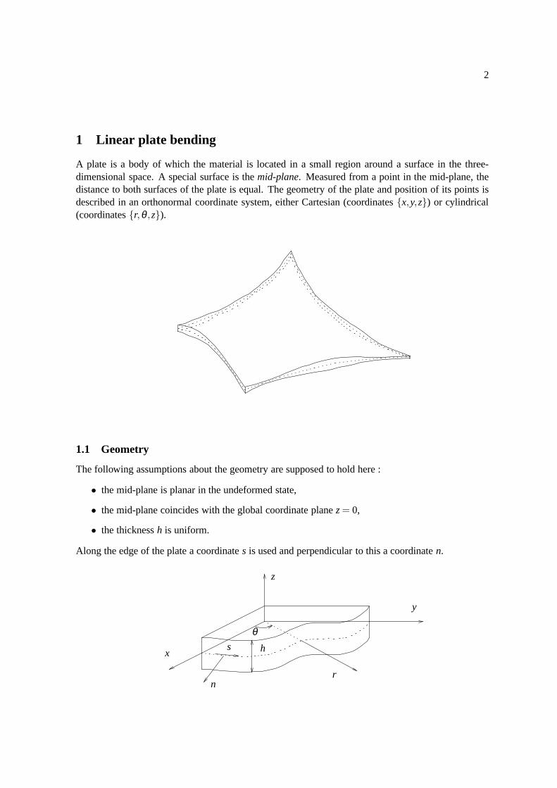
1 Linear plate bending
A plate is a body of which the material is located in a small region around a surface in the three-dimensional space. A special surface is themid-plane. Measured from a point in the mid-plane, thedistance to both surfaces of the plate is equal. The geometryof the plate and position of its points isdescribed in an orthonormal coordinate system, either Cartesian (coordinates{x,y,z}) or cylindrical(coordinates{r,θ ,z}).
1.1 Geometry
The following assumptions about the geometry are supposed to hold here :
• the mid-plane is planar in the undeformed state,
• the mid-plane coincides with the global coordinate planez = 0,
• the thicknessh is uniform.
Along the edge of the plate a coordinates is used and perpendicular to this a coordinaten.
hs
nr
θ
z
x
y
3
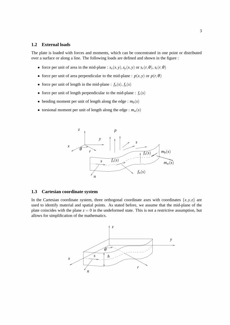
1.2 External loads
The plate is loaded with forces and moments, which can be concentrated in one point or distributedover a surface or along a line. The following loads are definedand shown in the figure :
• force per unit of area in the mid-plane :sx(x,y),sy(x,y) or sr(r,θ), st(r,θ)
• force per unit of area perpendicular to the mid-plane :p(x,y) or p(r,θ)
• force per unit of length in the mid-plane :fn(s), fs(s)
• force per unit of length perpendicular to the mid-plane :fz(s)
• bending moment per unit of length along the edge :mb(s)
• torsional moment per unit of length along the edge :mw(s)
rθ
z
x
y
s
nfn(s)
fs(s) mw(s)
mb(s)
p
fz(s)
s
1.3 Cartesian coordinate system
In the Cartesian coordinate system, three orthogonal coordinate axes with coordinates{x,y,z} areused to identify material and spatial points. As stated before, we assume that the mid-plane of theplate coincides with the planez = 0 in the undeformed state. This is not a restrictive assumption, butallows for simplification of the mathematics.
hs
nr
θ
z
x
y
4
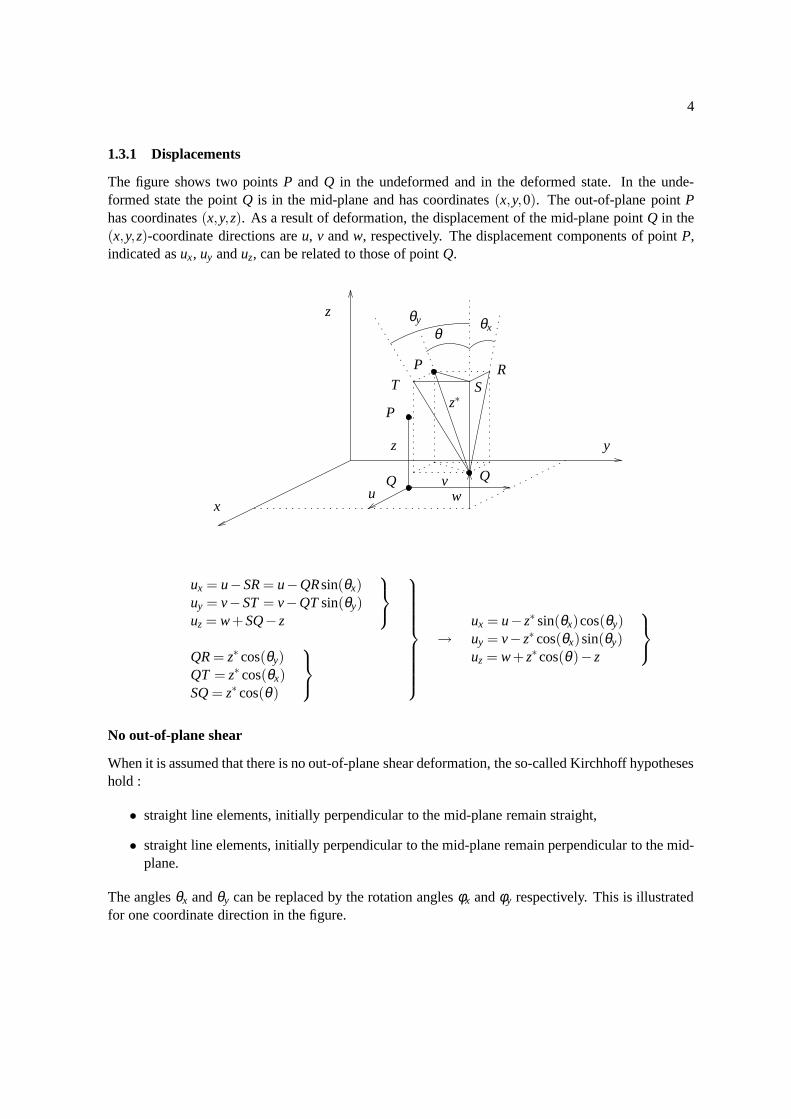
1.3.1 Displacements
The figure shows two pointsP and Q in the undeformed and in the deformed state. In the unde-formed state the pointQ is in the mid-plane and has coordinates(x,y,0). The out-of-plane pointPhas coordinates(x,y,z). As a result of deformation, the displacement of the mid-plane pointQ in the(x,y,z)-coordinate directions areu, v andw, respectively. The displacement components of pointP,indicated asux, uy anduz, can be related to those of pointQ.
P
Q
z
θxθy
θ
z∗
wv
u
z
y
x
SR
T
P
Q
ux = u−SR = u−QRsin(θx)uy = v−ST = v−QT sin(θy)uz = w + SQ− z
QR = z∗ cos(θy)QT = z∗ cos(θx)SQ = z∗ cos(θ)
→ux = u− z∗ sin(θx)cos(θy)uy = v− z∗ cos(θx)sin(θy)uz = w + z∗cos(θ)− z
No out-of-plane shear
When it is assumed that there is no out-of-plane shear deformation, the so-called Kirchhoff hypotheseshold :
• straight line elements, initially perpendicular to the mid-plane remain straight,
• straight line elements, initially perpendicular to the mid-plane remain perpendicular to the mid-plane.
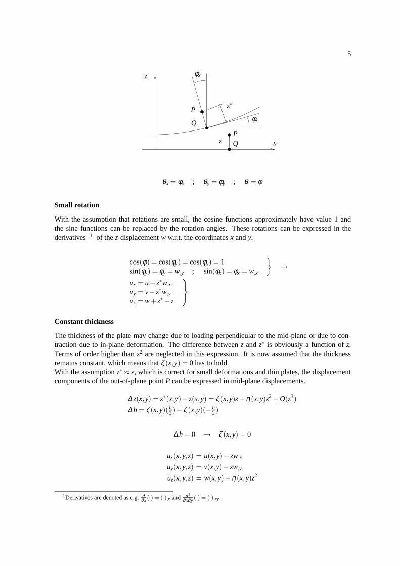
The anglesθx andθy can be replaced by the rotation anglesφx andφy respectively. This is illustratedfor one coordinate direction in the figure.
5
x
φx
z
P
Q
PQz
φx
z∗
θx = φx ; θy = φy ; θ = φ
Small rotation
With the assumption that rotations are small, the cosine functions approximately have value 1 andthe sine functions can be replaced by the rotation angles. These rotations can be expressed in thederivatives 1 of thez-displacementw w.r.t. the coordinatesx andy.
cos(φ) = cos(φy) = cos(φx) = 1sin(φy) = φy = w,y ; sin(φx) = φx = w,x
}
→
ux = u− z∗w,x
uy = v− z∗w,y
uz = w + z∗− z
Constant thickness
The thickness of the plate may change due to loading perpendicular to the mid-plane or due to con-traction due to in-plane deformation. The difference between z andz∗ is obviously a function ofz.Terms of order higher thanz2 are neglected in this expression. It is now assumed that the thicknessremains constant, which means thatζ (x,y) = 0 has to hold.With the assumptionz∗ ≈ z, which is correct for small deformations and thin plates, the displacementcomponents of the out-of-plane pointP can be expressed in mid-plane displacements.
∆z(x,y) = z∗(x,y)− z(x,y) = ζ (x,y)z+ η(x,y)z2 + O(z3)
∆h = ζ (x,y)(h2)−ζ (x,y)(− h
2)
∆h = 0 → ζ (x,y) = 0
ux(x,y,z) = u(x,y)− zw,x
uy(x,y,z) = v(x,y)− zw,y
uz(x,y,z) = w(x,y)+ η(x,y)z2
1Derivatives are denoted as e.g.∂∂ x ( ) = ( ),x and ∂ 2
∂ x∂ y ( ) = ( ),xy
6
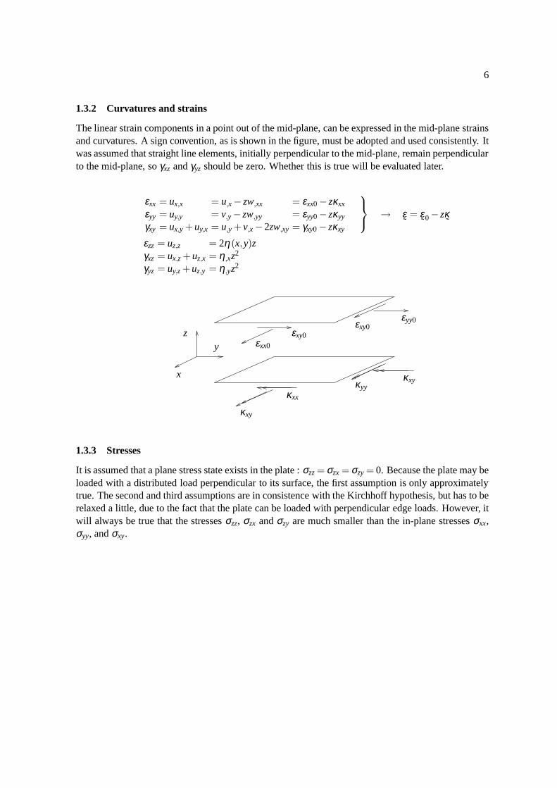
1.3.2 Curvatures and strains
The linear strain components in a point out of the mid-plane,can be expressed in the mid-plane strainsand curvatures. A sign convention, as is shown in the figure, must be adopted and used consistently. Itwas assumed that straight line elements, initially perpendicular to the mid-plane, remain perpendicularto the mid-plane, soγxz andγyz should be zero. Whether this is true will be evaluated later.
εxx = ux,x = u,x − zw,xx = εxx0− zκxx
εyy = uy,y = v,y − zw,yy = εyy0− zκyy
γxy = ux,y + uy,x = u,y + v,x −2zw,xy = γxy0− zκxy
→ ε˜= ε
˜0− zκ˜
εzz = uz,z = 2η(x,y)zγxz = ux,z + uz,x = η,xz2
γyz = uy,z + uz,y = η,yz2
x
yz
εxx0
εxy0εxy0
εyy0
κxy
κxx
κyyκxy
1.3.3 Stresses
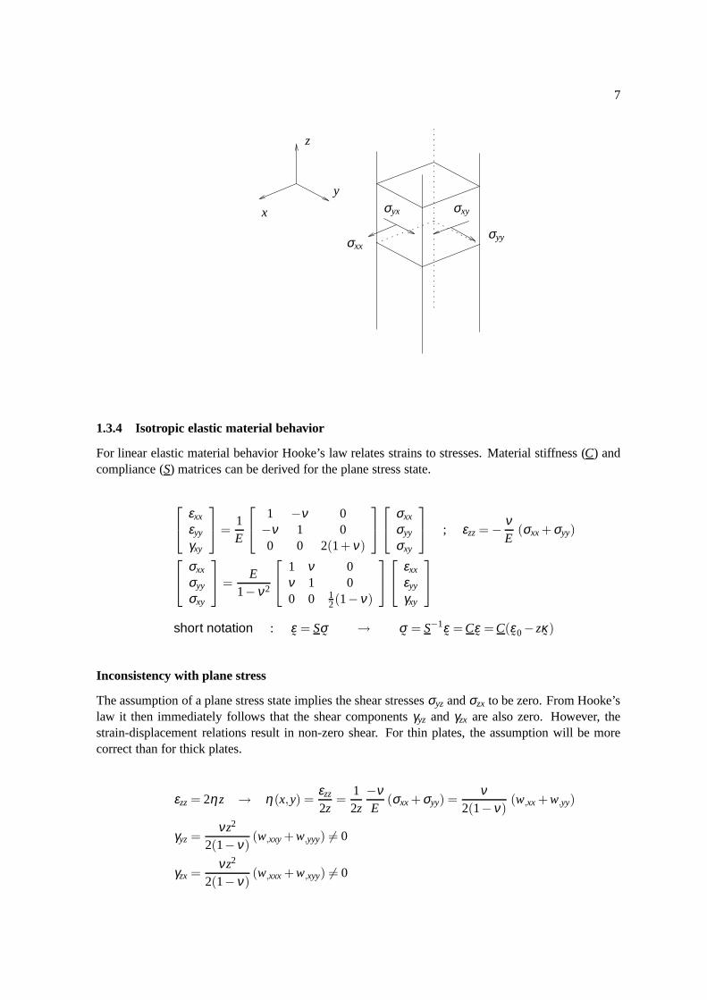
It is assumed that a plane stress state exists in the plate :σzz = σzx = σzy = 0. Because the plate may beloaded with a distributed load perpendicular to its surface, the first assumption is only approximatelytrue. The second and third assumptions are in consistence with the Kirchhoff hypothesis, but has to berelaxed a little, due to the fact that the plate can be loaded with perpendicular edge loads. However, itwill always be true that the stressesσzz, σzx andσzy are much smaller than the in-plane stressesσxx,σyy, andσxy.
7
x
y
z
σxx
σxyσyx
σyy
1.3.4 Isotropic elastic material behavior
For linear elastic material behavior Hooke’s law relates strains to stresses. Material stiffness (C) andcompliance (S) matrices can be derived for the plane stress state.
εxx
εyy
γxy
=1E
1 −ν 0−ν 1 00 0 2(1+ ν)
σxx
σyy
σxy
; εzz = −νE
(σxx + σyy)
σxx
σyy
σxy
=E
1−ν2
1 ν 0ν 1 00 0 1
2(1−ν)
εxx
εyy
γxy
short notation : ε˜= Sσ
˜→ σ
˜= S−1ε
˜= Cε
˜= C(ε
˜0− zκ˜)
Inconsistency with plane stress
The assumption of a plane stress state implies the shear stressesσyz andσzx to be zero. From Hooke’slaw it then immediately follows that the shear componentsγyz andγzx are also zero. However, thestrain-displacement relations result in non-zero shear. For thin plates, the assumption will be morecorrect than for thick plates.
εzz = 2ηz → η(x,y) =εzz
2z=
12z
−νE
(σxx + σyy) =ν
2(1−ν)(w,xx + w,yy)
γyz =νz2
2(1−ν)(w,xxy + w,yyy) 6= 0
γzx =νz2
2(1−ν)(w,xxx + w,xyy) 6= 0
8
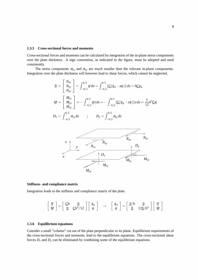
1.3.5 Cross-sectional forces and moments
Cross-sectional forces and moments can be calculated by integration of the in-plane stress componentsover the plate thickness. A sign convention, as indicated inthe figure, must be adopted and usedconsistently.
The stress componentsσzx and σzy are much smaller than the relevant in-plane components.Integration over the plate thickness will however lead to shear forces, which cannot be neglected.
N˜
=
Nxx
Nyy
Nxy
=
∫ h/2
−h/2σ˜
dz =
∫ h/2
−h/2{C(ε
˜0− zκ˜)}dz = hCε
˜0
M˜
=
Mxx
Myy
Mxy
= −
∫ h/2
−h/2σ˜
zdz = −
∫ h/2
−h/2{C(ε
˜0− zκ˜)}zdz =
112
h3Cκ˜
Dx =∫ h/2
−h/2σzx dz ; Dy =
∫ h/2
−h/2σzy dz
x
yz
Nxy
Dx
Dy
Myy
Mxx
Mxy
Nyy
NxyNxx
Mxy
Stiffness- and compliance matrix
Integration leads to the stiffness and compliance matrix ofthe plate.
[
NM̃˜
]
=
[
Ch 00 Ch3/12
][
ε˜0κ˜
]
→
[
ε˜0κ˜
]
=
[
S/h 00 12S/h3
][
NM̃˜
]
1.3.6 Equilibrium equations
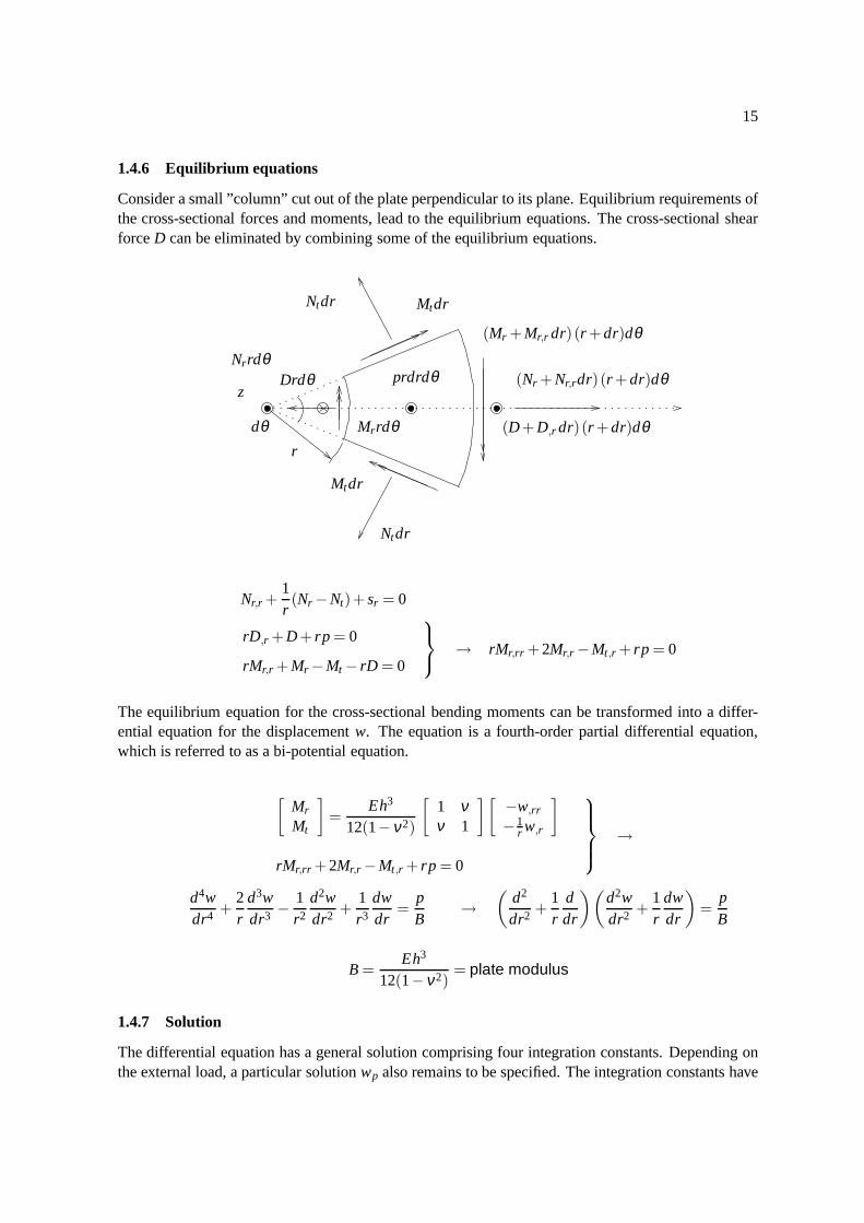
Consider a small ”column” cut out of the plate perpendicularto its plane. Equilibrium requirements ofthe cross-sectional forces and moments, lead to the equilibrium equations. The cross-sectional shearforcesDx andDy can be eliminated by combining some of the equilibrium equations.
9
Nxx,x + Nxy,y + sx = 0
Nyy,y + Nxy,x + sy = 0
Dx,x + Dy,y + p = 0
Mxy,x + Myy,y −Dy = 0
Mxy,y + Mxx,x −Dx = 0
→ Mxx,xx + Myy,yy +2Mxy,xy + p = 0
The equilibrium equation for the cross-sectional bending moments can be transformed into a differ-ential equation for the displacementw. The equation is a fourth-order partial differential equation,which is referred to as a bi-potential equation.
Mxx
Myy
Mxy
=Eh3
12(1−ν2)
1 ν 0ν 1 00 0 1
2(1−ν)
w,xx
w,yy
2w,xy
Mxx,xx + Myy,yy +2Mxy,xy + p = 0
→
∂ 4w∂x4 +
∂ 4w∂y4 +2
∂ 4w∂x2∂y2 = (
∂ 2
∂x2 +∂ 2
∂y2 )(∂ 2w∂x2 +
∂ 2w∂y2 ) =
pB
B =Eh3
12(1−ν2)= plate modulus
1.3.7 Orthotropic elastic material behavior
A material which properties are in each point symmetric w.r.t. three orthogonal planes, is called or-thotropic. The three perpendicular directions in the planes are denoted as the 1-, 2- and 3-coordinateaxes and are referred to as the material coordinate directions. Linear elastic behavior of an orthotropicmaterial is characterized by 9 independent material parameters. They constitute the components ofthe compliance (S) and stiffness (C) matrix.
10
ε11
ε22
ε33
γ12
γ23
γ31
=
E−11 −ν21E−1
2 −ν31E−13 0 0 0
−ν12E−11 E−1
2 −ν32E−13 0 0 0
−ν13E−11 −ν23E−1
2 E−13 0 0 0
0 0 0 G−112 0 0
0 0 0 0 G−123 0
0 0 0 0 0 G−131
σ11
σ22
σ33
σ12
σ23
σ31
ε˜= Sσ
˜→ σ
˜= S−1ε
˜= Cε
˜
C =1∆
1−ν32ν23E2E3
ν31ν23+ν21E2E3
ν21ν32+ν31E2E3
0 0 0ν13ν32+ν12
E1E3
1−ν31ν13E1E3
ν12ν31+ν32E1E3
0 0 0ν12ν23+ν13
E1E2
ν21ν13+ν23E1E2
1−ν12ν21E1E2
0 0 00 0 0 ∆G12 0 00 0 0 0 ∆G23 00 0 0 0 0 ∆G31
with ∆ =(1−ν12ν21−ν23ν32−ν31ν13−ν12ν23ν31−ν21ν32ν13)
E1E2E3
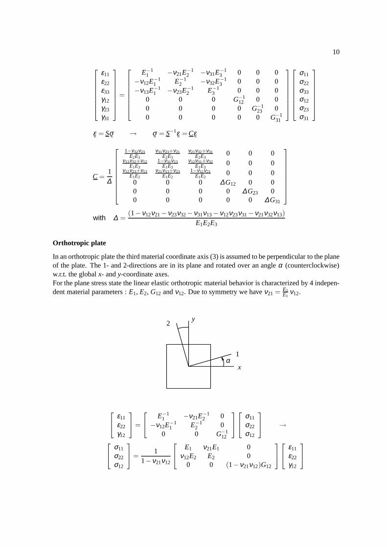
Orthotropic plate
In an orthotropic plate the third material coordinate axis (3) is assumed to be perpendicular to the planeof the plate. The 1- and 2-directions are in its plane and rotated over an angleα (counterclockwise)w.r.t. the globalx- andy-coordinate axes.For the plane stress state the linear elastic orthotropic material behavior is characterized by 4 indepen-dent material parameters :E1, E2, G12 andν12. Due to symmetry we haveν21 = E2
E1ν12.
y
α1
2
x
ε11
ε22
γ12
=
E−11 −ν21E−1
2 0−ν12E−1
1 E−12 0
0 0 G−112
σ11
σ22
σ12
→
σ11
σ22
σ12
=1
1−ν21ν12
E1 ν21E1 0ν12E2 E2 0
0 0 (1−ν21ν12)G12
ε11
ε22
γ12
11
Using a transformation matricesT ε andT σ , for strain and stress components, respectively, the strainand stress components in the material coordinate system (index∗) can be related to those in the globalcoordinate system.
c = cos(α) ; s = sin(α)
εxx
εyy
γxy
=
c2 s2 −css2 c2 cs2cs −2cs c2− s2
ε11
ε22
γ12
→ ε˜= T−1
ε ε˜∗
σxx
σyy
σxy
=
c2 s2 −2css2 c2 2cscs −cs c2− s2
σ11
σ22
σ12
→ σ˜
= T−1σ σ
˜∗
ε˜= T−1
ε ε˜∗ idem σ
˜= T−1
σ σ˜∗ →
ε˜= T−1
ε ε˜∗ = T−1
ε S∗σ˜∗ = T−1
ε S∗T σ σ˜
= Sσ˜
σ˜
= T−1σ σ
˜∗ = T−1
σ C∗ε˜∗ = T−1
σ C∗T ε ε˜= C ε
˜
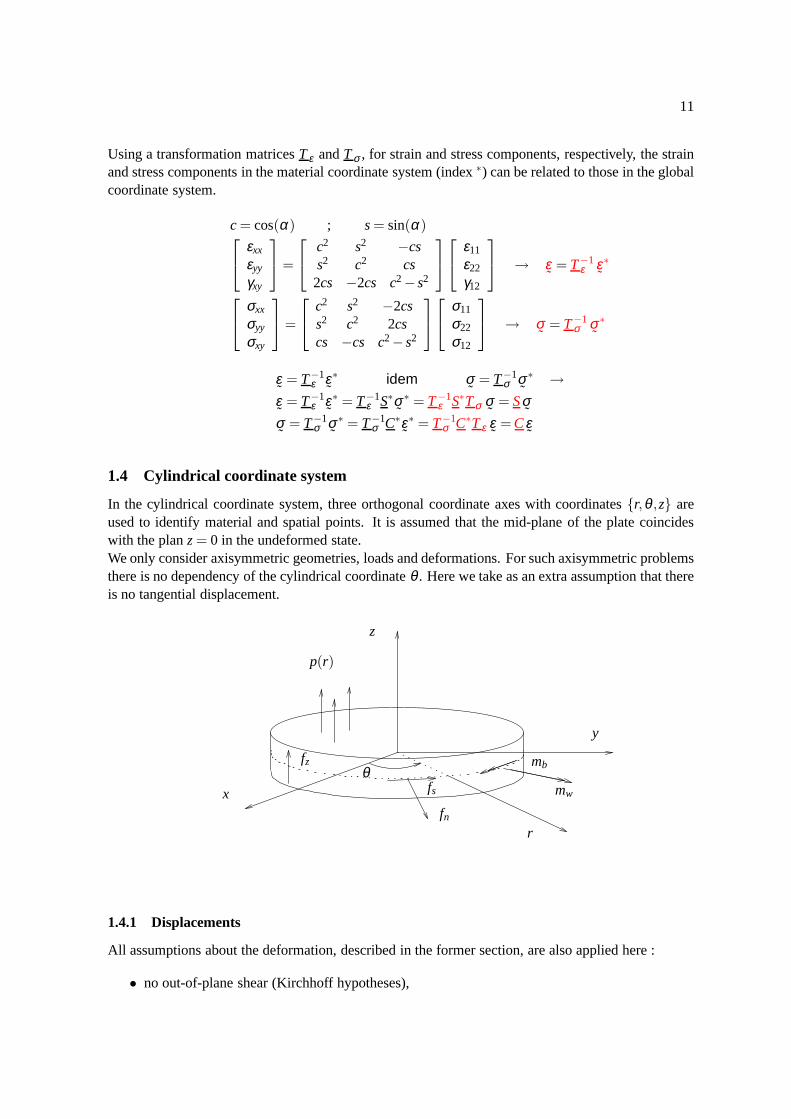
1.4 Cylindrical coordinate system
In the cylindrical coordinate system, three orthogonal coordinate axes with coordinates{r,θ ,z} areused to identify material and spatial points. It is assumed that the mid-plane of the plate coincideswith the planz = 0 in the undeformed state.We only consider axisymmetric geometries, loads and deformations. For such axisymmetric problemsthere is no dependency of the cylindrical coordinateθ . Here we take as an extra assumption that thereis no tangential displacement.
fs mw
z
x
y
fz
p(r)
fn
θmb
r
1.4.1 Displacements
All assumptions about the deformation, described in the former section, are also applied here :
• no out-of-plane shear (Kirchhoff hypotheses),
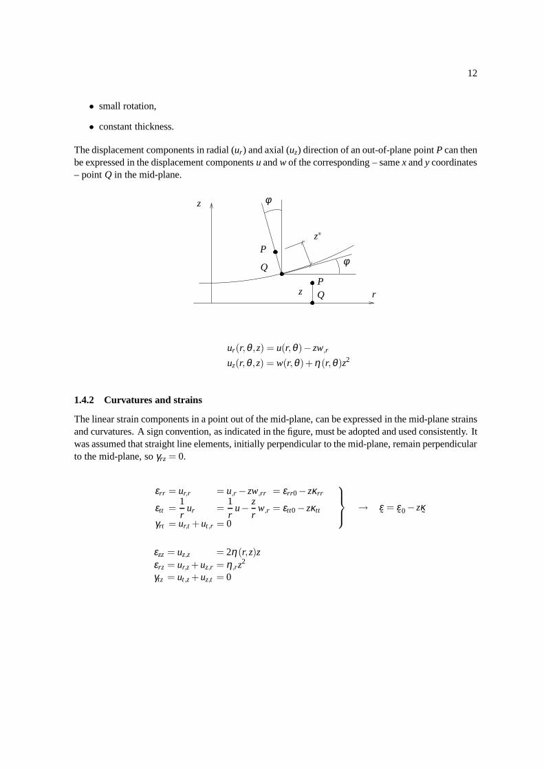
12
• small rotation,
• constant thickness.
The displacement components in radial (ur) and axial (uz) direction of an out-of-plane pointP can thenbe expressed in the displacement componentsu andw of the corresponding – samex andy coordinates– pointQ in the mid-plane.
r
φ
z
P
Q
PQz
φ
z∗
ur(r,θ ,z) = u(r,θ)− zw,r
uz(r,θ ,z) = w(r,θ)+ η(r,θ)z2
1.4.2 Curvatures and strains
The linear strain components in a point out of the mid-plane,can be expressed in the mid-plane strainsand curvatures. A sign convention, as indicated in the figure, must be adopted and used consistently. Itwas assumed that straight line elements, initially perpendicular to the mid-plane, remain perpendicularto the mid-plane, soγrz = 0.
εrr = ur,r = u,r − zw,rr = εrr0− zκrr
εtt =1r
ur =1r
u−zr
w,r = εtt0− zκtt
γrt = ur,t + ut,r = 0
→ ε˜= ε
˜0− zκ˜
εzz = uz,z = 2η(r,z)zεrz = ur,z + uz,r = η,rz
2
γtz = ut,z + uz,t = 0
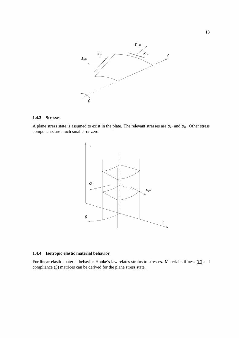
13
θ
εrr0
κrr rκttεtt0
1.4.3 Stresses
A plane stress state is assumed to exist in the plate. The relevant stresses areσrr andσtt . Other stresscomponents are much smaller or zero.
θr
z
σrr
σtt
1.4.4 Isotropic elastic material behavior
For linear elastic material behavior Hooke’s law relates strains to stresses. Material stiffness (C) andcompliance (S) matrices can be derived for the plane stress state.
14
[
εrr
εtt
]
=1E
[
1 −ν−ν 1
][
σrr
σtt
]
; εzz = −νE
(σrr + σtt)
[
σrr
σtt
]
=E
1−ν2
[
1 νν 1
][
εrr
εtt
]
short notation : ε˜= Sσ
˜→ σ
˜= S−1ε
˜= Cε
˜= C (ε
˜0− zκ˜)
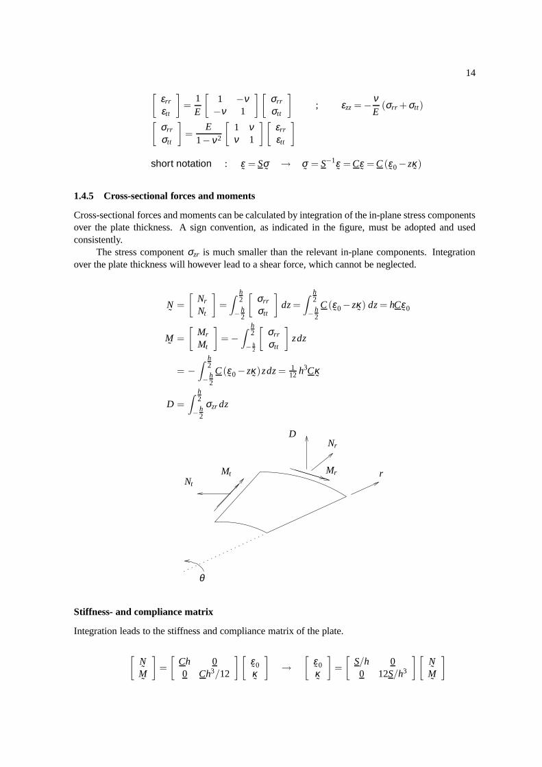
1.4.5 Cross-sectional forces and moments
Cross-sectional forces and moments can be calculated by integration of the in-plane stress componentsover the plate thickness. A sign convention, as indicated inthe figure, must be adopted and usedconsistently.
The stress componentσzr is much smaller than the relevant in-plane components. Integrationover the plate thickness will however lead to a shear force, which cannot be neglected.
N˜
=
[
Nr
Nt
]
=∫
h2
−h2
[
σrr
σtt
]
dz =∫
h2
−h2
C (ε˜0− zκ
˜) dz = hCε
˜0
M˜
=
[
Mr
Mt
]
= −
∫
h2
− h2
[
σrr
σtt
]
zdz
= −
∫
h2
−h2
C (ε˜0− zκ
˜)zdz = 1
12 h3Cκ˜
D =∫
h2
−h2
σzr dz
θ
rMtNt
Mr
DNr
Stiffness- and compliance matrix
Integration leads to the stiffness and compliance matrix ofthe plate.
[
NM̃˜
]
=
[
Ch 00 Ch3/12
][
ε˜0κ˜
]
→
[
ε˜0κ˜
]
=
[
S/h 00 12S/h3
][
NM̃˜
]
15
1.4.6 Equilibrium equations
Consider a small ”column” cut out of the plate perpendicularto its plane. Equilibrium requirements ofthe cross-sectional forces and moments, lead to the equilibrium equations. The cross-sectional shearforceD can be eliminated by combining some of the equilibrium equations.
z
r
Mrrdθ (D + D,r dr) (r + dr)dθ
prdrdθ
dθ
Drdθ (Nr + Nr,rdr) (r + dr)dθ
(Mr + Mr,r dr) (r + dr)dθNrrdθ
Mtdr
MtdrNtdr
Ntdr
Nr,r +1r(Nr −Nt)+ sr = 0
rD,r + D + rp = 0
rMr,r + Mr −Mt − rD = 0
→ rMr,rr +2Mr,r −Mt,r + rp = 0
The equilibrium equation for the cross-sectional bending moments can be transformed into a differ-ential equation for the displacementw. The equation is a fourth-order partial differential equation,which is referred to as a bi-potential equation.
[
Mr
Mt
]
=Eh3
12(1−ν2)
[
1 νν 1
][
−w,rr
−1r w,r
]
rMr,rr +2Mr,r −Mt,r + rp = 0
→
d4wdr4 +
2r
d3wdr3 −
1r2
d2wdr2 +
1r3
dwdr
=pB
→
(
d2
dr2 +1r
ddr
)(
d2wdr2 +
1r
dwdr
)
=pB
B =Eh3
12(1−ν2)= plate modulus
1.4.7 Solution
The differential equation has a general solution comprising four integration constants. Depending onthe external load, a particular solutionwp also remains to be specified. The integration constants have
16
to be determined from the available boundary conditions, i.e. from the prescribed displacements andloads.The cross-sectional forces and moments can be expressed in the displacementw and/or the straincomponents.
w = a1 + a2r2 + a3 ln(r)+ a4r2 ln(r)+ wp
Mr = −B
(
d2wdr2 +
νr
dwdr
)
Mt = −B
(
1r
dwdr
+ νd2wdr2
)
D =dMr
dr+
1r
(Mr −Mt) = −B
(
d3wdr3 +
1r
d2wdr2 −
1r2
dwdr
)
1.4.8 Examples
This section contains some examples of axisymmetric plate bending problems.
• Plate with central hole
• Solid plate with distributed load
• Solid plate with vertical point load
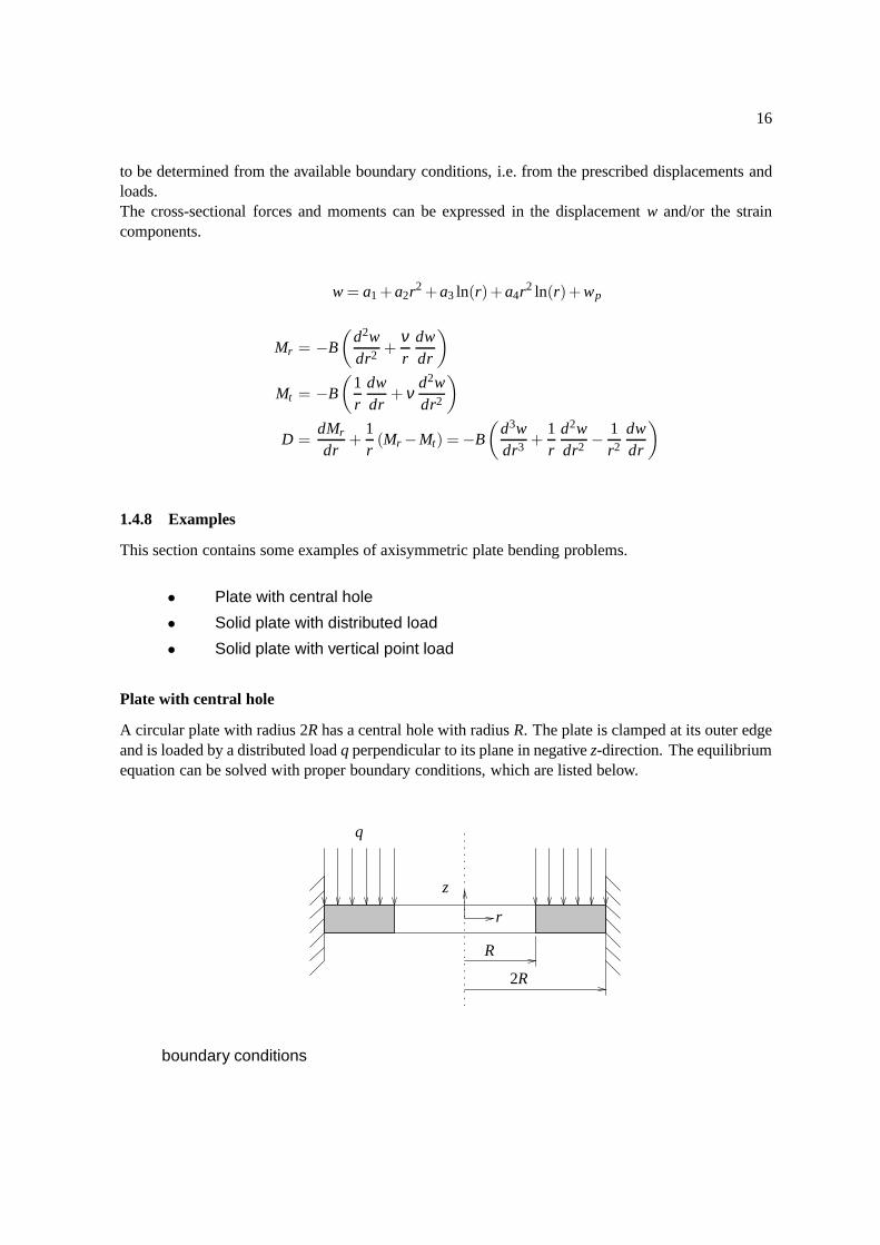
Plate with central hole
A circular plate with radius 2R has a central hole with radiusR. The plate is clamped at its outer edgeand is loaded by a distributed loadq perpendicular to its plane in negativez-direction. The equilibriumequation can be solved with proper boundary conditions, which are listed below.
z
r
R
2R
q
boundary conditions
17
• w(r = 2R) = 0 •
(
dwdr
)
(r = 2R) = 0
• mb(r = R) = Mr(r = R) = 0 • fz(r = R) = D(r = R) = 0
differential equation
d4wdr4 +
2r
d3wdr3 −
1r2
d2wdr2 +
1r3
dwdr
= −qB
general solution w = a1 + a2r2 + a3 ln(r)+ a4r2 ln(r)+ wp
particulate solution wp = αr4 → substitution →
24α +48α −12α +4α = −qB
→ α = −q
64B
solution w = a1 + a2r2 + a3 ln(r)+ a4r2 ln(r)−q
64Br4
The 4 constants in the general solution can be solved using the boundary conditions. For this purposethese have to be elaborated to formulate the proper equations.
dwdr
= 2a2r +a3
r+ a4(2r ln(r)+ r)−
q16B
r3
Mr = −B
(
d2wdr2 +
νr
dwdr
)
= −B
{
2(1+ ν)a2− (1−ν)1r2 a3 +2(1+ ν) ln(r)a4 +(3+ ν)a4− (3+ ν)
q16B
r2}
Mt = −B
(
νd2wdr2 +
1r
dwdr
)
= −B
{
2(1+ ν)a2 +(1−ν)1r2a3 +2(1+ ν) ln(r)a4 +(3ν +1)a4− (3ν +1)
q16B
r2}
D =dMr
dr+
1r
(Mr −Mt)
= B
(
−4r
a4 +q
2Br
)
The equations are summarized below. The 4 constants can be solved.After solving the constants, the vertical displacement at the inner edge of the hole can be calculated.
18
w(r = 2R) = a1 +4a2R2 + a3 ln(R)+4a4R2 ln(R)−q
4BR4 = 0
dwdr
(r = 2R) = 4a2R +1
2Ra3 +4a4R ln(R)+2a4R−
q2B
R3 = 0
Mr(r = R) = −B
{
2(1+ ν)a2− (1−ν)1
R2 a3+
(2(1+ ν) ln(R)+ (3+ ν))a4− (3+ ν)q
16BR2
}
= 0
D(r = R) = B
(
−4R
a4 +q
2BR
}
= 0
w(r = R) = −qR4
64B
{
−9(5+ ν)+48(3+ ν) ln(2)−64(1+ ν)(ln(2))2
5−3ν
}
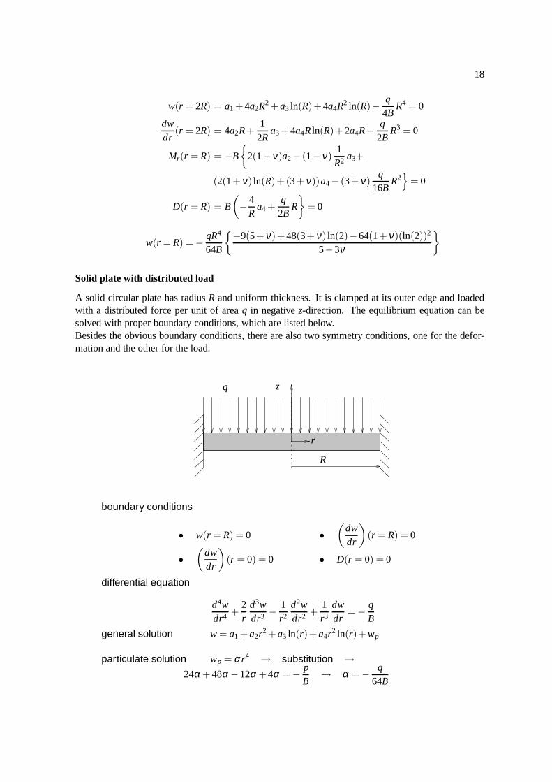
Solid plate with distributed load
A solid circular plate has radiusR and uniform thickness. It is clamped at its outer edge and loadedwith a distributed force per unit of areaq in negativez-direction. The equilibrium equation can besolved with proper boundary conditions, which are listed below.Besides the obvious boundary conditions, there are also twosymmetry conditions, one for the defor-mation and the other for the load.
r
q
R
z
boundary conditions
• w(r = R) = 0 •
(
dwdr
)
(r = R) = 0
•
(
dwdr
)
(r = 0) = 0 • D(r = 0) = 0
differential equation
d4wdr4 +
2r
d3wdr3 −
1r2
d2wdr2 +
1r3
dwdr
= −qB
general solution w = a1 + a2r2 + a3 ln(r)+ a4r2 ln(r)+ wp
particulate solution wp = αr4 → substitution →
24α +48α −12α +4α = −pB
→ α = −q
64B
19
solution w = a1 + a2r2 + a3 ln(r)+ a4r2 ln(r)−q
64Br4
The 4 constants in the general solution can be solved using the boundary and symmetry conditions.For this purpose these have to be elaborated to formulate theproper equations.
The two symmetry conditions result in two constants to be zero. The other two constants can bedetermined from the boundary conditions.
After solving the constants, the vertical displacement atr = 0 can be calculated.
dwdr
= 2a2r +a3
r+ a4(2r ln(r)+ r)−
q16B
r3
D =dMr
dr+
1r
(Mr −Mt)
= B
(
−4r
a4 +q
2Br
)
boundary conditions(
dwdr
)
(r = 0) = 0 → a3 = 0
D(r = 0) = 0 → a4 = 0(
dwdr
)
(r = R) = 2a2R−q
16BR3 = 0 → a2 =
q32B
R2
w(r = R) = a1 + a2R2−q
64BR4 = 0 → a1 = −
q64B
R4
displacement in the center
w(r = 0) = −q
64BR4
Solid plate with vertical point load
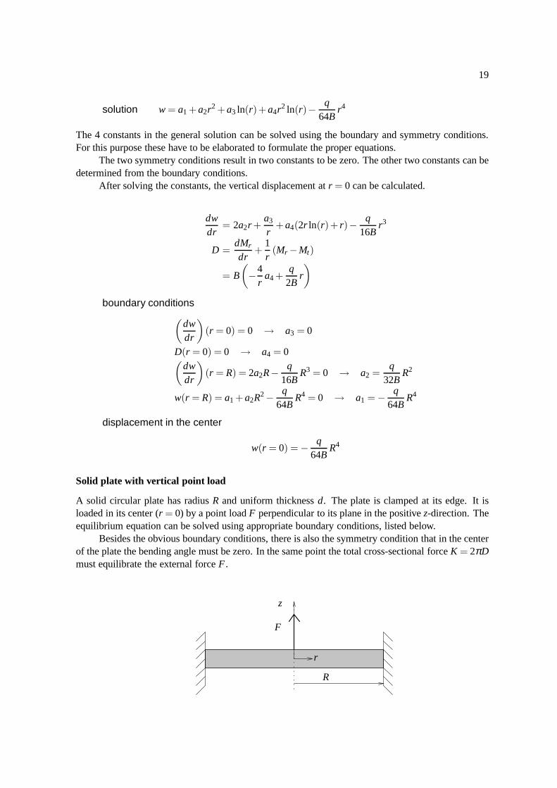
A solid circular plate has radiusR and uniform thicknessd. The plate is clamped at its edge. It isloaded in its center (r = 0) by a point loadF perpendicular to its plane in the positivez-direction. Theequilibrium equation can be solved using appropriate boundary conditions, listed below.
Besides the obvious boundary conditions, there is also the symmetry condition that in the centerof the plate the bending angle must be zero. In the same point the total cross-sectional forceK = 2πDmust equilibrate the external forceF.
r
R
z
F
20
boundary conditions
• w(r = R) = 0 •
(
dwdr
)
(r = R) = 0
•
(
dwdr
)
(r = 0) = 0 • K(r = 0) = −F
differential equation
d4wdr4 +
2r
d3wdr3 −
1r2
d2wdr2 +
1r3
dwdr
= 0
general solution w = a1 + a2r2 + a3 ln(r)+ a4r2 ln(r)
The derivative ofw and the cross-sectional loadD can be written as a function ofr.The symmetry condition results in one integration constantto be zero. Because the derivative of
w is not defined forr = 0, a limit has to be taken. The cross-sectional equilibrium results in a knownvalue for another constant. The remaining constants can be determined from the boundary conditionsat r = R.
After solving the constants, the vertical displacement atr = 0 can be calculated.
dwdr
= 2a2r +a3
r+ a4(2r ln(r)+ r)
D =dMr
dr+
1r
(Mr −Mt) = B
(
−4r
a4
)
boundary conditions
limr→0
(
dwdr
)
= limr→0
{
2a2r +a3
r+ a4(2r ln(r)+ r)
}
= 0 → a3 = 0
K(r) = 2πrD(r) = −8πBa4 = −F → a4 =F
8πB
w(r = R) = a1 + a2R2 +F
8πBR2 ln(R) = 0
(
dwdr
)
(r = R) = 2Ra2 +F
8πB(2R ln(R)+ R) = 0
→
a1 =FR2
16πB
a2 = −F
16πB(2lnR +1)
displacement at the center
w(r = 0) = limr→0
FR2
16πB
{
1−( r
R
)2+2
( rR
)2ln
( rR
)
}
=FR2
16πB
The stresses can also be calculated. They are a function of both coordinatesr andz. We can concludethat at the center, where the force is applied, the stresses become infinite, due to the singularity,provoked by the point load.
21
σrr = −3Fzπd3
{
1+(1+ ν) ln( r
R
)}
σtt = −3Fzπd3
{
ν +(1+ ν) ln( r
R
)}
22
2 Laminates
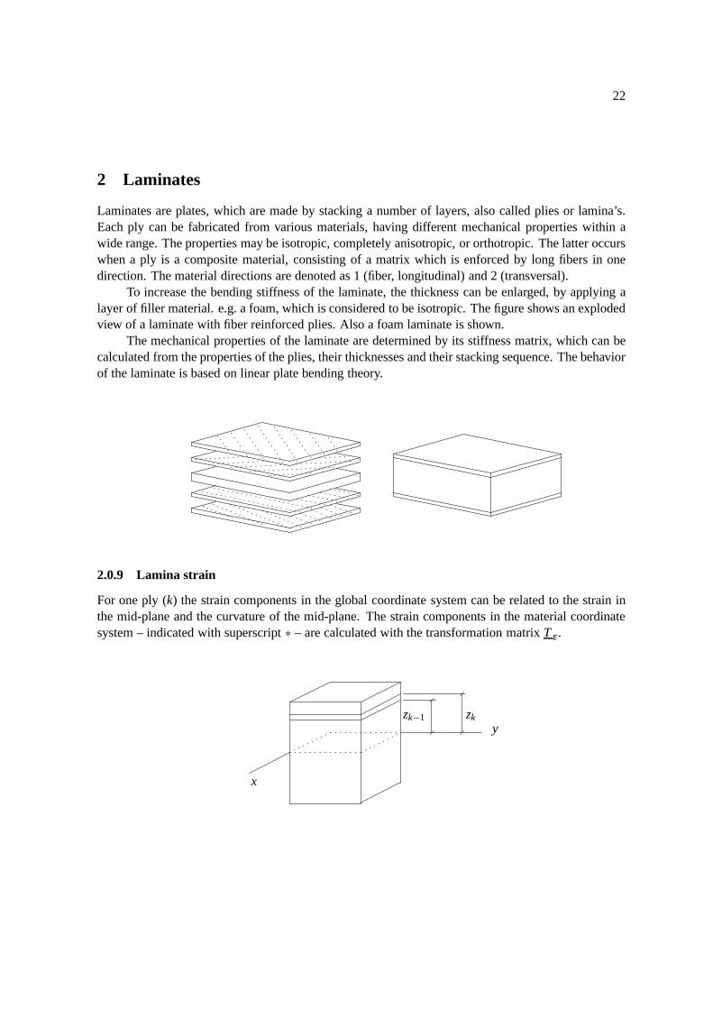
Laminates are plates, which are made by stacking a number of layers, also called plies or lamina’s.Each ply can be fabricated from various materials, having different mechanical properties within awide range. The properties may be isotropic, completely anisotropic, or orthotropic. The latter occurswhen a ply is a composite material, consisting of a matrix which is enforced by long fibers in onedirection. The material directions are denoted as 1 (fiber, longitudinal) and 2 (transversal).
To increase the bending stiffness of the laminate, the thickness can be enlarged, by applying alayer of filler material. e.g. a foam, which is considered to be isotropic. The figure shows an explodedview of a laminate with fiber reinforced plies. Also a foam laminate is shown.
The mechanical properties of the laminate are determined byits stiffness matrix, which can becalculated from the properties of the plies, their thicknesses and their stacking sequence. The behaviorof the laminate is based on linear plate bending theory.
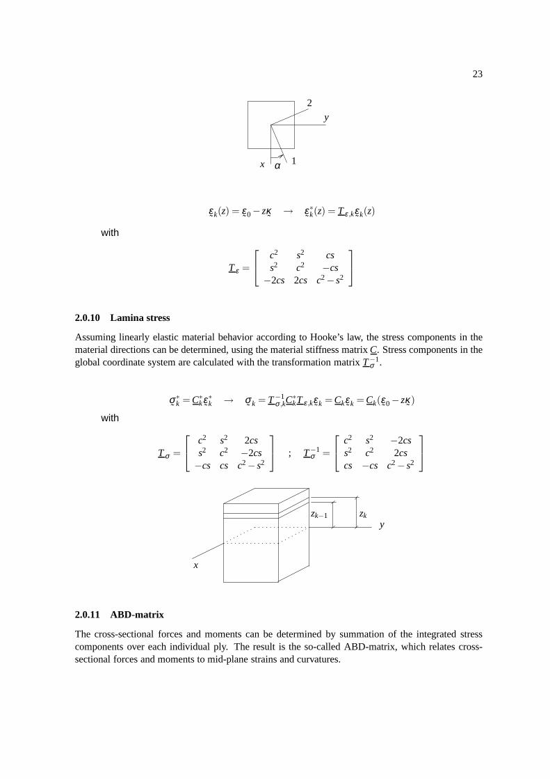
2.0.9 Lamina strain
For one ply (k) the strain components in the global coordinate system can be related to the strain inthe mid-plane and the curvature of the mid-plane. The straincomponents in the material coordinatesystem – indicated with superscript∗ – are calculated with the transformation matrixT ε .
zk−1 zky
x
23
x
y
1
2
α
ε˜k(z) = ε
˜0− zκ˜
→ ε˜∗k(z) = T ε ,kε
˜k(z)
with
T ε =
c2 s2 css2 c2 −cs
−2cs 2cs c2− s2
2.0.10 Lamina stress
Assuming linearly elastic material behavior according to Hooke’s law, the stress components in thematerial directions can be determined, using the material stiffness matrixC. Stress components in theglobal coordinate system are calculated with the transformation matrixT−1
σ .
σ˜∗k = C∗
kε˜∗k → σ
˜ k = T−1σ ,kC
∗kT ε ,kε
˜k = Ckε˜k = Ck(ε˜0− zκ
˜)
with
T σ =
c2 s2 2css2 c2 −2cs−cs cs c2− s2
; T−1σ =
c2 s2 −2css2 c2 2cscs −cs c2− s2
zk−1 zky
x
2.0.11 ABD-matrix
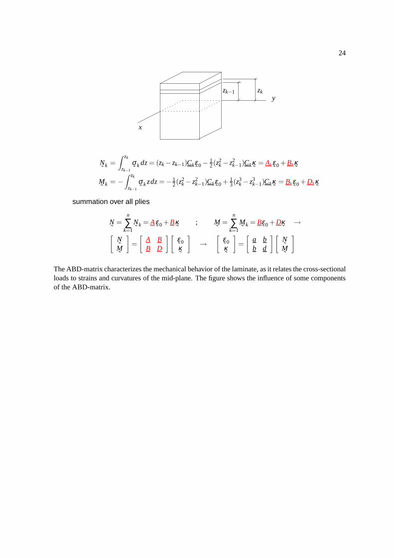
The cross-sectional forces and moments can be determined bysummation of the integrated stresscomponents over each individual ply. The result is the so-called ABD-matrix, which relates cross-sectional forces and moments to mid-plane strains and curvatures.
24
zk−1 zky
x
N˜ k =
∫ zk
zk−1
σ˜ k dz = (zk − zk−1)Ckε
˜0−12(z2
k − z2k−1)Ckκ
˜= Akε
˜0 + Bkκ˜
M˜ k = −
∫ zk
zk−1
σ˜ k zdz = −1
2(z2k − z2
k−1)Ckε˜0 + 1
3(z3k − z3
k−1)Ckκ˜
= Bkε˜0 + Dkκ
˜
summation over all plies
N˜
=n
∑k=1
N˜ k = Aε
˜0 + Bκ˜
; M˜
=n
∑k=1
M˜ k = Bε
˜0 + Dκ˜
→
[
NM̃˜
]
=
[
A BB D
][
ε˜0κ˜
]
→
[
ε˜0κ˜
]
=
[
a bb d
][
NM̃˜
]
The ABD-matrix characterizes the mechanical behavior of the laminate, as it relates the cross-sectionalloads to strains and curvatures of the mid-plane. The figure shows the influence of some componentsof the ABD-matrix.
25
D22 D23
D33
A33
A12 A13
A22 A23
D11
B12 B22 B23
B13
B13
D12 D13
B33B23
A11 B11 B12
2.0.12 Thermal and humidity loading
When the laminate is subjected to a change in temperature, thermal strains will occur due to thermalexpansion. In each ply these strains will generally be different, leading to deformation. Analogously,the laminate can be placed in a humid environment, which alsocauses strains caused by absorption.
The thermal and humidity strains can be calculated in each ply, given its coefficients of thermalexpansion (α1 andα2) and humid driven expansion (β1 andβ2). To calculate stresses these strainsε̂
˜kmust be subtracted from the mechanical strainsε
˜∗k.
The cross-sectional forces and moments are related to the mid-plane strains and curvatures bythe ABD-matrix. The forces caused by thermal and humidity expansion are simply added.
strains in ply k due to temperature change ∆Tk and absorption ck
ε̂11
ε̂22
γ̂12
=
α1
α2
0
∆Tk +
β1
β2
0
ck → ε̂˜∗k = α
˜ k∆Tk + β˜ k
ck
stresses due to thermal(absorption) and mechanical strains ε˜∗k
σ˜∗k = C∗
k(ε˜∗k − ε̂
˜∗k) → σ
˜ k = Ck(ε˜k − ε̂˜k) = Ck(ε˜0− zκ
˜− ε̂
˜k)
forces and moments in ply k :
26
N˜ k =
∫ zk
zk−1
σ˜ k dz = Akε
˜0 + Bkκ˜−Akε̂
˜k → N˜
=n
∑k=1
N˜ k
M˜ k = −
∫ zk
zk−1
σ˜ k zdz = Bkε
˜0 + Dkκ˜−Bkε̂
˜k → M˜
=n
∑k=1
M˜ k
[
NM̃˜
]
=
[
A BB D
][
ε˜0κ˜
]
−
[
N̂˜̂M˜
]
→
[
ε˜0κ˜
]
=
[
a bb d
]{[
NM̃˜
]
+
[
N̂˜̂M˜
]}
2.0.13 Stacking
The fibers in the plies can be oriented randomly, however, mostly a certain orientation relative to theorientation in other plies is chosen, resulting incross-ply, angle-ply andregular angle-ply laminates.Fiber orientation in plies above and under the mid-plane canbe symmetric andanti-symmetric. Theresulting mechanical behavior is related to certain components in the ABD-matrix.
The notation of the ply-orientations is illustrated with the next examples :
[0/0/0/90/90/90/45/..] total stacking and orientation sequence is given[03/902/45/..] total stacking and orientation sequence given; index gives
number of plies[03/902/45/−453]s symmetric laminate
cross-ply • orthotropic plies• material directions = global directions.• A13 = A23 = 0
angle-ply • orthotropic plies• each ply material direction 1 is rotated over αo w.r.t.
global direction x.regular angle-ply • orthotropic plies
• subsequent plies have material direction 1 rotated alter-natingly over αo and −αo w.r.t. the global x-axis.
• even number of plies → A13 = A23 = 0
symmetric • symmetric stacking w.r.t. mid-plane• B = 0
anti-symm. • anti-symmetric stacking w.r.t. mid-plane• D13 = D23 = 0
quasi-isotropic • αk = k πn with k = 1, ..,n (n = number of plies)
Recommendations for laminate stacking
There are no general rules for the number of plies in a laminate, their (mutual) fiber orientation andtheir stacking sequence. For most applications, however, there are some recommendations.
27
• Choose a symmetric laminate.Because B = 0, there is no coupling between forces and curvatures and betweenstrains and moments.
• Minimize material direction differences in subsequent plies.Large differences lead to high inter-laminar shear stresses, which may causedelamination.
• Minimize stiffness differences of subsequent plies.Large difference lead to high inter-laminar shear stresses.
• Avoid neighboring plies with the same orientation.The same orientation results in high inter-laminar shear stresses under thermalloading.
• Ensure negative inter-laminar normal stresses (pressure).Negative stresses (tensile) may lead to delamination.
2.0.14 Damage
Several damage phenomena can occur in a laminate :
• fibre rupture
• fibre buckling
• matrix cracking
• fibre-matrix de-adhesion
• interlaminar delamination
The occurence of these damage phenomena can be monitored with a damage criterion.
Damage : Tsai-Hill
For anisotropic materials the yield criterion of Tsai-Hillis often used. Either tensile (Ti) or compres-sive (Ci) yield limits are used. The shear limit is denoted asS. The yield criterion is used in each plyof the laminate in the material coordinate system.Failure can also occur by exceeding the maximum strain in longitudinal (ε f l) or transversal (ε f t )direction.
Tsai-Hill yield criterion for tensile loading
(
σ211
T 2l
)
−
(
σ11σ22
T 2l
)
+
(
σ222
T 2t
)
+
(
σ212
S2
)
= 1
Tsai-Hill yield criterion for compressive loading
(
σ211
C2l
)
−
(
σ11σ22
C2l
)
+
(
σ222
C2t
)
+
(
σ212
S2
)
= 1
28
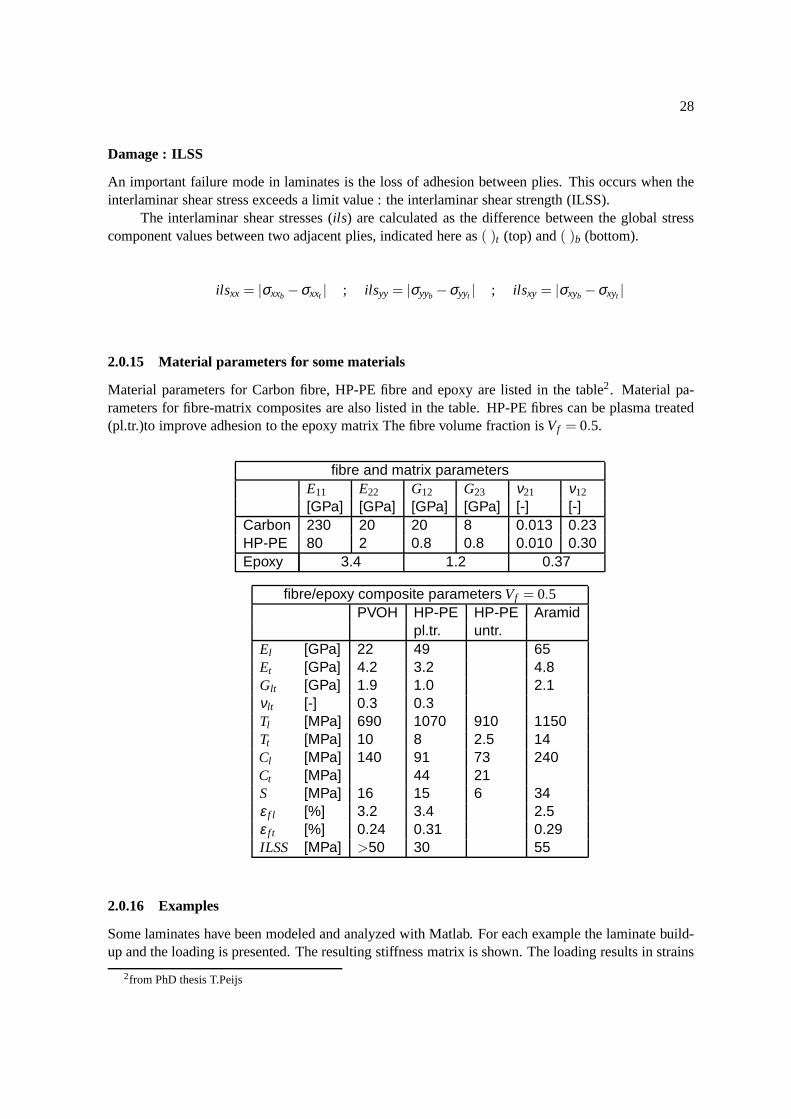
Damage : ILSS
An important failure mode in laminates is the loss of adhesion between plies. This occurs when theinterlaminar shear stress exceeds a limit value : the interlaminar shear strength (ILSS).
The interlaminar shear stresses (ils) are calculated as the difference between the global stresscomponent values between two adjacent plies, indicated here as( )t (top) and( )b (bottom).
ilsxx = |σxxb −σxxt | ; ilsyy = |σyyb −σyyt | ; ilsxy = |σxyb −σxyt |
2.0.15 Material parameters for some materials
Material parameters for Carbon fibre, HP-PE fibre and epoxy are listed in the table2. Material pa-rameters for fibre-matrix composites are also listed in the table. HP-PE fibres can be plasma treated(pl.tr.)to improve adhesion to the epoxy matrix The fibre volume fraction isVf = 0.5.
fibre and matrix parametersE11 E22 G12 G23 ν21 ν12
[GPa] [GPa] [GPa] [GPa] [-] [-]Carbon 230 20 20 8 0.013 0.23HP-PE 80 2 0.8 0.8 0.010 0.30Epoxy 3.4 1.2 0.37
fibre/epoxy composite parameters Vf = 0.5PVOH HP-PE HP-PE Aramid
pl.tr. untr.El [GPa] 22 49 65Et [GPa] 4.2 3.2 4.8Glt [GPa] 1.9 1.0 2.1νlt [-] 0.3 0.3Tl [MPa] 690 1070 910 1150Tt [MPa] 10 8 2.5 14Cl [MPa] 140 91 73 240Ct [MPa] 44 21S [MPa] 16 15 6 34ε f l [%] 3.2 3.4 2.5ε f t [%] 0.24 0.31 0.29ILSS [MPa] >50 30 55
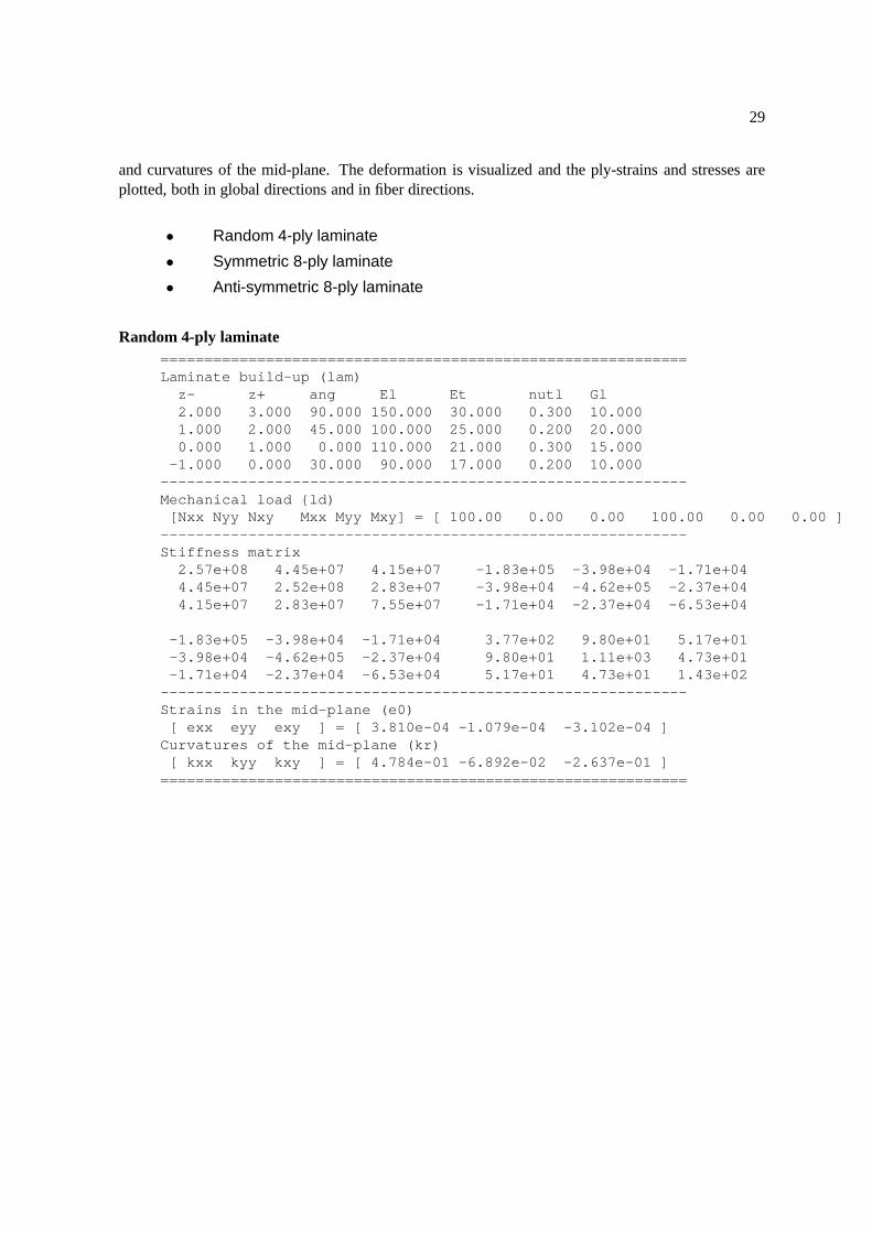
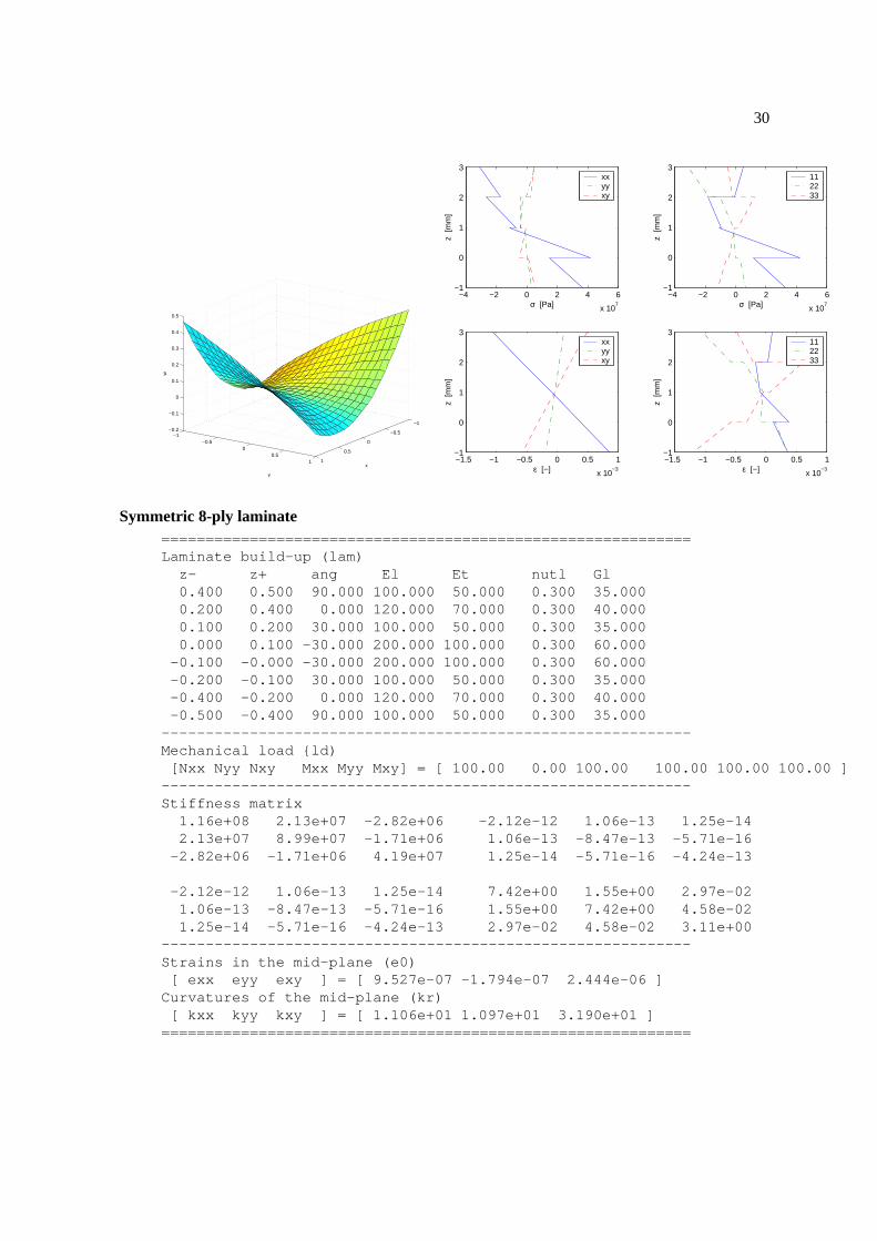
2.0.16 Examples
Some laminates have been modeled and analyzed with Matlab. For each example the laminate build-up and the loading is presented. The resulting stiffness matrix is shown. The loading results in strains
2from PhD thesis T.Peijs
29
and curvatures of the mid-plane. The deformation is visualized and the ply-strains and stresses areplotted, both in global directions and in fiber directions.
• Random 4-ply laminate
• Symmetric 8-ply laminate
• Anti-symmetric 8-ply laminate
Random 4-ply laminate============================================================Laminate build-up (lam)
z- z+ ang El Et nutl Gl2.000 3.000 90.000 150.000 30.000 0.300 10.0001.000 2.000 45.000 100.000 25.000 0.200 20.0000.000 1.000 0.000 110.000 21.000 0.300 15.000
-1.000 0.000 30.000 90.000 17.000 0.200 10.000------------------------------------------------------------Mechanical load {ld)[Nxx Nyy Nxy Mxx Myy Mxy] = [ 100.00 0.00 0.00 100.00 0.00 0.00 ]
------------------------------------------------------------Stiffness matrix
2.57e+08 4.45e+07 4.15e+07 -1.83e+05 -3.98e+04 -1.71e+044.45e+07 2.52e+08 2.83e+07 -3.98e+04 -4.62e+05 -2.37e+044.15e+07 2.83e+07 7.55e+07 -1.71e+04 -2.37e+04 -6.53e+04
-1.83e+05 -3.98e+04 -1.71e+04 3.77e+02 9.80e+01 5.17e+01-3.98e+04 -4.62e+05 -2.37e+04 9.80e+01 1.11e+03 4.73e+01-1.71e+04 -2.37e+04 -6.53e+04 5.17e+01 4.73e+01 1.43e+02
------------------------------------------------------------Strains in the mid-plane (e0)[ exx eyy exy ] = [ 3.810e-04 -1.079e-04 -3.102e-04 ]
Curvatures of the mid-plane (kr)[ kxx kyy kxy ] = [ 4.784e-01 -6.892e-02 -2.637e-01 ]
============================================================
30
−1
−0.5
0
0.5
1
−1−0.5
00.5
1
−0.2
−0.1
0
0.1
0.2
0.3
0.4
0.5
x
y
w
−4 −2 0 2 4 6
x 107
−1
0
1
2
3
z [m
m]
σ [Pa]
xxyyxy
−4 −2 0 2 4 6
x 107
−1
0
1
2
3
z [m
m]
σ [Pa]
112233
−1.5 −1 −0.5 0 0.5 1
x 10−3
−1
0
1
2
3
z [m
m]
ε [−]
xxyyxy
−1.5 −1 −0.5 0 0.5 1
x 10−3
−1
0
1
2
3
z [m
m]
ε [−]
112233
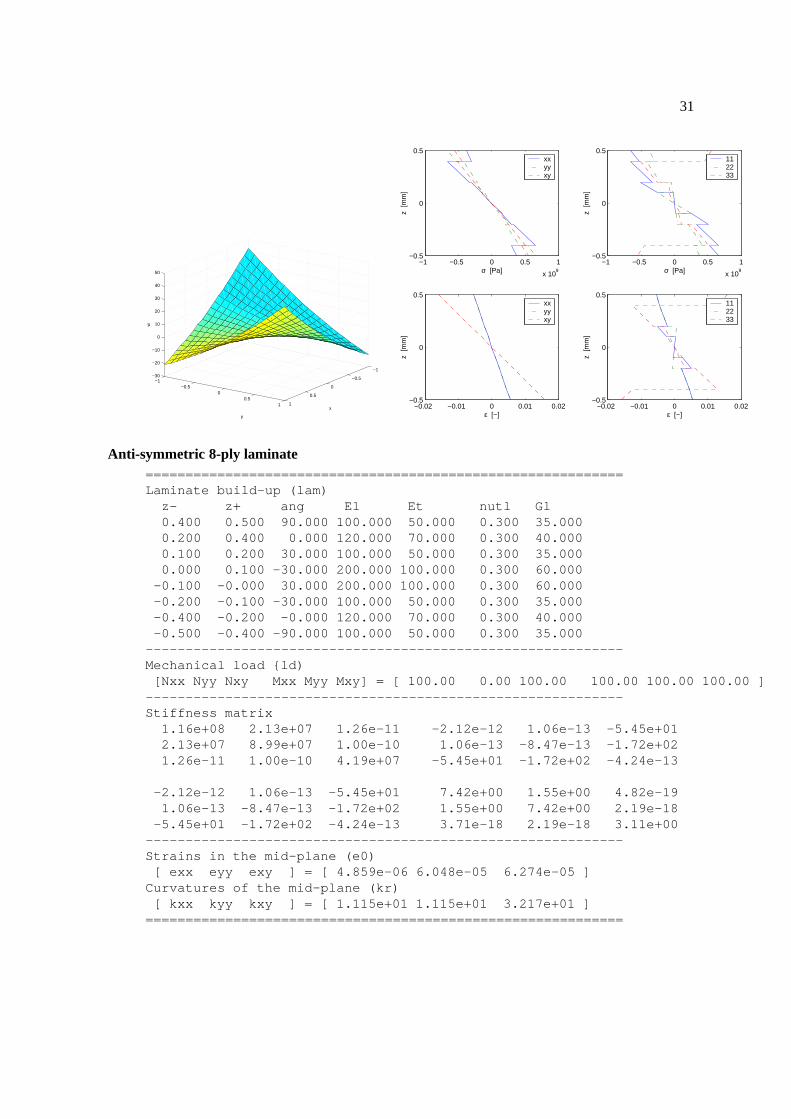
Symmetric 8-ply laminate============================================================Laminate build-up (lam)
z- z+ ang El Et nutl Gl0.400 0.500 90.000 100.000 50.000 0.300 35.0000.200 0.400 0.000 120.000 70.000 0.300 40.0000.100 0.200 30.000 100.000 50.000 0.300 35.0000.000 0.100 -30.000 200.000 100.000 0.300 60.000
-0.100 -0.000 -30.000 200.000 100.000 0.300 60.000-0.200 -0.100 30.000 100.000 50.000 0.300 35.000-0.400 -0.200 0.000 120.000 70.000 0.300 40.000-0.500 -0.400 90.000 100.000 50.000 0.300 35.000
------------------------------------------------------------Mechanical load {ld)[Nxx Nyy Nxy Mxx Myy Mxy] = [ 100.00 0.00 100.00 100.00 100.00 100.00 ]
------------------------------------------------------------Stiffness matrix
1.16e+08 2.13e+07 -2.82e+06 -2.12e-12 1.06e-13 1.25e-142.13e+07 8.99e+07 -1.71e+06 1.06e-13 -8.47e-13 -5.71e-16
-2.82e+06 -1.71e+06 4.19e+07 1.25e-14 -5.71e-16 -4.24e-13
-2.12e-12 1.06e-13 1.25e-14 7.42e+00 1.55e+00 2.97e-021.06e-13 -8.47e-13 -5.71e-16 1.55e+00 7.42e+00 4.58e-021.25e-14 -5.71e-16 -4.24e-13 2.97e-02 4.58e-02 3.11e+00
------------------------------------------------------------Strains in the mid-plane (e0)[ exx eyy exy ] = [ 9.527e-07 -1.794e-07 2.444e-06 ]
Curvatures of the mid-plane (kr)[ kxx kyy kxy ] = [ 1.106e+01 1.097e+01 3.190e+01 ]
============================================================
31
−1
−0.5
0
0.5
1
−1−0.5
00.5
1
−30
−20
−10
0
10
20
30
40
50
x
y
w
−1 −0.5 0 0.5 1
x 109
−0.5
0
0.5
z [m
m]
σ [Pa]
xxyyxy
−1 −0.5 0 0.5 1
x 109
−0.5
0
0.5
z [m
m]
σ [Pa]
112233
−0.02 −0.01 0 0.01 0.02−0.5
0
0.5
z [m
m]
ε [−]
xxyyxy
−0.02 −0.01 0 0.01 0.02−0.5
0
0.5
z [m
m]
ε [−]
112233
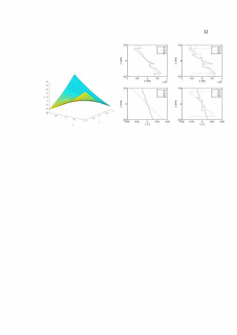
Anti-symmetric 8-ply laminate============================================================Laminate build-up (lam)
z- z+ ang El Et nutl Gl0.400 0.500 90.000 100.000 50.000 0.300 35.0000.200 0.400 0.000 120.000 70.000 0.300 40.0000.100 0.200 30.000 100.000 50.000 0.300 35.0000.000 0.100 -30.000 200.000 100.000 0.300 60.000
-0.100 -0.000 30.000 200.000 100.000 0.300 60.000-0.200 -0.100 -30.000 100.000 50.000 0.300 35.000-0.400 -0.200 -0.000 120.000 70.000 0.300 40.000-0.500 -0.400 -90.000 100.000 50.000 0.300 35.000
------------------------------------------------------------Mechanical load {ld)[Nxx Nyy Nxy Mxx Myy Mxy] = [ 100.00 0.00 100.00 100.00 100.00 100.00 ]
------------------------------------------------------------Stiffness matrix
1.16e+08 2.13e+07 1.26e-11 -2.12e-12 1.06e-13 -5.45e+012.13e+07 8.99e+07 1.00e-10 1.06e-13 -8.47e-13 -1.72e+021.26e-11 1.00e-10 4.19e+07 -5.45e+01 -1.72e+02 -4.24e-13
-2.12e-12 1.06e-13 -5.45e+01 7.42e+00 1.55e+00 4.82e-191.06e-13 -8.47e-13 -1.72e+02 1.55e+00 7.42e+00 2.19e-18
-5.45e+01 -1.72e+02 -4.24e-13 3.71e-18 2.19e-18 3.11e+00------------------------------------------------------------Strains in the mid-plane (e0)[ exx eyy exy ] = [ 4.859e-06 6.048e-05 6.274e-05 ]
Curvatures of the mid-plane (kr)[ kxx kyy kxy ] = [ 1.115e+01 1.115e+01 3.217e+01 ]
============================================================
32
−1
−0.5
0
0.5
1
−1−0.5
00.5
1
−30
−20
−10
0
10
20
30
40
50
x
y
w
−1 −0.5 0 0.5 1
x 109
−0.5
0
0.5
z [m
m]
σ [Pa]
xxyyxy
−1 −0.5 0 0.5 1
x 109
−0.5
0
0.5
z [m
m]
σ [Pa]
112233
−0.02 −0.01 0 0.01 0.02−0.5
0
0.5
z [m
m]
ε [−]
xxyyxy
−0.02 −0.01 0 0.01 0.02−0.5
0
0.5
z [m
m]
ε [−]
112233
![Índicegeneral - uncornominan láminas planas, placas o losas, mientras que cuando las superficies son ... se emplean en cursos sobre placas y cáscaras incluyen Ugural [12], Billington](https://img.pdfslide.tips/doc/110x75/5e9e004041706a353935bfc7/ndicegeneral-nominan-lminas-planas-placas-o-losas-mientras-que-cuando-las.jpg)