POLAR DECOMPOSITIONOF SQUARE MATRICES

SHIZUO KAJI (YAMAGUCHI UNIVERSITY / JST PRESTO)

「情報セキュリティにおける数学的方法とその実践」2016年12月21日 北海道大学

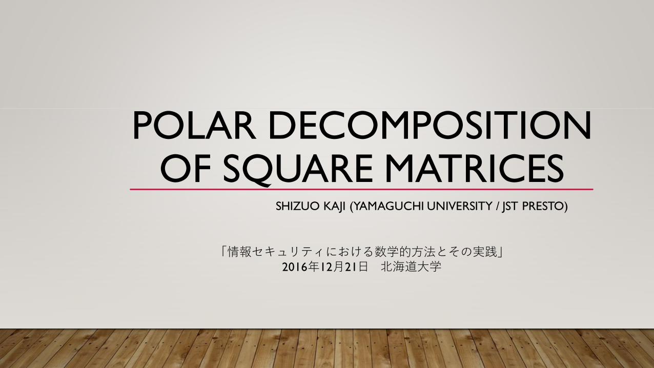
WHAT IS POLAR DECOMPOSITION?

can be decomposed uniquely as where

: Lie group can be decomposed uniquely as

Similarly,

where

maximal compact

: contractible

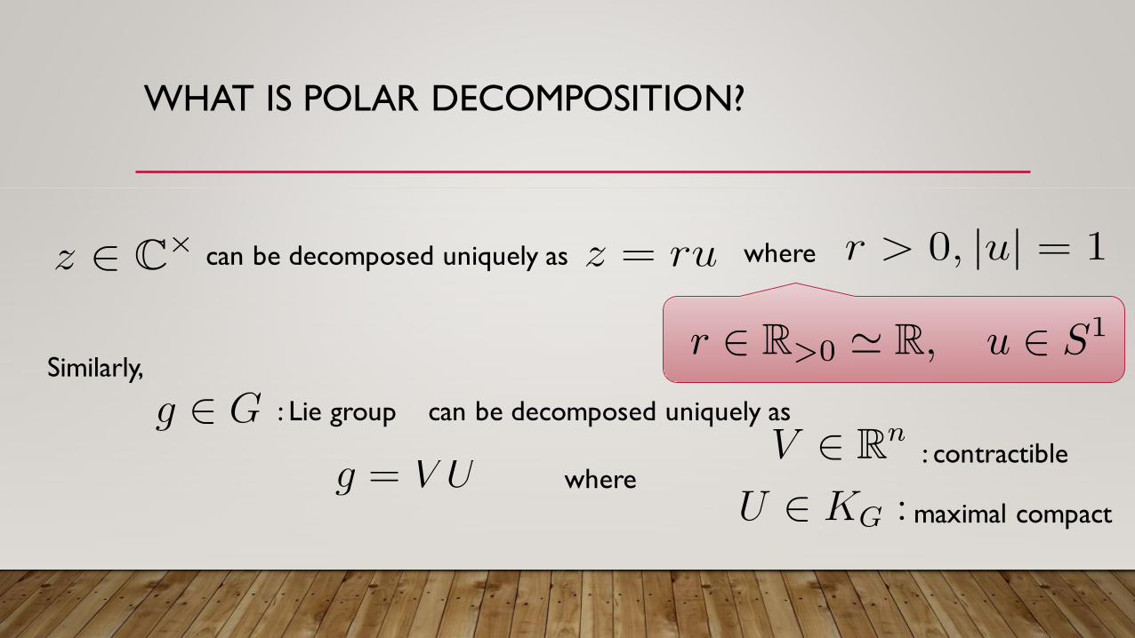
POLAR DECOMPOSITION OF A MATRIX

We focus on G=GL(n, R): the group of real nxn-invertible matrices

where symmetric positive definite matrix

orthogonal matrix

V: positive definite xTVx>0 for any x ≠ 0

UTU=E

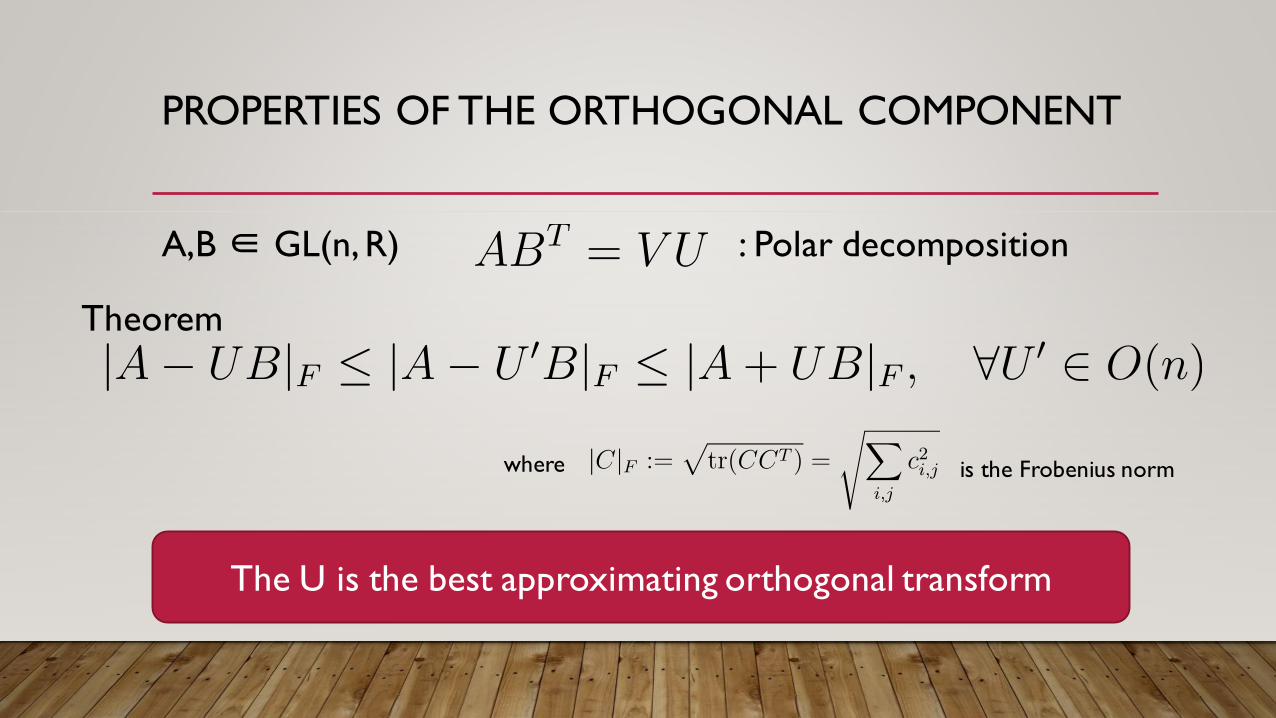
PROPERTIES OF THE ORTHOGONAL COMPONENT

A,B ∈ GL(n, R) : Polar decomposition

Theorem

The U is the best approximating orthogonal transform

where is the Frobenius norm

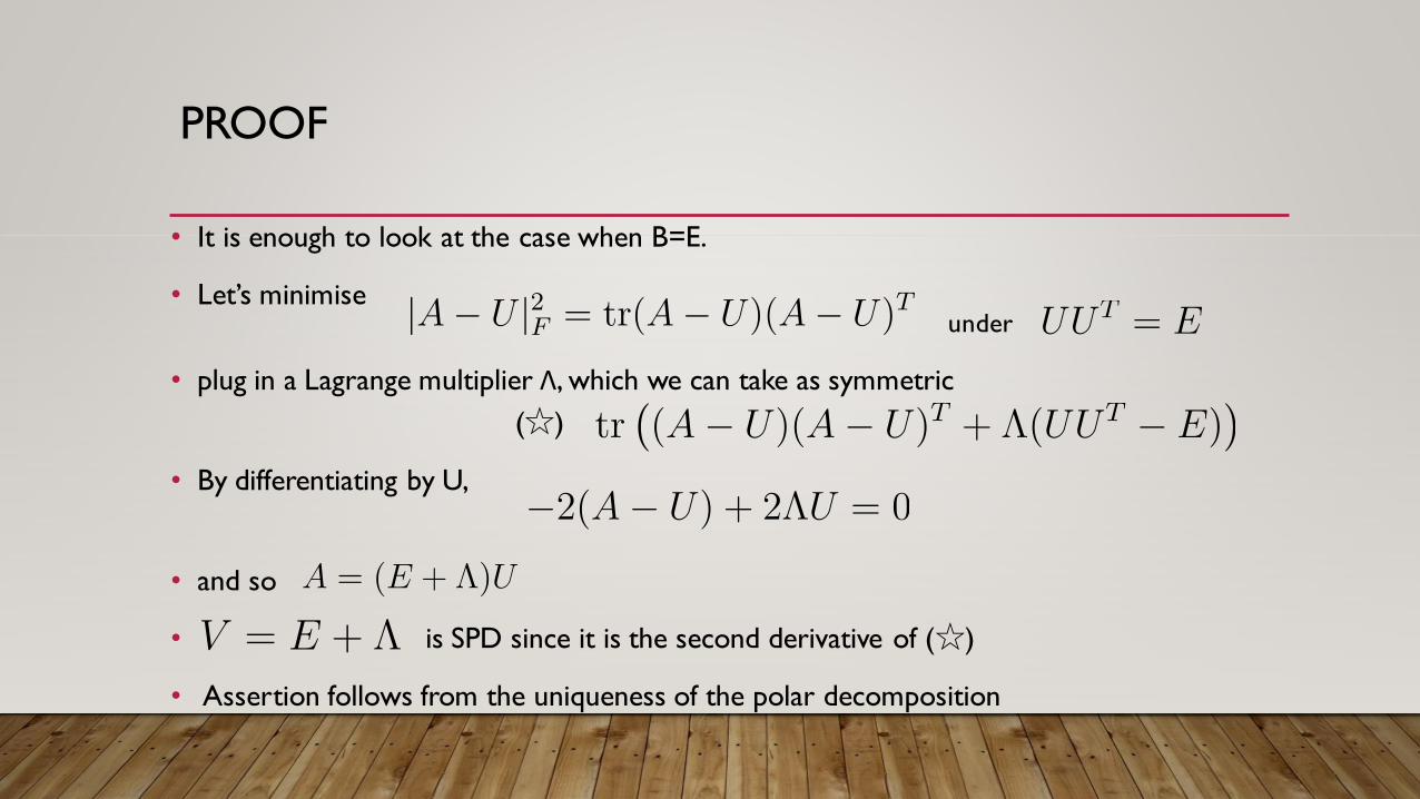
PROOF

• It is enough to look at the case when B=E.

• Let’s minimise

• plug in a Lagrange multiplier Λ, which we can take as symmetric

(☆)

• By differentiating by U,

• and so

• is SPD since it is the second derivative of (☆)

• Assertion follows from the uniqueness of the polar decomposition

under

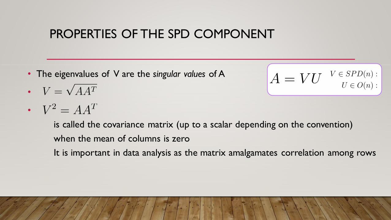
PROPERTIES OF THE SPD COMPONENT

• The eigenvalues of V are the singular values of A

•

•

is called the covariance matrix (up to a scalar depending on the convention)

when the mean of columns is zero

It is important in data analysis as the matrix amalgamates correlation among rows

TWO REMARKS

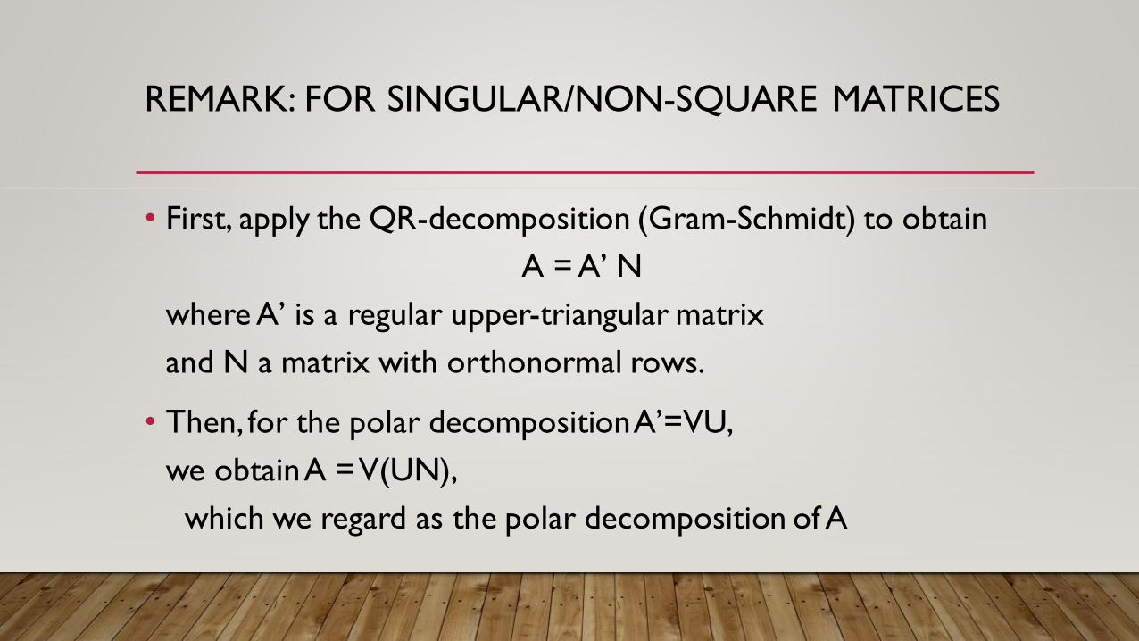
REMARK: FOR SINGULAR/NON-SQUARE MATRICES

• First, apply the QR-decomposition (Gram-Schmidt) to obtain

A = A’ N

where A’ is a regular upper-triangular matrix

and N a matrix with orthonormal rows.

• Then, for the polar decomposition A’=VU,

we obtain A = V(UN),

which we regard as the polar decomposition of A

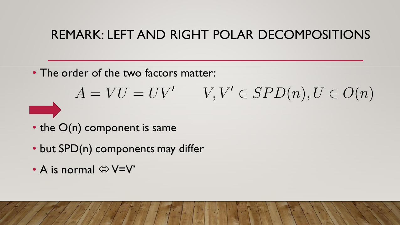
REMARK: LEFT AND RIGHT POLAR DECOMPOSITIONS

• The order of the two factors matter:

• the O(n) component is same

• but SPD(n) components may differ

• A is normal V=V’

APPLICATIONS IN DATA ANALYSIS

WHITENING

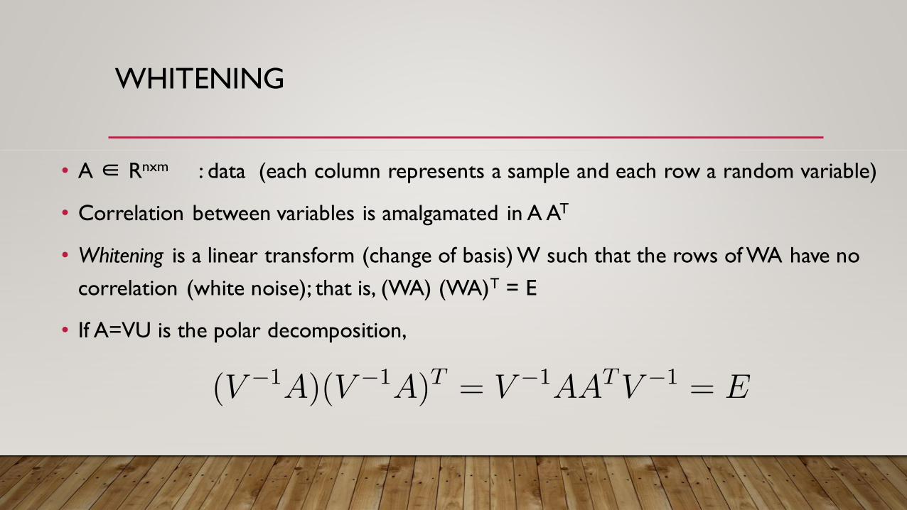
• A ∈ Rnxm : data (each column represents a sample and each row a random variable)

• Correlation between variables is amalgamated in A AT

• Whitening is a linear transform (change of basis) W such that the rows of WA have no

correlation (white noise); that is, (WA) (WA)T = E

• If A=VU is the polar decomposition,

DATA ALIGNMENT

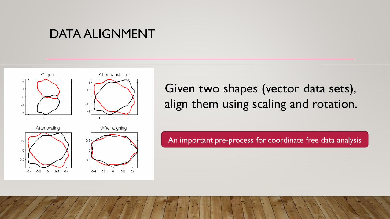
Given two shapes (vector data sets),

align them using scaling and rotation.

An important pre-process for coordinate free data analysis

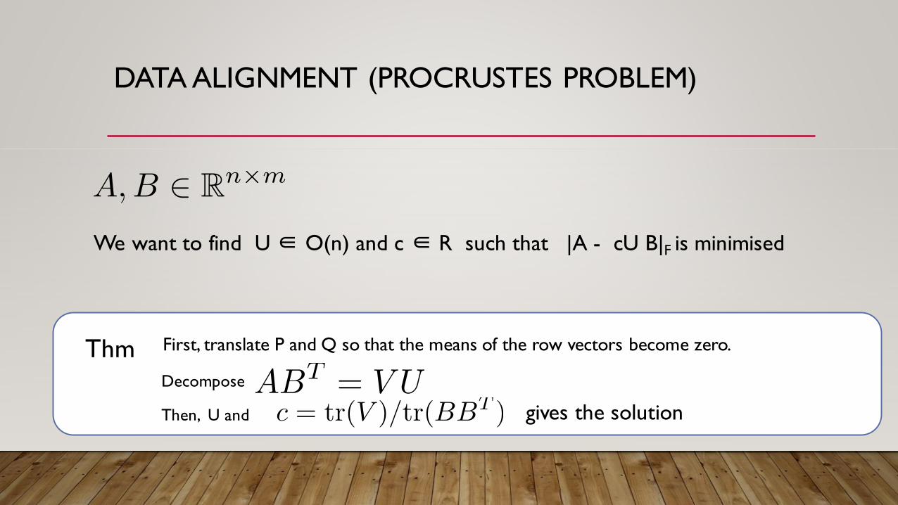
DATA ALIGNMENT (PROCRUSTES PROBLEM)

We want to find U ∈ O(n) and c ∈ R such that |A - cU B|F is minimised

ThmDecompose

Then, U and

First, translate P and Q so that the means of the row vectors become zero.

gives the solution

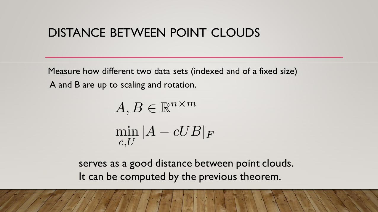
DISTANCE BETWEEN POINT CLOUDS

Measure how different two data sets (indexed and of a fixed size)

A and B are up to scaling and rotation.

serves as a good distance between point clouds.

It can be computed by the previous theorem.

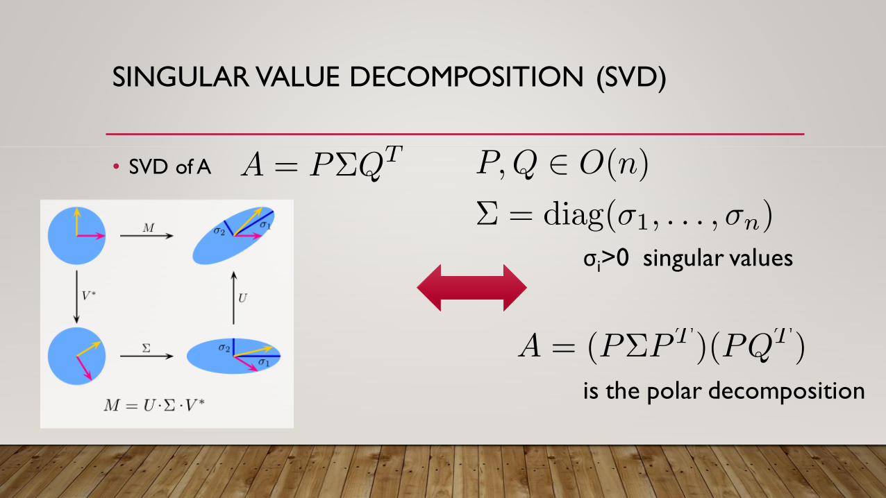
SINGULAR VALUE DECOMPOSITION (SVD)

• SVD of A

σi>0 singular values

is the polar decomposition

APPLICATIONS OF SVD

• pseudo inverse

Ax=b => A+b is the least norm solution when there is a solution

x=A+b minimises |Ax-b|2 when there is no solution

(least square solution)

• matrix approximation by low rank matrix: (equivalent to PCA)setting lower singular values to zero, one obtains the best approximation

in terms of the Frobenius normAQ=PΣ gives the

components

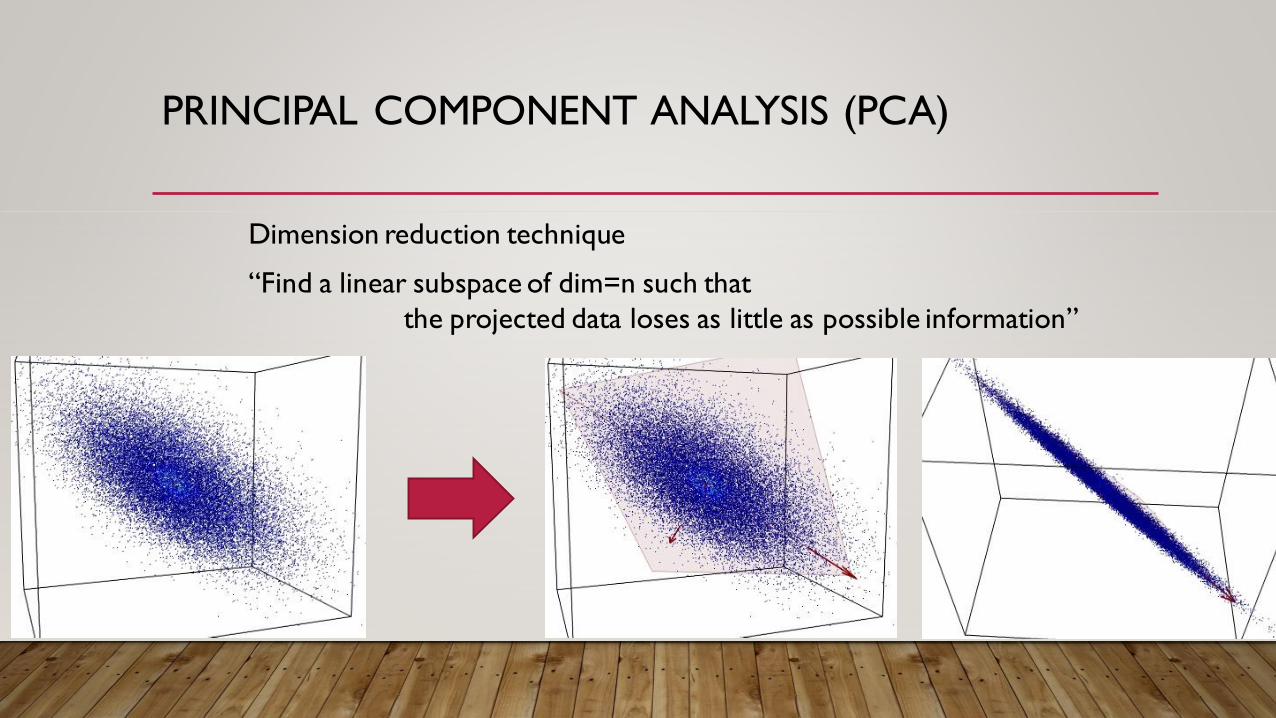
PRINCIPAL COMPONENT ANALYSIS (PCA)

Dimension reduction technique

“Find a linear subspace of dim=n such that

the projected data loses as little as possible information”

COMPUTATION OF POLAR DECOMPOSITION

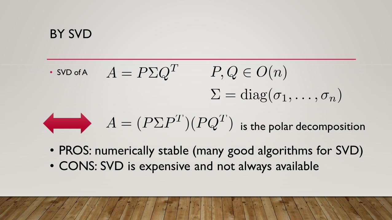
BY SVD

• SVD of A

is the polar decomposition

• PROS: numerically stable (many good algorithms for SVD)

• CONS: SVD is expensive and not always available

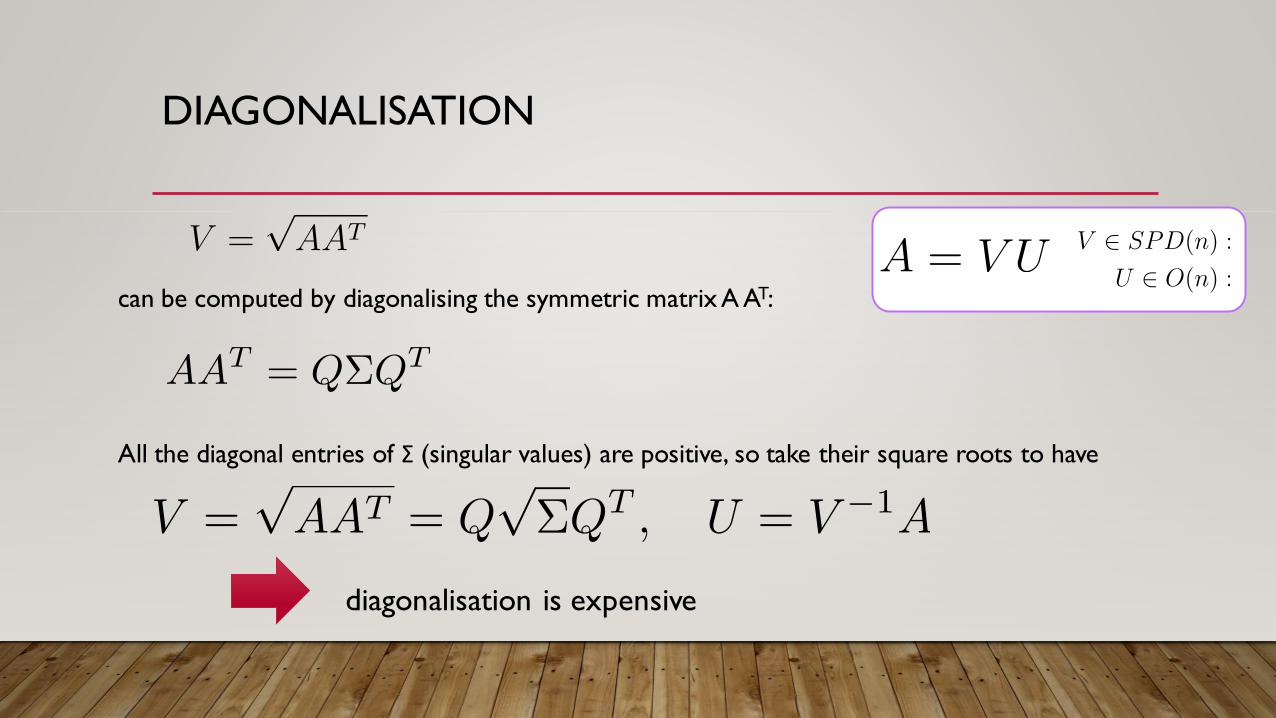
DIAGONALISATION

can be computed by diagonalising the symmetric matrix A AT:

All the diagonal entries of Σ (singular values) are positive, so take their square roots to have

diagonalisation is expensive

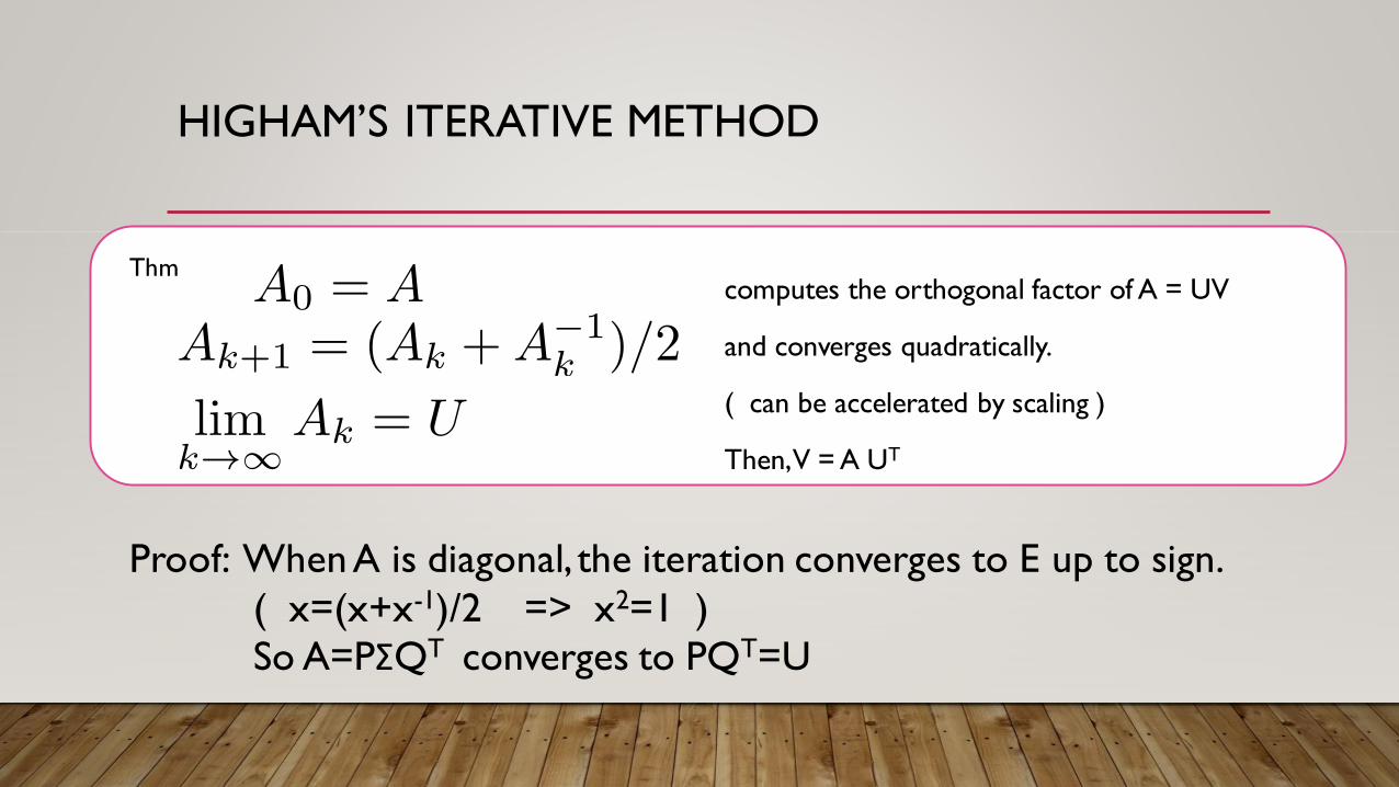
HIGHAM’S ITERATIVE METHOD

computes the orthogonal factor of A = UV

and converges quadratically.

( can be accelerated by scaling )

Then, V = A UT

Thm

Proof: When A is diagonal, the iteration converges to E up to sign.

( x=(x+x-1)/2 => x2=1 )

So A=PΣQT converges to PQT=U

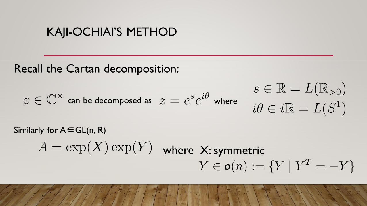
KAJI-OCHIAI’S METHOD

Recall the Cartan decomposition:

can be decomposed as where

Similarly for A∈GL(n, R)

where X: symmetric

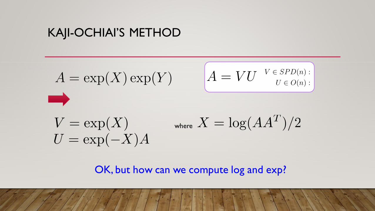
KAJI-OCHIAI’S METHOD

where

OK, but how can we compute log and exp?

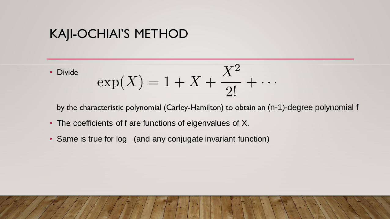
KAJI-OCHIAI’S METHOD

• Divide

by the characteristic polynomial (Carley-Hamilton) to obtain an (n-1)-degree polynomial f

• The coefficients of f are functions of eigenvalues of X.

• Same is true for log (and any conjugate invariant function)

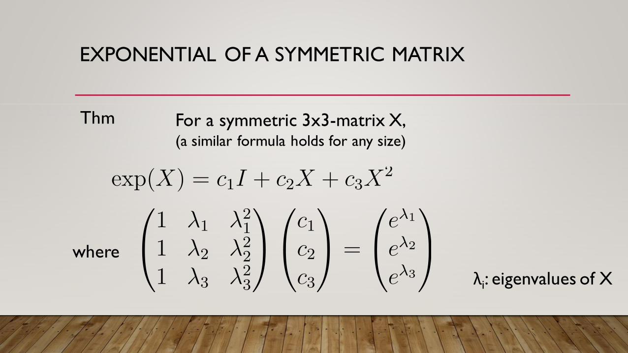
EXPONENTIAL OF A SYMMETRIC MATRIX

Thm

where

For a symmetric 3x3-matrix X,(a similar formula holds for any size)

λi: eigenvalues of X

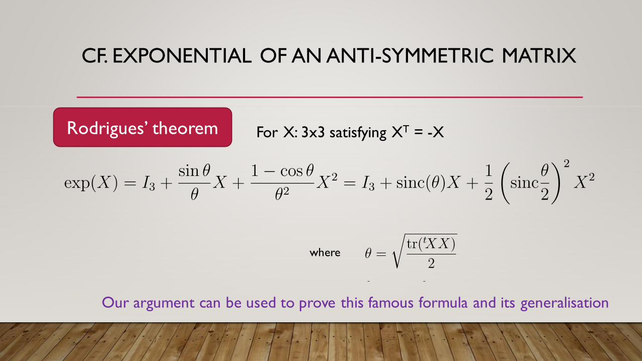
CF. EXPONENTIAL OF AN ANTI-SYMMETRIC MATRIX

For X: 3x3 satisfying XT = -XRodrigues’ theorem

where

Our argument can be used to prove this famous formula and its generalisation

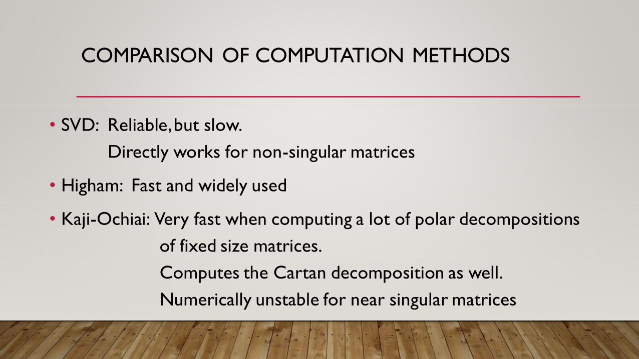
COMPARISON OF COMPUTATION METHODS

• SVD: Reliable, but slow.

Directly works for non-singular matrices

• Higham: Fast and widely used

• Kaji-Ochiai: Very fast when computing a lot of polar decompositions

of fixed size matrices.

Computes the Cartan decomposition as well.

Numerically unstable for near singular matrices

CODES

MIT licensed C++ codes are available at

https://github.com/shizuo-kaji/AffineLib

which contain all four algorithms and more

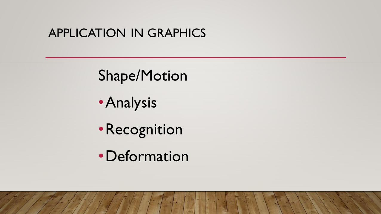
APPLICATION IN GRAPHICS

Shape/Motion

•Analysis

•Recognition

•Deformation

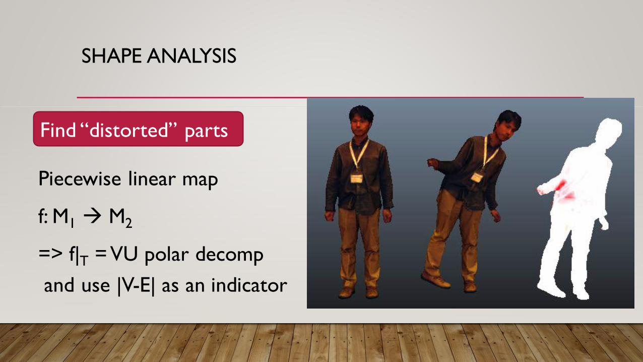
SHAPE ANALYSIS

Piecewise linear map

f: M1 M2

=> f|T = VU polar decomp

and use |V-E| as an indicator

Find “distorted” parts

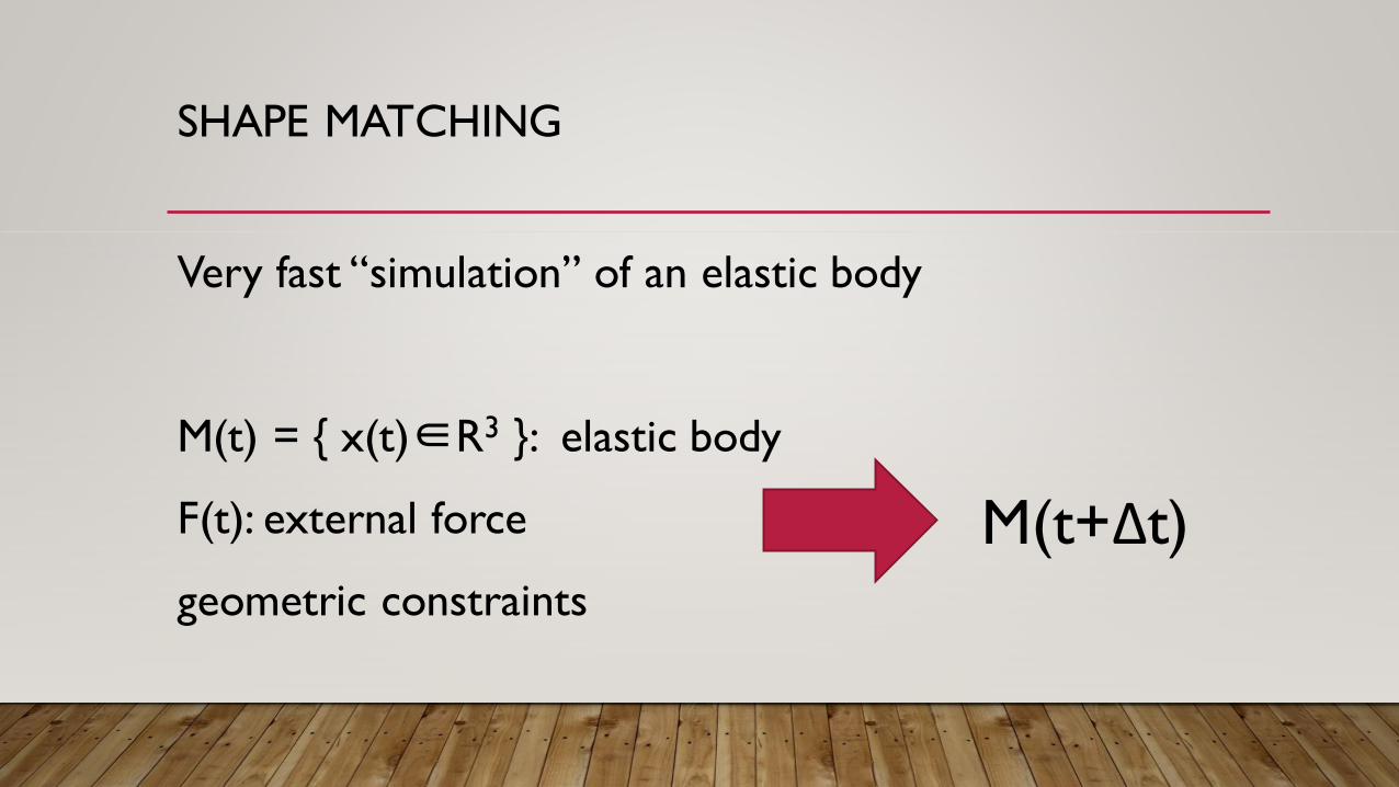
SHAPE MATCHING

Very fast “simulation” of an elastic body

M(t) = { x(t)∈R3 }: elastic body

F(t): external force

geometric constraints

M(t+Δt)

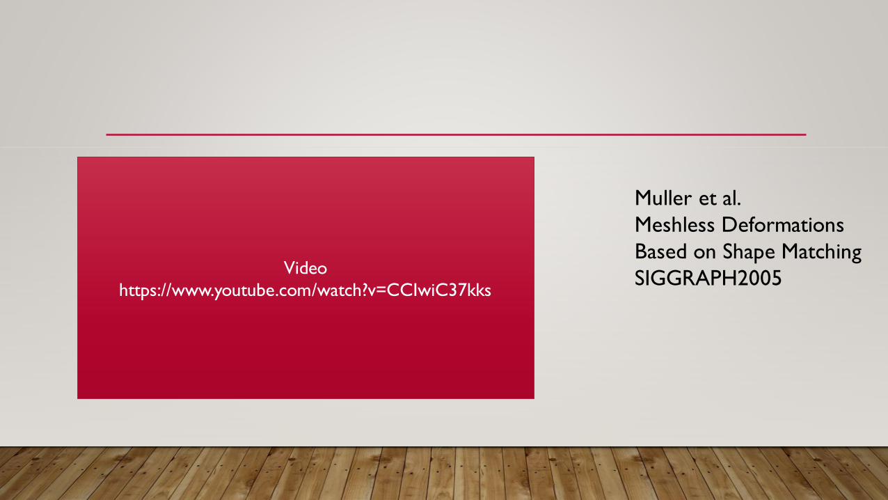
Muller et al.

Meshless Deformations

Based on Shape Matching

SIGGRAPH2005 Video

https://www.youtube.com/watch?v=CCIwiC37kks

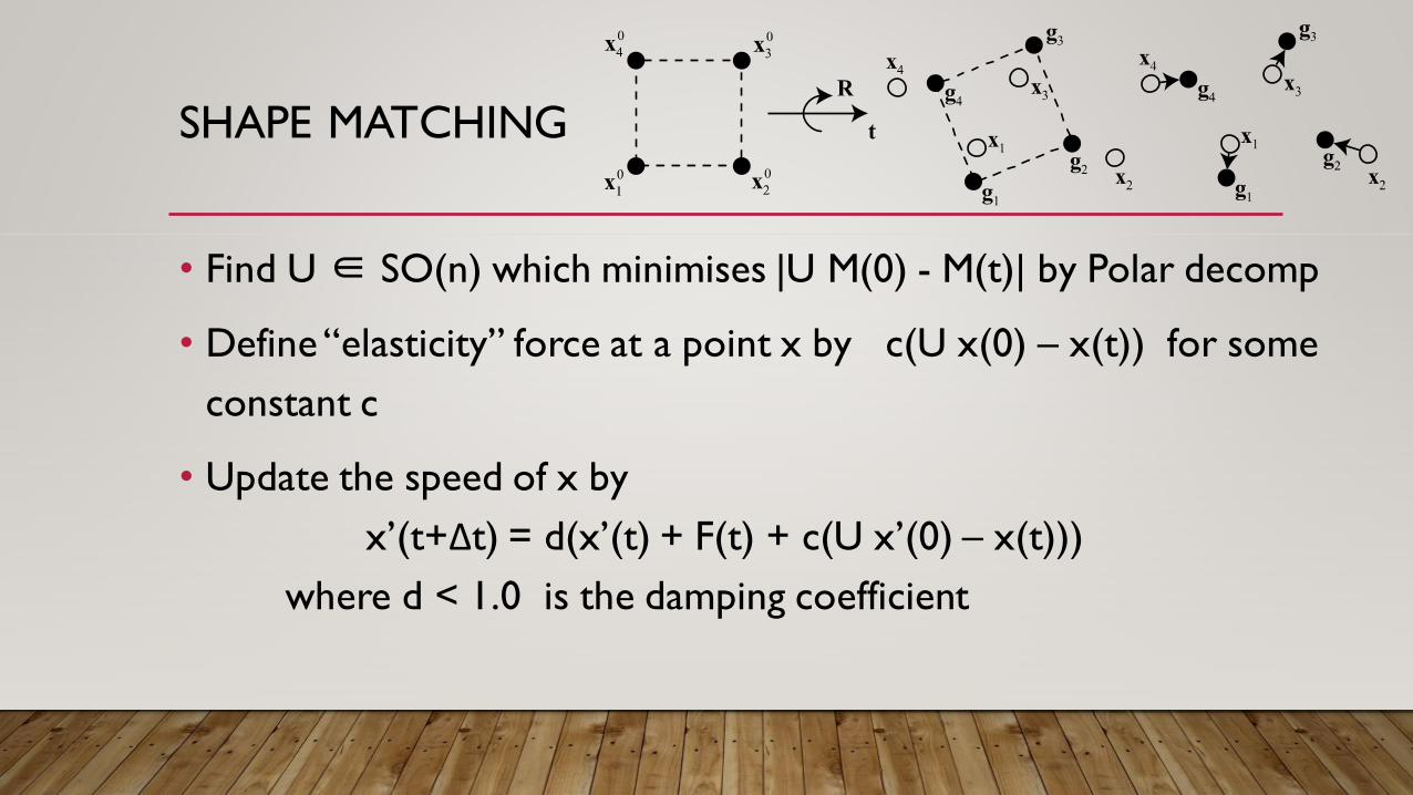
SHAPE MATCHING

• Find U ∈ SO(n) which minimises |U M(0) - M(t)| by Polar decomp

• Define “elasticity” force at a point x by c(U x(0) – x(t)) for some

constant c

• Update the speed of x by

x’(t+Δt) = d(x’(t) + F(t) + c(U x’(0) – x(t)))

where d < 1.0 is the damping coefficient

shape + user interaction => deformed shape

？

SHAPE MODELLING

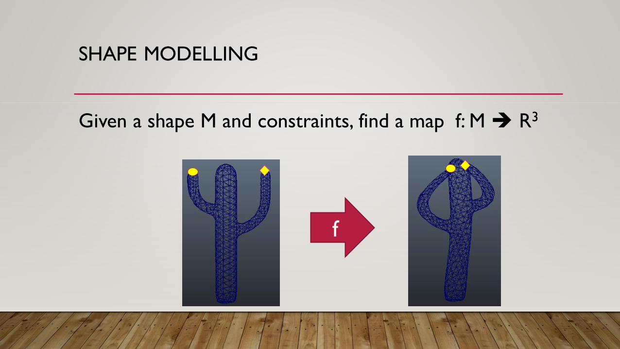
SHAPE MODELLING

Given a shape M and constraints, find a map f: M R3

f

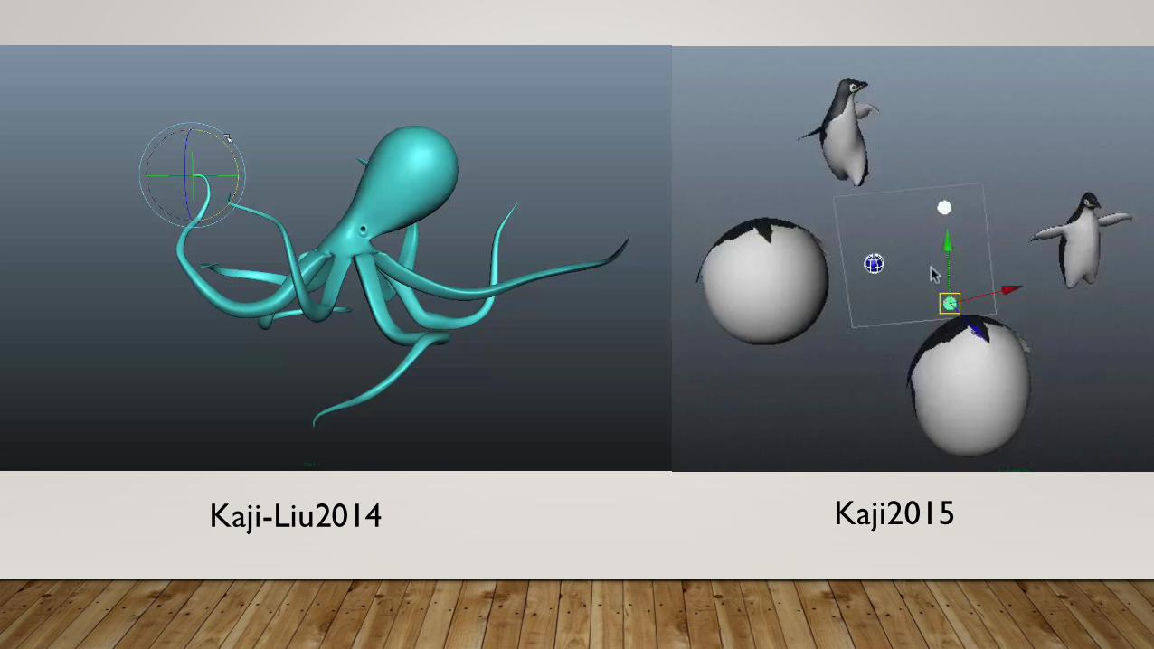
Kaji-Liu2014 Kaji2015

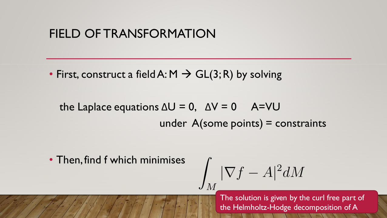
FIELD OF TRANSFORMATION

• First, construct a field A: M GL(3; R) by solving

the Laplace equations ΔU = 0, ΔV = 0 A=VU

under A(some points) = constraints

• Then, find f which minimises

The solution is given by the curl free part of

the Helmholtz-Hodge decomposition of A

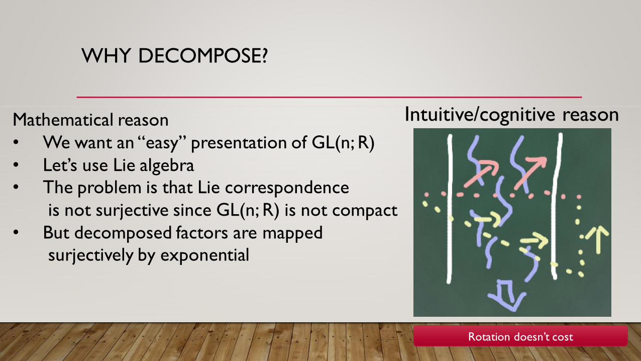
WHY DECOMPOSE?

Mathematical reason

• We want an “easy” presentation of GL(n; R)

• Let’s use Lie algebra

• The problem is that Lie correspondence

is not surjective since GL(n; R) is not compact

• But decomposed factors are mapped

surjectively by exponential

Intuitive/cognitive reason

Rotation doesn’t cost

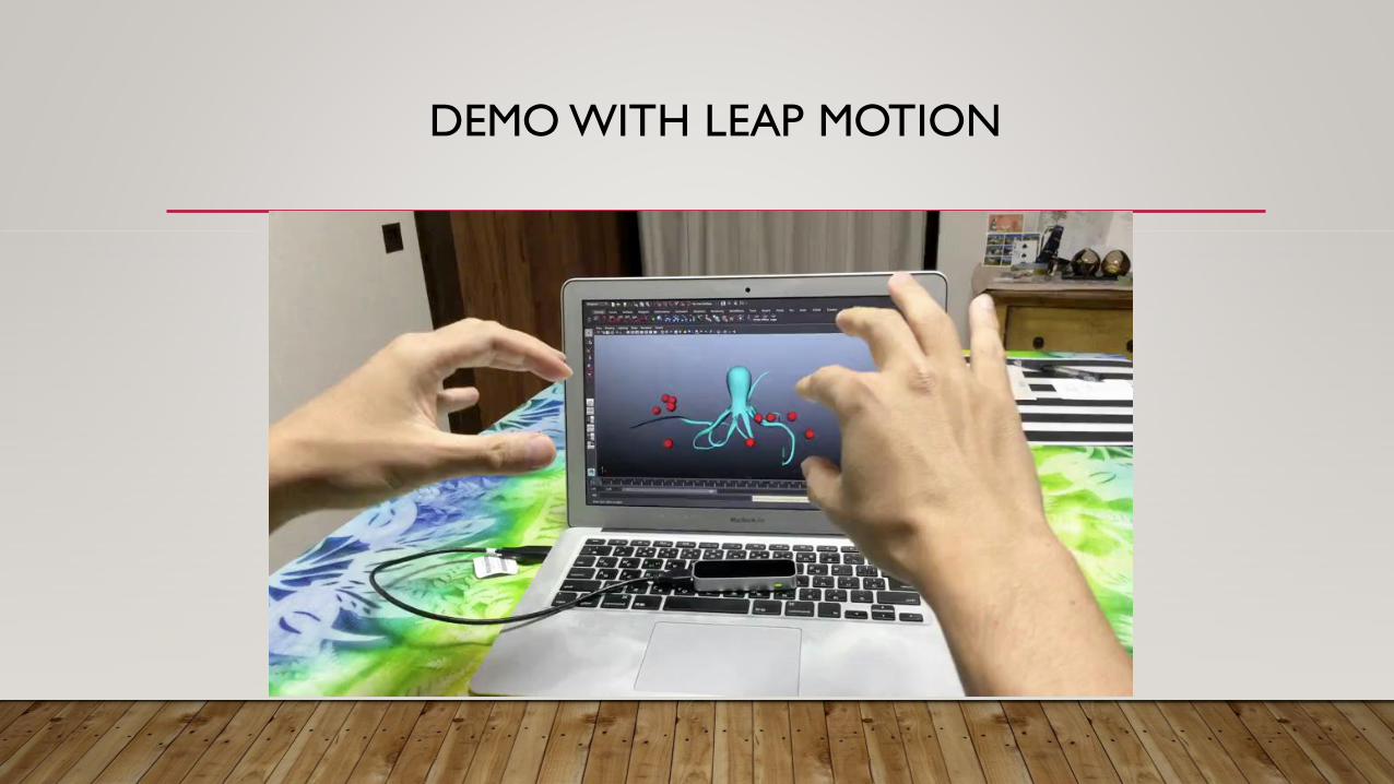
DEMO WITH LEAP MOTION

DISCRETE DIFFERENTIAL GEOMETRY

DDG discusses how to define Δ, ∇, ∫ for discrete objects

and is getting popular in data sciences

Mantra:

• (meaningful) Big data in a high dimensional Euclidean space should lie on a

manifold

(dimension reduction)

• Geometry of the manifold tells a lot (curvature / intrinsic metric)

• Much of geometry is captured by the Laplacian

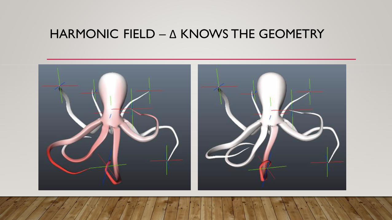
HARMONIC FIELD – Δ KNOWS THE GEOMETRY

THANK YOU!