Polit ln ch04

Copyright ©2010 by Pearson Education, Inc.Upper Saddle River, New Jersey 07458

All rights reserved.

Statistics and Data Analysis for Nursing Research, Second EditionDenise F. Polit

Statistics and Data Analysisfor Nursing Research

Second Edition

CHAPTER

Bivariate Description: Crosstabulation, Risk Indexes, and Correlation

4




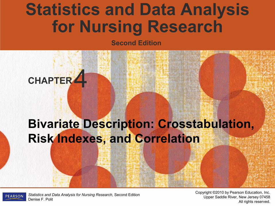
Bivariate Descriptive Statistics

• Bivariate descriptive statistics are used to describe relationships between two variables– Examples:

Height and weight Smoking status and lung cancer

incidence

• Appropriate statistic depends on the variables’ level of measurement




Crosstabulation

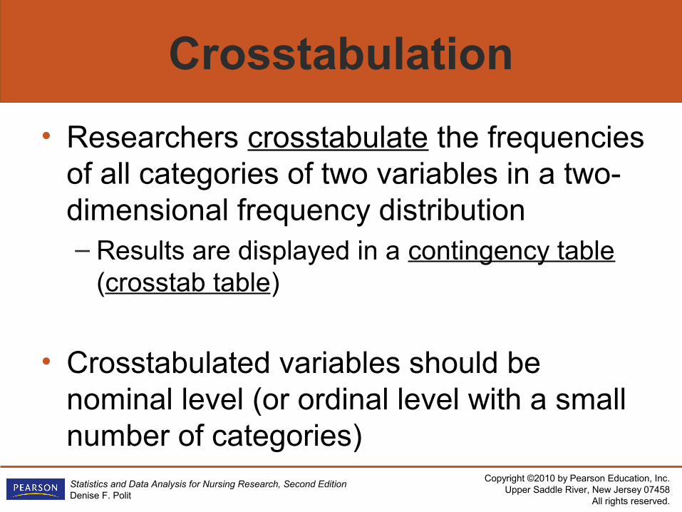
• Researchers crosstabulate the frequencies of all categories of two variables in a two-dimensional frequency distribution– Results are displayed in a contingency table

(crosstab table)

• Crosstabulated variables should be nominal level (or ordinal level with a small number of categories)




Crosstab Tables

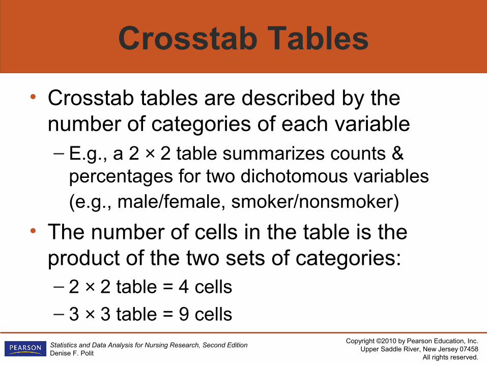
• Crosstab tables are described by the number of categories of each variable– E.g., a 2 × 2 table summarizes counts &

percentages for two dichotomous variables (e.g., male/female, smoker/nonsmoker)

• The number of cells in the table is the product of the two sets of categories:– 2 × 2 table = 4 cells– 3 × 3 table = 9 cells




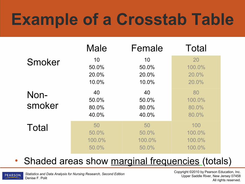
Example of a Crosstab Table

• Shaded areas show marginal frequencies (totals)

Male Female Total

Smoker 1050.0%20.0%10.0%

1050.0%20.0%10.0%

20100.0%20.0%20.0%

Non-smoker

4050.0%80.0%40.0%

4050.0%80.0%40.0%

80100.0%80.0%80.0%

Total 5050.0%100.0%50.0%

5050.0%100.0%50.0%

100100.0%100.0%100.0%




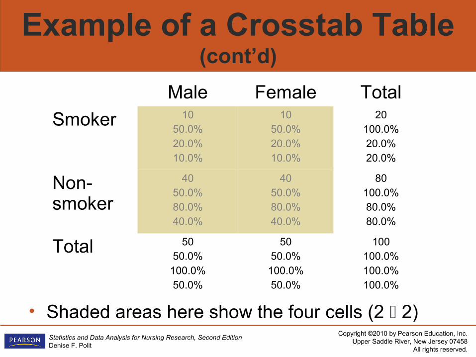
Example of a Crosstab Table (cont’d)

• Shaded areas here show the four cells (2 2)

Male Female Total

Smoker 1050.0%20.0%10.0%

1050.0%20.0%10.0%

20100.0%20.0%20.0%

Non-smoker

4050.0%80.0%40.0%

4050.0%80.0%40.0%

80100.0%80.0%80.0%

Total 5050.0%100.0%50.0%

5050.0%100.0%50.0%

100100.0%100.0%100.0%




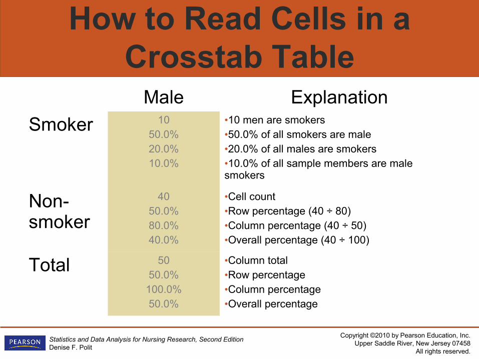
How to Read Cells in a Crosstab Table

Male Explanation

Smoker 1050.0%20.0%10.0%

•10 men are smokers•50.0% of all smokers are male•20.0% of all males are smokers•10.0% of all sample members are male smokers

Non-smoker

4050.0%80.0%40.0%

•Cell count•Row percentage (40 ÷ 80)•Column percentage (40 ÷ 50)•Overall percentage (40 ÷ 100)

Total 5050.0%

100.0%50.0%

•Column total•Row percentage•Column percentage•Overall percentage




Risk Indexes

• Risk indexes have been developed to describe risk outcomes and facilitate clinical decision making

• Indexes discussed here: For situations with two dichotomous variables (2 × 2 situation)– One is a risk factor—or an intervention status

(e.g., smoked/did not smoke)– The other is the outcome (lung cancer/no lung

cancer)




Risk Index Scenarios

• Prospective (cohort) design: – Some people have exposure to the risk factor,

others do not – Both groups are followed to assess outcome

• Retrospective (case-control) design– Some people have a bad outcome (cases)

others do not (controls)– Groups are compared regarding prior

exposure to the risk factor




Risk Index Scenarios (cont’d)

• Experimental design (clinical trials): – Some people are assigned (often at random)

to a control group in which they have ongoing or “baseline” exposure to risks, while others are assigned to an experimental group in which they receive an intervention hypothesized to reduce risk

– Both groups are followed to assess outcome




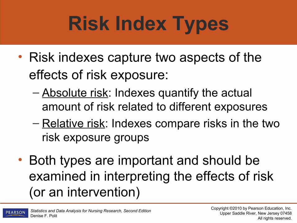
Risk Index Types

• Risk indexes capture two aspects of the effects of risk exposure: – Absolute risk: Indexes quantify the actual

amount of risk related to different exposures– Relative risk: Indexes compare risks in the two

risk exposure groups

• Both types are important and should be examined in interpreting the effects of risk (or an intervention)




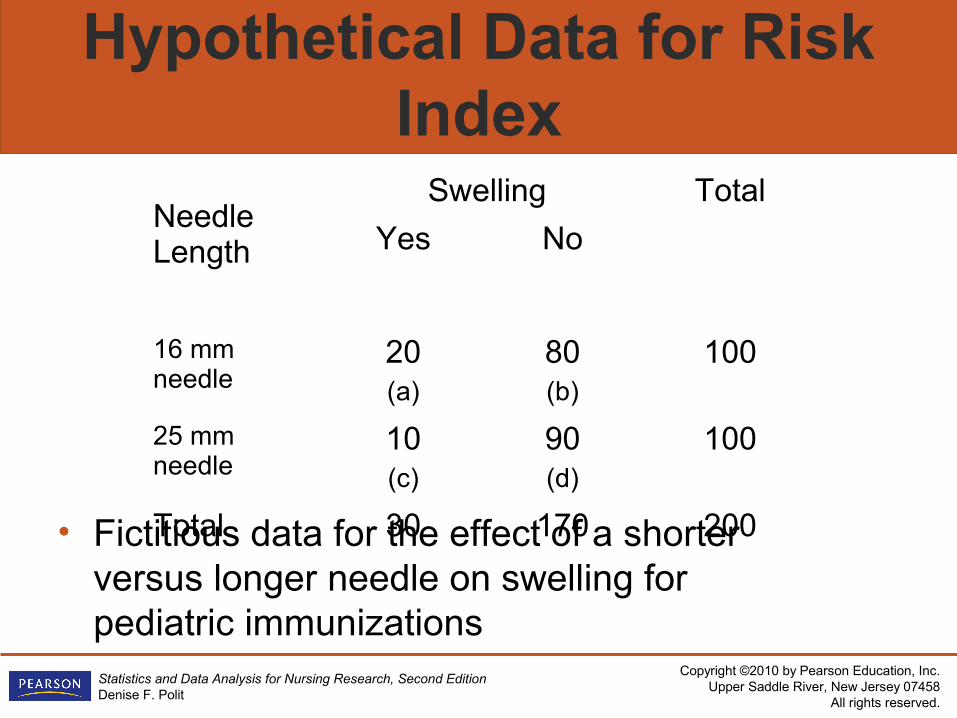
Hypothetical Data for Risk Index

• Fictitious data for the effect of a shorter versus longer needle on swelling for pediatric immunizations

Needle Length

Swelling Total

Yes No

16 mm needle

20(a)

80(b)

100

25 mm needle

10(c)

90(d)

100

Total 30 170 200




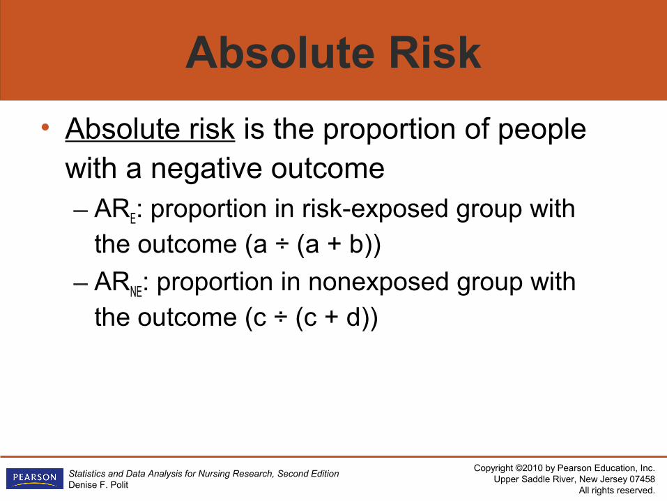
Absolute Risk

• Absolute risk is the proportion of people with a negative outcome – ARE: proportion in risk-exposed group with

the outcome (a ÷ (a + b))

– ARNE: proportion in nonexposed group with the outcome (c ÷ (c + d))




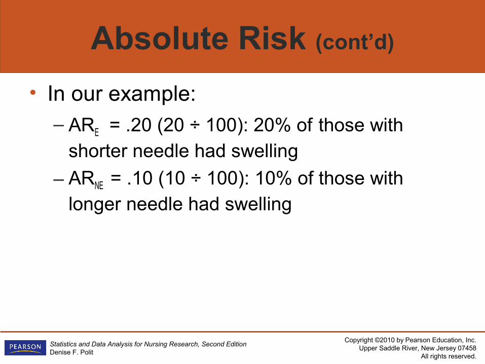
Absolute Risk (cont’d)

• In our example:– ARE = .20 (20 ÷ 100): 20% of those with

shorter needle had swelling

– ARNE = .10 (10 ÷ 100): 10% of those with longer needle had swelling




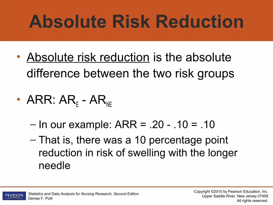
Absolute Risk Reduction

• Absolute risk reduction is the absolute difference between the two risk groups

• ARR: ARE - ARNE

– In our example: ARR = .20 - .10 = .10– That is, there was a 10 percentage point

reduction in risk of swelling with the longer needle




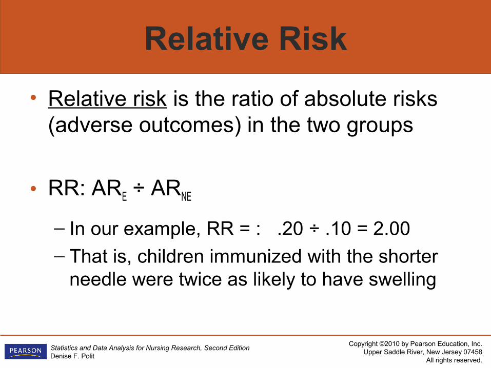
Relative Risk

• Relative risk is the ratio of absolute risks (adverse outcomes) in the two groups

• RR: ARE ÷ ARNE

– In our example, RR = : .20 ÷ .10 = 2.00– That is, children immunized with the shorter

needle were twice as likely to have swelling




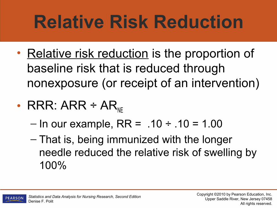
Relative Risk Reduction

• Relative risk reduction is the proportion of baseline risk that is reduced through nonexposure (or receipt of an intervention)

• RRR: ARR ÷ ARNE

– In our example, RR = .10 ÷ .10 = 1.00– That is, being immunized with the longer

needle reduced the relative risk of swelling by 100%




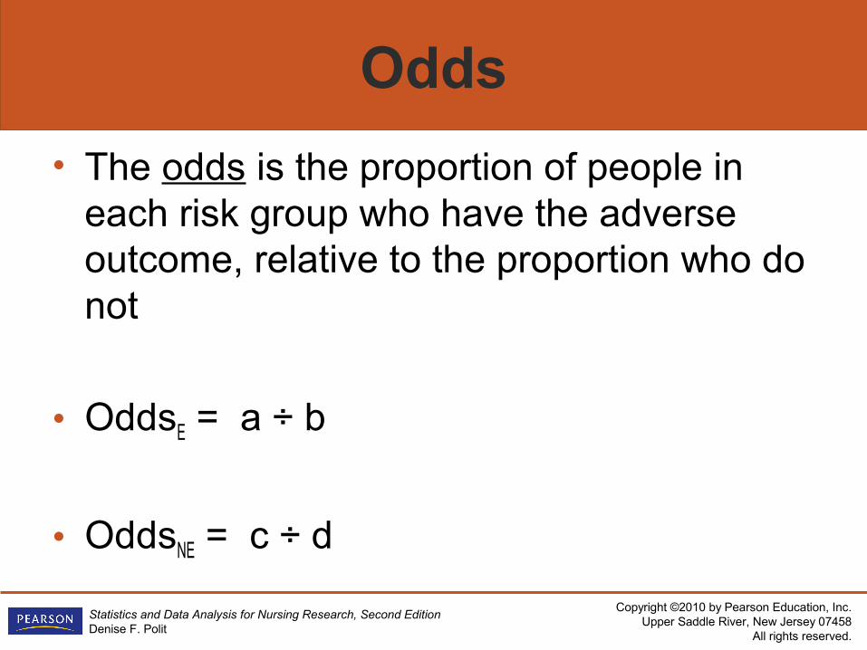
Odds

• The odds is the proportion of people in each risk group who have the adverse outcome, relative to the proportion who do not

• OddsE = a ÷ b

• OddsNE = c ÷ d




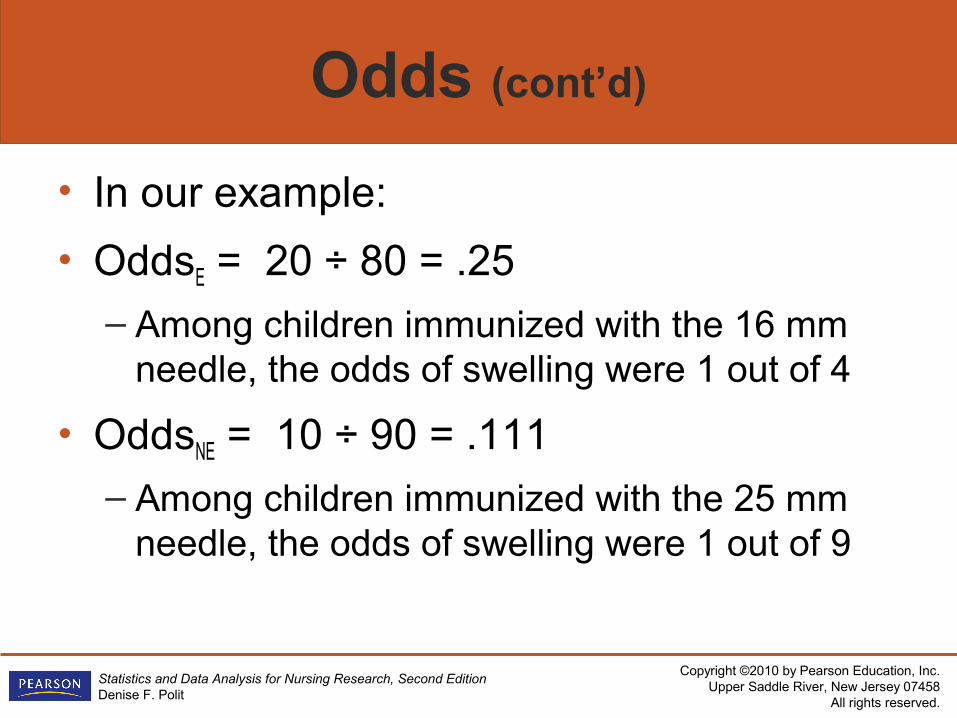
Odds (cont’d)

• In our example:

• OddsE = 20 ÷ 80 = .25 – Among children immunized with the 16 mm

needle, the odds of swelling were 1 out of 4

• OddsNE = 10 ÷ 90 = .111 – Among children immunized with the 25 mm

needle, the odds of swelling were 1 out of 9




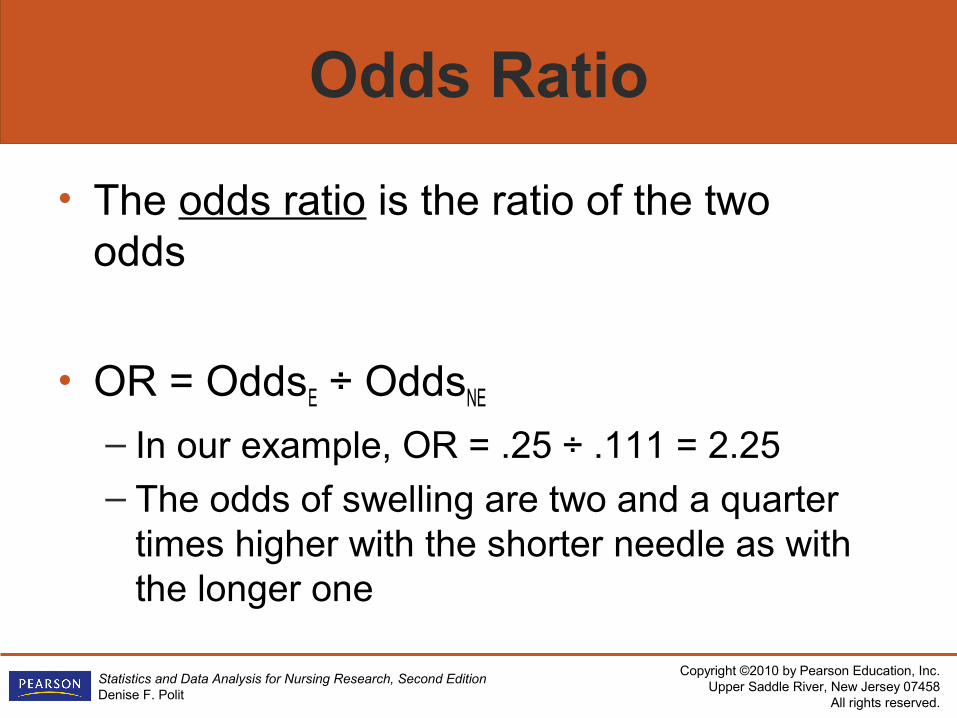
Odds Ratio

• The odds ratio is the ratio of the two odds

• OR = OddsE ÷ OddsNE – In our example, OR = .25 ÷ .111 = 2.25– The odds of swelling are two and a quarter

times higher with the shorter needle as with the longer one




Number Needed to Treat

• Number needed to treat: Estimate of how many people would need to avoid the exposure (or get a treatment) to prevent one negative outcome

• NNT = 1 ÷ ARR – In our example, NNT = 1 ÷ .10 = 10.0– 10 children would need to be immunized with

the 25 mm needle rather than the 16 mm one to prevent one case of swelling




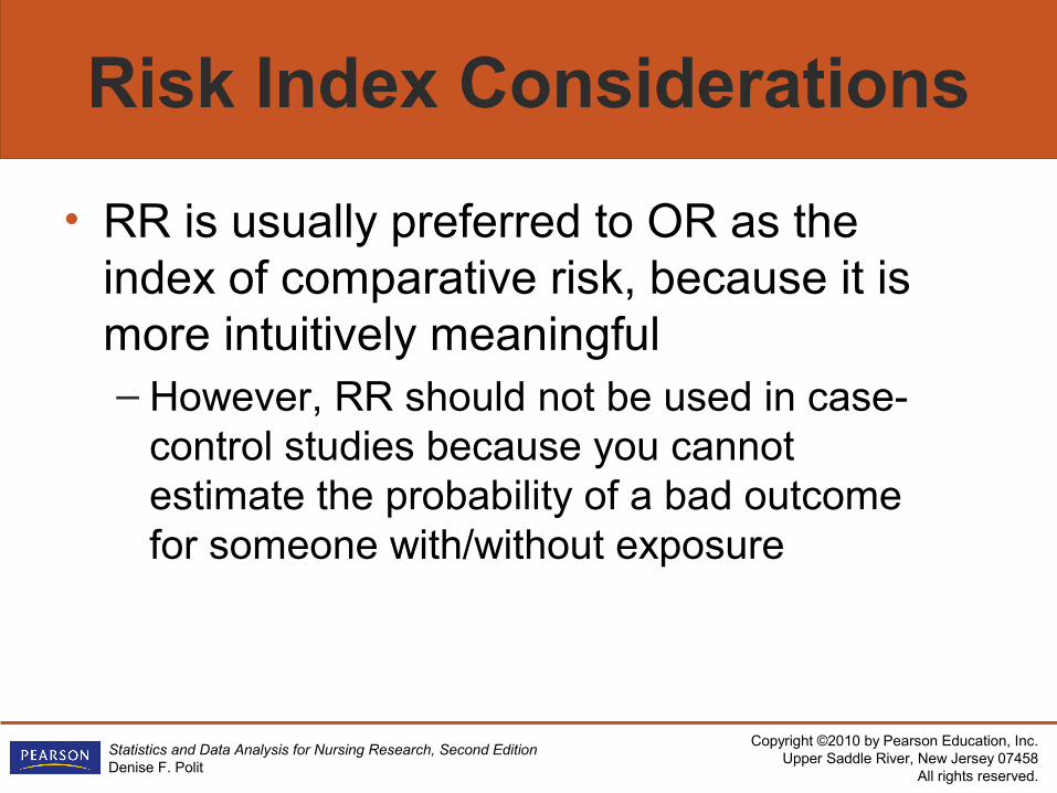
Risk Index Considerations

• RR is usually preferred to OR as the index of comparative risk, because it is more intuitively meaningful– However, RR should not be used in case-

control studies because you cannot estimate the probability of a bad outcome for someone with/without exposure




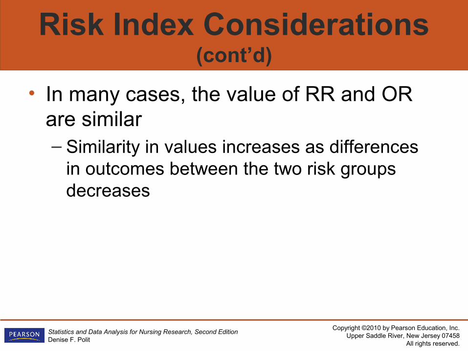
Risk Index Considerations (cont’d)

• In many cases, the value of RR and OR are similar– Similarity in values increases as differences

in outcomes between the two risk groups decreases




Risk Index Considerations (cont’d)

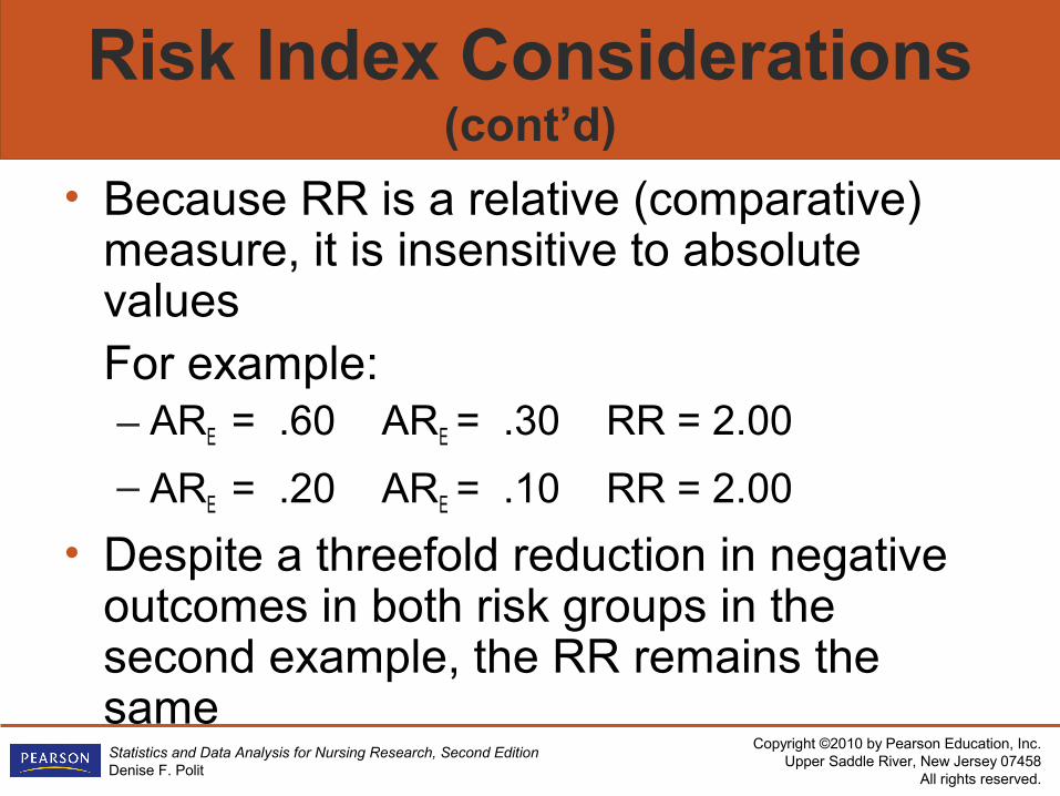
• Because RR is a relative (comparative) measure, it is insensitive to absolute valuesFor example:– ARE = .60 ARE = .30 RR = 2.00

– ARE = .20 ARE = .10 RR = 2.00 • Despite a threefold reduction in negative

outcomes in both risk groups in the second example, the RR remains the same




Correlation

• A correlation is a bond or connection between variables– Variation in one variable is systematically

related to variation in another

• Correlations between two quantitative variables can be graphed in a scatterplot




Scatterplot

• A scatterplot graphs the values of one variable on the X axis and the values of the second one on the Y axis of a graph




Scatterplot (cont’d)

• A scatterplot indicates whether the variables have a linear relationship with each other– A linear (straight line) relationship occurs

when there is a constant rate of change between the two variables

• Scatterplots indicate direction and magnitude of the relationship




Scatterplots and Types of Relationships

Variable X

1211109876543210

Var

iabl

e Y

12

11

10

9

8

7

6

5

4

3

2

10

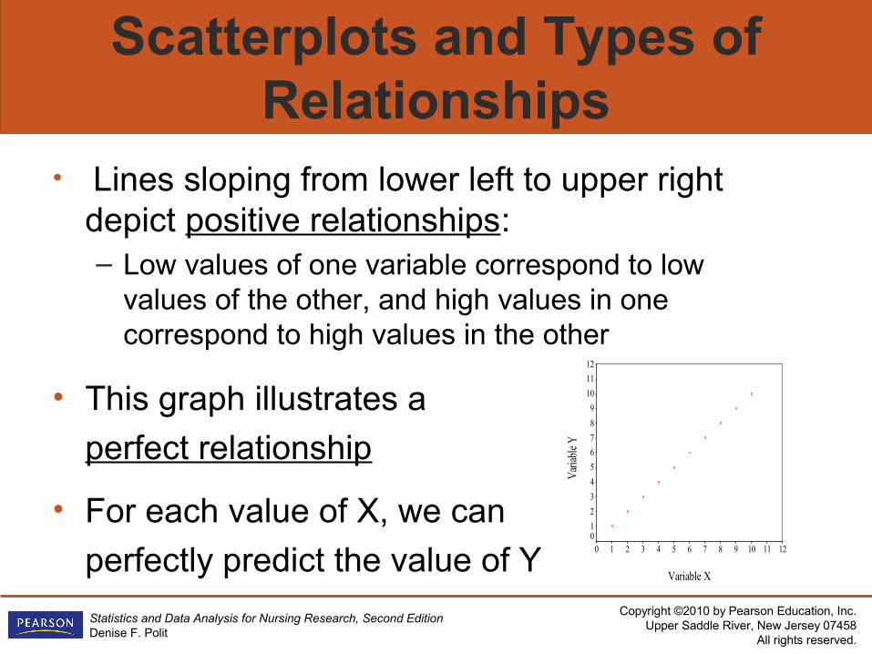
• Lines sloping from lower left to upper right depict positive relationships:– Low values of one variable correspond to low

values of the other, and high values in one correspond to high values in the other

• This graph illustrates a

perfect relationship

• For each value of X, we can

perfectly predict the value of Y




Scatterplots and Negative Relationships

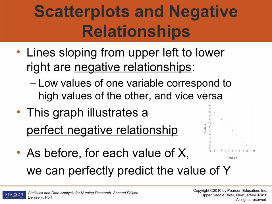
• Lines sloping from upper left to lower right are negative relationships:– Low values of one variable correspond to

high values of the other, and vice versa

• This graph illustrates a

perfect negative relationship

• As before, for each value of X,

we can perfectly predict the value of YVariable X

1211109876543210

Varia

ble Y

12

11

10

9

8

7

6

5

4

3

2

10




Scatterplots and Relationship Strength

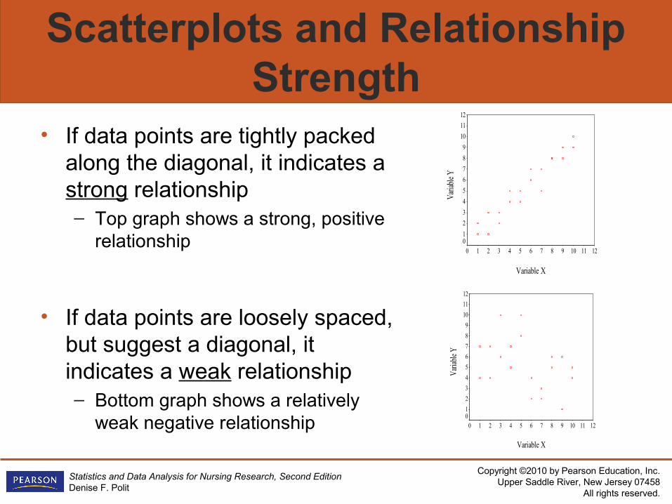
• If data points are tightly packed along the diagonal, it indicates a strong relationship– Top graph shows a strong, positive

relationship

• If data points are loosely spaced, but suggest a diagonal, it indicates a weak relationship– Bottom graph shows a relatively

weak negative relationship

Variable X

1211109876543210

Varia

ble Y

12

11

10

9

8

7

6

5

4

3

2

10

Variable X

1211109876543210

Varia

ble Y

12

11

10

9

8

7

6

5

4

3

2

10




Other Types of Relationship

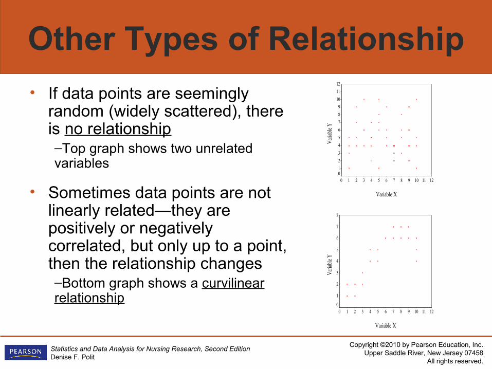
• If data points are seemingly random (widely scattered), there is no relationship–Top graph shows two unrelated variables

• Sometimes data points are not linearly related—they are positively or negatively correlated, but only up to a point, then the relationship changes–Bottom graph shows a curvilinear relationship

Variable X

1211109876543210

Varia

ble Y

12

11

10

9

8

7

6

5

4

3

2

10

Variable X

1211109876543210

Varia

ble Y

8

7

6

5

4

3

2

1

0




Correlation Coefficients

• A correlation coefficient is a statistic that summarizes the magnitude and direction of relationships between two variables

• Most widely used correlation coefficient: Pearson’s product moment correlation coefficient– Often called Pearson’s r– Pearson’s r is computed with variables that

are interval- or ratio-level measures




Correlation Coefficient Values• Correlation coefficients range from

-1.00 through .00 to 1.00

• The sign of the coefficient indicates direction: – Minus sign = negative correlation – Plus sign (or no sign) = positive correlation

• The absolute value of the coefficient indicates strength– r = -.75 is stronger than r = .50




Correlation Coefficient Computation

• Formula for computing Pearson’s r is cumbersome, though not really difficult

• Formula involves calculating and manipulating the deviation scores from the two variables (i.e., deviation of each score from its own mean)

• Computation is rarely done manually




Correlation Coefficient Examples• 1.00 = Perfect positive relationship

E.g., a flat $1 tax for every $5 earned

• .35 = Weak/moderate positive relationship E.g., nurses’ degree of autonomy and job satisfaction (those with

more autonomy are somewhat more satisfied)

• .00 = No relationship E.g., nurses’ degree of autonomy and height (tall and short nurses

equally autonomous)

• -.20 = Weak negative relationshipE.g., diabetic knowledge and a person’s age (older people

are somewhat less knowledgeable)• -.70 = Strong negative relationship

E.g., levels of depression and life satisfaction (those with high levels of depression have lower life satisfaction)




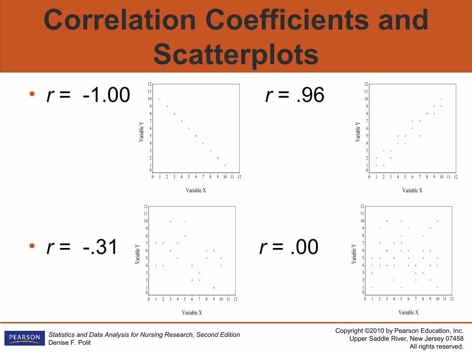
Correlation Coefficients and Scatterplots

• r = -1.00 r = .96

• r = -.31 r = .00

Variable X

1211109876543210

Varia

ble Y

12

11

10

9

8

7

6

5

4

3

2

10

Variable X

1211109876543210

Varia

ble Y

12

11

10

9

8

7

6

5

4

3

2

10

Variable X

1211109876543210

Varia

ble Y

12

11

10

9

8

7

6

5

4

3

2

10

Variable X

1211109876543210

Varia

ble Y

12

11

10

9

8

7

6

5

4

3

2

10




Interpretation of Correlation Coefficients

• A correlation between two variables never implies that one variable caused the other– Correlations indicate a link, not necessarily a causal link

• The square of r indicates the proportion of variability in one variable accounted for or explained by the second variable– If the r between height and weight = .60, then 36% of

the variation in weight is accounted for by height (r2 = .36)

– The remaining 64% of variation in weight is accounted for by other factors (e.g., caloric intake, amount of exercise, metabolic factors, etc.)




Correlation Matrix

• A two-dimensional correlation matrix is an efficient way to display several correlation coefficients

• A correlation matrix lists all variables in the top row and first column—then information about the correlation between variables is entered in the appropriate “cells”

• Diagonals (the cell for the variable’s correlation with itself) usually is blank or has the value of 1.00




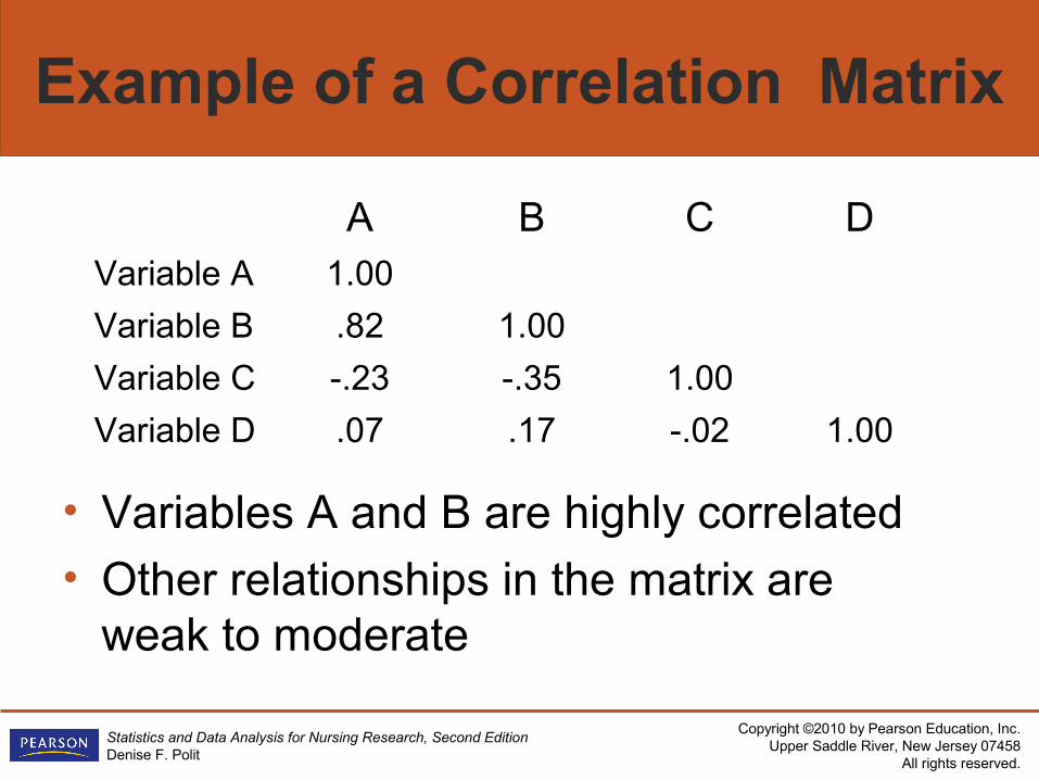
Example of a Correlation Matrix

• Variables A and B are highly correlated• Other relationships in the matrix are

weak to moderate

A B C DVariable A 1.00

Variable B .82 1.00

Variable C -.23 -.35 1.00

Variable D .07 .17 -.02 1.00




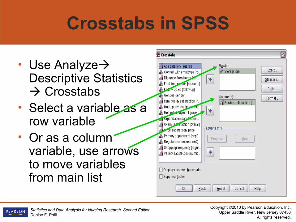
Crosstabs in SPSS

• Use Analyze Descriptive Statistics Crosstabs

• Select a variable as a row variable

• Or as a column variable, use arrows to move variables from main list




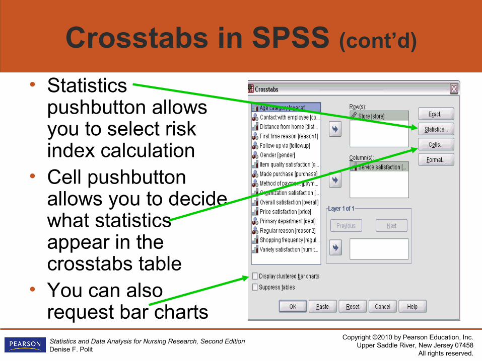
Crosstabs in SPSS (cont’d)

• Statistics pushbutton allows you to select risk index calculation

• Cell pushbutton allows you to decide what statistics appear in the crosstabs table

• You can also request bar charts




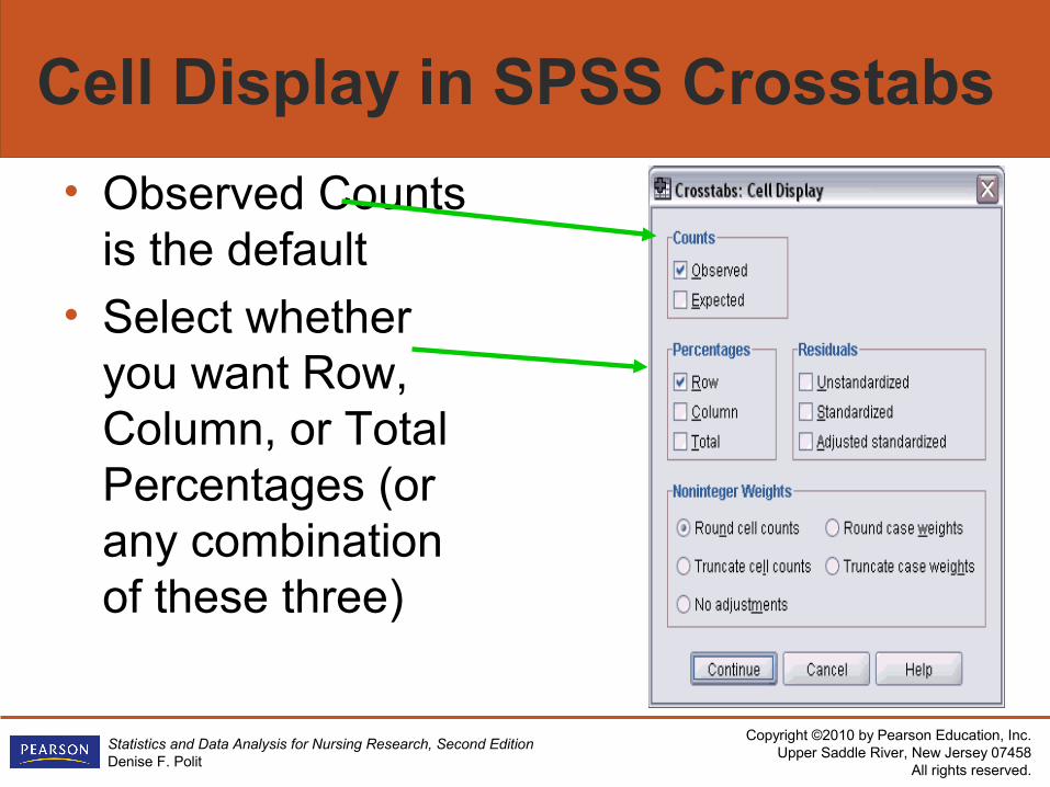
Cell Display in SPSS Crosstabs

• Observed Counts is the default

• Select whether you want Row, Column, or Total Percentages (or any combination of these three)




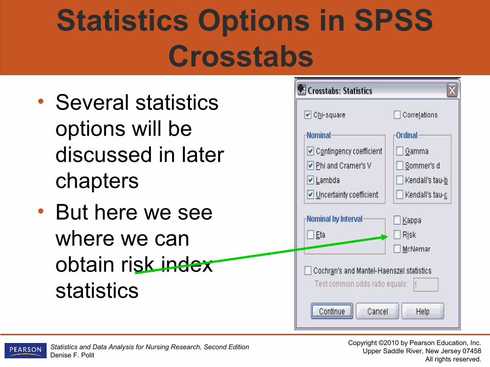
Statistics Options in SPSS Crosstabs

• Several statistics options will be discussed in later chapters

• But here we see where we can obtain risk index statistics




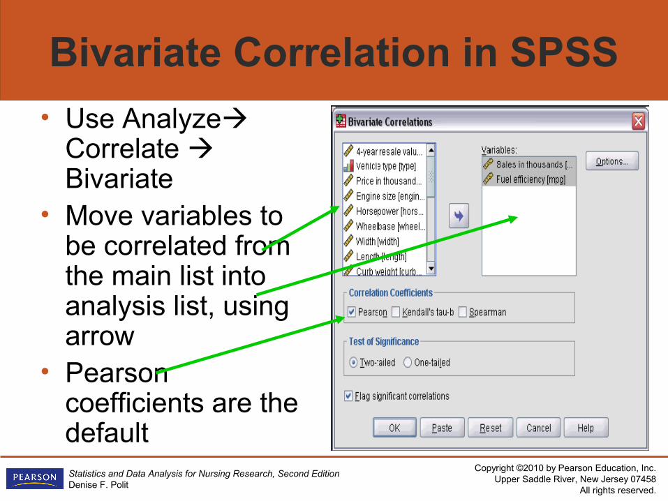
Bivariate Correlation in SPSS

• Use Analyze Correlate Bivariate

• Move variables to be correlated from the main list into analysis list, using arrow

• Pearson coefficients are the default

Documents

Polit ln ch04