POLITECNICO DI MILANO

Facoltà di Ingegneria Industriale

Corso di Laurea in Ingegneria AeronauticaCorso di Laurea in Ingegneria Spaziale

Decentralized control system for a hexapod robotby using neural networks

Relatore: Prof. Mauro MASSARI

Tesi di laurea di:

Fabio ORTALLI Matr. 725152

Alessandro SPALLA Matr. 721871

Anno Accademico 2009-2010

Contents

1 Introduction 11.1 Walking systems . . . . . . . . . . . . . . . . . . . . . . . . . 11.2 Biomimicry . . . . . . . . . . . . . . . . . . . . . . . . . . . . . 31.3 Goals . . . . . . . . . . . . . . . . . . . . . . . . . . . . . . . . 51.4 State of the art . . . . . . . . . . . . . . . . . . . . . . . . . . . 6

1.4.1 Mobot Lab robots . . . . . . . . . . . . . . . . . . . . . 61.4.2 Randall Beer’s robots . . . . . . . . . . . . . . . . . . . 71.4.3 SCORPION . . . . . . . . . . . . . . . . . . . . . . . . 71.4.4 Walknet . . . . . . . . . . . . . . . . . . . . . . . . . . 8

1.5 Thesis contributions . . . . . . . . . . . . . . . . . . . . . . . 9

2 Neural networks 112.1 Overview . . . . . . . . . . . . . . . . . . . . . . . . . . . . . . 112.2 Structure . . . . . . . . . . . . . . . . . . . . . . . . . . . . . . 122.3 Classification . . . . . . . . . . . . . . . . . . . . . . . . . . . . 13

2.3.1 Propagation rule . . . . . . . . . . . . . . . . . . . . . 132.3.2 Activation function . . . . . . . . . . . . . . . . . . . . 132.3.3 Topology . . . . . . . . . . . . . . . . . . . . . . . . . . 142.3.4 Static and dynamic networks . . . . . . . . . . . . . . 15

2.4 Choice criteria . . . . . . . . . . . . . . . . . . . . . . . . . . . 162.5 An overview on CTRNNs . . . . . . . . . . . . . . . . . . . . 172.6 Network training . . . . . . . . . . . . . . . . . . . . . . . . . 20

3 Control strategy - The problem of walking 233.1 General features . . . . . . . . . . . . . . . . . . . . . . . . . . 233.2 The walking system . . . . . . . . . . . . . . . . . . . . . . . . 243.3 Problem definition . . . . . . . . . . . . . . . . . . . . . . . . 253.4 Global controller architecture . . . . . . . . . . . . . . . . . . 263.5 The control of a single leg . . . . . . . . . . . . . . . . . . . . 28

3.5.1 Swing phase . . . . . . . . . . . . . . . . . . . . . . . . 303.5.2 Stance phase . . . . . . . . . . . . . . . . . . . . . . . . 323.5.3 Phase transition . . . . . . . . . . . . . . . . . . . . . . 353.5.4 Reflexes . . . . . . . . . . . . . . . . . . . . . . . . . . 35

3.6 Legs coordination . . . . . . . . . . . . . . . . . . . . . . . . . 363.6.1 Stability . . . . . . . . . . . . . . . . . . . . . . . . . . 373.6.2 Gaits . . . . . . . . . . . . . . . . . . . . . . . . . . . . 383.6.3 Coordination rules . . . . . . . . . . . . . . . . . . . . 403.6.4 Curve walking . . . . . . . . . . . . . . . . . . . . . . 42

iii

Contents

3.7 Final control structure . . . . . . . . . . . . . . . . . . . . . . 43

4 Single leg controller 454.1 Swing control . . . . . . . . . . . . . . . . . . . . . . . . . . . 45

4.1.1 Static network . . . . . . . . . . . . . . . . . . . . . . . 464.1.2 Dynamic network . . . . . . . . . . . . . . . . . . . . . 50

4.2 Stance controller . . . . . . . . . . . . . . . . . . . . . . . . . . 544.2.1 Local positive velocity feedback . . . . . . . . . . . . 554.2.2 Height control . . . . . . . . . . . . . . . . . . . . . . . 584.2.3 Velocity control . . . . . . . . . . . . . . . . . . . . . . 604.2.4 Direction control . . . . . . . . . . . . . . . . . . . . . 61

4.3 State selector . . . . . . . . . . . . . . . . . . . . . . . . . . . . 624.3.1 PEP net . . . . . . . . . . . . . . . . . . . . . . . . . . . 64

4.4 Reflexes . . . . . . . . . . . . . . . . . . . . . . . . . . . . . . . 654.4.1 Avoiding reflex . . . . . . . . . . . . . . . . . . . . . . 654.4.2 Searching reflex . . . . . . . . . . . . . . . . . . . . . . 684.4.3 Stepping reflex . . . . . . . . . . . . . . . . . . . . . . 72

5 Coordination 775.1 Cruse’s coordination rules . . . . . . . . . . . . . . . . . . . . 775.2 Porta and Celaya model . . . . . . . . . . . . . . . . . . . . . 805.3 Coordination model . . . . . . . . . . . . . . . . . . . . . . . 845.4 AEP targeting . . . . . . . . . . . . . . . . . . . . . . . . . . . 935.5 Results . . . . . . . . . . . . . . . . . . . . . . . . . . . . . . . 98

5.5.1 Wave gaits . . . . . . . . . . . . . . . . . . . . . . . . . 985.5.2 Leg failure . . . . . . . . . . . . . . . . . . . . . . . . . 102

6 Numerical results 1056.1 Model . . . . . . . . . . . . . . . . . . . . . . . . . . . . . . . . 105

6.1.1 Simulation environment . . . . . . . . . . . . . . . . . 1066.1.2 Multibody model . . . . . . . . . . . . . . . . . . . . . 1066.1.3 Actuators model . . . . . . . . . . . . . . . . . . . . . 1086.1.4 Sensors model . . . . . . . . . . . . . . . . . . . . . . . 1096.1.5 Ground contact model . . . . . . . . . . . . . . . . . . 1116.1.6 Control model implementation . . . . . . . . . . . . . 1126.1.7 Simulation parameters . . . . . . . . . . . . . . . . . . 112

6.2 Dynamic model results . . . . . . . . . . . . . . . . . . . . . . 1136.2.1 Slow wave gait . . . . . . . . . . . . . . . . . . . . . . 1136.2.2 Tripod gait . . . . . . . . . . . . . . . . . . . . . . . . . 1166.2.3 Curve walking . . . . . . . . . . . . . . . . . . . . . . 119

iv

Contents

7 Walking platform 1257.1 Design requirements . . . . . . . . . . . . . . . . . . . . . . . 1257.2 Mechanical system . . . . . . . . . . . . . . . . . . . . . . . . 126

7.2.1 General layout . . . . . . . . . . . . . . . . . . . . . . 1267.2.2 Joint design . . . . . . . . . . . . . . . . . . . . . . . . 1297.2.3 Structural analysis . . . . . . . . . . . . . . . . . . . . 130

7.3 Electrical design . . . . . . . . . . . . . . . . . . . . . . . . . . 1337.3.1 DC electric motors . . . . . . . . . . . . . . . . . . . . 1347.3.2 Angular position sensors . . . . . . . . . . . . . . . . 1357.3.3 Contact force sensors . . . . . . . . . . . . . . . . . . . 1357.3.4 Communication and connection system . . . . . . . . 138

7.4 Weight evaluation . . . . . . . . . . . . . . . . . . . . . . . . . 1397.5 Software . . . . . . . . . . . . . . . . . . . . . . . . . . . . . . 141

7.5.1 Low level controller . . . . . . . . . . . . . . . . . . . 141

8 Conclusion 1438.1 Results of the work . . . . . . . . . . . . . . . . . . . . . . . . 1438.2 Innovation . . . . . . . . . . . . . . . . . . . . . . . . . . . . . 1448.3 Future developments . . . . . . . . . . . . . . . . . . . . . . . 145

List of Acronyms 147

Bibliography 149

v

List of Figures

1.1 A stick insect Carausius Morosus . . . . . . . . . . . . . . . . . 41.2 Mobot Lab robots . . . . . . . . . . . . . . . . . . . . . . . . . 61.3 Randall Beer’s robot . . . . . . . . . . . . . . . . . . . . . . . 71.4 The SCORPION robot . . . . . . . . . . . . . . . . . . . . . . 81.5 Walknet-controlled robots . . . . . . . . . . . . . . . . . . . . 9

2.1 Neural networks topology . . . . . . . . . . . . . . . . . . . . 142.2 An example of neural unit . . . . . . . . . . . . . . . . . . . . 162.3 Limit cycle and attraction point in a two-neurons CTRNN . 192.4 Flow chart of the genetic algorithm . . . . . . . . . . . . . . . 21

3.1 Leg orientation and angular variables . . . . . . . . . . . . . 253.2 CPG vs. reflex-based approach . . . . . . . . . . . . . . . . . 273.3 Swing and stance phases . . . . . . . . . . . . . . . . . . . . . 293.4 Scheme for the controller of a single leg . . . . . . . . . . . . 303.5 Swing control module . . . . . . . . . . . . . . . . . . . . . . 313.6 Swing trajectory geometric parameters . . . . . . . . . . . . . 323.7 Stance control module . . . . . . . . . . . . . . . . . . . . . . 343.8 Overview on reflexes . . . . . . . . . . . . . . . . . . . . . . . 363.9 Static stability . . . . . . . . . . . . . . . . . . . . . . . . . . . 373.10 Gait diagrams of the most significant wave gaits . . . . . . . 393.11 Coordination rules . . . . . . . . . . . . . . . . . . . . . . . . 413.12 Gait changes during a curve walking . . . . . . . . . . . . . . 433.13 Block diagram of the complete control structure . . . . . . . 44

4.1 Static swing net . . . . . . . . . . . . . . . . . . . . . . . . . . 474.2 Angles and angular velocities of a swing trajectory . . . . . . 484.3 Swing trajectories with different start and target positions . 494.4 Response of the swing controller to an external disturbance . 494.5 Field of velocities . . . . . . . . . . . . . . . . . . . . . . . . . 494.6 Error on target as function of trajectory parameters . . . . . 504.7 Dynamic swing net . . . . . . . . . . . . . . . . . . . . . . . . 514.8 Angles and angular velocities of a reference swing trajectory 534.9 Swing trajectories with different start and target positions . 534.10 Response of the swing controller to an external disturbance . 534.11 Field of velocities . . . . . . . . . . . . . . . . . . . . . . . . . 544.12 Error on target as function of trajectory parameters . . . . . 544.13 High pass filtered positive feedback . . . . . . . . . . . . . . 564.14 Angles and angular velocities of a reference stance trajectory 57

vii

List of Figures

4.15 Body height control . . . . . . . . . . . . . . . . . . . . . . . . 594.16 Error on body height calculated by the ANN . . . . . . . . . 604.17 Control of the advancing velocity . . . . . . . . . . . . . . . . 614.18 The selector network . . . . . . . . . . . . . . . . . . . . . . . 634.19 Error on PEP calculated by the Artificial Neural Network

(ANN) . . . . . . . . . . . . . . . . . . . . . . . . . . . . . . . 654.20 Angles and angular velocities during the avoiding reflexes . 674.21 Angles and angular velocities during a searching reflex . . . 714.22 Foot trajectory in the x-z plane during a searching reflex . . 714.23 Foot trajectory in the x-y plane during a searching reflex . . 714.24 Error on advancing movement depending on starting height 724.25 Angles and angular velocities during a stepping reflex . . . 744.26 Trajectories in the x-y plane during a stepping reflex . . . . . 744.27 Trajectories in the x-z plane during a stepping reflex . . . . . 754.28 Error on stepping movement depending on starting position 75

5.1 Coordinating influences . . . . . . . . . . . . . . . . . . . . . 785.2 Simplified Cruse’s coordination model . . . . . . . . . . . . . 795.3 Legs configuration in the Porta and Celaya model . . . . . . 825.4 Wave gait emerging from the Porta and Celaya model . . . . 835.5 Slow gait with an unmodified Porta and Celaya model . . . 855.6 Effects of a too much high threshold T on the coordination . 875.7 Effects of a too much small threshold T on the coordination . 885.8 Effects due to the absence of coordinating mechanism 2 . . . 895.9 Effects due to the absence of coordinating mechanism 3 . . . 905.10 Targeting on AEP in a stick insect . . . . . . . . . . . . . . . . 945.11 Targeting on AEP with the simple form of the target net . . . 965.12 Targeting on AEP with the complete form of the target net . 975.13 Gait diagram of a slow wave gait . . . . . . . . . . . . . . . . 985.14 Advancing speed and stepping patterns of a slow wave gait 985.15 Gait diagram of a slow ripple gait . . . . . . . . . . . . . . . . 995.16 Advancing speed and stepping patterns of a slow ripple gait 995.17 Gait diagram of a fast ripple gait . . . . . . . . . . . . . . . . 995.18 Advancing speed and stepping patterns of a fast ripple gait 1005.19 Gait diagram of a tripod gait . . . . . . . . . . . . . . . . . . . 1005.20 Advancing speed and stepping patterns of a tripod gait . . . 1005.21 Effects of changes in the velocity command Gv . . . . . . . . 1025.22 Gait diagram with a leg failure on L2 . . . . . . . . . . . . . . 1035.23 Advancing speed and stepping patterns with a leg failure

on L2 . . . . . . . . . . . . . . . . . . . . . . . . . . . . . . . . 103

6.1 Conceptual scheme of the complete multibody model . . . . 107

viii

List of Figures

6.2 Electric scheme of a potentiometer with a resistive load . . . 1106.3 Angles of the middle left leg during a slow gait . . . . . . . . 1146.4 Angular velocities of the middle left leg during a slow gait . 1146.5 Joint torques of the middle left leg during a slow gait . . . . 1146.6 Gait diagram of a slow gait . . . . . . . . . . . . . . . . . . . 1156.7 Global advancing velocity for a slow gait . . . . . . . . . . . 1156.8 Trajectory in the x-y plane for a slow gait . . . . . . . . . . . 1166.9 Trajectory in the x-z plane for a slow gait . . . . . . . . . . . 1166.10 Angles of the middle left leg during a tripod gait . . . . . . . 1176.11 Angular velocities of the middle left leg during a tripod gait 1176.12 Joint torques of the middle left leg during a tripod gait . . . 1176.13 Gait diagram of a tripod gait . . . . . . . . . . . . . . . . . . . 1186.14 Global advancing velocity for a tripod gait . . . . . . . . . . 1186.15 Trajectory in the x-y plane for a tripod gait . . . . . . . . . . 1196.16 Trajectory in the x-z plane for a tripod gait . . . . . . . . . . . 1196.17 Angles of the middle left leg during a curve gait . . . . . . . 1206.18 Angles of the middle right leg during a curve gait . . . . . . 1206.19 Angular velocities of the middle left leg during a curve gait 1206.20 Angular velocities of the middle right leg during a curve gait 1216.21 Joint torques of the middle left leg during a curve gait . . . . 1216.22 Joint torques of the middle right leg during a curve gait . . . 1216.23 Gait diagram of a curve gait . . . . . . . . . . . . . . . . . . . 1226.24 Global advancing velocity for a curve gait . . . . . . . . . . . 1226.25 Trajectory in the x-y plane for a curve gait . . . . . . . . . . . 1236.26 Trajectory in the x-z plane for a curve gait . . . . . . . . . . . 1236.27 Effects of variations in Yawre f and Gv on x-y plane trajectory 1246.28 Effects of changings in Yawre f and Gv on turning radius R . . 1246.29 Osculating circle definition for two different curve trajectories124

7.1 General layout of NEMeSys . . . . . . . . . . . . . . . . . . . 1277.2 Meter gear dimension and joint example . . . . . . . . . . . . 1307.3 Beam model constraints and most loaded sections . . . . . . 1327.4 The NEMeSys robot in a simulated martian environment . . 1337.5 Force sensor construction and characteristic curve . . . . . . 1367.6 Electrical interface for force sensor . . . . . . . . . . . . . . . 1377.7 Electrical connection scheme . . . . . . . . . . . . . . . . . . . 1387.8 Partition of the weights between type of components . . . . 139

ix

List of Tables

4.1 GA parameters for the static swing net training . . . . . . . . 484.2 GA parameters for the dynamic swing net training . . . . . . 524.3 Angles and duration times required for the avoiding reflexes 664.4 GA parameters for the training process of avoiding reflexes . 684.5 Frequency and phase parameters for a searching reflex . . . 694.6 GA parameters for the training process of a searching reflex 704.7 Limit and reference values for the stepping reflex . . . . . . 73

5.1 Reference parameters for Cruse’s coordination rules . . . . . 80

6.1 Multibody model parameters . . . . . . . . . . . . . . . . . . 1086.2 Ground contact parameters for two different terrains . . . . 112

7.1 Mechanical limits for angle γ . . . . . . . . . . . . . . . . . . 1297.2 Bevel gear specifications . . . . . . . . . . . . . . . . . . . . . 1297.3 Mechanical properties of 6061-O aluminum alloy . . . . . . . 1317.4 Maximum internal forces of beam model . . . . . . . . . . . 1327.5 Motor specifications . . . . . . . . . . . . . . . . . . . . . . . 1347.6 Adapter specifications . . . . . . . . . . . . . . . . . . . . . . 1357.7 Potentiometer specifications . . . . . . . . . . . . . . . . . . . 1357.8 Force sensor specifications . . . . . . . . . . . . . . . . . . . . 1367.9 Weight of the principal subparts of NEMeSys . . . . . . . . . 1407.10 Weight comparison between versions of NEMeSys . . . . . . 140

xi

Abstract

The reproduction of what the nature offers us has been for long timeone of the most exciting challenges to scientists and engineers. The thrustto copy the animals and their behavior is justified by the fact that biologicalsystems tend to have a better efficiency than those found in their artificialcounterparts. This concept can also be applied in space exploration, re-placing with legged robots inspired by the animals, the classic rovers. Thelatters, in fact, show mobility difficulties, particularly on rough terrain.Because of this the choise to design a controller based on observed nat-ural behavior. The main source of inspiration is the stick insect, becauseof its high level of mobility and of the ease with which it can be studied.This approach led to the creation of a decentralized control system thathas proven better performance and flexibility than those of classical con-trol algorithms. A physical platform to test the designed controller hasbeen finally built.

Key words: neural networks, hexapod robot, walking, advanced control,gait, biomimicry.

Sommario

La riproduzione di ciò che la natura ci offre è stato per molto tempo unadelle più avvincenti sfide lanciate da scienziati e ingegneri. La spinta acopiare gli animali e i loro comportamenti è giustificata dal fatto che i sis-temi biologici tendono ad avere un’efficienza maggiore di quella riscontra-bile nelle loro controparti artificiali. Questo concetto può essere applicatoanche nell’ambito dell’esplorazione spaziale, sostituendo con robot mu-niti di zampe ispirati al mondo animale i classici robot a ruote. Questiultimi, infatti, presentano difficoltà di mobilità, particolarmente su terrenisconnessi. Per questo si è scelto di progettare un controllore basato sulcomportamento osservato in natura. La principale fonte di ispirazione èl’insetto stecco, vista la sua ottima mobilità e la facilità con cui può esserestudiato. Tale approccio ha portato alla creazione di un sistema di con-trollo decentralizzato che ha dimostrato prestazioni e flessibilità superioria quelle dei classici algoritmi di comando. Infine è stata costruita una pi-attaforma fisica per testare il controllore progettato.

Parole chiave: reti neurali, robot esapode, camminata, controllo avanzato,gait, biomimesi.

Chapter 1

IntroductionThis thesis aims to improve the understanding of walking robots for spaceexploration both creating a control system and realizing an hardware plat-form to test theoretical results experimentally as part of the developmentof the Neural Ento-Mechanic System (NEMeSys) project.

Interest on walking robots depends on current trends in space explo-ration: no human missions on celestial bodies has been planned for theimmediate future so this essential part of scientific research relies on semi-autonomous probes only.

1.1 Walking systems

Since the start of the space race only few semi-autonomous rovers havebeen actually employed and all of them mounted wheels to propel them-selves on the ground. This choice can be easily justified by examiningtheir advantages mainly as for legs. A wheeled system is almost alwayssimpler, cheaper and more reliable than a legged one, and it also showscontinuous stability, that can be achieved without any control strategy.

The problem is to understand when legs become preferable to wheels.There are two main reasons supporting the first option: legs don’t requirea continuous area of solid ground for moving and navigation is not con-strained.

Investigating the first reason it’s possible to say that ground alwaysoffers a non-continuous support and the evaluation of motion dependson the relationship between gap distance and wheel size. A wheel is ableto cross horizontal discontinuities as larger as its radius, but it can climbonly much smaller vertical ones. The other main problem is that a largegap/radius relation drives to a very irregular and energetically inefficientbody motion. Furthermore wheel size can’t be changed during the motionand this reduces vehicle flexibility. For a leg instead, overcoming eitherhorizontal or vertical gap it’s conceptually the same thing and the qualityof motion isn’t so strictly related to discontinuities dimensions. A leg hasalso greater flexibility because each step can be adapted to the current gapsize thus optimizing energetic efficiency.

The second reason involves the total controlled Degree of Freedom(DoF)s of each system. A wheeled vehicle moving on ground is a non-holonomic system because it controls fewer variables than those defining

1

Chapter 1

its position. The problem descends from the single wheel that is controlledonly by two variables, angular velocity and wheel direction. So a wheeledvehicle is able to explore the whole space, but only with a high numberof trajectory corrections and an advanced navigation planning. A typicalexample of such a problem is a car parking maneuver. In opposition, ajointed leg is able to reach every allowed position directly, without anykind of trajectory adjustment. This drives to a simpler and more flexiblemotion planning.

All the considerations used on wheels can be extended to other kindsof mechanisms to transmit motion on ground, particularly to all the non-holonomic systems such as whegs or oscillators, because their behaviorscan be easily reduced to the wheels’ ones.

After explaining the advantages in legs usage the attention can be fo-cused on how this kind of systems works. From this point of view themost important issues are stability, complexity, and control structure.

A legged system is not stable per se, like a wheeled one, because itsstability depends fundamentally on how many legs touch simultaneouslythe ground. If during the walk, three or more legs are always in contact,the motion is a mere juxtaposition of equilibrium state and the system iscalled statically stable. This means the stability is not time dependant anda global stability controller is not required. When only two legs or fewerare in contact at the same time the system requires continuous adjustmentsto posture and inertia to maintain its stability since it becomes dynamicallystable. It’s obvious that the former ones are safer and more robust than thelatter ones but they require at least four legs and a coordination betweenall the legs in contact with the ground. On the other hand, dynamicallystable systems are more suitable for fast locomotion.

The single jointed leg, as said above, is an holonomic system becausethe number of controlled variables is the same of the total DoFs in its taskspace. Extending the problem to a complete robot and considering onlystatic-stable cases, the systems become redundant, because the task is thebody motion control producing a 6-dimensional task space, but the controlvariables, i.e. the joints angles, are 9 or more. This property is a great ad-vantage relating to nonholonomic systems for the previously shown rea-sons, but it needs also a much more complex controller that is the maindisadvantage of legged systems.

The structure of any legged locomotion controllers can be analyzed atthree different levels: body trajectory, inter-leg coordination and singleleg motion. The first typically depends on the direction and the speed re-quired for the vehicle and it’s normally a higher-level command. Oncefixed where the body should be, it’s possible to calculate the legs’ move-

2

Introduction

ment and hence joint positioning. However, each leg must take into ac-count the motion of the other one, otherwise the robot could fall or walkinefficiently. To avoid this a coordination among the legs is required. Themain advantage of such a structure is the possibility to design each levelindependently because they are only weakly coupled. This allows the useof a simpler, decentralized control system, since it requires a less perform-ing CPU than a global controller.

From the spatial point of view a global evaluation of the legged ve-hicles can be done. The exploration of a space environment requires avery robust behavior, so a statically stable robot with an high number oflegs is preferable. The complexity of an high DoFs system is balanced byits adaptability to an unknown environment and its flexibility to achievelots of different tasks. It also makes it more fault tolerant, since the robotcan lose a leg without losing its capability for walking. The possibilitiesoffered by using a decentralized control matches the requirements of thelow-performances space-certified CPUs.

At the start of the NEMeSys project a trade-off among some multi-legged robots was done, driving to choose the six-legged one. The mainreason supporting this choice is the double symmetry of such a system:they are both reflectional and translational symmetric with respect to thewalking direction. This simplifies the problem allowing to design onlyone leg and obtaining the others by symmetry. Another reason is the highnumber of existing works on these systems also from non-engineeringfields such as entomology or neurobiology.

1.2 Biomimicry

In engineering, as in other scientific fields, it’s usual to evaluate existingnatural models and emulate them on the purpose of obtaining the sameresults. This process is called biomimicry from the ancient Greek βιoς,meaning life, and µιµησις, meaning imitation.

Nature offers lots of perfectly walking systems and, at this level of de-velopment of our science, they work all better than their artificial counter-part. This means that some design ideas can be helpful in the pursuit forbuilding truly autonomous robots.

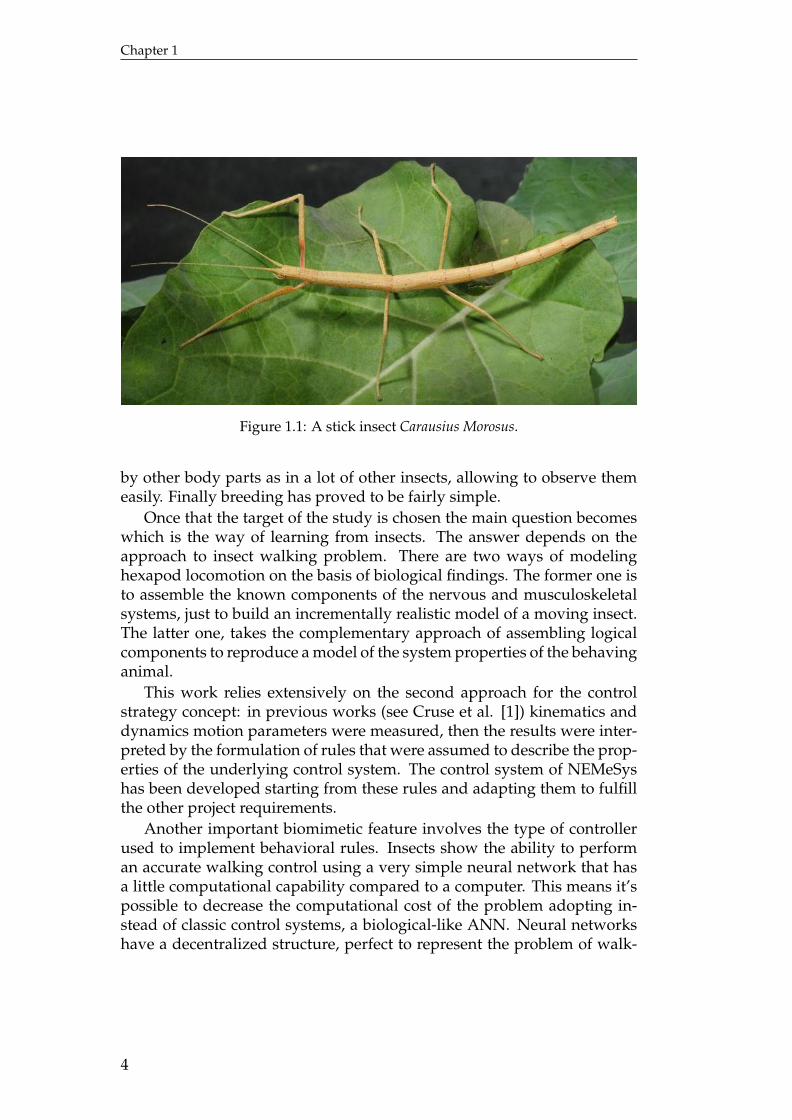
Obviously the best walking hexapod are insects, the most studied ofthem are stick insects, particularly the specie Carausius Morosus, the ’com-mon’, ’Indian’ or ’laboratory’ stick insect (see figure 1.1). One of the rea-sons to choose this stick insect as a model is its researcher-friendly mor-phology. It has a long, straight body allowing to strap it onto differentdevices for researching it’s walking. The stick insect’s legs aren’t hidden

3

Chapter 1

Figure 1.1: A stick insect Carausius Morosus.

by other body parts as in a lot of other insects, allowing to observe themeasily. Finally breeding has proved to be fairly simple.

Once that the target of the study is chosen the main question becomeswhich is the way of learning from insects. The answer depends on theapproach to insect walking problem. There are two ways of modelinghexapod locomotion on the basis of biological findings. The former one isto assemble the known components of the nervous and musculoskeletalsystems, just to build an incrementally realistic model of a moving insect.The latter one, takes the complementary approach of assembling logicalcomponents to reproduce a model of the system properties of the behavinganimal.

This work relies extensively on the second approach for the controlstrategy concept: in previous works (see Cruse et al. [1]) kinematics anddynamics motion parameters were measured, then the results were inter-preted by the formulation of rules that were assumed to describe the prop-erties of the underlying control system. The control system of NEMeSyshas been developed starting from these rules and adapting them to fulfillthe other project requirements.

Another important biomimetic feature involves the type of controllerused to implement behavioral rules. Insects show the ability to performan accurate walking control using a very simple neural network that hasa little computational capability compared to a computer. This means it’spossible to decrease the computational cost of the problem adopting in-stead of classic control systems, a biological-like ANN. Neural networkshave a decentralized structure, perfect to represent the problem of walk-

4

Introduction

ing control that doesn’t need a global supervision and can be divided infairly independent subtasks. Therefore they can show a nonlinear behav-ior, very useful to simulate the leg motion that is an intrinsically nonlinearphysical phenomenon.

1.3 Goals

After an overview of the known walking systems and their biomimeticalfeatures, it’s possible to identify the higher-level goals of this work. Theformer of them is the realization of a ANN-based walking controller ableto generate the angular reference signal for each of the joints that managethe walk. This goal can be achieved by fulfilling some tasks:

- the fundamental signal is able to produce a stereotypic leg motion.This means that the system is able to walk also with no external inputimproving fault tolerance;

- the reference signal can be changed depending on sensory feedback.This requirement is necessary to guarantee the motion adaptabilityto unpredictable external conditions such as: rough terrain, chang-ing slope and obstacles;

- the reference signal can be changed depending on the high-levelpath control. This allows the possibility to vary walking speed, walk-ing direction or body attitude;

The other main goal is to design and build a walking robot on which totest the control system. Starting from the results of the former NEMeSysworks it’s possible to identify the tasks as follows:

- the mechanical project need to be redone both to reduce the globalmass and to improve the mechanical efficiency of the robot;

- the electronics is already complete, but needs some improvements.The main of them is the introduction of a force sensors to evalu-ate the ground contact, in the place of the switch sensors previouslymounted. Other changes will be done in order to simplify the hard-ware and to reduce the global weight;

- the software interface exists but has to be changed in order to beadapted to the new control architecture.

5

Chapter 1

1.4 State of the art

To better understand how certain choices have been taken, as described inthe next chapters, it can be useful to look at some important examples oflegged locomotion in the robotics field. Because this work aims either tobuild a robot or to project its control system, the overview shown belowinvolves both of these features: each example is an existing walking robothaving a particular kind of control structure.

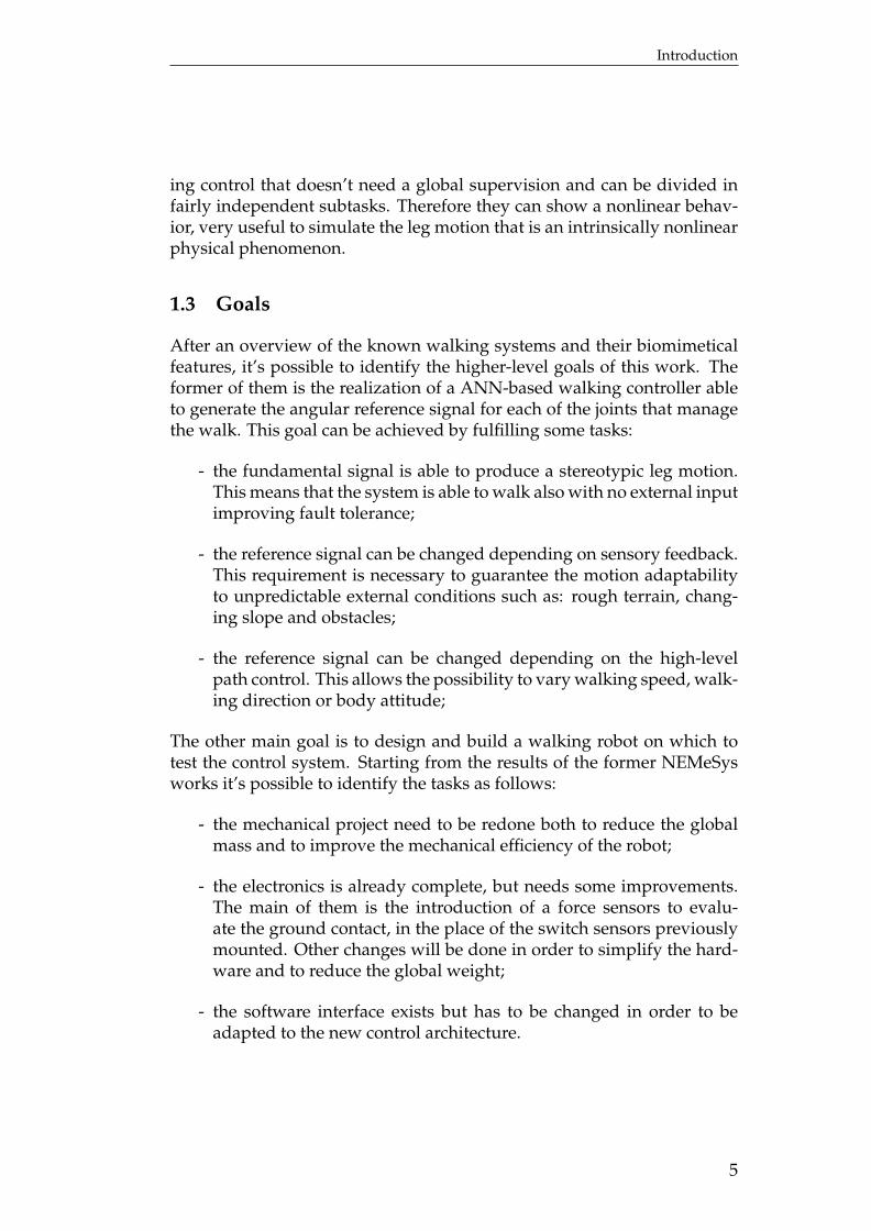
1.4.1 Mobot Lab robotsThe Mobot Lab of the MIT developed some interesting space-orientedrobots in the first half of the ’90s (see figure 1.2). The first of them wasGenghis an hexapod with only 2 DoFSs for each leg, but very compactwith a length of 35 cm and a weight of 1 kg. The sensors allow to measurehigh-level path parameters like body orientation or obstacles contact. Thecontroller is mounted on-board.

Figure 1.2: Mobot Lab robots. From the left: Genghis, Attila and Hannibal.

The most interesting feature of this robot is its control system: it relieson a network of elementary agents called Finite State Machines or FSM[2]. Each of them managed only a very simple task, depending on fewinputs from sensors. Although this isn’t an actual neural network it canbe considered like a precursor of NEMeSys, since the main ideas behindthe projects are the same:

- modularity: the controller is decentralized on various blocks, eachof them working only on a limited task, almost independently fromthe others;

- incremental growth: the project starts fulfilling only the simplesttasks, adding more complex behaviors step-by-step.

After Genghis a couple of more complex robots were developed: Attilaand Hannibal [3]. They had 3-DoFs legs and were smaller than their pre-decessor. The main advantage of these systems was the capability to main-tain a stable configuration also with high slopes, thanks to an additionalDoF in the body.

6

Introduction

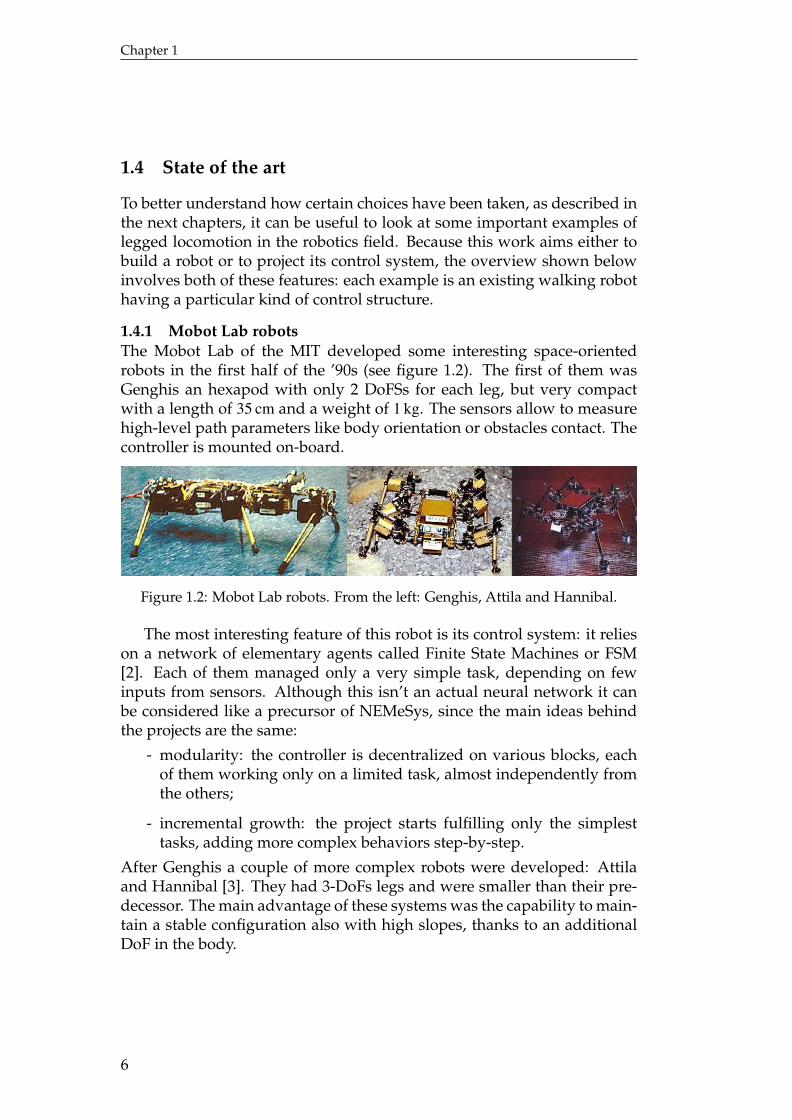
Figure 1.3: Randall Beer’s robots. From the left: Robot I and Robot II.

1.4.2 Randall Beer’s robotsThe guidelines of the earlier development of the NEMeSys project hadbeen taken from the work of professor Randall D. Beer [4]. He and histeam worked extensively on the theory of neural networks-based con-trollers and also realized some interesting walking platform.

Their first work is Robot I a hexapod with 2-DoFs legs. The controlsystem is a decentralized neural network with a single net controllingeach leg. The inter-leg coordination depends on the mutual influencesamong the controllers of each single leg, with the aid of a global super-visor. Another interesting feature of Robot I is the design approach: thecontrol parameters has been selected via a large number of simulation,using biological-like evolutionary algorithms.

Robot II, the second model, is quite different: it relies on six 3-DoFs legsand has a completely different controller based on reflexes. It means thatwalking behaviors emerges only from the interaction between the robotand the environment and is not generated autonomously by the platform.

Robot I and II aren’t designed for space exploration but are among thebest examples of working legged vehicles that are controlled by ANNs.

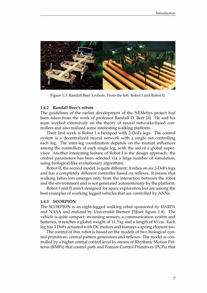
1.4.3 SCORPIONThe SCORPION is an eight-legged walking robot sponsored by DARPAand NASA and realized by Universität Bremen [5](see figure 1.4). Thevehicle is quite compact: mounting sensors, a communication system andbatteries, it reaches a global weight of 11.5 kg and a length of 65 cm. Eachleg has 3 DoFs actuated with DC motors and features a spring element too.

The control of this robot is based on the models of two biological con-trol primitives: central pattern generators and reflexes. The model is con-trolled by a higher central control level by means of Rhythmic Motion Pat-terns (RMPs) that control path and Posture Control Primitives (PCPs) that

7

Chapter 1

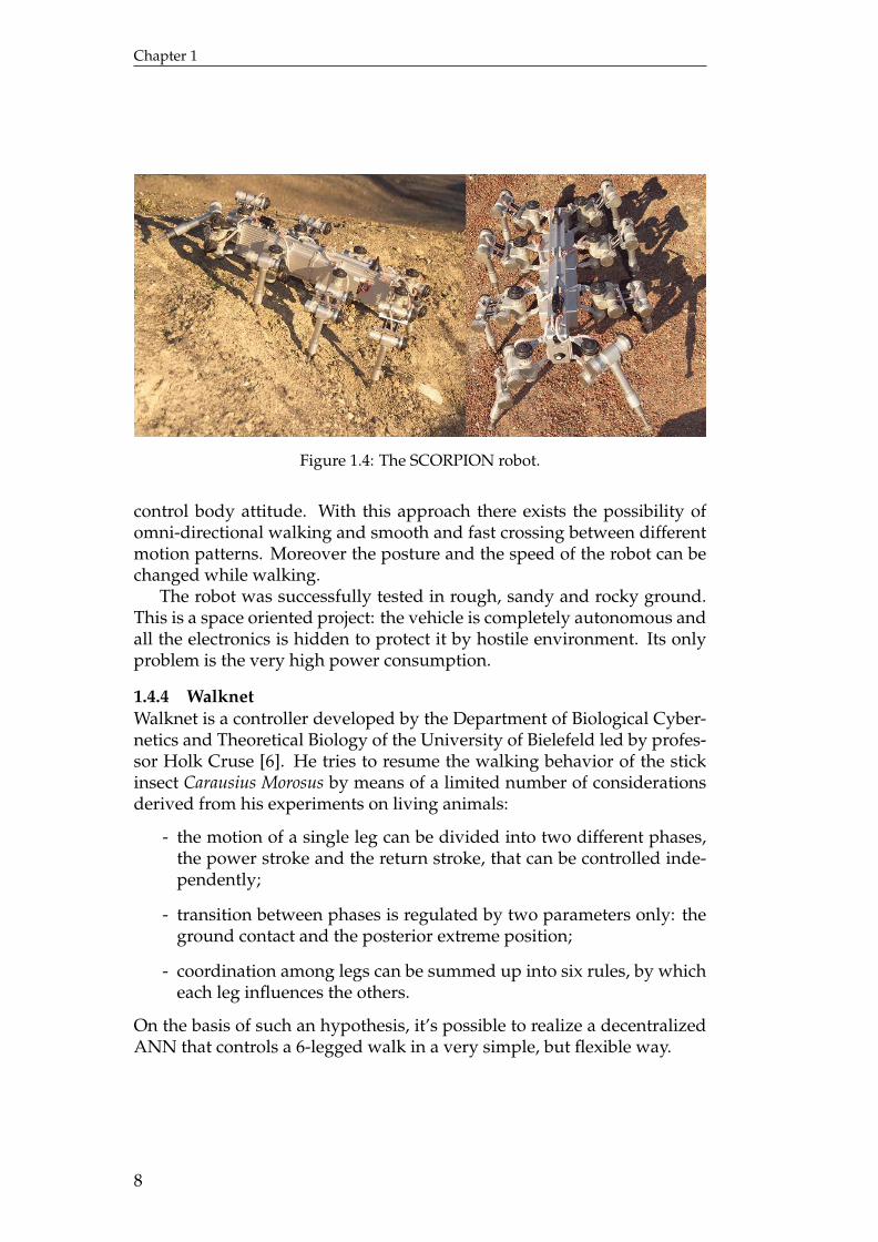
Figure 1.4: The SCORPION robot.

control body attitude. With this approach there exists the possibility ofomni-directional walking and smooth and fast crossing between differentmotion patterns. Moreover the posture and the speed of the robot can bechanged while walking.

The robot was successfully tested in rough, sandy and rocky ground.This is a space oriented project: the vehicle is completely autonomous andall the electronics is hidden to protect it by hostile environment. Its onlyproblem is the very high power consumption.

1.4.4 WalknetWalknet is a controller developed by the Department of Biological Cyber-netics and Theoretical Biology of the University of Bielefeld led by profes-sor Holk Cruse [6]. He tries to resume the walking behavior of the stickinsect Carausius Morosus by means of a limited number of considerationsderived from his experiments on living animals:

- the motion of a single leg can be divided into two different phases,the power stroke and the return stroke, that can be controlled inde-pendently;

- transition between phases is regulated by two parameters only: theground contact and the posterior extreme position;

- coordination among legs can be summed up into six rules, by whicheach leg influences the others.

On the basis of such an hypothesis, it’s possible to realize a decentralizedANN that controls a 6-legged walk in a very simple, but flexible way.

8

Introduction

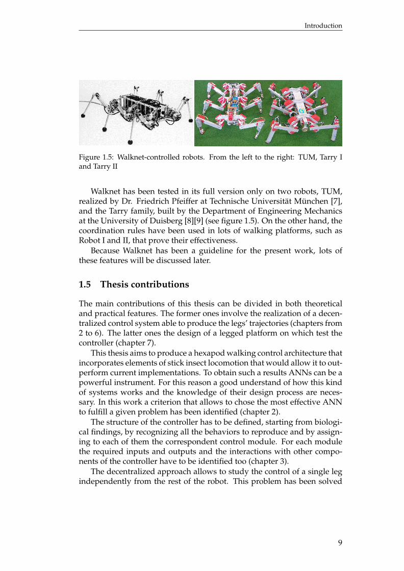
Figure 1.5: Walknet-controlled robots. From the left to the right: TUM, Tarry Iand Tarry II

Walknet has been tested in its full version only on two robots, TUM,realized by Dr. Friedrich Pfeiffer at Technische Universität München [7],and the Tarry family, built by the Department of Engineering Mechanicsat the University of Duisberg [8][9] (see figure 1.5). On the other hand, thecoordination rules have been used in lots of walking platforms, such asRobot I and II, that prove their effectiveness.

Because Walknet has been a guideline for the present work, lots ofthese features will be discussed later.

1.5 Thesis contributions

The main contributions of this thesis can be divided in both theoreticaland practical features. The former ones involve the realization of a decen-tralized control system able to produce the legs’ trajectories (chapters from2 to 6). The latter ones the design of a legged platform on which test thecontroller (chapter 7).

This thesis aims to produce a hexapod walking control architecture thatincorporates elements of stick insect locomotion that would allow it to out-perform current implementations. To obtain such a results ANNs can be apowerful instrument. For this reason a good understand of how this kindof systems works and the knowledge of their design process are neces-sary. In this work a criterion that allows to chose the most effective ANNto fulfill a given problem has been identified (chapter 2).

The structure of the controller has to be defined, starting from biologi-cal findings, by recognizing all the behaviors to reproduce and by assign-ing to each of them the correspondent control module. For each modulethe required inputs and outputs and the interactions with other compo-nents of the controller have to be identified too (chapter 3).

The decentralized approach allows to study the control of a single legindependently from the rest of the robot. This problem has been solved

9

Chapter 1

by using a innovative solutions, e.g. dynamic neural networks, positivefeedback or nonlinear approximation. These ones has been combined withclassic control systems, in order to obtain the best results both in terms ofperformances and reliability (chapter 4)

The single legs motion must be coordinated to obtain the desired globalmotion. This works want to find a controller for the coordination thatensure the stability of the robot during the entire motion with a structureas simple as possible. It must also guarantee a great flexibility by allowingto change the motion over a wide range of possibilities or to introduce newbehaviors, without any changes in the coordination system (chapter 5).

The complete control system needs to be tested. At first it can be eval-uated on a multibody model of a legged system in a dynamic simulationenvironment in order to identify possible problems or lacks into the pre-vious design process (chapter 6).

The last major purpose of this thesis is the design of a legged robot. Ithas to be a functional 18-DOF hexapod capable of straight-line and curvewalking able to respond to external forces through measurements takenfrom foot-mounted force sensors and joint-mounted angular displacementsensors. Its weight has to be kept down and the dimensions must be lim-ited. Moreover it should has autonomous power and the capacity for au-tonomous control (chapter 7).

10

Chapter 2

Neural networksBiomimetic findings shown in section 1.2 imply that the problem of walk-ing control can be solved in a better way by using an artificial version ofthe insects’ neural network instead of a classic controller. To better under-stand which is the most adapt network to fulfil a given requirement, it’snecessary to know which kind of networks exist, how each type worksand how to design it. In this chapter, after an overview of such systems(sections 2.1 to 2.3), the criteria to choice the correct type of neural net-work will be evaluated (section 2.4) and the calculation methods for itsparameters will be explained (sections 2.6).

2.1 Overview

An ANN is a mathematical model that tries to simulate the structure andfunctional aspects of biological neural networks. It consists of group ofunits, called artificial neurons, mutually joined by weighted connections,called synapses. Information can be processed using a connectionist ap-proach to computation: this means that, in opposition to a typical com-puter, tasks aren’t accomplished solving a deterministic sequence of oper-ations, but with a distributed, parallel and local processing involving allthe units.

These characteristics result in some interesting advantages. Such astructure allows to manage large amounts of data with great accuracy,thus approximating complex mappings. They’re fairly independent to ev-ery assumption on data’s distribution and interaction among components.Fundamentally they are sophisticated statistical systems with a good ro-bustness to noisy, incomplete or totally missing inputs; if some units workincorrectly, the network could suffer a degradation of the level of its per-formances, but almost never stops its work. They are able to generalizeby giving an output also when unknown inputs appear. It’s possible toimplement them in a parallel hardware optimizing their computationalefficiency.

Opposite to advantages, one must note that the model produced byANNs, although very efficient, can’t be explained with an analytical ap-proach: results must be taken as they come and neural networks have to betreated like black boxes. It’s not possible to understand how certain inputscause certain outputs so the only way to obtain an efficient ANN is to start

11

Chapter 2

from a set of well-chosen statistical data. If the problem to solve is com-plex, the number of data needed to a correct ANN design is very high andthe calculation of the network parameters become very computer inten-sive. Theorems or models that permit to define the best network structureare not available yet, so the final result is obtained with heuristic methodsthat heavily rely on the experience of their creator.

In this work all the networks aren’t realized by a dedicated hardware,but with a software working on a classic computer. This strategy reducesthe computational efficiency of the neural approach, but allows to use ex-isting components and avoids to waste resources on problems that are tofar from walking control.

2.2 Structure

An ANN consists of a pool of simple processing units which communicateby sending signals to each other over a large number of weighted connec-tions. It is called network because the output of each unit is defined asa composition of functions depending on other units. All of the existingANNs show the same structure, composed by:

- a set of processing units called neurons;

- connections between the units. Generally each connection is definedby a weight wi j which determines the effect which the signal of uniti has on unit j. For positive wi j the contribution is considered anexcitation and for negative wi j an inhibition.

Every neuron is characterized by four different features:

- a state of activation yi, which is equivalent to the output of the unit;

- a propagation rule, which determines the effective input S i from itsexternal inputs;

- an activation function Φ, which determines the new level of activa-tion based on the effective input S i and the current activation yi;

- an activation offset or bias θi.

The whole process of outputs generation by the elaboration of inputs iscalled combination.

12

Neural networks

2.3 Classification

On the basis of these fundamental assumptions a huge number of differenttype of ANNs has been proposed in the past, so that a brief classificationis necessary to elaborate the discriminating criteria that enable to find thebest network that fulfills the requirements of this work.

2.3.1 Propagation ruleThe first criterion depends on the propagation rules and the way to calcu-late the effective input starting from external inputs and weights: it can bea linear combination (Linear nodes), a polynomial combination (Sigma-pinodes) or a nonlinear boolean function (Cubic nodes).

2.3.2 Activation functionThe second classification can be traced on the basis of different types ofactivation function. Basically they can be divided in two great categories:the step-like functions and the radial basis functions. The former oneshave been the first to be used and are composed by generalized forms ofthe step-function. The most important functions of this class are:

- step function: it’s very easy to be implemented, but it’s not invertibleand it’s not up to approximate smooth functions;

- linear ramp: it’s simple, but has a linear zone that can imitate con-tinuous functions. It’s not invertible;

- sigmoid: it’s invertible and continuously differentiable. It can bothapproximate functions and take fuzzy decisions, but it’s more ex-pensive in terms of computational cost and its outputs are limited topositive values;

- hyperbolic tangent: has the same advantages of the sigmoid and canalso produce both positive and negative outputs. It’s difficult to beimplemented.

All of these function are very important because show a behavior veryclose to the biological neurons’ one. In subsection 2.3.4 is shown a veryuseful applications of such a type of functions.

The radial basis functions are inspired to the biological neurons of thevisual cortex: they produce a significant response only close to a specificpoint in the space of inputs called center and the amplitude can be modu-lated by a scale factor. A typical example of these functions are the gaus-sian, the multiquadric, the polyharmonic spline and the thin plate spline.

13

Chapter 2

Figure 2.1: Two typical topologies for an ANN.

They are mainly used to approximate given functions particularly in timeseries prediction and control of nonlinear systems with a sufficiently sim-ple chaotic behavior and also in 3D reconstruction in computer graphics.

A last activation function has to be considered, the linear activationfunction. In this case the neural state is the same as the effective input,which allows to approximate non limited behaviors too.

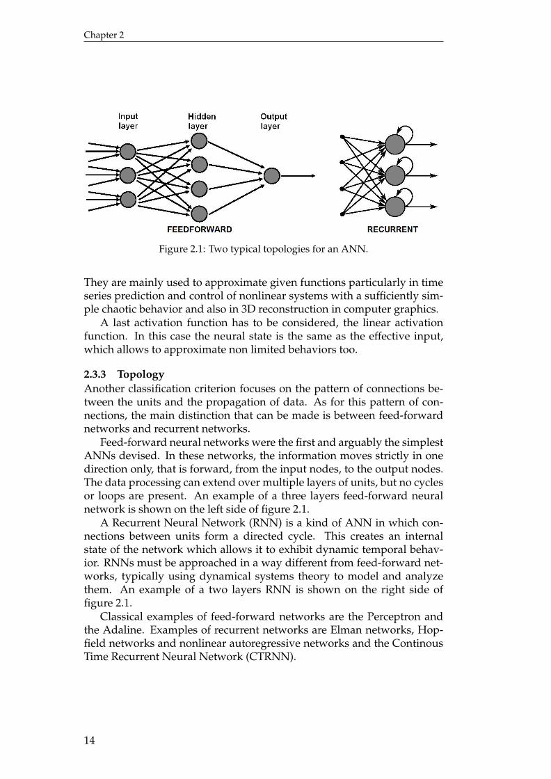
2.3.3 TopologyAnother classification criterion focuses on the pattern of connections be-tween the units and the propagation of data. As for this pattern of con-nections, the main distinction that can be made is between feed-forwardnetworks and recurrent networks.

Feed-forward neural networks were the first and arguably the simplestANNs devised. In these networks, the information moves strictly in onedirection only, that is forward, from the input nodes, to the output nodes.The data processing can extend over multiple layers of units, but no cyclesor loops are present. An example of a three layers feed-forward neuralnetwork is shown on the left side of figure 2.1.

A Recurrent Neural Network (RNN) is a kind of ANN in which con-nections between units form a directed cycle. This creates an internalstate of the network which allows it to exhibit dynamic temporal behav-ior. RNNs must be approached in a way different from feed-forward net-works, typically using dynamical systems theory to model and analyzethem. An example of a two layers RNN is shown on the right side offigure 2.1.

Classical examples of feed-forward networks are the Perceptron andthe Adaline. Examples of recurrent networks are Elman networks, Hop-field networks and nonlinear autoregressive networks and the ContinousTime Recurrent Neural Network (CTRNN).

14

Neural networks

2.3.4 Static and dynamic networksIn the present work the most important distinction among ANNs is basedon their capability to model time-dependant phenomena. From this pointof view static ANNs and dynamic ANNs can be identified.

A static network is an ANN that produces a specific output depend-ing only on the inputs given in the current instant. Systems showing thisbehavior are called reactive agents, because they produce a direct, time-independent reaction.

For this reason to obtain the desired network is sufficient to know aset of inputs and the corresponding desired set of outputs. Starting fromthese sample data, by means of a training process, is possible to calculatethe correct set of parameters defining the network univocally. The adapt-ability of a such a model allows, if the sample has been correctly chosen,to produce acceptable outputs also when inputs are different from onesthought of in the initial design.

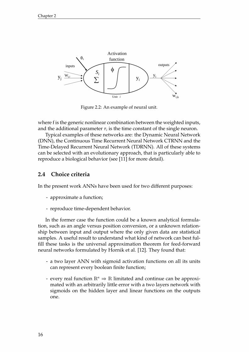
Almost all the static networks are composed by neurons that, with littlevariations, are versions of the first neural unit proposed by McCullochand Pitts in 1943 [10]: the perceptron. A typical perceptron-like neuronuses a type of composition called nonlinear weighted sum, that can bemathematically summarized as:

yi = Φ (S i) (2.1)

where S i, called the net sum, is defined as follows:

S i =

N∑j=1

wi jy j + θi (2.2)

The scheme that represents such a structure is illustrated in figure 2.2. Thisformulation shows that in a static network, after that the structure hasbeen chosen selecting the number of neuron and the combination rule, theonly sizing parameters are the synaptic weights and the activation offsets.

A dynamic network not only deals with nonlinear multivariate reactivebehavior, but can also include time-dependent features such as varioustransient phenomena and delay effects. Its neurons have an internal statedepending not only on the inputs received at a given time but also onthe states evaluated in the previous instants. For this reason they are alsocalled pro-reactive agents. The state of the single neuron can be calculatedby a differential equation of the following form generally resumed in:

yi = f (τi,wi j, y j, θi) j = 1 : N (2.3)

15

Chapter 2

φ

∑ yiyj

Wj,i

inputs outputs

Activationfunction

Si

Unit i wi,k

yi

θ i

Figure 2.2: An example of neural unit.

where f is the generic nonlinear combination between the weighted inputs,and the additional parameter τi is the time constant of the single neuron.

Typical examples of these networks are: the Dynamic Neural Network(DNN), the Continuous Time Recurrent Neural Network CTRNN and theTime-Delayed Recurrent Neural Network (TDRNN). All of these systemscan be selected with an evolutionary approach, that is particularly able toreproduce a biological behavior (see [11] for more detail).

2.4 Choice criteria

In the present work ANNs have been used for two different purposes:

- approximate a function;

- reproduce time-dependent behavior.

In the former case the function could be a known analytical formula-tion, such as an angle versus position conversion, or a unknown relation-ship between input and output where the only given data are statisticalsamples. A useful result to understand what kind of network can best ful-fill these tasks is the universal approximation theorem for feed-forwardneural networks formulated by Hornik et al. [12]. They found that:

- a two layer ANN with sigmoid activation functions on all its unitscan represent every boolean finite function;

- every real function Rn ⇒ R limitated and continue can be approxi-mated with an arbitrarily little error with a two layers network withsigmoids on the hidden layer and linear functions on the outputsone.

16

Neural networks

- every function can be approximated with a three layers network hav-ing the output layer made of linear units.

It means that a quite simple ANN can be used instead of a complex non-linear analytical function reaching the same results. It’s important to un-derline that this drives to a reduction of the computational cost of the op-eration, but increases also the capability to manage noisy or incompletedata.

In this work all the functions to approximate are of the second class, sothe networks to choose are two-layers feed-forward ANNs with sigmoidson the first layer and linear functions on the second one. The simplest wayto calculate the parameters of this kind of networks is to use an existingtool like the Neural Network Fitting Tool comprised in MATLAB that useshyperbolic tangent sigmoid activation function.

For the latter case, it’s clear that the only way to simulate a dynamicsystem pass through a dynamic network, but lots of ANNs, althoughshowing dynamics behavior, cannot model an arbitrarly complex time-dependent system. To understand which type of network is better to use,another approximation theorem involving CTRNNs exists (see Funahashiand Nakamura [13]). It states that for any finite interval of time, they canapproximate the trajectories of any smooth dynamical system on a com-pact subset ofRn arbitrarily well. This means that, despite their simplicity,they are universal dynamics approximators. For this reason they has beenadopted in this work to reproduce dynamic behavior. In the section belowa deeper analisys of this type of ANNs will be developed.

2.5 An overview on CTRNNs

A CTRNN can be identified by a set of differential equations of the follow-ing general form:

yi =1τi

−yi +

N∑i=1

wi jΦ(y j + θ j) +

Ni∑k=1

WikIk

(2.4)

where yi is the state of each neuron, τi is its time constant (τi>0), w ji is thestrength of the connection from the j-th to the i-th neuron, θ j is a bias term,Φ is the activation function, Ik represents a constant external input and Wik

is the weigth of the k-th input in the i-th neuron. The activation functionusually adopted is the sigmoid one, but for the particular applications ofthis project it is better to use the hyperbolic tangent as was shown in pre-vious works [14][15].

17

Chapter 2

With N neurons and Ni inputs, the network can be completely identi-fied by giving a total number of parameters equal to:

Ntot = N(N + Ni + 2) (2.5)

It has already been said that a CTRNN can approximate every dynamicmodel, but the problem is how many units have to be used to obtain asufficiently accurate approximation. A high number of neurons producesoptimal results but requires a very long and computationally expensivetraining process to obtain the correct set of parameters, so it can be usefulto investigate small networks and their behavior.

These networks show some typical aspects of nonlinear systems:

- they do not follow the principle of superposition (linearity and ho-mogeneity);

- they may have multiple isolated equilibrium points;

- they may exhibit particular behaviors such as limit-cycle or bifurca-tion.

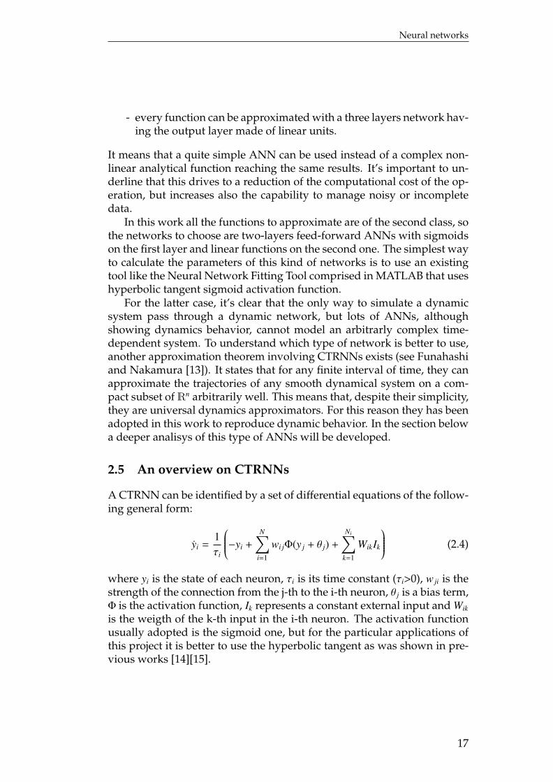
A limit cycle is a closed trajectory in the phase space, producing peri-odic behaviour in the time domain and it has the property that each tra-jectory sufficiently close to the limit cycle tends to it asimptotically. Abifurcation occurs when a small smooth change made in the parametervalues causes a sudden change in its behaviour, thus changing equilibriafrom stable to unstable ones but also turning an equilibrium point into alimit cycle.

The first property can be challenging because it makes it impossible toanalyze the system within the classic LTI theory. So to evaluate a CTRNNit is necessary to use another instrument, the phase plane method, thatallows to investigate the equilibrium points, the bifurcations and the limitcycles.

The analysis of the CTRNN state-space produces a very interesting re-sult: the simplest CTRNN with only two neurons shows up to nine equi-librium points, stable and unstable, and a limit cycle depending on thechoice of the parameters (see Beer [16]). This means that also a networkwith a few units can model lots of different and quite complex behavioursincluding periodic trajectories in the time domain and attractors in thestate domain, both fixed-points and limit cycles. Moreover: the chararac-teristics of the attractors can be varied acting on external input I. An exam-ple of such a behaviors are shown in figure 2.3. Since the goal of this workis to design a controller, at this point the problem is not only to model a

18

Neural networks

2.3.1: Attraction point.

2.3.2: Limit cycle.

Figure 2.3: Limit cycle and attraction point in a two-neurons CTRNN.

dynamic system, but it’s also necessary to achieve all the characteristics ofrobusteness required by the control theory (see Friedland [17]). From thispoint of view CTRNNs are powerful instruments because:

- they react very well to disturbance, filtering noise on inputs, evenwithout any specification during training;

- they respond with an acceptable output even when presented withinputs that they have never seen before;

- if correctly trained, they produce good results even when parameterschange in an important measure.

In conclusion a CTRNN can be used like a controller each time that it’snecessary to simulate a periodic behaviour or to reach a given target point.

The simplest way to implement a neural controller consists in usingmeasured or observed variables as states and, as control signal, the statesderivatives. If applicable, this method allows to avoid every integration,thus producing a very efficient and robust control system also from a nu-merical point of view.

19

Chapter 2

2.6 Network training

The identification of the set of parameters that defines a ANN is calledlearinig or training process. Given a specific task to solve, learning meansusing a set of observations to find the one which solves the task in someoptimal sense. The optimum is obtained defining a cost (or fitness) func-tion that evaluates how far away a particular solution is from an optimalsolution. The cost function is dependent on the task of approximate amodel and on a priori assumptions related to the implicit properties of themodel, its parameters and the observed variables.

The learning can be classified from two different points of view: thelearning paradigm and the learning algorithm. The learning paradigmis related to the model of the environment where the ANN works. Thelearning algorithm consists in a set of learning rules each of them used tomodify the value of the network parameters. The criterion to follow tomodify the parameters is the minimization of the cost function, insertedin a iterative process.

There are three major learning paradigms, each corresponding to a par-ticular abstract learning task. In supervised learning, there is a given set ofsample couples of input/output and the aim is the one of finding a func-tion that matches those data. The cost function is related to the mismatchbetween network mapping and the data. In unsupervised learning thereare some given inputs and the cost function to be minimized, that can beany function of the inputs, and the network’s output.

Classic learning algorithms, such as Hebbian rule, Back-Propagationand Forward-Propagation, are based on some form of gradient descent.This is done by simply taking the derivative of the cost function with re-spect to the network parameters and then changing those parameters in agradient-related direction. There is another interesting method based onan evolutionary approach: genetic algorithms, widely adopted in previ-ous works.

Since classic learning applied to CTRNN is very slow, a feasible alter-native for weight optimization is aGenetic Algorithm (GA). From a mathe-matical standpoint, genetic algorithms are fundamentally stochastic meth-ods based on the casual generation of solutions, called individuals, eachof them identified by a set of parameters, called chromosomes. There aremany individuals that make up the population. Once fixed the network’sstrucure the method works by the an iterative process that evolves throughthe following steps:

1. definition of an existance field for each parameter (maximum andminumum permitted values);

20

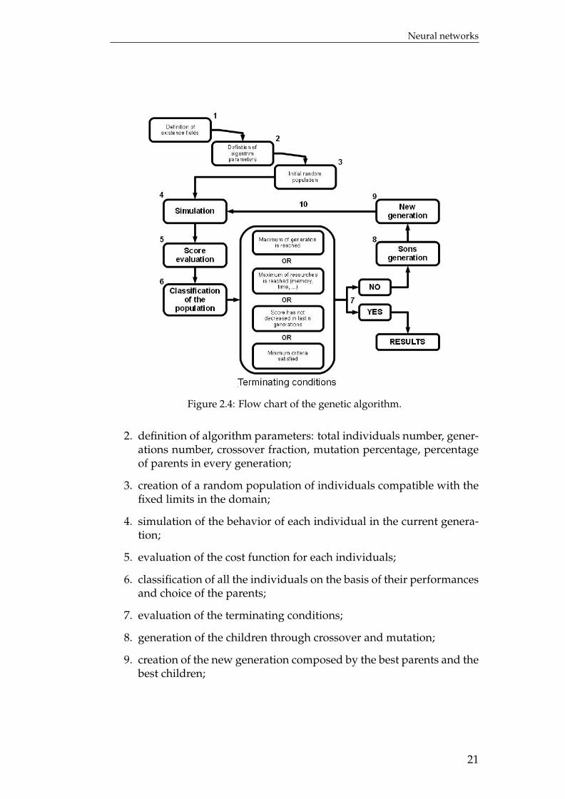
Neural networks

Figure 2.4: Flow chart of the genetic algorithm.

2. definition of algorithm parameters: total individuals number, gener-ations number, crossover fraction, mutation percentage, percentageof parents in every generation;

3. creation of a random population of individuals compatible with thefixed limits in the domain;

4. simulation of the behavior of each individual in the current genera-tion;

5. evaluation of the cost function for each individuals;

6. classification of all the individuals on the basis of their performancesand choice of the parents;

7. evaluation of the terminating conditions;

8. generation of the children through crossover and mutation;

9. creation of the new generation composed by the best parents and thebest children;

21

Chapter 2

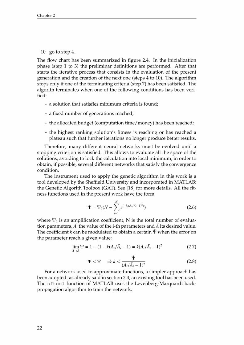
10. go to step 4.

The flow chart has been summarized in figure 2.4. In the inizializationphase (step 1 to 3) the preliminar definitions are performed. After thatstarts the iterative process that consists in the evaluation of the presentgeneration and the creation of the next one (steps 4 to 10). The algorithmstops only if one of the terminating criteria (step 7) has been satisfied. Thealgorith terminates when one of the following conditions has been veri-fied:

- a solution that satisfies minimum criteria is found;

- a fixed number of generations reached;

- the allocated budget (computation time/money) has been reached;

- the highest ranking solution’s fitness is reaching or has reached aplateau such that further iterations no longer produce better results.

Therefore, many different neural networks must be evolved until astopping criterion is satisfied. This allows to evaluate all the space of thesolutions, avoiding to lock the calculation into local minimum, in order toobtain, if possible, several different networks that satisfy the convergencecondition.

The instrument used to apply the genetic algorithm in this work is atool developed by the Sheffield University and incorporated in MATLAB:the Genetic Algorith Toolbox (GAT). See [18] for more details. All the fit-ness functions used in the present work have the form:

Ψ = Ψ0(N −N∑

i=1

e(−ki(Ai/Ai−1)2)) (2.6)

where Ψ0 is an amplification coefficient, N is the total number of evalua-tion parameters, Ai the value of the i-th parameters and A its desired value.The coefficient k can be modulated to obtain a certain Ψ when the error onthe parameter reach a given value:

limA→A

Ψ = 1 − (1 − k(Ai/Ai − 1) = k(Ai/Ai − 1)2 (2.7)

Ψ < Ψ ⇒ k <Ψ

(Ai/Ai − 1)2(2.8)

For a network used to approximate functions, a simpler approach hasbeen adopted: as already said in section 2.4, an existing tool has been used.The nftool function of MATLAB uses the Levenberg-Marquardt back-propagation algorithm to train the network.

22

Chapter 3

Control strategy - The problem of walkingThe aim of this chapter is to illustrate the main ideas that are the foun-dation of the NEMeSys control system. At first the global aspects of thewalking behavior will be studied and then a particular solution of thisproblem will be discussed. In the last sections of the chapter all the partsof this solution will be explained in detail.

3.1 General features

Walk can be defined, in the most general way, similarly to a method ofterrestrial locomotion that uses limbs. The main differences with otherkinds of movement are the presence of a non-continuous contact with asubstrate and the usage of more than one multiple-DoFs appendage.

Walking is one of many behaviors where machines still lag notably be-hind the performance of animals, so it is natural to examine walking inanimals to look for hints to improve the performance of machines. Froma cognitive standpoint, walking appears to be a fairly automatic behavior.Nevertheless, it’s also immediate arguing that walking in a natural envi-ronment requires considerable capabilities from the controller, involvingdifferent features, and it’s all but a trivial behavior.

The most important global aspects of the walking problem can be sum-marized as follows:

- redundancy. In systems concerned with walking, the number of de-grees of freedom is normally larger than the one necessary to per-form the task. Thus, there may be a manifold of leg postures for agiven kinematic boundary condition;

- autonomy. The redundancy requires the system to select among dif-ferent alternatives according to some, often context-dependent, opti-mization criteria, which means that the system usually has to adoptsome choices without external command;

- embodiment of the controller. To maintain the problem at a levelas simple as possible, the controller needs the ability to exploit thephysical properties of the body

- situatedness of the body in its environment. Each walking systemis a physical systems situated in complex and often unpredictable

23

Chapter 3

environments, which means that any movement may be modifiedby the physics of the system and the environment.

The best solution to fulfill all these tasks, as described in section 1.1,is a decentralized control structure that consists of a number of distinctmodules each one solving particular subtasks. The division into mod-ules and the choice of the subtasks have been accomplished starting frombiomimetics findings: the followed approach consist in assembling logicalcomponents to model the system properties of the behaving animal.

Although many animals have body appendages that can be used forwalking, only a few species have been investigated in sufficient detail.Among them, the stick insect is the more suitable for the purposes of thiswork thanks to its capability to walk on very complex and irregular sub-strates.

3.2 The walking system

Before starting the discussion about the structure of the controller it’s use-ful to evaluate the main characteristics of the system to be controlled. Itis a simplified model of a stick insect, with a rigid body supported by sixlegs: two legs are called ipsilateral if situated on the same side, contralateralif situated on the opposite side.

Each leg has been modeled as a manipulator with three joints anddivided into three movable sections: the coxa, closest to the body, thetrochanter-femur, or just femur as they are fused and the tibia. A fourthpart, the tarsus, provides and holds the ground contact in real stick in-sects, but it’s not strictly necessary to perform a walking behavior and thisis why it won’t be considered in this model.

The Body-Coxa (BC) joint is best described as a socket joint, whereasthe Coxa-Trochanter (CT) joint and the Femur-Tibia (FT) joint are hingejoints. The CT and the FT axis are parallel, hence, the femur and tibia lieon the same plane.

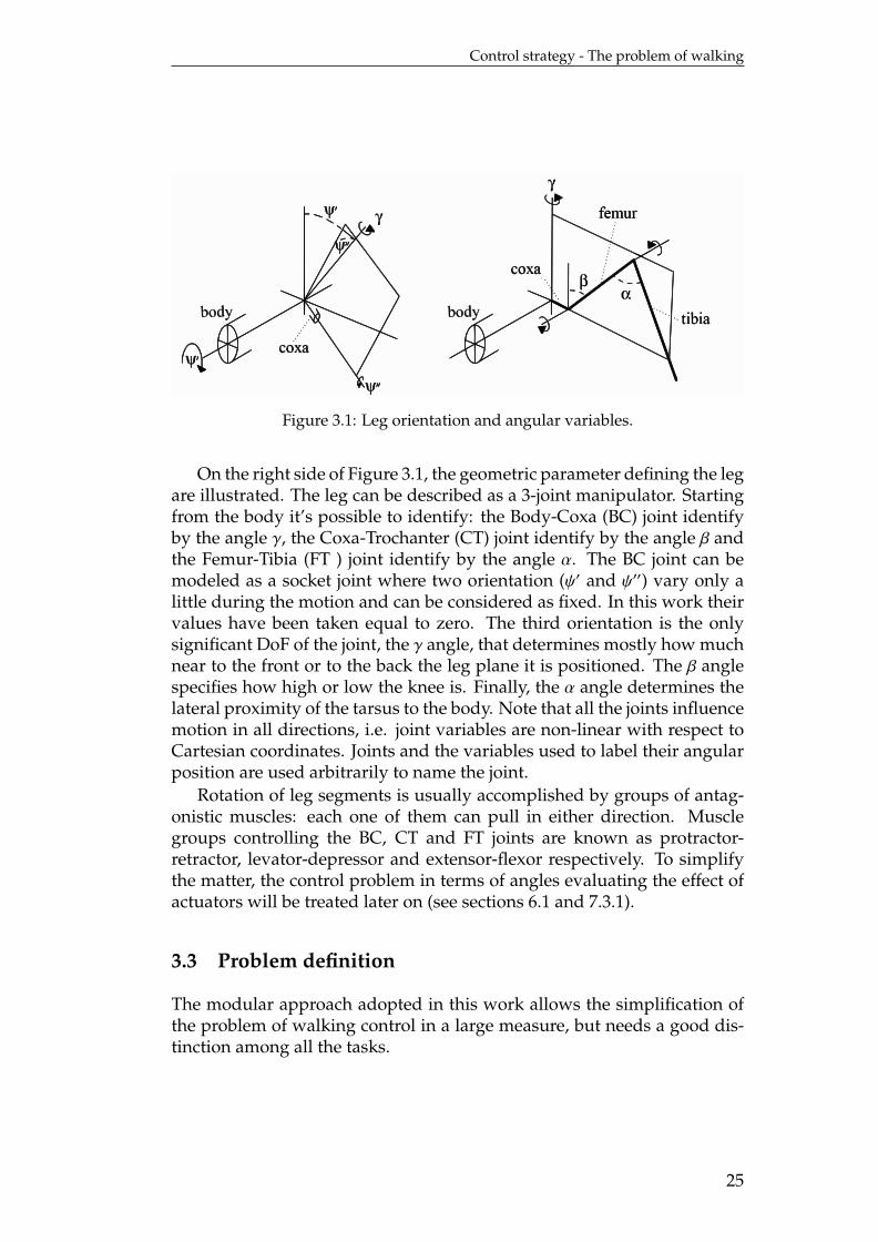
Orientation and motion of the coxa segment out of the body can be de-scribed by three orthogonal rotations, one of which is dominant. On theleft hand side of Figure 3.1 there are shown the two orientations ψ′ and ψ′′

that change the least, thus both are considered fixed. However, althoughvariability during the walk is small, the angle ψ′ in the stick insect is large.In this model, instead, both these angles have been taken equal to zero,which drives the third axis to be perpendicular to the body plane and re-ducing the BC joint to a hinge joint like the other ones. In this way all theDoFs can be treated almost in the same manner.

24

Control strategy - The problem of walking

Figure 3.1: Leg orientation and angular variables.

On the right side of Figure 3.1, the geometric parameter defining the legare illustrated. The leg can be described as a 3-joint manipulator. Startingfrom the body it’s possible to identify: the Body-Coxa (BC) joint identifyby the angle γ, the Coxa-Trochanter (CT) joint identify by the angle β andthe Femur-Tibia (FT ) joint identify by the angle α. The BC joint can bemodeled as a socket joint where two orientation (ψ′ and ψ′′) vary only alittle during the motion and can be considered as fixed. In this work theirvalues have been taken equal to zero. The third orientation is the onlysignificant DoF of the joint, the γ angle, that determines mostly how muchnear to the front or to the back the leg plane it is positioned. The β anglespecifies how high or low the knee is. Finally, the α angle determines thelateral proximity of the tarsus to the body. Note that all the joints influencemotion in all directions, i.e. joint variables are non-linear with respect toCartesian coordinates. Joints and the variables used to label their angularposition are used arbitrarily to name the joint.

Rotation of leg segments is usually accomplished by groups of antag-onistic muscles: each one of them can pull in either direction. Musclegroups controlling the BC, CT and FT joints are known as protractor-retractor, levator-depressor and extensor-flexor respectively. To simplifythe matter, the control problem in terms of angles evaluating the effect ofactuators will be treated later on (see sections 6.1 and 7.3.1).

3.3 Problem definition

The modular approach adopted in this work allows the simplification ofthe problem of walking control in a large measure, but needs a good dis-tinction among all the tasks.

25

Chapter 3

Biological findings about various animals (e.g. Wendler [19]) show thatthe movements of individual legs are managed by fairly independent con-trol systems. On the other hand each leg has an influence on the other onesand it’s the combination of all these influences that allows to generate anefficient walk. This means that the global motion problem can be solvedby accomplishing two macro-tasks:

- control the motion of each single leg;

- coordinate all the legs;

The control of the single leg it’s fundamentally the problem of gener-ate the step cycle. During the walking, the individual legs typically movecyclically and, in order to facilitate the analysis, the motion of a leg is oftenpartitioned into phases: the control of each phase and transition amongphases are called subtasks of the walking problem. Other features regard-ing the single leg control are related to maintaining a fixed leg and to re-acting to external disturbances. In section 3.5 all these arguments will bediscussed deeply.

The coordination among legs is essential to regulate global parameterssuch as advancing speed, stability margin or body attitude and position.The first task consists in maintaining a steady motion and it can be ob-tained introducing local weighted influences among neighboring legs. Tofulfill more complex task like regulating body attitude, local rules aren’tenough and a global planning is required. The whole problem will betreated in section 3.6.

In this work a bottom-to-top approach has been adopted to create anincrementally realistic motion generator. Starting from the design of ef-ficient controllers for every phase of the step cycle, a selector regulatingthe transition among phases has been developed producing a completesingle leg controller. At this level mutual influences among neighboringlegs have been introduced and only in the last phase of the work globalcoordination parameters have been taken into account accomplishing theglobal task of walking control.

3.4 Global controller architecture

The approach to the problem of walking control is not unique: it heavydepends on external parameters such as substrate properties and globalrequired speed. Walking in predictable environments and fast running, toa large degree, rely on leg mechanical properties. Conversely, slow walk-ing in unpredictable terrain, e.g. climbing in rugged structures, has to

26

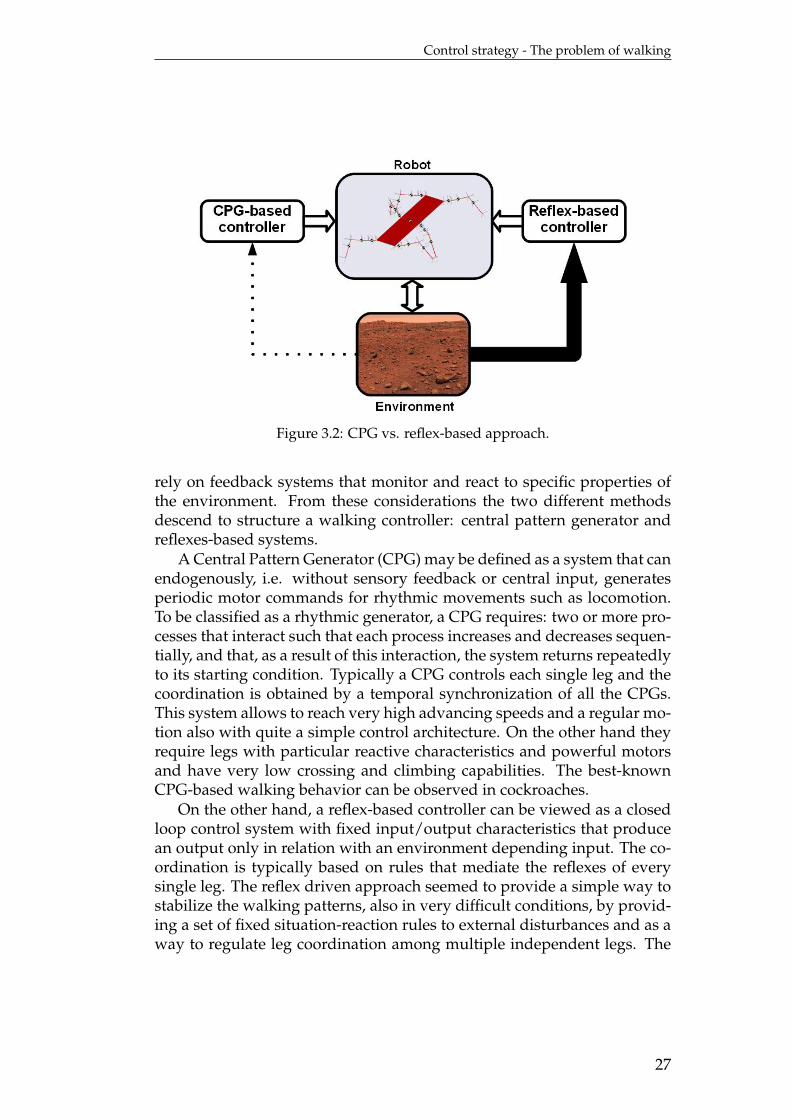
Control strategy - The problem of walking

Figure 3.2: CPG vs. reflex-based approach.

rely on feedback systems that monitor and react to specific properties ofthe environment. From these considerations the two different methodsdescend to structure a walking controller: central pattern generator andreflexes-based systems.

A Central Pattern Generator (CPG) may be defined as a system that canendogenously, i.e. without sensory feedback or central input, generatesperiodic motor commands for rhythmic movements such as locomotion.To be classified as a rhythmic generator, a CPG requires: two or more pro-cesses that interact such that each process increases and decreases sequen-tially, and that, as a result of this interaction, the system returns repeatedlyto its starting condition. Typically a CPG controls each single leg and thecoordination is obtained by a temporal synchronization of all the CPGs.This system allows to reach very high advancing speeds and a regular mo-tion also with quite a simple control architecture. On the other hand theyrequire legs with particular reactive characteristics and powerful motorsand have very low crossing and climbing capabilities. The best-knownCPG-based walking behavior can be observed in cockroaches.

On the other hand, a reflex-based controller can be viewed as a closedloop control system with fixed input/output characteristics that producean output only in relation with an environment depending input. The co-ordination is typically based on rules that mediate the reflexes of everysingle leg. The reflex driven approach seemed to provide a simple way tostabilize the walking patterns, also in very difficult conditions, by provid-ing a set of fixed situation-reaction rules to external disturbances and as away to regulate leg coordination among multiple independent legs. The

27

Chapter 3

problem of this system is the complexity required to be sufficiently flexi-ble: to be able to face lots of situation, a high number of reflex has to betaken into account. The most relevant example of such a behavior can befound in stick insects.

In insects only one of this structure isn’t able to explain all the observedbehavior as underlined, among the other, by Porcino [20]. For a space-oriented project, like this one, it’s clear that, at this level of development,a very fast CPG-based robot has only little utility. In an unknown envi-ronment, like planetary surfaces, the first priority for a robot is to ensure asteady motion in any moment. A walking robot, besides, must be able toreach locations out of the range of wheeled ones, balancing its complex-ity with its higher capabilities. Furthermore a slow locomotion allows toreduce energy consumption and to avoid shocks to the scientific payload.All these considerations favored the choice on a reflex-based controller.

3.5 The control of a single leg

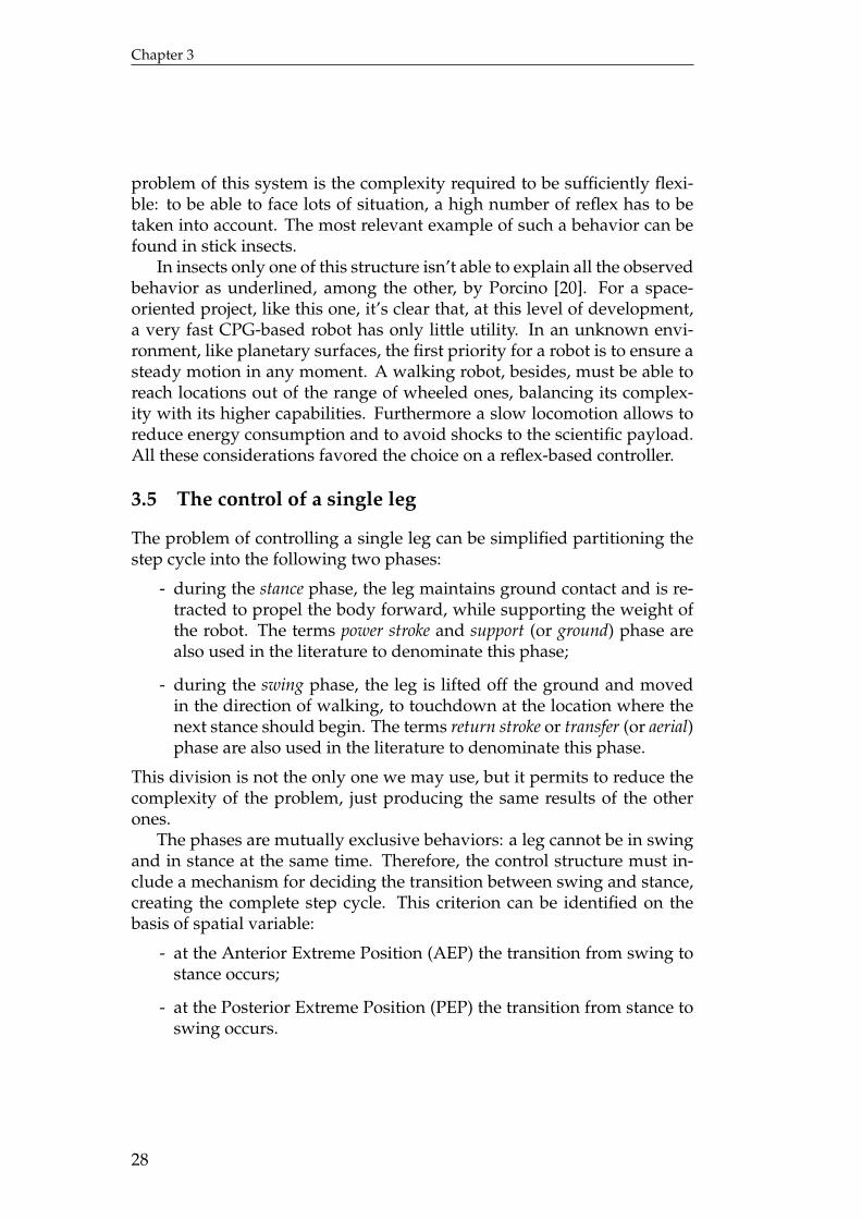
The problem of controlling a single leg can be simplified partitioning thestep cycle into the following two phases:

- during the stance phase, the leg maintains ground contact and is re-tracted to propel the body forward, while supporting the weight ofthe robot. The terms power stroke and support (or ground) phase arealso used in the literature to denominate this phase;

- during the swing phase, the leg is lifted off the ground and movedin the direction of walking, to touchdown at the location where thenext stance should begin. The terms return stroke or transfer (or aerial)phase are also used in the literature to denominate this phase.

This division is not the only one we may use, but it permits to reduce thecomplexity of the problem, just producing the same results of the otherones.

The phases are mutually exclusive behaviors: a leg cannot be in swingand in stance at the same time. Therefore, the control structure must in-clude a mechanism for deciding the transition between swing and stance,creating the complete step cycle. This criterion can be identified on thebasis of spatial variable:

- at the Anterior Extreme Position (AEP) the transition from swing tostance occurs;

- at the Posterior Extreme Position (PEP) the transition from stance toswing occurs.

28

Control strategy - The problem of walking

Figure 3.3: Swing and stance phases.

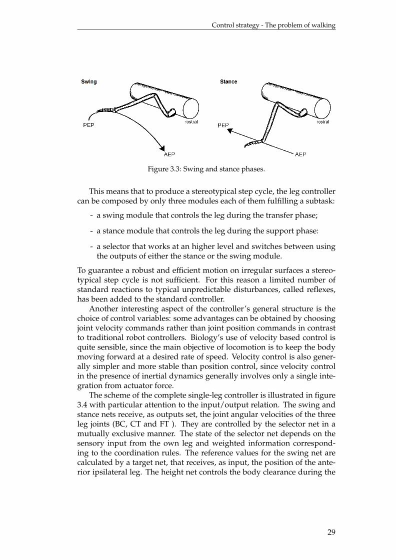
This means that to produce a stereotypical step cycle, the leg controllercan be composed by only three modules each of them fulfilling a subtask:

- a swing module that controls the leg during the transfer phase;

- a stance module that controls the leg during the support phase:

- a selector that works at an higher level and switches between usingthe outputs of either the stance or the swing module.

To guarantee a robust and efficient motion on irregular surfaces a stereo-typical step cycle is not sufficient. For this reason a limited number ofstandard reactions to typical unpredictable disturbances, called reflexes,has been added to the standard controller.

Another interesting aspect of the controller’s general structure is thechoice of control variables: some advantages can be obtained by choosingjoint velocity commands rather than joint position commands in contrastto traditional robot controllers. Biology’s use of velocity based control isquite sensible, since the main objective of locomotion is to keep the bodymoving forward at a desired rate of speed. Velocity control is also gener-ally simpler and more stable than position control, since velocity controlin the presence of inertial dynamics generally involves only a single inte-gration from actuator force.

The scheme of the complete single-leg controller is illustrated in figure3.4 with particular attention to the input/output relation. The swing andstance nets receive, as outputs set, the joint angular velocities of the threeleg joints (BC, CT and FT ). They are controlled by the selector net in amutually exclusive manner. The state of the selector net depends on thesensory input from the own leg and weighted information correspond-ing to the coordination rules. The reference values for the swing net arecalculated by a target net, that receives, as input, the position of the ante-rior ipsilateral leg. The height net controls the body clearance during the

29

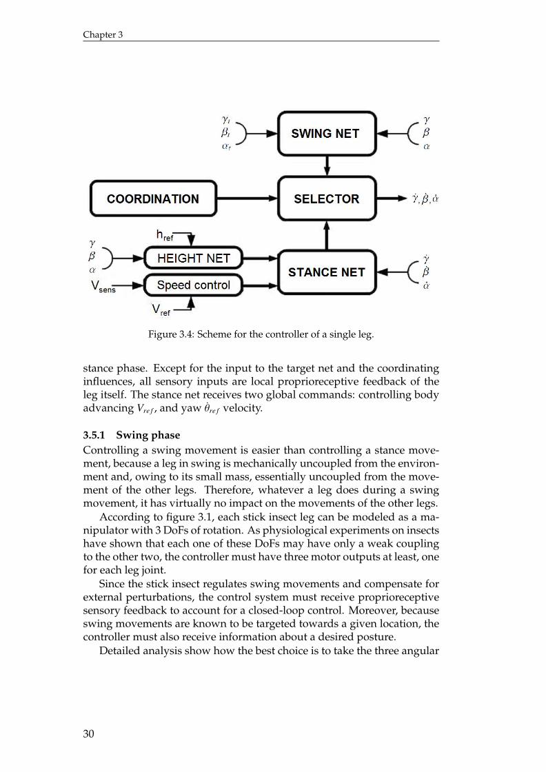
Chapter 3

Figure 3.4: Scheme for the controller of a single leg.

stance phase. Except for the input to the target net and the coordinatinginfluences, all sensory inputs are local proprioreceptive feedback of theleg itself. The stance net receives two global commands: controlling bodyadvancing Vre f , and yaw θre f velocity.

3.5.1 Swing phaseControlling a swing movement is easier than controlling a stance move-ment, because a leg in swing is mechanically uncoupled from the environ-ment and, owing to its small mass, essentially uncoupled from the move-ment of the other legs. Therefore, whatever a leg does during a swingmovement, it has virtually no impact on the movements of the other legs.

According to figure 3.1, each stick insect leg can be modeled as a ma-nipulator with 3 DoFs of rotation. As physiological experiments on insectshave shown that each one of these DoFs may have only a weak couplingto the other two, the controller must have three motor outputs at least, onefor each leg joint.

Since the stick insect regulates swing movements and compensate forexternal perturbations, the control system must receive proprioreceptivesensory feedback to account for a closed-loop control. Moreover, becauseswing movements are known to be targeted towards a given location, thecontroller must also receive information about a desired posture.

Detailed analysis show how the best choice is to take the three angular

30

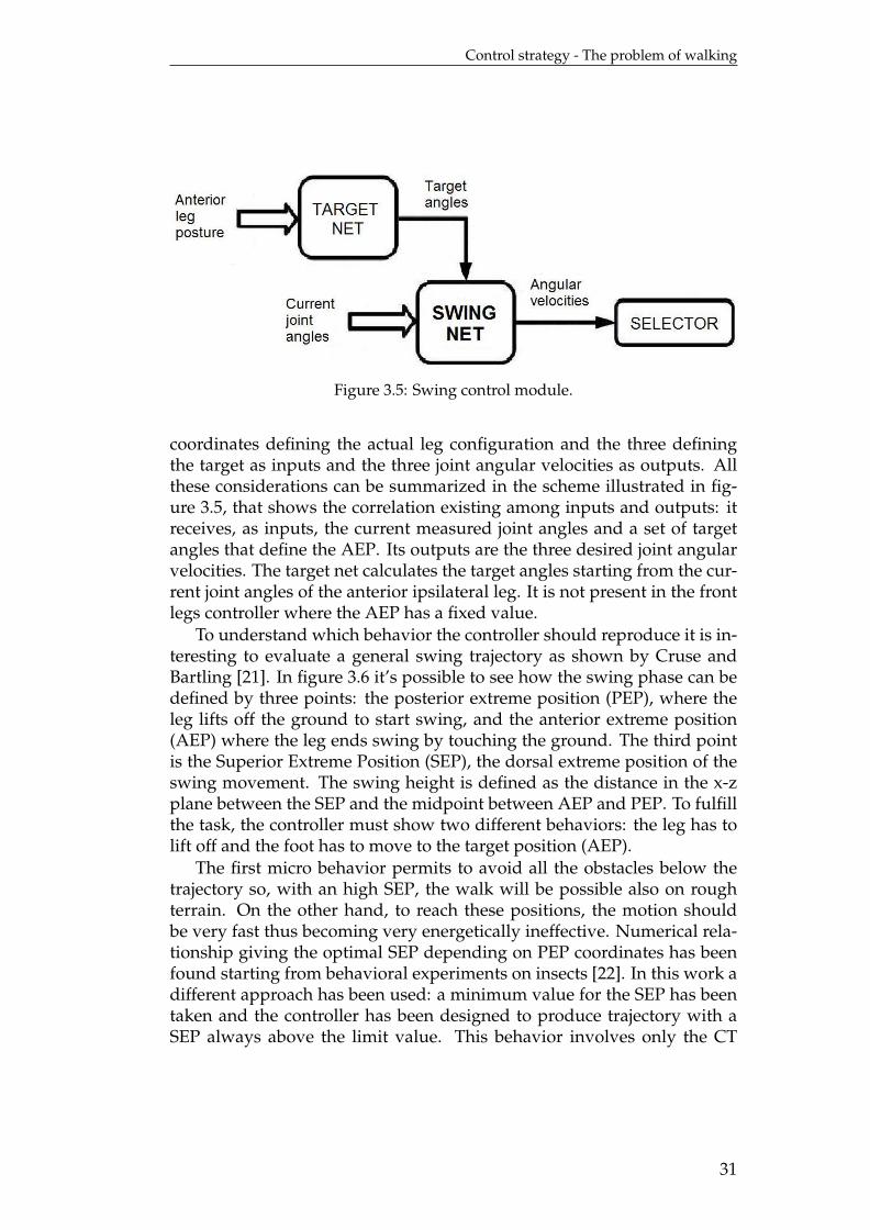
Control strategy - The problem of walking

Figure 3.5: Swing control module.

coordinates defining the actual leg configuration and the three definingthe target as inputs and the three joint angular velocities as outputs. Allthese considerations can be summarized in the scheme illustrated in fig-ure 3.5, that shows the correlation existing among inputs and outputs: itreceives, as inputs, the current measured joint angles and a set of targetangles that define the AEP. Its outputs are the three desired joint angularvelocities. The target net calculates the target angles starting from the cur-rent joint angles of the anterior ipsilateral leg. It is not present in the frontlegs controller where the AEP has a fixed value.

To understand which behavior the controller should reproduce it is in-teresting to evaluate a general swing trajectory as shown by Cruse andBartling [21]. In figure 3.6 it’s possible to see how the swing phase can bedefined by three points: the posterior extreme position (PEP), where theleg lifts off the ground to start swing, and the anterior extreme position(AEP) where the leg ends swing by touching the ground. The third pointis the Superior Extreme Position (SEP), the dorsal extreme position of theswing movement. The swing height is defined as the distance in the x-zplane between the SEP and the midpoint between AEP and PEP. To fulfillthe task, the controller must show two different behaviors: the leg has tolift off and the foot has to move to the target position (AEP).

The first micro behavior permits to avoid all the obstacles below thetrajectory so, with an high SEP, the walk will be possible also on roughterrain. On the other hand, to reach these positions, the motion shouldbe very fast thus becoming very energetically ineffective. Numerical rela-tionship giving the optimal SEP depending on PEP coordinates has beenfound starting from behavioral experiments on insects [22]. In this work adifferent approach has been used: a minimum value for the SEP has beentaken and the controller has been designed to produce trajectory with aSEP always above the limit value. This behavior involves only the CT

31

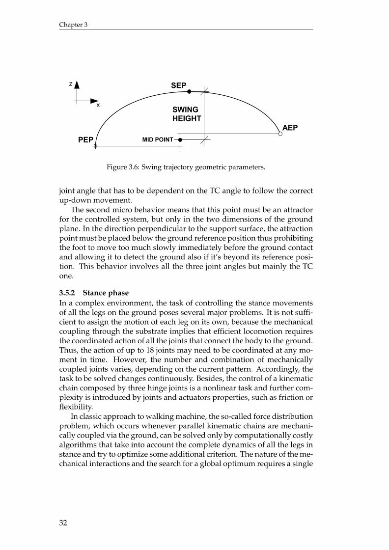
Chapter 3

SEP

AEPPEP

SWINGHEIGHT

MID POINT

x

x

z

Figure 3.6: Swing trajectory geometric parameters.

joint angle that has to be dependent on the TC angle to follow the correctup-down movement.

The second micro behavior means that this point must be an attractorfor the controlled system, but only in the two dimensions of the groundplane. In the direction perpendicular to the support surface, the attractionpoint must be placed below the ground reference position thus prohibitingthe foot to move too much slowly immediately before the ground contactand allowing it to detect the ground also if it’s beyond its reference posi-tion. This behavior involves all the three joint angles but mainly the TCone.

3.5.2 Stance phaseIn a complex environment, the task of controlling the stance movementsof all the legs on the ground poses several major problems. It is not suffi-cient to assign the motion of each leg on its own, because the mechanicalcoupling through the substrate implies that efficient locomotion requiresthe coordinated action of all the joints that connect the body to the ground.Thus, the action of up to 18 joints may need to be coordinated at any mo-ment in time. However, the number and combination of mechanicallycoupled joints varies, depending on the current pattern. Accordingly, thetask to be solved changes continuously. Besides, the control of a kinematicchain composed by three hinge joints is a nonlinear task and further com-plexity is introduced by joints and actuators properties, such as friction orflexibility.

In classic approach to walking machine, the so-called force distributionproblem, which occurs whenever parallel kinematic chains are mechani-cally coupled via the ground, can be solved only by computationally costlyalgorithms that take into account the complete dynamics of all the legs instance and try to optimize some additional criterion. The nature of the me-chanical interactions and the search for a global optimum requires a single

32

Control strategy - The problem of walking

central control system instead of a distributed processing. In technical so-lutions, such centralized system makes real-time control difficult, even insimple cases.

Although the task to coordinate many joints appears complex, insectsmaster it with their simple nervous system. This means that they use,instead of a centralized controller, a decentralized approach able to exploitthe dynamics of the body-environment interaction without calculating allthe required information explicitly, e.g. the mutual influences among thejoints.

To solve this particular problem in a very easy way, Cruse et al. [23][24]propose to replace a central controller with distributed control in the formof local positive feedback. For more detail on positive feedback in biolog-ical systems see De Angelis [25]. The positive feedback occurs at the levelof the single joint, feeding back the position signal to control the motoroutput of the same joint, without direct relationship with the rest of thekinematic chain.

To understand how positive displacement feedback works, one mustconsider, a standing legged system that begins to move one joint, whilekeeping all the feet on the ground. Owing to the mechanical connections,all other joints of the moved leg, and even joints of the other legs, passivelyadjust to the active joint movement. Thus, the movement direction andspeed of each joint do not have to be computed because this informationis already provided by the physics of the whole system.

This example is related to postural control, a problem ruled by resis-tance reflexes that maintain the position of each leg with local negativefeedback circuits. In the control of walking a resistance reflex may be re-placed by an assistance reflex: it can be modeled by a positive feedbackthat transforms this passive movement into an active one.

There are, however, several problems to be solved. The first is that pos-itive feedback using the raw position signal would lead to unpredictablechanges in movement speed and not necessarily to the nearly constantwalking speed which is usually desired. This problem can be solved byintroducing a kind of band-pass filter into the feedback loop. The effectis to make the feedback proportional to the angular velocity of the jointmovement and not proportional the angular position. This strategy is alsoknown as Local Positive Velocity Feedback (LPVF).

The second problem is that using positive feedback for all three legjoints leads to unpredictable changes in body height, even in a computersimulation excluding gravity. To avoid these effects the height control hasbeen decoupled to forward movement. According to experiments on stickinsect, LPVF has been applied only on γ and α angles, that are deputy

33

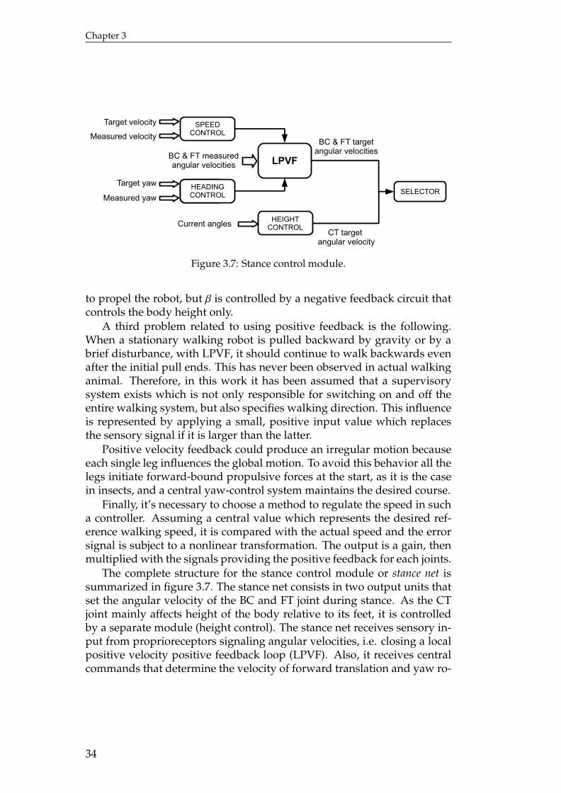
Chapter 3

BC & FT measured angular velocities LPVF

Target velocity

Measured velocitySPEED

CONTROL

Speedcontrol

Target yaw

Measured yawHEADINGCONTROL

BC & FT target angular velocities

HEIGHTCONTROL

SELECTOR

Current anglesCT target

angular velocity

Figure 3.7: Stance control module.

to propel the robot, but β is controlled by a negative feedback circuit thatcontrols the body height only.

A third problem related to using positive feedback is the following.When a stationary walking robot is pulled backward by gravity or by abrief disturbance, with LPVF, it should continue to walk backwards evenafter the initial pull ends. This has never been observed in actual walkinganimal. Therefore, in this work it has been assumed that a supervisorysystem exists which is not only responsible for switching on and off theentire walking system, but also specifies walking direction. This influenceis represented by applying a small, positive input value which replacesthe sensory signal if it is larger than the latter.

Positive velocity feedback could produce an irregular motion becauseeach single leg influences the global motion. To avoid this behavior all thelegs initiate forward-bound propulsive forces at the start, as it is the casein insects, and a central yaw-control system maintains the desired course.

Finally, it’s necessary to choose a method to regulate the speed in sucha controller. Assuming a central value which represents the desired ref-erence walking speed, it is compared with the actual speed and the errorsignal is subject to a nonlinear transformation. The output is a gain, thenmultiplied with the signals providing the positive feedback for each joints.

The complete structure for the stance control module or stance net issummarized in figure 3.7. The stance net consists in two output units thatset the angular velocity of the BC and FT joint during stance. As the CTjoint mainly affects height of the body relative to its feet, it is controlledby a separate module (height control). The stance net receives sensory in-put from proprioreceptors signaling angular velocities, i.e. closing a localpositive velocity positive feedback loop (LPVF). Also, it receives centralcommands that determine the velocity of forward translation and yaw ro-

34

Control strategy - The problem of walking

tation. Both of these signals are subtracted from a corresponding sensoryinput signal, thus closing a negative feedback loops.

3.5.3 Phase transitionThe problem of transition between phases seems to be complex, but truthto say it’s simple and depends on two parameters only identified by nu-merous authors, e.g. Cruse [26]. They are the following:

- the Ground Contact (GC) input excites the stance phase, at the sametime as it inhibits the swing phase;

- the Posterior Extreme Position (PEP) input indicates that it is timefor the transition to the swing phase.

This process can be controlled by a single module, called selector, thatswitches the outputs calculation from a phase to the other one. Even ifthe two motion phases are mutually exclusive, the output units receiveself-excitation (i.e. positive feedback) to fix into a state. This was found tobe less sensitive than the use of mutual inhibition from the output units.

3.5.4 ReflexesA reflex is a type of behavior that can be roughly defined as a rapid, au-tomatic involuntary response triggered by external stimuli. The responsepersists for the duration of the stimulus and its intensity is correlated withthe stimulus’s strength. Reflexes are very useful during locomotion, mak-ing the animal able to react to any unpredictable situation rapidly.

The control system described in this work for the generation of a stepcycle in each leg of the robot, is based on reflexes as it is illustrated insection 3.4. This approach allows an higher flexibility than for CPG-basedsystems, but the reflexes introduced in that model are only a part of thetotal reactive behaviors shown by a stick insect: an assistance reflex topropel the body and a step reflex to lift-off the leg.

In real animals other reflexes exist, that allow them not only to generatea regular walking pattern, but also to produce the correct behavior in reac-tion to a large number of unpredictable changes in the environment. Fromthis point of view a reflex may be considered as a stereotypical responseto a standard changing in the external inputs. Now the problem is howmany reflexes must be implemented in the controller to solve the problemof walking correctly. Recent studies of neurophysiologists identified threemore different typologies of reflex in insects (Beer et al., 1997):

- stepping reflex: when a leg slides or assumes a configuration poorlystable, performs a limited aerial phase to return in a posture able toensure a sufficient stability;

35

Chapter 3

Figure 3.8: Overview on reflexes.

- avoidance reflex: when a leg touches a obstacle, it moves away from itand changes its elevation to produce a trajectory able to avoid it;

- searching reflex: when a leg doesn’t find the ground at the end of itsswing phase, starts a rhythmical motion in an increasing region ofspace until a supporting surface is found.

In figure 3.8 such behaviors are shown. They will be discussed in detail insection 4.4.

3.6 Legs coordination

The second macro behavior required in walking control is the coordinationamong single legs movements. The problem must consider two things atleast. First, the timing of lift-off and touchdown in each leg must not im-pair the stability of the whole body. Second, the number of legs in stancedetermines the upper bound of propulsive force. Therefore, efficient tim-ing and coordination of power and stance direction of all legs in stancemust be controlled to ensure their synergistic action. This two featureswill be developed in section 3.6.1 and 3.6.2 respectively.

These two first requirements can be fulfilled without a central plan-ning. To reach a satisfying solution it is sufficient to insert local influencesthat link each limb only with its neighbors. This method, shown in sub-section 3.6.3, allows to simplify the problem considerably, reducing com-putational costs.

Some other problems need a global supervision on all the legs to becorrectly solved: the main of them is the control of the body’s height andattitude. To manage these parameters, it’s necessary both to measure andcontrol variables of all the legs and to perform global calculation. Theother global feature, treated in subsection 3.6.4, involves the generation

36

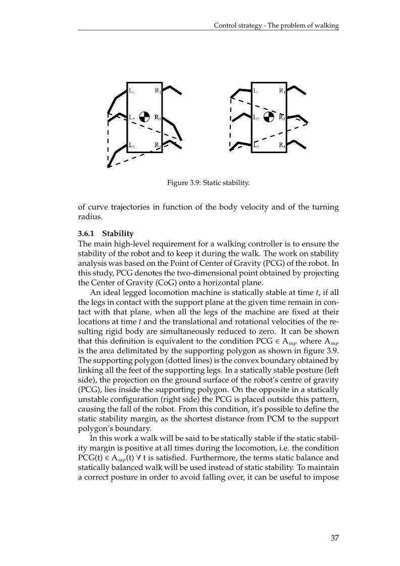
Control strategy - The problem of walking

Figure 3.9: Static stability.

of curve trajectories in function of the body velocity and of the turningradius.

3.6.1 StabilityThe main high-level requirement for a walking controller is to ensure thestability of the robot and to keep it during the walk. The work on stabilityanalysis was based on the Point of Center of Gravity (PCG) of the robot. Inthis study, PCG denotes the two-dimensional point obtained by projectingthe Center of Gravity (CoG) onto a horizontal plane.

An ideal legged locomotion machine is statically stable at time t, if allthe legs in contact with the support plane at the given time remain in con-tact with that plane, when all the legs of the machine are fixed at theirlocations at time t and the translational and rotational velocities of the re-sulting rigid body are simultaneously reduced to zero. It can be shownthat this definition is equivalent to the condition PCG ∈ Asup where Asup

is the area delimitated by the supporting polygon as shown in figure 3.9.The supporting polygon (dotted lines) is the convex boundary obtained bylinking all the feet of the supporting legs. In a statically stable posture (leftside), the projection on the ground surface of the robot’s centre of gravity(PCG), lies inside the supporting polygon. On the opposite in a staticallyunstable configuration (right side) the PCG is placed outside this pattern,causing the fall of the robot. From this condition, it’s possible to define thestatic stability margin, as the shortest distance from PCM to the supportpolygon’s boundary.

In this work a walk will be said to be statically stable if the static stabil-ity margin is positive at all times during the locomotion, i.e. the conditionPCG(t) ∈ Asup(t) ∀ t is satisfied. Furthermore, the terms static balance andstatically balanced walk will be used instead of static stability. To maintaina correct posture in order to avoid falling over, it can be useful to impose

37

Chapter 3

the static stability condition during the entire walk.With a static balance requirement, at least three legs have to touch the

ground at the same time for locomotion if an ideal legged locomotion ma-chine is assumed. This means that biped and quadruped walker requiremore complex dynamical balancing to reach good performances, but it’snot a problem for hexapod: previous studies on insects show that the walkpatterns allowing to reach the highest speeds for six-legged walking plat-form are all statically balanced (see Wilson [27] and Song and Waldron[28]).

Another consideration can be done supporting the choice of limitingthe stability analysis to statically stable gaits: the concept of a safe walkcan be introduced, to be a walk where, if all the joints are suddenly frozen,the system still ends up in a statically stable equilibrium. This conceptdoes not imply a statically balanced gait, since falling is allowed as longas the system ends in a safe configuration.

3.6.2 GaitsA gait can be generally defined as a manner of moving the legs in walk-ing or running or, more properly, as a pattern of locomotion characteristicfor a limited range of speeds described by a number of quantities, oneor more of which change discontinuously at the moment of transition toother gaits. The concept of gait is strictly related to the stride concept, thatis a period of locomotion defined by the complete cycle of a reference limb.

A gait can be numerically quantified by four parameters:

- the stride duration, the duration of one stride;

- the stride length, the distance the trunk translates during one stride;

- the duty factor (typically denoted β), the temporal fraction of a stepcycle during which the foot is on the ground;

- the relative phase of leg l (typically denoted φl), described as the leg’sphase with respect to a reference leg.

The simplest way to define a gait mathematically is a sequence of binaryvectors that indicates the phase (swing or stance) of each leg and the phaseduration. The gait is thus defined by the sequence in which the legs changephase. This analysis can be summarized in a gait diagram showing thephases of the different legs as a function of time.

In six-legged walkers the gaits that ensure the best performances canbe chosen from biological findings. In his reference work on hexapod loco-motion Wilson [27] shows that all the typical gaits observed in stick insectsare based on five concepts:

38

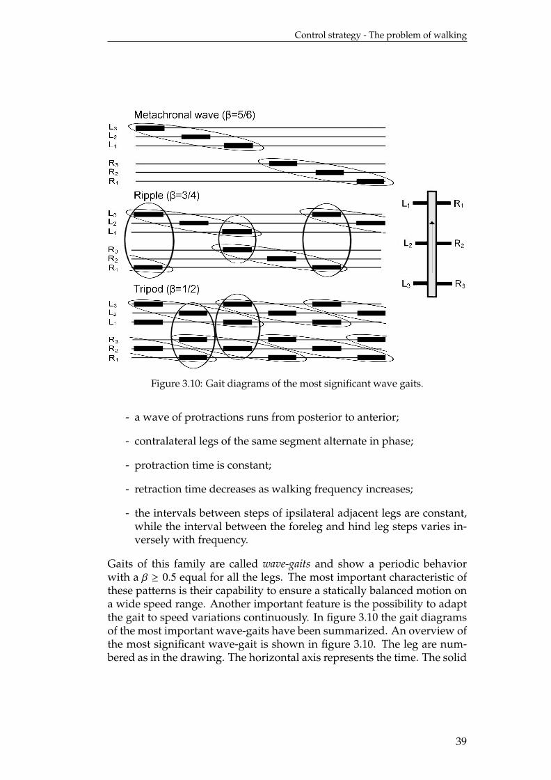
Control strategy - The problem of walking

Figure 3.10: Gait diagrams of the most significant wave gaits.

- a wave of protractions runs from posterior to anterior;

- contralateral legs of the same segment alternate in phase;

- protraction time is constant;

- retraction time decreases as walking frequency increases;

- the intervals between steps of ipsilateral adjacent legs are constant,while the interval between the foreleg and hind leg steps varies in-versely with frequency.

Gaits of this family are called wave-gaits and show a periodic behaviorwith a β ≥ 0.5 equal for all the legs. The most important characteristic ofthese patterns is their capability to ensure a statically balanced motion ona wide speed range. Another important feature is the possibility to adaptthe gait to speed variations continuously. In figure 3.10 the gait diagramsof the most important wave-gaits have been summarized. An overview ofthe most significant wave-gait is shown in figure 3.10. The leg are num-bered as in the drawing. The horizontal axis represents the time. The solid

39

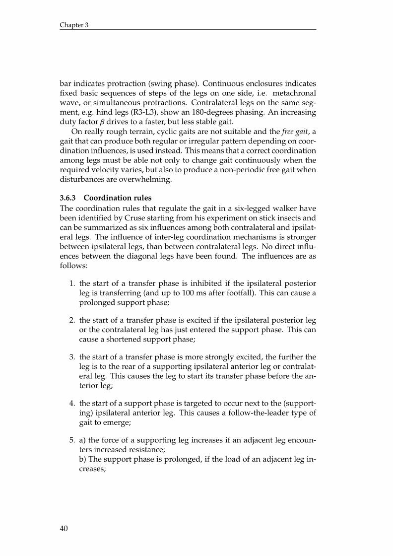
Chapter 3

bar indicates protraction (swing phase). Continuous enclosures indicatesfixed basic sequences of steps of the legs on one side, i.e. metachronalwave, or simultaneous protractions. Contralateral legs on the same seg-ment, e.g. hind legs (R3-L3), show an 180-degrees phasing. An increasingduty factor β drives to a faster, but less stable gait.

On really rough terrain, cyclic gaits are not suitable and the free gait, agait that can produce both regular or irregular pattern depending on coor-dination influences, is used instead. This means that a correct coordinationamong legs must be able not only to change gait continuously when therequired velocity varies, but also to produce a non-periodic free gait whendisturbances are overwhelming.

3.6.3 Coordination rulesThe coordination rules that regulate the gait in a six-legged walker havebeen identified by Cruse starting from his experiment on stick insects andcan be summarized as six influences among both contralateral and ipsilat-eral legs. The influence of inter-leg coordination mechanisms is strongerbetween ipsilateral legs, than between contralateral legs. No direct influ-ences between the diagonal legs have been found. The influences are asfollows:

1. the start of a transfer phase is inhibited if the ipsilateral posteriorleg is transferring (and up to 100 ms after footfall). This can cause aprolonged support phase;

2. the start of a transfer phase is excited if the ipsilateral posterior legor the contralateral leg has just entered the support phase. This cancause a shortened support phase;

3. the start of a transfer phase is more strongly excited, the further theleg is to the rear of a supporting ipsilateral anterior leg or contralat-eral leg. This causes the leg to start its transfer phase before the an-terior leg;

4. the start of a support phase is targeted to occur next to the (support-ing) ipsilateral anterior leg. This causes a follow-the-leader type ofgait to emerge;

5. a) the force of a supporting leg increases if an adjacent leg encoun-ters increased resistance;b) The support phase is prolonged, if the load of an adjacent leg in-creases;

40

Control strategy - The problem of walking

Figure 3.11: Coordination rules that couple step cycles of neighboring legs.

6. if a foot is placed on the top of another foot, the placed foot is repo-sitioned slightly to the rear (to avoid stumbling).

A scheme of how this coordinating system works is shown in figure 3.11.Each of the six legs (boxes labeled L1 to L3 for the left front, the middleand the hind legs, respectively, and R1 to R3 for the corresponding rightlegs) signals information about its current state to its neighbors (arrows).The known coordination rules are numbered according to the list to theright. Numbers next to the arrows denote the rules known to be presentin a given signaling pathway. The actions/goals correspondence that canbe associated with the experimental evidence, is listed aside.

These rules have been implemented on lots of numerical control mod-els, some of them applied on real walking platforms. Applications showthat mechanisms from 1 to 3 are sufficient to produce all the hexapod stat-ically stable gaits, ensuring a correct control of the walk over a wide rangeof velocity.

The main problem of this approach is the calculation of the weights thatmodulate the mutual influences among legs. It’s a very expensive processbecause it requires a simulation of the complete multi-legged model thatinvolves a large number of parameters. Moreover, if the weights aren’tcorrectly calculated, the said rules don’t guarantee a stable gait for thewhole operative range of velocity.

A different approach has been introduced by Porta and Celaya: it al-lows to use Boolean criteria only to coordinate the legs, and its parameters

41

Chapter 3

can be easily hand-tuned. The main disadvantage of this method is itsincapability to produce an efficient gait at low velocities.

In this work a mixed approach has been adopted: starting from thesimplest set of rules producing an always stable gait, then corrected withsome of the six rules developed by Cruse to obtain a more efficient gait.

3.6.4 Curve walkingThe production of curve trajectories is another important aspect of the legscoordination. The course control is a very complex problem that requiresa specific action on each limb changing both the control law for the singleleg and the gait pattern adopted for the straight walk case.

Basically, the behaviors observed in insect depend on one parameteronly: the turning radius, defined as the radius of the arc of circumferenceto be followed at a given moment. The decreasing of the value of this vari-able produces five behaviors identified by Zolotov for the Apis Mellifera[29]. They are the following:

1. at the inner flank: gait unchanged, decrease of the stride length,change of the step direction; at the outer flank: increase of the stridelength;

2. at the inner flank: decrease of frequency and velocity of metachronalwaves; at the outer flank: increase frequency and velocity of themetachronal waves;

3. at the inner flank: anchoring of the hind leg, lateral steps in the foreand middle legs;

4. at the outer flank: anchoring of the hind leg;

5. at the inner flank: backward marching.

This means that to produce a large curve trajectory (case 1) it is sufficient tochange the stance velocity of the legs on the outer and the inner side and tovary the calculation of the AEP for the inner side, without any alteration ingait structure. These results can be easily obtained with two updates onlyon the original controller. The cases of smaller radii haven’t be consideredin this work.

Some examples of curve gait, observed by Zollikofer [30], are shown infigure 3.12. Solid-line triangles indicates tripods R1-L2-R3 and dashed-linetriangles indicates tripods L1-R2-L3. The longitudinal axis of the body isindicated from head position (dot) to centre of mass (end of line). Walkingdirection is from left to right. With high turning radii (10÷20 units), the

42

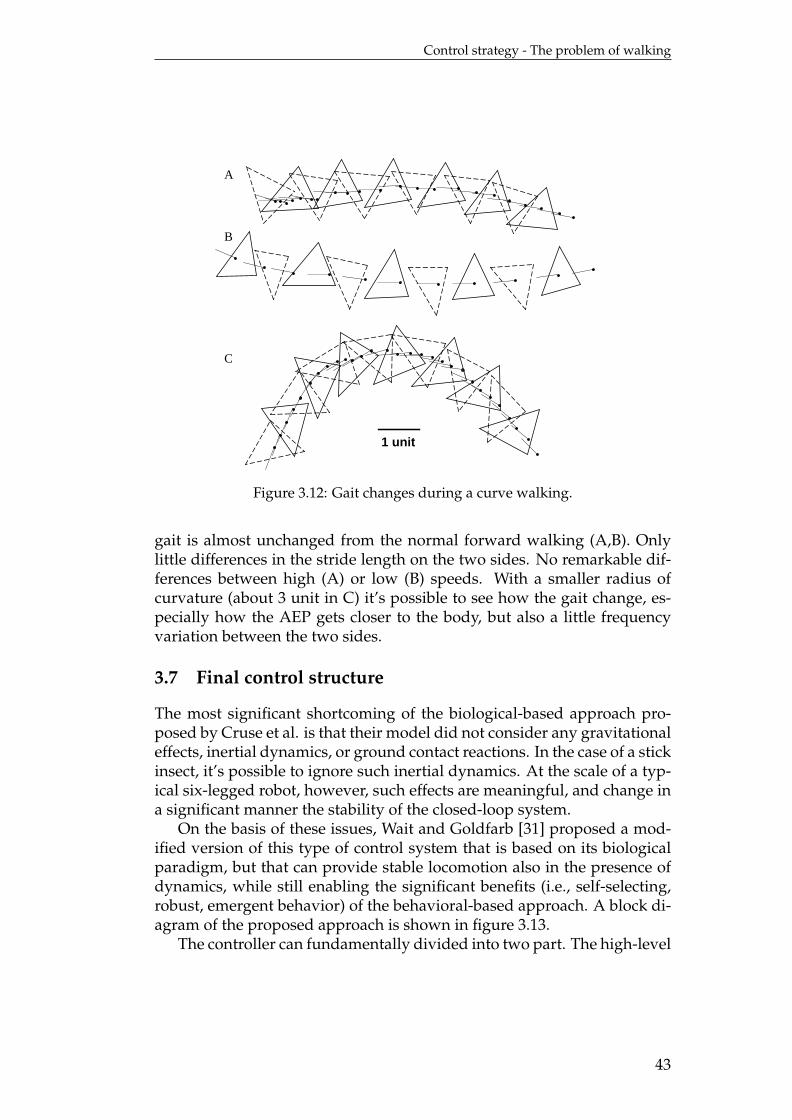
Control strategy - The problem of walking

A

B

C

1 unit

Figure 3.12: Gait changes during a curve walking.

gait is almost unchanged from the normal forward walking (A,B). Onlylittle differences in the stride length on the two sides. No remarkable dif-ferences between high (A) or low (B) speeds. With a smaller radius ofcurvature (about 3 unit in C) it’s possible to see how the gait change, es-pecially how the AEP gets closer to the body, but also a little frequencyvariation between the two sides.

3.7 Final control structure

The most significant shortcoming of the biological-based approach pro-posed by Cruse et al. is that their model did not consider any gravitationaleffects, inertial dynamics, or ground contact reactions. In the case of a stickinsect, it’s possible to ignore such inertial dynamics. At the scale of a typ-ical six-legged robot, however, such effects are meaningful, and change ina significant manner the stability of the closed-loop system.

On the basis of these issues, Wait and Goldfarb [31] proposed a mod-ified version of this type of control system that is based on its biologicalparadigm, but that can provide stable locomotion also in the presence ofdynamics, while still enabling the significant benefits (i.e., self-selecting,robust, emergent behavior) of the behavioral-based approach. A block di-agram of the proposed approach is shown in figure 3.13.

The controller can fundamentally divided into two part. The high-level

43

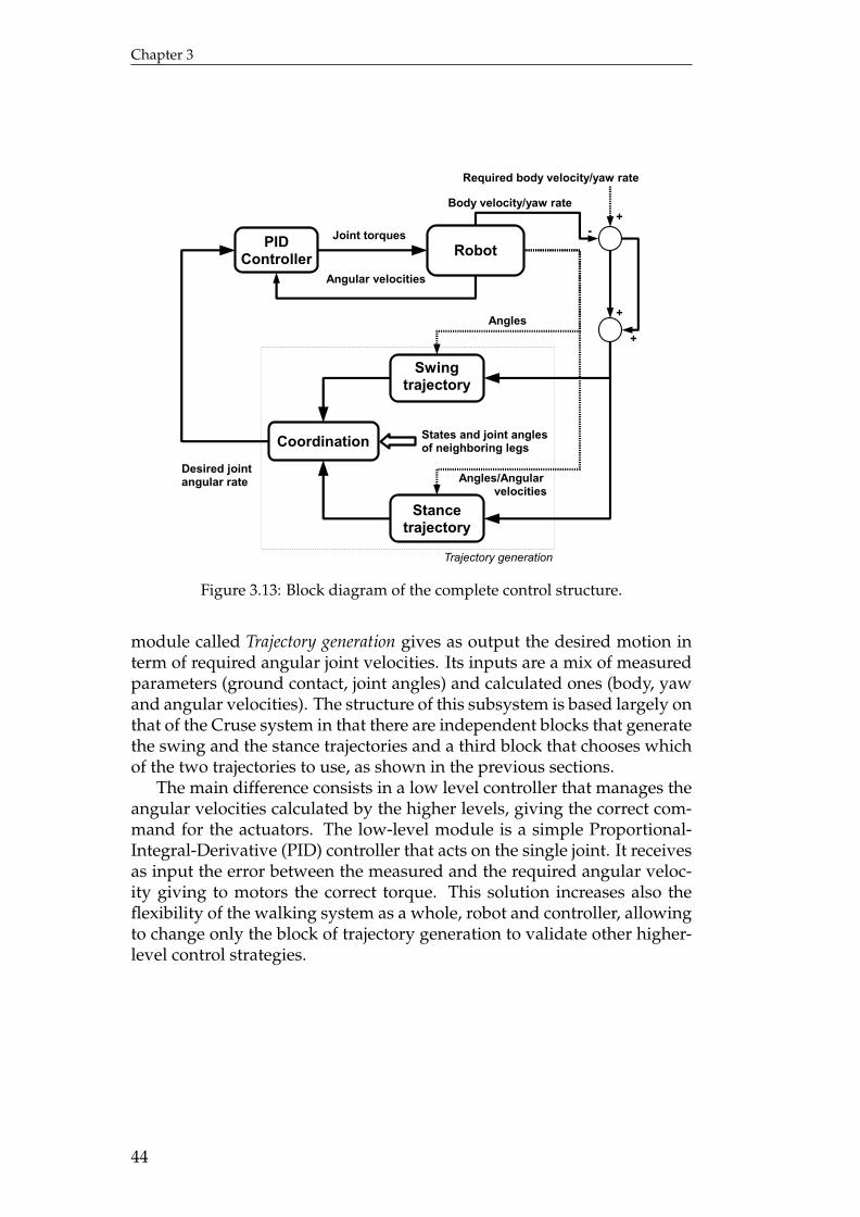
Chapter 3

Swingtrajectory

Stancetrajectory

Coordination

RobotPIDController

Joint torques

States and joint angles of neighboring legs

Trajectory generation

Desired joint angular rate

Angles

Angles/Angular velocities

Angular velocities

Body velocity/yaw rate

-

+

+

Required body velocity/yaw rate

+

Figure 3.13: Block diagram of the complete control structure.

module called Trajectory generation gives as output the desired motion interm of required angular joint velocities. Its inputs are a mix of measuredparameters (ground contact, joint angles) and calculated ones (body, yawand angular velocities). The structure of this subsystem is based largely onthat of the Cruse system in that there are independent blocks that generatethe swing and the stance trajectories and a third block that chooses whichof the two trajectories to use, as shown in the previous sections.

The main difference consists in a low level controller that manages theangular velocities calculated by the higher levels, giving the correct com-mand for the actuators. The low-level module is a simple Proportional-Integral-Derivative (PID) controller that acts on the single joint. It receivesas input the error between the measured and the required angular veloc-ity giving to motors the correct torque. This solution increases also theflexibility of the walking system as a whole, robot and controller, allowingto change only the block of trajectory generation to validate other higher-level control strategies.

44

Chapter 4

Single leg controllerIn the present chapter the controller for a single leg will be described indetail. To understand the whole structure, the architecture and the resultsfor each single module will be illustrated. For a simulation of the completeleg motion see section 6.2.

4.1 Swing control

The control of the swing phase can be achieved with a single module thatgenerates the desired trajectory during this phase. This trajectory, as pre-viously described in section 3.5.1, must show two different behaviors: thelift off from the ground and the targeting on the AEP. In the present workthe control module consists in an artificial neural network called swing net.

The variables of the problem are the angular positions and the threetarget angle that define the AEP univocally. The current angles can bemeasured directly by angular displacement sensors while the AEP anglesare calculated apart and reflect a spatial coordination between adjacentlegs (see section 5.4). On the basis of these two kinds of inputs it’s possibleto calculate the desired joints angular velocities for each time step.

The training process of each ANN requires the definition of a fitnessfunction (see 2.6). In the present case the network must simulate two dif-ferent behaviors but only one of them requires to be scored in the fitnessfunction. Every quantitative evaluation of the lift-off properties, needs aknowledge of the shape of the whole trajectory that isn’t required to cor-rectly design a swing phase. For this reason, instead of a curve-fittingcriterion, a Boolean one has been adopted: the solution is considered suit-able only if the trajectory shows a SEP higher than a reference value. Thescore given by the fitness function evaluates the targeting on AEP only interms of minimum distance of the foot from the desired position.

The fitness is evaluated in a purely kinematics simulation of the legmotion. To stop this simulation a temporal criterion has been used: whenthe time reaches a given value the simulation stops and the evaluationof the fitness is done on the best result obtained, i.e. the closest to thetarget. To speed up the swing phase, when a sufficiently precise targethas been reached, one more training must be done to maximize the meanangular velocities. The maximum allowed velocity depends on actuatorscharacteristics and it’s equal to 91 deg s−1 (see subsection 7.3.1).

45

Chapter 4

The other requirement in the project of a ANN is the structure of thenetwork, meaning with this definition the type of neuron, the numberof units and the connection among them. Two distinct cases have beeninvestigated: static ANN (see subsection 4.1.1) and dynamic ANN (seesubsection 4.1.2), by evaluating if the latter more complex solution mightperform better than the simpler former one.

4.1.1 Static networkThe usage of a static network to control the swing phase is the solutionproposed by Cruse et al. [32] for their Walknet controller. The referencepaper for this application has been written by Linder [33]. In that workhe suggests that the simplest possible network was sufficient to solve theproblem. This ANN is a single-layer feed-forward network consisting ofthree neural unit, the outputs of which are the angular velocity of the BC(γ), CT (β) and FT joint (α) respectively . Each unit receives a weightedinput from external sensors that signal the current joint angles (γ, β, α).Further inputs are the target angles (γt, βt, αt) from the target net.

In a detailed study using genetic algorithms, Linder shown that sevennon-zero weights out of a total of 18 are sufficient to simulate typical swingmovements. The structure of the network is illustrated in figure 4.1. Thissolution consists essentially of three negative feedback controllers, one foreach of the three leg joints. The control loop is closed via the leg itself, asmovement changes the posture and, thus, the sensory input. Moreover,the controller of the BC joint (protraction) and the CT joints (elevation)are coupled via a seventh weight that is responsible for the lift-off/touch-down behavior. Its variation allows to modulate the maximum heightreached by the trajectory (SEP). A sensitivity analysis on this parametershows how an increase in the SEP produces a decrease in the accuracy ofthe targeting behavior. From a mathematical point of view the networkstructure can be summarized by the equations set as follows:

γ = wγγ γ + wγγt γt (4.1a)β = wβγ γ + wβγt γt + wββ β + wββt βt (4.1b)α = wαα α + wααt αt (4.1c)

Starting from these considerations the weights for this network adapted tothe present geometry have been calculated. The parameters for the train-ing algorithm are shown in table 4.1. Remembering the characteristicsof the behavior to simulate, it’s possible to fix some constraints on theweights:

- the maximum permitted magnitude is 2;

46

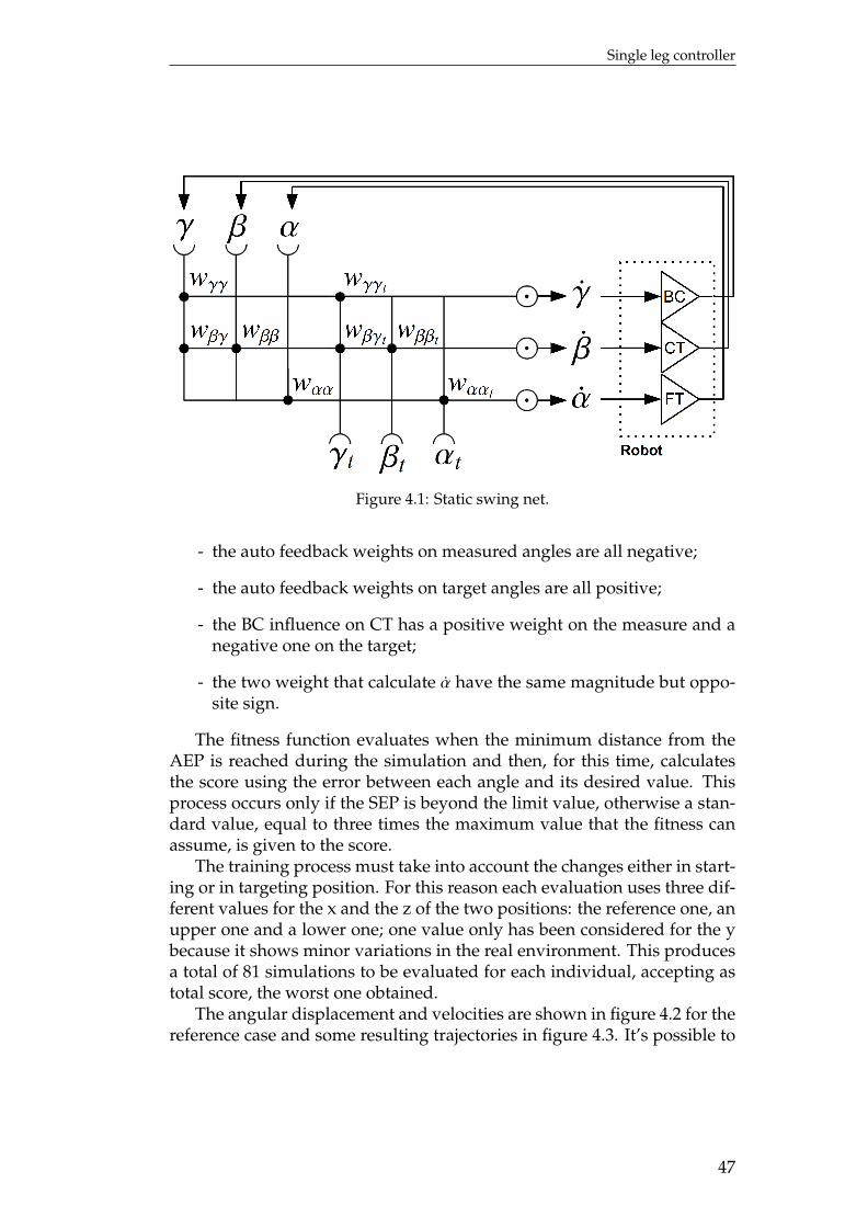
Single leg controller

Figure 4.1: Static swing net.

- the auto feedback weights on measured angles are all negative;

- the auto feedback weights on target angles are all positive;

- the BC influence on CT has a positive weight on the measure and anegative one on the target;

- the two weight that calculate α have the same magnitude but oppo-site sign.

The fitness function evaluates when the minimum distance from theAEP is reached during the simulation and then, for this time, calculatesthe score using the error between each angle and its desired value. Thisprocess occurs only if the SEP is beyond the limit value, otherwise a stan-dard value, equal to three times the maximum value that the fitness canassume, is given to the score.

The training process must take into account the changes either in start-ing or in targeting position. For this reason each evaluation uses three dif-ferent values for the x and the z of the two positions: the reference one, anupper one and a lower one; one value only has been considered for the ybecause it shows minor variations in the real environment. This producesa total of 81 simulations to be evaluated for each individual, accepting astotal score, the worst one obtained.

The angular displacement and velocities are shown in figure 4.2 for thereference case and some resulting trajectories in figure 4.3. It’s possible to

47

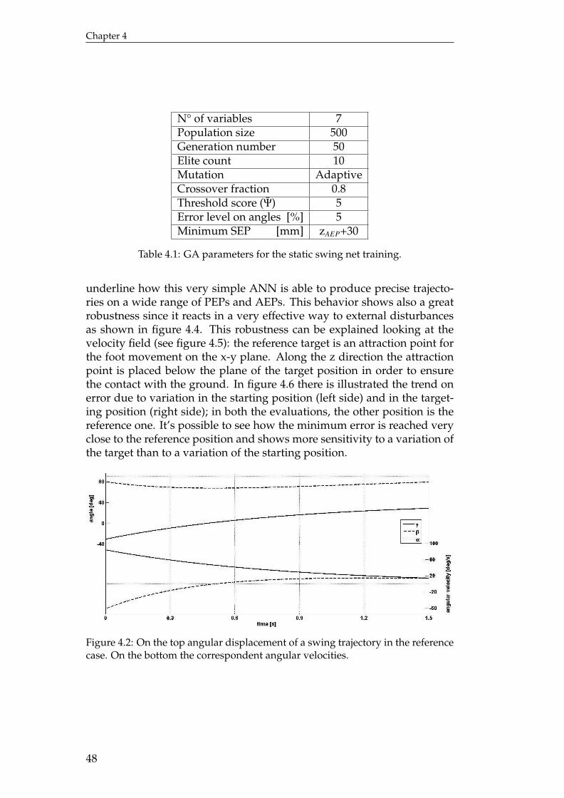
Chapter 4

N° of variables 7Population size 500Generation number 50Elite count 10Mutation AdaptiveCrossover fraction 0.8Threshold score (Ψ) 5Error level on angles [%] 5Minimum SEP [mm] zAEP+30

Table 4.1: GA parameters for the static swing net training.

underline how this very simple ANN is able to produce precise trajecto-ries on a wide range of PEPs and AEPs. This behavior shows also a greatrobustness since it reacts in a very effective way to external disturbancesas shown in figure 4.4. This robustness can be explained looking at thevelocity field (see figure 4.5): the reference target is an attraction point forthe foot movement on the x-y plane. Along the z direction the attractionpoint is placed below the plane of the target position in order to ensurethe contact with the ground. In figure 4.6 there is illustrated the trend onerror due to variation in the starting position (left side) and in the target-ing position (right side); in both the evaluations, the other position is thereference one. It’s possible to see how the minimum error is reached veryclose to the reference position and shows more sensitivity to a variation ofthe target than to a variation of the starting position.

Figure 4.2: On the top angular displacement of a swing trajectory in the referencecase. On the bottom the correspondent angular velocities.

48

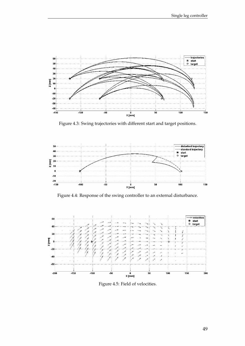
Single leg controller

Figure 4.3: Swing trajectories with different start and target positions.

Figure 4.4: Response of the swing controller to an external disturbance.

Figure 4.5: Field of velocities.

49

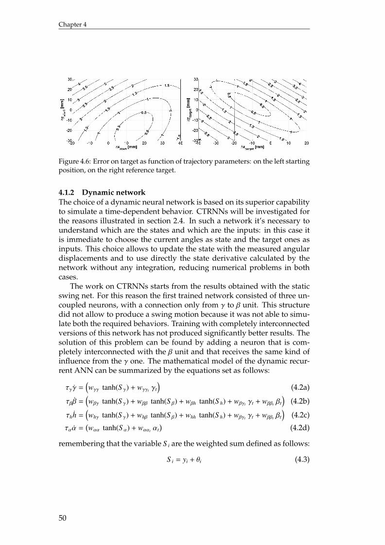
Chapter 4

Figure 4.6: Error on target as function of trajectory parameters: on the left startingposition, on the right reference target.

4.1.2 Dynamic networkThe choice of a dynamic neural network is based on its superior capabilityto simulate a time-dependent behavior. CTRNNs will be investigated forthe reasons illustrated in section 2.4. In such a network it’s necessary tounderstand which are the states and which are the inputs: in this case itis immediate to choose the current angles as state and the target ones asinputs. This choice allows to update the state with the measured angulardisplacements and to use directly the state derivative calculated by thenetwork without any integration, reducing numerical problems in bothcases.

The work on CTRNNs starts from the results obtained with the staticswing net. For this reason the first trained network consisted of three un-coupled neurons, with a connection only from γ to β unit. This structuredid not allow to produce a swing motion because it was not able to simu-late both the required behaviors. Training with completely interconnectedversions of this network has not produced significantly better results. Thesolution of this problem can be found by adding a neuron that is com-pletely interconnected with the β unit and that receives the same kind ofinfluence from the γ one. The mathematical model of the dynamic recur-rent ANN can be summarized by the equations set as follows:

τγγ =(wγγ tanh(S γ) + wγγt γt

)(4.2a)

τββ =(wβγ tanh(S γ) + wββ tanh(S β) + wβh tanh(S h) + wβγt γt + wββt βt

)(4.2b)

τhh =(whγ tanh(S γ) + whβ tanh(S β) + whh tanh(S h) + wβγt γt + wββt βt

)(4.2c)

ταα =(wαα tanh(S α) + wααt αt

)(4.2d)

remembering that the variable S i are the weighted sum defined as follows:

S i = yi + θi (4.3)

50

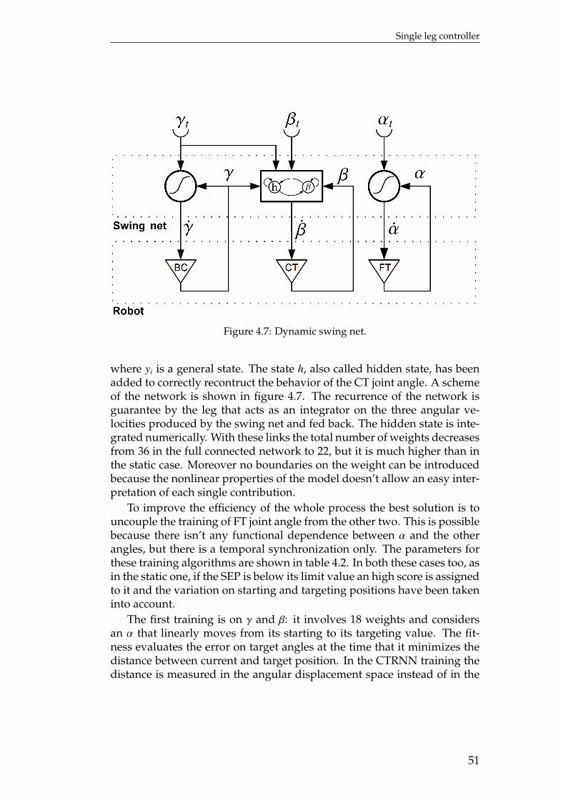
Single leg controller

Figure 4.7: Dynamic swing net.

where yi is a general state. The state h, also called hidden state, has beenadded to correctly recontruct the behavior of the CT joint angle. A schemeof the network is shown in figure 4.7. The recurrence of the network isguarantee by the leg that acts as an integrator on the three angular ve-locities produced by the swing net and fed back. The hidden state is inte-grated numerically. With these links the total number of weights decreasesfrom 36 in the full connected network to 22, but it is much higher than inthe static case. Moreover no boundaries on the weight can be introducedbecause the nonlinear properties of the model doesn’t allow an easy inter-pretation of each single contribution.

To improve the efficiency of the whole process the best solution is touncouple the training of FT joint angle from the other two. This is possiblebecause there isn’t any functional dependence between α and the otherangles, but there is a temporal synchronization only. The parameters forthese training algorithms are shown in table 4.2. In both these cases too, asin the static one, if the SEP is below its limit value an high score is assignedto it and the variation on starting and targeting positions have been takeninto account.

The first training is on γ and β: it involves 18 weights and considersan α that linearly moves from its starting to its targeting value. The fit-ness evaluates the error on target angles at the time that it minimizes thedistance between current and target position. In the CTRNN training thedistance is measured in the angular displacement space instead of in the

51

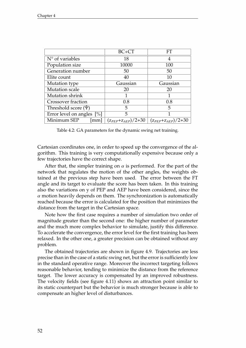
Chapter 4

BC+CT FTN° of variables 18 4Population size 10000 100Generation number 50 50Elite count 40 10Mutation type Gaussian GaussianMutation scale 20 20Mutation shrink 1 1Crossover fraction 0.8 0.8Threshold score (Ψ) 5 5Error level on angles [%] 5 1Minimum SEP [mm] (zPEP+zAEP)/2+30 (zPEP+zAEP)/2+30

Table 4.2: GA parameters for the dynamic swing net training.

Cartesian coordinates one, in order to speed up the convergence of the al-gorithm. This training is very computationally expensive because only afew trajectories have the correct shape.

After that, the simpler training on α is performed. For the part of thenetwork that regulates the motion of the other angles, the weights ob-tained at the previous step have been used. The error between the FTangle and its target to evaluate the score has been taken. In this trainingalso the variations on y of PEP and AEP have been considered, since theα motion heavily depends on them. The synchronization is automaticallyreached because the error is calculated for the position that minimizes thedistance from the target in the Cartesian space.

Note how the first case requires a number of simulation two order ofmagnitude greater than the second one: the higher number of parameterand the much more complex behavior to simulate, justify this difference.To accelerate the convergence, the error level for the first training has beenrelaxed. In the other one, a greater precision can be obtained without anyproblem.

The obtained trajectories are shown in figure 4.9. Trajectories are lessprecise than in the case of a static swing net, but the error is sufficiently lowin the standard operative range. Moreover the incorrect targeting followsreasonable behavior, tending to minimize the distance from the referencetarget. The lower accuracy is compensated by an improved robustness.The velocity fields (see figure 4.11) shows an attraction point similar toits static counterpart but the behavior is much stronger because is able tocompensate an higher level of disturbances.

52

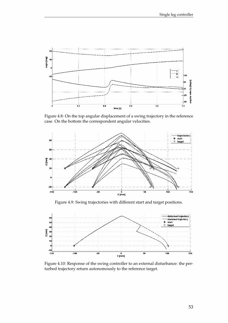
Single leg controller

Figure 4.8: On the top angular displacement of a swing trajectory in the referencecase. On the bottom the correspondent angular velocities.

Figure 4.9: Swing trajectories with different start and target positions.

Figure 4.10: Response of the swing controller to an external disturbance: the per-turbed trajectory return autonomously to the reference target.

53

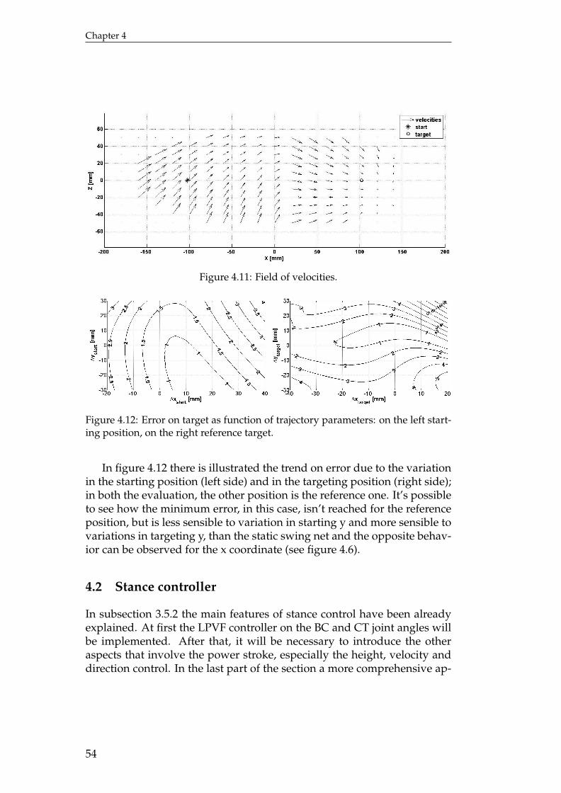
Chapter 4

Figure 4.11: Field of velocities.

Figure 4.12: Error on target as function of trajectory parameters: on the left start-ing position, on the right reference target.

In figure 4.12 there is illustrated the trend on error due to the variationin the starting position (left side) and in the targeting position (right side);in both the evaluation, the other position is the reference one. It’s possibleto see how the minimum error, in this case, isn’t reached for the referenceposition, but is less sensible to variation in starting y and more sensible tovariations in targeting y, than the static swing net and the opposite behav-ior can be observed for the x coordinate (see figure 4.6).

4.2 Stance controller

In subsection 3.5.2 the main features of stance control have been alreadyexplained. At first the LPVF controller on the BC and CT joint angles willbe implemented. After that, it will be necessary to introduce the otheraspects that involve the power stroke, especially the height, velocity anddirection control. In the last part of the section a more comprehensive ap-

54

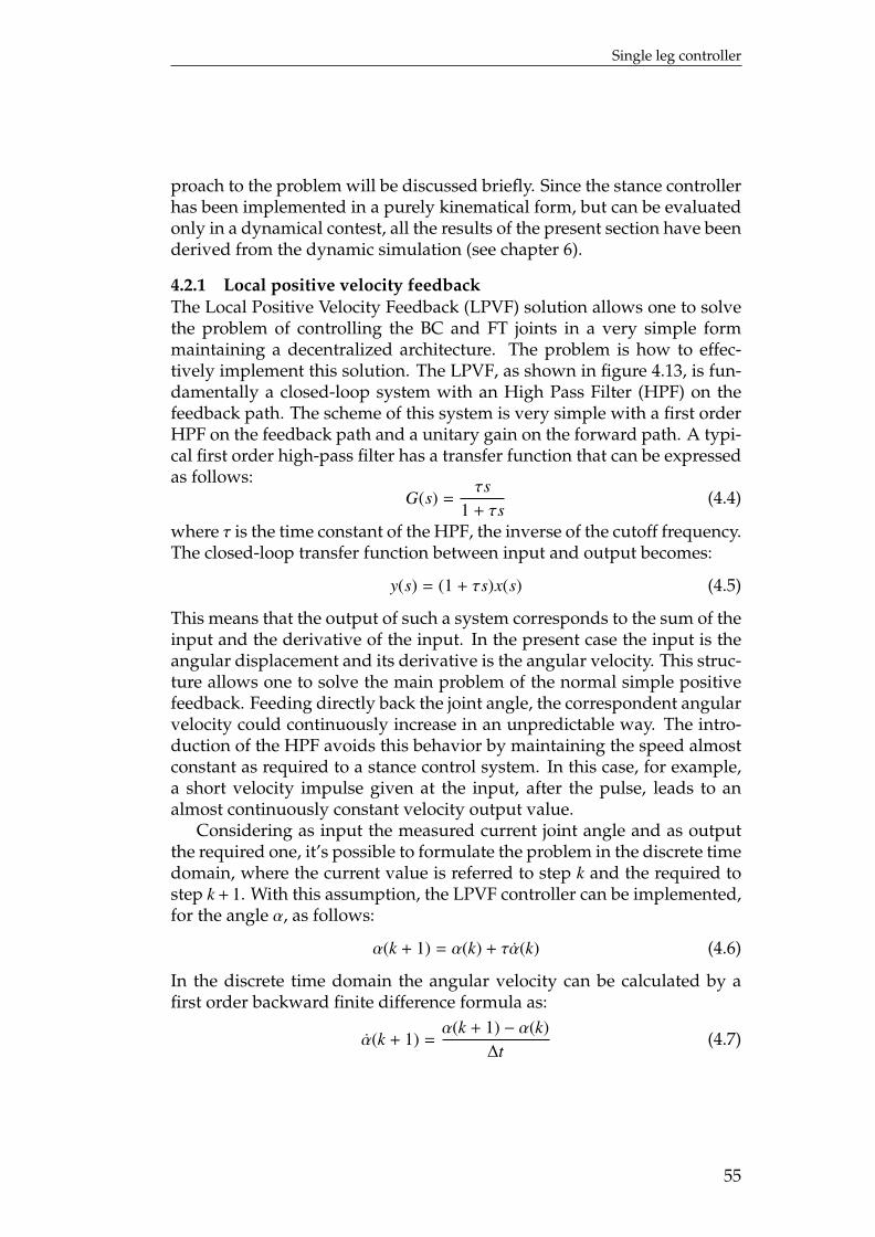
Single leg controller

proach to the problem will be discussed briefly. Since the stance controllerhas been implemented in a purely kinematical form, but can be evaluatedonly in a dynamical contest, all the results of the present section have beenderived from the dynamic simulation (see chapter 6).

4.2.1 Local positive velocity feedbackThe Local Positive Velocity Feedback (LPVF) solution allows one to solvethe problem of controlling the BC and FT joints in a very simple formmaintaining a decentralized architecture. The problem is how to effec-tively implement this solution. The LPVF, as shown in figure 4.13, is fun-damentally a closed-loop system with an High Pass Filter (HPF) on thefeedback path. The scheme of this system is very simple with a first orderHPF on the feedback path and a unitary gain on the forward path. A typi-cal first order high-pass filter has a transfer function that can be expressedas follows:

G(s) =τs

1 + τs(4.4)

where τ is the time constant of the HPF, the inverse of the cutoff frequency.The closed-loop transfer function between input and output becomes:

y(s) = (1 + τs)x(s) (4.5)

This means that the output of such a system corresponds to the sum of theinput and the derivative of the input. In the present case the input is theangular displacement and its derivative is the angular velocity. This struc-ture allows one to solve the main problem of the normal simple positivefeedback. Feeding directly back the joint angle, the correspondent angularvelocity could continuously increase in an unpredictable way. The intro-duction of the HPF avoids this behavior by maintaining the speed almostconstant as required to a stance control system. In this case, for example,a short velocity impulse given at the input, after the pulse, leads to analmost continuously constant velocity output value.

Considering as input the measured current joint angle and as outputthe required one, it’s possible to formulate the problem in the discrete timedomain, where the current value is referred to step k and the required tostep k + 1. With this assumption, the LPVF controller can be implemented,for the angle α, as follows:

α(k + 1) = α(k) + τα(k) (4.6)

In the discrete time domain the angular velocity can be calculated by afirst order backward finite difference formula as:

α(k + 1) =α(k + 1) − α(k)

∆t(4.7)

55

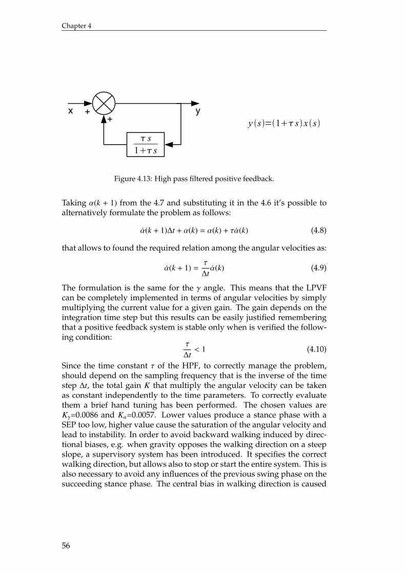
Chapter 4

s1 s

++x y

y s=1 s x s

Figure 4.13: High pass filtered positive feedback.

Taking α(k + 1) from the 4.7 and substituting it in the 4.6 it’s possible toalternatively formulate the problem as follows:

α(k + 1)∆t + α(k) = α(k) + τα(k) (4.8)

that allows to found the required relation among the angular velocities as:

α(k + 1) =τ

∆tα(k) (4.9)

The formulation is the same for the γ angle. This means that the LPVFcan be completely implemented in terms of angular velocities by simplymultiplying the current value for a given gain. The gain depends on theintegration time step but this results can be easily justified rememberingthat a positive feedback system is stable only when is verified the follow-ing condition:

τ

∆t< 1 (4.10)

Since the time constant τ of the HPF, to correctly manage the problem,should depend on the sampling frequency that is the inverse of the timestep ∆t, the total gain K that multiply the angular velocity can be takenas constant independently to the time parameters. To correctly evaluatethem a brief hand tuning has been performed. The chosen values areKγ=0.0086 and Kα=0.0057. Lower values produce a stance phase with aSEP too low, higher value cause the saturation of the angular velocity andlead to instability. In order to avoid backward walking induced by direc-tional biases, e.g. when gravity opposes the walking direction on a steepslope, a supervisory system has been introduced. It specifies the correctwalking direction, but allows also to stop or start the entire system. This isalso necessary to avoid any influences of the previous swing phase on thesucceeding stance phase. The central bias in walking direction is caused

56

Single leg controller

Figure 4.14: Angles and angular velocities of a reference stance trajectory in adynamic simulation environment.

by a constant, small offset value, which replaces the sensory informationof the BC joint angular velocity γ if it is larger than the latter. This addedcontribution can also be seen as a pulse that allow to the LPVF to reach anon null constant angular velocity. The offset value has always been takenequal to 5 deg/s, less than 6 % of the maximum permitted value.

This alternative formulation allows to give directly an angular veloc-ity command to the actuator as required in section 3.5. The problem is thatthe sensors mounted on the joints measure angular displacements only. Toobtain an information about the angular velocity is necessary to numeri-cally calculate the derivative of the measure. In the present work a secondorder backward finite difference formula has been used.

The stance phase, although it’s implemented by a kinematic rule, couldbe evaluated only in a taking into account the interactions with the envi-ronment. For this reason the result shown in figure 4.14 have been ob-tained by a dynamic simulation (see chapter 6). During a reference stancephase the most part of the motion depends on the γ angle that move theleg backward, propelling the body forward. The angular velocity showsthe behavior previously predicted for a system with LPVF, remaining al-most constant after a starting initial perturbation, given by the walkingdirection offset. The angle α shows small variations only, due to numeri-cal error, but also to the motion of the other legs. This behavior can justifya different control strategy, e.g. a closed-loop negative feedback to increaselateral stability.

57

Chapter 4

4.2.2 Height controlThe control of the body clearance depends completely on the CT joint inorder to maintain the modularity approach adopted so far: the γ and α an-gles are responsible for ground parallel movements and thus they providethe thrust by using LPVF, whereas the β angle doesn’t show any rever-sal reflex, but controls the movement in the direction perpendicular to theground. This action is performed by the simplest control system possible.The required angular velocity is calculated by a classical closed-loop regu-lator that uses negative feedback. The actual body height, evaluated at theleg insertion point, is compared to a reference value. The resulting error istransformed into a desired angular velocity, equivalent to a desired changein the angular position in the discrete time domain, by a linear character-istic. The choice of using a simple proportional controller has its biologicalcounterpart in the findings on height control in stick insects that show anindividual proportional element acting as a servomechanism on each leg(see Cruse et al. [34]). The control law can be summarized as follows:

β = Kβ(hsens − hre f ) (4.11)

The proportional gain Kβ has been set equal to 2.5 deg s−1 mm−1. Thebody height in the reference configuration has been considered as refer-ence body height hre f . The results obtained with this controller are illus-trated in figure 4.15. If the ground has a step (bold line), when the legpasses from swing (dashed line) to stance (solid line), it sees a change inthe local body height. The controller tries to maintain the reference bodyheight (dash-dotted line), by feeding-back a β command, proportional tothe error on height. The system reacts by reaching the regime value in lessthan 0.5 s. This results can be justified remembering that the linearizedmodel of the closed-loop system can be represented by a first-order trans-fer function with an integrator on the forward path, that transform β inh, and a unitary gain on the feedback path. The gain of the integrator isKβG where G is the derivative of h(β) evaluated in the reference positionthat assume the value of 2.65 mm deg−1. The resulting closed-loop transferfunction is:

H(s) =KβG 1

s

1 + KβG 1s

=1

1 + 1KβG

s(4.12)

This means that the time constant can be estimated as τ ≈ 1/(KβG). The ob-tained value of τ=0.15 s means that the regime condition should be reachedin about 4τ=0.6 s that is almost exactly the data given by the simulation.

The value of the current body height hsens isn’t directly measured byany sensor but can be easily deduced by the measure of the joint angles.

58

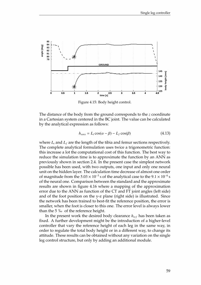
Single leg controller

0 0.5 1 1.5 2 2.5 3 3.5 4 4.5

79808182838485

ang

le [

deg

]

0 0.5 1 1.5 2 2.5 3 3.5 4 4.5125

130

135

140

145

bo

dy

hei

gh

t [m

m]

time [s]

GROUND

Figure 4.15: Body height control.

The distance of the body from the ground corresponds to the z coordinatein a Cartesian system centered in the BC joint. The value can be calculatedby the analytical expression as follows:

hsens = Lt cos(α − β) − L f cos(β) (4.13)

where Lt and L f are the length of the tibia and femur sections respectively.The complete analytical formulation uses twice a trigonometric function:this increase a lot the computational cost of this function. The best way toreduce the simulation time is to approximate the function by an ANN aspreviously shown in section 2.4. In the present case the simplest networkpossible has been used, with two outputs, one input and only one neuralunit on the hidden layer. The calculation time decrease of almost one orderof magnitude from the 5.03 × 10−5 s of the analytical case to the 9.1 × 10−6 sof the neural one. Comparison between the standard and the approximateresults are shown in figure 4.16 where a mapping of the approximationerror due to the ANN as function of the CT and FT joint angles (left side)and of the foot position on the y-z plane (right side) is illustrated. Sincethe network has been trained to best-fit the reference position, the error issmaller, when the foot is closer to this one. The error level is always lowerthan the 5 ‰ of the reference height.

In the present work the desired body clearance hre f has been taken asfixed. A further development might be the introduction of a higher-levelcontroller that vary the reference height of each leg in the same way, inorder to regulate the total body height or in a different way, to change itsattitude. These results can be obtained without any variation on the singleleg control structure, but only by adding an additional module.

59

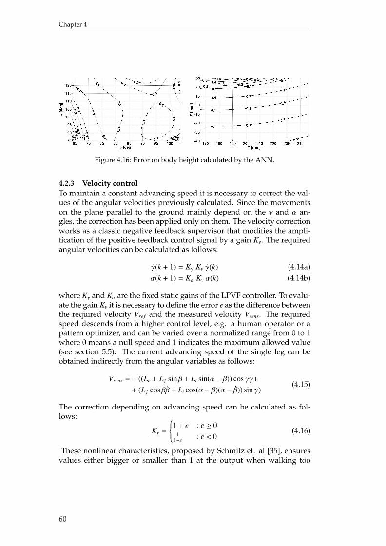
Chapter 4

Figure 4.16: Error on body height calculated by the ANN.

4.2.3 Velocity controlTo maintain a constant advancing speed it is necessary to correct the val-ues of the angular velocities previously calculated. Since the movementson the plane parallel to the ground mainly depend on the γ and α an-gles, the correction has been applied only on them. The velocity correctionworks as a classic negative feedback supervisor that modifies the ampli-fication of the positive feedback control signal by a gain Kv. The requiredangular velocities can be calculated as follows:

γ(k + 1) = Kγ Kv γ(k) (4.14a)α(k + 1) = Kα Kv α(k) (4.14b)

where Kγ and Kα are the fixed static gains of the LPVF controller. To evalu-ate the gain Kv it is necessary to define the error e as the difference betweenthe required velocity Vre f and the measured velocity Vsens. The requiredspeed descends from a higher control level, e.g. a human operator or apattern optimizer, and can be varied over a normalized range from 0 to 1where 0 means a null speed and 1 indicates the maximum allowed value(see section 5.5). The current advancing speed of the single leg can beobtained indirectly from the angular variables as follows:

Vsens = − ((Lc + L f sin β + Lt sin(α − β)) cos γγ+

+ (L f cos ββ + Lt cos(α − β)(α − β)) sin γ)(4.15)

The correction depending on advancing speed can be calculated as fol-lows:

Kv =

1 + e : e ≥ 01

1−e : e < 0(4.16)

These nonlinear characteristics, proposed by Schmitz et. al [35], ensuresvalues either bigger or smaller than 1 at the output when walking too

60

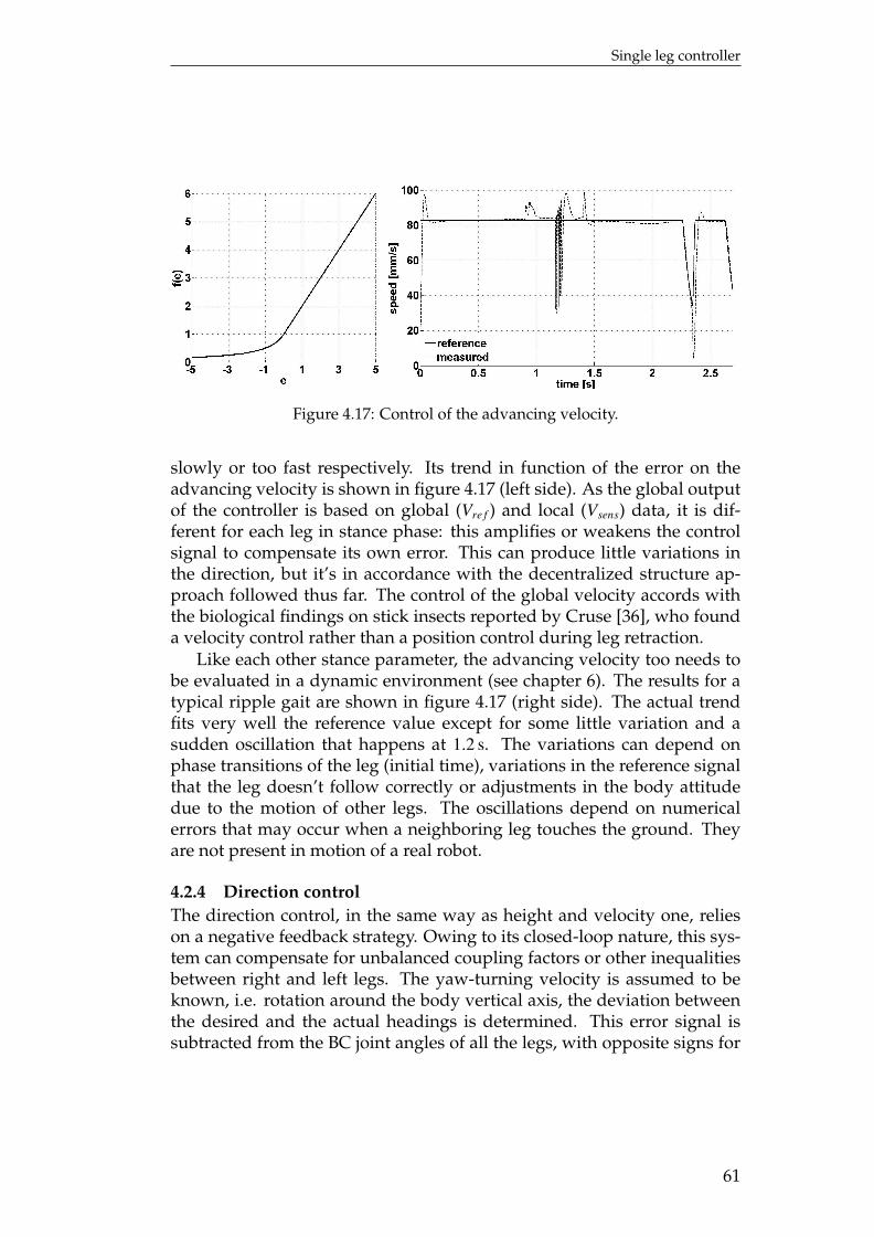
Single leg controller

Figure 4.17: Control of the advancing velocity.

slowly or too fast respectively. Its trend in function of the error on theadvancing velocity is shown in figure 4.17 (left side). As the global outputof the controller is based on global (Vre f ) and local (Vsens) data, it is dif-ferent for each leg in stance phase: this amplifies or weakens the controlsignal to compensate its own error. This can produce little variations inthe direction, but it’s in accordance with the decentralized structure ap-proach followed thus far. The control of the global velocity accords withthe biological findings on stick insects reported by Cruse [36], who founda velocity control rather than a position control during leg retraction.

Like each other stance parameter, the advancing velocity too needs tobe evaluated in a dynamic environment (see chapter 6). The results for atypical ripple gait are shown in figure 4.17 (right side). The actual trendfits very well the reference value except for some little variation and asudden oscillation that happens at 1.2 s. The variations can depend onphase transitions of the leg (initial time), variations in the reference signalthat the leg doesn’t follow correctly or adjustments in the body attitudedue to the motion of other legs. The oscillations depend on numericalerrors that may occur when a neighboring leg touches the ground. Theyare not present in motion of a real robot.

4.2.4 Direction controlThe direction control, in the same way as height and velocity one, relieson a negative feedback strategy. Owing to its closed-loop nature, this sys-tem can compensate for unbalanced coupling factors or other inequalitiesbetween right and left legs. The yaw-turning velocity is assumed to beknown, i.e. rotation around the body vertical axis, the deviation betweenthe desired and the actual headings is determined. This error signal issubtracted from the BC joint angles of all the legs, with opposite signs for

61

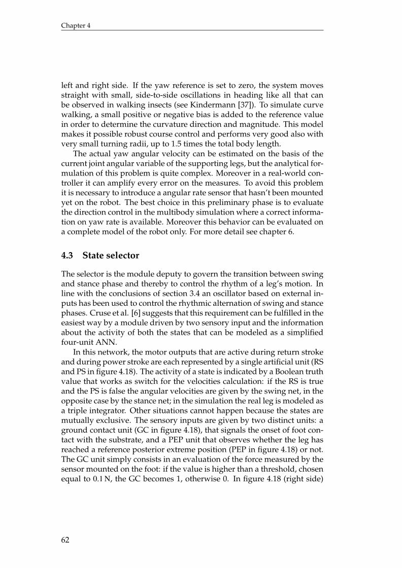
Chapter 4

left and right side. If the yaw reference is set to zero, the system movesstraight with small, side-to-side oscillations in heading like all that canbe observed in walking insects (see Kindermann [37]). To simulate curvewalking, a small positive or negative bias is added to the reference valuein order to determine the curvature direction and magnitude. This modelmakes it possible robust course control and performs very good also withvery small turning radii, up to 1.5 times the total body length.

The actual yaw angular velocity can be estimated on the basis of thecurrent joint angular variable of the supporting legs, but the analytical for-mulation of this problem is quite complex. Moreover in a real-world con-troller it can amplify every error on the measures. To avoid this problemit is necessary to introduce a angular rate sensor that hasn’t been mountedyet on the robot. The best choice in this preliminary phase is to evaluatethe direction control in the multibody simulation where a correct informa-tion on yaw rate is available. Moreover this behavior can be evaluated ona complete model of the robot only. For more detail see chapter 6.

4.3 State selector

The selector is the module deputy to govern the transition between swingand stance phase and thereby to control the rhythm of a leg’s motion. Inline with the conclusions of section 3.4 an oscillator based on external in-puts has been used to control the rhythmic alternation of swing and stancephases. Cruse et al. [6] suggests that this requirement can be fulfilled in theeasiest way by a module driven by two sensory input and the informationabout the activity of both the states that can be modeled as a simplifiedfour-unit ANN.

In this network, the motor outputs that are active during return strokeand during power stroke are each represented by a single artificial unit (RSand PS in figure 4.18). The activity of a state is indicated by a Boolean truthvalue that works as switch for the velocities calculation: if the RS is trueand the PS is false the angular velocities are given by the swing net, in theopposite case by the stance net; in the simulation the real leg is modeled asa triple integrator. Other situations cannot happen because the states aremutually exclusive. The sensory inputs are given by two distinct units: aground contact unit (GC in figure 4.18), that signals the onset of foot con-tact with the substrate, and a PEP unit that observes whether the leg hasreached a reference posterior extreme position (PEP in figure 4.18) or not.The GC unit simply consists in an evaluation of the force measured by thesensor mounted on the foot: if the value is higher than a threshold, chosenequal to 0.1 N, the GC becomes 1, otherwise 0. In figure 4.18 (right side)

62

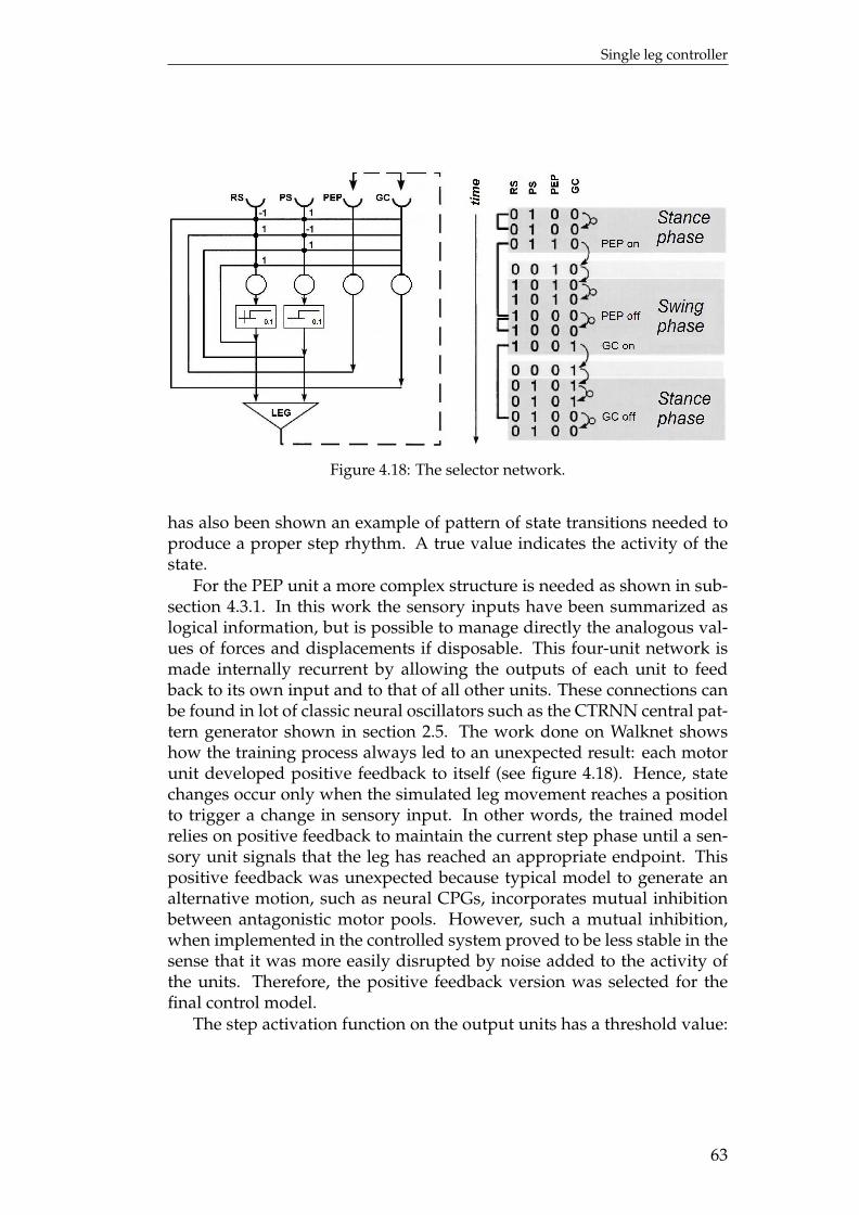
Single leg controller

Figure 4.18: The selector network.

has also been shown an example of pattern of state transitions needed toproduce a proper step rhythm. A true value indicates the activity of thestate.

For the PEP unit a more complex structure is needed as shown in sub-section 4.3.1. In this work the sensory inputs have been summarized aslogical information, but is possible to manage directly the analogous val-ues of forces and displacements if disposable. This four-unit network ismade internally recurrent by allowing the outputs of each unit to feedback to its own input and to that of all other units. These connections canbe found in lot of classic neural oscillators such as the CTRNN central pat-tern generator shown in section 2.5. The work done on Walknet showshow the training process always led to an unexpected result: each motorunit developed positive feedback to itself (see figure 4.18). Hence, statechanges occur only when the simulated leg movement reaches a positionto trigger a change in sensory input. In other words, the trained modelrelies on positive feedback to maintain the current step phase until a sen-sory unit signals that the leg has reached an appropriate endpoint. Thispositive feedback was unexpected because typical model to generate analternative motion, such as neural CPGs, incorporates mutual inhibitionbetween antagonistic motor pools. However, such a mutual inhibition,when implemented in the controlled system proved to be less stable in thesense that it was more easily disrupted by noise added to the activity ofthe units. Therefore, the positive feedback version was selected for thefinal control model.

The step activation function on the output units has a threshold value:

63

Chapter 4

this simply means that the state can be considered active only when thecorrespondent output has a value larger than zero. The value for thethreshold has been arbitrarily taken equal to 0.1 but any other value com-prised in the interval (0,1). This is a good choice in the case of non Booleansensory inputs.

This architecture, unlike a purely central neural oscillator or a mixedmodel, does make the model entirely dependent on the reliability of itssensory input. In the insect, the large number of units contributing tomeasure leg parameters should guarantee sufficient reliability, but in thismodel it isn’t so. This implies that the robot will be less robust to each sen-sor failure and that with this kind of controller, the only way to improvethe robustness is to mount redundant sensors. This is the main disadvan-tage of a completely reflex-based control strategy.

4.3.1 PEP netThe selector requires a Boolean information that indicates if the foot haspassed or not its posterior extreme position. This evaluation can be doneonly by knowing both the PEP value and the current position of the foot.In order to simplify the problem the comparison is done in terms of Carte-sian coordinate taking into account the x one only, because is the mostsignificant. The PEP can be calculated starting from a reference value of119 mm and adding all the coordinating influences (see chapter 5 for moredetails). The current x coordinate of the foot requires a more complexprocedure. Since it’s not directly measured, in opposition with the GC pa-rameter, it needs to be calculated starting from the current joint angles asfollows:

x = Lc + L f sin β + Lt sin(α − β)) sin γ (4.17)

This analytical expression, as the body height one, involves trigonomet-ric functions that produces an increase in the computational cost. Thesolution is the same: replace the exact formulation with an approximat-ing ANN. The structure requires three inputs, one output and a mini-mum number of hidden unit of three. With such a network the calcula-tion time becomes one order of magnitude smaller than the original case:6.95 × 10−5 s versus 7.35 × 10−6 s. A mapping of the approximation errordue to the ANN as function of foot position on the x-y plane (left side)and of the foot position on the x-z plane (right side) is illustrated in figure4.19. The error tends to be smaller closer to the reference position in thex-z plane, but not in the y direction due to the nonlinearity of the behavior.It increases faster after the reference PEP because it is a limit position forthe motion. The error level is always lower than the 1 % of the referencelength.

64

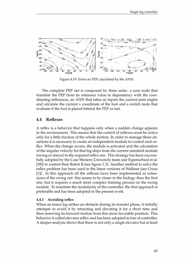
Single leg controller

Figure 4.19: Error on PEP calculated by the ANN.

The complete PEP net is composed by three units: a sum node thattranslate the PEP from its reference value in dependency with the coor-dinating influences, an ANN that takes as inputs the current joint anglesand calculate the current x coordinate of the foot and a switch node thatevaluate if the foot is placed behind the PEP or not.

4.4 Reflexes

A reflex is a behavior that happens only when a sudden change appearsin the environment. This means that the control of reflexes must be activeonly for a little fraction of the whole motion. In order to manage these sit-uations it is necessary to create an independent module to control each re-flex. When the change occurs, the module is activated and the calculationof the angular velocity for that leg skips from the current standard module(swing or stance) to the required reflex one. This strategy has been success-fully adopted by the Case Western University team (see Espenschied et al.[38]) to control their Robot II (see figure 1.3). Another method to solve thereflex problem has been used in the latest versions of Walknet (see Cruse[1]). In this approach all the reflexes have been implemented as exten-sions of the swing net: this seems to be closer to the biology than the firstone, but it requires a much more complex training process on the swingmodule. To maintain the modularity of the controller, the first approach ispreferable and has been adopted in the present work.

4.4.1 Avoiding reflexWhen an insect leg strikes an obstacle during its transfer phase, it initiallyattempts to avoid it by retracting and elevating it for a short time andthen renewing its forward motion from this more favorable position. Thisbehavior is called elevator reflex and has been adopted in lots of controller.A deeper analysis shows that there is not only a single elevator but at least

65

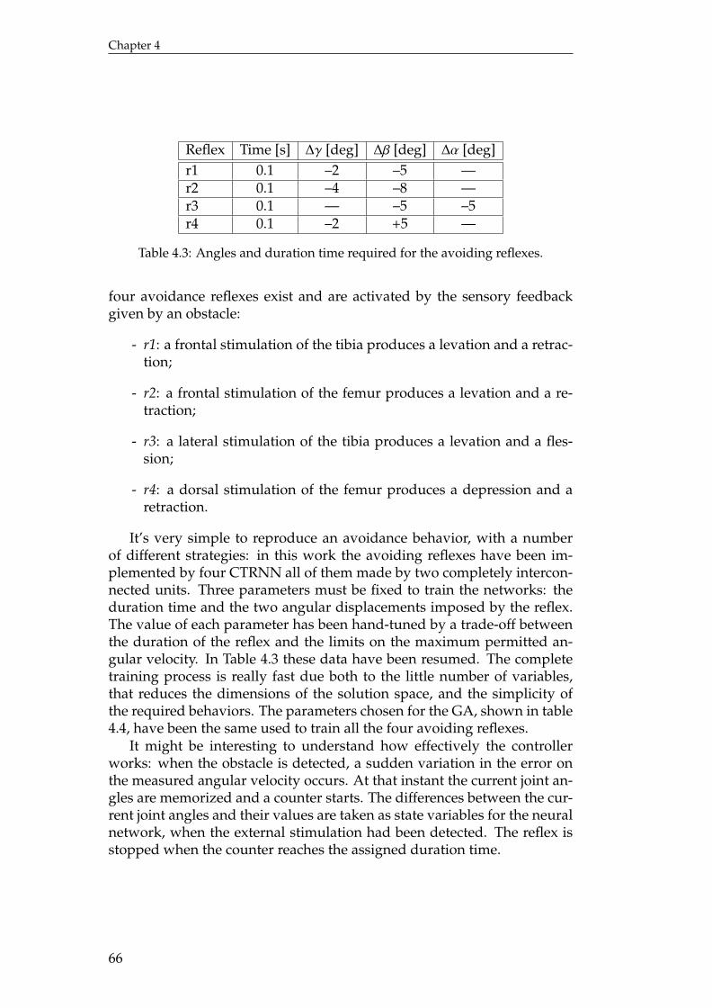
Chapter 4

Reflex Time [s] ∆γ [deg] ∆β [deg] ∆α [deg]r1 0.1 –2 –5 —r2 0.1 –4 –8 —r3 0.1 — –5 –5r4 0.1 –2 +5 —

Table 4.3: Angles and duration time required for the avoiding reflexes.

four avoidance reflexes exist and are activated by the sensory feedbackgiven by an obstacle:

- r1: a frontal stimulation of the tibia produces a levation and a retrac-tion;

- r2: a frontal stimulation of the femur produces a levation and a re-traction;

- r3: a lateral stimulation of the tibia produces a levation and a fles-sion;

- r4: a dorsal stimulation of the femur produces a depression and aretraction.

It’s very simple to reproduce an avoidance behavior, with a numberof different strategies: in this work the avoiding reflexes have been im-plemented by four CTRNN all of them made by two completely intercon-nected units. Three parameters must be fixed to train the networks: theduration time and the two angular displacements imposed by the reflex.The value of each parameter has been hand-tuned by a trade-off betweenthe duration of the reflex and the limits on the maximum permitted an-gular velocity. In Table 4.3 these data have been resumed. The completetraining process is really fast due both to the little number of variables,that reduces the dimensions of the solution space, and the simplicity ofthe required behaviors. The parameters chosen for the GA, shown in table4.4, have been the same used to train all the four avoiding reflexes.

It might be interesting to understand how effectively the controllerworks: when the obstacle is detected, a sudden variation in the error onthe measured angular velocity occurs. At that instant the current joint an-gles are memorized and a counter starts. The differences between the cur-rent joint angles and their values are taken as state variables for the neuralnetwork, when the external stimulation had been detected. The reflex isstopped when the counter reaches the assigned duration time.

66

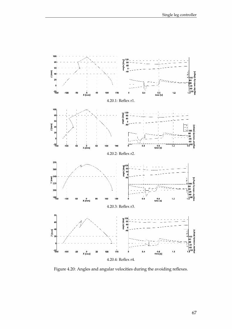
Single leg controller

4.20.1: Reflex r1.

4.20.2: Reflex r2.

4.20.3: Reflex r3.

4.20.4: Reflex r4.

Figure 4.20: Angles and angular velocities during the avoiding reflexes.

67

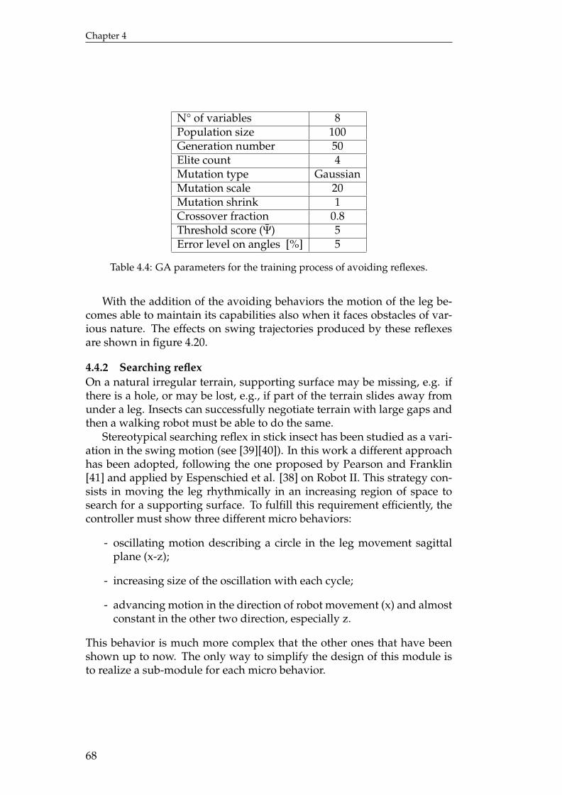
Chapter 4

N° of variables 8Population size 100Generation number 50Elite count 4Mutation type GaussianMutation scale 20Mutation shrink 1Crossover fraction 0.8Threshold score (Ψ) 5Error level on angles [%] 5

Table 4.4: GA parameters for the training process of avoiding reflexes.

With the addition of the avoiding behaviors the motion of the leg be-comes able to maintain its capabilities also when it faces obstacles of var-ious nature. The effects on swing trajectories produced by these reflexesare shown in figure 4.20.

4.4.2 Searching reflexOn a natural irregular terrain, supporting surface may be missing, e.g. ifthere is a hole, or may be lost, e.g., if part of the terrain slides away fromunder a leg. Insects can successfully negotiate terrain with large gaps andthen a walking robot must be able to do the same.

Stereotypical searching reflex in stick insect has been studied as a vari-ation in the swing motion (see [39][40]). In this work a different approachhas been adopted, following the one proposed by Pearson and Franklin[41] and applied by Espenschied et al. [38] on Robot II. This strategy con-sists in moving the leg rhythmically in an increasing region of space tosearch for a supporting surface. To fulfill this requirement efficiently, thecontroller must show three different micro behaviors:

- oscillating motion describing a circle in the leg movement sagittalplane (x-z);

- increasing size of the oscillation with each cycle;

- advancing motion in the direction of robot movement (x) and almostconstant in the other two direction, especially z.

This behavior is much more complex that the other ones that have beenshown up to now. The only way to simplify the design of this module isto realize a sub-module for each micro behavior.

68

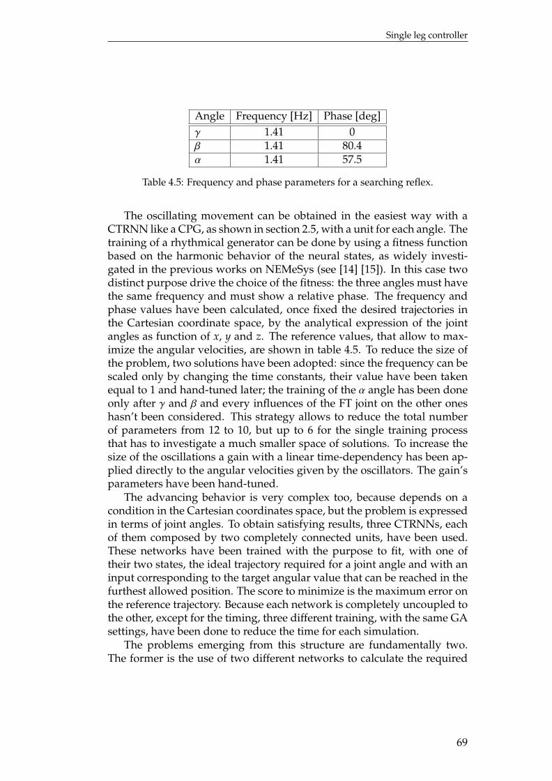
Single leg controller

Angle Frequency [Hz] Phase [deg]γ 1.41 0β 1.41 80.4α 1.41 57.5

Table 4.5: Frequency and phase parameters for a searching reflex.

The oscillating movement can be obtained in the easiest way with aCTRNN like a CPG, as shown in section 2.5, with a unit for each angle. Thetraining of a rhythmical generator can be done by using a fitness functionbased on the harmonic behavior of the neural states, as widely investi-gated in the previous works on NEMeSys (see [14] [15]). In this case twodistinct purpose drive the choice of the fitness: the three angles must havethe same frequency and must show a relative phase. The frequency andphase values have been calculated, once fixed the desired trajectories inthe Cartesian coordinate space, by the analytical expression of the jointangles as function of x, y and z. The reference values, that allow to max-imize the angular velocities, are shown in table 4.5. To reduce the size ofthe problem, two solutions have been adopted: since the frequency can bescaled only by changing the time constants, their value have been takenequal to 1 and hand-tuned later; the training of the α angle has been doneonly after γ and β and every influences of the FT joint on the other oneshasn’t been considered. This strategy allows to reduce the total numberof parameters from 12 to 10, but up to 6 for the single training processthat has to investigate a much smaller space of solutions. To increase thesize of the oscillations a gain with a linear time-dependency has been ap-plied directly to the angular velocities given by the oscillators. The gain’sparameters have been hand-tuned.

The advancing behavior is very complex too, because depends on acondition in the Cartesian coordinates space, but the problem is expressedin terms of joint angles. To obtain satisfying results, three CTRNNs, eachof them composed by two completely connected units, have been used.These networks have been trained with the purpose to fit, with one oftheir two states, the ideal trajectory required for a joint angle and with aninput corresponding to the target angular value that can be reached in thefurthest allowed position. The score to minimize is the maximum error onthe reference trajectory. Because each network is completely uncoupled tothe other, except for the timing, three different training, with the same GAsettings, have been done to reduce the time for each simulation.

The problems emerging from this structure are fundamentally two.The former is the use of two different networks to calculate the required

69

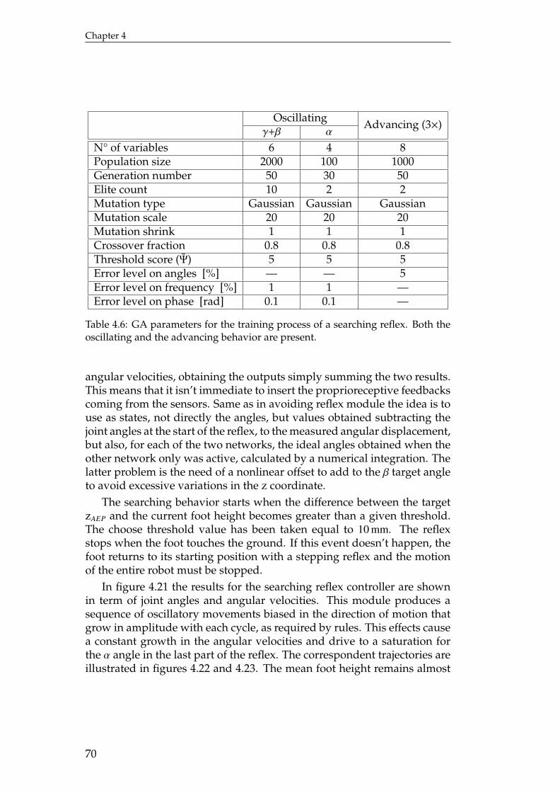
Chapter 4

Oscillating Advancing (3×)γ+β α

N° of variables 6 4 8Population size 2000 100 1000Generation number 50 30 50Elite count 10 2 2Mutation type Gaussian Gaussian GaussianMutation scale 20 20 20Mutation shrink 1 1 1Crossover fraction 0.8 0.8 0.8Threshold score (Ψ) 5 5 5Error level on angles [%] — — 5Error level on frequency [%] 1 1 —Error level on phase [rad] 0.1 0.1 —

Table 4.6: GA parameters for the training process of a searching reflex. Both theoscillating and the advancing behavior are present.

angular velocities, obtaining the outputs simply summing the two results.This means that it isn’t immediate to insert the proprioreceptive feedbackscoming from the sensors. Same as in avoiding reflex module the idea is touse as states, not directly the angles, but values obtained subtracting thejoint angles at the start of the reflex, to the measured angular displacement,but also, for each of the two networks, the ideal angles obtained when theother network only was active, calculated by a numerical integration. Thelatter problem is the need of a nonlinear offset to add to the β target angleto avoid excessive variations in the z coordinate.

The searching behavior starts when the difference between the targetzAEP and the current foot height becomes greater than a given threshold.The choose threshold value has been taken equal to 10 mm. The reflexstops when the foot touches the ground. If this event doesn’t happen, thefoot returns to its starting position with a stepping reflex and the motionof the entire robot must be stopped.

In figure 4.21 the results for the searching reflex controller are shownin term of joint angles and angular velocities. This module produces asequence of oscillatory movements biased in the direction of motion thatgrow in amplitude with each cycle, as required by rules. This effects causea constant growth in the angular velocities and drive to a saturation forthe α angle in the last part of the reflex. The correspondent trajectories areillustrated in figures 4.22 and 4.23. The mean foot height remains almost

70

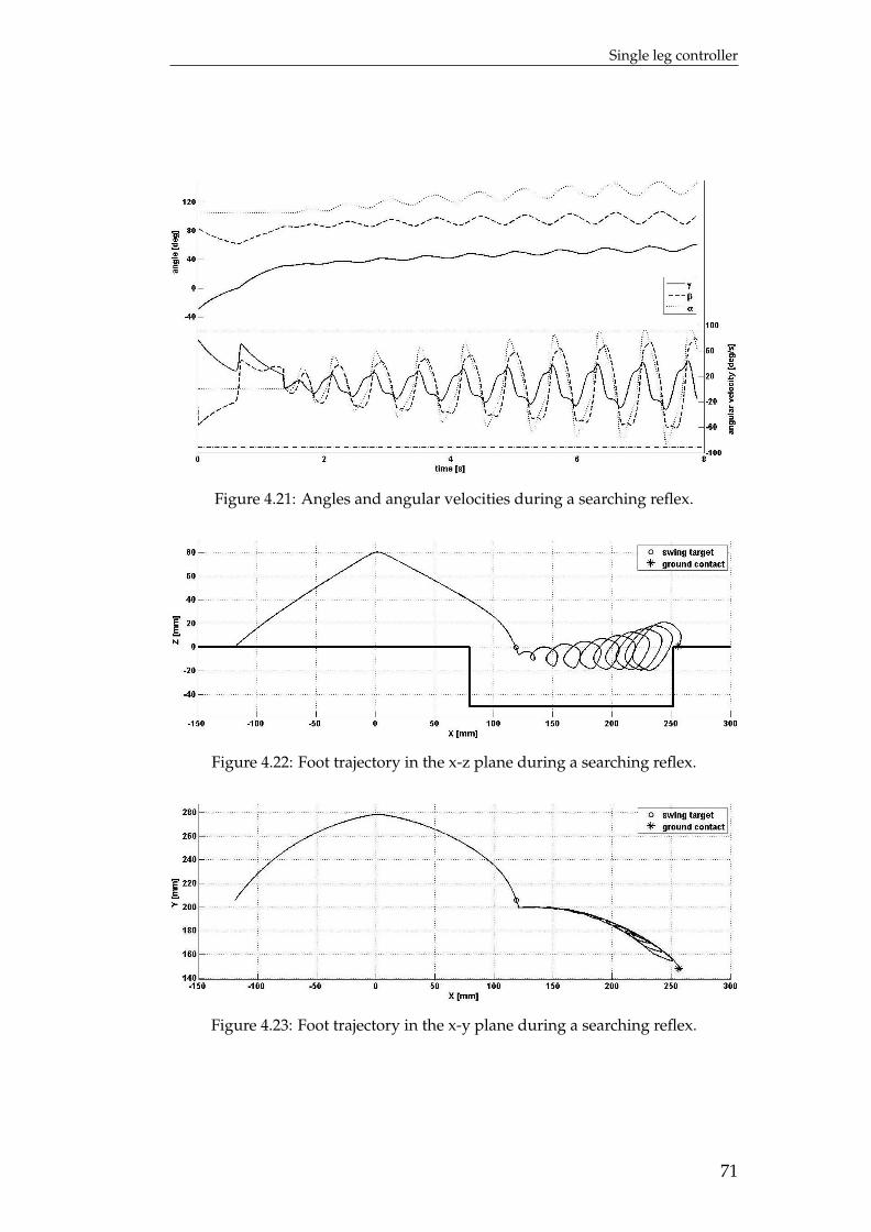
Single leg controller

Figure 4.21: Angles and angular velocities during a searching reflex.

Figure 4.22: Foot trajectory in the x-z plane during a searching reflex.

Figure 4.23: Foot trajectory in the x-y plane during a searching reflex.

71

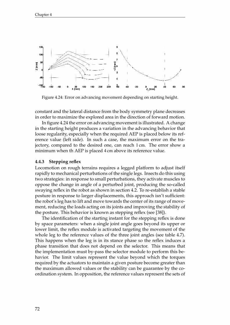
Chapter 4

Figure 4.24: Error on advancing movement depending on starting height.

constant and the lateral distance from the body symmetry plane decreasesin order to maximize the explored area in the direction of forward motion.

In figure 4.24 the error on advancing movement is illustrated. A changein the starting height produces a variation in the advancing behavior thatloose regularity, especially when the required AEP is placed below its ref-erence value (left side). In such a case, the maximum error on the tra-jectory, compared to the desired one, can reach 1 cm. The error show aminimum when th AEP is placed 4 cm above its reference value.

4.4.3 Stepping reflexLocomotion on rough terrains requires a legged platform to adjust itselfrapidly to mechanical perturbations of the single legs. Insects do this usingtwo strategies: in response to small perturbations, they activate muscles tooppose the change in angle of a perturbed joint, producing the so-calledswaying reflex in the robot as shown in section 4.2. To re-establish a stableposture in response to larger displacements, this approach isn’t sufficient:the robot’s leg has to lift and move towards the center of its range of move-ment, reducing the loads acting on its joints and improving the stability ofthe posture. This behavior is known as stepping reflex (see [38]).

The identification of the starting instant for the stepping reflex is doneby space parameters: when a single joint angle goes beyond its upper orlower limit, the reflex module is activated targeting the movement of thewhole leg to the reference values of the three joint angles (see table 4.7).This happens when the leg is in its stance phase so the reflex induces aphase transition that does not depend on the selector. This means thatthe implementation must by-pass the selector module to perform this be-havior. The limit values represent the value beyond which the torquesrequired by the actuators to maintain a given posture become greater thanthe maximum allowed values or the stability can be guarantee by the co-ordination system. In opposition, the reference values represent the sets of

72

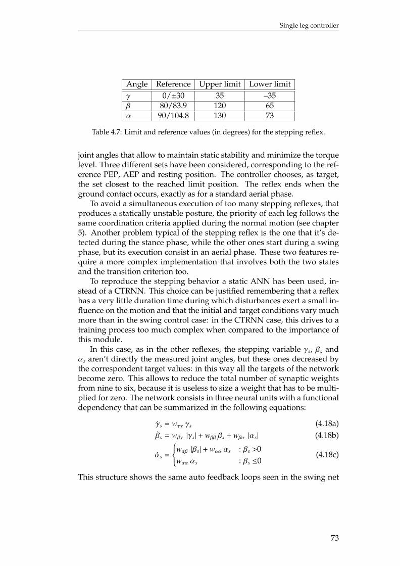
Single leg controller

Angle Reference Upper limit Lower limitγ 0/±30 35 –35β 80/83.9 120 65α 90/104.8 130 73

Table 4.7: Limit and reference values (in degrees) for the stepping reflex.

joint angles that allow to maintain static stability and minimize the torquelevel. Three different sets have been considered, corresponding to the ref-erence PEP, AEP and resting position. The controller chooses, as target,the set closest to the reached limit position. The reflex ends when theground contact occurs, exactly as for a standard aerial phase.

To avoid a simultaneous execution of too many stepping reflexes, thatproduces a statically unstable posture, the priority of each leg follows thesame coordination criteria applied during the normal motion (see chapter5). Another problem typical of the stepping reflex is the one that it’s de-tected during the stance phase, while the other ones start during a swingphase, but its execution consist in an aerial phase. These two features re-quire a more complex implementation that involves both the two statesand the transition criterion too.

To reproduce the stepping behavior a static ANN has been used, in-stead of a CTRNN. This choice can be justified remembering that a reflexhas a very little duration time during which disturbances exert a small in-fluence on the motion and that the initial and target conditions vary muchmore than in the swing control case: in the CTRNN case, this drives to atraining process too much complex when compared to the importance ofthis module.

In this case, as in the other reflexes, the stepping variable γs, βs andαs aren’t directly the measured joint angles, but these ones decreased bythe correspondent target values: in this way all the targets of the networkbecome zero. This allows to reduce the total number of synaptic weightsfrom nine to six, because it is useless to size a weight that has to be multi-plied for zero. The network consists in three neural units with a functionaldependency that can be summarized in the following equations:

γs = wγγ γs (4.18a)βs = wβγ |γs| + wββ βs + wβα |αs| (4.18b)

αs =

wαβ |βs| + wαα αs : βs >0wαα αs : βs ≤0

(4.18c)

This structure shows the same auto feedback loops seen in the swing net

73

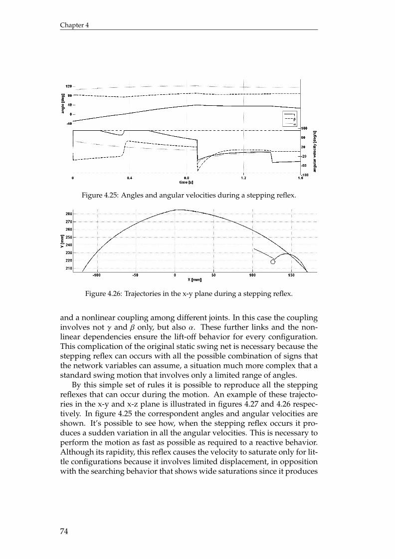
Chapter 4

Figure 4.25: Angles and angular velocities during a stepping reflex.

Figure 4.26: Trajectories in the x-y plane during a stepping reflex.

and a nonlinear coupling among different joints. In this case the couplinginvolves not γ and β only, but also α. These further links and the non-linear dependencies ensure the lift-off behavior for every configuration.This complication of the original static swing net is necessary because thestepping reflex can occurs with all the possible combination of signs thatthe network variables can assume, a situation much more complex that astandard swing motion that involves only a limited range of angles.

By this simple set of rules it is possible to reproduce all the steppingreflexes that can occur during the motion. An example of these trajecto-ries in the x-y and x-z plane is illustrated in figures 4.27 and 4.26 respec-tively. In figure 4.25 the correspondent angles and angular velocities areshown. It’s possible to see how, when the stepping reflex occurs it pro-duces a sudden variation in all the angular velocities. This is necessary toperform the motion as fast as possible as required to a reactive behavior.Although its rapidity, this reflex causes the velocity to saturate only for lit-tle configurations because it involves limited displacement, in oppositionwith the searching behavior that shows wide saturations since it produces

74

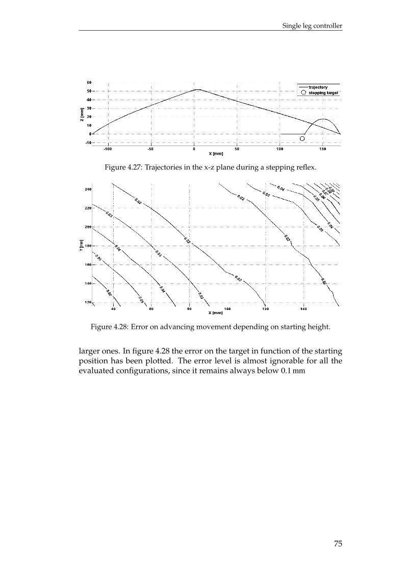
Single leg controller

Figure 4.27: Trajectories in the x-z plane during a stepping reflex.

Figure 4.28: Error on advancing movement depending on starting height.

larger ones. In figure 4.28 the error on the target in function of the startingposition has been plotted. The error level is almost ignorable for all theevaluated configurations, since it remains always below 0.1 mm

75

Chapter 5

CoordinationThe strategy of the present work is to design a free-gait controller able toadapt the coordination among legs to produce the most efficient gait de-pending on required advancing velocity and external environment. Thisproblem can be solved by the application of local influence that varies themotion of each limb in dependency of its neighbors. Advantages of localrules are their simplicity and the resulting simpler implementation. How-ever, the global behavior of a system of local rules can only be predictedwith difficulty. Therefore, it is also hard to set the design process to meetcertain criteria, e.g. body stability. The best tested system of local coor-dination rules is the one based on stick insects behavior, elaborated byCruse [42]. Another very interesting model of this type has been proposedby Porta and Celaya [43]. These two systems will be discussed in sections5.1 and 5.2 respectively. The main idea of the this chapter is to merge thestructures of the two controllers, taking features of both of them, in or-der to create a coordination model that had all the advantages of the twosystems, but also reduced the problems of each one. This process will bedescribed in section 5.3.

5.1 Cruse’s coordination rules

The behaviors of the legs affected by coordinating influences have beenalready illustrated in subsection 3.6.3. In this section a quantitative for-mulation of those rules will be introduced. Cruse’s model implementedin its simplest version introduces only three of the coordination rules (1-3) plus a fourth rule (4) that involves the targeting of the swing phase: itwill be discussed apart (see section 5.4). The model for rules 1 to 3 usesdefault positions for the PEP of each leg. The local coordination rules shiftthese default PEPs along the x-axis. These relationships can be summa-rized qualitatively as follows:

1. the PEP of the affected leg is shifted backwards along the x-axis ifthe ipsilateral posterior leg is protracting. This prolongs retractionin the affected leg;

2. the PEP of the affected leg is temporarily shifted forward if the ip-silateral posterior leg or the contralateral leg has just changed fromprotraction to retraction. This shortens retraction in the affected leg;

77

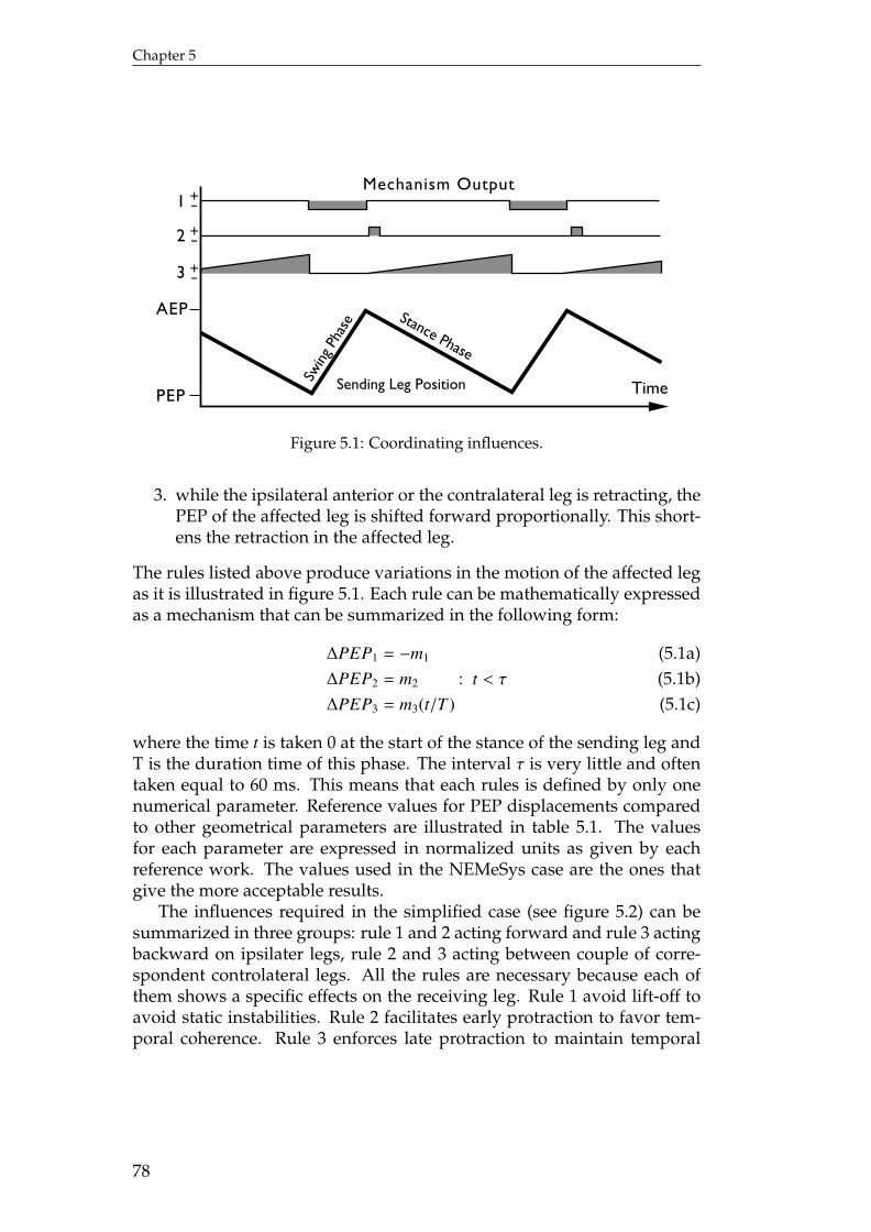
Chapter 5

TimeSending Leg PositionPEP

AEP

1

2

3

Mechanism Output

Swin

g Ph

ase Stance Phase

++

+-

+-

+-

Figure 5.1: Coordinating influences.

3. while the ipsilateral anterior or the contralateral leg is retracting, thePEP of the affected leg is shifted forward proportionally. This short-ens the retraction in the affected leg.

The rules listed above produce variations in the motion of the affected legas it is illustrated in figure 5.1. Each rule can be mathematically expressedas a mechanism that can be summarized in the following form:

∆PEP1 = −m1 (5.1a)∆PEP2 = m2 : t < τ (5.1b)∆PEP3 = m3(t/T ) (5.1c)

where the time t is taken 0 at the start of the stance of the sending leg andT is the duration time of this phase. The interval τ is very little and oftentaken equal to 60 ms. This means that each rules is defined by only onenumerical parameter. Reference values for PEP displacements comparedto other geometrical parameters are illustrated in table 5.1. The valuesfor each parameter are expressed in normalized units as given by eachreference work. The values used in the NEMeSys case are the ones thatgive the more acceptable results.

The influences required in the simplified case (see figure 5.2) can besummarized in three groups: rule 1 and 2 acting forward and rule 3 actingbackward on ipsilater legs, rule 2 and 3 acting between couple of corre-spondent controlateral legs. All the rules are necessary because each ofthem shows a specific effects on the receiving leg. Rule 1 avoid lift-off toavoid static instabilities. Rule 2 facilitates early protraction to favor tem-poral coherence. Rule 3 enforces late protraction to maintain temporal

78

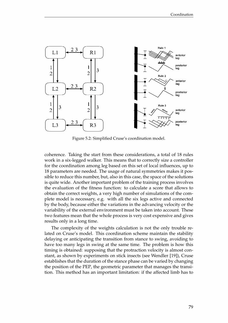
Coordination

Figure 5.2: Simplified Cruse’s coordination model.

coherence. Taking the start from these considerations, a total of 18 ruleswork in a six-legged walker. This means that to correctly size a controllerfor the coordination among leg based on this set of local influences, up to18 parameters are needed. The usage of natural symmetries makes it pos-sible to reduce this number, but, also in this case, the space of the solutionsis quite wide. Another important problem of the training process involvesthe evaluation of the fitness function: to calculate a score that allows toobtain the correct weights, a very high number of simulations of the com-plete model is necessary, e.g. with all the six legs active and connectedby the body, because either the variations in the advancing velocity or thevariability of the external environment must be taken into account. Thesetwo features mean that the whole process is very cost expensive and givesresults only in a long time.

The complexity of the weights calculation is not the only trouble re-lated on Cruse’s model. This coordination scheme maintain the stabilitydelaying or anticipating the transition from stance to swing, avoiding tohave too many legs in swing at the same time. The problem is how thistiming is obtained: supposing that the protraction velocity is almost con-stant, as shown by experiments on stick insects (see Wendler [19]), Cruseestablishes that the duration of the stance phase can be varied by changingthe position of the PEP, the geometric parameter that manages the transi-tion. This method has an important limitation: if the affected limb has to

79

Chapter 5

Parameter Espenschied Roggendorf NEMeSysStep size 2 20 1Mechanism 1 0.59 15÷20 0.7Mechanism 2 1 3.5 0.5Mechanism 3 0.58 6 0.2÷0.25

Table 5.1: Reference parameters for Cruse’s coordination rules.

remain in contact with the ground for a long time, e.g. the middle leg,when the hind leg performs a searching reflex, the PEP should be shiftedfar behind. This motion is not possible because the maximum allowedposterior position is limited either by the geometry of the leg, e.g. seg-ments length and limit angular displacements, or by the physical contactwith the body. In such a situation becomes it is impossible to maintainthe static stability of the robot by simply using the above said rules; otherrules or global criteria have to be introduced, losing the advantages of adecentralized controller.

In its comparative analysis on some significant coordination mecha-nism for a free-gait controller, Roggendorf [44] found the same difficultiesin the calculation of the parameters of the Cruse’s model and identifiedother problems of this method: it performed reliably only when walkingslowly on even ground while its performance worsened with higher walk-ing speeds; during the simulation of an obstacle crossing, the model showsinstabilities while ascending the obstacle and while descending it; duringa curve walking it shows a high probability to become statically unstable.

5.2 Porta and Celaya model

In order to describe the model of the gait generator proposed by Portaand Celaya [43], the term of neighboring legs must be defined. Accordingto the Porta and Celaya model, the legs connected by arrows in figure5.2 are neighboring, with the exception of the middle legs, which are notconsidered neighbors. Thus each leg has exactly two neighbors.

To ensure stability, it must be granted that a sufficient set of legs stay onthe ground supporting the body at any time. In the case of most six-leggedrobots, this requirement can be satisfied by observing the following rule:

Rule 1. Never have neighboring legs raised from the ground at the same time.

In their work Porta and Celaya assume that Rule 1 is a sufficient con-dition to guarantee statically stable gaits. The fulfillment of this rule as-

80

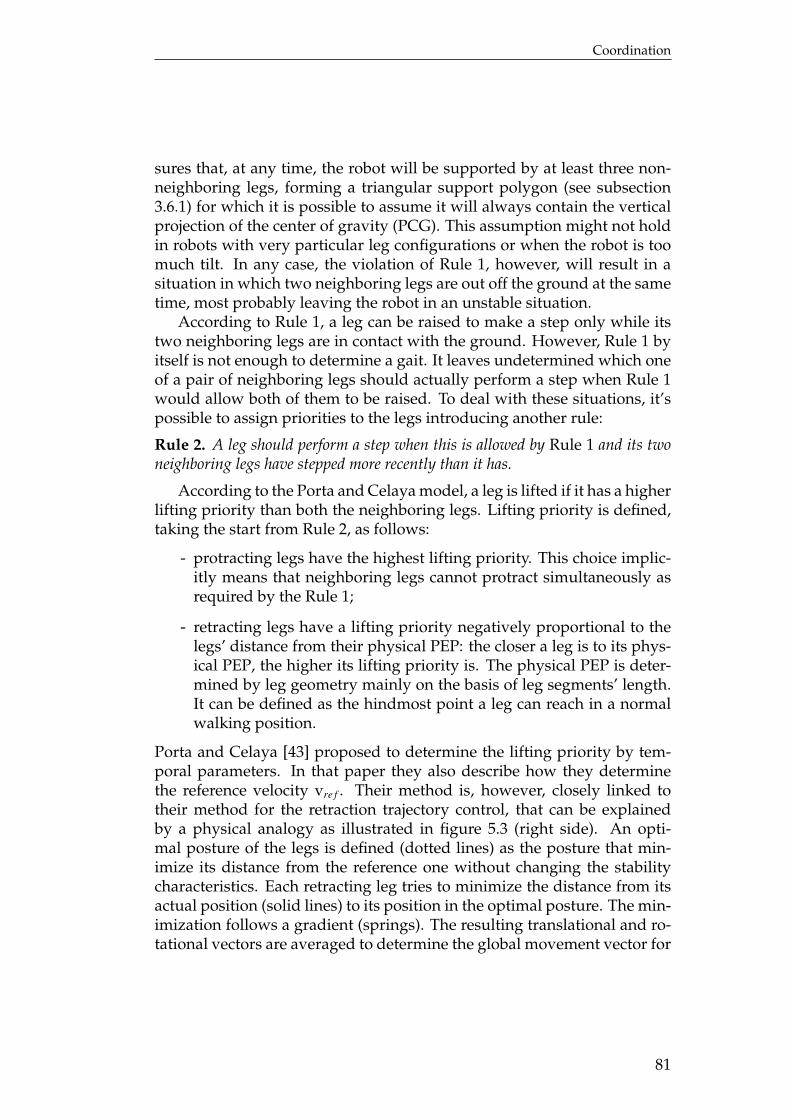
Coordination

sures that, at any time, the robot will be supported by at least three non-neighboring legs, forming a triangular support polygon (see subsection3.6.1) for which it is possible to assume it will always contain the verticalprojection of the center of gravity (PCG). This assumption might not holdin robots with very particular leg configurations or when the robot is toomuch tilt. In any case, the violation of Rule 1, however, will result in asituation in which two neighboring legs are out off the ground at the sametime, most probably leaving the robot in an unstable situation.

According to Rule 1, a leg can be raised to make a step only while itstwo neighboring legs are in contact with the ground. However, Rule 1 byitself is not enough to determine a gait. It leaves undetermined which oneof a pair of neighboring legs should actually perform a step when Rule 1would allow both of them to be raised. To deal with these situations, it’spossible to assign priorities to the legs introducing another rule:

Rule 2. A leg should perform a step when this is allowed by Rule 1 and its twoneighboring legs have stepped more recently than it has.

According to the Porta and Celaya model, a leg is lifted if it has a higherlifting priority than both the neighboring legs. Lifting priority is defined,taking the start from Rule 2, as follows:

- protracting legs have the highest lifting priority. This choice implic-itly means that neighboring legs cannot protract simultaneously asrequired by the Rule 1;

- retracting legs have a lifting priority negatively proportional to thelegs’ distance from their physical PEP: the closer a leg is to its phys-ical PEP, the higher its lifting priority is. The physical PEP is deter-mined by leg geometry mainly on the basis of leg segments’ length.It can be defined as the hindmost point a leg can reach in a normalwalking position.

Porta and Celaya [43] proposed to determine the lifting priority by tem-poral parameters. In that paper they also describe how they determinethe reference velocity vre f . Their method is, however, closely linked totheir method for the retraction trajectory control, that can be explainedby a physical analogy as illustrated in figure 5.3 (right side). An opti-mal posture of the legs is defined (dotted lines) as the posture that min-imize its distance from the reference one without changing the stabilitycharacteristics. Each retracting leg tries to minimize the distance from itsactual position (solid lines) to its position in the optimal posture. The min-imization follows a gradient (springs). The resulting translational and ro-tational vectors are averaged to determine the global movement vector for

81

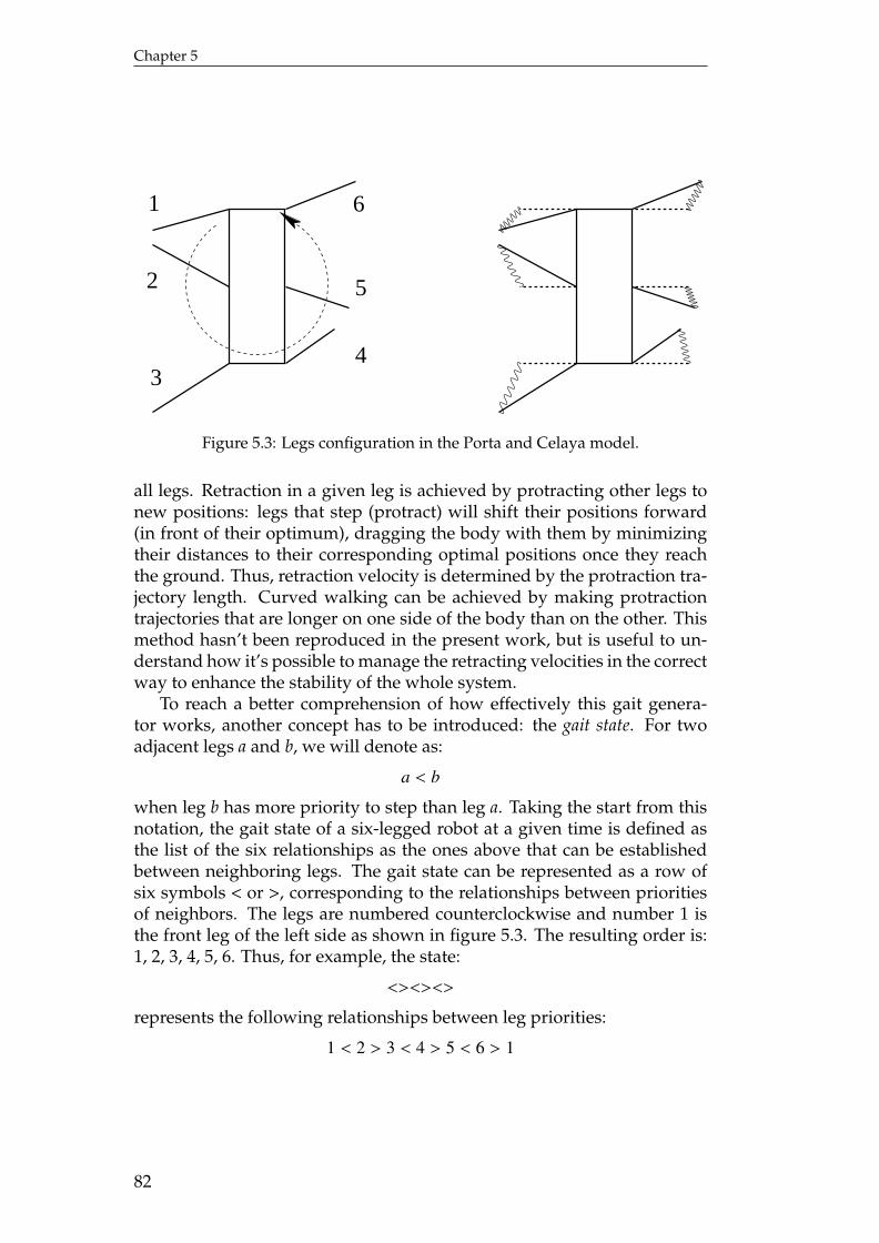
Chapter 5

61

2

3

5

4

Figure 5.3: Legs configuration in the Porta and Celaya model.

all legs. Retraction in a given leg is achieved by protracting other legs tonew positions: legs that step (protract) will shift their positions forward(in front of their optimum), dragging the body with them by minimizingtheir distances to their corresponding optimal positions once they reachthe ground. Thus, retraction velocity is determined by the protraction tra-jectory length. Curved walking can be achieved by making protractiontrajectories that are longer on one side of the body than on the other. Thismethod hasn’t been reproduced in the present work, but is useful to un-derstand how it’s possible to manage the retracting velocities in the correctway to enhance the stability of the whole system.

To reach a better comprehension of how effectively this gait genera-tor works, another concept has to be introduced: the gait state. For twoadjacent legs a and b, we will denote as:

a < b

when leg b has more priority to step than leg a. Taking the start from thisnotation, the gait state of a six-legged robot at a given time is defined asthe list of the six relationships as the ones above that can be establishedbetween neighboring legs. The gait state can be represented as a row ofsix symbols < or >, corresponding to the relationships between prioritiesof neighbors. The legs are numbered counterclockwise and number 1 isthe front leg of the left side as shown in figure 5.3. The resulting order is:1, 2, 3, 4, 5, 6. Thus, for example, the state:

<><><>

represents the following relationships between leg priorities:

1 < 2 > 3 < 4 > 5 < 6 > 1

82

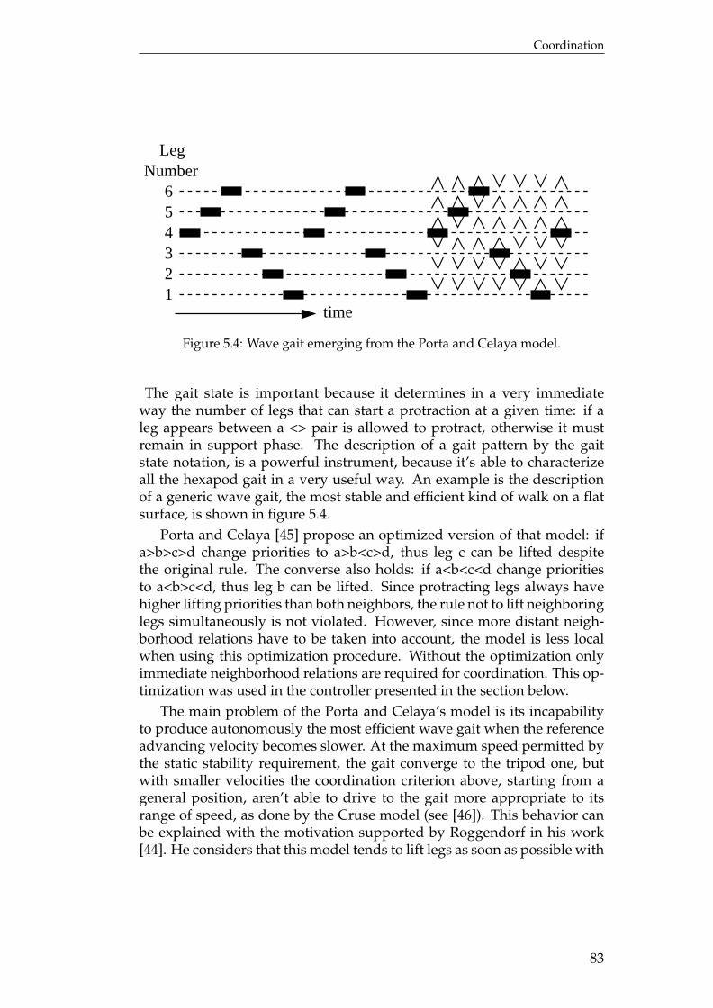
Coordination

LegNumber

time

654321

Figure 5.4: Wave gait emerging from the Porta and Celaya model.

The gait state is important because it determines in a very immediateway the number of legs that can start a protraction at a given time: if aleg appears between a <> pair is allowed to protract, otherwise it mustremain in support phase. The description of a gait pattern by the gaitstate notation, is a powerful instrument, because it’s able to characterizeall the hexapod gait in a very useful way. An example is the descriptionof a generic wave gait, the most stable and efficient kind of walk on a flatsurface, is shown in figure 5.4.

Porta and Celaya [45] propose an optimized version of that model: ifa>b>c>d change priorities to a>b<c>d, thus leg c can be lifted despitethe original rule. The converse also holds: if a<b<c<d change prioritiesto a<b>c<d, thus leg b can be lifted. Since protracting legs always havehigher lifting priorities than both neighbors, the rule not to lift neighboringlegs simultaneously is not violated. However, since more distant neigh-borhood relations have to be taken into account, the model is less localwhen using this optimization procedure. Without the optimization onlyimmediate neighborhood relations are required for coordination. This op-timization was used in the controller presented in the section below.

The main problem of the Porta and Celaya’s model is its incapabilityto produce autonomously the most efficient wave gait when the referenceadvancing velocity becomes slower. At the maximum speed permitted bythe static stability requirement, the gait converge to the tripod one, butwith smaller velocities the coordination criterion above, starting from ageneral position, aren’t able to drive to the gait more appropriate to itsrange of speed, as done by the Cruse model (see [46]). This behavior canbe explained with the motivation supported by Roggendorf in his work[44]. He considers that this model tends to lift legs as soon as possible with

83

Chapter 5

the purpose of maximize the advancing velocity. This requirement drivesthe walking pattern to the tripod gait that is the fastest possible, but, at thesame time produce a very poor performance with low retraction velocities.The generation of gaits at the lower velocities becomes a problem becausethis controller tends to concentrate the swing phases in almost the sametime slice, producing a situation in which the legs are all close to their PEPand the robot is too inclined. This is the kind of posture in which Rule 1doesn’t ensure static stability and an unstable gait can occurs.

5.3 Coordination model

In the present section the coordination model adopted for the gait gen-eration of the NEMeSys robot will be discussed. The system consists ina hybrid version of the two models summarized above that tries to takeinto account advantages and disadvantages of both of them. The purposeis the design of the simplest controller possible able to fulfill, at the sametime, the two following requirements:

1. ensure static stability in all the situations. The criteria on which isbased the generation of the gait pattern, must ensure a statically sta-ble motion not only during a typical walk, but also on a wider rangeof possible movement, i.e. during a searching reflex. Thus the con-troller must be able to decrease the advancing velocity of the wholerobot or to stop it if necessary;

2. produce an efficient gait. The fulfillment of the stability requirementshall not reduce the efficiency of the gait. Thus, during the walkingon flat surface the free-gait has to naturally evolve through a stereo-typical wave-gait. This behavior should ensure to obtain the mostefficient gait at every speed, in the entire range of velocities.

The first requirement implies that another criterion, based on the retrac-tion velocity, has to be considered. This criterion must be global, to man-age the advancing velocity and has to be as simple as possible to avoidany decrease in the computational efficiency of the whole system. Thesecond requirement implies that the rules that produce a certain wave-gait must be found. These rules must be obviously local and have to beimplemented in their simplest form. Moreover they should be the sameused for the stability control, or at least don’t have to be in conflict withthem.

The comparison done by Roggendorf shows how the most effectivesystem for the generator of gaits, among the tested ones, is represented

84

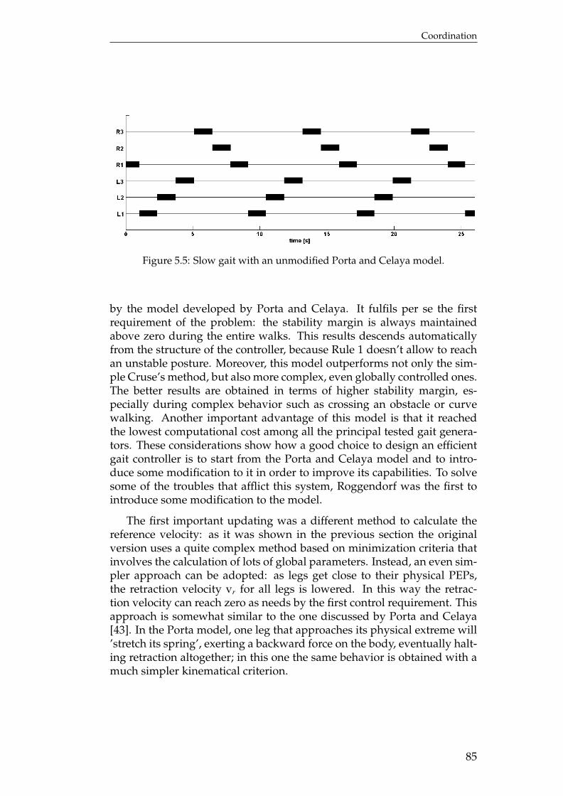
Coordination

Figure 5.5: Slow gait with an unmodified Porta and Celaya model.

by the model developed by Porta and Celaya. It fulfils per se the firstrequirement of the problem: the stability margin is always maintainedabove zero during the entire walks. This results descends automaticallyfrom the structure of the controller, because Rule 1 doesn’t allow to reachan unstable posture. Moreover, this model outperforms not only the sim-ple Cruse’s method, but also more complex, even globally controlled ones.The better results are obtained in terms of higher stability margin, es-pecially during complex behavior such as crossing an obstacle or curvewalking. Another important advantage of this model is that it reachedthe lowest computational cost among all the principal tested gait genera-tors. These considerations show how a good choice to design an efficientgait controller is to start from the Porta and Celaya model and to intro-duce some modification to it in order to improve its capabilities. To solvesome of the troubles that afflict this system, Roggendorf was the first tointroduce some modification to the model.

The first important updating was a different method to calculate thereference velocity: as it was shown in the previous section the originalversion uses a quite complex method based on minimization criteria thatinvolves the calculation of lots of global parameters. Instead, an even sim-pler approach can be adopted: as legs get close to their physical PEPs,the retraction velocity vr for all legs is lowered. In this way the retrac-tion velocity can reach zero as needs by the first control requirement. Thisapproach is somewhat similar to the one discussed by Porta and Celaya[43]. In the Porta model, one leg that approaches its physical extreme will’stretch its spring’, exerting a backward force on the body, eventually halt-ing retraction altogether; in this one the same behavior is obtained with amuch simpler kinematical criterion.

85

Chapter 5

Another problem of the Porta and Celaya model is its tendency to liftoff the leg as soon as possible. This allows to reach the most effective tri-pod gait earlier than in the other models, but with low retraction velocity,the PEPs are shifted very far forward, eventually to positions shortly be-hind the AEPs, to maintain the correct timing. This can lead to dangerousinstabilities because the support polygon assume a very stretched configu-ration. An example of this behavior is illustrated in figure 5.5. To avoid it asecond modification of the Porta and Celaya model has been proposed. Inthis version, the lifting rules were applied only if the distance D of a givenleg from its physical PEP was smaller than a preset threshold T. In hiswork the threshold is set to 5.0 length units in the simulation, comparedto mean step size of 20 units. These parameters are used to calculate theactual retraction velocity vr. Each retracting leg proposes a desired globalretraction velocity accorded by equations 5.2.vr = D

T vrre f : D<Tvr = vrre f : D≥ T

(5.2)

This method to calculate the global reference velocity implies that theleg with the smallest proposal determines the actual vre f . The calculatedreference velocity will obviously be a fraction of the required one (vrre f )and in the ideal case of perfectly coordinated legs movement, it will as-sume exactly the required value. This coordination rule requires a globalplanning to be performed: all the reference velocities proposed by the sixlegs have to be taken into account to calculate the actual one. The introduc-tion of a global rule seems to make the method lose the properties depend-ing to its decentralization. This situation, however, doesn’t produce anydecrease in the performances, because the formulation of the rule is verysimple and involve only parameters that have been already calculated.

Roggendorf proposed another modification to the Porta and Celayamodel. This control system made use of the threshold T for calculation ofvr only, but it calculated the lifting priorities with a different approach. Itwas checked whether the walker would become unstable if that leg werelifted: a leg was lifted only if the walker retained static stability. The prob-lem is evaluating the stability a global parameter as the stability marginmust be calculated. This means that this extension implies a much moreadvanced planning than the previous ones and drives to a greater increasein the computational cost. This is the reason why it will not be employedin this work.

The only parameter involved in the sizing process of this modifiedPorta and Celaya model is the value of the threshold T. The reference value

86

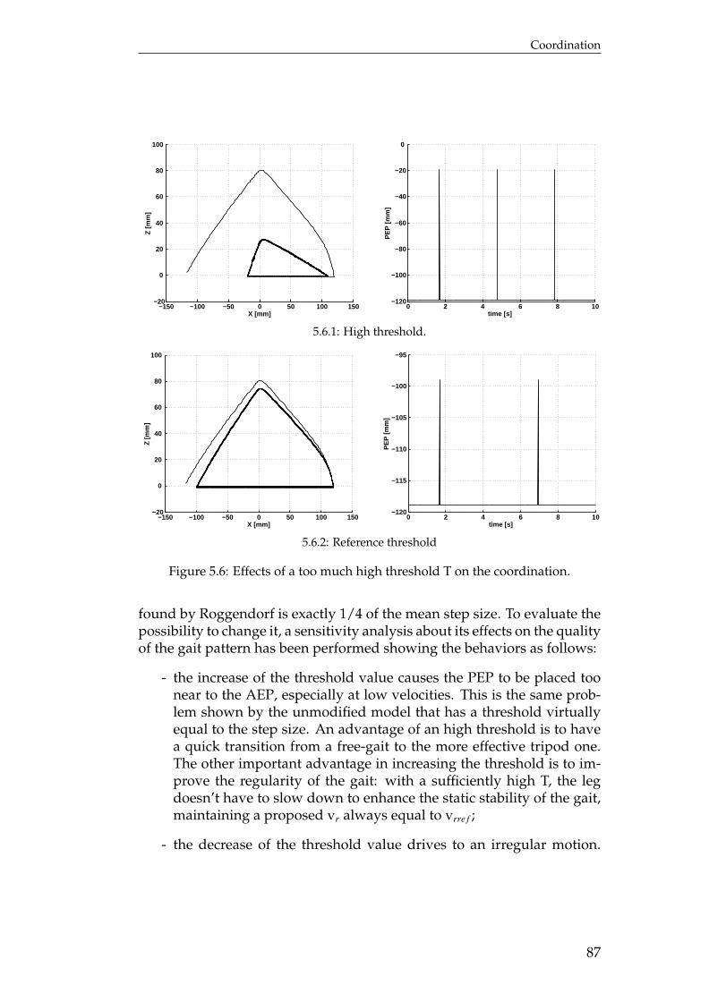
Coordination

−150 −100 −50 0 50 100 150−20

0

20

40

60

80

100

X [mm]

Z [m

m]

0 2 4 6 8 10−120

−100

−80

−60

−40

−20

0

time [s]

PE

P [m

m]

5.6.1: High threshold.

−150 −100 −50 0 50 100 150−20

0

20

40

60

80

100

X [mm]

Z [m

m]

0 2 4 6 8 10−120

−115

−110

−105

−100

−95

time [s]

PE

P [m

m]

5.6.2: Reference threshold

Figure 5.6: Effects of a too much high threshold T on the coordination.

found by Roggendorf is exactly 1/4 of the mean step size. To evaluate thepossibility to change it, a sensitivity analysis about its effects on the qualityof the gait pattern has been performed showing the behaviors as follows:

- the increase of the threshold value causes the PEP to be placed toonear to the AEP, especially at low velocities. This is the same prob-lem shown by the unmodified model that has a threshold virtuallyequal to the step size. An advantage of an high threshold is to havea quick transition from a free-gait to the more effective tripod one.The other important advantage in increasing the threshold is to im-prove the regularity of the gait: with a sufficiently high T, the legdoesn’t have to slow down to enhance the static stability of the gait,maintaining a proposed vr always equal to vrre f ;

- the decrease of the threshold value drives to an irregular motion.

87

Chapter 5

Figure 5.7: Effects of a too much small threshold T on the coordination.

With a too much little T, the leg hasn’t enough time to correctly de-crease its velocity, and this causes to a loss of coordination. Duringa poorly coordinated walk, the controller tries to keep a leg on theground as longer as possible stopping its motion; this is the reasonwhy the advancing velocity becomes irregular. The main advantageof this behavior is the possibility of having the PEP closer to its refer-ence value, producing a legs’ motion that allows to reach a globallyoptimal posture.

The irregularity effects occurs only for threshold values very close tozero, so the sizing criterion is to minimize the threshold, but, at same time,to maintain a regular motion. The limit value has been found equal to1/12 of the mean step size. Smaller values produce sudden decrease in theadvancing velocities followed by returns to the reference ones, when theglobal configuration allows it. This behavior can be identified especiallyat the fastest gaits.

The version of the Porta and Celaya model modified by Roggendorfand adopted in this work fulfils the stability requirement completely, butdoesn’t allows to solve the incapability of this model to reproduce a wave-gait for low velocities. On the other hand, as it has already been said,the same behavior autonomously emerges from the Cruse’s set of rules.The solution might be to understand which of the rules are responsible ofthis particular behavior and to insert them into the modified version of thePorta and Celaya model, paying attention not to lose the useful capabilitiesthat it shows per se.

The evaluation of a decentralized control system, as the one adopted tomanage the coordination, is very difficult to obtain with classic techniques.The way used in related works, as in the present one, is the Kindermann’sethological approach to systems analysis that consists of an evaluation and

88

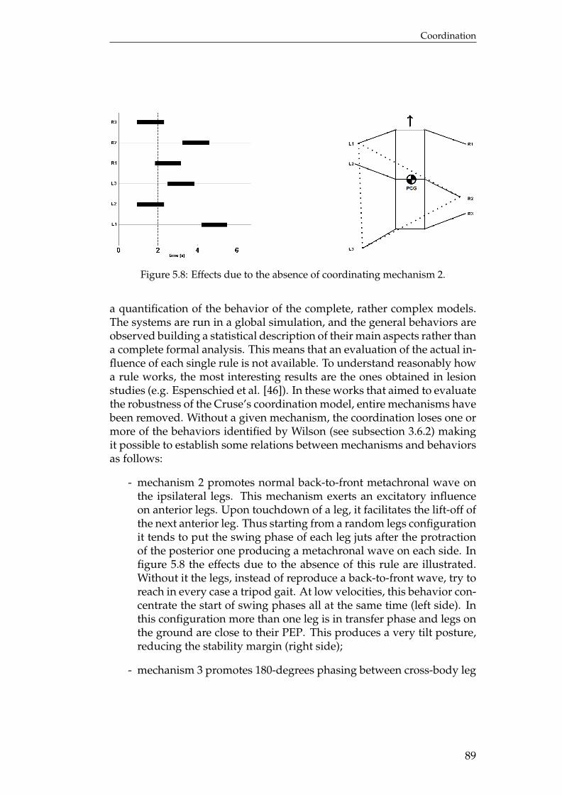
Coordination

Figure 5.8: Effects due to the absence of coordinating mechanism 2.

a quantification of the behavior of the complete, rather complex models.The systems are run in a global simulation, and the general behaviors areobserved building a statistical description of their main aspects rather thana complete formal analysis. This means that an evaluation of the actual in-fluence of each single rule is not available. To understand reasonably howa rule works, the most interesting results are the ones obtained in lesionstudies (e.g. Espenschied et al. [46]). In these works that aimed to evaluatethe robustness of the Cruse’s coordination model, entire mechanisms havebeen removed. Without a given mechanism, the coordination loses one ormore of the behaviors identified by Wilson (see subsection 3.6.2) makingit possible to establish some relations between mechanisms and behaviorsas follows:

- mechanism 2 promotes normal back-to-front metachronal wave onthe ipsilateral legs. This mechanism exerts an excitatory influenceon anterior legs. Upon touchdown of a leg, it facilitates the lift-off ofthe next anterior leg. Thus starting from a random legs configurationit tends to put the swing phase of each leg juts after the protractionof the posterior one producing a metachronal wave on each side. Infigure 5.8 the effects due to the absence of this rule are illustrated.Without it the legs, instead of reproduce a back-to-front wave, try toreach in every case a tripod gait. At low velocities, this behavior con-centrate the start of swing phases all at the same time (left side). Inthis configuration more than one leg is in transfer phase and legs onthe ground are close to their PEP. This produces a very tilt posture,reducing the stability margin (right side);

- mechanism 3 promotes 180-degrees phasing between cross-body leg

89

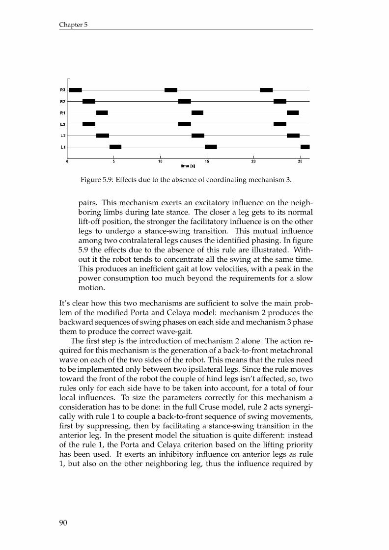
Chapter 5

Figure 5.9: Effects due to the absence of coordinating mechanism 3.

pairs. This mechanism exerts an excitatory influence on the neigh-boring limbs during late stance. The closer a leg gets to its normallift-off position, the stronger the facilitatory influence is on the otherlegs to undergo a stance-swing transition. This mutual influenceamong two contralateral legs causes the identified phasing. In figure5.9 the effects due to the absence of this rule are illustrated. With-out it the robot tends to concentrate all the swing at the same time.This produces an inefficient gait at low velocities, with a peak in thepower consumption too much beyond the requirements for a slowmotion.

It’s clear how this two mechanisms are sufficient to solve the main prob-lem of the modified Porta and Celaya model: mechanism 2 produces thebackward sequences of swing phases on each side and mechanism 3 phasethem to produce the correct wave-gait.

The first step is the introduction of mechanism 2 alone. The action re-quired for this mechanism is the generation of a back-to-front metachronalwave on each of the two sides of the robot. This means that the rules needto be implemented only between two ipsilateral legs. Since the rule movestoward the front of the robot the couple of hind legs isn’t affected, so, tworules only for each side have to be taken into account, for a total of fourlocal influences. To size the parameters correctly for this mechanism aconsideration has to be done: in the full Cruse model, rule 2 acts synergi-cally with rule 1 to couple a back-to-front sequence of swing movements,first by suppressing, then by facilitating a stance-swing transition in theanterior leg. In the present model the situation is quite different: insteadof the rule 1, the Porta and Celaya criterion based on the lifting priorityhas been used. It exerts an inhibitory influence on anterior legs as rule1, but also on the other neighboring leg, thus the influence required by

90

Coordination

rule 2 is different from the one needed in the reference case. The actualvalues for the parameters could be far different from the reference ones asshown in table 5.1, especially for one reason: the Porta and Celaya modeltends to put the swing phase of each strictly before or after the protractionof its posterior neighbor. Since the wave-gait can be obtained in the firstcase only, in the second one the influences have to be very high to coun-terbalance. To calculate them an hand-tuning process has been performedstarting from the standard values and evaluating the sensitivity of the gaitproperties depending on each parameters. This process allows to classifythree important behaviors:

- the duration of the mechanism has to be extended up to the wholefirst half of the power stroke of the sending leg. This is an impor-tant change when compared to the classic formulation in which thisduration was very small: about 60 ms by temporal criteria, less thanthe 5% of the power stroke duration for a tripod walk. The effect ofthis behavior is to accelerate the transition from a free-gait to a wave-gait, by locking the swing of a leg as soon as possible just after theprotraction of its posterior neighbor. With a smaller duration time,the wave-gait emerges only after a high number of steps, especiallyat lower velocities, while with greater ones, the motion becomes un-stable during the faster gaits;

- the influence of the mechanism depends on advancing velocity. Atlower velocities the duration of the stance phase is much higher thanwith the swing one. This means that a value of influence compara-ble with the step length has to be applied to ’unlock’ a swing phaseplaced just before the protraction of its posterior neighbor, insteadof after. This happens because, in this case, the swing is performedwhile the sending leg is at the end of its power stroke, so the differ-ence between the current location of the return stroke of the targetleg and the required one is comparable with the length of the powerstroke itself. At higher velocities the problem is the same, but theduration of the stance phase is very close to the swing one and therequired effect can be obtained also with a smaller displacement ofthe PEP, compared with an half of the step. At these speeds anotherproblem occurs: a much higher value of displacements produce anunstable gait, so its value must be reduced;

- the regularity of the gait depends on the strength of the influence. Astrong influence, like a high duration time, is able to produce a fasttransition from a general free-gait, to a wave one. With a lower in-fluence some legs have to wait the other ones, that are still in stance,

91

Chapter 5

decreasing their protracting velocities. Since the global advancingvelocity is the minimum of these ones, the whole robot has to walkwith a slower speed, until the configuration allows to start with anew step sequence. This behavior generates an irregular advanc-ing velocity that causes an inefficient motion. The problem is thatit isn’t possible to increase the strength of the influence arbitrarily,because this could produce an instable gait, as discussed in the pre-vious point;

In this work the influences of both the mechanisms have been calculatedby spatial, instead of temporal, parameter. This choice has been preferredbecause the controller structure allows to have almost exact values of allthe geometric parameters starting from the measured joint angles, whilethe characteristic times of the motion could be only roughly estimated.The implementation of mechanism 2 is the same as show in section 5.1,but the threshold T2 is a displacement, instead of a time:

PEP1 = PEP1−re f + m2 : (AEP2 − x2) < T2 (5.3a)PEP2 = PEP2−re f + m2 : (AEP3 − x3) < T2 (5.3b)PEP5 = PEP5−re f + m2 : (AEP4 − x4) < T2 (5.3c)PEP6 = PEP6−re f + m2 : (AEP5 − x5) < T2 (5.3d)

The mechanism 2 is only able to produce statically stable gaits thatshow a metachronal wave propagating among the legs of each side, butto introduce correct relationship from a side to the other, is necessary tointroduce another rule. The second step consists of the usage of the mech-anism 3 to obtain the correct phasing between the two sides. Before start-ing with the sizing of the parameters of this mechanism, an importantconsideration must be done. The back-to-front wave of protracting hasbeen obtained with four rules acting from a leg toward its anterior neigh-bor: this means that on the couple of hind legs no more influences havebeen added to the Porta and Celaya model. But, more important, it alsoimplies that the coordination of the three legs attached on each side de-scends from the motion of the correspondent hind leg. Taking the startfrom this consideration it is possible to argue that the complete coordina-tion can be achieved by applying the mechanism 3 only between the twocontralateral hind-legs. This simplification could seems quite brutal, butthe results obtained by the simulation show all its effectiveness. Moreoverit allows to reduce the number of influences from six to only two. The onlyparameter that manages this mechanism is the maximum displacementreached at the end of the sending leg’s power stroke. The formulation for

92

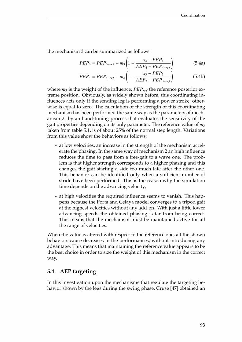
Coordination

the mechanism 3 can be summarized as follows:

PEP3 = PEP3−re f + m3

(1 −

x4 − PEP4

AEP4 − PEP4−re f

)(5.4a)

PEP4 = PEP4−re f + m3

(1 −

x3 − PEP3

AEP3 − PEP3−re f

)(5.4b)

where m3 is the weight of the influence, PEPre f the reference posterior ex-treme position. Obviously, as widely shown before, this coordinating in-fluences acts only if the sending leg is performing a power stroke, other-wise is equal to zero. The calculation of the strength of this coordinatingmechanism has been performed the same way as the parameters of mech-anism 2: by an hand-tuning process that evaluates the sensitivity of thegait properties depending on its only parameter. The reference value of m3

taken from table 5.1, is of about 25% of the normal step length. Variationsfrom this value show the behaviors as follows:

- at low velocities, an increase in the strength of the mechanism accel-erate the phasing. In the same way of mechanism 2 an high influencereduces the time to pass from a free-gait to a wave one. The prob-lem is that higher strength corresponds to a higher phasing and thischanges the gait starting a side too much late after the other one.This behavior can be identified only when a sufficient number ofstride have been performed. This is the reason why the simulationtime depends on the advancing velocity;

- at high velocities the required influence seems to vanish. This hap-pens because the Porta and Celaya model converges to a tripod gaitat the highest velocities without any add-on. With just a little loweradvancing speeds the obtained phasing is far from being correct.This means that the mechanism must be maintained active for allthe range of velocities.

When the value is altered with respect to the reference one, all the shownbehaviors cause decreases in the performances, without introducing anyadvantage. This means that maintaining the reference value appears to bethe best choice in order to size the weight of this mechanism in the correctway.

5.4 AEP targeting

In this investigation upon the mechanisms that regulate the targeting be-havior shown by the legs during the swing phase, Cruse [47] obtained an

93

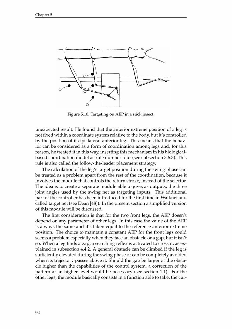
Chapter 5

Figure 5.10: Targeting on AEP in a stick insect.

unexpected result. He found that the anterior extreme position of a leg isnot fixed within a coordinate system relative to the body, but it’s controlledby the position of its ipsilateral anterior leg. This means that the behav-ior can be considered as a form of coordination among legs and, for thisreason, he treated it in this way, inserting this mechanism in his biological-based coordination model as rule number four (see subsection 3.6.3). Thisrule is also called the follow-the-leader placement strategy.

The calculation of the leg’s target position during the swing phase canbe treated as a problem apart from the rest of the coordination, because itinvolves the module that controls the return stroke, instead of the selector.The idea is to create a separate module able to give, as outputs, the threejoint angles used by the swing net as targeting inputs. This additionalpart of the controller has been introduced for the first time in Walknet andcalled target net (see Dean [48]). In the present section a simplified versionof this module will be discussed.

The first consideration is that for the two front legs, the AEP doesn’tdepend on any parameter of other legs. In this case the value of the AEPis always the same and it’s taken equal to the reference anterior extremeposition. The choice to maintain a constant AEP for the front legs couldseems a problem especially when they face an obstacle or a gap, but it isn’tso. When a leg finds a gap, a searching reflex is activated to cross it, as ex-plained in subsection 4.4.2. A general obstacle can be climbed if the leg issufficiently elevated during the swing phase or can be completely avoidedwhen its trajectory passes above it. Should the gap be larger or the obsta-cle higher than the capabilities of the control system, a correction of thepattern at an higher level would be necessary (see section 1.1). For theother legs, the module basically consists in a function able to take, the cur-

94

Coordination

rent joint angles of the correspondent anterior ipsilateral leg as inputs andgives the set of joint angles that represents the required AEP as outputs .This function can be expressed in its simplest form as follows:

xAEP = xant − ∆AEP (5.5a)yAEP = yant (5.5b)zAEP = zant (5.5c)

where the Cartesian coordinates are expressed in the absolute referenceframe and the value for ∆AEP has been taken equal to 60 mm. The reasonfor this choice can be justified remembering that the model of the robotuses monodimensional beams to simulate the limb’s segments, but thereal legs has a square section with a side of 25 mm (see chapter 7). In theworst case the contact between two feet may occur when the distance froma footprint to the other becomes lower than 35 mm about. Taking a marginequal to the side of the section the value of 60 mm is obtained. The requiredbehavior is shown in figure 5.11 (left side). The requirement is the same,independently from the current position of the target footholds.

In his work on leg targeting in stick insects, Cruse found that the actualbehavior is quite more complex, because the AEP shows a displacementnot only in the x direction, but also in the y one. Moreover, the value ofthese displacements changes as a function of the position of the sendingleg and it assumes different values when the target leg is a middle or ahind one. This complexity seems to be useless in the control of NEMeSysbecause it has a geometry far different from the one on which Cruse per-formed his test: the stick insect shows a differentiation among front, mid-dle and hind legs, while the robot have six legs with the same geometriccharacteristics. Other differences can be found in the position of the legson the body and in the ratios among characteristic lengths, such as thedistance among legs or the mean step length. The superior symmetry ofthe robot allows to use only the x-component of the required displacementobtaining the correct results.

The first idea could be to use the Cartesian coordinate directly to solvethe problem, but, since the model is completely controlled in terms of an-gular variables, this isn’t the best choice. Obviously the calculation of theAEP can be expressed in a very simple form, but this procedure requires adouble conversion, first from angles to displacements and then from dis-placements back to angle. The process involves nonlinear trigonometricfunctions that increase the computational cost, so, a better solution is toformulate the problem directly in the joint angles space.

This means that the aim is to fulfill a task in the Cartesian space onlyby using calculation in the joint space with angular variables. As shown

95

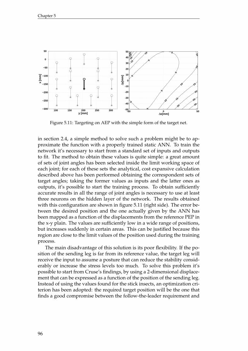
Chapter 5

100 150 200 250 300−300

−250

−200

−150

−100

−50

0

50

y [mm]

x [m

m]

5

5

5

5

5

5

5

10

10

10

10

10

15

15

15

20

20

20

25

25

30

30

∆x[mm]

∆y[m

m]

-50 0 50-50

-40

-30

-20

-10

0

10

20

30

40

50

Figure 5.11: Targeting on AEP with the simple form of the target net.

in section 2.4, a simple method to solve such a problem might be to ap-proximate the function with a properly trained static ANN. To train thenetwork it’s necessary to start from a standard set of inputs and outputsto fit. The method to obtain these values is quite simple: a great amountof sets of joint angles has been selected inside the limit working space ofeach joint; for each of these sets the analytical, cost expansive calculationdescribed above has been performed obtaining the correspondent sets oftarget angles; taking the former values as inputs and the latter ones asoutputs, it’s possible to start the training process. To obtain sufficientlyaccurate results in all the range of joint angles is necessary to use at leastthree neurons on the hidden layer of the network. The results obtainedwith this configuration are shown in figure 5.11 (right side). The error be-tween the desired position and the one actually given by the ANN hasbeen mapped as a function of the displacements from the reference PEP inthe x-y plain. The values are sufficiently low in a wide range of positions,but increases suddenly in certain areas. This can be justified because thisregion are close to the limit values of the position used during the trainingprocess.

The main disadvantage of this solution is its poor flexibility. If the po-sition of the sending leg is far from its reference value, the target leg willreceive the input to assume a posture that can reduce the stability consid-erably or increase the stress levels too much. To solve this problem it’spossible to start from Cruse’s findings, by using a 2-dimensional displace-ment that can be expressed as a function of the position of the sending leg.Instead of using the values found for the stick insects, an optimization cri-terion has been adopted: the required target position will be the one thatfinds a good compromise between the follow-the-leader requirement and

96

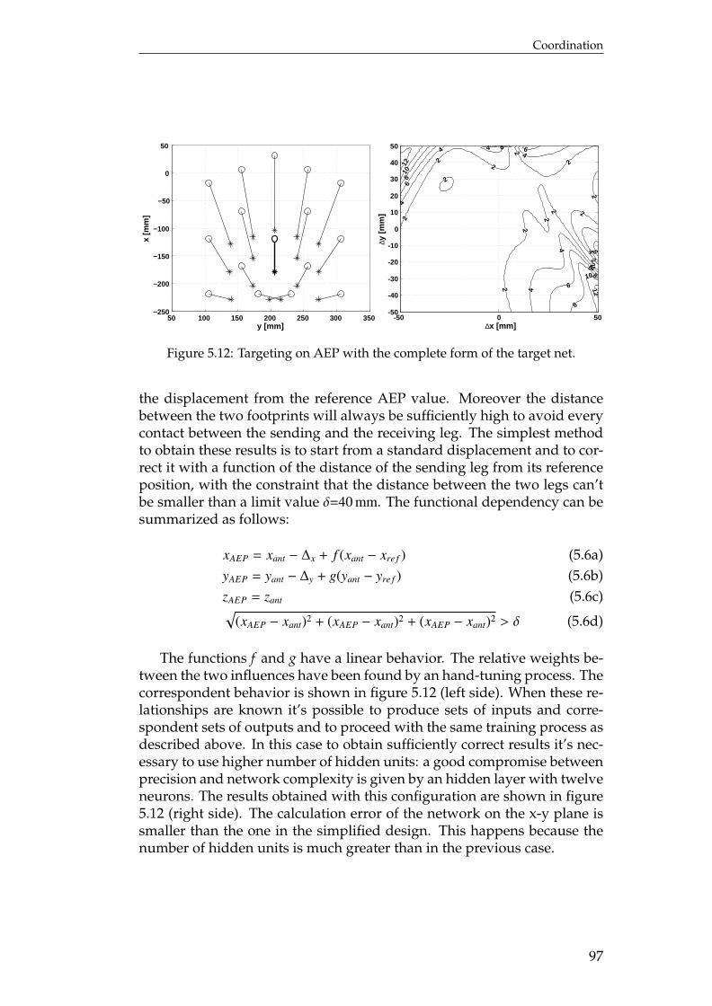
Coordination

50 100 150 200 250 300 350−250

−200

−150

−100

−50

0

50

y [mm]

x [m

m]

2

2

2

2

2

2

2

22

22

2

2

2

4

4

4

4

44

4

4

6

6

66

6

6

8

8

8

10

10

12

12

∆x [mm]

∆y [

mm

]

-50 0 50-50

-40

-30

-20

-10

0

10

20

30

40

50

Figure 5.12: Targeting on AEP with the complete form of the target net.

the displacement from the reference AEP value. Moreover the distancebetween the two footprints will always be sufficiently high to avoid everycontact between the sending and the receiving leg. The simplest methodto obtain these results is to start from a standard displacement and to cor-rect it with a function of the distance of the sending leg from its referenceposition, with the constraint that the distance between the two legs can’tbe smaller than a limit value δ=40 mm. The functional dependency can besummarized as follows:

xAEP = xant − ∆x + f (xant − xre f ) (5.6a)yAEP = yant − ∆y + g(yant − yre f ) (5.6b)zAEP = zant (5.6c)√

(xAEP − xant)2 + (xAEP − xant)2 + (xAEP − xant)2 > δ (5.6d)

The functions f and g have a linear behavior. The relative weights be-tween the two influences have been found by an hand-tuning process. Thecorrespondent behavior is shown in figure 5.12 (left side). When these re-lationships are known it’s possible to produce sets of inputs and corre-spondent sets of outputs and to proceed with the same training process asdescribed above. In this case to obtain sufficiently correct results it’s nec-essary to use higher number of hidden units: a good compromise betweenprecision and network complexity is given by an hidden layer with twelveneurons. The results obtained with this configuration are shown in figure5.12 (right side). The calculation error of the network on the x-y plane issmaller than the one in the simplified design. This happens because thenumber of hidden units is much greater than in the previous case.

97

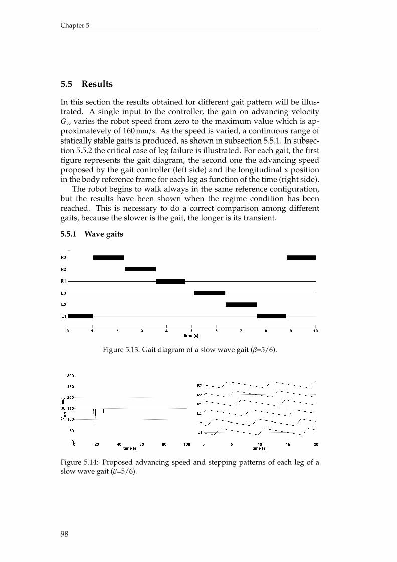
Chapter 5

5.5 Results

In this section the results obtained for different gait pattern will be illus-trated. A single input to the controller, the gain on advancing velocityGv, varies the robot speed from zero to the maximum value which is ap-proximatevely of 160 mm/s. As the speed is varied, a continuous range ofstatically stable gaits is produced, as shown in subsection 5.5.1. In subsec-tion 5.5.2 the critical case of leg failure is illustrated. For each gait, the firstfigure represents the gait diagram, the second one the advancing speedproposed by the gait controller (left side) and the longitudinal x positionin the body reference frame for each leg as function of the time (right side).

The robot begins to walk always in the same reference configuration,but the results have been shown when the regime condition has beenreached. This is necessary to do a correct comparison among differentgaits, because the slower is the gait, the longer is its transient.

5.5.1 Wave gaits

Figure 5.13: Gait diagram of a slow wave gait (β=5/6).

Figure 5.14: Proposed advancing speed and stepping patterns of each leg of aslow wave gait (β=5/6).

98

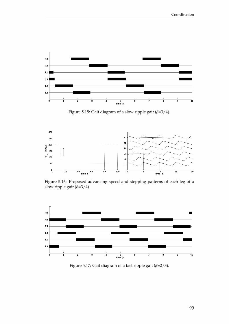
Coordination

Figure 5.15: Gait diagram of a slow ripple gait (β=3/4).

Figure 5.16: Proposed advancing speed and stepping patterns of each leg of aslow ripple gait (β=3/4).

Figure 5.17: Gait diagram of a fast ripple gait (β=2/3).

99

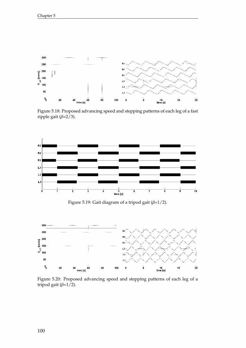
Chapter 5

Figure 5.18: Proposed advancing speed and stepping patterns of each leg of a fastripple gait (β=2/3).

Figure 5.19: Gait diagram of a tripod gait (β=1/2).

Figure 5.20: Proposed advancing speed and stepping patterns of each leg of atripod gait (β=1/2).

100

Coordination

The gait diagrams previously illustrated, show how the coordinationsystem fulfils all of the requirement: the gaits range from the slow wavegait to the tripod gait, all of which display a metachronal back-to-frontwave. More important, the gait controller avoids to any couple of neigh-boring leg to be in swing phase at the same time, automatically ensuringa statically stable motion. These results show also an almost perfect ac-cordance with the ones obtained by Wilson [27] in its work on insects (seefigure 3.10). The main difference is that, in an actual insect gait, betweenthe swing phases of a couple of neighboring legs there is always a pe-riod during which both of them are in stance. This is a further strategyto improve the robustness of the gait that hasn’t been considered for theNEMeSys controller.

The trend for the proposed velocity is the same for every gait: after abrief transient phase, during which its value can repeatedly decrease re-turning to the reference value in less than a second, the gait reaches itsregime condition and the proposed velocity remains constant ensuringthe regularity of the motion. This means that the main disadvantage ofthis controller, the possibility to produce an irregular advancing motion,doesn’t occur in the entire range of the wave gaits.

The behavior of the x-position of the foot allows to identify two char-acteristics of a stereotypical wave-gait. The former is that the duration of aswing phase remains constant, independently from the global advancingvelocity that is regulated by the speed of the protracting legs only. Thelatter is the 180-degree phasing that exist between two contralateral legs.Both of these two behaviors are correctly simulated by the gait controllerin all the evaluated gait pattern.

It may be interesting to evaluate quantitatively the effect of the refer-ence velocity command Gv on the two most important gait parameter: theduty factor β and the actual advancing speed. In both the case the func-tions β(Gv) and V(Gv) monotonically decrease as shown in figure 5.21. It’spossible to obtain analytical expression of these functions by a least meansquare approximation. It gives the following results for the duty factor β:

β = 0.7853 ×G2v − 1.8847 ×Gv + 1.6047 (5.7)

and for the global advancing speed V :

V = 278.68 ×Gv − 113.13 (5.8)

These two functions can be very useful to command the actual robot ina real-time application. By inverting them it’s possible to assign directly,as command, the advancing speed or the gait form, expressed in terms ofduty factor.

101

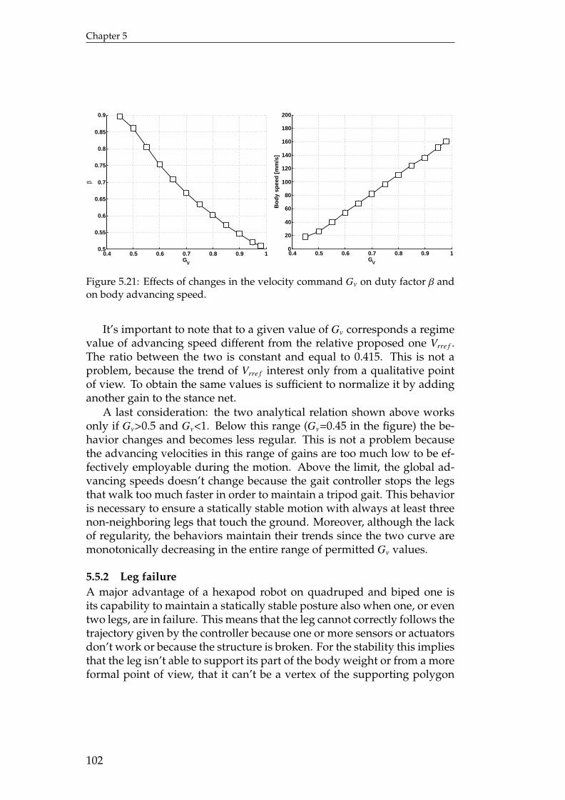
Chapter 5

0.4 0.5 0.6 0.7 0.8 0.9 10.5

0.55

0.6

0.65

0.7

0.75

0.8

0.85

0.9

GV

β

0.4 0.5 0.6 0.7 0.8 0.9 10

20

40

60

80

100

120

140

160

180

200

GV

Bo

dy

spee

d [

mm

/s]

Figure 5.21: Effects of changes in the velocity command Gv on duty factor β andon body advancing speed.

It’s important to note that to a given value of Gv corresponds a regimevalue of advancing speed different from the relative proposed one Vrre f .The ratio between the two is constant and equal to 0.415. This is not aproblem, because the trend of Vrre f interest only from a qualitative pointof view. To obtain the same values is sufficient to normalize it by addinganother gain to the stance net.

A last consideration: the two analytical relation shown above worksonly if Gv>0.5 and Gv<1. Below this range (Gv=0.45 in the figure) the be-havior changes and becomes less regular. This is not a problem becausethe advancing velocities in this range of gains are too much low to be ef-fectively employable during the motion. Above the limit, the global ad-vancing speeds doesn’t change because the gait controller stops the legsthat walk too much faster in order to maintain a tripod gait. This behavioris necessary to ensure a statically stable motion with always at least threenon-neighboring legs that touch the ground. Moreover, although the lackof regularity, the behaviors maintain their trends since the two curve aremonotonically decreasing in the entire range of permitted Gv values.

5.5.2 Leg failureA major advantage of a hexapod robot on quadruped and biped one isits capability to maintain a statically stable posture also when one, or eventwo legs, are in failure. This means that the leg cannot correctly follows thetrajectory given by the controller because one or more sensors or actuatorsdon’t work or because the structure is broken. For the stability this impliesthat the leg isn’t able to support its part of the body weight or from a moreformal point of view, that it can’t be a vertex of the supporting polygon

102

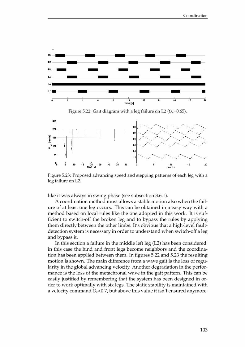
Coordination

Figure 5.22: Gait diagram with a leg failure on L2 (Gv=0.65).

Figure 5.23: Proposed advancing speed and stepping patterns of each leg with aleg failure on L2.

like it was always in swing phase (see subsection 3.6.1).A coordination method must allows a stable motion also when the fail-

ure of at least one leg occurs. This can be obtained in a easy way with amethod based on local rules like the one adopted in this work. It is suf-ficient to switch-off the broken leg and to bypass the rules by applyingthem directly between the other limbs. It’s obvious that a high-level fault-detection system is necessary in order to understand when switch-off a legand bypass it.

In this section a failure in the middle left leg (L2) has been considered:in this case the hind and front legs become neighbors and the coordina-tion has been applied between them. In figures 5.22 and 5.23 the resultingmotion is shown. The main difference from a wave gait is the loss of regu-larity in the global advancing velocity. Another degradation in the perfor-mance is the loss of the metachronal wave in the gait pattern. This can beeasily justified by remembering that the system has been designed in or-der to work optimally with six legs. The static stability is maintained witha velocity command Gv<0.7, but above this value it isn’t ensured anymore.

103

Chapter 6

Numerical resultsThis chapter describes the derivation of a dynamic model of NEMeSys.The complete model is too complex for formal derivation, so a numeri-cal approach based on a multibody software was used. The first sectiondiscusses aspects of modeling walking robots, gives general and specificassumptions to NEMeSys. Then section 6.2 describes the results obtainedby an application of the controller developed in the previous chapters.

6.1 Model

In order to simulate the robot’s behavior, some kind of model of a leggedsystem is necessary, as underlined by Riddenström [49]. This virtual en-vironment is also very useful for analysis and control design. A relativelycomplete simulation of a walking robot requires several kinds of models:

- kinematic differential equations and dynamic differential equationsof the robot’s rigid body model;

- actuator and sensor models;

- models of the environment, such as a model of the ground and theinteraction between foot and ground, including ground geometryand characteristics or a model of external and internal disturbances;

- model of control implementation and communication system.

To test the controller it is important the introduction of a dynamicmodel of the robot and of dynamics effects in the components and in theinteraction with the environment. Without this complexity it would beimpossible to understand how the system effectively reacts to the gravityor if it’s really able to walk upon the terrain. For the design phase, on theother hand, it might be enough just a partial kinematic description of therobot as shown in the previous chapters.

The usage of an analytical description of the dynamics and the kine-matics could be interesting with a traditional control system design thatrequires a complete knowledge of the equations that control the motion.In this case a partial definition of the kinematic equation that describesthe robot has been sufficient to design the controller completely, so, to

105

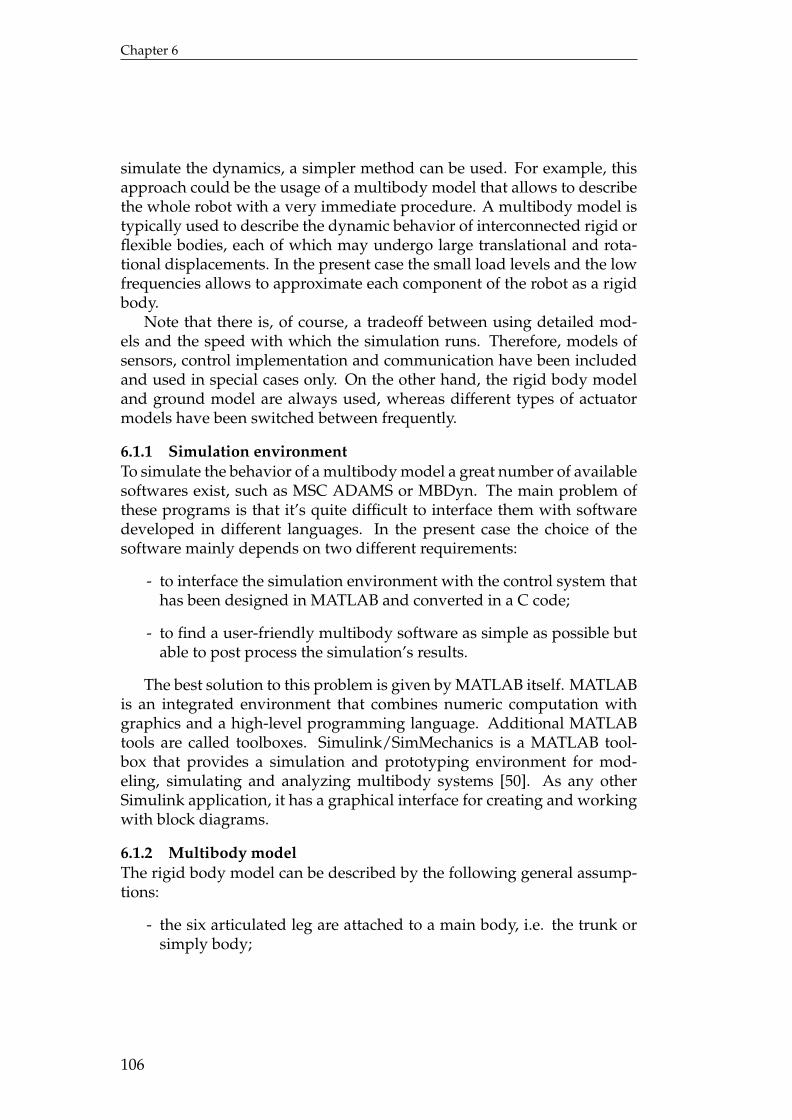
Chapter 6

simulate the dynamics, a simpler method can be used. For example, thisapproach could be the usage of a multibody model that allows to describethe whole robot with a very immediate procedure. A multibody model istypically used to describe the dynamic behavior of interconnected rigid orflexible bodies, each of which may undergo large translational and rota-tional displacements. In the present case the small load levels and the lowfrequencies allows to approximate each component of the robot as a rigidbody.

Note that there is, of course, a tradeoff between using detailed mod-els and the speed with which the simulation runs. Therefore, models ofsensors, control implementation and communication have been includedand used in special cases only. On the other hand, the rigid body modeland ground model are always used, whereas different types of actuatormodels have been switched between frequently.

6.1.1 Simulation environmentTo simulate the behavior of a multibody model a great number of availablesoftwares exist, such as MSC ADAMS or MBDyn. The main problem ofthese programs is that it’s quite difficult to interface them with softwaredeveloped in different languages. In the present case the choice of thesoftware mainly depends on two different requirements:

- to interface the simulation environment with the control system thathas been designed in MATLAB and converted in a C code;

- to find a user-friendly multibody software as simple as possible butable to post process the simulation’s results.

The best solution to this problem is given by MATLAB itself. MATLABis an integrated environment that combines numeric computation withgraphics and a high-level programming language. Additional MATLABtools are called toolboxes. Simulink/SimMechanics is a MATLAB tool-box that provides a simulation and prototyping environment for mod-eling, simulating and analyzing multibody systems [50]. As any otherSimulink application, it has a graphical interface for creating and workingwith block diagrams.

6.1.2 Multibody modelThe rigid body model can be described by the following general assump-tions:

- the six articulated leg are attached to a main body, i.e. the trunk orsimply body;

106

Numerical results

BC CT FT

Coxa Femur TibiaTrunk

BC

CoxaFemur

CTFT

Ground GroundTibia

Figure 6.1: Conceptual scheme of the complete multibody model.

- the force or torque applied at each joint is the output of an actuatormodel, or zero for an non actuated joint. Friction, backlash and elas-ticity in the power transmission are modeled in the actuator model.Similarly, the actuator model also includes models of the physicaljoint limits;

- the interaction with the environment is completely described by ex-ternal forces, i.e. outputs of a ground model or baricentric gravita-tional effects.

The last assumption implies that the rigid body model is modeled as anopen mechanical loop regardless of the number of feet in contact with theground. A different approach could have been to assume that a foot incontact with the ground creates a closed mechanical loop, with a differentset of differential equations since the number of degrees of freedom haschanged. However, the open loop alternative was chosen since it makesit easier to model slipping and a wide variety of ground characteristics bysimply changing a little set of parameters.

Each leg is structurally identical and consists of three rigid bodies thatcorrespond to the three sections of the leg, as described in section 3.2, withrotational joints between each couple of bodies. This assumption impliesthat some mechanical details of NEMeSys have been ignored:

- the mechanisms that physically composed each joint such as bevelgears and shafts aren’t modeled as separate bodies, but lumped withthe section on which are connected;

- the foot is not modeled as a separate rigid body. Instead, the foot’smass and inertia is lumped with the tibia ones. Moreover, one mayneglect, in a complete measure, the motion of the additional DoFs

107

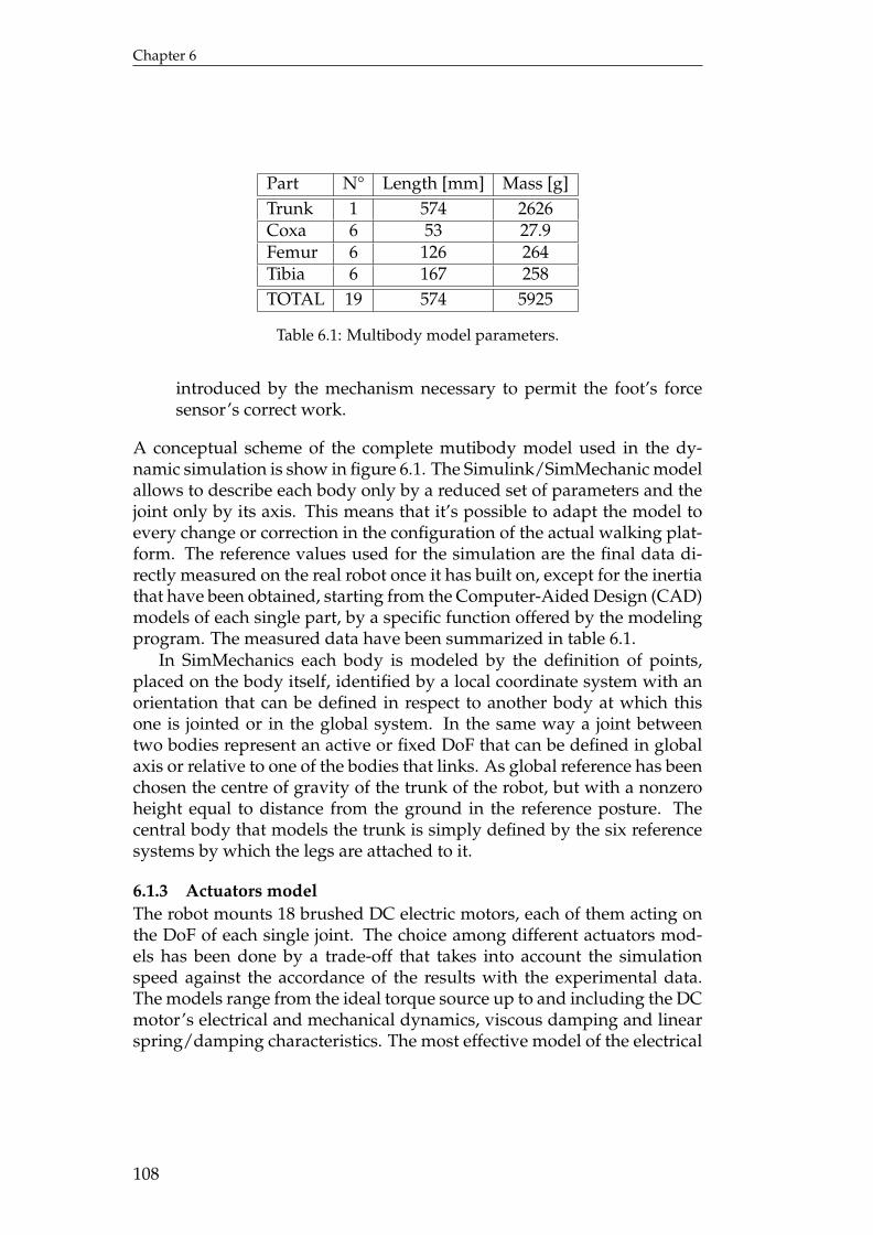
Chapter 6

Part N° Length [mm] Mass [g]Trunk 1 574 2626Coxa 6 53 27.9Femur 6 126 264Tibia 6 167 258TOTAL 19 574 5925

Table 6.1: Multibody model parameters.

introduced by the mechanism necessary to permit the foot’s forcesensor’s correct work.

A conceptual scheme of the complete mutibody model used in the dy-namic simulation is show in figure 6.1. The Simulink/SimMechanic modelallows to describe each body only by a reduced set of parameters and thejoint only by its axis. This means that it’s possible to adapt the model toevery change or correction in the configuration of the actual walking plat-form. The reference values used for the simulation are the final data di-rectly measured on the real robot once it has built on, except for the inertiathat have been obtained, starting from the Computer-Aided Design (CAD)models of each single part, by a specific function offered by the modelingprogram. The measured data have been summarized in table 6.1.

In SimMechanics each body is modeled by the definition of points,placed on the body itself, identified by a local coordinate system with anorientation that can be defined in respect to another body at which thisone is jointed or in the global system. In the same way a joint betweentwo bodies represent an active or fixed DoF that can be defined in globalaxis or relative to one of the bodies that links. As global reference has beenchosen the centre of gravity of the trunk of the robot, but with a nonzeroheight equal to distance from the ground in the reference posture. Thecentral body that models the trunk is simply defined by the six referencesystems by which the legs are attached to it.

6.1.3 Actuators modelThe robot mounts 18 brushed DC electric motors, each of them acting onthe DoF of each single joint. The choice among different actuators mod-els has been done by a trade-off that takes into account the simulationspeed against the accordance of the results with the experimental data.The models range from the ideal torque source up to and including the DCmotor’s electrical and mechanical dynamics, viscous damping and linearspring/damping characteristics. The most effective model of the electrical

108

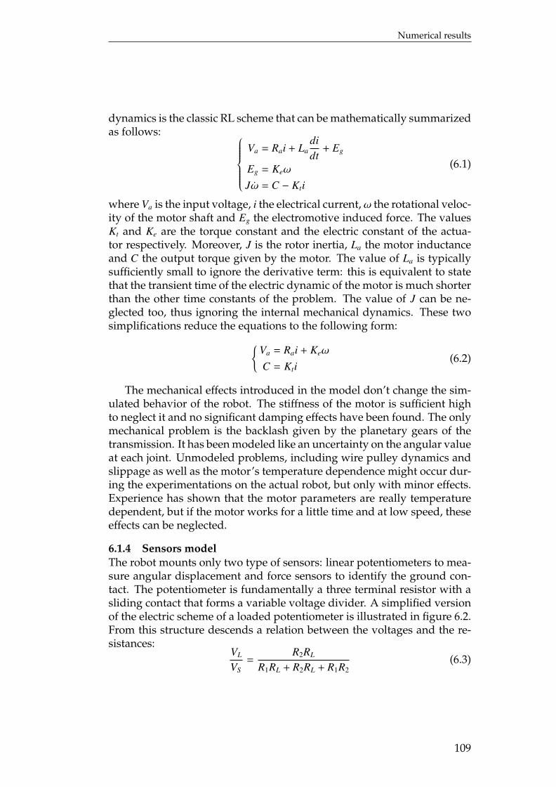
Numerical results

dynamics is the classic RL scheme that can be mathematically summarizedas follows:

Va = Rai + Ladidt

+ Eg

Eg = Keω

Jω = C − Kti

(6.1)

where Va is the input voltage, i the electrical current, ω the rotational veloc-ity of the motor shaft and Eg the electromotive induced force. The valuesKt and Ke are the torque constant and the electric constant of the actua-tor respectively. Moreover, J is the rotor inertia, La the motor inductanceand C the output torque given by the motor. The value of La is typicallysufficiently small to ignore the derivative term: this is equivalent to statethat the transient time of the electric dynamic of the motor is much shorterthan the other time constants of the problem. The value of J can be ne-glected too, thus ignoring the internal mechanical dynamics. These twosimplifications reduce the equations to the following form:

Va = Rai + Keω

C = Kti(6.2)

The mechanical effects introduced in the model don’t change the sim-ulated behavior of the robot. The stiffness of the motor is sufficient highto neglect it and no significant damping effects have been found. The onlymechanical problem is the backlash given by the planetary gears of thetransmission. It has been modeled like an uncertainty on the angular valueat each joint. Unmodeled problems, including wire pulley dynamics andslippage as well as the motor’s temperature dependence might occur dur-ing the experimentations on the actual robot, but only with minor effects.Experience has shown that the motor parameters are really temperaturedependent, but if the motor works for a little time and at low speed, theseeffects can be neglected.

6.1.4 Sensors modelThe robot mounts only two type of sensors: linear potentiometers to mea-sure angular displacement and force sensors to identify the ground con-tact. The potentiometer is fundamentally a three terminal resistor with asliding contact that forms a variable voltage divider. A simplified versionof the electric scheme of a loaded potentiometer is illustrated in figure 6.2.From this structure descends a relation between the voltages and the re-sistances:

VL

VS=

R2RL

R1RL + R2RL + R1R2(6.3)

109

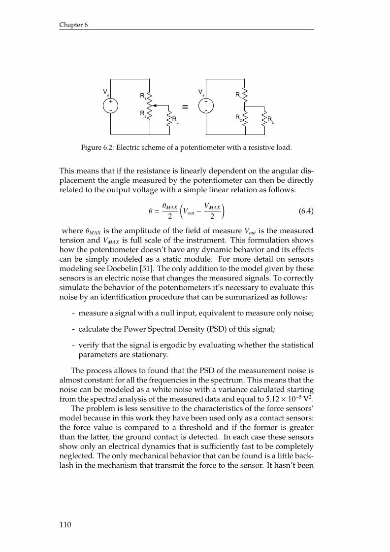
Chapter 6

+-

Vs R

1

R2 R

L

+-

R1

R2 R

L

Vs

=

Figure 6.2: Electric scheme of a potentiometer with a resistive load.

This means that if the resistance is linearly dependent on the angular dis-placement the angle measured by the potentiometer can then be directlyrelated to the output voltage with a simple linear relation as follows:

θ =θMAX

2

(Vout −

VMAX

2

)(6.4)

where θMAX is the amplitude of the field of measure Vout is the measuredtension and VMAX is full scale of the instrument. This formulation showshow the potentiometer doesn’t have any dynamic behavior and its effectscan be simply modeled as a static module. For more detail on sensorsmodeling see Doebelin [51]. The only addition to the model given by thesesensors is an electric noise that changes the measured signals. To correctlysimulate the behavior of the potentiometers it’s necessary to evaluate thisnoise by an identification procedure that can be summarized as follows:

- measure a signal with a null input, equivalent to measure only noise;

- calculate the Power Spectral Density (PSD) of this signal;

- verify that the signal is ergodic by evaluating whether the statisticalparameters are stationary.

The process allows to found that the PSD of the measurement noise isalmost constant for all the frequencies in the spectrum. This means that thenoise can be modeled as a white noise with a variance calculated startingfrom the spectral analysis of the measured data and equal to 5.12 × 10−5 V2.

The problem is less sensitive to the characteristics of the force sensors’model because in this work they have been used only as a contact sensors:the force value is compared to a threshold and if the former is greaterthan the latter, the ground contact is detected. In each case these sensorsshow only an electrical dynamics that is sufficiently fast to be completelyneglected. The only mechanical behavior that can be found is a little back-lash in the mechanism that transmit the force to the sensor. It hasn’t been

110

Numerical results

considered for two reasons: it is sufficiently little to become negligiblecompared to the other effects and its introduction complicates too muchthe whole model, by introducing an additional DoF in each leg. In thesame way as for the potentiometers, also for the force sensors, the onlybehavior that must be model is an electrical noise that could be evaluatedwith the same method. In the actual model this contribution hasn’t beeninserted because a sufficiently high value of threshold for the ground con-tact level makes it useless.

All the sensors give an analog information, so the errors dependingon discretization and quantization had to be taken into account. In thepresent simulation this hasn’t been done because no sampling has beenmodeled, considering the sampling and the quantization processes suffi-ciently accurate to avoid any significant degradation phenomena.

6.1.5 Ground contact modelTerrain geometry is described using plane surfaces. In this work it hasbeen assumed that the ground applies forces only and no torques, andthat this action is limited to the foot contact point. This simplification canbe justified by the small footpad radius (about 25 mm).

The ground force is calculated as a function of the penetration depthand the velocity with some typical parameters illustrated in table 6.2. Alinear spring/damper model is easy to use, but can result in discontinuousimpact forces, due to damping and nonzero impact velocities. For theforce perpendicular to the surface, a nonlinear spring-damper model toavoid these effects is typically used. In the present work the formulationproposed by Lankarani and Nikravesh [52] has been used, that can besummarized as follows:

Fz = −kzδnz − dzδzδz (6.5)

where kz and dz are the stiffness and damping coefficients, and δz is thepenetration depth. For the x and y-components, a smoothed viscous fric-tion with a maximum saturation based on the vertical force is used as by .They can be summarized as follows:

Fx = −γFz2π

arctan(dh

xFz

π

2

)(6.6a)

Fy = −γFz2π

arctan(dh

yFz

π

2

)(6.6b)

where γ is the friction coefficient and x and y are the velocities in the x andy direction respectively.

111

Chapter 6

Type of terrain kz [ Nm ] dz [ Ns

m2 ] γ dh [ Nsm ] n

Weakly damped 70’000 2’000 0.7 2’000 1Heavily damped 50’000 100’000 0.7 2’000 1

Table 6.2: Ground contact parameters for two different terrains.

6.1.6 Control model implementationIn order to simulate a limited control frequency, instead of using differentsimulation times for the dynamic model of the robot and the controller,a filtering of the sensory inputs and actuator commands have been per-formed. Similarly, signals are delayed to reflect the fact that the control isdone over a bus, but the corresponding effects, e.g. irregularity in the mo-tion, haven’t been modeled. However, the simulation runs substantiallyslower when including this model, but the results don’t change in a signif-icant way, so usually it’s not used. Moreover a single step delay has beenintroduced on some signals to avoid algebraic loops in the model.

Another problem that can be found during the implementation of thecontroller, is the definition of geometric conditions that control the someparts of motion, e.g. the transition from stance to swing. The introductionof dynamical effects produce the risk of oscillating behavior close to thecross of the condition because the solver identifies a sudden change inthe parameter of the problem and tries to reduce the time step. Furtherproblems occur when a time delay has been introduced. To avoid thiskind of problems it is sufficient to introduce a threshold suitably low tonot change the structure of the controller.

6.1.7 Simulation parametersThe last important consideration that should be done involves the param-eters of the dynamic simulation. At first it’s necessary to identify an inte-gration method. In this case a variable step solver has been used to avoidthe troubles depending on the variability of the problem due to the groundcontact. Each time a leg lifts off or touches the ground, the geometry ofthe kinematics chains that composed the model changes and this requiresa different level of accuracy. On the other hand a fixed step method hadto use a time step with the same order of magnitude of the minimum timeconstant of the problem that in this case can be estimated as the one ofthe spring-damper that models the foot-ground interaction. With such anonlinear behavior, the time step should become too much small to allowthe simulation to be completed in a reasonable time.

The other main problem is the identification of which method effec-

112

Numerical results

tively use. The present model shows a quite stiff behavior, because it in-corporates very fast dynamics such as the foot-ground interaction and theelectric model of the DC-motor. For this reason a multistep solver for stiffproblem has been used: it is a variable order integration method basedon the numerical differentiation formulas (NDFs). Optionally, it uses thebackward differentiation formulas (BDFs, also known as Gear’s method)that are usually less efficient.

It is also requires the choice of suitable initial values and/or a methodto start the simulation. In the present work all the simulations start withthe six legs placed at a little distance (about 2 mm) above the ground:this method allows to avoid the generation of unreasonably high forces oroscillating effects due to an incorrect interaction with the ground.

6.2 Dynamic model results

In this section the results given by the complete simulation will be dis-cussed. The most important difference between the kinematic evaluationused during the design process and the analysis of a model that takes intoaccount dynamic effects is the possibility to estimate the torque level re-quired by the actuators to produce the trajectories defined by the gait con-troller.

To better understand the behavior of the system the simulation hasbeen performed in three different conditions: a slow forward walking (seesubsection 6.2.1), a fast forward walking (see subsection 6.2.2) and a curvewalking (see subsection 6.2.3). For each condition all the joint parame-ters (angles, angular velocities and torques) of the most loaded leg will beshown. For a regular wave gait, this one is a middle leg, alternatively theleft one and the right one, depending on the time slice. In this case themiddle left leg has been chosen (L2 in figure 5.2 or 2 in figure 5.3). Otherglobal data such as the gait diagram and the body parameters (coordinatesand velocities) will be illustrated.

6.2.1 Slow wave gaitTo obtain a slow wave gait a velocity command Gv equal to 0.5 has beenassigned. According to the gait analysis performed in chapter 5, equation5.7 gives a correspondent value of duty factor β=0.859. The mean dutyfactor obtained by the simulation is β=0.843 with an error on the actualvalue that corresponds to the 1.9% of the ideal one. This is a demonstrationof the effectiveness of the control approach proposed in section 5.5.

The angles and the angular velocities for the left middle leg are shownin figure 6.3 and 6.4 respectively. The behavior is very regular with a per-

113

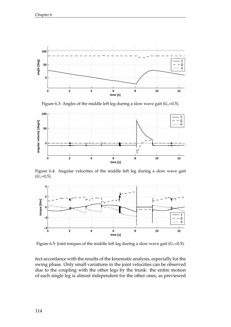
Chapter 6

0 2 4 6 8 10 12

0

50

100

ang

le [

deg

]

time [s]

γβα

Figure 6.3: Angles of the middle left leg during a slow wave gait (Gv=0.5).

0 2 4 6 8 10 12

0

50

100

ang

ula

r ve

loci

ty [

deg

/s]

time [s]

γβα

Figure 6.4: Angular velocities of the middle left leg during a slow wave gait(Gv=0.5).

0 2 4 6 8 10 12−4

−2

0

2

4

torq

ue [N

m]

time [s]

γβα

Figure 6.5: Joint torques of the middle left leg during a slow wave gait (Gv=0.5).

fect accordance with the results of the kinematic analysis, especially for theswing phase. Only small variations in the joint velocities can be observeddue to the coupling with the other legs by the trunk: the entire motionof each single leg is almost independent for the other ones, as previewed

114

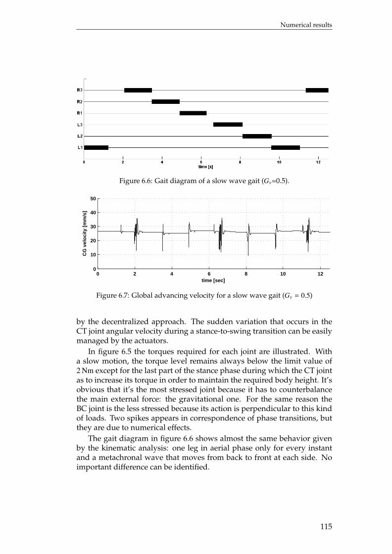
Numerical results

Figure 6.6: Gait diagram of a slow wave gait (Gv=0.5).

0 2 4 6 8 10 120

10

20

30

40

50

CG

vel

oci

ty [

mm

/s]

time [sec]

Figure 6.7: Global advancing velocity for a slow wave gait (Gv = 0.5)

by the decentralized approach. The sudden variation that occurs in theCT joint angular velocity during a stance-to-swing transition can be easilymanaged by the actuators.

In figure 6.5 the torques required for each joint are illustrated. Witha slow motion, the torque level remains always below the limit value of2 Nm except for the last part of the stance phase during which the CT jointas to increase its torque in order to maintain the required body height. It’sobvious that it’s the most stressed joint because it has to counterbalancethe main external force: the gravitational one. For the same reason theBC joint is the less stressed because its action is perpendicular to this kindof loads. Two spikes appears in correspondence of phase transitions, butthey are due to numerical effects.

The gait diagram in figure 6.6 shows almost the same behavior givenby the kinematic analysis: one leg in aerial phase only for every instantand a metachronal wave that moves from back to front at each side. Noimportant difference can be identified.

115

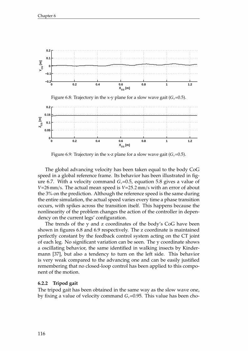
Chapter 6

0 0.2 0.4 0.6 0.8 1 1.2−0.2

−0.1

0

0.1

0.2

YC

G [m

]

XCG

[m]

Figure 6.8: Trajectory in the x-y plane for a slow wave gait (Gv=0.5).

0 0.2 0.4 0.6 0.8 1 1.20

0.05

0.1

0.15

0.2

Z CG

[m

]

XCG

[m]

Figure 6.9: Trajectory in the x-z plane for a slow wave gait (Gv=0.5).

The global advancing velocity has been taken equal to the body CoGspeed in a global reference frame. Its behavior has been illustrated in fig-ure 6.7. With a velocity command Gv=0.5, equation 5.8 gives a value ofV=26 mm/s. The actual mean speed is V=25.2 mm/s with an error of aboutthe 3% on the prediction. Although the reference speed is the same duringthe entire simulation, the actual speed varies every time a phase transitionoccurs, with spikes across the transition itself. This happens because thenonlinearity of the problem changes the action of the controller in depen-dency on the current legs’ configuration.

The trends of the y and z coordinates of the body’s CoG have beenshown in figures 6.8 and 6.9 respectively. The z coordinate is maintainedperfectly constant by the feedback control system acting on the CT jointof each leg. No significant variation can be seen. The y coordinate showsa oscillating behavior, the same identified in walking insects by Kinder-mann [37], but also a tendency to turn on the left side. This behavioris very weak compared to the advancing one and can be easily justifiedremembering that no closed-loop control has been applied to this compo-nent of the motion.

6.2.2 Tripod gaitThe tripod gait has been obtained in the same way as the slow wave one,by fixing a value of velocity command Gv=0.95. This value has been cho-

116

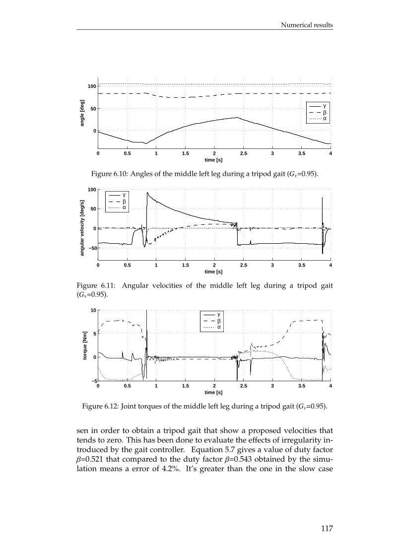
Numerical results

0 0.5 1 1.5 2 2.5 3 3.5 4

0

50

100an

gle

[d

eg]

time [s]

γβα

Figure 6.10: Angles of the middle left leg during a tripod gait (Gv=0.95).

0 0.5 1 1.5 2 2.5 3 3.5 4

−50

0

50

100

angu

lar

velo

city

[deg

/s]

time [s]

γβα

Figure 6.11: Angular velocities of the middle left leg during a tripod gait(Gv=0.95).

0 0.5 1 1.5 2 2.5 3 3.5 4−5

0

5

10

torq

ue [N

m]

time [s]

γβα

Figure 6.12: Joint torques of the middle left leg during a tripod gait (Gv=0.95).

sen in order to obtain a tripod gait that show a proposed velocities thattends to zero. This has been done to evaluate the effects of irregularity in-troduced by the gait controller. Equation 5.7 gives a value of duty factorβ=0.521 that compared to the duty factor β=0.543 obtained by the simu-lation means a error of 4.2%. It’s greater than the one in the slow case

117

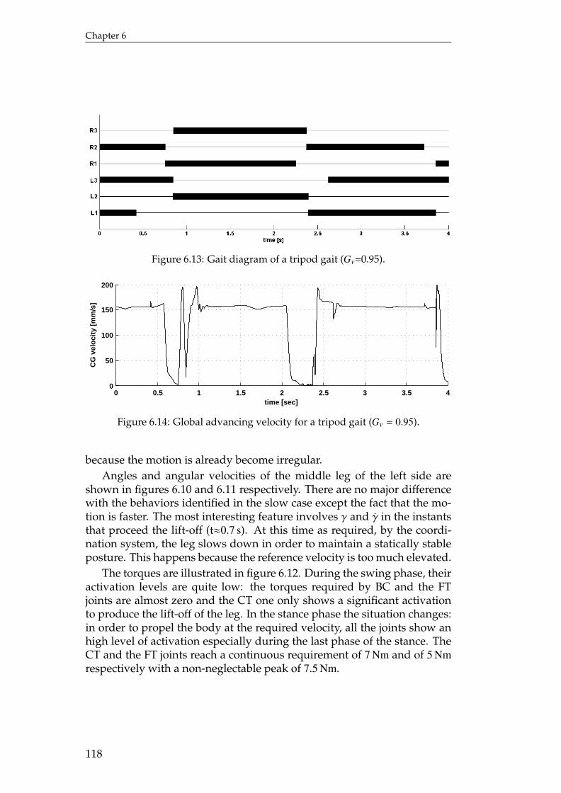
Chapter 6

Figure 6.13: Gait diagram of a tripod gait (Gv=0.95).

0 0.5 1 1.5 2 2.5 3 3.5 40

50

100

150

200

CG

vel

oci

ty [

mm

/s]

time [sec]

Figure 6.14: Global advancing velocity for a tripod gait (Gv = 0.95).

because the motion is already become irregular.Angles and angular velocities of the middle leg of the left side are

shown in figures 6.10 and 6.11 respectively. There are no major differencewith the behaviors identified in the slow case except the fact that the mo-tion is faster. The most interesting feature involves γ and γ in the instantsthat proceed the lift-off (t≈0.7 s). At this time as required, by the coordi-nation system, the leg slows down in order to maintain a statically stableposture. This happens because the reference velocity is too much elevated.

The torques are illustrated in figure 6.12. During the swing phase, theiractivation levels are quite low: the torques required by BC and the FTjoints are almost zero and the CT one only shows a significant activationto produce the lift-off of the leg. In the stance phase the situation changes:in order to propel the body at the required velocity, all the joints show anhigh level of activation especially during the last phase of the stance. TheCT and the FT joints reach a continuous requirement of 7 Nm and of 5 Nmrespectively with a non-neglectable peak of 7.5 Nm.

118

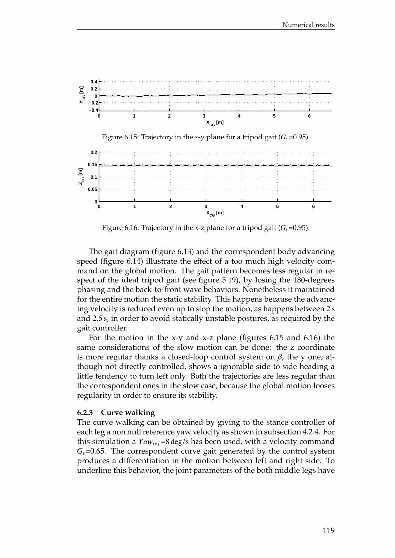
Numerical results

0 1 2 3 4 5 6−0.4

−0.20

0.2

0.4Y

CG

[m]

XCG

[m]

Figure 6.15: Trajectory in the x-y plane for a tripod gait (Gv=0.95).

0 1 2 3 4 5 60

0.05

0.1

0.15

0.2

Z CG

[m

]

XCG

[m]

Figure 6.16: Trajectory in the x-z plane for a tripod gait (Gv=0.95).

The gait diagram (figure 6.13) and the correspondent body advancingspeed (figure 6.14) illustrate the effect of a too much high velocity com-mand on the global motion. The gait pattern becomes less regular in re-spect of the ideal tripod gait (see figure 5.19), by losing the 180-degreesphasing and the back-to-front wave behaviors. Nonetheless it maintainedfor the entire motion the static stability. This happens because the advanc-ing velocity is reduced even up to stop the motion, as happens between 2 sand 2.5 s, in order to avoid statically unstable postures, as required by thegait controller.

For the motion in the x-y and x-z plane (figures 6.15 and 6.16) thesame considerations of the slow motion can be done: the z coordinateis more regular thanks a closed-loop control system on β, the y one, al-though not directly controlled, shows a ignorable side-to-side heading alittle tendency to turn left only. Both the trajectories are less regular thanthe correspondent ones in the slow case, because the global motion loosesregularity in order to ensure its stability.

6.2.3 Curve walkingThe curve walking can be obtained by giving to the stance controller ofeach leg a non null reference yaw velocity as shown in subsection 4.2.4. Forthis simulation a Yawre f =8 deg/s has been used, with a velocity commandGv=0.65. The correspondent curve gait generated by the control systemproduces a differentiation in the motion between left and right side. Tounderline this behavior, the joint parameters of the both middle legs have

119

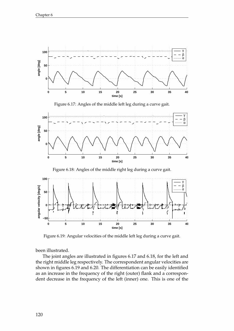
Chapter 6

0 5 10 15 20 25 30 35 40

0

50

100

ang

le [

deg

]

time [s]

γβα

Figure 6.17: Angles of the middle left leg during a curve gait.

0 5 10 15 20 25 30 35 40

0

50

100

ang

le [

deg

]

time [s]

γβα

Figure 6.18: Angles of the middle right leg during a curve gait.

0 5 10 15 20 25 30 35 40

−50

0

50

100

angu

lar

velo

city

[deg

/s]

time [s]

γβα

Figure 6.19: Angular velocities of the middle left leg during a curve gait.

been illustrated.The joint angles are illustrated in figures 6.17 and 6.18, for the left and

the right middle leg respectively. The correspondent angular velocities areshown in figures 6.19 and 6.20. The differentiation can be easily identifiedas an increase in the frequency of the right (outer) flank and a correspon-dent decrease in the frequency of the left (inner) one. This is one of the

120

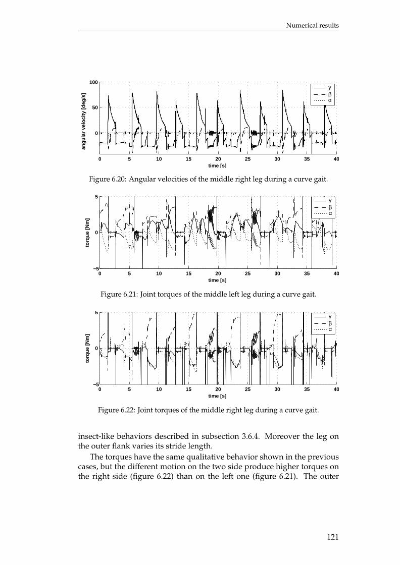
Numerical results

0 5 10 15 20 25 30 35 40

0

50

100an

gu

lar

velo

city

[d

eg/s

]

time [s]

γβα

Figure 6.20: Angular velocities of the middle right leg during a curve gait.

0 5 10 15 20 25 30 35 40−5

0

5

torq

ue [N

m]

time [s]

γβα

Figure 6.21: Joint torques of the middle left leg during a curve gait.

0 5 10 15 20 25 30 35 40−5

0

5

torq

ue [N

m]

time [s]

γβα

Figure 6.22: Joint torques of the middle right leg during a curve gait.

insect-like behaviors described in subsection 3.6.4. Moreover the leg onthe outer flank varies its stride length.

The torques have the same qualitative behavior shown in the previouscases, but the different motion on the two side produce higher torques onthe right side (figure 6.22) than on the left one (figure 6.21). The outer

121

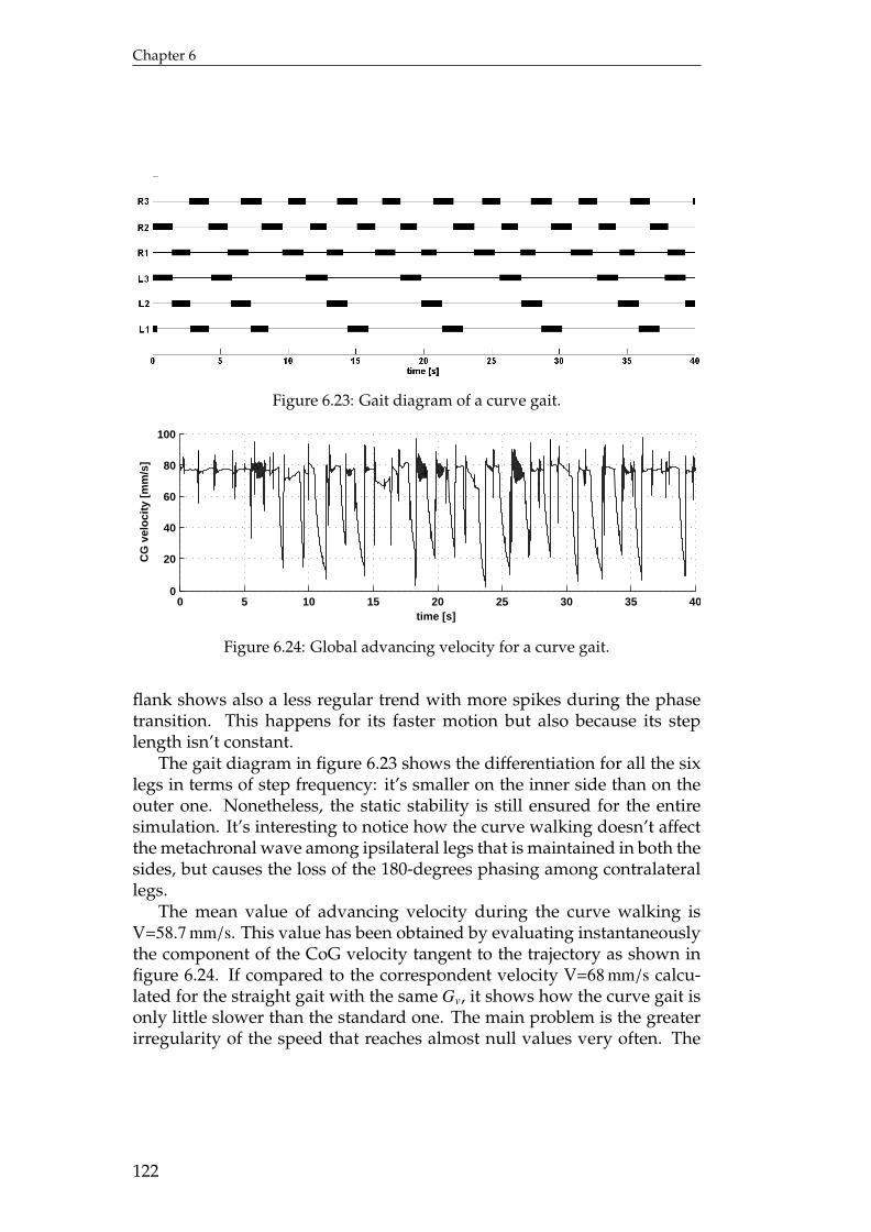
Chapter 6

Figure 6.23: Gait diagram of a curve gait.

0 5 10 15 20 25 30 35 400

20

40

60

80

100

CG

vel

oci

ty [

mm

/s]

time [s]

Figure 6.24: Global advancing velocity for a curve gait.

flank shows also a less regular trend with more spikes during the phasetransition. This happens for its faster motion but also because its steplength isn’t constant.

The gait diagram in figure 6.23 shows the differentiation for all the sixlegs in terms of step frequency: it’s smaller on the inner side than on theouter one. Nonetheless, the static stability is still ensured for the entiresimulation. It’s interesting to notice how the curve walking doesn’t affectthe metachronal wave among ipsilateral legs that is maintained in both thesides, but causes the loss of the 180-degrees phasing among contralaterallegs.

The mean value of advancing velocity during the curve walking isV=58.7 mm/s. This value has been obtained by evaluating instantaneouslythe component of the CoG velocity tangent to the trajectory as shown infigure 6.24. If compared to the correspondent velocity V=68 mm/s calcu-lated for the straight gait with the same Gv, it shows how the curve gait isonly little slower than the standard one. The main problem is the greaterirregularity of the speed that reaches almost null values very often. The

122

Numerical results

−0.5 0 0.5 1 1.5 2 2.50

0.2

0.4

0.6

0.8

1

1.2

1.4

1.6

1.8Y

CG

[m]

XCG

[m]

Figure 6.25: Trajectory in the x-y plane for a curve gait.

0 0.2 0.4 0.6 0.8 1 1.2 1.4 1.6 1.8 20

0.1

0.2

Z CG

[m

]

XCG

[m]

Figure 6.26: Trajectory in the x-z plane for a curve gait.

incapability to ensure a regular motion during a regular curve walking isthe main problem of this kind of gait control.

The trajectories in the x-y plane (figure 6.25) illustrates in the best waythe turning of the body. Asterisks indicated the start and the stop of thenon null yaw reference. The robot react to this command without anyremarkable delays. The z coordinates (figure 6.26) is maintained constantfor all the simulation, independently from the value of the yaw command,thanks to the feedback controller.

Finally a sensitivity analysis on the turning behavior has been per-formed, by changing two global parameter: the yaw reference velocityYawre f and the velocity command Gv. In figures 6.27 and 6.28 are illus-trated the changes in the x-y trajectories and in the mean turning radiusR respectively. The mean turning radius is the radius of the osculatingcircle (figure 6.29) obtained as solution of a least mean square problem.The trends show by the diagrams indicated that R doesn’t vary signifi-

123

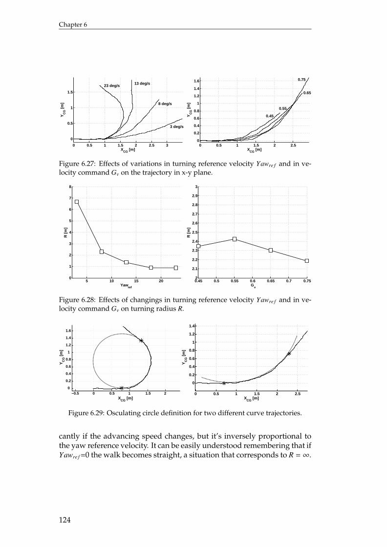
Chapter 6

0 0.5 1 1.5 2 2.5 3

0

0.5

1

1.5

YC

G [

m]

XCG

[m]0 0.5 1 1.5 2 2.5

0

0.2

0.4

0.6

0.8

1

1.2

1.4

1.6

YC

G [

m]

XCG

[m]

3 deg/s

8 deg/s

13 deg/s23 deg/s

0.75

0.45

0.55

0.65

Figure 6.27: Effects of variations in turning reference velocity Yawre f and in ve-locity command Gv on the trajectory in x-y plane.

5 10 15 200

1

2

3

4

5

6

7

8

Yawref

R [

m]

0.45 0.5 0.55 0.6 0.65 0.7 0.752

2.1

2.2

2.3

2.4

2.5

2.6

2.7

2.8

2.9

3

Gv

R [

m]

Figure 6.28: Effects of changings in turning reference velocity Yawre f and in ve-locity command Gv on turning radius R.

−0.5 0 0.5 1 1.5 20

0.2

0.4

0.6

0.8

1

1.2

1.4

1.6

0 0.5 1 1.5 2 2.5

0

0.2

0.4

0.6

0.8

1

1.2

1.4

YC

G [

m]

XCG

[m]XCG

[m]

YC

G [

m]

Figure 6.29: Osculating circle definition for two different curve trajectories.

cantly if the advancing speed changes, but it’s inversely proportional tothe yaw reference velocity. It can be easily understood remembering that ifYawre f =0 the walk becomes straight, a situation that corresponds to R = ∞.

124

Chapter 7

Walking platformThe purpose of this section is giving an overview of the robot on whichthe control system shown in previous chapters will be tested. First of allthe design of the new mechanical platform will be presented, than thediscussion will be on the changes of the electrical parts necessary to adaptthe old components to the new ones (especially the contact sensors).

7.1 Design requirements

NEMeSys was initially thought as a robot for space exploration, but, afterthe evaluation of what this means in term of construction techniques, thetarget was translated to a platform to test new control structures. Thischoice was made to match the fixed limits on the costs and the complexityof the robot.

In this project the same guideline is followed, and it tries to recover theinitial idea of space application whenever possible. Starting from theseconsiderations some important targets have been fixed:

- reduction of the weight. This is important both for a space explo-ration use of NEMeSys and for a correct motion of the robot. Thecost of the transfer to another planet is dependent on the weight ofthe payload heavily, so, the higher the weight is the higher will bethe cost of the launch. Furthermore the test on the old version ofthe robot showed that the CP requested torque was higher than themaximum available from the propulsive system, so that a reductionof the weight is mandatory;

- reduction of the costs. To minimize the total cost is necessary to use,in the largest possible measure, components from the old robot. Par-ticularly the motors and the planetary gear adaptors must be the oldones, so that some parameters, e.g. the dimensions of propulsive sys-tem but also the maximum torque available, are fixed. For the samereason, where possible, the use of common materials and profiles forthe design of the structure is to prefer;

- reduction of the dimensions. The robot must be as small as possible,with respect of the size of the electronic boards and of the motors,taken from the old robot, but hasn’t to limit the movement of the

125

Chapter 7

legs, within the range set during the design of the controller (see ta-ble 4.7). Moreover, thinking about the stowage of the robot duringthe transfer to a planet, if possible it should be able to reach a config-uration that employs the least volume possible;

- some parts must be removed without difficulties to permit changesor reparations. This requirement is very important because this robotis going to be a platform for future tests also with controllers com-pletely different from the one presented in this work, so that changesin structure, or more probably in sensors and actuators must be pos-sible and quite easy. This necessity is very common in the sphere ofspace exploration because the number of production is very small,so that is usual to update a lot of time the same object rather thanbuilding a new one.

In order to comply with this requirement the choice made is to completelyrebuild the structure, to study a new way for the transmission of the torqueand to modify the electronic system of the old version of NEMeSys in theleast possible percentage.

7.2 Mechanical system

At first the new mechanical system has been designed beginning from thegeneral layout and than focusing on the most demanding parts, especiallythe construction of the joints. At least some structural analysis have beenmade in order to calculate the distribution of internal forces and to checkvalidate the design.

7.2.1 General layoutStarting from the considerations described in the previous section, a struc-ture based on a mix of standard profiles with a square section and milledfrom solid parts, both in aluminum, has been designed.

This solution permits a high level of modularity because the dimen-sions of the body and of the legs are dependent from the length of thestandard profile, so that the geometry can be easily and cheaply varied bychanging the profiles themselves. On the contrary the milled from solidparts form a rigid and robust box for the transmission of the torques and,if needed, can be re-used if the shape of the robot will be changed.

In order to ensure the possibility of disassembling the robot, most partsof the junctions between the pieces are made with screws and nuts. For theshaft that connect the parts in mutual motion, a shape-based connectionhas been used.

126

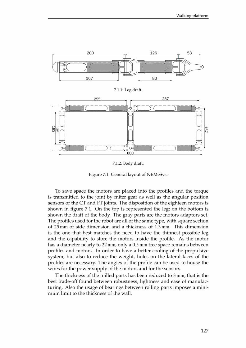
Walking platform

200

167 80

126 53

7.1.1: Leg draft.

255 287

600

167

193135

7.1.2: Body draft.

Figure 7.1: General layout of NEMeSys.

To save space the motors are placed into the profiles and the torqueis transmitted to the joint by miter gear as well as the angular positionsensors of the CT and FT joints. The disposition of the eighteen motors isshown in figure 7.1. On the top is represented the leg; on the bottom isshown the draft of the body. The gray parts are the motors-adaptors set.The profiles used for the robot are all of the same type, with square sectionof 25 mm of side dimension and a thickness of 1.3 mm. This dimensionis the one that best matches the need to have the thinnest possible legand the capability to store the motors inside the profile. As the motorhas a diameter nearly to 22 mm, only a 0.5 mm free space remains betweenprofiles and motors. In order to have a better cooling of the propulsivesystem, but also to reduce the weight, holes on the lateral faces of theprofiles are necessary. The angles of the profile can be used to house thewires for the power supply of the motors and for the sensors.

The thickness of the milled parts has been reduced to 3 mm, that is thebest trade-off found between robustness, lightness and ease of manufac-turing. Also the usage of bearings between rolling parts imposes a mini-mum limit to the thickness of the wall.

127

Chapter 7

The size of a walking robot and length/width or length/height ratiosare limited by different and sometimes conflicting considerations:

- ensure the correct motion. The joints must be able to reach adequateangles and two ipsilateral legs must not to collide when the posteriorone is at the AEP and the anterior one at the PEP. In this configura-tion a gap between the feet is desirable, so that a further motion e.g.a searching of the posterior one may be possible. This requirementfixes a lower limit to the longitudinal distance from two BC joints,and consequently to the body length;

- limit the joint torques. In section 7.3.1 the maximum torques avail-able from the motor-adaptor set are shown. An analysis of the typ-ical shape and posture of an hexapod robots (but also of insect likeCarausius Morosus) display that the most stressed joint is the CT one.The torque on this joint depends (once that the weight of the robotand the gait are fixed) on the horizontal distance between CT and FTjoint, function of CT-FT joints distance and of β angle. The lower isthe gap between the two joints, the lower the torque required willbe;

- size of the components and of the payload. In order to have compactrobot, the motors have been placed into the profiles that form thestructure. This poses a minimum limit to the length of the profiles.At the moment no payload is installed on the robot, but in the futurea set of optical or attitude sensors are expected;

- capability of overtake obstacles. This requirement affects the heightof the body from the ground. This parameter is a function of thelength of the femur and of the tibia and of the value of α and β an-gles. Ones that the standard (at rest) height is fixed, is usual in robottests to fix the highest obstacle that the robot has to overtake, as apercentage of the body height (usually 50-60%).

Taking the start from these consideration the best trade-off has been foundwith the configuration shown in figure 7.1.

At first the dimensions of the leg have been set. The femur has theminimum length necessary to carry the motor-adaptor group, so that theCT-FT joint distance is 126 mm. The reference for β has been set at 80°,giving the robot a little lateral stability. For the length of the tibia a valueof 167 mm has been chosen, so that, using a reference for α of 90° in restingposition, the robot should be able to overtake obstacles with a height of70 mm. The coxa is 52 mm long, to allow a correct range of γ.

128

Walking platform

Minimum γ [deg] Maximum γ [deg]Front legs –38 +128Middle legs –38 +38Posterior legs –128 +38

Table 7.1: Mechanical limits for angle γ.

The body has a length of 604 mm, a width of 194 mm and a thickness of32 mm. This size is the one that most matches the necessity of storing theelectronic boards and the correct distance between ipsilateral legs. Oncethat the boards dimensions will be reduced, the width of the body couldbe decreased until a minimum of approximately 100 mm only by changingthree profiles.

The choice of the body’s length of is also a result of the setting of theresting position of the legs. In order to use the same identical controllerfor all the legs, the resting configuration chosen is the same for all the legs,with γ=30°, β=80° and α=90°. The range of γ around the resting positionduring normal walking is set to a maximum of ±30°. Is mechanical limitsare the ones shown in table 7.1. Choosing the length of 600 mm for thebody a minimum longitudinal distance of about 60 mm between feet ofconsecutive legs is reached during normal walking.

7.2.2 Joint designIn order create the eighteen degrees of freedom (three for each leg) neces-sary for the motion of the robot, the same number of revolute joints mustbe created. The joints are composed by a shaft fixed to one of the two partin mutual motion and free to rotate with respect to the other one. A cou-ple of bearings are useful to avoid friction and early degradation of thealuminum parts.

After the creation of the joint, it is necessary to find a way to transmit

Producer MaedlerThansmission ratio 1:1No. of teeth 20B [mm] 4d [mm] 12ND [mm] 8Admissible MD [Ncm] 1.8

Table 7.2: Bevel gear specifications.

129

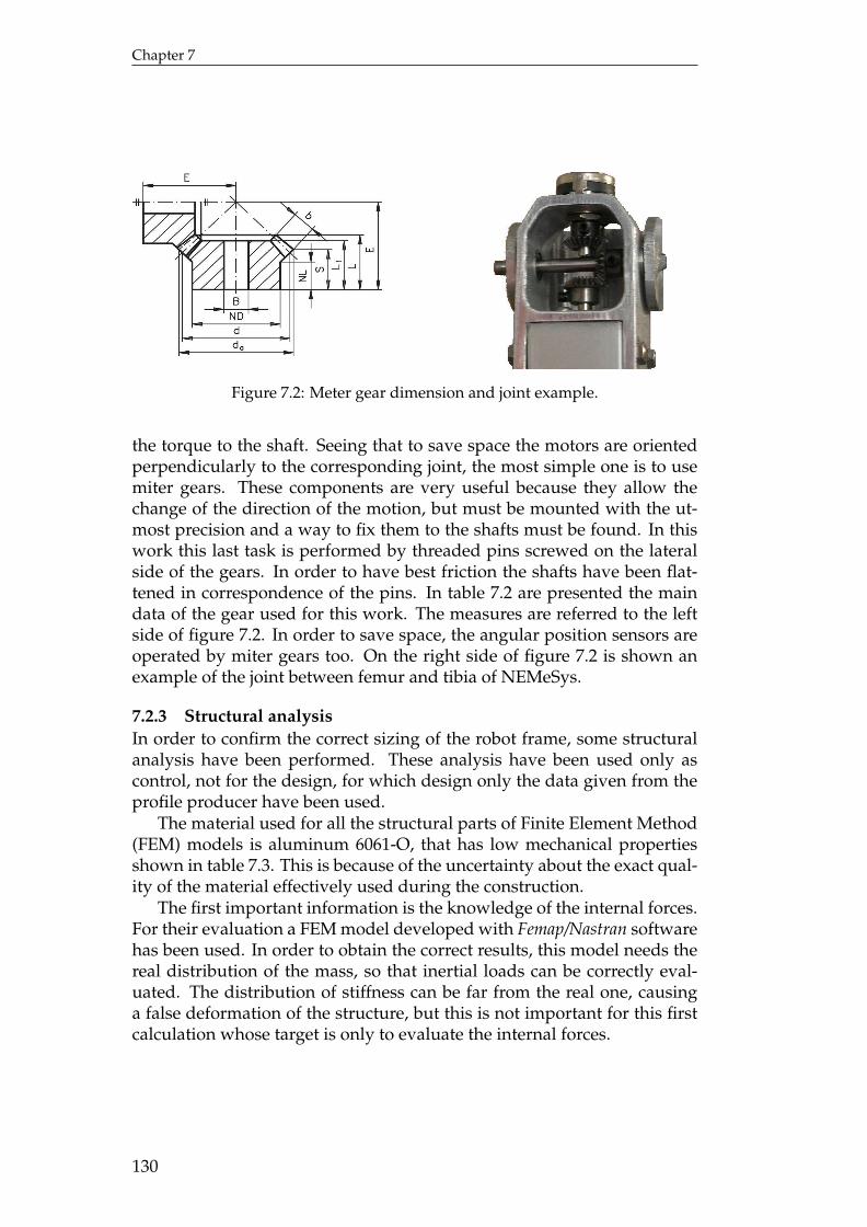
Chapter 7

Figure 7.2: Meter gear dimension and joint example.

the torque to the shaft. Seeing that to save space the motors are orientedperpendicularly to the corresponding joint, the most simple one is to usemiter gears. These components are very useful because they allow thechange of the direction of the motion, but must be mounted with the ut-most precision and a way to fix them to the shafts must be found. In thiswork this last task is performed by threaded pins screwed on the lateralside of the gears. In order to have best friction the shafts have been flat-tened in correspondence of the pins. In table 7.2 are presented the maindata of the gear used for this work. The measures are referred to the leftside of figure 7.2. In order to save space, the angular position sensors areoperated by miter gears too. On the right side of figure 7.2 is shown anexample of the joint between femur and tibia of NEMeSys.

7.2.3 Structural analysisIn order to confirm the correct sizing of the robot frame, some structuralanalysis have been performed. These analysis have been used only ascontrol, not for the design, for which design only the data given from theprofile producer have been used.

The material used for all the structural parts of Finite Element Method(FEM) models is aluminum 6061-O, that has low mechanical propertiesshown in table 7.3. This is because of the uncertainty about the exact qual-ity of the material effectively used during the construction.

The first important information is the knowledge of the internal forces.For their evaluation a FEM model developed with Femap/Nastran softwarehas been used. In order to obtain the correct results, this model needs thereal distribution of the mass, so that inertial loads can be correctly eval-uated. The distribution of stiffness can be far from the real one, causinga false deformation of the structure, but this is not important for this firstcalculation whose target is only to evaluate the internal forces.

130

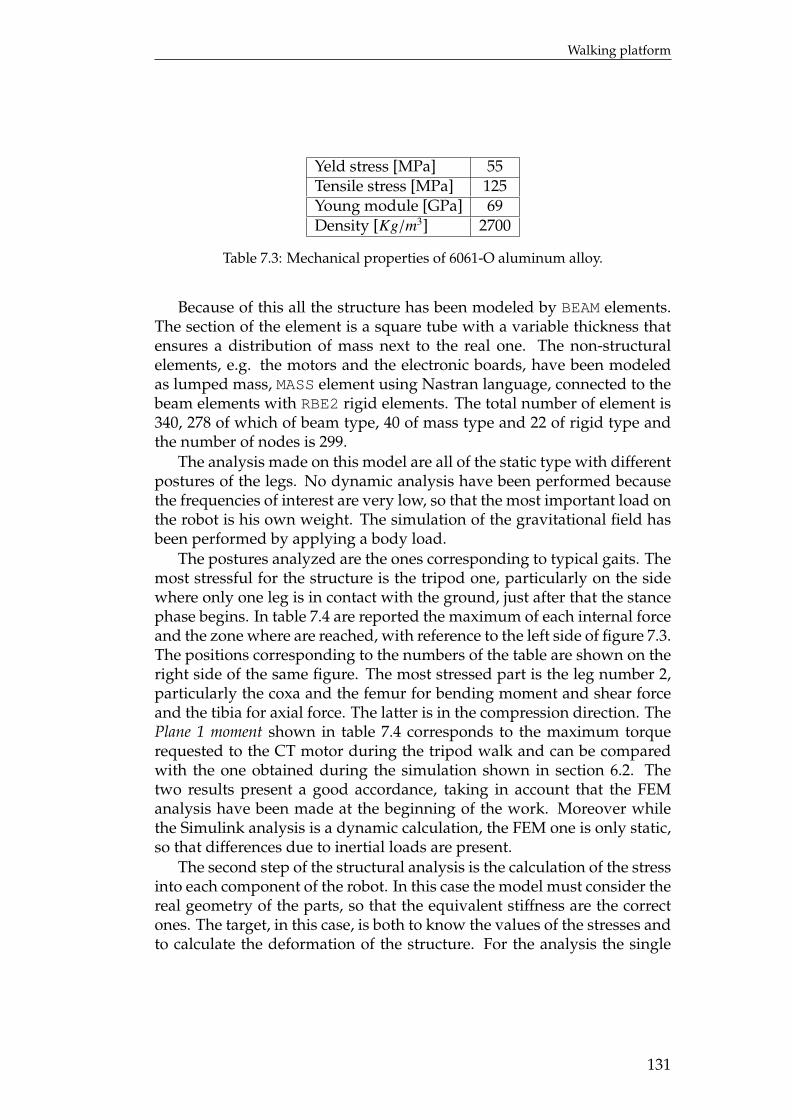
Walking platform

Yeld stress [MPa] 55Tensile stress [MPa] 125Young module [GPa] 69Density [Kg/m3] 2700

Table 7.3: Mechanical properties of 6061-O aluminum alloy.

Because of this all the structure has been modeled by BEAM elements.The section of the element is a square tube with a variable thickness thatensures a distribution of mass next to the real one. The non-structuralelements, e.g. the motors and the electronic boards, have been modeledas lumped mass, MASS element using Nastran language, connected to thebeam elements with RBE2 rigid elements. The total number of element is340, 278 of which of beam type, 40 of mass type and 22 of rigid type andthe number of nodes is 299.

The analysis made on this model are all of the static type with differentpostures of the legs. No dynamic analysis have been performed becausethe frequencies of interest are very low, so that the most important load onthe robot is his own weight. The simulation of the gravitational field hasbeen performed by applying a body load.

The postures analyzed are the ones corresponding to typical gaits. Themost stressful for the structure is the tripod one, particularly on the sidewhere only one leg is in contact with the ground, just after that the stancephase begins. In table 7.4 are reported the maximum of each internal forceand the zone where are reached, with reference to the left side of figure 7.3.The positions corresponding to the numbers of the table are shown on theright side of the same figure. The most stressed part is the leg number 2,particularly the coxa and the femur for bending moment and shear forceand the tibia for axial force. The latter is in the compression direction. ThePlane 1 moment shown in table 7.4 corresponds to the maximum torquerequested to the CT motor during the tripod walk and can be comparedwith the one obtained during the simulation shown in section 6.2. Thetwo results present a good accordance, taking in account that the FEManalysis have been made at the beginning of the work. Moreover whilethe Simulink analysis is a dynamic calculation, the FEM one is only static,so that differences due to inertial loads are present.

The second step of the structural analysis is the calculation of the stressinto each component of the robot. In this case the model must consider thereal geometry of the parts, so that the equivalent stiffness are the correctones. The target, in this case, is both to know the values of the stresses andto calculate the deformation of the structure. For the analysis the single

131

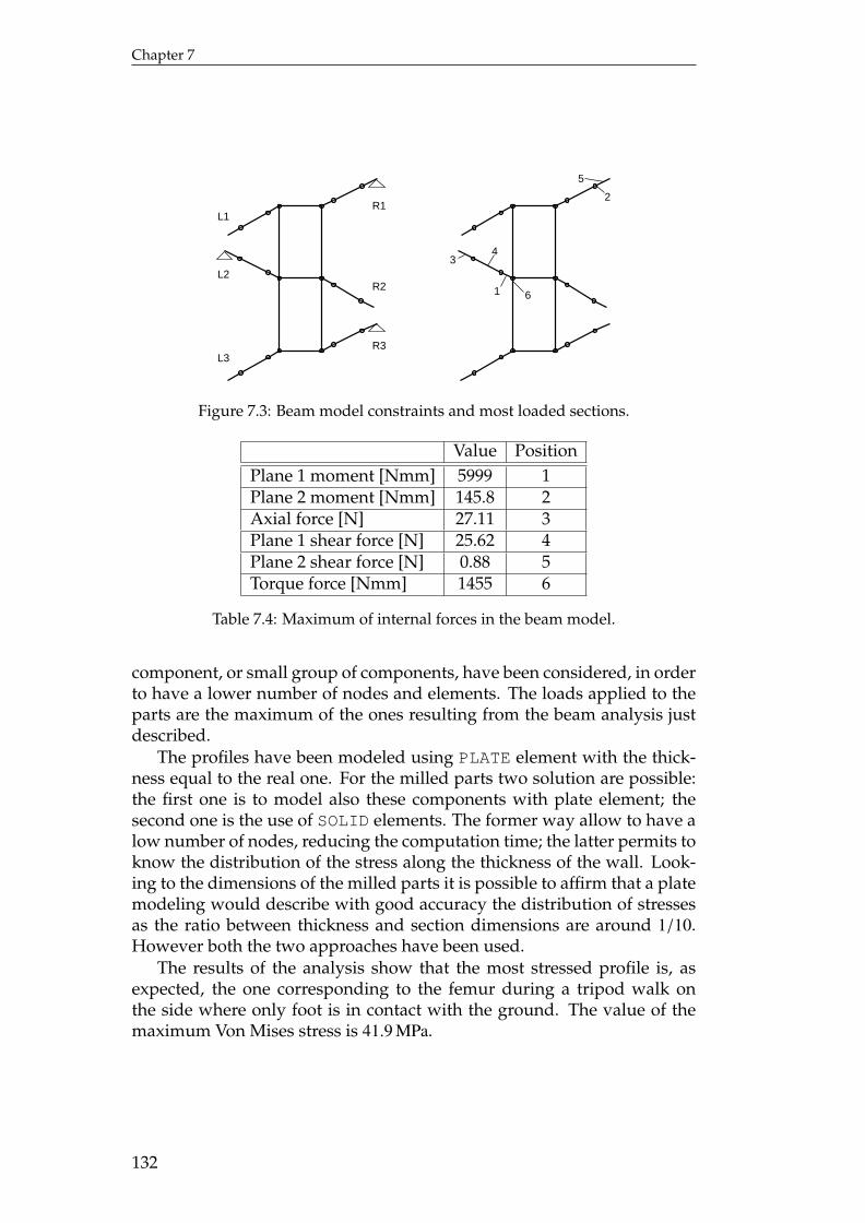
Chapter 7

L1

L2

L3R3

R2

R1

1

34

2

5

6

Figure 7.3: Beam model constraints and most loaded sections.

Value PositionPlane 1 moment [Nmm] 5999 1Plane 2 moment [Nmm] 145.8 2Axial force [N] 27.11 3Plane 1 shear force [N] 25.62 4Plane 2 shear force [N] 0.88 5Torque force [Nmm] 1455 6

Table 7.4: Maximum of internal forces in the beam model.

component, or small group of components, have been considered, in orderto have a lower number of nodes and elements. The loads applied to theparts are the maximum of the ones resulting from the beam analysis justdescribed.

The profiles have been modeled using PLATE element with the thick-ness equal to the real one. For the milled parts two solution are possible:the first one is to model also these components with plate element; thesecond one is the use of SOLID elements. The former way allow to have alow number of nodes, reducing the computation time; the latter permits toknow the distribution of the stress along the thickness of the wall. Look-ing to the dimensions of the milled parts it is possible to affirm that a platemodeling would describe with good accuracy the distribution of stressesas the ratio between thickness and section dimensions are around 1/10.However both the two approaches have been used.

The results of the analysis show that the most stressed profile is, asexpected, the one corresponding to the femur during a tripod walk onthe side where only foot is in contact with the ground. The value of themaximum Von Mises stress is 41.9 MPa.

132

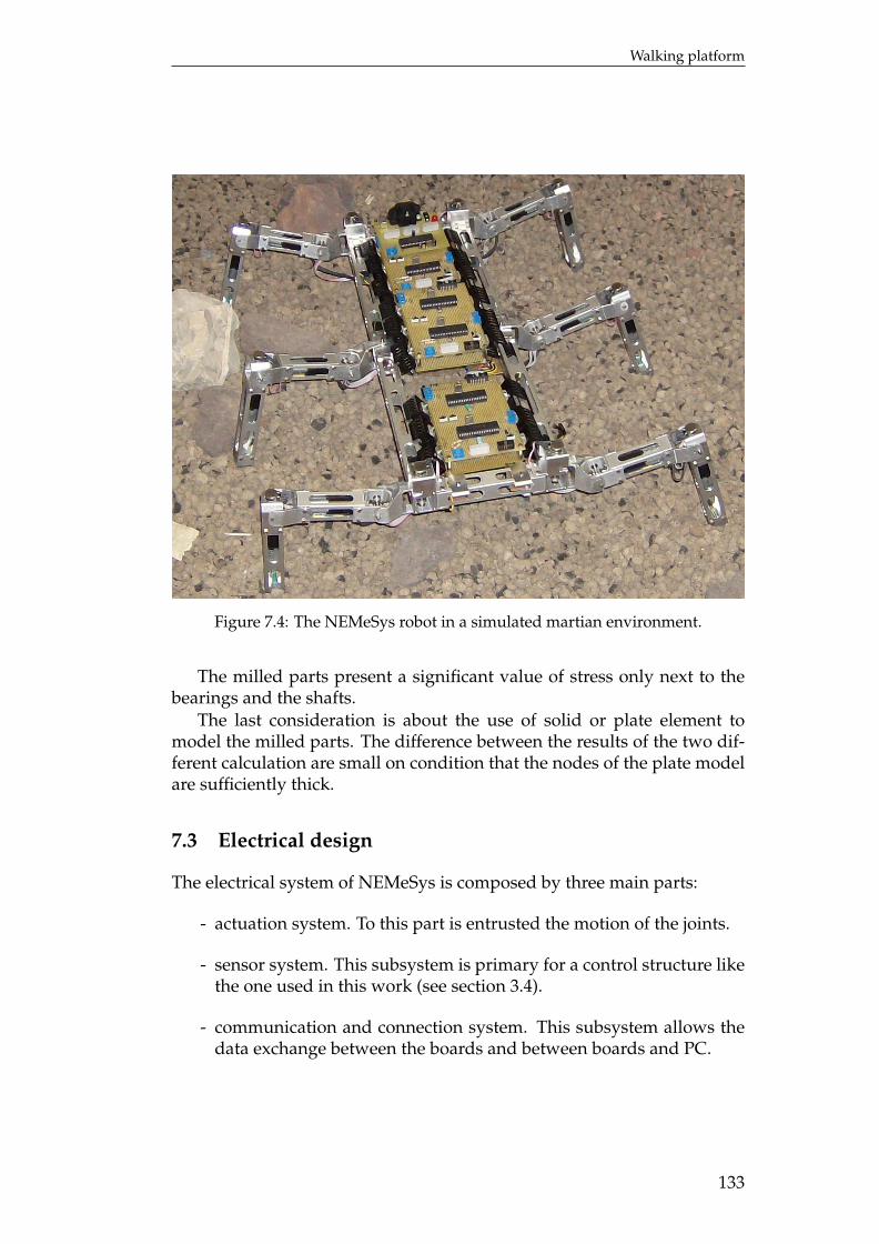
Walking platform

Figure 7.4: The NEMeSys robot in a simulated martian environment.

The milled parts present a significant value of stress only next to thebearings and the shafts.

The last consideration is about the use of solid or plate element tomodel the milled parts. The difference between the results of the two dif-ferent calculation are small on condition that the nodes of the plate modelare sufficiently thick.

7.3 Electrical design

The electrical system of NEMeSys is composed by three main parts:

- actuation system. To this part is entrusted the motion of the joints.

- sensor system. This subsystem is primary for a control structure likethe one used in this work (see section 3.4).

- communication and connection system. This subsystem allows thedata exchange between the boards and between boards and PC.

133

Chapter 7

Some parts of these system are existing from the old versions of NEMeSys;some others have been updated or completely replaced by new ones.

7.3.1 DC electric motorsThe actuation of the eighteen joints is assigned to as many DC electricalmotors. A planetary gear set to reduce the speed and increase the torquemust be introduced between the motors and the joints. These two com-ponents have been taken from the old robot, so no changes with respectof previous work have been made (see [14] for more details). In tables 7.5and 7.6 the principal data of the components are summarized.

The data show that the maximum continuous torque generated fromthe motor-adapter is of 5.12 Nm, and a peak of 15 Nm can be reached. Insection 6.2 the torque diagrams show that for the most of the time the nec-essary torque is below the maximum continuous and reaches a maximumbelow the permitted continuous torque for all the gaits except for the tri-pod one. During this last gait a peak of 7.5 Nm is achieved. This value islow in relation to the one allowed from the motor, but is high with respectto the maximum torque of the adapter. Only the wave gait respects thetorque limit of the adaptors, with a maximum of 2.7 Nm. In the test madewith old version of NEMeSys the exceeding of the torque didn’t cause anyfailure, so that also in this work these components are used.

The command to the motor is given by using a Pulse Width Modulation(PWM) technique. This is a very efficient way when the is necessary anintermediate amount of electrical power. The basic idea is to use a rectan-gular pulse wave whose pulse width is modulated resulting in the varia-tion of the average value of the waveform. The electrical circuit necessaryfor the use of PWM has been developed during the first two works onNEMeSys. For more detail see [14] and [53].

Producer MaxonProduct code A-max 22Input voltage [V] 12Maximum power [W] 6Maximum continuous torque [mNm] 7.425Stall torque [mNm] 22Maximum speed [RPM] 10500Torque constant [mNm/A] 10.9Speed constant [RPM/V] 875

Table 7.5: Motor specifications.

134

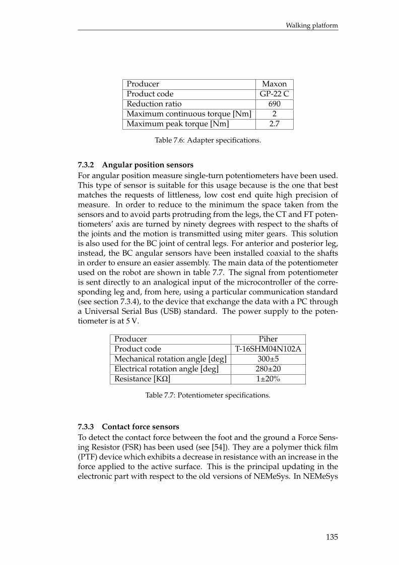
Walking platform

Producer MaxonProduct code GP-22 CReduction ratio 690Maximum continuous torque [Nm] 2Maximum peak torque [Nm] 2.7

Table 7.6: Adapter specifications.

7.3.2 Angular position sensorsFor angular position measure single-turn potentiometers have been used.This type of sensor is suitable for this usage because is the one that bestmatches the requests of littleness, low cost end quite high precision ofmeasure. In order to reduce to the minimum the space taken from thesensors and to avoid parts protruding from the legs, the CT and FT poten-tiometers’ axis are turned by ninety degrees with respect to the shafts ofthe joints and the motion is transmitted using miter gears. This solutionis also used for the BC joint of central legs. For anterior and posterior leg,instead, the BC angular sensors have been installed coaxial to the shaftsin order to ensure an easier assembly. The main data of the potentiometerused on the robot are shown in table 7.7. The signal from potentiometeris sent directly to an analogical input of the microcontroller of the corre-sponding leg and, from here, using a particular communication standard(see section 7.3.4), to the device that exchange the data with a PC througha Universal Serial Bus (USB) standard. The power supply to the poten-tiometer is at 5 V.

Producer PiherProduct code T-16SHM04N102AMechanical rotation angle [deg] 300±5Electrical rotation angle [deg] 280±20Resistance [KΩ] 1±20%

Table 7.7: Potentiometer specifications.

7.3.3 Contact force sensorsTo detect the contact force between the foot and the ground a Force Sens-ing Resistor (FSR) has been used (see [54]). They are a polymer thick film(PTF) device which exhibits a decrease in resistance with an increase in theforce applied to the active surface. This is the principal updating in theelectronic part with respect to the old versions of NEMeSys. In NEMeSys

135

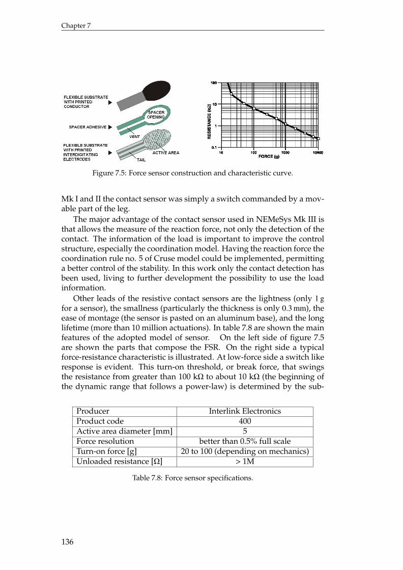
Chapter 7

Figure 7.5: Force sensor construction and characteristic curve.

Mk I and II the contact sensor was simply a switch commanded by a mov-able part of the leg.

The major advantage of the contact sensor used in NEMeSys Mk III isthat allows the measure of the reaction force, not only the detection of thecontact. The information of the load is important to improve the controlstructure, especially the coordination model. Having the reaction force thecoordination rule no. 5 of Cruse model could be implemented, permittinga better control of the stability. In this work only the contact detection hasbeen used, living to further development the possibility to use the loadinformation.

Other leads of the resistive contact sensors are the lightness (only 1 gfor a sensor), the smallness (particularly the thickness is only 0.3 mm), theease of montage (the sensor is pasted on an aluminum base), and the longlifetime (more than 10 million actuations). In table 7.8 are shown the mainfeatures of the adopted model of sensor. On the left side of figure 7.5are shown the parts that compose the FSR. On the right side a typicalforce-resistance characteristic is illustrated. At low-force side a switch likeresponse is evident. This turn-on threshold, or break force, that swingsthe resistance from greater than 100 kΩ to about 10 kΩ (the beginning ofthe dynamic range that follows a power-law) is determined by the sub-

Producer Interlink ElectronicsProduct code 400Active area diameter [mm] 5Force resolution better than 0.5% full scaleTurn-on force [g] 20 to 100 (depending on mechanics)Unloaded resistance [Ω] > 1M

Table 7.8: Force sensor specifications.

136

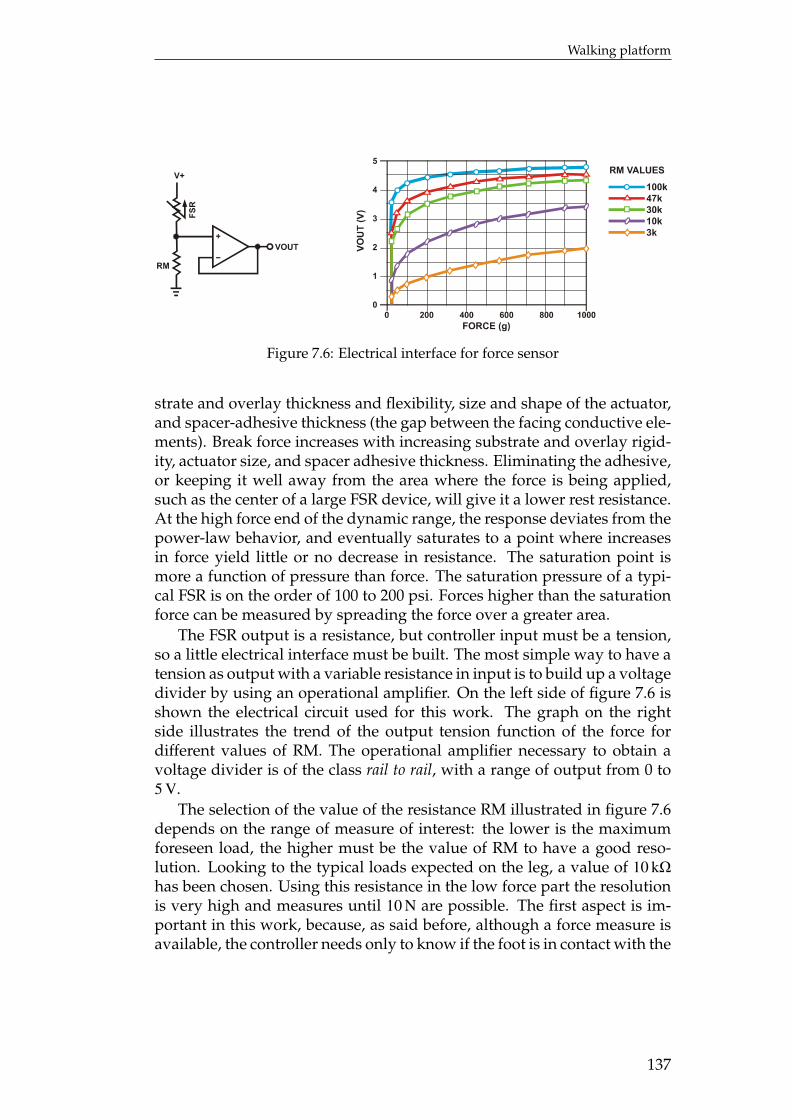
Walking platform

Figure 7.6: Electrical interface for force sensor

strate and overlay thickness and flexibility, size and shape of the actuator,and spacer-adhesive thickness (the gap between the facing conductive ele-ments). Break force increases with increasing substrate and overlay rigid-ity, actuator size, and spacer adhesive thickness. Eliminating the adhesive,or keeping it well away from the area where the force is being applied,such as the center of a large FSR device, will give it a lower rest resistance.At the high force end of the dynamic range, the response deviates from thepower-law behavior, and eventually saturates to a point where increasesin force yield little or no decrease in resistance. The saturation point ismore a function of pressure than force. The saturation pressure of a typi-cal FSR is on the order of 100 to 200 psi. Forces higher than the saturationforce can be measured by spreading the force over a greater area.

The FSR output is a resistance, but controller input must be a tension,so a little electrical interface must be built. The most simple way to have atension as output with a variable resistance in input is to build up a voltagedivider by using an operational amplifier. On the left side of figure 7.6 isshown the electrical circuit used for this work. The graph on the rightside illustrates the trend of the output tension function of the force fordifferent values of RM. The operational amplifier necessary to obtain avoltage divider is of the class rail to rail, with a range of output from 0 to5 V.

The selection of the value of the resistance RM illustrated in figure 7.6depends on the range of measure of interest: the lower is the maximumforeseen load, the higher must be the value of RM to have a good reso-lution. Looking to the typical loads expected on the leg, a value of 10 kΩ

has been chosen. Using this resistance in the low force part the resolutionis very high and measures until 10 N are possible. The first aspect is im-portant in this work, because, as said before, although a force measure isavailable, the controller needs only to know if the foot is in contact with the

137

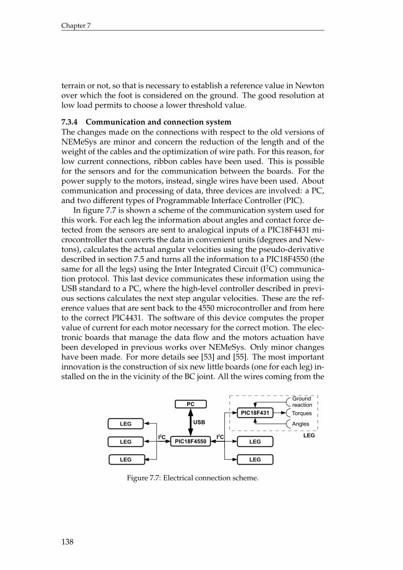
Chapter 7

terrain or not, so that is necessary to establish a reference value in Newtonover which the foot is considered on the ground. The good resolution atlow load permits to choose a lower threshold value.

7.3.4 Communication and connection systemThe changes made on the connections with respect to the old versions ofNEMeSys are minor and concern the reduction of the length and of theweight of the cables and the optimization of wire path. For this reason, forlow current connections, ribbon cables have been used. This is possiblefor the sensors and for the communication between the boards. For thepower supply to the motors, instead, single wires have been used. Aboutcommunication and processing of data, three devices are involved: a PC,and two different types of Programmable Interface Controller (PIC).

In figure 7.7 is shown a scheme of the communication system used forthis work. For each leg the information about angles and contact force de-tected from the sensors are sent to analogical inputs of a PIC18F4431 mi-crocontroller that converts the data in convenient units (degrees and New-tons), calculates the actual angular velocities using the pseudo-derivativedescribed in section 7.5 and turns all the information to a PIC18F4550 (thesame for all the legs) using the Inter Integrated Circuit (I2C) communica-tion protocol. This last device communicates these information using theUSB standard to a PC, where the high-level controller described in previ-ous sections calculates the next step angular velocities. These are the ref-erence values that are sent back to the 4550 microcontroller and from hereto the correct PIC4431. The software of this device computes the propervalue of current for each motor necessary for the correct motion. The elec-tronic boards that manage the data flow and the motors actuation havebeen developed in previous works over NEMeSys. Only minor changeshave been made. For more details see [53] and [55]. The most importantinnovation is the construction of six new little boards (one for each leg) in-stalled on the in the vicinity of the BC joint. All the wires coming from the

PC

PIC18F4550

PIC18F431USB

Torques

Ground reaction

LEGLEG

Angles

LEGLEG

LEG

LEG

I2C I2C

Figure 7.7: Electrical connection scheme.

138

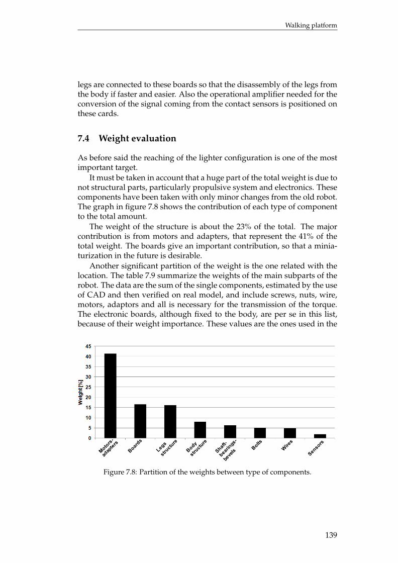
Walking platform

legs are connected to these boards so that the disassembly of the legs fromthe body if faster and easier. Also the operational amplifier needed for theconversion of the signal coming from the contact sensors is positioned onthese cards.

7.4 Weight evaluation

As before said the reaching of the lighter configuration is one of the mostimportant target.

It must be taken in account that a huge part of the total weight is due tonot structural parts, particularly propulsive system and electronics. Thesecomponents have been taken with only minor changes from the old robot.The graph in figure 7.8 shows the contribution of each type of componentto the total amount.

The weight of the structure is about the 23% of the total. The majorcontribution is from motors and adapters, that represent the 41% of thetotal weight. The boards give an important contribution, so that a minia-turization in the future is desirable.

Another significant partition of the weight is the one related with thelocation. The table 7.9 summarize the weights of the main subparts of therobot. The data are the sum of the single components, estimated by the useof CAD and then verified on real model, and include screws, nuts, wire,motors, adaptors and all is necessary for the transmission of the torque.The electronic boards, although fixed to the body, are per se in this list,because of their weight importance. These values are the ones used in the

Figure 7.8: Partition of the weights between type of components.

139

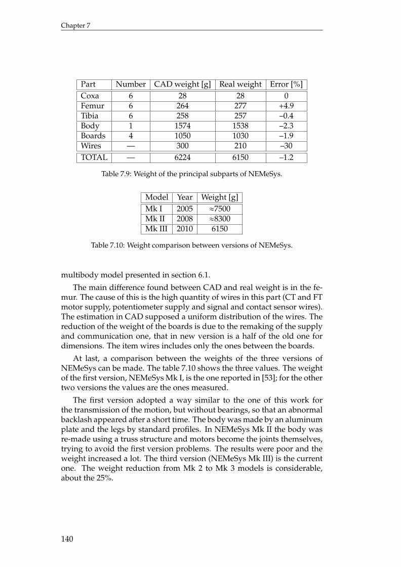
Chapter 7

Part Number CAD weight [g] Real weight Error [%]Coxa 6 28 28 0Femur 6 264 277 +4.9Tibia 6 258 257 –0.4Body 1 1574 1538 –2.3Boards 4 1050 1030 –1.9Wires — 300 210 –30TOTAL — 6224 6150 –1.2

Table 7.9: Weight of the principal subparts of NEMeSys.

Model Year Weight [g]Mk I 2005 ≈7500Mk II 2008 ≈8300Mk III 2010 6150

Table 7.10: Weight comparison between versions of NEMeSys.

multibody model presented in section 6.1.

The main difference found between CAD and real weight is in the fe-mur. The cause of this is the high quantity of wires in this part (CT and FTmotor supply, potentiometer supply and signal and contact sensor wires).The estimation in CAD supposed a uniform distribution of the wires. Thereduction of the weight of the boards is due to the remaking of the supplyand communication one, that in new version is a half of the old one fordimensions. The item wires includes only the ones between the boards.

At last, a comparison between the weights of the three versions ofNEMeSys can be made. The table 7.10 shows the three values. The weightof the first version, NEMeSys Mk I, is the one reported in [53]; for the othertwo versions the values are the ones measured.

The first version adopted a way similar to the one of this work forthe transmission of the motion, but without bearings, so that an abnormalbacklash appeared after a short time. The body was made by an aluminumplate and the legs by standard profiles. In NEMeSys Mk II the body wasre-made using a truss structure and motors become the joints themselves,trying to avoid the first version problems. The results were poor and theweight increased a lot. The third version (NEMeSys Mk III) is the currentone. The weight reduction from Mk 2 to Mk 3 models is considerable,about the 25%.

140

Walking platform

7.5 Software

The software used for the control of NEMeSys con be divided into threemain blocks:

- generation of the trajectory. The next-step angular velocity is gener-ated by the PC. This is the controller described in the previous sec-tions;

- follow the reference. Once that the reference value of angular ve-locity has been generated, it is necessary a low level controller thattakes as input the error between current angular velocity and refer-ence one and exits the correct value of current to give to the motor;

- management of the communication. This part comprises all the func-tions and the libraries necessary to have a correct I2C and USB com-munication. These software are at most available from the Microchip,the PIC producer, and only minor changes are necessary.

The high level controller is written using C language because of the goodtrade-off between ease of programming, the presence of a lot of functionsin the free libraries and the computational power needed that this lan-guage offers.

The low level controller, instead, has to be programmed using Assem-bler. This because has to work over the 4431 microcontrollers that havevery low computational power, so that the software must be optimizedas more as possible. Another advantage of the Assembler language is thepossibility of setting the system register to adapt the configuration of thedevice according to the requests. All the register settings are describedon the data sheets of the PIC devices [56][57]. The USB communicationsoftware is written using C; the I2C one is programmed in Assembler. Formore details see [55].

7.5.1 Low level controllerFor the low level controller three are the main requirements:

- low computational cost;

- high adaptability to changes of the high level controller;

- ease of calibration of the parameters.

For these reasons a PID (Proportional-Integral-Derivative) controllerhas been chosen. This is a very common and used class of feedback con-trollers, particularly when some variables of the problem are unknown or

141

Chapter 7

not completely modeled. Furthermore the calibration process of these con-troller can be made easily and only looking to the response of the system.A typical expression of a PID controller is shown in equation 7.1.

u(t) = Kpe(t) + Ki

∫ t

0e(τ)dτ + Kd

ddt

e(t) (7.1)

where Kp, Ki and Kd are proportional, integrative and derivative gains re-spectively, e(t) the error between reference and measure at current timeand u(t) the control action.

Referring now to this work, e(t) is the error between the angular veloc-ity requested from the high level controller and the one calculated fromthe measure of the potentiometer. To obtain the angular velocity from theangle measure has been implemented a second order formulation for thederivative numerical calculation (see 7.2).

y′(i) ≈12

y(i − 2) − 2y(i − 1) +32

y(i) (7.2)

Obviously a backward formulation has been used, as the calculation isreal-time performed. This forces to save in the PIC memory the valueof the angular position for the last two steps, but allows to have a betteraccuracy on the derivative calculation.

In order to estimate the integral of the error the trapezoidal rule (equa-tion 7.3) has been used.∫ b

af (t)dt ≈ (b − a)

( f (a) + f (b)2

(7.3)

In the present work a is the previous time step and b is the current one.f (a) and f (b) are the corresponding values of the angular velocities.

The values of the PID constants have been hand-tuned looking to theresponse of the multi-body model described in section 6.1. At least a pro-portional controller must be used. This type of controller, using an appro-priate value for Kp, is able to stabilize the response. Increasing the valueof Kp, beyond a certain value instability occurs. However, a proportionalcontroller produces a high error on the angular position. To recover theappropriate accuracy on the position, an integral controller is necessary.The final choice for this controller is a PI. This system can be also seen asa proportional controller both on the angular position and on the angu-lar velocity. The derivative control (equal to a proportional control of theerror on angular acceleration), usually used to decrease overshoot, is notnecessary in this case. The best result can be obtained with gains Kp = 0.02and Ki = 0.95.

142

Chapter 8

ConclusionIn this section are summarized the main results reached during this work,both in the control system and in the construction of the walking platform.At the end will be listed some possible improvements or changes for thenext work on NEMeSys.

8.1 Results of the work

The first result obtained is the control of the single leg motion. At firstonly the standard walking has been implemented, beginning from the twophases swing and stance. For the former one two possible model has beendesigned, one using a static network and one using a dynamic network.Both these two networks have been tested on a huge number of differentstart and target positions in order to evaluate advantages and disadvan-tages of each one. A positive feedback has been implemented in order tocontrol the power stroke. A closed loop has been applied on height andbody speed. Once that the single phases have been optimized, the designof the selector has permitted to reproduce a standard single leg motion.The next step has been the implementation of the reflexes by using ANN.These are the main expression of the interaction between the robot and theenvironment. Three types of reflexes have been identified looking to thebehavior of stick insect. The single leg motion is so completely simulated.

The coordination between the legs has been the following target. Be-ginning from two different existing models of coordination, a new one hasbeen designed, trying to keep the positive aspects of each one. The simu-lations of the motion using this new model have demonstrated to be ableto ensure the static stability of the robot for a large range of speed, thatcan be varied with continuity from a value next to zero to the maximumpermitted from the motors. The typical gaits of stick insect walking auto-matically emerge by changing the value of the reference velocity. On flatterrain wave gait from the rear to the front appears. It is demonstratedthat this type of gait is the most efficient one. Furthermore also in case offailure of one leg, the coordination is ensured. Also curve trajectory can beperformed only by giving a reference value of the angular speed of yaw,without any change in the control and coordination parameters. It is im-portant to underline that these results have been obtained by using onlykinematic models, without taking in account dynamic effects.

143

Chapter 8

In order to proof the effectiveness of the control system designed, it hasbeen tested on a multibody model. During these simulations a realisticmodel of the ground has been used in order to have the effective valuesof ground reactions. The output of these calculations have confirmed agood accordance with the kinematics ones demonstrating that the designcan be made ignoring the dynamic effects. However these simulationshave given the possibility to analyze particular behavior that can’t emergeonly considering the kinematics, especially during the stance phase, wherethe interaction with the environment is strong. The controller has alsodemonstrated a high level of robustness also against disturbance on themeasures.

The use of a reflex-based controller has the main disadvantage of need-ing the signal of the sensors, so that in case of sensor failure the generationof a correct trajectory is impossible. In this case the only way is to switchoff the corresponding leg and to continue with five legs, with a degrada-tion of the performances, but maintaining the control and the coordinationof the robot. This is also possible because of the high level of decentral-ization of the current controller, so that the trajectory of each leg can begenerated using the data from the sensors of the leg itself.

Meanwhile a mechanical platform has been designed and built. Themain result is a great reduction of the weight (about 20%) and of the sizeof the legs. The new type of junction allows to have more compact legsand body. Moreover the type of structure chosen for NEMeSys Mk IIIhas a high level of modularity, allowing to change the shape rapidly andcheaply maintaining the current milled parts and replacing the profiles.The new contact sensors permit the measure of the ground reaction in-stead of the only contact detection of the last works.

8.2 Innovation

The main innovative feature developed during this work is the new co-ordination model shown in chapter 5. Compared to the other proposeddecentralized coordination models, the present one matches the ability toensure the static stability of the robot and to generate wave gates on flatground. The static stability is maintained not only in case of standardwalking on flat terrain, but also un presence of obstacles and when par-ticular behaviors, e.g. reflexes, are activated. The emersion of wave gate,instead, ensures that the walking is performed by the most efficient way.

The second innovation is about the swing trajectory generation: in thiswork a dynamic ANN has been designed, trained and tested. The mainadvantage with respect to the static swing network is its robustness with

144

Conclusion

respect to the static one in front of disturbance.In order to represent particular behaviors a complete set of reflexes

have been implemented using ANN. These are an innovation with respectto the previous work because are completely uncoupled with respect to thenormal walking trajectory generation. They only work if a particular inputcomes from the environment, so that, normally, they have no influence onthe robot motion.

Moreover the modular approach improves the flexibility of the con-troller by allowing to introduce new behaviors in very simple way.

About the mechanical platform, the main innovation with respect tothe old versions of NEMeSys is the joint architecture and the use of mitergears for the transmission of the motion.

8.3 Future developments

About the future development, the first thing to be done is the test of thecontroller presented in this work on the walking platform. The softwarenecessary for this activity is at most already programmed by using C andAssembler. However it is necessary a check of the USB and I2C communi-cation and the calibration of the sensors. The first tests will be done withstraight reference trajectory beginning from low speed gait. If these testswill conclude successfully high speed and curve walking could be tested.

With regard to the controller, starting from the actual one, a lot of de-velopment can be thought. The first one is the implementation of a systemthat allows to maintain the position when the robot is stopped in presenceof disturbance. The LPVF acting during stance does not allow this behav-ior. It is necessary to introduce a stiffness on the joints somehow. The mostsimple way is the introduction of a negative feedback on the single jointevery time that the current position has to be held.

A weakness of the controller described in this work is that no raise ispossible if the robot falls. This because particular behavior are necessaryin this case. The solution could be to implement a system that first of alldetects the fall and computes a strategy for the lift. These strategy arestereotyped behaviors function of the position after the drop.

About the curve walking other behaviors can be applied: in this workhas been implemented only the change of frequency of the gait to performa curve trajectory, but other ones are possible. The simplest is the changingof the target position of the swing phase and of the PEP in relation to theyaw angular velocity reference. By this way it will be possible to reducethe radius of the trajectory, up to permit to the robot to turn on itself.

The presence of force sensors that measure the ground reaction on the

145

Chapter 8

foot allows to design a more complex selector that takes into account thelongitudinal and lateral position of the PEP and the amount of the reac-tion. The result of this will be a better control of the stability, that even-tually will change the coordination model, adding to the current one theequivalent of the rule 5 of the Cruse model (see section 5.1).

For the high level control, attitude sensors can be installed on the robot.By this way will be possible to command the orientation of the body. Thismeans that a better control of the reference height for each leg can be im-plemented, allowing, for example, to lift the forward part of the body ifan obstacle is detected. For a better interaction with the environment a setof vision sensors could be used. By this way the detection of an irregu-larity of the ground can be made in advance, and an optimization of thetrajectory and of the gait can be performed.

As previously said, with the current controller, in case of failure of fail-ure even of one sensor, it is necessary to switch off all the legs, that has tobe locked in swing position to avoid interference with the working legs.A strategy can be studied to try to use, perhaps with a degradation of theperformance, the damaged leg too. An idea can be to insert a shadow CPGthat, only in case of failure, using as input the signal of the remaining sen-sors of the leg, replaces the normal reflex-based controller. By this way thepattern generator is restored. Obviously this shadow controller must besynchronized through the coordination to the reflex-based ones workingon the healthy legs.

A parallel activity on the robot could be the identification of the modelfrom the data coming from the tests. By this work it could be possible tobuild a simple and efficient model for numerical simulation of any type ofcontroller.

About the mechanical platform, the first thing to do could be the minia-turization of the electronic boards. This would mean also a great reductionof the weight (supposed about 10%), so that a payload or a on-board CPUcould be installed.

146

List of AcronymsAEP Anterior Extreme Position

ANN Artificial Neural Network

BC Body-Coxa

CAD Computer-Aided Design

CoG Center of Gravity

CPG Central Pattern Generator

CT Coxa-Trochanter

CTRNN Continous Time Recurrent Neural Network

DNN Dynamic Neural Network

DoF Degree of Freedom

FEM Finite Element Method

FSR Force Sensing Resistor

FT Femur-Tibia

GA Genetic Algorithm

GC Ground Contact

HPF High Pass Filter

I2C Inter Integrated Circuit

LPVF Local Positive Velocity Feedback

NEMeSys Neural Ento-Mechanic System

PCG Point of Center of Gravity

PEP Posterior Extreme Position

PIC Programmable Interface Controller

PID Proportional-Integral-Derivative

147

Conclusion

PSD Power Spectral Density

PWM Pulse Width Modulation

RNN Recurrent Neural Network

SEP Superior Extreme Position

TDRNN Time-Delayed Recurrent Neural Network

USB Universal Serial Bus

148

Bibliography[1] H. Cruse, V. Dürr, and J. Schmitz. Insect walking is based on a decen-

tralized architecture revealing a simple and robust controller. Philo-sophical Transation of the Royal Society A, 365:221–250, 2007.

[2] R. A. Brooks. A robot that walks; emergent nehavior from a carefullyevolved network. Neural Computation, 1(2):253–262, 1989.

[3] C. Ferrel. Robust and adaptive locomotion of an autonomous hexa-pod. In Proceedings From Perception to Action Conference, pages 66–77,Lausanne, Switzerland, Sept. 1994.

[4] R.D. Beer, H.J. Chiel, R.D. Quinn, K. Espenschied, and P. Larsson. Adistributed neural network architecture for hexapod robot locomo-tion. Neural Computation, 4(3):356–365, 1992.

[5] S. Colombano, F. Kirchner, D. Spenneberg, and J. Hanratty. Explo-ration of planetary terrains with a legged robot as a scout adjunct toa rover. In AIAA Space 2004 Conference and Exhibit, pages 28–30, SanDiego (CA), USA, Sept. 2004.

[6] H. Cruse, T. Kindermann, M. Schumm, J. Dean, and J. T. Schmitz.Walknet - a biologically inspired network to control six-legged walk-ing. Neural Networks, 11:1435–1447, 1998.

[7] H.J. Weidemann, F. Pjeifer, and J. Eltze. The six-legged tum walk-ing robot. In Proceedings of the IEEE/RSJ/GI International Conference onIntelligent Robots and Systems IROS ’94., volume 2, pages 1026–1033,Munich, Germany, Sept. 1994.

[8] A. Buschmann. Home of Tarry I & II: design of the walking machineTarry II, March 2000. http://www.tarry.de.

[9] A. Buschmann. Home of Tarry I & II: frequently asked questionsabout Tarry, March 2000. http://www.tarry.de.

[10] W. McCulloch and W. Pitts. A logical calculus of the ideas imma-nent in nervous activity. Bulletin of Mathematical Biophysics, 7:115–133,1943.

[11] S. Nolfi and D. Floreano. Learning and evolution. Autonomous Robots,1:89–113, 1999.

149

Bibliography

[12] K. Hornik, M. Stinchcombe, and H. White. Multilayer feedforwardnetworks are universal approximators. Neural Networks, 2:359–366,1989.

[13] K. Funahashi and Y. Nakamura. Approximation of dynamical sys-tems by continuous time recurrent neural networks. Neural Networks,6:801–806, 1993.

[14] Alessandro Bursi and Marco Di Perna. Controllo di un robot a zampeper esplorazione planetaria con l’utilizzo di reti neurali dinamiche ealgoritmi evolutivi. Master Thesis in Space Engeneerig, Politecnicodi Milano, 2004.

[15] Gabriele Greco. Generazione e controllo della camminata di un robotesapode con reti neurali CTRNN e a mutua inibizione. Master Thesisin Space Engeneerig, Politecnico di Milano, 2009.

[16] R.D. Beer. On the dynamics of small continuous-time recurrent neuralnetworks. Adaptive Behavior, 3(4):469–509, 1995.

[17] Bernard Friedland. Control sytem design. McGraw-Hill, New York,NY, 1986.

[18] The MathWorks, Inc., Natick, MA. Genetic Algorithm and Direct SearchToolbox User’s Guide, January 2004. http://www.mathworks.com.

[19] G. Wendler. Laufen und stehen der stabheuschrecke: Sinnesborstenin den beingelenken als glieder von regelkreisen. Zeitschrift fuer Ver-gleichende Physiologie, 48:198–250, 1964.

[20] N. Porcino. Hexapod gait control by a neural network. In Interna-tional Joint Conference on Neural Networks, volume I, pages 189–194,San Diego (CA), USA, June 1990.

[21] H. Cruse and C. Bartling. Movement of joint angles in the legsof a walking insect, Carausius morosus. Journal of Insect Physiology,9(41):761–771, 1995.

[22] M. Schumm and H. Cruse. Control of swing movement: influencesof differently shaped substrate. Journal of Comparative Physiology,192:1147–1164, 2006.

[23] H. Cruse, C. Bartling, D.E. Brunn, J. Dean, M. Dreifert, T. Kinder-mann, and J. Schmitz. Walking: a complex behavior controlled bysimple systems. Adaptive Behavior, 3:385–418, 1995.

150

Bibliography

[24] H. Cruse, C. Bartling, and T. Kindermann. High-pass filtered posi-tive feedback for decentralized control of cooperation. In Advancesin artificial life, volume 929 of Lecture Notes in Computer Science, pages668–678. Springer Berlin / Heidelberg, 1995.

[25] D. DeAngelis, W. Post, and C. Travis. Feedback in Natural Systems.Springer, London, Berlin, Heidelberg, 1986.

[26] H. Cruse. Which parameters control the leg movement of a walkinginsect? ii. the start of the swing phase. The Journal of ExperimentalBiology, 116:357–362, 1985.

[27] D.M. Wilson. Insect walking. Annual Reviews Entomology, 11:103–122,1966.

[28] S.M. Song and K.J. Waldron. An analytical approach for gait studyand its application on wave gaits. The International Journal of RoboticsResearch, 6(2):60–71, 1987.

[29] V. Zolotov, L. Frantsevich, and E. M. Falk. Kinematik der phototaktis-chen drehung bei der honigbiene Apis mellifera. Journal of ComparativePhysiology, 97:339–353, 1975.

[30] C.P.E. Zollikofer. Stepping patterns in ants. i. influence of speed ancurvature. The Journal of Experimental Biology, 192:95–106, 1994.

[31] K.W. Wait and M. Goldfarb. A biologically inspired approach to thecoordination of hexapedal gait. In Proceedings of ICRA 2007, pages2655–2660, Rome, Italy, April 2007.

[32] H. Cruse, C. Bartling, G. Cymbalyuk, and M. Dreifert. A modularartificial neural net for controlling a six-legged walking system. Bio-logical Cybernetics, 72:421–430, 1995.

[33] C.R. Linder. Self organisation in a simple task of motor control. InProceedings of the 7th international conference on simulation of adaptivebehavior, pages 185–194, Edinburgh, UK, Aug. 2002. MIT Press.

[34] H. Cruse, D. Riemenschneider, and W. Stammer. Control of bodyposition of a stick insect standing on uneven surfaces. Biological Cy-bernetics, 61:71–77, 1989.

[35] J. Schmitz, T. Kindermann, M. Schumm, and H. Cruse. Simplifyingthe control of a walking hexapod by exploiting physical properties.

151

Bibliography

In Proceedings of European Mechatronics Colloquium, Euromech 375 - Bi-ology and Technology of Walking, pages 296–303, Munich, Germany,March 1998.

[36] H. Cruse. Which parameters control the leg movement of a walk-ing insect? i. velocity control during the stance phase. The Journal ofExperimental Biology, 116:343–355, 1985.

[37] T. Kindermann. Behavior and adaptability of a six-legged walkingsystem with highly distributed control. Adaptive Behavior, 9:16–41,2002.

[38] K.S. Espenschied, R.D. Quinn, R.D. Beer, and H.J. Chiel. Biologicallybased distributed control and local reflexes improve rough terrain lo-comotion in a hexapod robot. Robotics and Autonomous Systems, 18:59–64, 1996.

[39] H. Cruse and B. Blaesing. Stick insect locomotion in a complex envi-ronment: climbing over large gaps. The Journal of Experimental Biology,207:1273–1286, 2004.

[40] V. Dürr. Stereotypic leg searching-movements in the stick insect:kinematic analysis, behavioural context and simulation. The Journalof Experimental Biology, 204:1589–1604, 2001.

[41] K.G. Pearson and R. Franklin. Characteristics of leg movements andpatterns of coordination in locust walking on rough terrain. Interna-tional Journal of Robotics Research, 3(2):101–112, 1984.

[42] H. Cruse. What mechanisms coordinate leg movement in walkingarthropods? Trends in Neurosciences, 13:15–21, 1990.

[43] J.M. Porta and E. Celaya. A control structure for the locomotion of alegged robot on difficult terrain. IEEE Robot & Automation Magazine,5(2):43–51, 1998.

[44] T. Roggendorf. Comparing different controllers for the coordinationof a six-legged walker. Biological Cybernetics, 92:261–274, 2005.

[45] J.M. Porta and E. Celaya. Reactive free-gait generation to follow ar-bitrary trajectories with a hexapod robot. Robotics and AutonomousSystems, 47:187–201, 2004.

152

Bibliography

[46] K.S. Espenschied, R.D. Quinn, H.J. Chiel, and R.D. Beer. Leg coordi-nation mechanisms in stick insect applied to hexapod robot locomo-tion. Adaptive Behavior, 1(4):455–468, 1993.

[47] H. Cruse. The control of the anterior extreme position of the hind-leg of a walking insect, Carausius morosus. Physiological Entomology,4:121–124, 1979.

[48] J. Dean. Coding proprioceptive information to control movement toa target: simulation with a simple neural network. Biological Cyber-netics, 63:115–120, 1990.

[49] C. Ridderström. Legged locomotion: balance, control and tools - from equa-tion to action. PhD Thesis, Royal Institute of Technology, Stockholm,Sweden, 2003.

[50] The MathWorks, Inc., Natick, MA. SimscapeT M 3 User’s Guide, March2010. http://www.mathworks.com.

[51] Ernest O. Doebelin. Measurement Systems: Application and Design.McGraw-Hill, New York, NY, 5th edition, 2004.

[52] H.M. Lankarani and Nikravesh P.E. A contact force model with hys-teresis damping for impact analysis of multibody systems. Transactionof the ASME, Journal of Mechanical Design, 112:369–376, 1990.

[53] Paolo Massioni and Stefano Nebuloni. Progetto e sperimentazionedi sistemi di controllo per un prototipo di robot esapode per esplo-razione planetaria. Master Thesis in Space Engeneerig, Politecnico diMilano, 2005.

[54] Interlink Electronics, Inc., Camarillo, CA. FSR® Integration Guide& Evaluation Parts Catalog With Suggested Electrical Interfaces. www.interlinklelectronics.com.

[55] Antonio Pisciotta. Progetto del sistema motorio di un robot a piùarti. Master Thesis in Aeronautical Engeneerig, Politecnico di Milano,2008.

[56] Microchip Technology Inc., Chandler, AZ. PIC18F2331/2431/4331/4431 Data Sheet. http://ww1.microchip.com.

[57] Microchip Technology Inc., Chandler, AZ. PIC18F2455/2550 /4455/4550 Data Sheet. http://ww1.microchip.com.

153