Embed Size (px)
Citation preview

POLITECNICO DI TORINO
Corso di Laurea Magistrale in Ingegneria Elettrica
Tesi di Laurea Magistrale
A Multi-Site European Network for Real-Time Co-
Simulation of Transmission and Distribution
Systems
Relatore
prof. Ettore Bompard
Correlatori
prof. Antonello Monti
Marija Stevic
Abouzar Estebsari
Candidato
Renato Melloni
Luglio 2017


I
Table of contents
1 Introduction ................................................................................................................... 1
1.1 Grid integration of DERs ........................................................................................ 1
1.2 Integrated Transmission-Distribution Studies ........................................................ 1
1.2.1 Real-time simulation and test beds .................................................................. 2
1.3 ERIC – lab: European Real-time Integrated Co-simulation Laboratory ................ 3
1.4 Purposes and Contents of the Thesis ...................................................................... 4
1.4.1 Focus and contribution of the thesis ................................................................ 4
1.4.2 Outline of the thesis ......................................................................................... 5
2 Background .................................................................................................................... 6
2.1 Real-Time Simulation ............................................................................................. 6
2.1.1 Applications and Advantages of Real-Time Simulations ............................... 7
2.2 Motivation for integrated simulation of Transmission and Distribution networks . 7
2.2.1 Response of DG units to a network fault ......................................................... 7
2.2.2 Reverse power flow: behaviour of OLTC (on load tap changing) transformers
8
2.2.3 Realistic load models and demand-side management (DSM) ......................... 8
2.2.4 Frequency stability and regulation with high levels of DG penetration .......... 8
2.2.5 BESSs (Battery energy storage systems) ........................................................ 9
2.2.6 Advanced inverters: voltage and reactive power regulation ........................... 9
2.2.7 Extreme scenarios ............................................................................................ 9
2.3 Related Works ......................................................................................................... 9
2.3.1 Integrated grid modelling system (IGMS) ...................................................... 9
2.3.2 Simulation of Transmission and Distribution networks using Decomposition
11
2.3.3 Voltage Security analysis in scenarios with high PV penetration in DNs [23]
12
2.3.4 SmartNet Project ........................................................................................... 12
2.4 Frequency Regulation in future power systems .................................................... 13
2.4.1 Traditional Frequency control ....................................................................... 13
2.4.2 Challenges for frequency control posed by todays’ aspects of the power system
16

II
2.4.3 New approaches to frequency control ........................................................... 16
3 Modelling .................................................................................................................... 20
3.1 Transmission Network model ............................................................................... 20
3.2 Distribution Network models ................................................................................ 22
3.2.1 Turin DN model ............................................................................................ 22
3.2.2 Medium voltage benchmark network ............................................................ 23
3.3 Photovoltaic Power Plants model ......................................................................... 25
3.3.1 Solar Irradiation Dependence ........................................................................ 26
3.3.2 Low Voltage Ride Through capability .......................................................... 26
3.4 Fuel Cell System model ........................................................................................ 27
3.4.1 Model ............................................................................................................. 27
3.4.2 Controller ....................................................................................................... 31
3.4.3 Frequency controller ...................................................................................... 33
3.4.4 Frequency controller simulation test of Fuel cell system .............................. 34
3.5 Equivalent distribution network (DN) .................................................................. 38
3.5.1 Load model .................................................................................................... 39
3.5.2 PV system model ........................................................................................... 39
3.5.3 FC system model ........................................................................................... 39
3.5.4 Losses and components’ contribution ........................................................... 40
4 Combined simulations of Transmission and Distribution systems ............................. 42
4.1 Co-simulation setup .............................................................................................. 42
4.1.1 Local Co-simulation ...................................................................................... 42
4.2 PV systems allocation to distribution networks .................................................... 43
4.2.1 Turin DN ....................................................................................................... 43
4.2.2 Medium voltage DN benchmark ................................................................... 43
4.3 Simulation cases ................................................................................................... 45
4.4 Case 1A ................................................................................................................. 45
4.4.1 Scenario ......................................................................................................... 45
4.4.2 Fidelity of the interface between real-time simulators .................................. 46
4.4.3 Results ........................................................................................................... 46
4.4.4 Equivalent model for DNs validation ............................................................ 48
4.5 Case 1B ................................................................................................................. 51
4.5.1 Scenario ......................................................................................................... 51
III
4.5.2 Results ........................................................................................................... 52
4.6 Case 2A ................................................................................................................. 55
4.6.1 Scenario ......................................................................................................... 55
4.6.2 Results ........................................................................................................... 56
5 Frequency control in scenarios with high DG penetration .......................................... 59
5.1 Frequency metrics ................................................................................................. 59
5.2 Distribution network models with fuel cell systems ............................................. 61
5.3 Control strategies for fuel cell systems ................................................................. 61
5.4 Case 1A ................................................................................................................. 65
5.4.1 Scenario case 1A ........................................................................................... 65
5.4.2 Results ........................................................................................................... 66
5.5 Case 2A ................................................................................................................. 72
5.5.1 Scenario case 2A ........................................................................................... 72
5.5.2 Results ........................................................................................................... 74
6 Conclusions and future works ..................................................................................... 78
References ........................................................................................................................... 80
List of figures ...................................................................................................................... 84

IV

1
1 Introduction
1.1 Grid integration of DERs
Nowadays, distribution networks are changing greatly due to distributed energy resources
such as distributed generation (DG), energy storage systems (ESSs) and controllable
loads. These active distribution networks pose great challenges to the planning and
operation of electrical power systems.
Governments of many countries provided economic incentives for promoting the
widespread of distributed generation, with special regards to renewable and sustainable
resources. The consequent proliferation of these technologies require a new operation
management paradigm [1].
Furthermore, distribution networks (DNs) have been designed to operate with radial
topology and to efficiently supply power to the end consumers due to unidirectional
power flow. DNs should be considerably upgraded in order to follow the ongoing change
of paradigm [2].
The so-called “50.2 Hz problem” is a concern that arises because of the high level of
photovoltaic systems connected to the low-voltage in Europe, especially in Germany.
Distributed generation was required to switch off immediately if the frequency raised
above 50.2 Hz. The simultaneous disconnection of many generators resulted in a lack of
power generation, which could be hard to replace. To overcome this problem, a
degradation of feeding power according to a P(f) curve is now a requirement for inverters
of distributed generators.
Whilst on one hand DERs can threaten the overall reliability of the electrical power
system, on the other hand they could also have a positive effect if used properly for
network support. For instance, in [1] a centralised reactive power management strategy
for PV systems is proposed. It aims to reduce system’s losses by using the capability of
grid-connected PV inverter to provide reactive power.
When DER penetration was not significant to affect the power system operation and
stability, the protection of local resources was achieved by disconnecting the DER system
from the network under any abnormal condition. Recent national grid codes define
advanced requirements for DER functions, including active and reactive power control,
voltage and frequency support, and fault ride through (FRT) capability.
1.2 Integrated Transmission-Distribution Studies
The above mentioned considerations lead to the need of integrated simulations of
transmission and distribution networks, both represented with their corresponding
detailed models. Such simulations allow investigation of the impact of distributed energy
resources, installed in DNs, on the transmission network and their prospective support for
system stability and reliability.

2
Traditional studies of power systems can be divided in two categories: analysis of
transmission network and investigations of distribution networks.
When the focus is on the transmission network (TN), it is common to represent bulk
generation and high voltage levels accurately, while equivalent models are used for
distribution networks (DNs). This approach is used for example for frequency analysis,
TN load flow studies and investigations about system security.
On the other hand, when analysing load flow for medium voltage networks, optimal
configuration for distribution networks, power quality and in general any aspect
concerning the distribution level, TN is typically represented by a Thevenin equivalent.
This practice of simulating transmission and distribution network separately is adequate
until DNs can be considered as just passive networks and their influence on transmission
network is negligible.
Separate simulations for TNs and DNs are no longer enough to analyse some new
scenarios, occurrences and aspects of the electrical system and simulating transmission
and distribution networks together is becoming increasingly necessary.
Combined simulation and analysis of interactions between transmission and distribution
networks is nowadays an emerging research topic. Some projects focus on specific
occurrences and do not use complete joint simulations for transmission and distribution
networks [3], [4], while others introduce co-simulation platforms that can be used for
studying the modern power system [5], [6].
The widespread of DERs is also rapidly leading to new business opportunities, different
market models and new alternatives for ancillary services. For this reason, in [7] the
electrical system is examined with a wider approach, including commercial aspects (day
ahead commitment, real-time dispatch, etc.). In [8] TSOs and DSOs are involved in the
project in order to have a complete framework from each point of view.
1.2.1 Real-time simulation and test beds
With the purpose of studying the complete electrical system together with individual
components, an additional effort could be undertaken that is utilization of real-time
simulators. Simulations in real time allow testing of physical power components (such as
inverters) and actual controllers before connecting them to the real network. In [9], a
review on modern laboratories for testing of DERs and their controllers is presented. For
instance, the Austrian institute of technology has a laboratory (SmartEST), located in
Vienna, that allows advanced studies on physical devices and software algorithms.
Components can be tested under realistic conditions thanks to an infrastructure for
hardware-in-the-loop (HIL) real –time simulations.

3
1.3 ERIC – lab: European Real-time Integrated Co-simulation Laboratory
The main problem of real-time simulation is the amount of computational power required;
consequently, simulating a large and complex system is problematic and might require a
co-simulation. Separating the system under test among different real-time simulators
allows increase of the available computational power and simulation of larger models in
real time.
Real-time simulations and testing of devices can be carried out in a geographically
distributed way, by simulating subsystems of the monolithic system on different real-time
simulators located in different lab.
Project ERIC-lab [10] is based on the idea of interconnecting resources hosted in any of
the European federated laboratories [11]. For demonstrating the application of the
distributed simulation setup, a real-time co-simulation has been carried out. The system
under test consisted of interconnected transmission and distribution networks. It was
decoupled at the HV/MV interconnection point – the transmission network was simulated
in the laboratory of the E.ON Energy Research Center (Aachen, Germany) and the
distribution network Politecnico di Torino (Turin, Italy).
Interconnection of real-time laboratories across Europe provides some clear advantages:
Sharing of hardware and software equipment among federated labs. Each research
team could have at its disposal all the tools of the federation. That means allowing
researches to use facilities that are not available in their own laboratory by
providing remote access to another lab.
Allowing experts in different field to work together. Research teams can share
knowledge and experiences in order to reach common goals and to increase the
overall productivity of the federation. A team does not necessarily require experts
in all fields that are involved in a specific project: remote collaborations with
specialists from other groups would be possible, without physically exchanging
researchers or resources.
Joining computational power to obtain a greater real-time simulation capacity.
Simulating a large and complex system in real time can be challenging and,
sometimes, not even possible for a single laboratory. Combining simulation
capabilities allows larger and more complex simulations avoiding to afford
considerable expenses for buying new equipment.
Exchanging crucial information and results while keeping sensitive data and
models confidential. Companies and institutes might not want or might not be
authorised to share some models or data. Nevertheless, they could need
hardware/software in the loop (HIL/SIL) tests for power devices or controller. The
federation of real-time laboratories allows co-simulations without exchange of
confidential data, but just sharing the minimum of information.
Geographically distributed co-simulations require to exchange data in real-time among
labs which can be located in different countries using internet connection. It is important
to ensure that this communication does not threaten the quality and the reliability of co-

4
simulations. The conservation of energy at the interface and the impact of communication
delays on results are the main concerns while simulating power systems.
1.4 Purposes and Contents of the Thesis
1.4.1 Focus and contribution of the thesis
The first aim of this work is to explain and demonstrate interactions between transmission
and distribution networks with particular focus on the impact of distributed energy
resources on modern power systems.
Simulations are carried out in real-time environment thanks to a framework of
interconnected real-time simulators: the OPAL-RT real-time simulator is connected to an
RTDS rack through a GTFPGA card. Such kind of interconnections requires some
practical arrangements for ensuring reliable and stable co-simulations.
Transmission and distribution network models proposed by CIGRé [12] for studying
DERs integration are here implemented. The medium voltage network is modelled in
Matlab/Simulink for real-time simulation on OPAL-RT thanks to a fixed-step solver for
power systems (ARTEMiS) provided by OPAL-RT. The high-voltage transmission
benchmark model is implemented in RSCAD, which is the dedicated softer of RTDS real-
time simulator. Besides the benchmark DN, a DN model based on a portion of the
distribution system of Turin is used for co-simulations.
Since studies are performed in real-time simulation environment, the choice of
component models and their implementation is a key issue. The simulated system is
indeed very large and a detailed representation of each device would result in a lack of
computational resources. Thus, to obtain a flexible platform that allows investigations of
diversified aspects of the power system, each component should be represented by a
model that represents the most important behaviour of the physical component without
overburdening real-time simulation resources.
According to the considerations above, photovoltaic (PV) and solid oxide fuel cell
systems are modelled, taking into account their features from the network point of view.
PV model includes the low-voltage ride through capability required for distributed
generation by the Italian grid code. Since fuel cell systems will be used for support in
frequency regulation, their model must represent the realistic output power dynamics and
take into account the safe operating area for fuel cell systems.
Furthermore, an equivalent model for emulating the aggregated behaviour of a
distribution network is designed. It takes into account PV system disconnection for low-
voltage levels and fuel cells participation in primary frequency control.
In scope of the analysis of transmission-distribution system interactions, different
scenarios are considered. The studies include analysis of the behaviour of distributed
photovoltaic systems under critical conditions, such as the loss of a large conventional

5
power plant and the sudden change in weather conditions when the PV generation is
considerable Impact of the overall system is analysed as well.
Solid oxide fuel cell systems are used to support the primary frequency response of the
electrical power system. Different control strategies for using the capability of inverters
that connect SOFCs to the network are tested, and the voltage support through reactive
power injection is included in the investigation.
Designed co-simulation scenarios and benchmark models for transmission and
distribution networks implemented on a real-time co-simulation platform represent an
important output of this thesis work. It will allow studies and tests of components and
management strategies with the opportunity of using HIL and CIL testing.
1.4.2 Outline of the thesis
An overview on situations and aspects of the electric system that requires joint
simulations of transmission and distribution networks is presented in the second chapter
together with description of state of the art of co-simulation framework and a review of
related works.
Chapter 3 describes features and implementation of the models used for co-simulations:
a network model based on Turin DN, benchmark network models for DERs integration
assessments and single components such as disconnection algorithm for photovoltaic
power plants and solid oxide fuel cells.
With the intention of demonstrating transmission-distribution interactions, chapter 4
describes co-simulations of scenarios with mid/high PV penetration levels. Results
demonstrate the need for combined studies of transmission and distribution networks in
order to evaluate some aspects that cannot be investigated with traditional separate
simulations.
The last part of the work exploits co-simulations for analysing and evaluating the
participation of solid oxide fuel cell power plants in frequency control.
The evaluation of system frequency response is made using different strategies for FCs
frequency controller and is based on frequency metrics for variable renewable generation
proposed by LBNL [13].

6
2 Background
2.1 Real-Time Simulation
Simulations are imitations of the behaviour of a real process and can be divided in two
main categories: offline simulations and real-time simulations.
The so-called offline simulations aim to provide simulation results as fast as possible. In
other words, if the available computational power is high in relation to the complexity of
the simulated model, the absolute computing time is shorter than the simulation time.
Vice versa, the time needed for a simulation can be longer than the simulation time when
simulating relatively complex and/or large models.
In real-time simulations, the simulator must be capable of computing variables and
providing outputs within the same time that the physical system would take. That means
the computational time for a certain time-step must require less time than the duration of
the time-step with respect to the real clock. Simulator waits until the beginning of the next
time-step to provide outputs and to start computations with new values of the internal
variables [14].
Figure 2.1: Real-Time Simulation.
Figure 2.1 shows the sequential tasks of a real-time simulator. At the beginning of each
time step, it must provide required outputs, receive the internal states from the previous
time step and read the inputs. Those values are used for solving the model equations. At
the end of the computation, the real time simulator waits until the end of the predefined
time step before providing outputs and starts the computation for the next step. In offline
simulations, there is no any idle time since the time steps are computed successively.
In case of overruns, which mean that simulator tasks are not completed within the pre-
defined time step, real-time simulation fails and results cannot be validated.
The main constrain of existing real-time simulators is the need of using discrete-time-step
solver with constant step length. This bond can cause issues while simulating non-linear
systems, like active filters and HVDC.

7
The requirement of a fixed time step makes the choice of this value a crucial aspect to
obtain high fidelity simulation results. This decision is mainly influenced by the
frequency of the fastest transient of interest. Moreover, the available computational power
with regard to system complexity must be considered in order to avoid overruns.
2.1.1 Applications and Advantages of Real-Time Simulations
Real-time simulators allow researchers and designers to increase the productivity thanks
to three main application categories:
Rapid Control Prototyping (RCP). A controller developed on a real-time simulator
is debugged and tested on a real plant. This allow more flexibility and speeds up
the design process. When the controller prototype (on real-time simulator) meets
the required performances, an automatic code generator can easily implement the
controller from the model.
Hardware in the Loop (HIL). Physical components replace part of the simulated
model. HIL allow components testing even when the rest of system does not exist
yet or, more generally, is not available. Furthermore, testing the hardware in some
situations (faults, etc.) using the real plant, would damage other components or
affect the system operability. HIL simulation can be used for testing a physical
controller (control hardware in the loop) or even a power component, such as a
converter (power hardware in the loop) [15].
Software in the Loop (SIL). The control strategy under investigation is tested by
using a real-time simulator that simulate the plant model.
Exploiting the features of real-time simulations, designing costs and time can be reduced.
Studies in simulation environment are more repeatable, less expensive and risk-free
compared to those on physical benches are [16].
2.2 Motivation for integrated simulation of Transmission and Distribution
networks
Distribution networks are changing greatly because of distributed resources such as
distributed generation (DG), energy storage systems (ESSs) and controllable loads. These
active distribution networks pose great challenges to the electric power systems and the
separate simulations for TN and DNs are no longer enough to analyse some new
situations, occurrences and aspects of the electric system:
2.2.1 Response of DG units to a network fault
A fault in the transmission network will cause a voltage dip over a large area. In active
DNs, the fault might consequently result in the tripping of distributed generators (low
voltage protection). The disconnection of numerous distributed generators is like a large

8
increase of transmission loading. This will worsen an already difficult situation for the
TN because of the fault [3].
Therefore, it is necessary to study and test new connection requirement such as fault ride
through capability for the distributed generators and new strategy to improve their
behaviour during voltage dips [4].
2.2.2 Reverse power flow: behaviour of OLTC (on load tap changing) transformers
The transformers that connect the transmission level to the distribution grids are usually
OLTC transformers. The reverse power flow (from distribution to transmission) must be
carefully analysed, especially if the transformer uses a single resistor type on load tap-
changer. In fact, the single resistor on load changers behave differently under direct and
reverse power flows. The reverse power flow capability could be around 65% of the direct
one [17]. Obviously, any overload should be avoided in order to prevent security
problems for the system.
2.2.3 Realistic load models and demand-side management (DSM)
In order to have a proper TN performance under critical operational conditions would be
useful alleviating the total load through DSM actions. In the residential sector, there is
around 17% of deferrable load at the peak demand [18]; therefore, demand-side
management could become a powerful resource for the TSO. Even the primary frequency
response could be improved by modulating the load.
Analysing and improving the demand-side management strategies requires realistic load
model and an accurate identification of the manageable load portion.
Furthermore, a realistic load distribution factor is crucial to have reliable simulations
results (as shown in IGMS test [7]).
2.2.4 Frequency stability and regulation with high levels of DG penetration
A further increase in DG will cause a lack of traditional generators in terms of frequency
regulation [19]. The participation of distributed generators could be necessary to
guarantee a proper frequency regulation.
The frequency-issue for distributed generators is wide:
They are inertia-less (PV) or their rotational speed is decoupled from the network
frequency (wind turbines, micro turbines). If the total inertia in the system is too
low, a temporary power unbalance could cause a bad initial frequency. However,
a control can be implemented to give the DG units a “virtual inertia”. In this way,
the inertial response of the system is improved.
Initially, the renewable generation units did not have any role in primary
frequency control, because of the source uncertainty and the intention to exploit

9
the renewable sources without margins. Studies have been done to allow certain
type of distributed generation (wind turbines, micro turbines and fuel cell) to
contribute in primary voltage regulation [20].
Similarly, the DG do not contribute to secondary frequency regulation.
2.2.5 BESSs (Battery energy storage systems)
Battery energy storage systems could allow intermittent renewable energy resources to
take part in primary and secondary frequency regulation. In fact, since generators as PV
systems rely on an energy resource that is not perfectly forecastable, their power
production cannot be programmed. Furthermore, BESSs can be used in a stand-alone
configuration for supporting system operations such as voltage and reactive power
regulation and frequency control.
The main obstacle to the BESSs is their cost. For this reason, detailed economic analysis
are required to evaluate the feasibility [21].
2.2.6 Advanced inverters: voltage and reactive power regulation
Advanced inverters properly controlled improve the behaviour of DG, especially in terms
of voltage profile on the transmission buses [7].
2.2.7 Extreme scenarios
In the future, DG could be useful in extreme critical conditions [3] such as:
restoration after a black out
islanded mode operation during an interruption of the main grid supply
2.3 Related Works
The necessity of transmission-distribution co-simulation derives from the growing
interaction between transmission network and distribution grids caused by the increase in
DERs (DG, BESS, demand response). Following this requirement, research groups have
already been working on combined simulations of transmission and distribution
networks.
2.3.1 Integrated grid modelling system (IGMS)
IGMS is a platform, developed by National Renewable Energy Laboratory (NREL),
which combines many simulation tools. IGMS aims to allow a complete simulation of the
electrical system (from day ahead market to end user models) [7].
For every part of the electric system, a proper simulation tool is used:

10
FESTIV: day ahead commitment, real time commitment, real time dispatch,
reserves dispatch.
MATPOWER: AC transmission power flow.
GridLAB-D: unbalanced power flow for up to 1000s of distribution feeders, end-
use models.
Until now, IGMS has been used to analyse scenarios with high penetration of PVs, but in
the future it will be useful to investigate the behaviour of smart grids and demand
response, to test alternative markets.
Verifying IGMS Transmission and Distribution networks simulations
118-bus transmission network and 20% of distribution networks are represented in
detailed format and are used for running five simulations:
GridLAB-D (pre): transmission as a perfect nominal voltage source.
FESTIV/MATPOWER (pre): using the aggregated results of the GridLAB-D
(pre) simulation in order to have a perfect load forecast for day ahead and hour
ahead commitment decision.
IGMS: full-integrated simulation.
GridLAB-D (post): transmission voltage from the IGMS simulation (bus by bus).
FESTIV/MATPOWER (post): using the aggregated demand data from the IGMS
simulation.
By analysing results of these simulations, NREL emphasises relevant differences between
IGMS and separate simulations, especially in terms of power exchanges.
DGPV reactive power and voltage support for transmission network
With the aim of analysing the impact of the use of advance DGs’ inverters that provide
volt/VAR control, a full transmission-distribution system is represented in a detailed
format.
Only a little difference between reactive power demand with and without volt/VAR
control is detected, but the voltage profile at the transmission level is improved by using
advanced inverters for distributed generators.
Impact of ISO visibility of DGPV on bulk reserves
Impact of solar power visibility is investigated by simulating detailed models of 231
transmission buses and 950 distribution feeders with different levels of solar power
visibility (from no visibility to perfect forecast).
Additional visibility reduces overall production costs thanks to the decreased dispatch
costs. In the no-visibility case, more combustion turbines are dispatched in order to avoid
issues in load following caused by start-up and shutdown times. Area control error (ACE)
violations are reduced by increasing the visibility.

11
2.3.2 Simulation of Transmission and Distribution networks using Decomposition
Representing all distribution network in detail could be computationally very demanding,
but in a certain moment, not every DN participates in system dynamics. A research of the
University of Liege, in Belgium, proposes a method to overcome this computational
problem [22].
It is possible to use detailed models only for the DNs actively participating to the system
dynamics (these DNs are called active). Much smaller models represent the other DNs
(called latent).
The use of a decomposed scheme (each network is solved separately and the interface
variables are exchanged) allows to switch easily from detailed models to equivalent
models during the simulation without changing the size and recalculating all the Jacobian
matrices.
If apparent power of a distribution network has not changed (or remains nearly constant)
for some time, the DN is declared latent and is replaced by a linear model based on a
sensitivity matrix that is calculated from the full model at the moment of the switching
from active to latent.
System used for the simulations
A TN model has been modified replacing the aggregated distribution load with realistic
DNs. The distribution grids have been scaled in order to match the original loads.
TN: 53 buses, 222 branches, 20 synchronous machines.
146 DNs, each one includes: 100 buses, 108 branches, 6 wind turbines, 12
impedance loads and 133 dynamic loads.
To avoid identical behaviours in all the DNs, WTs are randomly initialized to produce
60%-100% of their nominal power.
Case studies
Three occurrence analysed:
Case 1: Loss of 90 MW wind generation (60 WTs disconnected) at the distribution
level in a certain area. Remote DNs are barely affected.
Case 2: Loss of one generator (400 MW, 100 MVAR) on TN. Remote DNs
remain unaffected.
Case 3: Short circuit near a TN bus. The whole system is affected by this
disturbance. All the DNs become active, but the remote ones turn latent in a short
time.
For all three cases, the behaviour of the control schemes and protections at the distribution
level, and the contribution of DNs in the overall system dynamics would not be possible
to analyse without dynamic simulation of the whole system.

12
2.3.3 Voltage Security analysis in scenarios with high PV penetration in DNs [23]
System used for the simulations:
Test networks IEEE-30bus and IEEE-34bus are used as transmission and distribution
networks, respectively.
DN IEEE-34bus is populated with thirteen PV power plants and is replicated three times
by connecting it to three adjacent TN buses remote from traditional generators.
A simple LVRT curve is taken into account: disconnection for voltages under 0.9 per unit
after 1.5 seconds.
Test: demonstrate the necessity of transmission-distribution associated simulation
During the simulation, the irradiation falls from 1000 W/m2 to 500 W/m2 in the whole
geographical area in which the PV generators are installed.
Two simulations are run:
Simulation of the DNs with TN as an ideal voltage source: The voltage at the
transmission level cannot be affected by the DNs. All of the bus voltages in DNs
remain higher than 0.9 pu. Therefore, the voltage protections of PV systems do
not disconnect.
Transmission-distribution associated simulation: The voltages of the transmission
buses, where detailed DNs are connected, decrease. Following this event, the PVs
disconnect from the grid.
Therefore, results show a substantial difference between the two simulations. The
“separate” simulation results in significant errors in evaluation of voltage security.
Associated simulation: sudden change in PV output
In half of the total geographical area of the three DNs, the operating conditions of PVs
change and the power generated in two DNs decreases.
This results in a decrease of the voltage at the transmission buses. Consequently, all the
PVs disconnect progressively.
2.3.4 SmartNet Project
Coordinated by the Italian research institute for the energetic system (RSE), SmartNet is
a recent project that aims to find practical solutions to issues posed by the increasing
penetration of DERs in the power system [8].

13
Thanks to 22 partners from industry, research organizations, DSOs and TSOs, SmartNet
would provide data and advanced instruments for analysing interactions between
transmission and distribution networks and for coordinating TSOs and DSOs.
2.4 Frequency Regulation in future power systems
In an AC electrical power system, the total power generated must be in equilibrium with
the total power consumed. This balance allow the system to maintain the pre-fixed value
of frequency. Every disturbance in the power equilibrium results in a deviation of the
system frequency from its desired value. In other words, generation must follow every
change in required power in order to preserve an acceptable frequency value. If an event
of a generator loss occurs, the remaining generators must compensate the power
imbalance. Regulation of frequency in a power system is divided, conceptually and
technically, in three stages: primary, secondary and tertiary frequency control.
2.4.1 Traditional Frequency control
For better understanding frequency concerns in modern and future power systems, this
section provides a simple explanation of frequency regulation in classical power systems,
where power generation is mainly provided by large traditional power plants.
Primary Frequency Control
When an imbalance between generated and consumed power occurs, frequency changes
its value following a curve that is determined by the total kinetic energy of rotating
machines in the system (mechanical inertia). Few seconds after the event, the effect of
primary frequency controller of generators is noticeable and frequency stops changing.
For purposes of illustration, the simplified representation of frequency dynamics of a
power system illustrated in figure 2.2 is taken into account.
Figure 2.2: Primary Control - Block Diagram
The parameter EL represents the compensation effect of loads: power consumed by
electric motors increase with the speed and thus with the frequency. If frequency deviates

14
from the nominal value, the consequent change in absorbed power of some loads tents to
counteract the power imbalance.
Figure 2.3: Frequency dynamic after a sudden power imbalance
The participation of generators in primary frequency control is given by the energy Ep. It
depends on the total rated power of generators participating in primary regulation Pn and
on their droop constant σ. Generally, each power plant can have a different value of droop
constant (2 ÷ 8%), according to the type of turbine and controller. An aggregated value σ
is considered here.
𝐸𝑝 =𝑃𝑛𝜎 ∙ 𝑓0
(2.1)
Considering the set-point frequency a fixed value (Δf0 = 0), the steady-state frequency
error, after the action of primary frequency regulation, is calculated as follow:
∆𝑃𝑚 = ∆𝑃𝑒 = −𝐸𝑝 ∙ ∆𝑓∞ = ∆𝑃𝐿 + 𝐸𝐿 ∙ ∆𝑓∞ ⇒ ∆𝑓∞ = −
∆𝑃𝐿𝐸𝑝 + 𝐸𝐿
(2.2)
Where ΔPL is the power imbalance that caused the frequency variation and is positive
when the load increases or the generation decreases
Given a certain power unbalance, the steady-state frequency error is mainly determined
by the energy Ep, in other words by the total nominal power of generators participating
in primary frequency control and their equivalent droop constant.

15
Figure 2.4: Power Margins for Generators Participating in Primary Control – Values for Italy mainland
Traditional power plants with nominal power ≥ 10 MW are obliged to contribute in
primary frequency control. The scheduled power production of these generators must be
kept within a certain range in order to allow power variations in both directions for
participating in primary regulation of frequency. Figure 2.4 shows margins imposed by
the Italian TSO (TERNA) for generators participating in primary frequency control.
Furthermore, the power variation for frequency control must be provided within 30
seconds after the deviation of frequency occurs and the resulting power must be available
for at least 15 minutes.
Power margins of generators predisposed for contributing in primary frequency control
constitute the primary reserve for frequency regulation.
Secondary and Tertiary Frequency Control
Since the steady state error after primary control is not fully compensated, secondary
regulation is necessary to restore primary reserve and frequency to the original values (Δf
= 0).
Secondary frequency control also restores the scheduled power exchanges among areas.
For each synchronous area, a centralised controller measures frequency and exchanged
power in order to control plants that participate in secondary regulation in its area.
Tertiary regulation is a manual operation made by the network operator with the aim to
restore the secondary energy reserve. The network operator must obtain resources for
secondary and tertiary regulation on the energy market.

16
2.4.2 Challenges for frequency control posed by todays’ aspects of the power system
Frequency response of traditional power system is well known and has been improved
and optimized over decades by relying on large and centralised power plants.
Nevertheless, the spread of RESs (Renewable Energy Resources), distributed generators
and the use of HVDC for interconnection, introduce new concerns about frequency
security and reliability.
Distributed, and often non-dispatchable, generators are increasingly replacing traditional
large and well controllable power plants resulting in a lack of inertia from rotating
machines. Furthermore, as shown in section 2.5.1, performances of primary frequency
control strongly depends on the total nominal power of (synchronous) generators
participating in primary regulation.
Another aspect that could threaten the power system in terms of frequency behaviour is
the increasing use of HVDC connections. When two parts of the system are connected
through an AC connection, they share the mechanical inertia. This means that if a power
unbalance occurs in one area, synchronous generators installed in other areas contribute,
with their kinetic energy, to the inertial response of the system. On the contrary, if
interconnections are made by HVDC lines, the inertial response of each area depends
only on the kinetic energy of generators inside that area.
Since the minimum frequency value reached during a frequency transient mainly depends
on system inertia, a system that can rely on a low kinetic energy level is more vulnerable
to power unbalance. According to UCTE (Union for the Coordination of the Transmission
of Electricity), some loads must be disconnected if frequency reaches a critical level (49
Hz). Thus, it is important that the minimum frequency level does not reach this value.
However, this requirement could be challenging in low-inertia systems.
With respect to isolated power systems, two main aspects make these networks
particularly vulnerable to generation outages:
The limited size of the system results in a low inertia level.
Few large generators usually provide power.
The loss of one generator would jeopardize the system operation and stability by resulting
in a large frequency deviation.
Given the above consideration, it can be stated that the traditional statement “the larger
the power system is, the better the frequency behaviour will be” is entirely true for modern
and future power system. Indeed, other aspects must be taken into account and new
strategies and standard requirements should be enforced in order to deal with changes in
the electrical network, while ensuring an appropriate frequency regulation.
2.4.3 New approaches to frequency control
Besides issues and concerns, changing paradigm of electrical networks can bring new
opportunities and solutions for frequency control. Distributed generation, controllable

17
loads and energy storage systems can support the electrical system in every frequency-
related aspect, from inertial response to power reserves for frequency control. This is
possible thanks to new technologies and coordination among components and players
involved in grid operations. Nevertheless, also the rules imposed by TSOs and DSOs
should evolve in order to allow these new approaches to be implemented.
Inertial response
Research contributions to frequency control mainly address the issue of inertia in isolated
power systems. However, those solutions could be also applied in systems with a lack of
inertia caused by HVDC decoupling and/or high penetration of generation with low or
zero inertia.
The lowest frequency level reached during a transient is one of the most important
indicators for the system reliability. Indeed, substations are equipped with frequency
relays that gradually disconnect loads when the frequency reaches pre-fixed low levels.
Load shedding provides support in mitigating the frequency deviation by re-establishing
the power balance between generation and consumption.
Energy storage systems (ESSs) can withdraw or provide power in order reduce the
maximum frequency error and the ROCOF (rate of change of frequency) during a
frequency transient. ESSs can avoid load shedding by improving the inertial response of
the system: in [24], a distributed energy storage system based on ultra-capacitor storage
units is used for frequency support in an isolated system with high-level of wind and solar
generation. It is shown that load disconnections due to frequency relays are reduced
thanks to the fast response of these ESSs. However, the required amount of installed
storage increase with the penetration of wind and solar generators.
The variable output power of a power converter that emulates the inertial behaviour of a
synchronous generator is known as virtual or synthetic inertia. In many cases, the
response provided by power converters is faster than the inertial response of traditional
generators and thus enables slowing down frequency variations even faster than rotating
machines do.
Whatever energy source is used for providing virtual inertia behaviour, the response to
frequency variations can be calibrated by controlling the power converter. Moreover,
released energy by virtual inertia is “customised” and can be even larger than the power
imbalance that caused the frequency variation; on the contrary, the physical inertia of
synchronous machines provides the exact amount of energy related to the generation-
consumption imbalance. Therefore, synthetic inertia is more flexible and paves the way
to new and advanced approaches for stabilizing the frequency. In [25], for example,
moment of inertia and dumping factor are controlled in real time during the frequency
transient. The use of an adaptive virtual inertia results in a better frequency responses and
avoids system instabilities.
Certain types of generators, such as variable speed wind turbines and high speed
generators, do not usually support the system’s inertial response, although they have

18
rotating parts, and therefore kinetic energy. Since their rotational speed is decoupled from
the network frequency, a control loop is required for allowing these kind of generators to
improve the initial frequency response of the system [19].
In low-inertia systems, a valuable assistance can also be provided by demand response,
which is considered the most underutilized resource for network reliability [26]. Indeed,
certain loads, such as electric heater, air conditioning, electric vehicles, electrolysers, etc.
could easily provide a near instantaneous response. Reducing the power consumption of
loads helps in restoring the power balance and, since it can be achieved fast, it contributes
in compensating the lack of inertia in the system.
Primary and secondary frequency control
When significant part of generation is provided by offshore wind generators connected to
the onshore AC system through a MTDC (multi terminal DC) grid and many traditional
generators are displaced, offshore plants should provide inertial and primary frequency
control. In such a case, communication problems between the onshore AC network and
the offshore wind turbines could threaten the frequency behaviour of the system. To
overcome this concern about communication, a solution based only on local controls is
presented in [27]. The power converter that connects the MTDC grid to the AC onshore
system translates every frequency variation on the AC side to MTDC voltage variation
that determines the power sharing and reference. Similarly, converters between MTDC
grid and wind generators transform the voltage variation into a frequency change in the
offshore AC line. Wind turbines automatically participate with their inertia to frequency
control. This method allows transferring information about frequency from the AC
system to wind turbines without using any communication signal.
Besides their potential use for virtual inertia, battery energy storage systems (BESSs) are
perfectly suitable for participating in primary and secondary frequency regulation, at least
from a technical point of view. The biggest concern about the use of BESSs for frequency
control is the economic feasibility. Participation in primary or secondary control, stand-
alone installation or supporting a non-programmable power plant, strongly affect
revenues and lifetime. Also the local market influences the economic feasibility:
according to [21] and [28] in Italy it is more convenient to participate in secondary
regulation, while in Denmark the most convenient application for batteries is the primary
regulation.
Likewise with batteries, fuel cell (FC) power plants can participate in primary frequency
control. The type of fuel processor used for providing the hydrogen-rich fuel to FC stacks
depends on the technology used for the fuel cell. The reformer is often the main limit to
the dynamic performances of this kind of power plant. However, the use of certain types
of FC stacks and/or the presence of hydrogen storage, allow participating in primary
frequency control. In [20] a combination of fuel cells and wind turbines is used for
providing inertial and primary frequency regulation.

19
Fuel cells characteristics and their participation in frequency support will be more deeply
investigated in section 3.5 and in chapter 5.
Participation of inertia-less generators in frequency control without storage
Generators based on renewable and non-programmable resources provide usually the
maximum available power. In PVs this is obtained thanks to the maximum power point
tracking (MPPT) algorithm that controls the converter. The use of MPPT method makes
power increments impossible as the available power margin is zero.
Allowing PV power plants to participate in frequency regulation without using energy
storage but limiting the output power by working away from the MPP is a widely debated
topic [29], [30], [31].
Wind turbines are also managed in order to provide the maximum power but, unlike PVs,
they have kinetic energy that allows frequency support as mentioned above.
It must be noted that frequency regulation must not be completely provided by not
perfectly predictable energy sources, such as PV systems. The uncertainty of the primary
source would not guarantee the systems’ security and reliability. Furthermore, the
frequency variation could be caused precisely by the drop in power of generators that rely
on unpredictable energy and should support the frequency. One of the simulations
analysed in chapter 5 shows this kind of situation.

20
3 Modelling
The choice of the models and their implementation is the key aspect for analysing
transmission-distribution interactions in real time co-simulation environment. The
simulated system is indeed very large, and a detailed representation of each component
would result in a lack of computational resources. Thus, to obtain a flexible platform that
allows investigations of diversified aspects of the power system, each component should
be represented by a model that represents the most important characteristics of a real
component without overburdening real-time simulation resources.
This chapter describes the most important models to be used, their implementation and
motivation for their selection for real time co-simulations.
3.1 Transmission Network model
With aim of studying the integration of distributed energy resources in the electrical
power system, an appropriate transmission network model has been used. This model
represents a high voltage TN benchmark and it is a part of a set of benchmark networks
(HV, MV and LV, with different configurations) developed by the Council on Large
Electric Systems (CIGRÉ). CIGRÉ has proposed test networks that allow validations
and analysis of DERs integration in modern power systems in contexts such as
optimization and control, planning, power quality, protection and stability.
The European configuration of the TN benchmark is a three-phase high voltage network
with ideal transposition and solidly grounded ground wires. It is derived from the high
voltage network that covers areas of Manitoba, North Dakota and Minnesota but
operating values have been changed in order to match European standards, namely: 220
and 380 line-to-line kV for transmission lines, 22 kV at generation buses and frequency
of 50 Hz.
Obviously, number of nodes has been reduced compared to the physical network to enable
less demanding simulations, while maintaining the essential characteristics. Four large
synchronous generators provide power to constant-impedance loads through the 13-bus
network. Furthermore, three fixed capacitor banks support the voltage by injecting
reactive power in the network. Physical models of synchronous generators with turbine
governors and exciters represent generators.
Depending on the needs of the simulation, certain portions of the constant loads have
been replaced by the detailed DN model simulated in OPAL or by an appropriate
equivalent DN model (DN models described in section 3.2).
Transmission network described above has been implemented in RSCAD for real-time
simulations on RTDS. Turbine, governor and exciter models used came from the library
of RSCAD. The turbine is a multi-stage steam turbine and its model showed in Figure
3.2, while the internal structure of the exciter model is illustrated in Figure 3.1

21
Figure 3.1: Exciter model (RSCAD)
Figure 3.2: Governor and Turbine model (RSCAD)

22
The TN benchmark illustrated in figure 3.3 has been slightly modified for certain co-
simulation scenarios. Changes are explained in scenarios description in chapters 4 and 5.
Figure 3.3: Topology of European High Voltage TN Benchmark
3.2 Distribution Network models
Two different distribution network models have been used for co-simulations. One of
them represents a real distribution network placed in Turin (Italy) and was used for the
demonstration of the ERIC-lab platform [10].
The second DN model has been here implemented and represent a benchmark distribution
network that is deliberately designed for studying DERs integration in modern power
systems.
Both DN are modelled in MatLab/Simulink environments in order to be run on the real-
time simulator from OPAL-RT.
3.2.1 Turin DN model
The first model used represent a portion of the distribution system in the city of Turin, in
Italy. It consists of a substation with three HV/MV transformers that supply five
distribution feeders.
Six MV customers withdraw power from the feeder and low-voltage loads are aggregated
into 40 equivalent loads for a total contractual power of 37 MW. It must be underlined
that the consumers are not modelled as constant loads, but represent realistic load profiles.
The Turin DN model is divided among four OPAL cores. The master system contains the
interface for co-simulations, while each transformer and its feeders has a dedicated core.
Figure 3.4 shows the topology of the Turin DN used for co-simulations.

23
Figure 3.4: Portion of Turin DN used for co-simulations
3.2.2 Medium voltage benchmark network
Besides the HV transmission network benchmark, CIGRÉ proposed a medium voltage
DN benchmark for studying DERs integration in the electrical power system.
The European configuration of the DN benchmark is a three-phase medium voltage
network with two transformers and two feeders and it is based on a real network in the
southern Germany, which provides electric power to a small town and its surrounding
rural area. The rated line-to-line voltage is 20 kV and nominal frequency is 50 Hz.
Industrial and residential loads have a total installed power of 46,215 MVA and load
values follow load profiles showed in figure 3.5. These profiles are proposed by CIGRé
in [12] together with the benchmark networks.
Figure 3.5: Load Profiles
0
0.2
0.4
0.6
0.8
1
1.2
0 2 4 6 8 10 12 14 16 18 20 22 24
Po
wer
[p
u]
Time [h]
Industrial Loads Residential Loads

24
Even though in this work only the radial configuration is used, other configurations can
be investigated by controlling three switches. In radial configuration all the switches are
open and each transformer supplies its own feeder.
Figure 3.6: Topology of European Medium Voltage DN Benchmark
For validating the model, a standalone real-time simulation with power absorption equal
to loads nominal value has been carried out on OPAL-RT. Steady state results are
compared in table 3.1 with load flow data provided by CIGRé in [12].
BUS
Line-Line voltage Input current
expected measured error expected measured error
[kV rms] [kV rms] [%] [A rms] [A rms] [%]
0 110 110 0 256.6 246.859 3.796
1 20.52 20.467 0.257 727.89 725.794 0.288
2 20.09 20.072 0.089 125.27 124.608 0.529
3 19.43 19.423 0.036 125.98 125.276 0.559
4 19.4 19.398 0.011 48.98 48.688 0.596
5 19.38 19.382 0.008 36.57 36.366 0.557
6 19.35 19.354 0.018 15.79 15.687 0.653
7 19.33 19.317 0.069 2.52 2.494 1.047
8 19.33 19.340 0.051 62.31 61.971 0.544
9 19.31 19.328 0.094 43.43 43.179 0.578
10 19.29 19.324 0.178 25.21 25.097 0.450
11 19.29 19.322 0.166 9.48 9.423 0.604
12 20.04 19.990 0.250 612.21 611.026 0.193
13 19.94 20.056 0.582 18.27 18.381 0.606
14 19.88 20.018 0.695 17.18 17.286 0.619

25
CIGRé’s report suggest using an 110kV subtransmission line for connecting this DN
benchmark to the TN benchmark described above. Two identical 110 kV lines are
therefore used for supplying the two transformers.
These lines are very useful for implementation in OPAL-RT because they allow dividing
the model across different cores of the real-time simulator. In fact, subtransmission lines
can be designed for introducing a delay of one time step, which is required by OPAL-RT
to execute the model on multiple cores. Splitting the model across different cores is
necessary for the real time simulation. Given the size of the model and the number of
component that will be connected (PV and fuel cell systems), one single core is does not
have enough computational resources to avoid overruns.
Figure 3.4 is a schematic representation of model partitioning among three OPAL-RT
cores. The interface for OPAL-RTDS co-simulations and the 220/110 kV transformer are
executed on one core, while each distribution feeder is implemented on a dedicated core.
Figure 3.7: Split-up into OPAL cores
3.3 Photovoltaic Power Plants model
In this work, PV system models are connected to the medium voltage network and
represent the aggregated behaviour of smaller systems installed at low or medium voltage
level.
The PV system model used is represented by the Simulink block controllable load, which
is controlled by an algorithm that takes into account the main features from the network
point of view. Representing a more complex model would allow studying the internal
behaviour of PV systems, but it is not necessary for scenarios and purposes of this work,
which focuses on system analysis. Furthermore, each PV model would require much more
computational power. Therefore, the controller is developed considering the essential
characteristics of PV systems:
Dependence on solar irradiation of output power
Voltage disconnection with LVRT (low voltage ride through) capability
Reconnection algorithm after low voltage tripping

26
3.3.1 Solar Irradiation Dependence
The daily solar irradiation profile suggested in [12] and showed in Figure 3.8 is used. PV
output power follows this per-unit profile with regard to the PV system maximum power.
Figure 3.8: Solar Irradiation Profile
Variations in solar radiation can be easily implemented in the model with the aim of
simulating a sudden change in meteorological conditions.
3.3.2 Low Voltage Ride Through capability
One of the main requirements for distributed generation is the low voltage ride through
(LVRT) capability: when the network voltage drops, voltage protections of DGs should
not disconnect immediately after the event, because this could deteriorate the overall
power system operation.
Disconnection is allowed only if the low voltage persists for a certain time, which depends
of the magnitude of the voltage drop.
Furthermore, when the normal voltage level is re-established, DGs must reconnect to the
network within a pre-fixed time.
Voltage thresholds and disconnection time are summarized in the so-called LVRT curve,
which depends on the country. In this work, Italian rules are taken into account for
designing the PV model.
Italian technical regulation for DG disconnection
The Italian TSO (TERNA) imposes system requirements for distributed generation.
Regarding voltage disconnection and LVRT, requirements are applied to distributed
generators with a rated power ≥ 6 kVA belonging to categories:
Conventional generators directly connected to the distribution level (MV or LV).
0
0.1
0.2
0.3
0.4
0.5
0.6
0.7
0.8
0 2 4 6 8 10 12 14 16 18 20 22 24sola
r ir
rad
iati
on
-o
utp
ut
po
wer
[p
u]
time [hours]

27
Any other type of generation connected to the distribution grid through a power
converter (PVs are included in this category).
If the voltage at the point of common coupling (PCC) is within the range 0.85 - 1.1 per-
unit, the generator must stay connected to the grid without changing the output power.
Disconnection can occur for lower voltage levels, according to the LVRT curve showed
in Figure 3.9.
Figure 3.9: Low Voltage Ride Through curve for DGs in Italy
When the voltage is back in the normal range (0.85-1.1 pu), the power provided to the
grid must return around the value before the voltage drop within 200 ms.
Since the voltage can vary greatly along a distribution network, each PV model utilizes
local voltage measurement.
3.4 Fuel Cell System model
Solid Oxide Fuel Cell (SOFC) systems are widely used in stationary applications because
of their high efficiency.
Thanks to the high operating temperature of SOFCs, which is around 1000°C, CO and
hydrocarbons (e.g. CH4) can be internally converted to hydrogen [32], [33]. Therefore,
the input of SOFCs is not necessary pure hydrogen [34].
3.4.1 Model
The FC model implemented in MATLAB/Simulink is based on [35], [36] and [37]. It is
implemented in the controller of a negative controllable load block of the Simulink library
and contains the following assumptions:

28
Gases are real
Fixed temperature at all times
Nernst equation can be applied
The channels, which transport gases, have a fixed value but a small length: it is
enough to define one pressure inside the channel.
Time response of the power converter is much faster than that of the fuel cell
system. For this reason, the power converter model has been neglected.
The exhaust of each channel is via a single orifice and the ratio of internal and
external pressures is large enough to consider that the orifice is choked
The SOFC system model consists two main parts: the so-called balance of plant (BOP)
and the fuel cell stack. In the BOP, high-pressure fuel is delivered to the reformer by
controlling a valve. Here, the fuel is converted into hydrogen-rich fuel and delivered to
fuel cell stack. Reformer’s dynamic affects strongly the overall performance of the
system.
In solid oxide fuel cell stacks, the electrode reaction that occurs is shown by equations
(3.1). At the anode, oxygen ions react with hydrogen and water vapour besides is formed.
Electrical energy is released in form of electrons. At the cathode, electrons taken from the
anode react with oxygen
𝐴𝑛𝑜𝑑𝑒: 𝐻2 + 𝑂= → 𝐻2𝑂 + 2𝑒
−
(3.1)
𝐶𝑎𝑡ℎ𝑜𝑑𝑒: 1
2𝑂2 + 2𝑒
− → 𝑂=
When a mixture of gases of average molar mass M [kg/mol] and similar specific heat
ratios passes through an orifice that can be considered choked at a constant temperature,
the following characteristic is met:
𝑊
𝑃𝑢= 𝐾 ∙ √𝑀
(3.2)
where W is the mass flow [kg/s]; K is the valve constant and depends mainly on the area
of the orifice [√kmol kg/(atm s)] and Pu is the pressure inside the channel [atm].
Fuel utilization factor (u) is the ratio between the fuel flow that reacts and the fuel flow
injected to the stack and it is a way to express the water molar fraction at the exhaust.
Therefore, equation (3.2) for the anode can written as:
𝑊𝑎𝑛𝑃𝑎𝑛
= 𝐾𝑎𝑛 ∙ √(1 − 𝑢) ∙ 𝑀𝐻2 + 𝑢 ∙ 𝑀𝐻2𝑂
(3.3)
Where an indicates quantities regarding the anode.

29
If the molar flow of a gas through the valve can be considered proportional to its partial
pressure inside the channel, equation (3.5) is derived from expressions (3.4).
𝑁𝐻2𝑝𝐻2
=𝐾𝑎𝑛
√𝑀𝐻2= 𝐾𝐻2
𝑁𝐻2𝑂
𝑝𝐻2𝑂=
𝐾𝑎𝑛
√𝑀𝐻2𝑂= 𝐾𝐻2𝑂
(3.4)
𝑊𝑎𝑛𝑃𝑎𝑛
= 𝐾𝑎𝑛 ∙ (1 − 𝑢) ∙ √𝑀𝐻2 + 𝑢 ∙ √𝑀𝐻2𝑂
(3.5)
Where KH2 , KH2O are valve molar constant [kmol/(s atm)] for hydrogen and water,
NH2 , NH2O [kmol/s] are molar flows and pH2 , pH2O are partial pressures [atm].
If u > 70%, error of equation (3.5) is less than 7% compared to (3.3).
Calculation of partial pressures
With the aim of obtain the partial pressure of hydrogen, the derivate of the perfect gas
equation is applied, using the volume of the anode (Van):
𝑑
𝑑𝑡𝑝𝐻2 =
𝑑
𝑑𝑡𝑛𝐻2 ∙
𝑅 ∙ 𝑇
𝑉𝑎𝑛= 𝑁𝐻2 ∙
𝑅 ∙ 𝑇
𝑉𝑎𝑛
(3.6)
The hydrogen molar flow (qH2) has three relevant contributions: the input flow NH2in the
output flow NH2out and the hydrogen flow that reacts NH2
𝑟 .
𝑑
𝑑𝑡𝑝𝐻2 = (𝑁𝐻2
𝑖𝑛 − 𝑁𝐻2𝑜𝑢𝑡 − 𝑁𝐻2
𝑟 ) ∙𝑅 ∙ 𝑇
𝑉𝑎𝑛
(3.7)
The hydrogen flow that reacts can be computed according to equation (3.8).
𝑁𝐻2𝑟 =
𝑁0𝐼
2𝐹= 2𝐾𝑟𝐼
(3.8)
Where F is the Faraday’s constant [C/kmol], N0 is the number of cells in series, I is the
stack current [A] and Kr is model constant [kmol/(s A)
Therefore, (3.7) is rewritten as:
𝑑
𝑑𝑡𝑝𝐻2 = (𝑁𝐻2
𝑖𝑛 − 𝑁𝐻2𝑜𝑢𝑡 − 2𝐾𝑟𝐼) ∙
𝑅 ∙ 𝑇
𝑉𝑎𝑛
(3.9)

30
In conclusion, the hydrogen partial pressure is obtained by taking the Laplace transform
and by replacing the output flow from (3.4):
𝑝𝐻2 =
1𝐾𝐻2⁄
1 + 𝜏𝐻2𝑠(𝑁𝐻2
𝑖𝑛 − 2𝐾𝑟𝐼)
(3.10)
τH2is the time constant of the system pole associated with the hydrogen flow.
Similar operations lead to obtaining partial pressure of other reactants and products.
Stack Voltage
According to Nernst’s equation and Ohm’s law (parameter r represent ohmic losses), the
stack voltage is computed as:
𝑉 = 𝑁0 (𝐸0 +𝑅𝑇
2𝐹[𝑙𝑛𝑝𝐻2𝑝𝑂2
0.5
𝑝𝐻2𝑂]) − 𝑟 ∙ 𝐼
(3.11)
Where E0 [V] is the voltage associated with reaction free energy.
Figure 3.10 summarises above equations and represent the SOFC model implemented in
Simulink.
Figure 3.10: SOFC - block diagram

31
3.4.2 Controller
Operational limits
One of the most important parameters that affect the FC performances is the fuel
utilization factor [37]. It is defined as the ratio between the rate of hydrogen that reacts
and the rate of input hydrogen:
𝑢 =𝑁𝐻2𝑖𝑛 − 𝑁𝐻2
𝑜𝑢𝑡
𝑁𝐻2𝑖𝑛
=2𝐾𝑟𝐼
𝑁𝐻2𝑖𝑛
(3.12)
The fuel utilization factor must be kept within a certain range. Indeed, overused-fuel
conditions could result in permanent damage to the cells. On the other hand, underused-
fuel conditions will rapidly lead to overvoltages.
Furthermore, if the output voltage drops below a certain value, the power converter will
not be able to manage the operating condition, it will lose synchronism and the SOFC
will disconnect.
Strategy
The power conditioner controls the output current for matching the required output power
while maintaining the fuel cell within operational limits described above.
When a change in the reference power occurs, the output current is changed as fast as
possible for providing the required amount of power within a short time. However, for
maintaining a proper value of fuel utilization factor, current dynamic should be limited
with regard to the dynamic of the fuel processor: Once maximum and minimum values
for fuel utilization factor are set (0.9 and 0.7 in the model), current thresholds follow the
dynamic of the input hydrogen flow:
𝑖𝑚𝑎𝑥(𝑡) =𝑁𝐻2𝑖𝑛(𝑡) ∙ 𝑢𝑚𝑎𝑥
2 ∙ 𝐾𝑟 𝑖𝑚𝑖𝑛(𝑡) =
𝑁𝐻2𝑖𝑛(𝑡) ∙ 𝑢𝑚𝑖𝑛
2 ∙ 𝐾𝑟
(3.13)
The ideal current that allows the FC to provide the required power change continuously
during a transient because voltage changes according to (3.11).
𝐼𝑖𝑑𝑒𝑎𝑙(𝑡) =𝑃𝑟𝑒𝑓𝑉(𝑡)
=𝑃𝑟𝑒𝑓
𝑁0 (𝐸0 +𝑅𝑇2𝐹 [
𝑙𝑛𝑝𝐻2𝑝𝑂2
0.5
𝑝𝐻2𝑂]) − 𝑟 ∙ 𝐼(𝑡)
(3.14)
The output current is set by imposing limits defined in (3.13) to the ideal current and the
valve is controlled in order to obtain, in steady-state, the nominal fuel utilization factor.

32
Since the nominal utilization factor has been set to 0.8, in steady state conditions, given
a certain output current, the input hydrogen is:
𝑁𝐻2𝑖𝑛 =
2𝐾𝑟𝐼
0.8
(3.15)
In the model, power converter and its controller are considered as ideal components and
their dynamics have been neglected. Therefore, the Simulink implementation of chemical
processes and control strategy discussed above imposes power values directly to a
controllable load.
Figure 3.11 is a schematic representation of the solid oxide fuel cell system.
Figure 3.11: SOFC system: control and interface with the network
All the parameters used for FC modelling belongs to a 100kW fuel cell connected to low
voltage level. However, the model can be connected to the medium voltage network, and
its output power can be scaled up, with the aim of represent the aggregated behaviour of
several SOFC.
Control validation
For validating the control strategy, output power reference has been changed. Figure 3.12
shows simulation results: fuel utilization factor never exceed the thresholds, that means
the fuel cell stack works always inside the feasible operating area.
As expected, current limits have the same dynamic of the hydrogen input flow and, even
if reference power variations are instantaneous, the system responds in a proper manner.

33
Figure 3.12: Simulation for SOFC controller validation – results
3.4.3 Frequency controller
According to the Italian rules for frequency control, a power plant that participates in
primary frequency control, the power change in case of frequency variations (Δf) is
determined as following:
∆𝑃 = −∆𝑓
𝑓0∙𝑃𝑛𝜎
(3.16)
The Italian TSO (TERNA) suggests a droop constant in the range of 2-8% for traditional
generators. Furthermore, the frequency controller can have a dead zone of up to ±10mHz.
In order to allow fuel cell systems participating in primary frequency regulation, a
frequency controller must be implemented in the model.
The frequency controller for the FC power plants has been designed following the above
described guidelines and it is illustrated in Figure 3.13.

34
Figure 3.13: Fuel Cells' frequency controller
3.4.4 Frequency controller simulation test of Fuel cell system
A simple simulation has been carried out for testing the frequency controller designed for
the fuel cell plants. For this purpose, a simplified version of the Turin distribution network
model (3.2.1) has been used:
The DN model consists of only two feeders (“Grosso” and “Fiat”).
Three 300 kW solid oxide fuel cell plants have been added to the distribution
network.
The programmed generation level of each FC power plant is 0.5 pu (150kW), which
means a total generation from fuel cells equal to 450 kW in normal conditions.
Representation of Transmission network for frequency analysis
In order to analyse the frequency response, the main grid is represented by generator
model instead of an ideal voltage source. In this way, the frequency is not fixed at the
nominal value and can vary according to the power imbalance. The input mechanical
power of the generator is properly controlled in order to represent the behaviour of a
steam turbine and its primary frequency controller.
A steam power plant with a high-pressure turbine stage and a low-pressure turbine stage
represented in Figure 3.14is considered.
Figure 3.14: Steam Power Plant
The high-pressure stage has a very fast response, which can be considered instantaneous,
without dynamics. On the other side, the low-pressure stage has a much longer response

35
time (time constant τ). Therefore, the overall dynamic of mechanical power provided to
the generator can be computed according to (3.17, where A is the valve opening.
∆𝑃𝑚 = ∆𝑃𝐻𝑃 + ∆𝑃𝐿𝑃 = 𝐾𝐻𝑃 ∙ ∆𝐴 +𝐾𝐿𝑃
1 + 𝑠 ∙ 𝜏𝑡∙ ∆𝐴
(3.17)
Therefore, the transfer function (Gt) of the two turbine stages (high and low pressure) can
be written as following:
𝐺𝑡(𝑠) = 𝐾𝐻𝑃 +𝐾𝐿𝑃
1 + 𝑠 ∙ 𝜏𝑡=𝐾𝐻𝑃 + 𝑠 ∙ 𝜏𝑡 ∙ 𝐾𝐻𝑃 + 𝐾𝐿𝑃
1 + 𝑠 ∙ 𝜏𝑡= (𝐾𝐻𝑃 + 𝐾𝐿𝑃) ∙
1 + 𝑠 ∙ 𝜏𝑡 ∙𝐾𝐻𝑃
𝐾𝐻𝑃+𝐾𝐿𝑃
1 + 𝑠 ∙ 𝜏𝑡
(3.18)
The step response of this transfer function is showed in Figure 3.15.
Figure 3.15: Mechanical Power Dynamic of Steam power plant
Defining KHP + KLP = K𝑡 and 𝛼 = lim𝑡→∞
∆𝑃𝐻𝑃 ∆𝑃𝑚⁄ the turbine transfer function (3.18)
becomes:
𝐺𝑡(𝑠) = 𝐾𝑡 ∙1 + 𝑠𝛼 ∙ 𝜏𝑡1 + 𝑠 ∙ 𝜏𝑡
(3.19)
The valve time constant is much smaller than the one of the turbine and the valve transfer
function (Gv) can therefore be considered as a simple gain:
𝐺𝑣(𝑠) =𝐾𝑣
1 + 𝑠 ∙ 𝜏𝑣 𝜏𝑣≪𝜏𝑡 ⇒ 𝐺𝑣(𝑠) ≅ 𝐾𝑣
(3.20)
Figure 3.16 represent the block diagram of the steam system, from the frequency
regulation point of view.

36
Figure 3.16: Steam Turbine system - block diagram for frequency regulation
Since for a steam turbine plants the frequency controller can be a simple gain, for
providing mechanical power to the generator in the Simulink model, the following
transfer function should be implemented:
∆𝑃𝑚(𝑓0 − 𝑓)
= 𝐾𝑐 ∙ 𝐾𝑣 ∙ 𝐾𝑡 ∙1 + 𝑠𝛼 ∙ 𝜏𝑡1 + 𝑠 ∙ 𝜏𝑡
= 𝐸𝑝 ∙1 + 𝑠𝛼 ∙ 𝜏𝑡1 + 𝑠 ∙ 𝜏𝑡
(3.21)
This transfer function is almost the same for all types of turbine. In fact, faster turbines,
which can be modelled as a gain, should have a controller with a zero and a pole in order
to guarantee the system stability. For this reason, the model used is a good representation
of the aggregated behaviour of different types of power plants.
According to the above considerations, the input mechanical power is obtained by
modelling in Simulink the block diagram of the controller showed in Figure 3.17.
Figure 3.17: Frequency controller and turbine behaviour - block diagram
Where Pmset is the initial and pre-fixed value of mechanical power. The energy EP is
computed from the definition of droop constant (3.22), which is set to 5% in this
simulation.
𝜎𝑝 ≝𝑃𝑛
𝐸𝑝 ∙ 𝑓0
(3.22)
Simulation Results
In order to analyse the frequency response of the system, a sudden increase (+10%) in
load consumption has been simulated several times. The first simulation shows the
response without the participation of FC plants in primary frequency control. In fact, the
FC frequency controller was disabled. In the rest of simulations, the FC frequency
controller was enabled, each time with a different value of droop constant.

37
Figure 3.18: Frequency response with FCs participating in regulation
Figure 3.18 shows the overall frequency response with different droop constant values
for the FCs’ frequency controller
Recovery time results were barely affected by use of the fuel cell system for frequency
regulation. On the other hand, the values of the minimum frequency reached and the
steady state error are improved from this contribution. In other words, both inertial
response and primary control performance are improved by use of the fuel cell system in
frequency regulation.
Figure 3.19: FCs contribution in frequency regulation
Figure 3.19 shows the total output power of the three SOFC systems installed in the
distribution network. The fast increase in output power is due to the controller settings
used, which aim to exploit the fast response of the fuel cell stack while maintaining the
operating point inside the safe area. This is the reason why also the inertial response is
improved by using this type of controller.
It should be emphasized that this simulation had the aim of testing the frequency
controller and the dynamics of the SOFC during frequency transients. Result should
therefore be interpreted from a qualitative, and not quantitative, point of view.

38
3.5 Equivalent distribution network (DN)
An individual DN model typically cannot affect the transmission network, but
representing in a detailed form many DNs demands considerable resources due to real-
time simulation requirements.
Representing with detailed models only those distribution networks that must be
thoroughly and internally investigated enables to avoid the problem. Other DNs can be
represented by equivalent models, which represents the behaviour of the real network as
realistic as possible without demanding too much computational power.
As a result, aggregated behaviours of these DNs and their effects on the transmission
network can be examined, but there is no knowledge about internal dynamics of
equivalenced DNs.
Therefore, an equivalent and modular model for distribution network has been developed.
Modularity means that parts of the model can be easily added or removed according to
the necessities, thereby maintaining the model as less demanding as possible in terms of
computational power.
The DN equivalent model consists of a controller that imposes active and reactive power
values of a controllable load.
Voltage and frequency at the interconnection point are measured on the transmission
network and are sent to the controller. Other inputs, such as load profile and solar
irradiation, allow having more realistic behaviour. The controller contains also
parameters that allow calibrating the model depending on the network that should be
represented (installed load power, PV penetration, etc.). The controller consists of four
modules: loads, PVs, FCs and losses.
Figure 3.20: Equivalent model for DNs - conceptual scheme

39
3.5.1 Load model
The aggregated loads behaviour incorporates load profiles and dependencies of voltage
and frequency:
𝑃𝐿(𝑡) = 𝑃𝐿0(𝑡) ∙ (𝑉(𝑡)
𝑉0)𝛼
∙ (1 + 𝐾𝑃𝑓 ∙∆𝑓
𝑓0)
(3.23)
𝑄𝐿(𝑡) = 𝑄𝐿0(𝑡) ∙ (𝑉(𝑡)
𝑉0)𝛽
∙ (1 + 𝐾𝑄𝑓 ∙∆𝑓
𝑓0)
(3.24)
Equations (3.23) and(3.24) have been therefore implemented in the model.
PL0 and QL0 are inputs and represent respectively active and reactive power profiles at
nominal voltage and frequency values. Parameters KPf, KQf, α and β define the frequency
and voltage dependence of loads.
3.5.2 PV system model
The essential features of the PVs’ behaviour that have been considered to develop the
controller are:
Dependence on solar irradiation
Voltage disconnection with LVRT capability
Reconnection algorithm after low voltage tripping
The solar irradiation is model input, while cosφ of PV power generation and photovoltaic
penetration level can be set as necessary.
Disconnection and reconnection times as well as low voltage thresholds can be calibrated
according to system operator rules. In this work, the Italian LVRT capability curve for
distributed generators (Figure 3.9) is used. It must be noted that PV disconnection is
implemented as a rise in power consumption of the DN and represent a simultaneous
tripping of all photovoltaic plants.
3.5.3 FC system model
The essential features of SOFC systems participating in frequency control that have been
considered to develop the controller are:
Feasible operating area of fuel cell stacks according to maximum and minimum
values of fuel utilization factor
Dynamic behaviour affected by chemical processes
Frequency controller that allow FC systems to participate in primary frequency
regulation

40
Substantially, the same model presented in 3.4 has been used for obtaining FCs behaviour
(with respect to frequency) in the equivalent model for distribution networks. Here, FCs
penetration level and parameters of frequency controller can be customised.
Similarly as for the PV behaviour, the controller represents the aggregated action of all
the fuel cell systems installed inside the DN. However, it must be noted that an aggregated
model can better represent the participation in frequency control than voltage
disconnection. In fact, this equivalent model measures frequency and voltage at the TN
bus and uses these values for controlling active and reactive power. Whereas frequency
can be considered constant along a DN, voltage can change significantly. Therefore, at
DNs buses to which PVs are connected, voltage could be significantly different from the
value used by the controller for deciding disconnections.
3.5.4 Losses and components’ contribution
The influence of ohmic losses on the overall power of a DN can be relevant in case of
very high currents (overload situations, faults, etc.), but in normal conditions it is quite
low. These contributions should be used only if the parameter Kloss, Kind and Kcap, which
are the proportionality factors used in the model for computing ohmic losses and reactive
power contributions of components, can be correctly evaluated.
Furthermore, equations proposed here are a simple approximation of the real phenomena
and aim to provide the possibility of calibrating the model, while maintaining the model’s
simplicity.
Active power
Since power absorption due to ohmic losses is proportional to the square of the current, a
simply calculation is made inside the controller.
𝑃𝐿𝑜𝑠𝑠 ∝ 𝐼2
⇒ 𝑃𝐿𝑜𝑠𝑠 = (
√(𝑃𝑙𝑜𝑎𝑑 − 𝑃𝐷𝐺)2 + (𝑄𝑙𝑜𝑎𝑑 − 𝑄𝐷𝐺)
2
𝑉)
2
∙ 𝐾𝑙𝑜𝑠𝑠
(3.25)
The total current of the distribution network is taken into account for computing ohmic
losses by using the parameter Kloss as proportionality factor. Kloss depends on the overall
ohmic losses of the real DN and must be calibrated depending on the real network.
Reactive power
Part of the total reactive power absorbed by a distribution network is due to lines and
transformers. For including such contribution in the equivalent model for DNs, the overall
inductive and capacitive behaviour of these components is approximated by
implementing equations (3.26) and (3.27) in the controller.

41
𝑄𝑖𝑛𝑑 ∝ 𝐼2
⇒ 𝑄𝑖𝑛𝑑 = (
√(𝑃𝑙𝑜𝑎𝑑 − 𝑃𝐷𝐺)2 + (𝑄𝑙𝑜𝑎𝑑 − 𝑄𝐷𝐺)
2
𝑉)
2
∙ 𝐾𝑖𝑛𝑑
(3.26)
𝑄𝑐𝑎𝑝 ∝ 𝑉2
⇒ 𝑄𝑐𝑎𝑝 = 𝑉
2 ∙ 𝐾𝑐𝑎𝑝
(3.27)
The contribution of lines and transformers to the reactive power absorbed is therefore
implemented as the difference between the inductive contribution (Qind) and the
capacitive contribution (Qcap).

42
4 Combined simulations of Transmission and Distribution systems
As explained in section 2.2, integrated simulations of transmission and distribution
networks are becoming essential for studying modern and future power systems.
This chapter has the purpose to demonstrate interactions between transmission and
distribution networks and to underlie the benefits of integrated simulations for analysing
certain scenarios.
4.1 Co-simulation setup
Combined simulations of transmission and distribution networks are made by decupling
the model at the interconnection point. Two different real-time simulators have been used
for co-simulations:
Distribution network model has been implemented in Simulink and Artemis
solver from OPAL-RT and simulated on the simulator OP5600 by OPAL-RT.
Transmission network model has been developed in RSCAD and simulated on the
simulator by RTDS.
4.1.1 Local Co-simulation
For local co-simulations, communication between real-time simulators is obtained thanks
to an optic fibre connection between GPC card of the RTDS system and a Xilinx ML605
FPGA board, which is connected to OPAL-RT via PCIexpress. This digital connection
allows exchanging voltage and current values between transmission and distribution
network models. Substantially, the interface used is an ideal transformer:
TN voltages are used as input values for controllable voltage sources that
supply DN.
DN currents are used as input values for controllable current sources, which
represent the DN consumption, in the TN model.
Figure 4.1: Co-simulation setup

43
4.2 PV systems allocation to distribution networks
Co-simulations have been carried out using high-voltage TN benchmark as transmission
network and, as DN, both models described in section 3.2 (Turin DN and benchmark
DN), which have been populated with PV models explained in section 3.3.
4.2.1 Turin DN
As illustrated in Figure 4.2, nine PV systems with the same installed power have been
added to the Turin distribution network, obtaining a total power production of around
11.3 MW.
Figure 4.2: Turin DN – PVs placement
4.2.2 Medium voltage DN benchmark
Placement of PVs illustrated in Figure 4.3 is motivated by an example proposed by CIGRé
in [12] for DERs placement. Here, other types of distributed generation and energy
storage have been replaced with PVs.
Table 4.1 contains data for two different levels of PV penetration tested in the benchmark
distribution network: 6.9 % and 20.7 % with respect to the installed load power.

44
Figure 4.3: MV benchmark network – PVs placement
Node
Standard PV penetration High PV penetration
PV installed Power PV installed Power
[kW] [kW]
3 20 1100
4 20 800
5 663 1150
6 30 850
7 1500 1600
8 30 950
9 552 1250
10 254 700
11 10 850
total 3079 9250
penetration 6.88% 20.67%
Table 4.1: PV systems' data for two different level of penetration in MV benchmark network

45
4.3 Simulation cases
With the purpose to show interactions between transmission and distribution networks in
scenarios with a considerable photovoltaic penetration level, three different scenarios
have been simulated using the real-time co-simulation platform above discussed:
Case 1A: disconnection of one conventional generator from TN and resulting
consequences on the detailed distribution network.
Case 1B: interaction between two different distribution networks, through the TN,
caused by the disconnection of one traditional generator from the TN system.
Case 2A: interaction between two different distribution networks through the TN,
caused by a sudden change in weather conditions in one geographical area.
Since both detailed DN models, CIGRE benchmark and Turin, have been used for all the
co-simulations, the following sections show the most representative results from each
point of view.
4.4 Case 1A
The first case study aims to demonstrate the effect of transients in the transmission
network on distribution networks, with particular focus on distributed generation (PVs).
4.4.1 Scenario
Figure 4.4 illustrate the scenario of case study 1A: the detailed DN with PVs is connected
to the bus 4 of the transmission network, replacing a portion of the constant-Z load of that
bus.
Generator number 2 (G2) suddenly disconnects from the system, resulting in a voltage
drop that spreads rapidly across the TN and reaches the distribution network at bus 4 that
is represented with detailed model. Here, PVs would disconnect because of their voltage
protection. Effectiveness of low voltage ride through capability is also investigated.
Figure 4.4: Scenario case 1A

46
4.4.2 Fidelity of the interface between real-time simulators
It is important to evaluate fidelity of the interface between the two simulators, in order to
ensure that the co-simulation is working properly and simulation results are reliable. For
this purpose, voltages and currents at the interface are monitored during the simulation
from the RSCAD runtime console.
As can be seen in Figure 4.5, voltages and currents at the interconnection point are very
similar in both simulators.
Values showed here are collected during a voltage transient and, even in this situation,
the interface guarantees reliability by communicating the right values.
It should be noted that voltage waveforms have a delay that is the two times larger than
currents’ delay; since this data is collected from RTDS, Voltage waveforms in OPAL’s
are plotted after being sent to the RSCAD runtime console through the interface, thus
doubling the delay time. Therefore, voltages from OPAL here plotted have one time step
delay because of the communication from RTDS to OPAL and another time-step delay
due to the communication between OPAL and the runtime console in the RSCAD
software.
Figure 4.5: Voltages and Currents at the interconnection point
4.4.3 Results
After the generator disconnects, a voltage-drop spreads to the neighbouring buses
(especially 4 and 8). Consequently, even the voltages in the distribution network

47
connected to bus 4 decrease. This results in tripping of the PV systems and, therefore, the
power consumed by the distribution network increases.
From the results obtained for the Turin DN (Figure 4.6), it can be seen that the PVs do
not disconnect simultaneously, while data collected inside the detailed DN model allows
assessment of the behaviour of each photovoltaic power plant.
Figure 4.6: Detailed DN behaviour - Turin DN
Furthermore, the voltage profile along the distribution network is an important
information in order to evaluate potential problems that influence the MV and LV
consumers and to develop appropriate control strategies.
The importance of requiring LVRT capability for distributed generation is underlined by
results of co-simulations in which the benchmark model is used as DN (Figure 4.7).
Indeed, if the LVRT capability in PV models is disabled, all PVs installed in the DN will
disconnect after the voltage drops. On the contrary, if such capability is guaranteed, only
one PV system will not stay connected.
Furthermore, it should be noted that only with high PV penetration (around 21%) the
LVRT capability allows PVs to remain connected. This indicates that high levels of PV
penetration improve voltage profiles within the distribution network by reducing the
overall power consumption and, consequently, voltage drops along lines.

48
Figure 4.7: Impact of LVRT capability – MV benchmark network
4.4.4 Equivalent model for DNs validation
Scenario of case 1A has been also used for validating the equivalent model for distribution
networks in case of PVs disconnecting. For this purpose, parameters of the benchmark
distribution network with standard level of PV penetration have been used.
Table 4.2 contains parameters used for calibrating the behaviour of the equivalent DN
model in terms of loads and PV systems.
Parameter Value
Load Installed Power 44.74 MW
Loads cos φ 0.96
Load Profile 67%
PV Penetration 6.88%
PV cos φ 0.95
Table 4.2: Equivalent DN parameters - Loads and PV
Loads are considered not being dependent on neither voltage nor frequency, and are thus
represented as constant-power loads.

49
Since fuel cell systems are not encompassed in simulation case 1A, the algorithm that
emulates their behaviour was not implemented in the equivalent DN model for this
simulation.
Ohmic losses and components’ contribution in reactive power consumption
In this simulation, ohmic losses and reactive power consumption of transformers and lines
have been calibrated by considering the detailed model.
Since loads consumption (Pload, Qload) and DGs generation (PDG, QDG) are known,
coefficients for components contribution in reactive power (Kind and Kcap) can be obtained
by solving the system of two equations for two variables (4.1).
The network that is emulated should be simulated two times, with two different voltage
values (VS1, VS2).
The amount of the total reactive power absorbed by the DN during simulations (Qtot,S1,
Qtot,S2) allows obtaining the components’ contribution to the reactive power consumption
(Qtot - (Qload - QDG )).
𝑄𝑡𝑜𝑡,𝑆1 − (𝑄𝑙𝑜𝑎𝑑 − 𝑄𝐷𝐺) = (√(𝑃𝑙𝑜𝑎𝑑 − 𝑃𝐷𝐺)
2 + (𝑄𝑙𝑜𝑎𝑑 − 𝑄𝐷𝐺)2
𝑉𝑆1)
2
∙ 𝐾𝑖𝑛𝑑 − 𝑉𝑆12 ∙ 𝐾𝑐𝑎𝑝
(4.1)
𝑄𝑡𝑜𝑡,𝑆2 − (𝑄𝑙𝑜𝑎𝑑 − 𝑄𝐷𝐺) = (√(𝑃𝑙𝑜𝑎𝑑 − 𝑃𝐷𝐺)
2 + (𝑄𝑙𝑜𝑎𝑑 − 𝑄𝐷𝐺)2
𝑉𝑆2)
2
∙ 𝐾𝑖𝑛𝑑 − 𝑉𝑆22 ∙ 𝐾𝑐𝑎𝑝
With this method two standalone (and not real-time) simulations of the detail model
provide data for emulating the aggregated behaviour by using the equivalent model for
distribution networks explained in section 3.5.
Similarly, equivalent model’s coefficient for ohmic losses (Kloss) is obtained by
measuring the total active power withdrawn by the detailed DN model.
Equation (4.2) is then used for calculating the numeric value of the coefficient.
𝐾𝑙𝑜𝑠𝑠 =𝑃𝑡𝑜𝑡 − (𝑃𝑙𝑜𝑎𝑑 − 𝑃𝐷𝐺)
(√(𝑃𝑙𝑜𝑎𝑑 − 𝑃𝐷𝐺)
2 + (𝑄𝑙𝑜𝑎𝑑 − 𝑄𝐷𝐺)2
𝑉)
2
(4.2)
In the model used for this validation, ohmic losses are negligible compared with the total
active power flow in the distribution network. Contribution of lines and transformers in
reactive power consumption has instead a significant impact on the overall consumption.

50
Results
Simulation results show that the equivalent model designed for distribution networks
behaves similarly to the detailed model when disconnection is simultaneous for all PV
systems. In fact, the equivalent model here developed would not be able to emulate
neither multi-step disconnections nor partial disconnections.
Figure 4.8: Comparison between detailed and equivalent DN models in case of PVs disconnection (benchmark DN)
Figure 4.8 displays a comparison between the detailed model of the benchmark DN with
6.9 % of PV penetration and the equivalent model calibrated as explained previously.
With the exception of spikes during transients, P and Q errors of the equivalent model
never exceed 2 % with respect to the detailed model. Therefore, taking into account
limitations above discussed, this equivalent model can be considered a good
approximation of DNs from the transmission network point of view.

51
4.5 Case 1B
4.5.1 Scenario
The aim of case 1B is to demonstrate the interaction between different distribution
networks and the transmission network. For this purpose, the detailed DN is connected to
bus 5, while an equivalent model represents the distribution network at bus 4 (Figure 4.9).
As in case 1A, disconnection of generator G2 causes a voltage drop that spreads across
the system and affects DNs.
Figure 4.9: Scenario case 1B
Parameter Value
Load Installed Power 400 MW
Loads cos φ 0.91
Load Profile 100 %
PV Penetration 30 %
PV cos φ 0.94
Table 4.3: equivalent DN parameters for case 1B
In this simulation case, the focus is also on the importance of using proper DN models.
For this reason, the same simulations have been run with three times:
Detailed DN connected to bus 5 while the distribution network at bus 4 is
represented with a simple constant-impedance load.
Detailed DN connected to bus 5 and distribution network at bus 4 as constant-
power load.
Detailed DN connected to bus 5 and equivalent model for DN with PV
disconnection algorithm at bus 4. Table 4.3 contains parameters values used for
calibrating the equivalent model for distribution network in this simulation case.

52
4.5.2 Results
After generator 2 disconnects, the behaviour of the detailed DN (bus 5) strongly depends
on the model used for the DN connected to bus 4.
Figure 4.10: Comparison among equivalent DN models at bus 4 - Turin DN at bus 5
As it can be seen in Figure 4.10, when the PV disconnection algorithm is implemented in
the equivalent DN model, simulation results indicate an interaction between the two
distribution networks. Indeed, after G2 disconnects, the withdrawn power by the
equivalenced DN increases for emulating the low-voltage PV disconnection. This results
in further reduction of the voltage at bus 4 and, consequently, the PV systems installed
in the detailed DN disconnect as well.
In this simulation case, the use of an equivalent as DN at bus 4 provides the aggregated
behaviour for analysing the interaction between different DNs through the transmission
network. However, it does not provide any information about internal values of the
distribution network.

53
Use of detailed model for DN is therefore crucial whenever the investigation is focused
on issues within the distribution network. For example, by analysing data collected inside
the detailed DN model, it can be seen that PVs connected to the third transformer
disconnect later than the PVs connected to transformers 1 and 2.
This kind of findings are useful if the aim of the research is to find the optimal placement
for distributed resources in terms of LVRT capability or, more generally, whenever the
purpose is to design and optimize any aspect of the distribution network taking into
account the impact of the TN.
It should be noted that, without representing the PVs tripping in the equivalenced DN, the
voltages within the DN represented with a detailed model, do not reach the critical value
and PVs do not disconnect from the detailed DN.
Figure 4.11: Voltage at the end of feeders "Chieri", "Fiat" and "Brenta"Figure 4.11
illustrates values collected from OPAL of voltages at the last bus of three distribution
feeders while Figure 4.12 shows voltage profiles along two distribution feeders, before
and after the disconnection of G2. When the PV disconnection algorithm is implemented
in the equivalent DN model connected to bus 5, voltages along distribution feeders are
affected.
Figure 4.11: Voltage at the end of feeders "Chieri", "Fiat" and "Brenta"

54
Figure 4.12: Voltage levels along feeders "Chieri" and "Brenta"
Figure 4.13: Impact of LVRT capability (case1B) – MV benchmark network

55
In this simulation case, the use of a constant-impedance load for representing the
distribution network at bus 4 introduces a voltage error greater than 0.1 pu compared to
the use of the more realistic equivalent DN model with PV disconnection algorithm.
As in case 1A, the low-voltage ride through capability allows most of PV systems, which
are installed in the benchmark network with high PV penetration, to stay connected to the
system (Figure 4.13).
By analysing simulation results for case 1B from a network point of view, it can be stated
that PVs disconnection contributes to the spread of the voltage drop along the
transmission network. Indeed, only if PVs in the equivalent DN disconnects, the voltage
at bus 5 reaches the critical value that causes the action of low-voltage protections inside
the detailed DN.
4.6 Case 2A
For this simulation case, transmission benchmark network has been modified by
removing the generator connected to bus 2 and its transformer. This change could
represent the situation in which a traditional power plant is not dispatched because of high
levels of distributed generators in the system.
4.6.1 Scenario
As shown in Figure 4.14 the detailed DN model is connected to transmission network at
bus 2, where generator number 1 was connected according to the original network
provided by CIGRé. In addition, the equivalent DN model with PV disconnection is used
and it is connected to bus 5 of the transmission network. Table 4.4 contains parameters
values used for calibrating the equivalent model for distribution network in this
simulation case.
Parameter Value
Load Installed Power 495 MW
Loads cos φ 0.91
Load Profile 60 %
PV Penetration 40 %
PV cos φ 0.94
Table 4.4: Equivalent DN parameters for case 2A
Operating conditions of photovoltaic plants installed in the DN that is connected to TN’s
bus 5 change during the simulation. Solar irradiation decreases from 1000 W/m2 to 300
W/m2 and, consequently, the power produced by PVs changes from the maximum value
to thirty percent.

56
Figure 4.14: Scenario case 2A
4.6.2 Results
After the decrease of PV’s output in the equivalent DN model, voltage in the area
neighbouring to TN decreases. In particular, the voltage level of bus 5 reaches such a
critical value that PVs connected here get disconnect. After the disconnection, the voltage
of transmission network bus 2 further decreases. Since the detailed DN model is here
connected, the voltage drop spreads in the DN. This results in the action of voltage
protections that disconnect PVs from the detailed distribution network model.
Figure 4.15: Case 2A (DN: Turin) - simulation results

57
Figure 4.15 shows aggregated results of the co-simulation carried out connecting the
detailed model of the Turin DN to bus 2.
These results underline again the importance of implementing the PVs low-voltage
disconnection algorithm in the equivalent DN model, whenever the disconnection of PV
systems could influence the network because of a high level of photovoltaic penetration.
If PV systems installed in the DN follow the LVRT capability curve provided by the
Italian TSO, they will not disconnect simultaneously.
Thanks to the use of a detailed model for representing the distribution network connected
to TN’s bus 2, it is possible to analyse the behaviour of each PV system during the voltage
drop.
Figure 4.16 contains the output power of PVs when the detail model of the Turin DN is
used: LVRT capability allows photovoltaic systems connected to transformer number 3
(feeders “Magra” and “Brenta”) to disconnect later than other PVs. This indicates the
possibility to avoid PVs’ disconnection from these feeders by using an OLTC transformer
with a very short delay time.
Figure 4.16: PVs output power (Turin DN)

58
Figure 4.17: Impact of PV penetration level (case 2A) – MV benchmark network
In simulation case 2A, the highest penetration level of PVs in the benchmark network
makes most of the photovoltaic systems to remain connected, even when the LVRT
capability is disabled (Figure 4.17). This is obtained due to a smaller voltage drop along
distribution feeders, since the net power absorption is lower.

59
5 Frequency control in scenarios with high DG penetration
The instantaneous power balance between generation and load determines the frequency
in the electrical power system. Reliable operation of a power system depends on
maintaining frequency within a pre-fixed band around the scheduled value, which is, in
Europe, 50 Hertz.
The frequency is managed by system operators mainly through adjustments of the
operating points of the large system generators. The aim of these adjustments is to restore
the power balance. Therefore, if frequency decreases, generation should rise and vice
versa.
As discussed in chapter 2, the frequency declines after power imbalance is compensated
thanks to the primary frequency control. However, if the primary control is inadequate
for maintaining the frequency within the proper band, the so called under-frequency load
shedding will be applied. Load shedding is a drastic measure that is used when there are
no alternatives for restoring the power balance and avoid blackouts. The frequency
decline must be addressed before it reaches the value at which generators automatically
disconnect from the grid. If this happens, the power imbalance will be larger and the
frequency will drop further and the system will collapse. Ensuring adequate performance
of primary frequency control is thus the crucial aspect for the electrical power system.
Distributed energy resources pose new challenges to primary frequency regulation and,
at the same time, provide new alternatives for managing the system’s frequency. This
chapter analyses the participation of solid oxide fuel cells in primary frequency control
and their impact on the overall frequency response.
5.1 Frequency metrics
With the purpose of evaluating the effectiveness of FCs’ contribution in frequency
regulation, performance indices are here introduced.
The traditional metric for examining the primary frequency control of a power system
takes into account the steady-state frequency value after the action of primary controller.
Although this method has been widely used, it does not provide an evaluation about the
minimum frequency value reached during the transient. Initially the detection of the
lowest frequency point was not possible because of the lack of tools to analyse power
systems, but it is nowadays possible and necessary for the complete analysis of the
frequency response: indeed, the lowest value determines the action of load-shedding
strategies or the disconnection of generators because of their under-frequency protections.
Since slope of the initial variation in frequency after a power imbalance depends on the
systems’ inertia, the minimum frequency value is determined by the combination of
inertial response and primary regulation. Using a metric that considers the lowest value
is thus a method to evaluate also the inertial behaviour of the system.

60
According to the considerations above, the frequency response metrics introduced in [1]
for assessing the integration of renewable generation in the electrical power system are
used in this work.
𝑓𝑟𝑒𝑞𝑢𝑒𝑛𝑐𝑦 𝑟𝑒𝑠𝑝𝑜𝑛𝑠𝑒 𝑖𝑛𝑑𝑒𝑥 1 = 𝐹𝑅𝐼1 ≝𝑃𝑜𝑤𝑒𝑟 𝑢𝑛𝑏𝑎𝑙𝑎𝑛𝑐𝑒 [𝑀𝑊]
𝑓𝑖𝑛𝑖𝑡 − 𝑓𝑓𝑖𝑛
(5.1)
𝑓𝑟𝑒𝑞𝑢𝑒𝑛𝑐𝑦 𝑟𝑒𝑠𝑝𝑜𝑛𝑠𝑒 𝑖𝑛𝑑𝑒𝑥 2 = 𝐹𝑅𝐼2 ≝𝑃𝑜𝑤𝑒𝑟 𝑢𝑛𝑏𝑎𝑙𝑎𝑛𝑐𝑒 [𝑀𝑊]
𝑓𝑖𝑛𝑖𝑡 − 𝑓𝑚𝑖𝑛
(5.2)
where finit, fmin and ffin are respectively the frequency values before a disturbance occurs,
the minimum value and the stabilized frequency after the action of primary frequency
controllers.
Figure 5.1: Frequency response
The first metric (FRI1) provides the leading information for assessing the adequacy of
primary frequency control reserves.
Frequency response index 2 is an evaluation of the inertial response and of the rate at
which the power, which is used for restoring the generation-load balance, is provided to
the system.
Indices 1 and 2 ((5.1) and (5.2)) have been used for comparing system frequency
performances with and without FCs participation in two different scenarios.
In this work, the focus is on the initial 15-20 seconds after the power imbalance. This is
the most critical period from the primary control point of view, because it is when the
frequency decline must be stopped before the highest set point for under-frequency load
shedding is reached.

61
5.2 Distribution network models with fuel cell systems
For analysing the system’s frequency response, the medium-voltage benchmark network
described in section 3.2.2 has been used as detailed model for one distribution network
considering a photovoltaic penetration level of 6.9 %. Seven solid oxide fuel cell systems
(modelled as explained in section 3.4) have been placed according to Figure 5.2 in this
DN for providing frequency support.
Figure 5.2: SOFC systems placement
Two different FCs’ penetration levels have been tested: a total installed power of 1.4 MW
and a higher level, namely 3.5 MW of installed fuel cells’ power.
Furthermore, in order to affect the overall frequency response, the equivalent model for
DNs (discussed in section 3.5) has been connected to the transmission benchmark
network for providing the aggregated behaviour of other distribution networks in which
FCs participate in frequency regulation.
In this work, the fuel cell systems are considered as a resource available to system
operators for supporting the network operation in case of critical circumstances. In
addition they do not disconnect in case of low-voltage level, but stay connected.
5.3 Control strategies for fuel cell systems
The frequency control strategy for fuel cell systems described in section 3.4.3 is applied
to each FC system installed in the detailed DN and is thus used as a local controller.
Besides this method, in which each fuel cell autonomously varies its output power, a
centralised controller is considered.

62
Furthermore, it is possible to improve the voltage profile along distribution feeders by
controlling the reactive power provided by solid oxide fuel cells at certain buses.
Since the inverter of a SOFC plant is not an infinite source (or sink) of reactive power,
the maximum reactive power that it can provide at each instant is determined by its fixed
apparent power capability and the instantaneous real power generation:
|𝑄| ≤ √𝑆2 − 𝑃2 (5.3)
Obviously, the active power output can be reduced if the most important objective is the
voltage support. The controller here implemented considers the scheduled P and Q output
(Pset, Qset) of each fuel cell system and uses the residual margin for frequency and voltage
support (ΔP, ΔQ).
√(𝑃𝑠𝑒𝑡 + ∆𝑃)2 + (𝑄𝑠𝑒𝑡 + ∆𝑄)
2 ≤ 𝑆𝑚𝑎𝑥 (5.4)
When additional active and reactive power are required at the same time, the controller
utilizes the inverter capability in different ways by giving priority to frequency or voltage
support. If the priority of the controller is set to “frequency”, the required ΔP will be
provided and the residual capability margin will be used for reactive power. Vice versa,
if the voltage support has the priority, the reactive power will be guaranteed (without
exceeding the inverter capability limit) and active power for frequency control will be
provided only if possible according to the inverter capability characteristic.
Each fuel cell system should send the voltage at its bus to the controller and receives ΔP
and ΔQ values computed according to the control strategy. Figure 5.3 is a schematic
illustration of the centralised controller and its communications with fuel cell systems.
Figure 5.3: Centralised controller for fuel cells

63
Considering both local and centralised controllers, six control strategies have been
applied to fuel cell systems interconnected in the DN represented with a detailed model.
Each control strategy has been tested with two different levels of fuel cell systems
penetration in the detailed DN model, while additional simulations provide the frequency
behaviour when FC systems do not participate in frequency regulation.
Following subsections describe control strategies applied to fuel cells installed in the
detailed distribution network. When enabled, grid support of fuel cells installed in
equivalent DNs is limited to frequency control as explained in section 3.5.3. Furthermore,
the droop constant has been always set to 2% for every fuel cell system.
Simulation “s0”
Neither fuel cells installed detailed DN nor those installed in equivalent distribution
networks participate in frequency regulation.
This simulation provides the frequency behaviour of the system when only conventional
power plants control the frequency and it is used for evaluating the effectiveness of FC
participation in primary frequency control.
Simulation “s1”
Only fuel cell systems installed in equivalent distribution network participate in primary
frequency control. By comparison with output data of other simulations, these results
allow analysing the impact of one distribution network to the overall frequency response
of the system.
Simulation “sd”
In simulation called “sd” the distributed control method is applied to fuel cells in the
detailed distribution network. The controller is explained in section 3.4 and does not
include voltage support.
Simulation “s2”
The centralised controller computes the additional active power required for frequency
support and equally divides (in per-unit) this amount among fuel cells installed in the DN.
The voltage support is here disabled, therefore no additional reactive power is provided
by fuel cells is case of low-voltage levels.
This control strategy has been tested also with the higher FCs’ penetration level (“s2_h”).
Simulation “s3”
In simulation “s3”, the voltage support with reactive power is not enabled. However, the
total active power required for frequency support is partitioned among fuel cells taking

64
into account local voltage levels. Where the voltage level is more critical, a larger amount
of active power is generated. This method aims to improve voltage profile by reducing
voltage drop along certain parts of the feeders.
This control strategy have been tested also with the higher FCs’ penetration level
(“s3_h”).
Simulation “s4” – priority: frequency control
The centralised controller computes the additional active power required for frequency
support and equally divides (in per-unit) this amount among fuel cells installed in the DN.
The remaining inverter capability is used for providing reactive power for voltage
support. Since the voltage can vary substantially along distribution feeders, the reactive
power that would be necessary for voltage support is different for every fuel cell.
This control strategy has been tested also with the higher FCs’ penetration level (“s4_h”).
Simulation “s5” – priority: voltage support
The main purpose is the improvement of voltage profile. Firstly, the required additional
reactive power is allocated for each FC system. The controller tries then to divide the
additional active power for frequency control in equal parts between the fuel cells.
Since the frequency is global variable inside the DN, when a FC system is not able to
provide its portion of active power because of the inverter capability limitations, that
power is provided by other fuel cells. This algorithm, which redistributes the missing
active power, is repeated until all the required ΔP is allocated or until the capability limit
of every inverter is reached. In this way, the maximum possible amount of the required
active power is provided.
This control strategy has been tested also with the higher FCs’ penetration level (“s5_h”).
Simulation “s6” – priority: voltage support
Similar to strategy of simulation “s5”, the controller dispatches firstly the reactive power
and then uses the remaining capability for frequency control.
In “s6”, the active power is divided among fuel cells considering also the voltage levels.
Where the voltage level is more critical, a larger amount of active power is generated.
This aims to improve voltage profile by reducing voltage drop along certain parts of the
feeders.
When the maximum capability of one inverter is reached, the missing active power is
redistributed among other FCs like in simulation “s5”.
This control strategy has been tested also with the higher FCs’ penetration level (“s6_h”).

65
5.4 Case 1A
Since imbalances caused by the loss of large conventional generators are sudden and
unexpected, they represent a serious concern for power system operators. As explained
previously, primary frequency control actions aim to rapidly compensate the generation
loss that caused the frequency decline. The restoration of balance between generation and
load must be achieved quickly in order to arrest the frequency decline and avoid under-
frequency load shedding countermeasures.
The first simulation case aims to evaluate the effectiveness of FCs participation in
frequency regulation when the loss of a traditional power plant causes a power imbalance
and, consequently, a frequency drop.
5.4.1 Scenario case 1A
For testing FCs’ participation in frequency regulation when a large conventional
generator is suddenly lost, the scenario 1A used in chapter four is simulated here.
The detailed DN is connected to TN’ bus number 4 and generator G2 disconnects from
the system.
Table 5.1: Scenario case 1A
The equivalent model for distribution network is used 4 times for replacing part of the
constant-impedance loads of buses 2, 3, 5 and 6.
Half of the loads at these buses is still modelled as constant-impedance for stability
reasons: The controlled load model in RSCAD, which is used for implementing the
equivalent model for DNs, is an impedance that is changed according to voltage and
frequency for maintaining a constant power consumption. These adjustments are not
instantaneous and result in large voltage and frequency oscillations when this model
represents all the loads.

66
BUS
Constant-Z load Equivalent DN model
P
[MW]
Q
[MVAR]
Installed
Load [MW]
Loads
cosφ
Penetration
of PV [%]
PV
cosφ
Installed
FC
[MW]
2 142.5 100 270 0.91 30 0.965 100
3 162.5 122 300 0.9 30 0.97 100
5 51.5 31 125 0.91 55 0.94 20
6 217.5 148 400 0.91 25 0.92 200
Table 5.2: Constant-Z loads and eqv. DN models used in case 1A.
Table 5.2 shows load data for buses in which the equivalent DN model replaces part of
the constant impedance load. In every equivalent model, the scheduled FCs’ power
generation has been set to 50% of the installed FC power. By combining data of Table
5.2 it is possible to obtain the aggregated data for each bus: the behaviour of the equivalent
model and the constant-Z load can be considered as the behaviour of a single network.
Table 5.3 contains this aggregated data in normal operating conditions, namely when fuel
cells provide 50 % of their installed power and PV systems are connected to the network.
BUS
Aggregate DNs Data
P (net value)
[MW]
Q (net value)
[MVAR]
Penetration
of PV [%]
Penetration
of FC [%]
2 284.34 201.77 19.64 24.24
3 325.20 245.42 19.46 21.62
5 51.50 31.00 38.7 11.4
6 425.50 291.05 16.19 32.39
Table 5.3: Aggregate DNs data - case 1A
5.4.2 Results
In simulation case 1A, the loss of generator G2 connected to bus 3 is assumed as the
power imbalance at the root of frequency decline. However, PV installed in equivalent
DN models at TN’s buses 5 and 6 disconnect because of low-voltage protection in all the
simulations carried out for case 1A. Therefore, the overall loss of generation used for
computing frequency metrics is the sum of the power generated by G2 (300MW) and the
power that was provided by the disconnected PVs (177 MW).
Taking into account the frequency response of the system when only conventional plants
participate in regulation (simulation c0), it is possible to calculate the energy EG and
consequently the aggregate droop constant (σ).
EP is computed as the ratio between the power imbalance (in this case: 300+177=477MW)
and the steady state frequency error, which is 0.1972 Hz.

67
𝐸𝐺 =𝑝𝑜𝑤𝑒𝑟 𝑖𝑚𝑏𝑎𝑙𝑎𝑛𝑐𝑒
𝑠𝑡𝑒𝑎𝑑𝑦 𝑠𝑡𝑎𝑡𝑒 ∆𝑓=477 [𝑀𝑊]
0.1972 [𝐻𝑧]= 2418.9 [𝑀𝑊 𝐻𝑧⁄ ]
(5.5)
This value is an indication of the system’s capability of providing primary frequency
regulation and match with the frequency response index FRI1 described above. It depends
of the total power of generators that participate in primary frequency control and their
droop constants. To a minor extent, it also depends on the auto-regulating effect that can
be intrinsic for some of the loads.
It must be noted that the energy EG does not include the contribution of generator G2,
since it disconnects and thus does not participate in frequency regulation. Therefore, the
same system would respond in a different way to a power imbalance caused by a sudden
increase in load power. In such situation, the participation of G2 would improve the
frequency response.
Local and centralised control strategies
When fuel cell systems are managed by local controllers, which means they use local
frequency measures for computing the frequency error, each FC provides the same
amount of additional power (in per-unit) required for frequency control. Therefore, this
control strategy is equivalent to the control strategy “c2”, in which the centralised
controller allocates the total ΔP among FC systems in equal parts.
As an example, Figure 5.4 shows the output active power of the fuel cell system connected
at bus 10 of the detailed DN when controlled by local and centralised controller.
The output powers match perfectly because the frequency can be considered the same at
each point of the distribution network. Consequently, each local controller measures the
same frequency error and provides the same additional power because the droop constant
is set to the same value for each FC system.
Figure 5.4: Local and Centralised controller - Output P of FC at bus 10 of the detailed DN

68
The same equal partition is obtained by using the control method “c2”, which is
specifically designed for equally allocating the total active power required for frequency
regulation.
Since the distributed control strategy matches perfectly the control strategy c2, these
methods are not further analysed separately.
Impact of an individual DN on the frequency response
In simulation scenario c1, only fuel cell systems installed in equivalent DNs contribute to
frequency regulation while the frequency controller of those installed in the detailed DN
model is disabled. In this way, it is possible to evaluate the impact of one single
distribution network on the overall frequency response.
In the high-voltage benchmark network, each bus represents a portion of a realistic
network. This is commonly realised in benchmark networks with the purpose of reducing
the number of buses, but maintaining a realistic overall behaviour.
Consequently, loads connected to the HV benchmark network represent more than one
distribution network. The distribution network represented in a detailed format is
therefore much smaller than equivalent distribution network connected to other buses.
Figure 5.5: Frequency response - impact of the detailed distribution network (simulations c0, c1, c2, c2_h)
As can be seen from Figure 5.5, system’s frequency response is barely affected by the
fuel cells installed in the detailed model, even when each of them has a nominal power of
500 kW.
As a result of above considerations, different control strategies for fuel cells do not affect
the frequency response, since they are applied only to FC systems installed in the detailed
distribution network.
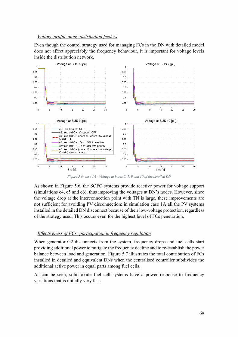
69
Voltage profile along distribution feeders
Even though the control strategy used for managing FCs in the DN with detailed model
does not affect appreciably the frequency behaviour, it is important for voltage levels
inside the distribution network.
Figure 5.6: case 1A - Voltage at buses 5, 7, 9 and 10 of the detailed DN
As shown in Figure 5.6, the SOFC systems provide reactive power for voltage support
(simulations c4, c5 and c6), thus improving the voltages at DN’s nodes. However, since
the voltage drop at the interconnection point with TN is large, these improvements are
not sufficient for avoiding PV disconnection: in simulation case 1A all the PV systems
installed in the detailed DN disconnect because of their low-voltage protection, regardless
of the strategy used. This occurs even for the highest level of FCs penetration.
Effectiveness of FCs’ participation in frequency regulation
When generator G2 disconnects from the system, frequency drops and fuel cells start
providing additional power to mitigate the frequency decline and to re-establish the power
balance between load and generation. Figure 5.7 illustrates the total contribution of FCs
installed in detailed and equivalent DNs when the centralised controller subdivides the
additional active power in equal parts among fuel cells.
As can be seen, solid oxide fuel cell systems have a power response to frequency
variations that is initially very fast.

70
Figure 5.7: Primary frequency control – total FCs power contribution (simulation c2)
This feature results in a faster arresting of the frequency decrease and, consequently, the
lower values reached during the transient is less critical compared to the simulation in
which fuel cell systems do not contribute.
Figure 5.8: Frequency at TN's bus 7 - without and with FC participation (simulations c0 and c2)
Figure 5.9: Comparison of Maximum and Steady-State Δf (simulations c0 and c2)

71
Figure 5.9 underlines the improvements in frequency response obtained thanks to the
participation of fuel cells in primary frequency regulation. Both the maximum and the
steady state frequency error are significantly reduced.
Table 5.4 and Table 5.5 contain significant data about frequency response for each
simulation carried out. The values represent the following: f0 is the frequency pre-
perturbation, f∞ is the steady-state frequency value reached after the action of primary
controllers and fmin is the minimum frequency level during the transient.
simulation f0 [Hz] f∞ [Hz] fmin
[Hz]
FRI1
[MW/Hz]
FRI2
[MW/Hz]
c0 49.9986 49.8014 49.52 2418.3 996.6893
d 49.9986 49.8596 49.6121 3431 1234.1
c1 49.9986 49.8596 49.6119 3429.1 1217.4
c2 49.9986 49.8596 49.6122 3431 1234.5
c3 49.9986 49.8596 49.6121 3431 1234.2
c4 49.9986 49.8588 49.6099 3410.5 1227.2
c5 49.9986 49.8586 49.6086 3407.2 1223
c6 49.9986 49.8586 49.6086 3405.8 1207.6
Table 5.4: Simulations' results case 1A - Frequency metrics
simulation f0 [Hz] f∞ [Hz] fmin
[Hz]
FRI1
[MW/Hz]
FRI2
[MW/Hz]
c2_h 49.9996 49.86 49.6118 3414.8 1230
c3_h 49.9996 49.8599 49.6117 3414.7 1229.8
c4_h 49.9996 49.8579 49.6065 3365.5 1213.5
c5_h 49.9994 49.8575 49.6032 3360.8 1203.8
c6_h 49.9994 49.8575 49.6031 3360.8 1203.5
Table 5.5: Simulations' results case 1A - Frequency metrics (higher FC penetration level)
According to Table 5.4 and Table 5.5 the system’s frequency response is slightly worse
when SOFCs provide reactive power for voltage support, namely in simulations c4, c5
and c6. If these control strategies are used, frequency indices are even worse compared
to those obtained in simulation c1, where FCs in the detailed DN do not participate neither
in frequency nor in voltage control.
This is caused by the constant-impedance loads used in the high-voltage TN model. In
fact, when fuel cells provide voltage support, the reactive power consumption at bus 4
decreases. Voltage levels at TN’s buses are thus improved and constant-Z loads withdraw
more active power. The amount of this additional consumption is larger than the amount
of active power provided by FCs (in the detailed DN) for frequency regulation and,
therefore, the frequency response is decayed.

72
5.5 Case 2A
The initial rate of decline of frequency after a power imbalance depends on the magnitude
of the imbalance and on the overall system inertia. In other words, reducing system inertia
will result in a faster frequency drop for equal power imbalance.
Similarly, a larger difference between generation and load power will cause a faster
frequency variation if the system inertia is fixed.
The most dangerous consequence of a fast frequency decline is related to the minimum
frequency value during the transient: holding the frequency response timing fixed, a faster
decline will result in a lower minimum point. That means, in low inertia systems, primary
frequency controllers should provide a faster response and follow imbalances with a
shorter delay.
In electrical power systems, the overall inertia could be reduced when inertia-less
generators, such as photovoltaic systems and fuel cells, replace large traditional power
plants.
In particular, when traditional power plants are not dispatched because of high level of
renewable and non-programmable resources, the system frequency stability is
endangered. In fact, whenever a significant part of generation is obtained thanks to non-
programmable resources, sudden and noticeable power imbalance could occur even
without faults or extraordinary events, but simply because of weather changes.
Case 2A has the purpose of analysing the frequency response of a low-inertia system with
high levels of PV penetration. In addition, support of fuel cell systems for frequency
regulation is investigated.
5.5.1 Scenario case 2A
The same scenario simulated in chapter 4.5 is here used to analyse the effectiveness of
FCs’ participation in primary frequency regulation when a sudden change in weather
conditions causes a power imbalance in scenarios with high level of PV penetration.
Table 5.6: Scenario case 2A

73
The generator G1 that was connected (according to CIGRé) to TN’s bus number 2 has
been removed for representing the shut-off of traditional generators that are not
dispatched because they have been replaced by a large number of distributed generators.
Here, the power imbalance between generation and load is caused by a reduction in solar
irradiation in the area of the DN (equivalent model) connected to TN’s bus 2.
Besides the equivalent model that represents this DN, loads of other three buses have
been partly replaced by the equivalent model that emulates the participation of FCs in
frequency support.
Table 5.7 and Table 5.8 contain the data used for constant-impedance loads and
equivalent DN model and the resulting aggregate properties for case 2A.
BUS
Constant-Z load Equivalent DN model
P
[MW]
Q
[MVAR]
Installed
Load
[MW]
Loads
cosφ
Load
profile
[pu]
Penetration
of PV [%]
PV
cosφ
Installed
FC
[MW]
3 162.5 122 300 0.9 1 30 0.97 100
4 163 122 275 0.88 1 25 0.9 100
5 0 0 495 0.91 0.6 40 0.94 0
6 217.5 148 400 0.91 1 25 0.92 200
Table 5.7: Constant-Z loads and eqv. DN models used in case 1A.
BUS
Aggregate DNs Data
P (net value)
[MW]
Q (net
value)
[MVAR]
Penetration
of PV [%]
Penetration
of FC [%]
3 325.20 245.42 19.46 21.62
4 326.13 240.46 15.70 22.83
5 110.88 157.98 40.00 0.00
6 425.50 291.05 16.19 32.39
Table 5.8: Aggregate DNs data - case 1A
In simulation case 2A, the reduction of PV generation in distribution network (equivalent
model) connected to bus 5 is assumed as the generation loss as the cause for frequency
decline. Therefore, it is used for computing frequency metrics. Any other PV
disconnection in other distribution network is considered as a result of an event in DN at
TN’s bus 5.
This assumption is made with the aim to identify a common initial cause for all the
simulations. Strategies that avoid PVs disconnection will thus result better also because
they reduce the net power imbalance between generation and loads.

74
Since PVs in the DN at bus 5 disconnect after the drop in solar irradiation level, the ΔP
that causes the frequency decline is the PV generation power in this distribution network
before the perturbation: 184 MW.
5.5.2 Results
Figure 5.10 shows the frequency response of the system when fuel cells do not contribute
to frequency regulation (simulation c0): during the transient, the frequency reaches the
minimum value of 49.844 Hz and then it is stabilised at 49.927 Hz. EG is computed as the
ratio between the power imbalance (in case 2A it is the reduction of PVs in the equivalent
DN at bus 5: 184 MW) and the steady state frequency error, which is 0.0721 Hz.
𝐸𝐺 =𝑝𝑜𝑤𝑒𝑟 𝑖𝑚𝑏𝑎𝑙𝑎𝑛𝑐𝑒
𝑠𝑡𝑒𝑎𝑑𝑦 𝑠𝑡𝑎𝑡𝑒 ∆𝑓=184 [𝑀𝑊]
0.0721 [𝐻𝑧]= 2552 [𝑀𝑊 𝐻𝑧⁄ ]
(5.6)
According to the energy EG, system configurations 1A and 2A turn out to have a similar
primary frequency capability. In both simulation cases, one of the generators of the
original HV benchmark network does not contribute to frequency control: in case 1A G2
cannot participate because it disconnects suddenly, while in case 2A generator G1 is shut
down.
Figure 5.10: Case 2A - frequency response without FCs' participation (simulation c0, measure at TN's bus 8)
Effectiveness of FCs’ participation in frequency regulation
Figure 5.11 illustrates the improvement in frequency response achieved thanks to the
participation of solid oxide fuel cells in primary frequency regulation.

75
Figure 5.11: Frequency at TN's bus 8 - without and with FC participation (simulations c0 and c2)
Since the control strategy that is used only slightly affects the overall frequency
behaviour, only simulation c2 is used for evaluating the effectiveness of the use of FCs
for frequency support. As in case 1A, both maximum and steady state Δf are significantly
reduced (Figure 5.12).
Figure 5.12: case 2A - Comparison of Maximum and Steady-State Δf (simulations c0 and c2)
The control strategy used for managing fuel cells strongly affect voltage profiles in the
distribution feeders. Figure 5.13 shows data about voltages along the feeder 1 of the
detailed distribution network model.

76
Figure 5.13: case 2A - Voltage at buses 5, 7, 9 and 10 of the detailed DN
Figure 5.14: Active power generation from PVs installed in the equivalent DN
Contrary to what happened in simulation case 1A, in this scenario the reactive power
provided by SOFCs in simulations c4, c5 and c6 results in voltage levels among feeders
that are higher than the disconnection threshold for PVs (0.85 pu). Therefore,

77
photovoltaic systems remain connected to the detailed DN model in simulations c4, c5
and c6. Obviously, the detailed DN withdraws less active and reactive power when
photovoltaic systems do not disconnect. The total PV generation within the detailed DN
is illustrated in Figure 5.14 for different control strategies.
It must be noted that the control strategy “c3”, which allocates larger portions of active
power to those buses where the voltage level is more critical but does not involve reactive
power, does not avoid the disconnection of PV generators. Its only effect is to barely
delay the disconnection compared to the strategy in which the additional active power for
frequency support is equally divided among SOFC systems (c2).
simulation f0 [Hz] f∞ [Hz] fmin
[Hz]
FRI1
[MW/Hz]
FRI2
[MW/Hz]
c0 49.9991 49.9270 49.8436 2552.7 1183.4
c1 49.9988 49.9496 49.9181 3739.6 2280.3
c2 49.9988 49.8596 49.9180 3741.4 2278.1
c3 49.9988 49.9495 49.9180 3734 2276.8
c4 49.9988 49.9501 49.9175 3782.8 2263.7
c5 49.9988 49.9501 49.9174 3782.6 2260.7
c6 49.9988 49.9501 49.9175 3783.6 2263.9
Table 5.9: Simulations' results case 2A - Frequency metrics
simulation f0 [Hz] f∞ [Hz] fmin
[Hz]
FRI1
[MW/Hz]
FRI2
[MW/Hz]
c2_h 49.9997 49.9512 49.9186 3789.9 2266.9
c3_h 49.9997 49.9512 49.9190 3791.8 2279.5
c4_h 49.9998 49.9504 49.9173 3727.2 2230.2
c5_h 49.9996 49.9504 49.9177 3737.7 2244.8
c6_h 49.9997 49.9504 49.9174 3728.9 2234.4
Table 5.10: Simulations' results case 2A - Frequency metrics (higher FC penetration level)
In terms of steady state frequency value following the primary regulation, strategies that
allow PVs to stay connected by providing reactive power for voltage support prove to be
more effective, even though the participation of FCs’ in frequency regulation is
completely annulled. The improvement of voltage levels in the transmission network and
the consequent increase of consumption of constant-Z loads also occurs in case 2A.
However, this effect is negligible compared to the power provided by PV systems
installed in the detailed network.
Therefore, strategies c5 and c6 ensure better performance compared to strategies that do
not consider the voltage support through injection of reactive power at specified DN’s
nodes.

78
6 Conclusions and future works
Real-time simulation represents a powerful tool for engineers and researchers and has
capabilities that are beyond those of conventional offline simulations, such as hardware
in the loop, software in the loop and rapid control prototyping.
The main concern about the use of real-time simulations is the computational power
required for achieving the real-time when the model under studies is large and complex.
Decoupling the model and running different parts on different real-time simulator
overcomes the computational limitations of a single simulator.
Analysis of electrical power systems are a suitable application for this type of real time
simulation. Indeed, in modern and future power systems, an increasing number of
interaction among components and operators is emerging. In order to face these new
challenges, simulations that include detailed models of different parts of the system are
crucial.
This work underlines the interactions between transmission and distribution networks in
scenarios with high levels of DG penetration and exploits potentialities of real-time
simulation co-simulation for power systems analysis.
Most of the phenomena analysed in this work would not be observable without the use of
joint simulations of transmission and distribution networks. This justifies the need of
simulation platforms that allow such kind of analysis.
Simulation results obtained in this work indicate that the low voltage ride through
capability proves to be a crucial requirement for distributed generation. Especially in
scenarios with a high level of PV penetration, this capability improves the overall
behaviour of distribution networks when a voltage drop spreads from the transmission
network to distribution feeders.
Furthermore, simulations demonstrate the potential interactions between different
distribution networks, which are caused by the change in weather condition in a
geographical area with a high PV penetration level. This indicates the need of
countermeasures that aim to prevent the propagation of voltage drops caused by the
disconnection of many generators that rely on intermittent energy resources.
A comprehensive set of simulation results prove that the use of solid oxide fuel cell
systems for primary frequency regulation is a promising solution. Due to their fast
response, even the inertial frequency response is improved significantly. Furthermore,
since fuel cell systems are easily controllable and do not rely on an intermittent energy
resource, their participation in frequency control is guaranteed regardless to weather
conditions. This overcomes reliability issue that would arise if the frequency regulation
was partly provided, for instance, by PV systems (PV curtailment technics). Under certain
conditions, exploiting the FCs inverter capability for providing voltage support through
reactive power injections instead of for providing active power, can be more effective
even from a frequency response point of view. In fact, if the voltage improvement avoids

79
the disconnection of distributed generation, the resulting effect is a lower power
imbalance and, consequently a better frequency response.
It must be noted that some simulations investigated here represent scenarios that are
intentionally created for extreme operating condition studies. In this way, the application
of co-simulation interface between OPAL and RTDS has been emphasized with
significant transients. In all the simulation cases analysed here, the interface has proven
to be stable and allows high-fidelity co-simulations.
Beyond the analysis of DERs integration in power systems, this work aimed to
consolidate the co-simulation platform OPAL-RTDS and provide a basis for future co-
simulations and studies about transmission-distribution interactions. Furthermore,
transmission and distribution benchmark networks here implemented, respectively for
being simulated in RTDS and OPAL, are designed for studying the integration of
distributed energy resources in the electrical power system. Therefore, they represent a
suitable framework for many contemporary analysis of the electrical system.
The clear modularity of the co-simulation platform allows an easy expansion of the
simulated system by running other detailed models by the use of other real-time
simulators. Therefore, other large models can be connected to the system, such as high-
voltage DC networks (HVDC), large offshore wind parks or simply other detailed
distribution networks.
Even though the use of the equivalent model for DNs (which emulates PV disconnection
and FCs participation in frequency control) has been successfully used in this work for
obtaining transmission-distribution interactions, modelling all the distribution networks
with detailed models would provide a higher fidelity co-simulation environment for
studying transmission-distribution interactions. In fact, the equivalent DN model provides
acceptable results in terms of aggregated characteristics, but it does not provide any
knowledge about transients inside the distribution network. Furthermore, studies and tests
that are affected by local values and local behaviour inside the distribution network
require a detailed model. For instance, the investigation about voltage support of fuel cell
systems carried out in chapter 5, requires a detailed representation of the distribution
network.
Another possible improvement could be the replacement of transformers in the
benchmark DN model by OLTC transformers. The use of OLTC transformers together
with a proper LVRT capability curve for DG should enhance the overall low-voltage ride
through behaviour of distribution network.

80
References
[1] A. Cagnano, E. D. Tuglie, M. Liserre and R. A. Mastromauro, “Online Optimal
Reactive Power Control Strategy of PV Inverters,” IEEE Transactions on Industrial
Electronics, vol. 58, pp. 4549 - 4558, 2011.
[2] S. A. A. Kazmi, M. K. Shahzad, A. Z. Khan and D. R. Shin, “Smart Distribution
Networks: A Review of Modern Distribution Concepts from a Planning
Perspective,” Energies, vol. 10, 2017.
[3] M. Bollen, Y. Yang and F. Hassan, “Integration of Distributed Generation in the
Power System – A Power Quality Approach,” in 13th International Conference on
Harmonics and Quality of Power, Wollongong, Australia, 2008.
[4] J. C. Boemer, B. G. Rawn, M. Gibescu, M. A. van der Meijden and W. L. Kling,
“Response of wind power park modules in distribution systems to transmission
network faults during reverse power flows,” IET Renewable Power Generation, vol.
9, pp. 1033-1042, 2015.
[5] “Dynamic Simulations of Combined Transmission and Distribution systems using
Decomposition and Localization,” in IEEE Grenoble Conference, Grenoble, 2013.
[6] W. Zhao, X. Shi, Q. Guo, H. Sun, F. Xu, Z. Li, T. Niu and B. Wang, “Voltage
security analysis with high PVs penetration considering the interaction of
transmission and distribution grids: Case studies,” in IEEE PES Asia-Pacific Power
and Energy Engineering Conference (APPEEC), Brisbane, Australia, 2015.
[7] B. Palmintier, E. Hale, T. Hansen, W. Jones, D. Biagioni, K. Baker, H. Wu, J.
Giraldez, H. Sorensen, M. Lunacek, N. Merket, J. Jorgenson and B.-M. Hodge,
“Final Technical Report: Integrated Distribution-Transmission Analysis for Very
High Penetration Solar PV,” 2016.
[8] “Smart Net,” [Online]. Available: http://smartnet-project.eu/.
[9] R. Brundlinger, T. Strasser, G. Lauss, A. Hoke, S. Chakraborty, G. Martin, B.
Kroposki, J. Johnson and E. d. Jong, “Lab Tests: Verifying That Smart Grid Power
Converters Are Truly Smart,” IEEE Power and Energy Magazine, vol. 13, pp. 30 -
42, 2015.
[10] “ERIC-LAB: European Real-time Integrated Co-simulation laboratory,” [Online].
Available: http://www.eric-lab.eu/.
[11] C. F. Covrig, G. D. Santi, G. Fulli, M. Masera, M. Olariaga, E. Bompard, G. Chicco,
A. Estebsari, T. Huang, E. Pons, F. Profumo, A. Tenconi, R. W. D. Doncker, M.
Grigull, A. Monti, M. Stevic and S. Vogel, A European Platform for Distributed

81
Real Time Modelling & Simulation of Emerging Electricity Systems, Publications
Office of the European Union, 2016.
[12] CIGRE, “Brochoure 575 - Benchmark Systems for Network Integration of
Renewable and Distributed Resources,” 15 May 2013. [Online]. Available:
http://www.e-cigre.org/Order/select.asp?ID=16639.
[13] J. H. Eto, “Use of Frequency Response Metrics to Assess the Planning and
Operating Requirements for Reliable Integration of Variable Renewable
Generation,” LBNL: Lawrence Berkeley National Laboratory, 2011.
[14] J. Bélanger, P. Venne and J.-N. Paquin, “The What, Where and Why of real-time
simulation,” IEEE Transactions on Smart Grid, pp. 37-49, 2010.
[15] M. D. O. Faruque, T. Strasser, G. Lauss, V. Jalili-Marandi, P. Forsyth, C. Dufour,
V. Dinavahi, A. Monti, P. Kotsampopoulos, J. A. Martinez, K. Strunz, M.
Saeedifard, X. Wang, D. Shearer and M. Paolone, “Real-Time Simulation
Technologies for Power Systems Design, Testing, and Analysis,” IEEE Power and
Energy Technology Systems Journal, vol. 2, pp. 63-73, June 2015.
[16] X. Guillaud, M. O. Faruque, A. Teninge, A. H. Hariri, L. Vanfretti, M. Paolone, V.
Dinavahi, P. Mitra, G. Lauss, C. Dufour, P. Forsyth, A. K. Srivastava, T. Strasser,
K. Strunz and A. Davoudi, “Applications of Real-Time Simulation Technologies in
Power and Energy Systems,” IEEE Power and Energy Technology Systems
Journal, vol. 2, no. 3, pp. 103-115, 2015.
[17] V. Levi, M. Kay and I. Povey, “Reverse power Flow Capability of tap-changers,”
in 18th International Conference and Exhibition on Electricity Distribution, Turin,
Italy, 2005.
[18] B. P. Hayes, A. J. Collin, J. L. Acosta and S. Z. Djokic, “Assessment of the
Influence of Distributed Generation and Demand Side Management on
Transmission System Performance,” in 7th Mediterranean Conference and
Exhibition on Power Generation, Transmission, Distribution and Energy
Conversion, Agia Napa, Cyprus, 2010.
[19] J. Morren, S. W. H. d. Haan and J. A. Ferreira, “Contribution of DG Units to
Primary Frequency Control,” in International Conference on Future Power
Systems, Amsterdam, Netherlands, 2006.
[20] J. Morren, S. W. d. Haan and J. Ferreira, “Primary Power/Frequency Control with
Wind Turbines and Fuel Cells,” in IEEE Power Engineering Society General
Meeting, 2006.
[21] M. Benini, S. Canevese, D. Cirio and A. Gatti, “Battery Energy Storage Systems
for the Provision of Primary and Secondary Frequency Regulation in Italy,” in IEEE
82
16th International Conference on Environment and Electrical Engineering
(EEEIC), Florence, Italy, 2016.
[22] P. Aristidou and T. V. Cutsem, “Dynamic Simulations of Combined Transmission
and Distribution systems using Decomposition and Localization,” in IEEE
Grenoble Conference, Grenoble, 2013.
[23] W. Zhao, X. Shi, Q. Guo, H. Sun, F. Xu, Z. Li, T. Niu and B. Wang, “Voltage
security analysis with high PVs penetration considering the interaction of
transmission and distribution grids: Case studies,” in IEEE PES Asia-Pacific Power
and Energy Engineering Conference (APPEEC), Brisbane, Australia, 2015.
[24] G. Delille, B. Francois and G. Malarange, “Dynamic Frequency Control Support by
Energy Sorage to Reduce the Impact of Wind and Solar Generation on Isolated
System's Inertia,” IEEE transactions on suitanable energy, vol. 3, no. 4, pp. 931-
939, 2012.
[25] J. Alipoor, Y. Miura and T. Ise, “Distributed generation grid integration using
virtual synchronous generator with adoptive virtual inertia,” in IEEE Energy
Conversion Congress and Exposition (ECCE), Denver, CO, USA, 2013.
[26] P. Author and B. Kirby, “Spinning Reserve From Responsive Loads,” Oak Ridge
National Laboratory, 2003.
[27] B. Silva, C. L. Moreira, L. Seca, Y. Phulpin and J. A. P. Lopes, “Provision of Inertial
and Primary Frequency Control Services Using Offshore Multiterminal HVDC
Networks,” IEEE Transactions on Sustainable Energy , vol. 3, no. 4, pp. 800-808,
2012.
[28] M. Świerczyński, D. I. Stroe, A. I. Stan and R. Teodorescu, “Primary frequency
regulation with Li-ion battery energy storage system: A case study for Denmark,”
in ECCE Asia Downunder, Melbourne, Australia, 2013.
[29] P. P. Zarina, S. Mishra and P. C. Sekhar, “Deriving inertial response from a non-
inertial PV system for frequency regulation,” in IEEE International Conference on
Power Electronics, Drives and Energy Systems (PEDES), Bengaluru, India, 2012.
[30] H. Xin, Y. Liu, Z. Wang, D. Gan and T. Yang, “A New Frequency Regulation
Strategy for Photovoltaic Systems Without Energy Storage,” IEEE Transactions on
Sustainable Energy, vol. 4, no. 4, pp. 985-993, 2013.
[31] J. Johnson, J. C. Neely, J. J. Delhotal and M. Lave, “Photovoltaic Frequency–Watt
Curve Design for Frequency Regulation and Fast Contingency Reserves,” IEEE
Journal of Photovoltaics, vol. 6, no. 6, pp. 1611-1618, 2016.
[32] M. H. Nehrir and C. Wang, Modeling and Control of Fuel Cells, IEEE Press, 2009.

83
[33] F. Gao, M. Kabalo, B. Blunier and A. Miraoui, “Chapter 6: Fuel Cell Systems,” in
Power Electronics for Renewable and Distributed Renewable and Distributed,
Golden, CO (USA), Springer, pp. 185-234.
[34] S. Chowdhury, S. Chowdhury and P. Crossley, “Appendix D: Application of solid-
oxide fuel cell in distributed power generation,” in Microgrids and Active
Distribution Networks, London, 2009, pp. 215-226.
[35] Y. Zhu and K. Tomsovic, “Development of models for analyzing the load-following
performance of micro-turbines and fuel cells,” J. Elect. Power Syst. Res., vol. 62,
no. 1, pp. 1-11, May 2000.
[36] Y. H. Li, S. S. Choi and S. Rajakaruna, “An analysis of the control and operation
of a solid oxide fuel-cell power plant in an isolated system,” IEEE Trans. Energy
Convers., vol. 20, no. 2, pp. 381-387, June 2005.
[37] J. Padullésa, G. Aultb and J. McDonalda, “An integrated SOFC plant dynamic
model for power systems simulation,” Journal of Power Sources, vol. 86, pp. 495-
500, March 2000.
[38] Y. H. Li, S. Rajakaruna and S. S. Choi, “Control of a Solid Oxide Fuel Cell Power
Plant in a Grid-Connected System,” IEEE Trans. Energy Convers., vol. 22, no. 2,
pp. 405-413, June 2007.

84
List of figures
Figure 2.1: Real-Time Simulation. ................................................................................... 6
Figure 2.2: Primary Control - Block Diagram ................................................................ 13
Figure 2.3: Frequency dynamic after a sudden power imbalance .................................. 14
Figure 2.4: Power Margins for Generators Participating in Primary Control – Values for
Italy mainland ................................................................................................................. 15
Figure 3.1: Exciter model (RSCAD) .............................................................................. 21
Figure 3.2: Governor and Turbine model (RSCAD) ...................................................... 21
Figure 3.3: Topology of European High Voltage TN Benchmark ................................. 22
Figure 3.4: Portion of Turin DN used for co-simulations .............................................. 23
Figure 3.5: Load Profiles ................................................................................................ 23
Figure 3.6: Topology of European Medium Voltage DN Benchmark ........................... 24
Figure 3.7: Split-up into OPAL cores ............................................................................. 25
Figure 3.8: Solar Irradiation Profile ............................................................................... 26
Figure 3.9: Low Voltage Ride Through curve for DGs in Italy ..................................... 27
Figure 3.10: SOFC - block diagram ............................................................................... 30
Figure 3.11: SOFC system: control and interface with the network .............................. 32
Figure 3.12: Simulation for SOFC controller validation – results ................................. 33
Figure 3.13: Fuel Cells' frequency controller ................................................................. 34
Figure 3.14: Steam Power Plant ..................................................................................... 34
Figure 3.15: Mechanical Power Dynamic of Steam power plant ................................... 35
Figure 3.16: Steam Turbine system - block diagram for frequency regulation .............. 36
Figure 3.17: Frequency controller and turbine behaviour - block diagram .................... 36
Figure 3.18: Frequency response with FCs participating in regulation .......................... 37
Figure 3.19: FCs contribution in frequency regulation ................................................. 37
Figure 3.20: Equivalent model for DNs - conceptual scheme ........................................ 38
Figure 4.1: Co-simulation setup ..................................................................................... 42
Figure 4.2: Turin DN – PVs placement .......................................................................... 43
Figure 4.3: MV benchmark network – PVs placement .................................................. 44
Figure 4.4: Scenario case 1A .......................................................................................... 45
Figure 4.5: Voltages and Currents at the interconnection point ..................................... 46
Figure 4.6: Detailed DN behaviour - Turin DN ............................................................. 47
Figure 4.7: Impact of LVRT capability – MV benchmark network ............................... 48
Figure 4.8: Comparison between detailed and equivalent DN models in case of PVs
disconnection (benchmark DN) ...................................................................................... 50
Figure 4.9: Scenario case 1B .......................................................................................... 51
Figure 4.10: Comparison among equivalent DN models at bus 4 - Turin DN at bus 5 . 52
Figure 4.11: Voltage at the end of feeders "Chieri", "Fiat" and "Brenta" ...................... 53
Figure 4.12: Voltage levels along feeders "Chieri" and "Brenta" .................................. 54
Figure 4.13: Impact of LVRT capability (case1B) – MV benchmark network ............. 54
Figure 4.14: Scenario case 2A ........................................................................................ 56
Figure 4.15: Case 2A (DN: Turin) - simulation results .................................................. 56
Figure 4.16: PVs output power (Turin DN) ................................................................... 57

85
Figure 4.17: Impact of PV penetration level (case 2A) – MV benchmark network ....... 58
Figure 5.1: Frequency response ...................................................................................... 60
Figure 5.2: SOFC systems placement ............................................................................ 61
Figure 5.3: Centralised controller for fuel cells .............................................................. 62
Figure 5.4: Local and Centralised controller - Output P of FC at bus 10 of the detailed
DN .................................................................................................................................. 67
Figure 5.5: Frequency response - impact of the detailed distribution network (simulations
c0, c1, c2, c2_h) .............................................................................................................. 68
Figure 5.6: case 1A - Voltage at buses 5, 7, 9 and 10 of the detailed DN ...................... 69
Figure 5.7: Primary frequency control – total FCs power contribution (simulation c2) 70
Figure 5.8: Frequency at TN's bus 7 - without and with FC participation (simulations c0
and c2) ............................................................................................................................ 70
Figure 5.9: Comparison of Maximum and Steady-State Δf (simulations c0 and c2) ..... 70
Figure 5.10: Case 2A - frequency response without FCs' participation (simulation c0,
measure at TN's bus 8) ................................................................................................... 74
Figure 5.11: Frequency at TN's bus 8 - without and with FC participation (simulations c0
and c2) ............................................................................................................................ 75
Figure 5.12: case 2A - Comparison of Maximum and Steady-State Δf (simulations c0 and
c2) ................................................................................................................................... 75
Figure 5.13: case 2A - Voltage at buses 5, 7, 9 and 10 of the detailed DN .................... 76
Figure 5.14: Active power generation from PVs installed in the equivalent DN ........... 76