Embed Size (px)
Citation preview
Projekt współfinansowany ze środków Unii Europejskiej w ramach Europejskiego Funduszu Społecznego
ROZWÓJ POTENCJAŁU I OFERTY DYDAKTYCZNEJ POLITECHNIKI WROCŁAWSKIEJ
Wrocław University of Technology
Renewable Energy Systems
Jan Iżykowski
POWER SYSTEM FAULTS
Wrocław 2011
Wrocław University of Technology
Renewable Energy Systems
Jan Iżykowski
POWER SYSTEM FAULTS
Advanced Technology in Electrical Power Generation
Wrocław 2011

Copyright © by Wrocław University of Technology
Wrocław 2011
Reviewer: Andrzej Wiszniewski
ISBN 978-83-62098-80-4
Published by PRINTPAP Łódź, www.printpap.pl

Contents
1. Introduction ........................................................................................................ 7
1.1. Nature and causes of faults ......................................................................... 7
1.2. Consequences of faults ............................................................................... 8
1.3. Fault statistics for different items of equipment in a power system ............ 8
1.4. Fault types .................................................................................................... 10
1.4.1. Linear models of faults ...................................................................... 11
1.4.2. Arcing faults ....................................................................................... 14
Dynamic model of arc ....................................................................... 15
Static model of primary arc .............................................................. 19
2. Basics of fault calculations ................................................................................ 21
2.1. Aim of fault calculations ............................................................................. 21
2.2. Pre-fault, fault and post-fault quantities ...................................................... 22
2.3. Per-unit system of fault calculations ........................................................... 24
3. Method of symmetrical components .................................................................. 29
3.1. Basics of the method ................................................................................... 29
3.2. Representation of three-phase balanced Y and ∆ loads in symmetrical components ................................................................................................ 32
3.3. Fault models in terms of symmetrical components of currents .................. 36
3.4. Earth faults – relation between symmetrical components of total fault current ......................................................................................................... 40
4. Modal transformation and phase co-ordinates approaches ................................ 42
4.1. Modal transformation .................................................................................. 42
4.2. Phase co-ordinates approach ....................................................................... 44
4.2.1. Introduction ....................................................................................... 44
4.2.2. Fault model ........................................................................................ 45
4.2.3. Example usage of phase co-ordinates approach ................................ 48
5. Models of rotating machines .............................................................................. 52
5.1. Introduction ................................................................................................. 52
5.2. Model of synchronous generator ................................................................ 52
5.3. Model of synchronous motor ...................................................................... 57
5.4. Model of induction motor ........................................................................... 57

4
6. Models of power transformers ........................................................................... 59
6.1. Introduction ................................................................................................. 59
6.2. Equivalent circuit diagrams of two-winding transformer ........................... 59
6.3. Vector groups of three-phase transformers ................................................. 62
6.4. Models of transformers for symmetrical components ................................ 65
7. Models of overhead and cable lines ................................................................... 69
7.1. Single-circuit overhead lines ....................................................................... 69
7.2. Double-circuit lines ..................................................................................... 70
7.3. Multi-terminal and tapped lines .................................................................. 75
7.4. Overhead line and cable composite networks ............................................. 77
7.5. Networks with series-compensated lines .................................................... 77
7.6. Models of overhead lines ............................................................................ 83
7.6.1. Lumped-parameter models ............................................................... 84
7.6.2. Distributed-parameter models .......................................................... 92
7.7. Cables .......................................................................................................... 93
8. Analysis of three-phase symmetrical faults ....................................................... 95
8.1. Simplification assumptions ......................................................................... 95
8.2. Three-phase fault model ............................................................................. 96
9. Analysis of unsymmetrical faults ...................................................................... 102
9.1. Introduction ................................................................................................. 102
9.2. Phase-to-earth fault ..................................................................................... 102
9.3. Phase-to-phase fault .................................................................................... 106
9.4. Phase-to-phase-to-earth fault ...................................................................... 110
10. Analysis of open-conductor conditions ............................................................. 114
10.1. Introduction ............................................................................................... 114
10.2. One opened conductor .............................................................................. 114
10.3. Two opened conductors ............................................................................ 119
10.4. Open conductor failure combined with single phase-to-earth fault .......... 121
11. Earth faults in medium voltage networks ......................................................... 122
11.1. Introduction ............................................................................................... 122
11.2. Methods of neutral earthing ...................................................................... 123
11.2.1. MV network with isolated neutral .................................................. 126
5
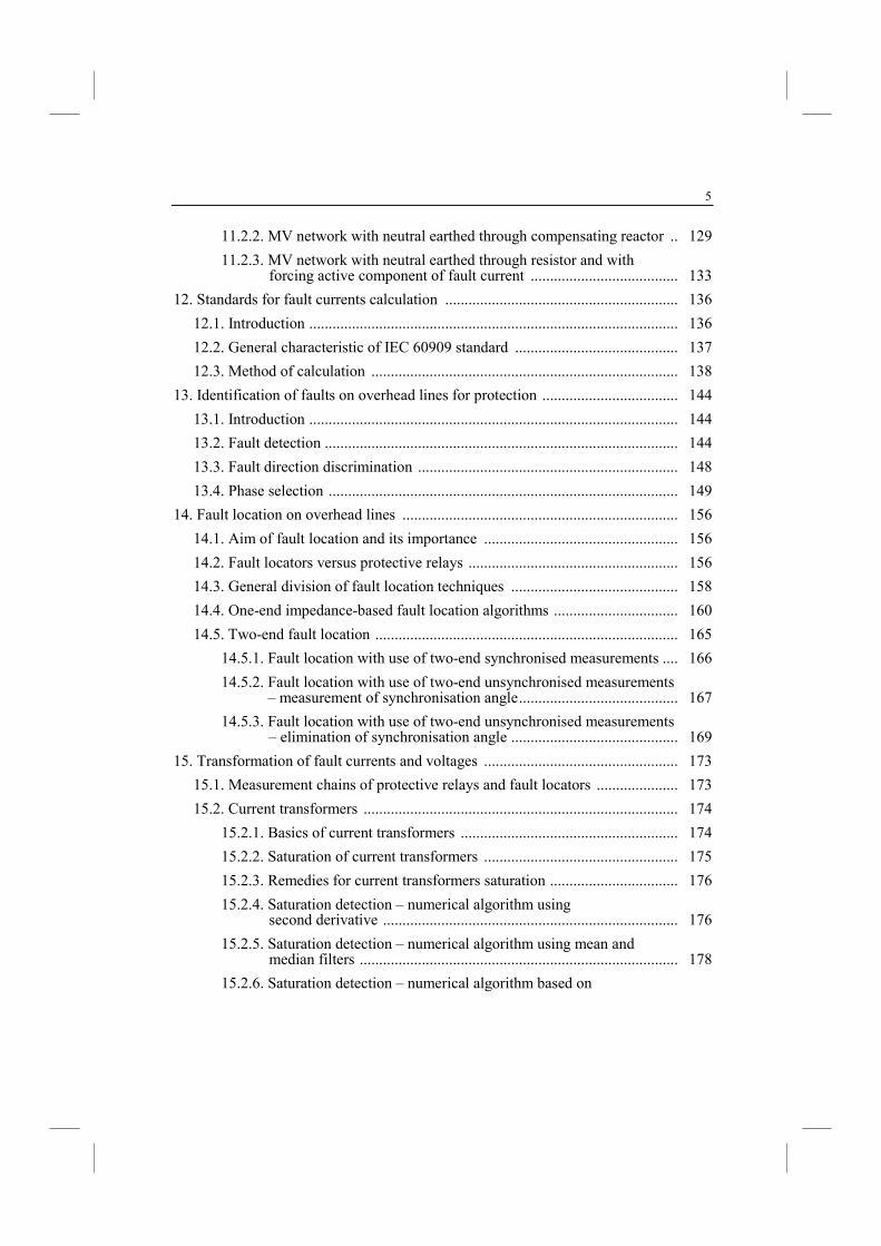
11.2.2. MV network with neutral earthed through compensating reactor .. 129
11.2.3. MV network with neutral earthed through resistor and with forcing active component of fault current ...................................... 133
12. Standards for fault currents calculation ............................................................ 136
12.1. Introduction ............................................................................................... 136
12.2. General characteristic of IEC 60909 standard .......................................... 137
12.3. Method of calculation ............................................................................... 138
13. Identification of faults on overhead lines for protection ................................... 144
13.1. Introduction ............................................................................................... 144
13.2. Fault detection ........................................................................................... 144
13.3. Fault direction discrimination ................................................................... 148
13.4. Phase selection .......................................................................................... 149
14. Fault location on overhead lines ....................................................................... 156
14.1. Aim of fault location and its importance .................................................. 156
14.2. Fault locators versus protective relays ...................................................... 156
14.3. General division of fault location techniques ........................................... 158
14.4. One-end impedance-based fault location algorithms ................................ 160
14.5. Two-end fault location .............................................................................. 165
14.5.1. Fault location with use of two-end synchronised measurements .... 166
14.5.2. Fault location with use of two-end unsynchronised measurements – measurement of synchronisation angle ......................................... 167
14.5.3. Fault location with use of two-end unsynchronised measurements – elimination of synchronisation angle ........................................... 169
15. Transformation of fault currents and voltages .................................................. 173
15.1. Measurement chains of protective relays and fault locators ..................... 173
15.2. Current transformers ................................................................................. 174
15.2.1. Basics of current transformers ........................................................ 174
15.2.2. Saturation of current transformers .................................................. 175
15.2.3. Remedies for current transformers saturation ................................. 176
15.2.4. Saturation detection – numerical algorithm using second derivative ............................................................................ 176
15.2.5. Saturation detection – numerical algorithm using mean and median filters .................................................................................. 178
15.2.6. Saturation detection – numerical algorithm based on
6
modal transformation ..................................................................... 178
15.2.7. Adaptive measuring technique ....................................................... 179
15.3. Capacitive voltage transformers ............................................................... 182
15.3.1. Basics of capacitive voltage transformers ...................................... 182
15.3.2. Transient performance of capacitive voltage transformers ............. 183
15.3.3. Dynamic compensation of capacitive voltage transformers ........... 185
References ........................................................................................................... 188

7
1. Introduction
1.1. ature and causes of faults
The power system items are designed to perform continuously a required function, except when undergo preventive maintenance or other planned actions, or due to lack of external resources. However, inability to perform this function appears due to faults, which are of random character. Faults can occur at any time and at any location of power system items. This is so since all fault causes are random in nature [B8].
In a power system consisting of generators, switchgear, transformers transmission and distribution circuits sooner or later in such a large network some failure will occur somewhere in the system.
A fault implies any abnormal condition which causes a reduction in the basic insulation strength between: • phase conductors or • phase conductors and earth, or any earthed screens surrounding the conductors.
Such reduction of the insulation is not considered as a fault until it produces some effect on the system, i.e. until it results either in an excess current or in the reduction of the impedance between conductors and earth to a value below that of the lowest load impedance to the circuit.
There are varies faults causes. Break-down of the insulation can be caused by lightning strokes on overhead lines. As a result, the connection with earth via an earth wire is established. Also such earth connection occurs when a tree or a man-made object is providing the connecting path. Main causes of failures: • breakdown at normal voltage on account of:
– deterioration of insulation, – damage due to unpredictable causes such as the perching of birds, accidental
short circuiting by snakes, kite strings, tree branches, etc. • breakdown at abnormal voltages (when insulation is healthy to withstand normal
voltage; note that usually a high insulation level of the order of 3 to 5 times the nominal value of the voltage is provided) on account of: – switching surges, – surges caused by lightning (lightning produces a very high voltage surge in

8
the power system of the order of millions of volts, travelling with the velocity of light (c=299 792 458 m/s), and thus it is feasible to provide an insulation which can withstand this abnormality).
Some faults are also caused by switching mistakes of the station personnel.
1.2. Consequences of faults
Fire is a serious result of a major un-cleared faults, may destroy the equipment of its origin, but also may spread in the system causing total failure.
The short circuit (the most common type of fault) may have any of the following consequences: • a great reduction of the line voltage over a major part of the power system, leading
to the breakdown of the electrical supply to the consumer and may produce wastage in production,
• an electrical arc – often accompanying a short circuit may damage the other apparatus in the system,
• damage to the other apparatus in the system due to overheating and mechanical forces,
• disturbances to the stability of the electrical system and this may even lead to a complete blackout of a given power system,
• considerable reduction of voltage on healthy feeders connected to the system having fault, which can cause abnormal currents drawn by motors or the motors will be stopped (causing loss of industrial production) and then will have to be restarted.
1.3. Fault statistics for different items of equipment
in a power system
In fault analysis it is very important how faults are distributed in the various sections of a power system. There are many statistics on that which are available in the literature and internet as well. However, typically, the distribution is as follows: • overhead lines: 50% (thus these faults account for a half of the total number of
faults or even more in the other statistics), • cables: 10%, • switchgear: 15%, • transformers: 12%, • current and voltage transformers (CTs and VT)s: 2%, • control equipment: 3%,
9
• miscellaneous: 8%.
The probability of the failure or occurrence of abnormal condition is more on overhead power lines. This is so due to their: • greater length, • exposure to the atmosphere.
Most of power system faults occur on transmission networks, especially on overhead lines. Lines are those elements in the system in charge of transporting important bulks of energy from generator plants to load centres. Due to their inherent characteristic of being exposed to atmospheric conditions, transmission lines have the highest fault rate in the system.
There are known varies fault statistics, which are related to different voltage levels, technical and weather conditions. All of them unambiguously indicate that more than 75% of total number of power system faults occur on transmission networks. This fact reveals very high importance of fault analysis for transmission networks.
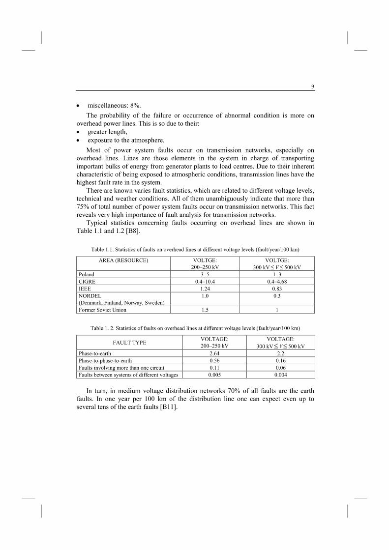
Typical statistics concerning faults occurring on overhead lines are shown in Table 1.1 and 1.2 [B8].
Table 1.1. Statistics of faults on overhead lines at different voltage levels (fault/year/100 km)
AREA (RESOURCE) VOLTGE: 200–250 kV
VOLTGE: 300 kV≤ V ≤ 500 kV
Poland 3–5 1–3 CIGRE 0.4–10.4 0.4–4.68 IEEE 1.24 0.83 NORDEL (Denmark, Finland, Norway, Sweden)
1.0 0.3
Former Soviet Union 1.5 1
Table 1. 2. Statistics of faults on overhead lines at different voltage levels (fault/year/100 km)
FAULT TYPE VOLTAGE: 200–250 kV
VOLTAGE: 300 kV≤V≤500 kV
Phase-to-earth 2.64 2.2 Phase-to-phase-to-earth 0.56 0.16 Faults involving more than one circuit 0.11 0.06 Faults between systems of different voltages 0.005 0.004
In turn, in medium voltage distribution networks 70% of all faults are the earth
faults. In one year per 100 km of the distribution line one can expect even up to several tens of the earth faults [B11].
10
1.4. Fault types
Faults on overhead transmission and distribution lines are the most frequent (see Section 1.3 – Fault statistics for different items of equipment in a power system). Therefore the considerations are limited here basically to such faults.
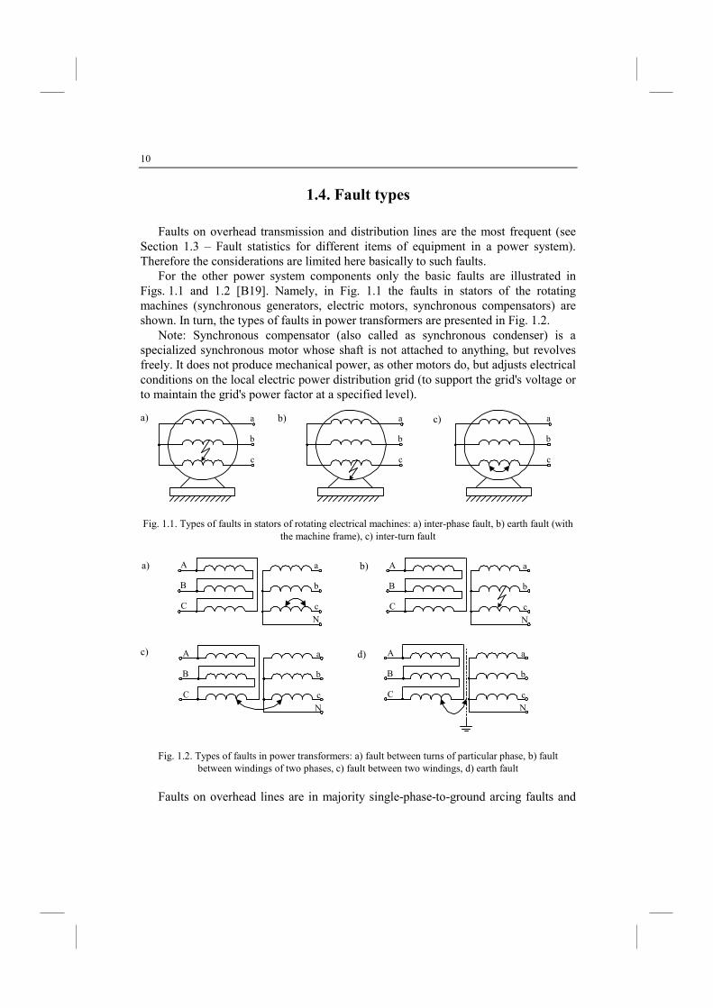
For the other power system components only the basic faults are illustrated in Figs. 1.1 and 1.2 [B19]. Namely, in Fig. 1.1 the faults in stators of the rotating machines (synchronous generators, electric motors, synchronous compensators) are shown. In turn, the types of faults in power transformers are presented in Fig. 1.2.
Note: Synchronous compensator (also called as synchronous condenser) is a specialized synchronous motor whose shaft is not attached to anything, but revolves freely. It does not produce mechanical power, as other motors do, but adjusts electrical conditions on the local electric power distribution grid (to support the grid's voltage or to maintain the grid's power factor at a specified level).
a
b
c
a
b
c
a
b
c
Fig. 1.1. Types of faults in stators of rotating electrical machines: a) inter-phase fault, b) earth fault (with the machine frame), c) inter-turn fault
A
B
C
a
b
c
N
A
B
C
a
b
c
N
A
B
C
a
b
c
N
A
B
C
a
b
c
N
Fig. 1.2. Types of faults in power transformers: a) fault between turns of particular phase, b) fault between windings of two phases, c) fault between two windings, d) earth fault
Faults on overhead lines are in majority single-phase-to-ground arcing faults and
a) b) c)
a) b)
c) d)
11
are temporary in most cases. Therefore, protective relays are provided with the automatic reclosing function [1, 18]. This function allows the line to be reclosed and kept in operation after the fault has disappeared because the arc can self-extinguish. The circuit breakers can operate on a single phase (single pole) or on all three phases. For applying a proper autoreclosing option the fault type is required to be correctly recognized by special techniques.
The main characteristic of faults on overhead lines is related to the fault impedance involved, which can basically be considered as fault resistance. In this respect, the faults are categorized as: • solid (bolted) faults which involve negligible fault resistance and • resistive faults.
Usually, for inter-phase faults, fault resistances are small and in general do not exceed 0.5 Ω. They may, however, become much higher during earth faults, because tower footing resistance may be as high as 10 Ω [20].
If there is a flashover of an insulator, the connection of towers with earth wires makes the resulting fault resistance smaller. In practice, it seldom exceeds 3 Ω. For some earth faults the fault resistances may become much higher, which happens in cases of fallen trees, or if a broken conductor lays on the high-resistive soil.
Mainly basic linear fault models, i.e. with linear fault resistances are taken into account in various studies. However, there are also some cases with treating faults as of non-linear character, i.e. considering the electric arc phenomenon [1, 2, 15]. Also, this phenomenon is widely used in digital simulations [B3] aimed at evaluating accuracy of the calculations performed with the linear fault models. Fault location on power lines is such an example.
1.4.1. Linear models of faults
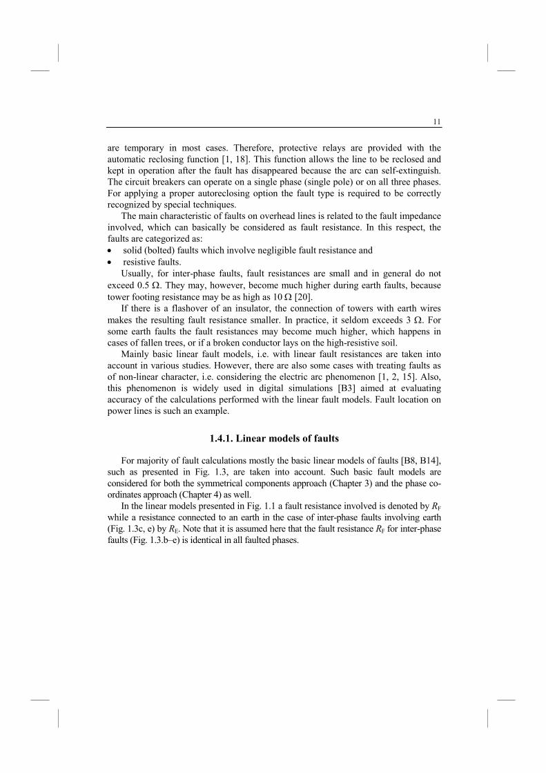
For majority of fault calculations mostly the basic linear models of faults [B8, B14], such as presented in Fig. 1.3, are taken into account. Such basic fault models are considered for both the symmetrical components approach (Chapter 3) and the phase co-ordinates approach (Chapter 4) as well.
In the linear models presented in Fig. 1.1 a fault resistance involved is denoted by RF while a resistance connected to an earth in the case of inter-phase faults involving earth (Fig. 1.3c, e) by RE. Note that it is assumed here that the fault resistance RF for inter-phase faults (Fig. 1.3.b–e) is identical in all faulted phases.
12
a
b
c
RF
a
b
c
RF
a
RF
b
c
RF
RE
a
RF
b
c
RF RF
RE
a
RF
b
c
RF RF
Fig. 1.3. Typical shunt faults: a) phase-to-earth, b) phase-to-phase, c) phase-to-phase-to-earth, d) three-phase, e) three-phase-to-earth
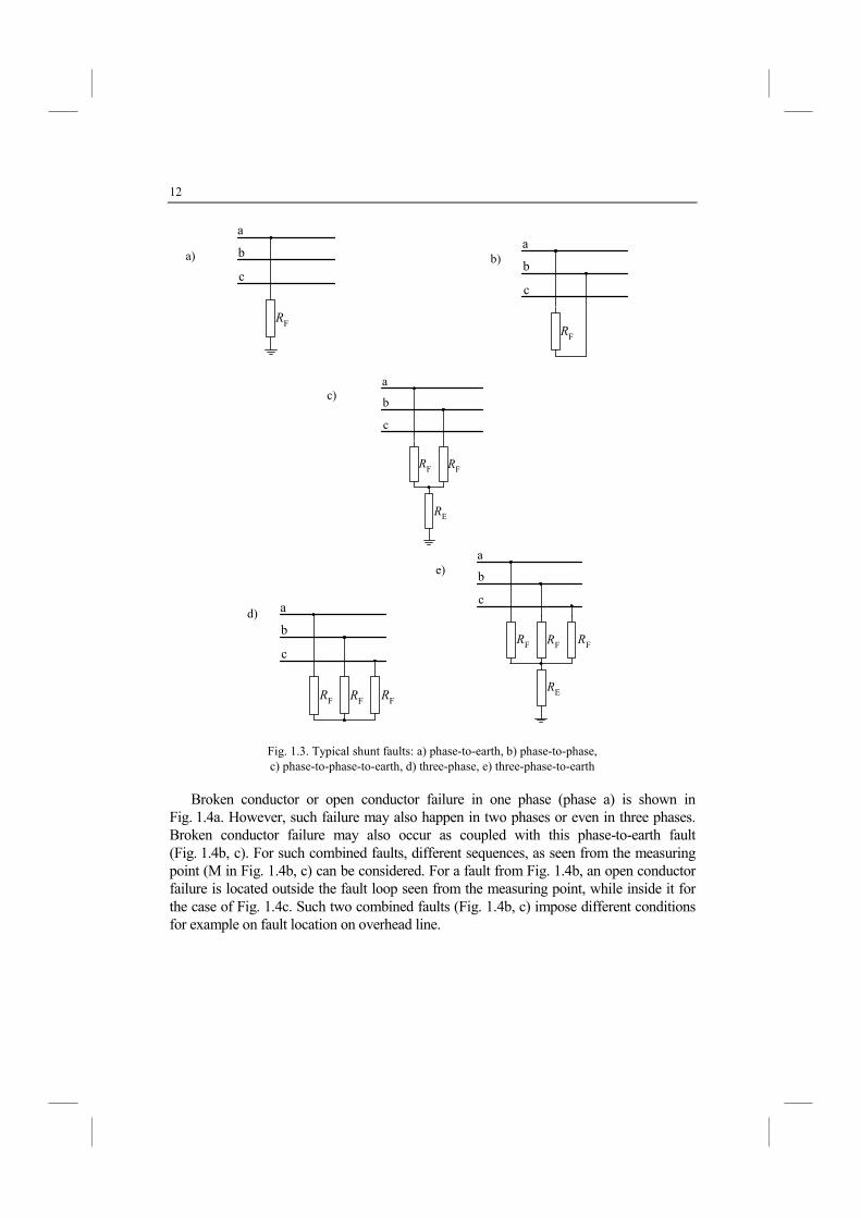
Broken conductor or open conductor failure in one phase (phase a) is shown in Fig. 1.4a. However, such failure may also happen in two phases or even in three phases. Broken conductor failure may also occur as coupled with this phase-to-earth fault (Fig. 1.4b, c). For such combined faults, different sequences, as seen from the measuring point (M in Fig. 1.4b, c) can be considered. For a fault from Fig. 1.4b, an open conductor failure is located outside the fault loop seen from the measuring point, while inside it for the case of Fig. 1.4c. Such two combined faults (Fig. 1.4b, c) impose different conditions for example on fault location on overhead line.
c)
a) b)
e)
d)
13
a
b
c
a
b
c
RF
M
a
b
c
RF
M
Fig. 1.4. Broken conductor faults: a) broken conductor failure alone, b) phase-to-earth fault with broken conductor, c) broken conductor with phase-to-earth fault
Sometimes more than one fault can occur simultaneously. For example, these may all be shunt faults, as shown in Fig. 1.5, where phase-to-earth fault occurs in combination with phase-to-phase fault for the remaining phases. In general, different fault resistances (RF1, RF2) can be involved in these faults.
a
b
c
RF1 RF2
Fig. 1.5. Phase-to-earth fault combined with phase-to-phase fault
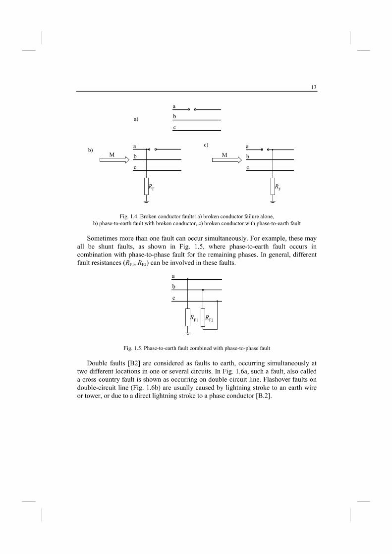
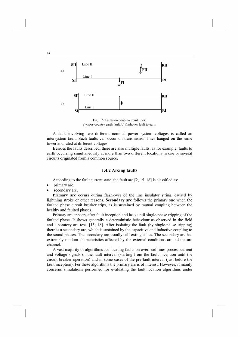
Double faults [B2] are considered as faults to earth, occurring simultaneously at two different locations in one or several circuits. In Fig. 1.6a, such a fault, also called a cross-country fault is shown as occurring on double-circuit line. Flashover faults on double-circuit line (Fig. 1.6b) are usually caused by lightning stroke to an earth wire or tower, or due to a direct lightning stroke to a phase conductor [B.2].
b) c)
a)
14
SI
SII
RI
RII
FII
FI
Line I
Line II
SI
SII
RI
RII
Line I
Line II
Fig. 1.6. Faults on double-circuit lines: a) cross-country earth fault, b) flashover fault to earth
A fault involving two different nominal power system voltages is called an intersystem fault. Such faults can occur on transmission lines hanged on the same tower and rated at different voltages.
Besides the faults described, there are also multiple faults, as for example, faults to earth occurring simultaneously at more than two different locations in one or several circuits originated from a common source.
1.4.2 Arcing faults
According to the fault current state, the fault arc [2, 15, 18] is classified as: • primary arc, • secondary arc.
Primary arc occurs during flash-over of the line insulator string, caused by lightning stroke or other reasons. Secondary arc follows the primary one when the faulted phase circuit breaker trips, as is sustained by mutual coupling between the healthy and faulted phases.
Primary arc appears after fault inception and lasts until single-phase tripping of the faulted phase. It shows generally a deterministic behaviour as observed in the field and laboratory arc tests [15, 18]. After isolating the fault (by single-phase tripping) there is a secondary arc, which is sustained by the capacitive and inductive coupling to the sound phases. The secondary arc usually self-extinguishes. The secondary arc has extremely random characteristics affected by the external conditions around the arc channel.
A vast majority of algorithms for locating faults on overhead lines process current and voltage signals of the fault interval (starting from the fault inception until the circuit breaker operation) and in some cases of the pre-fault interval (just before the fault inception). For these algorithms the primary arc is of interest. However, it mainly concerns simulations performed for evaluating the fault location algorithms under
a)
b)
15
study. This is so since vast majority of fault location algorithms apply linear model of the fault path for their formulation. Only few fault location algorithms take into account the primary arc model.
By measuring voltage on the line-side of a circuit breaker, the location of a permanent fault can be calculated using the transient caused by the fault clearing operation of the circuit breaker. Due to the fault clearing operation of the circuit breaker, a surge is initiated and travels between the opened circuit breaker and the fault, if the latter is still present. The distance to fault is determined by measuring the propagation time of the surge from the opened circuit breaker to the fault. In this relation, modelling the secondary arc is important.
Dynamic model of arc
The dynamic voltage-current characteristics of the electric arc have features of hysteresis. Extensive studies in [2, 15, 18] have shown that the dynamic volt-ampere characteristics of the electric arc can be exactly simulated by the empirical differential equation:
)(1
d
dkk
k
k gGTt
g−= (1.1)
where: the subscript k indicates the kind of arc (k = p for primary arc while k = s for secondary arc), gk – dynamic arc conductance, Gk – stationary arc conductance, Tk – time constant.
The stationary arc conductance Gk can be physically interpreted as the arc conductance value when the arc current is maintained for a sufficiently long time under constant external conditions. So, Gk is the static characteristic of the arc, which can be evaluated from:
kk
kliRv
iG
|)|(
||
0 += (1.2)
where: i – instantaneous arc current, v0k – arc voltage drop per unit length along the main arc column, R – characteristic arc resistance per unit length, lk – arc length.
For the primary arc v0p is constant and equal to about 15 V/cm for the range of current 1.3÷24.0 kA [2] and lp may be assumed constant and somehow wider than the length of the line insulator string. The value of the constant voltage parameter of the
16
secondary arc v0s is evaluated empirically on the basis of numerous investigation results in the range of low values of current, collected in [18]. For the range of peak
currents Is, from approximately 1÷55 A it can be roughly defined as 0.4ss0 75 −= Iv
V/cm. The arc length of the secondary current ls changes with time, and for relatively low
wind velocities (up to 1 m/s), it can be approximated as rps 10 tll = for s 1.0r >t but
when the secondary arc re-ignition time s 1.0r ≤t : ps ll = .
The secondary arc re-ignition voltage (in V/cm) can be calculated using the empirical formula [18]:
))(15.2(
16205
ers
er
TtI
Tv
−++
= (1.3)
where: Te – secondary arc extinguishing time (when tr ≤ Te, vr = 0), Is – peak value of current on the volt-ampere arc characteristic.
Time constants are determined as follows [18]:
k
kkk
l
IT
α= (1.4)
where αk – empirical coefficients. The empirical coefficients αk can be obtained by fitting equation (1.1) with
equations (1.2) and (1.4) to match the experimental dynamic volt-ampere characteristics of the heavy- and low-current arcs, accordingly.
The model (1.1) allows the arc conductance g(t) to be determined, from which the arc resistance rarc(t) = 1/g(t) is calculated.
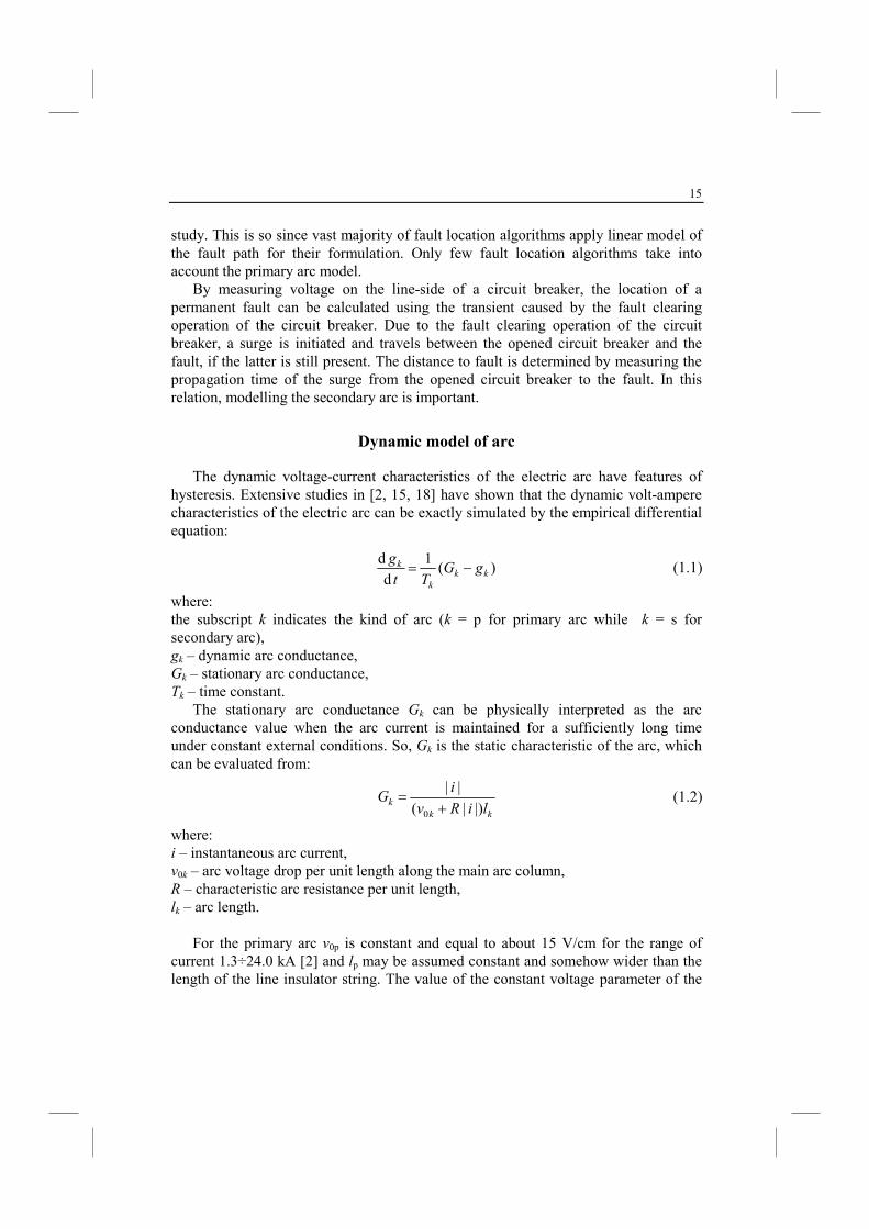
Fig. 1.7 presents the principle of using the ATP-EMTP simulation program [B.3] for arc fault simulation. According to this principle, an arc is reflected with the non-linear resistor – defined in the ELECTRICAL NETWORK unit of the ATP-EMTP, while the arc model – in the MODELS (Fig. 1.7). The arc current as the input quantity is measured on-line and the non-linear differential equation (1.1) is being solved. As a result, the arc resistance is determined and transferred for fixing the resistance of the resistor modelling the arc.
17
ELECTRICALNETWORK
MODELS
ARCMODEL
current
resistance
tim
e va
ryin
gre
sist
or
remainingpart of
the circuit
switch
Fig. 1.7. Modelling of primary arc with ATP-EMTP – interaction between the program units (Electrical Network, Models)
0 10 20 30 40 50
–15
–10
–5
0
5
10
15
Arc
vol
tage
(kV
)
Time (ms) 0 10 20 30 40 50
–15
–10
–5
0
5
10
15
Arc
cur
rent
(kA
)
Time (ms)
(Fig. 1.8 to be continued)
a) b)
18
15–15 –10 –5 0 5 10–15
–10
–5
0
5
10
15
Arc current (kA)
Arc
vol
tage
(kV
)
0 10 20 30 40 500
1
2
3
4
5
6
7
8
Time (ms)
Arc
res
ista
nce
(1/g
), (Ω
)
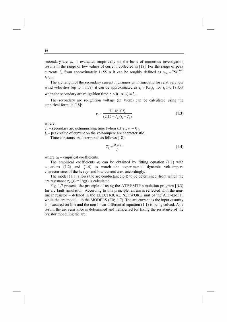
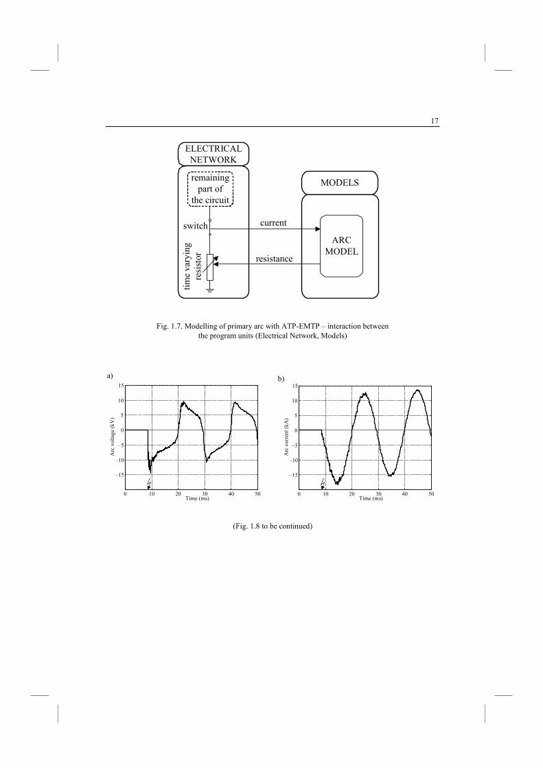
Fig. 1.8. Modelling of primary arc with ATP-EMTP: a) arc voltage, b) arc current, c) arc voltage vs. arc current (for a single cycle), d) arc resistance
c)
d)
19
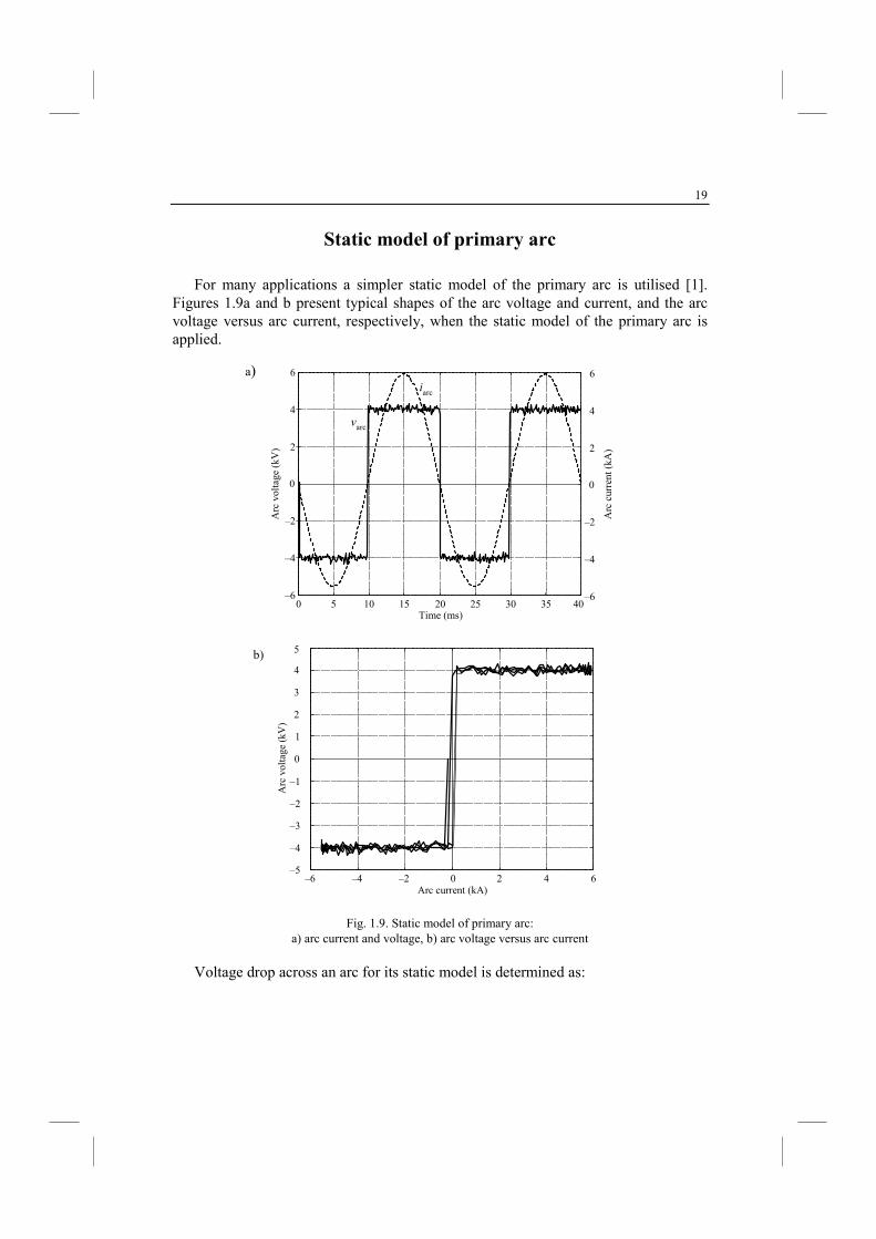
Static model of primary arc
For many applications a simpler static model of the primary arc is utilised [1]. Figures 1.9a and b present typical shapes of the arc voltage and current, and the arc voltage versus arc current, respectively, when the static model of the primary arc is applied.
0 5 10 15 20 25 30 35 40–6
–4
–2
0
2
4
6
–6
–4
–2
0
2
4
6
varc
iarc
Time (ms)
Arc
vol
tage
(kV
)
Arc
cur
rent
(kA
)
Arc
vol
tage
(kV
)
Arc current (kA)–6 –4 –2 0 2 4 6
–5
–4
–3
–2
–1
0
1
2
3
4
5
Fig. 1.9. Static model of primary arc: a) arc current and voltage, b) arc voltage versus arc current
Voltage drop across an arc for its static model is determined as:
a)
b)

20
)]()](signum[)( a ttiVtv ξ+= , (1.5)
where:
ppa lVV = – magnitude of rectangular wave (Vp, lp – as in (1.2)),
)(tξ – Gaussian noise with zero average value.
21
2. BASICS OF FAULT CALCULATIOS
2.1. Aim of fault calculations
There are the following terms in common use for fault analysis [B9]: • fault current calculations, • fault calculations.
The latter term: “fault calculations” appears as more general and is recommended for use. This is so, since besides the need for calculating faults in different points of a power system (for example at fault or at the measuring point), also one can require to calculate voltages at the specific nodes or impedances and other parameters.
Important feature of fault calculations is related to time, i.e. when they are performed: • at the design stage or • for systems in operation.
Faults influence both the power system devices (primary devices) operating at different voltage levels and the measuring, control and protection devices (secondary devices). Therefore, the fault calculations can be related to a primary or secondary device.
Basically, steady state fault calculations are performed, however, sometimes a need for determining transient calculations appears. For example, how transient components contained in the input signals of the protective device influence its performance. Dynamic behaviour of instrument transformers (both current and voltage transformers) could be of our interest. Due to complexity of calculations aimed at determining transients, usually they are replaced by dynamic simulation performed with use of the available software or the programs developed by the user.
The fault calculations results are aimed for diverse use [B9], as for example for: • design of power system apparatus with respect to thermal and mechanical
endurance, • design of configurations of the network with taking into account the expected
levels of fault currents, • design of busbars, • determination of the cross-section area of conductors and cables,
22
• selecting the methods for limiting the fault currents and design of the respective devices,
• analysis of performance of protective relays and their setting for proper their coordination,
• analysis of electrical safety conditions, • determination of influence of fault currents on electric and electronic devices.
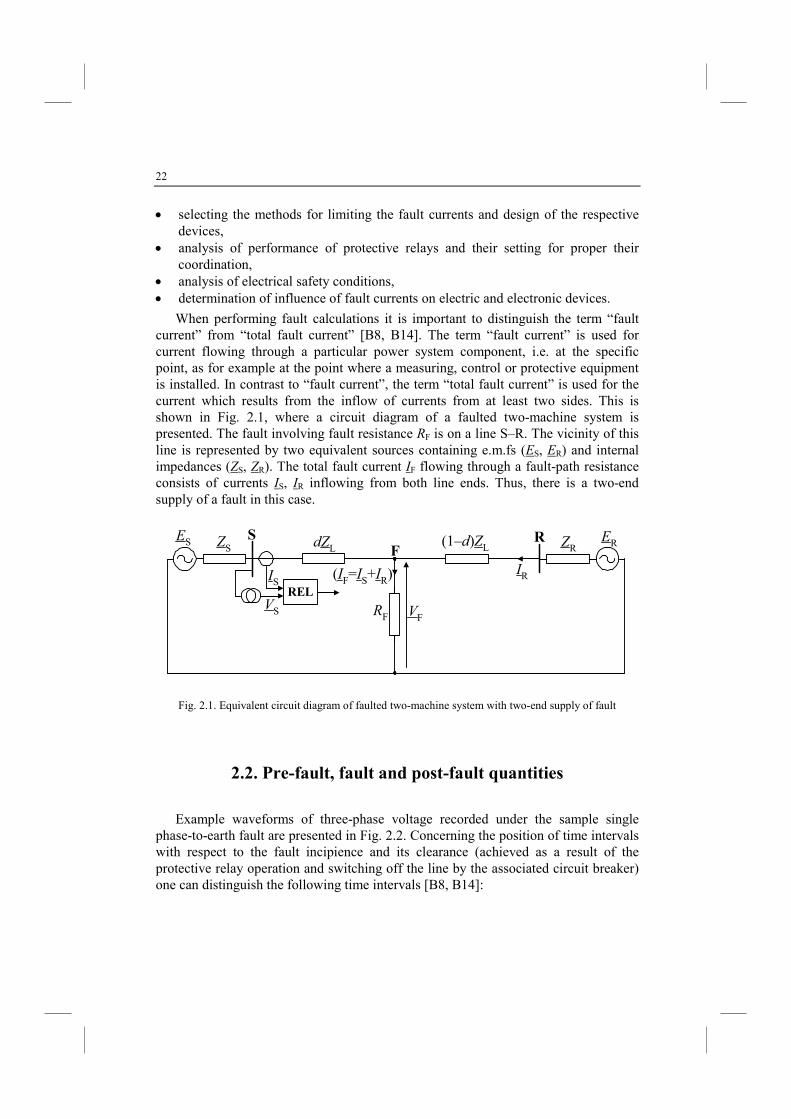
When performing fault calculations it is important to distinguish the term “fault current” from “total fault current” [B8, B14]. The term “fault current” is used for current flowing through a particular power system component, i.e. at the specific point, as for example at the point where a measuring, control or protective equipment is installed. In contrast to “fault current”, the term “total fault current” is used for the current which results from the inflow of currents from at least two sides. This is shown in Fig. 2.1, where a circuit diagram of a faulted two-machine system is presented. The fault involving fault resistance RF is on a line S–R. The vicinity of this line is represented by two equivalent sources containing e.m.fs (ES, ER) and internal impedances (ZS, ZR). The total fault current IF flowing through a fault-path resistance consists of currents IS, IR inflowing from both line ends. Thus, there is a two-end supply of a fault in this case.
RSdZL
(1–d)ZL
IS
VS VF
ZSES
F
(IF=IS+IR)
RF
REL
ERZR
IR
Fig. 2.1. Equivalent circuit diagram of faulted two-machine system with two-end supply of fault
2.2. Pre-fault, fault and post-fault quantities
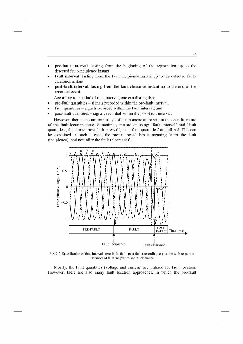
Example waveforms of three-phase voltage recorded under the sample single phase-to-earth fault are presented in Fig. 2.2. Concerning the position of time intervals with respect to the fault incipience and its clearance (achieved as a result of the protective relay operation and switching off the line by the associated circuit breaker) one can distinguish the following time intervals [B8, B14]:
23
• pre-fault interval: lasting from the beginning of the registration up to the detected fault-incipience instant
• fault interval: lasting from the fault incipience instant up to the detected fault-clearance instant
• post-fault interval: lasting from the fault-clearance instant up to the end of the recorded event.
According to the kind of time interval, one can distinguish: • pre-fault quantities – signals recorded within the pre-fault interval; • fault quantities – signals recorded within the fault interval; and • post-fault quantities – signals recorded within the post-fault interval.
However, there is no uniform usage of this nomenclature within the open literature of the fault-location issue. Sometimes, instead of using: ‘fault interval’ and ‘fault quantities’, the terms: ‘post-fault interval’, ‘post-fault quantities’ are utilized. This can be explained in such a case, the prefix ‘post-’ has a meaning ‘after the fault (incipience)’ and not ‘after the fault (clearance)’.
–1
–0.5
0
0.5
1
Thr
ee-p
hase
vol
tage
(10
5 V
)
PRE-FAULT FAULTPOST-
FAULT
Fault incipience
a b c
Time (ms)
Fault clearance
Fig. 2.2. Specification of time intervals (pre-fault, fault, post-fault) according to position with respect to instances of fault incipience and its clearance
Mostly, the fault quantities (voltage and current) are utilized for fault location. However, there are also many fault location approaches, in which the pre-fault
24
quantities are additionally included as the fault-locator input signals. However, sometimes, usage of the pre-fault measurements is treated as the drawback of the fault-location method. This is so, since in some cases the pre-fault quantities could be not recorded or they do not exist, as for example in the case of the current during some intervals of the automatic reclosure process. Also, the pre-fault quantities can be not of pure sinusoidal shape, due to the appearance of the fault symptoms just before its occurrence. Also, in some hardware solutions, measurement of pre-fault (load) currents is accomplished with lower accuracy than for much higher fault currents. Therefore, if it is possible, usually the usage of pre-fault measurements is avoided.
Rather rare usage of the post-fault quantities for the fault location purpose is observed.
2.3. Per-unit system of fault calculations
Power-system quantities such as voltage, current, power, and impedance are often expressed in per-unit or percent of specified base values. Usually, it is more convenient to perform calculations with per-unit quantities than with the actual quantities. Avoiding of many different voltage levels in fault calculations is the main reason of using the per-unit system. So, use of the per-unit system facilitates calculations for multi-level electric networks. The per-unit quantities can be compared more easily since some parameters expressed in per units are from the same range. This also allows finding the calculation errors.
Per unit quantity is calculated as follows:
itybase quant
ntityactual quauantityper unit q = (2.1)
where actual quantity is the value of the quantity in the actual units. The base value has the same units as the actual quantity, thus making the per unit quantity dimensionless.
For example, the per unit voltage (denoted with the subscript [p.u.] or also in many publications with omitting this subscript – for the sake of the simplification):
[V]
[V]
b]pu[
V
VV = (2.2a)
or:
[V]
[V]
bV
VV = (2.2b)
From (2.1) we obtain that:
25
itybase quantuantityper unit qntityactual qua ⋅= (2.3)
and thus:
[V] [V] b]pu[ VVV = (2.4a)
or:
[V] [V] bVVV = (2.4.b)
Different base quantities can be used for three-phase power system elements, but with strict consequence. As for example:
I SYSTEM:
Let us select as the base value: phase voltage (Vb ph) and magnitude of a single phase complex power (Sb ph). Then we obtain for:
current: ph b
ph bb
V
SI = (2.5a)
impedance: ph b
2ph b
ph b
ph bb
)(
S
V
I
VZ == (2.5b)
admittance: b
b1
ZY = (2.5c)
Note: The base value is always a real number and thus the angle of the per unit quantity is the same as the angle of the actual quantity. So: || ph bph b SS = – magnitude
of a complex number. Similarly for a current and voltage base quantities. Per units for the other quantities, as for example for a complex power (also
impedance or admittance) are calculated by dividing the real and imaginary part by the base power, which is a real number:
bbbb
jj
[VA]
[VA]
S
Q
S
P
S
QP
S
SS +=
+== (2.6)
26
II SYSTEM (preferred):
Let us select as the base value: line-to-line voltage (Vb = Vb L-L) and magnitude of a three-phase complex power (Sb = Sb 3ph). Then we obtain for:
current: b
bb
3V
SI = (2.7a)
impedance: b
2b
b
bb
)(
3 S
V
I
VZ == (2.7b)
admittance: b
b1
ZY = (2.7c)
Usually, for generators, transformers and motors, the rated voltage and rated power are assumed as the base quantities.
In order to prepare the common network containing power lines, transformers and generators, the parameters of all items have to be recalculated to the common base quantities. For example the base quantities assumed for the power line can be utilized for the common base. Let us assume the selected new base system (for example: SYSTEM I or II – defined above) for that, and let us denote this new base with use of the square bracket and the subscript ‘new’: • [Vb]new, • [Sb]new.
Using this common base quantities we can recalculate the per unit quantity obtained for the other base quantities, denoted as the ‘old’: • [Vb]old, • [Sb]old.
For example we have the transformer impedance (ZT[p.u.] = [Z]old), which was obtained in relation to the ‘old’ base impedance [Zb]old, resulting from [Vb]old and [Sb]old. There is a question how to recalculate the ‘old’ per unit impedance [Z]old to the ‘new’ per unit impedance [Z]new? This recalculation is as follows:
oldb
newb2
newb
2oldb
old
newb
2newb
oldb
2oldb
old
newb
oldbold
newb
oldbold
newbnew
][
][
)]([
)]([][
][
)]([
][
)]([
][
][
][][
][
][][
][
][ ][
S
S
V
VZ
S
V
S
V
Z
Z
ZZ
Z
ZZ
Z
ZZ
==
=⋅
=Ω
=
(2.8)
If we calculate fault currents without use of a computer we need to perform comparatively simple calculations, therefore, for a common base power we assume usually Sb=100 MVA or Sb=1000 MVA. However, if we use a computer this is not
27
obligatory. In some simplified calculations as the base voltage we do not assume the nominal
voltage of the network but this value increased by 5%: Vb = 1.05Vn. This is so since the nominal voltage of the transformers are usually higher than the nominal voltage of the network (by 5%) [B13].
Example 2.1. Recalculation of per unit reactance data from their own ratings to
the common base
Two generators rated at 10 MVA, 11 kV and 15 MVA, 11 kV, respectively, supply two motors rated 7.5 MVA and 10 MVA, respectively. The generators are connected in parallel to a common bus supplying the motors also connected in parallel. The rated voltage of motors is 9 kV. The reactance of each generator is 0.12 p.u. and that of each motor is 0.15 p.u. on their own ratings. Assume 50 MVA, 10 kV common base for recalculation of the per unit reactances.
Applying (2.8) we get:
Reactance of generator 1: p.u. 726.010
50
10
1112.0
2
G1 =
=X
Reactance of generator 2: p.u. 484.015
50
10
1112.0
2
G2 =
=X
Reactance of motor 1: p.u. 81.05.7
50
10
915.0
2
M1 =
=X
Reactance of motor 2: p.u. 6075.010
50
10
915.0
2
M2 =
=X
Example 2.2. Proof that per unit impedances of transformers do not change when
they are referred from one side of transformer to the other side
Consider a single-phase transformer with HIGH and LOW voltages and currents denoted by VH, VL and IH, IL, respectively.
We have: H
L
L
H
I
I
V
V=
Base impedance for high voltage sideH
H
I
V=
Base impedance for low voltage sideL
L
I
V=
Per unit impedance referred to high voltage sideH
HH
HH
H
V
IZ
IV
Z==
Per unit impedance referred to low voltage sideL
LL
LL
L
V
IZ
IV
Z==

28
Actual impedance referred to secondary
2
H
LH
=
V
VZ
Per unit impedance referred to low voltage side =
H
HH2
H
HHH2
H
LLH
L
L2
H
2L
H
L
L
2
H
LH
)()(
V
IZ
V
IVZ
V
IVZ
V
I
V
VZ
I
V
V
VZ
====
=
Thus: the per unit impedance referred to low voltage side = per unit impedance referred to high voltage side. This means that the per unit impedance referred remains the same for a transformer on either side.
29
3. METHOD OF SYMMETRICAL COMPOETS
3.1. Basics of the method
The method of symmetrical components, developed by C. L. FORTESCUE in 1918, is a powerful technique for analyzing three-phase systems [B5]. Although Fortescue’s original work is valid for poly-phase systems with n phases, only three-phase systems will be considered here.
The concept of symmetrical components is introduced here to lay a foundation and provide a framework for further considerations, especially for fault calculations [B5].
Fortescue defined a linear transformation from phase components to a new set of components called symmetrical components.
The advantages of this transformation: • for balanced three-phase networks the sequence networks (the circuits obtained
for the symmetrical components) are separated into three uncoupled networks, • for unbalanced three-phase networks (under faults) the three sequence
networks are connected only at points of unbalance.
Decoupling a detailed three-phase network into three simpler networks reveals complicated phenomena in more simplistic terms.
Definition of symmetrical components
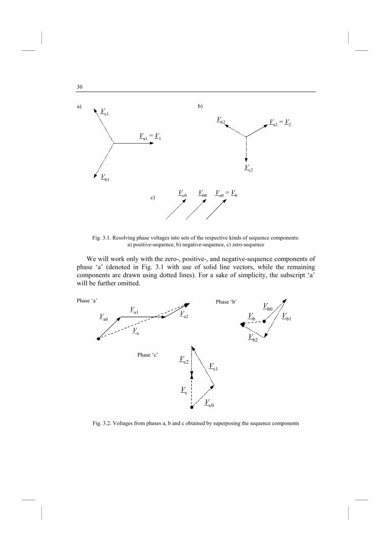
Positive sequence components – three phasors with equal magnitudes, ± 120o phase displacement, (Fig. 3.1a).
egative sequence components – three phasors with equal magnitudes, ± 120o phase displacement (Fig. 3.1b).
Zero sequence components – three phasors with equal magnitudes, 0o phase displacement (Fig. 3.1c);
In Fig. 3.2 voltages from phases a, b and c are obtained by superposing the respective sequence components.
30
Va1 = V1
Vb1
Vc1
Va2 = V2Vb2
Vc2
Vc0 Vb0 Va0 = V0
Fig. 3.1. Resolving phase voltages into sets of the respective kinds of sequence components: a) positive-sequence, b) negative-sequence, c) zero-sequence
We will work only with the zero-, positive-, and negative-sequence components of phase ‘a’ (denoted in Fig. 3.1 with use of solid line vectors, while the remaining components are drawn using dotted lines). For a sake of simplicity, the subscript ‘a’ will be further omitted.
Va0
Va1 Va2
Va
Vb0
Vb1
Vb2
Vb
Vc0
Vc1
Vc2
Vc
Fig. 3.2. Voltages from phases a, b and c obtained by superposing the sequence components
b)
c)
Phase ‘a’ Phase ‘b’
Phase ‘c’
a)
31
Symmetrical components transformation, which allows calculating phase quantities from the symmetrical components is defined as follows:
⋅
=
2
1
0
2
2
c
b
a
aa1
aa1
111
V
V
V
V
V
V
(3.1)
where:
2
3j5.0)3/2exp(ja +−=π= – a complex number with unit magnitude and 120o
phase angle, i.e. the operator which rotates by 120o (anticlockwise direction).
The transformation (3.1) can be written down in matrix notation:
sph VAV ⋅= (3.2)
where:
=
c
b
a
ph
V
V
V
V ,
=
2
1
0
s
V
V
V
V ,
=2
2
aa1
aa1
111
A – 3 x 3 transformation matrix.
Inverse of the transformation matrix A equals:
=−
aa1
aa1
111
3
1
2
21A (3.3)
where the superscript (–1) denotes the matrix inversion. Note: in Matlab programme the function ‘inv’ is used for making matrix inverse.
Between the transformation matrix (3.1) and its inverse (3.3) satisfies:
1AA1 =− (3.4)
Inverse transformation, which allows calculating symmetrical components when phase quantities are given, is stated as follows:
⋅
=
c
b
a
2
2
2
1
0
aa1
aa1
111
3
1
V
V
V
V
V
V
(3.5)
or in matrix notation:
ph1
s VAV ⋅= − (3.6)
Symmetrical components transformation and its inverse transformation applied to
32
currents are as follows:
sph IAI ⋅= (3.7)
ph1
s IAI ⋅= − (3.8)
Besides the presented transformations (phase quantities into symmetrical components and symmetrical components into phase quantities) also it is important how to represent power system components in symmetrical components. Such representations for three-phase balanced Y and D loads are derived in Section 3.2. In turn, Chapters 5 through 7 deal with representations of power generators, power transformers, overhead and cable lines in symmetrical components.
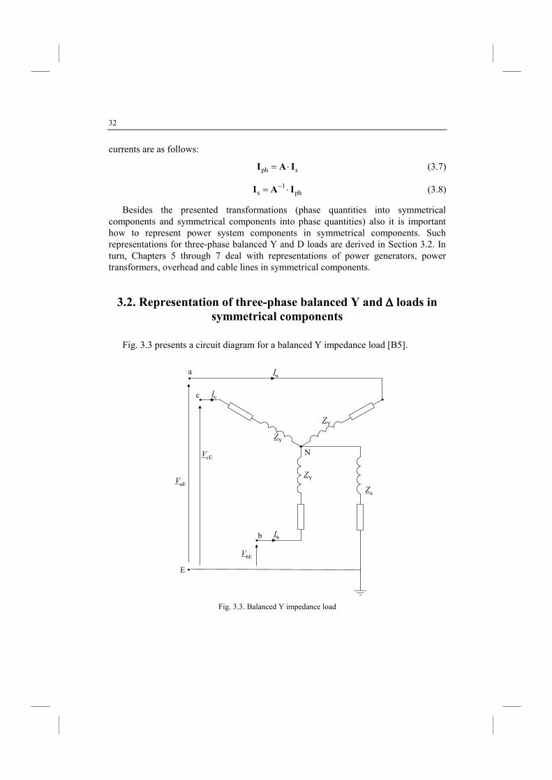
3.2. Representation of three-phase balanced Y and ∆∆∆∆ loads in symmetrical components
Fig. 3.3 presents a circuit diagram for a balanced Y impedance load [B5].
a
c
b
Ia
N
ZY
ZY
ZY
Zn
Ic
Ib
E
VaE
VbE
VcE
Fig. 3.3. Balanced Y impedance load
33
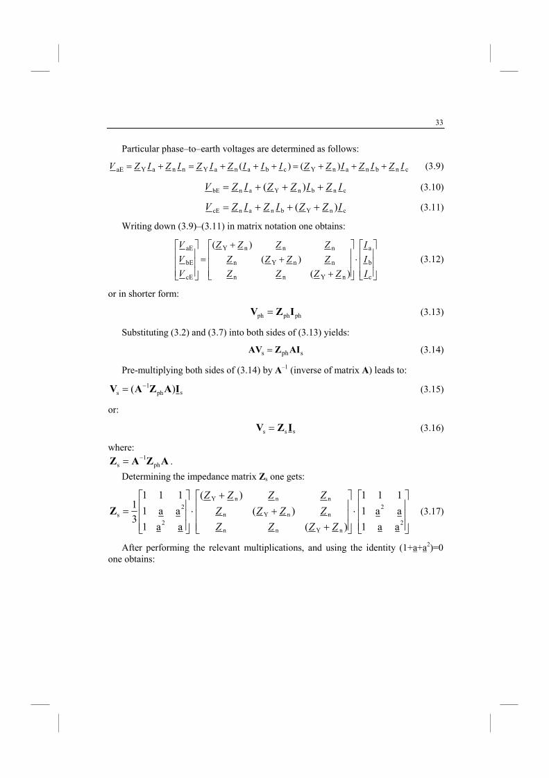
Particular phase–to–earth voltages are determined as follows:
cnbnanYcbanaYnnaYaE )()( IZIZIZZIIIZIZIZIZV +++=+++=+= (3.9)
cnbnYanbE )( IZIZZIZV +++= (3.10)
cnYbnancE )( IZZIZIZV +++= (3.11)
Writing down (3.9)–(3.11) in matrix notation one obtains:
⋅
+
+
+
=
c
b
a
nYnn
nnYn
nnnY
cE
bE
aE
)(
)(
)(
I
I
I
ZZZZ
ZZZZ
ZZZZ
V
V
V
(3.12)
or in shorter form:
phphph IZV = (3.13)
Substituting (3.2) and (3.7) into both sides of (3.13) yields:
sphs AIZAV = (3.14)
Pre-multiplying both sides of (3.14) by A–1 (inverse of matrix A) leads to:
sph1
s )( IAZAV−= (3.15)
or:
sss IZV = (3.16)
where:
AZAZ ph1
s−= .
Determining the impedance matrix Zs one gets:
⋅
+
+
+
⋅
=2
2
nYnn
nnYn
nnnY
2
2s
aa1
aa1
111
)(
)(
)(
aa1
aa1
111
3
1
ZZZZ
ZZZZ
ZZZZ
Z (3.17)
After performing the relevant multiplications, and using the identity (1+a+a2)=0 one obtains:
34
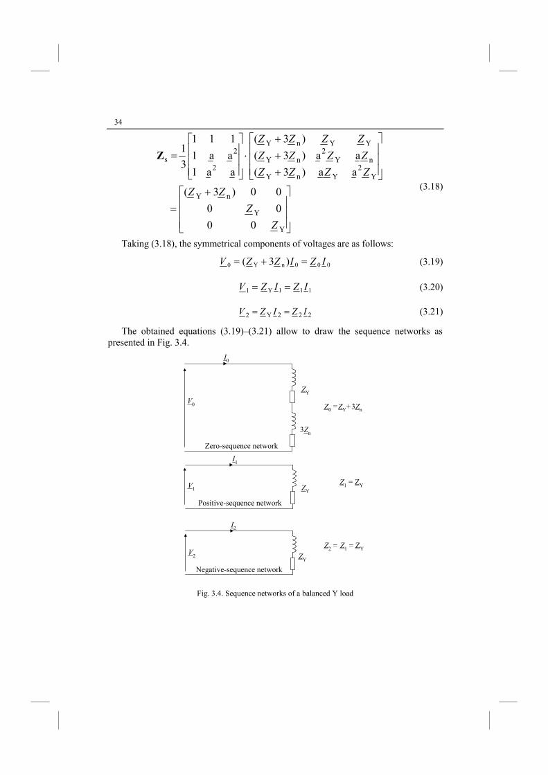
(3.18)
Taking (3.18), the symmetrical components of voltages are as follows:
000nY0 )3( IZIZZV =+= (3.19)
111Y1 IZIZV == (3.20)
222Y2 IZIZV == (3.21)
The obtained equations (3.19)–(3.21) allow to draw the sequence networks as presented in Fig. 3.4.
I0
V0
ZY
3Zn
Z0 =ZY+3Zn
ZY
ZY
Z1 = ZY
Z2 = Z1 = ZY
V1
V2
I1
I2
Zero-sequence network
Positive-sequence network
Negative-sequence network
Fig. 3.4. Sequence networks of a balanced Y load
1 1 1 (Z + 3Z ) Z Z
Y n Y Y1 2 2
Z =s 1 a a ⋅ + (Z 3Z ) a Z aZY n Y n3 2 21 a a ( + a Z 3Z ) aZ ZY n Y Y
(Z + Y 3Z n ) 0 0
= 0 ZY 0 0 0 Z
Y
35
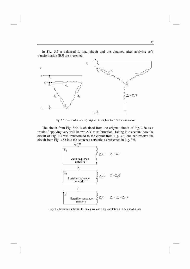
In Fig. 3.5 a balanced ∆ load circuit and the obtained after applying ∆/Y transformation [B5] are presented.
a
b
Z∆
Z∆ Z∆
c
Ia
Ic
Ib
a
c
b
N
ZY
ZY
ZY = Z∆/3
Ia
Ic
Ib
Fig. 3.5. Balanced ∆ load: a) original circuit, b) after ∆/Y transformation
The circuit from Fig. 3.5b is obtained from the original circuit of Fig. 3.5a as a
result of applying very well known ∆/Y transformation. Taking into account how the circuit of Fig. 3.3 was transformed to the circuit from Fig. 3.4, one can resolve the circuit from Fig. 3.5b into the sequence networks as presented in Fig. 3.6.
I0 = 0
V0
Z∆/3 Z0 = inf
Z1 =Z∆/3V1
V2
I1
I2
Zero-sequencenetwork
Positive-sequencenetwork
Negative-sequencenetwork
Z∆/3
Z2 = Z1 = Z∆/3Z∆/3
Fig. 3.6. Sequence networks for an equivalent Y representation of a balanced ∆ load
a)
b)
36
Note that in the circuit of Fig. 5b the point N is isolated from earth. Therefore, the sum of phase currents equals zero: Ia+Ib+Ic=0, which results in:
0)(3
1cba0 =++= IIII (3.22)
According to (3.22) there is no flow of the zero-sequence current and this is reflected in the zero-sequence network from Fig. 3.5b by inserting a discontinuity into the circuit. This results in getting infinite impedance: Z0=inf.
3.3. Fault models in terms of symmetrical components of
currents
For deriving of many algorithms for power system protection, the total fault current is being resolved into a linear combination of symmetrical components. This requires taking into account the boundary conditions (the constrains) for the considered faults [B8, B14].
Also in some power system protection applications, the relation between symmetrical components of total fault current is utilized. This is applied especially when considering the earth faults (Section 3.4).
Returning to the total fault current, it can be expressed as the following weighted sum of its symmetrical components:
F2F2F1F1F0F0F IaIaIaI ++= (3.23)
where: aF0, aF1, aF2 – weighting coefficients (complex numbers), dependent on fault type and the assumed priority for using particular symmetrical components, IF0, IF1, IF2 – zero-, positive- and negative-sequence components of total fault current, which are to be calculated or estimated.
Determination of the total fault current (3.23) is required for reflecting the voltage drop across the fault path (VF) in the fault loops considered in distance protection or the fault locator algorithms:
FFF IRV = (3.24)
It appears that there is some freedom in setting the weighting coefficients in (3.23). Example 3.1 illustrates this for a phase ‘a’ to earth fault.
37
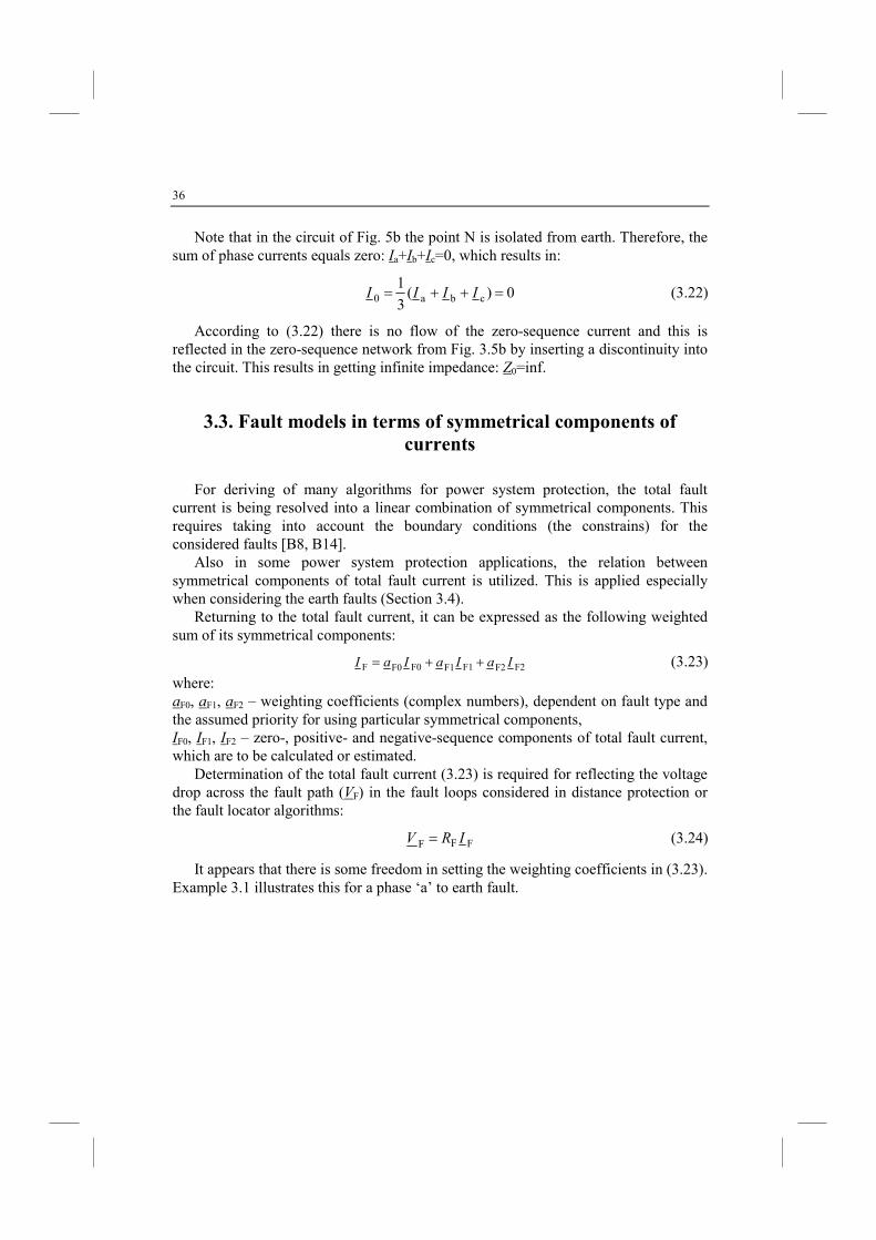
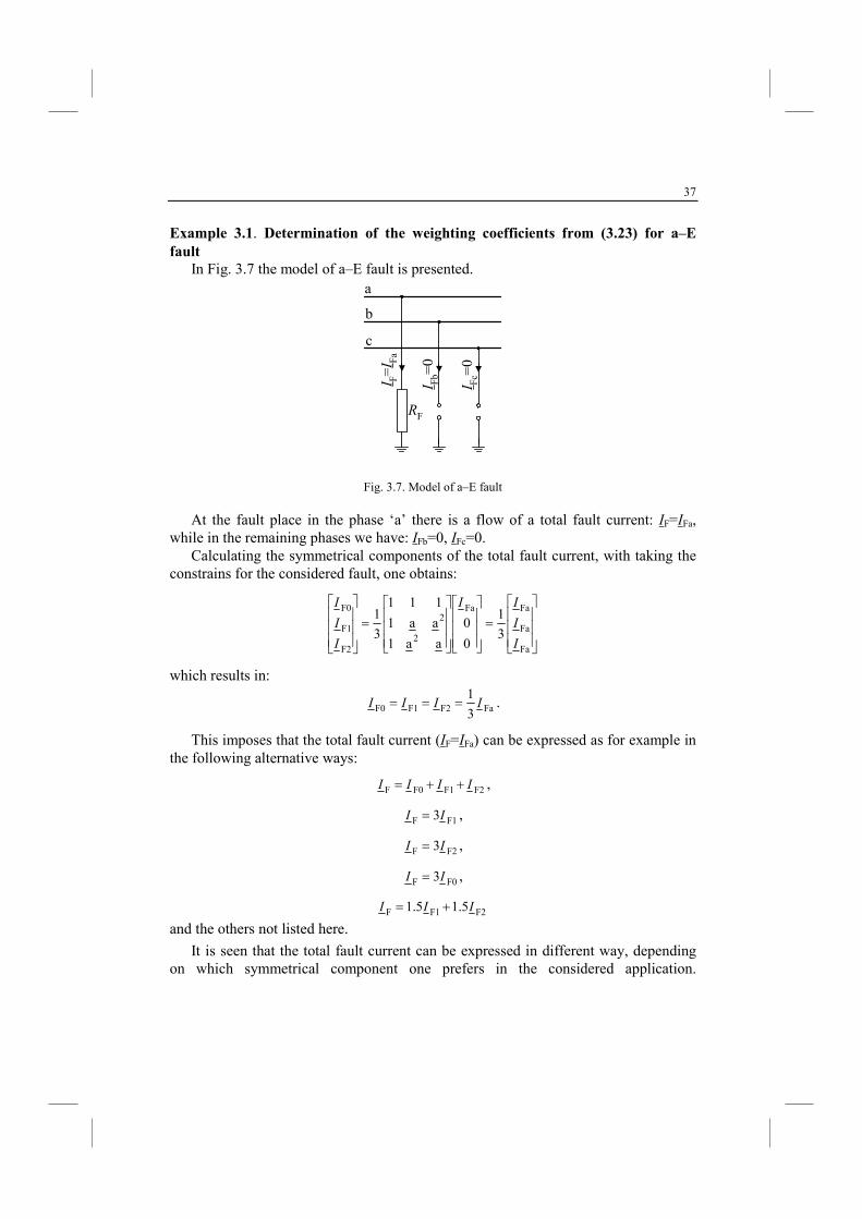
Example 3.1. Determination of the weighting coefficients from (3.23) for a–E fault
In Fig. 3.7 the model of a–E fault is presented. a
b
c
RF
I F=I F
a
I Fb=
0
I Fc=
0
Fig. 3.7. Model of a–E fault
At the fault place in the phase ‘a’ there is a flow of a total fault current: IF=IFa, while in the remaining phases we have: IFb=0, IFc=0.
Calculating the symmetrical components of the total fault current, with taking the constrains for the considered fault, one obtains:
=
=
Fa
Fa
FaFa
2
2
F2
F1
F0
3
1
0
0
aa1
aa1
111
3
1
I
I
II
I
I
I
which results in:
FaF2F1F0 3
1IIII === .
This imposes that the total fault current (IF=IFa) can be expressed as for example in the following alternative ways:
F2F1F0F IIII ++= ,
F1F 3II = ,
F2F 3II = ,
F0F 3II = ,
F2F1F 5.15.1 III +=
and the others not listed here.
It is seen that the total fault current can be expressed in different way, depending on which symmetrical component one prefers in the considered application.
38
Analogously, determination of the total fault current can be considered for the other fault types.
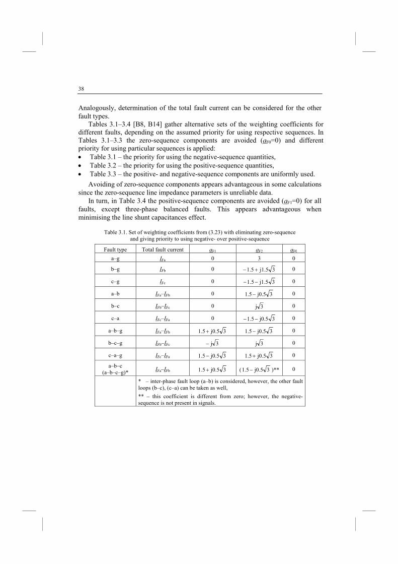
Tables 3.1–3.4 [B8, B14] gather alternative sets of the weighting coefficients for different faults, depending on the assumed priority for using respective sequences. In Tables 3.1–3.3 the zero-sequence components are avoided (aF0=0) and different priority for using particular sequences is applied: • Table 3.1 – the priority for using the negative-sequence quantities, • Table 3.2 – the priority for using the positive-sequence quantities, • Table 3.3 – the positive- and negative-sequence components are uniformly used.
Avoiding of zero-sequence components appears advantageous in some calculations since the zero-sequence line impedance parameters is unreliable data.
In turn, in Table 3.4 the positive-sequence components are avoided (aF1=0) for all faults, except three-phase balanced faults. This appears advantageous when minimising the line shunt capacitances effect.
Table 3.1. Set of weighting coefficients from (3.23) with eliminating zero-sequence and giving priority to using negative- over positive-sequence
Fault type Total fault current aF1 aF2 aF0
a–g IFa 0 3 0
b–g IFb 0 3j1.51.5 +− 0
c–g IFc 0 3j1.51.5−− 0
a–b IFa–IFb 0 3j0.51.5− 0
b–c IFb–IFc 0 3j 0
c–a IFc–IFa 0 3j0.51.5−− 0
a–b–g IFa–IFb 3j0.51.5+ 3j0.51.5− 0
b–c–g IFb–IFc 3j− 3j 0
c–a–g IFc–IFa 3j0.51.5 − 3j0.51.5 + 0
a–b–c (a–b–c–g)*
IFa–IFb 3j0.51.5+ ( 3j0.51.5− )** 0
* – inter-phase fault loop (a–b) is considered, however, the other fault loops (b–c), (c–a) can be taken as well,
** – this coefficient is different from zero; however, the negative-sequence is not present in signals.
39
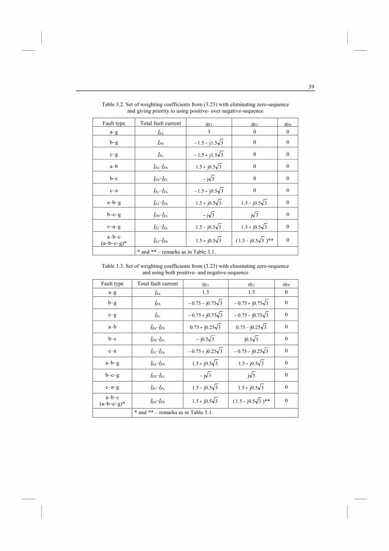
Table 3.2. Set of weighting coefficients from (3.23) with eliminating zero-sequence and giving priority to using positive- over negative-sequence
Fault type Total fault current aF1 aF2 aF0
a–g IFa 3 0 0
b–g IFb 3j1.51.5−− 0 0
c–g IFc 3j1.51.5+− 0 0
a–b IFa–IFb 3j0.51.5 + 0 0
b–c IFb–IFc 3j− 0 0
c–a IFc–IFa 3j0.51.5+− 0 0
a–b–g IFa–IFb 3j0.51.5 + 3j0.51.5− 0
b–c–g IFb–IFc 3j− 3j 0
c–a–g IFc–IFa 3j0.51.5 − 3j0.51.5 + 0
a–b–c (a–b–c–g)*
IFa–IFb 3j0.51.5 + ( 3j0.51.5− )** 0
* and ** – remarks as in Table 3.1.
Table 3.3. Set of weighting coefficients from (3.23) with eliminating zero-sequence and using both positive- and negative-sequence
Fault type Total fault current aF1 aF2 aF0
a–g IFa 1.5 1.5 0
b–g IFb 375.0j75.0 −− 375.0j75.0 +− 0
c–g IFc 375.0j75.0 +− 375.0j75.0 −− 0
a–b IFa–IFb 325.0j75.0 + 325.0j75.0 − 0
b–c IFb–IFc 35.0j− 35.0j 0
c–a IFc–IFa 325.0j75.0 +− 325.0j75.0 −− 0
a–b–g IFa–IFb 3j0.51.5+ 3j0.51.5− 0
b–c–g IFb–IFc 3j− 3j 0
c–a–g IFc–IFa 3j0.51.5 − 3j0.51.5 + 0
a–b–c (a–b–c–g)*
IFa–IFb 3j0.51.5+ ( 3j0.51.5− )** 0
* and ** – remarks as in Table 3.1.
40
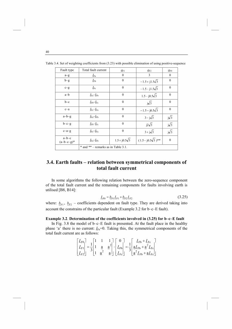
Table 3.4. Set of weighting coefficients from (3.23) with possible elimination of using positive-sequence
Fault type Total fault current aF1 aF2 aF0
a–g IFa 0 3 0
b–g IFb 0 3j1.51.5+− 0
c–g IFc 0 3j1.5–1.5– 0
a–b IFa–IFb 0 3j0.5–1.5 0
b–c IFb–IFc 0 3j 0
c–a IFc–IFa 0 35.0j5.1 −− 0
a–b–g IFa–IFb 0 3j3− 3j
b–c–g IFb–IFc 0 32j 3j
c–a–g IFc–IFa 0 33 j+ 3j
a–b–c (a–b–c–g)*
IFa–IFb 3j0.51.5+ ( 3j0.51.5− )** 0
* and ** – remarks as in Table 3.1.
3.4. Earth faults – relation between symmetrical components of
total fault current
In some algorithms the following relation between the zero-sequence component of the total fault current and the remaining components for faults involving earth is utilised [B8, B14]:
F2F2F1F1F0 IbIbI += (3.25)
where: F1b , F2b – coefficients dependent on fault type. They are derived taking into
account the constrains of the particular fault (Example 3.2 for b–c–E fault).
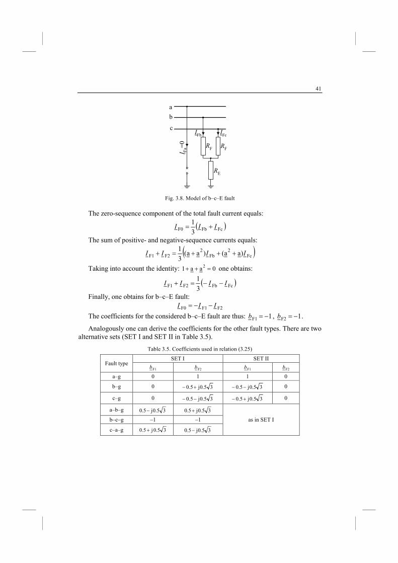
Example 3.2. Determination of the coefficients involved in (3.25) for b–c–E fault In Fig. 3.8 the model of b–c–E fault is presented. At the fault place in the healthy
phase ‘a’ there is no current: IFa=0. Taking this, the symmetrical components of the total fault current are as follows:
+
+
+
=
⋅
=
FcFb2
Fc2
Fb
FcFb
Fc
Fb2
2
F2
F1
F0
aa
aa3
10
aa1
aa1
111
3
1
II
II
II
I
I
I
I
I
41
IFc
a
RF
b
c
RF
RE
I Fa=
0
IFb
Fig. 3.8. Model of b–c–E fault
The zero-sequence component of the total fault current equals:
( )FcFbF0 3
1III +=
The sum of positive- and negative-sequence currents equals:
( )Fc2
Fb2
F2F1 )aa()aa(3
1IIII +++=+
Taking into account the identity: 0aa1 2 =++ one obtains:
( )FcFbF2F1 3
1IIII −−=+
Finally, one obtains for b–c–E fault:
F2F1F0 III −−=
The coefficients for the considered b–c–E fault are thus: 1F1 −=b , 1F2 −=b .
Analogously one can derive the coefficients for the other fault types. There are two alternative sets (SET I and SET II in Table 3.5).
Table 3.5. Coefficients used in relation (3.25)
Fault type SET I SET II
F1b F2b
F1b F2b
a–g 0 1 1 0
b–g 0 35.0j5.0 +− 35.0j5.0 −− 0
c–g 0 35.0j5.0 −− 35.0j5.0 +− 0
a–b–g 35.0j5.0 − 35.0j5.0 +
as in SET I b–c–g –1 –1
c–a–g 35.0j5.0 + 35.0j5.0 −
42
4. MODAL TRASFORMATIO AD PHASE
CO-ORDIATES APPROACHES
4.1. Modal transformation
Modal transformation method [B8, B14] is known from application to representing three-phase overhead lines. Applying this method, the line impedance matrix ZL and admittance matrix YL (see the line models presented in Chapter 7) are transformed into the matrices Zmode, Ymode:
iL1–
vmode TZTZ = (4.1)
vL1–
imode TYTY = (4.2)
where the superscript (–1) denotes the matrix inversion (note that the matrix inverse function in Matlab programme [B12] is denoted as: ‘inv’).
The transformation (4.1)–(4.2) is performed in such a way that the matrices Zmode, Ymode are diagonal, what means that the three-phase coupled network becomes decoupled into three decoupled single-phase networks.
Three-phase voltage V and current I matrices are transformed into the modal matrices Vmode, Imode:
VTV1–
vmode = (4.3)
ITI1–
imode = (4.4)
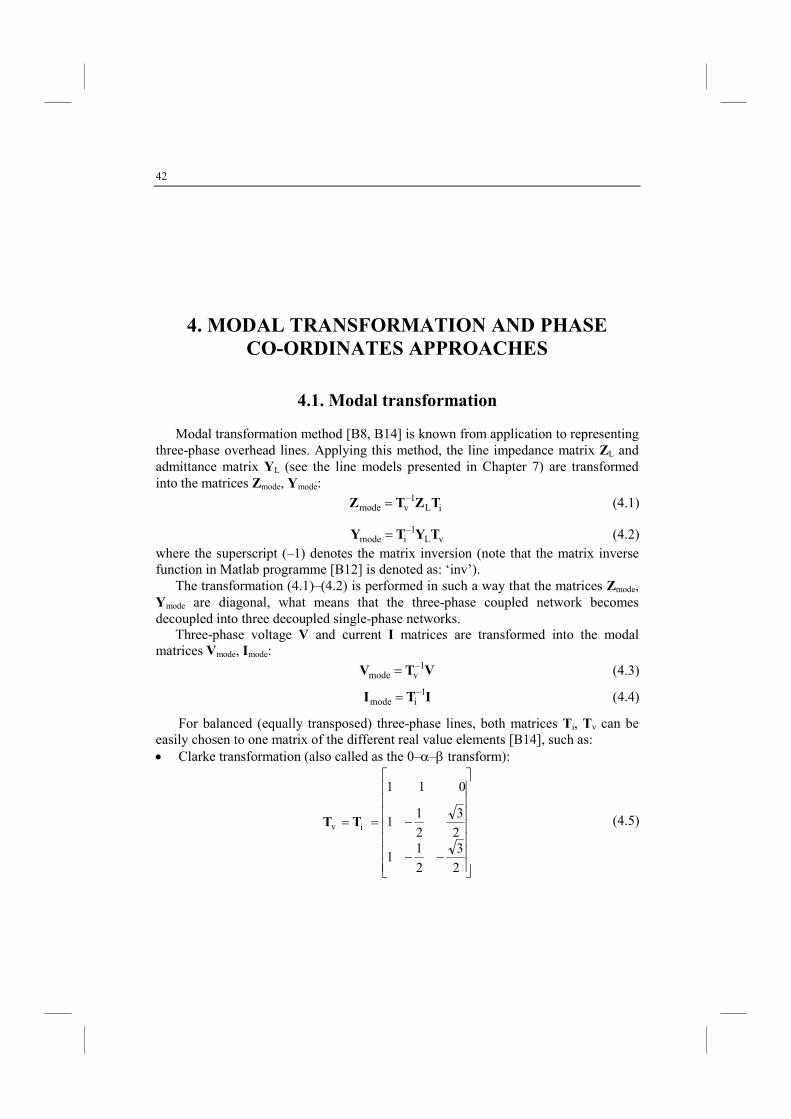
For balanced (equally transposed) three-phase lines, both matrices Ti, Tv can be easily chosen to one matrix of the different real value elements [B14], such as: • Clarke transformation (also called as the 0–α–β transform):
−−
−==
2
3
2
11
2
3
2
11
0 1 1
iv TT (4.5)
43
−
−−==
330
112
1 1 1
3
11–i
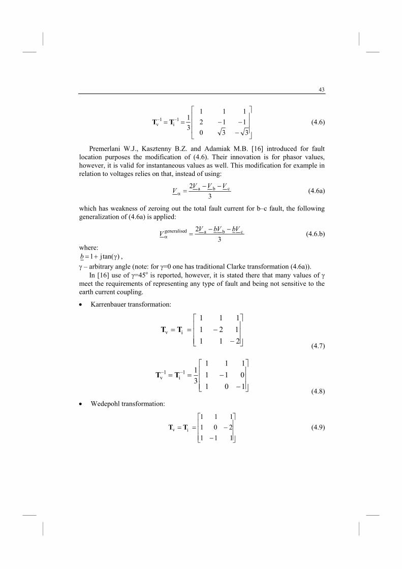
1–v TT (4.6)
Premerlani W.J., Kasztenny B.Z. and Adamiak M.B. [16] introduced for fault location purposes the modification of (4.6). Their innovation is for phasor values, however, it is valid for instantaneous values as well. This modification for example in relation to voltages relies on that, instead of using:
3
2 cba VVVV
−−=α (4.6a)
which has weakness of zeroing out the total fault current for b–c fault, the following generalization of (4.6a) is applied:
3
2 cbadgeneralise VbVbVV
−−=α (4.6.b)
where: )tan(j1 γ+=b ,
γ – arbitrary angle (note: for γ=0 one has traditional Clarke transformation (4.6a)). In [16] use of γ=45o is reported, however, it is stated there that many values of γ
meet the requirements of representing any type of fault and being not sensitive to the earth current coupling.
• Karrenbauer transformation:
−
−==
21 1
1 21
1 1 1
iv TT
(4.7)
−
−==
10 1
0 11
1 1 1
3
11–i
1–v TT
(4.8)
• Wedepohl transformation:
−
−==
111
201
1 1 1
iv TT (4.9)
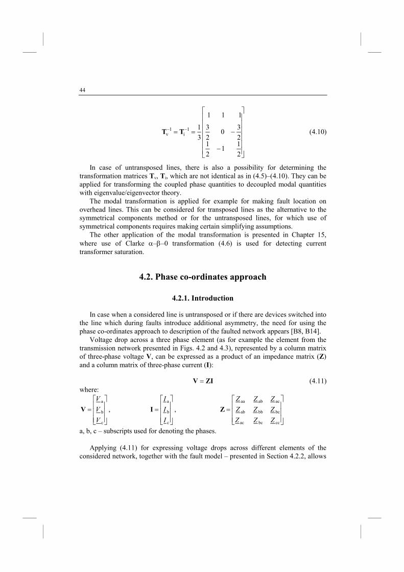
44
−
−==
2
11
2
12
30
2
3
1 1 1
3
11–i
1–v TT (4.10)
In case of untransposed lines, there is also a possibility for determining the transformation matrices Tv, Ti, which are not identical as in (4.5)–(4.10). They can be applied for transforming the coupled phase quantities to decoupled modal quantities with eigenvalue/eigenvector theory.
The modal transformation is applied for example for making fault location on overhead lines. This can be considered for transposed lines as the alternative to the symmetrical components method or for the untransposed lines, for which use of symmetrical components requires making certain simplifying assumptions.
The other application of the modal transformation is presented in Chapter 15, where use of Clarke α–β–0 transformation (4.6) is used for detecting current transformer saturation.
4.2. Phase co-ordinates approach
4.2.1. Introduction
In case when a considered line is untransposed or if there are devices switched into the line which during faults introduce additional asymmetry, the need for using the phase co-ordinates approach to description of the faulted network appears [B8, B14].
Voltage drop across a three phase element (as for example the element from the transmission network presented in Figs. 4.2 and 4.3), represented by a column matrix of three-phase voltage V, can be expressed as a product of an impedance matrix (Z) and a column matrix of three-phase current (I):
ZIV = (4.11) where:
=
c
b
a
V
V
V
V ,
=
c
b
a
I
I
I
I ,
=
ccbcac
bcbbab
acabaa
ZZZ
ZZZ
ZZZ
Z
a, b, c – subscripts used for denoting the phases. Applying (4.11) for expressing voltage drops across different elements of the
considered network, together with the fault model – presented in Section 4.2.2, allows
45
us to get complete description of the faulted network
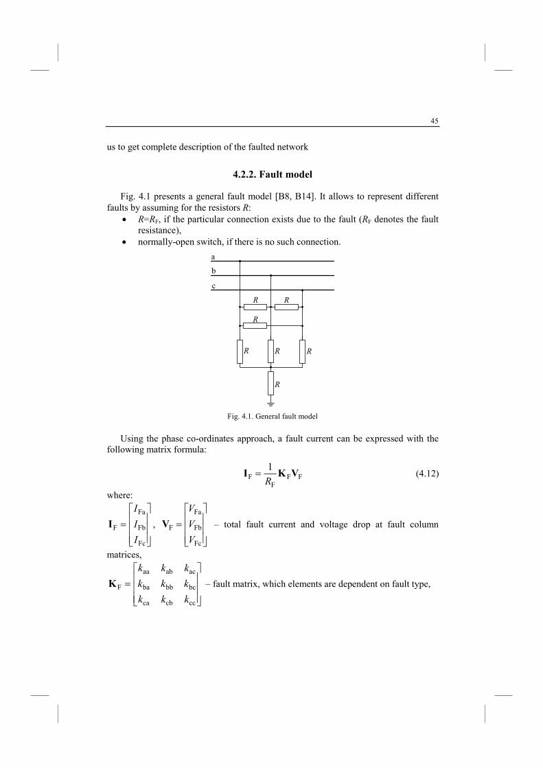
4.2.2. Fault model
Fig. 4.1 presents a general fault model [B8, B14]. It allows to represent different faults by assuming for the resistors R:
• R=RF, if the particular connection exists due to the fault (RF denotes the fault resistance),
• normally-open switch, if there is no such connection.
R
a
R
b
c
R R
R R
R
Fig. 4.1. General fault model
Using the phase co-ordinates approach, a fault current can be expressed with the following matrix formula:
FFF
F1
VKIR
= (4.12)
where:
=
Fc
Fb
Fa
F
I
I
I
I ,
=
Fc
Fb
Fa
F
V
V
V
V – total fault current and voltage drop at fault column
matrices,
=
cccbca
bcbbba
acabaa
F
kkk
kkk
kkk
K – fault matrix, which elements are dependent on fault type,
46
RF – fault resistance (Fig. 4.1). Fault matrix KF for different fault types is build in the following two-step
procedure: I-Step – calculate the diagonal and off-diagonal elements of the auxiliary matrix (KF):
c b, a, , otherwise ...0
faultin involved are , phases if ...1=
−
= jiji
kij . (4.13)
Note that the diagonal elements of the auxiliary matrix, which is to be recalculated in the II Step, are marked with parentheses (…). II-Step – substitute the result of summing of absolute values in the respective column for each diagonal element of the auxiliary matrix obtained in I-Step:
cb,a, c
a
== ∑=
=ikk
j
jijii . (4.14)
Use of this two-step procedure is explained in details in the Example 4.1.
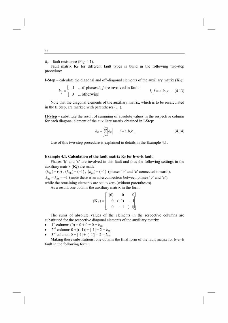
Example 4.1. Calculation of the fault matrix KF for b–c–E fault
Phases ‘b’ and ‘c’ are involved in this fault and thus the following settings in the auxiliary matrix (KF) are made:
(0))( aa =k , 1)()( bb −=k , 1)()( cc −=k (phases ‘b’ and ‘c’ connected to earth),
1cbbc −== kk (since there is an interconnection between phases ‘b’ and ‘c’),
while the remaining elements are set to zero (without parentheses). As a result, one obtains the auxiliary matrix in the form:
−−
−−=
)1(10
1)1(0
00)0(
)( FK
The sums of absolute values of the elements in the respective columns are substituted for the respective diagonal elements of the auxiliary matrix: • 1st column: (0) + 0 + 0 = 0 = kaa, • 2nd column: 0 + |(–1)| + |–1| = 2 = kbb, • 3rd column: 0 + |–1| + |(–1)| = 2 = kcc.
Making these substitutions, one obtains the final form of the fault matrix for b–c–E fault in the following form:
47
−
−=
210
120
000
F K .
Table. 4.1. Steps I and II of determining fault matrix KF for different faults
FAULT TYPE
I-STEP (4.13) II-STEP (4.14)
a–E
−
=
)0(00
0)0(0
00)1(
)( FK
=
000
000
001
FK
b–E
−=
)0(00
0)1(0
00)0(
)( FK
=
000
010
000
FK
c–E
−
=
)1(00
0)0(0
00)0(
)( FK
=
100
000
000
FK
a–b
−
−
=
)0(00
0)0(1
01)0(
)( FK
−
−
=
000
011
011
F K
b–c
−
−=
)0(10
1)0(0
00)0(
)( FK
−
−=
110
110
000
F K
c–a
−
−
=
)0(01
0)0(0
10)0(
)( FK
−
−
=
101
000
101
F K
a–b–E
−−
−−
=
)0(00
0)1(1
01)1(
)( FK
−
−
=
000
021
012
F K
b–c–E
−−
−−=
)1(10
1)1(0
00)0(
)( FK
−
−=
210
120
000
F K
48
c–a–E
−−
−−
=
)1(01
0)0(0
10)1(
)( FK
−
−
=
201
000
102
F K
a–b–c
−−
−−
−−
=
)0(11
1)0(1
11)0(
)( FK
−−
−−
−−
=
211
121
112
FK
a–b–c–E
−−−
−−−
−−−
=
)1(11
1)1(1
11)1(
)( FK
−−
−−
−−
=
311
131
113
FK
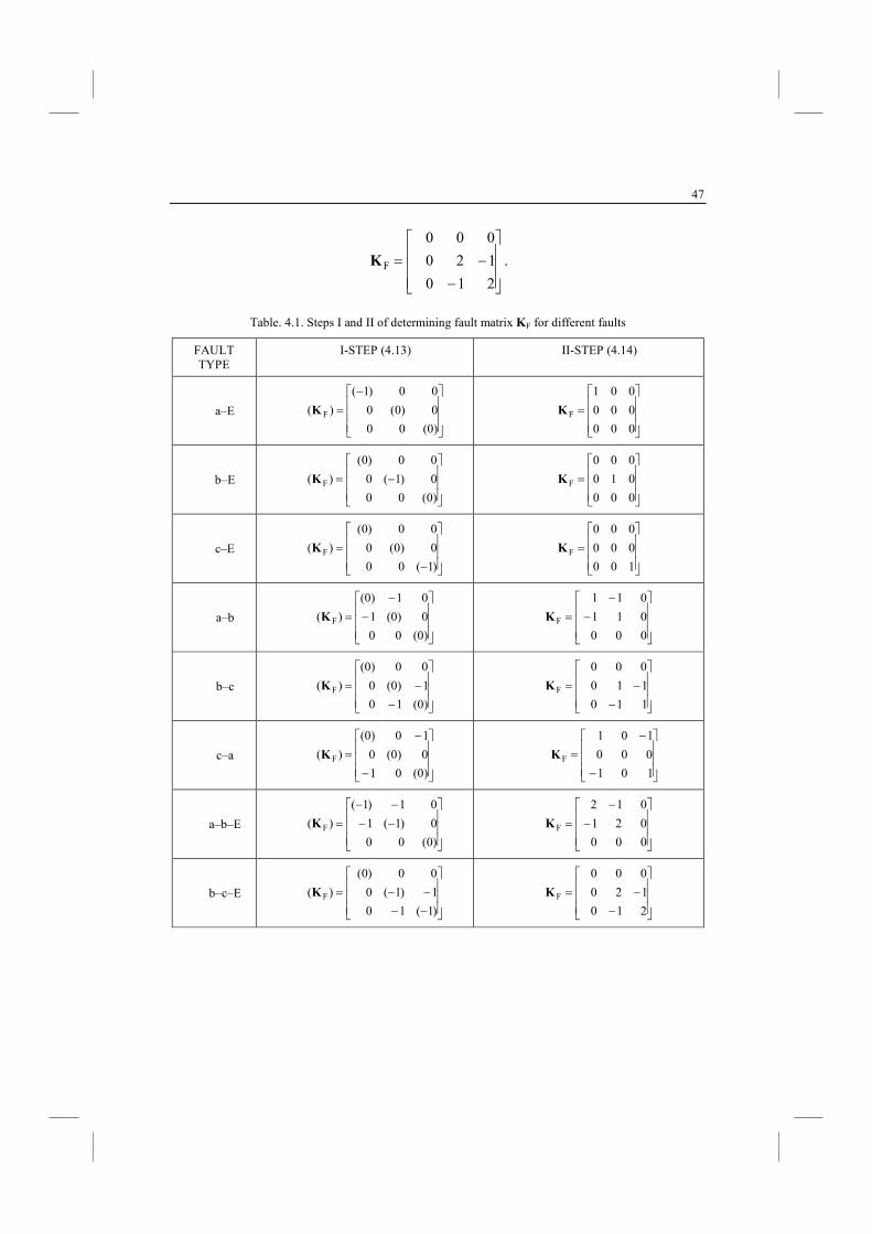
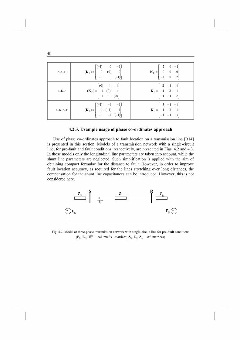
4.2.3. Example usage of phase co-ordinates approach
Use of phase co-ordinates approach to fault location on a transmission line [B14] is presented in this section. Models of a transmission network with a single-circuit line, for pre-fault and fault conditions, respectively, are presented in Figs. 4.2 and 4.3. In those models only the longitudinal line parameters are taken into account, while the shunt line parameters are neglected. Such simplification is applied with the aim of obtaining compact formulae for the distance to fault. However, in order to improve fault location accuracy, as required for the lines stretching over long distances, the compensation for the shunt line capacitances can be introduced. However, this is not considered here.
ESER
ZS ZRZL
S R
preSI
Fig. 4.2. Model of three-phase transmission network with single-circuit line for pre-fault conditions
(ES, ER, preSI – column 3x1 matrices; ZS, ZR, ZL – 3x3 matrices)
49
dZLIS(1–d)ZL
VS VF
IF=(1/RF)KFVF
ESER
ZS ZR
S RIR
Fig. 4.3. Model of three-phase transmission network with single-circuit line for fault conditions (ES, ER, IS, IR, IF, VS, VF – column 3x1 matrices; ZS, ZR, ZL, KF – 3x3 matrices)
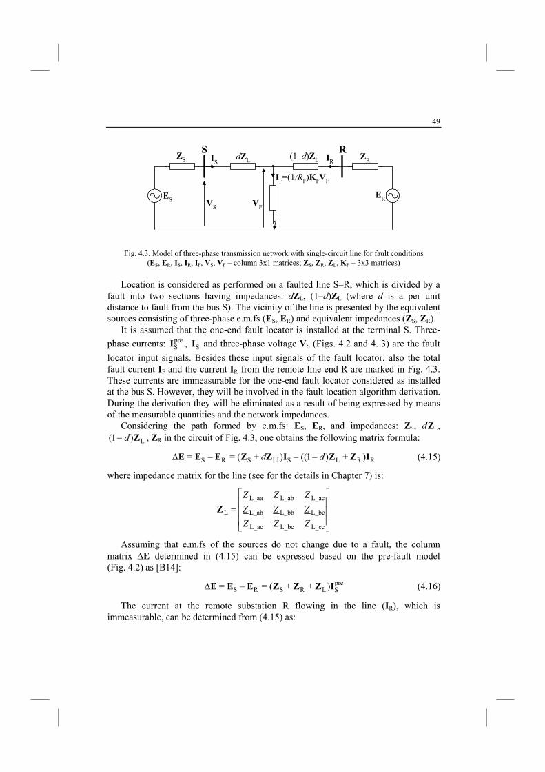
Location is considered as performed on a faulted line S–R, which is divided by a
fault into two sections having impedances: dZL, (1–d)ZL (where d is a per unit distance to fault from the bus S). The vicinity of the line is presented by the equivalent sources consisting of three-phase e.m.fs (ES, ER) and equivalent impedances (ZS, ZR).
It is assumed that the one-end fault locator is installed at the terminal S. Three-
phase currents: preSI , SI and three-phase voltage VS (Figs. 4.2 and 4. 3) are the fault
locator input signals. Besides these input signals of the fault locator, also the total fault current IF and the current IR from the remote line end R are marked in Fig. 4.3. These currents are immeasurable for the one-end fault locator considered as installed at the bus S. However, they will be involved in the fault location algorithm derivation. During the derivation they will be eliminated as a result of being expressed by means of the measurable quantities and the network impedances.
Considering the path formed by e.m.fs: ES, ER, and impedances: ZS, dZL,
L)1( Zd− , ZR in the circuit of Fig. 4.3, one obtains the following matrix formula:
RRLSLISRS )+)–1((–)+(=–= IZZIZZEEE dd∆ (4.15)
where impedance matrix for the line (see for the details in Chapter 7) is:
=
L_ccL_bcL_ac
L_bcL_bbL_ab
L_acL_abL_aa
L
ZZZ
ZZZ
ZZZ
Z
Assuming that e.m.fs of the sources do not change due to a fault, the column matrix ∆E determined in (4.15) can be expressed based on the pre-fault model (Fig. 4.2) as [B14]:
preSLRSRS )++(=–= IZZZEEE∆ (4.16)
The current at the remote substation R flowing in the line (IR), which is immeasurable, can be determined from (4.15) as:
50
))+(()+)–1((= SLS–1
RLR EIZZZZI ∆−dd (4.17)
Column matrices of the voltage across a fault path and total fault current (Fig. 4.3) are determined accordingly:
SLSF –= IZVV d (4.18)
RSF += III (4.19)
A general fault model with use of the matrix notation was described in Section 4.2.2: formula (4.12) and Table 4.1. Taking into account the general fault model (4.12) and equations (4.18)–(4.19) one obtains:
RSSLSFF
+=)–(1
IIIZVK dR
(4.20)
Combining (4.17) and (4.20), yields after the arrangements the following matrix equation:
0DCBA =+ F2 Rdd −− (4.21)
where:
SLFL= IZKZA ,
SLFRSLSFL +)+(= IZKZIZVKZB ,
SFRL )+(= VKZZC ,
))(++(= preSSRLS IIZZZD − .
Transforming (4.21) into the scalar form [B14] one obtains the following quadratic formula for complex numbers:
0=+ F012
2 RAdAdA −− (4.22)
where: PA=2A ,
PB=1A ,
PC=0A ,
DD
DP
T
T
= ,
Superscript T denotes transposition of the matrix (exchange between the rows and columns).
Note that in Matlab [B12], the matrix D transposition is performed by using the transpose operator: D'. At the same time one has to take into account that if the

51
elements of the matrix D are complex numbers, this operation also additionally calculates conjugates for those elements.
The scalar quadratic equation (4.22) can be resolved into the real and imaginary parts, from which one can calculate the unknown distance to fault (d) and fault resistance (RF).
52
5. MODELS OF ROTATIG MACHIES
5.1. Introduction
Rotating machines, such as synchronous generators, synchronous motors and induction motors are complex power system items. This concerns: • Their behaviour during faults, • design of protection and control systems.
Detailed models of those devices are known from the wide literature of the subject. However, the simplified sequence networks for rotating machines are commonly used in many power-system studies and considered as accurate enough for that. Such simplified models are derived without taking into account such phenomena as machine saliency, saturation effects, and more complicated transient effects [B5].
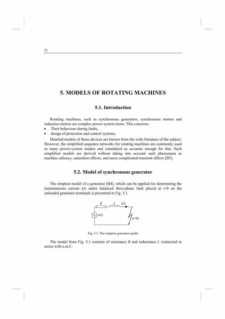
5.2. Model of synchronous generator
The simplest model of a generator [B4], which can be applied for determining the instantaneous current i(t) under balanced three-phase fault placed at t=0 on the unloaded generator terminals is presented in Fig. 5.1.
e(t)
R L i(t)
(t=0)
Fig. 5.1. The simplest generator model
The model from Fig. 5.1 consists of resistance R and inductance L connected in series with e.m.f.:
53
)sin()( m α+ω= tEte (5.1)
The transient current i(t) is given by:
⋅ϕ−α−ϕ−α+ω=
− tL
R
tZ
Eti e)sin()sin()( m (5.2)
where: 22 )( LRZ ω+= ,
ω=ϕ −
R
L1tan .
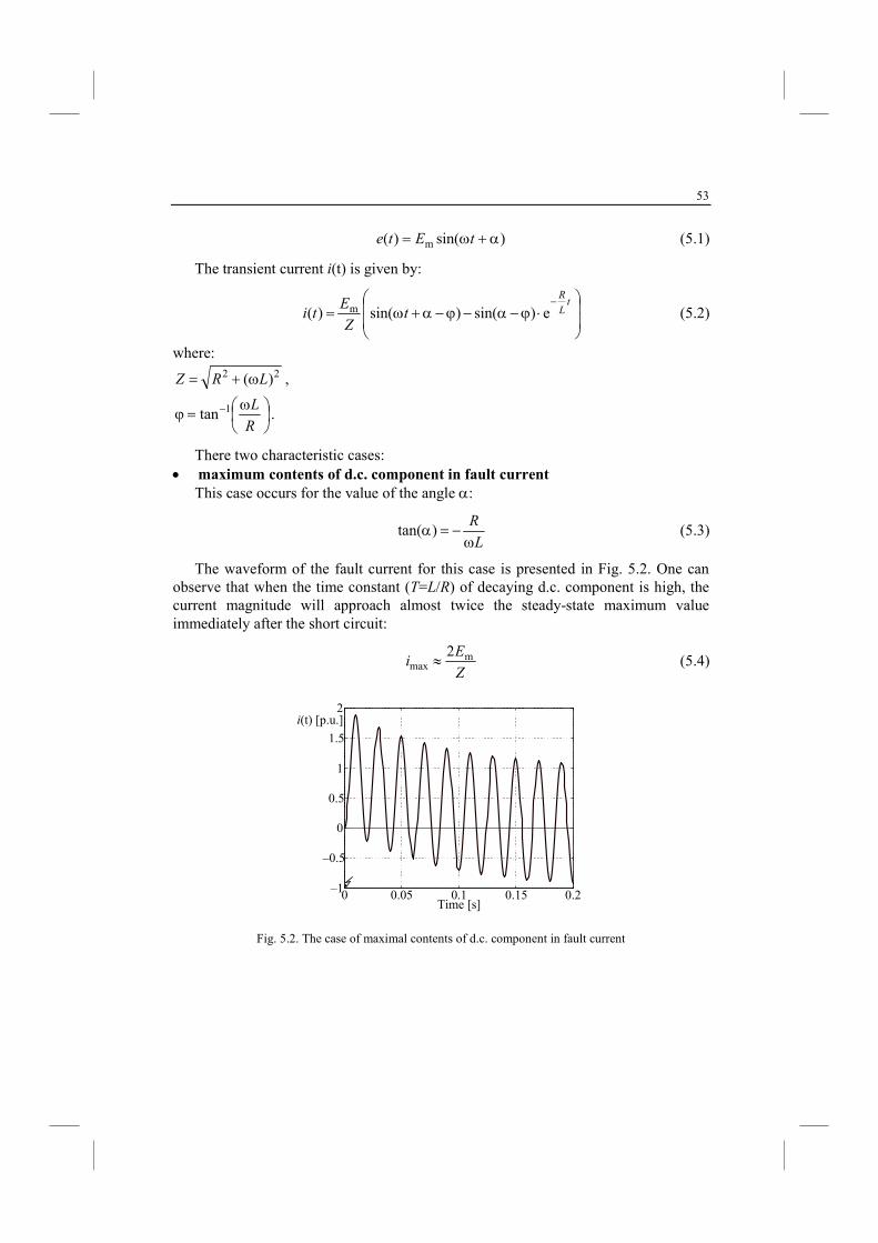
There two characteristic cases: • maximum contents of d.c. component in fault current
This case occurs for the value of the angle α:
L
R
ω−=α)tan( (5.3)
The waveform of the fault current for this case is presented in Fig. 5.2. One can observe that when the time constant (T=L/R) of decaying d.c. component is high, the current magnitude will approach almost twice the steady-state maximum value immediately after the short circuit:
Z
Ei mmax
2≈ (5.4)
0 0.05 0.1 0.15 0.2–1
–0.5
0
0.5
1
1.5
2
Time [s]
i(t) [p.u.]
Fig. 5.2. The case of maximal contents of d.c. component in fault current
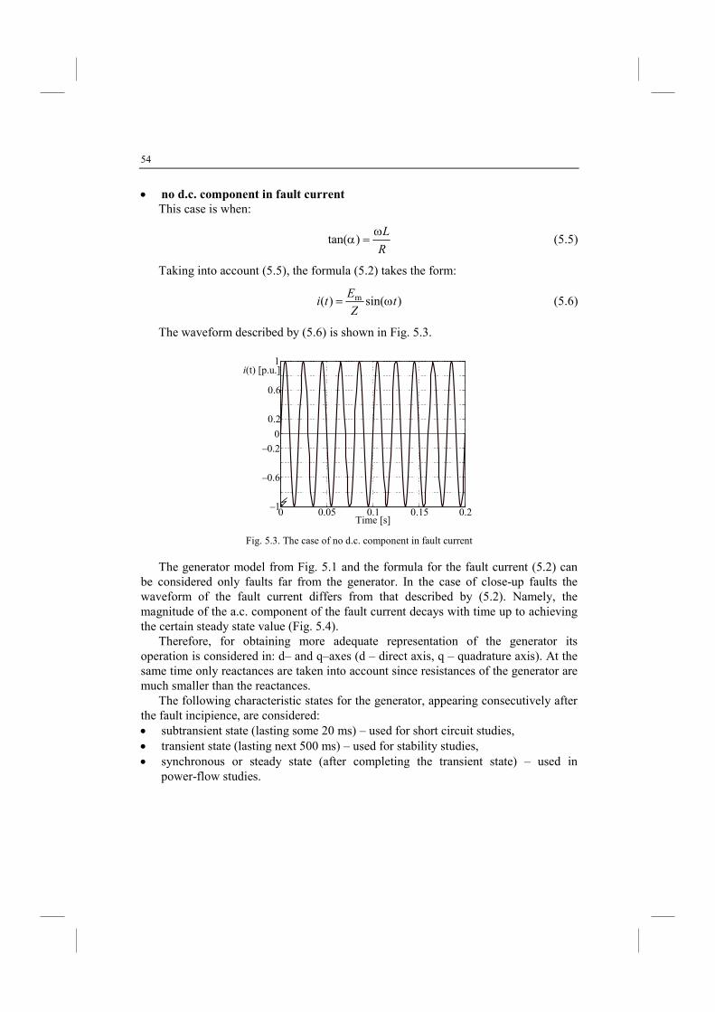
54
• no d.c. component in fault current
This case is when:
R
Lω=α)tan( (5.5)
Taking into account (5.5), the formula (5.2) takes the form:
)sin()( m tZ
Eti ω= (5.6)
The waveform described by (5.6) is shown in Fig. 5.3.
0 0.05 0.1 0.15 0.2–1
–0.6
–0.2
0
0.2
0.6
1
Time [s]
i(t) [p.u.]
Fig. 5.3. The case of no d.c. component in fault current
The generator model from Fig. 5.1 and the formula for the fault current (5.2) can be considered only faults far from the generator. In the case of close-up faults the waveform of the fault current differs from that described by (5.2). Namely, the magnitude of the a.c. component of the fault current decays with time up to achieving the certain steady state value (Fig. 5.4).
Therefore, for obtaining more adequate representation of the generator its operation is considered in: d– and q–axes (d – direct axis, q – quadrature axis). At the same time only reactances are taken into account since resistances of the generator are much smaller than the reactances.
The following characteristic states for the generator, appearing consecutively after the fault incipience, are considered: • subtransient state (lasting some 20 ms) – used for short circuit studies, • transient state (lasting next 500 ms) – used for stability studies, • synchronous or steady state (after completing the transient state) – used in
power-flow studies.
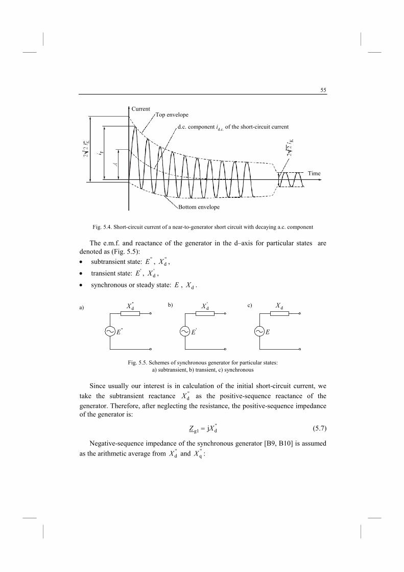
55
CurrentTop envelopeTop envelope
d.c. component id.c. of the short-circuit current
Bottom envelopeTopenvelope
Time
Fig. 5.4. Short-circuit current of a near-to-generator short circuit with decaying a.c. component
The e.m.f. and reactance of the generator in the d–axis for particular states are
denoted as (Fig. 5.5):
• subtransient state: ''E , ''dX ,
• transient state: 'E , 'dX ,
• synchronous or steady state: E , dX .
''E
''dX
'E
'dX
E
dX
Fig. 5.5. Schemes of synchronous generator for particular states: a) subtransient, b) transient, c) synchronous
Since usually our interest is in calculation of the initial short-circuit current, we
take the subtransient reactance ''dX as the positive-sequence reactance of the
generator. Therefore, after neglecting the resistance, the positive-sequence impedance of the generator is:
''dg1 jXZ = (5.7)
Negative-sequence impedance of the synchronous generator [B9, B10] is assumed
as the arithmetic average from ''dX and ''
qX :
a) b) c)
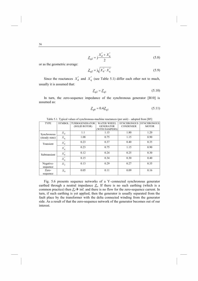
56
2
j''q
''d
g2
XXZ
+= (5.8)
or as the geometric average:
''q
''dg2 j XXZ ⋅= (5.9)
Since the reactances ''dX and ''
qX (see Table 5.1) differ each other not to much,
usually it is assumed that:
g1g2 ZZ = (5.10)
In turn, the zero-sequence impedance of the synchronous generator [B10] is assumed as:
g1g0 4.0 ZZ = (5.11)
Table 5.1. Typical values of synchronous-machine reactances (per unit) – adopted from [B5]
TYPE SYMBOL TURBOGENERATOR (SOLID ROTOR)
WATER WHEEL GENERATOR
(WITH DAMPERS)
SYNCHRONOUS CONDENSER
SYNCHRONOUS MOTOR
Synchronous (steady state)
dX 1.1 1.15 1.80 1.20
qX 1.08 0.75 1.15 0.90
Transient 'dX 0.23 0.37 0.40 0.35
'qX 0.23 0.75 1.15 0.90
Subtransient ''
dX 0.12 0.24 0.25 0.30
''qX 0.15 0.34 0.30 0.40
Negative-sequence
2X 0.13 0.29 0.27 0.35
Zero-sequence
0X 0.05 0.11 0.09 0.16
Fig. 5.6 presents sequence networks of a Y–connected synchronous generator
earthed through a neutral impedance Zn. If there is no such earthing (which is a common practice) then Zn inf. and there is no flow for the zero-sequence current. In turn, if such earthing is yet applied, then the generator is usually separated from the fault place by the transformer with the delta connected winding from the generator side. As a result of that the zero-sequence network of the generator becomes out of our interest.
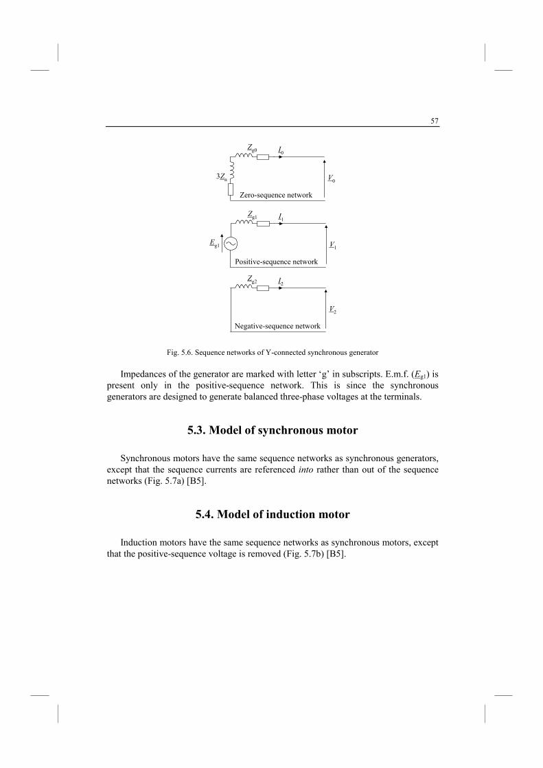
57
I0
V0
Zg0
3Zn
Zero-sequence network
I1
V1
Zg1
Positive-sequence network
Eg1
I2
V2
Zg2
Negative-sequence network
Fig. 5.6. Sequence networks of Y-connected synchronous generator
Impedances of the generator are marked with letter ‘g’ in subscripts. E.m.f. (Eg1) is
present only in the positive-sequence network. This is since the synchronous generators are designed to generate balanced three-phase voltages at the terminals.
5.3. Model of synchronous motor
Synchronous motors have the same sequence networks as synchronous generators, except that the sequence currents are referenced into rather than out of the sequence networks (Fig. 5.7a) [B5].
5.4. Model of induction motor
Induction motors have the same sequence networks as synchronous motors, except that the positive-sequence voltage is removed (Fig. 5.7b) [B5].
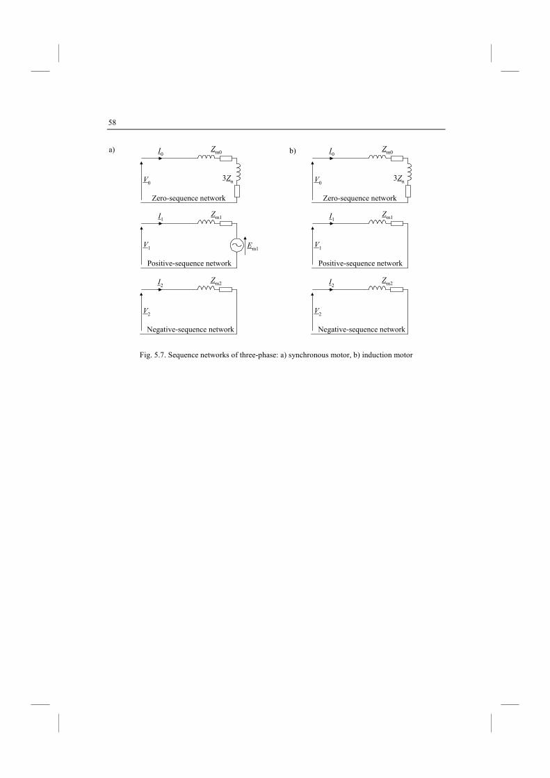
58
I0
V0
Zm0
3Zn
Zero-sequence network
Em1
I1
V1
Zm1
Positive-sequence network
I2
V2
Zm2
Negative-sequence network
I0
V0
Zm0
3Zn
Zero-sequence network
I1
V1
Zm1
Positive-sequence network
I2
V2
Zm2
Negative-sequence network
Fig. 5.7. Sequence networks of three-phase: a) synchronous motor, b) induction motor
a) b)
59
6. MODELS OF POWER TRASFORMERS
6.1. Introduction
In this Chapter the basics for representing power transformers in fault calculations are introduced. First, equivalent circuit diagrams, together with calculation of the parameters involved in these circuits, are presented. Then, transformer windings connections are considered. Finally, equivalent circuit diagrams of power transformers for symmetrical components are taken into consideration.
6.2. Equivalent circuit diagrams of two-winding transformer
The basic models of two-windings transformers for a symmetrical steady state are presented in Fig. 6.1 (H – high voltage side, L – low voltage side).
In the circuit diagram of Fig. 6.1a the longitudinal branches represent the windings resistances (RH, RL) and leakage reactances (XH, XL). In turn, the shunt branch represents iron losses (RFe) and magnetizing reactance (Xµ). The ideal transformer with the specified induced voltages at its both sides (EH and EL/ϑn, where ϑn=)H/)L is the nominal transformer ratio; )H, )L – numbers of the turns of the H and L side windings) completes the circuit diagram of Fig. 6.1a.
After recalculation of the current, voltage, winding resistance and leakage reactance from the L side to the H side we obtain the circuit diagram as shown in Fig. 6.1b.
Further simplification can be obtained by neglecting the shunt branch, also named as the excitation branch – Fig. 6.1c. Such simplification is commonly assumed for fault currents calculation.
Taking into account that there is a symmetry in transformer construction and that a transformer is a static (non-rotating) power system element, the schemes from Fig. 6.1 can be also utilized for representing transformers for the positive- and negative-sequences. Their adaptation to three-phase transformers requires only to include additionally the phase shift resulting from the three phases windings connection (the transformer vector group). Special considerations for representation of three-phase transformers for the zero-sequence are required.
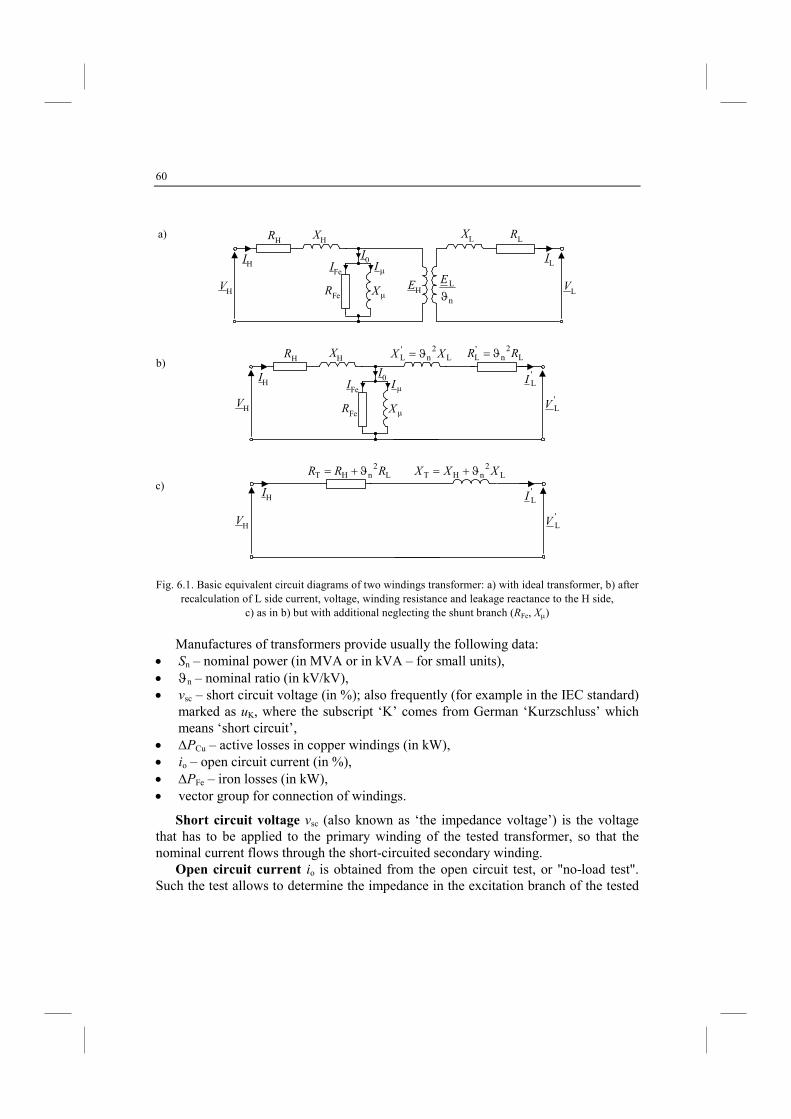
60
IH
VH
RHXH
EHn
L
ϑE
VL
XL RL
ILIFe
RFe µX
I0µI
IH
VH
RHXH L
2n
'L XX ϑ= L
2n
'L RR ϑ=
'LI
'LV
IFe
RFe µX
I0µI
IH
VH
L2
nHT RRR ϑ+= L2
nHT XXX ϑ+=
'LI
'LV
Fig. 6.1. Basic equivalent circuit diagrams of two windings transformer: a) with ideal transformer, b) after recalculation of L side current, voltage, winding resistance and leakage reactance to the H side,
c) as in b) but with additional neglecting the shunt branch (RFe, Xµ)
Manufactures of transformers provide usually the following data:
• Sn – nominal power (in MVA or in kVA – for small units), • ϑn – nominal ratio (in kV/kV), • vsc – short circuit voltage (in %); also frequently (for example in the IEC standard)
marked as uK, where the subscript ‘K’ comes from German ‘Kurzschluss’ which means ‘short circuit’,
• ∆PCu – active losses in copper windings (in kW), • io – open circuit current (in %), • ∆PFe – iron losses (in kW), • vector group for connection of windings.
Short circuit voltage vsc (also known as ‘the impedance voltage’) is the voltage that has to be applied to the primary winding of the tested transformer, so that the nominal current flows through the short-circuited secondary winding.
Open circuit current io is obtained from the open circuit test, or "no-load test". Such the test allows to determine the impedance in the excitation branch of the tested
a)
b)
c)
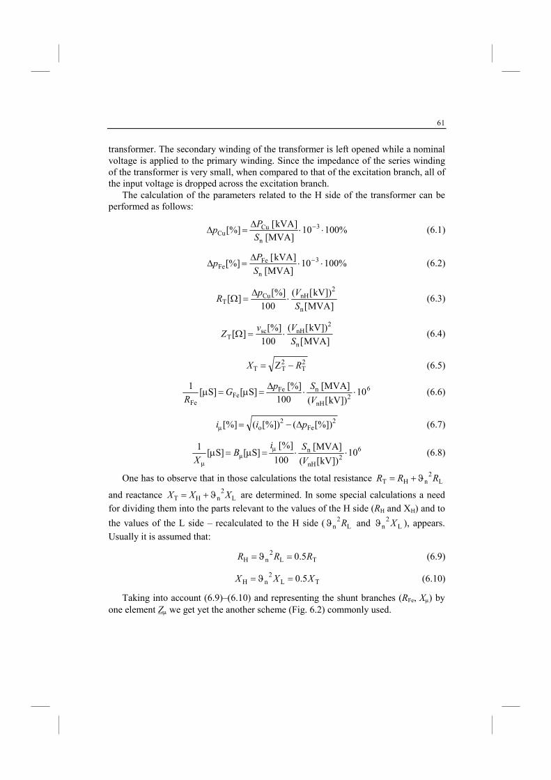
61
transformer. The secondary winding of the transformer is left opened while a nominal voltage is applied to the primary winding. Since the impedance of the series winding of the transformer is very small, when compared to that of the excitation branch, all of the input voltage is dropped across the excitation branch.
The calculation of the parameters related to the H side of the transformer can be performed as follows:
%10010[MVA]
]kVA[ [%] 3
n
CuCu ⋅⋅
∆=∆ −
S
Pp (6.1)
%10010[MVA]
]kVA[ [%] 3
n
FeFe ⋅⋅
∆=∆ −
S
Pp (6.2)
]MVA[
])kV[(
100
[%]][
n
2nHCu
TS
VpR ⋅
∆=Ω (6.3)
]MVA[
])kV[(
100
[%]][
n
2nHsc
TS
VvZ ⋅=Ω (6.4)
2T
2TT Z RX −= (6.5)
62
nH
nFeFe
Fe
10])kV[(
[MVA]
100
]%[ ]S[]S[
1⋅⋅
∆=µ=µ
V
SpG
R (6.6)
2Fe
2o [%])([%])([%] pii ∆−=µ (6.7)
62
nH
nµ
µ
10])kV[(
[MVA]
100
]%[ ]S[]S[
1⋅⋅=µ=µ µ
V
SiB
X (6.8)
One has to observe that in those calculations the total resistance L2
nHT RRR ϑ+=
and reactance L2
nHT XXX ϑ+= are determined. In some special calculations a need
for dividing them into the parts relevant to the values of the H side (RH and XH) and to
the values of the L side – recalculated to the H side ( L2
n Rϑ and L2
n Xϑ ), appears.
Usually it is assumed that:
TL2
nH 5.0 RRR =ϑ= (6.9)
TL2
nH 5.0 XXX =ϑ= (6.10)
Taking into account (6.9)–(6.10) and representing the shunt branches (RFe, Xµ) by one element Zµ we get yet the another scheme (Fig. 6.2) commonly used.
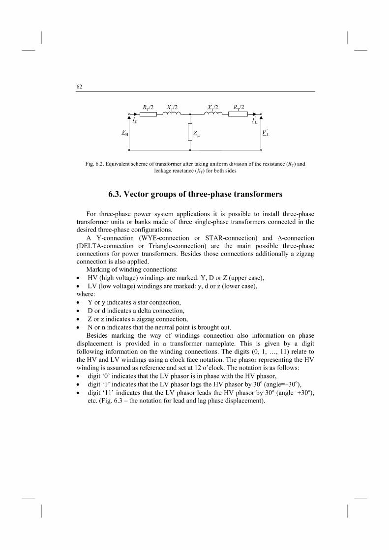
62
IH
VH
RT/2
'LI
'LV
XT/2 XT/2 RT/2
µZ
Fig. 6.2. Equivalent scheme of transformer after taking uniform division of the resistance (RT) and leakage reactance (XT) for both sides
6.3. Vector groups of three-phase transformers
For three-phase power system applications it is possible to install three-phase transformer units or banks made of three single-phase transformers connected in the desired three-phase configurations.
A Y-connection (WYE-connection or STAR-connection) and ∆-connection (DELTA-connection or Triangle-connection) are the main possible three-phase connections for power transformers. Besides those connections additionally a zigzag connection is also applied.
Marking of winding connections: • HV (high voltage) windings are marked: Y, D or Z (upper case), • LV (low voltage) windings are marked: y, d or z (lower case), where: • Y or y indicates a star connection, • D or d indicates a delta connection, • Z or z indicates a zigzag connection, • N or n indicates that the neutral point is brought out.
Besides marking the way of windings connection also information on phase displacement is provided in a transformer nameplate. This is given by a digit following information on the winding connections. The digits (0, 1, …, 11) relate to the HV and LV windings using a clock face notation. The phasor representing the HV winding is assumed as reference and set at 12 o’clock. The notation is as follows: • digit ‘0’ indicates that the LV phasor is in phase with the HV phasor, • digit ‘1’ indicates that the LV phasor lags the HV phasor by 30o (angle=–30o), • digit ‘11’ indicates that the LV phasor leads the HV phasor by 30o (angle=+30o),
etc. (Fig. 6.3 – the notation for lead and lag phase displacement).
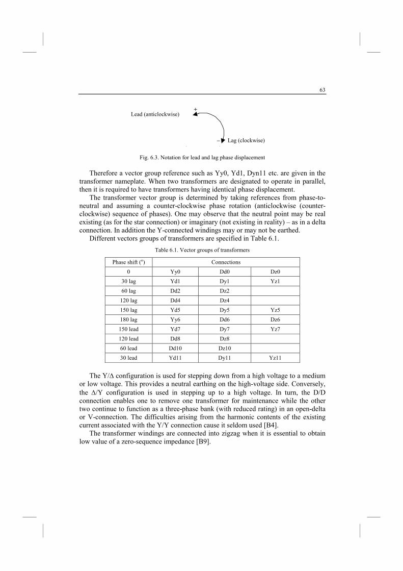
63
Lead (anticlockwise)
Lag (clockwise)
+
–
Fig. 6.3. Notation for lead and lag phase displacement
Therefore a vector group reference such as Yy0, Yd1, Dyn11 etc. are given in the
transformer nameplate. When two transformers are designated to operate in parallel, then it is required to have transformers having identical phase displacement.
The transformer vector group is determined by taking references from phase-to-neutral and assuming a counter-clockwise phase rotation (anticlockwise (counter-clockwise) sequence of phases). One may observe that the neutral point may be real existing (as for the star connection) or imaginary (not existing in reality) – as in a delta connection. In addition the Y-connected windings may or may not be earthed.
Different vectors groups of transformers are specified in Table 6.1.
Table 6.1. Vector groups of transformers
Phase shift (o) Connections
0 Yy0 Dd0 Dz0
30 lag Yd1 Dy1 Yz1
60 lag Dd2 Dz2
120 lag Dd4 Dz4
150 lag Yd5 Dy5 Yz5
180 lag Yy6 Dd6 Dz6
150 lead Yd7 Dy7 Yz7
120 lead Dd8 Dz8
60 lead Dd10 Dz10
30 lead Yd11 Dy11 Yz11
The Y/∆ configuration is used for stepping down from a high voltage to a medium
or low voltage. This provides a neutral earthing on the high-voltage side. Conversely, the ∆/Y configuration is used in stepping up to a high voltage. In turn, the D/D connection enables one to remove one transformer for maintenance while the other two continue to function as a three-phase bank (with reduced rating) in an open-delta or V-connection. The difficulties arising from the harmonic contents of the existing current associated with the Y/Y connection cause it seldom used [B4].
The transformer windings are connected into zigzag when it is essential to obtain low value of a zero-sequence impedance [B9].
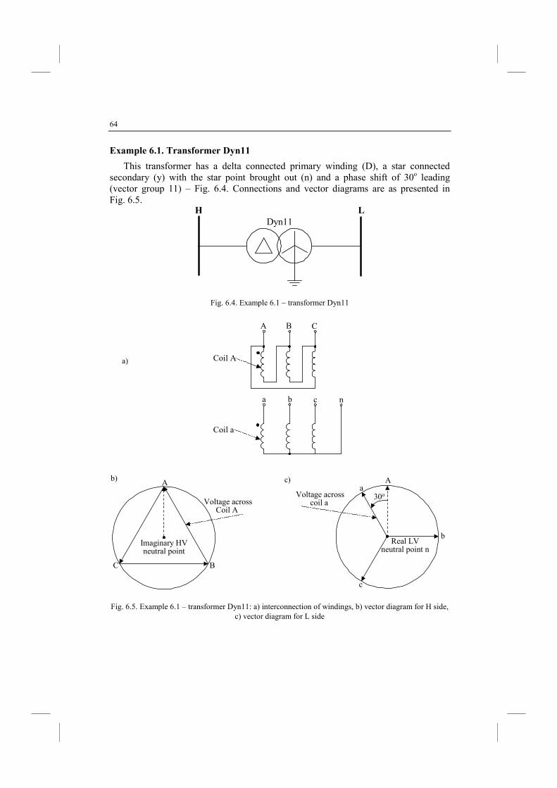
64
Example 6.1. Transformer Dyn11
This transformer has a delta connected primary winding (D), a star connected secondary (y) with the star point brought out (n) and a phase shift of 30o leading (vector group 11) – Fig. 6.4. Connections and vector diagrams are as presented in Fig. 6.5.
H L
Dyn11
Fig. 6.4. Example 6.1 – transformer Dyn11
Coil a
A B C
a b c n
Coil A
Voltage acrossCoil A
Imaginary HVneutral point
A
BC
Voltage acrosscoil a
Real LVneutral point n
b
c
30oa
A
Fig. 6.5. Example 6.1 – transformer Dyn11: a) interconnection of windings, b) vector diagram for H side, c) vector diagram for L side
a)
b) c)
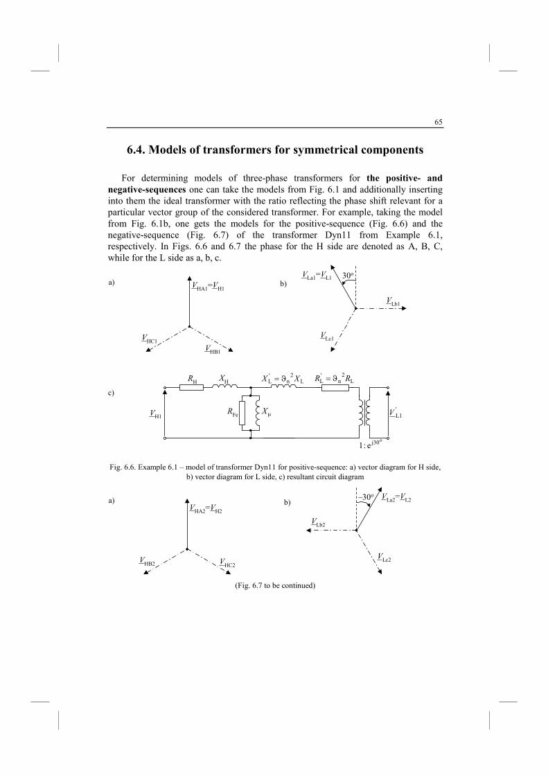
65
6.4. Models of transformers for symmetrical components
For determining models of three-phase transformers for the positive- and negative-sequences one can take the models from Fig. 6.1 and additionally inserting into them the ideal transformer with the ratio reflecting the phase shift relevant for a particular vector group of the considered transformer. For example, taking the model from Fig. 6.1b, one gets the models for the positive-sequence (Fig. 6.6) and the negative-sequence (Fig. 6.7) of the transformer Dyn11 from Example 6.1, respectively. In Figs. 6.6 and 6.7 the phase for the H side are denoted as A, B, C, while for the L side as a, b, c.
VHA1=VH1
VHB1
VHC1
VLa1=VL1 30o
VLc1
VLb1
VH1
RHXH
RFe
L2
n'L XX ϑ= L
2n
'L RR ϑ=
'L1V
oj30e:1
µX
Fig. 6.6. Example 6.1 – model of transformer Dyn11 for positive-sequence: a) vector diagram for H side, b) vector diagram for L side, c) resultant circuit diagram
VHA2=VH2
VHC2VHB2
VLa2=VL2–30o
VLb2
VLc2
(Fig. 6.7 to be continued)
a) b)
c)
a) b)
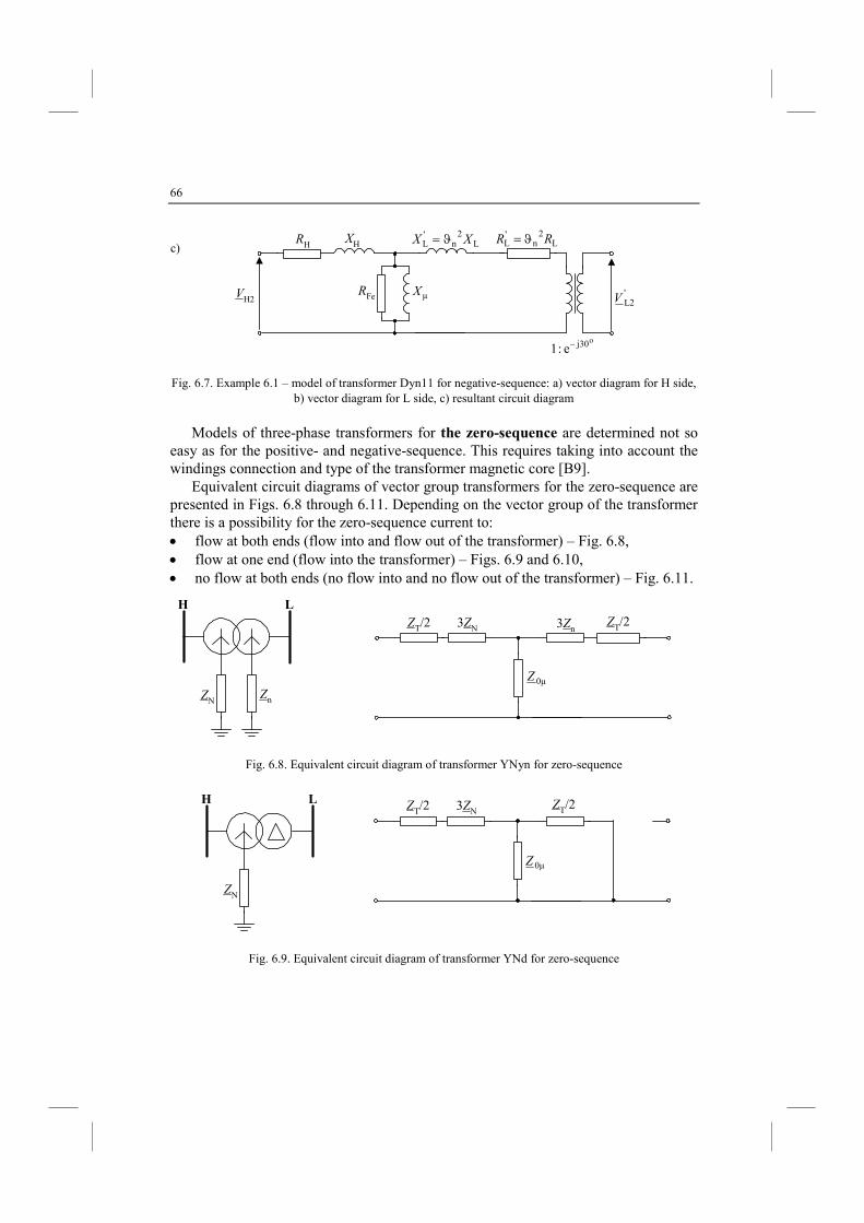
66
VH2
RHXH
RFe
L2
n'L XX ϑ= L
2n
'L RR ϑ=
'L2V
oj30e:1 −
µX
Fig. 6.7. Example 6.1 – model of transformer Dyn11 for negative-sequence: a) vector diagram for H side, b) vector diagram for L side, c) resultant circuit diagram
Models of three-phase transformers for the zero-sequence are determined not so
easy as for the positive- and negative-sequence. This requires taking into account the windings connection and type of the transformer magnetic core [B9].
Equivalent circuit diagrams of vector group transformers for the zero-sequence are presented in Figs. 6.8 through 6.11. Depending on the vector group of the transformer there is a possibility for the zero-sequence current to: • flow at both ends (flow into and flow out of the transformer) – Fig. 6.8, • flow at one end (flow into the transformer) – Figs. 6.9 and 6.10, • no flow at both ends (no flow into and no flow out of the transformer) – Fig. 6.11.
H L
ZNZn
ZT/2 3ZNZT/23Zn
0µZ
Fig. 6.8. Equivalent circuit diagram of transformer YNyn for zero-sequence
H L
ZN
ZT/2 3ZNZT/2
0µZ
Fig. 6.9. Equivalent circuit diagram of transformer YNd for zero-sequence
c)
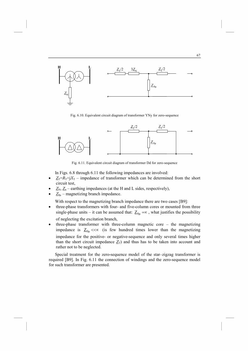
67
H L
ZN
ZT/2 3ZNZT/2
0µZ
Fig. 6.10. Equivalent circuit diagram of transformer YNy for zero-sequence
H L
ZT/2 ZT/2
0µZ
Fig. 6.11. Equivalent circuit diagram of transformer Dd for zero-sequence
In Figs. 6.8 through 6.11 the following impedances are involved:
• ZT=RT+jXT – impedance of transformer which can be determined from the short circuit test,
• ZN, Zn – earthing impedances (at the H and L sides, respectively), • Z0µ – magnetizing branch impedance.
With respect to the magnetizing branch impedance there are two cases [B9]: • three-phase transformers with four- and five-column cores or mounted from three
single-phase units – it can be assumed that: =∝0µZ , what justifies the possibility
of neglecting the excitation branch, • three-phase transformer with three-column magnetic core – the magnetizing
impedance is <<∝0µZ (is few hundred times lower than the magnetizing
impedance for the positive- or negative-sequence and only several times higher than the short circuit impedance ZT) and thus has to be taken into account and rather not to be neglected.
Special treatment for the zero-sequence model of the star–zigzag transformer is required [B9]. In Fig. 6.11 the connection of windings and the zero-sequence model for such transformer are presented.
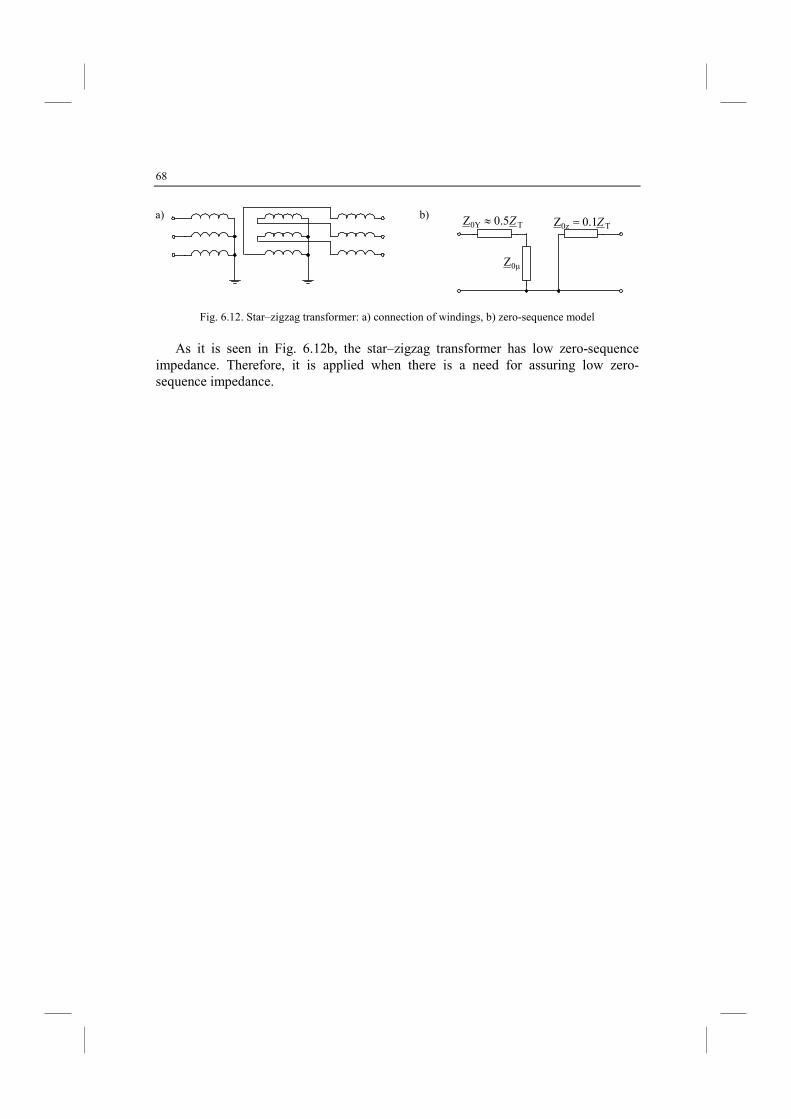
68
0µZ
T0Y 5.0Z Z≈ T0z 1.0Z Z=
Fig. 6.12. Star–zigzag transformer: a) connection of windings, b) zero-sequence model
As it is seen in Fig. 6.12b, the star–zigzag transformer has low zero-sequence
impedance. Therefore, it is applied when there is a need for assuring low zero-sequence impedance.
a) b)
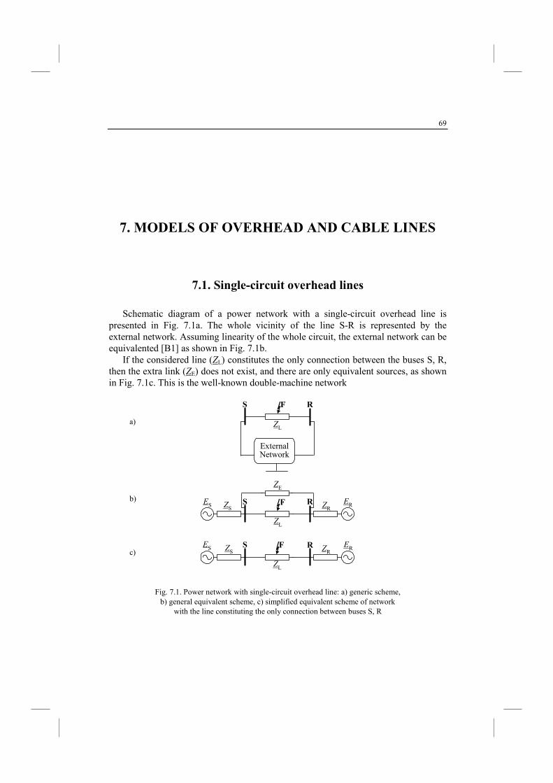
69
7. MODELS OF OVERHEAD AD CABLE LIES
7.1. Single-circuit overhead lines
Schematic diagram of a power network with a single-circuit overhead line is presented in Fig. 7.1a. The whole vicinity of the line S-R is represented by the external network. Assuming linearity of the whole circuit, the external network can be equivalented [B1] as shown in Fig. 7.1b.
If the considered line (ZL) constitutes the only connection between the buses S, R, then the extra link (ZE) does not exist, and there are only equivalent sources, as shown in Fig. 7.1c. This is the well-known double-machine network
RFS
ExternalNetwork
ZL
RFS
ZE
ZL
ZSES
ERZR
RFS
ZL
ZSES ERZR
Fig. 7.1. Power network with single-circuit overhead line: a) generic scheme, b) general equivalent scheme, c) simplified equivalent scheme of network
with the line constituting the only connection between buses S, R
a)
b)
c)
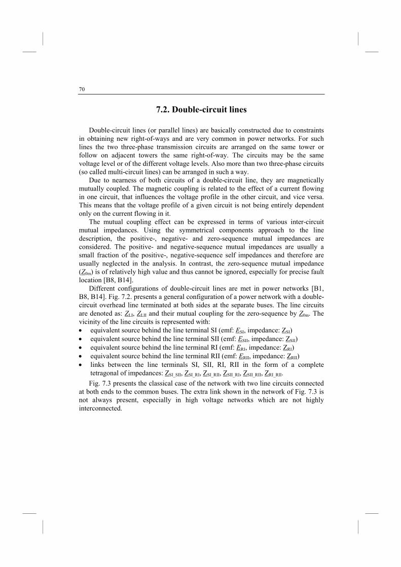
70
7.2. Double-circuit lines
Double-circuit lines (or parallel lines) are basically constructed due to constraints in obtaining new right-of-ways and are very common in power networks. For such lines the two three-phase transmission circuits are arranged on the same tower or follow on adjacent towers the same right-of-way. The circuits may be the same voltage level or of the different voltage levels. Also more than two three-phase circuits (so called multi-circuit lines) can be arranged in such a way.
Due to nearness of both circuits of a double-circuit line, they are magnetically mutually coupled. The magnetic coupling is related to the effect of a current flowing in one circuit, that influences the voltage profile in the other circuit, and vice versa. This means that the voltage profile of a given circuit is not being entirely dependent only on the current flowing in it.
The mutual coupling effect can be expressed in terms of various inter-circuit mutual impedances. Using the symmetrical components approach to the line description, the positive-, negative- and zero-sequence mutual impedances are considered. The positive- and negative-sequence mutual impedances are usually a small fraction of the positive-, negative-sequence self impedances and therefore are usually neglected in the analysis. In contrast, the zero-sequence mutual impedance (Z0m) is of relatively high value and thus cannot be ignored, especially for precise fault location [B8, B14].
Different configurations of double-circuit lines are met in power networks [B1, B8, B14]. Fig. 7.2. presents a general configuration of a power network with a double-circuit overhead line terminated at both sides at the separate buses. The line circuits are denoted as: ZLI, ZLII and their mutual coupling for the zero-sequence by Z0m. The vicinity of the line circuits is represented with: • equivalent source behind the line terminal SI (emf: ESI, impedance: ZSI) • equivalent source behind the line terminal SII (emf: ESII, impedance: ZSII) • equivalent source behind the line terminal RI (emf: ERI, impedance: ZRI) • equivalent source behind the line terminal RII (emf: ERII, impedance: ZRII) • links between the line terminals SI, SII, RI, RII in the form of a complete
tetragonal of impedances: ZSI_SII, ZSI_RI, ZSI_RII, ZSII_RI, ZSII_RII, ZRI_RII.
Fig. 7.3 presents the classical case of the network with two line circuits connected at both ends to the common buses. The extra link shown in the network of Fig. 7.3 is not always present, especially in high voltage networks which are not highly interconnected.
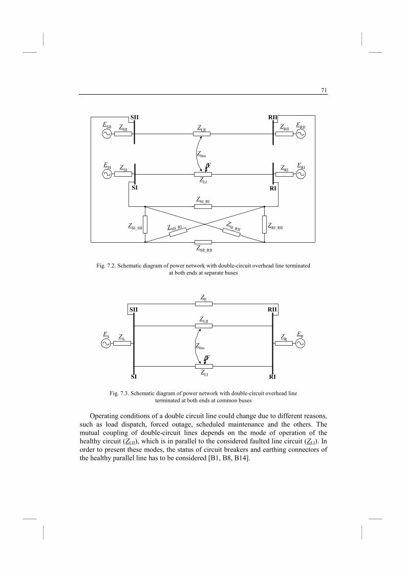
71
ESII
SI
SII
RI
RII
Z0m
F
ZSI_SII
ZSII
ESI ZSI
ERIIZRII
ERIZRI
ZRI_RII
ZSII_RII
ZSI_RI
ZSII_RIZ
SI_RII
ZLI
ZLII
Fig. 7.2. Schematic diagram of power network with double-circuit overhead line terminated at both ends at separate buses
ES
SI
SII
RI
RII
Z0m
F
ZSERZR
ZLI
ZLII
ZE
Fig. 7.3. Schematic diagram of power network with double-circuit overhead line terminated at both ends at common buses
Operating conditions of a double circuit line could change due to different reasons, such as load dispatch, forced outage, scheduled maintenance and the others. The mutual coupling of double-circuit lines depends on the mode of operation of the healthy circuit (ZLII), which is in parallel to the considered faulted line circuit (ZLI). In order to present these modes, the status of circuit breakers and earthing connectors of the healthy parallel line has to be considered [B1, B8, B14].
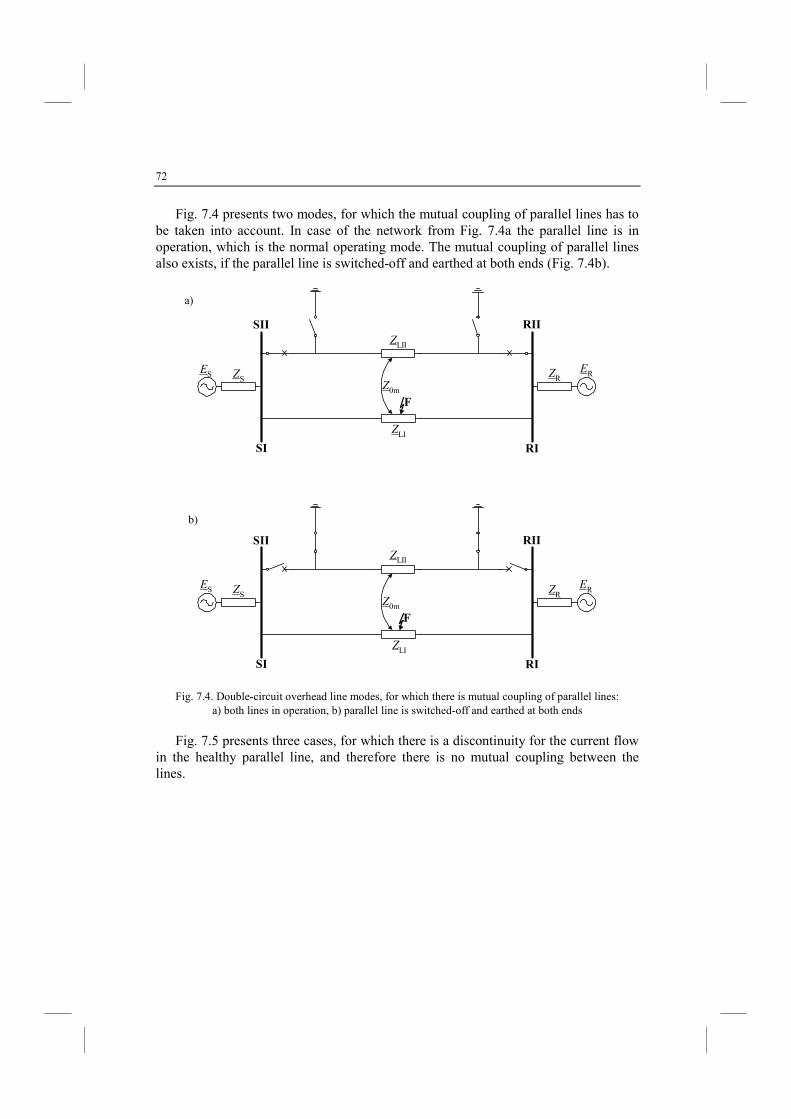
72
Fig. 7.4 presents two modes, for which the mutual coupling of parallel lines has to be taken into account. In case of the network from Fig. 7.4a the parallel line is in operation, which is the normal operating mode. The mutual coupling of parallel lines also exists, if the parallel line is switched-off and earthed at both ends (Fig. 7.4b).
ES
SI
SII
RI
RII
Z0m
F
ZSERZR
ZLI
ZLII
ES
SI
SII
RI
RII
Z0m
F
ZSERZR
ZLI
ZLII
Fig. 7.4. Double-circuit overhead line modes, for which there is mutual coupling of parallel lines: a) both lines in operation, b) parallel line is switched-off and earthed at both ends
Fig. 7.5 presents three cases, for which there is a discontinuity for the current flow in the healthy parallel line, and therefore there is no mutual coupling between the lines.
a)
b)
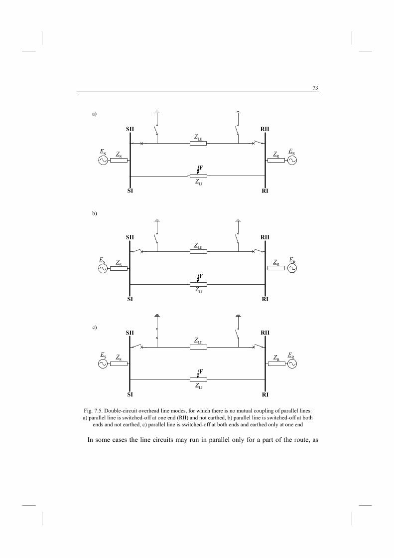
73
ES
SI
SII
RI
RII
F
ZSERZR
ZLI
ZLII
ES
SI
SII
RI
RII
F
ZSERZR
ZLI
ZLII
ES
SI
SII
RI
RII
F
ZSERZR
ZLI
ZLII
Fig. 7.5. Double-circuit overhead line modes, for which there is no mutual coupling of parallel lines: a) parallel line is switched-off at one end (RII) and not earthed, b) parallel line is switched-off at both
ends and not earthed, c) parallel line is switched-off at both ends and earthed only at one end
In some cases the line circuits may run in parallel only for a part of the route, as
a)
b)
c)
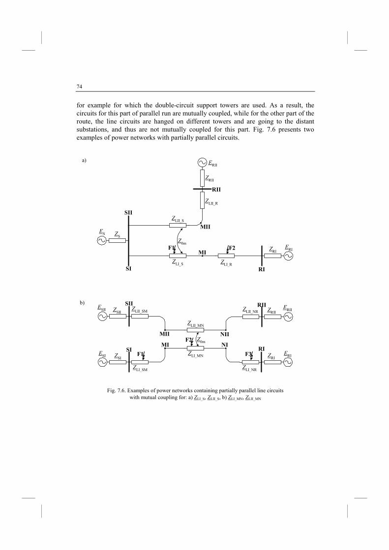
74
for example for which the double-circuit support towers are used. As a result, the circuits for this part of parallel run are mutually coupled, while for the other part of the route, the line circuits are hanged on different towers and are going to the distant substations, and thus are not mutually coupled for this part. Fig. 7.6 presents two examples of power networks with partially parallel circuits.
ES
SI
SII
RI
F1
ZS
ERIZRI
ZLI_S
ERII
Z0mF2
ZLII_S
ZLII_R
RII
ZRII
MII
MI
ZLI_R
ESI ZSIF1
F2
F3
Z0m
SI
SIIESII ZSII
ERIZRI
ERIIZRII
RI
RII
MI I
MII II
ZLII_SM
ZLII_MN
ZLII_NR
ZLI_SM
ZLI_MN
ZLI_NR
Fig. 7.6. Examples of power networks containing partially parallel line circuits with mutual coupling for: a) ZLI_S, ZLII_S, b) ZLI_MN, ZLII_MN
a)
b)
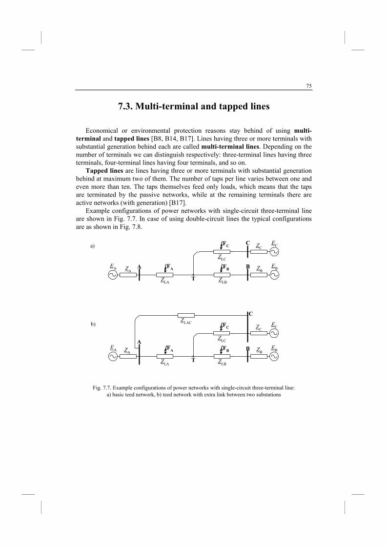
75
7.3. Multi-terminal and tapped lines
Economical or environmental protection reasons stay behind of using multi-terminal and tapped lines [B8, B14, B17]. Lines having three or more terminals with substantial generation behind each are called multi-terminal lines. Depending on the number of terminals we can distinguish respectively: three-terminal lines having three terminals, four-terminal lines having four terminals, and so on.
Tapped lines are lines having three or more terminals with substantial generation behind at maximum two of them. The number of taps per line varies between one and even more than ten. The taps themselves feed only loads, which means that the taps are terminated by the passive networks, while at the remaining terminals there are active networks (with generation) [B17].
Example configurations of power networks with single-circuit three-terminal line are shown in Fig. 7.7. In case of using double-circuit lines the typical configurations are as shown in Fig. 7.8.
BFAA
ZLA
ZAEA EBZB
C ECZC
ZLB
ZLC
T
FB
FC
BFA
A
ZLA
ZAEA EBZB
C
ECZC
ZLB
ZLC
T
FB
FC
ZLAC
Fig. 7.7. Example configurations of power networks with single-circuit three-terminal line: a) basic teed network, b) teed network with extra link between two substations
a)
b)
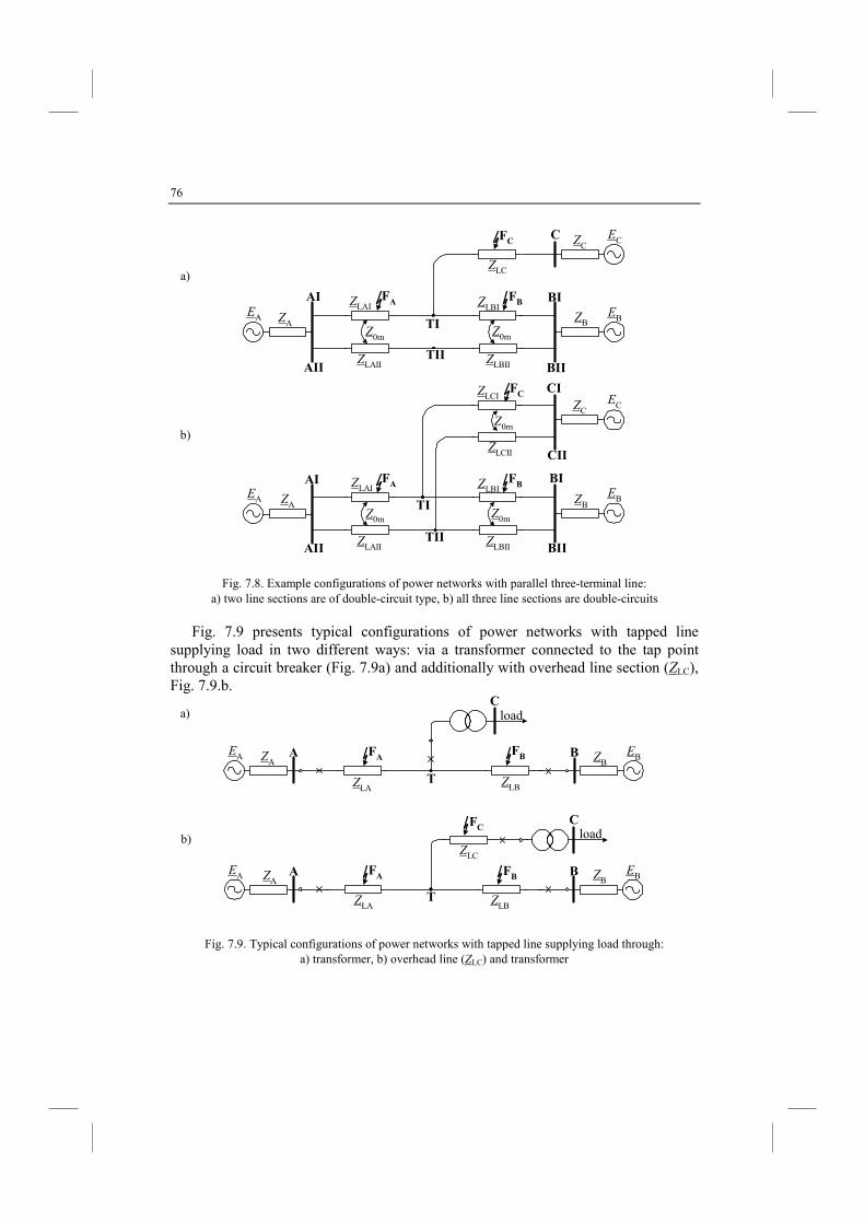
76
BIFAAI ZLAI
ZAEA EBZB
C ECZC
ZLC
TI
FB
FC
ZLAII
Z0m
TII ZLBII
Z0m
ZLBI
BIIAII
BIFAAI ZLAI
ZAEA
EBZB
CIECZC
ZLCII
TI
FB
FC
ZLAII
Z0m
TII ZLBII
Z0m
ZLBI
BIIAII
Z0m
ZLCI
CII
Fig. 7.8. Example configurations of power networks with parallel three-terminal line: a) two line sections are of double-circuit type, b) all three line sections are double-circuits
Fig. 7.9 presents typical configurations of power networks with tapped line supplying load in two different ways: via a transformer connected to the tap point through a circuit breaker (Fig. 7.9a) and additionally with overhead line section (ZLC), Fig. 7.9.b.
BFAA
ZLA
ZAEA EBZB
C
ZLBT
FB
load
BFAA
ZLA
ZAEA EBZB
C
ZLBT
FB
loadFC
ZLC
Fig. 7.9. Typical configurations of power networks with tapped line supplying load through: a) transformer, b) overhead line (ZLC) and transformer
a)
b)
a)
b)
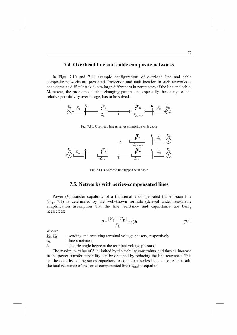
77
7.4. Overhead line and cable composite networks
In Figs. 7.10 and 7.11 example configurations of overhead line and cable composite networks are presented. Protection and fault location in such networks is considered as difficult task due to large differences in parameters of the line and cable. Moreover, the problem of cable changing parameters, especially the change of the relative permittivity over its age, has to be solved.
RFS
S
ZCABLE
ZSES ERZR
ZLT
FR
Fig. 7.10. Overhead line in series connection with cable
BFAA
ZCABLE
ZAEA E
BZB
C ECZC
ZLBZLA
T
FB
FC
Fig. 7.11. Overhead line tapped with cable
7.5. etworks with series-compensated lines
Power (P) transfer capability of a traditional uncompensated transmission line (Fig. 7.1) is determined by the well-known formula (derived under reasonable simplification assumption that the line resistance and capacitance are being neglected):
)δsin(||||
L
RS
X
VVP
⋅= (7.1)
where: VS, VR – sending and receiving terminal voltage phasors, respectively, XL – line reactance, δ – electric angle between the terminal voltage phasors.
The maximum value of δ is limited by the stability constraints, and thus an increase in the power transfer capability can be obtained by reducing the line reactance. This can be done by adding series capacitors to counteract series inductance. As a result, the total reactance of the series compensated line (Xtotal) is equal to:
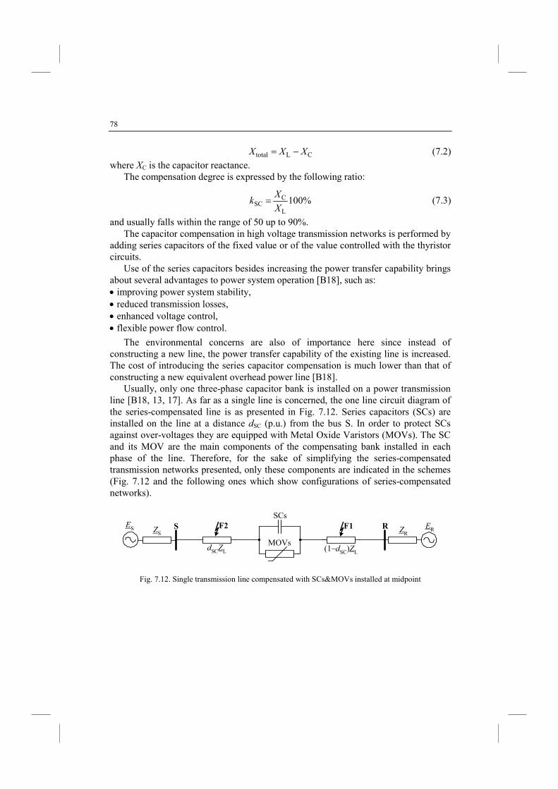
78
CLtotal XXX −= (7.2)
where XC is the capacitor reactance. The compensation degree is expressed by the following ratio:
%100L
CSC
X
Xk = (7.3)
and usually falls within the range of 50 up to 90%. The capacitor compensation in high voltage transmission networks is performed by
adding series capacitors of the fixed value or of the value controlled with the thyristor circuits.
Use of the series capacitors besides increasing the power transfer capability brings about several advantages to power system operation [B18], such as: • improving power system stability, • reduced transmission losses, • enhanced voltage control, • flexible power flow control.
The environmental concerns are also of importance here since instead of constructing a new line, the power transfer capability of the existing line is increased. The cost of introducing the series capacitor compensation is much lower than that of constructing a new equivalent overhead power line [B18].
Usually, only one three-phase capacitor bank is installed on a power transmission line [B18, 13, 17]. As far as a single line is concerned, the one line circuit diagram of the series-compensated line is as presented in Fig. 7.12. Series capacitors (SCs) are installed on the line at a distance dSC (p.u.) from the bus S. In order to protect SCs against over-voltages they are equipped with Metal Oxide Varistors (MOVs). The SC and its MOV are the main components of the compensating bank installed in each phase of the line. Therefore, for the sake of simplifying the series-compensated transmission networks presented, only these components are indicated in the schemes (Fig. 7.12 and the following ones which show configurations of series-compensated networks).
ES S F2ZS
ERZR
dSCZL
F1
(1–dSC)ZL
R
MOVs
SCs
Fig. 7.12. Single transmission line compensated with SCs&MOVs installed at midpoint
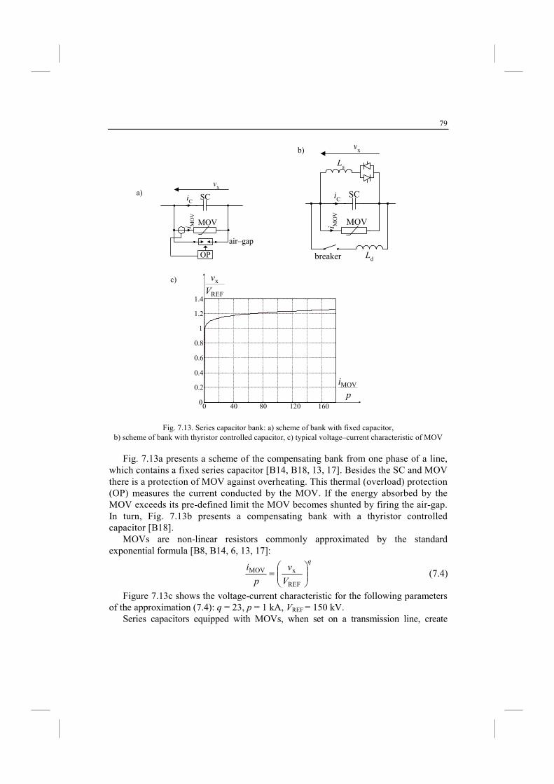
79
OP
i MO
V
MOV
air–gap
SC
vx
iC
i MO
V
MOV
SC
vx
iC
Ls
breaker Ld
0 40 80 1200
0.2
0.4
0.6
0.8
1
1.2
p
iMOV
160
REF
x
V
v
1.4
Fig. 7.13. Series capacitor bank: a) scheme of bank with fixed capacitor, b) scheme of bank with thyristor controlled capacitor, c) typical voltage–current characteristic of MOV
Fig. 7.13a presents a scheme of the compensating bank from one phase of a line, which contains a fixed series capacitor [B14, B18, 13, 17]. Besides the SC and MOV there is a protection of MOV against overheating. This thermal (overload) protection (OP) measures the current conducted by the MOV. If the energy absorbed by the MOV exceeds its pre-defined limit the MOV becomes shunted by firing the air-gap. In turn, Fig. 7.13b presents a compensating bank with a thyristor controlled capacitor [B18].
MOVs are non-linear resistors commonly approximated by the standard exponential formula [B8, B14, 6, 13, 17]:
q
V
v
p
i
=
REF
xMOV (7.4)
Figure 7.13c shows the voltage-current characteristic for the following parameters of the approximation (7.4): q = 23, p = 1 kA, VREF = 150 kV.
Series capacitors equipped with MOVs, when set on a transmission line, create
a)
b)
c)
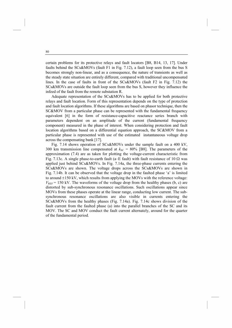
80
certain problems for its protective relays and fault locators [B8, B14, 13, 17]. Under faults behind the SCs&MOVs (fault F1 in Fig. 7.12), a fault loop seen from the bus S becomes strongly non-linear, and as a consequence, the nature of transients as well as the steady state situation are entirely different, compared with traditional uncompensated lines. In the case of faults in front of the SCs&MOVs (fault F2 in Fig. 7.12) the SCs&MOVs are outside the fault loop seen from the bus S, however they influence the infeed of the fault from the remote substation R.
Adequate representation of the SCs&MOVs has to be applied for both protective relays and fault location. Form of this representation depends on the type of protection and fault location algorithms. If these algorithms are based on phasor technique, then the SC&MOV from a particular phase can be represented with the fundamental frequency equivalent [6] in the form of resistance-capacitive reactance series branch with parameters dependent on an amplitude of the current (fundamental frequency component) measured in the phase of interest. When considering protection and fault location algorithms based on a differential equation approach, the SC&MOV from a particular phase is represented with use of the estimated instantaneous voltage drop across the compensating bank [17].
Fig. 7.14 shows operation of SCs&MOVs under the sample fault on a 400 kV, 300 km transmission line compensated at kSC = 80% [B8]. The parameters of the approximation (7.4) are as taken for plotting the voltage-current characteristic from Fig. 7.13c. A single phase-to-earth fault (a–E fault) with fault resistance of 10 Ω was applied just behind SCs&MOVs. In Fig. 7.14a, the three-phase currents entering the SCs&MOVs are shown. The voltage drops across the SCs&MOVs are shown in Fig. 7.14b. It can be observed that the voltage drop in the faulted phase ‘a’ is limited to around ±150 kV, which results from applying the MOVs with the reference voltage: VREF = 150 kV. The waveforms of the voltage drop from the healthy phases (b, c) are distorted by sub-synchronous resonance oscillations. Such oscillations appear since MOVs from these phases operate at the linear range, conducting low current. The sub-synchronous resonance oscillations are also visible in currents entering the SCs&MOVs from the healthy phases (Fig. 7.14a). Fig. 7.14c shows division of the fault current from the faulted phase (a) into the parallel branches of the SC and its MOV. The SC and MOV conduct the fault current alternately, around for the quarter of the fundamental period.
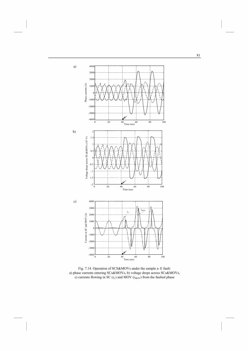
81
–4000
4000
0 20 40 60 80 100
–3000
–2000
–1000
0
1000
2000
3000
Time (ms)
a b cPha
se c
urre
nts (A
)
0 20 40 60 80 100–2
–1.5
–1
–0.5
0
0.5
1
1.5
2
Vol
tage
dro
ps a
cros
s SC
s&M
OV
s (1
05 V
)
Time (ms)
a b c
0 20 40 60 80 100–4000
–3000
–2000
–1000
0
1000
2000
3000
4000
Cur
rent
s in
SC
and
MO
V (A
)
Time (ms)
iMOViC
Fig. 7.14. Operation of SCS&MOVs under the sample a–E fault: a) phase currents entering SCs&MOVs, b) voltage drops across SCs&MOVs,
c) currents flowing in SC (iC) and MOV (iMOV) from the faulted phase
a)
b)
c)
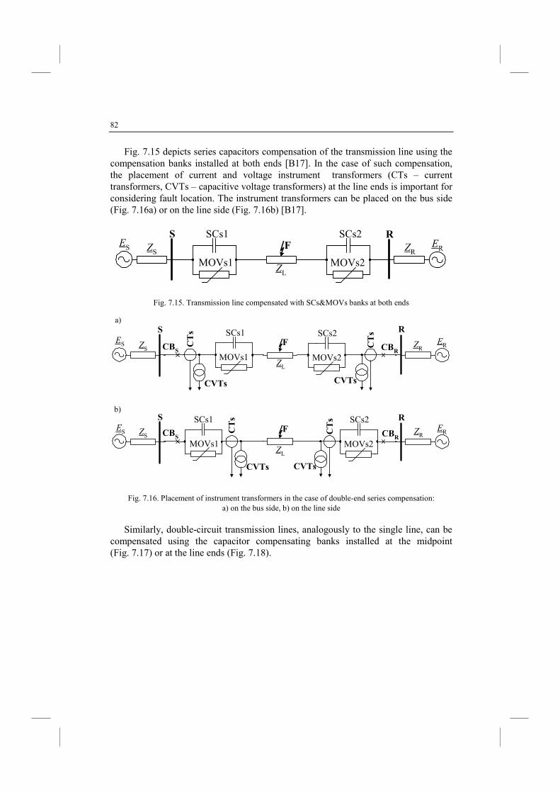
82
Fig. 7.15 depicts series capacitors compensation of the transmission line using the compensation banks installed at both ends [B17]. In the case of such compensation, the placement of current and voltage instrument transformers (CTs – current transformers, CVTs – capacitive voltage transformers) at the line ends is important for considering fault location. The instrument transformers can be placed on the bus side (Fig. 7.16a) or on the line side (Fig. 7.16b) [B17].
ES
S
ZS
ZL
F ERZR
R
MOVs2
SCs2
MOVs1
SCs1
Fig. 7.15. Transmission line compensated with SCs&MOVs banks at both ends
ES
S
ZS
ZL
F ERZR
R
CBS
CTs
CVTs
CBR
CTs
CVTs
MOVs1
SCs1
MOVs2
SCs2
ES
S
ZS
ZL
F ERZR
R
CBS CB
R
CTs
CVTs
CTs
CVTs
MOVs1
SCs1
MOVs2
SCs2
Fig. 7.16. Placement of instrument transformers in the case of double-end series compensation: a) on the bus side, b) on the line side
Similarly, double-circuit transmission lines, analogously to the single line, can be compensated using the capacitor compensating banks installed at the midpoint (Fig. 7.17) or at the line ends (Fig. 7.18).
a)
b)
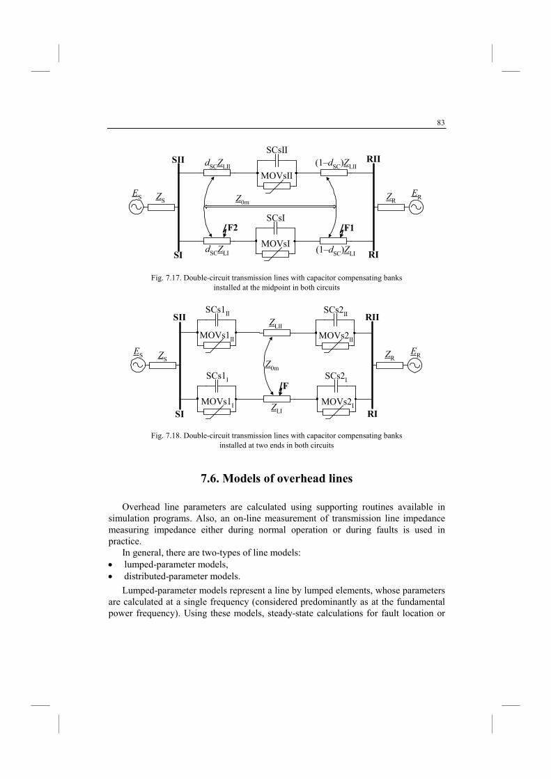
83
SI
ERZR
RII
ES ZS
F2
dSCZLI
F1
(1–dSC)ZLI
dSCZLII (1–dSC)ZLII
Z0m
SII
RI
MOVsII
SCsII
MOVsI
SCsI
Fig. 7.17. Double-circuit transmission lines with capacitor compensating banks installed at the midpoint in both circuits
SI
ERZR
RII
ES ZS
SII
RIZLI
F
ZLII
Z0m
MOVs1II
SCs1II
MOVs2II
SCs2II
MOVs1I
SCs1I
MOVs2I
SCs2I
Fig. 7.18. Double-circuit transmission lines with capacitor compensating banks installed at two ends in both circuits
7.6. Models of overhead lines
Overhead line parameters are calculated using supporting routines available in simulation programs. Also, an on-line measurement of transmission line impedance measuring impedance either during normal operation or during faults is used in practice.
In general, there are two-types of line models: • lumped-parameter models, • distributed-parameter models.
Lumped-parameter models represent a line by lumped elements, whose parameters are calculated at a single frequency (considered predominantly as at the fundamental power frequency). Using these models, steady-state calculations for fault location or
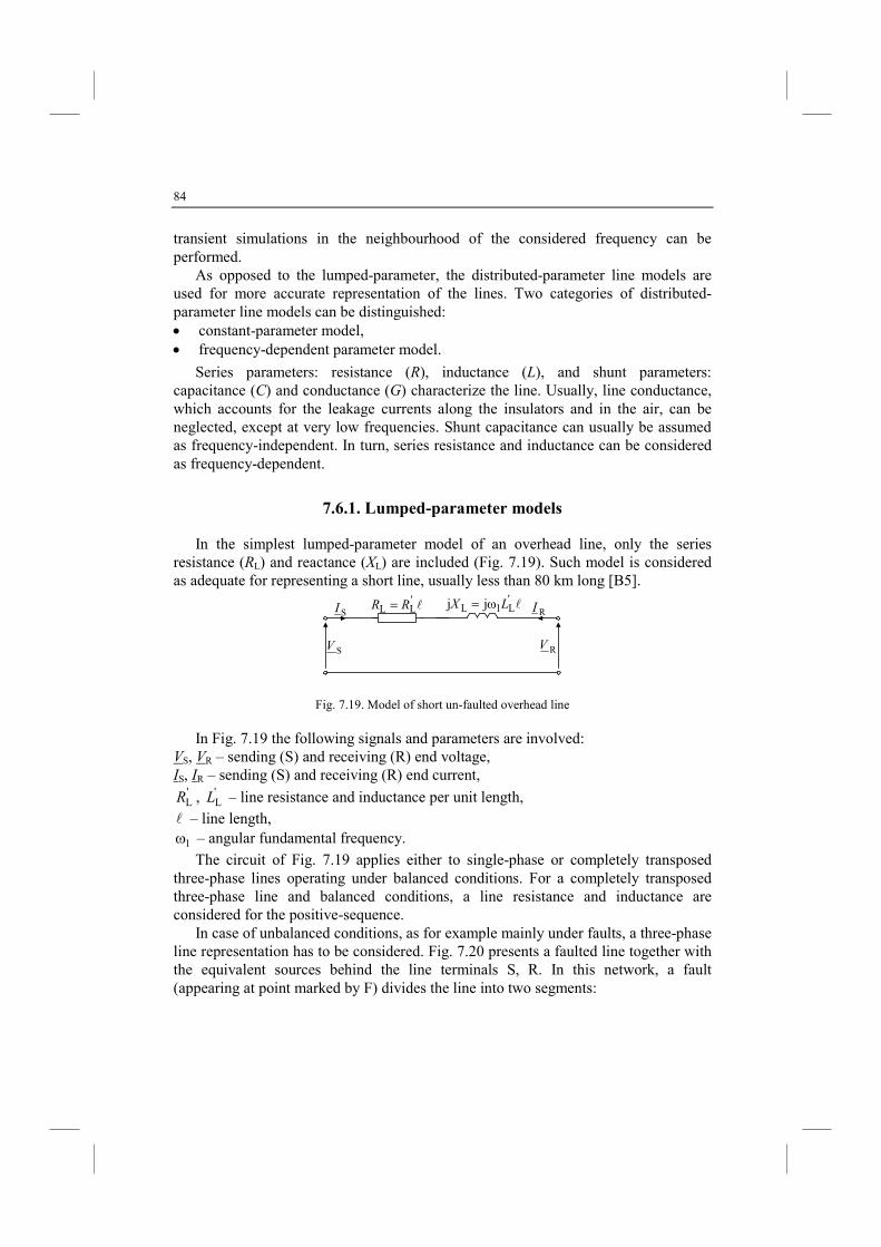
84
transient simulations in the neighbourhood of the considered frequency can be performed.
As opposed to the lumped-parameter, the distributed-parameter line models are used for more accurate representation of the lines. Two categories of distributed-parameter line models can be distinguished: • constant-parameter model, • frequency-dependent parameter model.
Series parameters: resistance (R), inductance (L), and shunt parameters: capacitance (C) and conductance (G) characterize the line. Usually, line conductance, which accounts for the leakage currents along the insulators and in the air, can be neglected, except at very low frequencies. Shunt capacitance can usually be assumed as frequency-independent. In turn, series resistance and inductance can be considered as frequency-dependent.
7.6.1. Lumped-parameter models
In the simplest lumped-parameter model of an overhead line, only the series resistance (RL) and reactance (XL) are included (Fig. 7.19). Such model is considered as adequate for representing a short line, usually less than 80 km long [B5].
l'RR LL = l
'LX L1L jj ω=
SV RV
SI RI
Fig. 7.19. Model of short un-faulted overhead line
In Fig. 7.19 the following signals and parameters are involved: VS, VR – sending (S) and receiving (R) end voltage, IS, IR – sending (S) and receiving (R) end current,
'LR , '
LL – line resistance and inductance per unit length,
l – line length,
1ω – angular fundamental frequency.
The circuit of Fig. 7.19 applies either to single-phase or completely transposed three-phase lines operating under balanced conditions. For a completely transposed three-phase line and balanced conditions, a line resistance and inductance are considered for the positive-sequence.
In case of unbalanced conditions, as for example mainly under faults, a three-phase line representation has to be considered. Fig. 7.20 presents a faulted line together with the equivalent sources behind the line terminals S, R. In this network, a fault (appearing at point marked by F) divides the line into two segments:
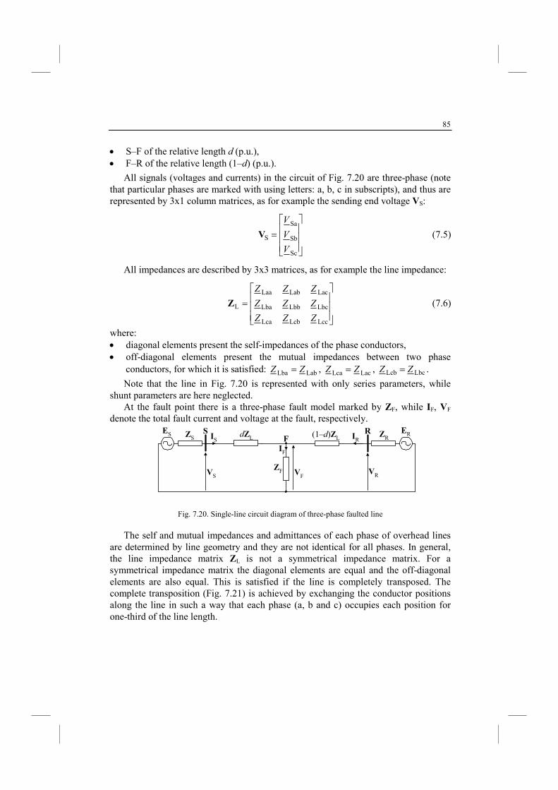
85
• S–F of the relative length d (p.u.), • F–R of the relative length (1–d) (p.u.).
All signals (voltages and currents) in the circuit of Fig. 7.20 are three-phase (note that particular phases are marked with using letters: a, b, c in subscripts), and thus are represented by 3x1 column matrices, as for example the sending end voltage VS:
=
Sc
Sb
Sa
S
V
V
V
V (7.5)
All impedances are described by 3x3 matrices, as for example the line impedance:
=
LccLcbLca
LbcLbbLba
LacLabLaa
L
ZZZ
ZZZ
ZZZ
Z (7.6)
where: • diagonal elements present the self-impedances of the phase conductors, • off-diagonal elements present the mutual impedances between two phase
conductors, for which it is satisfied: LabLba ZZ = , LacLca ZZ = , LbcLcb ZZ = .
Note that the line in Fig. 7.20 is represented with only series parameters, while shunt parameters are here neglected.
At the fault point there is a three-phase fault model marked by ZF, while IF, VF denote the total fault current and voltage at the fault, respectively.
RS dZL (1–d)ZLIS
VS VFVR
IRZS
ES ERZRF
IF
ZF
Fig. 7.20. Single-line circuit diagram of three-phase faulted line
The self and mutual impedances and admittances of each phase of overhead lines are determined by line geometry and they are not identical for all phases. In general, the line impedance matrix ZL is not a symmetrical impedance matrix. For a symmetrical impedance matrix the diagonal elements are equal and the off-diagonal elements are also equal. This is satisfied if the line is completely transposed. The complete transposition (Fig. 7.21) is achieved by exchanging the conductor positions along the line in such a way that each phase (a, b and c) occupies each position for one-third of the line length.
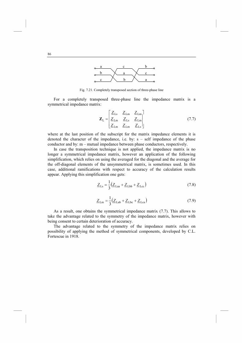
86
a
a
a
b
b
b
c
c
c
Fig. 7.21. Completely transposed section of three-phase line
For a completely transposed three-phase line the impedance matrix is a symmetrical impedance matrix:
=
LsLmLm
LmLsLm
LmLmLs
L
ZZZ
ZZZ
ZZZ
Z (7.7)
where at the last position of the subscript for the matrix impedance elements it is denoted the character of the impedance, i.e. by: s – self impedance of the phase conductor and by: m – mutual impedance between phase conductors, respectively.
In case the transposition technique is not applied, the impedance matrix is no longer a symmetrical impedance matrix, however an application of the following simplification, which relies on using the averaged for the diagonal and the average for the off-diagonal elements of the unsymmetrical matrix, is sometimes used. In this case, additional ramifications with respect to accuracy of the calculation results appear. Applying this simplification one gets:
( )LccLbbLaaLs 3
1ZZZZ ++= (7.8)
( )LcaLbcLabLm 3
1ZZZZ ++= (7.9)
As a result, one obtains the symmetrical impedance matrix (7.7). This allows to take the advantage related to the symmetry of the impedance matrix, however with being consent to certain deterioration of accuracy.
The advantage related to the symmetry of the impedance matrix relies on possibility of applying the method of symmetrical components, developed by C.L. Fortescue in 1918.
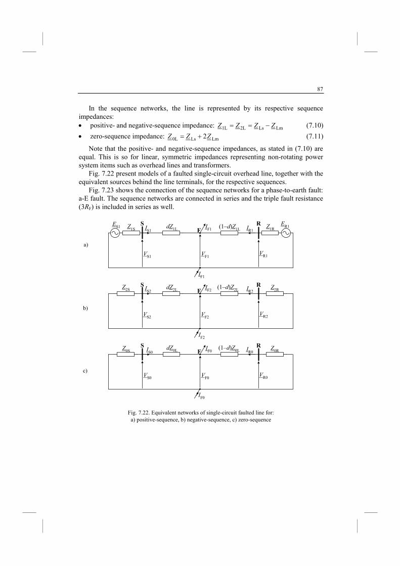
87
In the sequence networks, the line is represented by its respective sequence impedances: • positive- and negative-sequence impedance: LmLs2L1L ZZZZ −== (7.10)
• zero-sequence impedance: LmLs0L 2ZZZ += (7.11)
Note that the positive- and negative-sequence impedances, as stated in (7.10) are equal. This is so for linear, symmetric impedances representing non-rotating power system items such as overhead lines and transformers.
Fig. 7.22 present models of a faulted single-circuit overhead line, together with the equivalent sources behind the line terminals, for the respective sequences.
Fig. 7.23 shows the connection of the sequence networks for a phase-to-earth fault: a-E fault. The sequence networks are connected in series and the triple fault resistance (3RF) is included in series as well.
RS
dZ1L (1–d)Z1LIS1
VS1 VF1VR1
IR1Z1S
ES1ER1Z1RF
IF1
IF1 RS dZ2L (1–d)Z2LIS2
VS2 VF2VR2
IR2Z2S Z2RF
IF2
IF2 RS dZ0L (1–d)Z0LIS0
VS0 VF0VR0
IR0Z0S Z0RF
IF0
IF0
Fig. 7.22. Equivalent networks of single-circuit faulted line for: a) positive-sequence, b) negative-sequence, c) zero-sequence
b)
a)
c)
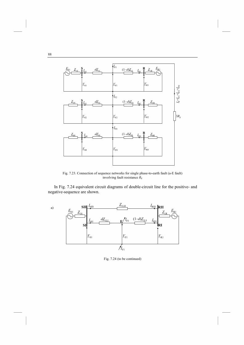
88
RS dZ1L (1–d)Z1LIS1
VS1 VF1VR1
IR1Z1S
ES1ER1Z1R
IF1
I F=I F
1=I F
2=I F
0
RS dZ2L (1–d)Z2LIS2
VS2 VF2VR2
IR2Z2S Z2R
RS dZ0L (1–d)Z0LIS0
VS0 VF0VR0
IR0Z0S Z0R
IF0
3RF
IF2
Fig. 7.23. Connection of sequence networks for single phase-to-earth fault (a-E fault) involving fault resistance RF
In Fig. 7.24 equivalent circuit diagrams of double-circuit line for the positive- and negative-sequence are shown.
SI
dZ1LI(1–d)Z1LIISI1
VS1 VF1
FIF1
IF1
Z1SES1
SIIZ1LII
RI
RIIER1Z1R
VR1
IRI1
ISII1 IRII1
Fig. 7.24 (to be continued)
a)
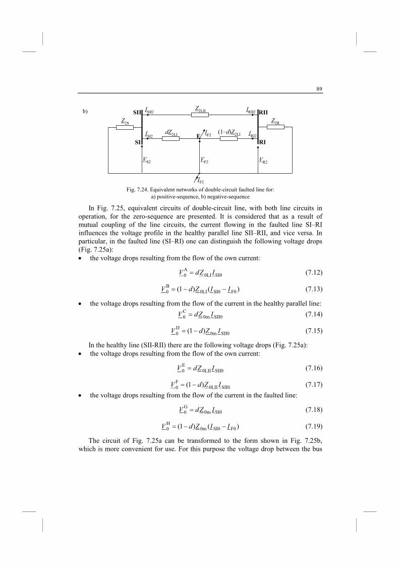
89
SI
dZ2LI(1–d)Z2LIISI2
VS2 VF2
FIF2
IF2
Z2S
SIIZ2LII
RI
RII
Z2R
VR2
IRI2
ISII2 IRII2
Fig. 7.24. Equivalent networks of double-circuit faulted line for:
a) positive-sequence, b) negative-sequence
In Fig. 7.25, equivalent circuits of double-circuit line, with both line circuits in operation, for the zero-sequence are presented. It is considered that as a result of mutual coupling of the line circuits, the current flowing in the faulted line SI–RI influences the voltage profile in the healthy parallel line SII–RII, and vice versa. In particular, in the faulted line (SI–RI) one can distinguish the following voltage drops (Fig. 7.25a): • the voltage drops resulting from the flow of the own current:
SI00LIA0 IZdV = (7.12)
)()1( F0SI00LIB0 IIZdV −−= (7.13)
• the voltage drops resulting from the flow of the current in the healthy parallel line:
SII00mC0 IZdV = (7.14)
SII00mD0 )1( IZdV −= (7.15)
In the healthy line (SII-RII) there are the following voltage drops (Fig. 7.25a): • the voltage drops resulting from the flow of the own current:
SII00LIIE0 IZdV = (7.16)
SII00LIIF0 )1( IZdV −= (7.17)
• the voltage drops resulting from the flow of the current in the faulted line:
SI00mG0 IZdV = (7.18)
)()1( F0SI00mH0 IIZdV −−= (7.19)
The circuit of Fig. 7.25a can be transformed to the form shown in Fig. 7.25b, which is more convenient for use. For this purpose the voltage drop between the bus
b)
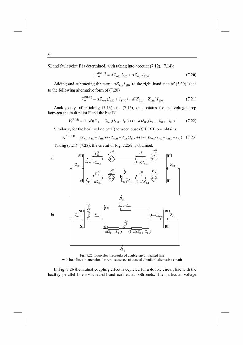
90
SI and fault point F is determined, with taking into account (7.12), (7.14):
SII00mSI00LIF)-(SI
0 IZdIZdV += (7.20)
Adding and subtracting the term: SI00m IZd to the right-hand side of (7.20) leads
to the following alternative form of (7.20):
SI00m0LISII0SI00mF)-(SI
0 )()( IZZdIIZdV −++= (7.21)
Analogously, after taking (7.13) and (7.15), one obtains for the voltage drop between the fault point F and the bus RI:
)()1())()(1( F0SII0SI00mF0SI00m0LIRI)-(F
0 IIIZdIIZZdV −+−+−−−= (7.22)
Similarly, for the healthy line path (between buses SII, RII) one obtains:
)()1()()( F0SII0SI00mSII00m0LIISII0SI00mRII)-SII(
0 IIIZdIZZIIdZV −+−+−++= (7.23)
Taking (7.21)–(7.23), the circuit of Fig. 7.25b is obtained.
SI
IF0
Z0S
SII
RI
RII
Z0R
dZ0LI (1–d)Z0LIISI0
F
IF0
+ –(ISI0–IF0)
+ –
A0V
C0V B
0VD0V
dZ0LII (1–d)Z0LIIISII0
+ – + –
E0V
G0V F
0VH0V
IF0
Z0SZ0RdZ0m (1–d)Z0m(I
SI0+I S
II0)
F
IF0
Z0LII–Z0m
ISI0
ISII0
d(Z0LI–Z0m) (1–d)(Z0LI–Z0m)
SI
SII
RI
RII
Fig. 7.25. Equivalent networks of double-circuit faulted line
with both lines in operation for zero-sequence: a) general circuit, b) alternative circuit
In Fig. 7.26 the mutual coupling effect is depicted for a double circuit line with the
healthy parallel line switched-off and earthed at both ends. The particular voltage
b)
a)
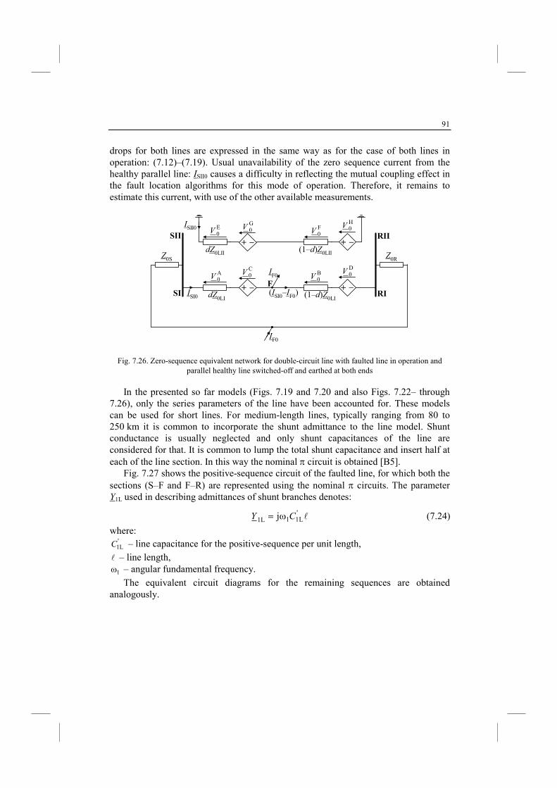
91
drops for both lines are expressed in the same way as for the case of both lines in operation: (7.12)–(7.19). Usual unavailability of the zero sequence current from the healthy parallel line: ISII0 causes a difficulty in reflecting the mutual coupling effect in the fault location algorithms for this mode of operation. Therefore, it remains to estimate this current, with use of the other available measurements.
SI
IF0
Z0S
SII
RI
RII
Z0R
dZ0LI (1–d)Z0LIISI0
F
IF0
+ –(ISI0–IF0)
+ –
A0V
C0V B
0VD0V
dZ0LII (1–d)Z0LII
ISII0
+ – + –
E0V
G0V F
0VH0V
Fig. 7.26. Zero-sequence equivalent network for double-circuit line with faulted line in operation and parallel healthy line switched-off and earthed at both ends
In the presented so far models (Figs. 7.19 and 7.20 and also Figs. 7.22– through 7.26), only the series parameters of the line have been accounted for. These models can be used for short lines. For medium-length lines, typically ranging from 80 to 250 km it is common to incorporate the shunt admittance to the line model. Shunt conductance is usually neglected and only shunt capacitances of the line are considered for that. It is common to lump the total shunt capacitance and insert half at each of the line section. In this way the nominal π circuit is obtained [B5].
Fig. 7.27 shows the positive-sequence circuit of the faulted line, for which both the sections (S–F and F–R) are represented using the nominal π circuits. The parameter Y1L used in describing admittances of shunt branches denotes:
l'L111L j CY ω= (7.24)
where: '1LC – line capacitance for the positive-sequence per unit length,
l – line length,
1ω – angular fundamental frequency.
The equivalent circuit diagrams for the remaining sequences are obtained analogously.
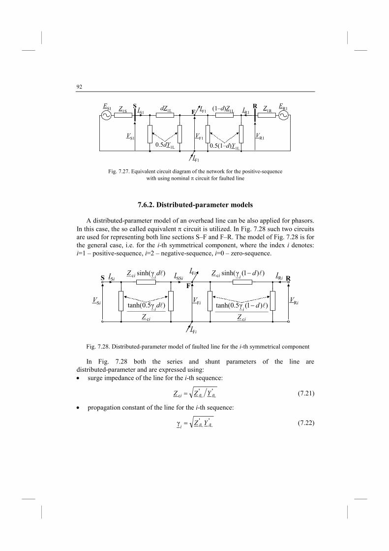
92
RS dZ1L (1–d)Z1LIS1
VS1 VF1VR1
IR1Z1S
Z1RFIF1
IF1
0.5dY1L 0.5(1–d)Y1L
ES1 ER1
Fig. 7.27. Equivalent circuit diagram of the network for the positive-sequence with using nominal π circuit for faulted line
7.6.2. Distributed-parameter models
A distributed-parameter model of an overhead line can be also applied for phasors. In this case, the so called equivalent π circuit is utilized. In Fig. 7.28 such two circuits are used for representing both line sections S–F and F–R. The model of Fig. 7.28 is for the general case, i.e. for the i-th symmetrical component, where the index i denotes: i=1 – positive-sequence, i=2 – negative-sequence, i=0 – zero-sequence.
)γsinh(c ldZii ))1(γsinh(c ldZ
ii −
i
i
Z
d
c
)γ5.0tanh( l
i
i
Z
d
c
))1(γ5.0tanh( l−
RS ISi
VSi VFiVRi
IRi
F
IFi
IFi
ISSi
Fig. 7.28. Distributed-parameter model of faulted line for the i-th symmetrical component In Fig. 7.28 both the series and shunt parameters of the line are
distributed-parameter and are expressed using: • surge impedance of the line for the i-th sequence:
''LLc iii YZZ = (7.21)
• propagation constant of the line for the i-th sequence:
''LLγ iii
YZ= (7.22)
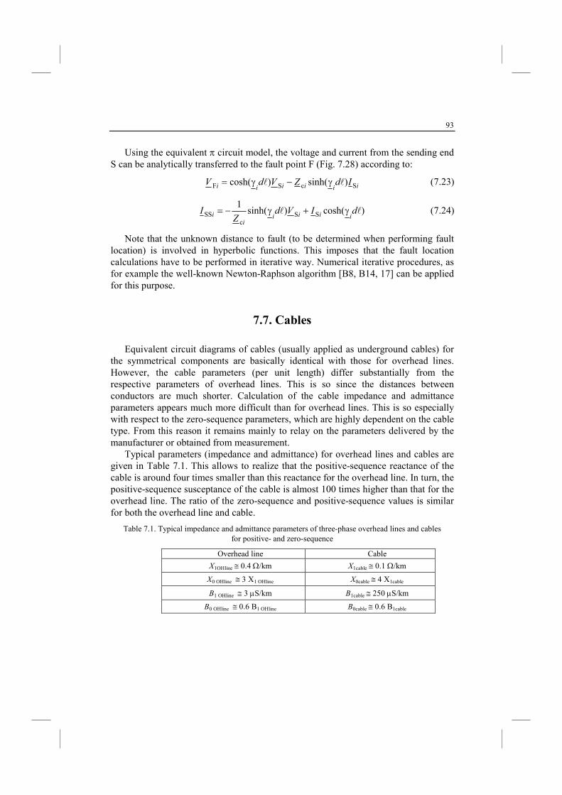
93
Using the equivalent π circuit model, the voltage and current from the sending end S can be analytically transferred to the fault point F (Fig. 7.28) according to:
iiiiii IdZVdV ScSF )sinh()cosh( ll γ−γ= (7.23)
)cosh()sinh(1
SSc
SS ll dIVdZ
Iiiii
i
i γ+γ−= (7.24)
Note that the unknown distance to fault (to be determined when performing fault location) is involved in hyperbolic functions. This imposes that the fault location calculations have to be performed in iterative way. Numerical iterative procedures, as for example the well-known Newton-Raphson algorithm [B8, B14, 17] can be applied for this purpose.
7.7. Cables
Equivalent circuit diagrams of cables (usually applied as underground cables) for the symmetrical components are basically identical with those for overhead lines. However, the cable parameters (per unit length) differ substantially from the respective parameters of overhead lines. This is so since the distances between conductors are much shorter. Calculation of the cable impedance and admittance parameters appears much more difficult than for overhead lines. This is so especially with respect to the zero-sequence parameters, which are highly dependent on the cable type. From this reason it remains mainly to relay on the parameters delivered by the manufacturer or obtained from measurement.
Typical parameters (impedance and admittance) for overhead lines and cables are given in Table 7.1. This allows to realize that the positive-sequence reactance of the cable is around four times smaller than this reactance for the overhead line. In turn, the positive-sequence susceptance of the cable is almost 100 times higher than that for the overhead line. The ratio of the zero-sequence and positive-sequence values is similar for both the overhead line and cable.
Table 7.1. Typical impedance and admittance parameters of three-phase overhead lines and cables for positive- and zero-sequence
Overhead line Cable
X1OHline ≅ 0.4 Ω/km X1cable ≅ 0.1 Ω/km
X0 OHline ≅ 3 X1 OHline X0cable ≅ 4 X1cable
B1 OHline ≅ 3 µS/km B1cable ≅ 250 µS/km
B0 OHline ≅ 0.6 B1 OHline B0cable ≅ 0.6 B1cable

94
In case of the conductance Gi for any of the sequences, it can be definitely neglected for both the overhead line and underground cable, when performing fault current calculations. As concerns the susceptance (Bi), its omitting in case of cables may lead to unacceptable errors.
95
8. AALYSIS OF THREE-PHASE SYMMETRICAL
FAULTS
8.1. Simplification assumptions
Three-phase fault calculations (presented in this chapter) as well as unsymmetrical faults calculations (to be presented in Chapter 9) will be performed using sequence networks of the considered example faulted power system. To construct zero-, positive- and negative-sequence networks for a given power system the following assumptions [B5] are made: 1. The power system operates under balanced steady-state conditions before the fault
occurrence. This makes that sequence networks are uncoupled before the fault occurs. During unsymmetrical faults they are interconnected only at the fault location.
2. Pre-fault load current is neglected. As a result of that the positive-sequence internal voltages of all machines are equal to the pre-fault voltage VF. Under neglecting pre-fault load currents we have no voltage drops in the pre-fault circuit and thus pre-fault voltage at each bus in the positive-sequence network equals VF.
3. Transformer winding resistances, shunt admittances and ∆–Y phase shifts are neglected.
4. Overhead line series resistances and shunt admittances are neglected. 5. Synchronous machine is simply represented (armature resistance, saliency and
saturation are neglected). 6. All non-rotating impedance loads are neglected. 7. Induction motors are represented as synchronous machines.
The aim of making the above listed assumptions is to get simplicity of calculations without considerable deteriorating accuracy of calculations. As a result of that the calculations can be performed even without computer.
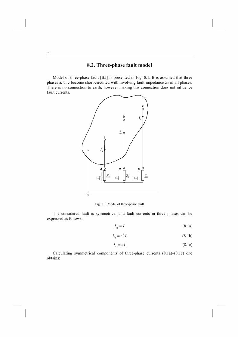
96
8.2. Three-phase fault model
Model of three-phase fault [B5] is presented in Fig. 8.1. It is assumed that three phases a, b, c become short-circuited with involving fault impedance ZF in all phases. There is no connection to earth; however making this connection does not influence fault currents.
a
b
c
Va
Ic
Ib
Ia
ZF ZF ZFVb
Vc
Fig. 8.1. Model of three-phase fault
The considered fault is symmetrical and fault currents in three phases can be
expressed as follows:
II =a (8.1a)
II2
b a= (8.1b)
II ac = (8.1c)
Calculating symmetrical components of three-phase currents (8.1a)–(8.1c) one obtains:
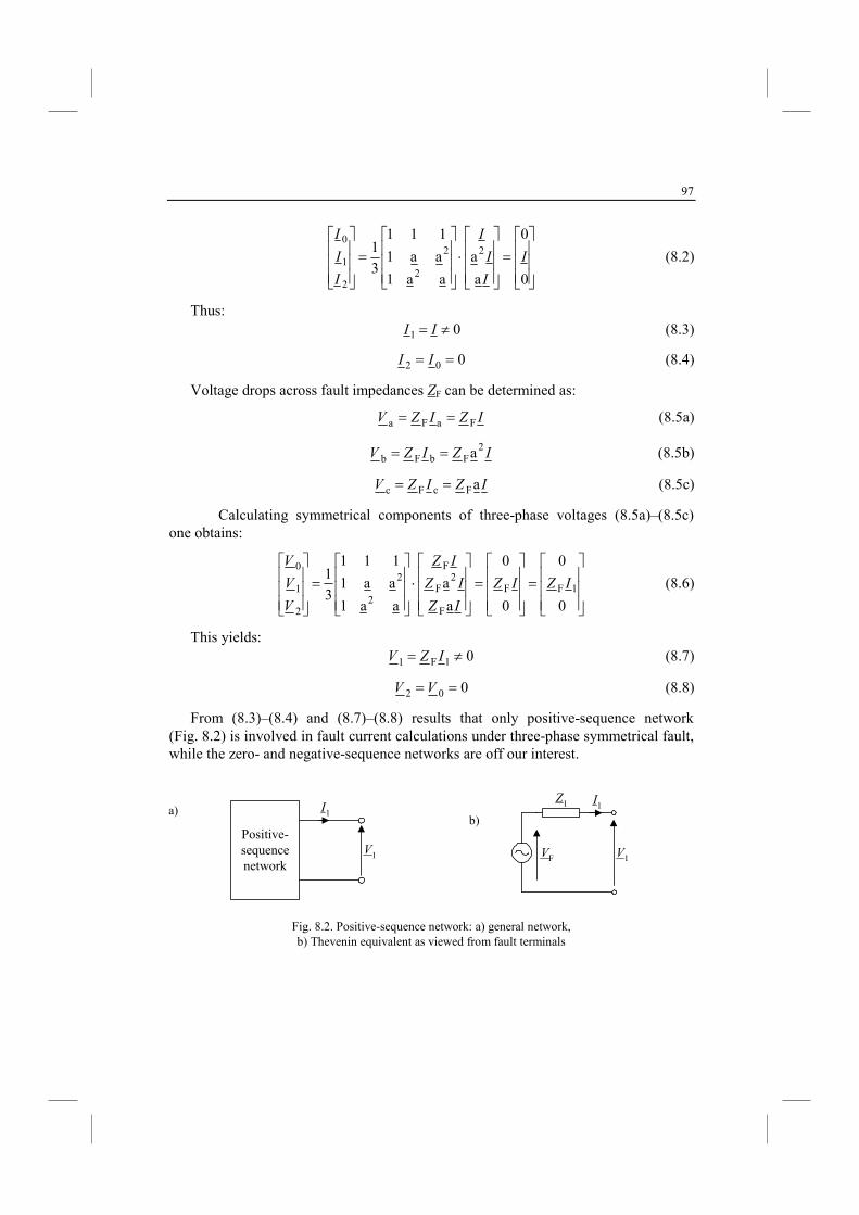
97
=
⋅
=
0
0
a
a
aa1
aa1
111
3
1 2
2
2
2
1
0
I
I
I
I
I
I
I
(8.2)
Thus: 01 ≠= II (8.3)
002 == II (8.4)
Voltage drops across fault impedances ZF can be determined as:
IZIZV FaFa == (8.5a)
IZIZV2
FbFb a== (8.5b)
IZIZV aFcFc == (8.5c)
Calculating symmetrical components of three-phase voltages (8.5a)–(8.5c) one obtains:
=
=
⋅
=
0
0
0
0
a
a
aa1
aa1
111
3
11FF
F
2F
F
2
2
2
1
0
IZIZ
IZ
IZ
IZ
V
V
V
(8.6)
This yields: 01F1 ≠= IZV (8.7)
002 ==VV (8.8)
From (8.3)–(8.4) and (8.7)–(8.8) results that only positive-sequence network (Fig. 8.2) is involved in fault current calculations under three-phase symmetrical fault, while the zero- and negative-sequence networks are off our interest.
Positive-sequencenetwork
I1
V1
I1
V1VF
Z1
Fig. 8.2. Positive-sequence network: a) general network, b) Thevenin equivalent as viewed from fault terminals
a) b)
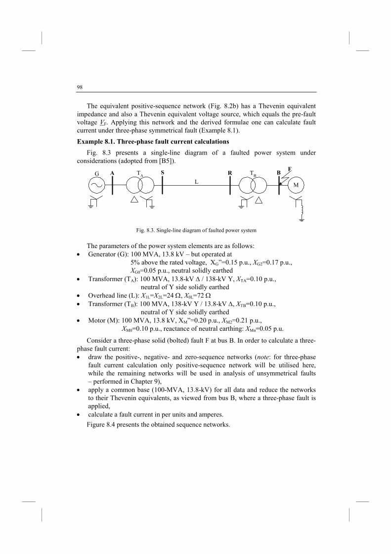
98
The equivalent positive-sequence network (Fig. 8.2b) has a Thevenin equivalent impedance and also a Thevenin equivalent voltage source, which equals the pre-fault voltage VF. Applying this network and the derived formulae one can calculate fault current under three-phase symmetrical fault (Example 8.1).
Example 8.1. Three-phase fault current calculations
Fig. 8.3 presents a single-line diagram of a faulted power system under considerations (adopted from [B5]).
A B
M
S RG TA TB
L
F
Fig. 8.3. Single-line diagram of faulted power system
The parameters of the power system elements are as follows:
• Generator (G): 100 MVA, 13.8 kV – but operated at 5% above the rated voltage, XG”=0.15 p.u., XG2=0.17 p.u., XG0=0.05 p.u., neutral solidly earthed
• Transformer (TA): 100 MVA, 13.8-kV ∆ / 138-kV Y, XTA=0.10 p.u., neutral of Y side solidly earthed
• Overhead line (L): X1L=X2L=24 Ω, X0L=72 Ω • Transformer (TB): 100 MVA, 138-kV Y / 13.8-kV ∆, XTB=0.10 p.u.,
neutral of Y side solidly earthed • Motor (M): 100 MVA, 13.8 kV, XM”=0.20 p.u., XM2=0.21 p.u.,
XM0=0.10 p.u., reactance of neutral earthing: XMn=0.05 p.u.
Consider a three-phase solid (bolted) fault F at bus B. In order to calculate a three-phase fault current: • draw the positive-, negative- and zero-sequence networks (note: for three-phase
fault current calculation only positive-sequence network will be utilised here, while the remaining networks will be used in analysis of unsymmetrical faults – performed in Chapter 9),
• apply a common base (100-MVA, 13.8-kV) for all data and reduce the networks to their Thevenin equivalents, as viewed from bus B, where a three-phase fault is applied,
• calculate a fault current in per units and amperes.
Figure 8.4 presents the obtained sequence networks.
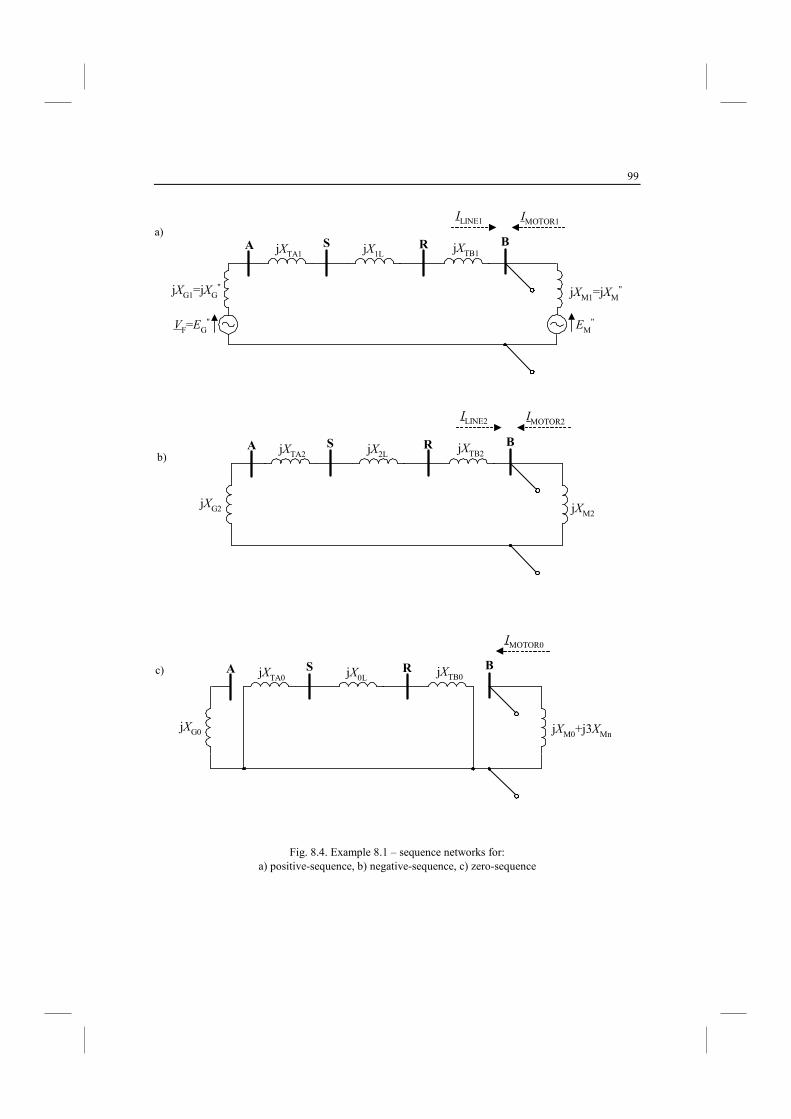
99
VF=EG''
A S R B
jXG1=jXG"
jXTA1 jX1LjXTB1
EM''
ILINE1 IMOTOR1
jXM1=jXM"
A S R B
jXG2
jXTA2 jX2LjXTB2
ILINE2 IMOTOR2
jXM2
A S R B
jXG0
jXTA0 jX0LjXTB0
IMOTOR0
jXM0+j3XMn
Fig. 8.4. Example 8.1 – sequence networks for: a) positive-sequence, b) negative-sequence, c) zero-sequence
a)
b)
c)
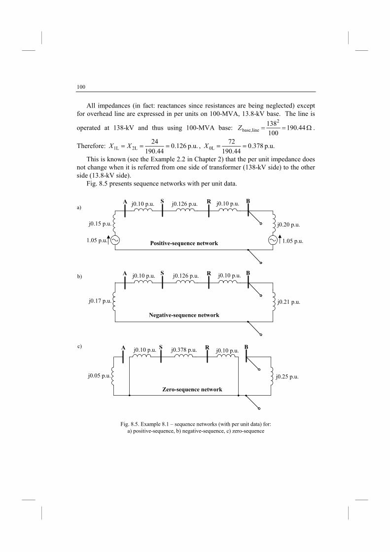
100
All impedances (in fact: reactances since resistances are being neglected) except for overhead line are expressed in per units on 100-MVA, 13.8-kV base. The line is
operated at 138-kV and thus using 100-MVA base: Ω== 44.190100
1382
linebase,Z .
Therefore: p.u. 126.044.190
242L1L === XX , p.u. 378.0
44.190
720L ==X
This is known (see the Example 2.2 in Chapter 2) that the per unit impedance does not change when it is referred from one side of transformer (138-kV side) to the other side (13.8-kV side).
Fig. 8.5 presents sequence networks with per unit data.
1.05 p.u.
A S R B
j0.15 p.u.
j0.10 p.u. j0.126 p.u. j0.10 p.u.
j0.20 p.u.
1.05 p.u.Positive-sequence network
A S R B
j0.17 p.u.
j0.10 p.u. j0.126 p.u. j0.10 p.u.
j0.21 p.u.
egative-sequence network
A S R B
j0.05 p.u.
j0.10 p.u. j0.378 p.u.
j0.25 p.u.
j0.10 p.u.
Zero-sequence network
Fig. 8.5. Example 8.1 – sequence networks (with per unit data) for: a) positive-sequence, b) negative-sequence, c) zero-sequence
c)
b)
a)
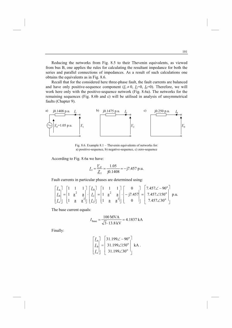
101
Reducing the networks from Fig. 8.5 to their Thevenin equivalents, as viewed from bus B, one applies the rules for calculating the resultant impedance for both the series and parallel connections of impedances. As a result of such calculations one obtains the equivalents as in Fig. 8.6.
Recall that for the considered here three-phase fault, the fault currents are balanced and have only positive-sequence component (I1 ≠ 0, I2=0, I0=0). Therefore, we will work here only with the positive-sequence network (Fig. 8.6a). The networks for the remaining sequences (Fig. 8.6b and c) will be utilised in analysis of unsymmetrical faults (Chapter 9).
I1
V1VF=1.05 p.u.
j0.1408 p.u.
I2
V2
j0.1475 p.u.
I0
V0
j0.250 p.u.
Fig. 8.6. Example 8.1 – Thevenin equivalents of networks for: a) positive-sequence, b) negative-sequence, c) zero-sequence
According to Fig. 8.6a we have:
p.u. 457.7j1408.0j
05.1
1
F1 −===
Z
VI
Fault currents in particular phases are determined using:
p.u.
30457.7
150457.7
90457.7
0
457.7j
0
aa1
aa1
111
aa1
aa1
111
o
o
o
2
2
2
1
0
2
2
c
b
a
∠
∠
−∠
=
−⋅
=
⋅
=
I
I
I
I
I
I
The base current equals:
kA 1837.4kV 8.133
MVA 100base =
⋅=I
Finally:
kA
30199.31
150199.31
90199.31
o
o
o
c
b
a
∠
∠
−∠
=
I
I
I
.
a) b) c)
102
9. AALYSIS OF USYMMETRICAL FAULTS
9.1. Introduction
In this Chapter the following unsymmetrical shunt faults are considered: • phase-to-earth fault • phase-to-phase fault • phase-to-phase-to-earth fault.
After deriving the equations relevant for the considered particular fault the interconnected sequence networks are drawn. Then, the fault currents in the faulted system from Example 8.1 are calculated. The calculated fault currents for the above stated unsymmetrical fault types are compared with the three-phase fault currents obtained in Example 8.1.
Analysis of unsymmetrical faults is carried out under assuming such phases involved in a fault that the obtained equations allow for their simple interpretation, i.e. leading to relatively simple interconnected sequence networks. In particular: • phase-to-earth fault: a–E fault • phase-to-phase fault: b–c fault • phase-to-phase-to-earth fault: b–c–E fault.
The introduced examples explain how to deal when the phases other than the above specified are involved in a fault. It is shown how to get simple form of interconnected sequence networks for such faults. Fault currents calculations are also included.
9.2. Phase-to-earth fault
Let us consider a phase-to-phase fault: a–E fault, as shown in Fig. 9.1 [B5]. It is assumed for generality that a fault impedance ZF is involved in this fault.
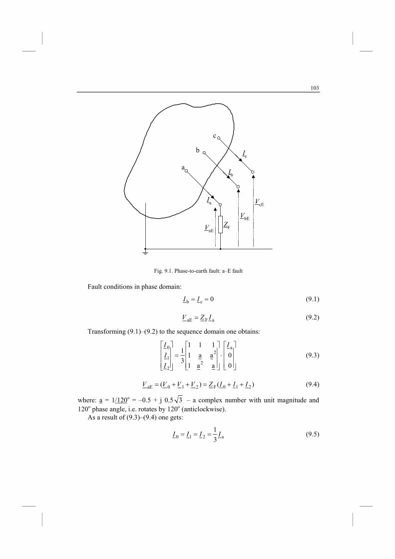
103
a
b
c
VaE
VbE
VcE
Ic
Ib
Ia
ZF
Fig. 9.1. Phase-to-earth fault: a–E fault
Fault conditions in phase domain:
0cb == II (9.1)
aFaE IZV = (9.2)
Transforming (9.1)–(9.2) to the sequence domain one obtains:
⋅
=
0
0
aa1
aa1
111
3
1a
2
2
2
1
0 I
I
I
I
(9.3)
)()( 210F210aE IIIZVVVV ++=++= (9.4)
where: a = 1/120o = –0.5 + j 0.5 3 – a complex number with unit magnitude and 120o phase angle, i.e. rotates by 120o (anticlockwise).
As a result of (9.3)–(9.4) one gets:
a210 3
1IIII === (9.5)
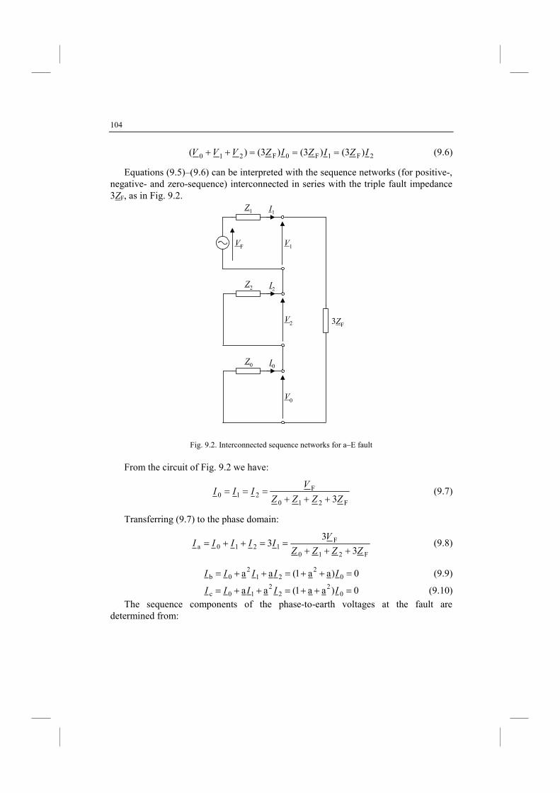
104
2F1F0F210 )3()3()3()( IZIZIZVVV ===++ (9.6)
Equations (9.5)–(9.6) can be interpreted with the sequence networks (for positive-, negative- and zero-sequence) interconnected in series with the triple fault impedance 3ZF, as in Fig. 9.2.
I1
V1VF
Z1
I2
V2
Z2
I0
V0
Z0
3ZF
Fig. 9.2. Interconnected sequence networks for a–E fault
From the circuit of Fig. 9.2 we have:
F210
F210 3ZZZZ
VIII
+++=== (9.7)
Transferring (9.7) to the phase domain:
F210
F1210a 3
33
ZZZZ
VIIIII
+++==++= (9.8)
0)aa1(aa 02
212
0b =++=++= IIIII (9.9)
0)aa1(aa 02
22
10c =++=++= IIIII (9.10)
The sequence components of the phase-to-earth voltages at the fault are determined from:
105
⋅
−
=
2
1
0
2
1
0
F
2
1
0
00
00
00
0
0
I
I
I
Z
Z
Z
V
V
V
V
(9.11)
This allows determining the phase-to-earth voltages at the fault, by applying (3.1):
⋅
=
2
1
0
2
2
cE
bE
aE
aa1
aa1
111
V
V
V
V
V
V
(9.12)
Example 9.1. Consider b–E fault and state how to get simple form of
interconnected sequence networks
In this case fault conditions in phase domain are as follows:
0ca == II (9.13)
bFbE IZV = (9.14)
Transforming (9.13)–(9.14) to the sequence domain one obtains:
⋅
=
0
0
aa1
aa1
111
3
1b
2
2
2
1
0
I
I
I
I
(9.15)
)aa()aa( 212
0F212
0bE IIIZVVVV ++=++= (9.16)
As a result of (9.3)–(9.4) one gets:
b0 3
1II = , b1 a
3
1II = , b
22 a
3
1II = (9.17)
or: 01 a II = , 12 a II = (9.18)
Voltage drop a fault path impedance:
0F212
0F212
0bE 3)aa()aa( IZIIIZVVVV =++=++= (9.19)
Conclusion: the relations between symmetrical components of fault currents (9.18) do not allow to get such simple do not allow to get the interconnected sequence networks such as in the case of a–E fault (Fig. 9.2). Utilisation of (9.18) for drawing the interconnected sequence networks requires applying the ideal transformers of the ratios being a complex number (a).
In order to get the interconnected sequence networks such as in the case of a–E
106
fault (Fig. 9.2 – the sequence networks connected in series) one has to change the sequence of phases.
Considering names of phases as: first, second, third, the transformation from phase to symmetrical components, and inversely, is in the case of currents (analogously for voltages):
⋅
=
third
second
first
2
2
2
1
0
aa1
aa1
111
3
1
I
I
I
I
I
I
(9.20a)
⋅
=
2
1
0
2
2
third
second
first
aa1
aa1
111
I
I
I
I
I
I
(9.20b)
The results for simple interpretation (Fig. 9.2 – the sequence networks connected in series) for a–E fault have been obtained assuming the following assignments:
c thirdb,second a,first →→→− :fault Ea (9.21a)
Therefore, it is advantageous if for b–E fault one applies:
a thirdc,second b,first →→→− :fault Eb (9.21b)
Analogously, it is advantageous if for c–E fault one applies:
b thirda,second c,first →→→− :fault Ec (9.21c)
So, we change the order of phases (in a sense which is considered as the first, second and third phase, respectively) keeping the clockwise direction of their rotation.
Applying consequently (9.20a)(9.20b) and analogous for voltages, together with the assignments (9.21b)–(9.21c) one can utilise the series connection of sequence networks (Fig. 9.2), also for b–E and c–E faults, respectively.
9.3. Phase-to-phase fault
Let us consider a phase-to-phase fault: b–c fault, as shown in Fig. 9.3 [B5]. It is assumed for generality that a fault impedance ZF is involved in this fault.
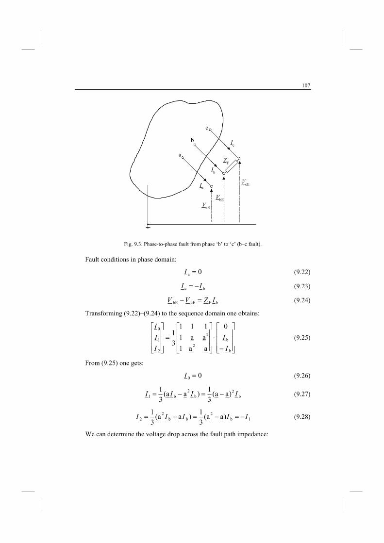
107
a
b
c
VaE
VbE
VcE
Ic
Ib
Ia
ZF
Fig. 9.3. Phase-to-phase fault from phase ‘b’ to ‘c’ (b–c fault).
Fault conditions in phase domain:
0a =I (9.22)
bc II −= (9.23)
bFcEbE IZVV =− (9.24)
Transforming (9.22)–(9.24) to the sequence domain one obtains:
−
⋅
=
b
b2
2
2
1
0 0
aa1
aa1
111
3
1
I
I
I
I
I
(9.25)
From (9.25) one gets:
00 =I (9.26)
b2
b2
b1 )aa(3
1)aa(
3
1IIII −=−= (9.27)
1b2
bb2
2 )aa(3
1)aa(
3
1IIIII −=−=−= (9.28)
We can determine the voltage drop across the fault path impedance:
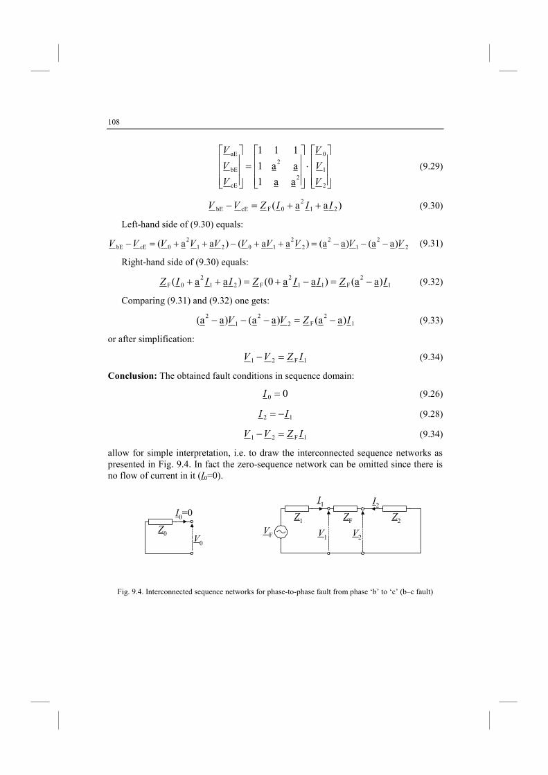
108
⋅
=
2
1
0
2
2
cE
bE
aE
aa1
aa1
111
V
V
V
V
V
V
(9.29)
)aa( 212
0FcEbE IIIZVV ++=− (9.30)
Left-hand side of (9.30) equals:
22
12
22
10212
0cEbE )aa()aa()aa()aa( VVVVVVVVVV −−−=++−++=− (9.31)
Right-hand side of (9.30) equals:
12
F112
F212
0F )aa()aa0()aa( IZIIZIIIZ −=−+=++ (9.32)
Comparing (9.31) and (9.32) one gets:
12
F22
12 )aa()aa()aa( IZVV −=−−− (9.33)
or after simplification:
1F21 IZVV =− (9.34)
Conclusion: The obtained fault conditions in sequence domain:
00 =I (9.26)
12 II −= (9.28)
1F21 IZVV =− (9.34)
allow for simple interpretation, i.e. to draw the interconnected sequence networks as presented in Fig. 9.4. In fact the zero-sequence network can be omitted since there is no flow of current in it (I0=0).
Z0
I0=0
V0
Z1
I1
VF V1
ZF
V2
Z2
I2
Fig. 9.4. Interconnected sequence networks for phase-to-phase fault from phase ‘b’ to ‘c’ (b–c fault)
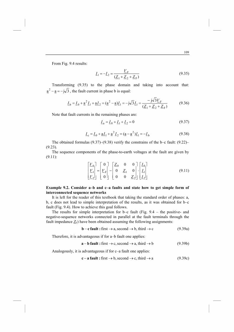
109
From Fig. 9.4 results:
)( F21
F21
ZZZ
VII
++=−= (9.35)
Transforming (9.35) to the phase domain and taking into account that:
3jaa2 −=− , the fault current in phase b is equal:
)(
3j3j)aa(aa
F21
F11
221
20b
ZZZ
VIIIIII
++
−=−=−=++= (9.36)
Note that fault currents in the remaining phases are:
0210a =++= IIII (9.37)
b12
22
10c )aa(aa IIIIII −=−=++= (9.38)
The obtained formulas (9.37)–(9.38) verify the constrains of the b–c fault: (9.22)–(9.23).
The sequence components of the phase-to-earth voltages at the fault are given by (9.11):
⋅
−
=
2
1
0
2
1
0
F
2
1
0
00
00
00
0
0
I
I
I
Z
Z
Z
V
V
V
V
(9.11)
Example 9.2. Consider a–b and c–a faults and state how to get simple form of
interconnected sequence networks
It is left for the reader of this textbook that taking the standard order of phases: a, b, c does not lead to simple interpretation of the results, as it was obtained for b–c fault (Fig. 9.4). How to achieve this goal follows.
The results for simple interpretation for b–c fault (Fig. 9.4 – the positive- and negative-sequence networks connected in parallel at the fault terminals through the fault impedance ZF) have been obtained assuming the following assignments:
c thirdb,second a,first →→→− :fault cb (9.39a)
Therefore, it is advantageous if for a–b fault one applies:
b thirda,second c,first →→→− :fault ba (9.39b)
Analogously, it is advantageous if for c–a fault one applies:
a thirdc,second b,first →→→− :fault ac (9.39c)
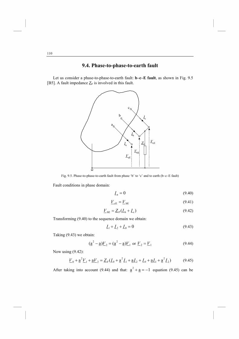
110
9.4. Phase-to-phase-to-earth fault
Let us consider a phase-to-phase-to-earth fault: b–c–E fault, as shown in Fig. 9.5 [B5]. A fault impedance ZF is involved in this fault.
a
b
c
VaE
VbE
VcE
Ic
Ib
IaZF
Fig. 9.5. Phase-to-phase-to-earth fault from phase ‘b’ to ‘c’ and to earth (b–c–E fault)
Fault conditions in phase domain:
0a =I (9.40)
bEcE VV = (9.41)
)( cbFbE IIZV += (9.42)
Transforming (9.40) to the sequence domain we obtain:
0021 =++ III (9.43)
Taking (9.43) we obtain:
12
22 )aa()aa( VV −=− or 12 VV = (9.44)
Now using (9.42):
)aaaa(aa 22
10212
0F212
0 IIIIIIZVVV +++++=++ (9.45)
After taking into account (9.44) and that: 1aa2 −=+ equation (9.45) can be
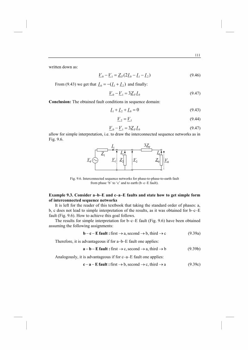
111
written down as:
)2( 210F10 IIIZVV −−=− (9.46)
From (9.43) we get that )( 210 III +−= and finally:
0F10 3 IZVV =− (9.47)
Conclusion: The obtained fault conditions in sequence domain:
0021 =++ III (9.43)
12 VV = (9.44)
0F10 3 IZVV =− (9.47)
allow for simple interpretation, i.e. to draw the interconnected sequence networks as in Fig. 9.6.
Z1
I1
VFV1
3ZF
V2 Z0
I0
Z2 V0
I2
Fig. 9.6. Interconnected sequence networks for phase-to-phase-to-earth fault from phase ‘b’ to ‘c’ and to earth (b–c–E fault).
Example 9.3. Consider a–b–E and c–a–E faults and state how to get simple form
of interconnected sequence networks
It is left for the reader of this textbook that taking the standard order of phases: a, b, c does not lead to simple interpretation of the results, as it was obtained for b–c–E fault (Fig. 9.6). How to achieve this goal follows.
The results for simple interpretation for b–c–E fault (Fig. 9.6) have been obtained assuming the following assignments:
c thirdb,second a,first →→→−− :fault Ecb (9.39a)
Therefore, it is advantageous if for a–b–E fault one applies:
b thirda,second c,first →→→−− :fault Eba (9.39b)
Analogously, it is advantageous if for c–a–E fault one applies:
a thirdc,second b,first →→→−− :fault Eac (9.39c)
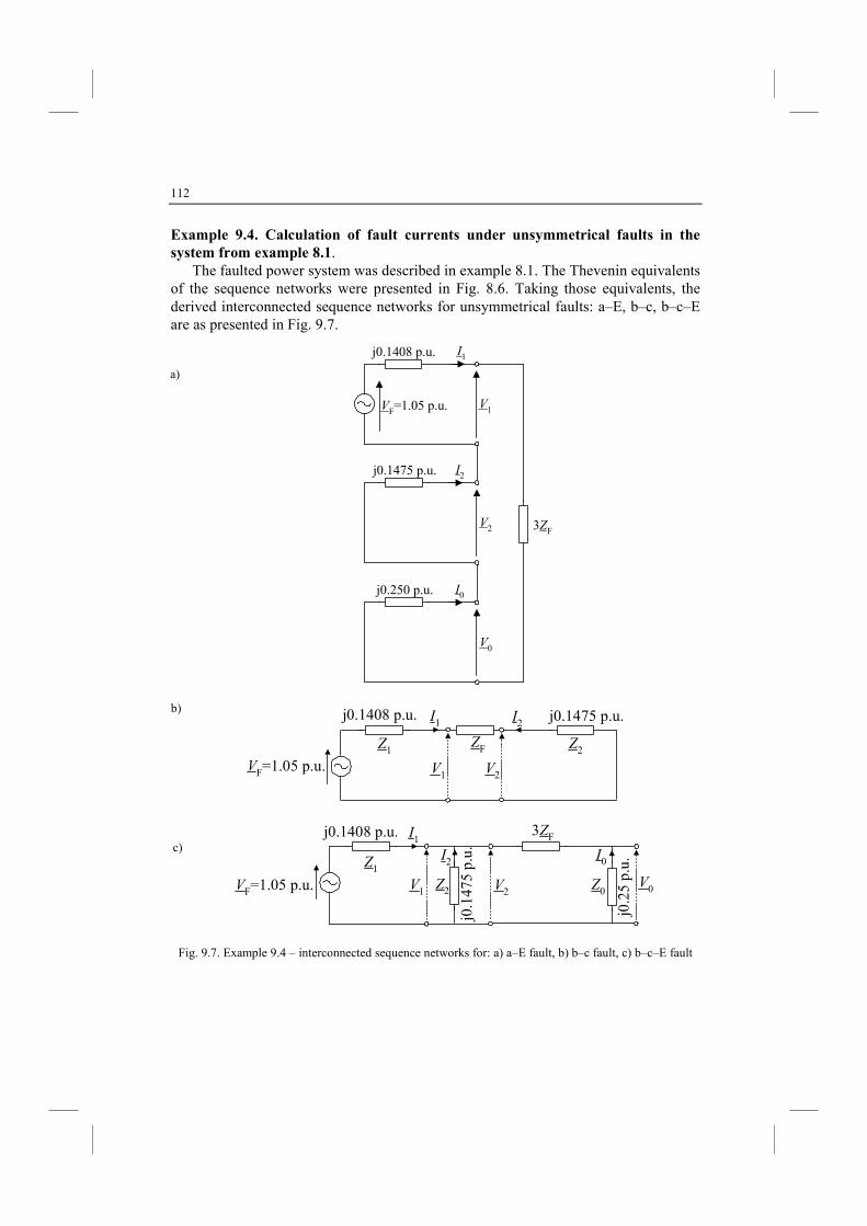
112
Example 9.4. Calculation of fault currents under unsymmetrical faults in the
system from example 8.1. The faulted power system was described in example 8.1. The Thevenin equivalents
of the sequence networks were presented in Fig. 8.6. Taking those equivalents, the derived interconnected sequence networks for unsymmetrical faults: a–E, b–c, b–c–E are as presented in Fig. 9.7.
I1
V1
I2
V2
I0
V0
3ZF
VF=1.05 p.u.
j0.1408 p.u.
j0.1475 p.u.
j0.250 p.u.
Z1
I1
VF=1.05 p.u. V1
ZF
V2
Z2
I2j0.1408 p.u. j0.1475 p.u.
Z1
I1
V1
3ZF
V2
I0
Z2V0VF=1.05 p.u.
j0.1408 p.u.
j0.1
475
p.u.
j0.2
5 p.
u.
I2
Z0
Fig. 9.7. Example 9.4 – interconnected sequence networks for: a) a–E fault, b) b–c fault, c) b–c–E fault
a)
b)
c)
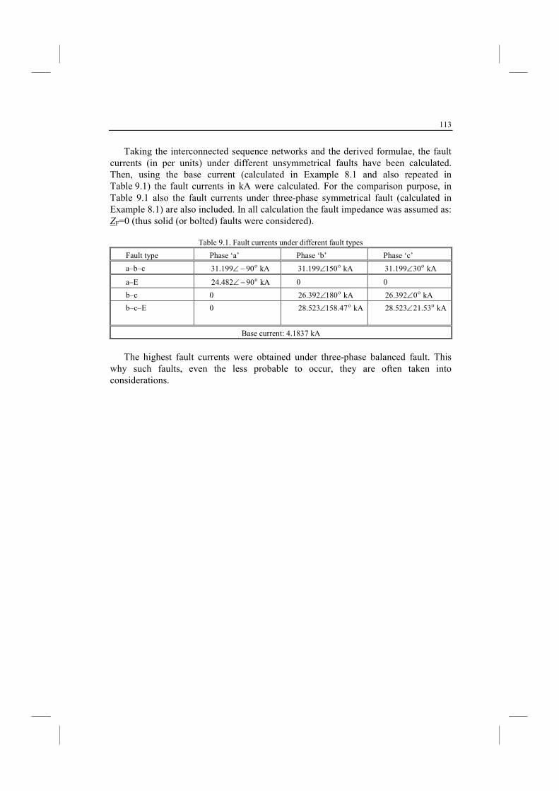
113
Taking the interconnected sequence networks and the derived formulae, the fault currents (in per units) under different unsymmetrical faults have been calculated. Then, using the base current (calculated in Example 8.1 and also repeated in Table 9.1) the fault currents in kA were calculated. For the comparison purpose, in Table 9.1 also the fault currents under three-phase symmetrical fault (calculated in Example 8.1) are also included. In all calculation the fault impedance was assumed as: ZF=0 (thus solid (or bolted) faults were considered).
Table 9.1. Fault currents under different fault types
Fault type Phase ‘a’ Phase ‘b’ Phase ‘c’
a–b–c kA 90199.31 o−∠ kA 150199.31 o∠ kA 30199.31 o∠
a–E kA 90482.24 o−∠ 0 0
b–c 0 kA 180392.26 o∠ kA 0392.26 o∠
b–c–E 0 kA 47.158523.28 o∠
kA 53.21523.28 o∠
Base current: 4.1837 kA
The highest fault currents were obtained under three-phase balanced fault. This
why such faults, even the less probable to occur, they are often taken into considerations.
114
10. AALYSIS OF OPE-CODUCTOR
CODITIOS
10.1. Introduction
In this Chapter the faults involving open-conductor conditions are considered. Such conditions may be caused by broken conductor failure, but also due to an intentional single-phase switching operation. Such faults may involve the opening of one or two phases of a three-phase circuit. The case of opening of all three phases has no practical meaning since in this case there is no flow of currents in all three phases. Open-conductor can happen also in combination with single phase to earth fault.
10.2. One opened conductor
Let us consider a balanced three-phase network with an overhead power line in
which the pre-fault current prea
pre1 II = flows and the conductor from the phase ‘a’
undergoes opened [B9, B19] (Fig. 10.1). The open-conductor condition can be reflected by inserting the voltage source
aV∆ in the phase ‘a’ which is affected by the broken conductor failure (Fig. 10.2):
0a ≠∆V (10.1)
The direction of the voltage source aV∆ is in opposite side with respect to the pre-
fault current preaI . The value of this voltage source is set at such value that the flowing
current decreases to zero (since there is a break). In the remaining healthy phases (b and c) the inserted voltage sources (Fig. 10.2)
are equal to zero: 0b =∆V (10.2)
0c =∆V (10.3)
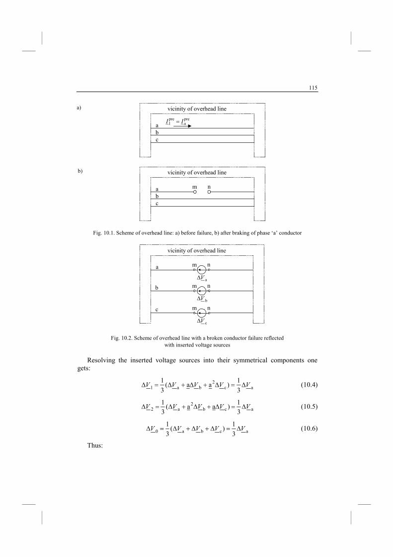
115
abc
vicinity of overhead line
prea
pre1 II =
abc
m n
vicinity of overhead line
Fig. 10.1. Scheme of overhead line: a) before failure, b) after braking of phase ‘a’ conductor
a
b
c
vicinity of overhead line
m n
m n
m n
aV∆
bV∆
cV∆
Fig. 10.2. Scheme of overhead line with a broken conductor failure reflected with inserted voltage sources
Resolving the inserted voltage sources into their symmetrical components one
gets:
ac2
ba1 3
1)aa(
3
1VVVVV ∆=∆+∆+∆=∆ (10.4)
acb2
a2 3
1)aa(
3
1VVVVV ∆=∆+∆+∆=∆ (10.5)
acba0 3
1)(
3
1VVVVV ∆=∆+∆+∆=∆ (10.6)
Thus:
a)
b)
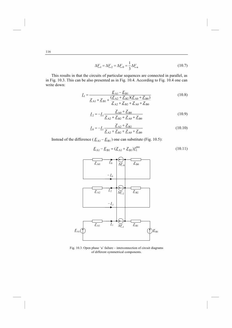
116
a021 3
1VVVV ∆=∆=∆=∆ (10.7)
This results in that the circuits of particular sequences are connected in parallel, as in Fig. 10.3. This can be also presented as in Fig. 10.4. According to Fig. 10.4 one can write down:
B0A0B2A2
B0A0B2A2B1A1
B1A11 ))((
ZZZZ
ZZZZZZ
EEI
+++++
++
−= (10.8)
B0A0B2A2
B0A012
ZZZZ
ZZII
+++
+−= (10.9)
B0A0B2A2
B2A210
ZZZZ
ZZII
+++
+−= (10.10)
Instead of the difference ( B1A1 EE − ) one can substitute (Fig. 10.5):
pre1B1A1B1A1 )( IZZEE +=− (10.11)
A1E B1E
A1Z B1Z1V∆1I
A2Z B2Z2V∆2I
A0Z B0Z0V∆0I
2I−
0I−
Fig. 10.3. Open phase ‘a’ failure – interconnection of circuit diagrams of different symmetrical components.
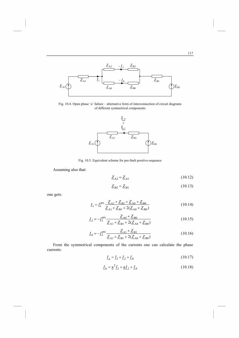
117
A1E B1E
A1Z B1Z1I
A2Z B2Z2I−
0I−
A0Z B0Z
Fig. 10.4. Open phase ‘a’ failure – alternative form of interconnection of circuit diagrams of different symmetrical components
A1E B1E
pre
apr
e1
II
=
A1Z B1Z
Fig. 10.5. Equivalent scheme for pre-fault positive-sequence
Assuming also that:
A1A2 ZZ = (10.12)
B1B2 ZZ = (10.13)
one gets:
)(2 B0A0B1A1
B0A0B1A1pre11
ZZZZ
ZZZZII
+++
+++= (10.14)
)(2 B0A0B1A1
B0A0pre12
ZZZZ
ZZII
+++
+−= (10.15)
)(2 B0A0B1A1
B1A1pre10
ZZZZ
ZZII
+++
+−= (10.16)
From the symmetrical components of the currents one can calculate the phase currents:
021a IIII ++= (10.17)
0212
b aa IIII ++= (10.18)
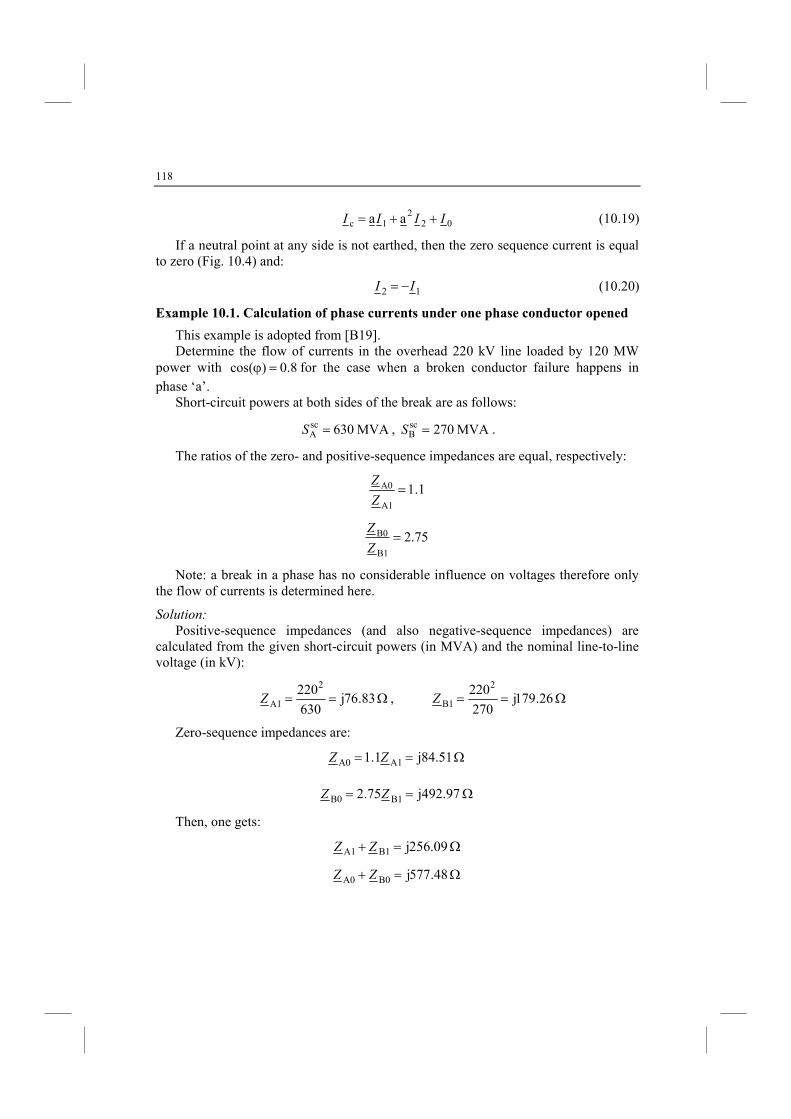
118
022
1c aa IIII ++= (10.19)
If a neutral point at any side is not earthed, then the zero sequence current is equal to zero (Fig. 10.4) and:
12 II −= (10.20)
Example 10.1. Calculation of phase currents under one phase conductor opened
This example is adopted from [B19]. Determine the flow of currents in the overhead 220 kV line loaded by 120 MW
power with 8.0)cos( =ϕ for the case when a broken conductor failure happens in
phase ‘a’. Short-circuit powers at both sides of the break are as follows:
MVA 630scA =S , MVA 270sc
B =S .
The ratios of the zero- and positive-sequence impedances are equal, respectively:
1.1A1
A0 =Z
Z
75.2B1
B0 =Z
Z
Note: a break in a phase has no considerable influence on voltages therefore only the flow of currents is determined here.
Solution:
Positive-sequence impedances (and also negative-sequence impedances) are calculated from the given short-circuit powers (in MVA) and the nominal line-to-line voltage (in kV):
Ω== 83.76j630
2202
A1Z , Ω== 26.179j270
2202
B1Z
Zero-sequence impedances are:
Ω== j84.511.1 A1A0 ZZ
Ω== 97.92j475.2 B1B0 ZZ
Then, one gets:
Ω=+ 09.256jB1A1 ZZ
Ω=+ 48.577jB0A0 ZZ
119
Pre-fault positive-sequence current equals:
A 65.3938.0000 2203
000 120
)cos(3
preA1 =
⋅⋅=
ϕ=
V
PI
The symmetrical components of currents according to (10.14)–(10.16):
A 64.232)(2 B0A0B1A1
B0A0B1A1pre11 =
+++
+++=
ZZZZ
ZZZZII
A 00.161)(2 B0A0B1A1
B0A0pre12 −=
+++
+−=
ZZZZ
ZZII
A 64.71)(2 B0A0B1A1
B1A1pre10 −=
+++
+−=
ZZZZ
ZZII
Therefore, the phase currents according to (10.17)–(10.19) are:
0021a =++= IIII
oj107.48021
2b e51.357aa −=++= IIII
oj107.4802
21c e51.357aa =++= IIII .
Conclusion: the broken conductor failure in phase ‘a’ causes a decrease of currents in the remaining healthy phases by around 10%:
908.065.393
51.357= .
10.3. Two opened conductors
Let us consider the conditions for two opened conductors in phases b and c (Fig. 10.6). The pre-fault positive-sequence current is as in the previous Section 10.2 (Fig. 10.5).
In this case the constrains are as follows:
0cb == II , 0a ≠= II (10.21)
0a =∆V (10.22)
From (10.21) one gets:
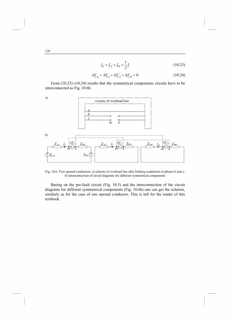
120
IIII3
1021 === (10.23)
0021a =∆+∆+∆=∆ VVVV (10.24)
From (10.23)–(10.24) results that the symmetrical components circuits have to be interconnected as Fig. 10.6b.
abc
m n
vicinity of overhead line
A1E B1E
A1Z B1Z1V∆1I A2Z B2Z2V∆
2I A0Z B0Z0V∆0I
nm nmnm
Fig. 10.6. Two opened conductors: a) scheme of overhead line after braking conductors in phases b and c, b) interconnection of circuit diagrams for different symmetrical components
Basing on the pre-fault circuit (Fig. 10.5) and the interconnection of the circuit
diagrams for different symmetrical components (Fig. 10.6b) one can get the solution, similarly as for the case of one opened conductor. This is left for the reader of this textbook.
a)
b)
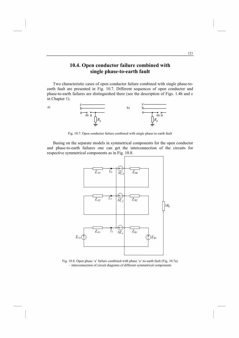
121
10.4. Open conductor failure combined with
single phase-to-earth fault
Two characteristic cases of open conductor failure combined with single phase-to-earth fault are presented in Fig. 10.7. Different sequences of open conductor and phase-to-earth failures are distinguished there (see the description of Figs. 1.4b and c in Chapter 1).
nmRF
abc
m nRF
abc
Fig. 10.7. Open conductor failure combined with single phase-to-earth fault
Basing on the separate models in symmetrical components for the open conductor
and phase-to-earth failures one can get the interconnection of the circuits for respective symmetrical components as in Fig. 10.8.
A1E B1E
A1Z B1Z1V∆1I
A2Z B2Z2V∆2I
A0Z B0Z0V∆0I
F3R
Fig. 10.8. Open phase ‘a’ failure combined with phase ‘a’-to-earth fault (Fig. 10.7a) – interconnection of circuit diagrams of different symmetrical components
a) b)
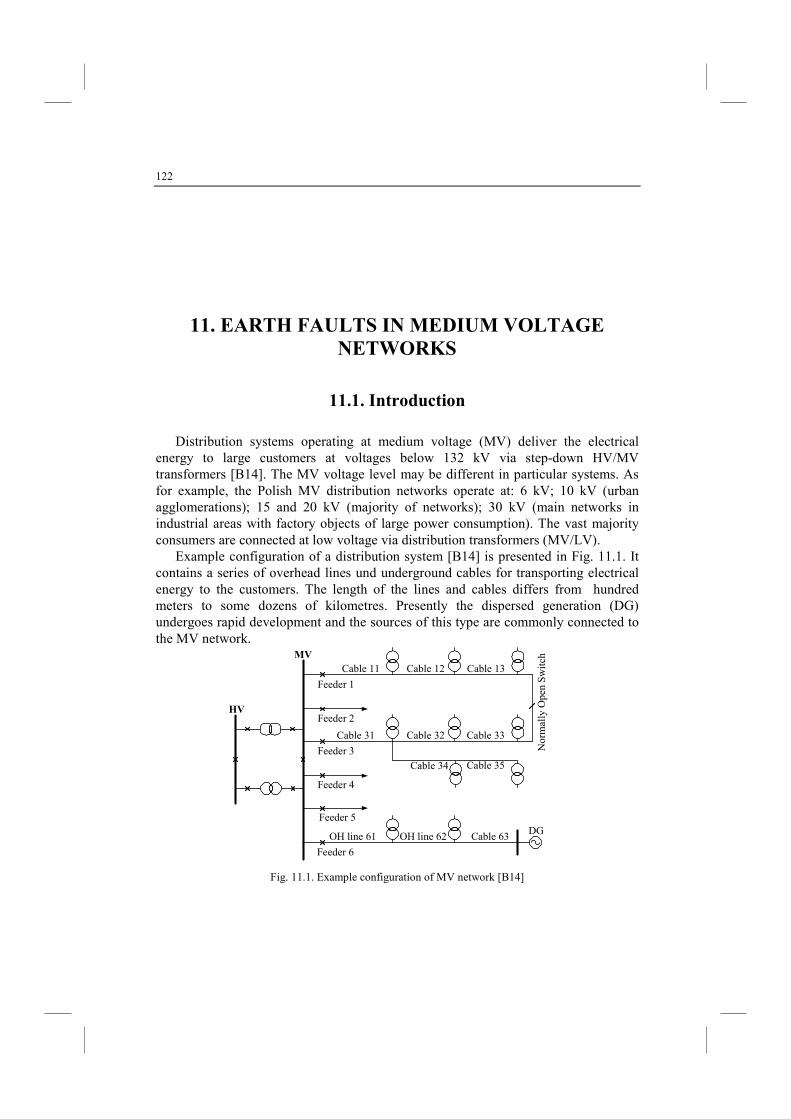
122
11. EARTH FAULTS I MEDIUM VOLTAGE
ETWORKS
11.1. Introduction
Distribution systems operating at medium voltage (MV) deliver the electrical energy to large customers at voltages below 132 kV via step-down HV/MV transformers [B14]. The MV voltage level may be different in particular systems. As for example, the Polish MV distribution networks operate at: 6 kV; 10 kV (urban agglomerations); 15 and 20 kV (majority of networks); 30 kV (main networks in industrial areas with factory objects of large power consumption). The vast majority consumers are connected at low voltage via distribution transformers (MV/LV).
Example configuration of a distribution system [B14] is presented in Fig. 11.1. It contains a series of overhead lines und underground cables for transporting electrical energy to the customers. The length of the lines and cables differs from hundred meters to some dozens of kilometres. Presently the dispersed generation (DG) undergoes rapid development and the sources of this type are commonly connected to the MV network.
Cable 11 Cable 12 Cable 13
Cable 31 Cable 32 Cable 33
Feeder 1
Feeder 2
Feeder 3
Feeder 4
Feeder 5
Feeder 6
OH line 61 OH line 62 Cable 63DG
Cable 34 Cable 35
Nor
mal
ly O
pen
Sw
itch
HV
MV
Fig. 11.1. Example configuration of MV network [B14]
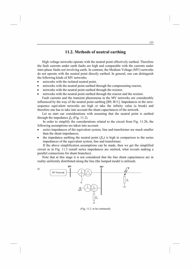
123
11.2. Methods of neutral earthing
High voltage networks operate with the neutral point effectively earthed. Therefore the fault currents under earth faults are high and comparable with the currents under inter-phase faults not involving earth. In contrast, the Medium Voltage (MV) networks do not operate with the neutral point directly earthed. In general, one can distinguish the following kinds of MV networks: • networks with the isolated neutral point, • networks with the neutral point earthed through the compensating reactor, • networks with the neutral point earthed through the resistor, • networks with the neutral point earthed through the reactor and the resistor.
Fault currents and the transient phenomena in the MV networks are considerably influenced by the way of the neutral point earthing [B9, B11]. Impedances in the zero-sequence equivalent networks are high or take the infinity value (a break) and therefore one has to take into account the shunt capacitances of the network.
Let us start our considerations with assuming that the neutral point is earthed through the impedance ZN (Fig. 11.2).
In order to simplify the considerations related to the circuit from Fig. 11.2b, the following assumptions are taken into account: • series impedances of the equivalent system, line and transformer are much smaller
than the shunt impedances, • the impedance earthing the neutral point (ZN) is high in comparison to the series
impedances of the equivalent system, line and transformer. If the above simplification assumptions can be made, then we get the simplified
circuit as in Fig. 11.3 (small series impedances are omitted, what reveals making a parallel connections for shunt branches).
Note that at this stage it is not considered that the line shunt capacitances are in reality uniformly distributed along the line (the lumped model is utilised).
HV MVF
HV Network
ZN
ZF
LV
(Fig. 11.2. to be continued)
a)
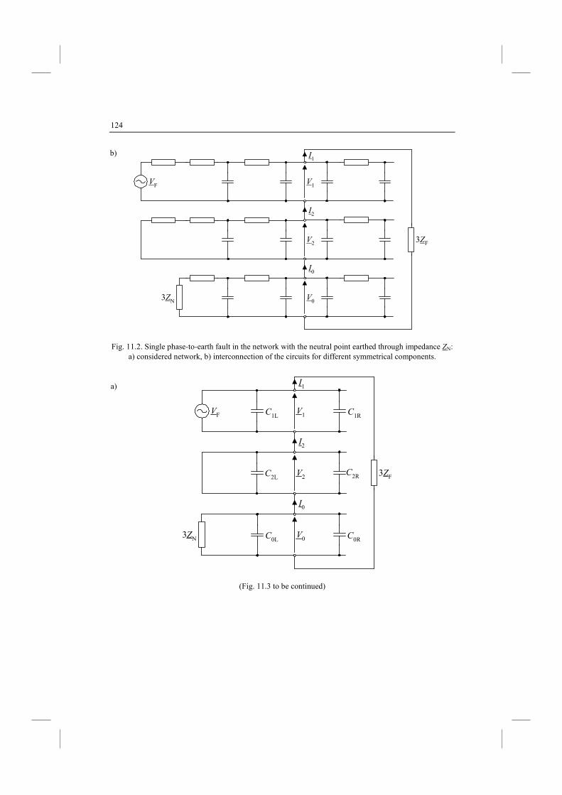
124
V1
V2
V0
3ZF
3ZN
VF
I1
I2
I0
Fig. 11.2. Single phase-to-earth fault in the network with the neutral point earthed through impedance ZN: a) considered network, b) interconnection of the circuits for different symmetrical components.
V1
V2
V0
3ZF
3ZN
VF
I1
I2
I0
C1L C1R
C2LC2R
C0RC0L
(Fig. 11.3 to be continued)
b)
a)
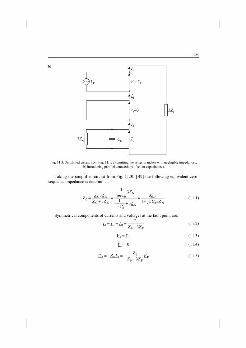
125
V1=VF
V2=0
V0
3ZF
3ZN
VF
I1
I2
I0
C0
Fig. 11.3. Simplified circuit from Fig. 11.1: a) omitting the series branches with negligible impedances, b) introducing parallel connections of shunt capacitances.
Taking the simplified circuit from Fig. 11.3b [B9] the following equivalent zero-
sequence impedance is determined:
N0
N
N0
N0
NC
NC0 3j1
3
3j
1
3j
1
3
3
ZC
Z
ZC
ZC
ZZ
ZZZ
ω+=
+ω
ω=
+= (11.1)
Symmetrical components of currents and voltages at the fault point are:
F0
F021 3ZZ
VIII
+=== (11.2)
F1 VV = (11.3)
02 =V (11.4)
FF0
0000 3
VZZ
ZIZV
+−=−= (11.5)
b)
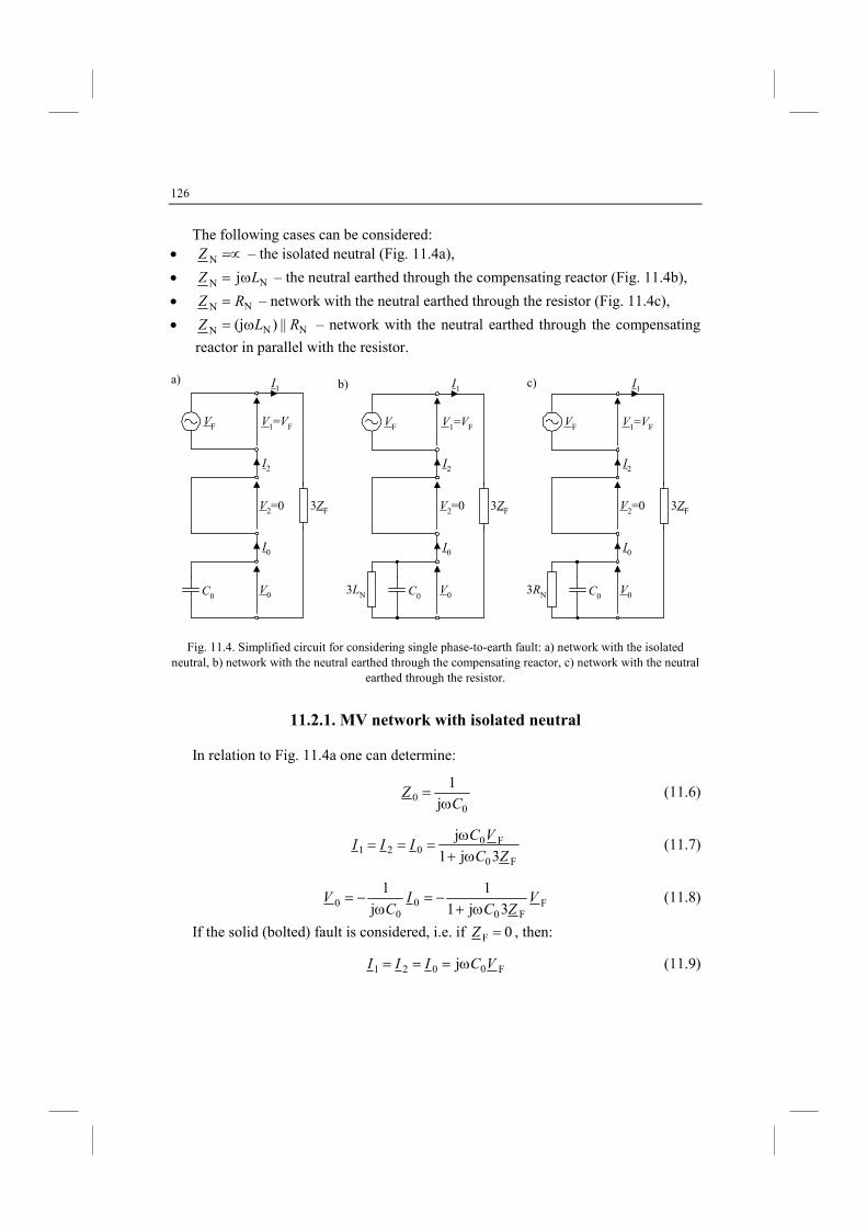
126
The following cases can be considered: • =∝NZ – the isolated neutral (Fig. 11.4a),
• NN j LZ ω= – the neutral earthed through the compensating reactor (Fig. 11.4b),
• NN RZ = – network with the neutral earthed through the resistor (Fig. 11.4c),
• NNN ||)(j RLZ ω= – network with the neutral earthed through the compensating
reactor in parallel with the resistor.
V1=VF
V2=0
V0
3ZF
VF
I1
I2
I0
C0
V1=VF
V2=0
V0
3ZF
3LN
VF
I1
I2
I0
C0
V1=VF
V2=0
V0
3ZF
3RN
VF
I1
I2
I0
C0
Fig. 11.4. Simplified circuit for considering single phase-to-earth fault: a) network with the isolated neutral, b) network with the neutral earthed through the compensating reactor, c) network with the neutral
earthed through the resistor.
11.2.1. MV network with isolated neutral
In relation to Fig. 11.4a one can determine:
0
0 j
1
CZ
ω= (11.6)
F0
F0021 3j1
j
ZC
VCIII
ω+ω
=== (11.7)
FF0
00
0 3j1
1
j
1V
ZCI
CV
ω+−=
ω−= (11.8)
If the solid (bolted) fault is considered, i.e. if 0F =Z , then:
F0021 j VCIII ω=== (11.9)
a) b) c)
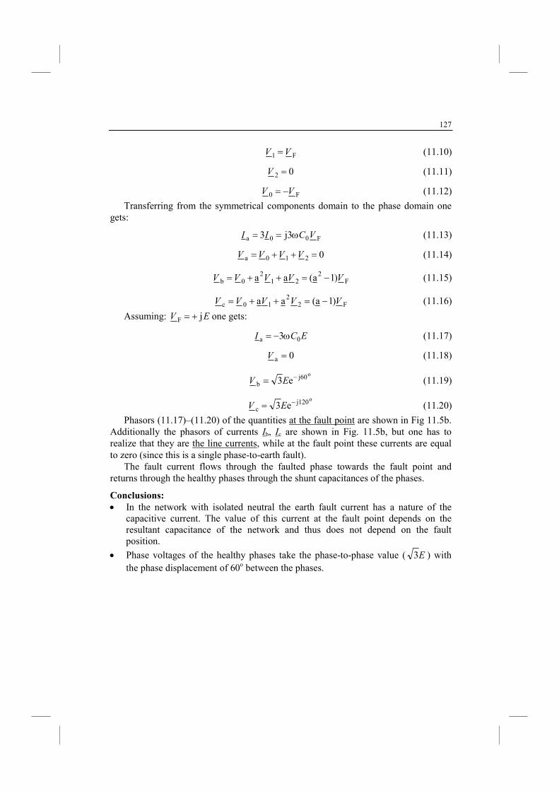
127
F1 VV = (11.10)
02 =V (11.11)
F0 VV −= (11.12)
Transferring from the symmetrical components domain to the phase domain one gets:
F00a j33 VCII ω== (11.13)
0210a =++= VVVV (11.14)
F2
212
0b )1a(aa VVVVV −=++= (11.15)
F22
10c )1a(aa VVVVV −=++= (11.16)
Assuming: EV jF += one gets:
ECI 0a 3ω−= (11.17)
0a =V (11.18)
oj60
b e3 −= EV (11.19)
oj120
c e3 −= EV (11.20)
Phasors (11.17)–(11.20) of the quantities at the fault point are shown in Fig 11.5b. Additionally the phasors of currents Ib, Ic are shown in Fig. 11.5b, but one has to realize that they are the line currents, while at the fault point these currents are equal to zero (since this is a single phase-to-earth fault).
The fault current flows through the faulted phase towards the fault point and returns through the healthy phases through the shunt capacitances of the phases.
Conclusions:
• In the network with isolated neutral the earth fault current has a nature of the capacitive current. The value of this current at the fault point depends on the resultant capacitance of the network and thus does not depend on the fault position.
• Phase voltages of the healthy phases take the phase-to-phase value ( E3 ) with the phase displacement of 60o between the phases.
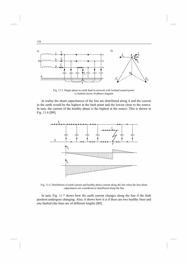
128
N
E
a
b
c
Ia
Ic
Ib
Ia
F
N
IaIb
Ic
E
VbVc
60o
Fig. 11.5. Single phase-to-earth fault in network with isolated neutral point: a) faulted circuit, b) phasor diagram
In reality the shunt capacitances of the line are distributed along it and the current
in the earth would be the highest at the fault point and the lowest close to the source. In turn, the current of the healthy phase is the highest at the source. This is shown in Fig. 11.6 [B9].
FE
Ib
Ia
IE
Ib
Fig. 11.6. Distribution of earth current and healthy phase current along the line when the line shunt capacitances are considered as distributed along the line
In turn, Fig. 11.7 shows how the earth current changes along the line if the fault
position undergoes changing. Also, it shows how it is if there are two healthy lines and one faulted (the lines are of different length) [B9].
a) b)
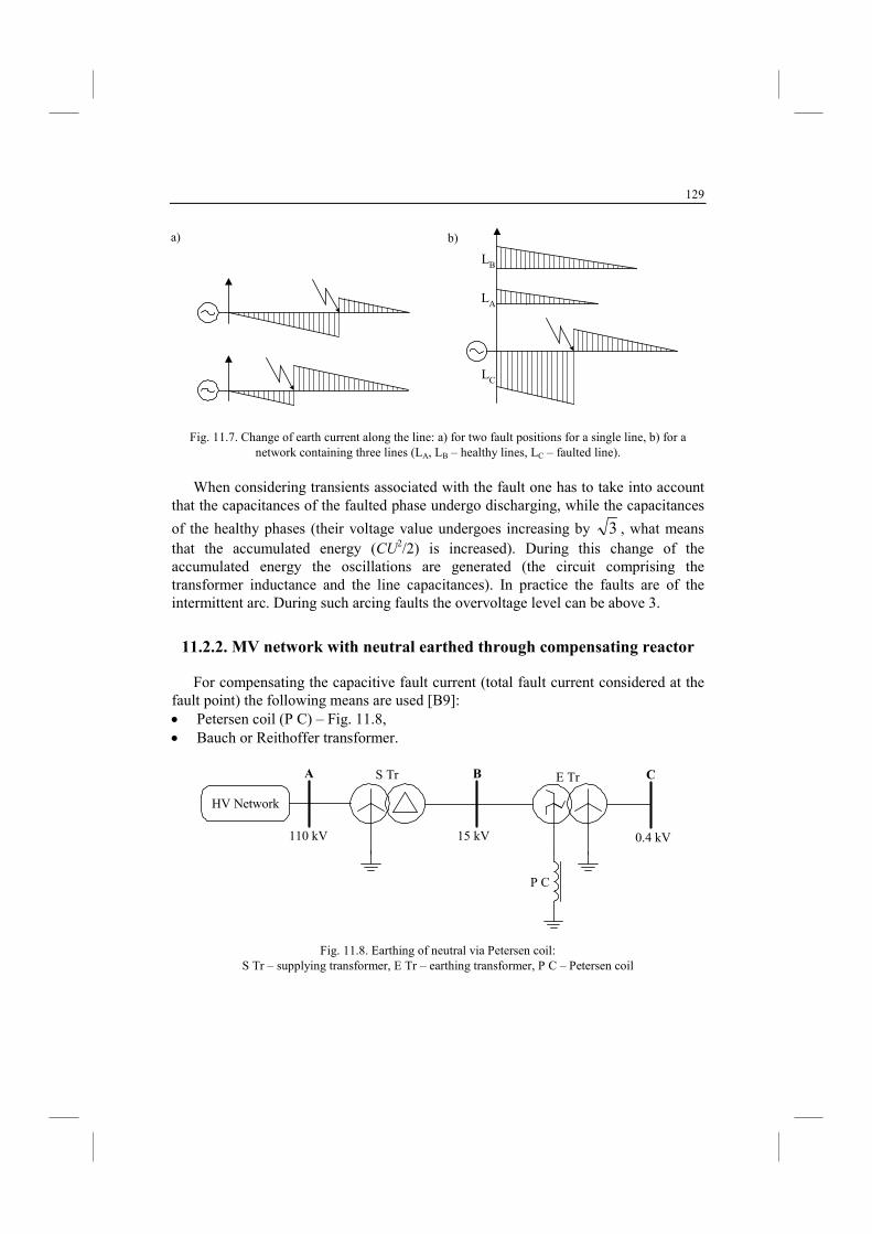
129
LA
LB
LC
Fig. 11.7. Change of earth current along the line: a) for two fault positions for a single line, b) for a network containing three lines (LA, LB – healthy lines, LC – faulted line).
When considering transients associated with the fault one has to take into account
that the capacitances of the faulted phase undergo discharging, while the capacitances
of the healthy phases (their voltage value undergoes increasing by 3 , what means that the accumulated energy (CU2/2) is increased). During this change of the accumulated energy the oscillations are generated (the circuit comprising the transformer inductance and the line capacitances). In practice the faults are of the intermittent arc. During such arcing faults the overvoltage level can be above 3.
11.2.2. MV network with neutral earthed through compensating reactor
For compensating the capacitive fault current (total fault current considered at the fault point) the following means are used [B9]: • Petersen coil (P C) – Fig. 11.8, • Bauch or Reithoffer transformer.
A B C
HV Network
110 kV 15 kV 0.4 kV
S Tr E Tr
P C
Fig. 11.8. Earthing of neutral via Petersen coil: S Tr – supplying transformer, E Tr – earthing transformer, P C – Petersen coil
a) b)
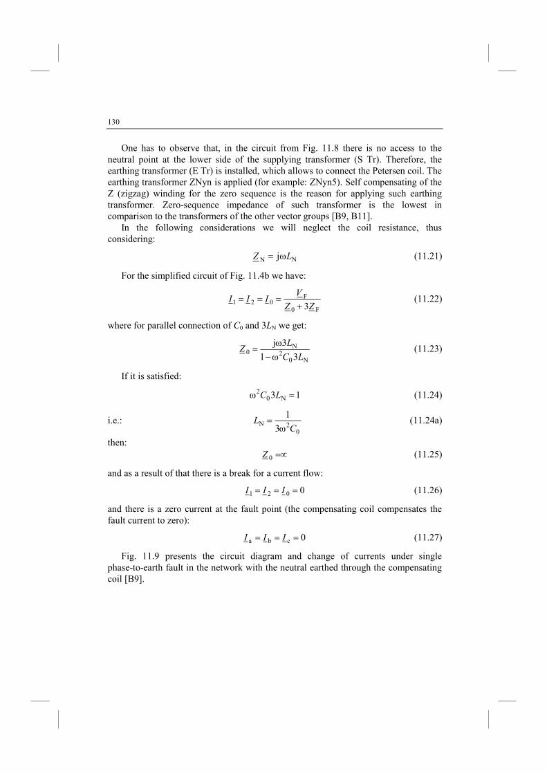
130
One has to observe that, in the circuit from Fig. 11.8 there is no access to the neutral point at the lower side of the supplying transformer (S Tr). Therefore, the earthing transformer (E Tr) is installed, which allows to connect the Petersen coil. The earthing transformer ZNyn is applied (for example: ZNyn5). Self compensating of the Z (zigzag) winding for the zero sequence is the reason for applying such earthing transformer. Zero-sequence impedance of such transformer is the lowest in comparison to the transformers of the other vector groups [B9, B11].
In the following considerations we will neglect the coil resistance, thus considering:
NN j LZ ω= (11.21)
For the simplified circuit of Fig. 11.4b we have:
F0
F021 3ZZ
VIII
+=== (11.22)
where for parallel connection of C0 and 3LN we get:
N0
2N
031
3j
LC
LZ
ω−
ω= (11.23)
If it is satisfied:
13 N02 =ω LC (11.24)
i.e.: 0
2N3
1
CL
ω= (11.24a)
then: =∝0Z (11.25)
and as a result of that there is a break for a current flow:
0021 === III (11.26)
and there is a zero current at the fault point (the compensating coil compensates the fault current to zero):
0cba === III (11.27)
Fig. 11.9 presents the circuit diagram and change of currents under single phase-to-earth fault in the network with the neutral earthed through the compensating coil [B9].
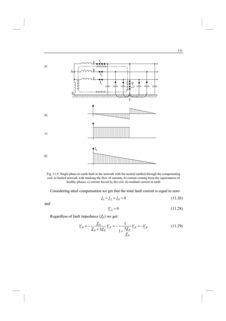
131
N
E
c
b
a
I a=0
Ia
Ib
Ic
F
IE
Fig. 11.9. Single phase-to-earth fault in the network with the neutral earthed through the compensating coil: a) faulted network with marking the flow of currents, b) current coming from the capacitances of
healthy phases, c) current forced by the coil, d) resultant current in earth
Considering ideal compensation we get that the total fault current is equal to zero:
0021 === III (11.26)
and 02 =V (11.28)
Regardless of fault impedance (ZF) we get:
FF
0
FF
F0
00 3
1
1
3VV
Z
ZV
ZZ
ZV −=
+−=
+−= (11.29)
a)
b)
c)
d)
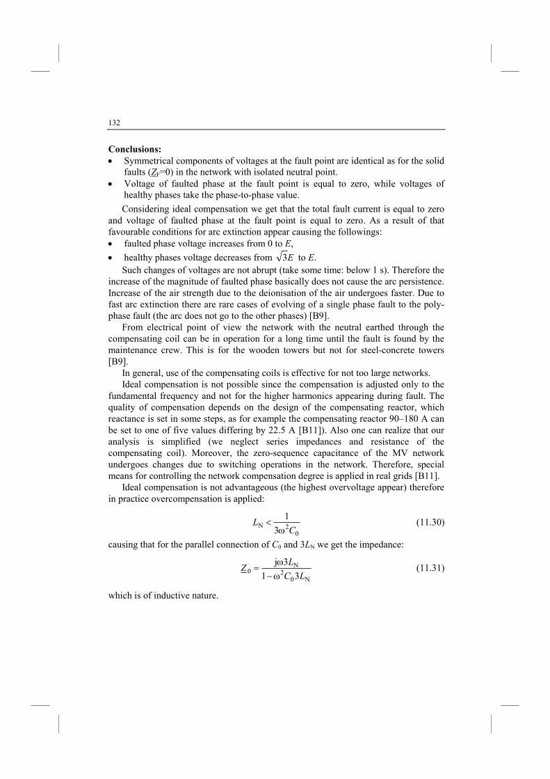
132
Conclusions:
• Symmetrical components of voltages at the fault point are identical as for the solid faults (ZF=0) in the network with isolated neutral point.
• Voltage of faulted phase at the fault point is equal to zero, while voltages of healthy phases take the phase-to-phase value.
Considering ideal compensation we get that the total fault current is equal to zero and voltage of faulted phase at the fault point is equal to zero. As a result of that favourable conditions for arc extinction appear causing the followings: • faulted phase voltage increases from 0 to E,
• healthy phases voltage decreases from E3 to E. Such changes of voltages are not abrupt (take some time: below 1 s). Therefore the
increase of the magnitude of faulted phase basically does not cause the arc persistence. Increase of the air strength due to the deionisation of the air undergoes faster. Due to fast arc extinction there are rare cases of evolving of a single phase fault to the poly-phase fault (the arc does not go to the other phases) [B9].
From electrical point of view the network with the neutral earthed through the compensating coil can be in operation for a long time until the fault is found by the maintenance crew. This is for the wooden towers but not for steel-concrete towers [B9].
In general, use of the compensating coils is effective for not too large networks. Ideal compensation is not possible since the compensation is adjusted only to the
fundamental frequency and not for the higher harmonics appearing during fault. The quality of compensation depends on the design of the compensating reactor, which reactance is set in some steps, as for example the compensating reactor 90–180 A can be set to one of five values differing by 22.5 A [B11]). Also one can realize that our analysis is simplified (we neglect series impedances and resistance of the compensating coil). Moreover, the zero-sequence capacitance of the MV network undergoes changes due to switching operations in the network. Therefore, special means for controlling the network compensation degree is applied in real grids [B11].
Ideal compensation is not advantageous (the highest overvoltage appear) therefore in practice overcompensation is applied:
0
2N3
1
CL
ω< (11.30)
causing that for the parallel connection of C0 and 3LN we get the impedance:
N0
2N
031
3j
LC
LZ
ω−
ω= (11.31)
which is of inductive nature.
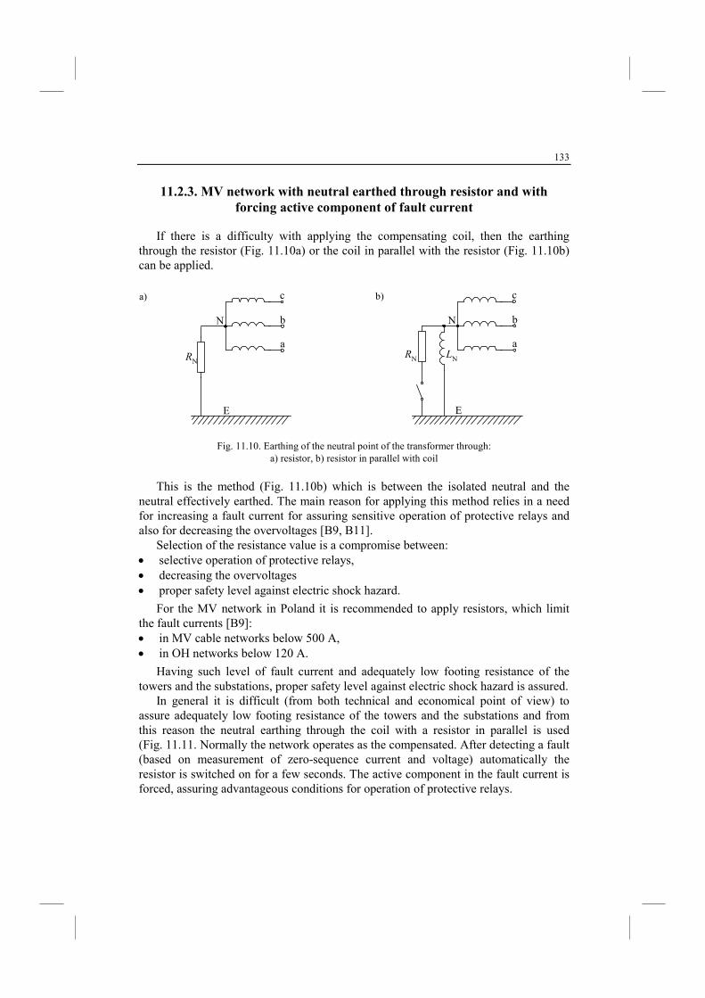
133
11.2.3. MV network with neutral earthed through resistor and with
forcing active component of fault current
If there is a difficulty with applying the compensating coil, then the earthing through the resistor (Fig. 11.10a) or the coil in parallel with the resistor (Fig. 11.10b) can be applied.
N
E
a
b
c
RN
N
E
a
b
c
RN LN
Fig. 11.10. Earthing of the neutral point of the transformer through: a) resistor, b) resistor in parallel with coil
This is the method (Fig. 11.10b) which is between the isolated neutral and the
neutral effectively earthed. The main reason for applying this method relies in a need for increasing a fault current for assuring sensitive operation of protective relays and also for decreasing the overvoltages [B9, B11].
Selection of the resistance value is a compromise between: • selective operation of protective relays, • decreasing the overvoltages • proper safety level against electric shock hazard.
For the MV network in Poland it is recommended to apply resistors, which limit the fault currents [B9]: • in MV cable networks below 500 A, • in OH networks below 120 A.
Having such level of fault current and adequately low footing resistance of the towers and the substations, proper safety level against electric shock hazard is assured.
In general it is difficult (from both technical and economical point of view) to assure adequately low footing resistance of the towers and the substations and from this reason the neutral earthing through the coil with a resistor in parallel is used (Fig. 11.11. Normally the network operates as the compensated. After detecting a fault (based on measurement of zero-sequence current and voltage) automatically the resistor is switched on for a few seconds. The active component in the fault current is forced, assuring advantageous conditions for operation of protective relays.
a) b)
134
In Poland there are the solutions for forcing the active component of the fault current from the range 15 A up to 40 A or in some rare cases around 100 A. Also in the other European countries (Austria, Czech Republic, Slovakian Republic, Hungary, Germany) the forcing of the active component of the fault current is commonly applied. In particular, in Germany the forcing of the active component current at the level around 1000 A or even higher is applied. In turn, in some countries the solution with complete shortening of the compensating reactor for a short time interval is applied, which results in getting solidly earthed network (for this interval) [B11].
In Fig. 11.11 different ways of connection of the resistor forcing the active component of the fault current are shown.
MV
LN
ControlCircuit
RN
LVV0
I0
MV
LN
ControlCircuit
RN
LV V0
I0
(Fig. 11.11 to be continued)
a)
b)
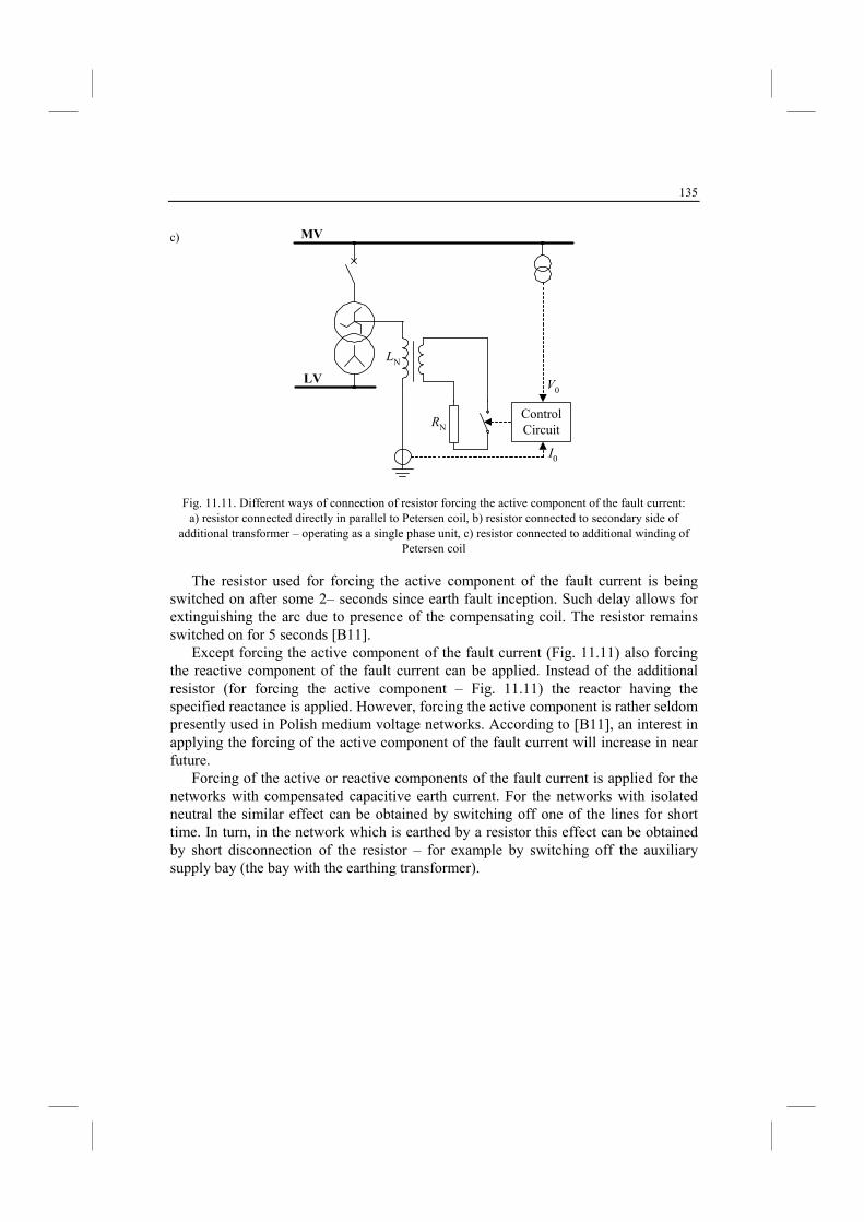
135
MV
LN
ControlCircuit
RN
LV V0
I0
Fig. 11.11. Different ways of connection of resistor forcing the active component of the fault current: a) resistor connected directly in parallel to Petersen coil, b) resistor connected to secondary side of
additional transformer – operating as a single phase unit, c) resistor connected to additional winding of Petersen coil
The resistor used for forcing the active component of the fault current is being
switched on after some 2– seconds since earth fault inception. Such delay allows for extinguishing the arc due to presence of the compensating coil. The resistor remains switched on for 5 seconds [B11].
Except forcing the active component of the fault current (Fig. 11.11) also forcing the reactive component of the fault current can be applied. Instead of the additional resistor (for forcing the active component – Fig. 11.11) the reactor having the specified reactance is applied. However, forcing the active component is rather seldom presently used in Polish medium voltage networks. According to [B11], an interest in applying the forcing of the active component of the fault current will increase in near future.
Forcing of the active or reactive components of the fault current is applied for the networks with compensated capacitive earth current. For the networks with isolated neutral the similar effect can be obtained by switching off one of the lines for short time. In turn, in the network which is earthed by a resistor this effect can be obtained by short disconnection of the resistor – for example by switching off the auxiliary supply bay (the bay with the earthing transformer).
c)
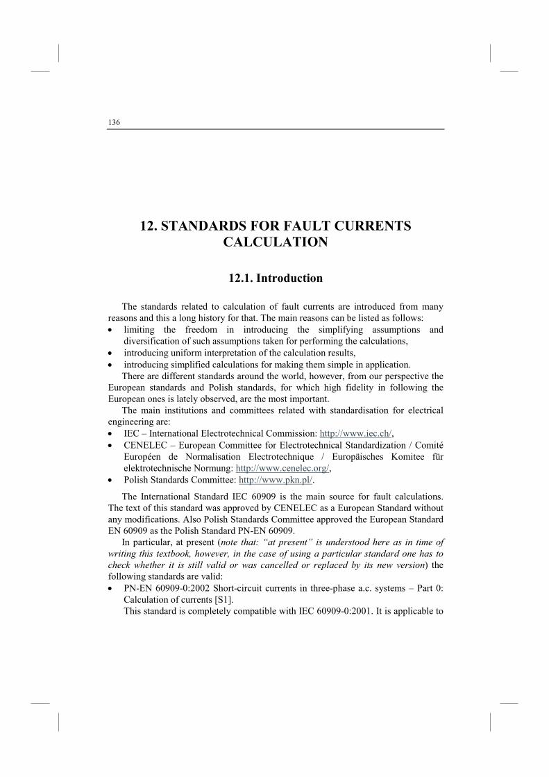
136
12. STADARDS FOR FAULT CURRETS
CALCULATIO
12.1. Introduction
The standards related to calculation of fault currents are introduced from many reasons and this a long history for that. The main reasons can be listed as follows: • limiting the freedom in introducing the simplifying assumptions and
diversification of such assumptions taken for performing the calculations, • introducing uniform interpretation of the calculation results, • introducing simplified calculations for making them simple in application.
There are different standards around the world, however, from our perspective the European standards and Polish standards, for which high fidelity in following the European ones is lately observed, are the most important.
The main institutions and committees related with standardisation for electrical engineering are: • IEC – International Electrotechnical Commission: http://www.iec.ch/, • CENELEC – European Committee for Electrotechnical Standardization / Comité
Européen de Normalisation Electrotechnique / Europäisches Komitee für elektrotechnische Normung: http://www.cenelec.org/,
• Polish Standards Committee: http://www.pkn.pl/.
The International Standard IEC 60909 is the main source for fault calculations. The text of this standard was approved by CENELEC as a European Standard without any modifications. Also Polish Standards Committee approved the European Standard EN 60909 as the Polish Standard PN-EN 60909.
In particular, at present (note that: “at present” is understood here as in time of writing this textbook, however, in the case of using a particular standard one has to
check whether it is still valid or was cancelled or replaced by its new version) the following standards are valid: • PN-EN 60909-0:2002 Short-circuit currents in three-phase a.c. systems – Part 0:
Calculation of currents [S1]. This standard is completely compatible with IEC 60909-0:2001. It is applicable to
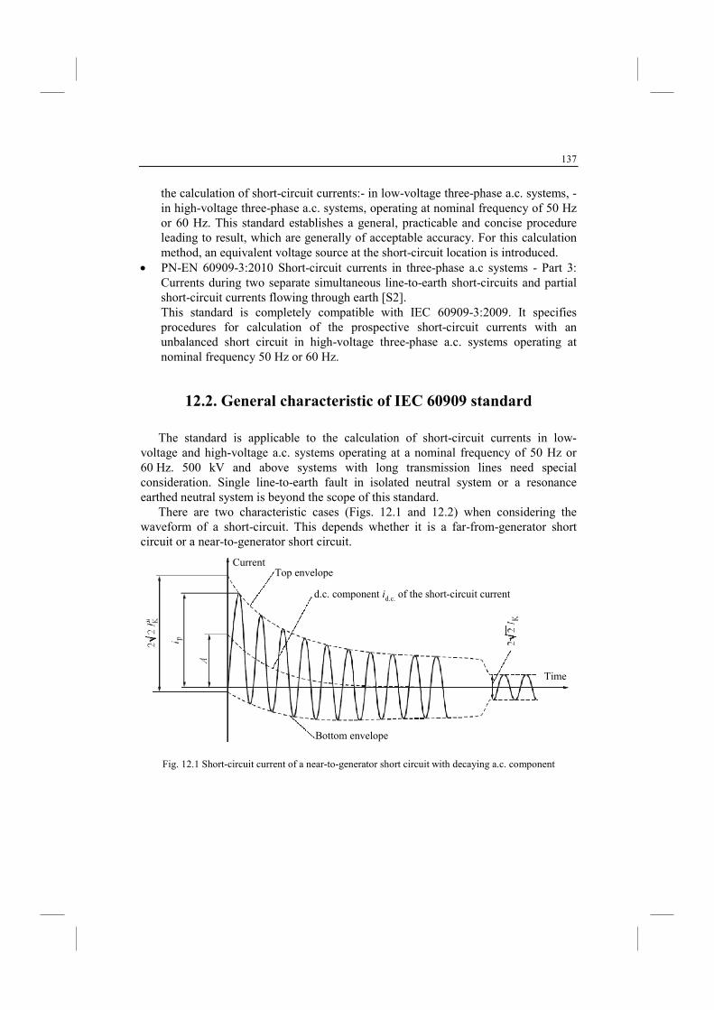
137
the calculation of short-circuit currents:- in low-voltage three-phase a.c. systems, - in high-voltage three-phase a.c. systems, operating at nominal frequency of 50 Hz or 60 Hz. This standard establishes a general, practicable and concise procedure leading to result, which are generally of acceptable accuracy. For this calculation method, an equivalent voltage source at the short-circuit location is introduced.
• PN-EN 60909-3:2010 Short-circuit currents in three-phase a.c systems - Part 3: Currents during two separate simultaneous line-to-earth short-circuits and partial short-circuit currents flowing through earth [S2]. This standard is completely compatible with IEC 60909-3:2009. It specifies procedures for calculation of the prospective short-circuit currents with an unbalanced short circuit in high-voltage three-phase a.c. systems operating at nominal frequency 50 Hz or 60 Hz.
12.2. General characteristic of IEC 60909 standard
The standard is applicable to the calculation of short-circuit currents in low-voltage and high-voltage a.c. systems operating at a nominal frequency of 50 Hz or 60 Hz. 500 kV and above systems with long transmission lines need special consideration. Single line-to-earth fault in isolated neutral system or a resonance earthed neutral system is beyond the scope of this standard.
There are two characteristic cases (Figs. 12.1 and 12.2) when considering the waveform of a short-circuit. This depends whether it is a far-from-generator short circuit or a near-to-generator short circuit.
CurrentTop envelopeTop envelope
d.c. component id.c. of the short-circuit current
Bottom envelopeTopenvelope
Time
Fig. 12.1 Short-circuit current of a near-to-generator short circuit with decaying a.c. component
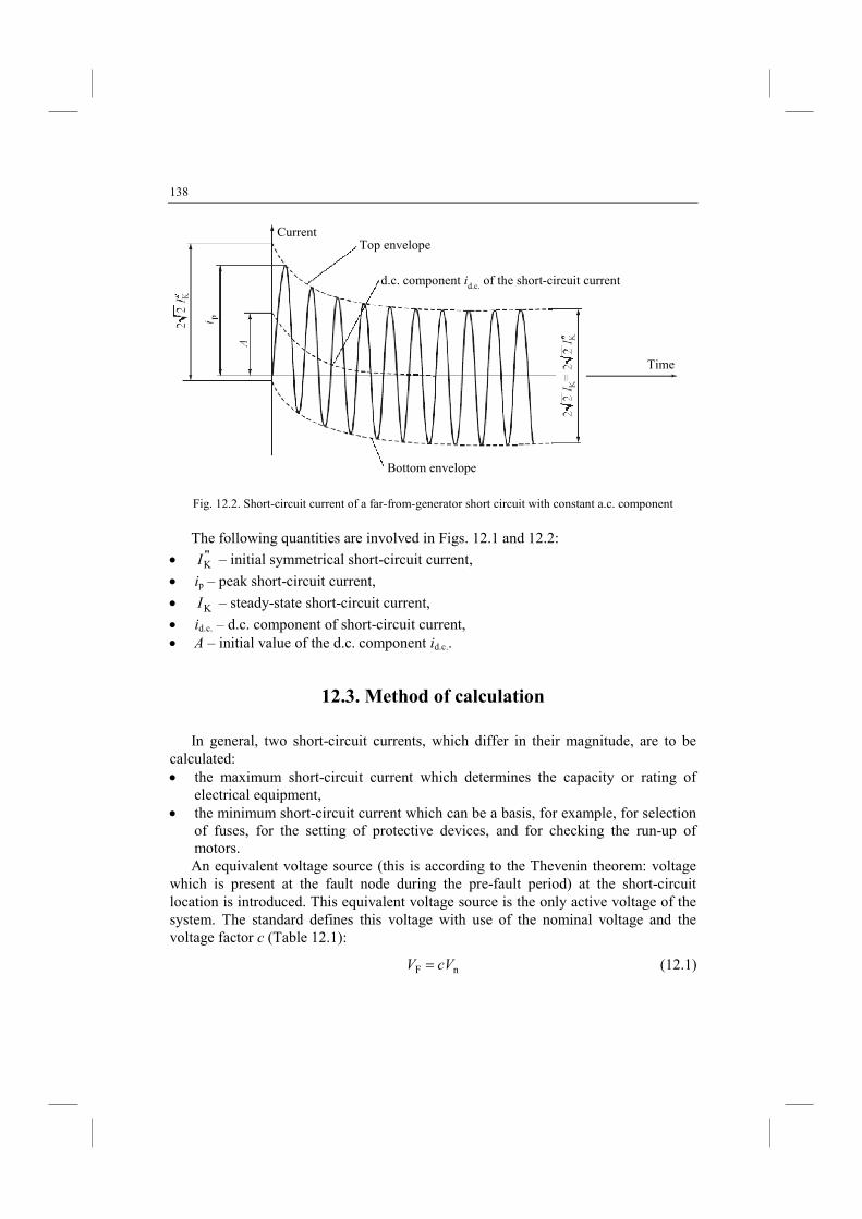
138
CurrentTop envelopeTop envelope
d.c. component id.c. of the short-circuit current
Bottom envelopeTop envelope
Time
Fig. 12.2. Short-circuit current of a far-from-generator short circuit with constant a.c. component
The following quantities are involved in Figs. 12.1 and 12.2:
• ''KI – initial symmetrical short-circuit current,
• ip – peak short-circuit current,
• KI – steady-state short-circuit current,
• id.c. – d.c. component of short-circuit current, • A – initial value of the d.c. component id.c..
12.3. Method of calculation
In general, two short-circuit currents, which differ in their magnitude, are to be calculated: • the maximum short-circuit current which determines the capacity or rating of
electrical equipment, • the minimum short-circuit current which can be a basis, for example, for selection
of fuses, for the setting of protective devices, and for checking the run-up of motors. An equivalent voltage source (this is according to the Thevenin theorem: voltage
which is present at the fault node during the pre-fault period) at the short-circuit location is introduced. This equivalent voltage source is the only active voltage of the system. The standard defines this voltage with use of the nominal voltage and the voltage factor c (Table 12.1):
nF cVV = (12.1)
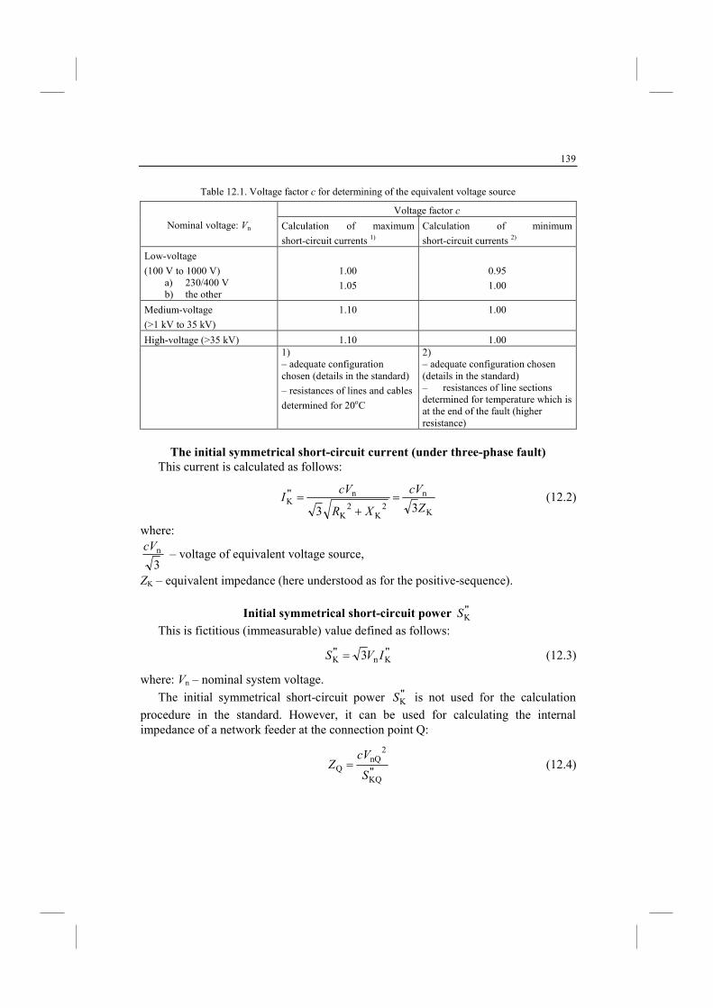
139
Table 12.1. Voltage factor c for determining of the equivalent voltage source
Nominal voltage: Vn
Voltage factor c
Calculation of maximum
short-circuit currents 1)
Calculation of minimum
short-circuit currents 2)
Low-voltage
(100 V to 1000 V) a) 230/400 V b) the other
1.00
1.05
0.95
1.00
Medium-voltage
(>1 kV to 35 kV)
1.10 1.00
High-voltage (>35 kV) 1.10 1.00
1) – adequate configuration chosen (details in the standard)
– resistances of lines and cables
determined for 20oC
2) – adequate configuration chosen (details in the standard) – resistances of line sections determined for temperature which is at the end of the fault (higher resistance)
The initial symmetrical short-circuit current (under three-phase fault)
This current is calculated as follows:
K
n
2K
2K
nK
33 Z
cV
XR
cVI =
+='' (12.2)
where:
3ncV
– voltage of equivalent voltage source,
ZK – equivalent impedance (here understood as for the positive-sequence).
Initial symmetrical short-circuit power ''KS
This is fictitious (immeasurable) value defined as follows:
''''KnK 3 IVS = (12.3)
where: Vn – nominal system voltage.
The initial symmetrical short-circuit power ''KS is not used for the calculation
procedure in the standard. However, it can be used for calculating the internal impedance of a network feeder at the connection point Q:
''KQ
2nQ
QS
cVZ = (12.4)
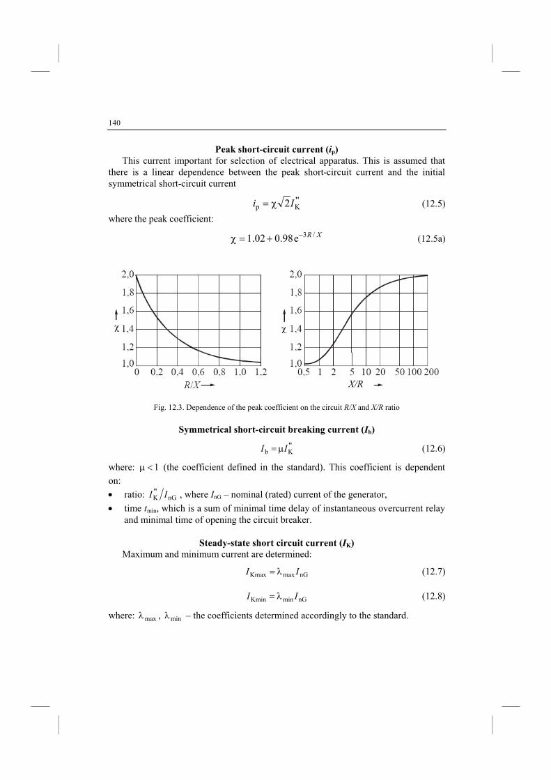
140
Peak short-circuit current (ip) This current important for selection of electrical apparatus. This is assumed that
there is a linear dependence between the peak short-circuit current and the initial symmetrical short-circuit current
''Kp 2Ii χ= (12.5)
where the peak coefficient:
XR /3e98.002.1 −+=χ (12.5a)
Fig. 12.3. Dependence of the peak coefficient on the circuit R/X and X/R ratio
Symmetrical short-circuit breaking current (Ib)
''Kb II µ= (12.6)
where: 1<µ (the coefficient defined in the standard). This coefficient is dependent
on:
• ratio: nGK II '' , where InG – nominal (rated) current of the generator,
• time tmin, which is a sum of minimal time delay of instantaneous overcurrent relay and minimal time of opening the circuit breaker.
Steady-state short circuit current (IK)
Maximum and minimum current are determined:
nGmaxKmax II λ= (12.7)
nGminKmin II λ= (12.8)
where: maxλ , minλ – the coefficients determined accordingly to the standard.
X/R
χ χ
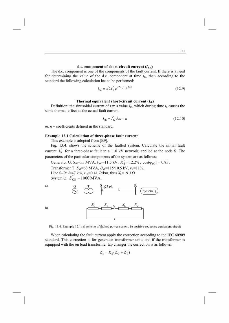
141
d.c. component of short-circuit current (id.c.)
The d.c. component is one of the components of the fault current. If there is a need for determining the value of the d.c. component at time tK, then according to the standard the following calculation has to be performed:
R/XfIi K t 2"Kdc e2 π−= (12.9)
Thermal equivalent short-circuit current (Ith)
Definition: the sinusoidal current of r.m.s value Ith, which during time tk causes the same thermal effect as the actual fault current:
nmII += "Kth (12.10)
m, n – coefficients defined in the standard.
Example 12.1 Calculation of three-phase fault current This example is adopted from [B9]. Fig. 13.4. shows the scheme of the faulted system. Calculate the initial fault
current "KI for a three-phase fault in a 110 kV network, applied at the node S. The
parameters of the particular components of the system are as follows:
Generator G: SnG=55 MVA, VnG=11.5 kV, %2.12"d =X , 85.0)cos( nG =ϕ .
Transformer T: SnT=63 MVA, ϑnT=115/10.5 kV, vK=11%. Line S–R: l=47 km, x1L=0.41 Ω/km, thus XL=19.3 Ω.
System Q
S RG TL
3 ph
SXG XT XL
XQ
Fig. 13.4. Example 12.1: a) scheme of faulted power system, b) positive-sequence equivalent circuit
When calculating the fault current apply the correction according to the IEC 60909 standard. This correction is for generator–transformer units and if the transformer is equipped with the on load transformer tap changer the correction is as follows:
)( T'GSS ZZKZ +=
a)
b)
''System Q: S =KQ 1000 MVA .
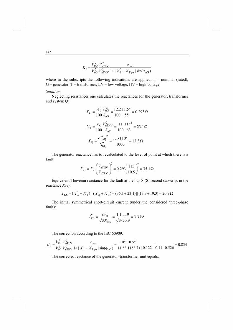
142
)sin(||1 nGpu T"d
max2nTHV
2nTLV
2nG
2nQ
Sϕ−+
=XX
c
V
V
V
VK
where in the subscripts the following indications are applied: n – nominal (rated), G – generator, T – transformer, LV – low voltage, HV – high voltage.
Solution:
Neglecting resistances one calculates the reactances for the generator, transformer and system Q:
Ω=== 293.055
5.11
100
2.12
100
2
nG
2nG
"d
GS
VXX
Ω=== 1.2363
115
100
11
100
2
nT
2nTHVK
TS
VvX
The generator reactance has to recalculated to the level of point at which there is a fault:
Ω=
=
= 1.35
5.10
115293.0
22
nTLV
nTHVG
'G
V
VXX
Equivalent Thevenin reactance for the fault at the bus S (S: second subscript in the reactance XKS):
Ω=++=++= 9.20)3.193.13(||)1.231.35()(||)( LQT'GKS XXXXX
The initial symmetrical short-circuit current (under the considered three-phase fault):
kA 3.39.203
1101.1
3 KS
nKS =
⋅
⋅==
X
cVI ''
The correction according to the IEC 60909:
834.0526.0|11.0122.0|1
1.1
115
5.10
5.11
110
)sin(||1 2
2
2
2
nGpu T"d
max2nTHV
2nTLV
2nG
2nQ
S =⋅−+
=ϕ−+
=XX
c
V
V
V
VK
The corrected reactance of the generator–transformer unit equals:
Ω=⋅
== 3.131000
1101.1 2
KQ
2nQ
Q ''S
cVX
143
Ω=+=+= 5.48)1.231.35(834.0)( T'GS
corr.S XXKX
The corrected equivalent Thevenin reactance for the fault at the bus S:
Ω=+=+= 5.19)3.193.13(||5.48)(|| LQcorr.S
corr.KS XXXX
The corrected initial short-circuit current:
( ) kA 6.35.193
1101.1
3 corr.KS
ncorr.
KS =⋅
⋅==
X
cVI '' .
As a result of the correction we obtained the initial symmetrical short-circuit current higher by around 10% (in comparison to the case with no correction).
144
13. IDETIFICATIO OF FAULTS O OVERHEAD
LIES FOR PROTECTIO
13.1. Introduction
Both, protective relays and fault locators for overhead lines are dependent on the results of the auxiliary algorithms, which are applied for identifying fault features, such as: • fault detection, • fault direction discrimination, • phase selection.
Fault detection is required to activate the measurement process of protective relays. In relation to specification of time intervals of the signals – introduced in Chapter 2, fault detection can be treated as distinguishing the fault interval from the pre-fault interval.
Fault direction is understood as the calculations aimed at answering a question whether a considered fault is forward or backward with respect to the direction at which the protective relay is design to respond. For example, a distance relay protecting a transmission line is designed to operate under forward faults appearing within 85% of the line length (typical first zone setting) or faults overreaching the protected line (the next protective zones). On the other hand, it is expected not to respond for backward faults, i.e. faults occurring back to the relaying point.
Phase selection is aimed at identifying the fault type, i.e. which phases are involved in a considered fault and whether it is an earthed fault or isolated one.
13.2. Fault detection
A number of approaches to fault detection are proposed in the literature. The abnormal conditions (not necessarily faults) are detected by watching the phase impedances and/or phase-current amplitudes and/or phase-voltage amplitudes and/or zero-sequence current amplitude. Depending on a particular application, different
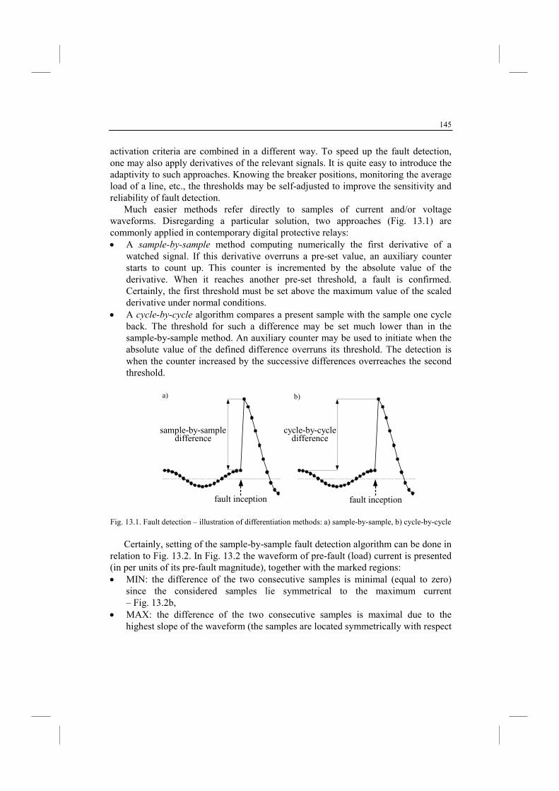
145
activation criteria are combined in a different way. To speed up the fault detection, one may also apply derivatives of the relevant signals. It is quite easy to introduce the adaptivity to such approaches. Knowing the breaker positions, monitoring the average load of a line, etc., the thresholds may be self-adjusted to improve the sensitivity and reliability of fault detection.
Much easier methods refer directly to samples of current and/or voltage waveforms. Disregarding a particular solution, two approaches (Fig. 13.1) are commonly applied in contemporary digital protective relays: • A sample-by-sample method computing numerically the first derivative of a
watched signal. If this derivative overruns a pre-set value, an auxiliary counter starts to count up. This counter is incremented by the absolute value of the derivative. When it reaches another pre-set threshold, a fault is confirmed. Certainly, the first threshold must be set above the maximum value of the scaled derivative under normal conditions.
• A cycle-by-cycle algorithm compares a present sample with the sample one cycle back. The threshold for such a difference may be set much lower than in the sample-by-sample method. An auxiliary counter may be used to initiate when the absolute value of the defined difference overruns its threshold. The detection is when the counter increased by the successive differences overreaches the second threshold.
a) b)
fault inception fault inception
sample-by-sampledifference
cycle-by-cycledifference
Fig. 13.1. Fault detection – illustration of differentiation methods: a) sample-by-sample, b) cycle-by-cycle
Certainly, setting of the sample-by-sample fault detection algorithm can be done in
relation to Fig. 13.2. In Fig. 13.2 the waveform of pre-fault (load) current is presented (in per units of its pre-fault magnitude), together with the marked regions: • MIN: the difference of the two consecutive samples is minimal (equal to zero)
since the considered samples lie symmetrical to the maximum current – Fig. 13.2b,
• MAX: the difference of the two consecutive samples is maximal due to the highest slope of the waveform (the samples are located symmetrically with respect
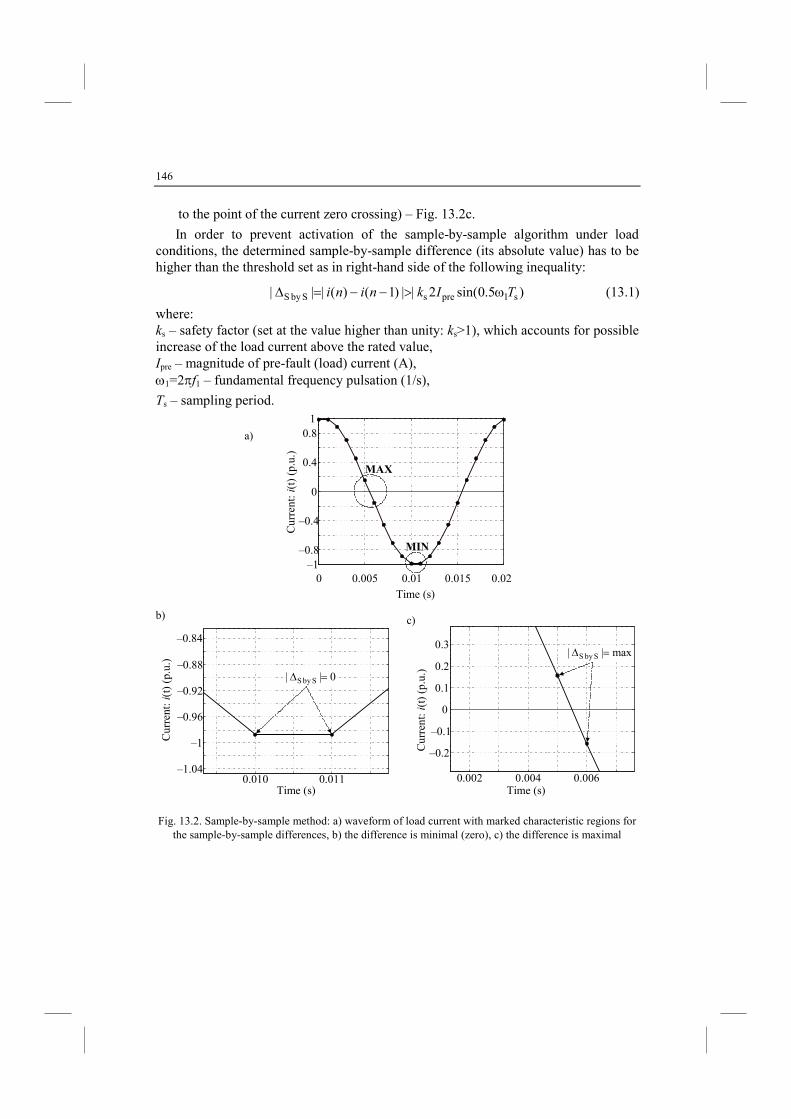
146
to the point of the current zero crossing) – Fig. 13.2c.
In order to prevent activation of the sample-by-sample algorithm under load conditions, the determined sample-by-sample difference (its absolute value) has to be higher than the threshold set as in right-hand side of the following inequality:
)5.0sin(2||)1()(||| s1presSby S TIknini ω>−−=∆ (13.1)
where: ks – safety factor (set at the value higher than unity: ks>1), which accounts for possible increase of the load current above the rated value, Ipre – magnitude of pre-fault (load) current (A), ω1=2πf1 – fundamental frequency pulsation (1/s),
Ts – sampling period.
0 0.005 0.01 0.015 0.02–1
–0.8
–0.4
0
0.4
0.81
MAX
MI
Time (s)
Cur
rent
: i(t) (p.
u.)
0.010 0.011–1.04
–1
–0.96
–0.92
–0.88
–0.84
Time (s)
Cur
rent
: i(t) (p.
u.)
0|| Sby S =∆
–0.1
0
0.1
0.2
0.3
Time (s)
Cur
rent
: i(t) (p.
u.)
max|| Sby S =∆
0.004 0.0060.002
–0.2
Fig. 13.2. Sample-by-sample method: a) waveform of load current with marked characteristic regions for the sample-by-sample differences, b) the difference is minimal (zero), c) the difference is maximal
a)
b) c)
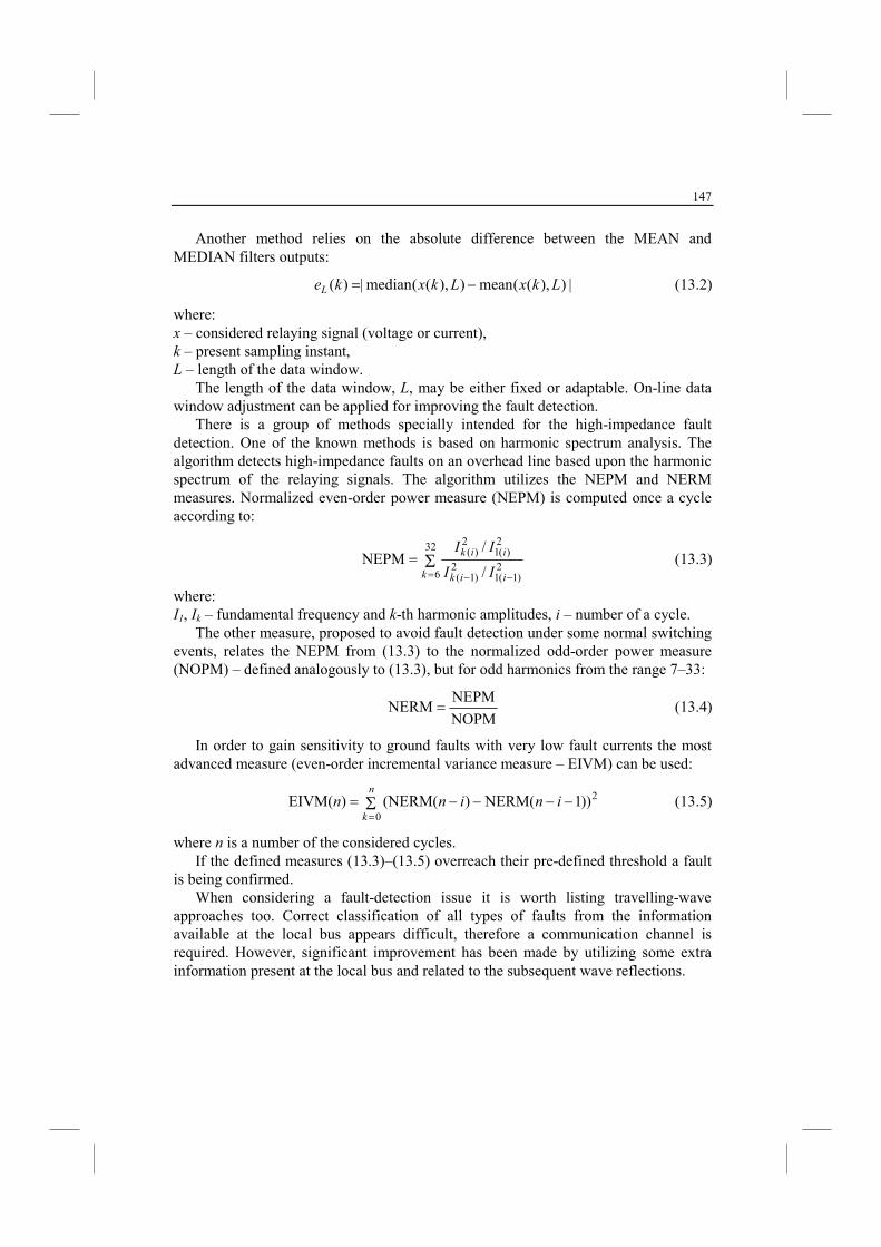
147
Another method relies on the absolute difference between the MEAN and MEDIAN filters outputs:
|)),((mean)),((median|)( LkxLkxkeL −= (13.2)
where: x – considered relaying signal (voltage or current), k – present sampling instant, L – length of the data window.
The length of the data window, L, may be either fixed or adaptable. On-line data window adjustment can be applied for improving the fault detection.
There is a group of methods specially intended for the high-impedance fault detection. One of the known methods is based on harmonic spectrum analysis. The algorithm detects high-impedance faults on an overhead line based upon the harmonic spectrum of the relaying signals. The algorithm utilizes the NEPM and NERM measures. Normalized even-order power measure (NEPM) is computed once a cycle according to:
2
)1(12
)1(
2)(1
2)(32
6 /
/NEPM
−−=Σ=
iik
iik
k II
II (13.3)
where: I1, Ik – fundamental frequency and k-th harmonic amplitudes, i – number of a cycle.
The other measure, proposed to avoid fault detection under some normal switching events, relates the NEPM from (13.3) to the normalized odd-order power measure (NOPM) – defined analogously to (13.3), but for odd harmonics from the range 7–33:
NOPM
NEPMNERM = (13.4)
In order to gain sensitivity to ground faults with very low fault currents the most advanced measure (even-order incremental variance measure – EIVM) can be used:
2
0))1NERM()(NERM()EIVM( −−−−= Σ
=ininn
n
k
(13.5)
where n is a number of the considered cycles. If the defined measures (13.3)–(13.5) overreach their pre-defined threshold a fault
is being confirmed. When considering a fault-detection issue it is worth listing travelling-wave
approaches too. Correct classification of all types of faults from the information available at the local bus appears difficult, therefore a communication channel is required. However, significant improvement has been made by utilizing some extra information present at the local bus and related to the subsequent wave reflections.
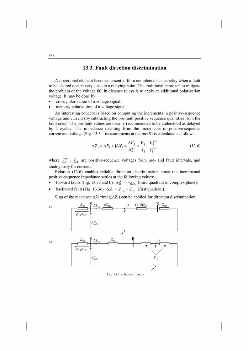
148
13.3. Fault direction discrimination
A directional element becomes essential for a complete distance relay when a fault to be cleared occurs very close to a relaying point. The traditional approach to mitigate the problem of the voltage fall in distance relays is to apply an additional polarization voltage. It may be done by: • cross-polarization of a voltage signal, • memory polarization of a voltage signal.
An interesting concept is based on computing the increments in positive-sequence voltage and current (by subtracting the pre-fault positive sequence quantities from the fault ones). The pre-fault values are usually recommended to be understood as delayed by 5 cycles. The impedance resulting from the increments of positive-sequence current and voltage (Fig. 13.3 – measurements at the bus S) is calculated as follows:
pre11
pre11
1
1111 j
II
VV
I
VXRZ
−
−=
∆
∆=∆+∆=∆ (13.6)
where pre1V , 1V are positive-sequence voltages from pre- and fault intervals, and
analogously for currents. Relation (13.6) enables reliable direction discrimination since the incremental
positive-sequence impedance settles at the following values: • forward faults (Fig. 13.3a and b): 1S1 ZZ −=∆ (third quadrant of complex plane),
• backward fault (Fig. 13.3c): 1R1L1 ZZZ +=∆ (first quadrant).
Sign of the reactance ∆X1=imag(∆Z1) can be applied for direction discrimination.
(1–d)Z1L
S1V∆
RS dZ1LZ1S Z1R
FS11S IZ ∆
S1I∆
S1V∆
RS Z1LZ1S
S11S IZ ∆
S1I∆
F
Z1R
(Fig. 13.3 to be continued)
a)
b)
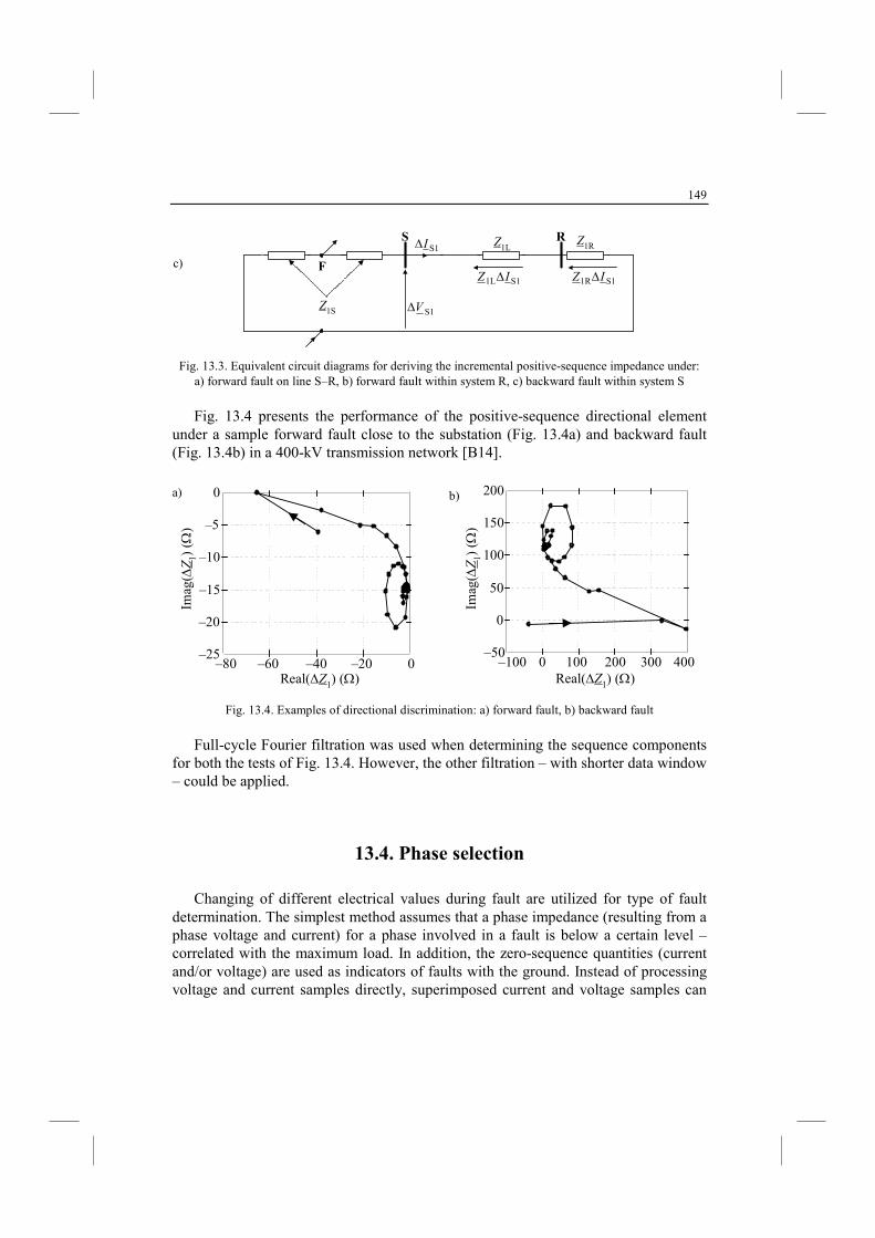
149
Z1L
S1V∆
RS
Z1S
Z1R
FS11L IZ ∆
S1I∆
S11R IZ ∆
Fig. 13.3. Equivalent circuit diagrams for deriving the incremental positive-sequence impedance under: a) forward fault on line S–R, b) forward fault within system R, c) backward fault within system S
Fig. 13.4 presents the performance of the positive-sequence directional element
under a sample forward fault close to the substation (Fig. 13.4a) and backward fault (Fig. 13.4b) in a 400-kV transmission network [B14].
–80 –60 –40 –20 0Real(∆Z1) (Ω)
–25
–20
–15
–10
–5
0
Imag
(∆Z
1) (Ω
)
–100 0 100 200 300 400–50
0
50
100
150
200
Real(∆Z1) (Ω)
Imag
(∆Z
1) (Ω
)
Fig. 13.4. Examples of directional discrimination: a) forward fault, b) backward fault
Full-cycle Fourier filtration was used when determining the sequence components
for both the tests of Fig. 13.4. However, the other filtration – with shorter data window – could be applied.
13.4. Phase selection
Changing of different electrical values during fault are utilized for type of fault determination. The simplest method assumes that a phase impedance (resulting from a phase voltage and current) for a phase involved in a fault is below a certain level – correlated with the maximum load. In addition, the zero-sequence quantities (current and/or voltage) are used as indicators of faults with the ground. Instead of processing voltage and current samples directly, superimposed current and voltage samples can
c)
a) b)
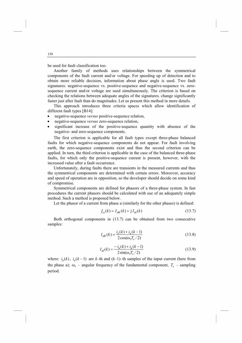
150
be used for fault classification too. Another family of methods uses relationships between the symmetrical
components of the fault current and/or voltage. For speeding up of detection and to obtain more reliable decision, information about phase angle is used. Two fault signatures: negative-sequence vs. positive-sequence and negative-sequence vs. zero-sequence current and/or voltage are used simultaneously. The criterion is based on checking the relations between adequate angles of the signatures. change significantly faster just after fault than do magnitudes. Let us present this method in more details.
This approach introduces three criteria spaces which allow identification of different fault types [B14]: • negative-sequence versus positive-sequence relation, • negative-sequence versus zero-sequence relation, • significant increase of the positive-sequence quantity with absence of the
negative- and zero-sequence components.
The first criterion is applicable for all fault types except three-phase balanced faults for which negative-sequence components do not appear. For fault involving earth, the zero-sequence components exist and thus the second criterion can be applied. In turn, the third criterion is applicable in the case of the balanced three-phase faults, for which only the positive-sequence current is present, however, with the increased value after a fault occurrence.
Unfortunately, during faults there are transients in the measured currents and thus the symmetrical components are determined with certain errors. Moreover, accuracy and speed of operation are in opposition, so the developer should decide on some kind of compromise.
Symmetrical components are defined for phasors of a three-phase system. In fast procedures the current phasors should be calculated with use of an adequately simple method. Such a method is proposed below.
Let the phasor of a current from phase a (similarly for the other phases) is defined:
)( j)()( aIaRa kIkIkI += (13.7)
Both orthogonal components in (13.7) can be obtained from two consecutive samples:
)2/cos(2
)1()()(
s1
aaaR
T
kikikI
ω−+
= (13.8)
)2/sin(2
)1()()(
s1
aaaI
T
kikikI
ω−+−
= (13.9)
where: )(a ki , )1(a −ki are k–th and (k–1)–th samples of the input current (here from
the phase a); 1ω – angular frequency of the fundamental component, sT – sampling
period.
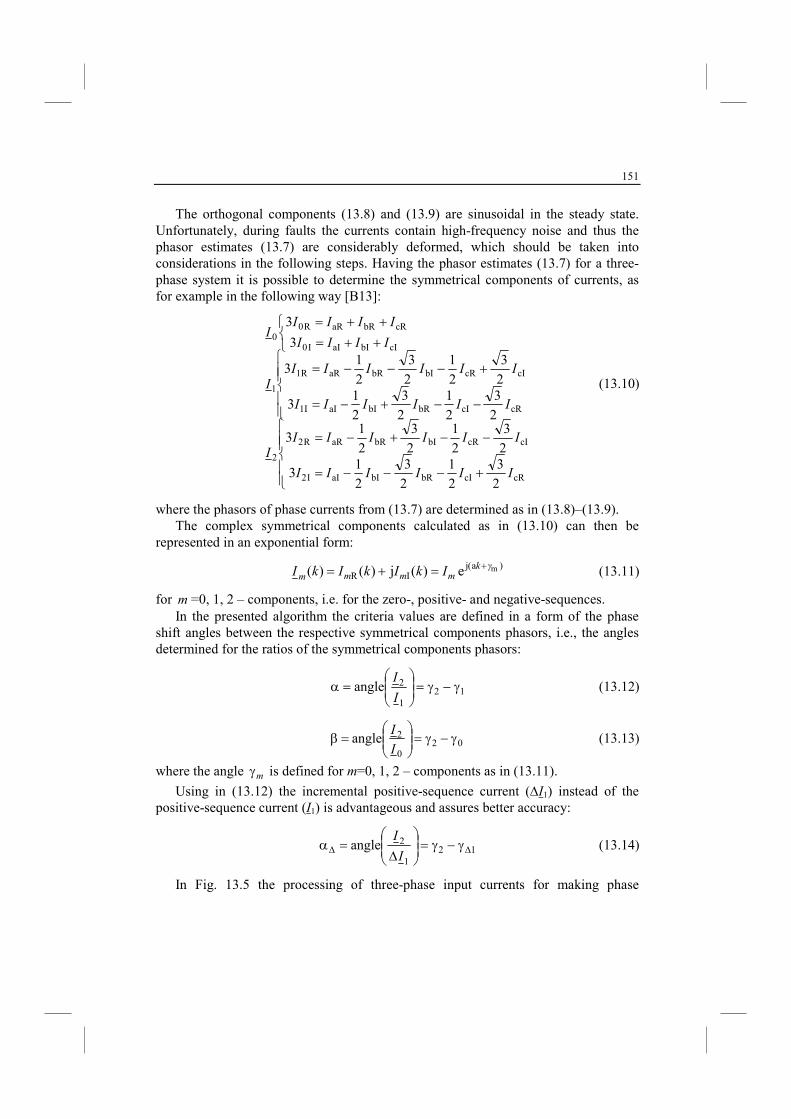
151
The orthogonal components (13.8) and (13.9) are sinusoidal in the steady state. Unfortunately, during faults the currents contain high-frequency noise and thus the phasor estimates (13.7) are considerably deformed, which should be taken into considerations in the following steps. Having the phasor estimates (13.7) for a three-phase system it is possible to determine the symmetrical components of currents, as for example in the following way [B13]:
+−−−=
−−+−=
−−+−=
+−−−=
++=
++=
cRcIbRbIaII2
cIcRbIbRaRR2
2
cRcIbRbIaII1
cIcRbIbRaRR1
1
cIbIaII0
cRbRaRR00
2
3
2
1
2
3
2
1 3
2
3
2
1
2
3
2
1 3
2
3
2
1
2
3
2
1 3
2
3
2
1
2
3
2
1 3
3
3
IIIIII
IIIIIII
IIIIII
IIIIIII
IIII
IIIII
(13.10)
where the phasors of phase currents from (13.7) are determined as in (13.8)–(13.9). The complex symmetrical components calculated as in (13.10) can then be
represented in an exponential form:
)a(jIR
me)(j)()( γkmmmm IkIkIkI
+=+= (13.11)
for m =0, 1, 2 – components, i.e. for the zero-, positive- and negative-sequences. In the presented algorithm the criteria values are defined in a form of the phase
shift angles between the respective symmetrical components phasors, i.e., the angles determined for the ratios of the symmetrical components phasors:
121
2angle γ−γ=
=α
I
I (13.12)
020
2angle γ−γ=
=β
I
I (13.13)
where the angle mγ is defined for m=0, 1, 2 – components as in (13.11).
Using in (13.12) the incremental positive-sequence current (∆I1) instead of the positive-sequence current (I1) is advantageous and assures better accuracy:
121
2angle ∆∆ γ−γ=
∆=α
I
I (13.14)
In Fig. 13.5 the processing of three-phase input currents for making phase
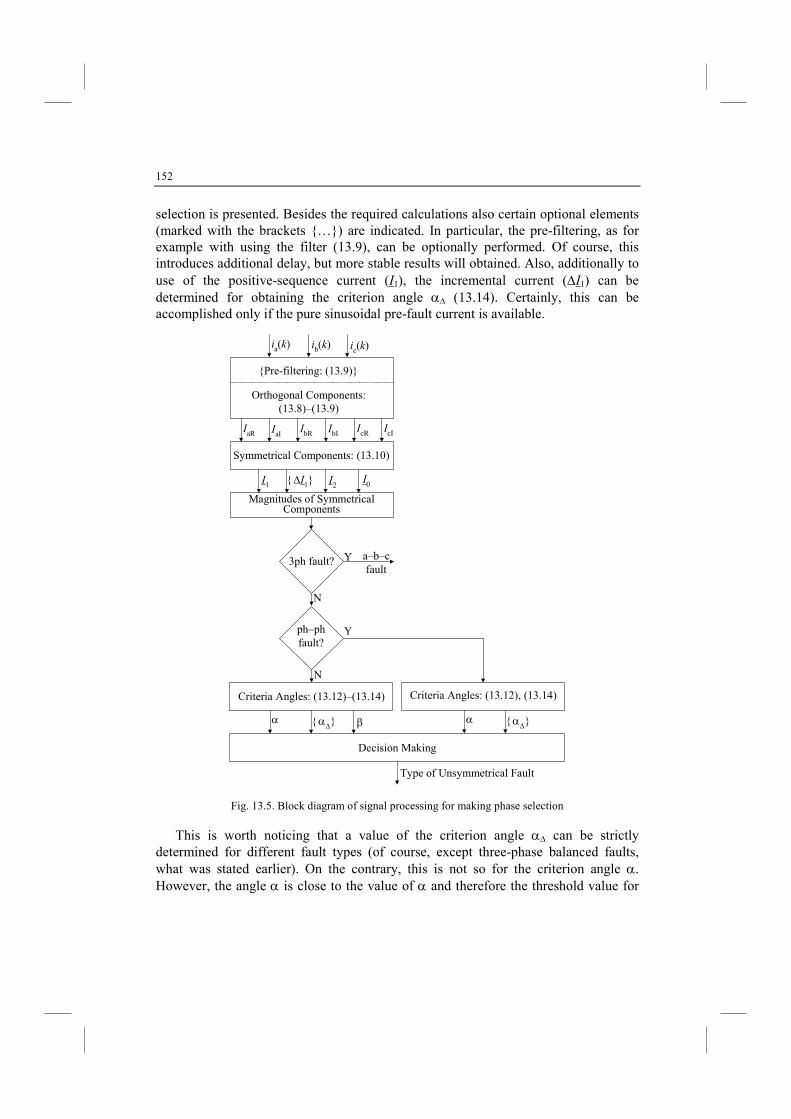
152
selection is presented. Besides the required calculations also certain optional elements (marked with the brackets …) are indicated. In particular, the pre-filtering, as for example with using the filter (13.9), can be optionally performed. Of course, this introduces additional delay, but more stable results will obtained. Also, additionally to use of the positive-sequence current (I1), the incremental current (∆I1) can be determined for obtaining the criterion angle α∆ (13.14). Certainly, this can be accomplished only if the pure sinusoidal pre-fault current is available.
Pre-filtering: (13.9)
Orthogonal Components:(13.8)–(13.9)
ia(k) ib(k) ic(k)
IaR IaI IbIIcR IcIIbR
Symmetrical Components: (13.10)
I1 ∆I1 I2 I0
Criteria Angles: (13.12)–(13.14)
Decision Making
Type of Unsymmetrical Fault
α α∆ β
Magnitudes of SymmetricalComponents
3ph fault? Y a–b–cfault
N
ph–phfault?
N
Y
α α∆
Criteria Angles: (13.12), (13.14)
Fig. 13.5. Block diagram of signal processing for making phase selection
This is worth noticing that a value of the criterion angle α∆ can be strictly determined for different fault types (of course, except three-phase balanced faults, what was stated earlier). On the contrary, this is not so for the criterion angle α. However, the angle α is close to the value of α and therefore the threshold value for
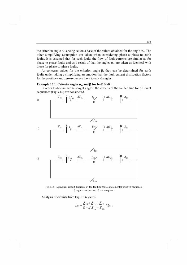
153
the criterion angle α is being set on a base of the values obtained for the angle α∆. The other simplifying assumption are taken when considering phase-to-phase-to earth faults. It is assumed that for such faults the flow of fault currents are similar as for phase-to-phase faults and as a result of that the angles α∆ are taken as identical with those for phase-to-phase faults.
As concerns values for the criterion angle β, they can be determined for earth faults under taking a simplifying assumption that the fault current distribution factors for the positive- and zero-sequence have identical angles.
Example 13.1. Criteria angles αααα∆∆∆∆ and ββββ for b–E fault In order to determine the sought angles, the circuits of the faulted line for different
sequences (Fig.3.16) are considered.
(1–d)Z1LRS dZ1LZ1S Z1R
F
S1I∆ F1I
F1I
(1–d)Z1LRS dZ1LZ1S Z1R
F
S2I F2I
F2I
(1–d)Z0LRS dZ0LZ0S Z0R
F
S0I F0I
F0I
Fig.13.6. Equivalent circuit diagrams of faulted line for: a) incremental positive-sequence, b) negative-sequence, c) zero-sequence
Analysis of circuits from Fig. 13.6 yields:
S11R1L
1R1L1SF1 )1(
IZZd
ZZZI ∆
+−
++= ,
a)
b)
c)
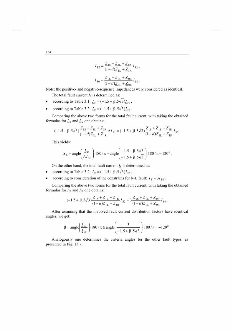
154
S21R1L
1R1L1SF2 )1(
IZZd
ZZZI
+−
++= ,
S00R0L
0R0L0SF0 )1(
IZZd
ZZZI
+−
++= .
Note: the positive- and negative-sequence impedances were considered as identical.
The total fault current IF is determined as:
• according to Table 3.1: F1F )35.1j5.1( II −−= ,
• according to Table 3.2: F2F )35.1j5.1( II +−= .
Comparing the above two forms for the total fault current, with taking the obtained formulas for IF1 and IF2 one obtains:
S21R1L
1R1L1SS1
1R1L
1R1L1S
)1()35.1j5.1(
)1()35.1j5.1( I
ZZd
ZZZI
ZZd
ZZZ
+−
+++−=∆
+−
++−− .
This yields:
o
1S
2S 120 /18035.1j5.1
35.1j5.1angle /180angle =π⋅
+−
−−=π⋅
∆=α∆
I
I.
On the other hand, the total fault current IF is determined as:
• according to Table 3.2: F2F )35.1j5.1( II +−= ,
• according to consideration of the constrains for b–E fault: F0F 3II = .
Comparing the above two forms for the total fault current, with taking the obtained formulas for IF2 and IF0 one obtains:
S00R0L
0R0L0SS2
1R1L
1R1L1S
)1(3
)1()35.1j5.1( I
ZZd
ZZZI
ZZd
ZZZ
+−
++=
+−
+++− .
After assuming that the involved fault current distribution factors have identical angles, we get:
o
S0
2S 120 /18035.1j5.1
3angle /180angle −=π⋅
+−≅π⋅
=β
I
I.
Analogously one determines the criteria angles for the other fault types, as presented in Fig. 13.7.
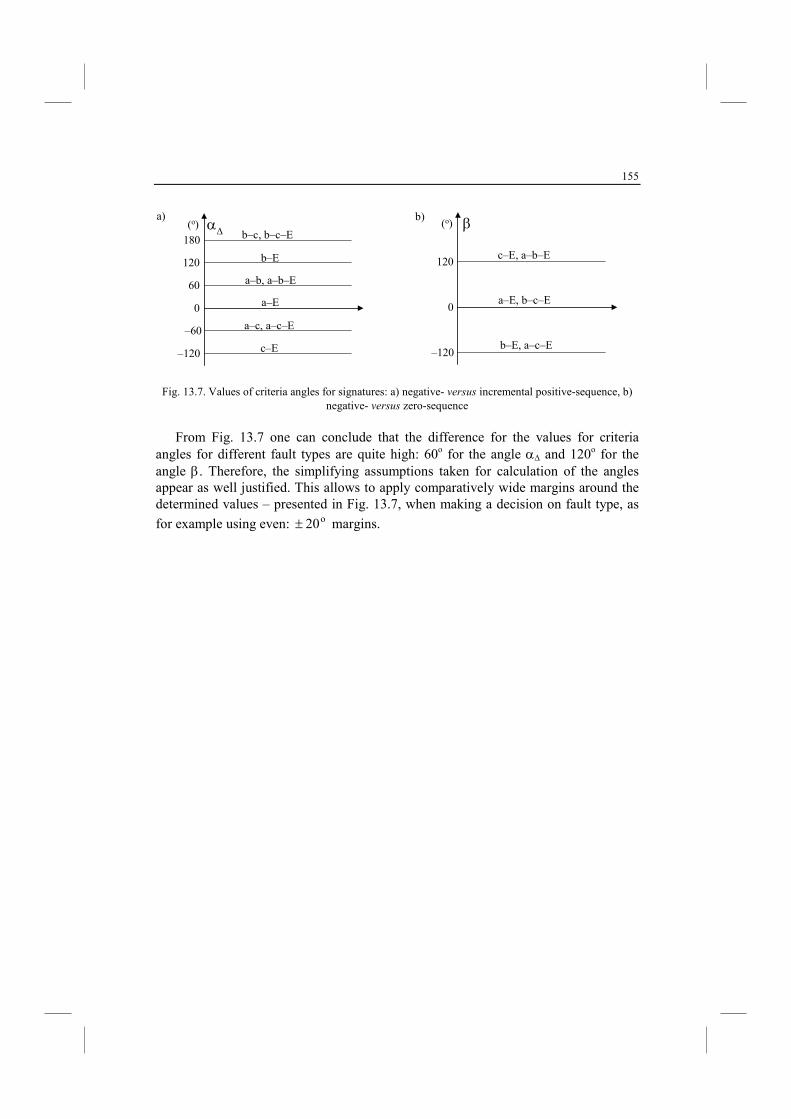
155
0
60
120
180
–60
–120
a–E
a–b, a–b–E
b–E
b–c, b–c–E
a–c, a–c–E
c–E
(o) α∆
0
120
–120
a–E, b–c–E
c–E, a–b–E
b–E, a–c–E
(o) β
Fig. 13.7. Values of criteria angles for signatures: a) negative- versus incremental positive-sequence, b) negative- versus zero-sequence
From Fig. 13.7 one can conclude that the difference for the values for criteria
angles for different fault types are quite high: 60o for the angle α∆ and 120o for the angle β. Therefore, the simplifying assumptions taken for calculation of the angles appear as well justified. This allows to apply comparatively wide margins around the determined values – presented in Fig. 13.7, when making a decision on fault type, as
for example using even: o20± margins.
a) b)
156
14. FAULT LOCATIO O OVERHEAD LIES
14.1. Aim of fault location and its importance
Fault location [B6] is a process aimed at locating faults with the possibly highest accuracy. Fault locators are the supplementary protection equipment, which apply the fault location algorithms for estimating the distance to fault. In case of locating faults on the line consisting of more than one section (multi-terminal line), initially the faulted section has to be identified and then a fault on this section has to be located.
Fault location function can be implemented in: • microprocessor-based relays • digital fault recorders (DFRs) • stand-alone fault locators • post-fault analysis programs.
Importance of fault locators is more obvious where foot patrols are relied upon, particularly on long lines, in rough terrain. Also, can help where maintenance jurisdiction is divided between different companies or divisions within a company.
14.2. Fault locators versus protective relays
Fault locators and protective relays are closely related, however, there are some important differences between them [B8, B14]. These differences can be considered as related to the following features: 1. accuracy of fault location 2. speed of determining the fault position 3. speed of transmitting data from remote site 4. used data window 5. digital filtering of input signals and complexity of calculations.
157
1. Fault locators are used for pinpointing the fault position accurately and not only for indication of the general area (defined by a protective zone) where a fault occurred - which is provided by protective relays.
2. In case of protective relays, both the measurement and decision making are performed in on-line. Requirement for fast clearing of faults demands that the decision for tripping transmission lines has to be made in short time, even faster than in one cycle of the fundamental frequency (20 ms for the systems operating at 50 Hz). In contrast, the calculations of fault locators are performed off-line since the results of these calculations (position of the fault and in case of some algorithms also the involved fault resistance) are for human users. This implies that the fault location speed of calculations can be measured in seconds or even minutes.
3. Low-speed data communications or Supervisory Control And Data Acquisition (SCADA) can be applied for fault location purpose, which differs from communication used by protective relays.
4. Best data window segment from the whole available window can be selected for fault location to reduce errors. This is so since the computations are performed in an off-line regime and searching for the best data window can be easily applied. The fault interval lasts from a fault incipience up to a fault clearing by a circuit breaker, and usually this takes around three fundamental frequency cycles, which is wider than required for fault location.
5. In case of the protective relays the required high speed imposes that the applied calculations have not to be too complex and much time-consuming. In contrast, fault location calculations do not have such limitations.
Depending on the currents at both line ends (IS, IR), the fault resistance RF can be seen as: • pure resistance (Fig. 14.2a), • resistance and capacitive reactance (Fig. 14.2b), • resistance and inductive reactance (Fig. 14.2c).
In last two cases (Fig. 14.2b and Fig. 1.2c) there is a contribution of the reactance (capacitive or inductive) in the ‘seen’ resistance, and therefore this effect is called as the “reactance effect”. This effect considerably influences the measurement of the fault loop impedance ZFL.
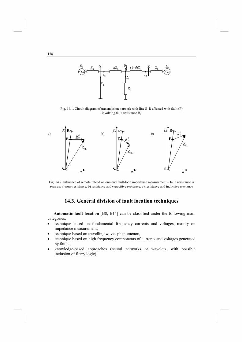
158
RFS dZLZS
ES ERZR(1–d)ZL
IS IRIF
RF
VS
Fig. 14.1. Circuit diagram of transmission network with line S–R affected with fault (F) involving fault resistance RF
S
R
ZFL
F
R
jX#FR
S
R
ZFL
F
R
jX
#FR
S
R
ZFL
F
R
jX#FR
Fig. 14.2. Influence of remote infeed on one-end fault-loop impedance measurement – fault resistance is seen as: a) pure resistance, b) resistance and capacitive reactance, c) resistance and inductive reactance
14.3. General division of fault location techniques
Automatic fault location [B8, B14] can be classified under the following main categories: • technique based on fundamental frequency currents and voltages, mainly on
impedance measurement, • technique based on travelling waves phenomenon, • technique based on high frequency components of currents and voltages generated
by faults, • knowledge-based approaches (neural networks or wavelets, with possible
inclusion of fuzzy logic).
a) b) c)
159
Except the automatic fault location, also some unconventional techniques are applied for making fault location, such as: • customer calls, • line inspection, • lightning detection system, • terminal and tracer methods for cables, • fault indicators – installed either in substations or on towers along the line, • monitoring transients of induced radiation from power-system arcing faults
– using both VLF and VHF reception.
Benefits of fault location are as follows: • fast repair to restore power system,
– improves system availability and performance and reduces operating costs, • saves time and expense of crew searching in bad weather and tough terrain, • aids crew in disturbance diagnostics,
– identifies temporary faults, – detects weak spots.
Making use of the fundamental frequency voltages and currents at the line terminal (or terminals), together with the line parameters, appears as the simplest automatic fault location. It is mainly considered that the calculated impedance of the faulted line segment is a measure of the distance to fault. The methods belonging to this category are simple and economical for implementing.
As concerning the position of time intervals with respect to this fault incipience and its clearance (achieved as a result of the protective relay operation and switching off the line by the circuit breaker) one can distinguish the following time intervals: • pre-fault interval: lasting from the beginning of the registration up to the detected
fault incipience instant (tflt_incipience), • fault interval: lasting from the fault incipience instant (tflt_incipience) up to the
detected fault clearance instant (tflt_clearance), • post-fault interval: lasting from the fault clearance instant (tflt_clearance) up to the end
of the registered event. Mostly, the fault quantities (voltage and current) are utilized for fault location.
However, there are also many fault location approaches, in which the pre-fault quantities are additionally included as the fault locator input signals. However, sometimes, usage of the pre-fault measurements is treated as the drawback of the fault location method. This is so, since in some cases the pre-fault quantities could be not registered or they do not exist, as for example in case of the current during some intervals of the automatic reclosure process. Also, the pre-fault quantities can be not of pure sinusoidal shape, due to appearance of the fault symptoms just before its occurrence. Also, in some hardware solutions, measurement of pre-fault (load) currents is accomplished with lower accuracy than for much higher fault currents. Therefore, if it is possible, usually the usage of pre-fault measurements is avoided.
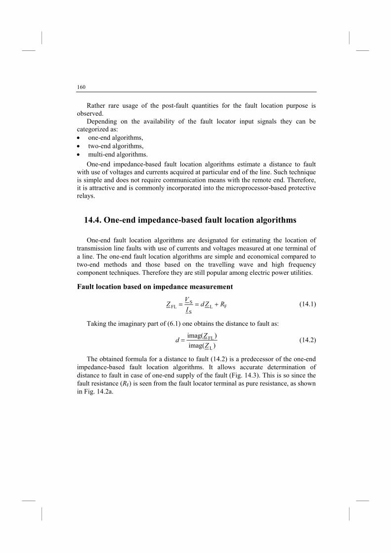
160
Rather rare usage of the post-fault quantities for the fault location purpose is observed.
Depending on the availability of the fault locator input signals they can be categorized as: • one-end algorithms, • two-end algorithms, • multi-end algorithms.
One-end impedance-based fault location algorithms estimate a distance to fault with use of voltages and currents acquired at particular end of the line. Such technique is simple and does not require communication means with the remote end. Therefore, it is attractive and is commonly incorporated into the microprocessor-based protective relays.
14.4. One-end impedance-based fault location algorithms
One-end fault location algorithms are designated for estimating the location of transmission line faults with use of currents and voltages measured at one terminal of a line. The one-end fault location algorithms are simple and economical compared to two-end methods and those based on the travelling wave and high frequency component techniques. Therefore they are still popular among electric power utilities.
Fault location based on impedance measurement
FLS
SFL RZd
I
VZ +== (14.1)
Taking the imaginary part of (6.1) one obtains the distance to fault as:
)imag(
)imag(
L
FL
Z
Zd = (14.2)
The obtained formula for a distance to fault (14.2) is a predecessor of the one-end impedance-based fault location algorithms. It allows accurate determination of distance to fault in case of one-end supply of the fault (Fig. 14.3). This is so since the fault resistance (RF) is seen from the fault locator terminal as pure resistance, as shown in Fig. 14.2a.
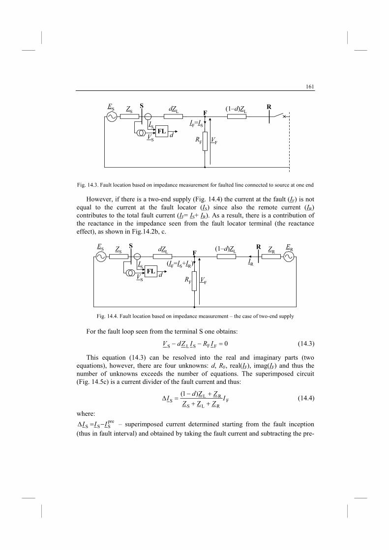
161
RS dZL (1–d)ZL
IS
VS VF
ZSES
F
IF=IS
RF
FLd
Fig. 14.3. Fault location based on impedance measurement for faulted line connected to source at one end
However, if there is a two-end supply (Fig. 14.4) the current at the fault (IF) is not equal to the current at the fault locator (IS) since also the remote current (IR) contributes to the total fault current (IF= IS+ IR). As a result, there is a contribution of the reactance in the impedance seen from the fault locator terminal (the reactance effect), as shown in Fig.14.2b, c.
RSdZL
(1–d)ZL
IS
VS VF
ZSES
F
(IF=IS+IR)
RF
FLd
ERZR
IR
Fig. 14.4. Fault location based on impedance measurement – the case of two-end supply
For the fault loop seen from the terminal S one obtains:
0FFSLS =−− IRIZdV (14.3)
This equation (14.3) can be resolved into the real and imaginary parts (two equations), however, there are four unknowns: d, RF, real(IF), imag(IF) and thus the number of unknowns exceeds the number of equations. The superimposed circuit (Fig. 14.5c) is a current divider of the fault current and thus:
FRLS
RLS Z
Z)1(I
ZZ
ZdI
++
+−=∆ (14.4)
where: preSSS III −=∆ – superimposed current determined starting from the fault inception
(thus in fault interval) and obtained by taking the fault current and subtracting the pre-
162
fault current (present before fault inception). Note: the recordings of the pre-fault current must be available.
This allows determining the total fault current as:
F
SF
k
II
∆= (14.5)
where the fault current distribution factor (kF) is determined as:
RLS
RLLjγFF Z
ZZe||
ZZ
Zdkk
++++−
== (14.6)
Substituting (14.5)–(14.6) into (14.3) results in:
0e||
SjγF
FSLS =∆−− I
k
RIZdV (14.7)
Multiplying (14.7) by the element ( *S
jγe I∆ ) and taking the imaginary part yields
the following formula for the unknown distance to fault:
)eimag(
)eimag(jγ*
SSL
jγ*SS
⋅∆⋅⋅
⋅∆⋅=
IIZ
IVd (14.8)
where x* denotes conjugate of x. Takagi [19] assumed that the current distribution factor is a real number (γ=0),
what facilitates calculations. This simplification comes from that all the impedances involved in (14.6) have approximately the same phases.
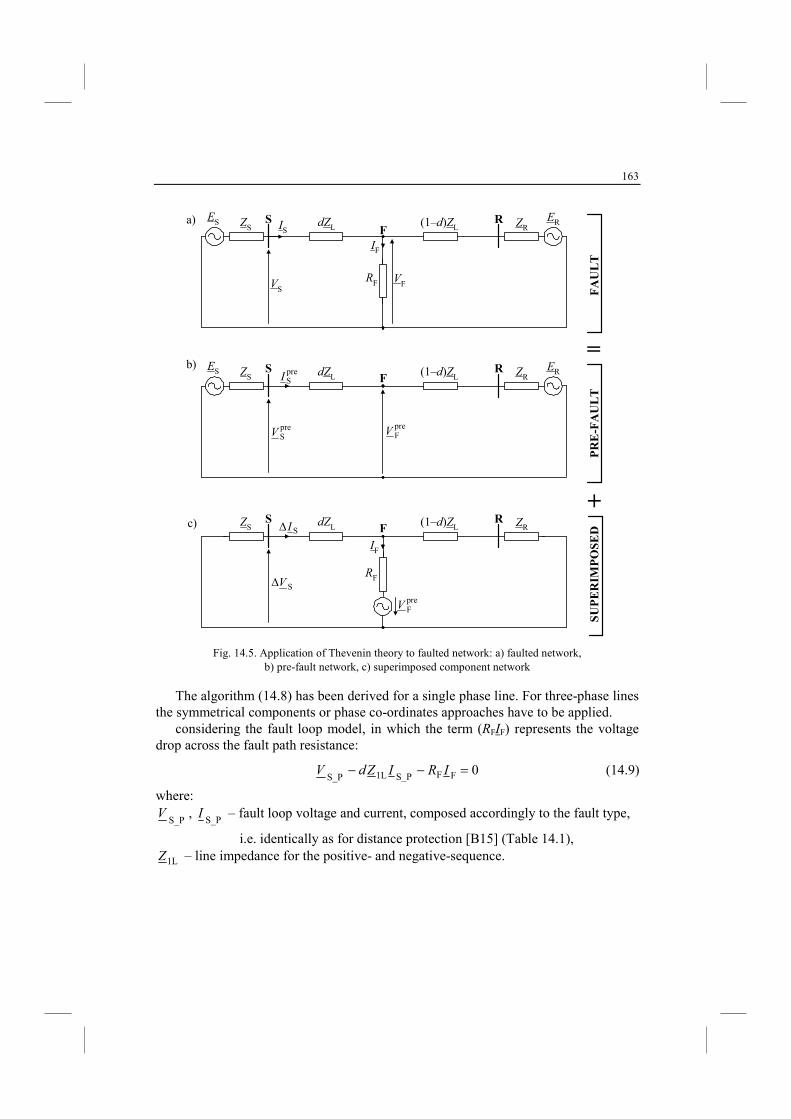
163
RS dZL (1–d)ZLIS
VSVF
ZSES ERZRF
IF
RF
preSV
RS dZL (1–d)ZLZSES ERZRF
preSI
preFV
SV∆
RS dZL (1–d)ZLZS ZRF
IF
RF
preFV
SI∆
=
+
FAULT
PRE-FAULT
SUPERIMPOSED
a)
b)
c)
Fig. 14.5. Application of Thevenin theory to faulted network: a) faulted network,
b) pre-fault network, c) superimposed component network
The algorithm (14.8) has been derived for a single phase line. For three-phase lines the symmetrical components or phase co-ordinates approaches have to be applied.
considering the fault loop model, in which the term (RFIF) represents the voltage drop across the fault path resistance:
0FFS_P1LS_P=−− IRIZdV (14.9)
where:
S_PV ,
S_PI – fault loop voltage and current, composed accordingly to the fault type,
i.e. identically as for distance protection [B15] (Table 14.1),
1LZ – line impedance for the positive- and negative-sequence.
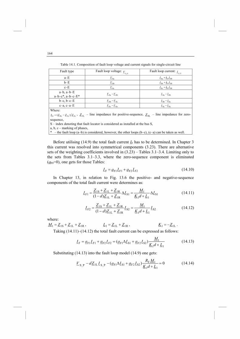
164
Table 14.1. Composition of fault loop voltage and current signals for single-circuit line
Fault type Fault loop voltage: S_P
V Fault loop current: S_P
I
a–E SaV S00Sa IkI +
b–E SbV S00Sb IkI +
c–E ScV S00Sc IkI +
a–b, a–b–E a–b–c*, a–b–c–E* SbSa VV −
SbSa II −
b–c, b–c–E ScSb VV − ScSb II −
c–a, c–a–E SaSc VV − SaSc II −
Where:
1L1L0L0 )( ZZZk −= , 1LZ – line impedance for positive-sequence,
0LZ – line impedance for zero-
sequence, S – index denoting that fault locator is considered as installed at the bus S, a, b, c – marking of phases, * – the fault loop (a–b) is considered, however, the other loops (b–c), (c–a) can be taken as well.
Before utilising (14.9) the total fault current IF has to be determined. In Chapter 3
this current was resolved into symmetrical components (3.23). There are alternative sets of the weighting coefficients involved in (3.23) – Tables 3.1–3.4. Limiting only to the sets from Tables 3.1–3.3, where the zero-sequence component is eliminated (aF0=0), one gets for those Tables:
F2F2F11FF IaIaI += (14.10)
In Chapter 13, in relation to Fig. 13.6 the positive- and negative-sequence components of the total fault current were determines as:
S111
1S1
1R1L
1R1L1SF1 )1(
ILdK
MI
ZZd
ZZZI ∆
+=∆
+−++
= (14.11)
S211
1S2
1R1L
1R1L1SF2 )1(
ILdK
MI
ZZd
ZZZI
+=
+−
++= (14.12)
where:
1R1L1S1 ZZZM ++= , 1R1L1 ZZL += , 1L1 ZK −= .
Taking (14.11)–(14.12) the total fault current can be expressed as follows:
11
1S22FS11FF2F2F11FF )(
LdK
MIaIaIaIaI
++∆=+= (14.13)
Substituting (14.13) into the fault loop model (14.9) one gets:
0)(11
1FS22FS11FS_P1LS_P
=+
+∆−−LdK
MRIaIaIZdV (14.14)
165
where:
S_PV ,
S_PI – fault loop voltage and current, as in Table 14.1,
1LZ – line impedance for the positive- and negative-sequence,
aF1, aF2 – weighting coefficients from one of Tables 3.1–3.3, ∆IS1, IS2 – superimposed positive-sequence and negative-sequence current from bus S, K1, L1, M1 – as defined in (14.12) for a single-circuit line.
Different ways of solving (14.14) in which the unknowns: d [p.u.] – distance to fault and RF – fault resistance are involved, have been proposed in literature.
Wiszniewski A. [20] proposed to use the simplifying assumption that the quantity ( )( 111 LdKM + ) is a real number. In this way there is no requirement for knowing
impedances of equivalent sources at both line ends. This is a great advantage for the cases when the impedances of the sources are considered as uncertain parameters.
Eriksson L., Saha M.M. and Rockefeller G.D. [3] resolved (14.14) into the real and imaginary parts for strict solution of it. Many years’ experience with the fault locator implemented into the product has proved successfully the validity of their approach.
14.5. Two-end fault location
Two-end algorithms process signals from both terminals of the line and thus larger amount of information is utilized. Therefore, performance of the two-end algorithms is generally superior in comparison to the one-end approaches. Different input signals are used for two-end fault locators, as for example: complete currents and voltages from the line terminals or quantities from impedance relays at the line terminals. Digital measurements at different line terminals can be performed synchronously if the GPS (Global Positioning System) is available. A synchronised measurement system requires that the measurements taken at different substations include, in addition to magnitude, the phase angle data with respect to an arbitrary but common reference. Phase information is obtained from knowledge of the absolute time at which the measurements were obtained (time tagging). The ability of GPS to provide a time reference signal, synchronised at widely separated locations has been widely recognised as having great potential of power system applications [B7, 9, 10].
24 satellites of the GPS, which are owned and operated by the US Department of Defence, maintain the so called Coordinated Universal Time with the accuracy of ∆t=± 0.5µs. For the fundamental frequency equal to 50 Hz this corresponds to the
angle: o6 0.009180/pi)100.5(502 ±=⋅⋅±⋅⋅π − . Thus very high accuracy is assured.
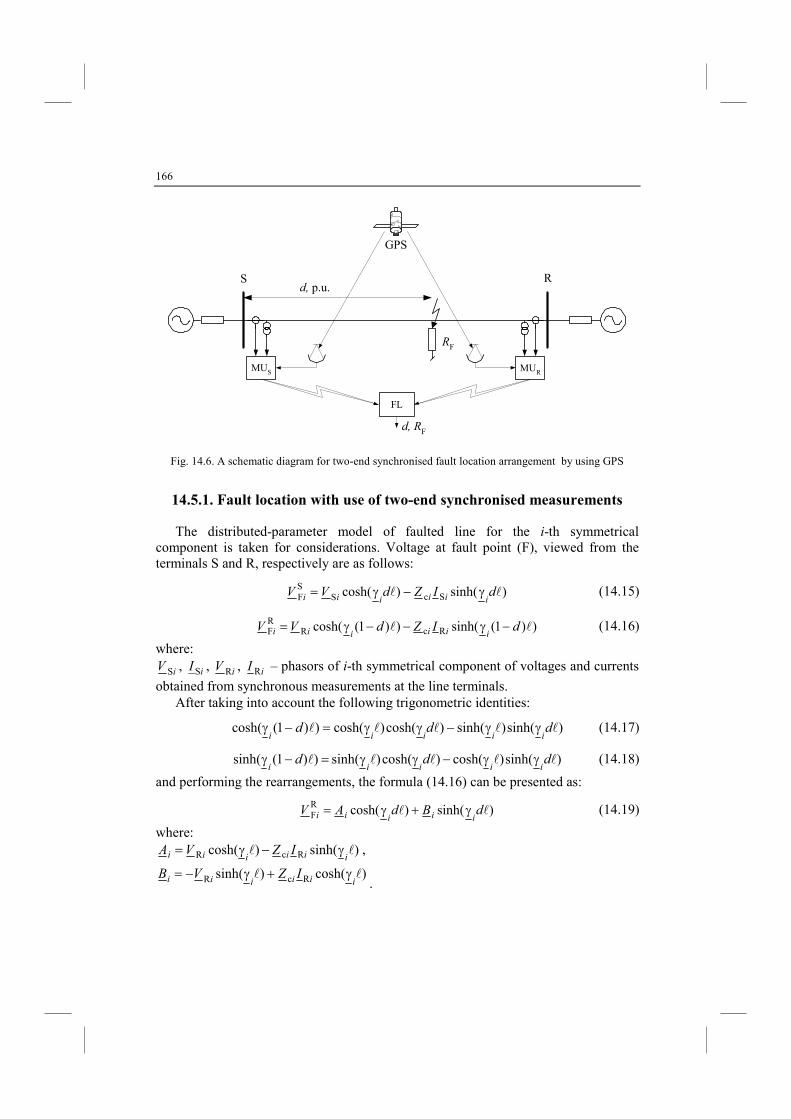
166
RSd, p.u.
RF
GPS
MUS MUR
FL
d, RF
Fig. 14.6. A schematic diagram for two-end synchronised fault location arrangement by using GPS
14.5.1. Fault location with use of two-end synchronised measurements
The distributed-parameter model of faulted line for the i-th symmetrical component is taken for considerations. Voltage at fault point (F), viewed from the terminals S and R, respectively are as follows:
)sinh()cosh( ScSSF ll dIZdVV
iiiiii γ−γ= (14.15)
))1(sinh())1(cosh( RcRRF ll dIZdVV
iiiiii −γ−−γ= (14.16)
where:
iV S , iIS , iV R , iI R – phasors of i-th symmetrical component of voltages and currents
obtained from synchronous measurements at the line terminals. After taking into account the following trigonometric identities:
)sinh()sinh()cosh()cosh())1(cosh( lllll dddiiiiiγγ−γγ=−γ (14.17)
)sinh()cosh()cosh()sinh())1(sinh( lllll dddiiiiiγγ−γγ=−γ (14.18)
and performing the rearrangements, the formula (14.16) can be presented as:
)sinh()cosh(RF ll dBdAV
iiiii γ+γ= (14.19)
where: )sinh()cosh( RcR ll
iiiiii IZVA γ−γ= ,
)cosh()sinh( RcR lliiiiii IZVB γ+γ−=
.
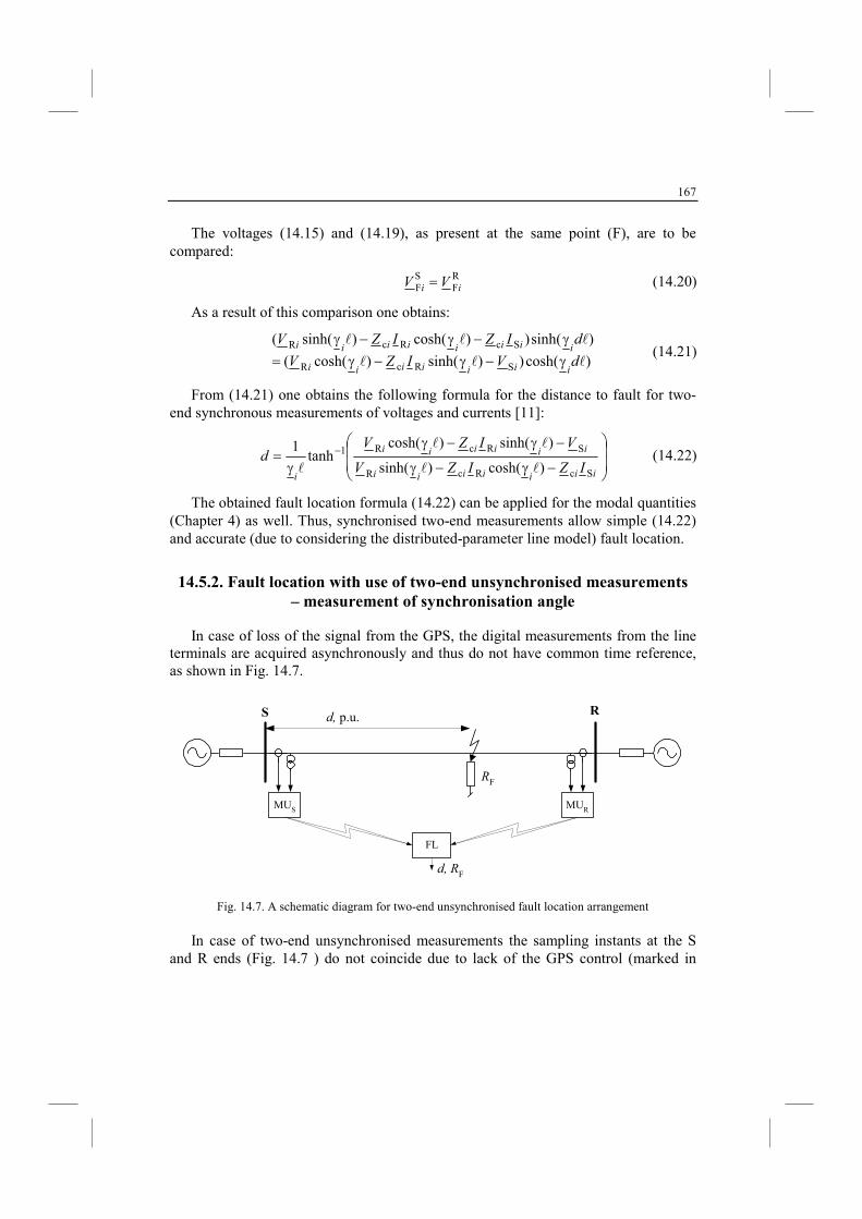
167
The voltages (14.15) and (14.19), as present at the same point (F), are to be compared:
RF
SF ii VV = (14.20)
As a result of this comparison one obtains:
)cosh())sinh()cosh((
)sinh())cosh()sinh((
SRcR
ScRcR
lll
lll
dVIZV
dIZIZV
iiiiiii
iiiiiiii
γ−γ−γ=
γ−γ−γ (14.21)
From (14.21) one obtains the following formula for the distance to fault for two-end synchronous measurements of voltages and currents [11]:
−γ−γ
−γ−γ
γ= −
iiiiiii
iiiiii
iIZIZV
VIZVd
ScRcR
SRcR1
)cosh()sinh(
)sinh()cosh(tanh
1
ll
ll
l (14.22)
The obtained fault location formula (14.22) can be applied for the modal quantities (Chapter 4) as well. Thus, synchronised two-end measurements allow simple (14.22) and accurate (due to considering the distributed-parameter line model) fault location.
14.5.2. Fault location with use of two-end unsynchronised measurements
– measurement of synchronisation angle
In case of loss of the signal from the GPS, the digital measurements from the line terminals are acquired asynchronously and thus do not have common time reference, as shown in Fig. 14.7.
RS d, p.u.
RF
MUS MUR
FL
d, RF
Fig. 14.7. A schematic diagram for two-end unsynchronised fault location arrangement
In case of two-end unsynchronised measurements the sampling instants at the S
and R ends (Fig. 14.7 ) do not coincide due to lack of the GPS control (marked in
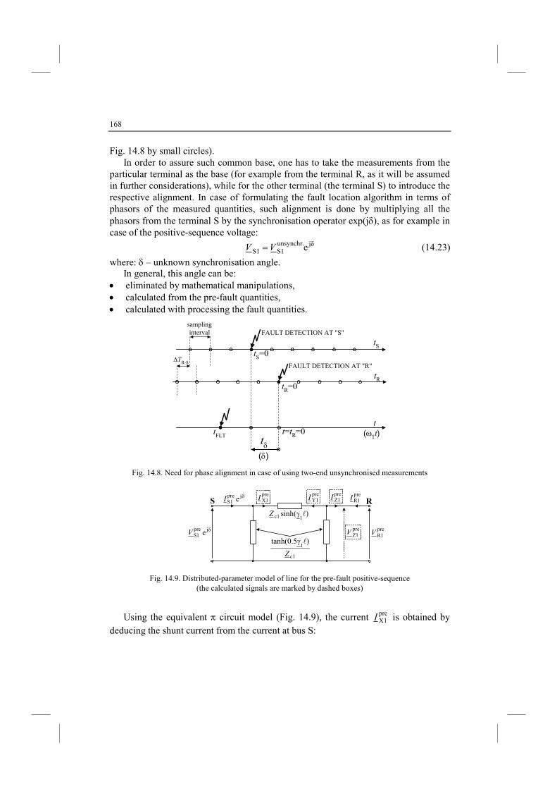
168
Fig. 14.8 by small circles). In order to assure such common base, one has to take the measurements from the
particular terminal as the base (for example from the terminal R, as it will be assumed in further considerations), while for the other terminal (the terminal S) to introduce the respective alignment. In case of formulating the fault location algorithm in terms of phasors of the measured quantities, such alignment is done by multiplying all the phasors from the terminal S by the synchronisation operator exp(jδ), as for example in case of the positive-sequence voltage:
jδunsynchr.S1S1 eVV = (14.23)
where: δ – unknown synchronisation angle. In general, this angle can be:
• eliminated by mathematical manipulations, • calculated from the pre-fault quantities, • calculated with processing the fault quantities.
tStS=0
tR
t
tR=0
tδ
t=tR=0
(δ)
(ω1t)
FAULT DETECTION AT "S"
tFLT
FAULT DETECTION AT "R"
samplinginterval
∆TR-S
Fig. 14.8. Need for phase alignment in case of using two-end unsynchronised measurements
)sinh(1c1 lγZ
c1
1)5.0tanh(
Z
lγ
RS
δjpreS1 eV
preX1I
preY1I
preZ1I
preZ1V
preR1I
preR1V
δjpreS1 eI
Fig. 14.9. Distributed-parameter model of line for the pre-fault positive-sequence (the calculated signals are marked by dashed boxes)
Using the equivalent π circuit model (Fig. 14.9), the current preX1I is obtained by
deducing the shunt current from the current at bus S:
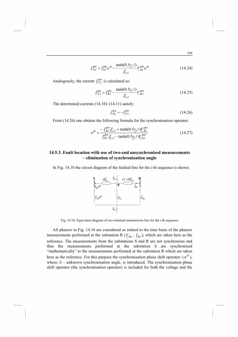
169
jδpreS1
c1
1jδpreS1
preX1 e
)5.0tanh(e V
ZII
lγ−= (14.24)
Analogously, the current preY1I is calculated as:
preR1
c1
1preR1
preY1
)5.0tanh(V
ZII
lγ−= (14.25)
The determined currents (14.10)–(14.11) satisfy:
preY1
preX1 II −= (14.26)
From (14.26) one obtains the following formula for the synchronisation operator:
preS11c1
preS1
preR11c1
preR1jδ
)5.0tanh(
)5.0tanh(e
VZI
VZI
l
l
γ−
γ+−= (14.27)
14.5.3. Fault location with use of two-end unsynchronised measurements
– elimination of synchronisation angle
In Fig. 14.10 the circuit diagram of the faulted line for the i-th sequence is shown.
VSiejδ
S dZiL (1–d)Z
iLR
ISiejδ
IFi
F IRi
VRiVFi
IFi
Fig. 14.10. Equivalent diagram of two terminal transmission line for the i-th sequence
All phasors in Fig. 14.10 are considered as related to the time basis of the phasors
measurements performed at the substation R ( iV R , iI R ), which are taken here as the
reference. The measurements from the substations S and R are not synchronous and thus the measurements performed at the substation S are synchronised “mathematically” to the measurements performed at the substation R which are taken
here as the reference. For this purpose the synchronisation phase shift operator: ( jδe ), where: δ – unknown synchronisation angle, is introduced. The synchronisation phase shift operator (the synchronisation operator) is included for both the voltage and the
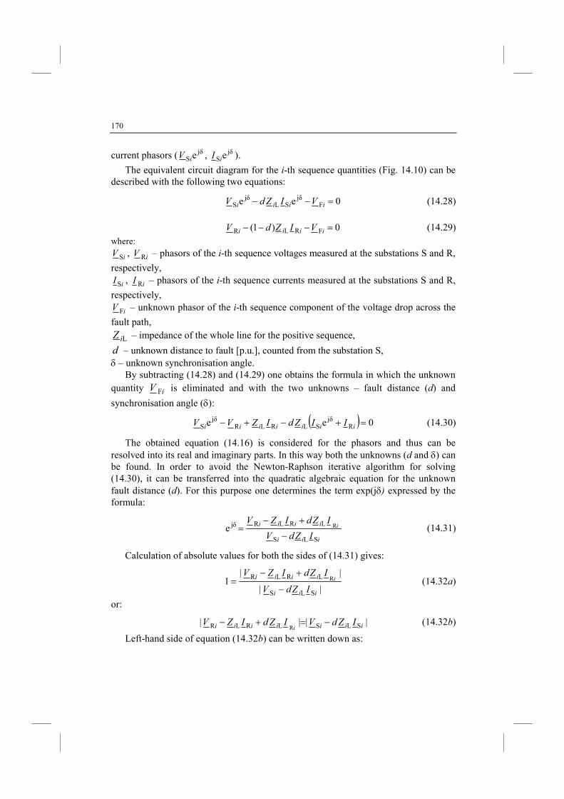
170
current phasors ( jδS eiV , jδ
S eiI ).
The equivalent circuit diagram for the i-th sequence quantities (Fig. 14.10) can be described with the following two equations:
0ee Fjδ
SLjδ
S =−− iiii VIZdV (14.28)
0)1( FRLR =−−− iiii VIZdV (14.29)
where:
iV S , iV R – phasors of the i-th sequence voltages measured at the substations S and R,
respectively,
iIS , iI R – phasors of the i-th sequence currents measured at the substations S and R,
respectively,
iV F – unknown phasor of the i-th sequence component of the voltage drop across the
fault path,
LiZ – impedance of the whole line for the positive sequence,
d – unknown distance to fault [p.u.], counted from the substation S, δ – unknown synchronisation angle.
By subtracting (14.28) and (14.29) one obtains the formula in which the unknown
quantity iV F is eliminated and with the two unknowns – fault distance (d) and
synchronisation angle (δ):
( ) 0ee Rjδ
SLRLRjδ
S =+−+− iiiiiii IIZdIZVV (14.30)
The obtained equation (14.16) is considered for the phasors and thus can be resolved into its real and imaginary parts. In this way both the unknowns (d and δ) can be found. In order to avoid the Newton-Raphson iterative algorithm for solving (14.30), it can be transferred into the quadratic algebraic equation for the unknown fault distance (d). For this purpose one determines the term exp(jδ) expressed by the formula:
iii
iiii
IZdV
IZdIZVi
SLS
LRLRjδ Re−
+−= (14.31)
Calculation of absolute values for both the sides of (14.31) gives:
||
||1
SLS
LRLR R
iii
iiii
IZdV
IZdIZVi
−
+−= (14.32a)
or:
|||| SLSLRLR R iiiiiii IZdVIZdIZVi
−=+− (14.32b)
Left-hand side of equation (14.32b) can be written down as:
171
|)(j)()(j)()(j)(|
||
imagLrealLimaglRLrealRLimagRrealR
LRLR
RR
R
ii
i
IZdIZdIZIZVV
IZdIZVL
iiiiiiii
iiii
++−−+=
+−=
(14.32c)
Continuing determination of the left-hand side of (14.32b) one obtains:
[ ] [ ]2 imagLimagRLimagR2
realLrealRLrealR )()()()()()(RR ii
IZdIZVIZdIZVL iiiiiiii +−++−=
(14.32d) After rearrangements one obtains:
( ) ( )2432
21 dLLdLLL +++= (14.32e)
where:
realRLrealR1 )()( iii IZVL −= ,
realL2 )(Ri
IZL i= ,
imagRLimagR3 )()( iii IZVL −= ,
imagL4 )(Ri
IZL i= .
Formula (14.32e) can also be written down as:
762
5 LdLdLL ++= (14.32f)
where: 2
42
25 LLL += ,
43216 22 LLLLL += ,
23
217 LLL += .
Right-hand side of equation (14.32b) can be written down as:
|)(j)()(j)(||| imagSLrealSLimagSrealSSLS iiiiiiiii IZdIZdVVIZdVR −−+=−= (14.32g)
Continuing determination on the right-hand side of (14.32g) one obtains:
[ ] [ ]2 imagSLimagS2
realSLrealS )()()()( iiiiii IZdVIZdVR −+−= (14.32h)
After further rearrangements one obtains:
( ) ( )2432
21 dRRdRRR −+−= (14.32i)
where:
realS1 )( iVR = ,
realSL2 )( ii IZR = ,
imagS3 )( iVR = ,
172
imagSL4 )( ii IZR = .
Formula (14.32i) can also be written as:
762
5 RdRdRR ++= (14.32j)
where: 2
42
25 RRR += ,
43216 22 RRRRR −−= ,
23
217 RRR += .
Taking the results of the above derivations (14.32b) can be written down as:
762
5762
5 RdRdRLdLdL ++=++ (14.32k)
where:
5L , 6L , 7L – as in (14.32f),
5R , 6R , 7R – as in (14.32j).
The formula (14.32k) results in the quadratic algebraic equation for the unknown fault distance (d):
0012
2 =++ AdAA d (14.32l)
where:
552 LRA −= ,
661 LRA −= ,
770 LRA −= .
There are two solutions (d1, d2) of (14.32l) for the distance to fault. The solution (d1 or d2) that falls between zero and one is taken as the valid solution. For some specific fault cases it may happen that both solutions of (14.32l) indicate the fault as occurring within the line range (0 to 1 [p.u.]). In such rare cases one has to perform additionally the fault location calculations, as in (14.32l) – where the i-th symmetrical components are involved, but for the other kind of symmetrical components (say for the j–th kind). This will allow for reliable selection of the valid solution from (d1, d2).
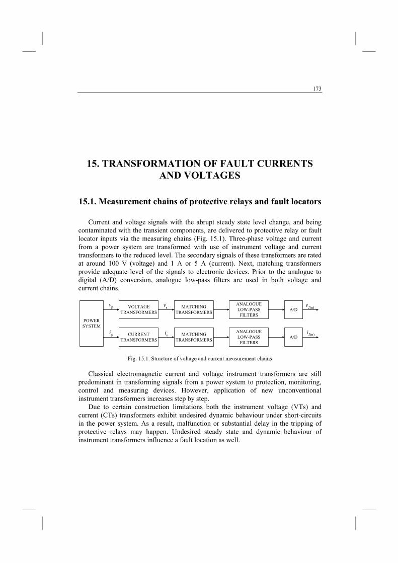
173
15. TRASFORMATIO OF FAULT CURRETS
AD VOLTAGES
15.1. Measurement chains of protective relays and fault locators
Current and voltage signals with the abrupt steady state level change, and being contaminated with the transient components, are delivered to protective relay or fault locator inputs via the measuring chains (Fig. 15.1). Three-phase voltage and current from a power system are transformed with use of instrument voltage and current transformers to the reduced level. The secondary signals of these transformers are rated at around 100 V (voltage) and 1 A or 5 A (current). Next, matching transformers provide adequate level of the signals to electronic devices. Prior to the analogue to digital (A/D) conversion, analogue low-pass filters are used in both voltage and current chains.
POWERSYSTEM
VOLTAGETRANSFORMERS
MATCHINGTRANSFORMERS
ANALOGUELOW-PASSFILTERS
A/D
CURRENTTRANSFORMERS
MATCHINGTRANSFORMERS
ANALOGUELOW-PASSFILTERS
A/D
vp
ip
vs
is
v2(n)
i2(n)
Fig. 15.1. Structure of voltage and current measurement chains
Classical electromagnetic current and voltage instrument transformers are still predominant in transforming signals from a power system to protection, monitoring, control and measuring devices. However, application of new unconventional instrument transformers increases step by step.
Due to certain construction limitations both the instrument voltage (VTs) and current (CTs) transformers exhibit undesired dynamic behaviour under short-circuits in the power system. As a result, malfunction or substantial delay in the tripping of protective relays may happen. Undesired steady state and dynamic behaviour of instrument transformers influence a fault location as well.
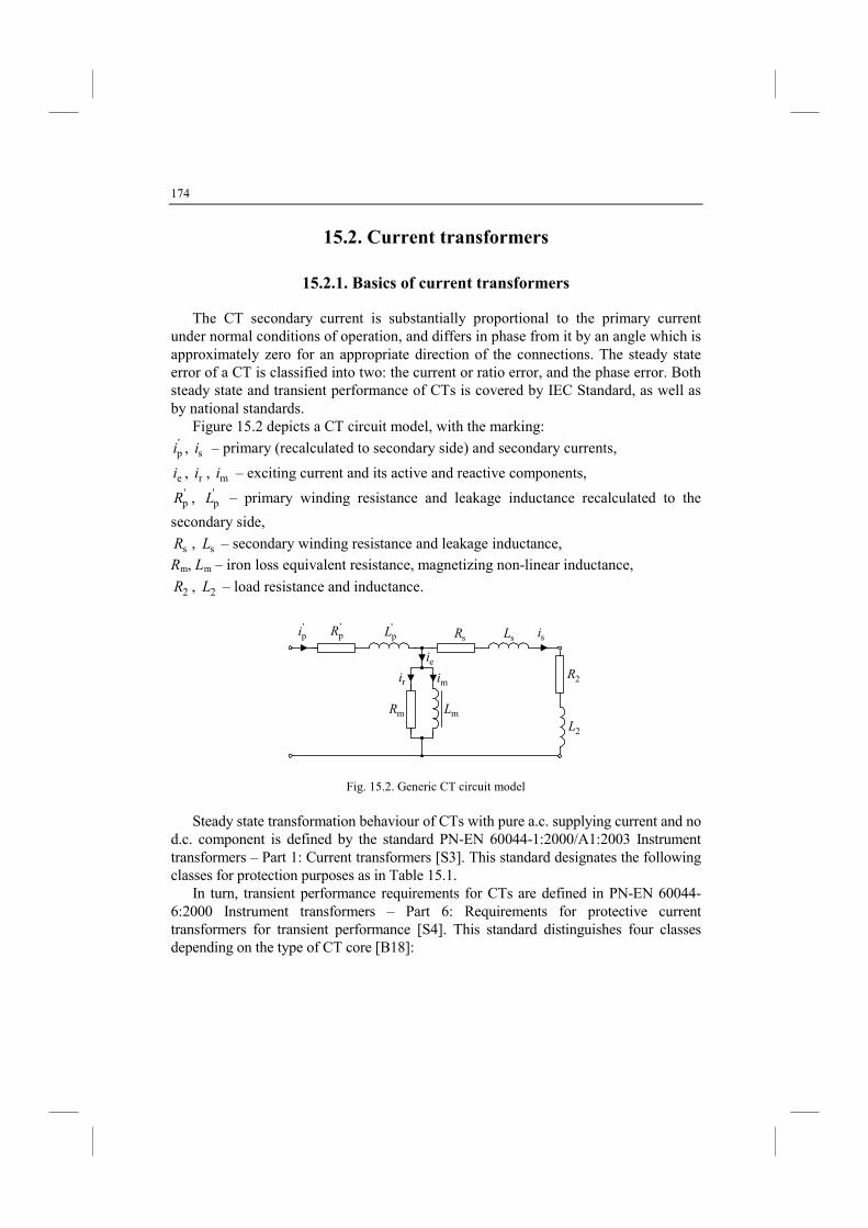
174
15.2. Current transformers
15.2.1. Basics of current transformers
The CT secondary current is substantially proportional to the primary current under normal conditions of operation, and differs in phase from it by an angle which is approximately zero for an appropriate direction of the connections. The steady state error of a CT is classified into two: the current or ratio error, and the phase error. Both steady state and transient performance of CTs is covered by IEC Standard, as well as by national standards.
Figure 15.2 depicts a CT circuit model, with the marking: 'pi , si – primary (recalculated to secondary side) and secondary currents,
ei , ri , mi – exciting current and its active and reactive components, 'pR , '
pL – primary winding resistance and leakage inductance recalculated to the
secondary side,
sR , sL – secondary winding resistance and leakage inductance,
Rm, Lm – iron loss equivalent resistance, magnetizing non-linear inductance,
2R , 2L – load resistance and inductance.
'pi si
mR mL
'pR
'pL sR sL
2R
2L
ei
miri
Fig. 15.2. Generic CT circuit model
Steady state transformation behaviour of CTs with pure a.c. supplying current and no
d.c. component is defined by the standard PN-EN 60044-1:2000/A1:2003 Instrument transformers – Part 1: Current transformers [S3]. This standard designates the following classes for protection purposes as in Table 15.1.
In turn, transient performance requirements for CTs are defined in PN-EN 60044-6:2000 Instrument transformers – Part 6: Requirements for protective current transformers for transient performance [S4]. This standard distinguishes four classes depending on the type of CT core [B18]:
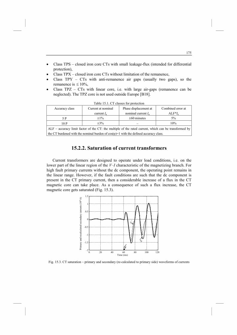
175
• Class TPS – closed iron core CTs with small leakage-flux (intended for differential protection),
• Class TPX – closed iron core CTs without limitation of the remanence, • Class TPY – CTs with anti-remanence air gaps (usually two gaps), so the
remanence is ≤ 10%, • Class TPZ – CTs with linear core, i.e. with large air-gaps (remanence can be
neglected). The TPZ core is not used outside Europe [B18].
Table 15.1. CT classes for protection
Accuracy class Current at nominal
current In
Phase displacement at
nominal current In
Combined error at
ALF*In
5 P %1± minutes 60± %5
10 P %3± – %10
ALF – accuracy limit factor of the CT: the multiple of the rated current, which can be transformed by
the CT burdened with the nominal burden of cos(ϕ)=1 with the defined accuracy class.
15.2.2. Saturation of current transformers
Current transformers are designed to operate under load conditions, i.e. on the lower part of the linear region of the V–I characteristic of the magnetizing branch. For high fault primary currents without the dc component, the operating point remains in the linear range. However, if the fault conditions are such that the dc component is present in the CT primary current, then a considerable increase of a flux in the CT magnetic core can take place. As a consequence of such a flux increase, the CT magnetic core gets saturated (Fig. 15.3).
0 20 40 60 80 100 120–2
–1.5
–1
–0.5
0
0.5
1
1.5
Time (ms)
Prim
ary
and
reca
lcul
ated
sec
onda
ry c
urre
nts (1
04 A
)
pi
'is
Fig. 15.3. CT saturation – primary and secondary (re-calculated to primary side) waveforms of currents
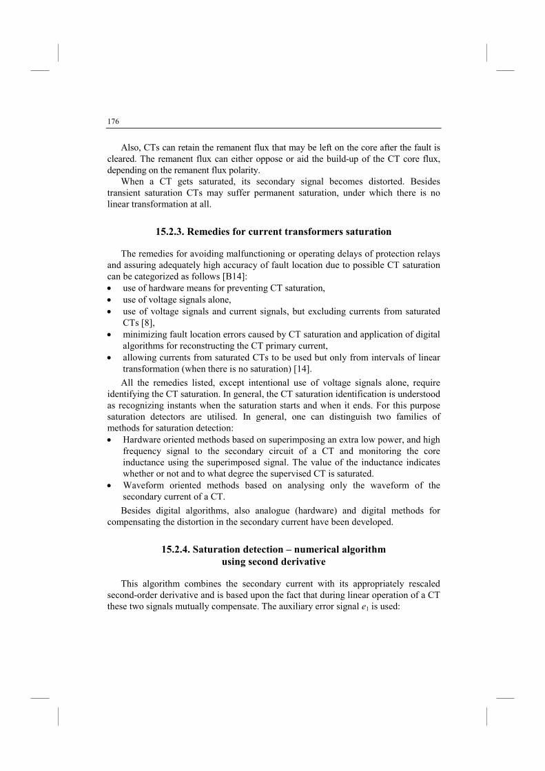
176
Also, CTs can retain the remanent flux that may be left on the core after the fault is cleared. The remanent flux can either oppose or aid the build-up of the CT core flux, depending on the remanent flux polarity.
When a CT gets saturated, its secondary signal becomes distorted. Besides transient saturation CTs may suffer permanent saturation, under which there is no linear transformation at all.
15.2.3. Remedies for current transformers saturation
The remedies for avoiding malfunctioning or operating delays of protection relays and assuring adequately high accuracy of fault location due to possible CT saturation can be categorized as follows [B14]: • use of hardware means for preventing CT saturation, • use of voltage signals alone, • use of voltage signals and current signals, but excluding currents from saturated
CTs [8], • minimizing fault location errors caused by CT saturation and application of digital
algorithms for reconstructing the CT primary current, • allowing currents from saturated CTs to be used but only from intervals of linear
transformation (when there is no saturation) [14].
All the remedies listed, except intentional use of voltage signals alone, require identifying the CT saturation. In general, the CT saturation identification is understood as recognizing instants when the saturation starts and when it ends. For this purpose saturation detectors are utilised. In general, one can distinguish two families of methods for saturation detection: • Hardware oriented methods based on superimposing an extra low power, and high
frequency signal to the secondary circuit of a CT and monitoring the core inductance using the superimposed signal. The value of the inductance indicates whether or not and to what degree the supervised CT is saturated.
• Waveform oriented methods based on analysing only the waveform of the secondary current of a CT.
Besides digital algorithms, also analogue (hardware) and digital methods for compensating the distortion in the secondary current have been developed.
15.2.4. Saturation detection – numerical algorithm
using second derivative
This algorithm combines the secondary current with its appropriately rescaled second-order derivative and is based upon the fact that during linear operation of a CT these two signals mutually compensate. The auxiliary error signal e1 is used:
177
)(
)()2(
)()(1
n
nnn
X
xpxe
⋅−= (15.1)
where x(2) is a second-order derivative of the secondary current denoted here as i:
( ))4()3()2()1()(s
)()2( 163016
12
1−−−− −+−+−= nnnnnn iiiii
Tx (15.2)
and where: Ts – sampling period, X – amplitude of signal x, ( )2121 fp π= – scaling
factor, f1 – fundamental frequency. Since (15.2) gives the second-order derivative but for the time marker (n–2), the
signal x in (15.1) should be, thus, delayed by two samples as well:
)2()( −= nn ix (15.3)
The error signal e1 (15.1) displays clear peaks when the supervised CT both gets in and out of saturation. Thus, the flag SAT (SAT=1: saturation; SAT=0: no saturation):
=→=>
=→=>
−
−
0:SAT )1(SAT & )B(
1:SAT )0(SAT & )A(
)()1(1)(1
)()1(1)(1
nnn
nnn
e
e (15.4)
where A1 and B1 are the thresholds optimized for a given CT. Figure 15.4 illustrates example operation of the algorithm.
0 0.02 0.04 0.06 0.08 0.1–100
–50
0
50
Cur
rent
s (A
)
0 0.02 0.04 0.06 0.08 0.1–2
0
2
4
6
e1
SA
T
Time (s)
Sig
nals: e
1, S
AT
a)
b)
si'pi
Fig. 15.4. Example performance of a saturation-detection algorithm based on a second-order derivative of current
178
As is seen (Fig. 15.4), the beginnings of the saturated periods are easier to detect. They reflect in higher values of the error signal (e1). This is the reason for using two different thresholds in (15.4). The method provides very good saturation recognition, but requires at least a 3-kHz sampling frequency.
15.2.5. Saturation detection – numerical algorithm
using mean and median filters
This algorithm combines the mean and the median digital filters applied to the waveform of the secondary current, and is based on the ability of such a pair of filters to detect changes in the shape of a signal. The auxiliary error signal e2 for this principle is defined as follows:
( ) ( )
)(
)()()(2
medianmean
n
nnn
I
iie
−= (15.5)
where I is the amplitude of the secondary current, while ‘mean’ and ‘median’ are mean and median functions – available for example in Matlab program. Those functions are to be determined over a selected number of samples.
15.2.6. Saturation detection – numerical algorithm
based on modal transformation
Another interesting saturation detector (Fig. 15.5), presented by Hosemann et al. [5], transforms modally the three-phase current vector (iabc) into the 0αβ components (the Clarke transformation – see Chapter 4: formula (4.6)):
abc0αα
330
112
111
3
1ii
−−= (15.6)
The α and β components are further processed with use of a pair of orthogonal filters (Fd, Fq) for obtaining two pairs of orthogonal components: (iαd, iαq) and (iβd, iβq). Then, these components are combined into the real and imaginary part of a blocked backward-rotating space vector:
βqαdd iii −= (15.7)
βdαqq iii += (15.8)
If none of the CTs from a three-phase bank is under saturation, then the trajectory of the blocked backward-rotating space current (id, iq) forms a circle (Fig. 15.6a). If
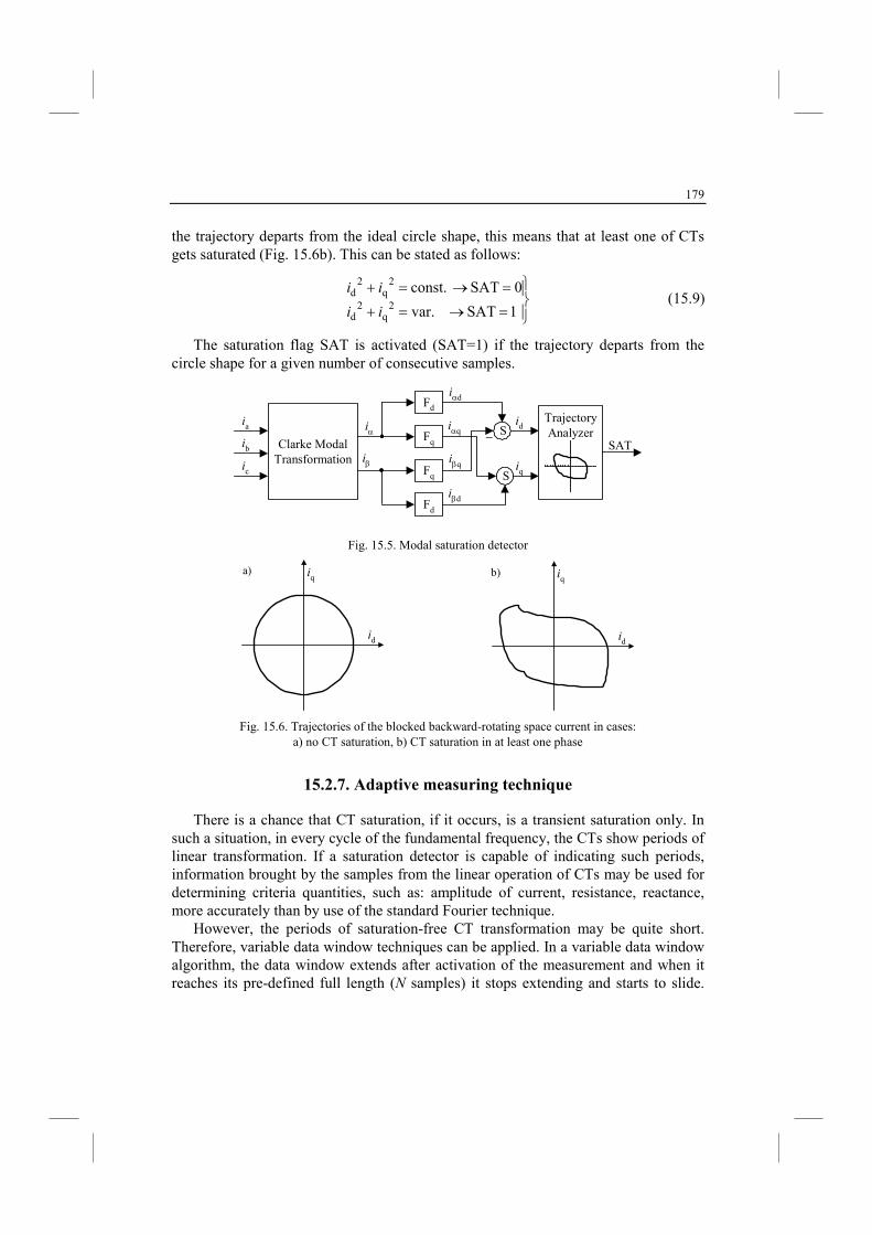
179
the trajectory departs from the ideal circle shape, this means that at least one of CTs gets saturated (Fig. 15.6b). This can be stated as follows:
=→=+
=→=+
1SAT var.
0SAT const.2
q2
d
2q
2d
ii
ii (15.9)
The saturation flag SAT is activated (SAT=1) if the trajectory departs from the circle shape for a given number of consecutive samples.
Clarke ModalTransformation
ia
ib
ic
Fd
Fq
Fq
Fd
iα
iβ
S
S
–
iαd
iαq
iβd
iβq
TrajectoryAnalyzer
id
iq
SAT
Fig. 15.5. Modal saturation detector
a)
id
iq b)
id
iq
Fig. 15.6. Trajectories of the blocked backward-rotating space current in cases:
a) no CT saturation, b) CT saturation in at least one phase
15.2.7. Adaptive measuring technique
There is a chance that CT saturation, if it occurs, is a transient saturation only. In such a situation, in every cycle of the fundamental frequency, the CTs show periods of linear transformation. If a saturation detector is capable of indicating such periods, information brought by the samples from the linear operation of CTs may be used for determining criteria quantities, such as: amplitude of current, resistance, reactance, more accurately than by use of the standard Fourier technique.
However, the periods of saturation-free CT transformation may be quite short. Therefore, variable data window techniques can be applied. In a variable data window algorithm, the data window extends after activation of the measurement and when it reaches its pre-defined full length () samples) it stops extending and starts to slide.
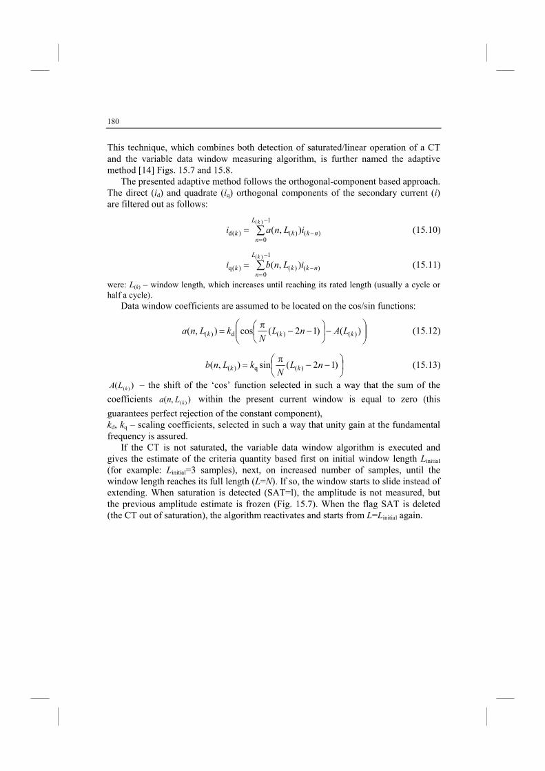
180
This technique, which combines both detection of saturated/linear operation of a CT and the variable data window measuring algorithm, is further named the adaptive method [14] Figs. 15.7 and 15.8.
The presented adaptive method follows the orthogonal-component based approach. The direct (id) and quadrate (iq) orthogonal components of the secondary current (i) are filtered out as follows:
∑−
=−=
1
0)()()(d
)(
) ,(kL
nnkkk iLnai (15.10)
∑−
=−=
1
0)()()(q
)(
) ,(kL
nnkkk iLnbi (15.11)
were: L(k) – window length, which increases until reaching its rated length (usually a cycle or half a cycle).
Data window coefficients are assumed to be located on the cos/sin functions:
−
−−
π= )()12(cos) ,( )()(d)( kkk LAnL
)kLna (15.12)
−−
π= )12(sin) ,( )(q)( nL
)kLnb kk (15.13)
)( )(kLA – the shift of the ‘cos’ function selected in such a way that the sum of the
coefficients ) ,( )(kLna within the present current window is equal to zero (this
guarantees perfect rejection of the constant component), kd, kq – scaling coefficients, selected in such a way that unity gain at the fundamental frequency is assured.
If the CT is not saturated, the variable data window algorithm is executed and gives the estimate of the criteria quantity based first on initial window length Linitial (for example: Linitial=3 samples), next, on increased number of samples, until the window length reaches its full length (L=)). If so, the window starts to slide instead of extending. When saturation is detected (SAT=l), the amplitude is not measured, but the previous amplitude estimate is frozen (Fig. 15.7). When the flag SAT is deleted (the CT out of saturation), the algorithm reactivates and starts from L=Linitial again.
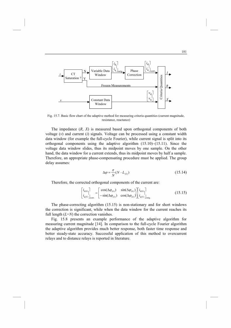
181
CTSaturation ?
PhaseCorrectioni
R
XCrite
ria
Qua
n titie
s
v Constant DataWindow
Variable DataWindow
Frozen Measurements
N
Y
I
q
d
v
v
orig.q
d
i
i
corr.q
d
i
i
Fig. 15.7. Basic flow chart of the adaptive method for measuring criteria quantities (current magnitude, resistance, reactance)
The impedance (R, X) is measured based upon orthogonal components of both
voltage (v) and current (i) signals. Voltage can be processed using a constant width data window (for example the full-cycle Fourier), while current signal is split into its orthogonal components using the adaptive algorithm (15.10)–(15.11). Since the voltage data window slides, thus its midpoint moves by one sample. On the other hand, the data window for a current extends, thus its midpoint moves by half a sample. Therefore, an appropriate phase-compensating procedure must be applied. The group delay assumes:
)–( )(kL))
πϕ =∆ (15.14)
Therefore, the corrected orthogonal components of the current are:
orig.)(q
)(d
)()(
)()(
corr.)(q
)(d
)cos()sin(
)sin()cos(
∆∆−
∆∆=
k
k
kk
kk
k
k
i
i
i
i
ϕϕϕϕ
(15.15)
The phase-correcting algorithm (15.15) is non-stationary and for short windows the correction is significant, while when the data window for the current reaches its full length (L=)) the correction vanishes.
Fig. 15.8 presents an example performance of the adaptive algorithm for measuring current magnitude [14]. In comparison to the full-cycle Fourier algorithm the adaptive algorithm provides much better response, both faster time response and better steady-state accuracy. Successful application of this method to overcurrent relays and to distance relays is reported in literature.
182
0 0.02 0.04 0.06 0.08 0.1–100
–50
0
50
Cur
rent
s (A
)
0 0.02 0.04 0.06 0.08 0.1–100
–50
0
50
100Adaptive method
Full-cycle Fourier
Com
pone
nt: i
d (A
)
Adaptive method
Full-cycle Fourier
Com
pone
nt: i
q (A
)
0 0.02 0.04 0.06 0.08 0.1–100
–50
0
50
100
0 0.02 0.04 0.06 0.08 0.10
10
20
30
40
Time (s)
Adaptive method
Full-cycle Fourier
Cur
rent
mag
nitu
de (A
)
si
'pi
a)
b)
c)
d)
Fig. 15.8. Example performance of adaptive algorithm for measuring current magnitude, in comparison to full-cycle Fourier algorithm: a) primary- and secondary-current waveforms, b) orthogonal component id,
c) orthogonal component iq, d) current magnitude
15.3. Capacitive voltage transformers
15.3.1. Basics of capacitive voltage transformers
At transmission and sub-transmission voltage levels the instrument-level voltage signals for protective, monitoring and measuring devices is provided by means of capacitive voltage transformers (CVTs). A CVT provides a cost-effective way of obtaining secondary voltage for HV and EHV systems [B16, B18, 7]. Its functional
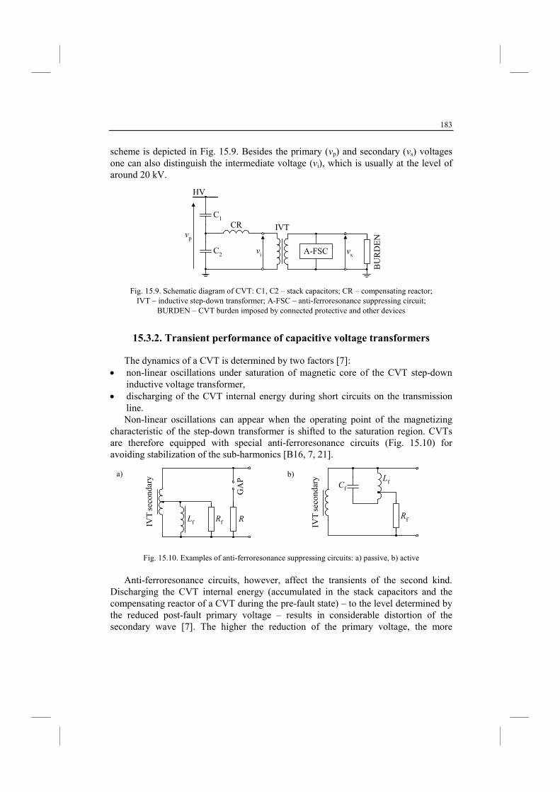
183
scheme is depicted in Fig. 15.9. Besides the primary (vp) and secondary (vs) voltages one can also distinguish the intermediate voltage (vi), which is usually at the level of around 20 kV.
A-FSC
vp
vi vs
C1
C2
CR IVT
HV
BU
RD
EN
Fig. 15.9. Schematic diagram of CVT: C1, C2 – stack capacitors; CR – compensating reactor; IVT – inductive step-down transformer; A-FSC – anti-ferroresonance suppressing circuit;
BURDEN – CVT burden imposed by connected protective and other devices
15.3.2. Transient performance of capacitive voltage transformers
The dynamics of a CVT is determined by two factors [7]: • non-linear oscillations under saturation of magnetic core of the CVT step-down
inductive voltage transformer, • discharging of the CVT internal energy during short circuits on the transmission
line. Non-linear oscillations can appear when the operating point of the magnetizing
characteristic of the step-down transformer is shifted to the saturation region. CVTs are therefore equipped with special anti-ferroresonance circuits (Fig. 15.10) for avoiding stabilization of the sub-harmonics [B16, 7, 21].
RfLfIVT sec
onda
ry
GA
P
R
Cf
Rf
Lf
IVT sec
onda
ry
Fig. 15.10. Examples of anti-ferroresonance suppressing circuits: a) passive, b) active
Anti-ferroresonance circuits, however, affect the transients of the second kind.
Discharging the CVT internal energy (accumulated in the stack capacitors and the compensating reactor of a CVT during the pre-fault state) – to the level determined by the reduced post-fault primary voltage – results in considerable distortion of the secondary wave [7]. The higher the reduction of the primary voltage, the more
a) b)
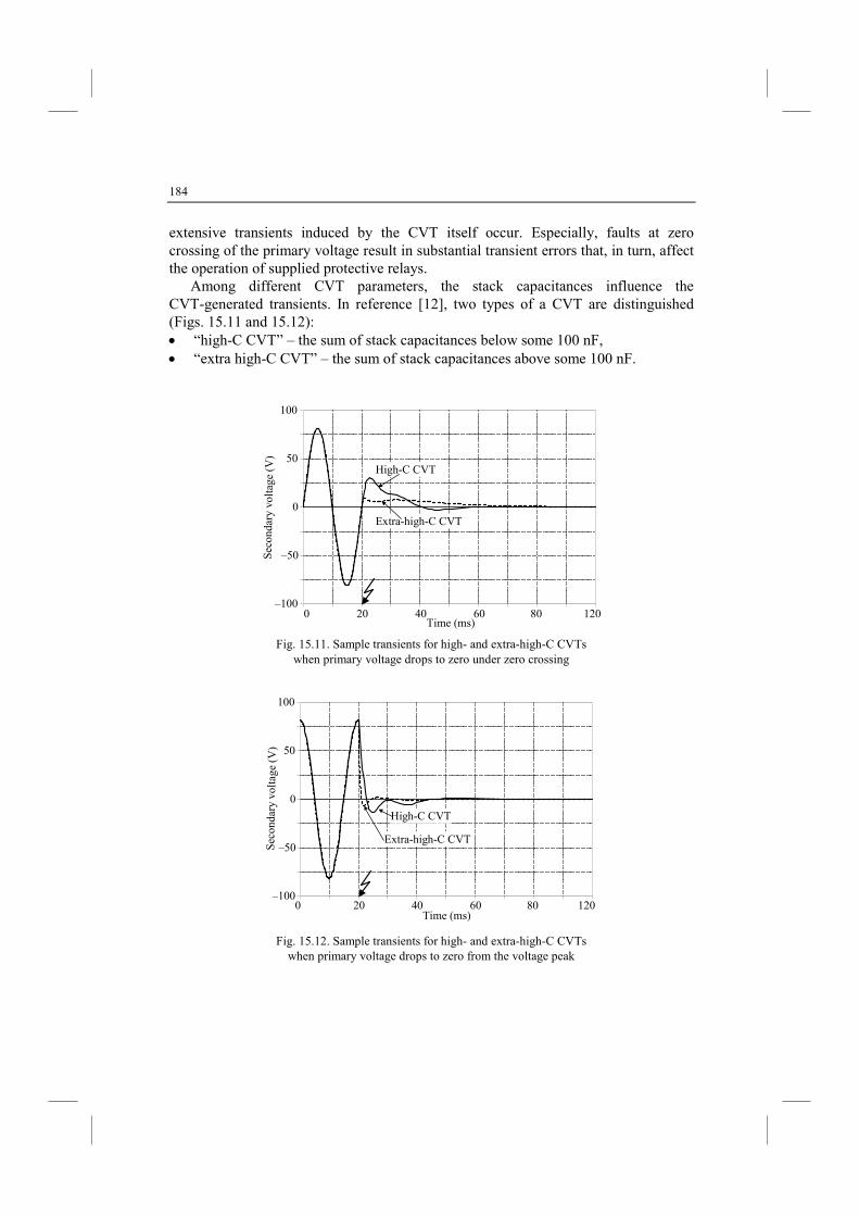
184
extensive transients induced by the CVT itself occur. Especially, faults at zero crossing of the primary voltage result in substantial transient errors that, in turn, affect the operation of supplied protective relays.
Among different CVT parameters, the stack capacitances influence the CVT-generated transients. In reference [12], two types of a CVT are distinguished (Figs. 15.11 and 15.12): • “high-C CVT” – the sum of stack capacitances below some 100 nF, • “extra high-C CVT” – the sum of stack capacitances above some 100 nF.
–100
–50
0
50
100
0 20 40 60 80 120Time (ms)
Sec
ond a
r y v
o lta
g e (V
)
High-C CVT
Extra-high-C CVT
Fig. 15.11. Sample transients for high- and extra-high-C CVTs when primary voltage drops to zero under zero crossing
0 20 40 60 80 120–100
–50
0
50
100
Time (ms)
Sec
ond a
r y v
o lta
ge (V
)
High-C CVT
Extra-high-C CVT
Fig. 15.12. Sample transients for high- and extra-high-C CVTs when primary voltage drops to zero from the voltage peak
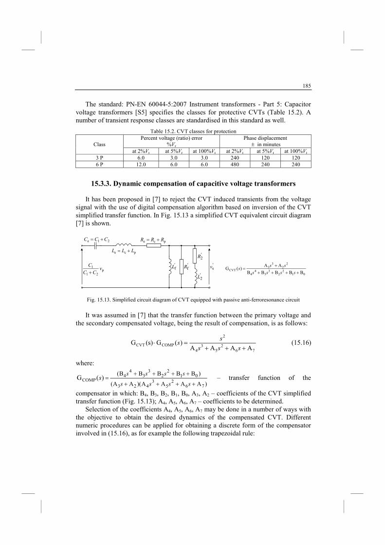
185
The standard: PN-EN 60044-5:2007 Instrument transformers - Part 5: Capacitor voltage transformers [S5] specifies the classes for protective CVTs (Table 15.2). A number of transient response classes are standardised in this standard as well.
Table 15.2. CVT classes for protection
Class Percent voltage (ratio) error
%Vr Phase displacement
± in minutes at 2%Vr at 5%Vr at 100%Vr at 2%Vr at 5%Vr at 100%Vr
3 P 6.0 3.0 3.0 240 120 120 6 P 12.0 6.0 6.0 480 240 240
15.3.3. Dynamic compensation of capacitive voltage transformers
It has been proposed in [7] to reject the CVT induced transients from the voltage signal with the use of digital compensation algorithm based on inversion of the CVT simplified transfer function. In Fig. 15.13 a simplified CVT equivalent circuit diagram [7] is shown.
'R2
'L2
'Rf'Lf
21e CCC +=
pce LLL +=
pce RRR +=
p21
1 vCC
C
+
'vs
012
23
34
4
22
33
CVTBBBBB
AA)(G
++++
+=
ssss
sss
Fig. 15.13. Simplified circuit diagram of CVT equipped with passive anti-ferroresonance circuit
It was assumed in [7] that the transfer function between the primary voltage and
the secondary compensated voltage, being the result of compensation, is as follows:
76
25
34
2
COMPCVTAAAA
)(G(s)G+++
=⋅sss
ss (15.16)
where:
)AAAA)(AA(
)BBBBB(
762
53
423
012
23
34
4COMP )(G
++++
++++=
ssss
sssss – transfer function of the
compensator in which: B4, B3, B2, B1, B0, A3, A2 – coefficients of the CVT simplified transfer function (Fig. 15.13); A4, A5, A6, A7 – coefficients to be determined.
Selection of the coefficients A4, A5, A6, A7 may be done in a number of ways with the objective to obtain the desired dynamics of the compensated CVT. Different numeric procedures can be applied for obtaining a discrete form of the compensator involved in (15.16), as for example the following trapezoidal rule:
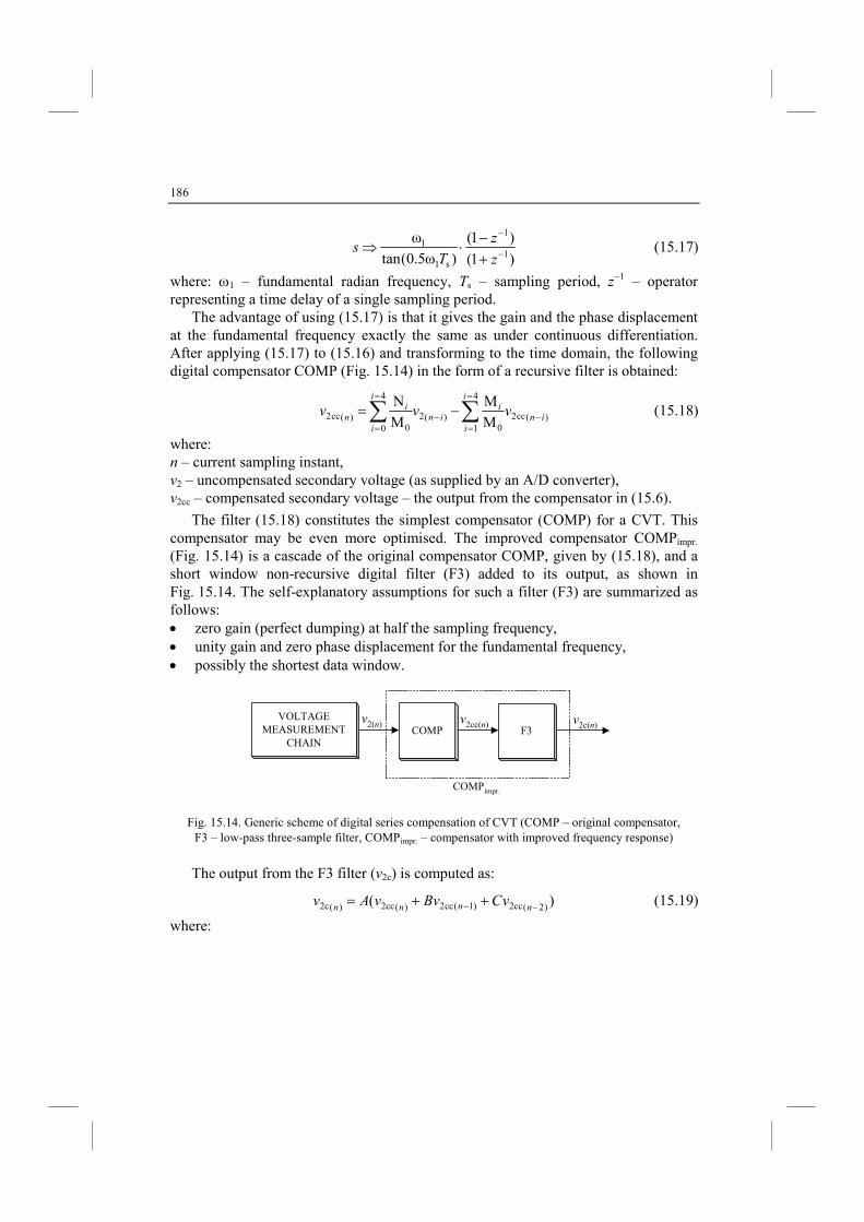
186
)1(
)1(
)ω5.0(tan
ω1
1
s1
1−
−
+−
⋅⇒z
z
Ts (15.17)
where: ω1 – fundamental radian frequency, Ts – sampling period, z–1 – operator representing a time delay of a single sampling period.
The advantage of using (15.17) is that it gives the gain and the phase displacement at the fundamental frequency exactly the same as under continuous differentiation. After applying (15.17) to (15.16) and transforming to the time domain, the following digital compensator COMP (Fig. 15.14) in the form of a recursive filter is obtained:
)(cc2
4
1 0)(2
4
0 0)(cc2 M
M
M
Nin
i
i
iin
i
i
in
vvv −
=
=−
=
=∑∑ −= (15.18)
where: n – current sampling instant, v2 – uncompensated secondary voltage (as supplied by an A/D converter), v2cc – compensated secondary voltage – the output from the compensator in (15.6).
The filter (15.18) constitutes the simplest compensator (COMP) for a CVT. This compensator may be even more optimised. The improved compensator COMPimpr. (Fig. 15.14) is a cascade of the original compensator COMP, given by (15.18), and a short window non-recursive digital filter (F3) added to its output, as shown in Fig. 15.14. The self-explanatory assumptions for such a filter (F3) are summarized as follows: • zero gain (perfect dumping) at half the sampling frequency, • unity gain and zero phase displacement for the fundamental frequency, • possibly the shortest data window.
VOLTAGEMEASUREMENT
CHAINCOMP
v2(n) v2cc(n)F3
v2c(n)
COMPimpr.
Fig. 15.14. Generic scheme of digital series compensation of CVT (COMP – original compensator, F3 – low-pass three-sample filter, COMPimpr. – compensator with improved frequency response)
The output from the F3 filter (v2c) is computed as:
)( )2(2cc)1(cc2)(2cc)(2c −− ++=nnnn
vCBvvAv (15.19)
where:
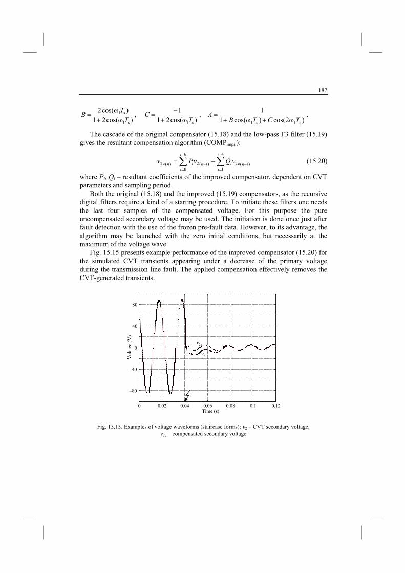
187
)ωcos(21
)ωcos(2
s1
s1
T
TB
+= ,
)ωcos(21
1
s1TC
+−
= , )ω2cos()ωcos(1
1
s1s1 TCTBA
++= .
The cascade of the original compensator (15.18) and the low-pass F3 filter (15.19) gives the resultant compensation algorithm (COMPimpr.):
)(c2
4
1)(2
6
0)(c2 in
i
i
iin
i
i
invQvPv −
=
=−
=
=∑∑ −= (15.20)
where Pi, Qi – resultant coefficients of the improved compensator, dependent on CVT parameters and sampling period.
Both the original (15.18) and the improved (15.19) compensators, as the recursive digital filters require a kind of a starting procedure. To initiate these filters one needs the last four samples of the compensated voltage. For this purpose the pure uncompensated secondary voltage may be used. The initiation is done once just after fault detection with the use of the frozen pre-fault data. However, to its advantage, the algorithm may be launched with the zero initial conditions, but necessarily at the maximum of the voltage wave.
Fig. 15.15 presents example performance of the improved compensator (15.20) for the simulated CVT transients appearing under a decrease of the primary voltage during the transmission line fault. The applied compensation effectively removes the CVT-generated transients.
0 0.02 0.04 0.06 0.08 0.1 0.12
–80
–40
0
40
80
Time (s)
Vol
tag e
(V
)
v2
v2c
Fig. 15.15. Examples of voltage waveforms (staircase forms): v2 – CVT secondary voltage, v2c – compensated secondary voltage
188
References – Books & Guides & Monographs
[B1] ANDERSON P.M., Power system protection, IEEE Press Power Engineering Series, Part I–VI, McGraw-Hill, 1999.
[B2] COOK V., Analysis of distance protection, Research Studies Press Ltd., John Wiley & Sons Inc., 1985.
[B3] DOMMEL H., Electro-Magnetic Transients Program, BPA, Portland, Oregon, 1986. [B4] El-HAWARY M.E., Electrical power systems design and analysis, Reston Publishing
Company, Virginia, 1983. [B5] GLOVER J.D., SARMA M., Power system analysis and design, PWS Publishing
Company, Boston, 2nd ed., 1994. [B6] IEEE Std C37.114Ł IEEE guide for determining fault location on AC transmission and
distribution lines, IEEE Power Engineering Society Publ., 8 June 2005. [B7] IEEE Std. C37.118: IEEE standard for synchrophasors for power systems, IEEE Power
Engineering Society Publ., 22 March 2006. [B8] IŻYKOWSKI J., Fault location on power transmission lines, Publisher of Wrocław
University of Technology, Wrocław, 2008. [B9] KACEJKO P., MACHOWSKI J., Power system faults, Scientific–Technical Publisher
WNT, Warszawa, 2002, (in Polish). [B10] KREMENS Z., SOBIERAJSKI M., Analysis of power systems, Scientific–Technical
Publisher WNT, Warszawa, 1996, (in Polish). [B11] LORENC J., Admittance earth fault protection, Publisher of Poznań Technical
University, Poznań, 2007, (in Polish). [B12] MATLAB user’s guide, The Math Works Inc., Natick, MA. [B13] ROSOŁOWSKI E., Digital signal processing for power system protection, Academic
Publisher EXIT, Warszawa, 2002, (in Polish). [B14] SAHA M.M., IŻYKOWSKI J., ROSOŁOWSKI E., Fault location on power networks,
Springer-Verlag London Limited, 2010. [B15] UNGRAD H., WINKLER W., WISZNIEWSKI A., Protection techniques in electrical
energy systems, Marcel Dekker, Inc., 1995. [B16] WISZNIEWSKI A., Instrument transformers in power systems, Scientific–Technical
Publisher WNT, Warszawa, 1992, (in Polish). [B17] ZIEGLER G. (Convener), Application guide on protection of complex transmission
network configuration, CIGRE SC34-WG04, 1990. [B18] ZIEGLER G., )umerical distance protection. Principles and applications, Editor:
Siemens AG, Publicis MCD Verlag, 2nd ed., 2006. [B19] ŻYDANOWICZ J., Power system protection and control, vol. 1, 2, 3, Scientific–
Technical Publisher WNT, Warszawa, 1979, (in Polish).
Papers
[1] DJURIC M.B., TERZIJA V.V., A new approach to the arcing faults detection for autoreclosure in transmission systems, IEEE Trans. on Power Delivery, Vol. 10, No. 4, 1995, pp. 1793–1798.
189
[2] DUDURYCH I., ROSOŁOWSKI E., Analysis of overvoltages in overhead ground
wires of EHV power transmission line shield under single phase-to-ground faults, Electric Power Systems Research, Vol. 53/2, December 1999, pp. 105–111.
[3] ERIKSSON L., SAHA M.M., ROCKEFELLER G.D., An accurate fault locator with
compensation for apparent reactance in the fault resistance resulting from remote-end
infeed, IEEE Trans. on Power Apparatus and Systems, Vol. PAS–104, No. 2, February 1985, pp. 424–436.
[4] HERRMANN H.J., Design numerical relays with regard to CT saturation, Proceedings of CIGRE 2001 S.C. 34 Colloquium, Sibiu, September 2001, Conference Publication No. 301, pp. 1–7.
[5] HOSEMANN G., STEIGERWALD H.M., Modal saturation detector for digital
differential protection, IEEE Trans. on Power Delivery, Vol. 8, No. 3, July 1993, pp. 933–940.
[6] IŻYKOWSKI J., KASZTENNY B., ROSOŁOWSKI E., SAHA M.M., Fundamental frequency equivalenting of series capacitors equipped with MOVs under fault
conditions of a series-compensated line, Proc. of the 8th International Symposium on
Short-Circuit Currents in Power Systems, Brussels, Belgium, October 1998, pp. 13–18. [7] IŻYKOWSKI J., KASZTENNY B., ROSOŁOWSKI E., SAHA M.M., HILLSTROM
B., Dynamic compensation of capacitive voltage transformers, IEEE Trans. on Power
Delivery, Vol. 113, No. 1, January 1998, pp. 116–122. [8] IŻYKOWSKI J., ROSOŁOWSKI E., SAHA M.M, BALCEREK P., Accurate algorithm
for locating faults in power transmission lines under saturation of current transformers,
Proceedings (CD) of Power Systems Computation Conference (PSCC), Liege, August 2005.
[9] JIANG J.-A., LIN Y.-H., YANG J.-Z., TOO T.-M., LIU C.-W., An adaptive PMU
based fault detection/location technique for transmission lines – Part II: PMU
implementation and performance evaluation, IEEE Trans. on Power Delivery, Vol. 15, No. 4, October 2000, pp. 1136–1146.
[10] JIANG J.-A., YANG J.-Z., LIN Y.-H., YANG J.-Z., LIU C.-W., MA J.-C., An adaptive PMU based fault detection/location technique for transmission lines – Part I: Theory and algorithms, IEEE Trans. on Power Delivery, Vol. 15, No. 2, April 2000, pp. 486–
493. [11] JOHNS A.T., JAMALI S., Accurate fault location technique for power transmission
lines, IEE Proceedings C, November 1990, Vol. 137, No. 6, pp. 395–402.
[12] KASZTENNY B., SHARPLES D., ASARO V., POZZUOLI M., Distance relays and capacitive voltage transformers – balancing speed and transient overreach, 55-th Annual Georgia Tech. Protective Relaying Conference, Atlanta, May 2–4, 2001, 22 p.
[13] KASZTENNY B., Distance protection of series compensated lines – problems and solutions, Proceedings of 28th Annual western Protective Relay Conference, Spokane, USA, 2001, pp. 1–34.
[14] KASZTENNY B., ROSOŁOWSKI E., ŁUKOWICZ M., IŻYKOWSKI J., Current related relaying algorithms immune to saturation of current transformers, Proceedings
190
of Sixth Int. Conference on Developments in Power System Protection, Publication No.
434, Nottingham 1997, pp. 365–369. [15] KIZILCAY M., PNIOK T., Digital simulation of fault arcs in power systems, ETEP-
European Trans. on Electrical Power, Vol. 1, No. 1, January/February 1991, pp. 55–60.
[16] PREMERLANI W.J., KASZTENNY B.Z., ADAMIAK M.G., Multi-ended fault
location system, US patent 7,472,026, December 30, 2008. [17] SAHA M.M., KASZTENNY B., ROSOŁOWSKI E., IŻYKOWSKI J., First zone
algorithm for protection of series compensated lines, IEEE Trans. on Power Delivery, Vol. 16, No. 2, 2001, pp. 200–207.
[18] SONG Y.H., AGGARWAL R.K., JOHNS A.T., Digital simulation of fault arcs on
long-distance compensated transmission systems with particular reference to adaptive
autoreclosure, ETEP – European Transactions on Electric Power, Vol. 5, September/October 1995, pp. 315–324.
[19] TAKAGI T., YAMAKOSI Y., YAMURA M., KONDOW R., MATSUSHIMA T., Development of new type fault locator using the one–terminal voltage and current data, IEEE Trans. on Power Apparatus and Systems, Vol. PAS–101, No. 8, August 1982, pp.
2892–2898. [20] WISZNIEWSKI A., Accurate fault impedance locating algorithm, IEE Proceedings –
Part C, Vol. 130, No. 6, 1983, pp. 311–315.
[21] WISZNIEWSKI A., IŻYKOWSKI J., Influence of ferroresonance suppression circuits upon the transient response of capacitive voltage transformers, IEE Conference Publ. No. 125, Developments in Power System Protection, London 1975.
Standards (check validity at http://www.pkn.pl/)
[S1] PN-EN 60909-0:2002 Short-circuit currents in three-phase a.c. systems – Part 0: Calculation of currents (compatible with IEC 60909-0:2001).
[S2] PN-EN 60909-3:2010 Short-circuit currents in three-phase a.c systems - Part 3: Currents during two separate simultaneous line-to-earth short-circuits and partial short-circuit currents flowing through earth (compatible with IEC 60909-3:2009).
[S3] PN-EN 60044-1:2000/A1:2003 Instrument transformers – Part 1: Current transformers (compatible with IEC 60044-1:1996, modified).
[S4] PN-EN 60044-6:2000 Instrument transformers – Part 6: Requirements for protective
current transformers for transient performance (compatible with IEC 60044-6:1992, modified).
[S5] PN-EN 60044-5:2007 Instrument transformers - Part 5: Capacitor voltage transformers
(compatible with IEC 60044-5, 2004).