Practice Problem: Chapter 2 #6 The rent control agency of NYC has found that aggregate demand is QD = 160-8P. Quantity is measured in tens of thousands

Practice Problem: Chapter 2 #6

The rent control agency of NYC has found that aggregate demand is QD = 160-8P. Quantity is measured in tens of thousands of apartments. Price, the average monthly rental rate, is measured in hundreds of dollars. The agency also noted that the increase in Q at lower P results from more three-person

families coming into the city and demanding apartments. The city’s board of realtors acknowledges that this is a good demand estimate and has shown

that supply is QS = 70+7P.

What is the free market price? What is the change in city population if the agency sets a maximum average monthly rent of $300 and all those who

cannot find an apartment leave the city?

Chapter 3 2 ©2005 Pearson Education, Inc.

Chapter 2 #3

Set quantity supply = quantity demandP = 6 (convert to $600)Q = 112 (convert to 1,120,000)


Chapter 2: #6

If the rent control agency sets the rental rate at $300, the quantity supplied would then be 910,000 (QS = 70 + (7)(3) = 91), a decrease of 210,000 apartments from the free market equilibrium. (Assuming three people per family per apartment, this would imply a loss of 630,000 people.) At the $300 rental rate, the demand for apartments is 1,360,000 units, and the resulting shortage is 450,000 units (1,360,000-910,000). However, excess demand (supply shortages) and lower quantity demanded are not the same concepts. The supply shortage means that the market cannot accommodate the new people who would have been willing to move into the city at the new lower price. Therefore, the city population will only fall by 630,000, which is represented by the drop in the number of actual apartments from 1,120,000 (the old equilibrium value) to 910,000, or 210,000 apartments with 3 people each.


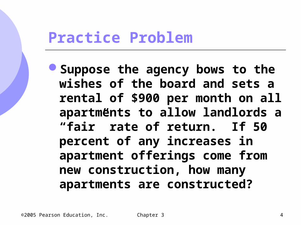
Practice Problem

Suppose the agency bows to the wishes of the board and sets a rental of $900 per month on all apartments to allow landlords a “fair” rate of return. If 50 percent of any increases in apartment offerings come from new construction, how many apartments are constructed?


Answer:

At a rental rate of $900, the supply of apartments would be 70 + 7(9) = 133, or 1,330,000 units, which is an increase of 210,000 units over the free market equilibrium. Therefore, (0.5)(210,000) = 105,000 units would be constructed. Note, however, that since demand is only 880,000 units, 450,000 units would go unrented


0

5

10

15

20

25

30

35

40

45

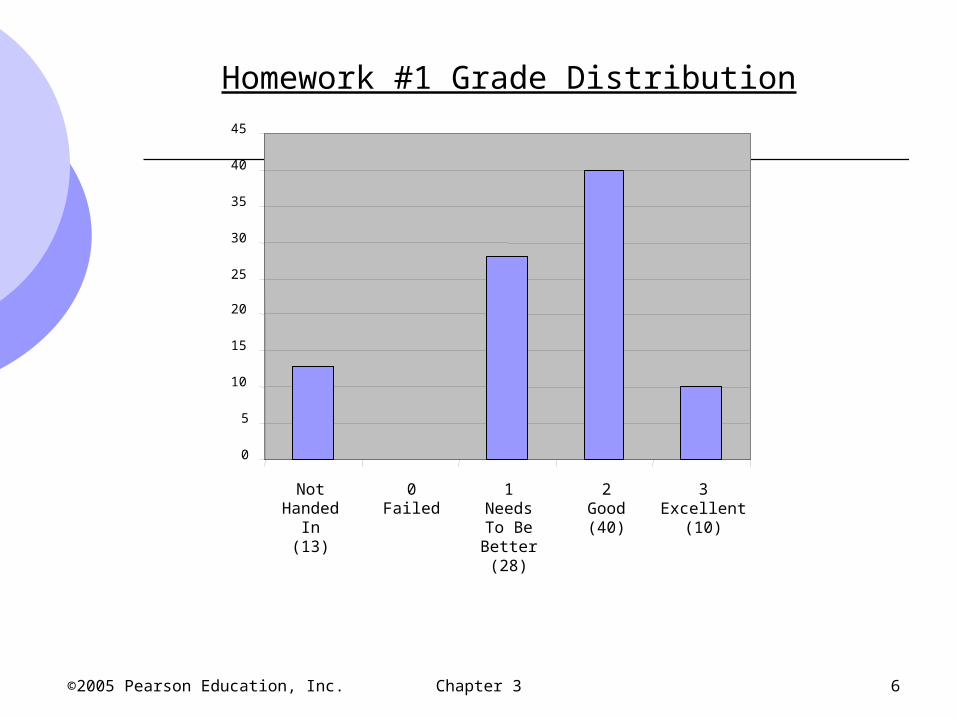
NotHanded

In(13)

0Failed

1NeedsTo BeBetter(28)

2Good(40)

3Excellent

(10)

Homework #1 Grade Distribution

Chapter 3

Consumer Behavior


Introduction

How are consumer preferences used to determine demand?

How do consumers allocate income to the purchase of different goods?


Consumer Behavior - Applications

1. How would General Mills determine the price to charge for a new cereal before it went to the market?

2. To what extent did the food stamp program provide individuals with more food versus merely subsidizing food they bought anyway?


Consumer Behavior Theory

There are three steps involved in the study of consumer behavior

1. Consumer Preferences To describe how and why people prefer

one good to another: algebra and graphs

2. Budget Constraints People have limited incomes/face prices


Consumer Behavior

3. Consumer Choices What combination of goods will consumers

buy to maximize their satisfaction, given preferences, income and prices?


Consumer Preferences

How might a consumer compare different groups of items available for purchase?

A market basket is a collection of one or more commodities

Individuals can choose between market baskets containing different goods


Consumer Preferences – Basic Assumptions

1. Preferences are complete Consumers can rank all market baskets

2. Preferences are transitive If they prefer A to B, and B to C, they must

prefer A to C (consistent)

3. Consumers always prefer more of any good to less

More is better


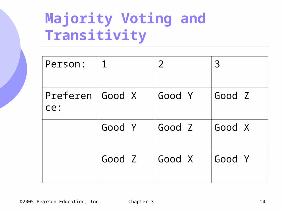
Majority Voting and Transitivity

Person: 1 2 3

Preference: Good X Good Y Good Z

Good Y Good Z Good X

Good Z Good X Good Y



Consumer preferences can be represented graphically using indifference curves

Indifference curves represent all combinations of market baskets that the person is indifferent to A person will be equally satisfied with either

choice


Indifference Curves: An Example

Market Basket Units of Food Units of Clothing

A 20 30

B 10 50

D 40 20

E 30 40

G 10 20

H 10 40



Graph the points with one good on the x-axis and one good on the y-axis

Plotting the points, we can make some immediate observations about preferences More is better


The consumer prefersA to all combinations

in the yellow box, whileall those in the pink

box are preferred to A.


Food

10

20

30

40

10 20 30 40

Clothing

50

G

A

EH

B

D


•Indifferent between points B, A, & D•E is preferred to points on U1

•Points on U1

are preferred to H & G


Food

10

20

30

40

10 20 30 40

Clothing

50

U1

G

D

A

EH

B


Indifference Curves

Indifference curves slope downward to the right If they sloped upward, they would violate the

assumption that more is preferred to lessSome points that had more of both goods would

be indifferent to a basket with less of both goods


Indifference Curves

To describe preferences for all combinations of goods/services, we have a set of indifference curves – an indifference map Each indifference curve in the map shows

the market baskets among which the person is indifferent


U2

U3

Indifference Map

Food

Clothing

U1

ABD

Market basket Ais preferred to B.Market basket B ispreferred to D.


Indifference Maps

Indifference maps give more information about shapes of indifference curves Indifference curves cannot cross

Violates assumption that more is better Why? What if we assume they can cross?


Indifference Maps

Food

Clothing •B is preferred to D•A is indifferent to B & D•B must be indifferent to D but that can’t be if B is preferred to D

U1

U1

U2

U2

A

B

D


Indifference Curves

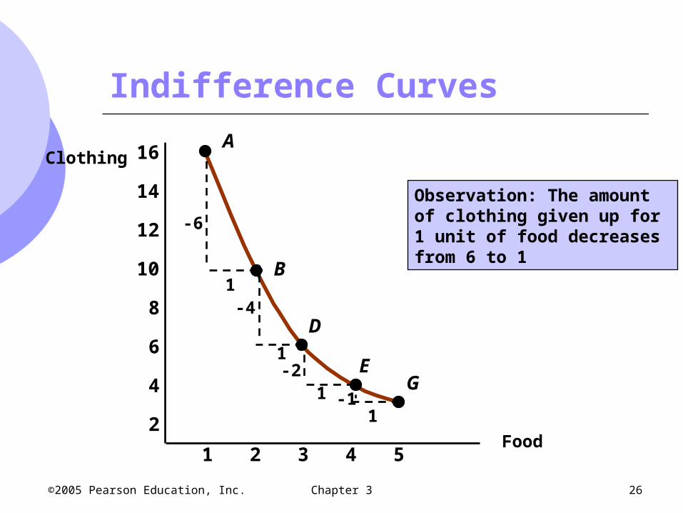
The shapes of indifference curves describe how a consumer is willing to substitute one good for another A to B, give up 6 clothing to get 1 food D to E, give up 2 clothing to get 1 food

The more clothing and less food a person has, the more clothing they will give up to get more food


A

B

D

EG

-1

-6

1

1

-4

-21

1

Observation: The amountof clothing given up for 1 unit of food decreasesfrom 6 to 1

Indifference Curves

Food

Clothing

2 3 4 51

2

4

6

8

10

12

14

16


Indifference Curves

We measure how a person trades one good for another using the marginal rate of substitution (MRS) It quantifies the amount of one good a

consumer will give up to obtain more of another good

It is measured by the slope of the indifference curve


Marginal Rate of Substitution

Food2 3 4 51

Clothing

2

4

6

8

10

12

14

16 A

B

D

EG

-6

1

1

11

-4

-2-1

MRS = 6

MRS = 2

FCMRS



Indifference curves are convex (bowed inward) As more of one good is consumed, a

consumer would prefer to give up fewer units of a second good to get additional units of the first one

Consumers generally prefer a balanced market basket



The MRS decreases as we move down the indifference curve Along an indifference curve there is a

diminishing marginal rate of substitution. The MRS went from 6 to 4 to 1



Indifference curves with different shapes imply a different willingness to substitute

Two polar cases are of interest Perfect substitutes Perfect complements



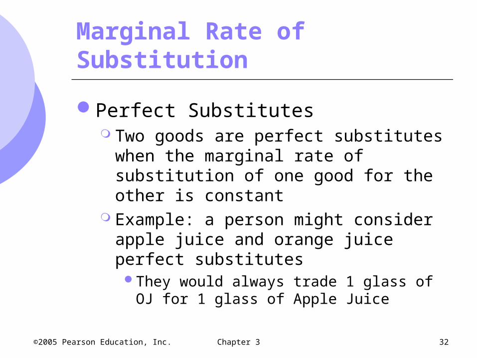
Perfect Substitutes Two goods are perfect substitutes when the

marginal rate of substitution of one good for the other is constant

Example: a person might consider apple juice and orange juice perfect substitutes

They would always trade 1 glass of OJ for 1 glass of Apple Juice



Orange Juice(glasses)

Apple Juice

(glasses)

2 3 41

1

2

3

4

0

PerfectSubstitute

s



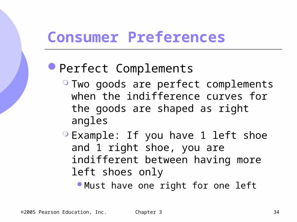
Perfect Complements Two goods are perfect complements when

the indifference curves for the goods are shaped as right angles

Example: If you have 1 left shoe and 1 right shoe, you are indifferent between having more left shoes only

Must have one right for one left



Right Shoes

LeftShoes

2 3 41

1

2

3

4

0

PerfectComplements



We have assumed all our commodities are “goods”

There are commodities we don’t want more of - bads Things for which less is preferred to more

Examples Air pollution Asbestos



How do we account for bads in our preference analysis? We redefine the commodity

Clean airPollution reductionAsbestos removal


Consumer Preferences: An Application

In designing new cars, automobile executives must determine how much time and money to invest in restyling versus increased performance Higher demand for car with better styling and

performance Both cost more to improve



An analysis of consumer preferences would help to determine where to spend more on change: performance or styling

Some consumers will prefer better styling and some will prefer better performance



These consumers

place a greater value

on performance than styling

Styling

Performance



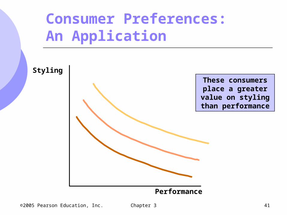
These consumers place a greater value on styling

than performance

Styling

Performance



Knowing which group dominates the market will help decide where redesigning dollars should go

A recent study in the US shows that over the past two decades, most consumers have preferred styling over performance


Preferences and Numerical Values

The theory of consumer behavior does not require assigning a numerical value to the level of satisfaction

Although ranking of market baskets is good, sometimes numerical value is useful



Utility A numerical score representing the

satisfaction that a consumer gets from a given market basket

If buying 3 copies of Microeconomics makes you happier than buying one shirt, then we say that the books give you more utility than the shirt


Utility

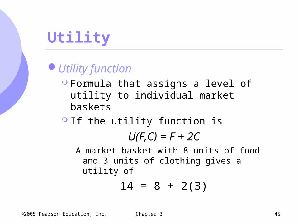
Utility function Formula that assigns a level of utility to

individual market baskets If the utility function is

U(F,C) = F + 2CA market basket with 8 units of food and 3 units of

clothing gives a utility of

14 = 8 + 2(3)


Utility - Example

Market Basket

Food Clothing Utility

A 8 3 8 + 2(3) = 14

B 6 4 6 + 2(4) = 14

C 4 4 4 + 2(4) = 12

Consumer is indifferent between A & B and prefers both to C


Utility - Example

Baskets for each level of utility can be plotted to get an indifference curve To find the indifference curve for a utility of

14, we can change the combinations of food and clothing that give us a utility of 14


Utility - Example

Food10 155

5

10

15

0

Clothing

U1 = 25

U2 = 50

U3 = 100A

B

C

Basket U = FC C 25 = 2.5(10) A 25 = 5(5) B 25 = 10(2.5)


Utility

Although we numerically rank baskets and indifference curves, numbers are ONLY for ranking

A utility of 4 is not necessarily twice as good as a utility of 2, just better

There are two types of rankings Ordinal ranking Cardinal ranking


Utility

Ordinal Utility Function Places market baskets in the order of most

preferred to least preferred, but it does not indicate how much one market basket is preferred to another

Interpersonal comparisons impossibleCardinal Utility Function

Utility function describing the extent to which one market basket is preferred to another


Budget Constraints

Preferences do not explain all of consumer behavior

Budget constraints also limit an individual’s ability to consume in light of the prices they must pay for various goods and services


Budget Constraints

The Budget Line Indicates all combinations of two

commodities for which total money spent equals total income

We assume only 2 goods are consumed, so we do not consider savings


The Budget Line

Let F equal the amount of food purchased, and C is the amount of clothing

Price of food = PF and price of clothing = PC

Then PFF is the amount of money spent on food, and PCC is the amount of money spent on clothing


ICPFPCF

The Budget Line

The budget line then can be written:

All income is allocated to food (F) and/or clothing (C)


The Budget Line

YXP

P

P

I

YPXPI

YPXPI

Y

X

Y

YX

YX


The Budget Line

Different choices of food and clothing can be calculated that use all income These choices can be graphed as the budget

line

Example: Assume income of $80/week, PF = $1 and PC

= $2


Budget Constraints

Market Basket

Food

PF = $1

Clothing

PC = $2

IncomeI = PFF + PCC

A 0 40 $80

B 20 30 $80

D 40 20 $80

E 60 10 $80

G 80 0 $80


C

F

P

P

F

C Slope -

2

1-

The Budget Line

10

20

A

B

D

E

G

(I/PC) = 40

Food40 60 80 = (I/PF)20

10

20

30

0

Clothing


The Budget Line

As consumption moves along a budget line from the intercept, the consumer spends less on one item and more on the other

The slope of the line measures the relative cost of food and clothing

The slope is the negative of the ratio of the prices of the two goods


The Budget Line

The slope indicates the rate at which the two goods can be substituted without changing the amount of money spent

We can rearrange the budget line equation to make this more clear


The Budget Line

YXP

P

P

I

YPXPI

YPXPI

Y

X

Y

YX

YX


Budget Constraints

The Budget Line The vertical intercept, I/PC, illustrates the

maximum amount of C that can be purchased with income I

The horizontal intercept, I/PF, illustrates the maximum amount of F that can be purchased with income I


The Budget Line

As we know, income and prices can change

As incomes and prices change, there are changes in budget lines

We can show the effects of these changes on budget lines and consumer choices


The Budget Line - Changes

The Effects of Changes in Income An increase in income causes the budget line

to shift outward, parallel to the original line (holding prices constant).

Can buy more of both goods with more income



The Effects of Changes in Income A decrease in income causes the budget line

to shift inward, parallel to the original line (holding prices constant)

Can buy less of both goods with less income



An increase inincome shifts

the budget lineoutward

Food(units per week)

Clothing(units

per week)

80 120 16040

20

40

60

80

0

(I = $160)L2

(I = $80)

L1

L3

(I =$40)

A decrease inincome shifts

the budget lineinward



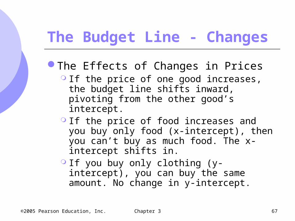
The Effects of Changes in Prices If the price of one good increases, the budget

line shifts inward, pivoting from the other good’s intercept.

If the price of food increases and you buy only food (x-intercept), then you can’t buy as much food. The x-intercept shifts in.

If you buy only clothing (y-intercept), you can buy the same amount. No change in y-intercept.



The Effects of Changes in Prices If the price of one good decreases, the

budget line shifts outward, pivoting from the other good’s intercept.

If the price of food decreases and you buy only food (x-intercept), then you can buy more food. The x-intercept shifts out.

If you buy only clothing (y-intercept), you can buy the same amount. No change in y-intercept.



(PF = 1)

L1

An increase in theprice of food to$2.00 changes

the slope of thebudget line and

rotates it inward.L3

(PF = 2)(PF = 1/2)

L2

A decrease in theprice of food to$.50 changes

the slope of thebudget line and

rotates it outward.

40Food(units per week)

Clothing(units

per week)

80 120 160

40



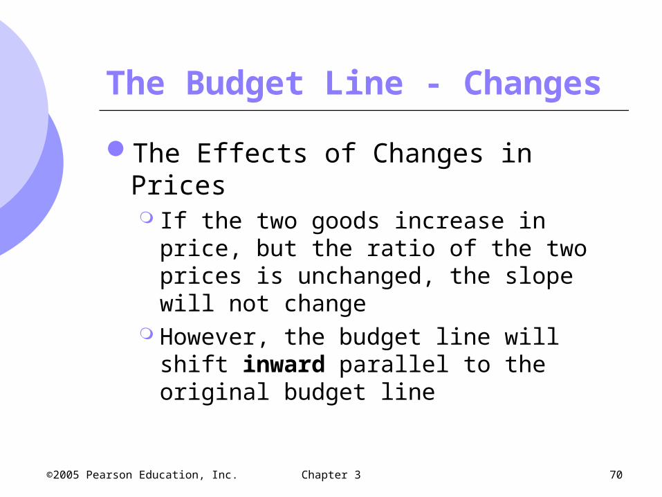
The Effects of Changes in Prices If the two goods increase in price, but the

ratio of the two prices is unchanged, the slope will not change

However, the budget line will shift inward parallel to the original budget line



The Effects of Changes in Prices If the two goods decrease in price, but the

ratio of the two prices is unchanged, the slope will not change

However, the budget line will shift outward parallel to the original budget line


Consumer Choice

Given preferences and budget constraints, how do consumers choose what to buy?

Consumers choose a combination of goods that will maximize their satisfaction, given the limited budget available to them


Consumer Choice

The maximizing market basket must satisfy two conditions:

1. It must be located on the budget line They spend all their income – more is better

2. It must give the consumer the most preferred combination of goods and services


Consumer Choice

Graphically, we can see different indifference curves of a consumer choosing between clothing and food

Remember that U3 > U2 > U1 for our indifference curves

Consumer wants to choose highest utility within their budget


Consumer Choice

U3

D

U2

C

Food (units per week)40 8020

Clothing(units per

week)

20

30

40

0

U1

A

B

•A, B, C on budget line•D highest utility but not affordable•C highest affordable utility•Consumer chooses C


Consumer Choice

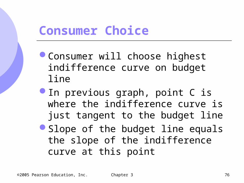
Consumer will choose highest indifference curve on budget line

In previous graph, point C is where the indifference curve is just tangent to the budget line

Slope of the budget line equals the slope of the indifference curve at this point


Consumer Choice

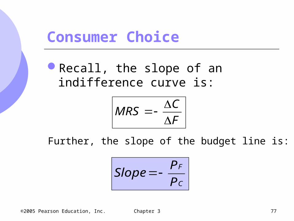
Recall, the slope of an indifference curve is:

F

CMRS

C

F

P

PSlope

Further, the slope of the budget line is:


Consumer Choice

Therefore, it can be said at consumer’s optimal consumption point,

C

F

P

PMRS


Consumer Choice

It can be said that satisfaction is maximized when marginal rate of substitution (of C for F) is equal to the ratio of the prices (of F to C)

Note this is ONLY true at the optimal consumption point


Consumer Choice

Optimal consumption point is where marginal benefits equal marginal costs

MB = MRS = benefit associated with consumption of 1 more unit of food

MC = cost of additional unit of food 1 unit food = ½ unit clothing PF/PC


Consumer Choice

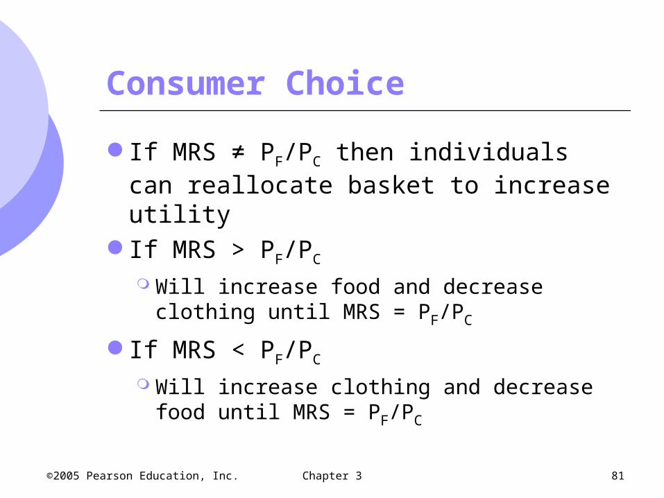
If MRS ≠ PF/PC then individuals can reallocate basket to increase utility

If MRS > PF/PC

Will increase food and decrease clothing until MRS = PF/PC

If MRS < PF/PC

Will increase clothing and decrease food until MRS = PF/PC


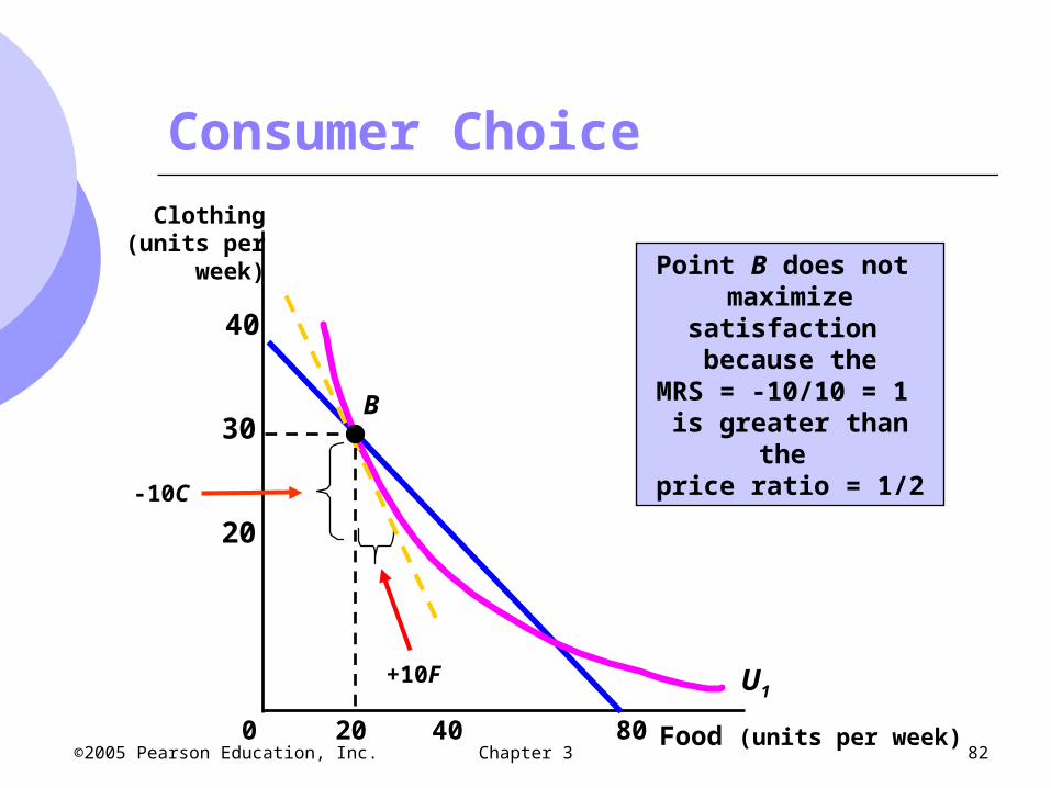
Consumer Choice

Food (units per week)

Clothing(units per

week)

40 8020

20

30

40

0

Point B does not maximize satisfaction

because theMRS = -10/10 = 1

is greater than the price ratio = 1/2

+10F U1

-10C

B


Consumer Choice: An Application Revisited

Consider two groups of consumers, each wishing to spend $10,000 on the styling and performance of a car

Each group has different preferences



By finding the point of tangency between a group’s indifference curve and the budget constraint, auto companies can see how much consumers value each attribute



Styling

Performance$10,000

$10,000 These consumerswant performance worth $7000 and

styling worth $3000

$3,000

$7,000



These consumers want

styling worth $7000 and

performance worth $3000

$3,000

$7,000

Styling

$10,000

$10,000

Performance



Once a company knows preferences, it can design a production and marketing plan

Company can then make a sensible strategic business decision on how to allocate performance and styling on new cars


Consumer Choice

A corner solution exists if a consumer buys in extremes, and buys all of one category of good and none of another MRS is not necessarily equal to PB/PA


A Corner Solution

Ice Cream (cup/month)

FrozenYogurt

(cupsmonthly)

B

A

U2 U3U1

A corner solutionexists at point B.


A Corner Solution

At point B, the MRS of frozen yogurt for ice cream is greater than the slope of the budget line

If the consumer could give up more frozen yogurt for ice cream, he would do so

However, there is no more frozen yogurt to give up

Opposite is true if corner solution was at point A


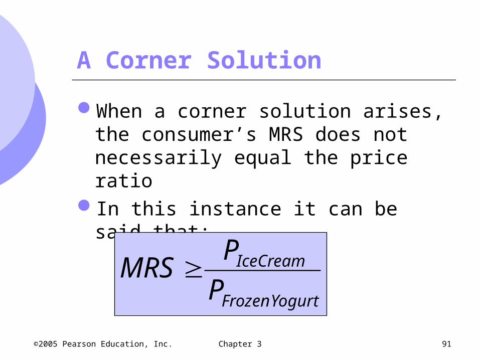
A Corner Solution

When a corner solution arises, the consumer’s MRS does not necessarily equal the price ratio

In this instance it can be said that:

YogurtFrozen

IceCream

P

PMRS


A Corner Solution

If the MRS is, in fact, significantly greater than the price ratio, then a small decrease in the price of frozen yogurt will not alter the consumer’s market basket


A Corner Solution - Example

Suppose Jane Doe’s parents set up a trust fund for her college education

The money must be used only for education

Although a welcome gift, an unrestricted gift might be better



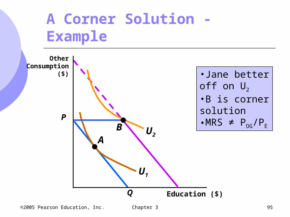
Original budget line, PQ, with a market basket, A, of education and other goods

Trust fund shifts out the budget line as long as trust fund, PB, is spent on education

Jane increases satisfaction, moving to higher indifference curve, U2



P

Q Education ($)

OtherConsumption

($)

U2A

U1

B

•Jane better off on U2

•B is corner solution•MRS ≠ POG/PE



P

Q Education ($)

OtherConsumption

($)

U2A

U1

B

•If gift is unrestricted, Jane can be at point C on U3

•Better off than with restricted gift

CU3


Marginal Utility and Consumer Choice

Marginal utility measures the additional satisfaction obtained from consuming one additional unit of a good How much happier is the individual from

consuming one more unit of food?


Marginal Utility - Example

The marginal utility derived from increasing from 0 to 1 units of food might be 9

Increasing from 1 to 2 might be 7Increasing from 2 to 3 might be 5Observation: Marginal utility is

diminishing as consumption increases


Marginal Utility

The principle of diminishing marginal utility states that as more of a good is consumed, the additional utility the consumer gains will be smaller and smaller

Note that total utility will continue to increase since consumer makes choices that make them happier


Marginal Utility and Indifference Curves

As consumption moves along an indifference curve: Additional utility derived from an increase in

the consumption one good, food (F), must balance the loss of utility from the decrease in the consumption in the other good, clothing (C)



Formally:

C)( MUF) (MU CF 0

No change in total utility along an indifference curve. Trade off of one good to the other leaves the consumer just as well off.



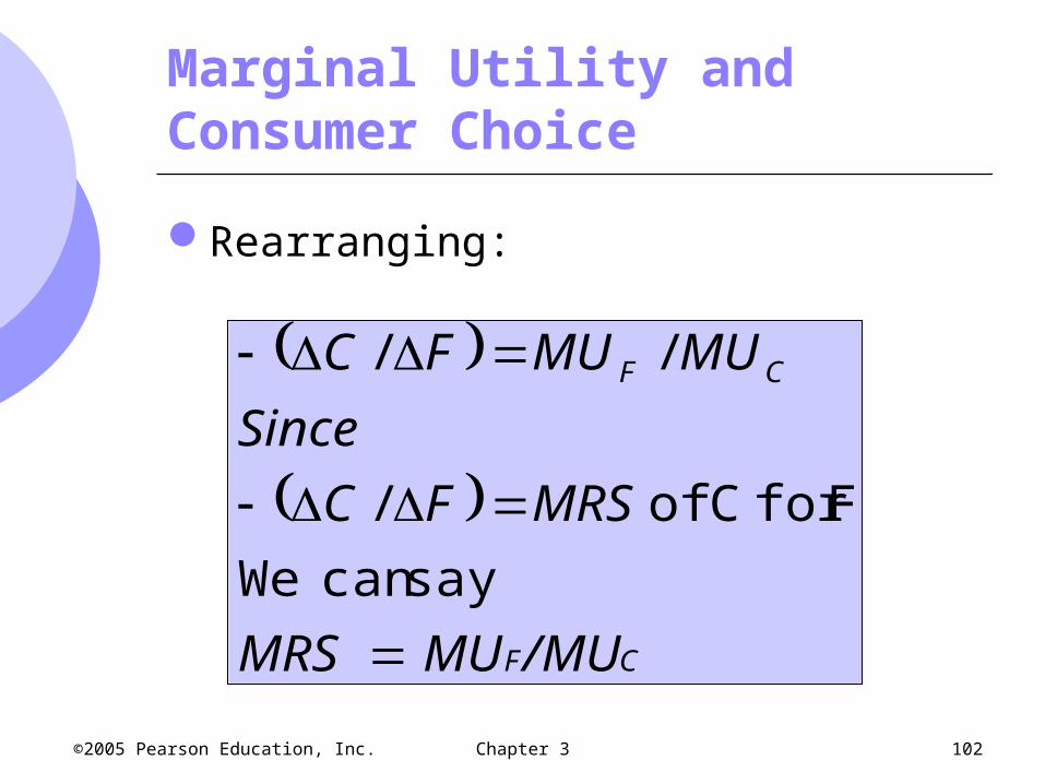
Rearranging:

CF

CF

/MU MUMRS

MRSFC

Since

MUMUFC

saycan We

Ffor C of /

//



When consumers maximize satisfaction:

CF /P PMRS

CF CF /P P /MUMU

Since the MRS is also equal to the ratio of the marginal utility of consuming F and C



Rearranging, gives the equation for utility maximization:

CCFF PMUPMU //



Total utility is maximized when the budget is allocated so that the marginal utility per dollar of expenditure is the same for each good.

This is referred to as the equal marginal principle.


Cost-of-Living Indexes

Social Security payments are given to qualifying individuals

Each year the benefit increases equal to the rate of increase of the Consumer Price Index (CPI) Ratio of the present cost of typical bundle of

goods/services in comparison to the cost during a base period



Does the CPI give a good measure of inflation and therefore a measure of the cost of living changes?

Should the CPI be used to measure how much cost of living has increased, determining increases in government payment programs?



The ideal cost of living index represents the cost of attaining a given level of utility at current prices relative to the cost of attaining the same utility at base prices

Takes into account the fact that consumers can and will substitute some goods for others



To obtain the ideal cost of living index would require too much information, such as consumer preferences as well as prices and expenditures

Actual price indexes are based on consumer purchases, not preferences



Laspeyres price index Amount of money at current year prices that

an individual requires to purchase a bundle of goods/services chosen in a base year divided by the cost of purchasing the same bundle at base-year prices

Ex: CPI



The Laspeyres price index assumes that consumers do not alter their consumption patterns as prices change

Tends to overstate the true cost of living index

Using the CPI to adjust retirement benefits will tend to overcompensate most recipients, requiring greater government expenditure



Paasche index Focuses on the cost of buying the current

year’s bundle Amount of money at current-year prices that

an individual requires to purchase a current bundle of goods/services divided by the cost of purchasing the same bundle in a base year



Comparison of indexes Both are fixed weight indexes Quantities of various goods and services in

each index remain unchanged Laspeyres index keeps quantities at base

year levels Paasche index keeps unchanged quantities

at current year levels



Paasche Index understates inflationOverstates the cost of the base year

bundle (current bundle at base year prices) – consumer would not have chosen that bundle with different relative prices

Thus, denominator overstated and index is understated



Chain-Weighted Indexes Cost-of-living index that accounts for

changes in quantities of goods and services Introduced to overcome problems that arose

when long-term comparisons were made using fixed weight price indexes


Practice: Chapter 3, #15

15. Jane receives utility from days spent traveling on vacation domestically (D) and days spent traveling on vacation in a foreign country (F), as given by the utility function: U = 10DF. In addition, the price of a day spent traveling domestically is $100, the price of a day spent traveling in a foreign country is $400, and Jane’s annual travel budget is $4,000.

Illustrate the indifference curve associated with a utility of 800 and the indifference curve associated with a utility of 1200.


Practice

The indifference curve with a utility of 800 has the equation 10DF=800, or DF=80. Choose combinations of D and F whose product is 80 to find a few bundles. The indifference curve with a utility of 1200 has the equation 10DF=1200, or DF=120. Choose combinations of D and F whose product is 120 to find a few bundles.


Practice

Can Jane afford any of the bundles that give her a utility of 800? What about a utility of 1200?

Yes she can afford some of the bundles that give her a utility of 800 as part of this indifference curve lies below the budget line. She cannot afford any of the bundles that give her a utility of 1200 as this whole indifference curve lies above the budget line.


Practice

Find Jane’s utility maximizing choice of days spent traveling domestically and days spent in a foreign country. (We will need to set the slope of the budget line equal to the slope of the indifference curve by taking two derivatives.)


Practice

The optimal bundle is where the slope of the indifference curve is equal to the slope of the budget line, and Jane is spending her entire income. The slope of the budget line is -PD/PF = -1/4

The slope of the indifference curve is: MRS= -MUD/MUF = -10F/10D = -F/D

Setting the two equal we get:-F/D = -1/4 We now have two equations and two unknowns:4F=D

and 100D+400F=$4000 Solving the above two equations gives D=20 and F=5.

Utility is 1000. This bundle is on an indifference curve between the two

you had previously drawn.


Practice: Chapter 3, #4

Janelle and Brian each plan to spend $20,000 on the styling and gas mileage features of a new car. They can each choose all styling, all gas mileage, or some combination of the two. Janelle does not care at all about styling and wants the best gas mileage possible. Brian likes both equally and wants to spend an equal amount on the two features. Using indifference curves and budget lines, illustrate the choice that each person will make.


Practice

Assume styling is on the vertical axis and gas mileage is on the horizontal axis. Janelle has indifference curves that are vertical. As her indifference curves move over to the right, she gains more gas mileage and more satisfaction. She will spend all $20,000 on gas mileage. This is a corner solution.


Practice

Brian has indifference curves that are L-shaped. He will not spend more on one feature than on the other feature. He will spend $10,000 on styling and $10,000 on gas mileage. Styling and gas mileage are perfect complements for Brian.


Homework Due Wednesday, October 24

Exercises Chapter 3: #3, #4 and #5Questions for Review Chapter 4: #3 and

#8

Documents

Practice Problem: Chapter 2 #6 The rent control agency of NYC has found that aggregate demand is QD = 160-8P. Quantity is measured in tens of thousands