Embed Size (px)
Citation preview
Precipitation Measurements withMicrowave Sensors
vorgelegt vonAndreas LeuenbergerMay 2009
Masterarbeit der Philosophisch-naturwissenschaftlichen Fakultätder Universität Bern
Leiter der Arbeit:Prof. Dr. Ch. Mätzler
Institut für Angewandte Physik

Contents
1 Introduction 1
1.1 Outline of this Document . . . . . . . . . . . . . . . . . . . . . . . . . . 2
2 Principles of Radiometry 3
2.1 Radiance and Radiative Flux . . . . . . . . . . . . . . . . . . . . . . . . 3
2.1.1 Spectral Radiance If . . . . . . . . . . . . . . . . . . . . . . . . . 3
2.1.2 Radiative Flux F . . . . . . . . . . . . . . . . . . . . . . . . . . . 3
2.2 Thermal Radiation . . . . . . . . . . . . . . . . . . . . . . . . . . . . . . 4
2.2.1 Planck Function . . . . . . . . . . . . . . . . . . . . . . . . . . . 4
2.2.2 Rayleigh-Jeans Approximation . . . . . . . . . . . . . . . . . . . 4
2.2.3 Stefan-Boltzmann Law . . . . . . . . . . . . . . . . . . . . . . . . 4
2.2.4 Brightness Temperature Tb . . . . . . . . . . . . . . . . . . . . . 5
2.3 Radiation and Interactions . . . . . . . . . . . . . . . . . . . . . . . . . . 5
2.3.1 Kirchho's Law . . . . . . . . . . . . . . . . . . . . . . . . . . . . 6
2.3.2 Cross Sections σi . . . . . . . . . . . . . . . . . . . . . . . . . . . 7
2.3.3 Eciencies Qi . . . . . . . . . . . . . . . . . . . . . . . . . . . . . 8
2.4 Scattering . . . . . . . . . . . . . . . . . . . . . . . . . . . . . . . . . . . 8
2.4.1 Scattering Regimes . . . . . . . . . . . . . . . . . . . . . . . . . . 8
2.4.2 Rayleigh Scattering . . . . . . . . . . . . . . . . . . . . . . . . . . 10
2.4.3 Mie Theory . . . . . . . . . . . . . . . . . . . . . . . . . . . . . . 10
2.5 Radiative Transfer . . . . . . . . . . . . . . . . . . . . . . . . . . . . . . 12
2.5.1 Opacity and the Law of Beer-Lambert . . . . . . . . . . . . . . . 12
2.5.2 Propagation Coecients (γext, γabs, γscat, γb) . . . . . . . . . . . 13
2.5.3 Propagation Through an Emitting Medium . . . . . . . . . . . . 14
3 Radar 17
3.1 The Radar Principle . . . . . . . . . . . . . . . . . . . . . . . . . . . . . 17
3.2 Range Resolution . . . . . . . . . . . . . . . . . . . . . . . . . . . . . . . 18
3.3 The Radar Equation . . . . . . . . . . . . . . . . . . . . . . . . . . . . . 18
3.3.1 Single Scatterer . . . . . . . . . . . . . . . . . . . . . . . . . . . . 18
3.3.2 Many Scatterers . . . . . . . . . . . . . . . . . . . . . . . . . . . 19
3.3.3 The Radar Reectivity Factor . . . . . . . . . . . . . . . . . . . . 20
3.3.4 The Equivalent Radar Reectivity . . . . . . . . . . . . . . . . . 21
i
ii CONTENTS
3.4 Doppler Frequency Shift . . . . . . . . . . . . . . . . . . . . . . . . . . . 21
4 Dielectric Properties 23
4.1 The Dielectric Constant . . . . . . . . . . . . . . . . . . . . . . . . . . . 23
4.1.1 Dielectric Mixing Formula . . . . . . . . . . . . . . . . . . . . . . 24
4.2 Polarization . . . . . . . . . . . . . . . . . . . . . . . . . . . . . . . . . . 25
4.2.1 Electronic Polarization . . . . . . . . . . . . . . . . . . . . . . . . 25
4.2.2 Atomic Polarization . . . . . . . . . . . . . . . . . . . . . . . . . 26
4.2.3 Orientation Polarization . . . . . . . . . . . . . . . . . . . . . . . 26
4.2.4 Space Charge Polarization . . . . . . . . . . . . . . . . . . . . . . 26
4.3 Dry Atmosphere . . . . . . . . . . . . . . . . . . . . . . . . . . . . . . . 26
4.4 Water Vapor . . . . . . . . . . . . . . . . . . . . . . . . . . . . . . . . . 27
4.5 Liquid Water . . . . . . . . . . . . . . . . . . . . . . . . . . . . . . . . . 28
4.6 Ice . . . . . . . . . . . . . . . . . . . . . . . . . . . . . . . . . . . . . . . 28
4.7 Cloud Water . . . . . . . . . . . . . . . . . . . . . . . . . . . . . . . . . 30
4.8 Rain . . . . . . . . . . . . . . . . . . . . . . . . . . . . . . . . . . . . . . 30
4.9 Dry Snow . . . . . . . . . . . . . . . . . . . . . . . . . . . . . . . . . . . 31
4.10 Wet Snow . . . . . . . . . . . . . . . . . . . . . . . . . . . . . . . . . . . 32
5 Physics of Precipitation 35
5.1 Stratiform Precipitation . . . . . . . . . . . . . . . . . . . . . . . . . . . 35
5.2 The Melting Layer . . . . . . . . . . . . . . . . . . . . . . . . . . . . . . 36
5.3 Classication . . . . . . . . . . . . . . . . . . . . . . . . . . . . . . . . . 37
5.4 Drop Size Distribution . . . . . . . . . . . . . . . . . . . . . . . . . . . . 38
5.5 Terminal Fall Velocity . . . . . . . . . . . . . . . . . . . . . . . . . . . . 39
5.5.1 Characteristic Fall Velocity of Rain . . . . . . . . . . . . . . . . . 39
5.6 Rain Rate . . . . . . . . . . . . . . . . . . . . . . . . . . . . . . . . . . . 40
6 TROWARA 43
6.1 Overview . . . . . . . . . . . . . . . . . . . . . . . . . . . . . . . . . . . 43
6.2 Statistical Algorithm . . . . . . . . . . . . . . . . . . . . . . . . . . . . . 43
6.3 Rened Algorithm . . . . . . . . . . . . . . . . . . . . . . . . . . . . . . 45
6.3.1 Cloud-free Periods . . . . . . . . . . . . . . . . . . . . . . . . . . 46
6.3.2 Example of TROWARA Measurements on a Rainless Day . . . . 48
6.3.3 Rain . . . . . . . . . . . . . . . . . . . . . . . . . . . . . . . . . . 49
6.3.4 Limitations of the Rened Algorithm . . . . . . . . . . . . . . . . 54
6.3.5 Example of TROWARA Measurements for a Rainy Day . . . . . 54
7 MRR 57
7.1 Overview . . . . . . . . . . . . . . . . . . . . . . . . . . . . . . . . . . . 57
7.2 Signal Processing . . . . . . . . . . . . . . . . . . . . . . . . . . . . . . . 59
7.2.1 Frequency Modulated Continuous-Wave (FMCW) Radar . . . . . 60
7.2.2 Height Resolution . . . . . . . . . . . . . . . . . . . . . . . . . . 61
7.2.3 Doppler Velocity . . . . . . . . . . . . . . . . . . . . . . . . . . . 62
CONTENTS iii
7.2.4 Distribution of the Terminal Fall Velocity . . . . . . . . . . . . . 62
7.2.5 Averaging . . . . . . . . . . . . . . . . . . . . . . . . . . . . . . . 63
7.3 Determining the Rain Parameters . . . . . . . . . . . . . . . . . . . . . . 63
7.3.1 Radar Equation . . . . . . . . . . . . . . . . . . . . . . . . . . . . 63
7.3.2 Drop Size Distribution . . . . . . . . . . . . . . . . . . . . . . . . 64
7.3.3 Radar Reectivity Factor . . . . . . . . . . . . . . . . . . . . . . 65
7.3.4 Rain Rate . . . . . . . . . . . . . . . . . . . . . . . . . . . . . . . 65
7.3.5 Liquid Water Content (LWC) . . . . . . . . . . . . . . . . . . . . 66
7.3.6 Characteristic Fall Velocity . . . . . . . . . . . . . . . . . . . . . 66
7.4 Example of MRR Data . . . . . . . . . . . . . . . . . . . . . . . . . . . . 66
7.5 Technical Summary . . . . . . . . . . . . . . . . . . . . . . . . . . . . . . 66
8 Stratiform Precipitation 69
8.1 Characteristics of Stratiform Precipitation . . . . . . . . . . . . . . . . . 69
8.1.1 Frequency Analysis . . . . . . . . . . . . . . . . . . . . . . . . . . 71
8.2 Estimation of the Rain Rate . . . . . . . . . . . . . . . . . . . . . . . . . 72
8.2.1 Rain Estimation by the MRR . . . . . . . . . . . . . . . . . . . . 72
8.2.2 Rain Estimation by the TROWARA . . . . . . . . . . . . . . . . 73
9 The Melting Layer 75
9.1 Radar Reectivity and Fall Velocity Proles . . . . . . . . . . . . . . . . 75
9.1.1 Model Function . . . . . . . . . . . . . . . . . . . . . . . . . . . . 76
9.2 Estimating the Depth of the Melting Layer . . . . . . . . . . . . . . . . 79
9.3 Melting Layer Statistics . . . . . . . . . . . . . . . . . . . . . . . . . . . 79
9.4 Temperature Prole . . . . . . . . . . . . . . . . . . . . . . . . . . . . . 82
9.5 Estimating the Height of the Melting Layer . . . . . . . . . . . . . . . . 83
9.5.1 Problems associated with Dening an Algorithm . . . . . . . . . 83
10 Radiative Model of the Melting Layer 87
10.1 Model of a Melting Snowake . . . . . . . . . . . . . . . . . . . . . . . . 87
10.1.1 Model . . . . . . . . . . . . . . . . . . . . . . . . . . . . . . . . . 87
10.1.2 Simplications and Assumptions . . . . . . . . . . . . . . . . . . 88
10.2 Emission of the Snowake Distribution . . . . . . . . . . . . . . . . . . . 90
10.2.1 Emission . . . . . . . . . . . . . . . . . . . . . . . . . . . . . . . . 90
10.2.2 Simplications and Assumptions . . . . . . . . . . . . . . . . . . 91
10.3 Characteristics of the Melting Layer . . . . . . . . . . . . . . . . . . . . 92
10.3.1 Liquid Water Fraction w . . . . . . . . . . . . . . . . . . . . . . . 92
10.3.2 Volume fraction fv . . . . . . . . . . . . . . . . . . . . . . . . . . 93
10.3.3 Fall Velocity vsnow . . . . . . . . . . . . . . . . . . . . . . . . . . 93
10.4 Model Results . . . . . . . . . . . . . . . . . . . . . . . . . . . . . . . . . 93
10.4.1 Absorption Coecient of the Melting Layer . . . . . . . . . . . . 93
10.4.2 Opacity of the Melting Layer . . . . . . . . . . . . . . . . . . . . 93
10.4.3 Inuence of the Depolarization Factor A1 . . . . . . . . . . . . . 94
10.5 Validation of the Model . . . . . . . . . . . . . . . . . . . . . . . . . . . 95
iv CONTENTS
10.5.1 Estimation of the Opacity of the Melting Layer . . . . . . . . . . 9510.5.2 Comparison of the Measured and the Modeled Opacity . . . . . . 97
10.6 Estimation of the Rain Rate using the ML Opacity . . . . . . . . . . . . 9910.7 The Opacity Ratio . . . . . . . . . . . . . . . . . . . . . . . . . . . . . . 10010.8 Discussion . . . . . . . . . . . . . . . . . . . . . . . . . . . . . . . . . . . 101
11 Conclusions and Outlook 103
Bibliography 105
A Setup of the Micro Rain Radar 107A.1 Setup . . . . . . . . . . . . . . . . . . . . . . . . . . . . . . . . . . . . . 107A.2 Data Storage . . . . . . . . . . . . . . . . . . . . . . . . . . . . . . . . . 107
A.2.1 Copy the Data from the MRR-PC . . . . . . . . . . . . . . . . . 107A.2.2 Insert the Data to the MySQL Database . . . . . . . . . . . . . . 108
A.3 Structure of the Database . . . . . . . . . . . . . . . . . . . . . . . . . . 109
B MATLAB Functions 111
C The Observed Time Series 115C.1 General Information . . . . . . . . . . . . . . . . . . . . . . . . . . . . . 115C.2 Long Precipitation Periods . . . . . . . . . . . . . . . . . . . . . . . . . . 116C.3 Events with Characteristic ML Prole . . . . . . . . . . . . . . . . . . . 117
D Cumulative Precipitation Examples 121
Acknowledgement 125
Chapter 1
Introduction
Water plays a prominent role in the atmosphere. It is important for the understandingof dynamic processes in the atmosphere, weather prediction, now-casting and climateresearch, just to name a few aspects of atmospheric water. Thus, there is great interestto measure atmospheric water in all its phases.
Water occurs in many dierent forms in the atmosphere. In its gas phase it occursas water vapor, in the liquid phase as cloud liquid water, drizzle or rain and its solidphase water occurs as cloud ice, dry snow or hail. Furthermore there exist some mixedforms where liquid water and ice are combined e.g. wet snow or graupel. As manyforms of appearance exist, as many properties have to be considered. This is a greatchallenge for the measurement technique.
Today, atmospheric water can be measured in many dierent ways: Directly inthe atmosphere by balloon or aircraft soundings, from space by satellites and from theground by rain sensors, rain radars or radiometers.
We focus on the measurement of atmospheric water as rain and wet snow by aradiometer. The radiometer is measuring the radiation at two frequencies in the mi-crowave range. Originally, it was designed to measure water vapor and cloud liquidwater. Now, it is enhanced to measure rain liquid.
Melting snow strongly interacts with microwave radiation, whereas the interactionwith rain is weaker and the interaction with dry snow is negligible. To retrieve informa-tion about the region of melting snow, the so-called melting layer, we use an additionalinstrument, a vertical pointing Doppler radar. This radar is a commercial productcalled Micro Rain Radar (MRR). With help of the Doppler eect, the fall velocity ofthe precipitation can be determined.
A radiative model of the melting layer is developed. With this model the opacityof the melting layer can be calculated. To verify this model the modeled opacity iscompared with measurements from the radiometer for selected special rain events whenthe melting layer was just above the altitude of the instruments.
It turned out that the opacity of the melting layer is proportional to the rain rate.With use of this information the algorithm estimating the rain can be improved.
1
2 CHAPTER 1. INTRODUCTION
Maybe the title of this work is a little bit too general, because we do not lookat precipitation in general. We focus on rain and melting snow. And we considerstratiform weather situations only. This limitation is caused by a property of theMRR. At non-stratiform, convective weather situations, strong up- and downdraftscan lead to incorrect interpretations of the measured fall velocity.
To summarize, we hope that this work contributes to a better understanding of theradiative processes of rain and wet snow.
1.1 Outline of this Document
This document can be divided into three parts.The rst part is a concise summary of all necessary theories. It is divided into
four chapters. The rst one summarizes general aspects of radiation: Planck's law,emission, absorption, transmission, scattering, the Rayleigh and Mie approach. In thesecond chapter we briey discuss the radar principles. The third chapter deals with thedielectric properties of the components of the atmosphere (water, water vapor, snowand ice). Relevant principles of clouds and precipitation are given in the fourth andlast chapter of the theory part.
The second part describes the used instruments and their properties, i.e. one chap-ter about the radiometer TROWARA and one about the Micro Rain Radar (MRR).Some measurements are shown and the data are interpreted.
Part three is the most important one in this work. Its rst chapter deals with thecharacteristics of stratiform rain measured by our instruments. Then we take a closerlook at the melting layer spending two chapters on it. We present the measured verticalproles and point out the characteristics of the melting layer. Then, we describe analgorithm to estimate the 0C temperature height. At last, a model of the radiativeproperties of the melting layer is presented and discussed. The model is validated withuse of the measurements of special rain events.
In the appendix, the engineering work of this project is described. This part mustnot be underestimated. A lot of time was used to set up the MRR and to automate theprocesses storing and visualizing the data. Thus, an overview of the setup and the datastorage processes is given. A list with a short description of the most important MAT-LAB functions is given. A last chapter in the appendix gives additional informationand statistics about the rain of the analyzed time series.
Chapter 2
Principles of Radiometry
This chapter is a concise summary of all necessary theories on electromagnetic ra-diation. For more details, we refer to books and scripts listed in the bibliography([13, 6, 22, 25]).
2.1 Radiance and Radiative Flux
2.1.1 Spectral Radiance If
We dene the radiance If by the radiative power dP passing through an area dA,within a solid angle dΩ and a frequency interval df in a certain direction (characterizedby the angle θ representing the tilt to the normal of the area dA). Thus, radiance canbe expressed in W/m2/Hz/sr.
dP = If · df · dA · cos θ · dΩ (2.1)
2.1.2 Radiative Flux F
The radiative ux is a measure for the power transported through an area independentof the direction. Thus, integrating the radiance over all directions (Ω = 4π), leads tothe spectral ux. The spectral ux is expressed in W/m2/Hz.
Ff =∫
4πIf cos θ dΩ (2.2)
If the integration is limited to the forward hemisphere, we call the result Ff+ andfor the backward hemisphere Ff−:
Ff± = ±∫
2πIf cos θ dΩ (2.3)
The sign is such as to provide positive values, and we can write: Ff = Ff+ − Ff−.
3
4 CHAPTER 2. PRINCIPLES OF RADIOMETRY
If we sum over all possible frequencies, we get the ux F (expressed in W/m2) fromthe spectral ux.
F =∫ ∞
0Ff df (2.4)
2.2 Thermal Radiation
2.2.1 Planck Function
If a medium behaves like a blackbody and is in thermal equilibrium, then it emits un-polarized and isotropic spectral radiance according to its frequency f and temperatureT .
The spectral radiance If is given by the Planck function as
If (T ) =2 h f3
c2 (eh f
kb T − 1). (2.5)
where T is the temperature, f the frequency, h = 6.6256 ·10−34 Js the Planck constant,c the speed of light and kb = 1.3805 · 10−23 J/K the Boltzmann constant.
We can replace the frequency f by the wavelength λ using f = c/λ, If df = −Iλ dλand df = −c/λ2 dλ and can write the spectral radiance Iλ as function of the wavelengthλ as
Iλ(T ) =2 h c2
λ5 (eh c
kb λ T − 1). (2.6)
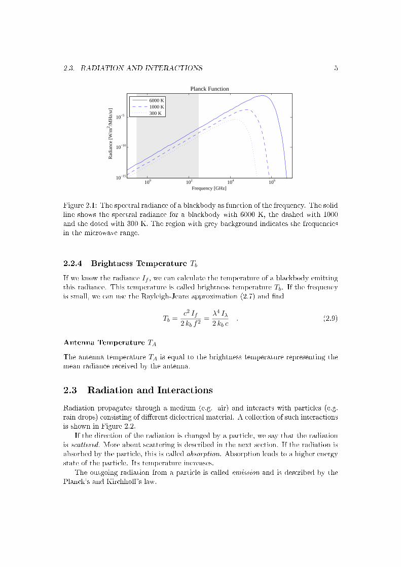
Figure 2.1 shows the spectral radiance If as a function of the frequency f for threedierent temperatures.
2.2.2 Rayleigh-Jeans Approximation
At low frequencies (h f kb T ) the Planck function can be simplied to the followingform. This form is called Rayleigh-Jeans approximation.
If (T ) =2 kb T f2
c2; Iλ(T ) =
2 kb c T
λ4(2.7)
This approximation is valid in the microwave range (wavelengths ranging from 1 mmto 1 m or frequencies between 0.3 GHz and 300 GHz) for usual temperatures in theatmosphere. An important property is that the radiance If increases linearly withtemperature T .
2.2.3 Stefan-Boltzmann Law
If we integrate the spectral radiance If of a blackbody (2.5) over a hemisphere (usingEquation (2.2)) and over all frequencies (using Equation (2.4)), we get the emittedpower per area of a blackbody.
F = σ · T 4 (2.8)
where σ = 5.67 · 10−8 Wm−2K−4 is the Stefan-Boltzmann constant.
2.3. RADIATION AND INTERACTIONS 5
Planck Function
Frequency [GHz]
Rad
ianc
e [W
/m2 /M
Hz/
sr]
100 102 104 10610−15
10−10
10−5
6000 K1000 K300 K
Figure 2.1: The spectral radiance of a blackbody as function of the frequency. The solidline shows the spectral radiance for a blackbody with 6000 K, the dashed with 1000and the doted with 300 K. The region with grey background indicates the frequenciesin the microwave range.
2.2.4 Brightness Temperature Tb
If we know the radiance If , we can calculate the temperature of a blackbody emittingthis radiance. This temperature is called brightness temperature Tb. If the frequencyis small, we can use the Rayleigh-Jeans approximation (2.7) and nd
Tb =c2 If
2 kb f2=
λ4 Iλ
2 kb c. (2.9)
Antenna Temperature TA
The antenna temperature TA is equal to the brightness temperature representing themean radiance received by the antenna.
2.3 Radiation and Interactions
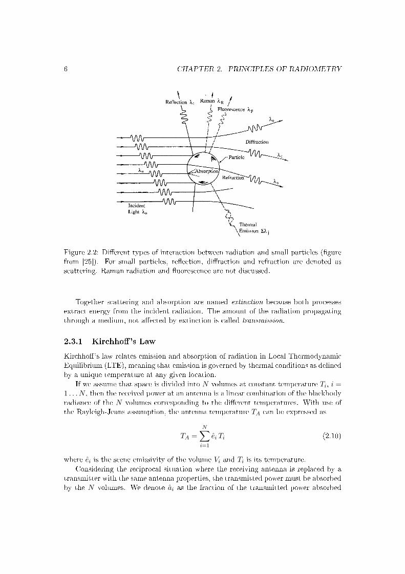
Radiation propagates through a medium (e.g. air) and interacts with particles (e.g.rain drops) consisting of dierent dielectrical material. A collection of such interactionsis shown in Figure 2.2.
If the direction of the radiation is changed by a particle, we say that the radiationis scattered. More about scattering is described in the next section. If the radiation isabsorbed by the particle, this is called absorption. Absorption leads to a higher energystate of the particle. Its temperature increases.
The outgoing radiation from a particle is called emission and is described by thePlanck's and Kirchho's law.
6 CHAPTER 2. PRINCIPLES OF RADIOMETRY
Figure 2.2: Dierent types of interaction between radiation and small particles (gurefrom [25]). For small particles, reection, diraction and refraction are denoted asscattering. Raman radiation and uorescence are not discussed.
Together scattering and absorption are named extinction because both processesextract energy from the incident radiation. The amount of the radiation propagatingthrough a medium, not aected by extinction is called transmission.
2.3.1 Kirchho's Law
Kirchho's law relates emission and absorption of radiation in Local ThermodynamicEquilibrium (LTE), meaning that emission is governed by thermal conditions as denedby a unique temperature at any given location.
If we assume that space is divided into N volumes at constant temperature Ti, i =1 . . . N , then the received power at an antenna is a linear combination of the blackbodyradiance of the N volumes corresponding to the dierent temperatures. With use ofthe Rayleigh-Jeans assumption, the antenna temperature TA can be expressed as
TA =N∑
i=1
ei Ti (2.10)
where ei is the scene emissivity of the volume Vi and Ti is its temperature.
Considering the reciprocal situation where the receiving antenna is replaced by atransmitter with the same antenna properties, the transmitted power must be absorbedby the N volumes. We denote ai as the fraction of the transmitted power absorbed
2.3. RADIATION AND INTERACTIONS 7
in volume Vi. ai is denoted as the scene absorptivity of the volume Vi. Due to theconservation of energy, we can write
N∑i=1
ai = 1 . (2.11)
Now, Kirchho's law states that the scene emissivity ei of a body is equal to itsscene absorptivity ai for all frequencies, directions and polarizations.
ei = ai (2.12)
And thus,N∑
i=1
ei = 1 (2.13)
A special case is the situation of a so-called grey body seen from a transparentmedium. In this situation the space is divided into 2 volumes (N = 2). T1 is thetemperature of the grey body and T2 the temperature of the surrounding backgroundvolume. According to Equation 2.10 and 2.13, we can write
TA = e1 T1 + (1− e1) T2 . (2.14)
In this situation e1 is the emissivity of the grey body.
2.3.2 Cross Sections σi
The concept of cross sections describes the eective area of a particle to absorb, toscatter or to extinct radiation. The product of the incoming radiative ux F0 with thecross section σi gives the scattered, absorbed or extincted power.
Pi = σi F0 ; [W ] = [m2] · [W/m2] (2.15)
where F0 is the incoming ux, σi the cross section, Pi is the absorbed, scattered orextincted power and i stands either for absorption (abs), scattering (scat) or extinction(ext).
As already dened above, extinction is the eect of absorption and scattering to-gether.
σext = σscat + σabs (2.16)
Dierential Cross Section σd
The amount of the scattered radiation depends on the angle ϑ between incoming andoutgoing radiation, and if the particle is not symmetric, the scattered radiation depends
8 CHAPTER 2. PRINCIPLES OF RADIOMETRY
on the orientation angle φ to the particle. Thus, we dene the dierential cross sectionσd as the ratio between scattered power per solid angle to the incoming ux F0.
σd(ϑ, φ) =F (ϑ, φ)
F0;
[m2
sr
]=
[W/sr][W/m2]
(2.17)
The relation between the dierential cross section and the scattering cross sectionis given as
σscat =∫ 2π
0
∫ π
0σd(ϑ, φ) sin ϑ dϑ dφ . (2.18)
Backscattering Cross Section σb
The backscattering cross section is dened as 4 π times the dierential cross section inopposite direction of the incoming ux.
σb = 4π σ180 (2.19)
2.3.3 Eciencies Qi
The eciencies of absorption Qabs, scattering Qscat, backscattering Qb or extinctionQext are dened as the corresponding cross sections normalized to the geometrical crosssection of the particle.
Qi =σi
σg(2.20)
where σg is the geometrical cross section of the particle. For spheres, σg = πD2/4,where D is the diameter of the particle.
2.4 Scattering
2.4.1 Scattering Regimes
Scattering depends strongly on the ratio between the wavelength λ of the radiation andthe size of the particles, expressed by the particle diameter Dp. As a measure for thisratio we use x as size parameter, where x = πDp/λ. We distinguish between dierenttypes of scattering. If the particle is very small compared to the wavelength (Dp λ)the scattering is negligible. If the particles are still small compared to the wavelength(x < 1), we are in the Rayleigh scattering regime and if x ≥ 1 we have to use the Mietheory. The Mie theory considers spheres only. If the wavelength is small compared tothe particle size (x 1), the scattering approaches the laws of geometric optics.
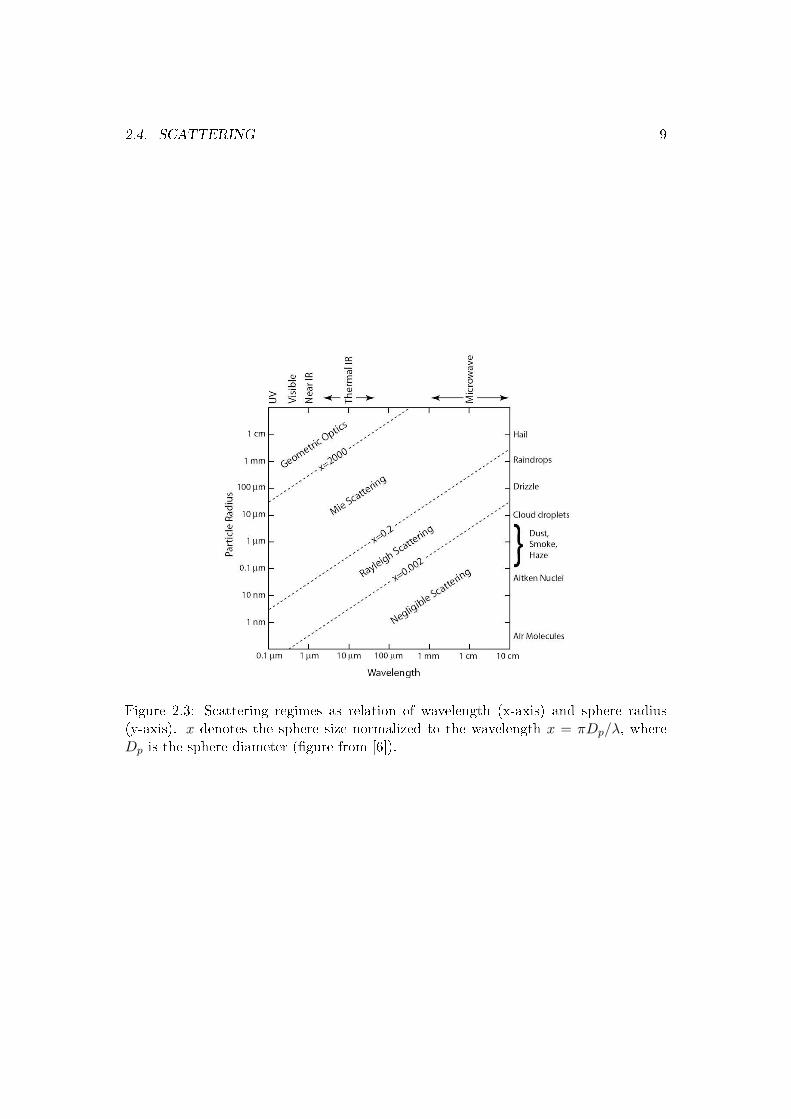
Figure 2.3 gives an overview of the scattering regimes. We use microwaves withwavelength in order of about 1 cm and the particles of interest are snowakes, raindrops and drizzle. As we see in Figure 2.3, the dimensions of the particles exceed thelimits of Rayleigh scattering, and we have to consider Mie scattering.
2.4. SCATTERING 9
Figure 2.3: Scattering regimes as relation of wavelength (x-axis) and sphere radius(y-axis). x denotes the sphere size normalized to the wavelength x = πDp/λ, whereDp is the sphere diameter (gure from [6]).
10 CHAPTER 2. PRINCIPLES OF RADIOMETRY
2.4.2 Rayleigh Scattering
If the sphere is small compared to the wavelength (size parameter x < 1), the scatteringcan be analyzed with the Rayleigh theory. If we assume that the dielectric constant ofthe ambient medium is one, we nd for the scattering eciency
Qscat =83
x4
∣∣∣∣ε− 1ε + 2
∣∣∣∣2 ∼ 1λ4
. (2.21)
ε is the dielectric constant of the material of the sphere. We assume that the particleconsists of a non-magnetic material (µ ≈ 1) and that the surrounding material is air(εair ≈ 1, µair ≈ 1).
The absorption eciency is given by
Qabs = 12xε′′
|ε + 2|2∼ 1
λ(2.22)
and the backscattering eciency by
Qb = 4x4
∣∣∣∣ε− 1ε + 2
∣∣∣∣2 ∼ 1λ4
. (2.23)
We see that the intensity of the scattered radiation is proportional to λ−4. Thus,shortwave radiation is scattered much more than long-wave radiation. The eect ofthe wavelength is not that strong for the absorption eciency. It is just proportionalto λ−1.
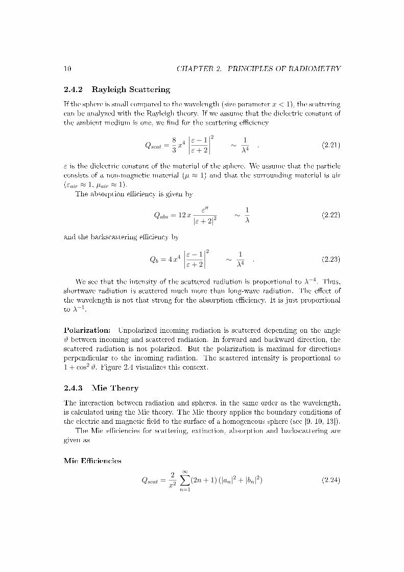
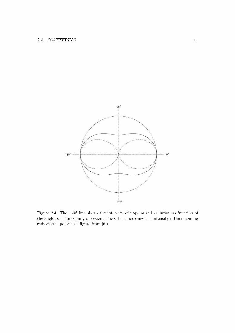
Polarization: Unpolarized incoming radiation is scattered depending on the angleϑ between incoming and scattered radiation. In forward and backward direction, thescattered radiation is not polarized. But the polarization is maximal for directionsperpendicular to the incoming radiation. The scattered intensity is proportional to1 + cos2 ϑ. Figure 2.4 visualizes this context.
2.4.3 Mie Theory
The interaction between radiation and spheres, in the same order as the wavelength,is calculated using the Mie theory. The Mie theory applies the boundary conditions ofthe electric and magnetic eld to the surface of a homogeneous sphere (see [9, 10, 13]).
The Mie eciencies for scattering, extinction, absorption and backscattering aregiven as
Mie Eciencies
Qscat =2x2
∞∑n=1
(2n + 1) (|an|2 + |bn|2) (2.24)
2.4. SCATTERING 11
Figure 2.4: The solid line shows the intensity of unpolarized radiation as function ofthe angle to the incoming direction. The other lines show the intensity if the incomingradiation is polarized (gure from [6]).
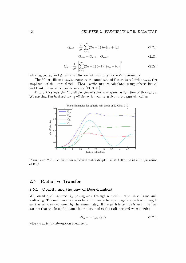
12 CHAPTER 2. PRINCIPLES OF RADIOMETRY
Qext =2x2
∞∑n=1
(2n + 1) Re[an + bn] (2.25)
Qabs = Qext −Qscat (2.26)
Qb =1x2
∣∣∣∣∣∞∑
n=1
(2n + 1) (−1)n (an − bn)
∣∣∣∣∣2
(2.27)
where an, bn, cn and dn are the Mie coecients and x is the size parameter.The Mie coecients an, bn compute the amplitude of the scattered eld, cn, dn the
amplitude of the internal eld. These coecients are calculated using spheric Besseland Hankel functions. For details see [13, 9, 10].
Figure 2.5 shows the Mie eciencies of spheres of water as function of the radius.We see that the backscattering eciency is most sensitive to the particle radius.
0 0.5 1 1.5 2 2.5 3 3.5 4 4.5 50
0.5
1
1.5
2
2.5
3
3.5
Particle radius [mm]
Mie
eff
icie
ncie
s
Mie efficiencies for spheric rain drops at 22 GHz, 0 °C
Q
ext
Qsca
Qabs
Qb
Figure 2.5: Mie eciencies for spherical water droplets at 22 GHz and at a temperatureof 0C.
2.5 Radiative Transfer
2.5.1 Opacity and the Law of Beer-Lambert
We consider the radiance Iλ propagating through a medium without emission andscattering. The medium absorbs radiation. Thus, after a propagating path with lengthds, the radiance decreased by the amount dIλ. If the path length ds is small, we canassume that the loss of radiance is proportional to the radiance and we can write
dIλ = − γabs Iλ ds (2.28)
where γabs is the absorption coecient.
2.5. RADIATIVE TRANSFER 13
To calculate the radiance as a function of the path, we can solve Equation (2.28)for Iλ(s) and get
Iλ(s) = Iλ,s0 e−
R ss0
γabs(s′) ds′
. (2.29)
Iλ,s0 is the radiance at the reference location s0.
With the denition of the opacity (or optical depth) τ
τ(s) =∫ s
s0
γabs(s′) ds′ , (2.30)
we can rewrite Equation (2.29) and get the law of Beer-Lambert.
Iλ(s) = Iλ,s0 e−τ(s) (2.31)
The term T = e−τ(s) lies in a range between 0 and 1 and represents the amountof radiance transmitting through the medium (from s0 to s). This term T is calledtransmittance or transmissivity.
2.5.2 Propagation Coecients (γext, γabs, γscat, γb)
The proportionality factor γabs already mentioned in Equation (2.28) is a called prop-agation coecient, or for the absorption, absorption coecient. In the same manner,propagation coecients for scattering, backscattering and extinction can be dened.
The value of the propagation coecient depends on the medium. If we considerair containing small particles, the propagation coecients depend on the material andthe sizes of the particles. The inuence of the air is neglected. In the previous section,we dened the cross section and eciency of a particle. If the size distribution N(D)of the particles as a function of the particle diameter is known, we can calculate thepropagation coecients as
γj =∫ ∞
0σj(D) N(D) dD =
π
4
∫ ∞
0D2 Qj(D) N(D) dD (2.32)
where the index j represents either extinction (ext), absorption (abs), scattering (scat)or backscattering (b). σj(D) and Qj(D) are the cross section and eciency, respectivelyand N(D) is the size distribution. The propagation coecients have the unit [1/length].
Knowing the dielectric properties of the medium, we can also express the absorptioncoecient as
γabs = 2 k′′ = 2n′′ k0 = 2n′′ω
c0=
4π n′′
λ(2.33)
where k′′ is the imaginary part of the wave number, n′′ the imaginary part of therefractive index, k0 the wave number in vacuum, c0 the speed of light in vacuum, ωthe angular frequency and λ the wavelength.
14 CHAPTER 2. PRINCIPLES OF RADIOMETRY
2.5.3 Propagation Through an Emitting Medium
In the previous section, we considered the absorption/extinction of the radiation bythe medium. What if the medium itself is emitting radiation?
In the following we use the Rayleigh-Jeans approximation (Equation (2.7)) andreplace the radiance by the brightness temperature.
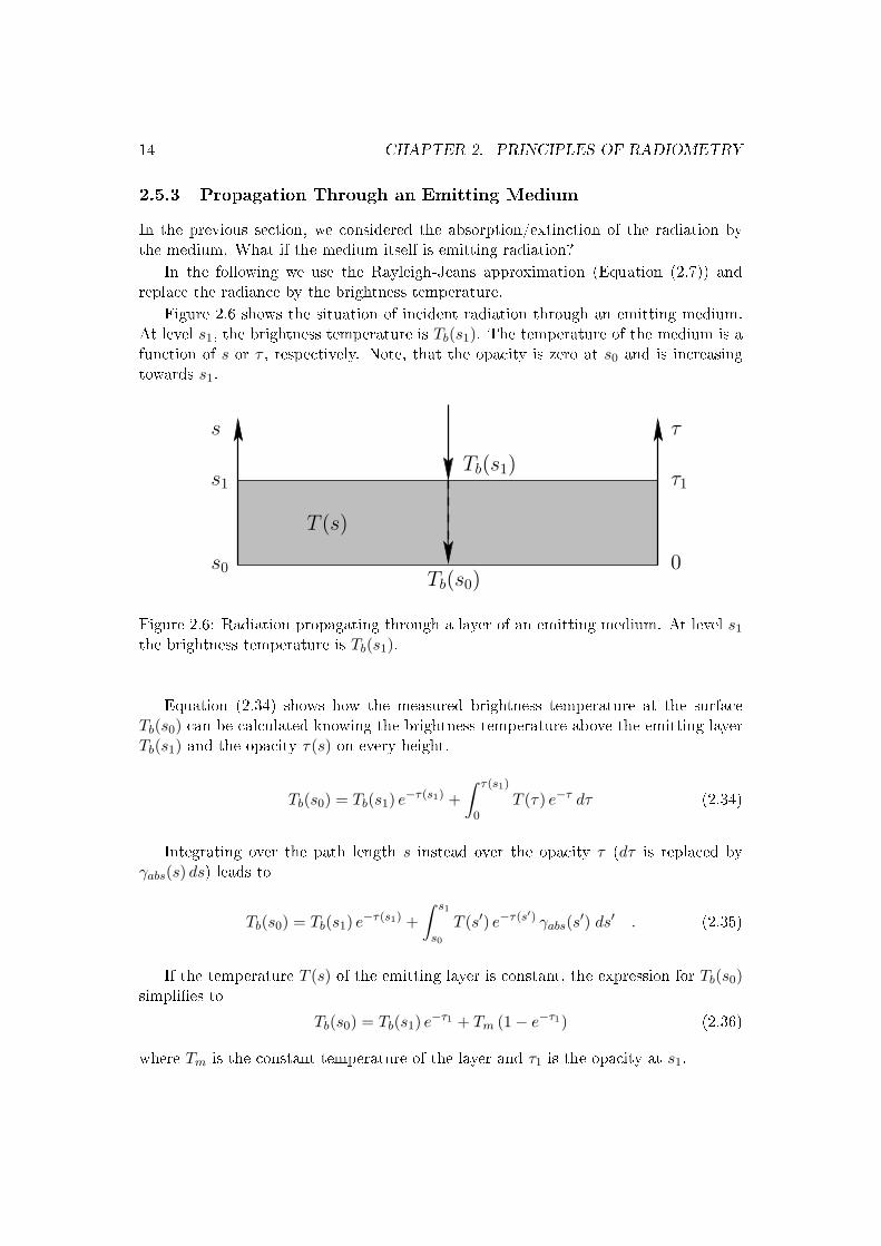
Figure 2.6 shows the situation of incident radiation through an emitting medium.At level s1, the brightness temperature is Tb(s1). The temperature of the medium is afunction of s or τ , respectively. Note, that the opacity is zero at s0 and is increasingtowards s1.
Tb(s1)
T (s)
s τ
τ1s1
s0 0Tb(s0)
Figure 2.6: Radiation propagating through a layer of an emitting medium. At level s1
the brightness temperature is Tb(s1).
Equation (2.34) shows how the measured brightness temperature at the surfaceTb(s0) can be calculated knowing the brightness temperature above the emitting layerTb(s1) and the opacity τ(s) on every height.
Tb(s0) = Tb(s1) e−τ(s1) +∫ τ(s1)
0T (τ) e−τ dτ (2.34)
Integrating over the path length s instead over the opacity τ (dτ is replaced byγabs(s) ds) leads to
Tb(s0) = Tb(s1) e−τ(s1) +∫ s1
s0
T (s′) e−τ(s′) γabs(s′) ds′ . (2.35)
If the temperature T (s) of the emitting layer is constant, the expression for Tb(s0)simplies to
Tb(s0) = Tb(s1) e−τ1 + Tm (1− e−τ1) (2.36)
where Tm is the constant temperature of the layer and τ1 is the opacity at s1.
2.5. RADIATIVE TRANSFER 15
Eective mean temperature: Usually the temperature of the layer is not constant.But we can dene the eective mean temperature according to the following equation
Tm =
∫ τ10 T (τ) e−τ dτ
1− e−τ1(2.37)
and this expression can be used as constant temperature as in Equation (2.36).If we assume that the temperature decreases/increases linearly with increasing opac-
ity τ , we set for the temperature T (τ) = Tc + Td τ and the previous calculation for theeective mean temperature gives
Tm = Tc + Td
[1− τ1 e−τ1
1− e−τ1
]. (2.38)
Setting Tm into Equation (2.36) leads to
Tb(s0) = Tb(s1) e−τ1 + (Tc + Td) (1− e−τ1)− Td τ1 e−τ1 . (2.39)
In an optically thin layer τ1 1, Tm can be approximated by Tm ≈ Tc + 0.5 Td τ1.And in an optical thick layer τ1 1, Tm can be approximated by Tm ≈ T (τ = 1) =Tc + Td.

16 CHAPTER 2. PRINCIPLES OF RADIOMETRY
Chapter 3
Radar
Measuring electromagnetic radiation emitted and scattered from objects is called ra-diometry. A passive method. Now, we shortly introduce radar, an active method, wherethe instrument itself transmits radiation and receives the backscattered radiation. Ad-ditionally to the information about the backscattering objects, we get information ontheir positions.
Most of the content described in this chapter is taken from [24] and [11]. The radarinstrument used in this work is described later. Here we describe only the basic radarprinciple.
3.1 The Radar Principle
Radar was invented at the end of the 19th century and is an abbreviation for RAdioDetection And Ranging. The principle can be divided into three main processes. First,the transmitting of the radiation by the radar antenna. Second, the backscatteringby the objects or particles and third, the receiving of the signal by the antenna. Theinformation about the scatterer is extracted from the time delay (or frequency shift) ofthe received signal to the transmitted signal. The intensity of the received signal givesinformation about the size and number of the backscattering objects.
There exist many dierent types of radar operation. We distinguish between pulsedand continuous wave radar. The pulsed radar transmits a burst of radiation and waitsfor the backscattered signal. After a time delay it transmits the next burst. Then aradar system can be coherent or non-coherent. In the rst case, there exists a phaserelation between the transmitted and the received signal. Here, we just consider mono-static radar, where the transmitter and the receiver are located at the same place, incontrast to the bi- or multi-static radar. Usually radar systems work in a frequencyrange from 10 MHz up to 100 GHz.
Figure 3.1 shows a schematic picture of the radar principle. On the left side thetransmitter and receiver are shown, and on the right side a scattering particle is drawn.
17
18 CHAPTER 3. RADAR
Pr
Pt
σb
StSr
r
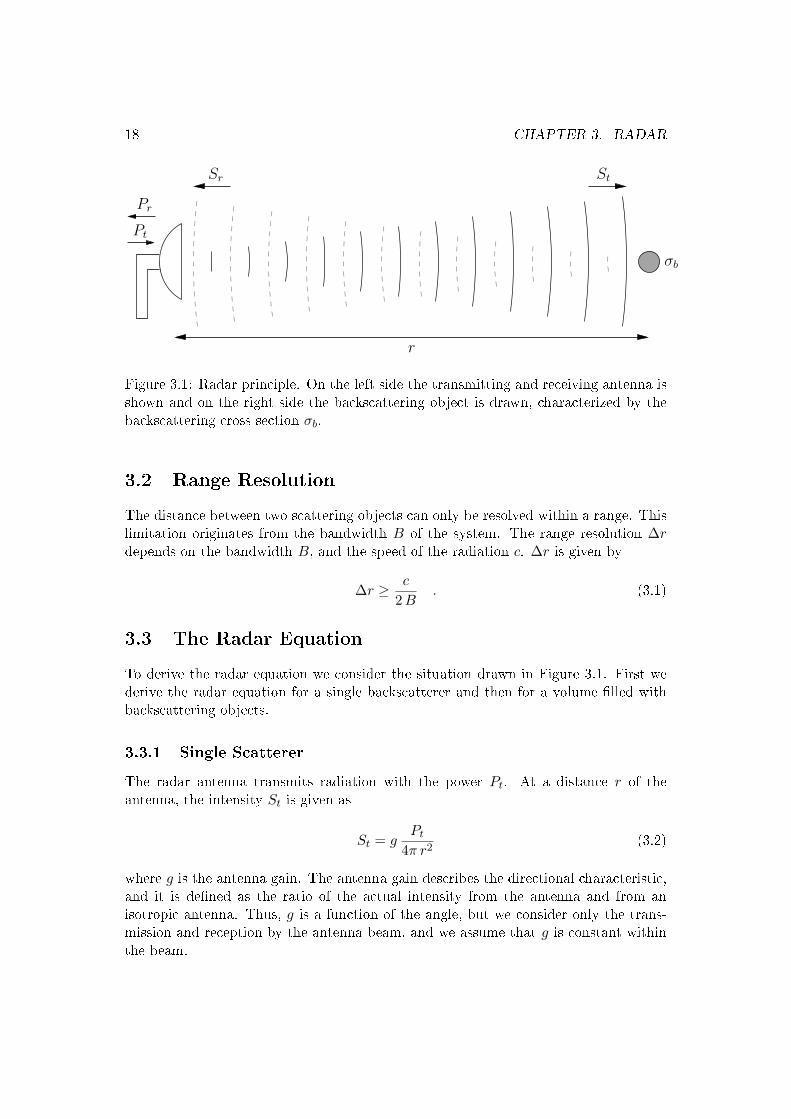
Figure 3.1: Radar principle. On the left side the transmitting and receiving antenna isshown and on the right side the backscattering object is drawn, characterized by thebackscattering cross section σb.
3.2 Range Resolution
The distance between two scattering objects can only be resolved within a range. Thislimitation originates from the bandwidth B of the system. The range resolution ∆rdepends on the bandwidth B, and the speed of the radiation c. ∆r is given by
∆r ≥ c
2 B. (3.1)
3.3 The Radar Equation
To derive the radar equation we consider the situation drawn in Figure 3.1. First wederive the radar equation for a single backscatterer and then for a volume lled withbackscattering objects.
3.3.1 Single Scatterer
The radar antenna transmits radiation with the power Pt. At a distance r of theantenna, the intensity St is given as
St = gPt
4π r2(3.2)
where g is the antenna gain. The antenna gain describes the directional characteristic,and it is dened as the ratio of the actual intensity from the antenna and from anisotropic antenna. Thus, g is a function of the angle, but we consider only the trans-mission and reception by the antenna beam, and we assume that g is constant withinthe beam.
3.3. THE RADAR EQUATION 19
The scattering object is characterized by the backscattering cross section σb. Thescattered power is the product of the incoming intensity St and the cross section σb.At the receiver the intensity Sr of the scattered object is given as
Sr =σb St
4π r2. (3.3)
From antenna theory we know that the ratio of received power to the intensity Sr
depends on the wavelength λ, and the antenna gain is given as
g = 4πPr
λ2 Sr. (3.4)
Summarizing the previous three equations and solving for the received power Pr,we get the radar equation for a single scatterer.
Pr =1
(4π)3g2 λ2Pt
σb
r4(3.5)
3.3.2 Many Scatterers
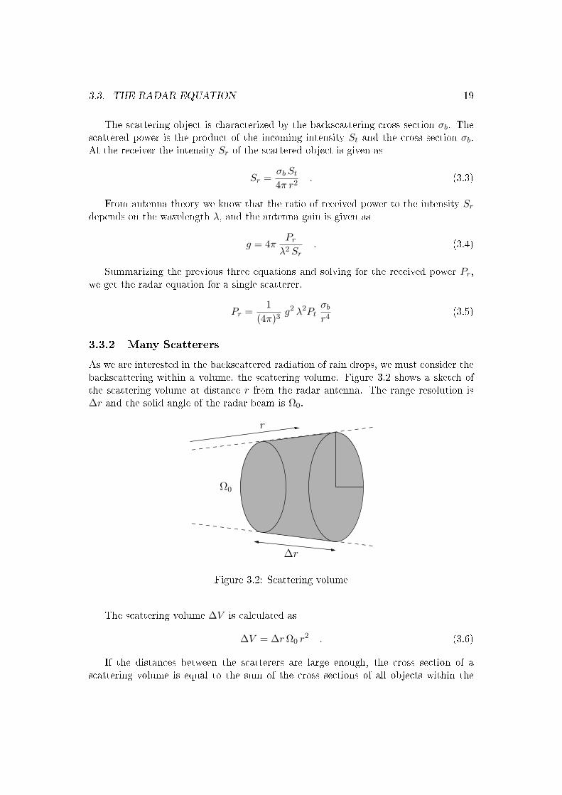
As we are interested in the backscattered radiation of rain drops, we must consider thebackscattering within a volume, the scattering volume. Figure 3.2 shows a sketch ofthe scattering volume at distance r from the radar antenna. The range resolution is∆r and the solid angle of the radar beam is Ω0.
Ω0
∆r
r
Figure 3.2: Scattering volume
The scattering volume ∆V is calculated as
∆V = ∆r Ω0 r2 . (3.6)
If the distances between the scatterers are large enough, the cross section of ascattering volume is equal to the sum of the cross sections of all objects within the
20 CHAPTER 3. RADAR
scattering volume. This total cross section divided by volume ∆V is described asvolume backscatter coecient η and can be calculated from
η =∑
i σb,i
∆V(3.7)
where i is an index for every scattering object.
With the total backscattering cross section∑
i σb,i = η ∆V , described by the volumebackscatter coecient η, the radar equation for a cloud of many backscatterer leads to
Pr =1
(4π)3g2 λ2Pt
η
r2∆r Ω0 (3.8)
If we measure the received power by the antenna and know the antenna character-istics, we can solve the equation for the volume backscatter coecient η.
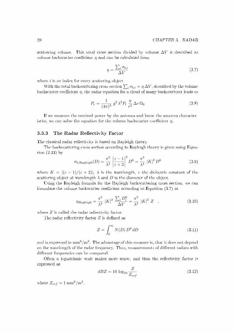
3.3.3 The Radar Reectivity Factor
The classical radar reectivity is based on Rayleigh theory.
The backscattering cross section according to Rayleigh theory is given using Equa-tion (2.23) by
σb,Rayleigh(D) =π5
λ4
∣∣∣∣ε− 1ε + 2
∣∣∣∣2 D6 =π5
λ4|K|2 D6 (3.9)
where K = |(ε − 1)/(ε + 2)|, λ is the wavelength, ε the dielectric constant of thescattering object at wavelength λ and D is the diameter of the object.
Using the Rayleigh formula for the Rayleigh backscattering cross section, we canformulate the volume backscatter coecient according to Equation (3.7) as
ηRayleigh =π5
λ4|K|2
∑i D
6i
∆V=
π5
λ4|K|2 Z . (3.10)
where Z is called the radar reectivity factor.
The radar reectivity factor Z is dened as
Z =∫ ∞
0N(D) D6 dD (3.11)
and is expressed in mm6/m3. The advantage of this measure is, that it does not dependon the wavelength of the radar frequency. Thus, measurements of dierent radars withdierent frequencies can be compared.
Often a logarithmic scale makes more sense, and thus the reectivity factor isexpressed as
dBZ = 10 log10
Z
Zref(3.12)
where Zref = 1 mm6/m3.
3.4. DOPPLER FREQUENCY SHIFT 21
3.3.4 The Equivalent Radar Reectivity
When the observed scattering volume does not satisfy the conditions of the Rayleighapproximation, it is convenient to characterize the radar reectivity factor Z by theequivalent radar reectivity Ze. Ze is equal to the reectivity factor of a population ofliquid and spherical particles satisfying the Rayleigh approximation and producing asignal of the same power. Thus,
Ze =λ4
π5 |Kw|2η (3.13)
where Kw is the dielectric factor of water.In the following text, when we write reectivity or radar reectivity, we mean the
equivalent radar reectivity Ze.
3.4 Doppler Frequency Shift
If an electromagnetic signal is reected at a moving object, the frequency of the reectedsignal is shifted. An object moving towards the antenna increases the frequency, movingaway from the antenna decreases the frequency. This eect is called Doppler eect andis used to determine the speed of the scattering objects.
The frequency shift is given as
∆fD =2λ
v (3.14)
where ∆fD is the frequency shift by the Doppler eect, λ is the wavelength and v isthe speed of the object in direction towards/away from the radar antenna.

22 CHAPTER 3. RADAR
Chapter 4
Dielectric Properties
We have seen that the properties to emit, to absorb, to transmit and to scatter dependon the size of the particles, and the inuence of the particle size was discussed inChapter 2 (Rayleigh and Mie theory).
The inuence of the matter itself is also very important. Thus, we are discussingthe dielectric properties of the material. As we are interested in rain and snow, wesummarize the dielectric properties of the dry atmosphere, of water vapor, of liquidwater, of cloud water, of ice, of rain, of dry and wet snow.
Most of the information in this chapter is taken from [13], [26] and [12].
4.1 The Dielectric Constant
If an electric eld E acts on a medium, the medium is polarized and inuences thedisplacement eld D. The strength of the polarization depends on the material. Theinuence of the material can be expressed by the dielectic constant ε′ (in vacuumε′ = 1).
D = ε0 E + P = ε′ ε0 E (4.1)
D is the displacement eld, E the electric eld, P the polarization, ε0 the vacuumpermittivity and ε′ the relative dielectric constant.
The complex relative dielectric constant ε is dened as
ε = ε′ + i ε′′ , (4.2)
where ε′ is the relative dielectric constant from Equation (4.1). The imaginary part ε′′
origins from Ohm's law and is dened as
j = σE = ε′′ ε0 ω E (4.3)
where j is the current density, σ the conductivity and ω the angular frequency.As the behavior of the material depends on the frequency, ε is a function of fre-
quency.
23
24 CHAPTER 4. DIELECTRIC PROPERTIES
The complex refractive index n is given as
n = n′ + i n′′ =√
ε µ ≈√
ε (4.4)
where µ is the relative magnetic permeability. In the following, we consider non-magnetic materials only (µ = 1) and use the approximation on the right side of Equa-tion (4.4).
The imaginary part n′′ of the refractive index n is a measure of the loss in thematerial. Thus, the following relation between the n′′ and the absorption coecientγabs is valid (as already expressed in Equation (2.33)).
γabs =4π n′′
λ(4.5)
λ is the wavelength.
4.1.1 Dielectric Mixing Formula
If we have a heterogeneous medium with structures much smaller than the wavelength,we can use the Maxwell-Garnett formula to calculate the eective dielectric constant εof the heterogeneous medium. We consider a host medium with the relative dielectricconstant εe with inserted particles with εi. Then the Maxwell-Garnett formula is givenas
ε =(1− fv) εe + fv εi K
1− fv + fv K(4.6)
where fv is the volume fraction and K is a parameter depending on the shape of theparticles. But K depends also on the orientation of the particles and generally we haveto consider K as diagonal tensor, where Ki is the element for the i-th principal axis.
If we assume that the inserted particles are ellipsoids and that they are orientedisotropically, we can use the average K factor dened as
K =13
3∑k=1
Ki ; with Ki =εe
εe + Ai (εi − εe). (4.7)
The Ki represent the shape factor in the principal axes and Ai is called depolarizationfactor of the ellipsoid along the i-axis. Note, that A1 + A2 + A3 = 1. If the ellipsoidis at like a disk, it is called oblate and A1 = A2 < 1/3, A3 > 1/3. If it looks like aneedle, it is called prolate and A1 = A2 > 1/3, A3 < 1/3.
For hydrometeors, the Maxwell-Garnett formula (4.6) can be simplied using Kfrom Equation (4.7) and assuming that the volume fraction fv is very small. Thisleads to
ε = εe +fv(εi − εe)
3
3∑k=1
εe
εe + Ak (εi − εe). (4.8)
4.2. POLARIZATION 25
4.2 Polarization
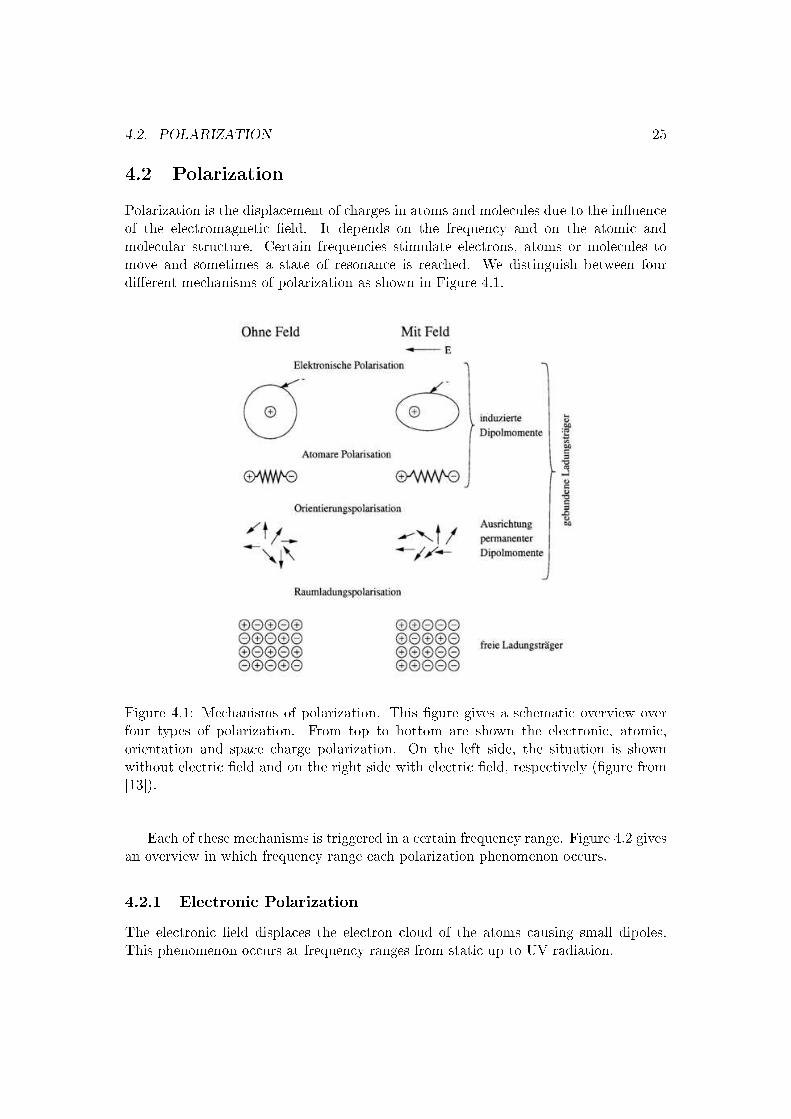
Polarization is the displacement of charges in atoms and molecules due to the inuenceof the electromagnetic eld. It depends on the frequency and on the atomic andmolecular structure. Certain frequencies stimulate electrons, atoms or molecules tomove and sometimes a state of resonance is reached. We distinguish between fourdierent mechanisms of polarization as shown in Figure 4.1.
Figure 4.1: Mechanisms of polarization. This gure gives a schematic overview overfour types of polarization. From top to bottom are shown the electronic, atomic,orientation and space charge polarization. On the left side, the situation is shownwithout electric eld and on the right side with electric eld, respectively (gure from[13]).
Each of these mechanisms is triggered in a certain frequency range. Figure 4.2 givesan overview in which frequency range each polarization phenomenon occurs.
4.2.1 Electronic Polarization
The electronic eld displaces the electron cloud of the atoms causing small dipoles.This phenomenon occurs at frequency ranges from static up to UV radiation.
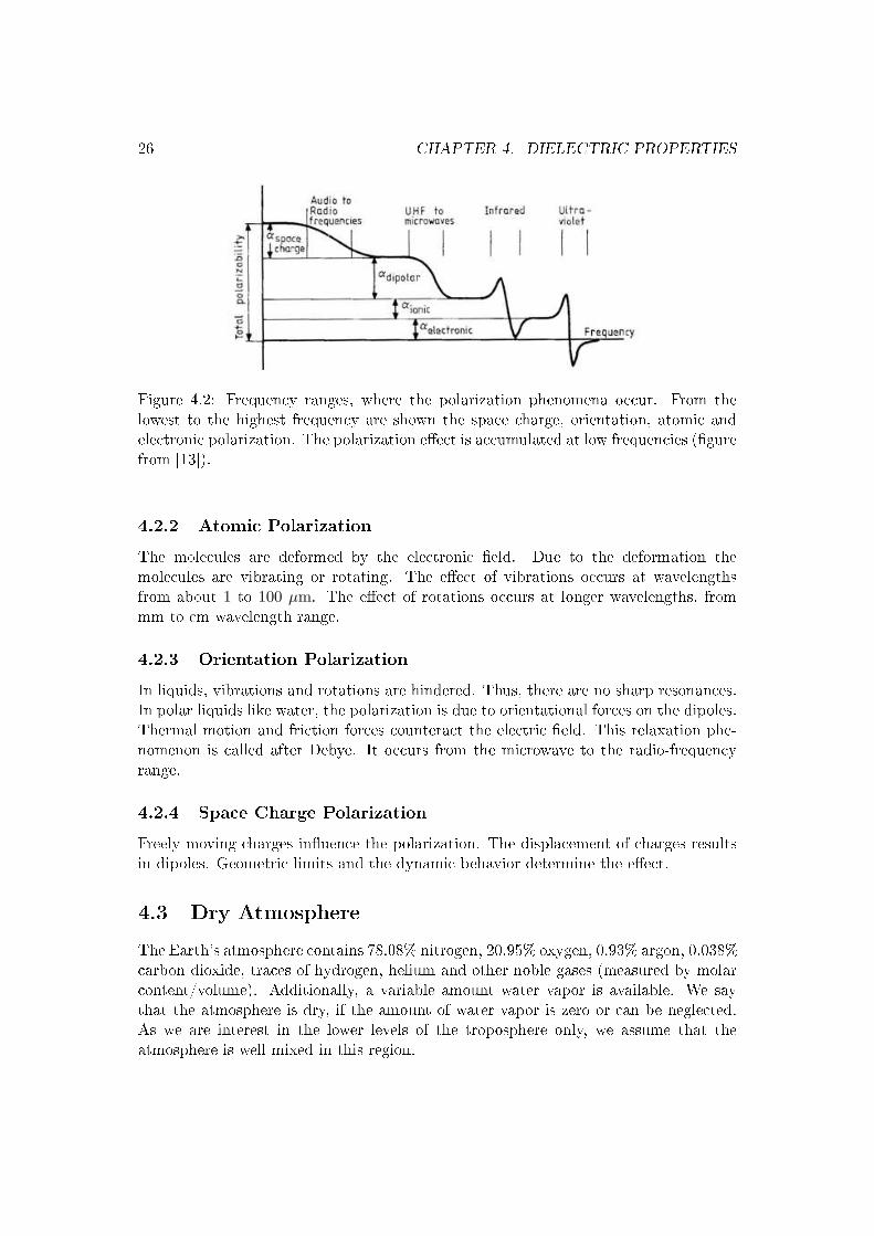
26 CHAPTER 4. DIELECTRIC PROPERTIES
Figure 4.2: Frequency ranges, where the polarization phenomena occur. From thelowest to the highest frequency are shown the space charge, orientation, atomic andelectronic polarization. The polarization eect is accumulated at low frequencies (gurefrom [13]).
4.2.2 Atomic Polarization
The molecules are deformed by the electronic eld. Due to the deformation themolecules are vibrating or rotating. The eect of vibrations occurs at wavelengthsfrom about 1 to 100 µm. The eect of rotations occurs at longer wavelengths, frommm to cm wavelength range.
4.2.3 Orientation Polarization
In liquids, vibrations and rotations are hindered. Thus, there are no sharp resonances.In polar liquids like water, the polarization is due to orientational forces on the dipoles.Thermal motion and friction forces counteract the electric eld. This relaxation phe-nomenon is called after Debye. It occurs from the microwave to the radio-frequencyrange.
4.2.4 Space Charge Polarization
Freely moving charges inuence the polarization. The displacement of charges resultsin dipoles. Geometric limits and the dynamic behavior determine the eect.
4.3 Dry Atmosphere
The Earth's atmosphere contains 78.08% nitrogen, 20.95% oxygen, 0.93% argon, 0.038%carbon dioxide, traces of hydrogen, helium and other noble gases (measured by molarcontent/volume). Additionally, a variable amount water vapor is available. We saythat the atmosphere is dry, if the amount of water vapor is zero or can be neglected.As we are interest in the lower levels of the troposphere only, we assume that theatmosphere is well mixed in this region.
4.4. WATER VAPOR 27
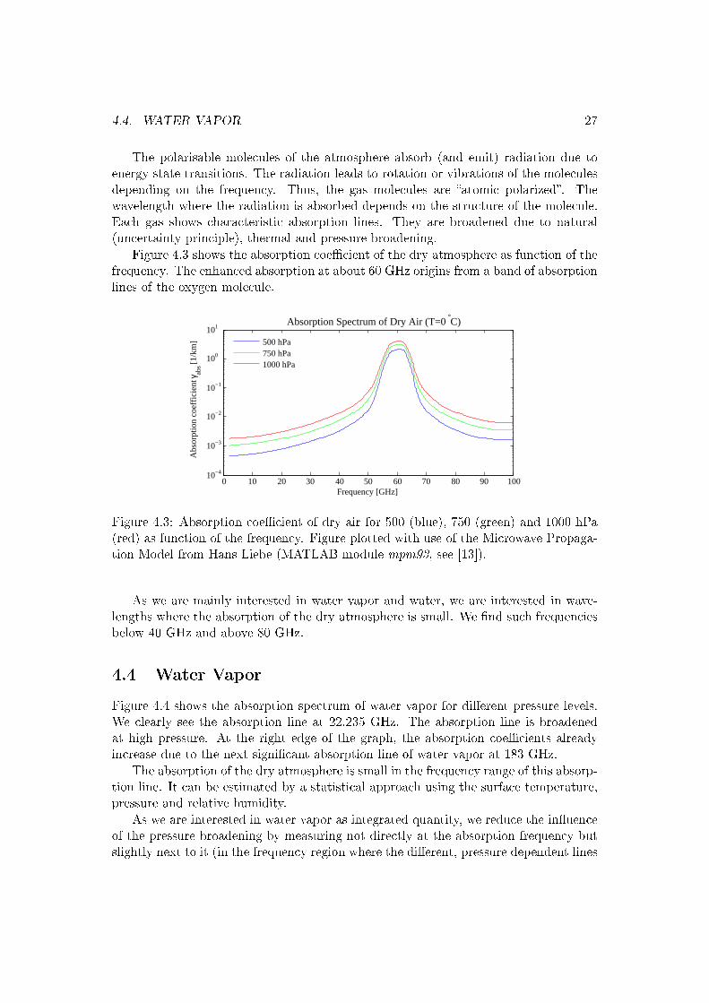
The polarisable molecules of the atmosphere absorb (and emit) radiation due toenergy state transitions. The radiation leads to rotation or vibrations of the moleculesdepending on the frequency. Thus, the gas molecules are atomic polarized. Thewavelength where the radiation is absorbed depends on the structure of the molecule.Each gas shows characteristic absorption lines. They are broadened due to natural(uncertainty principle), thermal and pressure broadening.
Figure 4.3 shows the absorption coecient of the dry atmosphere as function of thefrequency. The enhanced absorption at about 60 GHz origins from a band of absorptionlines of the oxygen molecule.
0 10 20 30 40 50 60 70 80 90 10010−4
10−3
10−2
10−1
100
101Absorption Spectrum of Dry Air (T=0 °C)
Frequency [GHz]
Abs
orpt
ion
coef
ficie
nt γ ab
s [1/k
m]
500 hPa750 hPa1000 hPa
Figure 4.3: Absorption coecient of dry air for 500 (blue), 750 (green) and 1000 hPa(red) as function of the frequency. Figure plotted with use of the Microwave Propaga-tion Model from Hans Liebe (MATLAB module mpm93, see [13]).
As we are mainly interested in water vapor and water, we are interested in wave-lengths where the absorption of the dry atmosphere is small. We nd such frequenciesbelow 40 GHz and above 80 GHz.
4.4 Water Vapor
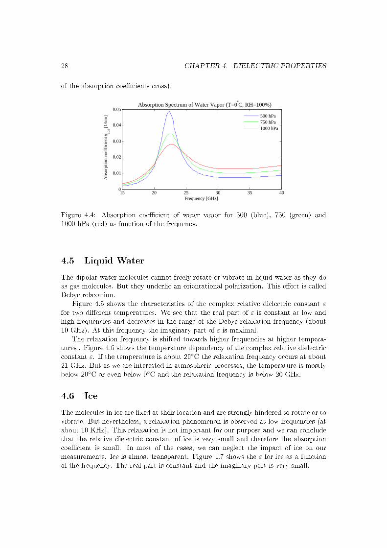
Figure 4.4 shows the absorption spectrum of water vapor for dierent pressure levels.We clearly see the absorption line at 22.235 GHz. The absorption line is broadenedat high pressure. At the right edge of the graph, the absorption coecients alreadyincrease due to the next signicant absorption line of water vapor at 183 GHz.
The absorption of the dry atmosphere is small in the frequency range of this absorp-tion line. It can be estimated by a statistical approach using the surface temperature,pressure and relative humidity.
As we are interested in water vapor as integrated quantity, we reduce the inuenceof the pressure broadening by measuring not directly at the absorption frequency butslightly next to it (in the frequency region where the dierent, pressure dependent lines
28 CHAPTER 4. DIELECTRIC PROPERTIES
of the absorption coecients cross).
15 20 25 30 35 400
0.01
0.02
0.03
0.04
0.05Absorption Spectrum of Water Vapor (T=0 °C, RH=100%)
Frequency [GHz]
Abs
orpt
ion
coef
fici
ent γ
abs [
1/km
]
500 hPa750 hPa1000 hPa
Figure 4.4: Absorption coecient of water vapor for 500 (blue), 750 (green) and1000 hPa (red) as function of the frequency.
4.5 Liquid Water
The dipolar water molecules cannot freely rotate or vibrate in liquid water as they doas gas molecules. But they underlie an orientational polarization. This eect is calledDebye relaxation.
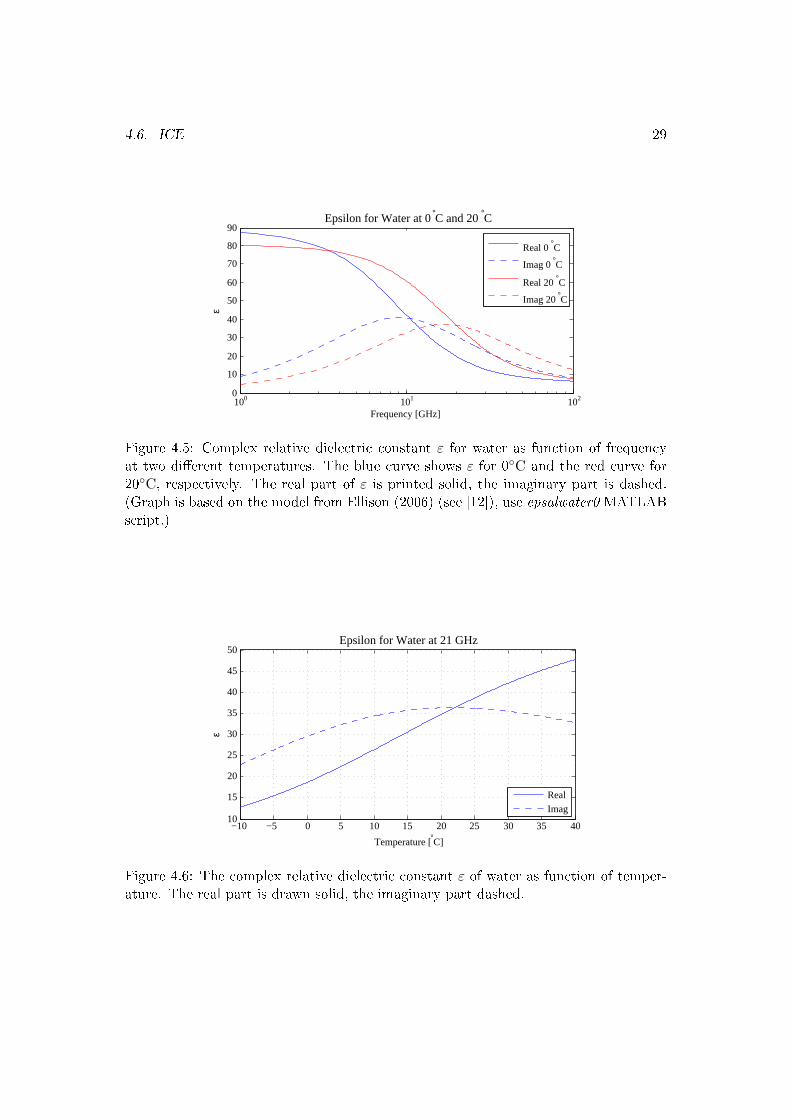
Figure 4.5 shows the characteristics of the complex relative dielectric constant εfor two dierent temperatures. We see that the real part of ε is constant at low andhigh frequencies and decreases in the range of the Debye relaxation frequency (about10 GHz). At this frequency the imaginary part of ε is maximal.
The relaxation frequency is shifted towards higher frequencies at higher tempera-tures . Figure 4.6 shows the temperature dependency of the complex relative dielectricconstant ε. If the temperature is about 20C the relaxation frequency occurs at about21 GHz. But as we are interested in atmospheric processes, the temperature is mostlybelow 20C or even below 0C and the relaxation frequency is below 20 GHz.
4.6 Ice
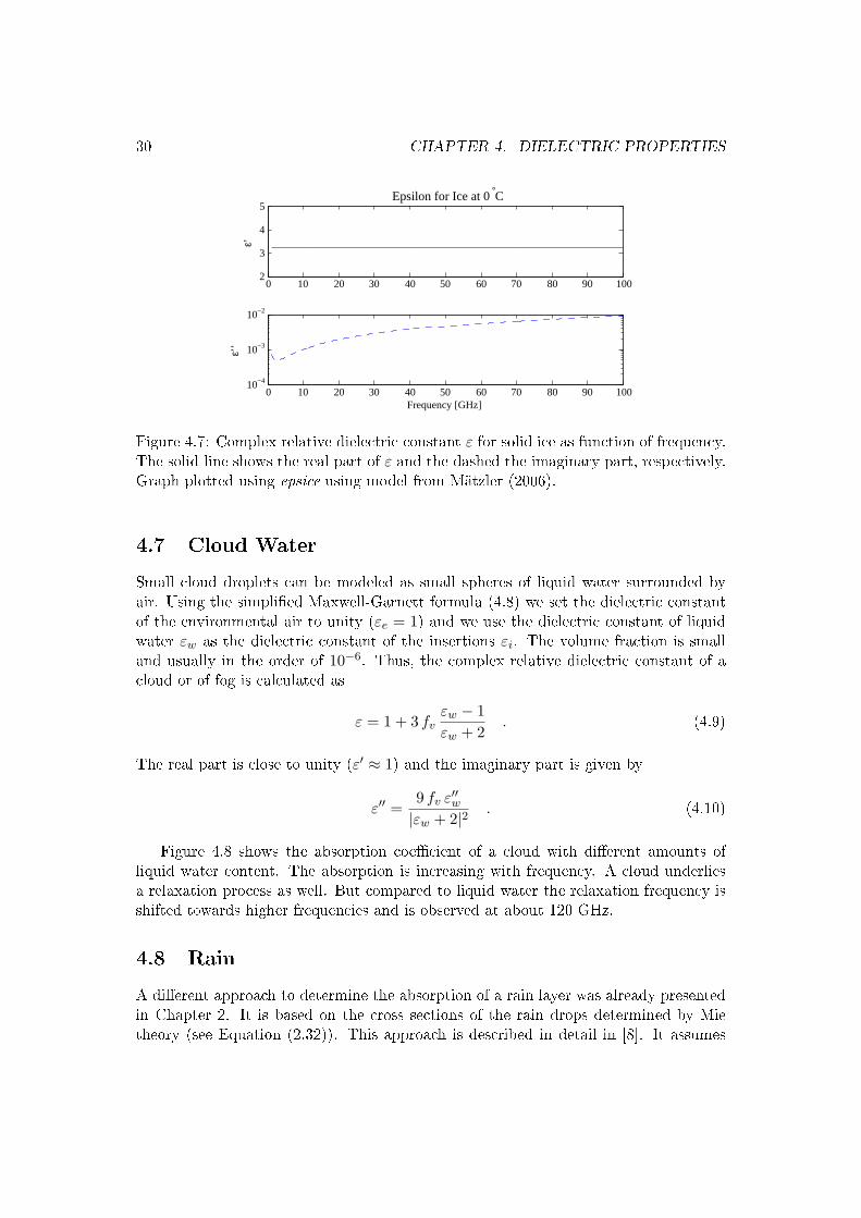
The molecules in ice are xed at their location and are strongly hindered to rotate or tovibrate. But nevertheless, a relaxation phenomenon is observed at low frequencies (atabout 10 KHz). This relaxation is not important for our purpose and we can concludethat the relative dielectric constant of ice is very small and therefore the absorptioncoecient is small. In most of the cases, we can neglect the impact of ice on ourmeasurements. Ice is almost transparent. Figure 4.7 shows the ε for ice as a functionof the frequency. The real part is constant and the imaginary part is very small.
4.6. ICE 29
100 101 1020
10
20
30
40
50
60
70
80
90Epsilon for Water at 0 °C and 20 °C
Frequency [GHz]
ε
Real 0 °C
Imag 0 °C
Real 20 °C
Imag 20 °C
Figure 4.5: Complex relative dielectric constant ε for water as function of frequencyat two dierent temperatures. The blue curve shows ε for 0C and the red curve for20C, respectively. The real part of ε is printed solid, the imaginary part is dashed.(Graph is based on the model from Ellison (2006) (see [12]), use epsalwater0 MATLABscript.)
−10 −5 0 5 10 15 20 25 30 35 4010
15
20
25
30
35
40
45
50Epsilon for Water at 21 GHz
Temperature [°C]
ε
Real
Imag
Figure 4.6: The complex relative dielectric constant ε of water as function of temper-ature. The real part is drawn solid, the imaginary part dashed.
30 CHAPTER 4. DIELECTRIC PROPERTIES
0 10 20 30 40 50 60 70 80 90 1002
3
4
5Epsilon for Ice at 0 °C
ε’
0 10 20 30 40 50 60 70 80 90 10010−4
10−3
10−2
Frequency [GHz]
ε’’
Figure 4.7: Complex relative dielectric constant ε for solid ice as function of frequency.The solid line shows the real part of ε and the dashed the imaginary part, respectively.Graph plotted using epsice using model from Mätzler (2006).
4.7 Cloud Water
Small cloud droplets can be modeled as small spheres of liquid water surrounded byair. Using the simplied Maxwell-Garnett formula (4.8) we set the dielectric constantof the environmental air to unity (εe = 1) and we use the dielectric constant of liquidwater εw as the dielectric constant of the insertions εi. The volume fraction is smalland usually in the order of 10−6. Thus, the complex relative dielectric constant of acloud or of fog is calculated as
ε = 1 + 3 fvεw − 1εw + 2
. (4.9)
The real part is close to unity (ε′ ≈ 1) and the imaginary part is given by
ε′′ =9 fv ε′′w|εw + 2|2
. (4.10)
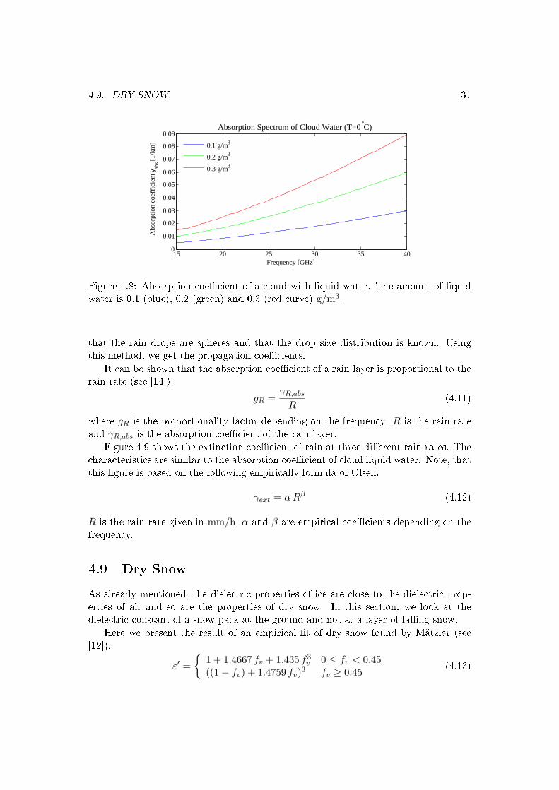
Figure 4.8 shows the absorption coecient of a cloud with dierent amounts ofliquid water content. The absorption is increasing with frequency. A cloud underliesa relaxation process as well. But compared to liquid water the relaxation frequency isshifted towards higher frequencies and is observed at about 120 GHz.
4.8 Rain
A dierent approach to determine the absorption of a rain layer was already presentedin Chapter 2. It is based on the cross sections of the rain drops determined by Mietheory (see Equation (2.32)). This approach is described in detail in [8]. It assumes
4.9. DRY SNOW 31
15 20 25 30 35 400
0.01
0.02
0.03
0.04
0.05
0.06
0.07
0.08
0.09Absorption Spectrum of Cloud Water (T=0 °C)
Frequency [GHz]
Abs
orpt
ion
coef
fici
ent γ
abs [
1/km
]
0.1 g/m3
0.2 g/m3
0.3 g/m3
Figure 4.8: Absorption coecient of a cloud with liquid water. The amount of liquidwater is 0.1 (blue), 0.2 (green) and 0.3 (red curve) g/m3.
that the rain drops are spheres and that the drop size distribution is known. Usingthis method, we get the propagation coecients.
It can be shown that the absorption coecient of a rain layer is proportional to therain rate (see [14]).
gR =γR,abs
R(4.11)
where gR is the proportionality factor depending on the frequency. R is the rain rateand γR,abs is the absorption coecient of the rain layer.
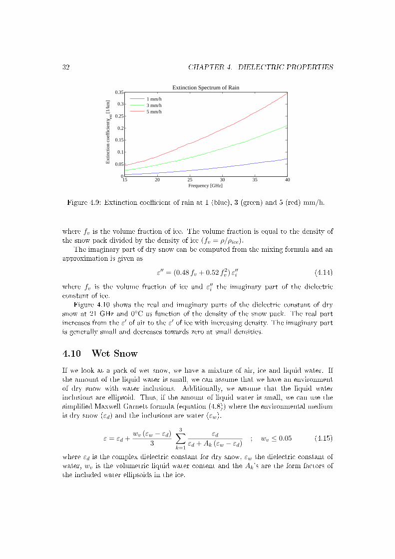
Figure 4.9 shows the extinction coecient of rain at three dierent rain rates. Thecharacteristics are similar to the absorption coecient of cloud liquid water. Note, thatthis gure is based on the following empirically formula of Olsen.
γext = α Rβ (4.12)
R is the rain rate given in mm/h, α and β are empirical coecients depending on thefrequency.
4.9 Dry Snow
As already mentioned, the dielectric properties of ice are close to the dielectric prop-erties of air and so are the properties of dry snow. In this section, we look at thedielectric constant of a snow pack at the ground and not at a layer of falling snow.
Here we present the result of an empirical t of dry snow found by Mätzler (see[12]).
ε′ =
1 + 1.4667 fv + 1.435 f3v 0 ≤ fv < 0.45
((1− fv) + 1.4759 fv)3 fv ≥ 0.45(4.13)
32 CHAPTER 4. DIELECTRIC PROPERTIES
15 20 25 30 35 400
0.05
0.1
0.15
0.2
0.25
0.3
0.35Extinction Spectrum of Rain
Frequency [GHz]
Ext
inct
ion
coef
fici
ent γ
ext [
1/km
]
1 mm/h3 mm/h5 mm/h
Figure 4.9: Extinction coecient of rain at 1 (blue), 3 (green) and 5 (red) mm/h.
where fv is the volume fraction of ice. The volume fraction is equal to the density ofthe snow pack divided by the density of ice (fv = ρ/ρice).
The imaginary part of dry snow can be computed from the mixing formula and anapproximation is given as
ε′′ = (0.48 fv + 0.52 f2v ) ε′′i (4.14)
where fv is the volume fraction of ice and ε′′i the imaginary part of the dielectricconstant of ice.
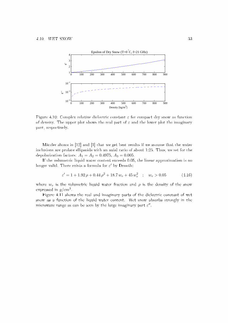
Figure 4.10 shows the real and imaginary parts of the dielectric constant of drysnow at 21 GHz and 0C as function of the density of the snow pack. The real partincreases from the ε′ of air to the ε′ of ice with increasing density. The imaginary partis generally small and decreases towards zero at small densities.
4.10 Wet Snow
If we look at a pack of wet snow, we have a mixture of air, ice and liquid water. Ifthe amount of the liquid water is small, we can assume that we have an environmentof dry snow with water inclusions. Additionally, we assume that the liquid waterinclusions are ellipsoid. Thus, if the amount of liquid water is small, we can use thesimplied Maxwell-Garnett formula (equation (4.8)) where the environmental mediumis dry snow (εd) and the inclusions are water (εw).
ε = εd +wv (εw − εd)
3
3∑k=1
εd
εd + Ak (εw − εd); wv ≤ 0.05 (4.15)
where εd is the complex dielectric constant for dry snow, εw the dielectric constant ofwater, wv is the volumetric liquid water content and the Ak's are the form factors ofthe included water ellipsoids in the ice.
4.10. WET SNOW 33
0 100 200 300 400 500 600 700 800 9001
2
3
4Epsilon of Dry Snow (T=0 °C, f=21 GHz)
ε’
0 100 200 300 400 500 600 700 800 90010−6
10−4
10−2
Density [kg/m3]
ε’’
Figure 4.10: Complex relative dielectric constant ε for compact dry snow as functionof density. The upper plot shows the real part of ε and the lower plot the imaginarypart, respectively.
Mätzler shows in [12] and [1] that we get best results if we assume that the waterinclusions are prolate ellipsoids with an axial ratio of about 1:25. Thus, we set for thedepolarization factors: A1 = A2 = 0.4975, A3 = 0.005.
If the volumetric liquid water content exceeds 0.05, the linear approximation is nolonger valid. There exists a formula for ε′ by Denoth:
ε′ = 1 + 1.92 ρ + 0.44 ρ2 + 18.7 wv + 45 w2v ; wv > 0.05 (4.16)
where wv is the volumetric liquid water fraction and ρ is the density of the snowexpressed in g/cm3.
Figure 4.11 shows the real and imaginary parts of the dielectric constant of wetsnow as a function of the liquid water content. Wet snow absorbs strongly in themicrowave range as can be seen by the large imaginary part ε′′.
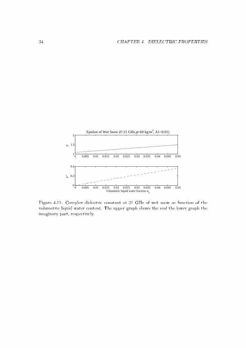
34 CHAPTER 4. DIELECTRIC PROPERTIES
0 0.005 0.01 0.015 0.02 0.025 0.03 0.035 0.04 0.045 0.051
1.5
2Epsilon of Wet Snow (f=21 GHz, ρ=60 kg/m3, A1=0.01)
ε’
0 0.005 0.01 0.015 0.02 0.025 0.03 0.035 0.04 0.045 0.050
0.2
0.4
Volumetric liquid water fraction wv
ε’’
Figure 4.11: Complex dielectric constant at 21 GHz of wet snow as function of thevolumetric liquid water content. The upper graph shows the real the lower graph theimaginary part, respectively.
Chapter 5
Physics of Precipitation
The physics of clouds and precipitation is a very widespread topic and we summarizehere just some selected properties relevant to our study. For more general informationabout this topic read [23], detailed information about the microphysics is given in [20]and some aspects about stratiform precipitation and about the melting layer are takenfrom [21] and [2].
5.1 Stratiform Precipitation
Clouds and precipitation develop due to cooling of moist air. When the cooling airgets saturated small water and cloud droplets form. When the amount of liquid waterwithin a cloud reaches a certain level, it starts to rain. The cooling of the air is mostlycaused by lifting of the air masses. We distinguish between convective and stratiformprecipitation.
The process causing convective precipitation uses the latent heat of the condensingwater vapor to enforce the upward vertical motion. The vertical motion intensies thecondensing process leading to even more latent heat release. This positive feedbackloop can cause heavy thunderstorms. Convective precipitation can occur within smallregions with updrafts on the order of m/s (on the order of tens of m/s for thunder-storms).
If the upward motion is caused by the large-scale weather situation (e.g. by abaroclinic cylone), air masses are lifted in a large region. This process is much slowerthan convective rain, and a clear horizontal structure is observed (hence the namestratiform). The precipitation is more continuous, falling from nimbostratus clouds.The vertical motion is in the order of a few tens of centimeters per second.
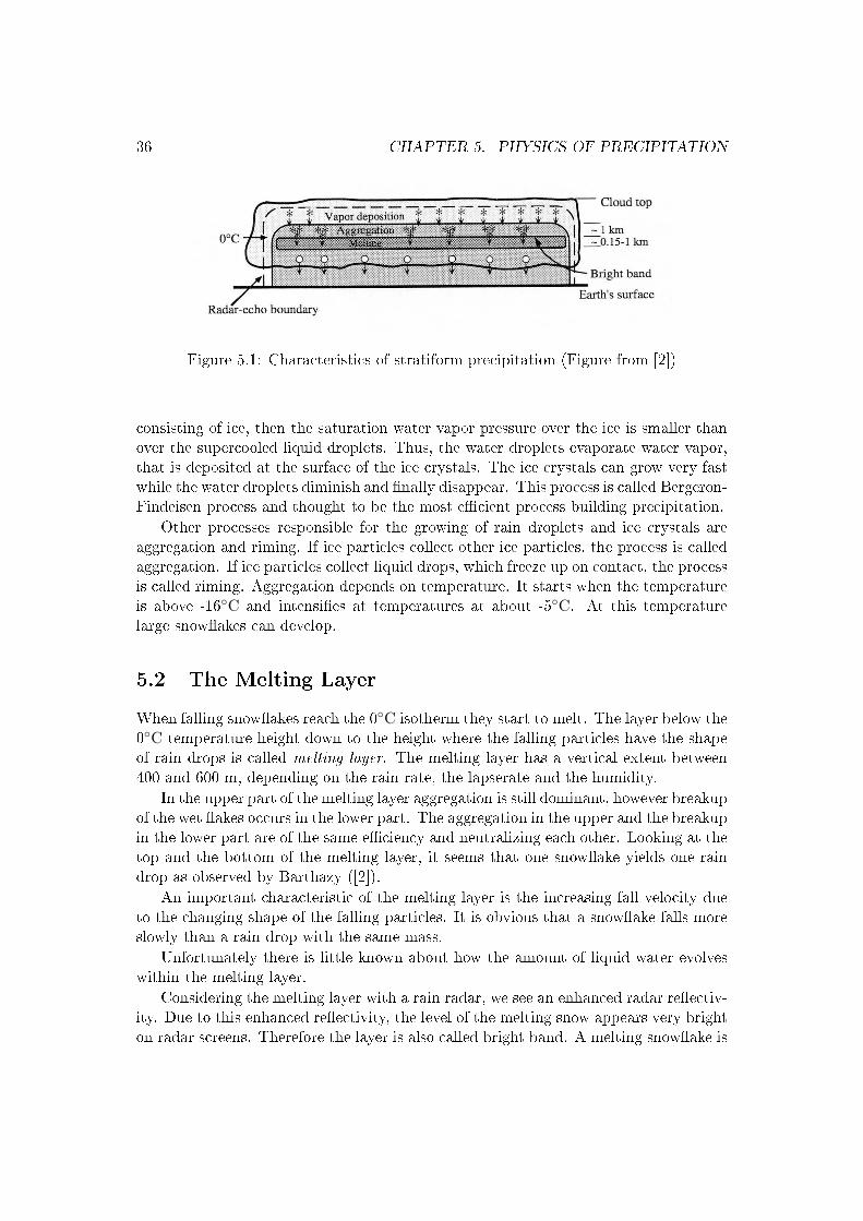
Figure 5.1 shows a schematic picture of a stratiform precipitation situation. At thetop of the cloud the water vapor condenses to cloud droplets (This is even possible ifthe temperature is below zero degrees leading to supercooled cloud drops.) or depositson tiny ice crystals. The condensation and deposition processes are very slow and canexplain the formation of very small droplets and crystals only.
If we have a cloud with tiny droplets consisting of supercooled water and some
35
36 CHAPTER 5. PHYSICS OF PRECIPITATION
Figure 5.1: Characteristics of stratiform precipitation (Figure from [2])
consisting of ice, then the saturation water vapor pressure over the ice is smaller thanover the supercooled liquid droplets. Thus, the water droplets evaporate water vapor,that is deposited at the surface of the ice crystals. The ice crystals can grow very fastwhile the water droplets diminish and nally disappear. This process is called Bergeron-Findeisen process and thought to be the most ecient process building precipitation.
Other processes responsible for the growing of rain droplets and ice crystals areaggregation and riming. If ice particles collect other ice particles, the process is calledaggregation. If ice particles collect liquid drops, which freeze up on contact, the processis called riming. Aggregation depends on temperature. It starts when the temperatureis above -16C and intensies at temperatures at about -5C. At this temperaturelarge snowakes can develop.
5.2 The Melting Layer
When falling snowakes reach the 0C isotherm they start to melt. The layer below the0C temperature height down to the height where the falling particles have the shapeof rain drops is called melting layer. The melting layer has a vertical extent between400 and 600 m, depending on the rain rate, the lapserate and the humidity.
In the upper part of the melting layer aggregation is still dominant, however breakupof the wet akes occurs in the lower part. The aggregation in the upper and the breakupin the lower part are of the same eciency and neutralizing each other. Looking at thetop and the bottom of the melting layer, it seems that one snowake yields one raindrop as observed by Barthazy ([2]).
An important characteristic of the melting layer is the increasing fall velocity dueto the changing shape of the falling particles. It is obvious that a snowake falls moreslowly than a rain drop with the same mass.
Unfortunately there is little known about how the amount of liquid water evolveswithin the melting layer.
Considering the melting layer with a rain radar, we see an enhanced radar reectiv-ity. Due to this enhanced reectivity, the level of the melting snow appears very brighton radar screens. Therefore the layer is also called bright band. A melting snowake is
5.3. CLASSIFICATION 37
covered by a thin lm of melt water, leading to a large surface of liquid water scatteringthe incident radiation. Thus, a melting snowake has the same backscattering crosssection as a large rain drop. Dry snowakes are less visible for the rain radar due tothe small reectance of ice.
Houze ([21]) points out that the enhanced reectivity cannot be explained by theincreasing amount of liquid water alone. He states that the aggregation process getsmore ecient in the upper layer of the bright band and thus the radar reectivityincreases due to the larger particles.
Pruppacher and Klett ([20]) explain that the melt water does not form a coatingaround the akes, but ows from the ake periphery to the linkage of the snowakebranches where it accumulates, leaving the ice skeleton of the ake uncovered withwater. But the melt water must form rst, before it can accumulate at the branches.
It is shown that the size distribution of snowakes is exponential and similar to thedrop size distribution of rain drops (see [2]), independent whether the diameter of theresulting melted drop or the real diameter was observed.
5.3 Classication
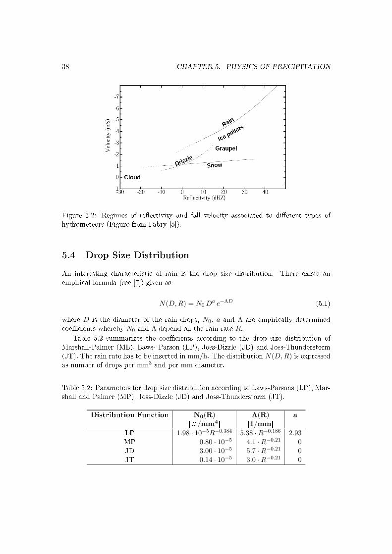
Precipitation occurs in various forms. As liquid it can be classied according to thedrop diameter. Then we say it is drizzle or rain. If the precipitation is frozen, we speakof graupel, hail or snow.
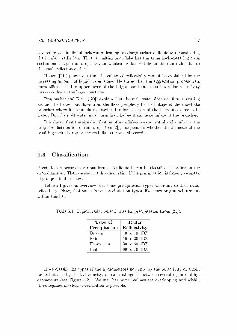
Table 5.1 gives an overview over some precipitation types according to their radarreectivity. Note, that some frozen precipitation types, like snow or graupel, are notwithin this list.
Table 5.1: Typical radar reectivities for precipitation (from [21]).
Type of RadarPrecipitation Reectivity
Drizzle 0 to 10 dBZRain 10 to 30 dBZHeavy rain 30 to 60 dBZHail 60 to 70 dBZ
If we classify the types of the hydrometeors not only by the reectivity of a rainradar but also by the fall velocity, we can distinguish between several regimes of hy-drometeors (see Figure 5.2). We see that some regimes are overlapping and withinthese regimes no clear classication is possible.
38 CHAPTER 5. PHYSICS OF PRECIPITATION
Figure 5.2: Regimes of reectivity and fall velocity associated to dierent types ofhydrometeors (Figure from Fabry [5]).
5.4 Drop Size Distribution
An interesting characteristic of rain is the drop size distribution. There exists anempirical formula (see [7]) given as
N(D,R) = N0 Da e−ΛD (5.1)
where D is the diameter of the rain drops, N0, a and Λ are empirically determinedcoecients whereby N0 and Λ depend on the rain rate R.
Table 5.2 summarizes the coecients according to the drop size distribution ofMarshall-Palmer (ML), Laws- Parson (LP), Joss-Dizzle (JD) and Joss-Thunderstorm(JT). The rain rate has to be inserted in mm/h. The distribution N(D,R) is expressedas number of drops per mm3 and per mm diameter.
Table 5.2: Parameters for drop size distribution according to Laws-Parsons (LP), Mar-shall and Palmer (MP), Joss-Dizzle (JD) and Joss-Thunderstorm (JT).
Distribution Function N0(R) Λ(R) a[#/mm4] [1/mm]
LP 1.98 · 10−5R−0.384 5.38 ·R−0.186 2.93MP 0.80 · 10−5 4.1 ·R−0.21 0JD 3.00 · 10−5 5.7 ·R−0.21 0JT 0.14 · 10−5 3.0 ·R−0.21 0
5.5. TERMINAL FALL VELOCITY 39
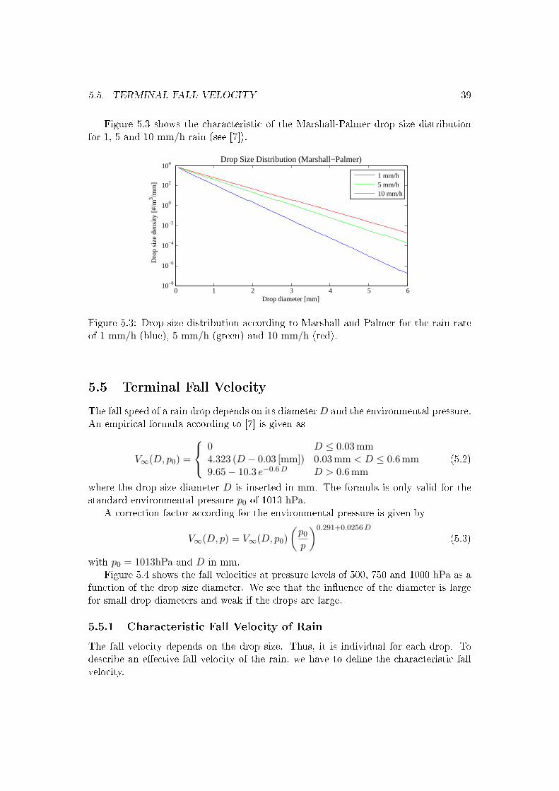
Figure 5.3 shows the characteristic of the Marshall-Palmer drop size distributionfor 1, 5 and 10 mm/h rain (see [7]).
0 1 2 3 4 5 610−8
10−6
10−4
10−2
100
102
104Drop Size Distribution (Marshall−Palmer)
Drop diameter [mm]
Dro
p si
ze d
ensi
ty [#
/m3 /mm
]
1 mm/h5 mm/h10 mm/h
Figure 5.3: Drop size distribution according to Marshall and Palmer for the rain rateof 1 mm/h (blue), 5 mm/h (green) and 10 mm/h (red).
5.5 Terminal Fall Velocity
The fall speed of a rain drop depends on its diameter D and the environmental pressure.An empirical formula according to [7] is given as
V∞(D, p0) =
0 D ≤ 0.03 mm4.323 (D − 0.03 [mm]) 0.03 mm < D ≤ 0.6 mm9.65− 10.3 e−0.6 D D > 0.6 mm
(5.2)
where the drop size diameter D is inserted in mm. The formula is only valid for thestandard environmental pressure p0 of 1013 hPa.
A correction factor according for the environmental pressure is given by
V∞(D, p) = V∞(D, p0)(
p0
p
)0.291+0.0256 D
(5.3)
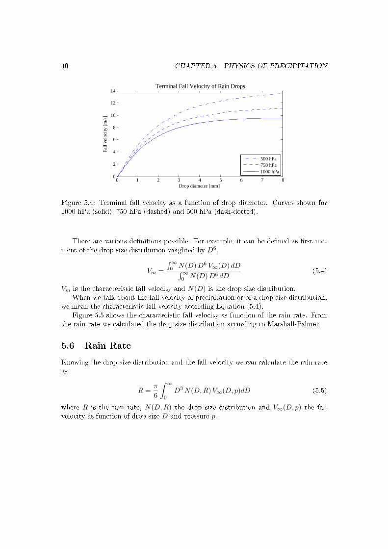
with p0 = 1013hPa and D in mm.Figure 5.4 shows the fall velocities at pressure levels of 500, 750 and 1000 hPa as a
function of the drop size diameter. We see that the inuence of the diameter is largefor small drop diameters and weak if the drops are large.
5.5.1 Characteristic Fall Velocity of Rain
The fall velocity depends on the drop size. Thus, it is individual for each drop. Todescribe an eective fall velocity of the rain, we have to dene the characteristic fallvelocity.
40 CHAPTER 5. PHYSICS OF PRECIPITATION
0 1 2 3 4 5 6 7 80
2
4
6
8
10
12
14Terminal Fall Velocity of Rain Drops
Drop diameter [mm]
Fall
velo
city
[m
/s]
500 hPa750 hPa1000 hPa
Figure 5.4: Terminal fall velocity as a function of drop diameter. Curves shown for1000 hPa (solid), 750 hPa (dashed) and 500 hPa (dash-dotted).
There are various denitions possible. For example, it can be dened as rst mo-ment of the drop size distribution weighted by D6.
Vm =
∫∞0 N(D) D6 V∞(D) dD∫∞
0 N(D) D6 dD(5.4)
Vm is the characteristic fall velocity and N(D) is the drop size distribution.When we talk about the fall velocity of precipitation or of a drop size distribution,
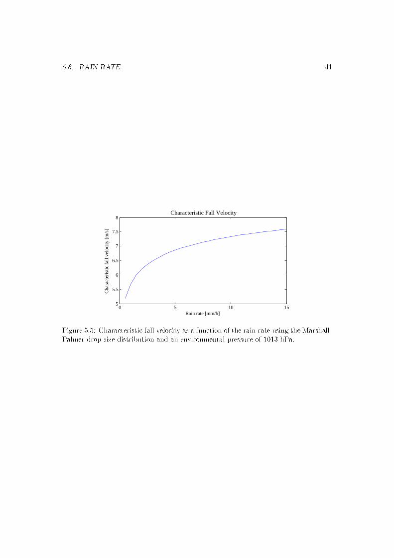
we mean the characteristic fall velocity according Equation (5.4).Figure 5.5 shows the characteristic fall velocity as function of the rain rate. From
the rain rate we calculated the drop size distribution according to Marshall-Palmer.
5.6 Rain Rate
Knowing the drop size distribution and the fall velocity we can calculate the rain rateas
R =π
6
∫ ∞
0D3 N(D,R) V∞(D, p)dD (5.5)
where R is the rain rate, N(D,R) the drop size distribution and V∞(D, p) the fallvelocity as function of drop size D and pressure p.
5.6. RAIN RATE 41
0 5 10 155
5.5
6
6.5
7
7.5
8Characteristic Fall Velocity
Rain rate [mm/h]
Cha
ract
eris
tic f
all v
eloc
ity [
m/s
]
Figure 5.5: Characteristic fall velocity as a function of the rain rate using the Marshall-Palmer drop size distribution and an environmental pressure of 1013 hPa.

42 CHAPTER 5. PHYSICS OF PRECIPITATION
Chapter 6
TROWARA (Tropospheric WaterVapor Radiometer)
6.1 Overview
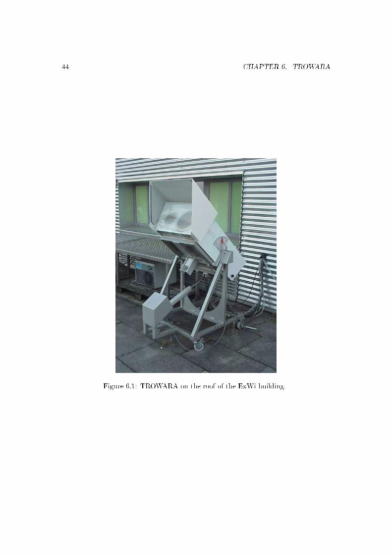
The TRopospheric WAter vapor RAdiometer (TROWARA) has operated since 1994on the roof of the ExWi building. It was designed to measure integrated water vapor(IWV) and integrated liquid water (ILW). And now, we try to expand its functionalityto estimate rain and snow as well. A very short description about its functionality isgiven in the STARTWAVE atmospheric database ([17]), for more detailed informationsee Peter and Kämpfer, 1992 [19] and Morland, 2002 ([18]).
TROWARA observes the sky at the xed zenith angle of 50. It contains threemicrowave sensors. One operates at 21.3 GHz (BW = 100 MHz) which is sensitive tothe water vapor absorption line at 22.235 GHz, another sensor measures at 31.5 GHz(BW = 200 MHz) which is more sensitive to liquid water, and since November 2007a third sensor at 22.2 GHz (BW = 400 MHz) was added which is even more sensitiveto water vapor as the 21.3 GHz sensor. Additionally, a thermal IR sensor (λ = 9.5 −11.5 µm) measures radiation from the same direction.
The original method to retrieve water vapor and liquid water uses a model of Wu(see Peter and Kämpfer, 1992 [19]). It is based on the linearization of brightnesstemperatures in analogy to opacities. But it was pointed out by Mätzler and Morland,2008 [14] that Wu's assumption that the absorption of cloud liquid water is proportionalto the square of the frequency was erroneous, especially at low temperatures. Thereforea new algorithm based on statistical analysis was built and later this algorithm wasrened with physical considerations.
6.2 Statistical Algorithm
A short summary about the statistical algorithm is given, for further information seeMätzler and Morland, 2008 ([14]).
43
44 CHAPTER 6. TROWARA
Figure 6.1: TROWARA on the roof of the ExWi building.
6.3. REFINED ALGORITHM 45
The idea behind this algorithm is that the parameters of interest can be estimatedby linear combinations of measured data. The measured data are the brightness tem-peratures by TROWARA and surface temperature, pressure, relative humidity andother parameters measured by the weather station on the roof of the ExWi build-ing. The coecients weighting the measured parameters are determined by statisticalmethods in comparison with radiosonde data.
Thus, the eective mean temperature Tmi of the atmosphere at microwave frequencyfi can be estimated by ground-based data as
Tmi = A0i + A1i TS + A2i US + A2i PS . (6.1)
TS denotes the temperature, US the relative humidity and PS the pressure at thesurface. The index i stands for the frequency fi. The coecients Aji are determinedby radiosonde data using the radiative model of Rosenkranz.
Knowing the eective mean temperature Tmi, we can use Equation (2.36) to calcu-late the opacities τi for each frequency.
τi = −µ ln(
Tmi − Tbi
Tmi − Tc
)(6.2)
Tbi denotes the measured brightness temperature, Tmi the eective mean temperatureand Tc is the cosmic background temperature. µ is the cosine of the zenith angle.
The integrated water vapor (IWV) and the integrated liquid water (ILW) can betted by a linear combination of the opacities τ21 and τ31 considering temperature,dry-air density and water vapor density measurements at the surface.
IWV = B0 + B1 τ21 + B2 τ31 + B3 TS + B4 DS + B5 VS (6.3)
ILW = C0 + C1 τ21 + C2 τ31 (6.4)
TS is the temperature, DS the dry-air density and VS the water vapor density at thesurface.
We can use the third TROWARA sensor at 22.2 GHz and nd a statistical retrievalin the same manner as described above.
In general the statistical algorithms have high accuracy. But due to enhancedmicrowave sensitivity to large water drops, the presence of precipitation leads to largesystematic errors.
6.3 Rened Algorithm
The zenith opacities during rainless periods can be found in the same manner as de-scribed by Equation (6.1) and (6.2). An useful property of the opacity is that it canbe divided into the opacities of dierent matter. Thus, the opacity of the entire atmo-sphere can be interpreted as sum of the opacities of the clear sky, the water vapor andthe liquid water, as done in the following equation.
τ21 = a21 + b21 IWV + c21 ILW (6.5)
τ31 = a31 + b31 IWV + c31 ILW (6.6)
46 CHAPTER 6. TROWARA
where τ21 and τ31 are the zenith opacities according to Equation (6.2) for 21 and31 GHz, respectively. a21 and a31 represent the dry atmosphere opacities. They dependon the temperature and pressure. They are rather constant, when divided by the dryair density DS . The parameters b21 and b31 are the coecients weighting the amountof water vapor in the atmosphere. It turns out that b21 is rather constant and canbe determined by statistical methods using radiosonde data (see Equation (6.7)). Theparameters c21 and c31 are the Rayleigh mass absorption coecients of cloud water,which can be calculated using the dielectric model of water by Ellison (2006).
The parameter b21 can be estimated by
b21 = D0 + D1 τ21 + D2 τ31 + D3 TS + D4 VS (6.7)
where τ21 and τ31 are the zenith opacities, TS is the temperature and VS is the watervapor density at the surface. And D0 to D4 are the statistically determined parameters.
We dene the ratios of the corresponding coecients as follows
α =a21
a31β =
b31
b21γ =
c21
c31(6.8)
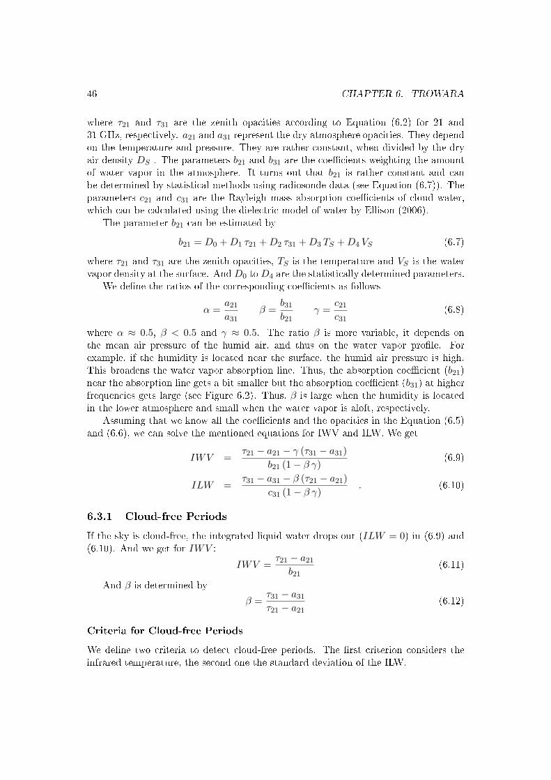
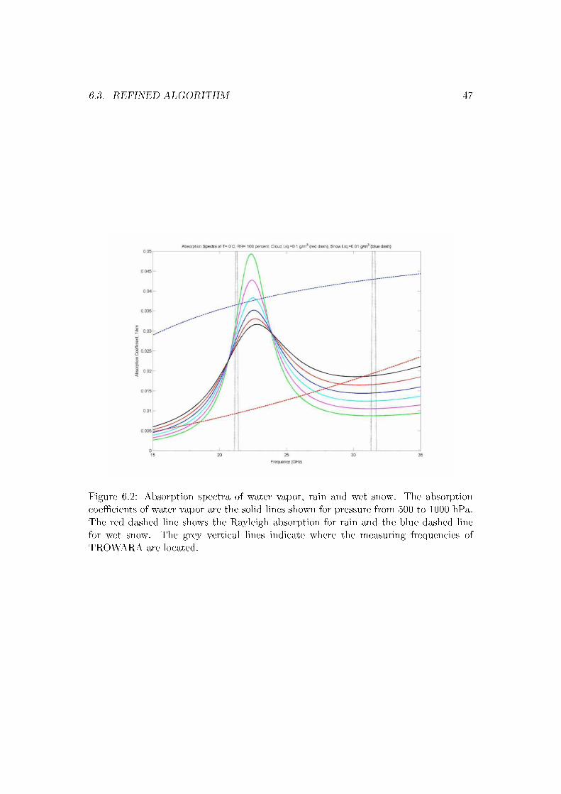
where α ≈ 0.5, β < 0.5 and γ ≈ 0.5. The ratio β is more variable, it depends onthe mean air pressure of the humid air, and thus on the water vapor prole. Forexample, if the humidity is located near the surface, the humid air pressure is high.This broadens the water vapor absorption line. Thus, the absorption coecient (b21)near the absorption line gets a bit smaller but the absorption coecient (b31) at higherfrequencies gets large (see Figure 6.2). Thus, β is large when the humidity is locatedin the lower atmosphere and small when the water vapor is aloft, respectively.
Assuming that we know all the coecients and the opacities in the Equation (6.5)and (6.6), we can solve the mentioned equations for IWV and ILW. We get
IWV =τ21 − a21 − γ (τ31 − a31)
b21 (1− β γ)(6.9)
ILW =τ31 − a31 − β (τ21 − a21)
c31 (1− β γ). (6.10)
6.3.1 Cloud-free Periods
If the sky is cloud-free, the integrated liquid water drops out (ILW = 0) in (6.9) and(6.10). And we get for IWV :
IWV =τ21 − a21
b21(6.11)
And β is determined by
β =τ31 − a31
τ21 − a21(6.12)
Criteria for Cloud-free Periods
We dene two criteria to detect cloud-free periods. The rst criterion considers theinfrared temperature, the second one the standard deviation of the ILW.
6.3. REFINED ALGORITHM 47
Figure 6.2: Absorption spectra of water vapor, rain and wet snow. The absorptioncoecients of water vapor are the solid lines shown for pressure from 500 to 1000 hPa.The red dashed line shows the Rayleigh absorption for rain and the blue dashed linefor wet snow. The grey vertical lines indicate where the measuring frequencies ofTROWARA are located.
48 CHAPTER 6. TROWARA
Infrared temperature: Knowing the integrated water vapor (IWV ), an empiricalt for the maximal possible cloud-free infra-red brightness temperature TB,IR,nocloud
(claimed by Emmanuel) is given by
TB,IR,nocloud = 192 + 3 · IWV − 0.032 · IWV 2 [K] . (6.13)
IWV has to be inserted in mm.Thus, if the measured IR temperature (TB,IR) is below this empirical limit, we
assume that we have a no cloud situation.
TB,IR < TB,IR,nocloud (6.14)
Standard deviation of ILW: During a cloud-free period, the ILW value is verysmall (ILW ≈ 0) and additionally it is very stable. Thus, we can dene our secondcriterion for cloud-free situation:
σILW < 0.0011 + 0.000012 · TS [mm] (6.15)
The mean surface temperature TS must be inserted in C. If the standard deviationof ILW (σILW ) is smaller than 0.0011 mm (plus a temperature depend term), we havea cloud-free situation. Note that the term on the right side of the inequation is onlyvalid if the TROWARA ILW samples are averaged over 12 seconds. For unaveragedILW values, σILW is higher. Additionally to this criterion, the IR temperature must bebelow 265 K, because small σILW values are also possible during stable fog situations.
If at least one of the two criteria is fullled, we assume that we have a cloud-freesituation, and we can use Equation (6.12) to calculate β.
6.3.2 Example of TROWARA Measurements on a Rainless Day
Figure 6.3 shows measurements from April 7, 2009. This day was a rainless day withblue sky in the morning and clouds in the afternoon. The temperature was at about10C during the night and increased up to almost 20C shortly after midday.
Figure (a) shows the infrared temperature during this day. In the rst half of theday, the IR temperature was between 210 and 220 K (corresponding to ≈ −60C).After 12:00 the temperature changed rapidly between about 220 and 270 K. The in-frared sensor measures the temperature of the clouds. If no clouds are present, thetemperature is very low and if cloud exists the temperature of the lowest cloud layer ismeasured. Thus, the rst half of April 7, 2009 was cloud-free while the sky was coveredwith clouds in the afternoon (interrupted by some holes in the cloud cover).
Figure (b) shows the brightness temperature for 21 (blue) and 31 GHz (red). Inthe morning the curves are stable, and in the afternoon we clearly see the inuence ofthe clouds.
Figure (c) shows the zenith opacities calculated with Equation (6.2). We see theinuence of the clouds in the afternoon again. Especially the 31 GHz opacity (red line)is sensitive to the liquid water.
6.3. REFINED ALGORITHM 49
Figure (d) shows the characteristic of the β parameter dened by Equation (6.8).The red circles show the β values when the algorithm detected a cloud-free periodaccording to the dened criteria. The black line is the estimation of the β parameterduring cloud periods or when no data were available. We see that β decreased duringthe morning. Thus, the water vapor was lifted up in the morning. Lifting of air massesleads to cooling and condensing of the water vapor leading to clouds in the afternoon.
Figure (e) shows the calculations of IWV and ILW according to the rened al-gorithm (Equation (6.9) and (6.10)). The amount of liquid water (ILW) is zero atcloud-free periods and increases when clouds are present. The IWV was stable duringthe morning and increased in the afternoon. The amount of water vapor can increase,when moister air masses reach the observed region by advection or when water is evap-orated and lifted from the ground. Looking at the β parameter, we see that β is stilldecreasing while the IWV is increasing. Thus, the amount of water vapor was accumu-lating in the upper atmosphere, probably lifted up by convection and accumulated byadvection. In the later afternoon, β increased. This corresponds to a higher amountof water vapor at lower altitudes, conrming the assumption that the increase of theIWV is generated by evaporation of surface water.
6.3.3 Rain
The same approach as done for situations without precipitation (Equation (6.5) and(6.6)) can be used to describe the zenith opacities τ21 and τ31 for situations with rainand snow. But we have to include two additional terms. The rst represents theabsorption of rain, the second the absorption of wet snow. Due to the small absorptionof ice, the contribution of ice and dry snow can be neglected.
The zenith opacities can be calculated as
τ21 = a21 + b21 IWV + c21 (ILW + GM,21 IRL) + d21 ISL (6.16)
τ31 = a31 + b31 IWV + c31 (ILW + GM,31 IRL) + d31 ISL (6.17)
where IRL is the integrated rain liquid and ISL integrated snow liquid. The termGM,i represents the Mie gain of rain. The Mie gain of rain is increasing rapidly fordrop diameters larger than 0.3 mm. The Mie gain at 21 GHz GM,21 can reach valuesup to 10 and at 31 GHz GM,31 up to 7 (see Figure 6.4).
The coecients d21 and d31 represent the emission of wet snow at 21 GHz and31 GHz, respectively. The emission of wet snow is larger than the emission of rain(di >> ci).
The ratio of the wet snow coecients (d21 to d31) is dened as δ and it is larger asthe ratio of the rain coecients (γ).
δ =d21
d31> γ =
c21
c31(6.18)
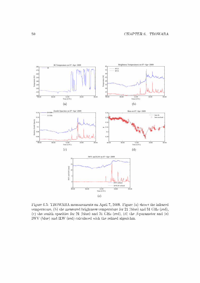
50 CHAPTER 6. TROWARA
00:00 06:00 12:00 18:00 00:00200
210
220
230
240
250
260
270
280
Time (UTC)
Tem
pera
ture
[K]
IR Temperature on 07−Apr−2009
IR
(a)
00:00 06:00 12:00 18:00 00:0020
25
30
35
40
45
50
55
60
Time (UTC)
Tem
pera
ture
[K]
Brightness Temperatures on 07−Apr−2009
BT21BT31
(b)
00:00 06:00 12:00 18:00 00:000.04
0.06
0.08
0.1
0.12
0.14
0.16
Time (UTC)
Rai
nles
s Z
enith
Opa
city
Zenith Opacities on 07−Apr−2009
21 GHz
31 GHz
(c)
00:00 06:00 12:00 18:00 00:00
0.29
0.3
0.31
0.32
0.33
0.34
Time (UTC)
β
Beta on 07−Apr−2009
beta fitbeta nocloud
(d)
00:00 06:00 12:00 18:00 00:00−5
0
5
10
15
20
Time (UTC)
IWV
and
ILW
[mm
]
IWV and ILW on 07−Apr−2009
IWV refined
50*ILW refined
(e)
Figure 6.3: TROWARA measurements on April 7, 2009. Figure (a) shows the infraredtemperature, (b) the measured brightness temperature for 21 (blue) and 31 GHz (red),(c) the zenith opacities for 21 (blue) and 31 GHz (red), (d) the β-parameter and (e)IWV (blue) and ILW (red) calculated with the rened algorithm.
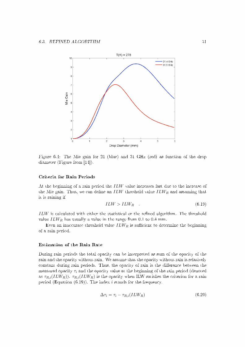
6.3. REFINED ALGORITHM 51
Figure 6.4: The Mie gain for 21 (blue) and 31 GHz (red) as function of the dropdiameter (Figure from [14]).
Criteria for Rain Periods
At the beginning of a rain period the ILW value increases fast due to the increase ofthe Mie gain. Thus, we can dene an ILW threshold value ILWR and assuming thatit is raining if
ILW > ILWR . (6.19)
ILW is calculated with either the statistical or the rened algorithm. The thresholdvalue ILWR has usually a value in the range from 0.1 to 0.4 mm.
Even an inaccurate threshold value ILWR is sucient to determine the beginningof a rain period.
Estimation of the Rain Rate
During rain periods the total opacity can be interpreted as sum of the opacity of therain and the opacity without rain. We assume that the opacity without rain is relativelyconstant during rain periods. Thus, the opacity of rain is the dierence between themeasured opacity τi and the opacity value at the beginning of the rain period (denotedas τR,i(ILWR)). τR,i(ILWR) is the opacity when ILW satises the criterion for a rainperiod (Equation (6.19)). The index i stands for the frequency.
∆τi = τi − τR,i(ILWR) (6.20)
52 CHAPTER 6. TROWARA
Here ∆τi represents a rst estimation of the rain opacity. Unfortunately, τi is basedon an estimation of the eective mean temperature Tmi which is not very accurateduring rain periods. Therefore the opacity of rain ∆τi is not accurate as well. We haveto nd another method to improve the expression for the rain opacity. Such a methodis described in the next subsection. In the following we use the term τrain,i for theimproved rain opacity.
It can be shown that the absorption coecient of rain γa,R,i in the frequency rangefrom 21 to 31 GHz is proportional to the rain rate R.
γa,R,i = R · gR,i (6.21)
where γa,R,i is the absorption coecient of rain, R is the rain rate and gR,i is theproportionality factor.
Knowing the absorption coecient γa,R,i and the depth of the rain layer HR, wecan calculate the rain opacity τrain,i. We assume that the rain rate is constant withinthe whole rain layer.
τrain,i = HR · γa,R,i (6.22)
The depth of the rain layer HR is equal to the distance from ground up to theheight where the ambient air temperature is 1C. Above this height it is snowing andat the moment we do not consider the contribution of the wet snow to the opacity.HR is calculated from the surface temperature TS assuming a constant moist-adiabaticlapse rate Γ .
HR =TS − 274.15
Γ(6.23)
where the surface temperature TS must be inserted in K. The lapserate Γ depends onthe weather situation and is between 4 and 8 K/km.
Using Equation (6.21) and (6.22) we get for the rain rate R
R =τrain,i
HR gR,i. (6.24)
Rain Opacity
As mentioned above, the estimation of the eective mean temperature Tmi is not veryaccurate during rain periods. And thus, the values of the total opacity τi and therain opacity ∆τi are not accurate in a rst estimation. In the following we describe amethod to get a better estimation of the rain opacity τrain,i.
We assume that the rain is constant within a layer with depth HR. Thus, themeasured brightness temperatures at the ground can be expressed using Equation(2.36).
Tb,i = Tb,norain,i e−τrain,i/µ + Tm,rain,i (1− e−τrain,i/µ) (6.25)
where Tb,i is the measured brightness temperature at frequency i, Tb,norain,i is thebrightness temperature of the atmosphere including water vapor and cloud liquid waterabove the rain layer. τrain,i is the rain opacity and Tm,rain,i is the eective meantemperature of the rain layer.
6.3. REFINED ALGORITHM 53
The brightness temperature without rain (Tb,norain,i) is given by
Tb,norain,i = Tc e−τR,i/µ + Tmi (1− e−τR,i/µ) (6.26)
where Tc denotes the cosmic background temperature. τR,i is the opacity just at thatmoment when the rain started (and it is assumed to be constant during rain periods).Tmi is the eective mean temperature of the atmosphere calculated with Equation(6.1).
The eective mean temperature Tm,rain,i of the rain layer is determined by Equation(2.37) as
Tm,rain,i =
∫ τrain,i/µ0 T (τ) e−τ dτ
1− e−τrain,i/µ(6.27)
Assuming that the temperature decreases linearly within the rain layer, we canwrite for the temperature within the rain layer:
T (τ) = TS − Γ h(τ) = TS − Γτ µ
γa,R,i(6.28)
where TS is the surface temperature, h(τ) the depth of the layer with opacity τ , Γ thelapse rate and γa,R,i is the absorption coecient of rain.
Inserting (6.28) in (6.27) we can simplify the expression for Tm,rain,i to (for moredetails see [14]):
Tm,rain,i = TS −12
(TS − Tml) e−0.19 τrain,i/µ (6.29)
where Tml is the temperature in the melting layer. Tml is about 1C.
Now, we would like to know the rain opacity τrain,i. Thus, we solve Equation (6.25)for τrain,i and we get
τrain,i = −µ ln(
Tm,rain,i − Tb,i
Tm,rain,i − Tb,norain,i
). (6.30)
In this equation we know Tb,i, Tb,norain,i is calculated with Equation (6.26) and Tm,rain,i
can be calculated using Equation (6.29). But Equation (6.29) uses the unknown rainopacity τrain,i.
We proceed iteratively to calculate τrain,i. First, we use ∆τi from (6.20) as rstestimation of τrain,i in (6.29). We get the eective mean temperature Tm,rain,i of therain layer as result. We insert this result in Equation (6.30) and get a second estimationof τrain,i.
Then, we do the same procedure again to get a third estimation of τrain,i. It isshown that two iteration steps are sucient to get an accurate estimation of the rainopacity.
54 CHAPTER 6. TROWARA
6.3.4 Limitations of the Rened Algorithm
Wet snow
We considered the contribution of rain to the total opacity τ and neglected the con-tribution of wet snow. Although the layer of wet snow is just a few hundred metersthick, its contribution cannot be neglected.
Later, we will describe a method to estimate the inuence of snow to improve thisalgorithm.
Depth of the rain layer
The depth of the rain layer is estimated by the surface temperature assuming a constantlapse rate. The exact value of the lapse rate is not known. For example, if we assumethat the depth HR is 600 m but in reality it is only 300 m, we underestimate the rainrate R by a factor of two.
In Chapter 9 we will show how we can use a vertical pointing rain radar to getmore accurate values for the depth of the rain layer.
6.3.5 Example of TROWARA Measurements for a Rainy Day
Here, we consider measurements made on a rainy day. We selected July 13, 2008. Itwas almost continuously raining during that day with some rainless periods or periodswith very little rain (especially between 11:00 and 17:00).
The lapserate was about 6 K/km and we set the IWL threshold value (ILWR) to0.4 mm. As there were no cloud-free periods during that day, the β parameter couldnot be determined and it was set to a mean value of 0.32.
A collection of measurement results is shown in Figure 6.5.
To begin with the main result, Figure (a) shows the cumulative rain estimated byTROWARA using the 21 (blue) and 31 GHz (red) channel. To verify this estimationthe cumulative rain measured at the ground is shown by the green lines (the solid greenline represents the tipping sensor and the green dashed line the optical sensor respec-tively). We see that the beginnings and endings of the rain periods of the TROWARAestimations agree well with the rain periods measured at the ground. The rain inten-sity is most of the time overestimated leading to a too large amount of rain at the endof the day. Increasing the ILW threshold value ILWR leads to less rain but also to ashortening of the rain periods. The lapserate was determined by a vertical pointingrain radar but we cannot say if it was constant within the rain layer. And we did notconsider the inuence of the wet snow in the melting layer.
Figure (b) shows the brightness temperatures measured at 21 (blue) and 31 GHz(red). We see that the brightness temperatures are higher during rain periods.
Figure (c) shows the rainless zenith opacities (again blue for 21 and red for 31 GHz).The rainless opacities are clipped during the rain periods as our algorithm assumes thatILW stays constant within a rain period.
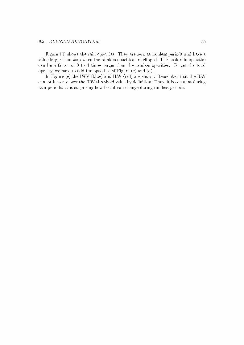
6.3. REFINED ALGORITHM 55
Figure (d) shows the rain opacities. They are zero at rainless periods and have avalue larger than zero when the rainless opacities are clipped. The peak rain opacitiescan be a factor of 3 to 4 times larger than the rainless opacities. To get the totalopacity, we have to add the opacities of Figure (c) and (d).
In Figure (e) the IWV (blue) and ILW (red) are shown. Remember that the ILWcannot increase over the ILW threshold value by denition. Thus, it is constant duringrain periods. It is surprising how fast it can change during rainless periods.
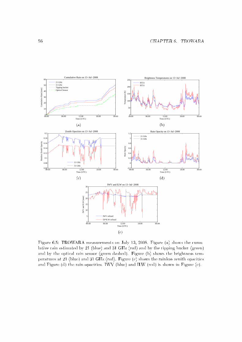
56 CHAPTER 6. TROWARA
00:00 06:00 12:00 18:00 00:000
10
20
30
40
50
60
Time (UTC)
Cum
ulat
ive
Rai
n [m
m]
Cumulative Rain on 13−Jul−2008
21 GHz31 GHzTipping bucketOptical Sensor
(a)
00:00 06:00 12:00 18:00 00:000
50
100
150
200
250
Time (UTC)
Tem
pera
ture
[K]
Brightness Temperatures on 13−Jul−2008
BT21BT31
(b)
00:00 06:00 12:00 18:00 00:000.06
0.08
0.1
0.12
0.14
0.16
0.18
0.2
Time (UTC)
Rai
nles
s Z
enith
Opa
city
Zenith Opacities on 13−Jul−2008
21 GHz
31 GHz
(c)
00:00 06:00 12:00 18:00 00:00−0.2
0
0.2
0.4
0.6
0.8
1
1.2
Time (UTC)
Rai
n O
paci
ty
Rain Opacity on 13−Jul−2008
21 GHz31 GHz
(d)
00:00 06:00 12:00 18:00 00:000
5
10
15
20
25
30
Time (UTC)
IWV
and
ILW
[mm
]
IWV and ILW on 13−Jul−2008
IWV refined
50*ILW refined
(e)
Figure 6.5: TROWARA measurements on July 13, 2008. Figure (a) shows the cumu-lative rain estimated by 21 (blue) and 31 GHz (red) and by the tipping bucket (green)and by the optical rain sensor (green dashed). Figure (b) shows the brightness tem-peratures at 21 (blue) and 31 GHz (red). Figure (c) shows the rainless zenith opacitiesand Figure (d) the rain opacities. IWV (blue) and ILW (red) is shown in Figure (e).
Chapter 7
The Micro Rain Radar (MRR)
7.1 Overview
The Micro Rain Radar (MRR) is a vertical pointing FM-CW Doppler Radar. Verticalpointing because it sends electromagnetic (EM) waves only in one direction, namelystraight upward. FM-CW stands for Frequency Modulated Continuous-Wave. Thatmeans the MRR continuously transmits EM-waves while the frequency varies (modu-lates). The mean frequency is 24 GHz corresponding to a wavelength of about 1.24 cm.
The transmitted EM-waves are inuenced by the matter in the atmosphere, mainlyby rain drops, hail, graupel and snowakes. A part of the EM-waves is reected towardsthe ground and can be detected by the receiver of the MRR. The reected signal givesinformation about the amount, speed and the size of the drops in the atmosphere.As the drops are falling in direction to the ground, we can use the Doppler eect todetermine the fall speed. How this is done is shown in detail later in this chapter (seeSection 7.2).
From the fall speed distribution we can derive many other parameters like the dropsize distribution, the rain rate and the liquid water content. To see how this is done,see Section 7.3.
The EM-waves need some time to propagate through the atmosphere. Thus, thereection of droplets close to the MRR reach the receiver earlier than the reection offar droplets. According to this propagation time we can distinguish between 30 heightlevels. The resolution distance between two height levels can be congured. We setthem to 100 m and later to 50 m.
A summary with all technical details is given in the table at the end of this chapter(Table 7.1).
Our MRR is located on the roof of the ExWi building of the University of Bern (seeFigure 7.1). On the same roof the tropospheric water vapor radiometer (TROWARA)is located directly next to the MRR and a weather station is there too. Thus, it ispossible to combine or to compare measurement results from all instruments.
In this chapter we look at the signal processing part of the received radar signaland how the atmosphere-relevant parameters are derived. But we do not go into the
57
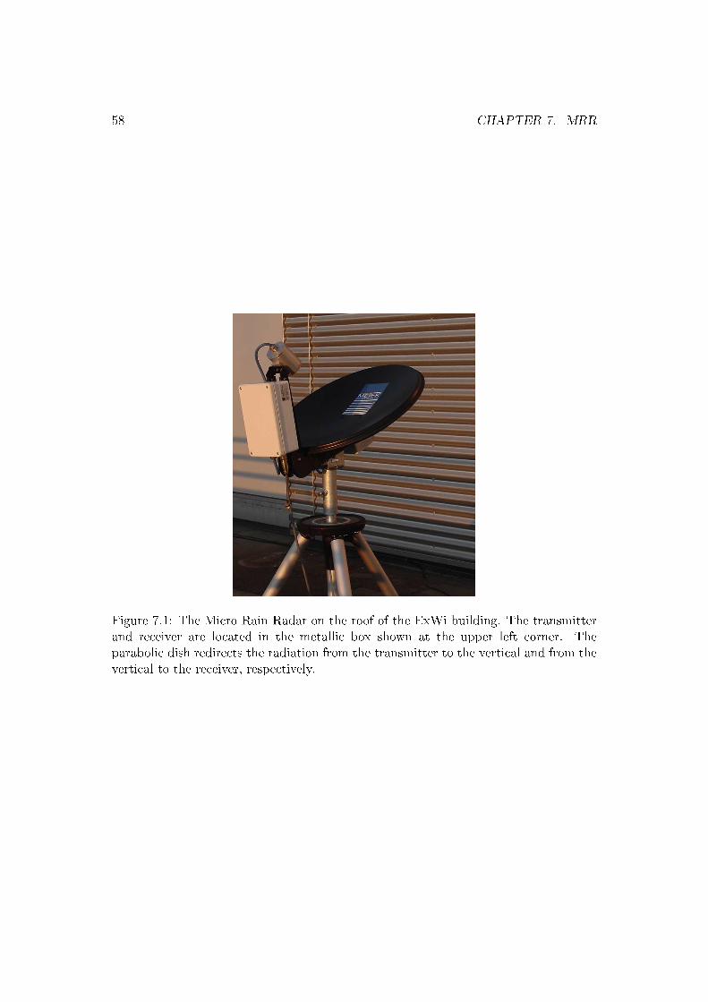
58 CHAPTER 7. MRR
Figure 7.1: The Micro Rain Radar on the roof of the ExWi building. The transmitterand receiver are located in the metallic box shown at the upper left corner. Theparabolic dish redirects the radiation from the transmitter to the vertical and from thevertical to the receiver, respectively.
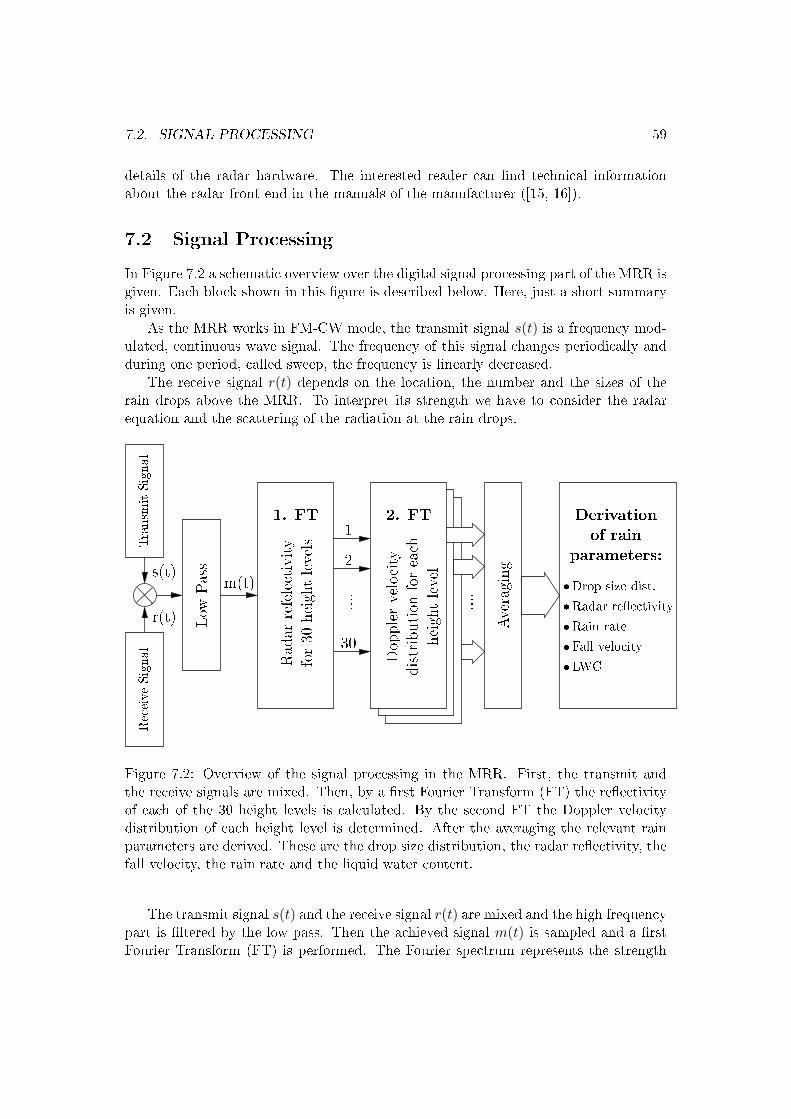
7.2. SIGNAL PROCESSING 59
details of the radar hardware. The interested reader can nd technical informationabout the radar front-end in the manuals of the manufacturer ([15, 16]).
7.2 Signal Processing
In Figure 7.2 a schematic overview over the digital signal processing part of the MRR isgiven. Each block shown in this gure is described below. Here, just a short summaryis given.
As the MRR works in FM-CW mode, the transmit signal s(t) is a frequency mod-ulated, continuous wave signal. The frequency of this signal changes periodically andduring one period, called sweep, the frequency is linearly decreased.
The receive signal r(t) depends on the location, the number and the sizes of therain drops above the MRR. To interpret its strength we have to consider the radarequation and the scattering of the radiation at the rain drops.
Radar reectivity
Rain rate
Fall velocity
LWC
Drop size dist.
Derivation
of rain
parameters:
Low
Pass
Averaging
heightlevel
distribution
foreach
Dopplervelocity
2. FT
Radar
refelectivity
for30
heightlevels
1. FT
ReceiveSignal
Transm
itSignal
m(t)
30
....
2
1
....
s(t)
r(t)
Figure 7.2: Overview of the signal processing in the MRR. First, the transmit andthe receive signals are mixed. Then, by a rst Fourier Transform (FT) the reectivityof each of the 30 height levels is calculated. By the second FT the Doppler velocitydistribution of each height level is determined. After the averaging the relevant rainparameters are derived. These are the drop size distribution, the radar reectivity, thefall velocity, the rain rate and the liquid water content.
The transmit signal s(t) and the receive signal r(t) are mixed and the high frequencypart is ltered by the low pass. Then the achieved signal m(t) is sampled and a rstFourier Transform (FT) is performed. The Fourier spectrum represents the strength
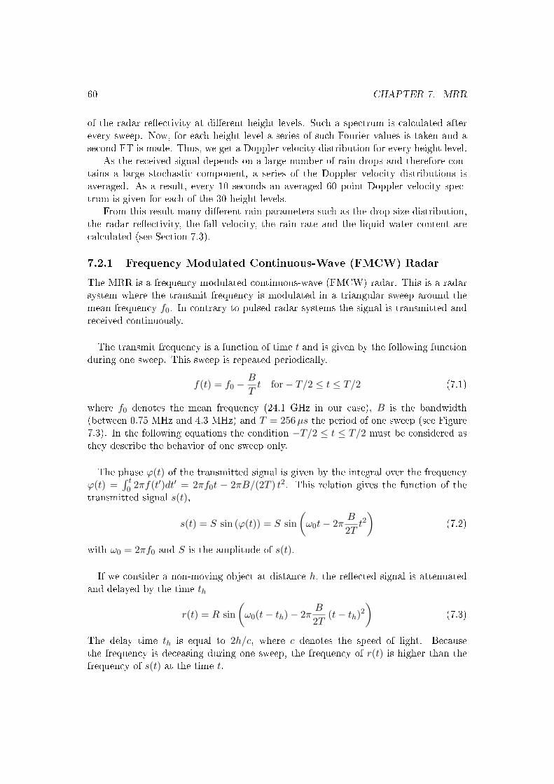
60 CHAPTER 7. MRR
of the radar reectivity at dierent height levels. Such a spectrum is calculated afterevery sweep. Now, for each height level a series of such Fourier values is taken and asecond FT is made. Thus, we get a Doppler velocity distribution for every height level.
As the received signal depends on a large number of rain drops and therefore con-tains a large stochastic component, a series of the Doppler velocity distributions isaveraged. As a result, every 10 seconds an averaged 60 point Doppler velocity spec-trum is given for each of the 30 height levels.
From this result many dierent rain parameters such as the drop size distribution,the radar reectivity, the fall velocity, the rain rate and the liquid water content arecalculated (see Section 7.3).
7.2.1 Frequency Modulated Continuous-Wave (FMCW) Radar
The MRR is a frequency modulated continuous-wave (FMCW) radar. This is a radarsystem where the transmit frequency is modulated in a triangular sweep around themean frequency f0. In contrary to pulsed radar systems the signal is transmitted andreceived continuously.
The transmit frequency is a function of time t and is given by the following functionduring one sweep. This sweep is repeated periodically.
f(t) = f0 −B
Tt for− T/2 ≤ t ≤ T/2 (7.1)
where f0 denotes the mean frequency (24.1 GHz in our case), B is the bandwidth(between 0.75 MHz and 4.3 MHz) and T = 256µs the period of one sweep (see Figure7.3). In the following equations the condition −T/2 ≤ t ≤ T/2 must be considered asthey describe the behavior of one sweep only.
The phase ϕ(t) of the transmitted signal is given by the integral over the frequencyϕ(t) =
∫ t0 2πf(t′)dt′ = 2πf0t − 2πB/(2T ) t2. This relation gives the function of the
transmitted signal s(t),
s(t) = S sin (ϕ(t)) = S sin(
ω0t− 2πB
2Tt2
)(7.2)
with ω0 = 2πf0 and S is the amplitude of s(t).
If we consider a non-moving object at distance h, the reected signal is attenuatedand delayed by the time th
r(t) = R sin(
ω0(t− th)− 2πB
2T(t− th)2
)(7.3)
The delay time th is equal to 2h/c, where c denotes the speed of light. Becausethe frequency is deceasing during one sweep, the frequency of r(t) is higher than thefrequency of s(t) at the time t.
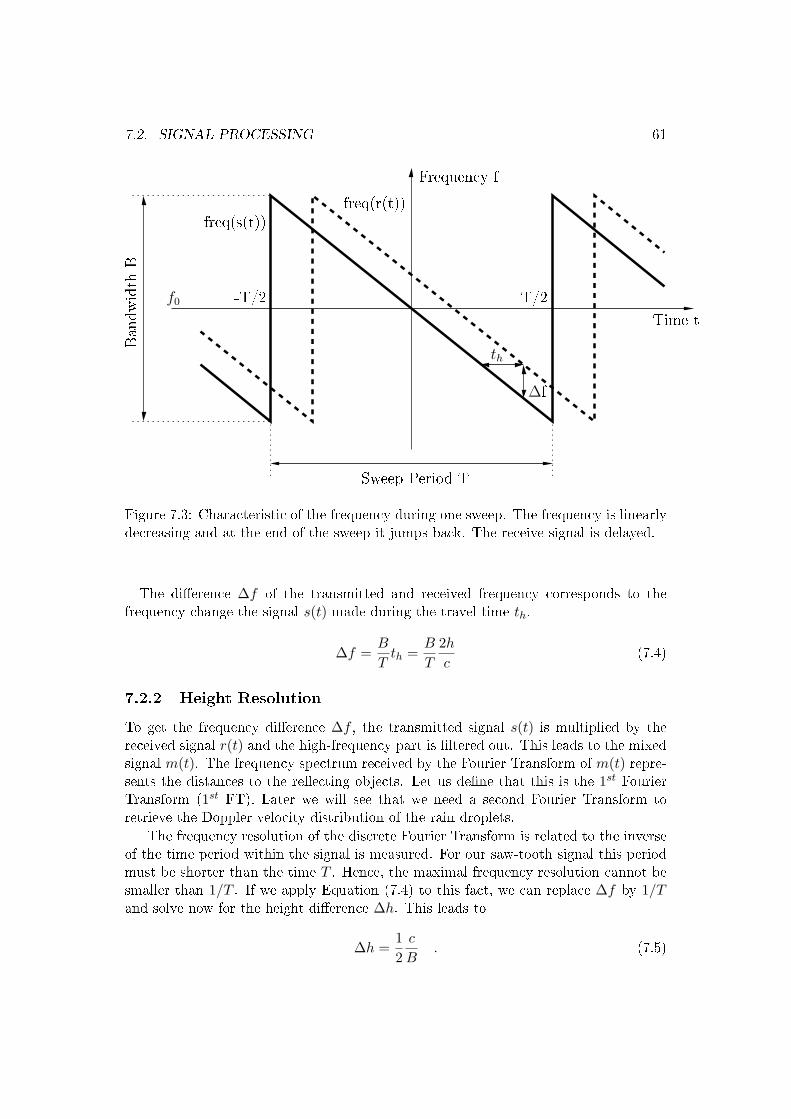
7.2. SIGNAL PROCESSING 61Bandwidth
B
T/2
Sweep Period T
f0 -T/2
freq(s(t))freq(r(t))
Frequency f
th
∆f
Time t
Figure 7.3: Characteristic of the frequency during one sweep. The frequency is linearlydecreasing and at the end of the sweep it jumps back. The receive signal is delayed.
The dierence ∆f of the transmitted and received frequency corresponds to thefrequency change the signal s(t) made during the travel time th.
∆f =B
Tth =
B
T
2h
c(7.4)
7.2.2 Height Resolution
To get the frequency dierence ∆f , the transmitted signal s(t) is multiplied by thereceived signal r(t) and the high-frequency part is ltered out. This leads to the mixedsignal m(t). The frequency spectrum received by the Fourier Transform of m(t) repre-sents the distances to the reecting objects. Let us dene that this is the 1st FourierTransform (1st FT). Later we will see that we need a second Fourier Transform toretrieve the Doppler velocity distribution of the rain droplets.
The frequency resolution of the discrete Fourier Transform is related to the inverseof the time period within the signal is measured. For our saw-tooth signal this periodmust be shorter than the time T . Hence, the maximal frequency resolution cannot besmaller than 1/T . If we apply Equation (7.4) to this fact, we can replace ∆f by 1/Tand solve now for the height dierence ∆h. This leads to
∆h =12
c
B. (7.5)
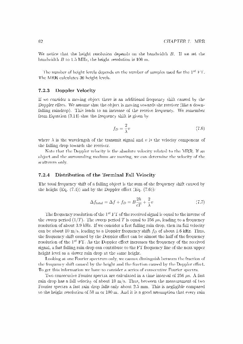
62 CHAPTER 7. MRR
We notice that the height resolution depends on the bandwidth B. If we set thebandwidth B to 1.5 MHz, the height resolution is 100 m.
The number of height levels depends on the number of samples used for the 1st FT.The MRR calculates 30 height levels.
7.2.3 Doppler Velocity
If we consider a moving object there is an additional frequency shift caused by theDoppler eect. We assume that the object is moving towards the receiver (like a down-falling raindrop). This leads to an increase of the receive frequency. We rememberfrom Equation (3.14) that the frequency shift is given by
fD =2λ
v (7.6)
where λ is the wavelength of the transmit signal and v is the velocity component ofthe falling drop towards the receiver.
Note that the Doppler velocity is the absolute velocity related to the MRR. If anobject and the surrounding medium are moving, we can determine the velocity of thescatterers only.
7.2.4 Distribution of the Terminal Fall Velocity
The total frequency shift of a falling object is the sum of the frequency shift caused bythe height (Eq. (7.4)) and by the Doppler eect (Eq. (7.6)):
∆ftotal = ∆f + fD = B2h
cT+
2λ
v (7.7)
The frequency resolution of the 1st FT of the received signal is equal to the inverse ofthe sweep period (1/T ). The sweep period T is equal to 256 µs, leading to a frequencyresolution of about 3.9 kHz. If we consider a fast falling rain drop, then its fall velocitycan be about 10 m/s, leading to a Doppler frequency shift fD of about 1.6 kHz. Thus,the frequency shift caused by the Doppler eect can be almost the half of the frequencyresolution of the 1st FT. As the Doppler eect increases the frequency of the receivedsignal, a fast falling rain drop can contribute to the FT frequency line of the next upperheight level as a slower rain drop at the same height.
Looking at one Fourier spectrum only, we cannot distinguish between the fraction ofthe frequency shift caused by the height and the fraction caused by the Doppler eect.To get this information we have to consider a series of consecutive Fourier spectra.
Two consecutive Fourier spectra are calculated in a time interval of 256 µs. A fastrain drop has a fall velocity of about 10 m/s. Thus, between the measurement of twoFourier spectra a fast rain drop falls only about 2.5 mm. This is negligible comparedto the height resolution of 50 m or 100 m. And it is a good assumption that every rain
7.3. DETERMINING THE RAIN PARAMETERS 63
drop contributes to the same height range considering a series of consecutive Fourierspectra.
What is the dierence between two consecutive Fourier spectra, if every rain dropcontributes to the same height range in both spectra? - It is the phase that changes.Due to the small distance a rain drop covered between the measurement of the twospectra, the phase is shifted. How much the phase changes, depends on the velocity ofthe rain drop. Considering a time series of a specic height range, we can determinethe frequency of the phase changes and hence the fall velocity of the rain drop. Inother words, a second Fourier Transform of a time series of a spectral line of the 1. FTcorresponds to the Doppler spectrum of the rain drops at the corresponding heightlevel.
The relation between fall velocity and Doppler frequency shift is given in Equation(7.6). The MRR calculates a Doppler frequency spectrum with 64 lines whereas theresolution is ∆fD = 30.52 Hz corresponding to a resolution in fall speed v of 0.19 m/s.Thus, the MRR can resolve the fall velocity of falling particles from 0.19 m/s up to12 m/s.
If a rain drop falls faster than the maximal resolvable fall velocity of 12 m/s, itcauses an aliasing eect leading to wrong results. The same eect can happen if upwardvertical winds lift rain drops. Small upward motion can appear as fast downwardvelocities in the Doppler spectrum.
7.2.5 Averaging
If the observed rain drops were distributed uniformly, we would not detect any phaseshift between two measured spectra. But rain is a stochastic process and is neveruniformly distributed. Thus, it is possible to measure the fall velocity distribution byconsidering the phase shift between two spectra.
But as rain is a stochastic process, a calculated Doppler spectrum gives stochasticinformation. To solve this problem, we have to calculate a large number of Dopplerspectra and average over them. The MRR measures about 150 spectra during 6 sec-onds. Then it computes the average of these spectra and transmits the result. Thetransmission takes about 4 seconds and thus, the MRR provides an averaged spectrumevery 10 seconds.
7.3 Determining the Rain Parameters
7.3.1 Radar Equation
As result of the 2nd FT we get the received spectral power dP (h, fD) as a function ofheight h and of the Doppler frequency fD. This received power is proportional to thereectivity of all rain drops in the backscattering volume within the Doppler frequencyresolution. We can use the radar equation (see Equation 3.8) to write
dP (h, fD) = C(h)1h2
η(fD) ∆h ∆fD (7.8)
64 CHAPTER 7. MRR
where C(h) is a calibration function containing radar specic parameters as thetransmit power, the antenna gain, the wavelength and other parameters of the MRR.η(fD) is the backscattering cross section per volume and per unit Doppler frequency(the spectral reectivity density). h is the height above the MRR and fD is the Dopplerfrequency shift.
In Equation (7.8) all parameters are known except η(fD). Thus, we can solve thisequation for η(fD).
7.3.2 Drop Size Distribution
From Equation (7.8) we know the spectral reectivity density η(fD) as function of theDoppler frequency fD and height h. And from Chapter 5 we know the relation betweenthe drop size and the fall velocity. As given in Equation (5.2).
Note that the fall velocity is equal to the Doppler velocity only if the ambient airhas no vertical motion. At precipitation situations this is never the case but at somesituation the vertical motion is small and it can be neglected.
The fall velocity must be corrected by a factor according to the environmental pres-sure. Equation (5.3) already gave a possibility to describe this correction factor. Herewe use the correction δv(h) as function of height assuming US Standard Atmosphereconditions.
δv(h) = 1 + 3.68 · 10−5 h + 1.71 · 10−9 h2 (7.9)
where h is given in meter above sea level.
To get the spectral reectivity density as a function of the drop diameter D, wecan use the Equation (7.6) and (5.2) to get
η(D) = η(fD)dfD
dv
dv
dD= η(fD)
2λ
6.18 e−0.6 D[mm]) δv(h) (7.10)
Dividing the spectral reectivity density η(D) by the backscattering cross sectionσb(D) of a single rain drop yields the drop size distribution N(D), the number of dropsper volume and diameter:
N(D) =η(D)σb(D)
(7.11)
For small drops we can use the Rayleigh approximation to calculate the backscat-tering cross section σb(D) (with use of the backscattering eciency Qb according toEquation (2.23)).
σb,R(D) =D2 π
4Qb(D) =
π5
λ4
∣∣∣∣ε− 1ε + 2
∣∣∣∣2 D6 =π5
λ4|K|2 D6 (7.12)
where ε is the complex dielectric constant of water. |K|2 for water is about 0.92 at24 GHz (for ice: |K|2 = 0.27).
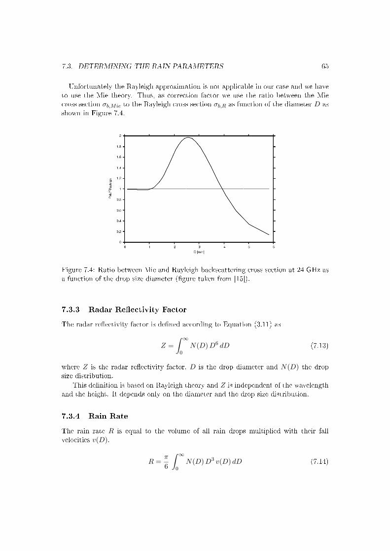
7.3. DETERMINING THE RAIN PARAMETERS 65
Unfortunately the Rayleigh approximation is not applicable in our case and we haveto use the Mie theory. Thus, as correction factor we use the ratio between the Miecross section σb,Mie to the Rayleigh cross section σb,R as function of the diameter D asshown in Figure 7.4.
Figure 7.4: Ratio between Mie and Rayleigh backscattering cross section at 24 GHz asa function of the drop size diameter (gure taken from [15]).
7.3.3 Radar Reectivity Factor
The radar reectivity factor is dened according to Equation (3.11) as
Z =∫ ∞
0N(D) D6 dD (7.13)
where Z is the radar reectivity factor, D is the drop diameter and N(D) the dropsize distribution.
This denition is based on Rayleigh theory and Z is independent of the wavelengthand the height. It depends only on the diameter and the drop size distribution.
7.3.4 Rain Rate
The rain rate R is equal to the volume of all rain drops multiplied with their fallvelocities v(D).
R =π
6
∫ ∞
0N(D) D3 v(D) dD (7.14)
66 CHAPTER 7. MRR
7.3.5 Liquid Water Content (LWC)
The liquid water content LWC is the volume of all rain drops multiplied with thedensity of water ρw per volume.
LWC = ρwπ
6
∫ ∞
0N(D) D3 dD (7.15)
7.3.6 Characteristic Fall Velocity
The characteristic fall velocity of a drop size distribution is dened according to Equa-tion (5.4).
Vm =
∫∞0 N(D) D6 v(D) dD∫∞
0 N(D) D6 dD(7.16)
Vm is the characteristic fall velocity.
7.4 Example of MRR Data
Figure 7.5 shows MRR data measured on September 13, 2008. On this day, it wasraining during three main periods. The rst rain period was from 3:00 to 5:00 UT, thesecond from 8:00 to 11:00 UT and the third from 17:00 to 22:00 UT.
Figures (a) and (b) show a time-height plot of the radar reectivity and the fallvelocity, respectively. A rain sequence from the rst rain period (from 03:00 to 04:40)is shown. The time is plotted on the horizontal axis and the height is plotted from 0to 1600 m over the MRR level on the vertical axis.
At the beginning of the plotted sequence, it was not raining. Thus, the small(dark blue) radar reectivity Z and fall velocity W values. Then, the rain startedand intensied until the end of the displayed time period. In Figure (a), we see somevertical streams with intense rain (red). These rain streaks are tilted because the rainsignal needs some time to reach the ground. In Figure (b), similar vertical regions withlarge fall velocity can be seen. Thus, intense rain falls faster than weak rain.
In Figure (c), the cumulative rain over the whole day is shown. The measurementof the MRR (blue) corresponds to the ground-based rain sensors (green). The threemain rain periods of that day can be clearly seen. The blue line is drawn by integratingthe rain rate of the 100 m height level.
7.5 Technical Summary
Table 7.1 summarizes the technical data of the Micro Rain Radar.
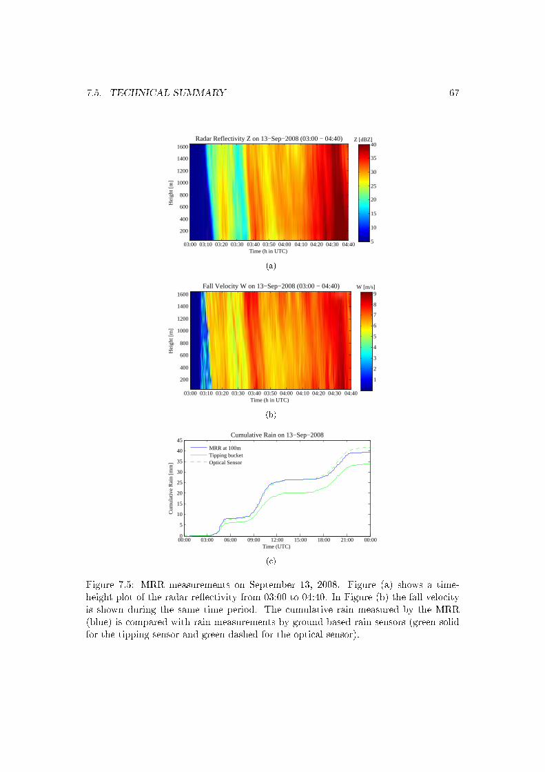
7.5. TECHNICAL SUMMARY 67
Time (h in UTC)
Hei
ght [
m]
Radar Reflectivity Z on 13−Sep−2008 (03:00 − 04:40)
03:00 03:10 03:20 03:30 03:40 03:50 04:00 04:10 04:20 04:30 04:40
200
400
600
800
1000
1200
1400
1600Z [dBZ]
5
10
15
20
25
30
35
40
(a)
Time (h in UTC)
Hei
ght [
m]
Fall Velocity W on 13−Sep−2008 (03:00 − 04:40)
03:00 03:10 03:20 03:30 03:40 03:50 04:00 04:10 04:20 04:30 04:40
200
400
600
800
1000
1200
1400
1600W [m/s]
1
2
3
4
5
6
7
8
9
(b)
00:00 03:00 06:00 09:00 12:00 15:00 18:00 21:00 00:000
5
10
15
20
25
30
35
40
45
Time (UTC)
Cum
ulat
ive
Rai
n [m
m]
Cumulative Rain on 13−Sep−2008
MRR at 100mTipping bucketOptical Sensor
(c)
Figure 7.5: MRR measurements on September 13, 2008. Figure (a) shows a time-height plot of the radar reectivity from 03:00 to 04:40. In Figure (b) the fall velocityis shown during the same time period. The cumulative rain measured by the MRR(blue) is compared with rain measurements by ground based rain sensors (green solidfor the tipping sensor and green dashed for the optical sensor).
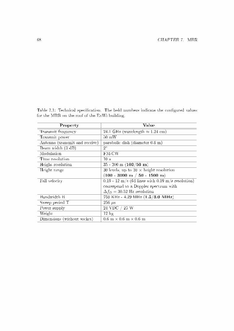
68 CHAPTER 7. MRR
Table 7.1: Technical specication. The bold numbers indicate the congured valuesfor the MRR on the roof of the ExWi building.
Property Value
Transmit frequency 24.1 GHz (wavelength ≈ 1.24 cm)
Transmit power 50 mW
Antenna (transmit and receive) parabolic dish (diameter 0.6 m)
Beam width (3 dB) 2
Modulation FM-CW
Time resolution 10 s
Height resolution 35 - 200 m (100/50 m)
Height range 30 levels, up to 30 × height resolution(100 - 3000 m / 50 - 1500 m)
Fall velocity 0.19 - 12 m/s (64 lines with 0.19 m/s resolution)correspond to a Doppler spectrum with∆fD = 30.52 Hz resolution
Bandwidth B 750 KHz - 4.29 MHz (1.5/3.0 MHz)
Sweep period T 256 µsPower supply 24 VDC / 25 W
Weight 12 kg
Dimensions (without socket) 0.6 m× 0.6 m× 0.6 m
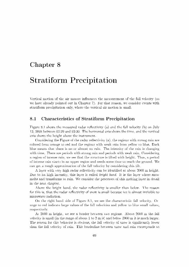
Chapter 8
Stratiform Precipitation
Vertical motion of the air masses inuences the measurement of the fall velocity (aswe have already pointed out in Chapter 7). For that reason, we consider events withstratiform precipitation only, where the vertical air motion is small.
8.1 Characteristics of Stratiform Precipitation
Figure 8.1 shows the measured radar reectivity (a) and the fall velocity (b) on July13, 2008 between 02:20 and 03:30. The horizontal axis shows the time, and the verticalaxis shows the height above the instrument.
Considering the Figure of the radar reectivity (a), the regions with strong rain arecolored from orange to red and the regions with weak rain from yellow to blue. Darkblue means that there is no or almost no rain. The intensity of the rain is changingwith time. There are periods with strong rain and periods with weak rain. Consideringa region of intense rain, we see that the structure is tilted with height. Thus, a periodof intense rain starts in an upper region and needs some time to reach the ground. Wecan get a rough approximation of the fall velocity by considering this tilt.
A layer with very high radar reectivity can be identied at about 2000 m height.Due to its high intensity, this layer is called bright band. It is the layer where snowmelts and transforms to rain. We consider the processes of this melting layer in detailin the next chapter.
Above the bright band, the radar reectivity is smaller than below. The reasonfor this is, that the radar reectivity of snow is small because ice is almost invisible tomicrowave radiation.
On the right hand side of Figure 8.1, we see the characteristic fall velocity. Or-ange to red indicate large values of the fall velocities and yellow to blue small values,respectively.
At 2000 m height, we see a border between two regions. Above 2000 m the fallvelocity is small (in the range of about 1 to 2 m/s) and below 2000 m it is much larger.The reason for this behavior is obvious, the fall velocity of snow is signicantly lowerthan the fall velocity of rain. This borderline between snow and rain corresponds to
69
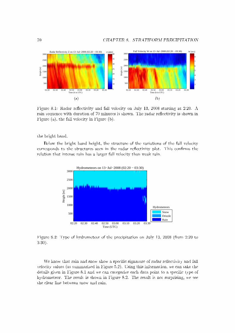
70 CHAPTER 8. STRATIFORM PRECIPITATION
Time (h in UTC)
Hei
ght [
m]
Radar Reflectivity Z on 13−Jul−2008 (02:20 − 03:30)
02:20 02:30 02:40 02:50 03:00 03:10 03:20 03:30
500
1000
1500
2000
2500
3000Z [dBZ]
5
10
15
20
25
30
35
40
(a)
Time (h in UTC)
Hei
ght [
m]
Fall Velocity W on 13−Jul−2008 (02:20 − 03:30)
02:20 02:30 02:40 02:50 03:00 03:10 03:20 03:30
500
1000
1500
2000
2500
3000W [m/s]
2
3
4
5
6
7
8
(b)
Figure 8.1: Radar reectivity and fall velocity on July 13, 2008 starting at 2:20. Arain sequence with duration of 70 minutes is shown. The radar reectivity is shown inFigure (a), the fall velocity in Figure (b).
the bright band.
Below the bright band height, the structure of the variations of the fall velocitycorresponds to the structures seen in the radar reectivity plot. This conrms therelation that intense rain has a larger fall velocity than weak rain.
Time (UTC)
Hei
ght [
m]
Hydrometeors on 13−Jul−2008 (02:20 − 03:30)
02:20 02:30 02:40 02:50 03:00 03:10 03:20 03:30
500
1000
1500
2000
2500
3000
SnowDrizzleRain
Hydrometeors
Figure 8.2: Type of hydrometeor of the precipitation on July 13, 2008 (from 2:20 to3:30).
We know that rain and snow show a specic signature of radar reectivity and fallvelocity values (as summarized in Figure 5.2). Using this information, we can take thedetails given in Figure 8.1 and we can categorize each data point to a specic type ofhydrometeor. The result is shown in Figure 8.2. The result is not surprising, we seethe clear line between snow and rain.
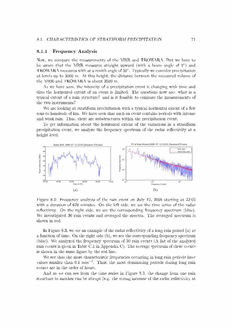
8.1. CHARACTERISTICS OF STRATIFORM PRECIPITATION 71
8.1.1 Frequency Analysis
Now, we compare the measurements of the MRR and TROWARA. But we have tobe aware that the MRR measures straight upward (with a beam angle of 2) andTROWARA measures with at a zenith angle of 50. Typically we consider precipitationat levels up to 3000 m. At this height, the distance between the measured volume ofthe MRR and TROWARA is about 3500 m.
As we have seen, the intensity of a precipitation event is changing with time andthus the horizontal extent of an event is limited. The questions now are: what is atypical extent of a rain structure? and is it feasible to compare the measurements ofthe two instruments?
We are looking at stratiform precipitation with a typical horizontal extent of a fewtens to hundreds of km. We have seen that such an event contains periods with intenseand weak rain. Thus, there are substructures within the precipitation event.
To get information about the horizontal extent of the variations in a stratiformprecipitation event, we analyze the frequency spectrum of the radar reectivity at aheight level.
21:00 00:00 03:00 06:00 09:00 12:00−20
−10
0
10
20
30
40
50
Time (UTC)
Rad
ar r
efle
ctiv
ity [d
BZ
]
Radar Refl. 2008−07−12 22:05 (Duration: 670 min)
(a)
10−2 10−1 10010−3
10−2
10−1
100
FT of Rain Period (2008−07−12 22:05, Duration:670 min)
Frequency [1/min]
Fre
quen
cy S
pect
rum
freq. spec.mean freq. spec.
(b)
Figure 8.3: Frequency analysis of the rain event on July 12, 2008 starting at 22:05with a duration of 670 minutes. On the left side, we see the time series of the radarreectivity. On the right side, we see the corresponding frequency spectrum (blue).We investigated 30 rain events and averaged the spectra. The averaged spectrum isshown in red.
In Figure 8.3, we see an example of the radar reectivity of a long rain period (a) asa function of time. On the right side (b), we see the corresponding frequency spectrum(blue). We analyzed the frequency spectrum of 30 rain events (A list of the analyzedrain events is given in Table C.1 in Appendix C). The average spectrum of these eventsis shown in the same gure by the red line.
We see that the most characteristic frequencies occurring in long rain periods havevalues smaller than 0.1 min−1. Thus, the most dominating periods during long rainevents are in the order of hours.
And as we can see from the time series in Figure 8.3, the change from one rainstructure to another can be abrupt (e.g. the strong increase of the radar reectivity at
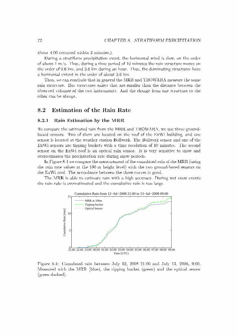
72 CHAPTER 8. STRATIFORM PRECIPITATION
about 4:00 occurred within 2 minutes.).
During a stratiform precipitation event, the horizontal wind is slow, on the orderof about 1 m/s. Thus, during a time period of 10 minutes the rain structure moves onthe order of 0.6 km, and 3.6 km during an hour. Thus, the dominating structures havea horizontal extent in the order of about 3.6 km.
Thus, we can conclude that in general the MRR and TROWARA measure the samerain structure. But structures exists that are smaller than the distance between theobserved volumes of the two instruments. And the change from one structure to theother can be abrupt.
8.2 Estimation of the Rain Rate
8.2.1 Rain Estimation by the MRR
To compare the estimated rain from the MRR and TROWARA, we use three ground-based sensors. Two of them are located on the roof of the ExWi building, and onesensor is located at the weather station Bollwerk. The Bollwerk sensor and one of theExWi sensors are tipping buckets with a time resolution of 10 minutes. The secondsensor on the ExWi roof is an optical rain sensor. It is very sensitive to snow andoverestimates the precipitation rate during snow periods.
In Figure 8.4 we compare the measurement of the cumulated rain of the MRR (usingthe rain rate values at the 100 m height level) with the two ground-based sensors onthe ExWi roof. The accordance between the three curves is good.
The MRR is able to estimate rain with a high accuracy. During wet snow eventsthe rain rate is overestimated and the cumulative rain is too large.
21:00 22:00 23:00 00:00 01:00 02:00 03:00 04:00 05:00 06:00 07:00 08:00 09:000
5
10
15
Time (UTC)
Cum
ulat
ive
Rai
n [m
m]
Cumulative Rain from 12−Jul−2008 21:00 to 13−Jul−2008 09:00
MRR at 100mTipping bucketOptical Sensor
Figure 8.4: Cumulated rain between July 12, 2008 21:00 and July 13, 2008, 9:00.Measured with the MRR (blue), the tipping bucket (green) and the optical sensor(green dashed).
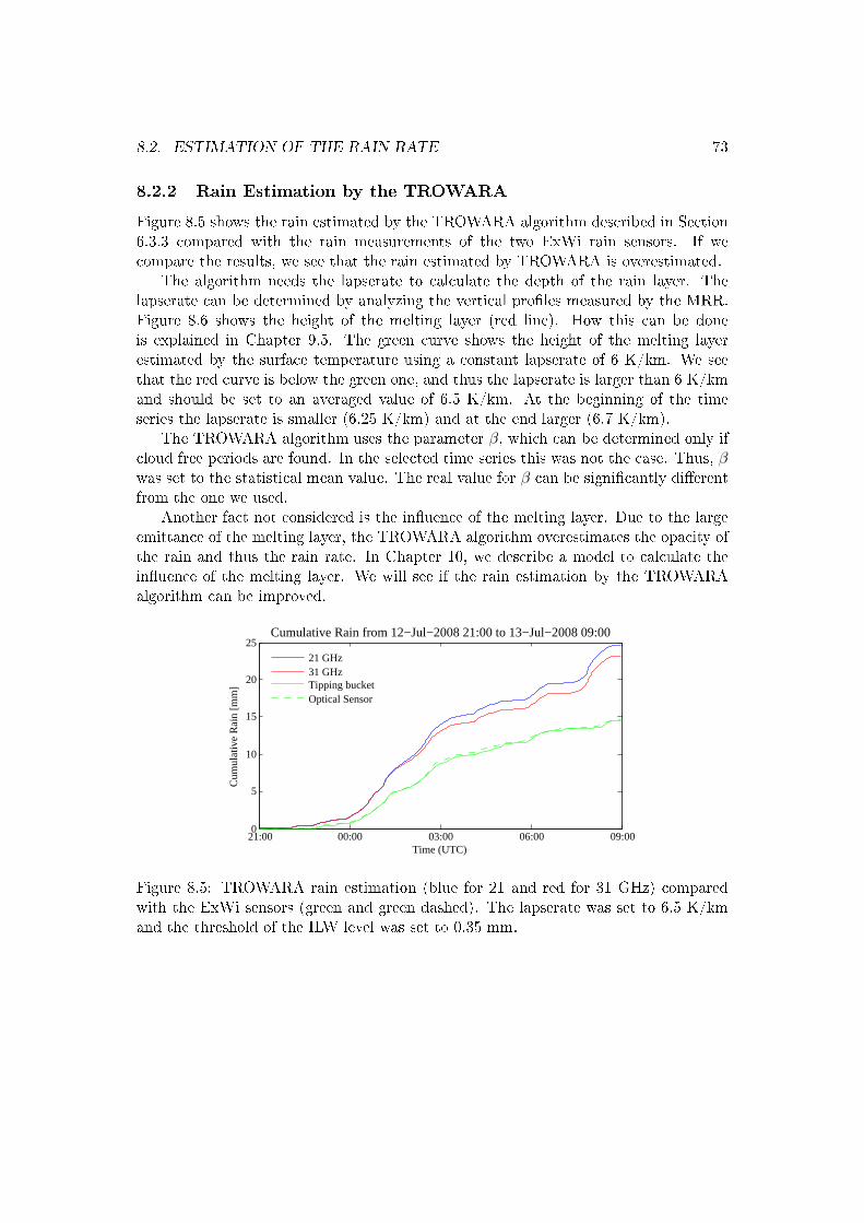
8.2. ESTIMATION OF THE RAIN RATE 73
8.2.2 Rain Estimation by the TROWARA
Figure 8.5 shows the rain estimated by the TROWARA algorithm described in Section6.3.3 compared with the rain measurements of the two ExWi rain sensors. If wecompare the results, we see that the rain estimated by TROWARA is overestimated.
The algorithm needs the lapserate to calculate the depth of the rain layer. Thelapserate can be determined by analyzing the vertical proles measured by the MRR.Figure 8.6 shows the height of the melting layer (red line). How this can be doneis explained in Chapter 9.5. The green curve shows the height of the melting layerestimated by the surface temperature using a constant lapserate of 6 K/km. We seethat the red curve is below the green one, and thus the lapserate is larger than 6 K/kmand should be set to an averaged value of 6.5 K/km. At the beginning of the timeseries the lapserate is smaller (6.25 K/km) and at the end larger (6.7 K/km).
The TROWARA algorithm uses the parameter β, which can be determined only ifcloud free periods are found. In the selected time series this was not the case. Thus, βwas set to the statistical mean value. The real value for β can be signicantly dierentfrom the one we used.
Another fact not considered is the inuence of the melting layer. Due to the largeemittance of the melting layer, the TROWARA algorithm overestimates the opacity ofthe rain and thus the rain rate. In Chapter 10, we describe a model to calculate theinuence of the melting layer. We will see if the rain estimation by the TROWARAalgorithm can be improved.
21:00 00:00 03:00 06:00 09:000
5
10
15
20
25
Time (UTC)
Cum
ulat
ive
Rai
n [m
m]
Cumulative Rain from 12−Jul−2008 21:00 to 13−Jul−2008 09:00
21 GHz31 GHzTipping bucketOptical Sensor
Figure 8.5: TROWARA rain estimation (blue for 21 and red for 31 GHz) comparedwith the ExWi sensors (green and green dashed). The lapserate was set to 6.5 K/kmand the threshold of the ILW level was set to 0.35 mm.
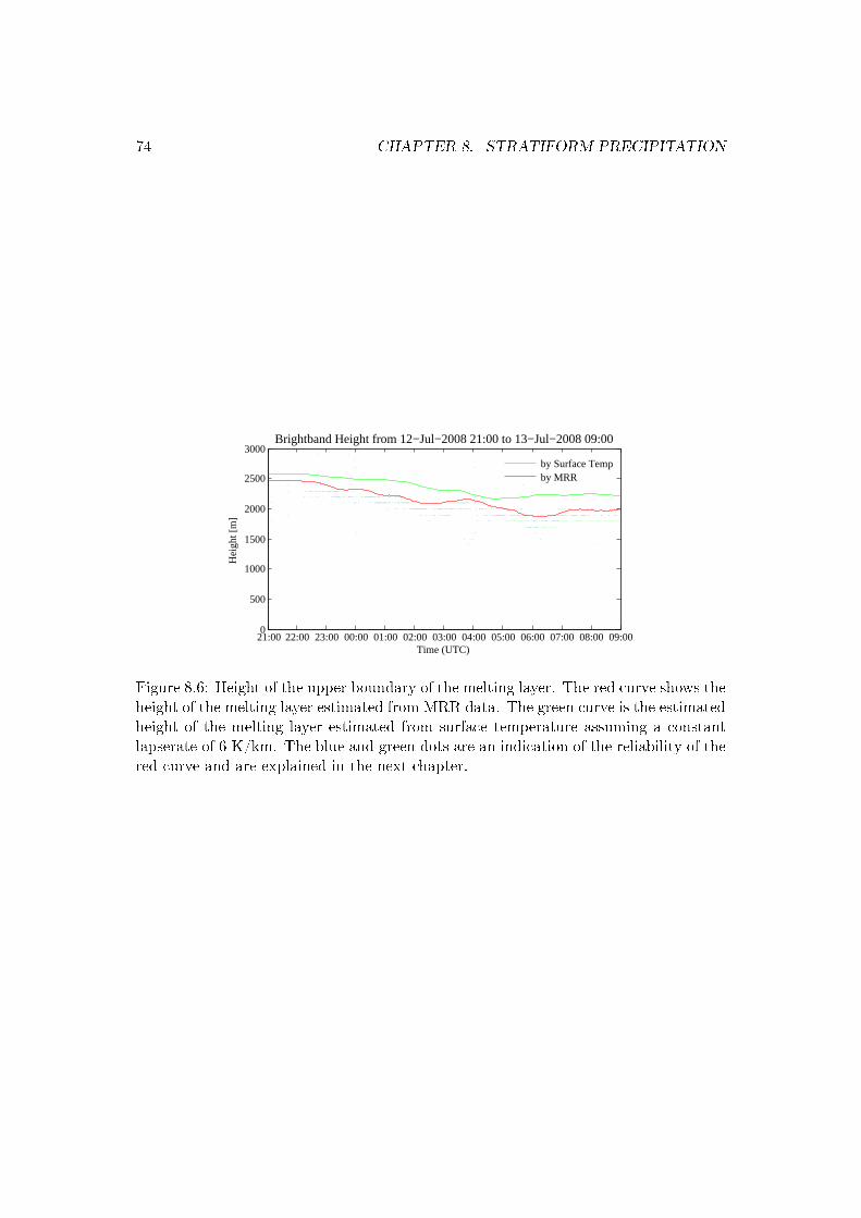
74 CHAPTER 8. STRATIFORM PRECIPITATION
21:00 22:00 23:00 00:00 01:00 02:00 03:00 04:00 05:00 06:00 07:00 08:00 09:000
500
1000
1500
2000
2500
3000
Time (UTC)
Hei
ght [
m]
Brightband Height from 12−Jul−2008 21:00 to 13−Jul−2008 09:00
by Surface Tempby MRR
Figure 8.6: Height of the upper boundary of the melting layer. The red curve shows theheight of the melting layer estimated from MRR data. The green curve is the estimatedheight of the melting layer estimated from surface temperature assuming a constantlapserate of 6 K/km. The blue and green dots are an indication of the reliability of thered curve and are explained in the next chapter.
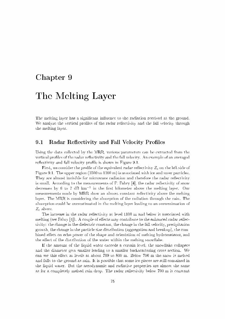
Chapter 9
The Melting Layer
The melting layer has a signicant inuence to the radiation received at the ground.We analyze the vertical proles of the radar reectivity and the fall velocity throughthe melting layer.
9.1 Radar Reectivity and Fall Velocity Proles
Using the data collected by the MRR, various parameters can be extracted from thevertical proles of the radar reectivity and the fall velocity. An example of an averagedreectivity and fall velocity prole is shown in Figure 9.1.
First, we consider the prole of the equivalent radar reectivity Ze on the left side ofFigure 9.1. The upper region (1500 to 1100 m) is associated with ice and snow particles.They are almost invisible for microwave radiation and therefore the radar reectivityis small. According to the measurements of F. Fabry [4], the radar reectivity of snowdecreases by 6 to 7 dB km−1 in the rst kilometer above the melting layer. Ourmeasurements made by MRR show an almost constant reectivity above the meltinglayer. The MRR is considering the absorption of the radiation through the rain. Theabsorption could be overestimated in the melting layer leading to an overestimation ofZe above.
The increase in the radar reectivity at level 1100 m and below is associated withmelting (see Fabry [4]). A couple of eects may contribute to the enhanced radar reec-tivity: the change in the dielectric constant, the change in the fall velocity, precipitationgrowth, the change in the particle size distribution (aggregation and breakup), the com-bined eect on echo power of the shape and orientation of melting hydrometeors, andthe eect of the distribution of the water within the melting snowake.
If the amount of the liquid water exceeds a certain level, the snowake collapsesand the diameter gets smaller leading to a smaller backscattering cross section. Wecan see this eect at levels at about 700 to 800 m. Below 700 m the snow is meltedand falls to the ground as rain. It is possible that some ice pieces are still contained inthe liquid water. But the aerodynamic and radiative properties are almost the sameas for a completely melted rain drop. The radar reectivity below 700 m is constant
75
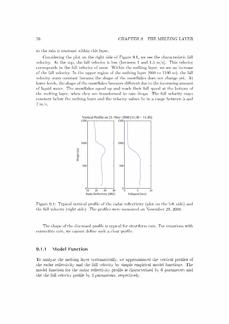
76 CHAPTER 9. THE MELTING LAYER
as the rain is constant within this layer.
Considering the plot on the right side of Figure 9.1, we see the characteristic fallvelocity. At the top, the fall velocity is low (between 1 and 1.5 m/s). This velocitycorresponds to the fall velocity of snow. Within the melting layer, we see an increaseof the fall velocity. In the upper region of the melting layer (900 to 1100 m), the fallvelocity stays constant because the shape of the snowakes does not change yet. Atlower levels, the shape of the snowakes becomes dierent due to the increasing amountof liquid water. The snowakes speed up and reach their full speed at the bottom ofthe melting layer, when they are transformed to rain drops. The fall velocity staysconstant below the melting layer and the velocity values lie in a range between 5 and7 m/s.
10 20 30 400
500
1000
1500
Hei
ght [
m]
Radar Reflectivity [dBZ]0 5 10
0
500
1000
1500
Fallspeed [m/s]
Vertical Profile on 21−Nov−2008 (11:30 − 11:45)
Figure 9.1: Typical vertical prole of the radar reectivity (plot on the left side) andthe fall velocity (right side). The proles were measured on November 21, 2008.
The shape of the discussed prole is typical for stratiform rain. For situations withconvective rain, we cannot dene such a clear prole.
9.1.1 Model Function
To analyze the melting layer systematically, we approximated the vertical proles ofthe radar reectivity and the fall velocity by simple empirical model functions. Themodel function for the radar reectivity prole is characterized by 6 parameters andthe the fall velocity prole by 4 parameters, respectively.
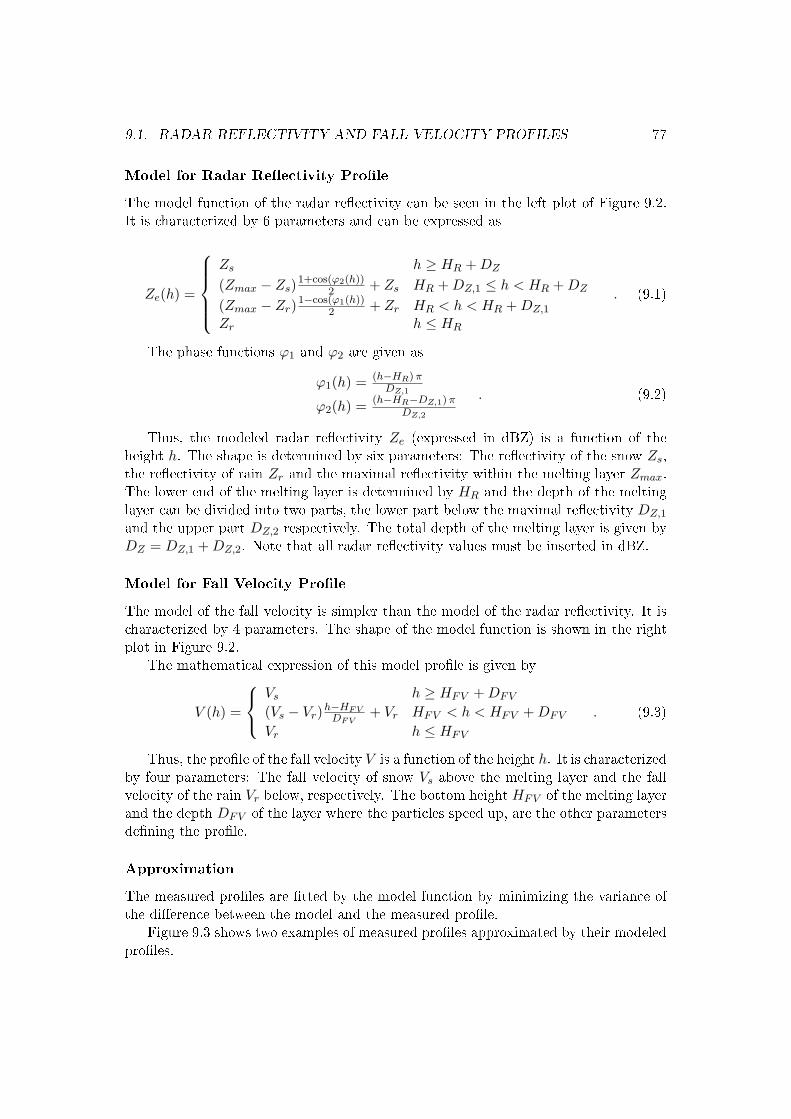
9.1. RADAR REFLECTIVITY AND FALL VELOCITY PROFILES 77
Model for Radar Reectivity Prole
The model function of the radar reectivity can be seen in the left plot of Figure 9.2.It is characterized by 6 parameters and can be expressed as
Ze(h) =
Zs h ≥ HR + DZ
(Zmax − Zs)1+cos(ϕ2(h))
2 + Zs HR + DZ,1 ≤ h < HR + DZ
(Zmax − Zr)1−cos(ϕ1(h))
2 + Zr HR < h < HR + DZ,1
Zr h ≤ HR
. (9.1)
The phase functions ϕ1 and ϕ2 are given as
ϕ1(h) = (h−HR) πDZ,1
ϕ2(h) = (h−HR−DZ,1) πDZ,2
. (9.2)
Thus, the modeled radar reectivity Ze (expressed in dBZ) is a function of theheight h. The shape is determined by six parameters: The reectivity of the snow Zs,the reectivity of rain Zr and the maximal reectivity within the melting layer Zmax.The lower end of the melting layer is determined by HR and the depth of the meltinglayer can be divided into two parts, the lower part below the maximal reectivity DZ,1
and the upper part DZ,2 respectively. The total depth of the melting layer is given byDZ = DZ,1 + DZ,2. Note that all radar reectivity values must be inserted in dBZ.
Model for Fall Velocity Prole
The model of the fall velocity is simpler than the model of the radar reectivity. It ischaracterized by 4 parameters. The shape of the model function is shown in the rightplot in Figure 9.2.
The mathematical expression of this model prole is given by
V (h) =
Vs h ≥ HFV + DFV
(Vs − Vr)h−HFVDFV
+ Vr HFV < h < HFV + DFV
Vr h ≤ HFV
. (9.3)
Thus, the prole of the fall velocity V is a function of the height h. It is characterizedby four parameters: The fall velocity of snow Vs above the melting layer and the fallvelocity of the rain Vr below, respectively. The bottom height HFV of the melting layerand the depth DFV of the layer where the particles speed up, are the other parametersdening the prole.
Approximation
The measured proles are tted by the model function by minimizing the variance ofthe dierence between the model and the measured prole.
Figure 9.3 shows two examples of measured proles approximated by their modeledproles.
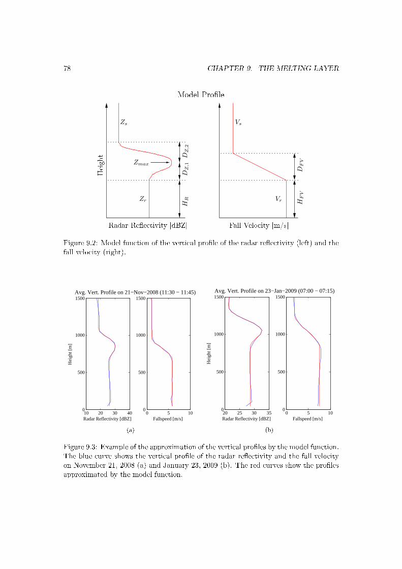
78 CHAPTER 9. THE MELTING LAYER
Height
Model Prole
Vs
DF
V
HR Vr HF
V
Radar Reectivity [dBZ] Fall Velocity [m/s]
Zs
Zmax
Zr
DZ
,1D
Z,2
Figure 9.2: Model function of the vertical prole of the radar reectivity (left) and thefall velocity (right).
10 20 30 400
500
1000
1500
Hei
ght [
m]
Radar Reflectivity [dBZ]0 5 10
0
500
1000
1500
Fallspeed [m/s]
Avg. Vert. Profile on 21−Nov−2008 (11:30 − 11:45)
(a)
20 25 30 350
500
1000
1500
Hei
ght [
m]
Radar Reflectivity [dBZ]0 5 10
0
500
1000
1500
Fallspeed [m/s]
Avg. Vert. Profile on 23−Jan−2009 (07:00 − 07:15)
(b)
Figure 9.3: Example of the approximation of the vertical proles by the model function.The blue curve shows the vertical prole of the radar reectivity and the fall velocityon November 21, 2008 (a) and January 23, 2009 (b). The red curves show the prolesapproximated by the model function.
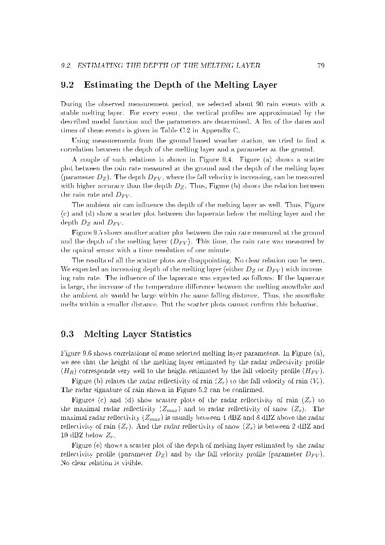
9.2. ESTIMATING THE DEPTH OF THE MELTING LAYER 79
9.2 Estimating the Depth of the Melting Layer
During the observed measurement period, we selected about 90 rain events with astable melting layer. For every event, the vertical proles are approximated by thedescribed model function and the parameters are determined. A list of the dates andtimes of these events is given in Table C.2 in Appendix C.
Using measurements from the ground-based weather station, we tried to nd acorrelation between the depth of the melting layer and a parameter at the ground.
A couple of such relations is shown in Figure 9.4. Figure (a) shows a scatterplot between the rain rate measured at the ground and the depth of the melting layer(parameter DZ). The depth DFV , where the fall velocity is increasing, can be measuredwith higher accuracy than the depth DZ . Thus, Figure (b) shows the relation betweenthe rain rate and DFV .
The ambient air can inuence the depth of the melting layer as well. Thus, Figure(c) and (d) show a scatter plot between the lapserate below the melting layer and thedepth DZ and DFV .
Figure 9.5 shows another scatter plot between the rain rate measured at the groundand the depth of the melting layer (DFV ). This time, the rain rate was measured bythe optical sensor with a time resolution of one minute.
The results of all the scatter plots are disappointing. No clear relation can be seen.We expected an increasing depth of the melting layer (either DZ or DFV ) with increas-ing rain rate. The inuence of the lapserate was expected as follows: If the lapserateis large, the increase of the temperature dierence between the melting snowake andthe ambient air would be large within the same falling distance. Thus, the snowakemelts within a smaller distance. But the scatter plots cannot conrm this behavior.
9.3 Melting Layer Statistics
Figure 9.6 shows correlations of some selected melting layer parameters. In Figure (a),we see that the height of the melting layer estimated by the radar reectivity prole(HR) corresponds very well to the height estimated by the fall velocity prole (HFV ).
Figure (b) relates the radar reectivity of rain (Zr) to the fall velocity of rain (Vr).The radar signature of rain shown in Figure 5.2 can be conrmed.
Figures (c) and (d) show scatter plots of the radar reectivity of rain (Zr) tothe maximal radar reectivity (Zmax) and to radar reectivity of snow (Zs). Themaximal radar reectivity (Zmax) is usually between 4 dBZ and 8 dBZ above the radarreectivity of rain (Zr). And the radar reectivity of snow (Zs) is between 2 dBZ and10 dBZ below Zr.
Figure (e) shows a scatter plot of the depth of melting layer estimated by the radarreectivity prole (parameter DZ) and by the fall velocity prole (parameter DFV ).No clear relation is visible.
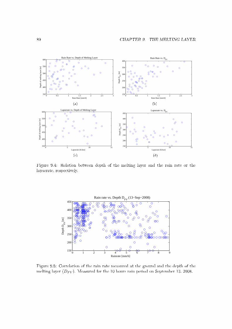
80 CHAPTER 9. THE MELTING LAYER
0 0.5 1 1.5 2 2.5 3350
400
450
500
550
600Rain Rate vs. Depth of Melting Layer
Rain Rate [mm/h]
Dep
th o
f m
eltin
g la
yer
[m]
(a)
0 0.5 1 1.5 2 2.5 3150
200
250
300
350
400
Rain Rate vs. DFV
Rain Rate [mm/h]
Dep
th D
FV [
m]
(b)
0 5 10 15350
400
450
500
550
600Lapserate vs. Depth of Melting Layer
Lapserate [K/km]
Dep
th o
f m
eltin
g la
yer
[m]
(c)
0 5 10 15150
200
250
300
350
400
450
Lapserate vs. DFV
Lapserate [K/km]
Dep
th D
FV [
m]
(d)
Figure 9.4: Relation between depth of the melting layer and the rain rate or thelapserate, respectively.
0 1 2 3 4 5 6 7 8 9150
200
250
300
350
400
450
Rainrate [mm/h]
Dep
th D
FS [m
]
Rain rate vs. Depth DFV
(13−Sep−2008)
Figure 9.5: Correlation of the rain rate measured at the ground and the depth of themelting layer (DFV ). Measured for the 10 hours rain period on September 13, 2008.
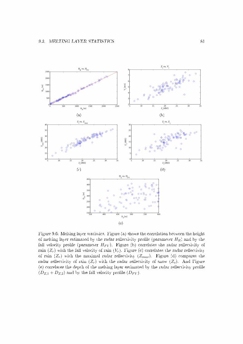
9.3. MELTING LAYER STATISTICS 81
0 500 1000 1500 2000 25000
500
1000
1500
2000
2500
HR vs. H
FV
HR
[m]
HFV
[m
]
(a)
5 10 15 20 25 30 352
3
4
5
6
7
8
Zr vs. V
r
Zr [dBZ]
Vr [
m/s
]
(b)
5 10 15 20 25 30 3510
15
20
25
30
35
40
Zr vs. Z
max
Zr [dBZ]
Zm
ax [
dBZ
]
(c)
5 10 15 20 25 30 350
5
10
15
20
25
30
Zr vs. Z
s
Zr [dBZ]
Zs [
dBZ
]
(d)
350 400 450 500 550 600150
200
250
300
350
400
450
DZ vs. D
FV
DZ [m]
DFV
[m
]
(e)
Figure 9.6: Melting layer statistics. Figure (a) shows the correlation between the heightof melting layer estimated by the radar reectivity prole (parameter HR) and by thefall velocity prole (parameter HFV ). Figure (b) correlates the radar reectivity ofrain (Zr) with the fall velocity of rain (Vr). Figure (c) correlates the radar reectivityof rain (Zr) with the maximal radar reectivity (Zmax). Figure (d) compares theradar reectivity of rain (Zr) with the radar reectivity of snow (Zs). And Figure(e) correlates the depth of the melting layer estimated by the radar reectivity prole(DZ,1 + DZ,2) and by the fall velocity prole (DFV ).
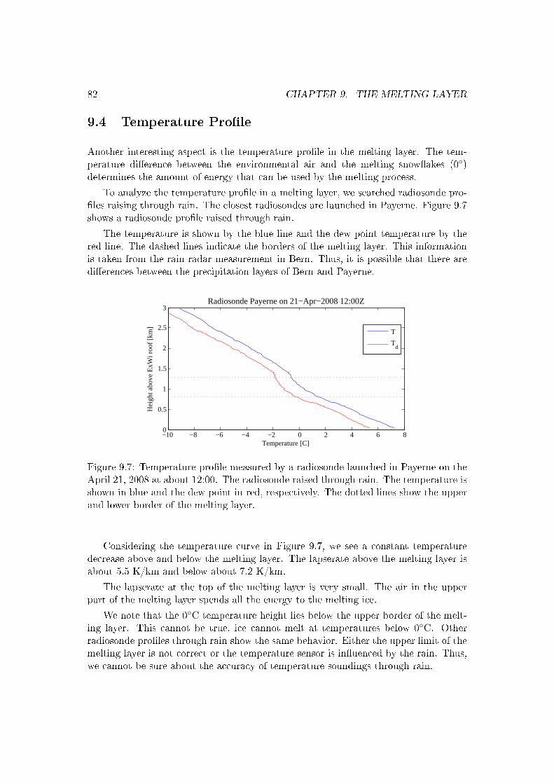
82 CHAPTER 9. THE MELTING LAYER
9.4 Temperature Prole
Another interesting aspect is the temperature prole in the melting layer. The tem-perature dierence between the environmental air and the melting snowakes (0)determines the amount of energy that can be used by the melting process.
To analyze the temperature prole in a melting layer, we searched radiosonde pro-les raising through rain. The closest radiosondes are launched in Payerne. Figure 9.7shows a radiosonde prole raised through rain.
The temperature is shown by the blue line and the dew point temperature by thered line. The dashed lines indicate the borders of the melting layer. This informationis taken from the rain radar measurement in Bern. Thus, it is possible that there aredierences between the precipitation layers of Bern and Payerne.
−10 −8 −6 −4 −2 0 2 4 6 80
0.5
1
1.5
2
2.5
3
Temperature [C]
Hei
ght a
bove
ExW
i roo
f [km
]
Radiosonde Payerne on 21−Apr−2008 12:00Z
T
Td
Figure 9.7: Temperature prole measured by a radiosonde launched in Payerne on theApril 21, 2008 at about 12:00. The radiosonde raised through rain. The temperature isshown in blue and the dew point in red, respectively. The dotted lines show the upperand lower border of the melting layer.
Considering the temperature curve in Figure 9.7, we see a constant temperaturedecrease above and below the melting layer. The lapserate above the melting layer isabout 5.5 K/km and below about 7.2 K/km.
The lapserate at the top of the melting layer is very small. The air in the upperpart of the melting layer spends all the energy to the melting ice.
We note that the 0C temperature height lies below the upper border of the melt-ing layer. This cannot be true, ice cannot melt at temperatures below 0C. Otherradiosonde proles through rain show the same behavior. Either the upper limit of themelting layer is not correct or the temperature sensor is inuenced by the rain. Thus,we cannot be sure about the accuracy of temperature soundings through rain.
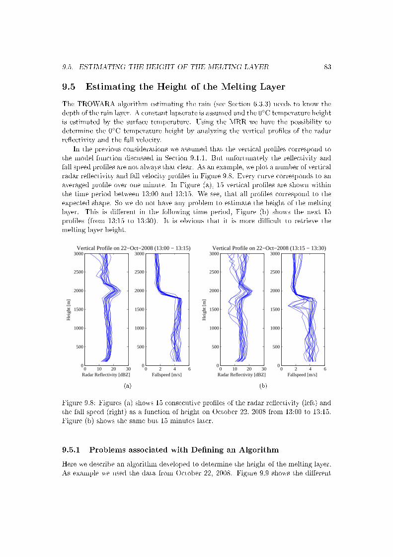
9.5. ESTIMATING THE HEIGHT OF THE MELTING LAYER 83
9.5 Estimating the Height of the Melting Layer
The TROWARA algorithm estimating the rain (see Section 6.3.3) needs to know thedepth of the rain layer. A constant lapserate is assumed and the 0C temperature heightis estimated by the surface temperature. Using the MRR we have the possibility todetermine the 0C temperature height by analyzing the vertical proles of the radarreectivity and the fall velocity.
In the previous considerations we assumed that the vertical proles correspond tothe model function discussed in Section 9.1.1. But unfortunately the reectivity andfall speed proles are not always that clear. As an example, we plot a number of verticalradar reectivity and fall velocity proles in Figure 9.8. Every curve corresponds to anaveraged prole over one minute. In Figure (a), 15 vertical proles are shown withinthe time period between 13:00 and 13:15. We see, that all proles correspond to theexpected shape. So we do not have any problem to estimate the height of the meltinglayer. This is dierent in the following time period, Figure (b) shows the next 15proles (from 13:15 to 13:30). It is obvious that it is more dicult to retrieve themelting layer height.
0 10 20 300
500
1000
1500
2000
2500
3000
Hei
ght [
m]
Radar Reflectivity [dBZ]0 2 4 6
0
500
1000
1500
2000
2500
3000
Fallspeed [m/s]
Vertical Profile on 22−Oct−2008 (13:00 − 13:15)
(a)
0 10 20 300
500
1000
1500
2000
2500
3000
Hei
ght [
m]
Radar Reflectivity [dBZ]0 2 4 6
0
500
1000
1500
2000
2500
3000
Fallspeed [m/s]
Vertical Profile on 22−Oct−2008 (13:15 − 13:30)
(b)
Figure 9.8: Figures (a) shows 15 consecutive proles of the radar reectivity (left) andthe fall speed (right) as a function of height on October 22, 2008 from 13:00 to 13:15.Figure (b) shows the same but 15 minutes later.
9.5.1 Problems associated with Dening an Algorithm
Here we describe an algorithm developed to determine the height of the melting layer.As example we used the data from October 22, 2008. Figure 9.9 shows the dierent
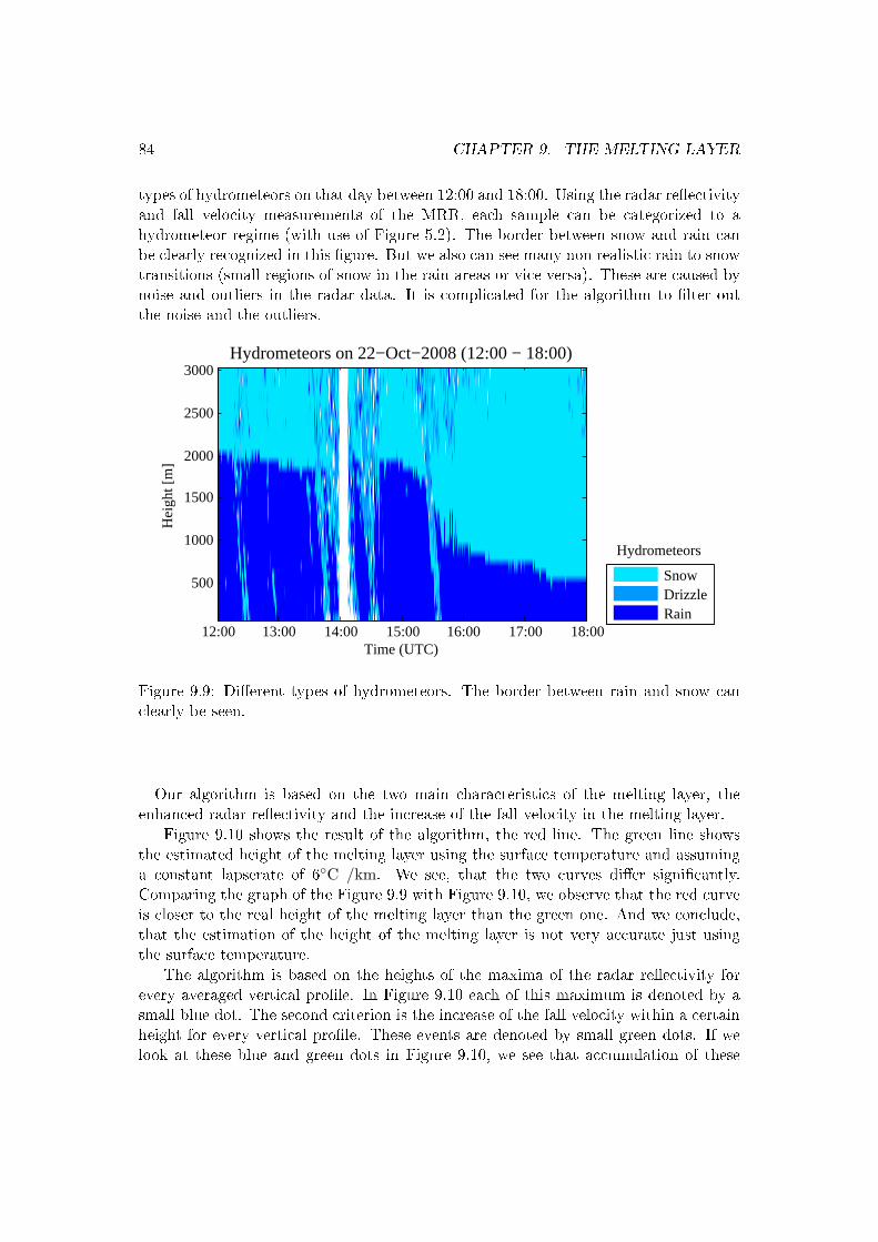
84 CHAPTER 9. THE MELTING LAYER
types of hydrometeors on that day between 12:00 and 18:00. Using the radar reectivityand fall velocity measurements of the MRR, each sample can be categorized to ahydrometeor regime (with use of Figure 5.2). The border between snow and rain canbe clearly recognized in this gure. But we also can see many non realistic rain to snowtransitions (small regions of snow in the rain areas or vice versa). These are caused bynoise and outliers in the radar data. It is complicated for the algorithm to lter outthe noise and the outliers.
Time (UTC)
Hei
ght [
m]
Hydrometeors on 22−Oct−2008 (12:00 − 18:00)
12:00 13:00 14:00 15:00 16:00 17:00 18:00
500
1000
1500
2000
2500
3000
SnowDrizzleRain
Hydrometeors
Figure 9.9: Dierent types of hydrometeors. The border between rain and snow canclearly be seen.
Our algorithm is based on the two main characteristics of the melting layer, theenhanced radar reectivity and the increase of the fall velocity in the melting layer.
Figure 9.10 shows the result of the algorithm, the red line. The green line showsthe estimated height of the melting layer using the surface temperature and assuminga constant lapserate of 6C /km. We see, that the two curves dier signicantly.Comparing the graph of the Figure 9.9 with Figure 9.10, we observe that the red curveis closer to the real height of the melting layer than the green one. And we conclude,that the estimation of the height of the melting layer is not very accurate just usingthe surface temperature.
The algorithm is based on the heights of the maxima of the radar reectivity forevery averaged vertical prole. In Figure 9.10 each of this maximum is denoted by asmall blue dot. The second criterion is the increase of the fall velocity within a certainheight for every vertical prole. These events are denoted by small green dots. If welook at these blue and green dots in Figure 9.10, we see that accumulation of these
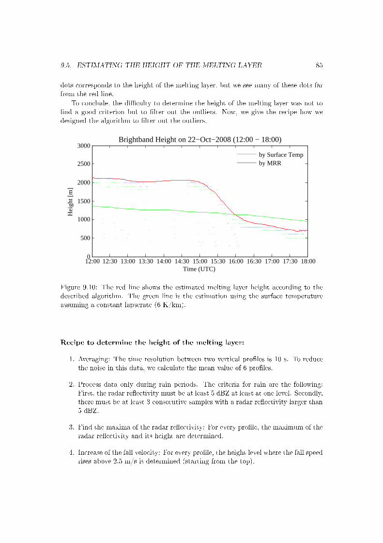
9.5. ESTIMATING THE HEIGHT OF THE MELTING LAYER 85
dots corresponds to the height of the melting layer, but we see many of these dots farfrom the red line.
To conclude, the diculty to determine the height of the melting layer was not tond a good criterion but to lter out the outliers. Now, we give the recipe how wedesigned the algorithm to lter out the outliers.
12:00 12:30 13:00 13:30 14:00 14:30 15:00 15:30 16:00 16:30 17:00 17:30 18:000
500
1000
1500
2000
2500
3000
Time (UTC)
Hei
ght [
m]
Brightband Height on 22−Oct−2008 (12:00 − 18:00)
by Surface Tempby MRR
Figure 9.10: The red line shows the estimated melting layer height according to thedescribed algorithm. The green line is the estimation using the surface temperatureassuming a constant lapserate (6 K/km).
Recipe to determine the height of the melting layer:
1. Averaging: The time resolution between two vertical proles is 10 s. To reducethe noise in this data, we calculate the mean value of 6 proles.
2. Process data only during rain periods. The criteria for rain are the following:First, the radar reectivity must be at least 5 dBZ at least at one level. Secondly,there must be at least 3 consecutive samples with a radar reectivity larger than5 dBZ.
3. Find the maxima of the radar reectivity: For every prole, the maximum of theradar reectivity and its height are determined.
4. Increase of the fall velocity: For every prole, the height level where the fall speedrises above 2.5 m/s is determined (starting from the top).
86 CHAPTER 9. THE MELTING LAYER
5. The height levels obtained from the reectivity and the fall speed criteria must lieat about the same height. Thus, samples are rejected, if the dierence betweenthe height levels are larger than 300 m.
6. Calculation of the height of the melting layer. The height of the melting layer iscalculated as the mean of the heights of the two criteria.
7. Remove outliers: 10 consecutive samples of the melting layer height are takenand the median is determined. All heights must lie within an interval of 200 mto the median height, otherwise the samples are rejected.
8. Smooth. The resulting curve is smoothed.
Chapter 10
Radiative Model of the MeltingLayer
To estimate the inuence of the melting layer to the received radiation at a radiometer,we introduce a radiative model of the melting layer. The goal of this radiative modelis to estimate the emission of the radiation within the microwave frequency range. Asmeasurable output value, the opacity is calculated.
Some simplications were necessary to describe the model, e.g. aggregation andbreakups within the melting layer are not considered and the depth of the meltinglayer is assumed to be constant (it is set to 500 m).
There are many possibilities to model the melting layer. F. Fabry presented sixother approaches (for further details see [3]).
10.1 Model of a Melting Snowake
10.1.1 Model
Amelting snowake consists of a mixture of water and ice surrounded by air. As the atshape of a snowake is dicult to model, we approximate it by a sphere. The snowakeconsists of air, ice crystals and water inclusions inside the sphere. We assume that thewater inclusions have the shape of ellipsoids as described in the discussion about wetsnow (Section 4.10). Figure 10.1 shows a schematic picture of such a snowake.
The volume of the snowake (Vsnowflake) is given by the sum of the volumes of eachof the three components.
Vsnowflake = Vair + Vice + Vliquid (10.1)
We dene the volume fraction fv as ratio of the volumetric water (liquid and ice)to the total volume.
fv =Vice + Vliquid
Vsnowflake(10.2)
87
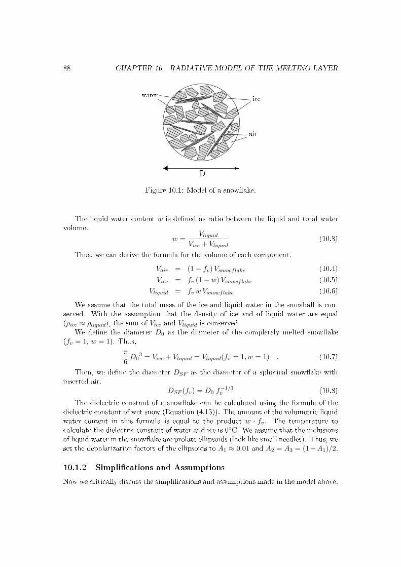
88 CHAPTER 10. RADIATIVE MODEL OF THE MELTING LAYER
D
ice
air
water
Figure 10.1: Model of a snowake.
The liquid water content w is dened as ratio between the liquid and total watervolume.
w =Vliquid
Vice + Vliquid(10.3)
Thus, we can derive the formula for the volume of each component.
Vair = (1− fv) Vsnowflake (10.4)
Vice = fv (1− w) Vsnowflake (10.5)
Vliquid = fv w Vsnowflake (10.6)
We assume that the total mass of the ice and liquid water in the snowball is con-served. With the assumption that the density of ice and of liquid water are equal(ρice ≈ ρliquid), the sum of Vice and Vliquid is conserved.
We dene the diameter D0 as the diameter of the completely melted snowake(fv = 1, w = 1). Thus,
π
6D0
3 = Vice + Vliquid = Vliquid(fv = 1, w = 1) . (10.7)
Then, we dene the diameter DSF as the diameter of a spherical snowake withinserted air.
DSF (fv) = D0 f−1/3v (10.8)
The dielectric constant of a snowake can be calculated using the formula of thedielectric constant of wet snow (Equation (4.15)). The amount of the volumetric liquidwater content in this formula is equal to the product w · fv. The temperature tocalculate the dielectric constant of water and ice is 0C. We assume that the inclusionsof liquid water in the snowake are prolate ellipsoids (look like small needles). Thus, weset the depolarization factors of the ellipsoids to A1 ≈ 0.01 and A2 = A3 = (1−A1)/2.
10.1.2 Simplications and Assumptions
Now we critically discuss the simplications and assumptions made in the model above.
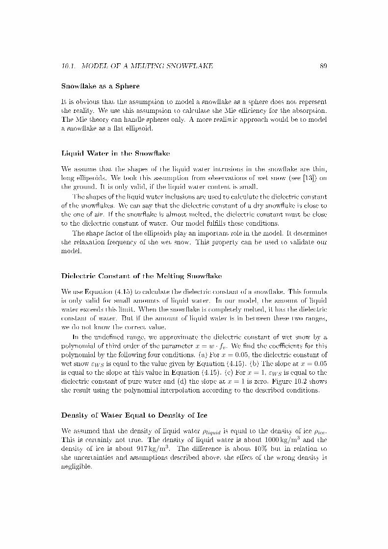
10.1. MODEL OF A MELTING SNOWFLAKE 89
Snowake as a Sphere
It is obvious that the assumption to model a snowake as a sphere does not representthe reality. We use this assumption to calculate the Mie eciency for the absorption.The Mie theory can handle spheres only. A more realistic approach would be to modela snowake as a at ellipsoid.
Liquid Water in the Snowake
We assume that the shapes of the liquid water intrusions in the snowake are thin,long ellipsoids. We took this assumption from observations of wet snow (see [13]) onthe ground. It is only valid, if the liquid water content is small.
The shapes of the liquid water inclusions are used to calculate the dielectric constantof the snowakes. We can say that the dielectric constant of a dry snowake is close tothe one of air. If the snowake is almost melted, the dielectric constant must be closeto the dielectric constant of water. Our model fullls these conditions.
The shape factor of the ellipsoids play an important role in the model. It determinesthe relaxation frequency of the wet snow. This property can be used to validate ourmodel.
Dielectric Constant of the Melting Snowake
We use Equation (4.15) to calculate the dielectric constant of a snowake. This formulais only valid for small amounts of liquid water. In our model, the amount of liquidwater exceeds this limit. When the snowake is completely melted, it has the dielectricconstant of water. But if the amount of liquid water is in between these two ranges,we do not know the correct value.
In the undened range, we approximate the dielectric constant of wet snow by apolynomial of third order of the parameter x = w · fv. We nd the coecients for thispolynomial by the following four conditions. (a) For x = 0.05, the dielectric constant ofwet snow εWS is equal to the value given by Equation (4.15). (b) The slope at x = 0.05is equal to the slope at this value in Equation (4.15). (c) For x = 1, εWS is equal to thedielectric constant of pure water and (d) the slope at x = 1 is zero. Figure 10.2 showsthe result using the polynomial interpolation according to the described conditions.
Density of Water Equal to Density of Ice
We assumed that the density of liquid water ρliquid is equal to the density of ice ρice.This is certainly not true. The density of liquid water is about 1000 kg/m3 and thedensity of ice is about 917 kg/m3. The dierence is about 10% but in relation tothe uncertainties and assumptions described above, the eect of the wrong density isnegligible.
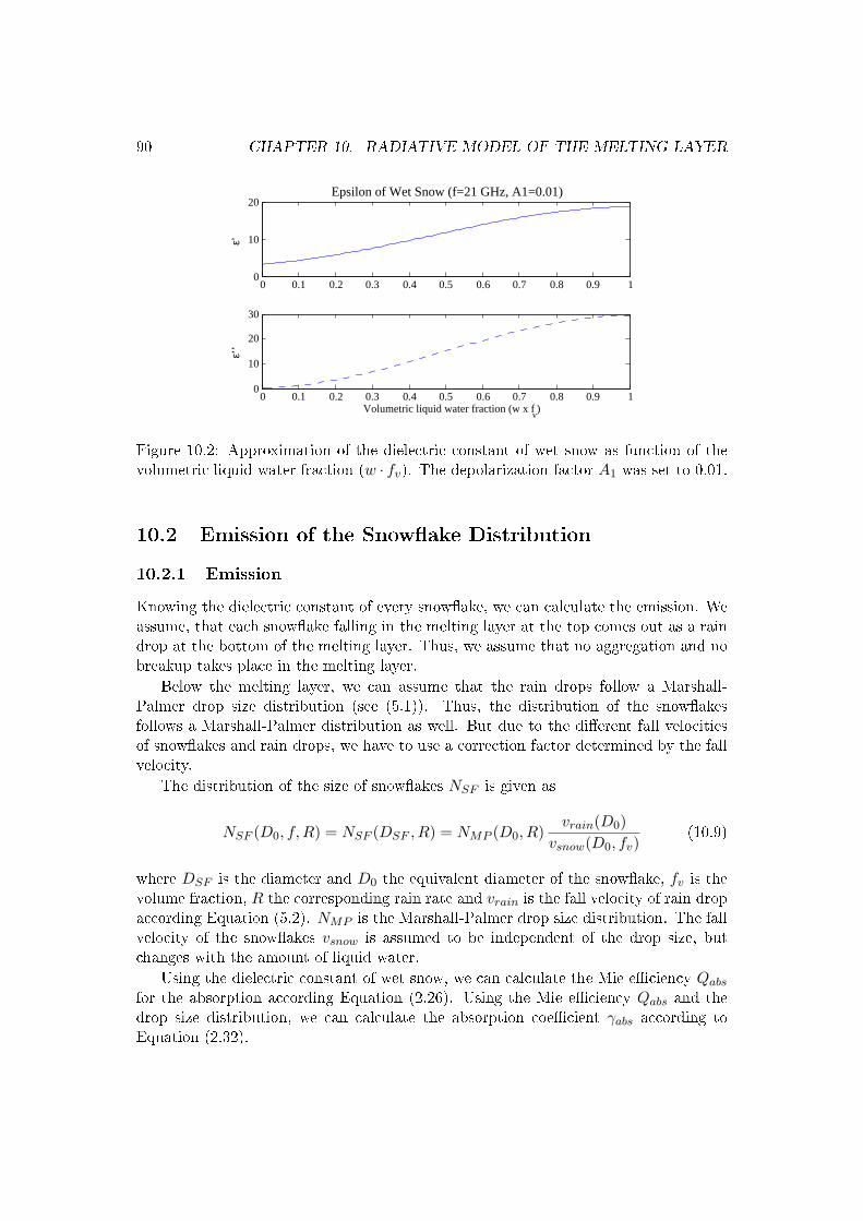
90 CHAPTER 10. RADIATIVE MODEL OF THE MELTING LAYER
0 0.1 0.2 0.3 0.4 0.5 0.6 0.7 0.8 0.9 10
10
20Epsilon of Wet Snow (f=21 GHz, A1=0.01)
ε’
0 0.1 0.2 0.3 0.4 0.5 0.6 0.7 0.8 0.9 10
10
20
30
Volumetric liquid water fraction (w x fv)
ε’’
Figure 10.2: Approximation of the dielectric constant of wet snow as function of thevolumetric liquid water fraction (w · fv). The depolarization factor A1 was set to 0.01.
10.2 Emission of the Snowake Distribution
10.2.1 Emission
Knowing the dielectric constant of every snowake, we can calculate the emission. Weassume, that each snowake falling in the melting layer at the top comes out as a raindrop at the bottom of the melting layer. Thus, we assume that no aggregation and nobreakup takes place in the melting layer.
Below the melting layer, we can assume that the rain drops follow a Marshall-Palmer drop size distribution (see (5.1)). Thus, the distribution of the snowakesfollows a Marshall-Palmer distribution as well. But due to the dierent fall velocitiesof snowakes and rain drops, we have to use a correction factor determined by the fallvelocity.
The distribution of the size of snowakes NSF is given as
NSF (D0, f, R) = NSF (DSF , R) = NMP (D0, R)vrain(D0)
vsnow(D0, fv)(10.9)
where DSF is the diameter and D0 the equivalent diameter of the snowake, fv is thevolume fraction, R the corresponding rain rate and vrain is the fall velocity of rain dropaccording Equation (5.2). NMP is the Marshall-Palmer drop size distribution. The fallvelocity of the snowakes vsnow is assumed to be independent of the drop size, butchanges with the amount of liquid water.
Using the dielectric constant of wet snow, we can calculate the Mie eciency Qabs
for the absorption according Equation (2.26). Using the Mie eciency Qabs and thedrop size distribution, we can calculate the absorption coecient γabs according toEquation (2.32).
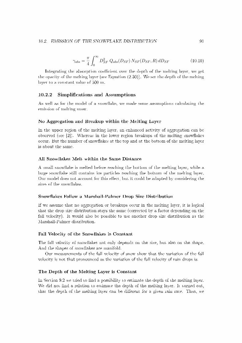
10.2. EMISSION OF THE SNOWFLAKE DISTRIBUTION 91
γabs =π
4
∫ ∞
0D2
SF Qabs(DSF ) NSF (DSF , R) dDSF (10.10)
Integrating the absorption coecient over the depth of the melting layer, we getthe opacity of the melting layer (see Equation (2.30)). We set the depth of the meltinglayer to a constant value of 500 m.
10.2.2 Simplications and Assumptions
As well as for the model of a snowake, we made some assumptions calculating theemission of melting snow.
No Aggregation and Breakup within the Melting Layer
In the upper region of the melting layer, an enhanced activity of aggregation can beobserved (see [2]). Whereas in the lower region breakups of the melting snowakesoccur. But the number of snowakes at the top and at the bottom of the melting layeris about the same.
All Snowakes Melt within the Same Distance
A small snowake is melted before reaching the bottom of the melting layer, while alarge snowake still contains ice particles reaching the bottom of the melting layer.Our model does not account for this eect, but it could be adapted by considering thesizes of the snowakes.
Snowakes Follow a Marshall-Palmer Drop Size Distribution
If we assume that no aggregation or breakups occur in the melting layer, it is logicalthat the drop size distribution stays the same (corrected by a factor depending on thefall velocity). It would also be possible to use another drop size distribution as theMarshall-Palmer distribution.
Fall Velocity of the Snowakes is Constant
The fall velocity of snowakes not only depends on the size, but also on the shape.And the shapes of snowakes are manifold.
Our measurements of the fall velocity of snow show that the variation of the fallvelocity is not that pronounced as the variation of the fall velocity of rain drops is.
The Depth of the Melting Layer is Constant
In Section 9.2 we tried to nd a possibility to estimate the depth of the melting layer.We did not nd a relation to estimate the depth of the melting layer. It turned out,that the depth of the melting layer can be dierent for a given rain rate. Thus, we
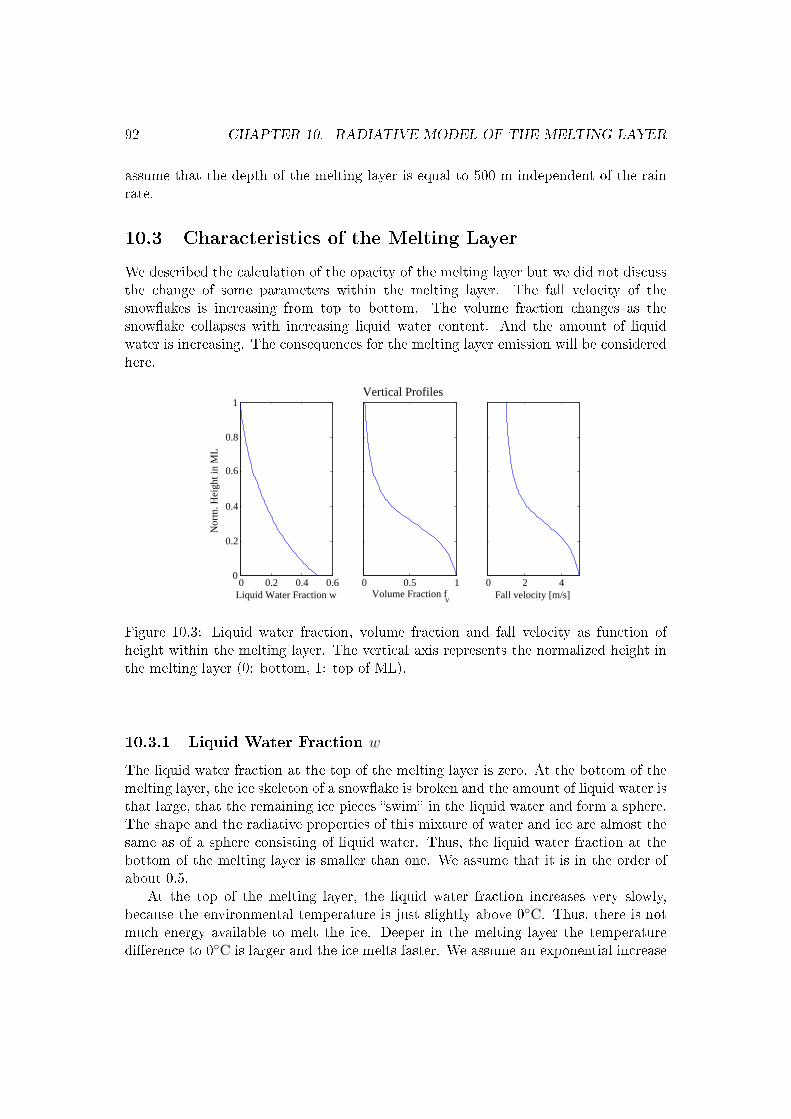
92 CHAPTER 10. RADIATIVE MODEL OF THE MELTING LAYER
assume that the depth of the melting layer is equal to 500 m independent of the rainrate.
10.3 Characteristics of the Melting Layer
We described the calculation of the opacity of the melting layer but we did not discussthe change of some parameters within the melting layer. The fall velocity of thesnowakes is increasing from top to bottom. The volume fraction changes as thesnowake collapses with increasing liquid water content. And the amount of liquidwater is increasing. The consequences for the melting layer emission will be consideredhere.
0 0.2 0.4 0.60
0.2
0.4
0.6
0.8
1
Liquid Water Fraction w
Nor
m. H
eigh
t in
ML
0 0.5 1Volume Fraction f
v
0 2 4Fall velocity [m/s]
Vertical Profiles
Figure 10.3: Liquid water fraction, volume fraction and fall velocity as function ofheight within the melting layer. The vertical axis represents the normalized height inthe melting layer (0: bottom, 1: top of ML).
10.3.1 Liquid Water Fraction w
The liquid water fraction at the top of the melting layer is zero. At the bottom of themelting layer, the ice skeleton of a snowake is broken and the amount of liquid water isthat large, that the remaining ice pieces swim in the liquid water and form a sphere.The shape and the radiative properties of this mixture of water and ice are almost thesame as of a sphere consisting of liquid water. Thus, the liquid water fraction at thebottom of the melting layer is smaller than one. We assume that it is in the order ofabout 0.5.
At the top of the melting layer, the liquid water fraction increases very slowly,because the environmental temperature is just slightly above 0C. Thus, there is notmuch energy available to melt the ice. Deeper in the melting layer the temperaturedierence to 0C is larger and the ice melts faster. We assume an exponential increase
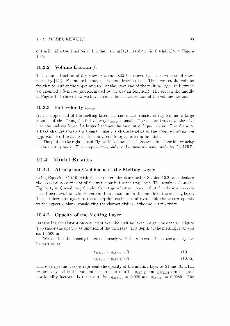
10.4. MODEL RESULTS 93
of the liquid water fraction within the melting layer, as shown in the left plot of Figure10.3.
10.3.2 Volume fraction fv
The volume fraction of dry snow is about 0.02 (as shown by measurements of snowpacks by [12]). For melted snow, the volume fraction is 1. Thus, we set the volumefraction to 0.02 at the upper and to 1 at the lower end of the melting layer. In betweenwe assumed a S-shape (approximated by an arc-tan function). The plot in the middleof Figure 10.3 shows how we have chosen the characteristics of the volume fraction.
10.3.3 Fall Velocity vsnow
At the upper end of the melting layer, the snowakes consist of dry ice and a largeamount of air. Thus, the fall velocity vsnow is small. The deeper the snowakes fallinto the melting layer the larger becomes the amount of liquid water. The shape ofa ake changes towards a sphere. Like the characteristics of the volume fraction weapproximated the fall velocity characteristic by an arc-tan function.
The plot on the right side of Figure 10.3 shows the characteristics of the fall velocityin the melting snow. This shape corresponds to the measurements made by the MRR.
10.4 Model Results
10.4.1 Absorption Coecient of the Melting Layer
Using Equation (10.10) with the characteristics described in Section 10.3, we calculatethe absorption coecient of the wet snow in the melting layer. The result is shown inFigure 10.4. Considering the plot from top to bottom, we see that the absorption coef-cient increases from almost zero up to a maximum in the middle of the melting layer.Then it decreases again to the absorption coecient of rain. This shape correspondsto the expected shape considering the characteristics of the radar reectivity.
10.4.2 Opacity of the Melting Layer
Integrating the absorption coecient over the melting layer, we get the opacity. Figure10.5 shows the opacity as function of the rain rate. The depth of the melting layer wasset to 500 m.
We see that the opacity increases linearly with the rain rate. Thus, the opacity canbe written as
τML,21 = gML,21 ·R (10.11)
τML,31 = gML,31 ·R (10.12)
where τML,21 and τML,31 represent the opacity of the melting layer at 21 and 31 GHz,respectively. R is the rain rate inserted in mm/h. gML,21 and gML,31 are the pro-portionality factors. It turns out that gML,21 = 0.020 and gML,31 = 0.0280. The
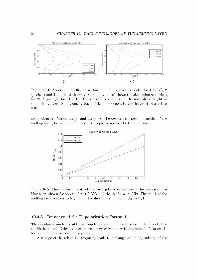
94 CHAPTER 10. RADIATIVE MODEL OF THE MELTING LAYER
0 0.05 0.1 0.15 0.2 0.250
0.2
0.4
0.6
0.8
1
γabs
[1/km]
Nor
m. H
eigh
t in
ML
Abs.Coef. in Melting Layer (21 GHz)
1 mm/h
2 mm/h
3 mm/h
(a)
0 0.05 0.1 0.15 0.2 0.25 0.3 0.350
0.2
0.4
0.6
0.8
1
γabs
[1/km]
Nor
m. H
eigh
t in
ML
Abs.Coef. in Melting Layer (31 GHz)
1 mm/h
2 mm/h
3 mm/h
(b)
Figure 10.4: Absorption coecient within the melting layer. Modeled for 1 (solid), 2(dashed) and 3 mm/h (dash-dotted) rain. Figure (a) shows the absorption coecientfor 21, Figure (b) for 31 GHz. The vertical axis represents the normalized height inthe melting layer (0: bottom, 1: top of ML). The depolarization factor A1 was set to0.01.
proportionality factors gML,21 and gML,31 can be denoted as specic opacities of themelting layer, because they represent the opacity normed by the rain rate.
0 0.5 1 1.5 2 2.5 3 3.5 4 4.5 50
0.02
0.04
0.06
0.08
0.1
0.12
0.14
Rain rate [mm/h]
Opa
city
τ ML
Opacity of Melting Layer
21 GHz31 GHz
Figure 10.5: The modeled opacity of the melting layer as function of the rain rate. Theblue curve shows the opacity for 21.2 GHz and the red for 31.5 GHz. The depth of themelting layer was set to 500 m and the depolarization factor A1 to 0.01.
10.4.3 Inuence of the Depolarization Factor A1
The depolarization factor of the ellipsoids plays an important factor in the model. Dueto this factor the Debye relaxation frequency of wet snow is determined. A larger A1
leads to a higher relaxation frequency.
A change of the relaxation frequency leads to a change of the dependency of the
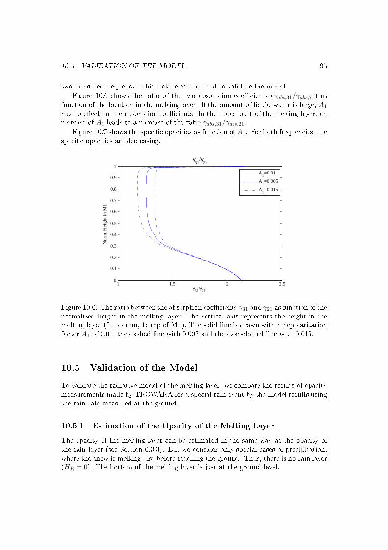
10.5. VALIDATION OF THE MODEL 95
two measured frequency. This feature can be used to validate the model.
Figure 10.6 shows the ratio of the two absorption coecients (γabs,31/γabs,21) asfunction of the location in the melting layer. If the amount of liquid water is large, A1
has no eect on the absorption coecients. In the upper part of the melting layer, anincrease of A1 leads to a increase of the ratio γabs,31/γabs,21.
Figure 10.7 shows the specic opacities as function of A1. For both frequencies, thespecic opacities are decreasing.
1 1.5 2 2.50
0.1
0.2
0.3
0.4
0.5
0.6
0.7
0.8
0.9
1
γ31
/γ21
Nor
m. H
eigh
t in
ML
γ31
/γ21
A
1=0.01
A1=0.005
A1=0.015
Figure 10.6: The ratio between the absorption coecients γ31 and γ21 as function of thenormalized height in the melting layer. The vertical axis represents the height in themelting layer (0: bottom, 1: top of ML). The solid line is drawn with a depolarizationfactor A1 of 0.01, the dashed line with 0.005 and the dash-dotted line with 0.015.
10.5 Validation of the Model
To validate the radiative model of the melting layer, we compare the results of opacitymeasurements made by TROWARA for a special rain event by the model results usingthe rain rate measured at the ground.
10.5.1 Estimation of the Opacity of the Melting Layer
The opacity of the melting layer can be estimated in the same way as the opacity ofthe rain layer (see Section 6.3.3). But we consider only special cases of precipitation,where the snow is melting just before reaching the ground. Thus, there is no rain layer(HR = 0). The bottom of the melting layer is just at the ground level.
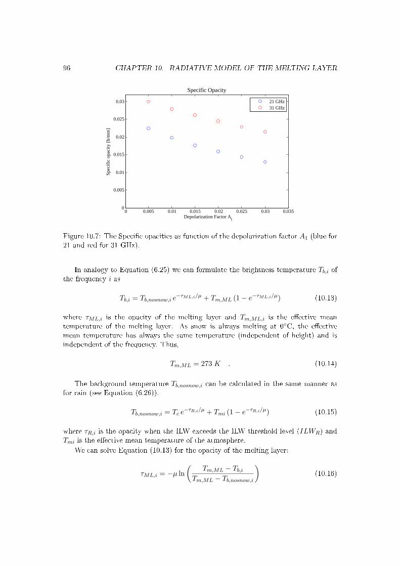
96 CHAPTER 10. RADIATIVE MODEL OF THE MELTING LAYER
0 0.005 0.01 0.015 0.02 0.025 0.03 0.0350
0.005
0.01
0.015
0.02
0.025
0.03
Specific Opacity
Depolarization Factor A1
Spec
ific
opa
city
[h/
mm
]
21 GHz31 GHz
Figure 10.7: The Specic opacities as function of the depolarization factor A1 (blue for21 and red for 31 GHz).
In analogy to Equation (6.25) we can formulate the brightness temperature Tb,i ofthe frequency i as
Tb,i = Tb,nosnow,i e−τML,i/µ + Tm,ML (1− e−τML,i/µ) (10.13)
where τML,i is the opacity of the melting layer and Tm,ML,i is the eective meantemperature of the melting layer. As snow is always melting at 0C, the eectivemean temperature has always the same temperature (independent of height) and isindependent of the frequency. Thus,
Tm,ML = 273 K . (10.14)
The background temperature Tb,nosnow,i can be calculated in the same manner asfor rain (see Equation (6.26)).
Tb,nosnow,i = Tc e−τR,i/µ + Tmi (1− e−τR,i/µ) (10.15)
where τR,i is the opacity when the ILW exceeds the ILW threshold level (ILWR) andTmi is the eective mean temperature of the atmosphere.
We can solve Equation (10.13) for the opacity of the melting layer:
τML,i = −µ ln(
Tm,ML − Tb,i
Tm,ML − Tb,nosnow,i
)(10.16)
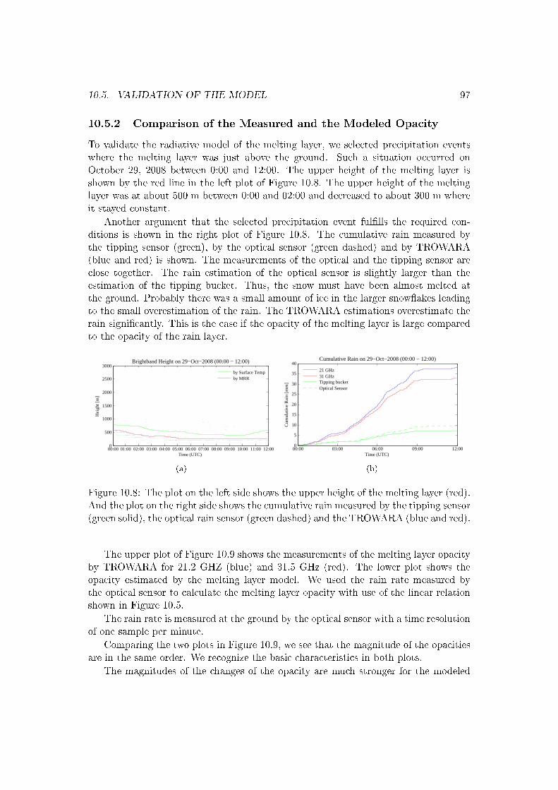
10.5. VALIDATION OF THE MODEL 97
10.5.2 Comparison of the Measured and the Modeled Opacity
To validate the radiative model of the melting layer, we selected precipitation eventswhere the melting layer was just above the ground. Such a situation occurred onOctober 29, 2008 between 0:00 and 12:00. The upper height of the melting layer isshown by the red line in the left plot of Figure 10.8. The upper height of the meltinglayer was at about 500 m between 0:00 and 02:00 and decreased to about 300 m whereit stayed constant.
Another argument that the selected precipitation event fullls the required con-ditions is shown in the right plot of Figure 10.8. The cumulative rain measured bythe tipping sensor (green), by the optical sensor (green dashed) and by TROWARA(blue and red) is shown. The measurements of the optical and the tipping sensor areclose together. The rain estimation of the optical sensor is slightly larger than theestimation of the tipping bucket. Thus, the snow must have been almost melted atthe ground. Probably there was a small amount of ice in the larger snowakes leadingto the small overestimation of the rain. The TROWARA estimations overestimate therain signicantly. This is the case if the opacity of the melting layer is large comparedto the opacity of the rain layer.
00:00 01:00 02:00 03:00 04:00 05:00 06:00 07:00 08:00 09:00 10:00 11:00 12:000
500
1000
1500
2000
2500
3000
Time (UTC)
Hei
ght [
m]
Brightband Height on 29−Oct−2008 (00:00 − 12:00)
by Surface Tempby MRR
(a)
00:00 03:00 06:00 09:00 12:000
5
10
15
20
25
30
35
40
Time (UTC)
Cum
ulat
ive
Rai
n [m
m]
Cumulative Rain on 29−Oct−2008 (00:00 − 12:00)
21 GHz31 GHzTipping bucketOptical Sensor
(b)
Figure 10.8: The plot on the left side shows the upper height of the melting layer (red).And the plot on the right side shows the cumulative rain measured by the tipping sensor(green solid), the optical rain sensor (green dashed) and the TROWARA (blue and red).
The upper plot of Figure 10.9 shows the measurements of the melting layer opacityby TROWARA for 21.2 GHZ (blue) and 31.5 GHz (red). The lower plot shows theopacity estimated by the melting layer model. We used the rain rate measured bythe optical sensor to calculate the melting layer opacity with use of the linear relationshown in Figure 10.5.
The rain rate is measured at the ground by the optical sensor with a time resolutionof one sample per minute.
Comparing the two plots in Figure 10.9, we see that the magnitude of the opacitiesare in the same order. We recognize the basic characteristics in both plots.
The magnitudes of the changes of the opacity are much stronger for the modeled
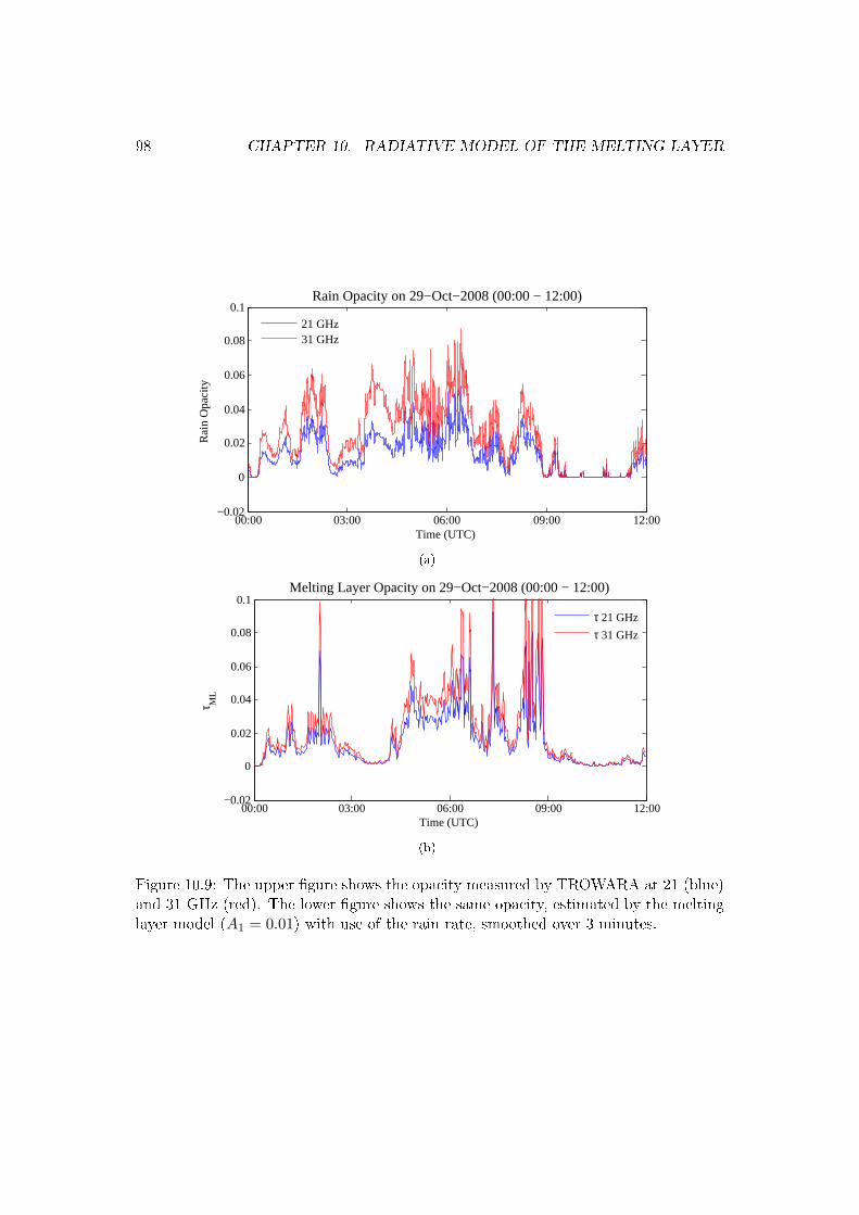
98 CHAPTER 10. RADIATIVE MODEL OF THE MELTING LAYER
00:00 03:00 06:00 09:00 12:00−0.02
0
0.02
0.04
0.06
0.08
0.1
Time (UTC)
Rai
n O
paci
ty
Rain Opacity on 29−Oct−2008 (00:00 − 12:00)
21 GHz31 GHz
(a)
00:00 03:00 06:00 09:00 12:00−0.02
0
0.02
0.04
0.06
0.08
0.1
Time (UTC)
τ ML
Melting Layer Opacity on 29−Oct−2008 (00:00 − 12:00)
τ 21 GHz
τ 31 GHz
(b)
Figure 10.9: The upper gure shows the opacity measured by TROWARA at 21 (blue)and 31 GHz (red). The lower gure shows the same opacity, estimated by the meltinglayer model (A1 = 0.01) with use of the rain rate, smoothed over 3 minutes.
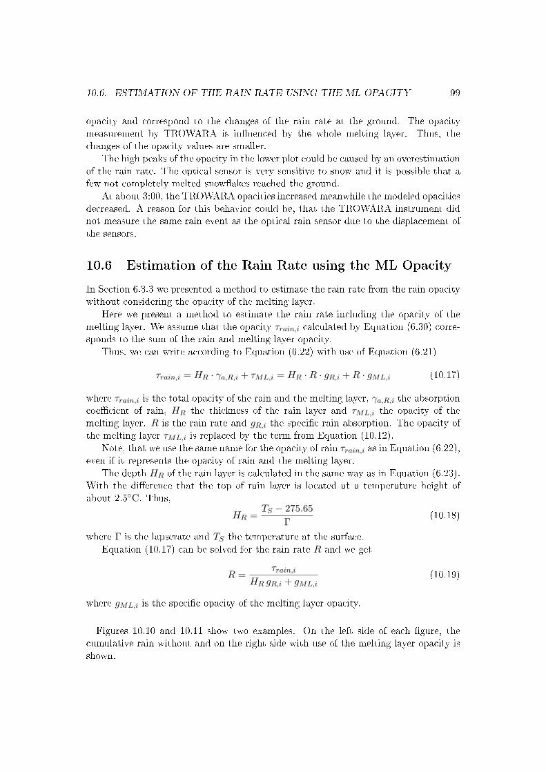
10.6. ESTIMATION OF THE RAIN RATE USING THE ML OPACITY 99
opacity and correspond to the changes of the rain rate at the ground. The opacitymeasurement by TROWARA is inuenced by the whole melting layer. Thus, thechanges of the opacity values are smaller.
The high peaks of the opacity in the lower plot could be caused by an overestimationof the rain rate. The optical sensor is very sensitive to snow and it is possible that afew not completely melted snowakes reached the ground.
At about 3:00, the TROWARA opacities increased meanwhile the modeled opacitiesdecreased. A reason for this behavior could be, that the TROWARA instrument didnot measure the same rain event as the optical rain sensor due to the displacement ofthe sensors.
10.6 Estimation of the Rain Rate using the ML Opacity
In Section 6.3.3 we presented a method to estimate the rain rate from the rain opacitywithout considering the opacity of the melting layer.
Here we present a method to estimate the rain rate including the opacity of themelting layer. We assume that the opacity τrain,i calculated by Equation (6.30) corre-sponds to the sum of the rain and melting layer opacity.
Thus, we can write according to Equation (6.22) with use of Equation (6.21)
τrain,i = HR · γa,R,i + τML,i = HR ·R · gR,i + R · gML,i (10.17)
where τrain,i is the total opacity of the rain and the melting layer, γa,R,i the absorptioncoecient of rain, HR the thickness of the rain layer and τML,i the opacity of themelting layer. R is the rain rate and gR,i the specic rain absorption. The opacity ofthe melting layer τML,i is replaced by the term from Equation (10.12).
Note, that we use the same name for the opacity of rain τrain,i as in Equation (6.22),even if it represents the opacity of rain and the melting layer.
The depth HR of the rain layer is calculated in the same way as in Equation (6.23).With the dierence that the top of rain layer is located at a temperature height ofabout 2.5C. Thus,
HR =TS − 275.65
Γ(10.18)
where Γ is the lapserate and TS the temperature at the surface.
Equation (10.17) can be solved for the rain rate R and we get
R =τrain,i
HR gR,i + gML,i(10.19)
where gML,i is the specic opacity of the melting layer opacity.
Figures 10.10 and 10.11 show two examples. On the left side of each gure, thecumulative rain without and on the right side with use of the melting layer opacity isshown.
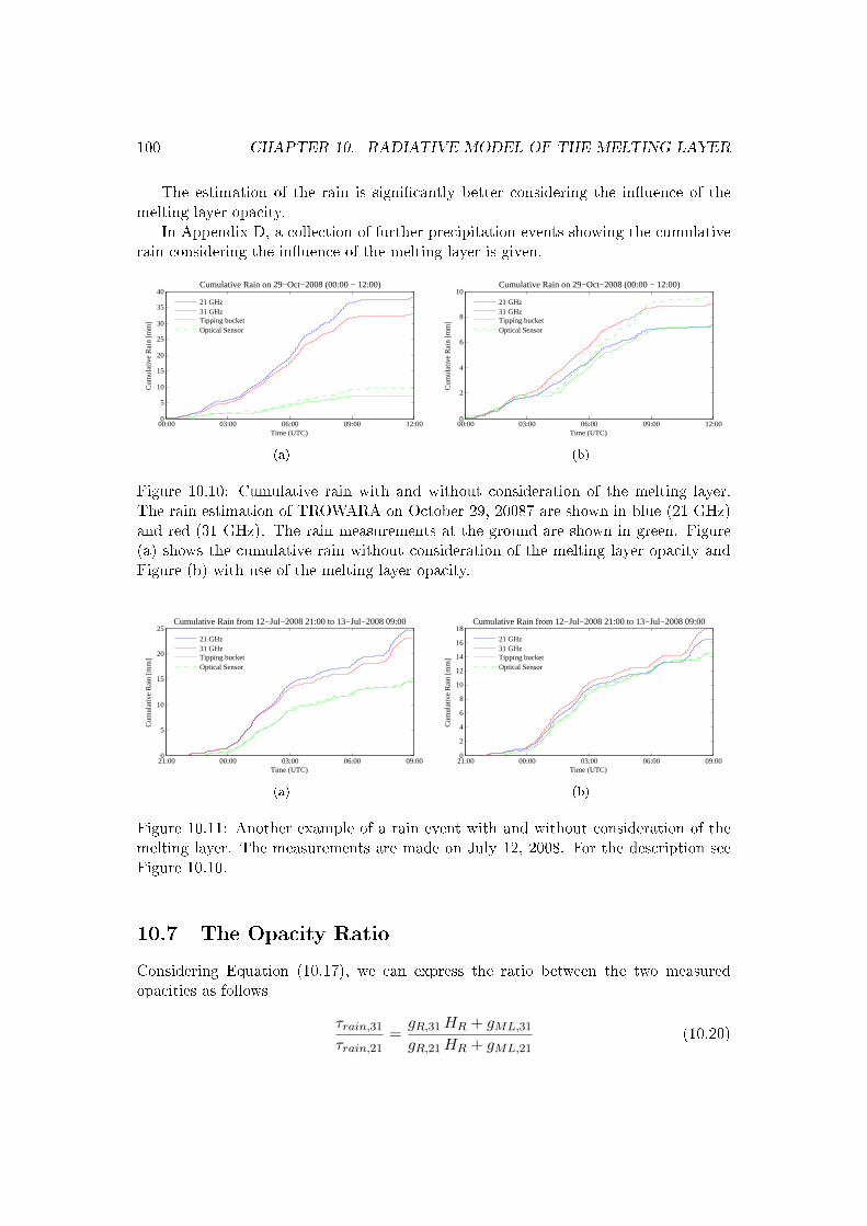
100 CHAPTER 10. RADIATIVE MODEL OF THE MELTING LAYER
The estimation of the rain is signicantly better considering the inuence of themelting layer opacity.
In Appendix D, a collection of further precipitation events showing the cumulativerain considering the inuence of the melting layer is given.
00:00 03:00 06:00 09:00 12:000
5
10
15
20
25
30
35
40
Time (UTC)
Cum
ulat
ive
Rai
n [m
m]
Cumulative Rain on 29−Oct−2008 (00:00 − 12:00)
21 GHz31 GHzTipping bucketOptical Sensor
(a)
00:00 03:00 06:00 09:00 12:000
2
4
6
8
10
Time (UTC)
Cum
ulat
ive
Rai
n [m
m]
Cumulative Rain on 29−Oct−2008 (00:00 − 12:00)
21 GHz31 GHzTipping bucketOptical Sensor
(b)
Figure 10.10: Cumulative rain with and without consideration of the melting layer.The rain estimation of TROWARA on October 29, 20087 are shown in blue (21 GHz)and red (31 GHz). The rain measurements at the ground are shown in green. Figure(a) shows the cumulative rain without consideration of the melting layer opacity andFigure (b) with use of the melting layer opacity.
21:00 00:00 03:00 06:00 09:000
5
10
15
20
25
Time (UTC)
Cum
ulat
ive
Rai
n [m
m]
Cumulative Rain from 12−Jul−2008 21:00 to 13−Jul−2008 09:00
21 GHz31 GHzTipping bucketOptical Sensor
(a)
21:00 00:00 03:00 06:00 09:000
2
4
6
8
10
12
14
16
18
Time (UTC)
Cum
ulat
ive
Rai
n [m
m]
Cumulative Rain from 12−Jul−2008 21:00 to 13−Jul−2008 09:00
21 GHz31 GHzTipping bucketOptical Sensor
(b)
Figure 10.11: Another example of a rain event with and without consideration of themelting layer. The measurements are made on July 12, 2008. For the description seeFigure 10.10.
10.7 The Opacity Ratio
Considering Equation (10.17), we can express the ratio between the two measuredopacities as follows
τrain,31
τrain,21=
gR,31 HR + gML,31
gR,21 HR + gML,21(10.20)
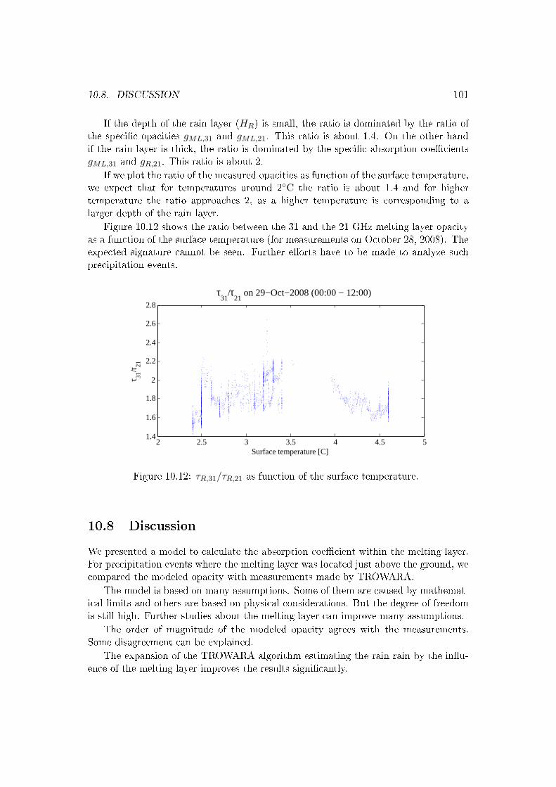
10.8. DISCUSSION 101
If the depth of the rain layer (HR) is small, the ratio is dominated by the ratio ofthe specic opacities gML,31 and gML,21. This ratio is about 1.4. On the other handif the rain layer is thick, the ratio is dominated by the specic absorption coecientsgML,31 and gR,21. This ratio is about 2.
If we plot the ratio of the measured opacities as function of the surface temperature,we expect that for temperatures around 2C the ratio is about 1.4 and for highertemperature the ratio approaches 2, as a higher temperature is corresponding to alarger depth of the rain layer.
Figure 10.12 shows the ratio between the 31 and the 21 GHz melting layer opacityas a function of the surface temperature (for measurements on October 28, 2008). Theexpected signature cannot be seen. Further eorts have to be made to analyze suchprecipitation events.
2 2.5 3 3.5 4 4.5 51.4
1.6
1.8
2
2.2
2.4
2.6
2.8
τ31
/τ21
on 29−Oct−2008 (00:00 − 12:00)
Surface temperature [C]
τ 31/τ 21
Figure 10.12: τR,31/τR,21 as function of the surface temperature.
10.8 Discussion
We presented a model to calculate the absorption coecient within the melting layer.For precipitation events where the melting layer was located just above the ground, wecompared the modeled opacity with measurements made by TROWARA.
The model is based on many assumptions. Some of them are caused by mathemat-ical limits and others are based on physical considerations. But the degree of freedomis still high. Further studies about the melting layer can improve many assumptions.
The order of magnitude of the modeled opacity agrees with the measurements.Some disagreement can be explained.
The expansion of the TROWARA algorithm estimating the rain rain by the inu-ence of the melting layer improves the results signicantly.
102 CHAPTER 10. RADIATIVE MODEL OF THE MELTING LAYER
The model is tested considering a few stratiform precipitation situations only. Toget a better approvement of the model, it is necessary to test the model with moreprecipitation events.
Chapter 11
Conclusions and Outlook
In this work we focused on the estimation of precipitation by microwave sensors. Forthat purpose we used two instruments: a ground-based radiometer measuring the ra-diation at two frequencies (21 and 31 GHz) near the 22 GHz water vapor absorptionline and a vertical pointing rain radar measuring at 24 GHz. A ground-based weatherstation helped to complete and to verify the measurement results.
The method of the rain radar to estimate rain is based on the radar reectivity andthe fall velocities of the rain drops. This method is well known and therefore we focuson the estimation of rain by the radiometer. The method of the radiometer is basedon the emission of the rain drops in the microwave range.
The radiative properties of rain drops are understood well but lack in the estimationthe emission of melting snow. The contribution of melting snow to the measuredradiation cannot be neglected. Thus, a large part of this work deals with the propertiesof the region of the melting snow, the melting layer. Or from the radar perspective,the bright band.
The rain radar is an adequate instrument to analyze the melting layer; verticalproles of the radar reectivity and the fall velocity can be measured. But as strongvertical winds inuence the radar measurements, weather situations with stratiformprecipitation are analyzed only.
With use of the vertical prole measurements and theoretical considerations, a ra-diative model of the melting layer is developed. It is based on the dielectrical propertiesof wet snow. The shape of the melt water of a snow ake plays a key role in the model.As a result, the model is able to estimate the absorption coecient of the melting snowand hence the opacity of the melting layer.
When the melting layer is just above the ground, it is possible to measure its opacityby the radiometer. Comparing the measured opacity with the model result, we canverify the accuracy of our melting layer model.
Although the model is restricted by mathematical limits (the Mie theory can handlespheres only) and the degree of freedom to tune the model is high, the modeled opacityof the melting layer corresponds well to the measurements.
Further it turns out that the opacity of the melting layer is proportional to the rain
103
104 CHAPTER 11. CONCLUSIONS AND OUTLOOK
rate. Using this important result we can improve the rain rate estimation algorithm ofthe radiometer.
To make the model more robust, it is necessary to verify its results by a large numberof precipitation events. The cumulative rain estimated by the radiometer algorithmcan be compared with measurements from ground-based rain sensors. Precipitationevents, when the melting layer is just above the ground, can be used to determine thefrequency dependence of the melting layer opacity. This information can help to adjustthe shape factor of the liquid water of a snowake.
A snowake can be modeled in many dierent ways. An alternative to the describedapproach would be to consider the snowake as a coated sphere with a low-densitycoating around a denser central part. This model can be used in Mie theory.
Other approaches to model the melting layer are described by F. Fabry (see [3]).The radiative properties of theses approaches could be calculated, and the results couldbe compared with the described model.
Bibliography
[1] Wiesmann A. and Mätzler C. Microwave emission model of layered snowpacks.Remote Sensing of Environment, 70:307316, 1999.
[2] Eszter Barthazy. Microphysical Properties of the Melting Layer. PhD thesis, SwissFederal Institute of Technologie (ETH), Zürich, Switzerland, 1998.
[3] F. Fabry and Szyrmer W. Modeling of the melting layer. Part II: Electromagnetic."J. Atmos. Sci.", 56:35933600, 1999.
[4] F. Fabry and I. Zawadzki. Long-Term Radar Observations of the Melting Layerof Precipitation and Their Interpretation. "J. Atmos. Sci.", 52:838851, 1994.
[5] F. Fabry and I. Zawadzki. Atmospheric Physics as Observed by a Vertically Point-ing Doppler RADAR. In Proceedings, 13th International Conference on Cloudsand Precipitation, pages 310313, Reno NV, 2000.
[6] Niklaus Kämpfer. Physik der Atmosphäre, 2007. Manuscript of the Lecture CourseIntroduction to Climate and Environmental Physics, Fall Semester 2007, Univer-sity of Bern.
[7] Christian Mätzler. Drop-Size Distributions and Mie Computations for Rain. IAPResearch Report 2002-16, Institut für angewandte Physik, Universität Bern, Bern,Switzerland, November 2002.
[8] Christian Mätzler. Eects of Rain on Propagation, Absorption and Scattering ofMicrowave Radiation Based on the Dielectric Model of Liebe. IAP Research Report2002-10, Institut für angewandte Physik, Universität Bern, Bern, Switzerland,December 2002.
[9] Christian Mätzler. MATLAB Functions for Mie Scattering and Absorption. IAPResearch Report 2002-08, Institut für angewandte Physik, Universität Bern, Bern,Switzerland, June 2002.
[10] Christian Mätzler. MATLAB Functions for Mie Scattering and Absorption, Ver-sion 2. IAP Research Report 2002-11, Institut für angewandte Physik, UniversitätBern, Bern, Switzerland, December 2002.
105
106 BIBLIOGRAPHY
[11] Christian Mätzler. Radarmeteorologie, 2003. Vorlesung Sommersemester 2003,Universität Bern.
[12] Christian Mätzler. Thermal Microwave Radiation: Applications for Remote Sens-ing. Number 52 in IEE Electromagnetic Wave series. The Institution of Engineer-ing and Technology (IET), 2006.
[13] Christian Mätzler. Physical Principles of Remote Sensing, 2007. Manuscript ofthe Lecture Course, Spring Semester 2007, University of Bern.
[14] Christian Mätzler and June Morland. Advances in Surface-Based Radiometry ofAtmospheric Water. IAP Research Report 2008-02-MW, Institut für angewandtePhysik, Universität Bern, Bern, Switzerland, February 2008.
[15] METEK. MRR - Physical Basics, 2005. Version 1.9.0.
[16] METEK. MRR-2 - User Manual, 2005. Version 4.01/4.10.
[17] J. Morland, B. Deuber, D. G. Feist, L. Martin, S. Nyeki, N. Kämpfer, C. Mätzler,P. Jeannet, and L. Vuilleumier. The STARTWAVE atmospheric water vapourdatabase. Atmospheric Chemistry and Physics, 6:20392056, 2006.
[18] June Morland. TROWARA - Tropospheric Water Vapour Radiometer. Radiome-ter review and new calibration model. IAP Research Report 2002-15, Institut fürangewandte Physik, Universität Bern, Bern, Switzerland, November 2002.
[19] R. Peter and N. Kämpfer. Radiometric determination of water vapor and liquidwater and its validation with other techniques. J. Geophysical Research, 97:18,17318,183, 1992.
[20] Hans R. Pruppacher and James D. Klett. Microphysics of Clouds and Precipita-tion. Kluwer Academic Publishers, Dordrecht, The Netherlands, 1997.
[21] Robert A. Houze. Cloud Dynamics. Academic Press, San Diego, CA, 1993.
[22] Walter Roedel. Physik unserer Umwelt: Die Atmosphäre. Springer-Verlag, 3rd
edition, 2000.
[23] R. R. Rogers and M. K. Yau. A Short Course in Cloud Physics. Butterworth-Heinemann, 3rd edition, 1989.
[24] Henri Sauvageot. Radar Meteorology. Artech House, Boston, MA, 1992.
[25] John H. Seinfeld and Spyros N. Pandis. Atmospheric Chemisty and Physics: FromAir Pollution to Climate Change. John Wiley and Sons, Inc., 2nd edition, 2006.
[26] Arthur von Hippel. Dielecrics and Waves. Artech House, 1st edition, 1954.
Appendix A
Setup of the Micro Rain Radar
In this appendix we describe the setup and the storage of the data of the Micro RainRadar. First, we give an overview over the physical setup of the equipment. A moredetailed description is given in the manual of the manufacturer (see [16]). Secondly, wedescribe the process converting and storing the measured data in the MySQL database.At last, the structure of the MySQL database, where the data is stored, is explained.
A.1 Setup
An overview of the physical setup of the MRR instrument is shown in Figure A.1. Onthe left side, we see the radar antenna with the radar module. The MRR is locatedon the roof of the ExWi building. The radar signal is processed in the radar moduleand averaging is done there. Every 10 seconds, the raw data are transmitted to theconnection box. This box is located inside the ExWi building. The connection boxforwards the raw data over a serial connection cable to a converter, where the data aretransmitted over the IAP network to the MRR PC.
The MRR PC receives the raw samples and stores them on its hard disc. Addition-ally, the raw data are processed to second level products as the radar reectivity, thefall velocity, etc. These processed data are stored on the hard disc of the MRR PC aswell.
At about 2:00 at night, the data of the previous day are read from the MRR PC andare inserted into the MySQL database of the IAP microwave institute. Only periodsare stored, where precipitation is detected at any height level.
A.2 Data Storage
A.2.1 Copy the Data from the MRR-PC
The processing of the radar signals to the raw data and the processing of the raw datato higher level products is well documented in the manual of the radar ([16]).
107
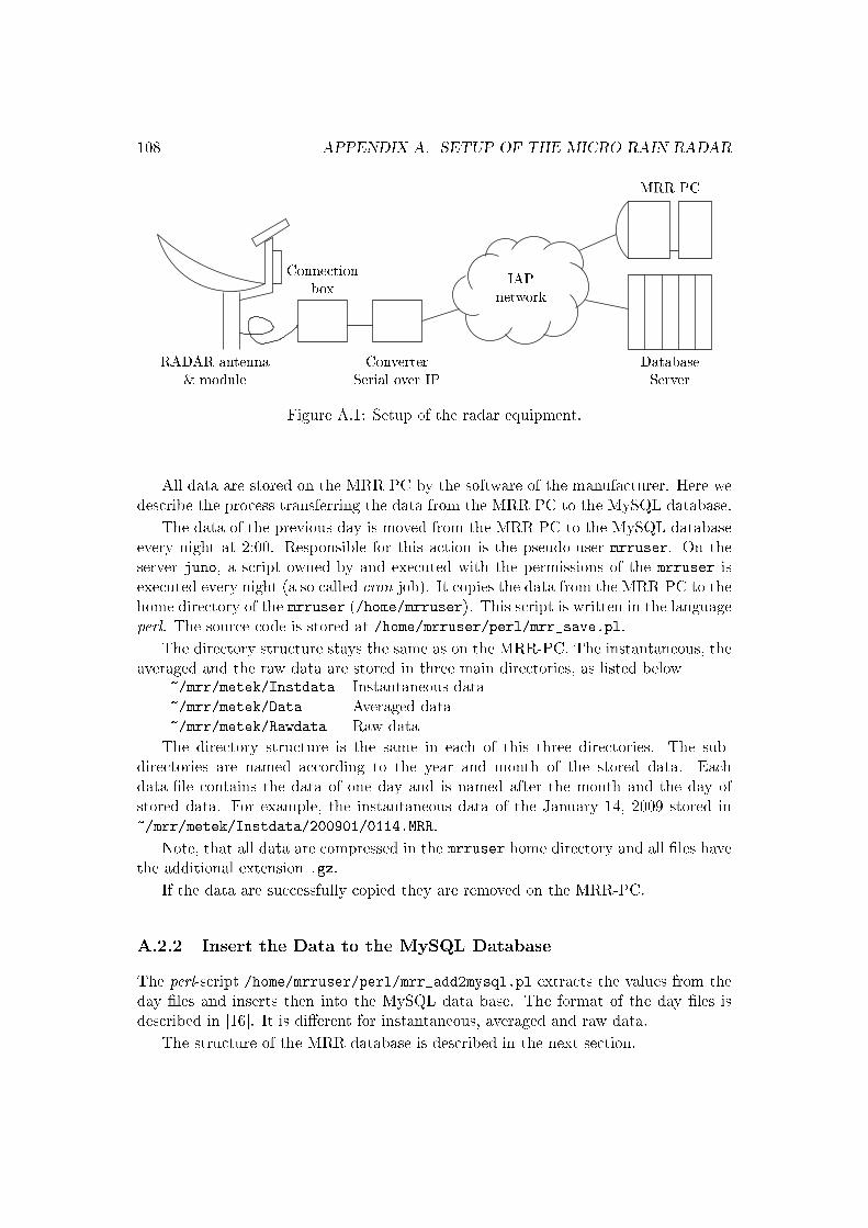
108 APPENDIX A. SETUP OF THE MICRO RAIN RADAR
Database
Server
IAP
network
Converter
Serial over IP
Connection
box
RADAR antenna
& module
MRR PC
Figure A.1: Setup of the radar equipment.
All data are stored on the MRR PC by the software of the manufacturer. Here wedescribe the process transferring the data from the MRR PC to the MySQL database.
The data of the previous day is moved from the MRR PC to the MySQL databaseevery night at 2:00. Responsible for this action is the pseudo-user mrruser. On theserver juno, a script owned by and executed with the permissions of the mrruser isexecuted every night (a so called cron-job). It copies the data from the MRR-PC to thehome directory of the mrruser (/home/mrruser). This script is written in the languageperl. The source code is stored at /home/mrruser/perl/mrr_save.pl.
The directory structure stays the same as on the MRR-PC. The instantaneous, theaveraged and the raw data are stored in three main directories, as listed below
~/mrr/metek/Instdata Instantaneous data~/mrr/metek/Data Averaged data~/mrr/metek/Rawdata Raw data
The directory structure is the same in each of this three directories. The sub-directories are named according to the year and month of the stored data. Eachdata-le contains the data of one day and is named after the month and the day ofstored data. For example, the instantaneous data of the January 14, 2009 stored in~/mrr/metek/Instdata/200901/0114.MRR.
Note, that all data are compressed in the mrruser home directory and all les havethe additional extension .gz.
If the data are successfully copied they are removed on the MRR-PC.
A.2.2 Insert the Data to the MySQL Database
The perl-script /home/mrruser/perl/mrr_add2mysql.pl extracts the values from theday les and inserts then into the MySQL data base. The format of the day les isdescribed in [16]. It is dierent for instantaneous, averaged and raw data.
The structure of the MRR database is described in the next section.
A.3. STRUCTURE OF THE DATABASE 109
A.3 Structure of the Database
The database on the MySQL server is called MRR. It contains three tables data, avgdataand rawdata, where data contains the instantaneous, avgdata the averaged and rawdatathe raw data.
Every data sample is specied by the time and the location. The column namefor the time specication is datetime and the one dimensional specication for thelocation is the height. The datetime is given in UTC and the height is the height inm above the MRR.
Example: Here an example is shown to read all values of the radar reectivity (Z)from the instantaneous table (data) at height 100 m in the time interval from March3, 2009 12:00 and 12:10.
mysql> SELECT Z FROM data WHERE height=100 AND datetime BETWEEN
'2009-03-05 12:00' AND '2009-03-05 12:10';
The columns in each of the three table correspond to a parameter measured by theMRR (except the time (datetime) and the height (height), we already discussed).
The following parameters are stored in the tables data and avgdata:Z Radar reectivity (in dBZ)W Fall velocity (in m/s)RR Rain rate (in mm/h)LWC Liquid water content (in g/m3)Fnn Spectral reectivity (in dB where (0 ≤ nn ≤ 63)Nnn Number of drops per volume and drop size (where 4 ≤ nn ≤ 49)

110 APPENDIX A. SETUP OF THE MICRO RAIN RADAR
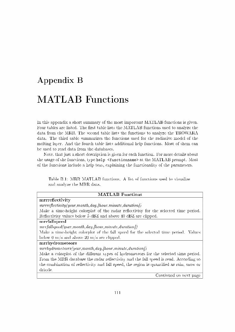
Appendix B
MATLAB Functions
In this appendix a short summary of the most important MATLAB functions is given.Four tables are listed. The rst table lists the MATLAB functions used to analyze thedata from the MRR. The second table lists the functions to analyze the TROWARAdata. The third table summarizes the functions used for the radiative model of themelting layer. And the fourth table lists additional help functions. Most of them canbe used to read data from the databases.
Note, that just a short description is given for each function. For more details aboutthe usage of the functions, type help <functionname> at the MATLAB prompt. Mostof the functions include a help text, explaining the functionality of the parameters.
Table B.1: MRR MATLAB functions. A list of functions used to visualizeand analyze the MRR data.
MATLAB Functions
mrrreectivitymrrreectivity(year,month,day,[hour,minute,duration])Make a time-height colorplot of the radar reectivity for the selected time period.Reectivity values below 5 dBZ and above 40 dBZ are clipped.
mrrfallspeedmrrfallspeed(year,month,day,[hour,minute,duration])Make a time-height colorplot of the fall speed for the selected time period. Valuesbelow 0 m/s and above 20 m/s are clipped.
mrrhydrometeorsmrrhydrometeors(year,month,day,[hour,minute,duration])Make a colorplot of the dierent types of hydrometeors for the selected time period.From the MRR database the radar reectivity and the fall speed is read. According tothe combination of reectivity and fall speed, the region is quantied as rain, snow ordrizzle.
Continued on next page
111
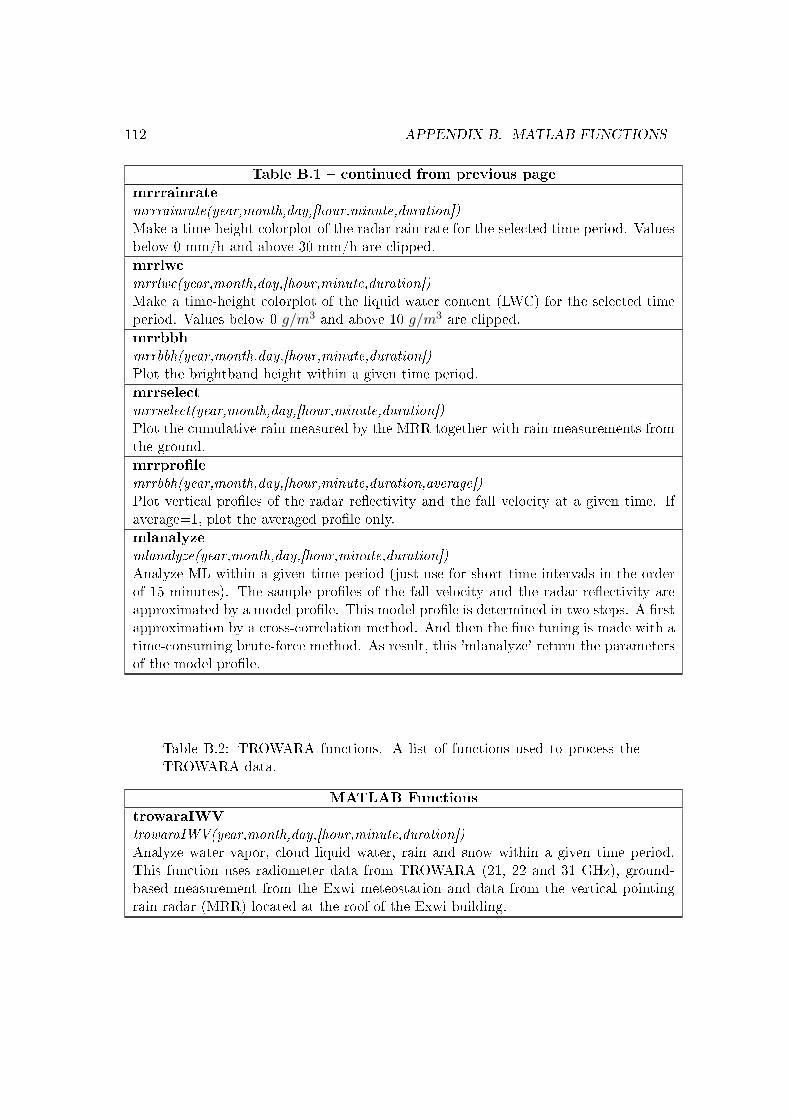
112 APPENDIX B. MATLAB FUNCTIONS
Table B.1 continued from previous page
mrrrainratemrrrainrate(year,month,day,[hour,minute,duration])Make a time-height colorplot of the radar rain rate for the selected time period. Valuesbelow 0 mm/h and above 30 mm/h are clipped.
mrrlwcmrrlwc(year,month,day,[hour,minute,duration])Make a time-height colorplot of the liquid water content (LWC) for the selected timeperiod. Values below 0 g/m3 and above 10 g/m3 are clipped.
mrrbbhmrrbbh(year,month,day,[hour,minute,duration])Plot the brightband height within a given time period.
mrrselectmrrselect(year,month,day,[hour,minute,duration])Plot the cumulative rain measured by the MRR together with rain measurements fromthe ground.
mrrprolemrrbbh(year,month,day,[hour,minute,duration,average])Plot vertical proles of the radar reectivity and the fall velocity at a given time. Ifaverage=1, plot the averaged prole only.
mlanalyzemlanalyze(year,month,day,[hour,minute,duration])Analyze ML within a given time period (just use for short time intervals in the orderof 15 minutes). The sample proles of the fall velocity and the radar reectivity areapproximated by a model prole. This model prole is determined in two steps. A rstapproximation by a cross-correlation method. And then the ne tuning is made with atime-consuming brute-force method. As result, this 'mlanalyze' return the parametersof the model prole.
Table B.2: TROWARA functions. A list of functions used to process theTROWARA data.
MATLAB Functions
trowaraIWVtrowaraIWV(year,month,day,[hour,minute,duration])Analyze water vapor, cloud liquid water, rain and snow within a given time period.This function uses radiometer data from TROWARA (21, 22 and 31 GHz), ground-based measurement from the Exwi meteostation and data from the vertical pointingrain radar (MRR) located at the roof of the Exwi building.
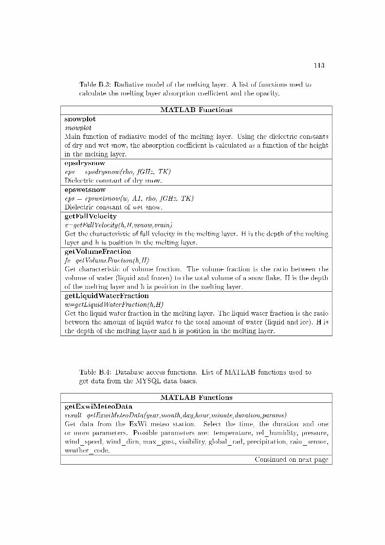
113
Table B.3: Radiative model of the melting layer. A list of functions used tocalculate the melting layer absorption coecient and the opacity.
MATLAB Functions
snowplotsnowplotMain function of radiative model of the melting layer. Using the dielectric constantsof dry and wet snow, the absorption coecient is calculated as a function of the heightin the melting layer.
epsdrysnoweps = epsdrysnow(rho, fGHz, TK)Dielectric constant of dry snow.
epswetsnoweps = epswetsnow(w, A1, rho, fGHz, TK)Dielectric constant of wet snow.
getFallVelocityv=getFallVelocity(h,H,vsnow,vrain)Get the characteristic of fall velocity in the melting layer. H is the depth of the meltinglayer and h is position in the melting layer.
getVolumeFractionfv=getVolumeFraction(h,H)Get characteristic of volume fraction. The volume fraction is the ratio between thevolume of water (liquid and frozen) to the total volume of a snow ake. H is the depthof the melting layer and h is position in the melting layer.
getLiquidWaterFractionw=getLiquidWaterFraction(h,H)Get the liquid water fraction in the melting layer. The liquid water fraction is the ratiobetween the amount of liquid water to the total amount of water (liquid and ice). H isthe depth of the melting layer and h is position in the melting layer.
Table B.4: Database access functions. List of MATLAB functions used toget data from the MYSQL data bases.
MATLAB Functions
getExwiMeteoDataresult=getExwiMeteoData(year,month,day,hour,minute,duration,params)Get data from the ExWi meteo station. Select the time, the duration and oneor more parameters. Possible parameters are: temperature, rel_humidity, pressure,wind_speed, wind_dirn, max_gust, visibility, global_rad, precipitation, rain_sensor,weather_code.
Continued on next page
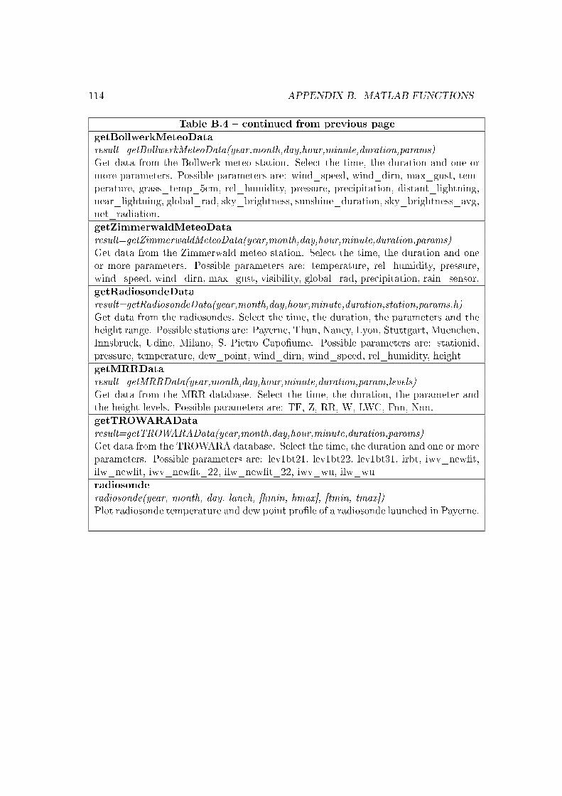
114 APPENDIX B. MATLAB FUNCTIONS
Table B.4 continued from previous page
getBollwerkMeteoDataresult=getBollwerkMeteoData(year,month,day,hour,minute,duration,params)Get data from the Bollwerk meteo station. Select the time, the duration and one ormore parameters. Possible parameters are: wind_speed, wind_dirn, max_gust, tem-perature, grass_temp_5cm, rel_humidity, pressure, precipitation, distant_lightning,near_lightning, global_rad, sky_brightness, sunshine_duration, sky_brightness_avg,net_radiation.
getZimmerwaldMeteoDataresult=getZimmerwaldMeteoData(year,month,day,hour,minute,duration,params)Get data from the Zimmerwald meteo station. Select the time, the duration and oneor more parameters. Possible parameters are: temperature, rel_humidity, pressure,wind_speed, wind_dirn, max_gust, visibility, global_rad, precipitation, rain_sensor.
getRadiosondeDataresult=getRadiosondeData(year,month,day,hour,minute,duration,station,params,h)Get data from the radiosondes. Select the time, the duration, the parameters and theheight range. Possible stations are: Payerne, Thun, Nancy, Lyon, Stuttgart, Muenchen,Innsbruck, Udine, Milano, S. Pietro Capoume. Possible parameters are: stationid,pressure, temperature, dew_point, wind_dirn, wind_speed, rel_humidity, height
getMRRDataresult=getMRRData(year,month,day,hour,minute,duration,param,levels)Get data from the MRR database. Select the time, the duration, the parameter andthe height levels. Possible parameters are: TF, Z, RR, W, LWC, Fnn, Nnn.
getTROWARADataresult=getTROWARAData(year,month,day,hour,minute,duration,params)Get data from the TROWARA database. Select the time, the duration and one or moreparameters. Possible parameters are: lev1bt21, lev1bt22, lev1bt31, irbt, iwv_newt,ilw_newt, iwv_newt_22, ilw_newt_22, iwv_wu, ilw_wu
radiosonderadiosonde(year, month, day, lanch, [hmin, hmax], [tmin, tmax])Plot radiosonde temperature and dew point prole of a radiosonde launched in Payerne.
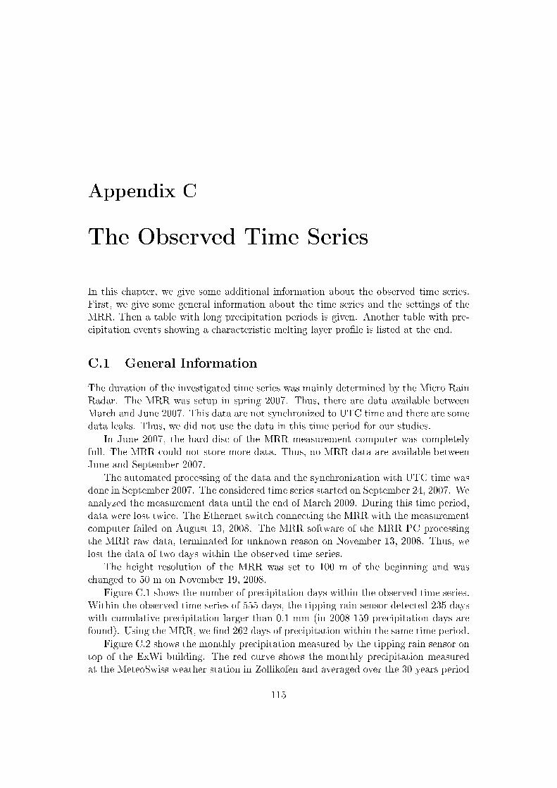
Appendix C
The Observed Time Series
In this chapter, we give some additional information about the observed time series.First, we give some general information about the time series and the settings of theMRR. Then a table with long precipitation periods is given. Another table with pre-cipitation events showing a characteristic melting layer prole is listed at the end.
C.1 General Information
The duration of the investigated time series was mainly determined by the Micro RainRadar. The MRR was setup in spring 2007. Thus, there are data available betweenMarch and June 2007. This data are not synchronized to UTC time and there are somedata leaks. Thus, we did not use the data in this time period for our studies.
In June 2007, the hard-disc of the MRR measurement computer was completelyfull. The MRR could not store more data. Thus, no MRR data are available betweenJune and September 2007.
The automated processing of the data and the synchronization with UTC time wasdone in September 2007. The considered time series started on September 24, 2007. Weanalyzed the measurement data until the end of March 2009. During this time period,data were lost twice. The Ethernet switch connecting the MRR with the measurementcomputer failed on August 13, 2008. The MRR software of the MRR PC processingthe MRR raw data, terminated for unknown reason on November 13, 2008. Thus, welost the data of two days within the observed time series.
The height resolution of the MRR was set to 100 m of the beginning and waschanged to 50 m on November 19, 2008.
Figure C.1 shows the number of precipitation days within the observed time series.Within the observed time series of 555 days, the tipping rain sensor detected 235 dayswith cumulative precipitation larger than 0.1 mm (in 2008 159 precipitation days arefound). Using the MRR, we nd 262 days of precipitation within the same time period.
Figure C.2 shows the monthly precipitation measured by the tipping rain sensor ontop of the ExWi building. The red curve shows the monthly precipitation measuredat the MeteoSwiss weather station in Zollikofen and averaged over the 30 years period
115
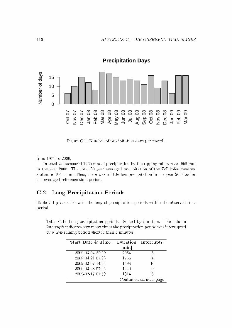
116 APPENDIX C. THE OBSERVED TIME SERIES
Oct
07
Nov
07
Dec
07
Jan
08
Feb
08
Mar
08
Apr
08
May
08
Jun
08
Jul 0
8
Aug
08
Sep
08
Oct
08
Nov
08
Dec
08
Jan
09
Feb
09
Mar
09
Precipitation Days
Num
ber
of d
ays
0
5
10
15
Figure C.1: Number of precipitation days per month.
from 1971 to 2000.In total we measured 1260 mm of precipitation by the tipping rain sensor, 905 mm
in the year 2008. The total 30 year averaged precipitation of the Zollikofen weatherstation is 1043 mm. Thus, there was a little less precipitation in the year 2008 as forthe averaged reference time period.
C.2 Long Precipitation Periods
Table C.1 gives a list with the longest precipitation periods within the observed timeperiod.
Table C.1: Long precipitation periods. Sorted by duration. The columninterrupts indicates how many times the precipitation period was interruptedby a non-raining period shorter than 5 minutes.
Start Date & Time Duration Interrupts[min]
2009-03-04 22:30 2954 52008-04-21 07:23 1766 42009-02-07 14:34 1498 102009-03-28 07:06 1440 02009-02-17 01:59 1314 6
Continued on next page
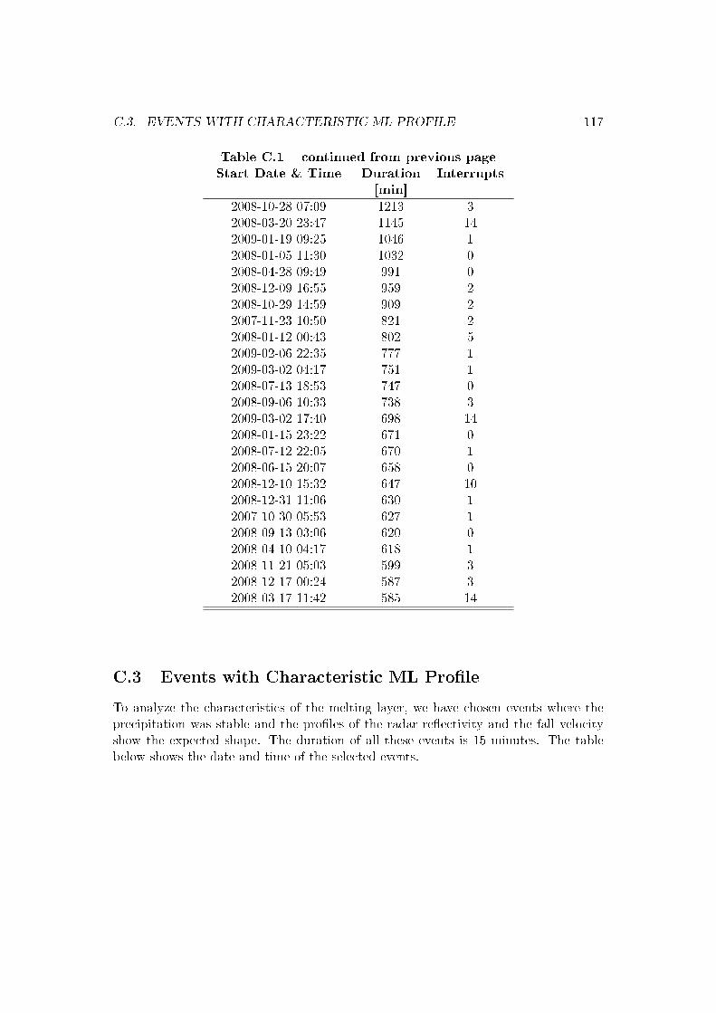
C.3. EVENTS WITH CHARACTERISTIC ML PROFILE 117
Table C.1 continued from previous pageStart Date & Time Duration Interrupts
[min]
2008-10-28 07:09 1213 32008-03-20 23:47 1145 142009-01-19 09:25 1046 12008-01-05 11:30 1032 02008-04-28 09:49 991 02008-12-09 16:55 959 22008-10-29 14:59 909 22007-11-23 10:50 821 22008-01-12 00:43 802 52009-02-06 22:35 777 12009-03-02 04:17 751 12008-07-13 18:53 747 02008-09-06 10:33 738 32009-03-02 17:40 698 142008-01-15 23:22 671 02008-07-12 22:05 670 12008-06-15 20:07 658 02008-12-10 15:32 647 102008-12-31 11:06 630 12007-10-30 05:53 627 12008-09-13 03:06 620 02008-04-10 04:17 618 12008-11-21 05:03 599 32008-12-17 00:24 587 32008-03-17 11:42 585 14
C.3 Events with Characteristic ML Prole
To analyze the characteristics of the melting layer, we have chosen events where theprecipitation was stable and the proles of the radar reectivity and the fall velocityshow the expected shape. The duration of all these events is 15 minutes. The tablebelow shows the date and time of the selected events.
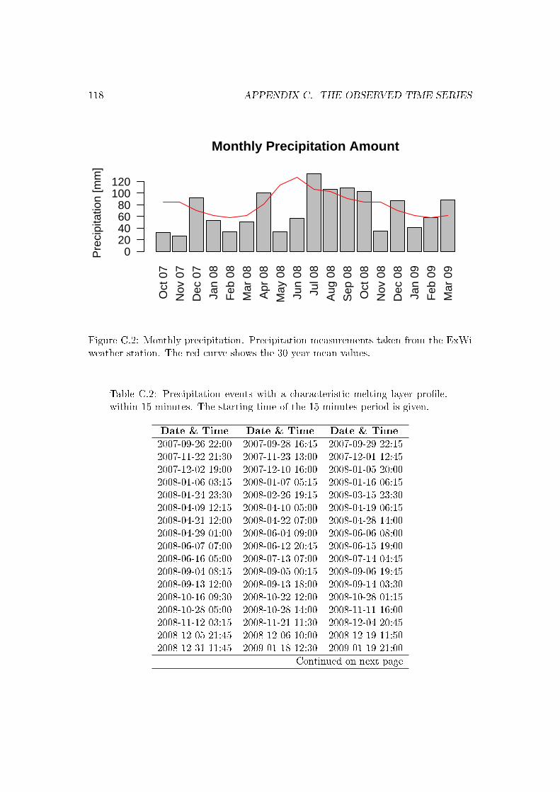
118 APPENDIX C. THE OBSERVED TIME SERIES
Oct
07
Nov
07
Dec
07
Jan
08
Feb
08
Mar
08
Apr
08
May
08
Jun
08
Jul 0
8
Aug
08
Sep
08
Oct
08
Nov
08
Dec
08
Jan
09
Feb
09
Mar
09
Monthly Precipitation Amount
Pre
cipi
tatio
n [m
m]
020406080
100120
Figure C.2: Monthly precipitation. Precipitation measurements taken from the ExWiweather station. The red curve shows the 30 year mean values.
Table C.2: Precipitation events with a characteristic melting layer prole.within 15 minutes. The starting time of the 15 minutes period is given.
Date & Time Date & Time Date & Time
2007-09-26 22:00 2007-09-28 16:45 2007-09-29 22:152007-11-22 21:30 2007-11-23 13:00 2007-12-01 12:452007-12-02 19:00 2007-12-10 16:00 2008-01-05 20:002008-01-06 03:15 2008-01-07 05:15 2008-01-16 06:152008-01-24 23:30 2008-02-26 19:15 2008-03-15 23:302008-04-09 12:15 2008-04-10 05:00 2008-04-19 06:152008-04-21 12:00 2008-04-22 07:00 2008-04-28 14:002008-04-29 01:00 2008-06-04 09:00 2008-06-06 08:002008-06-07 07:00 2008-06-12 20:45 2008-06-15 19:002008-06-16 05:00 2008-07-13 07:00 2008-07-14 04:452008-09-04 08:15 2008-09-05 00:15 2008-09-06 19:452008-09-13 12:00 2008-09-13 18:00 2008-09-14 03:302008-10-16 09:30 2008-10-22 12:00 2008-10-28 01:152008-10-28 05:00 2008-10-28 14:00 2008-11-11 16:002008-11-12 03:15 2008-11-21 11:30 2008-12-04 20:452008-12-05 21:45 2008-12-06 10:00 2008-12-19 11:502008-12-31 11:45 2009-01-18 12:30 2009-01-19 21:00
Continued on next page
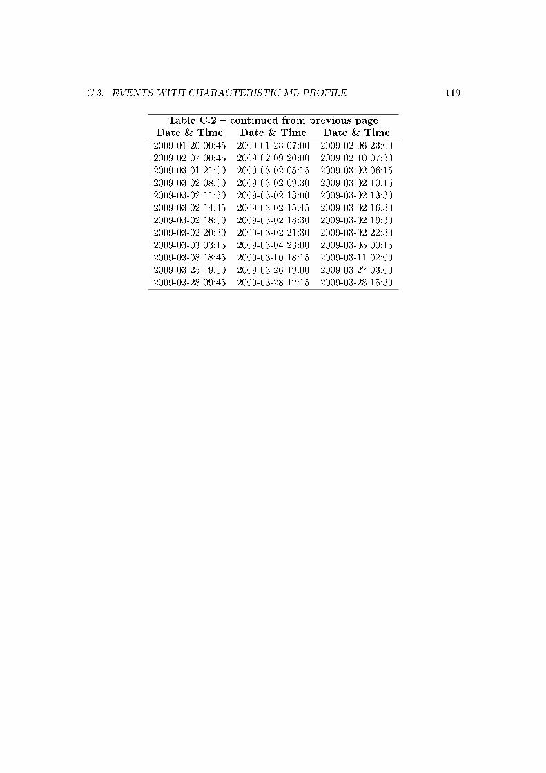
C.3. EVENTS WITH CHARACTERISTIC ML PROFILE 119
Table C.2 continued from previous pageDate & Time Date & Time Date & Time
2009-01-20 00:45 2009-01-23 07:00 2009-02-06 23:002009-02-07 00:45 2009-02-09 20:00 2009-02-10 07:302009-03-01 21:00 2009-03-02 05:15 2009-03-02 06:152009-03-02 08:00 2009-03-02 09:30 2009-03-02 10:152009-03-02 11:30 2009-03-02 13:00 2009-03-02 13:302009-03-02 14:45 2009-03-02 15:45 2009-03-02 16:302009-03-02 18:00 2009-03-02 18:30 2009-03-02 19:302009-03-02 20:30 2009-03-02 21:30 2009-03-02 22:302009-03-03 03:15 2009-03-04 23:00 2009-03-05 00:152009-03-08 18:45 2009-03-10 18:15 2009-03-11 02:002009-03-25 19:00 2009-03-26 19:00 2009-03-27 03:002009-03-28 09:45 2009-03-28 12:15 2009-03-28 15:30

120 APPENDIX C. THE OBSERVED TIME SERIES
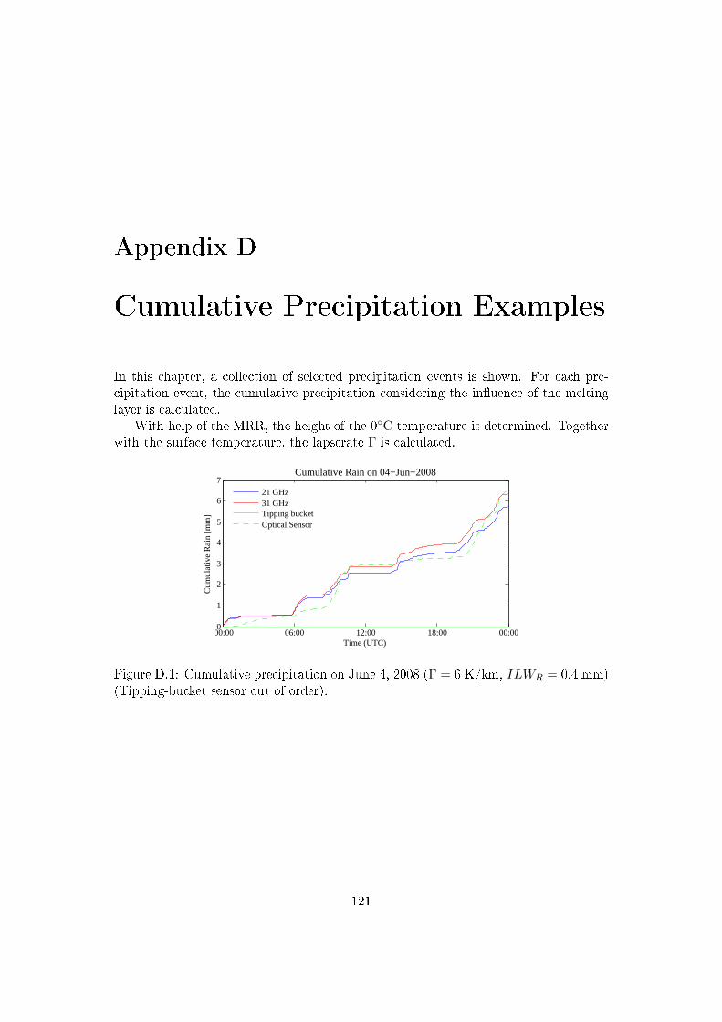
Appendix D
Cumulative Precipitation Examples
In this chapter, a collection of selected precipitation events is shown. For each pre-cipitation event, the cumulative precipitation considering the inuence of the meltinglayer is calculated.
With help of the MRR, the height of the 0C temperature is determined. Togetherwith the surface temperature, the lapserate Γ is calculated.
00:00 06:00 12:00 18:00 00:000
1
2
3
4
5
6
7
Time (UTC)
Cum
ulat
ive
Rai
n [m
m]
Cumulative Rain on 04−Jun−2008
21 GHz31 GHzTipping bucketOptical Sensor
Figure D.1: Cumulative precipitation on June 4, 2008 (Γ = 6 K/km, ILWR = 0.4 mm)(Tipping-bucket sensor out of order).
121
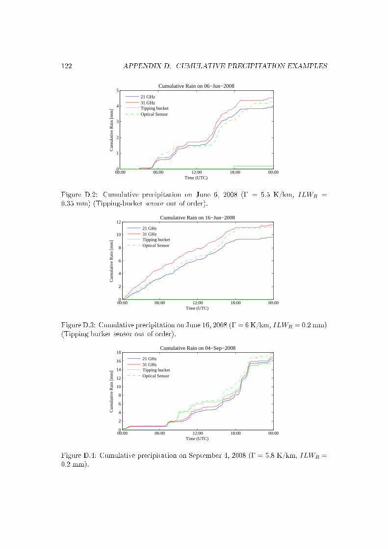
122 APPENDIX D. CUMULATIVE PRECIPITATION EXAMPLES
00:00 06:00 12:00 18:00 00:000
1
2
3
4
5
Time (UTC)
Cum
ulat
ive
Rai
n [m
m]
Cumulative Rain on 06−Jun−2008
21 GHz31 GHzTipping bucketOptical Sensor
Figure D.2: Cumulative precipitation on June 6, 2008 (Γ = 5.5 K/km, ILWR =0.35 mm) (Tipping-bucket sensor out of order).
00:00 06:00 12:00 18:00 00:000
2
4
6
8
10
12
Time (UTC)
Cum
ulat
ive
Rai
n [m
m]
Cumulative Rain on 16−Jun−2008
21 GHz31 GHzTipping bucketOptical Sensor
Figure D.3: Cumulative precipitation on June 16, 2008 (Γ = 6 K/km, ILWR = 0.2 mm)(Tipping-bucket sensor out of order).
00:00 06:00 12:00 18:00 00:000
2
4
6
8
10
12
14
16
18
Time (UTC)
Cum
ulat
ive
Rai
n [m
m]
Cumulative Rain on 04−Sep−2008
21 GHz31 GHzTipping bucketOptical Sensor
Figure D.4: Cumulative precipitation on September 4, 2008 (Γ = 5.8 K/km, ILWR =0.2 mm).
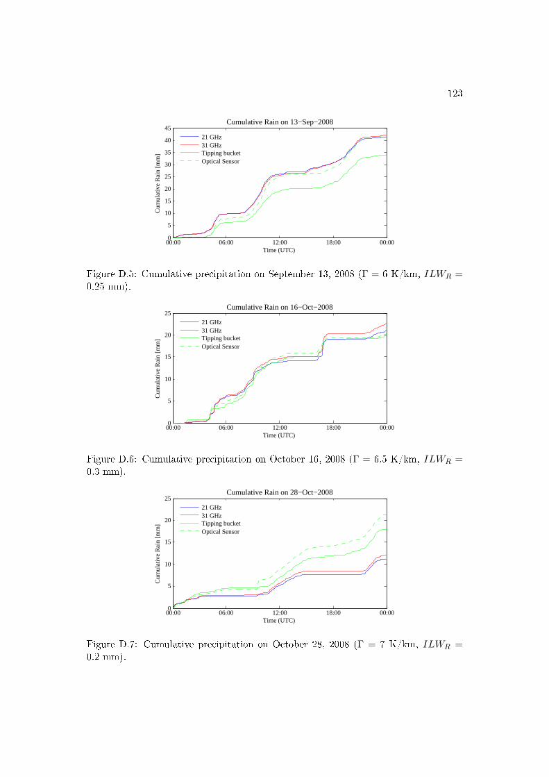
123
00:00 06:00 12:00 18:00 00:000
5
10
15
20
25
30
35
40
45
Time (UTC)
Cum
ulat
ive
Rai
n [m
m]
Cumulative Rain on 13−Sep−2008
21 GHz31 GHzTipping bucketOptical Sensor
Figure D.5: Cumulative precipitation on September 13, 2008 (Γ = 6 K/km, ILWR =0.25 mm).
00:00 06:00 12:00 18:00 00:000
5
10
15
20
25
Time (UTC)
Cum
ulat
ive
Rai
n [m
m]
Cumulative Rain on 16−Oct−2008
21 GHz31 GHzTipping bucketOptical Sensor
Figure D.6: Cumulative precipitation on October 16, 2008 (Γ = 6.5 K/km, ILWR =0.3 mm).
00:00 06:00 12:00 18:00 00:000
5
10
15
20
25
Time (UTC)
Cum
ulat
ive
Rai
n [m
m]
Cumulative Rain on 28−Oct−2008
21 GHz31 GHzTipping bucketOptical Sensor
Figure D.7: Cumulative precipitation on October 28, 2008 (Γ = 7 K/km, ILWR =0.2 mm).
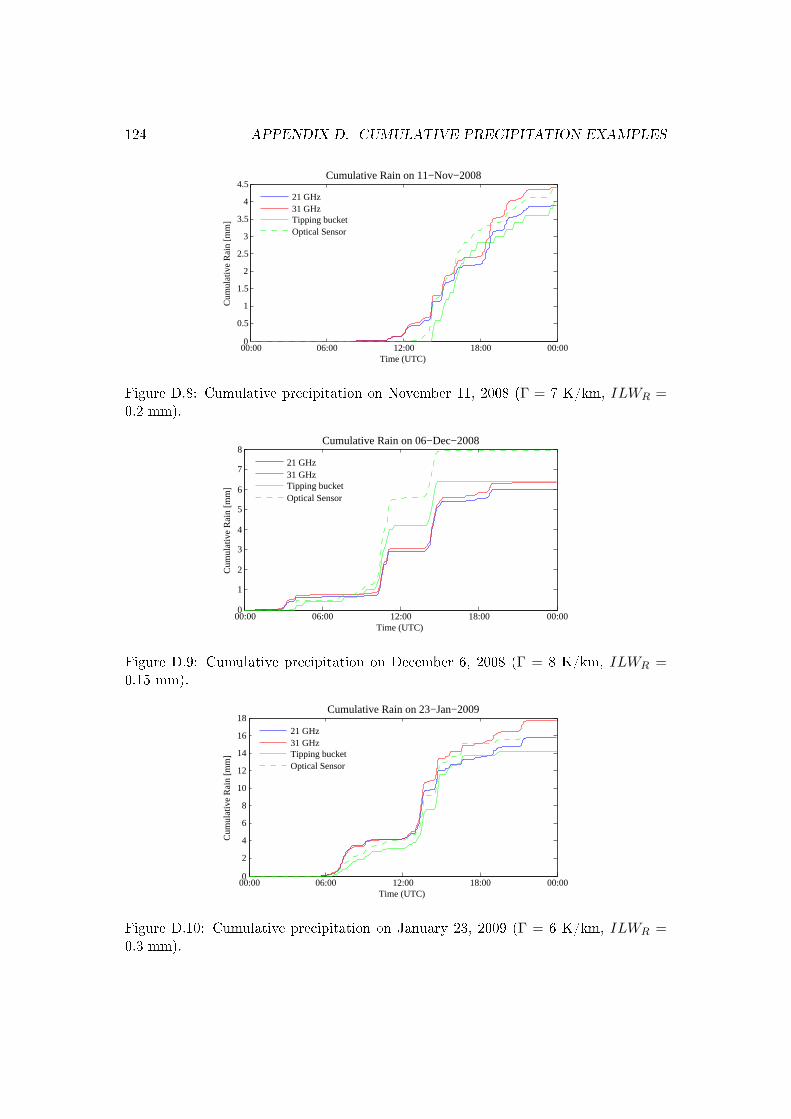
124 APPENDIX D. CUMULATIVE PRECIPITATION EXAMPLES
00:00 06:00 12:00 18:00 00:000
0.5
1
1.5
2
2.5
3
3.5
4
4.5
Time (UTC)
Cum
ulat
ive
Rai
n [m
m]
Cumulative Rain on 11−Nov−2008
21 GHz31 GHzTipping bucketOptical Sensor
Figure D.8: Cumulative precipitation on November 11, 2008 (Γ = 7 K/km, ILWR =0.2 mm).
00:00 06:00 12:00 18:00 00:000
1
2
3
4
5
6
7
8
Time (UTC)
Cum
ulat
ive
Rai
n [m
m]
Cumulative Rain on 06−Dec−2008
21 GHz31 GHzTipping bucketOptical Sensor
Figure D.9: Cumulative precipitation on December 6, 2008 (Γ = 8 K/km, ILWR =0.15 mm).
00:00 06:00 12:00 18:00 00:000
2
4
6
8
10
12
14
16
18
Time (UTC)
Cum
ulat
ive
Rai
n [m
m]
Cumulative Rain on 23−Jan−2009
21 GHz31 GHzTipping bucketOptical Sensor
Figure D.10: Cumulative precipitation on January 23, 2009 (Γ = 6 K/km, ILWR =0.3 mm).

Acknowledgement
I am appreciative to the following people who made this work possible:
Christian Mätzler for supervising my work and for having always time to answermy questions.
Niklaus Kämpfer for giving my the opportunity of joining the Institute of AppliedPhysics.
Eddy Graham for being my room mate and sharing his enthusiasm about cloudsand weather phenomena.
Stefan Müller and Lorenz Martin for the introduction to the system administra-tion and the good collaboration.
All the colleagues of the microwave department for the good colleagueship.
Jürg Stettbacher for giving me the opportunity to work occasionally. My studieswould not have been possible without this side job.
My friends for distracting me from work.
Sonja for her interest in my work and me.
125

126 APPENDIX D. CUMULATIVE PRECIPITATION EXAMPLES
Erklärung
gemäss Art. 28 Abs. 2 RSL 05
Name/Vorname: Leuenberger Andreas
Matrikelnummer: 92-903-756
Studiengang: Climate Sciences
Bachelor Master X Dissertation
Titel der Arbeit: Precipitation Measurements with Microwave Sensors
Leiter der Arbeit: Prof. Dr. Christian Mätzler
Ich erkläre hiermit, dass ich diese Arbeit selbständig verfasst und keine anderen alsdie angegebenen Quellen benutzt habe. Alle Stellen, die wörtlich oder sinngemässaus Quellen entnommen wurden, habe ich als solche gekennzeichnet. Mir ist bekannt,dass andernfalls der Senat gemäss Artikel 36 Absatz 1 Buchstabe o des Gesetzes vom5. September 1996 über die Universität zum Entzug des auf Grund dieser Arbeit ver-liehenen Titels berechtigt ist.
Bern, den 26. Mai 2009
Unterschrift