Probabilistic Online Prediction

of Robot Action Results

based on Physics Simulation

Dissertation zur Erlangung

des Doktorgrades Dr. rer. nat.

an der Fakultät für Mathematik,

Informatik und Naturwissenschaften

Fachbereich Informatik

der Universität Hamburg

vorgelegt von Sebastian Rockel

Hamburg, 2015

Disputation: 30. November 2015

Gutachter:

Prof. Dr. Jianwei Zhang

Prof. Bernd Neumann, Ph.D.

The most exciting phrase to hear in science, the one that heralds newdiscoveries, is not “Eureka!” (I found it!) but “That’s funny. . . ”

Isaac Asimov (b1920 - †1992)

Imagination . . . is more important than knowledge. Knowledge is limited.Imagination encircles the world.

Albert Einstein (October 26, 1929)

Abstract

The motivation for this work is the today’s abstraction gap between the high-levelrobot control involved in symbolic planning and the low-level, fine-grained control ofmobile robot motors. To deal with the complex, changeable environments in whichhumans live, state-of-the-art robots need to be able to exploit common-sense knowledge(i.e. physical laws) to calculate velocity, acceleration, friction and so on. Physicalprediction is typically the domain of a physics simulation, such as Gazebo.

The literature contains examples in which symbolic planning and reasoning meth-ods are extended, such as by adding geometric or temporal extensions or by offlinerecording of simulated actions.

The goal of this thesis is to question how a task-planning based robot system can beimproved by prediction derived from physical simulation and to provide some answers.The goal-directed approach is to integrate a realistic prediction of robot activities so asto allow these activities to be adapted before execution fails. The hypothesis, therefore,is that a system that integrates such prediction is more efficient than a comparablesystem that does not.

A probabilistic prediction method named “functional imagination” and a system archi-tecture have been developed. The prediction method was integrated into a blackboard-based robot control system and a PR2 robot and Gazebo were used for its evaluation.Experiments verified that simulation is indeed accurate and close to reality. The re-sults of three experimental scenarios in a restaurant domain supported the hypothesisthat the robustness and efficiency of such a planning and execution-based system areimproved by the addition of physics-based prediction.

The work concludes by summarizing its findings, limitations and possible further re-search directions and with a future perspective on how parallel and cloud computingwill affect the field of robotics in the context of simulation.

v

Zusammenfassung

Der Ansatz dieser Arbeit ist motiviert von der „Abstraktionslücke“ zwischen heutigersymbolischer Aufgabenplanung und Motoransteuerung. Denn gerade heutige Robotermüssen sich in komplexen und sich ändernden Umgebungen zurechtfinden können.Damit sie das tun können, muss eine Verarbeitung von physikalischem Allgemein-wissen möglich sein. Die physikalische Vorhersage von Roboteraktionen ist dabei dieParadedisziplin von Physiksimulationen, wie Gazebo.

In der fachverwandten Literatur werden bereits symbolische Planung und Schlussfol-gerung mit geometrischen sowie zeitlichen Komponenten, oder der Aufzeichung vonoffline simulierten Aktionen, erweitert.

Das Ziel dieser Arbeit ist die Beantwortung der Frage, wie ein planungs-basiertesRobotersystem sein Verhalten durch physik-basierte Vorhersage von Roboteraktionenverbessern kann. Der zielgerichtete Ansatz ist hier die Integration einer physikalischrealistischen Vorhersage um Ausführungsfehler zu verhindern. Erreicht wird das durchdie Anpassung oder Veränderung des aktuellen Roboterplans und seiner Aktionen. DieArbeitshypothese lautet deshalb, dass solch ein integriertes Vorhersagesystem Pläneeffizienter ausführt als ein System ohne dieses.

Im Verlauf dieser Arbeit wurden eine probabilistische Vorhersagemethode, “Functio-nal Imagination”, und eine Systemarchitektur entwickelt. Für die praktische Evalua-tion wurde der PR2 Roboter und Gazebo benutzt. Die Vorhersagemethode wurde inein Blackboard-basiertes Roboter-Kontroll-System integriert. Experimente verifizier-ten die Simulation als genau und sehr nahe an der Realität. Die Ergebnisse von dreiexperimentellen Szenarien in einer Restaurantdomäne unterstützen die Hypothese,dass die physikalische Vorhersage in Kombination mit Planungs- und Ausführungs-Komponenten einem System ohne diese Vorhersage überlegen ist, hinsichtlich Robust-heit und Effizienz.

Am Ende werden die Ergebnisse, Einschränkungen und mögliche zukünftige For-schungsfelder aufgezeigt und ein kurzer Ausblick im Simulationskontext gegeben, wieverteiltes Rechnen und Cloud-Computing das Forschungsfeld der Robotik in Zukunftbeeinflussen werden.

vii

Acknowledgements

In working on this dissertation, I have greatly benefited from the help and support ofmany people. Here are those I would like to thank especially.

First and foremost, I want to thank my advisors, Jianwei Zhang and Bernd Neumann,for their confidence in me realizing this work and their valuable advice. I would alsolike to thank William Morris for taking the time to read and comment on many draftsof this dissertation. Furthermore I am particular grateful to Denis Klimentjew for hishints and comments during my study and for becoming a friend.

Carrying out successful research in autonomous robotics is not possible without beinga member of a team. I had the luck of joining two of the best teams. Firstly theRACE team: I would like to thank especially Joachim Hertzberg for very encouragingdiscussions, ideas and comments on many stages of this work. Secondly special thanksgoes to the members of the TAMS team for providing me with one of the best technicalenvironments and expertise, for working with autonomous robots. I owe especiallymany thanks to Eugen Richter for his time and help, often on very short notice.

Most importantly, I want to thank Ricarda for her love and support, helping to createthis manuscript.

ix

Table of Contents

1 Introduction 1

1.1 Motivation and Goals . . . . . . . . . . . . . . . . . . . . . . . . . . . 11.2 Motivating Scenarios . . . . . . . . . . . . . . . . . . . . . . . . . . . 21.3 The Faculty of Imagination . . . . . . . . . . . . . . . . . . . . . . . 41.4 Research Question and Contribution . . . . . . . . . . . . . . . . . . 51.5 Structure of the Thesis and Related Publications . . . . . . . . . . . 6

2 Related Work 9

2.1 Symbolic and Geometric Task Planning . . . . . . . . . . . . . . . . . 92.2 Projection, Simulation, Imagination and Prediction . . . . . . . . . . 142.3 State-of-the-art Robot Operating Systems . . . . . . . . . . . . . . . 192.4 Benchmarking and Evaluation of Intelligent Robots . . . . . . . . . . 202.5 Summary . . . . . . . . . . . . . . . . . . . . . . . . . . . . . . . . . 22

3 Experimental Platform 23

3.1 The PR2 Robot . . . . . . . . . . . . . . . . . . . . . . . . . . . . . . 233.2 Actuators . . . . . . . . . . . . . . . . . . . . . . . . . . . . . . . . . 243.3 Tray . . . . . . . . . . . . . . . . . . . . . . . . . . . . . . . . . . . . 263.4 Sensors . . . . . . . . . . . . . . . . . . . . . . . . . . . . . . . . . . . 283.5 Power and Control . . . . . . . . . . . . . . . . . . . . . . . . . . . . 313.6 Navigation and Mapping . . . . . . . . . . . . . . . . . . . . . . . . . 333.7 Summary . . . . . . . . . . . . . . . . . . . . . . . . . . . . . . . . . 33

4 Frameworks and Tools 35

4.1 The RACE Project . . . . . . . . . . . . . . . . . . . . . . . . . . . . 354.2 ROS and the PR2 . . . . . . . . . . . . . . . . . . . . . . . . . . . . . 364.3 Gazebo Simulator . . . . . . . . . . . . . . . . . . . . . . . . . . . . . 374.4 Robot Capabilities . . . . . . . . . . . . . . . . . . . . . . . . . . . . 414.5 Summary . . . . . . . . . . . . . . . . . . . . . . . . . . . . . . . . . 43

5 Functional Imagination 45

5.1 Methodology . . . . . . . . . . . . . . . . . . . . . . . . . . . . . . . 455.2 Functional Imagination System Architecture . . . . . . . . . . . . . . 475.3 Integration of the PR2 with the Gazebo Simulation . . . . . . . . . . 515.4 Creating an Optimized Simulation Environment . . . . . . . . . . . . 525.5 Modeling Object Properties . . . . . . . . . . . . . . . . . . . . . . . 575.6 Update Simulation by Object Recognition Results . . . . . . . . . . . 58

xi

Table of Contents

5.7 Generating High-Level Activity Experiences . . . . . . . . . . . . . . 605.8 Generating Dynamics-based Experiences . . . . . . . . . . . . . . . . 645.9 Many Worlds Interpretation . . . . . . . . . . . . . . . . . . . . . . . 665.10 Summary . . . . . . . . . . . . . . . . . . . . . . . . . . . . . . . . . 69

6 Experimental Scenarios and Evaluation 71

6.1 Simulation Validation . . . . . . . . . . . . . . . . . . . . . . . . . . . 726.2 Spatial Prediction . . . . . . . . . . . . . . . . . . . . . . . . . . . . . 786.3 Physical Prediction and Probabilistic Method . . . . . . . . . . . . . 836.4 Summary . . . . . . . . . . . . . . . . . . . . . . . . . . . . . . . . . 88

7 Conclusion and Outlook 91

7.1 Conclusion . . . . . . . . . . . . . . . . . . . . . . . . . . . . . . . . . 927.2 Limitations and Future Research . . . . . . . . . . . . . . . . . . . . 93

A Appendix I

A.1 Gazebo Simulation . . . . . . . . . . . . . . . . . . . . . . . . . . . . IA.2 Dynamics Data . . . . . . . . . . . . . . . . . . . . . . . . . . . . . . IIA.3 Creating a 2D Occupancy Grid Map with the PR2 . . . . . . . . . . IXA.4 Moment of Inertia . . . . . . . . . . . . . . . . . . . . . . . . . . . . . IXA.5 Standard Deviation and Normal Distribution . . . . . . . . . . . . . . XA.6 Additional Robot Capabilities . . . . . . . . . . . . . . . . . . . . . . XIA.7 The Pepper Mill . . . . . . . . . . . . . . . . . . . . . . . . . . . . . . XIIIA.8 Statistical Analysis of Simulated Robot Actions . . . . . . . . . . . . XIVA.9 Statistical Analysis of Real Robot Actions . . . . . . . . . . . . . . . XX

Bibliography XXVII

Glossary XLI

List of Figures XLIII

List of Tables XLVII

List of Algorithms XLIX

xii

Introduction

1

1.1 Motivation and Goals

From the early days of robotics, a fundamental and interesting question has alwaysbeen how robots could adopt human cognitive processes. In this work an approachis proposed that implements the principle of cognitive imagination, otherwise namedfunctional imagination [MHN08]:

We define functional imagination in the context of artificial embodiedagents as the mechanism that allows an agent to simulate its own be-haviours, predict their sensory-based consequences and extract behaviouralbenefit from doing so. By behavioural benefit we mean an increase in re-ward or utility achieved by using internal simulation.

The approach combines into one hyperreal system the cognitive concept of imaginationwith high-level planning and execution. The proposed Hyperreality Imagination-basedReasoning and Evaluation System (HIRES) does not rely upon traditional spatialreasoning [RN07], but instead uses simulation as a tool that enables the testing of robotexecution before actions are actually performed. This naturally saves robot resourcesand, when optimized, total execution time, as well as improving system robustness.The approach is inspired by the concept of imagination [Cas71]. Imagination enableshumans to consult rules or principles but not merely to apply those rules [Loa01].Instead humans imagine what the consequences might be if the rules are, or are not,followed [Lod96]. The author notes that humans constantly use imaginative projectionand that imagination is essential for human reasoning. So why should it not also beused for robot reasoning in a human-robot environment?

According to Loasby [Loa01], reasoning is expensive in time and energy and shouldtherefore be used sparingly. The approach of this thesis is to combine the concept ofimagination with the concept of ‘Hyperreality’ [TT01]. The term Hyperreality comesfrom earlier work by Baudrillard [Bau94]. It originates in semiotics and postmodernphilosophy and is considered to be the condition in which an agent cannot distinguishreality from a simulation of reality. Therefore reality and virtual reality can be consid-ered interchangeable at some point. This blending of virtuality and reality can be seen

1

1 Introduction

in a broader sense as mixing human and artificial intelligence1. Baudrillard postulatesthat with ‘Hyperreality’ there is no longer a difference between real and imaginary -both exist at the same time. This seamless transition between simulation and realityis related to the term Mixed Reality (MR) as employed in [RKZ12, CMW09]).

An exact simulation of a scene can be used in order to execute robot actions (e.g.picking-up a mug from a counter and placing it in front of a guest) before they areactually performed. The consequence of simulating the action might be that thecurrent plan must be adapted in order for the task to succeed (e.g. after the failure ofplacing a mug in simulation).

The results from this work support the idea that applying a functional method ofimagination within the context of a hyperreal system improves robot autonomy andsaves resources. Results are described in Chapter 6.

1.2 Motivating Scenarios

To illustrate and evaluate the performance of such a system, a real-world dynamicenvironment should be appropriate. Thus the evaluation of this work employs variousscenarios in which a mobile service robot performs tasks in a human environment.These scenarios demonstrate how well the approach predicts spatial, temporal andphysics-related action results. As these scenarios benchmark the whole system, theyare also a measure of how well the system components are integrated. In the followingparagraphs, some possible situations are described.

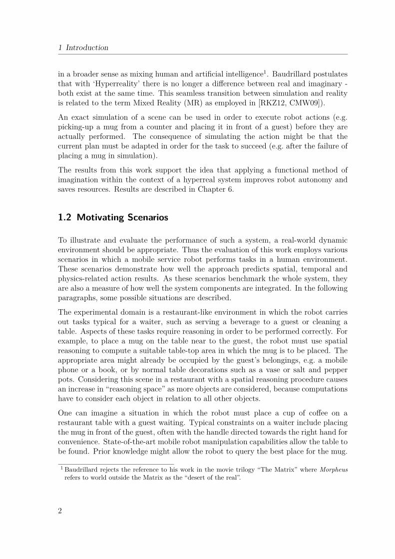
The experimental domain is a restaurant-like environment in which the robot carriesout tasks typical for a waiter, such as serving a beverage to a guest or cleaning atable. Aspects of these tasks require reasoning in order to be performed correctly. Forexample, to place a mug on the table near to the guest, the robot must use spatialreasoning to compute a suitable table-top area in which the mug is to be placed. Theappropriate area might already be occupied by the guest’s belongings, e.g. a mobilephone or a book, or by normal table decorations such as a vase or salt and pepperpots. Considering this scene in a restaurant with a spatial reasoning procedure causesan increase in “reasoning space” as more objects are considered, because computationshave to consider each object in relation to all other objects.

One can imagine a situation in which the robot must place a cup of coffee on arestaurant table with a guest waiting. Typical constraints on a waiter include placingthe mug in front of the guest, often with the handle directed towards the right hand forconvenience. State-of-the-art mobile robot manipulation capabilities allow the table tobe found. Prior knowledge might allow the robot to query the best place for the mug.

1 Baudrillard rejects the reference to his work in the movie trilogy “The Matrix” where Morpheus

refers to world outside the Matrix as the “desert of the real”.

2

1.2 Motivating Scenarios

Nevertheless the table might be occupied by other objects such as plates, cutlery or theguest’s belongings, such as a mobile phone. Modern reasoning and learning systemsconsist not only of knowledge representation systems and planning modules, but alsocontain reasoning and planning components. A spatial reasoning unit is concernedwith the spatial relation between objects (on the table) and calculates the best placeto put the mug, whereas a temporal unit tells the robot to deliver the drink while it isstill hot. A hierarchical planning module coordinates robot capabilities at a symboliclevel. Such modular task sharing increases the autonomous robustness of intelligentmobile systems and represents the state-of-the-art.

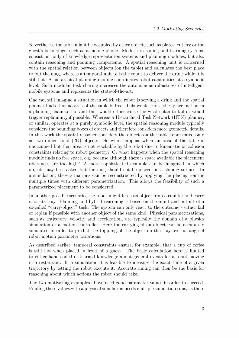
One can still imagine a situation in which the robot is serving a drink and the spatialplanner finds that no area of the table is free. This would cause the ‘place’ action ina planning chain to fail and thus would either cause the whole plan to fail or wouldtrigger replanning, if possible. Whereas a Hierarchical Task Network (HTN) planner,or similar, operates at a purely symbolic level, the spatial reasoning module typicallyconsiders the bounding boxes of objects and therefore considers more geometric details.In this work the spatial reasoner considers the objects on the table represented onlyas two dimensional (2D) objects. So what happens when an area of the table isunoccupied but that area is not reachable by the robot due to kinematic or collisionconstraints relating to robot geometry? Or what happens when the spatial reasoningmodule finds no free space, e.g. because although there is space available the placementtolerances are too high? A more sophisticated example can be imagined in whichobjects may be stacked but the mug should not be placed on a sloping surface. Ina simulation, these situations can be reconstructed by applying the placing routinemultiple times with different parametrization. This allows the feasibility of such aparametrized placement to be considered.

In another possible scenario, the robot might fetch an object from a counter and carryit on its tray. Planning and hybrid reasoning is based on the input and output of aso-called “carry-object” task. The system can only react to the outcome - either failor replan if possible with another object of the same kind. Physical parametrizations,such as trajectory, velocity and acceleration, are typically the domain of a physicssimulation or a motion controller. Here the carrying of an object can be accuratelysimulated in order to predict the toppling of the object on the tray over a range ofrobot motion parameter variations.

As described earlier, temporal constraints ensure, for example, that a cup of coffeeis still hot when placed in front of a guest. The basic calculation here is limitedto either hand-coded or learned knowledge about general events for a robot movingin a restaurant. In a simulation, it is feasible to measure the exact time of a giventrajectory by letting the robot execute it. Accurate timing can then be the basis forreasoning about which actions the robot should take.

The two motivating examples above need good parameter values in order to succeed.Finding these values with a physical simulation needs multiple simulation runs, as there

3

1 Introduction

is usually not just one best parameter (to test). Even though certain parameter valueshave a high likelihood of success in simulation, the outcome of the operation mightstill be different in reality. Hence this uncertainty has to be dealt with appropriately.

1.3 The Faculty of Imagination

Imagination is based upon images in the human mind that are not perceived throughthe ordinary senses. When somebody imagines the color of the sky at sun set, thismight involve 2D pictures. Imagining the rotation of a cube in order to ‘see’ the rearface might involve three dimensional (3D) images. In principle it should be possibleto create these images in a robot’s ‘mind’.

In this work the term ‘imagination’ is not related to the technical process in psy-chology of reviving in the mind aspects of objects formerly perceived. This rather‘reproductive’ process conflicts with the ‘productive’ process of imagination.

As the robot’s ‘mind’ is not technically defined, imagination must be implemented asa function within a robot control program. More concretely, a 3D physical simulationcan render 2D images with colors and textures in a very detailed manner close toreality as well as creating 3D motions with physical embodiments. Thus there mustbe a deeper reason for the fact that cognitive scientists see a fundamental differencebetween imagination and physical (or visual) simulation.

The answer might be found in the work of Ned Block and Philip N. Johnson-Laird.Block, the author of [Blo81], describes the long-lasting and still current “great debate”on the nature of mental images: are images pictures in the head or are they like thesymbol structures in computers? In other words, one could ask whether mental imagesare the consequence of cognitive processes or the tools of those processes. In anotherwork the author claims that mental images do indeed exist, both 2D and 3D [Blo83].Are people rotating mental images at measurable speeds? Imagine an experiment inwhich the task is to look at pairs of pictures showing rotated 3D blocks and to decidefrom the pictures whether or not the blocks are congruent. The experiment shows thatit is possible to measure the speed at which images are rotated in the human mind.Further experiments are presented, for example Map Scanning and an explanation ofMental Image is given.

The author of [JL83] deals with the fundamental question of the nature of mentalmodels. He argues that humans understand the world by building inner mental replicasof the relations between objects and events. The mind is therefore a model-buildingdevice that can itself be modeled on a computer. Furthermore this work providesa guide to the building of such a model. In [JL95], the same author considers thetwo main approaches to deductive thinking: formal rule-based inference as a syntacticprocess; and mental model theory, which includes the idea that deductive thinking

4

1.4 Research Question and Contribution

is a semantic process. The conclusion is that “Models are the natural way in whichthe human mind constructs reality, conceives alternative realities and searches out theconsequences of assumptions.” Models are the medium of thought, proposed [Cra43].According to Craik,

“thought is a term for the conscious working of a highly complex machine,built of parts having dimensions where the classical laws of mechanics arestill very nearly true, and having dimensions where space is, to all intentsand purposes, Euclidean. This mechanism has the power to represent,or parallel, certain phenomena in the external world as a calculating ma-chine will parallel — and so be able to ‘give an account of’ or ‘predict’most easily — those phenomena whose mechanism most resembles itself”(pp. 94-95).

But what is a mental model? Craik described the brain’s internal models as follows:

“My hypothesis then is that thought models, or parallels, reality — that itsessential feature is not ‘the mind’, ‘the self’, ‘sense data’, nor propositionsbut symbolism, and that this symbolism is largely of the same kind asthat which is familiar to us in mechanical devices which aid thought andcalculation”.

Craik goes further as he considers the use of physical models (for him they can servealso as symbols), as well as words and numbers for prediction and reasoning. Further-more he states that a mental model does not have to resemble the object or situationpictorially “since the physical object is ‘translated’ into a working model which givesa prediction. . . ”. In contrast to defining mental models, this thesis is about findingappropriate functional models that are computationally representable.

1.4 Research Question and Contribution

In this work one fundamental question posed is whether and how a physical simulationcan be used as a companion tool for predicting the results of robot actions. Anotherquestion is how this can improve robot competence, both quantitatively and qualita-tively. Competence here is referred to as adapting behavior in a goal-directed way tosave resources and succeed with the task at hand.

In order to verify that simulation is an appropriate tool for prediction, it has tobe evaluated with respect to its quantitative similarity with the real world. This isdiscussed in Chapter 6. Therefore reasonable metrics have to be proposed, applied andevaluated. Based on the assumption that the simulation in use has a sufficient degreeof realism, a prototype system able to exploit simulation as a companion tool mustbe integrated. The evaluation is based on the scenarios and software developed in theRobustness by Autonomous Competence Enhancement (RACE) project in the context

5

1 Introduction

of the European Union (EU) Framework Programme for Research and TechnologicalDevelopment (FP7). The RACE project is described in Chapter 4 and the scenarios aredescribed in Chapter 6. In order to support the hypothesis posed below, an evaluationmetric benchmarking the robot’s competence has to be defined. This is done for eachscenario and is described with the related experiments in Chapter 6.

The research question, approach and hypothesis of this thesis can be refined as:

Research question: How can a task planning based robot system be improved byprediction derived from physical simulation?

Approach: Integrate a realistic prediction of robot activities to allow these activitiesto be adapted (by a plan change or by replanning) before a sub-optimal (failing) activityis executed.

Hypothesis: A system integrating such prediction is more efficient (such as requiringless time, plan steps) than a comparable system without.

Answering the research question and verifying the stated hypothesis in this dissertationspans multiple topics:

• Design & Integration: How to integrate the cognitive science principle of ‘imag-ination’ into a mobile service robot.

• Physics & Robot Motor Control: Is an off-the-shelf physical simulation accurateenough to predict robot action results?

• Task planning & Execution: Does an integrated imagination approach improveplan-based execution?

• Algorithms & Data structures: Which algorithms and representations have tobe implemented to handle and reason about simulated robot action results?

• Motion Control and Navigation: How can robot motion control and navigationbe reasonably parametrized?

1.5 Structure of the Thesis and Related Publications

This thesis is organized as follows:

• Chapter 2 gives an overview of related literature in relevant fields.

• Chapter 3 describes in detail the hardware platform, sensors and actuators used.

• Chapter 4 gives an overview of the software tools and frameworks used for thiswork and discusses the decisions that led to the approach taken in this work.Contributing publications were [HZZ+14, RNZ+13].

6

1.5 Structure of the Thesis and Related Publications

• Chapter 5 contains the main contributions of the work. After stating the ob-jectives, a methodology and system architecture that integrate functional imag-ination are developed. The proposed system and its use cases are described.Publications that contributed to the chapter were [RKZZ14, CNSV14, KRZ13,ZRZ13, EKRZ13, KRZ12, RKZ12].

• Chapter 6 describes the experiments conducted and the way in which results werecollected. It also evaluates the results. [ZRP+13] contributed to this chapter.

• Chapter 7 concludes this thesis and gives an outlook of future research.

Work during the years leading up to this thesis has resulted in several publications thatwere accepted at conferences, workshops and seminars, including: contributions relat-ing primarily to plan-based, reasoning-and-learning mobile service robotic systems andtheir software architecture; simulation-based reasoning in mixed-reality environments;co-operative multi-robot systems; robot action prediction and system evaluation. Ap-pendix A.9 gives a comprehensive list of all publications resulting from this work.

7

Related Work

2

This chapter presents a summary of related work, starting by describing current ap-proaches to symbolic planning and recent extensions, such as geometric, spatial andtemporal planning. The chapter also introduces the main topic of this work - the com-bination of simulation with planning and execution - and describes how this approachgoes beyond related work. It also discusses some approaches to the evaluation of in-telligent robotic systems and introduces several software frameworks used partially inthis work. Various technical terms will also be introduced.

2.1 Symbolic and Geometric Task Planning

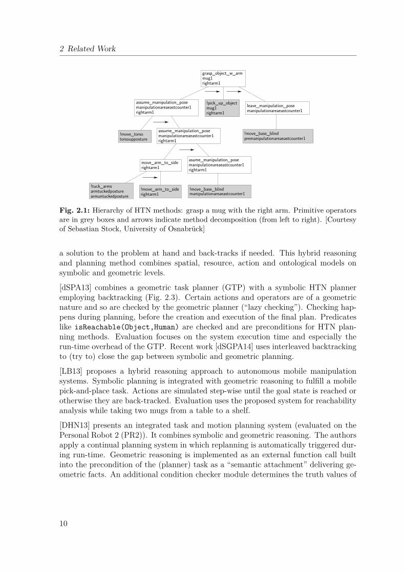
State-of-the-art reasoning and planning is based on symbolic, hybrid (spatial, tempo-ral, causal), kinematic and collision information, as well as on parameters obtainedthrough theoretical deduction or simulation. A classical approach to task planning isthe STanford Research Institute Problem Solver (STRIPS) method [FN71]. STRIPS-based planners focus on achieving a specified goal state, whereas HTN planners focuson solving abstract tasks. The latter is generally more efficient than classical planningbecause the search is limited to a given library of recipes. In this work a popularHTN planning method called “totally-ordered” HTN planning with partially orderedsub tasks (henceforth simply called HTN planning [NMAC+01]) is used. In this hi-erarchical approach, methods and operators are modelled along with their pre- andpost-conditions (effects). Decomposition of the problem definition creates a hierarchyof methods and operators to solve the task at hand, as shown in Fig. 2.1. As anoptimization, in this work the resulting plan is scheduled for parallel execution if therobot has the necessary resources. This is described in [EKRZ13].

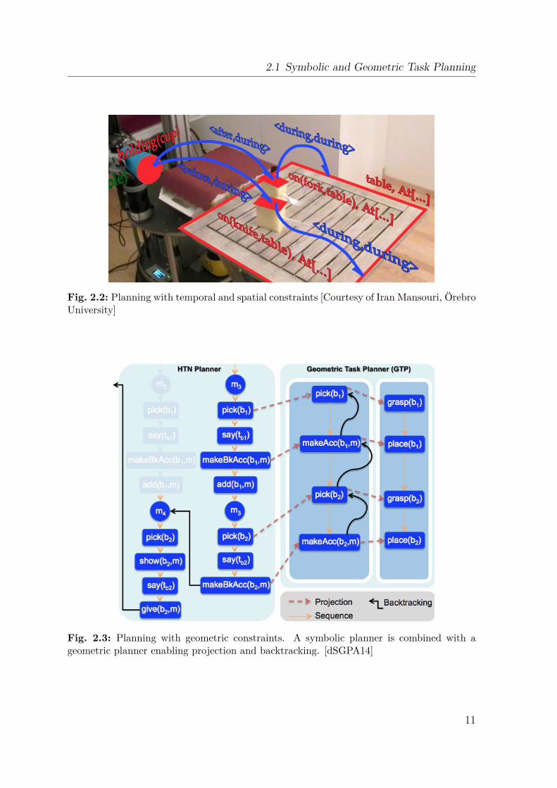
Extensions to traditional symbolic planning techniques incorporate additional con-straint processing techniques. They are based on a temporal knowledge representa-tion (KR), such as Allen’s Interval Algebra [All84]. The Meta-Constraint SatisfactionProblems (Meta-CSP) framework1 [MP06] enriches these representations with metricconstraints [vB90], see also Fig. 2.2. This method searches in a tree-like structure for

1 http://metacsp.org (March 16, 2015)

9

2 Related Work

!move_base_blindpremanipulationareaeastcounter1

leave_manipulation_posemanipulationareaeastcounter1

grasp_object_w_armmug1rightarm1

rightarm1mug1!pick_up_objectassume_manipulation_pose

manipulationareaeastcounter1rightarm1

!move_torsotorsoupposture

assume_manipulation_posemanipulationareaeastcounter1rightarm1

asume_manipulation_posemanipulationareaeastcounter1rightarm1

move_arm_to_siderightarm1

!tuck_armsarmtuckedposturearmuntuckedposture

!move_arm_to_siderightarm1 manipulationareaeastcounter1

!move_base_blind

Fig. 2.1: Hierarchy of HTN methods: grasp a mug with the right arm. Primitive operatorsare in grey boxes and arrows indicate method decomposition (from left to right). [Courtesyof Sebastian Stock, University of Osnabrück]

a solution to the problem at hand and back-tracks if needed. This hybrid reasoningand planning method combines spatial, resource, action and ontological models onsymbolic and geometric levels.

[dSPA13] combines a geometric task planner (GTP) with a symbolic HTN planneremploying backtracking (Fig. 2.3). Certain actions and operators are of a geometricnature and so are checked by the geometric planner (“lazy checking”). Checking hap-pens during planning, before the creation and execution of the final plan. Predicateslike isReachable(Object,Human) are checked and are preconditions for HTN plan-ning methods. Evaluation focuses on the system execution time and especially therun-time overhead of the GTP. Recent work [dSGPA14] uses interleaved backtrackingto (try to) close the gap between symbolic and geometric planning.

[LB13] proposes a hybrid reasoning approach to autonomous mobile manipulationsystems. Symbolic planning is integrated with geometric reasoning to fulfill a mobilepick-and-place task. Actions are simulated step-wise until the goal state is reached orotherwise they are back-tracked. Evaluation uses the proposed system for reachabilityanalysis while taking two mugs from a table to a shelf.

[DHN13] presents an integrated task and motion planning system (evaluated on thePersonal Robot 2 (PR2)). It combines symbolic and geometric reasoning. The authorsapply a continual planning system in which replanning is automatically triggered dur-ing run-time. Geometric reasoning is implemented as an external function call builtinto the precondition of the (planner) task as a “semantic attachment” delivering ge-ometric facts. An additional condition checker module determines the truth values of

10

2.1 Symbolic and Geometric Task Planning

Fig. 2.2: Planning with temporal and spatial constraints [Courtesy of Iran Mansouri, ÖrebroUniversity]

Fig. 2.3: Planning with geometric constraints. A symbolic planner is combined with ageometric planner enabling projection and backtracking. [dSGPA14]

11

2 Related Work

Logging

Simulationof Sensors

Motor /Manipulatorcommands

Internalstate

Object

Physicsrules

Environment Simulation

Beliefstate

TaskTree

...

......

Interpreter Plan

Plan Interpretation

statei

statei+1

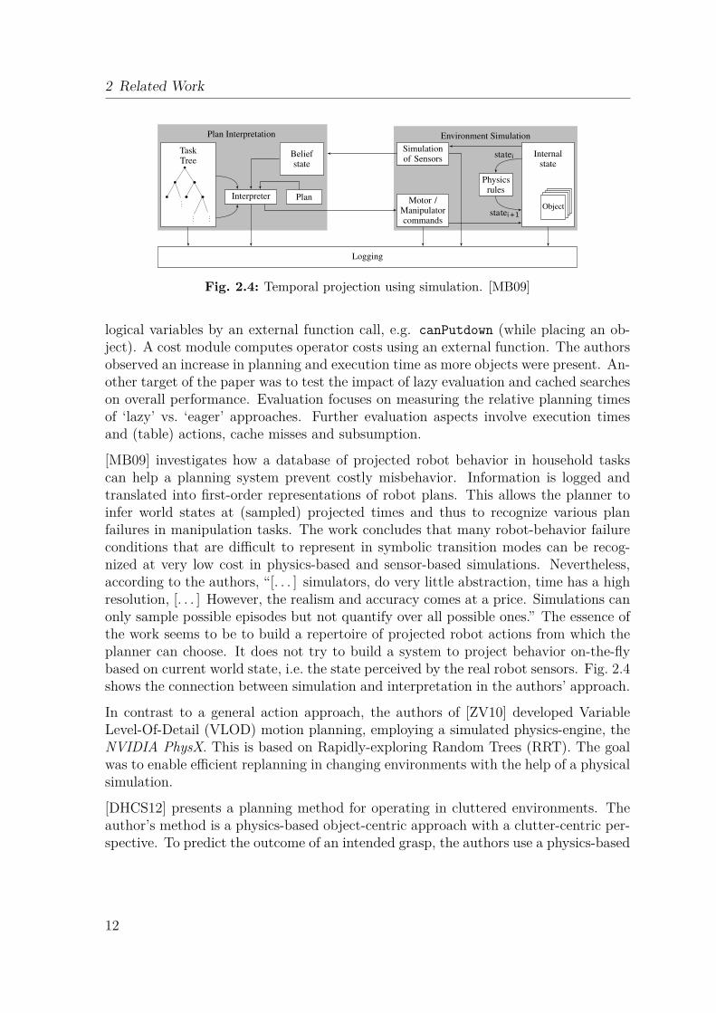
Fig. 2.4: Temporal projection using simulation. [MB09]

logical variables by an external function call, e.g. canPutdown (while placing an ob-ject). A cost module computes operator costs using an external function. The authorsobserved an increase in planning and execution time as more objects were present. An-other target of the paper was to test the impact of lazy evaluation and cached searcheson overall performance. Evaluation focuses on measuring the relative planning timesof ‘lazy’ vs. ‘eager’ approaches. Further evaluation aspects involve execution timesand (table) actions, cache misses and subsumption.

[MB09] investigates how a database of projected robot behavior in household taskscan help a planning system prevent costly misbehavior. Information is logged andtranslated into first-order representations of robot plans. This allows the planner toinfer world states at (sampled) projected times and thus to recognize various planfailures in manipulation tasks. The work concludes that many robot-behavior failureconditions that are difficult to represent in symbolic transition modes can be recog-nized at very low cost in physics-based and sensor-based simulations. Nevertheless,according to the authors, “[. . . ] simulators, do very little abstraction, time has a highresolution, [. . . ] However, the realism and accuracy comes at a price. Simulations canonly sample possible episodes but not quantify over all possible ones.” The essence ofthe work seems to be to build a repertoire of projected robot actions from which theplanner can choose. It does not try to build a system to project behavior on-the-flybased on current world state, i.e. the state perceived by the real robot sensors. Fig. 2.4shows the connection between simulation and interpretation in the authors’ approach.

In contrast to a general action approach, the authors of [ZV10] developed VariableLevel-Of-Detail (VLOD) motion planning, employing a simulated physics-engine, theNVIDIA PhysX. This is based on Rapidly-exploring Random Trees (RRT). The goalwas to enable efficient replanning in changing environments with the help of a physicalsimulation.

[DHCS12] presents a planning method for operating in cluttered environments. Theauthor’s method is a physics-based object-centric approach with a clutter-centric per-spective. To predict the outcome of an intended grasp, the authors use a physics-based

12

2.1 Symbolic and Geometric Task Planning

simulation method that computes the reaction of objects in the scene to a set of pos-sible robot movements. It considers simultaneous object interactions that can bepre-computed and cached. The authors state that object-object interaction would re-quire run-time capability, which is left out. The approach allows more possible graspsto be found for a given scene and it succeeds in more scenes. Validation uses a PR2showing that the predicted outcomes match real-life results. It is a partially onlineapproach that also explores sampling as the method of choice when handling uncertainparameters. A current limitation is that it considers only 2D collisions, i.e. no topplingor stacking of objects.

[BHKLP12, BKLP13] defines the diverse action manipulation (DAMA) problem con-cerning a robot, a set of movable objects and a set of diverse manipulation actions. Theaim is to find a sequence of actions that moves each of the objects to a goal configura-tion. The problem is addressed as a multi-modal planning problem and a hierarchicalalgorithm is proposed to deal with it. Although the work addresses robot manipula-tion problems that are similar to those addressed by this thesis, the authors do notuse physics planning or simulation to improve the robot’s autonomy or robustness.

[KLP12] presents geometric and symbolic representations in a hierarchical planningarchitecture called Hierarchical Planning in the Now (HPN). A system is integratedto generate behavior in a real robot that robustly achieves tasks in uncertain domains.Simulation is used to demonstrate the system but physics capabilities are not exploitedfor reasoning.

[LDS+14] combines symbolic and geometric reasoning. The authors use the PlanningDomain Definition Language (PDDL) and compute geometric alternatives for whole-body control with null space projections.

[KLP+14] uses an online Google text corpus to extract commonsense rules for use inrobot planning.

HTN planning is currently one of the most popular high-level planning strategiesfor mobile robotics. In this work the Simple Hierarchical Ordered Planner 2 (SHOP2)[NMAC+01] is used. A huge advantage of SHOP2 over other HTN planners is its abilityto generate partial-order plans. Unfortunately, HTN planners provide no facilities forparallelization or replanning. To compensate, in this work the planner is extendedwith a parallelization layer realized with State MACHine (SMACH) [BRGJ+11]. Thisallows the use of containers to assign different tasks to each state and thereby enablesany type of parallelized plan to be executed. This early work is described in [EKRZ13].

[KLP12] combines geometric and symbolic representations into a hierarchical planningarchitecture, referred to as HPN. A system is integrated to generate behavior in areal robot that robustly achieves tasks in uncertain domains. Simulation is used todemonstrate the system but not to exploit physical reasoning capabilities. [BHKLP12,BKLP13] define the DAMA problem concerning a robot, a set of movable objects anda diverse set of manipulation actions. The objective is to find a sequence of actions

13

2 Related Work

that moves each of the objects to a goal configuration. The manipulation problem isaddressed as a multi-modal planning problem and a hierarchical algorithm is proposedto deal with it. Although the work addresses robot manipulation activities similar tothose in this thesis, the authors do not use physical planning or simulation to improverobot autonomy or robustness.

Most state-of-the-art planning approaches are based on symbolic information (i.e.abstract information) and lack commonsense reasoning. Although current methodsare promising in combining high-level and low-level knowledge representation withreasoning and planning, there is still a gap. This is especially true when working inchanging and partially unknown environments where object information such as size,weight, and inertia are not even modelled.

2.2 Projection, Simulation, Imagination and Prediction

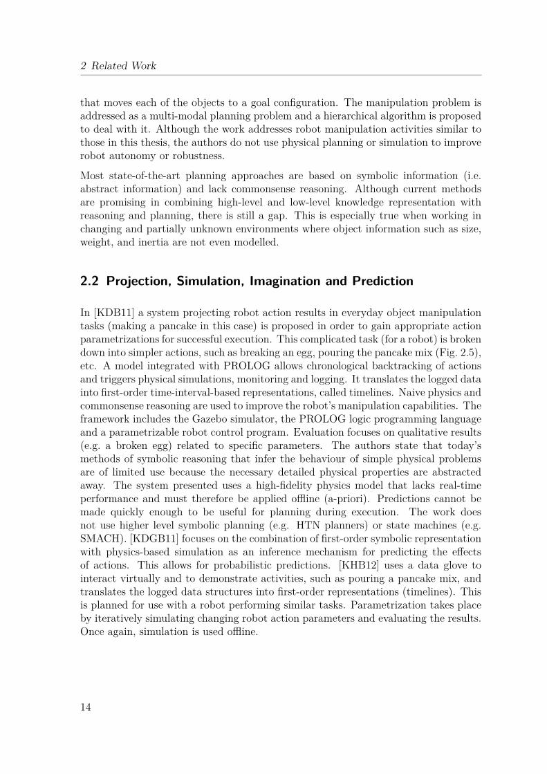
In [KDB11] a system projecting robot action results in everyday object manipulationtasks (making a pancake in this case) is proposed in order to gain appropriate actionparametrizations for successful execution. This complicated task (for a robot) is brokendown into simpler actions, such as breaking an egg, pouring the pancake mix (Fig. 2.5),etc. A model integrated with PROLOG allows chronological backtracking of actionsand triggers physical simulations, monitoring and logging. It translates the logged datainto first-order time-interval-based representations, called timelines. Naive physics andcommonsense reasoning are used to improve the robot’s manipulation capabilities. Theframework includes the Gazebo simulator, the PROLOG logic programming languageand a parametrizable robot control program. Evaluation focuses on qualitative results(e.g. a broken egg) related to specific parameters. The authors state that today’smethods of symbolic reasoning that infer the behaviour of simple physical problemsare of limited use because the necessary detailed physical properties are abstractedaway. The system presented uses a high-fidelity physics model that lacks real-timeperformance and must therefore be applied offline (a-priori). Predictions cannot bemade quickly enough to be useful for planning during execution. The work doesnot use higher level symbolic planning (e.g. HTN planners) or state machines (e.g.SMACH). [KDGB11] focuses on the combination of first-order symbolic representationwith physics-based simulation as an inference mechanism for predicting the effectsof actions. This allows for probabilistic predictions. [KHB12] uses a data glove tointeract virtually and to demonstrate activities, such as pouring a pancake mix, andtranslates the logged data structures into first-order representations (timelines). Thisis planned for use with a robot performing similar tasks. Parametrization takes placeby iteratively simulating changing robot action parameters and evaluating the results.Once again, simulation is used offline.

14

2.2 Projection, Simulation, Imagination and Prediction

Fig. 2.5: Different actions in a pancake making scenario: typical action, such as flippingthe pancake, are tested in simulation in order to find good action parameters, e.g. the angleby which the wrist must turn. [KDB11]

[BB07] presents a qualitative evaluation of a number of free, publicly available, physicsengines for simulation systems and game development. Simulation can be describedas solving the forward dynamics problem: given the forces acting on a system, howdoes the system move as a result? The authors present six major metrics of simulationperformance: the simulator paradigm, the integrator, object representation, collisiondetection, material properties and constraint implementation. Of the ten physics en-gines evaluated by [BB07], this work mainly uses the Open Dynamics Engine (ODE)2,version 1.0 of which is used in the Gazebo simulator. Bullet3 is compared as an enginesupported by recent versions of Gazebo.

In [BHH04] a mobile robot control architecture is introduced for projection-basedplanning, execution and learning. It supports the projection of navigation plans basedon learned models of such actions. This information is used to improve the robot’snavigation plan. The results show that navigational models learned in simulation canimprove physical robot performance.

In [AKPL13], the authors show how to use simulation to detect faults caused by theenvironment when releasing an object. The results are used to modify actions inorder to avoid such faults. The theory of these so-called external faults is investigatedfrequently. Such faults are sometimes also called interaction faults or unfavorable

2 http://www.ode.org (March 16, 2015)3 http://bulletphysics.org/wordpress (March 16, 2015)

15

2 Related Work

environment conditions and are also labeled as unforeseen events, exogenous eventsand errors. The authors use the ODE physics engine to predict robot action results.They evaluate their approach by comparing their N-Bins algorithm to popular machinelearning (ML) algorithms, such as decision trees and k-nearest neighbors. Results arejudged by comparing the model properties (such as object kinematics and dynamics)of the initial and final states. The approach is evaluated on a ‘release’ action of arobot manipulating an object. Simulation was used to estimate a good release statefor the manipulator in order to prevent external faults. Although this approach limitsthe simulation use-case to one action, it applies a similar paradigm to the predictionof robot action results: simulation, evaluation and action modification.

In [JLS12] the authors allow a robot to arrange the human environment by lettingthe robot anticipate and imagine human positions and then figuring out what thosevirtual humans are likely to do. This approach relies on learning how objects relateto human poses based on their affordances4, ease of use and reach-ability.

[MKNH08] defines the term functional imagination as the purposeful manipulationof information that is not directly available to the senses. It states that imaginationalways points to something that in reality is not there and that in order to be useful,imagination also needs to provide information about the likely consequences of actions.This is then to be used by a mechanism for translating imagined motor actions intosensory-based representations of their consequences. In [MHN08] the authors proposea framework for modelling functional imagination: an embodied agent that simulatesits own behaviors, predicts their sensory-based consequences and extracts behavioralbenefit from doing so. The system is based on a physics-based humanoid simulator -SIMNOS [GNHK06].

In [KS13] the authors developed a system that anticipates what a human will do nextwith the aim of allowing an assistive robot to plan ahead in response. A temporal,conditional, random field represents each possible future.

The term robot imagination was used in [VMJB13] for a system that generates modelsof objects prior to their perception. Robot imagination is defined here as the robot’scapability to generate feature parameter values of unknown objects by generalizingcharacteristics from previously presented objects.

Simulation has become an essential tool in the development of complex mobile roboticsystems. The availability of physical robots is limited and researchers often workin separate physical locations on different system parts. Consequently whole-systemevaluation and testing is often not possible. In such cases a realistic simulation isindispensable. Simulation as a verification and testing tool is widely adopted during

4 The term ‘affordance’ was coined by psychologist J.J. Gibbson (1904-79). In Gibson’s formulation,affordances are properties of the environment, independent of the perceiver. Later, Don Normen,a student of Gibbson, replaced the term with the notion of the actual and fundamental propertiesof the thing, such as how it can be used [Nor02].

16

2.2 Projection, Simulation, Imagination and Prediction

system development. Recent research into autonomous robot control extends the useof simulation for reasoning.

Harris et-al. [HC11] give a good outline of the available simulators, frameworks andtool-kits. The authors suggest that most simulators are not well documented (foranything but Windows environments), have no sensors or offer no possibilities for theintegration of new robots and sensors. Many tools are insufficiently precise, do notinclude physics engines or are no longer under active development. However, accordingto the authors, Robot Operating System (ROS) has been proven to be very suitable.The Gazebo-based simulator provided by ROS integrates many robots and sensors aswell as many libraries and tools. It also provides a physics engine and delivers accurateresults. Furthermore ROS is designed to be a partially real-time system according toHarris. This, in addition to very good PR2 integration, explains why ROS is currentlyone of the most popular robotics frameworks.

[KyHR03] developed a robotic system that incorporates a coupling between simulationand perception that keeps an internal world model of the robot’s environment up-to-date. This so called “object permanence” is used for conversational robots that canground the semantics of spoken language with sensorimotor representations. Themotivation for the work comes from the extensive use of visualization and imaginationin human cognition.

[LC01] discusses how a robot agent appears to be controlled by a human and alsodiscusses artificial intelligence in a broader sense. It defines requirements orthogonalto traditional artificial intelligence (AI) topics (such as planning, vision and learning)- namely being animate, adaptable and accessible. Such a robotic system is called asemi-sentient robot.

[KGT01] is a philosophical and psychological view of mental imagery. It discussesmental imagery as a basic process of cognitive functions, tackling interesting questionsabout the mechanisms used in other activities, such as perception and motor control.The work concludes that imagination affects the body, much as actual perceptualexperience can.

[Tho14] discusses Mental Imagery historically. According to the authors it is referredto as ‘visualizing’, “seeing in the mind’s eye”, “hearing in the head”, “imagining the feelof,” etc. It is a quasi-perceptual experience that occurs in the absence of appropriateexternal stimuli. Is it a mental representation or an experience? Despite this long-lasting discussion, it is believed to play a large role in both memory and motivation,in visuo-spatial reasoning and in inventive or creative thought. The work states thatimagery is “a dynamic process more like active perception than a passive recorder ofexperience”. Technically it mentions a development towards modeling mental imagesas digitized pictures generated within a computer simulation. It has also influencedcognitive science.

17

2 Related Work

As already mentioned in Chapter 1, handling uncertainty is essential when workingwith prediction models in the real world. Models are used to represent the probabilitythat a certain robot action succeeds. In addition they can determine suitable robotaction parametrization.

Beetz’ work [MB09, KDB11, KDGB11] with Bayesian networks seems suited to thecalculation and representation of the probabilities of action results. Combining theprobabilities, here called ‘nodes’, gives the success probability of a whole robot plan.The author considers nodes to be independent. Furthermore the latter approach han-dles uncertainties (caused by sensor noise) during simulated execution by projectingthe same plans multiple times. As projection takes place offline the approach devel-oped handles uncertainty by sampling single simulations per parametrization online.

In order to represent parameter sets, e.g. for motion parameters, a defined or learnedfuzzy set could be appropriate. Furthermore to learn from and reason about therelations between motion parameters and toppling events, a representation for speedparameters might have to be defined, e.g. a unifying vector for angular and linear sets.

Current HTN planners take only success and failure into account, not the probabilitiesof action results. A method of representing and handling probabilities has to bedefined.

In [Bee00] the author uses a weaker form of imagination integrated into (re-) planningand execution monitoring employing a dedicated planning language. However plangeneration does not scale well due to the complexity of the problem.

Predicting the results of robot actions is an interesting field of research. Two ap-proaches for arm motion and motion parameter prediction for a mobile base are brieflydiscussed below. These methods do not, however, use simulation to derive prediction.

[BBF14] deals with “Learning Predictive Models of a Depth Camera and Manipulatorfrom Raw Execution Traces”. The requirement of this approach is to show that aHilbert Space Embeddings variant of a Predictive State Representation (PSR) canlearn a model of a Color and Depth (RGB-D) camera and robotic arm directly fromuninterpreted actions and observations. The overall goal is to predict future actions.The approach represents an arm state as a set of conditional distributions of futureobservations given future and historic actions. The results show that it is possible topredict the movements of a 7-degree-of-freedom (DOF) arm after training.

[OSB14] developed a learning-based nonlinear model for predictive control to improvevision-based mobile robot path-tracking in challenging outdoor environments. Thesystem is able to predict the right motion parameters depending on the surface (rec-ognized visually).

On the basis of an accurate and recent simulation, the border between simulation(or virtual reality) and reality fades away. In philosophy and sociology the termHyperreality has been established to describe exactly this condition [Bau94].

18

2.3 State-of-the-art Robot Operating Systems

Lodato [Lod96] describes imagination as being central to human reasoning in that itallows us to organize and describe our experiences. And Loasby states that the creationof new patterns rests on imagination, not logic. In this work, robot imagination enablesreasoning about possible robot actions by inferring from simulation.

2.3 State-of-the-art Robot Operating Systems

A Multi-Robot System (MRS) allows multiple robots to operate in parallel. More im-portantly, it supports the running of encapsulated system components in a distributedmanner. In the following section the two main open source multi robot systems arebriefly introduced.

The Player Project, described in [GVH03], was previously used widely. It is a softwareMRS providing tools that simplify controller development, particularly for multiple-robot, distributed-robot and sensor network systems. Typically various heterogeneousmobile robots are controlled by a dedicated MRS.

An MRS provides hardware abstraction and driver encapsulation, where a driver is acontrol algorithm that supports the underlying hardware. For example, a driver mightcontrol differential drives, ranging sensors or localization. Furthermore an MRS typi-cally provides tools, drivers and software frameworks for accessing a range of differentrobots. Generally, concurrent robot activity and inter-robot communication are sup-ported. Nevertheless there is currently no framework for intelligent, networked devicebehavior.

The Player Project offers a basic set of functionality for every robot: perception,manipulation and representation of the environment in the form of a map. In particu-lar, any client based on this MRS can rely upon motion control, object manipulation(such as controlling a robot arm), perception of the environment via sensors and mo-tion planning towards a specified target. Motion planning includes the mapping ofsensory data to map coordinates (localization) and navigation.

A successor to the Player Project is ROS, which was based on central Player compo-nents, such as the navigation implementation. It adds state-of-the-art functionality,such as a publish-subscriber mechanism, to nodes.

ROS5 provides features similar to those of the Player/Stage project and uses algorithmsfrom that project and others [QCG+09]. Its focus is more on dynamic, peer-to-peercommunication between robot devices and on modular design. ROS supports client

5 http://www.ros.org (March 16, 2015)

19

2 Related Work

code in C++, Python, Octave and LISP. Other language support, such as a Java-Application Programming Interface (API) via Java Native Interface (JNI)6, is eitherplanned or currently in an early phase of support7.

ROS is an open source project consisting of many software modules that support avariety of users and developers.

In this thesis, ROS is used as a low-level framework and its integrated simulator provesto be suitable for research, testing and evaluation.

2.4 Benchmarking and Evaluation of Intelligent Robots

The evaluation of intelligent autonomous systems has been explored widely in theliterature, although ‘intelligent’ has no clear definition. Very little work has concen-trated on improving robot competence by learning from mistakes. One example ofsuch work is a system developed as part of an EU project that targets learning fromexperience, described in [RNZ+13]. Some approaches for evaluating intelligent systemsare presented below.

The RoboCup@Home league8 intends to develop service and assistive robot technologyfor domestic applications. The main topics concerned are human-robot interaction andcooperation, navigation and mapping in dynamic environments, computer vision andobject recognition in natural light conditions, object manipulation, adaptive behaviors,behavior integration, ambient intelligence, standardization and system integration.The only requirement for participation is the provision of an autonomous robot thatcan take part in at least one real-world scenario. At the time of writing, the testcriteria include that the project should:

• include a human-machine interaction,

• be socially relevant,

• be application directed/oriented,

• be scientifically challenging,

• be easy to set up and low cost,

• be simple and have self-explanatory rules,

• be interesting to watch,

• take a small amount of time.

6 http://en.wikipedia.org/wiki/Java_Native_Interface (July 26, 2011)7 http://www.ros.org/wiki/rosjava (July 26, 2011)8 http://www.robocupathome.org (March 16, 2015)

20

2.4 Benchmarking and Evaluation of Intelligent Robots

A basic home environment, supplied as a general scenario, provides at least a livingroom and a kitchen.

The European Robotics Research Network (EURON) Benchmarking Initiative9 statesthat defining a benchmark is difficult and proposes that success should be related toquality, i.e. the robot really must serve its purpose and “benchmarks should focus onparticular sub-domains, such as visual servoing, grasping, motion, planning etc.”

Defining benchmarks in industry environments seems to work differently, since manyresources for benchmark development can be provided. Furthermore this initiativegives an overview of current efforts in comparative robotics research and providessome initial results10. A classification of benchmarks as either analytic or functional isproposed. In both categories a benchmark can have either component or system levelfocus. [Bal00] gives an introduction to the benchmarking of mobile robots with respectto robot capability-specific tasks. [ILSKa05] focuses on reproducible test specificationsand evaluation criteria and also on benchmarking. It formalizes tests and presentsthem using domestic grasping and placement tasks.

In [vdZI11], a benchmarking approach in the context of RoboCup@Home provides acognitive benchmark for mobile robots where the order of task execution is left openin order to allow the robot flexibility when addressing new situations. In addition tocognition, it also provides benchmarks for robot capabilities, e.g. person recognition,object recognition, object manipulation, speech recognition etc. Due to yearly par-ticipation of robotics groups in this event, results are already available for more thanseven years beginning in 2008.

[HIvdZ13] discusses the requirements for the redefinition of benchmarking principlesfor the testing of domestic service robots, specifically when it comes to dynamic anduncertain environments that include humans. The work also explains the evolution ofthe RoboCup@Home statistical procedure to track and steer progress since 2006. Animportant recent milestone is, according to the authors, the benchmarking of robotcognition, i.e. the ability to understand and reason about the world. These tests in-volve for example an undefined order of deliberative actions and complex requirementsfor speech recognition. The work concludes that beside essential capabilities (naviga-tion, perception), there has been significant progress in all fields in recent years. Olderreports of this contest, such as [WvdZIS09, WvdZIS10], focused strictly on robot capa-bilities, such as person or object recognition, manipulation or mapping. [BGMH+12]presents Johnny, an autonomous mobile service robot with an ontology and plan-basedcontrol architecture. It has successfully taken part in the RoboCup@Home challenge.Individual robot capabilities are nevertheless evaluated.

The book [RM09] on performance evaluation and benchmarking of intelligent systemstries to present a comprehensive overview as the first book of its kind on the topic.

9 http://www.euron.org/activities/benchmarks/index (March 16, 2015)10 http://www.cas.kth.se/euron/euron-deliverables/ka1-10-benchmarking.pdf (March 16, 2015)

21

2 Related Work

Chapter three focuses on assistive robots in the medical care area, specifically on end-user evaluations and on performance measures using a Fitness to Ideal Model (FIM)approach. It concludes that performance measures should be dedicated to the relevantdomain and task at hand. Chapter six draws the connection between simulationand real robots. According to the authors, simulation does indeed accelerate robotdevelopment but simulation is also “doomed to succeed” as most simulation fails tosimulate the unexpected. The authors present a methodology and techniques forsimulation development with one of today’s leading simulation engines.

[Wis09] is related to RoboCup@Home and concentrates on benchmarking in scientificcompetitions for service robotics. It addresses the problem of defining standard bench-marks for quantitative performance evaluation of mobile service robots. It is intendedfor non-standardized environments in the real world (including human-robot interac-tion). It features co-evolutionary development processes between test procedures androbot capabilities and evaluates robot capability (sub-) levels to create a final score.

The Defense Advanced Research Projects Agency (DARPA) Grand Challenge has highpublic and media recognition and is very application-oriented.

Several interesting evaluation approaches for intelligent systems exist. However theyare typically focused on a dedicated use case, e.g. RoboCup@Home, medical careetc. Therefore use-case dependent benchmark criteria for measuring the benefit of animagination based robot control system will be presented in Chapter 6.

2.5 Summary

There has been much recent work on the development of plan-based systems and onextending current approaches with so called semantic attachments in order to reasonabout geometric, spatial, temporal and causal aspects. First approaches show howsimulation can help to train such systems for better parametrizations. Given theavailable planning, simulation, perception and robot control possibilities presentedin this chapter, an integration of reasonably chosen instances of each field promisesto be an efficient foundation for a physics-based prediction approach. To evaluateintelligent and learning systems, new approaches and metrics have to be developed, asthe methods presented here are either of limited scope or cannot benchmark the benefitof autonomous competence enhancement. The next chapter, Chapter 3, focuses onthe experimental platform used for this work.

22

Experimental Platform

3

This chapter introduces the physical robot platform used for experiments and eval-uation. The platform has a variety of sensors and two versatile arms, each with atwo-finger sensory gripper. Extra sensors have been mounted to augment the standardsensors with additional modalities. An open-source software framework is introduced.The framework helps with robot control and sensor data acquisition and with the de-velopment of software packages. Relevant hardware specifications are introduced anda description of the experimental physical domain, including mapping and navigation,concludes this chapter.

3.1 The PR2 Robot

In early 2012 when the research for this thesis started, the PR2 was probably themobile robot most commonly used by the robotics research community. It had recentlybeen added to the range of robots available at the Technical Aspects of MultimodalSystems (TAMS) laboratory. The PR2 robot was introduced by Willow Garage in2010 as a successor to the Personal Robot 1 (PR1) prototype developed at StanfordUniversity in the context of the personal robotics program1 in 2007 [WBVdLS08].Willow Garage was founded in 2006 by Scott Hassan, a prolific software engineer andan early Google employee, as a research lab dedicated to robotics. At that time ateam of researchers was put together with the goal of impact first, return on capitalsecond. Though labelled an experimental platform, the PR2 is intended for practicalrobot applications, e.g. serving in a restaurant as a waiter or, in personal life, doinglaundry or supporting humans in health or elderly care. With the ROS softwareframework, the PR2 allows new users to rapidly prototype an application, e.g. withina week. A main driver behind the PR2 is a world-wide community working on thesame hardware platform. This helps to avoid reinventing the wheel and allows a focuson new capabilities that can be shared among PR2 users. Last but not least, it is easyto reproduce results, which enables true scientific validation. At the time of writingthere are 34 PR2 users world-wide2.

1 http://personalrobotics.stanford.edu (March 16, 2015)2 http://www.willowgarage.com/pages/pr2/pr2-community (March 16, 2015)

23

3 Experimental Platform

3.2 Actuators

In order to manipulate its environment, a robot needs to move in a human environmentand to handle objects. Holonomic robots have a number of controllable degrees offreedom equal to the total degrees of freedom in the movement of the base. ThePR2, with four active casters each of two wheels (see Fig. 3.3), is considered to be aholonomic omnidirectional robot [SK08], although this is theoretically not true as thewheels might have to be rotated before the base can move in any particular direction.Examples of “real” omni wheels are, for instance, the Mecanum wheel3 and ball transferunits4. The robot operates in two dimensions and thus the (base) system state isdefined as x = [x y θ]T , where the robot position is represented as x, y ∈ R and itsorientation as θ ∈ R. The control input is u = [u v w]T with u ∈ R, v ∈ R and w ∈ R

being the linear and angular velocities of the robot. To derive practically feasibletrajectories, the following conditions should be satisfied:

0 < ‖u‖ ≤ umax, ‖au‖ ≤ au max

0 < ‖v‖ ≤ vmax, ‖av‖ ≤ av max

0 ≤ ‖w‖ ≤ wmax, ‖aw‖ ≤ aw max

(3.1)

Where au, av, aw ∈ R denote the linear and angular accelerations, respectively. umax,au max, vmax, av max, wmax, aw max ∈ R represent the corresponding maximum valuesof velocity and acceleration u, au, v, av, w, aw.

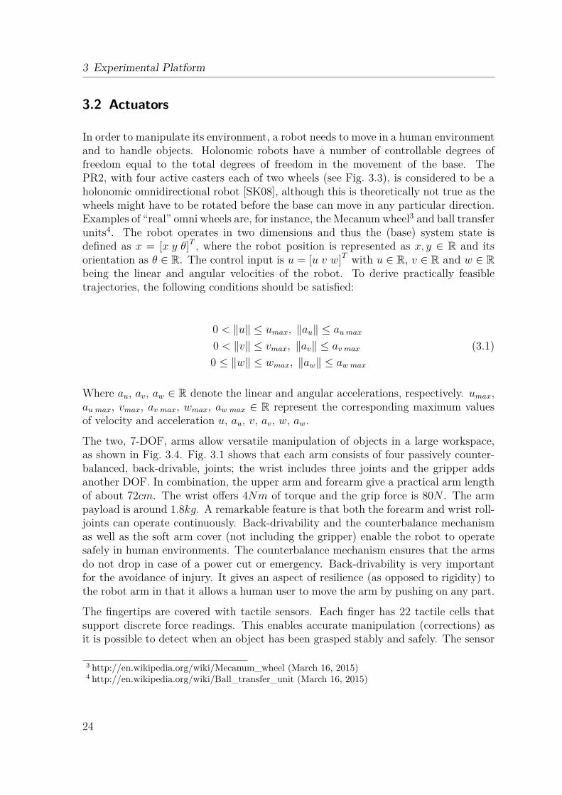
The two, 7-DOF, arms allow versatile manipulation of objects in a large workspace,as shown in Fig. 3.4. Fig. 3.1 shows that each arm consists of four passively counter-balanced, back-drivable, joints; the wrist includes three joints and the gripper addsanother DOF. In combination, the upper arm and forearm give a practical arm lengthof about 72cm. The wrist offers 4Nm of torque and the grip force is 80N . The armpayload is around 1.8kg. A remarkable feature is that both the forearm and wrist roll-joints can operate continuously. Back-drivability and the counterbalance mechanismas well as the soft arm cover (not including the gripper) enable the robot to operatesafely in human environments. The counterbalance mechanism ensures that the armsdo not drop in case of a power cut or emergency. Back-drivability is very importantfor the avoidance of injury. It gives an aspect of resilience (as opposed to rigidity) tothe robot arm in that it allows a human user to move the arm by pushing on any part.

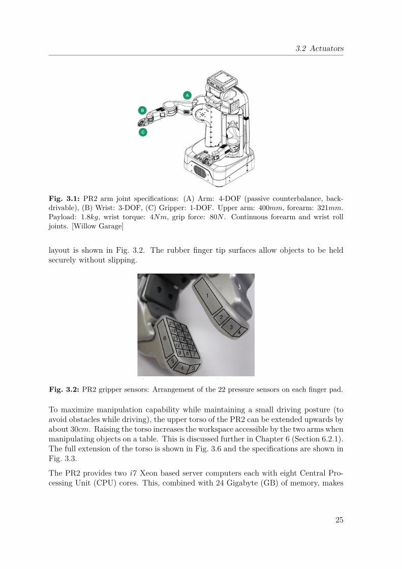
The fingertips are covered with tactile sensors. Each finger has 22 tactile cells thatsupport discrete force readings. This enables accurate manipulation (corrections) asit is possible to detect when an object has been grasped stably and safely. The sensor

3 http://en.wikipedia.org/wiki/Mecanum_wheel (March 16, 2015)4 http://en.wikipedia.org/wiki/Ball_transfer_unit (March 16, 2015)

24

3.2 Actuators

Fig. 3.1: PR2 arm joint specifications: (A) Arm: 4-DOF (passive counterbalance, back-drivable), (B) Wrist: 3-DOF, (C) Gripper: 1-DOF. Upper arm: 400mm, forearm: 321mm.Payload: 1.8kg, wrist torque: 4Nm, grip force: 80N . Continuous forearm and wrist rolljoints. [Willow Garage]

layout is shown in Fig. 3.2. The rubber finger tip surfaces allow objects to be heldsecurely without slipping.

Fig. 3.2: PR2 gripper sensors: Arrangement of the 22 pressure sensors on each finger pad.

To maximize manipulation capability while maintaining a small driving posture (toavoid obstacles while driving), the upper torso of the PR2 can be extended upwards byabout 30cm. Raising the torso increases the workspace accessible by the two arms whenmanipulating objects on a table. This is discussed further in Chapter 6 (Section 6.2.1).The full extension of the torso is shown in Fig. 3.6 and the specifications are shown inFig. 3.3.

The PR2 provides two i7 Xeon based server computers each with eight Central Pro-cessing Unit (CPU) cores. This, combined with 24 Gigabyte (GB) of memory, makes

25

3 Experimental Platform

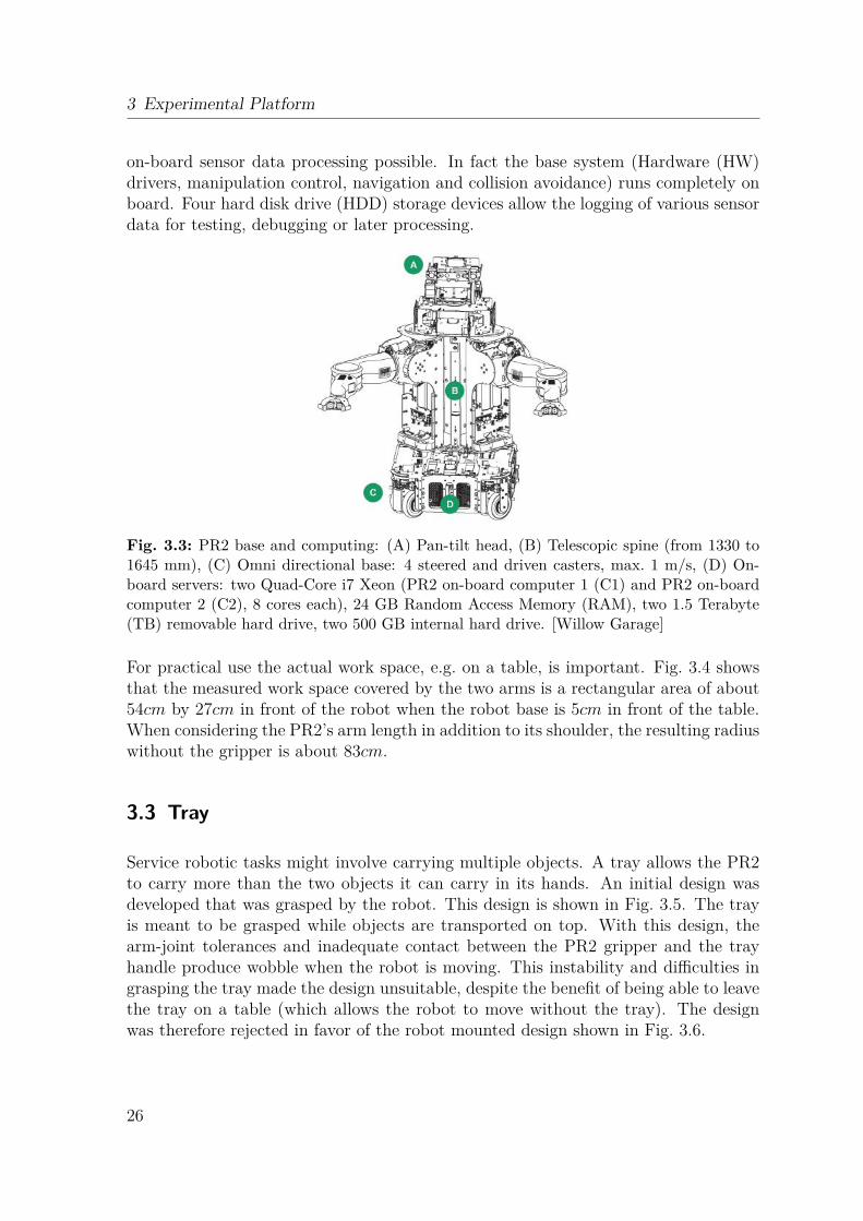
on-board sensor data processing possible. In fact the base system (Hardware (HW)drivers, manipulation control, navigation and collision avoidance) runs completely onboard. Four hard disk drive (HDD) storage devices allow the logging of various sensordata for testing, debugging or later processing.

Fig. 3.3: PR2 base and computing: (A) Pan-tilt head, (B) Telescopic spine (from 1330 to1645 mm), (C) Omni directional base: 4 steered and driven casters, max. 1 m/s, (D) On-board servers: two Quad-Core i7 Xeon (PR2 on-board computer 1 (C1) and PR2 on-boardcomputer 2 (C2), 8 cores each), 24 GB Random Access Memory (RAM), two 1.5 Terabyte(TB) removable hard drive, two 500 GB internal hard drive. [Willow Garage]

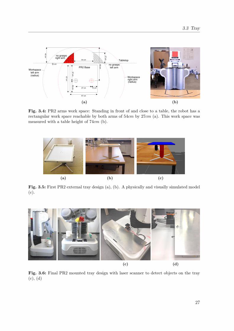
For practical use the actual work space, e.g. on a table, is important. Fig. 3.4 showsthat the measured work space covered by the two arms is a rectangular area of about54cm by 27cm in front of the robot when the robot base is 5cm in front of the table.When considering the PR2’s arm length in addition to its shoulder, the resulting radiuswithout the gripper is about 83cm.

3.3 Tray

Service robotic tasks might involve carrying multiple objects. A tray allows the PR2to carry more than the two objects it can carry in its hands. An initial design wasdeveloped that was grasped by the robot. This design is shown in Fig. 3.5. The trayis meant to be grasped while objects are transported on top. With this design, thearm-joint tolerances and inadequate contact between the PR2 gripper and the trayhandle produce wobble when the robot is moving. This instability and difficulties ingrasping the tray made the design unsuitable, despite the benefit of being able to leavethe tray on a table (which allows the robot to move without the tray). The designwas therefore rejected in favor of the robot mounted design shown in Fig. 3.6.

26

3.3 Tray

�����������������������������������������������������������������������������

�����������������������������������������������������������������������������

������������������������������������������������������������������

������������������������������������������������������������������

67 c

m

67 cm

5 cm

30 c

m37 c

m

15 cm

42 c

m

83 c

m

37 cm

54 cm

27 c

m

Tabletop

PR2 Base

right armno grasps

no graspsleft arm

Workspaceleft arm(radius)

(radius)right armWorkspace

(a) (b)

Fig. 3.4: PR2 arms work space: Standing in front of and close to a table, the robot has arectangular work space reachable by both arms of 54cm by 27cm (a). This work space wasmeasured with a table height of 74cm (b).

(a) (b) (c)

Fig. 3.5: First PR2 external tray design (a), (b). A physically and visually simulated model(c).

(c) (d)

Fig. 3.6: Final PR2 mounted tray design with laser scanner to detect objects on the tray(c), (d)

27

3 Experimental Platform

Even though the tray is not removable it should not limit the robots work space ornormal operation. A flat design at the robot’s base was a reasonable solution. Thisdesign does not extend the robot’s footprint and thus does not increase the likelihoodof collision with its environment.

3.4 Sensors

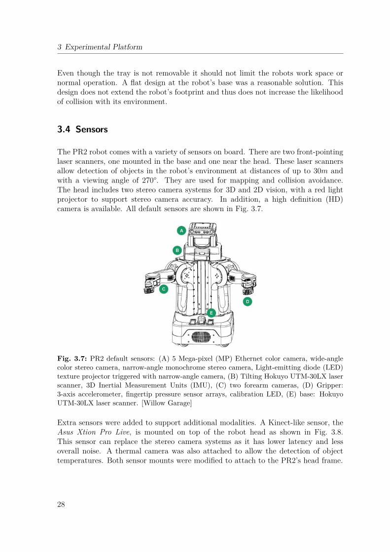
The PR2 robot comes with a variety of sensors on board. There are two front-pointinglaser scanners, one mounted in the base and one near the head. These laser scannersallow detection of objects in the robot’s environment at distances of up to 30m andwith a viewing angle of 270°. They are used for mapping and collision avoidance.The head includes two stereo camera systems for 3D and 2D vision, with a red lightprojector to support stereo camera accuracy. In addition, a high definition (HD)camera is available. All default sensors are shown in Fig. 3.7.

Fig. 3.7: PR2 default sensors: (A) 5 Mega-pixel (MP) Ethernet color camera, wide-anglecolor stereo camera, narrow-angle monochrome stereo camera, Light-emitting diode (LED)texture projector triggered with narrow-angle camera, (B) Tilting Hokuyo UTM-30LX laserscanner, 3D Inertial Measurement Units (IMU), (C) two forearm cameras, (D) Gripper:3-axis accelerometer, fingertip pressure sensor arrays, calibration LED, (E) base: HokuyoUTM-30LX laser scanner. [Willow Garage]

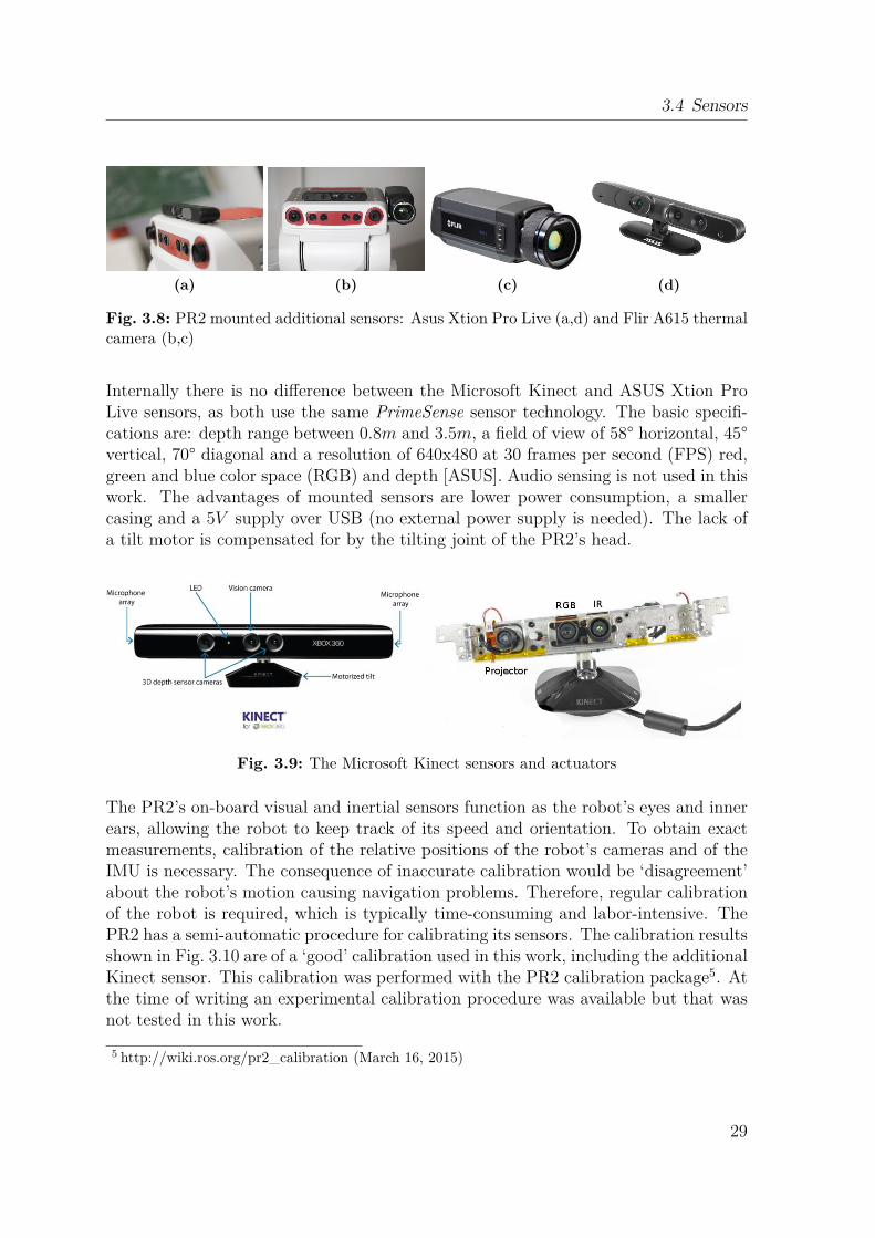
Extra sensors were added to support additional modalities. A Kinect-like sensor, theAsus Xtion Pro Live, is mounted on top of the robot head as shown in Fig. 3.8.This sensor can replace the stereo camera systems as it has lower latency and lessoverall noise. A thermal camera was also attached to allow the detection of objecttemperatures. Both sensor mounts were modified to attach to the PR2’s head frame.

28

3.4 Sensors

(a) (b) (c) (d)

Fig. 3.8: PR2 mounted additional sensors: Asus Xtion Pro Live (a,d) and Flir A615 thermalcamera (b,c)

Internally there is no difference between the Microsoft Kinect and ASUS Xtion ProLive sensors, as both use the same PrimeSense sensor technology. The basic specifi-cations are: depth range between 0.8m and 3.5m, a field of view of 58° horizontal, 45°vertical, 70° diagonal and a resolution of 640x480 at 30 frames per second (FPS) red,green and blue color space (RGB) and depth [ASUS]. Audio sensing is not used in thiswork. The advantages of mounted sensors are lower power consumption, a smallercasing and a 5V supply over USB (no external power supply is needed). The lack ofa tilt motor is compensated for by the tilting joint of the PR2’s head.

Fig. 3.9: The Microsoft Kinect sensors and actuators

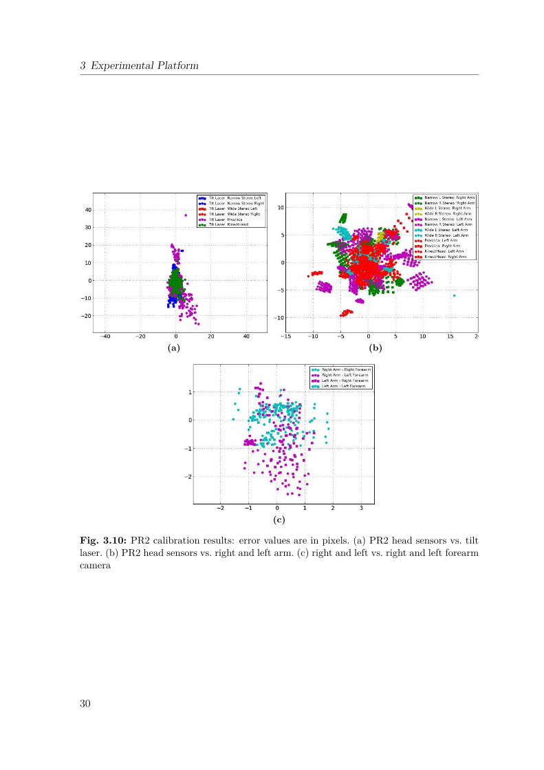
The PR2’s on-board visual and inertial sensors function as the robot’s eyes and innerears, allowing the robot to keep track of its speed and orientation. To obtain exactmeasurements, calibration of the relative positions of the robot’s cameras and of theIMU is necessary. The consequence of inaccurate calibration would be ‘disagreement’about the robot’s motion causing navigation problems. Therefore, regular calibrationof the robot is required, which is typically time-consuming and labor-intensive. ThePR2 has a semi-automatic procedure for calibrating its sensors. The calibration resultsshown in Fig. 3.10 are of a ‘good’ calibration used in this work, including the additionalKinect sensor. This calibration was performed with the PR2 calibration package5. Atthe time of writing an experimental calibration procedure was available but that wasnot tested in this work.

5 http://wiki.ros.org/pr2_calibration (March 16, 2015)

29

3 Experimental Platform

(a) (b)

(c)

Fig. 3.10: PR2 calibration results: error values are in pixels. (a) PR2 head sensors vs. tiltlaser. (b) PR2 head sensors vs. right and left arm. (c) right and left vs. right and left forearmcamera

30

3.5 Power and Control

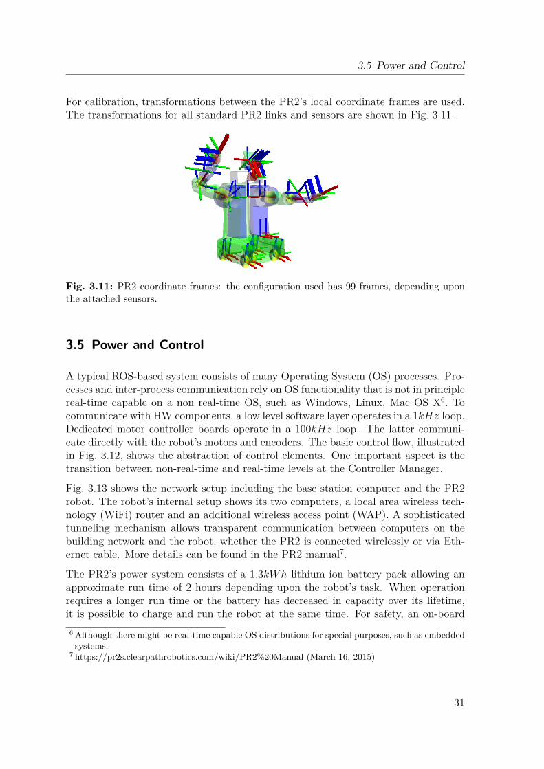
For calibration, transformations between the PR2’s local coordinate frames are used.The transformations for all standard PR2 links and sensors are shown in Fig. 3.11.

Fig. 3.11: PR2 coordinate frames: the configuration used has 99 frames, depending uponthe attached sensors.

3.5 Power and Control

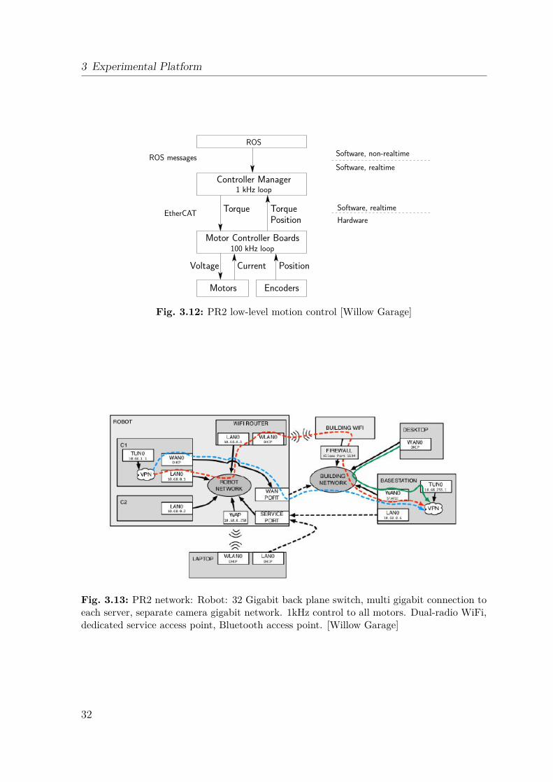
A typical ROS-based system consists of many Operating System (OS) processes. Pro-cesses and inter-process communication rely on OS functionality that is not in principlereal-time capable on a non real-time OS, such as Windows, Linux, Mac OS X6. Tocommunicate with HW components, a low level software layer operates in a 1kHz loop.Dedicated motor controller boards operate in a 100kHz loop. The latter communi-cate directly with the robot’s motors and encoders. The basic control flow, illustratedin Fig. 3.12, shows the abstraction of control elements. One important aspect is thetransition between non-real-time and real-time levels at the Controller Manager.

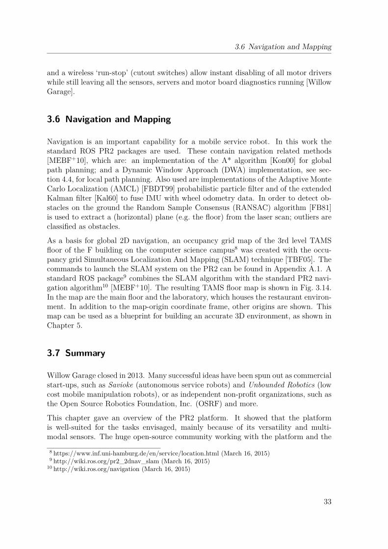
Fig. 3.13 shows the network setup including the base station computer and the PR2robot. The robot’s internal setup shows its two computers, a local area wireless tech-nology (WiFi) router and an additional wireless access point (WAP). A sophisticatedtunneling mechanism allows transparent communication between computers on thebuilding network and the robot, whether the PR2 is connected wirelessly or via Eth-ernet cable. More details can be found in the PR2 manual7.

The PR2’s power system consists of a 1.3kWh lithium ion battery pack allowing anapproximate run time of 2 hours depending upon the robot’s task. When operationrequires a longer run time or the battery has decreased in capacity over its lifetime,it is possible to charge and run the robot at the same time. For safety, an on-board

6 Although there might be real-time capable OS distributions for special purposes, such as embeddedsystems.

7 https://pr2s.clearpathrobotics.com/wiki/PR2%20Manual (March 16, 2015)

31

3 Experimental Platform

Software, realtime

Hardware

Software, non-realtime

Software, realtime

PositionTorqueTorque

100 kHz loop

Controller Manager

Motor Controller Boards

ROS

1 kHz loop

ROS messages

EtherCAT

CurrentVoltage Position

Motors Encoders

Fig. 3.12: PR2 low-level motion control [Willow Garage]

Fig. 3.13: PR2 network: Robot: 32 Gigabit back plane switch, multi gigabit connection toeach server, separate camera gigabit network. 1kHz control to all motors. Dual-radio WiFi,dedicated service access point, Bluetooth access point. [Willow Garage]

32

3.6 Navigation and Mapping

and a wireless ‘run-stop’ (cutout switches) allow instant disabling of all motor driverswhile still leaving all the sensors, servers and motor board diagnostics running [WillowGarage].

3.6 Navigation and Mapping

Navigation is an important capability for a mobile service robot. In this work thestandard ROS PR2 packages are used. These contain navigation related methods[MEBF+10], which are: an implementation of the A* algorithm [Kon00] for globalpath planning; and a Dynamic Window Approach (DWA) implementation, see sec-tion 4.4, for local path planning. Also used are implementations of the Adaptive MonteCarlo Localization (AMCL) [FBDT99] probabilistic particle filter and of the extendedKalman filter [Kal60] to fuse IMU with wheel odometry data. In order to detect ob-stacles on the ground the Random Sample Consensus (RANSAC) algorithm [FB81]is used to extract a (horizontal) plane (e.g. the floor) from the laser scan; outliers areclassified as obstacles.

As a basis for global 2D navigation, an occupancy grid map of the 3rd level TAMSfloor of the F building on the computer science campus8 was created with the occu-pancy grid Simultaneous Localization And Mapping (SLAM) technique [TBF05]. Thecommands to launch the SLAM system on the PR2 can be found in Appendix A.1. Astandard ROS package9 combines the SLAM algorithm with the standard PR2 navi-gation algorithm10 [MEBF+10]. The resulting TAMS floor map is shown in Fig. 3.14.In the map are the main floor and the laboratory, which houses the restaurant environ-ment. In addition to the map-origin coordinate frame, other origins are shown. Thismap can be used as a blueprint for building an accurate 3D environment, as shown inChapter 5.

3.7 Summary

Willow Garage closed in 2013. Many successful ideas have been spun out as commercialstart-ups, such as Savioke (autonomous service robots) and Unbounded Robotics (lowcost mobile manipulation robots), or as independent non-profit organizations, such asthe Open Source Robotics Foundation, Inc. (OSRF) and more.

This chapter gave an overview of the PR2 platform. It showed that the platformis well-suited for the tasks envisaged, mainly because of its versatility and multi-modal sensors. The huge open-source community working with the platform and the

8 https://www.inf.uni-hamburg.de/en/service/location.html (March 16, 2015)9 http://wiki.ros.org/pr2_2dnav_slam (March 16, 2015)

10 http://wiki.ros.org/navigation (March 16, 2015)

33

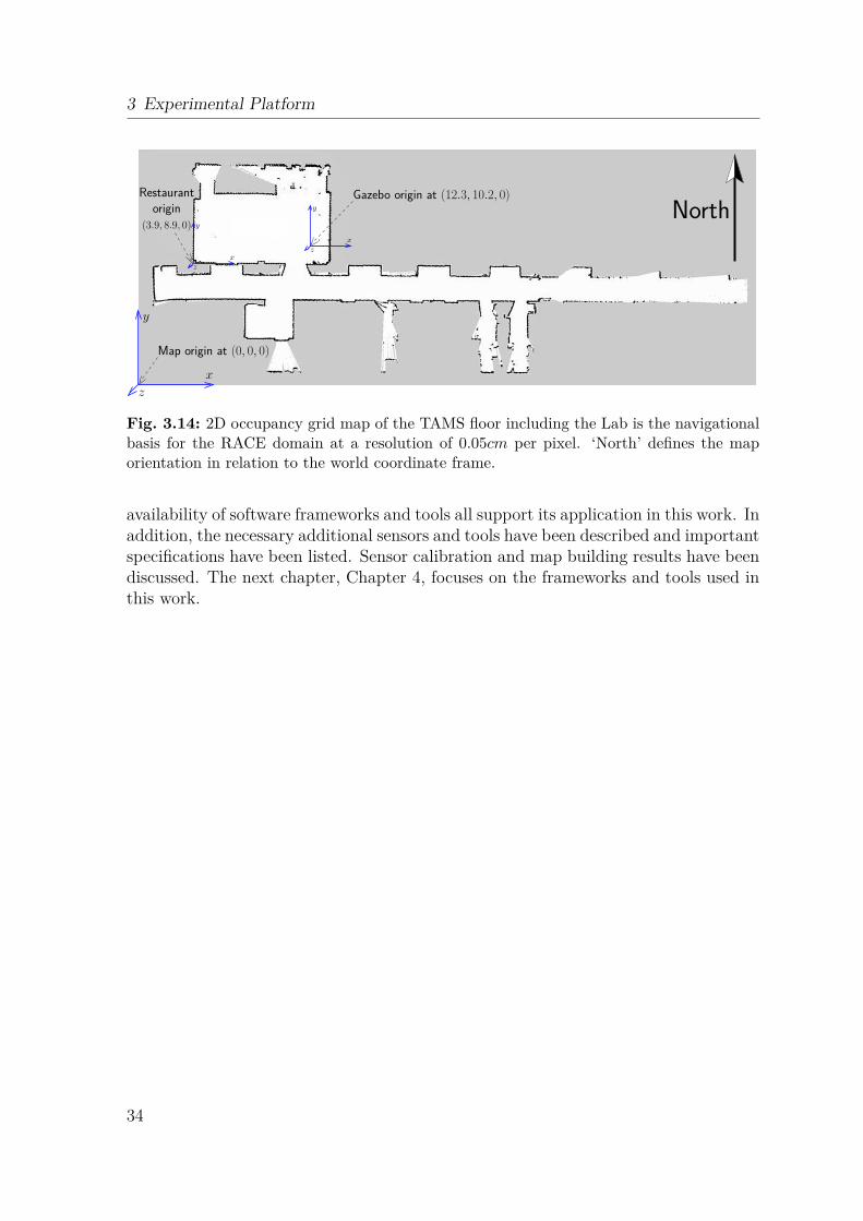
3 Experimental Platform

Map origin at (0, 0, 0)

Restaurantorigin

(3.9, 8.9, 0)

Gazebo origin at (12.3, 10.2, 0)

y

x

z

y

xz

y

xz

North

Fig. 3.14: 2D occupancy grid map of the TAMS floor including the Lab is the navigationalbasis for the RACE domain at a resolution of 0.05cm per pixel. ‘North’ defines the maporientation in relation to the world coordinate frame.

availability of software frameworks and tools all support its application in this work. Inaddition, the necessary additional sensors and tools have been described and importantspecifications have been listed. Sensor calibration and map building results have beendiscussed. The next chapter, Chapter 4, focuses on the frameworks and tools used inthis work.

34

Frameworks and Tools

4

This chapter introduces the software frameworks employed and developed in the courseof this work. The RACE project is introduced first, as it not only provides a devel-opment framework but it also serves as the foundation of the scenarios and ideas ofthis work. Related parts of ROS, such as the underlying development framework,will be discussed. An important tool is the Gazebo simulator and its physics-basedengine, ODE. These will be discussed, along with two frameworks developed to createtoppling experiences, to generate unsupervised experiences in changing environmentsand to create and record training data.

4.1 The RACE Project

In previous work, an ontology-based robot control architecture was developed to allowrobots to learn from experience [RNZ+13]. To focus the research on high-level tasks,such as learning from experience employed in the RACE project1, it is necessaryto be able to take the robustness and functionality of lower level components forgranted. The platform provides basic capabilities, such as navigation, manipulationand grasping.

The three year EU funded FP7 project RACE started in December, 2011 and ended inNovember, 2014. Most of the work of this thesis was developed in the context of thisproject. The overall aim of the project was to enhance the behavior of an autonomousmobile service robot by having the robot learn from conceptualized experiences ofprevious performances, based on initial models of the domain and on its own actions.The contributions of the project to the state of the art can be summarized as producinga robot:

• that is capable of storing experiences in a multi-level way using appropriatestructures,

• that is able to learn and generalize,

• that demonstrates enhanced competence by applying learned knowledge.

1 http://www.project-race.eu (March 16, 2015)

35

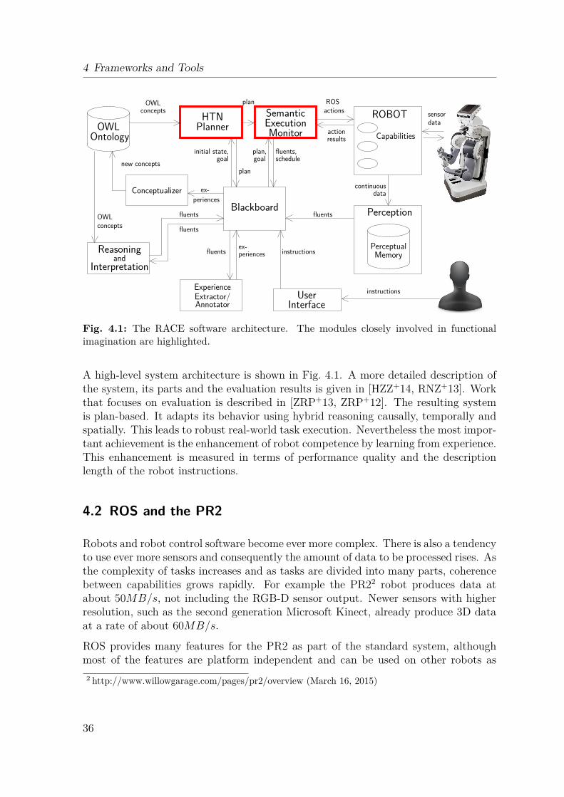
4 Frameworks and Tools

SemanticExecution

new concepts

fluents

plan

ex-

data

fluentsfluents

periences

sensoractionsROSplan

fluents

plan,goal

actionresults

OWLconcepts

Capabilities

and

ExperienceExtractor/Annotator

instructions

Memory

ROBOTOWL

Ontology

Conceptualizer

Perception

UserInterface

HTNPlanner

Blackboard

Perceptualperiencesex-

instructions

datacontinuous

concepts

initial state,goal schedule

fluents,

OWL

Reasoning

Interpretation

Monitor

Fig. 4.1: The RACE software architecture. The modules closely involved in functionalimagination are highlighted.

A high-level system architecture is shown in Fig. 4.1. A more detailed description ofthe system, its parts and the evaluation results is given in [HZZ+14, RNZ+13]. Workthat focuses on evaluation is described in [ZRP+13, ZRP+12]. The resulting systemis plan-based. It adapts its behavior using hybrid reasoning causally, temporally andspatially. This leads to robust real-world task execution. Nevertheless the most impor-tant achievement is the enhancement of robot competence by learning from experience.This enhancement is measured in terms of performance quality and the descriptionlength of the robot instructions.

4.2 ROS and the PR2

Robots and robot control software become ever more complex. There is also a tendencyto use ever more sensors and consequently the amount of data to be processed rises. Asthe complexity of tasks increases and as tasks are divided into many parts, coherencebetween capabilities grows rapidly. For example the PR22 robot produces data atabout 50MB/s, not including the RGB-D sensor output. Newer sensors with higherresolution, such as the second generation Microsoft Kinect, already produce 3D dataat a rate of about 60MB/s.

ROS provides many features for the PR2 as part of the standard system, althoughmost of the features are platform independent and can be used on other robots as

2 http://www.willowgarage.com/pages/pr2/overview (March 16, 2015)

36

4.3 Gazebo Simulator

well. Furthermore, tools providing additional functionality, e.g. image processing, of-ten have a ROS API and cooperate well with ROS. Examples are the Open sourceComputer Vision library (OpenCV)3 and the Point Cloud Library (PCL)4. Both soft-ware frameworks provide advanced perception filtering capabilities, such as 2D and 3Dimage processing. The standard ROS tools include applications for navigation, ma-nipulation, visualization, logging and playback, simulation and hardware diagnostics.A running ROS instance typically maintains many ‘nodes’ - processes in a graph-liketopology communicating with each other using streaming topics, Remote ProcedureCall (RPC) services and a parameter server. The node hierarchy is flat, consisting ofa master node and all other nodes. The master node is responsible for all communica-tion requests between nodes. It also acts as a network time server and both this andlimitations of the parameter server lead to difficulties in distributed systems. Theseare discussed in Section 5.3, together with possible solutions.

In the development phase, Willow Garage (originators of the PR2) used softwarecomponents from the Player Project5 to develop the application programming stackfor the PR2 robot. Its three components, Player, Stage and Gazebo, have all beenadapted for use within ROS. Thus important parts, such as drivers, algorithms andsimulation environments could be reused. The Player Project [GVH03] grew fromthe need for alternatives to existing closed source software and was developed in 2000initially by Brian Gerkey, Richard Vaughan and Kasper Stoy. It was hosted at theUniversity of Southern California (USC) Robotics Lab website before it migrated toSourceForge.

4.3 Gazebo Simulator

The Gazebo6 simulation is used in this work. The version used (1.0), which was re-leased early in the project (2012) and retained, brought major updates compared to theprevious version (0.1), such as the completely re-implemented Graphical User Inter-face (GUI) with “Cute” cross-platform programming library (QT4) and performanceimprovements, as well as an adapted Extensible Markup Language (XML) world filesyntax.

The simulator features7 related to this work are:

• the ability to simulate indoor environments with multiple robots in real-time

– multiple rooms (at least three), multiple objects, one PR2

3 http://wiki.ros.org/vision_opencv (March 18, 2015)4 http://www.pointclouds.org (March 18, 2015)5 http://playerstage.sourceforge.net (March 18, 2015)6 http://gazebosim.org (March 18, 2015)7 http://wiki.ros.org/gazebo/Version_1.0_Design_Specification (March 18, 2015)

37

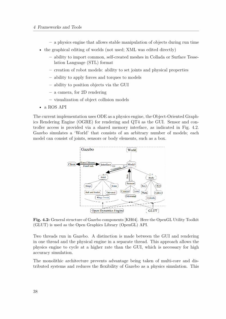
4 Frameworks and Tools

– a physics engine that allows stable manipulation of objects during run time

• the graphical editing of worlds (not used; XML was edited directly)

– ability to import common, self-created meshes in Collada or Surface Tesse-lation Language (STL) format

– creation of robot models: ability to set joints and physical properties

– ability to apply forces and torques to models

– ability to position objects via the GUI

– a camera, for 2D rendering

– visualization of object collision models

• a ROS API

The current implementation uses ODE as a physics engine, the Object-Oriented Graph-ics Rendering Engine (OGRE) for rendering and QT4 as the GUI. Sensor and con-troller access is provided via a shared memory interface, as indicated in Fig. 4.2.Gazebo simulates a ‘World’ that consists of an arbitrary number of models; eachmodel can consist of joints, sensors or body elements, such as a box.

Fig. 4.2: General structure of Gazebo components [KH04]. Here the OpenGL Utility Toolkit(GLUT) is used as the Open Graphics Library (OpenGL) API.

Two threads run in Gazebo. A distinction is made between the GUI and renderingin one thread and the physical engine in a separate thread. This approach allows thephysics engine to cycle at a higher rate than the GUI, which is necessary for highaccuracy simulation.

The monolithic architecture prevents advantage being taken of multi-core and dis-tributed systems and reduces the flexibility of Gazebo as a physics simulation. This

38

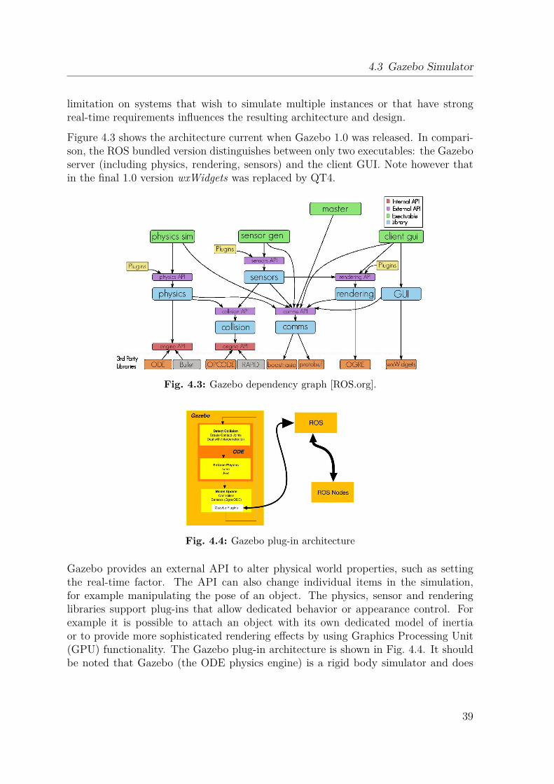
4.3 Gazebo Simulator

limitation on systems that wish to simulate multiple instances or that have strongreal-time requirements influences the resulting architecture and design.

Figure 4.3 shows the architecture current when Gazebo 1.0 was released. In compari-son, the ROS bundled version distinguishes between only two executables: the Gazeboserver (including physics, rendering, sensors) and the client GUI. Note however thatin the final 1.0 version wxWidgets was replaced by QT4.

Fig. 4.3: Gazebo dependency graph [ROS.org].

Fig. 4.4: Gazebo plug-in architecture

Gazebo provides an external API to alter physical world properties, such as settingthe real-time factor. The API can also change individual items in the simulation,for example manipulating the pose of an object. The physics, sensor and renderinglibraries support plug-ins that allow dedicated behavior or appearance control. Forexample it is possible to attach an object with its own dedicated model of inertiaor to provide more sophisticated rendering effects by using Graphics Processing Unit(GPU) functionality. The Gazebo plug-in architecture is shown in Fig. 4.4. It shouldbe noted that Gazebo (the ODE physics engine) is a rigid body simulator and does

39

4 Frameworks and Tools

not simulate soft objects - clothes or liquids, such as water. This limitation can bepartially offset by using particles (e.g. small spheres) to approximate the behavior ofliquids. This approach was applied, for example, in [KDB11].

4.3.1 Physical Simulation

Euler’s method [BW97] is often used as an integrator, such as in ODE:

x(t0 + h) = x0 + hx(t0) (4.1)

ODE supports static and kinetic friction as well as restitution, whereas Bullet does notprovide kinetic friction. The Bullet physics engine instead supports partial graphicsprocessing on the GPU for physics calculation. ODE is a constraint-based physicsengine with fixed time-stepping. The evaluation compares accurate ODE integratorcalculations for the costs of performance to those for Bullet. Tests include the dis-placement of a non-moving object compared to classical physics, which is:

r =1

2at2 (4.2)

where r is the body’s displacement, a is the body’s acceleration and t is the time.

Restitution is given in classical physics by:

CR =

√

h

H(4.3)

where CR is the coefficient of restitution, h is the bounce height and H is the dropheight. Friction is typically calculated according to the Coulomb friction model [KEP05].

The accuracy and performance of the physics engine when calculating friction, col-lisions and constraints are important for predicting robot action results in a typicaldomestic domain. ODE and Bullet differ slightly in these disciplines, but both providethe required capabilities. Nevertheless, no currently available engine offers superiorperformance in all situations. Thus the prediction model has to take variations andminor deviations from true behavior into account. Not all tested engines support noisemodels.

[WHR10] evaluates the Bullet engine as an ingredient of physical reasoning. It investi-gates the prediction accuracy of a physics engine when simulating a robot arm pushingflat objects across a table. The authors recommend reasoning about goals and actionsusing physics simulations. Successful reasoning is considered to imply the need for a

40

4.4 Robot Capabilities

strong understanding of dynamics and the effects of actions. Physics engines can com-plement classical rule-based reasoning systems by acting as a source of information oras an ‘oracle’. This can help answer questions concerning the stability of manipulatedobjects, such as whether they might tip over or start to roll, or how to shift severalobjects without changing their configuration. The authors propose that simulationaccuracy is a problem of selecting parameters for an optimal match to reality. Theparameters most important for optimization by a cost function are the object’s shapefactor and friction between the object and the ground and fingers.

E(P, P′

) =1

n

n∑

j=1

∥

∥

∥cj − c′

j

∥

∥

∥ (4.4)

Here the error E of the real and simulated poses, P and P′

respectively, is the sumof the deviations of all object corner points cj in contact with the ground. The au-thors propose using a combination of the simplex algorithm [NM65] and differentialevolution [SP97] to search for optimal parameter values.

The authors conclude that accurate prediction of real world interactions is possiblewith state-of-the-art physics engines. However their focus is on flat objects that arepushed across tables. Furthermore the accuracy of the particular engine used has beenoptimized to reduce errors by 50 percent when compared to default values. They pro-pose employing the simulation for learning processes and combining it with qualitativeand quantitative simulation.

4.4 Robot Capabilities

The perception capabilities of the PR2 are based on the Object Recognition Kitchen(ORK) framework, which uses the ROS tabletop module8. The procedure is describedin [ML09]. Firstly, a (table) plane is extracted from the point cloud by the RANSACalgorithm [FB81]. Remaining points are clustered and each cluster is processed us-ing the Iterative Distance Fitter (IDF) technique for rotationally symmetric objects.This compares the cluster with Computer-Aided Design (CAD) models stored in aCouchDB database and results in a confidence value for each possible object type. Forobject recognition, the recognizable objects have to be rotationally symmetrical. Inthe case of recognized objects, grasping relies on learned gripper configurations (mul-tiple configurations per object can be stored in the database) in relation to the object.In the case of new objects, grasping relies on bounding boxes calculated around theobject’s segmented point cloud. For a recognizable object, the bias is that the objecthas the same upright orientation stored in the database.

8 http://wiki.ros.org/tabletop_object_detector (September 8, 2015)

41

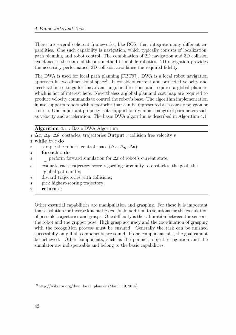
4 Frameworks and Tools

There are several coherent frameworks, like ROS, that integrate many different ca-pabilities. One such capability is navigation, which typically consists of localization,path planning and robot control. The combination of 2D navigation and 3D collisionavoidance is the state-of-the-art method in mobile robotics. 2D navigation providesthe necessary performance; 3D collision avoidance the required fidelity.

The DWA is used for local path planning [FBT97]. DWA is a local robot navigationapproach in two dimensional space9. It considers current and projected velocity andacceleration settings for linear and angular directions and requires a global planner,which is not of interest here. Nevertheless a global plan and cost map are required toproduce velocity commands to control the robot’s base. The algorithm implementationin use supports robots with a footprint that can be represented as a convex polygon ora circle. One important property is its support for dynamic changes of parameters suchas velocity and acceleration. The basic DWA algorithm is described in Algorithm 4.1.

Algorithm 4.1 : Basic DWA Algorithm1 ∆x, ∆y, ∆θ, obstacles, trajectories Output : collision free velocity v2 while true do

3 sample the robot’s control space (∆x, ∆y, ∆θ);4 foreach v do

5 perform forward simulation for ∆t of robot’s current state;

6 evaluate each trajectory score regarding proximity to obstacles, the goal, theglobal path and v;

7 discard trajectories with collisions;8 pick highest-scoring trajectory;9 return v;

Other essential capabilities are manipulation and grasping. For these it is importantthat a solution for inverse kinematics exists, in addition to solutions for the calculationof possible trajectories and grasps. One difficulty is the calibration between the sensors,the robot and the gripper pose. High grasp accuracy and the coordination of graspingwith the recognition process must be ensured. Generally the task can be finishedsuccessfully only if all components are sound. If one component fails, the goal cannotbe achieved. Other components, such as the planner, object recognition and thesimulator are indispensable and belong to the basic capabilities.

9 http://wiki.ros.org/dwa_local_planner (March 19, 2015)

42

4.5 Summary

4.5 Summary

This chapter gave an overview of the software frameworks and tools used in this work.The RACE project - the foundation of this work - was introduced, and its high-levelarchitecture was presented. ROS, the underlying open-source development framework,was described, and PR2-related components were discussed. The Gazebo simulator,which is the basis of the functional imagination approach in this work, was introduced,and robot capabilities necessary for the experimental scenarios were presented. In thenext chapter, Chapter 5, a detailed look will be taken at the approach taken by thiswork.

43

Functional Imagination

5

This chapter describes the methods and algorithms of the proposed system. It alsodescribes the robot capabilities developed for the experiments. Experimental methodsand scenarios are developed and the scenario setup is discussed in detail. The modelsrequired to represent the problem domain are developed and a detailed architecture iscrafted.

The chapter also gives an overview of the physical realization of the approach interms of software and hardware. It describes in detail how frameworks and toolsare employed, combined and optimized. The goal of this chapter is to develop andintegrate a simulation system that provides a basis upon which robot action resultscan be predicted and exploited for plan adaptation in order to prevent sub-optimalactivity (cf. Section 1.4).

5.1 Methodology

A pragmatic approach to the use of physics-based simulation for predicting robotaction results is to simulate an action and then to evaluate the resulting simulationstate. The three important parts of the process are:

1. intention

2. simulated execution

3. simulated result

In this work, the intention is the action the robot is supposed to execute, i.e. the plan(step) created by the symbolic planner; the simulated execution is the manipulationof the world state, i.e. execution in Gazebo; the simulated result is the world state inthe simulation after the execution has finished.

45

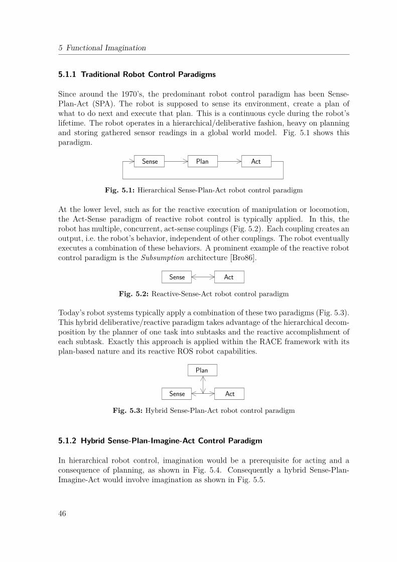
5 Functional Imagination

5.1.1 Traditional Robot Control Paradigms

Since around the 1970’s, the predominant robot control paradigm has been Sense-Plan-Act (SPA). The robot is supposed to sense its environment, create a plan ofwhat to do next and execute that plan. This is a continuous cycle during the robot’slifetime. The robot operates in a hierarchical/deliberative fashion, heavy on planningand storing gathered sensor readings in a global world model. Fig. 5.1 shows thisparadigm.

ActSense Plan

Fig. 5.1: Hierarchical Sense-Plan-Act robot control paradigm

At the lower level, such as for the reactive execution of manipulation or locomotion,the Act-Sense paradigm of reactive robot control is typically applied. In this, therobot has multiple, concurrent, act-sense couplings (Fig. 5.2). Each coupling creates anoutput, i.e. the robot’s behavior, independent of other couplings. The robot eventuallyexecutes a combination of these behaviors. A prominent example of the reactive robotcontrol paradigm is the Subsumption architecture [Bro86].

Sense Act

Fig. 5.2: Reactive-Sense-Act robot control paradigm

Today’s robot systems typically apply a combination of these two paradigms (Fig. 5.3).This hybrid deliberative/reactive paradigm takes advantage of the hierarchical decom-position by the planner of one task into subtasks and the reactive accomplishment ofeach subtask. Exactly this approach is applied within the RACE framework with itsplan-based nature and its reactive ROS robot capabilities.

ActSense

Plan

Fig. 5.3: Hybrid Sense-Plan-Act robot control paradigm

5.1.2 Hybrid Sense-Plan-Imagine-Act Control Paradigm

In hierarchical robot control, imagination would be a prerequisite for acting and aconsequence of planning, as shown in Fig. 5.4. Consequently a hybrid Sense-Plan-Imagine-Act would involve imagination as shown in Fig. 5.5.

46

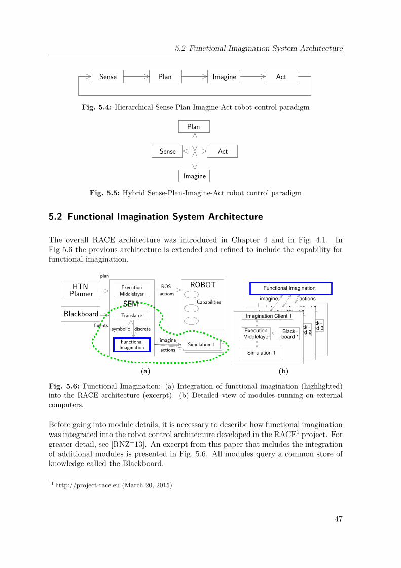
5.2 Functional Imagination System Architecture

ImagineSense Plan Act

Fig. 5.4: Hierarchical Sense-Plan-Imagine-Act robot control paradigm

Imagine

Sense

Plan

Act

Fig. 5.5: Hybrid Sense-Plan-Imagine-Act robot control paradigm

5.2 Functional Imagination System Architecture

The overall RACE architecture was introduced in Chapter 4 and in Fig. 4.1. InFig 5.6 the previous architecture is extended and refined to include the capability forfunctional imagination.

MiddlelayerExecution

fluents

actions

imagine

discretesymbolic

Translator

ImaginationFunctional

plan

ROBOT

Blackboard

PlannerHTN

Capabilities

actions

ROS

SEM

Simulation 1

(a)

Functional Imagination

board 3

Simulation 3

Imagination Client 3

MiddlelayerExecution Black−

imagine actions

Imagination Client 2

Black−board 2

Simulation 2

ExecutionMiddlelayer

MiddlelayerExecution

board 1Black−

Imagination Client 1

Simulation 1

(b)

Fig. 5.6: Functional Imagination: (a) Integration of functional imagination (highlighted)into the RACE architecture (excerpt). (b) Detailed view of modules running on externalcomputers.

Before going into module details, it is necessary to describe how functional imaginationwas integrated into the robot control architecture developed in the RACE1 project. Forgreater detail, see [RNZ+13]. An excerpt from this paper that includes the integrationof additional modules is presented in Fig. 5.6. All modules query a common store ofknowledge called the Blackboard.

1 http://project-race.eu (March 20, 2015)

47

5 Functional Imagination

Without imagination, the nominal system workflow is as follows. On receiving anew task, the task planner generates a plan based on the current state retrievedfrom the Blackboard. This plan, which uses the basic capabilities of the PR2 robotto achieve the task, is sent to the Semantic Execution Monitor (SEM). The SEMmonitors the preconditions and effects of plan actions and dispatches new actions asappropriate. It maintains a temporal network that represents temporal expectationsabout execution [KSPS14], e.g. the earliest possible start or finish time of an action.This temporal network is updated based upon real world observations. Temporalobservations, such as trajectory durations, could also be obtained by simulation, i.e.from functional imagination.

Actions are dispatched by sending them to the Execution Middlelayer, which calls theappropriate ROS actions implementing basic robot capabilities.

To enable the use of functional imagination, this workflow needed several extensions.Some plan actions need to be simulated with a variety of different parameters beforethey are executed on the real robot. The plan therefore needs to indicate which actionsshould be simulated, at which step this should be done and which parameters shouldbe tested. To this end a dedicated imagine operator is introduced into the planningdomain.

Beside the planning domain, no changes to the planner itself are necessary; this workuses the off-the-shell HTN planner SHOP2 [NIK+03] integrated into the RACE system.Domain modeling of the planner is described in [SGH14]. The new operator !imagine

?action ?arg1 ?arg2 takes as arguments the action to be simulated and that action’sown arguments. Methods using the new operator have to be modified by adding a newaction (with arguments): !imagine !move_base_param ?area slow/fast. With theaction !move_base_param the robot is able to drive to a goal position with a specifiedmotion and acceleration set, such as slow or fast. The definitions for both sets usedin the experiments are listed in Table 5.1. The !imagine operator can simulate avariety of robot actions. Whereas the !imagine operator is specific to simulation,actions like !move_base_param apply both to the real robot and to the simulation.

The SEM has to analyze the plan and send each action to be tested to the ImaginationClient instead of to the Execution Middlelayer. Furthermore, it is important to notethat as the goal is to simulate the execution of an action at a later stage of the plan,the current states of the robot and its environment will be unsuitable. Therefore, theSEM needs to project the state at the later plan stage and send that to the ImaginationClient.

Furthermore, the Imagination Client needs to know the poses of all objects and ofthe robot together with the robot’s configuration, in order to initialize the simula-tion accordingly. This is done by the Translator module, which is given the projectedsymbolic world state and returns this state in a format that can be used as input tothe simulation. This information contains discrete values for the object poses, such

48

5.2 Functional Imagination System Architecture

as x, y, z coordinates instead of ‘table1’. The translation is based on initial knowledgeabout a sub-set of the world’s objects present in the Blackboard. The SEM generatesthe expected world state and calls the Translator in order to decouple the ImaginationClient from the symbolic representation used by the Execution Monitor. This decou-pling allows imagination to be integrated more easily into other systems by adjustingthe Translator module. Generation of the expected world state works as follows. Foreach action a given to an !imagine operator, a world state has to be generated. Thegenerator considers both the current Blackboard state and the sequence of actions ex-ecuted before a. With this information it is possible to conclude how the world statewill have changed by the time a is executed.

The Imagination Client will be provided with the altered world state, action to besimulated and possible parameters. At the same time all other operators, with theexception of !imagine operators, are executed as usual. Potential further !imagine

operators are handled the same way as the first. Upon successful execution the Imagi-nation Client returns an ordered list of action parametrizations along with the expected(simulated) duration of the parametrization with the highest confidence. The confi-dence calculation is described in Section 6.3. If the Imagination Client does not finishsimulating an action in time, the plan can wait for imagination to return. However,where there are hard real-time requirements, the action must be executed directly,without waiting, using default parameters defined in the planning domain.

For each parameter combination the Imagination Client starts a separate subset of theRACE system on a different machine, i.e. each with an independent ROS system, aspresented in Fig. 5.6.

The prediction system is based on the previously developed HIRES framework, de-scribed in [RKZZ14]. It has been integrated into the RACE framework and extendedto predict commonsense physics events and to handle uncertainty. A standard PR2platform equipped with a tray, which is used to deliver a pepper mill, is employed.

In the following paragraphs, model- and scenario-related definitions are introduced.α is the smallest angle between the perpendicular up-axis (z) of the global referenceframe and the principal axis of the tray object, as shown in Fig. 5.7. A topple-state st

is a value from a set of three possible topple-states, st : {notopple, topple, shaking}which are defined in Eq. 5.1. The thresholds are defined as follows: αn = 0.01 rad(≈ 0.5°), αt = 0.5 rad (≈ 29°). The threshold angles were defined empirically andare automatically and continuously measured during experiments. Furthermore anytoppling is automatically detected and the tray object is put back on its start positionto detect more potential topple events. For the experimental scenario a cylindricalobject (the pepper mill) of height 27.4cm and radius 3.7cm with a point mass of 140ghas been modelled to match the real object. The object inertia has been definedappropriately.

49

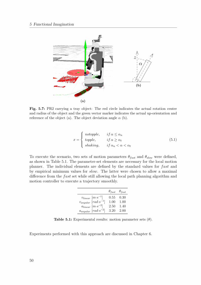
5 Functional Imagination

(a)

αz

(b)

Fig. 5.7: PR2 carrying a tray object: The red circle indicates the actual rotation centerand radius of the object and the green vector marker indicates the actual up-orientation andreference of the object (a). The object deviation angle α (b).

x =

notopple,

topple,

shaking,

if α ≤ αn

if α ≥ αt

if αn < α < αt

(5.1)

To execute the scenario, two sets of motion parameters θfast and θslow were defined,as shown in Table 5.1. The parameter-set elements are necessary for the local motionplanner. The individual elements are defined by the standard values for fast andby empirical minimum values for slow. The latter were chosen to allow a maximaldifference from the fast set while still allowing the local path planning algorithm andmotion controller to execute a trajectory smoothly.

θfast θfast

vlinear [m·s−1] 0.55 0.30vangular [rad·s−1] 1.00 1.00

alinear [m·s−2] 2.50 1.40aangular [rad·s−2] 3.20 2.00

Table 5.1: Experimental results: motion parameter sets (θ).

Experiments performed with this approach are discussed in Chapter 6.

50

5.3 Integration of the PR2 with the Gazebo Simulation

5.3 Integration of the PR2 with the Gazebo Simulation

This section elaborates some different approaches to combining a ROS based robotsimultaneously with its simulated version. This is not supported by ROS, which has acentral node structure that can have only one master node. A related approach withthe Player Project framework is presented in [RKZ12]. Here, multiple robots interactand communicate with each other in an agent-based system.

The ROS framework, described in Section 4.2, is used. There are two possibilities toachieve the goal:

1. Multiple networked computers run separate instances of ROS (each with its own‘rosmaster’ process). This restricts communication between ROS instances to a pro-prietary protocol, as rosmasters can only communicate with nodes, not with otherrosmasters.

This approach is promising because individual instances run with standard ROS com-ponents and configurations. This allows out-of-the-box support for existing robotcapabilities, such as navigation, manipulation, vision etc. The drawback is that com-munication between ROS instances has to be implemented from scratch to transportexisting ROS message formats between instances via the network. One approach wouldbe to enable inter-computer communication using sockets. In each ROS instance, anode would listen/publish information on the communication channel within its own“ROS world” with a unique instance Identifier (ID) added. This approach can beimplemented quickly for a basic demo (e.g. involving sharing just odometry data) butcomplexity increases quickly as more information is shared, e.g. for navigation, ma-nipulation etc. Furthermore, being proprietary and thus not (yet) supported by theopen-source community, it might become obsolete in future releases of ROS.

2. A second approach is to use existing ROS network facilities. This involves hav-ing just one rosmaster running on the network (computers) and sharing informationstrictly via ROS topics. This method seems straightforward and appealing as it usesthe existing ROS interfaces. Nevertheless, at the time of writing, ROS PR2 supportis limited to only one PR2 running at a time. Even if this issue is solved (work isongoing to support multiple simultaneous PR2s), other issues may arise. For example,if different namespaces are used for each robot, existing ROS modules for basic robotcapabilities (navigation, manipulation or movement of the robot base) that rely onthe standard PR2/ROS configuration (with respect to topic names and namespaces aswell as service and parameter names) must be adapted. This tedious work is expensivein developer costs.

In this work the first approach was chosen for following reasons: Namespace issuesalone preclude the use of the second approach, but the approach has a further problemin that it violates a ROS requirement that the real and simulated (in Gazebo) robotspublish consistent system clock values. In the second approach they would not, causing

51

5 Functional Imagination

problems in all modules. The selected first approach is based on the multimasterpackage2. The package provides topics that each rosmaster can access. With this basicfacility it is possible to construct any message-based ROS communication betweenmultiple rosmasters.

5.4 Creating an Optimized Simulation Environment

This section describes the creation of an accurate and computationally efficient sim-ulation environment and the related tools used for this work. As described in theprevious chapter, Gazebo serves as the simulation base. The following section firstlydescribes how to build the environment and tools and then presents the procedure forthe optimization of simulation speed.

5.4.1 Tools

The basis for an accurate 3D simulation environment is the 2D map created by therobot itself, as described in Chapter 3. The map indicates the footprints of walls andstatic objects. The following list contains the tools used to create these 3D objectsand to adapt properties such as appearance:

• Sweet Home 3D3(GNU General Public License): a free interior design applicationfor drawing the plan of a house, arranging furniture and rendering the results in3D.

• Wings3D4(Custom License): a lightweight 3D modeling tool.

• MeshLab5(GNU General Public License): an editing tool for unstructured 3Dtriangular meshes.

• Blender6(GNU General Public License): a comprehensive 3D modeling tool forrendering, animations and game play.

• Gimp7(GNU General Public License): the comprehensive GNU image manipu-lation program.

2 http://wiki.ros.org/multimaster (June 7, 2015)3 http://www.sweethome3d.com (March 18, 2015)4 http://www.wings3d.com (March 18, 2015)5 http://meshlab.sourceforge.net (March 18, 2015)6 http://www.blender.org (March 18, 2015)7 http://www.gimp.org (March 18, 2015)

52

5.4 Creating an Optimized Simulation Environment

5.4.2 Performance Requirements and Implementation

With the tools presented it is possible to create the functional simulation environmentshown in Fig. 5.8. The use of simulation as a companion tool for real robot executionimposes real-time requirements. The initial simulation setup produced an approximatereal-time factor of ~0.1, i.e. 10% of real-time, when running the Blackboard, localiza-tion, navigation and manipulation. As such poor simulation performance would notbe sufficient in a practical system, several performance improvements had to be made.

This section describes an iterative optimization process that reduces CPU time forsimulation. Measurements refer to the real-time factor of simulation (Equation 5.2),i.e. how fast "simulated time" can be computed in simulation. When simulation timepasses more slowly than real time, this factor is typically a value smaller than 1.0; whensimulation time passes more quickly, the factor is greater than 1.0. Measurements weretaken both before and after optimization. The factor Fsr represents the simulationtime compared with real-time and is defined in Equation 5.2. The time durations Tare independent of the task performed, thus Ts and Tr represent the time passed (in s)in simulation and reality respectively. An example would be that the simulation wasable to simulate 6 seconds in “simulation time” whereas in real-time 10 seconds passed.This would then result in Fsr = 6s

10s= 0.6. Compared to real-time, the simulation time

might not be linear, as the duration of the simulation steps calculation is dependent onthe particular situation, e.g. checking for object collisions with one or many contactpoints. The Gazebo internal physics update rate is defined by the real-time factorFrt resulting from the real-time update rate Rr in s−1 and the maximum step sizeS in s, typically 0.001s, as shown in Equation 5.3. As this equation is dependenton the computation speed it defines only the maximum real-time factor. A factorFrt = 1000s−1 · 0.001s would define a maximum real-time factor of 1.0. Whereas Frt

defines the upper limit, Fsr measures the actual real-time factor and is used in thefollowing benchmarks.

Fsr =Ts

Tr

(5.2)

Frt = Rr · S (5.3)

Running scenarios with the PR2 in the simulation takes quite a lot of computationtime, even on fast computers. For example, a serve-a-coffee scenario (see [ZRP+12]for details) involves 3D collision checking, 2D navigation and collision checking as wellas running the RACE framework. This configuration runs at approximately 0.3 timesreal-time8. It should be possible to save some CPU cycles by reducing (appropriately)

8 The computer used was a 64-bit Intelr Core™ i5-3570 CPU operating at its maximum speed,3.4 GHz. The CPU had 4 physical cores (without hyper-threading) and 8 GB of working memory.The graphics card was an nVidiar Quadror 600 with 1 GB of working memory.

53

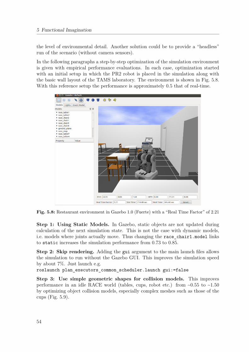
5 Functional Imagination

the level of environmental detail. Another solution could be to provide a “headless”run of the scenario (without camera sensors).

In the following paragraphs a step-by-step optimization of the simulation environmentis given with empirical performance evaluations. In each case, optimization startedwith an initial setup in which the PR2 robot is placed in the simulation along withthe basic wall layout of the TAMS laboratory. The environment is shown in Fig. 5.8.With this reference setup the performance is approximately 0.5 that of real-time.

Fig. 5.8: Restaurant environment in Gazebo 1.0 (Fuerte) with a “Real Time Factor” of 2.21

Step 1: Using Static Models. In Gazebo, static objects are not updated duringcalculation of the next simulation state. This is not the case with dynamic models,i.e. models where joints actually move. Thus changing the race_chair1.model linksto static increases the simulation performance from 0.73 to 0.85.

Step 2: Skip rendering. Adding the gui argument to the main launch files allowsthe simulation to run without the Gazebo GUI. This improves the simulation speedby about 7%. Just launch e.g.roslaunch plan_executors_common_scheduler.launch gui:=false

Step 3: Use simple geometric shapes for collision models. This improvesperformance in an idle RACE world (tables, cups, robot etc.) from ~0.55 to ~1.50by optimizing object collision models, especially complex meshes such as those of thecups (Fig. 5.9).

54

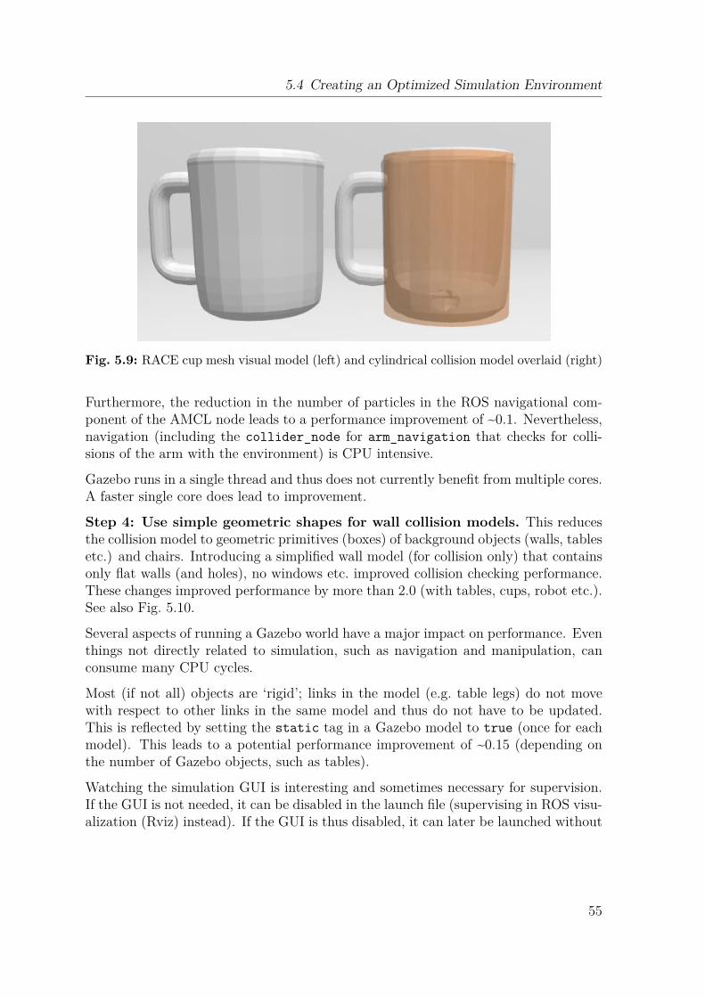
5.4 Creating an Optimized Simulation Environment

Fig. 5.9: RACE cup mesh visual model (left) and cylindrical collision model overlaid (right)

Furthermore, the reduction in the number of particles in the ROS navigational com-ponent of the AMCL node leads to a performance improvement of ~0.1. Nevertheless,navigation (including the collider_node for arm_navigation that checks for colli-sions of the arm with the environment) is CPU intensive.

Gazebo runs in a single thread and thus does not currently benefit from multiple cores.A faster single core does lead to improvement.

Step 4: Use simple geometric shapes for wall collision models. This reducesthe collision model to geometric primitives (boxes) of background objects (walls, tablesetc.) and chairs. Introducing a simplified wall model (for collision only) that containsonly flat walls (and holes), no windows etc. improved collision checking performance.These changes improved performance by more than 2.0 (with tables, cups, robot etc.).See also Fig. 5.10.

Several aspects of running a Gazebo world have a major impact on performance. Eventhings not directly related to simulation, such as navigation and manipulation, canconsume many CPU cycles.

Most (if not all) objects are ‘rigid’; links in the model (e.g. table legs) do not movewith respect to other links in the same model and thus do not have to be updated.This is reflected by setting the static tag in a Gazebo model to true (once for eachmodel). This leads to a potential performance improvement of ~0.15 (depending onthe number of Gazebo objects, such as tables).

Watching the simulation GUI is interesting and sometimes necessary for supervision.If the GUI is not needed, it can be disabled in the launch file (supervising in ROS visu-alization (Rviz) instead). If the GUI is thus disabled, it can later be launched without

55

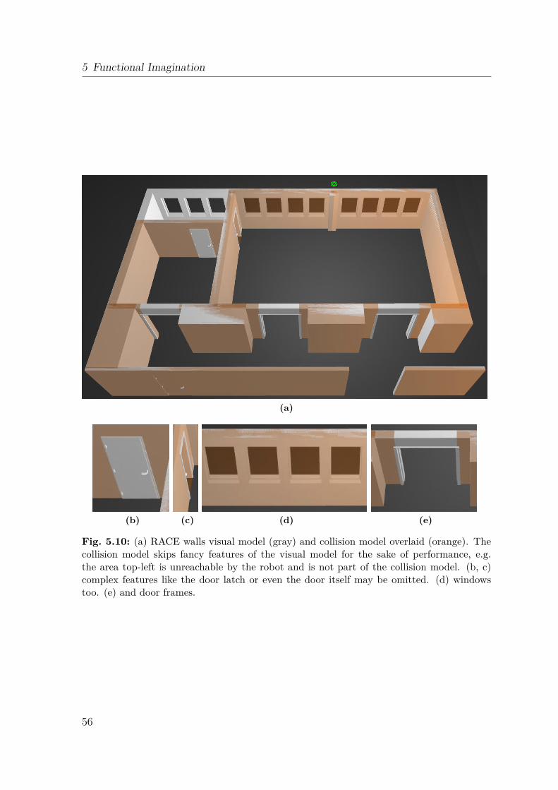
5 Functional Imagination

(a)

(b) (c) (d) (e)

Fig. 5.10: (a) RACE walls visual model (gray) and collision model overlaid (orange). Thecollision model skips fancy features of the visual model for the sake of performance, e.g.the area top-left is unreachable by the robot and is not part of the collision model. (b, c)complex features like the door latch or even the door itself may be omitted. (d) windowstoo. (e) and door frames.

56

5.5 Modeling Object Properties

restarting the whole simulation (by the rosrun gazebo gui command). Disablingthe GUI yields a possible improvement of ~0.10.

A lot of computation is needed for collision avoidance in the simulation and so usingsimplified collision models is crucial. Simplification involves using geometric primi-tives like boxes and cylinders for the collision model (or parts of it) instead of moreaccurate shapes. This is especially helpful when using a complex mesh (with manyfaces). For example a wonderful mesh cup could have a cylinder collision model. Suchsimplifications could lead to an improvement of up to ~2.5.

On the subject of simplification, collisions with walls must almost always be checked.Simplified environmental and collision models therefore help a lot (especially whenusing a mesh model, e.g. Collada or STL format). Improvements of between ~0.33and 3.0 are possible.

In Gazebo these improvements can be realized using different models for the <visual>

and <collision> tags. For visualization a sophisticated version can be used and forcollision checking a much simpler version might be sufficient. It is irrelevant whethermesh, box or cylinder is used.

Besides the simulation environment, optimization of robot capabilities is also possible.Navigation and localization can easily reduce performance by ~0.5. One can thereforetry to reduce the number of particles on which AMCL localization is based, for exam-ple, inside the amcl_node{*}.xml configuration file. In this work the min_particles

and max_particles are reduced by a factor of 50 (from 500 to 10 and from 5000 to100 respectively). The navigation system must be verified with these settings. A veryaccurate localization map created within the simulation itself improves accuracy signif-icantly. An empirical test showed improvements of ~0.10. On the system tested, thisis a small improvement. On other systems this number can vary and the optimizationis given here only for completeness.

The performance improvements were collected in chronological optimization order andare probably very dependent on the Gazebo world used.

5.5 Modeling Object Properties

Inertia I describes how an object resists rotational acceleration. It can be seen asthe rotational analogue of mass9. I has units of [mass] · [length]2. In this work andfor convenience, objects are considered to have symmetric mass distributions, withconstant density throughout the object; the axis of rotation is taken to be throughthe center of mass. In the case of a cylinder, as shown in Fig. 5.11, the inertia for thecentral axis, i.e. the z-axis here, is Iz = 1

2mr2. The inertia for the x- and y-axes is

9 http://en.wikipedia.org/wiki/List_of_moments_of_inertia (March 18, 2015)

57

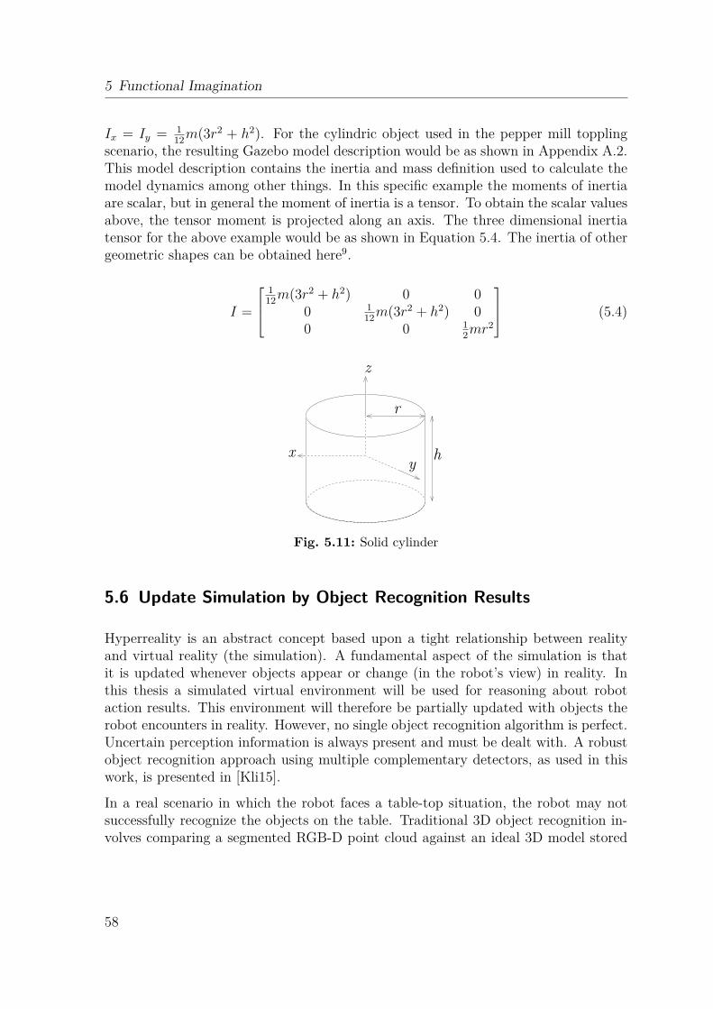
5 Functional Imagination

Ix = Iy = 112

m(3r2 + h2). For the cylindric object used in the pepper mill topplingscenario, the resulting Gazebo model description would be as shown in Appendix A.2.This model description contains the inertia and mass definition used to calculate themodel dynamics among other things. In this specific example the moments of inertiaare scalar, but in general the moment of inertia is a tensor. To obtain the scalar valuesabove, the tensor moment is projected along an axis. The three dimensional inertiatensor for the above example would be as shown in Equation 5.4. The inertia of othergeometric shapes can be obtained here9.

I =

112

m(3r2 + h2) 0 00 1

12m(3r2 + h2) 0

0 0 12mr2

(5.4)

x h

z

y

r

Fig. 5.11: Solid cylinder

5.6 Update Simulation by Object Recognition Results

Hyperreality is an abstract concept based upon a tight relationship between realityand virtual reality (the simulation). A fundamental aspect of the simulation is thatit is updated whenever objects appear or change (in the robot’s view) in reality. Inthis thesis a simulated virtual environment will be used for reasoning about robotaction results. This environment will therefore be partially updated with objects therobot encounters in reality. However, no single object recognition algorithm is perfect.Uncertain perception information is always present and must be dealt with. A robustobject recognition approach using multiple complementary detectors, as used in thiswork, is presented in [Kli15].

In a real scenario in which the robot faces a table-top situation, the robot may notsuccessfully recognize the objects on the table. Traditional 3D object recognition in-volves comparing a segmented RGB-D point cloud against an ideal 3D model stored

58

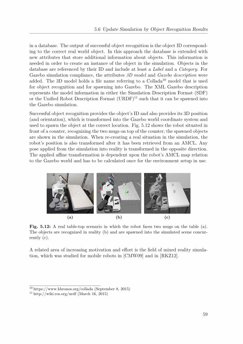
5.6 Update Simulation by Object Recognition Results

in a database. The output of successful object recognition is the object ID correspond-ing to the correct real world object. In this approach the database is extended withnew attributes that store additional information about objects. This information isneeded in order to create an instance of the object in the simulation. Objects in thedatabase are referenced by their ID and include at least a Label and a Category. ForGazebo simulation compliance, the attributes 3D model and Gazebo description wereadded. The 3D model holds a file name referring to a Collada10 model that is usedfor object recognition and for spawning into Gazebo. The XML Gazebo descriptionrepresents the model information in either the Simulation Description Format (SDF)or the Unified Robot Description Format (URDF)11 such that it can be spawned intothe Gazebo simulation.

Successful object recognition provides the object’s ID and also provides its 3D position(and orientation), which is transformed into the Gazebo world coordinate system andused to spawn the object at the correct location. Fig. 5.12 shows the robot situated infront of a counter, recognizing the two mugs on top of the counter; the spawned objectsare shown in the simulation. When re-creating a real situation in the simulation, therobot’s position is also transformed after it has been retrieved from an AMCL. Anypose applied from the simulation into reality is transformed in the opposite direction.The applied affine transformation is dependent upon the robot’s AMCL map relationto the Gazebo world and has to be calculated once for the environment setup in use.

(a) (b) (c)

Fig. 5.12: A real table-top scenario in which the robot faces two mugs on the table (a).The objects are recognized in reality (b) and are spawned into the simulated scene concur-rently (c).

A related area of increasing motivation and effort is the field of mixed reality simula-tion, which was studied for mobile robots in [CMW09] and in [RKZ12].

10 https://www.khronos.org/collada (September 8, 2015)11 http://wiki.ros.org/urdf (March 16, 2015)

59

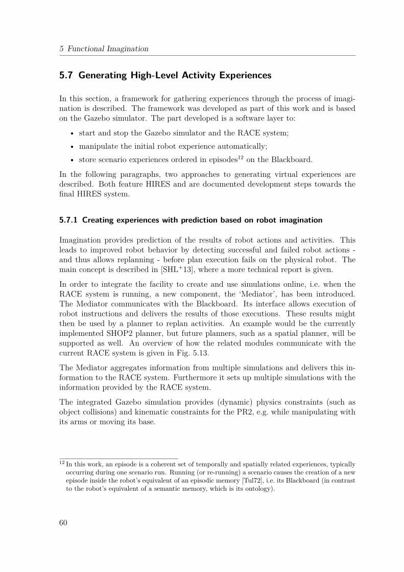
5 Functional Imagination

5.7 Generating High-Level Activity Experiences

In this section, a framework for gathering experiences through the process of imagi-nation is described. The framework was developed as part of this work and is basedon the Gazebo simulator. The part developed is a software layer to:

• start and stop the Gazebo simulator and the RACE system;

• manipulate the initial robot experience automatically;

• store scenario experiences ordered in episodes12 on the Blackboard.

In the following paragraphs, two approaches to generating virtual experiences aredescribed. Both feature HIRES and are documented development steps towards thefinal HIRES system.

5.7.1 Creating experiences with prediction based on robot imagination

Imagination provides prediction of the results of robot actions and activities. Thisleads to improved robot behavior by detecting successful and failed robot actions -and thus allows replanning - before plan execution fails on the physical robot. Themain concept is described in [SHL+13], where a more technical report is given.

In order to integrate the facility to create and use simulations online, i.e. when theRACE system is running, a new component, the ‘Mediator’, has been introduced.The Mediator communicates with the Blackboard. Its interface allows execution ofrobot instructions and delivers the results of those executions. These results mightthen be used by a planner to replan activities. An example would be the currentlyimplemented SHOP2 planner, but future planners, such as a spatial planner, will besupported as well. An overview of how the related modules communicate with thecurrent RACE system is given in Fig. 5.13.

The Mediator aggregates information from multiple simulations and delivers this in-formation to the RACE system. Furthermore it sets up multiple simulations with theinformation provided by the RACE system.

The integrated Gazebo simulation provides (dynamic) physics constraints (such asobject collisions) and kinematic constraints for the PR2, e.g. while manipulating withits arms or moving its base.

12 In this work, an episode is a coherent set of temporally and spatially related experiences, typicallyoccurring during one scenario run. Running (or re-running) a scenario causes the creation of a newepisode inside the robot’s equivalent of an episodic memory [Tul72], i.e. its Blackboard (in contrastto the robot’s equivalent of a semantic memory, which is its ontology).

60

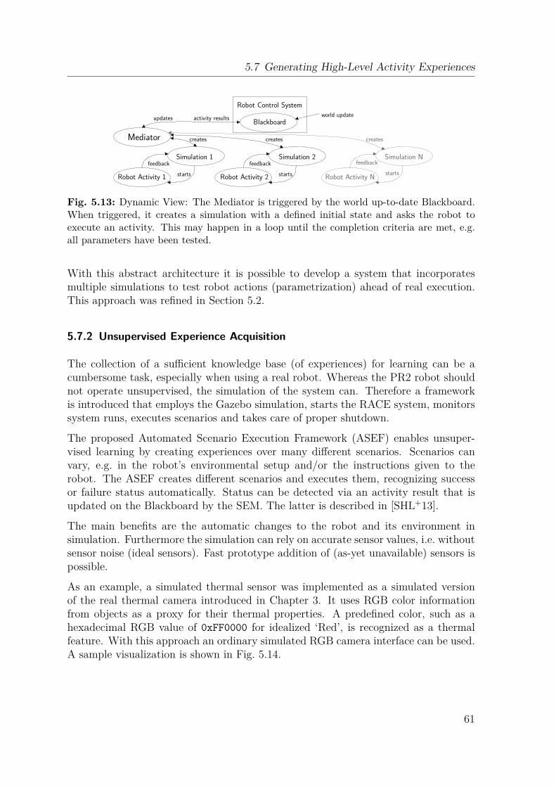
5.7 Generating High-Level Activity Experiences

Robot Control System

starts

feedback

starts

feedback

starts

feedback

updates

createscreates creates

activity results

Mediator

Simulation NSimulation 2Simulation 1

Robot Activity 1 Robot Activity 2 Robot Activity N

world updateBlackboard

Fig. 5.13: Dynamic View: The Mediator is triggered by the world up-to-date Blackboard.When triggered, it creates a simulation with a defined initial state and asks the robot toexecute an activity. This may happen in a loop until the completion criteria are met, e.g.all parameters have been tested.

With this abstract architecture it is possible to develop a system that incorporatesmultiple simulations to test robot actions (parametrization) ahead of real execution.This approach was refined in Section 5.2.

5.7.2 Unsupervised Experience Acquisition

The collection of a sufficient knowledge base (of experiences) for learning can be acumbersome task, especially when using a real robot. Whereas the PR2 robot shouldnot operate unsupervised, the simulation of the system can. Therefore a frameworkis introduced that employs the Gazebo simulation, starts the RACE system, monitorssystem runs, executes scenarios and takes care of proper shutdown.

The proposed Automated Scenario Execution Framework (ASEF) enables unsuper-vised learning by creating experiences over many different scenarios. Scenarios canvary, e.g. in the robot’s environmental setup and/or the instructions given to therobot. The ASEF creates different scenarios and executes them, recognizing successor failure status automatically. Status can be detected via an activity result that isupdated on the Blackboard by the SEM. The latter is described in [SHL+13].

The main benefits are the automatic changes to the robot and its environment insimulation. Furthermore the simulation can rely on accurate sensor values, i.e. withoutsensor noise (ideal sensors). Fast prototype addition of (as-yet unavailable) sensors ispossible.

As an example, a simulated thermal sensor was implemented as a simulated versionof the real thermal camera introduced in Chapter 3. It uses RGB color informationfrom objects as a proxy for their thermal properties. A predefined color, such as ahexadecimal RGB value of 0xFF0000 for idealized ‘Red’, is recognized as a thermalfeature. With this approach an ordinary simulated RGB camera interface can be used.A sample visualization is shown in Fig. 5.14.

61

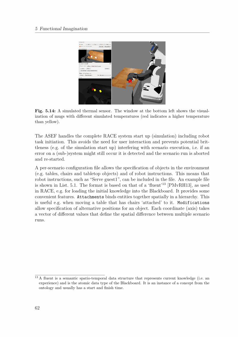
5 Functional Imagination

Fig. 5.14: A simulated thermal sensor. The window at the bottom left shows the visual-ization of mugs with different simulated temperatures (red indicates a higher temperaturethan yellow).

The ASEF handles the complete RACE system start up (simulation) including robottask initiation. This avoids the need for user interaction and prevents potential brit-tleness (e.g. of the simulation start up) interfering with scenario execution, i.e. if anerror on a (sub-)system might still occur it is detected and the scenario run is abortedand re-started.

A per-scenario configuration file allows the specification of objects in the environment(e.g. tables, chairs and tabletop objects) and of robot instructions. This means thatrobot instructions, such as “Serve guest1”, can be included in the file. An example fileis shown in List. 5.1. The format is based on that of a ‘fluent’13 [PMvRH13], as usedin RACE, e.g. for loading the initial knowledge into the Blackboard. It provides someconvenient features. Attachments binds entities together spatially in a hierarchy. Thisis useful e.g. when moving a table that has chairs ‘attached’ to it. Modifications

allow specification of alternative positions for an object. Each coordinate (axis) takesa vector of different values that define the spatial difference between multiple scenarioruns.

13 A fluent is a semantic spatio-temporal data structure that represents current knowledge (i.e. anexperience) and is the atomic data type of the Blackboard. It is an instance of a concept from theontology and usually has a start and finish time.

62

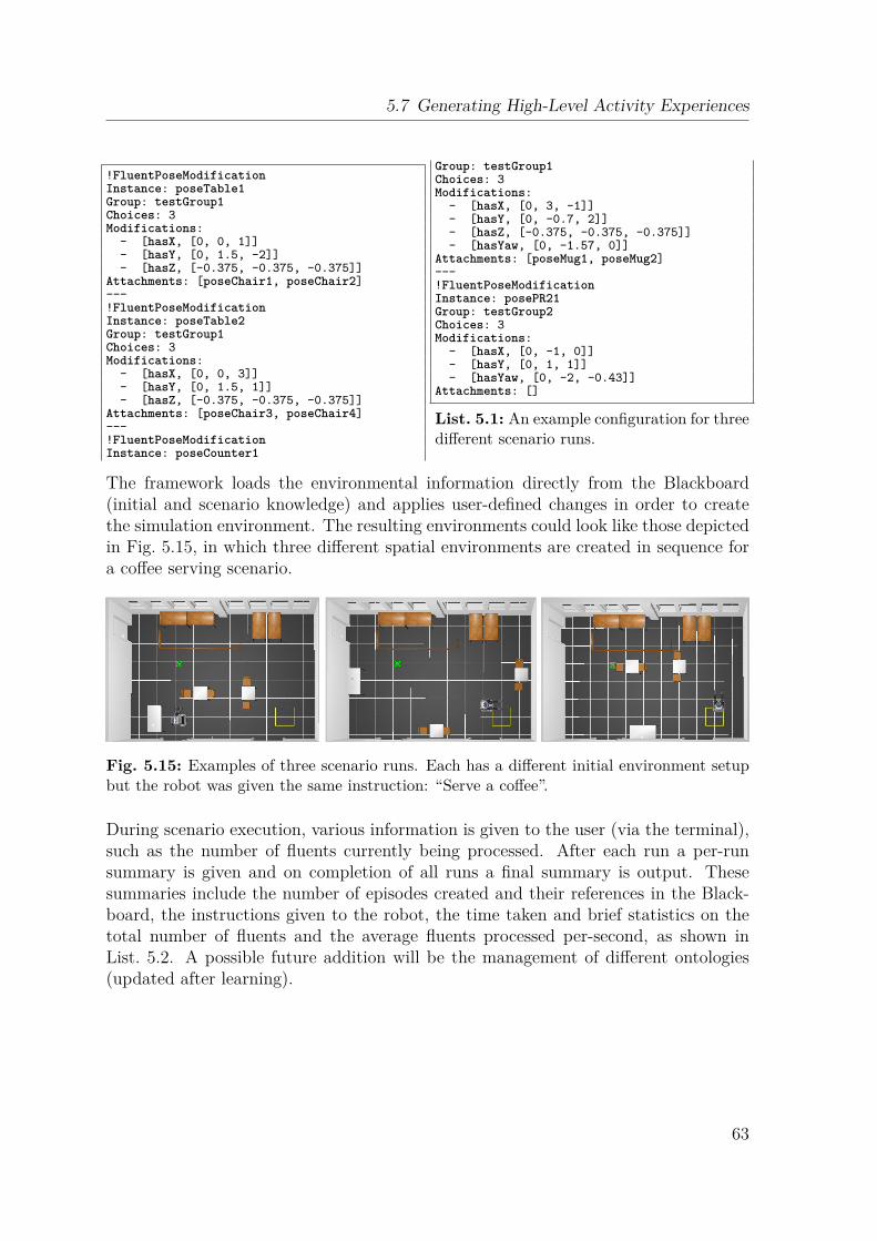
5.7 Generating High-Level Activity Experiences

!FluentPoseModificationInstance: poseTable1Group: testGroup1Choices: 3Modifications:

- [hasX, [0, 0, 1]]- [hasY, [0, 1.5, -2]]- [hasZ, [-0.375, -0.375, -0.375]]

Attachments: [poseChair1, poseChair2]---!FluentPoseModificationInstance: poseTable2Group: testGroup1Choices: 3Modifications:

- [hasX, [0, 0, 3]]- [hasY, [0, 1.5, 1]]- [hasZ, [-0.375, -0.375, -0.375]]

Attachments: [poseChair3, poseChair4]---!FluentPoseModificationInstance: poseCounter1

Group: testGroup1Choices: 3Modifications:

- [hasX, [0, 3, -1]]- [hasY, [0, -0.7, 2]]- [hasZ, [-0.375, -0.375, -0.375]]- [hasYaw, [0, -1.57, 0]]

Attachments: [poseMug1, poseMug2]---!FluentPoseModificationInstance: posePR21Group: testGroup2Choices: 3Modifications:

- [hasX, [0, -1, 0]]- [hasY, [0, 1, 1]]- [hasYaw, [0, -2, -0.43]]

Attachments: []

List. 5.1: An example configuration for threedifferent scenario runs.

The framework loads the environmental information directly from the Blackboard(initial and scenario knowledge) and applies user-defined changes in order to createthe simulation environment. The resulting environments could look like those depictedin Fig. 5.15, in which three different spatial environments are created in sequence fora coffee serving scenario.

Fig. 5.15: Examples of three scenario runs. Each has a different initial environment setupbut the robot was given the same instruction: “Serve a coffee”.

During scenario execution, various information is given to the user (via the terminal),such as the number of fluents currently being processed. After each run a per-runsummary is given and on completion of all runs a final summary is output. Thesesummaries include the number of episodes created and their references in the Black-board, the instructions given to the robot, the time taken and brief statistics on thetotal number of fluents and the average fluents processed per-second, as shown inList. 5.2. A possible future addition will be the management of different ontologies(updated after learning).

63

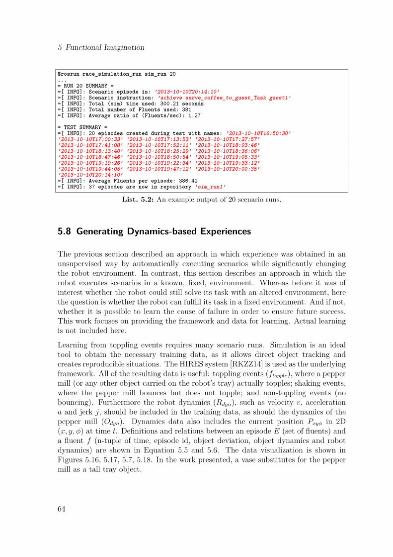
5 Functional Imagination

$rosrun race_simulation_run sim_run 20...= RUN 20 SUMMARY ==[ INFO]: Scenario episode is: ’2013-10-10T20:14:10’=[ INFO]: Scenario instruction: ’achieve serve_coffee_to_guest_Task guest1’=[ INFO]: Total (sim) time used: 300.21 seconds=[ INFO]: Total number of Fluents used: 381=[ INFO]: Average ratio of (Fluents/sec): 1.27

= TEST SUMMARY ==[ INFO]: 20 episodes created during test with names: ’2013-10-10T16:50:30’’2013-10-10T17:00:33’ ’2013-10-10T17:13:53’ ’2013-10-10T17:27:57’’2013-10-10T17:41:08’ ’2013-10-10T17:52:11’ ’2013-10-10T18:03:46’’2013-10-10T18:13:40’ ’2013-10-10T18:25:29’ ’2013-10-10T18:36:06’’2013-10-10T18:47:46’ ’2013-10-10T18:50:54’ ’2013-10-10T19:05:33’’2013-10-10T19:19:26’ ’2013-10-10T19:22:34’ ’2013-10-10T19:33:12’’2013-10-10T19:44:05’ ’2013-10-10T19:47:12’ ’2013-10-10T20:00:35’’2013-10-10T20:14:10’=[ INFO]: Average Fluents per episode: 386.42=[ INFO]: 37 episodes are now in repository ’sim_run1’

List. 5.2: An example output of 20 scenario runs.

5.8 Generating Dynamics-based Experiences

The previous section described an approach in which experience was obtained in anunsupervised way by automatically executing scenarios while significantly changingthe robot environment. In contrast, this section describes an approach in which therobot executes scenarios in a known, fixed, environment. Whereas before it was ofinterest whether the robot could still solve its task with an altered environment, herethe question is whether the robot can fulfill its task in a fixed environment. And if not,whether it is possible to learn the cause of failure in order to ensure future success.This work focuses on providing the framework and data for learning. Actual learningis not included here.

Learning from toppling events requires many scenario runs. Simulation is an idealtool to obtain the necessary training data, as it allows direct object tracking andcreates reproducible situations. The HIRES system [RKZZ14] is used as the underlyingframework. All of the resulting data is useful: toppling events (ftopple), where a peppermill (or any other object carried on the robot’s tray) actually topples; shaking events,where the pepper mill bounces but does not topple; and non-toppling events (nobouncing). Furthermore the robot dynamics (Rdyn), such as velocity v, accelerationa and jerk j, should be included in the training data, as should the dynamics of thepepper mill (Odyn). Dynamics data also includes the current position Pxyφ in 2D(x, y, φ) at time t. Definitions and relations between an episode E (set of fluents) anda fluent f (n-tuple of time, episode id, object deviation, object dynamics and robotdynamics) are shown in Equation 5.5 and 5.6. The data visualization is shown inFigures 5.16, 5.17, 5.7, 5.18. In the work presented, a vase substitutes for the peppermill as a tall tray object.

64

5.8 Generating Dynamics-based Experiences

f ∈ E

∀f ∈ E, ∃ftopple = 1

f = (t, Eid, Odev, Odyn, Rdyn)

Odev = (α, s)

Odyn = Rdyn = (Dlin, Dang, Pxyφ)

Dlin = Dang = (v, a, j)

Pxyφ = (x, y, φ)

(5.5)

~s =

xy0

, ~ω =

00ω

v(t) =s(t2) − s(t1)

t2 − t1

j(t) = a(t) = v(t)

ω(t) =α(t2) − α(t1)

t2 − t1

aangular = ω(t)

jangular = aangular(t) = ω(t)

(5.6)

In this scenario, an episode starts from the beginning of the scenario or from the lasttoppling event and lasts until the next toppling event. During an episode, fluentscontaining significant information are constantly created and stored. The fluent high-level format is shown in Listing 5.3 and a sample fluent is shown in Listing 5.4 in adata-mining friendly format.

To train with realistic data, a scenario was created that lets the PR2 robot drive toa pre-manipulation area (PMA) selected sequentially from those stored in the Black-board. A qualitative comparison of real and simulated results is presented in Chap-ter 6, Section 6.1.

5.8.1 Toppling Detection

Detection of toppling is generally straightforward in a simulation. Every object isconstantly updated in the simulation event loop - at 1000Hz in Gazebo. An object’sposition on the robot tray can be queried and can be used to calculate quite accurateobject dynamics. In this scenario an object like a pepper mill is tracked. To obtain avertical deviation, the object’s normal vector is compared to its initial normal vector(robot z-axis, upward), see Figure 5.7. To obtain the horizontal deviation the object’scurrent position is compared to its initial position. Any toppling event is detectedand stored in the data trace for later processing. As described before, a topplingevent concludes an episode and starts a new one, resetting the tray object’s pose andorientation.

5.8.2 Data Storage and Learning

In order to provide a facility for (offline) learning, all data generated during scenarioexecution is stored on-the-fly in a database. The database can later be mined to aidlearning about the toppling demo.

65

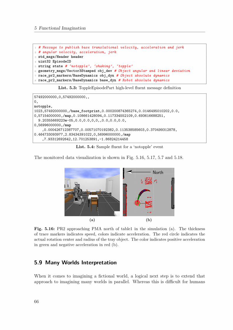
5 Functional Imagination

1 # Message to publish base translational velocity, acceleration and jerk

2 # angular velocity, acceleration, jerk

3 std_msgs/Header header

4 uint32 EpisodeID

5 string state # ‘notopple’, ‘shaking’, ‘topple’

6 geometry_msgs/Vector3Stamped obj_dev # Object angular and linear deviation

7 race_pr2_markers/BaseDynamics obj_dyn # Object absolute dynamics

8 race_pr2_markers/BaseDynamics base_dyn # Robot absolute dynamics

List. 5.3: ToppleEpisodePart high-level fluent message definition

57492000000,0,57492000000,,

0,

notopple,

1023,57492000000,/base_footprint,0.000200874365274,0.0146495010202,0.0,

0,57154000000,/map,0.108661428094,0.117334552109,0.693616688251,

9.20355669223e-05,0.0,0.0,0,0,,0.0,0.0,0.0,

0,56996000000,/map

,0.000426712387707,0.00571070192382,0.113538585603,0.370499312878,

0.464733093977,2.83434391022,0,56996000000,/map

,7.93312692642,12.701253891,-1.86824214458

List. 5.4: Sample fluent for a ‘notopple’ event

The monitored data visualization is shown in Fig. 5.16, 5.17, 5.7 and 5.18.

(a)

North

(b)

Fig. 5.16: PR2 approaching PMA north of table1 in the simulation (a). The thicknessof trace markers indicates speed, colors indicate acceleration. The red circle indicates theactual rotation center and radius of the tray object. The color indicates positive accelerationin green and negative acceleration in red (b).

5.9 Many Worlds Interpretation

When it comes to imagining a fictional world, a logical next step is to extend thatapproach to imagining many worlds in parallel. Whereas this is difficult for humans

66

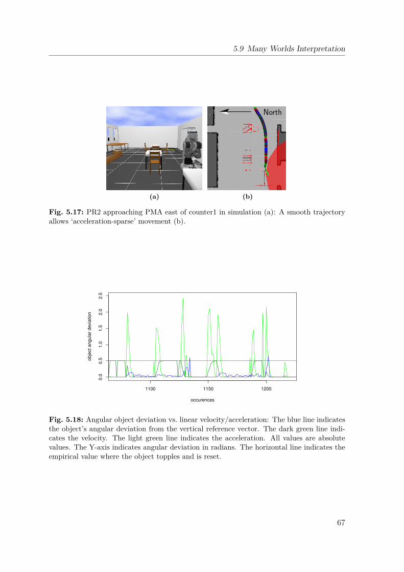
5.9 Many Worlds Interpretation

(a)

North

(b)

Fig. 5.17: PR2 approaching PMA east of counter1 in simulation (a): A smooth trajectoryallows ‘acceleration-sparse’ movement (b).

1100 1150 1200

0.0

0.5

1.0

1.5

2.0

2.5

occurences

obje

ct angula

r devia

tion

Fig. 5.18: Angular object deviation vs. linear velocity/acceleration: The blue line indicatesthe object’s angular deviation from the vertical reference vector. The dark green line indi-cates the velocity. The light green line indicates the acceleration. All values are absolutevalues. The Y-axis indicates angular deviation in radians. The horizontal line indicates theempirical value where the object topples and is reset.

67

5 Functional Imagination

it is straightforward for computers if appropriate resources are available. A systemimagining multiple scenes of the same or different scenarios would naturally save timeresources in the process of predicting future events.

The Many Worlds Interpretation (MWI) is a theory originating from quantum physics.It states that all possible alternative histories exist in parallel, i.e. any event that canpossibly happen does actually happen thus leading to a “many-worlds universe”. HughEverett III first published this theory in 1956 in his doctoral thesis The Theory of theUniversal Wave Function, which was compiled later in [BSD73]. It is about the secondmost accepted theory in quantum mechanics, after the Copenhagen theory [Teg98].Some recent popular work by David Deutsch employs the concept in theoretical sup-port of quantum computers [Deu85].

In theory, the ability to access multiple worlds allows the results of different actionsor action parametrizations to be evaluated. The common ground (i.e. the domain)has to be the same in all worlds investigated. In practice this would work as follows.Firstly, a scenario is created, different actions are applied (with a robot) within thescenario and the results are collected. The results are then evaluated and the bestis selected (according to some selection criteria). The “action parametrization” fromthe selected world is then extracted and applied to the real environment. The term“action parametrization” will be explained later.

In order to predict events, the range of possible alternatives is important. Relevantquestions would, for example, be: what would happen if the robot took this routerather than that route, what if it placed an object in one position on the table ratherthan another? Combining the theory of MWI with the capability of today’s availablecomputational power allows a many-simulation interpretation of future action results,in particular for robotics.

One programmatic approach is to map an action parameter to one simulated world.For each reasonable parameter a new world is created, with the upper limit to thenumber of possible worlds depending upon the available computational power. Afteran action finishes, the related world is either terminated, in order to save resources, orre-used for a similar simulation. Each simulation provides information on the resultof the action and back-tracking leads to the parameters which caused that result.

Another approach is not to limit a simulation to one action but to “keep it running”.That means creating a simulation at a specific time, executing consecutive actionswithin it and tracing the simulation state at the end of a complete episode (or indefi-nitely). As small variations during the simulation can lead to very different simulationstates, this approach is very computationally intensive and thus provides very littlepractical granularity.

In the example of a robot given the task of moving to a table, depending upon itsinitial position and its environment, the robot can decide whether to approach thetable from one side or another. The decision will determine the robot’s trajectory and

68

5.10 Summary

might have other implications. The action could be parametrized with two valid goalpositions. Thus in this work, the term “action parametrization” refers to the possibilityfor a robot action to be instantiated with different parameters that possibly result indifferent world states after execution.

5.10 Summary

This chapter developed the methods and experimental design required in order toensure a robust realization of the approach initially stated (cf. Section 1.4). Thescenario setup was introduced and the required robot capabilities were developed. Amodel for representing the problem domain was developed and a detailed architecturewas created. The chapter also introduced the tools and methods necessary for thecreation of a simulation environment for the problem domain. In order to help meetreal-time constraints, a detailed performance optimization was performed on variouselements of the simulation. A framework proposal to integrate imagination into aBlackboard-based robot control system, such as the RACE framework, was givenand two frameworks for creating unsupervised experiences were described. Finallyan overview of overlapping aspects of this work and the MWI was presented. Thenext chapter, Chapter 6, describes experiments that measure the effects of addingfunctional imagination to a robot system.

69

Experimental Scenarios and

Evaluation

6

This chapter presents the experiments used to evaluate the functional imaginationapproach described in Chapter 5. The simulation used to implement imagination isverified for accuracy and repeatability. If the simulation is accurate, it is possible tocompare simulated and real world action results. Assuming the correctness of the sim-ulation, it will be shown that predicted results from a simulation can prevent failuresin reality. Furthermore the results will show that multiple aspects of reasoning (spa-tial, temporal, causal) derived from simulation can enhance a plan-based system thatuses execution monitoring and will thus support the hypothesis stated in Section 1.4.

In order to verify simulation the same experiments were executed in simulation (Gazebo)and on the real robot (PR2). The experiments for evaluating action result predictionwere performed on the real robot (with simulation based imagination). The experi-mental restaurant environment is shown in the ROS visualization in Fig. 6.1. Thisfigure shows labels of both real world and artificial concepts. Whereas most labelsin the robot domain relate to existing objects (for example the label ‘table1’ refersto the first table in the restaurant environment), a label for an artificial concept hasalso been introduced. The representation of a pre-manipulation area (PMA) was in-troduced because the underlying collision avoidance system prevents the robot fromnavigating close to an object. The robot also has limited ability to manipulate objects.For example, putting an object on the robot’s tray would cause a collision with thetable next to the robot. With the concept of a PMA, a robot action dedicated to nav-igating close to tables was developed for the RACE project. Throughout this work,whenever a robot trajectory is mentioned, it refers to a trajectory between PMAs.

The following sections first present the results of validating simulated actions againstreality. Subsequently, the results of executing the proposed system on a PR2 arepresented.

71

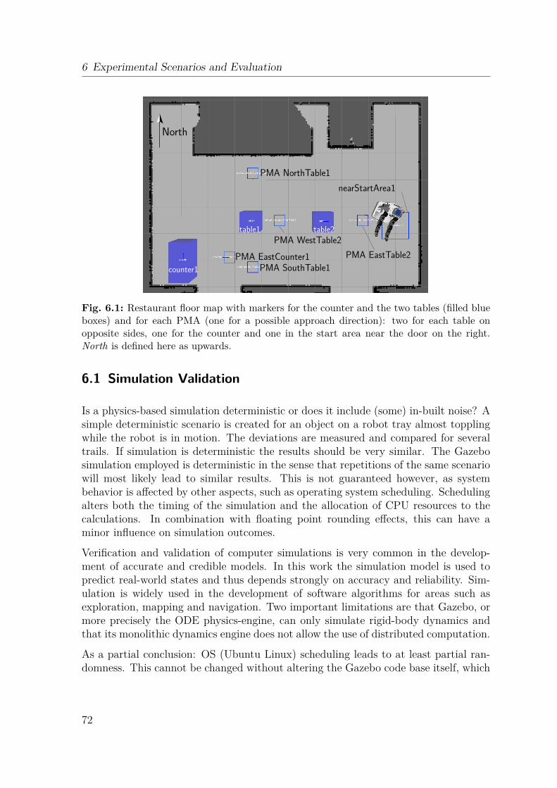
6 Experimental Scenarios and Evaluation

PMA EastCounter1

PMA WestTable2

PMA EastTable2

PMA NorthTable1

nearStartArea1

PMA SouthTable1

North

counter1

table1 table2

Fig. 6.1: Restaurant floor map with markers for the counter and the two tables (filled blueboxes) and for each PMA (one for a possible approach direction): two for each table onopposite sides, one for the counter and one in the start area near the door on the right.North is defined here as upwards.

6.1 Simulation Validation

Is a physics-based simulation deterministic or does it include (some) in-built noise? Asimple deterministic scenario is created for an object on a robot tray almost topplingwhile the robot is in motion. The deviations are measured and compared for severaltrails. If simulation is deterministic the results should be very similar. The Gazebosimulation employed is deterministic in the sense that repetitions of the same scenariowill most likely lead to similar results. This is not guaranteed however, as systembehavior is affected by other aspects, such as operating system scheduling. Schedulingalters both the timing of the simulation and the allocation of CPU resources to thecalculations. In combination with floating point rounding effects, this can have aminor influence on simulation outcomes.

Verification and validation of computer simulations is very common in the develop-ment of accurate and credible models. In this work the simulation model is used topredict real-world states and thus depends strongly on accuracy and reliability. Sim-ulation is widely used in the development of software algorithms for areas such asexploration, mapping and navigation. Two important limitations are that Gazebo, ormore precisely the ODE physics-engine, can only simulate rigid-body dynamics andthat its monolithic dynamics engine does not allow the use of distributed computation.

As a partial conclusion: OS (Ubuntu Linux) scheduling leads to at least partial ran-domness. This cannot be changed without altering the Gazebo code base itself, which

72

6.1 Simulation Validation

is outside the scope of this work.

There has been some work on this topic in the literature. [BB07] presents a qualitativeevaluation of free, publicly available, physics engines. Its criteria are the number ofconstraints implemented (among others). The most useful constraints are models ofreal life system behavior. Common constraints are, for example, those affecting joints(prismatic, revolute and spherical). [WHR10], in contrast, evaluates the Bullet engineas an ingredient for physical reasoning. It studies how accurately the pushing of flatobjects across a table with a robotic arm can be predicted. [OFY07] implements anomnidirectional camera model for Gazebo and verifies it by qualitative comparison ofrendered images with images obtained by a real omnidirectional vision sensor.

[KH04] describes the design and usage paradigms of the Gazebo simulator. Fig. 4.2shows how a model is constructed in a tree-like hierarchical structure and how worldmodels are connected to the external Gazebo interfaces. [FCK+09] verifies a Zigbeebased distributed communication system by comparing simulated and real results.

Generally a physics-based simulation has no noise apart from the minor noise intro-duced by the underlying hardware and OS, i.e. scheduling. An obvious exception isnoise that is explicitly modeled, such as the Gaussian noise used in the Gazebo lasersimulation. Also, the standard deviation σ of the durations of actions measured inthe restaurant environment within Gazebo is small, as can be seen in Table 6.1. Thecorresponding measurements with the PR2 are shown in Table 6.2. A comparison ofthe same actions in simulation and in reality is shown graphically in Fig. 6.2. The twotables list the action executed, with parameters as appropriate. In each table, ‘Sam-ples’ is the number of iterations performed, σ =

√

1N

∑Ni=1(xi − µ)2 is the standard

deviation of the duration, µ is the mean duration and ‘to/from’ gives the acronymsof the starting pose or posture of the robot. As discussed earlier, for the move_base

action, ET2 corresponds to EastTable2, EC1 is EastCounter1 and so on. For themove_torso action, ‘U’ means up and ‘D’ means down. The tuck_arms action uses‘U’ for untucked arms and ‘T’ for tucked arms.

The probability distributions of these measurements are shown in Appendix A.8. Anexample measurement is shown in Fig. 6.3. It shows the !move_base_param actiondriving the robot from PMA east of counter1 to PMA south of table1. Although thetest data size is rather small with only 24 samples, the histogram and the overlaiddensity of action duration show an approximately standard Gaussian distribution.The QQ plot shows independent standard normal data (in seconds) on the verticalaxis against a standard normal population on the horizontal axis. The linear fit tothe data indicates that they are normally distributed. There are some clear outliersthat do not fit (five in total in Fig. 6.3 a,b and two in Fig. 6.3 c,d). They show updisproportionately in the plots because of the small sample size.

The validation data was retrieved by running the robot capabilities (perception, ac-tuation) and the RACE system. The system load on each computer performing the

73

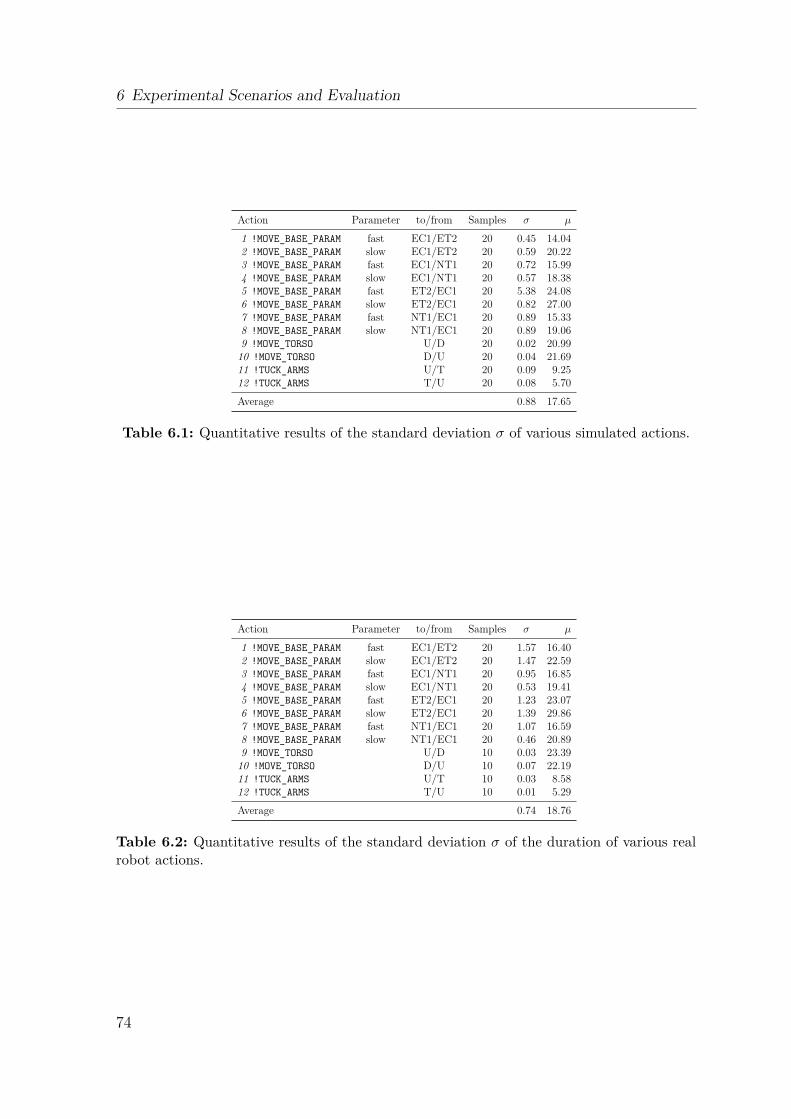
6 Experimental Scenarios and Evaluation

Action Parameter to/from Samples σ µ

1 !MOVE_BASE_PARAM fast EC1/ET2 20 0.45 14.042 !MOVE_BASE_PARAM slow EC1/ET2 20 0.59 20.223 !MOVE_BASE_PARAM fast EC1/NT1 20 0.72 15.994 !MOVE_BASE_PARAM slow EC1/NT1 20 0.57 18.385 !MOVE_BASE_PARAM fast ET2/EC1 20 5.38 24.086 !MOVE_BASE_PARAM slow ET2/EC1 20 0.82 27.007 !MOVE_BASE_PARAM fast NT1/EC1 20 0.89 15.338 !MOVE_BASE_PARAM slow NT1/EC1 20 0.89 19.069 !MOVE_TORSO U/D 20 0.02 20.99

10 !MOVE_TORSO D/U 20 0.04 21.6911 !TUCK_ARMS U/T 20 0.09 9.2512 !TUCK_ARMS T/U 20 0.08 5.70

Average 0.88 17.65

Table 6.1: Quantitative results of the standard deviation σ of various simulated actions.

Action Parameter to/from Samples σ µ

1 !MOVE_BASE_PARAM fast EC1/ET2 20 1.57 16.402 !MOVE_BASE_PARAM slow EC1/ET2 20 1.47 22.593 !MOVE_BASE_PARAM fast EC1/NT1 20 0.95 16.854 !MOVE_BASE_PARAM slow EC1/NT1 20 0.53 19.415 !MOVE_BASE_PARAM fast ET2/EC1 20 1.23 23.076 !MOVE_BASE_PARAM slow ET2/EC1 20 1.39 29.867 !MOVE_BASE_PARAM fast NT1/EC1 20 1.07 16.598 !MOVE_BASE_PARAM slow NT1/EC1 20 0.46 20.899 !MOVE_TORSO U/D 10 0.03 23.39

10 !MOVE_TORSO D/U 10 0.07 22.1911 !TUCK_ARMS U/T 10 0.03 8.5812 !TUCK_ARMS T/U 10 0.01 5.29

Average 0.74 18.76

Table 6.2: Quantitative results of the standard deviation σ of the duration of various realrobot actions.

74

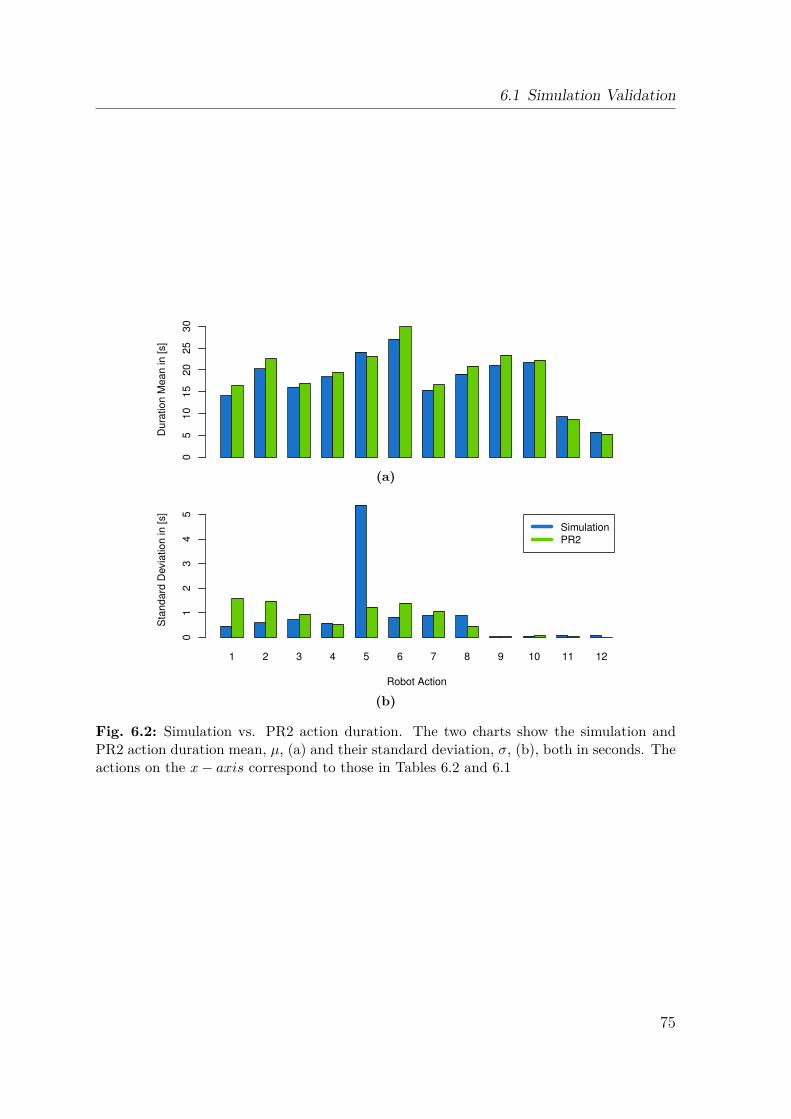
6.1 Simulation Validation

Du

ratio

n M

ea

n in

[s]

05

10

15

20

25

30

(a)

1 2 3 4 5 6 7 8 9 10 11 12

Robot Action

Sta

nd

ard

Devia

tio

n in

[s]

01

23

45

Simulation

PR2

(b)

Fig. 6.2: Simulation vs. PR2 action duration. The two charts show the simulation andPR2 action duration mean, µ, (a) and their standard deviation, σ, (b), both in seconds. Theactions on the x − axis correspond to those in Tables 6.2 and 6.1

75

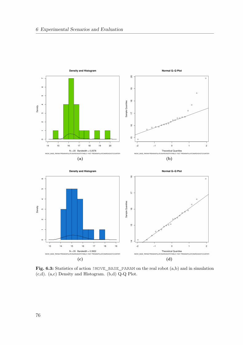
6 Experimental Scenarios and Evaluation

14 15 16 17 18 19 20

01

23

45

67

Density and Histogram

N = 20 Bandwidth = 0.2578

Density

!MOVE_BASE_PARAM PREMANIPULATIONAREANORTHTABLE1 FAST PREMANIPULATIONAREAEASTCOUNTER1

(a)

●

●

●●

●

●

●

●

●

●

●

●

●

●

●

●

●

●

●

●

−2 −1 0 1 2

15

16

17

18

19

20

Normal Q−Q Plot

Theoretical Quantiles

Sam

ple

Quantile

s

!MOVE_BASE_PARAM PREMANIPULATIONAREANORTHTABLE1 FAST PREMANIPULATIONAREAEASTCOUNTER1

(b)

13 14 15 16 17 18 19

01

23

45

6

Density and Histogram

N = 20 Bandwidth = 0.3932

Density

!MOVE_BASE_PARAM PREMANIPULATIONAREANORTHTABLE1 FAST PREMANIPULATIONAREAEASTCOUNTER1

(c)

●

●

●

●

●

●

●

●

●

●

●

●

●

●

●

●

●

●

●

●

−2 −1 0 1 2

14

15

16

17

18

Normal Q−Q Plot

Theoretical Quantiles

Sam

ple

Quantile

s

!MOVE_BASE_PARAM PREMANIPULATIONAREANORTHTABLE1 FAST PREMANIPULATIONAREAEASTCOUNTER1

(d)

Fig. 6.3: Statistics of action !MOVE_BASE_PARAM on the real robot (a,b) and in simulation(c,d). (a,c) Density and Histogram. (b,d) Q-Q Plot.

76

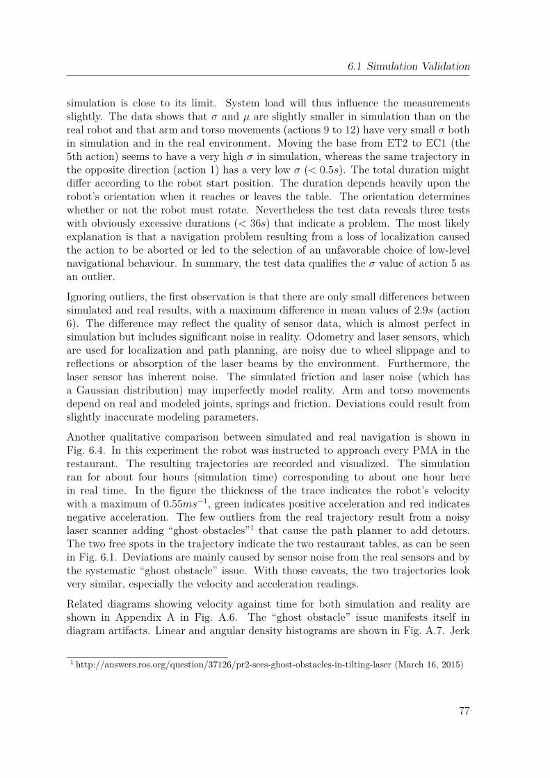
6.1 Simulation Validation

simulation is close to its limit. System load will thus influence the measurementsslightly. The data shows that σ and µ are slightly smaller in simulation than on thereal robot and that arm and torso movements (actions 9 to 12) have very small σ bothin simulation and in the real environment. Moving the base from ET2 to EC1 (the5th action) seems to have a very high σ in simulation, whereas the same trajectory inthe opposite direction (action 1) has a very low σ (< 0.5s). The total duration mightdiffer according to the robot start position. The duration depends heavily upon therobot’s orientation when it reaches or leaves the table. The orientation determineswhether or not the robot must rotate. Nevertheless the test data reveals three testswith obviously excessive durations (< 36s) that indicate a problem. The most likelyexplanation is that a navigation problem resulting from a loss of localization causedthe action to be aborted or led to the selection of an unfavorable choice of low-levelnavigational behaviour. In summary, the test data qualifies the σ value of action 5 asan outlier.

Ignoring outliers, the first observation is that there are only small differences betweensimulated and real results, with a maximum difference in mean values of 2.9s (action6). The difference may reflect the quality of sensor data, which is almost perfect insimulation but includes significant noise in reality. Odometry and laser sensors, whichare used for localization and path planning, are noisy due to wheel slippage and toreflections or absorption of the laser beams by the environment. Furthermore, thelaser sensor has inherent noise. The simulated friction and laser noise (which hasa Gaussian distribution) may imperfectly model reality. Arm and torso movementsdepend on real and modeled joints, springs and friction. Deviations could result fromslightly inaccurate modeling parameters.

Another qualitative comparison between simulated and real navigation is shown inFig. 6.4. In this experiment the robot was instructed to approach every PMA in therestaurant. The resulting trajectories are recorded and visualized. The simulationran for about four hours (simulation time) corresponding to about one hour herein real time. In the figure the thickness of the trace indicates the robot’s velocitywith a maximum of 0.55ms−1, green indicates positive acceleration and red indicatesnegative acceleration. The few outliers from the real trajectory result from a noisylaser scanner adding “ghost obstacles”1 that cause the path planner to add detours.The two free spots in the trajectory indicate the two restaurant tables, as can be seenin Fig. 6.1. Deviations are mainly caused by sensor noise from the real sensors and bythe systematic “ghost obstacle” issue. With those caveats, the two trajectories lookvery similar, especially the velocity and acceleration readings.

Related diagrams showing velocity against time for both simulation and reality areshown in Appendix A in Fig. A.6. The “ghost obstacle” issue manifests itself indiagram artifacts. Linear and angular density histograms are shown in Fig. A.7. Jerk

1 http://answers.ros.org/question/37126/pr2-sees-ghost-obstacles-in-tilting-laser (March 16, 2015)

77

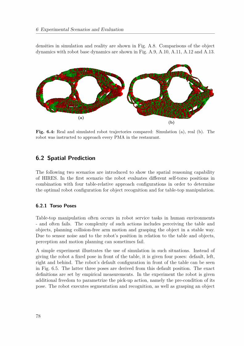
6 Experimental Scenarios and Evaluation

densities in simulation and reality are shown in Fig. A.8. Comparisons of the objectdynamics with robot base dynamics are shown in Fig. A.9, A.10, A.11, A.12 and A.13.

(a)(b)

Fig. 6.4: Real and simulated robot trajectories compared: Simulation (a), real (b). Therobot was instructed to approach every PMA in the restaurant.

6.2 Spatial Prediction

The following two scenarios are introduced to show the spatial reasoning capabilityof HIRES. In the first scenario the robot evaluates different self-torso positions incombination with four table-relative approach configurations in order to determinethe optimal robot configuration for object recognition and for table-top manipulation.

6.2.1 Torso Poses

Table-top manipulation often occurs in robot service tasks in human environments- and often fails. The complexity of such actions includes perceiving the table andobjects, planning collision-free arm motion and grasping the object in a stable way.Due to sensor noise and to the robot’s position in relation to the table and objects,perception and motion planning can sometimes fail.

A simple experiment illustrates the use of simulation in such situations. Instead ofgiving the robot a fixed pose in front of the table, it is given four poses: default, left,right and behind. The robot’s default configuration in front of the table can be seenin Fig. 6.5. The latter three poses are derived from this default position. The exactdefinitions are set by empirical measurements. In the experiment the robot is givenadditional freedom to parametrize the pick-up action, namely the pre-condition of itspose. The robot executes segmentation and recognition, as well as grasping an object

78

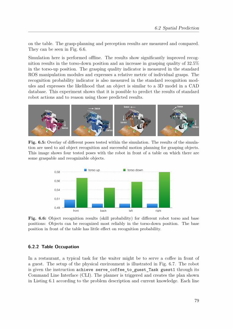
6.2 Spatial Prediction

on the table. The grasp-planning and perception results are measured and compared.They can be seen in Fig. 6.6.

Simulation here is performed offline. The results show significantly improved recog-nition results in the torso-down position and an increase in grasping quality of 32.5%in the torso-up position. The grasping quality indicator is measured in the standardROS manipulation modules and expresses a relative metric of individual grasps. Therecognition probability indicator is also measured in the standard recognition mod-ules and expresses the likelihood that an object is similar to a 3D model in a CADdatabase. This experiment shows that it is possible to predict the results of standardrobot actions and to reason using those predicted results.

Fig. 6.5: Overlay of different poses tested within the simulation. The results of the simula-tion are used to aid object recognition and successful motion planning for grasping objects.This image shows four tested poses with the robot in front of a table on which there aresome graspable and recognizable objects.

Recognition Probability

0,49

0,51

0,54

0,56

0,58

front back left right

torso up torso down

Fig. 6.6: Object recognition results (skill probability) for different robot torso and basepositions: Objects can be recognized most reliably in the torso-down position. The baseposition in front of the table has little effect on recognition probability.

6.2.2 Table Occupation

In a restaurant, a typical task for the waiter might be to serve a coffee in front ofa guest. The setup of the physical environment is illustrated in Fig. 6.7. The robotis given the instruction achieve serve_coffee_to_guest_Task guest1 through itsCommand Line Interface (CLI). The planner is triggered and creates the plan shownin Listing 6.1 according to the problem description and current knowledge. Each line

79

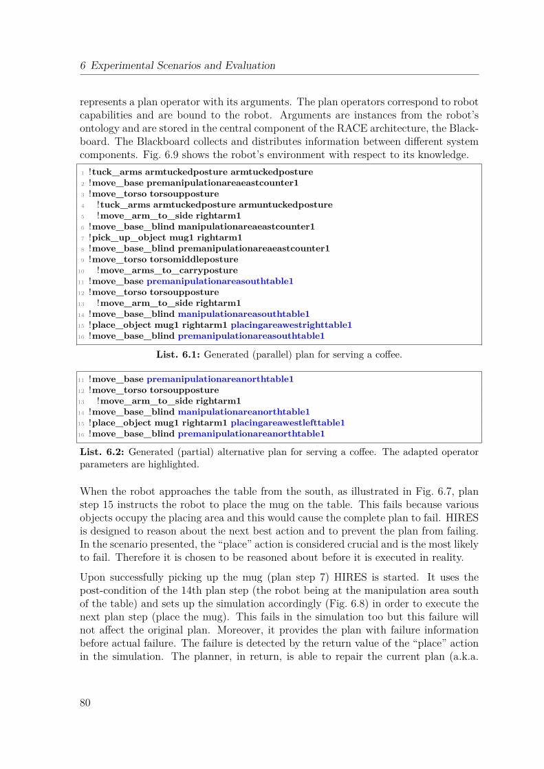
6 Experimental Scenarios and Evaluation

represents a plan operator with its arguments. The plan operators correspond to robotcapabilities and are bound to the robot. Arguments are instances from the robot’sontology and are stored in the central component of the RACE architecture, the Black-board. The Blackboard collects and distributes information between different systemcomponents. Fig. 6.9 shows the robot’s environment with respect to its knowledge.

1 !tuck_arms armtuckedposture armtuckedposture2 !move_base premanipulationareaeastcounter13 !move_torso torsoupposture4 !tuck_arms armtuckedposture armuntuckedposture5 !move_arm_to_side rightarm16 !move_base_blind manipulationareaeastcounter17 !pick_up_object mug1 rightarm18 !move_base_blind premanipulationareaeastcounter19 !move_torso torsomiddleposture

10 !move_arms_to_carryposture11 !move_base premanipulationareasouthtable112 !move_torso torsoupposture13 !move_arm_to_side rightarm114 !move_base_blind manipulationareasouthtable115 !place_object mug1 rightarm1 placingareawestrighttable116 !move_base_blind premanipulationareasouthtable1

List. 6.1: Generated (parallel) plan for serving a coffee.

11 !move_base premanipulationareanorthtable112 !move_torso torsoupposture13 !move_arm_to_side rightarm114 !move_base_blind manipulationareanorthtable115 !place_object mug1 rightarm1 placingareawestlefttable116 !move_base_blind premanipulationareanorthtable1

List. 6.2: Generated (partial) alternative plan for serving a coffee. The adapted operatorparameters are highlighted.

When the robot approaches the table from the south, as illustrated in Fig. 6.7, planstep 15 instructs the robot to place the mug on the table. This fails because variousobjects occupy the placing area and this would cause the complete plan to fail. HIRESis designed to reason about the next best action and to prevent the plan from failing.In the scenario presented, the “place” action is considered crucial and is the most likelyto fail. Therefore it is chosen to be reasoned about before it is executed in reality.

Upon successfully picking up the mug (plan step 7) HIRES is started. It uses thepost-condition of the 14th plan step (the robot being at the manipulation area southof the table) and sets up the simulation accordingly (Fig. 6.8) in order to execute thenext plan step (place the mug). This fails in the simulation too but this failure willnot affect the original plan. Moreover, it provides the plan with failure informationbefore actual failure. The failure is detected by the return value of the “place” actionin the simulation. The planner, in return, is able to repair the current plan (a.k.a.

80

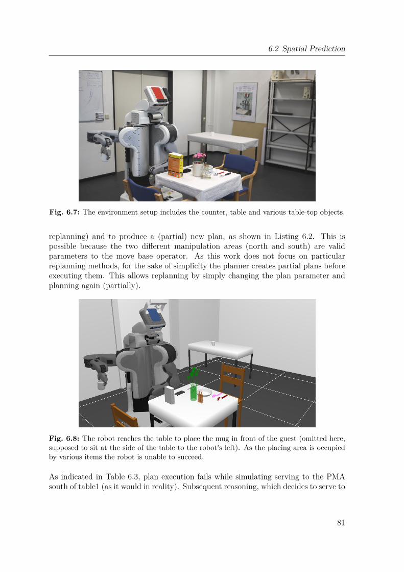
6.2 Spatial Prediction

Fig. 6.7: The environment setup includes the counter, table and various table-top objects.

replanning) and to produce a (partial) new plan, as shown in Listing 6.2. This ispossible because the two different manipulation areas (north and south) are validparameters to the move base operator. As this work does not focus on particularreplanning methods, for the sake of simplicity the planner creates partial plans beforeexecuting them. This allows replanning by simply changing the plan parameter andplanning again (partially).

Fig. 6.8: The robot reaches the table to place the mug in front of the guest (omitted here,supposed to sit at the side of the table to the robot’s left). As the placing area is occupiedby various items the robot is unable to succeed.

As indicated in Table 6.3, plan execution fails while simulating serving to the PMAsouth of table1 (as it would in reality). Subsequent reasoning, which decides to serve to

81

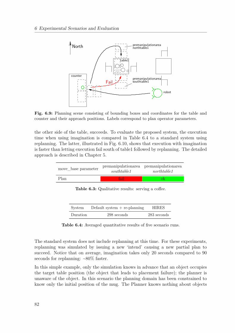
6 Experimental Scenarios and Evaluation

southtable1premanipulationarea

robot

counter

North premanipulationareanorthtable1

table1

Fail

Fig. 6.9: Planning scene consisting of bounding boxes and coordinates for the table andcounter and their approach positions. Labels correspond to plan operator parameters.

the other side of the table, succeeds. To evaluate the proposed system, the executiontime when using imagination is compared in Table 6.4 to a standard system usingreplanning. The latter, illustrated in Fig. 6.10, shows that execution with imaginationis faster than letting execution fail south of table1 followed by replanning. The detailedapproach is described in Chapter 5.

move_base parameterpremanipulationarea premanipulationarea

southtable1 northtable1

Plan fail ok

Table 6.3: Qualitative results: serving a coffee.

System Default system + re-planning HIRES

Duration 298 seconds 283 seconds

Table 6.4: Averaged quantitative results of five scenario runs.

The standard system does not include replanning at this time. For these experiments,replanning was simulated by issuing a new ‘intend’ causing a new partial plan tosucceed. Notice that on average, imagination takes only 20 seconds compared to 90seconds for replanning: ~80% faster.

In this simple example, only the simulation knows in advance that an object occupiesthe target table position (the object that leads to placement failure); the planner isunaware of the object. In this scenario the planning domain has been constrained toknow only the initial position of the mug. The Planner knows nothing about objects

82

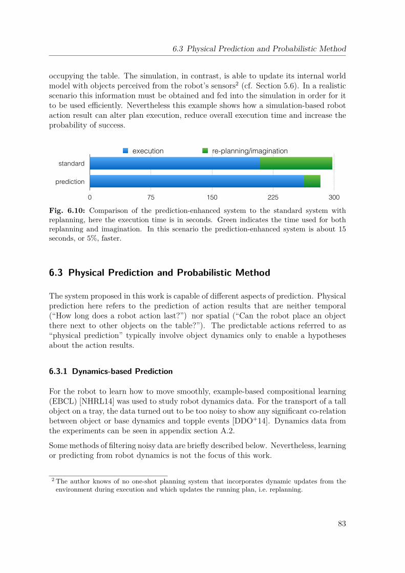
6.3 Physical Prediction and Probabilistic Method

occupying the table. The simulation, in contrast, is able to update its internal worldmodel with objects perceived from the robot’s sensors2 (cf. Section 5.6). In a realisticscenario this information must be obtained and fed into the simulation in order for itto be used efficiently. Nevertheless this example shows how a simulation-based robotaction result can alter plan execution, reduce overall execution time and increase theprobability of success.

standard

prediction

0 75 150 225 300

execution re-planning/imagination

Fig. 6.10: Comparison of the prediction-enhanced system to the standard system withreplanning, here the execution time is in seconds. Green indicates the time used for bothreplanning and imagination. In this scenario the prediction-enhanced system is about 15seconds, or 5%, faster.

6.3 Physical Prediction and Probabilistic Method

The system proposed in this work is capable of different aspects of prediction. Physicalprediction here refers to the prediction of action results that are neither temporal(“How long does a robot action last?”) nor spatial (“Can the robot place an objectthere next to other objects on the table?”). The predictable actions referred to as“physical prediction” typically involve object dynamics only to enable a hypothesesabout the action results.

6.3.1 Dynamics-based Prediction

For the robot to learn how to move smoothly, example-based compositional learning(EBCL) [NHRL14] was used to study robot dynamics data. For the transport of a tallobject on a tray, the data turned out to be too noisy to show any significant co-relationbetween object or base dynamics and topple events [DDO+14]. Dynamics data fromthe experiments can be seen in appendix section A.2.

Some methods of filtering noisy data are briefly described below. Nevertheless, learningor predicting from robot dynamics is not the focus of this work.

2 The author knows of no one-shot planning system that incorporates dynamic updates from theenvironment during execution and which updates the running plan, i.e. replanning.

83

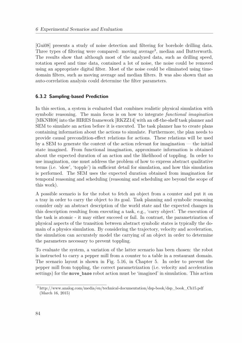
6 Experimental Scenarios and Evaluation

[Gui08] presents a study of noise detection and filtering for borehole drilling data.Three types of filtering were compared: moving average3, median and Butterworth.The results show that although most of the analyzed data, such as drilling speed,rotation speed and time data, contained a lot of noise, the noise could be removedusing an appropriate digital filter. Most of the noise could be eliminated using time-domain filters, such as moving average and median filters. It was also shown that anauto-correlation analysis could determine the filter parameters.

6.3.2 Sampling-based Prediction

In this section, a system is evaluated that combines realistic physical simulation withsymbolic reasoning. The main focus is on how to integrate functional imagination[MKNH08] into the HIRES framework [RKZZ14] with an off-the-shelf task planner andSEM to simulate an action before it is executed. The task planner has to create planscontaining information about the actions to simulate. Furthermore, the plan needs toprovide causal precondition-effect relations for actions. These relations will be usedby a SEM to generate the context of the action relevant for imagination — the initialstate imagined. From functional imagination, approximate information is obtainedabout the expected duration of an action and the likelihood of toppling. In order touse imagination, one must address the problem of how to express abstract qualitativeterms (i.e. ‘slow’, ‘topple’) in sufficient detail for simulation, and how this simulationis performed. The SEM uses the expected duration obtained from imagination fortemporal reasoning and scheduling (reasoning and scheduling are beyond the scope ofthis work).

A possible scenario is for the robot to fetch an object from a counter and put it ona tray in order to carry the object to its goal. Task planning and symbolic reasoningconsider only an abstract description of the world state and the expected changes inthis description resulting from executing a task, e.g., ‘carry object’. The execution ofthe task is atomic - it may either succeed or fail. In contrast, the parametrization ofphysical aspects of the transition between abstract symbolic states is typically the do-main of a physics simulation. By considering the trajectory, velocity and acceleration,the simulation can accurately model the carrying of an object in order to determinethe parameters necessary to prevent toppling.

To evaluate the system, a variation of the latter scenario has been chosen: the robotis instructed to carry a pepper mill from a counter to a table in a restaurant domain.The scenario layout is shown in Fig. 5.16, in Chapter 5. In order to prevent thepepper mill from toppling, the correct parametrization (i.e. velocity and accelerationsettings) for the move_base robot action must be ‘imagined’ in simulation. This action

3 http://www.analog.com/media/en/technical-documentation/dsp-book/dsp_book_Ch15.pdf(March 16, 2015)

84

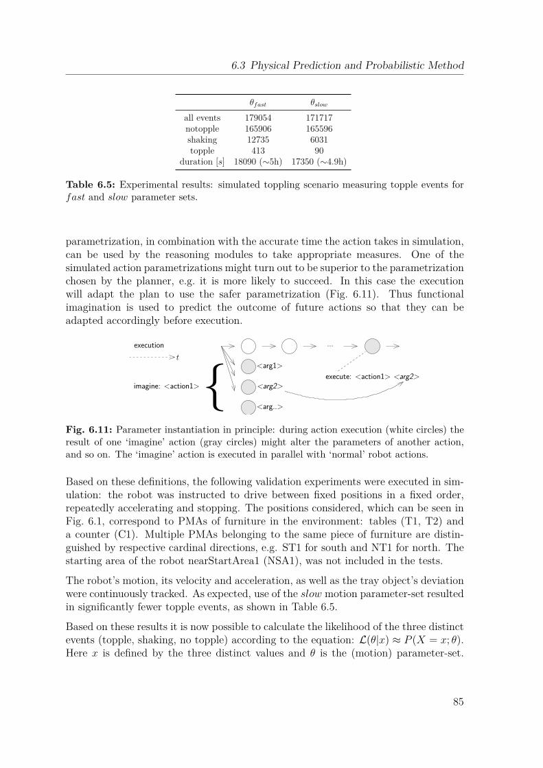
6.3 Physical Prediction and Probabilistic Method

θfast θslow

all events 179054 171717notopple 165906 165596shaking 12735 6031topple 413 90

duration [s] 18090 (∼5h) 17350 (∼4.9h)

Table 6.5: Experimental results: simulated toppling scenario measuring topple events forfast and slow parameter sets.

parametrization, in combination with the accurate time the action takes in simulation,can be used by the reasoning modules to take appropriate measures. One of thesimulated action parametrizations might turn out to be superior to the parametrizationchosen by the planner, e.g. it is more likely to succeed. In this case the executionwill adapt the plan to use the safer parametrization (Fig. 6.11). Thus functionalimagination is used to predict the outcome of future actions so that they can beadapted accordingly before execution.

...

execute: <action1> <arg2>

<arg1>

<arg2>imagine: <action1>{execution

<arg..>

t

Fig. 6.11: Parameter instantiation in principle: during action execution (white circles) theresult of one ‘imagine’ action (gray circles) might alter the parameters of another action,and so on. The ‘imagine’ action is executed in parallel with ‘normal’ robot actions.

Based on these definitions, the following validation experiments were executed in sim-ulation: the robot was instructed to drive between fixed positions in a fixed order,repeatedly accelerating and stopping. The positions considered, which can be seen inFig. 6.1, correspond to PMAs of furniture in the environment: tables (T1, T2) anda counter (C1). Multiple PMAs belonging to the same piece of furniture are distin-guished by respective cardinal directions, e.g. ST1 for south and NT1 for north. Thestarting area of the robot nearStartArea1 (NSA1), was not included in the tests.

The robot’s motion, its velocity and acceleration, as well as the tray object’s deviationwere continuously tracked. As expected, use of the slow motion parameter-set resultedin significantly fewer topple events, as shown in Table 6.5.

Based on these results it is now possible to calculate the likelihood of the three distinctevents (topple, shaking, no topple) according to the equation: L(θ|x) ≈ P (X = x; θ).Here x is defined by the three distinct values and θ is the (motion) parameter-set.

85

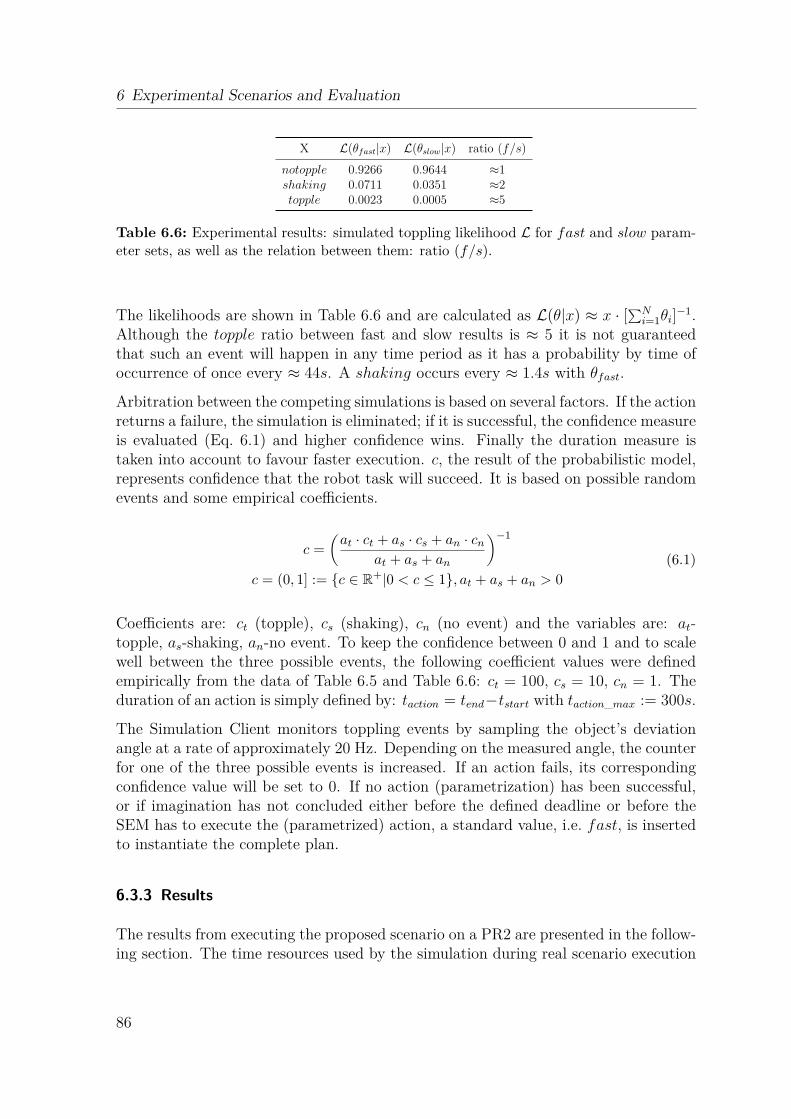
6 Experimental Scenarios and Evaluation

X L(θfast|x) L(θslow|x) ratio (f/s)

notopple 0.9266 0.9644 ≈1shaking 0.0711 0.0351 ≈2topple 0.0023 0.0005 ≈5

Table 6.6: Experimental results: simulated toppling likelihood L for fast and slow param-eter sets, as well as the relation between them: ratio (f/s).

The likelihoods are shown in Table 6.6 and are calculated as L(θ|x) ≈ x · [∑N

i=1θi]−1.

Although the topple ratio between fast and slow results is ≈ 5 it is not guaranteedthat such an event will happen in any time period as it has a probability by time ofoccurrence of once every ≈ 44s. A shaking occurs every ≈ 1.4s with θfast.

Arbitration between the competing simulations is based on several factors. If the actionreturns a failure, the simulation is eliminated; if it is successful, the confidence measureis evaluated (Eq. 6.1) and higher confidence wins. Finally the duration measure istaken into account to favour faster execution. c, the result of the probabilistic model,represents confidence that the robot task will succeed. It is based on possible randomevents and some empirical coefficients.

c =(

at · ct + as · cs + an · cn

at + as + an

)

−1

c = (0, 1] := {c ∈ R+|0 < c ≤ 1}, at + as + an > 0

(6.1)

Coefficients are: ct (topple), cs (shaking), cn (no event) and the variables are: at-topple, as-shaking, an-no event. To keep the confidence between 0 and 1 and to scalewell between the three possible events, the following coefficient values were definedempirically from the data of Table 6.5 and Table 6.6: ct = 100, cs = 10, cn = 1. Theduration of an action is simply defined by: taction = tend−tstart with taction_max := 300s.

The Simulation Client monitors toppling events by sampling the object’s deviationangle at a rate of approximately 20 Hz. Depending on the measured angle, the counterfor one of the three possible events is increased. If an action fails, its correspondingconfidence value will be set to 0. If no action (parametrization) has been successful,or if imagination has not concluded either before the defined deadline or before theSEM has to execute the (parametrized) action, a standard value, i.e. fast, is insertedto instantiate the complete plan.

6.3.3 Results

The results from executing the proposed scenario on a PR2 are presented in the follow-ing section. The time resources used by the simulation during real scenario execution

86

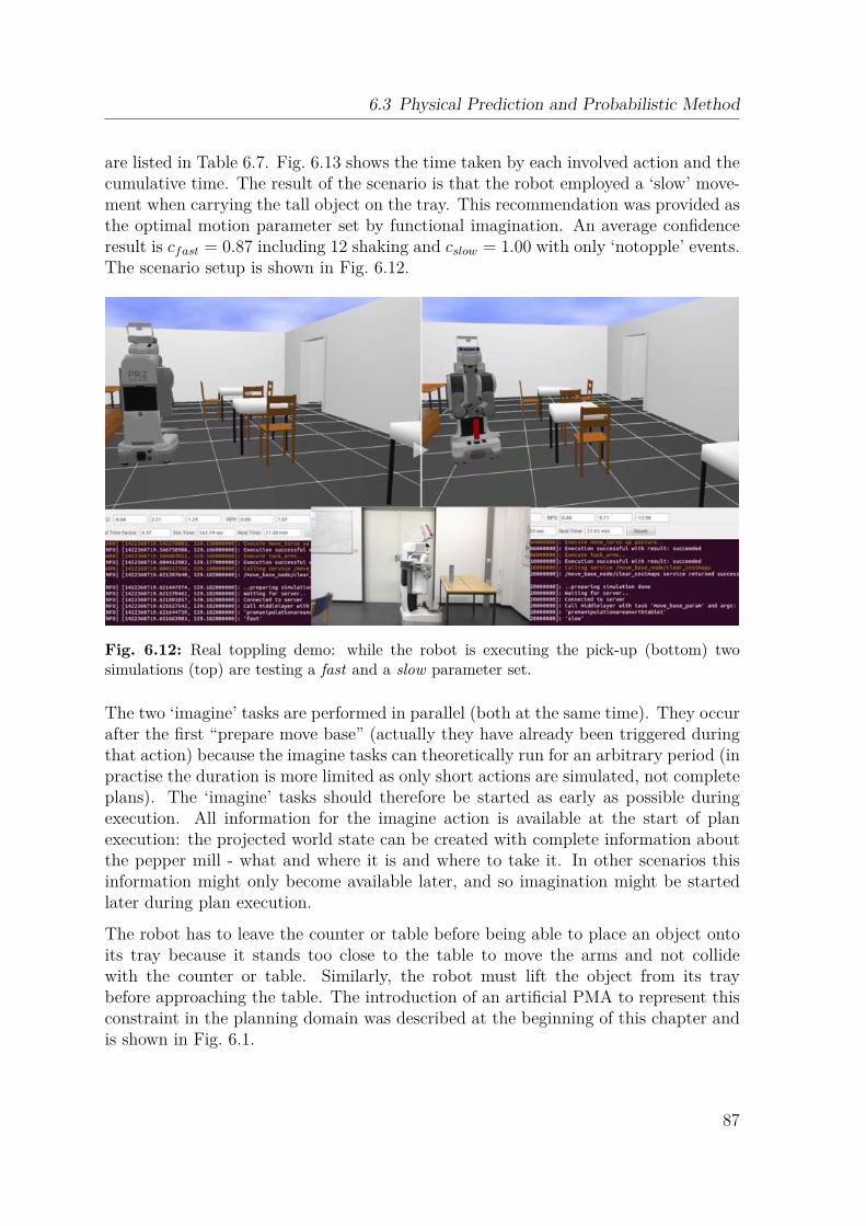
6.3 Physical Prediction and Probabilistic Method

are listed in Table 6.7. Fig. 6.13 shows the time taken by each involved action and thecumulative time. The result of the scenario is that the robot employed a ‘slow’ move-ment when carrying the tall object on the tray. This recommendation was provided asthe optimal motion parameter set by functional imagination. An average confidenceresult is cfast = 0.87 including 12 shaking and cslow = 1.00 with only ‘notopple’ events.The scenario setup is shown in Fig. 6.12.

Fig. 6.12: Real toppling demo: while the robot is executing the pick-up (bottom) twosimulations (top) are testing a fast and a slow parameter set.

The two ‘imagine’ tasks are performed in parallel (both at the same time). They occurafter the first “prepare move base” (actually they have already been triggered duringthat action) because the imagine tasks can theoretically run for an arbitrary period (inpractise the duration is more limited as only short actions are simulated, not completeplans). The ‘imagine’ tasks should therefore be started as early as possible duringexecution. All information for the imagine action is available at the start of planexecution: the projected world state can be created with complete information aboutthe pepper mill - what and where it is and where to take it. In other scenarios thisinformation might only become available later, and so imagination might be startedlater during plan execution.

The robot has to leave the counter or table before being able to place an object ontoits tray because it stands too close to the table to move the arms and not collidewith the counter or table. Similarly, the robot must lift the object from its traybefore approaching the table. The introduction of an artificial PMA to represent thisconstraint in the planning domain was described at the beginning of this chapter andis shown in Fig. 6.1.

87

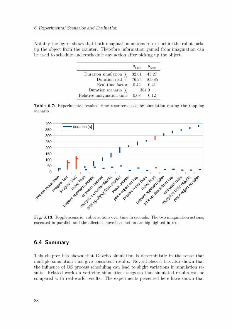
6 Experimental Scenarios and Evaluation

Notably the figure shows that both imagination actions return before the robot picksup the object from the counter. Therefore information gained from imagination canbe used to schedule and reschedule any action after picking up the object.

θfast θslow

Duration simulation [s] 32.01 45.27Duration real [s] 76.24 109.85Real-time factor 0.42 0.41

Duration scenario [s] 384.0Relative imagination time 0.08 0.12

Table 6.7: Experimental results: time resources used by simulation during the topplingscenario.

Fig. 6.13: Topple scenario: robot actions over time in seconds. The two imagination actions,executed in parallel, and the affected move base action are highlighted in red.

6.4 Summary

This chapter has shown that Gazebo simulation is deterministic in the sense thatmultiple simulation runs give consistent results. Nevertheless it has also shown thatthe influence of OS process scheduling can lead to slight variations in simulation re-sults. Related work on verifying simulations suggests that simulated results can becompared with real-world results. The experiments presented here have shown that

88

6.4 Summary

simulation results from the selected physics engine (ODE) can accurately predict real-world states. Related work suggests that ODE performs well in comparison with otherphysics engines.

These results have shown that offline simulation can be of benefit in obtaining optimalparameters. The results from various experimental scenarios show merit in the causal,temporal and spatial aspects of simulation. The different aspects of the proposedprediction system have shown that prediction aided by simulation can prevent planfailures, i.e. by plan change or replanning. It has also been shown that the resultingsystem is more efficient, i.e. actions execute in less time, supporting the hypothesisstated in Section 1.4. The final chapter, Chapter 7, presents some conclusions and anoutlook.

89

Conclusion and Outlook

7

This chapter summarizes the evaluation and findings of this work. It discusses thevalue of the results and finally looks at future developments.

This work set out to answer the research question stated in Chapter 1: How can atask planning based robot system be improved by prediction derived from physical sim-ulation? A precondition for success was that simulation is accurate enough to allowcomparison with real world execution. The very similar test durations in simulationand on the real robot (shown by the results in Section 6.1) indicate that such compar-ison is indeed valid and support the use of the selected physics engine.

To answer the research question, the method of “functional imagination” was inte-grated: a realistic prediction of robot activities, based on physical simulation, wasintegrated into a plan and execution-based system (Chapter 5 describes how it isdone, i.e. the approach, cf. Section 1.4). As the results in Chapter 6 show, this systemadapts its plan (or replans) before executing plan actions that simulation shows arelikely to fail.

The PR2 mobile robot platform is accurate, extensible and well suited as an evaluationplatform. Hardware extensions are straightforward to apply. This allowed the mount-ing of a tray (to carry additional objects) and of extra sensors (such as a laser rangefinder and a thermal camera) as well as the addition of auxiliary robot capabilitiesthat allowed objects to be carried with the robot arms while driving. The robot wasable to execute all scenarios related to the evaluation of this work.

As a basis for the software framework used in this work, a distributed ROS-basedrobot control architecture was developed in the context of the RACE project. Thiswas extended to incorporate a physics-based simulation that predicts robot actionresults with a high-level, plan-based, cognitive system.

To compensate for execution speed limitations caused by simulation, a method thatinterleaves simulation and real-world action execution was chosen. A probabilisticapproach was used to project perfect simulation results onto the real world. The stateof each simulation was sampled during execution to obtain the probability distributionof possible outcomes. The simulation granularity, in terms of action parametrization,remains limited by execution speed to certain planned actions and alternatives.

91

7 Conclusion and Outlook

The hypothesis stated in this work was:

A system integrating such prediction is more efficient (such as requiring less time, plansteps) than a comparable system without.

The experiments in Chapter 6 showed that various failure conditions could be detectedand that such failure prediction could lead to improved overall system robustness (thescenario could be completed) and execution time. Similarly, in physical predictionscenarios the use of simulation allowed the robot to carry objects without the objecttoppling. This improves the robustness of robot actions and allows tasks to be carriedout more efficiently. The results verify the hypothesis.

In principle, the computational cost of simulation limits the sample size and the dura-tion of actions. Nevertheless the practical scenario presented showed that interleavingsimulation with execution does not necessarily incur extra costs.

7.1 Conclusion

The main experimental findings are summarized in Chapter 6. This section assemblesthe findings to answer the study’s research question: How can a task planning basedrobot system be improved by prediction derived from physical simulation?

1. Functional imagination methodology: The system architecture presentedhere combines the traditional SPA control paradigm with functional imagina-tion to create a high-level, plan-based, reasoning and execution system (cf. Sec-tion 5.1). This has been demonstrated in a conceptional and experimental way.

2. Plan operators: The limitation of simulating only plan actions instead of (par-tial) plans appeared to be purely qualitative, as not all actions must be simulated.Assigning each imagination action to an imagination operator in a symbolic HTNplanner provided an abstract and adaptable method (cf. Section 5.2).

3. Handling uncertainty: The proposed probabilistic approach samples simula-tion to accommodate uncertainty and allows uncertainty to be represented as aconfidence value (cf. Section 6.3).

4. Simulation accuracy: The experiments verified that in simulation, robot ac-tions execute accurately enough to allow the comparison of simulation resultswith reality (cf. Section 6.1).

5. Distributed system approach: The distributed system architecture presentedhere provides the required performance and compensates for the resource bot-tleneck imposed by sophisticated physical simulation (cf. Section 5.2). Theperformance scales linearly with the number of actions to be simulated O(n),and is constant when actions are executed in parallel O(1), in the sense thatadditional hardware can be added on demand.

92

7.2 Limitations and Future Research

6. Common Sense: Experiments testing recognition and manipulation of the en-vironment using different robot postures demonstrated the potential for physicalsimulation to enhance competence (cf. Section 6.2.1).

7. Action parametrization: The parametrization approach showed that actionfailure (and thus possible plan failure) could be prevented and that the plan couldbe successfully completed. Execution measurements demonstrated that althoughsimulation is expensive, overall system execution time could be improved (cf.Sections 6.2.2, 6.3.2).

8. Training data generation for learning: The proposed automated executionframework ASEF supports the creation of training data from robot experiences(cf. Section 5.7).

While compliant with state-of-the-art approaches (cf. [KDB11, dSPA13]), this workdiffers significantly in the way simulation is applied to the finding of optimal actionparameters and to the discovery of a suitable robot plan. Its main contribution is theuse of simulation as a general companion tool to robot reasoning. Moreover, it usessimulation during (plan) execution in order to adapt current behavior to unforeseenevents in the robot environment. And it contributes to the understanding of theprobabilistic nature of real world uncertainty in robot action results.

Evidence from this work and that of several others, including Beetz [KHB12, KDB11,KDGB11, Bee00, MB09], indicates that simulation is a suitable companion for im-proving real world robot competence, beside being a helpful tool in developing andevaluating software for robots. Empirical findings in this work show that simulationcan be used to represent the world state, to reason about it and to adapt robot be-havior on-the-fly. The theoretical arguments in favour of this method could influencefuture methodologies in the design of robot control programs and could thus supportcognitive improvement of future systems.

7.2 Limitations and Future Research

The proposed simulation-based prediction approach is capable of testing all robotactions before they are executed in reality. The current approach is limited to ‘imag-ining’ one action a time, which makes functional imagination strongly dependent onplan-step granularity; granularity is based on the underlying atomic robot capabilities,such as moving the robot to a destination. A valid future research question, therefore,is how functional imagination could benefit from either intra-plan-step prediction orpartial-plan prediction. An example could be whether parametrization of the robot’sdrive action can be extended to adapt to a global optimized trajectory. This can berealized by dividing a trajectory into multiple parts, for each of which a simulationprovides the optimal motion parametrization. This approach should lead to faster

93

7 Conclusion and Outlook

overall trajectories, as only part of each trajectory might have to be executed with aslow-motion parameter set.

The current approach uses simulated action results in order to parametrize actions ofan existing plan. If an action fails in all tested configurations, it will be necessary toproduce a new plan, i.e. to perform re-scheduling. Therefore future research mightinvestigate whether a re-scheduling integration approach improves robot competence.

Action durations are determined during simulation (temporal prediction), but thepresent system takes no advantage of these (although they are quite accurate, cf.Section 6.1). For example, in the case of temporal-constraint execution monitoring,an action must be executed before or after another action, or it might not be executedat all. Thus taking simulated action durations into account during execution alsoenforces re-scheduling.

Other future research questions arise from the development of faster computer hard-ware and more complex scenarios: How can parallelization help a plan benefit fromfaster distributed systems? And how does the use of greater computational power af-fect action simulation granularity? In a recent article [Pra15] the author sees a “Cam-brian Explosion-like” development in robotics, partly coming from cloud-computing.“Learning from Imagination” is supposed to be one of the biggest ideas exploitingcloud-computing for robotics. Computational simulation power helps therein

. . . to explore circumstances that may be faced by a robot in the futureand to experiment with possible solutions, remembering only those thatworked. Such simulations can be done without the need for any physicalactivity, and every robot’s dreams will improve the performance of allrobots.

As a final future research recommendation, there is the question of how other phys-ical simulation engines perform compared to the ODE engine used here. Qualitativeperformance and feature analyses might be helpful. For example other engines mightsupport non-rigid-body interactions.

This thesis has presented an evaluative perspective of simulation accuracy and of theimprovements achieved in mobile robot performance and competence. The inclusionof many more test samples would certainly strengthen the findings.

Furthermore this thesis has presented an approach by which common-sense physicsknowledge can be exploited to prevent robot action failure in the field of mobile servicerobotics. It is hoped that this approach will help advance research and developmentand that it will support the creation of new service robotics applications. The workcovered four major aspects in this context. Firstly, it defined and implemented aprobabilistic method for the use of simulation as a direct model representing therobot’s world state. Secondly, it validated the simulation of real-robot actions as anappropriate tool. Thirdly, it developed the concept of “functional imagination” using

94

7.2 Limitations and Future Research

simulation to predict robot action results. Finally, it designed an architecture thatintegrates “functional imagination” into a high-level, cognitive, plan-based system.

The system presented integrated high-level symbolic reasoning and concrete physics-based reasoning and ran in parallel on a PR2 robot and in the Gazebo simulation. Thescenarios presented in Chapter 6 showed how physics-based common-sense knowledgecan improve a plan-based high-level cognitive system via action parametrization.

In summary, this work proposed a methodology for the use of a physical simulationto make planning and reasoning systems more robust when dealing with real-worldscenarios. Similar systems have in recent years made significant progress, incorporatingdedicated geometric robot capabilities into the planning and reasoning process. Thishas already led to a significant increase in robot system performance. The innovationrate and the number of publications in this field indicate the potential importance ofemploying non-abstract reasoning in symbolic-based AI systems. This work provides ageneral approach by which systems can benefit from low-level, physics-based reasoning.This, it is hoped, will contribute to and accelerate the acceptance of simulation-basedprediction in future intelligent mobile service robotics.

95

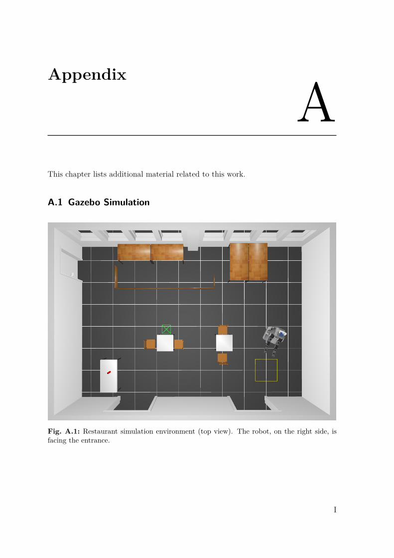
Appendix

A

This chapter lists additional material related to this work.

A.1 Gazebo Simulation

Fig. A.1: Restaurant simulation environment (top view). The robot, on the right side, isfacing the entrance.

I

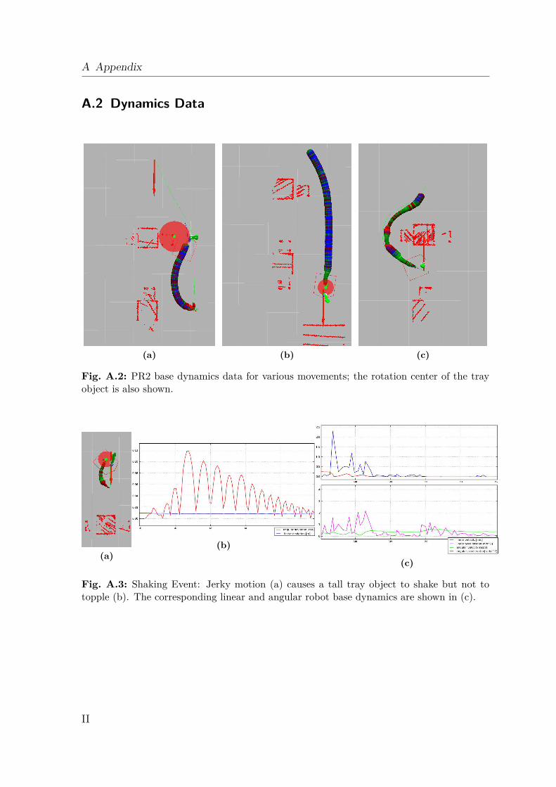
A Appendix

A.2 Dynamics Data

(a) (b) (c)

Fig. A.2: PR2 base dynamics data for various movements; the rotation center of the trayobject is also shown.

(a)(b)

(c)

Fig. A.3: Shaking Event: Jerky motion (a) causes a tall tray object to shake but not totopple (b). The corresponding linear and angular robot base dynamics are shown in (c).

II

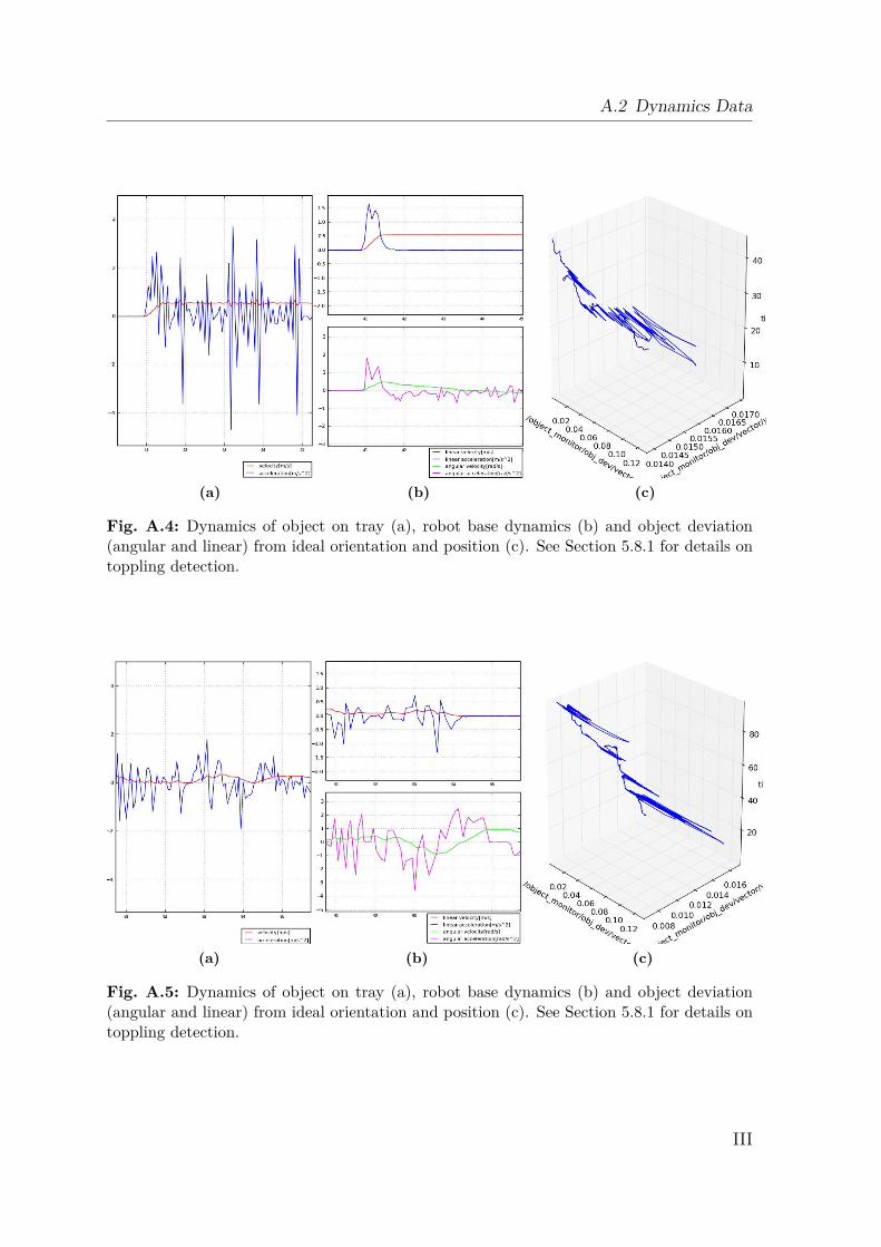
A.2 Dynamics Data

(a) (b) (c)

Fig. A.4: Dynamics of object on tray (a), robot base dynamics (b) and object deviation(angular and linear) from ideal orientation and position (c). See Section 5.8.1 for details ontoppling detection.

(a) (b) (c)

Fig. A.5: Dynamics of object on tray (a), robot base dynamics (b) and object deviation(angular and linear) from ideal orientation and position (c). See Section 5.8.1 for details ontoppling detection.

III

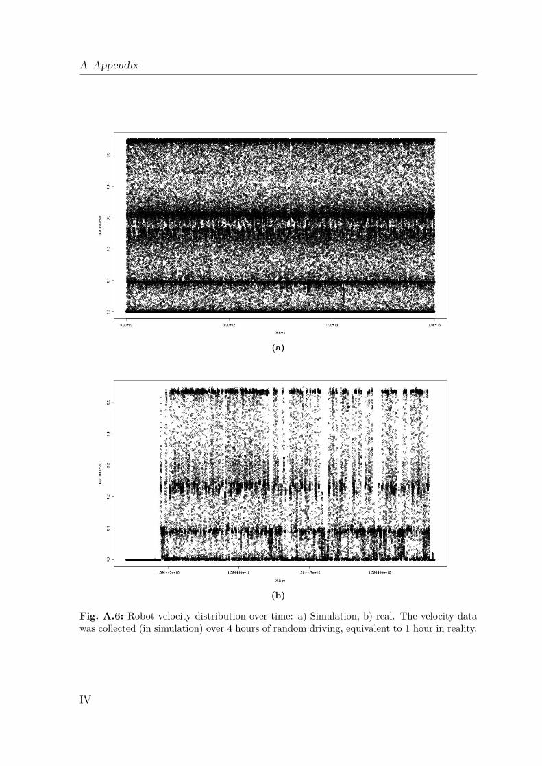
A Appendix

(a)

(b)

Fig. A.6: Robot velocity distribution over time: a) Simulation, b) real. The velocity datawas collected (in simulation) over 4 hours of random driving, equivalent to 1 hour in reality.

IV

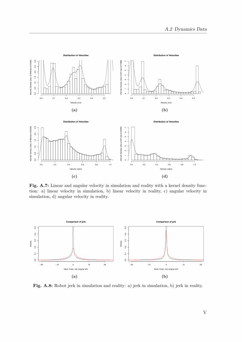
A.2 Dynamics Data

Distribution of Velocities

Velocity (m/s)

(Kern

el) D

ensity (

obs=

97309,b

w=

0.0

1833)

0.0 0.1 0.2 0.3 0.4 0.5

0.0

0.5

1.0

1.5

2.0

2.5

3.0

(a)

Distribution of Velocities

Velocity (m/s)

(Kern

el) D

ensity (

obs=

41031,b

w=

0.0

1989)

0.0 0.1 0.2 0.3 0.4 0.5

01

23

45

67

(b)

Distribution of Velocities

Velocity (rad/s)

(Kern

el) D

ensity (

obs=

97309,b

w=

0.0

2335)

0.0 0.2 0.4 0.6 0.8 1.0

0.0

0.5

1.0

1.5

2.0

2.5

(c)

Distribution of Velocities

Velocity (rad/s)

(Kern

el) D

ensity (

obs=

41031,b

w=

0.0

3094)

0.0 0.2 0.4 0.6 0.8 1.0

01

23

45

67

(d)

Fig. A.7: Linear and angular velocity in simulation and reality with a kernel density func-tion: a) linear velocity in simulation, b) linear velocity in reality, c) angular velocity insimulation, d) angular velocity in reality.

−20 −10 0 10 20

0.0

0.1

0.2

0.3

0.4

0.5

Comparison of jerk

black: linear, red: angular jerk

Density

(a)

−20 −10 0 10 20

0.0

0.1

0.2

0.3

0.4

0.5

Comparison of jerk

black: linear, red: angular jerk

Density

(b)

Fig. A.8: Robot jerk in simulation and reality: a) jerk in simulation, b) jerk in reality.

V

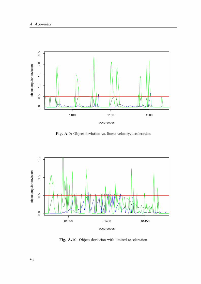
A Appendix

1100 1150 1200

0.0

0.5

1.0

1.5

2.0

2.5

occurences

ob

ject

an

gu

lar

devia

tio

n

Fig. A.9: Object deviation vs. linear velocity/acceleration

61350 61400 61450

0.0

0.5

1.0

1.5

occurences

ob

ject

an

gu

lar

devia

tio

n

Fig. A.10: Object deviation with limited acceleration

VI

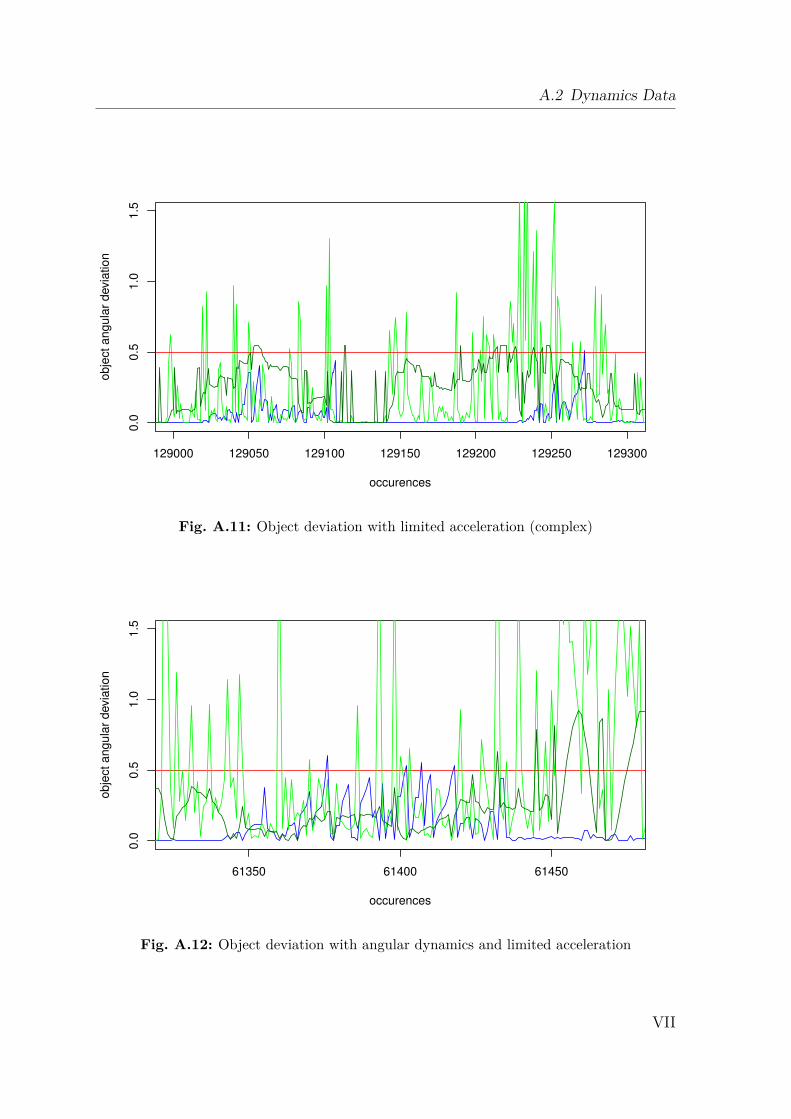
A.2 Dynamics Data

129000 129050 129100 129150 129200 129250 129300

0.0

0.5

1.0

1.5

occurences

ob

ject

an

gu

lar

devia

tio

n

Fig. A.11: Object deviation with limited acceleration (complex)

61350 61400 61450

0.0

0.5

1.0

1.5

occurences

ob

ject

an

gu

lar

devia

tio

n

Fig. A.12: Object deviation with angular dynamics and limited acceleration

VII

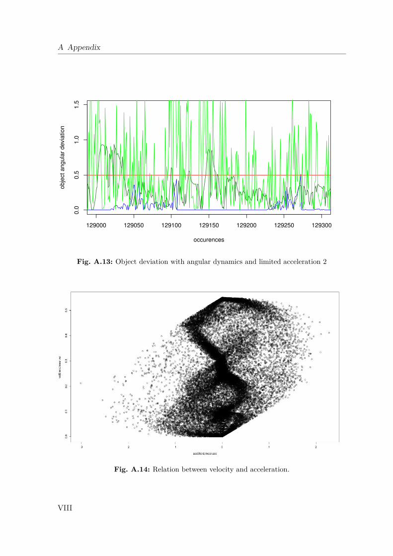
A Appendix

129000 129050 129100 129150 129200 129250 129300

0.0

0.5

1.0

1.5

occurences

ob

ject

an

gu

lar

devia

tio

n

Fig. A.13: Object deviation with angular dynamics and limited acceleration 2

Fig. A.14: Relation between velocity and acceleration.

VIII

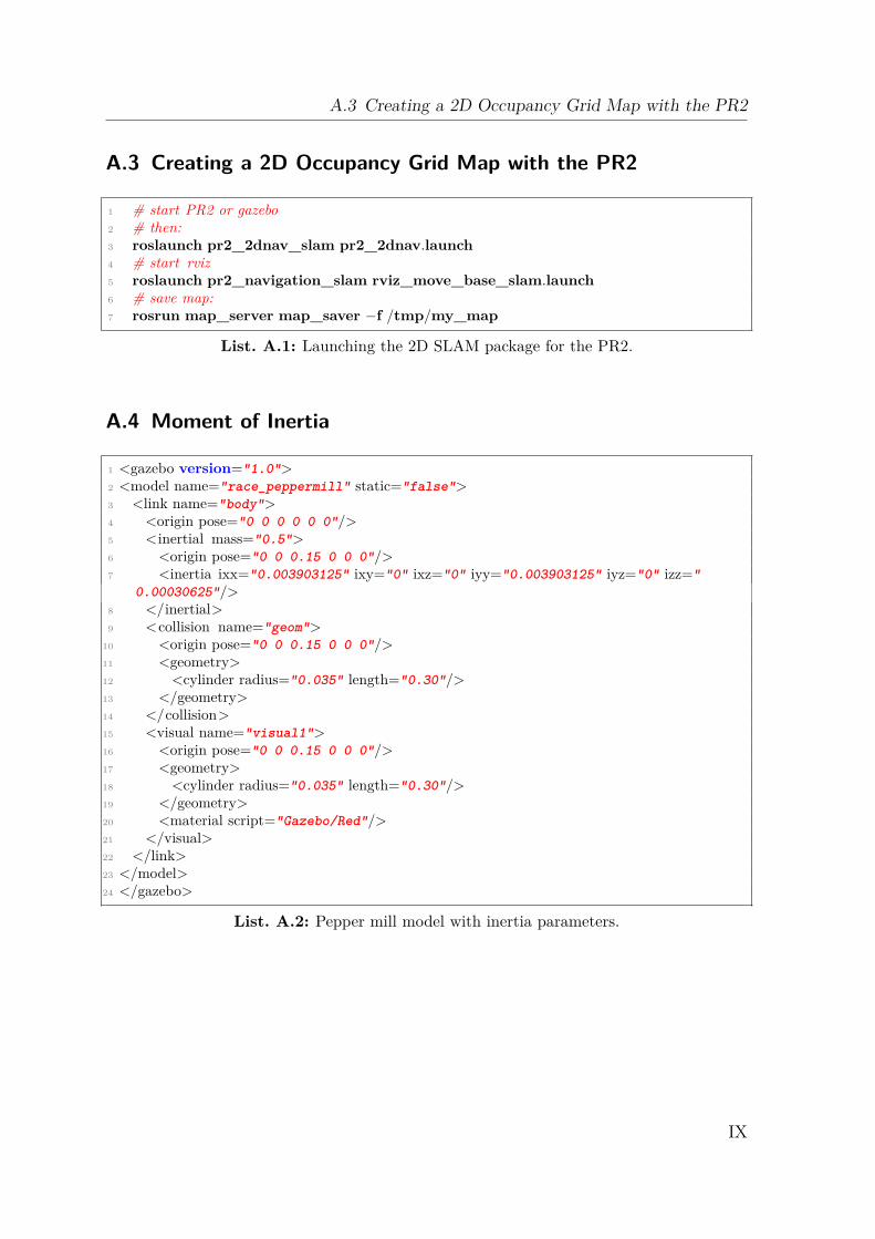
A.3 Creating a 2D Occupancy Grid Map with the PR2

A.3 Creating a 2D Occupancy Grid Map with the PR2

1 # start PR2 or gazebo

2 # then:

3 roslaunch pr2_2dnav_slam pr2_2dnav.launch4 # start rviz

5 roslaunch pr2_navigation_slam rviz_move_base_slam.launch6 # save map:

7 rosrun map_server map_saver −f /tmp/my_map

List. A.1: Launching the 2D SLAM package for the PR2.

A.4 Moment of Inertia

1 <gazebo version="1.0">2 <model name="race_peppermill" static="false">3 <link name="body">4 <origin pose="0 0 0 0 0 0"/>5 <inertial mass="0.5">6 <origin pose="0 0 0.15 0 0 0"/>7 <inertia ixx="0.003903125" ixy="0" ixz="0" iyy="0.003903125" iyz="0" izz="

0.00030625"/>8 </inertial>9 <collision name="geom">

10 <origin pose="0 0 0.15 0 0 0"/>11 <geometry>12 <cylinder radius="0.035" length="0.30"/>13 </geometry>14 </collision>15 <visual name="visual1">16 <origin pose="0 0 0.15 0 0 0"/>17 <geometry>18 <cylinder radius="0.035" length="0.30"/>19 </geometry>20 <material script="Gazebo/Red"/>21 </visual>22 </link>23 </model>24 </gazebo>

List. A.2: Pepper mill model with inertia parameters.

IX

A Appendix

A.5 Standard Deviation and Normal Distribution

Here the random variable is X and the mean value is µ. The standard deviation iscalculated as follows σ =

√

(X − µ)2. For discrete distributions the following equation

is appropriate: σ =

√

1N

N∑

i=1(xi − µ)2, where µ = 1

N

N∑

i=1xi, for the same probability and

for all x. The normal probability density function is as follows: f(x) = 1σ

√

2πe−

1

2σ2

(x−µ)2

X

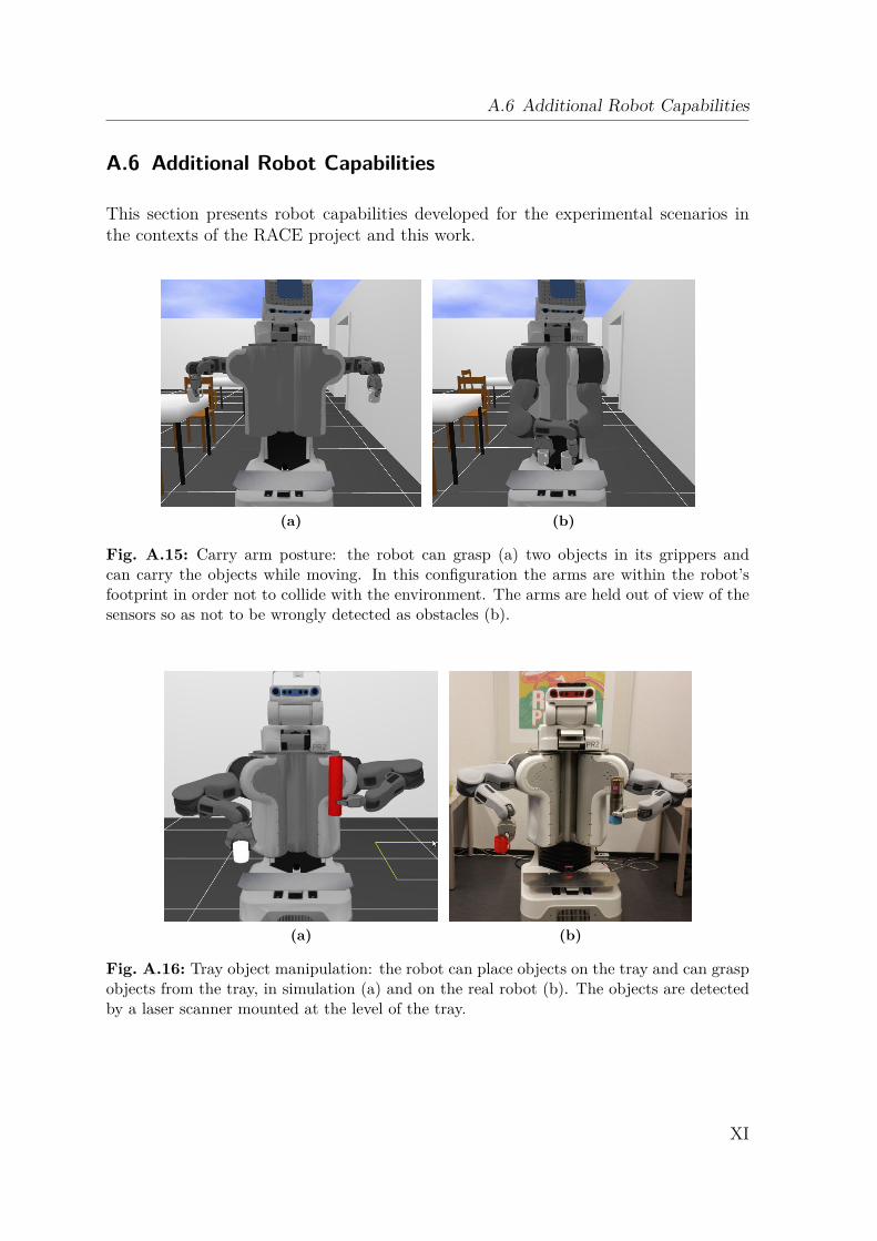
A.6 Additional Robot Capabilities

A.6 Additional Robot Capabilities

This section presents robot capabilities developed for the experimental scenarios inthe contexts of the RACE project and this work.

(a) (b)

Fig. A.15: Carry arm posture: the robot can grasp (a) two objects in its grippers andcan carry the objects while moving. In this configuration the arms are within the robot’sfootprint in order not to collide with the environment. The arms are held out of view of thesensors so as not to be wrongly detected as obstacles (b).

(a) (b)

Fig. A.16: Tray object manipulation: the robot can place objects on the tray and can graspobjects from the tray, in simulation (a) and on the real robot (b). The objects are detectedby a laser scanner mounted at the level of the tray.

XI

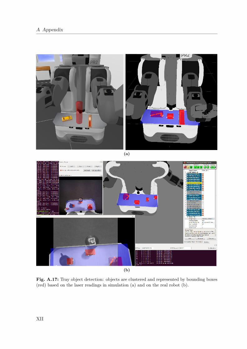
A Appendix

(a)

(b)

Fig. A.17: Tray object detection: objects are clustered and represented by bounding boxes(red) based on the laser readings in simulation (a) and on the real robot (b).

XII

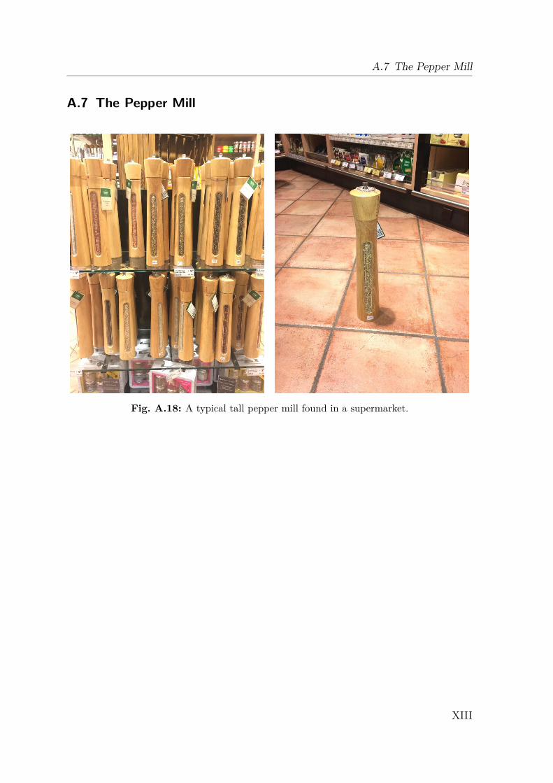
A.7 The Pepper Mill

A.7 The Pepper Mill

Fig. A.18: A typical tall pepper mill found in a supermarket.

XIII

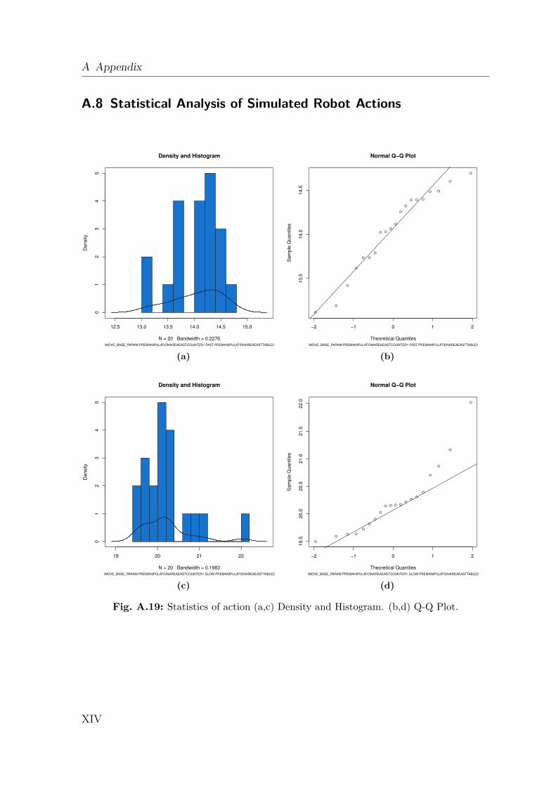
A Appendix

A.8 Statistical Analysis of Simulated Robot Actions

12.5 13.0 13.5 14.0 14.5 15.0

01

23

45

Density and Histogram

N = 20 Bandwidth = 0.2276

Density

!MOVE_BASE_PARAM PREMANIPULATIONAREAEASTCOUNTER1 FAST PREMANIPULATIONAREAEASTTABLE2

(a)

●

●

●

●

●

●

●

●

●

●

●

●

●

●

●

●

●

●

●

●

−2 −1 0 1 2

13.5

14.0

14.5

Normal Q−Q Plot

Theoretical Quantiles

Sam

ple

Quantile

s

!MOVE_BASE_PARAM PREMANIPULATIONAREAEASTCOUNTER1 FAST PREMANIPULATIONAREAEASTTABLE2

(b)

19 20 21 22

01

23

45

Density and Histogram

N = 20 Bandwidth = 0.1983

Density

!MOVE_BASE_PARAM PREMANIPULATIONAREAEASTCOUNTER1 SLOW PREMANIPULATIONAREAEASTTABLE2

(c)

●

●

●

●

●

●

●

●

●

●

●

●

●

●

●

●

●●

●

●

−2 −1 0 1 2

19.5

20.0

20.5

21.0

21.5

22.0

Normal Q−Q Plot

Theoretical Quantiles

Sam

ple

Quantile

s

!MOVE_BASE_PARAM PREMANIPULATIONAREAEASTCOUNTER1 SLOW PREMANIPULATIONAREAEASTTABLE2

(d)

Fig. A.19: Statistics of action (a,c) Density and Histogram. (b,d) Q-Q Plot.

XIV

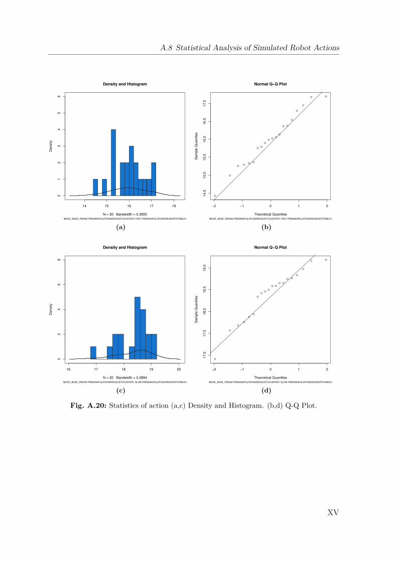
A.8 Statistical Analysis of Simulated Robot Actions

14 15 16 17 18

01

23

45

6

Density and Histogram

N = 20 Bandwidth = 0.3655

Density

!MOVE_BASE_PARAM PREMANIPULATIONAREAEASTCOUNTER1 FAST PREMANIPULATIONAREANORTHTABLE1

(a)

●

●

●

●

●●

●

●

●

●

●

●

●

●

●

●

●

●

●

●

−2 −1 0 1 214.5

15.0

15.5

16.0

16.5

17.0

Normal Q−Q Plot

Theoretical Quantiles

Sam

ple

Quantile

s

!MOVE_BASE_PARAM PREMANIPULATIONAREAEASTCOUNTER1 FAST PREMANIPULATIONAREANORTHTABLE1

(b)

16 17 18 19 20

02

46

8

Density and Histogram

N = 20 Bandwidth = 0.2894

Density

!MOVE_BASE_PARAM PREMANIPULATIONAREAEASTCOUNTER1 SLOW PREMANIPULATIONAREANORTHTABLE1

(c)

●

●

●

●

●

●

●

●

●

●

●

●

●

●

●

●

●

●

●

●

−2 −1 0 1 2

17.0

17.5

18.0

18.5

19.0

Normal Q−Q Plot

Theoretical Quantiles

Sam

ple

Quantile

s

!MOVE_BASE_PARAM PREMANIPULATIONAREAEASTCOUNTER1 SLOW PREMANIPULATIONAREANORTHTABLE1

(d)

Fig. A.20: Statistics of action (a,c) Density and Histogram. (b,d) Q-Q Plot.

XV

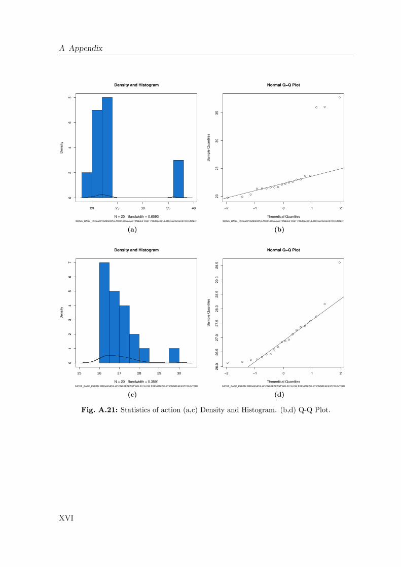
A Appendix

20 25 30 35 40

02

46

8

Density and Histogram

N = 20 Bandwidth = 0.6593

Density

!MOVE_BASE_PARAM PREMANIPULATIONAREAEASTTABLE2 FAST PREMANIPULATIONAREAEASTCOUNTER1

(a)

●

●

●

●

●

●

●●

●

●●

●

●

●

●

●

●

●●

●

−2 −1 0 1 2

20

25

30

35

Normal Q−Q Plot

Theoretical Quantiles

Sam

ple

Quantile

s

!MOVE_BASE_PARAM PREMANIPULATIONAREAEASTTABLE2 FAST PREMANIPULATIONAREAEASTCOUNTER1

(b)

25 26 27 28 29 30

01

23

45

67

Density and Histogram

N = 20 Bandwidth = 0.3591

Density

!MOVE_BASE_PARAM PREMANIPULATIONAREAEASTTABLE2 SLOW PREMANIPULATIONAREAEASTCOUNTER1

(c)

●

●

●

●

●

●

●

●

●

●

●

●

●●

●

●

●

●

●

●

−2 −1 0 1 2

26.0

26.5

27.0

27.5

28.0

28.5

29.0

29.5

Normal Q−Q Plot

Theoretical Quantiles

Sam

ple

Quantile

s

!MOVE_BASE_PARAM PREMANIPULATIONAREAEASTTABLE2 SLOW PREMANIPULATIONAREAEASTCOUNTER1

(d)

Fig. A.21: Statistics of action (a,c) Density and Histogram. (b,d) Q-Q Plot.

XVI

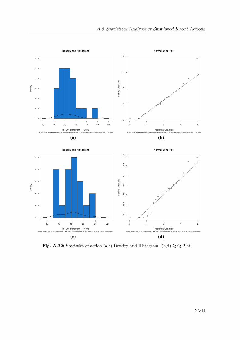
A.8 Statistical Analysis of Simulated Robot Actions

13 14 15 16 17 18 19

01

23

45

6

Density and Histogram

N = 20 Bandwidth = 0.3932

Density

!MOVE_BASE_PARAM PREMANIPULATIONAREANORTHTABLE1 FAST PREMANIPULATIONAREAEASTCOUNTER1

(a)

●

●

●

●

●

●

●

●

●

●

●

●

●

●

●

●

●

●

●

●

−2 −1 0 1 214

15

16

17

18

Normal Q−Q Plot

Theoretical Quantiles

Sam

ple

Quantile

s

!MOVE_BASE_PARAM PREMANIPULATIONAREANORTHTABLE1 FAST PREMANIPULATIONAREAEASTCOUNTER1

(b)

17 18 19 20 21 22

01

23

45

Density and Histogram

N = 20 Bandwidth = 0.4108

Density

!MOVE_BASE_PARAM PREMANIPULATIONAREANORTHTABLE1 SLOW PREMANIPULATIONAREAEASTCOUNTER1

(c)

●

●

●

●

●

● ●

●

●

●

●

●

●

●

● ●

●

●

●

●

−2 −1 0 1 2

18.0

18.5

19.0

19.5

20.0

20.5

21.0

Normal Q−Q Plot

Theoretical Quantiles

Sam

ple

Quantile

s

!MOVE_BASE_PARAM PREMANIPULATIONAREANORTHTABLE1 SLOW PREMANIPULATIONAREAEASTCOUNTER1

(d)

Fig. A.22: Statistics of action (a,c) Density and Histogram. (b,d) Q-Q Plot.

XVII

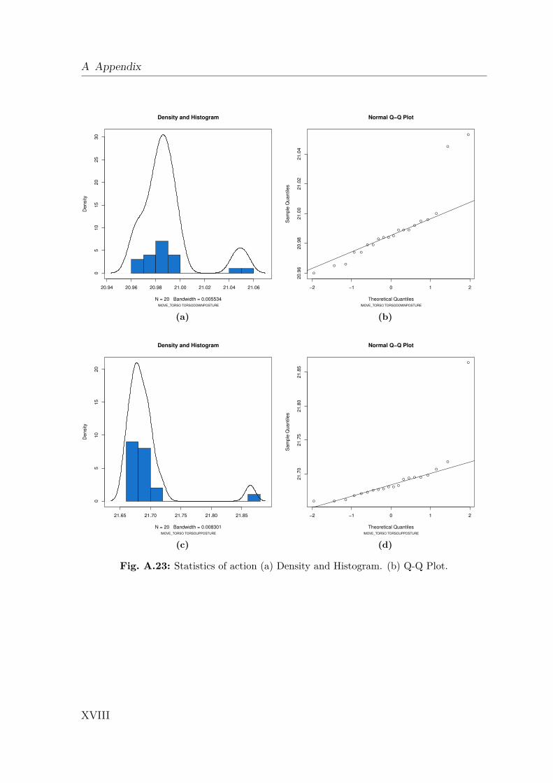
A Appendix

20.94 20.96 20.98 21.00 21.02 21.04 21.06

05

10

15

20

25

30

Density and Histogram

N = 20 Bandwidth = 0.005534

Density

!MOVE_TORSO TORSODOWNPOSTURE

(a)

●

●

●

●

●

●

●

●

●●

●

●

●

●●

●

●

●

●

●

−2 −1 0 1 2

20.9

620.9

821.0

021.0

221.0

4

Normal Q−Q Plot

Theoretical Quantiles

Sam

ple

Quantile

s

!MOVE_TORSO TORSODOWNPOSTURE

(b)

21.65 21.70 21.75 21.80 21.85

05

10

15

20

Density and Histogram

N = 20 Bandwidth = 0.008301

Density

!MOVE_TORSO TORSOUPPOSTURE

(c)

●

●

●

●

●

●●

●●

●

●

●

●

●●

●

●

●

●

●

−2 −1 0 1 2

21.7

021.7

521.8

021.8

5

Normal Q−Q Plot

Theoretical Quantiles

Sam

ple

Quantile

s

!MOVE_TORSO TORSOUPPOSTURE

(d)

Fig. A.23: Statistics of action (a) Density and Histogram. (b) Q-Q Plot.

XVIII

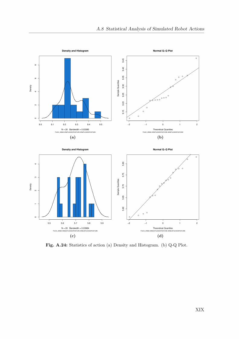
A.8 Statistical Analysis of Simulated Robot Actions

9.0 9.1 9.2 9.3 9.4 9.5

02

46

8

Density and Histogram

N = 20 Bandwidth = 0.03385

Density

!TUCK_ARMS ARMTUCKEDPOSTURE ARMTUCKEDPOSTURE

(a)

●

●

●

●

●

●

●

●

●

●

●

●

●

●

●

●

●●

●

●

−2 −1 0 1 29.1

59.2

09.2

59.3

09.3

59.4

09.4

5

Normal Q−Q Plot

Theoretical Quantiles

Sam

ple

Quantile

s

!TUCK_ARMS ARMTUCKEDPOSTURE ARMTUCKEDPOSTURE

(b)

5.5 5.6 5.7 5.8 5.9

01

23

4

Density and Histogram

N = 20 Bandwidth = 0.03984

Density

!TUCK_ARMS ARMUNTUCKEDPOSTURE ARMUNTUCKEDPOSTURE

(c)

●

●

●

●

●

●

●

●

●

●

●

●

●

●

●

●

●

●

●

●

−2 −1 0 1 2

5.6

05.6

55.7

05.7

55.8

0

Normal Q−Q Plot

Theoretical Quantiles

Sam

ple

Quantile

s

!TUCK_ARMS ARMUNTUCKEDPOSTURE ARMUNTUCKEDPOSTURE

(d)

Fig. A.24: Statistics of action (a) Density and Histogram. (b) Q-Q Plot.

XIX

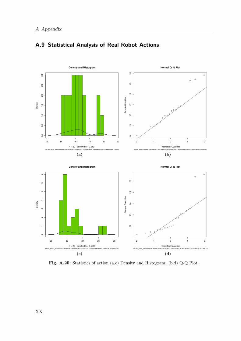
A Appendix

A.9 Statistical Analysis of Real Robot Actions

12 14 16 18 20 22

0.0

0.5

1.0

1.5

2.0

2.5

3.0

Density and Histogram

N = 20 Bandwidth = 0.6121

Density

!MOVE_BASE_PARAM PREMANIPULATIONAREAEASTCOUNTER1 FAST PREMANIPULATIONAREAEASTTABLE2

(a)

●

●

●

●●

●

● ●

●

●

●

●

●

●

●

●

●

●

●

●

−2 −1 0 1 2

14

15

16

17

18

19

20

Normal Q−Q Plot

Theoretical Quantiles

Sam

ple

Quantile

s

!MOVE_BASE_PARAM PREMANIPULATIONAREAEASTCOUNTER1 FAST PREMANIPULATIONAREAEASTTABLE2

(b)

20 22 24 26 28

01

23

45

67

Density and Histogram

N = 20 Bandwidth = 0.5239

Density

!MOVE_BASE_PARAM PREMANIPULATIONAREAEASTCOUNTER1 SLOW PREMANIPULATIONAREAEASTTABLE2

(c)

●

●

●

●

●

●●

●

●

●

●

●

●

●

●

●

●

●

●

●

−2 −1 0 1 2

22

23

24

25

26

Normal Q−Q Plot

Theoretical Quantiles

Sam

ple

Quantile

s

!MOVE_BASE_PARAM PREMANIPULATIONAREAEASTCOUNTER1 SLOW PREMANIPULATIONAREAEASTTABLE2

(d)

Fig. A.25: Statistics of action (a,c) Density and Histogram. (b,d) Q-Q Plot.

XX

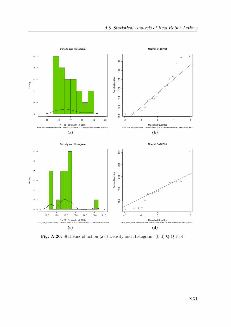
A.9 Statistical Analysis of Real Robot Actions

15 16 17 18 19 20

01

23

45

Density and Histogram

N = 20 Bandwidth = 0.3888

Density

!MOVE_BASE_PARAM PREMANIPULATIONAREAEASTCOUNTER1 FAST PREMANIPULATIONAREANORTHTABLE1

(a)

●

●

●

●●

●

●

●

●

●

●

●

●

●

●

●

●

●

●

●

−2 −1 0 1 215.5

16.0

16.5

17.0

17.5

18.0

18.5

Normal Q−Q Plot

Theoretical Quantiles

Sam

ple

Quantile

s

!MOVE_BASE_PARAM PREMANIPULATIONAREAEASTCOUNTER1 FAST PREMANIPULATIONAREANORTHTABLE1

(b)

18.5 19.0 19.5 20.0 20.5 21.0 21.5

01

23

45

6

Density and Histogram

N = 20 Bandwidth = 0.1678

Density

!MOVE_BASE_PARAM PREMANIPULATIONAREAEASTCOUNTER1 SLOW PREMANIPULATIONAREANORTHTABLE1

(c)

●

●

●

●

●●●●

●

●

●

●

●

●

●

●

●

●

●

●

−2 −1 0 1 2

19.0

19.5

20.0

20.5

21.0

Normal Q−Q Plot

Theoretical Quantiles

Sam

ple

Quantile

s

!MOVE_BASE_PARAM PREMANIPULATIONAREAEASTCOUNTER1 SLOW PREMANIPULATIONAREANORTHTABLE1

(d)

Fig. A.26: Statistics of action (a,c) Density and Histogram. (b,d) Q-Q Plot.

XXI

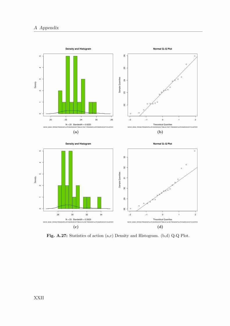
A Appendix

20 22 24 26 28

01

23

45

Density and Histogram

N = 20 Bandwidth = 0.6253

Density

!MOVE_BASE_PARAM PREMANIPULATIONAREAEASTTABLE2 FAST PREMANIPULATIONAREAEASTCOUNTER1

(a)

●

●

●

●

●

●

●

●●

●

●

●

●

●

●

●

● ●

●

●

−2 −1 0 1 2

22

23

24

25

26

Normal Q−Q Plot

Theoretical Quantiles

Sam

ple

Quantile

s

!MOVE_BASE_PARAM PREMANIPULATIONAREAEASTTABLE2 FAST PREMANIPULATIONAREAEASTCOUNTER1

(b)

28 30 32 34

01

23

45

Density and Histogram

N = 20 Bandwidth = 0.5629

Density

!MOVE_BASE_PARAM PREMANIPULATIONAREAEASTTABLE2 SLOW PREMANIPULATIONAREAEASTCOUNTER1

(c)

●

●

●

●

●

●

●

●

●

●

●

●

●

●

●

●

●

●

●

●

−2 −1 0 1 2

28

29

30

31

32

33

Normal Q−Q Plot

Theoretical Quantiles

Sam

ple

Quantile

s

!MOVE_BASE_PARAM PREMANIPULATIONAREAEASTTABLE2 SLOW PREMANIPULATIONAREAEASTCOUNTER1

(d)

Fig. A.27: Statistics of action (a,c) Density and Histogram. (b,d) Q-Q Plot.

XXII

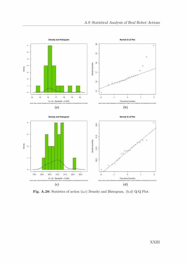
A.9 Statistical Analysis of Real Robot Actions

14 15 16 17 18 19 20

01

23

45

67

Density and Histogram

N = 20 Bandwidth = 0.2578

Density

!MOVE_BASE_PARAM PREMANIPULATIONAREANORTHTABLE1 FAST PREMANIPULATIONAREAEASTCOUNTER1

(a)

●

●

●●

●

●

●

●

●

●

●

●

●

●

●

●

●

●

●

●

−2 −1 0 1 215

16

17

18

19

20

Normal Q−Q Plot

Theoretical Quantiles

Sam

ple

Quantile

s

!MOVE_BASE_PARAM PREMANIPULATIONAREANORTHTABLE1 FAST PREMANIPULATIONAREAEASTCOUNTER1

(b)

19.5 20.0 20.5 21.0 21.5 22.0 22.5

01

23

4

Density and Histogram

N = 20 Bandwidth = 0.2325

Density

!MOVE_BASE_PARAM PREMANIPULATIONAREANORTHTABLE1 SLOW PREMANIPULATIONAREAEASTCOUNTER1

(c)

●

●●

●

●

●

●

●

●

●

●

●

●

●

●

●

●

●

●●

−2 −1 0 1 2

20.5

21.0

21.5

22.0

Normal Q−Q Plot

Theoretical Quantiles

Sam

ple

Quantile

s

!MOVE_BASE_PARAM PREMANIPULATIONAREANORTHTABLE1 SLOW PREMANIPULATIONAREAEASTCOUNTER1

(d)

Fig. A.28: Statistics of action (a,c) Density and Histogram. (b,d) Q-Q Plot.

XXIII

A Appendix

23.35 23.40 23.45

05

10

15

Density and Histogram

N = 10 Bandwidth = 0.01497

Density

!MOVE_TORSO TORSODOWNPOSTURE

(a)

●

●

●

●

●

●

●

●

●

●

−1.5 −1.0 −0.5 0.0 0.5 1.0 1.5

23.3

623.3

723.3

823.3

923.4

023.4

123.4

2

Normal Q−Q Plot

Theoretical Quantiles

Sam

ple

Quantile

s

!MOVE_TORSO TORSODOWNPOSTURE

(b)

22.15 22.20 22.25 22.30 22.35 22.40

010

20

30

40

50

Density and Histogram

N = 10 Bandwidth = 0.003496

Density

!MOVE_TORSO TORSOUPPOSTURE

(c)

●

●●

●

●

● ●

●●

●

−1.5 −1.0 −0.5 0.0 0.5 1.0 1.5

22.1

522.2

022.2

522.3

022.3

522.4

0

Normal Q−Q Plot

Theoretical Quantiles

Sam

ple

Quantile

s

!MOVE_TORSO TORSOUPPOSTURE

(d)

Fig. A.29: Statistics of action (a) Density and Histogram. (b) Q-Q Plot.

XXIV

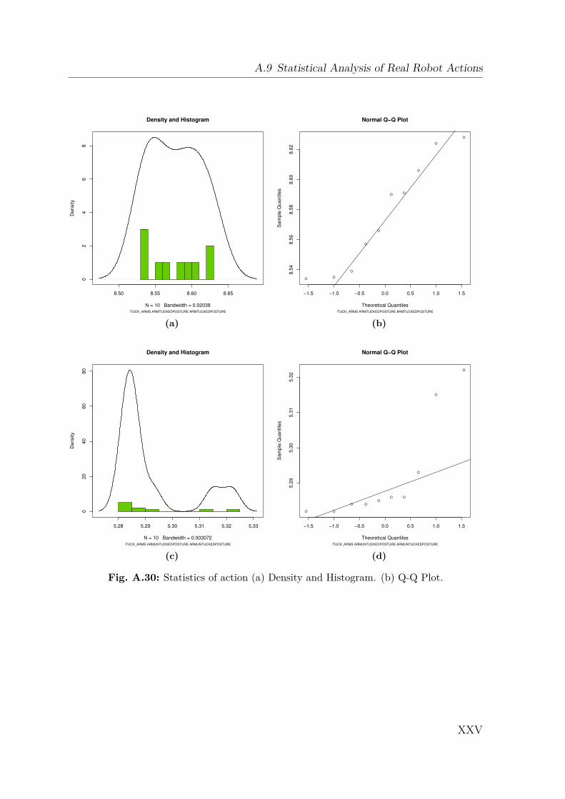
A.9 Statistical Analysis of Real Robot Actions

8.50 8.55 8.60 8.65

02

46

8

Density and Histogram

N = 10 Bandwidth = 0.02038

Density

!TUCK_ARMS ARMTUCKEDPOSTURE ARMTUCKEDPOSTURE

(a)

●

●

●

●

●

●

●

●

●

●

−1.5 −1.0 −0.5 0.0 0.5 1.0 1.58.5

48.5

68.5

88.6

08.6

2

Normal Q−Q Plot

Theoretical Quantiles

Sam

ple

Quantile

s

!TUCK_ARMS ARMTUCKEDPOSTURE ARMTUCKEDPOSTURE

(b)

5.28 5.29 5.30 5.31 5.32 5.33

020

40

60

80

Density and Histogram

N = 10 Bandwidth = 0.003072

Density

!TUCK_ARMS ARMUNTUCKEDPOSTURE ARMUNTUCKEDPOSTURE

(c)

●

●

●

● ●

●

●

●

●

●

−1.5 −1.0 −0.5 0.0 0.5 1.0 1.5

5.2

95.3

05.3

15.3

2

Normal Q−Q Plot

Theoretical Quantiles

Sam

ple

Quantile

s

!TUCK_ARMS ARMUNTUCKEDPOSTURE ARMUNTUCKEDPOSTURE

(d)

Fig. A.30: Statistics of action (a) Density and Histogram. (b) Q-Q Plot.

XXV

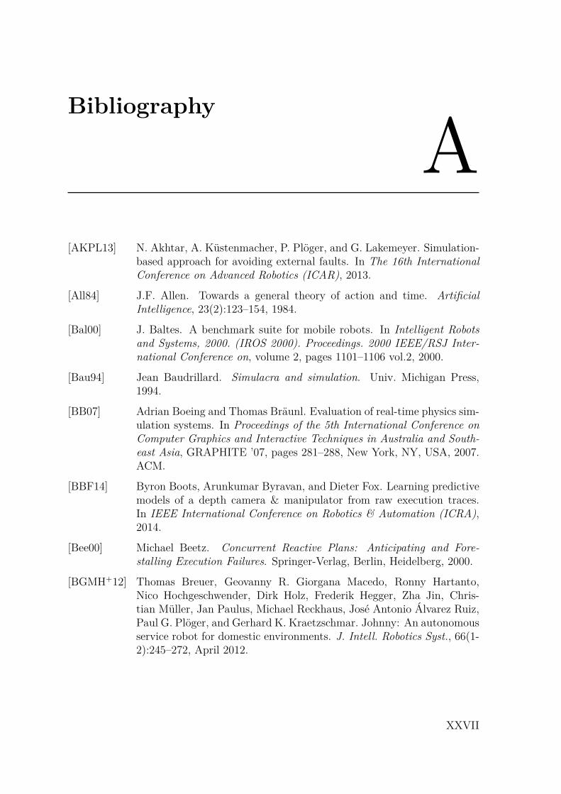
Bibliography

A

[AKPL13] N. Akhtar, A. Küstenmacher, P. Plöger, and G. Lakemeyer. Simulation-based approach for avoiding external faults. In The 16th InternationalConference on Advanced Robotics (ICAR), 2013.

[All84] J.F. Allen. Towards a general theory of action and time. ArtificialIntelligence, 23(2):123–154, 1984.

[Bal00] J. Baltes. A benchmark suite for mobile robots. In Intelligent Robotsand Systems, 2000. (IROS 2000). Proceedings. 2000 IEEE/RSJ Inter-national Conference on, volume 2, pages 1101–1106 vol.2, 2000.

[Bau94] Jean Baudrillard. Simulacra and simulation. Univ. Michigan Press,1994.

[BB07] Adrian Boeing and Thomas Bräunl. Evaluation of real-time physics sim-ulation systems. In Proceedings of the 5th International Conference onComputer Graphics and Interactive Techniques in Australia and South-east Asia, GRAPHITE ’07, pages 281–288, New York, NY, USA, 2007.ACM.

[BBF14] Byron Boots, Arunkumar Byravan, and Dieter Fox. Learning predictivemodels of a depth camera & manipulator from raw execution traces.In IEEE International Conference on Robotics & Automation (ICRA),2014.

[Bee00] Michael Beetz. Concurrent Reactive Plans: Anticipating and Fore-stalling Execution Failures. Springer-Verlag, Berlin, Heidelberg, 2000.

[BGMH+12] Thomas Breuer, Geovanny R. Giorgana Macedo, Ronny Hartanto,Nico Hochgeschwender, Dirk Holz, Frederik Hegger, Zha Jin, Chris-tian Müller, Jan Paulus, Michael Reckhaus, José Antonio Álvarez Ruiz,Paul G. Plöger, and Gerhard K. Kraetzschmar. Johnny: An autonomousservice robot for domestic environments. J. Intell. Robotics Syst., 66(1-2):245–272, April 2012.

XXVII

Bibliography

[BHH04] Thorsten Belker, Martin Hammel, and Joachim Hertzberg. Plan projec-tion under the appeal robot control architecture. In 8th Conf. IntelligentAutonomous Systems (IAS-8), pages 809–817, Amsterdam, The Nether-lands, 2004. IOS Press.

[BHKLP12] J. Barry, K. Hsiao, L. P. Kaelbling, and T. Lozano-Pérez. Manipulationwith multiple action types. In International Symposium on ExperimentalRobotics, June 2012.

[BKLP13] J. Barry, L.P. Kaelbling, and T. Lozano-Perez. A hierarchical ap-proach to manipulation with diverse actions. In Robotics and Automa-tion (ICRA), 2013 IEEE International Conference on, pages 1799–1806,May 2013.

[Blo81] Ned Block. Imagery (Bradford Books). MIT Press (MA), 1981.

[Blo83] Ned Block. Mental pictures and cognitive science. Philosophical Review,93(October):499–542, 1983.

[BRGJ+11] J. Bohren, R.B. Rusu, E. Gil Jones, E. Marder-Eppstein, C. Panto-faru, M. Wise, L. Mosenlechner, W. Meeussen, and S. Holzer. Towardsautonomous robotic butlers: Lessons learned with the pr2. In IEEEInternational Conference on Robotics and Automation (ICRA), pages5568–5575. IEEE, 2011.

[Bro86] Rodney A. Brooks. A robust layered control system for a mobile robot.IEEE Journal of Robotics and Automation, 2(1):14–23, 1986.

[BSD73] Neill Graham Bryce Seligman DeWitt, editor. The Many-Worlds Inter-pretation of Quantum Mechanics. Princeton Series in Physics. PrincetonUniversity Press, 1973. ISBN 0-691-08131-X.

[BW97] David Baraff and Andrew Witkin. Physically based modeling: Principlesand practice. Carnegie Mellon University, 1997.

[Cas71] Edward S. Casey. Imagination: Imagining and the image. Philosophyand Phenomenological Research, 31(4):pp. 475–490, 1971.

[CMW09] I.Y.-H. Chen, B. MacDonald, and B. Wunsche. Mixed reality simulationfor mobile robots. In Robotics and Automation, 2009. ICRA ’09. IEEEInternational Conference on, pages 232–237, May 2009.

[CNSV14] Anthony G. Cohn, Bernd Neumann, Alessandro Saffiotti, and MarkusVincze. Robots learning from experiences (dagstuhl seminar 14081). InDagstuhl Reports, volume 4, pages 97,107–108, 2014.

[Cra43] Kenneth J. W. Craik. The Nature of Explanation. Cambridge UniversityPress, 1943.

XXVIII

Bibliography

[DDO+14] K. Dubba, P. Duckworth, M. A. Omari, J. Tayyub, Y. Gatsoulis, A. G.Cohn, D. C. Hogg, L. Hotz, B. Neumann, S. Rockel, L. S. Lopes,M. Oliveira, G. H. Lim, S. H. Kasaei, and V. Mokhtari. Conceptu-alising environment activities and events. Technical report, EuropeanCommission - Information and Communication Technologies - SeventhFramework Programme, November 2014.

[Deu85] David Deutsch. Quantum theory, the church-turing principle and theuniversal quantum computer. Proceedings of the Royal Society of Lon-don, 400:97–117, 1985.

[DHCS12] Mehmet Dogar, Kaijen Hsiao, Matei Ciocarlie, and Siddhartha Srini-vasa. Physics-based grasp planning through clutter. In Robotics: Sci-ence and Systems VIII, July 2012.

[DHN13] Christian Dornhege, Andreas Hertle, and Bernhard Nebel. Lazy eval-uation and subsumption caching for search-based integrated task andmotion planning. In Workshop at the International Conference on In-telligent Robots and Systems (IROS), 2013.

[dSGPA14] Lavindra de Silva, Mamoun Gharbi, Amit Kumar Pandey, and RachidAlami. A new approach to combined symbolic-geometric backtrackingin the context of human-robot interaction. In IEEE International Con-ference on Robotics & Automation (ICRA), 2014.

[dSPA13] Lavindra de Silva, Amit Kumar Pandey, and Rachid Alami. An in-terface for interleaved symbolic-geometric planning and backtracking.In International Conference on Intelligent Robots and Systems (IROS),2013.

[EKRZ13] Lasse Einig, Denis Klimentjew, Sebastian Rockel, and Jianwei Zhang.Parallel plan execution and re-planning on a mobile robot using statemachines with htn planning systems. In IEEE International Conferenceon Robotics and Biomimetics (ROBIO), December 2013.

[FB81] Martin A. Fischler and Robert C. Bolles. Random sample consensus:A paradigm for model fitting with applications to image analysis andautomated cartography. Commun. ACM, 24(6):381–395, June 1981.

[FBDT99] Dieter Fox, Wolfram Burgard, Frank Dellaert, and Sebastian Thrun.Monte carlo localization: Efficient position estimation for mobile robots.In In Proc. of the National Conference on Artificial Intelligence (AAAI),pages 343–349, 1999.

[FBT97] D. Fox, W. Burgard, and S. Thrun. The dynamic window approach tocollision avoidance. Robotics Automation Magazine, IEEE, 4(1):23–33,Mar 1997.

XXIX

Bibliography

[FCK+09] Jonathan Fink, Tom Collins, Vijay Kumar, Yasamin Mostofi, JohnBaras, and Brian Sadler. A simulation environment for modeling and de-velopment of algorithms for ensembles of mobile microsystems. In SPIEDefense, Security, and Sensing, volume 7318, pages 73180N–73180N–10.International Society for Optics and Photonics, 2009.

[FN71] Richard E. Fikes and Nils J. Nilsson. Strips: A new approach to theapplication of theorem proving to problem solving. In Proceedings of the2Nd International Joint Conference on Artificial Intelligence, IJCAI’71,pages 608–620, San Francisco, CA, USA, 1971. Morgan Kaufmann Pub-lishers Inc.

[GNHK06] David Gamez, Richard Newcombe, Owen Holland, and Rob Knight.Two simulation tools for biologically inspired virtual robotics. Proceed-ings of the IEEE 5th chapter conference on advances in cybernetic sys-tems, Sheffield, pages 85–90, 2006.

[Gui08] Meen-Wah Gui. The basics of noise detection and filtering for boreholedrilling data. In The Open Civil Engineering Journal, volume 2, pages113–120, Taipei 106, Taiwan, 2008. Department of Civil Engineering,National Taipei University of Technology.

[GVH03] Brian P. Gerkey, Richard T. Vaughan, and Andrew Howard. Theplayer/stage project: Tools for multi-robot and distributed sensor sys-tems. In Proceedings of the 11th International Conference on AdvancedRobotics (ICAR), Coimbra, Portugal, June 2003.

[HC11] A. Harris and J. M. Conrad. Survey of popular robotics simulators,frameworks, and toolkits. In IEEE Southeastcon, pages 243–249, 2011.

[HIvdZ13] Dirk Holz, Luca Iocchi, and Tijn van der Zant. Benchmarking intelli-gent service robots through scientific competitions: The robocup@homeapproach. In Designing Intelligent Robots: Reintegrating AI II, AAAISpring Symposium, Stanford (USA), March 25-27 2013.

[HZZ+14] Joachim Hertzberg, Jianwei Zhang, Liwei Zhang, Sebastian Rockel,Bernd Neumann, Jos Lehmann, Krishna S. R. Dubba, Anthony G.Cohn, Alessandro Saffiotti, Federico Pecora, Masoumeh Mansouri, Šte-fan Konecný, Martin Günther, Sebastian Stock, Luis Seabra Lopes,Miguel Oliveira, Gi Hyun Lim, Hamidreza Kasaei, Vahid Mokhtari,Lothar Hotz, and Wilfried Bohlken. The race project. KI - KünstlicheIntelligenz, 2014.

[ILSKa05] I. Iossifidis, G. Lawitzky, and R. Zöllner S. Knoop and. Towards Bench-marking of Domestic Robotic Assistants, volume 14 of Advances inHuman-Robot Interaction. Springer-Verlag, Heidelberg, 2005.

XXX

Bibliography

[JL83] Philip N. Johnson-Laird. Mental Models. Harvard University Press,1983.

[JL95] Philip N. Johnson-Laird. Mental models, deductive reasoning, and thebrain. In The Cognitive Neurosciences, pages 999–1008. Mit Press, 1995.

[JLS12] Yun Jiang, Marcus Lim, and Ashutosh Saxena. Learning object arrange-ments in 3d scenes using human context. In ICML, 2012.

[Kal60] Rudolph Emil Kalman. A new approach to linear filtering and predictionproblems. Transactions of the ASME–Journal of Basic Engineering,82(Series D):35–45, 1960.

[KDB11] Lars Kunze, Mihai Emanuel Dolha, and Michael Beetz. Logic program-ming with simulation-based temporal projection for everyday robot ob-ject manipulation. In 2011 IEEE/RSJ International Conference on In-telligent Robots and Systems (IROS), San Francisco, CA, USA, Septem-ber, 25–30 2011. Best Student Paper Finalist.

[KDGB11] Lars Kunze, Mihai Emanuel Dolha, Emitza Guzman, and Michael Beetz.Simulation-based temporal projection of everyday robot object manip-ulation. In Yolum, Tumer, Stone, and Sonenberg, editors, Proc. of the10th Int. Conf. on Autonomous Agents and Multiagent Systems (AA-MAS 2011), Taipei, Taiwan, May, 2–6 2011. IFAAMAS.

[KEP05] Danny M. Kaufman, Timothy Edmunds, and Dinesh K. Pai. Fast fric-tional dynamics for rigid bodies. In ACM SIGGRAPH 2005 Papers,SIGGRAPH ’05, pages 946–956, New York, NY, USA, 2005. ACM.

[KGT01] S. M. Kosslyn, G. Ganis, and W. L. Thompson. Neural foundations ofimagery. In Nature Reviews: Neuroscience, 2001.

[KH04] N. Koenig and A Howard. Design and use paradigms for gazebo, anopen-source multi-robot simulator. In Intelligent Robots and Systems,2004. (IROS 2004). Proceedings. 2004 IEEE/RSJ International Con-ference on, volume 3, pages 2149–2154 vol.3, Sept 2004.

[KHB12] Lars Kunze, Andrei Haidu, and Michael Beetz. Making virtual pancakes— acquiring and analyzing data of everyday manipulation tasks throughinteractive physics-based simulations. In Poster and Demo Track ofthe 35th German Conference on Artificial Intelligence (KI-2012), Saar-brücken, Germany, September 24–27 2012.

[Kli15] Denis Klimentjew. Szenenanalyse in unstruktuierter Umgebung Adap-tives Verfahren zur Objekterkennung basierend auf der Multi-Sensor-Fusion und aktiven Wahrnehmung. PhD thesis, Universität Hamburg,2015.

XXXI

Bibliography

[KLP12] Leslie Pack Kaelbling and Tomás Lozano-Pérez. Integrated robot taskand motion planning in belief space, 2012.

[KLP+14] Peter Kaiser, Mike Lewis, Ronald P. A. Petrick, Tamim Asfour, andMark Steedman. Extracting common sense knowledge from text forrobot planning. In IEEE International Conference on Robotics & Au-tomation (ICRA), 2014.

[Kon00] K. Konolige. A gradient method for realtime robot control. In IntelligentRobots and Systems, 2000. (IROS 2000). Proceedings. 2000 IEEE/RSJInternational Conference on, volume 1, pages 639–646 vol.1, 2000.

[KRZ12] Denis Klimentjew, Sebastian Rockel, and Jianwei Zhang. Towards sceneanalysis based on multi-sensor fusion, active perception and mixed re-ality in mobile robotics. In Proceedings of the IEEE First Interna-tional Conference on Cognitive Systems and Information Processing(CSIP2012), 2012.

[KRZ13] Denis Klimentjew, Sebastian Rockel, and Jianwei Zhang. Active sceneanalysis based on multi-sensor fusion and mixed reality on mobile sys-tems. Foundations and Practical Applications of Cognitive Systems andInformation Processing (Chapter 69), Advances in Intelligent Systemsand Computing, 215:795–810, 2013.

[KS13] Hema Swetha Koppula and Ashutosh Saxena. Anticipating humanactivities using object affordances for reactive robotic response. InRobotics: Science and Systems, 2013.

[KSPS14] Stefan Konecný, Sebastian Stock, Federico Pecora, and Alessandro Saf-fiotti. Planning domain + execution semantics: a way towards robustexecution? In Proc. of Qualitative Representations for Robots, AAAISpring Symposium, 2014.

[KyHR03] Nikolaos Mavridis Kai-yuh Hsiao and Deb Roy. Coupling perception andsimulation: Steps towards conversational robotics. In The Proceedings ofIEEE/RSJ International Conference on Intelligent Robots and Systems(IROS), 2003.

[LB13] Daniel Leidner and Christoph Borst. Hybrid reasoning for mobile ma-nipulation based on object knowledge. In Workshop at the InternationalConference on Intelligent Robots and Systems (IROS), 2013.

[LC01] L.S. Lopes and J.H. Connell. Semisentient robots: routes to integratedintelligence. Intelligent Systems, IEEE, 16(5):10–14, Sep 2001.

XXXII

Bibliography

[LDS+14] Daniel Leidner, Alexander Dietrich, Florian Schmidt, Christoph Borst,and Alin Albu-Schäffer. Object-centered hybrid reasoning for whole-body mobile manipulation. In IEEE International Conference onRobotics & Automation (ICRA), 2014.

[Loa01] Brian J. Loasby. Cognition, imagination and institutions in demandcreation. Journal of Evolutionary Economics, 11:7–21, 2001.

[Lod96] Janice E. Lodato. Moral imagination: Implications of cognitive sciencefor ethics. Dialogue: Canadian Philosophical Review/Revue canadiennede philosophie, 35:204–207, December 1996.

[MB09] Lorenz Mösenlechner and Michael Beetz. Using physics- and sensor-based simulation for high-fidelity temporal projection of realistic robotbehavior. In 19th International Conference on Automated Planning andScheduling (ICAPS), 2009.

[MEBF+10] Eitan Marder-Eppstein, Eric Berger, Tully Foote, Brian Gerkey, andKurt Konolige. The office marathon: Robust navigation in an indooroffice environment. In International Conference on Robotics and Au-tomation (ICRA), 2010.

[MHN08] Hugo Gravato Marques, Owen Holland, and Richard Newcombe. Amodelling framework for functional imagination. In AISB Convention,pages 51–58, 2008.

[MKNH08] Hugo Gravato Marques, Rob Knight, Richard Newcombe, and OwenHolland. An anthropomimetic robot with imagination: one step closer tomachine consciousness? In Nokia Workshop on Machine Consciousness,2008.

[ML09] Marius Muja and David G. Lowe. Fast approximate nearest neighborswith automatic algorithm configuration. In International Conference onComputer Vision Theory and Application VISSAPP’09), pages 331–340.INSTICC Press, 2009.

[MP06] M.D. Moffitt and M.E. Pollack. Optimal rectangle packing: A meta-CSP approach. In Proc. of the 16th Int’l Conf. on Automated Planningand Scheduling (ICAPS), 2006.

[NHRL14] Bernd Neumann, Lothar Hotz, Pascal Rost, and Jos Lehmann. A robotwaiter learning from experiences. Machine Learning and Data Miningin Pattern Recognition, LNCS 8556:285–299, 2014.

[NIK+03] Dana Nau, Okhtay Ilghami, Ugur Kuter, J. William Murdock, Dan Wu,and Fusun Yaman. Shop2: An htn planning system. Journal of ArtificialIntelligence Research, 20:379–404, 2003.

XXXIII

Bibliography

[NM65] J. A. Nelder and R. Mead. A simplex method for function minimization.The Computer Journal, 7(4):308–313, 1965.

[NMAC+01] Dana Nau, Héctor Muñoz-Avila, Yue Cao, Amnon Lotem, and StevenMitchell. Total-order planning with partially ordered subtasks. In Pro-ceedings of the 17th International Joint Conference on Artificial Intel-ligence - Volume 1, IJCAI’01, pages 425–430, San Francisco, CA, USA,2001. Morgan Kaufmann Publishers Inc.

[Nor02] Donald A. Norman. The Design of Everyday Things. Basic Books, Inc.,New York, NY, USA, 2002.

[OFY07] Fumitaka Otsuka, Hikari Fujii, and Kazuo Yoshida. Developmentof three dimensional dynamics simulator with omnidirectional visionmodel. In Gerhard Lakemeyer, Elizabeth Sklar, DomenicoG. Sorrenti,and Tomoichi Takahashi, editors, RoboCup 2006: Robot Soccer WorldCup X, volume 4434 of Lecture Notes in Computer Science, pages 523–531. Springer Berlin Heidelberg, 2007.

[OSB14] Chris J. Ostafew, Angela P. Schoellig, and Timothy D. Barfoot.Learning-based nonlinear model predictive control to improve vision-based mobile robot path-tracking in challenging outdoor environments.In IEEE International Conference on Robotics & Automation (ICRA),2014.

[PMvRH13] Federico Pecora, Masoumeh Mansouri, Stephanie von Riegen, andLothar Hotz. Deliverable d1.2 - software framework for hybrid knowl-edge representation and reasoning. Technical report, European Commis-sion - Information and Communication Technologies - Seventh Frame-work Programme, 6 2013.

[Pra15] Gill A. Pratt. Is a cambrian explosion coming for robotics? Journal ofEconomic Perspectives, 29(3):51–60, 2015.

[QCG+09] Morgan Quigley, Ken Conley, Brian Gerkey, Josh Faust, Tully B. Foote,Jeremy Leibs, Rob Wheeler, and Andrew Y. Ng. ROS: an open-sourcerobot operating system. In ICRA Workshop on Open Source Software,2009.

[RKZ12] Sebastian Rockel, Denis Klimentjew, and Jianwei Zhang. A multi-robotplatform for mobile robots - a novel evaluation and development ap-proach with multi-agent technology. In Proceedings of the IEEE Interna-tional Conference on Multisensor Fusion and Integration for IntelligentSystems (MFI), pages 470–477, Hamburg, Germany, 2012. University ofHamburg.

XXXIV

Bibliography

[RKZZ14] Sebastian Rockel, Denis Klimentjew, Liwei Zhang, and Jianwei Zhang.An hyperreality imagination based reasoning and evaluation system(hires). In IEEE/RSJ International Conference on Robots and Automa-tion (ICRA), Hong Kong (China), June 2014.

[RM09] Elena Messina Raj Madhavan, Edward Tunstel. Performance Evalua-tion and Benchmarking of Intelligent Systems. Springer, 2009. ISBN:978-1-4419-0491-1 (Print) 978-1-4419-0492-8 (Online).

[RN07] Jochen Renz and Bernhard Nebel. Qualitative spatial reasoning usingconstraint calculi. In Marco Aiello, Ian Pratt-Hartmann, and Johan vanBenthem, editors, Handbook of Spatial Logics, pages 161–215. Springer,2007.

[RNZ+13] S. Rockel, B. Neumann, J. Zhang, K. S. R. Dubba, A. G. Cohn, S.Konecný, M. Mansouri, F. Pecora, A. Saffiotti, M. Günther, S. Stock,J. Hertzberg, A. M. Tomé, A. J. Pinho, L. S. Lopes, S. von Riegen, andL. Hotz. An ontology-based multi-level robot architecture for learningfrom experiences. In Designing Intelligent Robots: Reintegrating AI II,AAAI Spring Symposium, Stanford (USA), March 2013.

[SGH14] Sebastian Stock, Martin Günther, and Joachim Hertzberg. Generat-ing and executing hierarchical mobile manipulation plans. In Proc. ofISR/Robotik, 2014.

[SHL+13] S. Stock, J. Hertzberg, J. Lehmann, B. Neumann, W. Bohlken, L. Hotz,S. Rockel, and Š. Konecný. Deliverable d4.2 - consolidated versions ofprediction, expectation, and plan execution. Technical report, EuropeanCommission - Information and Communication Technologies - SeventhFramework Programme, 11 2013.

[SK08] Bruno Siciliano and Oussama Khatib, editors. Springer Handbook ofRobotics, chapter 17. Springer, 2008.

[SP97] Rainer Storn and Kenneth Price. Differential evolution – a simple andefficient heuristic for global optimization over continuous spaces. Journalof Global Optimization, 11(4):341–359, 1997.

[TBF05] Sebastian Thrun, Wolfram Burgard, and Dieter Fox. Probabilisticrobotics. MIT press, 2005.

[Teg98] Max Tegmark. The interpretation of quantum mechanics: Many worldsor many words? In Fortsch.Phys., 1998. arXiv:quant-ph/9709032.

[Tho14] Nigel J.T. Thomas. Mental imagery. In Edward N. Zalta, editor, TheStanford Encyclopedia of Philosophy. Stanford University, spring 2014edition, 2014.

XXXV

Bibliography

[TT01] Nobuyoshi Terashima and John Tiffin. HyperReality: Paradigm for theThird Millenium. Routledge, 2001.

[Tul72] Endel Tulving. Organization of Memory, chapter Episodic and SemanticMemory, pages 381–402. Academic Press, New York, 1972.

[vB90] Peter van Beek. Exact and approximate reasoning about qualitative tem-poral relations. PhD thesis, University of Waterloo, Waterloo, Ont.,Canada, Canada, 1990. UMI Order No. GAXNN-61098.

[vdZI11] Tijn van der Zant and Luca Iocchi. Robocup@home: Adaptive bench-marking of robot bodies and minds. In Bilge Mutlu, Christoph Bart-neck, Jaap Ham, Vanessa Evers, and Takayuki Kanda, editors, SocialRobotics, volume 7072 of Lecture Notes in Computer Science, pages214–225. Springer Berlin Heidelberg, 2011.

[VMJB13] J.G. Victores, S. Morante, A. Jardon, and C. Balaguer. Towards robotimagination through object feature inference. In Intelligent Robots andSystems (IROS), 2013 IEEE/RSJ International Conference on, pages5694–5699, Nov 2013.

[WBVdLS08] K.A. Wyrobek, E.H. Berger, H.F.M. Van der Loos, and J.K. Salisbury.Towards a personal robotics development platform: Rationale and de-sign of an intrinsically safe personal robot. In Robotics and Automation,2008. ICRA 2008. IEEE International Conference on, pages 2165–2170,May 2008.

[WHR10] Erik Weitnauer, Robert Haschke, and Helge Ritter. Evaluating a physicsengine as an ingredient for physical reasoning. In Noriaki Ando, StephenBalakirsky, Thomas Hemker, Monica Reggiani, and Oskar Stryk, edi-tors, Simulation, Modeling, and Programming for Autonomous Robots,volume 6472 of Lecture Notes in Computer Science, pages 144–155.Springer Berlin Heidelberg, 2010.

[Wis09] Thomas Wisspeintner. Prototyping and benchmarking autonomous mo-bile service robot applications. PhD thesis, University of Berlin, June2009.

[WvdZIS09] Thomas Wisspeintner, Tijn van der Zant, Luca Iocchi, and Stefan Schif-fer. Robocup@home: Scientific competition and benchmarking for do-mestic service robots. Interaction Studies, 10(3):392–426, 2009.

[WvdZIS10] Thomas Wisspeintner, Tijn van der Zant, Luca Iocchi, and Ste-fan Schiffer. Robocup@home: Results in benchmarking domesticservice robots. In Jacky Baltes, Michail G. Lagoudakis, TadashiNaruse, and Saeed Shiry Ghidary, editors, RoboCup 2009, chapter

XXXVI

Bibliography

RoboCup@Home: results in benchmarking domestic service robots,pages 390–401. Springer-Verlag, Berlin, Heidelberg, 2010.

[ZRP+12] Liwei Zhang, Sebastian Rockel, Federico Pecora, Luís Seabra Lopes,Alessandro Saffiotti, and Bernd Neumann. Deliverable d5.1 - evaluationinfrastructure. Technical report, European Commission - Informationand Communication Technologies - Seventh Framework Programme,November 2012.

[ZRP+13] Liwei Zhang, Sebastian Rockel, Federico Pecora, Lothar Hotz, ZhenliLu, and Jianwei Zhang. Evaluation metrics for an experience based mo-bile artificial cognitive system. In IEEE/RSJ International Conferenceon Intelligent Robots and Systems (IROS), Tokyo (Japan), 2013.

[ZRZ13] Liwei Zhang, Sebastian Rockel, and Jianwei Zhang. Exception handlingfor experience-based mobile cognitive systems in restaurant environ-ments exemplified by guest detection. In IEEE International Conferenceon Information and Automation (ICIA), Yinchuan (China), 2013.

[ZV10] S. Zickler and M. Veloso. Variable level-of-detail motion planning inenvironments with poorly predictable bodies. In 19th European Confer-ence on Artificial Intelligence, ECAI 2010, August 2010.

XXXVII

Publications

The following publications either resulted from this thesis or include significant resultsfrom the thesis. The list is ordered by date.

• Sebastian Rockel, Štefan Konecný, Sebastian Stock, Joachim Hertzberg, Fed-erico Percora, Jianwei Zhang, Integrating physics-based Prediction with SemanticPlan Execution Monitoring, IEEE/RSJ International Conference on IntelligentRobots and Systems (IROS), Hamburg, Germany, 2015. (accepted)

• Haiyang Jin, Liwei Zhang, Sebastian Rockel, Jun Zhang, Ying Hu, JianweiZhang, Optical Tracking based Tele-control System for Tabletop Object Manip-ulation Tasks, IEEE/RSJ International Conference on Intelligent Robots andSystems (IROS), Hamburg, Germany, 2015. (accepted)

• J. Hertzberg, J. Zhang, L. Zhang, S. Rockel, B. Neumann, J. Lehmann, K. S.R. Dubba, A. G. Cohn, A. Saffiotti, F. Pecora, M. Mansouri, Š. Konecný, M.Günther, S. Stock, L. S. Lopes, M. Oliveira, G. H. Lim, H. Kasaei, V. Mokhtari,L. Hotz, W. Bohlken, The RACE Project, KI - Künstille Intelligenz Journal,Springer Berlin Heidelberg, 2014.

• Anthony G. Cohn, Bernd Neumann, Alessandro Saffiotti, Markus Vincze, RobotsLearning from Experiences (Dagstuhl Seminar 14081), Dagstuhl Reports, vol. 4,num. 2, 2014, Dagstuhl, (Germany).

• Sebastian Rockel, Denis Klimentjew, Liwei Zhang, Jianwei Zhang, An Hyperre-ality Imagination based Reasoning and Evaluation System (HIRES), 2014 IEEEInternational conference on Robotics and Automation (ICRA 2014), Hong Kong(China), 2014.

• Sebastian Rockel, Predicting Robot Action Results physically correct: TowardsImaginary Planning, Dagstuhl Seminar Feb 16-21, 2014, Robots Learning fromExperiences, Wadern (Germany).

• Liwei Zhang, Sebastian Rockel, Alessandro Saffiotti, Federico Pecora, LotharHotz, Zhenli Lu, Denis Klimentjew, Jianwei Zhang, Evaluation Metrics for anExperience-based Mobile Artificial Cognitive System, IEEE/RSJ Int. Conf. on In-telligent Robots and Systems (IROS), Workshop on Metrics of Embodied Learn-ing Processes in Robots and Animals, Tokyo (Japan), 2013.

• Liwei Zhang, Sebastian Rockel, Jianwei Zhang, Exception Handling for Experience-based Mobile Cognitive Systems in Restaurant Environments Exemplified by GuestDetection, IEEE International Conference on Information and Automation (ICIA),August 2013, Yinchuan (China).

• Lasse Einig, Denis Klimentjew, Sebastian Rockel, Jianwei Zhang, Parallel PlanExecution and Re-planning on a Mobile Robot using State Machines with HTNPlanning Systems, IEEE International Conference on Robotics and Biomimetics(ROBIO), December 2013, Shenzhen (China).

• S. Rockel, B. Neumann, J. Zhang, K. S. R. Dubba, A. G. Cohn, S. Konecný,M. Mansouri, F. Pecora, A. Saffiotti, M. Günther, S. Stock, J. Hertzberg, A. M.Tomé, A. J. Pinho, L. S. Lopes, S. von Riegen, L. Hotz, An Ontology-based Multi-level Robot Architecture for Learning from Experiences, In: Proc. DesigningIntelligent Robots: Reintegrating AI II, AAAI Spring Symposium, March 25-27,Stanford (USA), 2013.

• Denis Klimentjew, Sebastian Rockel, Jianwei Zhang, Active Scene Analysis Basedon Multi-Sensor Fusion and Mixed Reality on Mobile Systems, Foundations andPractical Applications of Cognitive Systems and Information Processing (Chap-ter 69), Advances in Intelligent Systems and Computing, Vol. 215, SoftcoverISBN 978-3-642-37834-8, eBook ISBN 978-3-642-37835-5, Springer 2013.

• Denis Klimentjew, Sebastian Rockel, Jianwei Zhang, Towards Scene Analysisbased on Multi-Sensor Fusion, Active Perception and Mixed Reality in MobileRobotics, In Proceedings of the IEEE First International Conference on CognitiveSystems and Information Processing (CSIP2012), to be held on Dec. 15-17, 2012in Beijing, China, 2012.

• Sebastian Rockel, Denis Klimentjew, Jianwei Zhang, A Multi-Robot Platform forMobile Robots - A Novel Evaluation and Development Approach with Multi-AgentTechnology, In Proceedings of the IEEE International Conference on MultisensorFusion and Integration for Intelligent Systems (MFI), University of Hamburg,Hamburg, Germany, 2012.

Glossary

The following bibliographical references are al-phabetically sorted according to the last name ofthe first author.

2D two dimensional. 3, 4, 12, 28, 33, 38, 41, 53,64

3D three dimensional. 4, 28, 33, 36, 41, 52, 53,58, 59, 78

AI artificial intelligence. 17, 95

AMCL Adaptive Monte Carlo Localization. 33,54, 57, 59

API Application Programming Interface. 19, 36,38, 39

ASEF Automated Scenario Execution Frame-work. 61, 93

C1 PR2 on-board computer 1. 26

C2 PR2 on-board computer 2. 26

CAD Computer-Aided Design. 41, 78

CLI Command Line Interface. 79

CPU Central Processing Unit. 25, 53, 54, 55, 71

DAMA diverse action manipulation. 13

DARPA Defense Advanced Research ProjectsAgency. 22

DOF degree-of-freedom. 18, 24

DWA Dynamic Window Approach. 33, 42

EBCL example-based compositional learning. 83

EU European Union. 5, 20, 35

EURON European Robotics Research Network.21

FIM Fitness to Ideal Model. 21

FP7 Framework Programme for Research andTechnological Development. 5, 35

FPS frames per second. 28

GB Gigabyte. 25, 26, 53

GLUT the OpenGL Utility Toolkit. 38

GNU GNU’s Not Unix!. 52

GPU Graphics Processing Unit. 39, 40

GTP geometric task planner. 10

GUI Graphical User Interface. 37, 38, 39, 55

HD high definition. 28

HDD hard disk drive. 25

HIRES Hyperreality Imagination-based Reason-ing and Evaluation System. 1, 49, 60, 64,78, 80

HPN Hierarchical Planning in the Now. 13

HTN Hierarchical Task Network. 3, 9, 10, 13,14, 18, 48, 92

HW Hardware. 25, 31

ID Identifier. 51, 58, 59

IDF Iterative Distance Fitter. 41

IMU Inertial Measurement Units. 28, 29, 33

JNI Java Native Interface. 19

KR knowledge representation. 9

LED Light-emitting diode. 28

Meta-CSP Meta-Constraint Satisfaction Prob-lems. 9

ML machine learning. 15

MP Mega-pixel. 28

MR Mixed Reality. 1

MRS Multi-Robot System. 19

MWI Many Worlds Interpretation. 68, 69

XLI

Glossary

ODE Open Dynamics Engine. 14, 15, 35, 38, 39,40, 72, 88, 94

OGRE Object-Oriented Graphics Rendering En-gine. 38

OpenCV Open source Computer Vision library.36

OpenGL the Open Graphics Library. 38

ORK Object Recognition Kitchen. 41

OS Operating System. 31, 72, 73, 88

OSRF Open Source Robotics Foundation, Inc..33

PCL Point Cloud Library. 36

PDDL Planning Domain Definition Language.13

PMA pre-manipulation area. 65, 66, 71, 73, 77,81, 85, 87

PR1 Personal Robot 1. 23

PR2 Personal Robot 2. 10, 12, 17, 23, 24, 25, 26,28, 29, 31, 33, 36, 37, 41, 42, 49, 51, 53, 60,61, 65, 71, 73, 91, 95

PROLOG A general purpose logic programminglanguage. 14

PSR Predictive State Representation. 18

QQ plot A Quantile-Quantile plot is a probabil-ity plot indicating either a standard nor-mal distribution of the underlying data orrejecting it. 73

QT4 “Cute” cross-platform programming li-brary. 37, 38, 39

RACE Robustness by Autonomous CompetenceEnhancement. 5, 33, 35, 42, 46, 47, 48, 49,53, 54, 55, 60, 61, 62, 69, 71, 73, 79, 91, XI

RAM Random Access Memory. 26

RANSAC Random Sample Consensus. 33, 41

RGB red, green and blue color space. 28, 61

RGB-D Color and Depth. 18, 36, 58

ROS Robot Operating System. 17, 19, 20, 23,31, 33, 35, 36, 37, 38, 39, 41, 42, 46, 48,50, 51, 54, 78, 91

RPC Remote Procedure Call. 36

RRT Rapidly-exploring Random Trees. 12

Rviz ROS visualization. 55

SDF Simulation Description Format. 58

SEM Semantic Execution Monitor. 47, 48, 61,84, 86

SHOP2 Simple Hierarchical Ordered Planner 2.13, 48, 60

SIMNOS A real-time physics engine-based sim-ulation. 16

SLAM Simultaneous Localization And Mapping.33

SMACH State MACHine. 13, 14

SPA Sense-Plan-Act. 45, 92

STL Surface Tesselation Language. 38, 57

STRIPS STanford Research Institute ProblemSolver. 9

TAMS Technical Aspects of Multimodal Sys-tems. 23, 33, 54

TB Terabyte. 26

URDF Unified Robot Description Format. 58

USC University of Southern California. 37

VLOD Variable Level-Of-Detail. 12

WAP wireless access point. 31

WiFi local area wireless technology. 31

XML Extensible Markup Language. 37, 38, 58

XLII

List of Figures

2.1 Hierarchy of HTN methods . . . . . . . . . . . . . . . . . . . . . . . . 102.2 Planning with temporal and spatial constraints . . . . . . . . . . . . 112.3 Planning with geometric constraints . . . . . . . . . . . . . . . . . . . 112.4 Temporal projection using simulation . . . . . . . . . . . . . . . . . . 122.5 Different actions in a pancake making scenario . . . . . . . . . . . . . 15

3.1 PR2 arm joint specifications . . . . . . . . . . . . . . . . . . . . . . . 253.2 PR2 gripper sensors . . . . . . . . . . . . . . . . . . . . . . . . . . . . 253.3 PR2 base and internal computers . . . . . . . . . . . . . . . . . . . . 263.4 PR2 arms work space . . . . . . . . . . . . . . . . . . . . . . . . . . . 273.5 First PR2 external tray design . . . . . . . . . . . . . . . . . . . . . . 273.6 PR2 mounted final tray design . . . . . . . . . . . . . . . . . . . . . . 273.7 PR2 default sensors . . . . . . . . . . . . . . . . . . . . . . . . . . . . 283.8 PR2 mounted additional sensors . . . . . . . . . . . . . . . . . . . . . 293.9 The Microsoft Kinect sensors and actuators . . . . . . . . . . . . . . 293.10 PR2 calibration results . . . . . . . . . . . . . . . . . . . . . . . . . . 303.11 PR2 coordinate frames . . . . . . . . . . . . . . . . . . . . . . . . . . 313.12 PR2 low-level motion control . . . . . . . . . . . . . . . . . . . . . . . 323.13 PR2 network . . . . . . . . . . . . . . . . . . . . . . . . . . . . . . . 323.14 RACE 2D occupancy grid map . . . . . . . . . . . . . . . . . . . . . 34

4.1 The RACE software architecture . . . . . . . . . . . . . . . . . . . . 364.2 General structure of Gazebo components . . . . . . . . . . . . . . . . 384.3 Gazebo dependency graph . . . . . . . . . . . . . . . . . . . . . . . . 394.4 Gazebo plug-in architecture . . . . . . . . . . . . . . . . . . . . . . . 39

5.1 Hierarchical Sense-Plan-Act robot control paradigm . . . . . . . . . . 465.2 Reactive-Sense-Act robot control paradigm . . . . . . . . . . . . . . . 465.3 Hybrid Sense-Plan-Act robot control paradigm . . . . . . . . . . . . . 465.4 Hierarchical Sense-Plan-Imagine-Act robot control paradigm . . . . . 475.5 Hybrid Sense-Plan-Imagine-Act robot control paradigm . . . . . . . . 475.6 Functional imagination architecture . . . . . . . . . . . . . . . . . . . 475.7 Tray object reference orientation visualization . . . . . . . . . . . . . 505.8 Simulation run of environment and robot . . . . . . . . . . . . . . . . 545.9 Cup 3D model . . . . . . . . . . . . . . . . . . . . . . . . . . . . . . . 555.10 3D environment walls model . . . . . . . . . . . . . . . . . . . . . . . 565.11 Solid cylinder . . . . . . . . . . . . . . . . . . . . . . . . . . . . . . . 58

XLIII

List of Figures

5.12 Recognized objects are spawned into simulation . . . . . . . . . . . . 595.13 Dynamic view of imagination with a mediator . . . . . . . . . . . . . 615.14 Simulated thermal sensor . . . . . . . . . . . . . . . . . . . . . . . . . 625.15 Different environment setups per-scenario . . . . . . . . . . . . . . . . 635.16 PR2 dynamics and object visualization . . . . . . . . . . . . . . . . . 665.17 PR2 dynamics and object visualization 2 . . . . . . . . . . . . . . . . 675.18 Object deviation vs. acceleration . . . . . . . . . . . . . . . . . . . . 67

6.1 Restaurant floor map . . . . . . . . . . . . . . . . . . . . . . . . . . . 726.2 Simulation vs. PR2 action duration . . . . . . . . . . . . . . . . . . . 756.3 Fast motion statistics of simulation and reality . . . . . . . . . . . . . 766.4 Real and simulated robot trajectories compared . . . . . . . . . . . . 786.5 Picking objects: testing different robot poses in simulation . . . . . . 796.6 Object recognition in different robot positions . . . . . . . . . . . . . 796.7 Scenario setup . . . . . . . . . . . . . . . . . . . . . . . . . . . . . . . 816.8 Simulation: Failure during place action . . . . . . . . . . . . . . . . . 816.9 Planning scene with areas . . . . . . . . . . . . . . . . . . . . . . . . 826.10 Comparison prediction-enhanced to standard system . . . . . . . . . 836.11 Parameter instantiation in principle . . . . . . . . . . . . . . . . . . . 856.12 Real toppling demo . . . . . . . . . . . . . . . . . . . . . . . . . . . . 876.13 Robot and imagination actions over time . . . . . . . . . . . . . . . . 88

A.1 Restaurant simulation environment . . . . . . . . . . . . . . . . . . . IA.2 PR2 base dynamics data during different movements . . . . . . . . . IIA.3 Shaking Event . . . . . . . . . . . . . . . . . . . . . . . . . . . . . . . IIA.4 Tray object and robot dynamics 1 . . . . . . . . . . . . . . . . . . . . IIIA.5 Tray object and robot dynamics 2 . . . . . . . . . . . . . . . . . . . . IIIA.6 Robot velocity distribution over time . . . . . . . . . . . . . . . . . . IVA.7 Linear and angular velocity in simulation and reality . . . . . . . . . VA.8 Robot jerk in simulation and reality . . . . . . . . . . . . . . . . . . . VA.9 Object deviation vs. linear velocity/acceleration . . . . . . . . . . . . VIA.10 Object deviation with limited acceleration . . . . . . . . . . . . . . . VIA.11 Object deviation with limited acceleration (complex) . . . . . . . . . VIIA.12 Object deviation with angular dynamics and limited acceleration . . . VIIA.13 Object deviation with angular dynamics and limited acceleration 2 . . VIIIA.14 Relation between velocity and acceleration . . . . . . . . . . . . . . . VIIIA.15 Carry Arm Posture . . . . . . . . . . . . . . . . . . . . . . . . . . . . XIA.16 Tray Object Manipulation . . . . . . . . . . . . . . . . . . . . . . . . XIA.17 Tray Object Detection . . . . . . . . . . . . . . . . . . . . . . . . . . XIIA.18 The Pepper Mill . . . . . . . . . . . . . . . . . . . . . . . . . . . . . . XIIIA.19 Move_base_param fast/slow statistics 1 . . . . . . . . . . . . . . . . XIVA.20 Move_base_param fast/slow statistics 2 . . . . . . . . . . . . . . . . XVA.21 Move_base_param fast/slow statistics 3 . . . . . . . . . . . . . . . . XVI

XLIV

List of Figures

A.22 Move_base_param fast/slow statistics 4 . . . . . . . . . . . . . . . . XVIIA.23 Move_torso statistics 1 . . . . . . . . . . . . . . . . . . . . . . . . . . XVIIIA.24 Tuck_arms statistics 1 . . . . . . . . . . . . . . . . . . . . . . . . . . XIXA.25 Move_base_param fast/slow statistics 1 . . . . . . . . . . . . . . . . XXA.26 Move_base_param fast/slow statistics 2 . . . . . . . . . . . . . . . . XXIA.27 Move_base_param fast/slow statistics 3 . . . . . . . . . . . . . . . . XXIIA.28 Move_base_param fast/slow statistics 4 . . . . . . . . . . . . . . . . XXIIIA.29 Move_torso statistics 1 . . . . . . . . . . . . . . . . . . . . . . . . . . XXIVA.30 Tuck_arms statistics 1 . . . . . . . . . . . . . . . . . . . . . . . . . . XXV

XLV

List of Tables

5.1 Experimental results: motion parameter sets . . . . . . . . . . . . . . 50

6.1 Quantitative results of simulated robot actions . . . . . . . . . . . . . 746.2 Quantitative results of real robot actions . . . . . . . . . . . . . . . . 746.3 Qualitative results: serving a coffee. . . . . . . . . . . . . . . . . . . . 826.4 Averaged quantitative results of five scenario runs. . . . . . . . . . . . 826.5 Topple events for fast and slow parameter sets during experiments . . 856.6 Toppling likelihood for fast and slow parameter sets . . . . . . . . . . 866.7 Time resources used by simulation . . . . . . . . . . . . . . . . . . . . 88

XLVII

List of Algorithms

4.1 Basic DWA Algorithm . . . . . . . . . . . . . . . . . . . . . . . . . . . 42

XLIX

Eidesstattliche Versicherung

Hiermit erkläre ich an Eides statt, dass ich die vorliegende Dissertationsschrift selbstverfasst und keine anderen als die angegebenen Hilfsmittel benutzt habe.

Hamburg, den 10. September 2015

Sebastian Rockel