Embed Size (px)
Citation preview

Probability, contd

Learning Objectives
By the end of this lecture, you should be able to:
– Describe the difference between discrete random variables and continuous random variables.
– Describe how to determine the mean for both discrete and continuous random variables.
– Be able to do probability calculations for discrete and continuous random variables. In particular, be able to calculate the ‘expected value’ of a discrete random variable.
Discrete DataA discrete space is one in which all possible outcomes can be clearly identified and counted:
– Die Roll: S = {1,2,3,4,5,6}
– Number of Boys among 4 children: S = {0, 1, 2, 3, 4}
– Number of baskets made on two free throws: S = {0, 1, 2}
Data that can has a clearly finite number of values is known as discrete data.
A non-discrete space, which is called called a continuous interval/space, is one in which the outcomes are too numerous to
identify every possible outcome:
•Height of Human Beings: S = [0.00 inches, 100.00 inches] It is impractical to specify every possible height from 0.00 to
100.00.
•Muscle gain over 1 year of weight training: [0 pounds, 100+ pounds]
As with disjoint/non-disjoint, independent/non-independent, we will see that there are different probability formulas that are
used depending on whether the sample space is discrete or not.

A basketball player shoots three free throws. He typically makes a basket exactly 60% of the time.
The random variable X is the number of baskets successfully made.
Value of X 0 1 2 3
Probability 0.064 0.288 0.432 0.216
What is the probability that the
player successfully makes at
least* two baskets? Answer:
P(X≥2) = P(X=2 or X=3)
= (0.432+0.216) = 0.648
Through careful reading of the question, we see that the event we are interested in is “2 or more free throws”. The possible values of X making up this event are {2, 3}.
Key Point: The sample space discussed in this example contains discrete data.
* “At least”: A concept that has a way of showing up very often in real life (and on exams).
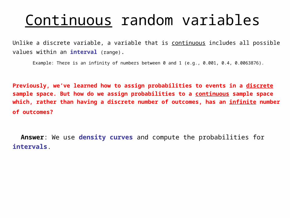
Unlike a discrete variable, a variable that is continuous includes all possible values within an interval
(range).
Example: There is an infinity of numbers between 0 and 1 (e.g., 0.001, 0.4, 0.0063876).
Previously, we’ve learned how to assign probabilities to events in a discrete sample space. But
how do we assign probabilities to a continuous sample space which, rather than having a discrete
number of outcomes, has an infinite number of outcomes?
Answer: We use density curves and compute the probabilities for intervals.
Continuous random variables
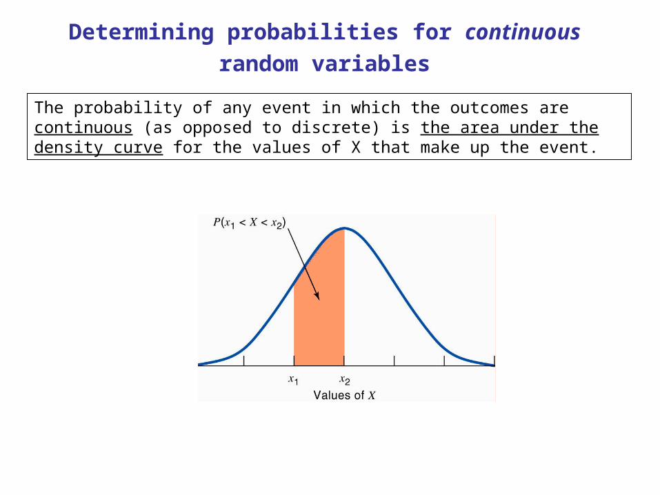
Determining probabilities for continuous random variables
The probability of any event in which the outcomes are continuous (as opposed to discrete) is the area under the density curve for the values of X that make up the event.

Example: The height of a sample of women has a distribution of approximately N(64.5, 2.5).
What is the probability, if we pick one woman at random, that her height will be between 68
and 70 inches. I.e. P(68 < X < 70)?
As we’ve done before, we calculate the z-scores for 68 and 70 and determine the area between them.
For x = 68",
For x = 70",
z(x )
4.15.2
)5.6468(
z
z(70 64.5)2.5
2.2
The area under the curve for the interval [68" to 70"] is 0.9861 − 0.9192 = 0.0669.
I.e. The probability that a randomly chosen woman falls into this range is 0.0669.
0.98610.9192
N(µ, ) = N(64.5, 2.5)
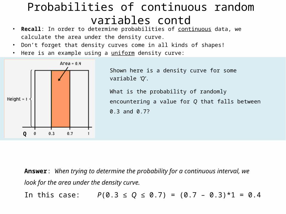
• Recall: In order to determine probabilities of continuous data, we calculate the area under
the density curve.• Don’t forget that density curves come in all kinds of shapes! • Here is an example using a uniform density curve:
Probabilities of continuous random variables contd
What is the probability of randomly encountering a value for Q
that falls between 0.3 and 0.7?
Shown here is a density curve for some variable ‘Q’.
Q
Answer: When trying to determine the probability for a continuous interval, we look
for the area under the density curve.
In this case: P(0.3 ≤ Q ≤ 0.7) = (0.7 – 0.3)*1 = 0.4

Only intervals can have a non-zero probability
The probability of a single event is meaningless for a continuous random variable. In fact, the calculated value is 0.
Only intervals can have a non-zero probability.

Example: The height of a sample of women has a distribution of approximately N(64.5,
2.5). What is the probability, if we pick one woman at random, that her height will be 67
inches?
Answer: We can NOT say! Recall
that with continuous variables, it is
not possible to determine the
probability of a single value. We
can only determine the probability
of a range of values.
N(64.5, 2.5)
67”

Calculating the mean of a random variable
- Mean of a discrete random variable- Mean of a continuous random variable

Mean of a discrete random variable
For a discrete random variable X with
the probability distribution shown here,
the mean µ of X is found by multiplying each possible value of X by its probability, and then
adding the products.
The mean µ of X is
µ = (0*0.064) + (1*0.288) + (2*0.432) + (3*0.216)
= 1.8
A 60% shooting basketball player shoots three free throws. The random variable X is
the number of baskets successfully made.
In other words, out of 3 throws, in the long run, this player would make 1.8 baskets.
Value of X 0 1 2 3
Probability 0.064 0.288 0.432 0.216
1.8 Baskets?!• This number represents the average number of baskets the thrower would make
out of many many 3-throw attempts. – Obviously on any invidivual attempt at 3 throws, the thrower could only make 0, 1, 2, or 3 baskets.
• This is similar to the idea that the average American household has 1.2 children. While no household has this particular number, this is the average number when looking at all households.
• There is a special name given to the mean value of a random variable (whether discrete or continuous). It is called the expected value.

Expected Value
Calculating expected value: The mean of a random variable X is a weighted average of the possible values of X.
Weighted: We take each value of X and multiply it by its probability. We then add all those values together.
The mean of a random variable X is called the expected value of X. Be aware that the
method of calculating the mean of a random variable changes depending on whether the
variable in question is discrete or continuous.
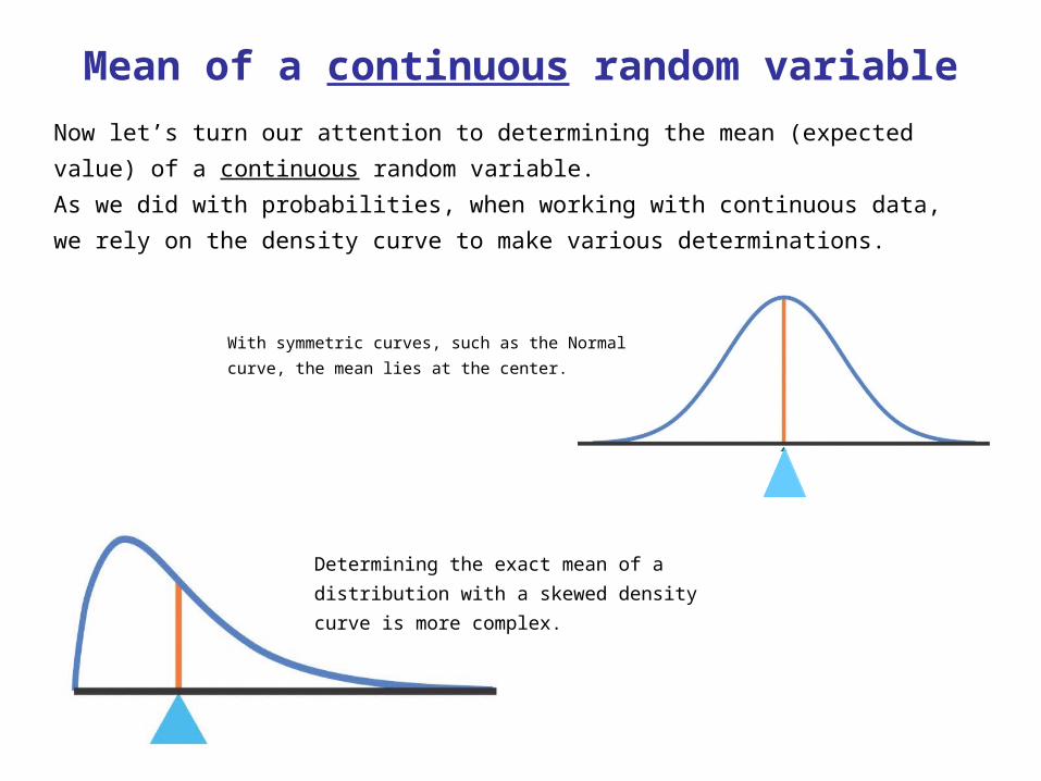
Now let’s turn our attention to determining the mean (expected value) of a continuous random
variable.
As we did with probabilities, when working with continuous data, we rely on the density curve
to make various determinations.
Mean of a continuous random variable
With symmetric curves, such as the Normal
curve, the mean lies at the center.
Determining the exact mean of a distribution
with a skewed density curve is more complex.

Standard Deviation of a random variable
• As with expected value (i.e. mean) of a random variable, we can also calculate the standard deviation of a random variable.
• Calculation: Once again, we need to carefully take into account the probability of each outcome.

Standard Deviation of a discrete random variable
For a discrete random variable X
with the probability distribution shown
and mean µX, the sd of X is found by multiplying each deviation by its probability and then adding all the
products.
This formula shows variance, taking the square root would give us SD:
The variance σ2 of X is
σ2 = 0.064*(0−1.8)2 + 0.288*(1−1.8)2 + 0.432*(2−1.8)2 + 0.216*(3−1.8)2
= 0.20736 + 0.18432 + 0.01728 + 0.31104
= 0.72 Take the square root to get SD: SD = 0.85
A basketball player shoots three free throws. The random variable X is the
number of baskets successfully made.
µX = 1.8.Value of X 0 1 2 3
Probability 0.064 0.288 0.432 0.216

• This topic and formula is a bit more involved. We will not discuss it for now. • However, don’t ever forget that while we like to think about measures of center (e.g.
the mean), when examining a dataset, we should never neglect to also consider the spread (e.g. standard deviation).
Standard Deviation of a continuous random variable
Example
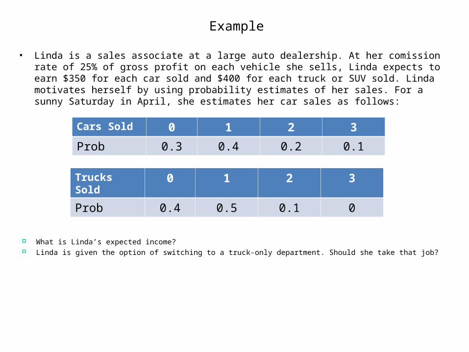
• Linda is a sales associate at a large auto dealership. At her comission rate of 25% of gross profit on each vehicle she sells, Linda expects to earn $350 for each car sold and $400 for each truck or SUV sold. Linda motivates herself by using probability estimates of her sales. For a sunny Saturday in April, she estimates her car sales as follows:
Cars Sold 0 1 2 3
Prob 0.3 0.4 0.2 0.1
Trucks Sold 0 1 2 3
Prob 0.4 0.5 0.1 0
What is Linda’s expected income? Linda is given the option of switching to a truck-only department. Should she take that job?

Cars Sold 0 1 2 3
Prob 0.3 0.4 0.2 0.1
Trucks Sold 0 1 2 3
Prob 0.4 0.5 0.1 0
Recall how with certain probability questions you have to ask yourself “disjoint or non-disjoint” or “independent or non-indepndent”. Similarly, when calculating an expected value, the very first question you must ask yourself is “discrete or non-discrete” since the method of determining the mean is completely different for each.
Because the type of variable we are discussing (# cars/trucks sold) is discrete, we will use the formula for calculating the mean of discrete data that was described earlier:
μcars sold = 0*0.3 + 1*0.4 + 2+0.2 + 3*0.1 = 1.1 cars
μtrucks sold = 0*0.4 + 1*0.5 + 2*0.1 + 3*0 = 0.7 trucks
If she gets $350 per car, and $400 per truck, Linda would expect to make: $350*1.1 + $400*0.7 = $665
What is Linda’s expected income?

Cars Sold 0 1 2 3
Prob 0.3 0.4 0.2 0.1
Trucks Sold 0 1 2 3
Prob 0.4 0.5 0.1 0
Answer: It might be tempting to compare expected value for each: 350*1.1 = $385 for cars v.s. 400*0.7 = $280 for trucks and infer that Linda should focus specifically on cars and just forget about trucks.
However, this would be a mistake. Can you see why?
Answer: If Linda focused only on trucks, she would not be spending any of her time on cars. As a result, she is likely to sell more than 0.7 trucks on a given day. However, we have no idea just how many more trucks she would sell. In other words, we do not have enough information to make a sound decision.
IMPORTANT: In fact, the expected value for income we calculated earlier is not enough. To do a proper evaluation of Linda’s expected income and so on, we should not have neglected to also consider the spread (e.g. the standard deviation). However, we left out these calculations for the time being, as they are very tedious to do by hand. Statistical software would give us this information.
Linda is given the option of switching to a truck-only department. Should she take that job?