Embed Size (px)
Citation preview
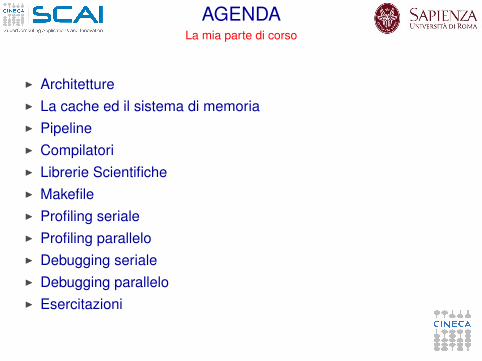
AGENDALa mia parte di corso
I ArchitettureI La cache ed il sistema di memoriaI PipelineI CompilatoriI Librerie ScientificheI MakefileI Profiling serialeI Profiling paralleloI Debugging serialeI Debugging paralleloI Esercitazioni
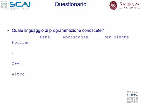
Questionario
I Quale linguaggio di programmazione conoscete?Bene Abbastanza Per niente
Fortran
C
C++
Altro
Questionario
I In quale ambiente lavorate abitualmente?Windows
Unix/Linux
Mac
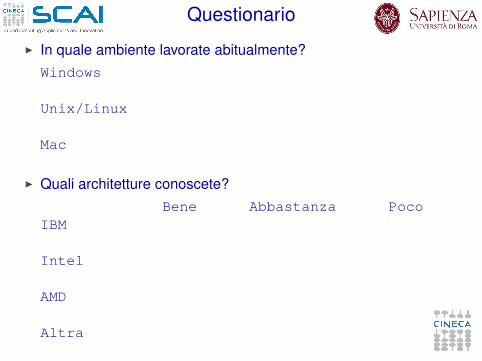
I Quali architetture conoscete?Bene Abbastanza Poco
IBM
Intel
AMD
Altra
Questionario
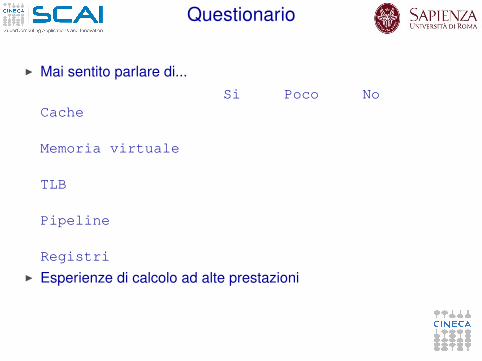
I Mai sentito parlare di...Si Poco No
Cache
Memoria virtuale
TLB
Pipeline
Registri
I Esperienze di calcolo ad alte prestazioni
Outline
Introduction
Architectures
Cache and memory system
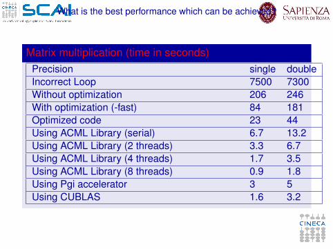
What is the best performance which can be achieved?
Matrix multiplication (time in seconds)Precision single doubleIncorrect Loop 7500 7300Without optimization 206 246With optimization (-fast) 84 181Optimized code 23 44Using ACML Library (serial) 6.7 13.2Using ACML Library (2 threads) 3.3 6.7Using ACML Library (4 threads) 1.7 3.5Using ACML Library (8 threads) 0.9 1.8Using Pgi accelerator 3 5Using CUBLAS 1.6 3.2
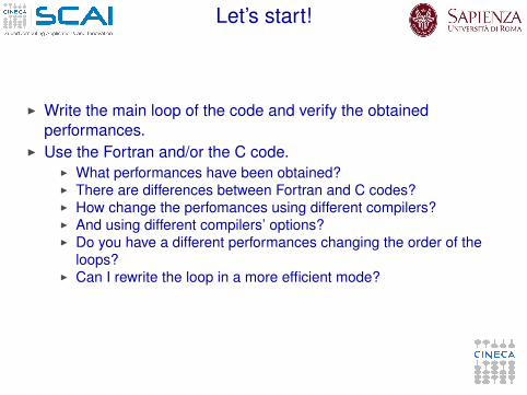
Let’s start!
I Write the main loop of the code and verify the obtainedperformances.
I Use the Fortran and/or the C code.I What performances have been obtained?I There are differences between Fortran and C codes?I How change the perfomances using different compilers?I And using different compilers’ options?I Do you have a different performances changing the order of the
loops?I Can I rewrite the loop in a more efficient mode?
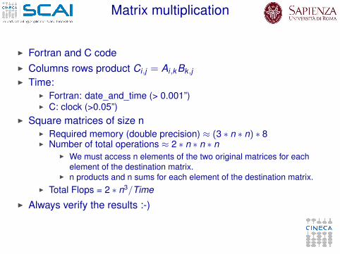
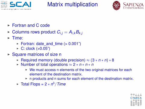
Matrix multiplication
I Fortran and C codeI Columns rows product Ci,j = Ai,kBk ,jI Time:
I Fortran: date_and_time (> 0.001”)I C: clock (>0.05”)
I Square matrices of size nI Required memory (double precision) ≈ (3 ∗ n ∗ n) ∗ 8I Number of total operations ≈ 2 ∗ n ∗ n ∗ n
I We must access n elements of the two original matrices for eachelement of the destination matrix.
I n products and n sums for each element of the destination matrix.I Total Flops = 2 ∗ n3/Time
I Always verify the results :-)

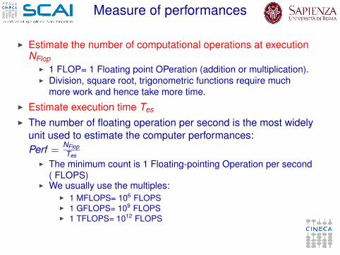
Measure of performances
I Estimate the number of computational operations at executionNFlop
I 1 FLOP= 1 Floating point OPeration (addition or multiplication).I Division, square root, trigonometric functions require much
more work and hence take more time.I Estimate execution time Tes
I The number of floating operation per second is the most widelyunit used to estimate the computer performances:Perf = NFlop
TesI The minimum count is 1 Floating-pointing Operation per second
( FLOPS)I We usually use the multiples:
I 1 MFLOPS= 106 FLOPSI 1 GFLOPS= 109 FLOPSI 1 TFLOPS= 1012 FLOPS
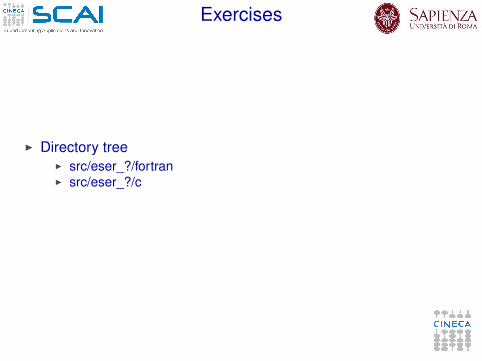
Exercises
I Directory treeI src/eser_?/fortranI src/eser_?/c
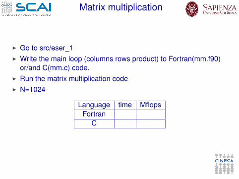
Matrix multiplication
I Go to src/eser_1I Write the main loop (columns rows product) to Fortran(mm.f90)
or/and C(mm.c) code.I Run the matrix multiplication codeI N=1024
Language time MflopsFortran
C
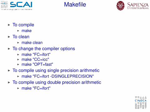
Makefile
I To compileI make
I To cleanI make clean
I To change the compiler optionsI make "FC=ifort"I make "CC=icc"I make "OPT=fast"
I To compile using single precision arithmeticI make "FC=ifort -DSINGLEPRECISION"
I To compile using double precision arithmeticI make "FC=ifort"
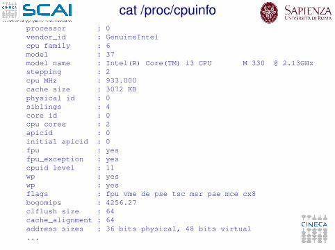
cat /proc/cpuinfoprocessor : 0vendor_id : GenuineIntelcpu family : 6model : 37model name : Intel(R) Core(TM) i3 CPU M 330 @ 2.13GHzstepping : 2cpu MHz : 933.000cache size : 3072 KBphysical id : 0siblings : 4core id : 0cpu cores : 2apicid : 0initial apicid : 0fpu : yesfpu_exception : yescpuid level : 11wp : yeswp : yesflags : fpu vme de pse tsc msr pae mce cx8bogomips : 4256.27clflush size : 64cache_alignment : 64address sizes : 36 bits physical, 48 bits virtual...
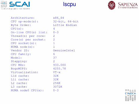
lscpu
Architecture: x86_64CPU op-mode(s): 32-bit, 64-bitByte Order: Little EndianCPU(s): 4On-line CPU(s) list: 0-3Thread(s) per core: 2Core(s) per socket: 2CPU socket(s): 1NUMA node(s): 1Vendor ID: GenuineIntelCPU family: 6Model: 37Stepping: 2CPU MHz: 933.000BogoMIPS: 4255.78Virtualization: VT-xL1d cache: 32KL1i cache: 32KL2 cache: 256KL3 cache: 3072KNUMA node0 CPU(s): 0-3

Matrix multiplication
What do you think about the obtained results?
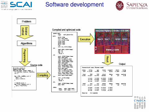
Software development
Solution Method
I A problem can typically be solved in many different waysI we have to choose a correct and efficient solution method
I A solution may include many different stages of computationusing different algorithms
I Example : first solve a linear equation system, then do a matrixmultiplication and after that a FFT
I Each stage in the solution may operate on the same dataI the data representation should be well suited for all the stages
of the computationI different stages in the solution may have conflicting
requirements on how data is represented
Algorithms
I A specific problem can typically be solved usinga number of different algorithms
I The algorithm has toI be correctI give the required numerical accuracyI be efficient, both with respect to execution time and use of
memoryI The choice of the numerical algorithm significantly affects the
performances.I efficient algorithm→ good performancesI inefficient algorithm→ bad performances
I Good performances are related to the choice of the algorithm.I Golden rule
I Before writing code choose an efficient algorithm:otherwise, the code must be rewritten!!!!
ProgrammingI We program in high level languages
I C,C++,Fortran,Java PythonI To achieve best performances, languages which are compiled
to executable machine code are preferred (C,C++,Fortran,..)I the differences in efficiency between these depend mainly on
how well developed the compiler is, not so much on thelanguages themselves
I Interpreted languages, and languages based on byte code arein general less efficient (Python, Java, JavaScript, PHP, ...)
I the program code is not directly executed by the processor, butgoes instead through a second step of interpretation
I High-level code is translated into machine code by a compilerI the compiler transforms the program into an equivalent but
more efficient programI the compiler must ensure that the optimized program
implements exactly the same computation as the originalprogram
Compiler optimizationI The compiler analyzes the code and tries to apply
a number of optimization techniques to improve theperformance
I it tries to recognize code which can be replaced with equivalent,but more efficient code
I Modern compilers are very good at low-level optimizationI register allocation, instruction reordering, dead code removal,
common subexpression elimination, function inlining , loopunrolling, vectorization, ...
I To enable the compiler to analyze and optimize the code theprogrammer should:
I avoid using programming language constructs which are knownto be inefficient
I avoid programming constructs that are difficult for the compilerto optimize (optimization blockers)
I avoid unnecessarily complicated constructs or tricky code,which makes the compiler analysis difficult
I write simple and well-structured code, which is easy for thecompiler to analyze and optimize
Execution
I Modern processors are very complex systemsI superscalar, superpipelined architectureI out of order instruction executionI multi-level cache with pre-fetching and write-combiningI branch prediction and speculative instruction executionI vector operations
I It is very difficult to understand exactly how instruction areexecuted by the processor
I Difficult to understand how different alternative programsolutions will affect performance
I programmers often have a weak understanding of whathappens when a program is executed
What to optimize
I Find out where the program spends most of its timeI it is unnecessary to optimize code that is seldom executed
I The 90/10 ruleI a program spends 90% of its time in 10% of the codeI look for optimizations in this 10% of the code
I Use tools to find out where a program spends its timeI profilersI hardware counters
Outline
Introduction
Architectures
Cache and memory system
Von Neuman achitecture
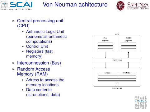
I Central processing unit(CPU)
I Arithmetic Logic Unit(perfoms all arithmeticcomputations)
I Control UnitI Registers (fast
memory)I Interconnession (Bus)I Random Access
Memory (RAM)I Adress to access the
memory locationsI Data contents
(istrunctions, data)
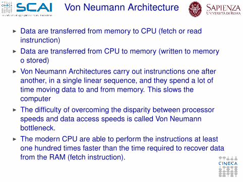
Von Neumann Architecture
I Data are transferred from memory to CPU (fetch or readinstrunction)
I Data are transferred from CPU to memory (written to memoryo stored)
I Von Neumann Architectures carry out instrunctions one afteranother, in a single linear sequence, and they spend a lot oftime moving data to and from memory. This slows thecomputer
I The difficulty of overcoming the disparity between processorspeeds and data access speeds is called Von Neumannbottleneck.
I The modern CPU are able to perform the instructions at leastone hundred times faster than the time required to recover datafrom the RAM (fetch instruction).

The evolution of computing systems
The solution for the von Neumann bottleneck are:I Caching
Very fast memories that are physically located on the chip ofthe processor.There are multi levels of cache (first, second and third).
I Virtual memoryThe RAM works as a cache to store large amounts of data.
I Instruction level parallelismA family of processor and compiler design techniques thatspeed up execution by causing individual machine operationsto execute in parallel (pipelining ,multiple issue).
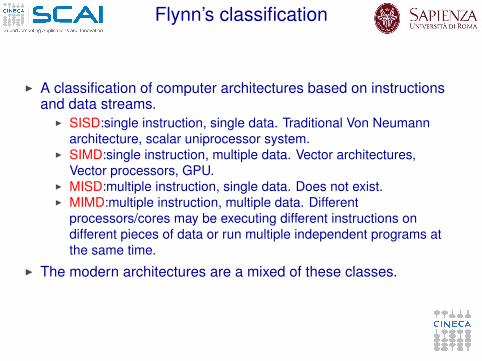
Flynn’s classification
I A classification of computer architectures based on instructionsand data streams.
I SISD:single instruction, single data. Traditional Von Neumannarchitecture, scalar uniprocessor system.
I SIMD:single instruction, multiple data. Vector architectures,Vector processors, GPU.
I MISD:multiple instruction, single data. Does not exist.I MIMD:multiple instruction, multiple data. Different
processors/cores may be executing different instructions ondifferent pieces of data or run multiple independent programs atthe same time.
I The modern architectures are a mixed of these classes.
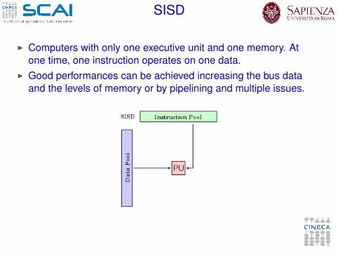
SISD
I Computers with only one executive unit and one memory. Atone time, one instruction operates on one data.
I Good performances can be achieved increasing the bus dataand the levels of memory or by pipelining and multiple issues.
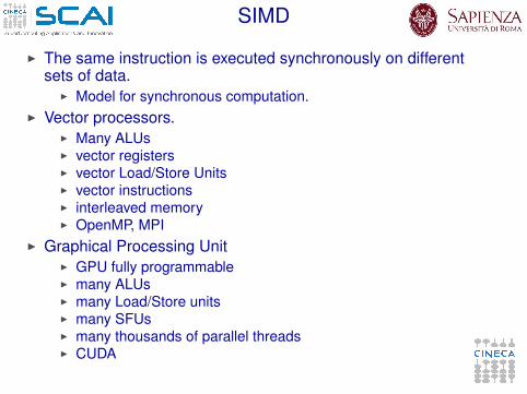
SIMD
I The same instruction is executed synchronously on differentsets of data.
I Model for synchronous computation.I Vector processors.
I Many ALUsI vector registersI vector Load/Store UnitsI vector instructionsI interleaved memoryI OpenMP, MPI
I Graphical Processing UnitI GPU fully programmableI many ALUsI many Load/Store unitsI many SFUsI many thousands of parallel threadsI CUDA
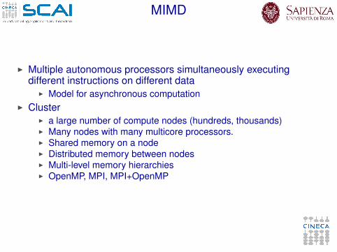
MIMD
I Multiple autonomous processors simultaneously executingdifferent instructions on different data
I Model for asynchronous computationI Cluster
I a large number of compute nodes (hundreds, thousands)I Many nodes with many multicore processors.I Shared memory on a nodeI Distributed memory between nodesI Multi-level memory hierarchiesI OpenMP, MPI, MPI+OpenMP
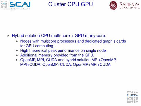
Cluster CPU GPU
I Hybrid solution CPU multi-core + GPU many-core:I Nodes with multicore processors and dedicated graphis cards
for GPU computing.I High theoretical peak performance on single nodeI Additional memory provided from the GPU.I OpenMP, MPI, CUDA and hybrid solution MPI+OpenMP,
MPI+CUDA, OpenMP+CUDA, OpenMP+MPI+CUDA
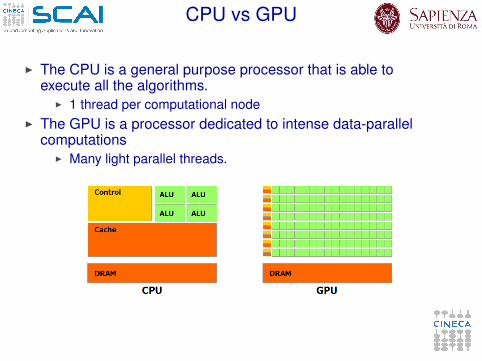
CPU vs GPU
I The CPU is a general purpose processor that is able toexecute all the algorithms.
I 1 thread per computational nodeI The GPU is a processor dedicated to intense data-parallel
computationsI Many light parallel threads.
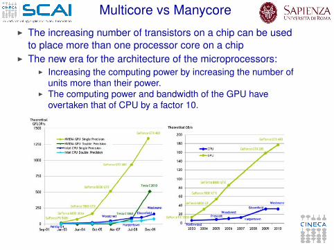
Multicore vs ManycoreI The increasing number of transistors on a chip can be used
to place more than one processor core on a chipI The new era for the architecture of the microprocessors:
I Increasing the computing power by increasing the number ofunits more than their power.
I The computing power and bandwidth of the GPU haveovertaken that of CPU by a factor 10.
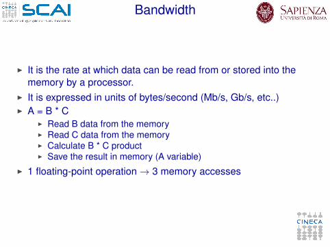
Bandwidth
I It is the rate at which data can be read from or stored into thememory by a processor.
I It is expressed in units of bytes/second (Mb/s, Gb/s, etc..)I A = B * C
I Read B data from the memoryI Read C data from the memoryI Calculate B * C productI Save the result in memory (A variable)
I 1 floating-point operation→ 3 memory accesses
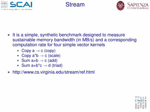
Stream
I It is a simple, synthetic benchmark designed to measuresustainable memory bandwidth (in MB/s) and a correspondingcomputation rate for four simple vector kernels
I Copy a→ c (copy)I Copy a*b→ c (scale)I Sum a+b→ c (add)I Sum a+b*c→ d (triad)
I http://www.cs.virginia.edu/stream/ref.html

Shared and distibuted memory
I The MIMD architectures and hybrid CPU GPU architecturescan be divided in two classes.
I Shared memory systems where where every single core accessthe full memory
I Distributed memory systems where different CPU units havetheir own memory systems and are able to communicate witheach other by exchanging explicit messages
I Modern multicore systems have shared memory on node anddistributed memory between nodes.
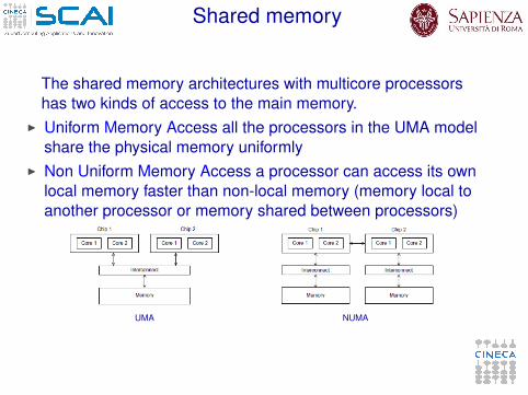
Shared memory
The shared memory architectures with multicore processorshas two kinds of access to the main memory.
I Uniform Memory Access all the processors in the UMA modelshare the physical memory uniformly
I Non Uniform Memory Access a processor can access its ownlocal memory faster than non-local memory (memory local toanother processor or memory shared between processors)
UMA NUMA
UMA NUMA
I Main disadvantages:I UMA machines: Thread synchronization and accessing shared
resources can cause the code to execute serially, and possiblyproduce bottlenecks. For example, when multiple processorsuse the same bus to access the memory, the bus can becomesatured.
I NUMA machines: the increased cost of accessing remotememory over local memory can affect performances.
I Solutions:I Software can maximize performance by increasing usage of
local memoryI binding to keep processes , or threads on a particular processor.I memory affinityI on AIX architecture, set MEMORY_AFFINITY environment
variable.I where is supported use numactl command.

NETWORKS
I All high performance computer systems are clusters of nodeswith shared memory on node and distributed memory betweennodes
I A cluster must have multiple network connections betweennodes, forming cluster interconnect.
I The more commonly used network communications protocols:I Gigabit Ethernet : the more common, cheap, low performances.I Infiniband : very common, high perfomances, very expansive.
I Others:I MyrinetI QuadricsI Cray
Outline
Introduction
Architectures
Cache and memory system
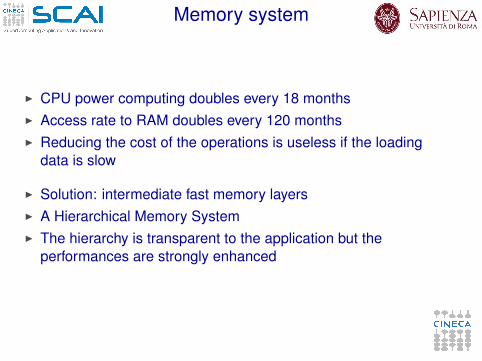
Memory system
I CPU power computing doubles every 18 monthsI Access rate to RAM doubles every 120 monthsI Reducing the cost of the operations is useless if the loading
data is slow
I Solution: intermediate fast memory layersI A Hierarchical Memory SystemI The hierarchy is transparent to the application but the
performances are strongly enhanced
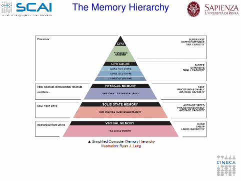
The Memory Hierarchy
Clock cycle
I The speed of a computer processor, or CPU, is determined bythe clock cycle, which is the amount of time between twopulses of an oscillator.
I Generally speaking, the higher number of pulses per second,the faster the computer processor will be able to processinformation
I The clock speed is measured in Hz, typically either megahertz(MHz) or gigahertz (GHz). For example, a 4GHz processorperforms 4,000,000,000 clock cycles per second.
I Computer processors can execute one or more instructions perclock cycle, depending on the type of processor.
I Early computer processors and slower CPUs can only executeone instruction per clock cycle, but modern processors canexecute multiple instructions per clock cycle.
The Memory Hierarchy
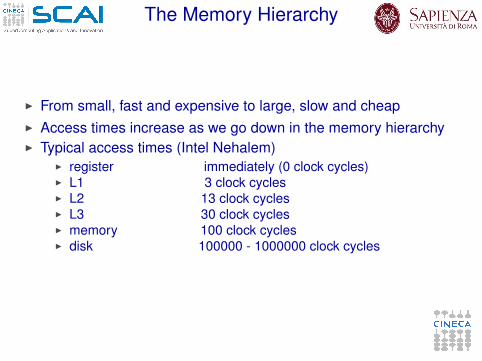
I From small, fast and expensive to large, slow and cheapI Access times increase as we go down in the memory hierarchyI Typical access times (Intel Nehalem)
I register immediately (0 clock cycles)I L1 3 clock cyclesI L2 13 clock cyclesI L3 30 clock cyclesI memory 100 clock cyclesI disk 100000 - 1000000 clock cycles

The Cache
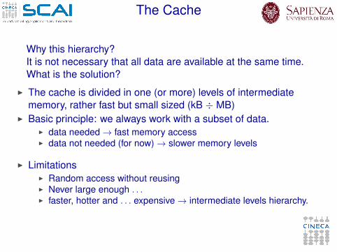
Why this hierarchy?
It is not necessary that all data are available at the same time.What is the solution?
I The cache is divided in one (or more) levels of intermediatememory, rather fast but small sized (kB ÷ MB)
I Basic principle: we always work with a subset of data.I data needed→ fast memory accessI data not needed (for now)→ slower memory levels
I LimitationsI Random access without reusingI Never large enough . . .I faster, hotter and . . . expensive→ intermediate levels hierarchy.

The Cache
Why this hierarchy?It is not necessary that all data are available at the same time.What is the solution?
I The cache is divided in one (or more) levels of intermediatememory, rather fast but small sized (kB ÷ MB)
I Basic principle: we always work with a subset of data.I data needed→ fast memory accessI data not needed (for now)→ slower memory levels
I LimitationsI Random access without reusingI Never large enough . . .I faster, hotter and . . . expensive→ intermediate levels hierarchy.
The cache
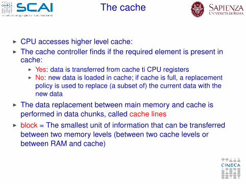
I CPU accesses higher level cache:I The cache controller finds if the required element is present in
cache:I Yes: data is transferred from cache ti CPU registersI No: new data is loaded in cache; if cache is full, a replacement
policy is used to replace (a subset of) the current data with thenew data
I The data replacement between main memory and cache isperformed in data chunks, called cache lines
I block = The smallest unit of information that can be transferredbetween two memory levels (between two cache levels orbetween RAM and cache)
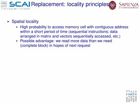
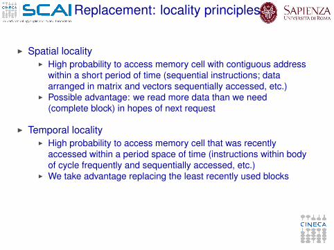
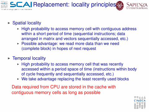
Replacement: locality principles
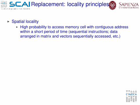
I Spatial localityI High probability to access memory cell with contiguous address
within a short period of time (sequential instructions; dataarranged in matrix and vectors sequentially accessed, etc.)
I Possible advantage: we read more data than we need(complete block) in hopes of next request
I Temporal localityI High probability to access memory cell that was recently
accessed within a period space of time (instructions within bodyof cycle frequently and sequentially accessed, etc.)
I We take advantage replacing the least recently used blocks
Data required from CPU are stored in the cache withcontiguous memory cells as long as possible
Replacement: locality principles
I Spatial localityI High probability to access memory cell with contiguous address
within a short period of time (sequential instructions; dataarranged in matrix and vectors sequentially accessed, etc.)
I Possible advantage: we read more data than we need(complete block) in hopes of next request
I Temporal localityI High probability to access memory cell that was recently
accessed within a period space of time (instructions within bodyof cycle frequently and sequentially accessed, etc.)
I We take advantage replacing the least recently used blocks
Data required from CPU are stored in the cache withcontiguous memory cells as long as possible

Cache:Some definition
I Hit: The requested data from CPU is stored in cacheI Miss: The requested data from CPU is not stored in cacheI Hit rate: The percentage of all accesses that are satisfied by
the data in the cache.I Miss rate:The number of misses stated as a fraction of
attempted accesses (miss rate = 1-hit rate).I Hit time: Memory access time for cache hit (including time to
determine if hit or miss)I Miss penalty: Time to replace a block from lower level,
including time to replace in CPU (mean value is used)I Miss time: = miss penalty + hit time, time needed to retrieve
the data from a lower level if cache miss is occurred.

Cache: access cost
Level access costL1 1 clock cycleL2 7 clock cycles
RAM 36 clock cycles
I 100 accesses with 100% cache hit: → t=100I 100 accesses with 5% cache miss in L1: → t=130I 100 accesses with 10% cache miss in L1→ t=160I 100 accesses with 10% cache miss in L2→ t=450I 100 accesses with 100% cache miss in L2→ t=3600
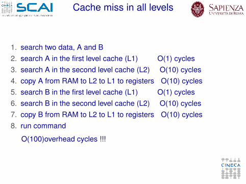
Cache miss in all levels
1. search two data, A and B2. search A in the first level cache (L1) O(1) cycles3. search A in the second level cache (L2) O(10) cycles4. copy A from RAM to L2 to L1 to registers O(10) cycles5. search B in the first level cache (L1) O(1) cycles6. search B in the second level cache (L2) O(10) cycles7. copy B from RAM to L2 to L1 to registers O(10) cycles8. run command
O(100)overhead cycles !!!
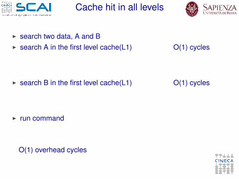
Cache hit in all levels
I search two data, A and BI search A in the first level cache(L1) O(1) cycles
I search B in the first level cache(L1) O(1) cycles
I run command
O(1) overhead cycles
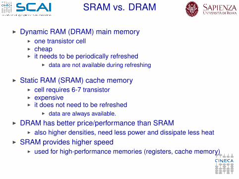
SRAM vs. DRAM
I Dynamic RAM (DRAM) main memoryI one transistor cellI cheapI it needs to be periodically refreshed
I data are not available during refreshing
I Static RAM (SRAM) cache memoryI cell requires 6-7 transistorI expensiveI it does not need to be refreshed
I data are always available.I DRAM has better price/performance than SRAM
I also higher densities, need less power and dissipate less heatI SRAM provides higher speed
I used for high-performance memories (registers, cache memory)

Performance estimate: an example
f l o a t sum = 0.0f;for (i = 0; i < n; i++)sum = sum + x[i]*y[i];
I At each iteration, one sum and one multiplication floating-pointare performed
I The number of the operations performed is 2×n
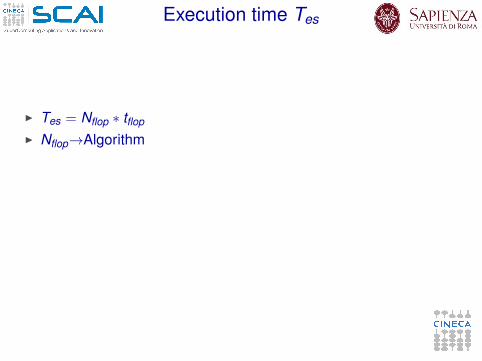
Execution time Tes
I Tes = Nflop ∗ tflop
I Nflop→Algorithm
I tflop→ HardwareI consider only execution timeI What are we neglecting?I tmem The required time to access data in memory.
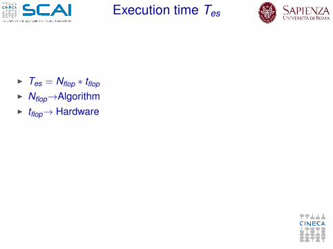
Execution time Tes
I Tes = Nflop ∗ tflop
I Nflop→AlgorithmI tflop→ Hardware
I consider only execution timeI What are we neglecting?I tmem The required time to access data in memory.
Execution time Tes
I Tes = Nflop ∗ tflop
I Nflop→AlgorithmI tflop→ HardwareI consider only execution timeI What are we neglecting?
I tmem The required time to access data in memory.
Execution time Tes
I Tes = Nflop ∗ tflop
I Nflop→AlgorithmI tflop→ HardwareI consider only execution timeI What are we neglecting?I tmem The required time to access data in memory.
Therefore . . .
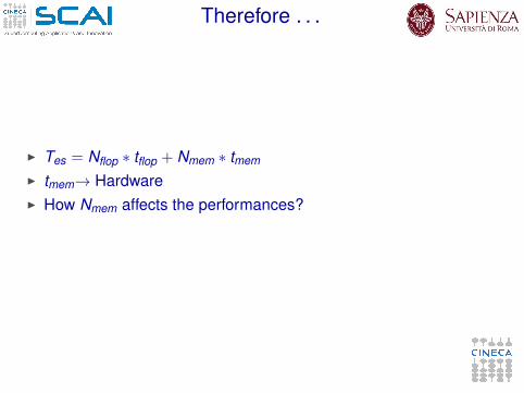
I Tes = Nflop ∗ tflop + Nmem ∗ tmem
I tmem→ HardwareI How Nmem affects the performances?

Nmem Effect
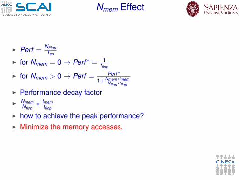
I Perf = NFlopTes
I for Nmem = 0→ Perf ∗ = 1tflop
I for Nmem > 0→ Perf = Perf∗
1+Nmem∗tmemNflop∗tflop
I Performance decay factorI Nmem
Nflop∗ tmem
tflop
I how to achieve the peak performance?
I Minimize the memory accesses.
Nmem Effect
I Perf = NFlopTes
I for Nmem = 0→ Perf ∗ = 1tflop
I for Nmem > 0→ Perf = Perf∗
1+Nmem∗tmemNflop∗tflop
I Performance decay factorI Nmem
Nflop∗ tmem
tflop
I how to achieve the peak performance?I Minimize the memory accesses.
Matrix multiplication
I Fortran and C codeI Columns rows product Ci,j = Ai,kBk ,jI Time:
I Fortran: date_and_time (> 0.001”)I C: clock (>0.05”)
I Square matrices of size nI Required memory (double precision) ≈ (3 ∗ n ∗ n) ∗ 8I Number of total operations ≈ 2 ∗ n ∗ n ∗ n
I We must access n elements of the two original matrices for eachelement of the destination matrix.
I n products and n sums for each element of the destination matrix.I Total Flops = 2 ∗ n3/Time
Measure of performances
I Estimate the number of computational operations at executionNFlop
I 1 FLOP= 1 Floating point OPeration (addition or multiplication).I Division, square root, trigonometric functions require much
more work and hence take more time.I Estimate execution time Tes
I The number of floating operation per second is the most widelyunit used to estimate the computer performances:Perf = NFlop
TesI The minimum count is 1 Floating-pointing Operation per second
( FLOPS)I We usually use the multiples:
I 1 MFLOPS= 106 FLOPSI 1 GFLOPS= 109 FLOPSI 1 TFLOPS= 1012 FLOPS
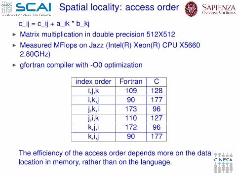
Spatial locality: access order
c_ij = c_ij + a_ik * b_kjI Matrix multiplication in double precision 512X512I Measured MFlops on Jazz (Intel(R) Xeon(R) CPU X5660
2.80GHz)I gfortran compiler with -O0 optimization
index order Fortran Ci,j,k 109 128i,k,j 90 177j,k,i 173 96j,i,k 110 127k,j,i 172 96k,i,j 90 177
The efficiency of the access order depends more on the datalocation in memory, rather than on the language.
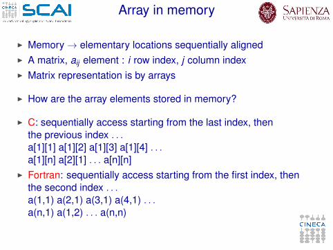
Array in memory
I Memory→ elementary locations sequentially alignedI A matrix, aij element : i row index, j column indexI Matrix representation is by arrays
I How are the array elements stored in memory?
I C: sequentially access starting from the last index, thenthe previous index . . .a[1][1] a[1][2] a[1][3] a[1][4] . . .a[1][n] a[2][1] . . . a[n][n]
I Fortran: sequentially access starting from the first index, thenthe second index . . .a(1,1) a(2,1) a(3,1) a(4,1) . . .a(n,1) a(1,2) . . . a(n,n)
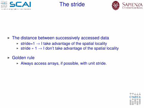
The stride
I The distance between successively accessed dataI stride=1→ I take advantage of the spatial localityI stride » 1→ I don’t take advantage of the spatial locality
I Golden ruleI Always access arrays, if possible, with unit stride.
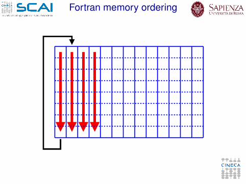
Fortran memory ordering
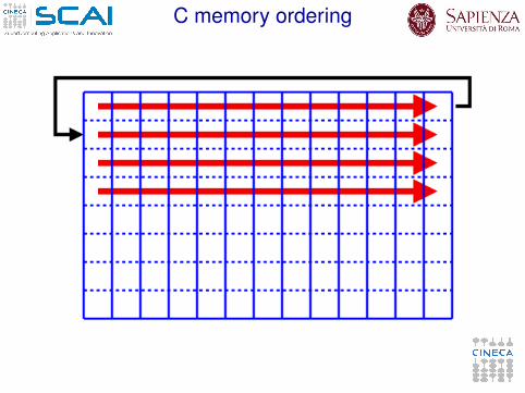
C memory ordering
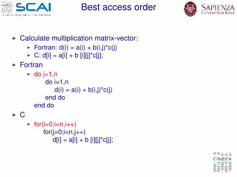
Best access order
I Calculate multiplication matrix-vector:I Fortran: d(i) = a(i) + b(i,j)*c(j)I C: d[i] = a[i] + b [i][j]*c[j];
I FortranI do j=1,n
do i=1,nd(i) = a(i) + b(i,j)*c(j)
end doend do
I CI for(i=0;i<n,i++)
for(j=0;i<n,j++)d[i] = a[i] + b [i][j]*c[j];
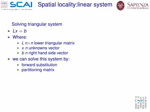
Spatial locality:linear system
Solving triangular systemI Lx = bI Where:
I L n×n lower triangular matrixI x n unknowns vectorI b n right hand side vector
I we can solve this system by:I forward substitutionI partitioning matrix
What is faster?Why?
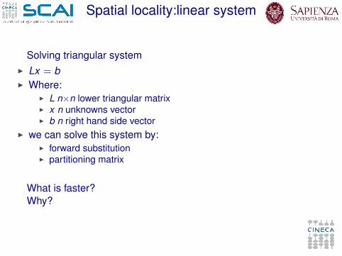
Spatial locality:linear system
Solving triangular systemI Lx = bI Where:
I L n×n lower triangular matrixI x n unknowns vectorI b n right hand side vector
I we can solve this system by:I forward substitutionI partitioning matrix
What is faster?Why?
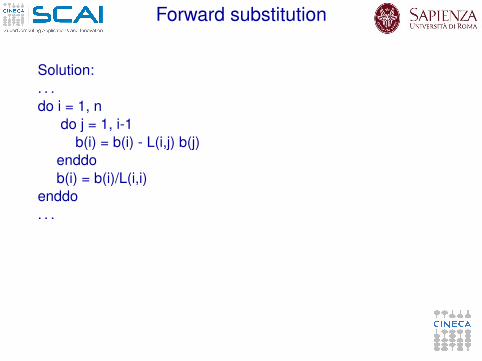
Forward substitution
Solution:. . .do i = 1, n
do j = 1, i-1b(i) = b(i) - L(i,j) b(j)
enddob(i) = b(i)/L(i,i)
enddo. . .
[vruggie1@fen07 TRI]$ ./a.out
time for solution 8.0586

Forward substitution
Solution:. . .do i = 1, n
do j = 1, i-1b(i) = b(i) - L(i,j) b(j)
enddob(i) = b(i)/L(i,i)
enddo. . .[vruggie1@fen07 TRI]$ ./a.out
time for solution 8.0586
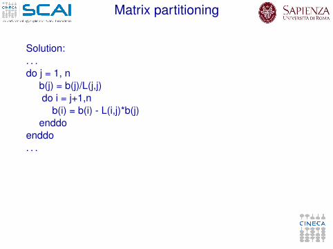
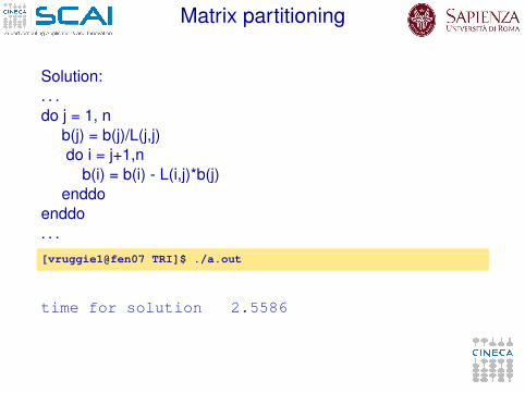
Matrix partitioning
Solution:. . .do j = 1, n
b(j) = b(j)/L(j,j)do i = j+1,n
b(i) = b(i) - L(i,j)*b(j)enddo
enddo. . .
[vruggie1@fen07 TRI]$ ./a.out
time for solution 2.5586
Matrix partitioning
Solution:. . .do j = 1, n
b(j) = b(j)/L(j,j)do i = j+1,n
b(i) = b(i) - L(i,j)*b(j)enddo
enddo. . .[vruggie1@fen07 TRI]$ ./a.out
time for solution 2.5586

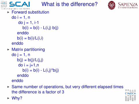
What is the difference?I Forward substitution
do i = 1, ndo j = 1, i-1
b(i) = b(i) - L(i,j) b(j)enddob(i) = b(i)/L(i,i)
enddoI Matrix partitioning
do j = 1, nb(j) = b(j)/L(j,j)do i = j+1,n
b(i) = b(i) - L(i,j)*b(j)enddo
enddo
I Same number of operations, but very different elapsed timesthe difference is a factor of 3
I Why?
What is the difference?I Forward substitution
do i = 1, ndo j = 1, i-1
b(i) = b(i) - L(i,j) b(j)enddob(i) = b(i)/L(i,i)
enddoI Matrix partitioning
do j = 1, nb(j) = b(j)/L(j,j)do i = j+1,n
b(i) = b(i) - L(i,j)*b(j)enddo
enddoI Same number of operations, but very different elapsed times
the difference is a factor of 3I Why?
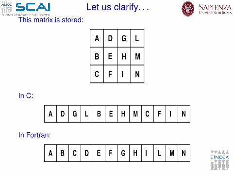
Let us clarify. . .This matrix is stored:
In C:
In Fortran:
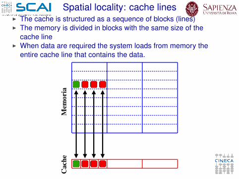
Spatial locality: cache linesI The cache is structured as a sequence of blocks (lines)I The memory is divided in blocks with the same size of the
cache lineI When data are required the system loads from memory the
entire cache line that contains the data.
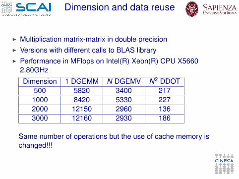
Dimension and data reuse
I Multiplication matrix-matrix in double precisionI Versions with different calls to BLAS libraryI Performance in MFlops on Intel(R) Xeon(R) CPU X5660
2.80GHz
Dimension 1 DGEMM N DGEMV N2 DDOT500 5820 3400 217
1000 8420 5330 2272000 12150 2960 1363000 12160 2930 186
Same number of operations but the use of cache memory ischanged!!!
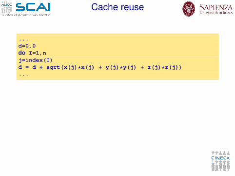
Cache reuse
...d=0.0do I=1,nj=index(I)d = d + sqrt(x(j)*x(j) + y(j)*y(j) + z(j)*z(j))...
Can I change the code to obtain best performances?
...d=0.0do I=1,nj=index(I)d = d + sqrt(r(1,j)*r(1,j) + r(2,j)*r(2,j) + r(3,j)*r(3,j))...

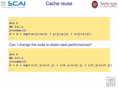
Cache reuse
...d=0.0do I=1,nj=index(I)d = d + sqrt(x(j)*x(j) + y(j)*y(j) + z(j)*z(j))...
Can I change the code to obtain best performances?
...d=0.0do I=1,nj=index(I)d = d + sqrt(r(1,j)*r(1,j) + r(2,j)*r(2,j) + r(3,j)*r(3,j))...
Cache reuse
...d=0.0do I=1,nj=index(I)d = d + sqrt(x(j)*x(j) + y(j)*y(j) + z(j)*z(j))...
Can I change the code to obtain best performances?
...d=0.0do I=1,nj=index(I)d = d + sqrt(r(1,j)*r(1,j) + r(2,j)*r(2,j) + r(3,j)*r(3,j))...
Registers
I Registers are memory locations inside CPUsI small amount of them (typically, less than 128), but with zero
latencyI All the operations performed by computing units
I take the operands from registersI return results into registers
I transfers memory↔ registers are different operationsI Compiler uses registers
I to store intermediate values when computing expressionsI too complex expressions or too large loop bodies force the so
called “register spilling”I to keep close to CPU values to be reusedI but only for scalar variables, not for array elements
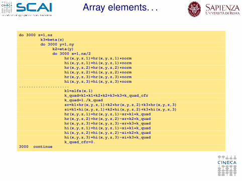
Array elements. . .
do 3000 z=1,nzk3=beta(z)do 3000 y=1,ny
k2=eta(y)do 3000 x=1,nx/2
hr(x,y,z,1)=hr(x,y,z,1)*normhi(x,y,z,1)=hi(x,y,z,1)*normhr(x,y,z,2)=hr(x,y,z,2)*normhi(x,y,z,2)=hi(x,y,z,2)*normhr(x,y,z,3)=hr(x,y,z,3)*normhi(x,y,z,3)=hi(x,y,z,3)*norm
.....................k1=alfa(x,1)k_quad=k1*k1+k2*k2+k3*k3+k_quad_cfrk_quad=1./k_quadsr=k1*hr(x,y,z,1)+k2*hr(x,y,z,2)+k3*hr(x,y,z,3)si=k1*hi(x,y,z,1)+k2*hi(x,y,z,2)+k3*hi(x,y,z,3)hr(x,y,z,1)=hr(x,y,z,1)-sr*k1*k_quadhr(x,y,z,2)=hr(x,y,z,2)-sr*k2*k_quadhr(x,y,z,3)=hr(x,y,z,3)-sr*k3*k_quadhi(x,y,z,1)=hi(x,y,z,1)-si*k1*k_quadhi(x,y,z,2)=hi(x,y,z,2)-si*k2*k_quadhi(x,y,z,3)=hi(x,y,z,3)-si*k3*k_quadk_quad_cfr=0.
3000 continue
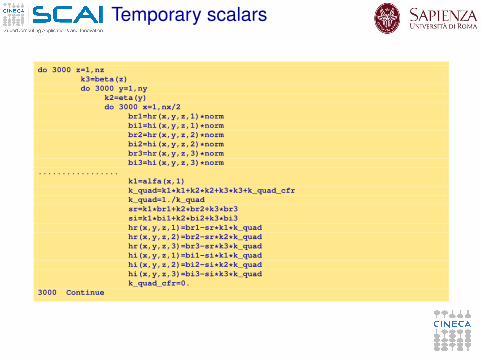
Temporary scalars
(time -25% )
do 3000 z=1,nzk3=beta(z)do 3000 y=1,ny
k2=eta(y)do 3000 x=1,nx/2
br1=hr(x,y,z,1)*normbi1=hi(x,y,z,1)*normbr2=hr(x,y,z,2)*normbi2=hi(x,y,z,2)*normbr3=hr(x,y,z,3)*normbi3=hi(x,y,z,3)*norm
.................k1=alfa(x,1)k_quad=k1*k1+k2*k2+k3*k3+k_quad_cfrk_quad=1./k_quadsr=k1*br1+k2*br2+k3*br3si=k1*bi1+k2*bi2+k3*bi3hr(x,y,z,1)=br1-sr*k1*k_quadhr(x,y,z,2)=br2-sr*k2*k_quadhr(x,y,z,3)=br3-sr*k3*k_quadhi(x,y,z,1)=bi1-si*k1*k_quadhi(x,y,z,2)=bi2-si*k2*k_quadhi(x,y,z,3)=bi3-si*k3*k_quadk_quad_cfr=0.
3000 Continue
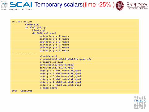
Temporary scalars(time -25% )
do 3000 z=1,nzk3=beta(z)do 3000 y=1,ny
k2=eta(y)do 3000 x=1,nx/2
br1=hr(x,y,z,1)*normbi1=hi(x,y,z,1)*normbr2=hr(x,y,z,2)*normbi2=hi(x,y,z,2)*normbr3=hr(x,y,z,3)*normbi3=hi(x,y,z,3)*norm
.................k1=alfa(x,1)k_quad=k1*k1+k2*k2+k3*k3+k_quad_cfrk_quad=1./k_quadsr=k1*br1+k2*br2+k3*br3si=k1*bi1+k2*bi2+k3*bi3hr(x,y,z,1)=br1-sr*k1*k_quadhr(x,y,z,2)=br2-sr*k2*k_quadhr(x,y,z,3)=br3-sr*k3*k_quadhi(x,y,z,1)=bi1-si*k1*k_quadhi(x,y,z,2)=bi2-si*k2*k_quadhi(x,y,z,3)=bi3-si*k3*k_quadk_quad_cfr=0.
3000 Continue
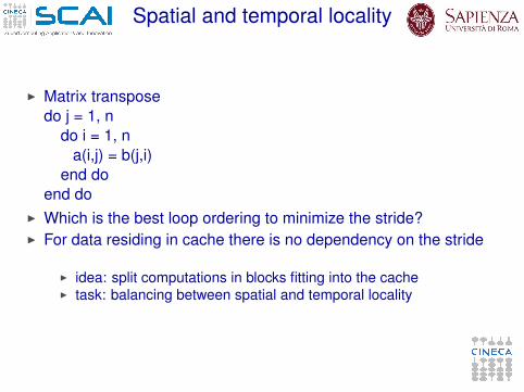
Spatial and temporal locality
I Matrix transposedo j = 1, n
do i = 1, na(i,j) = b(j,i)
end doend do
I Which is the best loop ordering to minimize the stride?I For data residing in cache there is no dependency on the stride
I idea: split computations in blocks fitting into the cacheI task: balancing between spatial and temporal locality
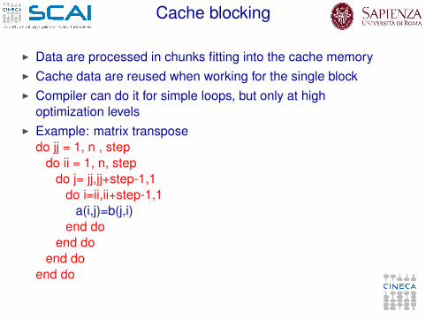
Cache blocking
I Data are processed in chunks fitting into the cache memoryI Cache data are reused when working for the single blockI Compiler can do it for simple loops, but only at high
optimization levelsI Example: matrix transpose
do jj = 1, n , stepdo ii = 1, n, step
do j= jj,jj+step-1,1do i=ii,ii+step-1,1
a(i,j)=b(j,i)end do
end doend do
end do
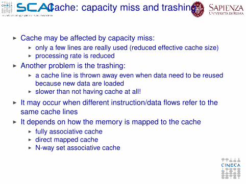
Cache: capacity miss and trashing
I Cache may be affected by capacity miss:I only a few lines are really used (reduced effective cache size)I processing rate is reduced
I Another problem is the trashing:I a cache line is thrown away even when data need to be reused
because new data are loadedI slower than not having cache at all!
I It may occur when different instruction/data flows refer to thesame cache lines
I It depends on how the memory is mapped to the cacheI fully associative cacheI direct mapped cacheI N-way set associative cache
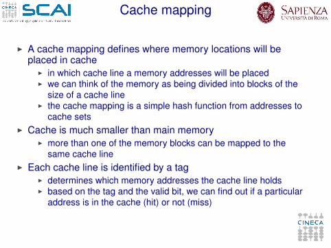
Cache mapping
I A cache mapping defines where memory locations will beplaced in cache
I in which cache line a memory addresses will be placedI we can think of the memory as being divided into blocks of the
size of a cache lineI the cache mapping is a simple hash function from addresses to
cache setsI Cache is much smaller than main memory
I more than one of the memory blocks can be mapped to thesame cache line
I Each cache line is identified by a tagI determines which memory addresses the cache line holdsI based on the tag and the valid bit, we can find out if a particular
address is in the cache (hit) or not (miss)
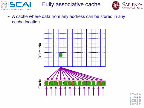
Fully associative cache
I A cache where data from any address can be stored in anycache location.
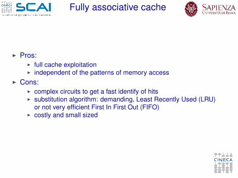
Fully associative cache
I Pros:I full cache exploitationI independent of the patterns of memory access
I Cons:I complex circuits to get a fast identify of hitsI substitution algorithm: demanding, Least Recently Used (LRU)
or not very efficient First In First Out (FIFO)I costly and small sized
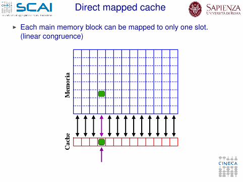
Direct mapped cache
I Each main memory block can be mapped to only one slot.(linear congruence)
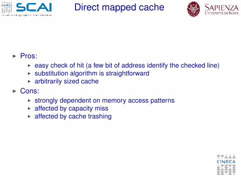
Direct mapped cache
I Pros:I easy check of hit (a few bit of address identify the checked line)I substitution algorithm is straightforwardI arbitrarily sized cache
I Cons:I strongly dependent on memory access patternsI affected by capacity missI affected by cache trashing
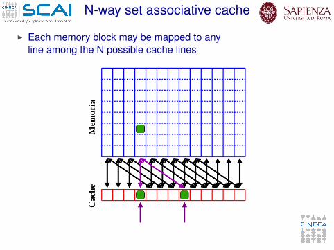
N-way set associative cache
I Each memory block may be mapped to anyline among the N possible cache lines
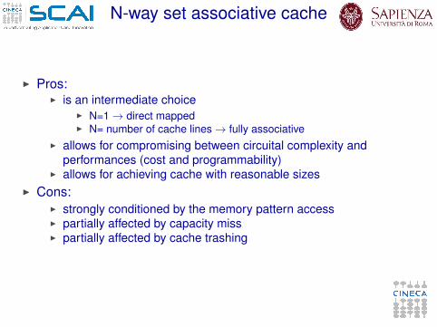
N-way set associative cache
I Pros:I is an intermediate choice
I N=1 → direct mappedI N= number of cache lines → fully associative
I allows for compromising between circuital complexity andperformances (cost and programmability)
I allows for achieving cache with reasonable sizesI Cons:
I strongly conditioned by the memory pattern accessI partially affected by capacity missI partially affected by cache trashing
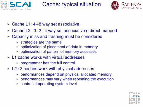
Cache: typical situation
I Cache L1: 4÷8 way set associativeI Cache L2÷3: 2÷4 way set associative o direct mappedI Capacity miss and trashing must be considered
I strategies are the sameI optimization of placement of data in memoryI optimization of pattern of memory accesses
I L1 cache works with virtual addressesI programmer has the full control
I L2÷3 caches work with physical addressesI performances depend on physical allocated memoryI performances may vary when repeating the executionI control at operating system level
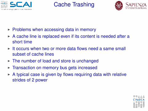
Cache Trashing
I Problems when accessing data in memoryI A cache line is replaced even if its content is needed after a
short timeI It occurs when two or more data flows need a same small
subset of cache linesI The number of load and store is unchangedI Transaction on memory bus gets increasedI A typical case is given by flows requiring data with relative
strides of 2 power
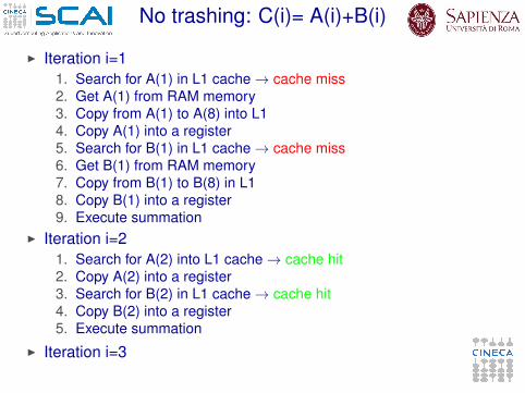
No trashing: C(i)= A(i)+B(i)
I Iteration i=11. Search for A(1) in L1 cache→ cache miss2. Get A(1) from RAM memory3. Copy from A(1) to A(8) into L14. Copy A(1) into a register5. Search for B(1) in L1 cache→ cache miss6. Get B(1) from RAM memory7. Copy from B(1) to B(8) in L18. Copy B(1) into a register9. Execute summation
I Iteration i=21. Search for A(2) into L1 cache→ cache hit2. Copy A(2) into a register3. Search for B(2) in L1 cache→ cache hit4. Copy B(2) into a register5. Execute summation
I Iteration i=3

Trashing: C(i)= A(i)+B(i)
I Iteration i=11. Search for A(1) in the L1 cache→ cache miss2. Get A(1) from RAM memory3. Copy from A(1) to A(8) into L14. Copy A(1) into a register5. Search for B(1) in L1 cache→ cache miss6. Get B(1) from RAM memory7. Throw away cache line A(1)-A(8)8. Copy from B(1) to B(8) into L19. Copy B(1) into a register
10. Execute summation
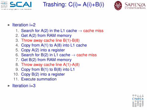
Trashing: C(i)= A(i)+B(i)
I Iteration i=21. Search for A(2) in the L1 cache→ cache miss2. Get A(2) from RAM memory3. Throw away cache line B(1)-B(8)4. Copy from A(1) to A(8) into L1 cache5. Copy A(2) into a register6. Search for B(2) in L1 cache→ cache miss7. Get B(2) from RAM memory8. Throw away cache line A(1)-A(8)9. Copy from B(1) to B(8) into L1
10. Copy B(2) into a register11. Execute summation
I Iteration i=3
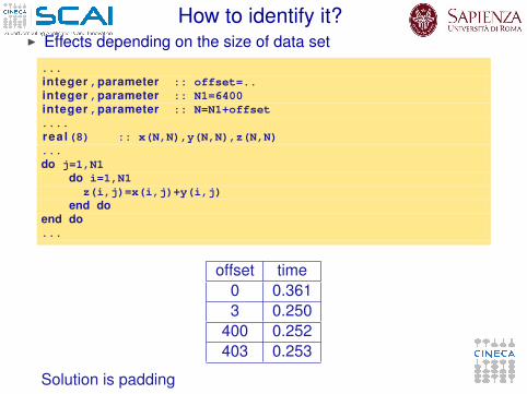
How to identify it?I Effects depending on the size of data set
...integer ,parameter :: offset=..integer ,parameter :: N1=6400integer ,parameter :: N=N1+offset....rea l(8) :: x(N,N),y(N,N),z(N,N)...do j=1,N1
do i=1,N1z(i,j)=x(i,j)+y(i,j)
end doend do...
offset time0 0.3613 0.250
400 0.252403 0.253
Solution is padding
Cache padding
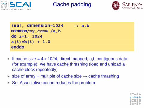
real , dimension=1024 :: a,bcommon/my_comm /a,bdo i=1, 1024a(i)=b(i) + 1.0enddo
I If cache size = 4 ∗ 1024, direct mapped, a,b contiguous data(for example): we have cache thrashing (load and unload acache block repeatedly)
I size of array = multiple of cache size→ cache thrashingI Set Associative cache reduces the problem
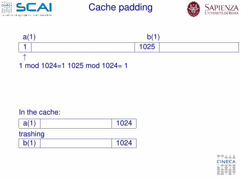
Cache padding
a(1) b(1)1 1025↑
1 mod 1024=1 1025 mod 1024= 1
In the cache:a(1) 1024
trashingb(1) 1024
Cache padding
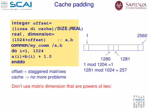
integer offset=(linea di cache)/SIZE(REAL)real , dimension=(1024+offset) :: a,bcommon/my_comm /a,bdo i=1, 1024a(i)=b(i) + 1.0enddo
offset→ staggered matrixescache→ no more problems
1 2560↓ ↙
↗ ↖1280 1281
1 mod 1204 =11281 mod 1024 = 257
Don’t use matrix dimension that are powers of two:
Misaligned accesses
I Bus transactions get doubledI On some architectures:
I may cause run-time errorsI emulated in software
I A problem when dealing withI structured types ( TYPE and struct)I local variablesI “common”
I SolutionsI order variables with decreasing orderI compiler options (if available. . .)I different commonI insert dummy variables into common
Misaligned Accesses
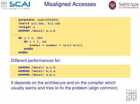
parameter (nd=1000000)rea l*8 a(1:nd), b(1:nd)integer ccommon /data1/ a,c,b
....do j = 1, 300
do i = 1, ndsomma1 = somma1 + (a(i)-b(i))
enddoenddo
Different performances for:common /data1/ a,c,bcommon /data1/ b,c,acommon /data1/ a,b,c
It depends on the architecure and on the compiler whichusually warns and tries to fix the problem (align common)
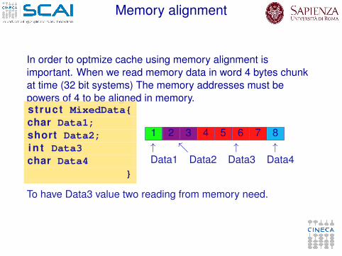
Memory alignment
In order to optmize cache using memory alignment isimportant. When we read memory data in word 4 bytes chunkat time (32 bit systems) The memory addresses must bepowers of 4 to be aligned in memory.struct MixedData{char Data1;short Data2;i n t Data3char Data4
}
1 2 3 4 5 6 7 8↑ ↖ ↑ ↑Data1 Data2 Data3 Data4
To have Data3 value two reading from memory need.
Memory alignment
With alignment:
struct MixedData{char Data1;char Padding1[1];short Data2;i n t Data3char Data4char Padding2[3];
}
Data1 Data2 Data3 Data4↓ ↓ ↓ ↓1 2 3 4 5 6 7 8 9 10 11 12
↑ ↑Padding1 Padding2
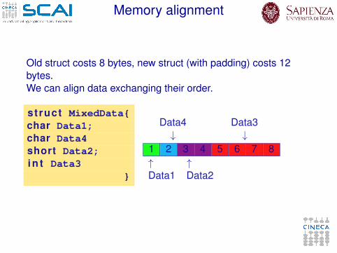
Memory alignment
Old struct costs 8 bytes, new struct (with padding) costs 12bytes.We can align data exchanging their order.
struct MixedData{char Data1;char Data4short Data2;i n t Data3
}
Data4 Data3↓ ↓
1 2 3 4 5 6 7 8↑ ↑Data1 Data2
Memory alignment
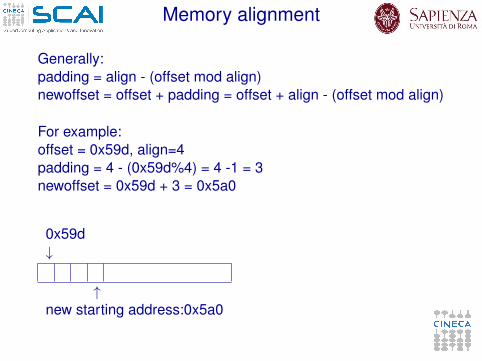
Generally:padding = align - (offset mod align)newoffset = offset + padding = offset + align - (offset mod align)
For example:offset = 0x59d, align=4padding = 4 - (0x59d%4) = 4 -1 = 3newoffset = 0x59d + 3 = 0x5a0
0x59d↓
↑new starting address:0x5a0
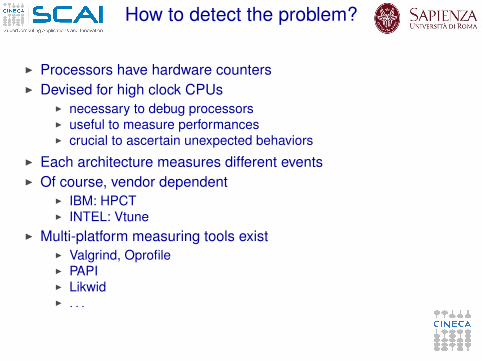
How to detect the problem?
I Processors have hardware countersI Devised for high clock CPUs
I necessary to debug processorsI useful to measure performancesI crucial to ascertain unexpected behaviors
I Each architecture measures different eventsI Of course, vendor dependent
I IBM: HPCTI INTEL: Vtune
I Multi-platform measuring tools existI Valgrind, OprofileI PAPII LikwidI . . .
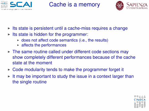
Cache is a memory
I Its state is persistent until a cache-miss requires a changeI Its state is hidden for the programmer:
I does not affect code semantics (i.e., the results)I affects the performances
I The same routine called under different code sections mayshow completely different performances because of the cachestate at the moment
I Code modularity tends to make the programmer forget itI It may be important to study the issue in a context larger than
the single routine
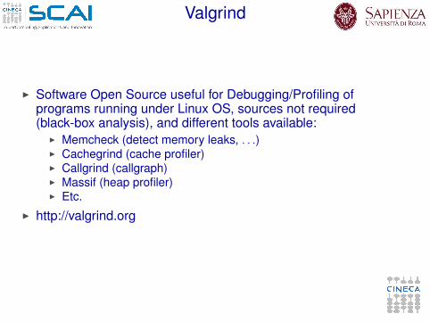
Valgrind
I Software Open Source useful for Debugging/Profiling ofprograms running under Linux OS, sources not required(black-box analysis), and different tools available:
I Memcheck (detect memory leaks, . . .)I Cachegrind (cache profiler)I Callgrind (callgraph)I Massif (heap profiler)I Etc.
I http://valgrind.org
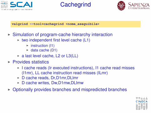
Cachegrind
valgrind --tool=cachegrind <nome_eseguibile>
I Simulation of program-cache hierarchy interactionI two independent first level cache (L1)
I instruction (I1)I data cache (D1)
I a last level cache, L2 or L3(LL)I Provides statistics
I I cache reads (Ir executed instructions), I1 cache read misses(I1mr), LL cache instruction read misses (ILmr)
I D cache reads, Dr,D1mr,DLlmrI D cache writes, Dw,D1mw,DLlmw
I Optionally provides branches and mispredicted branches
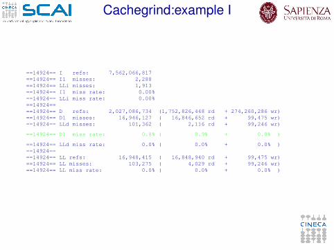
Cachegrind:example I
==14924== I refs: 7,562,066,817==14924== I1 misses: 2,288==14924== LLi misses: 1,913==14924== I1 miss rate: 0.00%==14924== LLi miss rate: 0.00%==14924====14924== D refs: 2,027,086,734 (1,752,826,448 rd + 274,260,286 wr)==14924== D1 misses: 16,946,127 ( 16,846,652 rd + 99,475 wr)==14924== LLd misses: 101,362 ( 2,116 rd + 99,246 wr)
==14924== D1 miss rate: 0.8% ( 0.9% + 0.0% )
==14924== LLd miss rate: 0.0% ( 0.0% + 0.0% )==14924====14924== LL refs: 16,948,415 ( 16,848,940 rd + 99,475 wr)==14924== LL misses: 103,275 ( 4,029 rd + 99,246 wr)==14924== LL miss rate: 0.0% ( 0.0% + 0.0% )
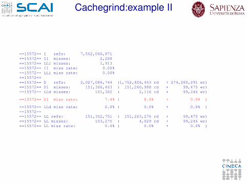
Cachegrind:example II
==15572== I refs: 7,562,066,871==15572== I1 misses: 2,288==15572== LLi misses: 1,913==15572== I1 miss rate: 0.00%==15572== LLi miss rate: 0.00%==15572====15572== D refs: 2,027,086,744 (1,752,826,453 rd + 274,260,291 wr)==15572== D1 misses: 151,360,463 ( 151,260,988 rd + 99,475 wr)==15572== LLd misses: 101,362 ( 2,116 rd + 99,246 wr)
==15572== D1 miss rate: 7.4% ( 8.6% + 0.0% )
==15572== LLd miss rate: 0.0% ( 0.0% + 0.0% )==15572====15572== LL refs: 151,362,751 ( 151,263,276 rd + 99,475 wr)==15572== LL misses: 103,275 ( 4,029 rd + 99,246 wr)==15572== LL miss rate: 0.0% ( 0.0% + 0.0% )

Cachegrind:cg_annotate
I Cachegrind automatically produces the filecachegrind.out.<pid>
I In addition to the previous information, more detailed statisticsfor each function is made available
cg_annotate cachegrind.out.<pid>
Cachegrind:options
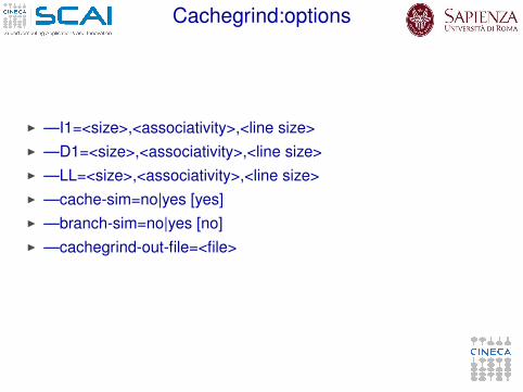
I —I1=<size>,<associativity>,<line size>I —D1=<size>,<associativity>,<line size>I —LL=<size>,<associativity>,<line size>I —cache-sim=no|yes [yes]I —branch-sim=no|yes [no]I —cachegrind-out-file=<file>
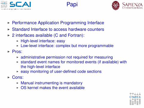
Papi
I Performance Application Programming InterfaceI Standard Interface to access hardware countersI 2 interfaces available (C and Fortran):
I High-level interface: easyI Low-level interface: complex but more programmable
I Pros:I administrative permission not required for measuringI standard event names for monitored events (if available) with
the high-level interfaceI easy monitoring of user-defined code sections
I Cons:I Manual instrumenting is mandatoryI OS kernel makes the event available
Papi Events
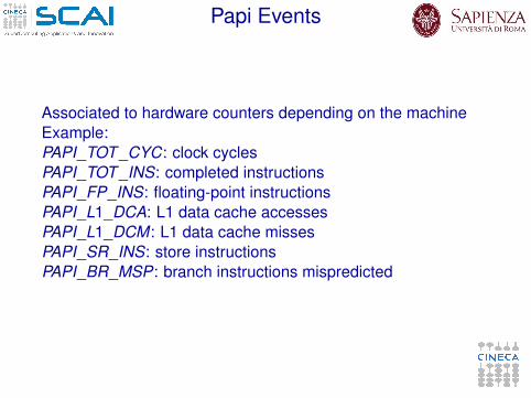
Associated to hardware counters depending on the machineExample:PAPI_TOT _CYC: clock cyclesPAPI_TOT _INS: completed instructionsPAPI_FP_INS: floating-point instructionsPAPI_L1_DCA: L1 data cache accessesPAPI_L1_DCM: L1 data cache missesPAPI_SR_INS: store instructionsPAPI_BR_MSP: branch instructions mispredicted
Papi: interface
I High-level library calls are intuitiveI It is possible to simultaneously monitor different eventsI In Fortran:
# include "fpapi_test.h"integer events(2), retval ; integer*8 values(2)......events(1) = PAPI_FP_INS ; events(2) = PAPI_L1_DCM......c a l l PAPIf_start_counters(events, 2, retval)c a l l PAPIf_read_counters(values, 2, retval) ! Clear values< sezione di codice da monitorare >c a l l PAPIf_stop_counters(values, 2, retval)pr in t*,’Floating point instructions’,values(1)pr in t*,’L1 Data Cache Misses: ’,values(2).......
Papi: interface
I It is possible to handle errors analyzing a variable returned bythe subroutine
I It is possible to perform queries to check the availability ofhardware counters, etc.
I It is recommended to call a dummy subroutine after themonitored section to ensure that the optimization has notaltered the instruction flow


![Elementi di Programmazione Avanzata in R - SUPSI - Dalle …people.idsia.ch/~azzimonti/ProgrammazioneAvanzataInR.pdf · Introduzione R [1]èunlinguaggiodiprogrammazione,nonchéunprogrammaperinter-pretaretalelinguaggio,orientatoadapplicazioniinambitostatistico,ideato](https://img.pdfslide.tips/doc/110x75/5c671c5809d3f2c85f8b566f/elementi-di-programmazione-avanzata-in-r-supsi-dalle-azzimontiprogrammazioneavanzatainrpdf.jpg)