Propagators for the time-dependent Kohn-Sham equations (II)

Alberto Castro

�

, Miguel A. L. Marques

�and Angel Rubio

�

�

Freie Universitat Berlin�

Donostia International Physics Center

– p.1/23

The problem

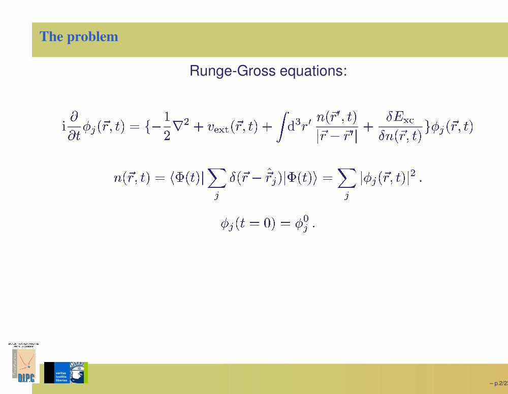
Runge-Gross equations:

� ��� ��� �� � � � ��� �� � � ��� �� � �� � � � � � � � �� � � � � � � � !" � #! � �� � � $ �� �� � �

� � � � � � %& � � �

! � � � '� � & � � ( � � �� �� � � �)

��� � � � * � � +� )

– p.2/23

The problem

� ,,� � � � ( � '.- � � � � � ( )

� � � � * ( � � +( )

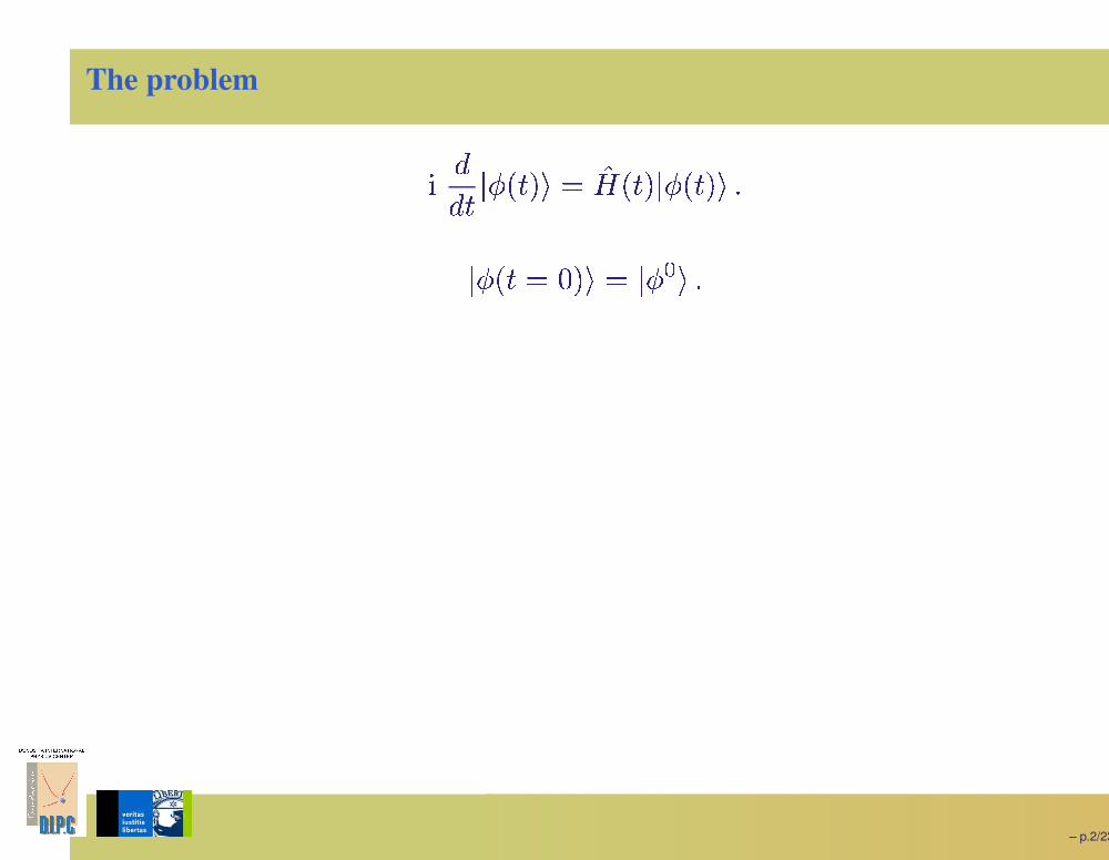
– p.2/23

The problem

� ,,� � � � ( � '.- � � � � � ( )

� � � � * ( � � +( )

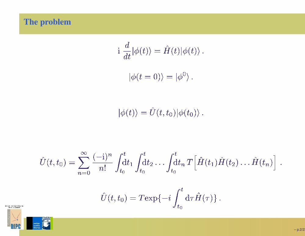
� � � ( � '0/ � � � � + � � � + ( )

– p.2/23

The problem

� ,,� � � � ( � '.- � � � � � ( )

� � � � * ( � � +( )

� � � ( � '0/ � � � � + � � � + ( )

'0/ � � � � + �1

23 +�� � 2

� 45

576� �98

5576

� � �) ) )5

576� � 2 : ; '0- � �98 '0- � � � ) ) ) '0- � � 2 < )

'=/ � � � � + � :?>@ A � � B 55 6

�=C '=- � C $)

– p.2/23

The problem

Find

'0/ DE E � � � F � � �

such that:

G H �?IKJ 5L +'./ D E E � � � F � � �

'=/ � � � F � � � � ' �

G

It is unitary if

'=- � �

is hermitian:

'=/ DE E � � � � F � � � '=/ DE E � � � F � � � � ' �

G

It preserves time-reversal symmetry:

'./ D E E M8 � � � F � � � � './ DE E � � � � � F �

G

It permits stable simulations.G

It is computationally affordable.

– p.3/23

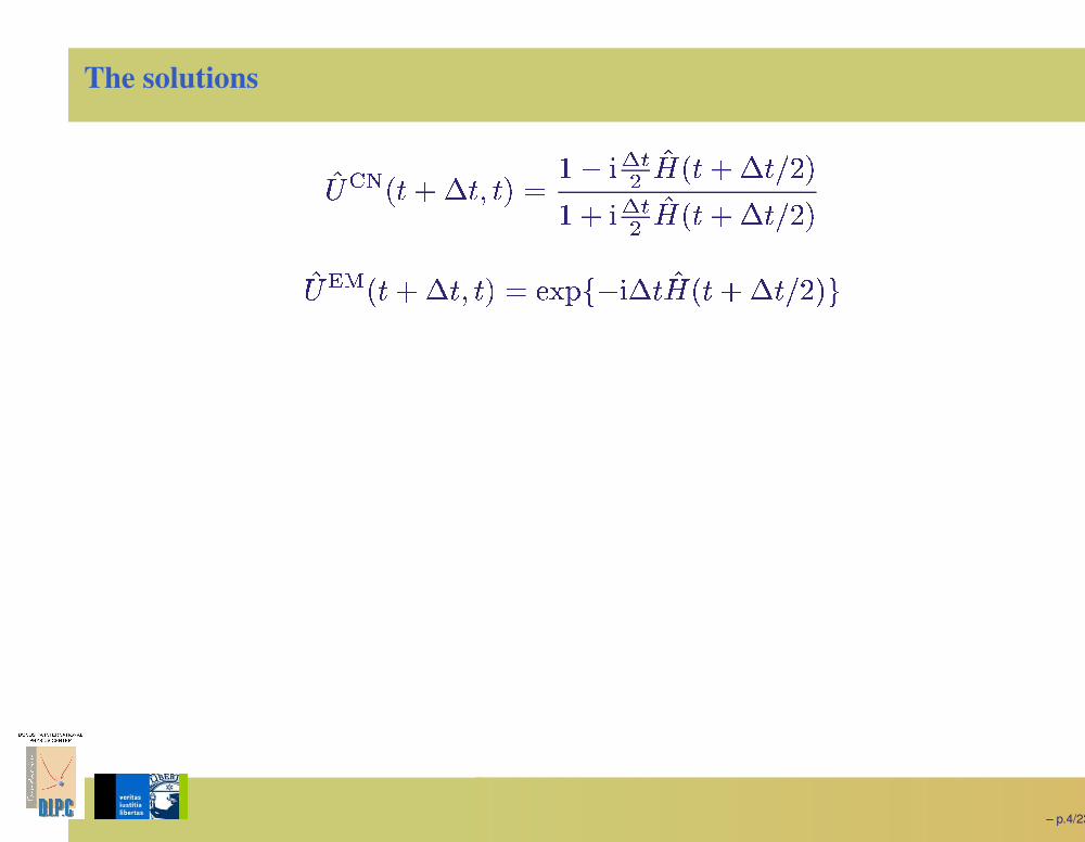
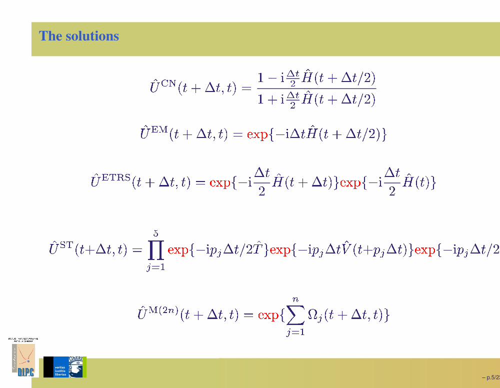
The solutions

'./ NO � � � F � � � � � � � J 5� '.- � � � F � P �

� � � J 5� '0- � � � F � P �

– p.4/23

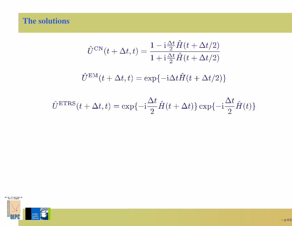
The solutions

'./ NO � � � F � � � � � � � J 5� '.- � � � F � P �

� � � J 5� '0- � � � F � P �

' / QR � � � F � � � � > @ A ��� � F � '- � � � F � P � $

– p.4/23

The solutions

'./ NO � � � F � � � � � � � J 5� '.- � � � F � P �

� � � J 5� '0- � � � F � P �

' / QR � � � F � � � � > @ A ��� � F � '- � � � F � P � $

'./ QS T U � � � F � � � � >@ A ��� � F �� '.- � � � F � $ > @ A ��� � F �� '.- � � $

– p.4/23

The solutions

'./ NO � � � F � � � � � � � J 5� '.- � � � F � P �

� � � J 5� '0- � � � F � P �

' / QR � � � F � � � � > @ A ��� � F � '- � � � F � P � $

'./ QS T U � � � F � � � � >@ A ��� � F �� '.- � � � F � $ > @ A ��� � F �� '.- � � $

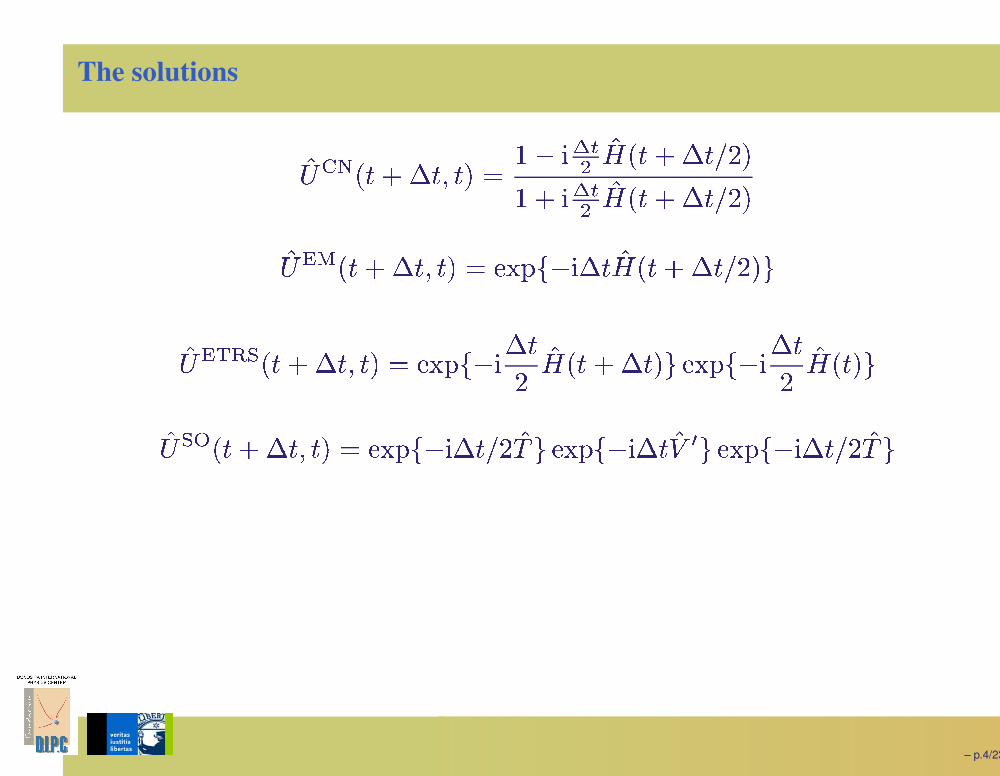
'./ UV � � � F � � � � >@ A � � � F � P � ' : $ >@ A ��� � F � '.W � $ > @ A ��� � F � P � ' : $

– p.4/23

The solutions

'./ NO � � � F � � � � � � � J 5� '.- � � � F � P �

� � � J 5� '0- � � � F � P �

' / QR � � � F � � � � > @ A ��� � F � '- � � � F � P � $

'./ QS T U � � � F � � � � >@ A ��� � F �� '.- � � � F � $ > @ A ��� � F �� '.- � � $

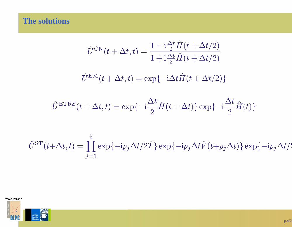
'0/ U S � � � F � � � �X

� 38>@ A � � �?Y � F � P � ' : $ > @ A ��� �Y � F � '0W � � � Y � F � $ >@ A ��� �Y � F � P �

– p.4/23

The solutions

'./ NO � � � F � � � � � � � J 5� '.- � � � F � P �

� � � J 5� '0- � � � F � P �

' / QR � � � F � � � � > @ A ��� � F � '- � � � F � P � $

'./ QS T U � � � F � � � � >@ A ��� � F �� '.- � � � F � $ > @ A ��� � F �� '.- � � $

'0/ U S � � � F � � � �X

� 38>@ A � � �?Y � F � P � ' : $ > @ A ��� �Y � F � '0W � � � Y � F � $ >@ A ��� �Y � F � P �

'./ R Z � 2[ � � � F � � � � >@ A � 2� 38

\ � � � � F � � � $

– p.4/23

The solutions

'./ NO � � � F � � � � � � � J 5� '.- � � � F � P �

� � � J 5� '0- � � � F � P �

' / QR � � � F � � � � > @ A ��� � F � '- � � � F � P � $

'./ QS T U � � � F � � � � >@ A ��� � F �� '- � � � F � $ > @ A ��� � F �� '.- � � $

'0/ U S � � � F � � � �X

� 38>@ A � � �?Y � F � P � ' : $ >@ A ��� �?Y � F � ' W � � � Y � F � $ >@ A ��� �?Y � F � P �

'./ R Z � 2[ � � � F � � � � >@ A � 2� 38

\ � � � � F � � � $

– p.5/23

The exponential

>@ A �] $ �1

� 3 +�

^ 4 ] � )

If is not diagonal, diagonalize:

and

– p.6/23

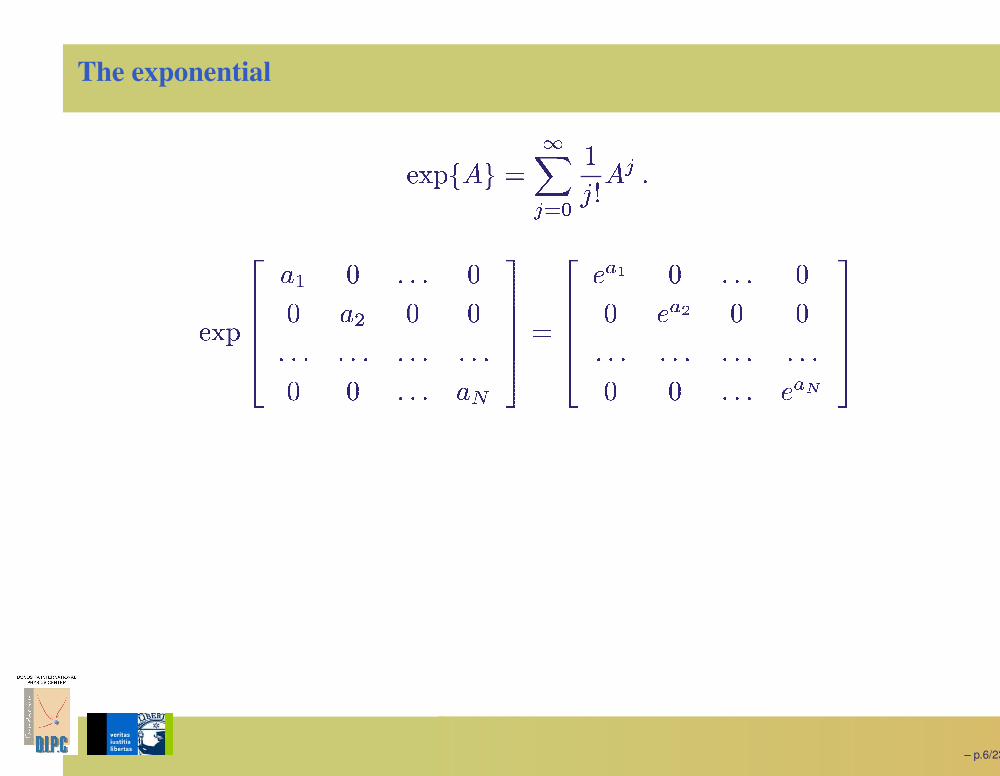
The exponential

>@ A �] $ �1

� 3 +�

^ 4 ] � )

>@ A_

`a`b`acd8 * ) ) ) *

* d � * *

) ) ) ) ) ) ) ) ) ) ) )* * ) ) ) dfeg

hahbhai �_

`a`b`acj kl * ) ) ) *

* j km * *

) ) ) ) ) ) ) ) ) ) ) )* * ) ) ) j kng

hahbhai

If is not diagonal, diagonalize:

and

– p.6/23

The exponential

>@ A �] $ �1

� 3 +�

^ 4 ] � )

>@ A_

`a`b`acd8 * ) ) ) *

* d � * *

) ) ) ) ) ) ) ) ) ) ) )* * ) ) ) dfeg

hahbhai �_

`a`b`acj kl * ) ) ) *

* j km * *

) ) ) ) ) ) ) ) ) ) ) )* * ) ) ) j kng

hahbhai

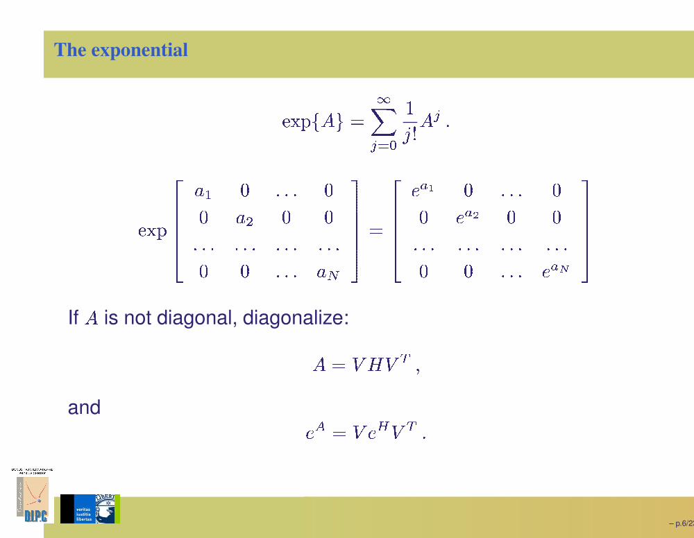
If

]

is not diagonal, diagonalize:

] � W - W o �

and j p � W j q W o)

– p.6/23

The exponential: small matrices

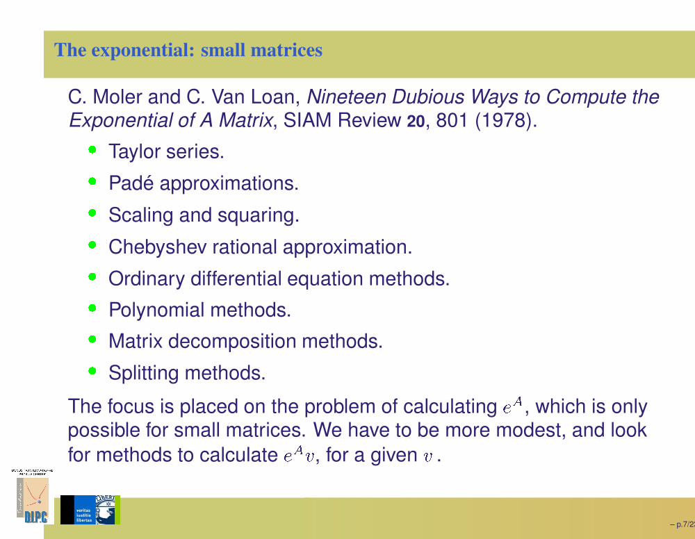
C. Moler and C. Van Loan, Nineteen Dubious Ways to Compute theExponential of A Matrix, SIAM Review 20, 801 (1978).G

Taylor series.G

Padé approximations.G

Scaling and squaring.G

Chebyshev rational approximation.G

Ordinary differential equation methods.G

Polynomial methods.G

Matrix decomposition methods.G

Splitting methods.

The focus is placed on the problem of calculating j p

, which is onlypossible for small matrices. We have to be more modest, and lookfor methods to calculate j p� , for a given� .

– p.7/23

The exponential: small matrices

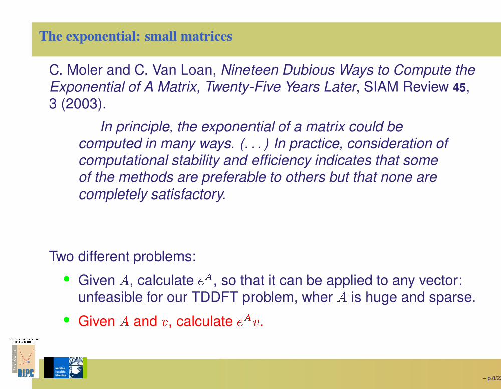
C. Moler and C. Van Loan, Nineteen Dubious Ways to Compute theExponential of A Matrix, Twenty-Five Years Later, SIAM Review 45,3 (2003).

In principle, the exponential of a matrix could becomputed in many ways. (. . . ) In practice, consideration ofcomputational stability and efficiency indicates that someof the methods are preferable to others but that none arecompletely satisfactory.

Two different problems:

Given , calculate , so that it can be applied to any vector:unfeasible for our TDDFT problem, wher is huge and sparse.

Given and , calculate .

– p.8/23

The exponential: small matrices

C. Moler and C. Van Loan, Nineteen Dubious Ways to Compute theExponential of A Matrix, Twenty-Five Years Later, SIAM Review 45,3 (2003).

In principle, the exponential of a matrix could becomputed in many ways. (. . . ) In practice, consideration ofcomputational stability and efficiency indicates that someof the methods are preferable to others but that none arecompletely satisfactory.

Two different problems:G

Given

]

, calculate j p, so that it can be applied to any vector:

unfeasible for our TDDFT problem, wher

]

is huge and sparse.G

Given

]

and� , calculate j p� .

– p.8/23

N-th order expansion

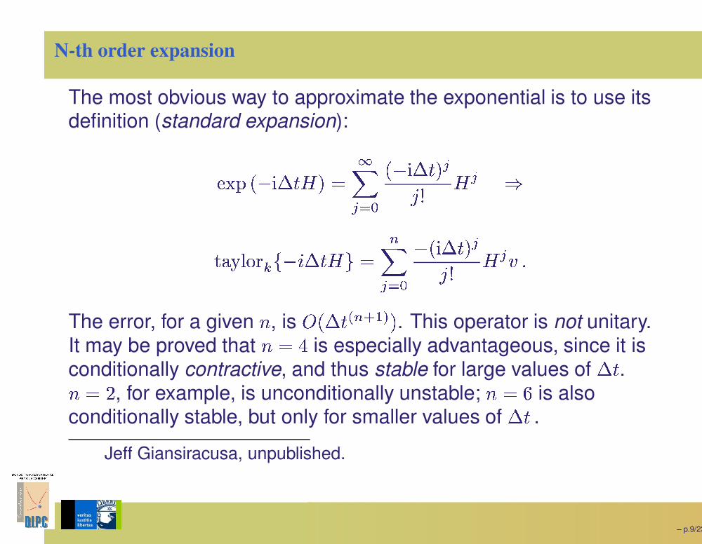
The most obvious way to approximate the exponential is to use itsdefinition (standard expansion):

>@ A �� � F � - �1

� 3 +�� � F � �

^ 4 - � r

sutv Hxwy z ��� B F � - $ �2

� 3 +� � � F � �

^ 4 - � � )

The error, for a given �, is

{ � F � Z 2|8 [ . This operator is not unitary.

It may be proved that � � }is especially advantageous, since it is

conditionally contractive, and thus stable for large values of

F � .� � �

, for example, is unconditionally unstable; � � ~

is alsoconditionally stable, but only for smaller values of

F � .

Jeff Giansiracusa, unpublished.

– p.9/23

Chebyshev expansion

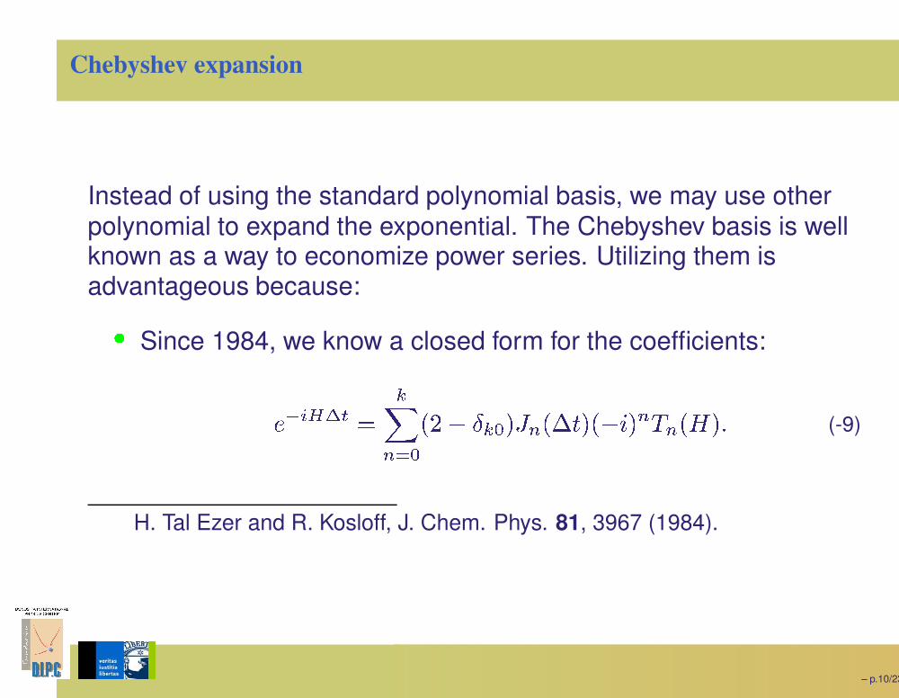
Instead of using the standard polynomial basis, we may use otherpolynomial to expand the exponential. The Chebyshev basis is wellknown as a way to economize power series. Utilizing them isadvantageous because:

G

Since 1984, we know a closed form for the coefficients:

j M � q J 5 �z

23 +� � � ! z + � 2� F � �� B 2 : 2� - ) (-9)

H. Tal Ezer and R. Kosloff, J. Chem. Phys. 81, 3967 (1984).

– p.10/23

G

Evaluation of the polynomials may be done at low cost(essentially the same than with standard expansion) thanks toClenshaw’s algorithm .

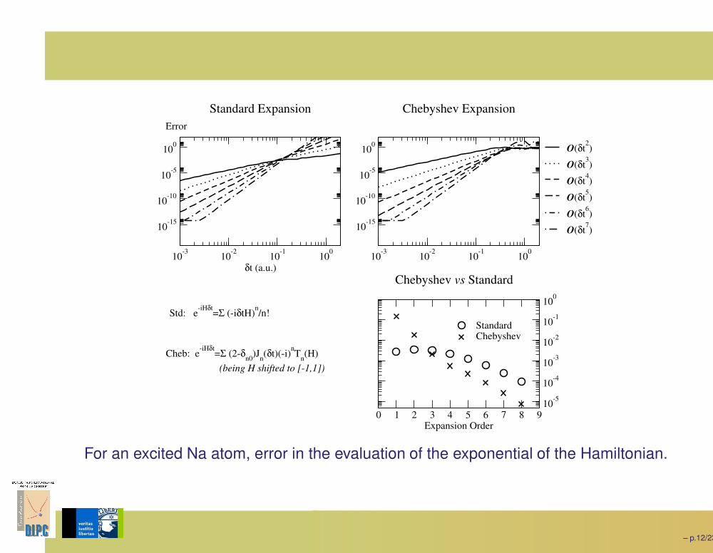
Chebyshev expansion error vs standard expansion error

C. W. Clenshaw, MTAC 9, 118 (1955).

– p.11/23

10-3 10-2 10-1 100

δt (a.u.)

10-15

10-10

10-5

100

Error

Standard Expansion

10-3 10-2 10-1 100

10-15

10-10

10-5

100 O(δt2)

O(δt3)

O(δt4)

O(δt5)

O(δt6)

O(δt7)

Chebyshev Expansion

0 1 2 3 4 5 6 7 8 9Expansion Order

10-5

10-4

10-3

10-2

10-1

100

StandardChebyshev

Chebyshev vs Standard

Std: e-iHδt=Σ (-iδtH)n/n!

Cheb: e-iHδt=Σ (2-δn0)Jn(δt)(-i)nTn(H)(being H shifted to [-1,1])

For an excited Na atom, error in the evaluation of the exponential of the Hamiltonian.

– p.12/23

Split-Operator Approaches

G

The Kohn-Sham hamiltonian

-

has the form

- � : � W, where:

is diagonal if reciprocal space, and

W

is diagonal in realspace. This suggests the use of the Strang splitting(split-operator, split step, ...):

>@ A �� B F � - � > @ A �� B F � P � : > @ A �� B F � W >@ A �� B F � P � :

(-9)

G

The split-operator may be kinetic or potential referenced.G

The error is third order in

F � . The method is unitary andunconditionally stable.G

A wealth of other splitting schemes are possible.

W. C. Strang, J. Numer. Anal. 6, 506 (1968).R. Kosloff, J. Phys. Chem. 92, 2087 (1988)-N. N. Yanenko, The Method of Fractional Steps, Springer, 1971.

– p.13/23

Suzuki-Trotter

G

Suzuki generalized Strang splitting to higuer orders. Forexample, to fourth order.

j � q � ��� ��� �X

� 38� � � Y � � � (-9)

where Y � is a set of real numbers, and� � ��

is the normalStrang splitting.G

The number of FFTs is multiplied by five. It is thus unclear thatthis method involves overall increase in speed over normalStrang splitting.

M. Suzuki, J. Phys. Soc. Jpn. 61, L3015 (1992);

O. Sugino and Y. Miyamoto, Phys. Rev. B 59, 2579 (1999).

– p.14/23

G

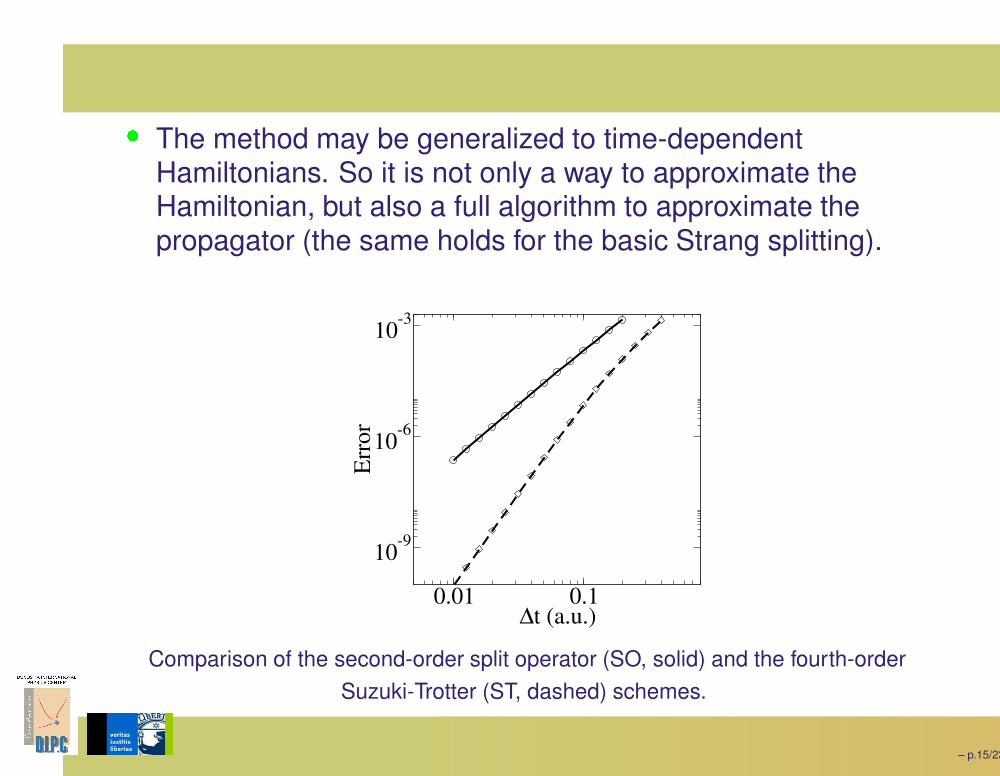
The method may be generalized to time-dependentHamiltonians. So it is not only a way to approximate theHamiltonian, but also a full algorithm to approximate thepropagator (the same holds for the basic Strang splitting).

0.01 0.1∆t (a.u.)

10-9

10-6

10-3

Err

or

Comparison of the second-order split operator (SO, solid) and the fourth-orderSuzuki-Trotter (ST, dashed) schemes.

– p.15/23

Krylov subspace projection

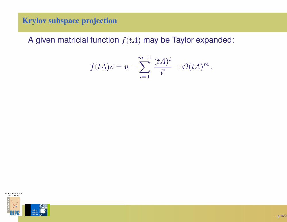
A given matricial function

� � � ]

may be Taylor expanded:

� � � ] � � � � � M8� 38

� � ] �B 4 � � � � ] �)

This provides us with a polynomial approximation of degree :

It is not the only possible polynomial approximation. All possibilitiesare elements of the Krylov subspace:

What is the element of that optimally approximates?

– p.16/23

Krylov subspace projection

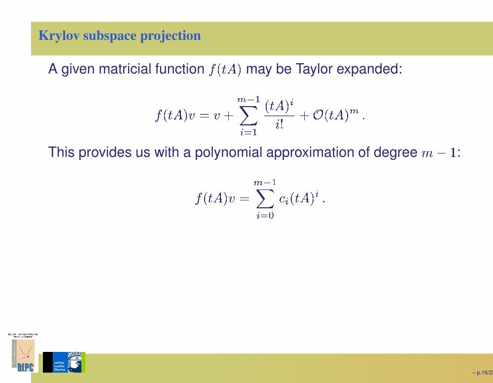
A given matricial function

� � � ]

may be Taylor expanded:

� � � ] � � � � � M8� 38

� � ] �B 4 � � � � ] �)

This provides us with a polynomial approximation of degree � � �

:

� � � ] � �� M8

� 3 +� � � � ] � )

It is not the only possible polynomial approximation. All possibilitiesare elements of the Krylov subspace:

What is the element of that optimally approximates?

– p.16/23

Krylov subspace projection

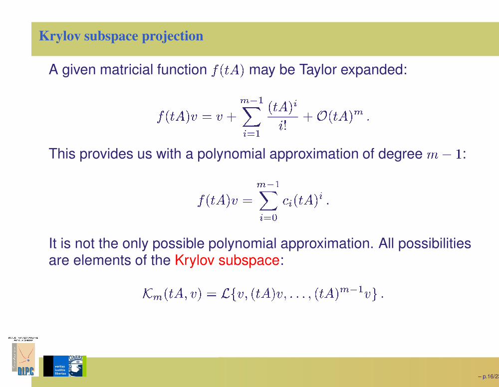
A given matricial function

� � � ]

may be Taylor expanded:

� � � ] � � � � � M8� 38

� � ] �B 4 � � � � ] �)

This provides us with a polynomial approximation of degree � � �

:

� � � ] � �� M8

� 3 +� � � � ] � )

It is not the only possible polynomial approximation. All possibilitiesare elements of the Krylov subspace:

� � � � ] �� � � �� � � � ] � �) ) ) � � � ] � M8 � $)

What is the element of that optimally approximates?

– p.16/23

Krylov subspace projection

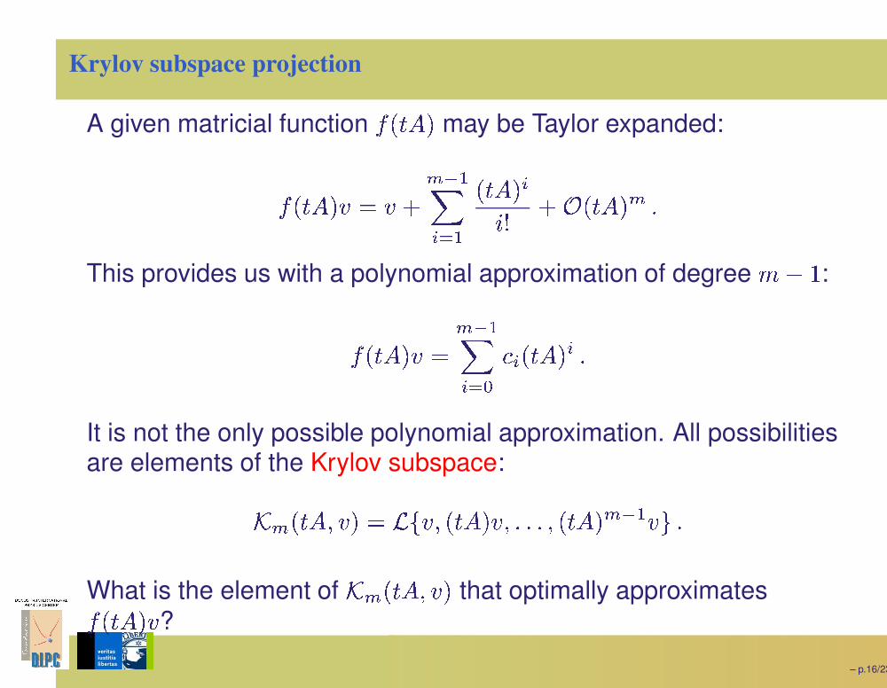
A given matricial function

� � � ]

may be Taylor expanded:

� � � ] � � � � � M8� 38

� � ] �B 4 � � � � ] �)

This provides us with a polynomial approximation of degree � � �

:

� � � ] � �� M8

� 3 +� � � � ] � )

It is not the only possible polynomial approximation. All possibilitiesare elements of the Krylov subspace:

� � � � ] �� � � �� � � � ] � �) ) ) � � � ] � M8 � $)

What is the element of

� � � � ] ��

that optimally approximates� � � ] � ?

– p.16/23

Krylov subspace projection

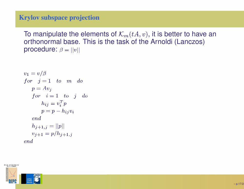
To manipulate the elements of

� � � � ] ��

, it is better to have anorthonormal base. This is the task of the Arnoldi (Lanczos)procedure: �0� � ��� � �

�� � � � �

���� � � � ��� � ��

 � ¡�¢���� £� � ��� � ��¤¦¥¢ � � §¥  

 �  ©¨ ¤ª¥¢ � ¥«¬ �¤¢ ­�¯® ¢ � � �   � �

�¢ ­� �   � ¤¢ ­�¯® ¢«¬ �

– p.17/23

Krylov subspace projection

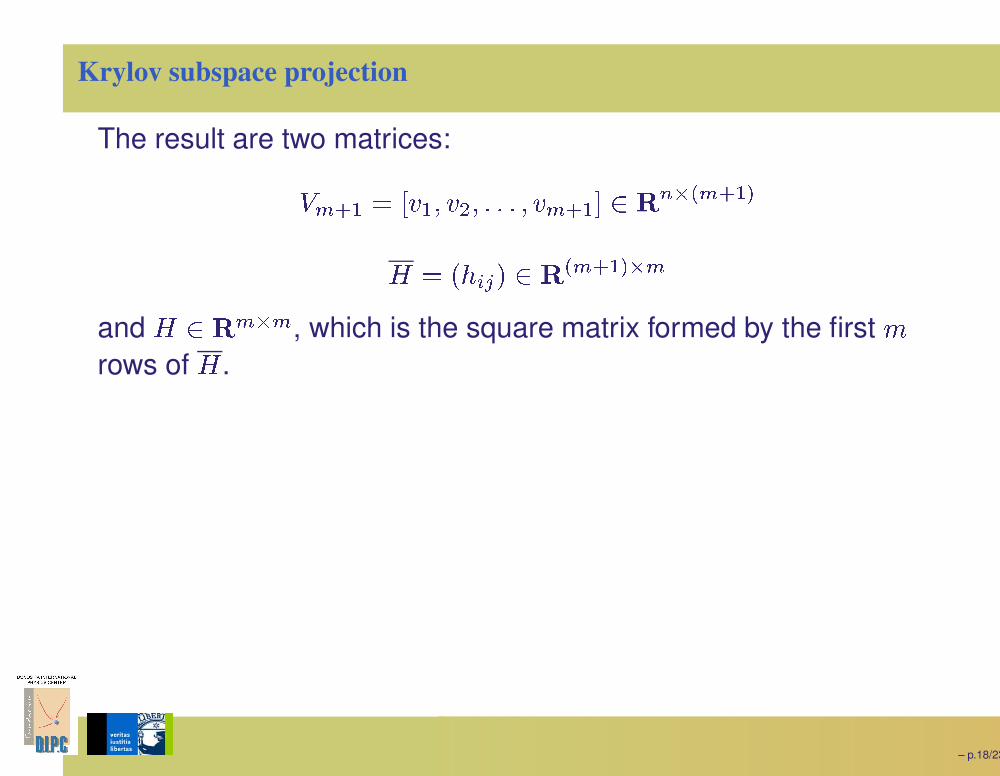
The result are two matrices:

W � |8 � °� 8 �� � �) ) ) �� � |8 ±³² ´ 2µ Z � |8 [

- � �¶ � � ² ´ Z � |8 [ µ �and

- ² ´ � µ �

, which is the square matrix formed by the first �

rows of

-

.

These matrices satisfy:

– p.18/23

Krylov subspace projection

The result are two matrices:

W � |8 � °� 8 �� � �) ) ) �� � |8 ±³² ´ 2µ Z � |8 [

- � �¶ � � ² ´ Z � |8 [ µ �and

- ² ´ � µ �

, which is the square matrix formed by the first �

rows of

-

.These matrices satisfy:

W o� ] W � � - �

] W � � W � |8 -

W o� W � � ·

– p.18/23

Krylov subspace projection

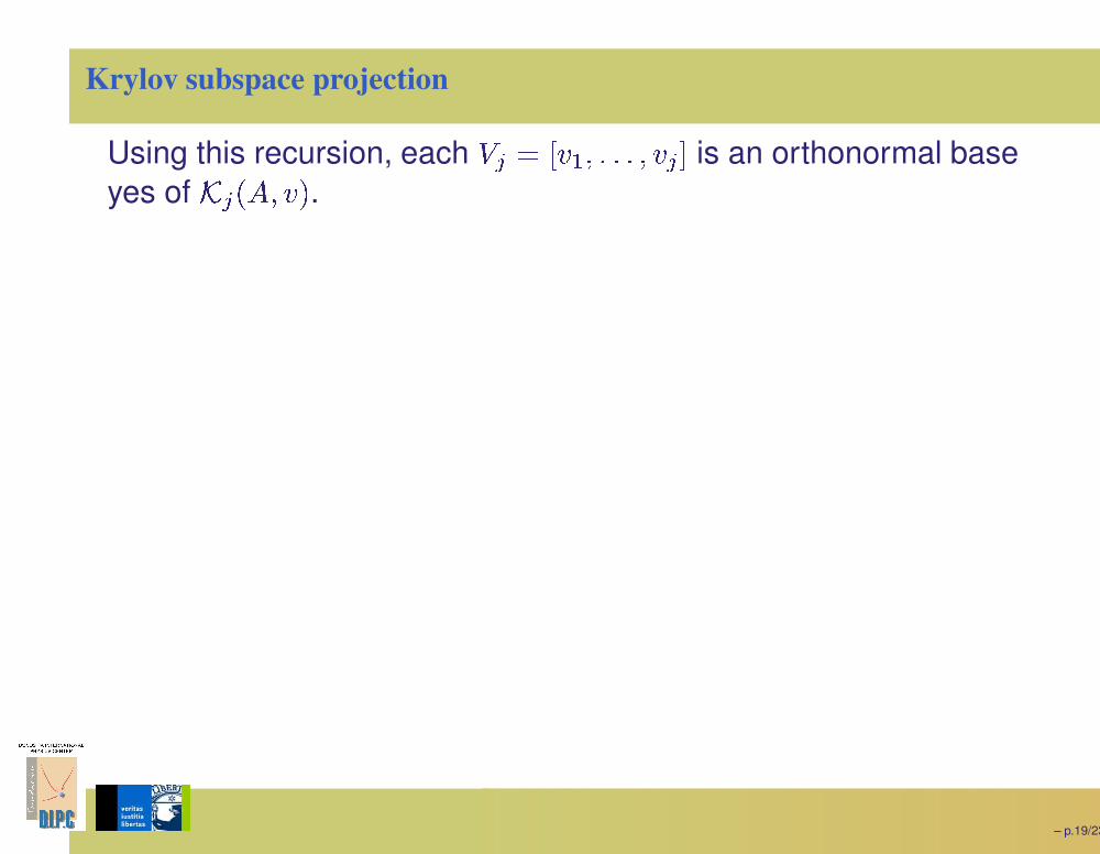
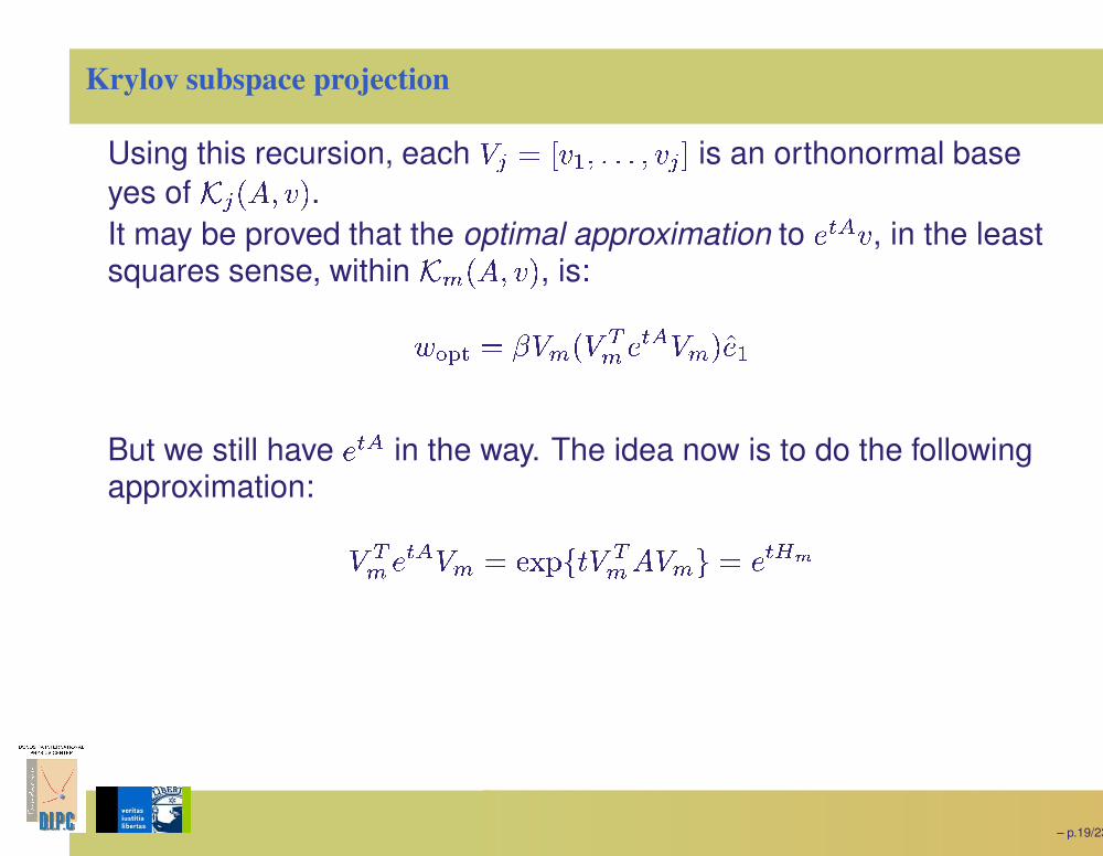
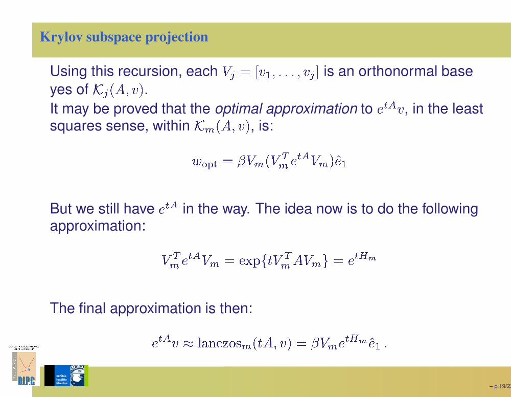
Using this recursion, each

W � � °� 8 �) ) ) �� � ±

is an orthonormal baseyes of

��� �] ��

.

It may be proved that the optimal approximation to , in the leastsquares sense, within , is:

But we still have in the way. The idea now is to do the followingapproximation:

The final approximation is then:

– p.19/23

Krylov subspace projection

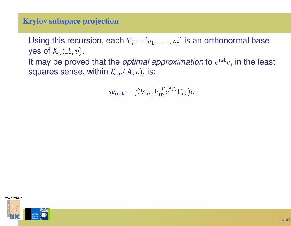
Using this recursion, each

W � � °� 8 �) ) ) �� � ±

is an orthonormal baseyes of

��� �] ��

.It may be proved that the optimal approximation to j 5 p� , in the leastsquares sense, within

� � �] ��

, is:

¸¦¹º � � » W � � W o� j 5 p W � ' j8

But we still have in the way. The idea now is to do the followingapproximation:

The final approximation is then:

– p.19/23

Krylov subspace projection

Using this recursion, each

W � � °� 8 �) ) ) �� � ±

is an orthonormal baseyes of

��� �] ��

.It may be proved that the optimal approximation to j 5 p� , in the leastsquares sense, within

� � �] ��

, is:

¸¦¹º � � » W � � W o� j 5 p W � ' j8But we still have j 5 p

in the way. The idea now is to do the followingapproximation:

W o� j 5 p W � � >@ A � � W o� ] W � $ � j 5 q½¼

The final approximation is then:

– p.19/23

Krylov subspace projection

Using this recursion, each

W � � °� 8 �) ) ) �� � ±

is an orthonormal baseyes of

��� �] ��

.It may be proved that the optimal approximation to j 5 p� , in the leastsquares sense, within

� � �] ��

, is:

¸¦¹º � � » W � � W o� j 5 p W � ' j8But we still have j 5 p

in the way. The idea now is to do the followingapproximation:

W o� j 5 p W � � >@ A � � W o� ] W � $ � j 5 q½¼

The final approximation is then:

j 5 p� ¾ Ht¿ ÀÁ w � � � ] �� � » W � j 5 qü ' j8 )

– p.19/23

G

For a given order �, the method is

{ � � � � .G

For any m, the method is unitary.G

The computational cost grows linearly with �.G

The dimension � is increased recursively until someconvergence criterium (

» °Ä>@ A �� B F � - � ± �ÆÅ �). The decay of theerror decays superlinearly with �. So the method is of arbitraryaccuracy.

– p.20/23

10-3 10-2 10-1 100 101

∆t (a.u.)

10-15

10-10

10-5

100

Nor

mal

ized

resi

due

8th order ChebyshevLanczos

3 45

6

7

8 16 63

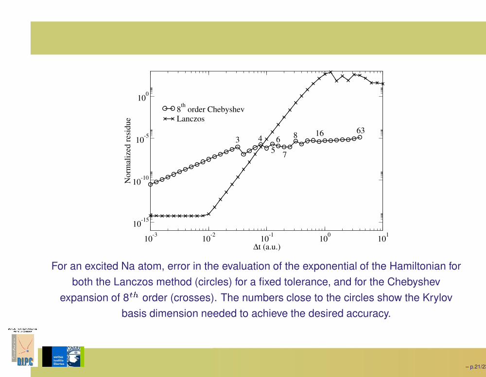
For an excited Na atom, error in the evaluation of the exponential of the Hamiltonian forboth the Lanczos method (circles) for a fixed tolerance, and for the Chebyshev

expansion of 8

Ç È

order (crosses). The numbers close to the circles show the Krylovbasis dimension needed to achieve the desired accuracy.

– p.21/23

0

100

200StandardChebyshevLanczos

0

100

200

p(δt

)/δt

(a.u

.-1)

0.1 0.2 0.3 0.4δt (a.u.)

0

100

200

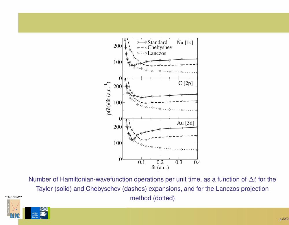
Na [1s]

C [2p]

Au [5d]

Number of Hamiltonian-wavefunction operations per unit time, as a function of

É �

for theTaylor (solid) and Chebyschev (dashes) expansions, and for the Lanczos projection

method (dotted)

– p.22/23

Conclusions

G

There is not an “always optimal” algorithm for the propagationof the TDKS equations.G

For long time propagations, assuring time-reversal symmetry isvery important.G

Some methods require the calculation of the action of theexponential of Hamiltonian matrices; there are efficientmethods to perform this task.G

The Lanczos-Krylov subspace projection seems to be the bestalgorithm to calculate the action of exponentials.G

For problems involving very high frequencies, Magnusexpansion are advantageous.G

Otherwise, a combination of the EM rule with Lanczossubspace projection is sufficient.

– p.23/23