Embed Size (px)
Citation preview

14.5.2018
1
Spatial Database System Prostorové databázové systémy
Jiří Horák
2nd part – Spatial databases
v. 2018
Literature • Aitkinson A. (2009): Beginning Spatial with MS SQL 2008. Apress. ISBN 978-1-4302-
1830-2. 425 pages. • Bělka L: Možnosti využití databáze pro uložení ortofotosnímků. Seminární práce. • Ďuráková D: Lecture7-8.PDF, GIS - Spatial SQL. • Kaufmann, San Francisco, 2002. ISBN 1-55860-588-6. 410 pages. • Lacko L. (2002): Oracle. Správa, programování a použití databázového systému.
ComputerPress. ISBN 80-7226-699-3 • Manolopoulos Y., Papadopoulos, Vassilakopoulos M.: Spatial Databases:
Technologies, Techniques, Trends. Idea Group Publishing. 340 stran, Hershey, 2005. ISBN 1-59140-387-1.
• Nabil R.A., Gangopadhyay A. (1997): Database Issues in Geographical Information Systems. Kluwer.
• Nabil R.A., Gangopadhyay Aryya (1998): Database Issues in Geographic Information Systems. Kluwer, 2.vydání, 1998.
• Pokorný, J.: Prostorové datové struktury. Sborník konference GIS’98, Ostrava, 1998. • Pokorný J.: Prostorové datové struktury a jejich použití. GIS Ostrava 2000. • Pokorný J.: Prostorové objekty a SQL. GIS Ostrava 2001. • Rigaux P., Scholl M., Voisard A. (2002): Spatial Databases with Application to GIS.
Literature 2 • Samet H. (1989): The Design and Analysis of Spatial Data Structures. Addison-
Wesley Publishing Company. ISBN 0-201-50255-0. 493 pp.
• Samet H. (1990): Application of Spatial Data Structures: computer graphics, image processing and GIS. Addison-Wesley Publishing Company. ISBN 0-201-50300-X. 507 pp.
• Sandbox1: http://wp.soulwasted.net/msz/pdb/prostorove-databaze-problemy-indexace-bodu-v-prostoru-algoritmy-stromove-hasovaci-kombinovane
• Šarmanová skripta INS.PDF
• Troch, J.: http://jt.sf.cz
• wiki 1: http://cs.wikipedia.org/wiki/Prostorov%C3%A1_datab%C3%A1ze
• http://www.geo.unizh.ch/oai/spatialdb/folien/ogcsf.pdf: Daniel Wirz, Department of Geography - GIS Division, University of Zurich [email protected], January 2004, OGC Simple Features (for SQL and XML/GML).
• Yeung A., Hall G. (2007): Spatial Database Systems. Desing, Implementation and Project Management. Springer, Dordrecht, 2007. ISBN 10-1-4020-5393-2. 553 pages.
• Žemlička: http://www.ksi.mff.cuni.cz/~zemlicka/vyuka/OZD/spatial/TitlePage.html
Introduction • Gütting (1994): spatial database system is the class of DBS which satisfies 3 basic
features: – Fulfil common properties of DBS – Offer spatial data types (SDT) in the database model and in the query language – Support implementation of spatial data types using spatial indexing (minimal requirement)
and highly performing algorithms for spatial join.
• spatial database system: – Satisfies requirements for standard database system , – Offers extended functions enabling to perform tasks specific for spatial data.
• Use various methods for overlaying and combining of features which utilize their location and topology.
• Spatial dbs do not replace SW for GIS but only facilitate part of functions specific for GIS.
• Spatial DBS today still more in the form of spatial data warehouses, • Their goal – to provide users (GIS) appropriate data in time and space (including
temporal consistency, appropriate aggregation etc.) • Features in reality are subjects of changes where the time of finishing changes are
so long that overcross usual response time and that is why we need to perform it as long transactions to assure consistency of database
• The goal of spatial data modelling in db (Pokorný):
– Enable to deal appropriate way with neighbourhood of spatial objects and its connectivity.
• Emphasizes topological properties required for data processing.
Proprietary data formats and structures
• ESRI shapefile: – SHP - for geometry
– DBF – storage of attribute (lexical) data
– SHX – indexation
– SBN and SBX – spatial indexation
– FBN and FBX - spatial indexation, only for reading
– PRJ – coordinate system
– AIN a AIH - attribute indexation
– IXS, MXS – geocoding
– SHP.XML - metadata in XML
– CPG – code page specification for DBF

14.5.2018
2
Proprietary data structures
• We can imagine it as relational table
• Not always are useful for user requirements
• Suitable data structure - enables effectively evaluate spatial queries (i.e. query for the polygon area, query for the intersection of 2 regions, query to find nearest neighbours of the object etc.)
• Structures in relational tables enable to deal with topological relationships but not easy way.
• Suitable to use other, auxiliary structures which directly represents topological relationships and real spatial objects represent a second layer.
• Spatial indexation, Spatial data structures (PDS)
• Spatial indexation can be applied for both vector and raster data
• spatial indexation is not enough to solve (evaluation) all spatial queries.
• We need in queries also lexical data (attributes), providing alphanumerical and temporal values, or modelling various relationships. Such data can be easily represented by i.e. relational tables with explicit link to spatial objects using ID.
• Necessity of integrated querying
Spatial indexation • We cannot use directly common indexation methods known from usual
databases.
• I.e. B-tree, which is suitable for primary key indexation, or any other attribute, is not sufficient for spatial data because of its multidimensionality.
• If we use directly some multidimensional spatial data structure like multidimensional grid or multidimensional B-trees, we reach the multidimensional spaces, nevertheless we do not cross the fact that this methods were proposed for multidimensional queries and not spatial queries.
• The problem of sequential ordering not simultaneous (coincident) ordering.
• Spatial queries, like query to i.e. nearest neighbour or intersection of objects, are multidimensional variants of classic method evaluated quite ineffective or non-evaluated.
• Another problem – these methods were proposed for point data but not always the spatial object can be represented by points.
Spatial data structures
• Each data structure for large data set has to be effectively transformed into disk (memory) pages.
• No each spatial data structure is suitable for all types of spatial queries.
• It is useful to measure not only spatial requirements for SDS but also complexity of each operation (INSERT, DELETE, UPDATE) because they are usually implemented by quite a lot complicated algorithms. Various versions of these algorithms enable to create new independent SDS.
• Next question – how dynamic are applications for given SDS? Are suitable for frequent update operations or more suitable for the velocity of evaluation of a spatial query?
• Independent operation is the initial building of the structure from the set of data (BUILD operation).
Operation with SQL
• Manipulation operations – insert
– delete
– update – modification of the object shape, attribute update etc.
• Selection (of objects): – graphical (show me ...)
– attributed
– Spatial query (for region etc.) – topological operators
• Creating new objects using operation : – UNION
– INTERSECTION
– DIFFERENCE
– And other specific spatial
• geometrical attribute = attribute contains geometry
• Spatial relation = relation including geometrical attribute
• Spatial relation have other properties than conventional relations, because they address mainly topological and metric relationships of concerned objects.
14.5.2018
3
Generation of GIS development according to Pokorný
according to Pokorný • 1st generation
– Spatial objects, their attributes and indexes are stored in files.
– Spatial queries are available, but no on-line links to other db data (necessary to transform data from db into proprietary files using export/import).
• 2nd generation – Attribute data as well as other application data are stored in relational database
– Geometrical objects and indexes are still stored in the file system.
– Integration of spatial data and other data are indirect. It is possible to make queries to spatial objects and to data connected with these objects. But the access is limited to requirements which can be easily decomposed into geometrical and lexical components.
– Query cannot be globally optimised.
• 3rd generation – They are controlled dominantly from the database side not from the GIS side.
– Spatial data types and respective operation and function are integrated into relational DBMS.
– Various implementation, the most advanced are represented by modules linked with object-relational DBMS (ORDBMS)
Generation of GIS development by Yeung, Hall According to Yeung, Hall
• 1st generation (to middle of 90) – Usage of specialised SW for GIS with specific API and also proprietary data storage in
specific file formats
• 2nd generation(to end of 90) – Increase utilisation of RDBMS in GIS – typical attribute data are stored in relational
database while geometrical part are still stored in proprietary files.
– GIS uses standard SQL queries for communication with DBS.
– Spatial data processing is performed only in GIS.
• 3rd generation (since the end of 90) – Spatial data is stored in ORDBMS including part of spatial functions.
– Except of using classic GIS engines there are new spatial application which do not use special SW for GIS but use only basic spatial functions available in current DBMS.
– Role of GIS – mainly data collection, graphical data editing, analysis, synthesis and modelling, cartography and visualisation
– Role of OODBMS – mainly data storage, its management, spatial indexing, data safety and integration, querying of spatial data
Spatial data storage in relational DB
4 methods of implementation of the geometrical model OGC or SQL/MM. First 3 were specified by OGC, the 4th comes from the possibility of object extension in language SQL:1999 specification
1. Spatial data are stored in tables in 1NF, objects are implemented by tables in SQL92 using numerical data type for storage of geometrical objects
2. Spatial data are stored as non-structured large binary objects (BLOB) or “opaque types”, objects using table in SQL92 with binary types for geometrical objects storage like BLOB or other LOB
3. Spatial data are stored in relational database extended with types of spatial data, objects using table in SQL92 with geometrical types such way that geometrical characteristics are accessible through text form as well as binary form
4. Spatial data are implemented using user defined types, or ADT respectively. Objects specified by tables in SQL:1999 using ADT
1. Spatial data as table in 1NF with numerical attributes
• Spatial objects have to be decomposed into primitive objects and these objects are stored using coordinates and numbers.
• Geometrical attributes are implemented using foreign keys to the table of geometrical objects.
• Table of geometrical objects is the part of other, classic normalised tables
• Topological model – polygons, edges, nodes.
• Each application usually applies own functions and integrity constraints.
• Processing of spatial queries are not well supported, because spatial data are dealt like any other data and no geometrical properties of the space are utilised.
• To find i.e. answer to the intersection of 2 geometries requires more accesses to more relations which commonly can be located on more places on the disk.

14.5.2018
4
Example for tetrahedron
• We need to implement a body consists of disjunctive tetrahedrons using relational database.
• tetrahedrons are specified by planes (faces), edges and points (nodes).
• Relevant data are stored into 4 relations: TETRAHEDRONS, PLANES, EDGES and POINTS.
• Relation TETRAHEDRONS contains pairs (t,f), where t is the ID of the TETRAHEDRON, f is the ID of one of its PLANES.
• Relation PLANES contains pairs (f,e), where f is the ID of the plane and e is one of the edge in the plane.
• Relation EDGES contains triples (e,p,q), where e is the ID of edges, p and q are end nodes of the edge.
• Relation POINTS contains tetrads (p,x,y,z), where p is the ID of POINT and x, y, z are their coordinates.
• The problem is to find simple answer for query, if the given line crosses the given tetrahedron.
Principles in Oracle
• Primitive objects in 2D are points, lines and polygons.
• Elements of these types can be combined into sets shaping geometrical objects identified by unique identifier (GID).
• These objects can also have non-spatial attributes
• Integration of objects into layers
• layers with heterogeneous geometry (contain together objects with different type and the same dimension),
• layers with homogeneous geometry (only 1 type of geometry is in the layer)
Structure of relational database
• Four relational tables
<layer_name> _LAYER(ORDCNT, LEVEL) <layer_name> _DIM(DIMNUM, LB, UB, TOLERANCE, DIMNAME) <layer_name> _GEOM(GID, ESEQ, TYPE, SEQ, X1, Y1, …, Xn, Yn) <layer_name> _INDEX(GID, CODE, MAXCODE)
Table LAYER
• ORDCNT contains the number of coordinates in each row of the GEOM table (geometrical objects).
• LEVEL column contains information about the number of division of quadrants in quadtree
Table DIM
• Each dimension (axe) is described, using its:
– number (DIMNUM),
– minimal coordinates (LB)
– maximal coordinates (UB),
– tolerance (TOLERANCE) which specifies the precision of separation for 2 points,
– the name of the dimension (f.e. X dimension, latitude).

14.5.2018
5
Table GEOM • parts of each geometrical objects are described in separated
rows
• For each GID following information is provided: – ESEQ a number of element
– ETYPE type of element (0 for point, 1 for line, 2 for polygon) (but for Oracle + 1),
– SEQ - the order of the row inside one element (i.e. lines of polygons are ordered in the direction (clockwise) or against the direction of clock (anticlockwise).
– Other columns contain coordinates of individual parts of the primitive elements.
• I.e. for octagon we need 8 rows in the GEOM table and 4 coordinates in each row for one line which builds octagon.
• 1 object = 1 GID
• 2 elements (0 and 1), both with type=3 (polygon)
INDEX
• Information about the indexation of geometrical objects
• Indexation uses quadtrees. Their projection into 2D plane creates a regular grid.
• The quadtree has not be balanced, thus some quadrants can be divided into more details than others. It depends on an user requirements and requirements of his/her application.
Querying geometries • Query is specified in SQL for these tables.
• To improve the efficiency the query the evaluation has usually 2 phases. F.e. in ORACLE RDBMS: – Primary filter: the query window is connected with the grid specified
by quadtree using JOIN operation. The quadtree is specified in the INDEX table. This way we obtain geometrical objects which can have not null intersection with the window,
– secondary filter: after primary filtering a detail calculation (solution of a geometrical intersection) is provided and the result is created.
• efficiency of the 1st phase depends on the depth of the index quadtree. Deeper quadtree improves the spatial resolution which lead to a better elimination of useless squares
2. Spatial data as BLOB and opaque types
• Storage of raster map – difficult manipulation
• Cannot deal with parts of spatial objects
• Better possibility - “opaque type” (black box)
• The object looks like binary object for DBMS but in reality it encompasses a structure which has to be decoded by special SW (GIS SW)
• MicroStation

14.5.2018
6
Storage by BLOB -2
• geometrical objects are frequently implemented by Well-Known Binary Representation for Geometry (WKBGeometry).
• Geometrical objects are stored with Minimal Boundary Rectangles
• It supports index creation (i.e. using R-trees)
• Usage of WKBGeometry is understandable also for the ODBC standard
3. Relational database extended by spatial data types
• Data types for geometry
• A new structure is added which is implemented ad hoc or again by tables, and respective new operations.
• The column with geometrical values is implemented through values of geometrical type
• LINESTRING (10 10, 20 20, 30 40)
• Text representation
• Is is necessary to have a function converting object in a given reference system from textual representation into geometrical one
• Standardization of data representation for description of the reference system. Implemented by Well-Known Text Representation of Spatial Reference System
• Support of special index structure
4. User defined types, ADT
• Functions modelling object’s behaviour are integrated into DBMS which improves optimisation of queries. We speak about user defined types (UDT) and functions (UDF). Mechanisms of their creation are parts of language constructors (SQL)
• In SQL3 abstract data type (ADT) is used for UDT and UDF as a more universal term
• ADT can be used to declare a new type of column including ADF functions (i.e. text, image, audio, video, time series, point, line, OLE).
• ADT encapsulates data and functions in the same meaning as in object oriented approach. Relational SŘBD provides new constructors to create both data types (i.e. ARRAY) and CREATE TYPE for creation of ADT.
• Using ARRAYs you can easily store coordinates of spatial objects. Using referencing through REF type you can easily link objects (inc. spatial objects) into more complex spatial spatial objects.
4. Geometrical objects with ADT
• Other suitable constructors:
• ROW TYPES – user can specify types and functions for rows in tables. Row components may be: – basic type,
– ADT,
– REF (references),
– type for modelling multivalue attributes:
Multivalue attribute is usually modelled using ARRAY. But current implementations of ORSŘBD offer also SET and BAG (multisets) constructors.
• Nested tables – also suitable for implementation of spatial objects. Its hierarchy can represent a hierarchy of spatial objects (i.e. highway -> road -> communication)
• Table can be specified by CREATE TABLE using a list of attributes or a type of row is defined before (using CREATE ROW TYPE T) and after that the table is specified using CREATE TABLE R OF T
Example
• Using ADT it is possible to create a line as a set of point array (i.e. with maximal 10 points per each line). Points use the type „point“ which was defined previously. The LENGTH method is used to calculate the length of line.
• CREATE TYPE linie AS (uzly point ARRAY [10]) METHOD length ( );
CREATE TABLE – using list of attributes
CREATE TABLE city (nazev VARCHAR(30), populace INTEGER, stranky VARCHAR(200) ARRAY[10], poloha ST_ POINT);
• City are described by an array of strings (i.e. list of web pages), the location is a spatial attribute with the point as the type.
• A row insertion into City table can implemented by following programmes:
BEGIN DECLARE city_location ST_POINT; SET city_location = NEW ST_POINT(100.0, 200.0); INSERT INTO city VALUES ( ‘Opava’, 60500, ARRAY [‘http:\\www.city-opava.cz’; ‘http:\\www.opava.cz’], city_location); END
14.5.2018
7
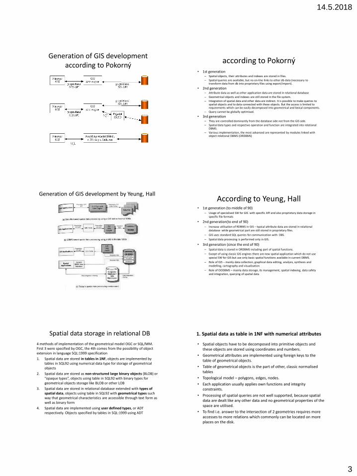
• Queries to geometrical properties of objects using SQL together with method utilization.
• Find x-coordinate of Opavy city:
SELECT poloha.X FROM city WHERE nazev = ‘Opava’;
• ADT can be implemented two ways – as a black box or white box
ADT as “black box” 1. Implementation of internal structure of ADT and relevant
functions in external programming language (i.e. C/C++, Java)
2. using DDL for type registration in DBMS requires to specify: 1. The instance size of the type
2. Input and output functions (including constructors of instances),
3. Other functions and operators, incl. signatures and implementations, which should be linked,
4. Data for query optimizer;
3. Finally use ADT similarly as a native data type and function and operators will become available for queries
Example definition of DDL CREATE TYPE Point ( internallength = 16; -- for point structure {double x, double y} input = point_in; -- for reading constants of the Point type output = point_out; -- for output of results of the Point type );
• internallenght describes of instance size 2x8B. CREATE FUNCTION point_in(Text) RETURNS Point AS EXTERNAL NAME 'MI_HOME/functions/point.so' LANGUAGE C;
CREATE FUNCTION point_out(Point) RETURNS Text AS EXTERNAL NAME 'MI_HOME/functions/point.so' LANGUAGE C;
CREATE FUNCTION je_v_sousedství(Point, Point) RETURNS Boolean AS EXTERNAL NAME 'MI_HOME/functions/pointfuns.so' LANGUAGE C;
Example of usage • May have PLACE attribute (place of resident) Point
type in the OSOBY table.
• Find name of persons where Mr. Novák lives in their neighbourhood and write them together with their residents:
SELECT O1.JMENO, O1.PLACE FROM OSOBY O1, OSOBY O2 WHERE is_in_neighbourhood(O1.PLACE, O2.PLACE) AND O2. JMENO = 'Novák';
Example definition of DDL in C# + MS SQL SERVER 2008 - 1
• using System;
• using System.Data;
• using System.Data.SqlTypes;
• using Microsoft.SqlServer.Server;
• using System.Text;
•
• [Serializable]
• [Microsoft.SqlServer.Server.SqlUserDefinedType(Format.Native,
• IsByteOrdered = true, ValidationMethodName = "ValidatePoint")]
• public struct Point : INullable
• {
• private bool is_Null;
• private Int32 _x;
• private Int32 _y;
Example definition of DDL in C# + MS SQL SERVER 2008 - 2
• public bool IsNull
• {
• get
• {
• return (is_Null);
• }
• }
•
• public static Point Null
• {
• get
• {
• Point pt = new Point();
• pt.is_Null = true;
• return pt;
• }
• }

14.5.2018
8
Example definition of DDL in C# + MS SQL SERVER 2008 - 3
• // Use StringBuilder to provide string representation of UDT.
• public override string ToString()
• {
• // Since InvokeIfReceiverIsNull defaults to 'true'
• // this test is unneccesary if Point is only being called
• // from SQL.
• if (this.IsNull)
• return "NULL";
• else
• {
• StringBuilder builder = new StringBuilder();
• builder.Append(_x);
• builder.Append(",");
• builder.Append(_y);
• return builder.ToString();
• }
• }
Reading string with x,y
• [SqlMethod(OnNullCall = false)] • public static Point Parse(SqlString s) • { • // With OnNullCall=false, this check is unnecessary if • // Point only called from SQL. • if (s.IsNull) • return Null; • // Parse input string to separate out points. • Point pt = new Point(); • string[] xy = s.Value.Split(",".ToCharArray()); • pt.X = Int32.Parse(xy[0]); • pt.Y = Int32.Parse(xy[1]); • // Call ValidatePoint to enforce validation • // for string conversions. • if (!pt.ValidatePoint()) • throw new ArgumentException("Invalid XY coordinate values."); • return pt; • }
Insert into X, Y coordinates
• // X and Y coordinates exposed as properties. • public Int32 X • { • get • { • return this._x; • } • // Call ValidatePoint to ensure valid range of Point values. • set • { • Int32 temp = _x; • _x = value; • if (!ValidatePoint()) • { • _x = temp; • throw new ArgumentException("Invalid X coordinate value."); • } • } • }
• public Int32 Y
• {
• get
• {
• return this._y;
• }
• set
• {
• Int32 temp = _y;
• _y = value;
• if (!ValidatePoint())
• {
• _y = temp;
• throw new ArgumentException("Invalid Y coordinate value.");
• }
• }
• }
• // Validation method to enforce valid X and Y values.
• private bool ValidatePoint()
• {
• // Allow only zero or positive integers for X and Y coordinates.
• if ((_x >= 0) && (_y >= 0))
• {
• return true;
• }
• else
• {
• return false;
• }
• }
• // Distance from 0 to Point method. • [SqlMethod(OnNullCall = false)] • public Double Distance() • { • return DistanceFromXY(0, 0); • } • // Distance from Point to the specified point method. • [SqlMethod(OnNullCall = false)] • public Double DistanceFrom(Point pFrom) • { • return DistanceFromXY(pFrom.X, pFrom.Y); • } • // Distance from Point to the specified x and y values method. • [SqlMethod(OnNullCall = false)] • public Double DistanceFromXY(Int32 iX, Int32 iY) • { • return Math.Sqrt(Math.Pow(iX - _x, 2.0) + Math.Pow(iY - _y, 2.0)); • } • }
distance calculation to the point
14.5.2018
9
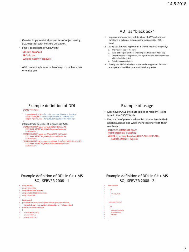
Utilisation
• Needed to enable using DLL in the database:
sp_configure 'clr enabled', 1
Reconfigure
• Link DLL to the database: Source (http://technet.microsoft.com/en-us/library/ms131079.aspx)
CREATE ASSEMBLY Point
FROM 'c:\palo\testUDT\UDTPoint.dll'
WITH PERMISSION_SET = SAFE;
• Create user data type Point from my DLL: Source (http://technet.microsoft.com/en-us/library/ms131079.aspx) CREATE TYPE dbo.Point
EXTERNAL NAME Point.[Point];
• Create table: create table city
(
name nvarchar(50),
location dbo.Point
)
• Insert records: insert into city (name,location) values ('obec3','1,1'), ('obec3','1,3'), ('obec3','0,0')
SELECT name , location.X as X, location.Y as Y, location, location.ToString() as locationString FROM horak.[dbo].[city]
Distance from 0
select location.Distance()AS DistanceFromZero FROM horak.[dbo].[city]
Distance from obec1
• declare @obec as Point
• set @obec = (select location from horak.[dbo].[city] where name='obec1')
• select location.DistanceFrom(@obec) as DistanceFromXY FROM horak.[dbo].[city]
ADT as ”white box”
1. Describe ADT structure using DDL in SQL:1999
2. Definition of attributes are considered as common specification of columns. It enables to utilize SQL possibilities like NULL value, nesting, integrity constraints, etc.;
3. implement relevant function directly in SQL or in external programming language;
4. Use functions generated by the system for the access and editing objects;
5. inform query optimizer;
6. Use the new data type like any other implemented data types when functions and operators will become available for queries.

14.5.2018
10
Example of DDL definition (for DB/2)
CREATE TYPE Point AS ( x double, y double, );
CREATE FUNCTION vzdalenost(p1 Point, p2 Point) RETURNS Integer LANGUAGE SQL INLINE NOT VARIANT RETURN sqrt((p2..y-p1..y)*(p2..y-p1..y) + (p2..x-p1..x)*(p2..x-p1..x));
• Notation .. is replaced in SQL:1999 by classic (simple) dot notation
Example continues
• Consider urban spaces represented by polygons. For polygons a method Centroid is considered which returns centroid of the polygon.
• Find names of persons who live within 25 kms from the centre of Ostrava :
SELECT O.JMENO FROM OSOBY O, CITY M WHERE M.NAZEV = 'Ostrava' AND vzdalenost(O.POLOHA, M.POLOHA.centroid) < 25;
1. Spatial ADT, thus geometric data structures with corresponding operations and relationships between objects. Such defined objects enable users to deal with spatial data on the level of whole objects and without knowledge of internal implementation (i.e. to store coordinates).
2. Display of graphical results of queries including visualization of relevant aspatial attributes,
3. Possibility to dynamic combined of queries results, thus utilize results of previous queries for creation of new query,
4. Possibility to display of context information which is not direct outputs of the query but it is necessary for correct results interpretations. During the graphical presentation of the query results it is usually necessary to display surroundings where the object is situated (i.e. display of other objects which were not selected by the query, display of basemap etc.). If we search Ostrava in the map, it is required to display it with surroundings and not only black point on the white wall.
5. To process more results together a mechanisms of object identification in the final image must exists,
Spatial Query Language (Egenhofer) Spatial Query Language (Egenhofer)
Spatial Query Language (Egenhofer)
6. Use pointing devices for modification of view (pan, zoom in, zoom out) or selection by the cursor – using pointing device (mouse typically) for selection from the query result,
7. Variable portraying of objects (colours, patterns, hatch etc.),
8. Support of displaying explanation information in the legend (similarly to a map),
9. Support of portraying of labels which is important for orientation and for following selections and queries,
10. Possibility of voluntary numerical scale of displaying query results in a map window,
11. Set an area of interest (part of the whole area, „spatial“ filter) which we will work with (search, apply next queries etc.)
12. Work with coordinate systems
14.5.2018
11
• Minimal extension of SQL: – Respect principles of SQL
– Deal with spatial objects on the high level
– Build spatial operations and relationships
• Proposal of Egenhofer from 1994 apply classic construction of SELECT FROM WHERE as in classic SQL, results of such query are relations.
• 3 types of instructions in S-SQL exists: – user query – description of the data set which has to be displayed.
– display queries to divide results of query into subsets where each of them will be displayed different ways (different colours, etc.).
– display description – description how to portrait results.
• On the base of such approach two parts of spatial language can be delimited:
– 1. query language for description of information,
– 2. presentation language for displaying results of the query
Process how to use instructions
• 1. user set parameters of displaying environment (portraying instructions).
• 2. user put queries (results are displayed according to previous setting, displaying environment is not changed).
• 3. user (possibly) change parameters of displaying environment (but displaying content is not changed).
• Spatial SQL contains limited tools for data editing.
Spatial representation of objects
• using
– vector data model
– raster data model
• basic concepts used to build topological vector data models:
– Topological data model based on combinatorial topology
– Realm data model
Topological data model based on combinatorial topology
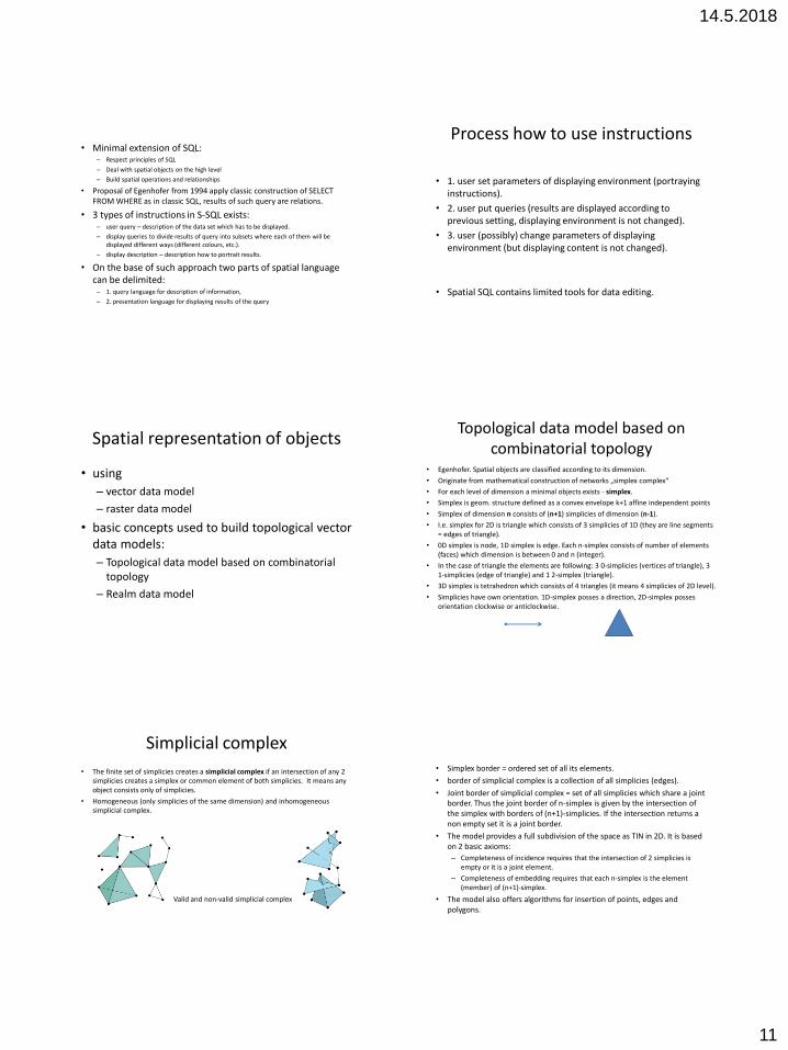
• Egenhofer. Spatial objects are classified according to its dimension.
• Originate from mathematical construction of networks „simplex complex“
• For each level of dimension a minimal objects exists - simplex.
• Simplex is geom. structure defined as a convex envelope k+1 affine independent points
• Simplex of dimension n consists of (n+1) simplicies of dimension (n-1).
• I.e. simplex for 2D is triangle which consists of 3 simplicies of 1D (they are line segments = edges of triangle).
• 0D simplex is node, 1D simplex is edge. Each n-simplex consists of number of elements (faces) which dimension is between 0 and n (integer).
• In the case of triangle the elements are following: 3 0-simplicies (vertices of triangle), 3 1-simplicies (edge of triangle) and 1 2-simplex (triangle).
• 3D simplex is tetrahedron which consists of 4 triangles (it means 4 simplicies of 2D level).
• Simplicies have own orientation. 1D-simplex posses a direction, 2D-simplex posses orientation clockwise or anticlockwise.
Simplicial complex
• The finite set of simplicies creates a simplicial complex if an intersection of any 2 simplicies creates a simplex or common element of both simplicies. It means any object consists only of simplicies.
• Homogeneous (only simplicies of the same dimension) and inhomogeneous simplicial complex.
Valid and non-valid simplicial complex
• Simplex border = ordered set of all its elements.
• border of simplicial complex is a collection of all simplicies (edges).
• Joint border of simplicial complex = set of all simplicies which share a joint border. Thus the joint border of n-simplex is given by the intersection of the simplex with borders of (n+1)-simplicies. If the intersection returns a non empty set it is a joint border.
• The model provides a full subdivision of the space as TIN in 2D. It is based on 2 basic axioms:
– Completeness of incidence requires that the intersection of 2 simplicies is empty or it is a joint element.
– Completeness of embedding requires that each n-simplex is the element (member) of (n+1)-simplex.
• The model also offers algorithms for insertion of points, edges and polygons.

14.5.2018
12
Realm model • Nabil (1997)
• He provides a definition of Spatial Data Type (SDT)
• Properties: – Generality – provides a link of Spatial Data Type to corresponding spatial
operations.
– Rigorous definition – requires an unambiguous definition of SDT and its functions and operations
– Finite resolution – storage and processing of spatial data is performed with a finite resolution. Processing of continual data or models is necessarily accompanied by certain error (i.e. functional dependency of temperature development in the field).
– Geometrical consistency - requires to apply geometrical restrictions in spatial relationships of 2 features. I.e. joint border of 2 adjacent features must be maintained in SDT which were used for its definition.
– Common object model of interface - requires to apply the high-level interface which integrate SDT into DBMS. The definition of SDT remains independent to implementation of DBMS.
Realm model 2
• Basic construction is a finite graphical data structure called realm.
• Model is described by 3 basic layers:
1. geometrical primitives (bottom layer),
2. Storage of certain structures (middle layer)
3. Definition of SDT (upper layer)
Bottom layer • Description of finite 2D space of NxN using points, lines and functions which
describe spatial relationships between points and lines in this space (discrete space).
• Point (designated as N-point) is represented by the pair of coordinates (x,y) from NxN.
• Line segment (N-segment) is described by the pair of N-points (p,q).
• Basic cornerstone in this layer is that coordinates of points are integer parameters and return logical or integer values.
• For points it is possible to use 3 operators (predicates): – = (returns TRUE if both points have the same coordinates)
– On (tests if the point lays on certain line segment)
– In (tests if the point is one of the ending points of certain line segment).
• For relationships of 2 line segments it is possible to use following operators : – Equal (tests if 2 segments are equal)
– Intersect (tests if 2 segments are crossing)
– Parallel (tests if 2 segments are parallel)
– Overlap (tests if 2 segments are collinear and have some joint part)
– Aligned (tests if 2 segments are collinear and do not have some joint part)
– Meet (tests if 2 segments have joint just 1 ending point, the node)
– Disjoint (tests if 2 segments do not meet, not aligned and not overlap)
Bottom layer • Each spatial object consists of segments and points.
• Objects are connected with their components using pointers designed as realm object identifiers ROID.
• To the opposite, components are linked with spatial objects using a set of other pointers designed as spatial component identifier SCID.
• This both-directional linkage is provided for faster access in both directions.
• Further the envelope and the window of spatial objects is defined
Middle layer
• In the next layer there are descriptions of structures and its relationships. Structures are R-cycle, R-face, R-unit and R-block: – R-cycle - polygon bordered by edges is called R-segments.
– R-point may be in, on or out of R-cycle.
– R-face - R-cycle which contains a set of disjoint R-cycles; thus it is a polygon with holes (represented again by polygons).
• R-face is such couple (c, H) where c is R-cycle, H = {h1,…,hm} is a set of R-cycles. It is valid that all R-cycles are embedded by edges and every R-cycles are disjunctive by edges. No other cycle can be created from segments (describing this place).
– R-unit is defined as a minimal R-face.
– R-block is a set of line segments which are mutually interlinked (create a continual graph).
• Prefix R means „realm“.
Upper layer
• Upper layer is created by SDT where points, lines and regions correspond to R-points, R-blocks and R-faces.
• Above SDT there are defined:
– set operations (i.e. union, intersection, difference)
– topological operations (i.e.. disjoint, adjacent, inside).
14.5.2018
13
Final properties of realm
• Each standalone point (node) is the point (node) of the network
• Every ending point of the line is the point (node) of the network
• No internal point of the line (vertex) is recorded
• No 2 lines have any intersection or overlapping
• Complex units are created from lines
• = basic expression of topological rules in 2D
ROSE
• algebra ROSE (RObust Spatial Extension) is sometimes used for the explanation of the vector model. It comes from descriptors and complex objects are obtained by their composition. Basic objects are points, lines and areas (multipolygons).
• Algebra ROSE defines a location of two objects like: – Embedded by area,
– Embedded by edges,
– Embedded by vertices,
– Disjunctive by area,
– Disjunctive by edges,
– Disjunctive by vertices (fully disjunctive).
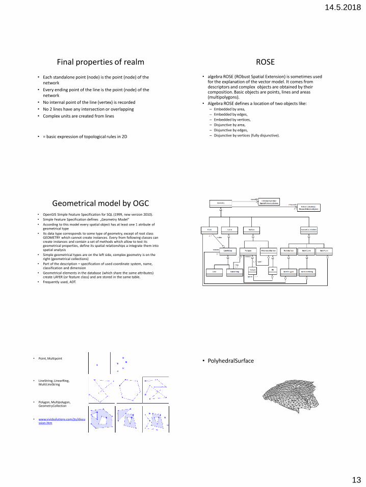
Geometrical model by OGC • OpenGIS Simple Feature Specification for SQL (1999, new version 2010).
• Simple Feature Specification defines „Geometry Model“
• According to this model every spatial object has at least one 1 atribute of geometrical type
• Its data type corresponds to some type of geometry, except of root class GEOMETRY which cannot create instances. Every from following classes can create instances and contain a set of methods which allow to test its geometrical properties, define its spatial relationships a integrate them into spatial analysis
• Simple geometrical types are on the left side, complex geometry is on the right (geometrical collections)
• Part of the description – specification of used coordinate system, name, classification and dimension
• Geometrical elements in the database (which share the same attributes) create LAYER (or feature class) and are stored in the same table.
• Frequently used, ADT.
• Point, Multipoint
• LineString, LinearRing, MultiLineString
• Polygon, Multipolygon, GeometryCollection
• www.vividsolutions.com/jts/discussion.htm
• PolyhedralSurface
14.5.2018
14
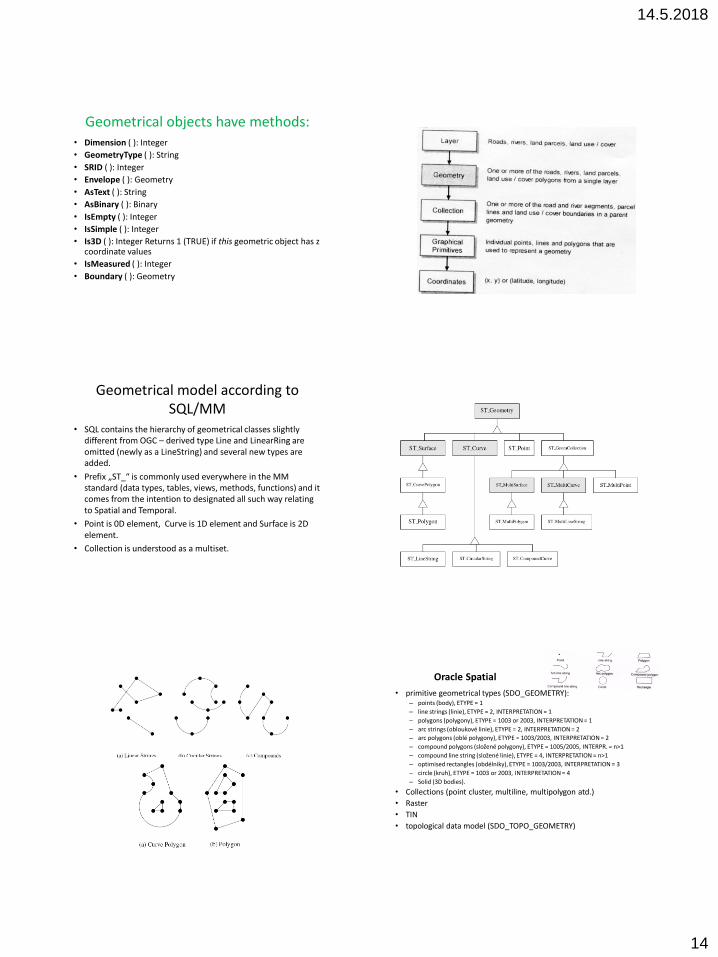
Geometrical objects have methods: • Dimension ( ): Integer
• GeometryType ( ): String
• SRID ( ): Integer
• Envelope ( ): Geometry
• AsText ( ): String
• AsBinary ( ): Binary
• IsEmpty ( ): Integer
• IsSimple ( ): Integer
• Is3D ( ): Integer Returns 1 (TRUE) if this geometric object has z coordinate values
• IsMeasured ( ): Integer
• Boundary ( ): Geometry
Geometrical model according to SQL/MM
• SQL contains the hierarchy of geometrical classes slightly different from OGC – derived type Line and LinearRing are omitted (newly as a LineString) and several new types are added.
• Prefix „ST_“ is commonly used everywhere in the MM standard (data types, tables, views, methods, functions) and it comes from the intention to designated all such way relating to Spatial and Temporal.
• Point is 0D element, Curve is 1D element and Surface is 2D element.
• Collection is understood as a multiset.
Oracle Spatial
• primitive geometrical types (SDO_GEOMETRY): – points (body), ETYPE = 1
– line strings (linie), ETYPE = 2, INTERPRETATION = 1
– polygons (polygony), ETYPE = 1003 or 2003, INTERPRETATION = 1
– arc strings (obloukové linie), ETYPE = 2, INTERPRETATION = 2
– arc polygons (oblé polygony), ETYPE = 1003/2003, INTERPRETATION = 2
– compound polygons (složené polygony), ETYPE = 1005/2005, INTERPR. = n>1
– compound line string (složené linie), ETYPE = 4, INTERPRETATION = n>1
– optimised rectangles (obdélníky), ETYPE = 1003/2003, INTERPRETATION = 3
– circle (kruh), ETYPE = 1003 or 2003, INTERPRETATION = 4
– Solid (3D bodies).
• Collections (point cluster, multiline, multipolygon atd.)
• Raster
• TIN
• topological data model (SDO_TOPO_GEOMETRY)
14.5.2018
15
IBM DB2 Spatial Extender
• SDT - geometry type
• hierarchy: – points (body),
– multi-points (sada bodů),
– line strings (linie),
– multi-line strings (sada linií),
– polygons (polygony),
– multi-polygons (multipolygony, areály),
– ellipses (elipsy).
PostrgreSQL
• Representation of following 2D geometrical types:
• point – pair of coordinates, in round bracket (as a output) or without parenthis .
• lseg (line segment) – represented by a pair of points (ends of segment). Variable syntax with parenthesis (square bracket for output).
• line (linie) – not fully implemented
• path (open or closed series of line segments). – „open path“ (not circle according to theory of graphs) do not connect first and last points, syntax [ ( x1 , y1 ) , ... , ( xn ,
yn ) ].
– „closed path“ (circle) has first and last points connected, syntax ( ( x1 , y1 ) , ... , ( xn , yn ) ) or other variants without square brackets.
• polygon (delimited path on the perimeter) – represented as series of points which are polygon vertices. Again various forms of syntax with parenthesis, i.e. ( ( x1 , y1 ) , ... , ( xn , yn ) ).
• box (obdélník) – delimited by the pair of opposite points. Voluntary input, internally is transformed and points of upper right and bottom left corners are stored ( ( x1 , y1 ) , ( x2 , y2 ) )
• circle (kruh) – defined by the center and diameter. Variable syntax, i.e. < ( x , y ) , r >
PostrgreSQL PostGIS Geography Type • GEOGRAPHY column using the CREATE TABLE syntax (or use
AddGeometryColumns()): – POINT
– LINESTRING
– POLYGON
– MULTIPOINT
– MULTILINESTRING
– MULTIPOLYGON
– GEOMETRYCOLLECTION
• CREATE TABLE testgeog(gid serial PRIMARY KEY, the_geog geography(POINT,4326) );
• suffixes: Z, M and ZM - 'LINESTRINGM' for 3D, 3rd coordinates is the measured value, Z = height.
Verification • These 2 commands return the same output - valid
geometry of PostGIS:
– SELECT ST_MakePoint(15,48) AS bod;
– SELECT ('(15,48)'::point)::geometry AS bod;
• Internal geometrical data types can be transformed with PostGIS extension into geometrical types which is not presented in standard Postgres.
• In the frame of PostGIS it is possible to apply spatial functions and operators (after retyping into Geometry type).
ESRI ArcGIS Geodatabase • Uses 4 basic types of geometry:
– point,
– multipoint,
– polyline,
– polygon.
• Point geometry is described by coordinates X and Y, or X, Y, Z.
• Similarly for the set of points.
• Line geometry contains 1 or more paths created by any of 4 segment types: – line (přímkové),
– circular arc (kruhové oblouky),
– elliptical arc (eliptické oblouky)
– Bezier curve (beziérovy křivky).
• Line geometry may be associated with Z value (height) or M value (measurement of distances).
• Polygon geometry consists of 1 or more circles (according to graph theory), and creates continual, closed and non-crossing set of segments. Again polygon geometry may be associated with Z value for height.

14.5.2018
16
Raster data model
• ODBMS as ADT
• ESRI:
– ArcSDE (Raster Dataset)
– GeoRaster (SDO_GEORASTER)
– Image Server
ArcSDE
• Raster Dataset is in Oracle 7 db tables:
1. business table,
2. feature table,
3. spatial index table,
4. auxiliary table
5. block table
6. band table
7. raster description table
Business table • Main table for storing spatial data into SDE geodatabase
in Oracle
• During a raster storing a new column RASTER is added and any new record in this column references a raster stored in the table system
• In case of Raster Dataset it contains only 1 row.
• 2 attributes: – attribute FOOTPRINT
• Link to spatial delimitation of raster
• In the example 1 value OBJECT_ID 2669 identifies the Feature table;
– attribute RASTER • Link to the raster data
• In the example a value 221 is recorded which is used to assign 4 tables for storing raster data
References in system tables
• Information about the RASTER column is stored in the system table SDE.RASTER_COLUMNS using the value of RASTERCOLUMN_ID attribute (in our example a value of 221).
• The system table SDE.COLUMN_REGISTRY uses 2 attributes: COLUMN_NAME contains names of every column of business table and OBJECT_ID identifies corresponding tables

14.5.2018
17
Feature table • Shape and spatial extent delimitation of Raster Dataset (using coordinates) (envelope)
• Feature table has only 1 raw in the case of raster dataset (RD)
• attribute FID = foreign key for business table.
• Numbers in EMINX, EMINY, EMAXX and EMAXY columns contain coordinates of bottom left and upper right corner RD in the given coordinate system. It is the minimal rectangle covering RD (MBR)
• AREA attribute contains an area of RD
• LEN attribute = perimeter of RD.
• ENTITY attribute using a number code defines a geometry of the stored element. In the case of raster it is polygon (code 8).
• NUMOFPTS attribute provides the number of point delimiting the element (in case of raster it is polygon thus for the squared tile it is 4 points).
• POINTS contains coordinates of these points in the LONG RAW format or BLOB.
• EMINZ and EMAXZ - it is possible to store also raster 3D files with Z coordinate to the database (i.e. elevation models).
• Feature table identification is done through the value of LAYER_ID attribute which is the part of system table SDE.LAYERS. The identification is also included in the SDE.COLUMN_REGISTRY table.
Spatial index table • It contains a link to regular index grid used to support spatial queries and recording the
location of spatial elements in this grid.
• this table (and the grid) is used in the case of spatial query to fast searching appropriate region above the raster envelope. After that corresponding binary stored spatial data are required.
• The fast navigation during spatial queries for rasters is supported by pyramid layers stored alike original data in the LONG RAW or BLOB formats in the Raster block table.
• GX and GY attributes identify the location of corresponding cell of the grid where the stored element is assigned. Due to the fact the spatial extent of the element may be larger than 1 cell of the grid, the relationship between feature table (and business table) and the spatial index table is 1 : N.
• EMINX, EMINY, EMAXX and EMAXY attributes are the same as in the feature table (contain coordinates of bottom left and upper right corner RD in the given coordinate system).
• Spatial index table is used in Raster Catalogue for indexation of the „vector layer“ of spatial extension (envelopes) of all rasters in the catalogue. In the case of RD the table is created but has no records, because only 1 envelope exists for the given RD.
• Raster description
– description of the raster (image data),
– 3 attributes and they are used of description of RD: • RASTER_ID – unique identification of RD corresponding to the values
in the RASTER column in the business table.
• RASTERFLAGS - number, identification of deleted records in the business table
• DESCRIPTION – textual description of the raster
– identification of deleted records in the other tables is in situation when other application (different from ArcSDE) delete the record in the business table.
The real raster data is stored into following tables
Raster band • metadata about spectral bands,
• RASTERBAND_ID is primary key (the number of the spectral band),
• In case of visible part of image this table has 3 rows (bands R, G, B).
• Table is logically linked with the business table and with raster description table through RASTER_ID attribute.
• BAND_WIDTH and BAND_HEIGHT – spatial extent for each band (number of pixels in both directions).
• EMINX, EMINY, EMAXX and EMAXY
• BLOCK_WIDTH and BLOCK_HEIGHT – the block size in which pixels of the original image are clustered (stored). The size of the block can be selected (in the example 128).
• CDATE and MDATE – date of creation and the last change of the spectral band
• Using RASTERBAND_ID primary key the table is linked with 2 following tables.
Raster auxiliary
• Table of colours, statistics, coordinate transformation and other auxiliary data
• This information is stored for each band identified by foreign key RASTERBAND_ID.
• TYPE attribute differentiates by specific codes what kind of information is stored:
– TYPE=2 …. statistics,
– TYPE=3 …. Colour table,
– TYPE=4 …. coordinate transformation,
– TYPE=5 …. geodatabase
– TYPE=6 …. other data.
• data of auxiliary information LONG RAW or BLOB formats is stored OBJECT column.
Raster block
• Real image data for each spectral band
• Data is stored by each band, pyramid level and block.
• RASTERBAND_ID is foreign key providing the number of spectral band,
• RRD_FACTOR the number of pyramid,
• ROW_NBR the number of row in the tile block
• COL_NBR the number of the column in the tile block
• data is stored as LONG RAW or BLOB in the BLOCK_DATA column.

14.5.2018
18
Example
• In the example only several rows are listed (whole table has 25 138 rows).
• You can see 6 levels of pyramid, the level 0 indicates original data.
• Value range for ROW_NBR as well as COL_NBR attribute is from 0 to 78, it means 79 values.
• 79 values gives you number of block tiles with 128 pixels (10000 / 128) in the direction rows and columns.
Advantages and disadvantages
• + possibility of calculation of overview layers (pyramid) for fast data displaying and possibility of statistics calculation statistik used for possible radiometric modifications.
• - lost of borders between segments and information (metadata) about these segments . Access to such metadata may be obtained though usage of the polygon layer with corresponding attributes. The collection of attributes would be similar Raster Catalogue creation.
• ArcSDE Raster Dataset can be recommended for data providing to users i.e. in internet applications where the end user directly does not need any other descriptive information only image data.
Integrity of spatial data and integrity constraints
• Cockcroft (1997) adds other integrity constraints especially for spatial data which are divided into static and transition IC (Yeung A., Hall G. 2007).
• IC has to be defined during the conceptual model. They should be a part of metadata.
• The result is the set of following 6 types of spatial IC.
Topological IC
• Deal with geometrical properties of spatial relationships between features (i.e. neighbourhood, embedding, connectivity)
– Static topological IC – i.e. all polygons have to be closed.
– Transition topological IC – i.e. when the border of polygon is changed it is necessary to change the given polygon as well as the neighbouring polygon sharing the same border.
Semantic IC
• database rules control the spatial behaviour of objects in database
• i.e. land lots can be placed in water bodies
– Static semantic IC – i.e. parcel’s area cannot be negative
– transition semantic IC – i.e. after a parcel subdivision the sum of areas of new parcels has to be equal the original area
User defined IC
• Usually specified rules for the concrete situation similarly those IC defined in the database
• i.e. the house construction is prohibited within 50 meters of forest’s protected area
– Static user defined IC – e.g. rivers wider than 2 meters have to be stored using polygon geometry
– Transition user defined IC – e.g. after acceptance of the change of parcel classification the relevant db change has to be completed within 2 days.
14.5.2018
19
Multi-representation of spatial data in S-DBS
• The request of multiple representation of spatial data arises: – Multiuse database
– creating dbs integrating different sources to satisfy different request of applications
– Co-existence various data in databases which represent the same real features but using different database models, geometries, descriptions and other characteristics
– Ability to manage and control such data in DBS a consistent way without manual modification.
• Traditional database tools (e.g. views) are not suitable for such purpose.
• Existing approaches = manage data sets for different representation of the same object (different scale, purpose) separately
Disadvantages of separated storage of representation
• Lack of flexibility – It is impossible to assume requirements of all applications and keep various data sets
for different representations.
– New requirement (not corresponding to any of existing representations): • Use not relevant data set (not customised to the requirements), it leads to doubtful results,
• Provide data conversion and data transformation ourselves to obtain appropriate data set.
• insufficient maintenance of consistency between representations – Maintenance of several db and data sources and assurance of their consistency is
problematic and demanding.
– Frequent changes in reality – it is difficult to assure adequate and consistent mirroring of these changes into all relevant data sets.
– Absence of logical rules -> need of laborious and non-automated maintenance. Even worse for long transactions.
• Uncertainty arisen from the usage of different data sets in analyses – Lack of logical and physical relationships between data sets = we are not able to
evaluate differences of outputs of analysis with different representations (with different data sets).
– Namely impacts for decision support are negative.
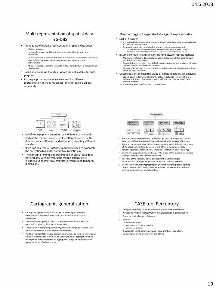
• Relief (topography) – described by 4 different data models.
• Each of the models can be used for different sources, with different scale, different standardization (respecting different standards).
• If we find an error in 1 of these models we need to propagate the correction to all other models automatic way
• The concept of multiple representation of spatial data does not deal only with different data models but usually it includes also geometrical, graphical, semantic and temporal dimensions.
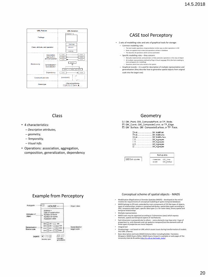
• The school may be represented by different geometrical shapes for different scales, use different cartographic symbols according to the type of the map
• The school may be labelled different way according to the different perception of the situation by different observers and different purposes for data collection (school: urbanised area, educational institution, public building).
• During time progress it may be changes - the shape of the building, its purpose (change the school into community centre).
• The need of the spatial database development towards multiple representation (Multiple Representation Spatial Database, MRSDB).
• Do not confuse multiple representation and data versioning (corresponding only to the temporal changes). Both aspects are complementary and have their own utilisation for spatial database.
Cartographic generalization
• Cartographic generalization has a special meaning for multiple representation because it enables to automates a set of required operations.
• The cartographic generalization is scale dependent that is why this approach is called multi-scale representation
• The problem is computing demandingness and ambiguity of some tasks for automation (the human expertise is required).
• multiple representation has a special importance also for data warehouses which are intended to store data on various levels of aggregation which corresponds to requirements for aggregation of spatial representation (generalization) of relevant objects.
CASE tool Perceptory • Designed especially for requirements of spatial data warehouses
• It supports multiple representation using cartographic generalization.
• Based on UML, diagram of classes
• 3 parts: – Project description
– catalogue and scheme of metadata
– scheme and dictionary
• It uses main constructors : package, class, attribute, operation, association, among many others and others
14.5.2018
20
CASE tool Perceptory
• 2 sets of modelling rules and sets of graphical tools for storage:
– Common modelling rules • The tool models operations of generalization similar way as other operations in OO
• Rules are applied only to data and operations written in database
• The describe all operations which can be automated.
– Specific modelling rules – they concern: • Manually implemented, semiautomatic or fully automatic operations in the class of object
• All multiple representations defined by Plug-in Visual Language (PVL) (the font enabling to store pictograms for modelling)
• Geometry which has to be stored in the system
– Graphical records – it is used for description of multiple representation and generalization (they describe how to generalise spatial objects from original
scale into the target one)
Class
• 4 characteristics:
– Descriptive attributes,
– geometry,
– Temporality,
– Visual Info.
• Operations: association, aggregation, composition, generalization, dependency
Geometry
Example from Perceptory Conceptual scheme of spatial objects - MADS
• Modélisation d’Applications á Données Spatiales (MADS) – developed at the end of nineties for requirements of conceptual modelling of spatio-temporal databases
• MADS belongs to ER tools; extended by main components of OO like types of objects, types of relationships, simple or composed attributes, spatial data types according to OGC, temporary data types, specific data types (i.e. for raster data), binary spatial and temporal relationships
• Multiple representation.
• MADS tools may be organised according to 3 dimensions (axes) which express thematic, spatial and temporal aspects of real features.
• Each dimension is perpendicular to others – some elements may have only 1 type of properties (i.e. only thematic and not spatial or temporal) but the elements with all three types of properties are more frequent.
• integral tool
• Disadvantage – not based on UML which causes issues during transformation of models into UML schemes.
• Basic description and tools (MADS Schema Editor including Builder, Translator, Wrappers; MADS Query Editor; MADS Query Viewer) is available on web pages of the University Libré de Bruxelles http://cs.ulb.ac.be/mads_tools/
14.5.2018
21
Thematic dimension • 2 basic types of relationships :
– is-a (ISA) – used for: • relations 1:1 between entity types (binary relationships)
• Restricting relationships between the set of OID from one entity type and the other set of OID from the second entity type (probably referential integrity).
– may-be relation – used in the case of 1:1 between instances, no relation between sets is enforced
• ISA relation is used for inheritance modelling – in the form of specialization or redefinition:
– Specialization enables to create subclasses for basic types. I.e. subtypes CITY (polygonal geometry) and VILLAGE (point geometry) were build by specialization from the basic spatial data type SETTLEMENT.
– Redefinition enables to create a new attribute with the same name as the subtype. It supports to associate several geometries to the same object.
• MADS offers for multiple representation support 3 specific types of relationships : – Aggregation – represents binary relationships from the parts to the whole objects (i.e. Bruntál, Frýdek-
Místek, Karviná, Nový Jičín, Opava and Ostrava-město districts constitute Moravian-Silesian region).
– Generation – newly created entities are linked to parent’s entities
– Transition – applications are enabled to record changed classification of database objects as the mirror of changes in the real world.
Spatial dimension • Support for discrete (vector) and continual (raster or field) representation of features.
• discrete representation – used for the specification of the spatial abstract data types (SADT) hierarchy which contains simple data types (point, line, simple polygon and oriented line) and complex types (set of points, set of lines, complex areal - multipolygons, set of oriented lines).
• It enables to deal with uncertain locations (an accuracy level)
• The position is defined absolute way (coordinates) or relative way (linear georeferencing)
• The entity type is spatial if it has the specific attribute geometry used by SADT for the value domain (i.e. geometry attribute is just one of SADT type).
• The attribute may be also spatial if it uses SADT for the value domain.
• MADS supports 2 pre-defined categories of spatial relationships – topological and spatial aggregation.
• The continual representation in the MADS is supported using space-varying attributes. The value of such attribute is set by a function with the domain of geometry element set (points, lines or polygons) from which the geometry of modelled object or attribute is constructed. I.e. the height is represented by the set of elevation data measured in randomly or regularly distributed points.
Hiearchy of spatial types Spatial attribute geometry
• One-value or multi-valued
• Spatial object is considered as an object or an attribute:
Attribute, N reservoirs on the river Reservoir as a point object belonging to the river
Spatial relationship
• Pre-defined :
– Topological
– Spatial
aggregation
„county“ consists of 10 to 1000 districts
Generalization in MADS
• Spatial and aspatial objects
a) aspatial objects may have a spatial subtype
b) The spatial subtype inherit the geometry
c) Geometries of subtypes may be different
d) Overdefinition of the geometry, its specification
14.5.2018
22
Temporal dimension • MADS supports discrete (instant) and continual (interval) spatial
representation of features assuming these entity types and relationship types have their own life cycle.
• The temporal attribute uses a value from basic simple (instant, interval) or composed (instant set, interval set) temporal abstract data types (TADT).
• The important feature of this model is usage of time stamps.
• It is possible to „stamp“ entities, attributes, relationships such way to record when they were created, modified or deleted. Such stamping enables to define:
– transition relationships – changes of object classification),
– generation relationships – creation of new objects from others),
– timing relationships – specifies time relationships between entities
– time-based aggregation – time dependent entities are linked to their time snaps or cuts.
– Synchronization – enforces to satisfy temporal integrity constraints i.e. in the form respecting the life cycle of joint entities.
Visual tools MADS • The set of visual modelling tools called SUPER-G. It enables graphical
representation of entities, attributes and relationships.
• Example demonstrates some MADS possibilities: – ISA relationship between a parcel and an owner,
– Composed attribute ADDRESS (created from STREET and CITY),
– Derived attribute LANDOWNER.LAND TOTAL (calculated from other attributes),
– The relationship OWN has an attribute,
– Specialization from PERSON to LANDOWNER
Access to spatial objects (SDS)
• It is used to accelerate an access to spatial objects.
• It enables to filtrate spatial objects during given query or spatial operation -> to obtain the smaller set of relevant spatial objects where the required operation can be performed.
• Filtration is necessary to accelerate the processing (demandingness of operations)
• Frequent 2-stage approach: – primary filter reduces number of operation candidates using a spatial index. The
candidate set is much more smaller the original data set and it contains only objects relevant for the given operation.
– secondary filter – the concrete spatial operation is applied on the set of candidates (result of the primary filter).
• It is recommended for binary operations (between 2 geometries), it has no sense for unary operations.
Spatial data structures
• SDS is used for storage and indexing of spatial objects
Classification of SDS • According to the initial space:
1. Transformation of spatial objects into a space with different dimension where these objects are projected as points.
2. Space is divided into subspace (buckets)
• According to the level of space covering: 1. Full covering
2. Partially covering
• According to the way of subspace overlaying: 1. Disjunctive
2. overlaying
• According to the equality of data distribution
• According to the maximal dimension of used geometrical objects • Points – plenty of methods
• Objects of non-zero dimension – R tree or others
• According to the suitability for vector and raster data
Used classification:
• Transformation approach
• Space subdivision:
– Using non-overlapping areas
– Using overlapping areas

14.5.2018
23
Transformation approach
• Uses 2 main principles:
1. Possibility of the object recording into another dimension (transformation into the space of higher dimension)
2. Using of space-filling curve and space indexation according to the process of index creation (transformation into the space of lower dimension, usually 1D)
Transformation of object records into another dimension
• Each record in the table is the point of multidimensional space.
• Non-geometrical objects and multidimensionality: – E.g. table row of OBEC(NAZEV, POPULACE, ADRESA, ROZLOHA) is the point in the 4-
dimensional space.
– Such points can be organized i.e. in multidimensional grid where axis correspond to the table columns and points on the axe correspond to the items from the domain of the column. It is enough to have defined ordering. Such way a task of interval query for towns with area between 12-15 km2 and 10-30 thousands of inhabitants are solved as finding of a cube in the space and corresponding points inside the cube.
• Geometrical objects:
• By transformation of spatial objects of initial space P you can reach spaces with the same, lower or higher dimension than P
• Line segment in 2D space can be represented by coordinates of its ending points like one point (x1, y1, x2, y2) in 4D space.
• object is represented by a representative point
• It is a transformation from the P-dimension into a space of 2P dimension
Advantages and disadvantages
• Advantage – simplicity
• disadvantages:
– Do not respect neighbourhood -> impact to effectiveness of spatial operations.
If 2 lines are close together in 2D space it does not mean that respecting points in 4D space are also close together.
– Some queries are not executable
– Mapping is difficult, sometime impossible,
– problem of reverse transformation of the result
Transformation of records using space filling curves
• Divide the space into cells of the same size and number them according to some space filling curve
• Spatial object can be represented by a set of numbers or even as one-dimensional object.
• Transformation into the space of lower dimension
• For 1D objects a common B-tree can be applied
• Space filling curves were designed for transformation 2D data structure (i.e. raster) into 1D structure , namely for the request of 1 dimensional type of data storage in memories.
• These curves goes through the full mapping space (usually 2D or 3D), visit every place just 1x and respect spatial proximity between places
Territory subdivision using non-overlapping areas
• P space is divided into disjunctive subspaces.
• 2 types of methods: – Duplication of objects
– clipping objects
• In the 1st case subspaces are indexed. If the object is placed in s subspaces, object ID is copied in the index s-times.
• In the 2nd case the object is clipped (cut) into subobjects such way that each of them is within just one subspace. Thus ID object in the index is unique. The borders of subspaces (cells, buckets) are used to cut objects into smaller parts.
• Some authors did not distinguish between these methods and commonly speak about object clipping.
Advantages and disadvantages
• Using such representation it is possible to index objects such way as for 1D data. It does not depend if the spatial object is point or object of higher dimension. All can be included in one file. But for saving of spatial relationships it is more convenient to store certain spatial hierarchy using a tree.
• disadvantages: – Redundancy (duplicity) of object recording. Also INSERT and DELETE
commands require higher overheads.
– Reverse aggregation (clustering, joining) of clipped objects is not easy
– Methods are data dependent, thus subspaces corresponds (some way) to . Spatial objects which may complicate some operations.
14.5.2018
24
• It is possible to divide space equally (grid) or use quadtrees. The 1st case is suitable in the environment with equally distributed objects (i.e. houses in the city), in the second case there are no dependence on the data distribution.
• If we consider spatial objects only as points the methods of non-overlapping areas are suitable.
• Well-known SDS: R+ trees, cell trees and a set of quadtree variants, classic k-d-trees or k-d-B-trees and many others.
Territory subdivision with overlapping areas
• Each object is included in just one subspace P (covering the object).
• subspaces can be overlapped.
• Typical subspaces: – MBC minimal boundary cube
– minimal boundary rectangle MBR in 2D, circle, ellipse, arbitrary polygon.
• Areas differs in overheads required for its representation and the size of the dead space (space between the object and its overlapping subspace).
• Object is bounded in the minimal cube (parallelopiped) of the given dimension which edges are parallel to axes of coordinate system. Easy calculations.
• It may happen the minimal cube do not correspond to the object well – it may have a volume multi times larger than the object. Big dead space.
• Overlapping areas are constructed hierarchical way (usually bottom up)
• They may overlap
• Usually organized as a tree structure.
• Typical R-tree and its variants
• To reach effectivity for processing of such structures may be difficult
• The goal is to minimise overlapping of MBRs. Such way you have a better chance to go through less segments in the tree during object searching (shorter path = faster searching).
• A special issue is the SDS maintenance because changes in objects’ configuration may cause changes of MBRs. A change of object’s shape requires to modify MBR, mutual shift of objects will cause changes of higher levels of hierarchy.
• It creates more possible paths for searching, but nobody knows how many which will cause problems for design of parallel processes of the task.
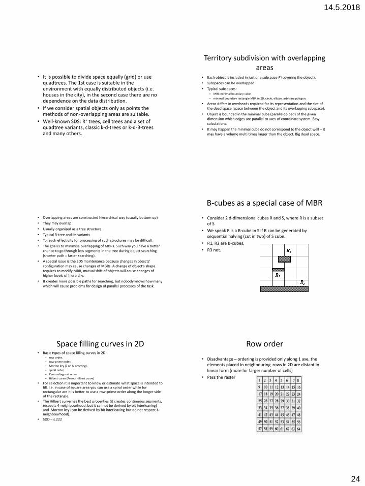
B-cubes as a special case of MBR
• Consider 2 d-dimensional cubes R and S, where R is a subset of S
• We speak R is a B-cube in S if R can be generated by sequential halving (cut in two) of S cube.
• R1, R2 are B-cubes,
• R3 not.
Space filling curves in 2D • Basic types of space filling curves in 2D:
– row order,
– row-prime order,
– Morton key (Z or N ordering),
– spiral order,
– Canon-diagonal order
– Hilbert curve (Peano-Hilbert curve)
• For selection it is important to know or estimate what space is intended to fill. I.e. in case of square area you can use a spiral order while for rectangular are it is better to use a row-prime order along the longer side of the rectangle.
• The Hilbert curve has the best properties (it creates continuous segments, respects 4-neighbourhood, but it cannot be derived by bit interleaving) and Morton key (can be derived by bit interleaving but do not respect 4-neighbourhood).
• SDD – s.222
Row order
• Disadvantage – ordering is provided only along 1 axe, the elements placed in neighbouring rows in 2D are distant in linear form (more for larger number of cells)
• Pass the raster

14.5.2018
25
Row-prime order • Disadvantage – ordering is provided only along 1 axe, the elements placed
in neighbouring rows in 2D are distant in linear form
• Better than row ordering – each 2 neighbouring elements in 1D (linear ordering) are neighbours also in 2D.
Canton-diagonal order
• Canton-diagonal order uses diagonal order
• order is similar to prime-order.
Spiral order
• Only for square matrix
Číslování do šířky
Adresování cestou
Morton key • Ordering according to the letter Z or N (according to axe orientation)
• Quadrants usually in the order: NW, NE, SW, SE (letter Z).
• Advantage - bit interleaving where position of each element can be found by interleaving bits of its X and Y coordinates.
• Disadvantage – it does not respect 4-neighbours (each 2 neighbouring elements according to 4-neighbours in 2D do not be neighbours in 1D (linear order). F.e. cells 1 and 2 do not meet across the edge.
• Arbitrary level of detail (fractal structure)
14.5.2018
26
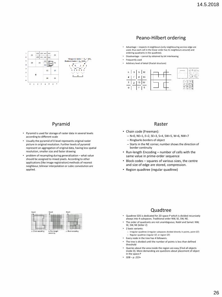
Peano-Hilbert ordering
• Advantage – respects 4-neighbours (only neighbouring accross edge are used, thus each cell in the linear order has its neighbours around) and ordering quadrants in the quadtree).
• Disadvantage – cannot by obtained by bit interleaving
• Frequently used
• Arbitrary level of detail (fractal structure)
Pyramid
• Pyramid is used for storage of raster data in several levels according to different scale
• Usually the pyramid of 0 level represents original raster picture in original resolution. Further levels of pyramid represent an aggregation of original data, having less spatial resolution, smaller size and faster drawing
• problem of resampling during generalization – what value should be assigned to mixed pixels. According to other applications (like image registration) methods of nearest neighbour, bilinear interpolation or cubic convolution are applied.
Raster
• Chain code (Freeman): – N=0, NE=1, E=2, SE=3, S=4, SW=5, W=6, NW=7
– Ringbarks borders of object
– Starts in the NE corner, number shows the direction of border continuity
• Run-length Encoding – number of cells with the same value in prime-order sequence
• Block codes – squares of various sizes, the centre and size of edge are stored, compression.
• Region quadtree (regular quadtree)
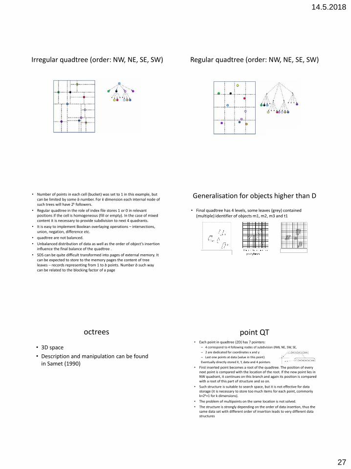
Quadtree • Quadtree SDS is dedicated for 2D space P which is divided recursively
always into 4 subspaces. Traditional order NW, SE, SW, NE.
• The order of quadrants are not unambiguous; Nabil and Samet: NW, SE, SW, NE (letter Z)
• 2 basic variants: – Irregular quadtree (irregular subspaces divided directly in points, point QT)
– Regular quadtree (regular QT, or region QT)
• Every node in the tree has 4 followers.
• The tree is divided until the number of points is less than defined threshold
• Queries about the area inside the region are easy (Find all objects inside D). More demanding are questions about placement of object in the space P
• SDB – p. 223+
14.5.2018
27
Irregular quadtree (order: NW, NE, SE, SW) Regular quadtree (order: NW, NE, SE, SW)
• Number of points in each cell (bucket) was set to 1 in this example, but can be limited by some b number. For k dimension each internal node of such trees will have 2k followers.
• Regular quadtree in the role of index file stores 1 or 0 in relevant positions if the cell is homogeneous (fill or empty). In the case of mixed content it is necessary to provide subdivision to next 4 quadrants.
• It is easy to implement Boolean overlaying operations – intersections, union, negation, difference etc.
• quadtree are not balanced.
• Unbalanced distribution of data as well as the order of object’s insertion influence the final balance of the quadtree .
• SDS can be quite difficult transformed into pages of external memory. It can be expected to store to the memory pages the content of tree leaves – records representing from 1 to b points. Number b such way can be related to the blocking factor of a page
Generalisation for objects higher than D
• Final quadtree has 4 levels, some leaves (grey) contained (multiple) identifier of objects m1, m2, m3 and t1
octrees
• 3D space
• Description and manipulation can be found in Samet (1990)
point QT • Each point in quadtree (2D) has 7 pointers:
– 4 correspond to 4 following nodes of subdivision (NW, NE, SW, SE,
– 2 are dedicated for coordinates x and y
– Last one points at data (value in this point)
Eventually directly stored X, Y, data and 4 pointers
• First inserted point becomes a root of the quadtree. The position of every next point is compared with the location of the root. If the new point lies in NW quadrant, it continues on this branch and again its position is compared with a root of this part of structure and so on.
• Such structure is suitable to search space, but it is not effective for data storage (it is necessary to store too much items for each point, commonly k+2k+1 for k dimensions).
• The problem of multipoints on the same location is not solved.
• The structure is strongly depending on the order of data insertion, thus the same data set with different order of insertion leads to very different data structures
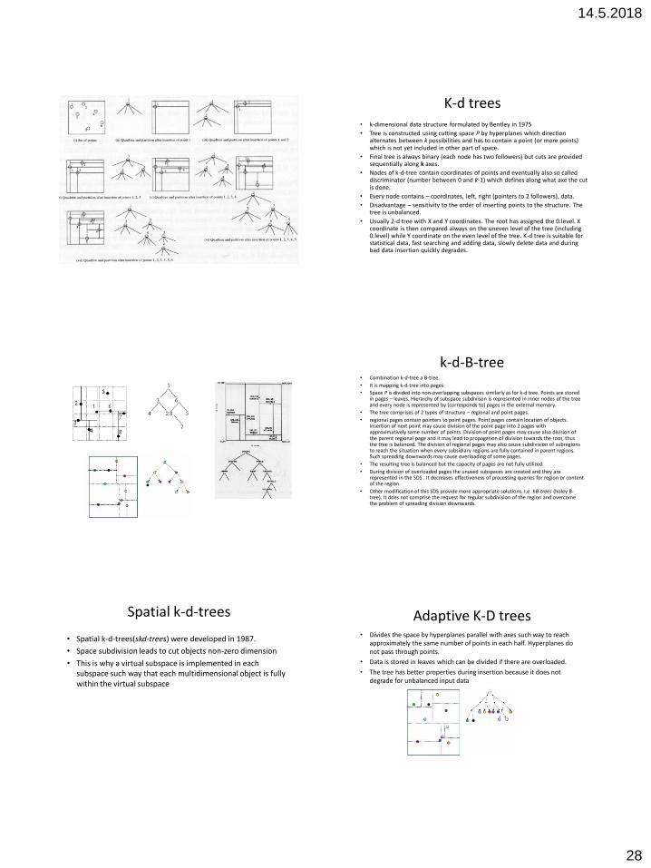
14.5.2018
28
K-d trees • k-dimensional data structure formulated by Bentley in 1975
• Tree is constructed using cutting space P by hyperplanes which direction alternates between k possibilities and has to contain a point (or more points) which is not yet included in other part of space.
• Final tree is always binary (each node has two followers) but cuts are provided sequentially along k axes.
• Nodes of k-d-tree contain coordinates of points and eventually also so called discriminator (number between 0 and k-1) which defines along what axe the cut is done.
• Every node contains – coordinates, left, right (pointers to 2 followers), data.
• Disadvantage – sensitivity to the order of inserting points to the structure. The tree is unbalanced.
• Usually 2-d tree with X and Y coordinates. The root has assigned the 0.level. X coordinate is then compared always on the uneven level of the tree (including 0.level) while Y coordinate on the even level of the tree. K-d tree is suitable for statistical data, fast searching and adding data, slowly delete data and during bad data insertion quickly degrades.
k-d-B-tree • Combination k-d-tree a B-tree.
• It is mapping k-d-tree into pages.
• Space P is divided into non-overlapping subspaces similarly as for k-d tree. Points are stored in pages – leaves. Hierarchy of subspace subdivison is represented in inner nodes of the tree and every node is represented by (corresponds to) pages in the external memory.
• The tree comprises of 2 types of structure – regional and point pages.
• regional pages contain pointers to point pages. Point pages contain location of objects. Insertion of next point may cause division of the point page into 2 pages with approximatively same number of points. Division of point pages may cause also division of the parent regional page and it may lead to propagation of division towards the root, thus the tree is balanced. The division of regional pages may also cause subdivision of subregions to reach the situation when every subsidiary regions are fully contained in parent regions. Such spreading downwards may cause overloading of some pages.
• The resulting tree is balanced but the capacity of pages are not fully utilized.
• During division of overloaded pages the unused subspaces are created and they are represented in the SDS . It decreases effectiveness of processing queries for region or content of the region.
• Other modification of this SDS provide more appropriate solutions. I.e. hB-trees (holey B-tree). It does not comprise the request for regular subdivision of the region and overcome the problem of spreading division downwards.
Spatial k-d-trees
• Spatial k-d-trees(skd-trees) were developed in 1987.
• Space subdivision leads to cut objects non-zero dimension
• This is why a virtual subspace is implemented in each subspace such way that each multidimensional object is fully within the virtual subspace
Adaptive K-D trees • Divides the space by hyperplanes parallel with axes such way to reach
approximately the same number of points in each half. Hyperplanes do not pass through points.
• Data is stored in leaves which can be divided if there are overloaded.
• The tree has better properties during insertion because it does not degrade for unbalanced input data
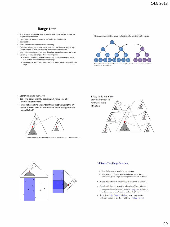
14.5.2018
29
Range tree • Are dedicated to facilitate searching point objects in the given interval, or
ranges in all dimensions
• Data carried by points is stored to leaf nodes (terminal nodes)
• Balanced tree
• Internal nodes are used to facilitate searching
• Each dimension creates its own searching tree. Each internal node in one dimension posses a link to searching tree in another dimension
• Leaf nodes are referenced so many times how many dimensions you have.
• Searching of required range is done following way:
– first find a point which value is slightly (by minimal increment) higher than bottom border of the searched range,
– 2nd search all points with values less than upper border of the searched range
http://www.emilstefanov.net/Projects/RangeSearchTree.aspx
• Search range [x1, x2][y1, y2]
• 1st – find points with the coordinate X within [x1, x2] -> interval, set of subtrees
• Instead of searching all points in these subtrees using the link we can move to trees for Y coordinate and select appropriate interval [y1, y2]
https://www.cs.umd.edu/class/spring2008/cmsc420/L21.RangeTrees.pdf
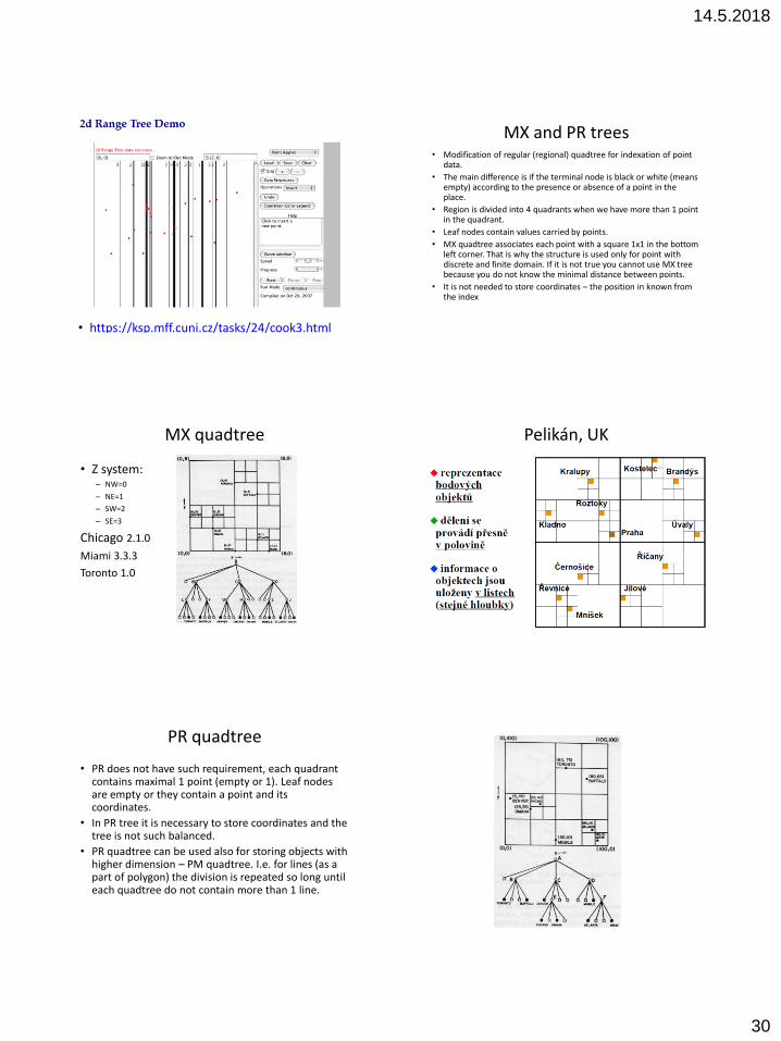
14.5.2018
30
• https://ksp.mff.cuni.cz/tasks/24/cook3.html
MX and PR trees • Modification of regular (regional) quadtree for indexation of point
data.
• The main difference is if the terminal node is black or white (means empty) according to the presence or absence of a point in the place.
• Region is divided into 4 quadrants when we have more than 1 point in the quadrant.
• Leaf nodes contain values carried by points.
• MX quadtree associates each point with a square 1x1 in the bottom left corner. That is why the structure is used only for point with discrete and finite domain. If it is not true you cannot use MX tree because you do not know the minimal distance between points.
• It is not needed to store coordinates – the position in known from the index
MX quadtree
• Z system: – NW=0
– NE=1
– SW=2
– SE=3
Chicago 2.1.0
Miami 3.3.3
Toronto 1.0
Pelikán, UK
PR quadtree
• PR does not have such requirement, each quadrant contains maximal 1 point (empty or 1). Leaf nodes are empty or they contain a point and its coordinates.
• In PR tree it is necessary to store coordinates and the tree is not such balanced.
• PR quadtree can be used also for storing objects with higher dimension – PM quadtree. I.e. for lines (as a part of polygon) the division is repeated so long until each quadtree do not contain more than 1 line.
14.5.2018
31
Pelikán, UK TV trees
• TV trees (telescopic-vector) were designed by Lin et al. (1994) for multidimensional data stored as points in multidimensional space using dynamic extension and shrinkage vectors.
• Eliminates the issue of exponential extension of the index structure known for kD-trees, R-trees or R+trees, thus it has less depth of the tree and faster accesses. Each node in the TV tree represents MBR for followers.
BSP trees (Binary Space Partitioning Tree)
• BSP trees perform similarly as adaptive k-d trees but the division of space by hyperplanes are not parallel with axes.
• BSP is a binary tree, thus in each step the division into 2 parts of arbitrary size is done. The method can be applied to data of any dimension.
• The separating lines (in 2D) are not necessarily parallel.
• Subdivision is provided until the number of points in subspaces drops bellow the given threshold (not necessarily 1 as for k-d trees).
• To identify regions left and right from the separating line it is necessary to define the direction for each line. After that use some criteria to identify if the region is on left or right. Use the equation for line ax+by+c=0. If the term ax+by+c>0, the region falls to the right node below the separating line. In the case of negative value, the region is attached to the left node (Samet 1990).
Pelikán, UK
Pelikán, UK
14.5.2018
32
BSP tree for lines
• Worboys (254-255) describes the algorithm for lines:
1. Place the 1st line
2. Extend this line on both ends to cross the whole region. If some line is crossed, cut it and divide into 2 segments
3. Take next line (or segment), find, if it is on the left or right from previous line and according that use left or right pointer in the tree.
4. If it si not the last line continue with 2nd step. During the line extension you can cut only non-processed lines. The processed lines (stored in the tree) act like barriers limiting extension of the cutting line.
Worboys, s. 255, storing lines with BSP
Region BSP (Pelikán, UK)
Also for non-convex polygons
Region BSP (Pelikán, UK)
Buddy trees • Buddy trees represent a hybrid solution. Utilizes a tree containing
MBR and divide the space until reaching given number of points in MBR
• Buddy-trees are suitable for storing points. If you wish to store complex objects, you need to double the dimension of the space and for each original coordinate store bottom and upper limits
Multidimensional grid • Each axe is divided in some initial increments = scale
• This is initial subdivision of the set into intervals.
• Corresponding perpendicular cuts create the grid which consists of so called basic cubes.
• The content of basic cubes are mapped into pages of the external memory such way that more than 1 basic cube may be inside the memory page. These cubes must create a convex body.
• I.e. a multidimensional grid has 9 basic cubes. Blocking factor is 2, so 3 pages are needed (white lines define 3 pages). We speak about a bucket capacity.
14.5.2018
33
• Cubes are called buckets.
• The bucket has defined occurrence of points on the border. The bucket is stitched together on the bottom and left sides. It means points laying on these borders are assigned to this bucket. To the opposite points on the right and upper side belong to other buckets (neighbour bucket on the right and up respectively).
• The bucket size is set according to average diameter of searched area by users.
• Variants include grid with regular cells and grid with irregular cells. irregular cells are dynamically created according to inserting or deleting individual points.
Example continues • If we insert point A, it is necessary to split the page by:
– fining the grid (situation on the image – the splitting is shown by inserted line, further the original page will be divided into 2 new standalone pages by new white line) OR
– splitting is done within the existing grid
• fining is done by cutting grid by hyperplane (for k dimensions it is possible to define k directions of such cutting).
The process of creating irregular grid during sequential inserting points
There are 2 points in the bucket. Next point insertion into crowded bucket will cause its overflowing and the request for splitting. Splitting buckets is done alternately along X axe and Y axe. Dotted borders are „dissolved“, points are stored together to the same bucket to utilize its capacity. Thus we need to maintain the grid directory (A,B,C..)
A,B,C,A,D,D,E,E,E
X: 40, 80
Y: 15, 75
• We need to maintain 2 auxiliary structure – the grid directory and the scale for each axe. The grid directory defines what blocks are contained in each bucket. The scale defines borders of each block along the axe.
• In the space is divided into regular grid we do not need auxiliary file for saving scale of the axe. If the interval is splitted, the same splitting is applied to all intervals along the same axe. The structure enables faster access.
• If we know positions of all points in advance you can optimize the structure of the grid.
• The scale and multidimensional grid are stored in arrays from where there is direct access to pages in the external memory. Such fields are implemented by trees or hash functions.
• multidimensional grid can be used for arbitrary multidimensional data with defined ordering in each dimension. Queries to the region and area (content of) the region are performed very effectively. Another advantage is that the structure was designed for data stored in external memory.
Two-Level Grid File
• Two-Level Grid is such grid which buckets are also grid.
• (fig. left: NW and SW create 1 bucket, while NE and SE each standalone bucket, each bucket = next grid)
• Similar principle (4 levels of grid) is used by MS SQL.
14.5.2018
34
Balanced And Nested Grid File (BANG)
• Such grid improves properties for unbalanced distribution of inserted points.
• Grid cells are overlaid and data is stored in the tree (the cell has minimal and maximal value).
• Issues with building and modification of trees
Twin Grid File
• Uses secondary grid for overflowing data in the cell.
• Cells are not always splitted and primary and secondary grid is switched according to the need.
• Some points are stored in primary grid and others in the secondary one. Fig - Primary grid on the left, secondary grid on the right
• Suitable for parallel computation
PM quadtree
• PM (polygon maps) quadtrees represents a set of quadtree enabling to store nodes and edges (direct lines).
• Q-edges (segments) represent a subset of edges created by subdivision of PM quadtree. Only these one are stored.
• PM1 has the strongest rules which lead to the most detail subdivision of the quadtree
• PM2 and PM3 have simpler rules, less branching of the tree, but more complex records are stored in the region (cell).
PM1 requirements • Up to 1 vertex can be inside the region represented by the leaf node.
• If the leaf node contains a vertex, all segments inside the region must meet in this vertex.
• If the leaf node does not contain a vertex it can contain up to 1 segment
• In each region the number of leaf nodes is maximal
PM2 requirements • Up to 1 vertex can be inside the region represented by the leaf node.
• If the leaf node contains a vertex, it may also contain a segment which is not meet in the vertex.
• If the leaf node does not contain a vertex it can contain only segments which meet in a vertex outside the region
• In each region the number of leaf nodes is maximal
14.5.2018
35
PM3 requirements
• Up to 1 vertex can be inside the region represented by the leaf node.
• the leaf node can contain arbitrary number of edges
• In each region the number of leaf nodes is maximal
PMR quadtree
R-trees • Simple modification of B-trees
• Records in leaf nodes contain pointers to data objects representing spatial objects
• objects may be objects of higher dimension (mainly 1D, 2D).
• objects may be represented by ID.
• objects are not fragmented.
• Node of R-tree is implemented as 1 page in the external memory. This influences a design of the order of R-tree.
• Maximal number of items in each node is the branching factor m
• It is selected such way to satisfy paging and disc I/O buffering.
• Indexation of objects are performed by the couple (I, ID) where I is MBR bordering corresponding spatial object. These couples are called index records.
• Each I (MBR) has for k-dimensions a form (I0, I1,..., Ik-1) where Ii is the interval [ai,bi] describing bordering of object in the dimension i. Thus there are maximal and minimal coordinates in the given dimension. For k = 2 (2D) we need 4 parameters (Xmin, Xmax, Ymin, Ymax).
• Internal nodes contain records with the form (I, pointer) where the pointer point at the subtree in R-tree where I covers all MBR which are placed inside.
• Opposite to the B-tree the rule of minimal half filling of the nodes (in the worst case) is not strictly applied. In the R-tree is a m-order tree then m1 indicates parameter for which m1<=m/2 is valid.
• SDB – s. 237
R-tree of the order (m1, m)
• Every internal node has n followers
• Each leaf node contains n index records.
• n is between < m1, m > .
• Root has minimal 2 followers if it is not leaf.
• All paths in R-tree have the same length.
Příklad

14.5.2018
36
• R-tree is a dynamic structure, it means it is base on splitting pages (for INSERT) and merging pages (for DELETE).
• To the opposite to B-trees searching in R-tree is not defined by 1 branch.
• Because MBR in individual subtrees can be overlapped it is possible to have more than 1 possibility to continue searching the tree from 1 node.
• All optimisation used for R-tree construction are based on the requirement for maximal separation of MBRs to minimise the space of searching. We are trying to insert the new element into such leaf which requires the minimal changes of its MBR.
• From these a special requirements are established for INSERT operation where we can apply various heuristics offering more or less satisfactory solution of this problem.
• The algorithm of inserting an index record into R-tree has essential importance for further processing of queries. It is based on the strategy to find the best branch in the tree (or the best node of the R-tree) that it will cause the minimal changes of cubes (MBRs) on the path to the root.
• The procedure for splitting is also important. It represents an issue how to divide disordered set of cubes into 2 nodes. Division of records into 2 nodes is done such way to reach the minimal probability of the situation when it is necessary to test both nodes during searching Because nodes are visited from the node-predecessor, it is needed to minimise the volume corresponding to the region I. These actions may propagate to the root of R-tree in the worst case.
• To divide the content of nodes, it is possible to use the exhaustive algorithm. The global minimum is searched and the algorithm has exponential complexity.
• Other algorithms - linear-cost algorithm and quadratic-cost algorithm – only approximate the solution
• During construction of R-tree it is necessary to take into account also the dynamics of the application environment. It differs if the R-tree evolve by sequential INSERT operations or the spatial objects are known in advance. In the 2nd case it is possible to pre-process them and after that to create R-tree. Objects close together are grouped (packing) and R-tree is constructed by a batch from the bottom. The packing is provided in accordance with some space-filling curve (it means linearization), but there are also possibilities to construct R-tree directly in k dimensions.
• R-trees are one of the most cited SDS. They are usually taken as a reference SDS for comparison with (performance of) other SDS.
R*trees • R*-trees encompass combined optimization of the size of bounded region,
the size of borders (perimeter for MBR) and the overlapping size.
• More complicated implementation. R*-tree provides more effective variant than R-tree.
• The reason is to minimize the dead space due to minimizing the size of fenced space. It improves decision taking what path to use during searching nodes on upper levels. Minimizing overlapping leads to decrease the number of paths which are requested to be checked during searching. Minimizing of fenced space leads to squares for MBR.
• It is interesting the performance of the tree rapidly drops with increasing number of dimensions.

14.5.2018
37
X trees
• X-trees modifies R-trees to minimize overlapping in nodes of upper levels.
• They use so called supernodes (certain linear fields) which contains the information about splitting.
• Using X-trees the performance of R*-trees increases by 2 orders.
Vantage-Point trees
• divide the space according to relative distances between points instead of using absolute coordinates.
• Instead of hyperplanes parallel to axes special vantage points are used for splitting the space.
• Using threshold distance a circle is defined around the vantage point (for 2D) in which near points are placed, while the others are „distant“.
• Such way the binary tree arises – in the left branch are followers near to VP, in the right branch the distant followers.
SS-trees • Designed especially for queries to the nearest neighbour in high dimension spaces
where such SDS as k-d-B-trees and R*-trees have difficulties.
• Use thresholding circles.
• Its centre is equal to the centre of the group of points.
• During inserting a new point p the algorithm INSERT determines the best subtree which gravity centre is the nearest to p.
• SDS is dynamic structure; during overflowing of nodes the splitting is applied.
• The circle in the dimension of k is represented by k+1 parameters, instead of covering cubes with 2k+1 parameters. Such way the number of records in nodes increases and the depth of the tree decreases
SR-trees
• Extension of R*-trees and SS-trees.
• Combines of bordering circle and MBD (here square).
• It improves the complexity of the query for nearest neighbours by reduction of both the volume of the area as well as its diameter.
• SR-trees also overcome its ancestors in situations where data are not equally distributed
R+-trees • Extension of k-d-B-trees for working with spatial objects with higher
dimension than 0.
• To the opposite (to k-d-B-trees), not the full space P is divided but only these parts which are necessary.
• Using MBR but they are not-overlapping
• Performs clipping objects
• Number of records in the node may fall bellow m1
• To the opposite to R-trees, by the INSERT operation the object can be added into more leaves (its corresponding MBR is decomposed).
• Splitting nodes may, similar to k-d-B-trees, lead to propagation of changes towards parent nodes but also towards children nodes
• If the object crosses more cells which are not neighbours it is necessary to insert a cell for the middle part or extend the existing cell (it may create a problem).
• Testing has resulted that queries for points require only half accesses to external memory. The queries require passing the tree only on 1 path.
14.5.2018
38
Seed trees
• Seed trees are R-trees which have some level divided into 2 categories – seed and growing.
• From the root there are several levels of seed, the others are growing
• R-tree is stored such way that R-trees rooted from the last seed level are stored separately (creates a forest of R-trees).
• Seed level may be common for more sets of objects (spatial relations), and only growing levels are generated.
• High performance
Cell trees • To the opposite of R+-trees all space P is decomposed and use
hyperplanes to create convex polygons.
• Suitable for objects possessing more common shapes than rectangles.
• Uses clipping of objects
• If you wish to place non-convex object to P, it is necessary to decompose it by clipping (not only disjunctive way). The possible result is that 1 component may be placed in more subspaces. It is divided into cells which are placed in leaves.
• Subspace division is binary, thus it can be described by a binary tree (BT).
• It prevents complications with clipping objects.
Other types of trees
• Strip trees
• Sphere trees
• OBB trees
Spatial extension of SQL
• Reasons: – SQL is a database standard which is offered practically with each
database product.
– Spatial databases without any lexical data are quite seldom in practice.
• Majority of systems combines both data types and good querying language enables create following types of queries: – queries only to spatial properties (Find all towns splitted by a river),
– queries only to aspatial properties (How many people live in Ostrava?),
– Combination of previous types (list names of all neighbours for the house No. 15 in Soukenická street).
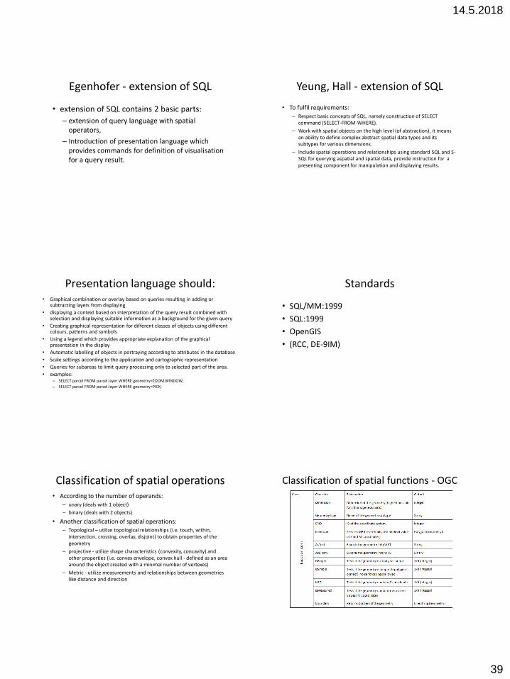
14.5.2018
39
Egenhofer - extension of SQL
• extension of SQL contains 2 basic parts:
– extension of query language with spatial operators,
– Introduction of presentation language which provides commands for definition of visualisation for a query result.
Yeung, Hall - extension of SQL
• To fulfil requirements: – Respect basic concepts of SQL, namely construction of SELECT
command (SELECT-FROM-WHERE).
– Work with spatial objects on the high level (of abstraction), it means an ability to define complex abstract spatial data types and its subtypes for various dimensions.
– Include spatial operations and relationships using standard SQL and S-SQL for querying aspatial and spatial data, provide instruction for a presenting component for manipulation and displaying results.
Presentation language should: • Graphical combination or overlay based on queries resulting in adding or
subtracting layers from displaying
• displaying a context based on interpretation of the query result combined with selection and displaying suitable information as a background for the given query
• Creating graphical representation for different classes of objects using different colours, patterns and symbols
• Using a legend which provides appropriate explanation of the graphical presentation in the display
• Automatic labelling of objects in portraying according to attributes in the database
• Scale settings according to the application and cartographic representation
• Queries for subareas to limit query processing only to selected part of the area.
• examples: – SELECT parcel FROM parcel.layer WHERE geometry=ZOOM.WINDOW;
– SELECT parcel FROM parcel.layer WHERE geometry=PICK;
Standards
• SQL/MM:1999
• SQL:1999
• OpenGIS
• (RCC, DE-9IM)
Classification of spatial operations • According to the number of operands:
– unary (deals with 1 object)
– binary (deals with 2 objects)
• Another classification of spatial operations: – Topological – utilize topological relationships (i.e. touch, within,
intersection, crossing, overlay, disjoint) to obtain properties of the geometry
– projective - utilize shape characteristics (convexity, concavity) and other properties (i.e. convex envelope, convex hull - defined as an area around the object created with a minimal number of vertexes)
– Metric - utilize measurements and relationships between geometries like distance and direction
Classification of spatial functions - OGC
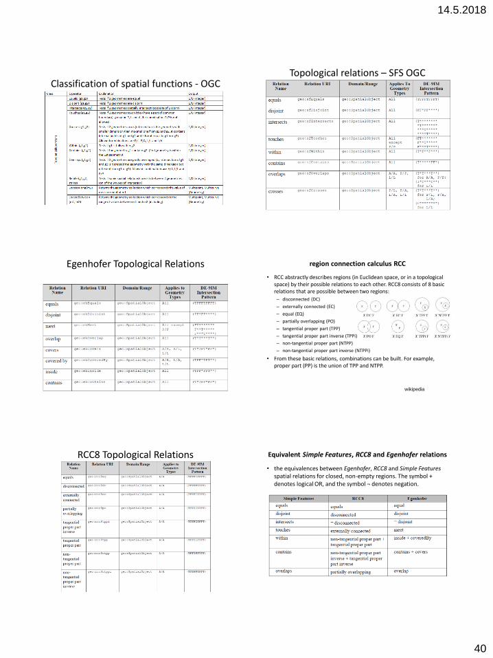
14.5.2018
40
Classification of spatial functions - OGC Topological relations – SFS OGC
Egenhofer Topological Relations region connection calculus RCC
• RCC abstractly describes regions (in Euclidean space, or in a topological space) by their possible relations to each other. RCC8 consists of 8 basic relations that are possible between two regions:
– disconnected (DC)
– externally connected (EC)
– equal (EQ)
– partially overlapping (PO)
– tangential proper part (TPP)
– tangential proper part inverse (TPPi)
– non-tangential proper part (NTPP)
– non-tangential proper part inverse (NTPPi)
• From these basic relations, combinations can be built. For example, proper part (PP) is the union of TPP and NTPP.
wikipedia
RCC8 Topological Relations Equivalent Simple Features, RCC8 and Egenhofer relations
• the equivalences between Egenhofer, RCC8 and Simple Features spatial relations for closed, non-empty regions. The symbol + denotes logical OR, and the symbol ¬ denotes negation.
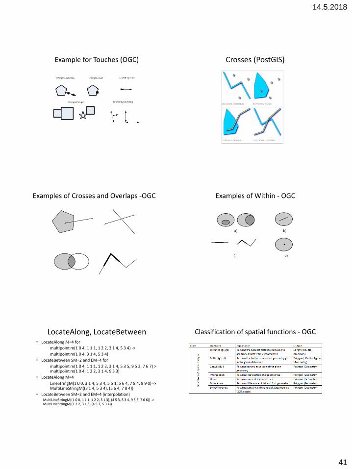
14.5.2018
41
Example for Touches (OGC) Crosses (PostGIS)
Examples of Crosses and Overlaps -OGC Examples of Within - OGC
LocateAlong, LocateBetween • LocateAlong M=4 for
multipoint m(1 0 4, 1 1 1, 1 2 2, 3 1 4, 5 3 4) ->
multipoint m(1 0 4, 3 1 4, 5 3 4)
• LocateBetween SM=2 and EM=4 for
multipoint m(1 0 4, 1 1 1, 1 2 2, 3 1 4, 5 3 5, 9 5 3, 7 6 7) > multipoint m(1 0 4, 1 2 2, 3 1 4, 9 5 3)
• LocateAlong M=4
LineStringM(1 0 0, 3 1 4, 5 3 4, 5 5 1, 5 6 4, 7 8 4, 9 9 0) -> MultiLineStringM((3 1 4, 5 3 4), (5 6 4, 7 8 4))
• LocateBetween SM=2 and EM=4 (interpolation) MultiLineStringM((1 0 0, 1 1 1, 1 2 2, 3 1 3), (4 5 3, 5 3 4, 9 5 5, 7 6 6)) -> MultiLineStringM((1 2 2, 3 1 3),(4 5 3, 5 3 4))
Classification of spatial functions - OGC
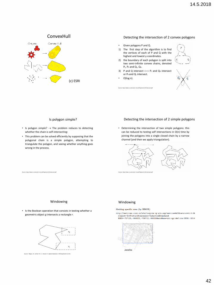
14.5.2018
42
ConvexHull
(c) ESRI
Detecting the intersection of 2 convex polygons
• Given polygons P and Q.
1) The first step of the algorithm is to find the vertices of each of P and Q with the highest and lowest y-coordinates.
2) the boundary of each polygon is split into two semi-infinite convex chains, denoted PL, PR and QL, QR.
3) P and Q intersect PL and QR intersect or PR and QL intersect.
• O(log n).
Source: https://www.cs.umd.edu/~mount/Papers/crc04-intersect.pdf
Is polygon simple?
• Is polygon simple? The problem reduces to detecting
whether the chain is self-intersecting:
• This problem can be solved efficiently by supposing that the
polygonal chain is a simple polygon, attempting to
triangulate the polygon, and seeing whether anything goes
wrong in the process.
Source: https://www.cs.umd.edu/~mount/Papers/crc04-intersect.pdf
Detecting the intersection of 2 simple polygons
• Determining the intersection of two simple polygons: this
can be reduced to testing self intersections in O(n) time by
joining the polygons into a single closed chain by a narrow
channel (and then we apply triangulation).
Source: https://www.cs.umd.edu/~mount/Papers/crc04-intersect.pdf
Windowing
• Is the Boolean operation that consists in testing whether a
geometric object g intersects a rectangle r.
Source: Rigaux, M., Scholl, M., O., Voisard, A. Spatial Databases: With Application to GIS.
Windowing
Janečka
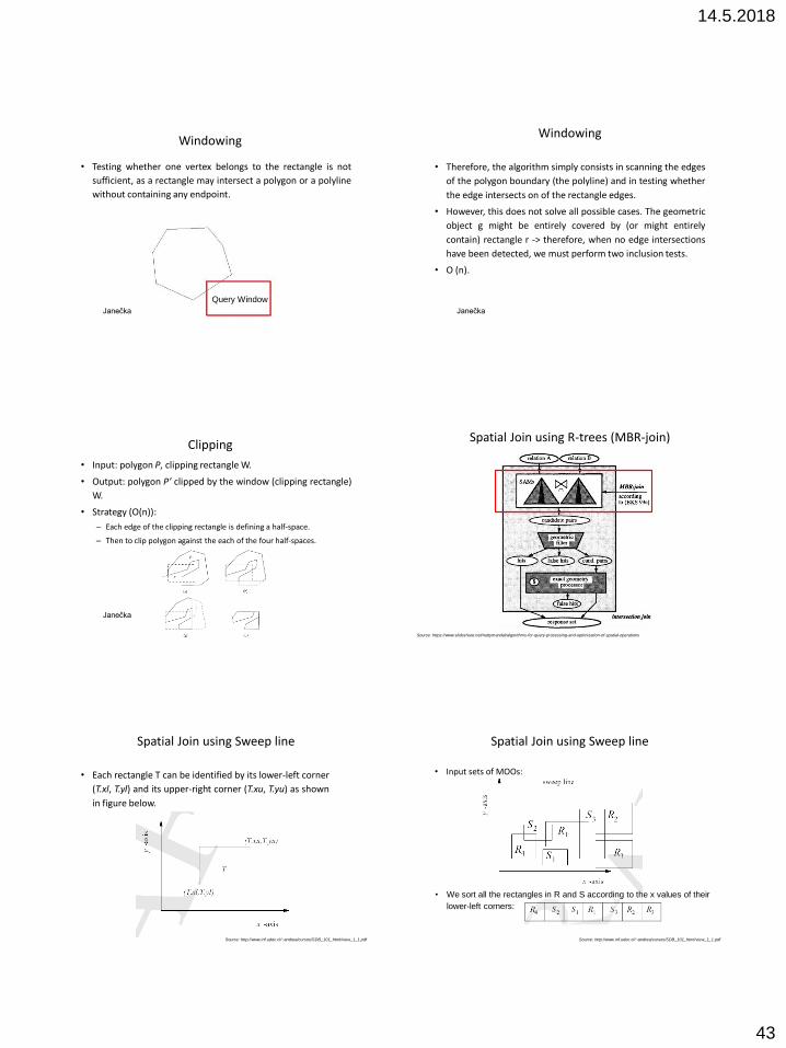
14.5.2018
43
Windowing
• Testing whether one vertex belongs to the rectangle is not
sufficient, as a rectangle may intersect a polygon or a polyline
without containing any endpoint.
Query Window
Janečka
Windowing
• Therefore, the algorithm simply consists in scanning the edges
of the polygon boundary (the polyline) and in testing whether
the edge intersects on of the rectangle edges.
• However, this does not solve all possible cases. The geometric
object g might be entirely covered by (or might entirely
contain) rectangle r -> therefore, when no edge intersections
have been detected, we must perform two inclusion tests.
• O (n).
Janečka
Clipping
• Input: polygon P, clipping rectangle W.
• Output: polygon P’ clipped by the window (clipping rectangle)
W.
• Strategy (O(n)):
– Each edge of the clipping rectangle is defining a half-space.
– Then to clip polygon against the each of the four half-spaces.
Janečka
Spatial Join using R-trees (MBR-join)
Source: https://www.slideshare.net/nuttymandal/algorithms-for-query-processing-and-optimization-of-spatial-operations
Spatial Join using Sweep line
• Each rectangle T can be identified by its lower-left corner
(T.xl, T.yl) and its upper-right corner (T.xu, T.yu) as shown
in figure below.
Source: http://www.inf.udec.cl/~andrea/cursos/SDB_101_html/view_1_1.pdf
Spatial Join using Sweep line
• Input sets of MOOs:
• We sort all the rectangles in R and S according to the x values of their
lower-left corners:
Source: http://www.inf.udec.cl/~andrea/cursos/SDB_101_html/view_1_1.pdf

14.5.2018
44
• Then we proceed (with sorted set of rectangles) as follows:
1. Move a sweep line from left to right and stop at the first entry in R U S.
This is the rectangle T with the smallest T.xl value. Now T is R4.
2. Search through the sorted rectangles of S until arriving at the first
rectangle Sf such Sf.xl > T.xu. Clearly, the relation [T.xl, T.xu] ∩ [Sj.xl,
Sj.xu] holds nonempty for all 1 ≤ j < f. In our example Sf is S1. Thus S2
is a candidate rectangle that may overlap R4. This will be confirmed in
the next step.
3. If the relation [T.yl, T.yu] ∩ [Sj.yl, Sj.yu] holds for any 1 ≤ j < f, then the
rectangle Sj intersects T. Thus this step confirms that R4 and S2 indeed
overlap and <R4,S2> are part of the join result. Remove T from R U S.
4. Move the sweep line across the set R U S until it reaches the next
rectangle entry. This is rectangle S2 in our example. Now proceed as in
steps 2 and 3.
5. Stop when the R U S = Ø.
Source: http://www.inf.udec.cl/~andrea/cursos/SDB_101_html/view_1_1.pdf
Spatial Join using Sweep line
• The first step of the spatial-join algorithm results in:
– <R4,S2>
– <R1,S2>
– <R1,S3>
– <R2,S3>
– <R3,S3>
as candidate pairs for the
refinement step, based on
the exact geometries of
the objects.
Janečka
Spatial operators
• Spatial operators are written in the prefix notation as functions. Users do not need advanced mathematical knowledge.
• example: distance(city.geometry, highway.geometry)
• Measured in the coordinate system of the 1st geometrical object
• Operators may occur after SELECT or in WHERE part as a part of a non-spatial predicate. They are used on same places as aggregation functions.
• In the case of ordering, it is possible to use predicates: – left/right,
– north/south,
– over/under.
Oracle Spatial SQL • 2 groups of operations:
– Main spatial operators • SDO_FILTER,
• SDO_JOIN,
• SDO_NN,
• SDO_NN_DISTANCE,
• SDO_RELATE,
• SDO_WITHIN_DISTANCE
– „comfortable“ spatial operators for usage with operator SDO_RELATE • SDO_ANYINTERACT,
• SDO_CONTAINS,
• SDO_COVEREDBY,
• SDO_COVERS,
• SDO_EQUAL,
• SDO_INSIDE,
• SDO_ON,
• SDO_OVERLAPBDYDISJOINT,
• SDO_OVERLAPBDYINTERSECT,
• SDO_OVERLAPS,
• SDO_TOUCH
Main spatial operators
• SDO_FILTER (geometry1, geometry2, otherParams)
– Specifies which geometries may interact with a given geometry.
• SDO_WITHIN_DISTANCE(geometry1, geometry2, ’distance = NN’)
– Determines if two geometries are within a specified Euclidean distance
from one another.
• SDO_NN(geometry1, geometry2, ’num_res = NN’)
– Determines the nearest neighbor geometries to a geometry.
Janečka
„comfortable“ spatial operators
14.5.2018
45
SDO_ANYINTERACT
• Example – find rivers (lines) reaching any way (flows through, rises, ...) Moravian-Silesian region (polygon)
SELECT DISTINCT R.NAZEV REKA FROM KRAJE K, REKY R WHERE SDO_ANYINTERACT(K.GEOM, R.GEOM) = 'TRUE' AND K.KODRE = 'OST' AND R.NAZEV IS NOT NULL ORDER BY REKA ASC;
SDO_COVERS
• Example: find municipalities with authorized offices (2nd type) (polygons) which do not share the border with the border of Moravian-Silesian region (polygon), thus they lie totally within the region
SELECT O.NAZOB OBEC FROM MS_KRAJ K, MS_OBCE2 O WHERE SDO_COVERS(K.GEOM, O.GEOM) != 'TRUE' ORDER BY OBEC ASC;
• Result: Bílovec, Fulnek, Havířov, Horní Benešov, Kopřivnice, Ostrava, Příbor, Studénka, Vratimov
SDO_EQUAL
• Example - find municipalities which are both municipalities of the 2nd and 3rd order (type) in the Moravian-Silesian region
SELECT O2.NAZOB FROM MS_OBCE2 O2, MS_OBCE3 O3 WHERE SDO_EQUAL(O2.GEOM, O3.GEOM) = 'TRUE' ORDER BY O2.NAZOB ASC;
• Result: Bohumín, Český Těšín, Frenštát pod Radhoštěm, Frýdek–Místek, Frýdlant nad Ostravicí, Havířov, Hlučín, Jablunkov, Karviná, Kravaře, Odry, Opava, Orlová, Rýmařov, Třinec, Vítkov
SDO_INSIDE
• Example – find rivers (lines) in the Moravian-Silesian region (polygon) which do not flow off this region or flow from another region
SELECT R.NAZEV REKA FROM MS_KRAJ K, MS_REKY R WHERE SDO_INSIDE(R.GEOM, K.GEOM) = 'TRUE' ORDER BY REKA ASC;
• Černý potok, Lubina, Moravice, Ostravice, Podolský potok.
Spatial Query Processing in Oracle Spatial
Computational Geometry
Algorithms
Janečka
Point clouds in Oracle Spatial
Janečka
14.5.2018
46
Janečka
Multiple representation
• An object may posses a multiple representation.
• I.e. CITY table has 2 representations – the polygon for the scale 1:20000 and the point of the centre for 1:200000.
CREATE TABLE city
(
name char (20)
geometry spatial_2
generalizedGeometry spatial_0
);
PICK • PICK enables to create queries referencing spatial objects portrayed on the display
• It can be used for every spatial attribute in WHERE (it is possible to select any type of geometry and object).
• Execution of the selection depends on a spatial dimension of the target. In the case of point out the place in the map window:
– In the case of 0D or 1D objects the closest one is selected
– In the case of 2D objects the polygon with indicated point inside is selected
• If there are 2 objects of the requested type with the same distance from the point, the user should obtain a list of (2) variants for selection. The similar list is displayed also in the case of ambiguous selections (i.e. the border of 2 polygons is picked).
• Example: – CREATE TABLE MĚSTA ( JMÉNO VARCHAR(30) UMÍSTĚNÍ SPATIAL_2 );
– SELECT JMÉNO FROM MĚSTA WHERE UMÍSTĚNÍ = PICK;
• We have a map of countries with borders and large cities (as points). The user asks by clicking to a point.
• SELECT name FROM city WHERE geometry = PICK; -> city name
• SELECT name FROM country WHERE geometry = PICK; -> country name
Spatial methods according to SQL/MM
• Majority of spatial methods are classified into 4 categories: 1. Conversion between feature and external data format
2. Obtaining properties and values of features
3. Comparison of 2 features with respect to their spatial relationship
4. Creation of new feature from existing one
• Some operation are difficult to classified. I.e. ST_StartPoint returns 1st point from the line (LineString), thus it provides a property of the line, but simultaneously it creates a new feature (point).
Conversion between feature and external data format
• SQL/MM specifies 3 external data formats that can be used for (by implementation) independent description of the feature: – WKT (well-known text representation) – WKB (well-known binary representation) – GML (geography markup language)
• Import functions: – ST_WKTToSQL(awkt CHARACTER LARGE OBJECT) – ST_WKBToSQL(awkb BINARY LARGE OBJECT) – ST_GMLToSQL
• Export functions: – ST_AsText – ST_AsBinary – ST_AsGML
• Import (creation) of the feature:
– Each feature type enables to create a new feature in WKT and WKB
formats and provides also identifiers of the coordinate system.
– No appropriate constructors are available for GML, instead of them
functions like ST_LineFromGML or ST_MPointFromGML are applied
– To improve the compatibility (mainly with OGC SFS) the standard
defines also functions like ST_PointFromText or
ST_GeometryFromWKB.
• Export (storage) of the feature:
– Transformation of the feature into WKT format (WKB or GML formats
resp.) is provided thanks to functions like ST_AsText (ST_AsBinary and
ST_AsGML, resp.).

14.5.2018
47
SQL/MM – implementation of selected topological operators
There are binary spatial operations resulting in the number indicating if the requirement
is satisfied (success of the operation).
SQL/MM: Obtaining properties and values of features
• All feature types have such properties like dimension or if the feature is empty, and add specific properties according to the type.
• Unary spatial operations may be understand as functions on spatial objects. They include Dim (Dimension in the geometrical model) and Boundary. Each such operation have own version specialised for certain dimension (i.e. BoundingNodes, BoundingEdges).
• Another group of unary spatial operations implements operations like Length, Area and Volume.
• Combination of previous operations we will obtain further operations. I.e. the perimeter will be obtained by sum of length of bordering lines
• Other unary spatial operations – i.e. extreme coordinates.
Selected operations of SQL/MM querying for properties
SQL/MM - comparison of 2 features with respect to their spatial relationship
• Binary spatial operations – Distance and Direction.
• Arguments are also spatial objects
• Result is the non-negative real number for distance and the angle 0 …359°59’59’’ for azimuth.
Extension of SQL language for visualisation of spatial data
• Embedding all commands necessary for displaying management –> the query will be to long and complicated.
• It is better to divide each query into smaller and more transparent subgroups of actions:
– User query (specifies what to display),
– Additional queries to specify displaying (display queries),
– (result of the main query can be subdivided into groups where we can apply different formats of displaying)
– Setting of display parameters (define how to display each data group).
• I.e. Spatial SQL - searching and presentation language.
• It is not necessary to set parameters of displaying every time with every query. Instead of it the setting is stored in a display environment. It contains a set of parameters which will be used for drawing results of each new query until their redefinition.
• Using SQL or GPL commands for operative work may be too long. Writing long queries and keywords from keyboards is not effective. Thus any system should be equipped by suitable GUI. Namely operations like ZOOM, PAN, SET WINDOW are dedicated to be used with some pointing device. Such way it is possible to perform interactively all selections of colours, patterns, symbols etc.
Graphic Presentation Language, GPL
• The key term in GPL is the displaying environment which contains all current settings influencing result displaying.
• During result processing these settings are eventually changed according to user requirements. If the user does not change the displaying environment using GPL instructions every query produces a result (map) portrayed with the same style.
• SET - setting of concrete displaying parameters
• CANCEL – cancelling of parameters settings
• SHOW – show the current value of the given parameter
• Commands SET and CANCEL may be completed with a temporal settings: – PERMANENT - the setting is stored for further work with the system
– IMMEDIATELY – the setting is applied immediately, thus it redraw the existing query result (otherwise parameters are applied for the next query).

14.5.2018
48
Parameters for setting of GPL
• the display mode SET MODE
• the graphical presentation SET LEGEND
• the scale of the drawing SET SCALE
• the window to be shown SET WINDOW
• the spatial context SET CONTEXT
• the examination of the content.
More details • display mode – specifies how to deal with the output; alphanumeric option, but also graphical
possibilities: NEW (draw a new drawing), OVERLAY (add to the previous drawing), REMOVE (remove from the previous drawing), INTERSECT (display those objects which were presented also in the previous drawing), HIGHLIGHT (highlighting of objects).
• graphical presentation – using LEGEND command provides setting of various visual variables like hatching, colours, etc. – it enables to set various parameters for groups of objects in the result and create specific views for presented data.
• scale of the drawing – using SET SCALE command it is possible to set the scale; write a positive number n for the scale 1:n.
• window to be shown – using SET WINDOW we set the window of displayed map window; write coordinates of 2 opposite corners of the bordering rectangle (it means minimal and maximal coordinates of bordering).
• spatial context – using SET CONTEXT we set what further objects (except of direct query results) are to be drawn.
• examination of the content (what was displayed) – in 1 image results from many queries may be displayed and also with variants using OVERLAY and REMOVE modes, thus it may be difficult to understand what the user see; using SHOW CONTENT a query is created that specifies how to create such drawing (the current drawing should be obtained by execution of this query).
Display the map of Soukenické street with all parcels, houses and streets. Show dwellings (residential housing) by green, commercial houses by blue and borders
of parcel lots by dashed black line. Hatch roads narrower than 4.5 m
• SET LEGEND COLOR ČERNÁ PATTERN ČÁRKOVANĚ FOR SELECT BOUNDARY(POLOHA) FROM POZEMKY;
• SET LEGEND COLOR GREEN, BLUE FOR SELECT RESIDENCE.POLOHA, KOMERČNÍ.POLOHA FROM DOMY RESIDENCE, DOMY KOMERČNÍ WHERE RESIDENCE.TYP = ‘OBYTNÝ’ AND KOMERČNÍ.TYP = ‘KOMERČNÍ;
• SET LEGEND PATTERN ŠRAFOVANĚ FOR SELECT INTERIOR(POLOHA) FROM ULICE WHERE ŠÍŘKA < 4,5;
• Next set the window and the context for road displaying:
• SET WINDOW SELECT POLOHA FROM ULICE WHERE MĚSTA.JMÉNO = ‘PRAHA’;
• It was set immediately because it does not include „FOR SELECT“.
• SET CONTEXT FOR ULICE.POLOHA SELECT POZEMKY.POLOHA, DOMY.POLOHA, ULICE.NÁZEV FROM ULICE, POZEMKY, DOMY;
• Finally set the regime for displaying of the new map and write the SQL query:
• SET MODE NEW; SELECT ULICE.POLOHA FROM ULICE, MĚSTA WHERE MĚSTA.JMÉNO = ‘PRAHA’ AND ULICE.NÁZEV = ‘SOUKENICKÁ’ AND ULICE.POLOHA INSIDE MĚSTA.POLOHA;
• Highlight the building on the Soukenická 15:
SET MODE HIGHLIGHT; SELECT DOMY.POLOHA FROM DOMY WHERE ADRESA = ‘SOUKENICKÁ 15’;
• The insurance company is surely interested how far is the nearest fire station from the building.
SET MODE ALPHA; SELECT HASICI.ADRESA, DISTANCE(DOMY.POLOHA,HASICI.POLOHA) FROM DOMY, DOMY HASICI WHERE DOMY = PICK AND HASICI.TYP = ‘HASICÍ’;
• The result is the list of fire stations and their distances to the object selected by the user by the cursor (the area of Prague was set in the parameter WINDOW in the last case and it is still valid).
• Further we display all hydrants within 30 m from the building:
• SET LEGEND COLOR červená SYMBOL ‘2mm kolečko’ FOR SELECT POLOHA FROM SÍTĚ WHERE TYP = ‘HYDRANT’ SET MODE OVERLAY;
• SELECT UMÍSTĚNÍ FROM SÍTĚ, DOMY WHERE SÍTĚ.TYP = ‘HYDRANT’ AND DOMY.UMÍSTĚNÍ = PICK AND DISTANCE(DOMY.UMÍSTĚNÍ, SÍTĚ.UMÍSTĚNÍ) < 30;
• Finally we would find on what parcels the fires have occurred since 1980.
• SET IMMEDIATELY COLOR RED FOR SELECT INTERIOR(POLOHA) FROM POZEMKY WHERE ROK_POŽÁRU >= 1980;

14.5.2018
49
Constraint SQL
• odlišný přístup k manipulaci prostorových objektů v rámci SQL
• aritmetická omezení nad reálnými (racionálními) čísly součástí řádků tabulek.
• Omezení (constraints) se vyjadřují jako disjunkce konjunkcí. Pro naše účely se můžeme omezit pouze na lineární omezení.
• regiony v 2D:
• bod v 3D:
• hodnoty prostorových atributů se vyjadřují pomocí těchto formulí.
• Typ prostorového atributu je dán jeho dimenzí, např. R1, R2, R2.
• Přístup podle souřadnic x, y, z se provádí pozičně, např. UMÍSTĚNÍ. Lze tak realizovat jakési zobecněné projekce, k dispozici jsou agregační funkce z SQL a další jako Area, Volume, Surface a Lenght. Autoři jazyka navíc připouštějí hnízdění agregačních funkcí, což umožňuje realizovat zajímavé dotazy.
• Je-li prostorový atribut UMÍSTĚNÍ.[ 1] v tabulce MĚSTA typu R2, tj. např. polygon, pak dotaz „Najdi město s nejmenší x-souřadnicí“ se vyjádří jako:
• SELECT JMÉNO, MIN(UMÍSTĚNÍ.[ 1] ) FROM MĚSTA;
• Relace PROSTOROVÉ_OBJEKTY(JMÉNO, TYP, UMÍSTĚNÍ) obsahuje různé objekty typu řeky, jezera, lesy apod.
• Najdi pro každý typ prostorového objektu jeho celkovou plochu:
• SELECT TYP, AREA(UNION(UMÍSTĚNÍ)) FROM MĚSTA GROUP BY TYP;
• Nechť LESY a CESTY jsou relace s atributy JMÉNO a UMÍSTĚNÍ
• Najdi ty části cest, které procházejí lesem
• SELECT C.JMÉNO, UNION(INTERSECT(C.UMÍSTĚNÍ, L.UMÍSTĚNÍ)) FROM CESTY C, LESY L WHERE C.UMÍSTĚNÍ INTERSECTS L.UMÍSTĚNÍ GROUP BY C.JMÉNO;
Solutions in database systems
Oracle Spatial - GeoRaster • storage, organization, analysis, querying and distribution of
geographical georeferenced raster data including relevant metadata
• Raster storage – BLOB
• Except of pixel values following data is stored: – spatial range,
– Temporal and dimensional range (i.e. number of channels for images with more spectral bands),
– Attributes connected to pixels,
– metadata
– Supporting structures for management
GeoRaster
• Spatial dimension - records of raster size (number of pixels) in the direction of rows and columns
• band dimension – number of spectral bands or thematic rasters stored in 1 object
• GeoRaster Table (GRT)
• Raster Data Table (RDT) – storage of raster data, according to the level of pyramid and blocks

14.5.2018
50
GeoRaster functions • CREATE TABLE GDT a RDT, SDO_GEOR.init nebo SDO_GEOR.createBlank - new object Georaster
• SDO_GEOR.importFrom
• SDO_GEOR.getCellValue - returns the value of the selected pixel
• SDO_GEOR.getRasterData - BLOB of all GeoRaster object in the given pyramid level
• SDO_GEOR.changeCellValue
• SDO_GEOR.getBandDimSize - number of spectral bands of the GeoRaster object
• SDO_GEOR.getHistogram – show the histogram of the selected layer
• SDO_GEOR.getLayerDimension - number of layers of the GeoRaster object
• SDO_GEOR.getPyramidMaxLevel - number of pyramid layers
• SDO_GEOR.getSpatialResolutions – the pixel size in the direction of row and column
• SDO_GEOR.generatePyramid
• SDO_GEOR.subset – create a subset
• SDO_GEOR.mosaic
• SDO_GEOR.generateStatistics
• SDO_GEOR.exportTo
MS SQL Server 2008 - Spatial
• OGC Simple Features Specification for SQL
• Used data types: – point
– LineString
– polygon
– Multipoint, MultiLineString and MultiPolygon – homogeneous collections
– GeometryCollection may contain arbitrary combination of objects (i.e. even combination of linestrings and polygons)
MS SQL – way of storage
• Head:
– Used spatial data type
– SRID
– Number of vertex points creating the object
• Row of coordinates – 8B binary format
MS SQL – 2 data types • Geometry – plain system, local coordinates, no SRID, just X
and Y.
• compliance with SFS OGC
• Geography – geographical system (related to the reference body of the Earth).
• For analytical and numerical operations the geographical coordinate system is used with implicit WGS 84
• Other SRID is possible to define
• Not fully compliant (compatible) with SFS OGC
MS SQL spatial indexation • Space is subdivided by the grid.
• Each cell is further divided into 4-level grid.
• Each level is divided into defined number of cells with respect to the size and number of objects in the given space
• Cell covering the spatial objects are linearly numbered using Hilbert space filling curve. This way you obtain the 1D numerical key.
• This number is indexed by B-tree
• Rules of indexation effectivity:
– Covering rule (if it covers the full cell, it is not more divided)
– Rule of deepest cell (only cells of the deepest level are stored in the index)
– rule „CELLS_PER_OBJECT“ (explicitly defines the maximal number of cells by which the object is covered and which are stored to the index. If the limit is reached the cell is not more divided to more detail level)
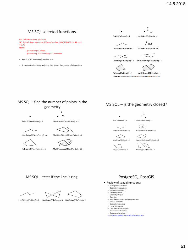
14.5.2018
51
MS SQL selected functions
DECLARE @LineString geometry
SET @LineString = geometry::STGeomFromText (`LINESTRING(-120 48, -122 47)’, 0)
SELECT
@LineString AS Shape,
@LineString, STDimension() As Dimension
• Result of STDimension () method is: 1
• it creates the lineString and after that it tests the number of dimensions.
MS SQL – find the number of points in the geometry
MS SQL – is the geometry closed?
MS SQL – tests if the line is ring
PostgreSQL PostGIS • Review of spatial functions:
– Management Functions
– Geometry Constructors
– Geometry Accessors
– Geometry Editors
– Geometry Outputs
– Operators
– Spatial Relationships and Measurements
– SFCGAL Functions
– Geometry Processing
– Linear Referencing
– Long Transactions Support
– Miscellaneous Functions
– Exceptional Functions
http://postgis.net/docs/manual-2.1/reference.html
14.5.2018
52
Management Functions • AddGeometryColumn — Adds a geometry column to an existing table of attributes.
DropGeometryColumn — Removes a geometry column from a spatial table.
• DropGeometryTable — Drops a table and all its references in geometry_columns.
• PostGIS_Full_Version — Reports full postgis version and build configuration infos.
• PostGIS_GEOS_Version — Returns the version number of the GEOS library.
• PostGIS_LibXML_Version — Returns the version number of the libxml2 library.
• PostGIS_Lib_Build_Date — Returns build date of the PostGIS library.
• PostGIS_Lib_Version — Returns the version number of the PostGIS library.
• PostGIS_PROJ_Version — Returns the version number of the PROJ4 library.
• PostGIS_Scripts_Build_Date — Returns build date of the PostGIS scripts.
• PostGIS_Scripts_Installed — Returns version of the postgis scripts installed in this database.
• PostGIS_Scripts_Released — Returns the version number of the postgis.sql script released with the installed postgis lib.
• PostGIS_Version — Returns PostGIS version number and compile-time options.
• Populate_Geometry_Columns — Ensures geometry columns are defined with type modifiers or have appropriate spatial constraints
• UpdateGeometrySRID — Updates the SRID of all features in a geometry column, geometry_columns metadata and srid. If it was enforced with constraints, the constraints will be updated with new srid constraint. If the old was enforced by type definition, the type definition will be changed.
Geometry Constructors – 1st part
• ST_BdPolyFromText — Construct a Polygon given an arbitrary collection of closed linestrings as a MultiLineString Well-Known
text representation.
• ST_BdMPolyFromText — Construct a MultiPolygon given an arbitrary collection of closed linestrings as a MultiLineString text
representation Well-Known text representation.
• ST_Box2dFromGeoHash — Return a BOX2D from a GeoHash string.
• ST_GeogFromText — Return a specified geography value from Well-Known Text representation or extended (WKT).
• ST_GeographyFromText — Return a specified geography value from Well-Known Text representation or extended (WKT).
• ST_GeogFromWKB — Creates a geography instance from a Well-Known Binary geometry representation (WKB) or extended
Well Known Binary (EWKB).
• ST_GeomCollFromText — Makes a collection Geometry from collection WKT with the given SRID. If SRID is not give, it
defaults to 0.
• ST_GeomFromEWKB — Return a specified ST_Geometry value from Extended Well-Known Binary representation (EWKB).
• ST_GeomFromEWKT — Return a specified ST_Geometry value from Extended Well-Known Text representation (EWKT).
• ST_GeometryFromText — Return a specified ST_Geometry value from Well-Known Text representation (WKT). This is an
alias name for ST_GeomFromText
• ST_GeomFromGeoHash — Return a geometry from a GeoHash string.
• ST_GeomFromGML — Takes as input GML representation of geometry and outputs a PostGIS geometry object
• ST_GeomFromGeoJSON — Takes as input a geojson representation of a geometry and outputs a PostGIS geometry object
• ST_GeomFromKML — Takes as input KML representation of geometry and outputs a PostGIS geometry object
• ST_GMLToSQL — Return a specified ST_Geometry value from GML representation. This is an alias name for
ST_GeomFromGML
• ST_GeomFromText — Return a specified ST_Geometry value from Well-Known Text representation (WKT).
• ST_GeomFromWKB — Creates a geometry instance from a Well-Known Binary geometry representation (WKB) and optional
SRID.
• ST_LineFromMultiPoint — Creates a LineString from a MultiPoint geometry.
• ST_LineFromText — Makes a Geometry from WKT representation with the given SRID. If SRID is not given, it defaults to 0.
• ST_LineFromWKB — Makes a LINESTRING from WKB with the given SRID
• ST_LinestringFromWKB — Makes a geometry from WKB with the given SRID.
• ST_MakeBox2D — Creates a BOX2D defined by the given point geometries.
Geometry Accessors – 1st part
• GeometryType — Returns the type of the geometry as a string. Eg: 'LINESTRING', 'POLYGON', 'MULTIPOINT', etc.
• ST_Boundary — Returns the closure of the combinatorial boundary of this Geometry.
• ST_CoordDim — Return the coordinate dimension of the ST_Geometry value.
• ST_Dimension — The inherent dimension of this Geometry object, which must be less than or equal to the coordinate
dimension.
• ST_EndPoint — Returns the last point of a LINESTRING geometry as a POINT.
• ST_Envelope — Returns a geometry representing the double precision (float8) bounding box of the supplied geometry.
• ST_ExteriorRing — Returns a line string representing the exterior ring of the POLYGON geometry. Return NULL if the
geometry is not a polygon. Will not work with MULTIPOLYGON
• ST_GeometryN — Return the 1-based Nth geometry if the geometry is a GEOMETRYCOLLECTION, (MULTI)POINT,
(MULTI)LINESTRING, MULTICURVE or (MULTI)POLYGON, POLYHEDRALSURFACE Otherwise, return NULL.
• ST_GeometryType — Return the geometry type of the ST_Geometry value.
• ST_InteriorRingN — Return the Nth interior linestring ring of the polygon geometry. Return NULL if the geometry is not a
polygon or the given N is out of range.
• ST_IsClosed — Returns TRUE if the LINESTRING's start and end points are coincident. For Polyhedral surface is closed
(volumetric).
• ST_IsCollection — Returns TRUE if the argument is a collection (MULTI*, GEOMETRYCOLLECTION, ...)
• ST_IsEmpty — Returns true if this Geometry is an empty geometrycollection, polygon, point etc.
• ST_IsRing — Returns TRUE if this LINESTRING is both closed and simple.
• ST_IsSimple — Returns (TRUE) if this Geometry has no anomalous geometric points, such as self intersection or self
tangency.
• ST_IsValid — Returns true if the ST_Geometry is well formed.
• ST_IsValidReason — Returns text stating if a geometry is valid or not and if not valid, a reason why.
• ST_IsValidDetail — Returns a valid_detail (valid,reason,location) row stating if a geometry is valid or not and if not valid, a
reason why and a location where.
• ST_M — Return the M coordinate of the point, or NULL if not available. Input must be a point.
• ST_NDims — Returns coordinate dimension of the geometry as a small int. Values are: 2,3 or 4.
• ST_NPoints — Return the number of points (vertexes) in a geometry.
Geometry Editors – 1st part
• ST_AddPoint — Adds a point to a LineString before point <position> (0-based
index).
• ST_Affine — Applies a 3d affine transformation to the geometry to do things
like translate, rotate, scale in one step.
• ST_Force2D — Forces the geometries into a "2-dimensional mode" so that all
output representations will only have the X and Y coordinates.
• ST_Force3D — Forces the geometries into XYZ mode. This is an alias for
ST_Force3DZ.
• ST_Force3DZ — Forces the geometries into XYZ mode. This is a synonym for
ST_Force3D.
• ST_Force3DM — Forces the geometries into XYM mode.
• ST_Force4D — Forces the geometries into XYZM mode.
• ST_ForceCollection — Converts the geometry into a
GEOMETRYCOLLECTION.
Geometry Outputs
• ST_AsBinary — Return the Well-Known Binary (WKB) representation of the geometry/geography without
SRID meta data.
• ST_AsEWKB — Return the Well-Known Binary (WKB) representation of the geometry with SRID meta
data.
• ST_AsEWKT — Return the Well-Known Text (WKT) representation of the geometry with SRID meta data.
• ST_AsGeoJSON — Return the geometry as a GeoJSON element.
• ST_AsGML — Return the geometry as a GML version 2 or 3 element.
• ST_AsHEXEWKB — Returns a Geometry in HEXEWKB format (as text) using either little-endian (NDR)
or big-endian (XDR) encoding.
• ST_AsKML — Return the geometry as a KML element. Several variants. Default version=2, default
precision=15
• ST_AsSVG — Returns a Geometry in SVG path data given a geometry or geography object.
• ST_AsX3D — Returns a Geometry in X3D xml node element format: ISO-IEC-19776-1.2-X3DEncodings-
XML
• ST_GeoHash — Return a GeoHash representation of the geometry.
• ST_AsText — Return the Well-Known Text (WKT) representation of the geometry/geography without
SRID metadata.
• ST_AsLatLonText — Return the Degrees, Minutes, Seconds representation of the given point.
Operators
• && — Returns TRUE if A's 2D bounding box intersects B's 2D bounding box.
• &&& — Returns TRUE if A's n-D bounding box intersects B's n-D bounding box.
• &< — Returns TRUE if A's bounding box overlaps or is to the left of B's.
• &<| — Returns TRUE if A's bounding box overlaps or is below B's.
• &> — Returns TRUE if A' bounding box overlaps or is to the right of B's.
• << — Returns TRUE if A's bounding box is strictly to the left of B's.
• <<| — Returns TRUE if A's bounding box is strictly below B's.
• = — Returns TRUE if A's bounding box is the same as B's. Uses double precision bounding
box.
• >> — Returns TRUE if A's bounding box is strictly to the right of B's.
• @ — Returns TRUE if A's bounding box is contained by B's.
• |&> — Returns TRUE if A's bounding box overlaps or is above B's.
• |>> — Returns TRUE if A's bounding box is strictly above B's.
• ~ — Returns TRUE if A's bounding box contains B's.
• ~= — Returns TRUE if A's bounding box is the same as B's.
• <-> — Returns the 2D distance between the centroids of A and B bounding boxes.
• <#> — Returns the 2D distance between bounding boxes of 2 geometries.
14.5.2018
53
Spatial Relationships and Measurements - 1st part
• ST_3DClosestPoint — Returns the 3-dimensional point on g1 that is closest to g2. This
is the first point of the 3D shortest line.
• ST_3DDistance — For geometry type Returns the 3-dimensional cartesian minimum
distance (based on spatial ref) between two geometries in projected units.
• ST_3DDWithin — For 3d (z) geometry type Returns true if two geometries 3d distance
is within number of units.
• ST_3DDFullyWithin — Returns true if all of the 3D geometries are within the specified
distance of one another.
• ST_3DIntersects — Returns TRUE if the Geometries "spatially intersect" in 3d - only for
points and linestrings
• ST_3DLongestLine — Returns the 3-dimensional longest line between two geometries
• ST_3DMaxDistance — For geometry type Returns the 3-dimensional cartesian
maximum distance (based on spatial ref) between two geometries in projected units.
• ST_3DShortestLine — Returns the 3-dimensional shortest line between two geometries
• ST_Area — Returns the area of the surface if it is a polygon or multi-polygon. For
"geometry" type area is in SRID units. For "geography" area is in square meters.
• ST_Azimuth — Returns the north-based azimuth as the angle in radians measured
clockwise from the vertical on pointA to pointB.
• ST_Centroid — Returns the geometric center of a geometry.
SFCGAL Functions
• postgis_sfcgal_version — Returns the version of SFCGAL in use
• ST_Extrude — Extrude a surface to a related volume
• ST_StraightSkeleton — Compute a straight skeleton from a geometry
• ST_Orientation — Determine surface orientation
• ST_ForceLHR — Force LHR orientation
• ST_MinkowskiSum — Performs Minkowski sum
• ST_3DIntersection — Perform 3D intersection
• ST_3DArea — Computes area of 3D geometries
• ST_Tesselate — Perform surface Tesselation
Geometry Processing – 1st part
• ST_Buffer — (T) For geometry: Returns a geometry that represents all points
whose distance from this Geometry is less than or equal to distance. Calculations
are in the Spatial Reference System of this Geometry. For geography: Uses a
planar transform wrapper. Introduced in 1.5 support for different end cap and mitre
settings to control shape. buffer_style options:
quad_segs=#,endcap=round|flat|square,join=round|mitre|bevel,mitre_limit=#.#
• ST_BuildArea — Creates an areal geometry formed by the constituent linework of
given geometry
• ST_Collect — Return a specified ST_Geometry value from a collection of other
geometries.
• ST_ConcaveHull — The concave hull of a geometry represents a possibly concave
geometry that encloses all geometries within the set. You can think of it as shrink
wrapping.
• ST_ConvexHull — The convex hull of a geometry represents the minimum convex
geometry that encloses all geometries within the set.
• ST_CurveToLine — Converts a CIRCULARSTRING/CURVEDPOLYGON to a
LINESTRING/POLYGON
Linear Referencing
• ST_LineInterpolatePoint — Returns a point interpolated along a line. Second argument is a float8
between 0 and 1 representing fraction of total length of linestring the point has to be located.
• ST_LineLocatePoint — Returns a float between 0 and 1 representing the location of the closest point on
LineString to the given Point, as a fraction of total 2d line length.
• ST_LineSubstring — Return a linestring being a substring of the input one starting and ending at the
given fractions of total 2d length. Second and third arguments are float8 values between 0 and 1.
• ST_LocateAlong — Return a derived geometry collection value with elements that match the specified
measure. Polygonal elements are not supported.
• ST_LocateBetween — Return a derived geometry collection value with elements that match the specified
range of measures inclusively. Polygonal elements are not supported.
• ST_LocateBetweenElevations — Return a derived geometry (collection) value with elements that
intersect the specified range of elevations inclusively. Only 3D, 4D LINESTRINGS and
MULTILINESTRINGS are supported.
• ST_InterpolatePoint — Return the value of the measure dimension of a geometry at the point closed to
the provided point.
• ST_AddMeasure — Return a derived geometry with measure elements linearly interpolated between the
start and end points. If the geometry has no measure dimension, one is added. If the geometry has a
measure dimension, it is over-written with new values. Only LINESTRINGS and MULTILINESTRINGS
are supported.
Long Transactions Support
• AddAuth — Add an authorization token to be used in current transaction.
• CheckAuth — Creates trigger on a table to prevent/allow updates and deletes of rows based on
authorization token.
• DisableLongTransactions — Disable long transaction support. This function removes the long
transaction support metadata tables, and drops all triggers attached to lock-checked tables.
• EnableLongTransactions — Enable long transaction support. This function creates the required
metadata tables, needs to be called once before using the other functions in this section. Calling
it twice is harmless.
• LockRow — Set lock/authorization for specific row in table
• UnlockRows — Remove all locks held by specified authorization id. Returns the number of locks
released.
Miscellaneous Functions
• ST_Accum — Aggregate. Constructs an array of geometries.
• Box2D — Returns a BOX2D representing the maximum extents of the geometry.
• Box3D — Returns a BOX3D representing the maximum extents of the geometry.
• ST_EstimatedExtent — Return the 'estimated' extent of the given spatial table. The
estimated is taken from the geometry column's statistics. The current schema will be
used if not specified.
• ST_Expand — Returns bounding box expanded in all directions from the bounding
box of the input geometry. Uses double-precision
• ST_Extent — an aggregate function that returns the bounding box that bounds rows
of geometries.
• ST_3DExtent — an aggregate function that returns the box3D bounding box that
bounds rows of geometries.
• Find_SRID — The syntax is find_srid(a_db_schema, a_table, a_column) and the
function returns the integer SRID of the specified column by searching through the
GEOMETRY_COLUMNS table.
• ST_Mem_Size — Returns the amount of space (in bytes) the geometry takes.
• ST_Point_Inside_Circle — Is the point geometry insert circle defined by center_x,
center_y, radius

14.5.2018
54
Exceptional Functions
• PostGIS_AddBBox — Add bounding box to the geometry.
• PostGIS_DropBBox — Drop the bounding box cache from the geometry.
• PostGIS_HasBBox — Returns TRUE if the bbox of this geometry is cached, FALSE
otherwise.
Functions for dealing with raster – Raster Management
– Raster Constructors
– Raster Accessors
– Raster Band Accessors
– Raster Pixel Accessors and Setters
– Raster Editors
– Raster Band Editors
– Raster Band Statistics and Analytics
– Raster Outputs
– Raster Processing:
• Map Algebra
• Built-in Map Algebra Callback Functions
• DEM (Elevation)
• Raster to Geometry
– Raster Operators
http://postgis.net/docs/manual-2.1/RT_reference.html
THE END