Embed Size (px)
Citation preview

Python을 기반으로
C, Fortran, CUDA-C, OpenCL-C
코드 통합하기
김기환
(재)한국형수치예보모델개발사업단
GTC Korea 2015

회사 소개
• 목표: 독자 수치예보모델 개발
• 2011년 시작 (2019년 완료)
• 약 900억 예산

수치예보모델
• GEOS 5 (Goddard Earth Observing System)
• 미국 항공우주국(NASA)에서 개발한 전지구 대기 모델
• 7 km 격자 해상도, 30분 시간간격
• Visualizations by Greg Shirah on August 10, 2014
동영상

Motivation
• 대부분의 수치예보모델은 Fortran으로만 개발되고 있다
• 모델이 막대한 계산성능(그리고 전력소모)을 요구함에도 불구하고, 새로운 저전력 고성능 머신들(eg. GPU, MIC, FPGA)을 활용하기가 매우 힘들다 – 25km 해상도, 15초 간격, 10일 예보 6시간 @5400 cores
• 모델 전체 코드 중 계산이 집중된 부분은 상대적으로 비중이 낮다
• Python이 대안이 될 수 있지 않을까?

Goal
• 전체 모델 코드는 Python으로 작성 – 입출력, 전처리, 후처리, 가시화, 유닛테스트, 유지보수 유리
• 계산이 집중된 부분(hotspot)만 컴파일 언어로 대체 – CPU : Fortran, C
– GPU : CUDA-C, OpenCL-C
– MIC, FPGA : OpenCL-C
• Python의 장점과 컴파일 언어들의 장점 모두 활용

간결하고 가독성 높은 문법 (≈ pseudo code)
쉬운 디버깅 정신건강에 이로움
활용도가 높은 표준 모듈들 (battery included)
과학/공학 계산에 유용한 확장 모듈들
(Numpy, Scipy, Matplotlib, H5Py, MPI4Py, …)
컴파일 언어 (C, C++, FORTRAN) 와의 쉬운 결합
간편한 GPU, MIC 활용 (PyCUDA, PyOpenCL)
풍부한 기술문서 (http://docs.python.org)
내가 좋아하는 Python 장점들

참조 : www.scipy.org/Topical_Software
Science Tools for Python General Numpy Scipy GPGPU Computing PyCUDA PyOpenCL Parallel Computing PETSc PyMPI Pypar mpi4py Wrapping C/C++/Fortran SWIG Cython ctypes
Plotting &
Visualization
Matplotlib
Vislt
Chaco
MayaVi
AI
Pyem
Ffnet
Pymorph
Monte
Biology
Brian
SloppyCell
PySAT
Molecular &
Atomic Modeling
PyMOL
Biskit
GPAW
Geosciences
GIS Python
PyClimate
ClimPy
CDAT
Bayesian Stats
PyMC
Optimization
OpenOpt
Symbolic Math
SymPy
Electromagnetics
PyFemax
Astronomy
AstroLib
PySolar
Dynamic Systems
Simpy
PyDSTool
Finite Elements
SfePy
escript

Numpy : 과학/공학 계산을 위한 기본 모듈 패키지
• 풍부한 기능의 N-차원 배열
• Broadcasting 함수 연산
• C, C++, FORTRAN 코드 결합을 위한 도구 (f2py)
• Linear algebra, Fourier transform, Random number
Scipy : 확장 모듈 패키지
Numpy & Scipy
• statistics
• optimization
• numerical integration
• linear algebra
• Fourier transforms
• signal processing
• image processing
• ODE solvers
• special functions
참조 : www.scipy.org

1-D Poisson equation
Problem
Exact solution
Scipy 예제 - 1D Poisson Eq.
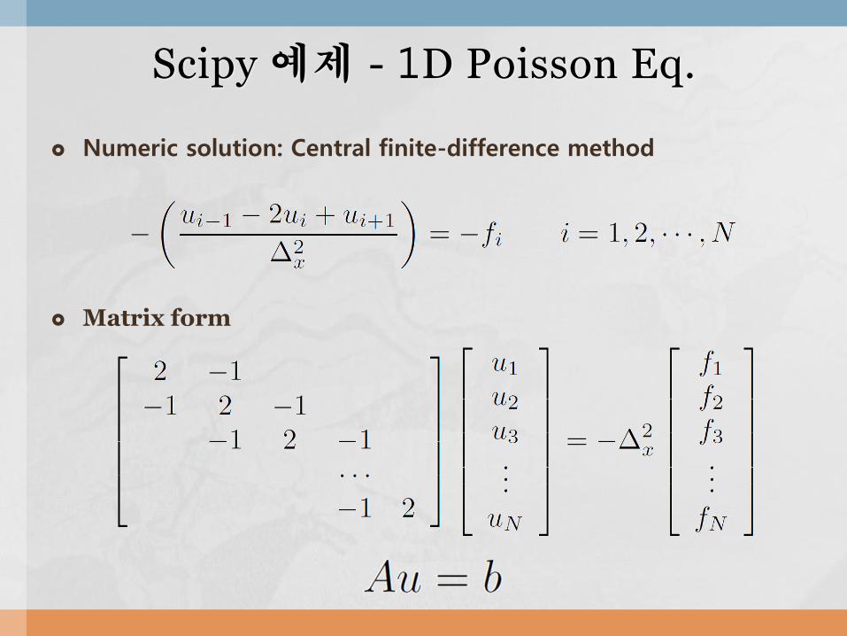
Numeric solution: Central finite-difference method
Matrix form
Scipy 예제 - 1D Poisson Eq.

Scipy 예제 - 1D Poisson Eq.
import numpy as np
from scipy.sparse import spdiags
from scipy.sparse.linalg import spsolve
omega = 5.4
u0, u1 = 0, 1
func = lambda x: omega**2 * np.sin(omega * x)
nx = 100; x = np.linspace(0, 1, nx); dx = x[1] – x[0]
u_exact = np.sin(omega*x) – (np.sin(omega) – 1) * x
arr = np.ones(nx-2)
A = spdiags([-arr, 2*arr, -arr], [-1, 0, 1], nx-2, nx-2)
b = func(x[1:-1]) * dx**2; b[0] += u0; b[-1] += u1
u = np.zeros_like(x)
u[0], u[-1], u[1:-1] = u0, u1, spsolve(A.tocsr(), b)
print np.linalg.norm(u_exact, u) == 0
$ python 1d_poisson.py
True
실행

Scipy 예제 - 1D Poisson Eq. (Plot)
import matplotlib.pyplot as plt
plt.plot(x, u_exact, '.-k', label='Exact')
plt.plot(x, u_scipy, '.-b', label='Scipy')
plt.title('1-D Poisson')
plt.xlabel('x'); plt.ylabel(‘u(x)'); plt.legend()
plt.show()

2-D wave equation
Numerics : Central finite-difference
Numpy 예제 – 2D Wave Eq.
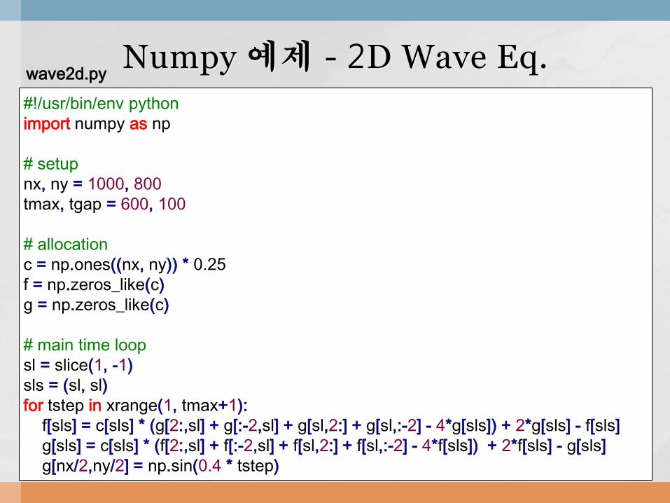
Numpy 예제 - 2D Wave Eq.
#!/usr/bin/env python
import numpy as np
# setup
nx, ny = 1000, 800
tmax, tgap = 600, 100
# allocation
c = np.ones((nx, ny)) * 0.25
f = np.zeros_like(c)
g = np.zeros_like(c)
# main time loop
sl = slice(1, -1)
sls = (sl, sl)
for tstep in xrange(1, tmax+1):
f[sls] = c[sls] * (g[2:,sl] + g[:-2,sl] + g[sl,2:] + g[sl,:-2] - 4*g[sls]) + 2*g[sls] - f[sls]
g[sls] = c[sls] * (f[2:,sl] + f[:-2,sl] + f[sl,2:] + f[sl,:-2] - 4*f[sls]) + 2*f[sls] - g[sls]
g[nx/2,ny/2] = np.sin(0.4 * tstep)
wave2d.py

Numpy 예제 - 2D Wave Eq.
# allocation
(…)
# plot
import matplotlib.pyplot as plt
imag = plt.imshow(f, vmin=-0.1, vmax=0.1)
plt.colorbar()
# main time loop
for tstep in xrange(1, tmax+1):
(…)
if tstep % tgap == 0:
print('tstep= %d' % tstep)
imag.set_array(f)
plt.savefig('./png/%.4d.png' % tstep)
#plt.draw()
Plot
$ ./wave2d.py
tstep= 100
tstep= 200
tstep= 300
tstep= 400
tstep= 500
tstep= 600
$ display png/*
실행

Numpy 예제 - 2D Wave Eq. Plot
0100.png 0400.png 0600.png

Hotspot을
Fortran 코드로 바꿔봅시다

f2py
• Python과 Fortran과의 쉬운 연동 제공
• Fortran의 Subroutine, Function, Module을 Python에서 호출
• Fortran에서 Python function 호출 (callback)
• Multi-dimensional Numpy array 인자 가능
• Fortran 77/90/95 지원
• Signature 파일 (.pyf)로부터 Python 확장 모듈 생성
• NumPy 프로젝트에서 개발
Python + Fortran using f2py
참조 : www.scipy.org

Numpy 예제 - 2D Wave Eq.
코어 계산 부분을 function으로 선언
#!/usr/bin/env python
import numpy as np
def update_core(f, g, c):
sl = slice(1, -1)
sls = (sl, sl)
f[sls] = c[sls] * (g[2:,sl] + g[:-2,sl] + g[sl,2:] + g[sl,:-2] - 4*g[sls]) + 2*g[sls] - f[sls]
(…)
# main time loop
for tstep in xrange(1, tmax+1):
update_core(f, g, c)
update_core(g, f, c)
(…)
wave2d_python.py

2D Wave Eq. (Python + Fortran)
update_core() 함수를 Fortran subroutine으로 변경
SUBROUTINE update_core(f, g, c, nx, ny)
IMPLICIT NONE
INTEGER, INTENT(in) :: nx, ny
DOUBLE PRECISION, DIMENSION(nx,ny), INTENT(inout) :: f
DOUBLE PRECISION, DIMENSION(nx,ny), INTENT(in) :: g, c
f(:nx-1,2:ny-1) = c(2:nx-1,2:ny-1) * (g(3:,2:ny-1) + g(:nx-2,2:ny-1) &
+ g(2:nx-1,3:) + g(2:nx-1,:ny-2) - 4*g(2:nx-1,2:ny-1)) &
+ 2*g(2:nx-1,2:ny-1) - f(2:nx-1,2:ny-1)
END SUBROUTINE update_core
ext_core.f90
컴파일, ext_core.so 생성
$ f2py –c –fcompiler=gnu95 –m ext_f90.so ext_core.f90

2D Wave Eq. (Python + Fortran)
계산 코어를 Fortran subroutine으로 변경
#!/usr/bin/env python
import numpy as np
from ext_f90 import update_core
(…)
# main time loop
for tstep in xrange(1, tmax+1):
update_core(f, g, c)
update_core(g, f, c)
(…)
wave2d_fortran.py

Hotspot을
C 코드로 바꿔봅시다

2D Wave Eq. (Python + C)
update_core() 함수를 C function으로 변경
#include <Python.h>
#include <numpy/arrayobject.h>
static PyObject *update_core_py(PyObject *self, PyObject *args) {
int nx, ny;
PyArrayObject *F, *G, *C;
if (!PyArg_ParseTuple(args, “OOOii”, &F, &G, &C, &nx, &ny)) return NULL;
double *f, *g, *c;
int i, j, idx;
f = (double *)(F->data);
g = (double *)(G->data);
c = (double *)(C->data);
for (i = 0; i < nx; i++) {
for (j = 0; j < ny; j++) {
idx = i*ny +j;
f[idx] = c[idx] * (g[idx-ny] + g[idx+ny] + g[idx-1] + g[idx+1] - 4*g[idx]) + 2*g[idx] - f[idx];
}
}
Py_RETURN_NONE;
}
ext_core.c
(계속)
Python C API 사용

2D Wave Eq. (Python + C)
update_core() 함수를 C function으로 변경
static PyMethodDef ufunc_methods[] = {
{“update_core”, update_core_py, METH_VARARGS, “”},
{NULL, NULL, 0, NULL}
};
PyMODINIT_FUNC initext_c() {
Py_InitModule(“ext_c”, ufunc_methods);
import_array();
}
이어서
컴파일, ext_core.so 생성
$ gcc –O3 –fPIC –g –I/usr/include/python2.7 –c ext_core.c –o ext_c.o
$ gcc –shared ext_core.o –o ext_c.so

Hotspot을
CUDA 코드로 바꿔봅시다

GPU (Graphics Processing Unit)
CPU는 임의의 메모리 접근, 흐름 제어를 포함하는 범용 연산에 적합
GPU는 많은 데이터에 동일한 연산을 수행하는 데이터 병렬 연산에 적합
GPU의 메모리 대역폭이 CPU보다 높다 (eg. 180 GB/s vs 40 GB/s)
CPU vs GPU

데이터 병렬 연산 – ex) 벡터합
모든 데이터에 동일한 연산

CUDA/OpenCL의 Python wrapper
모든 객체의 동적 할당/자동 해제
자동 에러 체크 : 파이썬 예외처리로 변환
JIT (Just-In-Time) 컴파일
빠른 개발 및 디버깅
PyCUDA/PyOpenCL
mathema.tician.de/software/pycuda mathema.tician.de/software/pyopencl
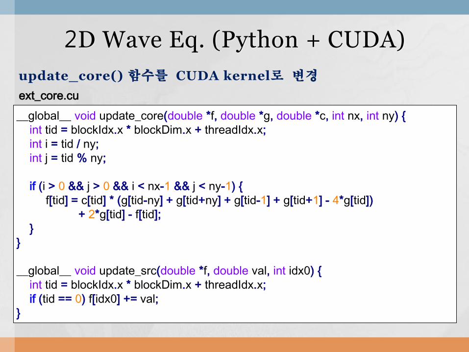
2D Wave Eq. (Python + CUDA)
update_core() 함수를 CUDA kernel로 변경
__global__ void update_core(double *f, double *g, double *c, int nx, int ny) {
int tid = blockIdx.x * blockDim.x + threadIdx.x;
int i = tid / ny;
int j = tid % ny;
if (i > 0 && j > 0 && i < nx-1 && j < ny-1) {
f[tid] = c[tid] * (g[tid-ny] + g[tid+ny] + g[tid-1] + g[tid+1] - 4*g[tid])
+ 2*g[tid] - f[tid];
}
}
__global__ void update_src(double *f, double val, int idx0) {
int tid = blockIdx.x * blockDim.x + threadIdx.x;
if (tid == 0) f[idx0] += val;
}
ext_core.cu

2D Wave Eq. (Python + CUDA)
#!/usr/bin/env python
import numpy as np
import pycuda.driver as cuda
import pycuda.autoinit
# setup
nx, ny = 1000, 800
tmax, tgap = 600, 100
# allocation
c = np.ones((nx, ny)) * 0.25
f = np.zeros_like(c)
c_gpu = cuda.to_device(c)
f_gpu = cuda.to_device(f)
g_gpu = cuda.to_device(f)
wave2d_cuda.py
(계속)

2D Wave Eq. (Python + CUDA)
# cuda kernels
from pycuda.compiler import SourceModule
kernels = open('ext_core.cu').read()
mod = SourceModule(kernels)
update_core = mod.get_function('update_core')
update_src = mod.get_function('update_src')
bs, gs = (256,1,1), (nx*ny/256+1,1)
nnx, nny = np.int32(nx), np.int32(ny)
src_val = lambda tstep: np.sin(0.4 * tstep)
src_idx = np.int32( (nx/2)*ny + ny/2 )
# plot
(…)
# main time loop
for tstep in xrange(1, tmax+1):
update_core(f_gpu, g_gpu, c_gpu, nnx, nny, block=bs, grid=gs)
update_core(g_gpu, f_gpu, c_gpu, nnx, nny, block=bs, grid=gs)
update_src(g_gpu, src_val(tstep), src_idx, block=bs, grid=(1,1))
(…)
(이어서)

Hotspot을
OpenCL 코드로 바꿔봅시다

Intel MIC (Many Integrated Core)
~ 60 pentium cores

2D Wave Eq. (Python + OpenCL)
update_core() 함수를 OpenCL kernel로 변경
#pragma OPENCL EXTENSION cl_amd_fp64 : enable
__kernel void update_core(__global double *f, __global double *g, __global double *c, int nx, int
ny) {
int tid = get_global_id(0);
int i = tid / ny;
int j = tid % ny;
if (i > 0 && j > 0 && i < nx-1 && j < ny-1)
f[tid] = c[tid] * (g[tid-ny] + g[tid+ny] + g[tid-1] + g[tid+1] - 4*g[tid])
+ 2*g[tid] - f[tid];
}
__kernel void update_src(__global double *f, __global double val, int idx0) {
int tid = get_global_id(0);
if (tid == 0) f[idx0] += val;
}
ext_core.cl

2D Wave Eq. (Python + OpenCL)
#!/usr/bin/env python
import numpy as np
import pyopencl as cl
platforms = cl.get_platforms()
devices = platforms[0].get_devices() # 1st platform
context = cl.Context(devices)
queue = cl.CommandQueue(context, devices[0]) # 1st device
# setup
nx, ny = 1000, 800
tmax, tgap = 600, 100
# allocation
c = np.ones((nx, ny)) * 0.25
f = np.zeros_like(c)
c_dev = cl.Buffer(context, cl.mem_flags.COPY_HOST_PTR, hostbuf=c)
f_dev = cl.Buffer(context, cl.mem_flags.COPY_HOST_PTR, hostbuf=f)
g_dev = cl.Buffer(context, cl.mem_flags.COPY_HOST_PTR, hostbuf=f)
wave2d_opencl.py
(계속)

2D Wave Eq. (Python + OpenCL)
# opencl kernels
kernels = open('ext_core.cl').read()
mod = cl.Program(context, kernels).build()
update_core = mod.update_core
update_src = mod. update_src
bs, gs = (60,), (nx*ny/256+1,)
nnx, nny = np.int32(nx), np.int32(ny)
src_val = lambda tstep: np.sin(0.4 * tstep)
src_idx = np.int32( (nx/2)*ny + ny/2 )
# plot
(…)
# main time loop
for tstep in xrange(1, tmax+1):
update_core(queue, bs, gs, f_dev, g_dev, c_dev, nnx, nny)
update_core(queue, bs, gs, g_dev, f_dev, c_dev, nnx, nny)
update_src(queue, bs, gs, g_dev, src_val(tstep), src_idx)
(…)
(이어서)

Python 성능 비교
동일한 조건의 3차원 전자기 시뮬레이션 (FDTD) 실행 시간 비교
빛의 이중 슬릿 투과 시뮬레이션 (Maxwell 방정식)

Python 성능 비교
빛의 이중 슬릿 투과 시뮬레이션 결과

Python 성능 비교 (CPU)
Python-C API를 사용하여 계산이 집중된 부분만 C 코드로 작성함
Single CPU thread 최적화 코드 (SSE, OpenMP)
C Python+C C Python+C
GFLOPS 0.35 0.35 4.60 4.52
1.7 % 성능 차이

Python 성능 비교 (GPU)
PyCUDA를 사용하여 계산이 집중된 부분만 CUDA 커널로 작성
CUDA-C PyCUDA
GFLOPS 20.16 20.16
거의 차이 없음

Python에서 C, Fortran, CUDA-C, OpenCL-C와 쉽게 연동할 수 있다
수치모델 메인은 Python으로 작성, 계산이 집중된 부분만 컴파일 언어로 대체한다.
계산성능이 중요한 대규모의 과학계산 분야에서도 Python은 훌륭한 대안이 될 수 있다
Wrap up

Have your fun with Python!
Thank you


![인카금융서비스 - ssl.pstatic.net€¦ · 인카금융서비스 [211050] ‘핀테크 영업시스템’ 기반으로 꾸준한 성장 기대 인카금융서비스 > 기업형](https://img.pdfslide.tips/doc/110x75/5f1d1257cc84136b1e7d2667/eoeoee-ssl-eoeoee-211050-aoe-oeoea.jpg)


![[OpenStack Days Korea 2016] Track1 - 카카오는 오픈스택 기반으로 어떻게 5000VM을 운영하고 있을까?](https://img.pdfslide.tips/doc/110x75/587004f31a28ab427f8b5d43/openstack-days-korea-2016-track1-.jpg)