arX

iv:h

ep-t

h/97

0910

3v3

26

Oct

199

7

qq

q

�

�

�

qq

q

�

�

�

qq

q

�

�

�

qq

q

�

�

�

qq

q

�

�

�

MM

Mqq

qMM

Mqq

qMM

Mqq

qMM

Mqq

qMM

Mqq

q

�

�

�

MM

M

�

�

�

MM

M

�

�

�

MM

M

�

�

�

MM

M

�

�

�

MM

M

00?>=<89:;M

M

21?>=<89:;M

M

01?>=<89:;M

M

30?>=<89:;M

M

30?>=<89:;�

�

�

02?>=<89:;�

�

�

20?>=<89:;�

�

�

03?>=<89:;�

�

�

03?>=<89:;q

q

10?>=<89:;q

q

12?>=<89:;q

q

00?>=<89:;q

q

00?>=<89:;

11

0

21?>=<89:;11

qq

2

12?>=<89:;MM

1

21?>=<89:;

12

1

12?>=<89:;

21

2

01?>=<89:;12

qq

0

11?>=<89:;MM

221qq

1

10?>=<89:;MM

0

01?>=<89:;

13

2

11?>=<89:;

22

0

10?>=<89:;

31

1

30?>=<89:;13

qq

1

02?>=<89:;MM

022qq

2

20?>=<89:;MM

131qq

0

03?>=<89:;MM

2

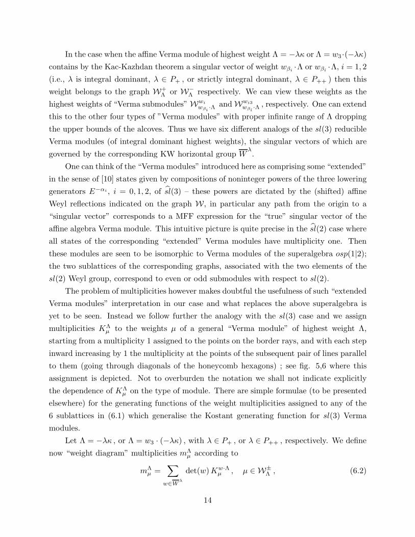
fig. 1

The p′/p = 3/4 admissible alcove.

•

Λ/.-,()*+qqq

1

⋆MMM 2

•

•

2

⋆

◦

1

⋆

•'&%$ !"#qqqq

1

•MM

MM 2 •qqqq

0

•MM

MM 1 ◦qqqq

2

◦MM

MM 0 ◦'&%$ !"#qqqq

1

◦MM

MM 2

⋆

⋆

2

◦

◦

1

•

•

0

◦

◦

2

◦

◦

1

◦

◦'&%$ !"#qqqq

1

◦MM

MM 2 ⋆qqqq

0

◦MM

MM 1 ◦qqqq

2

◦MM

MM 0 ◦'&%$ !"#qqqq

1

◦MM

MM 2 ◦qqqq

0

◦MM

MM 1 ◦qqqq

2

◦MM

MM 0 ◦'&%$ !"#qqqq

1

◦MM

MM 2

◦

◦

2

◦

◦

1

◦

◦

0

◦

◦

2

◦

⋆

1

◦

◦

0

◦

◦

2

◦

◦

1

◦

◦'&%$ !"#qqqq

1

◦MM

MM 2 ◦qqqq

0

◦MM

MM 1 ◦qqqq

2

◦MM

MM 0 ◦'&%$ !"#qqqq

1

◦MM

MM 2 ◦qqqq

0

⋆MM

MM 1 ⋆qqqq

2

◦MM

MM 0 ◦'&%$ !"#qqqq

1

◦MM

MM 2 ◦qqqq

0

◦MM

MM 1 ◦qqqq

2

◦MM

MM 0 ◦'&%$ !"#qqqq

1

◦MM

MM 2

Λ

• qqqqqq

•

• qqqqqqqq

• MMMM

MMMM•

•MM

MM

MMMM

•

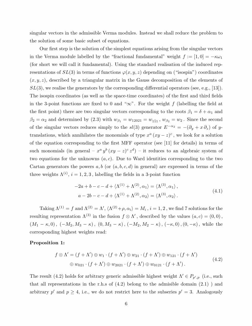
fig. 2

The begining of W+Λ with the weight diagram GΛ, Λ = [1, 0].

•

Λqqq

1

⋆MMM 2

•

•

2

⋆

◦

1

◦

•qqqq

1

•MM

MM 2 •qqqq

0

•MM

MM 1 ◦qqqq

2

◦

◦

2

•

•

1

•

•

0

⋆

•qqqq

1

•MM

MM 2 ◦qqqq

0

•MM

MM 1 •qqqq

2

•MM

MM 0 •qqqq

1

◦MM

MM 2

⋆

⋆

2

•

◦

1

•

•

0

•

•

2

◦

◦

1

⋆

◦MM

MM 1 ◦qqqq

2

◦MM

MM 0 •qqqq

1

•MM

MM 2 •qqqq

0

◦MM

MM 1 ◦qqqq

2

◦

◦

2

◦

◦

1

◦

◦

0

◦

◦MM

MM 1 ◦qqqq

2

◦MM

MM 0 ◦qqqq

1

◦MM

MM 2

◦

◦

2

◦

⋆

1

◦

⋆MM

MM 1 ⋆qqqq

2

Λ/.-,()*+• qqq

qqq

•

• qqqqqqqq

•'&%$ !"#MMMM

MMMM

• qqqqqqqq

•

• qqqqqqqq

•'&%$ !"#MMMM

MMMM•

•MM

MM

MMMM

•'&%$ !"#•

MMMM

MMMM

•qqqqqqqq •

MMMM

MMMM

•'&%$ !"#

•

•MM

MM

MMMM

•'&%$ !"#• qq

qqqqqq

• MMMM

MMMM

•

•

• qqqqqqqq

•

•

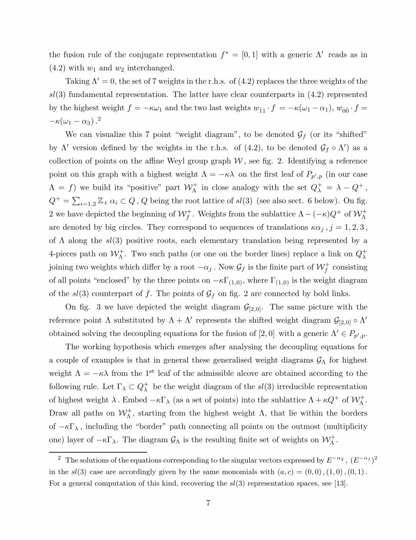
fig. 3

The weight diagram G[2,0]. The big circles indicate the sl(3) counterpart diagram −κΓ(2,0).

1'&%$ !"#1'&%$ !"#

qqqq

1

1'&%$ !"#MMMM 2

1'&%$ !"#

2'&%$ !"#2

1'&%$ !"#

2'&%$ !"#1

1'&%$ !"#2'&%$ !"#MM

MM 2 2'&%$ !"#qqqq

0

3'&%$ !"#MMMM 1 2'&%$ !"#

qqqq

2

2'&%$ !"#MMMM 0 1'&%$ !"#

qqqq

1

2

2

1

3

4

0

2

2

2

1'&%$ !"#2'&%$ !"#

qqqq

2

3'&%$ !"#MMMM 0 4'&%$ !"#

qqqq

1

3'&%$ !"#MMMM 2 2'&%$ !"#

qqqq

0

1'&%$ !"#MMMM 1

1'&%$ !"#

1'&%$ !"#0

3'&%$ !"#

2'&%$ !"#2

3'&%$ !"#

2'&%$ !"#1

1'&%$ !"#

1'&%$ !"#0

1'&%$ !"#1'&%$ !"#MM

MM 2 2'&%$ !"#qqqq

0

2'&%$ !"#MMMM 1 2'&%$ !"#

qqqq

2

1'&%$ !"#MMMM 0 1'&%$ !"#

qqqq

1

2

1'&%$ !"#0

fig. 4

The [1,1] diagram with weight multiplicities indicated in the circles.

1'&%$ !"#1'&%$ !"#

qqqq

1

1'&%$ !"#MMMM 2

1'&%$ !"#

2'&%$ !"#2

1'&%$ !"#

2'&%$ !"#1

1'&%$ !"#1'&%$ !"#

qqqq

1

2'&%$ !"#MMMM 2 2'&%$ !"#

qqqq

0

3'&%$ !"#MMMM 1 2'&%$ !"#

qqqq

2

2'&%$ !"#MMMM 0 1'&%$ !"#

qqqq

1

1'&%$ !"#MMMM 2

1

2

2

2

3

1

3

4

0

2

3

2

1

2

1

1'&%$ !"#2'&%$ !"#MM

MM 2 2'&%$ !"#qqqq

0

3'&%$ !"#MMMM 1 3'&%$ !"#

qqqq

2

4'&%$ !"#MMMM 0 4'&%$ !"#

qqqq

1

4'&%$ !"#MMMM 2 3'&%$ !"#

qqqq

0

3'&%$ !"#MMMM 1 2'&%$ !"#

qqqq

2

2'&%$ !"#MMMM 0 1'&%$ !"#

qqqq

11'&%$ !"# 1'&%$ !"#2 3 4 4 3 2

fig. 5

The begining of W+ with multiplicities indicated in circles.

1'&%$ !"#

2'&%$ !"#0

2'&%$ !"#

1'&%$ !"#0

1'&%$ !"#qqqq

2

2'&%$ !"#MMMM 0 2'&%$ !"#

qqqq

1

2'&%$ !"#MMMM 2 1'&%$ !"#

qqqq

0

1'&%$ !"#MMMM 1

2'&%$ !"#0

2'&%$ !"#

3'&%$ !"#2

2'&%$ !"#

3'&%$ !"#1

1'&%$ !"#2'&%$ !"#MM

MM 0 2'&%$ !"#qqqq

1

3'&%$ !"#MMMM 2 3'&%$ !"#

qqqq

0

4'&%$ !"#MMMM 1 3'&%$ !"#

qqqq

2

3'&%$ !"#MMMM 0 2'&%$ !"#

qqqq

1

2'&%$ !"#MMMM 2 1'&%$ !"#

qqqq

01 1

fig. 6

The beginning of W− with multiplicities in circles.

1'&%$ !"#

2'&%$ !"#0

◦

◦

0

⋆qqqq

2

1'&%$ !"#MMMM 0 2'&%$ !"#

qqqq

1

1'&%$ !"#MMMM 2 ⋆

qqqq

0

◦MM

MM 1

◦

0

1'&%$ !"#

◦

2

1'&%$ !"#

◦

1

◦

◦qqqq

1

⋆MM

MM 2 ◦qqqq

0

◦MM

MM 1 ◦qqqq

2

⋆MM

MM 0 ◦qqqq

◦MM

MM 2

◦

⋆

0

1'&%$ !"#2'&%$ !"#

qqqqqqqq

1'&%$ !"#MMMM

MMMM

1'&%$ !"#

2'&%$ !"#

fig. 7

The beginning of W− with the resolution of [[1,1]]. The multiplicities of G[[1,1]] are in circles.

•

•

•

•

•

•

•

•

•

•

•

•

•

•

•

•

•

•

•

•

•

•

•

•

•

•

•

∗

∗

∗

∗

∗

∗

∗

∗

∗

∗

∗

∗

∗

∗

∗

∗

∗

∗

∗

∗

∗

∗

◦

◦

◦

◦

◦

◦

◦

◦

◦

◦

◦

◦

◦

◦

◦

◦

x

x

x

x

x

x

x

x

x

x

x

⋆

•q

q

⋆

• MM

⋆

�

�

�

• MM

M

⋆

�

�

�

•q

qq

⋆

MM

M

�

�

�

•q

qq M

MM

�

�

�

qq

q

•

•qq

qqα1

1

∗

◦MM

MM∗

qqqq

•

• MMMMα2

2

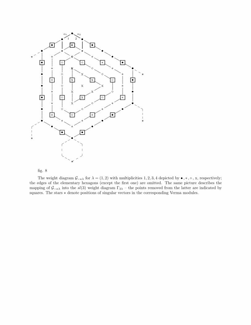
fig. 8

The weight diagram G−κλ for λ = (1, 2) with multiplicities 1, 2, 3, 4 depicted by • , ∗ , ◦ , x, respectively;the edges of the elementary hexagons (except the first one) are omitted. The same picture describes themapping of G−κλ into the sl(3) weight diagram Γ3λ – the points removed from the latter are indicated bysquares. The stars ⋆ denote positions of singular vectors in the corresponding Verma modules.

•

•

α1

•

•

•

•

•

•

•

•

•

•

•

•

•

•

•

•

•

•

•

•

•

•

α2

∗

∗

∗

∗

∗

∗

∗

∗

∗

∗

∗

∗

∗

∗

∗

∗

∗

∗

∗

∗

∗

∗

∗

∗

∗

∗

∗

∗

∗

∗

⋆

∗M

M

⋆

∗q

q

⋆

MM

M

�

�

�

⋆

qq

q

∗�

�

�

⋆

�

�

�

MM

M

•

∗

0

•

∗qqqq

1

∗MM

MM 2 •qqqq

0

•

•

2

∗MM

MM 1 ∗qqqq

2

∗

1

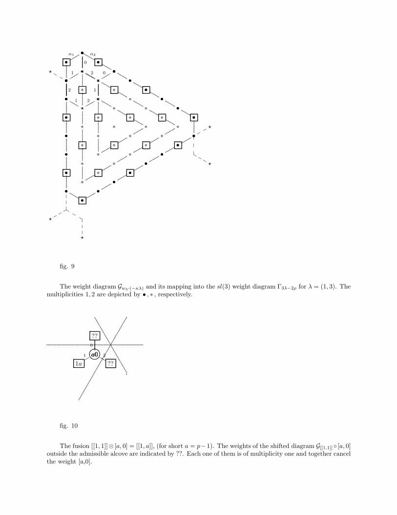
fig. 9

The weight diagram Gw3·(−κλ) and its mapping into the sl(3) weight diagram Γ3λ−2ρ for λ = (1, 3). Themultiplicities 1, 2 are depicted by • , ∗ , respectively.

a0?>=<89:;

??

0

a0?>=<89:;??

MMM2a0?>=<89:;

1aqq1

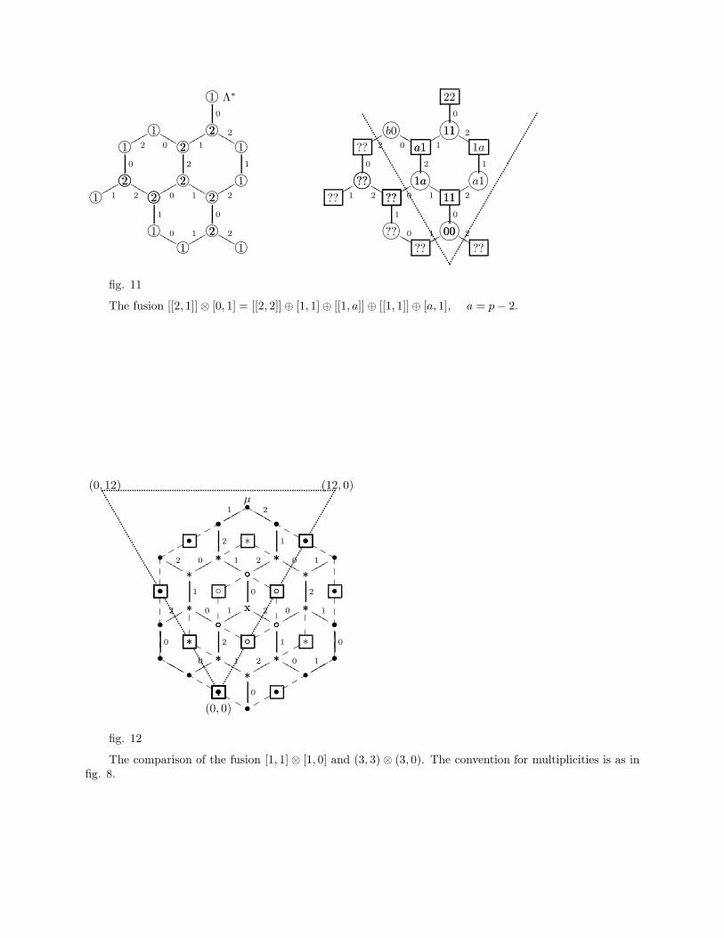
fig. 10

The fusion [[1, 1]]⊗ [a, 0] = [[1, a]], (for short a = p−1). The weights of the shifted diagram G[[1,1]] ◦ [a, 0]outside the admissible alcove are indicated by ??. Each one of them is of multiplicity one and together cancelthe weight [a,0].

Λ∗1'&%$ !"#

2'&%$ !"#0

2'&%$ !"#qqqq

1

1'&%$ !"#MMMM01'&%$ !"#qqq

q

2

2'&%$ !"#0

1'&%$ !"#qqqq

1

2

1'&%$ !"#MMMM 2

1'&%$ !"#1

2'&%$ !"#qqqq

2

2'&%$ !"#MMMM12'&%$ !"#qqq

q

0

2'&%$ !"#MMMM2

2

2

2

2

2

0

2'&%$ !"#

1'&%$ !"#1

1'&%$ !"#MMMM 0 2'&%$ !"#

qqqq

1

1'&%$ !"#MMMM 2

22

11?>=<89:;0

a1qq

1

b076540123MMM

0??qqq

2

??765401230

??qqq

1

11

1aMM2

a1?>=<89:;1

11qq

2

1a?>=<89:;MM

1??qqq

0

??76540123MMM

2

a1

1a

2

11

00

0

??

??765401231

??MM

M0 00?>=<89:;qqq

1

??MM

M2

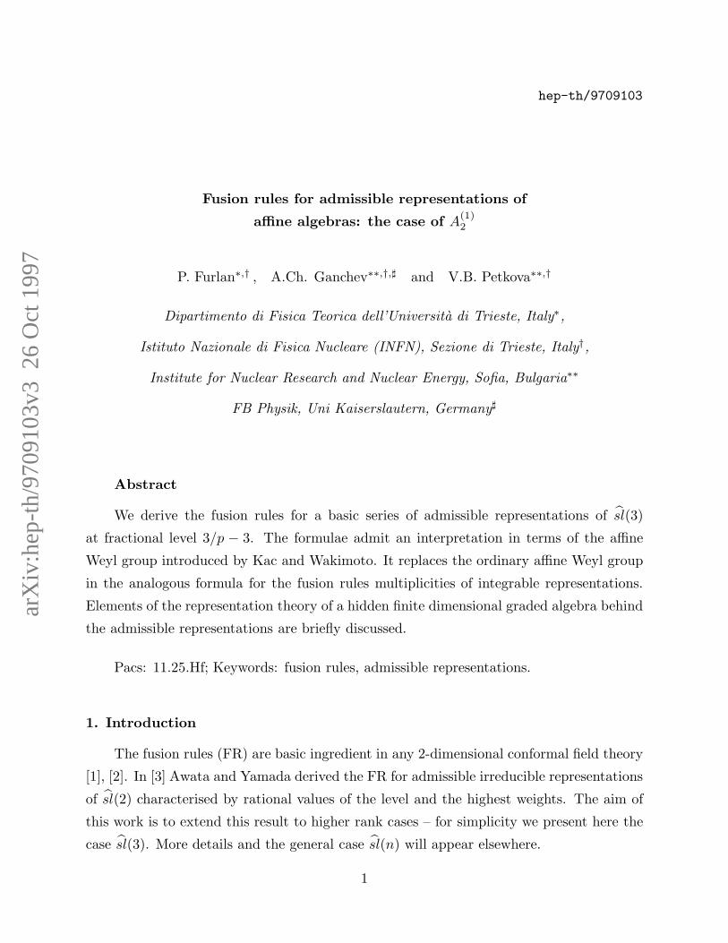
fig. 11

The fusion [[2, 1]]⊗ [0, 1] = [[2, 2]]⊕ [1, 1]⊕ [[1, a]]⊕ [[1, 1]]⊕ [a, 1], a = p− 2.

(0, 0)

(12, 0)(0, 12)µ

•

◦

◦

•

•

∗

••

•M

M •q

q

qq

qq

qq

•�

�

�

�

�

�

�

�

�

• MM

M

MM

MM

MM

•q

qq

qq

q

qq

q

•�

�

�

�

�

�

�

�

�

•M

MM

MM

M

∗

∗q

q∗

MM

∗

∗

�

�

∗M

M

∗

∗

�

�

∗q

q

◦

◦M

M

◦

�

�

◦

◦q

q

◦

�

�

◦

◦M

M ◦q

q

•

•qqqq

1

•MM

MM 2

•

∗

2

•

∗

1

•

∗MM

MM 2 ∗qqqq

0

◦MM

MM 1 ∗qqqq

2

∗MM

MM 0 •qqqq

1

∗

∗

1

◦

x

0

∗

∗

2

•

∗qqqq

2

◦MM

MM 0 xqqqq

1

◦MM

MM 2 ∗qqqq

0

•MM

MM 1

•

•

0

◦

∗

2

◦

∗

1

•

•

0

•

•MM

MM ∗qqqq

0

∗MM

MM 1 ∗qqqq

2

•MM

MM 0 •qqqq

1

∗

•

0

fig. 12

The comparison of the fusion [1, 1]⊗ [1, 0] and (3, 3)⊗ (3, 0). The convention for multiplicities is as infig. 8.

arX

iv:h

ep-t

h/97

0910

3v3

26

Oct

199

7

hep-th/9709103

Fusion rules for admissible representations of

affine algebras: the case of A(1)2

P. Furlan∗,† , A.Ch. Ganchev∗∗,†,♯ and V.B. Petkova∗∗,†

Dipartimento di Fisica Teorica dell’Universita di Trieste, Italy∗,

Istituto Nazionale di Fisica Nucleare (INFN), Sezione di Trieste, Italy†,

Institute for Nuclear Research and Nuclear Energy, Sofia, Bulgaria∗∗

FB Physik, Uni Kaiserslautern, Germany♯

Abstract

We derive the fusion rules for a basic series of admissible representations of sl(3)

at fractional level 3/p − 3. The formulae admit an interpretation in terms of the affine

Weyl group introduced by Kac and Wakimoto. It replaces the ordinary affine Weyl group

in the analogous formula for the fusion rules multiplicities of integrable representations.

Elements of the representation theory of a hidden finite dimensional graded algebra behind

the admissible representations are briefly discussed.

Pacs: 11.25.Hf; Keywords: fusion rules, admissible representations.

1. Introduction

The fusion rules (FR) are basic ingredient in any 2-dimensional conformal field theory

[1], [2]. In [3] Awata and Yamada derived the FR for admissible irreducible representations

of sl(2) characterised by rational values of the level and the highest weights. The aim of

this work is to extend this result to higher rank cases – for simplicity we present here the

case sl(3). More details and the general case sl(n) will appear elsewhere.

1

There is a formula for the FR multiplicities [4], [5], [6] in the case of integrable rep-

resentations of sl(n), equivalent to the better known Verlinde formula. It generalises

the classical expression for the multiplicity of an irreducible representation in the tensor

product of two finite dimensional sl(n) representations, resulting from the Weyl character

formula. The derivation in [6] was based essentially on the fundamental role played by the

representation theory of sl(n) and of its quantum counterpart Uq(sl(n)) at roots of unity.

What complicates the problem under consideration is precisely the lack of knowledge of

what is the finite dimensional algebra and its quantum counterpart, whose representation

theory lies behind the fusion rules of admissible representations. In the case of sl(2) Feigin

and Malikov [7] have noticed that the relevant algebra is the superalgebra osp(1|2) and its

deformed counterpart. Inverting somewhat the argumentation in [6], we shall try to show

that the understanding of the fusion rules for admissible representations leads naturally

to a set of finite dimensional representations of some (graded) algebra with well defined

ordinary tensor product.

2. Admissible weights.

We start with introducing some notation. The simple roots of sl(3) are αi, i =

0, 1, 2 . The affine Weyl group W is generated by the three simple reflections wi = wαi.

For short let wij... = wiwj . . . and furthermore w1 = w020 = w202, w2 = w010 = w101,

w0 = w121 = w212 , corresponding to the real positive roots αı = δ − αi , δ = α0 + α3 =

α0 + α1 + α2 . The elements wıi and wiı constitute (elementary) affine translations t±αi,

where α0 = −α3 , αi = αi , i = 1, 2 . Denote the fundamental weights by ω0 , ωi + ω0 ,

i = 1, 2 , ωi being the horizontal sl(3) subalgebra fundamental weights. Let P =∑2

i=1 Zωi ,

P+ =∑2

i=1 Z+ ωi , P++ =∑2

i=1 Nωi be the sl(3) weight lattice, the integral dominant

and strictly integral dominant weights and P k+ = {λ ∈ P+ , 〈λ, α3〉 ≤ k} , P k+3

++ = {λ ∈

P++ , 〈λ, α3〉 ≤ k + 2} (k ∈ Z+) , the corresponding alcoves. For short we shall denote all

sl(3) weights at an arbitrary level k with their horizontal projections Λ =∑

i=1,2 〈Λ, αi〉ωi .

Accordingly w ·Λ will indicate the horizontal projection of the shifted (by ω1 +ω2 +3ω0)

action on Λ+kω0 of the affine Weyl group. For nonnegative integer k λ ∈ P k+ (P k+3

++ ) runs

over highest weights (shifted by ρ = ω1 +ω2 highest weights) of integrable representations

at level k.

2

Given a fractional level k such that κ ≡ k + 3 = p′/p with p, p′ coprime integers and

p′ ≥ 3 , the set of admissible weights of sl(3) is defined [8] as1

Pp′,p = {λ′−λκ |λ′ ∈ P p′−3+ , λ ∈ P p−1

+ }∪{w3 · (λ′−λκ) |λ′ ∈ P p′−3

+ , λ ∈ P p+1++ } . (2.1)

Due to invariance with respect to a Coxeter element generated subgroup of the horizontal

Weyl group W (see [8] for details) the domain in (2.1) can be equivalently represented

using other elements w ∈W .

We shall refer to Pp′,p as the admissible alcove and to its first, second subsets as its

first, second leaf. We have reversed the traditional notation putting the prime on the

integer part of the weights and leaving the fractional part unprimed, the reason being

that in this paper we shall restrict ourselves mostly to the particular series of admissible

representations defined by p′ = 3, p ≥ 4 , in which only λ′ = 0 survives in the pairs (λ′, λ)

of sl(3) weights appearing in (2.1). The addmissible alcove P3,p (to be called sometimes

“the double alcove”) is described by a collection of(p+12

)+(p2

)= p2 integrable weights at

integer levels p− 1 and p− 2, entering the fractional parts of the weights of the first and

second leaf respectively. The choice p′ = 3 is not very restrictive since the novel features

of the fusion rules are essentially governed by the fractional part of the admissible highest

weights and furthermore the subseries p′ = 3 is interesting by itself. Shorthand notation

[n1, n2] and [[n1, n2 ]] , ni = 〈λ, αi〉 , will be used for the weights Λ = −λκ on the 1st leaf and

Λ = w3 · (−λκ) on the 2nd leaf of P3,p in (2.1), respectively; n3 = n1 + n2. For Λ ∈ P3,p

we shall exploit the automorphism groups Z3 of the alcoves P p−1+ and P p+1

++ generated by

σ : Λ = [n1, n2] 7→ σ(Λ) = [p− 1− n3, n1] ,

σ : Λ = [[n1, n2 ]] 7→ σ(Λ) = [[n2, p+ 1− n3 ]] .(2.2)

The sl(3) Verma modules labelled by admissible highest weights are reducible, with

submodules determined by the Kac-Kazhdan theorem [9]. In general for an arbitrary

weight Λ let Mi = 〈Λ+ρ+κω0, αi〉 , i = 0, 1, 2 . If for a fixed i = 0, 1, 2 , the projection Mi

can be written asMi = m′i−(mi−1) κ (or asMi = −m′

i+mi κ ), where m′i , mi ∈ N , there

is a singular vector of weight wβi· Λ (or wβı

· Λ ) in the Verma module of highest weight

Λ. It corresponds to the affine real positive root βi = (mi − 1) δ + αi (or βı = mi δ − αi )

respectively. These Weyl reflections can be represented as

wβi= t−(mi−1) αi

wi = wi(wıi)mi−1 , wβı

= t(mi−1) αiwı = wı(wiı)

mi−1 , i = 0, 1, 2 .

(2.3)

1 We neglect the terms dδ in the full admissible highest weights as irrelevant to our purposes.

3

The corresponding singular vectors were constructed in [10]. To a decomposition of the

reflections (2.3) into a product of simple reflections corresponds a monomial of the lowering

generators of sl(3), namely every wi, i = 0, 1, 2, is substituted by E−αi to an appropriate

(in general complex) power, see [11] for more explicit presentation in the case of sl(3).

Consider the Weyl groups Wλand Wλ generated for the representations on the first

(second) leaf of (2.1) by the reflections wβi(wβı

) , i = 1, 2 , βi = 〈λ, αi〉 δ + αi (βı =

−〈λ, w3(αi)〉 δ − αi ) and wβi(wβı

) , i = 0, 1, 2 , with β0 = (p − 1 − 〈λ, α3〉)δ + α0 (β0 =

(p+ 1− 〈λ, α3〉)δ − α0) respectively. Similarly one defines 4 more variants corresponding

to the various equivalent ways of representing the admissible alcove. The groups Wλand

Wλ are isomorphic toW andW and were introduced and exploited by Kac and Wakimoto

(KW) [8] in the study of the characters of admissible representations. We shall refer to

these groups, which will play a crucial role in what follows, as the KW groups. Apparently

any element of the KW group Wλ depends on (and is determined by) the point on which

it acts, so in a sense this is a “local” group acting on the double alcove and “spreading” it

much in the same way as the ordinary affine Weyl group acts on the fundamental integrable

alcove. This is more transparent using an alternative description of P3,p.

3. Alternative description of the admissible alcove P3,p . Affine Weyl group

graph replacing the weight lattice.

First recall that the affine Weyl group W can be represented as a graph to be denoted

W. This is the well known “honeycomb” lattice (which we saw for the first time in [12] )

covering the plane, consisting of hexagons with links labelled by the three elementary

reflections wi, i = 0, 1, 2, – so that at each vertex meet 3 (always different) links, while

along any hexagon two of the three reflections appear at an alternating order. (All figures

in this paper depict some finite part of this graph; the labels 0,1,2 on the edges correspond

to the reflections w0, w1, w2.) The three different hexagons appearing on the graph depict

the three 6-term relations among the generators wi, i = 0, 1, 2, e.g., w121 = w212. Thus if

we choose an origin, a vertex of this graph, to represent the identity element of W , then

the vertices are in bijective correspondence with the elements of W , while the different

paths connecting a vertex with the origin depict the different presentations of an element

of W in terms of the generators wi.

The dual lattice has as vertices the centers of the hexagons, 6 dual links meet at a

dual vertex, and the elementary cells are triangles centered at the vertices of the hexagonal

4

lattice. For given κ = 3/p consider a triangle in the dual lattice the sides of which consist

of p dual links. The weights in P3,p can be arranged on the piece of W enclosed by this

triangle. This “big” alcove consists of p2 elementary triangles, equivalently p2 vertices of

the honeycomb. The three vertices sitting at the three corners are connected with the

other points of the alcove by the three possible links 0, 1, 2. Choose the corner vertex

that is connected by a 0-link as the origin and assign to it the weight [0,0]. To the other

vertices of the alcove assign weights by the shifted action of W . The vertices at an even

number of links from the origin accommodate weights on the 1st leaf while the ones at

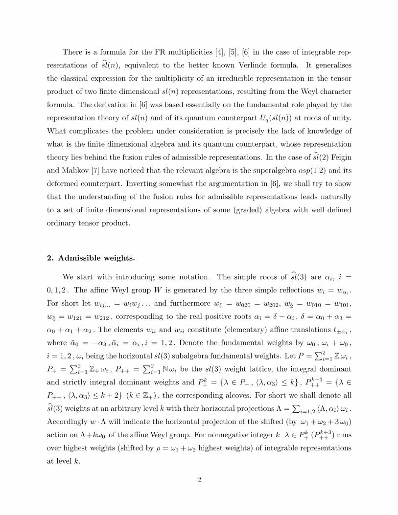
an odd number – on the 2nd leaf. The example p = 4 is depicted on fig. 1. The three

lines of the dual lattice cutting out the alcove are indicated by dotted lines. The weights

[n,m] are in circles, the weights [[n,m]] in boxes. (In general the first few points are e.g.,

w20 · [0, 0] = [p − 2, 1] , w120 · [0, 0] = [[ 1, p − 2 ]] , w0120 · [0, 0] = [0, p − 3] , etc., obtained

by adding and subtracting p′ = pκ.) The border lines (paths) of the big alcove consist of

highest weights Λ such that wi · Λ 6∈ P3,p , or wı · Λ 6∈ P3,p , for some i = 0, 1, 2 – they

precisely exhaust the weights labelling the border points of the two alcoves P p−1+ , P p+1

++ .

“Reflecting” Λ in the three boundary lines enclosing the alcove we land at a weight

of a singular vector in the sl(3) Verma module of highest weight Λ. These reflections

generate a group that coincides with Wλ. The alcove is a fundamental domain with

respect to the action of this group. In this realisation the affine Weyl group graph W

plays the role of “weight lattice”. The choice of the reflecting “hyperplanes” described by

〈Λ′+ρ+κω0, βi〉 = 0 and 〈Λ′+ρ+κω0, βı〉 = 0 , i = 0, 1, 2 (i.e., their precise identification

with the three planes cutting the big triangle) depends on the value of p and the given

highest weight Λ in the alcove.

As it is clear from fig. 1. any “big” alcove P3,p can be canonically mapped into P 3p++ ,

the admissible highest weights being identified with a subset of the triality 0 integrable

(shifted by ρ) highest weights at level 3p− 3.

4. Decoupling of states generated by singular vectors. Affine Weyl group graph

replacing the root lattice.

In view of the complexity of the Malikov-Feigin-Fuks (MFF) singular vectors in the

case sl(n) , n > 2 , it is not realistic to repeat the derivation for n = 2 in [3], by solving all

equations for the 3-point blocks expressing the decoupling of the submodules generated by

5

singular vectors in the admissible Verma modules. Instead we shall reduce the problem to

the solution of some basic subset of equations.

Our first step is the solution of the simplest equations arising from the singular vectors

in the Verma module labelled by the “fractional fundamental” weight f := [1, 0] = −κω1

(for short we will call it fundamental). Using the standard realisation of the induced rep-

resentations of SL(3) in terms of functions ϕ(x, y, z) depending on (“isospin”) coordinates

(x, y, z), described by a triangular matrix in the Gauss decomposition of the elements of

SL(3), we realise the generators by the corresponding differential operators (see, e.g., [13]).

The isospin coordinates (as well as the space-time coordinates) of the first and third fields

in the 3-point functions are fixed to 0 and “∞”. For the weight f (labelling the field at

the first point) there are two singular vectors corresponding to the roots β1 = δ + α1 and

β2 = α2 and determined by (2.3) with wβ1= w12021 = w111 , wβ2

= w2 . Since the second

of the singular vectors reduces simply to the sl(3) generator E−α2 = −(∂y + x ∂z) of y-

translations, which annihilates the monomials of type xa (xy − z)c , we look for a solution

of the equation corresponding to the first MFF operator (see [11] for details) in terms of

such monomials (in general – xa yb (xy − z)c zd) – it reduces to an algebraic system of

two equations for the unknowns (a, c). Due to Ward identities corresponding to the two

Cartan generators the powers a, b (or (a, b, c, d) in general) are expressed in terms of the

three weights Λ(i), i = 1, 2, 3 , labelling the fields in a 3-point function

−2a+ b− c− d+ 〈Λ(1) +Λ(2), α1〉 = 〈Λ(3), α1〉 ,

a− 2b− c− d+ 〈Λ(1) +Λ(2), α2〉 = 〈Λ(3), α2〉 .(4.1)

Taking Λ(1) = f and Λ(2) = Λ′, 〈Λ(2)+ρ, αi〉 =Mi , i = 1, 2 , we find 7 solutions for the

resulting representation Λ(3) in the fusion f ⊗ Λ′ , described by the values (a, c) = (0, 0) ,

(M1 − κ, 0) , (−M2,M3 − κ) , (0,M3 − κ) , (−M2,M2 − κ) , (−κ, 0) , (0,−κ) , while the

corresponding highest weights read:

Proposition 1:

f ⊗ Λ′ = (f + Λ′)⊕ w1 · (f +Λ′)⊕ w21 · (f + Λ′)⊕ w121 · (f + Λ′)

⊕ w021 · (f + Λ′)⊕ w2021 · (f + Λ′)⊕ w0121 · (f + Λ′) .(4.2)

The result (4.2) holds for arbitrary generic admissible highest weight Λ′ ∈ Pp′,p (i.e., such

that all representations in the r.h.s of (4.2) belong to the admisible domain (2.1) ) and

arbitrary p′ and p ≥ 4, i.e., we do not restrict here to the subseries p′ = 3. Analogously

6

the fusion rule of the conjugate representation f∗ = [0, 1] with a generic Λ′ reads as in

(4.2) with w1 and w2 interchanged.

Taking Λ′ = 0, the set of 7 weights in the r.h.s. of (4.2) replaces the three weights of the

sl(3) fundamental representation. The latter have clear counterparts in (4.2) represented

by the highest weight f = −κω1 and the two last weights w11 · f = −κ(ω1 −α1), w00 · f =

−κ(ω1 − α3) .2

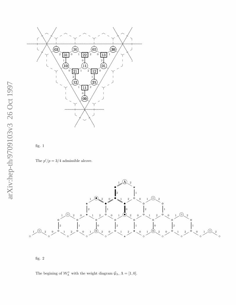
We can visualize this 7 point “weight diagram”, to be denoted Gf (or its “shifted”

by Λ′ version defined by the weights in the r.h.s. of (4.2), to be denoted Gf ◦ Λ′) as a

collection of points on the affine Weyl group graph W , see fig. 2. Identifying a reference

point on this graph with a highest weight Λ = −κλ on the first leaf of Pp′,p (in our case

Λ = f) we build its “positive” part W+Λ in close analogy with the set Q+

λ = λ − Q+ ,

Q+ =∑

i=1,2 Z+ αi ⊂ Q , Q being the root lattice of sl(3) (see also sect. 6 below). On fig.

2 we have depicted the beginning of W+f . Weights from the sublattice Λ− (−κ)Q+ of W+

Λ

are denoted by big circles. They correspond to sequences of translations καj , j = 1, 2, 3 ,

of Λ along the sl(3) positive roots, each elementary translation being represented by a

4-pieces path on W+Λ . Two such paths (or one on the border lines) replace a link on Q+

λ

joining two weights which differ by a root −αj . Now Gf is the finite part of W+f consisting

of all points “enclosed” by the three points on −κΓ(1,0), where Γ(1,0) is the weight diagram

of the sl(3) counterpart of f . The points of Gf on fig. 2 are connected by bold links.

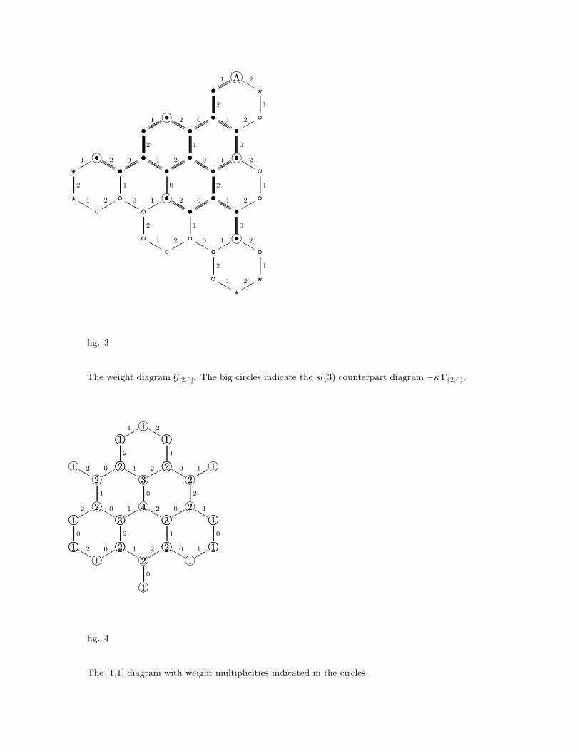
On fig. 3 we have depicted the weight diagram G[2,0]. The same picture with the

reference point Λ substituted by Λ + Λ′ represents the shifted weight diagram G[2,0] ◦ Λ′

obtained solving the decoupling equations for the fusion of [2, 0] with a generic Λ′ ∈ Pp′,p.

The working hypothesis which emerges after analysing the decoupling equations for

a couple of examples is that in general these generalised weight diagrams GΛ for highest

weight Λ = −κλ from the 1st leaf of the admissible alcove are obtained according to the

following rule. Let Γλ ⊂ Q+λ be the weight diagram of the sl(3) irreducible representation

of highest weight λ . Embed −κΓλ (as a set of points) into the sublattice Λ+ κQ+ of W+Λ .

Draw all paths on W+Λ , starting from the highest weight Λ, that lie within the borders

of −κΓλ , including the “border” path connecting all points on the outmost (multiplicity

one) layer of −κΓλ. The diagram GΛ is the resulting finite set of weights on W+Λ .

2 The solutions of the equations corresponding to the singular vectors expressed by E−α2 , (E−α1)2

in the sl(3) case are accordingly given by the same monomials with (a, c) = (0, 0) , (1, 0) , (0, 1) .

For a general computation of this kind, recovering the sl(3) representation spaces, see [13].

7

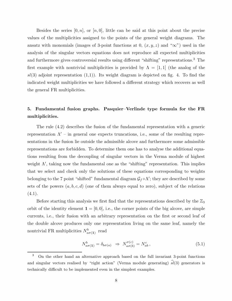
Besides the series [0, n], or [n, 0], little can be said at this point about the precise

values of the multiplicities assigned to the points of the general weight diagrams. The

ansatz with monomials (images of 3-point functions at 0, (x, y, z) and “∞”) used in the

analysis of the singular vectors equations does not reproduce all expected multiplicities

and furthermore gives controversial results using different “shifting” representations.3 The

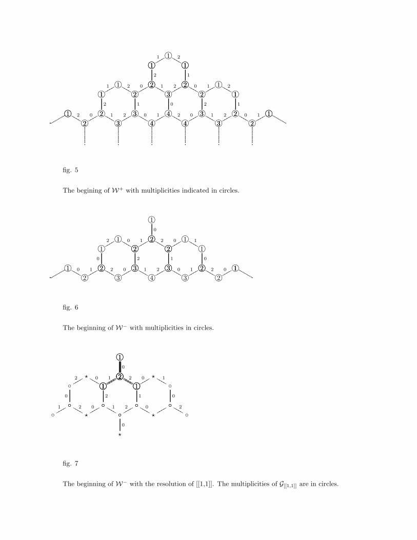
first example with nontrivial multiplicities is provided by Λ = [1, 1] (the analog of the

sl(3) adjoint representation (1,1)). Its weight diagram is depicted on fig. 4. To find the

indicated weight multiplicities we have followed a different strategy which recovers as well

the general FR multiplicities.

5. Fundamental fusion graphs. Pasquier–Verlinde type formula for the FR

multiplicities.

The rule (4.2) describes the fusion of the fundamental representation with a generic

representation Λ′ – in general one expects truncations, i.e., some of the resulting repre-

sentations in the fusion lie outside the admissible alcove and furthermore some admissible

representations are forbidden. To determine them one has to analyse the additional equa-

tions resulting from the decoupling of singular vectors in the Verma module of highest

weight Λ′, taking now the fundamental one as the “shifting” representation. This implies

that we select and check only the solutions of these equations corresponding to weights

belonging to the 7 point “shifted” fundamental diagram Gf ◦Λ′; they are described by some

sets of the powers (a, b, c, d) (one of them always equal to zero), subject of the relations

(4.1).

Before starting this analysis we first find that the representations described by the Z3

orbit of the identity element 1 = [0, 0], i.e., the corner points of the big alcove, are simple

currents, i.e., their fusion with an arbitrary representation on the first or second leaf of

the double alcove produces only one representation living on the same leaf, namely the

nontrivial FR multiplicities N baσ(1) read

N baσ(1) = δbσ(a) ⇒ N

σ(c)aσ(b) = N c

ab , (5.1)

3 On the other hand an alternative approach based on the full invariant 3-point functions

and singular vectors realised by “right action” (Verma module generating) sl(3) generators is

technically difficult to be implemented even in the simplest examples.

8

where we have denoted by the same letter the action of the two (different) Z3 groups defined

in (2.2). The second equality in (5.1) is a consequence of the first and the associativity of the

fusion rules and enables one, as in the integrable case, to reduce the computation of the FR

on any Z3 orbit to the FR of one representative of that orbit. The simple current property

is established solving the relevant singular vector equations. E.g., for σ(1) = [p − 1, 0]

they correspond to the roots β1 , β0 , β2 and the affine Weyl group elements w1 , w0 , w2 ,

respectively.

We look next at the fusion of the fundamental representation with the representations

on the border line [0, n] , 0 < n < p − 1. These representations are counterparts of the

conjugates of the symmetric representations and the intersection of their assumed shifted

weight diagrams G[0,n] ◦ f with the fundamental 7 point diagram Gf ◦ [0, n] (both defined

by the “shifted” highest weight f +[0, n] = [1, n] ) contains at most 3 points corresponding

to the elements 1 , w121 , and w0121 acting on the weight [1, n], see e.g. for n = 2 the

mirror counterpart of the diagram on fig. 2. The fusion of the representations on the other

two 1st leaf border lines ([n1, n2] , n2 = 0 , or n1 + n2 = p − 1 ) are recovered by the Z3

symmetry using (5.1).

We next turn to the fusion of the fundamental representation f with the represen-

tations on the second leaf starting with the point [[ 1, 1 ]] . The two systems of algebraic

equations corresponding to the roots βı = δ − αi , i = 1, 2 , exclude all but 3 of the

representations in (4.2) expressed by the action of w21 , w121 , and w0121 . Similarly for

representations on the border line [[n, 1 ]] , 1 < n < p− 1 , of the second alcove the solution

of the additional system of equations corresponding to the root β1 = δ − α1 excludes the

first two of the seven terms in (4.2). Once again we extend this result to the rest 2nd leaf

border lines using the Z3 symmetry.

The truncations described appear only on the borders of the double alcove (invariant

under the symmetry (2.2)). Note that all representations in the r.h.s. of (4.2) belong to

the admissible domain whenever the weight Λ′ in the l.h.s is an interior point (i.e., the

interior points are generic points) – this is easier to visualize on the “big” alcove, see fig 1,

whose “border” lines accommodate all border points of the double alcove. – simply attach

the 7 point diagram to the given highest weight.

In principle one should look further at the solutions of the remaining equations re-

sulting from more complicated MFF vectors and check whether they lead to further trun-

cations. E.g., in the case [[n, 1 ]] we should consider also the singular vector corresponding

to the root β2 = nδ − α2 ; apparently the (reduced to polynomials) form of this MFF

9

singular vector gets increasingly complicated for large n. On the other hand it is natural

to expect that if there are additional truncations they will appear for smaller p. So we

have considered more thoroughly the smallest case p = 4 where the MFF vectors are the

simplest possible – the outcome is that there are no further truncations.

The result of this analysis is summarised in the following

Proposition 2:

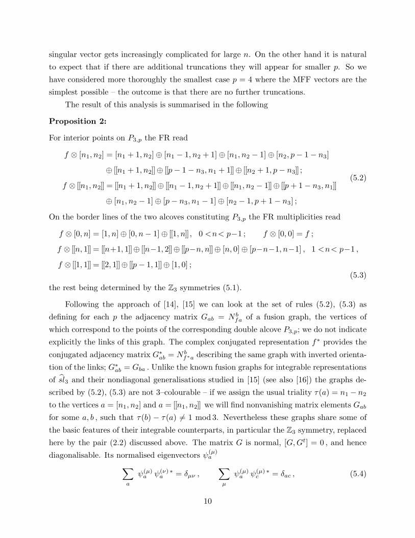
For interior points on P3,p the FR read

f ⊗ [n1, n2] = [n1 + 1, n2]⊕ [n1 − 1, n2 + 1]⊕ [n1, n2 − 1]⊕ [n2, p− 1− n3]

⊕ [[n1 + 1, n2 ]] ⊕ [[ p− 1− n3, n1 + 1 ]] ⊕ [[n2 + 1, p− n3 ]] ;

f ⊗ [[n1, n2 ]] = [[n1 + 1, n2 ]] ⊕ [[n1 − 1, n2 + 1 ]] ⊕ [[n1, n2 − 1 ]] ⊕ [[ p+ 1− n3, n1 ]]

⊕ [n1, n2 − 1]⊕ [p− n3, n1 − 1]⊕ [n2 − 1, p+ 1− n3] ;

(5.2)

On the border lines of the two alcoves constituting P3,p the FR multiplicities read

f ⊗ [0, n] = [1, n]⊕ [0, n− 1]⊕ [[ 1, n ]] , 0 <n< p−1 ; f ⊗ [0, 0] = f ;

f ⊗ [[n, 1 ]] = [[n+1, 1 ]] ⊕ [[n−1, 2 ]] ⊕ [[ p−n, n ]] ⊕ [n, 0]⊕ [p−n−1, n−1] , 1 <n< p−1 ,

f ⊗ [[ 1, 1 ]] = [[ 2, 1 ]] ⊕ [[ p− 1, 1 ]] ⊕ [1, 0] ;

(5.3)

the rest being determined by the Z3 symmetries (5.1).

Following the approach of [14], [15] we can look at the set of rules (5.2), (5.3) as

defining for each p the adjacency matrix Gab = N bfa of a fusion graph, the vertices of

which correspond to the points of the corresponding double alcove P3,p; we do not indicate

explicitly the links of this graph. The complex conjugated representation f∗ provides the

conjugated adjacency matrix G∗ab = N b

f∗a describing the same graph with inverted orienta-

tion of the links; G∗ab = Gba . Unlike the known fusion graphs for integrable representations

of sl3 and their nondiagonal generalisations studied in [15] (see also [16]) the graphs de-

scribed by (5.2), (5.3) are not 3–colourable – if we assign the usual triality τ(a) = n1 − n2

to the vertices a = [n1, n2] and a = [[n1, n2 ]] we will find nonvanishing matrix elements Gab

for some a, b , such that τ(b) − τ(a) 6= 1 mod 3. Nevertheless these graphs share some of

the basic features of their integrable counterparts, in particular the Z3 symmetry, replaced

here by the pair (2.2) discussed above. The matrix G is normal, [G,Gt] = 0 , and hence

diagonalisable. Its normalised eigenvectors ψ(µ)a

∑

a

ψ(µ)a ψ(ν) ∗

a = δµν ,∑

µ

ψ(µ)a ψ(µ) ∗

c = δac , (5.4)

10

labelled by some set {µ} of p2 indices can be used to write down a formula for the general

FR multiplicities N cab of the type first considered by Pasquier [14]4

N cab =

∑

µ

ψ(µ)a ψ

(µ)b ψ

(µ) ∗c

ψ(µ)1

. (5.5)

The formula can be looked at as a generalisation of the Verlinde formula with the matrix

ψ(µ)a replacing the (symmetric) modular matrix. In (5.5) the vector ψ

(µ)1

, the (dual) Perron-

Frobenius vector, is required to have nonvanishing entries. In the simplest example of p = 4

we have checked that there exists a choice of the eigenvector matrix ψ(µ)a consistent with this

requirement (and furthermore ψ(µ)1

> 0 ) and such that (5.5) produces nonnegative integers

for the matrix elements of all Na matrices, (Na)cb = N c

ab . The arbitrariness in determining

the eigenvectors is caused by the presence of eigenvalues of G of multiplicity greater than

one. The eigenvalues χa(µ) = ψ(µ)a /ψ

(µ)1

provide 1 - dimensional representations (“q-

characters”) of the algebra of Na-matrices. In the sl(2) case the analogous to (5.5) formula

(which is more explicit since there is a general expression for the matrices ψ(µ)a ) reproduces

indeed the known [3] FR multiplicities at level 2/p− 2. It should be stressed that the 1st

leaf representation f and its adjoint f∗ do not exhaust the fundamental set of fields needed

to generate a fusion ring. However the description of that set is not needed in formula

(5.5), the latter providing the full information about the fusion rule. In writing (5.5) we

have essentially assumed that the admissible reps fusion algebra is a “C – algebra” (from

“Characters – algebra”), following the terminology in [17], i.e., an associative, commutative

algebra over C with real structure constants, with a finite basis, an identity element, an

involution (here the map of a weight to its adjoint) requiring some standard properties

of the structure constants. The knowledge of the fundamental matrix Nf specifies the

algebra and allows to describe the common to all matrices Na eigenvector matrix ψ(µ)a .

The fact that the general formula (5.5) for the “C – algebra” structure constants gives

nonnegative integers is highly nontrivial. Comparing with [15] (where such “C – algebras”

were discussed and used), recall that the nonnegativity of the integers in the l.h.s. of

formulae analogous to (5.5) selects a subclass of the graphs related to modular invariants

of the integrable models; a counterexample, where this nonnegativity cannot be achieved,

is provided e.g., by the E7 Dynkin diagram.

4 More precisely a formula analogous to the dual version of (5.5), obtained by a summation

over the vertices, appeared in [14], producing in general noninteger structure constants Mνµλ .

11

Thus the knowledge of the fundamental fusion graph allows to determine in principle

all FR multiplicities.

Remark: The graphs appearing in the study of the admissible representations and

the structures they determine deserve further investigation. In particular it is yet unclear

whether the “dual” version of (5.5), describing the structure constants of a dual “C –

algebra”, has any importance. It would be also interesting to check whether the set {µ} ,

can be interpreted as some “exponents” set in the sense of [16]. These questions have

sense already for the case of admissible representations of sl(2) at level 2/p− 2 where the

corresponding graphs (or their unfolded colourable ladder type counterparts) look rather

simple.

The basic FR (5.2), (5.3) which we have derived are checked to admit another in-

terpretation which generalises the corresponding fusion formula of [4],[5],[6] in the case of

integrable representations. First a representation Λ′′ appears in the fusion f ⊗ Λ′ only if

it belongs to the intersection of the 7 points “shifted” weight diagram of the fundamental

representation Gf ◦ Λ′ with the double alcove P3,p; if Gf ◦ Λ′ ⊂ P3,p all 7 points in the

fusion survive. The truncations in (5.3) are precisely described by (intersections of) orbits

of the KW affine Weyl group starting from a point on Gf ◦Λ′∩ P3,p and reaching points of

Gf ◦ Λ′ outside of P3,p. Assigning (according to (4.2) ) multiplicity one to all points of Gf

(or to its isomorphic image Gf ◦Λ′), the points on any orbit contribute with a sign det(w)

determined by the corresponding element w = wβ ; here det(w) is 1 or −1 if the number of

elementary reflections of W representing wβ is even or odd. To visualize these orbits draw

the big alcove for a given p as in fig. 1. and attach on it the shifted diagram Gf ◦Λ′ – the

shifted highest weight itself can be outside of the alcove.

Another example of this truncation mechanism is provided by the fusions of [1, 1].

Taking a sufficiently large Λ′ in the fusion [1, 1] ⊗ Λ′ – i.e., Λ′ and p such that G[1,1] ◦

Λ′ ⊂ P3,p, so that no truncations occur, the FR multiplicities coincide with the weight

multiplicities of [1, 1] and can be computed from the general formula (5.5). Alternatively

the same weight multiplicities can be recovered (and that is how originally we obtained

the values indicated on fig. 4), by the above mechanism of truncation along orbits of the

KW group, given the FR multiplicities for “smaller” Λ′ and p.

12

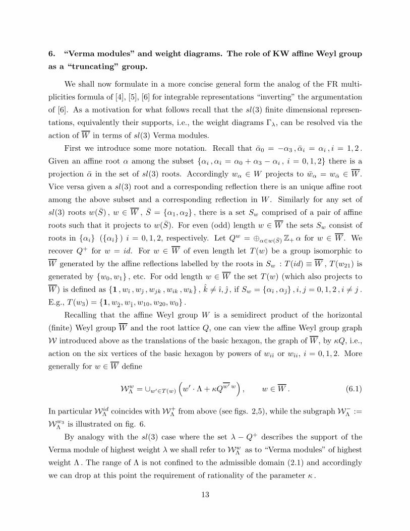
6. “Verma modules” and weight diagrams. The role of KW affine Weyl group

as a “truncating” group.

We shall now formulate in a more concise general form the analog of the FR multi-

plicities formula of [4], [5], [6] for integrable representations “inverting” the argumentation

of [6]. As a motivation for what follows recall that the sl(3) finite dimensional represen-

tations, equivalently their supports, i.e., the weight diagrams Γλ, can be resolved via the

action of W in terms of sl(3) Verma modules.

First we introduce some more notation. Recall that α0 = −α3 , αi = αi , i = 1, 2 .

Given an affine root α among the subset {αi , αı = α0 + α3 − αi , i = 0, 1, 2} there is a

projection α in the set of sl(3) roots. Accordingly wα ∈ W projects to wα = wα ∈ W .

Vice versa given a sl(3) root and a corresponding reflection there is an unique affine root

among the above subset and a corresponding reflection in W . Similarly for any set of

sl(3) roots w(S) , w ∈ W , S = {α1, α2} , there is a set Sw comprised of a pair of affine

roots such that it projects to w(S). For even (odd) length w ∈ W the sets Sw consist of

roots in {αi} ({αı} ) i = 0, 1, 2, respectively. Let Qw = ⊕α∈w(S) Z+ α for w ∈ W . We

recover Q+ for w = id. For w ∈ W of even length let T (w) be a group isomorphic to

W generated by the affine reflections labelled by the roots in Sw : T (id) ≡ W , T (w21) is

generated by {w0, w1} , etc. For odd length w ∈ W the set T (w) (which also projects to

W ) is defined as {1 , wı , w , wjk , wik , wk} , k 6= ı, , if Sw = {αı , α} , i, j = 0, 1, 2 , i 6= j .

E.g., T (w3) = {1, w2, w1, w10, w20, w0} .

Recalling that the affine Weyl group W is a semidirect product of the horizontal

(finite) Weyl group W and the root lattice Q, one can view the affine Weyl group graph

W introduced above as the translations of the basic hexagon, the graph of W , by κQ, i.e.,

action on the six vertices of the basic hexagon by powers of wiı or wıi, i = 0, 1, 2. More

generally for w ∈W define

WwΛ = ∪w′∈T (w)

(w′ · Λ+ κQw′ w

), w ∈W . (6.1)

In particular WidΛ coincides with W+

Λ from above (see figs. 2,5), while the subgraph W−Λ :=

Ww3

Λ is illustrated on fig. 6.

By analogy with the sl(3) case where the set λ − Q+ describes the support of the

Verma module of highest weight λ we shall refer to WwΛ as to “Verma modules” of highest

weight Λ . The range of Λ is not confined to the admissible domain (2.1) and accordingly

we can drop at this point the requirement of rationality of the parameter κ .

13

In the case when the affine Verma module of highest weight Λ = −λκ or Λ = w3 ·(−λκ)

contains by the Kac-Kazhdan theorem a singular vector of weight wβi·Λ or wβı

·Λ, i = 1, 2

(i.e., λ is integral dominant, λ ∈ P+ , or strictly integral dominant, λ ∈ P++ ) then this

weight belongs to the graph W+Λ or W−

Λ respectively. We can view these weights as the

highest weights of “Verma submodules” Wwi

wβi·Λ and Wwi3

wβı·Λ , respectively. One can extend

this to the other four types of ”Verma modules” with proper infinite range of Λ dropping

the upper bounds of the alcoves. Thus we have six different analogs of the sl(3) reducible

Verma modules (of integral dominant highest weights), the singular vectors of which are

governed by the corresponding KW horizontal group Wλ.

One can think of the “Verma modules” introduced here as comprising some “extended”

in the sense of [10] states given by compositions of noninteger powers of the three lowering

generators E−αi , i = 0, 1, 2, of sl(3) – these powers are dictated by the (shifted) affine

Weyl reflections indicated on the graph W, in particular any path from the origin to a

“singular vector” corresponds to a MFF expression for the “true” singular vector of the

affine algebra Verma module. This intuitive picture is quite precise in the sl(2) case where

all states of the corresponding “extended” Verma modules have multiplicity one. Then

these modules are seen to be isomorphic to Verma modules of the superalgebra osp(1|2);

the two sublattices of the corresponding graphs, associated with the two elements of the

sl(2) Weyl group, correspond to even or odd submodules with respect to sl(2).

The problem of multiplicities however makes doubtful the usefulness of such “extended

Verma modules” interpretation in our case and what replaces the above superalgebra is

yet to be seen. Instead we follow further the analogy with the sl(3) case and we assign

multiplicities KΛµ to the weights µ of a general “Verma module” of highest weight Λ,

starting from a multiplicity 1 assigned to the points on the border rays, and with each step

inward increasing by 1 the multiplicity at the points of the subsequent pair of lines parallel

to them (going through diagonals of the honeycomb hexagons) ; see fig. 5,6 where this

assignment is depicted. Not to overburden the notation we shall not indicate explicitly

the dependence of KΛµ on the type of module. There are simple formulae (to be presented

elsewhere) for the generating functions of the weight multiplicities assigned to any of the

6 sublattices in (6.1) which generalise the Kostant generating function for sl(3) Verma

modules.

Let Λ = −λκ , or Λ = w3 · (−λκ) , with λ ∈ P+ , or λ ∈ P++ , respectively. We define

now “weight diagram” multiplicities mΛµ according to

mΛµ =

∑

w∈Wλ

det(w)Kw·Λµ , µ ∈ W±

Λ , (6.2)

14

and we shall refer to the (finite) collection of points {µ} with nonzero mΛµ as “weight

diagram” of Λ to be denoted GΛ. The proof that this definition has sense, i.e., that the

numbers in the l.h.s. of (6.2) are nonnegative integers, extends the corresponding argument

for the weight diagrams of the finite dimensional representations of sl(3) and will appear

elsewhere. The previously discussed examples are easily checked to fit the definition – in

fact we have arrived at the Verma module multiplicities KΛµ “inverting” (6.2), i.e., solving

it for small values of KΛµ with the l.h.s. provided by the examples. An example of a

weight diagram of the second kind (i.e., of highest weight Λ = w3 · (−λκ) , λ ∈ P++ ) is

provided by the 4-point diagram of the representation h = [[ 1, 1 ]] – the “Verma modules

resolution” formula (6.2) for this case is illustrated in fig. 7, while figs. 2,3 illustrate (6.2)

for Λ = [1, 0] and Λ = [2, 0]. On all these figures the positions of the singular vectors

(the two fundamental ones corresponding to the simple reflections in Wλand the ones

corresponding to compositions of such reflections) are indicated by ⋆.

The two types of diagrams GΛ are illustrated furthermore on figs. 8,9. by two generic

examples. View the vertices of GΛ as lying on a set of “concentric” “hexagons” (which could

degenerate into triangles); they are drawn through diagonals of the honeycomb elementary

hexagons. The points on the outmost hexagon have multiplicity 1, and with every step

inward the multiplicity increases by one if the layers are hexagons or stays constant once

the layers degenerate into triangles. This is the direct generalisation of the rule for the

sl(3) weight diagram Γλ multiplicities. In general the intersection of an weight diagram

with any of the 6 lattices in (6.1) (for fixed w = 1 , or w = w3) decomposes into a collection

of weight diagrams of sl(3) irreducible representations.

The same pictures admit another interpretation which may serve as an alternative

definition leading to (6.2): refining by 3 the lattice Qκ (i.e., p→ 3p) and scaling by 3 the

weights λ we can identify the two types of diagrams of highest weight Λ with standard sl(3)

weight diagrams with some points removed. Namely we map the highest weight Λ = −λκ

(λ ∈ P+) to i(Λ) := 3λ , and Λ = w3 · (−λκ) (λ ∈ P++) to i(w3 · (−λκ)) = 3λ − 2ρ ,

resp. The points removed from the sl(3) weight diagrams originate from the centers of

the honeycomb hexagons shaping GΛ, i.e., having at least 3 (2) common links with GΛ, see

figs. 8,9, where these points are indicated by squares. The weight multiplicities defined in

(6.2) coincide with the sl(3) weight multiplicities of the corresponding surviving points.

The same embedding applies to the supports of the Verma modules. The sl(3) coun-

terparts of the weights µ ∈ W±Λ are recovered from the highest weight Λ. More explicitly,

the same definition of the map i applies to the points µ on the first, w′ = 1 lattice in (6.1),

15

w = 1 , containing the highest weight. The rest are recovered from such points. Namely

for Λ = −λκ and µ ∈ Λ + Q+κ , we have i(w · µ) = i(µ) + w−1 · (0, 0) , for w ∈ W. The

points removed from the support 3λ−Q+ of the sl(3) Verma module of highest weight 3λ

(not representing images of W+Λ ) belong to the subset ∪α>0

(3λ− 3Q+ − (3− 〈α, ρ〉)α

).

This rule can be also used to recover the images of the “Verma modules” of highest weight

w3 ·(−λκ), representing each point of W−Λ as w ·µ , with w ∈W and some µ ∈ −λκ+Q+κ .

The definition (6.2) of the weight diagram multiplicities and the mapping into sl(3) repre-

sentations extend to the other 4 of the 6 different types of “Verma modules” (6.1), taken

with a proper choice of the simple root system generating Wλ; we omit here the details.

Apparently this map preserves (up to permutation) the positions of the singular vectors,

e.g., i(wβj· Λ) = wj · i(Λ) , j = 1, 2 , i(wβ1

wβ2· Λ) = w21 · i(Λ) , etc., i.e. the action of the

KW groups is “converted” under this map into ordinary Weyl group action. This together

with the conservation of the multiplicities KΛµ = K

i(Λ)i(µ) , the latter denoting the multiplicity

of the weight i(µ) in the sl(3) Verma module of highest weight i(Λ), converts (6.2) into

the standard Verma modules resolution formula for sl(3) taken for a subset of weights.

Note that if Λ is in addition an admissible highest weight at level 3/p − 3 the above

defined weight i(Λ) is an integrable highest weight at level 3p− 3.

Because of the trivial triality of the sl(3) counterparts (their weights lying on the sl(3)

root lattice Q) all diagrams of both types contain a “middle” point Λ0 mapped to the sl(3)

weight (0, 0). It is given by Λ0 = σ−τ(Λ)([0, 0]) , where we recall that τ(Λ) = n1 − n2 mod

3 for Λ = [n1, n2] or Λ = [[n1 , n2 ]] ; Λ0 has a (maximal) multiplicity 3 min(n1, n2) + 1 and

3 min(n1, n2)− 1 , respectively.

We have already discussed the “shifted weight diagram” GΛ ◦Λ′ assigned to a highest

weight Λ sitting on the first leaf of P3,p. In general for Λ , Λ′ ∈ P3,p the shifted weight

diagram GΛ ◦ Λ′ is a diagram isomorphic to GΛ , GΛ ∋ µ = w · Λ 7→ w · (Λ ◦ Λ′) ∈ GΛ ◦ Λ′ ,

w ∈ W , with a reference point (shifted highest weight) Λ ◦ Λ′ := Λ + w(Λ′) with w = 1

(w = w3) if Λ is on the first (second) leaf of P3,p, respectively. The weight multiplicities

of GΛ ◦ Λ′ are given by

mΛ;Λ′

w·(Λ◦Λ′) := mΛw·Λ , w ∈ W , (6.3)

where the r.h.s. is determined from (6.2). Alternatively the shifted weight diagram can

be recovered from its middle point σ−τ(Λ)(Λ′) ; recall that the definition of the generating

element σ(Λ′) in (2.2) depends on the type of Λ′.

The mapping into sl(3) diagrams preserving weight multiplicities can be extended

to the shifted diagrams identifying in particular the sl(3) shifted highest weight with

16

i(Λ) + i(Λ′) . Note that if both Λ , Λ′ are points on the 2nd leaf this weight originates

from a center of a (boundary) hexagon on the shifted weight diagram GΛ ◦ Λ′ , i.e, from

a point beyond GΛ ◦ Λ′ itself. The image of the shifted highest weight coincides with

w(i(Λ))+ i(Λ′) (a point on the sl(3) shifted weight diagram), where w = 1 (w = w3) if Λ′

is on the first (second) leaf, respectively.

We are now at a position to formulate the analog of the FR multiplicities formula in

[4], [5], [6].

Proposition 3. The FR multiplicities of (a triple of) admissible weights on the

double alcove P3,p are given by the formula

NΛ′′

ΛΛ′ =∑

w∈Wλ′′

det(w)mΛ;Λ′

w·Λ′′ . (6.4)

At present this statement is rather a conjecture supported by a lot of empirical data,

in particular it is established if one of the three highest weights in (6.4) coincides with

the fundamental weights f or f∗. It has been also thoroughly checked for small values of

p ≥ 4; (6.4) extends to the degenerated case p = 2 , p′ = 3 excluded so far.

An example illustrating (6.4) with Λ sitting on the second leaf of the alcove is provided

by the representation h = [[ 1, 1 ]] . Its weight diagram appeared in fig. 7. and its fusions

read5

h⊗ Λ′ = 2Λ′ ⊕ w1 · Λ′ ⊕ w2 · Λ

′ ⊕ w0 · Λ′ (6.5)

for any representations Λ′ on the second leaf and for generic (i.e., not on the border lines of

the alcove) representations Λ′ on the first leaf. For border representations on the first leaf

(6.5) reduces to three multiplicity one terms (or to one such term if Λ′ = σl(1)). Apparently

the latter truncation is a result of a 2-points orbit leading to mΛ′ −mwi·Λ′ = 2− 1 = 1 for

Λ′ such that wi ·Λ′ 6∈ P3,p , for some (one) i = 0, 1, 2 or to a 3-points orbit for Λ′ = σl(1) ,

in which case wi · Λ′ 6∈ P3,p , for at least two i = 0, 1, 2 . The example Λ′ = σ2(1) is

illustrated on fig. 10.

For another example see fig. 11 and the Appendix. Note that unlike the integrable case

there are no analogs here of “q-dim= 0” representations since the walls of the admissible

alcove and its images by the action of the KW group do not support (being on the lattice

dual to the graph W) weights of “classical” representations.

5 This simplest representative of the 2nd leaf admissible representations has to be included

along with {f , f∗} in the fundamental set generating the fusion ring.

17

The nonnegativity of the FR multiplicities in (6.4) is ensured in general by the fact

that the r.h.s of (6.4) can be expressed in terms of sl(3) weight diagram multiplicities and

the ordinary affine Weyl group W adapting the map i discussed above. One recovers in

this way the r.h.s. of the formula in [4], [5], [6] for the FR multiplicities Ni(Λ′′)i(Λ)i(Λ′)(3p) for

particular triples of triality zero highest weights in an integrable theory at level 3p − 3.

(Recall that the Verlinde multiplicities are Z3 graded.) The details will be presented else-

where, here we only illustrate this statement with an example depicted on fig. 12, see the

Appendix for more details. The essential property used is that the (shifted action) Weyl

group orbit of a “removed” point contains only “removed” points. This reformulation of

(6.4) is a generalisation of the same type of relation between admissible and integrable

representations FR multiplicities in the case of sl(2) pointed out in (4.1) of [18]; in partic-

ular we expect that the general fusion rules for p′ ≥ 3 will admit a similar factorised form

in terms of fusion multiplicities for integrable representations at levels p′ − 3 and 3p− 3 ,

see Appendix.

The formula (6.4) admits as in [6] a reformulation in terms of the analogs mΛ′′

ΛΛ′ of the

sl(3) tensor product multiplicities. It applies to weights Λ = w · (−λκ) , w ∈W , λ ∈ Pw+ ,

where P 1

+ = P+ , Pw3

+ = P++ , and Pwi

+ ≡ Pwi3

+ = {λ ∈ P+ , 〈λ, αi〉 6= 0} , i = 1, 2 . In

particular for Λ,Λ′ of the type w · (−λκ) , w = 1 , w3 , the multiplicities mΛ′′

ΛΛ′ are defined

as in (6.4), with the affine KW group Wλ′′

replaced by its horizontal counterpart Wλ′′

,

generated by wγi, γi := 〈λ

′′

, αi〉δ + w(αi) , i = 1, 2 , for Λ = w · (−λ′′

κ) , w ∈ W . It

has been checked on numerous examples that the latter definition of mΛ′′

ΛΛ′ makes sense,

in particular leading to the conservation of the “classical” dimensions computed from the

weight diagrams. We conclude with some of the simplest examples

f ⊗ f∗ = 1⊕ h⊕ [1, 1] , (7× 7 = 1 + 5 + 43) ,

f ⊗ f = f∗ ⊕ [2, 0]⊕ w1 · [2, 0] , (7× 7 = 7 + 19 + 23) ,

h⊗ h = 1⊕ 2h⊕ w1 · h⊕ w2 · h , (5× 5 = 1 + 2.5 + 7 + 7) ,

h⊗ f = f ⊕ w1 · f ⊕ [[ 2, 1 ]] , (5× 7 = 7 + 5 + 23) .

(6.6)

This is a strong indication that our weight diagrams are the supports of finite dimen-

sional representations of a “hidden” algebra. Its q-version at roots of unity would provide

eventually a truncated tensor product equivalent to the fusion rules.

18

7. Summary and conclusions.

There are several different descriptions and derivations of the fusion rules at integer

level. No one of them is easily extendable to the case of fractional level. Instead we have

used a combination of several methods – neither of them is completely rigorous or thorough

at present.

We started with the method which directly generalises the approach exploited by [3]

in the derivation of the admissible representations fusion rules in the sl(2) case. This

is the singular vectors decoupling method applied to 3-point functions which works for

fusions resulting in trivial (zero or one) fusion multiplicities. In particular it enabled us

to determine the fusion of the (fractional) fundamental representations f = [1, 0] and

f∗ = [0, 1] with an arbitrary generic admissible representation Λ′. The notions of weight

diagram and shifted weight diagram described by a set of words in the affine Weyl group

naturally arise as generalisations of the sl(3) counterparts.

Unlike the sl(2) case the decoupling method is technically rather involved due to

the complexity of the general MFF singular vectors and presumably it has to be further

elaborated in order to treat cases with nontrivial multiplicities. Instead we have followed a

strategy influenced to some extent by the study [14], [15] of graphs (generalising the ADE

Dynkin diagrams) related to nondiagonal modular invariants of the integrable WZNW

theories. Namely selecting and analysing a subset of the decoupling systems of equations,

corresponding to representations on the border paths of the admissible alcove, we have

determined (under some additional assumptions) for p′ = 3 and any p ≥ 4 a fundamental

fusion graph described by the fusion matrix Nf . This allowed us to write a formula,

borrowed from [14], [15], for the general FR multiplicities at level 3/p − 3 . It generalises

the Verlinde formula in which the symmetric modular matrix is replaced by the eigenvectors

matrix ψ(µ)a of Nf . It is highly nontrivial that a formula of this kind gives nonnegative

integers – we have no general proof of this fact checked for small values of p.

Knowing the matrix Nf one can determine in principle for any p its eigenvectors – yet

the proposed Pasquier – Verlinde type formula (5.5) is still not very explicit in view of the

absence so far of a general analytic formula for ψ(µ)a . So our next step was to look for an

alternative formula for FR multiplicities, generalising our old work in [6], see also [4], [5].

While the previous approach can be looked at as related to a resolution of the irreducible

admissible representations in terms of a kind of generalised reducible “Fock modules” (since

the differential operators realisation of the generators of sl(3) is equivalent to a generalised

19

free field bosonic realisation) the formula (6.4) described in section 6 rather relies on the

idea of “Verma modules” resolution.

We recall that the starting point in [6] was the standard Weyl formula for the mul-

tiplicities of irreps in tensor products of sl(n) finite dimensional representations. This

formula involves the weight multiplicities of sl(n) finite dimensional representations, i.e.,

their weight diagrams, which can be recovered by resolution of sl(n) Verma modules. So it

was natural to try to interpret similarly the generalised weight diagrams we have encoun-

tered in section 4 – formula (6.2) is precisely of this type with the Weyl group W replaced

by the horizontal KW group Wλ.

The hard part in this alternative approach is the absence initially of an obvious candi-

date for the finite dimensional algebra whose representation theory matches the structures

introduced in section 6. Instead we have described the “Verma modules” by their supports,

i.e., the set of weights and their multiplicities. Our final step was as in [6] to “deform” the

classical formulae replacing the horizontal Weyl group with its affine analog, in our case the

affine KW group Wλ. While in [6] we have been guided at this step by the representation

theory of the deformed algebra Uq(sl(n)) for q – a root of unity, here once again we lack

so far the q− counterpart of the hidden algebra – rather the consistency of (6.4) with the

alternative approaches suggests the existence of such deformation.

The emerging finite dimensional (graded) algebra (and its q – counterpart) behind

the series κ = 3/p of A(1)2 admissible representations is the most interesting outcome of

this work. It might be possible to recover this algebra (containing sl(3) as a subalgebra)

from the supports of the (reducible) Verma modules introduced above. In fact there is

some evidence that the algebra is encoded by the 43 - dimensional representation [1, 1],

the fractional ”adjoint” representation. In particular the map i discussed in section 6

provides a natural way of introducing a root system related to the weight diagram of this

representation. While a subset of these roots sits on the sl(3) weight lattice P (which

contains the sl(3) root lattice Q), there are “fractional” roots beyond it.

Another remaining related problem is the description of the characters of the finite

dimensional representations of this algebra and their q-version, i.e., the derivation of an

explicit formula for the eigenvectors matrix ψ(µ)a . This would give more substance to the

analog (5.5) of the Verlinde formula and would eventually allow to prove its equivalence

to (6.4), so far checked only on examples.

20

Starting from an explicit finite dimensional algebra may simplify also a more abstract

derivation of the sl(3) admissible representations fusion rules as well as their generalisation

to sl(n).

These questions are under investigation.

Let us finally mention that the problem of deriving the admissible representations

fusion rules might be relevant for the analogous problem for representations of W -algebras

obtained by quantum (non principal) Drinfeld–Sokolov reduction from the affine algebras

– see the analogous reduction of Verma modules singular vectors in [11].

Acknowledgements

We would like to thank V. Dobrev, V. Molotkov, Tch. Palev, I. Penkov, V. Schomerus

and V. Tolstoy for useful discussions. A.Ch.G. and V.B.P. acknowledge the hospitality and

the support of INFN, Trieste. A.Ch.G. acknowledges the support of the Alexander von

Humboldt Foundation. This paper was partially supported by the Bulgarian Foundation

for Fundamental Research under contract Φ− 404− 94.

Appendix A. Examples

On figs. 11 we illustrate the fusion

[[2, 1]]⊗ [0, 1] = [[2, 2]]⊕ [1, 1]⊕ [[1, a]]⊕ [[1, 1]]⊕ [a, 1] , a = p− 2 .

On the first fig. 11a we depict the weight diagram GΛ for Λ = [[2, 1]]; the multiplicities are

indicated in circles. On fig. 11b we depict the same diagram but shifted by Λ′ = [0, 1], i.e.,

the shifted diagram GΛ ◦Λ′ having σ2(Λ′) = [1, a] at the middle point; for short a = p− 2,

b = p− 3. The shifted diagram is situated on the graph W viewed as a weight lattice. All

weights sitting outside the addmissible alcove are indicated by (??) and the weights of the

first and the second leaf are indicated by circles and boxes, respectively. Reflecting in the

dotted lines (the walls of the alcove) gives the truncations. The weights [[a,1]] and [1,a]

get their multiplicities truncated to 0 = 2 − 2; [b,0] to 0 = 1 − 1; [0,0] to 0 = 2 − 1 − 1;

[[1,1]] and [1,1] to 1 = 2− 1.

On fig. 12 we illustrate the relation between the fusion rules of admissible represen-

tations at level 3/p− 3 and of the integrable representations at level 3p− 3. We compare

the fusions [1, 1]⊗ [1, 0] and (3, 3)⊗ (3, 0) choosing p = 4.

21

The shifted weight diagram G[1,1] ◦ [1, 0] is mapped into the weight diagram Γ(3,3) +

(3, 0)+ρ, the shifted highest weight µ = [1, 1]+[1, 0] = [2, 1] is identified on the picture with

the sl(3) shifted highest weight (6, 3)+ρ = (7, 4). The reason we shift here in addition the

integrable weight with ρ is that following the tradition we describe the fusion of integrable

representations geometrically by ordinary, nonshifted Weyl group action, but acting on

the shifted by ρ weights; in the final result all surviving weights are shifted back with −ρ.

The boundary triangle enclosing the admissible alcove P3,4 is mapped into the boundary

lines of the sl(3) integrable alcove P 12+ . The origin [0, 0] of P3,4 corresponds to the sl(3)

weight (10, 1) , i.e., the corner point σ((1, 1)) of the alcove P 12++. (For p = 5 it would have

corresponded to (1, 13) = σ∗((1, 1)) in P 15++.)

The ”removed” weights sitting at the centers of the elementary hexagons are indicated

by squares. Such are in particular the weights λ′′ , λ′′ + ρ = (7, 4) − 2α1 , (7, 4)− 2α3 −

α1 , (7, 4)−α3 appearing with multiplicity one in the product (3, 3)⊗(3, 0) . The remaining

7 weights λ′′ in this product, λ′′ + ρ = (7, 4) , (5, 5) , (1, 7) , (4, 4) , (5, 2) , (4, 1) , (2, 5) , have

admissible counterparts all of multiplicity one, recovered by the inverse map i−1. E.g.,

i([2, 1]) = (6, 3) , and hence i−1((6, 3)) = [2, 1] . Similarly i−1((3, 0)) = [1, 0] = w00 · [2, 1] ,

i−1((0, 6)) = [0, 2] = w11 · [2, 1] . Furthermore i(w1 · [2, 1]) = i([2, 1])− α1 = (6, 3)− α1 =

(4, 4) , hence i−1((4, 4)) = w1 · [2, 1] = [[ 1, 2 ]] . Similarly i−1((4, 1)) = i−1((6, 3) − 2α3) =

w3 · [2, 1] = [[ 2, 1 ]] , and i−1((1, 4)) = w2 · [0, 2] = w021 · [2, 1] = [[ 2, 2 ]] , i−1((3, 3)) =

i−1((6, 3)− α1 − α3) = w21 · [2, 1] = [1, 1] .

The final result can be checked to coincide with what is prescribed by (4.2). It can

be cast into the form

Λ1 ⊗ Λ2 =∑

λ3

′

Nλ3

3λ1 3λ2

(3p) w(λ3) · (Λ1 +Λ2) , (A.1)

where w(λ3) ∈ W is determined from i(w(λ3) · (Λ1 + Λ2)

)= λ3 as described above, the

multiplicity in the r.h.s. is the integrable FR multiplicity at level 3p− 3 and the prime in

the sum indicates that all ”removed” points are excluded.

By analogy with (4.1) of [11] the expected generalisation for arbitrary p′ and admissible

(1st leaf) highest weights Λi = λ′

i − λiκ , i = 1, 2 reads

Λ1 ⊗ Λ2 =∑

λ′

3

∑

λ3

′

Nλ′

3

λ′

1,λ′

2

(p′)Nλ3

3λ1 3λ2

(3p) w(λ3) · (λ′3 − κ(λ1 + λ2)) , (A.2)

where Nλ′

3

λ′

1,λ′

2

(p′) is the integrable FR multiplicity at level p′ − 3.

22

References

[1] A. Belavin, A. Polyakov and A. Zamolodchikov, Nucl. Phys. B241 (1984) 333.

[2] E. Verlinde, Nucl. Phys. B300 [FS22] (1988) 360.

[3] H. Awata and Y. Yamada, Mod. Phys. Lett. A7 (1992) 1185.

[4] V.G. Kac, Infinite-dimensional Lie Algebras, third edition (Cambridge University

Press, Cambridge 1990.

[5] M. Walton, Nucl.Phys. B 340 (1990) 777.

[6] P. Furlan, A.Ch. Ganchev and V.B. Petkova, Nucl. Phys. B 343 (1990) 205.

[7] B.L. Feigin and F.G. Malikov, Lett. Math. Phys. 31 (1994) 315; Modular functor and

representation theory of ˆsl(2) at a rational level, q-alg/9511011.

[8] V.G. Kac and M. Wakimoto, Proc. Natl. Sci. USA 85 (1988) 4956 ;

V.G. Kac and M. Wakimoto, Adv. Ser. Math. Phys. 7 (1989) 138 ;

V.G. Kac and M. Wakimoto, Acta Applicandae Math. 21 (1990) 3.

[9] V.G. Kac and D.A. Kazhdan, Adv. Math. 34 (1979) 97.

[10] F.G. Malikov, B.L. Feigin and D.B. Fuks, Funkt. Anal. Prilozhen. 20, no. 2 (1987) 25.

[11] P. Furlan, A.Ch. Ganchev and V.B. Petkova, Nucl. Phys. B 431 (1994) 622.

[12] V.K. Dobrev, Multiplet classification of the indecomposable highest weight modules

over affine Lie algebras and invariant differential operators: the A(1)l example, ICTP

preprint IC/85/9.

[13] D.P. Zhelobenko, Compact Lie Groups and their Representations, (Amer. Math. Soc.,

Providence, 1973, translated from the Russian edition, Nauka, Moscow, 1970).

[14] V. Pasquier, J. Phys. A20 (1987) 5707.

[15] P. Di Francesco and J.-B. Zuber, Nucl. Phys. B338 (1990) 602;

P. Di Francesco and J.-B. Zuber, in Recent Developments in Conformal Field Theories,

Trieste Conference 1989, S. Randjbar-Daemi, E. Sezgin and J.-B. Zuber eds., World

Scientific 1990 ;

P. Di Francesco, Int. J. Mod. Phys. A7 (1992) 407.

[16] J.-B. Zuber, Comm. Math. Phys. 179 (1996) 265.

[17] E. Bannai, T. Ito,Algebraic Combinatorics I: Association Schemes, Benjamin/Cummings

(1984).

[18] P. Furlan, A.Ch. Ganchev and V.B. Petkova, Nucl. Phys. B 491 [PM] (1997) 635.

23