Embed Size (px)
Citation preview
Quantum Computing:
Lecture Notes
Ronald de Wolf
Preface
These lecture notes were formed in small chunks during my “Quantum computing” course at theUniversity of Amsterdam, Feb-May 2011, and compiled into one text thereafter. Each chapterwas covered in a lecture of 2× 45 minutes, with an additional 45-minute lecture for exercises andhomework. The first half of the course (Chapters 1–7) covers quantum algorithms, the second halfcovers quantum complexity (Chapters 8–9), stuff involving Alice and Bob (Chapters 10–13), anderror-correction (Chapter 14). A 15th lecture about physical implementations and general outlookwas more sketchy, and I didn’t write lecture notes for it.
These chapters may also be read as a general introduction to the area of quantum computationand information from the perspective of a theoretical computer scientist. While I made an effortto make the text self-contained and consistent, it may still be somewhat rough around the edges; Ihope to continue polishing and adding to it. Comments & constructive criticism are very welcome,and can be sent to [email protected]
Those who want to read more (much more. . . ): see the book by Nielsen and Chuang [89].
Attribution and acknowledgments
Most of the material in Chapters 1–6 comes from the first chapter of my PhD thesis [108], with anumber of additions: the lower bound for Simon, the Fourier transform, the geometric explanationof Grover. Chapter 7 is newly written for these notes, inspired by Santha’s survey [95]. Chapters 8and 9 are largely new as well. Section 3 of Chapter 8, and most of Chapter 10 are taken (withmany changes) from my “quantum proofs” survey paper with Andy Drucker [42]. Chapters 11and 12 are partly taken from my non-locality survey with Harry Buhrman, Richard Cleve, andSerge Massar [26]. Chapters 13 and 14 are new. Thanks to Giannicola Scarpa for useful commentson some of the chapters.
January’13 : updated and corrected a few things for the Feb-Mar 2013 version of this course, andincluded exercises for each chapter. Thanks to Harry Buhrman, Florian Speelman, and JeroenZuiddam for spotting some typos in the earlier version.
April’13 : more updates, clarifications and corrections; moved some material from Chapter 2 to 1;changed and added some exercises. Thanks to Jouke Witteveen for some useful comments.
April’14 : fixed and clarified a few more things. Thanks to Maarten Wegewijs for spotting a typoin Chapter 4.
March’15 : updated a few small things.
July’15 : updated and corrected a few small things, added more exercises. Thanks to SrinivasanArunachalam, Carla Groenland, and Koen Groenland for comments.
May’16 : a few more corrections, thanks to Ralph Bottesch for comments.
Jan’18 : many more corrections, more exercises, a new Chapter 6 about HSP (the above-mentionedchapter numbers are for the earlier version of the notes), and moved the hints about exercisesto an Appendix for students who want to try the exercises first without hints. Thanks to Joranvan Apeldoorn, Srinivasan Arunachalam, Rens Baardman, Alexander Belov, Koen de Boer, DanielChernowitz, Andras Gilyen, Ronald de Haan, Leon Ingelse, Rafael Kiesel, Jens Klooster, SamKuypers, Christian Nesenberend, and Christian Schaffner for comments.
Ronald de Wolf, January 2018, Amsterdam
ii
Contents
1 Quantum Computing 1
1.1 Introduction . . . . . . . . . . . . . . . . . . . . . . . . . . . . . . . . . . . . . . . . . 1
1.2 Quantum mechanics . . . . . . . . . . . . . . . . . . . . . . . . . . . . . . . . . . . . 2
1.2.1 Superposition . . . . . . . . . . . . . . . . . . . . . . . . . . . . . . . . . . . . 2
1.2.2 Measurement . . . . . . . . . . . . . . . . . . . . . . . . . . . . . . . . . . . . 3
1.2.3 Unitary evolution . . . . . . . . . . . . . . . . . . . . . . . . . . . . . . . . . . 4
1.3 Qubits and quantum memory . . . . . . . . . . . . . . . . . . . . . . . . . . . . . . . 5
1.4 Elementary gates . . . . . . . . . . . . . . . . . . . . . . . . . . . . . . . . . . . . . . 6
1.5 Example: quantum teleportation . . . . . . . . . . . . . . . . . . . . . . . . . . . . . 7
2 The Circuit Model and Deutsch-Jozsa 11
2.1 Quantum computation . . . . . . . . . . . . . . . . . . . . . . . . . . . . . . . . . . . 11
2.1.1 Classical circuits . . . . . . . . . . . . . . . . . . . . . . . . . . . . . . . . . . 11
2.1.2 Quantum circuits . . . . . . . . . . . . . . . . . . . . . . . . . . . . . . . . . . 12
2.2 Universality of various sets of elementary gates . . . . . . . . . . . . . . . . . . . . . 13
2.3 Quantum parallelism . . . . . . . . . . . . . . . . . . . . . . . . . . . . . . . . . . . . 14
2.4 The early algorithms . . . . . . . . . . . . . . . . . . . . . . . . . . . . . . . . . . . . 14
2.4.1 Deutsch-Jozsa . . . . . . . . . . . . . . . . . . . . . . . . . . . . . . . . . . . . 15
2.4.2 Bernstein-Vazirani . . . . . . . . . . . . . . . . . . . . . . . . . . . . . . . . . 16
3 Simon’s Algorithm 19
3.1 The problem . . . . . . . . . . . . . . . . . . . . . . . . . . . . . . . . . . . . . . . . 19
3.2 The quantum algorithm . . . . . . . . . . . . . . . . . . . . . . . . . . . . . . . . . . 19
3.3 Classical algorithms for Simon’s problem . . . . . . . . . . . . . . . . . . . . . . . . . 20
3.3.1 Upper bound . . . . . . . . . . . . . . . . . . . . . . . . . . . . . . . . . . . . 20
3.3.2 Lower bound . . . . . . . . . . . . . . . . . . . . . . . . . . . . . . . . . . . . 21
4 The Fourier Transform 25
4.1 The classical discrete Fourier transform . . . . . . . . . . . . . . . . . . . . . . . . . 25
4.2 The Fast Fourier Transform . . . . . . . . . . . . . . . . . . . . . . . . . . . . . . . . 26
4.3 Application: multiplying two polynomials . . . . . . . . . . . . . . . . . . . . . . . . 26
4.4 The quantum Fourier transform . . . . . . . . . . . . . . . . . . . . . . . . . . . . . . 27
4.5 An efficient quantum circuit . . . . . . . . . . . . . . . . . . . . . . . . . . . . . . . . 28
4.6 Application: phase estimation . . . . . . . . . . . . . . . . . . . . . . . . . . . . . . . 29
iii
5 Shor’s Factoring Algorithm 31
5.1 Factoring . . . . . . . . . . . . . . . . . . . . . . . . . . . . . . . . . . . . . . . . . . 31
5.2 Reduction from factoring to period-finding . . . . . . . . . . . . . . . . . . . . . . . . 31
5.3 Shor’s period-finding algorithm . . . . . . . . . . . . . . . . . . . . . . . . . . . . . . 33
5.4 Continued fractions . . . . . . . . . . . . . . . . . . . . . . . . . . . . . . . . . . . . . 35
6 Hidden Subgroup Problem 39
6.1 Hidden Subgroup Problem . . . . . . . . . . . . . . . . . . . . . . . . . . . . . . . . . 39
6.1.1 Group theory reminder . . . . . . . . . . . . . . . . . . . . . . . . . . . . . . 39
6.1.2 Definition and some instances of the HSP . . . . . . . . . . . . . . . . . . . . 40
6.2 An efficient quantum algorithm if G is Abelian . . . . . . . . . . . . . . . . . . . . . 41
6.2.1 Representation theory and the quantum Fourier transform . . . . . . . . . . . 41
6.2.2 A general algorithm for Abelian HSP . . . . . . . . . . . . . . . . . . . . . . . 42
6.3 General non-Abelian HSP . . . . . . . . . . . . . . . . . . . . . . . . . . . . . . . . . 43
6.3.1 The symmetric group and the graph isomorphism problem . . . . . . . . . . 43
6.3.2 Non-Abelian QFT on coset states . . . . . . . . . . . . . . . . . . . . . . . . . 44
6.3.3 Query-efficient algorithm . . . . . . . . . . . . . . . . . . . . . . . . . . . . . 45
7 Grover’s Search Algorithm 47
7.1 The problem . . . . . . . . . . . . . . . . . . . . . . . . . . . . . . . . . . . . . . . . 47
7.2 Grover’s algorithm . . . . . . . . . . . . . . . . . . . . . . . . . . . . . . . . . . . . . 47
7.3 Amplitude amplification . . . . . . . . . . . . . . . . . . . . . . . . . . . . . . . . . . 50
7.4 Application: satisfiability . . . . . . . . . . . . . . . . . . . . . . . . . . . . . . . . . 51
8 Quantum Walk Algorithms 55
8.1 Classical random walks . . . . . . . . . . . . . . . . . . . . . . . . . . . . . . . . . . . 55
8.2 Quantum walks . . . . . . . . . . . . . . . . . . . . . . . . . . . . . . . . . . . . . . . 56
8.3 Applications . . . . . . . . . . . . . . . . . . . . . . . . . . . . . . . . . . . . . . . . . 58
8.3.1 Grover search . . . . . . . . . . . . . . . . . . . . . . . . . . . . . . . . . . . . 59
8.3.2 Collision problem . . . . . . . . . . . . . . . . . . . . . . . . . . . . . . . . . . 59
8.3.3 Finding a triangle in a graph . . . . . . . . . . . . . . . . . . . . . . . . . . . 60
9 Quantum Query Lower Bounds 63
9.1 Introduction . . . . . . . . . . . . . . . . . . . . . . . . . . . . . . . . . . . . . . . . . 63
9.2 The polynomial method . . . . . . . . . . . . . . . . . . . . . . . . . . . . . . . . . . 64
9.3 The quantum adversary method . . . . . . . . . . . . . . . . . . . . . . . . . . . . . 66
10 Quantum Complexity Theory 71
10.1 Most functions need exponentially many gates . . . . . . . . . . . . . . . . . . . . . . 71
10.2 Classical and quantum complexity classes . . . . . . . . . . . . . . . . . . . . . . . . 72
10.3 Classically simulating quantum computers in polynomial space . . . . . . . . . . . . 73
11 Quantum Encodings, with a Non-Quantum Application 77
11.1 Mixed states and general measurements . . . . . . . . . . . . . . . . . . . . . . . . . 77
11.2 Quantum encodings and their limits . . . . . . . . . . . . . . . . . . . . . . . . . . . 78
11.3 Lower bounds on locally decodable codes . . . . . . . . . . . . . . . . . . . . . . . . 80
iv
12 Quantum Communication Complexity 8312.1 Classical communication complexity . . . . . . . . . . . . . . . . . . . . . . . . . . . 8312.2 The quantum question . . . . . . . . . . . . . . . . . . . . . . . . . . . . . . . . . . . 8412.3 Example 1: Distributed Deutsch-Jozsa . . . . . . . . . . . . . . . . . . . . . . . . . . 8512.4 Example 2: The Intersection problem . . . . . . . . . . . . . . . . . . . . . . . . . . 8612.5 Example 3: The vector-in-subspace problem . . . . . . . . . . . . . . . . . . . . . . . 8712.6 Example 4: Quantum fingerprinting . . . . . . . . . . . . . . . . . . . . . . . . . . . 87
13 Entanglement and Non-locality 9313.1 Quantum non-locality . . . . . . . . . . . . . . . . . . . . . . . . . . . . . . . . . . . 9313.2 CHSH: Clauser-Horne-Shimony-Holt . . . . . . . . . . . . . . . . . . . . . . . . . . . 9513.3 Magic square game . . . . . . . . . . . . . . . . . . . . . . . . . . . . . . . . . . . . . 9613.4 A non-local version of distributed Deutsch-Jozsa . . . . . . . . . . . . . . . . . . . . 97
14 Quantum Cryptography 10114.1 Quantum key distribution . . . . . . . . . . . . . . . . . . . . . . . . . . . . . . . . . 10114.2 Reduced density matrices and the Schmidt decomposition . . . . . . . . . . . . . . . 10314.3 The impossibility of perfect bit commitment . . . . . . . . . . . . . . . . . . . . . . . 10414.4 More quantum cryptography . . . . . . . . . . . . . . . . . . . . . . . . . . . . . . . 105
15 Error-Correction and Fault-Tolerance 10915.1 Introduction . . . . . . . . . . . . . . . . . . . . . . . . . . . . . . . . . . . . . . . . . 10915.2 Classical error-correction . . . . . . . . . . . . . . . . . . . . . . . . . . . . . . . . . . 10915.3 Quantum errors . . . . . . . . . . . . . . . . . . . . . . . . . . . . . . . . . . . . . . . 11015.4 Quantum error-correcting codes . . . . . . . . . . . . . . . . . . . . . . . . . . . . . . 11115.5 Fault-tolerant quantum computation . . . . . . . . . . . . . . . . . . . . . . . . . . . 11315.6 Concatenated codes and the threshold theorem . . . . . . . . . . . . . . . . . . . . . 114
A Some Useful Linear Algebra 117A.1 Some terminology and notation . . . . . . . . . . . . . . . . . . . . . . . . . . . . . . 117A.2 Unitary matrices . . . . . . . . . . . . . . . . . . . . . . . . . . . . . . . . . . . . . . 118A.3 Diagonalization and singular values . . . . . . . . . . . . . . . . . . . . . . . . . . . . 118A.4 Trace . . . . . . . . . . . . . . . . . . . . . . . . . . . . . . . . . . . . . . . . . . . . . 119A.5 Tensor products . . . . . . . . . . . . . . . . . . . . . . . . . . . . . . . . . . . . . . . 120A.6 Rank . . . . . . . . . . . . . . . . . . . . . . . . . . . . . . . . . . . . . . . . . . . . . 120A.7 Dirac notation . . . . . . . . . . . . . . . . . . . . . . . . . . . . . . . . . . . . . . . 121
B Some other Useful Math and CS 123
C Hints for Exercises 125
v

vi
Chapter 1
Quantum Computing
1.1 Introduction
Today’s computers—both in theory (Turing machines) and practice (PCs, tablets, smartphones,. . . )—are based on classical physics. They are limited by locality (operations have only local effects) andby the classical fact that systems can be in only one state at the time. However, modern quantumphysics tells us that the world behaves quite differently. A quantum system can be in a superpo-sition of many different states at the same time, and can exhibit interference effects during thecourse of its evolution. Moreover, spatially separated quantum systems may be entangled with eachother and operations may have “non-local” effects because of this.
Quantum computation is the field that investigates the computational power and other prop-erties of computers based on quantum-mechanical principles. An important objective is to findquantum algorithms that are significantly faster than any classical algorithm solving the sameproblem. The field started in the early 1980s with suggestions for analog quantum computers byYuri Manin [80] (and appendix of [81]), Richard Feynman [48, 49], and Paul Benioff [17], andreached more digital ground when in 1985 David Deutsch defined the universal quantum Turingmachine [39]. The following years saw only sparse activity, notably the development of the first algo-rithms by Deutsch and Jozsa [41] and by Simon [101], and the development of quantum complexitytheory by Bernstein and Vazirani [21]. However, interest in the field increased tremendously afterPeter Shor’s very surprising discovery of efficient quantum algorithms for the problems of integerfactorization and discrete logarithms in 1994 [100]. Since most of current classical cryptography isbased on the assumption that these two problems are computationally hard, the ability to actuallybuild and use a quantum computer would allow us to break most current classical cryptographicsystems, notably the RSA system [93, 94]. (In contrast, a quantum form of cryptography due toBennett and Brassard [20] is unbreakable even for quantum computers.)
Let us mention three different motivations for studying quantum computers, from practical tomore philosophical:
1. The process of miniaturization that has made current classical computers so powerful andcheap, has already reached micro-levels where quantum effects occur. Chip-makers tend togo to great lengths to suppress those quantum effects, but instead one might also try to workwith them, enabling further miniaturization.
2. Making use of quantum effects allows one to speed-up certain computations enormously
1
(sometimes exponentially), and even enables some things that are impossible for classicalcomputers The main purpose of this course is to explain these things (algorithms, crypto,etc.) in detail.
3. Finally, one might state the main goal of theoretical computer science as “study the powerand limitations of the strongest-possible computational devices that nature allows us.” Sinceour current understanding of nature is quantum mechanical, theoretical computer scienceshould be studying the power of quantum computers, not classical ones.
Before limiting ourselves to theory, let us say a few words about practice: to what extent willquantum computers ever be built? At this point in time, it is just too early to tell. The first small2-qubit quantum computer was built in 1997 and in 2001 a 5-qubit quantum computer was used tosuccessfully factor the number 15 [105]. Since then, experimental progress on a number of differenttechnologies has been steady but slow. Currently, the largest quantum computers have a few dozenqubits.
The practical problems facing physical realizations of quantum computers seem formidable.The problems of noise and decoherence have to some extent been solved in theory by the discov-ery of quantum error-correcting codes and fault-tolerant computing (see, e.g., Chapter 15 in thesenotes or [89, Chapter 10]), but these problems are by no means solved in practice. On the otherhand, we should realize that the field of physical realization of quantum computing is still in itsinfancy and that classical computing had to face and solve many formidable technical problemsas well—interestingly, often these problems were even of the same nature as those now faced byquantum computing (e.g., noise-reduction and error-correction). Moreover, while the difficultiesfacing the implementation of a full quantum computer may seem daunting, more limited appli-cations involving quantum communication have already been implemented with some success, forexample teleportation (which is the process of sending qubits using entanglement and classicalcommunication), and quantum cryptography is nowadays even commercially available.
Even if the theory of quantum computing never materializes to a real large-scale physical com-puter, quantum-mechanical computers are still an extremely interesting idea which will bear fruitin other areas than practical fast computing. On the physics side, it may improve our understand-ing of quantum mechanics. The emerging theory of entanglement has already done this to someextent. On the computer science side, the theory of quantum computation generalizes and enrichesclassical complexity theory and may help resolve some of its problems.
1.2 Quantum mechanics
Here we give a brief and abstract introduction to quantum mechanics. In short: a quantum stateis a superposition of classical states, to which we can apply either a measurement or a unitaryoperation. For the required linear algebra and Dirac notation we refer to Appendix A.
1.2.1 Superposition
Consider some physical system that can be in N different, mutually exclusive classical states. Callthese states |1〉, |2〉, . . . , |N〉. Roughly, by a “classical” state we mean a state in which the systemcan be found if we observe it. A pure quantum state (usually just called state) |φ〉 is a superpositionof classical states, written
|φ〉 = α1|1〉+ α2|2〉+ · · ·+ αN |N〉.
2
Here αi is a complex number that is called the amplitude of |i〉 in |φ〉 (see Appendix B for a briefexplanation of complex numbers). Intuitively, a system in quantum state |φ〉 is in all classicalstates at the same time! It is in state |1〉 with amplitude α1, in state |2〉 with amplitude α2, and soon. Mathematically, the states |1〉, . . . , |N〉 form an orthonormal basis of an N -dimensional Hilbertspace (i.e., an N -dimensional vector space equipped with an inner product) of dimension N , and aquantum state |φ〉 is a vector in this space.
There are two things we can do with a quantum state: measure it or let it evolve unitarilywithout measuring it. We will deal with measurement first.
1.2.2 Measurement
Measurement in the computational basis
Suppose we measure state |φ〉. We cannot “see” a superposition itself, but only classical states.Accordingly, if we measure state |φ〉 we will see one and only one classical state |j〉. Which specific|j〉 will we see? This is not determined in advance; the only thing we can say is that we willsee state |j〉 with probability |αj |2, which is the squared norm of the corresponding amplitude αj
(|a + ib| =√a2 + b2). Thus observing a quantum state induces a probability distribution on the
classical states, given by the squared norms of the amplitudes. This implies∑N
j=1 |αj |2 = 1, so thevector of amplitudes has (Euclidean) norm 1. If we measure |φ〉 and see classical state |j〉 as a result,then |φ〉 itself has “disappeared,” and all that is left is |j〉. In other words, observing |φ〉 “collapses”the quantum superposition |φ〉 to the classical state |j〉 that we saw, and all “information” thatmight have been contained in the amplitudes αi is gone.
Projective measurement
For most of the topics in this text, the above “measurement in the computational (or standard)basis” suffices. However, somewhat more general kinds of measurement than the above are possibleand sometimes useful. This will be used only sparsely in the course, so it may be skipped on afirst reading. A projective measurement is described by projectors P1, . . . , Pm (m ≤ N) which sumto identity. These projectors are then pairwise orthogonal, meaning that PiPj = 0 if i 6= j. Theprojector Pj projects on some subspace Vj of the total Hilbert space V , and every state |φ〉 ∈ V canbe decomposed in a unique way as |φ〉 =∑m
j=1 |φj〉, with |φj〉 = Pj |φ〉 ∈ Vj . Because the projectorsare orthogonal, the subspaces Vj are orthogonal as well, as are the states |φj〉. When we applythis measurement to the pure state |φ〉, then we will get outcome j with probability ‖|φj〉‖2 =Tr(Pj |φ〉〈φ|) and the state will then “collapse” to the new state |φj〉/‖|φj〉‖ = Pj |φ〉/‖Pj |φ〉‖.
For example, a measurement in the standard basis (a.k.a. the computational basis) is the specificprojective measurement wherem = N and Pj = |j〉〈j|. That is, Pj projects onto the computationalbasis state |j〉 and the corresponding subspace Vj is the one-dimensional space spanned by |j〉.Consider the state |φ〉 =
∑Nj=1 αj |j〉. Note that Pj |φ〉 = αj|j〉, so applying our measurement to
|φ〉 will give outcome j with probability ‖αj |j〉‖2 = |αj |2, and in that case the state collapses toαj |j〉/‖αj |j〉‖ =
αj
|αj | |j〉. The norm-1 factorαj
|αj | may be disregarded because it has no physical
significance, so we end up with the state |j〉 as we saw before.
As another example, a measurement that distinguishes between |j〉 with j ≤ N/2 and |j〉with j > N/2 corresponds to the two projectors P1 =
∑j≤N/2 |j〉〈j| and P2 =
∑j>N/2 |j〉〈j|.
Applying this measurement to the state |φ〉 = 1√3|1〉+
√23 |N〉 will give outcome 1 with probability
3
‖P1|φ〉‖2 = 1/3, in which case the state collapses to |1〉, and will give outcome 2 with probability‖P2|φ〉‖2 = 2/3, in which case the state collapses to |N〉.
Observables
A projective measurement with projectors P1, . . . , Pm and associated distinct outcomes λ1, . . . , λm,can be written as one matrix M =
∑mi=1 λiPi, which is called an observable. This is a succinct
way of writing down the projective measurement as one matrix, and has the added advantagethat the expected value of the outcome can be easily calculated: if we are measuring a state |φ〉,the probability of outcome λi is ‖Pi|φ〉‖2 = Tr(Pi|φ〉〈φ|), so the expected value of the outcome is∑m
i=1 λiTr(Pi|φ〉〈φ|) = Tr(M |φ〉〈φ|) (where we used that trace is linear). Note thatM is Hermitian:M =M∗. Conversely, since every HermitianM has a spectral decompositionM =
∑mi=1 λiPi, there
is a one-to-one correspondence between observables and Hermitian matrices.
POVM measurement
If we only care about the final probability distribution on the m outcomes, not about the resultingpost-measurement state, then the most general thing we can do is a so-called positive-operator-valued measure (POVM). This is specified by m positive semidefinite matrices E1, . . . , Em thatsum to identity. When measuring a state |φ〉, the probability of outcome i is given by Tr(Ei|φ〉〈φ|).A projective measurement is the special case of a POVM where the measurement elements Ei areprojectors.1
1.2.3 Unitary evolution
Instead of measuring |φ〉, we can also apply some operation to it, i.e., change the state to some
|ψ〉 = β1|1〉+ β2|2〉+ · · ·+ βN |N〉.
Quantum mechanics only allows linear operations to be applied to quantum states. What thismeans is: if we view a state like |φ〉 as an N -dimensional vector (α1, . . . , αN )T , then applying anoperation that changes |φ〉 to |ψ〉 corresponds to multiplying |φ〉 with an N × N complex-valuedmatrix U :
U
α1...αN
=
β1...βN
.
Note that by linearity we have |ψ〉 = U |φ〉 = U (∑
i αi|i〉) =∑
i αiU |i〉.Because measuring |ψ〉 should also give a probability distribution, we have the constraint∑N
j=1 |βj |2 = 1. This implies that the operation U must preserve the norm of vectors, and hence
must be a unitary transformation. A matrix U is unitary if its inverse U−1 equals its conjugatetranspose U∗. This is equivalent to saying that U always maps a vector of norm 1 to a vector ofnorm 1. Because a unitary transformation always has an inverse, it follows that any (non-measuring)operation on quantum states must be reversible: by applying U−1 we can always “undo” the actionof U , and nothing is lost in the process. On the other hand, a measurement is clearly non-reversible,because we cannot reconstruct |φ〉 from the observed classical state |j〉.
1Note that if Ei is a projector, then Tr(Ei|φ〉〈φ|) = Tr(E2i |φ〉〈φ|) = Tr(Ei|φ〉〈φ|Ei) = ‖Ei|φ〉‖2, using the fact
that Ei = E2i and the cyclic property of the trace.
4
1.3 Qubits and quantum memory
In classical computation, the unit of information is a bit, which can be 0 or 1. In quantum compu-tation, this unit is a quantum bit (qubit), which is a superposition of 0 and 1. Consider a system
with 2 basis states, call them |0〉 and |1〉. We identify these basis states with the vectors
(10
)
and
(01
), respectively. A single qubit can be in any superposition
α0|0〉+ α1|1〉, |α0|2 + |α1|2 = 1.
Accordingly, a single qubit “lives” in the vector space C2. Similarly we can think of systems ofmore than 1 qubit, which “live” in the tensor product space of several qubit systems. For instance,a 2-qubit system has 4 basis states: |0〉⊗ |0〉, |0〉⊗ |1〉, |1〉⊗ |0〉, |1〉⊗ |1〉. Here for instance |1〉⊗ |0〉means that the first qubit is in its basis state |1〉 and the second qubit is in its basis state |0〉. Wewill often abbreviate this to |1〉|0〉, |1, 0〉, or even |10〉.
More generally, a register of n qubits has 2n basis states, each of the form |b1〉⊗ |b2〉⊗ . . .⊗|bn〉,with bi ∈ 0, 1. We can abbreviate this to |b1b2 . . . bn〉. We will often abbreviate 0 . . . 0 to 0n.Since bitstrings of length n can be viewed as numbers between 0 and 2n − 1, we can also writethe basis states as numbers |0〉, |1〉, |2〉, . . . , |2n − 1〉. A quantum register of n qubits can be in anysuperposition
α0|0〉+ α1|1〉+ · · ·+ α2n−1|2n − 1〉,2n−1∑
j=0
|αj |2 = 1.
If we measure this in the computational basis, we obtain the n-bit state state |j〉 with probability|αj |2.
Measuring just the first qubit of a state would correspond to the projective measurement thathas the two projectors P0 = |0〉〈0| ⊗ I2n−1 and P1 = |1〉〈1| ⊗ I2n−1 . For example, applying this
measurement to the state 1√3|0〉|φ〉+
√23 |1〉|ψ〉 will give outcome 0 with probability 1/3 (the state
then becomes |0〉|φ〉) and outcome 1 with probability 2/3 (the state then becomes |1〉|ψ〉). Similarly,measuring the first n qubits of an (n +m)-qubit state in the computational basis corresponds tothe projective measurement that has 2n projectors Pj = |j〉〈j| ⊗ I2m for j ∈ 0, 1n.
An important property that deserves to be mentioned is entanglement, which refers to quantumcorrelations between different qubits. For instance, consider a 2-qubit register that is in the state
1√2|00〉+ 1√
2|11〉.
Such 2-qubit states are sometimes called EPR-pairs in honor of Einstein, Podolsky, and Rosen [45],who first examined such states and their seemingly paradoxical properties. Initially neither of thetwo qubits has a classical value |0〉 or |1〉. However, if we measure the first qubit and observe, say,a |0〉, then the whole state collapses to |00〉. Thus observing the first qubit immediately fixes alsothe second, unobserved qubit to a classical value. Since the two qubits that make up the registermay be far apart, this example illustrates some of the non-local effects that quantum systems canexhibit. In general, a bipartite state |φ〉 is called entangled if it cannot be written as a tensorproduct |φA〉 ⊗ |φB〉 where |φA〉 lives in the first space and |φB〉 lives in the second.
5
At this point, a comparison with classical probability distributions may be helpful. Supposewe have two probability spaces, A and B, the first with 2n possible outcomes, the second with 2m
possible outcomes. A probability distribution on the first space can be described by 2n numbers(non-negative reals summing to 1; actually there are only 2n − 1 degrees of freedom here) and adistribution on the second by 2m numbers. Accordingly, a product distribution on the joint spacecan be described by 2n + 2m numbers. However, an arbitrary (non-product) distribution on thejoint space takes 2n+m real numbers, since there are 2n+m possible outcomes in total. Analogously,an n-qubit state |φA〉 can be described by 2n numbers (complex numbers whose squared modulisum to 1), an m-qubit state |φB〉 by 2m numbers, and their tensor product |φA〉 ⊗ |φB〉 by 2n +2m
numbers. However, an arbitrary (possibly entangled) state in the joint space takes 2n+m numbers,since it lives in a 2n+m-dimensional space. We see that the number of parameters required todescribe quantum states is the same as the number of parameters needed to describe probabilitydistributions. Also note the analogy between statistical independence2 of two random variables Aand B and non-entanglement of the product state |φA〉 ⊗ |φB〉. However, despite the similaritiesbetween probabilities and amplitudes, quantum states are much more powerful than distributions,because amplitudes may have negative (or even complex) parts which can lead to interferenceeffects. Amplitudes only become probabilities when we square them. The art of quantum computingis to use these special properties for interesting computational purposes.
1.4 Elementary gates
A unitary that acts on a small number of qubits (say, at most 3) is often called a gate, in analogyto classical logic gates like AND, OR, and NOT; more about that in the next chapter. Two simplebut important 1-qubit gates are the bitflip gate X (which negates the bit, i.e., swaps |0〉 and |1〉)and the phaseflip gate Z (which puts a − in front of |1〉). Represented as 2 × 2 unitary matrices,these are
X =
(0 11 0
), Z =
(1 00 −1
).
Another important 1-qubit gate is the phase gate Rφ, which merely rotates the phase of the |1〉-stateby an angle φ:
Rφ|0〉 = |0〉Rφ|1〉 = eiφ|1〉
This corresponds to the unitary matrix
Rφ =
(1 00 eiφ
).
Note that Z is a special case of this: Z = Rπ, because eiπ = −1. The Rπ/4-gate is often called the
T -gate.Possibly the most important 1-qubit gate is the Hadamard transform, specified by:
H|0〉 = 1√2|0〉+ 1√
2|1〉
H|1〉 = 1√2|0〉 − 1√
2|1〉
2Two random variables A and B are independent if their joint probability distribution can be written as a productof individual distributions for A and for B: Pr[A = a ∧B = b] = Pr[A = a] · Pr[B = b] for all possible values a, b.
6
As a unitary matrix, this is represented as
H =1√2
(1 11 −1
).
If we apply H to initial state |0〉 and then measure, we have equal probability of observing |0〉or |1〉. Similarly, applying H to |1〉 and observing gives equal probability of |0〉 or |1〉. However,if we apply H to the superposition 1√
2|0〉 + 1√
2|1〉 then we obtain |0〉: the positive and negative
amplitudes for |1〉 cancel out! This effect is called interference, and is analogous to interferencepatterns between light or sound waves.
An example of a two-qubit gate is the controlled-not gate CNOT. It negates the second bit ofits input if the first bit is 1, and does nothing if the first bit is 0:
CNOT|0〉|b〉 = |0〉|b〉CNOT|1〉|b〉 = |1〉|1− b〉
The first qubit is called the control qubit, the second the target qubit. In matrix form, this is
CNOT =
1 0 0 00 1 0 00 0 0 10 0 1 0
.
More generally, if U is some single-qubit gate (i.e., 2 × 2 unitary matrix), then the two-qubitcontrolled-U gate corresponds to the following 4× 4 unitary matrix:
1 0 0 00 1 0 00 0 U11 U12
0 0 U21 U22
.
1.5 Example: quantum teleportation
In the next chapter we will look in more detail at how we can use and combine such elementarygates, but as an example we will here already explain teleportation [18]. Suppose there are twoparties, Alice and Bob. Alice has a qubit α0|0〉+α1|1〉 that she wants to send to Bob via a classicalchannel. Without further resources this would be impossible, but Alice also shares an EPR-pair
1√2(|00〉+ |11〉)
with Bob (say Alice holds the first qubit and Bob the second). Initially, their joint state is
(α0|0〉+ α1|1〉)⊗1√2(|00〉+ |11〉).
The first two qubits belong to Alice, the third to Bob. Alice performs a CNOT on her two qubitsand then a Hadamard transform on her first qubit. Their joint state can now be written as
12 |00〉(α0|0〉+ α1|1〉) +12 |01〉(α0|1〉+ α1|0〉) +12 |10〉(α0|0〉 − α1|1〉) +12 |11〉︸︷︷︸Alice
(α0|1〉 − α1|0〉)︸ ︷︷ ︸Bob
.
7
Alice then measures her two qubits in the computational basis and sends the result (2 randomclassical bits) to Bob over a classical channel. Bob now knows which transformation he must doon his qubit in order to regain the qubit α0|0〉 + α1|1〉. For instance, if Alice sent 11 then Bobknows that his qubit is α0|1〉−α1|0〉. A bitflip (X) followed by a phaseflip (Z) will give him Alice’soriginal qubit α0|0〉 + α1|1〉. In fact, if Alice’s qubit had been entangled with other qubits, thenteleportation preserves this entanglement: Bob then receives a qubit that is entangled in the sameway as Alice’s original qubit was.
Note that the qubit on Alice’s side has been destroyed: teleporting moves a qubit from A to B,rather than copying it. In fact, copying an unknown qubit is impossible [109], see Exercise 1.
Exercises
1. Prove the quantum no-cloning theorem: there does not exist a 2-qubit unitary U that maps
|φ〉|0〉 7→ |φ〉|φ〉
for every qubit |φ〉.
2. Show that unitaries cannot “delete” information: there is no one-qubit unitary U that maps|φ〉 7→ |0〉 for every one-qubit state |φ〉.
3. Compute the result of applying a Hadamard transform to both qubits of |0〉⊗ |1〉 in two ways(the first way using tensor product of vectors, the second using tensor product of matrices),and show that the two results are equal:
H|0〉 ⊗H|1〉 = (H ⊗H)(|0〉 ⊗ |1〉).
4. Show that a bit-flip operation, preceded and followed by Hadamard transforms, equals aphase-flip operation: HXH = Z.
5. Show that surrounding a CNOT gates with Hadamard gates switches the role of the control-bit and target-bit of the CNOT: (H⊗H)CNOT(H⊗H) is the 2-qubit gate where the secondbit controls whether the first bit is negated (i.e., flipped).
6. Prove that an EPR-pair 1√2(|00〉+ |11〉) is an entangled state, i.e., that it cannot be written
as the tensor product of two separate qubits.
7. A matrix A is inner product-preserving if the inner product 〈Av|Aw〉 between Av and Awequals the inner product 〈v|w〉, for all vectors v,w. A is norm-preserving if ‖Av‖ = ‖v‖ for allvectors v, i.e., A preserves the Euclidean length of the vector. A is unitary if A∗A = AA∗ = I.
In the following, you may assume for simplicity that the entries of the vectors and matricesare real, not complex.
(a) Prove that A is norm-preserving if, and only if, A is inner product-preserving.
(b) Prove that A is inner product-preserving iff A∗A = AA∗ = I.
(c) Conclude that A is norm-preserving iff A is unitary.
Bonus: prove the same for complex instead of real vector spaces.
8
8. Suppose Alice and Bob are not entangled. If Alice sends a qubit to Bob, then this can giveBob at most one bit of information about Alice.3 However, if they share an EPR-pair, theycan transmit two classical bits by sending one qubit over the channel; this is called superdensecoding [19]. This exercise will show how this works.
(a) They start with a shared EPR-pair, 1√2(|00〉 + |11〉). Alice has classical bits a and b.
Suppose she does an X-operation on her half of the EPR-pair if a = 1, and then a Z-operation if b = 1 (she does both if ab = 11, and neither if ab = 00). Write the resulting2-qubit state.
(b) Suppose Alice sends her half of the state to Bob, who now has two qubits. Show thatBob can determine both a and b from his state. Write Bob’s operation as a quantumcircuit with Hadamard and CNOT gates.
3This is actually a deep statement, a special case of Holevo’s theorem. More about this may be found in Chapter 11.
9

10
Chapter 2
The Circuit Model and Deutsch-Jozsa
2.1 Quantum computation
Below we explain how a quantum computer can apply computational steps to its register of qubits.Two models exist for this: the quantum Turing machine [39, 21] and the quantum circuit model [40,111]. These models are equivalent, in the sense that they can simulate each other in polynomialtime, assuming the circuits are appropriately “uniform.” We only explain the circuit model here,which is more popular among researchers.
2.1.1 Classical circuits
In classical complexity theory, a Boolean circuit is a finite directed acyclic graph with AND, OR,and NOT gates. It has n input nodes, which contain the n input bits (n ≥ 0). The internalnodes are AND, OR, and NOT gates, and there are one or more designated output nodes. Theinitial input bits are fed into AND, OR, and NOT gates according to the circuit, and eventuallythe output nodes assume some value. We say that a circuit computes some Boolean functionf : 0, 1n → 0, 1m if the output nodes get the right value f(x) for every input x ∈ 0, 1n.
A circuit family is a set C = Cn of circuits, one for each input size n. Each circuit has oneoutput bit. Such a family recognizes or decides a language L ⊆ 0, 1∗ = ∪n≥00, 1n if, for everyn and every input x ∈ 0, 1n, the circuit Cn outputs 1 if x ∈ L and outputs 0 otherwise. Sucha circuit family is uniformly polynomial if there is a deterministic Turing machine that outputsCn given n as input, using space logarithmic in n.1 Note that the size (number of gates) of thecircuits Cn can then grow at most polynomially with n. It is known that uniformly polynomialcircuit families are equal in power to polynomial-time deterministic Turing machines: a languageL can be decided by a uniformly polynomial circuit family iff L ∈ P [90, Theorem 11.5], where Pis the class of languages decidable by polynomial-time Turing machines.
Similarly we can consider randomized circuits. These receive, in addition to the n input bits,also some random bits (“coin flips”) as input. A randomized circuit computes a function f if itsuccessfully outputs the right answer f(x) with probability at least 2/3 for every x (probability takenover the values of the random bits; the 2/3 may be replaced by any 1/2 + ε). Randomized circuitsare equal in power to randomized Turing machines: a language L can be decided by a uniformly
1Logarithmic space implies time that’s at most polynomial in n, because such a machine will have only poly(n)different internal states, so it either halts after poly(n) steps or cycles forever.
11
polynomial randomized circuit family iff L ∈ BPP, where BPP (“Bounded-error ProbabilisticPolynomial time”) is the class of languages that can efficiently be recognized by randomized Turingmachines with success probability at least 2/3.
2.1.2 Quantum circuits
A quantum circuit (also called quantum network or quantum gate array) generalizes the idea ofclassical circuit families, replacing the AND, OR, and NOT gates by elementary quantum gates. Aquantum gate is a unitary transformation on a small (usually 1, 2, or 3) number of qubits. We sawa number of examples already in the previous chapter: the bitflip gate X, the phaseflip gate Z,the Hadamard gate H. The main 2-qubit gate we have seen is the controlled-NOT (CNOT) gate.Adding another control register, we get the 3-qubit Toffoli gate, also called controlled-controlled-not (CCNOT) gate. This negates the third bit of its input if both of the first two bits are 1. TheToffoli gate is important because it is complete for classical reversible computation: any classicalcomputation can be implemented by a circuit of Toffoli gates. This is easy to see: using auxiliarywires with fixed values, Toffoli can implement AND (fix the 3rd ingoing wire to 0) and NOT (fix the1st and 2nd ingoing wire to 1). It is known that AND and NOT-gates together suffice to implementany classical Boolean circuit, so if we can apply (or simulate) Toffoli gates, we can implement anyclassical computation in a reversible manner.
Mathematically, such elementary quantum gates can be composed into bigger unitary operationsby taking tensor products (if gates are applied in parallel to different parts of the register), andordinary matrix products (if gates are applied sequentially). We have already seen a simple exampleof such a circuit of elementary gates in the previous chapter, namely to implement teleportation.
For example, if we apply the Hadamard gate H to each bit in a register of n zeroes, we obtain1√2n
∑j∈0,1n |j〉, which is a superposition of all n-bit strings. More generally, if we apply H⊗n to
an initial state |i〉, with i ∈ 0, 1n, we obtain
H⊗n|i〉 = 1√2n
∑
j∈0,1n(−1)i·j |j〉, (2.1)
where i · j =∑nk=1 ikjk denotes the inner product of the n-bit strings i, j ∈ 0, 1n. For example:
H⊗2|01〉 = 1√2(|0〉+ |1〉)⊗ 1√
2(|0〉 − |1〉) = 1
2
∑
j∈0,12(−1)01·j |j〉.
Note that Hadamard happens to be its own inverse (it’s unitary and Hermitian, hence H = H∗ =H−1), so applying it once more on the right-hand side of the above equation would give us back|01〉. The n-fold Hadamard transform will be very useful for the quantum algorithms explainedlater.
As in the classical case, a quantum circuit is a finite directed acyclic graph of input nodes,gates, and output nodes. There are n nodes that contain the input (as classical bits); in additionwe may have some more input nodes that are initially |0〉 (“workspace”). The internal nodes of thequantum circuit are quantum gates that each operate on at most two or three qubits of the state.The gates in the circuit transform the initial state vector into a final state, which will generally bea superposition. We measure some dedicated output bits of this final state to (probabilistically)obtain an answer.
12
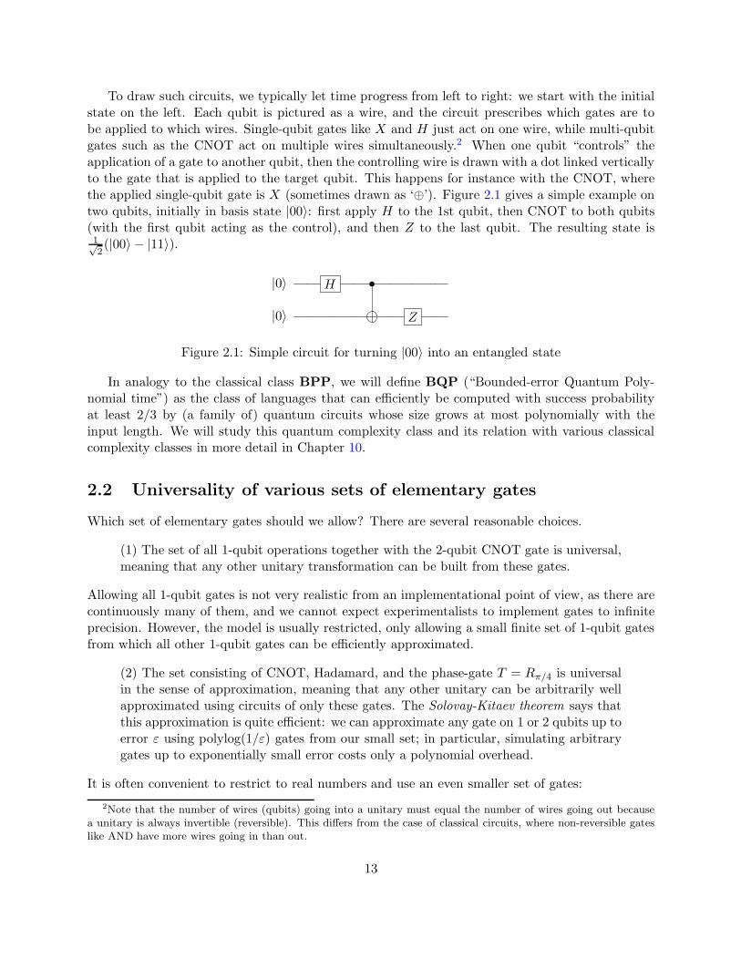
To draw such circuits, we typically let time progress from left to right: we start with the initialstate on the left. Each qubit is pictured as a wire, and the circuit prescribes which gates are tobe applied to which wires. Single-qubit gates like X and H just act on one wire, while multi-qubitgates such as the CNOT act on multiple wires simultaneously.2 When one qubit “controls” theapplication of a gate to another qubit, then the controlling wire is drawn with a dot linked verticallyto the gate that is applied to the target qubit. This happens for instance with the CNOT, wherethe applied single-qubit gate is X (sometimes drawn as ‘⊕’). Figure 2.1 gives a simple example ontwo qubits, initially in basis state |00〉: first apply H to the 1st qubit, then CNOT to both qubits(with the first qubit acting as the control), and then Z to the last qubit. The resulting state is1√2(|00〉 − |11〉).
|0〉 H •
|0〉 Z
Figure 2.1: Simple circuit for turning |00〉 into an entangled state
In analogy to the classical class BPP, we will define BQP (“Bounded-error Quantum Poly-nomial time”) as the class of languages that can efficiently be computed with success probabilityat least 2/3 by (a family of) quantum circuits whose size grows at most polynomially with theinput length. We will study this quantum complexity class and its relation with various classicalcomplexity classes in more detail in Chapter 10.
2.2 Universality of various sets of elementary gates
Which set of elementary gates should we allow? There are several reasonable choices.
(1) The set of all 1-qubit operations together with the 2-qubit CNOT gate is universal,meaning that any other unitary transformation can be built from these gates.
Allowing all 1-qubit gates is not very realistic from an implementational point of view, as there arecontinuously many of them, and we cannot expect experimentalists to implement gates to infiniteprecision. However, the model is usually restricted, only allowing a small finite set of 1-qubit gatesfrom which all other 1-qubit gates can be efficiently approximated.
(2) The set consisting of CNOT, Hadamard, and the phase-gate T = Rπ/4 is universalin the sense of approximation, meaning that any other unitary can be arbitrarily wellapproximated using circuits of only these gates. The Solovay-Kitaev theorem says thatthis approximation is quite efficient: we can approximate any gate on 1 or 2 qubits up toerror ε using polylog(1/ε) gates from our small set; in particular, simulating arbitrarygates up to exponentially small error costs only a polynomial overhead.
It is often convenient to restrict to real numbers and use an even smaller set of gates:
2Note that the number of wires (qubits) going into a unitary must equal the number of wires going out becausea unitary is always invertible (reversible). This differs from the case of classical circuits, where non-reversible gateslike AND have more wires going in than out.
13
(3) The set of Hadamard and Toffoli (CCNOT) is universal for all unitaries with realentries in the sense of approximation, meaning that any unitary with only real entriescan be arbitrarily well approximated using circuits of only these gates (again the Solovay-Kitaev theorem says that this simulation can be done efficiently).
2.3 Quantum parallelism
One uniquely quantum-mechanical effect that we can use for building quantum algorithms is quan-tum parallelism. Suppose we have a classical algorithm that computes some function f : 0, 1n →0, 1m. Then we can build a quantum circuit U (consisting only of Toffoli gates) that maps|x〉|0〉 → |x〉|f(x)〉 for every x ∈ 0, 1n. Now suppose we apply U to a superposition of all inputs x(which is easy to build using n Hadamard transforms):
U
1√
2n
∑
x∈0,1n|x〉|0〉
=
1√2n
∑
x∈0,1n|x〉|f(x)〉.
We applied U just once, but the final superposition contains f(x) for all 2n input values x! However,by itself this is not very useful and does not give more than classical randomization, since observingthe final superposition will give just one random |x〉|f(x)〉 and all other information will be lost.As we will see below, quantum parallelism needs to be combined with the effects of interferenceand entanglement in order to get something that is better than classical.
2.4 The early algorithms
The two main successes of quantum algorithms so far are Shor’s factoring algorithm from 1994 [100]and Grover’s search algorithm from 1996 [56], which will be explained in later chapters. In thissection we describe some of the earlier quantum algorithms that preceded Shor’s and Grover’s.
Virtually all quantum algorithms work with queries in some form or other. We will explainthis model here. It may look contrived at first, but eventually will lead smoothly to Shor’s andGrover’s algorithm. We should, however, emphasize that the query complexity model differs fromthe standard model described above, because the input is now given as a “black-box.” This meansthat the exponential quantum-classical separations that we describe below (like Simon’s) do not bythemselves give exponential quantum-classical separations in the standard model.
To explain the query setting, consider an N -bit input x = (x1, . . . , xN ) ∈ 0, 1N . Usually wewill have N = 2n, so that we can address bit xi using an n-bit index i. One can think of the inputas an N -bit memory which we can access at any point of our choice (a Random Access Memory).A memory access is via a so-called “black-box,” which is equipped to output the bit xi on input i.As a quantum operation, this would be the following unitary mapping on n+ 1 qubits:
Ox : |i, 0〉 → |i, xi〉.
The first n qubits of the state are called the address bits (or address register), while the (n+ 1)stqubit is called the target bit. Since this operation must be unitary, we also have to specify whathappens if the initial value of the target bit is 1. Therefore we actually let Ox be the followingunitary transformation:
Ox : |i, b〉 → |i, b⊕ xi〉,
14
here i ∈ 0, 1n, b ∈ 0, 1, and ⊕ denotes exclusive-or (addition modulo 2). In matrix representa-tion, Ox is now a permutation matrix and hence unitary. Note that a quantum computer can applyOx on a superposition of various i, something a classical computer cannot do. One application ofthis black-box is called a query, and counting the required number of queries to compute this orthat function of x is something we will do a lot in the first half of these notes.
Given the ability to make a query of the above type, we can also make a query of the form|i〉 7→ (−1)xi |i〉 by setting the target bit to the state |−〉 = 1√
2(|0〉 − |1〉) = H|1〉:
Ox (|i〉|−〉) = |i〉 1√2(|xi〉 − |1− xi〉) = (−1)xi |i〉|−〉.
This ±-kind of query puts the output variable in the phase of the state: if xi is 1 then we get a −1 inthe phase of basis state |i〉; if xi = 0 then nothing happens to |i〉. This “phase-oracle” is sometimesmore convenient than the standard type of query. We sometimes denote the corresponding n-qubitunitary transformation by Ox,±.
2.4.1 Deutsch-Jozsa
Deutsch-Jozsa problem [41]:For N = 2n, we are given x ∈ 0, 1N such that either(1) all xi have the same value (“constant”), or(2) N/2 of the xi are 0 and N/2 are 1 (“balanced”).The goal is to find out whether x is constant or balanced.
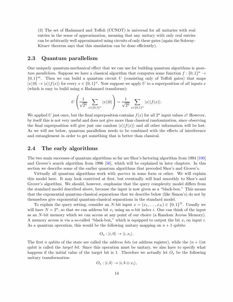
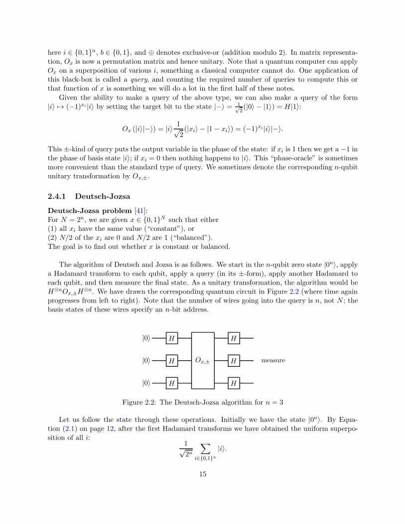
The algorithm of Deutsch and Jozsa is as follows. We start in the n-qubit zero state |0n〉, applya Hadamard transform to each qubit, apply a query (in its ±-form), apply another Hadamard toeach qubit, and then measure the final state. As a unitary transformation, the algorithm would beH⊗nOx,±H⊗n. We have drawn the corresponding quantum circuit in Figure 2.2 (where time againprogresses from left to right). Note that the number of wires going into the query is n, not N ; thebasis states of these wires specify an n-bit address.
|0〉
|0〉
|0〉
measure
H
H
H
H
H
H
Ox,±
Figure 2.2: The Deutsch-Jozsa algorithm for n = 3
Let us follow the state through these operations. Initially we have the state |0n〉. By Equa-tion (2.1) on page 12, after the first Hadamard transforms we have obtained the uniform superpo-sition of all i:
1√2n
∑
i∈0,1n|i〉.
15
The Ox,±-query turns this into1√2n
∑
i∈0,1n(−1)xi |i〉.
Applying the second batch of Hadamards gives (again by Equation (2.1)) the final superposition
1
2n
∑
i∈0,1n(−1)xi
∑
j∈0,1n(−1)i·j |j〉,
where i · j =∑nk=1 ikjk as before. Since i · 0n = 0 for all i ∈ 0, 1n, we see that the amplitude of
the |0n〉-state in the final superposition is
1
2n
∑
i∈0,1n(−1)xi =
1 if xi = 0 for all i,−1 if xi = 1 for all i,0 if x is balanced.
Hence the final observation will yield |0n〉 if x is constant and will yield some other state if xis balanced. Accordingly, the Deutsch-Jozsa problem can be solved with certainty using only 1quantum query and O(n) other operations (the original solution of Deutsch and Jozsa used 2queries, the 1-query solution is from [37]).
In contrast, it is easy to see that any classical deterministic algorithm needs at least N/2 + 1queries: if it has made only N/2 queries and seen only 0s, the correct output is still undetermined.However, a classical algorithm can solve this problem efficiently if we allow a small error probability:just query x at two random positions, output “constant” if those bits are the same and “balanced”if they are different. This algorithm outputs the correct answer with probability 1 if x is constantand outputs the correct answer with probability 1/2 if x is balanced. Thus the quantum-classicalseparation of this problem only holds if we consider algorithms without error probability.
2.4.2 Bernstein-Vazirani
Bernstein-Vazirani problem [21]:For N = 2n, we are given x ∈ 0, 1N with the property that there is some unknown a ∈ 0, 1nsuch that xi = (i · a) mod 2. The goal is to find a.
The Bernstein-Vazirani algorithm is exactly the same as the Deutsch-Jozsa algorithm, but nowthe final observation miraculously yields a. Since (−1)xi = (−1)(i·a) mod 2 = (−1)i·a, we can writethe state obtained after the query as:
1√2n
∑
i∈0,1n(−1)xi |i〉 = 1√
2n
∑
i∈0,1n(−1)i·a|i〉.
Since Hadamard is its own inverse, applying a Hadamard to each qubit of the above state will turnit into the classical state |a〉 and hence solves the Bernstein-Vazirani problem with 1 query andO(n) other operations. In contrast, any classical algorithm (even a randomized one with small errorprobability) needs to ask n queries for information-theoretic reasons: the final answer consists of nbits and one classical query gives at most 1 bit of information.
Bernstein and Vazirani also defined a recursive version of this problem, which can be solvedexactly by a quantum algorithm in poly(n) steps, but for which every classical randomized algorithmneeds nΩ(logn) steps.
16
Exercises
1. Is the controlled-NOT operation C Hermitian? Determine C−1.
2. Show that every unitary one-qubit gate with real entries can be written as a rotation matrix,possibly preceded and followed by Z-gates. In other words, show that for every 2 × 2 realunitary U , there exist signs s1, s2, s3 ∈ 1,−1 and angle θ ∈ [0, 2π) such that
U = s1
(1 00 s2
)(cos(θ) − sin(θ)sin(θ) cos(θ)
)(1 00 s3
)
3. Construct a CNOT from two Hadamard gates and one controlled-Z (the controlled-Z gatemaps |11〉 7→ −|11〉 and acts like the identity on the other basis states).
4. A SWAP-gate interchanges two qubits: it maps basis state |a, b〉 to |b, a〉. Implement aSWAP-gate using a few CNOTs.
5. Let U be a 1-qubit unitary that we would like to implement in a controlled way, i.e., wewant to implement a map |c〉|b〉 7→ |c〉U c|b〉 for all c, b ∈ 0, 1. Suppose there exist 1-qubitunitaries A, B, and C, such that ABC = I and AXBXC = U (remember that X is theNOT-gate). Give a circuit that acts on two qubits and implements a controlled-U gate, usingCNOTs and (uncontrolled) A, B, and C gates.
6. It is possible to avoid doing any intermediate measurements in a quantum circuit, using oneauxiliary qubit for each one-qubit measurement that needs to be delayed until the end of thecomputation. Show how.
7. (a) Give a circuit that maps |0n, b〉 7→ |0n, 1− b〉 for b ∈ 0, 1, and that maps |i, b〉 7→|i, b〉 whenever i ∈ 0, 1n\0n. You are allowed to use every type of elementary gatementioned in the lecture notes (incl. Toffoli gates), as well as auxiliary qubits that areinitially |0〉 and that should be put back to |0〉 at the end of the computation.
You can draw a Toffoli gate similar to a CNOT gate: a bold dot on each of the twocontrol wires, and a ‘⊕’ on the target wire.
(b) Suppose we can make queries of the type |i, b〉 7→ |i, b⊕ xi〉 to input x ∈ 0, 1N , withN = 2n. Let x′ be the input x with its first bit flipped (e.g., if x = 0110 then x′ = 1110).Give a circuit that implements a query to x′. Your circuit may use one query to x.
(c) Give a circuit that implements a query to an input x′′ that is obtained from x (analo-gously to (b)) by setting its first bit to 0. Your circuit may use one query to x.
8. In Section 2.4 we showed that a query of the type |i, b〉 7→ |i, b⊕ xi〉 (where i ∈ 0, . . . , N −1and b ∈ 0, 1) can be used to implement a phase-query, i.e., one of the type |i〉 7→ (−1)xi |i〉.Is the converse possible: can a query of the first type be implemented using phase-queries,and possibly some auxiliary qubits and other gates? If yes, show how. If no, explain why not.
9. Give a randomized classical algorithm (i.e., one that can flip coins during its operation) thatmakes only two queries to x, and decides the Deutsch-Jozsa problem with success probabilityat least 2/3 on every possible input. A high-level description is enough, no need to write outthe classical circuit.
17
10. Suppose our N -bit input x satisfies the following promise:either (1) the first N/2 bits of x are all 0 and the second N/2 bits are all 1; or (2) the numberof 1s in the first half of x plus the number of 0s in the second half, equals N/2. Modify theDeutsch-Jozsa algorithm to efficiently distinguish these two cases (1) and (2).
11. A parity query to input x ∈ 0, 1N corresponds to the (N+1)-qubit unitary map Qx : |y, b〉 7→|y, b⊕ (x · y)〉, where x ·y =
∑N−1i=0 xiyi mod 2. For a fixed function f : 0, 1N → 0, 1, give
a quantum algorithm that computes f(x) using only one such query (i.e., one application ofQx), and as many elementary gates as you want. You do not need to give the circuit in fulldetail, an informal description of the algorithm is good enough.
18
Chapter 3
Simon’s Algorithm
The Deutsch-Jozsa problem showed an exponential quantum improvement over the best determin-istic classical algorithms; the Bernstein-Vazirani problem shows a polynomial improvement overthe best randomized classical algorithms that have error probability ≤ 1/3. In this chapter we willcombine these two features: we will see a problem where quantum computers are exponentiallymore efficient than bounded-error randomized algorithms.
3.1 The problem
Let N = 2n, and [N ] = 1, . . . , N, which we can identify with 0, 1n. Let j⊕s be the n-bit stringobtained by bitwise adding the n-bit strings j and s mod 2.
Simon’s problem [101]:For N = 2n, we are given x = (x1, . . . , xN ), with xi ∈ 0, 1n, with the property that there is someunknown non-zero s ∈ 0, 1n such that xi = xj iff (i = j or i = j ⊕ s). The goal is to find s.
Note that x, viewed as a function from [N ] to [N ] is a 2-to-1 function, where the 2-to-1-nessis determined by the unknown mask s. The queries to the input here are slightly different frombefore: the input x = (x1, . . . , xN ) now has variables xi that themselves are n-bit strings, and onequery gives such a string completely (|i, 0n〉 7→ |i, xi〉). However, we can also view this problem ashaving n2n binary variables that we can query individually. Since we can simulate one xi-queryusing only n binary queries (just query all n bits of xi), this alternative view will not affect thenumber of queries very much.
3.2 The quantum algorithm
Simon’s algorithm starts out very similar to Deutsch-Jozsa: start in a state of 2n zero qubits|0n〉|0n〉 and apply Hadamard transforms to the first n qubits, giving
1√2n
∑
i∈0,1n|i〉|0n〉.
19
At this point, the second n-qubit register still holds only zeroes. A query turns this into
1√2n
∑
i∈0,1n|i〉|xi〉.
Now the algorithm measures the second n-bit register (this measurement is actually not necessary,but it facilitates analysis). The measurement outcome will be some value xi and the first registerwill collapse to the superposition of the two indices having that xi-value:
1√2(|i〉+ |i⊕ s〉)|xi〉.
We will now ignore the second register and apply Hadamard transforms to the first n qubits. UsingEquation (2.1) and the fact that (i⊕ s) · j = (i · j)⊕ (s · j), we can write the resulting state as
1√2n+1
∑
j∈0,1n(−1)i·j |j〉+
∑
j∈0,1n(−1)(i⊕s)·j |j〉
=
1√2n+1
∑
j∈0,1n(−1)i·j
(1 + (−1)s·j
)|j〉
.
Note that |j〉 has non-zero amplitude iff s · j = 0 mod 2. Measuring the state gives a uniformlyrandom element from the set j | s ·j = 0 mod 2. Accordingly, we get a linear equation that givesinformation about s. We repeat this algorithm until we have obtained n − 1 independent linearequations involving s. The solutions to these equations will be 0n and the correct s, which we cancompute efficiently by a classical algorithm (Gaussian elimination modulo 2). This can be done bymeans of a classical circuit of size roughly O(n3).
Note that if the j’s you have generated at some point span a space of size 2k, for some k < n−1,then the probability that your next run of the algorithm produces a j that is linearly independentof the earlier ones, is (2n−1 − 2k)/2n−1 ≥ 1/2. Hence an expected number of O(n) runs of thealgorithm suffices to find n − 1 linearly independent j’s. Simon’s algorithm thus finds s using anexpected number of O(n) xi-queries and polynomially many other operations.
3.3 Classical algorithms for Simon’s problem
3.3.1 Upper bound
Let us first sketch a classical randomized algorithm that solves Simon’s problem using O(√2n)
queries, based on the so-called “birthday paradox.” Our algorithm will make T randomly chosendistinct queries i1, . . . , iT , for some T to be determined later. If there is a collision among thosequeries (i.e., xik = xiℓ for some k 6= ℓ), then we are done, because then we know ik = iℓ ⊕ s,equivalently s = ik ⊕ iℓ. How large should T be such that we are likely to see a collision in cases 6= 0n? (there won’t be any collisions if s = 0n.) There are
(T2
)= 1
2T (T − 1) ≈ T 2/2 pairs in oursequence that could be a collision, and since the indices are chosen randomly, the probability for afixed pair to form a collision is 1/(2n − 1). Hence by linearity of expectation, the expected numberof collisions in our sequence will be roughly T 2/2n+1. If we choose T =
√2n+1, we expect to have
roughly 1 collision in our sequence, which is good enough to find s. Of course, an expected value of1 collision does not mean that we will have at least one collision with high probability, but a slightlymore involved calculation shows the latter statement as well.
20
3.3.2 Lower bound
Simon [101] proved that any classical randomized algorithm that finds s with high probability needsto make Ω(
√2n) queries, so the above classical algorithm is essentially optimal. This was the first
proven exponential separation between quantum algorithms and classical bounded-error algorithms(let us stress again that this does not prove an exponential separation in the usual circuit model,because we are counting queries rather than ordinary operations here). Simon’s algorithm inspiredShor to his factoring algorithm, which we describe in Chapter 5.
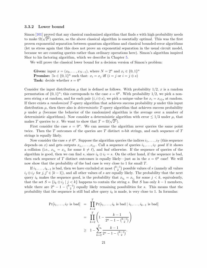
We will prove the classical lower bound for a decision version of Simon’s problem:
Given: input x = (x0, . . . , xN−1), where N = 2n and xi ∈ 0, 1nPromise: ∃s ∈ 0, 1n such that: xi = xj iff (i = j or i = j ⊕ s)Task: decide whether s = 0n
Consider the input distribution µ that is defined as follows. With probability 1/2, x is a randompermutation of 0, 1n; this corresponds to the case s = 0n. With probability 1/2, we pick a non-zero string s at random, and for each pair (i, i⊕s), we pick a unique value for xi = xi⊕s at random.If there exists a randomized T -query algorithm that achieves success probability p under this inputdistribution µ, then there also is deterministic T -query algorithm that achieves success probabilityp under µ (because the behavior of the randomized algorithm is the average over a number ofdeterministic algorithms). Now consider a deterministic algorithm with error ≤ 1/3 under µ, thatmakes T queries to x. We want to show that T = Ω(
√2n).
First consider the case s = 0n. We can assume the algorithm never queries the same pointtwice. Then the T outcomes of the queries are T distinct n-bit strings, and each sequence of Tstrings is equally likely.
Now consider the case s 6= 0n. Suppose the algorithm queries the indices i1, . . . , iT (this sequencedepends on x) and gets outputs xi1 , . . . , xiT . Call a sequence of queries i1, . . . , iT good if it showsa collision (i.e., xik = xiℓ for some k 6= ℓ), and bad otherwise. If the sequence of queries of thealgorithm is good, then we can find s, since ik ⊕ iℓ = s. On the other hand, if the sequence is bad,then each sequence of T distinct outcomes is equally likely—just as in the s = 0n case! We willnow show that the probability of the bad case is very close to 1 for small T .
If i1, . . . , ik−1 is bad, then we have excluded at most(k−1
2
)possible values of s (namely all values
ij ⊕ ij′ for j, j′ ∈ [k− 1]), and all other values of s are equally likely. The probability that the next
query ik makes the sequence good, is the probability that xik = xij for some j < k, equivalently,that the set S = ik ⊕ ij | j < k happens to contain the string s. But S has only k − 1 members,
while there are 2n − 1 −(k−1
2
)equally likely remaining possibilities for s. This means that the
probability that the sequence is still bad after query ik is made, is very close to 1. In formulas:
Pr[i1, . . . , iT is bad] =
T∏
k=2
Pr[i1, . . . , ik is bad | i1, . . . , ik−1 is bad]
=
T∏
k=2
(1− k − 1
2n − 1−(k−12
))
≥ 1−T∑
k=2
k − 1
2n − 1−(k−1
2
) .
21
Here we used the fact that (1 − a)(1 − b) ≥ 1 − (a + b) if a, b ≥ 0. Note that∑T
k=2(k − 1) =
T (T − 1)/2 ≈ T 2/2, and 2n − 1−(k−12
)≈ 2n as long as k ≪
√2n. Hence we can approximate the
last formula by 1− T 2/2n+1. Accordingly, if T ≪√2n then with probability nearly 1 (probability
taken over the distribution µ) the algorithm’s sequence of queries is bad. If it gets a bad sequence,it cannot “see” the difference between the s = 0n case and the s 6= 0n case, since both cases resultin a uniformly random sequence of T distinct n-bit strings as answers to the T queries. This showsthat T has to be Ω(
√2n) in order to enable the algorithm to get a good sequence of queries with
high probability.
Exercises
1. Analyze the different steps of Simon’s algorithm if s = 0n (so all xi-values are distinct), andshow that the final output j is uniformly distributed over 0, 1n.
2. Suppose we run Simon’s algorithm on the following input x (with N = 8 and hence n = 3):
x000 = x111 = 000x001 = x110 = 001x010 = x101 = 010x011 = x100 = 011
Note that x is 2-to-1 and xi = xi⊕111 for all i ∈ 0, 13, so s = 111.
(a) Give the starting state of Simon’s algorithm.
(b) Give the state after the first Hadamard transforms on the first 3 qubits.
(c) Give the state after applying the oracle.
(d) Give the state after measuring the second register (suppose the measurement gave |001〉).(e) Using H⊗n|i〉 = 1√
2n
∑j∈0,1n(−1)i·j |j〉, give the state after the final Hadamards.
(f) Why does a measurement of the first 3 qubits of the final state give information about s?
(g) Suppose the first run of the algorithm gives j = 011 and a second run gives j = 101.Show that, assuming s 6= 000, those two runs of the algorithm already determine s.
3. Consider the following generalization of Simon’s problem: the input is x = (x0, . . . , xN−1),with N = 2n and xi ∈ 0, 1n, with the property that there is some unknown subspaceV ⊆ 0, 1n such that xi = xj iff there exists a v ∈ V such that i = j ⊕ v. The usualdefinition of Simon’s problem corresponds to the case where the subspace V has dimensionat most 1.
Show that one run of Simon’s algorithm now produces a j ∈ 0, 1n that is orthogonal to thewhole subspace (i.e., j · v = 0 mod 2 for every v ∈ V ).
4. (a) Suppose x is an N -bit string. What happens if we apply a Hadamard transform to each
qubit of the N -qubit state1√2N
∑
y∈0,1N(−1)x·y|y〉?
22
(b) Give a quantum algorithm that uses T queries to N -bit string x, and that maps |y〉 7→(−1)x·y|y〉 for every y ∈ 0, 1N that contains at most T 1s (i.e., for every y of Hammingweight ≤ T ). You can argue on a high level, no need to write out circuits in detail.
(c) Give a quantum algorithm that with high probability outputs x, using at most N/2 +2√N queries to x.
(d) Argue that a classical algorithm needs at least N − 1 queries in order to have successprobability at least 1/2 of outputting the correct x.
23

24
Chapter 4
The Fourier Transform
4.1 The classical discrete Fourier transform
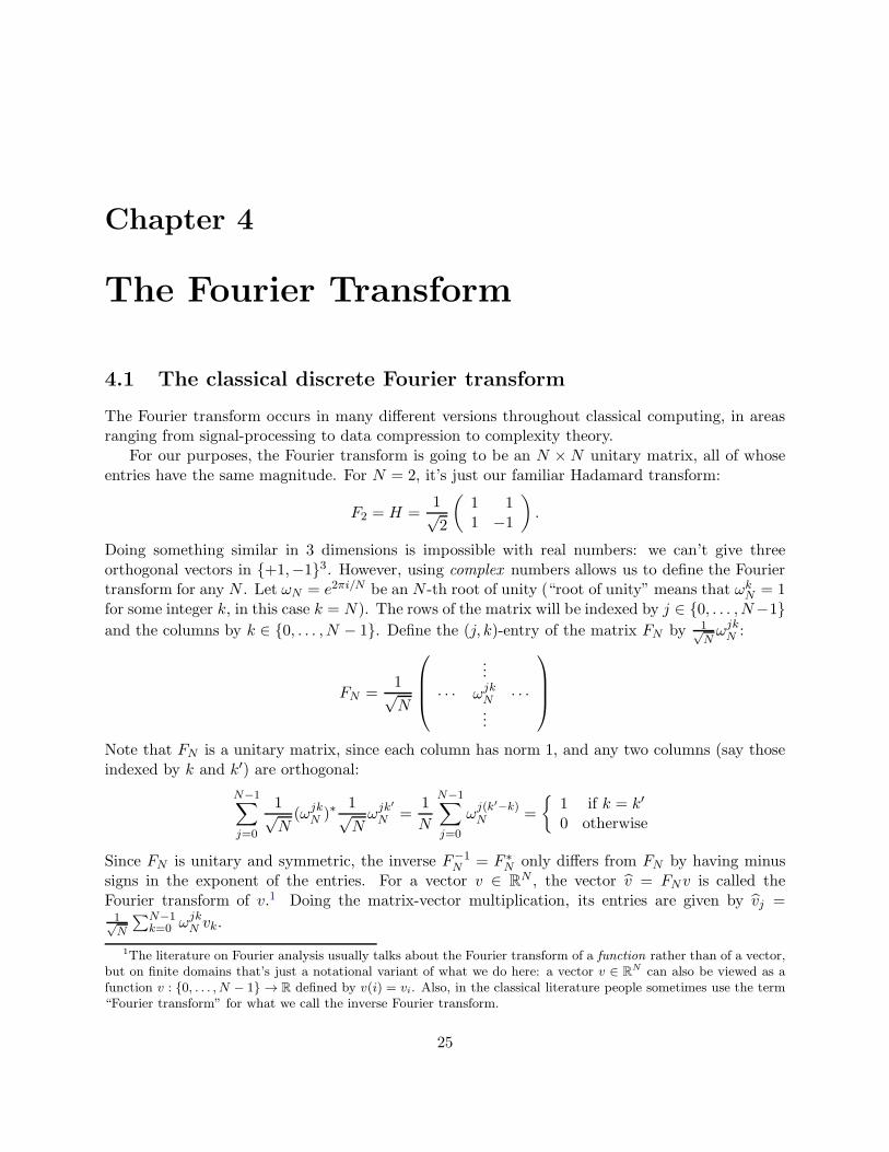
The Fourier transform occurs in many different versions throughout classical computing, in areasranging from signal-processing to data compression to complexity theory.
For our purposes, the Fourier transform is going to be an N ×N unitary matrix, all of whoseentries have the same magnitude. For N = 2, it’s just our familiar Hadamard transform:
F2 = H =1√2
(1 11 −1
).
Doing something similar in 3 dimensions is impossible with real numbers: we can’t give threeorthogonal vectors in +1,−13. However, using complex numbers allows us to define the Fouriertransform for any N . Let ωN = e2πi/N be an N -th root of unity (“root of unity” means that ωk
N = 1for some integer k, in this case k = N). The rows of the matrix will be indexed by j ∈ 0, . . . , N−1and the columns by k ∈ 0, . . . , N − 1. Define the (j, k)-entry of the matrix FN by 1√
NωjkN :
FN =1√N
...
· · · ωjkN · · ·...
Note that FN is a unitary matrix, since each column has norm 1, and any two columns (say thoseindexed by k and k′) are orthogonal:
N−1∑
j=0
1√N
(ωjkN )∗
1√Nωjk′
N =1
N
N−1∑
j=0
ωj(k′−k)N =
1 if k = k′
0 otherwise
Since FN is unitary and symmetric, the inverse F−1N = F ∗
N only differs from FN by having minussigns in the exponent of the entries. For a vector v ∈ RN , the vector v = FNv is called theFourier transform of v.1 Doing the matrix-vector multiplication, its entries are given by vj =1√N
∑N−1k=0 ω
jkN vk.
1The literature on Fourier analysis usually talks about the Fourier transform of a function rather than of a vector,but on finite domains that’s just a notational variant of what we do here: a vector v ∈ RN can also be viewed as afunction v : 0, . . . , N − 1 → R defined by v(i) = vi. Also, in the classical literature people sometimes use the term“Fourier transform” for what we call the inverse Fourier transform.
25
4.2 The Fast Fourier Transform
The naive way of computing the Fourier transform v = FNv of v ∈ RN just does the matrix-vector multiplication to compute all the entries of v. This would take O(N) steps (additions andmultiplications) per entry, and O(N2) steps to compute the whole vector v. However, there is amore efficient way of computing v. This algorithm is called the Fast Fourier Transform (FFT,due to Cooley and Tukey in 1965), and takes only O(N logN) steps. This difference between thequadratic N2 steps and the near-linear N logN is tremendously important in practice when N islarge, and is the main reason that Fourier transforms are so widely used.
We will assume N = 2n, which is usually fine because we can add zeroes to our vector to makeits dimension a power of 2 (but similar FFTs can be given also directly for most N that aren’t apower of 2). The key to the FFT is to rewrite the entries of v as follows:
vj =1√N
N−1∑
k=0
ωjkN vk
=1√N
( ∑
even k
ωjkN vk + ωj
N
∑
odd k
ωj(k−1)N vk
)
=1√2
(1√N/2
∑
even k
ωjk/2N/2 vk + ωj
N
1√N/2
∑
odd k
ωj(k−1)/2N/2 vk
)
Note that we’ve rewritten the entries of the N -dimensional Fourier transform v in terms of twoN/2-dimensional Fourier transforms, one of the even-numbered entries of v, and one of the odd-numbered entries of v.
This suggest a recursive procedure for computing v: first separately compute the Fourier trans-form veven of the N/2-dimensional vector of even-numbered entries of v and the Fourier transformvodd of the N/2-dimensional vector of odd-numbered entries of v, and then compute the N entries
vj =1√2(vevenj + ωj
N voddj).
Strictly speaking this is not well-defined, because veven and vodd are just N/2-dimensional vectors.However, if we define vevenj+N/2 = vevenj (and similarly for vodd) then it all works out.
The time T (N) it takes to implement FN this way can be written recursively as T (N) =2T (N/2) + O(N), because we need to compute two N/2-dimensional Fourier transforms and doO(N) additional operations to compute v. This recursion works out to time T (N) = O(N logN),as promised. Similarly, we have an equally efficient algorithm for the inverse Fourier transformF−1N = F ∗
N , whose entries are 1√Nω−jkN .
4.3 Application: multiplying two polynomials
Suppose we are given two real-valued polynomials p and q, each of degree at most d:
p(x) =
d∑
j=0
ajxj and q(x) =
d∑
k=0
bkxk
26
We would like to compute the product of these two polynomials, which is
(p · q)(x) =
d∑
j=0
ajxj
(
d∑
k=0
bkxk
)=
2d∑
ℓ=0
(
2d∑
j=0
ajbℓ−j
︸ ︷︷ ︸cℓ
)xℓ,
where implicitly we set aj = bj = 0 for j > d and bℓ−j = 0 if j > ℓ. Clearly, each coefficient cℓ byitself takes O(d) steps (additions and multiplications) to compute, which suggests an algorithm forcomputing the coefficients of p ·q that takes O(d2) steps. However, using the fast Fourier transformwe can do this in O(d log d) steps, as follows.
The convolution of two vectors a, b ∈ RN is a vector a ∗ b ∈ RN whose ℓ-th entry is definedby (a ∗ b)ℓ = 1√
N
∑N−1j=0 ajbℓ−jmodN . Let us set N = 2d + 1 (the number of nonzero coefficients
of p · q) and make the above (d + 1)-dimensional vectors of coefficients a and b N -dimensional byadding d zeroes. Then the coefficients of the polynomial p · q are proportional to the entries of theconvolution: cℓ =
√N(a ∗ b)ℓ. It is easy to show that the Fourier coefficients of the convolution of
a and b are the products of the Fourier coefficients of a and b: for every ℓ ∈ 0, . . . , N − 1 we have(a ∗ b
)ℓ= aℓ ·bℓ. This immediately suggests an algorithm for computing the vector of coefficients cℓ:
apply the FFT to a and b to get a and b, multiply those two vectors entrywise to get a ∗ b, applythe inverse FFT to get a∗b, and finally multiply a∗b with
√N to get the vector c of the coefficients
of p · q. Since the FFTs and their inverse take O(N logN) steps, and pointwise multiplication oftwo N -dimensional vectors takes O(N) steps, this algorithm takes O(N logN) = O(d log d) steps.
Note that if two numbers ad · · · a1a0 and bd · · · b1b0 are given in decimal notation, then we caninterpret their digits as coefficients of single-variate degree-d polynomials p and q, respectively:p(x) =
∑dj=0 ajx
j and q(x) =∑d
k=0 bkxk. The two numbers will now be p(10) and q(10). Their
product is the evaluation of the product-polynomial p · q at the point x = 10. This suggests thatwe can use the above procedure (for fast multiplication of polynomials) to multiply two numbers inO(d log d) steps, which would be a lot faster than the standard O(d2) algorithm for multiplicationthat one learns in primary school. However, in this case we have to be careful since the steps of theabove algorithm are themselves multiplications between numbers, which we cannot count at unitcost anymore if our goal is to implement a multiplication between numbers! Still, it turns out thatimplementing this idea carefully allows one to multiply two d-digit numbers in O(d log d log log d)elementary operations. This is known as the Schonhage-Strassen algorithm [96] (slightly improvedfurther by Furer [53]), and is one of the ingredients in Shor’s algorithm in the next chapter. We’llskip the details.
4.4 The quantum Fourier transform
Since FN is an N ×N unitary matrix, we can interpret it as a quantum operation, mapping an N -dimensional vector of amplitudes to another N -dimensional vector of amplitudes. This is called thequantum Fourier transform (QFT). In case N = 2n (which is the only case we will care about), thiswill be an n-qubit unitary. Notice carefully that this quantum operation does something differentfrom the classical Fourier transform: in the classical case we are given a vector v, written on a pieceof paper so to say, and we compute the vector v = FNv, and also write the result on a piece ofpaper. In the quantum case, we are working on quantum states; these are vectors of amplitudes, but
27
we don’t have those written down anywhere—they only exist as the amplitudes in a superposition.We will see below that the QFT can be implemented by a quantum circuit using O(n2) elementarygates. This is exponentially faster than even the FFT (which takes O(N logN) = O(2nn) steps),but it achieves something different: computing the QFT won’t give us the entries of the Fouriertransform written down on a piece of paper, but only as the amplitudes of the resulting state.
4.5 An efficient quantum circuit
Here we will describe the efficient circuit for the n-qubit QFT. The elementary gates we will allowourselves are Hadamards and controlled-Rs gates, where
Rs =
(1 0
0 e2πi/2s
).
Note that R1 = Z =
(1 00 −1
), R2 =
(1 00 i
). For large s, e2πi/2
sis close to 1 and hence
the Rs-gate is close to the identity-gate I. We could implement Rs-gates using Hadamards andcontrolled-R1/2/3 gates, but for simplicity we will just treat each Rs as an elementary gate.
Since the QFT is linear, it suffices if our circuit implements it correctly on basis states |k〉, i.e.,it should map
|k〉 7→ FN |k〉 = 1√N
N−1∑
j=0
ωjkN |j〉.
The key to doing this efficiently is to rewrite FN |k〉, which turns out to be a product state (so FN
does not introduce entanglement when applied to a basis state |k〉). Let |k〉 = |k1 . . . kn〉, k1 beingthe most significant bit. Note that for integer j = j1 . . . jn, we can write j/2n =
∑nℓ=1 jℓ2
−ℓ. Forexample, binary 0.101 is 1·2−1+0·2−2+1·2−3 = 5/8. We have the following sequence of equalities:
FN |k〉 =1√N
N−1∑
j=0
e2πijk/2n |j〉
=1√N
N−1∑
j=0
e2πi(∑n
ℓ=1 jℓ2−ℓ)k|j1 . . . jn〉
=1√N
N−1∑
j=0
n∏
ℓ=1
e2πijℓk/2ℓ |j1 . . . jn〉
=
n⊗
ℓ=1
1√2
(|0〉+ e2πik/2
ℓ |1〉).
Note that e2πik/2ℓ= e2πi0.kn−ℓ+1...kn : the n− ℓ most significant bits of k don’t matter for this value.
As an example, for n = 3 we have the 3-qubit product state
F8|k1k2k3〉 =1√2(|0〉+ e2πi0.k3 |1〉)⊗ 1√
2(|0〉+ e2πi0.k2k3 |1〉)⊗ 1√
2(|0〉+ e2πi0.k1k2k3 |1〉).
This example suggests what the circuit should be. To prepare the first qubit of the desired stateF8|k1k2k3〉, we can just apply a Hadamard to |k3〉, giving state 1√
2(|0〉+(−1)k3 |1〉) and observe that
28
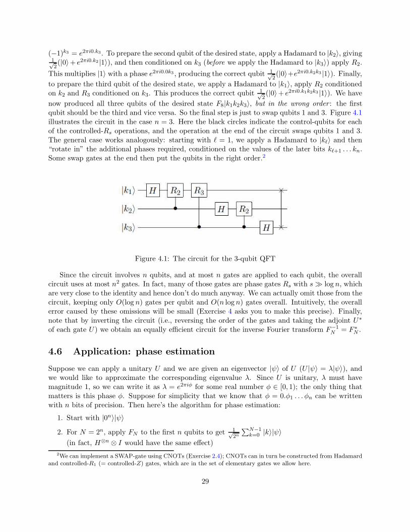
(−1)k3 = e2πi0.k3 . To prepare the second qubit of the desired state, apply a Hadamard to |k2〉, giving1√2(|0〉+ e2πi0.k2 |1〉), and then conditioned on k3 (before we apply the Hadamard to |k3〉) apply R2.
This multiplies |1〉 with a phase e2πi0.0k3 , producing the correct qubit 1√2(|0〉+e2πi0.k2k3 |1〉). Finally,
to prepare the third qubit of the desired state, we apply a Hadamard to |k1〉, apply R2 conditionedon k2 and R3 conditioned on k3. This produces the correct qubit
1√2(|0〉+ e2πi0.k1k2k3 |1〉). We have
now produced all three qubits of the desired state F8|k1k2k3〉, but in the wrong order : the firstqubit should be the third and vice versa. So the final step is just to swap qubits 1 and 3. Figure 4.1illustrates the circuit in the case n = 3. Here the black circles indicate the control-qubits for eachof the controlled-Rs operations, and the operation at the end of the circuit swaps qubits 1 and 3.The general case works analogously: starting with ℓ = 1, we apply a Hadamard to |kℓ〉 and then“rotate in” the additional phases required, conditioned on the values of the later bits kℓ+1 . . . kn.Some swap gates at the end then put the qubits in the right order.2
Figure 4.1: The circuit for the 3-qubit QFT
Since the circuit involves n qubits, and at most n gates are applied to each qubit, the overallcircuit uses at most n2 gates. In fact, many of those gates are phase gates Rs with s≫ log n, whichare very close to the identity and hence don’t do much anyway. We can actually omit those from thecircuit, keeping only O(log n) gates per qubit and O(n log n) gates overall. Intuitively, the overallerror caused by these omissions will be small (Exercise 4 asks you to make this precise). Finally,note that by inverting the circuit (i.e., reversing the order of the gates and taking the adjoint U∗
of each gate U) we obtain an equally efficient circuit for the inverse Fourier transform F−1N = F ∗
N .
4.6 Application: phase estimation
Suppose we can apply a unitary U and we are given an eigenvector |ψ〉 of U (U |ψ〉 = λ|ψ〉), andwe would like to approximate the corresponding eigenvalue λ. Since U is unitary, λ must havemagnitude 1, so we can write it as λ = e2πiφ for some real number φ ∈ [0, 1); the only thing thatmatters is this phase φ. Suppose for simplicity that we know that φ = 0.φ1 . . . φn can be writtenwith n bits of precision. Then here’s the algorithm for phase estimation:
1. Start with |0n〉|ψ〉
2. For N = 2n, apply FN to the first n qubits to get 1√2n
∑N−1k=0 |k〉|ψ〉
(in fact, H⊗n ⊗ I would have the same effect)
2We can implement a SWAP-gate using CNOTs (Exercise 2.4); CNOTs can in turn be constructed from Hadamardand controlled-R1 (= controlled-Z) gates, which are in the set of elementary gates we allow here.
29
3. Apply the map |k〉|ψ〉 7→ |k〉Uk|ψ〉 = e2πiφk|k〉|ψ〉. In other words, apply U to the secondregister for a number of times given by the first register.
4. Apply the inverse Fourier transform F−1N to the first n qubits and measure the result.
Note that after step 3, the first n qubits are in state 1√N
∑N−1k=0 e
2πiφk|k〉 = FN |2nφ〉, hence the
inverse Fourier transform is going to give us |2nφ〉 = |φ1 . . . φn〉 with probability 1.In case φ cannot be written exactly with n bits of precision, one can show that this procedure
still (with high probability) spits out a good n-bit approximation to φ. We’ll omit the calculation.
Exercises
1. For ω = e2πi/3 and F3 =1√3
1 1 11 ω ω2
1 ω2 ω
, calculate F3
010
and F3
1ω2
ω
2. Prove that the Fourier coefficients of the convolution of vectors a and b are the product ofthe Fourier coefficients of a and b. In other words, prove that for every a, b ∈ RN and every
ℓ ∈ 0, . . . , N − 1 we have(a ∗ b
)ℓ= aℓ · bℓ. Here the Fourier transform a is defined as the
vector FNa, and the ℓ-entry of the convolution-vector a∗b is (a∗b)ℓ = 1√N
∑N−1j=0 ajbℓ−jmodN .
3. The Euclidean distance between two states |φ〉 =∑
i αi|i〉 and |ψ〉 =∑
i βi|i〉 is defined as‖|φ〉 − |ψ〉‖ =
√∑i |αi − βi|2. Assume the states are unit vectors with (for simplicity) real
amplitudes. Suppose the distance is small: ‖|φ〉 − |ψ〉‖ = ǫ. Show that then the probabilitiesresulting from a measurement on the two states are also close: the “total variation distance”between the distributions is 1
2
∑i
∣∣α2i − β2i
∣∣ ≤ ǫ (this implies that for every possible event E,the probabilities of E under the two distributions differ by at most ε).
4. The operator norm of a matrix A is defined as ‖A‖ = maxv:‖v‖=1
‖Av‖.The distance between two matrices A and B is defined as ‖A−B‖.
(a) What is the distance between the 2× 2 identity matrix and the phase-gate
(1 00 eiφ
)?
(b) Suppose we have a product of n-qubit unitaries U = UTUT−1 · · ·U1 (for instance, each Ui
could be an elementary gate on a few qubits, tensored with identity on the other qubits).Suppose we drop the j-th gate from this sequence: U ′ = UTUT−1 · · ·Uj+1Uj−1 · · ·U1.Show that ‖U ′ − U‖ = ‖I − Uj‖.
(c) Suppose we also drop the k-th unitary: U ′′ = UTUT−1 · · ·Uj+1Uj−1 · · · · · ·Uk+1Uk−1 · · ·U1.Show that ‖U ′′ − U‖ ≤ ‖I − Uj‖+ ‖I − Uk‖.
(d) Give a quantum circuit with O(n log n) elementary gates that has distance less than 1/nfrom the Fourier transform F2n .
5. Suppose a ∈ RN is a vector which is r-periodic in the following sense: there exists an integerr such that aℓ = 1 whenever ℓ is an integer multiple of r, and aℓ = 0 otherwise. Compute theFourier transform FN a of this vector, i.e., write down a formula for the entries of the vectorFNa. Assuming r divides N and r ≪ N , write down a simple closed form for the formula forthe entries. What are the entries with largest magnitude in the vector FN a?
30
Chapter 5
Shor’s Factoring Algorithm
5.1 Factoring
Probably the most important quantum algorithm so far is Shor’s factoring algorithm [100]. It canfind a factor of a composite number N in roughly (logN)2 steps, which is polynomial in the lengthlogN of the input. On the other hand, there is no known classical (deterministic or randomized)algorithm that can factor N in polynomial time. The best known classical randomized algorithmsrun in time roughly
2(logN)α ,
where α = 1/3 for a heuristic upper bound [76] and α = 1/2 for a rigorous upper bound [77].In fact, much of modern cryptography is based on the conjecture that no fast classical factoringalgorithm exists [94]. All this cryptography (for example RSA) would be broken if Shor’s algorithmcould be physically realized. In terms of complexity classes: factoring (rather, the decision problemequivalent to it) is provably in BQP but is not known to be in BPP. If indeed factoring is notin BPP, then the quantum computer would be the first counterexample to the “strong” Church-Turing thesis, which states that all “reasonable” models of computation are polynomially equivalent(see [46] and [90, p.31,36]).
5.2 Reduction from factoring to period-finding
The crucial observation of Shor was that there is an efficient quantum algorithm for the problemof period-finding and that factoring can be reduced to this, in the sense that an efficient algorithmfor period-finding implies an efficient algorithm for factoring.
We first explain the reduction. Suppose we want to find factors of the composite number N > 1.We may assume N is odd and not a prime power, since those cases can easily be filtered out by aclassical algorithm. Now randomly choose some integer x ∈ 2, . . . , N − 1 which is coprime to N .If x is not coprime to N , then the greatest common divisor of x and N is a nontrivial factor of N ,so then we are already done. From now on consider x and N are coprime, so x is an element of themultiplicative group Z∗
N . Consider the sequence
1 = x0 (mod N), x1 (mod N), x2 (mod N), . . .
This sequence will cycle after a while: there is a least 0 < r ≤ N such that xr = 1 (mod N). Thisr is called the period of the sequence (a.k.a. the order of the element x in the group Z∗
N ). Assuming
31
N is odd and not a prime power (those cases are easy to factor anyway), it can be shown that withprobability ≥ 1/2, the period r is even and xr/2 + 1 and xr/2 − 1 are not multiples of N .1 In thatcase we have:
xr ≡ 1 mod N ⇐⇒(xr/2)2 ≡ 1 mod N ⇐⇒
(xr/2 + 1)(xr/2 − 1) ≡ 0 mod N ⇐⇒(xr/2 + 1)(xr/2 − 1) = kN for some k.
Note that k > 0 because both xr/2 + 1 > 0 and xr/2 − 1 > 0 (x > 1). Hence xr/2 + 1 or xr/2 − 1will share a factor with N . Because xr/2 + 1 and xr/2 − 1 are not multiples of N this factor willbe < N , and in fact both these numbers will share a non-trivial factor with N . Accordingly, if wehave r then we can compute the greatest common divisors2 gcd(xr/2 + 1, N) and gcd(xr/2 − 1, N),and both of these two numbers will be non-trivial factors of N . If we are unlucky we might havechosen an x that does not give a factor (which we can detect efficiently), but trying a few differentrandom x gives a high probability of finding a factor.
Thus the problem of factoring reduces to finding the period r of the function given by modularexponentiation f(a) = xa mod N . In general, the period-finding problem can be stated as follows:
The period-finding problem:We are given some function f : N → [N ] with the property that there is some unknown r ∈ [N ]such that f(a) = f(b) iff a = b mod r. The goal is to find r.
We will show below how we can solve this problem efficiently, using O(log logN) evaluations off and O(log logN) quantum Fourier transforms. An evaluation of f can be viewed as analogousto the application of a query in the previous algorithms. Even a somewhat more general kind ofperiod-finding can be solved by Shor’s algorithm with very few f -evaluations, whereas any classicalbounded-error algorithm would need to evaluate the function Ω(N1/3/
√logN) times in order to
find the period [34].How many steps (elementary gates) does Shor’s algorithm take? For a = NO(1), we can
compute f(a) = xa mod N in O((logN)2 log logN log log logN) steps, as follows. First com-pute x2 mod N,x4 mod N,x8 mod N, . . . by repeated squaring3 Second, write a in binary asa =
∑i≥0 ai2
i and observe that xa =∏
i≥0 xai2
i=∏
i:ai=1 x2i . Hence multiplying together some of
the numbers produced in the first step (mod N) gives us f(a).
1For those familiar with basic number theory, here is a proof for the special case where N = p1p2 is the productof two distinct primes p1 and p2; for the general case see [89, Theorem A4.13]. By the Chinese remainder theorem,choosing a uniformly random x mod N is equivalent to choosing, independently and uniformly at random, an x1
mod p1 and an x2 mod p2. Let r be the period of the sequence (xa mod N)a, and (for i ∈ 1, 2) let ri be the periodof the sequence (xa
i mod pi)a. Because (xi, 1) generates a size-ri subgroup of the size-r group generated by (x1, x2),Lagrange’s Theorem implies that ri divides r. Hence if r is odd then both r1 and r2 must be odd. The probabilitythat ri is odd is 1/2, because the group of numbers mod pi is cyclic and of even size, so half of its elements are squares.Hence the probability that r is odd, is at most (1/2)2 = 1/4. If r is even, then xr/2 6= 1 mod N , for otherwise theperiod would be at most r/2. If xr/2 = −1 mod N , then xr/2 = −1 mod p1 and mod p2, which has probability atmost (1/2)2 = 1/4. Hence Pr[r is odd or xr/2 = 1 or xr/2 = −1] ≤ Pr[r is odd] + Pr[xr/2 = −1] ≤ 1
4+ 1
4= 1
2.
2The greatest common divisor of two integers a and b is the largest positive integer c that divides both a and b.If gcd(a, b) = 1 then a and b are called coprime. The gcd can be computed efficiently (in time roughly linear in thenumber of bits of a and b) on a classical computer by Euclid’s algorithm.
3Using the Schonhage-Strassen algorithm for fast multiplication [96, 73], see Exercise 1. We could also use themore recent improvement of Furer [53], who removes most of the log logN factor.
32
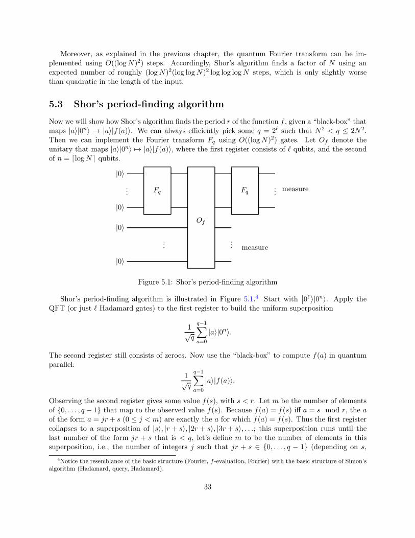
Moreover, as explained in the previous chapter, the quantum Fourier transform can be im-plemented using O((logN)2) steps. Accordingly, Shor’s algorithm finds a factor of N using anexpected number of roughly (logN)2(log logN)2 log log logN steps, which is only slightly worsethan quadratic in the length of the input.
5.3 Shor’s period-finding algorithm
Now we will show how Shor’s algorithm finds the period r of the function f , given a “black-box” thatmaps |a〉|0n〉 → |a〉|f(a)〉. We can always efficiently pick some q = 2ℓ such that N2 < q ≤ 2N2.Then we can implement the Fourier transform Fq using O((logN)2) gates. Let Of denote theunitary that maps |a〉|0n〉 7→ |a〉|f(a)〉, where the first register consists of ℓ qubits, and the secondof n = ⌈logN⌉ qubits.
|0〉...
|0〉
|0〉
|0〉
measure
measure
...Fq
......
Of
Fq
Figure 5.1: Shor’s period-finding algorithm
Shor’s period-finding algorithm is illustrated in Figure 5.1.4 Start with∣∣0ℓ⟩|0n〉. Apply the
QFT (or just ℓ Hadamard gates) to the first register to build the uniform superposition
1√q
q−1∑
a=0
|a〉|0n〉.
The second register still consists of zeroes. Now use the “black-box” to compute f(a) in quantumparallel:
1√q
q−1∑
a=0
|a〉|f(a)〉.
Observing the second register gives some value f(s), with s < r. Let m be the number of elementsof 0, . . . , q − 1 that map to the observed value f(s). Because f(a) = f(s) iff a = s mod r, the aof the form a = jr+ s (0 ≤ j < m) are exactly the a for which f(a) = f(s). Thus the first registercollapses to a superposition of |s〉, |r + s〉, |2r + s〉, |3r + s〉, . . .; this superposition runs until thelast number of the form jr + s that is < q, let’s define m to be the number of elements in thissuperposition, i.e., the number of integers j such that jr + s ∈ 0, . . . , q − 1 (depending on s,
4Notice the resemblance of the basic structure (Fourier, f -evaluation, Fourier) with the basic structure of Simon’salgorithm (Hadamard, query, Hadamard).
33
this m will be ⌈q/r⌉ or ⌊q/r⌋). The second register collapses to the classical state |f(s)〉. We cannow ignore the second register, and have in the first:
1√m
m−1∑
j=0
|jr + s〉.
Applying the QFT again gives
1√m
m−1∑
j=0
1√q
q−1∑
b=0
e2πi (jr+s)b
q |b〉 = 1√mq
q−1∑
b=0
e2πi sb
q
m−1∑
j=0
e2πi jrb
q
|b〉.
We want to see which |b〉 have large squared amplitudes—those are the b we are likely to see if wenow measure. Using that
∑m−1j=0 zj = (1− zm)/(1 − z) for z 6= 1 (see Appendix B), we compute:
m−1∑
j=0
e2πijrbq =
m−1∑
j=0
(e2πi
rbq
)j=
m if e2πi rb
q = 1
1−e2πimrb
q
1−e2πi rbq
if e2πi rb
q 6= 1(5.1)
Easy case: r divides q. Let us do an easy case first. Suppose r divides q, so the whole period“fits” an integer number of times in the domain 0, . . . , q− 1 of f , and m = q/r. For the first caseof Eq. (5.1), note that e2πirb/q = 1 iff rb/q is an integer iff b is a multiple of q/r. Such b will havesquared amplitude equal to (m/
√mq)2 = m/q = 1/r. Since there are exactly r such b, together
they have all the amplitude. Thus we are left with a superposition where only the b that are integermultiples of q/r have non-zero amplitude. Observing this final superposition gives some randommultiple b = cq/r, with c a random number 0 ≤ c < r. Thus we get a b such that
b
q=c
r,
where b and q are known to the algorithm, and c and r are not. There are φ(r) ∈ Ω(r/ log log r)numbers smaller than r that are coprime to r [61, Theorem 328], so c will be coprime to r withprobability Ω(1/ log log r). Accordingly, an expected number of O(log logN) repetitions of theprocedure of this section suffices to obtain a b = cq/r with c coprime to r.5 Once we have such ab, we can obtain r as the denominator by writing b/q in lowest terms.
Hard case: r does not divide q. Because our q is a power of 2, it is actually quite likely thatr does not divide q. However, the same algorithm will still yield with high probability a b whichis close to a multiple of q/r. Note that q/r is no longer an integer, and m = ⌊q/r⌋, possibly +1.All calculations up to and including Eq. (5.1) are still valid. Using |1 − eiθ| = 2| sin(θ/2)|, we canrewrite the absolute value of the second case of Eq. (5.1) to
|1− e2πimrbq |
|1− e2πi rb
q |=
| sin(πmrb/q)|| sin(πrb/q)| .
5The number of required f -evaluations for period-finding can actually be reduced from O(log logN) to O(1).
34
The right-hand side is the ratio of two sine-functions of b, where the numerator oscillates muchfaster than the denominator because of the additional factor of m. Note that the denominator isclose to 0 (making the ratio large) iff b is close to an integer multiple of q/r. For most of those b,the numerator won’t be close to 0. Hence, roughly speaking, the ratio will be small if b is far froman integer multiple of q/r, and large for most b that are close to a multiple of q/r. Doing thecalculation precisely, one can show that with high probability the measurement yields a b such that
∣∣∣∣b
q− c
r
∣∣∣∣ ≤1
2q.
As in the easy case, b and q are known to us while c and r are unknown.Two distinct fractions, each with denominator ≤ N , must be at least 1/N2 > 1/q apart.6
Therefore c/r is the only fraction with denominator ≤ N at distance ≤ 1/2q from b/q. Applying aclassical method called “continued-fraction expansion” to b/q efficiently gives us the fraction withdenominator ≤ N that is closest to b/q (see the next section). This fraction must be c/r. Again,with good probability c and r will be coprime, in which case writing c/r in lowest terms gives us r.
5.4 Continued fractions
Let [a0, a1, a2, . . .] (finite or infinite) denote
a0 +1
a1 +1
a2+1...
This is called a continued fraction (CF). The ai are the partial quotients. We assume these to bepositive natural numbers ([61, p.131] calls such CF “simple”). [a0, . . . , an] is the nth convergent ofthe fraction. [61, Theorem 149 & 157] gives a simple way to compute numerator and denominatorof the nth convergent from the partial quotients:
Ifp0 = a0, p1 = a1a0 + 1, pn = anpn−1 + pn−2
q0 = 1, q1 = a1, qn = anqn−1 + qn−2
then [a0, . . . , an] =pnqn
. Moreover, this fraction is in lowest terms.
Note that qn increases at least exponentially with n (qn ≥ 2qn−2). Given a real number x, thefollowing “algorithm” gives a continued fraction expansion of x [61, p.135]:
a0 := ⌊x⌋, x1 := 1/(x− a0)a1 := ⌊x1⌋, x2 := 1/(x− a1)a2 := ⌊x2⌋, x3 := 1/(x− a2). . .
Informally, we just take the integer part of the number as the partial quotient and continue with theinverse of the decimal part of the number. The convergents of the CF approximate x as follows [61,Theorem 164 & 171]:
6Consider two fractions z = x/y and z′ = x′/y′ with y, y′ ≤ N . If z 6= z′ then |xy′ − x′y| ≥ 1, and hence|z − z′| = |(xy′ − x′y)/yy′| ≥ 1/|yy′| ≥ 1/N2.
35
If x = [a0, a1, . . .] then
∣∣∣∣x− pnqn
∣∣∣∣ <1
q2n.
Recall that qn increases exponentially with n, so this convergence is quite fast. Moreover, pn/qnprovides the best approximation of x among all fractions with denominator ≤ qn [61, Theorem 181]:
If n > 1, q ≤ qn, p/q 6= pn/qn, then
∣∣∣∣x− pnqn
∣∣∣∣ <∣∣∣∣x− p
q
∣∣∣∣.
Exercises
1. This exercise is about efficient classical implementation of modular exponentiation.
(a) Given n-bit numbers x and N (where n = ⌈log2N⌉), compute the whole sequencex0 mod N, x1 mod N , x2 mod N , x4 mod N , x8 mod N ,x16 mod N, . . . , x2
n−1mod N ,
using O(n2 log(n) log log(n)) steps.
(b) Suppose n-bit number a can be written as a = an−1 . . . a1a0 in binary. Express xa modN as a product of the numbers computed in part (a).
(c) Show that you can compute f(a) = xa mod N in O(n2 log(n) log log(n)) steps.
2. Use Shor’s algorithm to find the period of the function f(a) = 7a mod 10, using a Fouriertransform over q = 128 elements. Write down all intermediate superpositions of the algorithmfor this case (don’t just copy the general expressions from the notes). You may assume you’relucky, meaning the first run of the algorithm already gives a b = cq/r with c coprime to r.
3. This exercise explains basic RSA encryption. Suppose Alice wants to allow other people tosend encrypted messages to her, such that she is the only one who can decrypt them. Shebelieves that factoring an n-bit number can’t be done efficiently (efficient = in time polynomialin n). So in particular, she doesn’t believe in quantum computing.
Alice chooses two large random prime numbers, p and q, and computes their product N =p · q (a typical size is to have N a number of n = 1024 bits, which corresponds to bothp and q being numbers of roughly 512 bits). She computes the so-called Euler φ-function:φ(N) = (p − 1)(q − 1); she also chooses an encryption exponent e, which doesn’t share anynontrivial factor with φ(N) (i.e., e and φ(N) are coprime). Group theory guarantees there isan efficiently computable decryption exponent d such that de = 1 mod φ(N). The public keyconsists of e and N (Alice puts this on her homepage), while the secret key consists of d and N .Any number m ∈ 1, . . . , N − 1 that is coprime to N , can be used as a message. There areφ(N) such m, and these numbers form a group under the operation of multiplication mod N .The number of bits n = ⌈log2N⌉ of N is the maximal length (in bits) of a message m andalso the length (in bits) of the encryption. The encryption function is defined as C(m) = me
mod N , and the decryption function is D(c) = cd mod N .
(a) Give a randomized algorithm by which Alice can efficiently generate the secret and publickey.
(b) Show that Bob can efficiently compute the encoding C(m) of the message m that hewants to send to Alice, knowing the public key but not the private key.
(c) Show that D(C(m)) = m for all possible messages.
36
(d) Show that Alice can efficiently decrypt the encryption C(m) she receives from Bob.
(e) Show that if Charlie could factor N , then he could efficiently decrypt Bob’s message.
37

38
Chapter 6
Hidden Subgroup Problem
6.1 Hidden Subgroup Problem
6.1.1 Group theory reminder
A group G consists of a set of elements (which is usually denoted by G as well) and an operation : G×G→ G (often written as addition or multiplication), such that
1. the operation is associative: g (h k) = (g h) k for all g, h, k ∈ G;
2. there is an identity element e ∈ G satisfying e g = g e = g for every g ∈ G;
3. and every g ∈ G has an inverse g−1 ∈ G, such that g g−1 = g−1 g = e (if the groupoperation is written as addition, then g−1 is written as −g).
We often abbreviate g h to gh. The group is Abelian (or commutative) if gh = hg for all g, h ∈ G.Simple examples of finite additive Abelian groups are G = 0, 1n with bitwise addition mod 2as the group operation, and G = ZN , the “cyclic group” of integers mod N . The set G = Z∗
N isthe multiplicative group consisting of all integers in 1, . . . , N − 1 that are coprime to N , withmultiplication mod N as the group operation.1 An important example of a non-Abelian group isthe “symmetric group” Sn, which is the group of n! permutations of n elements, using compositionas the group operation.
A subgroup H of G, denoted H ≤ G, is a subset of G that is itself a group, i.e., it contains eand is closed under taking products and inverses. A (left) coset of H is a set gH = gh | h ∈ H,i.e., a translation of H by the element g. All cosets of H have size |H|, and it is easy to show thattwo cosets gH and g′H are either equal or disjoint, so the set of cosets partitions G into equal-sizedparts.2 Note that g and g′ are in the same coset of H iff g−1g′ ∈ H.
If T ⊆ G, then we use 〈T 〉 to denote the set of elements of G that we can write as products ofelements from T and their inverses. This H = 〈T 〉 is a subgroup of G, and T is called a generatingset of H. Note that adding one more element t 6∈ 〈T 〉 to T at least doubles the size of the generatedsubgroup, because H and tH are disjoint and H ∪ tH ⊆ 〈T ∪ t〉. This implies that every H ≤ Ghas a generating set of size ≤ log |H| ≤ log |G|. We abbreviate 〈γ〉 to 〈γ〉, which is the cyclicgroup generated by γ; every cyclic group of size N is isomorphic to ZN .
1This group Z∗N is isomorphic to the additive group Zφ(N), where Euler’s φ-function counts the elements of
1, . . . , N − 1 that are coprime to N . For example, Z∗p is isomorphic to Zp−1.
2This also proves Lagrange’s theorem for finite groups: if H ≤ G then |H | divides |G|.
39
6.1.2 Definition and some instances of the HSP
The Hidden Subgroup Problem is the following:
Given a known group G and a function f : G→ S where S is some finite set.Suppose f has the property that there exists a subgroup H ≤ G such that f is constantwithin each coset, and distinct on different cosets: f(g) = f(g′) iff gH = g′H.Goal: find H.
We assume f can be computed efficiently, meaning in time polynomial in log |G| (the latter is thenumber of bits needed to describe an input g ∈ G for f). Since H may be large, “finding H”typically means finding a generating set for H.
This looks like a rather abstract algebraic problem, but many important problems can be writtenas an instance of the HSP. We will start with some examples where G is Abelian.
Simon’s problem. This is a very natural instance of HSP. Here G is the additive group Zn2 =
0, 1n of size 2n, H = 0, s for a “hidden” s ∈ 0, 1n, and f satisfies f(x) = f(y) iff x− y ∈ H.Clearly, finding the generator of H (i.e., finding s) solves Simon’s problem.
Period-finding. As we saw in Chapter 5, we can factor a large number N if we can solve thefollowing: given an x that is coprime toN and associated function f : Z → Z∗
N by f(a) = xa modN ,find the period r of f .3 Since 〈x〉 is a size-r subgroup of the group Z∗
N , the period r divides|Z∗
N | = φ(N). Hence we can restrict the domain of f to Zφ(N).
Period-finding is an instance of the HSP as follows. Let G = Zφ(N) and consider its subgroupH = 〈r〉 of all multiples of r up to φ(N) (i.e., H = rZφ(N) = 0, r, 2r, . . . , φ(N) − r). Note thatbecause of its periodicity, f is constant on each coset s+H of H, and distinct on different cosets.Also, f is efficiently computable by repeated squaring. Since the hidden subgroup H is generatedby r, finding the generator of H solves the period-finding problem.
Discrete logarithm. Another problem often used in classical public-key cryptography is thediscrete logarithm problem: given a generator γ of a cyclic multiplicative group C of size N (soC = γa | a ∈ 0, . . . , N − 1), and A ∈ C, can we find the unique a ∈ 0, 1, . . . , N − 1 such thatγa = A? This a is called the discrete logarithm of A (w.r.t. generator γ). It is generally believedthat classical computers need time roughly exponential in logN to compute a from A (and onecan actually prove this in a model where we can only implement group operations via some “black-box”). This assumption underlies for instance the security of Diffie-Hellman key exchange (whereC = Z∗
p for some large prime p, see Exercise 3), as well as elliptic-curve cryptography.
Discrete log is an instance of the HSP as follows. We take G = ZN × ZN and define functionf : G → C by f(x, y) = γxA−y, which is efficiently computable by repeated squaring. For groupelements g1 = (x1, y1), g2 = (x2, y2) ∈ G we have
f(g1) = f(g2) ⇐⇒ γx1−ay1 = γx2−ay2 ⇐⇒ (x1 − x2) = a(y1 − y2) mod N ⇐⇒ g1 − g2 ∈ 〈(a, 1)〉.
Let H be the subgroup of G generated by the element (a, 1), then we have an instance of the HSP.Finding the generator of the hidden subgroup H gives us a, solving the discrete log problem.
3This r is also known as the order of the element x in the group Z∗N , so this problem is also known as order-finding.
40
6.2 An efficient quantum algorithm if G is Abelian
In this section we show that HSPs where G (and hence H) is Abelian, and where f is efficientlycomputable, can be solved efficiently by a quantum algorithm. This generalizes Shor’s factoringalgorithm, and will also show that discrete logarithms can be computed efficiently.
6.2.1 Representation theory and the quantum Fourier transform
We start by explaining the basics of representation theory. The idea here is to replace groupelements by matrices, so that linear algebra can be used as a tool in group theory. A d-dimensionalrepresentation of a multiplicative group G is a map ρ : g 7→ ρ(g) from G to the set of d×d invertiblecomplex matrices, satisfying ρ(gh) = ρ(g)ρ(h) for all g, h ∈ G. The latter property makes the map ρa homomorphism. It need not be an isomorphism; for example, the constant-1 function is a trivialrepresentation of any group. The character corresponding to ρ is the map χρ : G → C defined byχρ(g) = Tr(ρ(g)).
Below we restrict attention to the case where G is Abelian (and usually finite). In this casewe may assume the dimension d to be 1 without loss of generality, so a representation ρ and thecorresponding character χρ are just the same function. Also, it is easy to see that the complexvalues χρ(g) have modulus 1, because |χρ(g
k)| = |χρ(g)|k for all integers k. The “Basis Theorem” ofgroup theory says that every finite Abelian group G is isomorphic to a direct product ZN1×· · ·×ZNk
of cyclic groups. First consider just one cyclic group ZN , written additively. Consider the discreteFourier transform (Chapter 4), which is an N × N matrix. Ignoring the normalizing factor of
1/√N , its kth column may be viewed as a map χk : ZN → C defined by χk(j) = ωjk
N , whereωN = e2πi/N . Note that χk(j + j′) = χk(j)χk(j
′), so χk is actually a 1-dimensional representation(i.e., a character function) of ZN . In fact, the N characters corresponding to the N columns ofthe Fourier matrix are all the characters of ZN . For Abelian groups G that are (isomorphic to) aproduct ZN1×· · ·×ZNk
of cyclic groups, the |G| = N1 · · ·Nk characters are just the products of thecharacters of the individual cyclic groups ZNj . Note that the characters are pairwise orthogonal.
The set of all characters of G forms a group G with the operation of pointwise multiplication.This is called the dual group of G. If H ≤ G, then the following is a subgroup of G of size |G|/|H|:
H⊥ = χk | χk(h) = 1 for all h ∈ H.Let us interpret the quantum Fourier transform in terms of the characters. For k ∈ ZN , define thestate whose entries are the (normalized) values of χk:
|χk〉 =1√N
N−1∑
j=0
χk(j)|j〉 =1√N
N−1∑
j=0
ωjkN |j〉.
With this notation, the QFT just maps the standard (computational) basis of CN to the orthonor-mal basis corresponding to the characters:
FN : |k〉 7→ |χk〉.As we saw in Chapter 4, this map can be implemented by an efficient quantum circuit if N is apower of 2. The QFT corresponding to a group G that is isomorphic to ZN1 × · · · ×ZNk
is just thetensor product of the QFTs for the individual cyclic groups. For example, the QFT correspondingto Z2 is the Hadamard gate H, so the QFT corresponding to Zn
2 is H⊗n (which is of course verydifferent from the QFT corresponding to Z2n).
41
6.2.2 A general algorithm for Abelian HSP
The following is an efficient quantum algorithm for solving the HSP for some Abelian group G(written additively) and function f : G → S. This algorithm, sometimes called the “standardalgorithm” for HSP, was first observed by Kitaev [70] (inspired by Shor’s algorithm) and workedout further by many, for instance Mosca and Ekert [85].
1. Start with |0〉|0〉, where the two registers have dimension |G| and |S|, respectively.
2. Create a uniform superposition over G in the first register:1√|G|
∑
g∈G|g〉|0〉.
3. Compute f in superposition:1√|G|
∑
g∈G|g〉|f(g)〉.
4. Measure the second register. This yields some value f(s) for unknown s ∈ G. The firstregister collapses to a superposition over the g with the same f -value as s (i.e., the coset
s+H):1√|H|
∑
h∈H|s+ h〉.
5. Apply the QFT corresponding to G to this state, giving1√|H|
∑
h∈H|χs+h〉.
6. Measure and output the resulting g.
The key to understanding this algorithm is to observe that step 5 maps the uniform superpositionover the coset s+H to a uniform superposition over the labels of H⊥:
1√|H|
∑
h∈H|χs+h〉 =
1√|H||G|
∑
h∈H
∑
g∈Gχs+h(g)|g〉
=1√
|H||G|∑
g∈Gχs(g)
∑
h∈Hχh(g)|g〉 =
√|H||G|
∑
g:χg∈H⊥
χs(g)|g〉,
where the last equality follows from the orthogonality of characters of the group H (note that χg
restricted to H is a character of H, and it’s the constant-1 character iff χg ∈ H⊥):
∑
h∈Hχh(g) =
∑
h∈Hχg(h) =
|H| if χg ∈ H⊥
0 if χg 6∈ H⊥
The phases χs(g) do not affect the probabilities of the final measurement, since |χs(g)|2 = 1. Theabove algorithm thus samples uniformly from the (labels of) elements of H⊥. Each such elementχg ∈ H⊥ gives us a constraint on H because χg(h) = 1 for all h ∈ H.4 Generating a small numberof such elements will give sufficient information to find the generators of H itself. Consider ourearlier examples of Abelian HSP:
4This is a linear constraint mod N . For example, say G = ZN1 × ZN2 , and g = (g1, g2) is the label of an elementof H⊥. Then 1 = χg(h) = ωg1h1
N1ωg2h2N2
for all h = (h1, h2) ∈ H , equivalently g1h1N2 + g2h2N1 = 0 mod N .
42
Simon’s problem. Recall that G = Zn2 = 0, 1n and H = 0, s for the HSP corresponding to
Simon’s problem. Setting up the uniform superposition over G can be done by applying H⊗n to theinitial state |0n〉 of the first register. The QFT corresponding to G is just H⊗n. The 2n characterfunctions are χg(x) = (−1)x·g. The algorithm will uniformly sample from labels of elements of
H⊥ = χg | χg(h) = 1 for all h ∈ H = χg | g · s = 0.
Accordingly, the algorithm samples uniformly from the g ∈ 0, 1n such that g · s = 0 (mod 2).Doing this an expected O(n) times gives n− 1 linearly independent equations about s, from whichwe can find s using Gaussian elimination.
Period-finding. For the HSP corresponding to period-finding, G = Zφ(N) and H = 〈r〉, and
H⊥ = χb | e2πibh/φ(N) = 1 for all h ∈ H = χb | br/φ(N) ∈ 0, . . . , r − 1.
Accordingly, the output of the algorithm is an integer multiple b = cφ(N)/r of φ(N)/r, for uniformlyrandom c ∈ 0, . . . , r − 1.
Notice that the algorithm doesn’t actually know φ(N), which creates two problems. First, ofthe 4 numbers b, c, φ(N), r involved in the equation b = cφ(N)/r we only know the measurementoutcome b, which is not enough to compute r. Second, step 5 of the algorithm wants to do aQFT corresponding to the group Zφ(N) but it doesn’t know φ(N) (and even if we knew φ(N),we’ve only seen how to efficiently do a QFT over Zq when q is a power of 2). Fortunately, if weactually use the QFT over Zq for q a power of 2 that is roughly N2 (and in step 1 set up a uniformsuperposition over Zq instead of G), then one can show that the above algorithm still works, withhigh probability yielding a number b that’s close to an integer multiple of q/r.5 This is basicallyjust Shor’s algorithm as described in Chapter 5.
Discrete logarithm. For the HSP corresponding to the discrete log problem, whereG = ZN×ZN
and H = 〈(a, 1)〉, a small calculation shows that H⊥ = χ(c,−ac) | c ∈ ZN (see Exercise 2). Hence
sampling from H⊥ yields some label (c,−ac) ∈ G of an element of H⊥, from which we can computethe discrete logarithm a. The QFT corresponding to G is FN ⊗ FN , which we don’t know how toimplement efficiently, but which we can replace by Fq ⊗ Fq for some power-of-2 q somewhat largerthan N .
In the above algorithm we assumed G is a finite Abelian group. These techniques have been muchextended to the case of infinite groups such as G = Z and even Rd, to obtain efficient quantumalgorithms for problems like Pell’s equation [58], and computing properties in number fields [22].
6.3 General non-Abelian HSP
6.3.1 The symmetric group and the graph isomorphism problem
The Abelian HSP covers a number of interesting computational problems, including period-findingand discrete log. However, there are also some interesting computational problems that can be cast
5There is something to be proved here, but we will skip the details. In fact one can even use a Fourier transformfor q = O(N) instead of O(N2) [57]. Note that this also reduces the number of qubits used by Shor’s algorithm fromroughly 3 logN to roughly 2 logN .
43
as an instance of HSP with a non-Abelian G. Unfortunately we do not have an efficient algorithmfor most non-Abelian HSPs.
A good example is the graph isomorphism (GI) problem: given two undirected n-vertex graphsG1 and G2, decide whether there exists a bijection taking the vertices of G1 to those of G2 thatmakes the two graphs equal. No efficient classical algorithm is known for GI, so it would be greatif we could solve this efficiently on a quantum computer.6
How can we try to solve this via the HSP? Let G be the 2n-vertex graph that is the disjointunion of the two graphs G1 and G2. Let G = S2n. Let f map π ∈ S2n to π(G), which means thatedge (i, j) becomes edge (π(i), π(j)). Let H be the automorphism group Aut(G) of G, which is theset of all π ∈ S2n that map G to itself. This gives an instance of the HSP, and solving it would giveus a generating set of H = Aut(G).
Assume for simplicity that each of G1 and G2 is connected. If G1 and G2 are not isomorphic,then the only automorphisms of G are the ones that permute vertices inside G1 and inside G2:Aut(G) = Aut(G1) × Aut(G2). However, if the two graphs are isomorphic, then Aut(G) will alsocontain a permutation that swaps the first n with the second n vertices. Accordingly, if we wereable to find a generating set of the hidden subgroup H = Aut(G), then we can just check whetherall generators are in Aut(G1)×Aut(G2) and decide graph isomorphism.
6.3.2 Non-Abelian QFT on coset states
One can try to design a quantum algorithm for general, non-Abelian instances of the HSP alongthe lines of the earlier standard algorithm: set up a uniform superposition over a random cosetof H, apply the QFT corresponding to G, measure the final state, and hope that the result givesuseful information about H. QFTs corresponding to non-Abelian G are much more complicatedthan in the Abelian case, because the representations ρ can have dimension d > 1 and hence donot coincide with the corresponding character χρ. For completeness, let’s write down the QFT
anyway. Let G denote the set of “irreducible” representations of G, and dim(ρ) be the dimension ofa particular ρ ∈ G. We can assume without loss of generality that the dim(ρ)×dim(ρ) matrices ρ(g)are unitary. The QFT corresponding to G is defined as follows:
|g〉 7−→∑
ρ∈G
√dim(ρ)
|G| |ρ〉dim(ρ)∑
i,j=1
ρ(g)ij |i, j〉,
where |ρ〉 denotes a name or label of ρ. It can be shown that this map is unitary. In particular,|G| = ∑
ρ∈G dim(ρ)2, which implies that the dimensions on the left and the right are the same,and that the right-hand state has norm 1. In many cases this QFT can still be implementedwith an efficient quantum circuit, including for the symmetric group G = S2n that is relevant forgraph isomorphism [13, 83]. However, that is not enough for an efficient algorithm: the standardalgorithm does not always yield much information about the hidden H ≤ S2n [55, 84, 59].
There are some special cases of non-Abelian HSP that can be computed efficiently, for instancefor normal subgroups [60], solvable groups [106], and nil-2 groups [66].
6For a long time, the best algorithm for GI took time roughly 2√
n [11], but in a recent breakthrough Babai gave a
“quasi-polynomial” algorithm, which is n(log n)O(1)
[10]. That’s not yet polynomial time, but a lot faster than before.
44
6.3.3 Query-efficient algorithm
While we do not have a general efficient quantum algorithm for the non-Abelian HSP, there doesexist an algorithm that needs to compute f only a few times, i.e., a query-efficient algorithm. Wewill sketch this now. Consider steps 1–4 of the standard algorithm for the Abelian case. Even in thegeneral non-Abelian case, this produces a coset state, i.e., a uniform superposition over the elementsof a uniformly random coset of H. Suppose we do this m times, producing a state |ψH〉 which isthe tensor product of m random coset states.7 One can show that the states corresponding todifferent hidden subgroups are pairwise almost orthogonal: |〈ψH |ψH′〉| is exponentially small in m.The hidden subgroup H is generated by a set of ≤ log |G| elements. Hence the total number of
possible H that we want to distinguish is at most( |G|log |G|
)≤ 2(log |G|)2 . This allows us to define a
POVM measurement EH (see Section 1.2.2), with one element for each possible hidden subgroupH, such that if we measure |ψH〉 with this POVM, then we are likely to get the correct outcome H(see Exercise 4 for the idea). Choosing m some polynomial in log |G| suffices for this. While thisPOVM need not be efficiently implementable, at least the number of times we need to query thefunction f is only m. Ettinger et al. [47] even showed that m = O(log |G|) suffices.
For those interested in more HSP results, a good source is Childs’s lecture notes [31, Chapter 4–14].
Exercises
1. Show that the Deutsch-Jozsa problem for n = 1 (i.e., where f : 0, 1 → 0, 1) is an instanceof the HSP. Explicitly say what G, f , H, and H⊥ are, and how sampling from H⊥ allows youto solve the problem.
2. Show that for the HSP corresponding to discrete log, we indeed haveH⊥ = χ(c,−ac) | c ∈ ZNas claimed near the end of Section 6.2.2.
3. This exercise explains Diffie-Hellman key exchange, which is secure under the assumptionthat the adversary cannot efficiently compute discrete logarithms. Alice and Bob choose apublic key consisting of a large prime p (say, of 1000 or 2000 bits) and generator γ of thegroup Z∗
p, which has size φ(p) = p − 1. To agree on a shared secret key K, Alice chooses auniformly random a ∈ 0, . . . , p− 2 and sends Bob the group element A = γa; Bob choosesa uniformly random b ∈ 0, . . . , p−2 and sends Alice B = γb. Alice and Bob use K = γab astheir secret key, which they can use for instance to encrypt messages using a one-time pad.
(a) Show that both Alice and Bob can efficiently compute K given the communication.
(b) Show that an adversary who can efficiently compute discrete logarithms, can computeK from the public key and the communication tapped from the channel (i.e., A, B, pand γ, but not a and b).
4. Suppose we are given an unknown state |ψi〉 from a known set of K states |ψj〉 | j ∈ [K].
(a) Suppose the states are pairwise orthogonal: 〈ψj |ψk〉 = δjk. Give a projective measure-ment that determines i with probability 1.
7Strictly speaking we should consider the tensor product of m copies of the mixed state ρH that is the uniformaverage over all coset states of H .
45
(b) Suppose the states are pairwise almost orthogonal: |〈ψj |ψk〉| ≪ 1/K2 for all distinct
j, k ∈ [K]. Define Ei =23 |ψi〉〈ψi|. Show that I −∑K
i=1Ei is positive semidefinite.
(c) Under the same assumption as (b), give a POVM that determines i with success prob-ability at least 2/3.
5. Suppose we have an efficient algorithm to produce, from a given undirected n-vertex graph G,the following n2-qubit state, where the basis states correspond to n× n adjacency matrices:
aG∑
π∈Sn
|π(G)〉.
Here aG is a scalar that makes the norm equal to 1. Use this procedure to efficiently decidewhether two given graphs G1 and G2 are isomorphic or not.
46
Chapter 7
Grover’s Search Algorithm
The second-most important quantum algorithm after Shor’s, is Grover’s quantum search problemfrom 1996 [56]. While it doesn’t provide an exponential speed-up, it is much more widely applicablethan Shor’s algorithm.
7.1 The problem
The search problem:For N = 2n, we are given an arbitrary x ∈ 0, 1N . The goal is to find an i such that xi = 1 (andto output ‘no solutions’ if there are no such i).
This problem may be viewed as a simplification of the problem of searching an N -slot unordereddatabase. Classically, a randomized algorithm would need Θ(N) queries to solve the search problem.Grover’s algorithm solves it in O(
√N) queries, and O(
√N logN) other gates.
7.2 Grover’s algorithm
Let Ox,±|i〉 = (−1)xi |i〉 denote the ±-type oracle for the input x, and R be the unitary transfor-mation that puts a −1 in front all basis states |i〉 where i 6= 0n, and that does nothing to the otherbasis states |0n〉.1 The Grover iterate is G = H⊗nRH⊗nOx,±. Note that 1 Grover iterate makes 1query.
Grover’s algorithm starts in the n-bit state |0n〉, applies a Hadamard transformation to eachqubit to get the uniform superposition |U〉 = 1√
N
∑i |i〉 of all N indices, applies G to this state k
times (for some k to be chosen later), and then measures the final state. Intuitively, what happensis that in each iteration some amplitude is moved from the indices of the 0-bits to the indices ofthe 1-bits. The algorithm stops when almost all of the amplitude is on the 1-bits, in which case ameasurement of the final state will probably give the index of a 1-bit. Figure 7.1 illustrates this.
To analyze this, define the following “good” and “bad” states:
|G〉 = 1√t
∑
i:xi=1
|i〉 and |B〉 = 1√N − t
∑
i:xi=0
|i〉.
1This R is independent of the input x, and can be implemented using O(n) elementary gates (see Exercise 2.7).
47
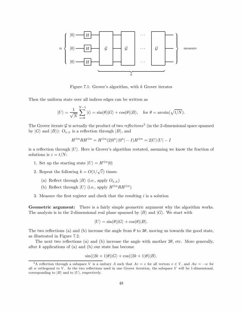
n
|0〉
|0〉
|0〉
measure
H
H
H
G G
. . .
. . .
. . .
G
︸ ︷︷ ︸k
Figure 7.1: Grover’s algorithm, with k Grover iterates
Then the uniform state over all indices edges can be written as
|U〉 = 1√N
N−1∑
i=0
|i〉 = sin(θ)|G〉+ cos(θ)|B〉, for θ = arcsin(√t/N).
The Grover iterate G is actually the product of two reflections2 (in the 2-dimensional space spannedby |G〉 and |B〉): Ox,± is a reflection through |B〉, and
H⊗nRH⊗n = H⊗n(2|0n〉〈0n| − I)H⊗n = 2|U〉〈U | − I
is a reflection through |U〉. Here is Grover’s algorithm restated, assuming we know the fraction ofsolutions is ε = t/N :
1. Set up the starting state |U〉 = H⊗n|0〉
2. Repeat the following k = O(1/√ε) times:
(a) Reflect through |B〉 (i.e., apply Ox,±)
(b) Reflect through |U〉 (i.e., apply H⊗nRH⊗n)
3. Measure the first register and check that the resulting i is a solution
Geometric argument: There is a fairly simple geometric argument why the algorithm works.The analysis is in the 2-dimensional real plane spanned by |B〉 and |G〉. We start with
|U〉 = sin(θ)|G〉+ cos(θ)|B〉.
The two reflections (a) and (b) increase the angle from θ to 3θ, moving us towards the good state,as illustrated in Figure 7.2.
The next two reflections (a) and (b) increase the angle with another 2θ, etc. More generally,after k applications of (a) and (b) our state has become
sin((2k + 1)θ)|G〉+ cos((2k + 1)θ)|B〉.2A reflection through a subspace V is a unitary A such that Av = v for all vectors v ∈ V , and Aw = −w for
all w orthogonal to V . In the two reflections used in one Grover iteration, the subspace V will be 1-dimensional,corresponding to |B〉 and to |U〉, respectively.
48
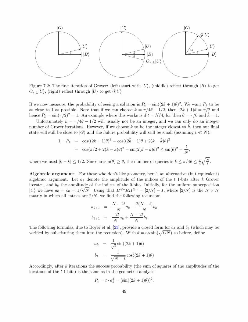
|B〉
|G〉
θ
|U〉
|B〉
|G〉
θθ
|U〉
Ox,±|U〉
③|B〉
|G〉
θ2θ
|U〉
G|U〉
Figure 7.2: The first iteration of Grover: (left) start with |U〉, (middle) reflect through |B〉 to getOx,±|U〉, (right) reflect through |U〉 to get G|U〉
If we now measure, the probability of seeing a solution is Pk = sin((2k + 1)θ)2. We want Pk to beas close to 1 as possible. Note that if we can choose k = π/4θ − 1/2, then (2k + 1)θ = π/2 andhence Pk = sin(π/2)2 = 1. An example where this works is if t = N/4, for then θ = π/6 and k = 1.
Unfortunately k = π/4θ − 1/2 will usually not be an integer, and we can only do an integernumber of Grover iterations. However, if we choose k to be the integer closest to k, then our finalstate will still be close to |G〉 and the failure probability will still be small (assuming t≪ N):
1− Pk = cos((2k + 1)θ)2 = cos((2k + 1)θ + 2(k − k)θ)2
= cos(π/2 + 2(k − k)θ)2 = sin(2(k − k)θ)2 ≤ sin(θ)2 =t
N,
where we used |k − k| ≤ 1/2. Since arcsin(θ) ≥ θ, the number of queries is k ≤ π/4θ ≤ π4
√Nt .
Algebraic argument: For those who don’t like geometry, here’s an alternative (but equivalent)algebraic argument. Let ak denote the amplitude of the indices of the t 1-bits after k Groveriterates, and bk the amplitude of the indices of the 0-bits. Initially, for the uniform superposition|U〉 we have a0 = b0 = 1/
√N . Using that H⊗nRH⊗n = [2/N ] − I, where [2/N ] is the N × N
matrix in which all entries are 2/N , we find the following recursion:
ak+1 =N − 2t
Nak +
2(N − t)
Nbk
bk+1 =−2t
Nak +
N − 2t
Nbk
The following formulas, due to Boyer et al. [23], provide a closed form for ak and bk (which may beverified by substituting them into the recursion). With θ = arcsin(
√t/N) as before, define
ak =1√tsin((2k + 1)θ)
bk =1√N − t
cos((2k + 1)θ)
Accordingly, after k iterations the success probability (the sum of squares of the amplitudes of thelocations of the t 1-bits) is the same as in the geometric analysis
Pk = t · a2k = (sin((2k + 1)θ))2.
49
Accordingly, we have a bounded-error quantum search algorithm with O(√N/t) queries, assuming
we know t. We now list (without full proofs) a number of usuful variants of grover:
• If we know t exactly, then the algorithm can be tweaked to end up in exactly the good state.Roughly speaking, you can make the angle θ slightly smaller, such that k = π/4θ − 1/2becomes an integer (see Exercise 7).
• If we do not know t, then there is a problem: we do not know which k to use, so we donot know when to stop doing the Grover iterates. Note that if k gets too big, the successprobability Pk = (sin((2k + 1)θ))2 goes down again! However, a slightly more complicatedalgorithm due to [23] (basically running the above algorithm with systematic different guessesfor k) shows that an expected number of O(
√N/t) queries still suffices to find a solution if
there are t solutions. If there is no solution (t = 0), then we can easily detect that by checkingxi for the i that the algorithm outputs.
• If we know a lower bound τ on the actual (possibly unknown) number of solutions t, then theabove algorithm uses an expected number of O(
√N/τ ) queries. If we run this algorithm for up
to three times its expected number of queries, then (by Markov’s inequality) with probabilityat least 2/3 it will have found a solution. This way we can turn an expected runtime into aworst-case runtime.
• If we do not know t but would like to reduce the probability of not finding a solution to somesmall ε > 0, then we can do this using O(
√N log(1/ε)) queries (see Exercise 8).
NB: The important part here is that the log(1/ε) is inside the square-root; usual error-reduction by O(log(1/ε)) repetitions of basic Grover would give the worse upper bound ofO(
√N log(1/ε)) queries.
7.3 Amplitude amplification
The analysis that worked for Grover’s algorithm is actually much more generally applicable (wewill also see it again in the next chapter). Let χ : Z → 0, 1 be any Boolean function; inputsz ∈ Z satisfying χ(z) = 1 are called solutions. Suppose we have an algorithm to check whether zis a solution. This can be written as a unitary Oχ that maps |z〉 7→ (−1)χ(z)|z〉. Suppose also wehave some (quantum or classical) algorithm A that uses no intermediate measurements and hasprobability p of finding a solution when applied to starting state |0〉. Classically, we would haveto repeat A roughly 1/p times before we find a solution. The amplitude amplification algorithmbelow only needs to run A O(1/
√p) times:
1. Setup the starting state |U〉 = A|0〉
2. Repeat the following O(1/√p) times:
(a) Reflect through |B〉 (i.e., apply Oχ)
(b) Reflect through |U〉 (i.e., apply ARA−1)
3. Measure the first register and check that the resulting element x is marked.
50
Defining θ = arcsin(√p) and good and bad states |G〉 and |B〉 in analogy with the earlier geometric
argument for Grover’s algorithm, the same reasoning shows that amplitude amplification indeedfinds a solution with high probability. This way, we can speed up a very large class of classicalheuristic algorithms: any algorithm that has some non-trivial probability of finding a solutioncan be amplified to success probability nearly 1 (provided we can efficiently check solutions, i.e.,implement Oχ).
Note that the Hadamard transform H⊗n can be viewed as an algorithm with success probabilityp = t/N for a search problem of size N with t solutions, because H⊗n|0n〉 is the uniform superpo-sition over all N locations. Hence Grover’s algorithm is a special case of amplitude amplification,where Oχ = Ox and A = H⊗n.
7.4 Application: satisfiability
Grover’s algorithm has many applications: basically any classical algorithm that has some search-component can be improved using Grover’s algorithm as a subroutine. This includes many basiccomputer applications such as finding shortest paths and minimum spanning trees, various othergraph algorithms, etc.
We can also use it to speed up the computation of NP-complete problems, albeit only quadrati-cally, not exponentially. As an example, consider the satisfiability problem: we are given a Booleanformula φ(i1, . . . , in) and want to know if it has a satisfying assignment, i.e., a setting of the bitsi1, . . . , in that makes φ(i1, . . . , in) = 1. A classical brute-force search along all 2n possible assign-ments takes time roughly 2n.
To find a satisfying assignment faster, define the N = 2n-bit input to Grover’s algorithm byxi = φ(i), where i ∈ 0, 1n. For a given assignment i = i1 . . . in it is easy to compute φ(i)classically in polynomial time. We can write that computation as a reversible circuit (using onlyToffoli gates), corresponding to a unitary Uφ that maps |i, 0, 0〉 7→ |i, φ(i), wi〉, where the thirdregister holds some classical workspace the computation may have needed. To apply Grover weneed an oracle that puts the answer in the phase and doesn’t leave workspace around (as thatwould mess up the interference effects). Define Ox as the unitary that first applies Uφ, then appliesa Z-gate to the second register, and then applies U−1
φ to “clean up” the workspace again. This hasthe form we need for Grover: Ox,±|i〉 = (−1)xi |i〉. Now we can run Grover and find a satisfyingassignment with high probability if there is one, using a number of elementary operations that is√2n times some polynomial factor.
Exercises
1. (a) Suppose n = 2, and x = x00x01x10x11 = 0001. Give the initial, intermediate, and finalsuperpositions in Grover’s algorithm, for k = 1 queries. What is the success probability?
(b) Give the final superposition for the above x after k = 2 iterations. What is now thesuccess probability?
2. Show that if the number of solutions is t = N/4, then Grover’s algorithm always finds asolution with certainty after just one query. How many queries would a classical algorithmneed to find a solution with certainty if t = N/4? And if we allow the classical algorithmerror probability 1/10?
51
3. Let x = x0 . . . xN−1 be a sequence of distinct integers, where N = 2n. We can query thesein the usual way, i.e., we can apply unitary Ox : |i, 0〉 7→ |i, xi〉, as well as its inverse. Theminimum of x is defined as minxi | i ∈ 0, . . . , N − 1. Give a quantum algorithm thatfinds (with probability ≥ 2/3) an index achieving the minimum, using at most O(
√N logN)
queries to the input.
Bonus: give a quantum algorithm that uses O(√N) queries. This result is from [44].
4. Let x = x0 . . . xN−1, where N = 2n and xi ∈ 0, 1n, be an input that we can query in theusual way. We are promised that this input is 2-to-1: for each i there is exactly one other jsuch that xi = xj.
3 Such an (i, j)-pair is called a collision.
(a) Suppose S is a randomly chosen set of s elements of 0, . . . , N − 1. What is theprobability that there exists a collision in S?
(b) Give a classical randomized algorithm that finds a collision (with probability ≥ 2/3)using O(
√N) queries to x.
(c) Give a quantum algorithm that finds a collision (with probability ≥ 2/3) using O(N1/3)queries.
5. Suppose we have a database with N = 2n binary slots, containing t ones (solutions) and N−tzeroes. You may assume you know the number t.
(a) Show that we can use Grover’s algorithm to find the positions of all t ones, using anexpected number of O(t
√N) queries to the database. You can argue on a high level, no
need to draw actual quantum circuits.
(b) Show that this can be improved to an expected number of O(√tN) queries.
6. Consider an undirected graph G = (V,E), with vertex set V = 1, . . . , n and edge-set E.We say G is connected if, for every pair of vertices i, j ∈ V , there is a path between i andj in the graph. The adjacency matrix of G is the n × n Boolean matrix M where Mij = 1iff (i, j) ∈ E (note that M is a symmetric matrix because G is undirected). Suppose we aregiven input graph G in the form of a unitary that allows us to query whether an edge (i, j)is present in G or not:
OM : |i, j, b〉 7→ |i, j, b ⊕Mij〉.
(a) Assume G is connected. Suppose we have a set A of edges which we already know to bein the graph (so A ⊆ E; you can think of A as given classically, you don’t have to queryit). Let GA = (V,A) be the subgraph induced by only these edges, and suppose GA isnot connected, so it consists of c > 1 connected components. Call an edge (i, j) ∈ E“good” if it connects two of these components. Give a quantum algorithm that finds agood edge with an expected number of O(n/
√c− 1) queries to M .
(b) Give a quantum algorithm that uses at most O(n3/2) queries to M and decides (withsuccess probability at least 2/3) whether G is connected or not. This result is due to [43].
(c) Show that classical algorithms for deciding (with success probability at least 2/3) whetherG is connected, need to make Ω(n2) queries to M .
3The 2-to-1 inputs for Simon’s algorithm are a very special case of this, where xi equals xj if i = j ⊕ s for fixedbut unknown s ∈ 0, 1n.
52
7. At the end of Section 7.2 we claimed without proof that Grover’s algorithm can be tweakedto work with probability 1 if we know the number of solutions exactly. For N = 2n, thisquestion will ask you to provide such an exact algorithm for an N -bit database x ∈ 0, 1Nwith a unique solution (so we are promised that there is exactly one i ∈ 0, 1n with xi = 1,and our goal is to find this i).
(a) Give the success probability of the basic version of Grover’s algorithm after k iterations.
(b) Suppose the optimal number of iterations k = π4 arcsin(1/
√N)
− 12 is not an integer. Show
that if we round k up to the nearest integer, doing ⌈k⌉ iterations, then the algorithmwill have success probability strictly less than 1.
(c) Define a new 2N -bit database y ∈ 0, 12N , indexed by (n+1)-bit strings j = j1 . . . jnjn+1,by setting
yj =
1 if xj1...jn = 1 and jn+1 = 0,0 otherwise.
Show how you can implement the following (n+ 1)-qubit unitary
Sy : |j〉 7→ (−1)yj |j〉,
using one query to x (of the usual form Ox : |i, b〉 7→ |i, b⊕ xi〉) and a few elementarygates.
(d) Let γ ∈ [0, 2π) and let Uγ =
(cos γ − sin γsin γ cos γ
)be the corresponding rotation matrix.
Let A = H⊗n ⊗ Uγ be an (n+ 1)-qubit unitary. What is the probability (as a functionof γ) that measuring the state A
∣∣0n+1⟩gives a solution j ∈ 0, 1n+1 for y (i.e., such
that yj = 1)?
(e) Give a quantum algorithm that finds the unique solution in database x with probability 1using O(
√N) queries to x.
8. Given query access to x ∈ 0, 1N , with unknown Hamming weight t = |x|, we want to finda solution, i.e., an index i ∈ 0, . . . , N − 1 such that xi = 1. If x = 0N then our searchalgorithm should output “no solution.”
(a) Suppose we know an integer s such that t ∈ 1, . . . , s. Give a quantum algorithm thatfinds a solution with probability 1, using O(
√sN) queries to x.
(b) Suppose we know that t ∈ s + 1, . . . , N. Give a quantum algorithm that finds asolution with probability at least 1− 2−s, using O(
√sN) queries to x.
(c) For given ε > 2−N , give a quantum algorithm that solves the search problem withprobability ≥ 1− ε using O(
√N log(1/ε)) queries, without assuming anything about t.
53

54
Chapter 8
Quantum Walk Algorithms
8.1 Classical random walks
Consider an undirected graph G with N vertices. Suppose at least an ε-fraction of the vertices are“marked,” and we would like to find a marked vertex. One way to do this is with a random walk :
Start at some specific vertex y of the graph.Repeat the following a number of times: Check if y is marked, and if not then chooseone of its neighbors at random and set y to be that neighbor.
This may seem like a stupid algorithm, but it has certain advantages. For instance, it only needsspace O(logN), because you only need to keep track of the current vertex y, and maybe a counterthat keeps track of how many steps you’ve already taken.1 Such an algorithm can for exampledecide whether there is a path from a specific vertex y to a specific vertex x using O(logN) space.We’d start the walk at y and only x would be marked; one can show that if there exists a pathfrom y to x in G, then we will reach x in poly(N) steps.
Let us restrict attention to d-regular graphs without self-loops, so each vertex has exactly dneighbors. Also assume the graph is connected. A random walk on such a graph corresponds toan N ×N symmetric matrix P , where Px,y = 1/d if (x, y) is an edge in G, and Px,y = 0 otherwise.If v ∈ RN is a vector with a 1 at position y and 0s elsewhere, then Pv is a vector whose xth entryis (Pv)x = 1/d if (x, y) is an edge, and (Pv)x = 0 otherwise. In other words, Pv is the uniformprobability distribution over the neighbors of y, which is what you get by taking one step of therandom walk starting at y. More generally, if v is a probability distribution on the vertices, thenPv is the new probability distribution on vertices after taking one step of the random walk, andP kv is the probability distribution after taking k steps.
Suppose we start with some probability-distribution vector v (which may or may not be con-centrated at one vertex y). Then P kv will converge to the uniform distribution over all vertices,and the speed of convergence is determined by the difference between the first and second-largesteigenvalues of P . This can be seen as follows. Let λ1 ≥ λ2 ≥ · · · ≥ λN be the eigenvalues of P , or-dered by size, and v1, . . . , vN be corresponding orthogonal eigenvectors. First, the largest eigenvalueis λ1 = 1, and corresponds to the eigenvector v1 = u = (1/N) which is the uniform distribution
1Here we’re assuming the neighbors of any one vertex are efficiently computable, so you don’t actually need tokeep the whole graph in memory. This will be true for all graphs we consider here.
55
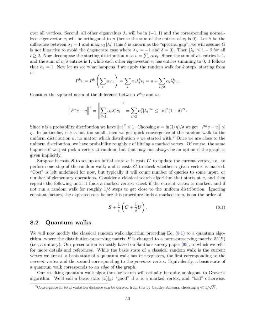
over all vertices. Second, all other eigenvalues λi will be in (−1, 1) and the corresponding normal-ized eigenvector vi will be orthogonal to u (hence the sum of the entries of vi is 0). Let δ be thedifference between λ1 = 1 and maxi≥2 |λi| (this δ is known as the “spectral gap”; we will assume Gis not bipartite to avoid the degenerate case where λN = −1 and δ = 0). Then |λi| ≤ 1 − δ for alli ≥ 2. Now decompose the starting distribution v as v =
∑i αivi. Since the sum of v’s entries is 1,
and the sum of v1’s entries is 1, while each other eigenvector vi has entries summing to 0, it followsthat α1 = 1. Now let us see what happens if we apply the random walk for k steps, starting fromv:
P kv = P k
(∑
i
αivi
)=∑
i
αiλki vi = u+
∑
i≥2
αiλki vi.
Consider the squared norm of the difference between P kv and u:
∥∥∥P kv − u∥∥∥2=
∥∥∥∥∥∥∑
i≥2
αiλki vi
∥∥∥∥∥∥
2
=∑
i≥2
α2i |λi|2k ≤ ‖v‖2(1− δ)2k.
Since v is a probability distribution we have ‖v‖2 ≤ 1. Choosing k = ln(1/η)/δ we get∥∥P kv − u
∥∥ ≤η. In particular, if δ is not too small, then we get quick convergence of the random walk to theuniform distribution u, no matter which distribution v we started with.2 Once we are close to theuniform distribution, we have probability roughly ε of hitting a marked vertex. Of course, the samehappens if we just pick a vertex at random, but that may not always be an option if the graph isgiven implicitly.
Suppose it costs S to set up an initial state v; it costs U to update the current vertex, i.e., toperform one step of the random walk; and it costs C to check whether a given vertex is marked.“Cost” is left undefined for now, but typically it will count number of queries to some input, ornumber of elementary operations. Consider a classical search algorithm that starts at v, and thenrepeats the following until it finds a marked vertex: check if the current vertex is marked, and ifnot run a random walk for roughly 1/δ steps to get close to the uniform distribution. Ignoringconstant factors, the expected cost before this procedure finds a marked item, is on the order of
S +1
ε
(C +
1
δU
). (8.1)
8.2 Quantum walks
We will now modify the classical random walk algorithm preceding Eq. (8.1) to a quantum algo-rithm, where the distribution-preserving matrix P is changed to a norm-preserving matrix W (P )(i.e., a unitary). Our presentation is mostly based on Santha’s survey paper [95], to which we referfor more details and references. While the basis state of a classical random walk is the currentvertex we are at, a basis state of a quantum walk has two registers, the first corresponding to thecurrent vertex and the second corresponding to the previous vertex. Equivalently, a basis state ofa quantum walk corresponds to an edge of the graph.
Our resulting quantum walk algorithm for search will actually be quite analogous to Grover’salgorithm. We’ll call a basis state |x〉|y〉 “good” if x is a marked vertex, and “bad” otherwise.
2Convergence in total variation distance can be derived from this by Cauchy-Schwarz, choosing η ≪ 1/√N .
56
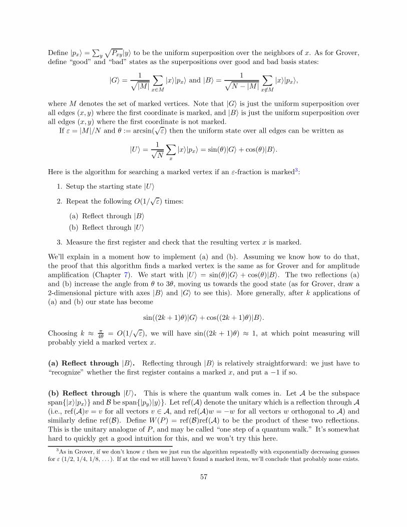
Define |px〉 =∑
y
√Pxy|y〉 to be the uniform superposition over the neighbors of x. As for Grover,
define “good” and “bad” states as the superpositions over good and bad basis states:
|G〉 = 1√|M |
∑
x∈M|x〉|px〉 and |B〉 = 1√
N − |M |∑
x 6∈M|x〉|px〉,
where M denotes the set of marked vertices. Note that |G〉 is just the uniform superposition overall edges (x, y) where the first coordinate is marked, and |B〉 is just the uniform superposition overall edges (x, y) where the first coordinate is not marked.
If ε = |M |/N and θ := arcsin(√ε) then the uniform state over all edges can be written as
|U〉 = 1√N
∑
x
|x〉|px〉 = sin(θ)|G〉+ cos(θ)|B〉.
Here is the algorithm for searching a marked vertex if an ε-fraction is marked3:
1. Setup the starting state |U〉
2. Repeat the following O(1/√ε) times:
(a) Reflect through |B〉(b) Reflect through |U〉
3. Measure the first register and check that the resulting vertex x is marked.
We’ll explain in a moment how to implement (a) and (b). Assuming we know how to do that,the proof that this algorithm finds a marked vertex is the same as for Grover and for amplitudeamplification (Chapter 7). We start with |U〉 = sin(θ)|G〉 + cos(θ)|B〉. The two reflections (a)and (b) increase the angle from θ to 3θ, moving us towards the good state (as for Grover, draw a2-dimensional picture with axes |B〉 and |G〉 to see this). More generally, after k applications of(a) and (b) our state has become
sin((2k + 1)θ)|G〉+ cos((2k + 1)θ)|B〉.
Choosing k ≈ π4θ = O(1/
√ε), we will have sin((2k + 1)θ) ≈ 1, at which point measuring will
probably yield a marked vertex x.
(a) Reflect through |B〉. Reflecting through |B〉 is relatively straightforward: we just have to“recognize” whether the first register contains a marked x, and put a −1 if so.
(b) Reflect through |U〉. This is where the quantum walk comes in. Let A be the subspacespan|x〉|px〉 and B be span|py〉|y〉. Let ref(A) denote the unitary which is a reflection through A(i.e., ref(A)v = v for all vectors v ∈ A, and ref(A)w = −w for all vectors w orthogonal to A) andsimilarly define ref(B). Define W (P ) = ref(B)ref(A) to be the product of these two reflections.This is the unitary analogue of P , and may be called “one step of a quantum walk.” It’s somewhathard to quickly get a good intuition for this, and we won’t try this here.
3As in Grover, if we don’t know ε then we just run the algorithm repeatedly with exponentially decreasing guessesfor ε (1/2, 1/4, 1/8, . . . ). If at the end we still haven’t found a marked item, we’ll conclude that probably none exists.
57
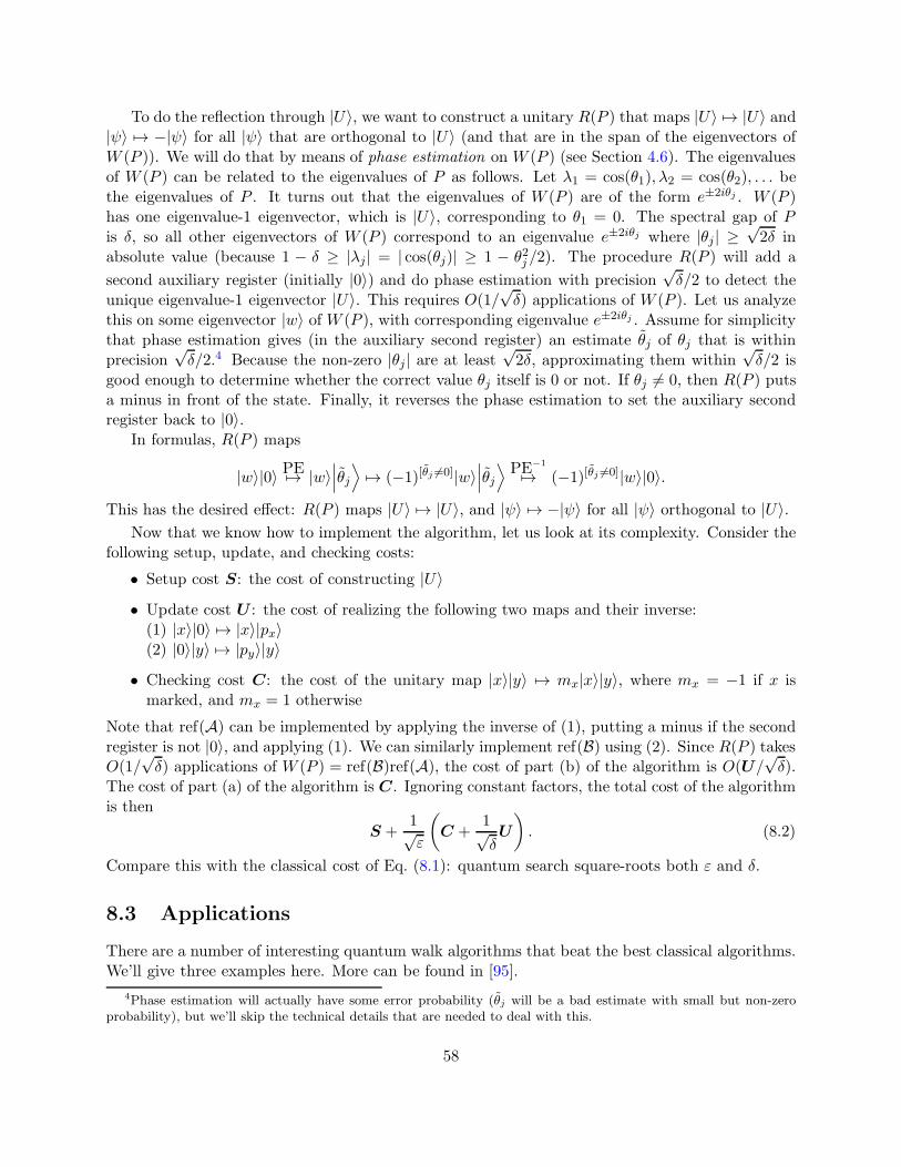
To do the reflection through |U〉, we want to construct a unitary R(P ) that maps |U〉 7→ |U〉 and|ψ〉 7→ −|ψ〉 for all |ψ〉 that are orthogonal to |U〉 (and that are in the span of the eigenvectors ofW (P )). We will do that by means of phase estimation on W (P ) (see Section 4.6). The eigenvaluesof W (P ) can be related to the eigenvalues of P as follows. Let λ1 = cos(θ1), λ2 = cos(θ2), . . . bethe eigenvalues of P . It turns out that the eigenvalues of W (P ) are of the form e±2iθj . W (P )has one eigenvalue-1 eigenvector, which is |U〉, corresponding to θ1 = 0. The spectral gap of Pis δ, so all other eigenvectors of W (P ) correspond to an eigenvalue e±2iθj where |θj | ≥
√2δ in
absolute value (because 1 − δ ≥ |λj | = | cos(θj)| ≥ 1 − θ2j/2). The procedure R(P ) will add a
second auxiliary register (initially |0〉) and do phase estimation with precision√δ/2 to detect the
unique eigenvalue-1 eigenvector |U〉. This requires O(1/√δ) applications of W (P ). Let us analyze
this on some eigenvector |w〉 of W (P ), with corresponding eigenvalue e±2iθj . Assume for simplicitythat phase estimation gives (in the auxiliary second register) an estimate θj of θj that is withinprecision
√δ/2.4 Because the non-zero |θj| are at least
√2δ, approximating them within
√δ/2 is
good enough to determine whether the correct value θj itself is 0 or not. If θj 6= 0, then R(P ) putsa minus in front of the state. Finally, it reverses the phase estimation to set the auxiliary secondregister back to |0〉.
In formulas, R(P ) maps
|w〉|0〉 PE7→ |w〉∣∣∣θj⟩7→ (−1)[θj 6=0]|w〉
∣∣∣θj⟩PE−1
7→ (−1)[θj 6=0]|w〉|0〉.
This has the desired effect: R(P ) maps |U〉 7→ |U〉, and |ψ〉 7→ −|ψ〉 for all |ψ〉 orthogonal to |U〉.Now that we know how to implement the algorithm, let us look at its complexity. Consider the
following setup, update, and checking costs:
• Setup cost S: the cost of constructing |U〉
• Update cost U : the cost of realizing the following two maps and their inverse:(1) |x〉|0〉 7→ |x〉|px〉(2) |0〉|y〉 7→ |py〉|y〉
• Checking cost C: the cost of the unitary map |x〉|y〉 7→ mx|x〉|y〉, where mx = −1 if x ismarked, and mx = 1 otherwise
Note that ref(A) can be implemented by applying the inverse of (1), putting a minus if the secondregister is not |0〉, and applying (1). We can similarly implement ref(B) using (2). Since R(P ) takesO(1/
√δ) applications of W (P ) = ref(B)ref(A), the cost of part (b) of the algorithm is O(U/
√δ).
The cost of part (a) of the algorithm is C. Ignoring constant factors, the total cost of the algorithmis then
S +1√ε
(C +
1√δU
). (8.2)
Compare this with the classical cost of Eq. (8.1): quantum search square-roots both ε and δ.
8.3 Applications
There are a number of interesting quantum walk algorithms that beat the best classical algorithms.We’ll give three examples here. More can be found in [95].
4Phase estimation will actually have some error probability (θj will be a bad estimate with small but non-zeroprobability), but we’ll skip the technical details that are needed to deal with this.
58
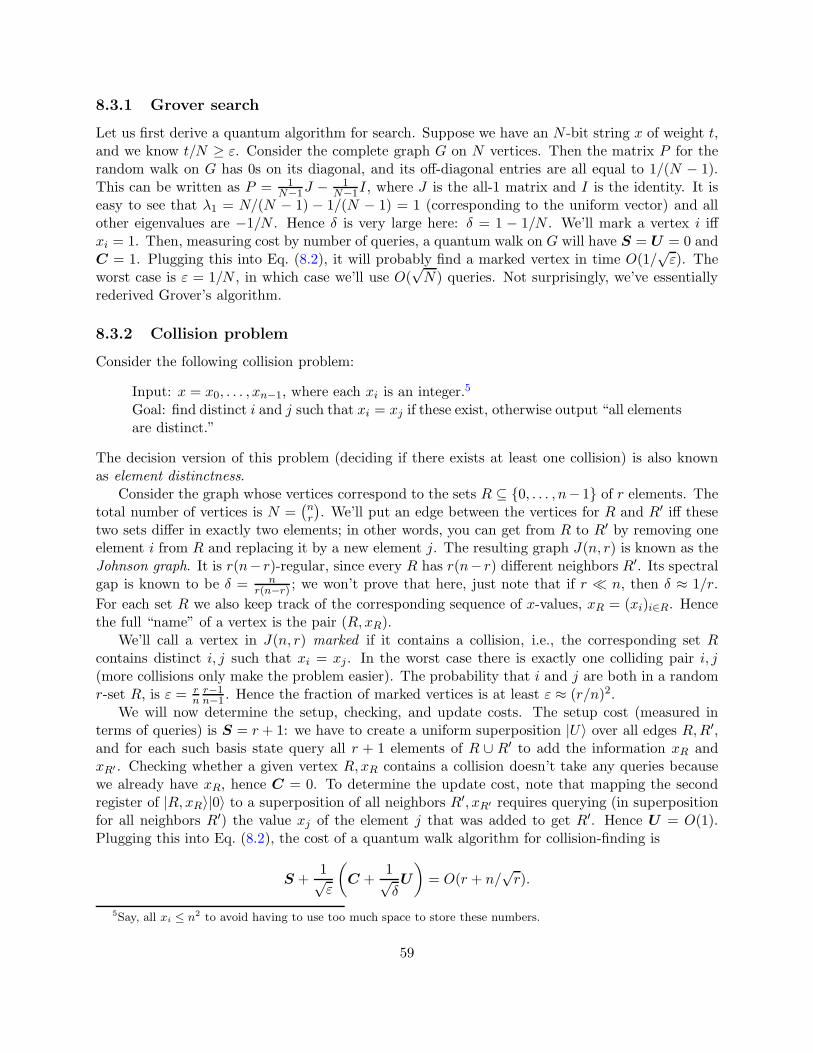
8.3.1 Grover search
Let us first derive a quantum algorithm for search. Suppose we have an N -bit string x of weight t,and we know t/N ≥ ε. Consider the complete graph G on N vertices. Then the matrix P for therandom walk on G has 0s on its diagonal, and its off-diagonal entries are all equal to 1/(N − 1).This can be written as P = 1
N−1J − 1N−1I, where J is the all-1 matrix and I is the identity. It is
easy to see that λ1 = N/(N − 1) − 1/(N − 1) = 1 (corresponding to the uniform vector) and allother eigenvalues are −1/N . Hence δ is very large here: δ = 1 − 1/N . We’ll mark a vertex i iffxi = 1. Then, measuring cost by number of queries, a quantum walk on G will have S = U = 0 andC = 1. Plugging this into Eq. (8.2), it will probably find a marked vertex in time O(1/
√ε). The
worst case is ε = 1/N , in which case we’ll use O(√N) queries. Not surprisingly, we’ve essentially
rederived Grover’s algorithm.
8.3.2 Collision problem
Consider the following collision problem:
Input: x = x0, . . . , xn−1, where each xi is an integer.5
Goal: find distinct i and j such that xi = xj if these exist, otherwise output “all elementsare distinct.”
The decision version of this problem (deciding if there exists at least one collision) is also knownas element distinctness.
Consider the graph whose vertices correspond to the sets R ⊆ 0, . . . , n− 1 of r elements. Thetotal number of vertices is N =
(nr
). We’ll put an edge between the vertices for R and R′ iff these
two sets differ in exactly two elements; in other words, you can get from R to R′ by removing oneelement i from R and replacing it by a new element j. The resulting graph J(n, r) is known as theJohnson graph. It is r(n− r)-regular, since every R has r(n− r) different neighbors R′. Its spectralgap is known to be δ = n
r(n−r) ; we won’t prove that here, just note that if r ≪ n, then δ ≈ 1/r.
For each set R we also keep track of the corresponding sequence of x-values, xR = (xi)i∈R. Hencethe full “name” of a vertex is the pair (R,xR).
We’ll call a vertex in J(n, r) marked if it contains a collision, i.e., the corresponding set Rcontains distinct i, j such that xi = xj . In the worst case there is exactly one colliding pair i, j(more collisions only make the problem easier). The probability that i and j are both in a randomr-set R, is ε = r
nr−1n−1 . Hence the fraction of marked vertices is at least ε ≈ (r/n)2.
We will now determine the setup, checking, and update costs. The setup cost (measured interms of queries) is S = r + 1: we have to create a uniform superposition |U〉 over all edges R,R′,and for each such basis state query all r + 1 elements of R ∪ R′ to add the information xR andxR′ . Checking whether a given vertex R,xR contains a collision doesn’t take any queries becausewe already have xR, hence C = 0. To determine the update cost, note that mapping the secondregister of |R,xR〉|0〉 to a superposition of all neighbors R′, xR′ requires querying (in superpositionfor all neighbors R′) the value xj of the element j that was added to get R′. Hence U = O(1).Plugging this into Eq. (8.2), the cost of a quantum walk algorithm for collision-finding is
S +1√ε
(C +
1√δU
)= O(r + n/
√r).
5Say, all xi ≤ n2 to avoid having to use too much space to store these numbers.
59
This is O(n2/3) if we set r = n2/3. This O(n2/3) turns out to be the optimal query complexity for thecollision problem [2]. By some more work involving efficient data structures, the time complexity(= total number of elementary quantum gates) can be brought down to n2/3(log n)O(1) [7].
8.3.3 Finding a triangle in a graph
Consider the following triangle-finding problem:
Input: the adjacency matrix of a graph H on n vertices.Goal: find vertices u, v, w that form a triangle (i.e., (u, v), (v,w), (w, u) are all edges inthe graph), if they exist.
We’ll assume we have query access to the entries of the adjacency matrix of H, which tells uswhether (u, v) is an edge or not. There are
(n2
)bits in this oracle, one for each potential edge
of H. It is not hard to see that a classical algorithm needs Ω(n2) queries before it can decidewith good probability whether a graph contains a triangle or not. For example, take a bipartitegraph consisting of 2 sets of n/2 vertices each, such that any pair of vertices from different sets isconnected by an edge. Such a graph is triangle-free, but adding any one edge will create a triangle.A classical algorithm would have to query all those edges separately.
Let us try a quantum walk approach. Again consider the Johnson graph J(n, r). Each vertexwill correspond to a set R ⊆ 0, . . . , n − 1 of r vertices, annotated with the result of queryingall possible
(r2
)edges having both endpoints in R. We will call the vertex for set R marked if it
contains one edge of a triangle. If there is at least one triangle in the graph, the fraction of markedvertices is at least ε ≈ (r/n)2. Getting a good upper bound for the checking cost C requires somework—namely Grover search plus another quantum walk!
The setup cost will be S =(r2
). The update cost will be U = 2r − 2, because if we remove one
vertex i from R then we have to remove information about r − 1 edges in H, and if we add a newj to R we have to query r − 1 new edges in H.
Suppose we are given a set R of r vertices. How do we decide whether R contains an edge of atriangle? If we can efficiently decide, for a given u and R, whether R contains vertices v,w such thatu, v, w form a triangle in H, then we could combine this with a Grover search over all n possiblevertices u of H. Given u and R, let us design a subroutine based on another quantum walk, this timeon the Johnson graph J(r, r2/3). Each vertex of this Johnson graph corresponds to a subset R′ ⊆ Rof r′ = r2/3 vertices. Its spectral gap is δ′ = r/r′(r − r′) ≈ 1/r2/3. We’ll mark R′ if it containsvertices v,w such that u, v, w form a triangle. If there is at least one triangle involving u and somev,w ∈ R, then the fraction of marked vertices R′ in J(r, r2/3) is at least ε′ ≈ (r′/r)2 = 1/r2/3. Forthis subroutine, the setup cost is O(r2/3) (for each v ∈ R, query whether (u, v) is an edge in H);the update cost is O(1) (if we replace v in R by w, then we need to “unquery” edge (u, v) andquery edge (u,w)); and the checking cost is 0. Plugging this into Eq. (8.2), we can decide whethera fixed u forms a triangle with two vertices in R′, using O(r2/3) queries. Let’s ignore the smallerror probability of the latter subroutine (it can be dealt with, but that’s technical). Then we cancombine it with Grover search over all n vertices u to get checking cost C = O(
√nr2/3).
Plugging these S, U , and C into Eq. (8.2), the overall cost of a quantum walk algorithm fortriangle-finding is
S +1√ε
(C +
1√δU
)= O
(r2 +
n
r(√nr2/3 + r3/2)
).
60
This is O(n13/10) if we set r = n3/5 [79]. The exponent 13/10 can be slightly improved further [16,75, 67], and the current best exponent is 5/4 [74]. It is an open question what the optimal quantumquery complexity for triangle-finding is; the best lower bound is only n. Also, the optimal quantumtime complexity of this problem is still wide open.
Exercises
1. Let P be the projector on a d-dimensional subspace V ⊆ Rn that is spanned by orthonormalvectors v1, . . . , vd. This means that Pv = v for all v ∈ V , and Pw = 0 for all w that areorthogonal to V .
(a) Show that P can be written in Dirac notation as P =∑d
i=1 |vi〉〈vi|.(b) Show that R = 2P − I is a reflection through the subspace corresponding to P , i.e.,
Rv = v for all v in the subspace, and Rw = −w for all w that are orthogonal to thesubspace.
2. This exercise is about obtaining a quantum algorithm for the collision problem with a slightlydifferent quantum walk. Consider the problem of Section 8.3.2: we can query elements ofthe sequence of integers x0, . . . , xn−1, and want to find distinct i and j such that xi = xj(or report that there are no collisions). Again consider the Johnson graph J(n, r), for somer to be optimized over later. Deviating from Section 8.3.2, now call a vertex R marked ifthere exist i ∈ R and j ∈ [n] \ R such that xi = xj . Show that we can find a marked vertexin this graph with high probability using O(n2/3) queries to x. You may ignore small errorprobabilities, for example when using Grover’s algorithm. Be explicit about what data youstore about x at each vertex R.
3. Let A, B, and C be n × n matrices with real entries. We’d like to decide whether or notAB = C. Of course, you could multiply A and B and compare the result with C, but matrixmultiplication is expensive (the current best algorithm takes time roughly O(n2.38)).
(a) Give a classical randomized algorithm that verifies whether AB = C (with success prob-ability at least 2/3) using O(n2) steps, using the fact that matrix-vector multiplicationcan be done in O(n2) steps.
(b) Show that if we have query-access to the entries of the matrices (i.e., oracles that mapi, j, 0 7→ i, j, Ai,j and similarly for B and C), then any classical algorithm with smallerror probability needs at least n2 queries to detect a difference between AB and C.
(c) Give a quantum walk algorithm that verifies whether AB = C (with success probabilityat least 2/3) using O(n5/3) queries to matrix-entries.
4. A 3-SAT instance φ over n Boolean variables x1, . . . , xn is a formula which is the AND of anumber of clauses, each of which is an OR of 3 variables or their negations. For example,φ(x1, . . . , x4) = (x1 ∨x2 ∨ x3)∧ (x2 ∨ x3 ∨x4) is a 3-SAT formula with 2 clauses. A satisfyingassignment is a setting of the n variables such that φ(x1, . . . , xn) = 1 (i.e, TRUE). You mayassume the number of clauses is at most some polynomial in n. In general it is NP-hardto find a satisfying assignment to such a formula. Brute force would try out all 2n possibletruth-assignments, but something better can be done by a classical random walk. Consider
61
the following simple algorithm of Schoning [97], which is a random walk on the set of allN = 2n truth assignments:
Start with a uniformly random x ∈ 0, 1n.Repeat the following at most 3n times: if φ(x) = 1 then STOP, else find the leftmostclause that is false, randomly choose one of its 3 variables and flip its value.
One can show that this algorithm has probability at least (3/4)n of finding a satisfyingassignment (if φ is satisfiable). You may assume this without proof.
(a) Use the above to give a classical algorithm that finds a satisfying assignment with highprobability in time (4/3)n · p(n), where p(n) is some polynomial factor (no need to usethe C,U, S-framework of the chapter here; the answer is much simpler).
(b) Give a quantum algorithm that finds one (with high probability) in time√
(4/3)n ·p(n).
62
Chapter 9
Quantum Query Lower Bounds
9.1 Introduction
Almost all the algorithms we have seen so far in this course worked in the query model. Herethe goal is to compute some function f : 0, 1N → 0, 1 on a given input x ∈ 0, 1N . Thedistinguishing feature of the query model is the way x is accessed: x is not given explicitly, butis stored in a random access memory, and we’re being charged unit cost for each query that wemake to this memory. Informally, a query asks for and receives the i-th element xi of the input.Formally, we model a query unitarily as the following 2-register quantum operation Ox, where thefirst register is N -dimensional and the second is 2-dimensional1:
Ox : |i, b〉 7→ |i, b⊕ xi〉.
In particular, |i, 0〉 7→ |i, xi〉. This only states what Ox does on basis states, but by linearitydetermines the full unitary. Note that a quantum algorithm can apply Ox to a superposition ofbasis states, gaining some sort of access to several input bits xi at the same time.
A T -query quantum algorithm starts in a fixed state, say the all-0 state |0 . . . 0〉, and then in-terleaves fixed unitary transformations U0, U1, . . . , UT with queries. The algorithm’s fixed unitariesmay act on a workspace-register, in addition to the two registers on which Ox acts. In this case weimplicitly extend Ox by tensoring it with the identity operation on this extra register, so it maps
Ox : |i, b, w〉 7→ |i, b⊕ xi, w〉.
Hence the final state of the algorithm can be written as the following matrix-vector product:
UTOxUT−1Ox · · ·OxU1OxU0|0 . . . 0〉.
This state depends on the input x only via the T queries. The output of the algorithm is obtainedby a measurement of the final state. For instance, if the output is Boolean, the algorithm couldjust measure the final state in the computational basis and output the first bit of the result.
The query complexity of some function f is now the minimal number of queries needed for analgorithm that outputs the correct value f(x) for every x in the domain of f (with error probabilityat most 1/3, say). Note that we just count queries to measure the complexity of the algorithm, while
1If the input x consists of non-binary items xi (as is the case for instance with the input for Simon’s algorithm)then those can be simulated by querying individual bits of each xi.
63
the intermediate fixed unitaries are treated as costless. In many cases, the overall computation timeof quantum query algorithms (as measured by the total number of elementary gates, say) is notmuch bigger than the query complexity. This justifies analyzing the latter as a proxy for the former.This is the model in which essentially all the quantum algorithm we’ve seen work: Deutsch-Jozsa,Simon, Grover, the various random walk algorithms. Even the period-finding algorithm that is thequantum core of Shor’s algorithm works because it needs only few queries to the periodic function.
9.2 The polynomial method
From quantum query algorithms to polynomials. An N -variate multilinear polynomial pis a function p : CN → C that can be written as
p(x1, . . . , xN ) =∑
S⊆[N ]
aS∏
i∈Sxi,
for some complex numbers aS . The degree of p is deg(p) = max|S| : aS 6= 0. It is easy to showthat every function f : 0, 1N → C has a unique representation as such a polynomial; deg(f) isdefined as the degree of that polynomial. For example, the 2-bit AND function is p(x1, x2) = x1x2,and the 2-bit Parity function is p(x1, x2) = x1 + x2 − 2x1x2. Both polynomials have degree 2.Sometimes a lower degree suffices for a polynomial to approximate the function. For example,p(x1, x2) =
13(x1 + x2) approximates the 2-bit AND function up to error 1/3 for all inputs, using
degree 1.
A very useful property of T -query algorithms is that the amplitudes of their final state aredegree-T N -variate polynomials of x [50, 14]. More precisely: consider a T -query algorithm withinput x ∈ 0, 1N acting on an m-qubit space. Then its final state can be written
∑
z∈0,1mαz(x)|z〉,
where each αz is a multilinear polynomial in x of degree at most T .
Proof. The proof is by induction on T . The base case (T = 0) trivially holds: the algorithm’sstate U0|0 . . . 0〉 is independent of x, so its amplitudes are constants.
For the induction step, suppose we have already done T queries. Then by the induction hy-pothesis the state after UT can be written as
∑
z∈0,1mαz(x)|z〉,
where each αz is a multilinear polynomial in x of degree at most T . Each basis state |z〉 = |i, b, w〉consists of 3 registers: the two registers |i, b〉 of the query, and a workspace register containing basisstate |w〉. The algorithm now makes another query Ox followed by a unitary UT+1. The queryswaps basis states |i, 0, w〉 and |i, 1, w〉 if xi = 1, and doesn’t do anything to these basis states ifxi = 0. This changes amplitudes as follows:
αi,0,w(x)|i, 0, w〉+ αi,1,w(x)|i, 1, w〉 7→((1− xi)αi,0,w(x) + xiαi,1,w(x))|i, 0, w〉+ (xiαi,0,w(x) + (1− xi)αi,1,w(x))|i, 1, w〉.
64
Now the new amplitudes are of the form (1−xi)αi,0,w(x)+xiαi,1,w(x) or xiαi,0,w(x)+(1−xi)αi,1,w(x).The new amplitudes are still polynomials in x1, . . . , xN . Their degree is at most 1 more than thedegree of the old amplitudes, so at most T+1. Finally, since UT+1 is a linear map that is independentof x, it does not increase the degree of the amplitudes further (the amplitudes after UT+1 are linearcombinations of the amplitudes before UT+1). This concludes the induction step.
Note that this construction could introduce degrees higher than 1, e.g., terms of the form x2i .However, our inputs xi are 0/1-valued, so we have xki = xi for all integers k ≥ 1. Accordingly, wecan reduce higher degrees to 1, making the polynomials multilinear without increasing degree.
Suppose our algorithm acts on an m-qubit state. If we measure the first qubit of the final stateand output the resulting bit, then the probability of output 1 is given by
p(x) =∑
z∈1×0,1m−1
|αz(x)|2,
which is a real-valued polynomial of x of degree at most 2T . Note that if the algorithm computesf with error ≤ 1/3, then p is an approximating polynomial for f : if f(x) = 0 then p(x) ∈ [0, 1/3]and if f(x) = 1 then p(x) ∈ [2/3, 1]. This gives a method to lower bound the minimal numberof queries needed to compute f : if one can show that every polynomial that approximates f hasdegree at least d, then every quantum algorithm computing f with error ≤ 1/3 must use at leastd/2 queries.
Applications of the polynomial method. For our examples we will restrict attention to sym-metric functions.2 Those are the ones where the function value f(x) only depends on the Hammingweight (number of 1s) in the input x. Examples are N -bit OR, AND, Parity, Majority, etc.
Suppose we have a polynomial p(x1, . . . , xN ) that approximates f with error ≤ 1/3. Then it iseasy to see that a polynomial that averages over all permutations π of the N input bits x1, . . . , xN :
q(x) =1
N !
∑
π∈SN
p(π(x)),
still approximates f . As it turns out, we can define a single-variate polynomial r(z) of the samedegree as q, such that q(x) = r(|x|).3 This r is defined on all real numbers, and we know somethingabout its behavior on integer points 0, . . . , N. Thus it suffices to lower bound the degree ofsingle-variate polynomials with the appropriate behavior.
For an important example, consider the N -bit OR function. Grover’s algorithm can find an isuch that xi = 1 (if such an i exists) and hence can compute the OR function with error ≤ 1/3using O(
√N) queries. By the above reasoning, any T -query quantum algorithm that computes the
OR with error ≤ 1/3 induces a single-variate polynomial r satisfying
2One can also use the polynomial method for non-symmetric functions, for instance to prove a tight lower bound ofΩ(N2/3) queries for the general problem of collision-finding; this matches the quantum walk algorithm of the previouslecture (Section 8.3.2). However, that lower bound proof is substantially more complicated and we won’t give it here.
3To see why this is the case, note that for every degree i, all degree-i monomials in the symmetrized polynomialq have the same coefficient ai. Moreover, on input x ∈ 0, 1N of Hamming weight z, exactly
(
zi
)
of the degree-i
monomials are 1, while the others are 0. Hence q(x) =∑d
i=0 ai(|x|
i
)
. Since(
zd
)
= z(z − 1) · · · (z − d + 1)/d! is a
single-variate polynomial in z of degree d, we can define r(z) =∑d
i=0 ai(
zi
)
.
65
r(0) ∈ [0, 1/3], and r(t) ∈ [2/3, 1] for all integers t ∈ 1, . . . , N.
This polynomial r(x) “jumps” between x = 0 and x = 1 (i.e., it has a derivative r′(x) ≥ 1/3 forsome x ∈ [0, 1]), while it remains fairly constant on the domain 1, . . . , N. By a classical theoremfrom approximation theory (proved independently around the same time by Ehlich and Zeller, andby Rivlin and Cheney), such polynomials must have degree d ≥ Ω(
√N). Hence T ≥ Ω(
√N) as
well. Accordingly, Grover’s algorithm is optimal (up to a constant factor) in terms of number ofqueries.
What about exact algorithms for OR? Could we tweak Grover’s algorithm so that it alwaysfinds a solution with probability 1 (if one exists), using O(
√N) queries? This turns out not to be
the case: a T -query exact algorithm for OR induces a polynomial r of degree ≤ 2T that satisfies
r(0) = 0, and r(t) = 1 for all integers t ∈ 1, . . . , N.
It is not hard to see that such a polynomial needs degree at least N : observe that r(x) − 1 is anon-constant polynomial with at least N roots.4 Hence T ≥ N/2. Accordingly, Grover cannot bemade exact without losing the square-root speed-up!
Using the polynomial method, one can in fact show for every symmetric function f that isdefined on all 2N inputs, that quantum algorithms cannot provide a more-than-quadratic speed-upover classical algorithms. More generally, for every function f (symmetric or non-symmetric) thatis defined on all inputs5, quantum algorithms cannot provide a more-than-6th-root speed-up overclassical algorithms (see Exercise 9).
9.3 The quantum adversary method
The polynomial method has a strength which is also a weakness: it applies even to a stronger (andless physically meaningful) model of computation where we allow any linear transformation on thestate space, not just unitary ones. As a result, it does not always provide the strongest possiblelower bound for quantum query algorithms.
Ambainis [5, 6] provided an alternative method for quantum lower bounds, the quantum adver-sary. This exploits unitarity in a crucial way and in certain cases yields a provably better boundthan the polynomial method [6]. We will present a very simple version of the adversary methodhere. Stronger versions may be found in [65, 64]; the latter one actually gives optimal bounds forevery Boolean function [92]! Recall that a quantum query algorithm is a sequence
UTOxUT−1Ox · · ·OxU1OxU0,
applied to the fixed starting state |0 . . . 0〉, where the basic “query transformation” Ox dependson the input x, and U0, U1, . . . , UT are arbitrary unitaries that don’t depend on x. Consider theevolution of our quantum state under all possible choices of x; formally, we let
∣∣ψtx
⟩denote the state
at time t (i.e., after applying Ox for the t-th time) under input x. In particular,∣∣ψ0
x
⟩= |0 . . . 0〉 for
all x (and 〈ψ0x|ψ0
y〉 = 1 for each x, y). Now if the algorithm computes the Boolean function f withsuccess probability 2/3 on every input, then the final measurement must accept every x ∈ f−1(0)
4A “root” is an x such that r(x) = 0. It is a well-known fact from algebra that every non-constant polynomial ofdegree d has at most d roots (over any field).
5Note that this doesn’t include functions where the input has to satisfy a certain promise, such as Deutsch-Jozsaand Simon’s problem.
66
with probability ≤ 1/3, and accept every y ∈ f−1(1) with probability ≥ 2/3. It is not hard toverify that this implies |〈ψT
x |ψTy 〉| ≤ 17
18 .6 This suggests that we find a R ⊆ f−1(0) × f−1(1) of
hard-to-distinguish (x, y)-pairs, and consider the progress measure
St =∑
(x,y)∈R|〈ψt
x|ψty〉|
as a function of t. By our observations, initially we have S0 = |R|, and in the end we must haveST ≤ 17
18 |R|. Also, crucially, the progress measure is unaffected by each application of a unitary Ut,since each Ut is independent of the input and unitary transformations preserve inner products.
If we can determine an upper bound ∆ on the change |St+1 − St| in the progress measure at
each step, we can conclude that the number T of queries is at least |R|18∆ . Ambainis proved the
following. Suppose that
(i) each x ∈ f−1(0) appearing in R, appears at least m0 times in pairs (x, y) in R;
(ii) each y ∈ f−1(1) appearing in R, appears at least m1 times in pairs (x, y) in R;
(iii) for each x ∈ f−1(0) and i ∈ [N ], there are at most ℓ0 inputs y ∈ f−1(1) such that (x, y) ∈ Rand xi 6= yi;
(iv) for each y ∈ f−1(1) and i ∈ [N ], there are at most ℓ1 inputs x ∈ f−1(0) such that (x, y) ∈ Rand xi 6= yi.
Then for all t ≥ 0, |St+1 − St| = O(√
ℓ0m0
· ℓ1m1
· |R|), and therefore
T = Ω
(√m0
ℓ0· m1
ℓ1
). (9.1)
Intuitively, conditions (i)-(iv) imply that |St+1 − St| is small relative to |R| by bounding the “dis-tinguishing ability” of any query. The art in applying this technique lies in choosing the relation Rcarefully to maximize this quantity, i.e., make m0 and/or m1 large, while keeping ℓ0 and ℓ1 small.
Note that for the N -bit OR function this method easily gives the optimal Ω(√N) lower bound,
as follows. Choose R = (x, y) : x = 0N , y has Hamming weight 1. Then m0 = N while m1 =ℓ0 = ℓ1 = 1. Plugging this into Eq. (9.1) gives the right bound.
Let us give another application, a lower bound that is much harder to prove using the polynomialmethod. Suppose f : 0, 1N → 0, 1 is a 2-level AND-OR tree, with N = k2 input bits: f is theAND of k ORs, each of which has its own set of k inputs bits. By carefully doing 2 levels of Groversearch (search for a subtree which is 0k), one can construct a quantum algorithm that computes fwith small error probability and O(
√k ·
√k) = O(
√N) queries. It was long an open problem to
give a matching lower bound on the approximate degree, and this was proved only in 2013 [98, 30].In contrast, the adversary method gives the optimal lower bound on the quantum query complexityquite easily: choose the relation R as follows
6Remember Exercise 3 from Chapter 4 for states |φ〉 and |ψ〉: if ‖φ− ψ‖ = ε then the total variation distancebetween the probability distributions you get from measuring |φ〉 and |ψ〉, respectively, is at most ε. Hence if weknow there is a two-outcome measurement that accepts |φ〉 with probability ≤ 1/3 and accepts |ψ〉 with probability≥ 2/3, then we must have total variation distance at least 1/3 and hence ε ≥ 1/3. Assume for simplicity that theinner product 〈φ|ψ〉 is real. Via the equation ε2 = ‖φ− ψ‖2 = 2 − 2〈φ|ψ〉, this translates into an upper bound|〈φ|ψ〉| ≤ 1− ε2/2 ≤ 17/18.
67
R consists of those pairs (x, y) wherex has one subtree with input 0k and the other k − 1 subtrees have an arbitrary k-bitinput of Hamming weight 1 (note f(x) = 0)y is obtained from x by changing one of the bits of the 0k-subtree to 1 (note f(y) = 1).
Then m0 = m1 = k and ℓ0 = ℓ1 = 1, and we get a lower bound of Ω(√
m0m1ℓ0ℓ1
)= Ω(k) = Ω(
√N).
Exercises
1. Consider a 2-bit input x = x0x1 with an oracle Ox : |i〉 7→ (−1)xi |i〉. Write out the final stateof the following 1-query quantum algorithm: HOxH|0〉. Give a degree-2 polynomial p(x0, x1)that equals the probability that this algorithm outputs 1 on input x. What function doesthis algorithm compute?
2. Consider polynomial p(x1, x2) = 0.3 + 0.4x1 + 0.5x2, which approximates the 2-bit OR func-tion. Write down the symmetrized polynomial q(x1, x2) = 1
2(p(x1, x2) + p(x2, x1)). Give asingle-variate polynomial r such that q(x) = r(|x|) for all x ∈ 0, 12.
3. Let f be the N -bit Parity function, which is 1 if its input x ∈ 0, 1N has odd Hammingweight, and 0 if the input has even Hamming weight (assume N is an even number).
(a) Give a quantum algorithm that computes Parity with success probability 1 on everyinput x, using N/2 queries.
(b) Show that this is optimal, even for quantum algorithms that have error probability ≤ 1/3on every input
4. Suppose we have a T -query quantum algorithm that computes the N -bit AND function withsuccess probability 1 on all inputs x ∈ 0, 1N . In Section 9.2 we showed that such analgorithm has T ≥ N/2 (we showed it for OR, but the same argument works for AND).Improve this lower bound to T ≥ N .
5. Consider the following 3-bit function f : 0, 13 → 0, 1:f(x1, x2, x3) = 1 if x1 = x2 = x3, and f(x1, x2, x3) = 0 otherwise
(a) How many queries does a classical deterministic algorithm need to compute f? Explainyour answer.
(b) Give a quantum algorithm that computes f with success probability 1 using 2 queries.
(c) Show that 2 queries is optimal: there is no quantum algorithm that computes f withsuccess probability 1 using only 1 query.
6. Let f be the N -bit Majority function, which is 1 if its input x ∈ 0, 1N has Hamming weight> N/2, and 0 if the input has Hamming weight ≤ N/2 (assume N is even).
(a) Prove that deg(f) ≥ N/2. What does this imply for the query complexity of exactquantum algorithms that compute majority?
(b) Use the adversary method to show that every bounded-error quantum algorithm forcomputing Majority, needs Ω(N) queries. Be explicit about what relation R you’reusing, and about the values of the parameters m0,m1, ℓ0, ℓ1.
68
7. Let k be an odd natural number, N = k2, and define the Boolean function f : 0, 1N → 0, 1as the k-bit majority of k separate k-bit OR functions. In other words, the N -bit input isx = x(1) . . . x(k) with x(i) ∈ 0, 1k for each i ∈ [k], and f(x) is the majority value of the kbits OR(x(1)), . . . ,OR(x(k)). Use the adversary method to prove that computing this f witherror probability ≤ 1/3 requires Ω(N3/4) quantum queries. Be explicit about what relationR you’re using, and about the values of the parameters m0,m1, ℓ0, ℓ1.
8. Consider the sorting problem: there are N numbers a1, . . . , aN and we want to sort these. Wecan only access the numbers by making comparisons. A comparison is similar to a black-boxquery: it takes 2 indices i, j as input and outputs whether ai < aj or not. The output ofa sorting algorithm should be the list of N indices, sorted in increasing order. It is knownthat for classical computers, N log2(N) + O(N) comparisons are necessary and sufficient forsorting. Prove that a quantum algorithm needs at least Ω(N) comparisons for sorting, evenif it is allowed an error probability ≤ 1/3.
9. Consider a total Boolean function f : 0, 1N → 0, 1. Given an input x ∈ 0, 1N andsubset B ⊆ [N ] of indices of variables, let xB denote the N -bit input obtained from x byflipping all bits xi whose index i is in B. The block sensitivity bs(f, x) of f at input x, is themaximal integer k such that there exist disjoint sets B1, . . . , Bk satisfying f(x) 6= f(xBi) forall i ∈ [k]. The block sensitivity bs(f) of f is maxx bs(f, x).
(a) Show that the bounded-error quantum query complexity of f is Ω(√bs(f)).
(b) It is known that for every total Boolean function f , there is a classical deterministicalgorithm that computes it using O(bs(f)3) many queries. What can you concludefrom this and part (a) about the relation between deterministic and quantum querycomplexity for total functions?
69

70
Chapter 10
Quantum Complexity Theory
10.1 Most functions need exponentially many gates
As we have seen, quantum computers seem to provide enormous speed-ups for problems like fac-toring, and square-root speed-ups for various search-related problems. Could they be used to speedup almost all problems, at least by some amount? Here we will show that this is not the case:as it turns out, quantum computers are not significantly better than classical computers for mostcomputational problems.
Consider the problem of computing a Boolean function f : 0, 1n → 0, 1 by means of aquantum circuit. Ideally, most such functions would be computable by efficient quantum circuits(i.e., using at most poly(n) elementary gates). Instead, we will show by means of a simple countingargument that almost all such functions f have circuit complexity nearly 2n. This is a variant of awell-known counting argument for classical Boolean circuits due to Shannon.
Let us fix some finite set of elementary gates, for instance the Shor basis H,Pπ/8,CNOT orH,Toffoli. Suppose this set has k types of gates, of maximal fanout 3. Let us try to count thenumber of distinct circuits that have at most C elementary gates. For simplicity we include theinitial qubits (the n input bits as well as workspace qubits, which are initially |0〉) as a (k + 1)sttype among those C gates. First we need to choose which type of elementary gate each of the Cgates is; this can be done in (k + 1)C ways. Now every gate has at most 3 ingoing and 3 outgoingwires. For each of its 3 outgoing wires we can choose an ingoing wire for one of the gates in thefollowing level; this can be done in at most (3C)3 ways. Hence the total number of circuits withup to C elementary gates is at most (k + 1)C(3C)3C = CO(C). We are clearly overcounting here,but that’s OK because we want an upper bound on the number of circuits.
We’ll say that a specific circuit computes a Boolean function f : 0, 1n → 0, 1 if for everyinput x ∈ 0, 1n, a measurement of the first qubit of the final state (obtained by applying thecircuit to initial state |x, 0〉) gives value f(x) with probability at least 2/3. Each of our CO(C)
circuits can compute at most one f (in fact some of those circuits don’t compute any functionat all). Accordingly, with C gates we can compute at most CO(C) distinct Boolean functionsf : 0, 1n → 0, 1. Hence even if we just want to be able to compute 1% of all 22
nBoolean
functions then we already need
CO(C) ≥ 1
10022
n, which implies C ≥ Ω(2n/n).
Accordingly, very few computational problems will be efficiently solvable on a quantum computer.
71
Below we will try to classify those using the tools of complexity theory.
10.2 Classical and quantum complexity classes
A “complexity class” is a set of decision problems (a.k.a. “languages”) that all have similar com-plexity in some sense, for instance the ones that can be solved with polynomial time or polynomialspace. Let us first mention some of the main classical complexity classes:
• P. The class of problems that can be solved by classical deterministic computers usingpolynomial time.
• BPP. The problems that can be solved by classical randomized computers using polynomialtime (and with error probability ≤ 1/3 on every input).
• NP. The problems where the ‘yes’-instances can be verified in polynomial time if someprover gives us a polynomial-length “witness.” Some problems in this class are NP-complete,meaning that any other problem in NP can be reduced to it in polynomial time. Hencethe NP-complete problems are the hardest problems in NP. An example is the problem ofsatisfiability: we can verify that a given n-variable Boolean formula is satisfiable if a provergives us a satisfying assignment, so it is in NP, but one can even show that is NP-complete.Other examples are integer linear programming, travelling salesman, graph-colorability, etc.
• PSPACE. The problems that can be solved by classical deterministic computers usingpolynomial space.
We can consider quantum analogues of all such classes, an enterprise that was started by Bernsteinand Vazirani [21]:
• EQP. The class of problems that can be solved exactly by quantum computers using poly-nomial time. This class depends on the set of elementary gates one allows, and is not sointeresting.
• BQP. The problems that can be solved by quantum computers using polynomial time (andwith error probability ≤ 1/3 on every input). This class is the accepted formalization of“efficiently solvable by quantum computers.”
• “quantum NP”. In analogy with the above definition of NP, one could define quantum NPas the class of problems where the ‘yes’-instances can be verified efficiently if some provergives us a “quantum witness” of a polynomial number of qubits. For every ‘yes’-instancethere should be a quantum witness that passes the verification with probability 1, while for‘no’-instances every quantum witness should be rejected with probability 1. This class isagain dependent on the elementary gates one allows, and not so interesting. Allowing errorprobability ≤ 1/3 on every input, we get a class called QMA (“quantum Merlin-Arthur”).This is a more robust and more interesting quantum version of NP; unfortunately we don’thave time to study it in this course.
• QPSPACE. The problems that can be solved by quantum computers using polynomialspace. This turns out to be the same as classical PSPACE.
72
As explained in Appendix B, in all the above cases the error probability 1/3 can be reducedefficiently to much smaller constant ε > 0: just run the computation O(log(1/ε)) times and takethe majority of the answers given by these runs.
We should be a bit careful about what we mean by a “polynomial time [or space] quantumalgorithm.” Our model for computation has been quantum circuits, and we need a separate quan-tum circuits for each new input length. So a quantum algorithm of time p(n) would correspond toa family of quantum circuits Cn, where Cn is the circuit that is used for inputs of length n; itshould have at most p(n) elementary gates.1
In the next section we will prove that BQP ⊆ PSPACE. We have BPP ⊆ BQP, becausea BPP-machine on a fixed input length n can be written as a polynomial-size reversible circuit(i.e., consisting of Toffoli gates) that starts from a state that involves some coin flips. Quantumcomputers can generate those coin flips using Hadamard transforms, then run the reversible circuit,and measure the final answer bit. It is believed that BQP contains problems that aren’t in BPP,for example factoring large integers: this problem (or rather decision-version thereof) is in BQPbecause of Shor’s algorithm, and is generally believed not to be in BPP. Thus we have the followingsequence of inclusions:
P ⊆ BPP ⊆ BQP ⊆ PSPACE.
It is generally believed that P = BPP, while the other inclusions are believed to be strict. Notethat a proof that BQP is strictly greater than BPP (for instance, a proof that factoring cannotbe solved efficiently by classical computers) would imply that P 6= PSPACE, solving what hasbeen one of the main open problems in computers science since the 1960s. Hence such a proof—ifit exists at all—will probably be very hard.
What about the relation between BQP and NP? It’s generally believed that NP-completeproblems are probably not in BQP. The main evidence for this is the lower bound for Groversearch: a quantum brute-force search on all 2n possible assignments to an n-variable formula givesa square-root speed-up, but not more. This is of course not a proof, since there might be clever,non-brute-force methods to solve satisfiability. There could also be problems in BQP that are notin NP, so it may well be that BQP and NP are incomparable. Much more can be said aboutquantum complexity classes; see for instance Watrous’s survey [107].
10.3 Classically simulating quantum computers in polynomial space
When Richard Feynman first came up with quantum computers [48], he motivated them by
“the full description of quantum mechanics for a large system with R particles is given bya function q(x1, x2, . . . , xR, t) which we call the amplitude to find the particles x1, . . . , xR[RdW: think of xi as one qubit], and therefore, because it has too many variables, itcannot be simulated with a normal computer with a number of elements proportionalto R or proportional to N.” [. . . ]“Can a quantum system be probabilistically simulated by a classical (probabilistic, I’dassume) universal computer? In other words, a computer which will give the same
1To avoid smuggling loads of hard-to-compute information into this definition (e.g., Cn could contain informationabout whether the nth Turing machine halts or not), we will require this family to be efficiently describable: thereshould be a classical Turing machine which, on input n and j, outputs (in time polynomial in n) the jth elementarygate of Cn, with information about where its incoming and outcoming wires go.
73
probabilities as the quantum system does. If you take the computer to be the classicalkind I’ve described so far, (not the quantum kind described in the last section) andthere are no changes in any laws, and there’s no hocus-pocus, the answer is certainly,No!”
The suggestion to devise a quantum computer to simulate quantum physics is of course a brilliantone, but the main motivation is not quite accurate. As it turns out, it is not necessary to keeptrack of all (exponentially many) amplitudes in the state to classically simulate a quantum system.Here we will show that it can actually be simulated efficiently in terms of space [21], though notnecessarily in terms of time.
Consider a circuit with T = poly(n) gates that acts on S qubits. Assume for simplicity thatall gates are either the 1-qubit Hadamard or the 3-qubit Toffoli gate (as mentioned before, thesetwo gates suffice for universal quantum computation), and that the classical output (0 or 1) of thealgorithm is determined by a measurement of the first qubit of the final state. Without loss ofgenerality S ≤ 3T , because T Toffoli gates won’t affect more than 3T qubits. Let Uj be the unitarythat applies the jth gate to its (1 or 3) qubits, and applies identity to all other qubits. The entriesof this matrix are of a simple form (0, 1/
√2, or −1/
√2 for Hadamard; 0 or 1 for Toffoli) and easy
to compute. Let |i0〉 = |x〉∣∣0S−n
⟩be the starting state, where x ∈ 0, 1n is the classical input, and
the second register contains the workspace qubits the algorithm uses. The final state will be
|ψx〉 = UTUT−1 · · ·U2U1|i0〉.
The amplitude of basis state |iT 〉 in this final state is
〈iT |ψx〉 = 〈iT |UTUT−1UT−2 · · ·U2U1|i0〉.
Inserting an identity matrix I =∑
i∈0,1S |i〉〈i| between the gates, we can rewrite this as2
〈iT |ψx〉 = 〈iT |UT
∑
iT−1
|iT−1〉〈iT−1|
UT−1
∑
iT−2
|iT−2〉〈iT−2|
UT−1 · · ·U2
(∑
i1
|i1〉〈i1|)U1|x, 0〉
=∑
iT−1,...,i1
T∏
j=1
〈ij |Uj |ij−1〉.
The number 〈ij |Uj|ij−1〉 is just one entry of the matrix Uj and hence easy to calculate. Then∏Tj=1 〈ij |Uj |ij−1〉 is also easy to compute, in polynomial space (and polynomial time). If ℓ of the
T gates are Hadamards, then each such number is either 0 or ±1/√2ℓ.
Adding up∏T
j=1 〈ij |Uj |ij−1〉 for all iT−1, . . . , i1 is also easy to do in polynomial space if wereuse space for each new iT−1, . . . , i1. Hence the amplitude 〈iT |ψx〉 can be computed exactlyusing polynomial space.3 We assume that the BQP machine’s answer is obtained by measuringthe first qubit of the final state. Then its acceptance probability is the sum of squares of allamplitudes of basis states starting with a 1:
∑iT :(iT )1=1 |〈iT |ψx〉|2. Since we can compute each
〈iT |ψx〉 in polynomial space, the acceptance probability of a BQP-circuit on classical input x canbe computed in polynomial space.
2For the physicists: this is very similar to a path integral.3Of course, the calculation will take exponential time, because there are 2S(T−1) different sequences iT−1, . . . , i1
that we need to go over sequentially.
74
Exercises
1. The following problem is a decision version of the factoring problem:
Given positive integers N and k, decide if N has a prime factor p ∈ k, . . . ,N − 1.
Show that if you can solve this decision problem efficiently (i.e., in time polynomial in theinput length n = ⌈logN⌉), then you can also find the prime factors of N efficiently.
2. (a) Let U be an S-qubit unitary which applies a Hadamard gate to the kth qubit, andidentity gates to the other S − 1 qubits. Let i, j ∈ 0, 1S . Show an efficient way (i.e.,using time polynomial in S) to calculate the matrix-entry Ui,j = 〈i|U |j〉 (note: eventhough U is a tensor product of 2× 2 matrices, it’s still a 2S × 2S matrix, so calculatingU completely isn’t efficient).
(b) Let U be an S-qubit unitary which applies a CNOT gate to the kth and ℓth qubits, andidentity gates to the other S − 2 qubits. Let i, j ∈ 0, 1S . Show an efficient way tocalculate the matrix-entry Ui,j = 〈i|U |j〉.
3. Consider a circuit C with T = poly(n) elementary gates (only Hadamards and Toffolis) actingon S = poly(n) qubits. Suppose this circuit computes f : 0, 1n → 0, 1 with bounded errorprobability: for every x ∈ 0, 1n, when we start with basis state
∣∣x, 0S−n⟩, run the circuit
and measure the first qubit, then the result equals f(x) with probability at least 2/3.
(a) Consider the following quantum algorithm: start with basis state∣∣x, 0S−n
⟩, run the
above circuit C without the final measurement, apply a Z gate to the first qubit, andreverse the circuit C. Denote the resulting final state by |ψx〉. Show that if f(x) = 0then the amplitude of basis state
∣∣x, 0S−n⟩in |ψx〉 is in the interval [1/3, 1], while if
f(x) = 1 then the amplitude of∣∣x, 0S−n
⟩in |ψx〉 is in [−1,−1/3].
(b) PP is the class of computational decision problems that can be solved by classicalrandomized polynomial-time computers with success probability > 1/2 (however, thesuccess probability could be exponentially close to 1/2, i.e., PP is BPP without the ‘B’for bounded-error). Show that BQP ⊆ PP.
75

76
Chapter 11
Quantum Encodings, with a
Non-Quantum Application
11.1 Mixed states and general measurements
So far, we have restricted our states to so-called pure states: unit vectors of amplitudes. In theclassical world we often have uncertainty about the state of a system, which can be expressed byviewing the state as a random variable that has a certain probability distribution over the setof basis states. Similarly we can define a mixed quantum state as a probability distribution (or“mixture”) over pure states. While pure states are written as vectors, it is most convenient to writemixed states as density matrices. A pure state |φ〉 corresponds to the density matrix |φ〉〈φ|, whichis the outer product of the vector |φ〉. For example, the pure state |φ〉 = α|0〉 + β|1〉 correspondsto the density matrix
|φ〉〈φ| =(
|α|2 αβ∗
α∗β |β|2).
A mixed state that is in pure states |φ1〉, . . . , |φm〉 with probabilities p1, . . . , pm, respectively, cor-responds to the density matrix
∑mi=1 pi|φi〉〈φi|.1 The set of density matrices is exactly the set of
positive semidefinite (PSD) matrices of trace 1. A mixed state is pure if, and only if, it has rank 1.Applying a unitary U to a pure state |φ〉 gives pure state U |φ〉. Written in terms of rank-1
density matrices, this corresponds to the map
|φ〉〈φ| 7→ U |φ〉〈φ|U∗.
By linearity, this actually tells us how a unitary acts on an arbitrary mixed state:
ρ 7→ UρU∗.
What about measurements? Recall from Section 1.2.2 that an m-outcome projective measurementcorresponds to m orthogonal projectors P1, . . . , Pm that satisfy
∑mi=1 Pi = I. When applying this
measurement to a mixed state ρ, the probability to see outcome i is given by pi = Tr(Piρ). If weget outcome i, then the state collapses to PiρPi/pi (the division by pi renormalizes the state to havetrace 1). This may look weird, but let’s recover our familiar measurement in the computational
1Note that applying the probabilities pi to the vectors |φi〉 (rather than to the matrices |φi〉〈φi|) does not makesense in general, because
∑mi=1 pi|φi〉 need not be a unit vector.
77
basis in this framework. Suppose we measure a state |φ〉 =∑dj=1 αj |j〉 using d projectors Pi = |i〉〈i|
(note that∑
i Pi is the identity on the d-dimensional space). The probability to get outcome i isgiven by pi = Tr(Pi|φ〉〈φ|) = |〈i|φ〉|2 = |αi|2. If we get outcome i then the state collapses toPi|φ〉〈φ|Pi/pi = αi|i〉〈i|α∗
i /pi = |i〉〈i|. This is exactly the measurement in the computational basisas we have used it until now. Similarly, a measurement of the first register of a two-register statecorresponds to projectors Pi = |i〉〈i| ⊗ I, where i goes over all basis states of the first register.
If we only care about the final probability distribution on the m outcomes, not about theresulting state, then the most general thing we can do is a POVM. This is specified by m positivesemidefinite matrices E1, . . . , Em satisfying
∑mi=1Ei = I. When measuring a state ρ, the probability
of outcome i is given by Tr(Eiρ).
11.2 Quantum encodings and their limits
Quantum information theory studies the quantum generalizations of familiar notions from classicalinformation theory such as Shannon entropy, mutual information, channel capacities, etc. Here wewill discuss a few quantum information-theoretic results that all have the same flavor: they saythat a low-dimensional quantum state (i.e., a small number of qubits) cannot contain too muchaccessible information.
Holevo’s Theorem: The mother of all such results is Holevo’s theorem from 1973 [63], whichpredates the area of quantum computing by several decades. Its proper technical statement isin terms of a quantum generalization of mutual information, but the following consequence of it(derived by Cleve et al. [36]) about two communicating parties, suffices for our purposes.
Theorem 1 (Holevo, CDNT) Suppose Alice want to communicate some classical string x toBob.
• If Alice sends Bob m qubits, and they did not share any prior entanglement, then Bob receivesat most m bits of information about x.
• If Alice sends Bob m qubits, and they did share some prior entangled state, then Bob receivesat most 2m bits of information about x.
• If Alice sends Bob m classical bits, and they did share some prior entangled state, then Bobreceives at most m bits of information about x.
This theorem is slightly imprecisely stated here, but the intuition should be clear: if Bob makesany measurement on his state after the communication, then the mutual information between hisclassical outcome and Alice’s x, is bounded by m or 2m. In particular, the first part of the theoremsays that if we encode some classical random variable X in an m-qubit state2, then no measurementon the quantum state can give more thanm bits of information about X. If we encoded the classicalinformation in an m-bit system instead of an m-qubit system this would be a trivial statement,but the proof of Holevo’s theorem is quite non-trivial. Thus we see that an m-qubit state, despitesomehow “containing” 2m complex amplitudes, is no better than m classical bits for the purposeof storing information. Prior entanglement can improve this by a factor of 2 because of superdensecoding (see Exercise 1.8), but no more than that.
2Via an encoding map x 7→ ρx; we generally use capital letters like X to denote random variables, lower case likex to denote specific values.
78
Low-dimensional encodings: Here we provide a “poor man’s version” of Holevo’s theorem dueto Nayak [86, Theorem 2.4.2], which has a simple proof and often suffices for applications. Supposewe have a classical random variable X, uniformly distributed over [N ] = 1, . . . , N.3 Let x 7→ ρxbe some encoding of [N ], where ρx is a mixed state in a d-dimensional space. Let E1, . . . , EN bethe POVM operators applied for decoding; these sum to the d-dimensional identity operator. Thenthe probability of correct decoding in case X = x, is
px = Tr(Exρx) ≤ Tr(Ex).
The sum of these success probabilities is at most
N∑
x=1
px ≤N∑
x=1
Tr(Ex) = Tr
(N∑
x=1
Ex
)= Tr(I) = d. (11.1)
In other words, if we are encoding one of N classical values in a d-dimensional quantum state, thenany measurement to decode the encoded classical value has average success probability at mostd/N (uniformly averaged over all N values that we can encode). For example, if we encode n bitsinto m qubits, we will have N = 2n, d = 2m, and the average success probability of decoding is atmost 2m/2n.
Random access codes: The previous two results dealt with the situation where we encoded aclassical random variable X in some quantum system, and would like to recover the original valueX by an appropriate measurement on that quantum system. However, suppose X = X1 . . . Xn isa string of n bits, uniformly distributed and encoded by a map x 7→ ρx, and it suffices for us ifwe are able to decode individual bits Xi from this with some probability p > 1/2. More precisely,for each i ∈ [n] there should exist a measurement Mi, I −Mi allowing us to recover xi: for eachx ∈ 0, 1n we should have Tr(Miρx) ≥ p if xi = 1 and Tr(Miρx) ≤ 1 − p if xi = 0. An encodingsatisfying this is called a quantum random access code, since it allows us to choose which bit ofX we would like to access. Note that the measurement to recover xi can change the state ρx, sogenerally we may not be able to decode more than one bit of x. (also, we cannot copy ρx becauseof the no-cloning theorem – see Chapter 1).
An encoding that allows us to recover (with high success probability) an n-bit string requiresabout n qubits by Holevo. Random access codes only allow us to recover each of the n bits. Canthey be much shorter? In small cases they can be: for instance, one can encode two classical bitsinto one qubit, in such a way that each of the two bits can be recovered with success probability85% from that qubit (see Exercise 2). However, Nayak [86] proved that asymptotically quantumrandom access codes cannot be much shorter than classical.
Theorem 2 (Nayak) Let x 7→ ρx be a quantum random access encoding of n-bit strings intom-qubit states such that, for each i ∈ [n], we can decode Xi from |φX〉 with success probability p(averaged over a uniform choice of x and the measurement randomness). Then m ≥ (1 −H(p))n,where H(p) = −p log p− (1− p) log(1− p) is the binary entropy function.
The intuition of the proof is quite simple: since the quantum state allows us to predict the bitXi with probability pi, it reduces the “uncertainty” about Xi from 1 bit to H(pi) bits. Hence itcontains at least 1−H(pi) bits of information about Xi. Since all n Xi’s are independent, the statehas to contain at least
∑ni=1(1−H(pi)) bits of information about X in total.
3NB: unlike in most of these lecture notes, N need not equal 2n in this chapter!
79
11.3 Lower bounds on locally decodable codes
Here we will give an application of quantum information theory to a classical problem.4
The development of error-correcting codes is one of the success stories of science in the secondhalf of the 20th century. Such codes are eminently practical, and are widely used to protectinformation stored on discs, communication over channels, etc. From a theoretical perspective,there exist codes that are nearly optimal in a number of different respects simultaneously: theyhave constant rate, can protect against a constant noise-rate, and have linear-time encoding anddecoding procedures. We refer to Trevisan’s survey [103] for a complexity-oriented discussion ofcodes and their applications.
One drawback of ordinary error-correcting codes is that we cannot efficiently decode smallparts of the encoded information. If we want to learn, say, the first bit of the encoded messagethen we usually still need to decode the whole encoded string. This is relevant in situations wherewe have encoded a very large string (say, a library of books, or a large database), but are onlyinterested in recovering small pieces of it at any given time. Dividing the data into small blocksand encoding each block separately will not work: small chunks will be efficiently decodable butnot error-correcting, since a tiny fraction of well-placed noise could wipe out the encoding of onechunk completely. There exist, however, error-correcting codes that are locally decodable, in thesense that we can efficiently recover individual bits of the encoded string.
Definition 1 C : 0, 1n → 0, 1N is a (q, δ, ε)-locally decodable code (LDC) if there is a classicalrandomized decoding algorithm A such that
1. A makes at most q queries to an N -bit string y.
2. For all x and i, and all y ∈ 0, 1N with Hamming distance d(C(x), y) ≤ δN we havePr[Ay(i) = xi] ≥ 1/2 + ε.
The notation Ay(i) reflects that the decoder A has two different types of input. On the onehand there is the (possibly corrupted) codeword y, to which the decoder has oracle access and fromwhich it can read at most q bits of its choice. On the other hand there is the index i of the bit thatneeds to be recovered, which is known fully to the decoder.
The main question about LDCs is the tradeoff between the codelength N and the number ofqueries q (which is a proxy for the decoding-time). This tradeoff is still not very well understood.The only case where we know the answer is the case of q = 2 queries (1-query LDCs don’t existonce n is sufficiently large [68]). For q = 2 there is the Hadamard code: given x ∈ 0, 1n, definea codeword of length N = 2n by writing down the bits x · z mod 2, for all z ∈ 0, 1n. One candecode xi with 2 queries as follows: choose z ∈ 0, 1n uniformly at random and query the (possiblycorrupted) codeword at indices z and z⊕ ei, where the latter denotes the string obtained from z byflipping its i-th bit. Individually, each of these two indices is uniformly distributed. Hence for eachof them, the probability that the returned bit of is corrupted is at most δ. By the union bound,with probability at least 1− 2δ, both queries return the uncorrupted values. Adding these two bitsmod 2 gives the correct answer:
C(x)z ⊕ C(x)z⊕ei = (x · z)⊕ (x · (z ⊕ ei)) = x · ei = xi.
4There is a growing number of such applications of quantum tools to non-quantum problems. See [42] for a survey.
80
Thus the Hadamard code is a (2, δ, 1/2 − 2δ)-LDC of exponential length.The only superpolynomial lower bound known on the length of LDCs is for the case of 2 queries:
there one needs an exponential codelength and hence the Hadamard code is essentially optimal.This is shown via a quantum argument [69]—despite the fact that the result is a purely classicalresult, about classical codes and classical decoders. The easiest way to present this argument is toassume the following fact, which states a kind of “normal form” for the decoder.
Fact 1 (Katz & Trevisan [68] + folklore) For every (q, δ, ε)-LDC C : 0, 1n → 0, 1N , andfor each i ∈ [n], there exists a set Mi of Ω(δεN/q
2) disjoint tuples, each of at most q indices from[N ], and a bit ai,t for each tuple t ∈ Mi, such that the following holds:
Prx∈0,1n
xi = ai,t ⊕
∑
j∈tC(x)j
≥ 1/2 + Ω(ε/2q), (11.2)
where the probability is taken uniformly over x. Hence to decode xi from C(x), the decoder can justquery the indices in a randomly chosen tuple t from Mi, outputting the sum of those q bits andai,t.
Note that the above decoder for the Hadamard code is already of this form, with Mi = (z, z⊕ei).We omit the proof of Fact 1. It uses purely classical ideas and is not hard.
Now suppose C : 0, 1n → 0, 1N is a (2, δ, ε)-LDC. We want to show that the codelengthN must be exponentially large in n. Our strategy is to show that the following N -dimensionalquantum encoding is in fact a quantum random access code for x (with some success probabilityp > 1/2):
x 7→ |φx〉 =1√N
N∑
j=1
(−1)C(x)j |j〉.
Theorem 2 then implies that the number of qubits of this state (which is ⌈logN⌉) is at least(1−H(p))n = Ω(n), and we are done.
Suppose we want to recover xi from |φx〉. We’ll do this by a sequence of two measurements,as follows. We turn each Mi from Fact 1 into a measurement: for each pair (j, k) ∈ Mi form theprojector Pjk = |j〉〈j| + |k〉〈k|, and let Prest =
∑j 6∈∪t∈Mi
t |j〉〈j| be the projector on the remaining
indices. These |Mi|+1 projectors sum to the N -dimensional identity matrix, so they form a validprojective measurement. Applying this to |φx〉 gives outcome (j, k) with probability ‖Pjk|φx〉‖2 =2/N for each (j, k) ∈ Mi. There are |Mi| = Ω(δεN) different (j, k)-pairs in Mi, so the probabilityto see one of those as outcome of the measurement, is |Mi| · 2/N = Ω(δε). With the remainingprobability r = 1 − Ω(δε), we’ll get “rest” as outcome of the measurement. In the latter case wedidn’t get anything useful from the measurement, so we’ll just output a fair coin flip as our guessfor xi (then the output will equal xi with probability exactly 1/2). In case we got one of the (j, k)as measurement outcome, the state has collapsed to the following useful superposition:
1√2
((−1)C(x)j |j〉+ (−1)C(x)k |k〉
)=
(−1)C(x)j√2
(|j〉 + (−1)C(x)j⊕C(x)k |k〉
)
We know what j and k are, because it is the outcome of the measurement on |φx〉. Doing a2-outcome measurement in the basis 1√
2(|j〉 ± |k〉) now gives us the value C(x)j ⊕ C(x)k with
81
probability 1. By Eq. (11.2), if we add the bit ai,(j,k) to this, we get xi with probability at least1/2 + Ω(ε). The success probability of recovering xi, averaged over all x, is
p ≥ 1
2r +
(1
2+ Ω(ε)
)(1− r) =
1
2+ Ω(δε2).
Thus we have constructed a random access code that encodes n bits into logN qubits, and hassuccess probability at least p. Applying Theorem 2 and using that 1 − H(1/2 + η) = Θ(η2) forη ∈ [0, 1/2], we obtain the following:
Theorem 3 If C : 0, 1n → 0, 1N is a (2, δ, ε)-locally decodable code, then N ≥ 2Ω(δ2ε4n).
Exercises
1. (a) Give the density matrix that corresponds to a 50-50 mixture of |0〉 and |1〉.(b) Give the density matrix that corresponds to a 50-50 mixture of |+〉 = 1√
2(|0〉+ |1〉) and
|−〉 = 1√2(|0〉 − |1〉).
2. (a) Give a quantum random access code that encodes 2 classical bits into 1 qubit, such thateach of the two classical bits can be recovered from the quantum encoding with successprobability p ≥ 0.85.
(b) Give a good upper bound (as a function of n) on the maximal success probability p fora random access code that encodes n classical bits into 1 qubit.
3. Teleportation transfers an arbitrary unknown qubit from Alice to Bob, using 1 EPR-pair and2 classical bits of communication from Alice to Bob (see Section 1.5). Prove that these 2 bitsof communication are necessary, i.e., you cannot teleport an arbitrary unknown qubit using1 EPR-pair and only 1 classical bit of communication.
4. Consider the Hadamard code C that encodes n = 2 bits x1x2 into a codeword of N = 4 bits.
(a) Give the 4-bit codeword C(11).
(b) What are the states |φx〉 that arise as quantum random access code when we apply theLDC lower bound proof of Section 11.3 to C?
(c) What is the measurement used for recovering x2 in that proof?
82
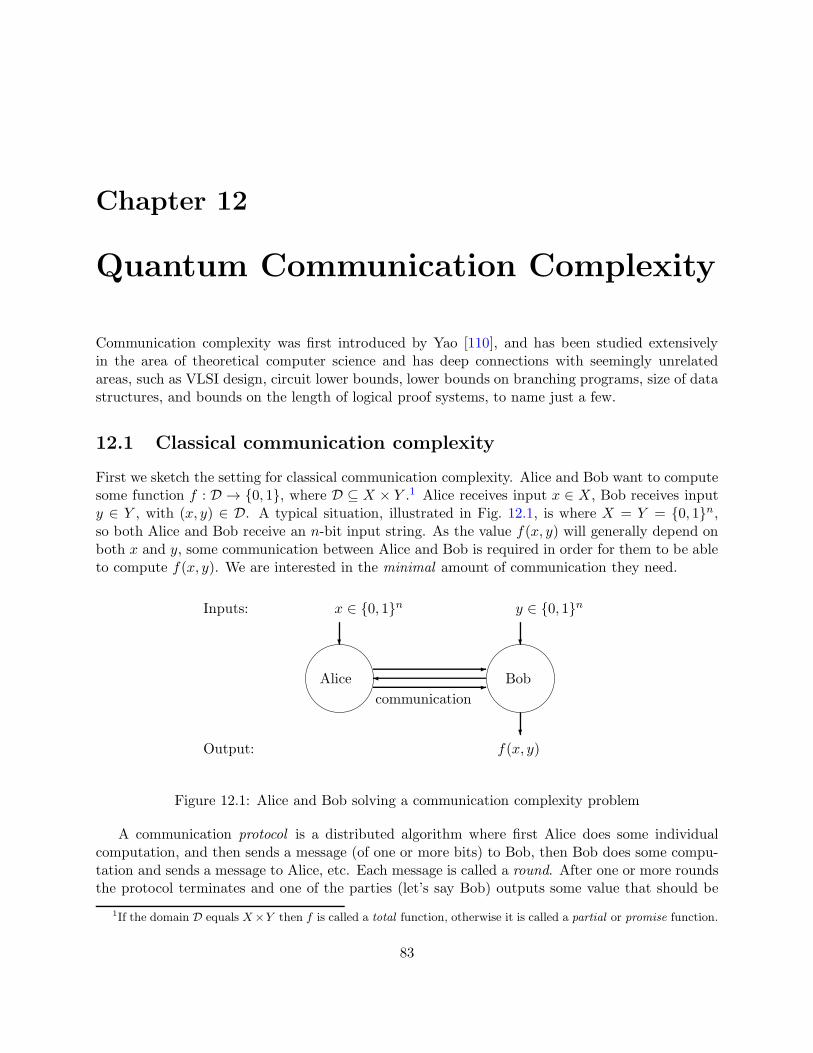
Chapter 12
Quantum Communication Complexity
Communication complexity was first introduced by Yao [110], and has been studied extensivelyin the area of theoretical computer science and has deep connections with seemingly unrelatedareas, such as VLSI design, circuit lower bounds, lower bounds on branching programs, size of datastructures, and bounds on the length of logical proof systems, to name just a few.
12.1 Classical communication complexity
First we sketch the setting for classical communication complexity. Alice and Bob want to computesome function f : D → 0, 1, where D ⊆ X × Y .1 Alice receives input x ∈ X, Bob receives inputy ∈ Y , with (x, y) ∈ D. A typical situation, illustrated in Fig. 12.1, is where X = Y = 0, 1n,so both Alice and Bob receive an n-bit input string. As the value f(x, y) will generally depend onboth x and y, some communication between Alice and Bob is required in order for them to be ableto compute f(x, y). We are interested in the minimal amount of communication they need.
Alice
x ∈ 0, 1n
Bob
y ∈ 0, 1n
f(x, y)
communication
Inputs:
Output:
Figure 12.1: Alice and Bob solving a communication complexity problem
A communication protocol is a distributed algorithm where first Alice does some individualcomputation, and then sends a message (of one or more bits) to Bob, then Bob does some compu-tation and sends a message to Alice, etc. Each message is called a round. After one or more roundsthe protocol terminates and one of the parties (let’s say Bob) outputs some value that should be
1If the domain D equals X×Y then f is called a total function, otherwise it is called a partial or promise function.
83
f(x, y). The cost of a protocol is the total number of bits communicated on the worst-case input.A deterministic protocol for f always has to output the right value f(x, y) for all (x, y) ∈ D. Ina bounded-error protocol, Alice and Bob may flip coins and the protocol has to output the rightvalue f(x, y) with probability ≥ 2/3 for all (x, y) ∈ D. We could either allow Alice and Bob to tosscoins individually (local randomness, or “private coin”) or jointly (shared randomness, or “publiccoin”). A public coin can simulate a private coin and is potentially more powerful. However, New-man’s theorem [87] says that having a public coin can save at most O(log n) bits of communication,compared to a protocol with a private coin.
To illustrate the power of randomness, let us give a simple yet efficient bounded-error protocolfor the equality problem, where the goal for Alice is to determine whether her n-bit input is thesame as Bob’s or not: f(x, y) = 1 if x = y, and f(x, y) = 0 otherwise. Alice and Bob jointly toss arandom string r ∈ 0, 1n. Alice sends the bit a = x · r to Bob (where ‘·’ is inner product mod 2).Bob computes b = y · r and compares this with a. If x = y then a = b, but if x 6= y then a 6= b withprobability 1/2. Repeating this a few times, Alice and Bob can decide equality with small errorusing O(n) public coin flips and a constant amount of communication. This protocol uses publiccoins, but note that Newman’s theorem implies that there exists an O(log n)-bit protocol that usesa private coin (see Exercise 6 for an explicit protocol).
12.2 The quantum question
Now what happens if we give Alice and Bob a quantum computer and allow them to send eachother qubits and/or to make use of EPR-pairs that they share at the start of the protocol?
Formally speaking, we can model a quantum protocol as follows. The total state consistsof 3 parts: Alice’s private space, the channel, and Bob’s private space. The starting state is|x〉|0〉|y〉: Alice gets x, the channel is initialized to 0, and Bob gets y. Now Alice applies a unitarytransformation to her space and the channel. This corresponds to her private computation as wellas to putting a message on the channel (the length of this message is the number of channel-qubitsaffected by Alice’s operation). Then Bob applies a unitary transformation to his space and thechannel, etc. At the end of the protocol Alice or Bob makes a measurement to determine theoutput of the protocol. This model was introduced by Yao [111].
In the second model, introduced by Cleve and Buhrman [35], Alice and Bob share an unlimitednumber of EPR-pairs at the start of the protocol, but now they communicate via a classical channel:the channel has to be in a classical state throughout the protocol. We only count the communication,not the number of EPR-pairs used. Protocols of this kind can simulate protocols of the first kindwith only a factor 2 overhead: using teleportation, the parties can send each other a qubit usingan EPR-pair and two classical bits of communication. Hence the qubit-protocols that we describebelow also immediately yield protocols that work with entanglement and a classical channel. Notethat an EPR-pair can simulate a public coin toss: if Alice and Bob each measure their half of thepair of qubits, they get the same random bit.
The third variant combines the strengths of the other two: here Alice and Bob start out withan unlimited number of EPR-pairs and they are allowed to communicate qubits. This third kindof communication complexity is in fact equivalent to the second, up to a factor of 2, again byteleportation.
Before continuing to study this model, we first have to face an important question: is thereanything to be gained here? At first sight, the following argument seems to rule out any significant
84
gain. Suppose that in the classical world k bits have to be communicated in order to compute f .Since Holevo’s theorem says that k qubits cannot contain more information than k classical bits, itseems that the quantum communication complexity should be roughly k qubits as well (maybe k/2to account for superdense coding, but not less). Surprisingly (and fortunately for us), this argumentis false, and quantum communication can sometimes be much less than classical communicationcomplexity. The information-theoretic argument via Holevo’s theorem fails, because Alice andBob do not need to communicate the information in the k bits of the classical protocol; they areonly interested in the value f(x, y), which is just 1 bit. Below we will go over four of the mainexamples that have so far been found of differences between quantum and classical communicationcomplexity.
12.3 Example 1: Distributed Deutsch-Jozsa
The first impressively large gaps between quantum and classical communication complexity wereexhibited by Buhrman, Cleve, and Wigderson [28]. Their protocols are distributed versions ofknown quantum query algorithms, like the Deutsch-Jozsa and Grover algorithms. Let us startwith the first one. It is actually explained most easily in a direct way, without reference to theDeutsch-Jozsa algorithm (though that is where the idea came from). The problem is a promiseversion of the equality problem. Suppose the n-bit inputs x and y are restricted to the followingcase:
Distributed Deutsch-Jozsa: either x = y, or x and y differ in exactly n/2 positions
Note that this promise only makes sense if n is an even number, otherwise n/2 would not be integer.In fact it will be convenient to assume n a power of 2. Here is a simple quantum protocol to solvethis promise version of equality using only log n qubits:
1. Alice sends Bob the log n-qubit state 1√n
∑ni=1(−1)xi |i〉, which she can prepare unitarily from
x and log n |0〉-qubits.
2. Bob applies the unitary map |i〉 7→ (−1)yi |i〉 to the state, applies a Hadamard transform toeach qubit (for this it is convenient to view i as a log n-bit string), and measures the resultinglog n-qubit state.
3. Bob outputs 1 if the measurement gave∣∣0logn
⟩and outputs 0 otherwise.
It is clear that this protocol only communicates log n qubits, but why does it work? Note that thestate that Bob measures is
H⊗ logn
(1√n
n∑
i=1
(−1)xi+yi |i〉)
=1
n
n∑
i=1
(−1)xi+yi∑
j∈0,1log n
(−1)i·j |j〉
This superposition looks rather unwieldy, but consider the amplitude of the∣∣0logn
⟩basis state. It
is 1n
∑ni=1(−1)xi+yi , which is 1 if x = y and 0 otherwise because the promise now guarantees that
x and y differ in exactly n/2 of the bits! Hence Bob will always give the correct answer.
What about efficient classical protocols (without entanglement) for this problem? Provinglower bounds on communication complexity often requires a very technical combinatorial analysis.
85
Buhrman, Cleve, and Wigderson used a deep combinatorial result from [51] to prove that everyclassical errorless protocol for this problem needs to send at least 0.007n bits.
This log n-qubits-vs-0.007n-bits example was the first exponentially large separation of quantumand classical communication complexity. Notice, however, that the difference disappears if we moveto the bounded-error setting, allowing the protocol to have some small error probability. We canuse the randomized protocol for equality discussed above or even simpler: Alice can just send a few(i, xi) pairs to Bob, who then compares the xi’s with his yi’s. If x = y he will not see a difference,but if x and y differ in n/2 positions, then Bob will probably detect this. Hence O(log n) classicalbits of communication suffice in the bounded-error setting, in sharp contrast to the errorless setting.
12.4 Example 2: The Intersection problem
Now consider the Intersection function, which is 1 if xi = yi = 1 for at least one i. Buhrman, Cleve,and Wigderson [28] also presented an efficient quantum protocol for this, based on Grover’s searchalgorithm. We can solve Intersection if we can solve the following search problem: find some i suchthat xi = yi = 1 (if such an i exists).2 We want to find a solution to the search problem on thestring z = x ∧ y (which is the bit-wise AND of x and y), since zi = 1 whenever both xi = 1 andyi = 1. The idea is now to let Alice run Grover’s algorithm to search for such a solution. Clearly,she can prepare the uniform starting state herself. She can also apply H and R herself. The onlything where she needs Bob’s help, is in implementing Oz. This they do as follows. Whenever Alicewants to apply Oz to a state
|φ〉 =n∑
i=1
αi|i〉,
she tags on her xi in an extra qubit and sends Bob the state
n∑
i=1
αi|i〉|xi〉.
Bob applies the unitary map
|i〉|xi〉 7→ (−1)xi∧yi |i〉|xi〉
and sends back the result. Alice sets the last qubit back to |0〉 (which she can do unitarily becauseshe has x), and now she has the state Oz|φ〉! Thus we can simulate Oz using 2 messages of log(n)+1qubits each. Thus Alice and Bob can run Grover’s algorithm to find an intersection, using O(
√n)
messages of O(log n) qubits each, for total communication of O(√n log n) qubits. Later Aaronson
and Ambainis [1] gave a more complicated protocol that uses O(√n) qubits of communication.
What about lower bounds? It is a well-known result of classical communication complexity thatclassical bounded-error protocols for the Intersection problem need about n bits of communication.Thus we have a quadratic quantum-classical separation for this problem. Could there be a quantumprotocol that uses much less than
√n qubits of communication? This question was open for quite a
few years after [28] appeared, until finally Razborov [91] showed that any bounded-error quantumprotocol for Intersection needs to communicate about
√n qubits.
2This is sometimes called the appointment-scheduling problem: view x and y as Alice’s and Bob’s agendas, respec-tively, with a 1 indicating a free timeslot. Then the goal is to find a timeslot where Alice and Bob are both free, sothey can schedule an appointment.
86
12.5 Example 3: The vector-in-subspace problem
Notice the contrast between the examples of the last two sections. For the Distributed Deutsch-Jozsa problem we get an exponential quantum-classical separation, but the separation only holdsif we require the classical protocol to be errorless. On the other hand, the gap for the disjointnessfunction is only quadratic, but it holds even if we allow classical protocols to have some errorprobability.
Here is a function where the quantum-classical separation has both features: the quantumprotocol is exponentially better than the classical protocol, even if the latter is allowed some error:
Alice receives a unit vector v ∈ Rm
Bob receives two m-dimensional projectors P0 and P1 such that P0 + P1 = IPromise: either P0v = v or P1v = v.Question: which of the two?
As stated, this is a problem with continuous input, but it can be discretized in a natural way byapproximating each real number by O(logm) bits. Alice and Bob’s input is now n = O(m2 logm)bits long. There is a simple yet efficient 1-round quantum protocol for this problem: Alice views vas a logm-qubit state and sends this to Bob; Bob measures with operators P0 and P1, and outputsthe result. This takes only logm = O(log n) qubits of communication.
The efficiency of this protocol comes from the fact that an m-dimensional unit vector can be“compressed” or “represented” as a logm-qubit state. Similar compression is not possible withclassical bits, which suggests that any classical protocol will have to send the vector v more or lessliterally and hence will require a lot of communication. This turns out to be true, but the proof isquite hard [71]. It shows that any bounded-error protocol needs to send Ω(m1/3) bits.
12.6 Example 4: Quantum fingerprinting
The examples of the previous section were either exponential quantum improvements for promiseproblems (Deutsch-Jozsa and vector-in-subspace) or polynomial improvements for total problems(disjointness). We will now give an exponential improvement for the total problem of equality-testing, but in a restricted setting called the simultaneous message passing (SMP) model. Aliceand Bob receive n-bit input x and y, respectively. They do not have any shared resources like sharedrandomness or an entangled state, but they do have local randomness. They don’t communicatewith each other directly, but instead send a single message to a third party, called the Referee. TheReferee, upon receiving message mA from Alice and mB from Bob, should output the value f(x, y).The goal is to compute f(x, y) with a minimal amount of communication from Alice and Bob tothe Referee.
We will see that for the equality problem there is an exponential savings in communicationwhen qubits are used instead of classical bits. Classically, the problem of the bounded-error com-munication complexity of equality in the SMP model was first raised by Yao [110], and was openfor almost twenty years until Newman and Szegedy [88] exhibited a lower bound of Ω(
√n) bits.
This is tight, since Ambainis [4] constructed a bounded-error protocol for this problem where themessages are O(
√n) bits long (see Exercise 5). In contrast, in the quantum setting this problem
can be solved with very little communication: only O(log n) qubits suffice [27].The quantum trick is to associate each x ∈ 0, 1n with a short quantum state |φx〉, called
the quantum fingerprint of x. Just like with physical fingerprints, the idea is that a quantum
87
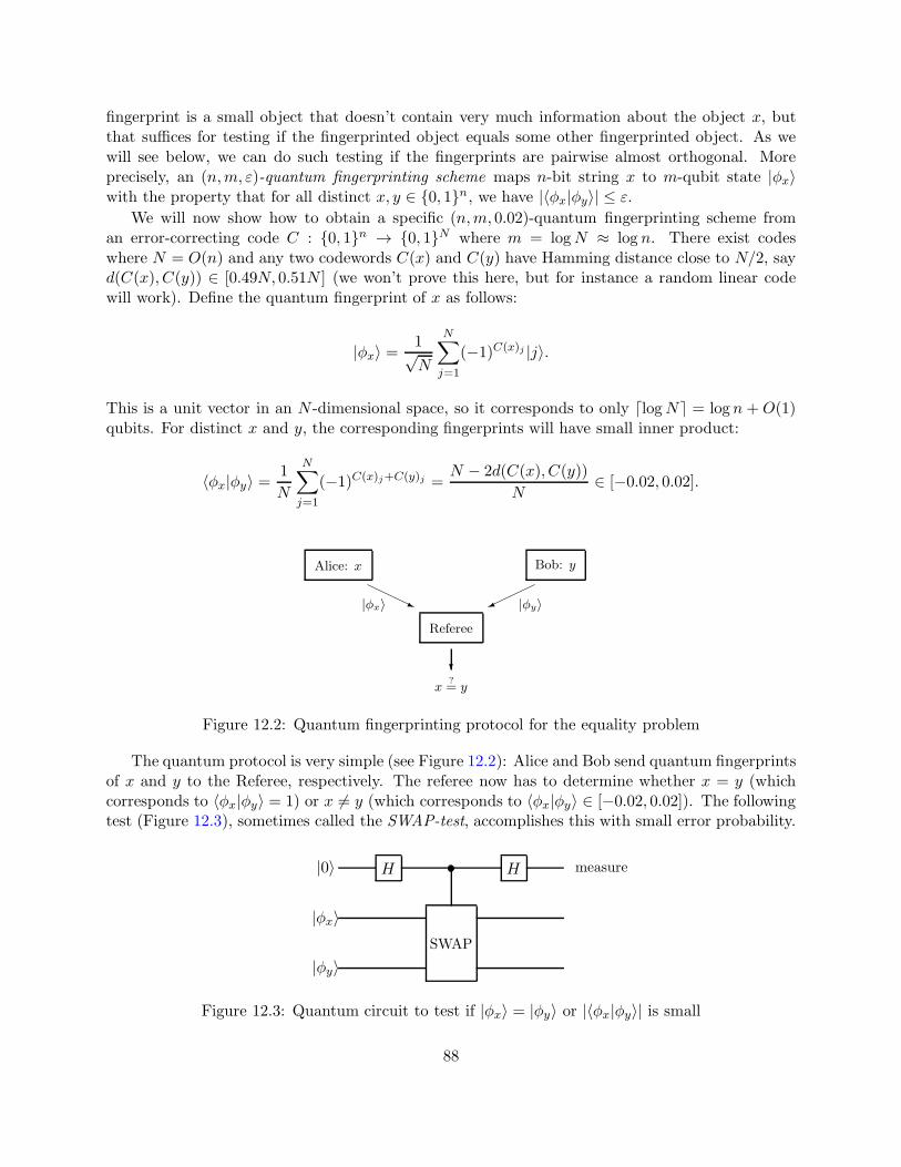
fingerprint is a small object that doesn’t contain very much information about the object x, butthat suffices for testing if the fingerprinted object equals some other fingerprinted object. As wewill see below, we can do such testing if the fingerprints are pairwise almost orthogonal. Moreprecisely, an (n,m, ε)-quantum fingerprinting scheme maps n-bit string x to m-qubit state |φx〉with the property that for all distinct x, y ∈ 0, 1n, we have |〈φx|φy〉| ≤ ε.
We will now show how to obtain a specific (n,m, 0.02)-quantum fingerprinting scheme froman error-correcting code C : 0, 1n → 0, 1N where m = logN ≈ log n. There exist codeswhere N = O(n) and any two codewords C(x) and C(y) have Hamming distance close to N/2, sayd(C(x), C(y)) ∈ [0.49N, 0.51N ] (we won’t prove this here, but for instance a random linear codewill work). Define the quantum fingerprint of x as follows:
|φx〉 =1√N
N∑
j=1
(−1)C(x)j |j〉.
This is a unit vector in an N -dimensional space, so it corresponds to only ⌈logN⌉ = log n + O(1)qubits. For distinct x and y, the corresponding fingerprints will have small inner product:
〈φx|φy〉 =1
N
N∑
j=1
(−1)C(x)j+C(y)j =N − 2d(C(x), C(y))
N∈ [−0.02, 0.02].
Alice: x Bob: y
|φx〉 |φy〉Referee
x
?= y
Figure 12.2: Quantum fingerprinting protocol for the equality problem
The quantum protocol is very simple (see Figure 12.2): Alice and Bob send quantum fingerprintsof x and y to the Referee, respectively. The referee now has to determine whether x = y (whichcorresponds to 〈φx|φy〉 = 1) or x 6= y (which corresponds to 〈φx|φy〉 ∈ [−0.02, 0.02]). The followingtest (Figure 12.3), sometimes called the SWAP-test, accomplishes this with small error probability.
|0〉
|φx〉
|φy〉
measureH H
SWAP
Figure 12.3: Quantum circuit to test if |φx〉 = |φy〉 or |〈φx|φy〉| is small
88
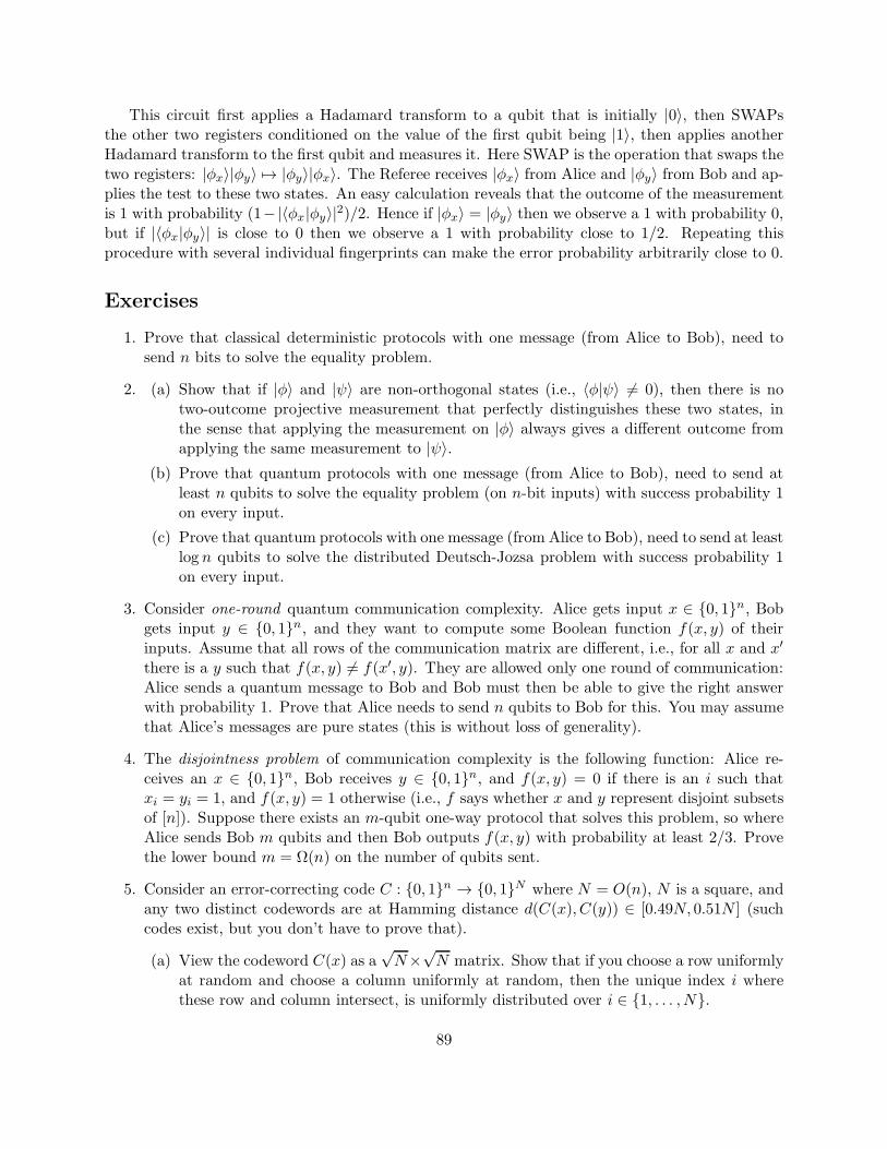
This circuit first applies a Hadamard transform to a qubit that is initially |0〉, then SWAPsthe other two registers conditioned on the value of the first qubit being |1〉, then applies anotherHadamard transform to the first qubit and measures it. Here SWAP is the operation that swaps thetwo registers: |φx〉|φy〉 7→ |φy〉|φx〉. The Referee receives |φx〉 from Alice and |φy〉 from Bob and ap-plies the test to these two states. An easy calculation reveals that the outcome of the measurementis 1 with probability (1−|〈φx|φy〉|2)/2. Hence if |φx〉 = |φy〉 then we observe a 1 with probability 0,but if |〈φx|φy〉| is close to 0 then we observe a 1 with probability close to 1/2. Repeating thisprocedure with several individual fingerprints can make the error probability arbitrarily close to 0.
Exercises
1. Prove that classical deterministic protocols with one message (from Alice to Bob), need tosend n bits to solve the equality problem.
2. (a) Show that if |φ〉 and |ψ〉 are non-orthogonal states (i.e., 〈φ|ψ〉 6= 0), then there is notwo-outcome projective measurement that perfectly distinguishes these two states, inthe sense that applying the measurement on |φ〉 always gives a different outcome fromapplying the same measurement to |ψ〉.
(b) Prove that quantum protocols with one message (from Alice to Bob), need to send atleast n qubits to solve the equality problem (on n-bit inputs) with success probability 1on every input.
(c) Prove that quantum protocols with one message (from Alice to Bob), need to send at leastlog n qubits to solve the distributed Deutsch-Jozsa problem with success probability 1on every input.
3. Consider one-round quantum communication complexity. Alice gets input x ∈ 0, 1n, Bobgets input y ∈ 0, 1n, and they want to compute some Boolean function f(x, y) of theirinputs. Assume that all rows of the communication matrix are different, i.e., for all x and x′
there is a y such that f(x, y) 6= f(x′, y). They are allowed only one round of communication:Alice sends a quantum message to Bob and Bob must then be able to give the right answerwith probability 1. Prove that Alice needs to send n qubits to Bob for this. You may assumethat Alice’s messages are pure states (this is without loss of generality).
4. The disjointness problem of communication complexity is the following function: Alice re-ceives an x ∈ 0, 1n, Bob receives y ∈ 0, 1n, and f(x, y) = 0 if there is an i such thatxi = yi = 1, and f(x, y) = 1 otherwise (i.e., f says whether x and y represent disjoint subsetsof [n]). Suppose there exists an m-qubit one-way protocol that solves this problem, so whereAlice sends Bob m qubits and then Bob outputs f(x, y) with probability at least 2/3. Provethe lower bound m = Ω(n) on the number of qubits sent.
5. Consider an error-correcting code C : 0, 1n → 0, 1N where N = O(n), N is a square, andany two distinct codewords are at Hamming distance d(C(x), C(y)) ∈ [0.49N, 0.51N ] (suchcodes exist, but you don’t have to prove that).
(a) View the codeword C(x) as a√N×
√N matrix. Show that if you choose a row uniformly
at random and choose a column uniformly at random, then the unique index i wherethese row and column intersect, is uniformly distributed over i ∈ 1, . . . , N.
89
(b) Give a classical bounded-error SMP-protocol for the equality problem where Alice andBob each send O(
√n) bits to the Referee.
6. Alice and Bob want to solve the equality problem on n-bit inputs x and y. x = y. They donot share randomness (or entanglement) but can use local (private) randomness.
(a) Fix a prime number p ∈ [3n, 6n], then the set Fp of integers modulo p is a finite field(i.e., it has a well-defined addition and multiplication). For x = (x0, . . . , xn−1) ∈ 0, 1n,define the univariate polynomial Px : Fp → Fp of degree < n as Px(t) =
∑n−1i=0 xit
i (notethat the n bits of x are used as coefficients here, not as the argument of the polynomial).Show that for distinct n-bit strings x and y, we have Prt∈Fp [Px(t) = Py(t)] ≤ 1/3, wherethe probability is taken over a uniformly random t ∈ Fp.
(b) Use (a) to give a classical communication protocol where Alice sends an O(log n)-bitmessage to Bob, and Bob can decide whether x = y with success probability ≥ 2/3.
(c) Use (a) to give a quantum fingerprinting scheme x 7→ |φx〉, where quantum state |φx〉has O(log n) qubits, and |〈φx|φy〉| ∈ [0, 1/3] for all distinct n-bit strings x and y (provethe latter property explicitly, it’s not enough to write down only the states).
7. Suppose Alice and Bob each have n-bit agendas, and they know that for exactly 25% ofthe timeslots they are both free. Give a quantum protocol that finds such a timeslot withprobability 1, using only O(log n) qubits of communication.
8. The inner product problem in communication complexity is the function f : 0, 1n ×0, 1n → 0, 1 defined by f(x, y) =
∑ni=1 xiyi mod 2. Suppose there exists a quantum
protocol P for Alice and Bob that uses q qubits of communication (possibly using multiplemessages between Alice and Bob) and computes the inner product function with success prob-ability 1 (on every possible inputs x, y). The protocol does not assume any shared entangledstate at the start.
(a) Give a quantum protocol that uses 2q qubits of communication and implements the 2n-qubit map |x〉A|y〉B 7→ (−1)x·y|x〉A|y〉B (possibly with some auxiliary qubits for each ofAlice and Bob; these should start and end in state |0〉).
(b) Give a quantum protocol where Alice transmits x to Bob using 2q qubits of communi-cation.
(c) Derive a lower bound on q from (b) and Holevo’s theorem.
9. Consider the following problem in communication complexity. Alice’s input has two parts:a unit vector v ∈ Rm and two orthogonal projectors P0 and P1. Bob’s input is an m × munitary U . They are promised that the vector Uv either lies in the subspace corresponding toP0 (i.e., P0Uv = v) or in the subspace corresponding to P1 (i.e., P1Uv = v), and the problemfor Alice and Bob is to find out which of these two cases holds.
(a) Give a quantum protocol that uses two messages of O(logm) qubits (one message fromAlice to Bob and one from Bob to Alice) to solve this problem with success probability 1.
(b) Show that there exists a constant c > 0 such that classical protocols need to send Ω(mc)bits of communication to solve this problem with error probability ≤ 1/3, even whenthey are allowed to send many messages.
90
10. Consider the following communication complexity problem, called the “Hidden MatchingProblem,” from [12]. Alice’s input is some x ∈ 0, 1n. Bob’s input is a matching M , i.e., apartition of 1, . . . , n into n/2 disjoint pairs (assume n is a power of 2). Their goal is thatBob outputs a pair (i, j) ∈M together with the parity xi⊕xj of the two bits indexed by thatpair. It doesn’t matter which pair (i, j) ∈ M Bob outputs, as long as the additional bit ofoutput equals the parity of the two indexed bits of x. Show that they can solve this problemwith success probability 1 using only a message of log n qubits from Alice to Bob (and nocommunication from Bob to Alice).
91

92
Chapter 13
Entanglement and Non-locality
13.1 Quantum non-locality
Entangled states are those that cannot be written as a tensor product of separate states. The mostfamous one is the EPR-pair:
1√2(|00〉+ |11〉).
Suppose Alice has the first qubit of the pair, and Bob has the second. If Alice measures her qubitin the computational basis and gets outcome b ∈ 0, 1, then the state collapses to |bb〉. Similarly,if Alice measures her qubit in some other basis, this will collapse the joint state (including Bob’squbit) to some state that depends on her measurement basis as well as its outcome. SomehowAlice’s action seems to have an instantaneous effect on Bob’s side—even if the two qubits arelight-years apart! This was a great bother to Einstein, whose theory of relativity posits thatinformation and causation cannot travel faster than the speed of light. Einstein called such effectsof entanglement “spooky action at a distance” (in German: “spukhafte Fernwirkungen”), andviewed it as a fundamental problem for quantum mechanics [45]. In his view, quantum mechanicsshould be replaced by some “local realist” physical theory that would still have the same predictivepower as quantum mechanics. Here “local” means that information and causation act locally, notfaster than light, and “realistic” means that physical systems have definite, well-defined properties(even if those properties may be unknown to us).
Note that the above experiment where Alice measures her half of the EPR-pair doesn’t actuallyviolate locality: no information is transfered from Alice and Bob. From Bob’s perspective thereis no difference between the situation where Alice measured and the situation where she didn’t.1
For this experiment, a shared coin flip between Alice and Bob is a local realist physical modelthat has exactly the same observable consequences as measuring the qubits of the EPR-pair in thecomputational basis: a 50-50 distribution on outcomes |00〉 and |11〉. This shared-coin-flip modelis local because no information is transfered between Alice and Bob, and it’s realist because thecoin flip has a definite outcome (even if that outcome is unknown to Alice and Bob before theymeasure).
Given this example, one might hope (and Einstein expected) that any kind of behavior thatcomes from entangled states can be replaced by some local realist physical model. This way,quantum mechanics could be replaced by an alternative physical theory with less counter-intuitive
1In fact, one can show that entanglement can never replace communication.
93
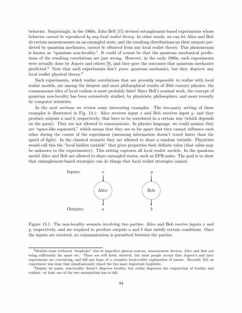
behavior. Surprisingly, in the 1960s, John Bell [15] devised entanglement-based experiments whosebehavior cannot be reproduced by any local realist theory. In other words, we can let Alice and Bobdo certain measurements on an entangled state, and the resulting distributions on their outputs pre-dicted by quantum mechanics, cannot be obtained from any local realist theory. This phenomenonis known as “quantum non-locality.” It could of course be that the quantum mechanical predic-tions of the resulting correlations are just wrong. However, in the early 1980s, such experimentswere actually done by Aspect and others [9], and they gave the outcomes that quantum mechanicspredicted.2 Note that such experiments don’t prove quantum mechanics, but they disprove anylocal realist physical theory.3
Such experiments, which realize correlations that are provably impossible to realize with localrealist models, are among the deepest and most philosophical results of 20th century physics: thecommonsense idea of local realism is most probably false! Since Bell’s seminal work, the concept ofquantum non-locality has been extensively studied, by physicists, philosophers, and more recentlyby computer scientists.
In the next sections we review some interesting examples. The two-party setting of theseexamples is illustrated in Fig. 13.1: Alice receives input x and Bob receives input y, and theyproduce outputs a and b, respectively, that have to be correlated in a certain way (which dependson the game). They are not allowed to communicate. In physics language, we could assume theyare “space-like separated,” which means that they are so far apart that they cannot influence eachother during the course of the experiment (assuming information doesn’t travel faster than thespeed of light). In the classical scenario they are allowed to share a random variable. Physicistswould call this the “local hidden variable” that gives properties their definite value (that value maybe unknown to the experimenter). This setting captures all local realist models. In the quantummodel Alice and Bob are allowed to share entangled states, such as EPR-pairs. The goal is to showthat entanglement-based strategies can do things that local realist strategies cannot.
Alice
x
a
Bob
y
b
Inputs:
Outputs:
Figure 13.1: The non-locality scenario involving two parties: Alice and Bob receive inputs x andy, respectively, and are required to produce outputs a and b that satisfy certain conditions. Oncethe inputs are received, no communication is permitted between the parties.
2Modulo some technical “loopholes” due to imperfect photon sources, measurement devices, Alice and Bob notbeing sufficiently far apart etc. These are still hotly debated, but most people accept that Aspect’s and laterexperiments are convincing, and kill any hope of a complete local-realist explanation of nature. Recently [62] anexperiment was done that simultaneously closed the two most important loopholes.
3Despite its name, non-locality doesn’t disprove locality, but rather disproves the conjunction of locality andrealism—at least one of the two assumptions has to fail.
94
13.2 CHSH: Clauser-Horne-Shimony-Holt
In the CHSH game [33] Alice and Bob receive input bits x and y, and their goal is to output bitsa and b, respectively, such that
a⊕ b = x ∧ y, (13.1)
(‘∧’ is logical AND; ‘⊕’ is parity, i.e. addition mod 2) or, failing that, to satisfy this condition withas high a probability as possible.
First consider the case of classical deterministic strategies, so without any randomness. Forthese, Alice’s output bit depends solely on her input bit x, and similarly for Bob. Let a0 be thebit that Alice outputs if her input is x = 0, and a1 the bit she outputs if x = 1. Let b0, b1 be theoutputs Bob gives on inputs y = 0 and y = 1, respectively. These four bits completely characterizeany deterministic strategy. Condition (13.1) becomes
a0 ⊕ b0 = 0,
a0 ⊕ b1 = 0,
a1 ⊕ b0 = 0,
a1 ⊕ b1 = 1. (13.2)
It is impossible to satisfy all four equations simultaneously, since summing them modulo 2 yields0 = 1. Therefore it is impossible to satisfy Condition (13.1) perfectly. Since a probabilistic strategy(where Alice and Bob share randomness) is a probability distribution over deterministic strategies,it follows that no probabilistic strategy can have success probability better than 3/4 on everypossible input (the 3/4 can be achieved simultaneously for every input, see Exercise 2).4
Now consider the same problem but where Alice and Bob are supplied with a shared two-qubitsystem initialized to the entangled state
1√2(|00〉 − |11〉).
Such a state can easily be obtained from an EPR-pair, for instance if Alice applies a Z to her qubit.Now the parties can produce outputs that satisfy Condition (13.1) with probability cos(π/8)2 ≈ 0.85(higher than what is possible in the classical case), as follows. Recall the unitary operation that
rotates the qubit by angle θ: R(θ) =
(cos θ − sin θsin θ cos θ
). If x = 0 then Alice applies R(−π/16) to
her qubit; and if x = 1 she applies R(3π/16). Then Alice measures her qubit in the computationalbasis and outputs the resulting bit a. Bob’s procedure is the same, depending on his input bit y. Itis straightforward to calculate that if Alice rotates by θA and Bob rotates by θB , the state becomes
1√2(cos(θA + θB)(|00〉 − |11〉) + sin(θA + θB)(|01〉+ |10〉)) .
After the measurements, the probability that a ⊕ b = 0 is cos(θA + θB)2. Note that if x ∧ y = 0
then θA + θB = ±π/8, while if x ∧ y = 1 then θA + θB = 3π/8. Hence Condition 13.1 is satisfiedwith probability cos(π/8)2 for all four input possibilities, showing that quantum entanglementallows Alice and Bob to win the game with a probability that’s higher than what the best classicalstrategy can achieve. Tsirelson [32] showed that cos(π/8)2 is the best that quantum strategies cando for CHSH, even if they are allowed to use much more entanglement than one EPR-pair (see thelast exercise of this chapter).
4Such statements, upper bounding the optimal success probability of classical strategies for a specific game, areknown as Bell inequalities. This specific one is called the CHSH inequality.
95
13.3 Magic square game
Is there a game where the quantum protocol always succeeds, while the best classical successprobability is bounded below 1? A particularly elegant example is the following magic squaregame [8]. Consider the problem of labeling the entries of a 3×3 matrix with bits so that the parityof each row is even, whereas the parity of each column is odd. This is clearly impossible: if theparity of each row is even then the sum of the 9 bits is 0 mod 2, but if the parity of each columnis odd then the sum of the 9 bits is 1 mod 2. The two matrices
0 0 0
0 0 0
1 1 0
0 0 0
0 0 0
1 1 1
each satisfy five out of the six constraints. For the first matrix, all rows have even parity, but onlythe first two columns have odd parity. For the second matrix, the first two rows have even parity,and all columns have odd parity.
Consider the game where Alice receives x ∈ 1, 2, 3 as input (specifying the number of a row),and Bob receives y ∈ 1, 2, 3 as input (specifying the number of a column). Their goal is to eachproduce 3-bit outputs, a1a2a3 for Alice and b1b2b3 for Bob, such that
1. They satisfy the row/column parity constraints: a1 ⊕ a2 ⊕ a3 = 0 and b1 ⊕ b2 ⊕ b3 = 1.
2. They are consistent where the row intersects the column: ay = bx.
As usual, Alice and Bob are forbidden from communicating once the game starts, so Alice does notknow y and Bob does not know x. We shall show the best classical strategy has success probability8/9, while there is a quantum strategy that always succeeds.
An example of a deterministic strategy that attains success probability 8/9 (when the input xyis uniformly distributed) is where Alice plays according to the rows of the first matrix above andBob plays according the columns of the second matrix above. This succeeds in all cases, exceptwhere x = y = 3. To see why this is optimal, note that for any other classical strategy, it is possibleto represent it as two matrices as above but with different entries. Alice plays according to therows of the first matrix and Bob plays according to the columns of the second matrix. We canassume that the rows of Alice’s matrix all have even parity; if she outputs a row with odd paritythen they immediately lose, regardless of Bob’s output. Similarly, we can assume that all columnsof Bob’s matrix have odd parity.5 Considering such a pair of matrices, the players lose at eachentry where they differ. There must be such an entry, since otherwise it would be possible to haveall rows even and all columns odd with one matrix. Thus, when the input xy is chosen uniformlyfrom 1, 2, 3 × 1, 2, 3, the success probability of any classical strategy is at most 8/9.
We now give the quantum strategy for this game. Let I, X, Y , Z be the 2× 2 Pauli matrices:
I =
(1 00 1
), X =
(0 11 0
), Y =
(0 −ii 0
), and Z =
(1 00 −1
). (13.3)
Each is an observable (see Section 1.2.2) with eigenvalues in +1,−1. That is, each can be writtenas P+−P− where P+ and P− are orthogonal projectors that sum to identity, and hence define a two-outcome measurement with outcomes +1 and −1. For example, Z = |0〉〈0| − |1〉〈1|, corresponding
5In fact, the game can be simplified so that Alice and Bob each output just two bits, since the parity constraintdetermines the third bit.
96
to a measurement in the computational basis (with |b〉 corresponding to outcome (−1)b). AndX = |+〉〈+|− |−〉〈−|, corresponding to a measurement in the Hadamard basis. The Pauli matricesare self-inverse, they anti-commute (e.g., XY = −Y X), and X = iZY , Y = iXZ, and Z = iY X.Consider the following table, where each entry is a tensor product of two Paulis:
X ⊗X Y ⊗ Z Z ⊗ Y
Y ⊗ Y Z ⊗X X ⊗ Z
Z ⊗ Z X ⊗ Y Y ⊗X
Because (P+−P−)⊗(Q+−Q−) = (P+⊗Q++P−⊗Q−)−(P+⊗Q−+P−⊗Q+), each such productis itself an observable. Hence each product of Pauli matrices corresponds to a measurement on atwo-qubit space, with outcomes +1 and −1.
Note that the observables along each row commute and their product is I⊗I, and the observablesalong each column commute and their product is −I ⊗ I. This implies that for any two-qubitstate, performing the three measurements along any row results in three +1,−1-valued bitswhose product is +1. Also, performing the three measurements along any column results in three+1,−1-valued bits whose product is −1.
We can now describe the quantum protocol. It uses two pairs of entangled qubits, each of whichis in initial state
1√2(|01〉 − |10〉)
(again, such states can be obtained from EPR-pairs by local operations). Alice, on input x, appliesthree two-qubit measurements corresponding to the observables in row x of the above table. Foreach measurement, if the result is +1 then she outputs 0, and if the result is −1 then she outputs 1.Similarly, Bob, on input y, applies the measurements corresponding to the observables in columny, and converts the ±1-outcomes into bits.
We have already established that Alice and Bob’s output bits satisfy the required parity con-straints. It remains to show that Alice and Bob’s output bits agree at the point where the rowmeets the column. For that measurement, Alice and Bob are measuring with respect to the sameobservable in the above table. Because all the observables in each row and in each column com-mute, we may assume that the place where they intersect is the first observable applied. Thosebits are obtained by Alice and Bob each measuring 1
2(|01〉 − |10〉)(|01〉 − |10〉) with respect to theobservable in entry (x, y) of the table. To show that their measurements will agree for all cases ofxy, we consider the individual Pauli measurements on the individual entangled pairs of the form1√2(|01〉 − |10〉). Let a′ and b′ denote the outcomes of the first measurement (in terms of bits), and
a′′ and b′′ denote the outcomes of the second. Since the measurement associated with the tensorproduct of two observables is operationally equivalent to measuring each individual observable andtaking the product of the results, we have ay = a′ ⊕ a′′ and bx = b′ ⊕ b′′. It is straightforward toverify that if the same measurement from I,X, Y, Z is applied to each qubit of 1√
2(|01〉 − |10〉)
then the outcomes will be distinct: a′ ⊕ b′ = 1 and a′′ ⊕ b′′ = 1. We now have ay = bx, because
ay ⊕ bx = (a′ ⊕ a′′)⊕ (b′ ⊕ b′′) = (a′ ⊕ b′)⊕ (a′′ ⊕ b′′) = 1⊕ 1 = 0. (13.4)
13.4 A non-local version of distributed Deutsch-Jozsa
The previous two examples used small amounts of entanglement: one EPR-pair for CHSH, twoEPR-pairs for magic square. In both cases we could show that classical protocols need at least
97
some communication if they want to achieve the same as what entanglement-based protocols canachieve. We will now give a non-locality game that’s parametrized by a number n, and whereAlice and Bob’s quantum strategy uses log n EPR-pairs [24]. The advantage is that we can showthat classical protocols for this game need much classical communication rather than at least somenon-zero amount.
Non-local DJ problem: Alice and Bob receive n-bit inputs x and y that satisfy theDJ promise: either x = y, or x and y differ in exactly n/2 positions. The task is forAlice and Bob to provide outputs a, b ∈ 0, 1log n such that if x = y then a = b, and ifx and y differ in exactly n/2 positions then a 6= b.
They achieve this as follows
1. Alice and Bob share log n EPR-pairs, i.e., the maximally entangled state 1√n
∑n−1i=0 |i〉|i〉.6
2. They both apply locally a conditional phase to obtain: 1√n
∑n−1i=0 (−1)xi |i〉(−1)yi |i〉.
3. They both apply a Hadamard transform, obtaining
1
n√n
n−1∑
i=0
(−1)xi+yi∑
a∈0,1log n
(−1)i·a|a〉∑
b∈0,1log n
(−1)i·b|b〉
=1
n√n
∑
a,b∈0,1log n
(n−1∑
i=0
(−1)xi+yi+i·(a⊕b)
)|a〉|b〉.
4. They measure in the computational basis and output the results a and b, respectively.
For every a, the probability that both Alice and Bob obtain the same result a is:
∣∣∣∣∣1
n√n
n−1∑
i=0
(−1)xi+yi
∣∣∣∣∣
2
,
which is 1/n if x = y, and 0 otherwise. This solves the problem perfectly using prior entanglement.
What about classical protocols? Suppose there is a classical protocol that uses C bits of com-munication. If they ran this protocol, and then Alice communicated her output a to Bob (usingan additional log n bits), he could solve the distributed Deutsch-Jozsa problem since he could thencheck whether a = b or a 6= b. But we know that solving the distributed Deutsch-Jozsa problem re-quires at least 0.007n bits of communication. Hence C+log n ≥ 0.007n, so C ≥ 0.007n−log n. Thuswe have a non-locality problem that can be solved perfectly if Alice and Bob share log n EPR-pairs,while classically it needs not just some communication, but actually a lot of communication.
6Note that k EPR-pairs(
1√2(|00〉+ |11〉)
)⊗k
can also be written as1√2k
∑
i∈0,1k|i〉|i〉 if we reorder the qubits,
putting Alice’s k qubits on the left and Bob’s on the right. While these two ways of writing the state strictly speakingcorrespond to two different vectors of amplitudes, they still represent the same bipartite physical state, and we willtypically view them as equal.
98
Exercises
1. Suppose Alice and Bob share an EPR-pair 1√2(|00〉+ |11〉).
(a) Let U be a unitary with real entries. Show that the following two states are the same:(1) the state obtained if Alice applies U to her qubit of the EPR-pair;(2) the state obtained if Bob applies the transpose UT to his qubit of the EPR-pair.
(b) What state do you get if both Alice and Bob apply a Hadamard transform to their qubitof the EPR-pair?
2. Give a classical strategy using shared randomness for the CHSH game, such that Alice andBob win the game with probability at least 3/4 for every possible input x, y (note the orderof quantification: the same strategy has to work for every x, y).
3. “Mermin’s game” is the following. Consider three space-like separated players: Alice, Bob,and Charlie. Alice receives input bit x, Bob receives input bit y, and Charlie receives inputbit z. The input satisfies the promise that x⊕ y⊕ z = 0. The goal of the players is to outputbits a, b, c, respectively, such that a⊕ b⊕ c = OR(x, y, z). In other words, the outputs shouldsum to 0 (mod 2) if x = y = z = 0, and should sum to 1 (mod 2) if x+ y + z = 2.
(a) Show that every classical deterministic strategy will fail on at least one of the 4 allowedinputs.
(b) Show that every classical randomized strategy has success probability at most 3/4 underthe uniform distribution on the four allowed inputs xyz.
(c) Suppose the players share the following entangled 3-qubit state:
1
2(|000〉 − |011〉 − |101〉 − |110〉).
Suppose each player does the following: if his/her input bit is 1, apply H to his/herqubit, otherwise do nothing. Describe the resulting 3-qubit superposition.
(d) Using (c), give a quantum strategy that wins the above game with probability 1 on everypossible input.
4. This question examines how well the best quantum protocol can do for CHSH (resulting in theso-called “Tsirelson bound” [32]). Consider a protocol where Alice and Bob share a 2k-qubitstate |ψ〉 = |ψ〉AB with k qubits for Alice and k for Bob (the state can be arbitrary and neednot consist of EPR-pairs). Alice has two possible ±1-valued observables7 A0 and A1, andBob has two possible ±1-valued observables B0 and B1. Each of these observables acts on kqubits. On inputs x ∈ 0, 1 and y ∈ 0, 1, respectively, Alice measures her half of |ψ〉 withAx and outputs the resulting sign a ∈ +1,−1, and Bob measures his half of |ψ〉 with By
and outputs the resulting sign b. Note that we treat the output bits as signs instead of 0/1now. However, the winning condition is the same: the AND of the input bits should equalthe parity (XOR) of the output bits. So Alice and Bob win the game if (−1)xy = ab.
7Remember that a ±1-valued observable A can be written as A = P − Q, where P and Q are projectors on twoorthogonal subspaces such that P +Q = I . This corresponds to a two-outcome measurement specified by projectorsP and Q with outcomes +1 and −1, respectively.
99
(a) Show that the expected value of the product ab on inputs x, y is 〈ψ|Ax ⊗By|ψ〉 (this isthe same as Tr [(Ax ⊗By)|ψ〉〈ψ|]).
(b) Define 2k-qubit operator C = A0 ⊗B0 +A0 ⊗B1 +A1 ⊗B0 −A1 ⊗B1. Show that thewinning probability of the protocol (averaged over all 4 inputs pairs x, y) is 1
2+18〈ψ|C|ψ〉.
(c) Show that C2 = 4I +(A0A1 −A1A0)⊗ (B1B0 −B0B1), where I is the 2k-qubit identitymatrix.
(d) Show that 〈ψ|C|ψ〉 ≤√8.
(e) What can you conclude about the best-possible winning probability among all possiblequantum protocols for CHSH?
100
Chapter 14
Quantum Cryptography
14.1 Quantum key distribution
One of the most basic tasks of cryptography is to allow Alice to send a message to Bob (whomshe trusts) over a public channel, without allowing a third party Eve (for “eavesdropper”) toget any information about M from tapping the channel. Suppose Alice wants to send messageM ∈ 0, 1n to Bob. The goal here is not minimal communication, but secrecy. This is often doneby public-key cryptography such as RSA. Such schemes, however, are only computationally secure,not information-theoretically secure: all the information about the private key can be computedfrom the public key, it just appears to take a lot of time to compute it—assuming of course thatproblems like factoring are classically hard, and that nobody builds a quantum computer. . .
In contrast, the following “one-time pad” scheme is information-theoretically secure. If Aliceand Bob share a secret key K ∈ 0, 1n then Alice can send C =M⊕K over the channel. By addingK to what he received, Bob learns M . On the other hand, if Eve didn’t know anything about Kthen she learns nothing about M from tapping the message M ⊕ K that goes over the channel.How can we make Alice and Bob share a secret key? In the classical world this is impossible, butwith quantum communication it can be done!
Below we describe the famous BB84 quantum key distribution protocol of Bennett and Bras-sard [20]. Consider two possible bases: basis 0 is the computational basis |0〉, |1〉, and basis 1 isthe Hadamard basis |+〉, |−〉. The main property of quantum mechanics that we’ll use, is that ifa bit b is encoded in an unknown basis, then Eve cannot get information about b without disturbingthe state, and the latter can be detected by Alice and Bob.1
1. Alice chooses n random bits a1, . . . , an and n random bases b1, . . . , bn. She sends ai to Bobin basis bi over the public quantum channel. For example, if ai = 0 and bi = 1 then the ithqubit that she sends is in state |+〉.
2. Bob chooses random bases b′1, . . . , b′n and measures the qubits he received in those bases,
yielding bits a′1, . . . , a′n.
1Quantum key distribution might in fact better be called “quantum eavesdropper detection.” There are some moreassumptions underlying BB84 that should be made explicit: we assume that the classical channel used in steps 3–5is “authenticated,” meaning that Alice and Bob know they are talking to each other, and Eve can listen but notchange the bits sent over the classical channel (in contrast to the qubits sent during step 1 of the protocol, which Eveis allowed to manipulate in any way she wants).
101
3. Bob sends Alice all b′i, and Alice sends Bob all bi. Note that for roughly n/2 of the i’s, Aliceand Bob used the same basis bi = b′i. For those i’s Bob should have a′i = ai (if there was nonoise and Eve didn’t tamper with the ith qubit on the channel). Both Alice and Bob knowfor which i’s this holds. Let’s call these roughly n/2 positions the “shared string.”
4. Alice randomly selects n/4 locations in the shared string, and sends Bob those locations aswell as the values ai at those locations. Bob then checks whether they have the same bitsin those positions. If the fraction of errors is bigger than some number p, then they suspectsome eavesdropper was tampering with the channel, and they abort.2
5. If the test is passed, then they discard the n/4 test-bits, and have roughly n/4 bits left in theirshared string. This is called the “raw key.” Now they do some classical postprocessing on theraw key: “information reconciliation” to ensure they end up with exactly the same sharedstring, and “privacy amplification” to ensure that Eve has negligible information about thatshared string.3
The communication is n qubits in step 1, 2n bits in step 3, O(n) bits in step 4, and O(n) bits instep 5. So the required amount of communication is linear in the length of the shared secret keythat Alice and Bob end up with.
It’s quite hard to formally prove that this protocol yields (with high probability) a sharedkey about which Eve has negligible information. In fact it took more than 12 years before BB84was finally proven secure [82, 78]. The main reason it works is that when the qubits that encodea1, . . . , an are going over the public channel, Eve doesn’t know yet in which bases b1, . . . , bn theseare encoded (she will learn the bi later from tapping the classical communication in step 3, butat that point this information is not of much use to her anymore). She could try to get as muchinformation as she can about a1, . . . , an by some measurement, but there’s an information-vs-disturbance tradeoff : the more information Eve learns about a1, . . . , an by measuring the qubits,the more she will disturb the state, and the more likely it is that Alice and Bob will detect herpresence in step 4.
We won’t go into the full proof details here, just illustrate the information-disturbance tradeofffor the case where Eve individually attacks the qubits encoding each bit in step 1 of the protocol.4
In Fig. 14.1 we give the four possible states for one BB84-qubit. If Alice wants to send ai = 0,then she sends a uniform mixture of |0〉 and |+〉 across the channel; if Alice wants to send ai = 1she sends a uniform mixture of |1〉 and |−〉. Suppose Eve tries to learn ai from the qubit on thechannel. The best way for her to do this is to measure in the orthonormal basis corresponding tostate cos(π/8)|0〉+sin(π/8)|1〉 and − sin(π/8)|0〉+cos(π/8)|1〉. Note that the first state is halfwaybetween the two encodings of 0, and the second state is halfway between the two encodings of 1(remember that |−〉 and −|−〉 are physically indistinguishable). This will give her the value ofai with probability cos(π/8)2 ≈ 0.85 (remember the 2-to-1 quantum random access code fromExercise 2 of Chapter 11). However, this measurement will change the state of the qubit by anangle of at least π/8, so if Bob now measures the qubit he receives in the same basis as Alice, his
2The number p can for instance be set to the natural error-rate that the quantum channel would have if therewere no eavesdropper.
3This can be done for instance by something called the “leftover hash lemma.”4The more complicated situation where Eve does an n-qubit measurement on all qubits of step 1 simultaneously
can be reduced to the case of individual-qubit measurements by something called the quantum De Finetti theorem,but we won’t go into the details here.
102
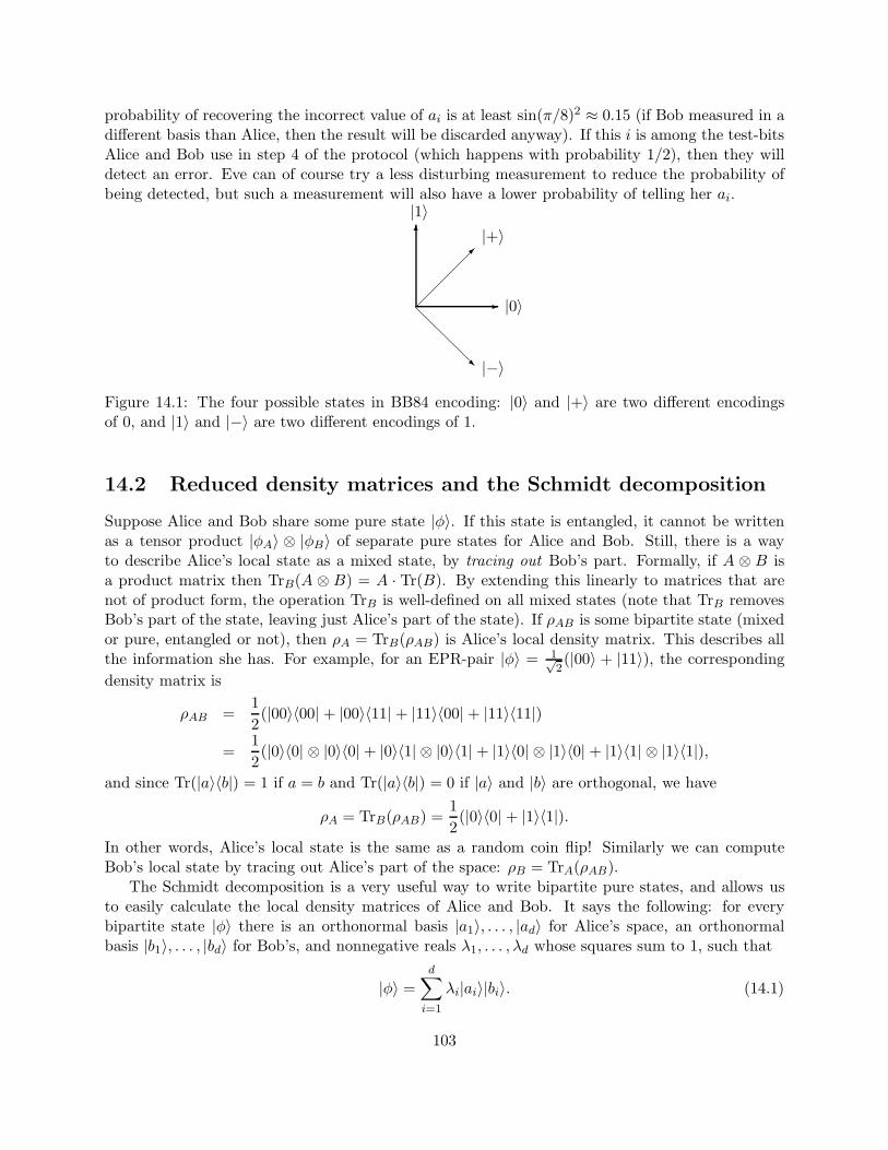
probability of recovering the incorrect value of ai is at least sin(π/8)2 ≈ 0.15 (if Bob measured in a
different basis than Alice, then the result will be discarded anyway). If this i is among the test-bitsAlice and Bob use in step 4 of the protocol (which happens with probability 1/2), then they willdetect an error. Eve can of course try a less disturbing measurement to reduce the probability ofbeing detected, but such a measurement will also have a lower probability of telling her ai.
|0〉
|1〉|+〉
|−〉
Figure 14.1: The four possible states in BB84 encoding: |0〉 and |+〉 are two different encodingsof 0, and |1〉 and |−〉 are two different encodings of 1.
14.2 Reduced density matrices and the Schmidt decomposition
Suppose Alice and Bob share some pure state |φ〉. If this state is entangled, it cannot be writtenas a tensor product |φA〉 ⊗ |φB〉 of separate pure states for Alice and Bob. Still, there is a wayto describe Alice’s local state as a mixed state, by tracing out Bob’s part. Formally, if A ⊗ B isa product matrix then TrB(A ⊗ B) = A · Tr(B). By extending this linearly to matrices that arenot of product form, the operation TrB is well-defined on all mixed states (note that TrB removesBob’s part of the state, leaving just Alice’s part of the state). If ρAB is some bipartite state (mixedor pure, entangled or not), then ρA = TrB(ρAB) is Alice’s local density matrix. This describes allthe information she has. For example, for an EPR-pair |φ〉 = 1√
2(|00〉 + |11〉), the corresponding
density matrix is
ρAB =1
2(|00〉〈00| + |00〉〈11| + |11〉〈00| + |11〉〈11|)
=1
2(|0〉〈0| ⊗ |0〉〈0| + |0〉〈1| ⊗ |0〉〈1| + |1〉〈0| ⊗ |1〉〈0| + |1〉〈1| ⊗ |1〉〈1|),
and since Tr(|a〉〈b|) = 1 if a = b and Tr(|a〉〈b|) = 0 if |a〉 and |b〉 are orthogonal, we have
ρA = TrB(ρAB) =1
2(|0〉〈0| + |1〉〈1|).
In other words, Alice’s local state is the same as a random coin flip! Similarly we can computeBob’s local state by tracing out Alice’s part of the space: ρB = TrA(ρAB).
The Schmidt decomposition is a very useful way to write bipartite pure states, and allows usto easily calculate the local density matrices of Alice and Bob. It says the following: for everybipartite state |φ〉 there is an orthonormal basis |a1〉, . . . , |ad〉 for Alice’s space, an orthonormalbasis |b1〉, . . . , |bd〉 for Bob’s, and nonnegative reals λ1, . . . , λd whose squares sum to 1, such that
|φ〉 =d∑
i=1
λi|ai〉|bi〉. (14.1)
103
The number of nonzero λi’s is called the Schmidt rank of the state. For example, an EPR-pair hasSchmidt coefficients λ1 = λ2 = 1/
√2 and hence has Schmidt rank 2.
The existence of the Schmidt decomposition is shown as follows. Let ρA = TrB(|φ〉〈φ|) be Alice’slocal density matrix. This is Hermitian, so it has a spectral decomposition ρA =
∑i µi|ai〉〈ai| with
orthonormal eigenvectors |ai〉 and nonnegative real eigenvalues µi. Note∑
i µi = Tr(ρA) = 1.Since the |ai〉 form an orthonormal set, we can extend it to an orthonormal basis for Alice’sd-dimensional space (adding additional orthonormal |ai〉 and µi = 0). Hence there are cij such that
|φ〉 =d∑
i,j=1
√µicij |ai〉|j〉,
where the |j〉 are the computational basis states for Bob’s space. Define λi =√µi and |bi〉 =∑
j cij |j〉. This gives the decomposition of |φ〉 of Eq. (14.1). It only remains to show that |bi〉 isan orthonormal set, which we do as follows. The density matrix version of Eq. (14.1) is
|φ〉〈φ| =d∑
i,j=1
λiλj|ai〉〈aj | ⊗ |bi〉〈bj |.
We know that if we trace out the B-part from |φ〉〈φ|, then we should get ρA =∑
i λ2i |ai〉〈ai|, but
that can only happen if 〈bj |bi〉 = Tr(|bi〉〈bj |) = 1 for i = j and 〈bj |bi〉 = 0 for i 6= j. Hence the|bi〉 form an orthonormal set. Note that from Eq. (14.1) it easily follows that Bob’s local densitymatrix is ρB =
∑i λ
2i |bi〉〈bi|.
14.3 The impossibility of perfect bit commitment
Key distribution is just one of the many tasks cryptographers would like to solve. Another importantprimitive is bit commitment. In this scenario there is no eavesdropper, but Alice and Bob don’ttrust each other. Suppose Alice has a bit b which for the time being she doesn’t want to revealto Bob, though she would like to somehow convince Bob that she has already made up her mindabout b and won’t change its value later. A protocol for bit commitment comes in two stages, eachof which may involve several rounds of communication:
1. In the “commit” phase Alice gives Bob a state which is supposed to commit her to the valueof b (without informing Bob about the value of b).
2. In the “reveal” phase Alice sends b to Bob, and possibly some other information to allow himto check that this is indeed the same value b that Alice committed to before.
A protocol is binding if Alice can’t change her mind, meaning she can’t get Bob to “open” 1 − b.A protocol is concealing if Bob cannot get any information about b before the “reveal phase.”5
A good protocol for bit commitment would be a very useful building block for many othercryptographic applications. For instance, it would allow Alice and Bob (who still don’t trust eachother) to jointly flip a fair coin. Maybe they’re going through a divorce, and need to decide who
5A good metaphor to think about this: in the commit phase Alice locks b inside a safe which she sends to Bob.This commits her to the value of b, since the safe is no longer in her hands. During the reveal phase she sends Bobthe key to the safe, who can then open it and learn b.
104
gets to keep their joint car. Alice can’t just flip the coin by herself because Bob doesn’t trust herto do this honestly, and vice versa. Instead, Alice would pick a random coin b and commit to it.Bob would then pick a random coin c and send it to Alice. Alice then reveals b, and the outcome ofthe coin flip is defined to be b⊕ c. As long as at least one of the two parties follows this protocol,the result will be a fair coin flip.
Perfect coin flipping (and hence also perfect bit commitment) are known to be impossible inthe classical world. After BB84 there was some hope that perfect bit commitment (and hence alsoperfect coin flipping) would be possible in the quantum world, and there were some seemingly-secure proposals for quantum protocols to achieve this. Unfortunately it turns out that there is noquantum protocol for bit commitment that is both perfectly binding and perfectly concealing.
To show that a protocol for perfect bit commitment is impossible, consider the joint purestate |φb〉 that Alice and Bob would have if Alice wants to commit to bit-value b, and they bothhonestly followed the protocol.6 If the protocol is perfectly concealing, then the reduced densitymatrix on Bob’s side should be independent of b, i.e., TrA(|φ0〉〈φ0|) = TrA(|φ1〉〈φ1|). The way weconstructed the Schmidt decomposition in the previous section now implies that there exist Schmidtdecompositions of |φ0〉 and |φ1〉 with the same λi’s and the same bi’s: there exist orthonormal basesai and a′i such that
|φ0〉 =d∑
i=1
λi|ai〉|bi〉 and |φ1〉 =d∑
i=1
λi∣∣a′i⟩|bi〉
Now Alice can locally switch from |φ0〉 to |φ1〉 by just applying on her part of the state the map|ai〉 7→ |a′i〉. Alice’s map is unitary because it takes one orthonormal basis to another orthonormalbasis. But then the protocol is not binding at all: Alice can still freely change her mind about thevalue of b after the “commit” phase is over! Accordingly, if a quantum protocol for bit commitmentis perfectly concealing, it cannot be binding at all.
14.4 More quantum cryptography
Quantum cryptography is by now a pretty large subset of the area of quantum information andcomputation. Here we just briefly mention a few other topics in quantum crypto:
• There are quantum protocols for bit commitment that are partially concealing and partiallybinding—something which is still impossible in the classical world. A primitive called “weakcoin flipping” can be implemented almost perfectly in the quantum world, and cannot beimplemented at all in the classical world.
• Under assumptions on the fraction of dishonest players among a set of k parties, it is possibleto implement secure multi-party quantum computation. This is a primitive that allows theplayers to compute any function of their k inputs, without revealing more information toplayer i than can be inferred from i’s input plus the function value.
• One can actually do nearly perfect bit commitment, coin flipping, etc., assuming the dishonestparty has bounded quantum storage, meaning that it can’t keep large quantum states coherent
6The assumption that the state is pure rather than mixed is without loss of generality.
105
for longer times. At the present state of quantum technology this is a very reasonable as-sumption (though a breakthrough in physical realization of quantum computers would wipeout this approach).
• In device-independent cryptography, Alice and Bob want to solve certain cryptographic taskslike key distribution or randomness generation without trusting their own devices (for instancebecause they don’t trust the vendor of their apparatuses). Roughly speaking, the idea hereis to use Bell-inequality violations to prove the presence of entanglement, and then use thisentanglement for cryptographic purposes. Even if Alice or Bob’s apparatuses have beentampered with, they can still only violate things like the CHSH inequality if they actuallyshare an entangled state.
• Experimentally it is much easier to realize quantum key distribution than general quantumcomputation, because you basically just need to prepare qubits (usually photons) in either thecomputational or the Hadamard basis, send them across a channel (usually an optical fibre,but sometimes free space), and measure them in either the computational or the Hadamardbasis. Many sophisticated experiments have already been done. Somewhat surprisingly, youcan already commercially buy quantum key distribution machinery. Unfortunately the im-plementations are typically not perfect (for instance, we don’t have perfect photon counters),and once in a while another loophole is exposed in the implementation, which the vendorthen tries to patch, etc.
Exercises
1. Here we will consider in more detail the information-disturbance tradeoff for measuring aqubit in one of the four BB84 states (each of which occurs with probability 25%).
(a) Suppose Eve measures the qubit in the orthonormal basis given by cos(θ)|0〉+ sin(θ)|1〉and − sin(θ)|0〉+cos(θ)|1〉, for some parameter θ ∈ [0, π/4]. For each of the four possibleBB84 states, give the probabilities of outcome 0 and outcome 1 (so the answer consistsof 8 numbers, each of which is a function of θ).
(b) What is the average probability that Eve’s measurement outcome equals the encodedbit ai, as function of θ? (average taken both over the uniform distribution over the fourBB84 states, and over the probabilities calculated in part (a))
(c) What is the average absolute value of the angle by which the state is changed if Eve’soutcome is the encoded bit ai? Again, the answer should be a function of θ.
2. (a) What is the Schmidt rank of the state 12(|00〉+ |01〉+ |10〉+ |11〉)?
(b) Suppose Alice and Bob share k EPR-pairs. What is the Schmidt rank of their jointstate?
(c) Prove that a pure state |φ〉 is entangled if, and only if, its Schmidt rank is greater than 1.
3. Prove that Alice cannot give information to Bob by doing a unitary operation on her part ofan entangled pure state.
106
4. Suppose Alice sends two n-bit messages M1 and M2 with the one-time pad scheme, reusingthe same n-bit key K. Show that Eve can now get some information about M1,M2 fromtapping the classical channel.
107

108
Chapter 15
Error-Correction and Fault-Tolerance
15.1 Introduction
When Shor’s algorithm had just appeared in 1994, most people (especially physicists) were ex-tremely skeptical about the prospects of actually building a quantum computer. In their view, itwould be impossible to avoid errors when manipulating small quantum systems, and such errorswould very quickly overwhelm the computation, rendering it no more useful than classical com-putation. However, in the few years that followed, the theory of quantum error-correction andfault-tolerant computation was developed. This shows, roughly speaking, that if the error-rate peroperation can be brought down to something reasonably small (say 1%), then under some rea-sonable assumptions we can actually do near-perfect quantum computing for as long as we want.Below we give a succinct and somewhat sketchy introduction to this important but complex area,just explaining the main ideas. See the surveys by Gottesman [54] and Terhal [102] for much more(in particular the “surface code”).
15.2 Classical error-correction
In the early days of classical computing, errors were all over the place: memory-errors, errors inbits sent over a channel, incorrectly applied instructions, etc.1 Nowadays hardware is much morereliable, but we also have much better “software solutions” for errors, in particular error-correctingcodes. Such codes take a string of data and encode it in a larger string (the “codeword”), addinga lot of redundancy so that a small fraction of errors on the codeword won’t be able to reduce theinformation about the encoded data.
The simplest example is of course the repetition code. If we want to protect a bit b, we couldrepeat it three times:
b 7→ bbb.
If we want to decode the encoded bit b from the (possibly corrupted) 3-bit codeword, we just takethe majority value of the 3 bits.
Consider a very simple noise model: every bit is flipped (independently of the other bits) withprobability p. Then initially, before applying the code, b has probability p to be flipped. But ifwe apply the repetition code, the probability that the majority-value of the three bits is different
1The name “bugs” actually comes from insects getting stuck inside the computer and causing errors.
109
from b, is the probability of 2 or 3 bitflips, which is 3p2(1 − p) + p3 < 3p2. Hence the error-ratehas been reduced from p to less than 3p2. If the initial error-rate p0 was < 1/3, then the newerror-rate p1 < 3p20 is less than p0 and we have made progress: the error-rate on the encoded bit issmaller than before. If we’d like it to be even smaller, we could concatenate the code with itself,i.e., repeat each of the three bits in the code three times, so the codelength becomes 9. This wouldgive error-rate p2 = 3p21(1−p1)+p31 < 3p21 < 27p40, giving a further improvement. As we can see, aslong as the initial error-rate p was at most 1/3, we can reduce the error-rate to whatever we want:k levels of concatenation encode one “logical bit” into 3k “physical bits,” but the error-rate for eachlogical bit has been reduced to 1
3(3p0)2k . This is a very good thing: if the initial error is below the
threshold of 1/3, then k levels of concatenation increases the number of bits exponentially (in k),but reduces the error-rate double-exponentially fast !
Typically, already a small choice of k gets the error-rate down to negligible levels. For example,suppose we want to protect some polynomial (in some n) number of bits for some polynomialnumber of time-steps, and our physical error-rate is some fixed p0 < 1/3. Choosing k = 2 log log n
levels of concatenation already suffices for this, because then pk ≤ 13(3p0)
2k ∼ 2−(log n)2 = n− logn
goes to 0 faster than any polynomial. With this choice of k, each logical bit would be encodedin 3k = (log n)2 log2(3) physical bits, so we only increase the number of bits by a polylogarithmicfactor.
15.3 Quantum errors
The need for error-correction is far greater for quantum computers than for classical computers,because “quantum hardware” is much more fragile than classical hardware. Unfortunately, error-correction is also substantially more difficult in the quantum world, for several reasons:
• The classical solution of just repeating a state is not available in general in the quantumworld, because of the no-cloning theorem.
• The classical world has basically only bitflip-errors, while the quantum world is continuousand hence has infinitely many different possible errors.
• Measurements that test whether a state is correct can collapse the state, losing information.
Depending on the specific model of errors that one adopts, it is possible to deal with all of theseissues. We will consider the following simple error model. Consider quantum circuits with Squbits, and T time-steps; in each time-step, several gates on disjoint sets of qubits may be appliedin parallel. After each time-step, at each qubit, independently from the other qubits, some unitaryerror hits that qubit with probability p. Note that we assume the gates themselves to operateperfectly; this is just a convenient technical assumption, since a perfect gate followed by errors onits outgoing qubits is the same as an imperfect gate.
Let’s investigate what kind of (unitary) errors we could get on one qubit. Consider the fourPauli matrices:
I =
(1 00 1
), X =
(0 11 0
), Y =
(0 −ii 0
), Z =
(1 00 −1
).
These have an interpretation as possible errors: I corresponds to no-error, X is a bitflip-error, Z isa phaseflip-error, and Y = iXZ is a phaseflip-error followed by a bitflip-error (and a global phase
110
of i, which doesn’t matter). These four matrices span the space of all possible 2 × 2 matrices, soevery possible error-operation E on a qubit is some linear combination of the 4 Pauli matrices.More generally, every 2k × 2k matrix can be written uniquely as a linear combinations of matricesthat each are the tensor product of k Pauli matrices.
Consider for example the error which puts a small phase φ on |1〉:
E =
(1 00 eiφ
)= eiφ/2 cos(φ/2)I − ieiφ/2 sin(φ/2)Z.
Note that for small φ most of the weight in this linear combination sits on I, which corresponds tothe fact that E is close to I. The sum of squared moduli of the two coefficients is 1 in this case.That’s not a coincidence: whenever we write a unitary as a linear combination of Pauli matrices,the sum of squares of the coefficients will be 1 (see Exercise 1).
The fact that all one-qubit errors are linear combinations of I,X, Y, Z, together with the linearityof quantum mechanics, implies that if we can correct bitflip-errors, phaseflip-errors, and theirproduct, then we can correct all possible unitary errors on a qubit.2 So typically, quantum error-correcting codes are designed to correct bitflip and phaseflip-errors (their product is then typicallyalso correctable), and all other possible errors are then also handled without further work.
Our noise model does not explicitly consider errors on multiple qubits that are not a productof errors on individual qubits. However, even such a joint error on, say, k qubits simultaneouslycan still be written as a linear combination of products of k Pauli matrices. So also here the mainobservation applies: if we can just correct bitflip and phaseflip-errors on individual qubits, then wecan correct all possible errors!
15.4 Quantum error-correcting codes
Quantum error-correcting codes encode a number of “logical qubits” into a larger number of “phys-ical qubits,” in such a way that errors on some number of its qubits can be corrected. The firstand simplest is Peter Shor’s 9-qubit code [99], which encodes 1 logical qubit into 9 physical qubits,and can correct an error on any one of the 9 physical qubits. Here are the codewords for the twological basis states:
|0〉 7→∣∣0⟩=
1√8(|000〉+ |111〉)(|000〉+ |111〉)(|000〉+ |111〉)
|1〉 7→∣∣1⟩=
1√8(|000〉 − |111〉)(|000〉 − |111〉)(|000〉 − |111〉)
These two quantum codewords∣∣0⟩and
∣∣1⟩span a 2-dimensional space α
∣∣0⟩+ β
∣∣1⟩. This 2-
dimensional subspace of the overall 29-dimensional space is called the “codespace.”
Suppose an error happens on one of these 9 qubits. We would like to have a procedure thatmaps the resulting state back to the codespace. By linearity, it suffices if we can do this for thebasis states
∣∣0⟩and
∣∣1⟩. First consider bitflip and phaseflip-errors.
2We can even correct the non-unitary errors that arise from undesired interaction between qubits of our circuitwith the environment, but we won’t talk about such errors here.
111
Detecting a bitflip-error. If a bitflip-error occurs on one the first 3 qubits, we can detect itslocation by noting which of the 3 positions is the minority bit. We can do this for each of thethree 3-qubit blocks. Hence there is a unitary that writes down in 4 auxiliary qubits (which are allinitially |0〉) a number eb ∈ 0, 1, . . . , 9. Here eb = 0 means that no bitflip-error was detected, andeb ∈ 1, . . . , 9 means that a bitflip-error was detected on qubit number eb. Note that we don’tspecify what should happen if more than one bitflip-error occurred.
Detecting a phaseflip-error. To detect a phaseflip-error, we can consider the relative phasefor each of the three blocks |000〉 ± |111〉, and if they are not all the same, unitarily write downin 2 more auxiliary qubits (again, initially |0〉) a number ep ∈ 0, 1, 2, 3. Here ep = 0 means thatno phaseflip-error was detected, and ep ∈ 1, 2, 3 means that a phaseflip-error was detected in theepth block.3
Together the above two procedures form one unitary U (i.e., one circuit) that acts on 9+4+2 = 15qubits, and that “writes down” both eb and ep in auxiliary qubits. For example, suppose we havethe state
∣∣0⟩. If Xi denotes a bitflip-error on the ith qubit and Zj denotes a phaseflip-error on the
jth qubit (let j′ denote the number of the block in which qubit j lies). Then after these errors ourstate is XiZj
∣∣0⟩. After fresh auxiliary qubits
∣∣04⟩∣∣02
⟩are added, U maps
XiZj
∣∣0⟩∣∣04
⟩∣∣02⟩7→ XiZj
∣∣0⟩|i〉∣∣j′⟩.
Together, eb = i and ep = j′ form the “error syndrome”; this tells us which error occurred where.The error-correction procedure can now measure this syndrome in the computational basis, andtake corrective action depending on the classical outcomes eb and ep: apply an X to qubit eb (orno X if eb = 0), and apply a Z to one qubit in the ep-th block (or no Z if ep = 0). The case of aY -error on the ith qubit corresponds to the case where i = j (i.e., the ith qubit is hit by both aphaseflip and a bitflip); our procedure still works in this case. Hence we can perfectly correct onePauli error on any one of the 9 codeword qubits.
As we argued before, the ability to correct Pauli-errors suffices to correct all possible errors.Let’s see in more detail how this works. Consider for instance some 9-qubit unitary error E. Assumeit can be decomposed as a linear combination of 9-qubit products of Paulis, each having at mostone bitflip-error and one phaseflip-error:
E =∑
i,j
αijXiZj .
Suppose this error occurs on∣∣0⟩:
E∣∣0⟩=∑
i,j
αijXiZj
∣∣0⟩.
If we now add auxiliary qubits∣∣04⟩∣∣02
⟩and apply the above unitary U , then we go into a super-
position of error syndromes:
U(E ⊗ I⊗6)∣∣0⟩∣∣04
⟩∣∣02⟩=∑
i,j
αijXiZj
∣∣0⟩|i〉∣∣j′⟩.
3Note that we are not discovering on which of the 9 qubits the phaseflip-error happened (in contrast to the caseof bitflips), but that’s OK: we can correct it nonetheless.
112
Measuring the auxiliary qubits will now probabilistically give us one of the syndromes |i〉|j′〉, andcollapse the state to
XiZj
∣∣0⟩|i〉∣∣j′⟩.
In a way, this measurement of the syndrome “discretizes” the continuously many possible errors tothe finite set of Pauli errors. Once the syndrome has been measured, we can apply a corrective Xand/or Z to the first 9 qubits to undo the specific error corresponding to the specific syndrome wegot as outcome of our measurement.
So now we can correct an error on one qubit. To achieve this, however, we have substantiallyincreased the number of locations where such an error could occur: the number of qubits has gonefrom 1 to 9 (even to 15 if we count the auxiliary qubits as well), and we need a number of time-stepsto compute and measure the syndrome, and to correct a detected error. Hence this procedure onlygains us something if the error-rate p is so small that the probability of 2 or more errors on the largerencoded system is smaller than the probability of 1 error in the unencoded qubit. We will get backto this issue below, when talking about the threshold theorem. Note also that each new applicationof the correction-procedure need a new, fresh 6-qubit register initialized to
∣∣04⟩∣∣02
⟩. After one run
of the error-correction procedure these auxiliary qubits will contain the measured error syndrome,and we can just discard this. In a way, error correction acts like a refrigerator: a fridge pumps heatout of its system and dumps it into the environment, and error-correction pumps noise out of itssystem and dumps it in the environment in the form of the discarded auxiliary qubits.
The above 9-qubit code is just one example of a quantum error-correcting code. Better codesexist, and a lot of work has gone into simultaneously optimizing the different parameters: wewant to encode a large number of logical qubits into a not-much-larger number of physical qubits,while being able to correct as many errors as possible. The shortest code that encodes one logicalqubit and protects against one error, has five physical qubits. There are also asymptotically goodquantum error-correcting codes, which encode k logical qubits into O(k) physical qubits and cancorrect errors on a constant fraction of the physical qubits (rather than just an error on one of thequbits).
15.5 Fault-tolerant quantum computation
Encoding a quantum state in a quantum error-correcting code to protect it against noise is good, butnot enough: we also need to be able to do operations on the encoded qubits (Hadamards, CNOTs,etc.). One way is to decode the logical qubits, do the operation on them, and then re-encode them.This, however, is a recipe for disaster: if an error occurs between the decoding and subsequentencoding, we’re unprotected. Accordingly, we need to be able to do operations on the logical qubitswhile they are encoded. Additionally, we need operations for regular stages of error-correction, i.e.,measuring the syndrome and correcting. These operations may also introduce errors.4
There is a 7-qubit code (due to Andrew Steane) which is used often because it has nice prop-erties: a Hadamard on the logical qubit corresponds to H⊗7 on the physical qubits, and a CNOTbetween two logical qubits corresponds to applying CNOTs between the 7 pairs of the two blocksof physical qubits (i.e., between the 1st qubit of one block and the 1st qubit of the other block,etc.). Adding the gate that maps |b〉 7→ eibπ/4|b〉 to this suffices for universal quantum computation;
4It’s like being inside a leaky boat on the open seas, using a leaky bucket to scoop out water all the time to preventthe boat from filling up with water and sinking. It’s doable, but not easy.
113
unfortunately, implementing this gate fault-tolerantly takes a lot more work, and we won’t go intothat here.
When designing schemes for fault-tolerant computing, it is very important to ensure that errorsdo not spread too quickly. Consider for instance a CNOT: if its control-bit is erroneous, then afterdoing the CNOT also its target bit will be erroneous. The trick is to keep this under control in sucha way that regular phases of error-correction don’t get overwhelmed by the errors. In addition, weneed to be able to fault-tolerantly prepare states, and measure logical qubits in the computationalbasis. We won’t go into the (many) further details of fault-tolerant quantum computing (seeExercise 7 for one approach, and [54] for more).
15.6 Concatenated codes and the threshold theorem
The idea to concatenate a code with itself, described at the end of Section 15.2, also applies toquantum codes. Suppose we have some code that encodes one qubit into C qubits, that can correctone error on one of its C qubits, and uses D time-steps per stage of error-correcting (each time-stepmay involve a number of elementary gates in parallel). Instead of only 1, we now have CD locationswhere an error could occur! Assuming error-rate p per-qubit-per-timestep, the probability for thecode to fail on a specific logical qubit at a specific time (i.e., to have more than 1 physical erroron its CD locations) is p′ =
∑CDi=2
(CDi
)pi. If p is a sufficiently small constant, then this sum is
dominated by the term for i = 2, and we have p′ ≈ (CD)2p2. Hence if the initial error-rate p isbelow some magical constant ≈ 1/CD, then each level of error-correction reduces the error-rate.
More generally, suppose we concatenate this code k times with itself. Then every “logicalqubit” gets encoded into Ck qubits, but (by the same calculation as in Section 15.2) the error-
rate for each logical qubit gets reduced to O((CDp)2k). Suppose we want to be able to “survive”
T = poly(n) time-steps without any error on the logical qubits; that is what we would need torun an efficient quantum algorithm on faulty quantum hardware. Then it suffices if we reduce theerror rate to ≪ 1/T , for which k = O(log log T ) levels of concatenation are enough. These layersof error-correction increase the number of qubits and the computation time by a factor which isexponential in k, but that is still only a polylogarithmic overhead, since 2O(log log T ) = (log T )O(1).
The above sketch (when implemented precisely) gives us the famous “threshold theorem” [3, 72]:if the initial error-rate of the quantum hardware can be brought down below some magical constant(known as the “fault-tolerance threshold”), then we can use software-solutions like quantum error-correcting codes and fault-tolerant computing to ensure that we can quantum compute for longperiods of time without serious errors. Much research has gone into finding the best value for thisfault-tolerance threshold. The more efficient our basic quantum error-correcting codes are (i.e.,the smaller C and D), the higher (= better) the value of the threshold is. Currently the bestrigorous estimates for the threshold are around 0.1%, but there is numerical evidence that even afew percent would be tolerable. This is actually one of the most important results in the area ofquantum computing, and is the main answer to the skeptics mentioned at the start of the chapter:as long as experimentalists manage to implement basic operations within a few percent of errorin a scalable way, then we should be able to build large-scale quantum computers.5 Currentlythere seems to be no fundamental reason why we cannot do this; it is, however, an extremely hardengineering problem.
5This is of course assuming our simple model of independent noise on each physical qubit is not too far off; if thenoise can be correlated in devious ways it becomes much harder (though often still possible) to protect against.
114
Exercises
1. Let E be an arbitrary 1-qubit unitary. We know that it can be written as
E = α0I + α1X + α2Y + α3Z,
for some complex coefficients αi. Show that∑3
i=0 |αi|2 = 1.
2. (a) Write the 1-qubit Hadamard transform H as a linear combination of the four Paulimatrices.
(b) Suppose an H-error happens on the first qubit of α∣∣0⟩+ β
∣∣1⟩using the 9-qubit code.
Give the various steps in the error-correction procedure that corrects this error.
3. Give a quantum circuit for the encoding of Shor’s 9-qubit code, i.e., a circuit that maps∣∣008⟩7→∣∣0⟩and
∣∣108⟩7→∣∣1⟩. Explain why the circuit works.
4. Shor’s 9-qubit code allows to correct a bit flip and/or a phase flip on one of its 9 qubits.Below we give a 4-qubit code which allows to detect a bitflip and/or a phaseflip. By this wemean that after the detection procedure we either have the original uncorrupted state back,or we know that an error occurred (though we do not know which one). The logical 0 and 1are encoded as:
∣∣0⟩= 1
2(|00〉+ |11〉)⊗ (|00〉+ |11〉)∣∣1⟩= 1
2(|00〉 − |11〉)⊗ (|00〉 − |11〉)
(a) Give a procedure (either as a circuit or as sufficiently-detailed pseudo-code) that detectsa bitflip error on one of the 4 qubits of α
∣∣0⟩+ β
∣∣1⟩.
(b) Give a procedure (either as a circuit or as sufficiently-detailed pseudo-code) that detectsa phaseflip error on one of the 4 qubits of α
∣∣0⟩+ β
∣∣1⟩.
(c) Does that mean that we can now detect any unitary 1-qubit error on one of the 4 qubits?Explain your answer.
5. Show that there cannot be a quantum code that encodes one logical qubit into 2k physicalqubits while being able to correct errors on up to k of the physical qubits.
6. Suppose we have a qubit whose density matrix is ρ = αII + αXX + αY Y + αZZ, whereαI , αX , αY , αZ are real coefficients and I,X, Y, Z are the Pauli matrices.
(a) Show that αI = 1/2.
(b) Depolarizing noise (of strength p ∈ [0, 1]) acts on a qubit as follows: with probability1− p nothing happens to the qubit, and with probability p the qubit is replaced by the“completely mixed state” of a qubit, whose density matrix is I/2.
Show that depolarizing noise on the above qubit doesn’t change the coefficient αI , butshrinks each of αX , αY , αZ by a factor of 1− p.
7. Suppose we have a qubit |φ〉 = α|0〉+β|1〉 to which we would like to apply a T =
(1 0
0 eiπ/4
)
gate, but for some reason we cannot. However, we have a second qubit available in state
1√2(|0〉+ eiπ/4|1〉), and we can apply a CNOT gate and an S =
(1 00 i
)gate.
115
(a) What state do we get if we apply a CNOT to the first and second qubit?
(b) Suppose we measure the second qubit. What are the probabilities of outcomes 0 and 1,respectively?
(c) Suppose the measurement yields 0. Show how we can get T |φ〉 in the first qubit.
(d) Suppose the measurement yields 1. Show how we can get T |φ〉 in the first qubit, up toan (irrelevant) global phase.
NB: This way of implementing the T -gate is very helpful in fault-tolerant computing, whereoften CNOT and S are easy to do on encoded states but T is not. What this exercise shows isthat we can prepare (encodings of) the so-called “magic state” 1√
2(|0〉+ eiπ/4|1〉) beforehand
(offline, assuming we can store them for long enough), and use those to indirectly implementa T -gate.
116
Appendix A
Some Useful Linear Algebra
In this appendix we sketch some useful parts of linear algebra, most of which will be used somewhereor other in these notes.
A.1 Some terminology and notation
We use V = Cd to denote the d-dimensional complex vector space, which is the set of all columnvectors of d complex numbers. We assume familiarity with the basic rules of matrix addition andmultiplication. A set of vectors v1, . . . , vm ∈ V is linearly independent if the only way to get∑m
i=1 aivi equal to the zero-vector 0, is to set a1 = · · · = am = 0. A basis for V is a set of vectorsv1, . . . , vd such that every vector v ∈ V can be written as a linear combination of those basis vectorsv =
∑di=1 aivi. One can show that a basis is linearly independent.
We use Aij for the (i, j)-entry of a matrix A and AT for its transpose, which has ATij = Aji.
We use Id to denote the d × d identity matrix, which has 1s on its diagonal and 0s elsewhere; weusually omit the subscript d when the dimension is clear from context. If A is square and there isa matrix B such that AB = BA = I, then we use A−1 to denote this B, which is called the inverseof A (and is unique if it exists). Note that (AB)−1 = B−1A−1. If A is a matrix (not necessarilysquare), then A∗ denotes its conjugate transpose: the matrix obtained by transposing A and takingthe complex conjugates of all entries. Note that (AB)∗ = B∗A∗. Physicists often write A† insteadof A∗.
For vectors v,w, we use 〈v|w〉 = v∗w =∑
i v∗iwi for their inner product. The combination of the
vector space V with this inner product is called a Hilbert space. Two vectors v,w are orthogonalif 〈v|w〉 = 0. The inner product induces a vector norm ‖v‖ =
√〈v|v〉 =
√∑i |vi|2. The norm in
turn induces a distance ‖v − w‖ between vectors v and w. Note that distance and inner productare closely related:
‖v − w‖2 = 〈v − w|v − w〉 = ‖v‖2 + ‖w‖2 − 〈v|w〉 − 〈w|v〉.
In particular, for unit vectors v and w the real part of their inner product equals 1 − 12‖v − w‖2.
Hence unit vectors that are close together have an inner product close to 1, and vice versa. TheCauchy-Schwarz inequality gives |〈v|w〉| ≤ ‖v‖ · ‖w‖ (see Appendix B).
A set vi of vectors is called an orthogonal set if all vectors are pairwise orthogonal: 〈vi|vj〉 = 0if i 6= j. If additionally the vectors all have norm 1, then the set is called orthonormal. The outerproduct of v and w is the matrix vw∗. Below we will restrict attention to square matrices, unless
117
explicitly mentioned otherwise. The complex number λ is an eigenvalue of square matrix A if thereis some nonzero vector v (called an eigenvector) such that Av = λv.
A.2 Unitary matrices
A matrix A is unitary if A−1 = A∗. The following conditions are equivalent:
1. A is unitary
2. A preserves inner product: 〈Av|Aw〉 = 〈v|w〉 for all v,w
3. A preserves norm: ‖Av‖ = ‖v‖ for all v
4. ‖Av‖ = 1 if ‖v‖ = 1
(1) implies (2) because if A is unitary then A∗A = I, and hence 〈Av|Aw〉 = (v∗A∗)Aw = 〈v|w〉. (2)implies (1) as follows: if A is not unitary then A∗A 6= I, so then there is a w such that A∗Aw 6= wand, hence, a v such that 〈v|w〉 6= 〈v|A∗Aw〉 = 〈Av|Aw〉, contradicting (2). Clearly (2) implies (3).Moreover, it is easy to show that (3) implies (2) using the following identity:
‖v + w‖2 = ‖v‖2 + ‖w‖2 + 〈v|w〉 + 〈w|v〉.
The equivalence of (3) and (4) is obvious. Note that by (4), the eigenvalues of a unitary matrixhave absolute value 1.
A.3 Diagonalization and singular values
Matrices A and B are similar if there is an invertible matrix S such that A = SBS−1. Note thatif Av = λv, then BS−1v = λS−1v, so similar matrices have the same eigenvalues. Schur’s lemmastates that every matrix A is similar to an upper triangular matrix: A = U−1TU for some unitaryU and upper triangular T . Since similar matrices have the same eigenvalues and the eigenvalues ofan upper triangular matrix are exactly its diagonal entries, the eigenvalues of A form the diagonalof T .
A matrix D is diagonal if Dij = 0 whenever i 6= j. Let S be some matrix satisfying AS = SDfor some diagonal matrix D. Let vi be the ith column of S and λi be the ith entry on the diagonalof D, then
......
Av1 · · · Avd...
...
︸ ︷︷ ︸AS
=
......
λ1v1 · · · λdvd...
...
︸ ︷︷ ︸SD
,
and we see that vi is an eigenvector of A associated with eigenvalue λi. Conversely, if v1, . . . , vd areeigenvectors of A with eigenvalues λ1, . . . , λd, then we have AS = SD, where S has the vi as columnsand D is the diagonal matrix of λi. We call a square matrix A diagonalizable if it is similar to somediagonal matrix D: A = SDS−1. This D then has A’s eigenvalues λi on its diagonal, some of whichmay be zero. Note that A is diagonalizable iff it has a linearly independent set of d eigenvectors.These eigenvectors will form the columns of S, giving AS = SD, and linear independence ensures
118
that S has an inverse, giving A = SDS−1. A matrix A is unitarily diagonalizable iff it can bediagonalized via a unitary matrix U : A = UDU−1. If the columns of U are the vectors ui, and thediagonal entries of D are λi, then we can also write A =
∑i λiuiu
∗i ; this is sometimes called the
spectral decomposition of A. By the same argument as before, A will be unitarily diagonalizable iffit has an orthonormal set of d eigenvectors.
A matrix A is normal if it commutes with its conjugate transpose (A∗A = AA∗). For example,unitary matrices are normal. If A is normal and A = U−1TU for some upper triangular T (whichmust exist because of Schur’s lemma), then T = UAU−1 and T ∗ = UA∗U−1, so TT ∗ = UAA∗U−1 =UA∗AU−1 = T ∗T . Hence T is normal and upper triangular, which implies (with a little work) thatT is diagonal. This shows that normal matrices are unitarily diagonalizable. Conversely, if A isdiagonalizable as U−1DU , then AA∗ = U−1DD∗U = U−1D∗DU = A∗A, so then A is normal. Thusa matrix is normal iff it is unitarily diagonalizable. If A is not normal, it may still be diagonalizablevia a non-unitary S, for example:
(1 10 2
)
︸ ︷︷ ︸A
=
(1 10 1
)
︸ ︷︷ ︸S
·(
1 00 2
)
︸ ︷︷ ︸D
·(
1 −10 1
)
︸ ︷︷ ︸S−1
.
If A = UDU−1 then A∗ = UD∗U−1, so the eigenvalues of A∗ are the complex conjugates of theeigenvalues of A.
An important class of normal (and hence unitarily diagonalizable) matrices are the Hermitianmatrices, which are the ones satisfying A = A∗. Note that the previous paragraph implies thatthe eigenvalues of Hermitian matrices are real. A Hermitian matrix is called positive definite(resp. positive semidefinite) if all its eigenvalues are positive (resp. non-negative). If all eigenvaluesare 0 or 1, then A is called a projection (or projection matrix or projector). This is equivalent torequiring A2 = A.
Not all matrices are diagonalizable, for instance A =
(0 10 0
). However, every matrix A has
a singular value decomposition, as follows. It is easy to see that the matrix A∗A has the sameeigenvectors as A and that its eigenvalues are the squared absolute values of the eigenvalues ofA. Since A∗A is Hermitian and hence normal, we have A∗A = UDU−1 for some U and somenon-negative real diagonal matrix D. The entries of Σ =
√D are called the singular values of A.
Every A has a singular value decomposition A = UΣV −1, with U, V unitary. This implies that Acan be written as A =
∑i λiuiv
∗i , with ui the columns of U and vi the columns of V .
A.4 Trace
The trace of a matrix A is the sum of its diagonal entries: Tr(A) =∑
iAii. Some important andeasily verified properties of Tr(A) are:
• Tr(A+B) = Tr(A) + Tr(B)
• Tr(AB) = Tr(BA) (the “cyclic property” of the trace)
• Tr(A) is the sum of the eigenvalues of A(This follows from Schur and the previous item: Tr(A) = Tr(UTU−1) = Tr(U−1UT ) =Tr(T ) =
∑i λi)
119
A.5 Tensor products
If A = (Aij) is anm×nmatrix and B anm′×n′ matrix, then their tensor product (a.k.a. Kroneckerproduct) is the mm′ × nn′ matrix
A⊗B =
A11B · · · A1nBA21B · · · A2nB
. . .
Am1B · · · AmnB
.
The following properties of the tensor product are easily verified:
• c(A⊗B) = (cA) ⊗B = A⊗ (cB) for all scalars c
• (A⊗B)∗ = A∗ ⊗B∗ (and similarly for inverse and transpose)
• A⊗ (B + C) = (A⊗B) + (A⊗ C)
• A⊗ (B ⊗ C) = (A⊗B)⊗ C
• (A⊗B)(C ⊗D) = (AC)⊗ (BD)
Different vector spaces can also be combined using tensor products. If V and V ′ are vectors spaces ofdimension d and d′ with basis v1, . . . , vd and v′1, . . . , v′d′, respectively, then their tensor productspace is the d · d′-dimensional space W = V ⊗ V ′ spanned by vi ⊗ v′j | 1 ≤ i ≤ d, 1 ≤ j ≤ d′.Applying a linear operation A to V and B to V ′ corresponds to applying the tensor product A⊗Bto the tensor product space W .
A.6 Rank
The rank of a matrix A (over a field F) is the size of the largest linearly independent set of rows ofA (linear independence taken over F). Unless mentioned otherwise, we take F to be the field of realnumbers. We say that A has full rank if its rank equals its dimension. The following propertiesare all easy to show:
• rank(A) = rank(A∗)
• rank(A) equals the number of non-zero eigenvalues of A (counting multiplicity)
• rank(A+B) ≤ rank(A) + rank(B)
• rank(AB) ≤ minrank(A), rank(B)
• rank(A⊗B) = rank(A) · rank(B)
• A has an inverse iff A has full rank
120
A.7 Dirac notation
Physicists often write their linear algebra in Dirac notation, and we will follow that custom fordenoting quantum states. In this notation we write |v〉 = v and 〈v| = v∗. The first is called a ket,the second a bra. Note that
• 〈v|w〉 = 〈v||w〉
• If A is unitarily diagonalizable, then A =∑
i λi|vi〉〈vi| for some orthonormal set of eigenvec-tors vi
• |v〉〈v| ⊗ |w〉〈w| = (|v〉 ⊗ |w〉)(〈v| ⊗ 〈w|)
121

122
Appendix B
Some other Useful Math and CS
Here we collect various basic but useful facts and definitions needed in parts of the lecture notes.
• A complex number is of the form c = a + bi, where a, b ∈ R, and i is the imaginary unit,which satisfies i2 = −1. Such a c can also be written as c = reiφ where r = |c| =
√a2 + b2 is
the magnitude of c, and φ ∈ [0, 2π) is the angle that c makes with the positive horizontal axiswhen we view it as a point (a, b) in the plane. Note that complex numbers of magnitude 1lie on the unit circle in this plane. We can also write those as eiφ = cos(φ) + i sin(φ). Thecomplex conjugate c∗ is a− ib, equivalently c∗ = re−iφ.
• The Cauchy-Schwarz inequality: for a = (a1, . . . , an) ∈ Rn and b = (b1, . . . , bn) ∈ Rn
n∑
i=1
aibi ≤
√√√√n∑
i=1
a2i
√√√√n∑
i=1
b2i .
Equivalently, written in terms of inner products and norms of vectors: |〈a, b〉| ≤ ‖a‖ · ‖b‖.Proof: for every real λ we have 0 ≤ 〈a− λb, a− λb〉 = ‖a‖2 + λ2‖b‖2 − 2λ〈a, b〉. Now set λ = ‖a‖/‖b‖ and
rearrange (a slightly more complicated proof works if a, b ∈ Cn).
•m−1∑
j=0
zj =
m if z = 11−zm
1−z if z 6= 1
Proof: The case z = 1 is obvious; for the case z 6= 1, observe (1−z)(∑m−1j=0 zj) =
∑m−1j=0 zj−∑m
j=1 zj = 1−zm.
For example, if z = e2πir/N is a root of unity, with r an integer in 1, . . . , N − 1, then∑N−1j=0 zj = 1−e2πir
1−e2πir/N .
• The above ratio can be rewritten using the identity |1−eiθ| = 2| sin(θ/2)|; this identity can beseen by drawing the numbers 1 and eiθ as vectors from the origin in the complex plane, anddividing their angle θ in two. Some other useful trigonometric identities: cos(θ)2+sin(θ)2 = 1,sin(2θ) = 2 sin(θ) cos(θ).
• 1 + x ≤ ex for all real numbers x (positive as well as negative).
• If εj ∈ [0, 1] then 1−k∑
j=1
εj ≤k∏
j=1
(1− εj) ≤ e−∑k
j=1 εj .
Proof: The upper bound comes from the preceding item. The lower bound follows easily by induction, using
the fact that (1− ε1)(1− ε2) = 1− ε1 − ε2 + ε1ε2 ≥ 1− ε1 − ε2.
123
• When we do not care about constant factors, we’ll often use big-Oh notation: T (n) = O(f(n))means there exist constants c, d ≥ 0 such that for all integers n, we have T (n) ≤ cf(n) + d.Similarly, big-Omega notation is used for lower bounds: T (n) = Ω(f(n)) means there existconstants c, d ≥ 0 such that T (n) ≥ cf(n) − d for all n. T (n) = Θ(f(n)) means thatsimultaneously T (n) = O(f(n)) and T (n) = Ω(f(n)).
• Three basic upper bounds on the tails of probability distributions:
Markov: if X is a nonnegative random variable with expectation µ, then Pr[X ≥ kµ] ≤ 1/k.Proof: Since X is nonnegative, µ ≥ Pr[X ≥ kµ] · kµ.Chebyshev: if X is a random variable with expectation µ and standard deviation σ, thenPr[|X − µ| ≥ kσ] ≤ 1/k2.Proof: Apply Markov to the random variable |X − µ|2, whose expectation is σ2.
Chernoff/Hoeffding: if X =∑n
i=1Xi is the sum of n independent, identically distributedrandom variables Xi ∈ 0, 1, each with expectation Pr[Xi = 1] = p, then X has expectationµ = np, and exponentially decreasing tail bound Pr[|X − µ| ≥ αn] ≤ 2e−2α2n.Proof idea: For all parameters λ, we have Pr[X − µ ≥ t] = Pr[eλX ≥ eλ(t+µ)]. Upper bound the latter
probability by applying Markov to the random variable eλX . This is a product of n independent random
variables eλXi , so its expectation is easy to analyze. Then choose λ to minimize the upper bound.
• When we say an algorithm has error probability ≤ 1/3, this typically means in the worstcase: for every possible input, the algorithm produces the correct answer with probability≥ 2/3. Such statements do not refer to “most” inputs under some input distribution.
• If a (classical or quantum) algorithm produces the correct answer in expected running time T ,then we can convert that into an algorithm with worst-case running time 3T and error prob-ability ≤ 1/3, as follows. Run the original algorithm for 3T steps, and just cut it off if ithasn’t terminated by itself. The probability of non-termination within 3T steps is at most1/3 by Markov’s inequality. Hence with probability ≥ 2/3 we will have the correct answer.
• If a (classical or quantum) algorithm with 0/1-outputs has error probability ≤ 1/3, thenwe can cheaply reduce this error probability to small ε > 0, as follows. Choose odd n =O(log(1/ε)) such that 2e−2α2n ≤ ε for α = 1/6. Run the original algorithm n times andoutput the majority among the n output bits. The probability that this majority is wrong(i.e., that the number of correct output bits is more than αn below its expectation), is atmost ε by the Chernoff bound.
124
Appendix C
Hints for Exercises
Chapter 1
1. Consider what U has to do when |φ〉 = |0〉, when |φ〉 = |1〉, and when |φ〉 is a superposition ofthese two.
Chapter 2
6. Instead of measuring the qubit, apply a CNOT that “copies” it to a new |0〉-qubit, which is thenleft alone until the end of the computation. Analyze what happens.11. Use Bernstein-Vazirani.
Chapter 3
4.c. Approximate the state of part (a) using the subroutine of part (b), and see what happens if
you apply Hadamards to the approximate state. Use the fact that 12N
∑N/2+2√N
w=0
(nw
)is nearly 1.
This result is by van Dam [38].
Chapter 4
3. Use |α2i − β2i | = |αi − βi| · |αi + βi| and the Cauchy-Schwarz inequality.
4.c. Use triangle inequality.4.d. Drop all phase-gates with small angles φ < 1/n3 from the O(n2)-gate circuit for F2n explainedin Section 4.5. Calculate how many gates are left in the circuit, and analyze the distance betweenthe unitaries corresponding to the new circuit and the original circuit.
Chapter 5
1.a. The Schonhage-Strassen algorithm computes the product of two n-bit integers mod N , inO(n log(n) log log(n)) steps.3.a. The prime number theorem implies that roughly N/ lnN of the numbers between 1 and N areprime; also there is an efficient classical algorithm to test if a given number is prime. Be explicitin how many bits your primes p and q will have.3.b. Use Exercise 1.
125
3.c. The set of all possible messages forms a group of size φ(N). Euler’s Theorem says that in anygroup G, we have a|G| = 1 for all a ∈ G (here ‘1’ is the identity element in the group).
Chapter 6
5. Use the SWAP test from Section 12.6.
Chapter 7
3. Start with m = xi for a random i, and repeatedly use Grover’s algorithm to find an index j suchthat xj < m and update m = xj . Continue this until you can find no element smaller than m, andanalyze the number of queries of this algorithm. You are allowed to argue about this algorithm ona high level (i.e., things like “use Grover to search for a j such that. . . ” are OK), no need to writeout complete circuits.4.b. What is the probability in (a) if s =
√N?
4.c. Choose a set S of size s = N1/3, and classically query all its elements. First check if S containsa collision. If yes, then you’re done. If not, then use Grover to find a j 6∈ S that collides with ani ∈ S. This result is by Brassard, Høyer, and Tapp [25].5.b. Recall that if there are i solutions, Grover’s algorithm finds a solution using an expectednumber of O(
√N/i) queries.
7.e. Choose γ in (d) such that applying ⌈k⌉ rounds of amplitude amplification to A results in asolution for y with probability 1.8.a. Try running the exact version of Grover (see end of Section 7.2) with different guesses for whatthe actual t is.
Chapter 8
3.a. Choose a uniformly random vector v ∈ 0, 1n, calculate ABv and Cv, and check whetherthese two vectors are the same. This result is by Freivalds [52].3.b. Consider the case A = I.3.c. Modify the algorithm for collision-finding: use a random walk on the Johnson graph J(n, r),where each vertex corresponds to a set R ⊆ [n], and that vertex is marked if there are i, j ∈ R suchthat (AB)i,j 6= Ci,j. This result is by Buhrman and Spalek [29].4.b. View the 3n-step random walk algorithm as a deterministic algorithm with an additional inputr ∈ 0, 1n×1, 2, 33n, where the first n bits determine x, and the last 3n entries determine whichvariable of the leftmost false clauses will be flipped in the 3n steps of the random walk. Use Groversearch on the space of all such r (no need to write out complete circuits here).
Chapter 9
3.a. Use Exercise 1.3.b. Show that the symmetrized approximate polynomial r induced by the algorithm has degreeat least N .5.c. Use the result of Exercise 4 for N = 2.6.b. When defining the relation R, consider that the hardest task for this algorithm is to distinguishinputs of weight N/2 from inputs of weight N/2 + 1.8. Show how you can use sorting to solve the Majority-problem and then use the lower bound from
126
the previous exercise to get an Ω(N) lower bound on sorting. (It is actually known that sortingtakes Ω(N logN) comparisons even on a quantum computer, but you don’t have to show that.)9.a. Reduce the bs(f)-bit OR function (restricted to inputs of weight 0 or 1) to f and invoke thelower bound we know for OR. The results in this exercise are from [14].
Chapter 10
1. Use binary search, running the algorithm with different choices of k to “zoom in” on the largestprime factor.3.a. Write |ψx〉 = α|0〉|φ0〉+β|1〉|φ1〉, and consider the inner product between (Z⊗I)|ψx〉 and |ψx〉.3.b. Use part (a). Analyze the amplitude of
∣∣x, 0S−n⟩in the final state |ψx〉, using ideas from the
proof of BQP ⊆ PSPACE in Section 10.3. Note that in contrast to that proof, you cannot usemore than polynomial time for this exercise.
Chapter 11
2.a. It suffices to use pure states with real amplitudes as encoding. Try to “spread out” the 4encodings |φ00〉, |φ01〉, |φ10〉, |φ11〉 in the 2-dimensional real plane as well as possible.3. Use the fact that 1 classical bit of communication can only send 1 bit of information, no matterhow much entanglement Alice and Bob share. Combine this fact with superdense coding.
Chapter 12
1. Argue that if Alice sends the same message for distinct inputs x and x′, then Bob doesn’t knowwhat to output if his input is y = x.2.a. Argue that if P is a projector then we can’t have both P |φ〉 = |φ〉 and P |ψ〉 = 0.2.c. Observe that among Alice’s possible n-bit inputs are the n codewords of the Hadamard codethat encodes log n bits (see Section 11.3); each pair of distinct Hadamard codewords is at Hammingdistance exactly n/2. Use part (a) to argue that Alice needs to send pairwise orthogonal states forthose n inputs, and hence her message-space must have dimension at least n.3. Use the fact that 2 non-orthogonal states cannot be distinguished perfectly (Exercise 2), andthat a set of 2n vectors that are pairwise orthogonal must have dimension 2n.4. Invoke the quantum random access lower bound, Theorem 2 of Section 11.2.5.b. Let Alice send a random row of C(x) (with the row-index) and let Bob send a random columnof C(y) (with the column-index).6.a. Two distinct polynomials, each of degree ≤ d, are equal on at most d points of the domain Fp.8.b. Run the protocol of part (a) on an initial state where Bob has a well-chosen superpositionover many |y〉.9.b. You can derive this from one of the communication lower bounds mentioned in this chapter,you don’t need to prove this from scratch.10. The matchingM induces a projective measurement that Bob can do on the message he receives.
Chapter 13
1.b. You could write this out, but you can also get the answer almost immediately from part (a)and the fact that HT = H−1.2. For every fixed input x, y, there is a classical strategy that gives a wrong output only on that
127
input, and that gives a correct output on all other possible inputs. Use the shared randomness torandomly choose one of those deterministic strategies.4.c. Use that A2
x and B2y are the k-qubit identity matrix.
4.d. You may use that (〈ψ|C|ψ〉)2 ≤ 〈ψ|C2|ψ〉 and 〈ψ|D ⊗ E|ψ〉 ≤ 〈ψ|D ⊗ I|ψ〉 · 〈ψ|I ⊗ E|ψ〉 forHermitian matrices D and E (these inequalities follow from Cauchy-Schwarz, but you don’t haveto show that).4.e. cos(π/8)2 = 1
2 +1√8.
Chapter 14
3. Show that a unitary on Alice’s side of the state won’t change Bob’s local density matrix ρB .
Chapter 15
1. Compute the trace Tr(E∗E) in two ways, and use the fact that Tr(AB) = 0 if A and B aredistinct Paulis, and Tr(AB) = Tr(I) = 2 if A and B are the same Pauli.5. Given an unknown qubit α|0〉+ β|1〉 encoded using this code, you could split the 2k qubits intotwo sets of k qubits each, and use each to recover a copy of the unknown qubit.
128
Bibliography
[1] S. Aaronson and A. Ambainis. Quantum search of spatial regions. Theory of Computing,1(1):47–79, 2005. Earlier version in FOCS’03. quant-ph/0303041.
[2] S. Aaronson and Y. Shi. Quantum lower bounds for the collision and the element distinctnessproblems. Journal of the ACM, 51(4):595–605, 2004.
[3] D. Aharonov and M. Ben-Or. Fault tolerant quantum computation with constant error.SIAM Journal on Computing, 38(4):1207–1282, 2008. Earlier version in STOC’97. quant-ph/9611025.
[4] A. Ambainis. Communication complexity in a 3-computer model. Algorithmica, 16(3):298–301, 1996.
[5] A. Ambainis. Quantum lower bounds by quantum arguments. Journal of Computer andSystem Sciences, 64(4):750–767, 2002. Earlier version in STOC’00. quant-ph/0002066.
[6] A. Ambainis. Polynomial degree vs. quantum query complexity. Journal of Computer andSystem Sciences, 72(2):220–238, 2006. Earlier version in FOCS’03. quant-ph/0305028.
[7] A. Ambainis. Quantum walk algorithm for element distinctness. SIAM Journal on Computing,37(1):210–239, 2007. Earlier version in FOCS’04. quant-ph/0311001.
[8] P. K. Aravind. A simple demonstration of Bell’s theorem involving two observers and noprobabilities or inequalities. quant-ph/0206070, 2002.
[9] A. Aspect, Ph. Grangier, and G. Roger. Experimental tests of realistic local theories viaBell’s theorem. Physical Review Letters, 47:460, 1981.
[10] L. Babai. Graph isomorphism in quasipolynomial time. In Proceedings of 48th ACM STOC,pages 684–697, 2016. arXiv:1512.03547.
[11] L. Babai and E. M. Luks. Canonical labeling of graphs. In Proceedings of 15th ACM STOC,pages 171–183, 1983.
[12] Z. Bar-Yossef, T. S. Jayram, and I. Kerenidis. Exponential separation of quantum andclassical one-way communication complexity. SIAM Journal on Computing, 38(1):366–384,2008. Earlier version in STOC’04.
[13] R. Beals. Quantum computation of Fourier transforms over symmetric groups. In Proceedingsof 29th ACM STOC, pages 48–53, 1997.
129
[14] R. Beals, H. Buhrman, R. Cleve, M. Mosca, and R. de Wolf. Quantum lower bounds bypolynomials. Journal of the ACM, 48(4):778–797, 2001. Earlier version in FOCS’98. quant-ph/9802049.
[15] J. S. Bell. On the Einstein-Podolsky-Rosen paradox. Physics, 1:195–200, 1964.
[16] A. Belovs. Span programs for functions with constant-sized 1-certificates. In Proceedings of43rd ACM STOC, pages 77–84, 2012. arXiv:1105.4024.
[17] P. A. Benioff. Quantum mechanical Hamiltonian models of Turing machines. Journal ofStatistical Physics, 29(3):515–546, 1982.
[18] C. Bennett, G. Brassard, C. Crepeau, R. Jozsa, A. Peres, and W. Wootters. Teleporting anunknown quantum state via dual classical and Einstein-Podolsky-Rosen channels. PhysicalReview Letters, 70:1895–1899, 1993.
[19] C. Bennett and S. Wiesner. Communication via one- and two-particle operators on Einstein-Podolsky-Rosen states. Physical Review Letters, 69:2881–2884, 1992.
[20] C. H. Bennett and G. Brassard. Quantum cryptography: Public key distribution and cointossing. In Proceedings of the IEEE International Conference on Computers, Systems andSignal Processing, pages 175–179, 1984.
[21] E. Bernstein and U. Vazirani. Quantum complexity theory. SIAM Journal on Computing,26(5):1411–1473, 1997. Earlier version in STOC’93.
[22] J-F. Biasse and F. Song. Efficient quantum algorithms for computing class groups and solvingthe principal ideal problem in arbitrary degree number fields. In Proceedings of 27th ACM-SIAM SODA, pages 893–902, 2016.
[23] M. Boyer, G. Brassard, P. Høyer, and A. Tapp. Tight bounds on quantum searching.Fortschritte der Physik, 46(4–5):493–505, 1998. Earlier version in Physcomp’96. quant-ph/9605034.
[24] G. Brassard, R. Cleve, and A. Tapp. The cost of exactly simulating quantum entangle-ment with classical communication. Physical Review Letters, 83(9):1874–1877, 1999. quant-ph/9901035.
[25] G. Brassard, P. Høyer, and A. Tapp. Quantum algorithm for the collision problem. ACMSIGACT News (Cryptology Column), 28:14–19, 1997. quant-ph/9705002.
[26] H. Buhrman, R. Cleve, S. Massar, and R. de Wolf. Non-locality and communication com-plexity. Reviews of Modern Physics, 82:665–698, 2010. arXiv:0907.3584.
[27] H. Buhrman, R. Cleve, J. Watrous, and R. de Wolf. Quantum fingerprinting. Physical ReviewLetters, 87(16), September 26, 2001. quant-ph/0102001.
[28] H. Buhrman, R. Cleve, and A. Wigderson. Quantum vs. classical communication and com-putation. In Proceedings of 30th ACM STOC, pages 63–68, 1998. quant-ph/9802040.
[29] H. Buhrman and R. Spalek. Quantum verification of matrix products. In Proceedings of 17thACM-SIAM SODA, pages 880–889, 2006. quant-ph/0409035.
130
[30] M. Bun and J. Thaler. Dual lower bounds for approximate degree and Markov-Bernsteininequalities. In Proceedings of 40th ICALP, volume 7965 of Lecture Notes in ComputerScience, pages 303–314, 2013.
[31] A. Childs. Lecture notes on quantum algorithms. Technical report, University of Maryland,2017. Available at https://cs.umd.edu/ amchilds/qa/.
[32] B. S. Cirel’son. Quantum generalizations of Bell’s inequality. Letters in Mathematical Physics,4(2):93–100, 1980.
[33] J. F. Clauser, M. A. Horne, A. Shimony, and R. A. Holt. Proposed experiment to test localhidden-variable theories. Physical Review Letters, 23(15):880–884, 1969.
[34] R. Cleve. The query complexity of order-finding. In Proceedings of 15th IEEE Conference onComputational Complexity, pages 54–59, 2000. quant-ph/9911124.
[35] R. Cleve and H. Buhrman. Substituting quantum entanglement for communication. PhysicalReview A, 56(2):1201–1204, 1997. quant-ph/9704026.
[36] R. Cleve, W. van Dam, M. Nielsen, and A. Tapp. Quantum entanglement and the com-munication complexity of the inner product function. In Proceedings of 1st NASA QCQCconference, volume 1509 of Lecture Notes in Computer Science, pages 61–74. Springer, 1998.quant-ph/9708019.
[37] R. Cleve, A. Ekert, C. Macchiavello, and M. Mosca. Quantum algorithms revisited. InProceedings of the Royal Society of London, volume A454, pages 339–354, 1998. quant-ph/9708016.
[38] W. van Dam. Quantum oracle interrogation: Getting all information for almost half theprice. In Proceedings of 39th IEEE FOCS, pages 362–367, 1998. quant-ph/9805006.
[39] D. Deutsch. Quantum theory, the Church-Turing principle, and the universal quantum Turingmachine. In Proceedings of the Royal Society of London, volume A400, pages 97–117, 1985.
[40] D. Deutsch. Quantum computational networks. In Proceedings of the Royal Society of London,volume A425, 1989.
[41] D. Deutsch and R. Jozsa. Rapid solution of problems by quantum computation. In Proceedingsof the Royal Society of London, volume A439, pages 553–558, 1992.
[42] A. Drucker and R. de Wolf. Quantum proofs for classical theorems. Theory of Computing,2011. ToC Library, Graduate Surveys 2. arXiv:0910.3376.
[43] C. Durr, M. Heiligman, P. Høyer, and M. Mhalla. Quantum query complexity of some graphproblems. SIAM Journal on Computing, 35(6):1310–1328, 2006. Earlier version in ICALP’04.quant-ph/0401091.
[44] C. Durr and P. Høyer. A quantum algorithm for finding the minimum. quant-ph/9607014,18 Jul 1996.
[45] A. Einstein, B. Podolsky, and N. Rosen. Can quantum-mechanical description of physicalreality be considered complete? Physical Review, 47:777–780, 1935.
131
[46] P. van Emde Boas. Machine models and simulations. In van Leeuwen [104], pages 1–66.
[47] M. Ettinger, P. Høyer, and M. Knill. The quantum query complexity of the hidden subgroupproblem is polynomial. Information Processing Letters, 91(1):43–48, 2004. quant-ph/0401083.
[48] R. Feynman. Simulating physics with computers. International Journal of TheoreticalPhysics, 21(6/7):467–488, 1982.
[49] R. Feynman. Quantum mechanical computers. Optics News, 11:11–20, 1985.
[50] L. Fortnow and J. Rogers. Complexity limitations on quantum computation. Journal ofComputer and System Sciences, 59(2):240–252, 1999. Earlier version in Complexity’98. Alsocs.CC/9811023.
[51] P. Frankl and V. Rodl. Forbidden intersections. Transactions of the American MathematicalSociety, 300(1):259–286, 1987.
[52] R. Freivalds. Probabilistic machines can use less running time. In IFIP Congress, pages839–842, 1977.
[53] M. Furer. Faster integer multiplication. SIAM Journal on Computing, 39(3):979–1005, 2009.Earlier version in STOC’07.
[54] D. Gottesman. An introduction to quantum error correction and fault-tolerant quantumcomputation. arXiv:0904.2557, 16 Apr 2009.
[55] M. Grigni, L. Schulman, M. Vazirani, and U. Vazirani. Quantum mechanical algorithmsfor the nonabelian hidden subgroup problem. Combinatorica, 24(1):137–154, 2004. Earlierversion in STOC’01.
[56] L. K. Grover. A fast quantum mechanical algorithm for database search. In Proceedings of28th ACM STOC, pages 212–219, 1996. quant-ph/9605043.
[57] L. Hales and S. Hallgren. An improved quantum Fourier transform algorithm and applica-tions. In Proceedings of 41st IEEE FOCS, pages 515–525, 2000.
[58] S. Hallgren. Polynomial-time quantum algorithms for Pell’s equation and the principal idealproblem. Journal of the ACM, 54(1):653–658, 2007. Earlier version in STOC’02.
[59] S. Hallgren, C. Moore, M. Roetteler, A. Russell, and P. Sen. Limitations of quantumcoset states for graph isomorphism. Journal of the ACM, 57(6):34, 2010. Earlier versionin STOC’06.
[60] S. Hallgren, A. Russell, and A. Ta-Shma. The hidden subgroup problem and quantum com-putation using group representations. SIAM Journal on Computing, 32(4):916–934, 2003.Earlier version in STOC’00.
[61] G. H. Hardy and E. M. Wright. An Introduction to the Theory of Numbers. Oxford UniversityPress, New York, fifth edition, 1979.
132
[62] B. Hensen, H. Bernien, A. E. Dreau, A. Reiserer, N. Kalb, M. S. Blok, J. Ruitenberg,R. F. L. Vermeulen, R. N. Schouten, C. Abellan, W. Amaya, V. Pruneri, M. W. Mitchell,M. Markham, D. J. Twitchen, D. Elkouss, S. Wehner, T. H. Taminiau, and R. Hanson.Loophole-free Bell inequality violation using electron spins separated by 1.3 kilometres. Na-ture, 526, 29 October 2015.
[63] A. S. Holevo. Bounds for the quantity of information transmitted by a quantum commu-nication channel. Problemy Peredachi Informatsii, 9(3):3–11, 1973. English translation inProblems of Information Transmission, 9:177–183, 1973.
[64] P. Høyer, T. Lee, and R. Spalek. Negative weights make adversaries stronger. In Proceedingsof 39th ACM STOC, pages 526–535, 2007. quant-ph/0611054.
[65] P. Høyer and R. Spalek. Lower bounds on quantum query complexity. Bulletin of the EATCS,87:78–103, October 2005.
[66] G. Ivanyos, L. Sanselme, and M. Santha. An efficient quantum algorithm for the hiddensubgroup problem in nil-2 groups. Algorithmica, 62(1–2):480–498, 2012. arXiv:0707.1260.
[67] S. Jeffery, R. Kothari, and F. Magniez. Nested quantum walks with quantum data structures.In Proceedings of 24th ACM-SIAM SODA, pages 1474–1485, 2013. arXiv:1210.1199.
[68] J. Katz and L. Trevisan. On the efficiency of local decoding procedures for error-correctingcodes. In Proceedings of 32nd ACM STOC, pages 80–86, 2000.
[69] I. Kerenidis and R. de Wolf. Exponential lower bound for 2-query locally decodable codesvia a quantum argument. Journal of Computer and System Sciences, 69(3):395–420, 2004.Earlier version in STOC’03. quant-ph/0208062.
[70] A. Yu. Kitaev. Quantum measurements and the Abelian stabilizer problem. quant-ph/9511026, 12 Nov 1995.
[71] B. Klartag and O. Regev. Quantum one-way communication is exponentially stronger thanclassical communication. In Proceedings of 43rd ACM STOC, 2011. arXiv:1009.3640.
[72] M. Knill, R. Laflamme, and W. Zurek. Threshold accuracy for quantum computation. quant-ph/9610011, 15 Oct 1996.
[73] D. E. Knuth. The Art of Computer Programming. Volume 2: Seminumerical Algorithms.Addison-Wesley, third edition, 1997.
[74] F. Le Gall. Improved quantum algorithm for triangle finding via combinatorial arguments.In Proceedings of 55th IEEE FOCS, pages 216–225, 2014. arXiv:1407.0085.
[75] T. Lee, F. Magniez, and M. Santha. Improved quantum query algorithms for triangle findingand associativity testing. Algorithmica, 77(2):459–486, 2017. arXiv:1210.1014.
[76] A. K. Lenstra and H. W. Lenstra, Jr. The Development of the Number Field Sieve, volume1554 of Lecture Notes in Mathematics. Springer, 1993.
[77] H. W. Lenstra and C. Pomerance. A rigorous time bound for factoring integers. Journal ofthe American Mathematical Society, 5:483–516, 1992.
133
[78] H-K. Lo and H. F. Chau. Unconditional security of quantum key distribution over arbitrarilylong distances. quant-ph/9803006, 3 Mar 1998.
[79] F. Magniez, M. Santha, and M. Szegedy. Quantum algorithms for the triangle problem. InProceedings of 16th ACM-SIAM SODA, pages 1109–1117, 2005. quant-ph/0310134.
[80] Y. Manin. Vychislimoe i nevychislimoe (computable and noncomputable). Soviet Radio,pages 13–15, 1980. In Russian.
[81] Y. Manin. Classical computing, quantum computing, and Shor’s factoring algorithm. quant-ph/9903008, 2 Mar 1999.
[82] D. Mayers. Unconditional security in quantum cryptography. quant-ph/9802025, 10 Feb1998.
[83] C. Moore, D. N. Rockmore, and A. Russell. Generic quantum Fourier transforms. ACMTransactions on Algorithms, 2(4):707–723, 2006. quant-ph/0304064.
[84] C. Moore, A. Russell, and L. Schulman. The symmetric group defies strong Fourier sampling.SIAM Journal on Computing, 37(6):1842–1864, 2008. quant-ph/0501056+66. Earlier versionin FOCS’05.
[85] M. Mosca and A. Ekert. The hidden subgroup problem and eigenvalue estimation on aquantum computer. In Proceedings of 1st NASA QCQC conference, volume 1509 of LectureNotes in Computer Science, pages 174–188. Springer, 1998. quant-ph/9903071.
[86] A. Nayak. Optimal lower bounds for quantum automata and random access codes. InProceedings of 40th IEEE FOCS, pages 369–376, 1999. quant-ph/9904093.
[87] I. Newman. Private vs. common random bits in communication complexity. InformationProcessing Letters, 39(2):67–71, 1991.
[88] I. Newman and M. Szegedy. Public vs. private coin flips in one round communication games.In Proceedings of 28th ACM STOC, pages 561–570, 1996.
[89] M. A. Nielsen and I. L. Chuang. Quantum Computation and Quantum Information. Cam-bridge University Press, 2000.
[90] C. H. Papadimitriou. Computational Complexity. Addison-Wesley, 1994.
[91] A. Razborov. Quantum communication complexity of symmetric predicates. Izvestiya of theRussian Academy of Sciences, mathematics, 67(1):159–176, 2003. quant-ph/0204025.
[92] B. Reichardt. Span programs and quantum query complexity: The general adversary boundis nearly tight for every Boolean function. In Proceedings of 50th IEEE FOCS, pages 544–551,2009.
[93] R. Rivest, A. Shamir, and L. Adleman. A method for obtaining digital signatures and publickey cryptosystems. Communications of the ACM, 21:120–126, 1978.
[94] R. L. Rivest. Cryptography. In van Leeuwen [104], pages 717–755.
134
[95] M. Santha. Quantum walk based search algorithms. In Proceedings of 5th TAMC, pages31–46, 2008. arXiv/0808.0059.
[96] A. Schonhage and V. Strassen. Schnelle Multiplikation grosser Zahlen. Computing, 7:281–292,1971.
[97] U. Schoning. A probabilistic algorithm for k-SAT and constraint satisfaction problems. InProceedings of 40th IEEE FOCS, pages 410–414, 1999.
[98] A. Sherstov. Approximating the AND-OR tree. Theory of Computing, 9(20):653–663, 2013.
[99] P. W. Shor. Scheme for reducing decoherence in quantum memory. Physical Review A,52:2493, 1995.
[100] P. W. Shor. Polynomial-time algorithms for prime factorization and discrete logarithms on aquantum computer. SIAM Journal on Computing, 26(5):1484–1509, 1997. Earlier version inFOCS’94. quant-ph/9508027.
[101] D. Simon. On the power of quantum computation. SIAM Journal on Computing, 26(5):1474–1483, 1997. Earlier version in FOCS’94.
[102] B. M. Terhal. Quantum error correction for quantum memories. Reviews of Modern Physics,87:307, 2015. arXiv:1302.3428.
[103] L. Trevisan. Some applications of coding theory in computational complexity. Quaderni diMatematica, 13:347–424, 2004.
[104] J. van Leeuwen, editor. Handbook of Theoretical Computer Science. Volume A: Algorithmsand Complexity. MIT Press, Cambridge, MA, 1990.
[105] L. Vandersypen, M. Steffen, G. Breyta, C. Yannoni, R. Cleve, and I. Chuang. Experimentalrealization of an order-finding algorithm with an NMR quantum computer. Physical ReviewLetters, 85(25):5452–5455, 2000. quant-ph/0007017.
[106] J. Watrous. Quantum algorithms for solvable groups. In Proceedings of 33rd ACM STOC,pages 60–67, 2001.
[107] J. Watrous. Quantum computational complexity. In Encyclopedia of Complexity and SystemScience. Springer, 2009. arXiv:0804.3401.
[108] R. de Wolf. Quantum Computing and Communication Complexity. PhD thesis, University ofAmsterdam, 2001.
[109] W. K. Wootters and W. H. Zurek. A single quantum cannot be copied. Nature, 299:802–803,1982.
[110] A. C-C. Yao. Some complexity questions related to distributive computing. In Proceedingsof 11th ACM STOC, pages 209–213, 1979.
[111] A. C-C. Yao. Quantum circuit complexity. In Proceedings of 34th IEEE FOCS, pages 352–360,1993.
135