Embed Size (px)
Citation preview

Quantum Liquid Crystals
Vladimir Cvetkovic


Quantum Liquid Crystals
PROEFSCHRIFT
ter verkrijging van
de graad van Doctor aan de Universiteit Leiden,
op gezag van de Rector Magnificus Dr. D.D. Breimer,
hoogleraar in de faculteit der Wiskunde en
Natuurwetenschappen en die der Geneeskunde,
volgens besluit van het College voor Promoties
te verdedigen op donderdag 29 maart 2006
te klokke 15.15 uur
door
Vladimir Cvetkovic
geboren op 26 februari 1977te Jagodina, Servie

Promotiecommissie:
Promotor: Prof. dr. J. ZaanenReferent: Prof. dr. ir. W. van SaarloosOverige leden: Prof. dr. E. Demler (Harvard University, Verenigde Staten)
Prof. dr. D. van der Marel (Universite de Geneve, Zwitserland)Prof. dr. ir. H.T.C. Stoof (Universiteit Utrecht)Prof. dr. J. van den Brink (Radboud Universiteit Nijmegen)Prof. dr. H.W.J. BloteProf. dr. P.H. Kes
ISBN: 90-8593-011-1
Thesis – Instituut-Lorentz, Universiteit Leiden, 2006Casimir Ph.D. series, Delft-Leiden, 2006-04Printed by PrintPartners Ipskamp, Enschede
Het onderzoek beschreven in dit proefschrift is onderdeel van het wetenschappelijke pro-gramma van de Stichting voor Fundamenteel Onderzoek der Materie (FOM) en de Neder-landse Organisatie voor Wetenschappelijk Onderzoek (NWO).
The research described in this thesis has been carried out as part of the scientific programmeof the Foundation for Fundamental Research on Matter (FOM) and the Netherlands Or-ganisation for Scientific Research (NWO).
Cover: a random configuration of dislocations on a 2D triangular lattice.

Contents
1 Introduction 1
1.1 Order vs. disorder . . . . . . . . . . . . . . . . . . . . . . . . . . . . . . . 1
1.2 Correlated electrons and high-Tc superconductivity . . . . . . . . . . . . . 3
1.3 Motivation and the main results . . . . . . . . . . . . . . . . . . . . . . . . 7
1.4 Definitions and conventions . . . . . . . . . . . . . . . . . . . . . . . . . . 9
2 A tutorial: Abelian-Higgs duality 13
2.1 Vortex duality . . . . . . . . . . . . . . . . . . . . . . . . . . . . . . . . . . 15
2.2 The disorder field . . . . . . . . . . . . . . . . . . . . . . . . . . . . . . . . 20
2.3 Green’s functions, the Zaanen-Mukhin relation and the ‘dual censorship’ . 26
2.4 Dual view on the critical regime . . . . . . . . . . . . . . . . . . . . . . . . 35
2.5 Abelian-Higgs duality in higher dimensions . . . . . . . . . . . . . . . . . . 42
3 Elasticity and its topological defects 47
3.1 The potential energy of an elastic medium . . . . . . . . . . . . . . . . . . 49
3.2 Path integral formulation . . . . . . . . . . . . . . . . . . . . . . . . . . . . 54
3.3 Topological defects in solids . . . . . . . . . . . . . . . . . . . . . . . . . . 59
3.4 Topological kinematic constraints: dislocations and the glide principle . . . 66
4 Dual elastic theory – nematic phases 77
4.1 Dual elasticity . . . . . . . . . . . . . . . . . . . . . . . . . . . . . . . . . . 81
4.2 Defect fields and their dynamics . . . . . . . . . . . . . . . . . . . . . . . . 86
4.3 Ideal crystal as the dual Coulomb phase . . . . . . . . . . . . . . . . . . . 96
4.4 The ordered nematic phase of a solid . . . . . . . . . . . . . . . . . . . . . 103
4.5 The topological nematic phase . . . . . . . . . . . . . . . . . . . . . . . . . 122
4.6 Burgers Higgs fields and the isotropic nematic phase . . . . . . . . . . . . . 131
5 Superconductivity in nematic phases 145
5.1 A tutorial: electrodynamics of elastic media and physical observables . . . 148
5.2 Dual electromagnetism . . . . . . . . . . . . . . . . . . . . . . . . . . . . . 156
5.3 Charged isotropic nematic phase . . . . . . . . . . . . . . . . . . . . . . . . 161
5.4 Charged ordered nematic . . . . . . . . . . . . . . . . . . . . . . . . . . . . 177
v
6 Conclusion 185
A Mapping of a nonlocal interaction to Ψ4 term 189
B Defect current conservation laws 195
C Irreducible tensors of the symmetry group 197
Samenvatting 213
Curriculum Vitæ 217
Publications 219
Acknowledgments 221
Chapter 1
Introduction
1.1 Order vs. disorder
The ability of physicists to completely enumerate the properties of physical systems isstrongly dependent on the strength of interaction among its basic constituents. For exam-ple, the non-interacting gas is perfectly described by the ideal gas equation of state whichfollows entirely from the kinematical considerations of single molecules. In real classicalgases, the weak interaction between particles implies that the proper equation of state isnot the ideal gas equation of state, but rather the ‘van der Waals’ equation
(p− an2
V 2)(V − bn) = nRT. (1.1)
Due to the limited influence of the interparticle interaction, van der Waals could drawthe conclusion that the additional terms, with respect to the ideal gas equation of state,correspond to the interaction among the particles, the ‘long-tail’ attractive forces and the‘excluded volume’ hard-core repulsion. The exact origin of the interaction (dipolar forces)was later explained by Debye. When the constituents of the same gas condense into theliquid state, e.g. steam condenses into liquid water, the proximity of molecules results inmuch stronger interactions between them. It is much harder to understand the physicsof the liquid state, based only on the premise of interacting particles, and the theoreticalunderstanding is limited to phenomenological theories, where a direct link between themicroscopic physics associated with individual particles and the macroscopic behaviourof the liquid is intentionally avoided. Ultimately, the solid state of matter is completelygoverned by the interaction between the molecules, while their kinetic properties appearonly as corrections to the ideal crystal state. The solid loses the knowledge about theinternal constituents to such a degree that even if a portion of molecules is removed froma crystal in the form of vacancies, the crystal will still be in the same state. This propertyof solids, that the global degrees of freedom are effectively independent from these of theindividual particles, acts as the major obstacle in the understanding of solids in terms ofloose particles.
1

2 Introduction
Nevertheless, our understanding of solids is very strong because it is based not onthe single particle approach, but rather on the approach in terms of collective fields. In aclassical solid there is a “classical wave function” Ψ0
cl. corresponding to the ground state andthe excitations are parametrized in terms of the phonon excitations. None of these carriesany information about the individual molecules. Surely, the phonons, as well as pressureor temperature which are defined throughout all the phases, are emergent concepts. Ifwe would consider two-, three- or ten isolated molecules, no one could say whether thecondensation to the solid occurred or what the temperature is. The difference is that thepressure and temperature in the gas have emerged from the collective kinetic properties,whereas in the solid they originate in the interactions. The emergence of phonons in solidsis the more interesting feature. An observer embedded in a solid could only measure theproperties of its vacuum implied by the classical state Ψ0
cl., i.e. the vacuum excitationsdispersing linearly as phonons and he or she could hardly anticipate that there might existdifferent vacua or that his/her ‘theory of everything’ inside the crystal is just an effectivetheory emerging from another, more complicated, universe. This idea of emergence isdirectly related to the concept of duality which will be one of the key ingredients of thisthesis. Namely, the universe of our ‘crystal embedded’ experimentalist is a very simpleone, with linear dispersing phonons acting as the unique force carrying particles, while thecrystalline defects act as massive particles, being the sources for the phonons. This physicistdoes not need to have any knowledge of individual molecules, nor of strong interactionswhich would make his life as a physicist tough. So, when it comes to understanding astate of matter which is not a solid, but close to a solid with respect to the relevance ofthe interparticle interaction, the ‘solid experimentalist’ will have serious advantages overhis/her colleague who uses ‘single-particle’ type of theories. At the same time, the theoryof solid is still a robust construct able to cope even with some flaw in the crystalline order,like the mentioned vacancy disorder.
The scale based on the strength of the interactions extends between two extremes.One extreme is the ‘gas limit’, already mentioned, which serves as a starting point forthe theories in the weak coupling regime. The other one has just been discussed: the‘solid limit’ offers an easy description of strong coupled systems in terms of the collectivefields. Each of the limiting theories sees the vacuum and the excitations of the othertheory as a complicated mixture of its own excitations. This underlies the basic idea ofthe duality: the state which is complex due to the dominant interactions compared tothe kinetic energy can alternatively be seen as the order state in terms of the collectiveemergent fields, which significantly simplifies the description. There may still be a rangewhere interactions compete with the kinetic energy and perturbative methods startingfrom either of the two limiting theories require more attention to obtain good physicalpredictions.

1.2 Correlated electrons and high-Tc superconductivity 3
1.2 Correlated electrons and high-Tc superconductiv-
ity
The same hierarchy of interactions and phases as in the classical physical systems occursin the quantum realms, where the phases of matter are determined by the level of quantumfluctuations, rather than by thermal disorder [1]. In the absence of any interactions, quan-tum matter can exist in only two ‘gaseous’ states, pending the irreducible representation ofthe permutation group they belong to. For bosonic systems, the symmetric representationresults in the Bose-Einstein gas which may eventually condense into the BEC condensate,the feature originally predicted by Bose and Einstein [2, 3] and only recently experimen-tally demonstrated [4, 5, 6, 7]. When the interactions among the constituents are muchstronger, such as in Helium-4, the Bose-Einstein gas picture requires significant modifi-cations, as first pointed out by Landau [8], in order to describe the phase that can becalled the Bose-Einstein liquid, rather than the Bose-Einstein gas. A prominent feature ofsuperfluid helium is the roton minimum in the excitation spectrum which is yet anothersignature of the competition between the interacting and non-interacting states of matter.At large scales, helium shows the collective superfluid behaviour which does not reveal anyinformation regarding individual constituents. However, at short scales the behaviour ofits particle degrees of freedom resurfaces. The unique way to ‘patch’ the spectra of thesetwo worlds is through the roton minimum.
Helium-4 represents a bosonic system without Umklapp. In the bosonic systems whereUmklapp processes become relevant, the ordered- and disordered phases of matter are givenby the superfluid and the bosonic Mott-insulator. In recent years, the physics of bosonicmatter in optical lattices has flourished. A commonly studied bosonic model with relevantUmklapp processes is the Bose-Hubbard model which will be addressed in this thesis forthe demonstrational purposes.
Fermions are particles corresponding to the antisymmetric representation of the per-mutation group. The most obvious example of the fermionic gas is the state of electronsin metals. Other interesting quantum fermionic states of matter are found in Helium-3,but here we are more interested in the electronic systems which are at the focus of ourattention. In a metal, the perfect Fermi gas is never literally realized. The interactionscan be usually treated perturbatively, leading to the theory of Fermi liquid, a state whoseinnate excitations (quasiparticles) are electrons ‘dressed’ with interactions.
The Umklapp processes are important for the fate of the strongly interacting state offermionic matter too. When the Umklapp is absent and there are no other relevant fields,there are basically two states of matter: the Fermi liquid realized at high electron densitiesand the Wigner crystal [9] which is realized in the low density limit, when electrons form atriangular lattice. The entire scale of the electron density/interaction on the phase diagramshould be covered by either one or the other phase with a first order transition betweenthe two. In a recent work, Jamei et al. [10] demonstrated that this direct transition maybe obstructed if the Coulomb force is weaker than some critical value when ‘microemul-sion’ phases of matter set in between the Wigner crystal and Fermi liquid phase. These
4 Introduction
intermediate phases consist of bubbles or stripes of Fermi liquid inside a Wigner crystal orvice versa, of Wigner crystal inside a Fermi liquid.
When the weak coupling of electrons to the lattice phonons is considered, another limitarises, namely the BCS superconductor state. The experimental discovery of the supercon-ductivity was made by Kamerling-Onnes in Leiden almost one hundred years ago [11]. Inthe next forty years the understanding of the superconductivity slowly progressed drivenby experimental discoveries, such as the Meissner effect [12] and more or less successfultheories of which the London [13] and Ginzburg-Landau phenomenological theory [14] areworth noticing noticing. In the 1950-s, the dependence of the superconducting transitiontemperature on the isotopic mass of the constituents [15, 16] pointed at the relevance ofelectron-phonon interactions which soon led to the BCS theory [17] which can be consid-ered as the first complete microscopic description of the conventional superconductivity.This turned out to be another fundament for the development of more complete theo-ries of interacting fermions on which theories, such as the Eliashberg [18, 19] theory ofsuperconductivity.
When the magnetic fields are high, the electronic matter without Umklapp processesrealizes itself in the form of the incompressible quantum Hall state of matter. The timescale for the development of the fundamental understanding of the quantum Hall effectwas shorter than the corresponding time for the BCS superconductivity. The theory byLaughlin [20, 21] appeared shortly after the experiments by Von Klitzing [22] and byTsui and Stormer [23]. There were even some approximate calculations, that precededthe experiments, suggesting the quantization of Hall resistance [24]. From this emergentconcept, many new ideas in physics flourished, let us just mention the smectic and nematicquantum Hall stripe phases [25, 26], the ingenious concept of composite fermions [27, 28]and generalizations thereof like the C2F theories [29].
The presence of the Umklapp in electron systems implies, as by rule, a nontrivialphysics even in the limit of high electron densities. Examples include Mot insulators, spinliquids, high-Tc superconductors, stripes, quantum liquid crystals, non-Fermi liquids, etc.We are particularly interested in the high-temperature superconductors. Their discoveryby Bednorz and Muller [30] sparked a giant quest in physics which is still going on withconsiderable intensity. The high-Tc superconductors are just a subclass of a broader familyof strongly correlated electron systems. In the BCS superconductors a simple canonicaltransformation connects Cooper pairs and the original electrons as shown by Bogolyubov[31]. In contrast, the adiabatic continuation between the constituting electrons and thegenuine excitations of the high-temperature superconductors appeared as a hard nut tocrack.
For almost twenty years, both theoretical and experimental physicists strove to under-stand better the strongly correlated electron systems and particularly the unconventionalsuperconductivity found in these systems. An early idea which was widely accepted amongphysicists refers to the application of the two-dimensional Hubbard model. The physicalarguments are reasonable: the parent compounds consist of alternating layers of rare earthsand perovskite planes. In the perovskite planes one finds a density of one missing electronper CuO2 unit cell and in the absence of interactions this should be a metal. Experi-

1.2 Correlated electrons and high-Tc superconductivity 5
ments, however, show that these are antiferromagnetic insulators. This is well understoodin terms of the language of the Hubbard model: these are so-called Mott-insulators, whichare insulating because of the strong local Coulomb repulsions. The role of the “chargereservoir” layers is to dope these Mott-insulators with free charge carriers in a way whichis quite similar to what is happening in simple semiconductors. While armies of men andwomen produced countless publications on every possible variation of the Hubbard model,the answer to the ultimate question of why Tc is high or even regarding the basic physicsof these electron systems is still in the air.
There were, however, many useful and fundamental results among which the presenceof stripes plays an important role in the motivation for the ideas in this thesis. Stripe ordercan be imagined as follows: the magnetic coupling between the electrons in the perovskiteplanes is antiferromagnetic which results in the Neel ground state for the undoped com-pound. This state is a Mott-insulator, which cannot conduct charge due to the strong localCoulomb potential, when the charge density is commensurate with the lattice potential.The doping removes some electrons out of the perovskite planes, i.e. it introduces holes,which leads to the destruction of the Neel state already at doping levels of x ≈ 0.02. Atthe doping levels slightly higher than the 0.02, the introduced holes would like to delocalizein order to reduce their kinetic energy. However, due to the antiferromagnetic interaction,the delocalization costs energy instead of gaining it. The tendency toward the stripe for-mation just means that the holes arrange into lines of missing charges/spins to minimizethe energy. In this respect, the stripe phase can be seen as a discommensuration of latticeassociated with the commensurate Mott-state. The first theoretical predictions of stripescame soon after the discovery of the high-Tc superconductivity [32], with few others thatfollowed [33, 34]. The experimental confirmation of stripes however had to wait untill 1995when the incommensurate charge and spin peaks were found in the neutron experimentson the underdoped cuprates and nickelates [35, 36].
The presence of static stripes in the underdoped regime of high-Tc cuprates and someearly experiments suggesting the presence of dynamical stripes in the optimally dopedregime, led Kivelson, Fradkin and Emery [37] to suggest that the phase diagram of thesuperconductivity may be understood as associated with zero temperature quantum elec-tronic liquid crystal phases. In contrast with the classical liquid crystals where the disorderis of thermal origin, in the quantum version it is driven by quantum fluctuations indicedby doping. The Neel state, underdoped-, optimally- and overdoped regimes correspondto the crystal, smectic, nematic and isotropic state of a liquid crystal as seen in Fig. 1.1.The presence of static stripes [32, 34, 33] observed in the cuprates [35, 36, 38], and theirdisordering and fractionalization [39, 40] finds a natural place in this picture.
It was demonstrated by various experiments that the previous claims are not just a the-oretical speculation, but have a real support in strongly correlated electron systems. Forexample, the incommensurable spin fluctuations associated with the stripes were foundin various neutron scattering experiments on optimally doped YBCO [41], but the signalwas present only above a certain energy gap. This means that although the static stripescannot exist in the superconducting phase, some notion of spatial order is still presentin the superconducting phase. The order is however transient and can persist only for

6 Introduction
Tem
pera
ture
Crystal
Smectic
Nematic
Isotropic (Disordered)
Superconducting
B
T2
T1
C C12C3
h!
a) b) c) d)
Figure 1.1: The phase diagram of electronic liquid crystals (taken from Ref. [37]): Thetemperature is on the vertical and doping on the horizontal axis. The Mott-insulator correspondswith a) commensurate crystal; the regions with the static stripe order corresponds to b) a smecticphase of the liquid crystal; the ‘superconducting dome’ on the phase diagram corresponds withc) a nematic phase and the overdoped region on the phase diagram is related to d) the isotropicphase.
relatively short times and lengths. Another relevant experiment is the scanning tunnel-ing spectroscopy of magnetic vortex cores in BiSCO2212 by Davis et al. [42] where thepresence of a spatially ordered electron state (mutually perpendicular layers of stripes orcheckerboard) in the vortex core is observed. An interpretation could be that the ‘tran-sient’ fluctuations become static when the superconductivity is suppressed by the externalmagnetic field. Finally, recent experiment employing the neutron scattering on optimally
1.3 Motivation and the main results 7
doped ‘untwinned’ YBCO123 crystals [43] shows an anisotropy in the superconducting gapwhich appears to be much higher than one would expect it from the anisotropy implied bythe CuO chains located between the perovskite planes.
1.3 Motivation and the main results
These ideas about liquid crystalline electronic order and the experimental signs of fluctu-ating order in the superconducting state form the main motivation for the scope of thisthesis. The mainstream in the theory of high-Tc superconductivity is preoccupied with amicroscopic description of electrons in the cuprate planes. This approach has had onlya limited success, especially considering the amount of energy invested in it. Even theplausible theories are fairly complicated, which is not surprising when one realizes howdistinct bare electrons and, for example, d-way Cooper pairs are, which these theories wishto adiabatically connect. Bearing these fact in mind, the approach employed in this thesisstarts from the opposite, collective limit. We expect that in this way the handicap of theapproach by means of the individual degrees of freedom can be avoided, in analogy withthe classical solids where the interaction is dominant.
The pioneering work in this direction was presented by Zaanen, Mukhin and Nussinov[44], where the quantum melting of a crystal is considered in terms of the dual gaugefield theories. In this thesis we take up the considerable challenge posed by this researchprogram. We identify several shortcomings in the original approach. By curing these,we manage to generalize these ideas further with, as the main result, that we arrive at avariety of predictions which can be tested experimentally, at least in principle,but it seemsalso experimentally.
In this approach, the notion of liquid crystals appears in the context of the famousNelson, Halperin and Young [45, 46, 47] theory of classical melting (NHY). The aim is tokeep some residual order in the melted phase, because some residual order was measuredin the electronic liquid of cuprates. This is possible to achieve if the melting is drivenexclusively by dislocation topological defects. In that respect the melted phases can beregarded as the quantum generalization of the NHY melting. In analogy with the liquidcrystal nematic and smectic phases, which are on a halfway between the solid and theliquid, the ‘hexatic’ phase of NHY or the quantum melted crystalline phases, presented inRef. [44] and here, represent the nematic phases of a matter.
One of the important conclusions in Ref. [44] was that the charged crystal that under-goes quantum melting transition driven by dislocation defects, develops a (unconventional)Meissner term, i.e. it becomes impenetrable for the electromagnetic fields, which is theexclusive trademark of superconductors. Thus, next to the experiments supporting theclaims of Kivelson et al. [37], the theory of a melted quantum solid seems as a perfect can-didate for the liquid crystalline theory that may deliver an unconventional superconductingstate. We know that the cuprates exhibit many properties not innate to the conventionalBCS superconductors.
The results presented in this thesis treat the problem of the quantum nematic state of

8 Introduction
matter in a detailed manner including the physically relevant electromagnetic observablesthat can be measured in experiments in order to put the theory under the test. In thecourse of developing the theory, as a sideline two novel results were found. One pertainsto the duality and the possibility to measure the correlation of the disorder operators bymeans of the order operators. We call the screening of the disorder correlation the ‘dualcensorship’ and show that it is not absolute, i.e. that some of the disorder operators mayshow up in the order-fields correlation functions due to the dual representation of thedegrees of freedom. By investigating the critical regime, a connection between the modesof ordered and disordered phase is established. The other result deals with the kinematicalconstraint on the topological crystalline defects which is known as the glide constraint.Given the fact that the work in this thesis rests on the dual field theory of elasticity, theconstraint had to be implemented in a strict mathematical way.The proof is presentedfirst in its original form, but the later additions to the proof including the higher ordercorrections and the conservation laws for the topological defect currents in solids are alsogiven.
The key results found in this thesis may be split in two conceptual parts. The firstgroup of results is relevant for the electrically neutral quantum solids and their melting.The dislocation dynamics which was absent in Ref. [44] is considered and new modes inthe elastic response function (phonon propagators) are found. The phase diagram of thequantum solid is presented and a novel phase is predicted. From the other two phasespredicted in Ref. [44], one is recalculated with the dynamical dislocation gas, resultingin some quite unconventional and counterintuitive properties. For the other, the claim ismade that it requires ‘beyond Gaussian’ treatment in order to encapsulate all the effects ofthe dynamical condensate. The other group of results pertains to the charged media andin that respect it is crucial since it represents a candidate theory for the electronic liquid incuprates. The results obtained are astonishing, unconventional and very counterintuitive.The theory predicts magnetic and electric screening with unconventional overscreening asone of the features and the effect that the propagation of electromagnetic photon (light)becomes diffusive. Finally, due to the dynamical dislocation condensate in the supercon-ducting phase, we predict the presence of additional poles in the response functions. Someunconventional experiments are suggested that could prove or disprove the relevance ofthese findings for strongly correlated electron systems.
This thesis is organized in the following way: The main part of the thesis is composed ofsix chapters. Beside this introductory- and concluding chapter, two of the four remainingchapters have more of an introductory/tutorial character, while the two other chaptersconsist of mostly new results. The next chapter is aimed to accustom the reader to theideas associated with the duality. For that purpose, the Abelian-Higgs duality in 2+1-dimensions is considered, both for its educative value, for explaining duality, and its actualimplementation in the remainder of the thesis. This chapter contains original results onthe ‘dual censorship’ and it closes with an overview of higher dimensional generalizationof the Abelian-Higgs duality. The third chapter introduces the other basic ingredient ofthe theory, the theory of elasticity. After the basics of the theory are reviewed and thephonon propagators are introduced as the physically relevant quantities, we proceed with

1.4 Definitions and conventions 9
the introduction of the description of crystalline topological defects. The final sectionintroduces a novel result: the formulation of the glide constraint in terms of the dynamicaldefect currents.
The fourth chapter starts with the construction of the dual elasticity theory, inspiredby the work of Kleinert [48], representing the unification of the key concepts introducedin the two previous chapters. After constructing the Ginzburg-Landau-Wilson theory fordynamical dislocation condensate, the phase diagram of the quantum solid is discussedwith one section devoted to each specific phase. Because of some controversy regardingsome of the presented results, the last section shows that some of the ‘self-inconsistant’results actually have a different physical interpretation and belong to a different phase thanoriginally anticipated, based on the input to the theory. This novel phase is characterizedby isotropy and the rotational symmetry breaking at the same time, which may seemcontradicting at first, having however some interesting physical consequences. Chapterfive applies the previously developed dual elasticity theory to a charged medium. Thisinvolves a generalization of the dualization of elasticity, now including the EM fields. Afterthis has been done, the two next sections present the physically relevant EM responsefunctions, discussing possible experiments which require some unconventional techniquesin order to detect the weak fingerprints of the liquid crystalline order in the charged liquids.
In addition, there are three appendices to the thesis. The first presents the mapping ofthe loop gas onto the GLW action, as originally developed by Kiometzis et al. [49] with onenovel addition: the arbitrary non-local inter-particle potential. The second appendix hasdetailed proofs for the dynamical defect current conservation laws which were originallypublished as a part of the paper on the glide constraint [50]. The final appendix discussesthe role of the symmetry in the problem. Using the irreducible representations of thegroup of point symmetries of the action, degrees of freedom are separated according totheir transformation properties under the symmetry group action.
1.4 Definitions and conventions
This final part of this introductory chapter is dedicated mostly to introducing a few techni-cal details in order to remove these from the main part of the text where they could distractthe attention of the reader. We also add a few general remarks about the imaginary timepath-integral formalism.
Let us first note that we employ by rule the imaginary time formalism with the Eu-clidian positive signature. There are a few reasons for this. First, we are interested inthe quantum theory and in order to get the statistics of the fields in the problem right,it is necessary, as standard text books demonstrate [51, 52], to consider a path integralover the configuration space where the temporal direction is either compactified with ra-dius ~/(kBT ) at finite temperatures or not compactified at zero temperature. In this way,the braiding of the particle world-lines brings in nontrivial imaginary contributions to theaction (Berry phases), that yield the statistics of the underlying particles. Then, there isthe issue of the equivalent treatment of the temporal- and spatial coordinates and positive

10 Introduction
Euclidina signature, which will prove useful at some stages of the work. Nevertheless, inmost of the text we will insist on the ‘space-time puritanism’, treating temporal and spa-tial fields on different grounds. This is often necessary, as we argue in the next chapter indetail, because both us and our experiments are fixed in a certain reference frame whichpromotes the temporal direction to a special one. Finally, when the work is finished, onewould like to have a theory which gives prediction in real time and that is possible usingan inverse Wick rotation τ → it on any desired quantity.
Most of our work will be done in the Fourier-Matsubara transformed fields. It isuseful to introduce a three-momentum pµ (we are considering only 2+1D theory) having atemporal component equal to the Matsubara frequency pτ = ωn and other two componentsproportional to the momentum q. However, there is an issue that we use different units forthe momenta and frequencies and in order to have them expressed in the same units, weconvert the momenta by q → cq. In a standard theory, the velocity c should be the velocityof light as pointed out by Einstein. We have a different view on this problem. As it turnsout, in our work the ‘space-time isotropy’ is achieved with use of some other velocities,like the spin-wave and the phonon velocity. Therefore, we decided not to implement therelativistic velocity of light as the conversion velocity and instead we will note it by clwhen it becomes relevant in chapter 5. Another standard convention which is implementedregards the Planck constant: ~ = 1.
Let us now turn to the bases defined by these momenta that, when used, greatlysimplify our work, e.g. the propagators have a (block)diagonal form. Due t the inequivalenttreatment of space and time in some segments of our problem, there are two types ofmomentum basis. One is used in situations when time is separated from space componentsand it is known under the name of ‘zweibeinen’ (with a third temporal direction added tocomplete the space-time):
eL = q =q
q= (cosφ, sinφ, 0), (1.2)
eT = ×q =×q
q= (− sinφ, cosφ, 0), (1.3)
eτ = (0, 0, 1). (1.4)
Clearly, the first vector is parallel to the spatial momentum q and the next one is its ortho-complement. Crossproduct × acts as the antisymmetric tensor rank-2 in two dimensions:acting on a pair of vectors it produces a scalar (one could think of a vector oriented in thetemporal or ‘z’ direction); acting on a single vector it produces a vector.
When both time and space are treated equally, one uses set of three vectors – ‘drei-beinen’. This basis is not independent of the choice for the velocity c used to converttime and space to the same units. The relativistic three-momentum momentum definesthe linear polarized version of ‘dreibeinen’:
e0 = p =p
p= (sin θ cosφ, sin θ sinφ, cos θ), (1.5)
e+1 = (− cos θ cosφ,− cos θ sinφ, sin θ), (1.6)
e−1 = (sinφ,− cosφ, 0). (1.7)

1.4 Definitions and conventions 11
Angles are defined by momentum to Matsubara frequency ratio tgθ = cqωn
.This linear choice of polarizations still splits the relevant directions into purely spatial
e−1 and admixed one e+1. An alternative is the basis with helical polarizations
e± =1√2(e+1 ± ie−1), (1.8)
each one being conjugate to another and admixing the spatial and temporal directionsequally.
Any tensor can be decomposed into components defined by any of the bases introducedin the above, Eq. (1.3), Eq. (1.6) or Eq. (1.8). However, one has to be careful with thesymmetry transformational properties since these basis vectors are well defined only inFourier space and one should maintain the important relation of the Fourier components
A(−pµ) = A(pµ)†. (1.9)
Acting with the inversion operator (pµ → −pµ) on the unit vectors, we find that eτ , e+1
and e± are invariant while all the others change sign. Components associated with thelatter basis vectors have to acquire an additional i prefactor in order to conform withthe symmetry transformation property Eq. (1.9). Hence, a single component vector isexpanded according to
Aµ = eτµAτ + ieµEAE = ie0µA0 + e+1
µ A+1 + ie−1µ A−1 = e0µA0 + eh
µAh. (1.10)
For multiple indices, the generalization is straightforward.Needless to say, summation over repeated indices is always assumed, unless stated oth-
erwise, and while Greek letters represent that the index may take both temporal and spatialvalues, small Latin indices are reserved for spatial indices exclusively. Sometimes we wishto stress that the indices belong to a certain basis: each basis has its own ‘reserved letters’:We already used h for helical components and we will continue to do so, both for linear andhelical basis. When referring exclusively to spatial components of the ‘zweibeinen’ basis(twiddled basis), letters E, F and G will be used, and when both spatial and temporaldirection have to be included, letters M andN are used.
Finally, in many places we will use projector onto spatial part of the momentum andits orthocomplement projector. These projectors are defined as
PLij = |q〉〈q| i,j→ qiqj
q2, (1.11)
P Tij = 1− |q〉〈q| i,j→ q2δij − qiqj
q2(1.12)
in operator and matrix form respectively.

12 Introduction
Chapter 2
A tutorial: Abelian-Higgs duality
The concept of duality [53, 54, 55, 56, 57] has been around for a long time in the highenergy and statistical physics communities, but only in relatively recent times has itspowers become increasingly appreciated in the condensed matter community. Althoughthere is yet no unifying formalism that could relate all known examples of duality, thegeneral working mechanism of duality follows a certain pattern. Consider a general physicalsystem (model) described in terms of certain observables (variables, operators, fields, eitherquantum or classical) and suppose that it undergoes a phase transition from an ordered intoa disordered phase. The transition is characterized by vanishing expectation values of theinitial observables and by rule, these observables become ill-defined or unpractical to workwith in the disordered phase. Initially it seems that one can say little or nothing aboutthe system beyond the phase transition. Fortunately, there is a way to circumvent thisproblem and give a proper description for the system on the disordered side – via disorderoperators. These entities, as their name suggests, measure the amount of disorder in thesystem and their eigenstates are the states whose presence indicates the disordered phase.Accordingly, in the disordered phase, the disorder operators become well-defined and thedisordered states have the highest weights. The duality in this context simply means thatthe disordered phase of the system can be viewed as the phase which experiences orderas expressed by the disorder operators. The disordered state can now be analysed usingmany of the known techniques developed for ordered systems. The duality works the otherway around too: the initial operators, the ones that were ordered in the ‘ordered phase’and became disordered in the ‘disordered’ phase, play the role of disordering agents in thedisordered phase: their reappearance implies that the order of the disorder operators isdestroyed and that the system is back in the ordered phase. Therefore, the duality makesthe meaning of words ‘order’ and ‘disorder’ relative to what one chooses as the appropriateobservables.
Let us illustrate this by a very simple (and historically the first) example of the duality,the Kramers-Wannier duality construction for the Ising model. In terms of Ising spins, thetheory knows two phases, the ordered phase at low temperatures with all spins pointing inthe same direction and the disordered phase, experienced at high temperatures where theaverage magnetization vanishes. An experimentalist equipped only with a machine capable
13

14 A tutorial: Abelian-Higgs duality
of measuring spins would agree with the previous statement and there would be very littleto say about the disordered phase except that it appears as an entropy driven state with nocorrelations whatsoever. Consider now what may happen if the same experimentalist couldbuild a machine that measures magnetization domain walls and their correlations instead ofspins. The experimentalist would decide that the high temperature phase appears orderedas the domain walls are present everywhere and their correlations extend over the wholesystem. The low temperature phase, on the other hand, seems disordered in terms ofdomain walls. With the duality in charge, the disorder is the order in disguise and it seemsthat this camouflage act is perfect.
When performing the dualization, perhaps the most difficult task is to identify thedisorder operators. In general, the dual order is carried by the topological excitations ofthe direct order. In continuum field theories these topological excitations are contained infield configurations that are singular (multivalued) and these will translate into topolog-ical operators carrying quantized charges. It takes an infinite number of order operatorsto construct a topological excitation so it seems fundamentally impossible for an ‘orderexperimentalist’ to observe any kind of correlations in the disorder phase. This statementon ‘dual censorship’ is surely correct for the Ising model in 2D where the domain wallcorrelations cannot be measured by means of pure spin experiments. However, the state-ment above is too strong as in certain cases of the duality, the disorder correlations can beprobed by means of order variables.
For our needs, we concentrate on a model that is very popular and used often as atoy model for the dualization of a continuum field theory. It is the vortex duality in2+1-dimensions [58, 59, 60], also known as the Abelian-Higgs duality. In the quantumcontext this model may be alternatively interpreted as the Bose-Hubbard model in 2+1Dat zero chemical potential [61]. The ordered phase represents a neutral superfluid, whereasthe quantum disordered phase corresponds to a dual Meissner phase characterized byBose condensed vortex-particles. This incompressible state corresponds to the Bose Mott-insulator [61].
On the ordered side, the excitation spectrum consists only of XY magnons. Whenon the ‘dual side’, the excitations of the Mott-insulator are massive degenerate doubletscorresponding to particle and hole states (see Fig. 2.1). However, using the dual descriptionof the XY model, one finds one Higgs (amplitude) mode (irrelevant for the case of strongtype-II transitions) and two massive photons. As it will turn out, linear combination ofthese two photons become the massive particle and hole excitations. Furthermore, withthe help of a simple expression relating the order and dual propagators (Zaanen-Mukhinrelation, Eq. (2.55)), we will demonstrate that the correlations of the dual order can inprinciple be measured by means of order operators circumventing the principle of the ‘dualcensorship’.
This connection between the order and disorder based on the concept of duality seemedto have been overlooked for quite a while and it was presented in a paper (co-authored withZaanen) [62]. In that paper, whose main ideas are part of this chapter, special attentionwas given to the critical regime of the Abelian-Higgs model. This is a necessity sincethe model in 2+1D is below its upper critical dimension and its critical state is strongly
2.1 Vortex duality 15
interacting. We present the complete description of this critical state (due to Hove andSudbø [63]) and derive the Green’s functions (superfluid velocity-velocity propagators) inthe critical regime relying on the dual critical propagators. Surprisingly, the transversaland longitudinal dual photons appear to be quite different even though they are governedby the same anomalous dimension, again reflecting the rather different status of ‘order’(transversal) and ‘disorder’ (longitudinal) when measured through velocity correlators.
In our work on the disordering of elastic solids, this model plays a central role as thetheory of elasticity can also be dualized and the dual model is by construction equivalentto the dual XY model with additional (Burgers) flavors. The nature of topological defectsin an elastic medium is far richer than that of a simple dual model and the aforementionedduality works only if the topological defects driving the duality are limited only to dislo-cations. That state of matter corresponds precisely with the nematic phase of the elasticmedia as described in the introductory chapter and resting on the fact that ‘dual censor-ship’ is violated in the Abelian-Higgs duality, the properties of the ‘dislocation disordered’solid, i.e. nematic phases, will be investigated later.
This chapter is organized in the following way: in the first section we review the XYmodel used as a playground for the Abelian-Higgs duality. Consequently, we perform thedualization where the main step is the introduction of dual gauge fields [60]. The disor-dering operators, vortices in this case, couple to gauge fields. We will devote the secondsection to finding an effective theory describing the disorder operator dynamics. The thirdsection analyses Green’s functions of the model and calculates them (to Gaussian order)both in the ordered and the disordered phase. The disordered phase Green’s functionscan be found only after the Zaanen-Mukhin relation is derived from the Legendre trans-formation in the same section. In this third section we also invoke different gauge fixingswhich can shed light on the physical interpretations of the gauge field degrees of freedom.The next section presents novel results for the critical regime of the Abelian-Higgs model.The critical response is used to patch the excitation spectrum between the ordered andthe disordered side of the model. Finally, the last section speculates on extensions tohigher dimensions based on some existing work [64] and suggests where the lessons of the2+1-dimensional case might be used.
2.1 Vortex duality
The system of interest is the well-known Bose-Hubbard model in 2+1D at vanishing chemi-cal potential [61]. Due to many interesting applications there is a vast amount of literatureabout this model [53, 61, 63, 65, 66, 67, 68]. A short exposition of the dualization procedurecan be found in a paper by Zee [59].
The model is defined on a bipartite 2D lattice and in phase representations its Hamil-tonian is
H =1
C
∑i
n2i − J
∑〈ij〉
cos(φi − φj); (2.1)

16 A tutorial: Abelian-Higgs duality
qp
h
ω
q
ω
q
∆
a) b) c) d)
Figure 2.1: The excitations in the weak/strong coupling limits of the Bose-Hubbard modelat zero chemical potential: The Goldstone boson (second sound) with linear dispersion (c) isassociated with the superfluid (phase ordered) state (a) at weak coupling. In the strong couplinglimit (b) a doublet of massive ‘excitons’ are found with gap ∆ (d) corresponding to propagatingunoccupied and doubly occupied sites, which can be alternatively understood at q → 0 as the ±1angular momentum eigenstates of an O(2) quantum rotor.
ni and φi are the number and phase operators on site i, satisfying the commutation relation[ni, φj] = iδij. The first and second terms in Eq. (2.1) represent the charging and Josephsonenergy respectively. When the coupling constant g = 2/(JC) is small, the Josephsonenergy will dominate and the phase is ordered at zero temperature, while the excitationspectrum consists of a single Goldstone mode (phase mode or second sound) shown inFig. 2.1a, c. On the other hand, when g is large the phase is quantum disordered while thenumber operator condenses such that ni = 0 modulo local fluctuations, signaling the Mott-insulator. It is worth noticing that there are no finite temperature phase transitions as thepartition function is a smooth function of the temperature [69]. Of central interest is theexcitation spectrum of the Mott-insulator. In the rotor language [1], the ground state of theMott-insulator is the angular momentum singlet while the lowest lying excitations consistof a doublet of propagating M = ±1 modes characterized by a zero-momentum mass gap(Fig. 2.1d). In the Bose-Hubbard interpretation these have a simple interpretation in thestrong coupling limit (g →∞) as bosons added (M = +1) or removed (M = −1) from thecharge-commensurate state (Fig. 2.1b), while their delocalization in the lattice producesa twofold degenerate dispersion due to the charge conjugation symmetry of the modelEq. (2.1).
We leave the propagator related questions aside for now as we first wish to establish aconnection between the original Bose-Hubbard model written in the Lagrangian formalismand its dual counterpart that will turn out to be the Maxwell EM theory in 2+1D. To do so,we expand the cosines and take the continuum limit, and obtain the effective long-distanceaction density (Lagrangian)
LXY =1
2g
[1
c2ph(∂τφ)2 + (∇φ)2
]=
1
2g(∂µφ)2. (2.2)

2.1 Vortex duality 17
The coupling constant g is proportional to the original coupling constant g. The spin-wavevelocity is given by the ratio of the stiffness and compression moduli c2ph = ρs/κs and set to1 in the last step to express time in units of length τ ′ → cphτ . This velocity is supposed tohave the status of the ‘velocity of light’ in the theory. It is left implicit that the phase fieldis compact, φ = φ + 2π. The phase variable φ is our order operator and it is well definedas long as g 1 since its fluctuations are strongly suppressed. The resulting state ofmatter is a superfluid. On the other hand, in the limit g 1 the phase can freely fluctuateso it averages to zero. In the disordered phase, the phase φ is not a well-defined object(multivaluedness) and it is better if we can substitute it with a (universal) field that haswell-defined values in both phases. The Hamiltonian strong-coupling regime of Eq. (2.1)suggests that the number operator ni becomes well-defined in the Mott-insulating phase.This is correct, but the number operator is not defined in the ordered phase, thus it is not auniversal field either. Besides, the ‘dual’ action has to be expressed in terms of topologicaloperators of the original model and these will originate in the phase degree of freedom.
When one deals with a compact U(1) field, the standard trick is to split the phase fieldφ into a smooth and a multivalued part [70]
φ = φsm + φMV . (2.3)
φsm is a non-compact (unbounded) field describing the smooth (non-topological) fluctu-ations of the phase variable. φMV enumerates the topological defects corresponding, inthis U(1) case, with vortices only. The vorticity is characterized through the non-trivialquantized circulation acquired by the multivalued field∮
dφMV = 2πN. (2.4)
N is the (integer) winding number of the encircled area, being invariant under the groupof all smooth transformations of the phase.
Villain obtained quite accurate predictions for the disordered phase by taking the pathintegral over the vortex charges Ni and treating the smooth part as a non-compact field[71]. As we mentioned before, the aim of the duality is to remove the ill-defined phase fieldφ and instead use the omnipotent dual operators. There are a number of different methodsto construct the dual theory having, naturally, the same outcomes. We use the one thatutilizes the Legendre transformation of the action (based on Ref. [60]). An alternativeapproach is to employ Hubbard-Stratanovich fields taking the role of dual variables (seeRef. [44]).
Let us begin by writing the partition function corresponding to the action densityEq. (2.2):
Z =
∫Dφ e−
Rdd+1xµLXY [φ,∂φ]. (2.5)
The action density is a functional of the phase field φ and its derivatives ∂µφ, and at firstwe wish to get rid of these derivatives. Conjugate fields are introduced, playing the role of

18 A tutorial: Abelian-Higgs duality
momenta
ξµ = −i ∂LXY
∂(∂µφ)= − i
g∂µφ. (2.6)
In a neutral superfluid, the fields ξµ have the physical intepretation of supercurrents. Thetemporal component ξτ is conjugate to the time derivative of the phase and, henceforth,corresponds to the number density. Notice that we work in the Euclidian space-time with aconventional prefactor −i in the definition Eq. (2.6) [60]. In the real-time duality formalismthis factor is usually omitted. Inverting Eq. (2.6), phase field derivatives are expressed interms of the momenta (and eventually phase φ). Using these, we construct the Hamiltoniandensity
HXY [φ, ξµ] = −iξµ∂µφ(φ, ξµ) + LXY [φ, ∂µφ(φ, ξµ)] =g
2ξµξµ. (2.7)
which is by construction a functional of the phase field φ and its conjugate momenta ξµ.Our intention is to recover relevant physical quantities from the partition function which isnow defined as the integral over all the paths in phase space (φ, ξµ). However, the weightingin a partition function is never given by the Hamiltonian, but rather by the dual action
Z =
∫DφDξµ e−
Rdd+1xνLdual . (2.8)
To obtain the dual action (density) we have to ‘undo’ the Legendre transformation inEq. (2.7)
LXY,dual = HXY + iξµ∂µφ. (2.9)
The last term is treated differently in this step as we do not wish to return to an actionwhich is a function of the phase field φ. Therefore, the derivatives ∂µφ are not reexpressedin terms of momenta ξµ, but instead split into the smooth and the multivalued part asin Eq. (2.3). The smooth part can be first integrated by parts iξµ∂µφ → −iφ∂µξµ andthen integrated out producing the momentum conservation law (continuity equation of thesuperflow)
∂µξµ = 0. (2.10)
The momentum conservation law is a direct consequence of the translational symmetry ofthe action. The Euler-Lagrange varying principle gives
∂µξµ = ∂µ∂L
∂(∂µφ)=∂L
∂φ= 0. (2.11)
The speciality of the 2+1-dimensional model is that a divergenceless vector field obeyingconservation law Eq. (2.10) can be written as the curl of another vector field
ξµ = εµνλ∂νAλ. (2.12)

2.1 Vortex duality 19
This vector field Aµ has the property of an U(1) gauge field. The physical variable mo-mentum ξµ as well as any other physically relevant quantity stays unchanged if we performa gauge (also referred to as gradient) transformation
Aµ → Aµ + ∂µα(xν), (2.13)
where α(xν) is an arbitrary smooth scalar function. The vector field Aµ is called the dualgauge field and after the construction is complete, it will play the role of gauge potentialsin the dual Maxwell theory.
That the dual theory has to do with the Maxwell theory becomes clear directly afterthe definition Eq. (2.12) is inserted back into the dual action Eq. (2.9). The term with thesingular part of the phase field is partially integrated with respect to the gauge field
iξµ∂µφMV = iεµνλ∂νAλ∂µφMV → iAλελνµ∂ν∂µφMV = iAλJλ. (2.14)
The minimally coupled topological current is
Jλ = ελνµ∂ν∂µφMV = ελνµ∂ν∂µφ. (2.15)
This is the vorticity current enumerating the density of singularities, as well as their kine-matic currents. Indeed, the temporal current component (charge density) integrated oversome area gives the vorticity (number of vortices N) of that area∫
dxdy Jτ =
∫dxdy ετab∂a∂bφ =
∮dxa ∂aφ =
∮dφ = 2πN. (2.16)
The spatial components Ji represent kinematical vortex currents. These can be thought ofas the product of topological charge and the velocity of the defect. The vortex current isconserved
∂µJµ = εµνλ∂µ∂ν∂λφ ≡ 0. (2.17)
If we introduce the field strengths in the usual way Fµν = ∂µAν−∂νAµ, the Hamiltonianpart Eq. (2.7) will play the role of Maxwell dynamical term and we arrive at the totaldualized action Eq. (2.9))
LXY,dual → LEM = g4FµνFµν + iJµAµ. (2.18)
This construction shows that vortex particles described by the current density Jµ actas sources for the gauge field Aµ and the latter plays the role of electromagnetic gaugepotential carrying force between the ‘charged’ vortices. Conversely, one can view theMaxwell theory of electromagnetism (at least in 2+1D) as a description of the orderedphase of an XY model in disguise.

20 A tutorial: Abelian-Higgs duality
2.2 The disorder field
For any small but finite coupling constant g, closed loops of vortex-antivortex pairs willappear in the system. By increasing the charging energy in the starting model Eq. (2.1),i.e. by increasing the coupling constant g, the characteristic size of the loops increases. Atthe critical value of coupling gc the size diverges and the system turns into a dense systemof strongly interacting vortex lines. According to Eq. (2.18) these lines behave precisely likethe world-lines of electrically charged particles. The unbinding transition and formationof a dense tangle of world-lines is something we are familiar with: the system becomes anAnderson-Higgs superconductor in terms of vortex charges [72, 73].
The Anderson-Higgs superconductor follows from the effective Ginzburg-Landau-Wil-son action [60] describing the tangle of electrically charged particles. This is the last piecein the complete dual description of the model Eq. (2.1), the dynamics of the dual gaugefields is already recovered in Eq. (2.18) and we repeat here the famous proof from statisticalphysics [60, 74, 75] that a gas of bosonic particles in d dimensions (or equivalently gas ofloops in d+1 dimensions with the extra dimension interpreted as time) can be mappedonto the GLW action.
We now give one version of the proof for the ‘free bosons – GLW action’ mapping basedon Ref. [44]. Let us start with a single vortex. It behaves as a random walker in the systemwith action proportional to the length of its world-line. The loop has to be closed becausethe vorticity is conserved or in other words, a vortex in a superfluid cannot be created outof nothing. A relativistic treatment means that the time direction is made equivalent tothe spatial directions. There is precisely one velocity cV that yields an isotropic space-time configuration space by τ ′ → cV τ . The space-time is ‘isotropic’ when a contributionof a world-line segment of length ∆x is equal to that of a line segment that extends for∆τ = ∆x/cV in a temporal direction. If ε is the ‘action cost’ per loop length, then thetotal action of a single loop is given by the relativistic expression
LV = ε
∮ds√xµxµ = ε
∮ds√c2V τ(s)τ(s) + x(s) · x(s). (2.19)
One could ask why we do not employ the ‘non-relativistic’ action for a boson particle (stan-dard kinetic energy term L ∼ m
2(∂τx)2)? The reason is that the initial action Eq. (2.2)
is relativistic, i.e. invariant under ‘Lorentz boosts’ where the phase velocity cph plays therole of light velocity. If vortices inherit their dynamical properties exclusively from theLagrangian Eq. (2.2) and if the temperature is precisely zero (this ensures that the con-figuration space is truly relativistic), the resulting effective theory of defects must also beinvariant under the relativistic boosts. It is well known from special relativity that thelength of a particle world-line as given in Eq. (2.19) is invariant under boost transforma-tions (with the velocity cV used as the light velocity in the boosts) and that it definesthe ‘Lorentz-invariant’ action [76]. Thus, for a zero temperature relativistic XY model,the vortex velocity cV is identical to the phase velocity cph and as we will argue later thisdegeneracy in velocities is necessary in order to connect the spectrum of the dual Maxwelltheory to that of the Bose-Hubbard Mott-insulator as we did [62].

2.2 The disorder field 21
Even if there were another mechanism responsible for the dynamics of the vortices,or if the temperature were finite (implying the compactified time axis), the underlyingtheory ultimately has to reflect the dynamics of the vortices by having some other, vortexpropagation, velocity cV in place of the phase velocity as the only difference. In the case ofthe BCS superconductor [17] the velocity associated with the condensate is proportionalto Fermi velocity vF [77, 78]. As a consequence, the electric and magnetic screening ina superconductor, although originating in the same superconducting gap ∆, have highlydiscrepant characteristic lengths. The magnetic sector (the transversal photon) is governedby the light velocity c and the London penetration length is λL = c/∆. This length is manyorders of magnitude larger than the electric screening length λe ∼ vF/∆.
The velocity cV is alternatively implied by the (relativistic) Klein-Gordon equation forthe bosonic vortex field. A bosonic field has to obey equation of motion [79].
0 = (∂2µ +m2)Ψ =
(1
c2V∂2
τ + ∂2i +m2
)Ψ. (2.20)
The collective field Ψ is the wave function of a single or multiple bosons and it relates to(bosonic) matter currents via
Jµ = i2
[(∂µΨ)Ψ−Ψ∂µΨ
]. (2.21)
These currents must obey the current conservation law
0 = ∂µJµ = i2
[(∂2
µΨ)Ψ−Ψ(∂2µΨ)
](2.22)
and this will be the case if we use the velocity cV to convert time to length in the definition(2.21) for the static charge
Jτ = i2
1c2V
[(∂τΨ)Ψ−Ψ∂τΨ
]. (2.23)
After this interlude on the velocities, let us now return to a partition function corre-sponding to one loop/random walker. For convenience, consider the problem on a (hyper-)cubic lattice with spacing a (which acts as a necessary cut-off). Note that the discretisationin the temporal direction is implied as ∆τ = a/cV . A single loop of length aN is a randomwalker which returns to its initial position (loop has to be closed). Knowing that the ac-tion is proportional to the world-line length, we can write the partition function of a singledefect loop as
Z1 =∑xµ,N
CN(xµ, xµ)
Ne−εaN . (2.24)
The length N of the loop can run from zero to infinity, but longer loops will be exponen-tially suppressed. The denominator factor N ensures that each loop is counted only onceand CN(xµ, yµ) is the number of loops of length N running from xµ to yµ. The problem of

22 A tutorial: Abelian-Higgs duality
finding CN is equivalent to the diffusion problem in a d + 1 = D-dimensional embeddingspace. The number of possible loops is determined from the recursion relation
CN(0, xµ) =∑aµ
CN−1(0, xµ − aµ). (2.25)
The vector aµ points toward nearest neighbours where the particle was present in theprevious step (time (N − 1)∆τ). The ‘diffusion’ equation Eq. (2.25) is easier to solve inFourier-transformed form
CN(pµ) =
∫dxν CN(xµ)e−ipµxµ = CN−1(pµ)
∑aµ
e−ipµaµ . (2.26)
The boundary condition C0(0, xµ) = δ(xµ) together with Eq. (2.26) implies a solution
CN(pµ) = [P (pµ)]N (2.27)
where we introduced the ‘sum of cosines’ P (pµ), often seen in problems on cubic lattices.At large distances (small wavelengths) it can be expanded up to quadratic order
P (pµ) =∑aµ
e−ipµaµ = 2D − a2pµpµ +O(p4). (2.28)
In the partition function Eq. (2.24), the solution Eq. (2.27) together with expansion
identity∑∞
N=1xN
N= − ln(1− x) yields the partition function
Z1 = −∑pµ
ln[1− P (pµ)e−εa
]. (2.29)
The grand canonical partition function of a gas of non-interacting loops is obtained byexponentiation of the single loop partition function
Ξ = eZ1 =∏pµ
1
1− P (pµ)e−εa≡∏pµ
[G0(pµ)]−1. (2.30)
The same product of the propagators is, on the other hand, reproduced if we perform aGaussian integration over the complex fields Ψ
Ξ =
∫DΨDΨ e−
12
RdxνΨ(xµ)G0(xµ)Ψ(xµ). (2.31)
The inverse propagator in the coordinate space with the continuum limit becomes thebosonic (Klein-Gordon) propagator
G0(xµ)−1 = (a2e−εa)[−∂µ∂µ +m2
], (2.32)

2.2 The disorder field 23
with the ‘mass’ defined by
m2 =eεa − 2D
a2. (2.33)
The stability of the ground state with no vortices present (vacuum) depends on thesign of the mass Eq. (2.33). When the energy/action costs of vortices are high, they canbe present only as bound pairs in the system. This is reflected in positive mass termEq. (2.33). On the other hand, if energy cost ε is small, the meandering entropy of vortexworld-lines can overcome it and the defects proliferate. This is seen through the mass termEq. (2.33) that becomes negative. The transition between the two phases occurs when atcritical value of coupling constant
εc =1
aln[2D + a2m2
]. (2.34)
When the vortices condense one has to regulate the density of the vortex tangle (averagenumber of vortices per volume). This is solved by a short-ranged repulsion term ω|Ψ|4which represents a ‘steric’ repulsion between the world-lines. In the appendix A we treat aproblem of non-relativistic diffusion based on results by Kiometzis et al. [75], generalizingtheir findings to a system of random walkers with an arbitrary repulsion potential betweenthem. As it turns out, the two-body repulsion can always be mapped to a Ψ4 term.
The Gaussian part of the random walker action Eq. (2.32) and the ‘steric’ repulsiontogether yield the action describing systems such as the vortices in the Abelian-Higgsduality. This action is precisely the Ginzburg-Landau-Wilson Ψ4 action
LGLW = 12|∂µΨ|2 + 1
2m2|Ψ|2 + ω|Ψ|4, (2.35)
so we have a proof that vortices can be mapped onto a GLW action.The ordered and disordered phases of the XY model Eq. (2.2) have other names, based
on the vortex duality and their interpretation in terms of the standard Maxwell theory.The ordered (superfluid) phase of the XY model is called Coulomb (vortex vacuum) andit is characterized by massless gauge fields Aµ. On the other hand, the disordered (Mott-insulating) phase is interpreted as a superconductor in the dual theory and it is also calledthe dual Higgs phase. The Higgs phase is a fully gapped (incompressible) superconductorunless there are additional constraints on gauge fields or currents that can interfere withthe Higgs mechanism.
The vacuum state of the Higgs (vortex-condensed) phase is determined by the minimumof the static potential between vortices (last two terms in Eq. (2.35)). The absolute valueof the GLW order parameter field is
Ψ0 =
√−m2
4ω, (2.36)
and it represents the vortex tangle density at which the energy gains through furtherproliferation of vortices are exactly compensated by their repulsion. Fluctuations in the

24 A tutorial: Abelian-Higgs duality
Higgs field amplitude can be ignored (strong type-II superconductor limit). The phase ofthe complex field, on the other hand, appears as the physical degree of freedom and if thebosons (vortices) were not interacting with the gauge fields, this degree of freedom wouldcorrespond to the Goldstone mode of the broken global U(1) symmetry [80].
The above picture is, however, not complete as we still need to find the role of couplingbetween the vortices and the gauge fields in the GLW action Eq. (2.35). To do so, we againanalyse a single vortex excitation. At this point we have to go back to 2+1D duality for thereasons that originate in geometrical structure of defects. Namely, the vortex defects arepoint particles (tracing world-lines in the imaginary direction) only in the 2+1D Abelian-Higgs model. In any higher dimension of the embedding space, the vortices become lines,branes, etc. and action Eq. (2.35) is not applicable anymore. Later, in section 2.5 we willanalyse higher-dimensional Abelian-Higgs duality and review problems associated with thedimensionality of vortex excitations in higher dimensions.
Let us parametrize the vortex world-line as xµ(s′) where the parameter s′ runs from 0to s and the boundary condition xµ(s) = xµ(0) is imposed in order to have a closed defectloop. This vortex excitation carries vortex current, expressed in terms of path xµ(s′) as
Jµ(xν) = 2πNδµ(xν). (2.37)
The winding number of the vortex is N . The line-delta function is defined as thetangent of the world-line path, i.e.
δµ(xν) =
∮ s
0
ds′ ∂s′xµ(s′)∏ν
δ [xν − xν(s′)] . (2.38)
The current conservation law Eq. (2.17) can be easily demonstrated using total derivativeidentities
∂µJµ = 2πN∂µ
∮ s
0
ds′ ∂s′xµ(s′)∏ν
δ [xν − xν(s′)]
= 2πN
∮ s
0
ds′ ∂s′xµ(s′)δ′ [xµ − xµ(s′)]∏ν 6=µ
δ [xν − xν(s′)]
= 2πN
∮ s
0
dδ [xµ − xµ(s′)]∏ν 6=µ
δ [xν − xν(s′)] ≡ 0. (2.39)
The definition of the vortex current Eq. (2.37) can be substituted in the minimal cou-pling term of the action to obtain the coupling of a single vortex line to gauge degrees offreedom
SAJ = i
∫dxν Aµ(xν)Jµ(xν) = i
∫dx Aµ(xν)
∮ s
0
ds′ ∂s′xµ(s′)δ [xν − xν(s′)]
= i
∮ s
0
ds′ ∂s′xµ(s′)Aµ(xν(s′)) = i
∮dxµAµ(xν). (2.40)

2.2 The disorder field 25
This tells us that a vortex behaves as a free particle moving in the gauge field potentialAµ. The canonical momentum immediately follows as
Pµ = pµ + Aµ = i∂µ + Aµ, (2.41)
which in turn implies that instead of the regular derivatives in the Ginzburg-Landau-Wilsonaction Eq. (2.35), one should use the covariant derivatives ∂µ − iAµ. The total action,including both the dynamic Maxwell term and the Ginzburg-Landau-Wilson action of thevortex condensate is
LEM,full = g4FµνFµν + 1
2|(∂µ − iAµ)Ψ|2 + 1
2m2|Ψ|2 + ω|Ψ|4 (2.42)
corresponding to the partition function
Z =
∫DAµDΨDΨ F(Aµ,Ψ,Ψ) e−
Rdxµ LEM,full . (2.43)
An alternative way to deduce the minimal coupling Eq. (2.41) in the GLW actionEq. (2.42) is related to the fact that vortices behave as charged particles in an electro-magnetic field governed by the potentials Aµ. It is well-known that, in order to preservegauge invariance of the action, the hopping in the EM field must change the phase of thewave function by iAµdxµ (i.e. the Wilson loop [55]). This adds to the standard phasechange which equals ipµdxµ, so the standard derivative has to be replaced by the covariantderivative Eq. (2.41).
The Maxwell part of the action Eq. (2.42) is invariant under the gradient transforma-tion Eq. (2.13). The same holds for the second, GLW part of the action provided thatthe transformation of the gauge fields is accompanied by the change in the phase of thecollective bosonic field Ψ(xν) → Ψ(xν)e
iα(xν). In order to keep the integration only overphysically distinct configurations, i.e. to avoid redundant configurations implied by thearbitrariness of the gradient function, we restrict the path integral only to one particularchoice of the gradient function, that is to one particular gauge fix. The gauge fix is impliedby a constraint F that acts both on the gauge fields and the phase of the bosonic field.In the next section, some particular choices will be made for the gauge fix, pending thecontent of the problem. The gauge fix is usually chosen in such way to either simplify thework or to give valid interpretations to physical results of the theory. However, regardlessof the choice of the gauge fix, the physical results must always be the same.
The most important consequence of the coupling between the disorder field and thegauge field is that the global phase symmetry of the disorder field Ψ has changed into alocal (gauge) symmetry. The complex phase mode in the disordered phase is thereforenot a Goldstone mode. Instead, it plays the role of the vortex condensate sound as willbecome clear in the next section. In the Higgs/Meissner phase, the complex phase degreeof freedom will be represented by a gapped EM photon and eventually the spectrum ofthe incompressible Mott-insulator will be recovered. It should be noted that, in contrastto a popular belief, a gauge symmetry cannot be broken [81] and the order carried by thisphase is in fact the topological order [82, 83]. Accordingly, we never call the phase withmassive gauge fields the phase with the broken gauge symmetry. Instead, it is referred toas the Higgs phase of the gauge theory.

26 A tutorial: Abelian-Higgs duality
2.3 Green’s functions, the Zaanen-Mukhin relation
and the ‘dual censorship’
Our toy model, the XY spin model given by Eq. (2.2), is formulated in terms of spinsand one would like to think of the excitations in the model as magnons (at least in theordered phase). On the other hand, in the previous section we hopefully managed toconvince the reader that the model can alternatively be view as a Maxwell theory withphotons as the primary degrees of freedom. The duality presented in the previous sectioncan be utilized only when we are able to express the propagators of the original XY modelin terms of photon propagators. It seems that until recently a direct relation betweenthe order propagators and the dual propagators was not established. In Ref. [44] such arelation (Zaanen-Mukhin) was derived for the case of elastic propagators and their dualcounterparts (and we will use it in later chapters). In a follow up paper [62] (togetherwith Zaanen), the Zaanen-Mukhin relation was used to address the Green’s functions ofthe XY model, showing that the dual censorship between the order and disorder phaseis not absolute as in the case of Kramers-Wannier duality. In other words, even whenthe system is in the disordered XY phase, it is possible to observe correlations of thetopological disorder operators by means of order operators. In this section these mattersare reviewed, the Zaanen-Mukhin relation is derived, the spectrum of the model is foundin both ordered and disordered phase and a link with the strong coupling expansion ofthe model is established. The dual gauge fields are given the status of physical degrees offreedom by imposing appropriate gauge fixes for each separate phase.
Let us begin our exploitation of the XY model by asking the most natural physicalquestion: what are the Green’s functions, i.e. XY phase propagators of the model? Thetime has a specific role in these matters. For example, despite the ‘relativistic’ form of theXY action Eq. (2.2), in the ‘Josephson junctions’ action Eq. (2.1) time had a specific role,different from the spatial components. This is true for most other physical applications ofthe XY model, as well as for other physical theories like the elasticity theory introducedlater. Any finite temperature, although not at the focus of our attention, isolates the timedirection from the spatial counterparts by its compactification. One should not forgethow much relativistic our experiments are. Namely, all our laboratories and machines arestatic only in a specific reference frame and their ‘world-lines’ define a preferred directionin space-time which is observed (by a machine or a person sitting next to it) as the timedirection in that frame of reference. Therefore, measurable quantities involving spatialcomponents of fields usually have different status from their ‘temporal’ counterparts. Inthis section the superfluid velocity is put forward as the experimentally relevant observableof the model and we calculate its correlation functions. The superfluid velocity is relatedto gradients of the phase field from the model Eq. (2.2). Based on the arguments presentedhere, we are interested only in the spatial superfluid velocities (∂iφ) whereas the temporalcomponent (∂τφ) is left out.
The claims in the previous paragraph are true for most of the physically relevant ques-tions, like the outcomes of the human-devised experiments. Nevertheless, there are still
2.3 Green’s functions, the Zaanen-Mukhin relation and the ‘dual censorship’ 27
some situations left where the ‘relativistic’ nature of the action should be appreciated andwhere time and space have to be treated on equivalent footing. This will certainly be thecase when the elastic theory is utilized to recover the emerging theory of gravity [84, 85],but also in cases of loop gas formulation (appendix A), introduction of true topologicaldefects and many other technical details that are resolved straightforwardly in the ‘rel-ativistic’ interpretation. Signifying the importance of both cases, both relativistic andnon-relativistic versions of the physical variables will be defined. However, due to thespecial direction of time in the rest frame of experiments, the non-relativistic versions willreceive the full treatment and they will be in charge when it comes to interpretation of ex-perimental observables. The difference in status of order and disorder correlations probedby means of order operators has much to do with the special role of the time direction.
The first natural order observable to consider should be the XY phase φ, but since itbecomes ill-defined in the disordered phase, we take the superfluid three-velocity
vµ(x) = ∂µφ(x) (2.44)
as the natural, ‘primitive’ observable of the orderly side. In the ordered phase, the mo-mentum space velocity-velocity propagator is proportional to the phase-phase propagator,〈〈vµ|vν〉〉q,ω = qµqν〈〈φ|φ〉〉q,ω and the latter suffices to calculate the order parameter prop-agator 〈〈eiφ|eiφ〉〉 (e.g., Ref. [61]). In the disordered phase, φ itself becomes multi-valuedand meaningless, but vµ continues to be single-valued and meaningful.
In the phase-ordered state the theory Eq. (2.2) is Gaussian and the velocity propagatoris easily computed by adding the external source term to the Lagrangian,
L [Jµ] = LXY + Jµ∂µφ, (2.45)
followed by taking the functional derivative of the generating functional
〈〈vµ|vν〉〉 =1
Z
∂2Z[Jµ]
∂Jµ∂Jν
∣∣∣∣Jµ=0
. (2.46)
The non-relativistic propagator measured in condensed matter experiments represents onlythe subset of components of the relativistic propagator Eq. (2.46) with spatial indices:〈〈vi|vj〉〉. In the phase ordered state of the XY model one can integrate the GaussianGoldstone fields in Eq. (2.45) with the result,
Z[Jµ] =∏pµ
√2πg
p2e
g2Jµ
pµpν
p2 Jν . (2.47)
and the propagators follow immediately from the identity Eq. (2.45). The relativistic andnon-relativistic versions are respectively,
〈〈vµ|vν〉〉 = gpµpν
p2, (2.48)
〈〈vi|vj〉〉 = gc2phq
2
ω2n + c2q2
PLij , (2.49)
28 A tutorial: Abelian-Higgs duality
denoting the three-momentum by pµ = (ωn, cphq) and the spatial part of the momentum byq. The longitudinal projection operator Eq. (1.11) is defined in the introductionary chapter.There is just one propagating degree of freedom in the system and it can be thought of asa XY magnon which is the Goldstone mode of the broken global U(1) symmetry.
Of course, the above procedure no longer works in the absence of the phase conden-sate. At any finite disorder there are configurations present containing topological defects(vortices), which are ignored in the path integral Eq. (2.47) but these are easily handledin the language of the dual disorder field theory. There is, however, one important step tobe made that we already announced: the dual theory is expressed in terms of dual (gauge)fields and we need to make a connection between the dual and the original Green’s func-tions. Although one might be tempted to think that, due to the linear relation Eq. (2.6),the propagators differ only by a prefactor, the nature of the Legendre (or alternatively theHubbard-Stratanovich) transformation yields a different identity. Begin with the actionEq. (2.45) and repeat the dualization as given in section 2.1. Interestingly, the conjugatemomenta acquire an additional term from the external source current term Eq. (2.45)
ξµ = − ig∂µφ− iJµ. (2.50)
When this identity is used in place of Eq. (2.6) to substitute derivatives ∂µφ, the Hamilto-nian density Eq. (2.7) acquires additional terms
HXY = g2ξµξµ − g
2JµJµ + igJµξµ. (2.51)
The double derivative of the partition function yields
∂2Z[Jµ]
∂Jµ∂Jν
∣∣∣∣Jµ=0
=
∫DξµDφ
∂2
∂Jµ∂Jν
eR
dxν
“ g2JµJµ−igJµξµ−
g2
ξµξµ−iξµ∂µφ”∣∣∣∣Jµ=0
(2.52)
=
∫DξµDφ (gδµν − g2ξµξµ) e
Rdxν
“−g
2ξµξµ−iξµ∂µφ
”(2.53)
= Z(gδµν − g2〈〈ξµ|ξν〉〉
), (2.54)
which implies the following exact relationship between the velocity and the supercurrentpropagators
〈〈vµ|∂νφ〉〉 = gδµν − g2〈〈ξµ|ξν〉〉. (2.55)
Because ξµ = εµνλ∂νAλ this implies that in fact the phase velocity/spin wave propagator isproportional to a linear combination of the physical photon propagators of the dual gaugedisorder-field theory. This implies that the poles of the magnon and photon propagatorhave to coincide and this has to be because both describe the same physics. However, thepole strengths might be quite different reflecting the ‘dual relativity principle’: pendingthe use of either order or disorder ‘tools’ one might get a very different view of the sameunderlying reality. The result Eq. (2.55), first derived in Ref. [44], shows that at least in the

2.3 Green’s functions, the Zaanen-Mukhin relation and the ‘dual censorship’ 29
Abelian-Higgs case, the two observers should actually agree more on what they see thanone could have expected a-priori. The key is that although the vortex condensate falls preyto dual censorship, the observer equipped with the ‘orderly measuring machines’ can stilllearn much about the dual world because he/she can probe the dual photons according toEq. (2.55).
Let us exercise these notions in the simple case of the phase ordered state. We know theanswer (the Goldstone mode, Eq. (2.48), we know the dual side (Maxwell theory, FµνF
µν),and we know how these relate (the ‘Zaanen-Mukhin’ relation, Eq. (2.55). It is indeed astraightforward exercise.
Although the dynamics is fully relativistic, the questions of relevance to condensedmatter experimentalists are not relativistic: only the spatial components of the propagatorare measurable (Eq. (2.49)). This makes it convenient to use the Coulomb gauge fix. TheMaxwell action in momentum-Matsubara frequency space becomes, including the externalsources Jext.
µ ,
LEM = g2
(A†
τ ,A†)( q2 −iωn〈q|
iωn|q〉 ω2n1 + c2phq
2P T
)(Aτ
A
)+ iJext.
τ Aτ + iJext. ·A†.(2.56)
where we have explicitly indicated the time (Xτ ) and space (X) components of the gaugefields and currents. The bra and ket in the gauge field propagator represent rows andcolumns qi, respectively.
Provided that we choose a gauge fix F that does not act on the temporal componentAτ , the temporal component can be integrated out. This yields the usual Lagrangian withCoulomb interactions between static sources,
LEM = 12g
J†τJτ
q2+ g
2
(ω2
n + c2phq2)A†P TA +
+i(JL −iωn
qJτ )A
†L + iJP TA†. (2.57)
The longitudinal component AL is unphysical (its source is iωnJτ −qJL → ∂τJτ +∂iJi = 0)and it should be removed by the Coulomb gauge
0 = ∂iAi = −qAL. (2.58)
We end up with two propagators for the gauge fields, as it should in 2+1D. We find onedynamical photon,
〈〈A†i |Aj〉〉 =
P Tij
g(ω2n + c2phq
2). (2.59)
and a propagator taking care of the Coulomb interactions between the static sources,
〈〈A†τ |Aτ 〉〉 =
1
gq2(2.60)

30 A tutorial: Abelian-Higgs duality
This is of course textbook electromagnetism, but be aware of the twist in the interpretation.The outcome is: the theory is carrying a ’Goldstone photon’ (AT , Eq. (2.59)) and it canmediate as well interactions between static vortices (Aτ , Eq. (2.60)).
Although a relativity textbook issue, let us make an observation on the seeminglyparadoxical nature of the Coulomb gauge fix. At this point one might object that theCoulomb law given by the first term of the action Eq. (2.57) violates the causality ofthe standard Maxwell electrodynamics. First of all, in imaginary time formalism thereis no causality issue as the disorder is just represented via path integral over all possibleconfigurations, including the ones that would correspond to motions with velocities greaterthan that of light when imaginary time is rotated to real time. However, disregarding thecontribution to the action from the thermal disorder, one finds, after rotation to the realtime, term ρ2
q2 . Interpreting this naively, an appearance of a charge at a certain point inthe system would be immediately detectable in the whole system, rendering the causalityprinciple invalid. However, the appearance of the charge (spontaneous or not) is strictlyforbidden due to the current conservation law Eq. (2.17). The direct violation by insertingextra charges is therefore not possible. Nevertheless, one might consider a rearrangementof charges that would be detected instantaneously, due to a change in dipole, quadrupole,octupole, etc. potentials. Such a process is in fact used for radio transmission. All antennaeplay the role of oscillating dipoles. Due to the oscillating charge, a current occurs couplingto the transversal electromagnetic field. It is these photons, travelling at the velocity oflight, that transport information from site to site. The dipole and higher order potentialson the other hand cannot be detected instantaneously due to the advanced potentials inthe actions that cancel their strength.
We are now in the position to evaluate the ’Zaanen-Mukhin’ relation Eq. (2.55). Forthis purpose, we are only interested in the spatial components of the supercurrents ξµ. Thesupercurrent propagator is easily found by using the definition Eq. (2.12), and the resultsfor the gauge field propagators Eqs. (2.59, 2.60). We find for its spatial components,
〈〈ξ†i |ξj〉〉 =1
g
[ω2
n
ω2n + c2phq
2PL
ij + P Tij
]. (2.61)
Using now the Zaanen-Mukhin relation Eq. (2.55),
〈〈vi|vj〉〉 = gδij − g2〈〈ξi|ξj〉〉 = g[PLij + P T
ij ]− g
[ω2
n
ω2n + c2phq
2PL
ij + P Tij
]
= gc2phq
2
ω2n + c2q2
PLij . (2.62)
After this long detour, we indeed have managed to recover the spin wave propagatorEq. (2.49)!
The lesson following from this simple exercise is that the dual photon language is ina way more complete than the description in terms of phase fields, in the sense that thegauge fields keep track in an explicit way of both the capacity of the medium to propagate

2.3 Green’s functions, the Zaanen-Mukhin relation and the ‘dual censorship’ 31
Goldstone bosons and the fact that it mediates interactions between its topological excita-tions. The Zaanen-Mukhin relation filters out the Goldstone sector from the ’omnipotent’dual gauge sector, keeping its topological side (the Coulomb propagator, requiring vortexsources) completely hidden from the eye of the ’orderly’ observer.
Surely, this dual route is a rather inefficient way to derive the propagator of a Goldstonemode. This changes drastically in the phase disordered state. Resting on the fact thatthe dual gauge theory is now governed by order, precise information on the second soundpropagator can be extracted with barely any extra investments. The only other option isthe strong coupling expansion in the Hamiltonian language and this becomes very tediousat intermediate couplings.
The phase disordered state corresponds to the Higgs phase of the gauge theory Eq. (2.42),corresponding to the state where vortex loops have blown up and the vortices have Bose-condensed. As a consequence, the bosonic disorder field Ψ = |Ψ0|eiφV acquires a finite ex-pectation value. This theory is fully relativistic, as we explained, and this vortex condensateis literally like the U(1) Higgs phase of high energy physics [86]. It will turn out to be quiteconvenient for the interpretation of the results to consider a non-relativistic extension ofthe theory characterized by a condensate velocity cV , which is different from the spin-wavevelocity cph, entering the time components of the covariant derivatives ∼ 1
cV(∂τ − iAτ ).
Let us employ the usual unitary gauge, corresponding to fixing the condensate phaseφV = 0. The finite expectation value of the disorder field results in the familiar Higgs termin the action
LHiggs = 12|Ψ0|2
[1
c2VAτAτ + AiAi
]. (2.63)
The only specialty is the velocity cV . In high energy physics this is the light velocity whilein the non-relativistic condensates of condensed matter physics cV is the sound velocity (inBCS theory ∼ vF [72, 73, 77, 78]), which is vanishingly small compared to the light velocitywith the consequence that one can get away with a time independent Ginzburg-Landautheory.
We now follow the same route as in the case of the ordered phase. Adding the Higgsterm the Lagrangian becomes,
Lfull = g2
(Aτ
A
)†( q2 + Ω2
c2V−ωn〈q|
−ωn|q〉 (ω2n + Ω2)1 + c2phq
2P T
)(Aτ
A
)+ iJτA
†τ + iJ ·A†.(2.64)
We introduced a convenient notation for the Higgs gap Ω, defined by
Ω2 =|Ψ0|2
g. (2.65)
Since the gauge has already been fixed, the temporal components Aτ can be safely

32 A tutorial: Abelian-Higgs duality
integrated out,
Lfull = g2A†[Ω2(ω2 + c2V q
2 + Ω2)
c2V q2 + Ω2
PL + (ω2n + c2phq
2 + Ω2)P T
]A +
iJext.
[1− c2V q
2
c2V q2 + Ω2
PL
]A† + 1
2g
Jext.†τ Jext.
τ
q2 + Ω2
c2V
. (2.66)
The external currents Jext.µ are separated from the internal ones (disorder currents) as they
do not have their own dynamics and are rather controlled from the outside (by experi-mentalists). From the way these currents couple to the gauge fields we can interpret theexternal source fields physically as infinitesimal test charges or currents associated withthe experiment. The last term corresponds to the interactions between the static vorticeswhich are now short-ranged. The interest is in the dynamics of the gauge fields itself.As before, we find a transversal photon AT characterized by a spin-wave (second sound)propagator which has acquired a Higgs mass. In addition, we find an extra longitudinalphoton (the first term) which is now physical. This is also characterized by the same Higgsmass but it is propagating at the condensate velocity, showing that it represents the phaserigidity of the dual superconducting matter sector.
The propagators for the gauge fields are easily determined from the inverse of the fullaction Eq. (2.64). The superfluid current propagator is decomposed into longitudinal andtransversal parts ξL,T (parallel and perpendicular to the momentum q respectively) andthe propagators are found to be
〈〈ξL|ξL〉〉 = 1g
ω2n
ω2n + c2phq
2 + Ω2, (2.67)
〈〈ξT |ξT 〉〉 = 1g
ω2n + c2V q
2
ω2n + c2V q
2 + Ω2. (2.68)
Using now the Zaanen-Mukhin relation 2.55 and the momentum propagators Eq. (2.67 -2.68), we obtain the result for the non-relativistic propagator for the superfluid velocity inthe disordered phase,
〈〈vi|vj〉〉 = g
[c2phq
2 + Ω2
ω2n + c2phq
2 + Ω2PL
ij +Ω2
ω2n + c2V q
2 + Ω2P T
ij
]. (2.69)
The spectral response from this propagator is plotted on Fig. 2.2b.The longitudinal (first) term represents, as before (Eq. (2.62)), the correlations asso-
ciated with the smooth part of the phase field : this is literally second sound (or the XYspin-wave) acquiring a mass associated with the disappearance of the superfluid rigidity atlarge lengths and times. We notice that in the static limit (ωn → 0) the longitudinal partbecomes a constant, signaling that even at the shortest distances superfluid correlationshave disappeared. This makes sense: when vortices populate the whole system, then anylong-living correlation is destroyed even between two neighboring sites when one waits longenough.

2.3 Green’s functions, the Zaanen-Mukhin relation and the ‘dual censorship’ 33
ω
q
ω
q
∆
a) b)
Figure 2.2: Spectral functions associated with the superfluid velocity-propagator, com-puted on the Gaussian level using the dual theory . These results should be accurate deepinside the ordered and disordered phase. (a) The ordered (superfluid) phase: the second soundpole of Fig. 2.1c is recovered as it should. (b) The disordered (Mott insulating) phase: we usedhere a condensate velocity (cV ) which is half the phase velocity cph for the mere purpose to makevisible the different behaviors of the strength of the second sound (higher branch) and dual (vor-tex) condensate (lower branch) poles. In reality these velocities are the same and the modes aredegenerate. For q → 0 the pole strengths of the two modes are the same, while they are governedby the same Higgs mass, and they can be combined in the ±1 helicity modes as expected fromthe strong coupling expansion in the Hamiltonian formalism (Fig. 2.1d). However, for increasingmomentum the condensate pole gradually loses strength while the second sound pole becomesmore and more like the ‘orderly’ result of (a), reflecting that at distances short compared to thedual London penetration depth the medium ‘rediscovers’ the order.
The second, transversal term is the interesting one: we indeed find a second modeand although it has the same mass as the gapped second sound it propagates with thecondensate velocity. It is of course the longitudinal photon reflecting the dynamics ofthe dual superconducting vortex matter. In order for the superfluid velocity correlatorto acquire a non-zero transversal component it is actually a requirement that the phasefield becomes non-integrable. This becomes clear by inspecting the transversal part of thesupercurrent Eq. (2.68),
ξT = −ieTi ξ
i = −eTi
∂i(φsm + φMV )
g(2.70)
= −1geT
i
(iqeL
i φsm + ∂iφMV
)= −1
geT
i ∂iφMV ,
where the smooth part has disappeared since it makes no sense to have derivatives in the
34 A tutorial: Abelian-Higgs duality
transversal direction for the case of smooth fields.
Let us analyse the result Eq. (2.69) in more detail. The velocity cV has done its job inestablishing that the transversal poles of Eq. (2.69) are indeed due to the superconductingvortex matter. Now we can analyse the special case of the relativistic zero-temperatureXY model where the vortex condensate velocity is the same as the spin-wave velocitycV = cph ≡ c. In this setup, the longitudinal and transversal modes become degenerate asthey should because of the degeneracy associated with the n = ±1 excitons, trivially seen inthe Hamiltonian formalism. A different issue is the pole strength of the second sound (IL)and condensate poles (IT ) as measured by the velocity-velocity correlator, characterizedby the ratio,
ILIT
= 1 +c2q2
Ω2(2.71)
Giving this a minute of thought this makes a perfect sense. First, at q = 0 both modesat real frequency ω = Ω have the same weight. It follows from the Hamiltonian formalismthat at wavelengths large compared to the London length the excitons correspond withthe helicity ±1 eigenstates of the angular momentum of the O(2) quantum rotors. Thesupercurrents have the status of canonical momenta and should therefore be combined incurrents with definite helicity ξ±1 ∼ ξL ± iξT . The implication is obvious: at q → 0 thelongitudinal and transversal poles of the velocity propagator should have the same strengthbecause all what exists in this limit is the helicity eigenstates.
What is changing at smaller distances? The characteristic momentum scale is of coursethe inverse dual London penetration depth qL ' 1/λL = Ω/c and from Eq. (2.71) it followsthat at larger momenta the strength of the dual condensate pole decreases quadraticallyin momentum relative to that of the second sound pole. Within the confines of thisGaussian treatment this makes again sense. At these short times and distances one entersa regime where one is probing mainly the phase ordered matter forming the backgroundin which the vortices move. This matter is the same stuff as the fully phase orderedmatter and accordingly it should carry the same Goldstone excitation. Eq. (2.69) tellshow to interpolate between the disorder physics at q → 0 with its number eigenstatesand the phase ordered regime at large momenta: the dual condensate pole loses its weightgradually, in fact in the same way as the Higgs mass loses its influence on the dispersion.
How to interpret the results Eq. (2.67 - 2.68) in terms of the dual EM fields? From thedefinition of the conjugate momenta in terms of the dual gauge fields Eq. (2.12) it followsthat these momenta represent strengths of 2+1D EM fields: the spatial indices correspondto electric field components (Ei = ετijξj) and the temporal component is simply a (scalar)magnetic field (B = ξτ ). Therefore, the propagators may also be interpreted as fieldpermeabilities of the medium. The presence of gaps means that both electric and magneticfields are screened and that the medium is in the Meissner phase. The implications ofthe vortex dynamics (ballistic objects with characteristic propagation velocity cV ) alsohas an EM corresponding phenomenon: a discrepancy in the London and the electricscreening lengths. This result was first obtained by Anderson through a RPA diagrammaticexpansion [87] added on a top of the classical, non-relativistic (cV →∞) BCS condensate

2.4 Dual view on the critical regime 35
[17]. Without the RPA corrections taken into account, the (classical) condensate couldnot screen the electric field, apart from the inherited Fermi liquid screening [72, 73, 88].With the proper velocity taken in the Higgs term, the RPA diagrammatic contributionsare in Gaussian order, reproduced and the appropriate screening length related to thesuperconducting gap is recovered.
Another physical quantity measurable by means of dual operators, is the longitudinalconductivity that can be extracted from the Kubo formula [51]. The Higgs phase of thedual XY model Eq. (2.42) has a conductivity equal to
σL = ωnω2
n + c2V q2 + Ω2
ω2n + c2V q
2. (2.72)
In the case of the ordered phase (Ω → 0), the conductivity is the one associated with thevacuum of the Maxwell electromagnetism: σL = ωn → iω. The disordered phase is, on theother hand, an ideal conductor as the conductivity Eq. (2.72) diverges in the appropriatelimit (q → 0, then ωn → 0) [51].
Let us finally consider what would happen if one decides to use some other gauge fix,different from the unitary one. The complex field phase φV is now a real degree of freedom,and in order to get the gauge field propagator that has to be used in the Zaanen-Mukhinrelation Eq. (2.55), we have to remove that degree of freedom by Gaussian integration.What is recovered is a superior version of the unitary Higgs term Eq. (2.63) which is validwith any arbitrary gauge fix choice. The two versions differ by the gauge variant part
LHiggs,gauge.inv. = LHiggs − 12|Ψ0|2
∣∣∣ 1c2V∂τAτ + ∂iAi
∣∣∣2ω2
n + c2V q2
= 12|Ψ0|2Aµ
[δµν −
pµpν
p2
]Aν . (2.73)
The velocity used in the last version of Higgs term is the vortex velocity cV (also notep2 = ω2
n + c2V q2). This form of the Higgs term is sometimes found in textbooks under
the name of the “gauge invariant Higgs term”. Inspection of the numerator of the gaugevariant part shows that the Higgs term Eq. (2.63) is valid not only under the unitary gaugefix, but also if the Lorentz gauge fix with the vortex velocity cV is chosen
0 = 1c2V∂τAτ + ∂iAi. (2.74)
Later, when working with the Higgs phase of the dual elastic theory, we’ll utilize a gaugefix of that kind; the calculation is simplified and the physical outcomes may be traced backto interpretations obtained in this simple Maxwell theory.
2.4 Dual view on the critical regime
We are not done yet. We have implicitly assumed up to this point that the fields arenon-interacting. Modulo perturbative corrections this would have been fine in dimensionsabove the upper critical dimension but the Abelian-Higgs model in 2+1D is below its upper

36 A tutorial: Abelian-Higgs duality
critical dimension duc = 3 + 1D. One has now to be cautious with considerations like theone in the previous section. Upon exceeding the scale Ω one does not re-enter the orderedphase but instead one enters the quantum critical regime which has no longer to do withorder or disorder but has acquired an identity of its own due to the strongly interactingnature of the critical point. Away from the critical coupling, the order (second sound) anddual order (longitudinal and transversal photons) excitations discussed so far still makesense because they will appear as bound states pulled out from the low energy side of thecontinuum of critical modes, with a pole-strength and binding energy diminishing uponapproaching the critical coupling. The missing link at this point is the appearance of thecontinua of critical modes as picked up by the velocity propagator. After some preliminarieswe will derive their form resting on the large body of knowledge on the 3D XY criticalstate. These critical continua turn out to behave in a quite surprising way, with the secondsound and condensate contributions showing a completely different behavior away fromq = 0 (see Fig. 2.3a,b). We will subsequently focus in on the detailed way the quasiparticlepoles (second sound, the excitons) develop as function of the distance from the criticalpoint, making the case that the critical continua have to be as they appear in order to beconsistent with the quasiparticle poles.
In order to describe the system close to and right at criticality, we introduce renor-malized parameters and critical exponents. The role of reduced temperature is taken bythe quantity ε = g−gc
gc, which is the reduced coupling constant. If ε < 0 or ε > 0, we
approach the quantum critical point at gc from the ordered and disordered side, respec-tively. Depending on whether we approach the critical point from the order or disorderside, the system will scale either to the stable fixed points associated with phase order andnon-interacting second sound (g = 0) or with non-interacting rotors (g = ∞). The reducedcoupling constant ε is therefore a relevant operator with scaling dimension yε > 0. Anotherrelevant field, which plays the role of the magnetic field in the standard scaling analysis,is the external source field Jµ. Since it is relevant at the transition, its scaling dimensionis also positive yJ > 0.
The model we consider is relativistic, with dynamical critical exponent z = 1, andits critical behaviour will coincide with that of the 3D XY-model. We use the state ofthe art for the exponents, based on analytic methods (high-temperature expansion [89],vortex-loop scaling [90], one-loop renormalization group [91]) as well as numerical resultsfrom Monte Carlo simulations [63, 92, 93]. The critical exponent η for the order parameterpropagator 〈eiφje−iφi〉 has been studied in great detail [61, 94, 95, 63, 68, 96]. However,our interest is in the velocity correlation function Eq. (2.49) which is not straightforwardlyrelated to the vertex correlator. Instead, we will use the knowledge of the scaling dimensionsof the dual field ηA to derive the form of the velocity propagator in the critical regime.
Let us first analyse the model and its propagators right at the critical point g = gc.The exponent ηA is usually defined as the critical exponent of the gauge fields correlationfunction right at the critical point g = gc, i.e. 〈〈AA〉〉 ∝ 1/p2−ηA . To be consistent withthe literature [63, 91], we have to change the gauge fix from ‘our’ Coulomb/unitary gaugefix to the Lorentz gauge fix (∂µAµ = 0, i.e. the vector potential is purely transversal). Inthis gauge fix, the gauge field can be projected onto a 3D linearly polarized basis (defined

2.4 Dual view on the critical regime 37
as e0 = pp, e−1 = −eT and e+1 = e−1 × e0). The component A0 is set to zero by the
gauge fix, with only the space-time transversal components of the fields being physical.The spatially transversal photon (second sound) degree of freedom AT is now representedby A−1. The remaining component A+1 that admixes the Coulomb and the longitudinalphotons plays the role of the vortex phase degree of freedom in this particular gauge fix.On the Gaussian level of the previous sections, the propagators for the gauge fields withinthe Lorentz gauge fix become degenerate and are given by
〈〈A†h|Ah′〉〉 = ρs
δh,h′
ω2n + c2q2 + Ω2
. (2.75)
In the Coulomb phase one finds the same propagator with a vanishing gap, Ω = 0. Theindices take ‘transversal’ values h, h′ = ±1. The coupling constant in the prefactor isexpressed in terms of the superfluid stiffness ρs = 1/g which is a quantity which doesrenormalize. It follows that the residues of the quasi-particle poles (order/disorder excita-tions) are also renormalized which would not be the case if the prefactor would correspondto the bare coupling g. The overall prefactor in the expression for the velocity propagatorscorresponds to g2
bρs in this scheme. The g2b is the bare critical coupling since the relation
between the dual and original propagators Eq. (2.55) is an exact relation from the Legen-dre transformation, which is also valid in the critical regime. Accordingly, both the secondsound of the ordered side and the excitons of the disordered side lose their pole strengthapproaching the critical point and this is governed by the renormalization of the superfluiddensity ρs which we will deduce starting from the known critical behaviour of the dualgauge field propagators.
Herbut and Tesanovic [91] analysed the charged XY model which is equivalent to thedual action Eq. (2.42). From their expression for the β-function governing the renormal-ization of the electrical charge, it follows that at the fixed point
0 = e20(D − 4 + ηA). (2.76)
Assuming that the charge scales to a finite value e0, it follows that ηA = 4 − D ≡ 1.The same result was obtained by Hove and Sudbø[63], using Monte-Carlo to determinethe exponent ηA from the vortex correlations at the critical point. They introduced arelation between the correlation function of the vortex tangle G(p) and the dual gaugefield propagator,
〈A†A〉 =2β
p2(1− 2βπ2G(p)
p2) (2.77)
valid for the case of the uncharged original/charged dual action. Notice that in Ref. [63] his used for the dual gauge fields and A for the original gauge fields. At the critical point thevortex correlator is given by limp→0 2βπ2G(p) = p2−C3(g)p
2+ηA + . . . and using Eq. (2.77)it follows that
p2〈A†A〉 = C3(g)pηA + . . . . (2.78)

38 A tutorial: Abelian-Higgs duality
According to their numerical simulation, Eq. (2.78) shows a linear behaviour and Hove andSudbø[63] conclude that ηA = 1.
The critical propagator of the dual gauge fields, Eq. (2.78), can be used to establish theform of the velocity propagator Eq. (2.49) in the critical regime. Comparing Eq. (2.78) withour form of the gauge field propagator Eq. (2.75), and bearing in mind the degeneracy, weconclude that each field component propagator corresponds to one half of the propagatorEq. (2.78),
〈〈A†hAh′〉〉 =
C3
2pηA−2δh,h′ + . . . . (2.79)
We can now use again the universal Zaanen-Mukhin relation Eq. (2.55) to obtain thevelocity propagator
〈〈vi|vj〉〉 ∼ PLij
[−ω2
n
p2−ηA+ . . .
]+ P T
ij [pηA + . . .] (2.80)
right at g = gc. This is the first main result of this section. The dots represent constantterms with no imaginary parts as well as short distance corrections. At least deep in thecritical regime the Wick rotation to real time is simple [1] because scale invariance impliesthat Euclidean propagators are power laws, turning into branch cuts in real frequency.With ηA = 1, right at the criticality, the spectral function has two quite different branchcuts in the longitudinal and the transversal channels
Im〈〈vi|vj〉〉L ∼ θ(ω2 − c2q2)ω2√
ω2 − c2q2, (2.81)
Im〈〈vi|vj〉〉T ∼ θ(ω2 − c2q2)√ω2 − c2phq
2, (2.82)
and we sketch both pieces of the velocity correlator in Fig. 2.3a. θ(x) is the Heaviside unitstep function.
This is quite an unexpected result. At q = 0 we find both spectral functions to besimply proportional to frequency, a simple behavior which of course originates in ηA = 1.Upon increasing momentum, the ‘sound’ and ‘condensate’ spectral functions start to behavevery differently near the threshold ω = cq although at large ω they merge together again.The sound part shows the usual [1] divergence ω2/(ω − cq)2−ηA ∼ ω2/(ω − cq) while thecondensate piece behaves like (ω2 − c2q2)ηA/2 =
√ω2 − c2q2. The degeneracy of the two
contributions at q = 0 rings a bell: at infinite wavelength it should be that the criticalfluctuations are eigenstates of rotor angular momentum, ‘equalizing’ the condensate andsound contributions as we found for the propagating excitations. To better understandwhy these contributions should become different at finite momenta, we should first analyzein more detail what happens with the quasiparticle poles close to the critical point.
To analyse the behavior of the quasiparticle poles in the ordered- and disordered phaseclose to the critical coupling, we need hyperscaling. Although one has to be careful [97, 98],recent numerical simulations [93] show that there is none or a very small violation of

2.4 Dual view on the critical regime 39
hyperscaling for 3D XY. Let us first repeat the standard hyperscaling arguments appliedto the velocity-velocity propagators. We denote the propagators of the gauge field in realspace as GA(x, ε). They are generated by the term JhAh in the action and this externalsource term of the gauge fields Jh plays a role similar to a magnetic field. It is a relevantfield with scaling dimension yJ . Hyperscaling requires that such fields act on a block ofbd+1 points in space-time, treated as a single variable. After a scale transformation, thenew propagator is related to the original one by
GA
(rb,J ′)
=∂2
(∂J ′)2lnZ[J ] ∼ b2(d+1)
λ2J
G(r,J ) (2.83)
where λJ = eyJ is the scaling factor of the external source field for the gauge fields.Repeating the scale transformation n times in the vicinity of the critical point, we
obtain
GA(r, ε) =λ2nJ
b2n(d+1)G(r/bn, λn
ε ε), (2.84)
with the scaling factor λε = eyε associated with the reduced coupling constant. Choosing nsuch that (λε)
nb = const, it follows from Eq. (2.84) that the propagator behaves universallyon both sides of the critical point as
GA(r, ε) ∝ |ε|2yε
(d+1−yJ )Φ±(r/|ε|−1yε ). (2.85)
The functions Φ± are universal functions associated with the ordered and disordered sidesof the critical regime, and given in terms of G(r, const). The denominator in its argumentis the correlation length that diverges at the critical point with exponent ν, implying thefamiliar relation ν = 1/yε. The relation of the ‘magnetic field’ exponent yJ to the scalingexponent ηA follows when we set ε = 0 in Eq. (2.84),
yJ =d+ 3− ηA
2→ 2 (2.86)
using the known value ηA = 1. Together with the relation for ν, Eq. (2.85) can be writtenas
GA(r, ε) ∝ |ε|ν(d−1+ηA)Φ±(r/|ε|−ν) (2.87)
→ |ε|2νΦ±(r/|ε|−ν). (2.88)
This is just the familiar result that the behaviour of the correlation function close to thecritical point is governed by the exponents ν and η (with η = 1 in the present case), andthe crossover functions Φ±.
Let us first approach the critical point from the disordered side, i.e. ε→ 0+. This phaseis characterized by the gap Eq. (2.65), which we can call (compare Ref. [1]) ∆+ = Ω. Thisgap is proportional to the inverse correlation length of the vortex tangle ξ = c/Ω. Uponapproaching the critical point, both the correlation length vanishes and the gap diverges

40 A tutorial: Abelian-Higgs duality
with characteristic exponent ν as ξ ∝ ε−ν and ∆+ ∝ εzν , where z is the dynamical exponentwhich equals one in this specific (relativistic) case. The 3D XY correlation length exponentν = 0.66 − 0.67 ≈ 2
3according to a large body of work [89, 90, 92, 93]. Given that there
are two dynamical fields in the problem (AT and the vortex phase field phase φV ) onecould be tempted to think that there are two correlation lengths in the problem, but this isnot the case. The problem is effectively Lorentz invariant, consistent with numerical work[63, 67, 68, 95] and an argument [94] linking it to the anomalous dimension of the gaugefield ηA [63, 91].
The scaling dimension of the superfluid density can be deduced from Eq. (2.75). AfterFourier transformation to space-time, the Gaussian propagator Eq. (2.75) behaves like
〈〈A†h′|Ah′〉〉 = ρs
1
xd−1Ψ+(
x
ξ) (2.89)
= ρsξ−(d−1)Φ+(
x
ξ) (2.90)
= ρsεν(d−1)Φ+(
x
ξ). (2.91)
Comparing it with the hyperscaling form for the gauge field propagator Eq. (2.85) weconclude that the superfluid density scales as
ρs ∝ |ε|ν(2−ηA) → |ε|ν (2.92)
at the disordered side of the critical point.We have now arrived at a point where we can determine the behaviour of the two
quasi-particle poles upon approaching the critical point from the disordered side. UsingEq. (2.80), the fact that g → g2
bρs and the scaling of both ρs and Ω, we conclude that thevortex-condensate pole ∼ P T has a strength proportional to ρsΩ
2 ∝ ε2zν+ν(2−ηA) → ε3ν ,vanishing upon approaching the critical point with an exponent 3ν ≈ 2 while its strengthdisappears in the critical continuum as indicated in Fig. 2.3b. Turning now to the secondsound pole ∼ PL, we observe that at long wavelength (q → 0) its strength behaves exactlylike the condensate pole. This has to be because eventually, at large enough distances, oneshould recover the fact that these excitons correspond to the exact rotor angular momentumeigenstates. However, for increasing momenta the term in the numerator ∼ c2q2 takes over,and the strength of the large momentum second sound pole is scaling more slowly to zeroupon approaching the critical point, governed now by the superfluid density exponentν(2 − ηA) ∼= 2
3. This is of course not different from what we found on the Gaussian level,
with the second sound pole overtaking the condensate pole when the vortex condensate is‘losing its grib’, governed by the Higgs mass Ω.
To complete the picture, let us finally consider what happens with the second sound poleapproaching the critical point from the ordered side. This is straightforward: as before,we should substitute g → g2
bρs in the Gaussian result Eq. (2.49) and ρs ∼ |ε|ν becauseρs renormalizes in the same way on both sides of the transition [99]. In other words, thestrength of the second sound pole on the ordered side coincides with its behavior at largemomenta on the disordered side.

2.4 Dual view on the critical regime 41
I
ωq1<q2<q3<q4
QCcrossover crossover
II
ω ω
Τ
ggcε<0 ε>0
a) b)
Figure 2.3: The spectral functions at and near the critical point: a) The spectral functionsassociated with the second sound (solid lines) and condensate (dashed lines) pieces of the velocitypropagator in the critical regime for various momenta (Eq. (2.82)). At q = 0 both criticalcontinua become degenerate and linear in ω reflecting the simple correlation function exponentηA = 1 associated with the dual gauge fields. However, at finite momenta it is seen that thesecond sound continuum diverges at threshold while the condensate piece is actually suppressed,although both continue to be governed by the same scaling dimension. At finite momenta thisdifferent behavior of the critical continua has to be present in order for them to be consistentwith the momentum dependence of the pole strengths of the propagating disorder excitationsappearing at the moment one moves from the critical coupling. b) Cartoon of the appearance ofthe second sound (solid lines) and dual condensate (dashed lines) contributions to the velocityspectral functions at finite momentum in the close vicinity of the quantum critical point, bothon the ordered (left) and disordered (right) side. Although the critical continua are expected tohave a very similar appearance, on the ordered side only a second sound pole is found. However,on the disordered side the system scales to dual superconducting order with the effect that onefinds both a propagating second sound and condensate excitations with strengths governed bythe XY correlation length exponent. However, the way their pole strengths develop as a functionof momentum tracks the Gaussian result shown in Fig. 2b and it turns out that the momentumdependence of the critical continua is just of the right kind to be consistent with the behavior ofthe disorder poles.
Not surprisingly, we have found that the ‘order poles’ behave quite like the results wefound on the Gaussian level in the previous sections except that renormalized mass scalesand quasiparticle residues have to be used, all governed by the same correlation exponent νbecause ηA ‘magically’ drops out. We can now use this knowledge to comprehend why thecritical continua of Fig. 2.3a behave the way they do. We already argued that at energies

42 A tutorial: Abelian-Higgs duality
far away from the threshold ω = cq the second sound and vortex condensate pieces pickedup by the velocity correlator merge in the same linear I ∼ ω behavior. At finite q thedifferences between the two are large near the threshold. With the knowledge regardingthe behavior of the quasiparticle poles at hand, this now makes sense. ρs being a relevantoperator, its influence at high energies is small while growing when times get longer. Abit away from the critical point, it takes over at a length ∼ ξ where the system gets undercontrol of the stable fixed points at zero or infinite coupling, which are also in charge ofprotecting the quasiparticle poles. Surely, the quasiparticles close the critical point can beviewed as bound states pulled out of the critical continuum due to the effect of the relevantoperators (Fig. 2.3b). However, because of the way the latter scale, the quasiparticles areformed from the low energy end of the critical continuum. What does this mean for ourvelocity propagator, ‘watching’ the true critical excitations through the ‘duality filter’? Wederived some clear rules for how the weights should be distributed over the quasiparticles:the condensate and sound poles of the disordered state should have equal weight at q = 0,but the former should lose its weight rapidly for increasing momentum. Inspecting nowthe low energy end of the critical continua for various momenta we see this rule also atwork (Fig. 2.3a)! We notice that this ‘weight-matching’ of the critical continua and thequasiparticle poles is to an extent even quantitative. For this purpose we inspect thepole strength ratio Eq. (2.71) close to the critical point. For fixed q, due to the gap inthe denominator, we learned already that the ratio diverges like ∼ q2/ε2ν . However, theprefactor of the second sound pole strength is proportional to q2. Comparing it with theratio of the spectral responses right at the critical point and near threshold (ω ≈ cq)(
ILIT
)gc
=ω2
ω2 − c2q2
ω≈cq−→ q2 × “divergent part”. (2.93)
We find a perfect match – the strengths of the spin-wave and the condensate excitationsare proportional to the strengths of their respective critical continua where they have their’origin’.
Surely, this does not explain everything, and to a degree Eq. (2.82) is a result whichstands on its own. However, given the simple integer ηA exponent, it appears to us to be aunique analytical form which obeys the general requirements of scale invariance and Wickrotation, having at the same time the right form to be consistent with the evolution of thespectral weights in the quasiparticle poles.
2.5 Abelian-Higgs duality in higher dimensions
It appears that the content of this chapter up to this point has answered all relevant ques-tions concerning the Abelian-Higgs duality in 2+1D. If we were only after the theory ofhigh Tc superconductivity as realized in quasi-2D cuprate planes, the previously given for-malism would suffice. There are, however, many other applications that require a differentspatial dimension. Let us just name few: our embedding space is three-dimensional andone would like to know the theory dual to XY model in three or more dimensions. A direct

2.5 Abelian-Higgs duality in higher dimensions 43
consequence would be a generalization of the quantum dislocation melting, as presentedin this thesis, to 3+1-dimensional elastic media. Finally, one would like to address howthe complete elastic theory in higher dimensions could relate to the models of emergentgravity.
Unfortunately, until the present day, only some futile attempts to construct the Abelian-Higgs duality in 3+1D or more dimensions have been undertaken. The shortcoming ofthe Abelian-Higgs duality as presented before, is that it works as a completely closedformalism only in 2+1D (or classical 3D). At first, the geometrical properties of the theoryand constraints do not allow mapping to the standard Maxwell theory. Although thisproblem seems not to be of great importance, the main obstacle comes from the geometricalstructure of the defects and our subsequent inability to construct the second-quantizedaction equivalent to the GLW action Eq. (2.35). This section will therefore only presentthe current state of matter hoping that in the near future a breakthrough can be achieved.
The vortices of the XY model Eq. (2.2) are point-like defects only in two spatial dimen-sions. As the dimensionality increases, the dimensionality of the vortex manifold increasesaccordingly. In three spatial dimension vortices become lines, in four they are sheets andin general, in d-dimensional medium, vortex excitations, i.e. set of singular points of thephase φ correspond to d − 2-branes. This result is implied by the beautiful theorem dueto Hopf stating that all but one homotopy groups of U(1) are trivial [100]
πm [U(1)] =
Z, m = 11, m 6= 1
. (2.94)
Each homotopy group has a physical interpretations: π0 counts how many disconnectedsubspaces exist in the configuration space and for the U(1) group the trivial homotopygroup means that all the configurations for the phase are smoothly connected. Nontrivialπ0 would mean that different regions of the system could end in different disconnectedvacua with domain walls (of dimensionality d− 1) between them acting as the topologicaloperators.
For us, the homotopy group π1 is of importance as the only nontrivial homotopy groupof U(1). What Eq. (2.94) means is that one can make loops inside the XY parameter spaceby winding the phase by an arbitrary integer number. That is, if one puts a phase fieldon a closed loop (i.e. xµ(s) with xµ(0) = xµ(L)), after one circulation around the loop,a multiple of 2π is collected by the phase (i.e. φ(xµ(0)) = φ(xµ(0)) + 2πm although wedescribe the same point in space). Given that any value of the phase from 0 to 2π can betaken as a vacuum of the XY model, it follows that a path can exist in a system aroundwhich a nontrivial circulation of the phase is recorded. Such paths cannot be smoothlyremoved from the system because they encircle a singularity in the phase field. We alreadyknow that the singularity of the XY model is represented by a vortex, but from Eq. (2.94)it follows that a vortex is a manifold of dimension d− 2, just as mentioned before.
Higher homotopy groups πm≥2 work in the same way except that a nontrivial config-uration on a closed m-sphere is considered. If any other homotopy group πm had beennontrivial, it would imply the existence of topological defects (sets of singular points) thatare d−m− 1-dimensional manifolds.

44 A tutorial: Abelian-Higgs duality
Forgetting the geometrical structure of the vortices for a moment, let us try to gener-alize the Abelian-Higgs dualization to a 3+1D XY model first. The part which precedesintroduction of the dual gauge fields Eq. (2.12) is identical to the 2+1D duality: con-jugate momenta are given by ξµ ∼ ∂µφ/g and the original and ordered propagators areconnected by the Zaanen-Mukhin relation Eq. (2.55). The difference arises when the su-percurrent conservation law Eq. (2.10) is invoked in order to define dual gauge fields. Thefour-dimensional curl can be constructed by means of an antisymmetric tensor contractedwith an antisymmetric rank-2 dual gauge field
ξµ = εµνρλ∂νAρλ. (2.95)
The gauge transformations leaving the physical fields unchanged are defined by a four-component gradient function gµ:
Aµν → A′µν = Aµν + ∂µgν − ∂νgµ. (2.96)
One should notice that there is a redundancy in the space of gradient functions. Twotransformations gµ and g′µ differing only by a smooth function gradient g′µ = gµ + ∂µΛproduce the same gauge transformation Eq. (2.96).
In the current duality mapping, we can go one step further and consider coupling of theconjugated momenta to singular configurations of the phase. In analogy with Eq. (2.14),we find a minimal coupling of antisymmetric gauge fields Eq. (2.95) to defect currents:
iξµ∂µφMV → iAµνεµνρλ∂ρ∂λφMV = iAµνJµν . (2.97)
The two antisymmetric indices in the current Jµν reflect that that the defect world-sheet has two tangent directions. If one of the indices is temporal (say the first one), thenthe component Jτi corresponds to static density of vortex lines extending in the i direction.When both indices are spatial, the component Jij is simply the current (charge times thevelocity) in the i direction of the vortex lines stretching in the j direction minus the currentin the j direction of the i-direction stretching vortex lines (due to antisymmetry in indices).Current components with both indices identical do not exist since sliding of a vortex alongits line has no physical consequences and cannot be observed.
For a single (closed) vortex world-sheet defined by xλ(s, t), the currents are definedin the same manner as for point-like vortices Eq. (2.37). This time, the antisymmetricsheet-delta function is introduced
δµν(xλ) =
∮dsdt (∂sxµ∂txν − ∂sxν∂txµ) δ [xλ − xλ(s, t)] (2.98)
leading to the definition of the current
Jµν(xλ) = 2πNδµν(xλ), (2.99)
where N is the winding number of the vortex line.

2.5 Abelian-Higgs duality in higher dimensions 45
Vortex currents are conserved in the following sense
0 = ∂µJµν (2.100)
which trivially follows from the identity on the sheet delta function
0 = ∂µδµν(xλ). (2.101)
This one is checked in analogy with Eq. (2.39) using the properties of total derivative (thevortex world-sheet has no edges!).
The minimal coupling of a single vortex world-sheet to the gauge fields is accordingly
SAJ =
∮Aµν(xλ)dxµdxν . (2.102)
At this point we are stuck. In contrast with the minimal coupling of point-particlesEq. (2.40), the minimal coupling Eq. (2.102) has no corresponding GLW-like action, trans-lating into a covariant derivative of an order parameter field. Such an effective action doesnot exist yet for strings and although some works on phase transitions of strings (crum-pling) have been presented in the past, these relate to a structural transition of stringsrather than to the transition between a vacuum with no strings at all and a dense packedtangle os strings.
One of the problems associated with the formulation of the second-quantized stringaction (analogous to GLW) is related to the ‘natural’ (Lorentz-invariant) way of definingthe action in terms of the surface of a world-sheet (a moving string draws a sheet behind).This is precisely the Nambu-Goto action for strings but when one wants to average overthe all possible disorder configurations, singularities that cannot be removed are brought inthe action. Namely, while ‘spiky’ trajectories of particles were possible but exponentiallysuppressed by the loop-length action Eq. (2.19), there are many ‘spiky’ surfaces extendingto infinity with finite surface measure. A trivial example is a funnel (generalized Gabriel’shorn) defined by
zα = x2 + y2 (2.103)
where −2 < α < 0.Since we cannot give a valid description of the 3+1D ‘Higgs’ phase of the XY model
Eq. (2.1), let us at least tackle the problem from the ordered side. In analogy with theCoulomb gauge fix employed for the ordered phase of 2+1D XY model, we separate thetemporal component from the other gauge field components. The components to be in-tegrated out are Aτ±, while the longitudinal static current AτL has no propagator and itfalls prey to one of the gauge fixing conditions. The resulting ‘Coulomb’ action is
LEM = 1g
J†τ+Jτ+ + J†τ−Jτ−
q2+ g(ω2
n + c2phq2)A†
+−A+− + i2J+−A†+−. (2.104)

46 A tutorial: Abelian-Higgs duality
All of the longitudinal components ALµ have been fixed by a generalized Coulomb gaugefix
0 = ∂iAiµ = −qALµ. (2.105)
The static interaction between segments of vortex loops is governed by the Coulomb law(the first term of Eq. (2.104)). One should note, however, that charges can exist only asstrings, not as point particles, and also that the sign of the ‘Coulomb’ force depends on therelative orientation of the strings. The force law in the three-dimensional case is reminiscentof the Ampere law for closed current loops. The remaining gauge field component A+−works as the ‘transversal photon’ and carries the physical Goldstone mode – XY magnonwhich is the unique excitation of the XY model.
The generalizations of the Abelian-Higgs duality can be continued in this manner to anarbitrary dimensional XY model. The difference is that both the gauge fields and defectdensities acquire an extra index per increased dimension. Defects, being d−2-branes, havetheir densities given in terms of antisymmetric brane (manifold) delta function
δµ1...µd−1(xν ,Σ) =
∮Σ
ds1 . . . dsd−1εi1...id−2∂si1
xµ1 . . . ∂sid−2xµd−2
δ[xν − xν(s)]. (2.106)
In the XY ordered (Coulomb) phase, the Coulomb gauge fix yields the physical correspon-dence of gauge degrees of freedom and physical observables. All fields components with atemporal index will be non-dynamical and result in the Coulomb force law between defectbranes. There is always precisely one dynamical degree of freedom, namely the gauge fieldcomponent with all the transversal indices. It is massless, propagates with velocity cph andobviously represents the XY magnon in this, dual formulation of the model.

Chapter 3
Elasticity and its topological defects
The basics of the theory of elasticity are easy to understand thanks to our everyday en-counter with solids. The roots go back to Hook, who was the first to realize a simplemathematical law relating a force acting on a spring and its deformation. With lateradditions, the whole field developed into what seems to be the first emergent physics the-ory – the theory describing elastic properties of a solid is universal and independent ofmicroscopic details. The only allowed microscopic detail that may enter the elasticity the-ory is the point group of the lattice symmetries. Its effects are represented by an elasticresponse which is dependent on the relative orientation between crystal facets and theapplied force or stress. Even this detail is vanishing in a solid like a piece of steel wherethe “self-averaging” yields a perfectly isotropic elastic energy.
When the forces exerted on a solid become sufficiently large, the crystalline constituentsmay stray away from their equilibrium positions and the resulting deformations are saidto be plastic. When this happens, the simple ‘Hooke’ laws become invalid. The plasticdeformations of solids are closely related to the elastic topological defects, but this wasnot realized until the 1930s. At that time, the existing models of plastic deformation insolids (based on “sliding planes”) predicted stress values needed for plastic deformationthat were some four orders of magnitude higher than the experimentally observed ones[48]. Roughly simultaneously, Orowan [101, 102], Polanyi [103] and Taylor [104] realizedthat plastic deformations occur due to development of dislocation defects, analysed at thebeginning of the century by Volterra. A complete new field in material science developed,largely driven by importance of the defects in metallurgy. For instance, cold working asknown for millennia is the process where dislocation defects are ‘inserted’ in the solid inorder to improve its stiffness, but the theory behind it is relatively new.
From the theoretical point of view, it has long been recognized that the energy-entropybalance of the topological defects was responsible (via deconfinement) for the meltingprocesses [70, 105, 106, 107, 108, 109, 110, 111, 112, 113]. Topological defects often displaysharp dynamical imprints and when present in low concentrations as in standard solids,they play an important factor in determining the plastic properties of the medium. Inglasses, an extensive configurational entropy of these defects [114] (from which ensuingrestrictive slow dynamics might follow [115, 116, 117, 118]) may be sparked. In recent
47

48 Elasticity and its topological defects
years, attempts were made to lift defect dynamics from the classical realms to the quantumtheory [44] aiming at a description of quantum (electronic) liquid crystals [37] and otherphases [37, 44]. The electronic constituents favor, in a certain parameter regime, theformation of a crystal-like stripe pattern which may then be perturbed, through a cascadeof transitions, to produce a rich variety of phases. Such stripe patterns are observed in thehigh-temperature superconductors and other oxides [35, 36] and in quantum Hall systems[119]. Defects naturally alter the local electronic density of states allowing for spatial (andtemporal) inhomogeneities of electronic properties [120, 121, 122]. Following the generalnotion that melting occurs by the condensation of topological defects (e.g. [70]), we maynaturally anticipate that the study of topological defects is pertinent to the understandingof quantum phase transitions between various zero-temperature states.
There is yet another, ‘modern’, view of the elastic theory, which reformulates the theoryin terms of differential geometry [123, 124, 125]. This conception will become convenientin this section for certain proofs, but its true power lies in the connection of the elasticitytheory to gravity (at least in 2+1D), as has been shown in some recent works [84, 85].It has only recently been recognized that the presence of defects in a crystal and thesubsequent quantum ‘melting’ can lead to an unconventional superconductor state thatwill be presented in chapter 5 as one of the central results of this thesis [44].
We shall interpret the theory of elasticity as a literal quantum theory formulated in aEuclidian path integral formalism. The first section of this chapter deals with the elasticpotential, shared by both classical and the more interesting quantum crystals. Our primaryinterest lies in elasticity in two spatial dimensions. However, to get a more general view,we present the basic linear and second order gradient elasticity in a form applicable toan arbitrary d-dimensional elastic medium. In the second section the complete theory ofelasticity is given via its path integral formulation. Green’s functions (phonon propagators)are introduced and we evaluate them in the ‘smooth-only field’ approximation and leavethe dual description for later chapters. In the next section we are interested in elasticdefects, where we will pay special attention to dislocation and disclination defects. TheWeingarten theorem that leads to definitions of the defect densities and the conservationlaws for these densities, is shown in its dimension independent form (the original proof wasdevised only for the 3D elastic medium). In the final section we take care of an importantdynamical constraint on the dislocation dynamics, the “glide constraint”. This constraintwas known for some time in metallurgy, but only recently new results were presented(coauthored with Nussinov and Zaanen) where the constraint was formulated in a formapplicable to field theories of elasticity [50]. This constraint can be proven in many waysand we give two natural paths for its formulation, but in the end it is naturally rootedin the conservation of the crystalline bulk material and has a special importance for thecompressional properties of the solid. We give the basic, linearized version and later discussthe more general expression that may improve the field theory by allowing the inclusion ofinterstitial excitations.

3.1 The potential energy of an elastic medium 49
3.1 The potential energy of an elastic medium
The elastic theory of solids is built on the premise that every constituent (atom, molecule,vortex, etc.) of a solid has its own equilibrium position [126]. The equilibrium configurationis determined by the global minimum in the interaction energy between the particles.This principle is violated for example when entropy of disordered configurations starts tocompete with the energy of the solid (the melting process) or if the system relaxes andlocks itself in a local minimum of its potential energy (like in glasses). If a relatively smallforce is applied to a solid, all of the constituents displace, but still do not move far awayfrom their equilibrium positions and the mutual spatial arrangement is unaffected. Thiscondition is necessary in order to have purely elastic forces in the system.
When a defect is subjected to a deformation, the relative positions between the con-stituents change, resulting in a slightly higher interaction energy. This change in energyis responsible for the elastic response of solids. Assuming that the potential is a smoothfunction of inter-particle distance, the effective elastic energy emerges from the microscopictheory losing all knowledge regarding the detailed nature of the constituents.
Suppose that a constituent with the equilibrium position R0 finds itself in a new po-sition R = R0 + u after an elastic deformation. The vector u defines the (crystalline)displacement. In practice, each particle has its own displacement. However, when we workwith systems where the lattice constant (or more generally the average interparticle dis-tance) is sufficiently small, we are allowed to coarse-grain the displacements and define thedisplacement field on a (continuum) real space. In order to have a well-defined continuumfield theory, the displacements have to be finite, so it is a necessary condition that thecrystalline displacements are large as compared to the lattice constant (u a).
The total potential energy V can be expanded in small displacements. Since it is afunction of multiple arguments (relative positions)
∆Rij = Ri −Rj = (R0i + ui)− (R0
j + uj) ≡ R(0)ij + uij, (3.1)
the expansion will depend only on relative displacements uij ≡ ui − uj and not on thedisplacements alone. The zeroth-order term in the expansion is just the equilibrium en-ergy of the solid and it plays no role in the elastic theory. Terms linear in the relativedisplacements are strictly forbidden as their presence would imply uncompensated forcesacting on the constituents and the equilibrium position would not be a minimum of thepotential energy as assumed. We are interested in the second order terms, written as
V(2) = 12
∂2V∂Ra
ij∂Rbkl
uaiju
bkl. (3.2)
These terms will contain all the relevant contributions to the potential energy. The thirdand higher order terms in the expansion contain the interaction physics which becomesrelevant beyond the Gaussian order, i.e. for processes such as scattering of the crystallineexcitations (phonons). These processes cause the dressing of the phonon propagators lead-ing to their finite lifetime and eventually may render the ground state of the solid unstable.

50 Elasticity and its topological defects
Such effects are not of interest to us since a) the stability of solids is well established andis robust up to a certain level of disorder or external stress, and b) the quantitative predic-tions rest on free parameters such as compression and shear rigidities, but in experimentsconcerning phonons we measure only their ‘dressed’ values.
Let us analyse what kind of elastic energy terms arise from the Gaussian part, Eq. (3.2).The relative displacements have to be expanded in a series
uaij = ua
i − uaj = R
(0)mij ∂mu
a +R
(0)mij R
(0)nij
2∂m∂nu
a + . . . (3.3)
As it will be explicitly demonstrated at the end of this section, the higher derivativesbecome relevant only when elasticity is considered at small distances, while these termsbecome irrelevant in the long wavelength limit. Therefore, we keep only the first-derivativeterm in Eq. (3.3) to recover the familiar linearized elastic energy.
Using the expansion Eq. (3.3) and the Gaussian potential energy Eq. (3.2), the followingpotential energy functional is obtained
e(x) = 12
∂2V∂Ra
ij∂Rbkl
R(0)mij R
(0)nkl ∂mu
a∂nub ≡ 1
2∂mu
aCmnab∂nub. (3.4)
Partial derivatives of the displacement field (∂nua) are called strains. The second derivatives
of the microscopic potential V are collected in the tensor Cmnab, which is known as theelastic tensor of the solid. Therefore, regardless of the microscopic details reflected in thepotential V , the effective theory of elasticity has a rather universal status which qualifiesit as a theory dealing with faithful emergence.
The elastic tensor Cmnab has in total d4 elements in a d-dimensional solid. However, dueto symmetries of space-time as well as due to the symmetries implied by the lattice (pointsymmetry group), only a few will be independent. The universal property of the elasticenergy is that (at least in the linear order) it cannot depend on a local rotation since a purerotation does not change the relative spacings between the crystalline constituents. Thisproperty is deeply wired into the invariance of the model under global rotations and will beelegantly formulated in terms of the Ehrenfest constraint [126] when the dual stress repre-sentation of the model is obtained. Due to this requirement, the potential energy Eq. (3.4)has to be independent on the local rotation operators, expressed as antisymmetrized straincomponents
ωa,b = 12
(∂au
b − ∂bua). (3.5)
Hence, the potential energy only depends on the symmetrized strains, which are sometimessimply called ‘strains’ in the literature
wa,b = 12
(∂au
b + ∂bua). (3.6)
This leads to an alternative way of writing the potential elastic energy as
e(x) = 12wi,jcij,klwk,l. (3.7)

3.1 The potential energy of an elastic medium 51
The constants cij,kl are naturally related to the elements of the elasticity tensor Cmnab
and the number of independent elements must be equal. To count them let us considera d dimensional solid: there are M = d(d + 1)/2 symmetrized strains; this number im-plies M(M + 1)/2 = [d(d+ 1)(d2 + d+ 2)] /8 independent coupling constants. For a two-dimensional solid there may be up to 6 independent elements, in three and four dimensions21 and 55 independent elements are possible, respectively.
These numbers reduce further when point group symmetries of the crystals are takeninto account. As a first example, let us consider a three-dimensional solid and collect allthe symmetrized strains in one column ua = (w1,1, w2,2, w3,3, 2w1,2, 2w1,3, 2w2,3). The elasticenergy is expressed via yet another version of the elastic tensor, which is the conventionalone from material science
e(x) = 12uacabub. (3.8)
The triclinic three-dimensional lattice, being the one with the lowest possible symmetry,has all 21 tensor elements independent representing the most general elasticity tensor
cab =
c11 c12 c13 c14 c15 c16
c22 c23 c24 c25 c26c33 c34 c35 c36
c44 c45 c46c55 c56
c66
. (3.9)
The monoclinic type of lattice has only one symmetry plane (crystallographic point groupC2), but that already reduces the number of independent constant to 13. The 32 crys-tallographic point groups divide into 9 classes for the elastic tensor cab. The general ruleis that the more symmetries the crystal lattice possesses, the fewer independent elasticconstants there are. Groups innate to the cubic type of lattice (T , Th, Td, O and Oh) havethe highest symmetry and accordingly only three independent elastic constants within theelasticity tensor
cab =
c11 c12 c12
c11 c12 0c11
c44 0 00 c44 0
c44
(3.10)
The constants appearing in Eq. (3.10) are familiar constants of the elasticity theory, c44 = µis the shear modulus and c12 = λ is the Lame constant. The remaining constant can berelated to the anisotropy of the material
ξ =c11 − c12
2c44. (3.11)

52 Elasticity and its topological defects
If the anisotropy ξ is close to or exactly equal to 1, the material has no preferred directionwith respect to its elastic properties. These kinds of elastic media will be in the centerof our attention because their simple properties are representative for the essence of thequantum phase transition we consider in later chapters.
In the case of a two-dimensional solid there are at most 6 independent coefficients, whichis realized for the oblique type of lattice (parallelogram unit cell). The square lattice, onthe other hand, contains only three independent elastic constants and the elastic energyhas the form
e(x) = 12c11(w
21,1 + w2
2,2) + c12w1,1w2,2 + 2c44w21,2. (3.12)
This class of elastic tensors with only 3 independent parameters Eq. (3.10) or Eq. (3.12),is common to any d-dimensional hypercubic lattice, where the energy has a simple form
e(x) = 12c11
d∑i=1
w2i,i + 1
2c12
d∑i,j=1i6=j
wi,iwj,j + c44
d∑i,j=1i6=j
w2i,j. (3.13)
The solids with the simplest elastic tensors are the isotropic ones. Generally speaking,a single crystal cannot have isotropic elastic properties with the 2D triangular lattice as theonly exception which is accidental. There, the gradient expansion yields isotropic elasticenergy. We met another possibility already with the anisotropy given by Eq. (3.11) set to1, but given the fact that c11 and c12 are derived from a microscopic theory, the probabilitythat all the microscopic couplings conspire to produce two identical elastic constants isvery unlikely. Alternatively, real materials like pieces of steel are not made of a singlecrystal and because they are amorphous on large scales they appear as isotropic elasticentities. Since the symmetry of such a coarse-grained state is the highest and the details ofthe lattice point group are entirely lost, the elastic properties are defined in terms of onlytwo constants: the compression and shear moduli. The compression modulus κ representsa response of a body to change of volume. It is not exclusively associated with solids sinceliquids and gases also respond to volume changes. The shear modulus µ (introduced in Eq.(3.10)) is associated with the response of a solid when deformed without any change in thevolume. Obviously, such stiffness is exclusive to solids and can even be used to make a sharpdistinction between a solid and a liquid state of matter. Resting on rotational symmetryprinciples (for more details see Appendix C), the two rigidities can be associated with twoirreducible representations of the rotation symmetry group. The change in the volumeis an operator invariant under rotations, and so compression corresponds to the singlet(spin-0) part of the elasticity tensor. Shear, on the other hand, transforms under thespin-2 representation and the corresponding part in the elasticity tensor has spin 2. Thetwo channels are separated by the introduction of d-dimensional projection operators ontospin-0 (rotation singlet) and spin-2 states (rotation multiplet, e.g. in d = 2 the state is adoublet)
P(0)ijab = 1
dδiaδjb, P
(2)ijab = 1
2(δijδab + δibδja)− 1
dδiaδab. (3.14)

3.1 The potential energy of an elastic medium 53
These operators are orthonormal and span the space of all symmetric matrices. They allowus to define the elastic tensor (written in the convenient form of Eq. (3.4)) of an isotropicd-dimensional solid as
Cijab = dκP(0)ijab + 2µP
(2)ijab (3.15)
with the compression and shear moduli κ and µ respectively.There are alternative constants used in the theory of linear elasticity to express elastic
properties of a solid [48]. When we introduced the compressibility, the Lame constantbecame redundant, because the two are related by
κ = λ+2µ
d. (3.16)
Other constants include the Poisson ratio ν and Young modulus E, with the former usedoften in combination with the shear modulus µ to express the compression modulus
κ = µ2
d
1 + ν
1− (d− 1)ν. (3.17)
We shall use a combination of these two parameters most of the time except when wewish to stress that some effect is due to compression, where we will use the compressionmodulus κ instead.
The Young modulus is defined as the inverse ratio of the relative elongation and theforce required to cause this deformation
E = 2µ(1 + ν). (3.18)
In a liquid there are no shear forces and elongation of a liquid is a process which does notcost energy and the Young modulus becomes zero.
It was already mentioned that a local rotation of a solid body or a rotation of a bodyas a whole does not contribute to its elastic energy. Solids, however, respond to torquedeformations: if two adjacent regions are mutually rotated, there are seemingly no de-formations inside any of these regions. However, on a larger scale, the distance betweentwo constituents located in two different regions is changed and such a deformations costsa finite energy. The elastic energy associated with these kinds of deformation is clearlyrelated to the derivatives of the local rotation operator Eq. (3.5) and we know wherethese terms came from: the second derivative term in the relative displacement expansionEq. (3.3) takes care of this, as well as of other terms of the same order in the numberof derivatives. When linearized elasticity is supplemented with these terms, one obtainsthe so called second-order gradient elasticity which describes the torque effects as well asother elastic effects related to gradients of the linear elastic deformations (strains). In anisotropic medium, only two terms are allowed by symmetry and each of these has a lengthassociated with it. The additional terms are (the local rotation ωa,b is defined in Eq. (3.5))
e2(x) = 122µ[
1−(d−2)ν1−(d−1)ν
`′2∂i∂juj∂i∂ku
k + `2∂iωa,b∂iωa,b
], (3.19)

54 Elasticity and its topological defects
with a length `′ describing the stiffness of the solid under compression gradient and alength ` describing ‘rotational stiffness’ (the response under a gradient of local rotations= torque). The choice of prefactors will become clear when we analyse the excitationspectrum. However, already at this level it is clear that at distances larger than `′ and `the contribution from Eq. (3.19) gets overwhelmed by the linear elasticity term Eq. (3.4).
Finally, we must set another condition on the elastic constants of a solid. Namely, thestability of a lattice can be compromised if any of the elastic deformations results in anegative energy. To prevent this from happening, any sub-determinant of elastic tensorEq. (3.9) must be strictly positive. In terms of (hyper-)cubic elastic constants, this meansthat
c11 > 0, c44 > 0, c11 > c12, c11 + 2c12 > 0. (3.20)
In order for the isotropic elastic medium to be stable, the shear and the compression modulimust be positive. The same is true for the Young modulus while the Lame coefficient mustobey the inequality
λ > −2dµ. (3.21)
The Poisson ratio is dimensionless, with allowed values in the range −1 ≤ ν ≤ 1d−1
.In most solids its value is positive, as a negative value would imply an elastic mediumthat reduces its cross section upon pressure, going against our daily intuition. The knownexceptions are the Abrikosov lattice in type-II superconductors (d = 2) [127] and α-quartz(d = 3) [128]. Recently, phases of biopolymers that experience a negative Poisson ratiohave been proposed [129].
3.2 Path integral formulation
The elastic theory can be easily constructed as a literal quantum field theory and thissection will be devoted to this construction. The continuum field of displacements isinterpreted as the order parameter field, the corresponding partition function is defined andthe relevant questions such as the Green’s functions of the model are analysed. Althoughour ultimate aim is to implement the duality in order to deal with defects of a solid withinthe ‘elastic field theory’, in this section only smooth displacement fields are considered.The results obtained in this way are reminiscent of the results in Eq. (2.49) obtained forthe XY model where only the Goldstone mode (magnon) is visible in the spectrum. Inthe same way, smooth displacements can carry only phonon excitations which are masslessGoldstone modes.
Viewing elasticity as a field theory of the displacement field, the corresponding partitionfunction is
Zel. =
∫Dua e−
RLel.dx. (3.22)

3.2 Path integral formulation 55
The Lagrangian Lel. is that of the elastic solid and in general, it is a function of displace-ments as well as their first and higher derivatives (depending on the number of derivativeterms considered in Eq. (3.3)). In the case of an electrically neutral solid, next to the elas-tic energy part Eq. (3.4), the action contains only the kinetic energy part. In a classicalcrystal, the kinetic energy is given simply as
t(x) = 12ρ (∂tu)2 , (3.23)
where ρ is the mass density of the solid. The kinetic term of a quantum crystal is a moresubtle issue, as it must, among other things, encapsulate the statistics of the crystallineconstituents. In a crystal with constituents other than bosons, a winding of particle world-lines (extending in the imaginary time direction) may give rise to nontrivial statistics bymeans of imaginary contributions to the action. Suppose, for example a fermionic crystal,and consider a configuration which contains a pair of fermions exchanging their positionover an imaginary time τ = ~/kBT . The action of such a configuration has, next to its realpart, acquired a contribution of iπ that will change the sign of its weight in the partitionfunction Eq. (3.22). The simple statistical methods applicable to bosons are at this pointno longer valid and we are confronted with the fermion sign problem which has botheredphysicists for quite a long time without any final solution. One could go a step furtherand imagine the effects on the action of considering configurations of some of the manypossible particles with ‘exotic statistics’, which might exist as the effective constituents ofstrongly correlated condensed matter systems.
In this respect we are safe with the quantum elasticity theory as long as we deal withbosons as the basic quantum solid constituents. Although one might object that in theclassical theories the phonons (basically the same as the displacements) are bosons re-gardless of the statistical nature of the constituents, this is a consequence of the finitetemperature compactification where ‘winding configurations’ such as the one mentionedabove are highly unlikely (radius of the imaginary time direction ~/kBT is relatively smallcompared to other lengths in the problem). If one deals with the quantum crystal at zerotemperature, the temporal direction extends to infinity and both space and time becomeentangled in such way that the statistics of the solid constituents becomes crucial.
The above statement is a bit strong and in fact, even at zero temperature crystallinephonons are bosonic excitations even for fermionic solids (e.g. Wigner crystal). This istrue only because expansion around the crystalline ground state involves configurations inwhich none of the particles is allowed to dwell far away from its equilibrium position. Evenwhen the displacements become larger than the lattice constant, the considered motionsare always collective as the phonons are represented only by smooth fields. When thesingular displacement field configurations are taken into account, as it will be the case inthe dual theory of the elasticity, the problem of imaginary action is on the table again andthis will be the reason to limit ourselves to the development of a theory applicable only tobosonic crystals in spite of the rich variety of particles seen in nature.
With a bosonic crystal, one can always rely on the classical kinetic term Eq. (3.23)continued to imaginary time by the Wick rotation t → −iτ . The kinetic term Eq. (3.23)

56 Elasticity and its topological defects
and the potential energy term Eq. (3.4) can be written in a compact form
L0(x) = 12ρ∂τu∂τu + 1
2∂iu
aCijab∂jub ≡ 1
2∂µu
aCµνab∂νub. (3.24)
The extended elastic tensor
Cµνab =
Cijab, µ = i, ν = jρδab, µ = ν = τ0, otherwise
(3.25)
now includes both elastic constants and the mass density and gives the action more of a rel-ativistic appearance, similar to the action Eq. (2.2). The action Eq. (3.24) is unfortunatelynot Lorentz-invariant, as the gradient expansion leading to the elastic energy Eq. (3.4)assumes that equilibrium positions of the constituents are static in a certain (our) refer-ence frame. The elasticity theory emerges on a non-relativistic concept of the equilibriumpositions and therefore it must abandon the Lorentz-invariance innate to the fundamentalmicroscopic theory.
We discussed how time has a special role in the physical theories due to our experimentsperformed in a specific reference frame and this is valid even with models that are originallyrelativistic, like the XY action Eq. (2.2). In the elastic theory, the special status of timeis only amplified on the level of the emergent theory. In addition, the field variables, thedisplacement, exist only in the spatial direction. The constraint uτ = 0 would have to beimposed, had we started with a Lorentz-invariant formulation of the theory equivalent tothe one with elastic action Eq. (3.24). These “upper labels” of the displacements, as wellas the upper labels that occur in the dual description will be called ‘flavours’.
We have now to ask physical questions such as what are the Green’s functions of themodel in terms of the displacement fields? Associated with a displacement ua, an externalsource term is added to the action
LJ = J aua (3.26)
so that the imaginary time propagator is found as the derivative of the generating functional
〈〈ua|ub〉〉 =1
Z
∂2Z[J ]
∂J a∂J b
∣∣∣∣J=0
. (3.27)
The real time propagator is then obtained by the analytic continuation of the propagatorEq. (3.27) back to real time by τ → it − δ (or ωn → −iω − δ for the propagator of theFourier components).
When only smooth displacement configurations are assumed in the path integral Eq. (3.22),one can transform the fields to the momentum-Matsubara frequency space. It is convenientto rotate the displacement flavours to the momentum (L, T , i.e. ‘zweibeinen’ Eq. (1.3)) ba-sis, but for the moment we keep the Cartesian indices and separate the longitudinal andthe transversal displacements by the projection operators Eq. (1.11, 1.12). When the lin-ear isotropic elasticity is considered, the elastic action including the external source terms

3.2 Path integral formulation 57
turns into
L = 12ua[(ρω2
n + µq2)δab + µ1−(d−3)ν1−(d−1)ν
qaqb
]ub + J aua
= 12ρua
[(ω2
n + c2Lq2)PL
ab +(ω2
n + c2T q2)P T
ab
]ub + J aua, (3.28)
introducing two velocities
c2L =2µ
ρ
1− (d− 2)ν
1− (d− 1)ν=κ+ 2µd−1
d
ρ, c2T =
µ
ρ(3.29)
which correspond to the longitudinal and transversal phonon velocities of the isotropicd-dimensional solid.
The Gaussian integration of the (exclusively smooth!) displacements yields the partitionfunction of the solid, including the external source terms,
Z[J a] =∏q,ωn
√2π
ρ(ω2n + c2Lq
2)
√2π
ρ(ω2n + c2T q
2)e
12J a
"P L
ab
ρ(ω2n+c2Lq2)
+P T
ab
ρ(ω2n+c2T q2)
#J b
= Z e
12J a
"P L
ab
ρ(ω2n+c2Lq2)
+P T
ab
ρ(ω2n+c2T q2)
#J b
. (3.30)
The imaginary-time displacement propagator for the elastic ideal solid is found to be
〈〈ua|ub〉〉 =1
ρ
(PL
ab
ω2n + c2Lq
2+
P Tab
ω2n + c2T q
2
). (3.31)
The excitation spectrum of an ideal crystal has a massless linear pole associated withthe longitudinal displacements, and d− 1 degenerate massless linear poles associated withthe transversal displacements. These are of course well-known, and go under the name ofthe longitudinal and transversal crystal phonons respectively. Liquids differ from solids forhaving no reactive shear rigidity which implies the absence of massless propagating polesin the transversal response (compare µ = 0 in Eq. (3.29)). Instead, a liquid responds toshear either by a dissipative response (as in a classical liquid) or it does not respond at allas in superfluid 4He. There, a response to shear is not present at all, all the way down tolength scales of a few lattice constants, where the shear response is recovered, signaled bythe roton minimum in its excitation spectrum.
The displacement propagator for a solid as described by the second order gradientelasticity is straightforwardly found in the same manner as the propagator Eq. (3.31).Two additional terms in the elastic energy density Eq. (3.19) are added to the inversepropagator, resulting in
〈〈ua|ub〉〉 =1
ρ
[PL
ab
ω2n + c2Lq
2(1 + `′2q2)+
P Tab
ω2n + c2T q
2(1 + `2q2)
]. (3.32)
The choice of the factors (lengths) `′ and ` in the second order gradient energy densityEq. (3.19) is now clear: second-order gradient elasticity effects become visible in the phonon

58 Elasticity and its topological defects
spectra only at lengths smaller than `′ in the longitudinal and ` in the transversal sector.Although the two lengths are in first instance irrelevant for the long-wavelength behaviour,the length ` does regulate the ratio of dislocation and disclination rest mass and it will benecessary to implicitly include it in the formalism in order to achieve the phase transitionto the nematic crystal [48, 44].
The existence of separate, decoupled, excitations in the ideal crystal displacement prop-agators (Eqs. (3.31, 3.32)) allows us to split the propagator into longitudinal and transversalparts. The longitudinal component of the displacement field is proportional to the com-pressional strain ∂au
a → −quL. Therefore, the longitudinal propagator is defined as thecorrelation function of the compression strain
GL = 〈〈∂aua|∂bu
b〉〉. (3.33)
The transversal part of the displacement is proportional to the local rotation operatorEq. (3.5) and the residual part of the displacement propagator is then the trace of thelocal rotation correlator
GT = 2〈〈ωa,b|ωa,b〉〉. (3.34)
The antisymmetric local rotation can in general be represented as a contraction of theLevi-Civita symbol and an axial-tensor of rank d−2. Thus, in two dimensions there is onlyone component of the local rotation (axial-scalar) ωτ = 1
2εab∂au
b, while in three dimensionsthe local rotation is represented by an axial-vector ωa = 1
2εabc∂bu
c. The transversal propa-gator Eq. (3.34) is the propagator of the local rotation excitation(s) and it is interesting tosee how the antisymmetric strain component, which does not even have an elastic stiffnessin the linear elasticity, acquires a nontrivial Green’s function.
Use of the strain propagators Eq. (3.33) and Eq. (3.34) ensures that these propa-gators stay well-defined even in the phase where the displacements are disordered. Thischoice of Green’s functions does, in analogy with the superfluid velocity-velocity correlatorsEq. (2.49), break the ‘dual censorship’ barrier and allows us to measure disorder/topologicalfield correlation in the disordered phase by means of (order) phonon propagators.
Hypothetically, one could construct a correlation function between compression strainand local rotation
Gchiral = 〈〈∂aua|ωb,c〉〉. (3.35)
Compression is always a true scalar, i.e. a rotation singlet invariant under spatial reflections.The local rotation transforms under a representation that depends on the dimensionality,but it is always an ‘axial’ object. This means that it changes sign under spatial reflections.Accordingly, the propagator Eq. (3.35) has to be an axial object as well, and it will changeits sign under spatial reflection. The only way for this propagator to acquire a non-zerovalue is that the ground state be chiral, i.e. it breaks the spatial reflection symmetry sothat it is not equivalent to its mirror image. In the ideal crystal, the two sectors aredecoupled and, as expected, the propagator Eq. (3.35) vanishes as there is no chirality

3.3 Topological defects in solids 59
breaking. Later, in the ordered nematic state, the Fourier transformed chiral propagatorwill acquire a nonzero value for certain values of angle between Burgers- and wave-vector.This is however not a sign of broken reflection symmetry since one needs to perform theinverse Fourier transformation after which the correlator (in real space) may vanish. Whenwe come to the exact expression of the chiral propagator in the ordered nematic phase, wewill use that opportunity to demonstrate conditions on the Fourier transformed correlatorsimplied by (un)broken reflection symmetry.
3.3 Topological defects in solids
The theory of the ideal crystal presented in the previous section is heavily used for commonsolids encountered on a daily basis like metal rods or springs. One might wonder why thegradient expansion works so well for the long-wavelength description of solids experiencinglow stress? What causes the simple elasticity picture to fail? The assumption that all thecrystalline constituents remain, for infinitely long times, close to their equilibrium positionsmay be jeopardized by many factors. First of all, no crystal growth process is perfect andoccasionally there will be a missing atom (vacancy) or an excess atom (interstitial) in thecrystal. Vacancies and interstitial pairs may be introduced by high energy processes suchas an irradiation of the crystal where an atom is ‘pushed’ out of its equilibrium position intoa new position, far enough away such that the recombination of the interstitial-vacancypair is not likely to occur. A vacancy or an interstitial can occur due to fluctuations in thesystem whether they are of classical (thermal) or quantum (zero-point) origin [48]. In realcrystals, the formation energy for a vacancy is of order of 0.5eV, resulting in roughly onepercent vacant sites for a piece of steel at 1000K, while the vacancy concentration is ∼ 10−7
at room temperature. The formation energy of interstitials is even higher, usually like 3-6eV, rendering only few of them at 1000K, while they are virtually non-existent at roomtemperature. A small concentration of vacancies is not in contradiction with long-rangecrystalline order: the vacancies by themselves ‘dilute’ the crystal by reducing the crystallineorder. In the quantum crystal matters are a bit different, as interstitial-vacancy pairs arebound in virtual pairs at small coupling constant while they might Bose-condense whenthe coupling constant increases, forming a supersolid (coexisting phase of crystalline orderand the vacancy Bose condensate). A further increase in the coupling constant leads toa transition into the superfluid phase where the crystalline order parameter is completelydiminished. This scenario becomes relevant when Umklapp scattering dominates, as inpopular toy models of the Bose-Hubbard variety [1] studied earlier.
The potential energy per vacancy/interstitial event in a solid is quite high and whenevera multitude of these point defects is present, they will, instead of leading a solitary life,get rather close in order to minimize their potential energy. What usually happens is thatinterstitials group into line defects, effectively removing a large number of frustrated bonds.In a two-dimensional crystal this is the way in which dislocation and disclination defectsare formed. The crystal deforms around the line to repair (remove) high strains caused byinterstitial defects which decreases the energy of the defect further, and the only place where

60 Elasticity and its topological defects
this repair is impossible is close to the line-end where the defect core is formed and wheremost of the defect energy is stored. In three dimensions, things are less obvious. Namely,following the manner of two-dimensional defects, rows of interstitials in three-dimensionscan stack onto each other, with further reduction in the potential energy. in this way sheetsof interstitials are created, the crystalline repair may again take place at the surface of thesheet only to fail at the edges which then form a line-like core of dislocation/disclinationdefects in the three-dimensional solid. However, the three-dimensional interstitials are stillpoint particles and they can significantly reduce the total energy by a delocalization. Inthis manner, the supersolid ground state can compete with the state dominated by thetopological defects even when there are no strong Umklapp processes present. In higherdimensions the topological defects are created by further stacking of interstitials so thatin d dimensions dislocations and disclinations are geometrical p-branes with p = d − 2.The increased dimensionality, however, favours even more strongly the realization of thesupersolid phase. Notice that the geometrical structure of dislocation/disclination defectsin an arbitrary-dimensional medium corresponds to that of vortex excitation in XY model(chapter 2) which will later be crucial in development of the elastic duality.
The coexistence of the solid and interstitial BEC parameter in a supersolid is in away possible due to the non-topological status of interstitial defects: presence of one ofthem in the lattice influences only other constituents in the vicinity of the defect. Bycontrast, the dislocation and disclination defects are topological excitations: whenever acirculation is made around one such defect, the displacement field u becomes ill-definedby acquiring a singular part. This muti-valuedness of the displacement field characterizesthe defect and, in analogy with the XY singular configurations, yields a precise descriptionof the topological defect as a part of the field theory. The same as with the vortices, thetopological defects of the elasticity theory can be ‘measured’ by an encircling contour whichcounts the discontinuities in the displacement and local rotation field, the former givingthe dislocation and the latter giving the disclination charge of the defect [130, 131]. Therequirement that symmetrized strains have to be smooth is analogous to the requirementthat the superfluid velocity of the XY model is a smooth function.
The discontinuity in the fields can alternatively be expressed as a jump of the corre-sponding fields across a surface (in 3D) which has the defect line as its only boundary. If adefect is unbound the surface will extend to infinity. If a defect forms a loop, the surface isusually taken to be finite. The choice for this surface, which is known as the Volterra cut,is physically irrelevant. If we imagine that a defect is made ‘by hand’, by cutting the solidand inserting extra material at that plane (as Volterra imagined), the crystal will relax to‘repair’ along this line (symmetrized strains match precisely) and the only physically ob-servable quantity is the singularity along the defect line which could have been achieved byany other arbitrary Volterra cut, having the defect line at its edge as the only requirement.
A dislocation charge, the Burgers vector, is defined by the displacement discontinuity,regardless of the number of embedding dimensions. A disclination charge is, on the otherhand, a dimension-sensitive quantity. This comes from the definition of local rotations asan antisymmetric tensor of rank-2, Eq. (3.5). Alternatively, this tensor (the local rotationfield) can be expressed as a contraction of the Levi-Civita tensor and an antisymmetric

3.3 Topological defects in solids 61
Figure 3.1: Topological defects in 2D: a) dislocation can be regarded as a line of interstitialscoming to an end in the bulk of a solid; b) stacking these lines of interstitials yields a wedge ofinterstitials which is a disclination.
axial-tensor of rank d− 2 which is known as the Frank charge of the disclination. Accord-ingly, a disclination of a two-dimensional medium has axial-scalar charge (Frank scalar)and one in a three-dimensional medium has axial-vector charge (Frank vector).
In Fig. 3.1 we can see how defects look in a two-dimensional solid. The dislocation canbe thought of as a a line of atoms coming to an end in a middle of the crystal [132, 133, 134].It is associated with the restoration of the broken translational symmetry in the crystaland causes discontinuities in the displacement field only. A disclination, on the otherhand, looks like a wedge of atoms inserted into the crystal. It is associated with therestoration of the rotational symmetries in the crystal and it causes discontinuities both inthe displacement and the local rotation field. Dislocation and disclination defects are notindependent: a disclination can be viewed as a stack of dislocations extending to infinityand a dislocation can conversely be seen as a bound pair of an anti-disclination and adisclination. Pursuing the analogy, a whole hierarchy of excitations in solids may be made:interstitials are made of bound dislocation-antidislocation pairs and phonons are just bondinterstitial-vacancy pairs (vacancy at the original constituent position R0, interstitial atits true position R0 + u).
The geometrical properties of the topological defects, their topological charges and theirmutual ‘alignment’ define different types of dislocations and disclinations. In two dimen-sions defects are point charges and there is no need for a classification although sometimesthey are regarded as if they were in slices of a three-dimensional medium (so that theyare referred to as ‘edge’ and ‘wedge’ respectively). Three-dimensional defects are lines andtopological charges are vectors so the classification is based on their alignment. A disloca-tion can be edge dislocation, with the Burgers charge perpendicular to the defect line, and
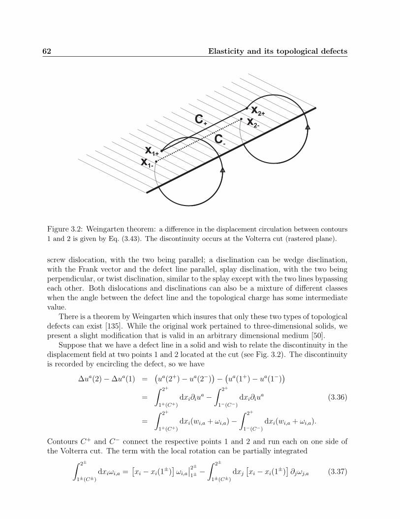
62 Elasticity and its topological defects
C+
x1+
x2+
x1-
x2-
C-
Figure 3.2: Weingarten theorem: a difference in the displacement circulation between contours1 and 2 is given by Eq. (3.43). The discontinuity occurs at the Volterra cut (rastered plane).
screw dislocation, with the two being parallel; a disclination can be wedge disclination,with the Frank vector and the defect line parallel, splay disclination, with the two beingperpendicular, or twist disclination, similar to the splay except with the two lines bypassingeach other. Both dislocations and disclinations can also be a mixture of different classeswhen the angle between the defect line and the topological charge has some intermediatevalue.
There is a theorem by Weingarten which insures that only these two types of topologicaldefects can exist [135]. While the original work pertained to three-dimensional solids, wepresent a slight modification that is valid in an arbitrary dimensional medium [50].
Suppose that we have a defect line in a solid and wish to relate the discontinuity in thedisplacement field at two points 1 and 2 located at the cut (see Fig. 3.2). The discontinuityis recorded by encircling the defect, so we have
∆ua(2)−∆ua(1) =(ua(2+)− ua(2−)
)−(ua(1+)− ua(1−)
)=
∫ 2+
1+(C+)
dxi∂iua −
∫ 2+
1−(C−)
dxi∂iua (3.36)
=
∫ 2+
1+(C+)
dxi(wi,a + ωi,a)−∫ 2+
1−(C−)
dxi(wi,a + ωi,a).
Contours C+ and C− connect the respective points 1 and 2 and run each on one side ofthe Volterra cut. The term with the local rotation can be partially integrated∫ 2±
1±(C±)
dxiωi,a =[xi − xi(1
±)]ωi,a
∣∣2±1±−∫ 2±
1±(C±)
dxj
[xi − xi(1
±)]∂jωj,a (3.37)

3.3 Topological defects in solids 63
and since
xi(1+) = xi(1
−), xi(2+) = xi(2
−), (3.38)
we arrive at
∆ua(2)−∆ua(1) = (xi(2)− xi(1))(ωi,a(2+)− ωi,a(2
−)) +∫C+
dxj [wj,a + (xi − xi(1))∂jωi,a]− (3.39)∫C−
dxj [wj,a + (xi − xi(1))∂jωi,a] .
The integrals are calculated over two different sides of the Volterra cut and they can bemerged into one integration over a contour C of the discontinuities∫
C+
−∫
C−→∫
C
dxj [∆wj,a + (xi − xi(1))∆∂jωi,a] . (3.40)
The discontinuity of the local rotation derivative can be reorganized into
∆(∂jωi,a) = 12∂j(∂iu
a(x+)− ∂aui(x+))− [x+ → x−]
= ∂iwj,a(x+)− ∂awj,i(x
+) + 12(∂j∂i − ∂i∂j)u
a(x+)− (3.41)12(∂j∂a − ∂a∂j)u
i(x+) + 12(∂a∂i − ∂i∂a)u
j(x+)− [x+ → x−].
Since the displacement field is smooth on both sides of the Volterra cut, all terms with twoderivatives vanish and the integral Eq. (3.40) turns into∫
C
dxj [∆wj,a + (xi − xi(1))∆(∂jwj,a − ∂awj,i)] . (3.42)
It was earlier assumed that both strains and their derivatives are smooth on the Volterracut. Accordingly, the integral Eq. (3.42) is identically zero. The discontinuity in thelocal rotation field defines an antisymmetric tensor Aij = ∆ωi,j, and we obtain the exactformulation of the Weingarten theorem
∆ua(2) = ∆ua(1) + Aab
[xb(2)− xb(1)
], (3.43)
which states that a discontinuity over a Volterra cut can only be a constant vector plusthe action of an antisymmetric tensor. Another way to formulate it is by saying thata discontinuity in the displacement around a defect line is independent of the path andalways given in the form∮
C
(dl · ∇)u = u(x+)− u(x−) = b0 + A (x− x0). (3.44)
We express the antisymmetric tensor A as
Ωa1a2...ad−2= 1
(d−2)!εa1a2...ad−2ijAij, (3.45)

64 Elasticity and its topological defects
and vice versa: A = εΩ (in symbolic form) and we recognize the second term of theWeingarten theorem Eq. (3.43) as a d-dimensional rotation. For a two- or three-dimensionaldefect line, the Frank scalar and vector respectively coincide with Ω and Ωa. Defects withΩ equal to zero are pure dislocations with the Burgers vector b = ∆u. The Burgers vectorof a disclination is on the other hand sensitive to the choice of the reference point 1 inthe Weingarten theorem Eq. (3.43). The most important consequence of the theorem is,however, that dislocations and disclinations are sufficient to cover any possible discontinuityand therefore there is no other kind of defect permitted.
An elastic topological defect is characterized by discontinuity at the defect manifold(point, line, brane, etc.). In analogy with the vortices of the Abelian-Higgs model, weintroduce the density of defects, dislocations and disclinations respectively, as
αai1i2...id−2
= εi1i2...id−2jk∂j∂kua, (3.46)
Θa1a2...ad−2
i1i2...id−2= εi1i2...id−2jkεa1a2...ad−2bc
12∂j∂k∂bu
c. (3.47)
d−2 lower indices represent the fact that the defect is an oriented manifold (a d−2-brane).The upper indices correspond to the Burgers charge (vector regardless of the number ofembedding dimension) and Frank charge (tensor of rank d− 2). By our earlier convention,we will refer to the upper index of the dislocation density as a ‘flavor’ index.
Let us suppose that a general topological defect is defined by singularities on a manifoldΣ. The defect densities can be expressed in terms of manifold delta function, Eq. (2.106),used in section 2.5
αai1i2...id−2
= δi1i2...id−2(Σ)(ba −Aabxb), (3.48)
Θa1a2...ad−2
i1i2...id−2= δi1i2...id−2
(Σ)Ωa1a2...ad−2 . (3.49)
Since the topological defects cannot have any edges, the derivative identity Eq. (2.101) isvalid for the manifold Σ. Accordingly, the conservation law for disclinations and a similarlaw for dislocations follow when we differentiate defect densities Eqs. (3.48 - 3.49)
∂jΘa1a2...ad−2
ji1i2...id−3= 0, (3.50)
∂jαaji1i2...id−3
= Aajδ...(Σ) = εajb1b2...bd−2Θ
b1b2...bd−2
ji1i2...id−3. (3.51)
The latter identity can be interpreted as the conservation law for dislocation densitiesvalid only in the absence of disclinations. In the presence of disclinations, it illustrates theinterdependence of dislocations and disclinations: ‘peeling’ of dislocations from the infinitestack that builds a disclination is allowed at no cost on the disclination Frank charge.This implies that, in order to create a dislocation, all we have to do is make a disclinationmove. This law works the other way around also: a moving disclination leaves a trail offree dislocation defects behind it. If these proofs seem superficial, a more precise proof,based on the analogies with differential geometry [48]. and gravity [123, 124, 125], will bepresented in appendix B.
Until now we were concerned only with defects of a classical elastic medium. Giventhat a quantum elastic medium has an additional coordinate, i.e. imaginary time, we

3.3 Topological defects in solids 65
Dv b=t
¶
Figure 3.3: Discontinuity in the velocity field or the ‘velocity dislocation’: such a disconti-nuity, though physically possible, violates the assumptions of the Weingarten theorem Eq. (3.44).Depending on the orientation of the Volterra cut with respect to the ‘velocity Burgers vector’ itrepresents slip of surfaces (parallel, full line) or adding/removing material (perpendicular, dashedline). For simplicity, we use the word ‘slip’ for both motions.
should repeat the whole procedure, now having the topological densities only as the static(temporal) components of the more general defect currents and generalizing the definitionsEq. (3.46 - 3.47) to accommodate the dynamical currents. The imaginary time directionshould have a special role in this generalization. However, it turns out that the generaliza-tion to the dynamical currents of a quantum solid is straightforward if we assume a mediumwith one more dimension which is assigned to the imaginary time and use the definitions,remarks, conservation laws, etc., from the previous paragraphs in this section. There is,however, a subtle change due to the special status of time in the elastic theory – crystallinedisplacements in the temporal direction (uτ = 0) are forbidden and this is reflected in thegeometrical structure of the defect topological charges. First, we note that the Burgersvector registers the displacement discontinuity which is only possible in the spatial direc-tions. Therefore, the dislocation currents with temporal flavor are not permitted and thedefinition of dynamical dislocation currents becomes
Jaµ1µ2...µd−1
= εµ1µ2...µd−1νλ∂ν∂λua. (3.52)
The Greek indices are now used to signify summing over both spatial and temporal indiceswhile the Burgers flavor is exclusively spatial.
The generalization of the disclination current Eq. (3.47) has to be performed withgreater care. Let us naively substitute all the indices in Eq. (3.47) by their Greek counter-

66 Elasticity and its topological defects
parts (space-time indices) to obtain the definition of the dynamical disclination current
Tα1α2...αd−1µ1µ2...µd−1
= 12εµνλεαβγ∂ν∂λ∂βu
γ. (3.53)
Braces represent a string of indices (say α = α1α2 . . .). Since the index γ cannot take thetemporal value τ in the summation of Eq. (3.53), one of the remaining indices, either any ofthe αi or β, has to be the temporal one. If one of α’s has taken the value τ , the remainingindices are all spatial, including β, and the topological charge operator Eq. (3.53) gives thediscontinuity in a local rotation. If, however, one takes the disclination current componentwith all of the α indices spatial, β is forced to take the temporal value and the topologicalcharge Eq. (3.53) is not measuring a discontinuity in a local rotation, but rather in thevelocity field ∂βu
γ → ∂τuc ≡ vc. Thus, this kind of generalized disclination current can
alternatively be thought of as a disclination in the velocity field. In principle, such eventsare possible in real solids, but what do they mean physically? In Fig. 3.3, we give anillustration of the effect of a velocity discontinuity. Pending the orientation of the Volterracut (which is physical now since the velocity field does not repair itself) with respect to
the velocity discontinuity, a nonzero value of the current Taµ means that two crystalline
surfaces slip over each other or that some additional material is added or removed from thedefect. These effects are in clear violation of the Weingarten theorem as it states that allthe symmetrized strains (and the velocity field can be regarded as such) have to be smooth.The conditions violating the Weingarten theorem imply further that the conservation lawsEq. (3.50 - 3.51) are no longer valid. The velocity slips act as defect factories, adding newmaterial from the outside and changing the total amount of crystalline material. As wewish to describe defects which are innate to the solids and conserved (equivalent to thecondition that no new matter is introduced into the system), the disclination currents withd − 1 spatial Frank indices are prohibited in the remainder of this work. Therefore, thecurrent Eq. (3.53) is redefined for a non-relativistic solid as
T a1...ad−2µ1µ2...µd−1
= 12εµνλεabc∂ν∂λ∂bu
c, (3.54)
so that only the Frank charge is represented in the upper label(s). It turns out that thedual elastic theory, which is supposed to treat all possible defects, decouples the prohibitedvelocity slips from the physical dual degrees of freedom at the end of the day.
3.4 Topological kinematic constraints: dislocations and
the glide principle
Defects such as interstitials/vacancies, dislocations or disclinations perturb the ideal per-fectly periodic crystal. Since they play a crucial role in the melting transition by theirdeconfinement, it is natural to expect that their kinematical and dynamical propertiesbecome essential when these transitions are analysed. An important example is the dis-location glide constraint. This constraint is very well known in the materials sciencecommunity, but the understanding of this constraint was always based on either heuristic

3.4 Topological kinematic constraints: dislocations and the glide principle 67
or numerical arguments. Recent work on the melting of quantum crystals [44] signified theimportance of the glide constraint for the properties of the new melted phases and it offereda formulation of glide in terms of the novel dynamical dislocation currents Eq. (3.52).
In this section we treat these matters carefully and show that the glide constraint, whichis a topological constraint, may be derived from a simple consideration that the matter isconserved inside the solid. To highlight the history of the subject and the beauty of theproof, we first derive the linear glide constraint for a charged solid, and later repeat theprocedure for an uncharged solid with the same result. The proof we give is independentof the number of embedding dimensions and it always constrains one of the dynamicalcurrents Eq. (3.52). To give a better feeling for the glide constraint in higher dimensions,the constraint is interpreted in two, three and four dimensions, and we point out howthe geometrical structure of the defect can allow local ‘leaks’. Because the constraint, asinitially derived by us, represents only the linear approximation to the exact expression, werevisit the proof without the linear approximation, rederive the exact expression and arguethat these corrections can accommodate the physics beyond the linear theory, involvinginterstitial events and finite lattice constant effects. There is another aspect of the glideconstraint: its transformation properties under the spatial symmetries of the system. Aswe show toward the end of this section, the glide constraint prohibits the only singletcurrent in the system, relieving the compression degree of freedom from the burden of thedisorder degrees of freedom. In the dual theory of the elasticity, this condition is sufficientto keep the compression rigidity present at all length scales.
In many standard texts, e.g. [132, 133, 134], the explanation of the glide constraintis not profound. A dislocation corresponds to a row of particles (atoms) ‘coming to anend’ in the middle of a solid. One way to move this entity is to cut the neighboringrow at the ‘altitude’ of the dislocation and consequently move over one tail to cure thecut (Fig. 3.4a). The net effect is that the dislocation is displaced. This easy mode ofmotion is termed ‘glide’. Moving in the orthogonal direction is not as easy. Let us try tomove the dislocation ‘upward’. This requires loose particles to lengthen or shorten the rowof particles (‘interstitials’ or ‘vacancies’) and since loose particles are energetically verycostly and they move very slowly (by diffusion) this ‘climb’ motion is strongly hindered.Estimates on ‘climb’ diffusion rates are provided in e.g. Ref. [136]. Climb is hindered tosuch an extent in real life situations (e.g. pieces of steel at room temperature) that it maybe ignored altogether. The lower dimensional glide motion of dislocations is reminiscentof dynamics in the heavily studied sliding phases [57, 137, 138, 139, 140, 141, 142, 143] inwhich an effective reduction of dimensionality occurs.
Earlier discussions on the glide constraint present it in a fairly quantitative way by de-manding that the dislocation motion obeys conservation of crystalline material. Suppose wehave a dislocation line specified by x(s) having a Burgers charge b. The three-dimensionalglide constraint is then expressed as∫
L
ds ∂sx · (b× x) = 0. (3.55)
It is given in integral form in order to leave room for the diffusion of the material over

68 Elasticity and its topological defects
a) b)
Figure 3.4: Possible motions of dislocation defects in a) two and b) three dimensions a)allowed (matter conserving) cutting and reconnecting of ‘atomic columns’ gives rise to the glidemotion of the dislocation line (at the center of figure) in the horizontal direction. By contrast, anemission or absorption of vacancies and interstitials is required for a climb motion (vertical motionof the dislocation in this figure). Thus, an absence of additional material (mass conservation)strictly prohibits the climb within, continuum limit, linear elasticity. b) in three dimensions, thesame principle is still valid for a motion of the defect as a whole line parallel or perpendicularto its Burgers vector. However, due to the geometrical structure of the defect, small exchangeof material is allowed across the defect line. That way, a segment of the defect line may locallyclimb at expense of its neighbours’ height.
the line. In spite of the fact that this diffusion process is not intensive, it is usually stillmuch stronger that the diffusion of the external interstitials. This motion, where a segmentof the three-dimensional dislocation can move perpendicular to its Burgers vector at theexpense of its neighbouring segment is known as restricted climb (see Fig. 3.4b ).
The glide formulation Eq. (3.55) may suffice for the needs of metallurgy. However, if wewant to write a consistent dual theory of quantum elasticity, the glide constraint should begiven in an exact mathematical form, involving the currents Eq. (3.52). This formulationof the constraint is the aim of this section.
Let us begin with the analysis of an electrically charged solid. Such a medium (“bosonicWigner crystal”) is interesting in itself [9, 144], and will be the central object of our studyin the chapter on our novel type of superconductivity (chapter 5). Here, it is merely utilizedas a convenient tool for implementing the material conservation law via gauge invariance,to subsequently derive the glide principle. Later on, we will independently derive theglide constraint by direct mass conservation without resorting to local gauge invarianceto implement it. As mass conservation pertains to a scalar quantity, such a conservationlaw translates into a condition on a linear combination of the topological defect currents

3.4 Topological kinematic constraints: dislocations and the glide principle 69
which is necessarily invariant under spatial rotations. Conservation laws (equivalent togauge invariance) may greatly restrict the dynamics of the system, leading to an effectivereduction in the dimensionality. We will now illustrate how this indeed transpires in solids:in linear elasticity, mass (‘charge’) conservation allows only glide motion of a dislocation.
From chapter 5, we borrow the (linear) EM coupling term Eq. (5.3) of a charged solidand add it to the total action density
LEM = (nee∗) [Aτ∂au
a − Aa∂τua] . (3.56)
For the exact derivation of this result we refer the reader to chapter 5. The charge andits density are given by e∗ and ne; the first term in Eq. (3.56) is the Coulomb repulsionenergy gained by compression of the solid, while the second term represents the Lorentzpotential of a moving charged particle. Charge conservation is closely related to gaugeinvariance – the gauge invariant action is equivalent to the statement that the charge isconserved. Therefore, we demand that the action Eq. (3.56) is invariant under the U(1)gauge transformation of the electromagnetic potentials Aµ given by
Aµ → Aµ + ∂µα, (3.57)
with α an arbitrarily smooth scalar field. Inserting the gauge transformed fields, Eq. (3.57),into Eq. (3.56), and performing an integration by parts, the gauge-variant part is found tobe
LEM → LEM + (nee)α [∂a∂τua − ∂τ∂au
a] . (3.58)
Since the gradient function α is arbitrary, the term in the brackets must be identically zeroin order to preserve the electric charge, and thus
∂a∂τua − ∂τ∂au
a = 0. (3.59)
This will be the glide constraint in terms of strain. Contracting the dynamical currentdefinition Eq. (3.52) with the Levi-Civita tensor and employing the identity
ετaµ1...µD−1εµ1...µD−1νλ = (D − 1)!
∣∣∣∣ δτν δτλ
δaν δaλ
∣∣∣∣ , (3.60)
the glide constraint Eq. (3.59) can be rewritten so that it acts on the dislocation currentsin any arbitrary dimension:
ετaµ1...µD−1Ja
µ1...µD−1= 0. (3.61)
This is none other than the glide constraint acting on the dislocation current in arbitrarydimensions! This result places on rigid mathematical footing the conventional glide “prin-ciple”. As we will illustrate later on, this result, now derived in full generality within thelinear regime, is violated by non-linear contributions. Towards the end of this section,
70 Elasticity and its topological defects
we will derive a complete non-linear glide constraint which will enable us to predict andestimate corrections to the linear order glide constraint in general elastic solids
At first sight this might appear as magic, but it is easy to see what is behind thisderivation. In order to derive Eq. (3.56) one has to assume that the gradient expansion iswell behaved, i.e. the displacements should be finite. This is not the case when interstitialsare present, because an interstitial is by definition an object which can dwell away aninfinite distance from its lattice position. Hence, in the starting point, Eq. (3.56), it isimplicitly assumed that the interstitial density is identically zero. The gauge argumentthen shows that gauge invariance exclusively communicates with the non-integrability ofthe displacement fields, Eq. (3.59). These non-integrabilities are of course nothing else thanthe topological currents – the glide constraint is a constraint on the dislocation current.If the glide constraint were not satisfied, electrical conservation would be violated locally,i.e. electrical charges would (dis)appear spontaneously, as if the dislocation were able tocreate or destroy crystalline matter. In the absence of interstitials this is not possible and,therefore, dislocations can only glide. The key is, of course, that by default, dislocationcurrents are decoupled from compressional stress in the linear non-relativistic theory.
We may indeed equivalently derive Eq. (3.61) without explicitly invoking EM gaugeinvariance to arrive at Eq. (3.59). Instead, we may directly rely from the very start onmass conservation – the continuity equation of the mass currents (which, as alluded toabove, is equivalent to local gauge invariance),
∂τρ+∇ · j = 0. (3.62)
To see how this is done directly, we compute the various mass current components jµ.By simple geometrical considerations, within the linear elastic regime, the mass density is
ρ = ρ0[1− ∂iui], (3.63)
with ρ0 the uniform background value: the divergence of u (signaling the local volumeincrease) yields the negative net mass (‘charge’) density variation at any point. Similarly,the spatial current density
j = ρ0∂τu. (3.64)
Compounding the mass continuity equation of Eq. (3.62) with the physical identification ofthe current (Eqs. (3.63, 3.64)), we obtain Eq. (3.59) from which Eq. (3.61) follows. Later,we will return to such a physical interpretation of the glide constraint from this perspectivein order to determine corrections to the glide principle which follow from anharmonic terms.We emphasize that the mass conservation law leading to Eq. (3.59) trivially holds in anymedium regardless of the underlying statistics [145] of potential quantum systems or theirdimension. Furthermore, within the linear elastic regime, such a discussion highlights thevalidity of Eq. (3.59) and the ensuing glide equation of Eq. (3.61) (when interpreted asdensity matrix averages) in crystals at any temperature in which strict linear order massconservation condition is imposed on all configurations. Needless to say, as temperature

3.4 Topological kinematic constraints: dislocations and the glide principle 71
is elevated, a departure occurs from such an imposed linear order condition through theenhanced appearance and diffusion of interstitials and vacancies leading to climb motions.The restriction on the dynamics in this regime is captured by a higher order variant ofEq. (3.61) (Eq. (3.76)) which will be derived later on.
Let us now pause to consider what Eq. (3.61) means physically. In two spatial di-mensions, Eq. (3.61) implies that the dislocation currents have to be symmetric [44]:εabJ
ba = Jy
x − Jxy = 0. Now, consider Fig. 3.4a. Here, the Burgers vector is pointing
in the horizontal x-direction implying that Jyµ = 0, while the glide constraint reduces to
Jxy = 0. This current (Jx
y ) is, by its very definition, the climb current perpendicular to theBurgers vector.
In three and higher spatial dimensions, the story is less easy, the reason being thatthe constraint on the motion is less absolute. This is of course known in the classictheory [48, 133], but the reader might convince him/herself that making use of Eq. (3.61)the analysis is much helped as compared to the rather pain-staking effort based on the‘intuitive’ arguments. In 3+1D, the constraint of Eq. (3.61) becomes
ετabcJabc = 0. (3.65)
Let us first consider a screw dislocation. These correspond to dislocation currents of theform Ja
aµ (i.e. the static µ = τ component corresponds to the orientation of the dislocationloop being parallel to the Burgers vector). It follows immediately that the constraintEq. (3.65) is not acting on screw dislocations and, henceforth, screw dislocations can movefreely in all directions. Edge dislocations are the other extreme, corresponding to dynamicalcurrents of the form Ja
bµ where a and b are orthogonal. The condition µ = a correspondsto glide: an edge dislocation with its loop oriented in a direction (b) perpendicular to theBurgers vector (a) can still move freely in the direction of the Burgers vector (a). Thedisplacement of a dislocation along the line is not a topological object and the currentwith two identical lower indices (µ = b) vanishes. The glide constraint only strikes whenall three labels are different. Let us consider a dislocation line extending in z directionwith Burgers vector in the x direction (see Fig. 3.4b). The only nonzero components of thecurrent are Jx
zµ and the glide constraint becomes Jxzy = 0. This automatically forbids any
motion in the y direction, that is perpendicular both to the dislocation line and its Burgersvector. The constraint is ‘leaky’ due to the extended nature of the defect. The materialneeded for the climb of one segment of the dislocation can be supplied by an adjacentsegment. The glide constraint has therefore only a real meaning through its integral form,
0 =
∫dV ετabcJ
cab. (3.66)
As illustrated in Fig. 3.4b, only the dislocation’s ‘center of mass’ is prohibited to move inthe climb direction. Local segments of the line may still move at expense of their neighbors,effectively transporting matter along the defect line. The ‘leaky’, locally defined, constraintof Eq. (3.66) corresponds with the intuitive idea of ‘restricted climb’ found in the elasticityliterature.

72 Elasticity and its topological defects
Having a mathematical definition of the glide constraint at our fingertips enables usto address its incarnations in even higher dimensional systems where direct visualizationis of little use. Notwithstanding that such crystals are, of course, not to be found instandard condensed matter, higher dimensional glide constraints might have implicationsfor ‘emergence theories’ of fundamental phenomena resting on elasticity theory [146, 85].Let us for example look how the constraint Eq. (3.61) acts in a 4+1D crystal. A dislocationis now a 2-brane, say, a plane extending in y and z directions. When its Burgers vector liesin this plane, this brane is analogous to a screw dislocation in the sense that its motionsare not affected by the glide constraint. The other extreme is the ‘edge dislocation brane’with a Burgers vector perpendicular to the brane, say in the x direction. In this casethe nontrivial currents correspond to Jx
yzµ. As noted earlier for three-dimensional defects,topological currents do not record any motion taking place within the defect-brane but onlyin directions perpendicular to it. The bottom line is that besides the static current (density)Jx
yzτ , the topological dynamical currents are Jxyzx and Jx
yzw, representing dislocation glideand climb respectively. The glide constraint Eq. (3.61) forbids the latter ‘in integral form’,allowing climb of a certain brane element only at the expense of the brane volume takenby a neighboring element.
Contrary to our rigorous (‘glide only’) result concerning the linear regime of continuumelasticity, in real crystals dislocations do climb (albeit at small rates). When dislocationscollide, interstitial matter will be exchanged and this process releases climb motions [44].In what follows, we will rederive the glide constraint, yet now do so within a fully generalframework which will enable us to address the implications of both (higher order) non-linearelasticity and the presence of a lattice cut-off. Higher order corrections to linear elasticitymodify the original glide constraints of Eq. (3.61) giving rise to dislocation climb.
To achieve this aim, we could invoke a more precise version of electromagnetic couplingterm Eq. (3.56), robust against particles that dwell away from their equilibrium positions(interstitials) and exact up to higher orders is given by
LEM = (nee∗)
[Aτ (R0 + u)
det(δij + ∂iuj)− Ai(R0 + u)∂iu
a
]. (3.67)
The denominator in the first term is the exact volume change due to the compression.The main difference between the approximate coupling Eq. (3.56) and the exact couplingEq. (3.67) is that now, particles ‘feel’ the EM potential Aµ not at their original crystallinepositions R0 but rather at their true positions, i.e. R0+u. Demanding the gauge-invarianceof coupling Eq. (3.67) under performed gauge transformation Eq. (3.57) yields the exactglide constraint. However, when we are in search for the exact glide constraint, the un-charged ‘mass conservation’ argument gives a far simpler derivation.
We return to the mass continuity equation invoked earlier (in unison with Eqs. (3.63,3.64)) yet now, by examining contributions of higher order derivatives of the displacementfield, we exercise far greater care in examining its ramifications. The continuity equationof Eq. (3.62) implicitly assumes that the density and current fields are functionals of localEulerian (distorted lattice) coordinates. On the other hand, the displacement, stress, andother elastic fields are functionals of substantial coordinates (i.e. the coordinates defined

3.4 Topological kinematic constraints: dislocations and the glide principle 73
relative to the undistorted lattice coordinates) – the Lagrangian coordinate frame. Aswas briefly done earlier (Eqs. (3.63, 3.64)), we express the local density and currents ofEq. (3.62) in terms of volume and velocities as ρ = ρ0
Vand j = ρ0v
V, with ρ0 the mass of the
ideal uniform medium in a unit volume in the undistorted original medium (i.e. the idealbackground mass density). Following a distortion, a unit volume element of the originalmedium now occupies a region of volume V . With these relations in tow, Eq. (3.62) reads
∂τV + (v · ∇)V ≡ DτV = V (∇ · v). (3.68)
This equation can be interpreted as a law governing the change of volume of the elasticmedium: the change in volume (the derivative on the left hand side) is exclusively dictatedby the motion of the boundaries – the gradient on the right hand side corresponds toa surface integral of the velocity field. This is just a reformulation of the same basicconstraint: the conservation of mass (or electrical charge). Throughout this section, massconservation was the primary ingredient leading to the glide constraint. To invoke the masscontinuity equation in the form of Eq. (3.68), let us express the actual atomic coordinatesRj in terms of the Eulerian coordinates (henceforth denoted by ri)
r[R, τ ] = R + u[R, τ ], R(r, τ) = r− u(r, τ), (3.69)
which gives the identity (valid for finite lattice constant a),
(∂Rj
∂ri)τ = (δij +
∞∑m=1
am−1
m!∂m
j ui)−1. (3.70)
Simplifying, we find that Eq. (3.68) may be recast as
∂τV = V (∂Rj
∂ri)τ∂i∂τu
j. (3.71)
This is an exact expression (entailing corrections to all order in gradients of u) detailingthe glide constraint. Retaining the leading order contributions and employing V = 1+∂iu
i,we recover the ‘familiar’ linearized glide constraint of Eq. (3.59).
What can we learn from this exact form of the glide constraint? Let us specialize tothe simple 2+1D medium. Assuming a vanishing lattice constant a, the volume of anelementary cell is simply given as V = det(δij + ∂iu
j). Inserting this in the exact glideexpression Eq. (3.71) we find that it simplifies,
0 = εabJbi (δia + ∂iu
a) = Jxx∂xu
y + Jxy (1 + ∂yu
y). (3.72)
The displacement derivative ∂iua includes both regular and singular components. When
∂iua is small compared to unity, the linearized glide constraint of Eq. (3.61) is recovered.
In the second step we chose a specific Burgers vector orientation b = bex so that all currentcomponents Jy
µ have to vanish.

74 Elasticity and its topological defects
The ‘climb’ current Jxy is non-zero in two cases. The dislocation may already glide
(Jxx 6= 0) and by following the smoothly displaced crystalline lines, a small climb motion
is present in rate of
Jxy ≈ −Jx
x∂xuy. (3.73)
This is however no true climb as the dislocation is still stuck to one crystalline line and the‘climb’ we find is just a result of motion of the dislocation conforming to the deformationof the lattice (drag by the underlying lattice). This is by no means a topological climbcurrent! By contrast, when ∂yu
y = −1 which represents the stacking of material in ydirection, i.e. presence of the interstitial matter, the current Jx
y may take arbitrary valuewhich means that the dislocation can freely climb.
At this point it seems that the field theory defined in Ref. [48] is not able to capturerelevant interstitial physics without inclusion of the anharmonic effects. In the next chap-ter we’ll however discuss the interstitial dynamical currents (strictly speaking they are nottopological) and show their relation to the dislocation current. Given that climbing dislo-cations represent sources and sinks for the interstitials, we’ll point out how to implementthe glide constraint in its local form to explicitly include the previous relation between theinterstitials and dislocations.
We reach the conclusion that higher orders in the displacements (non-linearities, anhar-monicities) have the effect of restoring the physics of interstitials. Another natural questionto ask regarding the continuum limit is whether there may be a hidden dependence on thelattice cut-off a. To investigate this issue, let us see what happens to Eq. (3.71) when weonly keep terms which are harmonic in the displacements, while imposing no conditionson the number of derivatives. These have to do with the volume of the unit cell. Let usspecialize to a simple hypercubic lattice with sides defined by the vectors (i = 1, . . . , D),
uj(Ri + ai)− uj(Ri) = δij +∞∑
m=1
am−1
m!∂m
i uj. (3.74)
The corresponding volume is a determinant of the matrix Eq. (3.74) and in the harmonicapproximation only the diagonal elements remain,
V = 1 +D∑
i,j=1
∞∑m=1
am−1
m!∂m
i uj. (3.75)
Using this expression for the volume, the exact equation of constraint (Eq. (3.71)) reads
ετai1...iD−1Ja
i1...iD−1= −(D − 1)!
D∑i=1
∂τea∂i − a∂i − 1
a∂i
∂iui. (3.76)
The remarkable fact is that it is possible to collect all higher order derivatives in a simpleexponent. Eq. (3.76) affords us with the general non-linear corrections to the glide con-straint of Eq. (3.61). Given any elastic media in which the magnitude of the gradient terms

3.4 Topological kinematic constraints: dislocations and the glide principle 75
are known, we may estimate the size of the non-linear corrections to the linear order glideconstraint.
Let us finally analyse the symmetry properties of the glide constraint. The static dis-locations and disclinations of higher dimensional media are geometrically complex entitiessuch as lines, sheets or p-branes with Burgers vectors and Frank tensors attached. Whenin motion, these branes sweep the additional time dimension. For instance, defects in twospace dimensions are point-like particles turning into world-lines in space-time, in threespace dimensions they form loops spreading out in strings etc. Nevertheless, regardless ofthe embedding dimensionality, all of these ‘branes’ share a universal property: there is aunique direction perpendicular to the brane. This direction can be related to the dynamicaldefect currents by contracting it with the D − 1 dimensional antisymmetric tensor havingone index set equal to time,
1(D−1)!
ετib1b2...bD−1Ja
b1b2...bD−1= ∂i∂τu
a − ∂τ∂iua = Ua
i , (3.77)
isolating the perpendicular direction i. Instead of the dislocation current J , we could haveused here also the disclination current T , but our interest in this subsection will be inthe former. The comparison of the tensor Eq. (3.77) with the glide constraint Eq. (3.59)illustrates that the glide condition turns into a constraint on the trace U i
i = 0. For rank-2tensors, the trace is the only invariant tensorial component of the D-dimensional orthog-onal group (O(D)), corresponding to all rotations and the inversion in the D-dimensionalmedium. It follows that the constrained current is the only ‘singlet’ (scalar) under thepoint group symmetries of the crystal (point group symmetries constitute a subgroup ofO(D)). The conjugate degree of freedom must have the same symmetry and this can onlybe compression, the only physical entity being a singlet under O(D). We have identifiedthe fundamental reason that glide implies the decoupling of dislocations and compressionalstress [44].
Apart from rotations, the glide constraint is also invariant under Galilean space-timetranslations. Needless to say, the constraint does not obey Euclidean Lorentz (space-time)invariance as the time direction has a special status both in Eq. (3.59) and Eq. (3.61). Theorigin of this lies, of course, in the definition of the crystalline displacement u and its rolein the minimal coupling Eq. (3.56). The displacements are defined under the assumptionthat every crystalline site has an equilibrium position which implicitly wires in that theirworld lines extend exclusively in the temporal direction.
We conclude with a speculation. As emphasized throughout, the basic physical ingredi-ent leading to the derived constrained glide dynamics in solids was mass conservation. In aformal setting, similar albeit more restrictive volume conserving diffeomorphisms (param-eterized by time) may be directly examined via the w∞ algebra in two spatial dimensionsand its extensions, e.g. [147, 148, 149]. We suspect that there might be a more fundamentalway of casting our relations by relying on the intricacies of such symmetries of space andtime.

76 Elasticity and its topological defects

Chapter 4
Dual elastic theory – nematic phases
The previous two chapters were of an introductory nature as we reviewed most of theknown results relevant for the Abelian-Higgs duality (chapter 2) and the elastic theory(chapter 3), adding a few novel results to each chapter. Now, having made the readeraccustomed to the basic ideas of duality and elasticity, we will proceed in this chapter tounify the two ideas in the dual theory of elasticity. This concept is fairly new in physics:it was introduced by Kleinert [48] and it seems that the scientific community has onlyrecently started to appreciate its full power. This unfortunate fact may be attributed tothe ‘sociological distance’ between the fields that dual elasticity binds together: on oneend of the spectrum, we have duality, often perceived as a mathematical trick of hard corefield theorists, and on the other end of the spectrum, elasticity and its topological defectsconsidered as a closed chapter in theoretical physics and left to material science. Hopefully,the pursuit represented by this thesis will close this gap and demonstrate that abandonedtheories can give fundamentally new results when dressed up in a field theoretical setting.
As we learned in chapter 2, ordered and disordered phases are relative concepts, relyingdirectly on the kind of machines our experiments are equipped with. Nevertheless, beingin the disordered state does not a priori ban us from seeing the correlations of the disorderobjects by experiments devised in terms of order observables [62]. Elasticity is superficiallysimilar to the XY model as seen by the comparison between their actions, Eq. (2.2) andEq. (3.4) respectively. The displacement fields u take the role of the phase field φ andthe difference comes from the ‘flavours’, showing that the dualization has to be performedwith respect to d spatial field components. The tensorial nature of the coupling constantEq. (3.25) and its symmetry properties, as well as the constraints on the topological de-fects, enrich the dual theory, leading to many counterintuitive results and interpretationswhich will be found throughout the present chapter. One of the basic ideas we wish tohighlight in this chapter is that the phonon propagators can measure correlations betweenthe topological defects, in a manner analogous to the capacity of the superfluid velocitycorrelators Eq. (2.49) to penetrate the dual barrier.
The scope of this thesis, and especially this chapter, is largely based on the pioneeringwork on quantum elasticity by Zaanen et al. [44]. Prior to that work there were no othertreatises on dual elasticity known to us that had addressed disorder in a way similar to the
77

78 Dual elastic theory – nematic phases
Abelian-Higgs duality. Although many older works focused on defect proliferation as themechanism behind melting transitions [70, 105, 106, 107, 108, 109, 110, 111, 112, 113], itwas not before this treatise that the gas of defects had been represented by a GLW actionin the context of the dual stress gauge formalism. In the same manner that EM photonsacquire mass in a superconductor (chapter 2), the dual stress photons, parameterizing thecrystalline degrees of freedom, acquire mass in the melted phase.
The special aspect of the dual elasticity melting presented here is that the GLW actioncan be invoked only for dislocation defects. In that respect, the phases found initially byZaanen et al. (called nematic phases, which we explain in a moment) are similar to thehexatic phase associated with the triangular lattice solid predicted long ago by Nelson,Halperin and Young [45, 46, 47], where the melting is caused exclusively by dislocationdefects. There are, however, a number of differences. The NHY melting was a classicaltreatise disregarding the statistics of the crystalline constituents and based principallyon the Kosterlitz-Thouless [110, 111] destruction of algebraic long-range order in the XYsystem. Further, the hexatic phase and the entire formalism developed in Refs. [45, 46,47] is innate to the triangular or hexagonal lattice (lattice point group of C6h type); onthe other hand, the quantum nematic is constructed from the dual action and such aconstruction is possible regardless the lattice point group. The unique advantage of theNHY construction is that, treating the defects on a classical level, it can handle bothdislocation and disclination defects. If a quantum crystal is considered, the geometricalphases associated with the winding of the disclination world lines and the ensuing statisticsinvalidate the GLW description.
Since the original work Ref. [44] contained a subtle flaw regarding the dynamics ofthe defect fields – a problem tackled in chapter 2 and a preprint of ours [62], the resultspresented here are derived with the dislocation condensate treated as a fully ‘relativistic’entity. The conceptual ideas of Ref. [44] are, however, all retained in this thesis and as aconsequence, a new phases of matter and novel mechanism for the superconductivity, basedon these new phases, are found. With respect to these result, this and the next chapterrepresent the core of this thesis. The treatise on neutral solids in this chapter forms a basisfor the following chapter where electrically charged solids are considered.
Let us review here the basic ingredients needed for construction of the dual elasticitytheory and the GLW disorder action that describes the nematic phases. The constructionof the dual theory alone is fairly unrestricted, as was the case with the XY model. The roleof the conjugate momenta is taken by stress fields. In more than two spatial dimensions itis still possible to define the dual stress gauge fields, but the dual theory shares a difficultywith the Abelian-Higgs duality: the gauge fields become d− 1 antisymmetric forms as dothe defect currents. When we introduce the dual elastic theory, we will proceed as faras possible with a dimension independent formulation of the formalism. Unfortunately,when the disorder fields are introduced in the theory, we will have to restrict ourselves to2+1D quantum solids, just as was the case with the Abelian-Higgs duality. There is onelucky circumstance for the application of this dual elasticity. It is generally believed thatthe physics behind high-Tc superconductivity in cuprates is restricted to two-dimensionalcopper-oxide planes. In this regard, our handicap seems not so important because the most

79
promising application of our theory is to high Tc superconductivity. One should howeverbe careful when electromagnetism is incorporated in the theory. The EM fields are inprinciple 3+1-dimensional and one should pay care to match the dimensions properly; inthe next chapter more attention will be paid to this issue.
In the previous chapter we argued that a nontrivial statistics of the solid constituentsmay give rise to nontrivial (imaginary) contributions to the quantum action. In order toprotect the dual disorder theory from these ‘signs’, we consider a solid made exclusivelyfrom bosonic (spin-0) particles. This condition implies that, when we wish to apply themodel to a certain physical system, there exists a temperature/energy scale where effectivebosonic excitations emerge.
Another important condition is that we consider only the so-called extreme type-IIkind of melting process where interstitials are prohibited in the formalism. The non-topological status of interstitial events makes it less obvious how to incorporate these inthe theory. Although we present some speculations in the conclusion on how to includeinterstitials defects into the field-theoretical description, the full formalism is still not fullydeveloped and so we leave it as an issue for further investigation. The finite Higgs massfor the stress fields at the same time means that there is a (shear) penetration depth λS
associated with the dual stress gauge fields. This length has to be large compared to themicroscopic scales associated with the constituents (Cooper pairs). This condition alsoimplies that the disordered phase is a quantum liquid crystal of the nematic kind. Thequantum phase transition from the crystal to the isotropic superconductor is necessarilyof the first order [150] and a continuous transition is required for a large λS. In the duallanguage, the nematic order implies the topological status of the phase in a sense thatdisclination defects are massive. The only permitted defects are dislocations, which are atthe same time “carriers of the disorder”.
In the previous chapter we learned that dislocations have a vectorial Burgers charge.Based on this charge, we introduce a Burgers director – a liquid-crystal like order pa-rameter whose value splits the nematic phase into two subphases: ordered and topological(disordered/isotropic) nematic. In the construction of the disorder field, the Burgers chargeacquires the status of a coupling constant with respect to the flavour label of the dual stressgauge fields. The order in the Burgers sector means that only one flavour of the dual gaugefields, the one parallel to the Burgers vector, is minimally coupled to the disorder field andonly this flavour will be subjected to the Higgs mechanism. The derivation of results forthis phase is straightforward, although it becomes technically tedious here and there. Onthe other hand, the problem of the disordered Burgers charge in the topological nematicphase has triggered some controversy. When a ‘naive’ (mean-field) average of the Burgersdirector is used, the ramifications of the dual disorder theory seem in contradiction withthe initial assumptions. Nevertheless, these results, still not published, are presented for afew reasons. First, if there is indeed a technical error in the results (inadequate averaging,gauge artifacts, etc.), a reader skillful in these matters might be able to find the correctionand this might help us to eliminate the flaw. However, at the end of the section on thetopological nematic, a claim will be presented that the three demands imposed on thisphase in Ref. [44] (‘isotropy’ in the Burgers sector, GLW action implying a Burgersless

80 Dual elastic theory – nematic phases
dislocation superfluid and Gaussian treatment) cannot be all simultaneously satisfied, atleast in the case when the dislocation condensate is treated dynamically. The last sectionis devoted to a vindication of the results obtained for the topological nematic by ‘naive’averaging and in that section it is shown that the controversial results have application toyet another, newly identified phase of the nematic type.
This chapter is organized in the following way. The first section is a straightforwardderivation of the dual elastic field theory. It leads to the introduction of dual stress gaugefield degrees of freedom and the identification of defect currents from section 3.3 as cur-rents which are minimally coupled to the dual gauge fields. The resulting formalism is ageneralization of the work of Kleinert [48], now applicable to an elastic solid of arbitrarydimension. Following the same storyline as in chapter 2, the second section contains theformalism required to treat the disorder field. We are limited to a 2+1D gas of bosonicdislocations and a simple GLW action of type Eq. (2.35) suffices for its description. Theproblem of order vs. disorder in the Burgers sector is formulated in this section and atthis point we rely on the analysis from Ref. [44] where a liquid crystal action is suggestedfor the Burgers director order parameter. The phase diagram based on these arguments isoutlined. In the third section, the dual stress gauge bosons are thoroughly analysed. Ini-tially, the ideal crystal phase is recovered as the Coulomb phase of the dual gauge theoryand the dual stress gauge field components are given a physical interpretation within theCoulomb gauge fixing. Subsequently, the Bose-condensation of the dislocations is consid-ered. The Higgs mechanism which is implied in one of the stress gauge field flavours leadsto the ordered nematic phase. The symmetry analysis, discussed in detail in appendix C,shows that after all relevant constraints have been implemented, only two ‘shear rigidity’gauge photons are left to interact with the defects. In the ordered nematic phase the Higgsmechanism acts only on one of the two shear doublet components. In the next section,the ‘naive average’ over the Burgers vector is discussed and the isotropic/topological phaseof the solid is obtained. Due to the problems already mentioned, the end of this sectionanalyses consistency of the topological nematic phase. Some physical interpretations ofthe existing results are offered, based on symmetry arguments. In the last section, analternative model for the disorder field is considered, which leads to an interpretation ofthe results of the previous section in a completely different light. The phase to which thecontroversial results are applicable and which we call the ‘isotropic nematic’, shares somefeatures with the topological nematic: the disclinations are massive and the Burgers direc-tor has no vacuum expectation value in either of the two phases. In fact, the last propertyseems responsible for the misinterpretation of the two phases since the only input in theconstruction of the disordered nematic phase was precisely that the Burgers director orderparameter vanishes (Qab = 0). The difference between the phases is in the following: inthe isotropic nematic phase there is a multitude of mutually interacting dislocation con-densates whose Burgers directors add to zero. At the same time, each condensate has awell-defined conserved Burgers vector. The topological phase, on the other hand, has onlyone bosonic degree of freedom whose Burgers director is disordered. It will be argued thatone must take higher order (interaction) terms into account in order to properly describethe ‘strong interaction’ effects of this phase.

4.1 Dual elasticity 81
4.1 Dual elasticity
The dual elastic theory should in principle be easy to obtain if we stick to the recipe givenin chapter 2, applying it directly to the theory defined throughout the action Eq. (3.24).That the procedure is everything but straightforward becomes clear when one is forcedto invert the “coupling constant”, the elastic tensor given in Eq. (3.25). Given that thesymmetries of space-time require the antisymmetric part of the elastic tensor to be singular,the construction of the dual theory has to be executed with great care. In his book [48],Kleinert considers only the symmetric strains Eq. (3.6) and the dual fields are introducedwith respect to these strains. The introduction of conservation laws on conjugate momentaEq. (2.10) in this approach lacks the symmetry in indices which motivated an alternativeprocedure in the construction of the dual elasticity presented here for the first time. Theprocedure is based on the same ideas that inspired Kleinert for his dual elastic theoryand in fact it amounts to nothing more than reshuffling of indices. However, due to itsapparent symmetry, this construction is tailored in such a way that it is easy to generalizeall important steps to a medium of arbitrary dimensions.
After the single curl dual stress gauge fields (in analogy with Eq. (2.12)) have beenintroduced and the ‘single curl’ dual field theory is found, the remainder of this sectionis used to show that this dual formulation cannot cope with the presence of disclinationdefects. It should be improved by the introduction of ‘double curl’ gauge fields. Inter-dependence of dislocation and disclination currents is cured when the ‘true’ topologicalcurrent is introduced. This topological current operator collects only the defect degrees offreedom (from both dislocation and disclination currents) that are not redundant in thelinear elasticity. Although in the remainder of the thesis the ‘true’ topological currentsand the ‘double curl’ dual theory are not of direct relevance, they are presented as part ofthe elastic duality which cannot be ignored in a general review of the subject. We mustalso notice that the introduction of the ‘true’ topological currents and their conjugate de-grees of freedom, double curl stress gauge fields, differs in this text from all the currentliterature known to us [48]. When Kleinert introduces the ‘double curl’ stress gauge fields,this is done for a classical crystal and all the indices have spatial values. Hopefully, wehave convinced the reader that the generalization to dynamical defect currents is a trickybusiness due to the lack of temporal displacements (uτ ≡ 0). We can take two definitionsfor the disclination currents as an example, Eq. (3.53) that does not respect the temporaldisplacement constraint and the corrected version Eq. (3.54). In this respect, the ‘doublecurl’ fields we introduce must take care of the inability of matter to displace in the temporaldirection, such that only the physical topological defect currents are tracked.
Let us now return to the initial action of an (electrically neutral) solid as given inEq. (3.24). The generalized momenta are defined according to
σaµ = −i ∂L0
∂(∂µua)= −iCµνab∂νu
b, (4.1)
and they have a physical meaning: components σai represent stress exerted on a portion of
the solid and the components σaτ are kinematical momentum densities. One is supposed

82 Dual elastic theory – nematic phases
to express all strains ∂µua in terms of the stress fields σa
µ. Unfortunately, Eq. (4.1) cannotbe directly inverted due to the singularity associated with the antisymmetric stresses. Atthis point an elegant way to avoid this singularity is introduced in this thesis. Next to thespin-0 and spin-2 projectors, Eq. (3.14), which span the space of symmetric tensors Cijab,we introduce the antisymmetric spin-1 projector
P(1)ij,ab = 1
2(δijδab − δibδja). (4.2)
The space of all rank-2-2 tensors is spanned by these three projectors as seen from theclosure relation
P(0)ijab + P
(1)ijab + P
(2)ijab = δijδab ≡ 1ijab. (4.3)
Projecting the definition of stress Eq. (4.1) on the three possible spin subspaces, the fol-lowing relations between the stresses and strains are found
P(0)ij,abσ
bj = −idκP (0)
ij,ab∂jub, (4.4)
P(1)ij,abσ
bj = 0, (4.5)
P(2)ij,abσ
bj = −i2µP (2)
ij,ab∂jub. (4.6)
These relations are derived for the isotropic elasticity theory characterized by the elastictensor Eq. (3.15) and we will use them in present work. In analogy with the decompositionEqs. (4.4 - 4.6), one can find the appropriate relations for an elasticity tensor of a solidwith lower point group symmetries.
The substitution of strains by stress fields in the action Eq. (3.24) and the recovery ofthe Hamiltonian is trivial if we employ the decomposition Eq. (4.3) and the orthonormalityof each projector (P 2 = P ). Inserting the unity operator between stress and strain fieldsone obtains
H = −iσaµ∂µu
a + L0 =1
2ρσa
τσaτ − iσa
i
(P
(0)ij,ab + P
(1)ij,ab + P
(2)ij,ab
)∂ju
b +
+12∂iu
a[P
(0)ij,abdκP
(0)jk,bc + P
(2)ij,ab2µP
(2)jk,bc
]∂ku
c = 12σa
µC−1µνabσ
bν . (4.7)
The terms containing temporal components σaτ factorize immediately and are trivially
dualized because there is no singularity in that sector. The inverse elastic tensor C−1µνab
should not be taken literally. Instead, this is just the symbolic notation for the tensorcoupling the stress fields
C−1µνab =
1
ρδτµδτνδab +
1
dκP
(0)µν,ab +
1
2µP
(2)µν,ab (4.8)
=1
ρδτµδτνδab +
1
4µ
[δ(2)µν δab + δµbδνa −
2ν
1 + νδµaδνb
]. (4.9)

4.1 Dual elasticity 83
The singular direction of the elasticity tensor does not appear in the ‘inverse’ elasticitytensor Eq. (4.9). Instead, the singularity implies the constraint on stresses (see Eq. (4.5))which is in fact the famous Ehrenfest constraint [126]
σba − σa
b = 0. (4.10)
In the previous chapter we argued that, based on the symmetry properties of expansionEq. (3.2), and the microscopic crystal potential V , the elasticity tensor in Eq. (3.4) can-not have an antisymmetric part. The implications are very fundamental. The Ehrenfestconstraint Eq. (4.10) is in fact much a deeper statement since the stress fields are definedin all media, be it solids, liquids or gases. The constraint is directly related to angularmomentum conservation: its violation would imply a violation of the angular momentumconservation. As it turns out, the symmetry of the elasticity tensor Eq. (3.25) is a funda-mental consequence of space isotropy. In contrast with the derivation presented here, it isa physical consequence, and not the cause of the Ehrenfest constraint defined on stressesEq. (4.10).
Together with the Ehrenfest constraint, the partition function acquires the form
Z =
∫DuaDσa
µ
∏a 6=b
δ(σba − σa
b ) e−
Rdxν Ldual , (4.11)
with dual action
Ldual = H + iσaµ∂µu
a. (4.12)
Following the duality procedure, the displacement field is decomposed into smooth andsingular parts. Integrating out the smooth part, the stress conservation law is obtained
∂µσaµ = 0. (4.13)
This constraint is nothing else than the equation of motion for stresses in an elastic medium[126]. The sum over spatial values of index µ is the divergence of the stress tensor. It isequal to the negative force, which is, according to the classical Newton law, precisely thekinematic momentum time derivative ∂τσ
aτ .
We are more interested in the use of the equations of motion Eq. (4.13), in a similarmanner as the momentum conservation law Eq. (2.10) was used. The ‘no divergence’condition implies that a gauge fields can be introduced, similar to those in Eq. (2.12), insuch a way that the stress is defined via
σaµ = εµνλ1...λd−1
∂νBaλ1...λd−1
. (4.14)
In analogy with the higher dimensional Abelian-Higgs duality, the number of lower indicesdepends on the dimension as d−1. Also, only antisymmetric (in lower indices) componentsof the gauge field have a physical meaning, but not all: some are part of the gauge volume

84 Dual elastic theory – nematic phases
and some are ‘eaten’ by the Ehrenfest constraint. The main difference between the Abelian-Higgs and elastic stress gauge fields is that the latter carry an upper (Burgers) label.
To treat the singular part of the displacement field, a partial integration of the multival-ued strain part of Eq. (4.12) with respect to the stress gauge fields is performed in the usualway. This results in the familiar coupling of the elastic gauge fields to the d+1-dimensinaldislocation currents, as defined earlier in Eq. (3.52)
iσaµ∂µu
aMV = iεµνλ1...λd−1
∂νBaλ1...λd−1
∂µuaMV
= iBaλ1...λd−1
ελ1...λd−1νµ∂ν∂µuaMV = iBa
λ1...λd−1Ja
λ1...λd−1. (4.15)
In a shorthand symbolical form, the total elastic action turns, after dualization, into
Ldual = 12(ε∂B)C−1(ε∂B) + iJB, (4.16)
with the Ehrenfest constraint explicitly imposed on the gauge fields. The partition function,with all of the constraints included, becomes
Z =
∫DBa
λ“DJaλ”
∏b
F b(Baλ)
∏a 6=b
δ(εaνλ∂νBbλ) e
−R
dxν Ldual . (4.17)
This result is astonishing, especially so in two spatial dimensions where, in analogywith vortex duality, we recover a Maxwell type of effective action with phonon degrees offreedom represented by gauge photons and dislocations acting as electric charges. Thereare, however, a couple of important differences. The most important is that this Maxwelltheory is about ‘flavored’ gauge fields and currents, the flavour corresponding to one upper(Burgers) index. The ‘coupling constant’ appears in the form of a tensor Eq. (4.9) whichcouples degrees of freedom in a quite unexpected way (longitudinal and transversal fieldcomponents are messed up). The final novelty comes from the Ehrenfest constraint whicheffectively removes some of the gauge degrees of freedom at the expense of inducing acoupling between the remaining ones.
One may wonder what has happened to the disclination defects: why are they missingfrom the dual action Eq. (4.16)? There must be a way to introduce these defects ina field theoretical formalism. To address this issue, we first check the validity of thedislocation coupling term in the dual action Eq. (4.16). The gauge transformations in thetwo- and three-dimensional vortex dualities where already introduced in chapter 2. Thetransformation is easily generalized to higher dimensions in such way that the transformedfields stay antisymmetric. The gauge invariance of the action Eq. (4.16) is tightly linkedto the dislocation current conservation condition
∂µJaµν1...νd−2
= 0. (4.18)
In the vortex duality no defects other than vortices exist and the vortex currents are alwaysconserved, validating the introduction of the gauge fields Aµ and their minimal couplingto the vortex currents. In dual elasticity this is not always the case due to the Weingarten

4.1 Dual elasticity 85
theorem [135] which states that the dislocations alone do not exhaust the spectrum ofall possible topological defects. Contrasting the dislocation conservation law Eq. (4.18)with the exact relation Eq. (3.51), it becomes clear that the ‘single curl’ dual stress gaugefields are no longer valid objects as soon as a single disclination is present in the system.Therefore, in such a case it is necessary to avoid the substitution Eq. (4.14). A naturalquestion which arises is: what can we do to develop a proper treatment of the disclinationcurrent densities within the dual field theory formalism? Comparing the definitions ofdislocation and disclination currents, Eqs. (3.52) and (3.54) respectively, we observe thatthe disclinations carry one more derivative of the displacements fields. By introducing anadditional curl in Eq. (4.14), the problem is removed, while now both dislocations anddisclinations are coupled to the physical stress degrees of freedom. These new fields arecalled the ‘double curl’ stress gauge fields [48]. Due to the dimension dependent nature ofthe Frank charge, the introduction of the double curl gauge fields is sensitive to the numberof dimensions of the solid. In two and three spatial dimensions it can easily be trackeddown to the following relations,
σaµ = εµνρ∂ν
[∂ah
1
ρ + ετab∂bh2
ρ
], (4.19)
σaµ = εµνρλετabc∂ν∂bh
c
ρ,λ. (4.20)
Again, due the special status of time in the theory, these fields are introduced in a slightlydifferent manner compared to Ref. [48].
By means of partial integration, the double curl gauge fields (h1,2
µ in two and hc
ρλ inthree spatial dimensions) couple minimally to field discontinuities given by
η1µ = εµνλ∂a∂νwλ,a,
η2µ = εµνλεab∂a∂νwλb (4.21)
in two or
ηλρ = ελρµνεabc∂b∂µwµ,c (4.22)
in three dimensions. The defect currents η are known as the “true defect currents” or“true topological currents”. They are related to the disclination and dislocation currentsvia relation which holds in all dimensions, although the contraction of the indices doesdepend on the number of dimensions, namely
η = T + ε∂J. (4.23)
Therefore, the true topological current groups redundant defect densities into one tensorialdefect density operator. It is important to notice that the true topological currents areincomplete if the second-order gradient elasticity terms Eq. (3.19) are added to the elasticaction. The rotational stiffness term introduces a new dual degree of freedom that shouldcouple to a discontinuity in a local rotation. The true topological currents are all defined

86 Dual elastic theory – nematic phases
as discontinuities in the symmetrized strains and therefore cannot code for all relevantdefects of the elastic theory.
In relativistic solids (relevant for emergent gravity [84, 85]), temporal displacements arepossible and the relativistic definition of the true topological currents in arbitrary numberof dimensions is the one given by Kleinert [48]
ηα1...αd−1µ1...µd−1
= εαβγεµνλ∂β∂νwλ,γ. (4.24)
which is a relativistic tensor. The relativistic true topological current Eq. (4.24) is sym-metric under the simultaneous exchange of all the upper with all the lower indices. Therelativistic double curl field is given by (compare with Eqs. (4.19 - 4.20))
σαµ = εµνλεαβγ∂γ∂νh
γλ, (4.25)
and due to the Ehrenfest constraint, the double curl gauge field h has the same symmetryproperties as the relativistic topological current Eq. (4.24). The antisymmetric part of
the field hγλ is unphysical and accordingly the ‘true’ topological currents couple only
physical degrees of freedom with singularities relevant for the linear elasticity. These areexpressed in the form of linear combinations of dislocation/disclination currents whilethe irrelevant/redundant components are left out. The number of the physically relevantcurrent components is, in this way, easy to establish.
In a non-relativistic solid, where the temporal dimension is not connected by Lorentzsymmetry to the spatial dimensions, the symmetrized strain Eq. (3.6) becomes corrupted inthe spatial direction (i.e. we should define wτ,a = ∂τu
a in Eqs. (4.21 and 4.22 )). Therefore,the previously introduced currents Eqs. (4.21, 4.22) cannot demonstrate, in an apparentway, the reduction of the number of independent components. Nevertheless, the numberof independent current components can be deduced from the smoothness requirement onthe symmetrized strain Eq. (3.6). It removes precisely one (2+1D) or three (3+1D) com-ponents from the theory, corresponding the number of independent double curl gauge fieldcomponents h with the number of independent true topological non-relativistic currentcomponents η. Again, when finer details of elasticity (the second-order gradient elastic-ity) are included, the true topological currents are rendered an incomplete set for a fulldescription of the physics of the crystalline defects.
4.2 Defect fields and their dynamics
After the appropriate Maxwell-like dual theory of elasticity is obtained, one has to developthe theory describing the dual disordering field. Complex geometrical properties of topo-logical defects in elastic media, more precisely the non-Abelian character of disclinations,represents a major obstacle for the construction of the complete quantum melting theory.We are only aware of a few attempts (by means of quantum double symmetry groups) toresolve the problem of a second quantization of the disclinations [151]. If disclination de-fects are entirely prohibited or appear as bound particle-antiparticle pairs, their role in the
4.2 Defect fields and their dynamics 87
long-wavelength theory can be ignored and the effective theory acquires a much simplerform. This is a consequence of the Abelian character of dislocations. The disclinationsare non-Abelian objects due to their relation to the curvature/rotational rigidity and ro-tational symmetry restoration. The dislocations, on the other hand, are related to shearrigidity, and their presence in the system restores the translational symmetry, broken bythe crystalline ground state. Since the group of all translations in d-dimensions is Abelian,the dislocations do not exhibit a nontrivial statistics regardless of the number of the em-bedding dimensions. By contrast, the Euclidian group E(d), containing both translationsand rotations, is not Abelian even in the two-dimensional case, implying that the quantumfield theory that comprises all the topological defects has to be nontrivial.
As announced in the introduction of this chapter and in the previous section, ourtreatise of defects will, for the reasons listed above, deal only with the dislocation defects in2+1D. The dual theory of the Maxwell kind that was constructed in the previous section,Eq. (4.16), is precisely tailored for our needs – the dislocation defects are the exclusivetopological defects treated by the theory and the disclinations are (implicitly) assumedto be absent. The ‘single-curl’ dual theory is based on the path integral formulationof elasticity in Eq. (4.17) which is rooted into the path integral formulation of the strainformalism, Eq. (3.22). The latter partition function assumes contributions originating fromall possible configurations in the smooth and singular displacement fields. After the duality,the smooth fields are reparametrized by means of dual stress gauge fields Eq. (4.14), whilethe singularities are recorded by the dislocation currents. Each singularity configurationhas its own ‘statistical weight’ in the path integral Eq. (4.17) given by the defect action.However, since we, at that particular step, still had to derive the specific action, the pathintegration was symbolically marked by quotation marks. In this section, this problem isaddressed in more detail. Based on the derivations of Ref. [44], and in analogy with vortexduality, a proper disorder field theory of GLW type is constructed, at least for the orderedphase of a nematic solid. Given that the Burgers vectors correspond to a liquid crystalorder parameter, the transition between the ordered and isotropic/topological nematic ismodeled in terms of a liquid crystal action, based on the work by de Gennes [150]. Based onthese ingredients, a phase diagram following from the theory is sketched and we thoroughlyanalyse the order of the transition between the various phases.
The guiding principle throughout this chapter is that the vortex duality can be gener-alized to the tensorial elastic action Eq. (3.24). The question which arises at this stage isif the disorder field can be constructed in the same manner as it was in chapter 2. Naivelylooking at the problem, one might fear that dislocations do not have much in commonwith vortices: the displacements, and accordingly dislocation currents, have, in contrast tovortices, Burgers flavors. The same holds for the structure of the gauge theory developedin the previous section. Due to the d = 2 flavours in the displacement field ua, the dualtheory is a “d-fold” vortex dual theory at least with respect to the gauge fields: the physicalstress fields as defined in terms of the stress gauge fields (Eq. (4.14)) are invariant undergauge transformations of the U(1)× U(1) kind
Baµ → Ba′
µ = Baµ + ∂µα
a, (4.26)

88 Dual elastic theory – nematic phases
where αa is an arbitrary smooth vectorial function. Gauge transformation in the formof Eq. (4.26) is the specialty of the duality in 2+1-dimensions. In higher dimensions onecannot just generalize transformation Eq. (4.26) by assuming a vectorial gauge functionαa. Instead, as we learned in section 2.5, each of the components of the gauge function αa
becomes an anti-symmetric d− 1-form.At this point one might argue that the gauge transformation Eq. (4.26) implies the
existence of two U(1) disorder (matter) wave-functions, one for each Burgers flavour. Aclaim similar to this one will be presented in the last section of this chapter where a differentkind of disorder field is considered. However, in this section, the disordered field theory isconstructed following the ideas of Zaanen et al. [44] where the final disorder action is amere clone of the GLW action Eq. (2.35), containing a single U(1) disorder field. So how dowe get rid of one of the U(1) gauge sectors and connect a gas of dislocations with a GLWtype of action? The answer to this question is based on the disorder treatise in the vortexduality, except that one needs to ‘strip off’ the Burgers vector from the dislocation in orderto make them bosonic point particles of the same kind as the vortices. The recipe lies ina simple decomposition of the dislocation current Eq. (3.52), taken from Kleinert’s book[48]. If one considers a single free dislocation, it can be viewed as a bosonic particle givenby a world-line (or world-loop) x(s) with a Burgers vector n attached to it. The bosonicworld-line of the dislocation defines a bosonic current in accordance with Eq. (2.37), whichwe denote by Jµ. Using the bosonic current and the Burgers vector as two independentdegrees of freedom, dislocation current is decomposed simply into
Jaµ = naJµ. (4.27)
For simplicity, the Burgers vector na will from now on be always considered as a unitvector, while the intensity of the bosonic current Jµ will take care of the difference inBurgers vectors.
In the ordered nematic, where all the Burgers vectors are aligned, the dislocation currentdecomposition Eq. (4.27) splits the original U(1)⊗ U(1) gauge structure into two sectors,one parallel to the Burgers vector and one perpendicular to it: U(1)⊗2 = U(1)‖ ⊗ U(1)⊥.The parallel gauge sector has one bosonic collective field of dislocations to which it mini-mally couples and accordingly it can be in Coulomb and Higgs phases. On the other hand,in the perpendicular sector there is no such field and the gauge fields from this sector canexperience only the Coulomb phase. The argument is quantitative when we consider a sin-gle dislocation world-line and couple it to the dual stress gauge fields as given in Eq. (4.16).In terms of the dislocation world-line the minimal coupling becomes
SBJ = i
∫dxdτ Ja
µBaµ
= i
∫dxdτ na
∮C
ds ∂sxµ δ[x− x(s)]δ[τ − τ(s)]Baµ = i
∮naBa
µ
∣∣∣∣x,τ
dxµ.(4.28)
This equation is in every respect equivalent to the vortex duality coupling derived inEq. (2.40). In the ordered nematic phase all the dislocations’ Burgers vectors point in the
4.2 Defect fields and their dynamics 89
same direction. Accordingly, only one kind of dislocation (bosonic) defects exists in thesystem and they are coupled minimally to an effective U(1) gauge field, given by
Aµ = naBaµ ≡ B‖
µ. (4.29)
Therefore, only stress gauge field components with their flavour parallel to the Burgersvector interact with the disorder field and can be considered relevant (or true) gauge fields.Their orthogonal (with respect to flavour) counterparts B⊥
µ = εabnaBb
µ do not interact withany disorder field and they represent the ‘perpendicular’ gauge fields without an associateddisorder field.
At this point we introduced new basis in the two-dimansional space defined by Burgersvectors
e‖ =n
n, e⊥ = “ez”× e‖. (4.30)
This basis will be used at a couple of other instances in the remainder of this thesis forillustrational purposes.
On a more superficial level, the dislocation current decomposition Eq. (4.27) can beused in a single line identity
SBJ = iBaµJ
aµ = iBa
µnaJµ = iAµJµ (4.31)
to argue that the coupling of the dual stress gauge fields and the disorder degrees of freedomare equivalent to that of the vortex duality Eq. (2.14).
Finally, we will have to determine the action describing the gas (tangle) of dislocations.Having their Burgers vector stripped off, the dislocations become bare bosonic point par-ticles and, based on the ‘random walker’ construction of section 2.2, the disorder actionfollows
Ldisl. = 12c2d|DτΨ|2 + 1
2|DiΨ|2 + 1
2m2
Ψ|Ψ|2 + λΨ|Ψ|4. (4.32)
The form of this action is identical to the vortex GLW action Eq. (2.35) since the baredislocations do not differ much in their dynamical nature from standard XY vortices.
One might worry that the action Eq. (4.32) cannot deal with the constrained dislocationdynamics (i.e. the glide constraint). However, such a constraint can be implemented on thelevel of the partition function Eq. (4.17) instead of directly on the bare dislocations. Letus illustrate this idea by the glide constraint studied in detail in section 3.4. Before youstart thinking how to impose the glide constraint on each single dislocation (that wouldautomatically reduce the dimensionality of action Eq. (4.32), a dangerous statement!),recall that the whole business with the exact mathematical formulation of the glide principlewas motivated by the intuitive nature of the classical formulation. That a single dislocationcannot climb is an intuitive claim, based on an intuitive picture of a single dislocation whereit actually turns out to be true. In a tangle of dislocations, the glide constraint on eachsingle defect is something with no support in any physical law. At this moment the strictly

90 Dual elastic theory – nematic phases
mathematically formulated glide constraint Eq. (3.61) shows its full power. When a tangleis formed out of defect world-lines, the collisions between dislocations allow tunneling ofinterstitial matter. The climb up is therefore possible if supported in material by a nearbydislocation that climbs down. The glide constraint was derived only as a constraint on thetotal, coarse-grained current density, and it should be applied in the same manner as we doin the remainder of the text. As a curiosity, let us just say that when the glide constraint isinvoked in this manner in the phase with no order in Burgers sector, it effectively reducesthe dislocation sound velocity cd (introduced in the next paragraph) by a factor
√2. This
was already shown in Ref. [44] (Appendix C) where the glide constraint was applied to afree dislocation gas. Here that proof is fully justified by means of the field theory and theimplicit representation of the glide constraint in terms of Lagrange multipliers. The ‘glidedressed’ velocity is denoted by cg = cd/
√2.
The velocity cd in Eq. (4.32) is the dislocation second sound velocity. This velocitydefines the relativistic dislocation dynamics and in this regard it is completely analogousto the vortex velocity cV in the vortex duality of chapter 2. One would like to avoidan additional free parameter in the theory, so let us try to find out if the dislocationsound velocity cd can be expressed in terms of the existing parameters of the theory in thefirst place in terms of the phonon velocities Eq. (3.29). In vortex duality, the apparentLorentz invariant formulation of the zero-temperature problem in Eq. (2.2), as well asthe connection of the order propagator Eq. (2.69), lead to the conclusion that the vortexvelocity has to be the same as the phase velocity cV = c. The corresponding elastic actionEq. (3.24) does not exhibit Lorentz-invariance and the previous argument cannot be used.There is, however, an estimate for the total energy of a moving 3D screw dislocation in thebook by Friedel [132]. The sound velocity is directly related to the energy and accordingto Friedel’s results it follows that cd = cT , i.e. the propagation velocity in the dislocationgas is dictated purely by shear rigidity. In 2+1D, the dislocations can only be of the edgetype and the above analysys is not directly applicable. Nevertheless, from the fact thatdislocations are tightly related to the shear rigidity, we could argue that the dislocationsound velocity has to be of order of the shear velocity if not equal to it. There are two otherarguments supporting this claim. One says that at zero temperature the dislocation secondsound velocity has to be a function of the remaining parameters of the theory. Based ondimensional analysis, the only two other parameters that could combine into a velocity aretwo phonon velocities Eq. (3.29). According to the other argument, the sound velocity ina medium plays the role of light velocity in the vacuum and any excitation with energylarger than the sound velocity should have diverging energy (when the imaginary time isrotated to its real counterpart). The dislocation sound velocity is precisely the velocitywhere the dislocation defect energy is supposed to diverge so it must not be larger thanthe longitudinal velocity cL.
Following the discussion in the previous paragraph, we may assure ourselves that thephysical predictions of our theory stay accurate when we set cd = cT . Whenever anyquantitative result is presented this will indeed be the case. However, as long as the theoryof the nematic solids is developed in a general theoretical framework, the two velocities willbe considered independent. The motivation lies in what we learned from vortex duality: the

4.2 Defect fields and their dynamics 91
separate tagging of the order (spin-wave or phonon) and the disorder (vortex or dislocation)velocities can aid in the proper interpretation of the physical outcomes.
At this point the story of the disorder dislocation fields is still not over. After thedecomposition Eq. (4.27), our work was focused entirely on the bosonic current Jµ whilethe Burgers vector was treated as a constant effective charge, having uniform precise valuethroughout the whole system. This is not true at all since Burgers vectors of dislocationsmay vary in space (and time) and the associated configurations lose weight which is ‘mea-sured’ by additional terms in the action. The argument for the existence of two separatenematic phases is based on the assumption that the theory might favour one or anotherground state (with respect to the Burgers vector).
To construct this action, we first have to redefine the order parameter associated withthe Burgers sector. Dislocations have an interesting property: a dislocations with Burgersvector n and a dislocation with Burgers vector −n mutually annihilate, so they maybe considered as a particle and an antiparticle of the same defect class. Therefore, twotangles of dislocation world-lines, one with Burgers vectors all pointing in the n directionand another with the Burgers vectors pointing in the −n directions represent exactly thesame tangle (the wave-function Ψ is bosonic and does not discriminate between particlesand antiparticles). This Z2 local symmetry in the disorder sector has to be obeyed by the‘disorder field’ order parameter. This is naturally not possible to obtain with a simplevector order parameter field; instead, an order parameter invariant under Z2 local gaugetransformations should be constructed. Such an order parameter has been known for along time in the liquid crystal theory [130, 150]. Classical liquid crystals are composed ofmicroscopic rod-shaped particles whose two ends are identical. Due to this Z2 symmetry, anorder parameter that transforms as a vector is not a good candidate as the orientationalorder parameter of the liquid crystal. What one does instead is to construct a spin-2(traceless) tensor out of the orientation vectors n
Qab = nanb − 12δab. (4.33)
This tensor is the standard order parameter for any O(d)/Z2 invariant theory as it isinvariant under the symmetry transformation n → −n. It is called the director orderparameter. However since we use it not to describe orientations of rods, but orientationof Burgers vectors, whenever the director order parameter is constructed from Burgersvectors, we will use the name ‘Burgers director’ order parameter.
An alternative argument for the nematic liquid crystalline order parameter, presentedin Ref. [44] is based on the fact that macroscopic ‘ferromagnetic polarization’ of the Burgersvectors is forbidden on grounds of the topological status of the nematic phases. A disloca-tion may be regarded as a pairing of a disclination and an anti-disclination, separated bya distance equivalent to the Burgers vector. Therefore, a presence of a total Burgers vec-tor that is macroscopically observable and comparable to the system size means that loosedisclinations are present in the system and this is topologically forbidden. The dislocationswith Burgers charge n have, in that respect, to be accompanied by the same amount ofthe dislocations of −n charge. The only observable quantity associated with this pair ofexcitations is the Burgers director Eq. (4.33).

92 Dual elastic theory – nematic phases
The theory of liquid crystals represents a glorious discipline of physics often associatedwith de Gennes who had made significant contributions to the field and presented us with abook on the subject [150]. One of the most relevant results of the liquid crystal theory is amean field action in terms of the director order parameter Eq. (4.33), which is reminiscentof the GLW action. Based only on the symmetries of the model, Zaanen et al. [44] deducedthat the most general action, allowed by symmetry, is
LQ = 12c2Q
∂τQab∂τQ
ba + 12∂iQ
ab∂iQba + 1
2(m2
Q − rQ|Ψ|4)QabQba + λQQabQbcQcdQda (4.34)
The velocity cQ is the second sound velocity associated with the Burgers vector degrees offreedom. After the paragraph on the dislocation velocity cd, the ‘Burgers velocity’ and itsorigin should be self-explanatory. In Ref. [44] this velocity was also not explicitly included.
Notice that the cubic term is not present in the action Eq. (4.34), in contrast with ageneral liquid crystal GLW actions where this term is allowed. The standard action for aliquid crystal is given for the O(3)/Z2 director order parameter, whereas in the case of thetwo-dimensional theory, the order parameter is rather a ‘semi-circle’ of directions and thecubic invariant is forbidden.
An additional peculiarity of action Eq. (4.34) comes from the term rQ|Ψ|4QabQba. Sucha term is usually not found in actions associated with liquid crystals. The origin of thisterm lies in the sequence of orderings for the disorder fields. When the action Eq. (4.34)was introduced in Ref. [44], it was argued that the Burgers director field Eq. (4.33) hasno physical interpretation before the dislocations, described by the action Eq. (4.32), pro-liferate forming a tangle (condensate). Therefore, it appears as a requirement to preventordering of the liquid crystalline order parameter Eq. (4.33) in the absence of the disloca-tion condensate. This condition implies that the bare director mass m2
Q must be strictlypositive. So, if we prohibit the ‘Burgers mass’ term m2
Q from being negative, how canBurgers vectors ever order? The answer to this question follows from the parentheses inthe third term of the action Eq. (4.34). One can see that the order and disorder of theBurgers director are governed not by the bare mass term m2
Q, but rather by an effectivemass m2
Q,eff. = m2Q − rQ|Ψ|4. Assuming a second order transition into the nematic phase
of a solid, the expectation value of the dislocation field grows as |Ψ|2 ∝(
gc−ggc
)2β
and the
effective mass follows as m2Q,eff. = m2
Q − r′(
gc−ggc
)4β
. The coupling constant g is a control
parameter used to express the transition from the ideal crystal to the nematic solid phase.The transition occurs at gc. If the bare mass m2
Q is strictly zero, upon proliferation ofdislocations, the effective mass becomes negative and the Burgers director parasiticallydevelops the order. The resulting ground state is that of the ordered nematic with all theBurgers vectors oriented along the same direction. However, if this mass term is non-zero,the dimensionless coupling g−gc
gchas to exceed a certain value g′ in order for the effec-
tive director mass to become negative. Hence, a state with disordered Burgers vectors isanticipated in the region gc < g < g′ of the coupling constant.
After the disorder (dislocation) field has been decomposed into a pure bosonic andBurgers sector, and appropriate fields and actions are assigned to each one of them, the
4.2 Defect fields and their dynamics 93
path integral under quotation marks in Eq. (4.17) can be substituted by the preciselymathematically defined path integral over a bosonic dislocation field and over a Burgersvector field
Z =
∫DBa
µDΨDna∏
b
F b(Baµ, n
a,Ψ)∏a 6=b
δ(εaνµ∂νBbµ) e−
Rdxν Ldual . (4.35)
The pair of gauge fixing currents F b acts not only on the dual stress gauge fields, but alsoon the bosonic field since its transformation is governed by the Burgers vector
Ψ → Ψ′ = Ψeinaαa
. (4.36)
The full dual action of the nematic phase Ldual contains the stress ‘Maxwell’ part (Eq. (4.16)without the current coupling), the bosonic GLW action Eq. (4.32), and the Burgers liquidcrystalline action Eq. (4.34).
The schematic phase diagram of the melting of an elastic solid is given in Fig. 4.1.On the left side, there is the ideal crystal phase with a perfect order of displacementfields and long-range correlations of phonon propagators. This phase is characterized bya ground state that breaks all translational and rotational symmetries. On the right side,we find a superfluid where, due to the complete quantum disorder, the displacement fieldis completely disordered and, apart from the superfluid sound, there are no long-rangedcorrelations. In this phase both translational and rotational symmetries are fully restoredby the proliferation of disclination defects. With the condensation of the disclinationdefects, the dislocations come for free in this phase, as suggested by Eq. (3.51). Restingon symmetry arguments,the transition between these two phases has to be first order.
The type of melting that we are interested in is the one where only dislocation defectsproliferate while the disclinations stay massive. There is a precisely defined prerequisite inorder to keep disclinations massive and allow free proliferation of dislocations. Recall thesecond-order gradient energy term Eq. (3.19) and its second term that defines the energycosts of curvature in the system. The disclinations are associated with the curvature so ahigh value of ` means that a disclination requires a large amount of energy in order to becreated. The dislocations, on the other hand, have their rest mass barely dependent onthe curvature rigidity `. It is therefore possible, for large enough values of the rotationalstiffness, to achieve proliferation of dislocations while simultaneously disclinations cannotproliferate as their kinetic energy gain cannot compensate for the high potential energycosts. This part of the phase diagram we call the nematic phase – the translational sym-metries are restored in one or all directions, while the rotational symmetry is still broken.Such an intermediate phase in classical solids has already been predicted [45, 46, 47, 48],but its splitting into the ordered and topological phases was only recently realized [44].Close to the end of this chapter, the diagram will be revised and an additional phase willbe added. It will also be argued that an emergent rotational symmetry may take place inthe topological nematic in spite of the absence of disclinations.
The position of the transition line between the order and disorder in the Burgers sectoris tilted so that the ordered nematic phase is closer to the superfluid phase whereas the

94 Dual elastic theory – nematic phases
inve
rse
ro
tatio
na
l stiffn
ess Crystal
defectvacuum
Superfluiddislocation +disclinationcondensate
Topological nematicdislocation condensate
Ordered nematicdislocation condensateBurgers vectors ordered
Ñw
Burgers vectorsdisordered
Figure 4.1: Suggested phase diagram of a quantum elastic solid at zero temperature [44]:The disorder is given on the horizontal axis. In the left part of the phase diagram the ideal crystalis realized, representing a defect vacuum in the dual language. On the right, superfluid may beseen as a condensate of both dislocation and disclination defects. On the vertical axis, the inverserotational stiffness is given. It controls the ratio of dislocation to disclination rest mass, andthus allow the existence of the nematic phases, which are the dual dislocation condensates withdisclination defects preserved massive.
ordered nematic phase is closer to the ideal crystal. The location of the transition linebetween ordered and topological nematic follows from a mere heuristic argument. Whatis the most important agent that takes care of the disorder of the Burgers directors? Asthe disorder increases, bound pairs of disclinations and antidisclinations grow in size andright at the transition point to the superfluid phase, their size diverges. It is importantto notice that these bound pairs do not have a direct influence on the long-wavelengthdynamics in the nematic phase. At short scales, however, a moving dislocation that passesonce thorough the loop rotates its Burgers vector precisely by an angle given by its Frankcharge [151]. Therefore, in the vicinity of the superfluid phase the ‘angular delocalization’of the Burgers vector is favoured and one expects a phase where dislocation defects loseany sense of the Burgers vector direction. Unfortunately, currently the ‘topology’ of thephase diagram cannot be determined more precisely, i.e. based on solid arguments we

4.2 Defect fields and their dynamics 95
cannot make any claims regarding the ending points of the topological to ordered nematictransition line.
In Ref. [44] where the topological nematic phase was introduced for the first time, thisphase was considered to be a phase of matter where one has to identify dislocations withoutreferral to their Burgers vector. This is an isotropic state of matter which is not the sameas an isotropic superfluid because disclination defects are massive. This phase is impossibleto envisage starting from the classical picture of a gas of rods. Nevertheless, a topologicallyordered state like this was identified before with use of elegant arguments based on gaugeinvariance. In their papers [152, 153], Lammert, Rokshar and Toner realized that in atheory based on Eq. (4.34), which is characterized by the Ising (Z2) gauge symmetryn → −n, the only meaningful object is the director Eq. (4.33). They argued that thetheory can be generalized by making the gauge symmetry explicit in terms of rotors nminimally coupled to Ising gauge fields σz living on lattice links (the theory is regularizedon a lattice) with Hamiltonian
H = −J∑〈i,j〉
niσzijnj −K
∑〈i,j,k,l〉
σzijσ
zjkσ
zklσ
zli. (4.37)
The first term represents the minimal coupling of the rotors and the gauge field. Thesecond term of the Hamiltonian is the Ising-Wilson action corresponding to a product ofIsing variables on a plaquette. This action Eq. (4.37) is gauge invariant under Z2 gaugesymmetry defined in the following way: each Z2 transformation of a rotor at site i isaccompanied by the simultaneous flipping of Ising fields sitting on links that originatefrom the flipped rotor (σz
ij). It is well known that this model has three phases:
1. A Higgs phase, where the rotors are ordered and the gauge fluxes (frustrated plaque-ttes) are confined;
2. A confining phase, where the rotors are disordered and the gauge fluxes proliferate;
3. A Coulomb phase, with the rotors disordered while gauge fluxes are confined; thisstate carries topological order.
Identifying the rotor degrees of freedom with Burgers vectors and gauge fluxes withπ-disclinations, Zaanen et al. concluded that the Higgs phase of the LRT model Eq. (4.37)corresponds to the ordered nematic phase, the confining phase corresponds to isotropicphase, i.e. superfluid (Burgers vectors disordered and disclinations proliferated) and finally,the Coulomb phase should be related to the topological nematic phase (therefore the name,due to the topological order in the Coulomb phase), since the Burgers vectors are disorderedand the topological excitations are massive.
The theory of quantum melting presented in this thesis is, however, a much richer theorythan the LRT model (Eq. (4.37)). While the LRT theory describes the Burgers sector withgreat accuracy, the dual elastic theory contains many other degrees of freedom besides theBurgers vector. If the LRT theory offered the entire description of the topological nematicand isotropic phases, there would be no measurable differences between the superfluid and

96 Dual elastic theory – nematic phases
the topological nematic phase apart from the massiveness of disclinations. We are howeverequipped with many other correlation functions, primarly phonons expressed by means ofdisplacements. When we try to describe the topological nematic in a later section andarrive at a ‘suspicious’ result, it will seem that the two phases are entirely different, andas if the topological nematic of ours resembles a regular solid at low energies. The firstargument for the difference between the topological nematic and the superfluid phase wasbased on the symmetry restorations in each of the phases. In the absence of disclinationsit was expected to have the rotational symmetry still broken. A state with broken globalrotational symmetry may develop a Goldstone mode associated with that symmetry break-ing [154]. This Goldstone mode is ‘hidden’ behind the translational photon which occursdue to the translational symmetry breaking, but when all the translational symmetries arerestored by the ground state, the ‘rotational Goldstone mode’ can show itself in the fulllight.
However, it turns out after the discussions in the last two sections that the theorydeveloped for the disordered nematic is in fact describing another nematic phase. In placeof one Burgers condensate with no well-defined Burgers director, this phase is characterizedby many independent condensates that ‘average’ all the directions resulting in the totalBurgers director Q = 0. The symmetry argument from the previous paragraph is in factapplicable to this newly found ‘isotropic nematic’ phase. It is left for the discussion inthis chapter and later for the conclusion to discuss possible restoration of the rotationalsymmetry in the phase with one dislocation condensate that has no sense of Burgers vectors.
Although counter-intuitive and not easy to accept for many, the concept of an isotropicground phase with a ground state that breaks the rotational symmtry is repeated in afar more familiar setup: the translational symmetry breaking. There, a solid that ishomogeneous has a ground state which breaks the translational symmetry. Let us justadd that the isotropic solid with elasticity tensor Eq. (3.15) is another example of anisotropic system that breaks rotational symmetry.
4.3 Ideal crystal as the dual Coulomb phase
That elastic solids can be mapped onto a flavoured Maxwell theory was already demon-strated in section 4.1. At this point in the thesis this fact is used to consider differentphases of elasticity theory in terms of the dual theory and their respective phases. In anal-ogy with the Abelian-Higgs duality, here the dual Coulomb phase represents the originalordered phase, which is precisely the ideal crystal phase. This phase, now represented viathe dual theory, will be studied in detail in this section. Let us mention the other phasesthat are considered in later chapters. There are various ways to destroy the crystallineorder. The dual theory constructed in the previous two sections cannot deal with thedisclination defects and therefore the superfluid phase stays out of our reach. Neverthe-less, that phase can be successfully described starting from the opposite limit: the ‘gas’of free particles. In between, the nematic ‘dome’ represents the phase where the crystalis disordered purely by means of the dislocations. The dual elastic theory seems to be

4.3 Ideal crystal as the dual Coulomb phase 97
the right choice for these phases. In the previous section it was demonstrated that outof two ‘flavoured’ dual Maxwell theories, only one, that parallel to the Burgers vector,has a minimally coupled matter field and accordingly only that ‘flavour’ of the Maxwelltheory can undergo the transition. In that regard, the ordered nematic phase correspondsto the dual Higgs phase realized in one of the‘flavours’ and the dual Coulomb phase in theanother. Finally, when the dual theories with each of the flavours are treated equally andboth undergo the transition to the Higgs phase, the isotropic nematic phase is obtained.
Based on our experience with vortex duality, one might expect that the constructionof the dual theory for the ideal crystal is only a slight detour via dual stress gauge fieldsto trivial results already obtained in section 3.2. Such a fairly simple task could then bejoined with some other section and not have a section of its own. However, due to somesteps in the dual elasticity which are not trivial even in the Coulomb phase, the treatmentof the ideal crystal deserves its own section. As we begin to implement the dual theoryand try to obtain the phonon propagators in this section, it will become clear that a directZaanen-Mukhin relation, analogous to Eq. (2.55) cannot be derived for the dual elastictheory, primarily because of the fact that the elastic tensor is singular. This problemcan be circumvented and the phonon propagators can actually be expressed in terms ofthe gauge field propagators. However, the resulting formalism becomes fairly nontrivial, soonly after a quite lengthy detour, we get to the theory resembling the Coulomb phase of thedual vortex model in chapter 2. A few of the tricks that we learn in this section will be quiteimportant in the two following sections and in this respect, this section may be regarded asa tutorial on the proper implementation of constraints and gauge fixing in the dual elastictheory in general. This is another reason for this section to find its place at this stage ofthe thesis. In spite of the fact that the theory for the dual elastic Coulomb phase, thatis the ideal crystal, does not involve any kind of disorder and could have been developedaccordingly before the treatment on defects in section 4.2, we thought that it would bebetter if the three phases are presented together in a sequence of increasing complexity inthe underlying physics. In this way, the experience gained in the construction of a theoryfor each phase is transfered to the next, more complex, section. For example, the ‘modifiedZaanen-Mukhin’ relation for the singular elastic tensor is introduced in this section to befurther generalized and employed in sections on the ordered and topological nematic. Also,the Higgs mechanism exhibited by the dual stress gauge fields in the ordered nematic is ina way further generalized in the section on the topological nematic.
After the problem with the singular coupling constant related to the Ehrenfest con-straint is removed, this section continues with the interpretation of the dual stress gaugefields as photons and dislocation Coulomb forces in analogy with the Coulomb phase ofthe Maxwell theory.
The easiest way to probe an elastic solid is by means of phonons defined via propagatorsEqs. (3.33) and (3.34). When the dual theory is in charge, these propagators have to beexpressed in terms of the dual stress field propagators. The naive generalization of theZaanen-Mukhin relation Eq. (2.55)
〈〈∂µua|∂νu
b〉〉 = C−1µνab − C−1
µκacC−1νλbd〈〈σ
cκ|σb
λ〉〉 (4.38)

98 Dual elastic theory – nematic phases
is not well-defined as the elastic tensor Eq. (3.25) does not have an inverse (C−1) and wecannot use it directly. This is at least true for the transversal propagator because it isdefined as the propagator between the local rotations for which the singularity is present.Although we cannot use the direct ‘elastic Zaanen-Mukhin’ relation Eq. (4.38), the wisdomthat led to the original relation Eq. (2.55) can be used here with a careful eye on thesingularity in order to obtain the relation between the dual and phonon propagators. Whenwe are not interested in elastic propagators, as in the following chapter, the dualizationas explained in section 4.1, with the singularity implemented in the form of the standardEhrenfest constraint, is sufficient.
In order to derive the relation between the dual and original propagators, we begin inthe style of the ‘Zaanen-Mukhin’ derivation, by adding two external source terms to theaction Eq. (3.24), K for the longitudinal and J for the transversal propagator
L0[K,J ] = L0 +Kδia∂iua + J ετia∂iu
a = L0 +KδiaP (0)ijab∂ju
b + J ετiaP(1)ijab∂ju
b. (4.39)
The closure relation Eq. (4.3) is inserted in the external source terms, leaving only therelevant projections. The action Eq. (4.39) can now be dualized using the recipe describedin section 4.1. The difference between this case and the one in the former section, withoutthe external source terms, is that Eqs. (4.4 - 4.6) now change into
P(0)ij,abσ
bj = −idκP (0)
ij,ab∂jub − iKP (0)
ij,abδjb, (4.40)
P(1)ij,abσ
bj = −iP (1)
ij,abετjbJ , (4.41)
P(2)ij,abσ
bj = −i2µP (2)
ij,ab∂jub. (4.42)
Two of the strain projections P (0)∂u and P (2)∂u can be found from the relationsEq. (4.40) and Eq. (4.42) respectively. The spin-1 relation just imposes the Ehrenfestconstraint on the gauge fields, letting the generating functional J be the difference of twoantisymmetric stresses
ετiaσai = −i2J . (4.43)
The Ehrenfest constraint is however not lifted as the external sources are set to zero at theend of calculation.
The remaining strain components P (1)∂u cannot be expressed in terms of dual stressfields but this does not pose any problem as it completely drops out of the Hamiltonian
H [K,J ] = −iσaµ∂µu
a + L0[K,J ] = 12σa
µC−1µνabσ
bν − 1
2
K2
κ+i
κKσa
a. (4.44)
Given that the dual Lagrangian contains the Hamiltonian Eq. (4.44) and given that the dis-location currents do not couple to the external source field K, the longitudinal propagatorfollows directly as
GL = 〈〈∂aua|∂bu
b〉〉 =1
κ− 1
κ2〈〈σa
a|σbb〉〉. (4.45)

4.3 Ideal crystal as the dual Coulomb phase 99
This result is in agreement with the incomplete Mukhin-Zaanen relation Eq. (4.38), asexpected. In the longitudinal sector, relation Eq. (4.38) does not involve the singularsubspace of the elasticity tensor. In the remainder of the text, there is no need for theexternal source field K since relation Eq. (4.45) is valid in all phases. Therefore, we keeponly the transversal phonon external source field J explicit in the remainder of the text anduse the ‘longitudinal Zaanen-Mukhin’ relation Eq. (4.45) when we need the longitudinalphonon propagator.
With the transversal propagator and its external source field J the derivation is moresubtle as we observe that it is missing from the Hamiltonian Eq. (4.44). A general formalismis not easy to obtain and we are left to explicitly impose the Ehrenfest constraint with theexternal source term, Eq. (4.43). After that step, explicit external source terms are foundin the dual action and the ‘singular Zaanen-Mukhin’ relation follows directly. Before doingthat, let us first write the partition function (generating functional)
Z[J ] =
∫DBa
µ“DJaµ” F b(Ba
µ) δ(∂aBaτ − ∂τB
aa + i2J )e−Sdual[B
aµ]. (4.46)
Although we set internal currents strictly to zero in the ideal crystal, the path integralover currents in Eq. (4.46) is kept since this partition function can be used in the next twosections. In this section, we can freely remove that term and allow only external dislocationcurrents (controlled from the outside) as the only source terms for the dual stress gaugefields.
For simplicity, the fields are Fourier transformed and their components are expressedin the momentum basis (‘zweibeinen’, Eq. (1.3)) rather than in the Cartesian one. Thedual action splits into two decoupled parts: longitudinal, governing the physics related tothe longitudinal propagator
LL = 12
1
2µ(1 + ν)
BTτ
BTL
BLT
† q2 −iqω −iνqωiqω ω2 νω2
iνqω νω2 ω2 + (1− ν2)c2Lq2
BTτ
BTL
BLT
+iBT †
τ JTτ + iBT †
L JTL + iBL†
T JLT ; (4.47)
and transversal
LT = 12
1
4µ
BLτ
BLL
BTT
† q2 −iqω iqωiqω ω2 −ω2
−iqω −ω2 ω2 + 4c2T q2
BLτ
BLL
BTT
+iBL†
τ JLτ + iBL†
L JLL + iBT †
T JTT . (4.48)
All the dislocation currents are written without the usual ext. label, but we implicitlyassume that their origin is external – someone has introduced them in the system as partof a (linear response) experiment.
There is some similarity between the dual vortex action Eq. (2.9) and the dual elasticaction Eqs. (4.47) and (4.48). In each sector there is a non-dynamical Coulomb force pho-ton BL,T
τ and one longitudinal and one transversal photon (with respect to lower indices).

100 Dual elastic theory – nematic phases
Notice however, that each transversal photon, supposed to carry order excitations, is notdecoupled from the other two (Coulomb and longitudinal) photons in its sector. Their barepropagation velocities are also not the respective phonon velocities. This should not worryus since the gauge fields are a mathematical construct which, as we learned in chapter 2,acquires true physical meaning only after the gauge fixing condition(s) have been imple-mented and non-dynamical degrees of freedom have been removed. An additional subtletylies in the transversal sector, where the Ehrenfest constraint removes one additional degreeof freedom. After all such considerations are taken into account, the phonon propagationvelocities get dressed to their true values and all degrees of freedom decouple in a naturalway.
Let us start with the longitudinal sector. In the ideal crystal there are no other con-straints in this sector apart from the gauge fixing which allows us to integrate out theCoulomb photon BT
τ which has no dynamics (propagator is q2). This photon is minimallycoupled to dislocation current with transversal label JT
τ , but it also couples to the othertwo photons. When removed the following longitudinal action is obtained
LL = 12
4κµ
κ+ µ
JT †τ JT
τ
q2+
1
2ρBL†
T
(ω2
n
c2L+ q2
)BL
T +
iBT †L (JT
L −iωn
qJT
τ ) + iBL†T (JL
T − νJTL ). (4.49)
The first term represents the static Coulomb interaction between defects of the same,transversal, Burgers flavour. In two cases the interaction energy between the dislocationsvanishes, when either the shear or compression modulus is zero. The former correspondsto a liquid where dislocations come for free, while the latter case cannot exist in nature:However it would correspond to a ‘compressionless’ solid where the excess row of atoms(constituing a dislocation) can be stacked on a top of another row at no energy costs.The second term contains the propagator for the longitudinal phonon, represented here bythe transversal gauge field photon BL
T . The transversal photon carries smooth (phonon)excitations in analogy with the dual vortex theory, except that the dual elastic gauge fieldscarry flavours. Its propagation velocity is dressed back to the expected longitudinal phononvelocity cL. The third term couples the longitudinal photon BT
L to a linear combinationof currents which vanishes since even the externally added currents must obey the con-servation law. The longitudinal component is anyway not physical and is removed in theCoulomb gauge
0 = ∂iBTi = −qBT
L (4.50)
The minimal coupling between the photon BLT (corresponding to the longitudinal pho-
non) and the defect currents is again nontrivial, owing to the tensorial nature and symme-tries of the system. Coupling to the dislocation current JT
L is acquired from the removedunphysical longitudinal gauge field BT
L . Identifying the current components as irreduciblerepresentations of the rotation symmetry group (appendix C), the coupled current is ex-pressed as a linear combination of the external glide (compression) and ‘electric’ shear

4.3 Ideal crystal as the dual Coulomb phase 101
dislocation currents
JLT − νJT
L =1 + ν
2(JL
T − JTL ) +
1− ν
2(JL
T + JTL ). (4.51)
It readily follows that the longitudinal phonon couples to a mixture of the two defectcurrents, depending on the Poisson ratio ν. In the unphysical limit of the compressionlesssolid ν = −1, only shear rigiditiy exist and, accordingly, only the shear current couplesto the physical degrees of freedom. In the opposite limit, ν = 1, the liquid has no shearrigidity and only the glide current couples to the longitudinal phonon. Although one maythink that the glide current in Eq. (4.51) should be set to zero as a consequence of theglide constraint, this is not correct. The glide constraint Eq. (3.61) was derived for internaldislocation currents without external influence. Currents in Eq. (4.51) are, on the otherhand, external currents and there is no reason that an outside observer/experimetalistcannot violate the glide principle by simple particle injection.
Let us now tackle the transversal sector, Eq. (4.48), where the situation is more subtledue to the indirect action of external source field J via the Ehrenfest constraint Eq. (4.43).One of the ways to implement the constraint Eq. (4.43) is via a Lagrange multiplier termthat would couple both to the external source field J and to the gauge fields. Then,after the gauge fixing has been implemented and the gauge fields have been integratedout, the Lagrange constraint acquires a propagating nature (quadratic term) which allowsus to integrate it out by means of a Gaussian integration. This produces an expressionwhich should yield the transversal propagator through the generating functional. Althoughseemingly quite universal, this implementation of the Ehrenfest constraint involves a gaugefixing procedure which has to be different from phase to phase. We therefore eschew such aprocedure and instead invoke the Ehrenfest constraint in the most natural way, by explicitremoval of one of gauge field components in flavour of other two fields and the generatingconstraint.
After the Fourier transformation, the Ehrenfest constraint Eq. (4.43) becomes
−qBLτ + iωnB
EE = −2iJ , (4.52)
and we eliminate the Coulomb photon BLτ in favour of the other two. Generally, the
physical results are the same if we remove any other component. We wish, however, tomake an action in the transversal sector where one can directly interpret gauge photons interms of physical degrees of freedom. Since we expect the transversal photon BT
T to carrysmooth (transversal) displacements, it is better to leave it explicit in the action. Whetherone choses to remove the Coulomb BL
τ or longitudinal BLL photon, the final action remains
the same.We choose the Coulomb photon since it is usually removed first in any treatment of
gauge theories. In the dual elastic gauge theory, the absence of the Coulomb photon in thetransversal sector has a precise physical implication: in an elastic solid described by a linearelastic theory, there are no forces between static dislocations with longitudinal Burgerscharges. When the second-order gradient terms are in charge, the dual theory admits

102 Dual elastic theory – nematic phases
additional dual degrees of freedom (fields called τ and τ ′, for details see Kleinert, Ref. [48])corresponding to second order gradient rigidities. The Ehrenfest constraint appears to besoftened as it acts not only on gauge fields, but also on the new dual degree of freedom τ .Hence, one can remove the new, curvature degree of freedom and keep the ‘longitudinal’Coulomb interaction. The interaction is however short-ranged with a characteristic fall offlength `. Thus, when interested in physical answers at length scales greater than `, theCoulomb interaction between Burgers longitudinal flavours becomes irrelevant.
Upon elimination of the Coulomb photon, the action including the external currentsreads
LT =1
2ρBT †
T
(ω2
n
c2T+ q2
)BT
T + iBL†L (JL
L −iωn
qJL
τ ) + iBT †T (JT
T − JLL )
− 1
2µJ †J +
1
µiωnB
T †T J − 2
qJL†
τ J . (4.53)
The first term is the propagator of the transversal photon BTT which has taken the role of the
transversal phonon as expected. The propagation velocity is cT in contrast with Eq. (4.48).The second term contains the coupling of a non-physical longitudinal photon BL
L to thecurrent conservation identity, as usual. The longitudinal photon is removed by the secondCoulomb gauge fixing BL
L = 0. The third term couples the transversal photon to a specificexternal dislocation current, namely the magnetic shear current JT
T − JLL (see Appendix
C). This current, together with the electric shear dislocation dynamical current, representsthe shear current doublet which transforms under the spin-2 irreducible representation(E2,−2). The remaining ‘rotation’ current JT
T + JLL is decoupled as a consequence of the
Ehrenfest constraint, or equivalently the absence of the rotational rigidity in the elasticaction Eq. (3.24).
At last, the external source field J is present explictly in the second line of Eq. (4.53).We may neglect the last term since we are not interested in the influence of external disloca-tion currents on the elastic propagators. In fact, such a term exists even in the longitudinalsector, coupling the external source field K with the external dislocation currents, as well asin the dual vortex theory where the external source field Jµ, which was the key ingredientin the derivation of the Zaanen-Mukhin relation, is coupled to the external vortex currentsin Eq. (2.55). Just as here, they were left out.
Relying only on the first two terms in the second line of Eq. (4.53), the ‘transversalZaanen-Mukhin’ relation is found to be
GT =1
µ− 1
µ2ω2
n〈〈BT †T |B
TT 〉〉. (4.54)
This relation reproduces the transversal propagator of the ideal crystal, Eqs. (3.31, 3.34).We must notice that Eq. (4.54) is unfortunately not the general relation applicable inall phases. Namely, we circumvented the problem of the singular elasticity tensor by anexplicit elimination of one of the gauge fields. In the process we used the gauge fieldpropagator from Eq. (4.48) which are valid only in the Coulomb phase – the ideal crystal.

4.4 The ordered nematic phase of a solid 103
Whenever the gauge field propagator in the transversal sector acquires additional terms,the ‘second line’ in action Eq. (4.53) has a different form, a major consequence is that anew ‘Zaanen-Mukhin’ relation has to be derived in the transversal sector. This is of greatimportance to us since additional (Higgs) terms are present in the nematic phases andwe will have to recalculate the ‘Zaanen-Mukhin’ relations for both the ordered and thetopological nematic.
At this point, the lengthy detour amounting to exercising the duality of the orderedphase of a solid is completed. We have demonstrated that the phonon propagators canbe recovered in the dual language. The dual elastic theory is quite similar to the vortexdual theory except that “it repeats itself twice”, once in the longitudinal and once inthe transversal sector. In analogy with vortex duality, in the ideal crystal a Coulombgauge fixing is imposed in each sector so that the gauge fields acquire a specific physicalinterpretation. The most important part of this section is that we learned how to treat theEhrenfest constraint in a way such that the appropriate ‘Zaanen-Mukhin’ relations can bederived despite the singular nature of the elasticity tensor Eq. (3.25).
4.4 The ordered nematic phase of a solid
In the previous section we have presented the dual treatment of the elastic theory for thesimplest case of the ideal crystal. Next to getting some familiarity with dual gauge fields,we learned how to treat the Ehrenfest constraint in a proper way in order to extract the‘transversal Zaanen-Mukhin’ relation Eq. (4.54) which is otherwise not possible to obtaindue to the singularity in the elasticity tensor. In this section, we derive the first truly novelresults of this chapter, the theory of the ordered nematic phase of a solid. When the dualelastic theory was derived in section 4.1, the next step was relatively easy to guess from theparallels drawn between vortex and elastic duality. One needs to introduce the disorder inthe system via a condensate of defects and the disordered phase is easily accessible by meansof dual fields. In vortex duality, the disordered phase corresponds to the incompressibleBose-Mott insulator. In the dual elasticity theory, the richer defect structure makes possibleseveral disordered phases (Fig. 4.1). Each of these states of matter can be regarded as amelted solid given that some kind of crystalline order has been destroyed. Conceptually,condensates of topological defects were recognized a long time ago as the proper way todescribe disordered/melted phases of solids [70, 105, 106, 107, 108, 109, 110, 111, 112, 113].Begining in this section we employ that wisdom in order to construct new interestingquantum phases of matter.
In this particular section, we focus on the ordered nematic phase. Given that this phaseis characterized by a well-defined value for the Burgers director, we leave out its fluctuationsas they would be beyond the scope of Gaussian/mean field theory. Therefore, the effectivefield theory is derived without explicit use of the Burgers field action Eq. (4.34). In theremainder of this section every time we encounter the Burgers vector, it will be assumedthat this vector has a predefined value, constant throughout the entire system. Resting onthis assumption, we can construct two ‘flavour’ components of the gauge fields, the parallel

104 Dual elastic theory – nematic phases
and perpendicular ‘flavoured’ gauge fields B‖µ and B⊥
µ respectively. Based on the dislocationaction Eq. (4.32) that was constructed in the section on defect dynamics, we conclude thatthe stress gauge field components with ‘parallel flavour’ exhibit the Higgs mechanism andas a consequence become short ranged when the dislocation defects proliferate. One hasto be careful, however, since there are two important constraints lurking in the theory, theEhrenfest constraint in its ‘external source term’ form Eq. (4.43) and the glide constraintEq. (3.61). The latter played no role until now, but since we now invoke internal dislocationcurrents, it has to be strictly imposed. These two constraints influence the stress gaugefields and the Higgs term in a way such that it is still possible to have some degrees offreedom which are massless despite their presence in the bare Higgs term. The degree offreedom associated with compression rigidity is of this kind. Due to the form of the glideprinciple, the elastic solid never loses its long-range compression rigidity, at least as longas it does not have a reservoir to exchange particles with it.
In the case of vortex duality, we learned that the Coulomb gauge fixing used in theprevious section, is not the best choice for the gauge fixing in the Higgs phase. Instead,it is better to use Lorentz gauge fixing with the vortex sound velocity Eq. (2.74). In thecase of the elastic Higgs phase, the disorder is caused by the dislocation tangle and hencethe best choice for the gauge fix seems to be Lorentz gauge fixing with the dislocationvelocity cd. Using that gauge fixing, we first find the ‘ideal crystal’ contribution to thegauge field propagator in matrix form and subsequently define the bare Higgs term andimplement the constraints in a proper way that takes care that degrees of freedom suchas compression are not subject to the Higgs mechanism. The ‘ideal crystal’ and the ‘con-strained Higgs’ contributions constitute the total propagator of the gauge fields. In theprocess, the ‘transversal Zaanen-Mukhin’ relation is obtained for the ordered nematic. Oneexpects intuitively that the ordered nematic phase be highly anisotropic with a liquid-likebehaviour along the Burgers vector direction, where the translational symmetry is restored,and a solid-like behaviour in the perpendicular direction, owing to the persisting symmetrybreaking. The results we obtain show anisotropy, but the periodicity of screening, as werotate our ‘experiment’, is not π as expected from the previous argument but π/2 instead.Although counterintuitive at first, this result makes perfect sense once we realize where theHiggs gap of the dual stress fields comes from. When the constraints are imposed in thedual theory of the ordered nematic, the only two allowed dislocation currents will be theelectric and magnetic shear currents (see Appendix C), and in fact only one of them will beresponsible for the Higgs mechanism. Given that these two currents transform as a spin-2doublet under spatial rotations, the screening periodicity begins to make sense. We donot wish to give away already which shear component is screened in what direction beforewe obtain the final results towards the end of the section. Let us just suppose that weorient our ‘experiment’ with respect to the Burgers vector in such a way that the magneticshear is screened whereas the electric shear stays unaffected by the Higgs mechanism. Ifthe experiment is rotated by 90 degrees, the screened shear component transforms intoitself modulo a minus sign, which is of no importance since the observables associated withHiggs gap are always about its absolute value. Quite counterintuitively, one should rotate
4.4 The ordered nematic phase of a solid 105
the screening direction by 45 degrees in order to cause screening in the longitudinal sec-tor (electric shear) and keep the transversal sector unchanged. Hopefully, we managed toconvince the reader using only words, that the screening has a spin-2 character, based onsymmetry arguments. The argument becomes precise when the Higgs term is determinedlater in this section.
When the propagation of a phonon makes an intermediate angle value (not 0, π/2or π/4), the screened shear component is a mixture of both electric and magnetic shear.The Higgs term therefore creates coupling between the longitudinal and the transversalsector of the action. Due to this coupling, computing the phonon propagators in theintermediate propagation directions becomes tedious, involving bi-cubic roots as poles ofthe propagators. We will find the exact inverse propagators for the dual stress gauge field,but to avoid work that is of little physical significance, the elastic propagators will befully analysed only in the ‘decoupled’ directions where either electric or magnetic shear isexclusively screened. In all the intermediate directions, only the long wavelength leadingexpansions of the phonon propagators will be addressed.
The coupling of the longitudinal and transversal sectors of the action has another,potentially dangerous, consequence. Recall the ‘chiral propagator’ Eq. (3.35). In theprevious chapter, we argued that this propagator has to be strictly zero or otherwisethe parity symmetry of the space is broken by the ground state. The ordered nematicground state should not break the spatial parity symmetry (its order parameter, the Burgersdirector Eq. (4.33) is Z2 invariant) and we expect the chiral propagator Eq. (3.35) tobe strictly zero. Nevertheless, the coupling between two sectors may and will producenonzero values for the 〈〈∂au
a|εab∂aub〉〉 propagator which can spark some worries. We
should note that we work with Fourier transformed fields and the chiral propagator writtenin the above is nonzero only when it measures correlation between the Fourier transformedstrains. To obtain the chiral propagator in real space one has to perform the inverseFourier transformation of the propagator Eq. (3.35). As it turns out, the nonzero chiralpropagator of the ordered nematic that we find in Fourier representation, averages tozero when the inverse Fourier transformation is performed. In fact, the broken parityhas a different consequence in the Fourier space: the chiral propagator has to be an oddfunction of relative angle between the director and wave-vector. This simple statement isa consequence of the fact that in Fourier space, the only reflection symmetry left is withregard to a line parallel to the wave vector. While the compression strain is invariant underthis transformation, the local rotation is not, so any “evenness” in the chiral propagatorimplies that system prefers one state over its mirror double.
Another ingredient required for the realization of the nematic phase is a high curvaturestiffness given by the value of ` in the potential energy density Eq. (3.19). Let us hererepeat the argument, first given by Kleinert [48], that the disclination rest mass is anincreasing function of the stiffness ` while the rest mass of dislocations is barely dependentof the curvature stiffness. For a high enough value of the curvature stiffness `, there is acertain range of disorder (see Fig. 4.1), where the “meandering entropy” of defect world-lines overwhelms the dislocation energy cost, while it still falls short for the unbinding ofthe disclination loops. One may wonder why we have not explicitly included the term

106 Dual elastic theory – nematic phases
Eq. (3.19) in the starting action Eq. (3.24), given that it is necessary for the nematic phaseformation? As mentioned before and demonstrated in the case of the dislocation Coulombforce, the effects of the second order gradient terms are visible only at length scales shorterthan the characteristic lengths ` and `′. If these lengths are “microscopic” or eventually afew orders of magnitude larger than the lattice constant, but still below the length scalesthat we can access in our experiments (we are ultimately interested in the longwavelengthbehaviour), then our experiments cannot resolve the difference between the ` ≡ 0 and finite` results. In the concluding chapter we will shortly discuss the dual theory of second ordergradient elasticity. The results we obtained for this theory are not included in this thesisas the entire formalism would take a whole new chapter to explain all the relevant steps aswell as its peculiarities. The concluding chapter contains only some final results that donot differ significantly from the ` = 0 case, so it readily follows that for any measurementat scales large compared to ` is completely blind to its direct effects.
Before we delve into the technicalities of the dual theory of the ordered nematic phase,let us make one more comparison of the ordered nematic with a classical phase that breaksthe symmetries in the same manner. We notice that the ordered nematic phase has thesymmetry properties of the “smectic-C” phase [130]: the translation symmetry is brokenonly in one direction and fully restored in the other direction. When the response ofthe ordered nematic is established towards the end of this section, it will be clear thatthe elastic properties do not match. When it comes to the smectic phase, it was shownindependently by Peierls and Landau [126] in the 1930’s, based on symmetry arguments(even before they knew that smectics existed!), that the elastic energy density of a layeredelastic medium can be written as
e(x) = 12
[B(∇‖u)
2 +K(∇2⊥u)
2]. (4.55)
When we compare the elastic response of the ordered nematic phase that we will findlater with the one that follows from the elastic energy Eq. (4.55), it becomes immediatelyclear that the two phases, apart from the symmetry breaking pattern, have not muchin common. The main difference comes from the presence of an additional mode in theordered nematic phase which can be tracked down to the dislocation condensate. Suchmode is not present at all in the smectic state of matter since the energy Eq. (4.55) doesnot deal with a displacement parallel to the planes. Neither of the two remaining poles inthe response function of the ordered nematic resembles the excitations of the “smectic-C”phase. We put emphasis that this fundamental difference in the excitation spectrum showsunambiguously that the ordered nematic is not a stack of decoupled sliding liquid layersas one might be tempted to think from the intuitive perception of the glide constraint. Ifthat had been the case, the whole work presented here would not make much sense sincethe Higgs mechanism is based on the long-range order assumption for the Higgs field. Dueto Mermin-Wagner-Hohenberg theorem [155, 156], uncoupled layers, which are effectivelyone-dimensional systems, cannot exhibit long-range order even at zero temperature.
After this lengthy introduction let us begin with the technical part of this section. Atthe beginning of the section we mentioned that a ‘Lorentz’ gauge fix will be imposed on the

4.4 The ordered nematic phase of a solid 107
gauge fields. The reason for this is the following: one would like to use ‘interpretational’gauge fixes, the Coulomb gauge fix for B⊥
µ flavour and the unitary gauge fix for the B‖µ
flavour, so that the remaining gauge field components (photons) have an easy physicalinterpretation. Although perfect for interpreting the final results, this choice of gauge fixeswould force us to perform the entire calculation three times: once for the propagationparallel to the Burgers vector, once for the perpendicular propagation, and finally forintermediate values of the angles. This is necessary since the Ehrenfest constraint actsdifferently depending the ‘orientation’ of the Coulomb photon BL
τ relative to the Burgersdirector.
An additional difficulty comes from the glide constraint. We learned that the glideconstraint acts exclusively on the dislocation currents Eq. (3.61). On the other hand,working in the unitary gauge fix means that the gauge fields take the role of currents.This is best illustrated by the simple case of the vortex duality. Recall the definition ofbosonic current Eq. (2.21) and its form in the Higgs phase (Ψ0 is the expectation value ofthe bosonic collective field)
Jµ = |Ψ0|2(∂µϕ− Aµ). (4.56)
With the unitary gauge imposed (ϕ ≡ 0), the vortex currents become proportional to thedual gauge fields. This consequence of the unitary gauge fix is rooted in the fact thatthe complex phase of the bosonic field, which usually determines the currents, transferedits degree of freedom to the longitudinal gauge field AL. Surprisingly (or not), with theunitary gauge fix, the constraints that are originally acting on currents, have now to beimposed on the gauge fields.
In the dual elastic theory, at least when applied to the ordered nematic phase, thedislocation currents are given by
Jaµ = na|Ψ0|2(∂µϕ− nbBb
µ) = na|Ψ0|2(∂µϕ−B‖µ). (4.57)
With the unitary gauge fix as our preference, the glide constraint implemented on thecurrent Eq. (4.57) reads
0 = εadJad = −|Ψ0|2εadn
anbBad = −|Ψ0|2B‖
⊥. (4.58)
In analogy with the Ehrenfest constraint, the ‘unitary gauge fix’ glide constraint Eq. (4.58)acts, pending the alignment of the wave-vector and the Burgers vector.
Bearing in mind everything said in the last two paragraphs, we have decided to sacrificethe physical interpretation of the gauge photons in exchange for a more concise derivationof the dual theory in the ordered nematic phase. It will be fairly easy to track down thephysical interpretations for these results, based on the experience we have obtained withthe vortex duality.
The choice for the gauge fix is therefore not governed by its elegance, but rather by thesimplifications it brings to the calculation. Since the unitary gauge fix is ruled out, the

108 Dual elastic theory – nematic phases
Higgs term must be written in gauge invariant form like in Eq. (2.73). The most desirablegauge fix that we can work in is
0 =1
c2d∂τB
aτ + ∂iB
ai , (4.59)
because, as we mentioned in chapter 2, the bare Higgs term (before the constraints areimplemented) is simply proportional to nanbBa†
h Bbh with h = ±1, where the summation
goes over the components in the linear polarized basis (‘dreibeinen’, Eq. (1.6)).By using the gauge fix Eq. (4.59), the Coulomb and longitudinal photons are merged
in one, temporally-spatially admixed transversal component A+1. For future purposes, wedefine the dislocation three-momentum as pµ
d = (ωn, cdqi) and its scalar value by pd =√ω2
n + c2dq2. The linearly polarized basis (“dreibeinen”, Eq. (1.6)) that we use, is defined
in terms of the three-momentum
e(0)µ =
pµd
pd
=
(ωn
pd
,cdqxpd
,cdqypd
)T
= (cos θ, sin θ cosφ, sin θ sinφ)T ; (4.60)
e+1µ =
(cdq
pd
,−ωnqxpdq
,−ωnqypdq
)T
= (sin θ,− cos θ cosφ,− cos θ sinφ)T ; (4.61)
e−1µ =
(0,qyq,−qxq
)T
= (0, sinφ,− cosφ)T . (4.62)
Any of the gauge fields components with Cartesian indices and flavours has to beexpressed in the linear polarized basis Eqs. (4.60 - 4.62). The general identity connectingcomponents of a vector in the two bases is given in the introduction. However, the dualstress gauge fields also carry flavours that can take spatial values and these have to bechanged to the momentum basis too (“zweibeinen”, Eq. (1.3)). The gauge fields withCartesian indices are therefore expressed in terms of linearly polarized basis via
Baµ = ieE
a
[e+1
µ BE+1 + ie−1
µ BE−1
]. (4.63)
Components Ba(0) are absent since they are set to zero by gauge fix Eq. (4.59). As usual,
the prefactors i take care that two fields with opposite momenta B(pµ) and B(−pµ) areconjugate to each other.
Let us now rewrite the gauge field propagator originating in the first term of Eq. (4.16).It is common to all phases of a solid and in the previous section where the Coulomb gaugefix was chosen, the longitudinal and transversal sectors of the propagator were found inEqs. (4.47, 4.53). To find the propagator with the gauge fix Eq. (4.59) imposed, we firsthave to find the action of the Ehrenfest constrain on the new fields and then use it toremove one gauge photon. When the gauge fields in the Ehrenfest constraint Eq. (4.43)are written according to Eq. (4.63), the Ehrenfest constrain reads
BL+1 = −iωn
pd
BT−1 +
2
pd
J . (4.64)

4.4 The ordered nematic phase of a solid 109
Similar to before, the gauge field component BL+1 is removed in favour of the compo-
nent BT−1 which is left (it is proportional to the transversal phonon-photon BT
T ). Theremainder fields are independent degrees of freedom and we put them in a column/rowB = (BT
+1, BL−1, B
T−1)
T . The dual action contribution from the Eq. (4.16) reads
Lideal = 12B†G−1
0 B − 12
K†Kκ
− 12
J †Jµ
+iK†pdBT+1 + iωnB
L−1
2κ+ iJ †ωnB
T−1
µ, (4.65)
where we left both eternal source terms, J and K, explicit so that the ‘Zaanen-Mukhin’relation can be recovered for the chiral propagator Eq. (3.35). Notice that external dislo-cation currents are left out for simplicity.
The inverse gauge field propagator is given as
G−10 =
1
µ
p2
d
2(1+ν)iνpdωn
2(1+ν)0
−iνpdωn
2(1+ν)
ω2n+(1−ν2)c2Lq2
2(1+ν)0
0 0 ω2n + c2T q
2
. (4.66)
The connection between the degrees of freedom in the action Eq. (4.65), and the degreesof freedom in the combined actions Eqs. (4.49) and (4.53) is the following: the transversalsector is trivially identified since we already noticed that the gauge field componentsBT
T andBT−1 differ only by a minus sign. The absence of a Coulomb force between dislocations with
longitudinal Burgers vectors is manifested by the constrained photon BL+1. The longitudinal
sector is spanned by the remaining two gauge fields BT+1 and BL
−1. As in the transversalsector, photon BL
−1 is the BLT photon with opposite sign. The remaining gauge field BT
+1
carries the Coulomb interaction between dislocations with transversal flavour.The action Eq. (4.65) recovers the ideal crystal phonons as its Green functions. Any
other result would mean that something went wrong with the gauge fix Eq. (4.59). Weare, however, not interested in yet another derivation of the very well known phononpropagators in the ideal crystal. Since our aim is the ordered nematic phase (and thedisordered one in the next section), which is nothing else than the dislocation meltedphase, we want to include dislocation defects in the dual theory and to extract consequencescoming from their proliferation. The defect action has already been constructed in section4.2. Due to the striking resemblance between the dislocation GLW action Eq. (4.32) andthe vortex GLW action Eq. (2.35), we already anticipate the Higgs term for the dual stressgauge fields when dislocation defects proliferate in the system. Unlike the situation inthe vortex duality, the construction of the Higgs term in elastic medium has to take intoaccount two constraints that are central to the dual elastic theory. One is the Ehrenfestconstraint Eq. (4.64), which we implement as usual, by removal of the gauge field BL
+1 infavour of the transversal photon BT
−1. When the constraint is implemented, there is howevera generating functional J involved. It follows that the Higgs term changes both linear andquadratic terms in the external source field J , so that the ‘transversal Zaanen-Mukhin’relation Eq. (4.54) acquires additional terms.

110 Dual elastic theory – nematic phases
At an earlier stage, we mentioned that the glide constraint Eq. (3.61) is only a coarse-grained (averaged) constraint and that it should not be imposed on independent disloca-tions, but instead, it should constrain only the total ‘climb’ of the dislocation world-linestangle. Such an action of the glide constraint is attainable by means of the Lagrangemultiplier term added to the total dual action
Lglide = iλετµaJaµ . (4.67)
The major consequence of the glide constraint invoked in the form of Eq. (4.67) is thatthe covariant derivative obtained from Eq. (4.28) acquires an additional term and, in theordered nematic phase, it reads
∂µΨ DµΨ = (∂µ − inaBaµ − iλετµa)Ψ. (4.68)
When the Higgs term is constructed, the minimal coupling Eq. (4.68) implies that, in placeof the curly gauge fields Eq. (4.29), one has to work with the constrained counterparts
A eff.µ = na(Ba
µ + λετµa). (4.69)
The effective gauge field yields linear and quadratic terms in the Lagrange multiplier λ so,after it is integrated out, the glide constraint is effectively in charge.
In the ordered nematic, the action of the Burgers sector Eq. (4.34) is not explicitlyincluded. We assume that the effects of this action have been exhausted when all theBurgers vectors are ordered in a particular direction n. Thus, instead of performing thepath integral over the Burgers vectors, we calculate the total partition function Eq. (4.35)with a contribution from a single Burgers vector orientation. This value corresponds tothe mean-field treatment of the Burgers sector. The Burgers director is substituted by themean-field value Q and its excited states couple only via higher order couplings with thegauge degrees of freedom, so these terms are left out.
The bare Higgs term we want to add to the action is initially written as
LHiggs = 12
Ω2
µ(Qab + 1
2δab)(Ba
µ + λετµa)
[δµν −
pµdp
νd
p2d
](Bb
ν + λετνb)
= 12
Ω2
µ(QEF + 1
2δEF )(BE†
h + λ†ετµaehµe
Ea )(BF
h + λετνbehν e
Fb ). (4.70)
While the first line is universal and written in Cartesian coordinates, in the second onewe summed exclusively over helical components h, h′ = ±1. The flavours E,F in the‘zweibeinen’ basis Eq. (1.3) take values L, T .
A Higgs gap is introduced in the Eq. (4.70) as Ω = |Ψ0|/√µ. The expectation value for
the dislocation field Ψ follows from action Eq. (4.32). When the effective dislocation massm2
Ψ has become negative, the average dislocation density is controlled by the short-rangerepulsion term λΨ so that |Ψ0|2 =
√−m2
Ψ/λΨ. When the elastic response of the nematicphase is found, a gapped mode will occur which will always have a gap precisely equal toΩ.

4.4 The ordered nematic phase of a solid 111
The first line of the Higgs term Eq. (4.70) is written as the gauge invariant Higs termEq. (2.73). Although it was earlier stated that the ‘Lorentz’ gauge fix Eq. (4.59) does notrequire this term to be explicitly included, when the Lagrange multiplier term Eq. (4.67)is added to the action, the new effective minimally coupled gauge field Eq. (4.69) does notobey the gauge fix Eq. (4.59) any more. Therefore, we have either to change that gauge fixto include the Lagrange multiplier λ or just work with the gauge invariant Higgs term. Wechoose the latter. The advantage of the helical basis Eqs. (4.60 - 4.62) is that the bracketterm in Eq. (4.70) is realized by summation over h = ±1 polarization indices, whereas theh = 0 component is omitted.
The final comment about the action Eq. (4.70) concerns the use of the Burgers directorfield Eq. (4.33). This Higgs terms was derived under the assumption that the Burgersvector is oriented in a particular direction n throughout the entire system. From thisBurgers vector, the Burgers director order parameter is constructed, acquiring the value
Q = 12[| ‖ 〉〈 ‖ | − | ⊥ 〉〈 ⊥ |] (4.71)
in the ordered nematic phase. Vectors | ‖ 〉 and | ⊥ 〉 are unit vectors parallel andperpendicular to the Burgers vector n respectively, Eq. (4.30). In the following sectionwe are concerned with the topological nematic phase, characterized by the disorder inBurgers vector. Quantitatively, this is expressed through the zero expectation value of theBurgers director. In the treatment that will follow, we will ‘naively’ use the bare Higgsaction Eq. (4.70) in the topological nematic phase. Since this action is valid, in a strictmathematical sense, only for the values of Q that belong to the ordered nematic phaseEq. (4.71), the generalization to the disordered nematic phase will bring some difficulties,but these are left for the discussion in the next section.
In the remainder of this section, we do not need the bare Higgs term expressed in termsof the Burgers vector, so one may assume that each instance of Qab + 1
2δab in Eq. (4.70)
should be simply replaced by nanb. Given that the entire theory is presented in the Fourierspace, the Burgers vector components bear L, T indices instead of the Cartesian ones (xand y). Since n2 = 1, only one parameter will be used to describe the orientation ofthe Burgers vector. We define angle η as the angle between the Burgers vector and thewave-vector so that n = (cos η, sin η)T .
Let us now return to the bare Higgs term Eq. (4.70) and treat the glide constraint first.From a direct calculation, it follows that the Lagrange multiplier λ becomes a ‘dynamicalfield’ with propagator term
12
Ω2
µλ†ω2
n + c2dq2 cos2 η
p2d
λ ≡ 12Ω2µλ†
p2η
p2d
λ. (4.72)
introducing a new ‘momentum’ p2η = ω2
n + c2dq2 cos2 η only for notational purposes.
Besides the quadratic term, the Lagrange multiplier λ couples linearly to the dual stressgauge fields as
λ†(iωn
pd
cos η sin ηBL+1 −
iωn
pd
sin2 ηBT+1 − cos2 ηBL
−1 + cos η sin ηBT−1
). (4.73)

112 Dual elastic theory – nematic phases
When it is removed by Gaussian integration, it produces a counter term in the bare Higgsterm Eq. (4.70) with the effect that the Higgs term acquires a simpler form
LHiggs = 12
Ω2
µ
|nE(nLpdBE+1 + nT iωnB
E−1)|2
p2η
. (4.74)
We see that despite the presence of all gauge field components in Eq. (4.70), the glideconstraint allows that only one gauge field component acquires mass in the Higgs termEq. (4.74). This degree of freedom can be identified on the basis of symmetry principles.The advantage of the gauge fix Eq. (4.59) is that it allows initially only four gauge degreesof freedom. Out of these four degrees of freedom, one transforms under the B0 irreduciblerepresentations of the group of all rotations O(2)
BR = |B0〉 = BL+1 + i
ωn
pd
BT−1. (4.75)
Physically, the B0 irreducible representation is associated with rotation and this field com-ponent indeed represents the rotational stress gauge boson. However, we know that theelastic action Eq. (3.24) excludes any rotational rigidities so this stress gauge boson has todisappear, which is precisely the statement of the Ehrenfest constraint (compare Eq. (4.75)with Eq. (4.64)). From the remaining three independent degrees of freedom, one is invari-ant under all rotations (irreducible representation A0) and this is precisely the compressiondegree of freedom
BC = |A0〉 = BT+1 + i
ωn
pd
BL−1. (4.76)
The remainder pair of the dual stress gauge bosons transform as a spin-2 doublet (E2,−2
irreducible representation). They correspond to the shear rigidity, which we split into‘electric’ (present in the longitudinal sector) and ‘magnetic’ (present in the transversalsector) shear
Bel.sh. = |EL2,−2〉 = BL
−1 + iωn
pd
BT+1, (4.77)
Bm.sh. = |ET2,−2〉 = BT
−1 + iωn
pd
BL+1. (4.78)
The gauge field component that acquires the Higgs mass Eq. (4.74) belongs to the spin-2subspace spanned by shear bosons Eqs. (4.77 - 4.78) and we conclude immediately thatthe Higgs mass can be acquired only by shear gauge bosons whereas the compression isprotected by the proper implementation of the glide constraint Eq. (3.61).
An alternative way to identify shear as the unique entity subjected to the action ofthe Higgs mechanism is to represent the specific stress boson from Eq. (4.74) in termsof physical stress fields. Through direct comparison, one finds that the stress gauge fieldappearing in Eq. (4.74) is precisely given by
nanb(∂τBba − ∂aB
bτ ) = εacn
anbσbc. (4.79)

4.4 The ordered nematic phase of a solid 113
This stress component can be seen as one of the shear stresses. It has a zero overlap withthe compression stress σi
i and pending the orientation of the Burgers vector this is eitherelectric or magnetic stress or their mixture. Let us try to explain this for specific valuesof angle η. Take first a propagation parallel to the Burgers vector, the shear componentEq. (4.79) becomes σL
T which corresponds precisely to the magnetic shear stress. The sameis true for η = π/2 since σT
L = σLT , except that the massive shear component acquired
one minus sign. This is precisely what one expects from spin-2 fields, after rotation byπ/2 they change sign. According to the spin-2 representation rules, one component of thedoublet should transform into its counterpart if rotated by η = π/4. We check this case(nL = nT = 1/
√2) and it follows immediately that the massive shear stress Eq. (4.79)
turns into the ‘electric’ shear stress σTT − σL
L. Naturally, for all other, intermediate values,the massive shear admixes two shear components.
Finally, let us add the Ehrenfest constraint to the action. We remove the gauge fieldcomponent BL
+1 according to the Ehrenfest constraint in form of Eq. (4.64). This resultsin the final Higgs terms for the ordered nematic phase
LHiggs = 12
Ω2
µ
p2d
p2η
[B†
HBH −4 cos4 η
p2d
J †J − i4J †
pd
BH
], (4.80)
introducing the ‘Higgs shear gauge field’
BH = − sin 2ηBT
+1 − iωn
pdBL−1
2− i
ωn
pd
cos 2ηBT−1 (4.81)
which equals precisely the screened component of shear, Eq. (4.79), with the Ehrenfestconstraint explicitly invoked. The external source field J is kept here in order for us torecover the transversal propagator. In the next chapter, when we ask questions aboutthe electric properties of the nematic phases and ignore the phonon propagators, termscontaining J can be removed from the Higgs term Eq. (4.80).
Bearing in mind that the inverse gauge field propagator in the ideal crystal, Eq. (4.66),can be regarded as the ‘unperturbed’ gauge field propagator in matrix form G−1
0 , the firstterm of Eq. (4.80) may be written as a self-energy contribution to the action as −1
2B†uHB.
The self-energy matrix uH originating in the Higgs mechanism is given by
−uH =Ω2
µ
(pd
2sin 2η, −iωn
2sin 2η,−iωn cos 2η)⊗ (pd
2sin 2η, iωn
2sin 2η, iωn cos 2η)
p2η
. (4.82)
Following this notation, the total inverse propagator for the elastic gauge fields is writtenas
G−1 = (G0)−1 − uH (4.83)
and this form will be used not only for the recovery of the phonon propagators, but alsoin the next chapter where we analyse how the self-energy Eq. (4.82) influences the electro-magnetic response of a solid.

114 Dual elastic theory – nematic phases
When the inverse total gauge field propagator matrix Eq. (4.83) of the ordered nematicphase is inverted, the result is the stress gauge field propagator matrix with elementscorresponding to propagators of different pairs of dual stress gauge fields. The dual stressgauge bosons always represent physical degrees of freedom, even in gauge fixes that havethe effect of encrypting the physics, so they have to be related to phonon propagators. Inorder to recover the connection, which is nothing else than a generalized ‘Zaanen-Mukhin’relation Eq. (2.55), we resort to the external source fields K and J that we kept explicitin the action all along.
Let us begin with the longitudinal propagator. The propagator can be directly extractedfrom the action Eq. (4.65) since the external source field K is not influenced by presenceof the Higgs field. Therefore, the relation which is universal to all the phases is recovered
GL =1
κ− p2
d
κ2〈〈B†
C |BC〉〉. (4.84)
This is the same relation as Eq. (4.45) except that we expressed the compressional stressin terms of the compression gauge photon Eq. (4.76). Eventually, this could have beenobtained by using directly the relation Eq. (2.55), since the longitudinal sector contains nosingularity in the elasticity tensor Eq. (3.25).
The transversal phonon propagator, on the other hand, is a subject of a significantchange as compared to its ideal crystal form Eq. (4.54). The Ehrenfest constraint implies acoupling of the external source field J to the Higgs field and the presence of the dislocationcondensate has consequences as seen from Eq. (4.80). The Zaanen-Mukhin relation for thetransversal phonon now becomes
GT =1
µ
(1 +
4Ω2 cos4 η
p2η
)− ω2
n
µ2〈〈B†
T |BT 〉〉. (4.85)
where we introduce a new linear combination of gauge fields which we call the ‘dressed’transversal phonon
BT =2pdΩ
2 cos2 η
ωnp2η
BH +BT−1. (4.86)
The physical content of Eq. (4.85) can be understood as follows: due to the presenceof the dislocation condensate, experiments that are designed to measure the transversalphonon response now couple to new degrees of freedom reflected in the ‘dressed transversalphonon’ Eq. (4.86). A physical interpretation of the photon “dressing” can be found inthe earlier claim (section 3.4 on glide) that dislocations live in the solid and thereforehave to conform to smooth elastic deformations. In a way defects ‘clutch’ to the medium.When the transversal elastic response is measured, the medium is forced from the outsideinto a ‘whirling motion’ at the probing points: the transversal phonons are defined as aresponse of the solid to external local rotation, see Eq. (3.34). It follows that the defectdegrees of freedom are excited also when a local deformation is made in order to probe thetransversal phonon. The defect excitations then become visible in the phonon propagators,

4.4 The ordered nematic phase of a solid 115
demonstrating that the ‘dual censorship’ can be broken even in a more direct way thanoriginally thought when the dual ‘Zaanen-Mukhin’ relation was derived. At the end of thesection, when we analyse the phonon propagators for specific values of angle η, we will givea pictorial representation of the dressed transversal phonon Eq. (4.86), at least for valuesη = 0 and η = π/2.
After the derivation of the longitudinal and transversal propagator, we could employthe external source terms to derive the ‘chiral’ propagator Eq. (3.35). The propagatorcorrelates the compression and the local rotation strains which belong to the longitudinaland transversal sector respectively. This correlator will therefore be nonzero only if thetwo sectors are coupled and that is indeed the case when angle η takes an intermediatevalue (not a multiple of π/4). The chiral propagator is obtained as a second derivative ofthe partition function Zel.[K,J ], once with respect to K and once with respect to J andit reads
Gchiral = GLT = 〈〈∂iui|εab∂au
b〉〉 =Ω2
κµ
p2d
p2η
〈〈B†C |BT 〉〉. (4.87)
Its conjugate propagator 〈〈εab∂aub|∂iu
i〉〉 is a chiral propagator too.Having introduced all four elastic propagators between spin-0 excitations, the com-
pression ∂aua and the local rotation Eq. (3.5), we can represent them in a matrix of the
form
G =
(GL GLT
GTL GT
)=⟨⟨
(∂aua, εab∂au
b)⊗2⟩⟩, (4.88)
If the phonon propagator of the ideal crystal is denoted by G0 = diag(G0L, G
0T ), while
the phonon propagator of the ordered nematic phase is G, one can introduce the ‘phononself-energy matrix’ Π in a standard way:
G =1
(G0)−1 − Π. (4.89)
All four phonon propagators of the ordered nematic phase can be expressed in a veryconvenient way if one uses the phonon self-energy Eq. (4.89). Avoiding steps with explicitforms of inverted matrices that are required in order to obtain the phonon propagators, wepresent only the final step where the ‘phonon self-energy’ becomes a projector to a specific‘vector’
−Π =µΩ2
c2T q2
1
c2T q2(ω2
n + cos2 ηc2dq2) + Ω2(ω2
n + 4 cos2 ηc2T q2)
(cos η sin ηc2T q
2
ω2n + 2 cos2 ηc2T q
2
)⊗2
,(4.90)
where the ‘tensorial square’ represents the outer product of the column with itself. Thisself-energy makes the anisotropic character of the screening apparent: tuning the Burgersorientation from η = 0 to η = π/2, the screening alternates from being purely in thetransversal sector to being exclusively in the longitudinal sector and than back. In the

116 Dual elastic theory – nematic phases
static limit (ωn → 0), the glide constraint has disappeared and the ‘phonon self-energy’Eq. (4.90) collapses to a far simpler expression
−Πωn→0 =µ
4 + λ2dq
2
(sin η
2 cos η
)⊗2
. (4.91)
The dislocation correlation length λd = cd/Ω is introduced here, and it represents the lengthabove which the dislocation excitations as represented by the complex phase gradient losetheir correlation (kinematical range of the dislocation second sound). From Eq. (4.91) onecan read the static screening anisotropy which is closer to our intuitive expectations: thescreening properties parallel and perpendicular to the (Burgers) director are in completecontrast. The continuous changes of angle η drive the screening between the transversaland the longitudinal correlator, but it takes angle π, not π/2 as in the dynamical case, toreturn to the same static correlator.
Until now, this whole section was dedicated to the derivation of the phonon propagatorwith all the peculiarities coming from the constraints in the dual elasticity theory, suc-ceeding when the phonon self-energy was finally obtained in Eq. (4.90). This job is notdone yet, because we need to analyse the phonon propagator Eq. (4.88) to find out thefeatures of the ordered nematic solid that make it distinct from the ideal crystal or thesuperfluid phases of matter. In the few remaining paragraphs of this section, the experi-mentally measurable phonon propagators are therefore carefully studied in relevant limits.Because of the anisotropy of the ordered nematic phase, the phonon propagators are anal-ysed thoroughly only in the cases when the two sectors of the action are decoupled (η isπ/4 times an integer). The propagators for intermediate η values are analysed only in thelong-wavelength limit which is in fact the most relevant one for the comparison with exper-iments. In this analysis, we will continue to use Matsubara frequency ωn when searchingfor poles. One should notice however that physical properties as obtained in experimentsare trivially recovered by rotation to real time/frequency ωn → −iω + δ.
Let us begin with the case of η = π/2, i.e. propagation perpendicular to the Burgersvector. The longitudinal propagator is the same as in the ideal crystal, but the transversalpropagator becomes
GT =1
µ
c2T q2 + Ω2
ω2n + c2T q
2 + Ω2(4.92)
developing a gap Ω for its only pole. This result is intuitively comprehensible imaginingdislocation currents that can run only in a perpendicular direction and theirimplied effecton the screening of the magnetic shear. The longitudinal propagator is off course unaffectedbecause the translational symmetry is still broken in the propagation direction.
The propagation along the Burgers direction is the first piece of physics defying ourintuition. Setting η = 0 in the phonon self-energy Eq. (4.90), we find that the longitudinalpropagator is again unchanged, but the transversal propagator turns into
GT =1
µ
c2T q2(ω2
n + c2dq2) + Ω2(ω2
n + 4c2T q2)
(ω2n + c2T q
2)(ω2n + c2dq
2) + Ω2ω2n
. (4.93)

4.4 The ordered nematic phase of a solid 117
This propagator experiences one massive pole at iωn = Ω, however an additional poleappears with no mass and quadratic dispersion iωn = cdcT q
2/Ω2. Based on the previousarguments on the spin-2 nature of the screening, we should understand why the longitudinalsector is unaffected. An additional argument comes from the geometrical nature of theelectric shear:the electric shear requires that the deformation is simultaneously contractionin the longitudinal and expansion in the transversal directions (or the opposite). Therefore,although one may anticipate a liquid-like behaviour along the Burgers vectors, the electricshear seeks “support” in the transversal direction where the system still remembers itssolid rigidities.
Now we have to find out where the extra mode in the transversal propagator comesfrom. Naively looking at the number of independent gauge degrees of freedom, one mightbe tempted to think that there is no more room for new modes in the transversal sector,but that is a misconception. Namely, by choosing gauge fix Eq. (4.59), we deliberatelyabandoned the Coulomb/unitary gauge fix where one physical mode corresponds to onegauge field component. In order to retrieve that point of view, we do not have to repeatthe entire calculation. In fact, it is sufficient to recall the ‘dual censorship’ violation inthe vortex duality. It is all about the phase degree of freedom of the condensate and itsemergence in form of the longitudinal photon. In the vortex duality, the condensate prop-agator became visible in the superfluid velocity correlator Eq. (2.69). Here, the dislocationcondensate wave-function Ψ has a phase degree of freedom translating in this dislocationsecond sound which is reborn (if the unitary gauge fix is chosen in the ‖ flavor) in the form
of the dual stress gauge photon B‖L. When η = 0, the phase becomes BL
L which turns froman entity in the gauge volume into a real physical degree of freedom.
The appearance of an additional mode is therefore justified. However, we still haveto understand why only one mode in the transversal phonon propagator is gapped, whilethe other is massless and quadratic. The proper answer to this question can be obtainedonly after the intermediate η behaviour has to be found and analysed at small η values.Therefore, this discussion is left for the end of this section when the transversal phononpropagator Eq. (4.93) will be revisited.
At this point we may return shortly to the case of the perpendicular Burgers vector(η = π/2) and clarify why there is no third mode in this particular Burgers orientation.Now, we know that the dislocation condensate materializes itself in form of the stressgauge field B
‖L → BT
L , but, at the same time we know that the glide constraint (in theunitary gauge fix) constrains pair of gauge fields BT
L and BLT . Therefore, it follows that the
dislocation phase degree of freedom is eaten by the glide constraint before it could appearin a phonon propagator. The mass term was “awarded” to the (transversal phonon) photonBT
T (it develops the gap) and to the Coulomb photon BTτ : a careful analysis of the external
current couplings show that the Coulomb force becomes shortranged with a characteristiclength λd. The longitudinal photon BT
L is forbidden to show up due to the glide constraint.
The remaining value of η where the ramifications of the Higgs mechanism in the orderednematic phase are expected to be simple is η = π/4, with the electric shear as the massiveshear component Eq. (4.79). Because the magnetic shear component does not participate

118 Dual elastic theory – nematic phases
in the Higgs term, one expects consequences exclusively in the longitudinal propagator.This is partially true. The longitudinal propagator is
GL =1
µ
c2Lq2
ω2n + c2Lq
2 − c2T q2Ω2
ω2n+
c2d2
q2+Ω2
, (4.94)
which can be seen as a ‘dressing’ of the longitudinal crystal phonon with a self-energy thatcorresponds to the interaction with a sliding condensate slanted by π/4 (thus the half inthe velocity in Eq. (4.94)). In the long-wavelength limit, the only rigidity which survivesis the compressional rigidity (propagation velocity is
√c2L − c2T ≡ cK). Only at distances
shorter than the ‘shear screening length’ λs = cT/Ω, the medium recovers its shear rigidityand behaves as a solid.
In the previous paragraph, a comment was made on the triviality of the propaga-tors when η = π/4. If one considers the gauge field propagators only, there is indeedonly one contribution to the action which screens the electric shear in the longitudinalsector. The difficulty begins with the transversal phonon external source field J whichappears in additional terms in the action only due to the changes in the ‘dressed transversalphonon’ Eq. (4.86). These changes produce nontrivial results not only in the transversalphonon propagator Eq. (3.34), but also in the off-diagonal terms of the phonon propa-gator Eq. (4.88), i.e. in the chiral propagators. We leave the results associated with thisparticular case out.
For the intermediate values of angle η there are three physical excitations in the system:two phonons and the condensate (longitudinal) photon, but due to the coupling between thetwo sectors, each phonon propagator sees all three poles. Given the length of the analyticalwork needed to analyse the corresponding bi-cubic equations in detail and the physical(in)significance of the obtained results, the results for intermediate η values are treated onlyin physically interesting limits, far below and well above the gap. As expected, at lengthsshorter than the shear screening length λs and frequencies smaller than the shear gap(cT q, ωn Ω), the self-energy contribution Eq. (4.90) is negligible compared to the idealcrystal part of the phonon propagator. Hence, the solid-like properties are recovered as allthe elastic degrees of freedom are insufficiently screened at these length scales. The opposite(long-wavelength) limit is more interesting as it yields the hydrodynamical properties ofthe system which can be related to the symmetry content of the model.
The possible gapped modes are found in limit q ωn,Ω. We retrieve only one gappedmode with an isotropic gap Ω. The massless modes are found in the regime Ω ωn, q, atinverse lengths and energies significantly smaller than the shear gap. Here, the self-energyEq. (4.90) simplifies into
−Π =µ
c2T q2
1
ω2n + 4 cos2 ηc2T q
2
(cos η sin ηc2T q
2
ω2n + 2 cos2 ηc2T q
2
)⊗2
. (4.95)
When the eigenvalues of the phonon propagator matrix are found, the velocities associated

4.4 The ordered nematic phase of a solid 119
ηπ2
π2−
cL
cK
cT
ηπ2
π2−
cL
cK
cT
a) b)
Figure 4.2: The anisotropic velocity softening in the ordered nematic: parallel (η = 0) andperpendicular (η = ±π/2) to the Burgers director, the longitudinal velocity is intact, while thetransversal phonon, i.e. the ‘magnetic shear’ is completely softened. In contrast, at η = ±π/4 the‘electric shear’ is completely screened leaving the longitudinal phonon with only compressionalrigidity, while the transversal phonon is intact. The two figures correspond to a) positive- andb) negative Poisson ratio ν when the hierarchy of the compression and shear velocities is inter-changed. The thickness of the lines corresponds to the long-wavelength limit pole strength in thelongitudinal phonon Eq. (3.33). While for the positive Poisson ratio the transversal phonon hasonly a weak signal which vanishes at η = ±π/4, when the compressional velocity is lower thanthe shear velocity, the two poles exhibit the avoided level crossing for the intermediate values ofη, so that at η = π/4 the entire strength of the longitudinal phonon lies in the lower pole.
with the two poles are given as
c21,2 = 12
[(c2K + c2T )±
√(c2K + c2T )2 − 4c2Kc
2T sin2 2η
]. (4.96)
Fig. 4.2 shows the periodic exchange of the shear softening between the longitudinal andtransversal sector.
The shear softening in the particular cases of angle η that we analysed earlier arereproduced here (disappearance or quadratic dispersion of a mode are considered to havethe vanishing propagation velocity). The general values of the propagation angle η showthat propagation velocities have a 4-fold angular periodicity, just as anticipated from thearguments on the spin-2 shear. The 4-fold periodicity is just an artifact due to squaringof spin-2 screening gap (recall relation sin2 2η = 1
2(1− cos 4η), just like the other physical

120 Dual elastic theory – nematic phases
spin-2 effects like d-wave superconductivity which shows four nodes).The angle dependence of the phonon velocities gives a good clue about the quadratic
mode in the propagator Eq. (4.93). The magnetic shear, which is the dominant degree offreedom in the transversal sector, becomes entirely gapped both in η = 0 and η = π/2cases and in the vicinity its velocity vanishes as
c1 ≈cKcTcL
sin 2η = 1+ν2cT sin 2η. (4.97)
A degree of freedom cannot vanish even when it becomes infinitely soft. It was earlierestablished that the exception in the η = π/2 case is due to the glide constraint which‘eats’ the condensate mode. When η = 0, this is no longer the case. One of the two polesin the transversal propagator become gapped as ω2
1 = Ω2 + (c2d + c2T )q2 + . . . and can bethought of as the fully gapped magnetic shear. The other mode lost all of its shear rigidityso one might at first expect that it has no dispersion ω = 0. On the other hand, thesecond mode becomes the dislocation condensate sound at small length scales ω ∝ cdq.The only way to ‘patch’ the short-wavelength linear dispersion with the ‘flat’ dispersion inthe long-wavelength limit is to make the excitations possible via the second order process.The ‘flat’ mode thus couples to the massive shear with dispersion ωn = iω1 so that thefirst-order perturbation theory gives the dispersion ω2 = cdcT q
2/ω1 which is exact.The behaviour of the dislocation condensate second sound is particularly interesting in
the physically relevant case of the resonant velocities cd ≡ cT . When the two velocities aredifferent, it is natural to expect that the dislocation sound pole has vanishing strength atshort length scales as one wants to recover the ideal crystal response. However, when thetwo velocities are precisely the same a miracle occurs: two poles of equivalent strengthsare present at all wavelengths having dispersions ω ≈ cT q. So how does it happen that wenever see two poles in the transversal phonon propagators but always only one? A closerinspection of the dispersion gives that the two excitations are split by the Higgs gap
ω1,2(q) = cT q ±Ω
2+
Ω2
8cT q+ . . . (4.98)
Such a spectral response is represented in Fig. 4.3. In order to be able to make thedistinction between these poles in an experiment, a resolution higher than the Higgs gap isrequired. In the ideal crystal this discrepancy between the poles is vanishing and therefore,only one transversal phonon is observed despite the fact that it represents a doublet of twomicroscopically distinct modes.
The journey through this new quantum phase of matter, the ordered quantum nematicphase is over and let us summarize the most important results. The phase itself is closelyrelated to the famous hexatic phase predicted by Nelson, Halperin and Young [45, 46, 47],apart from being a quantum version including the dynamics. The translational symmetryis restored, but, in contrast to the hexatic phase of NHY where the dislocations proliferatein all three directions permitted by lattice type, here, the lattice artifacts are merged intothe effective action Eq. (3.24) and the dislocations are only allowed to have a particularorientation of their Burgers directors. This direction is crucial for the identification of the

4.4 The ordered nematic phase of a solid 121
Ω
ω
qqs
Ω
ω
qqs
a) b)
Figure 4.3: The transversal phonon spectral response of the ordered nematic at η = 0: a) inthe long-wavelength sector, an additional mode is present originating in the dynamical condensate(longitudinal photon BL
L), one has the shear Higgs gap Ω, and another is diffusive; b) at scalessmaller than the shear penetration depth, the transversal phonon recovers. However, due to thevelocity resonance, it propagates in form of a doublet, split by the minute shear gap Ω.
shear component which has to become massive. This degree of freedom materializes itselfas the third mode, implying that the shear stress photons and the dislocation degrees offreedom are just two sides of the same coin, and we look at one of them accordingly tothe choice of the gauge fix. Since there is always one photon to be gapped, the sheargap is isotropic, but the phonon velocity softening is not, because it is subjected to spin-2 modulations. Clearly, the phase resembles, with regard to the translational symmetrybreaking, the smectic phase of liquid crystals, except that the translational symmetryrestoration is not implied by geometrical nature of liquid crystalline constituents (rodspointing in one direction), but rather by the dislocations Burgers vectors. In the static limitit even seems as that the strain correlations may match although the smectic phase doesnot have well-defined in-plane displacements. Nevertheless, once the dynamical featuresof the theory are considered, the symmetry properties of the shear excitations remove thesimilarities and the question to ask is if our theory may be dressed, e.g. by interstitialdegrees of freedom, to recover the classical smectic phase.

122 Dual elastic theory – nematic phases
4.5 The topological nematic phase
The last phase of matter that we wish to address in terms of Abelian-Higgs dual theoryapplied to elasticity is the topological nematic phase. This phase is characterized, similarlyto the superfluid, by the disorder in the Burgers director degree of freedom, short-rangedshear excitations and isotropy of the phase. This phase is, however, not identical to thesuperfluid because of the ‘status’ of topological defects therein: in a superfluid disclinationsare appearing as free excitations, whereas the nematic phases are by the definition phaseswhere any unbound disclination defects are strictly prohibited. In this respect, this phaserepresents the topological (or “Coulomb”) phase of the gauge field theory of rotors nminimally coupled to Ising gauge fields σz as given by Hamiltonian Eq. (4.37). Thisclaim, reviewd in detail in section 4.2 was presented first in Ref. [44], where Zaanen et al.realized that the generalization of the famous hexatic phase by Nelson, Halperin and Young[45, 46, 47] to the quantum case offers a richer phase diagram because of the possibilityof either (quantum) order or disorder in the Burgers sector. In the previous section wealready developed the theory for the case of a nematic characterized by order in its Burgerssector. When the Burgers order parameter Eq. (4.33) becomes disordered a new phase ofmatter is born and in this section we will try to find an appropriate theory for its physicaldescription.
One can wonder, what is behind the disorder of the Burgers director? Surely, the firstterm of the action Eq. (4.34) favours ‘angular’ delocalization of Burgers vectors, but onewould like to know where it is coming from. From a naive perception of a single dislocationin a solid, but also from the dislocation current conservation law, whose validity is requiredin phases described by ‘single curl’ stress gauge fields, a Burgers vector appears as a robusttopological object that likes to preserve its value over time. This is true as long as thereare no disclinations in the vicinity of the dislocations that could interfere with its Burgersvector orientation. Namely, whenever a finite disclination density is present in the system,the dislocation currents are not conserved as seen in Eq. (3.51) and as a consequence theBurgers vector of a dislocation is also not conserved. This can alternatively be seen as aconsequence of parallel transport of the Burgers vector in a curved space: in absence ofdisclinations curvature is absent, resulting in the conservation of the Burgers charge; pres-ence of disclination implies finite curvature and accordingly the Burgers vector is rotatedif subjected to the parallel transport in this curvature field. Given that disclination defectsare bound in the nematic phases, the dislocation currents and the ‘single curl’ stress gaugefield formalism are safe on the global level. Locally however, bound pairs of disclinationsand antidisclinations may be present and they will act as the disordering agents in theBurgers sector. This feature is especially prominent in the vicinity of the phase boundarybetween the ‘nematic’ region and the superfluid phase in Fig. 4.1, where bound pairs ofdisclinations start to appear in the system with growing characteristic lengths. A largecharacteristic size of the bound disclination loop greatly enhances the probability for these‘Burgers scattering’ processes which is the heuristic argument behind the placement ofthe phase boundary between the ordered and the topological nematic phases in the phasediagram on Fig. 4.1

4.5 The topological nematic phase 123
In order to construct a mathematically consistent theory of the topological nematicin this section, we rely on the ideas and formalisms developed in previous sections ofthis chapter. The main difference between the ordered and the topological nematic isthat the expectation value of the Burgers director order parameter Eq. (4.33) is vanishingwhich at the same time implies that the Burgers vector n is not well defined anymore. Aserious problem arises at this point, given that we want to couple ‘Burgersless’ dislocations,dislocations without any notion of the Burgers vector, to the dual stress gauge fields, sinceit was earlier shown in Eq. (4.29) that this coupling is always determined by the directionof the Burgers vector of the dislocation. One cannot just take the definition of the effectivegauge field Eq. (4.29) and make the mean field average with use of 〈n〉 = 0 as that wouldlead to theory without effective Burgers charges (dislocations decouple entirely from thetheory). The Burgers director order parameter is, however, the more relevant observable,being well-defined both in the phases with order or disordered in the Burgers sector. Inother words, the expectation value
〈nanb〉 = 〈Qab〉+ 12δab → 1
2δab (4.99)
is finite, in spite of the vanishing expectation value for the Burgers vector alone. Therefore,the mean-field averaging with respect to the Burgers degrees of freedom can be done withmeaningful implications on the role of the dislocations in the theory. Using the averagedvalue Eq. (4.99) for each quadratic appearance of the effective gauge fields Eq. (4.29), onecan obtain the Higgs term equivalent to the starting Higgs term Eq. (4.70) with the Burgersdirector Qab set to zero.
At this point we are obliged to provide a scientific disclaimer: the theory which will bedeveloped here is constructed as a pure mathematical treatise of the dual elastic theoryas presented in the previous sections of this chapter. All the results are obtained in theGaussian order and the topological phase is supposed more than anything else to be therepresentative phase in our theory of the nematic driven quantum melting of solids, ifthere had not been an inconsistency problem in the formalism that shines some doubtson the final results. Namely, after the ‘naive’ mean-field averaging of the Burgers sectoris performed, the number of degrees of freedom in the theory becomes augmented by one.This fact is in contradiction with the property of the Gaussian theories that the numberof degrees of freedom should not change, under any circumstances. Nevertheless, themotivation to present the results obtained within this formalism will be explained. If thetheory indeed has some kind of glitch (most probably some gauge artifact) due to the ‘naive’averaging, we hope that an expert in these matters could easily point us the proper wayto proceed with the formalism and the new theory should by rule be built on the presentstate of the formalism. We are however inclined to think that the results we obtain havea physical sense and are relevant to another phase, the one that will be introduced in thenext chapter and called the ‘isotropic’ nematic phase. For the moment it will be referredto as the Gaussian topological nematic. The discrepancy in the number of the degrees offreedom is of course related to the ‘naive’ averaging, but we will make the case that thesame results are alternatively obtained if one does the exact averaging procedure, basedon the path integral, and then keeps only the Gaussian terms in the action. Therefore, one
124 Dual elastic theory – nematic phases
thing has to be sacrificed. We can keep terms beyond the Gaussian order and obtain theformally correct and exact answers for the topological nematic phase, but the price we payis the need to calculate higher order corrections to the propagators. If we are determinedto keep only the Gaussian order terms in the action, the workings of the Higgs mechanismsare such that the Abelian-Higgs longitudinal photon (which we identified as related to theshear photons) splits its Higgs contribution to both longitudinal and transversal sectors.In fact, our claim is that the only Higgs term permitted by the symmetry requirements,(isotropy in Burgers ‘flavours’) is the one we construct here.
The exact arguments are kept for the end of this section as it will be easier to presentthem, once we went through the entire formalism. This problem might be viewed asthat the Gaussian approximation is in contradiction with itself and that the only way toproperly describe the topological nematic is to keep all higher order terms in the action.We do believe that such a treatise would produce the ‘strongly interacting’ topologicalnematic, the way that Zaanen et al. envisaged it, only with a dynamical dislocationcondensate. However, having analysed the theory only on the Gaussian level and we wantto find out if the Gaussian topological nematic can be ‘repaired’ into a mathematicallyconsistent theory. Based on the arguments in the following section, we believe that theanswer is positive, except that the theory of dislocations given in section 4.2 has to bechanged. This change implies, as its ultimate consequence, that the phase of matter thatwe describe in this section, which is at the same time the only isotropic nematic phase on theGaussian level, is rather a ‘collection’ of dislocation condensates, each with the Burgersdirector in a particular direction, than a single condensate of ‘Burgersless’ dislocations.Having a myriad of condensates at our disposal, each carrying its own sound degree offreedom, the problem of a missing degree of freedom is trivially patched. Unfortunately,this phase cannot be regarded as topological in a sense of Lammert, Toner and Roksharsince each of the condensates carries a well defined Burgers vector. The precise details ofthe construction of the disorder sector are left for the following section.
Let us now, begin with the construction of the action for the topological condensate.In spite of the complicated theory behind the Burgers vector disordering and problemsassociated with the counting of the degrees of freedom, the technical part of this sectionis more trivial than its corresponding part in the case of the ordered nematic. This isthe consequence of the fact that the coupling terms between the longitudinal and thetransversal sector average to zero. Since the two sectors are decoupled, the effective actioncontinues to factorize into longitudinal and transversal ‘sectors’, as was the case in theideal crystal. In addition, the chiral propagators are strictly equal to zero and the phaseis isotropic.
For reasons of compatibility with the previous section, we use the same, ‘Lorentz’ gaugefix Eq. (4.59). This choice for the gauge fix helps us in few aspects. We already found theEhrenfest constraint in this particular gauge fix in Eq. (4.64). The same is true for the idealcrystal contribution to the propagator, i.e. the first term of Eq. (4.16), which we do not haveto recalculate again, but instead we can just reuse the result from the Eq. (4.65). Finally,the Higgs term Eq. (4.70) with the Burgers director order parameter set to 〈Qab〉 = 0 isthe expression defining the Gaussian topological nematic phase. We, however, decide to

4.5 The topological nematic phase 125
make a detour at this point and instead of Eq. (4.70) we use an alternative route to obtainthe Higgs term of the topological nematic phase. The results obtained in this way arenaturally the same as if we employed the Higgs term Eq. (4.70). This alternative route tothe Higgs term of the topological nematic makes the workings of the disorder currents moreapparent by removing the constraint currents and gauge fields from the minimal couplingand leaving only the shear stress fields to be subjected to the Higgs mechanism. Thedifference with respect to the ordered nematic phase is that there is no notion of preferreddirection in the topological nematic phase. Accordingly, the dislocation condensate restoresthe translational continuous symmetry in all directions which reflects in the fact that bothelectric and magnetic shear acquire Higgs mass in a democratic fashion.
The separating of the compressional, rotational and shear dual stress photons in theminimal coupling term in Eq. (4.16) is performed by a ‘rotation’ of the original linearlypolarized dual stress gauge field components BE
h . The minimal coupling is rewritten as
LBJ = iBE†h JE
h =i
1 + cos2 θ
[(BL†
+1 − i cos θBT †−1)(J
L+1 + i cos θJT
−1)+
(BT †−1 − i cos θBL†
+1)(JL−1 + i cos θJT
+1) + (BT †+1 − i cos θBL†
−1)(JT+1 + i cos θJL
−1) +
(BL†−1 − i cos θBT †
+1)(JL−1 + i cos θJT
+1)]≡ iBE†
h JEh , (4.100)
with the ‘dynamical cosine’ already introduced in the definition of the polarization basisEq. (4.60 - 4.62) as cos θ = ωn/pd. The unitary transformation behind this rotation isdynamical which is seen from the definitions of the ‘curly’ gauge fields and ‘curly’ dynamicaldislocation currents
BL+1 =
1√1 + cos2 θ
(BL+1 + i cos θBT
−1), J L+1 =
1√1 + cos2 θ
(JL+1 + i cos θJT
−1),(4.101)
BT+1 =
1√1 + cos2 θ
(BT+1 + i cos θBL
−1), J T+1 =
1√1 + cos2 θ
(JT+1 + i cos θJL
−1),(4.102)
BL−1 =
1√1 + cos2 θ
(BL−1 + i cos θBT
+1), J L−1 =
1√1 + cos2 θ
(JL−1 + i cos θJT
+1),(4.103)
BT−1 =
1√1 + cos2 θ
(BT−1 + i cos θBL
+1), J T−1 =
1√1 + cos2 θ
(JT−1 + i cos θJL
+1).(4.104)
The connection to the earlier defined symmetric stress gauge fields, BC , BR, Bel.sh. andBm.sh. is obvious, the gauge fields Eq. (4.101 - 4.104) are the normalized versions of theformer gauge fields. The labels of the ‘curly’ currents are chosen in such way that eachstress gauge field or the dislocation current collapses onto its curly counterpart in thestatic limit (ωn → 0, i.e. cos θ = 0). Given that the minimal coupling term Eq. (4.100)is split into terms with different symmetry properties, the constraints are fairly trivial toimplement at this stage.
Let us first treat the glide constraint. Expressed in terms of the helical components,the constraint Eq. (3.61) transforms into
0 = εabJba = εabe
ha e
Eb J
Eh = JT
+1 + i cos θJL−1, (4.105)

126 Dual elastic theory – nematic phases
and this is precisely the curly dislocation current J L+1. Since this current cannot contribute
to the minimal coupling term, its conjugated stress gauge field is ‘protected’ from the Higgsmechanism. This dual stress gauge field, protected by the glide constraint, is BL
+1 and thisis just the (normalized) compression stress photon BC .
The Ehrenfest constraint is implemented in a similar fashion, except that the corre-sponding term is not completely removed from the minimal coupling Eq. (4.100). In-stead, the Ehrenfest constraint implemented accordingly to Eq. (4.64) requires BL
+1 =
2√
1 + cos2 θJ /pd, which introduces the external source field J into the Higgs term. Thepresence of the external source field of the transversal phonon has its influence on theZaanen-Mukhin relation of the topological phase. When we ask physical questions notdirectly related to the transversal phonon, this whole term is simply set to zero.
After the constraints have been implemented, the Higgs term of the topological phasein the Gaussian order reads
LHiggs = 12
Ω2
2µ
[BT †
+1BT+1 + BT †
−1BT−1 −
4(1 + cos2 θ)
p2d
J †J]. (4.106)
The curly stress gauge fields BT±1 correspond to the normalized “electric-” and “magnetic”
shear components, and according to the first two terms of Eq. (4.106), both of them acquirea Higgs mass. The presence of the ‘curly’ fields with exclusive transversal flavours in theHiggs term Eq. (4.106) can be interpreted as that the dislocation carry only the transversalBurgers charges. The statement is, however, correct only in the static limit, when the curlystress gauge fields become equivalent to their regular counterparts. At any finite frequency,this is no longer true as can be seen from the unitary transformation Eqs. (4.101 - 4.104)where the dual stress gauge fields with longitudinal and transversal flavours dynamicallyadmix into the shear photons.
The original strains as well as the Zaanen-Mukhin relations are usually given in termsof the linearly polarized dual stress gauge fields BE
h so the curly fields in Higgs termEq. (4.106) have to be‘rotated’ back, but is also necessary to use the Ehrenfest constraintagain as
BT−1 =
√1 + cos2 θBT
−1 +2
pJ . (4.107)
This leads to the final form of the topological nematic Higgs term
LHiggs = 12
Ω2
2µ
[|BT
+1 + i cos θBL−1|2
1 + cos2 θ+ (1 + cos2 θ)|BT
−1|2−
4
p2d
J †J + i2 cos θ(BT †−1J − J †BT
−1)
]. (4.108)
Terms not containing the external source term J can alternatively be written in terms ofthe stress gauge fields self-energy matrix as
−uH =Ω2
2µ
[(pd,−iωn, 0)⊗ (pd, iωn, 0)
2ω2n + c2dq
2+
2ω2n + c2dq
2
ω2n + c2dq
2(0, 0, 1)⊗2
]. (4.109)

4.5 The topological nematic phase 127
The tensorial square represents, like in the previous section, the outer product of a vectorwith itself resulting in a matrix. This self-energy matrix enters the total dual stress gaugefields propagator according to Eq. (4.83).
Now we can ask the ‘measurable’ questions again: what are the phonon propagatorsof the topological nematic phase described by Higgs term Eq. (4.108)? To answer thisquestion, one needs the Zaanen-Mukhin relations for phonons. The relation for the longi-tudinal phonon is, as it was the case in the ordered nematic, unchanged in the presenceof the condensate, implying that the Eq. (4.45) is still valid. When invoked, this relationyields the longitudinal phonon propagator of the topological nematic phase as
GL =1
µ
c2T q2(ω2
n + c2gq2 + Ω2)
(ω2n + c2Lq
2)(ω2n + c2gq
2) + Ω2(ω2n + c2Kq
2), (4.110)
introducing the ‘glide’ velocity cg = cd/√
2 in the problem. The effective halving of thedislocation condensate rigidity is not an accident: it is a consequence of the glide constraintapplied to the topological nematic [50, 44].
Although we recovered the exact expression for the longitudinal phonon, partially dueto the decoupling between the transversal and the longitudinal sector, we may want toanalyse Eq. (4.110) in physically relevant cases. However, there is actually no need forthat. The topological longitudinal photon Eq. (4.110) is exactly equal to its counterpartin the ordered nematic when the propagation angle is η = π/4. In the previous sectionwe analysed this case and found that the longitudinal phonon acquires an additional modecorresponding to the gapped electric shear photon. The original phonon mode stays mass-less, but at long wavelengths the shear rigidity is gone and the phonon propagates withthe compression velocity cK . At short wavelengths the shear rigidity is recovered and theoriginal longitudinal phonon velocity is restored.
In the transversal sector, the Zaanen-Mukhin relation is, just as before, sensitive to thepresence of the condensate and in order to recover it, a second derivative of the generat-ing functional corresponding with the topological nematic action is found. The resultingrelation is
GT =1
µ
(1 +
2Ω2
p2d
)− ω2
n
µ2
(1 +
Ω2
p2d
)2
〈〈BT †−1|BT
−1〉〉. (4.111)
When the dual gauge field propagator, extracted from the action with the self-energyEq. (4.109), is used in the topological nematic Zaanen-Mukhin relation Eq. (4.111), thetransversal phonon propagator of the Gaussian topological phase follows as
GT =1
µ
c2T q2(ω2
n + c2dq2) + Ω2(ω2
n + c2gq2 + c2T q
2) + Ω4
(ω2n + c2T q
2)(ω2n + c2dq
2) + Ω2(ω2n + c2gq
2), (4.112)
involving earlier introduced ‘glide’ velocity cg.Before delving deeper into the problems associated with the number of degrees of free-
dom in Eq. (4.112), let us just quickly review the excitation content and their behaviour

128 Dual elastic theory – nematic phases
at short- and long-wavelengths. The transversal propagator Eq. (4.112) has two poles. Atthe length scales smaller than the Higgs gap (q, ωn Ω), the ideal crystal transversalphoton is recovered. The other mode is the dislocation sound with approximate dispersionω ∼ cdq. In analogy with the ordered nematic phase, the dislocation sound pole strength isvanishing unless the transversal phonon and the dislocation sound velocities are resonant,cT = cd, when the resonant splitting of the transversal phonon by Ω is present for anyfinite dislocation density.
Surprisingly, this phase has a long-wavelength spectrum not much different from thatof the ideal crystal. If one considers only the low-energy sector, the massive mode withgap Ω is invisible, and the effective propagator
GT (Ω = ∞) =1
ρ
Ω2
ω2n + c2gq
2+O(1), (4.113)
has only one massless mode dispersing at the glide velocity. It may seem quite surprisingthat the glide velocity appears in the transversal sector, given the fact that the glideconstraint acts solely in the longitudinal sector. The physical interpretation of this mode,as well as of the other physical features represented by phonon propagators Eqs. (4.110and 4.112), will be given in the following section in terms of the disorder field that isconstructed in an alternative manner. This is necessary since these propagators face aserious problem regarding the number of physical degrees of freedom contained therein.
To explain this, let us count the degrees of freedom in the dual stress gauge fieldtheory as defined by the partition function Eq. (4.35). In the Coulomb phase there weretwo dynamical degrees of freedom, transversal photons BL,T
T corresponding to the phononexcitations and one non-dynamical degree of freedom, the Coulomb photon BT
τ . The otherCoulomb photon BL
τ is removed by the Ehrenfest constraint and the longitudinal photonsBL,T
L are removed by the gauge fix. In the section 4.2, it was demonstrated that onlyone U(1) disorder complex field suffices for the description of the ordered nematic phase.When the dislocation condensate is formed, the phase degree of freedom is transfered tothe longitudinal photon with the ‘parallel’ flavour, that is to B
‖L = naBa
µ, which becomesthe physical entity. Its counterpart, the ‘perpendicularly’ flavoured longitudinal photonB⊥
L , remains in the gauge volume, so that it is still an unphysical field. In the case ofthe ordered nematic, this ‘rule of thumb’ was mathematically consistent and yielded theadditional shear/dislocation sound mode.
This is no longer true when one considers the elastic response expressed through thephonon propagators Eqs. (4.110, 4.112). Each of these two propagators carries two poleswhich adds up to four degrees of freedom in total, which is greater by one than the num-ber of degrees of freedom that the theory started with. Obviously, the treatment of thetopological nematic phase presented in this section has introduced an additional mode inthe theory. On the other hand, the theory is Gaussian and the Gaussian theories may notchange the number of degrees of freedom in the theory. So where did we go wrong?
The procedure of ‘naive’ averaging of the Higgs term by invoking the isotropic Burg-ers director Eq. (4.99) might have already sparked some concern among the connoisseurs

4.5 The topological nematic phase 129
reading this text. Namely, in the phase where the Burgers vector is not well-defined, onecannot decide which flavour is supposed to take the role of the phase degree of freedomand the only isotropic solution is to Higgs both flavours (be it x and y or L and T ) equally,that is to construct the Higgs term as
LHiggs ∼ BaµB
aµ. (4.114)
Thus, here lies the answer to the question on the additional degree of freedom. By makingthe ‘democratic’ Higgs term of kind Eq. (4.114), there is not one, but two longitudinalphotons Ba
L that become physical. At the same time there is only one phase degree offreedom in the disorder field that would like to be represented by the longitudinal photonBL, therefore in the Higgs term Eq. (4.114) this degree of freedom got split in two. Since thedegrees of freedom are not supposed to split in the treatments of the Gaussian theories, theonly logical conclusion is that the Gaussian topological nematic phase is self-inconsistent.This might seem as a big blow to the theory presented in this section, however, the resultsobtained in this way may be justified, as it will be the case in the next section.
At this point we may try to ‘patch’ the theory in order to obtain the consistent theoryof the nematic phase with only one condensate whose Burgers vectors show no preferencefor any particular direction. The ‘mean-field’ Gaussian treatment with the ‘naive’ imple-mentation of the Higgs term Eq. (4.70) proved to be wrong, so let us step back to thepartition function Eq. (4.35) and give the special attention to the path integral over theBurgers vector directions Dn. For simplicity, it will be assumed, without a proof, thatthe path-integrations may exchange their order. The only two terms of the action thatdepend on the Burgers direction are the Burgers director action Eq. (4.34) and the minimalcoupling term which reads
LHiggs[n] = 12|Ψ0|2nanbBa
hBbh (4.115)
in the Higgs phase. For the sake of simpler notation, the argument is presented with theHiggs term Eq. (4.115) suited for the gauge fix Eq. (4.59). If any other gauge fix was chosenor the gauge invariant Higgs term of kind Eq. (2.73) was used, the arguments would followthe same line.
The Burgers director action Eq. (4.34) is supposed to weight the configurations of theBurgers vector field, i.e. treat it as a dynamical field. If the theory considers excitationsof the Burgers field, one of the consequences is the scattering on the Burgers vectors as itwould follow from the Higgs term Eq. (4.115). These scattering processes are not Gaussian,and given that we are interested in the Gaussian theory, the Burgers director excitationseffectively decouple from the dual stress gauge degrees of freedom. Hence, the Burgersdirector is treated only as a ‘global’ orientation field, which is the same throughout theentire system. The path integral reduces to a regular integral Dn dn, and the Burgersdirector action makes no discrimination between different orientations which results in thefollowing partition function
Z =
∫DBE
h FEhr.(BEh ) e−S[BE
h ]
∫dn
2πe−
12
Rdτdx |Ψ0|2nEnF BE
h BFh . (4.116)

130 Dual elastic theory – nematic phases
The action S[BEh ] is the total action modulo the Higgs term Eq. (4.115) which is dependent
on the Burgers director and therefore separated into the second exponent. The Ehrenfestconstraint is imposed by function FEhr.
The integral over the Burgers vector in the partition function Eq. (4.116) can be doneanalytically and the resulting contribution to the action, which corresponds to the effectiveHiggs term of the topological nematic, is exactly
Ltop. = |Ψ0|2[
12BE
h (12δEF )BF
h + ln I0(BL
hBLh
4) + ln I0(
BThB
Th
4) + 2 ln I0(
BLhB
Th
4)
],(4.117)
where I0(x) is the modified Bessel function of the first kind.Let us now expand the Higgs term Eq. (4.117) and keep only terms up to the Guassian
order. Series of the logarithms of the Bessel functions contain only fourth and higher orderterms in the dual gauge fields BE
h , so the only term that remains in the Gaussian order isthe first term. And such a Higgs term is precisely equivalent to the disputed Higgs termEq. (4.114)! Given the already demonstrated fact that such a Higgs term is inconsistentwith the disorder theory constructed from the action Eq. (4.32), it follows that one needsto explicitly treat the non-Gaussian terms caused by the expansion of the exact Higgs termEq. (4.117), in order to give the valid theory of the topological nematic. Reformulated,this statement reads: without the interaction terms, borne by the series expansion of theexact Higgs term Eq. (4.117), the theory of the topological nematic cannot be consistent.
One should not be surprised that the ‘isotropy’ in the Burgers sector yields the Higgsterm of Eq. (4.114) kind. Even before any a priori specific knowledge about the disorderfield, there are only two possible bare Higgs terms that are in agreement with the requiredsymmetry. This is the consequence of the fact that there are only two spinless rank-2tensors in two dimensions. One is the trace and it precisely corresponds to the Higgs termas used in this section or given in Eq. (4.114). While this invariant tensor represented theA0 irreducible representation tensor, the other spinless tensor belongs to B0 irreduciblerepresentation and it is given by the Levi-Civita symbol
LHiggs,B0 ∼ εabBahB
bh. (4.118)
Of course, the presence of such a Higgs term would be possible only if the ground state ofthe disorder field breaks the mirror symmetry of the original action. Even if that was thecase, in this particular dual theory, the chiral Higgs term Eq. (4.118) vanishes due to theAbelian character of the dual stress gauge fields. It would be an interesting challenge toconstruct a non-Abelian dual gauge field theory with a chiral Higgs term like the one inEq. (4.118).
At the end of the section we give the overview of neither the topological phase northe interpretation of the results obtained here due to the encountered problems with theself-consistency in the theory. Since it was demonstrated that the topological phase needsnon-Gaussian treatment, it will not be in the focus of our attention anymore, apart fromsome speculations in the concluding sections. Nevertheless, this section has two importantramifications, one of them being the statement on the concurrent consistency of three con-cepts: a) the ‘isotropy’ in the Burgers sector, b) the disordering dislocation gas described

4.6 Burgers Higgs fields and the isotropic nematic phase 131
in terms of a single function GLW action and c) the Gaussian theory. Any two of thesethree concepts can be featured simultaneously and these cases are represented in Fig. 4.4.A theory which is Gaussian and has its disorder described by a single GLW action is theordered nematic presented in the previous section. This phase is, however, preferring one‘flavour’ to the other, based on the orientation of the Burgers director, and therefore itviolates the isotropy. The topological nematic, on the other hand, has no preferred ‘flavour’and it has only one dislocation gas described by the field Ψ. However, it cannot be for-mulated in terms of the Gaussian theory as it just has been demonstrated. Finally, whathappens when one constructs a Gaussian theory of the nematic state which is isotropicin its ‘flavours’? The answer lies in phonon propagators Eqs. (4.110, 4.112), as well as inthe dual gauge field self-energy Eq. (4.109). These results, that represent the second bigramification of this section and of the entire thesis, have been derived from the ‘Burgersisotropic’ Gaussian treatment of the dual stress gauge field theory. However, before we maytrust them, find the physical interpretations and employ them in the next chapter wherethe charged nematic phases are considered, an alternative disorder field theory has to beconstructed, yielding the Higgs term Eq. (4.114) in a consistent mathematical manner.Naturally, this disorder theory cannot rely on the GLW action for a single gas.
4.6 Burgers Higgs fields and the isotropic nematic
phase
Facing the inconsistency problems of the “Gaussian topological nematic” in the previoussection, we need to find a different interpretation for its results: the dual stress field self-energy Eq. (4.109) and the phonon propagators Eqs. (4.110 and 4.112). Otherwise, themere mentioning of these results would not be appropriate for a scientific text such as thisthesis. The conclusion in the last section was that, if one wants to have a Gaussian theorywith an ‘isotropic’ Higgs term, the only consistent way to do it is to abandon the singleGLW approach via the dislocation action Eq. (4.32) and construct a different kind of thedisorder theory. Naturally, a modified disorder theory may predict phases which cannot bedescribed in terms of the action Eq. (4.32). In this section, the first task will be to developthat alternative disorder theory, with the Gaussian topological nematic as the primarilyobjective. However, while the disorder theory is being developed, its ramifications will bemuch stronger: it will justify use of the bare Higgs term Eq. (4.70) for any possible value ofthe Burgers director Eq. (4.33). Therefore, the total theory will be able not only to describethe two extreme cases, ordered and isotropic nematic, but in addition, the use of the Higgsterm Eq. (4.70) will be justified for all intermediate values of the Burgers director. Thephase with such an expectation value for its Burgers director order parameter will be calledthe “partially ordered nematic phase” and at the very end of the section, the case will bemade that all the relevant observables of the partially ordered nematic phase follow if thephase is considered as a mixture of the purely ordered and purely isotropic nematic phases.Before that is done, the physical interpretation of the phonon propagators Eqs. (4.110 and

132 Dual elastic theory – nematic phases
GLWsingle Ψ
Q = 0Gaussian
theory
Burgersisotropy
isotropic
orde
red
topological
Figure 4.4: “Inconsistency diagram”: a theory that would satisfy all three demands (singlewave-function GLW, Gaussian and no order in Burgers sector) is inconsistent. However, bysacrificing one of the demands and keeping the remaining two, a well defined theory can beconstructed with different types of the nematic phase as the outcome. These are the ordered,topological and isotropic phase.
4.112) will be presented. That task will not be difficult, once the alternative disorderfield theory is understood, because the additional poles and their features will be triviallyrelated to the disorder degrees of freedom.
Let us begin with the considerations for the alternative disorder theory. In the previ-ous section, the discrepancy in the number of degrees of freedom was traced back to theunique form for an ‘isotropic’ Higgs term Eq. (4.114). A single GLW degree of freedomis insufficient to generate the ‘double flavoured’ Higgs term so the first logical solution tothe problem would be to introduce an additional bosonic field and use its phase for thephysical realization of the second longitudinal dual stress gauge boson. This line of thoughtseems to be consistent with the structure of the dual gauge theory which is U(1) ⊗ U(1).

4.6 Burgers Higgs fields and the isotropic nematic phase 133
The disorder theory in the section 4.2 singled out one of these two U(1) gauge theoriesand associated matter with it. The other stayed decoupled and did not have the abilityto undergo the transition into the Higgs phase. Although quite logical and based on thedecomposition Eq. (4.27), this kind of action caused quite some trouble when the Burgersvectors became disordered. With two disorder scalar fields the problem with the number ofdegrees of freedom in the previous section is solved. Let us call the two fields Ψa (a = x, y)and minimally couple each of them to the dual stress gauge fields of the same flavour. Thetwo longitudinal photons Bx,y
L can now both become physical, each of them taking the roleof the phase of its minimally coupled scalar field.
In spite of the fact that the introduction of an additional scalar disorder field patchedthe problem associated with the counting of the degrees of freedom, one cannot say muchmore about the theory unless the scalar fields are given certain physical interpretationand accordingly an action. One might, based on the proposed minimal coupling, assumethat the field Ψx corresponds to the gas of dislocations bearing the Burgers director in xdirection and the field Ψy to the dislocation gas with y flavour. This interpretation mighthave worked if the theory was considering a squre lattice where only these two orientationsof the Burgers vector are allowed. However, in the isotropic elastic solid a dislocationmay point in any arbitrary direction and at that moment one cannot tell what the overlapbetween its wave function and either of the fields Ψx,y would be. A circumvention of thisproblem suggested here requires one scalar disorder field for each Burgers direction, whichare called “Burgers Higgs fields”. There is a grand disorder action associated with thesedisorder fields. It contains a ‘free’ GLW propagator for each individual Burgers directionand interaction terms between dislocations of different Burgers orientation. The mean-fieldtreatment of this disorder action will produce the long awaited Higgs term for the isotropicnematic phase, but before we get into details, let us first justify the use of a separatedisorder field for each particular Burgers orientation.
In order to define the ‘free particle’ action for each of these Burgers orientations, it isnecessary that the Burgers vector of a dislocation stays the same along its world-line. Thiscan be checked if the dislocation current conservation is applied to the decomposed currentEq. (4.27) as
0 = ∂µJaµ = ∂µ(naJµ) = (∂µn
a)Jµ + na(∂µJµ) = (∂µna)Jµ. (4.119)
The second term vanishes since dislocations are conserved objects in the system, i.e. adislocation cannot be made out of nothing. This conservation law leads to the conclusionthat the Burgers vector of a single dislocation does not change along its world-line. Inother words, the Burgers vector is a good quantum number, i.e. an integral of motion fora single dislocation.
The argument presented above is true only in the total absence of moving disclinations,because the precise left hand side of the conservation law Eq. (4.119) reads −εabTb. Ofcourse, any finite density of free disclinations is strictly prohibited in the system, but locallypresent bound pairs can violate the conservation law Eq. (4.119) and lead to the disorderof the Burgers vectors. However, the disorder of the Burgers vectors means that the

134 Dual elastic theory – nematic phases
isotropicordered
topological
crys
tal
superfluid
hω
Figure 4.5: Zoom on the ‘nematic dome’ of the newly suggested phase diagram: in additionto the ordered and topological nematic phase, already represented in Fig. 4.1, a new phaseis identified which we call the isotropic nematic phase. In order to stabilise each individualdislocation condensate in this phase, the absence of disclinations is required, which is the reasonto expect the presence of this phase at very high rotational stiffness parameter `. Compare thisphase diagram with Fig. 4.4.
phase is the topological nematic which we wish to avoid due to its notorious non-Gaussianfeatures. Thus, the disorder theory behind the isotropic nematic, which is constructed inthis chapter, works only away from the phase transition line to the superfluid phase. Basedon these heuristic arguments, an ‘upgraded’ phase diagram for the elastic solid is given inFig. 4.5.
Let us assign an index b to the scalar field corresponding to the gas of dislocationwith Burgers vector b. Given that the dislocation orientation is a continuous label, allthe Burgers fields and associated physical observables will represent the angular density ofthat field rather than the field itself. In order to obtain the physical fields one has thereforeto integrate the Burgers fields over the Burgers angle defined by b = (cos η, sin η). Noticethat η measures now the angle between the Burgers vectors and the x-axis.
With the previously introduced Burgers Higgs fields, the total GLW action can thenbe written as
Ldis =1
2
∫dη
2π
[|Pb
µ ψb|2 +m2|ψb|2 +
∫dη′
2π|ψb|2Vb·b′|ψb′|2
], (4.120)
where the first two terms represent the ‘free’ particle action and the last term originatesin the inter-particle interaction which is proven in the appendix A. The time is conversedto the length units with use of the dislocation sound velocity cd. The covariant derivative
Pbµ = ∂µ − ibaBa
µ. (4.121)

4.6 Burgers Higgs fields and the isotropic nematic phase 135
follows from the minimal coupling between a single dislocation with the Burgers vectorb and the dual stress gauge fields as demonstrated in Eq. (4.28), except that here thisscheme is applied to every single direction separately. As usual, the mass term m2 controlswhether bosonic fields are likely to proliferate (m2 negative) or stay bound (m2 positive).In an isotropic solid it must be independent on the Burgers vector η. The interactionterm, on the other hand, must depend only on the mutual angle between two interactingdislocations (b · b′). There are further restrictions based on symmetries and they will bediscussed in the text that follows.
The minimal coupling Eq. (4.121) also implies the transformational properties of eachof the Burgers fields under the gauge transformation Eq. (4.26). In order to keep thedisorder action Eq. (4.120), each of the Burgers Higgs fields should transform as
ψb → ψ′b = ψbeib·α. (4.122)
The Burgers bosonic current is
J nµ = i
2
[(Pb
µ ψb)ψb − h.c.], (4.123)
and together these imply the two-flavoured (physical) dislocation current
Jaµ =
∫ 2π
0
dη baJ bµ . (4.124)
When we have constructed the theory, it will become clear that all but two dislocationcurrent components from Eq. (4.123) decouple from the theory defined in pure strain(phonon) degrees of freedom. Although these currents cannot be measured by means ofthe phonon propagators, that does not imply that they are unphysical degrees of freedom.The only specialty is that one has to devise an alternative experiment that may capture allthe richness of the dislocation dynamical currents with each particular Burgers orientation,Eq. (4.123).
At this point the Z2 symmetry in the dislocation field has to be imposed onto theBurgers scalar fields. Recalling the discussion from the section 4.2 about the equivalencebetween the dislocation with the Burgers vecotr b and the antidislocation with the Burgersvector −b, the constraint is imposed by demanding that the Burgers dislocation currentswith the opposite Burgers vector are equal modulo the sign change, i.e.
J bµ = −J −b
µ . (4.125)
In terms of the scalar disorder fields, the statement about the Z2 symmetry is interpretedas the demand that the Burgers scalar fields with the opposite Burgers vectors are mutuallycomplex conjugate
ψb = ψ−b. (4.126)
To verify the constraint Eq. (4.126), it is substituted in the bosonic current definitionEq. (4.123). What follows is precisely the current constraint Eq. (4.125).
136 Dual elastic theory – nematic phases
The constraint Eq. (4.126) may be implemented in various manners. One could halfthe angular domain to the compactified [0, π) and declare the fields in the other half ofthe Burgers plane dependent. However, this way of imposing the constraint complicatessignificantly the work later when the angular label η is Fourier transformed. Therefore,the constraint is imposed in a completely different manner: the full domain [0, 2π) is keptin the Burgers label b, but only fields ψb are considered independent. The ‘other half’ ofthe fields, fields ψb are constrained fields as implied by Eq. (4.126). As a consequence ofthis constraint, the absolute values of the Burgers fields in Eq. (4.120) should be replacedby |ψb|2 ψ−bψb. One can wonder if there is a problem with the fact that we countthe same current twice. This redundancy is merged into definition of the physical currentsas seen in Eq. (4.124) where a half should stand in front of the definition. However, thisfactor is completely irrelevant unless one wishes to perform (an experimentally challenging)direct measurement of the Burgers dislocation currents Eq. (4.123) and relate them to theobservables in the phonon realm.
When the dislocation mass m2 in the action Eq. (4.120) is positive, each of the Burgersscalar fields has no expectation value and the system is in the ideal crystal phase. Let usnow assume that m2 < 0, so that the Burgers Higgs fields ψb may acquire some nontrivialexpectation value ψ
(0)b . Its precise angular dependence will follow from the repulsive short-
ranged potential Vb·b′ , and this will be analysed in some detail in the next paragraph. Fornow, we can assume that the expectation values are given and proceed with the constructionof the Higgs term. It arises from the minimal coupling Eq. (4.121), however, given thatthe unitary gauge fix cannot be imposed onto all Burgers fields, the Higgs term is writtenin its gauge invariant form
LHiggs = 12Ba
µ
[∫dη
2πba|ψ(0)
b |2bb] [δµν −
pµdp
νd
p2d
]Bb
ν . (4.127)
Comparing this action with the bare Higgs term Eq. (4.70), it readily follows that thedisorder theory constructed in this chapter can exactly reproduce that term. In contrastwith the derivation from that section, the Burgers director Q does not have to correspondonly with the Burgers director of the ordered nematic phase. Its expectation value isactually related to expectation value of Burgers Higgs fields as
Qab =
∫dη2πba|ψb|2bb∫dη2π|ψb|2
− 12δab =
1∫dη2π|ψb|2
∫dη
2π|ψη|2 1
2
(cos 2η sin 2ηsin 2η cos 2η
). (4.128)
The normalization prefactor was chosen in such way to make the ‘modulus’ of the Burgersdirector Eq. (4.128) equivalent to the one defined by two unit vectors Eq. (4.33), while thisprefactor represents the Higgs gap, written in the same notation as
|Ψ0|2 ≡∫
dη
2π|ψb|2. (4.129)
Notice that the Burgers director defined by Eq. (4.128) transforms as a spin-2 object (sineand cosine of 2η) just as it is expected for a gap related to the shear.

4.6 Burgers Higgs fields and the isotropic nematic phase 137
When one realizes that the isotropic expectation value for the Burgers field ψ(0)b = const.
yields the Burgers vector of the isotropic nematic phase, Q = 0, then the justification ofthe use of the ‘naive’ averaging in the Burgers sector is basically done. Before revisiting theresults of the previous section, we would like, however, to analyse what sort of potentialsfavour isotropic or ordered nematic phase.
When looking for the ground state configuration of the Burgers fields, it becomes handyto work with Fourier transformed fields. Due to the Z2 constraint on the dislocationcurrents, the transformation is defined only for
ψb =∑m
ψmeimη, (4.130)
while it automatically follows for the constrained conjugate fields. The Fourier coefficientsψm are given by the inverse transformation
ψm =
∫ 2π
0
dη
2πψbe
−imη (4.131)
and each one of them represents spin-m components of the Burgers scalar field. Theconstraint Eq. (4.126) on the conjugate fields reads
ψm =
∫ 2π
0
dη
2πψηe
−imη =
∫ 2π
0
dη
2πψη+πe
−imη = eimπψ−m. (4.132)
The ‘static’ potential energy between dislocations is Fourier transformed
V [ψb] = 12
∫dη
2π
[m2|ψb|+
∫dη′
2π|ψb|Vb·b′|ψ′b|
]→ 1
2
∑m
(−)mm2ψmψ−m + 12
∑m,n,k
(−)m+nψ−mψm+kV(k)ψ−nψn−k, (4.133)
where the amplitude for the spin-exchange V (k) is given by the standard Fourier transformof the potential
V (k) =
∫dη
2πeikηVη. (4.134)
This amplitude obeys he mirror symmetry which requires that Vη = V−η. On the level ofspin exchange this reads V (k) = V (−k) making left and right spin exchange equivalent.
When minimizing the static energy Eq. (4.133) we start not from the Higgs fields ψbut rather from the density operator nb = ψbψb which drives the Higgs term. The Fouriertransformed potential is
V [nb] = 12
∫dη
2πm2nb + 1
2
∫dηdη′
(2π)2nbVb·b′nb′ → 1
2m2n0 + 1
2
∑k
nkV(k)n−k. (4.135)

138 Dual elastic theory – nematic phases
Varying the previous expression with respect to the density nk, the classical equations areobtained for the density operator that read
0 = 12m2δk,0 + V (k)nk. (4.136)
If all the spin-exchange amplitudes Eq. (4.134) are positive, the solution of the Eq. (4.136)is nk = −m2
2V (k) δk,0, and that is precisely the state of the isotropic nematic! We concludethat the isotropic nematic ground state is favoured if there is sufficient repulsion betweendislocations with closely aligned Burgers vectors.
What happens if one of the spin-exchange amplitudes is zero or negative? If at leastone of the amplitudes is negative, say V (k) < 0, the ‘isotropic’ solution of the Eq. (4.136)represents the state with the maximum energy because populating the k-th harmonics n±k
decreases the total energy. The potential energy Eq. (4.135) doe not seem to be boundedfrom below, as any further increase of the wave-function amplitude ψ±k has the effectof lowering the energy further. However, there is a unilateral constraint on the numberoperator which has to be positive, following from its definition: nb = |ψb|2 ≥. Thus,the potential energy Eq. (4.135) has a lower bound due to the restrictions on the numberoperator of the spin-harmonics nk.
This notion may be exercised on a few interesting examples. Let us take a potentialVη = ω + U sin2 η with both parameters ω and U positive. It is obvious that this kindof potential favours aligning of the dislocation Burgers vector and minimzes the potentialenergy when all the Burgers directors are aligned. Therefore it will reproduce the orderednematic phase. Indeed, by substitution
ψη = 12Ψδ(2π)(η − η) + 1
2Ψδ(2π)(η − η − π), (4.137)
with the angular Dirac-delta function defined as
δ(2π)(α) =∞∑
k=−∞
eikα, (4.138)
the dislocation GLW action for the ordered nematic phase Eq. (4.32) is recovered, wherethe Burgers vector is fixed in the direction n = (cos η, sin η). Hence, the disorder theorypresented in this section can describe, among other, the ordered nematic state.
Can this theory also include the quantum version of the NHY ‘hexatic’ with its par-ticularities exactly reproduced, such as the triagonal/hexagonal lattice and the dislocationdefects with Burgers vectors only in those three directions? It seems that it can. Recallfirst the comment about the triangular lattice elasticity tensor from the chapter 3. Latticeswith this kind of the point group symmetry have their elastic properties indistinguishablefrom the isotropic elastic solid, at least in the long-wavelength limit. Therefore, the dualtheory that has already been constructed in this chapter, is at the same time applicable tothe triangular lattice seen in the HNY ‘hexatic’. Now, only the dislocation field has to beadjusted for the triangular lattice, and that is trivially performed by allowing only three

4.6 Burgers Higgs fields and the isotropic nematic phase 139
Burgers director orientations
ψη = ψ1δ(2π)(η − η) + ψ2δ
(2π)(η − η − π3) + ψ3δ
(2π)(η − η − 2π3
) +
ψ1δ(2π)(η − η − π) + ψ2δ
(2π)(η − η − 4π3
) + ψ3δ(2π)(η − η − 5π
3). (4.139)
In the ‘hexatic’ phase, none of the three lattice vectors is preferred over the other two,which implies that all three Burgers ‘hexatic’ functions ψ1,2,3 have the same expectation
value. The use of Eq. (4.128)) gives the isotropic Burgers director Q = 0. Hence, thedynamical ‘hexatic’ phase seems to be no different, at least in the long-wavelength limit,from the isotropic nematic phase.
There is yet another interesting feature of this disorder theory related to the fact thatspin-exchange amplitude V (k) may vanish for a certain k. In that case, the k-th spin-harmonic of the number operator nk is not defined well by the Eq. (4.136) so it can takeany value as long as all nb are positive. At this point the ground state is selected bythe mechanism of order out of disorder [157, 158] which chooses the ground state with thesoftest excitations due to the minimized entropy (classical) or zero-point energy (quantum).
Now, we would like to find out which dislocation degrees of freedom admix and get‘transfered’ to the physical longitudinal dual stress photons in the isotropic Higgs phase.This answer does not have an universal answer because it strongly depends on the BurgersHiggs fields expectation values. As an example, in the ordered nematic phase the longi-tudinal dual stress photon B
‖L took the role of the phase degree of freedom of precisely
one Burgers field, namely ψn. In the istropic nematic one expects an answer with a lessdiscrimination between the Burgers angles η. For the purpose of answering this question,the Fourier transformed fields Eq. (4.131) are far more suitable and for this reason thegauge transformation Eq. (4.122) will be revisited.
One of the ways to determine which disorder field degrees of freedom turn into thelongitudinal photon(s) is to find the expression for the disorder current without the min-imally coupled gauge fields. Observe first that the spin-0 harmonic ψ0 is real due to theconstraint Eq. (4.126). That constraint would have had the same physical meaning if anyother complex number had multiplied any of the sides, but it would also have changedthe complex phase of ψ0 to some other fixed value. All the other spin-harmonics have noexpectation value in the isotropic nematic phase.
For this occasion, yet another, holomorphic, basis in the flavor space is introduced
e± = 1√2[ex ± iey] , (4.140)
in which the unit vector making angle η with the x-axis has coordinates e±iη/√
2. Thissimplifies the dislocation current Eq. (4.124) expression to
J±µ =
∫dη
2π
e±iη
√2
i2[(∂µψη+π)ψη − h.c.] = i
2√
2
∑k
[(∂µψ−k∓1)ψk − h.c.] , (4.141)
which in the isotropic nematic collapses to
J±µ = i√2ψ0∂µψ∓1. (4.142)

140 Dual elastic theory – nematic phases
Hence, in the lowest order, the first two spin-harmonics play the role of the ‘complexphases’ of the Higgs field and their signature is seen in the two additional modes in theelastic response of the isotropic nematic solid. Each of these additional modes representsone of the two longitudinal photons B±
L .Notice that the spin-1 doublet of wave functions is not compact and has a trivial
topology, in contrast with the Abelian-Higgs duality (or the ordered nematic phase), wherethe complex phase of the disorder wave-function may be wound around magnetic vorticesthat puncture the dual superconductor. In that respect, one can argue whether the isotropicnematic phase may develop the type-II behaviour. By that, we mean that stress fluxesmay appear in the system followed by shear currents with nontrivial circulation that screenthese fluxes.
Let us conclude this treatise of the disorder theory with another curiosity. Although notnecessary in this thesis, the gauge transformational rules for the spin-harmonics Eq. (4.131)may be required in some future work. When the gauge transformation Eq. (4.122) isutilized in the spin-harmonic definition Eq. (4.131), a rather unusual gauge transformationis obtained
ψ′m =
∫dη
2πψ′ηe
−imη =
∫dη
2πe−imηψηe
ib·α
=
∫dη
2πe−imηeib·α
∑k
ψkeikη =
∑k
Am,kψk, (4.143)
introducing the spin-gauge transformation matrix
Am,k =
∫dη
2πψ′ηe
iη(k−m)ei(α+e−iη+α−eiη) = Jm−k(f)ei(m−k) arg α+
. (4.144)
The homomorphic gauge components are defined as usual. Jm−k is Bessel function of thefirst kind.
Having completed the construction of the alternative disorder theory, it is time toreturn to the results obtained in the previous section and give them the appropriate physicalinterpretation. We may start with the simpler longitudinal phonon propagator Eq. (4.110).It was mentioned already when this propagator was obtained, that this results is identicalto the one found for the longitudinal phonon propagator in the ordered nematic phasefor η = π/4, Eq. (4.94). In both cases, the electric shear photon is completely screened,while the compression rigidity is ‘saved’ by the glide constraint, so that the longitudinalresponse resembles that of the liquid at long-wavelengths and recovers its ‘ideal crystal’form at smaller distances.
The transversal phonon propagator is far harder to understand and its interpreta-tion will introduce a few unconventional concepts. The massive pole of the propagatorEq. (4.112) looks similar to the massive poles in the two cases where the magnetic shearwas screened. However, the massless sector is completely different than in any of thesecases. This is because in the η = π/2 case, the photon BT
T was screened, but the longitu-dinal photon in the transversal sector BL
L didn’t show up. In this way, the entire magnetic

4.6 Burgers Higgs fields and the isotropic nematic phase 141
shear was represented by BTT becoming totally gapped with no other modes appearing.
In the other case, η = 0, the longitudinal photon BLL becomes physical, so there are two
fields in the transversal sector, but only one, the shear photon BTT − BL
L , acquires mass,which leaves the photon BT
T +BLL massless and with quadratic dispersion. In the isotropic
nematic, the longitudinal photon becomes physical and both BTT and BL
L acquire mass,.However, when the Ehrenfest constraint is imposed, only one of two poles becomes massive,whereas the other acquires the linear dispersion. Similar as to the glide constraint in thelongitudinal sector, the Ehrenfest constraint keeps a certain current component conservedin the transversal sector. This is best illustrated recalling the identity between the dualgauge fields and the disorder currents in the unitary gauge fix
Jai = |Ψ0|2Ba
i , Jaτ = |Ψ0|2 1
c2dBa
τ . (4.145)
When the Ehrenfest constraint Eq. (4.10) is interpreted in terms of dislocation currentsaccordingly to the Eq. (4.145), a current constraint follows
c2d∂aJaτ = ∂τJ
aa , (4.146)
which disables the dislocation currents from generating mass for both transversal phononexcitations. Alternatively, when the current definition in terms of the spin-harmonics ofthe Burgers fields, Eq. (4.142), is substituted in the constraint Eq. (3.52), the identityimmediately follows.
Since the massive excitation in the transversal sector is easily traced back to the mag-netic shear photon, all what remains is the physical interpretation of the long-wavelengthmassless excitation. One way to recognize this mode is to directly inspect the long-wavelength propagator Eq. (4.113). In the isotropic nematic phase the displacementsare ill-defined, however, the local rotation field is still well-defined due to the absence ofdisclinations. Given that the transversal photon is actually the local rotation correlator(see Eq. (3.34)), effectively the same dynamical response would have been found if theaction was given by
Lω = 12
2µ
Ω2(∂τω)2 + 1
2
µc2dΩ2
(∇ω)2. (4.147)
The prefactor in front of the angular acceleration ∂τω represents precisely the (densityof) moment of inertia of a crystal patch with a size of the shear penetration depth λS =√
2cT/Ω. Hence, the first term in the action Eq. (4.147) is the coarse-grained kinetic energyof a system of rotors. The second term, as usual, couples the rotors locally. We could try togive a physical origin of this term. Since each of the rotors is as big as the shear penetrationdepth λS, it could be considered as an ideal crystal. When two ideal crystals are adjacentto each other, the patching in between requires dislocations and it costs energy which is, inthe isotropic nematic phase, given by the correlation length of the dislocation condensateµc2d/Ω
2 = c2d/Ω2 = λ2
d.Therefore, the isotropic nematic is hydrodynamically equivalent to a liquid, due to the
compressional rigidity, carrying a rotor which is in the ordered state. There is, however,

142 Dual elastic theory – nematic phases
a subtlety related to these rotors. By saying that the rotors are in the ordered state, weassume that the ground state of the isotropic nematic is characterized by disorder of thedisplacement fields and order of the local rotation ω ≡ 0, meaning that the orientation ofthe crystalline lattice is the same everywhere as it was in the ideal crystal. However, beingin the (isotropic) ideal crystal, a special direction implied by the rotor ground state cannotbe identified. At the same time, a global rotation to another ground state, ω 6= 0, producesthe same physical state with no measurable quantity that could distinct between the twoof them. Having no preferred direction, the rotor could be though of as the generalizationof the director order parameter. However, while the director had a local Z2 symmetrywhich resulted in the O(d)/Z2 order parameter, the local rotation field has a global O(2)symmetry so it can be regarded as O(2)/O(2) rotor.
Since the elastic action of the isotropic nematic phase is rotational invariant, while itsground state ω = 0 is not, it is not surprising that there is a massless linear mode in therotation correlator – this mode is the Goldstone mode associated with the broken rotationsymmetry. According to the folklore, phonons originate in the translational symmetrybreaking. When faced with the rotational symmetry breaking which also takes place inthe ideal crystal, it is usually assumed that the Goldstone mode of this symmetry isoverdamped due to the coupling to the dissipative shear. This is indeed true in the nematicphase of a classical liquid crystal. However, when the theory has no explicit dissipationas it is the case with our theory this argument cannot work. The general truth is thatthe rotation Goldstone mode is ‘hidden’ behind the Goldstone transversal phonon. In thelong-wavelength limit to which the Goldstone theorem applies, the infinitesimal excitationsof these two modes are equal [154]. Hence, it takes a theory where the translationalsymmetries are restored and the rotational left broken, such as the isotropic nematic phase,in order to reveal the rotation Goldstone mode.
To support this claim we may intentionally invalidate the conditions required for theGoldstone theorem, by removing the rotational invariance from the elastic action Eq. (3.24).Consider a solid on some substrate, such that rotations of the solid are energetically costlydue to the interaction with the substrate. This is implemented with addition of a localrotation coupling to the elasticity tensor
Cijab → Cijab + ε12(δijδab − δibδja), (4.148)
with ε being the ‘rotational stiffness’. Although it is breaking the Ehrenfest constraint,Eq. (4.10), this assumption is not violating the angular conservation since this solid is notan isolated system and it may exchange the angular momentum with the substrate. Insuch a setup the Lagrangian has only translational symmetries left over; rotation of a solidas a whole costs a finite amount of energy. When the dualization procedure is repeated,after the lengthy work with details left to an interested reader, the fourth mode is foundto acquire a gap equal to Ω2
ε = ε|Ψ0|2. Hence, by violating the global rotational symmetryof the action by addition of term Eq. (4.148) the fourth mode becomes massive.
An alternative way to envisage the transversal excitation of the isotropic nematic isillustrated in Fig. 4.6. In the ideal crystal the response to transversal motion is driven

4.6 Burgers Higgs fields and the isotropic nematic phase 143
a) b)
Figure 4.6: An alternative interpretation of the massless excitation in the transversalphonon spectrum: a) in the ideal crystal, the transversal motion induces reactive shear response;b) in the isotropic nematic phase the shear response is massive. However, the transversal motionmay cause plastic deformation and the resonance is acquired from the dynamical dislocationcondensate.
by the shear rigidity (Fig. 4.6a). In contrast, the isotropic nematic phase has no shearrigidity. Nevertheless, a transversal motion of the system induces a dislocation presencein the system (Fig. 4.6b). The resonance is governed by the velocity at which the disloca-tions propagate. The factor of 1/
√2 (the transversal excitation propagates with the glide
velocity in the long-wavelength limit) originates in the fact that on average, one half ofdislocations have the Burgers vector point along the propagation direction, while the otherhalf is present but do not contribute to the propagation due to their perpendicular Burgersvectors.

144 Dual elastic theory – nematic phases

Chapter 5
Superconductivity in nematic phases
Up to this point, the work presented here was focused exclusively on elastic media which aredecoupled from other physical fields. As an outcome, a number of novel phases of solid, likethe quantum melted phase, were identified and their physical properties, expressed throughthe response to external stress, were identified. In the real world, an experimentalist wouldlike to probe the elastic response of a system end make sure if the melting theory developedin chapter 4 is representative for that system. The long wavelength behaviour that waspredicted is not sufficient for those purposes. In the ordered nematic phase, the anisotropicphonon velocities may be attributed to anisotropy in the elasticity tensor Eq. (3.7) and thelong wavelength response of the topological isotropic nematic predicts a massless mode pereach phonon propagator which makes it impossible to see the difference from a standardsolid when we are equipped only with long-wavelength phonon measurement devices. Theonly feature of the nematic phases that one would like to measure and be sure that the phasehas undergone the transition into the dislocation melted solid, is the shear photon whichacquires its own pole in phonon propagators. This pole is however not easy to measure,because it becomes visible only at lengths shorter than the shear penetration depth andat frequencies higher than the shear gap. Recall that the expected values for the shearpenetration length have to be larger than the lattice constant (in order for the theoryto be applicable), but still in nanometer to micrometer range. When the correspondingshear gap is assessed, it turns out that, in order to test the predictions of the previoussections directly, that is by means of phonon propagators, one needs a machine that couldexert stresses at nanometer scales and modulate them with frequencies in giga or terahertzrange. While, to the best of our knowledge, the present day AFM tools have cantileversthat may achieve resolution as high as the required nanoscales, the shear gap frequency ismany orders of magnitude above the measurable threshold in frequencies.
This unfortunate technological drawback calls for an alternative way to probe an elasticsystem. In order to do that, the elastic medium must be coupled to another physical fieldand preferably the experiments related to this additional field should be able to probeterahertz/nanometer regime. The most natural and logical field for this purpose is theelectromagnetic field. In fact, dealing with the electron matter (our primary interest),the electrodynamical response is the only way the system can be interrogated. The only
145

146 Superconductivity in nematic phases
property which counts in the present context is its electrical charge. In this chapter,we develop the extension of the dual theory of nematic solids that will take care of theelectromagnetic fields and relate the properties of the nematic phases to measurable EMquantities. The requirement for this theory is, of course, that the crystalline constituentscarry electric charge, so this idea will not work for elastic media in general. The chargedelastic solids that are described by the theory developed in this chapter can be thought ofas Wigner crystals. Traditionally, the name Wigner crystal is reserved for the crystallinestate made out of electrons realized in the low density regime. Such a crystal carriesfermionic statistic and is thereby beyond the scope of this work. As mentioned before,in order to keep excitations with singular displacements bosonic, we must limit ourselvesto a medium made out of electrically charged bosons. To keep matters clear this state ofmatter will be referred to as the bosonic Wigner crystal [144]. What this practically meansis that we assume the existence of effective bosonic particles, be it Cooper pairs, holons orwhatsoever, below some energy scale.
Although it might appear that we develop the dual theory of a bosonic Wigner crystalfor the purpose of detecting nematic phases in standard elastic media, the real motivationis just the opposite. Our primary goal is to construct the dual theory of electronic liquidcrystals, and in that respect the previous section may be regarded only as an intermediatestep necessary in order to find the action of the dual stress degrees of freedom on theelectromagnetic fields. Our motivation in the electronic liquid crystals and, more notably,their quantum version was presented in the introductory chapter, so let us quickly repeatit here. The electron liquid in the high-Tc superconductors is strongly correlated and nu-merous experiments [35, 36, 41, 42] demonstrate that it is close to the point of crystalizinginto the electron (stripe) crystal. The paper by Kivelson, Fradkin and Emery [37] suggeststhe existence of electronic smectic and nematic phases in the high Tc superconductors.According to the arguments in the paper, the quantum phase transitions of a high tem-perature superconductor, with the dopant concentration x parameterizing the amount ofthe quantum disorder, can be viewed in terms of an effective liquid crystalline theory forthe electrons. The most recent support for the electronic liquid crystal theory comes fromthe recent experiment employing the neutron scattering on optimally doped ‘untwinned’YBCO crystals [43] in which an unreasonably high anisotropy in the superconducting gapis found. Could it be that the anisotropy is augmented by an electronic liquid that exhibitsspontaneous orientational order?
When we construct the dual theory of the elastic charged media it appears that someof these questions can be answered. The advantage of the duality construction is not onlygiven by the fact that we already developed the formalism that can treat liquid crystalphases, it is also expressed through the idea that the world seen through the duality hasa fundamentally different structure, so in a way one could say that the dual view shinesa completely different light on the problem. As one of the representative features, let usmention here that in the dual theory every elastic medium has a Meissner term so it qualifiesas a bare superconductor. The interaction with the dual stress gauge fields is, however,responsible for dressing of the Meissner term back to its effective value. The short-rangepropagation of the shear photons in the nematic phases is therefore the key ingredient in

147
the realization of the superconductivity. The precise statement which will be justified afterboth topological and nematic phases have been analysed is thst the necessary conditionfor an elastic medium to acquire a finite static Meissner term is that the magnetic shearphoton is an eigen direction of the shear Higgs term, i.e. there are no long-wavelength, zerofrequency parts in its bare propagator.
The presence of the bare Meissner term in the dual language can be understood asfollows The dual theories are naturally tailored to primarily describe the disordered side ofthe phase diagram. The ultimately disordered state of a zero-temperature quantum elasticmedium is the superfluid and there is a theorem due to Wen and Zee [159, 160, 161] whichstates that a charged superfluid is at the same time a superconductor. This argument worksregardless the ‘number of curls’ in the definition of the dual stress gauge fields. Naturally,when there are no defects present, the stress fields are powerfull enough to defeat theMeissner term, but as we mentioned, even a partial Higgs mechanism in the stress shearsector is sufficient to liberate the Meissner term which was present all the time in disguise.
This superconductivity mechanism in the nematic phases is not based on the standardBCS paradigm [17] and as it will turn out, the superconductivity is unconventional showinga myriad of electromagnetic features, many of them never predicted before by any existenttheoretical model known to us. These effects include an unconventional magnetic and elec-tric static screening, both experiencing overscreening effects, additional poles in the electricresponse functions and an unconventional propagation of light. From these findings, we willdeduce some predictions for novel experiments which up to now have not been carried out,which can serve the purpose to determine whether the theory of dual superconductivitywhich is constructed here is realized in cuprates. Non-BCS superconductivity models weresuggested before, with some of them being closely related to our work. Chronologicallythe first model was an early attempt to find a theory of conventional superconductivityby Frohlich [162, 163]. His idea of one-dimensional electrons that couple with phononsand move in a sliding fashion as a whole, resulted in an ideal conductor but also provedvulnerable to infinitesimal pinning. In a similar manner, the ideal Wigner crystal of ours isan ideal conductor since the pinning processes are not incorporated in the theory. There-fore one expects that, in manner of Frohlich superconductor, this ideal crystal becomesan insulator in the real physical world. Another drawback of the Wigner crystal is thatit is not a superconductor, in spite of its vanishing resistivity, since it can admit staticmagnetic fields. The nematic phases, on the other hand, develop a finite Meissner term,in a mechanism which is similar to the duality between the charge density-wave and su-perconductor discovered by D.H. Lee [164]. In this phase of matter, ignoring the pinningis justified since its effects are diminished. This is a consequence of the screening of thepinning potential, which is basically transmitted by shear, now screened by the dislocationcurrents. The remaining phase of matter, the superfluid phase, is not accessible by meansof the duality that is presented here, but if one wishes, its properties can be describedin the non-interacting gas limit which is the opposite of ours. Some of the answers arealready known such as that the phase is superconductor according to the theorem by Wenand Zee [159, 160, 161] we already mentioned. The mechanism of their proof is simple: acompression mode can be dualized into a pair of compression photons that couple to EM

148 Superconductivity in nematic phases
photons. Integrating the former out results in a mass gap for the latter.
This chapter is organized as follows: in the first section we introduce EM (gauge) fieldsand analyse the way they couple to the displacements of a charged elastic medium. Whendeveloping the dual theory of the charged elastic media, our final goal will always be toderive the effective EM gauge field propagators by integrating out all other, in this casedual stress, degrees of freedom. In order to interpret these propagators, we will deriverelations connecting the propagators to measurable physical quantities like electric andmagnetic susceptibility, conductivity and magnetic and electric screening. As a warm upexercise (but also as a check for the later work), we first analyse the electric propertiesof the ideal Wigner crystal by means of the strain formalism. In spite of the simplicityof the problem and some intuitive simple expectation for this phase, it will actually showsome counterintuitive properties, such as propagation of light by diffusion and a gap inthe transversal response. The next section is dedicated to the construction of the dualaction for a charged medium. The aforementioned bare Meissner term of the dual theoryis found and, after other (stress) degrees of freedom have been integrated out, its fateis determined. In the ideal crystal, the results that were already found in section 5.1are recovered. Another novel result presented in this section is the ‘dual Kubo’ formulawhich is engineered to relate the dual stress photon propagators to the conductivity of themedium. The remainder of this chapter will be split in two sections following the discussionof the two (sub)phases with the nematic order. One section deals with the electromagneticproperties of the ordered nematic phase and the other with the properties of the isotropicnematic phase. The order of the phases is permuted with respect to the previous chapterbecause of the simpler isotropic nature of the topological phase and its representativefeatures. Due to more complicated propagators and the coupling between the longitudinaland the transversal sectors of the ordered nematic phase, only a limited set of its physicalquantities is analysed and the discussion is centered on the values of the angle η where thecoupling between the elastic sectors is vanishing. We subsequently demonstrate that at allother, intermediate, values of η a coupling is induced between the electric and magneticproperties of the charged medium. Most of the results presented in this chapter are noveland not yet published with the exception of the introductionary electrodynamics part andthe results on the unconventional static magnetic screening properties which were shortlyaddressed in the preceding work by Zaanen et al. [44].
5.1 A tutorial: electrodynamics of elastic media and
physical observables
Whenever a new field is introduced into the theory, there are two questions to be addressed:what is the independent dynamics of the field and how does one have to couple the field tothe existing theory? These questions are fairly easy to answer when the fields of relevanceare the electromagnetic fields, given the status of the Maxwell theory in present day physicsas foundational principle. Although the coupling between the elastic media and the EM

5.1 A tutorial: electrodynamics of elastic media and physical observables 149
fields is discussed in the Landau-Lifschitz books [126], we will rederive these matters inthe beginning of this section in order to construct the minimal coupling term that will beeasier to treat under the duality. After these terms have been found, together with the(dynamical) Maxwell term for the EM gauge fields, the gauge fix is implemented on theEM gauge fields. For illustrational purposes, the problem of the electric fields coupled tothe Wigner crystal is solved and the self-energies for the EM photons are obtained. Whenthe EM observables are related to the self-energies of the EM gauge fields in the remainderof the section, these self-energies will be used to discuss the physics, showing that actuallyeven the bosonic Wigner crystal has untrivial EM properties.
We begin with discussing the minimal coupling between the elastic degrees of freedomand EM fields. Let us start with the contribution to the action associated with a singlecharged particle that is subjected to an EM field. If the particle’s effective electric charge ise∗ and its position at time τ is given by R(τ), then it contributes to the action as [165, 166]
LEM,1p. = ie∗∫
dτ[Aτ (R(τ), τ) + R(τ) ·A(R(τ), τ)
]. (5.1)
This action is the origin of the exact EM coupling Eq. (3.67) mentioned in the section 3.4dealing with the glide principle. The fields that the particle ‘feels’ at moment τ are takenat its precise position R(τ). The first term corresponds with the energy of the particle inthe Coulomb potential field Aτ , while the second term represents the generalized potentialassociated with the action of the Lorentz force on the moving particle. This is the naturalinterpretation of the EM action in terms of forces in the laboratory reference frame, butthe coupling term Eq. (5.1) is Lorentz-invariant. The existence of the minimal couplingEq. (5.1) in the Lagrangian formalism is a consequence of the fact that the EM forcesbelong to the class of generalized potential forces [167].
Since the basic action Eq. (3.24) which we use throughout this whole thesis is just aneffective action derived in the gradient expansion of true elastic energy Eq. (3.2), thereis no need to keep higher order terms in the displacements in the formalism than theones already present in Eq. (3.24). Therefore, we perform the gradient expansion of theminimal coupling Eq. (5.1), where the particle position is given in terms of its equilibriumposition and the displacement R(τ) = R0 + u(τ), and keep only terms that are linear indisplacement
LEM,1p. = ie∗∫
dτ [(u · ∇)Aτ + ∂τu ·A] +O(u2). (5.2)
In this step we subtracted the potential coming from the background charge, needed topreserve global electroneutrality. When a large number of these charged particles forms acrystal with density of ne particles per unit volume, the coupling term becomes simply
LEM = i(nee∗)
∫dxdτ [−Aτ∂au
a + Aa∂τua] ≡ iAa
µ∂µua. (5.3)
In order to have strains in both terms, a partial integration is performed. The EM poten-tials turn into effective ‘curly’ strain potentials
Aaµ = (nee
∗) [δµτAa − δµaAτ ] , (5.4)

150 Superconductivity in nematic phases
and the EM coupling in this form is naturally married to the stress degrees of freedomwhen the dual theory is developed in the next section.
Next to the coupling term, the dynamics of EM gauge fields has to be included in theaction by means of the Maxwell term
LMaxwell = 14FµνF
µν (5.5)
with field strengths defined as Fµν = ∂µAν − ∂νAµ. The absence of the prefactor is oftenencountered in a high-energy physics literature [80] and its advantage is that this formis dimension independent. Given that we restricted ourselves to the 2+1-dimensionaluniverse, it would be wise to keep the number of spatial dimensions that the EM fieldsare embedded into, which we also take two. Usual prefactors such as 1/(4πcl) in the CGSsystem of units or 1/µ0 = c2l ε0 in the SI system of units have specific values in threedimensions, but in any other number of dimensions they are meaningless. At the end ofour exposition it will be shown that this discussion is not crucial at all, because the onlyphysically relevant quantity involving the combination of the effective particle charge e∗,their density ne and the mentioned prefactor, in other words, that is the plasmon energyof the electron system. Notice however, that the specific choice of the prefactor will alterthe plasmon gap by a factor of 4π relative to commonly used definitions employing theCGS system.
Both the Maxwell part of the action Eq. (5.5) and the minimal coupling to strain fieldsEq. (5.3) have to be invariant under gauge transformations of the EM fields Aµ whichwere given earlier by Eq. (2.13). The gauge invariance is, per definition, obeyed by theMaxwell term, while the invariance of the minimal coupling term implies electric currentconservation. In the previous chapter, this condition was restated in terms of the glideconstraint on the dislocation currents [50]. Due to the gauge redundancy of the EM gaugefields, one has to choose a gauge fix. For the sake of the compatibility with the vastliterature (e.g. Ref. [51]), we will will employ throughout this chapter the Coulomb gaugefix
0 = ∂iAi = −qAL. (5.6)
It was already clarified in chapter 2, that this particular gauge fix simplifies matters bydecoupling the electric and magnetic effects, while its components can even be directlyinterpreted as real physical degrees of freedom. One might object at this point that we areafter a superconducting phase with massive EM photons, and that the massive gauge fieldsmay be better addressed in terms of the unitary gauge fix. Let us give two arguments infavour of the Coulomb gauge fix Eq. (5.6). In the first place, the final physical outcomesshould not be dependent on the gauge fix, so whatever gauge fix we choose the resultsare the same, and the Coulomb gauge fix will just simplify the computations significantly.There is also a conceptual side: here the unitary gauge fix becomes meaningless since itis proper only when the gauge fields acquire mass due to the Abelian-Higgs mechanismoriginating in the off-diagonal condensed long-range order in the constituent bosonic fields.Since the superconductivity in our dual theory has a completely different origin while, in

5.1 A tutorial: electrodynamics of elastic media and physical observables 151
fact, there is even not a bosonic wave-function minimally coupled to the EM gauge fields,the entire gauge redundancy resides in one of the components of the gauge field Aµ andthe Coulomb gauge fix Eq. (5.6) is just a quite natural choice.
Similarly to the case of the Coulomb phase from section 2.3, the Maxwell term Eq. (5.5)may be expressed in terms of the two remaining photons
LMaxwell = 12q2A†
τAτ + 12(ω2
n + c2l q2)A†
TAT . (5.7)
The Coulomb photon Aτ is associated with the Coulomb force and the physical longitudinalelectric field as EL = iqAτ , while the transversal photon AT represents EM radiationthrough its physical interpretations in the form of the magnetic field B = qAT and thetransversal electric field ET = −ωnAT .
Let us now switch gear back to the physics of the elastic medium to analyse the electricalproperties of the ideal Wigner crystal. For this purpose, the strain formalism with smoothdisplacement fields u is considered. The minimal coupling term Eq. (5.3) is transformed toFourier-Matsubara frequency space. Only the physical EM gauge fields are left resultingin
LEM = i(nee∗)[iωnu
TA†T + quLA†
τ
]. (5.8)
Although one might have noticed it earlier, the exclusive nature of the minimal coupling be-comes apparent when given in form of the Eq. (5.8). Here one can convince oneself that theCoulomb photon couples exclusively with the degrees of freedom in the longitudinal elasticsector, while the transversal photon communicates with the transversal elastic sector. Inthe isotropic phases, this will give rise to the fact that the electric effects are governed bylongitudinal elastic properties, whereas the magnetic effects and the light propagation aregoverned by the transversal elastic properties. The earlier claim of the coupling betweenthe electric and magnetic properties of the charged system is now readily anticipated inthe ordered nematic phase.
In order to obtain the effective EM gauge fix propagators, one has to remove thedisplacement degrees of freedom. In the ideal crystal this invokes a trivial Gaussian in-tegration, using the displacement propagators given in Eq. (3.31). The resulting effectiveaction for the EM gauge fields is
LEM,ideal = 12A†
τAτq2
[1 +
ω2p
ω2n + c2Lq
2
]+ 1
2A†
TAT
[ω2
n + c2l q2 + ω2
p
ω2n
ω2n + c2T
], (5.9)
introducing a gap ωp which corresponds to plasmon gap of the charged medium
ω2p =
(nee∗)2
ρ=nee
∗2
m∗ . (5.10)
The effective mass of a constituent is m∗. This expression differs from the one found instandard literature by factor of 4π for reasons we already mentioned (see Eq. (5.5) and the

152 Superconductivity in nematic phases
comment thereafter). An alternative way to represent the propagators in Eq. (5.9) is bymeans of their self-energies. Defining the vacuum EM gauge field propagators as
(G(0)τ )−1 = q2, (5.11)
(G(0)T )−1 = ω2
n + c2l q2, (5.12)
so that the total effective EM action is
L = 12A†
τ (Gτ )−1Aτ + 1
2A†
T (GT )−1AT + iA†τjτ + iA†
T jT , (5.13)
a self-energy term can be associated with each physical gauge field
−Πτ =q2ω2
p
ω2n + c2Lq
2, (5.14)
−ΠT =ω2
nω2p
ω2n + c2T q
2. (5.15)
In the following sections, this will be our standard way to represent the influence of acharged medium on the EM fields.
Let us now turn to the physical interpretation of the propagators Eq. (5.9). Their bareform does not yield much information when we recall the relations between the electric andmagnetic fields and the EM gauge fields. At this point it is useful to invoke the substantialMaxwell equations with a spatio-temporal dispersion. The first equation reads
∇ · (εE) = jext.τ , (5.16)
but after it has been transformed to the Fourier-Matsubara space and rewritten in termsof the EM gauge fields with the implicit Coulomb gauge fix, it becomes
q2εAτ + ijext.τ = 0. (5.17)
Comparing this Maxwell equation with the equation of motion that would follow from theaction Eq. (5.13), we conclude that
ε =G−1
τ
q2= 1− Πτ
q2. (5.18)
This dielectric function is commonly known as the longitudinal dielectric function, εL,because it serves as the propagator of the longitudinal electric field component [168].
Another Maxwell equation with source term is, in two dimensions,
c2l∇×B
µ= jext. + ∂τεE, (5.19)
introducing the magnetic susceptibility µ. It is a habit to set the magnetic susceptibilityto unity so that all the magnetic effects are defined in terms of the transversal dielectricfunction εT which enters the transversal projection of the Fourier transformed Eq. (5.19)
(εTω2n + c2l q
2)AT + ijext.T = 0. (5.20)

5.1 A tutorial: electrodynamics of elastic media and physical observables 153
Again, the Maxwell equation Eq. (5.20) is compared with the equation of motion followingfrom the action Eq. (5.13) and the transversal dielectric function is recovered as [51]
εT = 1− ΠT
ω2n
. (5.21)
Of course, the Fourier transformed equation Eq. (5.19) should involve the same dielectricfunction as the Eq. (5.18) on its right hand side and keep track of the magnetic propertiesby means of the magnetic permeability µ. Thus, the mathematically proper Maxwellequation reads (
εω2n +
1
µc2l q
2
)AT + ijext.
T = 0 (5.22)
so that the magnetic permeability can be given either in terms of the EM photon self-energies or in terms of the already introduced longitudinal and transversal dielectric func-tions [169]
1
µ= 1 +
Πτ
q2
ω2n
c2l q2− ΠT
c2l q2
= 1 +ω2
n
c2l q2(εT − εL). (5.23)
The presence of the light velocity in the denominator in Eq. (5.23) is sometimes used toargue that the effect of a medium on the magnetic fields can be ignored at any finite wave-lengths. The smallness of the magnetic permeability Eq. (5.23) is also behind the fact thatthere are no experiments devised yet that could measure the EM transversal gauge fieldpropagator GT at finite wavelengths. For example, optical conductivity experiments arejust one of the many experiments that work effectively at q = 0. In that respect, experi-mental physics is still handicapped with regard to probing the nematic phases by means ofelectromagnetical experiments since only half of the measurable quantities we predict are inprinciple accessible at this moment, and these are all related to the longitudinal response,i.e. the Coulomb photon and its propagator Gτ . Nevertheless, for completeness and alsoin the hope that in a near future experiments might be developed that probe the finite-wavelength regime of the transversal EM photon, both results relating to the Coulomb andto the transversal photon propagators will be presented for the various nematic phases.
The electric and magnetic response functions εL,T and µ are in last instance associatedwith experiments and physical effects. Let us start with the static screening effects. Theelectric static screening is governed by the poles of the inverse dielectric function Eq. (5.18).In the ideal Wigner crystal the dielectric function has the following static limit
εWC = 1 +ω2
p
ω2n + c2Lq
2
ωn→0−→ 1 +1
λ2cq
2, (5.24)
introducing the ideal crystal electric screening length λc = cL/ωp. The dielectric functionEq. (5.24) has zeros at q = ±iqc, with qc = λ−1
c the inverse crystalline electric screeninglength, which implies that instead of the standard Coulomb 1/r electric field fall-off, the

154 Superconductivity in nematic phases
ideal Wigner crystal exhibits electric screening with λc as the characteristic length. In a 1Dgeometry, the profile of the electric field has an exponential fall-off and in a 2D geometry(e.g. electric field flux penetrating the Wigner crystal at a certain point), the inverseFourier transformation yields a modified Bessel function of the second kind 1
λLK1(
rλL
)
which asymptotically behaves like√
πλL
2re− r
λL at large distance.
The magnetic permeability of the ideal Wigner crystal is
1
µWC
= 1 +c2Kc2l
ω2pω
2n
(ω2n + c2Lq
2)(ω2n + c2T q
2), (5.25)
which indeed shows minute deviations from unity. In the static limit, the second termvanishes so there are no static magnetic effects.
At the same time, the result in Eq. (5.25) confirms the claim of Bohm and Pines [170]who argued that the discrepancy between the two dielectric functions εL and εT is dueto the magnetic response of the medium, and corrections have to be of order ( v
cl)2 with v
being the characteristic velocity of the medium material. In the case of the ideal crystalthis velocity corresponds to the sound velocity cK .
Considering now the dynamical effects, one may want to focus on polaritons, the lightexcitations dressed by the strong interaction with the medium [171, 172]. Given that thepolaritons are,by definition, the same excitations as the transversal EM photons AT in thesystem, their spectra are identical. In general, there is an equation involving both electricand magnetic permeabilities
0 = ε(ωn, q)ω2n +
1
µ(ωn, q)c2l q
2. (5.26)
which yields the polariton spectrum. In the ideal Wigner crystal these poles are trivial tofind and there are two of them. In the long-wavelength limit one of the poles is gapped asω2
1 = ω2p + (c2l + c2T )q2 +O(q4) and this is what one usually finds in a metal – screening of
the electric field together with ideal conductivity results in the skin effect and the mediumis a mirror, reflecting all incoming EM radiation, provided that the frequency is lowerthan the plasmon gap. The other mode, however, involves a surprise as it develops aquadratic dispersion ω2 ≈ cl
ωpcT q as a consequence of level repulsion. Can we interpret this
mode? A possible answer lies in the fact that the electric field, which is also one of thephoton ingredients, is screened in the medium whereas, at the same time the magneticfield is unaffected at large distances. They are both carried by the photon AT , i.e. thepolariton, which couples with the long ranged transversal mode. In the fight betweenelectric screening and long-ranged shear, the EM photon can still survive but only as adiffusive, not freely propagating, degree of freedom. Alternatively, Eq. (5.26) which isthe polariton inverse propagator resembles the inverse propagator of the ordered nematicphase at η = 0, Eq. (4.93). In the same fashion as there, the second pole dispersion can beinterpreted as due to the second-order process via the massive first pole ω2 = clcT q
2/ω1,which is the unique way of that mode to ‘catch up’ with the short-wavelength dispersion(decoupled EM photon and the transversal phonon).

5.1 A tutorial: electrodynamics of elastic media and physical observables 155
Measurements of the dynamical dielectric function are in principle possible, by electronenergy loss spectroscopy (EELS) where the amount of energy that an electron leaves behindin the medium is related to the imaginary part of the inverse dielectric function [173]. Wehowever leave the details of this issue for the section on the charged isotropic nematic wherean important effect that can be measured by means of an EELS experiment is at the centerof the attention. Another experiment which appears to measure the dielectric function isresonant inelastic X-ray scattering [174] although this claim needs further theoretical andexperimental scrutiny. The dynamical magnetic permeability is, as we mentioned, at thismoment out of reach of the experimentalists.
A medium carrying charge is also characterized by conductivity which is just the ratiobetween the applied field and the internal currents carried by the constituent (intrinsic)particles. When analysing the conductivity, one can, in the spirit of the Maxwell-Lorentzanalysis of Maxwell’s substantial equations [166], split the internal currents and chargesinto the bound and free currents/charges. The bound currents, which have as physicalorigin constituents that do not move an infinite distance away from their starting points,are supposed to be integrated out to produce corrections to vacuum susceptibilities. Onthe other hand, the free currents, which represent particles that are not bound to theirinitial equilibrium position remain in the Maxwell equations. One can eventually invoke thedefinition of the conductivity and express these free currents in terms of the conductivitytensor as j = σ · E. The Maxwell equation Eq. (5.19) then becomes
c2l (∇×B) = jext. + σ · E + ∂τE. (5.27)
To find the conductivity, one would, however, need to use the full action, together withthe elastic part (3.24), Maxwell part Eq. (5.5) and their mutual coupling Eq. (5.3) in orderto find equations of motion, which can be compared with Eq. (5.27). Such a procedureseems an unnecessary detour to recover the conductivity, since we already know the electricresponse functions. As it turns out, the dielectric function and the conductivity are relatedthrough a familiar relation
ε = 1 +iσ
ω., (5.28)
This expression can be interpreted as stating that a conductor with conductivity σ canbe regarded as a Maxwell dielectric with complex electric susceptibility Eq. (5.28). Thecomponents of the dielectric function tensor ε in the identity Eq. (5.28) are related to thepreviously defined dielectric functions as εLL = εL = ε and εTT = εT . The off-diagonalelements εLT and εTL vanish in isotropic media, but in the ordered nematic phase theseterms will become nontrivial.
In the ideal Wigner crystal, the conductivity is found using Eq. (5.28),
σL,T = ω2p
ωn
ω2n + c2L,T q
2. (5.29)
The poles of the conductivity are found after the Wick-rotation to real time is carried out.Given that our elastic system is dissipationless, the real part of either of the conductivities

156 Superconductivity in nematic phases
shows only a delta-function pole. This peak is positioned at the phonon frequencies cor-responding to the resonant motion in the ideal crystal that would be seen if one appliedan oscillating spatially varying electric field. The correspondence between the phonon andthe conductivity poles is not an accident. When the ‘dual Kubo’ formula is derived in thenext section, it will be clear that the conductivity has to have the same poles as the elasticresponse of the charged system.
In Eq. (5.29), the longitudinal and transversal pole correspond to field variations parallelor perpendicular to its strength respectively, the difference between the two conductivitycomponents can be attributed to the magnetic response of medium. At q = 0, the twoare equal as we expect (no defined longitudinal and transversal directions). This limit isimportant since the dc-conductivity of a medium is determined by the ‘q → 0 then ω → 0’limiting procedure [51]. For the ideal crystal, we find the perfict conductivity σdc = ω2
pδ(ω)and conclude that our charged ideal crystal would accelerate infinitely in a homogeneousconstant electric field revealing that it is a perfect Frolich conductor because pinning isignored.
5.2 Dual electromagnetism
In the above we found that the strain formalism suffices to treat the electrodynamics of thecharged ideal crystal, but we already know that the duality has to be employed in order toderive the theory of charged nematic phases described in the previous chapter. In contrastwith the dual elasticity theory from the previous chapter, this time the additional termsEqs (5.3) and 5.5) are present, but the treatment should be straightforward if we applythe same rules as before, paying special attention to the pitfalls caused by the constraints.Although the EM fields lead to new terms in the dual action, slightly complicating theproblem, we no longer have to take care of the transversal phonon external source term Jwhich had to be handled with great care.
When the duality border is crossed, the physical interpretation of the theory is turnedupside-down with respect to that of the ideal crystal: we find that the dual theory providesthe system with the EM Meissner term for free, at the same time the couplings between thedual stress degrees of freedom and the EM fields are recovered. These are integrated outremoving the dual stress degrees of freedom and we find an effective Meissner term whichdetermines the EM response functions. This expression for the effective Meissner term isthe starting point for the two next sections, forming the basis for the response functionsin the topological and the ordered nematic. The electric response of the ideal Wignercrystal has already been discussed in terms of the strain formalism and in this sectionwe will confirm these results by means of the dual theory. At the end of this section, arelation between the dual stress gauge fields and the conductivity tensor, which we call the‘dual Kubo formula’, is derived. The advantage of such relation is that one can calculatethe conductivity of a medium, and extract the other electromagnetic response functionstherefrom, without invoking directly the EM fields. All that one needs to know is the dualstress gauge field propagator and the plasmon gap corresponding to the charged medium.

5.2 Dual electromagnetism 157
To get an overview, let us group together all terms in the action of the charged elasticmedium. There are three relevant contributions: the elastic part Eq. (3.24), the Maxwellaction responsible for the dynamics of the EM gauge fields Eq. (5.5) and their minimalcoupling Eq. (5.3). In combination, they read
L = 12∂µu
aCµνab∂νub +
1
4FµνFµν + iAa
µ∂µua. (5.30)
The phonon external source terms are intentionally left out as we are no longer directlyinterested in elastic response. The action Eq. (5.30) is dualized in the standard way. Firstwe define stress fields as conjugate momenta, Eq. (4.1), resulting in an additional term
σaµ = −iCµνab∂νu
b +Aaµ. (5.31)
The inverse relation ∂µua = iC−1
µνab(σbν −Ab
ν) is used to obtain the Hamiltonian density
H = 12σa
µC−1µνabσ
bν + 1
2Aa
µC−1µνabA
bν − σa
µC−1µνabA
bν + 1
4FµνFµν . (5.32)
Given that the field Aaµ contains no spin-1 parts, the singularity of the elasticity tensor
Eq. (3.15) is innocuous and it is safe to use the ‘inverse elasticity tensor’ Eq. (4.9) in theHamiltonian density. The Ehrenfest constraint, Eq. (4.10) without the external sourceterm, is implicitly imposed.
The treatment of the smooth and the singular displacement fields is identical to that inthe previous chapter. First, the smooth displacements are integrated out, producing thestress conservation equation of motion which leads to the introduction of the dual ‘singlecurl’ stress gauge fields, as in Eq. (4.14). Notice, however, that the stress as introducedin Eq. (5.31), differs from the elastic stress as found in standard textbooks on elasticity[126], because now, a term including the minimal coupling to the EM fields is included.Let us define the ‘standard’ stress as σ = σ−A and rewrite the stress conservation identityEq. (4.13) as
∂µσaµ = ∂µAa
µ = (nee∗)[∂τAa − ∂aAτ ] = −i(nee
∗)Ea. (5.33)
These are precisely the equations of motion for stress found in the textbooks (factor i comesfrom the Euclidian signature). This equation means that the divergence of the stress tensoris equal to the negative force per volume exerted on the elastic medium. The external forceoriginates in the only external, EM field.
The second step in the treatment of the displacements, involving the singular config-urations, is identical to the corresponding step in the electrically neutral elastic medium.The result is that the singular configurations in the displacement field (i.e. dislocations)minimally couple to the dual stress gauge field as iBa
µJaµ . At the same time, this means
that the topological defects carry no bare electric charge because they couple exclusivelyto the dual stress gauge fields. Nevertheless, the dislocations in a charged medium arenot completely immune to EM fields, due to the dual stress field which acts as a mediatorwhich couples both to the dislocation and EM fields. The effective interaction is, however,

158 Superconductivity in nematic phases
nonlocal both in time and space, which is easy to understand given the topological natureof the dislocations: a static dislocation present at a certain position will extend its influ-ence on the elastic displacements throughout the whole system, which implies that it willalso ‘feel’ the electric field throughout the entire space. Similarly, a dynamical (moving)dislocation couples to the dual stress fields, and these propagate with the phonon velocityto interact with the EM field somewhere else. Therefore, a dislocation’s ‘jitter’ at a certainpoint in space and time is ‘felt’ by the EM fields at some other point only after the ripplesin the fabric of the elastic medium caused by that jitter could have been transmitted there.
Let us now return to the analysis of the dual action, containing the HamiltonianEq. (5.32) and the minimal coupling term. A big surprise is associated with the sec-ond term in Eq. (5.32). When expressed in terms of EM gauge fields, it yields a bareMeissner term of the dual elastic solid
LMeiss.,bare = 12Aa
µCµνabAbν = 1
2ω2
p
[1
c2KAτAτ + AiAi
]. (5.34)
As it turns out, just by rewriting the model in terms of the dual stress gauge fields, aMeissner term arises even when the charged system is still forming a crystal. In strongcontrast with the standard particle language treatment where one has to work hard toderive superconductivity as a ramification of the off-diagonal long range order, the Meissnerterm comes now for free in this dual language and the difficulty is in fact that one has toget rid of it, knowing that in the ideal crystal it should vanish in static limit (comparewith Eq. (5.9)).
The resolution of this problem lies in the third term of Eq. (5.32) corresponding to alinear coupling of the EM gauge fields to the dual stress gauge fields. Could this interactionbe sufficient to “dress” the Meissner term back to its expected form Eq. (5.9)? This can beeasily checked. Let us first find the explicit form of this coupling. For reasons of convenienceand compatibility with the work in the previous chapter, let us choose to impose gaugefix Eq. (4.59) on the dual stress gauge fields. At the same time, we continue to use theCoulomb gauge fix Eq. (5.6) for the EM gauge fields. With these gauge fixes imposed, thecoupling term between the EM gauge fields and the dual stress gauge fields becomes
LEM,coupl. = −σaµC
−1µνabA
bν = −εµλρ∂λB
aρC
−1µνabA
bν
= −BaρερλµC
−1µνab∂λAb
ν → −BE†h gE
hMAM . (5.35)
The coupling constants follow, which are all vanishing except for
gT+1,τ =
(nee∗)
2κpd, gL
−1,τ = −(nee∗)
2κiωn, gT
−1,T =(nee
∗)
ρq. (5.36)
From these coupling constants it becomes apparent which dual elastic degrees of freedomare communicating with which EM sector. The correspondence between the electric andmagnetic EM sectors with the longitudinal and transversal elastic sectors, must be pre-served since the dualization just offers an alternative way to see the physical phenomena

5.2 Dual electromagnetism 159
but should not yield any new ones. In the EM transversal sector the coupling is simplersince there is just one dual stress photon BT
−1 coupled to the EM magnetic field. In thelongitudinal sector, there are two nontrivial couplings, but a careful inspection shows thatthe dual stress field that couples to the Coulomb photon Aτ is precisely the compressiongauge degree of freedom (BC). The fact to remember is that the electric shear dual stressgauge field Eq. (4.77) is neutral in the dual theory, and this will turn out to be crucial forthe experimental predictions for the nematic phases.
Given that the elastic degrees of freedom are internal degrees of freedom, appearing inthe partition function of the problem (e.g. Eq. (4.17), now with the external EM fieldsadded), these have to be removed by Gaussian integration, and we find an effective Meissnerterm for the EM fields having a general form,
LMeiss.eff. = 12ω2
p
[1
c2KAτAτ + AiAi
]− 1
2A†
MgE†hMG
EFhh′ g
Fh′NAN . (5.37)
The propagator for the elastic gauge fields G should be taken according to the phase whoseEM properties we wish to address.
Let us first test the action Eq. (5.37) for the ideal crystal. The bare Meissner termEq. (5.34) which sparked some worries regarding the dualization is removed when the dualstress gauge field propagator Eq. (4.65) is inserted in Eq. (5.37). Since the elastic degreesof freedom are long-ranged in the ideal crystal, their contribution is sufficient to dress thebare Meissner term to precisely the form we found within the strain formalism: the effectiveMeissner term of the ideal crystal Eq. (5.9). By doing this we also revealed the weak spotof the superconductivity from the point of view of the dual theory: the normal state ofthe ideal crystal is a consequence of the long-range propagation of the elastic degrees offreedom which mounts to a cancelation of the bare Meissner term Eq. (5.34). Thus, wecan already anticipate that the massiveness of the dual shear degrees of freedom in thenematic phases might lead to superconductivity, because this cancellation can no longerbe complete when a gap is present in the dual stress photon spectrum.
Let us conclude this section by deriving a useful relation for the conductivity, which wecall the ‘dual Kubo formula’. It allows one to find the electric conductivity of the elasticmedium without having to resort directly to the EM fields: all that one needs to know isthe dual stress propagator. In a way, all the other EM properties of the medium may bederived via this formula recalling the relation between the conductivity and the dielectricfunction tensor Eq. (5.28).
In the Coulomb gauge fix Eq. (5.6), the longitudinal electric field component, has adifferent definition in terms of the EM gauge fields, compared to the transversal field. Inorder to avoid three different derivations (for the longitudinal, the transversal and the off-diagonal conductivity), we adopt the radiative gauge fix, ∂τAτ = 0, only in this part ofthe text. This leads to an ‘isotropic’ formulation of the problem where one does not evenhave to refer directly to the longitudinal and transversal flavours. In this particular gaugefix the electrical field is simply given by Ea = i∂τAa = −ωnA
a.The conductivity tensor is defined usually by
Ja = σabEb = −σabωnAb, (5.38)

160 Superconductivity in nematic phases
where the electric field is expressed in terms of its gauge fields. The electric current carriedby the medium is proportional to the charge density and the local velocity field and it canbe expressed in terms of dual stress gauge fields as
Ja = −i(nee∗)∂τu
a =nee
∗
ρσa
τ =nee
∗
ρ[σa
τ − (nee∗)Aa]
=nee
∗
ρετij∂iB
aj − ω2
pAa =nee
∗
ρqBa
−1 − ω2pAa. (5.39)
If one wishes to work explicitly with the ‘zweibeinen’ directions, Eq. (5.39) has to be con-tracted with −ieE
a , in order to extract the two components E = L, T . In the remainder ofour derivation of the ‘dual Kubo formula’ we do just the opposite: the couplings Eq. (5.36)and the dual gauge field propagators have their ‘flavours’ transformed to Cartesian indicesfor the purpose of an ‘isotropic’ formulation.
The dual stress gauge field Ba−1 has to be removed from the electric current Eq. (5.39),
for which we use the equations of motion obtained by varying the total action with respectto the dual stress gauge field
(G−1)abhh′B
bh′ − gb
h,cAc = 0. (5.40)
The coupling constants Eq. (5.36) in the radiative gauge fix have a different form: onlytwo components are nontrivial
ga−1,c =
nee∗
ρqδac, (5.41)
while all others are identically zero. The dual stress field Ba−1 is found from Eq. (5.40),
and together with the coupling Eq. (5.41), the electric current Eq. (5.39) becomes
Ja = ω2pAa −
(nee
∗
ρ
)2
q2Gab−1,−1Ab. (5.42)
Comparing this with the definition of the conductivity tensor Eq. (5.38), it follows that
σab =ω2
p
ωn
[δab − q2
ρGab−1,−1
]. (5.43)
This is the ‘dual Kubo formula’ expressing the conductivity in terms of the dual stress fieldpropagator G. This expression has much in common with the standard Kubo formula. Thecurrent Eq. (5.38) is the current measured by experimentalists, which is just the averagelocal velocity of the charged medium. In contrast, the current that minimally couples tothe external fields in the Hamiltonian is proportional to the conjugate momentum σa
τ ,
ja =nee
∗
ρσa
τ =nee
∗
ρqBa
−1. (5.44)

5.3 Charged isotropic nematic phase 161
Thus the two dual stress photons that correspond to the longitudinal and transversalphonon degrees of freedom BL,T
−1 are at the same time proportional to the electric currentsEq. (5.44). The dual stress propagator G appearing in the dual Kubo formula Eq. (5.43)represents therefore the current-current correlator, modulo a constant, meaning that thedual Kubo formula Eq. (5.43) is equivalent to the standard Kubo formula
σab =ω2
p
ωn
δab − 1
ωn
〈〈ja|jb〉〉. (5.45)
Apart from serving the purpose of the direct derivation of the conductivity, the dualKubo formula Eq. (5.43) reveals also that direct measurements of the conductivity willreveal poles which are identical to the poles of the dual stress gauge propagator G, whichagain are just the propagators that could be seen in the elastic response.
In the ideal crystal, the dual Kubo formula Eq. (5.43) reproduces known results Eq. (5.29).In the isotropic nematic phase, the conductivity will be a diagonal tensor, due to the de-coupling of the longitudinal and transversal sector, but as the ordered nematic phase hasthese coupled, the off-diagonal terms in the conductivity tensor Eq. (5.43) will be nontrivial.This, does not mean that an effect analogous to the anomalous Hall effect (off-diagonalterms without external magnetic field) appear. Using the wisdom applied to the chiralpropagator Eq. (3.35), due to the symmetry properties of the medium, in the real spacethe off-diagonal terms vanish.
5.3 Charged isotropic nematic phase
The hard work has been done. In order to find the EM gauge field propagators, all that oneneeds to do is to take the effective Meissner term Eq. (5.37) and plug in one of the possibledual stress gauge field propagators derived in chapter 4. This yields self-energies for the EMgauge fields, and one can find the physical observables using the simple relations derivedin section 5.1, which are universal. In the previous section, it was already demonstratedthat the EM self-energy for the ideal crystal is recovered in this way. In this and thenext section, this straightforward exercise is repeated for the cases of the isotropic andordered nematic phases. We choose to invert the order of these phases for the followingreasons: in spite of the nontrivial physical picture behind the isotropic nematic phase,one can convince oneself that this phase shows simple isotropic electromagnetic behaviour,which is not the case with the ordered nematic. At the same time, given the discussionfrom the previous section, we anticipate that the shear screening in this phase will producea nontrivial Meissner term. Hence, this phase is a representative example for the dualmechanism of superconductivity, which is the main message we want to get across in thisthesis.
Given the fact that the quest for quantum liquid crystals began in the context of thestrongly correlated electronic liquid, the results for a charged medium presented here formthe highlight of this thesis. This is true not only because a novel fundamental mechanismfor superconductivity is proposed, the results from this section correspond to predictions

162 Superconductivity in nematic phases
for physical properties that can, in principle, be measured. The practical problem withthese measurements is the following: our ‘ordered’ superconductor is a unconventional typeof superconductor, exhibiting a host of properties which are not found in the conventionalBCS superconductors, and accordingly, have never been subject of attention for the exper-imentalists. Some of these require either experimental setups that operate at the edge ofthe limits of the present day technology or require a substantial modifications of existingtechniques. The features we find include unconventional static screening of both electricand magnetic fields, the existence of additional poles in the electric response functionsand the presence of a weak massless pole in the optical (transversal) conductivity at finitewavelengths. Experiments capable of detecting any of these features can prove crucial foranswering fundamental questions regarding the nature of high-Tc superconductors such asthe presence of the fluctuating order in the superconducting phase.
We are unaware of any experimental technique that can measure directly the profile ofa static field, be it magnetic or electric, at microscopic lengths. Experiments measuringthe London penetration depth exist.However, these assume conventional BCS-type mag-netic screening which renders them inapplicable for our purposes. For this reason, we onlypresent possible screening scenarios and speculate about their possible effect on (frustrated)charge separation, as observed in strongly correlated electron systems.For the similar rea-sons, we also present a prediction for the transversal conductivity to discuss briefly whatwe expect from an experimentalist will find in an optical conductivity measurement if thesecould be extended to finite wave-vectors.
Our most promising prediction is to our opinion related to the longitudinal dielectricfunction Eq. (5.18), where a new pole will appear in the nematic phases, corresponding tothe ‘dual shear’/‘dislocation sound’ degree of freedom. In principle, this response can bedirectly measured in electron energy loss spectroscopy (EELS) experiments [173]. Unfor-tunately, the ‘shear fingerprint’ pole has a strength which is roughly proportional to theinverse square of the wavelength, which requires a very high resolution (h 10meV ) measure-ment of the electron energy loss function at small but finite (“mesoscopic”) wavenumbers.An experimental technique is at present under development using low-energy electronswhich is promising in this regard [175]. An alternative experiment having this potential isresonant inelastic X-ray scattering although this technique is still under development [174].
Finally, let us make a remark about the ‘orderly’ status of the nematic superconductor.From the construction of the nematic phases, it follows that the superconducting state thatis implied by it has the maximum possible crystalline order. This claim will be furthersubstantiated by the results of this and the next section. In particular, the parametermeasuring the remaining order in the nematic phase is the shear penetration depth λS,which is inversely proportional to the shear Higgs gap Ω. The unconventional properties weidentified here will be most prominent when this gap is small such that the system is in closeproximity to the solid state. As this gap grows and the shear penetration depth is reduced,the superconducting state becomes more conventional. When the shear penetration depth(and the closely related dislocation correlation length) becomes of order of the microscopicelectric screening length λc, the crystalline order is completely destroyed and the resultingsuperconductor cannot be distinguished anymore from the BCS ‘gaseous’ state. Due to the

5.3 Charged isotropic nematic phase 163
large difference between the phonon and light velocities, an exception to this rule is offeredby the London penetration depth. This length is many orders of magnitude larger thanthe electric screening length, requiring that the shear penetration depth is at least of thatorder of magnitude or larger in order to exhibit unconventional screening effects. Althoughour the initial theory does not prohibit an arbitrary small dual Higgs gap, the necessity of afirst order transition between the ideal crystal and an isotropic superconductor may provean insurmountable obstacle for the realization of the unconventional magnetic screeningeffects.
After this discussion, we turn to the technical part of the section deriving the EMgauge field propagators first. Using the procedure we explained and invoking the dualstress gauge fields propagator (i.e. self-energy term Eq. (4.109) for the isotropic nematicphase, the inverse EM propagators are found, which we write as
(Gτ )−1 = q2
(1 +
ω2p(ω
2n + c2gq
2 + Ω2)
(ω2n + c2Lq
2)(ω2n + c2gq
2) + Ω2(ω2n + c2Kq
2)
), (5.46)
(GT )−1 = ω2n + c2l q
2 + ω2p
ω2n(ω2
n + c2dq2) + Ω2(ω2
n + c2gq2)
(ω2n + c2T q
2)(ω2n + c2dq
2) + Ω2(ω2n + c2gq
2). (5.47)
These are the key expressions in this section since all the results in the remainder follow.Before proceeding further, one can convince oneself that the propagators Eq. (5.46 - 5.47)do not vanish taking the order of limits ωn → 0 then q → 0. In short, the physical meaningof this nonvanishing limit is that both electric and magnetic static fields are expelled fromthe charged nematic phase which qualifies it as a superconducting state. Hence, the bareMeissner term Eq. (5.34) which is tailored by the dual theory for the maximally disordered,superconducting superfluid state, finally becomes ‘liberated’ when the shear stress photonsacquire a Higgs mass so that they lose their powers they have in the ideal crystal phase.
Let us start the analysis of Eq. (5.46 - 5.47) with the static magnetic screening of theisotropic nematic phase for the reason that this was the first identified EM property of thedual elasticity theory. Its unconventional properties were already pointed out by Zaanenet al. [44], and we repeat their discussion here. For this static property, the problemsassociated with the dynamical dislocation condensate are irrelevant. Since magnetic fieldsare carried by the transversal EM photon, its static correlator is proportional to the staticlimit of Eq. (5.47)
G−1mag. =
G−1T
c2l q2
∣∣∣∣ωn=0
= 1 +1
λ2Lq
2
1
1 + λ2sq
2, (5.48)
introducing the bare London length λL = cl/ωp and using the already introduced shearpenetration depth λs =
√2cT/Ω.
The poles of the q dependent propagator Eq. (5.48) are given by
q0 = ± i√2qs
[1±
√1− 4q2
L
q2s
]1/2
, (5.49)

164 Superconductivity in nematic phases
introducing the momenta corresponding to the London (qL = 1/λL) and shear (qs =1/λs) penetration depths. There are two different ways that one can interrogate the polesEq. (5.49). Either a magnetic charge (monopole, dipole, multipole, vortex, . . . ) can beinserted from the outside in the system and its influence can be deduced through the polestrengths of the propagator Eq. (5.48), or one can just take the homogenous solutionsfollowing from the poles Eq. (5.49) and impose boundary conditions in order to find themagnetic field profile. In the case of the magnetic field we opt for the latter one. Letus, for the sake of simplicity, first analyse what happens in 1D-geometry: in the ‘right’semiplane x > 0, the magnetic field obeys the equation Gmag.B = 0, with solutions in thisspecific type of geometry given as eiq0x. Patching these homogenous solutions to the ‘left’semiplane x < 0 where the magnetic field is a constant B0, the following profile is found
B(x) =B0
q(2)0 − q
(1)0
[q(2)0 eiq
(1)0 x − q
(1)0 eiq
(2)0 x], (5.50)
where q(1,2)0 are two solutions,of the possible four from Eq. (5.49), with a positive imaginary
part (in order to vanish in x→∞ limit).The qualitative shape of the profile turns out to be highly dependent on the ratio be-
tween the two penetration depths. This is already clear from the expression under thesquare root in Eq. (5.49) (which can change sign), but we also have a physical interpre-tation. Begin with the straightforward case of a small shear penetration depth and largeLondon length, qs > 2qL. The expression under the square root in Eq. (5.49) is positiveand the magnetic field is governed by two functions with an exponential fall-off. In thelimit when the shear length is much smaller than the London length, qs qL, the twopoles of the correlator Eq. (5.48) are approximately located at q
(1)0 ≈ qL and q
(2)0 ≈ qs. The
term with q(1)0 is dominant and the screening profile cannot be distinguished from that of a
conventional BCS superconductor B(x) = B0 exp(−r/λL). This can be understood in thefollowing way: the screening of the magnetic field occurs at depths of order λL. However,at these scales, the medium has lost any knowledge about the shear rigidity and it behavesprecisely as a ‘gaseous’ BCS superconductor. This limit, when the crystalline correlationsare smaller than the screening lengths will be called ‘near-superfluid’ limit for this reasonalthough in this case the shear penetration depth can still be quite large.
What is the behaviour of the screening in the opposite, ‘near-solid’ limit of the nematicphase? We anticipate unconventional effects, driven by the solid correlations. As soonas the shear length exceeds a half of the bare London depth, i.e. one crosses the disorderline qs < 2qL, the expression under the square root in Eq. (5.49) becomes negative, whichcauses the solutions in Eq. (5.49) to have both real- and imaginary part. The imaginarypart was present before being responsible for the exponential screening. The novelty isthe real part which leads to harmonic modulations of the magnetic field. Therefore, thetotal magnetic field decays in intensity, but its actual profile is a cosine function envelopedin a decaying exponential function. This overscreening effect is due to the residual solidcorrelations in the electron liquid. Recall that the magnetic screening in the chargedsuperfluid takes lengths of order of the London length λL to be screened, while at the same

5.3 Charged isotropic nematic phase 165
B0
rλLλs
B
B0
rλL λs
B
a) b)
Figure 5.1: Static screening of external magnetic field in the isotropic nematic phase: a)small shear screening length λs λL, i.e. ‘near-superfluid’ state, exhibits the standard ‘gaseousBCS like’ screening with the London penetration length λL as the characteristic length; b) abovethe disorder line λs > λL, the model has a remnant solid (shear) rigidity at scales of the Londonlength. An attempt to screen the magnetic field at that scale ends in slight overscreening whichcauses the remainder of the (halfplane) system to repeat the scenario, now with a changed fieldsign. The ‘near-solid’ region of the nematic phase is thus characterized by the oscillating magneticfield pattern.
time the solid prevents this from happening. When exposed to an external magnetic field,the nematic phase will try to react by creating diamagnetic currents expelling the magneticfield. However, at the depth where the magnetic field is completely screened (first zero inFig. 5.1b), due to the shear rigidity, which survives at lengths higher than the bare Londonlength, a drag of the remaining layers will occur resulting in a slight overscreening of theexternal magnetic field. The remainder of the semiplane can now be treated recursively,as trying to screen the negative magnetic field experienced at the first intensity minimum.The next layer is, due to the reversed sign of the ‘external field’, paramagnetic, to befollowed by a diamagnetic layer and so on. The result is naturally a decaying cosine. Inthe ‘near-solid’ limit, qs qL, the solutions of Eq. (5.49) turn into the geometrical meanof the two screening lengths q0 =
√qsqL exp (i(2k + 1)π/4) [44].Since the real part of the
the effective screening length cannot exceed the imaginary part (they are equal in the limit
λs λL), the field intensity at the first dip is at bound by e−π
Imq0Req0 ≈ 0.043 of the original
field. The characteristic fall-off length in this limit is the geometric mean of two lengths√λLλs.
If the geometry of the problem was 2D instead of 1D, in other words, if we wouldconsider a magnetic flux line penetrating a two-dimensional layer, matters change a little:the homogenous solutions of the equation for the magnetic field are now two Bessel func-tions K0(q0r), that behave asymptotically as eiq0r
√r
. This asymptotic behaviour is true even

166 Superconductivity in nematic phases
when q0 acquires a real part except that this situation corresponds to the configuration ofconcentric rings of dia- and paramagnetic supercurrents. The 3D geometry has no physicalimportance since no magnetic monopoles exist (and our system is strictly 2D!), however,if it had been true, the profile of the magnetic field would be exactly the one given by theYukawa potential B ∝ eiq0r
r. This expression is again applicable regardless on which sides
of the disorder line the system finds itself.Let us now turn to the static electric screening. Given the fact that the electric field
is carried by the Coulomb photon, their propagators are proportional. The static electricfield propagator follows directly from the propagator Eq. (5.46) in the limit ωn → 0. Thisis just the static dielectric function the same result
G−1el. (q) = ε(q, ωn → 0) =
Gτ
q2
∣∣∣∣ωn→0
= 1 +1 + λ2
gq2
λ2fq
2 + λ2cλ
2gq
4. (5.51)
Next to the known ideal crystal electric field screening length λc, two other screeninglengths are introduced: λf = cK/ωp is the screening length corresponding to the electricscreening in a liquid with a sound (compressional) velocity cK , and λg = cg/Ω is thescreening length associated with the dual longitudinal stress photons BE
L . Since theseare coding for the dislocation condensate degrees of freedom, this length has the physicalmeaning of correlation length of the dual condensate phase degree of freedom. In fact,due to the equality between the dislocation sound velocity cd and the transversal phononvelocity cT , this length is a half the shear screening length λg = λs.
Considering the solid (λg → ∞) and the liquid (λg → 0) limits, the standard electricfield screening behaviour of the charged crystal and the fluid (with the characteristic lengthλf ) are recovered. When the correlation length λg is finite, the screening is determined bythe poles of the propagator Eq. (5.51), given by
q0 = ± i√2λgλc
[λ2
g + λ2f ±
√(λ2
g + λ2f )
2 − 4λ2gλ
2c
]1/2
. (5.52)
In analogy with the magnetic screening, the sign of the expression under the square rootin Eq. (5.52) determines the nature of the screening. This expression can be rewritten inthe following manner
(λ2g + λ2
f )2 − 4λ2
gλ2c = (λ2
g + λ2f + 2λgλc)(λ
2g + λ2
f − 2λgλc)
= ((λg + λc)2 − λ2
g + λ2f )((λg − λc)
2 − λ2g + λ2
f ) (5.53)
= (λg + λc + λT )(λg + λc − λT )(λg − λc + λT )(λg − λc − λT ),
introducing the transversal screening length λT =√λ2
c − λ2f = cT/ωp, corresponding to the
penetration depth of a medium with only shear rigidity. The right hand side of Eq. (5.53)defines two disorder lines for the electric screening: λg = λc ± λT . In between these twolines, the poles Eq. (5.52) have both real and imaginary part corresponding to a dampedoscillatory profile for the electric field. Outside this regime, we find the ‘near-solid’ and

5.3 Charged isotropic nematic phase 167
λf
λc
λc+λTλc−λT
λ0(λ
g)
λg
Figure 5.2: Imaginary poles of the static Coulomb propagator Eq. (5.51): Black and whitepoints correspond to positive and negative strengths. In the ‘near-superfluid’ region on the left(λg < λc−λs), the minute dislocation correlation length λg does not have a sufficient strength anddoes not ‘extend’ enough to cause the attractive effective Coulomb potential. On the opposite,‘near-crystal’ side (λg > λc +λc), the corerlations in the dislocation condensate have longer rangethan the genuine Coulomb repulsion resulting in the change of the sign of the interaction at largedistances. Between the two disorder lines (λc − λT < λg < λc + λT ) the screening developsoscillating patterns of over- and under-screened regions.
‘near-superfluid’ regimes with purely imaginary poles. These purely imaginary poles givenby Eq. (5.52) are represented on Fig. 5.2. The pole strength is indicated by thicknessand the sign by colour: black – positive, white – negative. These pole strengths will benecessary to demonstrate another unconventional feature: the overscreening of electriccharge. This global effect is different from the overscreening in the regime between the twodisorder lines with alternating over- and under-screening layers.
In spite of the three different regimes predicted by the theory, only one is of physicalsignificance. This is a consequence of the microscopic electric screening lengths λc,f whichare always of order of the lattice constant. On the other hand, in order to secure the validityof this dual elasticity framework, one needs to keep the shear/dislocation screening lengthslarge as compared to the lattice size. Hence, the physically relevant regime is the ‘near-solid’ limit λg λc,f , which is at the same time the most interesting one due to its highlevel of correlations.
168 Superconductivity in nematic phases
Let us imagine that an electric charge is inserted in the system. We are right now onlyinterested in the behaviour of the electric field profile so we set the amount of charge tounity, although the units and constants in the 2D Maxwell theory are not properly defined.At the end of this discussion, an estimate for a 3D medium with 3D Coulomb forces willbe presented. The substantial Maxwell equation with the spatio-temporal dispersion forthe electric field in the nematic phase is in real space given by
∇x ·∫
dx′dτ ′ ε(x− x′, τ − τ ′)E(x′, τ ′) = ρel.(x, τ), (5.54)
where we used the Matsubara-Fourier transformed dielectric function Eq. (5.18).For simplicity , we consider first the one-dimensional problem. A static unit charge at
the coordinate origin ρ = δ(x) implies that the electric field, as follows from the solutionof Eq. (5.54), is in general given by
E(x) = A1eiq
(1)0 x + A2e
iq(2)0 x, (5.55)
where A1,2 correspond to the pole strengths of poles q(1,2)0 chosen in such way that the
electric field Eq. (5.55) vanishes at infinity. In the physically relevant ‘near-solid’ limit,qg qc, the poles and their strengths are approximately given by
q(1)0 = iqg +O(
q2g
qc), A1 = −
q3g
2q2T
+ . . . ,
q(2)0 = iqc +O(gg), A2 =
qc2
+ . . . . (5.56)
The latter pole corresponds with the electric screening pole found in the ideal crystal. Theformer pole is more interesting because, it has a negative strength, while the solution fol-lowing from it falls-off slower than the positive pole. This pole finds its origin in interactionof the dislocation condensate with the electric charge, which is clear from both its valueand from the effect that it appears only in the nematic phase. Although the dislocationsare electrically neutral, we already mentioned that their influence on the elastic mediumcauses a nonlocal coupling to the electric field, and vice versa. When an external electriccharge is inserted in the system, it will interact with the charged medium, inducing, at thesame time disturbances in the dislocation tangle. Because these inhomogeneities ‘extend’up to the correlation length of the condensate, the electric influence of the charge findsa way to circumvent the crystalline screening and to act at much larger distances thanpossible in the ideal crystal. Apparently, the dislocation condensate does not only screenthe electric field, it overscreens it according to the negative pole strength in Eq. (5.56). Asa consequence, the electric field becomes attractive after a distance which is exactly equalto
x0 =2λgλc
λg − λc
ln(
√2
1− ν
λg
λc
), (5.57)

5.3 Charged isotropic nematic phase 169
regardless the number of spatial dimensions. This effect, mediated by the condensate, hashowever a very weak strength and we may wonder if it has any true physical consequences.The minimum of the attractive potential can be analytically found in 1D case and it occursat
x′0 =4λgλc
λg − λc
ln( 4
√2
1− ν
λg
λc
), (5.58)
where the electric field has (negative) value of
E(x′0) =e−
x′0λc
2λc
(λc − λg
λc
). (5.59)
The leading expression is the strength of electric field that would be realized in the idealcrystal phase. The expression in the parentheses is negative and orders of magnitude largerthat one. Hence, the overscreening effect does not only change the sign of the electric field,it also enhances its intensity by many orders of magnitude. Unfortunately for the effect,this minimum happens only after a significant distance, i.e. in the tail of the exponentialfall-off, when, although much stronger than the original field, it is nevertheless much weakerthan the relevant energy scale.
In order to make an estimate in real physical systems, we better consider what wouldhappen in a real 3D system with the electric propagator given by Eq. (5.51). The electricfield potential caused by a charge qel inserted in this medium reads
Aτ (r) ≈1
4πε0
qelr
[e−
rλc − λ2
T
λ2g
e−r/λg
], (5.60)
with the dielectric constant of the vacuum which is given as 1/(4πε0) = 14.4eV A/e2 inthree dimensions. Now we need the bare electric screening length and the dislocation(shear) correlation length. The former is trivially defined and well known in the cupratesand it is a microscopic length of order of few Angrstroms. It is not entirely clear whereto look for the shear/dislocation length in the electron system of a cuprate. A scale thatnaturally arises in this system is the correlation length associated with the incommensuratespin fluctuations which is of order of few nanometers. Thus, the ratio between the twocharacteristic lengths is λg/λc ≈ 10. The Poission ratio is usually between 0 and 1, and weset it to ν = 0.28 in order to have rational phonon velocities (cT = 0.6cL and cK = 0.8cL).In fact, quantitatively very little depends on the Poisson ratio, unless it is close to unity(liquid), when due to the similarity between the ideal crystal and the liquid, the effects ofthe fluctuating order become less apparent.
With the parameter estimates presented in the previous paragraph, the attractive min-imum of the electric field can be numerically determined. In order to give the reader afeeling of the effect, the electric field is plotted in Fig. 5.3, zooming in on the region withthe attractive Coulomb potential. The minimum of the potential is realized at r′0 = 10.7λc
and the depth of the potential is approximately 10−4/λ2L[A] corresponding to a tenth of a

170 Superconductivity in nematic phases
V
100K
λg
λc
0.1K
0
50K
0
r
-0.1K
Figure 5.3: Overscreening of the Coulomb field in the isotropic nematic phase: The polestrength of the plasmon pole (dotted line in the main figure; thin solid line in the inset) is manyorders of magnitude larger than the strength of the attractive pole. However, due to its largerpenetration depth, the attractive potential (thin dashed line) eventually wins at larger distancescausing a shallow atractive well. From the estimates in the text, the depth of this potential fortwo electrons should be of order of mili to a tenth of a Kelvin.
Kelvin. This whole estimate is of course quite rough. However, even if we overestimatedthe value by one or two orders of magnitude, the depth of the potential would have been oforder of mK, which makes us speculate that this effect could be responsible for the chargeseparation effect, observed in cuprates.
Having addressed the static properties of the system, let us turn now to the dynamicalEM response functions. We leave the longitudinal dielectric function for the end of thissection, since it is experimentally the most relevant one and it will be discussed in detail.The EM response functions associated with the transversal elastic sector are the dynamicalmagnetic susceptibility µ(ωn,q), the transversal conductivity εT and the transversal opticalconductivity σT . These are not independent: determining one by an experiment the othersdirectly follow as it can be seen from Eq. (5.23) or Eq. (5.28). As it turns out, the signalsappearing within the nematic phase are visible only at finite wavelengths, whereas, theexperiments measuring the listed observables are always limited to the zero-momentum.This is pure consequence of the enormous discrepancy between the velocities in the mediumand the velocity of the EM photons, used to probe the system. Until now, this problemhas not been overcome by any experimentalist. In the area of the semiconductor physics,a technique exists which makes it possible to scan the dispersion of surface polaritons.

5.3 Charged isotropic nematic phase 171
This experiment involves a grating on the surface of the sample and in this manner thewavelength can be regulated. There are, however, many limiting factors to this technique:it allows control of the wavevector only parallel to the grating, the transversal field is notvery well defined, and the wavelengths obtained in this manner are still much larger thanthe unit cell. Another drawback of this method, when applied to the particular case ofYBCO, is that the roughness of the surface is always much higher than the desired grating.Given these limitations, our analysis of the transversal sector observables will be limitedto the long-wavelength limit, hoping that an experiment, devised to probe large but finitewavelengths, may catch the fingerprints of the nematic phase.
Let us start out considering the optical conductivity σT . It may be found from eitherthe transversal EM photon propagator Eq. (5.47) or from the dual Kubo formula Eq. (5.43)and in the isotropic nematic phase it reads
σT (ωn, q) =ω2
p
ωn
ω2n(ω2
n + c2dq2) + Ω2(ω2
n + c2gq2)
(ω2n + c2T q
2)(ω2n + c2dq
2) + Ω2(ω2n + c2gq
2). (5.61)
Inhe long-wavelength limit (q → 0) this recovers the conductivity of the ideal conductorσ = ω2
p/ωn which is not a surprise. Notice that here only the real part of the conductivityis considered. The imaginary part can be obtained either directly by Wick-rotation fromthe conductivity Eq. (5.61) or from the Kramers-Kroning relation.
What happens at finite wavelengths? The static pole ωn = 0 is still present which isthe hallmark of the superconductivity. Its strength, however, weakens according to
A0 =ω2
p
1 + λ2sq
2. (5.62)
This can be interpreted as that, at shorter scales, where the translational order is restored,the superconductivity fades away. However, in order for the strength Eq. (5.62) to de-crease significantly, one needs to examine the system at distances smaller than the shearpenetration length. This offers a potential experimental detection of the fingerprint of thenematic conductivity, given the fact that the shear penetration length is much larger thanthe lattice constant. Even though that this weakening of the signal may not be easilydetectible, one can focus instead on the signal from the other two poles which also containthis information due to the sum rules. As can be seen from the dual Kubo formula, thesepoles, reside at the same wavelengths as the neutral phonon poles. In the long-wavelengthlimit, the strengths of these two poles are similar and given by A1,2 = ω2
pλ2sq
2/4 + O(q4).Hence, by reducing the wavelengths probed in the optical conductivity experiment to theorder of the shear penetration length, two additional poles in the real part of the conduc-tivity should appear. The massless pole with the dispersion ω ≈ cgq might be hard todetect due to its proximity to a much more intense ideal conductivity pole. The other poleis, however, gapped, and this might be crucial for the experimental detection. Based onearlier estimates of the screening lengths and the Poisson ratio and including the value forthe plasmon gap ωp ≈ 1eV , the shear Higgs gap follows to be of order of Ω ≈ 60meV .This is of course a crude estimate, but it actually falls not so far from the spin-gap value

172 Superconductivity in nematic phases
(10 − 50meV ), which might be thought of as a relevant energy gap in cuprates. Noticealso that the shear Higgs gap is an order of magnitude lower than the plasmon gap. It hasto be smaller, because otherwise the shear screening length would have been microscopicand our theory would no longer be applicable.
Another interesting feature of the medium related to the transversal EM responseare the polaritons. It was already mentioned that the polariton dispersion follows fromthe transversal EM photon propagator, so we can directly use Eq. (5.47) to look for itspoles. This yields a bicubic equation, and instead of the exact expression, we only presentthe long-wavelength approximate solutions. One polariton pole is located at ω2
1 = ω2p +
O(q2) and it has a nonvanishing strength in the long-wavelength limit A1 ≈ 1/(2ωp).This is nothing else than the plasmon excitation of the electron liquid, which is robustto the presence of the dislocation condensate of the nematic phase. Recall the masslessdiffusion polariton pole of the ideal crystal. In the nematic phase an additional degreeof freedom appears and combined with the diffusion polariton, two modes appear. Oneis gapped with the shear Higgs gap ω2 ≈ Ω, while the other has the same dispersion asthe massless pole already encountered in the transversal sector. Hence, it appears as ifthe nematic superconductor can admit massless excitations which are, at least in the BCSsuperconductor, dangerous for the superconducting order since any supercurrent may decayinto these excitations if not protected by the superconducting gap. A possible explanationfor the coexistence of this massless degree and superconductivity may lie in fact that thissuperconductor does not acquire a gap according to the Abelian-Higgs or BCS mechanism.Therefore, it is the medium which acts as the carrier for the currents and accordingly, thesupercurrents are nothing else than matter (superfluid) currents of the charged nematicphase. The supercurrent cannot decay into the massless mode propagating at the glidevelocity because the supercurrent is already carried by that mode. It should also be clearthat the presence of this massless mode does not mean that the medium is incompressible.The compressibility follows from the longitudinal dielectric function and in the remainderof the text, the analysis thereof will show that the charged nematic isotropic phase isincompressible electronic liquid.
The presence of the massless mode in the polariton spectrum implies, among otherthings, that light can be freely propagate through a nematic solid, although the prop-agation velocity is only cg which results in a medium which is effectively totally reflec-tive. Another circumstance that hinders the propagation of the massless polariton is itspole strength. While the strength of the plasmon pole is roughly a constant in the long-wavelengh limit and the strength of the second polariton pole grows only proportionallyto q2, the massless polariton has a pole whose strength depends on the wave-number as q3
in the long-wavelength limit.The final result regarding the EM response of the isotropic nematic phase is the longitu-
dinal dielectric function 5.18. In the remainder of this section, we will study this responsefunction in detail to arrive at experimental predictions that can be measured in princi-ple although this requires a substantial upgrading of existing experimental methods. Thestandard experiment tailored to measure the longitudinal dielectric function is EELS [173],although there are other possibilities [174]. The outcome of our analysis will be that the

5.3 Charged isotropic nematic phase 173
electron energy loss spectrum acquires an additional pole in the nematic phase. The originof this pole may be traced back to the novel pole in the longitudinal elastic response of theneutral crystal: the excitation behind this pole is carried by the ‘dual shear superconduc-tor’. However, as with other measurable electric responses, this fingerprint of the nematicorder is absent in the long-wavelength limit and it is active only at finite wave-vectorswhich makes it hard to measure. This is a lucky circumstance for our theory: although wepredict a feature no one has yet seen up to now, the fact is that experiments did not lookinto the right direction or did not push their limits into the required kinematical region.Given our predictions, we can tell precisely where to look and what to seek in order to(dis)prove the applicability of this theory for cuprates or any other candidate system andanswer directly relevant questions for the cuprates such as the sense or nonsense of thefluctuating order.
Let us begin with the expression for the dynamical dielectric function. From theCoulomb propagatot of the nematic phase Eq. (5.46) the dielectric function readily fol-lows as
ε = 1 +ω2
p(ω2n + c2gq
2 + Ω2)
(ω2n + c2Lq
2)(ω2n + c2gq
2) + Ω2(ω2n + c2Kq
2). (5.63)
The ‘near-solid’ and ‘near-liquid’ limits are easily obtained
εsolid = 1 +ω2
p
ω2n + c2Lq
2, (5.64)
εliquid = 1 +ω2
p
ω2n + c2Kq
2, (5.65)
with a single plasmon mode, with a plasmon gap ωp and having dispersion given either bythe longitudinal (cL) or by the sound (compression) velocity (cK). Hence, deep in the solidor seep in the superconductor there is little new to be seen. However, when the competitionis severe, a new feature appears in the longitudinal dielectric function which can be seenas the experimental signature of fluctuating order: the “electrical shear photon”.
Before we present a detailed analysis of the dielectric function, let us review the ex-perimental significance. This is in first instance about EELS, but also soft X-ray inelasticscattering (RIXS). Let us focus on the EELS experiments and explain what do we expectto see in spectra of an nematic electron phase. The electron energy loss of a mediummeasured in a transmission EELS experiment is defined as
FT (ω, q) = Im1
ε(iω − δ, q)(5.66)
Recently, also experiments with low energy reflective EELS where performed where theloss function is given by
FR(ω, q) = Im1
1 + ε(iω − δ, q). (5.67)

174 Superconductivity in nematic phases
The difference between the two spectra, based on Eq. (5.63), results in an effective reductionof the plasmon frequency by factor of
√2. In fact, the factor unity in Eq. (5.63) comes from
the assumption that the background medium is featureless, having the dielectric functionof the vacuum ε = 1 which is not the case in cuprates. The oxygen atoms can polarize tosuch an extent to allow the dielectric functions εeff to be considerably larger than 1. The
effective plasmon frequency with such a background is then renormalized to ωp =√
ne(e∗)2
ρεeff.
The EELS formula Eq. (5.67) has the effect ofonly changing the effective permeability byone εeff → 1 + εeff resulting in a small change of the measured plasmon gap.
Given the fact that we wish to obtain quantitative predictions to guide experimentalists,we have to estimate values for gaps and velocities specific to cuprates. These were alreadyconsidered earlier so we continue to use these with one exception: In order to have agood illustration of the effect of the discrepancy between the shear and plasmon gap, theirratio is not fixed to 6/100, as it was the case in the previous part of this section, but weintroduce instead a new parameter ξ = Ω/ωp to analyse matters for arbitrary values of ξ.In the various plots we typically take ξ = 1/10 as a representative example where the gapsare differing precisely one order of magnitude. In absolute numbers, the plasmon gap iskept at its approximate measured value of ωp = 1eV , while the shear Higgs gap is set toΩ = 100meV . Since the shear penetration depth has to be large, this ratio cannot exceedunity. At the same time the glide velocity cg is given in terms of the phonon velocity cTsignificantly reducing the number of free parameters.
In Fig. 5.4 we represent two physically relevant cases of EELS spectra: a) Ω = 0: noshear gap is present (the shear screening length is infinite). The system is in the idealWigner crystal phase showing one strong pole that is just the longitudinal phonon havingacquired a plasmon gap; b) Ω ωp: the dual Higgs gap is present, meaning that thisspectrum corresponds to the nematic phase. However, the dual mass has to be smallcompared to the plasmon gap in order for the theory to be applicable. The ‘electric’ shearphoton is visible in the EELS spectrum, but its strength is much weaker that that of therobust plasmon pole. In order to asses their relative strengths, let us take the dielectricfunction Eq. (5.63) to analyse it in detail.
At this point we decided to introduce absolute dimensions in the problem, to expressevery physical length/frequency/etc. in their respective units. This is done purely for thepurpose of illustrating the quantitative behavior of the EELS poles. As it turns out, theentire effect depends only on the gap ratio ξ and the Poisson ratio ν, which we, at the end ofthe work, set to 1/10 and 0.28 respectively. The unit length we use is the electric screeninglength λc, so that the momentum is given by the dimensionless number k = q/qc = λcq.With regard to the frequencies, the unit frequency is given by the plasmon gap so thatwe express the Matsubara frequencies by $ = ωn/ωp, while in these units the shear Higgsgap is just ξ. This choice of units implies that the longitudinal velocity becomes the unitvelocity. Let us now use these units to rewrite the dielectric function Eq. (5.63)
ε($, k) = 1 +$2 + 1−ν
4k2 + ξ2
($2 + 1−ν4k2)($2 + k2) + ξ2($2 + 1+ν
2k2)
. (5.68)

5.3 Charged isotropic nematic phase 175
ω
ωp
qc q
ω
ωp
qc qΩ
qS
a) b)
Figure 5.4: Electron energy loss spectroscopy (physically relevant gap values): the spectrumis found from the inverse dielectric function as Im(1/ε): a) ideal Wigner crystal (Ω = 0), b)dominant plasmon gap (ωp Ω). The ‘plasmon’ dispersion is barely changed and only fewpercent of its strength moved to the ‘electric shear photon’.
The dispersion of the two poles of the function Eq. (5.66) using the dielectric functionEq. (5.68) is given by
$2 =1 + ξ2
2+ k2 5− ν
8±
√(1− ξ2
2
)2
+ k23 + ν + ξ2(1− 5ν)
8+ k4
(3 + ν
8
)2
. (5.69)
In the long-wavelength limit, the plasmon and the shear photons are both massive withdispersions, respectively,
$1 = 1 +k2
4
((1 + ν) +
1− ν
1− ξ2
)+O(k4), (5.70)
$2 = ξ + k2 1− ν
8
1− 3ξ2
1− ξ2+O(k4). (5.71)
As announced in the paragraph on polaritons, the dielectric function of the isotropic ne-matic Eq. (5.63) and its poles Eq. (5.71) demonstrate that the charged nematic isotropicphase is an incompressible phase of matter. Due to the hierarchy of the velocities, themodes do not cross and are therefore at short distances significantly smaller than any of thescreening lengths. The model predicts two poles to behave as the crystalline longitudinal

176 Superconductivity in nematic phases
qqeqS
Ip,sh
0.5 ωp
0.1 ξ ωp2
0.5 ξ ωp3
νa ) b)
Figure 5.5: Pole strength of the ‘electric shear photon’: a) the strength of the plasmon pole(solid) is many orders of magnitude larger than that of the ‘electric shear photon (dashed). Thereare two wavelength regimes with a different behaviour: at intermediate wavelengths (qS < q < qe)the pole develops the maximum strength (relative to the plasmon strength) of order of a tenthof ξ2, i.e. 0.3% for the gap estimates in the text; in the potentially experimentally accessiblelong-wavelength regime (q < qS), the strength grows with square of the wavelength and reachesvalues of order of ξ3 or 0.1%. b) The prefactor in Eq. (5.73) as a function of the Poisson ratio ν.At high Poisson ration (ν . 1), the strength is vanishing because the unmelted solid has a veryweak shear rigidity in the first place. The ‘electric shear photon’ strength is naturally the mostprominent when the entire crystalline rigidity rests on the shear (physically unlikely case ν = −1.
phonon ω1 = cLq+O(1) and decoupled condensate of gliding dislocations ω2 = cgq+O(1).Naturally, due to the vanishing coupling, the shear pole becomes practically invisible.
We denote the strengths of the poles respectively as
A1,2(q) = limω→ω1,2(q)
[(ω − ω1,2(q))F (ω, q)] (5.72)
and plot them in Fig. 5.5a. We do not show the lengthy expressions, to analyse Eq. (5.72)only in physically relevant cases. Already from looking at the figure, we can deduce thatthe plasmon mode is very robust to the presence of any charge and its strength does notchange significantly from the ‘uncharged’ case where A1 ∝ 1/
√1 + k2. The shear photon’s
strength is many orders of magnitude smaller and it vanishes both in the short- and long-wavelength limit, with a maximum at intermediate distances.
At first instance, we may look for this minimum by expanding Eqs. (5.72) in ξ, knowingthat this parameter is not larger than 0.1. The series up to a second order in ξ reproducewell short- and medium-wavelength regimes where the intensity maximum is located. Wefind its approximate position q0 ≈ qc2/
√3(3 + ν) and the intensity
A2(q0) = ωp
[3√
3− 3ν
16√
3 + νξ2 +O(ξ4)
]. (5.73)

5.4 Charged ordered nematic 177
The prefactor in Eq. (5.73) is plotted in Fig. 5.5b as a function of the Poisson ratio ν. Itis clear that regardless the value of the Poisson ratio, the intensity maximum A2 cannotexceed a fraction of ξ2. Having the strength of the plasmon pole close to ωp/2, the ratioof two pole strengths is limited to few parts per thousand relying on ‘optimistic’ estimatefor the shear gap of 100meV.
From the estimate on the momentum where the shear photon has the maximum in-tensity, we do run into the problem of applicability of the model. With q0 being of theorder of qc and therefore microscopic, the reliability of the result Eq. (5.73) is question-able. In addition, existing EELS experiments can reach up to mementa which are muchlower than the inverse microscopic lattice constant, i.e. the inverse electric screening depthqc. Thus, in order to make reliable predictions, we need to analyse the strength A2 inthe long-wavelength limit where the small ξ approximation is no longer valid. This is aconsequence of another small number in the problem: at wavenumbers of order or shorterthan the inverse shear screening length, the dimensionless momentum k is smaller thanthe gap ratio ξ, so that one has to expand first to small momenta. The series yield thelong-wavelength pole strength
A2(k) =ξ(1− ν)
4(1− ξ2)2k2 +O(k4) (5.74)
and at first sight it seems that instead of a square dependence of the strength in small ξ itis replaced by a linear one. Unfortunately, this is not true since the expansion Eq. (5.74)works only if k . ξ and the strength picks up therefore two additional powers of ξ. As aresult, the total strength of the shear pole in the experimentally accessible and physicallyrelevant regime of wavelengths longer than the shear penetration depth, acquires a weightthat cannot exceed. ξ3. The earlier estimate ξ = 1/10 results in an expected strength ratioof some parts per thousend which we expect to be measurable in a dedicated experiments
where the region with q . qg ∼ 0.1A−1
and ω . Ω ∼ 100meV is investigated with highresolution EELS.
The message from this section and especially from the last paragraph should be clear:the ‘fluctuating order’ in the electronic liquid, as suggested in preceding works and asconstructed here in terms of the dual elasticity theory, leaves its specific fingerprints onthe EM response functions of the system. Although these require specific nonconventionalexperiments, which have to be pushed to their limits, once the measurements reach thedesired kinematical regimes, the fluctuating order will reveal itself in terms of a uniqueexperimental signal.
5.4 Charged ordered nematic
Having learned about the effects of the screened shear and the dynamical dislocation con-densates in the isotropic nematic, the electric response functions of the ordered nematicphase of matter do not bring any real surprises. The effects seen in the charged isotropicphase are present here too, except that they are now modulated by the anisotropy. The

178 Superconductivity in nematic phases
bottomline is that the ordered nematic phase screens only one of the two shear photons,and only in the appropriate ‘flavor’ direction, the system behaves as a liquid, while inthe perpendicular direction it resembles a solid. In the neutral case, this naive perceptionhas been demonstrated to be only of relevance to the static limit, whereas at any finitefrequency a dynamical admixing of modes is found, associated with the spin-2 transfor-mational properties of the screened shear mode. Such an behaviour is not an exception incharged system. We find that the order nematic behaves as a liquid in one and solid inthe perpendicular direction only in the static limit. The dynamical response functions arefound to transform, similarly as in the neutral system, according to spin-2 representationof the rotation group.
In this section, the anisotropic dual stress gauge field propagator (expressed in termsof the self-energy Eq. (4.90)) is used together with the effective Meissner term Eq. (5.37)to recover the EM response functions. Given that the dual stress gauge field propagator isquite complicated at arbitrary angles η, so is the Meissner term, containing also off-diagonalterms that couple the electric and magnetic properties. In order to avoid these uninterestingand lengthy technicalities, the EM properties are analysed, as for the electrically neutralcase, for three specific angles η = 0, π/4, π/2 where the sectors are decoupled. In orderto demonstrate the significance of the anisotropy, and especially its effect on the electric-magnetic coupling, we address what happens at intermediate angles η using the EELSspectrum as a representative response function. However, we do this only in the long-wavelength limit which is relevant for the experiments. We find, next to the ‘electric shearphoton’, an even weaker excitation, the light polariton, leaving its dynamical fingerprintsin the EELS spectrum due to the coupling between electric and magnetic sectors.
Let us begin with the static properties of the ordered nematic phase. An advantageis that the coupling between the longitudinal and the transversal sector vanishes in thestatic limit, so the static Meissner term decouples into distinct magnetic and electric parts.In fact, the consequences of the static limit are much stronger. Consider the dual stressgauge field self-energy Eq. (4.90) and take the limit ωn → 0. There is only a single termsurviving, namely
− uH (ωn → 0) =Ω2
µ|BT
+1|2 sin2 η, (5.75)
which restates the fact that, in the static limit, the dislocations have only one relevant‘flavour’: the transversal one. The consequences for superconductivity are devastating asit appears that the ordered nematic phase has no ability to expel static magnetic fields. Wewill return to this issue after the effect of the ordered nematic on the electric screening isinvestigated. The static Meissner term following from the self-energy Eq. (5.75) acts onlyon the Coulomb photon and the total propagator for the EM Coulomb photon is identicalto the propagator Eq. (5.51) found in the isotropic nematic phase with the anisotropy inthe screening length given by
λg →λg√
2 sin η. (5.76)
5.4 Charged ordered nematic 179
Because the dislocation sound velocity cd is the same in all directions, from the lengthanisotropy Eq. (5.76) it follows that the static shear Higgs gap has spin-1 anisotropy definedas Ω(η) = Ω sin η/
√2 and it acts only in the electric (Coulomb) sector. The anisotropy
of the gap could be conversely seen as that the isotropic nematic averages its Higgs gapto value Ω. There is no need to analyse the behaviour of the electric field profile again,since the minimum shear penetration realized in the vicinity of angle η = π/2 belongsto the ‘near-solid’ regime. Hence, the static Coulomb screening of the ordered nematiccorresponds to a crystal screening in one direction and a ‘near-solid’ screening, presentedin the previous section, in another direction. The overscreening of the electric field and theattractive Coulomb potential are exhibited in all directions, except that the effect is thestrongest in directions almost perpendicular to the Burgers director and vanishes parallelto it.
There is however one exception to the behaviour presented in the previous paragraph.One might have noticed that the dual stress gauge field BT
+1 in the self-energy termEq. (4.90) cannot develop the mass in the case of η = π/2, which is in contrast to thelimit found in Eq. (5.75). This inconsistency follows from the fact that the Higgs termEq. (4.90) is not uniformly convergent at the (η = π/2, ωn = 0) point. Therefore, the staticlimit self-energy Eq. (5.75) is correct for all values of η, except η = π/2, representing thepropagation exactly perpendicular to the Burgers director. In the opposite order of limits,by first taking η → π/2, the dual Higgs self-energy Eq. (4.90) turns into a non-dynamicaldual stress Meissner term, which implies a non-vanishing Meissner term for the EM photonAT :
−uH =Ω2
µ|BT
−1|2 ⇒ −ΠT = ω2p
ω2n + Ω2
ω2n + c2T q
2 + Ω2. (5.77)
This implies that the superconductivity is recovered, of course only in this specific direction,while the Coulomb screening corresponds to that of the ideal crystal: there is a sharpdiscontinuity in the angular dependence of the EM response functions at this η value.
This extremely anisotropic superconductivity found in the ordered nematic phase doesnot correspond to the anisotropic superconductivty observed in YBCO [43], since it corre-sponds with the presence of the EM Meissner term only in a single direction. On the otherhand, the isotropic phase has perfectly isotropic EM response, so one would like to see thephase with the EM properties that are somewhere in between in order to relate the theoryto the superconductivity of cuprates. The solution to this problem can be found when oneintroduces the partially ordered nematic phase with the Burgers director order parametergiven by
Q =
(cos 2η sin 2ηsin 2η − cos 2η
)= 1+ε
2(cos η, sin η)⊗2 + 1−ε
2(− sin η, cos η)⊗2, (5.78)
corresponding to a ground state that has an anisotropic dislocation condensate density.Two limiting cases of the Burgers director Eq. (5.78) are ordered- (ε = 1) and isotropic(ε = 0) nematic phase. The full calculation for that phase is not presented because it
180 Superconductivity in nematic phases
would involve another chapter. However, the static case can easily be reproduced and herewe just list the implications for the EM response functions. The magnetic and electricsectors are decoupled as expected due to the vanishing coupling in the static limit. Theelectric screening can again be expressed through an anisotropic screening length thatvaries between two directions as
λ2g →
λ2g
(1− ε) + 2ε sin2 η. (5.79)
The properties of the isotropic and ordered nematic phases are easily recovered. Giventhat we already assumed the static limit when the screening length Eq. (5.79) was found,the nonuniform convergence of the Meissner term in the ordered nematic phase at η = π/2point is not apparent. Otherwise, the anisotropic gap Eq. (5.79) may be used for all ηvalues. Although just a speculation at this moment, the anisotropy in the Coulomb force,caused by the anisotropic screening Eq. (5.79), might lead to the anisotropy in formation ofCooper pairs if one supposes that an electron liquid coexists with another charged nematicphase.
The effect of partial Burgers order is also relevant for the static screening of the magneticfield. The static Meissner term of the partially ordered nematic phase is equivalent to thecorresponding term of the isotropic nematic Eq. (5.48) with the anisotropic shear screeninglength given by
λs → λs
√cos2 η
1− ε+
sin2 η
1 + ε. (5.80)
The anisotropy effects diminish in the isotropic limit (ε→ 0) and become most prominentin the ordered limit (ε→ 1) when the first term in the parentheses of Eq. (5.80) diverges,meaning that the magnetic field cannot penetrate the phase. However, the nonuniformconvergence is now manifest and one can convince oneself that the reversed order of limits(first η → π/2, then ε→ 1) does yield a finite Meissner term.
This is surely relevant for the experimentally observed anisotropic superconductivity incuprates [43]. In addition, the anisotropic screening length Eq. (5.80) may also give rise tothe oscillatory screening of the magnetic field, predicted already for the isotropic nematic.There, however, the necessity of the first order transition to the isotropic superconductorled to the fact that the shear penetration depth λs could not overwhelm the bare Londonpenetration depth λL which is known to be of order of thousands Angstroms. In the case ofthe partially ordered nematic state, one can circumvent this fact by a highly anisotropic, yetnot completely ordered nematic state. The effective anisotropic shear screening lengths aregiven, parallel and perpendicular to the dominant Burgers direction by λ‖,⊥ = λs/
√1∓ ε,
and the proximity of ε to the unity can result in one of these two lengths being largerthan the bare London length. In that case, the magnetic field would be screened in thestandard BCS-like exponential fashion in one direction, while in the other it would developthe oscillating screening pattern. This idea needs more thoughts since we do not know ifthis ‘almost ordered’ nematic state can be realized, either from the ideal Wigner crystal
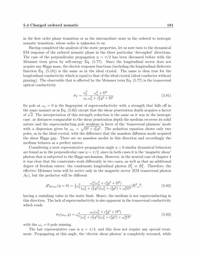
5.4 Charged ordered nematic 181
in the first order phase transition or as the intermediate state in the ordered to isotropicnematic transition, whose order is unknown to us.
Having completed the analysis of the static properties, let us now turn to the dynamicalEM response of the ordered nematic phase in the three particular ‘decoupled’ directions.The case of the perpendicular propagation η = π/2 has been discussed before with theMeissner term given by self-energy Eq. (5.77). Since the longitudinal sector does notacquire any Higgs mass, the electric response functions (including the longitudinal dielectricfunction Eq. (5.18)) is the same as in the ideal crystal. The same is then true for thelongitudinal conductivity which is equal to that of the ideal crystal (ideal conductor withoutpinning). The observable that is affected by the Meissner term Eq. (5.77) is the transversaloptical conductivity
σT =ω2
p
ωn
ω2n + Ω2
ω2n + c2T q
2 + Ω2. (5.81)
Its pole at ωn = 0 is the fingerprint of superconductivity with a strength that falls off inthe same manner as in Eq. (5.62) except that the shear penetration depth acquires a factorof√
2. The interpretation of this strength reduction is the same as it was in the isotropiccase: at distances comparable to the shear penetration depth the medium recovers its solidnature and the superconducting pole weakens in favor of the ‘transversal plasmon’ modewith a dispersion given by ωn =
√Ω2 + c2T q
2. The polariton equation shows only twopoles, as in the ideal crystal, with the difference that the massless diffusion mode acquiredthe shear Higgs gap. There are no massless modes in this direction and accordingly themedium behaves as a perfect mirror.
Considering a next representative propagation angle η = 0 similar dynamical behaviorsare found as in the perpendicular case η = π/2, since in both cases it is the ‘magnetic shear’photon that is subjected to the Higgs mechanism. However, in the neutral case of chapter 4it was clear that the constraints work differently in two cases, as well as that an additionaldegree of freedom enters: the condensate longitudinal photon B
‖L ≡ BL
L . Therefore, theeffective Meissner term will be active only in the magnetic sector (EM transversal photonAT ), but the prefactor will be different
LMeiss.(η = 0) = 12ω2
p
ω2n(ω2
n + c2dq2 + Ω2)
(ω2n + c2T q
2)(ω2n + c2dq
2) + ω2nΩ2
|BT−1|2, (5.82)
having a vanishing value in the static limit. Hence, the medium is not superconducting inthis direction. The lack of superconductivity is also apparent in the transversal conductivitywhich reads
σT (ωn, q) = ω2p
ωn(ω2n + c2dq
2 + Ω2)
(ω2n + c2T q
2)(ω2n + c2dq
2) + ω2nΩ2
, (5.83)
with the ωn = 0 pole missing.The last representative case is η = π/4, and this does not require any special treat-
ment. Propagating at this angle, the ‘electric shear photon’ is completely screened, while

182 Superconductivity in nematic phases
ηπ2
π2−
ω
ωp
Ω
ηπ2
π2−
Figure 5.6: A predicted outcome of an EELS experiment (long but finite wavelength) onthe ordered nematic: a) degenerate plasmon doublet has the dominant signal. The ‘electricshear photon’ is a faint feature, being the strongest at η = ±π/4 and vanishing perpendicularand parallel to the Burgers director. The weak diffusive polariton is visible at the bottom. b)when the low-energy region is zoomed in, the angular dependence of the pole strengths becomesmanifest.
the transversal sector is unaffected. Similar as in the neutral nematic medium, the lon-gitudinal sector for this direction is equivalent to the one of the isotropic nematic phase.Hence, at this specific angle the analysis of the EELS spectrum from the previous sectionapplies. This means nothing else than that the ordered nematic phase should also leave itsfingerprint in the EELS spectrum, except that the strength of the ‘electric shear photon’will be anisotropic, given the fact that the it is not present in the electron energy lossfunction at η = 0, π/2.
Beside the anisotropic ‘electric shear photon’, one should also expect that all dynamicalexcitations of the ordered nematic phase become visible as poles in the electron energy lossspectrum, given the fact that the longitudinal and transversal sector dynamically couple forgeneral values of η. There are in total four such degrees of freedom: two phonon degrees offreedom, the condensate (longitudinal stress photon) degree of freedom and finally the EMtransversal photon (light). In order to illustrate the angular dependence of the excitationpoles in an EELS experiment, we plotted this spectral function in Fig. 5.6 for the caseof the long but finite wavelength regime (q ≈ qe/100) which should be experimentallyaccessible. In a charged medium both phonon degrees of freedom acquire a plasmon gapand a large pole strength. Because electron energy loss spectroscopy probes the longitudinalsector, it has only direct access to the gapped longitudinal (compressional) plasmon at thecenter of discussion in the previous section. The contribution from the transversal plasmon

5.4 Charged ordered nematic 183
exists only when the system is probed in some intermediate direction where the dynamicalcoupling between the two sectors switches on. Given that the longitudinal and transversalplasmon are degenerate in the long-wavelength limit, this contribution cannot be directlyseparated from the direct longitudinal plasmon signal in a real EELS experiment. Thesetwo plasmon poles represent the dominant signal in EELS spectrum, being many orders ofmagnitude stronger than the other poles. Next, there is a contribution from the ‘electricshear photon’ which was the most important feature of the isotropic phase with respectto experiment. This mode is fully visible, as discussed in the previous paragraph, atη = π/4 and loses its strength as the angle deviates from that value. This is due to thefact that longitudinal plasmon couples to the ‘electric’ shear component, which has only afinite, angular dependent, overlap with the Higgs shear stress photon Eq. (4.81). Finally,there is the EM photon which turns into a polariton. From the long-wavelength limit of thedielectric function of the ordered nematic, we conclude that the dispersion of this polaritonis still diffusive
ω ≈ cTλLq2 sin 2η. (5.84)
Thus, it seems as that light couples only to the softened transversal photon (plasmon) inthe same way as it does in the ideal Wigner crystal. Because of the indirect coupling tothe longitudinal plasmon (via the transversal plasmon), the strength of this polariton isthe weakest in the EELS spectrum and it vanishes at the special ‘decoupling’ values of η.Unfortunately, there are fundamental experimental constraints prohibiting the detectingthe polariton pole given by Eq. (5.84). In a spectrum measured in an EELS experiment,the main contribution to the signal comes from the elastic zero-momentum peak. Itsstrength overwhelms all other poles by many orders of magnitude. Although there aremethods developed to subtract this signal, which is innate to the experiment and containsno information whatsoever about the probed system, the minute signal of the polaritonwill be overwhelmed by the noise of the elastic peak. In fact, given that the polariton hasthe weakest pole in the electron energy loss spectrum, and that earlier we argued that eventhe ‘electric shear photon’ is a faint feature, one easily concludes that the polariton wouldbe hard to observe even if one could remove the contributions from the elastic peak.

184 Superconductivity in nematic phases

Chapter 6
Conclusion
In this thesis a theory for electronic crystal melting has been presented, offering somequite surprising outcomes that one might expect to encounter in electron quantum liquidcrystals characterised by fluctuating translational order. Of course, this was not possiblewithout the use of the machinery of the duality where we relied on the notion that ‘orderand disorder are relative matters’. This change in point of view can significantly simplifythe theoretical description of the problem and we use this fact when describing the meltedphase in terms of the dual theory developed initially by Kleinert [48]. The dual theory ofmelting of a bosonic quantum crystal is developed in this way and new liquid crystallinephases are identified. A surprise that follows is that the dual theory, being tailored to treatthe melted phase as the ordered phase, yields the bare Meissner term Eq. (5.34) for thecharged quantum liquid. Hence, this dual point of view does us yet another favour: thesuperconductivity comes for free and the normal metallic phase is viewed as a the one wherethe dual order, represented by the bare Meissner term, is destroyed by the fluctuations ofthe long-ranged dual stress fields.
The phase that we are a particularly interested in is the quantum nematic phase,characterized by the proliferation and condensation of dislocations, while disclinations arestill massive. This phase, having the character of a liquid crystalline phase due to thepresence of a partial order, is in between the ideal crystal (fully crystalline ordered phase)and superfluid phase (fully disordered). Accordingly, its properties are a mix of those ofboth worlds, showing massive shear and long-ranged compression at large length scaleswhile the crystalline rigidities are recovering at short distances. The surprise is that underthese circumstances a new propagating mode appears: the dual shear photon characterizedby a Higgs mass expressing that at long distances shear rigidity has disappeared, while itresurfaces at shorter distances. This photon actually reflects the phase degree of freedomof the dual dislocation Bose condensate.
When the medium is also electric charged the theory predicts that the nematic phaseturns into a true superconductor, which is not so hard to understand being aware the work-ings of the dual shear superconductor. However, the electromagnetic response functionsof such a superconductor are now full of surprises. In contrast with the standard BCStheory, where the superconductivity arises as a ramification of the long-range off-diagonal
185

186 Conclusion
order of the constituent ‘gaseous’ bosons (Cooper pairs), the mechanism responsible forthe superconductivity in the nematic charged phases is entirely different. The superfluidis, by means of the dual theory, the ordered state. It is characterized exclusively by com-pressional rigidity and it has to be an electromagnetic superconductor as well because ofthe well-known Wen-Zee theorem [159, 160, 161]. The nematic state is characterized bycrystalline order at short distance. Nevertheless this order is transient and as such it can-not destroy the electromagnetic Meissner term. Because the transient order is present onlyat finite length- and time scales, all of its consequences on the Meissner term are apparentin the various response functions only at finite wavelengths and frequencies.
In this way, our theory for the electronic liquid crystalline states yields predictionswhich can be tested experimentally, although they require unconventional experiments.In principle, this amounts to a strategy to determine once and for ever if the notionsof fluctuating order do apply to e.g. high-Tc superconductivity. The feature that we findmost promising in this regard is the novel ‘electric shear photon’ pole in the electron energyloss function and at this moment some experimental groups have already undertaken firststeps to devise experiments that can probe the finite-wavelength regime and detect thepole’s weak signal. Other response functions like the optical (transversal) conductivity alsofeature excitations which are not of the kind found in conventional BCS superconductors.However, the existing experimental techniques are even more limited that EELS withregard to probing the relevant kinematical regimes. The transient order characterizingcharged quantum liquid crystals also leaves its imprint through the static overscreeningeffects of electric and magnetic fields. Unfortunately, existing experimental techniques aredesigned to measure only the standard BCS London length and it would be interesting tosee if experiments can be designed to search for the overscreening effects.
It would be unfair to not give the full credit to the pioneering work of Zaanen, Mukhinand Nussinov [44], where these ideas were employed for the first time. The theory pre-sented here, should be seen as a follow up, removed a flaw associated with the dynamical(relativistic) treatment of the dislocation condensate. Apart from encountering a problemassociated with the topological phase and identification of a new isotropic phase, we alsodid investigate the entire spectrum of EM properties of a charged liquid crystal. Somewhatas a sideline, we obtained results eventually of relevance to the construction of the dualtheory in general. We refer to the interpretational issues associated with the dual gaugedegrees of freedom as presented in section 2.3 and the glide principle derived in section3.4. The former result clarifies the appearance of the additional degrees of freedom in thenematic phases and reveals the hidden connection between the dual shear photons andthe dislocation degrees of freedom. The latter is a necessity for the understanding of theprotection of the compressional properties of the superfluid.
Given the new theoretical results presented in this thesis, it is now up to the experimen-talists to develop new experimental techniques, to measure the signatures of fluctuatingorder. One can wonder if our theoretical program is now completed or if there are stillloose ends that need further attention. In our opinion, there are still a number of unre-solved problems. One which does not require additional computations is related to theinterpretation of the excitation spectra in the nematic and charged media. We are partic-

187
ularly puzzled about the presence of the diffusive poles, as found in the ordered nematic(Eq. (4.93)), as well as in the polariton spectrum of both the ideal crystal (Eq. (5.15)) andthe ordered nematic (Eq. (5.84)). Although we presented some arguments referring to theloss of rigidity and second-order processes that could cause this diffusion, we find thoseexplanations unsatisfactory and we would like to understand better what is the precisephysical interpretation of these diffusive excitations. The other problem is more serious asit is related to the inconsistency encountered in the construction of the topological nematicstate when the dual condensate is treated in its full relativistic glory. In section 4.6, the‘inconsistent’ results previously obtained in section 4.5 were interpreted using a differentdisordering field. At that point we had to satisfy ourselves with the fact that we couldexplain only the isotropic nematic phase which, although showing quite unconventionalfeatures, is only a non-interacting approximation (in the Burgers sector) to the topologicalnematic phase. If the argument is correct, it implies that one needs to take into accountthe interactions coming from the expansion of the action Eq. (4.117). There is an openissue regarding the method one should use to treat these interaction effects. Apparently,the completely different mode content of the topological- and isotropic phase suggests thata perturbational approach might not work, although in principle it is possible that themode content changes if the theory is excluded the Gaussian approximation.
All other issues may be considered as extensions of the original theory. One further gen-eralization of the theory is to consider a less symmetric elasticity tensor than the isotropicone, Eq. (3.15), that we used throughout the thesis. Another possible extension is as-sociated with the treating of the second-order gradient elasticity (Eq. (3.19)). However,after the hard work of the dualization and construction of the disorder theory has beenaccomplished, these generalization turn into a complicated but straightforward. In fact, wehave some preliminary results where second-order gradient elasticity is included. However,because the dualization formalism for second-order gradient theories (see Ref. [48]) wouldrequire yet another chapter additional chapter to present, we decided to omit it. Let usjust mention unexpected outcome that the additional terms in the elastic energy do notaffect the shear Higgs mechanism, so that the phonon self-energies corresponding to thepropagators Eq. (4.110) and (4.112) are still valid.
A different matter is the addressing of the fundamental limitations we had to imposeonto our theory, which requires some further deep thoughts. These include the nontrivialstatistics of the crystal constituents, the dimensionality of the medium and the issue ofnon-topological (interstitial) as well as the non-Abelian topological defects (disclinations).Most of these problems are actually ‘holy grails’ of modern physics with deep fundamentalimplications. Despite the lacking of a general formalism required to treat fermionic- oreven anyonic crystals, we might still be able to speculate that in a medium melted byfermionic/anyonic dislocations the loss of shear rigidity is inevitable, resulting in a similarlong-wavelength description as for the bosonic case, although the shear photon mighthave a different meaning, being associated with a dynamical Fermi- or anyon dislocationgas. Although we could leave the dimensionality issue related to the construction of asecond-quantized theory of strings, to string theorists, we suspect that the Abelian-Higgsduality might be employed the other way round. In this manner, the condensation of

188 Conclusion
strings might be understood in terms of a type-II superconducting transition in higherdimensions, which could shed some light on this fundamental problem. The disorder fieldfor disclinations, which is highly nontrivial because of its non-Abelian nature, is in a waysimilar to the problem of treating fermionic dislocations. However, due to their particulargeometrical Berry phases associated with disclinations, it appears that the mathematicalidea of quantum double symmetry groups has a real potential to make substantial progresson this deep problem. On the other hand, it appears that the treatment of non-topologicaldefects in the theory (vacancies and interstitials), is a task which is relatively easy toaccomplish. One should bear in mind that an interstitial is not just a bound pair of adislocation and an antidislocation. These defects have the meaning of the classical wavefunction Ψcl.
0 amplitude fluctuations in a filed theoretical description and it appears that aproper theory may be constructed using the knowledge of type-I superconductivity.
To conclude, let us mention a number of other interesting questions related to the dualtheory of elasticity. One is concerned with the critical regime near the phase transitions inanalogy with the Abelian-Higgs duality critical regime discussed in the section 2.4. Thereis still a number of open questions. The critical exponents that were used in section 2.4were found for the case of a fully relativistic theory [63, 91]. The elastic action Eq. (3.24)does not satisfy this symmetry requirement and this can change the universality classof the transition and, accordingly, the values of the critical exponents. There is also anissue regarding the order of the transition: our theory with the disorder action Eq. (4.32)implicitly assumes that the transition from the ideal crystal to the nematic phase is ofsecond order which is necessary in order to find a critical regime. The transition from theclassical crystal to the nematic liquid crystal state is, however, of the first order, and thesame is true for the transition from a normal state to the isotropic EM superconductor.We believe that the definite answer to these questions follows from the theory when theinterstitial degrees of freedom are taken into account. This opens up a possibility that anew phase could emerge between the ideal crystal and the nematic phase.
The last important feature of the quantum nematic pertains to the problem of gravity.When we introduced elasticity in the introduction of chapter 3, we mentioned that thecurvature and torsion induced by the elastic deformations and the topological defects canalternatively be treated using the language of differential geometry. There is no torsion inour universe and in an earlier work [146] it was demonstrated that in 2+1D the universecan be seen as a nematic phase of a ‘world-crystal’ which has lost its torsion through theproliferation of dislocations. The 3+1D version of this problem could possibly result inan theory for emerging gravity. As a curiosity, the transformational properties of sheardegrees of freedom and gravitons match, because they are both spin-2 objects. Thereare, however, five shear degrees of freedom in an ideal crystal compared to two gravitons.Hence, the phase transition from the ideal ‘world crystal’ to the nematic ‘world’ phaseshould generate a Higgs mass for compression- and the three shear photons. This leavesus with two other shear photons having the highest helicity which should stay massless:these can be gravitons.

Appendix A
Mapping of a nonlocal interaction toΨ4 term
In chapter 2, we presented a mapping of action for a gas of random walkers onto theGLW action Eq. (2.35). The proof yielded quadratic contributions to the action in thelong-wavelength limit, and Ψ4 term was added ‘by hand’, corresponding to short-rangeinteraction between the particles. Then we promised to return to that issue in this ap-pendix where mapping of inter-particle interactions onto the Ψ4 term of action Eq. (2.35)is demonstrated. The exact proof presented here is, however, based on a different map-ping [49] and cannot be directly utilized for the description of the dislocation tangle. Thiswill become clear after the details are presented and we will discuss the differences inthe conclusion of this appendix. There are nevertheless two reasons that we include themapping in the form presented in this appendix. First, it illustrates the origin of the Ψ4
term in Eq. (2.35) in a setup that is only slightly different from ours. Another reasonis that the mapping, as presented by Kiometzis et al. [75], takes only local (short-range)interactions into account. The mapping given in this appendix uses the same idea as inRef. [75]. However, we manage to incorporate any kind of potential, local or nonlocal,between the particles, which then acquires a corresponding Ψ4-like term in Eq. (2.35). Tothe best of our knowledge, such a mapping, although a simple generalization of Ref. [75],has not been presented elsewhere. For us, it is of importance to stress that this mappingof arbitrary particle interactions can be further generalized to the case with a multitudeof different particles. In this manner, the interaction term in Eq. (4.120) can be linked tothe interaction between dislocations of different Burgers charges.
For the readers convenience we begin by repeating the ‘non-interacting’ part of themapping as given in Ref. [75]. The only difference here is that the mapping can be gener-alized to an arbitrary dimension with the minute change of a single factor in the partitionfunction. While the first part starts with the GLW complex theory and ends with a gasof free particles, the second part of the mapping, which incorporates the interaction, isperformed ‘backwards’. The interaction is added to the particle action, and, by means ofa Hubbard-Stratanovich auxiliary field, ‘pulled’ through the mapping so that it appearsas a Ψ4 term in the complex field theory. At the end of the appendix, a brief discussion
189

190 Mapping of a nonlocal interaction to Ψ4 term
regarding the differences between this mapping and that from chapter 2 is given.Let us begin with the Hamiltonian of a free complex field theory
H = 12
∫ddx
(|∇Ψ|2 +m2|Ψ|2
). (A.1)
This derivation is done for continuum theories, for discussions about the lattice derivationwe refer the reader to Refs. [60, 176, 177]. The correlation function defined by HamiltonianEq. (A.1) is explicitly given by
G(x) =
∫ddq
(2π)d
eiq·x
q2 +m2. (A.2)
This is written in the Schwinger proper-time representation [178] as an integral over theproper time s
G(x) =
∫ ∞
0
ds e−sm2
∫ddq
(2π)deiq·xe−sq2
=
∫ ∞
0
ds e−sm2
Γd s−d/2 e−
14x2/s, (A.3)
where we used the identity
1
a=
∫ ∞
0
ds e−sa. (A.4)
The factor Γd is a constant which depends only on the number of dimensions d in theproblem, and it follows after the momentum q has been integrated out. For example,Γ2 = 1/(4π) and Γ3 = 1/(8π3/2).
The right-hand side of Eq. (A.3) describes diffusion of a particle of mass 1/2, i.e. itrepresents a sum over all real space paths starting at x(s′ = 0) = 0 and ending at x(s′ =s) = x [179]
Γd s−d/2 e−
14x2/s =
∫ x(s′=s)=x
x(s′=0)=0
Dx(s′) e−S[x(s′),x(s′)], (A.5)
with ‘free’ action
S[x, x] = 14
∫ s
0
ds′ (x(s′))2. (A.6)
The additional Boltzmann factor exp(−sm2) exponentially suppresses loops with largeproper-time.
Having identified the Green’s function Eq. (A.2) with the diffusion problem Eq. (A.5),we may proceed to the partition function corresponding to Hamiltonian Eq. (A.1). Let usfirst integrate identity Eq. (A.4) to obtain
ln a = −∫ ∞
0
ds
se−sa + const. (A.7)
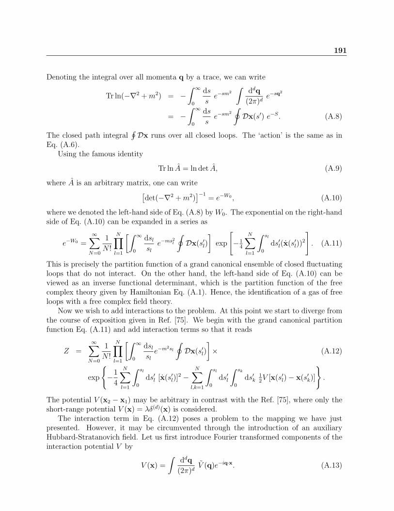
191
Denoting the integral over all momenta q by a trace, we can write
Tr ln(−∇2 +m2) = −∫ ∞
0
ds
se−sm2
∫ddq
(2π)de−sq2
= −∫ ∞
0
ds
se−sm2
∮Dx(s′) e−S. (A.8)
The closed path integral∮Dx runs over all closed loops. The ‘action’ is the same as in
Eq. (A.6).Using the famous identity
Tr ln A = ln det A, (A.9)
where A is an arbitrary matrix, one can write[det(−∇2 +m2)
]−1= e−W0 , (A.10)
where we denoted the left-hand side of Eq. (A.8) by W0. The exponential on the right-handside of Eq. (A.10) can be expanded in a series as
e−W0 =∞∑
N=0
1
N !
N∏l=1
[∫ ∞
0
dsl
sl
e−ms2l
∮Dx(s′l)
]exp
[−1
4
N∑l=1
∫ sl
0
ds′l(x(s′l))2
]. (A.11)
This is precisely the partition function of a grand canonical ensemble of closed fluctuatingloops that do not interact. On the other hand, the left-hand side of Eq. (A.10) can beviewed as an inverse functional determinant, which is the partition function of the freecomplex theory given by Hamiltonian Eq. (A.1). Hence, the identification of a gas of freeloops with a free complex field theory.
Now we wish to add interactions to the problem. At this point we start to diverge fromthe course of exposition given in Ref. [75]. We begin with the grand canonical partitionfunction Eq. (A.11) and add interaction terms so that it reads
Z =∞∑
N=0
1
N !
N∏l=1
[∫ ∞
0
dsl
sl
e−m2sl
∮Dx(s′l)
]× (A.12)
exp
−1
4
N∑l=1
∫ sl
0
ds′l [x(s′l)]2 −
N∑l,k=1
∫ sl
0
ds′l
∫ sk
0
ds′k12V [x(s′l)− x(s′k)]
.
The potential V (x2 − x1) may be arbitrary in contrast with the Ref. [75], where only theshort-range potential V (x) = λδ(d)(x) is considered.
The interaction term in Eq. (A.12) poses a problem to the mapping we have justpresented. However, it may be circumvented through the introduction of an auxiliaryHubbard-Stratanovich field. Let us first introduce Fourier transformed components of theinteraction potential V by
V (x) =
∫ddq
(2π)dV (q)e−iq·x. (A.13)

192 Mapping of a nonlocal interaction to Ψ4 term
The last term in the exponential in Eq. (A.12) becomes
N∑l,k=1
∫ sl
0
ds′l
∫ sk
0
ds′k
∫ddq
(2π)d12V (q)e−iq·[x(s′l)−x(s′k)]. (A.14)
Now, the auxiliary field σq is brought into the action via the identity∫Dσq exp
[−∫
ddq
(2π)dσ−q
1
2V (q)σq + i
∫ddq
(2π)d
∫ s
0
ds′σ−qeiq·x(s′)
]=
∏q
√2πV (q)× exp
[−1
2
∫dq
(2π)3
∫ s
0
ds′∫ s
0
ds′′ V (q)eiq·[x(s′)−x(s′′)]
]. (A.15)
The normalization constant (Jacobian of the HS transformation) comes from the Gaussianintegrations and it will be cancelled at the end of the procedure.
The partition function Eq. (A.12) is rewritten, with help of Eq. (A.15), as
Z =∏q
1√2πV (q)
∫Dσq exp
[−∫
ddq
(2π)dσ−q
1
2V (q)σq
]× (A.16)
∞∑N=0
1
N !
N∏l=1
[∫ ∞
0
dsl
sl
e−m2sl
∮Dx(s′l)
]exp
−
N∑l=1
∫ sl
0
ds′l
[1
4[x(s′l)]
2 − iσ[x(s′l)]
],
where σ[x] represents the auxiliary field in real-space coordinates. After this step weresort to the relation between the inverse functional determinant and the loop gas partitionfunction Eq. (A.10) and Eq. (A.11). The only difference with respect to the non-interactingcase is that now we have an additional auxiliary field which enters the complex field action
Z =∏q
1√2πV (q)
∫Dσq
[det(−∇2 +m2 − iσ)
]−1 ×
exp
[−∫
ddq
(2π)d
σ−qσq
2V (q)
]. (A.17)
The auxiliary field served the purpose of ‘smuggling’ the potential V through the mappingand now it can be integrated out. Together with the undesired Jacobian, this produces theΨ4 term in the following way∏
q
1√2πV (q)
∫Dσq exp
[−∫
dq
(2π)d
σ−qσq
2V (q)+ i
∫dx |Ψ(x)|2σ[x]
]
=∏q
1√2πV (q)
∫Dσq exp
[−∫
dq
(2π)d
(σ−qσq
2V (q)+ iσq
∫dx |Ψ(x)|2e−iq·x
)]
]
→ exp
−1
2
∫dxdx′ |Ψ(x)|2
[∫dq
(2π)dV (q)eiq·(x−x′)
]|Ψ(x′)|2
(A.18)
= exp
−1
2
∫dxdx′ |Ψ(x)|2V (x− x′)|Ψ(x′)|2
.

193
Hence, the interaction between two loop segments maps onto Ψ4 term so that the totalcomplex field action reads
SGLW = 12
∫ddx
[|∇xΨ(x)|2 +m2|Ψ(x)|2 +
∫ddx′|Ψ(x)|2V (x− x′)|Ψ(x′)|2
], (A.19)
and this completes our derivation.There is one technical detail we overlooked and now we return to it. Namely, the
original proof of Ref. [75] considered the delta-function interaction for which all the Fouriercoefficients are non-zero. On the other hand, a general potential V (x) that we wish tomap may exhibit a vanishing Fourier coefficient for an arbitrary value of moment q whichcompromises the Hubbard-Stratanovich identity Eq. (A.15). This problem is dealt with in away similar to the implementation of the Ehrenfest constraint. This should not be a surprisegiven the fact that the duality presented in this thesis was a kind of Hubbard-Stratanovichtransformation. What one should do in order to avoid the ‘singularity’ problem associatedwith the vanishing Fourier components V (q) = 0 is to separate the momenta with zeroFourier components from the momenta with finite components. The latter can safelyundergo the described treatment, while the components related to the former are absentin the course of mapping. In other words, one can assume that a constraint σq ≡ 0 isimposed for each q with vanishing Fourier component of the interaction. In the last stepin Eq. (A.18), the missing momenta do not contribute to the real-space potential V (x) asshould be the case, and the original interaction potential is recovered.
Let us now mention the reason we cannot directly utilize the mapping presented in thisappendix for the purpose of describing a tangle of defects (vortices or dislocations). It turnsout, despite the fact that both describe a gas of loops, that the grand canonical ensembleof loops, with its partition function Eq. (A.11), has a different phase space as comparedto the path integral Eq. (2.31). While in the original proof each loop is counted just onceand weighted according to its length Eq. (2.19), the path integral in this appendix has aredundant counting, since each loop can be parameterized by the Schwinger proper-timein infinitely many ways. Each parameterization has a different weight as implied by actionEq. (A.6). At the moment we are not aware if there is a relation that would link the weightobtained in that way to the weight given by the loop action Eq. (2.19), and hence we areforced to use the mapping of section 2.2.

194 Mapping of a nonlocal interaction to Ψ4 term

Appendix B
Defect current conservation laws
When the dislocation and disclination conservation laws Eq. (3.50 - 3.51) were presented,we had to resort to the identity Eq. (2.101) in order to derive these laws. There is yetanother proof based on the connection between elasticity and differential geometry [48].and gravity [123, 124, 125]. The disclination current conservation law obtained in thismanner is published as part of the article on the glide constraint [50]. Deep inside, theassumptions of this proof are not any different from those behind the identity Eq. (2.101).Nevertheless, this proof appears more ‘elegant’ due to its origins.
The dynamical version of the disclination conservation law can be traced back to thematerial conservation. As an example consider a wedge disclination: the material addedis proportional to the Frank vector (scalar in 2+1D) and it should not change over time.In this respect the disclination conservation law may be regarded as a generalization ofthe glide constraint for the general topological defects. The basic idea is that after theVolterra cutting procedure has been applied, no additional material should be introduced,which is the same as the requirement that all symmetrized strains and derivatives thereofare smooth everywhere, including the locus of the Volterra cut. This condition is hardwired into the proof of the generalized Weingarten theorem Eq. (3.44). As we will nowshow, the ramification of this principle for disclinations is a conservation law.
To make headway, it is convenient to first consider Euclidean Lorentz-invariant D + 1space time. The non-relativistic case will turn out to be a special case which directlyfollows from imposing the condition of the absence of time like displacements (uτ = 0).What follows rests heavily on elastic analogs of identities in differential geometry which arediscussed in detail in the last part of Kleinert’s book [48]. First, we introduce the tensor
Rµν,ρσ = (∂µ∂ν − ∂ν∂µ)∂ρuσ (B.1)
representing the Riemann-Christoffel curvature tensor in the geometrical formulation ofthe theory of elasticity (the u’s are the usual displacements). The smoothness assumptionsunderlying the Weingarten theorem may be expressed as,
0 = (∂µ∂ν − ∂ν∂µ)(∂ρuσ + ∂σu
ρ), (B.2)
0 = (∂µ∂ν − ∂ν∂µ)∂λ(∂ρuσ + ∂σu
ρ), (B.3)
195

196 Defect current conservation laws
which in turn imply smoothness of the displacement second derivative
0 = (∂µ∂ν − ∂ν∂µ)∂λ∂ρuσ. (B.4)
Cycling through the indices µ, ν, and λ of the smoothness equation Eq. (B.4), we obtainthe Bianchi identity for the displacement fields [180],
∂µRνλ,ρσ + ∂νRλµ,ρσ + ∂λRµν,ρσ = 0. (B.5)
Starting from the other end, let us analyze a candidate for a disclination conservationlaw, corresponding to ∂µT
α1α2...αD−1µν1ν2...νD−2 . This can be expressed in terms of the Riemann
tensor where α refers to a string of indices labeled by α,
∂µTα
µν = 12εµνκλεαρσ∂µ∂κ∂λ∂ρu
σ
= 12εµνκλεαρσ∂µ(∂κ∂λ − ∂λ∂κ + ∂λ∂κ)∂ρu
σ
= 12εµνκλεαρσ∂µRκλ,ρσ − ∂µT
αµν . (B.6)
The first term is zero as a consequence of the contraction of the Bianchi identityEq. (B.5) and the Levi-Civita symbol εµνκλ. This implies that relativistic disclinationcurrents are conserved. The non-relativistic case is just a special case: the vanishing oftime like displacements means that all upper labels are space-like (α→ a) and it follows,
∂µTa1a2...aD−2
µν1ν2...νD−2= 0. (B.7)
Let us now try to envisage the physical consequences of this dynamical conservation law.In 2+1D, only wedge dislocations exist and the message of the conservation law Eq. (B.7)is clear: the Frank charge – the angle of an inserted wedge in the Volterra construction –behaves as a trivially conserved scalar component of a tensor. In higher dimensions, thedisclination current similarly behaves as a conserved tensorial current. The defect densityhas information regarding both dislocations and disclinations. The disclination conser-vation law has separate ramifications for the defect density. The fundamental conditionEq. (B.4) can be directly rewritten into a conservation law for the defect density of a similarform as for the disclinations,
∂µηα1α2...αD−1µν1...νD−2
= 0. (B.8)
This is not surprising as defect currents are proportional to to disclination currents.Together with the glide constraint, this completes the picture: the conservation of
matter mandates that the ‘proper’ disclinations currents are also conserved. However,the ‘handicapped’ dislocation currents are not conserved a-priori (disclinations form theirsources) but they have to pay the price that they can only glide.

Appendix C
Irreducible tensors of the symmetrygroup
The idea that one can make important statements about a system by mere analysis ofsymmetries is often attributed to Landau. In this very last part of the thesis we utilizethis idea. By representing the field components of the physically relevant tensors (strains,stresses, dislocation currents and dual stress gauge fields) as irreducible tensors of thesymmetry group in the problem, we can interpret these and give each component a precisephysical meaning. The symmetry considerations presented here are simplified in the sensethat they exclude the translational symmetries of the model. As it turns out, the rotationaldegrees of freedom combined with space and time reflections are sufficient for our needs andat the end of the section the specific degrees of freedom, be it strains, stresses, dual stressgauge fields or the defect currents, mentioned in the main part of the thesis, are associatedwith different irreducible representations of the symmetry group. The physical degrees offreedom, on the other hand, also have certain transformation properties and matching thesewith the properties of the (dual) degrees of freedom leads to the proper interpretation. Asthe example already encountered in the thesis, recall the glide constraint Eq. (3.61) and itsrelation to the compression. The compression is invariant under all possible (point group)transformations. The same is true for the glide constrained component of the dynamicaldislocation currents. As a result, the suppression of the climb in the system is uniquelyassociated with the compressional rigidity. In the same manner, other degrees of freedomcan be traced to their physical origins.
Let us start with the group of symmetries that the elastic action Eq. (3.24) has toobey. The Euclidian group E(2) is broken down to the product of the group of discretelattice translations and the point group of the lattice. Since we are after the minimalmodel that is supposed to associate degrees of freedom with the irreducible representationsof the symmetry group, the translations will be neglected in this short exposition. Weconcentrate on rotations, i.e. the point group which is in general determined throughthe symmetry group of the underlying crystalline lattice. Given the fact that the theorypresented in this thesis is developed for the exclusive case of the isotropic elastic tensorEq. (3.15) (although the generalization to an arbitrary tensor Cijab is straightforward),
197

198 Irreducible tensors of the symmetry group
the point group symmetry explicitly analysed in this appendix will be the group of all(proper) rotations in two dimensions, denoted as C∞. This group does not exhaust all thesymmetries of the crystalline lattice, in addition there is the spatial reflection symmetryσv which, together with proper rotations forms the group C∞v. Finally, we should add thetime-inversion symmetry στ to cover the dynamics introduced in our action through termEq. (3.23). The total point symmetry group is then C∞vh.
The next step is to determine the action of these symmetries on the single componentvectors in the system, that is to find the vector representations of the symmetry group.Recalling from undergraduate physics courses in mechanics [167] as well as electromag-netism [165, 166], one should note that the space- and time-inversions act differently ondifferent kinds of vectors. For example, the radius-vector r perpendicular to the reflectionaxis, changes its orientation under the spatial reflection. The same is true for the force F.On the other hand, their cross-product is the torque vector which is invariant under thesame reflections. We shall refer to the former as polar-vectors, whereas the latter will becalled axial-vectors. The same pattern is followed by the time-inversion symmetry: whilethe radius vector r does not change under time-inversions, its first derivative, the velocityfield, does. In order to draw the line between the two sorts, the former will be called true-and the later pseudo-vectors. Accordingly, there are four classes of vectors: true-polar-,true-axial-, pseudo-polar- and pseudo-axial-vectors. The examples are respectively radiusvector, angular momentum, velocity and angular velocity. Let us add that in most of thecases, a distinction is not made between the spatial- and time-inversion with words ‘axial’and ‘pseudo’ identified. We stress however the difference between the two symmetries.
Scalars exhibit different transformation properties, in the same manner as vectors. Thesame is true for tensors with more indices. It is even possible for a tensor to have differentindices transforming differently under the same inversion. This will be the case, for exam-ple, when we analyse the dislocation currents. Let us just add that (proper) rotations arealways represented in the same way independently from the type of scalar/vector/tensor.Therefore, the representations of the symmetry group will be determined by simple groupmultiplication of a proper rotation and the appropriate representations for the symmetries.
Although not of direct interest for our problem, we may begin with scalars. A scalaris invariant under proper rotations, i.e. Dsc.[T |P ][P |A](Rα) ≡ 1. The first choice of letters Tand P stands for ‘true’ and ‘pseudo’, and the second letter can be P or A if the scalar isof ‘polar’ or ‘axial’ type. The space- and -time-reflections are represented in the followingway:
Dsc.TP (σv) = 1, Dsc.TP (στ ) = 1, (C.1)
Dsc.TA(σv) = −1, Dsc.TP (στ ) = 1, (C.2)
Dsc.PP (σv) = 1, Dsc.TP (στ ) = −1, (C.3)
Dsc.PA(σv) = −1, Dsc.TP (στ ) = −1. (C.4)
If the scalar representations sounded boring because we could not apply them to theproblems we presented in this thesis, now we turn to vectorial representation and theirproducts, and as a first example, the strain field is decomposed into physically relevant

199
components. Let us suppose that a two-dimensional vector is represented by a column oflength two (i.e. (ax, ay)
T ), and the 2+1-dimensional vector by a column with the first twoelements corresponding to the spatial indices and the third one to the temporal index (i.e.(ux, uy, uτ )
T ). A proper 2D-rotation is represented by the matrix
D[R(α)] =
cosα − sinα 0sinα cosα 0
0 0 1
, (C.5)
when acting on a three-vector. The two-dimensional (spatial) representation D, neededfor ‘flavour’ representations is given by simple erasing of the last column/row. We alsoneed to know how to represent reflections. The temporal inversion is represented by aunit matrix for representations of true-vectors and by a negative unit matrix for pseudo-vector representations. When defining spatial reflection representation, a certain axis hasto be chosen, say x, to serve as the reflection axis. Then, the polar-vectors transformaccording to DP [σv] = diag(−1, 1, 1), and axial-vectors according to the unit matrix. Ofcourse, the two-dimensional representation is again obtained by taking only the first twocolumns/rows.
For our first example, the strain field, we also need to determine the representationaccording to which the derivatives transform. This is a standard exercise in the generalrelativity which we repeat here. Begin with
∂
∂x′µ=∂xν
∂x′µ∂
∂xν. (C.6)
Then, express the old coordinate as xν = [D−1]νµx′µ and use the unitarity of the repre-
sentation [D−1]νµ = D νµ , to find that the derivative transforms under the representation
DT which is obtained by transposing representation D. Here and later in the text, unlessstated otherwise, the plain letter D represents the representation under which the coordi-nates transform. That is the true-polar representation for spatial indices and pseudo-polarfor the temporal index.
Knowing that the displacements transform the same way as a radial vector, that is as atrue-polar-vector, we find that the strain transforms under the product of representations
∂µ′ua′ = [DT ⊗D]µa′
µ′a∂µua. (C.7)
This composite representation is decomposed into the Clebsch-Gordon series of the irre-ducible representations of the group of symmetries [181]. In the case of the C∞vh group,the series read
D ⊗D = A+0 +B+
0 + E−1 + E+
2 . (C.8)
Let us first clarify the sub- and super-scripts of the representations. The subscript indi-cates the ‘spin’ of the representation. The super-scripts tell us whether the representation isinvariant under the temporal reflection or not (+ means it is invariant). A0 is the represen-tation invariant under rotations (spin-0), and also under spatial reflection, differently from

200 Irreducible tensors of the symmetry group
B0 (also spin-0) that changes sign under σv. The spinful (two-dimensional) representationsEm always see the spatial inversion as a conjugation. A proper rotation is represented aseimατz
with τ z being the Pauli matrix. The representation properties will help us identifystrains components.
Through projection operators [181], the eigenvectors (irreducible representation vec-tors) are found:
|A+0 〉 = ∂xu
x + ∂yuy = ∂iu
i, (C.9)
|B+0 〉 = ∂xu
y − ∂xuy = εij∂iu
j, (C.10)
|E−1 ,±〉 =
1√2
(∂τux ± i∂τu
y) = ∂τu±, (C.11)
|E+2 ,±〉 = 1
2(∂xu
x − ∂yuy)± i
2(∂xu
y + ∂xuy) = ∂∓u
±. (C.12)
Note that the first two strains can also be expressed in holomorphic (±) coordinates as∂+u
+ ± ∂−u−. Now we turn to the physical interpretation. The |A+
0 〉 is clearly the com-pression strain. It is invariant to all the transformations of the symmetry group. The nextis the rotation strain |B+
0 〉 which sees only the spatial inversion. The spin-1 doublet |E−±1〉
consists of two velocities written in holomorphic fashion. These velocities change signunder the time reflection and acquire phase e±iα upon rotation. Spin two strains |E+
±2〉represent shear, and in this notation these may be viewed as a helical composition of theelectric and magnetic shear.
Let us add for curiosity that these strains can be related to the vibrational degrees offreedom on a triangular lattice through the same analysis of the irreducible representa-tions, now of the group C3vh. The equivalence of the two is the reason behind the simple(isotropic) elastic tensor found in two-dimensional triangular lattice. Already in three spa-tial dimensions, the irreducible representations of the group of rotations O(3) differ fromthe irreducible representations associated with the vibrations of the simplest diamond lat-tice, which leads to the anisotropic elastic tensor as measured quite some time ago [182].Talking about the vibrational microscopic degrees of freedom, we may also mention a simi-lar classification of strains by Ahn et al. [183]. Their work is, however, focused on a squarelattice which makes space for additional degrees of freedom.
After this interesting ‘dissection’ of the strain degrees of freedom we may find its impli-cations on the form of the isotropic elastic tensor. When two irreducible tensor componentsare multiplied, their spins add up, while their parities (under each reflection separately)multiply. Since the only allowed terms in action must be invariant under all elements ofthe group representation, the only admitted terms must have total spin zero and containan even number of ‘pseudo’ and an even number of ‘axial’ components. In the case of thelinear elasticity, the most general action allowed by the C∞vh symmetry group has form
Linv =1
2
[KA(∂iui)
2 +KB(εij∂iuj)2 +K1∂τu
+∂τu− +K2∂−u
+∂+u−] . (C.13)
The coefficient KA is clearly the compression modulus κ. K2 is the shear modulus µ and K1
is the mass density ρ. This simplified approach cannot rule out the term with KB. This is

201
a consequence of the fact that we use only linear (matrix multiplicative) representations inour approach whereas the true physical rotation, in addition, shifts the local rotation fieldby a constant. The same form of the linear elastic energy as that of Eq. (C.13) could havealternatively been obtained by demanding that only singlet components of the elasticitytensor Eq. (3.9) may appear in the action.
Given the fact that stress fields transform under the same representation as strain(Eq. (C.7)), everything said for the strains from the symmetry point of view, applies alsoto the stresses. There are compressional (σa
a), rotational (εabσba) and two shear stresses
of spin-2 which were identified earlier in Eq. (4.79). The kinetic momenta densities formspin-1 stress fields σ±τ . Notice that the Ehrenfest constraint has a precise meaning in termsof the symmetry: the stress component sensitive to the spatial reflection is not allowed. Inanalogy with the action Eq. (C.13) one can construct the minimal dual stress action allowedby symmetry. Contrasting its constants with the ‘inverse’ elasticity tensor it readily followsthat Kσ
A = 1/(4κ), Kσ2 = 1/(4µ) and Kσ
1 = 1/ρ, illustrating how each coupling constantremains ‘confined’ to its own symmetry sector even after the dualization.
Finally, we arrive at most important and most interesting part of this appendix, theirreducible components of the dislocation currents. By identifying these, the appropriategauge degrees of freedom are automatically recovered. One should, however, be carefulsince gauge fields do not have direct physical meaning and can be shifted by an arbitrarygauge transformation. Nevertheless, the experience from the chapter 4 taught us that aftera definite gauge fixing has been chosen, one can correspond the dual stress gauge degreesof freedom with the physical degrees of freedom such as compression and shear.
We denote that repersentation with DJ so that we have
Ja′
µ′ = [DJ ]a′a
µ′µJaµ . (C.14)
The left-hand side can be expressed in the original strains
Ja′
µ′ = εµ′ν′ρ′∂ν′∂ρ′ua′ = εµ′ν′ρ′D
Tν′νD
Tρ′ρD
a′a∂ν∂ρua, (C.15)
as well as the right-hand side
[DJ ]a′a
µ′µJaµ = [DJ ]a
′aµ′µεµνρ∂ν∂ρu
a. (C.16)
The identity that follows is contracted with tensor ελνρ to find
[DJ ]a′a
µ′µ =1
2εµ′ν′ρ′εµνρD
Tν′νD
Tρ′ρD
a′a. (C.17)
This representation is decomposed into the Clebsch-Gordan series
DJ = A−0 +B−
0 + E+1 + E−
2 , (C.18)
which show one interesting difference compared to Eq. (C.8): the time-reflection status ishere inverted. The static currents |E+
1 〉 = J±τ are time-inverse invariant as they representthe static dislocation charge. The dynamical currents are, on the other hand, sensitiveto the time-inversion: the compression current |A−
0 〉 = εijJji , the rotation current |B−
0 〉 =J i
i and the doublet of shear currents |E−2 〉 = J∓± . On this level, the glide constraint is
exclusively associated with the dynamical singlet current |A−0 〉.

202 Irreducible tensors of the symmetry group

Bibliography
[1] S. Sachdev, Quantum Phase Transitions (Cambridge University Press, 1999).
[2] S. N. Bose, Z. Phys 26, 178 (1924).
[3] A. Einstein, Sitz. Ber. Preuss. Akad. Wiss. (Berlin) 22, 261 (1924).
[4] C. Monroe, W. S. H. Robinson, and C. Wieman, Phys. Rev. Lett. 65, 1571 (1990).
[5] M. Anderson, J. Ensher, M. Matthews, C. Wieman, and E. Cornell, Science 269,198 (1995).
[6] W. Ketterle, K. Davis, M. Joffe, A. Martin, and D. Pritchard, Phys. Rev. Lett. 70,2253 (1993).
[7] K. Davis et al., Phys. Rev. Lett. 75, 3969 (1995).
[8] L. Landau, Phys. Rev. 60, 356 (1941).
[9] E. Wigner, Phys. Rev. 46, 1002 (1934).
[10] R. Jamei, S. Kivelson, and B. Spivak, Phys. Rev. Lett. 94, 056805 (2005).
[11] H. Onnes, Commun. Phys. Lab. 12, 120 (1911).
[12] W. Meissner and R. Oschenfeld, Naturwiss. 21, 787 (1933).
[13] F. London and H. London, Proc. R. Soc. London A419, 71 (1935).
[14] V. Ginzburg and L. Landau, Zh. Eksp. Teor. Fiz. 20, 1064 (1950).
[15] E. Maxwell, Phys. Rev. 78, 477 (1950).
[16] C. Reynolds, B. Serin, W. Wright, and L. Nesbitt, Phys. Rev. 78, 487 (1950).
[17] J. Bardeen, L. Cooper, and J. Schrieffer, Phys. Rev. 108, 1175 (1957).
[18] G. Eliashberg, Zh. Eksp. Teor. Fiz. 38, 966 (1960).
[19] G. Eliashberg, Sov. Phys. JETP 11, 696 (1960).
203

204 BIBLIOGRAPHY
[20] R. Laughlin, Phys. Rev. B 23, 5632 (1981).
[21] R. Laughlin, Phys. Rev. Lett. 50, 1395 (1983).
[22] K. von Klitzing, G. Dorda, and M. Pepper, Phys. Rev. Lett. 45, 494 (1980).
[23] D. Tsui, H. Stormer, and A. Gossard, Phys. Rev. Lett. 48, 1559 (1982).
[24] T. Ando, Y. Matsumoto, and Y. Uemura, J. Phys. Soc. Jpn. 39, 279 (1975).
[25] E. Fradkin and S. Kivelson, Phys. Rev. B 59, 8065 (1999).
[26] L. Balents, Europhys. Lett. 33, 291 (1996).
[27] J. Jain, Phys. Rev. Lett. 63, 199 (1989).
[28] J. Jain, Phys. Rev. B 41, 7653 (1990).
[29] M. Goerbig, P. Lederer, and C. Morais Smith, Phys. Rev. B 69, 155324 (2004).
[30] J. Bednorz and K. Mueller, Z. Phys B64, 189 (1986).
[31] N. Bogoliubov, Zh. Eksp. Teor. Fiz. 34, 58 (1958).
[32] J. Zaanen and O. Gunnarson, Phys. Rev. B 40, 7391 (1989).
[33] H. Schultz, Phys. Rev. Lett. 64, 1445 (1990).
[34] V. Emery and S. Kivelson, Physica C 209, 597 (1993).
[35] J. Tranquada, B. Sternlieb, J. Axe, Y. Nakamura, and S. Uchida, Nature 375, 561(1995).
[36] S. More, C. Chen, and S. Cheong, Nature 392, 473 (1998).
[37] S. Kivelson, E. Fradkin, and V. Emery, Nature 393, 550 (1998).
[38] P. Abbamonte et al., Nature 431, 1078 (2004).
[39] Z. Nussinov and J. Zaanen, J. Phys. IV France 12, 245 (2002), cond-mat/0209437.
[40] Z. Nussinov and J. Zaanen, cond-mat/0209441.
[41] H. Mook, P. Dai, , and R. Hunt, Nature 404, 729 (2000).
[42] J. Hoffmann et al., Science 295, 466 (2002).
[43] V. Hinkov et al., Nature 430, 650 (2004).
[44] J. Zaanen, Z. Nussinov, and S. Mukhin, Annals of Physics 310/1, 181 (2004).

BIBLIOGRAPHY 205
[45] B. Halperin and D. Nelson, Phys. Rev. Lett. 41, 121 (1978).
[46] B. Halperin and D. Nelson, Phys. Rev. B 19, 2457 (1979).
[47] A. Young, Phys. Rev. B 19, 1855 (1979).
[48] H. Kleinert, Gauge fields in Condensed Matter, Vol. II: Stresses and Defects, Differ-ential Geometry, Crystal Defects (World Scientific, Singapore, 1989).
[49] M. K. H. Kleinert and A. Schakel, Phys. Rev. Lett. 73, 1975 (1994).
[50] V. Cvetkovic, Z. Nussinov, and J. Zaanen, cond-mat/0508664.
[51] G. Mahan, Many-particle Physics (Plenum Press, New York, 1981).
[52] A. Abrikosov, L. Gorkov, and I. Dzyaloshinski, Methods of Quantum Field Theoryin Statistical Physics (Dover Publications, 1977).
[53] R. Savit, Rev. Mod. Phys. 52, 453 (1980).
[54] H. Kramers and G. Wannier, Phys. Rev. 60, 252 (1941).
[55] J. Kogut, Rev. Mod. Phys. 51, 659 (1979).
[56] M. Halperin, Phys. Rev. D 19, 517 (1979).
[57] Z. Nussinov and E. Fradkin, Phys. Rev. B 71, 195120 (2005).
[58] D. Lee and M. Fisher, Phys. Rev. B 39, 2756 (1989).
[59] A. Zee, Physica A 281, 442 (2000).
[60] H. Kleinert, Gauge fields in Condensed Matter, Vol. I: Superflow and Vortex Lines,Disorder Fields, Phase Transitions (World Scientific, Singapore, 1989).
[61] M. Fisher, P. Weichman, G. Grinstein, and D. Fisher, Phys. Rev. B 40, 546 (1989).
[62] V. Cvetkovic and J. Zaanen, cond-mat/0511586, submitted to Phys. Rev. B.
[63] J. Hove and A. Sudbø, Phys. Rev. Lett. 84, 3426 (2000).
[64] K. Lee, PRD 48, 2493 (1993).
[65] R. Fazio and H. van der Zant, Phys. Rep. 355, 235 (2001).
[66] T. Banks, R. Myerson, and J. Kogut, Nucl. Phys. B 129, 493 (1977).
[67] A. Nguyen and A. Sudbø, Phys. Rev. B 60, 15307 (1999).
[68] J. Hove, S. Mo, and A. Sudbø, Phys. Rev. Lett. 85, 2368 (2000).

206 BIBLIOGRAPHY
[69] V. Vaks and I. Larkin, JETP 49, 975 (1965).
[70] A. Polyakov, Gauge Fields and Strings (Harwood Academic Publishers, 1987).
[71] J. Villain, J. Physique 36, 591 (1975).
[72] P. Anderson, Phys. Rev. 110, 827 (1958).
[73] P. Anderson, Phys. Rev. 130, 439 (1963).
[74] G. Parisi, Statistical Field Theory (Addison-Wesley, New York, 1988).
[75] M. Kiometzis, H. Kleinert, and A. Schakel, Fortschr. Phys. 43, 697 (1995).
[76] V. Zigman, Speciajlna teorija relativnosti (Studentski trg, Beograd, 1997).
[77] N. Bogolyubov, N. Tolmachev, and D. Shirkov, New Methods in the Theory ofSuperconductivity (Academy of Sciences of the U.S.S.R., Moscow, 1958).
[78] V. Galitskii, Sov. JETP 34, 1011 (1958).
[79] J. Bjorken and S. Drell, Relativistic quantum fields (McGraw-Hill, 1965).
[80] D. Popovic, Teorija elektroslabih interakcija, SFIN 2 (Institut za fiziku, Zemun,1995).
[81] S. Elitzur, Phys. Rev. D 12, 3978 (1975).
[82] T. Hansson, V. Oganesyan, and S. Sondhi, Annals of Physics 313, 497 (2004).
[83] X. Wen, Phys. Rev. B 65, 165113 (2002).
[84] H. Kleinert and J. Zaanen, Phys. Lett. A 324, 361 (2004).
[85] H. Kleinert, Br. J. of Phys. 35, 359 (2005).
[86] P. Higgs, Phys. Rev. Lett. 12, 132 (1964).
[87] P. Anderson, Phys. Rev. 112, 1900 (1958).
[88] P. Anderson, Phys. Rev. 130, 439 (1963).
[89] J. L. Guillou and J. Zinn-Justin, Phys. Rev. B 21, 3976 (1980).
[90] S. Shenoy, Phys. Rev. B 40, 5056 (1989).
[91] I. Herbut and Z. Tesanovic, Phys. Rev. Lett. 76, 4588 (1996).
[92] T. T. M. Hasenbusch, J. Phys. A: Math. Gen. 32, 6361 (1999).
[93] A. Gottlob and M. Hasenbusch, Physica A 201, 593 (1993), cond-mat/9305020.

BIBLIOGRAPHY 207
[94] P. Olsson, Europhys. Lett. 58, 705 (2002).
[95] P. Olsson and S. Teitel, Phys. Rev. Lett. 80, 1964 (1998).
[96] D. Fisher, M. Fisher, and D. Huse, Phys. Rev. B 43, 130 (1991).
[97] K. Binder, Phys. Rev. Lett. 47, 693 (1981).
[98] K. Binder, M. Naunberg, V. Privman, and A. Young, Phys. Rev. B 31, 1498 (1985).
[99] Notice that the Josephson correlation length scales according to,
ξJ = c/ρs ∝ |ε|−ν(2−ηA) ηA=1−→ |ε|−ν . (C.19)
It is well known [184] that ξJ is governed by the same exponent ν in charge of themass on the disordered side. According to the above equation, this can only be thecase when ηA = 1, once again highlighting the remarkable consistency of the dualityconstruction!
[100] C. Dodson and P. Parker, A User’s Guide to Algebraic Topology (Kluwer, Dordrecht,1997).
[101] E. Orowan, Z. Phys. 89, 605 (1934).
[102] E. Orowan, Z. Phys. 89, 634 (1934).
[103] M. Polanyi, Z. Phys. 89, 660 (1934).
[104] G. Taylor, Proc. Roy. Soc. A145, 362 (1934).
[105] R. E. Peierls, Phys. Rev. 54, 918 (1938).
[106] L. Onsager, Nuovo Cim. Suppl. 6, 249 (1949).
[107] L. Onsager, Ann, N.Y. Acad. Sci. 51, 627 (1949).
[108] R. Stoops, editor, L’Etat Solide, Proceeding of Neuvienne-Consail de Physique, Brus-sels, 1952, Solvay Institut de Physique.
[109] L. Burakovsky and D. Preston, Solid State Comm. 115, 341 (2000).
[110] J. Kosterlitz and D. Thouless, J. Phys. C 5, L124 (1972).
[111] J. Kosterlitz and D. Thouless, J. Phys. C 6, 181 (1973).
[112] C. Mott, Proc. Roy. Soc. A215, 1 (1952).
[113] D. Fisher, B. Halperin, and R. Morf, Phys. Rev. B 20, 4692 (1979).

208 BIBLIOGRAPHY
[114] Z. Nussinov, Phys. Rev. B 69, 014208 (2004).
[115] T. Kirkpatrick and P. Wolynes, Phys. Rev. A 35, 3072 (1987).
[116] T. Kirkpatrick and P. Wolynes, Phys. Rev. B 36, 8552 (1987).
[117] T. Kirkpatrick, D. Thirumalai, and P. Wolynes, Phys. Rev. A 40, 1045 (1989).
[118] T. Kirkpatrick and D. Thirumalai, Phys. Rev. Lett. 58, 2091 (1987).
[119] M. Lilly, K. Cooper, J. Eisenstein, L. Pfeiffer, and K. West, Phys. Rev. Lett. 82,394 (1999).
[120] J.-X. Zhu et al., Phys. Rev. Lett. 91, 057004 (2003).
[121] K. Ahn et al., J. of Superconductivity 17, 7 (2004).
[122] K. Ahn, T. Lookman, and A. Bishop, Nature 428, 401 (2004).
[123] H. Kleinert, Ann. d. Physik 44, 117 (1987).
[124] H. Kleinert, Proc. NATO Advanced Study Institute on Formation and Interaction ofTopological Defects at the University of Cambridge (Plenum Press, New York, 1995),cond-mat/9503030.
[125] H. Kleinert, Gen. Rel. Grav. 32, 769 (2000).
[126] L. Landau and E. Lifshitz, Theory of Elasticity (Pergamon, New York, 1970).
[127] W. Kleiner, L. Roth, and S. Autler, Phys. Rev. A133, 1226 (1964).
[128] E. Kittinger, J. Tichy, and E. Bertagnolli, Phys. Rev. Lett. 47, 712 (1981).
[129] A. Ahsan, J. Rudnick, and R. Bruinsma, cond-mat/0512423.
[130] P. Chaikin and T. Lubensky, Princliples of Condensed Matter Physics (CambridgeUniversity Press, 1995).
[131] D. Nelson, Defects and Geometry in Condensed Matter Physics (Cambridge Univer-sity Press, 2002).
[132] J. Friedel, Dislocations (Pergamon Press, New York, 1954).
[133] F. Nabarro, Theory of Dislocations (Clarendon, Oxford, 1967).
[134] J. Hirth and J. Lothe, Theory of Dislocations (McGrawHill, New York, 1968).
[135] G. Weingarten, Atti Accad. naz. Lincei Rc. [5] 10, 57 (1901).
[136] R. Bruinsma, B. Halperin, and A. Zippelius, Phys. Rev. B 25, 579 (1982).

BIBLIOGRAPHY 209
[137] C. O’Hern and T. Lubensky, Phys. Rev. E 58, 5948 (1998).
[138] L. Golubovic and M. Golubovic, Phys. Rev. Lett. 80, 4341 (1998).
[139] C. O’Hern, T. Lubensky, and J. Toner, Phys. Rev. Lett. 83, 2745 (1999).
[140] E. Fradkin and S. Kivelson, Phys. Rev. B 59, 8065 (1999).
[141] A. MacDonald and M. Fisher, Phys. Rev. B 61, 5724 (2000).
[142] V. Emery, E. Fradkin, S. Kivelson, and T. Lubensky, Phys. Rev. Lett. 85, 2160(2000).
[143] A. Vishwanath and D. Carpentier, Phys. Rev. Lett. 86, 676 (2001).
[144] B. Bernu and D. Ceperley, J. Phys.-Condens.Mat. 16, 701 (2004).
[145] F. Camino, W. Zhou, and V. Goldman, cond-mat/0502406.
[146] H. Kleinert and J. Zaanen, Phys. Lett. A 324, 361 (2004).
[147] E. Witten, Nucl. Phys. B 373, 187 (1992).
[148] J. Klebanov and A. Polyakov, Mod. Phys. Lett. A6, 3273 (1991).
[149] E. Witten and B. Zweibach, Nucl. Phys. B 377, 55 (1992).
[150] P. de Gennes and J. Prost, The Physics of Liquid Crystals, 2nd Ed (Clarendon Press,Oxford, 1993).
[151] N. Muller, Topological Interactions and Quantum Double Symmetries, PhD thesis,Rijksuniversiteit Groningen, 2002.
[152] P. Lammert, D. Rokshar, and J. Toner, Phys. Rev. Lett. 70, 1650 (1993).
[153] P. Lammert, D. Rokshar, and J. Toner, Phys. Rev. E 52, 1778 (1995).
[154] I. Low and A. Manohar, Phys. Rev. Lett. 88, 101602 (2002).
[155] N. Mermin and H. Wagner, Phys. Rev. Lett. 17, 1307 (1966).
[156] P. Hohenberg, Phys. Rev. 158, 383 (1967).
[157] E. Shender, Sov. Phys. JETP 56, 178 (1982).
[158] C. Henley, Phys. Rev. Lett. 62, 2056 (1989).
[159] X. Wen and A. Zee, Phys. Rev. B 41, 240 (1990).
[160] X. Wen and A. Zee, Int. J. Mod. Phys. B 4, 437 (1990).

210 BIBLIOGRAPHY
[161] X. Wen and A. Zee, Phys. Rev. Lett. 69, 1811 (1992).
[162] H. Frohlich, Phys. Rev. 79, 845 (1950).
[163] H. Frohlich, Proc. R. Soc. A 223, 296 (1954).
[164] D. Lee, Phys. Rev. Lett. 88, 227003 (2002).
[165] L. Jackson, Classical Electrodynamics (Wiley, New York, 1963).
[166] B. Milic, Kurs klasicne teorijske fizike II deo (Meksvelova elektrodinamika) (Uni-verzitet u Beogradu, Beograd, 1996).
[167] B. Milic, Kurs klasicne teorijske fizike I deo (Njutnova mehanika) (Univerzitet uBeogradu, Beograd, 1995).
[168] P. Martin, Phys. Rev. 161, 143 (1967).
[169] A. Rajagopal and K. Jain, Phys. Rev. A 5, 1475 (1972).
[170] D. Bohm and D. Pines, Phys. Rev. 82, 625 (1951).
[171] U. Fano, Phys. Rev. 103, 1202 (1956).
[172] J. Hopfield, Phys. Rev. 112, 1555 (1958).
[173] D. Penn, Phys. Rev. B 35, 482 (1987).
[174] J. van den Brink, cond-mat/0510140.
[175] K. Schulte, The interplay of Spectroscopy and Correlated Materials, PhD thesis,Universiteit van Amsterdam, 1998.
[176] J. Ambjørn, Fortschr. Phys. 36, 595 (1988).
[177] C. Itzykson and J. Drouffe, Statistical Field Theory (Cambridge Univ. Press, Cam-bridge, 1989).
[178] J. Schwinger, Phys. Rev. 82, 664 (1951).
[179] R. Feynman, Rev. Mod. Phys. 20, 367 (1948).
[180] S. Weinberg, Gravitation and Cosmology: Principles and Applications of the GeneralTheory of Relativity (Wiley, New York, 1972).
[181] M. Damjanovic, O simetriji u kvantnoj nerelativistickoj fizici (Fizicki fakultet,Beograd, 2000).
[182] H. McSkimin and W. Bond, Phys. Rev. 105, 116 (1957).

BIBLIOGRAPHY 211
[183] K. Ahn et al., Phys. Rev. B 68, 092101 (2003).
[184] M. Fisher, M. Barber, and D. Jasnow, Phys. Rev. A 8, 1111 (1972).

212 BIBLIOGRAPHY

Samenvatting
Op macroscopische schaal bestaan objecten zoals bijvoorbeeld een stoel, een fles wijn ofeen glas water uit ontzettend veel atomen. Om precies te zijn is het aantal deeltjes typischvan de orde 1023. Afhankelijk van de randvoorwaarden, temperatuur bijvoorbeeld, kan hetwater in het zojuist genoemde glas verkeren in een gas, vloeibaar of vaste toestand. Dezeeigenschappen op macroscopische schaal worden bepaald door processen op microscopischeschaal. Typisch hebben de atomen waaruit de vaste stof is opgebouwd een kinetischeenergie en doordat ze met elkaar wisselwerken hebben ze ook een potentiele energie. Eenvan de belangrijke grootheden die de fase van het fysische systeem bepaald is de verhoudingvan deze potentiele en kinetische energie.
In de afwezigheid van interacties tussen de deeltjes gedraagt het systeem zich als eenideaal gas dat zich ofwel klassiek, zoals in het geval van waterdamp, ofwel bij lage tem-peraturen quantum mechanisch gedraagt. In het laatste geval blijkt dat de deeltjes zichop twee fundamenteel verschillende manieren gedragen, en beschreven worden door of deFermi-Dirac statistiek of de Bose-Einstein statistiek.
Als we de interacties tussen de deeltjes meenemen dan blijkt dat we in de limiet vanzwakke wisselwerking het gas kunnen beschrijven door een ideaal gas van ‘aangeklede’ ofquasi-deeltjes. Het fysische beeld dat hierbij hoort is dat een deeltje dat door het gas heenvliegt de aanwezigheid van omringende deeltjes voelt en deze met zich meetrekt. Effectiefvormt zich dan een deeltje plus wolk van deeltjes die collectief door het gas propageren.Van der Waals gassen, de conventionele BCS supergeleiders, Bose-Einstein condensaten,electronen in metalen en neutronen in neutronensterren zijn slechts enkele voorbeelden vanwisselwerkende veel-deeltjes systemen die zich gedragen volgens dit beeld.
Echter, er zijn systemen waarvoor de interactie-energie tussen de deeltjes domineert ende kinetische energie verwaarloosbaar is. Voor de beschrijving van deze systemen kunnenwe het hierboven geschetste beeld van een gas van individuele quasi-deeltjes niet langertoepassen.
Gelukkig is er een manier om ook deze gevallen te behandelen. De fase waarin hetsysteem verkeert als de interactie energie veel groter is dan de kinetische energie kan wordenbeschouwd als een “ultiem gecorreleerde” toestand omdat elk deeltje sterk wisselwerkt metalle andere deeltjes. In het algemeen heeft de interactie tussen de deeltjes een localizerendeffect en ordent het systeem zich volgens een roosterstructuur opdat de interactie energiewordt geminimaliseerd. Het Wigner kristal is hier een voorbeeld van. Voor de beschrijvingvan deze sterk gecorreleerde of geordende fase kunnen we niet langer gebruik maken van de
213

214 Samenvatting
individuele deeltjes maar gebruiken we een nieuwe “duale” theorie. De collectieve excitatiesvan de sterk-gecorreleerde grondtoestand van de duale theorie nemen nu de rol van deeltjesop zich. Om dit punt toe te lichten kan men denken aan phononen, die geluid voortbrengenin de vaste stof fysika.
Door sterk-gecorreleerde systemen te beschrijven in termen van hun collectieve vrijhei-dsgraden is het mogelijk om het oorspronkelijke zeer gecompliceerde veel-deeltjes prob-leem sterk te vereenvoudigen. Bekende voorbeelden van dit soort systemen zijn de hoge-temperatuur supergeleiders die zijn waargenomen in de zogenaamde “cuprates”. Dooronzuiverheden in de kristal-structuur te introduceren verandert de chemische struktuurvan deze materialen en wordt een overgang tussen twee verschillende grondtoestanden vande sterk-wisselwerkende electronen vloeistof geinduceerd. De mate waarin onzuiverhedenzijn toegevoegd wordt de doping genoemd. In de afwezigheid van onzuiverheden domineertde coulomb interaktie en is het systeem een antiferromagnetische isolator. Zodra de dop-ing toeneemt wordt de antiferromagnetische orde van de grondtoestand verwoest en vindteen overgang naar de supergeleidende fase plaats. Het blijkt dat er tussen de AF isolatoren de supergeleidende fase nog een fase aanwezig is. In deze zogenaamde ‘stripe phase’organiseren de gaten zich door de sterke interacties in lijn-achtige structuren. Deze ‘stripephases’ is experimenteel waargenomen.
In de supergeleidende fase van de cuprates zijn Cooper-paren met een speciale d-golfsymmetrie aanwezig. Echter, voor de beschrijving van de supergeleidende fase kunnen wegeen gebruik maken van de BCS theorie voor de ‘klassieke’ supergeleiders. De reden hier-voor is dat de Cooper-paren in dit geval een hoge mate van correlatie vertonen. Er zijnexperimentele aanwijzingen dat de electronen vloeistof in de hoge-temperatuur supergelei-der op het punt staat om een overgang naar een sterk gecorreleerde toestand met kristalijneorde te ondergaan. Dit vormt mede een bron van inspiratie voor dit proefschrift.
In dit proefschrift wordt ingegaan op enkele aspecten van deze sterk gecorreleerde syste-men. Een centraal thema hierbij is de zogenaamde “dualiteit”. In hoofdstuk 2 introducerenwe dit concept en als voorbeeld beschouwen we de Abelse-Higgs dualiteit in 2+1 dimensies.Door gebruik te maken van zogenaamde duale ijkvelden kunnen zowel de geordende alsde ongeordende fase van het systeem worden beschreven. Expliciet laten we zien dat eenexperiment dat de correlaties in geordende fase meet ook geschikt is om correlaties in deongeordende fase te meten.
In hoofdstuk 3 introduceren we elasticiteit door middel van een veldentheorie en gevenwe een overzicht van zogenaamde topologische defecten. In het bijzonder beschouwen weeen belangrijke topologische kinematische randvoorwaarde, de zogenaamde glide constraintvan dislocaties.
Hoofdstuk 4 vormt de kern van dit proefschrift en richt zich op het gedeeltelijk verd-wijnen van de kristalijne orde in de elektro-neutrale vaste stof. Om dit smeltproces tebeschrijven maken we gebruik van soortgelijke technieken als in hoofdstuk 2. Het blijktdat we de gesmolten fase kunnen voorstellen als een Bose-Einstein condensaat van dislo-caties. Om preciezer te zijn kunnen we deze fase beschouwen als een intermediaire fasetussen de superfluide en kristalijne fase.
In hoofdstuk 5 kijken we naar een vaste stof die opgebouwd uit geladen deeltjes. In

Samenvatting 215
het bijzonder is dit relevant voor de hoge-temperatuur supergeleiders. Wederom kunnenwe de duale theorie opstellen voor dit systeem en het blijkt dat dit een totaal nieuwemanier is om naar supergeleiding te kijken. De gesmolten fase is een supergeleidende fasemaar het onderliggende mechanisme is totaal verschillend van dat in conventionele BCStheorie. Bovendien leidt het nieuwe mechanisme tot voorspellingen van niet conventioneleeigenschappen die gemeten zouden kunnen worden. In het bijzonder ligt het binnen deexperimentele mogelijkheden om de theorie te toetsen door te kijken naar het electronenergy loss spectrum. We voorspellen dat in dat spectrum een nieuwe excitatie zal ver-schijnen. Bovendien zal dit experiment uitsluitsel kunnen geven over de aanwezigheid vanfluctuerende orde in de hoge-temperatuur supergeleiders.

216 Samenvatting

Curriculum vitæ
I was born in Jagodina, Serbia (at that time Yugoslavia), on February 26th, 1977. From1992 to 1996 I attended the High School for Mathematics in Belgrade. During that time,but also during my primary education, I participated in various competitions in mathe-matics and in physics. The awarded prizes include an Honourable Mention Prize at theInternational Olympiad in Physics in Oslo in 1996, five first places on the national andrepublic levels of the competitions and one individual first prize and two (school) team vic-tories in ‘friendly’ school competitions in Moscow in 1993 and 1994. In this pre-universityperiod I conducted several research projects at Petnica Science Center, a science camp forgifted elementary/high-school students. One of the projects was awarded with an Hon-ourable Mention at the “First Step to Nobel Prize” competition in Poland in 1995.
In 1996, I enrolled in studies of physics as an undergraduate student at the Departmentof Physics at University of Belgrade. I graduated in 2001 with GPA 9.93 out of 10. Mydiploma thesis work in the field of granular media physics was conducted under supervisionof Prof. Dr. Suncica Elezovic-Hadzic. In 1999 and 2000 I had a 4-month traineeship atthe Fraunhofer Institute for Optics and Mechanics in Jena (Germany) working on opticalcoating of polymers.
In 2001 I began my Ph.D. studies under supervision of Prof. Dr. Jan Zaanen at theInstituut-Lorentz for theoretical physics in Leiden. The main results of the research arecontained within this thesis. In the last year of my graduate studies, I visited the StanfordUniversity for six weeks. As a graduate student, I participated in four international andseveral local (Dutch) conferences and workshops. I also presented my work in Switzerland(Universite de Fribourg), Serbia (University of Belgrade) and the United States (Stanford,Berkeley and Johns Hopkins University). As part of my position I taught several coursesas a teaching assistant.
I will continue my career as a postdoctoral researcher in the Department for Physicsand Astronomy of the Johns Hopkins University in Baltimore (United States).

218

List of publications
• “Spin nematics revisited”, V. Cvetkovic, Z. Nussinov and J. Zaanen, J. Phys. IV100, 265 (2002).
• “Ordered limit of superconductivity”, V. Cvetkovic, J. Zaanen, Z. Nussinov and S.Mukhin, J. Phys. IV 131, 81 (2005).
• “Topological kinematic constraints: dislocations and the glide principle”, V. Cvetko-vic, Z. Nussinov and J. Zaanen, Phil. Mag. 86, xxx (2006); cond-mat/0508664.
• “Vortex duality: watching the dual side with order propagators”, V. Cvetkovic andJ. Zaanen, submitted to Phys. Rev. B; cond-mat/0511586.

220

Acknowledgments
Obtaining a Ph.D. degree is not a solitary process. Through discussions with people inmy surroundings I was able to gain new insights and ideas or overcome problems I hadencountered in the course of my work. Sometimes the interactions were not exclusivelywork-related and in those times I enjoyed the company of these people.
In first place I owe special thanks to Zohar Nussinov for intensive collaboration andthe support during hard times of the graduation process. The ‘stripe club’ was a stronglyinteractive group, mimicking its own subject, with few of its members that were speciallyhelpful: Ian McCulloch, Sergei Mukhin, Jeroen van den Brink, Joseph Betouras and Dar-ius Sadri. Among other people at the Lorentz Institute where the general atmospherewas always pleasant, I greatly benefited from discussions with Daniel Nogradi, AlexanderMorozov, Falk Bruckman and Ana Achucarro. Finally, few of the people that were notdirectly involved in my work, but that I wish to explicitly mention include Dr. Dennis,Kepa, Jurke, Juan and of course Jelena.


![Non-conventional three-armed star-shaped mesogens based on ... · Liquid Crystals Publication details, including instructions for authors and subscription information: ... core mesogens,[7–10]](https://img.pdfslide.tips/doc/110x75/5f08a81f7e708231d423161b/non-conventional-three-armed-star-shaped-mesogens-based-on-liquid-crystals-publication.jpg)