Quantum morphogenesis: A variation on Thom’s catastrophe theory

Diederik Aerts1, Marek Czachor2, Liane Gabora1, Maciej Kuna2, Andrzej Posiewnik3, Jaros law Pykacz3, MonikaSyty2

1 Centrum Leo Apostel (CLEA) and Foundations of the Exact Sciences (FUND)Brussels Free University, 1050 Brussels, Belgium

2 Wydzia l Fizyki Technicznej i Matematyki StosowanejPolitechnika Gdanska, 80-952 Gdansk, Poland

3 Wydzia l Fizyki i Matematyki, Uniwersytet Gdanski, 80-952 Gdansk, Poland

Non-commutative propositions are characteristic of both quantum and non-quantum (sociologi-cal, biological, psychological) situations. In a Hilbert space model states, understood as correlationsbetween all the possible propositions, are represented by density matrices. If systems in questioninteract via feedback with environment their dynamics is nonlinear. Nonlinear evolutions of densitymatrices lead to phenomena of morphogenesis which may occur in non-commutative systems. Seve-ral explicit exactly solvable models are presented, including ‘birth and death of an organism’ and‘development of complementary properties’.

I. INTRODUCTION

Rene Thom’s catastrophe theory is an attempt of finding a universal mathematical treatment of morphogenesis [1]understood as a temporally stable change of form of a system. The theory works at a meta-level and does not crucialydepend on details of interactions that form a concrete ecosystem, organism, or society. In order to achieve this goalthe analysis must deal with qualitative classes of objects and has to possess certain universality properties.

The purpose of the present work is similar. We define a system by an abstract space of states. The set of propositionswhich define properties of the system is in general non-Boolean. In particular, propositions corresponding to the sameproperty may not be simultaneously measurable if considered at different times. Also at the same time there mayexist sets of mutually inconsistent propositions.

Although formal logical systems of this type are well known from quantum mechanics [2] it is also known thatthe scope of applications of non-Boolean logic is much wider [3–7]. Practically any situation which involves contextsbelongs to this cathegory. Formally a context means that a logical value associated with a given proposition dependson a history of the system. In particular, an order in which questions are asked is not irrelevant.

The systems we shall consider are probabilistic. The morphogenesis will be described in terms of probabilitiesor uncertainties associated with given sets of propositions. The contextual nature of the propositions will requirea representation of probabilities different from the Kolmogorovian framework [8] of sets and commuting projectors(characteristic functions). Propositions will be represented by projectors on subspaces of a Hilbert space.

Another element which we regard as crucial is a feedback . Feedback means that the system under considerationinteracts with some environment. The environment is influenced by the system and the system reacts to the changesof the environment. Even simplest models of such interactons lead effectively to nonlinear evolution equations [9].Therefore, instead of modeling the interaction we will say that the feedback is present if the dynamics of the systemis nonlinear, with some restrictions on the form of nonlinearity.

A system which interacts with environment is statistically characterized by nontrivial conditional probabilities.In the language of non-Kolmogorovian probability calculus this implies that states are not given by simple tensorproducts of states. On the other hand, a simple tensor describes a state involving no correlations and hence neitherinteractions nor feedback.

As a consequence, the nonlinearity representing feedback should disappear if the system in question and the environ-ment are in a product state. The latter property may be used to reduce the class of admissible nonlinear evolutions. Inthe Hilbert-space language the state of a subsystem is represented by a statistical operator ρ which is not a projector(i.e. ρ2 6= ρ) whenever the state of the composite system subsystem+environment is not a product state. Therefore,the condition ρ2 = ρ characterizes states of subsystems which do not interact with environments. This leads to thefollowing restriction: The dynamics of ρ is linear if ρ2 = ρ.

The latter condition is still not restrictive enough since it can be satisfied by both dissipative and non-dissipativeevolutions [10]. We shall restrict the dynamics to Hamiltonian systems. In the present paper the Hamiltonian functionswill be time independent, which roughly means that the form of the feedback does not change in time.

Finally, we want to make the discussion universal . By this we mean two things: (1) The Hamiltonian functionsshould be typical of a very large class of dynamical systems, and (2) the results should not crucially depend on theform of a feedback, but more on the very fact that the feedback is present.

1

The most universal Hamiltonian functions seem to correspond to Hamiltonians with equally spaced spectra or,more precisely, whose spectra contain equally spaced subsets. The class of Hamiltonians includes harmonic oscillators,quantum fields, spin systems, ensembles of identical objects, and many others. Quite recently the role of Hamiltoniansof the harmonic oscillator type was shown to be relevant to the dynamics of a stock market [11].

A linear Hamiltonian dynamics of ρ is given by the von Neumann equation

iρ = ωρ, (1)

with ωρ = [H, ρ]. The equation (1) may be also regarded as an abstract representation of a harmonic oscillator.An oscillator which occurs in many applications in biological sciences is however the nonlinear oscillator [12], whoseabstract version reads

iρ =∑

j

ωjfj(ρ). (2)

The ‘generic’ equation which is the basis of our analysis is therefore the von Neumann-type equation

iρ =∑

j

[Hj , fj(ρ)]. (3)

The index j is responsible for the possibility of having different parts of the system which differently interact via thefeedback. For the sake of simplicity in this paper we restrict the analysis to only one H and a single f :

iρ = [H, f(ρ)]. (4)

The only assumptions we make about f is that this is a standard operator function in the sense accepted in spectraltheory of self-adjoint operators, and that it should be linear whenever there is no feedback. Nontrivial examplesatisfying all the above requirements is an arbitrary polynomial

f(ρ) = a0 + a1ρ+ . . .+ anρn. (5)

II. RELATION TO REACTION-DIFFUSION MODELS

The typical reaction-diffusion models are of the form [13,14]

iX = ωX + ω1f(X) (6)

where ω = A∇2, and A and ω1 are, in general complex, matrices and X , f(X) are vectors. Particular cases of (6) arethe Swift-Hohenberg, λ− ω, and Ginzburg-Landau models [15–18].

To illustrate what kind of models we arrive at consider the quadratic nonlinearity f(ρ) = ρ2 and the harmonicoscillator Hamiltonian H =

∑∞n=0 n|n〉〈n|. In the simplest case of a one-dimensional harmonic oscillator our nonlinear

von Neumann equation iρ = [H, ρ2] reads in position space

iρ(x, y) =(

− ∂2x + ∂2y + x2 − y2)

∫

dzρ(x, z)ρ(z, y). (7)

So even simplest cases lead to rather complicated integro-partial-differential nonlinear equations. The no-feedbackcondition implies ρ(x, y) = ψ(x)ψ(y),

∫

dzψ(z)ψ(z) = 1, and the equation can be separated yielding the Schrodigerequation

iψ(x) = (−∂2x + x2 + const)ψ(x). (8)

The Schrodinger equation may be regarded as a diffusion equation in complex time. Similarly, the nonlinear vonNeumann equations can be mapped into diffusion type equations by replacing t by it, or by admitting non-HermitianHj . The Darboux techniques we are using are not restricted to Hermitian operators.

The self-switching solutions discussed below correspond to certain ρ(x, y) 6= ψ(x)ψ(y). The ‘patterns’ we find inexplicit examples are illustrated by the probability densities

pt,x = 〈x|ρt|x〉 = ρt(x, x). (9)

2

III. ENTITIES IN ENVIRONMENTS

Consider two Hilbert spaces: HE describing an ‘environment’ and spanned by vectors |E〉, and He describing an‘entity’ and spanned by vectors |e〉. The composite system ‘environment+entity’ is represented by either a state vector

|Ψ〉 =∑

E,e

ΨEe|E, e〉 =∑

E,e

ΨEe|E〉 ⊗ |e〉 (10)

or by a density matrix

ρ =∑

EE′ee′

ρEE′ee′ |E, e〉〈E′, e′| (11)

Assuming that all expectation values of random variables are represented in terms of quantum averages we can write

〈A〉Ψ = 〈Ψ|A|Ψ〉 (12)

or

〈A〉ρ = Tr ρA. (13)

Of particular interest are averages representing certain statistical quantities associated only with the entities, i.e. ofthe form

〈I ⊗Ae〉Ψ = 〈Ψ|I ⊗Ae|Ψ〉 = Tr eρeAe (14)

or

〈I ⊗Ae〉ρ = Tr ρ(I ⊗Ae) = Tr eρeAe. (15)

The reduced density matrices ρe are defined, respectively, by

ρe = TrE |Ψ〉〈Ψ| =∑

Eee′

Ψ∗EeΨEe′ |e〉〈e′| (16)

or

ρe = TrEρ =∑

Eee′

ρEEee′ |e〉〈e′| (17)

In particular, for product states , i.e. those of the form

|Ψ〉 =∑

E,e

ψEφe|E, e〉 = |ψ〉 ⊗ |φ〉 (18)

or

ρ =∑

EE′ee′

%EE′σee′ |E, e〉〈E′, e′| = %⊗ σ (19)

the reduced density matrices are, respectively,

ρe = TrE |Ψ〉〈Ψ| = |φ〉〈φ| (20)

and

ρe = TrEρ = σ. (21)

In such a case we say that the entity is uncorrelated with the environment, i.e. probabilities of events associated withthe entity are independent of all the events associated with the environment.

States of composite systems are of a product form if and only if entities are uncorrelated with environments.Interactions of entities with environments destroy the product forms and introduce correlations.

Reduced density matrices corresponding to nontrivial correlations satisfy the condition

3

ρ2e 6= ρe. (22)

Any density matrix ρ is Hermitian and positive. From the spectral theorem it follows that there exists a basis suchthat ρ is diagonal. For example, any density matrix of an entity can be written in some basis as

ρe =∑

e

pe|e〉〈e| (23)

Now consider a vector

|Ψ〉 =∑

e

√pe|Ψe〉 ⊗ |e〉 (24)

where |Ψe〉 ∈ HE are any orthonormal vectors belonging to the Hilbert space of the environment and |e〉 are theeigenvectors of ρe. Then

TrE |Ψ〉〈Ψ| =∑

e

pe|e〉〈e|. (25)

In other words, for any density matrix ρe one can find a state of the composite system guaranteeing that its reduceddensity matrix is identical to ρe. In what follows we shall therefore assume that a given initial ρe is a result ofcorrelations of the entity with the environment. If ρ2e 6= ρe then the correlations are nontrivial.

IV. FEEDBACK WITH THE ENVIRONMENT

Typical systems discussed in the biophysics literature involve nonlinearities given by non-polynomial functionsf . One often encounters Hill and other functions which are continuous approximations to step functions. A simpleone-dimensional reaction-diffusion model describing experiments on regeneration and transplantation in hydra involvesnonlinearities with positive and negative powers [19]. The environment is here modelled by two densities describingconcentration of activator and inhibitor producing cells. Essential to the model is the symmetry breaking of thetwo densities, a fact accounting for the nonsymmetric development of hydra. More refined models [20] do not needexternally imposed inhomogeneities but involve environments acting as active chemicals. The aim of complicatedfeedback behaviors is to account for the observed symmetry breaking of the development of hydra without a need ofputting the nonsymmetric elements by hand.

A close quantum analogue of biophysical dynamical systems is a ‘general’ nonlinear von Neumann equation (4)[21,22]. If f is to represent a feedback, the nonlinear effect should disappear if the entity is uncorrelated with theenvironment. Assuming the whole system is represented by a state vector |Ψ〉, the lack of correlations implies that|Ψ〉 = |ψ〉 ⊗ |φ〉 and ρe = |φ〉〈φ|. Such a reduced density matrix satisfies ρ2e = ρe. The condition ‘no correlations, nofeedback’ is formally translated into

[H, f(ρ)] = [H, ρ] if ρ2 = ρ. (26)

Let us note that the above restriction means that ρe = |φ〉〈φ| satisfies an equation which is equivalent to

i|φ〉 = H |φ〉. (27)

The latter is a general linear Schrodinger equation. In the absence of feedback the entity evolves according to therules of quantum mechanics, an assumption which is rather general and weak.

This property has also another interpretation which is entirely ‘classical’. Consider a system consisting of N classicalharmonic oscillators with frequencies ω1, . . . ωN . Denote by H the diagonal matrix diag(ω1, . . . , ωN ) and by |φ〉 acolumn vector with entries φk = qk + ipk. Then (27) is equivalent to the system of classical equations qk = ωkpk,pk = −ωkqk. As a consequence, the description we propose may be extended even to fully classical systems which aremodeled by ensembles of oscillators which evolve linearly and independently in the absence of a feedback.

Now, what are the restrictions imposed on f by (26)? As we have said before, a general density matrix has a formρe =

∑

e pe|e〉〈e|, where pe are probabilities. The spectral theorem implies that

f(ρe) =∑

e

f(pe)|e〉〈e|. (28)

4

The condition ρ2e = ρe implies that p2e = pe whose solutions are 0 and 1. Therefore (26) is satisfied by any f whichfulfills f(0) = 0 and f(1) = 1. In practical computations one can relax (26) by requiring only

[H, f(ρ)] ∼ [H, ρ] if ρ2 = ρ (29)

since having (29) one can always reparametrize the time variable t so that (26) is satisfied. The polynomial mentionedin the Introduction belongs to this cathegory.

The equation (4) possesses a number of interesting general properties. For example, the quantities

h = TrHf(ρ) (30)

cn = Tr (ρn), (31)

for all natural n, are time independent. h is the Hamiltonian function for the dynamics and, hence, plays the roleof the average energy of the entity (the feedback energy included). An analogous situation occurs in nonextensivestatistics where h has an interpretation of internal energy [22,36]. A system with conserved h is closed .

Conservation of cn implies that eigenvalues of ρ are conserved. The latter property means that there are certainfeatures of the system that occur with time independent probabilities. However, and this is very important, thefeatures themselves change in time in a way which is rather unusual in physical systems and has many analogies inevolution of biological systems.

V. SOLITON MORPHOGENESIS

There exists a class of solutions of (4) which exhibits a kind of a three-regime switching effect [23–25]: For times−∞ < t � t1 the dynamics looks as if there was not feedback, then in the switching regime t1 < t < t2 a ‘sudden’transition occurs which drives the system into a new state which for times t2 � t < ∞ evolves again as if therewas no feedback. Of course, the feedback is present for all times, but is ‘visible’ only during the switching period.Formally the effect is very similar to scattering between two asymptotically linear evolutions (‘self-scattering’). Onecan additionally complicate the dynamics by introducing an external element which makes the form of the feedbacktime dependent. We shall illustrate the effect on explicit examples.

The general equation (4) belongs to the family of equations integrable by means of soliton methods. One beginswith its Lax representation

zλ〈ψ| = 〈ψ|(ρ− λH), (32)

−i〈ψ| = 1

λ〈ψ|f(ρ). (33)

The construction requires two additional Lax pairs

zν〈χ| = 〈χ|(ρ− νH), (34)

−i〈χ| = 1

ν〈χ|f(ρ), (35)

zµ|ϕ〉 = (ρ− µH)|ϕ〉, (36)

i|ϕ〉 =1

µf(ρ)|ϕ〉. (37)

The method of solving (4) is based on the following theorem establishing the Darboux covariance of the Laxpair (32), (33) [25].

Theorem. Assume 〈ψ|, 〈χ| and |ϕ〉 are solutions of (32), (33), (34)–(37) and 〈ψ1|, ρ1, are defined by

〈ψ1| = 〈ψ|(

1+ν − µµ− λP

)

, (38)

ρ1 =(

1+µ− νν

P)

ρ(

1+ν − µµ

P)

, (39)

P =|ϕ〉〈χ|〈χ|ϕ〉 . (40)

Then

5

zλ〈ψ1| = 〈ψ1|(ρ1 − λH), (41)

−i〈ψ1| =1

λ〈ψ1|f(ρ1), (42)

iρ1 = [H, f(ρ1)]. (43)

Let us note that the theorem is valid even for non-Hermitian H , i.e. for systems which are open. However, in thepresent paper we restrict te analysis to closed (conservative) systems chracterized by self-adjoint H . Systems whoseaverage population does not change belong to this class.

One of the strategies of finding the ‘switching solutions’ is the following. One begins with a seed solution ρ suchthat the operator

∆a := f(ρ)− aρ, (44)

where [a,H ] = [a, ρ] = 0, satisfies [∆a, H ] = 0 and ∆a is not a multiple of the identity. Now we can write

iρ = [H, f(ρ)] = a[H, ρ] (45)

and

ρ(t) = e−iaHtρ(0)eiaHt. (46)

Taking the Lax pairs with µ = ν and repeating the construction from [23,24], we get

ρ1(t) = e−iaHt(

ρ(0) + (ν − ν)Fa(t)−1e−i∆at/ν [|χ(0)〉〈χ(0)|, H ]ei∆at/ν

)

eiaHt, (47)

where

Fa(t) = 〈χ(0)| exp(

iν − ν|ν|2 ∆at

)

|χ(0)〉

and 〈χ(0)| is an initial condition for the solution of the Lax pair.

VI. ‘SUDDEN’ MUTATION OF POPULATION

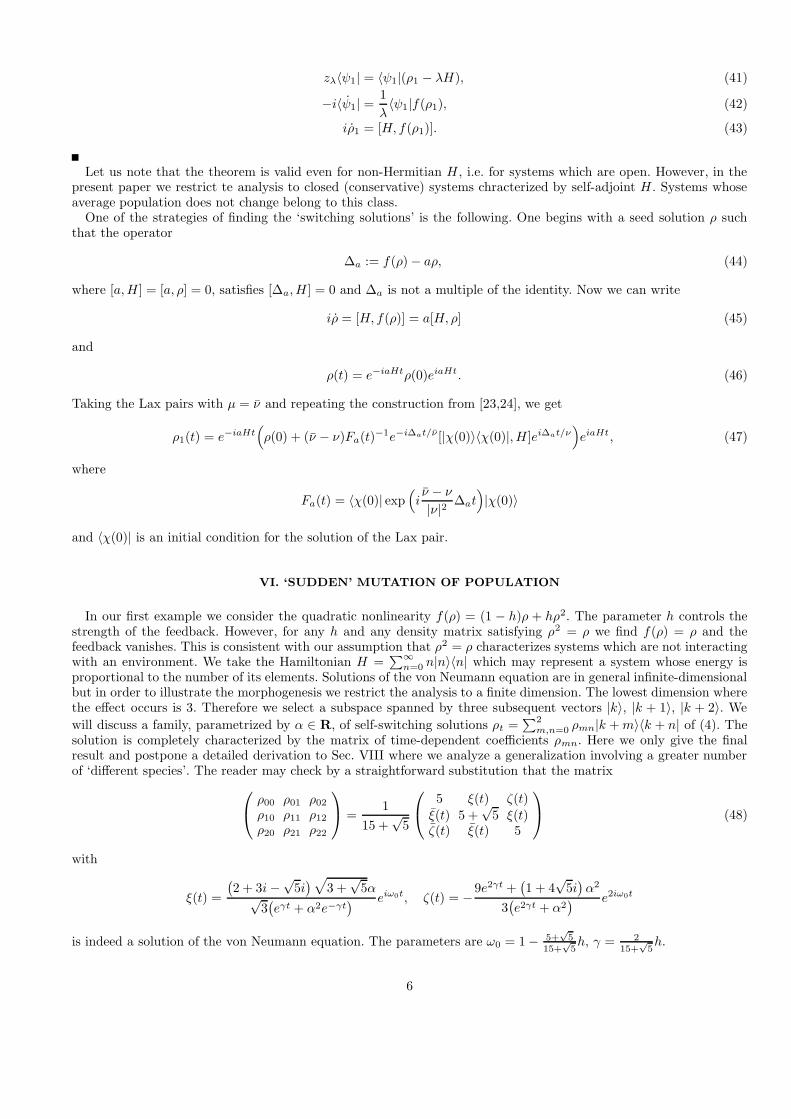
In our first example we consider the quadratic nonlinearity f(ρ) = (1 − h)ρ + hρ2. The parameter h controls thestrength of the feedback. However, for any h and any density matrix satisfying ρ2 = ρ we find f(ρ) = ρ and thefeedback vanishes. This is consistent with our assumption that ρ2 = ρ characterizes systems which are not interactingwith an environment. We take the Hamiltonian H =

∑∞n=0 n|n〉〈n| which may represent a system whose energy is

proportional to the number of its elements. Solutions of the von Neumann equation are in general infinite-dimensionalbut in order to illustrate the morphogenesis we restrict the analysis to a finite dimension. The lowest dimension wherethe effect occurs is 3. Therefore we select a subspace spanned by three subsequent vectors |k〉, |k + 1〉, |k + 2〉. We

will discuss a family, parametrized by α ∈ R, of self-switching solutions ρt =∑2m,n=0 ρmn|k +m〉〈k + n| of (4). The

solution is completely characterized by the matrix of time-dependent coefficients ρmn. Here we only give the finalresult and postpone a detailed derivation to Sec. VIII where we analyze a generalization involving a greater numberof ‘different species’. The reader may check by a straightforward substitution that the matrix

ρ00 ρ01 ρ02ρ10 ρ11 ρ12ρ20 ρ21 ρ22

=1

15 +√

5

5 ξ(t) ζ(t)

ξ(t) 5 +√

5 ξ(t)ζ(t) ξ(t) 5

(48)

with

ξ(t) =

(

2 + 3i−√

5i)

√

3 +√

5α√3(

eγt + α2e−γt) eiω0t, ζ(t) = −9e2γt +

(

1 + 4√

5i)

α2

3(

e2γt + α2) e2iω0t

is indeed a solution of the von Neumann equation. The parameters are ω0 = 1− 5+√5

15+√5h, γ = 2

15+√5h.

6

There exists a critical value h0 = 15+√5

5+√5

corresponding to ω0 = 0. Using the explicit position dependence of

the eigenstates of the harmonic oscillator Hamiltonian we can make a plot illustrating the time dependence of theprobability density pt,x in position space as a function of time and h.

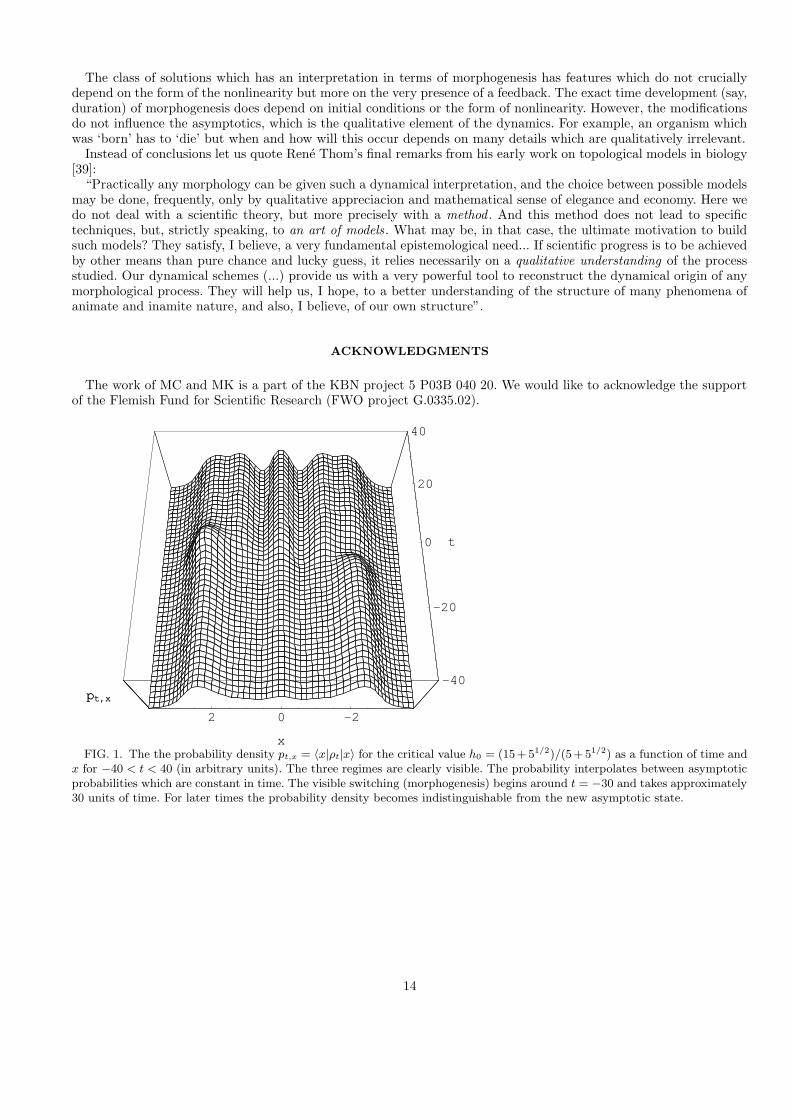
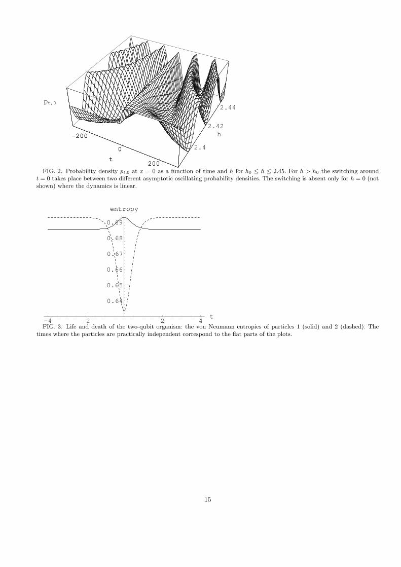
The dynamics we encounter in this example is particularly suggestive for h = h0 (Fig. 1) and resembles a mutationof the statistical ensemble described by ρ. The corresponding probability appears static for, roughly, −∞ < t < −40and then also for 40 < t <∞. Switching is ‘suddenly’ triggered in a neighborhood of t = 0. Fig. 2 shows the evolutionof the probability density at the origin pt,0 as a function of time for different values of h. For h 6= h0 the probabilitydensity is an oscillating function of time, but in the neighborhood of t = 0 one observes the ‘mutation’ which occursfor any h 6= 0, the longer the transition period the smaller h. Duration of the switching process is of the order 1/h.For h = 0 the dynamics is linear (no feedback) and there is no switching. The example shows that there occurs a kindof uncertainty relation between the strength of the feedback and duration of the switching: The smaller the feedbackthe longer the switching period.

Let us note that the probability density shown at Fig. 1 has this particular shape since we have used theposition-space wave functions characteristic of a quantum one dimensional harmonic oscillator (a Gaussian timesHermite polynomials). Had we chosen any other system which is isospectral to a one-dimensional harmonic oscillator(or any system with equally spaced spectrum, say, a 3D harmonic oscillator) we would have obtained a different shapeof the probability density. Although different choices of H imply different differential equations, their common featureis the efect of ‘mutation’.

VII. COMPOSITE ENTITIES: BIRTH AND DEATH OF AN ORGANISM

In this example we consider an organism, that is a composite entity which undergoes the feedback process as awhole. A simple model consists of a two-qubit system described by the Hamiltonian

H = H1 ⊗ 1+ 1⊗H2. (49)

The Hamiltonian does not contain an interaction term. However, the two subentities forming the ‘organism’ do notevolve independently. They are coupled to each other through the feedback with the envirinment, i.e. through thenonlinearity. As we shall see, they become asymptotically uncoulped at t → ±∞. In a ‘distant past’ the systemconsists of uncorrelated subentities which, after a period of certain joint activity, become again uncorrelated in thefuture. An analogy with ‘birth’ and ‘death’ is striking, and justifies the name ‘organism’.

To make the example concrete assume that

H = 2σx ⊗ 1+ 1⊗ σz (50)

We will start with the non-normalized density matrix

ρ(0) =1

2

5 +√

7 0 0 0

0 5−√

7 0 0

0 0 5 +√

15 0

0 0 0 5−√

15

(51)

which is written in such a basis that

H =

1 2 0 02 1 0 00 0 −1 20 0 2 −1

. (52)

The density matrix

ρ(t) = exp[−5iHt]ρ(0) exp[5iHt] (53)

is a solution of (4) with f(ρ) = ρ2. Such a ρ(t) describes simultaneously a dynamics of two non-interacting systemssatisfying the linear von Neumann equation

iρ = 5[2σx ⊗ 1+ 1⊗ σz , ρ]. (54)

To understand why this happenes it is sufficient to note that the solution satisfies

7

[H, ρ2] = [H, 5ρ] = [5H, ρ]. (55)

The environment does not trigger in this solution any switching, but only makes its evolution five times faster thanin the absence of the feedback. The Darboux transformation when applied to ρ(t) produces (for more details cf. [23])the solution

ρ1(t) = exp[−5iHt]ρint(t) exp[5iHt] (56)

where

ρint(t) =1

2

5−√

7 tanh 2t 0 −13i−3√7−√15−i

√105

8 cosh 2t−7i+3

√7−3√15+i

√105

8 cosh 2t

0 5 +√

7 tanh 2t 15i+√7−√15−i

√105

8 cosh 2t

√7+√15

2 cosh 2t13i−3

√7−√15+i

√105

8 cosh 2t−15i+

√7−√15+i

√105

8 cosh 2t 5 +√

15 tanh 2t 07i+3

√7−3√15−i

√105

8 cosh 2t

√7+√15

2 cosh 2t 0 5−√

15 tanh 2t

. (57)

Now the switching between the two asymptotic evolutions is triggered in the neighborhood of t = 0.If we look at the subentities forming the organism we notice that they do not evolve independently. The easiest

way of seeing this is to compute the reduced density matrices of the two subentities. Here we write explicitly theeigenvalues of the reduced density matrices. Both subsystems are two-dimensional so there are two eigenvalues foreach reduced density matrix. They read

p±(1) =1

2±√

15−√

7

20tanh 2t, particle 1 (58)

p±(2) =1

2±√

26 + 2√

105

40 cosh 2t, particle 2. (59)

The asymptotics are

ρint(−∞) =1

2

5−√

7 0 0 0

0 5 +√

7 0 0

0 0 5−√

15 0

0 0 0 5 +√

15

, (60)

ρint(+∞) =1

2

5 +√

7 0 0 0

0 5−√

7 0 0

0 0 5 +√

15 0

0 0 0 5−√

15

= ρ(0), (61)

and therefore the dynamics represents asymptotically two non-interacting subentities. It is also interesting that the+∞ asymptotics is ρ1(t) ≈ ρ(t). At large times the ‘organism’ which ‘dies’ becomes practically indistinguishable fromthe one that never ‘lived’.

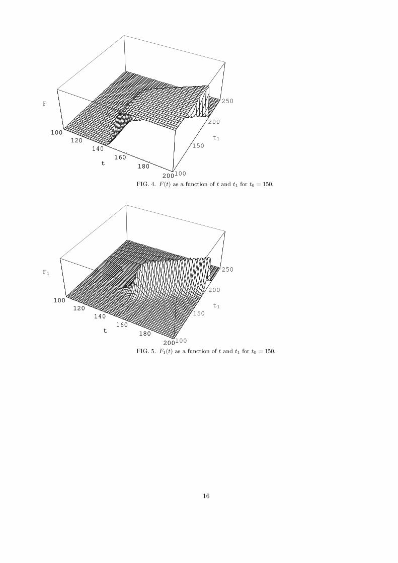
The ‘life’ of the organism is the period of time when the two subentities exhibit certain joint activity. Computing thevon Neumann entropies of reduced density matrices of the two subentities we can introduce a quantitative measure ofthis activity. The entropies of the two particles are shown in Fig. 3. The organism lives several units of time. Similarare the scales of time when the off diagonal matrix elements of ρint(t) become non-negligible. It should be stressed thatthe entropy characterizing the entire organism is time independent (since eigenvalues of solutions of (4) are constantsof motion for all f).

Although it is clear that the ‘organism’ behaves during the evolution as an indivisible entity, one should notconfuse this indivisiblility with the so-called nonseparability discussed in quantum information theory. The organismwe consider in the example is a two-qubit system and therefore one can check the separability of ρ1(t) by means ofthe Peres-Horodecki partial transposition criterion [26,27]: A two qubit density matrix ρ is separable if and only ifits partial transposition is positive. It turns out that partial transposition of ρ1(t) is positive for any t and, hence,ρ1(t) is in this sense separable (has ‘zero entanglement’). It is well known, however, that ‘zero entanglement’ does notmean ‘no quantum correlations’ in the system. The so called three-particle GHZ state [28] is fully entangled at thethree-particle level in spite of the fact that all its two-particle subsystems are described by separable density matrices.

8

VIII. MODEL WITH SEVERAL SPECIES

The models we have considered so far corresponded to a Hilbert space with basis vectors |n〉. The only characte-rization of a state was in terms of the quantum number n which could be regarded as the number of elements of agiven population. Now we want to extend the description to the situation where we have a population consisting ofseveral species characterized by numbers n1, . . . , nN . The basis vectors are

|n〉 = |n1, . . . , nN 〉 = |n1〉 ⊗ . . .⊗ |nN 〉 (62)

and the Hamiltonian

H =∑

nj

(n1 + . . .+ nN )|n1, . . . , nN〉〈n1, . . . , nN | (63)

=∑

n

En|n〉〈n|. (64)

The Hamiltonian has equally spaced spectrum and is formally very similar to those we have encountered in theprevious sections. The difference is that now the energy eigenstates are highly degenerated, a property which is veryuseful from the perspective of constructing multi-parameter and higher-dimensional self-switching solutions.

For simplicity consider two species (N = 2), the quadratic nonlinearity

f(ρ) = (1− h)ρ+ hρ2,

and take some three energy eigenvalues Ek, Ek+m, Ek+2m. For each energy take l+ 1 vectors, which will be denotedby

|0j〉 = |k − j, j〉, (65)

|1j〉 = |k +m− j, j〉, (66)

|2j〉 = |k + 2m− j, j〉, (67)

j = 0, 1, . . . l ≤ k. We start with the unnormalized density matrix

ρ(0) =

l∑

j=0

ρj(0) (68)

where

ρj(0) =a

2

(

|0j〉〈0j |+ |2j〉〈2j |)

+a+

√

a2 + 4(b−m2)2

|1j〉〈1j | −√a2 + 4b

2

(

|2j〉〈0j |+ |0j〉〈2j |)

. (69)

Positivity of ρj(0) restricts the parameters as follows: 0 < 4m2 < a2 + 4b < a2. The operator

∆a = ρ(0)2 − aρ(0) = bI −m2l∑

j=0

|1j〉〈1j | (70)

commutes with H . We denote by I and H the restrictions of the identity I and H to the 3(l+1)-dimensional subspace

spanned by (65)–(67). We will write H =∑lj=0Hj , where

Hj =2∑

n=0

(k + nm)|nj〉〈nj |. (71)

Consider the eigenvalue problem

(

ρj(0)− iHj)

|ϕj〉 = z|ϕj〉. (72)

We find that the two solutions

9

|ϕ(1)j 〉 = −2im+√

a2 + 4(b−m2)√2√a2 + 4b

|0j〉+1√2|2j〉 (73)

|ϕ(2)j 〉 = |1j〉 (74)

correspond to the same j-independent eigenvalue

z =a+

√

a2 + 4(b−m2)2

+ (k +m)i (75)

and therefore

(

ρ(0)− iH)

|ϕ〉 = z|ϕ〉. (76)

with the same z for any

|ϕ〉 =l∑

j=0

(

αj |ϕ(1)j 〉+ βj |ϕ(2)j 〉)

. (77)

The self-switching solution can thus be constructed by means of |ϕ〉 and reads

ρ1(t) = e−i(1+h(a−1))Ht(

ρ(0) + 2iFa(t)−1e−h∆at[|ϕ〉〈ϕ|, H ]e−h∆at

)

ei(1+h(a−1))Ht, (78)

with

Fa(t) = 〈ϕ| exp(

− 2h∆at)

|ϕ〉 = e−2hbtl∑

j=0

(

|αj |2 + e2hm2t|βj |2

)

= e−2hbt(

|α|2 + e2hm2t|β|2

)

. (79)

Probabilities analogous to Fig. 1 are found if a and h are tuned in a way which eliminates the oscillating parte−i(1+h(a−1))Ht, i.e. for h = 1/(1− a). In this case

ρ1(t) = ρ(0) + 2i(

|α|2 + e2m2t/(1−a)|β|2

)−1 l∑

j,j′=0

[(

αj |ϕ(1)j 〉+ βjem2t1−a |ϕ(2)j 〉

)(

αj′ 〈ϕ(1)j′ |+ βj′em2t1−a 〈ϕ(2)j′ |

)

, H]

(80)

The vectors

|Φj(t)〉 = αj |ϕ(1)j 〉+ βjem2t1−a |ϕ(2)j 〉 = |φj(t)〉 ⊗ |j〉 (81)

where

|φj(t)〉 =αj√

2

(

− 2im+√

a2 + 4(b−m2)√a2 + 4b

|k − j〉+ |k + 2m− j〉)

+ βjem2t1−a |k +m− j〉 (82)

are orthogonal for different j. Denoting H = H1 ⊗ I + I ⊗H2 one can easily compute the reduced density matrix ofthe first species,

ρI1(t) = Tr 2ρ1(t) = ρI(0) + 2i(

|α|2 + e2m2t/(1−a)|β|2

)−1[

l∑

j=0

|φj(t)〉〈φj(t)|, H1]

. (83)

The entire information about the dynamics of the first species is encoded in ρI1(t). Changes of properties of the speciesare given by the matrix elements

〈n|ρI1(t)|n′〉 = 〈n|ρI(0)|n′〉+ 2i(n′ − n)

∑lj=0〈n|φj(t)〉〈φj (t)|n′〉|α|2 + e2m2t/(1−a)|β|2 . (84)

An immediate conclusion from the above formula is that for n = n′ the expression is time independent. It follows thatthe number of elements of the ensemble does not change during the evolution. What changes are certain propertiesof the ensemble.

10

A. Example: k = m = 1, j = 0, 1, a = 5, b = −4

The two-species states in the subspace in question are

|00〉 = |1, 0〉, (85)

|10〉 = |2, 0〉, (86)

|20〉 = |3, 0〉, (87)

|01〉 = |0, 1〉, (88)

|11〉 = |1, 1〉, (89)

|21〉 = |2, 1〉. (90)

The two-species initial seed density matrix is given by

ρ0(0) =5

2

(

|1, 0〉〈1, 0|+ |3, 0〉〈3, 0|)

+5 +√

5

2|2, 0〉〈2, 0| − 3

2

(

|3, 0〉〈1, 0|+ |1, 0〉〈3, 0|)

, (91)

ρ1(0) =5

2

(

|0, 1〉〈0, 1|+ |2, 1〉〈2, 1|)

+5 +√

5

2|1, 1〉〈1, 1| − 3

2

(

|2, 1〉〈0, 1|+ |0, 1〉〈2, 1|)

, (92)

ρ(0) = ρ0(0) + ρ1(0). (93)

Assume α0 = α1 = 1/√

2, β0 = et0/4, β1 = et1/4. Then

|φ0(t)〉 =1

2

(

− 2i+√

5

3|1〉+ |3〉

)

+ e(t0−t)/4|2〉, (94)

|φ1(t)〉 =1

2

(

− 2i+√

5

3|0〉+ |2〉

)

+ e(t1−t)/4|1〉 (95)

Writing the restriction of H to the 6-dimensional subspace as

H =

1 0 0 0 0 00 1 0 0 0 00 0 2 0 0 00 0 0 2 0 00 0 0 0 3 00 0 0 0 0 3

(96)

we can represent the two-species density matrix ρ1 in the form

ρ1 =

521

2−i√5

3 ξ − 321+ 2−i√5

3 ζ2+i√5

3 ξT 5+√5

3 1 iξT

− 321+ 2+i√5

3 ζ −iξ 521

(97)

where 1 is the 2× 2 unit matrix, T denotes transposition, and

ξ(t) =et/4

et/2 + et0/2 + et1/2

(

et1/4 et0/4

et1/4 et0/4

)

(98)

ζ(t) =et/2

et/2 + et0/2 + et1/2

(

1 11 1

)

. (99)

One can verify by a straightforward calculation that (h = − 14 )

iρ1 = 54 [H, ρ1]− 14 [H, ρ21]. (100)

To illustrate the time variation of statistical quantities associated with the two-species system it is sufficient to visualizethe behavior of matrix elements of ρ1. There are only three types of functions occuring in ρ1:

11

F (t) =et/2

et/2 + et0/2 + et1/2, (101)

F0(t) =e(t+t0)/4

et/2 + et0/2 + et1/2, (102)

F1(t) =e(t+t1)/4

et/2 + et0/2 + et1/2. (103)

The two parameters t0, t1, control two types of three-regime behaviors of ρ1. The function F is responsible forasymptotic properties of ρ1 (via ζ). Functions F0, F1 determine properties of the switching regime (via ξ). For t0 � t1one finds F0(t) ≈ 0 for all t and the switching is controlled by F (t) and F1(t); the ‘moment’ of switching is shiftedproportionally to t1. For t0 � t1 one finds F1(t) ≈ 0 for all t and the switching is controlled by F (t) and F0(t);the ‘moment’ of switching does not depend on t1 and is determined by t0. Therefore the two types of switches arecharacterized by vanishing of those matrix elements of ρ1 which contain either F0 or F1.

The asyptotic behavior of the system is given by

F0(±∞) = F1(±∞) = F (−∞) = 0, (104)

F (+∞) = 1. (105)

The reduced density matrices of single species are

ρI1 =

52

2−i√5

3 F1 − 32 + 2−i√5

3 F 02+i√5

3 F1 5 +√52

2−i√5

3 F0 + iF1 − 32 + 2−i√5

3 F

− 32 + 2+i√5

3 F 2+i√5

3 F0 − iF1 5 +√52 iF0

0 − 32 + 2+i√5

3 F −iF0 52

(106)

ρII1 =

(

15+√5

22−i√5

3 F1 + iF02+i√5

3 F1 − iF0 15+√5

2

)

. (107)

Of course, all the density matrices are not normalized so that averages must be computed according to 〈A〉 =TrAρ1/Trρ1, etc. (note that Tr ρ1 is time independent).

IX. MORPHOGENESIS OF COMPLEMENTARITY

According to the ‘SSC theorem’ [30,31] a density matrix ρ is uniquely determined by correlations between all thepossible propositions associated with a given system. Each matrix element of a ρ can be given an interpretation interms of probabilities associated with some proposition. In the Hilbert space language a proposition is a projector,i.e. an operator with eigenvalues 1 and 0 (logical ‘true’ and ‘false’). Propositions which can be asked simultaneouslyare represented by commuting projectors. Propositions P1, P2 which do not commute are related by an uncertaintyrelation: The more is known about P1 the less is known about P2, and vice versa.

It is obvious that the above structures do not have to be associated with quantum systems. Just to give an example,many psychological tests are based on questionnaires which involve the same question asked many times in differentcontexts. The questions commute if the answer to a given question is always the same. However, in typical situationsthe same question has different answers within a single questionnaire. An ideal questionnaire involves all the possiblequestions asked in all the possible orders. In the Hilbert space formalism, where the questions are represented byprojectors, an ideal questionnaire encodes all the possible correlations and thus, via the SSC theorem, is equivalentto a density matrix.

It is also known that there exist simple examples of systems whose logic is non-Boolean, but which do not allowa Hilbert space formulation [29]. The density matrix language will probably not suffice here and one has to admit apossibility of other state spaces and other nonlinear evolutions. The richness of available structures is immense.

Let us finally give examples of propositions whose averages (i.e. probabilities) change in time according to selectedmatrix elements of the self-switching solutions. The function F (t) shown in Fig. 4 is associated with the proposition

P =1

2

1 0 1 00 0 0 01 0 1 00 0 0 0

(108)

12

corresponding to the first species as follows

p(t) =TrPρI1(t)

Tr ρI1(t)=

1

4

9 +√

5 + 8F (t)/3

15 +√

5. (109)

Here p(t) is the probability of the answer ‘true’ associated with P . Analogously F1(t) shown at Fig. 5 is associatedwith the proposition

P1 =1

2

1 1 0 01 1 0 00 0 0 00 0 0 0

(110)

by means of

p1(t) =TrP1ρ

I1(t)

Tr ρI1(t)=

1

4

15 +√

5 + 8F1(t)/3

15 +√

5. (111)

The evolution of the probabilities resembles the well known evolutions typically modelled by Hill functions [12] inthe so-called sigmoidal response models [32–35,37]. Square deviations associated with the two propositions satisfy theuncertainty relation

∆P∆P1 ≥1

2

∣

∣

∣

Tr [P, P1]ρI1(t)

Tr ρI1(t)

∣

∣

∣ =∣

∣

∣

√5(et/2 + e(t+t0)/4)− (3 +

√5)e(t+t1)/4

12(15 +√

5)(et/2 + et0/2 + et1/2)

∣

∣

∣. (112)

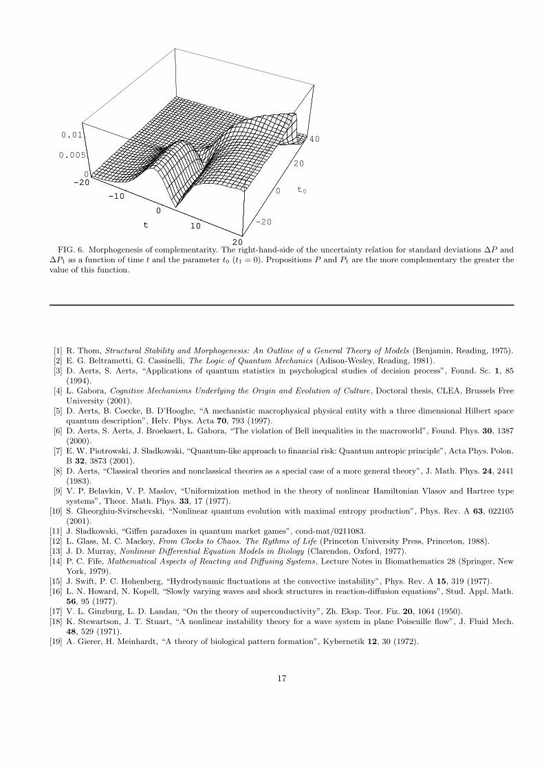
For any fixed t0, t1, the right-hand-side of the inequality vanishes for t→ −∞ and approaches√

5/[12(15 +√

5)] fort→ +∞. Fig. 6 shows this function for t1 = 0. The two propositions which were not complementary in the past evolveinto propositions satisfying an uncertainty relation.

In application to psychology a density matrix may represent an ideal questionnaire and, hence, a state of personalityof a given individual. The morphogenesis we have discussed is a simple model of development of two complementaryconcepts. The model is simplified and perhaps too far fetched. However, philosophically this is not very far from theapproaches of Thom [1] and particularly of Zeeman [38] in their catastrophe theory models of brain. More interestingin this context may be infinite dimensional cases whose preliminary analysis in terms of Darboux transformations forarbitrary f(ρ) can be found in [25].

X. DISCUSSION

The model of we have described satisfies the assumptions imposed by Thom on a system of forms in evolution ([1] Chapter 1.2.A). The model is continuous and the morphogenesis is a result of soliton dynamics. In this respectthe construction is analogous to nonlinear sigmoidal response models used in biochemistry [37]. What makes ourconstruction essentially different from the models one finds in the literature is the role of non-commutativity of thesystem of propositions.

Non-commutative propositions are related by uncertainty principles and are typical of systems which cannot, withoutan essential destruction, be separated into independent parts. The examples can be taken not only from quantumphysics, but also from sociology (communities), psychology (personalities), or biology (organisms). In all these casesthe dynamics of a system consists of two parts: One generated by internal interactions, and the other corresponding tocouplings with environment. We have considered only the simplest case where the internal dynamics is given a prioriby a Hamiltonian of a harmonic oscillator type, and different parts of an organism (community, etc.) are coupled toeach other only via the environment.

The coupling with environment leads to a feedback and, hence, nonlinear evolution. The systems we consider areconservative, but without difficulties can be generalized to explicitly time-dependent environments or non-HermitionHamiltonians.

We model propositions by projectors on subspaces of a Hilbert space. States of the systems are represented byall the possible correlations between all the possible, even non-commuting, propositions. The choice of the Hilbertspace language leads us therefore to a density matrix representation of states, and the dynamics is given in termsof nonlinear von Neumann equations. The formalism allows to consider morphogenesis of a completely new type, forexample a development of complementary properties.

13

The class of solutions which has an interpretation in terms of morphogenesis has features which do not cruciallydepend on the form of the nonlinearity but more on the very presence of a feedback. The exact time development (say,duration) of morphogenesis does depend on initial conditions or the form of nonlinearity. However, the modificationsdo not influence the asymptotics, which is the qualitative element of the dynamics. For example, an organism whichwas ‘born’ has to ‘die’ but when and how will this occur depends on many details which are qualitatively irrelevant.

Instead of conclusions let us quote Rene Thom’s final remarks from his early work on topological models in biology[39]:

“Practically any morphology can be given such a dynamical interpretation, and the choice between possible modelsmay be done, frequently, only by qualitative appreciacion and mathematical sense of elegance and economy. Here wedo not deal with a scientific theory, but more precisely with a method . And this method does not lead to specifictechniques, but, strictly speaking, to an art of models . What may be, in that case, the ultimate motivation to buildsuch models? They satisfy, I believe, a very fundamental epistemological need... If scientific progress is to be achievedby other means than pure chance and lucky guess, it relies necessarily on a qualitative understanding of the processstudied. Our dynamical schemes (...) provide us with a very powerful tool to reconstruct the dynamical origin of anymorphological process. They will help us, I hope, to a better understanding of the structure of many phenomena ofanimate and inamite nature, and also, I believe, of our own structure”.

ACKNOWLEDGMENTS

The work of MC and MK is a part of the KBN project 5 P03B 040 20. We would like to acknowledge the supportof the Flemish Fund for Scientific Research (FWO project G.0335.02).

-40

-20

0

20

40

t

-202

x

pt,xpt,x

FIG. 1. The the probability density pt,x = 〈x|ρt|x〉 for the critical value h0 = (15 + 51/2)/(5 + 51/2) as a function of time andx for −40 < t < 40 (in arbitrary units). The three regimes are clearly visible. The probability interpolates between asymptoticprobabilities which are constant in time. The visible switching (morphogenesis) begins around t = −30 and takes approximately30 units of time. For later times the probability density becomes indistinguishable from the new asymptotic state.

14

-200

0

200t

2.4

2.42

2.44

h

pt,0

-200

0

200t

FIG. 2. Probability density pt,0 at x = 0 as a function of time and h for h0 ≤ h ≤ 2.45. For h > h0 the switching aroundt = 0 takes place between two different asymptotic oscillating probability densities. The switching is absent only for h = 0 (notshown) where the dynamics is linear.

-4 -2 2 4t

0.64

0.65

0.66

0.67

0.68

0.69

entropy

FIG. 3. Life and death of the two-qubit organism: the von Neumann entropies of particles 1 (solid) and 2 (dashed). Thetimes where the particles are practically independent correspond to the flat parts of the plots.

15

100120

140160

180

200

t

100

150

200

250

t1

F

100120

140160

180

200

t

FIG. 4. F (t) as a function of t and t1 for t0 = 150.

100120

140160

180

200

t

100

150

200

250

t1

F1

100120

140160

180

200

t

FIG. 5. F1(t) as a function of t and t1 for t0 = 150.

16

-20

-10

0

10

20

t -20

0

20

40

t0

0

0.005

0.01

-20

-10

0

10

20

t

FIG. 6. Morphogenesis of complementarity. The right-hand-side of the uncertainty relation for standard deviations ∆P and∆P1 as a function of time t and the parameter t0 (t1 = 0). Propositions P and P1 are the more complementary the greater thevalue of this function.

[1] R. Thom, Structural Stability and Morphogenesis: An Outline of a General Theory of Models (Benjamin, Reading, 1975).[2] E. G. Beltrametti, G. Cassinelli, The Logic of Quantum Mechanics (Adison-Wesley, Reading, 1981).[3] D. Aerts, S. Aerts, “Applications of quantum statistics in psychological studies of decision process”, Found. Sc. 1, 85

(1994).[4] L. Gabora, Cognitive Mechanisms Underlying the Origin and Evolution of Culture, Doctoral thesis, CLEA, Brussels Free

University (2001).[5] D. Aerts, B. Coecke, B. D’Hooghe, “A mechanistic macrophysical physical entity with a three dimensional Hilbert space

quantum description”, Helv. Phys. Acta 70, 793 (1997).[6] D. Aerts, S. Aerts, J. Broekaert, L. Gabora, “The violation of Bell inequalities in the macroworld”, Found. Phys. 30, 1387

(2000).[7] E. W. Piotrowski, J. S ladkowski, “Quantum-like approach to financial risk: Quantum antropic principle”, Acta Phys. Polon.

B 32, 3873 (2001).[8] D. Aerts, “Classical theories and nonclassical theories as a special case of a more general theory”, J. Math. Phys. 24, 2441

(1983).[9] V. P. Belavkin, V. P. Maslov, “Uniformization method in the theory of nonlinear Hamiltonian Vlasov and Hartree type

systems”, Theor. Math. Phys. 33, 17 (1977).[10] S. Gheorghiu-Svirschevski, “Nonlinear quantum evolution with maximal entropy production”, Phys. Rev. A 63, 022105

(2001).[11] J. S ladkowski, “Giffen paradoxes in quantum market games”, cond-mat/0211083.[12] L. Glass, M. C. Mackey, From Clocks to Chaos. The Rythms of Life (Princeton University Press, Princeton, 1988).[13] J. D. Murray, Nonlinear Differential Equation Models in Biology (Clarendon, Oxford, 1977).[14] P. C. Fife, Mathematical Aspects of Reacting and Diffusing Systems, Lecture Notes in Biomathematics 28 (Springer, New

York, 1979).[15] J. Swift, P. C. Hohenberg, “Hydrodynamic fluctuations at the convective instability”, Phys. Rev. A 15, 319 (1977).[16] L. N. Howard, N. Kopell, “Slowly varying waves and shock structures in reaction-diffusion equations”, Stud. Appl. Math.56, 95 (1977).

[17] V. L. Ginzburg, L. D. Landau, “On the theory of superconductivity”, Zh. Eksp. Teor. Fiz. 20, 1064 (1950).[18] K. Stewartson, J. T. Stuart, “A nonlinear instability theory for a wave system in plane Poiseuille flow”, J. Fluid Mech.48, 529 (1971).

[19] A. Gierer, H. Meinhardt, “A theory of biological pattern formation”, Kybernetik 12, 30 (1972).

17

[20] W. Kemmner, “A model of head regeneration in hydra”, Differentiation 26, 83 (1984).[21] M. Czachor, “Nambu type generalization of the Dirac equation”, Phys. Lett. A 225, 1 (1997)[22] M. Czachor and J. Naudts, “Microscopic foundation of nonextensive statistics”, Phys. Rev. E 59, R2497 (1999)[23] S. B. Leble and M. Czachor, “Darboux-integrable nonlinear Liouville-von Neumann equation”, Phys. Rev. E 58, 7091

(1998)[24] M. Czachor, H. D. Doebner, M. Syty, K. Wasylka, “Von Neumann equations with time-dependent Hamiltonians and

supersymetric quantum meachanics”, Phys. Rev. E 61, 3325 (2000).[25] N. V. Ustinov, M. Czachor, M. Kuna, S. B. Leble, “Darboux integration of iρ = [H, f(ρ)]”, Phys. Lett. A 279, 333 (2001).[26] A. Peres, “Separability condition for density matrices”, Phys. Rev. Lett. 77, 1413 (1996).[27] M. Horodecki, P. Horodecki, R. Horodecki, “Separability of mixed states: Necessary and sufficient conditions”, Phys. Lett.

A 223, 1 (1996).[28] D. M. Greenberger, M. A. Horne, A. Shimony, A. Zeilinger, “Bell’s theorem without inequalities”, Am. J. Phys. 58, 1131

(1990).[29] D. Aerts, “A possible explanation for the probabilities of quantum mechanics”, J. Math. Phys. 27, 202 (1986)[30] S. Bergia, F. Cannata, A. Cornia, R. Livi, “On the actual measurability of the density matrix of a decaying system by

means of measurements on the decay products”, Found. Phys. 10, 723 (1980).[31] N. D. Mermin, “What is quantum mechanics trying to tell us?”, Am. J. Phys. 66, 753 (1998).[32] C. Walter, R. Parker, M. Ycas, “A model for binary logic in biochemical systems”, J. Theor. Biol. 15, 208 (1967).[33] L. Glass, S. A. Kauffman, “Co-operative components, spatial localization and oscillatory cellular dynamics”, J. Theor.

Biol. 34, 219 (1972).[34] L. Glass, S. A. Kauffman, “The logical analysis of continuous non-linear biochemical control networks”, J. Theor. Biol. 39,

103(1973).[35] J. J. Hopfield, D. W. Tank, “Computing with neural circuits: A model”, Science 233, 625 (1986).[36] C. Tsallis, R. S. Mendes, A. R. Plastino, “The role of constraints within generalized nonextensive statistics”, Physica A261543 (1998).

[37] S. A. Kauffman, The Origins of Order. Self-Organization and Selection in Evolution (Oxford University Press, Oxford,1993).

[38] E. C. Zeeman, ”Catastrophe theory in brain modelling”, Int. J. Neurosci. 6, 39 (1973).[39] R. Thom, “Topological models in biology”, in Towards a Theoretical Biology , vol. 3, ed. C. H. Waddington (Aldine, Chicago,

1970).

18