Embed Size (px)
Citation preview
Institut für Eisenhüttenkunde
Xiaohuan Zhang

Investigation of Mould Filling and Solidification during Ingot Casting
Process with Experiments and OpenFOAM Numerical Modelling
Von der Fakul tät für Georessourcen und Materialtechnik der
Rheinisch -Westfälischen Technischen Hochschule Aachen
zur Erlangung des akademischen Grades einer
Doktorin der Ingenieurwissenschaften
genehmigte Dissertation
vorgelegt von Master of Science
Xiaohuan Zhang
aus Shanxi, China
Berichter:
Univ.-Prof. Professor h.c. (CN) Dr.-Ing. Dr. h.c. (CZ) Dieter George Senk
Univ.-Prof. Dr.-Ing. Bernhard Peters
Univ.-Prof. Dr.-Ing. Yanping Bao
Tag der mündlichen Prüfung: 27. Januar 2016
Diese Dissertation ist auf den Internetseiten der Hochschulbibliothek online verfügbar


Acknowledgement
The research work reported in this thesis was carried out under the
supervision of Univ.-Prof. Dr.-Ing. Dieter Senk at the Department of Ferrous
Metallurgy (IEHK), RWTH Aachen University.
I gratefully acknowledge the encouragement and guidance of Prof. Senk.
My special thanks are given to Prof. Peters and Prof. Bao for their in-depth
discussions and valuable suggestions.
I would like to thank Zhiye Chen, Xiaoxue Liu and Shahid Maqbool for the
help in water model experiments. I would also like to express my sincere
thanks to Min Wang for reviewing the manuscript.
I am grateful to Prof. Peters and Florian Hoffmann for technical advice on
OpenFOAM. I also thank the OpenFOAM development team for sharing of
this excellent software.
I would also like to thank my husband who helped me a lot in finishing this
project.


Contents
i
Contents
Nomenclature .................................................................................................................................................. iii
Abstract ............................................................................................................................................................... v
Kurzfassung ...................................................................................................................................................... vi
1. Introduction .............................................................................................................................................. 1
2. Literature review .................................................................................................................................... 3
2.1. Filling of ingot moulds ........................................................................................................................................... 3
2.1.1. Bottom teeming process ............................................................................................................................ 3
2.1.2. Influencing parameters of the flow conditions ................................................................................ 6
2.2. Solidification of cast ingots .................................................................................................................................. 6
2.2.1. Structure of steel ingots ............................................................................................................................. 6
2.2.2. Mathematical modelling of the solidification process ................................................................ 10
2.3. Introduction of the OpenFOAM software .................................................................................................... 16
2.4. Objective and methods of the study ............................................................................................................... 18
3. Water model experiments of the mould filling process ......................................................... 20
3.1. Design of experiments ......................................................................................................................................... 20
3.1.1. Water model set-up ................................................................................................................................... 20
3.1.2. Model parameters ...................................................................................................................................... 22
3.1.3. Experimental procedure ......................................................................................................................... 24
3.2. Results about the models with one bottom nozzle .................................................................................. 26
3.2.1. Water-air two-phase flow without oil addition ............................................................................. 26
3.2.2. Water-air-oil three-phase flow with oil addition .......................................................................... 28
3.3. Results about the models with four bottom nozzles ............................................................................... 32
3.3.1. Features of the flow fields ...................................................................................................................... 33
3.3.2. Influence of the filling rate ..................................................................................................................... 35
3.3.3. Influence of the bottom nozzles ........................................................................................................... 42
3.3.4. ............................................................................................................ 47
3.4. Optimization of filling conditions ................................................................................................................... 50
3.4.1. Influence of experimental parameters on the open surface..................................................... 51
3.4.2. ....... 52
3.4.3. Optimal filling conditions ....................................................................................................................... 53
3.5. Conclusions .............................................................................................................................................................. 54
4. Numerical simulation of filling process with OpenFOAM software .................................... 55
4.1. Model description .................................................................................................................................................. 55
4.2. Results of the calculated flow fields ............................................................................................................... 57
4.2.1. Flow patterns in the early stage of teeming .................................................................................... 57
Contents
ii
4.2.2. Velocity fields of the flow ....................................................................................................................... 59
4.2.3. Comparison with the water model experiments .......................................................................... 62
4.3. Conclusions .............................................................................................................................................................. 63
5. Simulation of solidification process with OpenFOAM software .......................................... 65
5.1. Liquid-solid 2-phase model with phase change ....................................................................................... 65
5.1.1. Model assumptions ................................................................................................................................... 65
5.1.2. Governing equations ................................................................................................................................ 67
5.1.3. Solution algorithm ..................................................................................................................................... 73
5.2. Application to a steel ingot ................................................................................................................................ 76
5.2.1. Model setup .................................................................................................................................................. 76
5.2.2. Results ............................................................................................................................................................ 79
5.3. Attempt on the coupling of mould filling and solidification process ............................................... 88
5.4. Conclusions .............................................................................................................................................................. 90
6. Overall discussion ................................................................................................................................ 91
7. Summary .................................................................................................................................................. 96
8. Reference ................................................................................................................................................. 99

Nomenclature
iii
Nomenclature
cp: Specific heat capacity, J·kg-1·K -1;
C: Concentration of carbon, wt%;
Cls: Solute transfer rate from liquid to solid phase, kg·m-3·s -1;
Csl: Solute transfer rate from solid to liquid phase, kg ·m-3·s -1;
ds: Grain diameter, m;
D: Diffusion coefficient, m2·s -1;
f: Mass fraction;
: Grain packing limit;
: Fraction of the open surface;
g: Volume fraction;
g: Gravity vector, m·s-2;
h: Enthalpy, J ·kg-1;
kp: Partition ratio;
Kls: Drag force coefficient, kg·m-3·s -1;
L: Latent heat, J·kg-1;
m: Liquidus slope, K·wt %-1;
Mls: Mass transfer rate from liquid to solid phase, kg·m-3·s -1;
Ns: Nucleation rate, m-3·s -1;
n: Grain density, m-3;
nmax: Maximum grain density, m-3;
p: Pressure, N ·m-2;
Re: Reynolds number;
Sv: Interfacial area concentration, m-1;
t: Time, s;
T: Temperature, K;
Nomenclature
iv
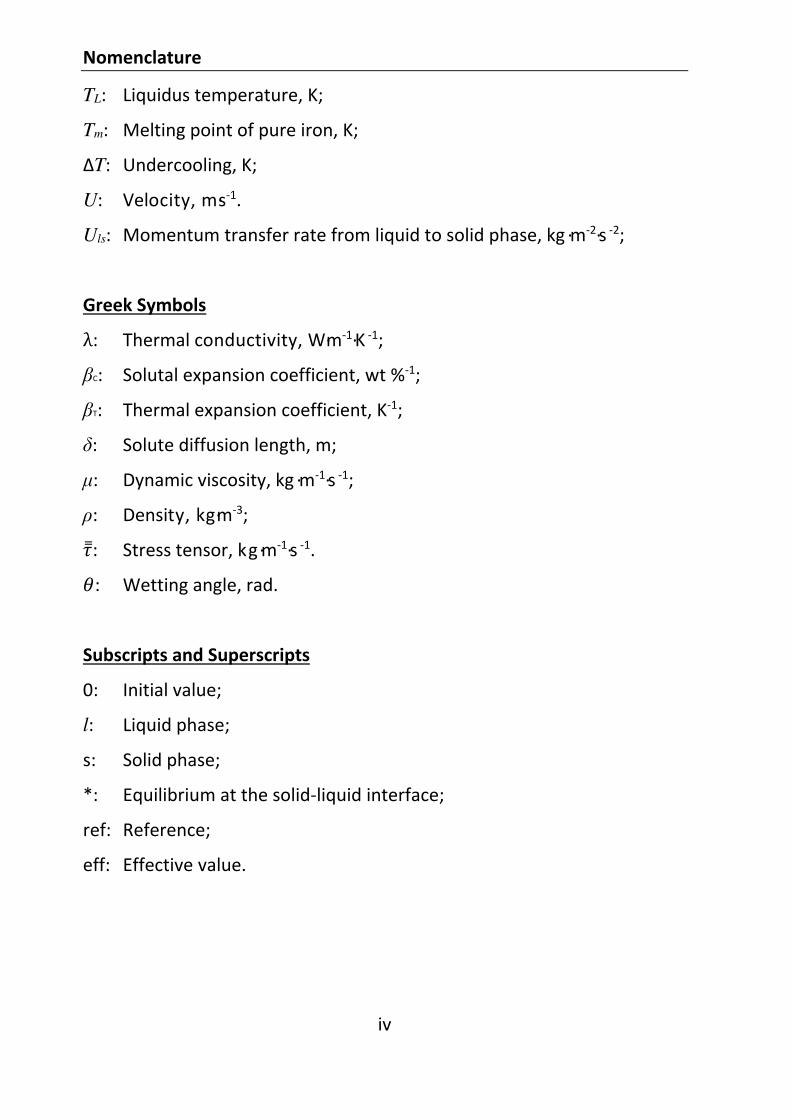
TL: Liquidus temperature, K;
Tm: Melting point of pure iron, K;
T: Undercooling, K;
U: Velocity, m·s-1.
Uls: Momentum transfer rate from liquid to solid phase, kg ·m-2·s -2;
Greek Symbols
: Thermal conductivity, W·m-1·K -1;
C: Solutal expansion coefficient, wt %-1;
T: Thermal expansion coefficient, K-1;
: Solute diffusion length, m;
: Dynamic viscosity, kg ·m-1·s -1;
: Density, kg·m-3;
: Stress tensor, kg·m-1·s -1.
: Wetting angle, rad.
Subscripts and Superscripts
0: Initial value;
l: Liquid phase;
s: Solid phase;
*: Equilibrium at the solid-liquid interface;
ref: Reference;
eff: Effective value.
Abstract
v
Abstract
The fluid flow and solidification of ingot casting was studied. In this study,
the fluid flow during the bottom teeming process was investigated with
water model experiments and numerical simulation. A user-defined liquid-
solid two-phase solidification solver was developed based on the software
platform of OpenFOAM, using Euler-Euler two-phase approach. The
solidification solver was performed on a 3-dimensional model of steel ingot
to simulate the solidification and macrosegregation distribution.
In water model experiments, water and vegetable oil were used to simulate
the molten steel and slag phase, respectively. The influence of model
parameters, such as the filling rate, nozzle dimensions and oil film thickness,
on the filling conditions was investigated, concerning two aspects: one is
the slag entrapment, and the other is reoxidation of molten steel. Both of
the two situations should be avoid to provide a better filling condition. The
numerical simulation on water-air two-phase flow with the interFoam
solver of OpenFOAM was performed. The obtained predictions were in
good agreement with the water model experiments.
The simulation of solidification can obtain the evolution of the solid fraction,
velocity, temperature, concentration and grain density fields. The
macrosegregation was indicated by the concentration of the only solute
carbon. The cone-shaped negative segregation at the bottom, positive
segregation at the top, V-segregation at the upper center of the ingot, and
the channel-shaped A-segregation were predicted. The simulation results
of macrosegregation ratio on certain lines were generally in agreement
with the experimental measurements from the literature, except for some
deviations at the bottom and the near-wall regions, where the predicted
degree of negative segregation was much stronger than the measured one.
Kurzfassung
vi
Kurzfassung
Der Fluidstrom und die Erstarrung des Blockguss wurden untersucht. In dieser Studie wurde der Fluidstrom während des Unterseite wimmelt Prozess mit Hilfe von den Wasser Modellexperimenten und numerischen Simulation untersucht. Eine benutzerdefinierte Flüssig-Fest-Zwei-Phasen-Erstarrungslöser wurde auf Basis der Softwareplattform von OpenFOAM mit Euler-Euler-Zwei-Phasen-Ansatz entwickelt. Der Erstarrungslöser wurde auf eine 3-dimensionale Modell des Stahlblocks ausgeführt, um die Erstarrung und die Verteilung der Makroseigerung zu simulieren. In Wasser Modellversuchen wurden Wasser und Pflanzenöl verwendet, um den geschmolzenen Stahl und die Schlacke zu simulieren. Der Einfluss von Modellparametern, wie die Füllungsrate, Düsenabmessungen und Ölfilmdicke wurde bei den Füllungsbedingungen unter Berücksichtigung von zwei Aspekten untersucht. Das sind die Schlackeneinschlüsse und die Reoxidation des geschmolzenen Stahl. Beide Situationen sollten vermieden werden, um einen besseren Füllungszustand bereitzustellen. Die numerische Simulation von Wasser-Luft-Zweiphasenströmung wurde mit der Interfoam Löser OpenFOAM durchgeführt. Die erhaltenen Voraussagen waren in guter Übereinstimmung mit den Ergebnissen von Wassermodell-versuchen. Die Evolution des Feststoffanteils, Geschwindigkeit, Temperatur, Konzentration und Korndichte können mit Hilfe von der Simulation der Erstarrung erhalten werden. Die Makroseigerung wurde durch die Konzentration des einzigen gelösten Stoffes (Kohlenstoff) angezeigt. Der kegelförmige negativer Seigerung am Boden, positive Seigerung an der Spitze, V-Seigerung an der oberen Mitte des Gussblock und die kanalförmigen A-Seigerung wurden vorhergesagt. Die Simulation-sergebnisse bezüglich des Verhältnisses bei der Makroseigerung auf bestimmten Linien stimmen im allgemeinen mit den experimentellen Untersuchungen aus der Literatur überein, mit Ausnahme einiger Abweichungen an der Unterseite und den wandnahen Bereichen, in denen der vorausgesagte Grad der negativen Seigerung viel stärker als gemessene Werte war.
1. Introduction
1
1. Introduction
The process of pouring molten steel from a ladle into an ingot mould until
the melt solidifies to an ingot is called ingot casting. The flow field during
the pouring process is of great importance for the development of
solidification structures and the removal of inclusions. Therefore, huge
efforts to improve the flow conditions and thereby the quality of cast ingots
and final steel products have been made.
Besides the inclusions, the chemical heterogeneities should also be
reduced as a way to minimize defects of products. The chemical
heterogeneities develop mainly during the solidification stage, which result
from the rejection of solutes from the solid phase back into the liquid phase.
This phenomenon is called segregation. It can be classified into
microsegregation and macrosegregation depending on the length scale.
The microsegregation takes place in the scale of dendrites, due to the
different solubility of chemical species in the solid and liquid phases. The
macrosegregation takes place at a larger scale ranging from 1 mm to 1 m.
The formation of macrosegregation is related to the relative motion
between the liquid and solid phases, and therefore the phenomenon of
melt convection and grain sedimentation are helping to understand the
macrosegregation. Macrosegregations are serious defects that should be
suppressed to improve the quality of as-cast products.
The objective of this thesis is to study the filling conditions as well as the
solidification phenomena during ingot casting process. The fluid flow of
filling stage was investigated by water modeling and numerical simulations.
Computational Fluid Dynamics (CFD) has become a widely used numerical
method to solve and analyze problems that involve fluid flows. There are
some famous commercial CFD software packages such as ANSYS CFX,
ANSYS Fluent, Star-CCM+ and others. These softwares are not only
expensive but also have low scalability for certain problems. In this study,
1. Introduction
2
an open-source CFD software, OpenFOAM, was employed to solve both the
fluid flow and solidification problems, synchronously.
This thesis includes the following chapters: After the general introduction,
literature reviews about the filling problems, solidification structure of a
typical steel ingot, previous simulation methods, and the features of
OpenFOAM software are described in chapter 2. Chapter 3 is about the
water model experiments of the mould filling process, aiming to optimize
the filling conditions of large ingot casting. Mathematical modelling of
mould filling process based on the OpenFOAM software was carried out
and the predicted results were compared with water models experiments,
as described in chapter 4. Further on, in chapter 5 a liquid-solid 2-phase
solidification model was developed and applied to a small steel ingot to
study the solidification process. The computational simulation work of this
thesis was done with OpenFOAM-2.1.1.
2. Literature review
3
2. Literature review
2.1. Filling of ingot moulds
During the steelmaking process, after the ladle metallurgical treatment and
secondary refining, the molten steel is poured into ingot moulds, where the
metal then solidified to form ingots.
There are two principal methods of pouring molten metal to ingot moulds:
top pouring and bottom teeming.
Top pouring is easy to carry out but has several disadvantages, such as the
considerable turbulence and splashing. As a result of the turbulent flow,
there is a tendency for non-metallic inclusions to become entrapped into
the melt and further more deteriorate the solidification structure.
Additionally, the accompanying splash is detrimental to the mould walls
and the ingot surface, which is subjected to highly erosive forces and the
life tends to be reduced.
A prevailing pouring method in steel industry is bottom teeming, which can
get better flow conditions than top pouring method, due to much less
turbulence and splashing [1, 2], and several moulds can be filled
synchronously from one feeder in a network of runners. In this thesis, the
bottom teeming method is concerned.
2.1.1. Bottom teeming process
The increasing demand for quality steels has led to the evolution of bottom
pouring technology for casting of steel ingots. This process constitutes of a
set up involving pouring sprue and runner system to deliver liquid steel into
one or more cast iron moulds through the bottom nozzles. Bottom teeming
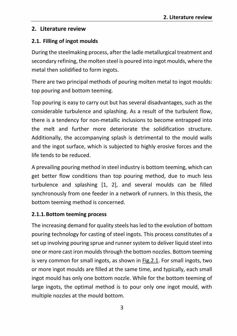
is very common for small ingots, as shown in Fig.2.1. For small ingots, two
or more ingot moulds are filled at the same time, and typically, each small
ingot mould has only one bottom nozzle. While for the bottom teeming of
large ingots, the optimal method is to pour only one ingot mould, with
multiple nozzles at the mould bottom.
2. Literature review
4
Fig. 2.1 Bottom teeming process of small steel ingots
In the traditional bottom teeming process, a bag of casting powder is
placed on the bottom or hung about 30 cm above the bottom of the mould
before pouring [2]. After the teeming started, when the liquid steel enters
the mould, the contacted powder receives maximum heat from the
meniscus and produces a fused or molten slag layer. The functions of this
liquid/fused slag layer in bottom teeming process are: (a) Protection from
the atmosphere; (b) Thermal insulation of the meniscus; (c) Absorption of
the non-metallic inclusions [3]. However, this slag layer may cause
undesirable problems meanwhile, such as slag entrapment, which leads to
formation of defects in the final products. It has been proved that during
gas stirred ladle metallurgy, due to the rising gas bubbles from a bottom
gas jet, a plume zone and an (slag less area) at the top of the
plume can be formed [4-6]. For the bottom teeming process, the liquid jet
from bottom nozzle has a similar effect on the surface behavior as the
submerged gas jet. For example, the mathematical modeling work by Z. Tan
et al. shows a hump on the surface above the bottom nozzle [7]. H.F.
Marston observed an ace as well as slag entrapment
at the early stage of teeming [2].
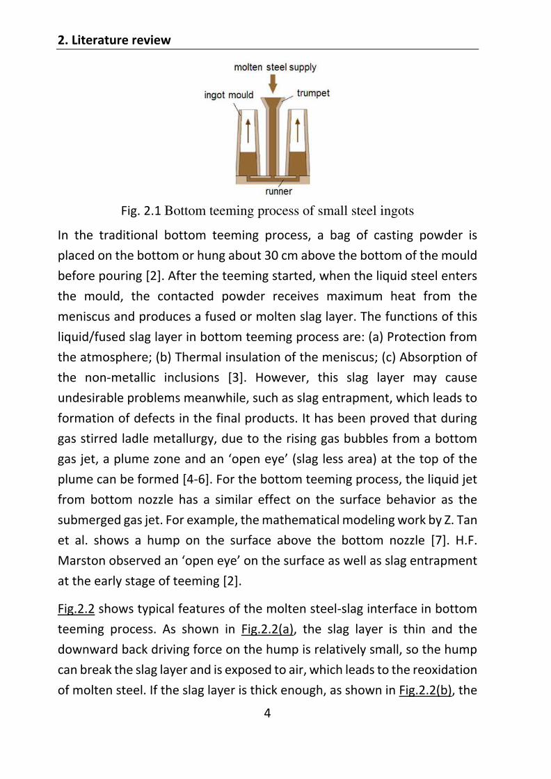
Fig.2.2 shows typical features of the molten steel-slag interface in bottom
teeming process. As shown in Fig.2.2(a), the slag layer is thin and the
downward back driving force on the hump is relatively small, so the hump
can break the slag layer and is exposed to air, which leads to the reoxidation
of molten steel. If the slag layer is thick enough, as shown in Fig.2.2(b), the
2. Literature review
5
movement of the hump was damped by the heavy layer and the metal is
totally covered by the slag layer, in which case the risk of reoxidation is
largely reduced [8, 9].
(a) (b)
Fig. 2.2 Steel-slag interface in bottom teeming process
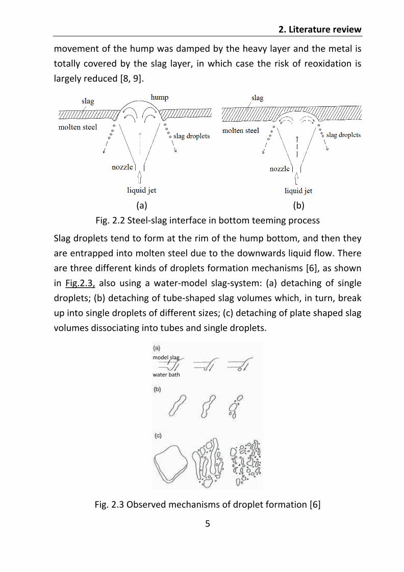
Slag droplets tend to form at the rim of the hump bottom, and then they
are entrapped into molten steel due to the downwards liquid flow. There
are three different kinds of droplets formation mechanisms [6], as shown
in Fig.2.3, also using a water-model slag-system: (a) detaching of single
droplets; (b) detaching of tube-shaped slag volumes which, in turn, break
up into single droplets of different sizes; (c) detaching of plate shaped slag
volumes dissociating into tubes and single droplets.
Fig. 2.3 Observed mechanisms of droplet formation [6]
model slag
water bath
2. Literature review
6
2.1.2. Influencing parameters of the flow conditions
Since the flow conditions, especially the surface behavior, have a significant
influence on slag entrapment and reoxidation of molten steel, theoretical
and experimental studies have been made on the influencing parameters.
By some studies of a liquid-submerged jet impinging on free surface [10-
12], it has been proved that the surface hump depends on both, the velocity
of jet and the distance from bottom nozzle to top surface. Large jet velocity
and small distance lead to large hump and instability of the surface. The
shape of the humps therefore decide the degree of slag entrapment and
reoxidation of molten steel.
2.2. Solidification of cast ingots
Solidification takes place when the heat is removed from the molten steel
through the ingot mould to the surrounding atmosphere. In the traditional
ingot casting process, the cooling methods are mainly natural cooling,
which gives lower cooling rate and can help to reduce the thermal stress
and structural stress defects of ingot. The solidification process is
associated with the phenomenon of heat transfer, solute redistribution,
fluid flow, nucleation, grain growth, and transport of solid fragments. All of
these phenomena dominate the structure of the cast ingots, especially the
morphology of the grains and macrosegregation level. The mathematical
modelling of solidification and macrosegregation during ingot casting
process has long received much attention.
2.2.1. Structure of steel ingots
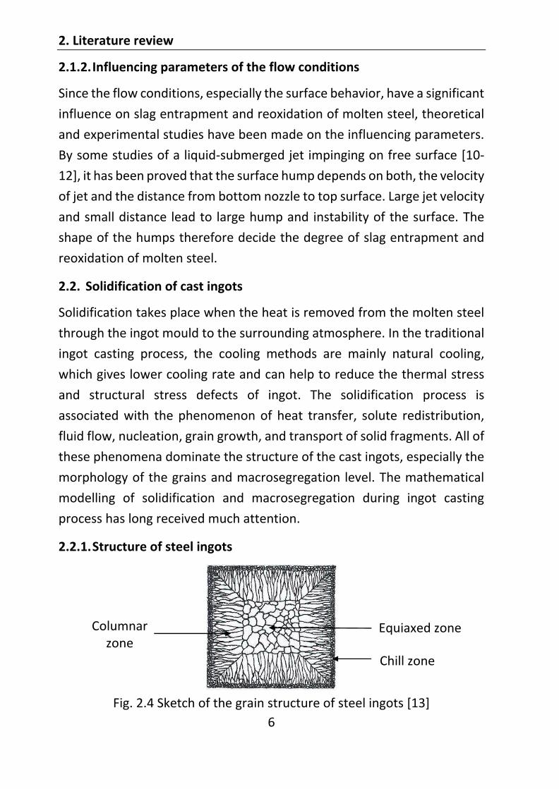
Fig. 2.4 Sketch of the grain structure of steel ingots [13]
Chill zone
Equiaxed zone Columnar zone
2. Literature review
7
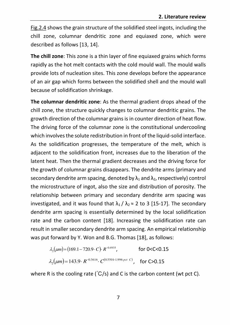
Fig.2.4 shows the grain structure of the solidified steel ingots, including the
chill zone, columnar dendritic zone and equiaxed zone, which were
described as follows [13, 14].
The chill zone: This zone is a thin layer of fine equiaxed grains which forms
rapidly as the hot melt contacts with the cold mould wall. The mould walls
provide lots of nucleation sites. This zone develops before the appearance
of an air gap which forms between the solidified shell and the mould wall
because of solidification shrinkage.
The columnar dendritic zone: As the thermal gradient drops ahead of the
chill zone, the structure quickly changes to columnar dendritic grains. The
growth direction of the columnar grains is in counter direction of heat flow.
The driving force of the columnar zone is the constitutional undercooling
which involves the solute redistribution in front of the liquid-solid interface.
As the solidification progresses, the temperature of the melt, which is
adjacent to the solidification front, increases due to the liberation of the
latent heat. Then the thermal gradient decreases and the driving force for
the growth of columnar grains disappears. The dendrite arms (primary and
secondary dendrite arm spacing, den 1 2, respectively) control
the microstructure of ingot, also the size and distribution of porosity. The
relationship between primary and secondary dendrite arm spacing was
1 2 [15-17]. The secondary
dendrite arm spacing is essentially determined by the local solidification
rate and the carbon content [18]. Increasing the solidification rate can
result in smaller secondary dendrite arm spacing. An empirical relationship
was put forward by Y. Won and B.G. Thomas [18], as follows:
4935.0
2 9.7201.169 RCm , for 0<C<0.15
CpctCRm
996.15501.03616.0
2 9.143 , for C>0.15
where R is the cooling rate ( /s) and C is the carbon content (wt pct C).

2. Literature review
8
2 predicted by
the above equation were compared with measured ones, as shown in
Fig.2.5.
Fig. 2.5 Comparison of the predicted and measured secondary dendrite arm spacing as a function of carbon content at various cooling rates [18]
The equiaxed zone: In the center, due to the low temperature gradient, the
equiaxed grains are formed with large size. During the solidification, if the
liquid in the center of the mould is undercooled sufficiently, grains may
nucleate and grow without contact with any surface. Such grains are also
equiaxed which grow to approximately equal dimensions in all 3
perpendicular directions. The grains in the center can also originate from
the fragment of the columnar dendrites, which may be broken or remelted
by the flow.
During the solidification of molten steel, due to the different solubility of
chemical elements in solid and liquid phase, the solute redistribution takes
place, which leads to regions either enriched in solute or depleted in solute.
Macrosegregation refers to the chemical heterogeneities at length scales
of the order of millimeters or meters, which is a very common defect and
undesirable for casting manufacturers due to the degraded quality and
mechanical properties of steel ingots [19, 20]. Fig.2.6 shows some typical

2. Literature review
9
macrosegregation pattern of steel ingots. In the figure, positive segregation
clearly from the figure that the macrosegregation generally includes the
following zones: positive segregations at the hot-top, cone-shaped
negative segregations at the bottom of ingots, channel-shaped A-
segregations and V-segregations at the center of ingots, also the banding
and inverse segregation region near the cold walls of ingot mould.
Fig. 2.6 Typical macrosegregation pattern of steel ingots [20]
Generally, there are two reasons for the formation of macrosegregation.
One reason is the flow of segregated liquid, including the solidification
shrinkage driven flow, and buoyancy driven flow. The buoyancy driven flow
is caused by the thermal gradient or solutal gradient in the liquid. Another
reason for macrosegregation is the sedimentation of free equiaxed grains
or solid fragments.
The positive segregation appears near the centerline, particularly at the top
of the ingot. It is caused by the buoyancy and shrinkage driven
interdendritic fluid flow during the final stage of solidification, where the
flow is enriched in solute, and therefore the segregation is positive. The
cone-shaped bottom negative segregation is a result of the sedimentation
of equiaxed dendrites, which formed in the early stage of solidification and

2. Literature review
10
poor in solute. The A-segregation is channel shaped and occurs at the end
of columnar zone [21]. It is also related with the buoyancy-driven flow.
Liquid with light element enriched can rise upwards and tend to dissolve
coarse dendrites in its path. As the stream progresses, channels are formed
in this path until the enriched melt freezes. The V-segregation in the center
is associated with large equiaxed grains settling down to the V-shaped
solidification front. The liquid surrounding the solidification front is solute-
rich. Near the end of solidification, due to the lower density of solid phase
than liquid phase and not enough liquid to compensate for solidification
shrinkage, the local pressure drops. Pores are nucleated when the pressure
drop exceeds a critical value [20]. The formation of porosity leads to
decrease in the mechanical properties of ingots. To diminish the shrinkage
porosity by feeding liquid steel as long as possible, the ingot moulds are
always designed with a hot-top, which is wider in upper level and thermally
isolated.
As shown in Fig.2.6, a region of inverse segregation arises near the cold wall
of ingot mould, which is positive segregation and forms due to the motion
of enriched interdendritic fluid towards the wall to feed solidification
shrinkage in the early stage of solidification [20, 22].
Adjacent to the inverse segregation region, several solute-rich or solute-
poor bands have been found. The banding segregation is considered
resulting from the abrupt changes in heat transfer rate. The solute-rich
bands can be formed due to reheating, which may be caused by the
formation of air gap at the mould-ingot interface. The reheating can also
expand the mushy zone, where the solid dendrites and liquid phase coexist
during solidification. The solute-poor bands result from reduction in cross
section through which fluid flow feed shrinkage takes place [20, 23].
2.2.2. Mathematical modelling of the solidification process
The mathematical modelling of solidification process has aroused great
interest. According the coupling method of the fluid flow in the bulk liquid
2. Literature review
12
equations for each phase. Therefore it cannot be simulated by the one-
domain continuum model.
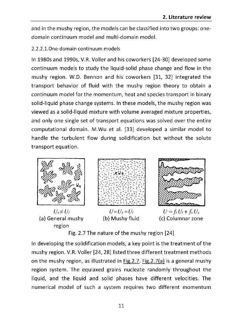
Fig.2.7(b) and Fig.2.7(c) of solid and
liquid. For the assumption of mushy fluid, the solid is fully dispersed in the
liquid phase and the velocities of solid and liquid are equal, so we have
U=Us =Ul. For the assumption of columnar zone, the solid matrix is distinct
from the liquid. The velocity of the mixture system can be calculated based
on the volume fraction with U = fl Ul + fs Us. For the ingot casting, the solid
velocity Us is 0 and then U = fl Ul ; while for the continuous casting, the
solid moves with a pre-described velocity.
To simulate the solidification of ingot casting process, the one-domain
model can be developed based on the assumptions of both mushy fluid and
columnar zone for mushy region. By this approach, only one single set of
governing equations is needed, which is valid not only in the mushy region
but also in the bulk liquid and solid regions.
The previous models are usually under the assumption of constant density
with sl . Then according to the mass fraction relationship of 1sl ff ,
it can be deduced that the liquid and solid volume fractions have the
relationship of 1sl gg .
The mass conservation equation takes the form:
0)( Ut
With constant density, it can be simplified to: 0)(U
The momentum conservation equation depends on the assumed nature of
the mushy region. With the assumption of mushy fluid, the momentum
equation has the form:
gPUUUt
Ueffmix
2. Literature review
13
In the momentum equation, the source due to buoyancy driven flow is
added based on the Boussinesq approximation with [34, 35]:
)]()([ refcrefTeff CCTT
The mixture viscosity mix is defined by llssmix gg . By this way, the
solid viscosity s is set as a very large value.
With the assumption of fixed columnar zone, the momentum equation has
the form:
momeffl SgPUUUt
U
In this equation, the source term Smom due to drag force is concerned, which
can be defined after the Carman-Kozeny equation as follows:
Ug
gKS
l
l
mom 3
2
0 )1(
The energy equation can be expressed by the conservation of enthalpy [24,
28, 36, 37], with the form:
hShc
ht
hU
Where h a function of temperature:
T
Tref
ref
dTchh
The source due to the latent heat of solidification is taken into account by
the use of an additional source term Sh in the energy equation, which also
depends on the assumed nature of the mushy region. With the assumption
of mushy fluid,
)()( ULfLft
S llh
While with the assumption of columnar zone,
2. Literature review
14
)()( ULLft
S lh
The solute transport equation in the case of mushy fluid can be written as:
11
11
)()()(p
sl
p
sls
p
lll
sssssk
UCfk
Cft
Ck
DgDgUCC
t
In the case of columnar zone, the solute transport equation has the form:
slpllllllll ft
CkfCt
CDgUCCt
)1()()()(
At the solid-liquid interface, the concentration of solute in the liquid and
solid phases can be related via lps CkC . Hence the solute transport can be
expressed in terms of the solute concentration in solid phase sC or in liquid
phase lC , resulting in different source terms on the right side of the above
two solute transport equations.
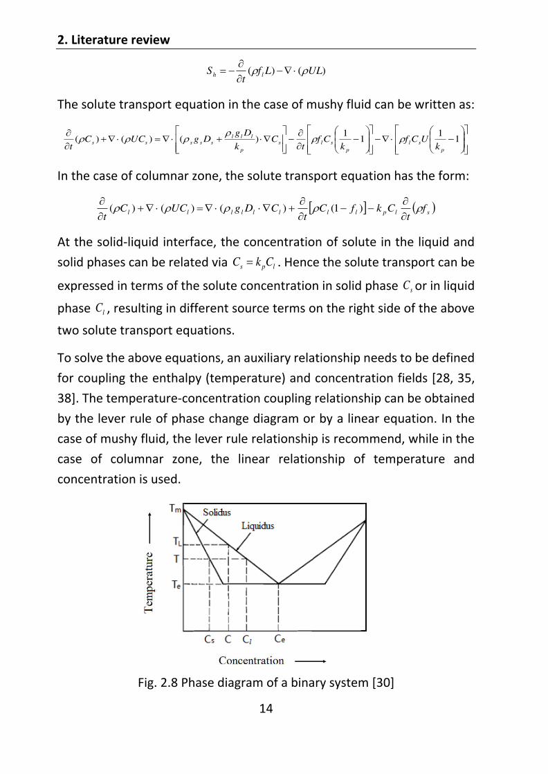
To solve the above equations, an auxiliary relationship needs to be defined
for coupling the enthalpy (temperature) and concentration fields [28, 35,
38]. The temperature-concentration coupling relationship can be obtained
by the lever rule of phase change diagram or by a linear equation. In the
case of mushy fluid, the lever rule relationship is recommend, while in the
case of columnar zone, the linear relationship of temperature and
concentration is used.
Fig. 2.8 Phase diagram of a binary system [30]

2. Literature review
16
56] developed a solidification model using Eulerian-Eulerian multiphase
approach and verified it by NH4Cl-H2O solidification experiment.
2.3. Introduction of the OpenFOAM software
To study the flow fields, Computational Fluid Dynamics (CFD) methodology
has been widely used. OpenFOAM is a kind of CFD software, and its name
comes from Open Source Field Operation and Manipulation. The greatest
strengths of OpenFOAM is that it is a free and open source software. The
highly capable free CFD codes can be applied to a wide variety of flow types,
and even to non-fluids applications, which make it possible to simulate
phase change such as solidification. The programming language of
OpenFOAM is C++ and it runs on Linux system.
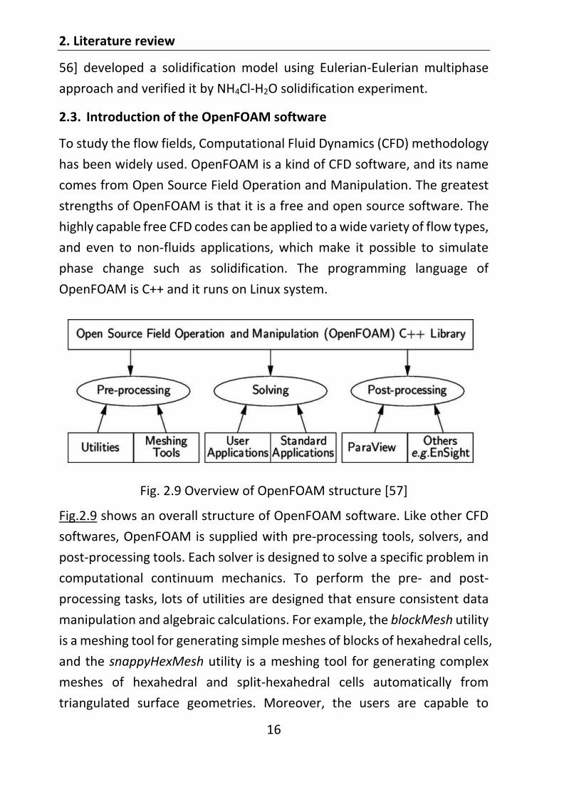
Fig. 2.9 Overview of OpenFOAM structure [57]
Fig.2.9 shows an overall structure of OpenFOAM software. Like other CFD
softwares, OpenFOAM is supplied with pre-processing tools, solvers, and
post-processing tools. Each solver is designed to solve a specific problem in
computational continuum mechanics. To perform the pre- and post-
processing tasks, lots of utilities are designed that ensure consistent data
manipulation and algebraic calculations. For example, the blockMesh utility
is a meshing tool for generating simple meshes of blocks of hexahedral cells,
and the snappyHexMesh utility is a meshing tool for generating complex
meshes of hexahedral and split-hexahedral cells automatically from
triangulated surface geometries. Moreover, the users are capable to
2. Literature review
17
convert a mesh that has been generated by a third-party software into a
format that OpenFOAM can read. After the calculation, the results are
obtained and listed in a set of time files. The post-processing utilities are
used to present the results. One of the post-processing utility is paraFoam
that uses ParaView, which is an open source third-party software. Also
other utilities are offered, including EnSight, Fieldview and the post-
processing supplied with Fluent.
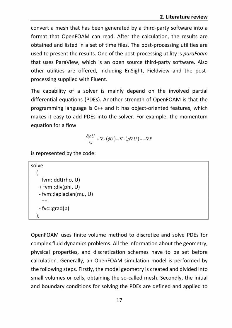
The capability of a solver is mainly depend on the involved partial
differential equations (PDEs). Another strength of OpenFOAM is that the
programming language is C++ and it has object-oriented features, which
makes it easy to add PDEs into the solver. For example, the momentum
equation for a flow
PUUt
U
is represented by the code:
solve ( fvm::ddt(rho, U) + fvm::div(phi, U) - fvm::laplacian(mu, U) == - fvc::grad(p)
);
OpenFOAM uses finite volume method to discretize and solve PDEs for
complex fluid dynamics problems. All the information about the geometry,
physical properties, and discretization schemes have to be set before
calculation. Generally, an OpenFOAM simulation model is performed by
the following steps. Firstly, the model geometry is created and divided into
small volumes or cells, obtaining the so-called mesh. Secondly, the initial
and boundary conditions for solving the PDEs are defined and applied to

2. Literature review
18
the geometry. Thirdly, the discretization schemes, time steps, data output
parameters are specified. Then the OpenFOAM solver is applied to the
model case, and the calculation results are presented using a post-
processing tool. More details about OpenFOAM can be found in the
OpenFOAM User Guide [57] [58].
OpenFOAM is supplied with several standard solvers which are used mainly
for CFD, for example, multiphase flow, incompressible and compressible
flow. So far, no standard solver has been released to simulate solidification
phenomenon. Even so, some projects on the simulation of solidification
with OpenFOAM software is already in progress, which refers to the
coupling of fluid flow with solidification, heat transfer, nucleation and
segregation.
OpenFOAM software is an excellent tool to tackle multi-physics problems,
which is also capable of simulating certain metallurgical process, such as
tundish filling, slag coverage of steel surface, mixing after ladle change. In
addition, B. Peters and his coworkers [59, 60] dedicated to the Extended
Discrete Element Method (XDEM), coupling to OpenFOAM to handle multi-
phase flow with granular materials or particles, by which method the
packed bed is modeled as a flow through a porous medium. The dripping
zone and cohesive zone of blast furnace have also been simulated, with
multi-phase flow, heat transfer and chemical reactions involved.
2.4. Objective and methods of the study
The flow conditions during the filling process has a crucial influence on the
quality of the solidified steel ingot. In this study the bottom teeming
process was concerned as the filling method. From the previous physical
and mathematical modeling of bottom teeming process, most of these
studies deal with small ingots, which have only one nozzle at the bottom of
the ingot mould. Few studies on large ingot with multiple bottom nozzles
have been reported in literatures. In this study, the initial filling conditions
2. Literature review
19
for the mould of a 60-tonne large steel ingot with 4 bottom nozzles were
investigated, by both water modelling and numerical simulation.
In the water model experiments, a layer of oil was added to the water
phase to study the behavior of the steel-slag interface. The water-air-oil
three-phase flow was investigated to describe how the flow conditions are
influenced by the model parameters such as filling rate, nozzle dimension,
thickness. Finally, the model parameters were optimized to
obtain better filling conditions.
The numerical simulation of filling process was performed with OpenFOAM
software to get more quantitative information about the flow field,
especially the velocity field which is directly related to the phenomenon of
surface turbulence and slag entrapment.
To study the solidification process, a solidification model was developed.
Since the one-domain continuum model, which has only one set of
governing equations, cannot correctly simulate the nucleation of solid
particles and the movement of solid dendrites, therefore it gives
unsatisfactory prediction of macrosegregation. In this study, an Euler-Euler
two-phase approach was used to develop a solidification model based on
OpenFOAM software. Then the solidification model was performed on a
reported steel ingot and the results was compared with experimental
measurements from literature.
3. Water model experiments of the mould filling process
20
3. Water model experiments of the mould filling process
To study the fluid flow conditions during the mould filling process, water
model experiments were carried out on water-air two-phase flow and
water-air-oil three-phase flow, where water was used to simulate the
molten steel as they have a similar kinematic viscosity, and vegetable oil
was used to study the fused slag. The density and viscosity of water,
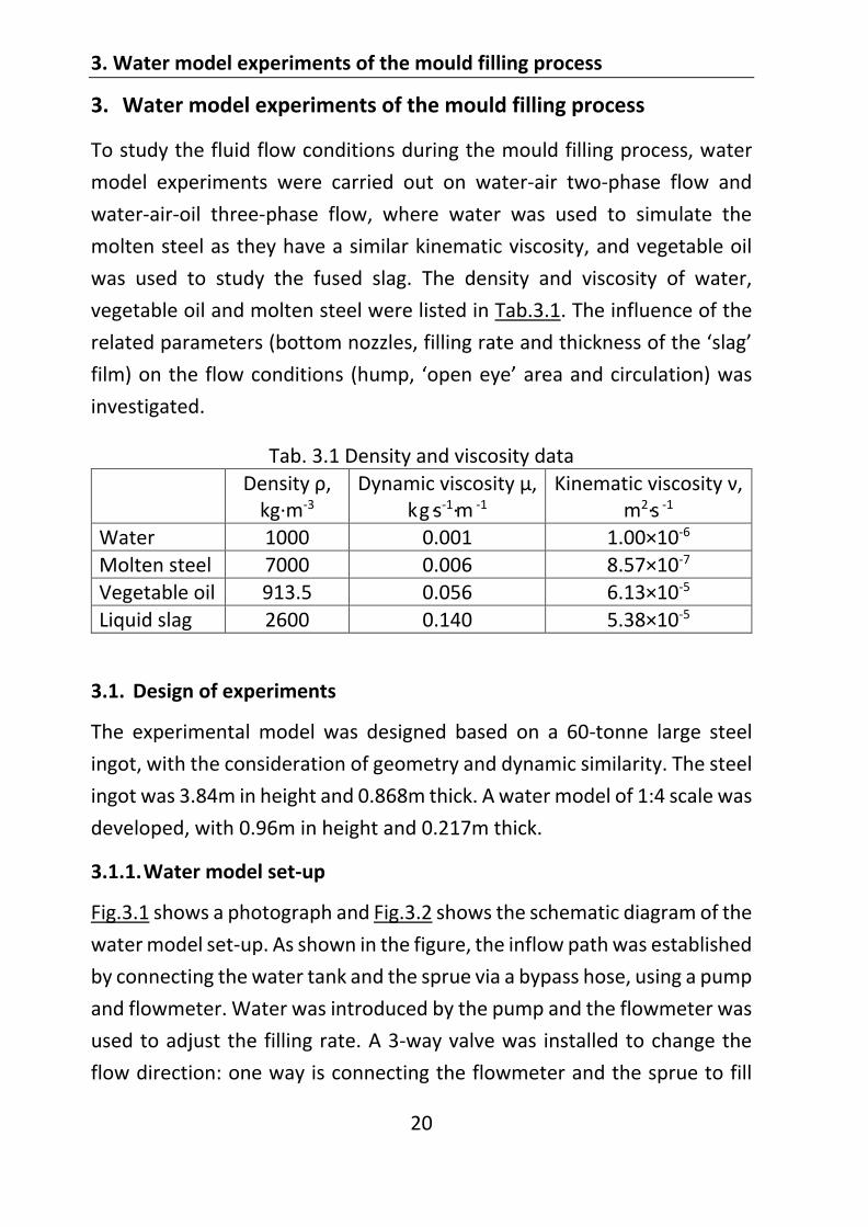
vegetable oil and molten steel were listed in Tab.3.1. The influence of the
investigated.
Tab. 3.1 Density and viscosity data
Densi
kg·m-3 Dynamic viscosity ,
kg·s-1·m -1
m2·s -1 Water 1000 0.001 1.00×10⁻⁶ Molten steel 7000 0.006 8.57×10⁻⁷ Vegetable oil 913.5 0.056 6.13×10⁻⁵ Liquid slag 2600 0.140 5.38×10⁻⁵
3.1. Design of experiments
The experimental model was designed based on a 60-tonne large steel
ingot, with the consideration of geometry and dynamic similarity. The steel
ingot was 3.84m in height and 0.868m thick. A water model of 1:4 scale was
developed, with 0.96m in height and 0.217m thick.
3.1.1. Water model set-up
Fig.3.1 shows a photograph and Fig.3.2 shows the schematic diagram of the
water model set-up. As shown in the figure, the inflow path was established
by connecting the water tank and the sprue via a bypass hose, using a pump
and flowmeter. Water was introduced by the pump and the flowmeter was
used to adjust the filling rate. A 3-way valve was installed to change the
flow direction: one way is connecting the flowmeter and the sprue to fill

3. Water model experiments of the mould filling process
21
the mould; the other way is making a water loop between the flowmeter
and the water tank, and then adjusting the flowmeter to obtain a constant
filling rate. The sprue, runner and mould were made of plexiglass due to its
good mechanical properties and transmittance. In order to study the
influence of nozzle dimensions on flow conditions, the nozzles on the
bottom plate of the mould were changeable.
Fig. 3.1 A photograph of the experimental set-up
Fig. 3.2 Schematic diagram of the water model set-up
In the real ingot casting process, casting powder melts into liquid slag after
getting contact with molten steel. However, the melting process cannot be
investigated by water modeling. Due to limited heat transfer, the melting
velocity decreases with increasing thickness of slag layer. Turbulence at the
steel-slag interface promotes the melting of mould powder. According to
3. Water model experiments of the mould filling process
22
the measurement of Kromhout [61] and Görnerup et al. [62], the melting
rate of mould powder is about 0.1mm/s irrespective of the slag layer
thickness. Therefore, the melting time of mould powder can be neglected.
To get a preliminary understanding of the steel-slag interface behavior by
water modeling, vegetable oil was used to simulate the liquid slag, without
consideration of the melting time. During the teeming process, a layer of
oil with dissolved pigment was added on the top surface of water and then
more water flowed into the mould through the bottom nozzles. Two video
cameras were used to record the flow characteristics from the front view
and top view respectively. The filling rate, nozzle dimensions and oil
thickness were studied concerning the flow conditions and surface
behaviors.
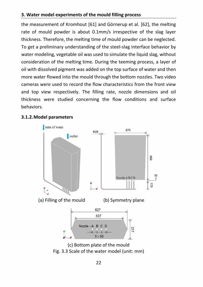
3.1.2. Model parameters
(a) Filling of the mould (b) Symmetry plane
(c) Bottom plate of the mould Fig. 3.3 Scale of the water model (unit: mm)

3. Water model experiments of the mould filling process
23
The prototype of the ingot mould came from a steel plant. It was used to
produce 60-tonne large steel ingots, and the mould was big-end-up, with 4
nozzles at the bottom plate of the mould. Based on the real ingot mould
and the gating system, a physical water model was designed in reduced
scale 1:4. Fig.3.3 shows a schematic diagram of the scale of the water
model. As shown in Fig.3.3(a), water is directed into the mould cavity
through four bottom nozzles. In order to distinguish the four nozzles, we
call them nozzle A, B, C, D respectively, as marked in Fig.3.3(c).
Besides the geometry similarity, the dynamic similarity between the
prototype and model is also important, which can be achieved by the
similarity in Reynolds number, Froude number and Weber number.
However, it is not possible to satisfy all of the three similarities
simultaneously for a reduced-scale model. The filling rate of molten steel is
about 1.0~1.8t/min for the ingot bottom teeming process, and the
corresponding Reynolds number can reach up to 6×10⁴, which represents
a fully developed turbulent flow. It was suggested that Reynolds similarity
is insignificant for such a fully developed turbulent flow [63, 64]. Weber
number is useful in analyzing fluid flow with interface between two fluids.
The present work aims to study the behavior of the steel-slag interface, and
therefore Weber similarity is the best choice. Weber number represents
the ratio between inertial force and surface tension force, which is defined
as:
LuWe
2
Where u is velocity; L is characteristic length; is density; is surface
tension. For molten steel, = 7000kg/m3 and = 1.6N/m; for water, =
1000kg/m3 and = 0.073N/m. Based on the Weber similarity and the filling
rate of 1.0~1.8t/min in real ingot bottom teeming process, the filling rate
of water is about 10.1~18.2L/min. In order to investigate the influence of
filling rate on the flow conditions, the filling rates of 10L/min, 15L/min and
19L/min were studied in water model experiments.

3. Water model experiments of the mould filling process
24
Besides the filling rate, the design of bottom nozzles is also important for
the flow field. In this model, the bottom nozzles are changeable and
different sizes of nozzles were used.
3.1.3. Experimental procedure
In the experiment, the control variable method was used to investigate the
influence of operation parameters on the flow conditions (filling rate,
number of nozzles, nozzle dimensions and oil thickness). Two types of
models were conducted, one with only one nozzle at the bottom plate of
the mould and the other with four bottom nozzles. Appropriate filling rates
were chosen: 10L/min, 15L/min, 19L/min for four-nozzle model; 6L/min,
8L/min, 12L/min for one-nozzle model. The initial water level in the mould
was about 10cm. The thickness of added oil layer changed from 1cm to 3cm.
Besides these filling variables, the design of bottom nozzles is also
important for the flow field. In this experiment, eight groups of nozzle
dimensions were studied, as listed in Tab.3.2.
Tab. 3.2 Diameters of the nozzles used in the experiments (unit: mm) Nozzle A Nozzle B Nozzle C Nozzle D Group 1 blocked 22.5 blocked blocked Group 2 15.0 15.0 15.0 15.0 Group 3 22.5 22.5 22.5 22.5 Group 4 25.0 25.0 25.0 25.0 Group 5 12.5 15.0 22.5 25.0 Group 6 25.0 22.5 15.0 12.5 Group 7 25.0 25.0 12.5 12.5 Group 8 12.5 12.5 25.0 25.0
In Group 1, besides Nozzle B the other three nozzles were blocked. The
diameters of the four nozzles were the same in Group 2-4. In Group 5, the
diameters of the four nozzles were arranged in ascending order from nozzle
A to D, however that were arranged in descending order in Group 6. Fig.3.4
3. Water model experiments of the mould filling process
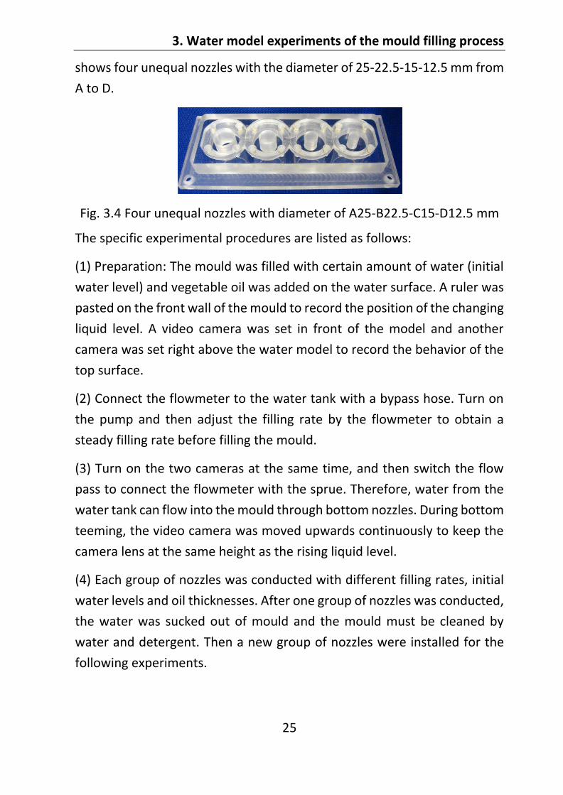
25
shows four unequal nozzles with the diameter of 25-22.5-15-12.5 mm from
A to D.
Fig. 3.4 Four unequal nozzles with diameter of A25-B22.5-C15-D12.5 mm
The specific experimental procedures are listed as follows:
(1) Preparation: The mould was filled with certain amount of water (initial
water level) and vegetable oil was added on the water surface. A ruler was
pasted on the front wall of the mould to record the position of the changing
liquid level. A video camera was set in front of the model and another
camera was set right above the water model to record the behavior of the
top surface.
(2) Connect the flowmeter to the water tank with a bypass hose. Turn on
the pump and then adjust the filling rate by the flowmeter to obtain a
steady filling rate before filling the mould.
(3) Turn on the two cameras at the same time, and then switch the flow
pass to connect the flowmeter with the sprue. Therefore, water from the
water tank can flow into the mould through bottom nozzles. During bottom
teeming, the video camera was moved upwards continuously to keep the
camera lens at the same height as the rising liquid level.
(4) Each group of nozzles was conducted with different filling rates, initial
water levels and oil thicknesses. After one group of nozzles was conducted,
the water was sucked out of mould and the mould must be cleaned by
water and detergent. Then a new group of nozzles were installed for the
following experiments.
3. Water model experiments of the mould filling process
26
(5) The videos were imported to a computer and analyzed with GIMP, Excel
and Origin software.
3.2. Results about the models with one bottom nozzle
With the nozzle of Group 1 (the diameter of Nozzle B was 22.5mm and the
other three nozzles were blocked), different tests were carried out to study
the influence of filling rate and oil thickness on the filling conditions.
3.2.1. Water-air two-phase flow without oil addition
When water flows into the mould, the incoming flow through the bottom
nozzle with high speed will generate a water jet to spread out to the mould.
As the liquid level rises in the mould, the impact force of the jet on the
surface will lead to a hump right above the nozzle, also turbulent surface.
It was observed in water model experiments that the variation of
turbulence degree with liquid level was consistent with the variation of
hump size. Strong surface turbulence and large humps were observed at
low liquid level. For quantitative description, hump height ( H) is
introduced as a parameter to evaluate the surface behavior. The hump
height is defined as the difference of the maximum height above nozzle
(Hm) and the liquid level (H), i.e. H= Hm-H (see Fig.3.5).
With the fixed nozzles, the hump height H is related with the filling rate.
Fig.3.6 shows the influence of filling rate on the hump height with rising
liquid level. As shown in the figure, the hump height decreases with the
decrease of filling rate, and with the increase of liquid level. In Fig.3.6(a),
regression analysis based on the water model experimental data describes
the relationship between the hump height, liquid level, and filling rate. The
regression lines satisfy the equation:
VHdVcHbaH
Where H represents the hump height with unit mm; H represents the
liquid level with unit m; V represents the filling rate with unit L/min. The
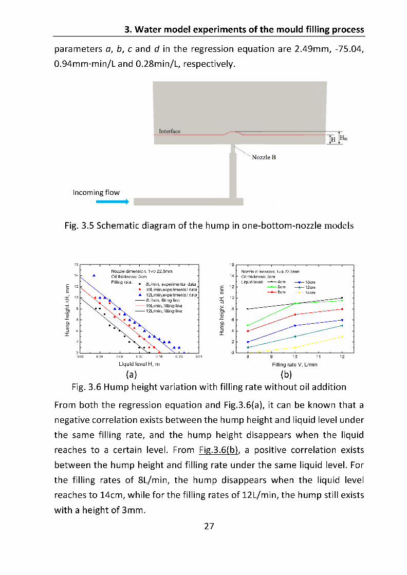
3. Water model experiments of the mould filling process
28
The influence of filling rate and liquid level on the hump height is easy to
understand, since the hump height depends on the impact force of the jet
on the top surface. A larger filling rate brings more energy to impact the
surface thus results in larger hump. The impact force of the jet is reduced
with the increasing distance between the bottom nozzle and the top water
level. As the water level rises, the hump height gradually declines to 0.
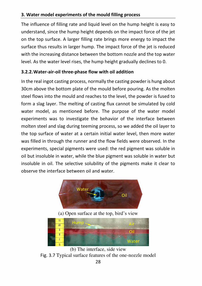
3.2.2. Water-air-oil three-phase flow with oil addition
In the real ingot casting process, normally the casting powder is hung about
30cm above the bottom plate of the mould before pouring. As the molten
steel flows into the mould and reaches to the level, the powder is fused to
form a slag layer. The melting of casting flux cannot be simulated by cold
water model, as mentioned before. The purpose of the water model
experiments was to investigate the behavior of the interface between
molten steel and slag during teeming process, so we added the oil layer to
the top surface of water at a certain initial water level, then more water
was filled in through the runner and the flow fields were observed. In the
experiments, special pigments were used: the red pigment was soluble in
oil but insoluble in water, while the blue pigment was soluble in water but
insoluble in oil. The selective solubility of the pigments make it clear to
observe the interface between oil and water.
(a) Open surface at the top
(b) The interface, side view
Fig. 3.7 Typical surface features of the one-nozzle model
Oil
Water
Air
Oil
Water
Hump

3. Water model experiments of the mould filling process
29
Fig.3.7 shows the typical surface features of the one-nozzle model. As
shown in Fig.3.7(a), the oil layer was open during teeming, developing an
open eye of eye
nozzle, and it was formed due to the upward water jet from the bottom
nozzle eye
indicates that the molten steel may be exposed to air without the
protection of slag. Therefore, the fraction of the open surface , defined
as the ratio between the area of water exposed to air Aopen and the total
area of liquid surface Abath, i.e. bathopenos AAf / , is an important parameter to
evaluate the risk of reoxidation. Fig.3.7(a) was obtained from the top view,
while Fig.3.7(b) from the front view. As observed in Fig.3.7(b), the water
hump was exposed to air, and some oil droplets were entrapped in the
water phase, which was related to the phenomenon of slag entrapment in
ingot casting process.
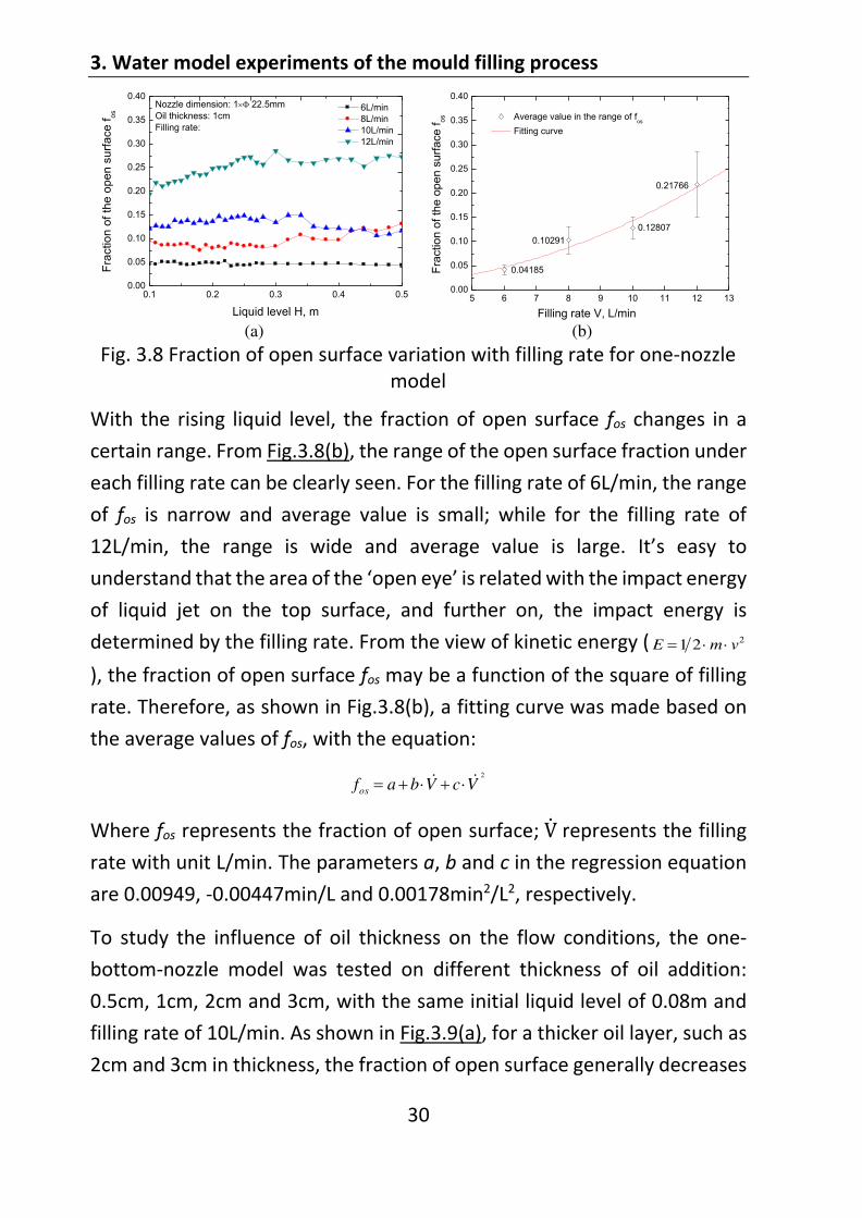
For a model with fixed bottom nozzles, the filling rate and oil thickness are
two important parameters to decide the surface behaviors. To study the
influence of filling rate, the one-bottom-nozzle model was tested on
different filling rates: 6L/min, 8L/min, 10L/min and 12L/min, with the same
initial liquid level of 0.08m and 1cm-thick oil. As illustrated in Fig.3.8(a), at
the same liquid level, the fraction of open surface increases with increasing
filling rate, which shows a consistent trend with the hump height. For the
filling rate of 6L/min, it shows that the fraction of open surface has no
significant change with rising liquid level. For the filling rate of 8L/min, the
fraction of open surface maintains steady firstly and then shows an
ascending trend during the mould filling at high liquid level. For the filling
rate of 10L/min and 12L/min, the fraction of open surface increases at the
beginning and then reaches a steady state with rising liquid level. The open
surface fraction for 12L/min filling rate is the largest, which indicates that
it has the greatest risk of reoxidation with a high filling rate.
3. Water model experiments of the mould filling process
30
0.1 0.2 0.3 0.4 0.50.00
0.05
0.10
0.15
0.20
0.25
0.30
0.35
0.40F
ractio
n o
f th
e o
pe
n s
urf
ace
fo
s
Liquid level H, m
6L/min
8L/min
10L/min
12L/min
Nozzle dimension: 1 22.5mm
Oil thickness: 1cm
Filling rate:
5 6 7 8 9 10 11 12 13
0.00
0.05
0.10
0.15
0.20
0.25
0.30
0.35
0.40
0.21766
0.12807
0.10291
Average value in the range of fos
Fitting curve
0.04185
Filling rate V, L/min
Fra
ction o
f th
e o
pen
surf
ace
fo
s
(a) (b)
Fig. 3.8 Fraction of open surface variation with filling rate for one-nozzle model
With the rising liquid level, the fraction of open surface fos changes in a
certain range. From Fig.3.8(b), the range of the open surface fraction under
each filling rate can be clearly seen. For the filling rate of 6L/min, the range
of fos is narrow and average value is small; while for the filling rate of
12L/min, the range is wide and average value is large.
understand that the area of the is related with the impact energy
of liquid jet on the top surface, and further on, the impact energy is
determined by the filling rate. From the view of kinetic energy ( 221 vmE
), the fraction of open surface fos may be a function of the square of filling
rate. Therefore, as shown in Fig.3.8(b), a fitting curve was made based on
the average values of fos, with the equation:
2
VcVbafos
Where fos represents the fraction of open surface; represents the filling
rate with unit L/min. The parameters a, b and c in the regression equation
are 0.00949, -0.00447min/L and 0.00178min2/L2, respectively.
To study the influence of oil thickness on the flow conditions, the one-
bottom-nozzle model was tested on different thickness of oil addition:
0.5cm, 1cm, 2cm and 3cm, with the same initial liquid level of 0.08m and
filling rate of 10L/min. As shown in Fig.3.9(a), for a thicker oil layer, such as
2cm and 3cm in thickness, the fraction of open surface generally decreases
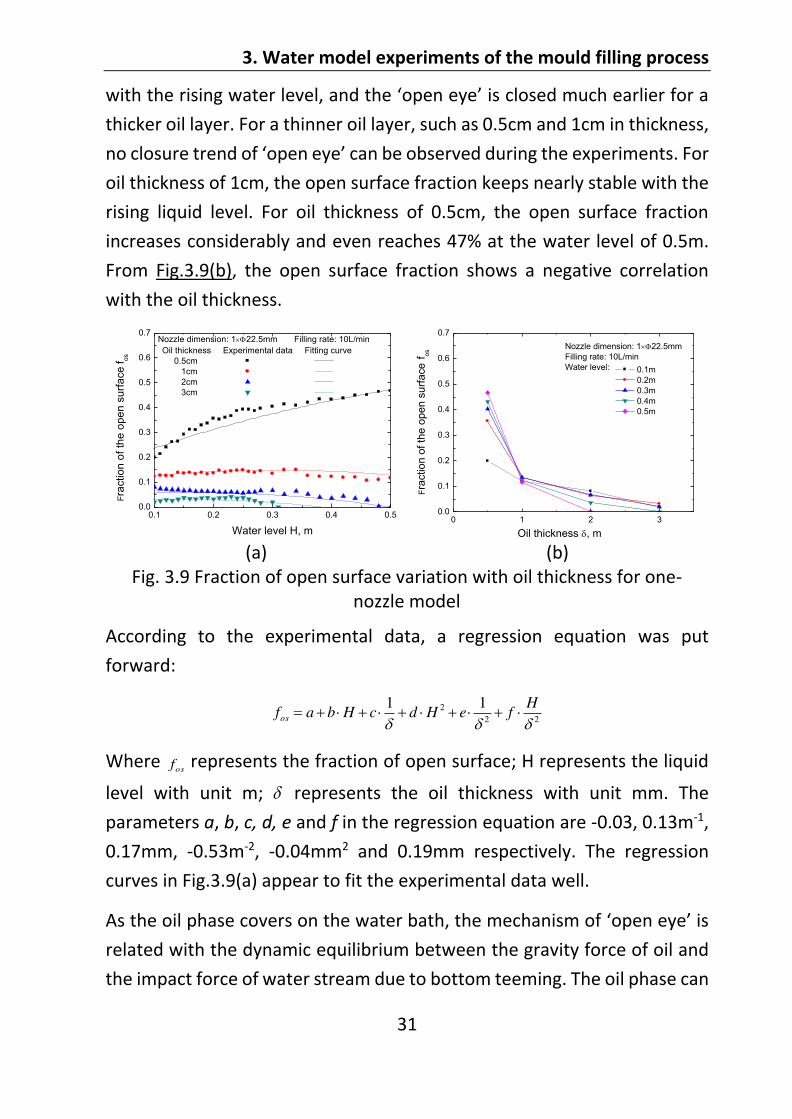
3. Water model experiments of the mould filling process
31
thicker oil layer. For a thinner oil layer, such as 0.5cm and 1cm in thickness,
no closure trend of open can be observed during the experiments. For
oil thickness of 1cm, the open surface fraction keeps nearly stable with the
rising liquid level. For oil thickness of 0.5cm, the open surface fraction
increases considerably and even reaches 47% at the water level of 0.5m.
From Fig.3.9(b), the open surface fraction shows a negative correlation
with the oil thickness.
0.1 0.2 0.3 0.4 0.50.0
0.1
0.2
0.3
0.4
0.5
0.6
0.7
Fra
ctio
n o
f th
e o
pe
n s
urf
ace
fo
s
Water level H, m
Oil thickness Experimental data Fitting curve
0.5cm
1cm
2cm
3cm
Nozzle dimension: 1 22.5mm Filling rate: 10L/min
0 1 2 3
0.0
0.1
0.2
0.3
0.4
0.5
0.6
0.7
0.1m
0.2m
0.3m
0.4m
0.5m
Nozzle dimension: 1 22.5mm
Filling rate: 10L/min
Water level:
Oil thickness , m
Fra
ction o
f th
e o
pen s
urf
ace
fo
s
(a) (b)
Fig. 3.9 Fraction of open surface variation with oil thickness for one-nozzle model
According to the experimental data, a regression equation was put
forward:
22
2 11 HfeHdcHbafos
Where osf represents the fraction of open surface; H represents the liquid
level with unit m; represents the oil thickness with unit mm. The
parameters a, b, c, d, e and f in the regression equation are -0.03, 0.13m-1,
0.17mm, -0.53m-2, -0.04mm2 and 0.19mm respectively. The regression
curves in Fig.3.9(a) appear to fit the experimental data well.
As the oil phase covers on the water bath, the mechanism of
related with the dynamic equilibrium between the gravity force of oil and
the impact force of water stream due to bottom teeming. The oil phase can

3. Water model experiments of the mould filling process
32
be treated as some parallel layers of fluid with high viscosity. The upward
water stream tends to break the oil layers from the bottom up to form
, while the top oil layers tends to make up the lower breaking
area due to gravity force. Therefore, a thicker oil film has more capacity to
counteract the impact force of water stream, which in turn causes a small
as consistent with Fig.3.9. Moreover, since the impace force of
water jet on top surface is reduced with the rising water level, the water
phase may be totally covered with the oil phase after reaching to a certain
level, which takes places only under the condition of enough oil thickness.
If the oil film is too thin, the inward flowing of oil due to gravity will be
weaker than the outward extension of which is caused by the
enlarging outward component force of water stream with rising water
level. As shown in Fig.3.9(a), the open surface fraction increases
considerably with rising water level when oil thickness is 0.5cm. In addition,
even at a high water level where the influence of water jet can be ignored,
water-oil interface, in particular under the condition of less oil addition.
3.3. Results about the models with four bottom nozzles
With a constant filling rate, the total volumetric flow rate streaming into
the mould is also constant. For a model with more bottom nozzles, the total
flow will be distributed to all the bottom nozzles. Therefore, for a model
with four bottom nozzles, the jet velocities through each nozzle become
smaller than that for a one-bottom-nozzle model. In this section, the flow
fields for the model with four bottom nozzles were studied. The dimensions
and arrangement of the nozzles were expected to influence the flow
conditions. Similarly to the one-bottom-nozzle model, the filling rate and
oil thickness also have influence on the filling conditions for the four-
bottom-nozzle models.

3. Water model experiments of the mould filling process
33
3.3.1. Features of the flow fields
For four-bottom-nozzle models, there are four humps at water-oil interface
and each hump corresponds to one bottom nozzle. The hump height is
related to the position of bottom nozzles. As observed in water models with
four equal bottom nozzles (see Tab.3.2, nozzles of Group 2, 3, 4), the hump
height above nozzle A is the smallest and that above nozzle D is the largest
at the same liquid level. The degree of turbulence and slag entrapment has
a positive correlation with the hump height, therefore, only the maximum
hump height was concerned in this work. As shown in Fig.3.10, the
maximum hump height H was defined again as the difference of the
maximum height above nozzle D (Hm) and the liquid level (H), i.e. H=Hm-H.
Fig. 3.10 Schematic of the humps in four-equal-bottom-nozzle models
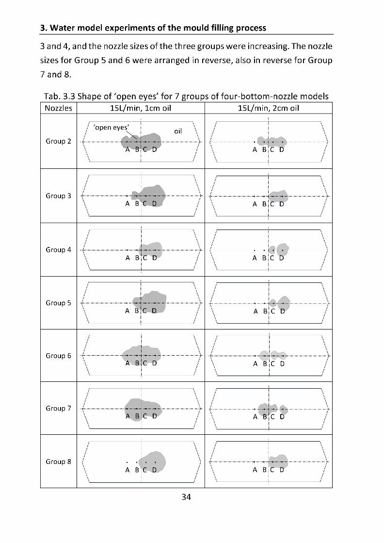
For the model with four bottom nozzles, the water jet from each nozzle
may break through the oil layer to form an
various forms of the open surface, such as a continuous region or four
separated
rising liquid level. Tab.3.3 lists the shape of the
of four-bottom-nozzle models, at the same water level of 0.15m, with the
same filling rate of 15L/min and oil thickness of 1cm or 2cm. In the figures,
the grey regions represent regions denote
that the surface is covered with oil phase. The vertical mapping points of
the centers of the four bottom nozzles A, B, C and D were marked in the
figures. As a supplement, Tab.3.4 gives the nozzle diameters used in the
seven groups of models. Four equal bottom nozzles were used in Group 2,
Incoming flow

3. Water model experiments of the mould filling process
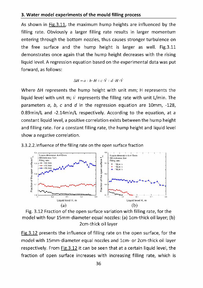
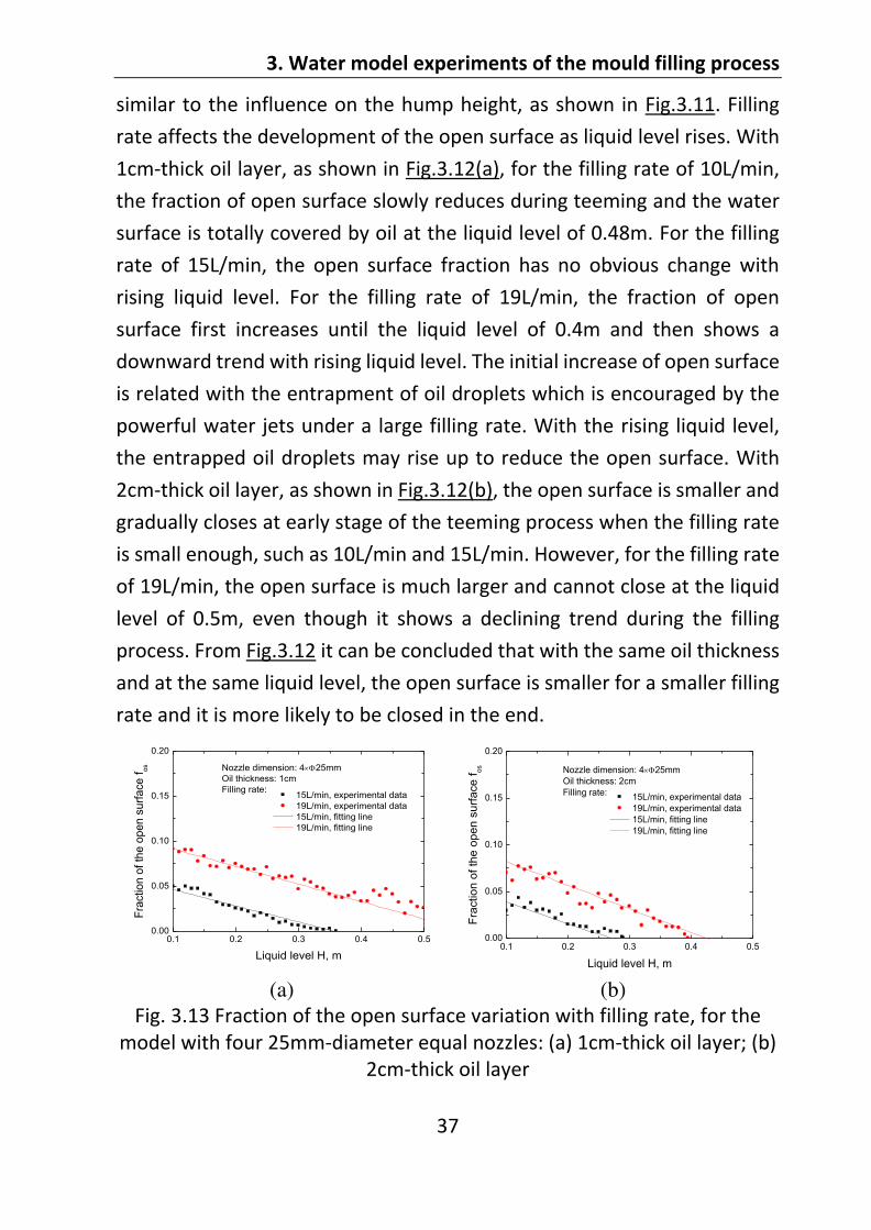
37
similar to the influence on the hump height, as shown in Fig.3.11. Filling
rate affects the development of the open surface as liquid level rises. With
1cm-thick oil layer, as shown in Fig.3.12(a), for the filling rate of 10L/min,
the fraction of open surface slowly reduces during teeming and the water
surface is totally covered by oil at the liquid level of 0.48m. For the filling
rate of 15L/min, the open surface fraction has no obvious change with
rising liquid level. For the filling rate of 19L/min, the fraction of open
surface first increases until the liquid level of 0.4m and then shows a
downward trend with rising liquid level. The initial increase of open surface
is related with the entrapment of oil droplets which is encouraged by the
powerful water jets under a large filling rate. With the rising liquid level,
the entrapped oil droplets may rise up to reduce the open surface. With
2cm-thick oil layer, as shown in Fig.3.12(b), the open surface is smaller and
gradually closes at early stage of the teeming process when the filling rate
is small enough, such as 10L/min and 15L/min. However, for the filling rate
of 19L/min, the open surface is much larger and cannot close at the liquid
level of 0.5m, even though it shows a declining trend during the filling
process. From Fig.3.12 it can be concluded that with the same oil thickness
and at the same liquid level, the open surface is smaller for a smaller filling
rate and it is more likely to be closed in the end.
0.1 0.2 0.3 0.4 0.50.00
0.05
0.10
0.15
0.20
Fra
ctio
n o
f th
e o
pen
su
rfa
ce
fos
Liquid level H, m
15L/min, experimental data
19L/min, experimental data
15L/min, fitting line
19L/min, fitting line
Nozzle dimension: 4 25mm
Oil thickness: 1cm
Filling rate:
0.1 0.2 0.3 0.4 0.5
0.00
0.05
0.10
0.15
0.20
Fra
ction o
f th
e o
pen
surf
ace f
os
Liquid level H, m
15L/min, experimental data
19L/min, experimental data
15L/min, fitting line
19L/min, fitting line
Nozzle dimension: 4 25mm
Oil thickness: 2cm
Filling rate:
(a) (b)
Fig. 3.13 Fraction of the open surface variation with filling rate, for the model with four 25mm-diameter equal nozzles: (a) 1cm-thick oil layer; (b)
2cm-thick oil layer


3. Water model experiments of the mould filling process
44
diameter nozzles. Even though the jet velocity is the largest for the model
with four 15mm-diameter equal nozzles, the total area of bottom nozzles
are the smallest. However, for the model with four 22.5mm-diameter equal
nozzles, both the jet velocity and the total area of bottom nozzles are
relatively large, which leads to the largest open surface.
0.1 0.2 0.3 0.4 0.50.00
0.05
0.10
0.15
0.20
0.25
0.30
0.35
Fra
ctio
n o
f th
e o
pe
n s
urf
ace
fo
s
Liquid level H, m
12.5-15-22.5-25
25-22.5-15-12.5
25-25-12.5-12.5
12.5-12.5-25-25
Filling rate: 15L/min
Oil thickness: 1cm
Nozzle dimension:
0.1 0.2 0.3 0.4 0.50.00
0.05
0.10
0.15
0.20
0.25
0.30
0.35
12.5-15-22.5-25
25-22.5-15-12.5
25-25-12.5-12.5
12.5-12.5-25-25
Filling rate: 19L/min
Oil thickness: 1cm
Nozzle dimension:Fra
ctio
n o
f t
he
op
en
su
rfa
ce
fo
s
Liquid level H, m
(a) (b)
0.1 0.2 0.3 0.4 0.50.00
0.05
0.10
0.15
0.20
0.25
0.30
0.35
Liquid level H, m
Fra
ction o
f th
e o
pen s
urf
ace
fo
s
12.5-15-22.5-25
25-22.5-15-12.5
25-25-12.5-12.5
12.5-12.5-25-25
Filling rate: 15L/min
Oil thickness: 2cm
Nozzle dimension:
0.1 0.2 0.3 0.4 0.5
0.00
0.05
0.10
0.15
0.20
0.25
0.30
0.35
12.5-15-22.5-25
25-22.5-15-12.5
25-25-12.5-12.5
12.5-12.5-25-25
Filling rate: 19L/min
Oil thickness: 2cm
Nozzle dimension:
Fra
ctio
n o
f th
e o
pe
n s
urf
ace
fo
s
Liquid level H, m (c) (d)
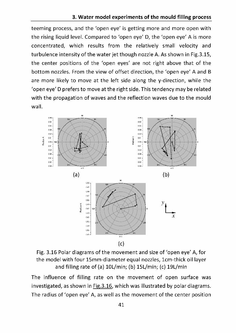
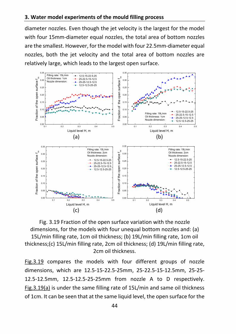
Fig. 3.19 Fraction of the open surface variation with the nozzle dimensions, for the models with four unequal bottom nozzles and: (a) 15L/min filling rate, 1cm oil thickness; (b) 19L/min filling rate, 1cm oil
thickness;(c) 15L/min filling rate, 2cm oil thickness; (d) 19L/min filling rate, 2cm oil thickness.
Fig.3.19 compares the models with four different groups of nozzle
dimensions, which are 12.5-15-22.5-25mm, 25-22.5-15-12.5mm, 25-25-
12.5-12.5mm, 12.5-12.5-25-25mm from nozzle A to D respectively.
Fig.3.19(a) is under the same filling rate of 15L/min and same oil thickness
of 1cm. It can be seen that at the same liquid level, the open surface for the
3. Water model experiments of the mould filling process
45
model with 12.5-15-22.5-25mm nozzles is smaller than that for the model
with 25-22.5-15-12.5mm nozzles, and the open surface for the model with
12.5-12.5-25-25mm nozzles is smaller than that for the model with 25-25-
12.5-12.5mm nozzles. Therefore, it can be concluded that under this filling
condition, the nozzle dimensions of ascending order from nozzle A to D is
better to reduce the risk of reoxidation. With higher filling rate of 19L/min,
as shown in Fig.3.19(b), even though the open surface fraction for the
model with 25-22.5-15-12.5mm nozzles and 12.5-12.5-25-25mm nozzles is
approximately the same, the open surface fraction for the model with 12.5-
15-22.5-25mm nozzles is the smallest, which reveals that the model with
ascending nozzle diameters from nozzle A to D is better as well. From
Fig.3.19(c) and 3.19(d), it is found that the nozzle dimensions have no
significant influence on the fraction of open surface for the model with
2cm-thick oil.
In general, with 1cm-thick oil layer, the development of the open surface
shows a growth tendency and it cannot close even at the liquid level of
0.5m. Moreover, the nozzle dimensions of ascending order from nozzle A
to D is better to reduce the risk of reoxidation. While with oil thickness of
2cm, the open surfaces are all closed in the end and the nozzle dimensions
have little effect on the fraction of the open surface.
2 3 4 5 6 7 80.00
0.05
0.10
0.15
0.20
0.25
Filling rate: 15L/min
Oil thickness: 1cm
Water level: 0.3m
Group Number
Fra
ction o
f th
e o
pen s
urf
ace f
os
Nozzle parameters (unit: mm)
Nozzle
A Nozzle
B Nozzle
C Nozzle
D Group 2 15.0 15.0 15.0 15.0
Group 3 22.5 22.5 22.5 22.5
Group 4 25.0 25.0 25.0 25.0
Group 5 12.5 15.0 22.5 25.0
Group 6 25.0 22.5 15.0 12.5
Group 7 25.0 25.0 12.5 12.5
Group 8 12.5 12.5 25.0 25.0
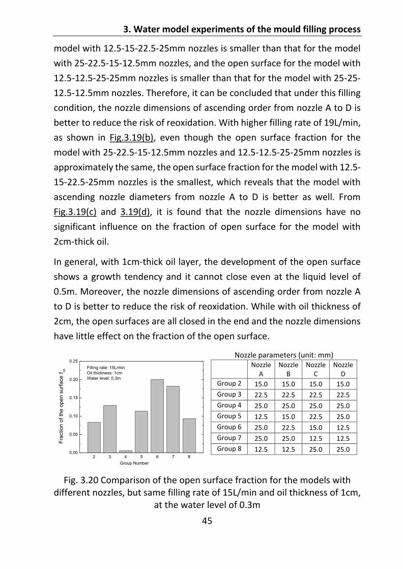
Fig. 3.20 Comparison of the open surface fraction for the models with different nozzles, but same filling rate of 15L/min and oil thickness of 1cm,
at the water level of 0.3m
3. Water model experiments of the mould filling process
46
In Fig.3.20, the fraction of open surface at the same water level of 0.3m for
different groups of nozzles was compared. It can be clearly seen that the
model with nozzles of group 4 (four equal 25mm nozzles) has the smallest
, while the model with nozzles of group 6 (25-22.5-15-12.5mm
For the model with nozzles of group 4,
the total area of nozzle cross section is the largest, which reduces the
average velocity through each nozzle, thus the impact force on top surface
is reduced. For the model with nozzles of group 6, the total area of nozzle
cross section is relatively small, and the nozzles are arranged in descending
order, in which case, the velocities through the last nozzles can be larger,
and therefore increase the impact force on top surface.
0.1 0.2 0.3 0.4 0.50.0
0.1
0.2
0.3
0.4
Filling rate: 15L/min
Oil thickness: 1cm
Nozzle dimension:
4 × 15mm
4 × 25mm
12.5-15-22.5-25mm
25-22.5-15-12.5mm
Liquid level H, m
Fra
ction o
f th
e o
pen s
urf
ace
fos
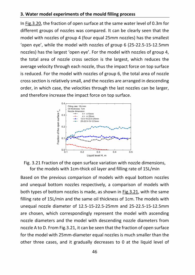
Fig. 3.21 Fraction of the open surface variation with nozzle dimensions, for the models with 1cm-thick oil layer and filling rate of 15L/min
Based on the previous comparison of models with equal bottom nozzles
and unequal bottom nozzles respectively, a comparison of models with
both types of bottom nozzles is made, as shown in Fig.3.21, with the same
filling rate of 15L/min and the same oil thickness of 1cm. The models with
unequal nozzle diameter of 12.5-15-22.5-25mm and 25-22.5-15-12.5mm
are chosen, which correspondingly represent the model with ascending
nozzle diameters and the model with descending nozzle diameters from
nozzle A to D. From Fig.3.21, it can be seen that the fraction of open surface
for the model with 25mm-diameter equal nozzles is much smaller than the
other three cases, and it gradually decreases to 0 at the liquid level of
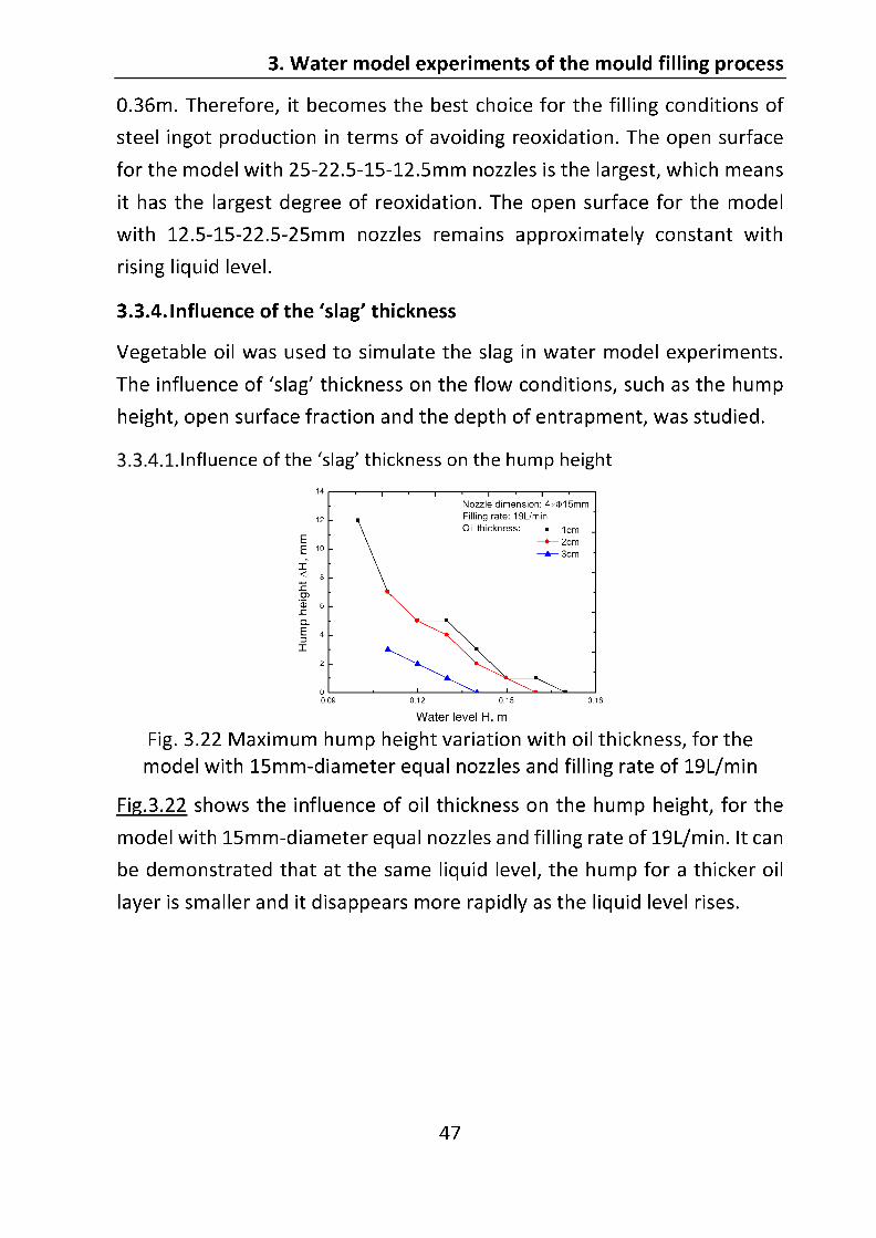
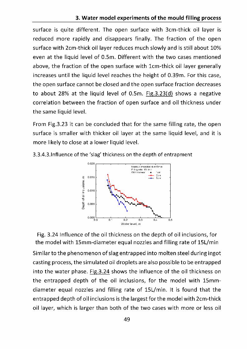
3. Water model experiments of the mould filling process
50
addition. One possible reason of this phenomenon may be that when the
liquid jet breaks through the oil layer, thin oil layer can be easily pushed
aside and keeps far away from the center of the liquid jet. The oil droplets
generated at the lower boundary of the hump are caused by the downward
force of reflux flow acting on the oil layer. Therefore, less oil droplets are
generated for thin oil layer. For a relatively thick oil layer, the lower
boundary of the hump is surrounded by oil, so oil droplets can easily form
and are entrapped into the downward flow. However, if the oil layer is too
thick, for example 3cm, only a few oil droplets were observed, and the
depth of oil inclusions reduced, perhaps due to the suppression of the
above heavy oil layer on the interface flow.
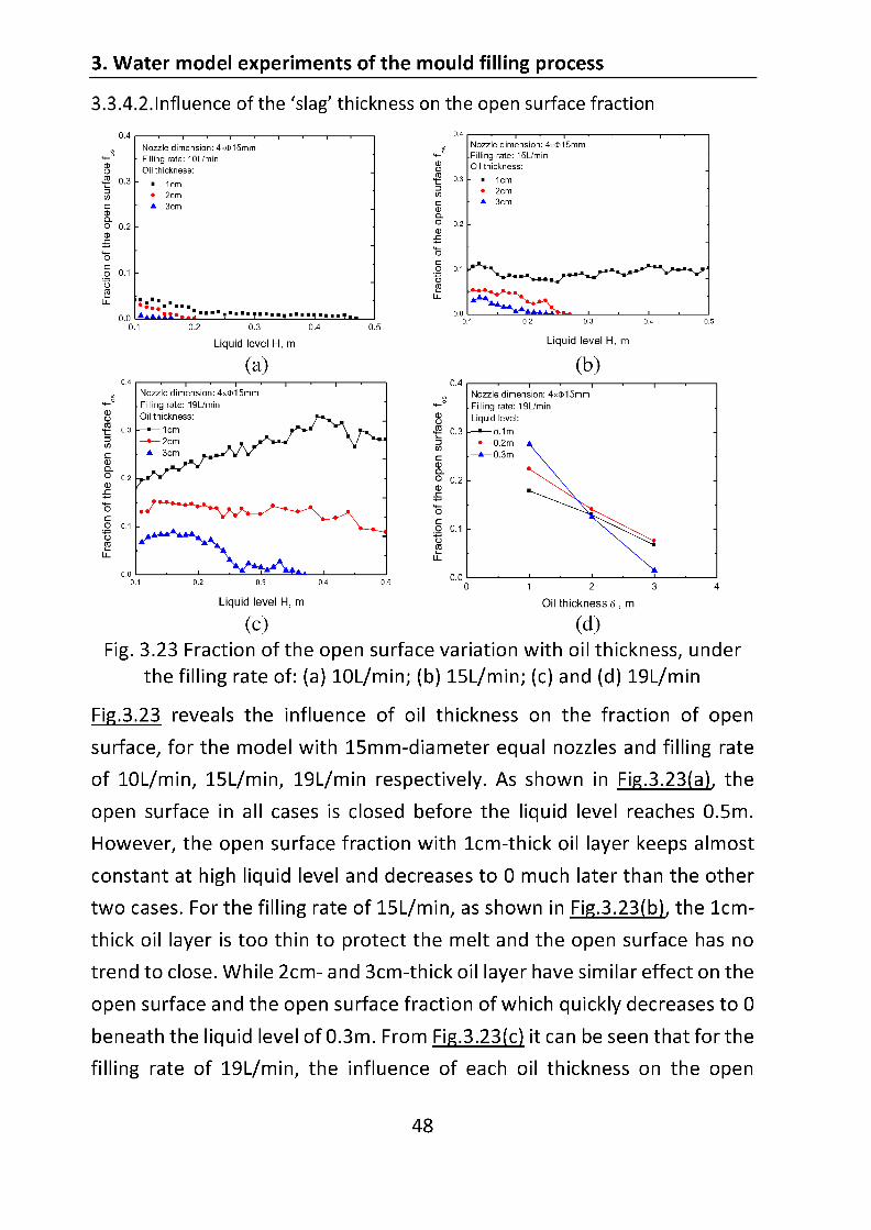
3.4. Optimization of filling conditions
Exogenous inclusions in ingots originate mainly from reoxidation of the
molten steel, slag entrapment, and lining erosion [1]. In general, the degree
of reoxidation is determined by the contact area between the molten steel
and air, which can be evaluated by the fraction of the open surface. From
the water model experiments, we can know that a thicker slag layer
contributes to smaller open surface so as less reoxidation. However, thicker
slag layer usually leads to more slag entrapment, which could become
inclusions in the final products. Also more slag addition means increased
cost of production. Therefore, the expected optimal filling conditions
should balance the risk of reoxidation and slag entrapment, which is also
the major objective of the experiments.
The risk of reoxidation can be evaluated by the fraction of the open surface,
while the degree of slag entrapment is related with the surface turbulence,
which can be evaluated by the hump height. The influence of experimental
parameters on the open surface and the hump height was summarized as
follows.
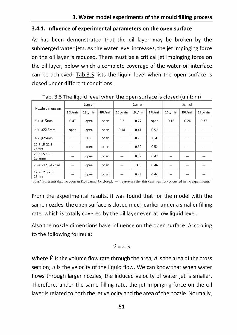
3. Water model experiments of the mould filling process
51
3.4.1. Influence of experimental parameters on the open surface
As has been demonstrated that the oil layer may be broken by the
submerged water jets. As the water level increases, the jet impinging force
on the oil layer is reduced. There must be a critical jet impinging force on
the oil layer, below which a complete coverage of the water-oil interface
can be achieved. Tab.3.5 lists the liquid level when the open surface is
closed under different conditions.
Tab. 3.5 The liquid level when the open surface is closed (unit: m)
Nozzle dimension 1cm oil 2cm oil 3cm oil
10L/min 15L/min 19L/min 10L/min 15L/min 19L/min 10L/min 15L/min 19L/min
mm 0.47 open open 0.2 0.27 open 0.16 0.24 0.37
mm open open open 0.18 0.41 0.52
mm 0.36 open 0.29 0.4
12.5-15-22.5-25mm
open open 0.32 0.52
25-22.5-15-12.5mm
open open 0.29 0.42
25-25-12.5-12.5m open open 0.3 0.46
12.5-12.5-25-25mm
open open 0.42 0.44
From the experimental results, it was found that for the model with the
same nozzles, the open surface is closed much earlier under a smaller filling
rate, which is totally covered by the oil layer even at low liquid level.
Also the nozzle dimensions have influence on the open surface. According
to the following formula:
uAV
Where is the volume flow rate through the area; A is the area of the cross
section; u is the velocity of the liquid flow. We can know that when water
flows through larger nozzles, the induced velocity of water jet is smaller.
Therefore, under the same filling rate, the jet impinging force on the oil
layer is related to both the jet velocity and the area of the nozzle. Normally,
3. Water model experiments of the mould filling process
52
the open surface is easy to close finally for the model with larger nozzle
diameters and lower filling rates.
As can be seen from Tab.3.5, the thickness of oil layer plays an important
role on the open surface. With the increase of oil thickness, the open
surface tends to be closed at lower liquid level. It is also revealed that 3cm-
thick oil layer can generate a smaller open surface than that of 1cm- and
2cm-thick oil layer. Therefore, in the real ingot casting process, the molten
steel can be well protected by more slag from reoxidation.
The open surface consists of open eyes . For the model with four equal
nozzles, open eye D has the largest average radius, while open eye A has
the smallest average radius and is the most concentrated, which is due to
the velocity distribution through the corresponding nozzles. The surface
behavior for models with different nozzle diameters is quite different under
specific filling conditions. In general, the smallest open surface was
observed in the model with four 25mm-diameter equal nozzles.
3.4.2. Influence of experimental parameters on the hump height and
entrapment
The hump height reduces with rising liquid level, decreasing filling rate and
increasing oil layer. The influence of nozzle dimensions on the hump height
is more complicated. Normally, the model with four 25mm-diameter equal
nozzles has relatively small humps, and the hump upon nozzle D is the
largest.
Generally, the larger the hump is, the stronger the downward flow at the
edge of the hump is, and therefore the larger degree of slag entrapment it
gives rise to. The water model experiments reveal
entrapment is also layer. For example,
it was found that the entrapped depth of oil inclusions was the largest for
the model with 2cm-thick oil layer, which was larger than both of the two
cases with more or less oil addition.

3. Water model experiments of the mould filling process
53
3.4.3. Optimal filling conditions
As mentioned above, the expected optimal filling conditions should
balance both the risk of reoxidation and slag entrapment. The production
cost should also be taken into account.
On one hand, in order to reduce the surface turbulence and slag
entrapment, the filling rate should be small. At a low liquid level, the hump
is large and the surface turbulence is strong due to the larger jet impinging
force on the top surface. Therefore, it is required to reduce the filling rate
to avoid On the other hand, too small filling rate
would cause undesirable problems, such as low productivity and strong
reoxidation of the molten steel, which results from the low rising velocity
of liquid surface and therefore the delayed contact between mould powder
and molten steel. Based on the above two aspects, it is recommended that
during the first several minutes of water modeling, the filling rate is kept at
a low value (10-13 L/min), and then after some time when the water level
reaches a certain height, the filling rate can be increased gradually (15-18
L/min). The hump height is expected to retain below 5mm to minimize the
oil entrapment in water modelling. Correspondingly, the filling rate of
molten steel for the real ingot casting process is about 1.0-1.3 t/min at the
beginning, and then gradually increases to about 1.5-1.8 t/min. Because the
water model was developed in reduced scale of 1:4, the maximum hump
height of molten steel is expected to below 20mm.
To reduce the reoxidation of molten steel, the open surface fraction should
be reduced, which can be realized by addition of more slag. However, more
slag addition can increase the production cost, and may lead to more slag
entrapment. It is expected to optimize the slag layer thickness to reduce
the risk of slag entrapment and reoxidation of melt at the same time.
From the experiments, the smallest open surface and humps were
observed in the model with four 25mm-diameter equal nozzles. It becomes
3. Water model experiments of the mould filling process
54
the best choice for the nozzle design in terms of minimizing the risk of
reoxidation and slag entrapment.
3.5. Conclusions
The water model experiments were carried out to simulate the molten
steel-slag interface during large steel ingot bottom teeming process. The
experimental results reveal the influence of model parameters, such as the
filling rate, nozzle dimensions and oil thickness on the filling conditions,
which can evaluate the risk of slag entrapment as well as reoxidation of
molten steel. The following conclusions can be drawn from the study:
(1) At a certain liquid level, with the reduction of filling rate, on one hand,
the hump height decrease, thus the risk of slag entrapment is reduced; on
the other hand, the fraction of open surface decreases, thus the risk of
reoxidation is reduced.
(2) The hump height is reduced with rising liquid level, so the slag
entrapment and surface turbulence at low liquid level is stronger. In order
to reduce slag entrapment and surface turbulence at low liquid level while
improve the productivity at high liquid level, it is recommended that during
the first several minutes, the filling rate of molten steel should be kept at a
low value (1.0-1.3 t/min), and then after the level of molten steel reaches
to a certain height where the hump is small enough, the filling rate can be
increased gradually (1.5-1.8 t/min). The hump height is expected to retain
below 20mm to minimize the slag entrapment.
(3) For a large steel ingot mould, it is better to design multiple bottom
nozzles to reduce the jet velocity through each nozzle. In the experiment
models, the model with four 25mm-diameter equal nozzles shows better
performance from the view of both slag entrapment and reoxidation.
(4) With the increase of slag thickness, the open surface decreases and
therefore the risk of reoxidation is reduced. However, more slag addition
may lead to more slag entrapment and increase the production cost as well.

4. Numerical simulation of filling process with OpenFOAM software
55
4. Numerical simulation of filling process with OpenFOAM software
The computational fluid dynamic simulations were performed with
OpenFOAM software to get more quantitative information about the flow
field during the filling process, especially the velocity field which is directly
related to the phenomenon of surface turbulence and slag entrapment.
4.1. Model description
OpenFOAM is supplied with a large set of standard solvers, in which
interFoam is designed to solve two incompressible, isothermal immiscible
fluids, using a VOF (volume of fluid) phase-fraction based interface
capturing approach [57]. In this study, the standard solver interFoam of
OpenFOAM 1.7.1 was used to calculate the water-air two-phase flow. The
geometry of the simulation model was the same as the water model, with
four nozzles at the mould bottom. As illustrated in Fig.3.3, the model has a
symmetry plane, therefore, only half of the total geometry was calculated
as the three dimensional computational domain to save computational
time.
The following assumptions were made to simplify the mathematical model:
(i) only the flow in the early stage of filling were concerned in this paper,
without the consideration of solidification as well as heat transfer; (ii)
room-temperature water was used to simulate molten steel; (iii) both
water and air are incompressible Newtonian fluids, and the physical
properties of the two fluids are constant. Then the flow is governed by the
following equations [65]:
The mass continuity equation: 0Ut
The momentum equation: FgTUUU
t
Where t is time; is density; U is velocity vector; T is total stress tensor; F
is the force due to surface tension . For a Newtonian fluid in local
thermodynamic equilibrium, T is defined as:

4. Numerical simulation of filling process with OpenFOAM software
56
T)(3
2UUIUT P
Where P is pressure; I is the unit tensor; µ is dynamic viscosity. At the
interface between water and air, VOF method is adopted to simulate the
evolution of free surface. The volume fraction of water, , is equal to 1 for
the cells completely occupied by water, and equal to 0 for the cells
completely occupied by air. Hence, the interface is located within the cells
where 0< <1. is governed by the phase conservation equation:
0Ut
Based on the VOF method, the physical properties of fluids in the above
governing equations, such as density and viscosity, are computed as follows:
airwater )1(
airwater )1(
For this incompressible Newtonian flow, Ubbink [65] reformulated the
momentum equation:
FUUgUUU
Pt
F
These transport equations were employed in the solver interFoam, also the
standard - model was adopted to simulate the turbulent behavior of the
flow. Therefore, the viscosity µ in the governing equations was replaced by
the effective viscosity µeff, which was defined as:
2
Cwith tteff
The initial and boundary conditions must be defined to complete the
mathematical model. For this transient flow, the system was initially filled
with air, and then water flowed into the mould from the inlet boundary
4. Numerical simulation of filling process with OpenFOAM software
57
with a constant uniform velocity. At the outlet boundary, atmosphere
boundary conditions were specified, where the pressure could be
calculated from the specified total pressure and local velocity. The
boundary conditions of symmetry plane were set to be symmetryPlane,
which is a standard boundary type in OpenFOAM. Moreover, no-slip
conditions were assumed on the walls of the model. Based on the finite
volume method, the governing equations described above were discretized
on meshes which were generated by a mesh-generation utility in
OpenFOAM called snappyHexMesh. The PISO (Pressure-Implicit Split-
Operator) algorithm was applied to solve the pressure-velocity coupling.
4.2. Results of the calculated flow fields
The numerical simulations were carried out on different parameters of
filling rate and nozzle dimensions. In chapter 3, the filling rates of 10L/min,
15L/min and 19L/min were studied with water model, which had a circular
entrance 26mm in diameter, so the corresponding inlet velocities for the
numerical model were 0.31m/s, 0.47m/s and 0.60m/s, respectively.
Furthermore, the calculated flow fields were compared with the
measurements of water modeling.
4.2.1. Flow patterns in the early stage of teeming
Fig.4.1 shows the calculated flow patterns on the symmetry plane after 4s
and 20s of bottom teeming start-up. In the early stage of teeming, when
water flows into the sprue, air is pushed out through the bottom nozzles.
As Fig.4.1(a) clearly shows, air bubbles are entrapped into the water flow
during mould filling. The air bubbles tend to rise due to low density. Once
the bubbles move to the first nozzle, they rise to the mould and spout out
at the liquid surface, which results in strong surface turbulence. After all
the air spouts out, the liquid level tends to be stable, as illustrated in
Fig.4.1(b), from which we can see clearly the interface between water and
air phases. The surface turbulence at the beginning can increase the risk of
slag entrapment, thus it is better to add casting powder after all the air
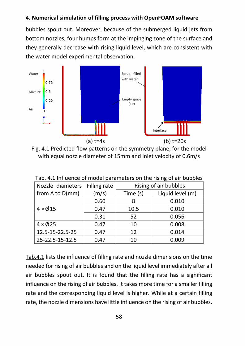
4. Numerical simulation of filling process with OpenFOAM software
58
bubbles spout out. Moreover, because of the submerged liquid jets from
bottom nozzles, four humps form at the impinging zone of the surface and
they generally decrease with rising liquid level, which are consistent with
the water model experimental observation.
(a) t=4s (b) t=20s
Fig. 4.1 Predicted flow patterns on the symmetry plane, for the model with equal nozzle diameter of 15mm and inlet velocity of 0.6m/s
Tab. 4.1 Influence of model parameters on the rising of air bubbles Nozzle diameters from A to D(mm)
Filling rate (m/s)
Rising of air bubbles Time (s) Liquid level (m)
4 × Ø15 0.60 8 0.010 0.47 10.5 0.010 0.31 52 0.056
4 × Ø25 0.47 10 0.008 12.5-15-22.5-25 0.47 12 0.014 25-22.5-15-12.5 0.47 10 0.009
Tab.4.1 lists the influence of filling rate and nozzle dimensions on the time
needed for rising of air bubbles and on the liquid level immediately after all
air bubbles spout out. It is found that the filling rate has a significant
influence on the rising of air bubbles. It takes more time for a smaller filling
rate and the corresponding liquid level is higher. While at a certain filling
rate, the nozzle dimensions have little influence on the rising of air bubbles.
Interface
Air
Empty space (air)
Sprue, filled
with water
Mixture
Water

4. Numerical simulation of filling process with OpenFOAM software
59
In the real ingot bottom teeming process, the mould powder should be
added at an appropriate level. On one hand, because the rising air bubbles
can result in strong surface turbulence, to avoid slag entrapment, the
mould powder should be added at a relatively high level where all the air
bubbles had spouted out. On the other hand, to protect the molten steel
from reoxidation, the mould powder should be added as early as possible,
which means adding the mould powder at a relatively low level or using a
larger filling rate. In conclusion, the level to add the mould powder should
take both the filling rate and rising of air bubbles into account.
4.2.2. Velocity fields of the flow
(a) Velocity field at t=60s
(b) Velocity vector field at t=20s
Fig. 4.2 Predicted velocity profile on the symmetry plane, for the model with 15mm-diameter equal nozzles and 0.6m/s inlet velocity
water Interface
Velocity, m/s
Interface
air

4. Numerical simulation of filling process with OpenFOAM software
60
Fig.4.2 shows the predicted velocity profile on the symmetry plane for the
model with four 15mm-diameter nozzles and 0.6m/s inlet velocity. It can
be seen that the liquid flow from bottom nozzles acts as powerful
submerged jets directed upward, and impinges on the water-air interface,
then results in humps on the surface. The velocities of the liquid jets are
considerably larger than that in the zone which is far away from the jets.
The velocities at each nozzle are directed upward and have different values.
As observed in the water model experiments, the shapes of the hump
above each nozzle were different, which were supposed to depend on the
energy flux of the water jets though the bottom nozzles. Hence, the velocity
and energy flux at each nozzle were studied.
0 5 10 15 20-0.3
0.0
0.3
0.6
0.9
1.2
1.5
Nozzle A
Nozzle B
Nozzle C
Nozzle D
Time, s
Ve
rtic
al velo
city c
om
po
ne
nt, m
/s
Fig. 4.3 Time variations of the vertical velocity component at the center point of each nozzle, for the model with 15mm-diameter equal nozzles
and 0.6m/s inlet velocity
Fig.4.3 shows the time variations of the vertical velocity component at the
center point of each nozzle, for the model with 15mm-diameter equal
nozzles and 0.6m/s inlet velocity. At the beginning of teeming, it is air or
mixture of air and water that flows through the nozzles, and therefore
causes strong velocity fluctuation. The velocity fluctuation of nozzle A is the
largest because most of the air flows out through nozzle A. After 8s of
teeming, it is totally water that flows through each nozzle and then the
velocity achieves stability. The velocity values are related to the position of
the nozzles. In this case, nozzle A has the smallest velocity of 0.417m/s, and
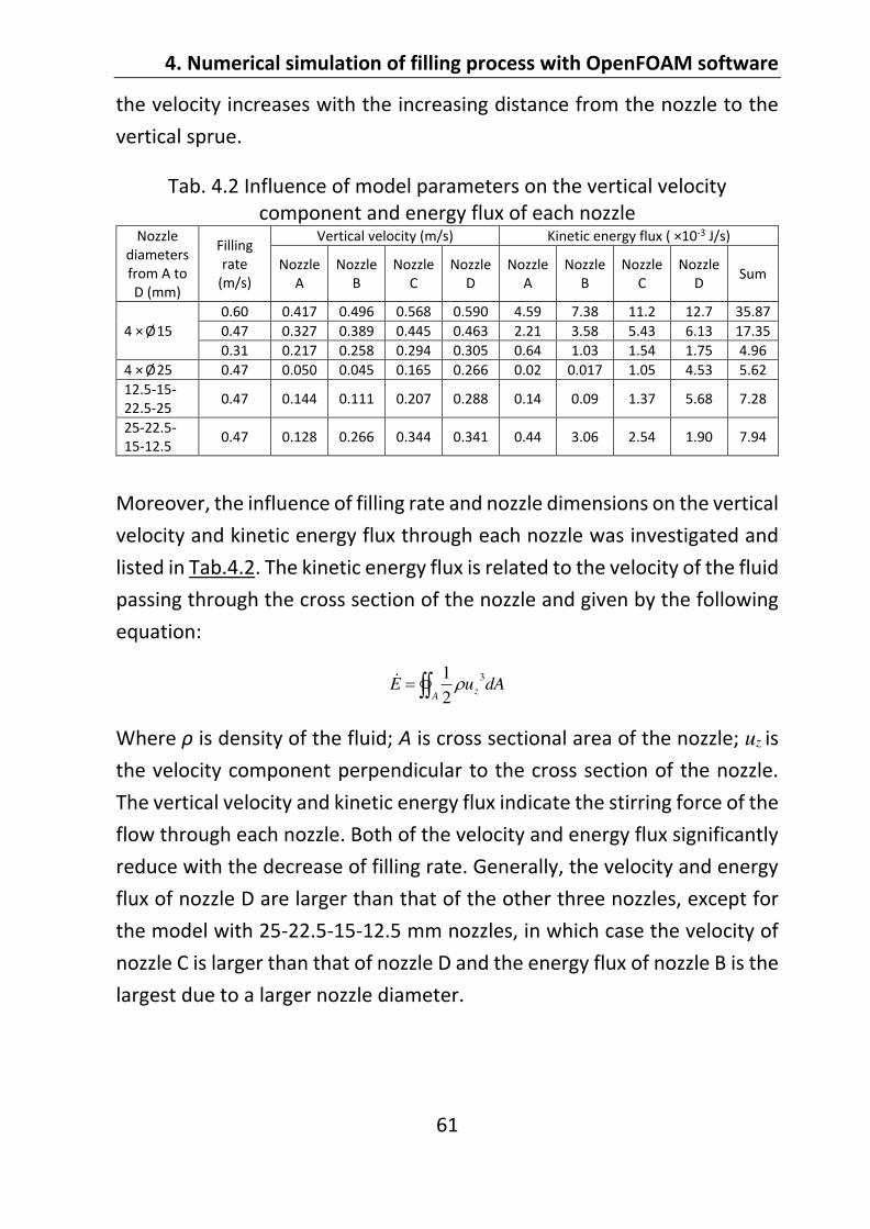
4. Numerical simulation of filling process with OpenFOAM software
61
the velocity increases with the increasing distance from the nozzle to the
vertical sprue.
Tab. 4.2 Influence of model parameters on the vertical velocity component and energy flux of each nozzle
Nozzle diameters from A to D (mm)
Filling rate
(m/s)
Vertical velocity (m/s) Kinetic energy flux ( ×10-3 J/s)
Nozzle A
Nozzle B
Nozzle C
Nozzle D
Nozzle A
Nozzle B
Nozzle C
Nozzle D
Sum
4 × Ø15 0.60 0.417 0.496 0.568 0.590 4.59 7.38 11.2 12.7 35.87 0.47 0.327 0.389 0.445 0.463 2.21 3.58 5.43 6.13 17.35 0.31 0.217 0.258 0.294 0.305 0.64 1.03 1.54 1.75 4.96
4 × Ø25 0.47 0.050 0.045 0.165 0.266 0.02 0.017 1.05 4.53 5.62 12.5-15-22.5-25
0.47 0.144 0.111 0.207 0.288 0.14 0.09 1.37 5.68 7.28
25-22.5-15-12.5
0.47 0.128 0.266 0.344 0.341 0.44 3.06 2.54 1.90 7.94
Moreover, the influence of filling rate and nozzle dimensions on the vertical
velocity and kinetic energy flux through each nozzle was investigated and
listed in Tab.4.2. The kinetic energy flux is related to the velocity of the fluid
passing through the cross section of the nozzle and given by the following
equation:
Az dAuE3
2
1
Where is density of the fluid; A is cross sectional area of the nozzle; uz is
the velocity component perpendicular to the cross section of the nozzle.
The vertical velocity and kinetic energy flux indicate the stirring force of the
flow through each nozzle. Both of the velocity and energy flux significantly
reduce with the decrease of filling rate. Generally, the velocity and energy
flux of nozzle D are larger than that of the other three nozzles, except for
the model with 25-22.5-15-12.5 mm nozzles, in which case the velocity of
nozzle C is larger than that of nozzle D and the energy flux of nozzle B is the
largest due to a larger nozzle diameter.
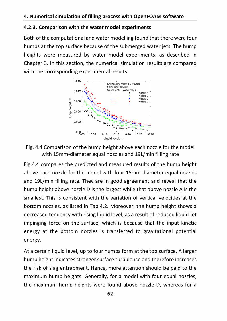
4. Numerical simulation of filling process with OpenFOAM software
62
4.2.3. Comparison with the water model experiments
Both of the computational and water modelling found that there were four
humps at the top surface because of the submerged water jets. The hump
heights were measured by water model experiments, as described in
Chapter 3. In this section, the numerical simulation results are compared
with the corresponding experimental results.
0.00 0.05 0.10 0.15 0.20 0.25 0.300.000
0.003
0.006
0.009
0.012
0.015
Nozzle dimension: 4 × 15mm
Filling rate: 19L/min
OpenFOAM Water model
Nozzle A
Nozzle B
Nozzle C
Nozzle D
Liquid level, m
Hu
mp
he
igh
t, m
Fig. 4.4 Comparison of the hump height above each nozzle for the model
with 15mm-diameter equal nozzles and 19L/min filling rate
Fig.4.4 compares the predicted and measured results of the hump height
above each nozzle for the model with four 15mm-diameter equal nozzles
and 19L/min filling rate. They are in good agreement and reveal that the
hump height above nozzle D is the largest while that above nozzle A is the
smallest. This is consistent with the variation of vertical velocities at the
bottom nozzles, as listed in Tab.4.2. Moreover, the hump height shows a
decreased tendency with rising liquid level, as a result of reduced liquid-jet
impinging force on the surface, which is because that the input kinetic
energy at the bottom nozzles is transferred to gravitational potential
energy.
At a certain liquid level, up to four humps form at the top surface. A larger
hump height indicates stronger surface turbulence and therefore increases
the risk of slag entrapment. Hence, more attention should be paid to the
maximum hump heights. Generally, for a model with four equal nozzles,
the maximum hump heights were found above nozzle D, whereas for a
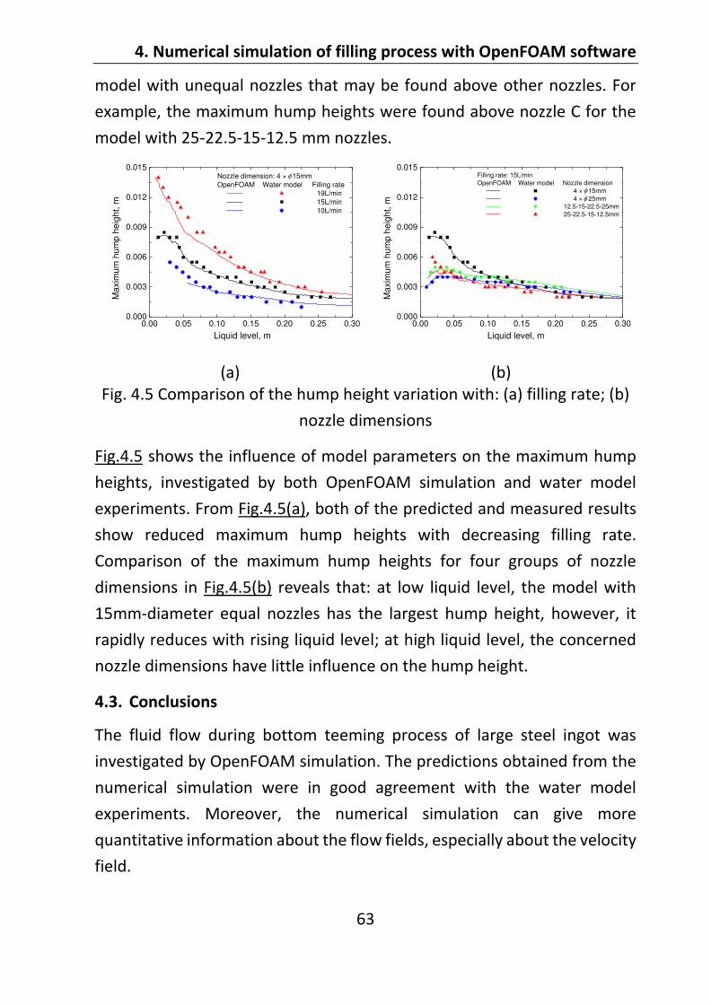
4. Numerical simulation of filling process with OpenFOAM software
63
model with unequal nozzles that may be found above other nozzles. For
example, the maximum hump heights were found above nozzle C for the
model with 25-22.5-15-12.5 mm nozzles.
0.00 0.05 0.10 0.15 0.20 0.25 0.300.000
0.003
0.006
0.009
0.012
0.015
Nozzle dimension: 4 × 15mm
OpenFOAM Water model Filling rate
19L/min
15L/min
10L/min
Liquid level, m
Maxim
um
hum
p h
eig
ht,
m
0.00 0.05 0.10 0.15 0.20 0.25 0.300.000
0.003
0.006
0.009
0.012
0.015
Filling rate: 15L/min
OpenFOAM Water model Nozzle dimension
4 × 15mm
4 × 25mm
12.5-15-22.5-25mm
25-22.5-15-12.5mm
Liquid level, m
Maxim
um
hum
p h
eig
ht,
m
(a) (b) Fig. 4.5 Comparison of the hump height variation with: (a) filling rate; (b)
nozzle dimensions
Fig.4.5 shows the influence of model parameters on the maximum hump
heights, investigated by both OpenFOAM simulation and water model
experiments. From Fig.4.5(a), both of the predicted and measured results
show reduced maximum hump heights with decreasing filling rate.
Comparison of the maximum hump heights for four groups of nozzle
dimensions in Fig.4.5(b) reveals that: at low liquid level, the model with
15mm-diameter equal nozzles has the largest hump height, however, it
rapidly reduces with rising liquid level; at high liquid level, the concerned
nozzle dimensions have little influence on the hump height.
4.3. Conclusions
The fluid flow during bottom teeming process of large steel ingot was
investigated by OpenFOAM simulation. The predictions obtained from the
numerical simulation were in good agreement with the water model
experiments. Moreover, the numerical simulation can give more
quantitative information about the flow fields, especially about the velocity
field.
4. Numerical simulation of filling process with OpenFOAM software
64
At the beginning of teeming, the incoming water flow pushes the air out
through bottom nozzles, especially through the first nozzle (Nozzle A). The
rising air bubbles can lead to surface turbulence and further increase the
risk of slag entrapment. Therefore, it is not recommended to add the mould
powder at a low liquid level with air bubbles. It takes more time for a
smaller filling rate to spout out all air bubbles. However, the contact
between the mould powder and molten steel cannot be too late, otherwise
it will increase the risk of reoxidation. So, the level to add the mould
powder should take both the filling rate and rising of air bubbles into
account.
After all air spouts out from the bottom nozzles, the jet velocity and kinetic
energy flux of each nozzle are stable. With rising liquid level, the input
kinetic energy at the bottom nozzles is transferred to gravitational
potential energy, and then the hump height decreases.
5. Simulation of solidification process with OpenFOAM software
65
5. Simulation of solidification process with OpenFOAM software
A liquid-solid 2-phase solidification model based on OpenFOAM software
was developed to predicate the macrosegregation of steel ingots. Then the
solidification model was performed on a steel ingot and the results were
compared with the experimental measurements from literature.
5.1. Liquid-solid 2-phase model with phase change
In this model, the mass transfer, melt convection, heat transfer as well as
solute transport were described using Euler-Euler two-phase approach. The
nucleation, grain growth and grain movement were also involved in the
model, which makes it possible to calculate the mass and solute transfer
between the liquid and solid phases.
Indeed, the present model was developed based on the previous
multiphase solidification models of M. .Combeau [66, 67],
M.Wu and A.Ludwig [46, 47, 68-70], C.Beckermann [71], W.Li [72] and W.Tu
[73].
5.1.1. Model assumptions
The solidification model was developed based on the following
assumptions:
The mould filling process is not considered and the solidification starts
from the total liquid phase as the temperature decreases. Two phases
are defined: the liquid phase (l) and solid phase (s). The corresponding
mass fractions have the relationship of .
The liquid phase is Newtonian and incompressible. The liquid flow is
laminar with a constant dynamic viscosity .
The solid phase consists of equiaxed grains, and the grains are globular.
The viscosity for the mixture of liquid and solid grains is calculated by
, where and represent the viscosity of the liquid
phase and solid phase, respectively. In mushy region, the mixture of
liquid and solid grains still retain some fluidity, like slurry. The viscosity

5. Simulation of solidification process with OpenFOAM software
66
of the mixture can be described as relative to the viscosity of the liquid
phase: , where is the relative viscosity (dimensionless).
Therefore, in the mushy region the viscosity for the solid phase can be
expressed as: )1(/ srsls ff . Depending on the concentration of
the solid grains, several models for describing the relative viscosity
were proposed. In this study, the model c
sfc
ssr ff5.2
)/1( was used,
where is the fraction of solid phase and is the packing limit [71].
Once the solid fraction reaches to the packing limit, the viscosity of solid
phase is assumed as an infinitely large value. With this method, nearly
zero velocity will be obtained in the packed bed region. Overall, the
viscosity of solid phase can be defined as [71]:
when , )1()/1(5.2
s
fc
ss
s
l
s ffff
cs ;
when , is infinitely large.
The densities of the liquid and solid phases are equal and constant,
. In the momentum equation, the Boussinesq approximation for
buoyancy-driven flow is used to take into account the influence of
temperature and solute concentration on the liquid density [34, 35].
)]()(1[, reflCrefTrefleff CCTT
Where: p
TT
1 is the thermal expansion coefficient;
pl
CC
1 is the solute expansion coefficient.
The shrinkage porosity is not taken into accounted, and the control
volume of the mixture is saturated, i.e., , where denotes
the volume fraction of the solid phase and denotes that of the liquid
phase.
The temperatures of the liquid and solid phases are equal, i.e.,
.
5. Simulation of solidification process with OpenFOAM software
68
)]()(1[ ,refllCrefTleff CCTT
The momentum exchange rate from liquid to solid phase, Uls, consists of
two parts: d
ls
p
lsls UUU . p
lsU is the part due to phase change, and it can be
calculated by: *UU ls
p
ls M , with lUU* for solidification and sUU* for
remelting [46, 68]. d
lsU is the part due to drag force, which can be calculated
by )( slls
d
ls K UUU . There are two methods to obtain the drag force
coefficient lsK :
(1) One-region method (valid for ) [68, 74]:
2
2
2 4
p
l
llsd
fK
with: 2/1
65
5 1
2332
3/42
2
9
p
s
C
f
3/1
sf
17.0
7.00
163.0lg26.1
2
l
l
e
e
pf
fC
The shape coefficient can be simplified to 1 for globular equiaxed grains.
(2) Two-region method [67]:
At the region with low solid fraction (valid for )
The flow regime in this region like free particles, and the drag force can be
modeled using the well-known Stokes law. For the free particle regime, the
drag coefficient for a single sphere is modeled as:
sl
p
ds
lsd
CfK UU
4
3
with: ie
kes
d CCf
CRe
48

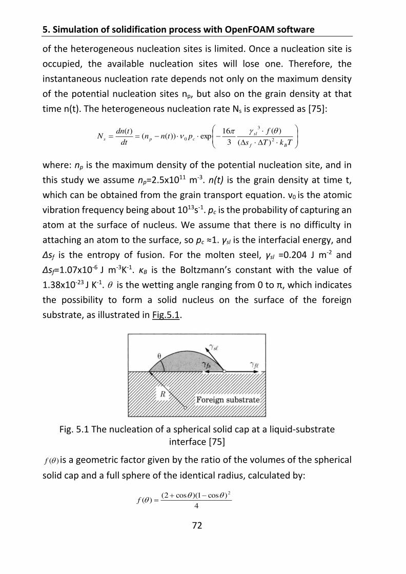
5. Simulation of solidification process with OpenFOAM software
72
of the heterogeneous nucleation sites is limited. Once a nucleation site is
occupied, the available nucleation sites will lose one. Therefore, the
instantaneous nucleation rate depends not only on the maximum density
of the potential nucleation sites np, but also on the grain density at that
time n(t). The heterogeneous nucleation rate Ns is expressed as [75]:
TkTs
fptnn
dt
tdnN
Bf
sl
cps 2
3
0)(
)(
3
16exp))((
)(
where: np is the maximum density of the potential nucleation site, and in
this study we assume np=2.5 1011 m-3. n(t) is the grain density at time t,
which can be obtained from the grain transport equation. 0 is the atomic
vibration frequency being about 1013s-1. pc is the probability of capturing an
atom at the surface of nucleus. We assume that there is no difficulty in
attaching an atom to the surface, so pc 1. sl is the interfacial energy, and
sf is the entropy of fusion. For the molten steel, sl =0.204 J m-2 and
sf=1.07 10-6 J m-3K-1. B is the Boltzmann s constant with the value of
1.38 10-23 J K-1. is the wetting angle ranging from 0 to , which indicates
the possibility to form a solid nucleus on the surface of the foreign
substrate, as illustrated in Fig.5.1.
Fig. 5.1 The nucleation of a spherical solid cap at a liquid-substrate
interface [75]
)(f is a geometric factor given by the ratio of the volumes of the spherical
solid cap and a full sphere of the identical radius, calculated by:
4
)cos1)(cos2()(
2
f
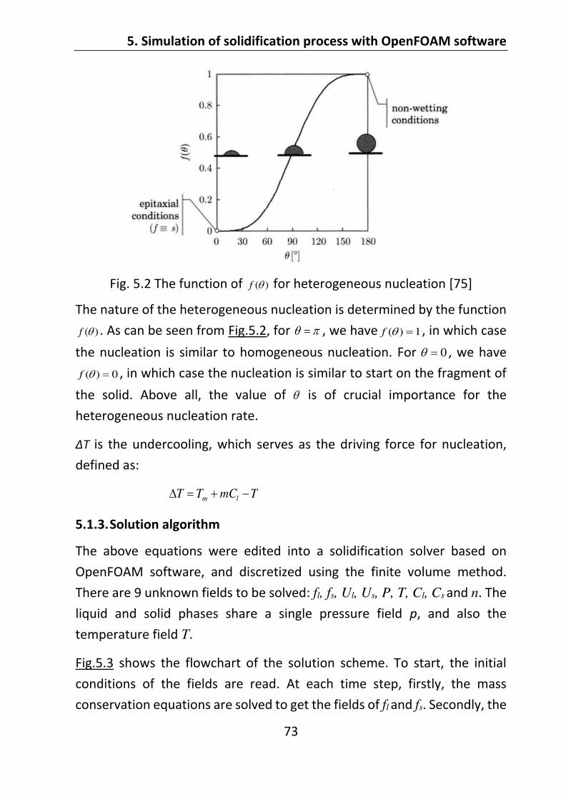
5. Simulation of solidification process with OpenFOAM software
73
Fig. 5.2 The function of )(f for heterogeneous nucleation [75]
The nature of the heterogeneous nucleation is determined by the function
)(f . As can be seen from Fig.5.2, for , we have 1)(f , in which case
the nucleation is similar to homogeneous nucleation. For 0 , we have
0)(f , in which case the nucleation is similar to start on the fragment of
the solid. Above all, the value of is of crucial importance for the
heterogeneous nucleation rate.
is the undercooling, which serves as the driving force for nucleation,
defined as:
TmCTT lm
5.1.3. Solution algorithm
The above equations were edited into a solidification solver based on
OpenFOAM software, and discretized using the finite volume method.
There are 9 unknown fields to be solved: fl, fs, Ul, Us, P, T, Cl, Cs and n. The
liquid and solid phases share a single pressure field p, and also the
temperature field T.
Fig.5.3 shows the flowchart of the solution scheme. To start, the initial
conditions of the fields are read. At each time step, firstly, the mass
conservation equations are solved to get the fields of fl and fs. Secondly, the
5. Simulation of solidification process with OpenFOAM software
74
momentum equations are solved to get intermediate velocity fields,
without the consideration of the pressure and buoyancy terms in the right
side of the momentum equations. The coupling of velocity and pressure is
handled by PISO algorithm (Pressure implicit with splitting of operator). The
intermediate velocities do not satisfy the mass conservation equations. To
ensure mass conservation of each phase, a pressure equation is
constructed using the velocity flux by considering the mass conservation
equations. After solving the pressure equation, the flux and velocity are
corrected. Next, solve the energy equation to get the temperature field.
After that, the concentration equations are solved to obtain the Cl and Cs
fields. Then calculate the undercooling T and nucleation rate Ns to solve
the grain transport equation and get n field. Finally, other parameters are
updated for the next time step, such as the transfer rate Mls, the main
grain diameter ds, the interfacial area concentration Sv, and the momentum
exchange coefficient Kls. The iterative procedure stops as the stopping time
is reached.

5. Simulation of solidification process with OpenFOAM software
75
Fig. 5.3 Flowchart of the solution scheme
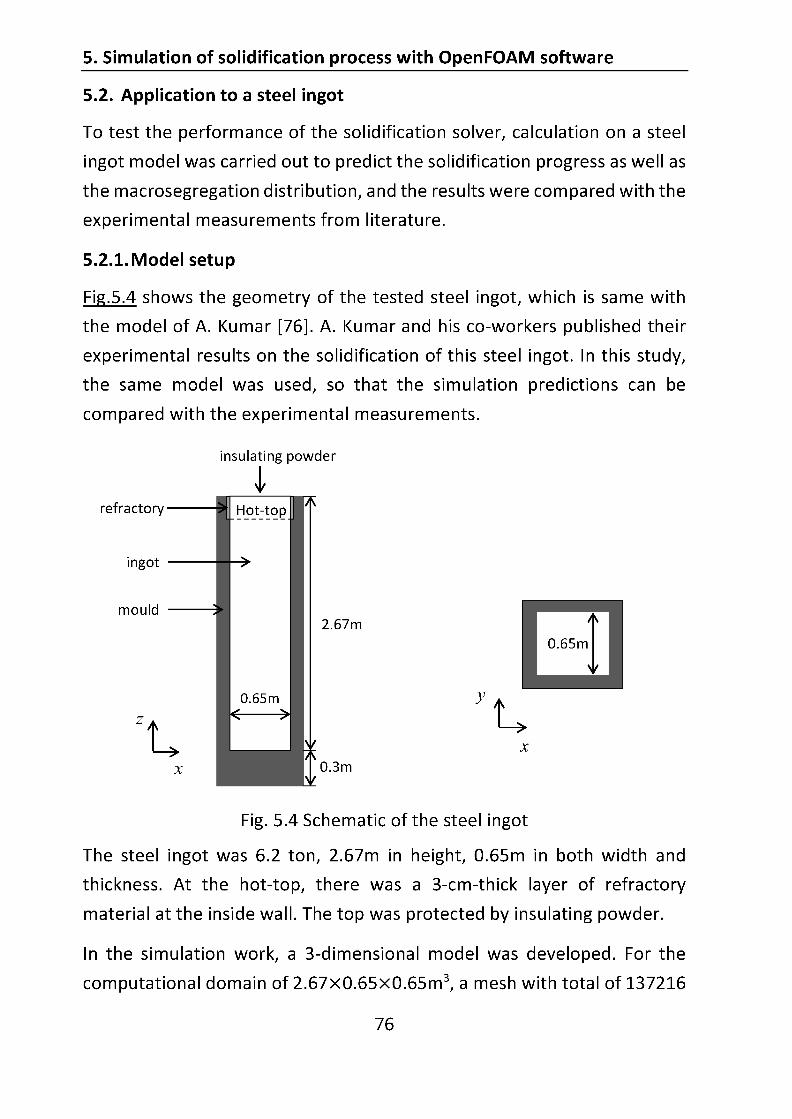
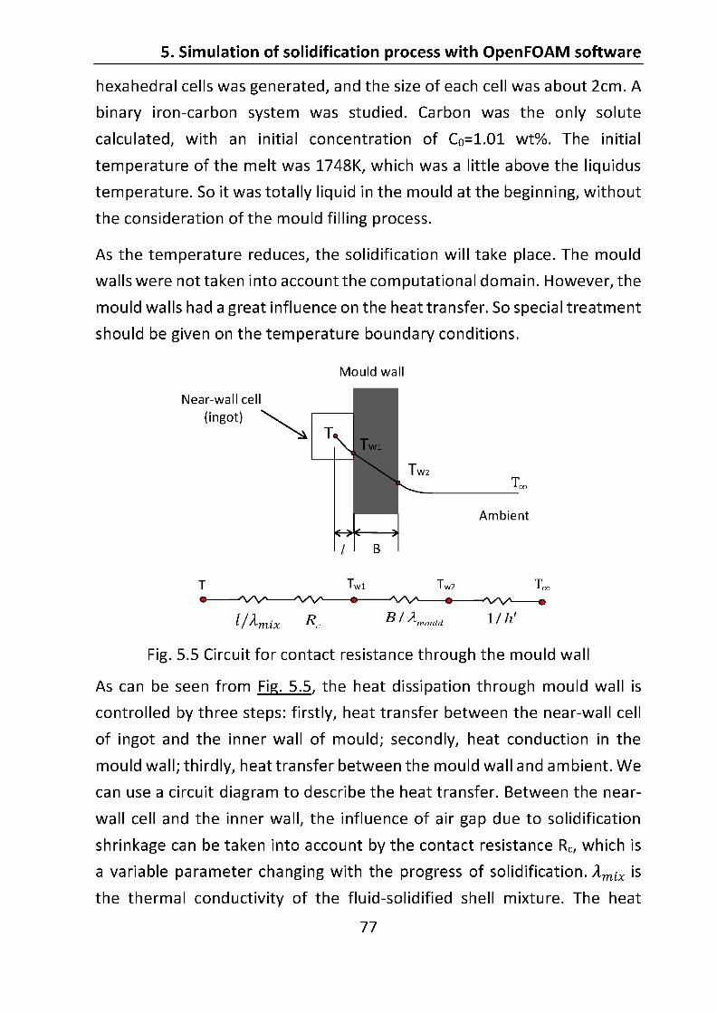
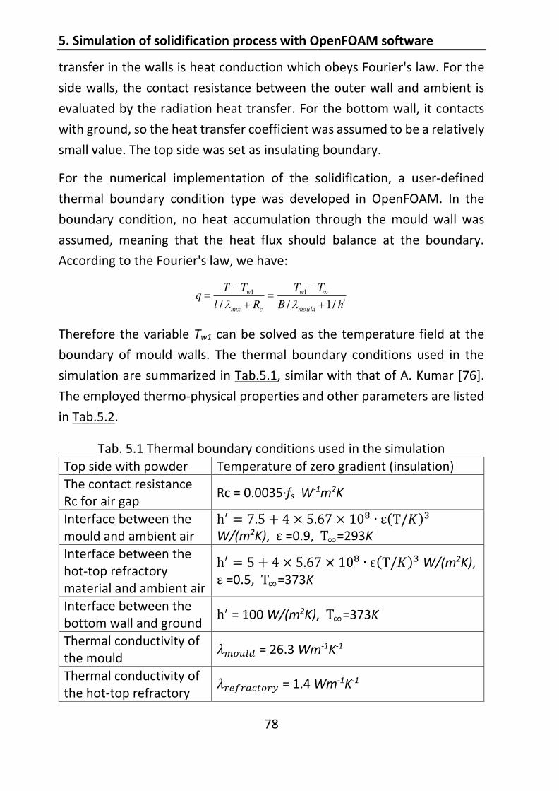
5. Simulation of solidification process with OpenFOAM software
78
transfer in the walls is heat conduction which obeys Fourier's law. For the
side walls, the contact resistance between the outer wall and ambient is
evaluated by the radiation heat transfer. For the bottom wall, it contacts
with ground, so the heat transfer coefficient was assumed to be a relatively
small value. The top side was set as insulating boundary.
For the numerical implementation of the solidification, a user-defined
thermal boundary condition type was developed in OpenFOAM. In the
boundary condition, no heat accumulation through the mould wall was
assumed, meaning that the heat flux should balance at the boundary.
According to the Fourier's law, we have:
hB
TT
Rl
TTq
mould
w
cmix
w
/1//
11
Therefore the variable Tw1 can be solved as the temperature field at the
boundary of mould walls. The thermal boundary conditions used in the
simulation are summarized in Tab.5.1, similar with that of A. Kumar [76].
The employed thermo-physical properties and other parameters are listed
in Tab.5.2.
Tab. 5.1 Thermal boundary conditions used in the simulation Top side with powder Temperature of zero gradient (insulation) The contact resistance Rc for air gap
Rc = 0.0035 fs W-1m2K
Interface between the mould and ambient air
W/(m2K), =0.9, =293K
Interface between the hot-top refractory material and ambient air
W/(m2K), =0.5, =373K
Interface between the bottom wall and ground
= 100 W/(m2K), =373K
Thermal conductivity of the mould
= 26.3 Wm-1K-1
Thermal conductivity of the hot-top refractory
= 1.4 Wm-1K-1
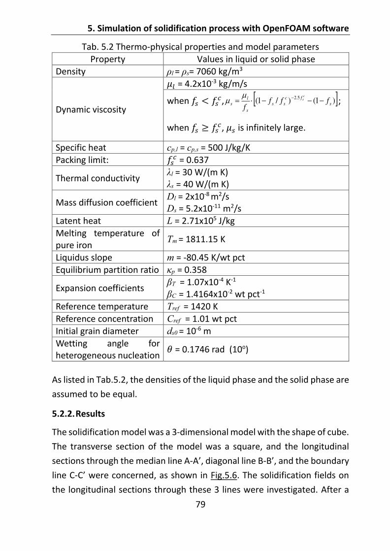
5. Simulation of solidification process with OpenFOAM software
79
Tab. 5.2 Thermo-physical properties and model parameters Property Values in liquid or solid phase
when , )1()/1(5.2
s
fc
ss
s
l
s ffff
cs ;
when , is infinitely large.
As listed in Tab.5.2, the densities of the liquid phase and the solid phase are
assumed to be equal.
5.2.2. Results
The solidification model was a 3-dimensional model with the shape of cube.
The transverse section of the model was a square, and the longitudinal
sections through the median line A- , diagonal line B- , and the boundary
line C- , as shown in Fig.5.6. The solidification fields on
the longitudinal sections through these 3 lines were investigated. After a
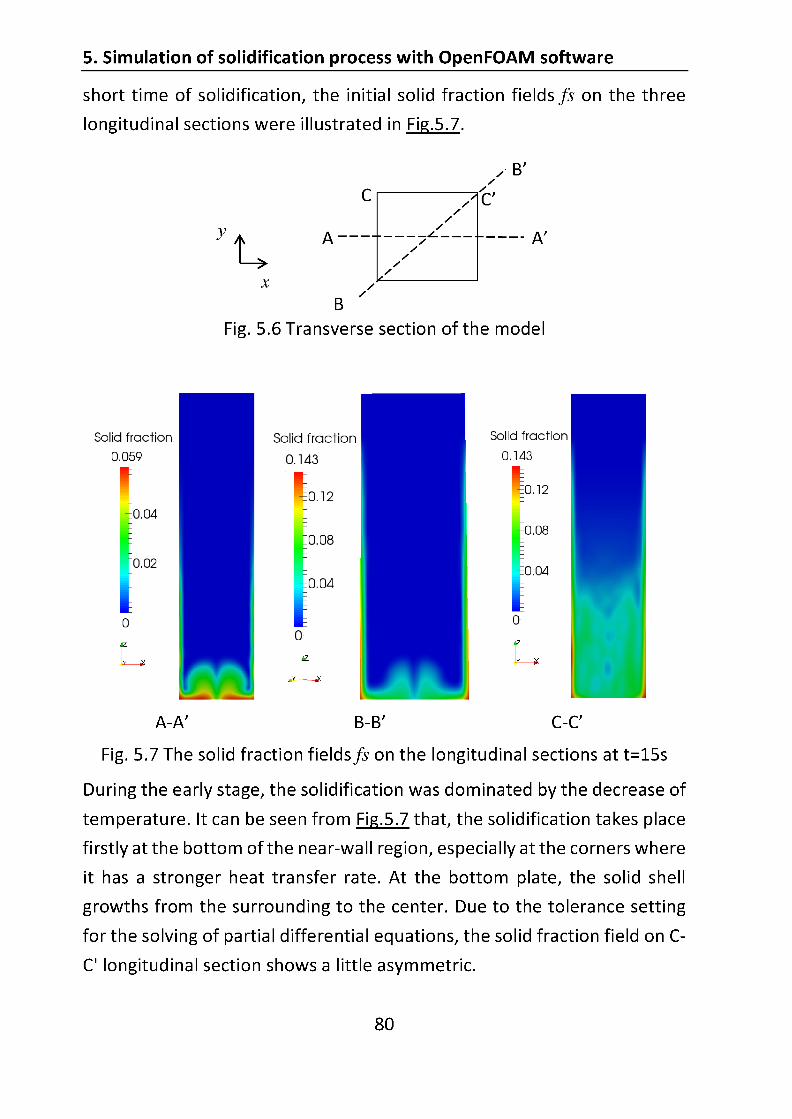
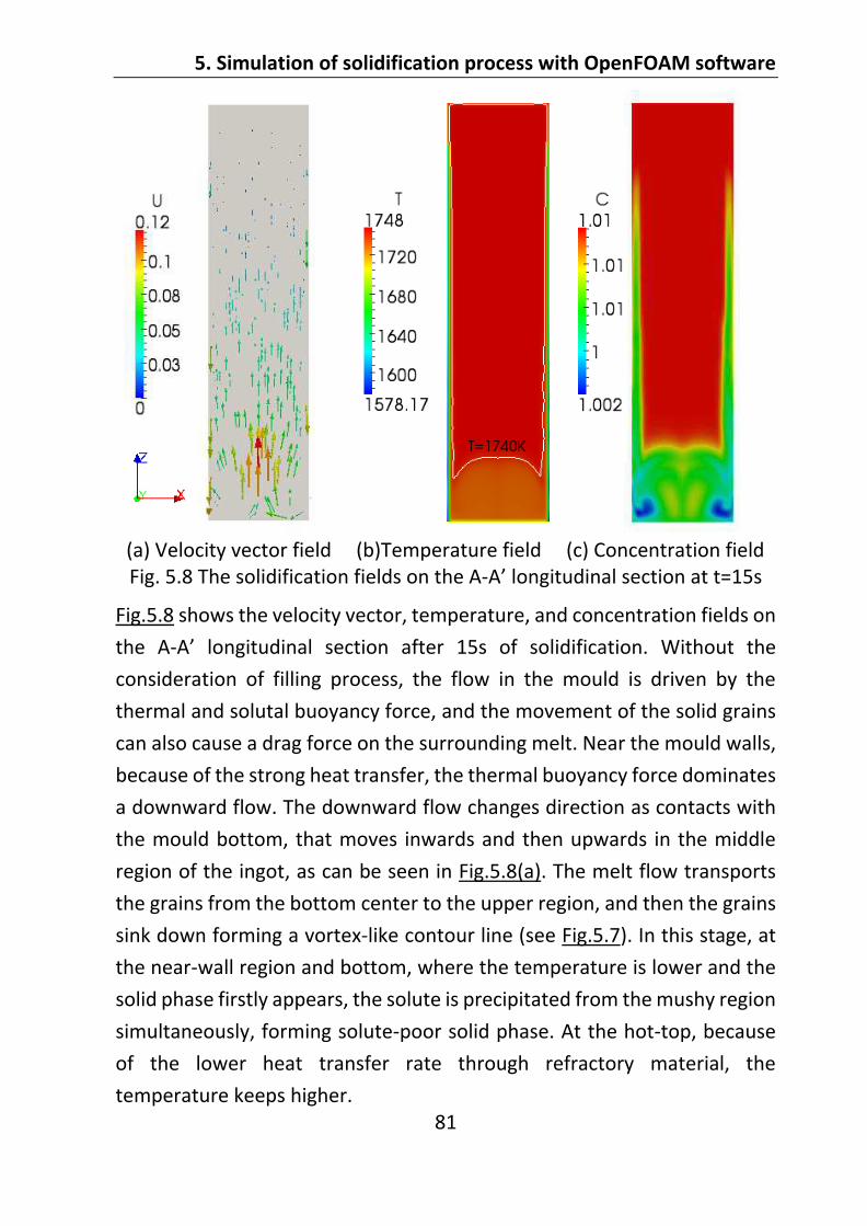
5. Simulation of solidification process with OpenFOAM software
81
(a) Velocity vector field (b)Temperature field (c) Concentration field Fig. 5.8 The solidification fields on the A-
Fig.5.8 shows the velocity vector, temperature, and concentration fields on
the A- Without the
consideration of filling process, the flow in the mould is driven by the
thermal and solutal buoyancy force, and the movement of the solid grains
can also cause a drag force on the surrounding melt. Near the mould walls,
because of the strong heat transfer, the thermal buoyancy force dominates
a downward flow. The downward flow changes direction as contacts with
the mould bottom, that moves inwards and then upwards in the middle
region of the ingot, as can be seen in Fig.5.8(a). The melt flow transports
the grains from the bottom center to the upper region, and then the grains
sink down forming a vortex-like contour line (see Fig.5.7). In this stage, at
the near-wall region and bottom, where the temperature is lower and the
solid phase firstly appears, the solute is precipitated from the mushy region
simultaneously, forming solute-poor solid phase. At the hot-top, because
of the lower heat transfer rate through refractory material, the
temperature keeps higher.

5. Simulation of solidification process with OpenFOAM software
82
t=300s t=800s t=1600s
t=2400s t=3200s t=4100s
Fig. 5.9 The sequence of solid fraction field fs on the A-section
5. Simulation of solidification process with OpenFOAM software
83
The progress of solidification can be presented by the time evolution of
solid fraction fs, as shown in Fig.5.9. The contour lines of solid fraction were
also plotted. The solid fraction of 0.637 was assumed as the packing limit,
so the solid phase in the mushy zone would be blocked when the local solid
fraction is larger than 0.637. The solid fraction of 0.99 represents that the
solidification in the local control volume is nearly completed. It can be seen
that, initially the contour lines of the solid fraction are U-shaped. Because
of the intensive heat transfer from the side walls, the temperature near the
side walls is much lower and the solid phase is formed much earlier. While
at the bottom, the heat transfer is relatively slow, and it stays in the mushy
region for a longer time. At the top region, the phase transfer rate is very
slow, due to the hot-top refractory material and insulating powder,
therefore, the contour lines of solid fraction becomes trumpet-shaped and
it takes a long time to finish the solidification. When the ingot is already
almost completely solidified, the near-top region is still mostly liquid. After
4100s, the liquid is completely solidified.
The distribution of carbon concentration reveals the degree of
macrosegregation. A variable, macrosegregation ratio R, was employed to
denote the macrosegregation, defined as:
0
0
C
CCR
where C0 is the initial carbon concentration. In this model, C0=1.01 wt%. For
the region where C>C0, we have R>0, then the segregation is positive; and
conversely that is negative segregation.
Fig.5.10 shows the sequence of the carbon concentration field at the A-
longitudinal section, plotted with three contour lines of macrosegregation
ratio: R=-0.1, 0, and 0.1. The white points in the figure were numerical
errors. From the contour lines of R=-0.1, we can see clearly the
development of the cone-shaped negative segregation, which expands
from the bottom of the ingot to the upper center. From the contour lines

5. Simulation of solidification process with OpenFOAM software
84
of R=0 and 0.1, the curves in the upper center region changes from A shape
to M shape, which indicate the V-shaped positive segregation in the center.
The formations of V-segregation is related to the sedimentation of
equiaxed grains, that generated from the solute-rich melt, at the V-shaped
solidification front (see Fig.5.9). Strong positive segregation was predicted
at the top of the ingot.
t=800s t=1600s t=4100s
Fig. 5.10 The sequence of concentration field at the A-section
The solidification is completed at time 4100s. Therefore, the corresponding
concentration field represents the final segregation distribution. To
observe the region near the cone-shaped negative segregation clearly, a
partial enlarged plot was made to display the segregation field in detail, as
shown in Fig.5.11. Fig.5.11(a) shows the segregation pattern at the A-
longitudinal section from the height of 0.1m to 2m, colored by a narrow
range of value. From this figure, some channels can be observed, as the so-
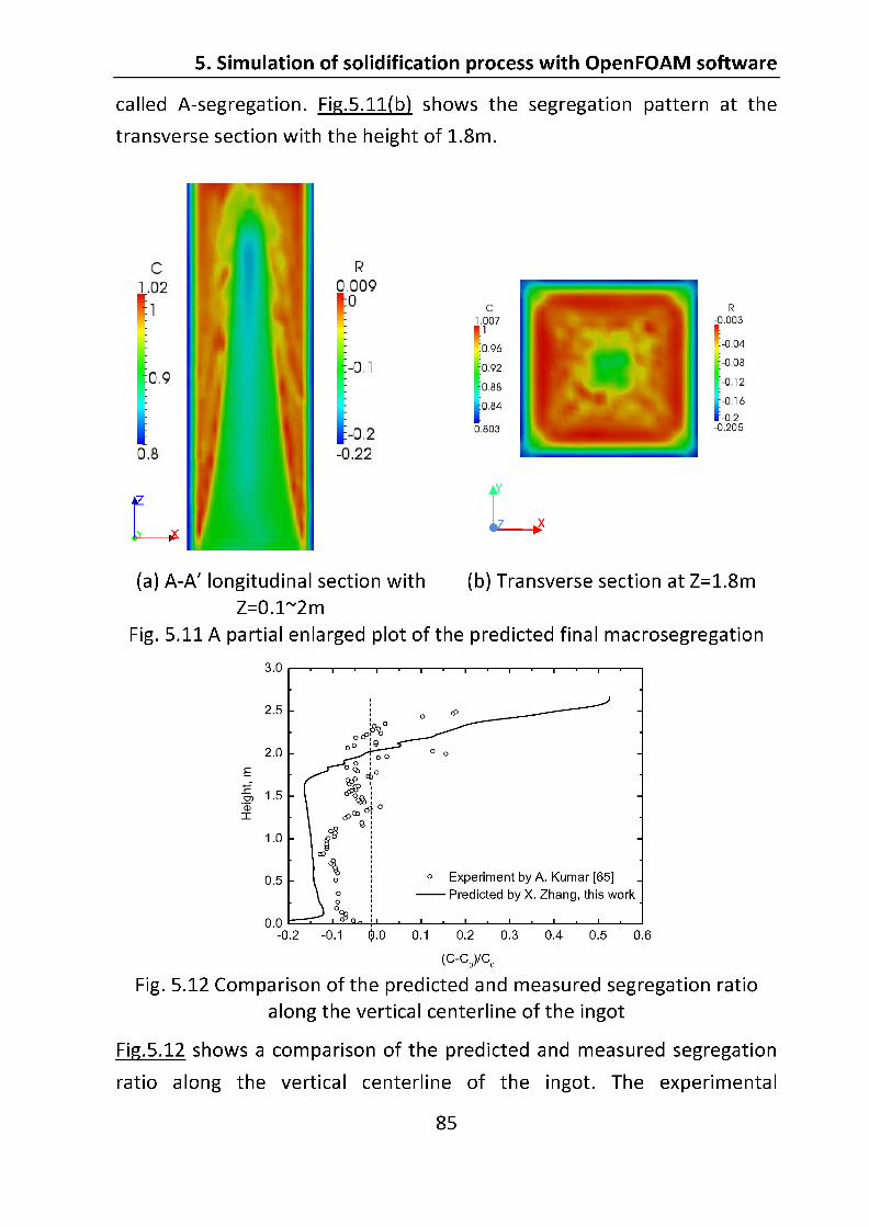

5. Simulation of solidification process with OpenFOAM software
86
measurements come from A. Kumar [76]. Both of the predicted and
measured results show positive segregation at the hot top, and negative
segregation at the bottom region of the ingot, up to the height of about 2
meter. However, the degree of the predicted segregations is stronger than
the measured segregations.
0.00 0.05 0.10 0.15 0.20 0.25 0.30 0.35-0.20
-0.15
-0.10
-0.05
0.00
0.05
0.10
Experiment by A. Kumar [65]
Predicted by X. Zhang, this work
Distance from center, m
(C-C
0)/
C0
(a) Along the median line A- of the transverse section
0.00 0.05 0.10 0.15 0.20 0.25 0.30 0.35-0.20
-0.15
-0.10
-0.05
0.00
0.05
0.10
Experiment by A. Kumar [65]
Predicted by X. Zhang, this work
Distance from center, m
(C-C
0)/
C0
(b) Along the diagonal line B- of the transverse section
Fig. 5.13 Comparison of the predicted and measured segregation ratio in the transverse section (Z=1.8m)
Fig.5.13 shows a comparison of the predicted and measured segregation
ratio in the transverse section, which is at the height of 1.8m. Both of the
segregations along the median line and along the diagonal line of the
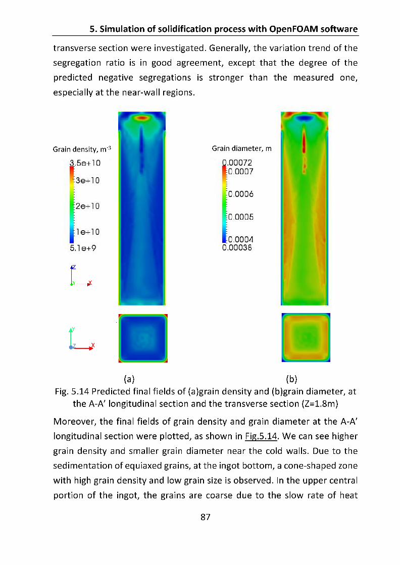
5. Simulation of solidification process with OpenFOAM software
88
transfer and solidification. The grain morphology at the hot top is more
complicate, with fine grain structure in the center which is surrounded by
coarse grains. Also the fields at the transverse section of Z=1.8m were
plotted. As can be seen that, the 4 corners have higher grain density and
smaller grain diameter, which is considered to be resulted from the strong
cooling at the corners.
5.3. Attempt on the coupling of mould filling and solidification process
In the solidification model developed above, only solid and liquid phases
were considered and the mould filling process cannot be simulated. In the
real ingot casting process, before the molten steel flows into the ingot
mould, it is totally air phase in the mould. As molten steel flows in, the air
will be pushed out from the top side of the mould. During the filling process,
with the decrease of temperature, the solidification may take place before
the finish of filling. Moreover, molten steel through the bottom nozzle can
induce a liquid jet. This stirring flow jet has a strong influence on the melt
convection in the mould, and therefore, it may impact on the growth of the
solid dendrites.
So far, most of the commercial solidification softwares divide the casting
process into two steps. The first step is mould filling, and the second step
is solidification, which assumes that the solidification starts after the mould
is fully filled. It is the same situation with my solidification mode developed
above. In this case, the initial solidification during the mould filling stage
cannot be well simulated. To combine the mould filling and solidification
process, it should be a liquid-solid-gas 3-phase model with phase change.
An advantage of my solidification model is that, it was developed based on
OpenFOAM software, which is an open-source software with well compiled
code structure. It is possible to extend the function of my solidification
model by the addition of more equations in the solver. So far, much effort
has been made to do this work but not yet succeed.
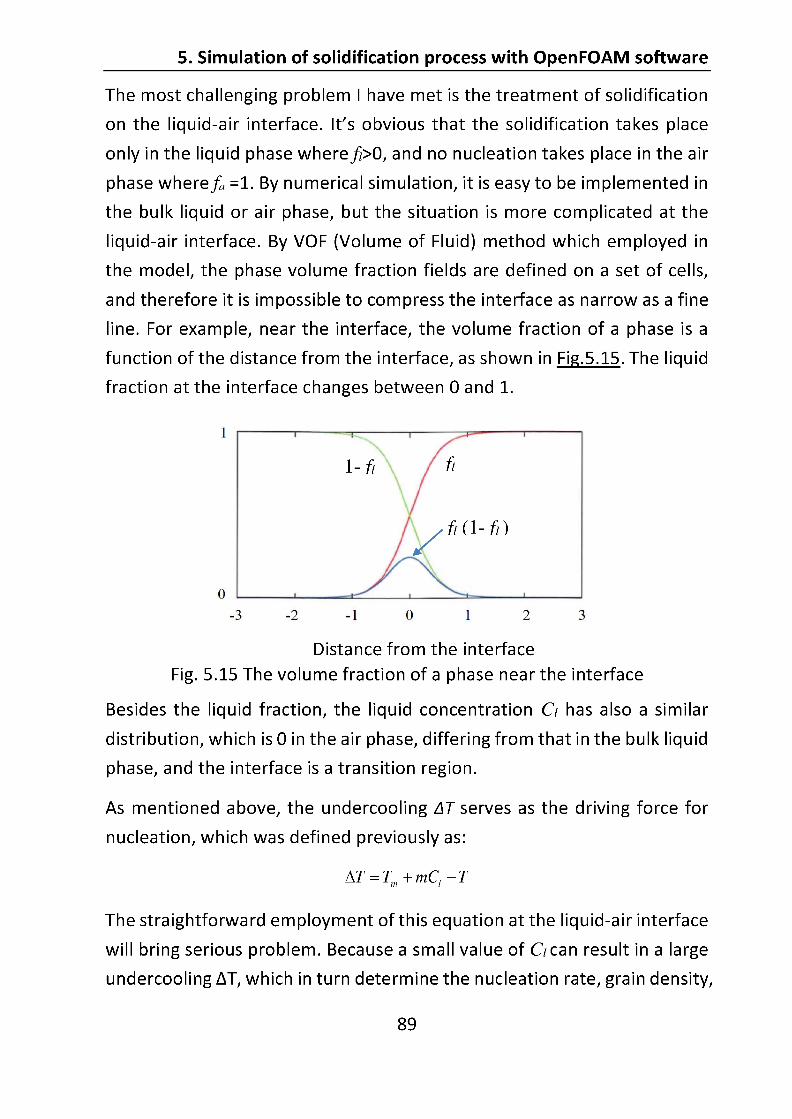
5. Simulation of solidification process with OpenFOAM software
90
grain interfacial area concentration Sv, mass transfer rate Mls, and finally
cause a fatal error on the liquid-solid phase change at the interface.
Although some assumed conditions of solidification at the interface had
been given, the calculation error occurred after some steps, which makes
the attempt on the coupling of mould filling and solidification process to
stop.
5.4. Conclusions
A solidification solver was developed based on OpenFOAM software using
the Euler-Euler two-phase approach. In the solver, the mass transfer, melt
convection, heat transfer as well as solute transport equations were
included. The nucleation, grain growth and grain movement were also
described, which makes it possible to calculate the mass and solute transfer
rate between the liquid and solid phases.
The solver was applied to simulate the solidification of a 3-dimensional
steel ingot. The evolution of the concerned fields was obtained, such as the
solid fraction field, velocity field, temperature field, concentration field and
grain density field. The predicted final macrosegregation pattern shows
strong positive segregation of carbon at the top of the ingot. While at the
bottom of the ingot, the segregation is negative with cone-shaped, and it
develops to the upper center of the ingot. The V-segregation at the upper
center and the channel-shaped A-segregation were also observed.
The predicted values of macrosegregation ratio were compared with the
experimental measurements from a literature. The comparison shows that
they generally were in good agreement, except that the degree of the
predicted macrosegregation ratio is much stronger than the measured one,
especially in the near-wall regions.
Extension of the liquid-solid 2-phase solidification model to a liquid-solid-
air 3-phase filling and solidification model was attempted. Due to the
numerical characteristic of the liquid-air interface, so far the attempt has
not succeeded yet.

6. Overall discussion
91
6. Overall discussion
In this study, the bottom teeming process as well as the solidification
process of ingot casting was investigated.
Water model experiments were carried out to study the flow conditions
during bottom teeming process of a large steel ingot. From the water
model experiments, it was observed that water jets from bottom nozzles
impacted on the top surface, which can form humps on the surface and the
size of humps reduced with the rising liquid level. The experimental results
have proven that the filling rate and also the bottom nozzle dimensions
have a significant influence on the humps. Comparing the hump height
under different filling rates at the same liquid level, it was found that the
hump height increases with the increase of filling rate. We can attribute it
to the powerful impact force of a submerged water jet under a larger filling
rate. The hump is formed mainly due to this impact force on top surface.
The influence of bottom nozzles on hump height is not only related to the
size of the nozzles, but also related to the arrangement of different nozzles,
in particular of multi-nozzles. According to the following formula:
uAV
where is the total volume flow rate; A is the area of the nozzle cross
section; u is the velocity of the flow through nozzle. Under the same filling
rate , a larger nozzle area will result in a smaller velocity of flow through
the nozzle, which in turn leads to a weaker impact force on the top surface
and thus the resulting hump height is smaller. In case of multi-nozzles, not
only the size of each nozzle, but also the arrangement of nozzles can affect
the velocity through each nozzle. Water model experiments with four equal
bottom nozzles were conducted, and it was found that the hump above the
last nozzle, which is the farthest away from the vertical sprue, is the largest.
This means that the velocity through the last nozzle is the largest, as has
been proved with OpenFOAM numerical simulation. Comparing the water
model experiments with four unequal bottom nozzles arranged in

6. Overall discussion
92
increasing size and in reverse order, little influence on the maximum hump
height was observed.
The numerical simulation of filling process with OpenFOAM software gave
more quantitative information about the flow field, and the predictions
were in good agreement with the water model measurements. From both
the water model experiments and OpenFOAM simulation, it was observed
that at the beginning of teeming, the incoming water flow pushes the
original air out mostly through the first nozzle which is the closest to the
vertical sprue. The air phase was pushed out as small bubbles. The rising air
bubbles cause strong turbulence. After all the air has been pushed out from
the runner, the water bath tends to be stable, only humps left on the top
surface. It was clear that for a small filling rate, more time is needed to push
out all the air bubbles. With the rising water level, the hump is reduced and
disappears when reaches to a certain water level, that was thought to be
related with the reduced impact force of water jet on top surface.
To study the molten steel-slag interface behavior, water model
experiments with oil addition were conducted. Vegetable oil was chosen as
an analogue of the fused slag phase, because that oil can float on water and
doesn't mix with water, like the behavior between molten steel and fused
slag phases. However, the density ratio of oil to water is not the same with
that of slag to molten steel. This may cause some uncertain difference
between the real molten steel-slag interface and simulated water-oil
interface behaviors. A better analogue of slag phase than oil may be found
in the future to give more accurate simulation.
As the oil film covers on water bath, during teeming the water jets from
bottom nozzles flow upwards and impinge on the oil phase, then the oil
film in the area above the jets may be open The
similar open between molten steel and slag phases in the real steel
ingot mould filling process indicates that the molten steel is exposed to air
and the risk of reoxidation increases, which is important to the quality of
6. Overall discussion
93
steel ingots. It was proved that the filling rate, nozzle dimensions and oil
At a certain liquid
level, with the reduction of filling rate, the fraction of open surface
decreases, which is also resulted from the reduced impact force of liquid
jet on top surface. Covering on the water bath, the gravity force of oil phase
can suppress the breaking of open surface. So with the increase of oil
thickness, the fraction of open surface decreases. 7 groups of nozzle
dimensions were used in the water model experiments. Comparing the
open surface at the same water level of 0.3m, it was fund that the model
with 25-22.5-15-
In the real ingot filling process, the hump height is related with the surface
the degree of reoxidation of molten steel. To optimize the filling conditions,
the risk of both reoxidation and slag entrapment should be reduced, by
adjusting the related parameters, such as the filling rate, nozzle dimensions
and slag thickness.
Obviously, water model experiments can simulate the mould filling process,
which is only the initial stage of ingot casting. The following solidification
stage was not simulated by water models in this study. However, in our
research group, a small water model with NH4Cl solution was carried out to
simulate the solidification[77]. The temperature of some special points was
measured during solidification. Various solidification phenomena, such as
columnar and equiaxed growth, CET (Columnar to Equiaxed Transition),
sedimentation of the equiaxed grains were observed and quantitatively
analyzed. A disadvantage of the solidification water model was that the
dimension of the model was too small (130mm width x 210mm height x
18mm depth) and the model was filled from the top side. A large water
model with NH4Cl solution is expect to simulate not only the bottom
teeming but also the solidification process, after solving the control
problems of cooling condition. In addition, the solidification of NH4Cl

6. Overall discussion
94
solution cannot simulate the macrosegregation phenomena which occurs
during the solidification of molten steel.
In this study, the solidification process was investigated with OpenFOAM
numerical simulation. The solidification solver was self-defined based on
several standard OpenFOAM multiphase flow solvers, by implanting the
governing equations of solidification. With the transport equations of mass,
momentum, heat, solute and grains, the concerned fields was solved,
including the solid fraction field, velocity field, temperature field,
concentration field and grain density field. After all the liquid was solidified,
the concentration field can indicate the degree of macrosegregation. As
agreed with the description in literatures, a cone-shaped negative
segregation at the bottom, positive segregation at the top, V-segregation
at the upper center of ingot, and channel-shaped A-segregation were
predicted. Regarding to the mechanism, the cone-shaped bottom negative
segregation is a result of the sedimentation of equiaxed grains, which are
mainly formed in the early stage of solidification and poor in solute. The
positive segregation at the top is caused by the buoyancy and shrinkage
driven interdendritic fluid flow during the final stage of solidification, where
the flow is enriched in solute. The V-segregation in the top center is
associated with large equiaxed grains settling down to the V-shaped
solidification front. The channel-shaped A-segregation is caused by the fact
that the liquid phase is enriched in solute with low melting points among
the dendrite due to the concentration and density difference. Near the cold
wall of ingot mould, it should be a region of inverse segregation, which is
positive and forms due to the motion of enriched interdendritic fluid
towards the wall to feed solidification shrinkage in the early stage of
solidification. However, in this study the near wall inverse segregation was
not successful predicted by the solidification model, which has some
deviations with the experimental measurements from literature.
The solidification model in this research was developed based on Euler-
Euler two-phase approach. The solidification process was simulated
6. Overall discussion
95
starting from the uniform field which was completely filled with liquid melt.
In other words, the initial filling process was not simulated. Actually, the
solidification may takes place early before the finish of mould filling. The
flow field during filling has influence on the solidification structure, also the
formation of solid phase can change the flow direction. To couple the filling
and solidification process, the air, liquid and solid phases are all involved.
Therefore the present liquid-solid 2-phase solidification model does not
have capability to couple the filling process. To solve this problem, a set of
governing equations for the air phase should be added in the solver.
Simultaneously, the liquid-air interface variables should be carefully
defined in case of phase change. This is a numerical difficulty on the VOF
method. In addition, the introduction of the third-phase equations makes
it possible to simulate the pore formation. Further studies on the coupling
of filling and solidification process should be tried.
7. Summary
96
7. Summary
The flow conditions during the filling process are of great importance on
the quality of the solidified steel ingots. In this study, the fluid flow during
the bottom teeming process was investigated with water model
experiments and OpenFOAM simulation.
In water model experiments, water was used to simulate the molten steel
and vegetable oil was used to simulate the slag phase. The water-oil
interface during the bottom teeming process was observed to study the
molten steel-slag interface at the initial stage of mould filling. The influence
of model parameters, such as the filling rate, nozzle dimensions and oil
thickness, on the filling conditions was investigated, concerning two
aspects: one is the slag entrapment, and the other is reoxidation of molten
steel. Both of the two situations should be avoid to provide a better filling
condition. Moreover, the computational simulation on water-air two-
phase flow with the interFoam solver of OpenFOAM software was
performed. The obtained predictions were in good agreement with the
water model experiments.
The main conclusions about the study of filling process are summarized as
follows:
(1) At the beginning of teeming, the incoming water flow pushes the air out
through bottom nozzles, especially through the first nozzle which is near
the vertical sprue. The rising air bubbles can lead to surface turbulence and
further increase the risk of slag entrapment. Therefore, it is not
recommended to add the mould powder at a low liquid level with air
bubbles.
(2) The hump height, which can indicate the surface turbulence, is gradually
reduced with rising liquid level. To reduce the slag entrapment caused by
surface turbulence, the filling rate at low liquid level should be smaller.

7. Summary
97
(3) However, the initial filling rate could not be too small, in which case the
time for rising of air bubbles will be extended, and before the formation of
slag layer the contact time between the melt and ambient air will also be
extended, which will further increase the risk of reoxidation of molten steel.
(4) After the level of molten steel reaches to a certain height where the
hump is small enough, the filling rate can be increased gradually to increase
productivity.
(5) It should be noted that even at high liquid level, the filling rate cannot
be too large. Because at a certain liquid level, with the reduce of filling rate,
on one hand, the hump height decrease, thus the risk of slag entrapment is
reduced; on the other hand, the fraction of open surface decreases, thus
the risk of reoxidation is reduced.
(6) For a large steel ingot mould, it is better to design multiple bottom
nozzles to reduce the jet velocity through each nozzle. For a mould with
multiple nozzles of equal size, the velocity of the flow through the last
nozzle, which is the farthest away from the vertical sprue, is the largest. In
the experiment models, the model with four 25mm-diameter equal nozzles
shows better performance of filling conditions from the view of both slag
entrapment and reoxidation.
(7) With the increase of slag thickness, the open surface decreases and
therefore the risk of reoxidation is reduced. However, more slag addition
may lead to more slag entrapment and increase the production cost as
well.
Besides the filling process, the solidification process was also investigated
with numerical simulation. A user-defined liquid-solid two-phase
solidification solver was developed based on the software platform of
OpenFOAM, using Euler-Euler two-phase approach. The globular equiaxed
grains was assumed as the solid morphology. In the solver, governing
equations about the mass transfer, melt convection, heat transfer, solute
7. Summary
98
transport, nucleation and grain transport were included, so that the
solidification as well as macrosegregation formation can be simulated.
The solidification solver was performed on a 3-dimensional model of a
reported steel ingot. The solid fraction, velocity, pressure, temperature,
concentration and grain density fields were calculated. The
macrosegregation was indicated by the carbon concentration. From the
predicted macrosegregation pattern, the cone-shaped negative
segregation at the bottom, positive segregation at the top, V-segregation
at the upper center of the ingot, and the channel-shaped A-segregation
were obtained. The simulation results of macrosegregation ratio on certain
lines were generally in agreement with the experimental measurements
from the literature, except for same deviations at the bottom and the near-
wall regions, where the predicted degree of negative segregation was much
stronger than the measured one.
In the present liquid-solid 2-phase solidification model, it was assumed that
the solidification occurs after the mould has been filled with liquid melt,
which means that the mould filling process was not coupled with the
solidification process. Extension of the liquid-solid 2-phase solidification
model to a liquid-solid-air 3-phase filling and solidification model was
attempted. Due to the numerical characteristic of the liquid-air interface,
so far the attempt has not succeeded yet. Further studies on this topic
would be conducted in the future.
8. Reference
99
8. Reference
[1] L. Zhang, B.G. Thomas, State of the art in the control of inclusions during steel, Metallurgical and Materials Transactions B, 37 (2006) 733-761.
[2] H.F. Marston, High quality ingots: the design of bottom pouring powders, 69th Steel Making Conference Proceedings, ISS, Warrandale, PA, (1986) 107-119.
[3] B.V.R. Raja, Selection of mould fluxes for production of High quality steel ingots, Steelword, Dec., (2008) 34-40.
[4] D. Mazumdar, H. Nakajima, R.I.L. Guthrie, Possible roles of upper slag phases on the fluid dynamics of gas stirred ladles, Metallurgical Transactions B, 19 (1988) 507-511.
[5] D. Mazumdar, R.I.L. Guthrie, The physical and mathematical modelling of gas stirred ladle systems, ISIJ International, 35 (1995) 1-20.
[6] J. Mietz, S. Schneider, F. Oeters, Emulsification and mass transfer in ladle metallurgy, Steel Research, 62 (1991) 10-15.
[7] Z. Tan, M. Ersson, P. Jönsson, Mathematical modeling of initial filling moment of uphill teeming process considering a trumpet, ISIJ International, 51 (2011) 1461-1467.
[8] X. Zhang, E.A.T. Wosch, D. Senk, Modeling of fluid flow in large ingot uphill teeming process, Tagungsband zum 27. Aachener Stahlkolloquium Metallurgie, Aachen, (2012) 257-269.
[9] X. Zhang, Z. Chen, D. Senk, X. Liu, S. Maqbool, Numerical and experimental investigation of fluid flow in large ingot uphill casting process, In Conference STEELSIM 2013 proceedings: 5th International Conference on Modelling and Simulation of Metallurgical Processes in Steelmaking, Session 4, Ostrava, (2013).
[10] A.K. Bin, Behavior of liquid surface impinged by turbulent jets, AIChE Journal, 31 (1985) 1397-1400.
[11] U. Narusawa, S. Takao, Y. Suzukawa, Rise in free surface caused by submerged jet directed upward, AIChE Journal, 29 (1983) 511-513.
[12] A. Maurel, S. Cremer, P. Jenffer, Experimental study of a submerged fountain, Europhys. Lett., 39 (1997) 503-508.
[13] T.F. Bower, M.C. Flemings, Structure of dendrites at chill surfaces, Trans. AIME, 239 (1967) 1620-1625.
8. Reference
100
[14] D.J. Hurtuk., Steel ingot casting, ASM Handbook, Vol. 15: Casting, ASM International, Materials Park, OH, (2008) 911-917.
[15] M. Imagumbai, Relationship between primary- and secondary-dendrite arm spacing of C-Mn steel uni-directionally solidified in steady state, ISIJ International, 34 (1994) 986-991.
[16] M. Imagumbai, Behaviors of manganese-sulfide in aluminum-killed steel solidified uni-directionally in steady state - dendrite structure and inclusions, ISIJ International, 34 (1994) 896-905.
[17] C. Cicutti, R. Boeri, On the relationship between primary and secondary dendrite arm spacing in continuous casting products, Scripta Materialia, 45 (2001) 1455-1460.
[18] Y.-M. Won, B.G. Thomas, Simple model of microsegregation during solidification of steels, Metallurgical and Materials Transactions A, 32 (2001) 1755-1767.
[19] C. Beckermann, Modelling of macrosegregation: applications and future needs, International Materials Reviews, 47 (2002) 243-261.
[20] E.J. Pickering, Macrosegregation in steel ingots: The applicability of modelling and characterisation techniques, ISIJ International, 53 (2013) 935-949.
[21] Z. Chen, D. Senk, Investigation on the A-segregation channel instable development in large ingot casting, In Conference STEELSIM 2013 proceedings: 5th International Conference on Modelling and Simulation of Metallurgical Processes in Steelmaking, Session 4, Ostrava, (2013).
[22] J.S. Kirkaldy, W.V. Youdelis, Contribution to the theory of inverse segregation, Transactions of The Metallurgical Society of AIME, 212 (1958) 833-840.
[23] M.C. Flemings, R. Mehrabian, G.E. Nereo, Macrosegregation, Part II, Transactions of The Metallurgical Society of AIME, 242 (1968) 41-49.
[24] V.R. Voller, A.D. Brent, C. Prakash, Modelling the mushy region in a binary alloy, Applied Mathematical Modelling, 14 (1990) 320-326.
[25] V.R. Voller, C. Prakash, A fixed grid numerical modelling methodology for convection-diffusion mushy region phase-change problems, International Journal of Heat and Mass Transfer, 30 (1987) 1709-1719.
8. Reference
101
[26] V.R. Voller, M. Cross, N.C. Markatos, An enthalpy method for convection/diffusion phase change, International Journal for Numerical Methods in Engineering, 24 (1987) 271-284.
[27] C.R.Swaminathan, V.R.Voller, On the enthalpy method, International Journal of Numerical Methods for Heat & Fluid Flow, 3 (1993) 233-244.
[28] V.R. Voller, A.D. Brent, The modelling of heat, mass and solute transport in solidification systems, International Journal of Heat and Mass Transfer, 32 (1989) 1719-1731.
[29] M. Rappaz, V. Voller, Modeling of micro-macrosegregation in solidification processes, Metallurgical Transactions A, 21 (1990) 749-753.
[30] C. Prakash, V. Voller, On the numerical solution of continuum mixture model equations describing binary solid-liquid phase change, Numerical Heat Transfer, Part B: Fundamentals, 15 (1989) 171-189.
[31] W.D. Bennon, F.P. Incropera, A continuum model for momentum, heat and species transport in binary solid-liquid phase change systems I. Model formulation, International Journal of Heat and Mass Transfer, 30 (1987) 2161-2170.
[32] W.D. Bennon, F.P. Incropera, Numerical analysis of binary solid-liquid phase change using a continuum model, Numerical Heat Transfer, 13 (1988) 277-296.
[33] M. Wu, A. Vakhrushev, G. Nummer, C. Pfeiler, A. Kharicha, A. Ludwig, Importance of melt flow in solidifying mushy zone, The Open Conservation Biology Journal, 2 (2010) 16-23.
[34] A.K. Singh, R. Pardeshi, B. Basu, Modelling of convection during solidification of metal and alloys, Sadhana, 26 (2001) 139-162.
[35] G. Arampatzis, D. Assimacopoulos, Numerical modeling of convection-diffusion phase change problems, Computational Mechanics, 21 (1998) 409-415.
[36] C.R. Swaminathan, V.R. Voller, A general enthalpy method for modeling solidification processes, Metallurgical Transactions B, 23 (1992) 651-664.
[37] V.R. Voller, C.R. Swaminathan, General source-based method for solidification phase change, Numerical Heat Transfer, Part B: Fundamentals, 19 (1991) 175-189.
8. Reference
102
[38] S. Chakraborty, P. Dutta, A generalized formulation for evaluation of latent heat functions in enthalpy-based macroscopic models for convection-diffusion phase change processes, Metallurgical and Materials Transactions B, 32 (2001) 562-564.
[39] M. Rappaz, Modelling of microstructure formation in solidification processes, International Materials Reviews, 34 (1989) 93-123.
[40] M.C. Schneider, C. Beckermann, Formation of macrosegregation by multicomponent thermosolutal convection during the solidification of steel, Metallurgical and Materials Transactions A, 26 (1995) 2373-2388.
[41] C. Wang, C. Beckermann, A two-phase mixture model of liquid-gas flow and heat transfer in capillary porous media - I. Formulation, International Journal of Heat and Mass Transfer, 36 (1993) 2747-2758.
[42] C. Beckermann, R. Viskanta, Mathematical modeling of transport phenomena during alloy solidification, Applied Mechanics Reviews, 46 (1993) 1-27.
[43] M. Wu, J. Domitner, A. Ludwig, Using a two-phase columnar solidification model to study the principle of mechanical soft reduction in slab casting, Metallurgical and Materials Transactions A, 43 (2012) 945-964.
[44] J. Li, M. Wu, J. Hao, A. Ludwig, Simulation of channel segregation using a two-phase columnar solidification model Part I: Model description and verification, Computational Materials Science, 55 (2012) 407-418.
[45] M. Wu, A. Ludwig, Modeling equiaxed solidification with melt convection and grain sedimentation I: Model description, Acta Materialia, 57 (2009) 5621-5631.
[46] M. Wu, A. Ludwig, A. Bührig-Polaczek, M. Fehlbier, P.R. Sahm, Influence of convection and grain movement on globular equiaxed solidification, International Journal of Heat and Mass Transfer, 46 (2003) 2819-2832.
[47] A. Ludwig, M. Wu, Modeling of globular equiaxed solidification with a two-phase approach, Metallurgical and materials transactions A, 33 (2002) 3673-3683.
[48] M. Wu, A. Ludwig, Using a three-phase deterministic model for the columnar-to-equiaxed transition, Metallurgical and Materials Transactions A, 38 (2007) 1465-1475.
8. Reference
103
[49] R. Tanzer, W. Schützenhöfer, G. Reiter, H.P. Fauland, L. Könözsy, A. Ishmurzin, M. Wu, A. Ludwig, Validation of a multiphase model for the macrosegregation and primary structure of high grade steel ingots, Metallurgical and Materials Transactions B, 40 (2009) 305-311.
[50] M. Wu, A. Fjeld, A. Ludwig, Modelling mixed columnar-equiaxed solidification with melt convection and grain sedimentation Part I: Model description, Computational Materials Science, 50 (2010) 32-42.
[51] M. Wu, A. Ludwig, A. Fjeld, Modelling mixed columnar-equiaxed solidification with melt convection and grain sedimentation Part II: Illustrative modelling results and parameter studies, Computational Materials Science, 50 (2010) 43-58.
[52] M. Wu, A. Ludwig, A three-phase model for mixed columnar-equiaxed solidification, Metallurgical and Materials Transactions A, 37 (2006) 1613-1631.
[53] L. Könözsy, A. Ishmurzin, M. Grasser, M.H. Wu, A. Ludwig, R. Tanzer, W. Schützenhöfer, Columnar to equiaxed transition during ingot casting using ternary alloy composition, Materials Science Forum, 649 (2010) 349-354.
[54] M. Wu, A. Ludwig, An idea to treat the dendritic morphology in mixed columnar equiaxed solidification, International Journal of Cast Metals Research, 22 (2009) 323-326.
[55] M.S. Kharicha, S. Eck, L. Könözsy, A. Kharicha, A. Ludwig, Experimental and numerical investigations of NH4Cl solidification in a mould. Part 1: Experimental results, International Journal of Cast Metals Research, 22 (2009) 168-171.
[56] L. Könözsy, S. Eck, M.S. Kharicha, M. Wu, A. Ludwig, Experimental and numerical investigations of NH4Cl solidification in a mould. Part 2: numerical results, International Journal of Cast Metals Research, 22 (2009) 172-174.
[57] OpenFOAM User Guide. OpenCFD Limited. Version 2.3.1, (2014).
[58] OpenFOAM Programmer's Guide. OpenCFD Limited. Version 2.3.1, (2014).
[59] B. Peters, The extended discrete element method (XDEM) for multi-physics applications, Scholarly Journal of Engineering Research, 2 (2013) 1-20.
8. Reference
104
[60] A.H. Mahmoudi, F. Hoffmann, B. Peters, Application of XDEM as a novel approach to predict drying of a packed bed, International Journal of Thermal Sciences, 75 (2014) 65-75.
[61] J.A. Kromhout, D.W. van der Plas, Melting speed of mould powders: determination and application in casting practice, Ironmaking & Steelmaking, 29 (2002) 303-307.
[62] M. Görnerup, M. Hayashi, C.-Å. Däcker, S. Seetharaman, Mould fluxes in continuous casting of steel - characterization and performance tuning, Proceedings of 7th International Conference on Molten Slags, Fluxes and Salts, The South African Institute of Mining and Metallurgy, (2004) 745-752.
[63] M.L. Yang, Z.S. Li, F.L. Wei, C.G. Cheng, X. Chen, S.B. Qi, Study on slag entrapment of molten steel in mold with electromagnetic stirring technology, Advanced Materials Research, 424-425 (2012) 811-816.
[64] L. Zhang, S. Yang, K. Cai, J. Li, X. Wan, B.G. Thomas, Investigation of fluid flow and steel cleanliness in the continuous casting strand, Metallurgical and Materials Transactions B, 38 (2007) 63-83.
[65] O. Ubbink, Numerical prediction of two fluid systems with sharp interfaces, PhD Thesis, University of London, (1997) 13-17.
macrosegregation in steel ingots: Influence of the motion and the morphology of equiaxed grains, Metallurgical and Materials Transactions B, 40 (2009) 289-304.
macroscopic transport and grain growth in a two-phase multiscale solidification model: Part I Model and solution scheme, Computational Materials Science, 48 (2010) 1-10.
[68] T. Wang, M. Wu, A. Ludwig, M. Abondano, B. Pustal, A. Bührig-Polaczek, Modelling the thermosolutal convection, shrinkage flow and grain movement of globular equiaxed solidification using a three phase model, International Journal of Cast Metals Research, 18 (2005) 221-228.

8. Reference
105
[69] T. Wang, M. Wu, A. Ludwig, M. Abondano, B. Pustal, A. Bührig-Polaczek, Globular equiaxed solidification with thermo-solutal convection, shrinkage flow and grain movement by a three-phase model, Proceedings of Modeling of Casting and Solidification Processes VI, (2004) 181-189.
[70] J. Li, M. Wu, A. Ludwig, A. Kharicha, Simulation of macrosegregation in a 2.45-ton steel ingot using a three-phase mixed columnar-equiaxed model, International Journal of Heat and Mass Transfer, 72 (2014) 668-679.
[71] C.Y. Wang, C. Beckermann, Equiaxed dendritic solidification with convection: Part I. Multiscale/multiphase modeling, Metallurgical and Materials Transactions A, 27 (1996) 2754-2764.
[72] W. Li, H. Shen, B. Liu, Numerical simulation of macrosegregation in steel ingots using a two-phase model, International Journal of Minerals, Metallurgy, and Materials, 19 (2012) 787-794.
[73] W. Tu, H. Shen, B. Liu, Two-phase modeling of macrosegregation in a 231 t steel ingot, ISIJ International, 54 (2014) 351-355.
[74] C.Y. Wang, S. Ahuja, C. Beckermann, H.C.d. Groh, Multiparticle interfacial drag in equiaxed solidification, Metallurgical and Materials Transactions B, 26 (1995) 111-119.
[75] J.A. Dantzig, M. Rappaz, Solidification, EPFL Press, Lausanne, (2009), 258-268.
structure and macrosegregation in an industrial steel ingot: comparison with experiment, International Journal of Advances in Engineering Sciences and Applied Mathematics, 2 (2010) 140-148.
[77] Z. Chen, D. Senk, F. Firsbach, Quantitative water-modeling of ingot solidification by using NH4Cl solution, In Conference STEELSIM 2013 proceedings: 5th International Conference on Modelling and Simulation of Metallurgical Processes in Steelmaking, Session 10, Ostrava, (2013).

![+HDOWK DQG &RPPXQLFDWLRQV 3OD GHPSUHVD SHU XQD … · +hdowk dqg &rppxqlfdwlrqv 3od g hpsuhvd shu xqd djqqfld gh frpxqlfdfly hvshfldolw]dgd hq vdoxw +hdowk dqg &rppxqlfdwlrqv 3odq](https://img.pdfslide.tips/doc/110x75/5f0c24077e708231d433f07b/hdowk-dqg-rppxqlfdwlrqv-3od-ghpsuhvd-shu-xqd-hdowk-dqg-rppxqlfdwlrqv.jpg)

![3 ADICIONAL DE PERICULOSIDADE E INSALUBRIDADE · /deru dqg (psor\phqw lq wkh &lylo &rgh ri dqg wkh &rqyhqwlrqv dqg ri wkh ,qwhuqdwlrqdo /deru 2ujdql]dwlrq )ru frpsdulvrq duh suhvhqwhg](https://img.pdfslide.tips/doc/110x75/5be6fc7f09d3f23a518dbd4c/3-adicional-de-periculosidade-e-deru-dqg-psorphqw-lq-wkh-lylo-rgh-ri-dqg.jpg)


![TEPPICHE | CARPETS | TAPIS€¦ · ÀH[LEO\ DQG DUH DEOH WR RIIHU \RX DQG \RXU FXVWRPHUV DQ HQRUPRXV VHOHFWLRQ RI VL]HV L H VWDQGDUG GLPHQVLRQV DQG HYHQ FXV-tomized sizes, which are](https://img.pdfslide.tips/doc/110x75/600c17d0a47704253132f4bd/teppiche-carpets-hleo-dqg-duh-deoh-wr-riihu-rx-dqg-rxu-fxvwrphuv-dq-hqruprxv.jpg)


![IRWR 0XQLFLSDOLWLHV OLQN · fuhdwhg qh[w wr wkh dqflhqw rqhv 7kh fhqwuhv ri 6flfol dqg 0rglfd zhuh pryhg dqg uhexlow lq dgmrlqlqj duhdv douhdg\ sduwldoo\ xuedql]hg dqg &dowdjlurqh](https://img.pdfslide.tips/doc/110x75/5fa10024ba35ef746a233a47/irwr-0xqlflsdolwlhv-olqn-fuhdwhg-qhw-wr-wkh-dqflhqw-rqhv-7kh-fhqwuhv-ri-6flfol.jpg)

![Billing Manager Manual -Version 2020-NLd59fdb59-dd50-4b66... · %loolqj 0dqdjhu *heuxlnhuvkdqgohlglqj (glwlh %loolqj 0dqdjhu *heuxlnhuvkdqgohlglqj ^ v ] ] À ] Ç w h v ] 3ur 3dfndjh](https://img.pdfslide.tips/doc/110x75/60130d1a837a917aca1392dd/billing-manager-manual-version-2020-nl-d59fdb59-dd50-4b66-loolqj-0dqdjhu.jpg)


![%DOODG IRU )OXHJHO +RUQ DQG -D]] (QVHPEOH](https://img.pdfslide.tips/doc/110x75/61980c3f43f30058b76c805a/doodg-iru-oxhjho-ruq-dqg-d-qvhpeoh.jpg)