Embed Size (px)
Citation preview

RUPRECHT-KARLS-UNIVERSITÄT HEIDELBERG
KIRCHHOFF-INSTITUT FÜR PHYSIK

DISSERTATION
submitted to theCombined Faculties for the Natural Sciences and for Mathematics
of theRuperto-Carola-University of Heidelberg, Germany
for the degree ofDoctor of Natural Sciences
presented by
Dipl.-Phys. Steffen Gunther Hohmannborn in Braunschweig, Germany
Date of oral examination: 18.05.2005


Stepwise Evolutionary
Training Strategies
for
Hardware Neural Networks
Referees: Prof. Dr. K. Meier
Prof. Dr. F. A. Hamprecht

Schrittweise evolutionare Trainingsstrategien fur neuronale Netzwerke in Hardware
Rein analoge und gemischt analog-digitale Realisierungen kunstlicher neuronaler Netzwerke in Hard-ware entziehen sich fur gewohnlich einer exakten quantitativen Beschreibung. Die Grunde dafur sinddie bei der Halbleiterherstellung unvermeidlichen Schwankungen der Bauteilparameter sowie zeitlicheFluktuationen der internen analogen Signale. Evolutionare Algorithmen eignen sich besonders gut furdas Training solcher Systeme, da sie keinerlei detaillierte Informationen uber das zu optimierende Sys-tem benotigen. Um die hohe Arbeitsgeschwindigkeit der neuronalen Netzwerke voll auszunutzen, wer-den einfache und schnelle Trainingsverfahren benotigt. Im Rahmen dieser Arbeit wurde eine spezielleschrittweise Trainingsmethode entwickelt, die es erlaubt, die synaptischen Gewichte eines gemischtanalog-digitalen neuronalen Netzwerkchips unter Zuhilfenahme einfacher evolutionarer Algorithmenauf effiziente Weise zu optimieren. Die vorgestellte Trainingsstrategie wurde an neun verbreitetenstandardisierten Aufgabenstellungen fur Klassifikationsprobleme getestet: den breast cancer, diabetes,heart disease, liver disorder, iris plant, wine, glass, E.coli und yeast Datensatzen. Es zeigt sich, dassdie erreichten Klassifikationsgenauigkeiten sehr gut mit denen von in Software realisierten neuronalenNetzwerken konkurrieren konnen. Weiterhin sind sie mit den besten Resultaten vergleichbar, die furandere Klassifikationsverfahren in der Literatur recherchiert werden konnten. Die vorgestellte Trai-ningsmethode begunstigt eine parallele Realisierung und eignet sich daruberhinaus gut zur Verwen-dung in Kombination mit einem speziell entwickelten Koprozessor, der die zeitaufwendigen genetischenOperationen in einer konfigurierbaren Logik realisiert und damit eine beschleunigte Ausfuhrung evo-lutionarer Algorithmen ermoglicht. Auf diese Weise kann das entwickelte Trainingsverfahren optimalvon der Geschwindigkeit neuronaler Hardware profitieren und stellt daher eine effiziente Methodedar, große neuronale Netzwerke auf dem verwendeten gemischt analog-digitalen Netzwerkchip furanspruchsvolle, praxisrelevante Klassifikationsprobleme zu trainieren.
Stepwise evolutionary training strategies for hardware neural networks
Analog and mixed-signal implementations of artificial neural networks usually lack an exact numericalmodel due to the unavoidable device variations introduced during manufacturing and the temporalfluctuations in the internal analog signals. Evolutionary algorithms are particularly well suited for thetraining of such networks since they do not require detailed knowledge of the system to be optimized.In order to make best use of the high network speed, fast and simple training approaches are required.Within the scope of this thesis, a stepwise training approach has been devised that allows for the use ofsimple evolutionary algorithms to efficiently optimize the synaptic weights of a fast mixed-signal neuralnetwork chip. The training strategy is tested on a set of nine well-known classification benchmarks:the breast cancer, diabetes, heart disease, liver disorder, iris plant, wine, glass, E.coli, and yeastdata sets. The obtained classification accuracies are shown to be more than competitive to thoseachieved by software-implemented neural networks and are comparable to the best reported results ofother classification algorithms that could be found in literature for these benchmarks. The presentedtraining method is readily suited for a parallel implementation and is fit for use in conjunction with aspecialized coprocessor architecture that speeds up evolutionary algorithms by performing the time-consuming genetic operations within a configurable logic. This way, the proposed strategy can fullybenefit from the speed of the neural hardware and thus provides efficient means for the training oflarge networks on the used mixed-signal chip for demanding real-world classification tasks.


Meinen lieben Eltern

Contents
Introduction 1
I Foundations 5
1 Artificial Neural Networks 71.1 The Human Brain . . . . . . . . . . . . . . . . . . . . . . . . . . . 8
1.1.1 The Neuron . . . . . . . . . . . . . . . . . . . . . . . . . . . 81.1.2 The Synapse . . . . . . . . . . . . . . . . . . . . . . . . . . 91.1.3 Neural Encoding . . . . . . . . . . . . . . . . . . . . . . . . 101.1.4 Learning in the Human Brain . . . . . . . . . . . . . . . . . 10
1.2 Neural Network Models . . . . . . . . . . . . . . . . . . . . . . . . 111.2.1 A General Neuron Model . . . . . . . . . . . . . . . . . . . 121.2.2 Networks of Artificial Neurons . . . . . . . . . . . . . . . . 121.2.3 Important Neuron Models . . . . . . . . . . . . . . . . . . . 151.2.4 Modeling Adaptation . . . . . . . . . . . . . . . . . . . . . 22
2 Feedforward Neural Networks 272.1 Single-Layer Feedforward Networks . . . . . . . . . . . . . . . . . . 27
2.1.1 Capability of the Simple Perceptron . . . . . . . . . . . . . 282.1.2 Training the Simple Perceptron . . . . . . . . . . . . . . . . 332.1.3 Continuous Outputs and Gradient Descent . . . . . . . . . 352.1.4 Generalization to Multiple Outputs . . . . . . . . . . . . . . 39
2.2 Multi-Layer Feedforward Networks . . . . . . . . . . . . . . . . . . 422.2.1 Computational Capabilities . . . . . . . . . . . . . . . . . . 432.2.2 Training Multi-Layer Networks . . . . . . . . . . . . . . . . 46
2.3 A Short Overview of Alternative Network Models . . . . . . . . . . 512.3.1 The Feature Space Revisited: Support Vector Machines . . 512.3.2 Hierarchical Approaches and the Neocognitron . . . . . . . 522.3.3 The Hopfield Network . . . . . . . . . . . . . . . . . . . . . 522.3.4 Computing Without Stable States . . . . . . . . . . . . . . 54
2.4 Hardware Neural Networks . . . . . . . . . . . . . . . . . . . . . . 542.4.1 Historical Overview . . . . . . . . . . . . . . . . . . . . . . 552.4.2 A Categorization of Neural Hardware . . . . . . . . . . . . 562.4.3 Performance Criteria . . . . . . . . . . . . . . . . . . . . . . 562.4.4 Challenges and Present Trends . . . . . . . . . . . . . . . . 57
I
Contents
2.4.5 Training Hardware Neural Networks . . . . . . . . . . . . . 58
3 Evolutionary Algorithms 61
3.1 Natural Evolution . . . . . . . . . . . . . . . . . . . . . . . . . . . 61
3.1.1 The Principles of Darwinian Evolution . . . . . . . . . . . . 62
3.1.2 Evolution on the Genetic Level . . . . . . . . . . . . . . . . 63
3.1.3 Speciation . . . . . . . . . . . . . . . . . . . . . . . . . . . . 65
3.2 Evolutionary Algorithms: An Overview . . . . . . . . . . . . . . . 65
3.2.1 The Main Constituents of an Evolutionary Algorithm . . . 67
3.3 General Features of Evolutionary Algorithms . . . . . . . . . . . . 71
3.3.1 Evolutionary Algorithms as Global optimizers . . . . . . . . 71
3.3.2 A Modular View of Evolutionary Algorithms . . . . . . . . 72
3.3.3 Evolutionary Algorithms as Model-Free Heuristics . . . . . 72
3.3.4 Extensions to the Basic Concept . . . . . . . . . . . . . . . 74
3.4 Evolutionary Algorithm Implementations . . . . . . . . . . . . . . 76
3.4.1 Selection Schemes . . . . . . . . . . . . . . . . . . . . . . . 77
3.4.2 Genetic Representations . . . . . . . . . . . . . . . . . . . . 80
3.4.3 Mutation Operators . . . . . . . . . . . . . . . . . . . . . . 81
3.4.4 Recombination Operators . . . . . . . . . . . . . . . . . . . 83
3.5 Theoretical Analysis: The Schema Theorem . . . . . . . . . . . . . 86
3.5.1 Schemata . . . . . . . . . . . . . . . . . . . . . . . . . . . . 86
3.5.2 The Processing of Schemata . . . . . . . . . . . . . . . . . . 87
3.5.3 Building Blocks, Deception and Challenges to the SchemaTheorem . . . . . . . . . . . . . . . . . . . . . . . . . . . . 88
4 Evolving Artificial Neural Networks 91
4.1 Evolving Synaptic Weights . . . . . . . . . . . . . . . . . . . . . . 92
4.1.1 Performance Evaluation and Fitness Function . . . . . . . . 92
4.1.2 Representations and the Permutation Problem . . . . . . . 93
4.1.3 Comparison with Gradient Based Training . . . . . . . . . 96
4.2 Evolving Network Architectures . . . . . . . . . . . . . . . . . . . . 97
4.2.1 Performance Evaluation - Architectures and Weights . . . . 97
4.2.2 Genetic Representations . . . . . . . . . . . . . . . . . . . . 98
4.2.3 Fixed vs. Evolved Architectures . . . . . . . . . . . . . . . 103
4.3 Alternative Black-Box Approaches . . . . . . . . . . . . . . . . . . 104
4.3.1 Simulated Annealing . . . . . . . . . . . . . . . . . . . . . . 104
4.3.2 Weight Perturbation . . . . . . . . . . . . . . . . . . . . . . 106
4.3.3 Comparison to Evolutionary Algorithms . . . . . . . . . . . 108
II Hardware Neural Network Framework 109
5 The HAGEN Chip 111
5.1 Design Considerations . . . . . . . . . . . . . . . . . . . . . . . . . 112
5.1.1 Speed and Efficiency . . . . . . . . . . . . . . . . . . . . . . 112
5.1.2 Scalability . . . . . . . . . . . . . . . . . . . . . . . . . . . . 112
II
Contents
5.1.3 The Mixed-Signal Approach . . . . . . . . . . . . . . . . . . 113
5.1.4 Trainability . . . . . . . . . . . . . . . . . . . . . . . . . . . 113
5.2 Network Model . . . . . . . . . . . . . . . . . . . . . . . . . . . . . 113
5.2.1 Configurable Topology . . . . . . . . . . . . . . . . . . . . . 114
5.2.2 Multiple Network Blocks . . . . . . . . . . . . . . . . . . . . 115
5.3 VLSI Implementation . . . . . . . . . . . . . . . . . . . . . . . . . 117
5.3.1 Binary Neurons, Trainability, and VLSI Design Implications 118
5.3.2 Circuit Design . . . . . . . . . . . . . . . . . . . . . . . . . 119
5.3.3 Implementation Properties . . . . . . . . . . . . . . . . . . 119
5.4 The HAGEN Prototype . . . . . . . . . . . . . . . . . . . . . . . . 122
5.4.1 Block Dimensioning . . . . . . . . . . . . . . . . . . . . . . 123
5.4.2 Block Interconnectivity . . . . . . . . . . . . . . . . . . . . 123
5.4.3 Weight Resolution and Dynamic Range . . . . . . . . . . . 124
5.4.4 Weight Configuration . . . . . . . . . . . . . . . . . . . . . 125
5.4.5 Performance and Scalability . . . . . . . . . . . . . . . . . . 126
5.5 Network Calibration . . . . . . . . . . . . . . . . . . . . . . . . . . 127
5.5.1 Types of Fixed Pattern Offsets . . . . . . . . . . . . . . . . 127
5.5.2 Determining the Offset Values . . . . . . . . . . . . . . . . 129
5.5.3 Calibration Measurements and Results . . . . . . . . . . . . 131
5.5.4 Calibration Practice . . . . . . . . . . . . . . . . . . . . . . 132
6 The Hardware Environment 137
6.1 The Used Hardware Framework . . . . . . . . . . . . . . . . . . . . 138
6.1.1 The Darkwing Board . . . . . . . . . . . . . . . . . . . . . . 139
6.1.2 The Host Computer . . . . . . . . . . . . . . . . . . . . . . 142
6.1.3 Common Chip-in-the-Loop Operation . . . . . . . . . . . . 142
6.2 The Evolutionary Coprocessor . . . . . . . . . . . . . . . . . . . . 144
6.2.1 Coprocessor Setup Overview . . . . . . . . . . . . . . . . . 144
6.2.2 Genetic Representation and Translation . . . . . . . . . . . 145
6.2.3 Pipeline Operation Overview . . . . . . . . . . . . . . . . . 146
6.2.4 Pipeline Control . . . . . . . . . . . . . . . . . . . . . . . . 148
6.2.5 Instruction Handling . . . . . . . . . . . . . . . . . . . . . . 150
6.2.6 The Evolutionary Coprocessor: Reflection and Outlook . . 152
6.3 An Advanced Hardware Environment . . . . . . . . . . . . . . . . 152
6.3.1 The NATHAN Board . . . . . . . . . . . . . . . . . . . . . 153
6.3.2 The Backplane System . . . . . . . . . . . . . . . . . . . . . 154
6.3.3 Implications for Network Training . . . . . . . . . . . . . . 155
7 The HANNEE Software 157
7.1 Overview . . . . . . . . . . . . . . . . . . . . . . . . . . . . . . . . 158
7.1.1 Standardized Hardware Access . . . . . . . . . . . . . . . . 158
7.1.2 Modular Structure . . . . . . . . . . . . . . . . . . . . . . . 160
7.1.3 Automatically Generated User Interfaces . . . . . . . . . . 160
7.1.4 Platform Independence . . . . . . . . . . . . . . . . . . . . 161
7.2 HObjects and the HAlgorithm Concept . . . . . . . . . . . . . . . 162
7.2.1 The HObject Framework . . . . . . . . . . . . . . . . . . . 162
III
Contents
7.2.2 Implementing New Algorithms as HAlgorithm subclasses . 166
7.3 The Hardware Abstraction Layer . . . . . . . . . . . . . . . . . . . 167
7.3.1 The HNetData class . . . . . . . . . . . . . . . . . . . . . . 169
7.3.2 The HNetMan class . . . . . . . . . . . . . . . . . . . . . . 170
7.3.3 The EvoCop class . . . . . . . . . . . . . . . . . . . . . . . 173
7.4 HEAF: An Object-Oriented Framework for Evolutionary Algorithms175
7.4.1 The HFitnessFunction Class . . . . . . . . . . . . . . . . . . 176
7.4.2 The Genome and HGenome Classes . . . . . . . . . . . . . 178
7.4.3 The HPopulation Class . . . . . . . . . . . . . . . . . . . . 180
7.4.4 The HSelectionScheme Class . . . . . . . . . . . . . . . . . 182
7.4.5 Evolutionary Algorithm Practice . . . . . . . . . . . . . . . 183
III Experiments and Results 189
8 A Simple Evolutionary Approach 191
8.1 Classification Benchmarks . . . . . . . . . . . . . . . . . . . . . . . 192
8.1.1 The Classification Tasks . . . . . . . . . . . . . . . . . . . . 192
8.1.2 Measuring the Generalization Performance . . . . . . . . . 193
8.2 Network Setup . . . . . . . . . . . . . . . . . . . . . . . . . . . . . 196
8.2.1 General Architecture and Number of Hidden Nodes . . . . 196
8.2.2 Input Representation . . . . . . . . . . . . . . . . . . . . . . 197
8.2.3 Output Representation . . . . . . . . . . . . . . . . . . . . . 200
8.2.4 Implementation on the HAGEN ASIC . . . . . . . . . . . . 201
8.3 The Evolutionary Training Algorithm . . . . . . . . . . . . . . . . 202
8.3.1 Genetic Representation and Operators . . . . . . . . . . . . 204
8.3.2 Selection Scheme and Evolution Parameters . . . . . . . . . 207
8.3.3 Fitness Estimation . . . . . . . . . . . . . . . . . . . . . . . 207
8.4 First Training Experiments . . . . . . . . . . . . . . . . . . . . . . 210
8.4.1 Experimental Setup . . . . . . . . . . . . . . . . . . . . . . 210
8.4.2 Results and Discussion . . . . . . . . . . . . . . . . . . . . . 212
8.4.3 Modified Training Setups . . . . . . . . . . . . . . . . . . . 214
8.4.4 Results Obtained with the Modified Setups . . . . . . . . . 215
8.4.5 Concluding Remarks . . . . . . . . . . . . . . . . . . . . . . 217
9 Stepwise Evolutionary Training Strategies 219
9.1 The Divide-and-Conquer Approach . . . . . . . . . . . . . . . . . . 220
9.1.1 Stepwise Network Training . . . . . . . . . . . . . . . . . . 220
9.1.2 Implications for Training . . . . . . . . . . . . . . . . . . . 222
9.1.3 Stepwise Training and Mixtures of Experts . . . . . . . . . 223
9.2 Experiments with the Stepwise Strategy . . . . . . . . . . . . . . . 224
9.2.1 Results and Discussion . . . . . . . . . . . . . . . . . . . . . 225
9.3 The Generalized Stepwise Strategy . . . . . . . . . . . . . . . . . . 227
9.3.1 Training Multiple Networks per Class . . . . . . . . . . . . 228
9.3.2 Network Ensembles: Theoretical Considerations . . . . . . 230
9.4 Experiments with the Extended Stepwise Strategy . . . . . . . . . 234
IV
Contents
9.4.1 General Observations . . . . . . . . . . . . . . . . . . . . . 2349.4.2 Hardware Limitations and Single-Layer Networks . . . . . . 2379.4.3 Approximately Linearly Separable Data Sets . . . . . . . . 2419.4.4 Exceptional Cases . . . . . . . . . . . . . . . . . . . . . . . 2439.4.5 Comparison to Previous Results . . . . . . . . . . . . . . . 2469.4.6 Multiple Subnetworks vs. Increased Subnetwork Size . . . . 252
9.5 The Stepwise Strategy: Conclusion . . . . . . . . . . . . . . . . . . 257
10 Hardware Implications 25910.1 Training Speed and Parallelization . . . . . . . . . . . . . . . . . . 259
10.1.1 Time Measurements . . . . . . . . . . . . . . . . . . . . . . 26110.1.2 Parallelization of the Generalized Stepwise Strategy . . . . 264
10.2 Network Transferability . . . . . . . . . . . . . . . . . . . . . . . . 26910.2.1 Transfer Experiments . . . . . . . . . . . . . . . . . . . . . 27010.2.2 Discussion and Further Improvements . . . . . . . . . . . . 275
10.3 Outlook: Coping with Chip Limitations . . . . . . . . . . . . . . . 27510.3.1 Varied Subnetwork Size . . . . . . . . . . . . . . . . . . . . 27610.3.2 Partitioned Input Layers . . . . . . . . . . . . . . . . . . . . 278
10.4 Outlook: Software Simulations . . . . . . . . . . . . . . . . . . . . 28010.4.1 Hardware Networks in Software . . . . . . . . . . . . . . . . 28110.4.2 Stepwise Training of Software Networks . . . . . . . . . . . 28210.4.3 Software Networks in Hardware . . . . . . . . . . . . . . . . 284
Summary and Outlook 287
Appendix i
A Exemplary HANNEE Code iii
B The Investigated Benchmark Problems vii
C Experimental Data xi
Bibliography xxxi
Danksagung (Acknowledgements) xlix
V

Introduction
All men by nature desire knowledge.
Aristotle, Metaphysics
The human brain is one of the most complex systems known to science and under-standing its functional principles is a question as old as mankind. Although thebrain is far from being completely understood, there is a basic comprehension ofits operation on a general level. The brain can be regarded as a highly nonlinear,dynamic, and massively parallel information-processing system that consists ofapproximately 1010 processing units called neurons.
Besides its complexity, the brain is also remarkable for its outstanding capa-bilities. It can readily perform a large variety of difficult information-processingtasks — like the recognition of familiar faces in unfamiliar environments — muchfaster and with greater reliability than conventional digital computers. Most no-tably, however, the human brain has the ability to acquire and store additionalknowledge and successfully apply it to the solution of successive tasks, a processwhich is commonly referred to as learning. At the same time, it contents itselfwith an average power consumption of only about 20 W.
These astonishing features of the brain are the motivation to build artificialsystems that mimic the way in which it performs a particular task of interest.The origins of scientific research on this topic can be traced back to the first halfof the 20th century. In 1943, Warren McCulloch and Walter Pitts published asimple binary neuron model that can be used to compute Boolean functions [135],and this work is considered to have founded the research area of artificial neuralnetworks.
Since then, neural networks have established themselves as a powerful computa-tional model and provide an interesting alternative to the Turing paradigm [211]that underlies the operation of common digital computers. It is one of the mostimportant aspects of neural networks that they can be optimized to solve the taskat hand by an iterative adaptation process denoted as training. In fact, the exis-tence of a feasible training algorithm is a vital precondition for a neural networkmodel to be of use in practice.
The common method to implement neural networks is to simulate their oper-ation in software. This provides a comparably easy and flexible way of testingand evaluating different neural network approaches, but it actually compromisesseveral initial advantages of neural systems: The principles of neural informationprocessing feature a high degree of inherent parallelism that can only insufficiently
1
Introduction
be exploited when the networks are simulated on sequential computers. While thisdeficiency can partly be compensated for by, e.g., the use of computer clusters,such an approach inevitably leads to a considerable increase in power consump-tion. Even only a single state-of-the-art microprocessor consumes in the order of100 W which already exceeds the power consumption of the brain by a factor offive.
These considerations motivate to implement artificial neural networks in a ded-icated parallel, low-power hardware and have eventually driven the design of theneural network chip HAGEN (Hardware AnaloG Evolvable Neural network). HA-GEN has been developed within the Electronic Vision(s) group of the Kirchhoff-Institute for Physics in Heidelberg and constitutes a dedicated VLSI (Very LargeScale Integration) architecture for the realization of artifical neural networks ina mixed-signal hardware. By combining analog computing with digital signaling,the implemented network model succeeds in reconciling the aim for a low powerconsumption and a massively parallel network operation with the desire for an easyscalability to larger networks. The current HAGEN prototype features 256 neu-rons and 32 k synapses and retains an average power consumption of less than 1 W.Using contemporary CMOS (Complementary Metal Oxide Semiconductor) tech-nologies, its underlying concepts allow for the feasible implementation of neuralnetworks in the megasynapse realm.
Besides speed, power consumption, and scalability, the usefulness of an artificialneural network persists to be closely bound to its trainability. In the case ofthe HAGEN chip, the employed binary neuron model in combination with thetemporal noise that inevitably affects the operation of analog circuits impede thedirect application of traditional gradient-based neural network training algorithmssuch as backpropagation. On the other hand, due to its high reconfigurationalspeed and fast operation, the HAGEN chip promotes the efficient utilization ofhighly iterative chip-in-the-loop approaches like, e.g., evolutionary algorithms thatcan automatically deal with these peculiarities.
Evolutionary algorithms apply the principles of natural evolution to the solutionof complex optimization problems and are widely accepted as powerful heuristicoptimization procedures. They do not require detailed knowledge about the searchspace they are operating on and are thus particularly well suited for the trainingof networks on the HAGEN chip1.
It remains that in order to take full advantage of the neural hardware duringtraining, the algorithm itself needs to be realized efficiently such that it can keepup pace with the networks. The used hardware environment includes a dedicatedcoprocessor architecture that accelerates evolutionary algorithms by performingthe time-consuming genetic manipulations in a configurable logic. While the co-processor provides efficient means to speed up the training, it imposes certainrestrictions on the complexity of the realizable genetic variation operators. Ingeneral, the desire for fast algorithm implementations motivates the use of sim-ple algorithms which in turn seems to interfere with the aim of training complexneural networks on the HAGEN chip for challenging tasks. In fact, the usual way
1Which eventually inspired its name.
2
Introduction
to cope with the difficulties of evolutionary neural network training is to employmore elaborate — and time-consuming — algorithms.
Within this thesis, a stepwise training strategy is investigated that allows forthe application of simple and fast evolutionary algorithms to the training of largenetworks on the HAGEN chip for real-world classification problems. Followingthis approach, the training procedure is divided into independent steps: Withinthe individual phases, only parts of the network are trained and optimized towardssolving different aspects of the whole problem.
It is demonstrated that each of the single steps can be accomplished by a sim-ple evolutionary algorithm that can readily benefit from the functionality of theevolutionary coprocessor. Apart from that, it is a notable feature of the proposedstepwise approach that the individual training phases can be performed entirelyindependently. This allows for a high degree of parallelism in the training processthat ideally complements a parallel hardware neural network framework.
The stepwise strategy is tested on a set of nine well-known classification bench-mark tasks: the breast cancer, diabetes, heart disease, liver disorder, iris plant,wine, glass, E.coli, and yeast problems. It is shown that the results are more thancompetitive to those that are obtained with software-implemented neural networksand are comparable to the performance of the best classification algorithms thathave been found for the respective benchmarks in literature.
The thesis is organized as follows. Part I provides an introduction to the basicmethodology of neural networks (chapters 1 and 2) and evolutionary algorithms(chapter 3) and discusses the special precautions that are required for the success-ful combination of these two concepts (chapter 4). A brief overview on the fieldof hardware-implemented networks is included in chapter 2.
The hardware neural network framework that is used for all presented experi-ments is introduced in part II: Chapter 5 describes the HAGEN prototype anddiscusses the concepts that form the basis of its design. In order to train andinterface the implemented networks, the HAGEN chip is embedded within a ded-icated hardware environment which is presented in chapter 6. As an importantpart of the used training setup, the chapter in particular includes an introductionto the evolutionary coprocessor. In the course of this thesis, a comfortable soft-ware environment has been developed that smoothly integrates with the hardwareframework and allows for the easy implementation and testing of different trainingapproaches. This software is the topic of chapter 7.
Part III presents the conducted experiments and a discussion of the obtainedresults. The basic experimental setup is described in chapter 8 which also presentsinitial measurements that investigate the general feasibility of simple evolutionaryalgorithms for the training of networks on the HAGEN chip. Chapter 9 providesa detailed description and evaluation of the proposed stepwise training strategy.Among other things, the performance of the trained networks is compared to thosethat have previously been reported by other authors. Chapter 10, finally, discussessome additional interesting aspects of the stepwise approach. Most notably, it isdemonstrated that the proposed strategy allows for a feasible parallelization ofthe training process within the used hardware environment.
3


Part I
Foundations
5

Chapter 1
Artificial Neural Networks
If the brain were so simple we could understand it,we would be so simple we couldn’t.
Lyall Watson
Artificial neural network (ANN) is the generic term for a specific kind of computa-tional model that is inspired by the structure and operation of biological nervoussystems, particularly the human brain.
In response to sensory input from the body and its environment, it is the purposeof a nervous system to make appropriate decisions and initiate correspondingreactions that benefit the well-being and survival of the organism. A sponge doesnot possess any nervous system and is not capable of reacting to changes in itsenvironment. If altered conditions inhibit further supply of nutrients, it is boundto die. A jellyfish, on the other hand, already exhibits a primitive network ofneural cells that enable it to actively approach and acquire food [207].
During the course of evolution, biological nervous systems have become increas-ingly complex resulting in more sophisticated and powerful realizations of the deci-sion making process and a more differentiated behavior of the respective organisms.This eventually lead to the evolution of brains which are not only remarkable fortheir potential to solve highly complex information-processing problems. Moredeveloped neural systems, most notably the brains of human beings, also have theability to acquire and store additional knowledge which is then advantageously in-corporated into succeeding decisions, a process which is commonly referred to aslearning. Furthermore, the human brain can perform many information-processingtasks — like the recognition of familiar faces in unfamiliar environments — muchfaster and with greater reliability than existing computers [84]. At the same time,it retains an average power consumption of only about 20 W.
These outstanding capabilities of the brain are the motivation to build artificialsystems that mimic the way in which it performs particular tasks of interest. It isimportant to note in this context that while the nervous systems of an earthwormor a jellyfish differ considerably from the human brain in structural and behavioralcomplexity, the underlying basic principles are the same. In general, it is commonto all biological information-processing systems that they perform the necessary
7
1.1 The Human Brain
computations in an entirely different fashion than conventional digital computers.As artificial neural networks are more or less simplified models of organic ner-
vous systems, it seems appropriate to start by investigating the most prominentexample of biological neural networks in more detail. The following sections give abrief overview of what is known about the basic physiological, organizational andfunctional principles of the human brain. This introduction cannot be exhaustive,but focuses on those aspects of the brain that seem relevant for the design ofartificial neural networks from an engineer’s perspective.
1.1 The Human Brain
The human brain is considered as one of the most complicated structures knownto science and is far from being completely understood [207]. However, thereis a basic understanding of its operation at a low level. The brain is a highlynonlinear, dynamic, and massively parallel information-processing system thatconsists of approximately 1010 processing units called neurons.
1.1.1 The Neuron
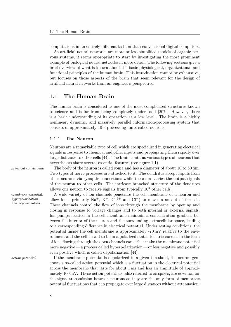
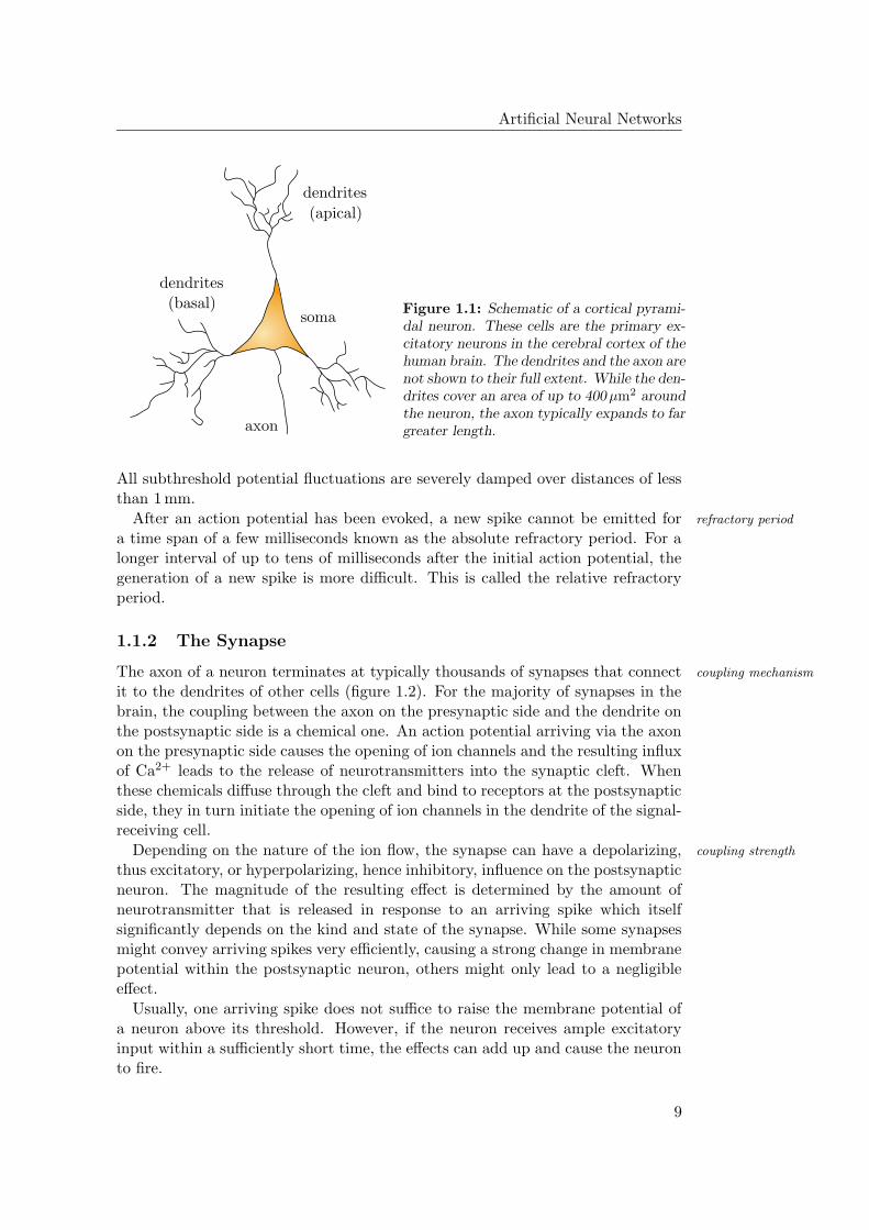
Neurons are a remarkable type of cell which are specialized in generating electricalsignals in response to chemical and other inputs and propagating them rapidly overlarge distances to other cells [44]. The brain contains various types of neurons thatnevertheless share several essential features (see figure 1.1).
The body of the neuron is called soma and has a diameter of about 10 to 50 µm.principal constituents
Two types of nerve processes are attached to it: The dendrites accept inputs fromother neurons via synaptic connections while the axon carries the output signalsof the neuron to other cells. The intricate branched structure of the dendritesallows one neuron to receive signals from typically 104 other cells.
A wide variety of ion channels penetrate the cell membrane of a neuron andmembrane potential,hyperpolarizationand depolarization
allow ions (primarily Na+, K+, Ca2+ and Cl−) to move in an out of the cell.These channels control the flow of ions through the membrane by opening andclosing in response to voltage changes and to both internal or external signals.Ion pumps located in the cell membrane maintain a concentration gradient be-tween the interior of the neuron and the surrounding extracellular space, leadingto a corresponding difference in electrical potential. Under resting conditions, thepotential inside the cell membrane is approximately -70 mV relative to the envi-ronment and the cell is said to be in a polarized state. Electric current in the formof ions flowing through the open channels can either make the membrane potentialmore negative — a process called hyperpolarization — or less negative and possiblyeven positive which is called depolarization [44].
If the membrane potential is depolarized to a given threshold, the neuron gen-action potential
erates a so-called action potential which is a fluctuation in the electrical potentialacross the membrane that lasts for about 1 ms and has an amplitude of approxi-mately 100 mV. These action potentials, also referred to as spikes, are essential forthe signal transmission between neurons as they are the only form of membranepotential fluctuations that can propagate over large distances without attenuation.
8
Artificial Neural Networks
PSfrag replacements
axon
dendrites
dendrites
soma(basal)
(apical)
Figure 1.1: Schematic of a cortical pyrami-dal neuron. These cells are the primary ex-citatory neurons in the cerebral cortex of thehuman brain. The dendrites and the axon arenot shown to their full extent. While the den-drites cover an area of up to 400 µm2 aroundthe neuron, the axon typically expands to fargreater length.
All subthreshold potential fluctuations are severely damped over distances of lessthan 1 mm.
After an action potential has been evoked, a new spike cannot be emitted for refractory period
a time span of a few milliseconds known as the absolute refractory period. For alonger interval of up to tens of milliseconds after the initial action potential, thegeneration of a new spike is more difficult. This is called the relative refractoryperiod.
1.1.2 The Synapse
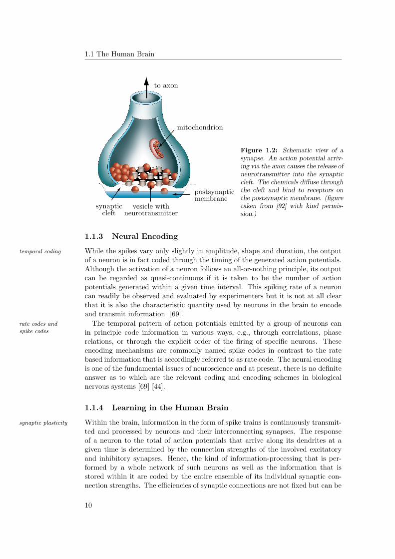
The axon of a neuron terminates at typically thousands of synapses that connect coupling mechanism
it to the dendrites of other cells (figure 1.2). For the majority of synapses in thebrain, the coupling between the axon on the presynaptic side and the dendrite onthe postsynaptic side is a chemical one. An action potential arriving via the axonon the presynaptic side causes the opening of ion channels and the resulting influxof Ca2+ leads to the release of neurotransmitters into the synaptic cleft. Whenthese chemicals diffuse through the cleft and bind to receptors at the postsynapticside, they in turn initiate the opening of ion channels in the dendrite of the signal-receiving cell.
Depending on the nature of the ion flow, the synapse can have a depolarizing, coupling strength
thus excitatory, or hyperpolarizing, hence inhibitory, influence on the postsynapticneuron. The magnitude of the resulting effect is determined by the amount ofneurotransmitter that is released in response to an arriving spike which itselfsignificantly depends on the kind and state of the synapse. While some synapsesmight convey arriving spikes very efficiently, causing a strong change in membranepotential within the postsynaptic neuron, others might only lead to a negligibleeffect.
Usually, one arriving spike does not suffice to raise the membrane potential ofa neuron above its threshold. However, if the neuron receives ample excitatoryinput within a sufficiently short time, the effects can add up and cause the neuronto fire.
9
1.1 The Human Brain
PSfrag replacements
to axon
mitochondrion
postsynapticmembrane
vesicle withneurotransmitter
synapticcleft
Figure 1.2: Schematic view of asynapse. An action potential arriv-ing via the axon causes the release ofneurotransmitter into the synapticcleft. The chemicals diffuse throughthe cleft and bind to receptors onthe postsynaptic membrane. (figuretaken from [92] with kind permis-sion.)
1.1.3 Neural Encoding
While the spikes vary only slightly in amplitude, shape and duration, the outputtemporal coding
of a neuron is in fact coded through the timing of the generated action potentials.Although the activation of a neuron follows an all-or-nothing principle, its outputcan be regarded as quasi-continuous if it is taken to be the number of actionpotentials generated within a given time interval. This spiking rate of a neuroncan readily be observed and evaluated by experimenters but it is not at all clearthat it is also the characteristic quantity used by neurons in the brain to encodeand transmit information [69].
The temporal pattern of action potentials emitted by a group of neurons canrate codes andspike codes in principle code information in various ways, e.g., through correlations, phase
relations, or through the explicit order of the firing of specific neurons. Theseencoding mechanisms are commonly named spike codes in contrast to the ratebased information that is accordingly referred to as rate code. The neural encodingis one of the fundamental issues of neuroscience and at present, there is no definiteanswer as to which are the relevant coding and encoding schemes in biologicalnervous systems [69] [44].
1.1.4 Learning in the Human Brain
Within the brain, information in the form of spike trains is continuously transmit-synaptic plasticity
ted and processed by neurons and their interconnecting synapses. The responseof a neuron to the total of action potentials that arrive along its dendrites at agiven time is determined by the connection strengths of the involved excitatoryand inhibitory synapses. Hence, the kind of information-processing that is per-formed by a whole network of such neurons as well as the information that isstored within it are coded by the entire ensemble of its individual synaptic con-nection strengths. The efficiencies of synaptic connections are not fixed but can be
10
Artificial Neural Networks
changed on different time scales by various processes and this variability is calledplasticity.
One of the basic phenomena that is believed to underly learning and memory Hebbian learning rule
in the human brain is the so-called activity-dependent synaptic plasticity. In thiscase, all changes in the connection strength of a specific synapse only dependon the activities of its presynaptic and postsynaptic neurons. The principles ofactivity-dependent plasticity were first formulated in 1949 by D.O. Hebb [85]:
When an axon of cell A is near enough to excite a cell B and repeatedlyor persistently takes part in firing it, some growth process or metabolicchange takes place in one or both cells such that A’s efficiency, as oneof the cells firing B, is increased.
Hebb proposed this mechanism as a basis of associative learning. He suggestedthat it would lead to the development of “neuronal assemblies” which reflect therelationships between the input and output patterns of the involved neurons asexperienced during the learning period. While the original Hebbian plasticityrule is only concerned with increases in synaptic strength, later versions havebeen generalized to also incorporate the depression of synaptic efficiency. Moregeneral forms regard the synaptic changes to be proportional to the correlation orcovariance of the activities of the pre- and postsynaptic neurons [69] [44].
1.2 Neural Network Models
Regarding the complexity of the human brain on the one hand and its efficiency motivation
on the other, there are at least two motivations to model biological neural systemsand thus to build artificial neural networks:
- to use them as a research tool for the interpretation and better understandingof neurobiological phenomena
- to use them as information-processing systems that have the potential toreproduce the efficiency, speed, adaptability, and fault tolerance of biologicalnetworks
A lot of work has been done to develop adequate network models in pursuit ofboth aims [44] [69] [84] [88] [118] [169]. As implied at the beginning of this chapter,this thesis deals with networks that are primarily designed for the second purpose.
It is not surprising that biologically plausible artificial networks whose dynamicsare to be comparable to those of real neural systems have to include reasonablycomplex models of neurons and synapses [44] [69] [118]. But it turns out that neural networks for
computationpowerful and adaptive information-processing systems can already be built byinterconnecting simple processing units that mimic only some basic properties ofbiological neurons [84] [88] [169]. The term artificial neural network commonlyrefers to this kind of biologically inspired information-processing systems and thefollowing sections give an overview of their basic principles, the various types andtheir interesting properties. This thesis largely confines itself to the discussion ofwhat can be denoted as the classical artificial neural network approach. The morebiologically motivated spiking network models will not be covered.
11
1.2 Neural Network Models
PSfrag replacements
I1(t)
I2(t)
I3(t)
Inin(t)
Ii(t) ∈ I
O(t) ∈ O
fO(t + ∆t)
= f(t, ρ1, . . . , ρk, I1(t), . . . , Inin(t))
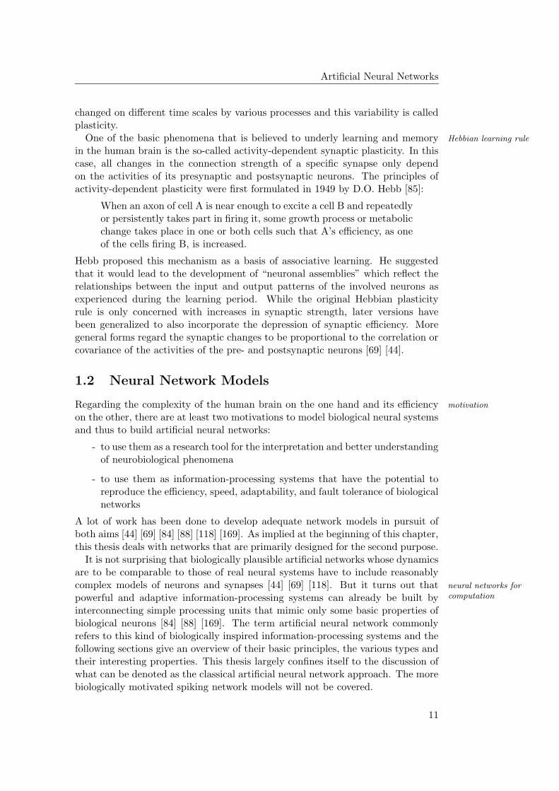
Figure 1.3: A general neuron model: The neuron transforms its nin inputs Ii(t) into anoutput O(t + ∆t) according to a given output function f .
1.2.1 A General Neuron Model
On an abstract level, the functionality of a neuron can be summarized as follows(see also figure 1.3):
1. At a given point in time t, a neuron receives input signals Ii(t) ∈ I, 1 ≤ i ≤nin via a set of nin ∈ N incoming synaptic connections.
2. Based on its input, the neuron computes its own output O(t + ∆t) ∈ O
according to a given output function f(t, ρ1, . . . , ρk) : Inin → O :
O(t + ∆t) = f(t, ρ1, . . . , ρk, I1(t), . . . , Inin(t)). (1.1)
The resulting output might depend on some inner parameters of the neuronρi with 1 ≤ i ≤ np and np ∈ N0 as well as the time t. It is available at timet + ∆t.
Starting from this basic functional description, various neuron models are con-ceivable. They differ in the kind of signals that can be transferred between theneurons — i.e., in the sets I and O — and the way in which the neuron determinesits output as defined by the output function f . Nevertheless, important featuresof artificial neural networks can already be discussed against the background ofthis elementary definition.
1.2.2 Networks of Artificial Neurons
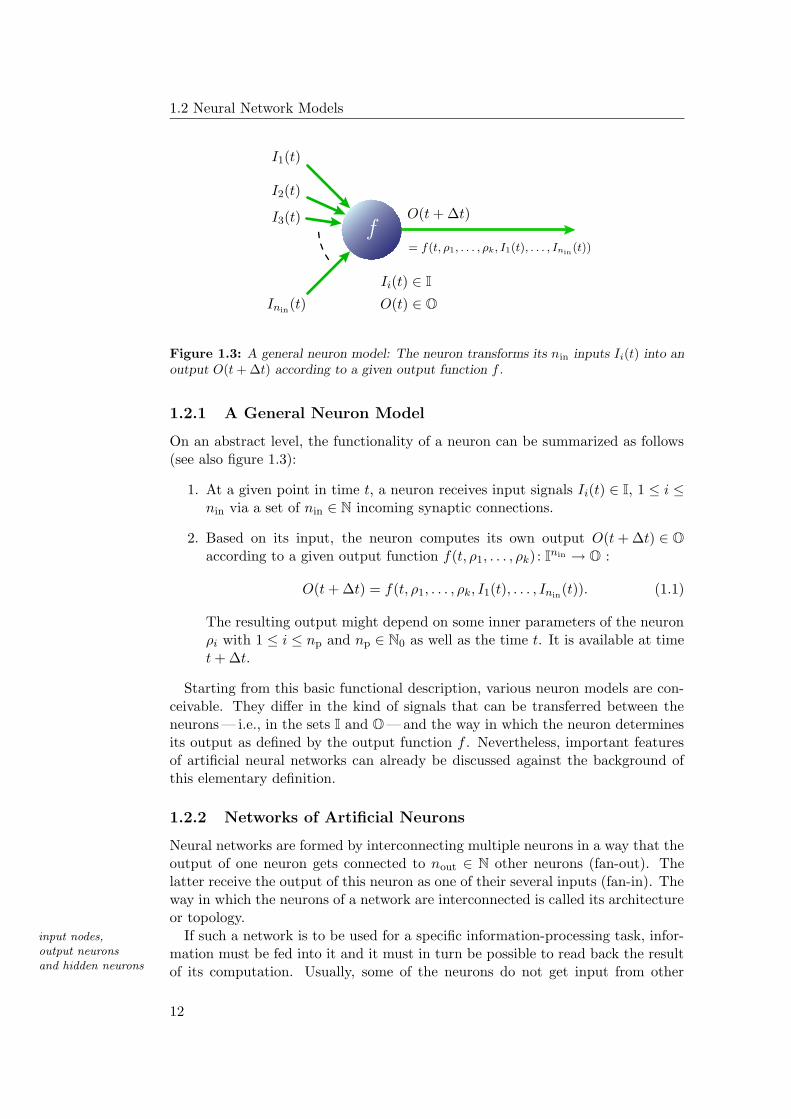
Neural networks are formed by interconnecting multiple neurons in a way that theoutput of one neuron gets connected to nout ∈ N other neurons (fan-out). Thelatter receive the output of this neuron as one of their several inputs (fan-in). Theway in which the neurons of a network are interconnected is called its architectureor topology.
If such a network is to be used for a specific information-processing task, infor-input nodes,output neuronsand hidden neurons
mation must be fed into it and it must in turn be possible to read back the resultof its computation. Usually, some of the neurons do not get input from other
12
Artificial Neural Networks
PSfrag replacements
inputs hidden neurons output neurons
I1
I2
I3
I4
O1
O2
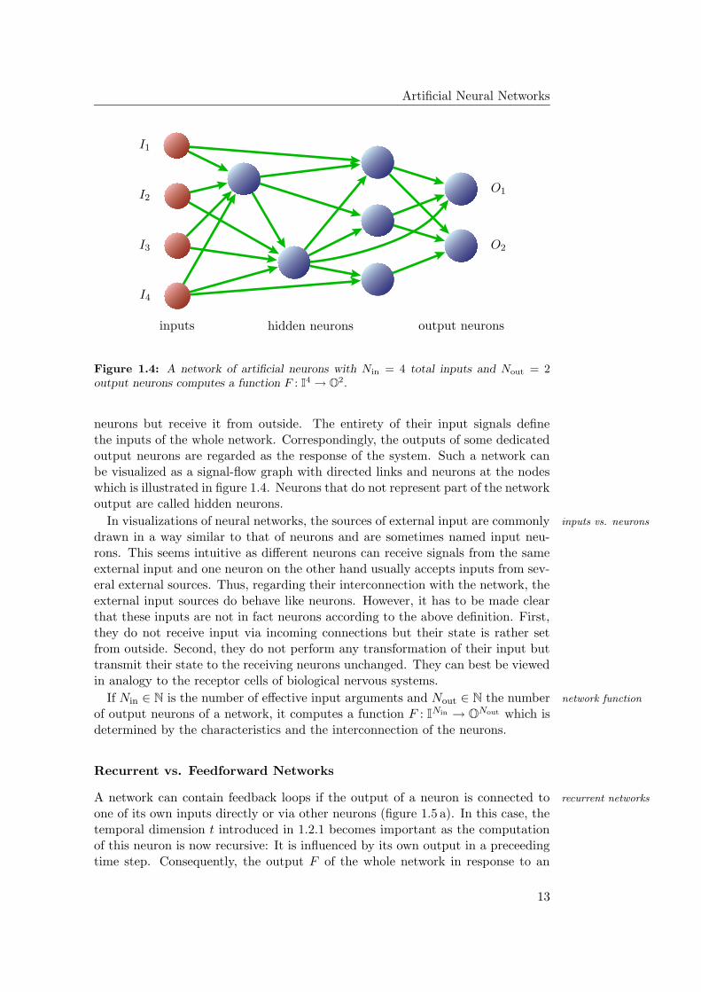
Figure 1.4: A network of artificial neurons with Nin = 4 total inputs and Nout = 2output neurons computes a function F : I4 → O2.
neurons but receive it from outside. The entirety of their input signals definethe inputs of the whole network. Correspondingly, the outputs of some dedicatedoutput neurons are regarded as the response of the system. Such a network canbe visualized as a signal-flow graph with directed links and neurons at the nodeswhich is illustrated in figure 1.4. Neurons that do not represent part of the networkoutput are called hidden neurons.
In visualizations of neural networks, the sources of external input are commonly inputs vs. neurons
drawn in a way similar to that of neurons and are sometimes named input neu-rons. This seems intuitive as different neurons can receive signals from the sameexternal input and one neuron on the other hand usually accepts inputs from sev-eral external sources. Thus, regarding their interconnection with the network, theexternal input sources do behave like neurons. However, it has to be made clearthat these inputs are not in fact neurons according to the above definition. First,they do not receive input via incoming connections but their state is rather setfrom outside. Second, they do not perform any transformation of their input buttransmit their state to the receiving neurons unchanged. They can best be viewedin analogy to the receptor cells of biological nervous systems.
If Nin ∈ N is the number of effective input arguments and Nout ∈ N the number network function
of output neurons of a network, it computes a function F : INin → ONout which isdetermined by the characteristics and the interconnection of the neurons.
Recurrent vs. Feedforward Networks
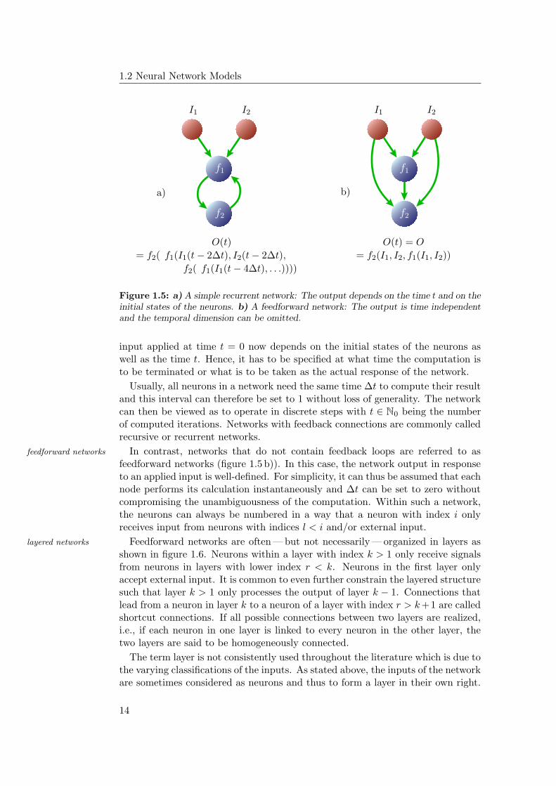
A network can contain feedback loops if the output of a neuron is connected to recurrent networks
one of its own inputs directly or via other neurons (figure 1.5 a). In this case, thetemporal dimension t introduced in 1.2.1 becomes important as the computationof this neuron is now recursive: It is influenced by its own output in a preceedingtime step. Consequently, the output F of the whole network in response to an
13
1.2 Neural Network Models
PSfrag replacementsI1I1 I2I2
f1f1
f2f2
Oa) b)
O(t)
= f2( f1(I1(t − 2∆t), I2(t − 2∆t),
f2( f1(I1(t − 4∆t), . . .))))
O(t) = O
= f2(I1, I2, f1(I1, I2))
Figure 1.5: a) A simple recurrent network: The output depends on the time t and on theinitial states of the neurons. b) A feedforward network: The output is time independentand the temporal dimension can be omitted.
input applied at time t = 0 now depends on the initial states of the neurons aswell as the time t. Hence, it has to be specified at what time the computation isto be terminated or what is to be taken as the actual response of the network.
Usually, all neurons in a network need the same time ∆t to compute their resultand this interval can therefore be set to 1 without loss of generality. The networkcan then be viewed as to operate in discrete steps with t ∈ N0 being the numberof computed iterations. Networks with feedback connections are commonly calledrecursive or recurrent networks.
In contrast, networks that do not contain feedback loops are referred to asfeedforward networks
feedforward networks (figure 1.5 b)). In this case, the network output in responseto an applied input is well-defined. For simplicity, it can thus be assumed that eachnode performs its calculation instantaneously and ∆t can be set to zero withoutcompromising the unambiguousness of the computation. Within such a network,the neurons can always be numbered in a way that a neuron with index i onlyreceives input from neurons with indices l < i and/or external input.
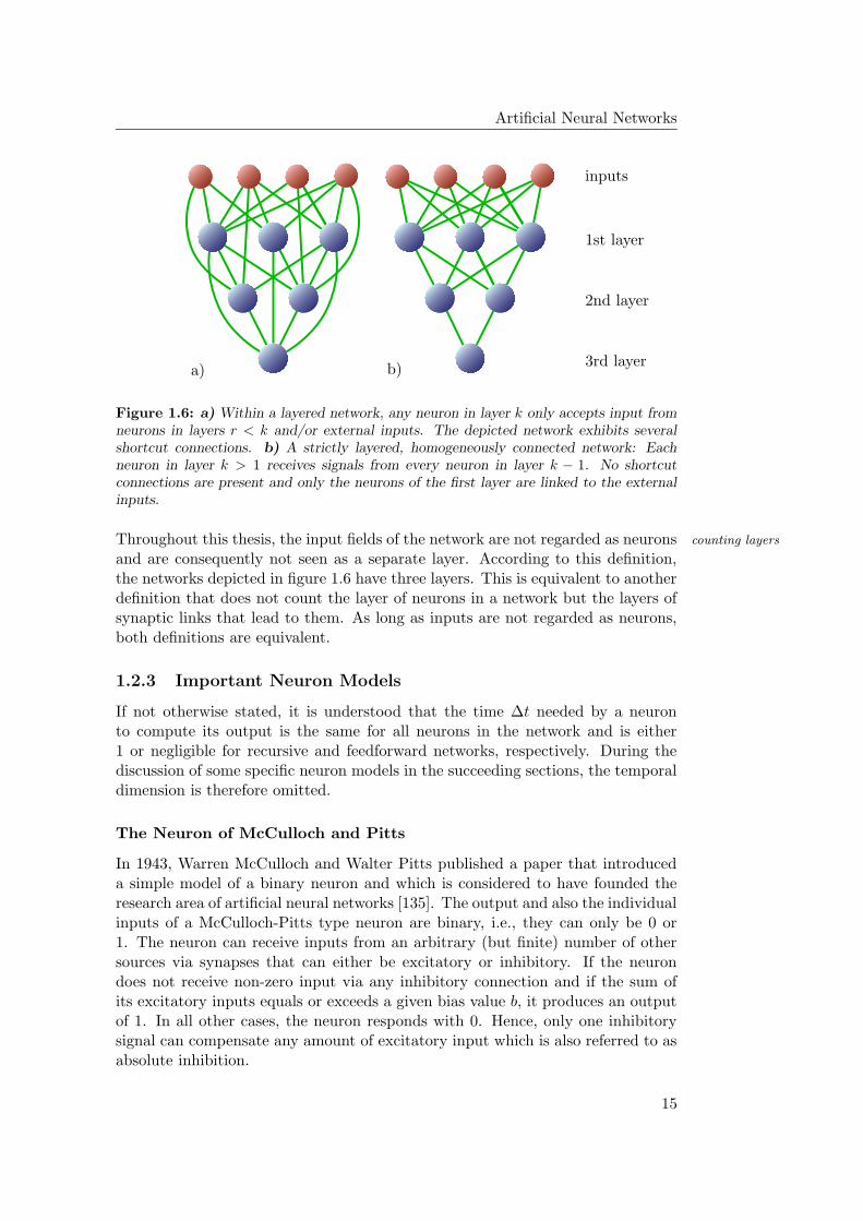
Feedforward networks are often — but not necessarily— organized in layers aslayered networks
shown in figure 1.6. Neurons within a layer with index k > 1 only receive signalsfrom neurons in layers with lower index r < k. Neurons in the first layer onlyaccept external input. It is common to even further constrain the layered structuresuch that layer k > 1 only processes the output of layer k − 1. Connections thatlead from a neuron in layer k to a neuron of a layer with index r > k+1 are calledshortcut connections. If all possible connections between two layers are realized,i.e., if each neuron in one layer is linked to every neuron in the other layer, thetwo layers are said to be homogeneously connected.
The term layer is not consistently used throughout the literature which is due tothe varying classifications of the inputs. As stated above, the inputs of the networkare sometimes considered as neurons and thus to form a layer in their own right.
14
Artificial Neural Networks
PSfrag replacements
inputs
1st layer
2nd layer
3rd layera) b)
Figure 1.6: a) Within a layered network, any neuron in layer k only accepts input fromneurons in layers r < k and/or external inputs. The depicted network exhibits severalshortcut connections. b) A strictly layered, homogeneously connected network: Eachneuron in layer k > 1 receives signals from every neuron in layer k − 1. No shortcutconnections are present and only the neurons of the first layer are linked to the externalinputs.
Throughout this thesis, the input fields of the network are not regarded as neurons counting layers
and are consequently not seen as a separate layer. According to this definition,the networks depicted in figure 1.6 have three layers. This is equivalent to anotherdefinition that does not count the layer of neurons in a network but the layers ofsynaptic links that lead to them. As long as inputs are not regarded as neurons,both definitions are equivalent.
1.2.3 Important Neuron Models
If not otherwise stated, it is understood that the time ∆t needed by a neuronto compute its output is the same for all neurons in the network and is either1 or negligible for recursive and feedforward networks, respectively. During thediscussion of some specific neuron models in the succeeding sections, the temporaldimension is therefore omitted.
The Neuron of McCulloch and Pitts
In 1943, Warren McCulloch and Walter Pitts published a paper that introduceda simple model of a binary neuron and which is considered to have founded theresearch area of artificial neural networks [135]. The output and also the individualinputs of a McCulloch-Pitts type neuron are binary, i.e., they can only be 0 or1. The neuron can receive inputs from an arbitrary (but finite) number of othersources via synapses that can either be excitatory or inhibitory. If the neurondoes not receive non-zero input via any inhibitory connection and if the sum ofits excitatory inputs equals or exceeds a given bias value b, it produces an outputof 1. In all other cases, the neuron responds with 0. Hence, only one inhibitorysignal can compensate any amount of excitatory input which is also referred to asabsolute inhibition.
15
1.2 Neural Network Models
For a McCulloch-Pitts type neuron with threshold b, let nin ∈ N be defined asoutput function
in 1.2.1 and let Iin ⊆ 1, . . . , nin be a subset of indices such that an input withindex i, 1 ≤ i ≤ nin of the neuron is inhibitory if i ∈ Iin and excitatory otherwise.Then its output O ∈ O = 0, 1 in response to a set of inputs Ii ∈ I = O = 0, 1can be computed as follows:
O = f(b, Iin, I1, . . . , Inin) =
0 if ∃ i ∈ Iin, Ii = 1
Θ
∑1≤i≤nin
i/∈Iin
Ii
− b
otherwise
(1.2)
where Θ(x), x ∈ R is the theta function defined by
Θ(x) =
0 x < 0
1 otherwise∀x ∈ R. (1.3)
A network consisting of McCulloch-Pitts type neurons can be regarded as asignal-flow graph with two types of directed links, namely the inhibitory and exci-tatory connections. These connections, however, are not weighted: All excitatoryconnections have equal influence on the output of the neuron and the same appliesto all inhibitory connections.
In terms of the general definition given in section 1.2.1, the bias value b ofthe neuron and the set of indices of its inhibitory connections Iin can be seen asinternal parameters ρ1, ρ2 of its output function.
Associating the numerical value of 0 with the Boolean value false and the valuecomputationalcapabilities 1 with true, it is easy to prove by construction that one single McCulloch-Pitts
type neuron with two inputs can compute the Boolean functions AND, OR, NOT,NAND and NOR. The first two of them do not require any inhibitory connection.In general, it can be shown that any Boolean function fB : 0, 1n → 0, 1 canbe computed by a corresponding feedforward network of McCulloch-Pitts typeneurons with two layers.
Threshold Neurons with Weighted Inputs
Like the biological original, a neuron of the McCulloch-Pitts type accepts twokinds of input: excitatory and inhibitory. It has been discussed in section 1.1.2 thatbeyond having an excitatory or inhibitory effect, the synaptic connections betweenneurons in the brain are individually weighted and do not in fact have equalinfluence on the postsynaptic neuron. The weighting of incoming connections caneasily be incorporated by making some small modifications to the McCulloch-Pittstype neuron.
In the modified neuron model, each incoming connection with index j is assigneda synaptic weight wj ∈ R such that an input Ij ∈ I = O = 0, 1 arriving via thisconnection contributes with wjIj to the total input of the neuron. The latter isgiven by the sum over all input signals and is also denoted as the network input
16
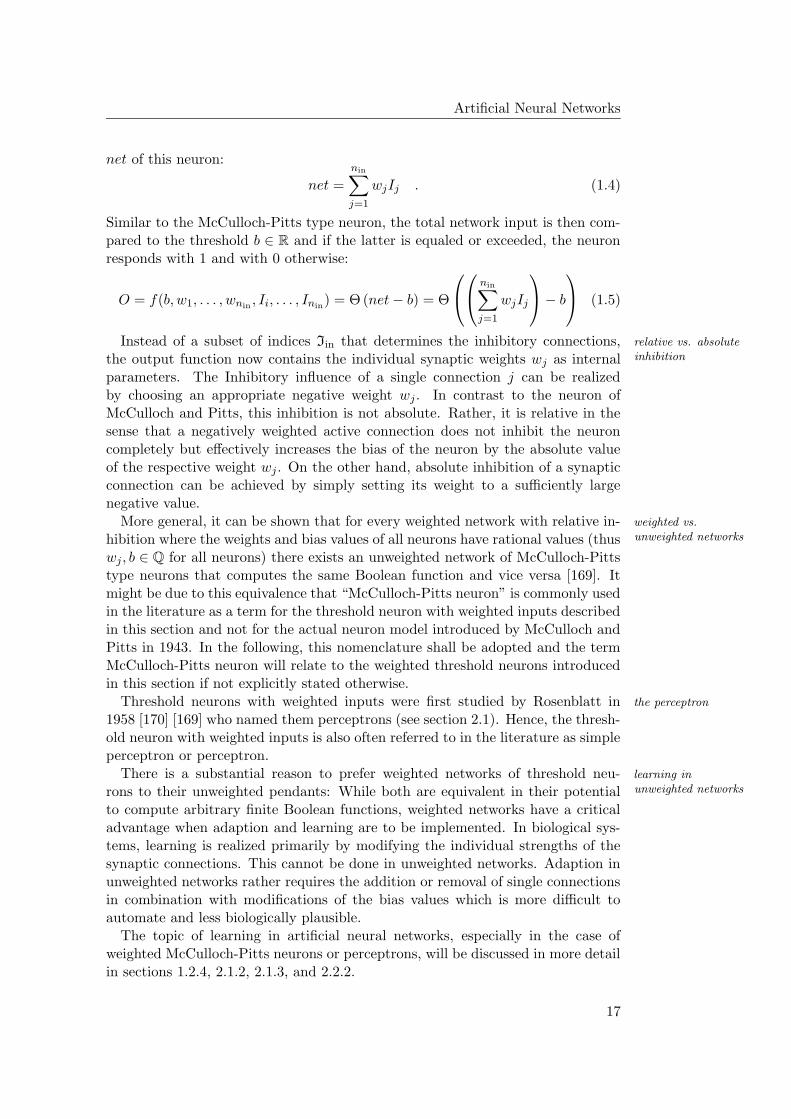
Artificial Neural Networks
net of this neuron:
net =
nin∑
j=1
wjIj . (1.4)
Similar to the McCulloch-Pitts type neuron, the total network input is then com-pared to the threshold b ∈ R and if the latter is equaled or exceeded, the neuronresponds with 1 and with 0 otherwise:
O = f(b, w1, . . . , wnin , Ii, . . . , Inin) = Θ (net − b) = Θ
nin∑
j=1
wjIj
− b
(1.5)
Instead of a subset of indices Iin that determines the inhibitory connections, relative vs. absoluteinhibitionthe output function now contains the individual synaptic weights wj as internal
parameters. The Inhibitory influence of a single connection j can be realizedby choosing an appropriate negative weight wj . In contrast to the neuron ofMcCulloch and Pitts, this inhibition is not absolute. Rather, it is relative in thesense that a negatively weighted active connection does not inhibit the neuroncompletely but effectively increases the bias of the neuron by the absolute valueof the respective weight wj . On the other hand, absolute inhibition of a synapticconnection can be achieved by simply setting its weight to a sufficiently largenegative value.
More general, it can be shown that for every weighted network with relative in- weighted vs.unweighted networkshibition where the weights and bias values of all neurons have rational values (thus
wj , b ∈ Q for all neurons) there exists an unweighted network of McCulloch-Pittstype neurons that computes the same Boolean function and vice versa [169]. Itmight be due to this equivalence that “McCulloch-Pitts neuron” is commonly usedin the literature as a term for the threshold neuron with weighted inputs describedin this section and not for the actual neuron model introduced by McCulloch andPitts in 1943. In the following, this nomenclature shall be adopted and the termMcCulloch-Pitts neuron will relate to the weighted threshold neurons introducedin this section if not explicitly stated otherwise.
Threshold neurons with weighted inputs were first studied by Rosenblatt in the perceptron
1958 [170] [169] who named them perceptrons (see section 2.1). Hence, the thresh-old neuron with weighted inputs is also often referred to in the literature as simpleperceptron or perceptron.
There is a substantial reason to prefer weighted networks of threshold neu- learning inunweighted networksrons to their unweighted pendants: While both are equivalent in their potential
to compute arbitrary finite Boolean functions, weighted networks have a criticaladvantage when adaption and learning are to be implemented. In biological sys-tems, learning is realized primarily by modifying the individual strengths of thesynaptic connections. This cannot be done in unweighted networks. Adaption inunweighted networks rather requires the addition or removal of single connectionsin combination with modifications of the bias values which is more difficult toautomate and less biologically plausible.
The topic of learning in artificial neural networks, especially in the case ofweighted McCulloch-Pitts neurons or perceptrons, will be discussed in more detailin sections 1.2.4, 2.1.2, 2.1.3, and 2.2.2.
17
1.2 Neural Network Models
PSfrag replacements
ϕ(x
)
β = 4β = 1β = 0.5
ϕl(x) = 11+e−βx
x-10 -8 -6 -4 -2
0
0 2 4 6 8 10
1
0.8
0.6
0.4
0.2
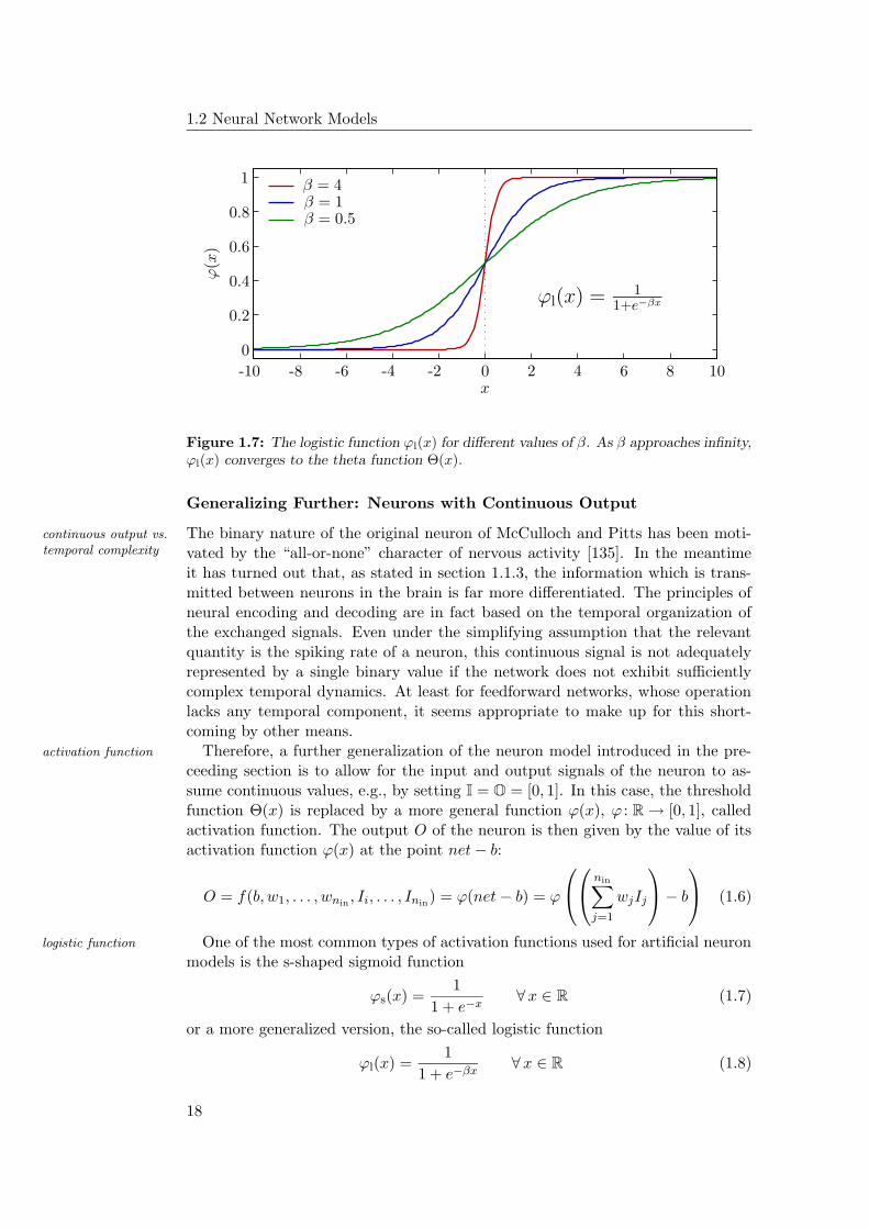
Figure 1.7: The logistic function ϕl(x) for different values of β. As β approaches infinity,ϕl(x) converges to the theta function Θ(x).
Generalizing Further: Neurons with Continuous Output
The binary nature of the original neuron of McCulloch and Pitts has been moti-continuous output vs.temporal complexity vated by the “all-or-none” character of nervous activity [135]. In the meantime
it has turned out that, as stated in section 1.1.3, the information which is trans-mitted between neurons in the brain is far more differentiated. The principles ofneural encoding and decoding are in fact based on the temporal organization ofthe exchanged signals. Even under the simplifying assumption that the relevantquantity is the spiking rate of a neuron, this continuous signal is not adequatelyrepresented by a single binary value if the network does not exhibit sufficientlycomplex temporal dynamics. At least for feedforward networks, whose operationlacks any temporal component, it seems appropriate to make up for this short-coming by other means.
Therefore, a further generalization of the neuron model introduced in the pre-activation function
ceeding section is to allow for the input and output signals of the neuron to as-sume continuous values, e.g., by setting I = O = [0, 1]. In this case, the thresholdfunction Θ(x) is replaced by a more general function ϕ(x), ϕ : R → [0, 1], calledactivation function. The output O of the neuron is then given by the value of itsactivation function ϕ(x) at the point net − b:
O = f(b, w1, . . . , wnin , Ii, . . . , Inin) = ϕ(net − b) = ϕ
nin∑
j=1
wjIj
− b
(1.6)
One of the most common types of activation functions used for artificial neuronlogistic function
models is the s-shaped sigmoid function
ϕs(x) =1
1 + e−x∀x ∈ R (1.7)
or a more generalized version, the so-called logistic function
ϕl(x) =1
1 + e−βx∀x ∈ R (1.8)
18
Artificial Neural Networks
with its additional slope parameter β. Figure 1.8 shows the characteristics ofsome logistic functions with different slope parameter β. It is to be noted thatas β approaches infinity, the logistic function converges to the threshold functionΘ(x). The threshold neuron in the preceeding section can thus be regarded as aspecial case of this generalized neuron model.
For analytical investigations, it is often convenient to consider neurons with an antisymmetricfunctionsoutput range of O = [−1, 1] which can, e.g., be accomplished by appropriately
rescaling and shifting the hitherto discussed activation functions. In case of thethreshold function Θ(x), this yields the so-called sign function sgn(x)
sgn(x) =
1 x ≥ 0
−1 x < 0∀x ∈ R. (1.9)
Instead of modifying the logistic function ϕl(x), it can alternatively be replaced bythe hyperbolic tangent function ϕth(x) = tanh(x) : R → [−1, 1] that also exhibitsthe desired behavior.
All functions introduced so far map the input space R onto a limited interval linear neurons
and are therefore denoted as squashing functions. In principle, the output of aneuron does not necessarily have to be restricted to a limited range of values andit is not uncommon to regard neurons with a linear activation function
ϕlin(x) =β
4x + γ ∀x ∈ R. (1.10)
The parameters β and γ are often set to 4 and 0 respectively in which case theactivation function ϕlin(x) becomes the identity and the neuron is then referredto as a linear neuron.
Any neuron with weighted inputs and a linear activation function effectivelycomputes a functional mapping that is multilinear in all its input arguments. Fur-thermore, any linear function l : Rm → Rn represented by a corresponding (m×n)-matrix with elements lij can be computed by a single-layer network of linear neu-rons with bias b = 0 if each synaptic weight wij of the connection leading frominput Ii, 1 ≤ i ≤ m to the output with index j, 1 ≤ j ≤ n is set to the corre-sponding value lij .
Therefore, feedforward networks of linear neurons can completely be described networks oflinear neuronsin the terms of linear algebra. Any composition of linear combinations of linear
functions yields a function that is, again, linear [53]. The consequence for neuralnetworks is that for any feedforward network of neurons with linear activationfunctions and with an arbitrary number of layers there exists an equivalent networkwith only one layer that computes the same linear function. For this reason, linearactivation functions are not well suited for the hidden neurons of a neural network.Rather, linear neurons are often used as outputs. For an output neuron, a non-linear activation function does not yield any computational benefit but a linearnetwork response is in some cases easier to interpret with regard to the currentlyinvestigated problem.
19
1.2 Neural Network Models
PSfrag replacements
I0 = −1
I1
I1
I2
I2
I3
IninInin
w1
w1
w2
w2
w3
wninwnin
w0 = b
∑∑ ϕϕOO
b
−
ffa) b)
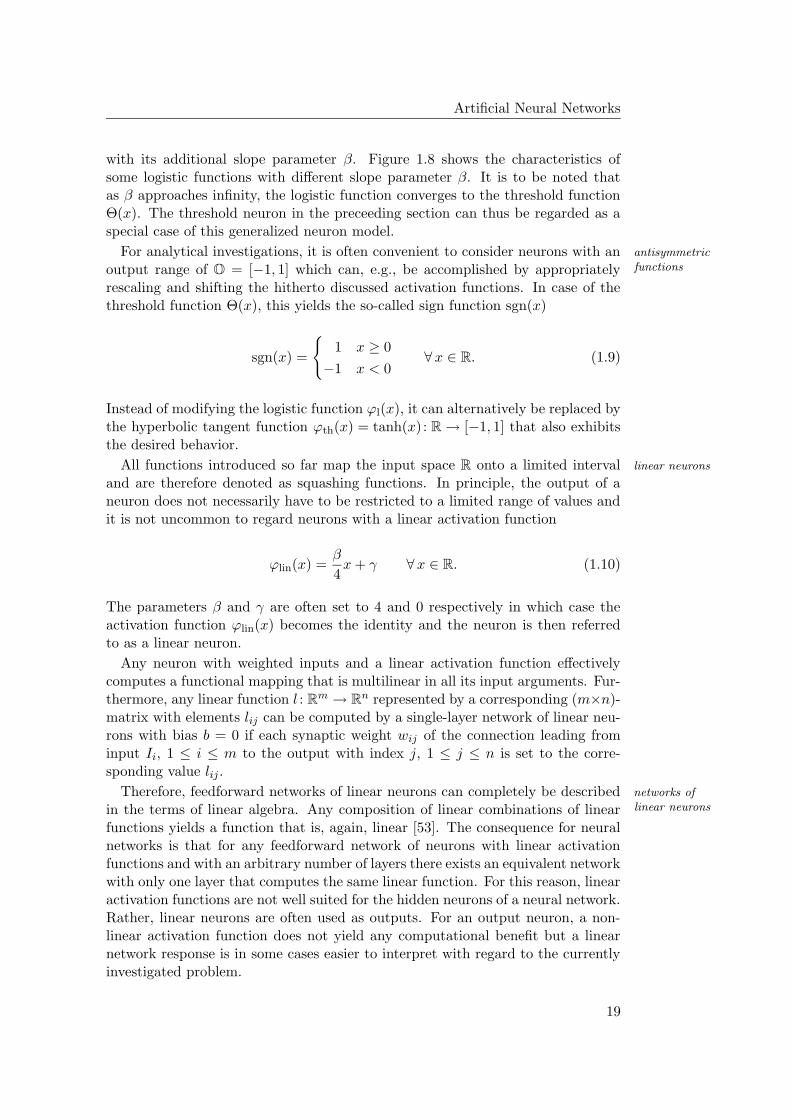
Figure 1.8: a) The bias b of the neuron is regarded as a separate internal parameter,the role of which is distinct from those of the weights wi and the inputs Ii. b) Withinthe alternative model, the bias is replaced by the synaptic weight w0 = b of an additionalInput I0 that is constantly set to -1.
A Note on the Internal Bias
It could be anticipated from equation 1.6 that the bias b of the neuron plays a rolewhich is clearly distinct from that of its inputs Ii and their corresponding weightswi. However, the expression for the output of the neuron can be simplified byregarding its bias as an additional weight w0 = b that belongs to an input I0
which is constantly set to -1. The bias then becomes a part of the total input net
net =
nin∑
j=1
wjIj
+ w0I0 =
nin∑
j=0
wjIj with w0 = b, I0 = −1 (1.11)
and the output of the neuron can be written in the more homogenous form
O = f(w0, . . . , wnin , I0, . . . , Inin) = ϕ(net) = ϕ
nin∑
j=0
wjIj
with I0 = −1.
(1.12)In other words, for each network of neurons with internal bias there exists anetworks with and
without bias functionally equivalent network of neurons without bias but an additional inputI0 that is constantly set to -1. It is evident that this equally applies to all neuronmodels that incorporate weighted inputs.
The difference between the two approaches is illustrated in figure 1.8. It mightseem purely academic to differentiate between them as they are obviously equiva-lent. In fact, the second form of the neuron output function f given in 1.12 provesto be advantageous for the formulation of adaptation algorithms as all adjustableinternal parameters of f become synaptic weights and can thus be treated in thesame fashion.
20
Artificial Neural Networks
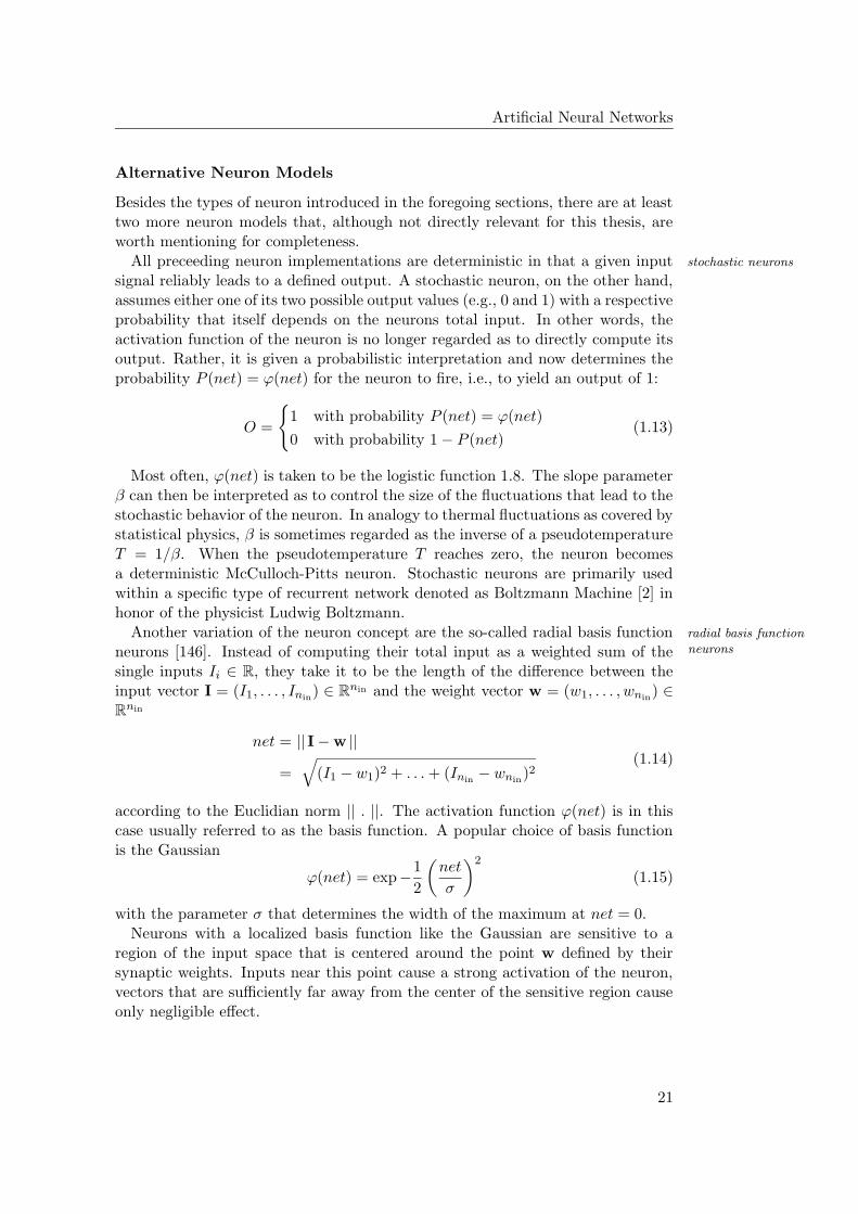
Alternative Neuron Models
Besides the types of neuron introduced in the foregoing sections, there are at leasttwo more neuron models that, although not directly relevant for this thesis, areworth mentioning for completeness.
All preceeding neuron implementations are deterministic in that a given input stochastic neurons
signal reliably leads to a defined output. A stochastic neuron, on the other hand,assumes either one of its two possible output values (e.g., 0 and 1) with a respectiveprobability that itself depends on the neurons total input. In other words, theactivation function of the neuron is no longer regarded as to directly compute itsoutput. Rather, it is given a probabilistic interpretation and now determines theprobability P (net) = ϕ(net) for the neuron to fire, i.e., to yield an output of 1:
O =
1 with probability P (net) = ϕ(net)
0 with probability 1 − P (net)(1.13)
Most often, ϕ(net) is taken to be the logistic function 1.8. The slope parameterβ can then be interpreted as to control the size of the fluctuations that lead to thestochastic behavior of the neuron. In analogy to thermal fluctuations as covered bystatistical physics, β is sometimes regarded as the inverse of a pseudotemperatureT = 1/β. When the pseudotemperature T reaches zero, the neuron becomesa deterministic McCulloch-Pitts neuron. Stochastic neurons are primarily usedwithin a specific type of recurrent network denoted as Boltzmann Machine [2] inhonor of the physicist Ludwig Boltzmann.
Another variation of the neuron concept are the so-called radial basis function radial basis functionneuronsneurons [146]. Instead of computing their total input as a weighted sum of the
single inputs Ii ∈ R, they take it to be the length of the difference between theinput vector I = (I1, . . . , Inin) ∈ Rnin and the weight vector w = (w1, . . . , wnin) ∈Rnin
net = ||I − w ||
=√
(I1 − w1)2 + . . . + (Inin − wnin)2
(1.14)
according to the Euclidian norm || . ||. The activation function ϕ(net) is in thiscase usually referred to as the basis function. A popular choice of basis functionis the Gaussian
ϕ(net) = exp−1
2
(net
σ
)2
(1.15)
with the parameter σ that determines the width of the maximum at net = 0.Neurons with a localized basis function like the Gaussian are sensitive to a
region of the input space that is centered around the point w defined by theirsynaptic weights. Inputs near this point cause a strong activation of the neuron,vectors that are sufficiently far away from the center of the sensitive region causeonly negligible effect.
21
1.2 Neural Network Models
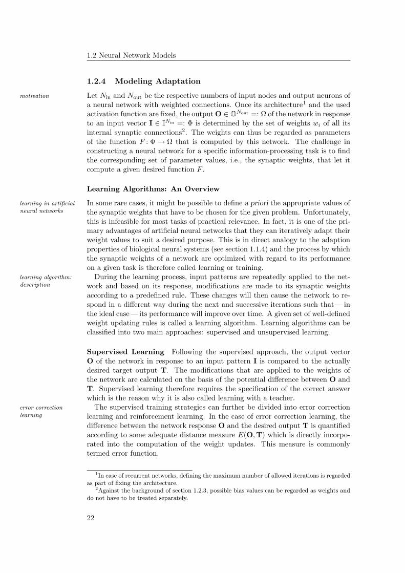
1.2.4 Modeling Adaptation
Let Nin and Nout be the respective numbers of input nodes and output neurons ofmotivation
a neural network with weighted connections. Once its architecture1 and the usedactivation function are fixed, the output O ∈ ONout =: Ω of the network in responseto an input vector I ∈ INin =: Φ is determined by the set of weights wi of all itsinternal synaptic connections2. The weights can thus be regarded as parametersof the function F : Φ → Ω that is computed by this network. The challenge inconstructing a neural network for a specific information-processing task is to findthe corresponding set of parameter values, i.e., the synaptic weights, that let itcompute a given desired function F .
Learning Algorithms: An Overview
In some rare cases, it might be possible to define a priori the appropriate values oflearning in artificialneural networks the synaptic weights that have to be chosen for the given problem. Unfortunately,
this is infeasible for most tasks of practical relevance. In fact, it is one of the pri-mary advantages of artificial neural networks that they can iteratively adapt theirweight values to suit a desired purpose. This is in direct analogy to the adaptionproperties of biological neural systems (see section 1.1.4) and the process by whichthe synaptic weights of a network are optimized with regard to its performanceon a given task is therefore called learning or training.
During the learning process, input patterns are repeatedly applied to the net-learning algorithm:description work and based on its response, modifications are made to its synaptic weights
according to a predefined rule. These changes will then cause the network to re-spond in a different way during the next and successive iterations such that — inthe ideal case— its performance will improve over time. A given set of well-definedweight updating rules is called a learning algorithm. Learning algorithms can beclassified into two main approaches: supervised and unsupervised learning.
Supervised Learning Following the supervised approach, the output vectorO of the network in response to an input pattern I is compared to the actuallydesired target output T. The modifications that are applied to the weights ofthe network are calculated on the basis of the potential difference between O andT. Supervised learning therefore requires the specification of the correct answerwhich is the reason why it is also called learning with a teacher.
The supervised training strategies can further be divided into error correctionerror correctionlearning learning and reinforcement learning. In the case of error correction learning, the
difference between the network response O and the desired output T is quantifiedaccording to some adequate distance measure E(O,T) which is directly incorpo-rated into the computation of the weight updates. This measure is commonlytermed error function.
1In case of recurrent networks, defining the maximum number of allowed iterations is regardedas part of fixing the architecture.
2Against the background of section 1.2.3, possible bias values can be regarded as weights anddo not have to be treated separately.
22
Artificial Neural Networks
During reinforcement learning, the weights are updated solely on the basis of reinforcementlearningwhether the network output has been right or wrong. But it has to be noted
that slightly different and more elaborate definitions of reinforcement learning canbe found in literature and that it can also be seen as an unsupervised trainingapproach [84]. The exact definition of the term reinforcement learning is not ofmajor relevance for this thesis and it shall henceforth be used in the above sense.
Unsupervised Learning In contrast to supervised learning, unsupervised train-ing strategies do not require a specification of the correct outputs and are thususeful for tasks where the correct outputs are not known at all. This particularlyapplies to cases where the goal is not to reproduce a certain output but ratherto find and extract correlations within the input data. Clustering is a prominentexample for this kind of problem.
The Hebb-rule introduced in section 1.1.4 represents an unsupervised learning biological plausibility
approach as the modifications to the synaptic weights of each neuron depend onlyon its own activity and the activities of the neurons it receives input from. Theupdating of the weights does not rely on any externally specified target output. Inso far, unsupervised learning can be regarded as the more appropriate model foradaptation in real nervous systems. Nevertheless, while not being as biologicallyplausible, supervised learning proves to be of exceptional use in numerous practicalapplications.
The task of neural network training can be extended to incorporate the con-struction of network architectures and/or the choice of activation functions thatare optimal for the problem in question. However, the majority of widespreadlearning algorithms and particularly all algorithms discussed in this and the nextchapter confine themselves to optimizing the weight values of a network. Someapproaches for the optimization of the network architecture during training willbe discussed in 4.2.
Types of Learning Tasks
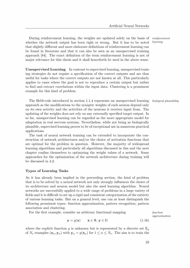
As it has already been implied in the preceeding section, the kind of problemthat is to be solved by a neural network not only strongly influences the choice ofits architecture and neuron model but also the used learning algorithm. Neuralnetworks are successfully applied to a wide range of problems in a large variety offields and it is difficult to set up a rigid and consistent categorization of the entiretyof various learning tasks. But on a general level, one can at least distinguish thefollowing prominent types: function approximation, pattern recognition, patternassociation and clustering.
For the first example, consider an arbitrary functional mapping functionapproximation
y = g(x) x ∈ Φ, y ∈ Ω (1.16)
where the explicit function g is unknown but is represented by a discrete set Eg
of Ne examples (xα,yα) with yα = g(xα) for 1 ≤ α ≤ Ne. The aim is to train the
23
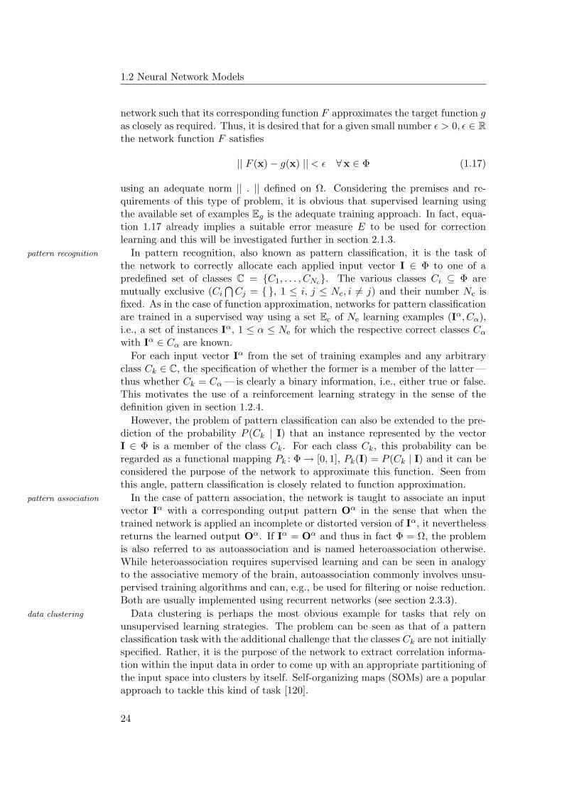
1.2 Neural Network Models
network such that its corresponding function F approximates the target function gas closely as required. Thus, it is desired that for a given small number ε > 0, ε ∈ R
the network function F satisfies
|| F (x) − g(x) || < ε ∀x ∈ Φ (1.17)
using an adequate norm || . || defined on Ω. Considering the premises and re-quirements of this type of problem, it is obvious that supervised learning usingthe available set of examples Eg is the adequate training approach. In fact, equa-tion 1.17 already implies a suitable error measure E to be used for correctionlearning and this will be investigated further in section 2.1.3.
In pattern recognition, also known as pattern classification, it is the task ofpattern recognition
the network to correctly allocate each applied input vector I ∈ Φ to one of apredefined set of classes C = C1, . . . , CNc. The various classes Ci ⊆ Φ aremutually exclusive (Ci
⋂Cj = , 1 ≤ i, j ≤ Nc, i 6= j) and their number Nc is
fixed. As in the case of function approximation, networks for pattern classificationare trained in a supervised way using a set Ec of Ne learning examples (Iα, Cα),i.e., a set of instances Iα, 1 ≤ α ≤ Ne for which the respective correct classes Cα
with Iα ∈ Cα are known.
For each input vector Iα from the set of training examples and any arbitraryclass Ck ∈ C, the specification of whether the former is a member of the latter —thus whether Ck = Cα — is clearly a binary information, i.e., either true or false.This motivates the use of a reinforcement learning strategy in the sense of thedefinition given in section 1.2.4.
However, the problem of pattern classification can also be extended to the pre-diction of the probability P (Ck | I) that an instance represented by the vectorI ∈ Φ is a member of the class Ck. For each class Ck, this probability can beregarded as a functional mapping Pk : Φ → [0, 1], Pk(I) = P (Ck | I) and it can beconsidered the purpose of the network to approximate this function. Seen fromthis angle, pattern classification is closely related to function approximation.
In the case of pattern association, the network is taught to associate an inputpattern association
vector Iα with a corresponding output pattern Oα in the sense that when thetrained network is applied an incomplete or distorted version of Iα, it neverthelessreturns the learned output Oα. If Iα = Oα and thus in fact Φ = Ω, the problemis also referred to as autoassociation and is named heteroassociation otherwise.While heteroassociation requires supervised learning and can be seen in analogyto the associative memory of the brain, autoassociation commonly involves unsu-pervised training algorithms and can, e.g., be used for filtering or noise reduction.Both are usually implemented using recurrent networks (see section 2.3.3).
Data clustering is perhaps the most obvious example for tasks that rely ondata clustering
unsupervised learning strategies. The problem can be seen as that of a patternclassification task with the additional challenge that the classes Ck are not initiallyspecified. Rather, it is the purpose of the network to extract correlation informa-tion within the input data in order to come up with an appropriate partitioning ofthe input space into clusters by itself. Self-organizing maps (SOMs) are a popularapproach to tackle this kind of task [120].
24
Artificial Neural Networks
From what has been said, it may be understood that the boundaries betweenthe different types of learning tasks are smooth and in specific cases it mightindeed not be possible to unambiguously allocate a given problem to one of them.Nevertheless, most applications of neural networks, from whatever field they mightoriginate, fall in at least one of the above categories. In particular, it has beensaid that all neural networks implement a specific functional mapping F : Φ → Ω.Training a network to perform a given information processing task can in this sensealways be regarded as some kind of function approximation (see also section 9.3.2).
Generalization
Within this thesis, emphasis is placed on pattern classification tasks in connection motivation
with supervised learning algorithms. As stated above, these are closely relatedto the solution of corresponding function approximation problems. Whenever anetwork is trained in a supervised way using a finite set E of examples, it is in factthe goal of the learning process that the fully trained network will also performcorrectly on hitherto unseen input vectors I ∈ Φ\E. The ability to use previously definition
gained knowledge to perform well in present and future decisions under similarbut different conditions is called generalization. Thus, the aim of neural networktraining is to produce a neural network that has good generalization ability.
While this comprehension might appear trivial, it is of great consequence forthe construction of neural networks and the formulation of training algorithms,especially with regard to pattern recognition tasks. This is due to the fact thatimproving the performance of a network on the training data does not in all casesguarantee an improvement in generalization ability but might actually result in adeterioration of the latter.
To understand this phenomenon, it is necessary to examine some explicit net-work architectures, including their capabilities and limitations, as well as the cor-responding learning algorithms more closely. The following chapter is devoted tothe important class of feedforward networks.
25

Chapter 2
Feedforward Neural Networks
It’s a poor sort of memory that only works backward.
Lewis Carroll
Feedforward architectures that do not contain any feedback loops form an im-portant class of artificial neural networks. A considerable variety of theoreticaland experimental investigations have been performed in order to illuminate theircomputational capabilities and to devise efficient algorithms for their training.
The experiments and novel training strategies presented in part III of this the-sis concern themselves with hardware-implemented, strictly layered, feedforwardnetworks for pattern classification tasks. Therefore, the aim of this chapter is tolay a solid foundation for the discussion of the achieved results by summarizingwhat is known about the general properties of this class of networks, expeciallywith regard to pattern categorization problems.
Beyond that, section 2.3 gives a brief overview of some alternative networktopologies and paradigms that have proven to be suitable approaches for the so-lution of classification problems as well. Finally, the chapter is to be concludedwith a discussion of hardware-implemented neural networks and the special re-quirements that have to be met by suitable algorithms for their training.
2.1 Single-Layer Feedforward Networks
The following sections address feedforward networks that exhibit only one single the perceptron
layer of weighted connections. Networks of this kind were first studied by Rosen-blatt in 1958 [170]. Originally, he investigated threshold neurons that receivedweighted input from a number of receptive neurons that were each sensitive to adifferent region of an artificial retina (see figure 2.1). In this initial version, theconnections between the retina and the receptive neurons were deterministic andfixed, whereas the weighted connections to the threshold neurons were initializedrandomly and tuned during training. Rosenblatt called this system perceptron.
In the following years, the model was refined further [22] and eventually simpli- the simple perceptron
fied and studied in more detail by Minsky and Papert [143]. Within their model,
27
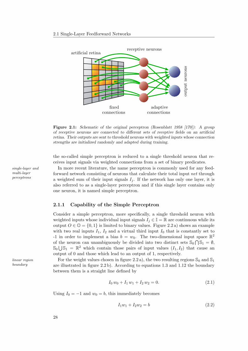
2.1 Single-Layer Feedforward Networks
PSfrag replacements
artificial retinareceptive neurons
fixed adaptiveconnectionsconnections
outp
ut
neu
rons
Figure 2.1: Schematic of the original perceptron (Rosenblatt 1958 [170]): A groupof receptive neurons are connected to different sets of receptive fields on an artificialretina. Their outputs are sent to threshold neurons with weighted inputs whose connectionstrengths are initialized randomly and adapted during training.
the so-called simple perceptron is reduced to a single threshold neuron that re-ceives input signals via weighted connections from a set of binary predicates.
In more recent literature, the name perceptron is commonly used for any feed-single-layer andmulti-layerperceptrons
forward network consisting of neurons that calculate their total input net througha weighted sum of their input signals Ij . If the network has only one layer, it isalso referred to as a single-layer perceptron and if this single layer contains onlyone neuron, it is named simple perceptron.
2.1.1 Capability of the Simple Perceptron
Consider a simple perceptron, more specifically, a single threshold neuron withweighted inputs whose individual input signals Ij ∈ I = R are continuous while itsoutput O ∈ O = 0, 1 is limited to binary values. Figure 2.2 a) shows an examplewith two real inputs I1, I2 and a virtual third input I0 that is constantly set to-1 in order to implement a bias b = w0. The two-dimensional input space R2
of the neuron can unambiguously be divided into two distinct sets S0⋂
S1 = ∅,S0⋃
S1 = R2 which contain those pairs of input values (I1, I2) that cause anoutput of 0 and those which lead to an output of 1, respectively.
For the weight values chosen in figure 2.2 a), the two resulting regions S0 and S1linear regionboundary are illustrated in figure 2.2 b). According to equations 1.3 and 1.12 the boundary
between them is a straight line defined by
I0 w0 + I1 w1 + I2 w2 = 0. (2.1)
Using I0 = −1 and w0 = b, this immediately becomes
I1w1 + I2w2 = b (2.2)
28
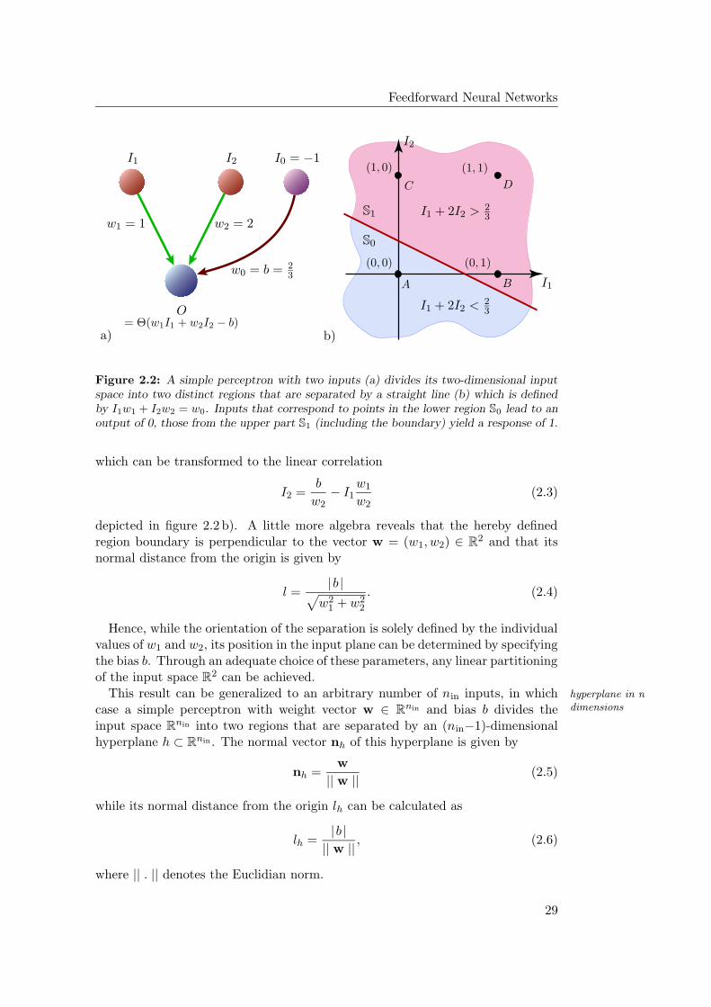
Feedforward Neural Networks
PSfrag replacements
I1 I2 I0 = −1
w1 = 1 w2 = 2
w0 = b = 23
O= Θ(w1I1 + w2I2 − b)
I1
I2
I1 + 2I2 < 23
I1 + 2I2 > 23
(0, 0) (0, 1)
(1, 0) (1, 1)
A B
C D
S1
S0
a) b)
Figure 2.2: A simple perceptron with two inputs (a) divides its two-dimensional inputspace into two distinct regions that are separated by a straight line (b) which is definedby I1w1 + I2w2 = w0. Inputs that correspond to points in the lower region S0 lead to anoutput of 0, those from the upper part S1 (including the boundary) yield a response of 1.
which can be transformed to the linear correlation
I2 =b
w2− I1
w1
w2(2.3)
depicted in figure 2.2 b). A little more algebra reveals that the hereby definedregion boundary is perpendicular to the vector w = (w1, w2) ∈ R2 and that itsnormal distance from the origin is given by
l =|b |√
w21 + w2
2
. (2.4)
Hence, while the orientation of the separation is solely defined by the individualvalues of w1 and w2, its position in the input plane can be determined by specifyingthe bias b. Through an adequate choice of these parameters, any linear partitioningof the input space R2 can be achieved.
This result can be generalized to an arbitrary number of nin inputs, in which hyperplane in ndimensionscase a simple perceptron with weight vector w ∈ Rnin and bias b divides the
input space Rnin into two regions that are separated by an (nin−1)-dimensionalhyperplane h ⊂ Rnin . The normal vector nh of this hyperplane is given by
nh =w
|| w || (2.5)
while its normal distance from the origin lh can be calculated as
lh =|b |
|| w || , (2.6)
where || . || denotes the Euclidian norm.
29
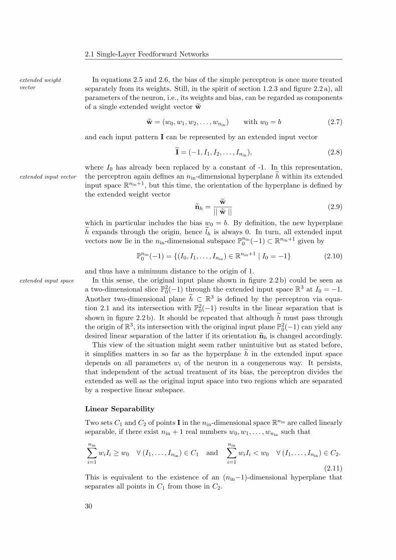
2.1 Single-Layer Feedforward Networks
In equations 2.5 and 2.6, the bias of the simple perceptron is once more treatedextended weightvector separately from its weights. Still, in the spirit of section 1.2.3 and figure 2.2 a), all
parameters of the neuron, i.e., its weights and bias, can be regarded as componentsof a single extended weight vector w
w = (w0, w1, w2, . . . , wnin) with w0 = b (2.7)
and each input pattern I can be represented by an extended input vector
I = (−1, I1, I2, . . . , Inin), (2.8)
where I0 has already been replaced by a constant of -1. In this representation,the perceptron again defines an nin-dimensional hyperplane h within its extendedextended input vector
input space Rnin+1, but this time, the orientation of the hyperplane is defined bythe extended weight vector
nh =w
|| w || (2.9)
which in particular includes the bias w0 = b. By definition, the new hyperplaneh expands through the origin, hence lh is always 0. In turn, all extended inputvectors now lie in the nin-dimensional subspace P
nin0 (−1) ⊂ Rnin+1 given by
Pnin0 (−1) = (I0, I1, . . . , Inin) ∈ Rnin+1 | I0 = −1 (2.10)
and thus have a minimum distance to the origin of 1.In this sense, the original input plane shown in figure 2.2 b) could be seen asextended input space
a two-dimensional slice P20(−1) through the extended input space R3 at I0 = −1.
Another two-dimensional plane h ⊂ R3 is defined by the perceptron via equa-tion 2.1 and its intersection with P2
0(−1) results in the linear separation that is
shown in figure 2.2 b). It should be repeated that although h must pass throughthe origin of R3, its intersection with the original input plane P2
0(−1) can yield anydesired linear separation of the latter if its orientation nh is changed accordingly.
This view of the situation might seem rather unintuitive but as stated before,it simplifies matters in so far as the hyperplane h in the extended input spacedepends on all parameters wi of the neuron in a congenerous way. It persists,that independent of the actual treatment of its bias, the perceptron divides theextended as well as the original input space into two regions which are separatedby a respective linear subspace.
Linear Separability
Two sets C1 and C2 of points I in the nin-dimensional space Rnin are called linearlyseparable, if there exist nin + 1 real numbers w0, w1, . . . , wnin such that
nin∑
i=1
wiIi ≥ w0 ∀ (I1, . . . , Inin) ∈ C1 and
nin∑
i=1
wiIi < w0 ∀ (I1, . . . , Inin) ∈ C2.
(2.11)This is equivalent to the existence of an (nin−1)-dimensional hyperplane thatseparates all points in C1 from those in C2.
30
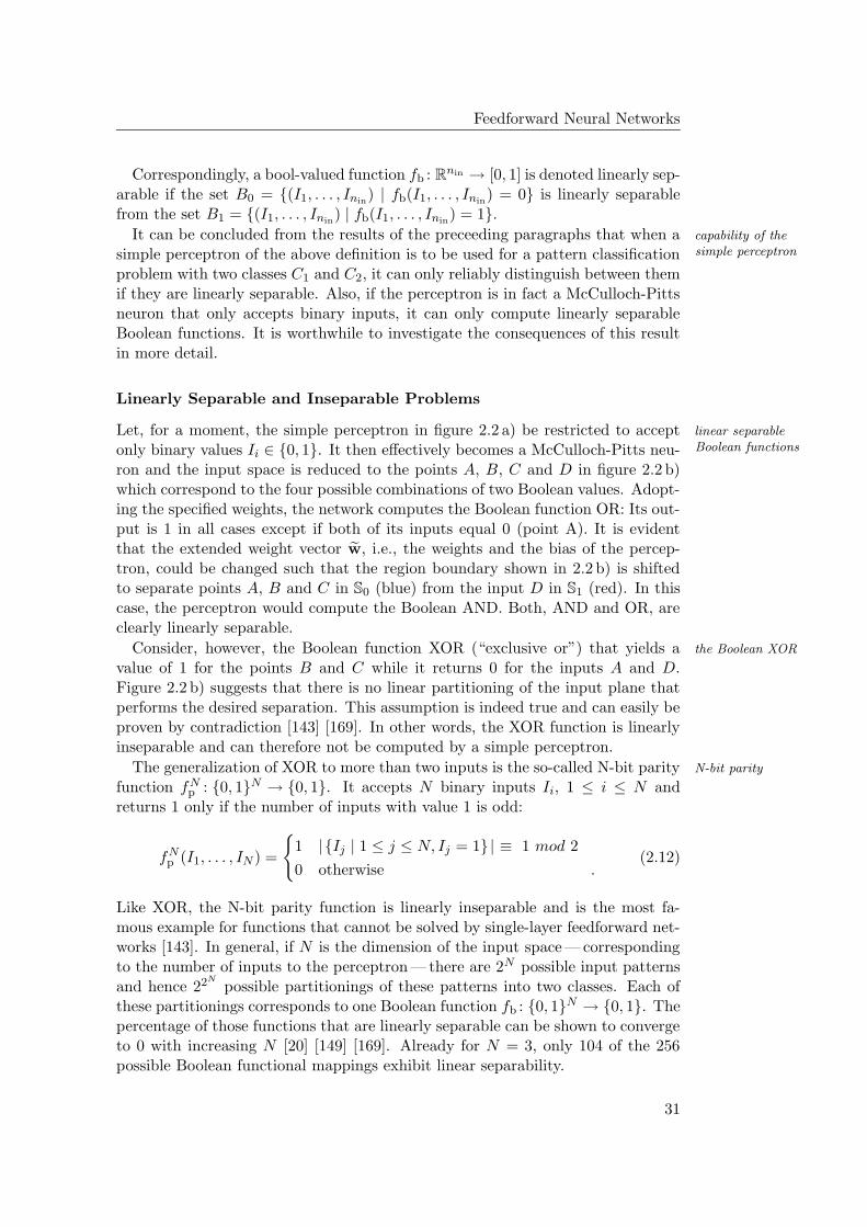
Feedforward Neural Networks
Correspondingly, a bool-valued function fb : Rnin → [0, 1] is denoted linearly sep-arable if the set B0 = (I1, . . . , Inin) | fb(I1, . . . , Inin) = 0 is linearly separablefrom the set B1 = (I1, . . . , Inin) | fb(I1, . . . , Inin) = 1.
It can be concluded from the results of the preceeding paragraphs that when a capability of thesimple perceptronsimple perceptron of the above definition is to be used for a pattern classification
problem with two classes C1 and C2, it can only reliably distinguish between themif they are linearly separable. Also, if the perceptron is in fact a McCulloch-Pittsneuron that only accepts binary inputs, it can only compute linearly separableBoolean functions. It is worthwhile to investigate the consequences of this resultin more detail.
Linearly Separable and Inseparable Problems
Let, for a moment, the simple perceptron in figure 2.2 a) be restricted to accept linear separableBoolean functionsonly binary values Ii ∈ 0, 1. It then effectively becomes a McCulloch-Pitts neu-
ron and the input space is reduced to the points A, B, C and D in figure 2.2 b)which correspond to the four possible combinations of two Boolean values. Adopt-ing the specified weights, the network computes the Boolean function OR: Its out-put is 1 in all cases except if both of its inputs equal 0 (point A). It is evidentthat the extended weight vector w, i.e., the weights and the bias of the percep-tron, could be changed such that the region boundary shown in 2.2 b) is shiftedto separate points A, B and C in S0 (blue) from the input D in S1 (red). In thiscase, the perceptron would compute the Boolean AND. Both, AND and OR, areclearly linearly separable.
Consider, however, the Boolean function XOR (“exclusive or”) that yields a the Boolean XOR
value of 1 for the points B and C while it returns 0 for the inputs A and D.Figure 2.2 b) suggests that there is no linear partitioning of the input plane thatperforms the desired separation. This assumption is indeed true and can easily beproven by contradiction [143] [169]. In other words, the XOR function is linearlyinseparable and can therefore not be computed by a simple perceptron.
The generalization of XOR to more than two inputs is the so-called N-bit parity N-bit parity
function fNp : 0, 1N → 0, 1. It accepts N binary inputs Ii, 1 ≤ i ≤ N and
returns 1 only if the number of inputs with value 1 is odd:
fNp (I1, . . . , IN ) =
1 |Ij | 1 ≤ j ≤ N, Ij = 1| ≡ 1 mod 2
0 otherwise .(2.12)
Like XOR, the N-bit parity function is linearly inseparable and is the most fa-mous example for functions that cannot be solved by single-layer feedforward net-works [143]. In general, if N is the dimension of the input space — correspondingto the number of inputs to the perceptron — there are 2N possible input patternsand hence 22N
possible partitionings of these patterns into two classes. Each ofthese partitionings corresponds to one Boolean function fb : 0, 1N → 0, 1. Thepercentage of those functions that are linearly separable can be shown to convergeto 0 with increasing N [20] [149] [169]. Already for N = 3, only 104 of the 256possible Boolean functional mappings exhibit linear separability.
31
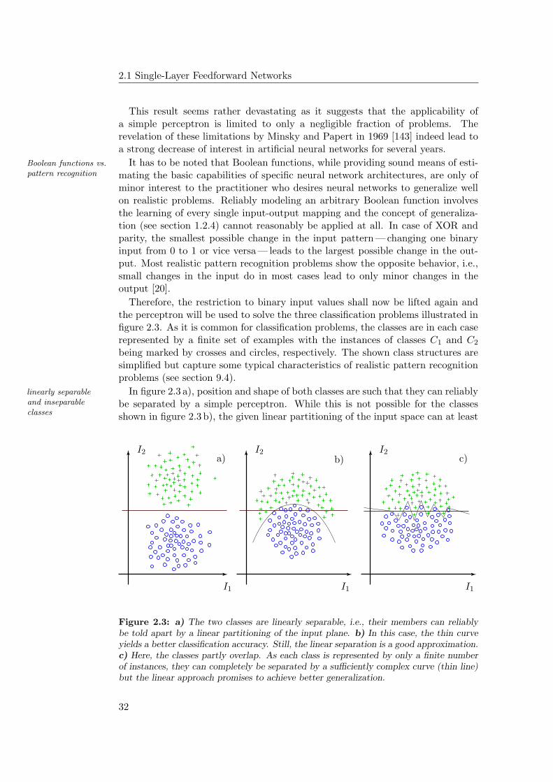
2.1 Single-Layer Feedforward Networks
This result seems rather devastating as it suggests that the applicability ofa simple perceptron is limited to only a negligible fraction of problems. Therevelation of these limitations by Minsky and Papert in 1969 [143] indeed lead toa strong decrease of interest in artificial neural networks for several years.
It has to be noted that Boolean functions, while providing sound means of esti-Boolean functions vs.pattern recognition mating the basic capabilities of specific neural network architectures, are only of
minor interest to the practitioner who desires neural networks to generalize wellon realistic problems. Reliably modeling an arbitrary Boolean function involvesthe learning of every single input-output mapping and the concept of generaliza-tion (see section 1.2.4) cannot reasonably be applied at all. In case of XOR andparity, the smallest possible change in the input pattern — changing one binaryinput from 0 to 1 or vice versa — leads to the largest possible change in the out-put. Most realistic pattern recognition problems show the opposite behavior, i.e.,small changes in the input do in most cases lead to only minor changes in theoutput [20].
Therefore, the restriction to binary input values shall now be lifted again andthe perceptron will be used to solve the three classification problems illustrated infigure 2.3. As it is common for classification problems, the classes are in each caserepresented by a finite set of examples with the instances of classes C1 and C2
being marked by crosses and circles, respectively. The shown class structures aresimplified but capture some typical characteristics of realistic pattern recognitionproblems (see section 9.4).
In figure 2.3 a), position and shape of both classes are such that they can reliablylinearly separableand inseparableclasses
be separated by a simple perceptron. While this is not possible for the classesshown in figure 2.3 b), the given linear partitioning of the input space can at least
PSfrag replacements
I1I1I1
I2I2I2a) b) c)
Figure 2.3: a) The two classes are linearly separable, i.e., their members can reliablybe told apart by a linear partitioning of the input plane. b) In this case, the thin curveyields a better classification accuracy. Still, the linear separation is a good approximation.c) Here, the classes partly overlap. As each class is represented by only a finite numberof instances, they can completely be separated by a sufficiently complex curve (thin line)but the linear approach promises to achieve better generalization.
32
Feedforward Neural Networks
be regarded as a reasonable first-order approximation of the real solution andwould in this case lead to a fraction of misclassifications of only 10 %. Still, thecurved thin line represents a far more suitable separation of the input space forthis classification problem.
The two classes shown in figure 2.3 c) partly overlap. But as they are each overlapping classregionsrepresented by only a finite number of instances, there exist intricate non-linear
separations of the input plane that seem to distinguish between them with 100 %accuracy. One of these possible separations is again illustrated as a thin blackline. If the individual instances of the two classes are spread over the input spaceaccording to some statistical distribution, it is most likely that additional instancesgenerated by the same underlying mechanism would not be classified correctly bythe shown specialized partitioning. In that case, the superiority of the non-linearseparation to the linear one would actually be an illusion caused by the use ofa finite set of examples. The shown linear partitioning, although not perfectlyclassifying the present instances, clearly provides a more adequate separation ofthe classes and is likely to yield a better generalization performance.
These reflections motivate that a simple perceptron with its limited compu-tational capabilities might nevertheless prove to be of value for the solution ofpattern recognition problems if the respective class structures exhibit character-istics similar to those of the above examples. It is reasonable to wonder whetherthis does in fact apply to any realistic tasks. A thorough investigation of this topicwill be the subject of chapter 9.
2.1.2 Training the Simple Perceptron
During the initial years after its introduction, the perceptron attracted high in-terest mainly because of the availability of a well-defined and effective trainingalgorithm that, for the first time, allowed an artificial network to be used as alearning machine.
As a simple perceptron consists of only one neuron, the number of inputs to thenetwork Nin is equivalent to the number of inputs to the neuron nin = Nin andthe number of outputs Nout equals 1. For simplicity, it is assumed that the neuronexhibits no internal bias. It is recalled from section 2.1.1 that this can always beachieved by discussing the problem in terms of an extended weight vector w andcorresponding extended input vectors I (see equations 2.7 and 2.8).
It has also been shown that a simple perceptron linearly divides its input space goal of the training
into two regions and can thus in principle solve any linearly separable classificationproblem with two classes C1 and C2. The network is to be trained for one suchtask using a finite training set E of input patterns Iα that are each associated withthe respective desired target output T α. Given this finite set of examples, it isthe purpose of the training algorithm to find a linear separation (represented by acorresponding weight vector w) that yields a correct classification of all instancesIα ∈ E.
To keep the formulation of the training algorithm simple, it will turn out tobe advantageous if one considers a threshold neuron that does not respond with0 or 1 but with -1 or 1 instead. As stated in section 1.2.3, this transition is
33
2.1 Single-Layer Feedforward Networks
straight forward — it merely involves a shifting and rescaling of the output — andeffectively turns the threshold activation function Θ(x) into the sign functionsgn(x) (equation 1.9). The learning task shall then be formulated such that inputpatterns I belonging to class C1 are desired to result in a network response ofT = 1 and those of class C2 are to yield an output of T = −1.
The perceptron learning algorithm [22] starts off by initializing the weights of allperceptron learningalgorithm connections with random values. It then proceeds by iteratively cycling through
all training examples Iα, presenting them to the network and comparing the re-spective network response Oα to the corresponding target output T α: If Oα = Tα
the training immediately continues with the next training pattern. Otherwise,the weight vector w is changed by a small vector ∆wα which is proportional tothe original input vector Iα. The weight change ∆wα shall be added to the oldweights w, if the target output T α = 1 and be subtracted if T α = −1. At thispoint, the choice of −1, 1 for the possible output values pays off, as the mod-ification of the weight vector after the application of each input pattern Iα canconveniently be formulated as
wnew = wold + ∆wα (2.13)
with
∆wα =1
2η (Tα − Oα) Iα (2.14)
where the constant η is an adjustable parameter of the algorithm denoted aslearning rate. This learning algorithm is an example for supervised training.
Discussing the Perceptron Learning Algorithm
According to an important result commonly known as the perceptron convergenceperceptronconvergencetheorem
theorem, the perceptron learning algorithm is guaranteed to find a complete so-lution of a given classification task within a finite number of iterations under thecondition that the problem can actually be solved by a perceptron, i.e., is linearlyseparable [22] [88] [143].
While the proof of this theorem shall not be reproduced here in detail, thegeometricaldiscussion weight updating scheme 2.14 can be motivated by some simple geometrical con-
siderations [88] [20]. In the extended input space, the perceptron defines a hy-perplane h that passes through the origin. Its orientation is given by the normalvector nh which in turn is determined by the weight vector w by virtue of equa-tion 2.9. According to this definition, an input vector I results in an output of 1 ifits projection onto w is positive and yields an output of -1 if the latter is negative.Thus, if a vector Iα is incorrectly classified, its projection pα
h = nhIα onto the
direction of w simply has the wrong sign which can iteratively be corrected byslightly changing the orientation of w into the appropriate direction. If the sign ofpα
h is false negative, w has to be rotated towards Iα, if it is false positive, w mustbe changed in the opposite direction. The learning rule 2.14 is the mathematicalformulation of this strategy.
34
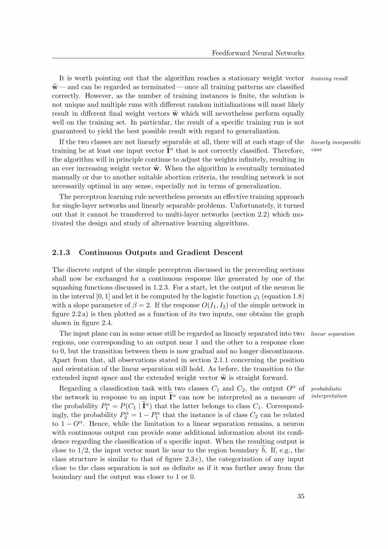
Feedforward Neural Networks
It is worth pointing out that the algorithm reaches a stationary weight vector training result
w — and can be regarded as terminated — once all training patterns are classifiedcorrectly. However, as the number of training instances is finite, the solution isnot unique and multiple runs with different random initializations will most likelyresult in different final weight vectors w which will nevertheless perform equallywell on the training set. In particular, the result of a specific training run is notguaranteed to yield the best possible result with regard to generalization.
If the two classes are not linearly separable at all, there will at each stage of the linearly inseparablecasetraining be at least one input vector Iα that is not correctly classified. Therefore,
the algorithm will in principle continue to adjust the weights infinitely, resulting inan ever increasing weight vector w. When the algorithm is eventually terminatedmanually or due to another suitable abortion criteria, the resulting network is notnecessarily optimal in any sense, especially not in terms of generalization.
The perceptron learning rule nevertheless presents an effective training approachfor single-layer networks and linearly separable problems. Unfortunately, it turnedout that it cannot be transferred to multi-layer networks (section 2.2) which mo-tivated the design and study of alternative learning algorithms.
2.1.3 Continuous Outputs and Gradient Descent
The discrete output of the simple perceptron discussed in the preceeding sectionsshall now be exchanged for a continuous response like generated by one of thesquashing functions discussed in 1.2.3. For a start, let the output of the neuron liein the interval [0, 1] and let it be computed by the logistic function ϕl (equation 1.8)with a slope parameter of β = 2. If the response O(I1, I2) of the simple network infigure 2.2 a) is then plotted as a function of its two inputs, one obtains the graphshown in figure 2.4.
The input plane can in some sense still be regarded as linearly separated into two linear separation
regions, one corresponding to an output near 1 and the other to a response closeto 0, but the transition between them is now gradual and no longer discontinuous.Apart from that, all observations stated in section 2.1.1 concerning the positionand orientation of the linear separation still hold. As before, the transition to theextended input space and the extended weight vector w is straight forward.
Regarding a classification task with two classes C1 and C2, the output Oα of probabilisticinterpretationthe network in response to an input Iα can now be interpreted as a measure of
the probability P α1 = P (C1 | Iα) that the latter belongs to class C1. Correspond-
ingly, the probability P α2 = 1 − Pα
1 that the instance is of class C2 can be relatedto 1 − Oα. Hence, while the limitation to a linear separation remains, a neuronwith continuous output can provide some additional information about its confi-dence regarding the classification of a specific input. When the resulting output isclose to 1/2, the input vector must lie near to the region boundary h. If, e.g., theclass structure is similar to that of figure 2.3 c), the categorization of any inputclose to the class separation is not as definite as if it was further away from theboundary and the output was closer to 1 or 0.
35
2.1 Single-Layer Feedforward NetworksPSfrag replacements
I1
I2
O(I
1,I
2)
1
0.8
0.6
0.4
0.2
I1 + 2I2 < 23
I1 + 2I2 > 23
-6 -6
-4-4
-2
-2
0
0
0
2
2
4
4
6
6
Figure 2.4: If the output neuron of the simple perceptron in figure 2.2 a) is assignedthe logistic transfer function ϕl, its output O(I1, I2) becomes a continuous function ofthe inputs. The position and orientation of the linear separation between output 0 and 1remain the same as in figure 2.2 b) but the transition becomes smooth.
Gradient Descent Training: The Delta Rule
Besides allowing for a more differentiated interpretation of the network output, adifferentiable networkoutput continuous neuron response as given by the logistic function ϕl is also advantageous
in so far as the neuron output function O(w, I) is now differentiable with respectto all input values Ii. Alternatively, given a fixed input vector Iα, the responseOα(w) = O(w, Iα) of the neuron can itself be regarded as a differentiable functionOα : Rnin+1 → O of the synaptic weights wi.
This important insight gives rise to a new training approach. Revisiting thedifferentiable networkerror two-class problem of section 2.1.2, let the error Eα of the network with regard
to an input pattern Iα ∈ E be defined in terms of the actual network responseO(w, Iα) and the respective target output T α ∈ 0, 1 as follows
Eα(w) =1
2
(O(w, Iα) − Tα
)2. (2.15)
Then, the overall performance of the network on the whole training set E can bemeasured by the error function
E(w) =∑
E
Eα(w) =∑
E
1
2
(O(w, Iα) − Tα
)2(2.16)
such that the smaller E(w), the better the choice of weights w for this particularproblem. The goal of training the network for a specific task could thus be iden-tified with the minimization of E(w). As by definition, E(w) is a continuous and
36
Feedforward Neural Networks
differentiable function of all weights wi, it seems appropriate to pursue this aimusing common gradient descent optimization methods [20].
Following an iterative approach similar to the one introduced in 2.1.2, the train- iterative gradientdescenting starts once more with some random initial weights w which are likely to yield
an undesirably large value of E(w). Therefore, the weight vector is updated bymoving into that direction of the weight space along which E(w) decreases mostrapidly. This direction is given by the negative gradient −∇ ewE and the weightchange can be written as
∆w = −η ∇ ew E∣∣
ew(2.17)
including an adjustable learning rate η. In case of the perceptron learning algo-rithm, the weights are updated after the processing and evaluation of each singleinput pattern Iα and the same scheme can also be adopted here. If, furthermore,the modification of each weight wi is regarded separately, one obtains
∆wαi = −η
∂Eα
∂wi
∣∣∣∣ew
∀ 1 ≤ i ≤ nin. (2.18)
Combining equations 1.12 and 2.15, it is straight forward to compute the involvedpartial derivatives of Eα to be
∂Eα
∂wi
∣∣∣∣ew
= ϕ′(netα) (O(w, Iα) − Tα) Iαi ∀ 1 ≤ i ≤ nin. (2.19)
It turns out that apart from the input pattern and the corresponding actual the delta rule
and desired outputs, the weight change ∆wαi depends also on the derivative of the
activation function ϕ′ at the point netα = w Iα. It can finally be written in theform
∆wαi = −η δα Iα
i ∀ 1 ≤ i ≤ nin, (2.20)
where δα is defined as
δα = ϕ′(netα) (O(w, Iα) − Tα) ∀ 1 ≤ i ≤ nin. (2.21)
The above result was first formulated by Widrow and Hoff in 1960 [227] for thecase of linear neurons (ϕ′(netα) = 1). Since then, this particular weight updatingscheme and its variants are known by several names including Widrow-Hoff rule,delta rule, adaline rule or LMS (least mean square) rule.
Discussing the Delta Rule
The delta rule is designed to iteratively minimize the error E(w) of the network onthe training patterns E and is therefore a perfect example for an error correctionlearning algorithm (section 1.2.4). Initially, the particular choice of the errorfunction given by equation 2.16 is only motivated by analytical simplicity andalternative functions of the network outputs and target values are conceivablewhich can serve as adequate error measures as well. Using the specific form 2.16can be motivated by some quite general assumptions concerning the underlyingstructure of the data [20].
37
2.1 Single-Layer Feedforward Networks
Unlike the perceptron learning approach, a training procedure based on thelinearly inseparablepatterns delta rule does not terminate automatically once a perfect set of weights is found.
Rather, it asymptotically approaches the minimum of the error E. If, as is the casefor most realistic applications, the training inputs are not linearly separable, it hasbeen said that an exact solution E = 0 can generally not be found. In the case oflinearly separable classes, however, it has already been suggested implicitly thatthe exact solution can be approximated as closely as required. More specifically, itcan be achieved that E < ε for any given small but nonzero number ε > 0, ε ∈ R.
As an example, consider once more a network with the structure and the weightsas shown in figure 2.2 a) but having a logistic activation function ϕl with β = 2.It is obvious from figures 2.2 b) and 2.4 that its weights could be readjusted as tomodel the Boolean OR as accurately as desired. In fact, choosing w1 = w2 = 4and w0 = 2, one obtains an error E with regard to all possible four input vectorsof less than 5×10⁻⁴.
Even if the problem is not linearly separable, there might be partial solutionspartial solutions
that correspond to minima of the error function with E 6= 0. Besides solvingthe OR problem, the above choice of the weights can be seen as one such partialsolution for the Boolean XOR. Again, considering all four possible inputs, thenetwork does in this case achieve E ≈ 1/2: Only the input (1, 1) results in aclearly incorrect output of approximately 1 instead of the desired 0.
When an exact linear separation does not exist, the perceptron algorithm doesasymptotic behavior
not automatically yield a suitable near-optimal partitioning of the input space andis, on the contrary, likely to infinitely oscillate between several bad ones. Gradientbased training approaches like the delta rule will under these circumstances at leastconverge to one of the existing partial solutions1. For real-world applications, thelatter behavior is usually more desirable and in this respect, the gradient basedtraining approach is clearly superior to the perceptron learning algorithm.
If, as in all hitherto discussed cases, the target values lie outside the actual rangelocal minima
of the output function, the error E(w) has a high probability of exhibiting addi-tional local minima besides those that represent reasonable partial solutions [88].It is a major problem of all gradient descent approaches that they cannot reliablybe prevented from getting stuck in a local minimum of this last type instead ofconverging to a set of weights w that yields a perfect or at least the best possibleperformance.
The remaining error E of the network at the end of the learning procedure is anappropriate measure for the quality of the found solution. In particular, any prob-lems due to unwanted local minima of the error function could be circumvented bytraining several networks and keeping only the one (or the ones) with the lowesterror E, hoping that it might represent the actually achievable optimum. Buteven then, a low residual error does not guarantee the best possible solution.
Finally, the convergence behavior of the delta rule critically depends on thechoosing the learningrate η choice of the learning rate η. While the individual weight changes reasonably occur
into the direction of the strongest decrease of the error function, they are discretein nature and their size is proportional to the steepness of the error function at
1Assuming adequate choices for the learning rate.
38
Feedforward Neural Networks
the current point. The scaling factor is given by η and if both, the absolute valueof the current gradient and the value of the learning rate are sufficiently large, themodification of a weight might in fact move the weight vector too far and beyondthe actual minimum. Depending on the error surface, the initial weight vectorand the precise value of η, this will lead to an oscillatory behavior which eitherconsiderably slows down the convergence towards the minimum or even causes theweights to reliably diverge from the optimal weight vector.
Too small a learning rate, on the other hand, naturally impedes a fast conver- small learning rates
gence as well. As the slope of the logistic activation function ϕl(x) is arbitraryclose to 0 for any input arguments that are sufficiently far away from the switchingpoint x = 0, the derivatives of the error function with respect to the weights tendto be relatively small within large domains of the weight space. Using a smalllearning rate η, it might take the algorithm many iterations to get out of theseflat regions of the error surface. If the algorithm is only allowed a fixed number oftraining steps before it is terminated — as is common in most realistic setups — theimpact of these plateaus on the training performance is equivalent to the effectscaused by local minima.
In practice, the delta rule is known to approach the optimal weight vectormeasurably faster than the perceptron learning algorithm but choosing the optimallearning rate often remains a matter of trial and error.
2.1.4 Generalization to Multiple Outputs
A network with only one output neuron cannot satisfactorily be applied to classifi- multi-class problems
cation tasks with more than two classes and in such cases, the network is thereforerequired to exhibit multiple outputs. It is common to allocate one output neuronof the network to each individual class of the currently investigated problem. Inthis setup, the desired response of the network after the application of an inputvector Iα is to distinctly activate the specific output neuron that is associated withthe respective correct class Cα.
Consider a classification problem with Nout classes and let the network exhibitNout output neurons that are labeled such that the output with index k is associ-ated with class Ck. If the input pattern Iα belongs to class Cα, the target valueTα
k for the kth neuron is reasonably set to 1 if k = α and to 0 otherwise.
Thus, regarding the coding of the network response and the appropriate assign-ing of target values, the transition to networks with multiple outputs is straightforward. However, as each of the individual output neurons of a one-layer percep-tron continues to perform just one single linear separation of the input, it remainsto be analyzed what kind of partitionings of the input set a network with multipleoutputs is able to perform.
Representational Capability
Figure 2.5 a) schematically visualizes the input space of an exemplary networkwith two input nodes and three output neurons. The weights of the networkshall be chosen such that the neurons with indices k = 1, 2, 3 perform the shown
39
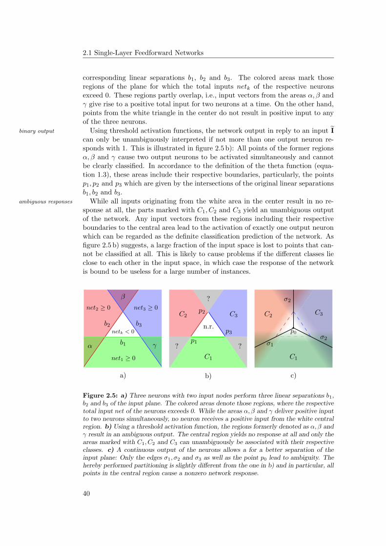
2.1 Single-Layer Feedforward Networks
corresponding linear separations b1, b2 and b3. The colored areas mark thoseregions of the plane for which the total inputs netk of the respective neuronsexceed 0. These regions partly overlap, i.e., input vectors from the areas α, β andγ give rise to a positive total input for two neurons at a time. On the other hand,points from the white triangle in the center do not result in positive input to anyof the three neurons.
Using threshold activation functions, the network output in reply to an input Ibinary output
can only be unambiguously interpreted if not more than one output neuron re-sponds with 1. This is illustrated in figure 2.5 b): All points of the former regionsα, β and γ cause two output neurons to be activated simultaneously and cannotbe clearly classified. In accordance to the definition of the theta function (equa-tion 1.3), these areas include their respective boundaries, particularly, the pointsp1, p2 and p3 which are given by the intersections of the original linear separationsb1, b2 and b3.
While all inputs originating from the white area in the center result in no re-ambiguous responses
sponse at all, the parts marked with C1, C2 and C3 yield an unambiguous outputof the network. Any input vectors from these regions including their respectiveboundaries to the central area lead to the activation of exactly one output neuronwhich can be regarded as the definite classification prediction of the network. Asfigure 2.5 b) suggests, a large fraction of the input space is lost to points that can-not be classified at all. This is likely to cause problems if the different classes lieclose to each other in the input space, in which case the response of the networkis bound to be useless for a large number of instances.
PSfrag replacements
net2 ≥ 0 net3 ≥ 0
net1 ≥ 0 C1 C1
C2 C2C3C3
b1
b2 b3p0
p1
p2
p3
σ1
σ2
σ2σ3
?
?
?
n.r.netk < 0
a) b) c)
α
β
γ
Figure 2.5: a) Three neurons with two input nodes perform three linear separations b1,b2 and b3 of the input plane. The colored areas denote those regions, where the respectivetotal input net of the neurons exceeds 0. While the areas α, β and γ deliver positive inputto two neurons simultaneously, no neuron receives a positive input from the white centralregion. b) Using a threshold activation function, the regions formerly denoted as α, β andγ result in an ambiguous output. The central region yields no response at all and only theareas marked with C1, C2 and C3 can unambiguously be associated with their respectiveclasses. c) A continuous output of the neurons allows a for a better separation of theinput plane: Only the edges σ1, σ2 and σ3 as well as the point p0 lead to ambiguity. Thehereby performed partitioning is slightly different from the one in b) and in particular, allpoints in the central region cause a nonzero network response.
40
Feedforward Neural Networks
If the neurons incorporate continuous activation functions, it is sufficient for the continuous output
respective correct neuron to yield the highest response among all outputs. The re-maining neurons are not required to exhibit an activation close to 0 as long as theone with the highest output is regarded as the classification response of the net-work. This leads to a partitioning of the input plane as illustrated in figure 2.5 c)which is clearly distinct from the one in figure 2.5 b). As before, the areas markedwith C1, C2 and C3 represent those parts of the input space that can unambigu-ously be allocated to the corresponding classes. But the separation between tworegions Ci and Ck is now defined by the points that cause the respective outputsOi, Ok to return the same value Oi(I) = Ok (I). The hereby defined boundariesturn out to be straight lines (σ1, σ2 and σ3) that meet in the point p0 which isunique in resulting in an equal response of all outputs.
It is to be emphasized that this new partitioning is different from the original improved response
separation performed by b1, b2 and b3. Most notably, there are no points left inthe input space that yield a network response of exactly 0. Even inputs fromthe central part (except p0 and those on σ1, σ2 and σ3) can each be assigned toone of the classes. In practice, it is common to define a threshold value thathas to be exceeded by a neuron output in order to be accepted as a trustworthyclassification. Fixing a threshold value of 1/2 would again declare the points ofthe central triangle (framed by the dashed lines) as not belonging to any class.
A comparison between figures 2.5 b) and 2.5 c) reveals that a differentiated neu- convex decisionregionsron output notably decreases the amount of unclassifiable inputs but it is also ev-
ident that in both cases, the pairwise separations between the different categoriespersist to be linear. Moreover, it can be anticipated from both figures and can alsobe proven mathematically that for monotonic activation functions, the individualclassification regions are always connected and convex. That is, for two points Iα
a
and Iαb being assigned to class Cα, all points Iµ that lie on the straight connection
between them (Iµ = Iαa + µ(Iα
b − Iαa ), 0 < µ ≤ 1) are inevitably assigned to class
Ck, too [20].
Going back to the classification problem depicted in figure 2.3 b), it has tobe concluded as a consequence of the above result that this specific task cannotaccurately be solved by a single-layer network even if it has one output neuronreserved for each class: The instances of the upper class in figure 2.3 b) form aregion that is not convex but concave.
The limitation to connected and convex classification regions as well as the motivation formultiple layersfrequent ambiguities caused by the undifferentiated output of threshold neurons
can be overcome by assigning multiple neurons to each class Ck. If the outputs ofthese neurons are appropriately combined, they can perform a potentially moredifferentiated and flexible decision concerning the allocation of a given input I tothe class Ck. This is in fact the main motivation to build feedforward networkswith more than one layer which will be the topic of section 2.2. The subjectof single-layer networks with multiple outputs shall be closed by discussing thenecessary modifications to the training approaches.
41
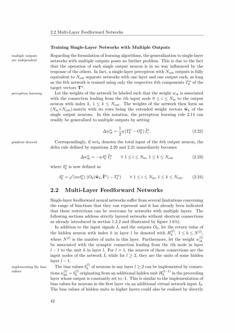
2.2 Multi-Layer Feedforward Networks
Training Single-Layer Networks with Multiple Outputs
Regarding the formulation of learning algorithms, the generalization to single-layermultiple outputsare independent networks with multiple outputs poses no further problem. This is due to the fact
that the operation of each single output neuron is in no way influenced by theresponse of the others. In fact, a single-layer perceptron with Nout outputs is fullyequivalent to Nout separate networks with one layer and one output each, as longas the kth network is trained using only the respective kth components T α
k of thetarget vectors Tα.
Let the weights of the network be labeled such that the weight wik is associatedperceptron learning
with the connection leading from the ith input node 0 ≤ i ≤ Nin to the outputneuron with index k, 1 ≤ k ≤ Nout. The weights of the network then form an(Nin×Nout)-matrix with its rows being the extended weight vectors wk of thesingle output neurons. In this notation, the perceptron learning rule 2.14 canreadily be generalized to multiple outputs by setting
∆wαik =
1
2η (Tα
k − Oαk ) Iα
i . (2.22)
Correspondingly, if netk denotes the total input of the kth output neuron, thegradient descent
delta rule defined by equations 2.20 and 2.21 immediately becomes
∆wαik = −η δα
k Iαi ∀ 1 ≤ i ≤ Nin, 1 ≤ k ≤ Nout (2.23)
where δαk is now defined as
δαk = ϕ′(netαk ) (Ok(wk, I
α) − Tαk ) ∀ 1 ≤ i ≤ Nin, 1 ≤ k ≤ Nout. (2.24)
2.2 Multi-Layer Feedforward Networks
Single-layer feedforward neural networks suffer from several limitations concerningthe range of functions that they can represent and it has already been indicatedthat these restrictions can be overcome by networks with multiple layers. Thefollowing sections address strictly layered networks without shortcut connectionsas already introduced in section 1.2.2 and illustrated by figure 1.6 b).
In addition to the input signals Ii and the outputs Ok, let the return value of
the hidden neuron with index h in layer l be denoted with H(l)h , 1 ≤ h ≤ N (l),
where N (l) is the number of units in this layer. Furthermore, let the weight w(l)ih
be associated with the synaptic connection leading from the ith node in layerl − 1 to the unit h in layer l. For l = 1, the sources of these connections are theinput nodes of the network Ii while for l ≥ 2, they are the units of some hiddenlayer l − 1.
The bias values b(l)h of neurons in any layer l ≥ 2 can be implemented by connec-implementing the bias
values tions w(l)0h = b
(l)h originating from an additional hidden unit H
(l−1)0 in the preceeding
layer whose output is constantly set to -1. This is similar to the implementation ofbias values for neurons in the first layer via an additional virtual network input I0.The bias values of hidden units in higher layers could also be realized by directly
42
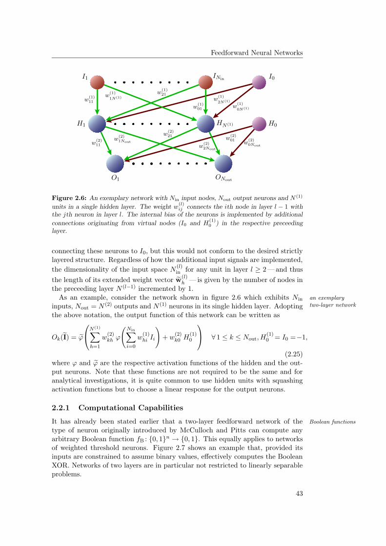
Feedforward Neural Networks
PSfrag replacements
I1 INin I0
w(1)11
w(1)
1N(1)
w(1)21
w(1)
2N(1)
w(1)01
w(1)
0N(1)
w(2)11
w(2)1Nout
w(2)21
w(2)2Nout
w(2)01
w(2)0Nout
H1 HN(1) H0
O1 ONout
Figure 2.6: An exemplary network with Nin input nodes, Nout output neurons and N (1)
units in a single hidden layer. The weight w(l)ij connects the ith node in layer l − 1 with
the jth neuron in layer l. The internal bias of the neurons is implemented by additional
connections originating from virtual nodes (I0 and H(1)0 ) in the respective preceeding
layer.
connecting these neurons to I0, but this would not conform to the desired strictlylayered structure. Regardless of how the additional input signals are implemented,
the dimensionality of the input space N(l)in for any unit in layer l ≥ 2 — and thus
the length of its extended weight vector w(l)h — is given by the number of nodes in
the preceeding layer N (l−1) incremented by 1.As an example, consider the network shown in figure 2.6 which exhibits Nin an exemplary
two-layer networkinputs, Nout = N (2) outputs and N (1) neurons in its single hidden layer. Adoptingthe above notation, the output function of this network can be written as
Ok (I) = ϕ
N(1)∑
h=1
w(2)kh ϕ
(Nin∑
i=0
w(1)hi Ii
)+ w
(2)k0 H
(1)0
∀ 1 ≤ k ≤ Nout, H
(1)0 = I0 =−1,
(2.25)where ϕ and ϕ are the respective activation functions of the hidden and the out-put neurons. Note that these functions are not required to be the same and foranalytical investigations, it is quite common to use hidden units with squashingactivation functions but to choose a linear response for the output neurons.
2.2.1 Computational Capabilities
It has already been stated earlier that a two-layer feedforward network of the Boolean functions
type of neuron originally introduced by McCulloch and Pitts can compute anyarbitrary Boolean function fB : 0, 1n → 0, 1. This equally applies to networksof weighted threshold neurons. Figure 2.7 shows an example that, provided itsinputs are constrained to assume binary values, effectively computes the BooleanXOR. Networks of two layers are in particular not restricted to linearly separableproblems.
43
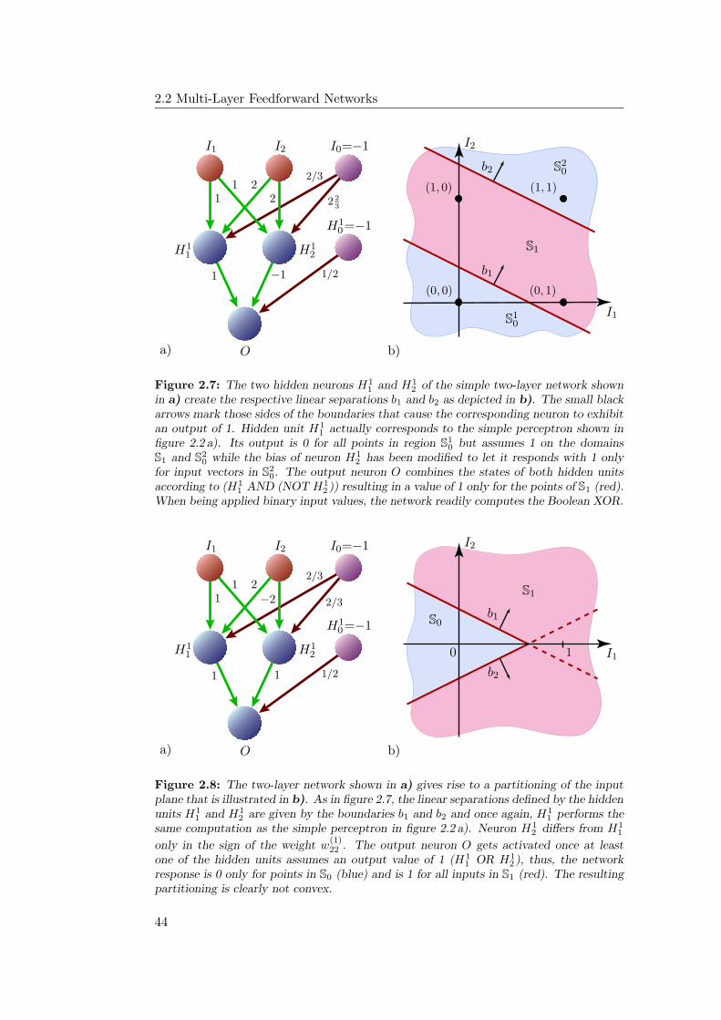
2.2 Multi-Layer Feedforward Networks
PSfrag replacements
I1 I2 I0=−1
H11 H1
2
H10=−1
11 2
2
−1
1/2
2/3
2 23
1 −1
O
I1
I2
(0, 0) (0, 1)
(1, 0) (1, 1)
b1
b2
S10
S1
S20
a) b)
Figure 2.7: The two hidden neurons H11 and H1
2 of the simple two-layer network shownin a) create the respective linear separations b1 and b2 as depicted in b). The small blackarrows mark those sides of the boundaries that cause the corresponding neuron to exhibitan output of 1. Hidden unit H1
1 actually corresponds to the simple perceptron shown infigure 2.2 a). Its output is 0 for all points in region S1
0 but assumes 1 on the domainsS1 and S2
0 while the bias of neuron H12 has been modified to let it responds with 1 only
for input vectors in S20. The output neuron O combines the states of both hidden units
according to (H11 AND (NOT H1
2 )) resulting in a value of 1 only for the points of S1 (red).When being applied binary input values, the network readily computes the Boolean XOR.
PSfrag replacements
I1 I2 I0=−1
H11 H1
2
H10=−1
1
11
0
2−2
1/2
2/3
2/3
1 1
O
I1
I2
b1
b2
S0
S1
a) b)
Figure 2.8: The two-layer network shown in a) gives rise to a partitioning of the inputplane that is illustrated in b). As in figure 2.7, the linear separations defined by the hiddenunits H1
1 and H12 are given by the boundaries b1 and b2 and once again, H1
1 performs thesame computation as the simple perceptron in figure 2.2 a). Neuron H1
2 differs from H11
only in the sign of the weight w(1)22 . The output neuron O gets activated once at least
one of the hidden units assumes an output value of 1 (H11 OR H1
2 ), thus, the networkresponse is 0 only for points in S0 (blue) and is 1 for all inputs in S1 (red). The resultingpartitioning is clearly not convex.
44
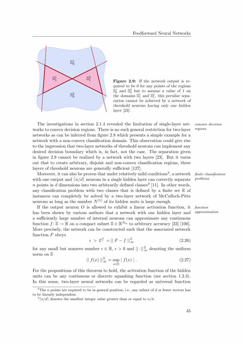
Feedforward Neural Networks
PSfrag replacements
S11 S2
1
S10
S20
Figure 2.9: If the network output is re-quired to be 0 for any points of the regionsS1
0 and S20 but to assume a value of 1 on
the domains S11 and S2
1, this peculiar sepa-ration cannot be achieved by a network ofthreshold neurons having only one hiddenlayer [23].
The investigations in section 2.1.4 revealed the limitation of single-layer net- concave decisionregionsworks to convex decision regions. There is no such general restriction for two-layer
networks as can be inferred from figure 2.8 which presents a simple example for anetwork with a non-convex classification domain. This observation could give riseto the impression that two-layer networks of threshold neurons can implement anydesired decision boundary which is, in fact, not the case. The separation givenin figure 2.9 cannot be realized by a network with two layers [23]. But it turnsout that to create arbitrary, disjoint and non-convex classification regions, threelayers of threshold neurons are generally sufficient [127].
Moreover, it can also be proven that under relatively mild conditions2, a network finite classificationproblemswith one output and dn/de neurons in a single hidden layer can correctly separate
n points in d dimensions into two arbitrarily defined classes3 [11]. In other words,any classification problem with two classes that is defined by a finite set E ofinstances can completely be solved by a two-layer network of McCulloch-Pittsneurons as long as the number N (1) of its hidden units is large enough.
If the output neuron O is allowed to exhibit a linear activation function, it functionapproximationhas been shown by various authors that a network with one hidden layer and
a sufficiently large number of internal neurons can approximate any continuousfunction f : S → R on a compact subset S ∈ RNin to arbitrary accuracy [23] [100].More precisely, the network can be constructed such that the associated networkfunction F obeys
ε > Ef = || F − f ||S∞ (2.26)
for any small but nonzero number ε ∈ R, ε > 0 and || · || S∞ denoting the uniform
norm on S
|| f(x) ||S∞ = supx∈S
| f(x) | . (2.27)
For the propositions of this theorem to hold, the activation function of the hiddenunits can be any continuous or discrete squashing function (see section 1.2.3).In this sense, two-layer neural networks can be regarded as universal function
2The n points are required to be in general position, i.e., any subset of d or fewer vectors hasto be linearly independent.
3dn/de denotes the smallest integer value greater than or equal to n/d.
45
2.2 Multi-Layer Feedforward Networks
approximators and therefore form an important class of networks for practicalapplications.
Note that the value set V of any continuous real function f on a compact setsigmoidal units
S ∈ RNin is itself compact [59]. Through shifting and rescaling, f can be modifiedto yield a corresponding function f ′ with a value set V ′ that obeys V ′ ⊂ [0, 1].On the other hand, for x ≈ 0 and/or β À 1, the logistic function ϕl(x) becomesapproximately linear. The above result can thus easily be transferred to networksthat consist entirely of sigmoidal units.
It has to be noted that most proofs for the universal approximation potential ofopen questions
two-layer networks are neither concerned about the number of hidden units thatis necessary to achieve a desired accuracy nor about whether networks with morelayers might be able to obtain the same result with a smaller number of neuronsand synaptic connections. Also, they do not provide an answer to the questionof how the network can actually be trained to perform the desired approxima-tion. Nevertheless, these issues are undoubtedly of critical relevance for practicalapplications.
Regarding the residual error EfN that remains when a network with N hiddennetwork sizing
units in a single hidden layer optimally approximates a given function f , theformer can be shown to decrease as O(1/
√N) when N grows [113]. Assuming thetrainability
existence of an efficient training algorithm that is capable of optimizing a networkwith N hidden units to yield the minimum achievable error E (equation 2.16) ona finite training set Et, it can be estimated how N has to grow with the number oftraining inputs Ne =| Et | in order to let the residual error Ef
N approximate 0 [219].It is to be emphasized that in contrast to the error E of the network on thetraining set, the value Ef
N refers to the remaining difference4 between the networkoutput F and the original function f on their whole domain S (see equation 2.27).Thus, feedforward networks can not only approximate any continuous function toarbitrary accuracy but can in principle also be taught to do so using a limitednumber of training examples which is a promising observation especially withregard to their generalization abilities.
Admittedly, this last theorem assumes two vital conditions that are both nottrivially fulfilled. First, it requires the network size to be adjusted appropriatelyand second, it depends on the existence of the aforementioned learning algorithmthat is able to reliably yield the global minimum of the network error E on thetraining set. It has already been shown for single-layer networks that the formu-lation of such a training algorithm is at best difficult and the following sectionsshall therefore address the important issue of training feedforward neural networkswith more than one layer.
2.2.2 Training Multi-Layer Networks
Each output neuron of a multi-layer feedforward network with L layers can bethe internal featurespace considered as a simple perceptron that receives its input signals from the N (L−1)
units of the last hidden layer and as such, it can only perform a linear partitioningof its input space Ψ ⊆ RN(L−1)
. Seen from this angle, it is the purpose of the
4according to the L2 norm [60]
46

Feedforward Neural Networks
earlier layers to map the original input vectors Iα ∈ Φ ⊆ RNin onto correspondinginternal representations Rα ∈ Ψ in such a way that within the feature space Ψ,the desired classification can be performed by simple linear separations. Followingthis view, the operation of the network is divided into two distinct steps: First, thenonlinear mapping of a given input onto its internal representation and second, theclassification of this pattern according to a linear separation of the intermediatefeature space.
The Credit Assignment Problem
If it is ensured that the preceeding layers provide an adequate internal represen- training the hiddennodestation in which a given set of training examples (Iα,Tα) is linearly separable (or
at least approximately so), the weights of the last layer could be trained using ei-ther the perceptron algorithm or the gradient based approach introduced in 2.1.2and 2.1.3. Unfortunately, training the hidden neurons to perform the requiredpreprocessing cannot be achieved via the same learning algorithms. While theycan equally be regarded as being like simple perceptrons, there are no target valuesavailable for the hidden units that could be assigned to their outputs. Thus, if thenetwork produces an incorrect output in response to a given input Iα, there is,initially, no way of determining which group of hidden units is responsible for thiserror. Consequently, there is no apparent procedure for calculating appropriatechanges of the synaptic weights. This is a fundamental issue that is commonlydenoted as the credit assignment problem.
Once the operation of the system is divided into the two distinct stages de-scribed in the preceeding paragraphs, it is not mandatory to let the first step beperformed by a feedforward network. Various alternative approaches have beenproposed that circumvent the credit assignment problem by using different typesof networks for the implementation of the initial nonlinear mapping to the featurespace. These approaches will briefly be introduced in section 2.3. Regarding multi-layer feedforward networks, there does in fact exist a relatively simple solution tothis problem if the output of the neurons is continuous.
Error Backpropagation
As long as the activation functions of all neurons are differentiable with respect differentiable networkfunctionto the synaptic weights, it is evident by virtue of the chain rule [61] [59] that the
same also applies to the output of a complete feedforward network regardless of thenumber of layers. For a network with one hidden layer, this can directly be inferredfrom equation 2.25. Therefore, the sum-of-squares error of the network on agiven set of training examples as defined by equation 2.16 becomes a differentiablefunction of the weights as well.
Similar to the case of single-layer networks, the derivatives with respect to the
individual synaptic weights w(l)ij can be used to minimize the network error function
E by employing appropriate methods like gradient descent. The procedure bywhich the necessary derivatives can be evaluated for feedforward networks withmultiple layers is known as error backpropagation or simply backpropagation [175].
47
2.2 Multi-Layer Feedforward Networks
In analogy to the iterative approaches described earlier, consider the networkdifferentiable networkerror error Eα obtained on a single training example (Iα,Tα) as given by equation 2.15
and let the network incorporate L layers of neurons. Using the common chain rule,
the derivative of Eα with respect to any synaptic weight w(l)ij within the network
can be calculated as
∂Eα
∂w(l)jk
=∂Eα
∂ net(l)k
· ∂ net(l)k
∂w(l)jk
(2.28)
for all index values 1 ≤ l ≤ L, 1 ≤ k ≤ N (l) and 1 ≤ j ≤ N (l−1) with N (0) = Nin
and N (L) = Nout. Here, net(l)k stands for the total input to the kth neuron of the
lth layer in the presence of the network input Iα. It is convenient to denote the
first term on the right hand side of 2.28 as δ(l)k , i.e.,
δ(l)k :=
∂Eα
∂ net(l)k
. (2.29)
In pursuit of a simple notation, it is understood that the regarded error E iscalculated on the basis of only a single training pattern and the index α shall inthe following be omitted. The second term in equation 2.28 can then readily bewritten as
∂ net(l)k
∂w(l)jk
= H(l−1)j
(w
(l−1)j , I
)= H
(l−1)j (2.30)
and the substitution of 2.29 and 2.30 into 2.28 yields the general result
∂E
∂w(l)jk
= δ(l)k · H(L−1)
j . (2.31)
For synaptic connections that lead to one of the output neurons in the last layeroutput neurons
L, the resulting δ(L)k ’s turn out to be similar to the δk’s that are obtained in the
case of a single-layer network
δ(L)k = ϕ′(net
(L)k )
(Ok
(w
(L)k , I
)− Tk
)∀ 1 ≤ k ≤ Nout = N (L)
= ϕ′(net(L)k ) (Ok − Tk) .
(2.32)
Therefore, the respective derivatives of the error function E equal those used forthe delta rule (section 2.1.3) with the network input Ij being replaced by the
output of the hidden unit H(L−1)j
∂E
∂w(L)jk
= ϕ′(net(L)k ) (Ok − Tk) H
(L−1)j . (2.33)
48
Feedforward Neural Networks
In the case of a connection that does not lead to a network output but rather hidden neurons
to the jth neuron of some hidden layer 1 ≤ l < L, the chain rule has to be appliedonce more. Thereby, equation 2.29 is reformulated to become
δ(l)j =
∂E
∂ net(l)j
=N(l+1)∑
k=1
∂E
∂ net(l+1)k
· ∂ net(l+1)k
∂ net(l)j
∀ 1 ≤ j ≤ N (l) (2.34)
where it has been used that any change in the total input of the considered neurondoes only affect the error E by effectively changing the total inputs of the otherneurons that it is connected to.
The first factor in each addend of the above sum is in fact the δ(l+1)k of the backpropagation of
the errorcorresponding receiving neuron in the next layer. The calculation of the secondfactor is straight forward and if the activation functions of all neurons in thenetwork are assumed to be the same, equation 2.34 can be rewritten as
δ(l)j = ϕ′(net
(l)j )
N(l+1)∑
k=1
w(l+1)jk δ
(l+1)k . (2.35)
In other words, the value of δ(l)j for a specific hidden unit can be obtained by
propagating the δ’s of neurons in higher layers backwards through the network.
For the output neurons, the values δ(L)k are explicitly given by equation 2.33.
Therefore, all values δ(l)j and correspondingly all possible partial derivatives of
the error function with respect to arbitrary synaptic weights can be calculated byrecursively applying equation 2.35.
Note that although the considerations so far assumed a network with a strictlylayered structure where the activation functions of all neurons are the same, theabove result can easily be generalized to any feedforward architecture and/ornetworks that incorporate different activation functions for different neurons [20].
Calculating the partial derivatives of the error function via backpropagation advantages ofbackpropagationhas two main advantages that are worth being pointed out explicitly. First, the
backpropagation scheme is local in the sense that calculating δ(l)j for a specific con-
nection only requires the knowledge of quantities that are available at the two endpoints of this synaptic link. Hence, all connections within one layer can be eval-uated independently which allows for a potentially fast parallel implementation.Second, computing the partial derivatives of the error function 2.15 directly wouldin the presence of W weights take O(W 2) operations. Using equations 2.31, 2.32and 2.35, all derivatives can be calculated in only O(W ) operations.
Training with Backpropagation
On the basis of the network error E after the application of an input pattern I and error backpropagationand gradient descentequipped with its partial derivatives with respect to each weight w
(l)ij , the gradient
descent training strategy introduced in section 2.1.3 can be applied to multi-layerfeedforward networks according to
∆w(l)ik = −η δ
(l)k H
(l−1)i
(I, w
(l−1)i
)∀ 1 ≤ i ≤ N (l−1), 1 ≤ k ≤ N (L) (2.36)
49
2.2 Multi-Layer Feedforward Networks
where the values δ(l)k are obtained via error backpropagation.
Often, the term backpropagation refers to this specific training approach thatcombines the calculation of the required partial derivatives using the rules derivedin the preceeding paragraphs with the gradient descent learning rule discussedin section 2.1.3. This convention shall be adopted in the following. Initially,the two parts are independent and the error-backpropagation scheme can also becombined with other optimization strategies that rely on the derivatives of theerror function [20] [88].
Various modifications are conceivable to the backpropagation training strategythat potentially benefit its ability to yield the minimum possible error of thenetwork on a given set of training examples. For example, it is straight forwardto replace the sum-of-squares error function by alternative differentiable errormeasures.
Furthermore, it has already been discussed in section 2.1.3 that the choice oflearning withmomentum learning rate η has a strong influence on the convergence behavior and speed of
gradient descent. To avoid divergent oscillations, η is preferably kept small whichin turn slows down the speed of the training. One way of dealing with this problemis the addition of a so-called momentum term in equation 2.36 that introduces acontribution from the preceeding learning step to each new weight change in theform of
∆w(l)ik (t + 1) = −η δ
(l)k H
(l−1)i + ν∆w
(l)ik (t) (2.37)
where t refers to the number of training iterations [176]. The momentum param-eter ν is bound to lie in [0, 1] and is commonly chosen to be 0.9. It turns out thatin the presence of a momentum term, the learning rate can safely be set to largervalues without running the risk of provoking divergent oscillations [218].
Another approach to avoid the difficulties in defining appropriate learning pa-learning rateadaption rameters η and ν is to let them be adjusted automatically during the training
process [109] [32].
While all these modifications promote a more reliable convergence of the traininglocal minima
algorithm towards a minimum of the error function, they provide no guarantee ofthe latter being the global minimum instead of a possible local one. For a multi-
layer network, the error surface as a function of the individual weight values w(l)ik
can be considerably complex and compared to single-layer networks, the number oflocal minima that correspond to suboptimal solutions of a given learning problemis most likely to be increased even further. Regarding the difficulties that arisedue to the existence of these local minima, the backpropagation algorithm and itsdifferent variants inherit all the problems that already affect the delta rule.
In spite of this, multilayer feedforward networks in combination with error back-propagation training algorithms constituted the working-horse of neural networkresearch for many years and have successfully been employed in various applica-tions ever since [123] [187].
50
Feedforward Neural Networks
2.3 A Short Overview of Alternative Network Models
While the remainder of this thesis primarily addresses implementations and appli-cations of the feedforward networks discussed so far, the following sections shallgive a brief summary of some important other types. These network models alsoprove to be of considerable value not only for scientific research but also for re-alistic pattern recognition applications. In so far, they can be seen as competingapproaches to ordinary feedforward networks.
An exhaustive discussion of the various known types of artificial neural networksthat would do justice to their interesting properties, capabilities and applicationsexceeds the scope of this thesis. The succeeding sections will examine alternativeapproaches only to an extent that is sufficient to allow for a reasonable comparisonwith classical feedforward networks and the training strategies presented in laterchapters. Some important neural network models like Boltzmann machines [2] andself-organizing maps [120] will not be covered. For a detailed investigation of thesetopics and a more exhaustive study of artificial neural network theory in general,the interested reader is referred to the available literature [20] [84] [88] [169].
2.3.1 The Feature Space Revisited: Support Vector Machines
Returning to the concept of the intermediate feature space Ψ brought forward insection 2.2.2, it has been said before that the corresponding nonlinear mappingr : Φ → Ψ of the original input vectors I ∈ Φ does not necessarily have to beperformed by a layered feedforward network of the hitherto discussed type.
A single hidden layer of N localized radial basis function neurons (see sec- radial basisfunction networkstion 1.2.3) implements a mapping r : Φ → RN that is essentially different from
those performed by ordinary neurons. Based on this mapping, a succeeding layerof simple binary or continuous-valued neurons can perform complex separationsof the original input space. For some applications, this strategy proves to be anadvantageous alternative to the partitionings provided by common feedforwardnetworks [146]. Systems of this kind are referred to as radial basis function net-works. Both, classical two-layer feedforward networks and radial basis functionnetworks can be summarized under the generalized framework of support vectormachines that attracted increasing interest during the last years [29] [40] [84] [112].
The methodology of support vector machines includes an efficient procedure support vectormachinesfor determining the optimal hyperplane that separates two classes of points rα in
some space Ψ. The considered points can (but do not have to) be the nonlinearprojections r(Iα) ∈ Ψ of some original vectors Iα ∈ Φ. If the two sets are linearlyseparable in Ψ, the found hyperplane is optimal in the sense that it retains thehighest possible normal distance from all vectors rα. For linearly inseparableclasses, it at least yields the minimum achievable classification error.
This optimal hyperplane is found by minimizing a Lagrangian that contains thevectors rα only in the form of inner products rα · rβ = r(Iα) · r(Iβ). With regardto the original input vectors Iα, this important feature allows to reformulate theinner product in Ψ as a symmetric Kernel function
K(Iα, Iβ) = r(Iα) · r(Iβ) (2.38)
51
2.3 A Short Overview of Alternative Network Models
on Φ. The task of separating the two classes in the original input space can thus besolved by finding an optimal hyperplane in an intermediate space without havingto consider this feature space itself in explicit form. The used non-linear mappingr and the feature space Ψ become manifest within the formulation of the solutiononly in the form of the Kernel function K. In particular, this allows to use featurespaces with very high or even infinite dimensions.
The desire for very high-dimensional intermediate spaces and hence the mo-high-dimensionalfeature spaces tivation for support vector machines arises from a general observation made by
Cover in 1965 [41]: The non-linear projections r(Iα) ∈ Ψ of patterns Iα fromsome Nin-dimensional input space Φ exhibit an increasing probability to be lin-early separable in the target space Ψ when the dimensionality of the latter grows.For general sets of input patterns, both, the nonlinearity of the mapping and theincreased dimensionality of the intermediate feature space are necessary precon-ditions to ensure an improved linear separability [41].
2.3.2 Hierarchical Approaches and the Neocognitron
Hierarchical networks like the neocognitron by K. Fukushima [63] [64] and relatedbasic idea
approaches [136] [205] divide the solution of a complex classification problem intoiterative nonlinear mappings between successive feature spaces. Each layer ofneurons combines localized patterns in the output of the preceeding layer to higher-level features that are in turn the inputs of the next level. Viewed in termsof its own input, each layer performs relatively simple classifications. However,with regard to the original input space, the hereby constructed features grow inabstractness and complexity with each hierarchical level. This way, a neuron inthe final output layer can exhibit a differentiated and robust sensitivity to thepresence or absence of complex features in the originally applied input patterns.
Among other things, the primary difference between the neocognitron approachspecifying the features
and ordinary feedforward models is that the features to be extracted by the indi-vidual layers are defined externally. Thus, the layers can in principle be trainedindependently using specialized supervised training algorithms [63] [64]. The suc-cess of this training concept critically depends on the selection of adequate featureswhich is usually straight forward for the first layer but poses a substantial chal-lenge in the cases of higher hierarchical levels. Variants of this approach thereforeaim to construct a single set of features that can be used in all layers [52] [205] orto find appropriate features through unsupervised learning [63] [64] [136].
Hierarchical networks are commonly applied to image classification tasks likehand-written digit classification [63] [64], object detection in realistic images [205]or character recognition [52].
2.3.3 The Hopfield Network
In the year 1982, the field of artificial neural networks received fresh impulse bya major contribution from the physicist J. Hopfield [98] who introduced a specialform of recurrent network architecture. Within a so-called Hopfield network, anyneuron 1 ≤ i ≤ N is connected to every other unit j 6= i apart from itself and
52
Feedforward Neural Networks
the synaptic weights are chosen to be symmetric, i.e., wij = wji, wii = 0 for symmetric weightcondition1 ≤ i, j ≤ N . Originally, the neurons are fixed to be weighted threshold units
with possible outputs of -1 and 1 but the concept has later been extended toneurons with continuous output as well [99].
As a consequence of its highly recurrent architecture, the Hopfield network temporal dynamics
exhibits distinct temporal dynamics. When the output states Oi of the neuronsare set to some initial states Oi(0) = Ii at time t = 0, each neuron output Oi(t)will in general be a function of time given by
Oi(t + ∆t) = sgn
∑
i6=j
wij Oj(t)
. (2.39)
In practice, it is common to implement this updating scheme by randomly selectinga new single neuron in each time step t and recalculating its activation due to thecurrent states of the remaining units to obtain its new output Oi(t + 1). Thestate of the whole network O(t) = (O1(t), . . . , ON (t)) is a discrete trajectory inthe configuration space −1, 1N . The question arises whether the network everreaches a stationary point Os, a so-called attractor, such that after some time ts,the network state obeys O(t) = Os ∀ t > ts.
The remarkable novelty in Hopfield’s theoretical investigation of this question energy function
is the introduction of an energy function H
H(t) = −1
2
∑
ij
wij Oi(t) Oj(t). (2.40)
If the network state evolves according to the update rule given by equation 2.39, itis the central property of the energy function 2.40 that in each time step, the energyH will either decrease or remain constant. Under the condition of symmetricweights, the network is furthermore guaranteed to eventually reach a minimum ofthe energy function and hence a stationary state after a finite time [98].
For this reason, Hopfield networks are attractive practical models of associative Hopfield networks asassociative memorymemory. Based on the energy function 2.40, it is possible to derive simple rules
for the adequate choice of weights wij that yield a network whose attractors aregiven by a predefined set of desired output patterns Tα [88]. The network canthen be regarded to have learned these patterns: If it is applied an external inputI by setting the initial states of all neurons to Oi(0) = Ii, 1 ≤ i ≤ N , thenetwork output O will after some finite time ts settle to the specific attractor Tα
that resembles the original input most. In other words, Hopfield networks areadequate systems to perform autoassociation tasks as introduced in section 1.2.4and are also often denoted as autoassociative networks.
Moreover, the formulation of the energy function H underlines Hopfield’s state- relation tostatistical physicsment that the introduced network architecture is “isomorphic with an Ising model”,
a model from statistical physics that describes ensembles of interacting two-statesystems [54] [98]. This important observation readily allowed a vast repertoire ofphysical theory to be applied to neural network research.
53
2.4 Hardware Neural Networks
2.3.4 Computing Without Stable States
Once the symmetric weight condition of the Hopfield model is abandoned, theunsymmetric weights
temporal dynamics of the network become more complicated. Being released froman initial configuration O0, the network is no longer guaranteed to reach a stableattractor. Experiments reveal that, started from different random states O0, itwill in most cases reach a stationary point, and will in the remaining trials atleast settle into limiting behaviors and wander around in only a small region ofthe configuration space [98]. These domains are centered around one particularminimum of the energy function.
At first sight, it might not seem desirable to have a neural network exhibit richtemporal dynamics. To be usable for autoassociation tasks, a network is requiredto converge to stable states within as short a time as possible. On the other hand, itcan be argued that the brain represents a highly recurrent system with complicatedtemporal behavior and nevertheless performs demanding computational tasks ontime scales of 100–150 ms that are not much longer than those defined by theoperation of its constituents, i.e., the neurons and synapses [208].
Motivated by this observation, Mass et al. [129] and Jaeger [110] independentlyliquid computingand echo states conceived a way of performing complex computations using neural systems without
stable states. The basic idea is to use highly recurrent neural networks that canreceive external input streams via dedicated input nodes. Such a system could,e.g., be implemented by a Hopfield network with some input sources Ij beingconnected to the neurons Oi. In any case, the purpose of the network is to act asa dynamical non-linear system whose current response O(t) is influenced by thepresent and past inputs I(t′), t′ ≤ t.
A simple readout unit that only processes the current state of the dynamicnetwork O(t) can then be trained to accomplish non-trivial classification taskson the original input patterns I(t). This readout can be as simple as a linearperceptron which permits the use of common optimization techniques like thosedescribed in sections 2.1.2 and 2.1.3.
It is a striking observation that different linear classifier systems can success-fully be trained for different computational tasks while processing the output ofthe very same randomly connected recurrent network, as long as the latter exhibitssufficiently complex temporal dynamics [129] [110]. The originally used networkmodels are more elaborate and closer to biology than the Hopfield networks de-scribed above but it has recently been shown that the temporal characteristicsof a recurrent network of threshold units suffice to allow a simple adjacent linearclassifier to perform non-trivial classification tasks [18] [184].
2.4 Hardware Neural Networks
It is one of the key features of artificial neural networks that their operationalmotivation
principles feature a high degree of inherent parallelism. In a feedforward network,for example, all neurons of a given layer can compute their outputs simultaneouslyand independently as soon as the outputs of all neurons in the former layer areavailable. Software implementations on ordinary sequential computers can only
54
Feedforward Neural Networks
insufficiently exploit this parallelism. Therefore, hardware realizations have beena topic of investigation almost from the outset of artificial neural network research.
The following sections are intended to provide a brief overview on the field organization
of hardware implemented neural networks. Past approaches, present trends, andchallenges to the development of dedicated hardware realizations are reviewed on ageneral level, and the discussion will be concluded by an investigation of suitabletraining approaches. These reflections serve as the basis for the more concreteconsiderations that drove the design of the actual neural network chip used forthe experiments presented in this work. An exhaustive description of this chipand the concepts that underly its design will be given in chapter 5.
2.4.1 Historical Overview
The first dedicated neural network hardware was introduced as early as 1951 byMinsky and Edmonds [142]. The SNARC (Stochastic Neural-Analog Reinforce- SNARC
ment Computer) was an electro-mechanical implementation and contained 40 neu-rons. Later, in parallel to computer simulations [171], Rosenblatt and co-workersdeveloped the MARK I, a hardware realization of the perceptron (section 2.1) that MARK I
already included automatic learning [83]. It comprised of a grid of 20×20 photore-ceptors that could each be connected to 40 of the 512 so-called associator units.The outputs of these units were conveyed to up to 8 threshold neurons (comparefigure 2.1). Although the MARK I was not particularly faster than software simu-lations of the perceptron [22], it was expected that for larger network architectures,the parallelized operation would result in a much higher performance gain.
When they originally published the delta rule in 1960 (section 2.1.3), Widrowand Hoff also presented the ADALINE (Adaptive Linear Element), a hardware- ADALINE
implemented threshold unit with 16 variable weights [227]. The weight adjustmentduring training had to be performed by a human operator. In the succeedingyears, the concept was extended to the MADALINE — the multiple ADALINE — MADALINE
in which several single ADALINEs were connected to a network. The MADALINEalso included automatic electronic learning.
The increasing speed of general-purpose microprocessors let software simulationsof neural networks become more and more feasible as well. Software packages likethe MARK I and MARK II 5 [86] fueled the desire for faster simulation speeds MARK I–IV
and this eventually drove the development of general purpose neural network ac-celerators (e.g., the MARK III and MARK IV ) [86].
In the late eighties, improvements in the fabrication process in conjunction with neural networksin CMOS VLSImore advanced design tools promoted the utilization of VLSI (Very Large Scale
Integration) technologies for the parallel implementation of neural networks onCMOS (Complementary Metal Oxide Semiconductor) substrates. In 1989, it wasshown by Mead [137] that neural systems can successfully be realized by directlyexploiting the physical features of the CMOS substrate instead of implementingthem on the basis of digital components. Since then, a large variety of analog
5The confusing resemblance with the MARK I perceptron by Rosenblatt is usually resolvedby setting the names of the software packages in a slanted font.
55
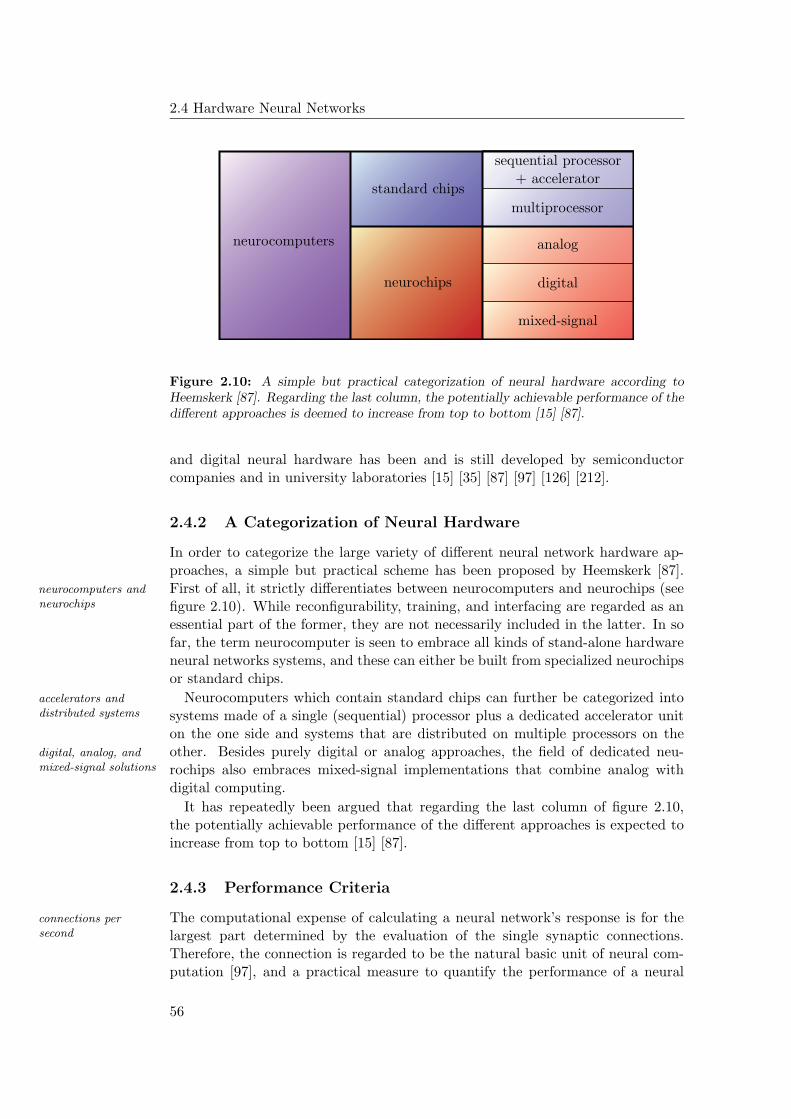
2.4 Hardware Neural Networks
PSfrag replacements
neurocomputers
standard chips
neurochips
sequential processor+ accelerator
multiprocessor
analog
digital
mixed-signal
Figure 2.10: A simple but practical categorization of neural hardware according toHeemskerk [87]. Regarding the last column, the potentially achievable performance of thedifferent approaches is deemed to increase from top to bottom [15] [87].
and digital neural hardware has been and is still developed by semiconductorcompanies and in university laboratories [15] [35] [87] [97] [126] [212].
2.4.2 A Categorization of Neural Hardware
In order to categorize the large variety of different neural network hardware ap-proaches, a simple but practical scheme has been proposed by Heemskerk [87].First of all, it strictly differentiates between neurocomputers and neurochips (seeneurocomputers and
neurochips figure 2.10). While reconfigurability, training, and interfacing are regarded as anessential part of the former, they are not necessarily included in the latter. In sofar, the term neurocomputer is seen to embrace all kinds of stand-alone hardwareneural networks systems, and these can either be built from specialized neurochipsor standard chips.
Neurocomputers which contain standard chips can further be categorized intoaccelerators anddistributed systems systems made of a single (sequential) processor plus a dedicated accelerator unit
on the one side and systems that are distributed on multiple processors on theother. Besides purely digital or analog approaches, the field of dedicated neu-digital, analog, and
mixed-signal solutions rochips also embraces mixed-signal implementations that combine analog withdigital computing.
It has repeatedly been argued that regarding the last column of figure 2.10,the potentially achievable performance of the different approaches is expected toincrease from top to bottom [15] [87].
2.4.3 Performance Criteria
The computational expense of calculating a neural network’s response is for theconnections persecond largest part determined by the evaluation of the single synaptic connections.
Therefore, the connection is regarded to be the natural basic unit of neural com-putation [97], and a practical measure to quantify the performance of a neural
56
Feedforward Neural Networks
network hardware implementation is provided by the achievable number of evalu-ated connections per second CPS:
CPS := connections/s. (2.41)
For the types of networks discussed in the preceeding sections, the calculation complexity of aconnectionof a connection boils down to the multiplication of an input signal I with the
associated synaptic weight w in order to yield the corresponding contribution tothe total input net of the respective neuron. The complexity of this operationclearly depends on the resolutions of both, the input signal and the synapticweight. This applies to digital implementations, where the adders and multipliersneed to be scaled to the precision of the operands, as well as to analog circuitsthe complexity of which is bound to grow with an increasing desired accuracy.Therefore, a more suitable performance measure is given by the number of so-called connection primitives per second CPPS
CPPS := bI · bw · connections/s (2.42)
where bI and bw are the respective resolutions of input signals and weight valuesmeasured in bit.
In the course of the training process, the weight values of a neural network are connection updates
repeatedly subject to modifications. Similar to the above measures that specify theperformance of the network during the evaluation phase, the number of availableconnection updates per second CUPS
CUPS := (connection updates)/s (2.43)
allows to quantify the reconfigurability of a hardware neural network during train-ing. A high CUPS value is of particular advantage when highly iterative chip-in-the-loop training approaches are to be applied (see section 2.4.5).
2.4.4 Challenges and Present Trends
The continuing increase in the available computing power of conventional comput- dedicated hardwarevs. softwareers— provided by an enhanced device integration [147] and a growing operational
speed — in connection with the flexibility of software solutions considerably chal-lenge the development of dedicated neural hardware. It can be argued that thepotential performance advantage of parallel hardware implementations might notbe required at all [183], particularly, as the necessary data pre- and post-processingstages cannot benefit from this parallelization.
Hybrid systems that combine analog with digital computation and which are analog andmixed-signal systems:drawbacks
apprehended to yield the highest performance gain come at the cost of a substan-tially increased engineering expense. This is mainly due to the poorly automateddesign process. Furthermore, in order to efficiently exploit the benefits of a parallelrealization in CMOS VLSI, a given neural network hardware is preferably designedto optimally suit a specific model. This naturally impedes the simultaneous in-vestigation of multiple different neural network concepts. Regarding the diversity
57
2.4 Hardware Neural Networks
of existing and competing network paradigms (see section 2.3), investments to acomparably inflexible neural hardware seem risky.
Therefore, the commercial interest in hardware implemented neural networksnoticeably decreased during the nineties. The competition with conventionalgeneral-purpose microprocessors mostly affected the research on digital neuralsystems [152]. Nevertheless, besides dedicated implementations for specific appli-cations [48], realizations of neural networks in configurable logic, such as FieldProgrammable Gate Arrays (FPGAs), lately received new attention [158] [168].
It remains that although software simulations and digital hardware solutionsanalog andmixed-signalsolutions: motivation
are potentially superior to analog or mixed-signal implementations in terms offlexibility, design times, and costs, they eventually suffer from a higher power-consumption and increased silicon area requirements. Aiming for the realizationof large neural networks whose complexity and performance are to be compa-rable to those of biological systems (see section 1.1), only dedicated analog ormixed-signal implementations have the potential to combine the necessary speed,area-efficiency, and low power-consumption. Several such approaches have beenproposed [16] [122] [137] [215] [216].
2.4.5 Training Hardware Neural Networks
Beyond speed, efficiency, and scalability, the usefulness of a hardware neural net-work is ultimately determined by its trainability. Unlike digital implementations,analog systems generally suffer from inevitable device mismatches and fluctuationsin the analog signals. This considerably impedes the application of training algo-training on unreliable
substrates rithms that rely on detailed information about the characteristics of all neuronsand synapses like the exact individual transfer functions or the current weights.Regarding equations 2.23, 2.24, 2.35, and 2.36, it has to be concluded that this ulti-mately limits the feasibility of all conventional gradient-based training approaches.
So-called off-chip learning algorithms try to circumvent this problem by opti-off-chip training
mizing the synaptic weights according to simplified models of the network im-plementation. Consequently, the hardware is not in fact involved in the learningprocess: The resulting weight values need not to be transferred to the hardwarebefore the training has been completed. Although this approach readily allows toutilize the traditional and well-proven algorithms presented in the preceeding sec-tions, it is limited in so far as it can only insufficiently deal with the peculiaritiesand deficiencies of the actual neuron and synapse implementations.
More promising approaches are on-chip or chip-in-the-loop algorithms that copewith noise and imperfections of the devices by implementing and evaluating thenetwork directly on the dedicated substrate [144] [212]. For on-chip learning, theon-chip training
procedure to calculate the necessary weight updates has to be implemented inhardware and, as implied by the name, has to be located directly on the ASIC.
In a chip-in-the-loop setup, the training algorithm is realized externally andchip-in-the-looptraining can, e.g., be executed as software on an ordinary computer (see figure 2.11). To be
suitable for this kind of training approach, a neural network ASIC needs to providemeans for the external specification of all variable network parameters like theweight values and/or the synaptic connectivity. During training, slightly modified
58
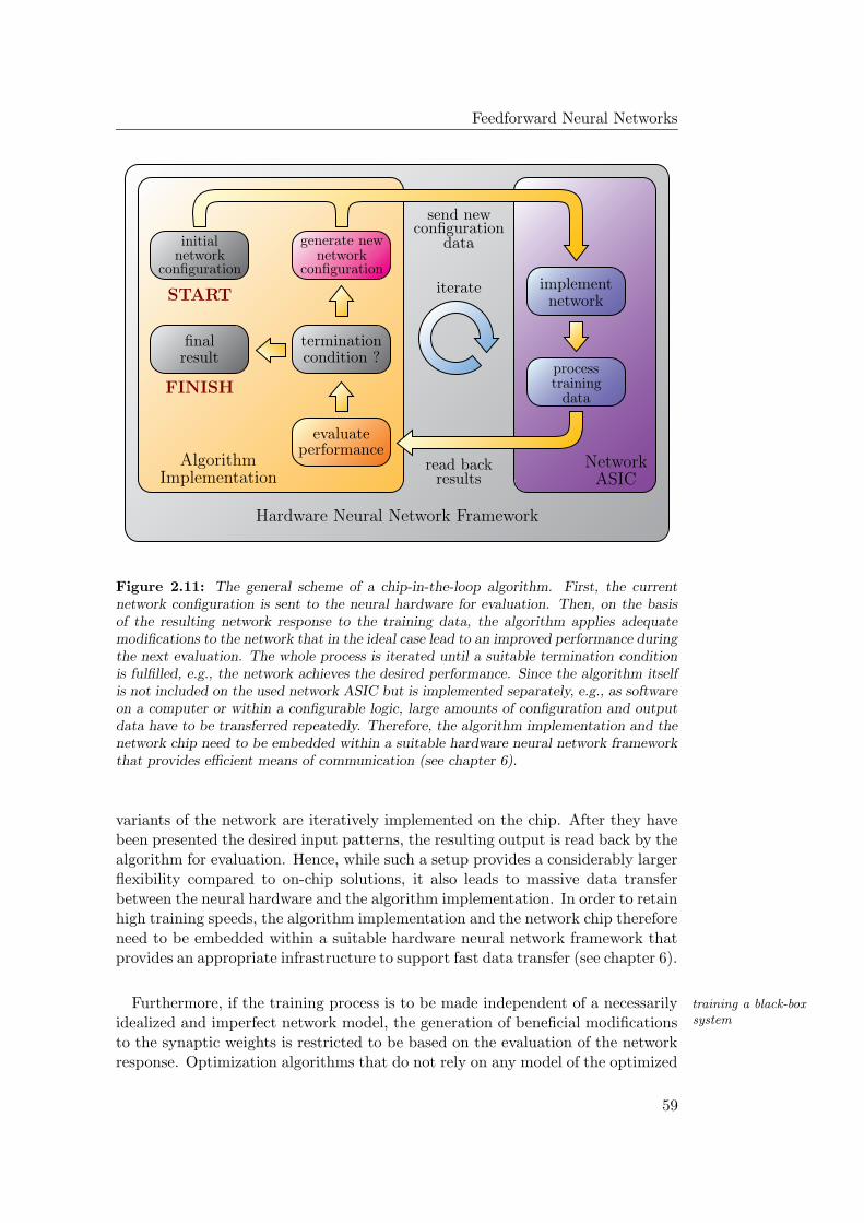
Feedforward Neural Networks
PSfrag replacements
START
FINISH
iterate
initial
network
network networkconfiguration configuration
generate new
finalresult
terminationcondition ?
evaluateperformance
send newconfiguration
data
read backresults
implement
processtraining
data
AlgorithmImplementation
NetworkASIC
Hardware Neural Network Framework
Figure 2.11: The general scheme of a chip-in-the-loop algorithm. First, the currentnetwork configuration is sent to the neural hardware for evaluation. Then, on the basisof the resulting network response to the training data, the algorithm applies adequatemodifications to the network that in the ideal case lead to an improved performance duringthe next evaluation. The whole process is iterated until a suitable termination conditionis fulfilled, e.g., the network achieves the desired performance. Since the algorithm itselfis not included on the used network ASIC but is implemented separately, e.g., as softwareon a computer or within a configurable logic, large amounts of configuration and outputdata have to be transferred repeatedly. Therefore, the algorithm implementation and thenetwork chip need to be embedded within a suitable hardware neural network frameworkthat provides efficient means of communication (see chapter 6).
variants of the network are iteratively implemented on the chip. After they havebeen presented the desired input patterns, the resulting output is read back by thealgorithm for evaluation. Hence, while such a setup provides a considerably largerflexibility compared to on-chip solutions, it also leads to massive data transferbetween the neural hardware and the algorithm implementation. In order to retainhigh training speeds, the algorithm implementation and the network chip thereforeneed to be embedded within a suitable hardware neural network framework thatprovides an appropriate infrastructure to support fast data transfer (see chapter 6).
Furthermore, if the training process is to be made independent of a necessarily training a black-boxsystemidealized and imperfect network model, the generation of beneficial modifications
to the synaptic weights is restricted to be based on the evaluation of the networkresponse. Optimization algorithms that do not rely on any model of the optimized
59

2.4 Hardware Neural Networks
system but are capable of finding improved versions merely by investigating theperformance of one or more given candidate solutions are commonly denoted asmodel-free or black-box approaches (see also section 3.3.3).
Against the background of what has been said above, it can be reasoned thatevolutionaryalgorithms such model-free algorithms promise to be the most adequate approach for the
training of analog or mixed-signal hardware neural networks. A prominent ex-ample for this kind of optimization procedure are the so-called evolutionary algo-rithms that mimic the principles of natural evolution and which shall be introducedin more detail in the following chapter.
60
Chapter 3
Evolutionary Algorithms
I have called this principle, by which each slight variation,if useful, is preserved, by the term Natural Selection.
Charles Darwin, On the Origin of Species
The field of evolutionary computation embraces a variety of algorithmic approachesthat are inspired by the mechanisms of natural evolution. Against the backgroundof the previous chapters that described how the principles of neural informationprocessing are successfully utilized in artificial systems, it is not surprising thatnatural evolution has been considered as a paradigm for the construction of pow-erful optimization algorithms. Over the course of time, evolution has created anenormous diversity of life-forms that are each remarkably well adapted to theirrespective ecological niche. Evolutionary algorithms aim to reproduce this effi-ciency by transferring the underlying principles of biological evolution to commonoptimization problems. Like in the case of artificial neural networks, the discus-sion of evolutionary algorithms shall be preluded by a short investigation of thebiological original.
3.1 Natural Evolution
The origins of the planet that we inhibit date back to about 4.6 billion years ago. the originsof lifeWithin the first 500 million years of its existence, the earth developed a solid shell,
the lithosphere, and a surrounding layer of gases called the atmosphere. Approxi-mately 4 billion years ago, the atmosphere cooled down to below 100C [66] [201],and it is believed that very simple life-forms initially appeared several 100 millionyears later.
From the very beginning, life in all its variants has influenced and changedboth the surface as well as the atmosphere of this planet to a far-reaching extent.Among the most primordial groups of life-forms are the archeabacteria and eu-bacteria that produce oxygen by photosynthesis and thereby gradually convertedthe atmosphere over a period of approximately 3 billion years. About 350 millionyears ago, the concentration of oxygen settled to its present value. Among otherthings, this distinct environmental change is assumed to have played the central
61
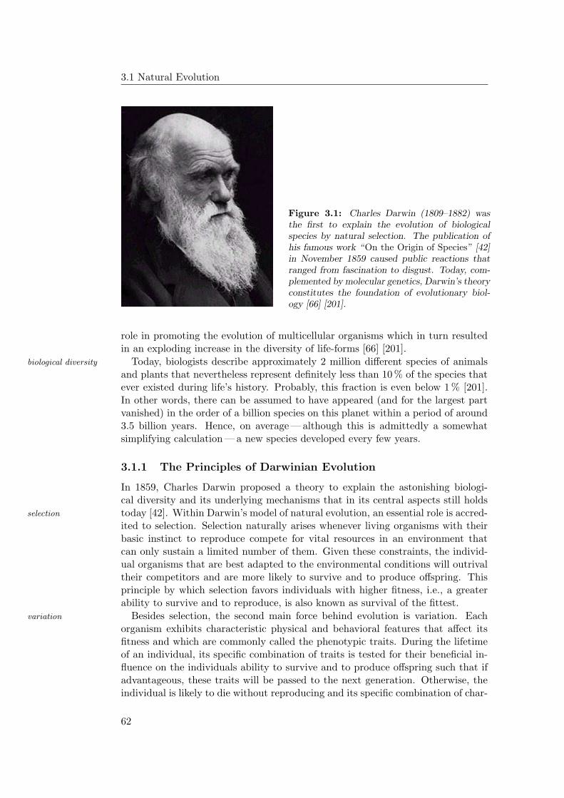
3.1 Natural Evolution
Figure 3.1: Charles Darwin (1809–1882) wasthe first to explain the evolution of biologicalspecies by natural selection. The publication ofhis famous work “On the Origin of Species” [42]in November 1859 caused public reactions thatranged from fascination to disgust. Today, com-plemented by molecular genetics, Darwin’s theoryconstitutes the foundation of evolutionary biol-ogy [66] [201].
role in promoting the evolution of multicellular organisms which in turn resultedin an exploding increase in the diversity of life-forms [66] [201].
Today, biologists describe approximately 2 million different species of animalsbiological diversity
and plants that nevertheless represent definitely less than 10 % of the species thatever existed during life’s history. Probably, this fraction is even below 1 % [201].In other words, there can be assumed to have appeared (and for the largest partvanished) in the order of a billion species on this planet within a period of around3.5 billion years. Hence, on average — although this is admittedly a somewhatsimplifying calculation — a new species developed every few years.
3.1.1 The Principles of Darwinian Evolution
In 1859, Charles Darwin proposed a theory to explain the astonishing biologi-cal diversity and its underlying mechanisms that in its central aspects still holdstoday [42]. Within Darwin’s model of natural evolution, an essential role is accred-selection
ited to selection. Selection naturally arises whenever living organisms with theirbasic instinct to reproduce compete for vital resources in an environment thatcan only sustain a limited number of them. Given these constraints, the individ-ual organisms that are best adapted to the environmental conditions will outrivaltheir competitors and are more likely to survive and to produce offspring. Thisprinciple by which selection favors individuals with higher fitness, i.e., a greaterability to survive and to reproduce, is also known as survival of the fittest.
Besides selection, the second main force behind evolution is variation. Eachvariation
organism exhibits characteristic physical and behavioral features that affect itsfitness and which are commonly called the phenotypic traits. During the lifetimeof an individual, its specific combination of traits is tested for their beneficial in-fluence on the individuals ability to survive and to produce offspring such that ifadvantageous, these traits will be passed to the next generation. Otherwise, theindividual is likely to die without reproducing and its specific combination of char-
62
Evolutionary Algorithms
acteristics will be discarded. Small occasional random variations of the relevantfeatures, so-called mutations, appear during reproduction from one generation tothe other. This leads to the occurrence of slightly modified compositions of traitsin the offspring. Once again, these new featural combinations get evaluated andare themselves put to the test of natural selection with the useful variations beingspread by reproduction and the unfavorable ones dying out. As this process iter-ates, the population of organisms gradually changes and evolves to be comprisesof individuals that are more and more adapted to the specific demands of theirenvironment.
It is worth emphasizing the different roles of the individual on the one hand and individuals andselectionthe population on the other. Individuals are said to be the unit of selection. While
their specific characteristics determine how well they perform in passing thesevery traits to succeeding generations, they are not in fact being modified directly.Rather, the continuing selection process in combination with occasional variations populations and
evolutionleads to continuous changes in the population and cause it to slowly converge toindividuals whose features optimally suit the environmental conditions. Hence,the population is to be regarded as the unit of evolution.
3.1.2 Evolution on the Genetic Level
While the Darwinian principles describe evolution from a macroscopic point of genotypes andphenotypesview, molecular genetics provide insight into its underlying mechanisms on a mi-
croscopic scale. Each living organism can be viewed as a duality of its pheno-type that represents the entirety of its physiological, morphological and behav-ioral traits, and its genotype that encodes the combination of these features on amolecular level. This encoding is complete in the sense that the genotype containsall information that is necessary to build the phenotype.
The genetic information about an organism is summarized within its genome genomes and genes
which itself consists of single genes. The gene is the basic functional unit of geneticencoding particularly with regard to heredity. In natural organisms, the mappingbetween individual phenotypic traits and the corresponding encoding genes is notone-to-one. A single gene might affect multiple phenotypic traits, a phenomenoncalled pleitropy, and one specific characteristic of the individual may in turn beinfluenced by more than one gene which is denoted as polygeny.
The genetic material of an organism, i.e., the complete set of its genes, is or- chromosomes
ganized in several chromosomes that contain the single genes in a linear arrange-ment. The number of chromosomes varies from species to species and while hu-man genomes include 23 of them, e.g., many birds exhibit in the order of 40 [201].Higher life-forms include two copies of each chromosome in most of their cells.These cells as well as the respective organisms are called diploid. Cells that partic-ipate in the reproduction process, i.e., sperms and egg cells, the so-called gametes,contain only one version of each chromosome and are denoted as haploid.
All phenotypic variations are caused by modifications on the genotypic level, variation duringreproductionmore specifically, by the mutation of single genes and the recombination of ge-
netic sequences during sexual reproduction. Recombination occurs in the courseof fertilization where the haploid sperm cell merges with the haploid egg cell to
63
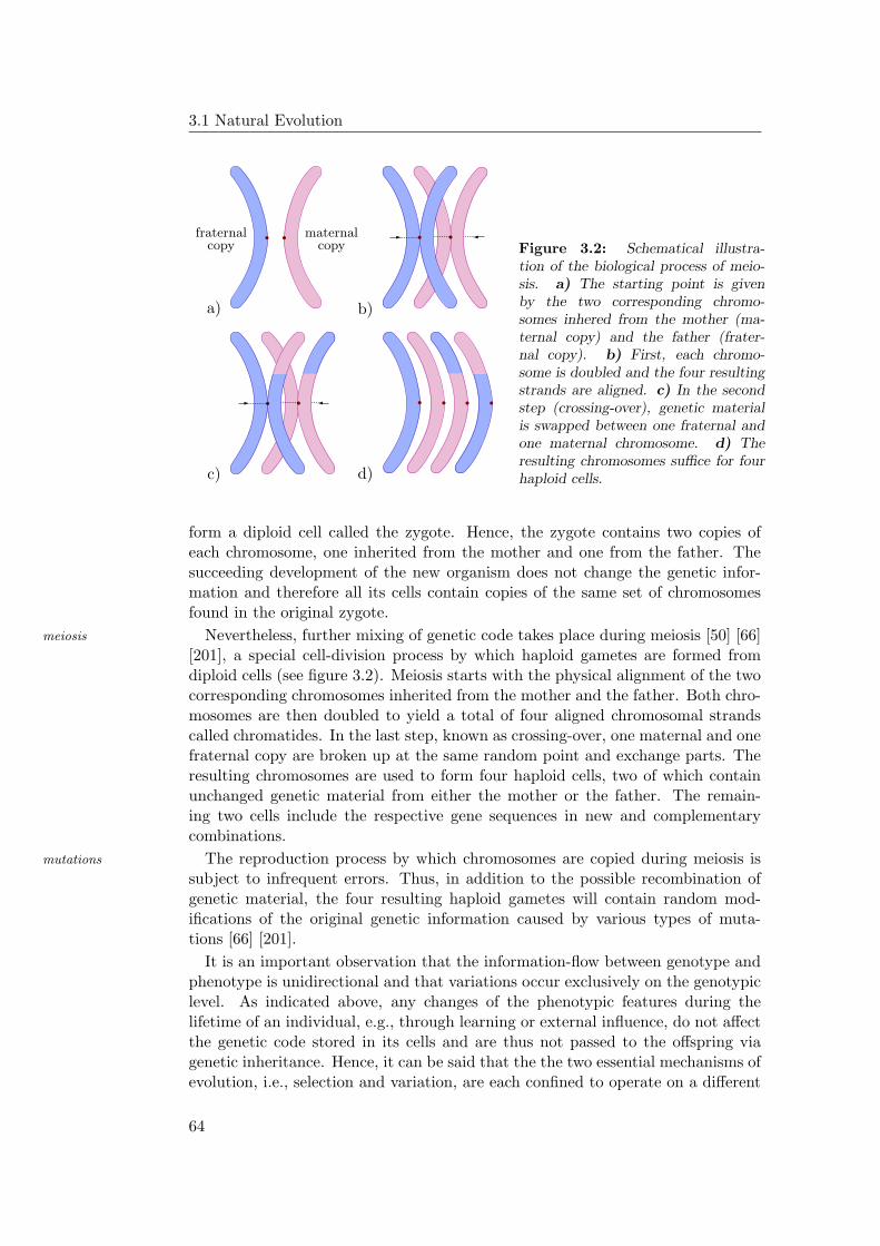
3.1 Natural Evolution
PSfrag replacements
a) b)
c) d)
fraternal maternalcopycopy Figure 3.2: Schematical illustra-
tion of the biological process of meio-sis. a) The starting point is givenby the two corresponding chromo-somes inhered from the mother (ma-ternal copy) and the father (frater-nal copy). b) First, each chromo-some is doubled and the four resultingstrands are aligned. c) In the secondstep (crossing-over), genetic materialis swapped between one fraternal andone maternal chromosome. d) Theresulting chromosomes suffice for fourhaploid cells.
form a diploid cell called the zygote. Hence, the zygote contains two copies ofeach chromosome, one inherited from the mother and one from the father. Thesucceeding development of the new organism does not change the genetic infor-mation and therefore all its cells contain copies of the same set of chromosomesfound in the original zygote.
Nevertheless, further mixing of genetic code takes place during meiosis [50] [66]meiosis
[201], a special cell-division process by which haploid gametes are formed fromdiploid cells (see figure 3.2). Meiosis starts with the physical alignment of the twocorresponding chromosomes inherited from the mother and the father. Both chro-mosomes are then doubled to yield a total of four aligned chromosomal strandscalled chromatides. In the last step, known as crossing-over, one maternal and onefraternal copy are broken up at the same random point and exchange parts. Theresulting chromosomes are used to form four haploid cells, two of which containunchanged genetic material from either the mother or the father. The remain-ing two cells include the respective gene sequences in new and complementarycombinations.
The reproduction process by which chromosomes are copied during meiosis ismutations
subject to infrequent errors. Thus, in addition to the possible recombination ofgenetic material, the four resulting haploid gametes will contain random mod-ifications of the original genetic information caused by various types of muta-tions [66] [201].
It is an important observation that the information-flow between genotype andphenotype is unidirectional and that variations occur exclusively on the genotypiclevel. As indicated above, any changes of the phenotypic features during thelifetime of an individual, e.g., through learning or external influence, do not affectthe genetic code stored in its cells and are thus not passed to the offspring viagenetic inheritance. Hence, it can be said that the the two essential mechanisms ofevolution, i.e., selection and variation, are each confined to operate on a different
64
Evolutionary Algorithms
level. While selection acts solely on the phenotype, all variation processes affectonly the genotype.
3.1.3 Speciation
So far, it has indirectly been assumed that the regarded population consists of inhomogeneouspopulationsindividuals from one single species. Thus, all individuals are biologically compat-
ible in that any two of them can have offspring (subject to the natural sexualconstraints). A given environment will contain individuals from various species.Seen from the perspective of one population, the presence of other species thatcompete for the same resources can be regarded as a special characteristic of theenvironment that contributes an additional aspect to the selective pressure on theindividuals.
In this sense, natural selection can not only be seen to act on single organisms allopatricspeciationbut also on whole species. In nature, this has lead to the adaption of species to
different available ecological niches. New species can develop when individuals ofone species are separated into two populations that do no longer exchange geneticmaterial among them. Most often, this separation is caused by geographical iso-lation (allopatric speciation), and the members of the two populations have tosurvive in different environments, each with its special demands and constraints.The interaction of variation and selection will therefore favor different types ofphenotypic traits within the two populations. Eventually, the differences betweenboth groups will have grown to be such that they are to be regarded as distinctspecies [201].
3.2 Evolutionary Algorithms: An Overview
Evolutionary algorithms apply the principles of natural evolution to the solution population basedoptimizationof optimization problems. Instead of modifying a single instance of the system
to be optimized, they process a whole group, a so-called population, of candidatesolutions that are now referred to as individuals. The performance of each in-dividual is measured by a fitness function which is usually (but not necessarily) fitness function
chosen in a way such that the better the performance of the candidate solution,the higher the fitness value.
An evolutionary algorithm starts with the generation of an initial populationof candidate solutions and the evaluation of their fitness values. Based on thefitness, a selection procedure then determines those individuals of the population parent selection
that are allowed to produce offspring in the form of new candidate solutions. Thereproduction itself is accomplished by applying appropriate variation operators tothe original individuals.
Two types of variation operators can be distinguished: While recombination recombination andmutationacts on two or more individuals to yield one or more new candidate solutions,
mutation operators are applied to single individuals, resulting in one offspring.These operators do not act on the individuals themselves but on suitable repre-sentations, i.e., special data structures that contain all parameters of a candidatesolution that are to be optimized by the algorithm.
65
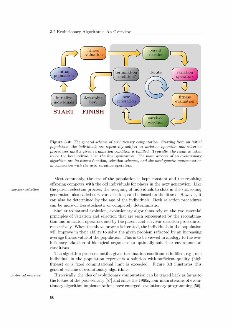
3.2 Evolutionary Algorithms: An Overview
PSfrag replacements
START FINISH
initializeindividuals
initialpopulation
fitness
fitness
evaluation
evaluationparent
selection
selection
variationoperators
survivor
newgeneration
terminationcondition?
determinebest
iterate
Figure 3.3: The general scheme of evolutionary computation. Starting from an initialpopulation, the individuals are repeatedly subject to variation operators and selectionprocedures until a given termination condition is fulfilled. Typically, the result is takento be the best individual in the final generation. The main aspects of an evolutionaryalgorithm are its fitness function, selection schemes, and the used genetic representationin connection with the used variation operators.
Most commonly, the size of the population is kept constant and the resultingoffspring competes with the old individuals for places in the next generation. Likethe parent selection process, the assigning of individuals to slots in the succeedingsurvivor selection
generation, also called survivor selection, can be based on the fitness. However, itcan also be determined by the age of the individuals. Both selection procedurescan be more or less stochastic or completely deterministic.
Similar to natural evolution, evolutionary algorithms rely on the two essentialprinciples of variation and selection that are each represented by the recombina-tion and mutation operators and by the parent and survivor selection procedures,respectively. When the above process is iterated, the individuals in the populationwill improve in their ability to solve the given problem reflected by an increasingaverage fitness value of the population. This is to be viewed in analogy to the evo-lutionary adaption of biological organisms to optimally suit their environmentalconditions.
The algorithm proceeds until a given termination condition is fulfilled, e.g., oneindividual in the population represents a solution with sufficient quality (highfitness) or a fixed computational limit is exceeded. Figure 3.3 illustrates thisgeneral scheme of evolutionary algorithms.
Historically, the idea of evolutionary computation can be traced back as far as tohistorical overview
the forties of the past century [57] and since the 1960s, four main streams of evolu-tionary algorithm implementations have emerged: evolutionary programming [56],
66
Evolutionary Algorithms
genetic algorithms [46] [71], evolution strategies [9] and, more recently, geneticprogramming [121]. These approaches differ mainly in the types of optimizationproblems they are commonly applied to as well as in the specific implementationsof the single components shown in figure 3.3.
While evolution strategies and genetic algorithms are typically employed for main fields
parameter optimization problems, evolutionary programming has initially beendeveloped to simulate evolution as a learning process with the aim of generatingartificial intelligence. Genetic programming, finally, is to be positioned in the fieldof machine learning. Apart from that, the distinction between these approaches aswell as their respective traditional conventions and notations merely have historicalorigins. Today, they are all seen as subareas of the whole field of evolutionarycomputation [140] [50]. In the spirit of this generalized view, the succeedingsections shall discuss the individual parts of an evolutionary algorithm in moredetail but on a generic level. Explicit realizations will be introduced in section 3.4.
3.2.1 The Main Constituents of an Evolutionary Algorithm
The following main components have to be specified in order to completely definea particular evolutionary algorithm:
- The representation, also denoted as the genetic coding, defines the data struc-ture that contains the information about all parameters of a candidate so-lution that are to be optimized by the algorithm.
- The variation operators determine the way in which recombination and mu-tation are implemented on the basis of the above representation.
- The fitness function provides a measure for the quality of an individual. Itsvalue is the actual quantity that is optimized by the algorithm.
- The parent selection and survivor selection procedures operate on the wholepopulation in that they transform the old generation of individuals to a newone.
The Representation
An evolutionary algorithm is desired to eventually yield a system that representsthe solution to a given problem. In terms of the simulated evolution, this systemand any candidate solutions evaluated during the search process can be regardedas the phenotypes. In contrast, the objects that are directly processed by thealgorithm are the corresponding genotypes. Each genotype, henceforth also calledgenome, is an instance of a data structure that summarizes all variable parametersof the respective candidate solution. The organization of this data structure as wellas the respective mapping from the phenotype to the genotype are both commonlydenoted as the (genetic) representation.
As an example, consider the case of a neural network with a fixed architecture example: networkweightspossessing n synapses. Here, each phenotype is completely defined by specifying
all synaptic weight values wi, 1 ≤ i ≤ n. Thus, a simple choice of genotype is
67
3.2 Evolutionary Algorithms: An Overview
a vector g = (g1, . . . , gn) ∈ Rn of real numbers that each represent one weightwi = gi. However, another valid representation would be to code all weight valuesin binary form with a resolution r and arrange them to a linear binary strings ∈ 0, 1(r·n).
The entirety of all different genomes that can possibly be realized by a givengenotype space
representation forms the genotype space G. In principle, this space is distinct fromthe phenotype space P that consists of all candidate solutions to the investigatedproblem. For the above examples, the mapping between them is straight forward.Depending on the problem and the chosen representation, the relation betweenthe genotype space and the phenotype space can be relatively complex [117] [121].
It is important to note that an evolutionary algorithm performs its search in thegenotype space. Hence, when designing the representation for a given optimizationtask, it has to be ensured that the desired solution can be defined by a valid genomeof the chosen kind, i.e., that there exists a point in the genotype space that codesan acceptable solution to the problem. Since for most realistic applications, thispoint will not be known in advance, the selection of a suitable representationoften has to be based on reasonable assumptions about the general nature of thesolution.
The Variation Operators
During evolution, new individuals are created from the old ones by applying ad-equate variation operators to the respective genotypes. In other words, in searchof the optimal solution, the algorithm progresses through the genotype space byvirtue of these operators. It is crucial for the success of the optimization processtraversing the
genotype space that the used genetic representation in connection with the corresponding varia-tion operators suit the investigated problem. More precisely, both are to be chosensuch that starting from a random initial population of points in the genotype spaceand iteratively applying recombination and mutation, the optimal solution can beexpected to be reached within a finite number of steps with a sufficiently largeprobability. Again, this would in principle require the exact knowledge of thesolution. In practice, the feasibility of a set of variation operators for a given taskcan only approximately be estimated in advance.
Recombination Recombination operators are also called crossover operators.They merge the information stored in the genotypes of two individuals, denotedas the parents, to yield one or two new genomes, named the offspring. This isusually achieved by randomly breaking up each of the original genomes into twoor more parts and exchanging some of the resulting segments among them.
The use of a crossover operator is inspired by the crossing-over that appearsbiological motivation
during meiosis in biological systems1 (see section 3.1.2). While its purpose is topracticability recombine advantageous features of the parents to form potentially improved new
individuals, the application of crossover is not guaranteed to be beneficial. Thequality of a specific implementation of the recombination process can be measured
1Note however, that while the crossover operator acts during reproduction, the biologicalcrossing-over occurs earlier during the development of gametes.
68
Evolutionary Algorithms
by the average probability by which it produces individuals that have equal orbetter fitness than their parents.
For a crossover operator to maximize this probability, its design has to account crossover andgenetic codingfor the structure of the chosen representation and vice versa. In particular, it is
the crossover operator that defines the smallest functional unit of the genome asbeing the minimum part that is not broken up during the segmentation step. Inanalogy to the biological original, this basic unit is called a gene and the differentvalues that it can assume are referred to as alleles.
Regarding the two examples above, the gene would in the first case be one realnumber gi and the vectors of the two parents would only be cut apart betweenany two components gi and gi+1. In the second encoding, a gene could correspondto a single binary digit of the string s. Note that in the first example, the mixingprocess merely recombines the weights of the two parent networks. The secondapproach, on the other hand, can produce new weight values by cutting apart andrecombining sequences of the original strings that in fact formed a translationalunit by coding one weight. Such a behavior might be beneficial, but due to thebinary nature of the encoding, the outcome of this recombination process is highlyunpredictable.
While this already provides a first insight into the close relation between the re-combination operator and the chosen genetic representation, a thorough discussionof this topic shall be deferred to sections 3.4.4 and 3.5.
Mutation A Mutation operator acts on single genotypes by applying a series single genemutationof stochastic modifications. Often, it affects each gene separately by randomly
changing the respective allele to a new value. Mutation operators that act onwhole groups of genes simultaneously are conceivable as well but in any case, thechanges are desired to be stochastic and unbiased and are applied with a given lowprobability. Returning to the examples of the real valued vector and the binarystring, a simple mutation operator could in the first case replace single componentswith new random numbers and in the second case randomly flip single bits.
The presence of mutations is vital for the performance of an evolutionary algo- mutation anddiversityrithm since they support the genetic diversity within the population. This way,
they balance the effects of selection that tend to reduce this diversity by repeatedlydiscarding the genetic material of individuals with low fitness. Viewed in terms ofthe search space, mutations ensure that this space is connected. For theoreticalconvergence proofs of evolutionary algorithms, it is often required that any allelecan be mutated into any other with nonzero probability [173] [174].
On the other hand, too frequent or too violent modifications of the genetic adjusting mutation
information in the population run the risk of impeding evolutionary progress bydestroying advantageous combinations of alleles. The correct adjustment of themutation rate in connection with the appropriate selective pressure is one of themain issues when tuning the parameters of an evolutionary algorithm.
69
3.2 Evolutionary Algorithms: An Overview
The Fitness Function
The fitness function has to be chosen as to provide a fair measure for the qualityof the candidate solutions that are evaluated during the search process. Since theselection procedures described below are based primarily on the fitness values ofthe individuals, the evolutionary algorithm can be seen as to optimize the fitness.At the same time, the desired result of the search is a system that solves the givenproblem.
In this sense, it is evident that the fitness function has to be designed suchsmooth fitnessmeasures that it assumes its maximum value on the optimal solution(s)2. Furthermore, it is
preferred to be as smooth as possible, i.e., to reward even small improvements inthe quality of an individual with a measurable increase in fitness. If two or moreindividuals can exhibit the same fitness value although one is actually closer tothe desired solution than the others, the efficiency of the selection procedure iscompromised.
Finally, it is understood that a worse individual should never be assigned ahigher fitness value than a better one. But it turns out that depending on thetask at hand, it is not necessarily straight-forward to formulate a simple fitnessfunction that is guaranteed to do so (see section 8.3.3).
The Selection Schemes
Given a population of individuals with known fitness values, it is the purpose ofparent selection
the parent selection scheme to chose some members of the population that will beused to create offspring: New candidate solutions that are potentially accepted forthe next generation. Usually, this is selection is probabilistic and individuals withhigher fitness stand a better chance to be selected than those with lower fitness.
After the desired number of offspring have been created and their fitness valuessurvivor selection
have been evaluated, the survivor selection process determines those individualsamong the old and the new candidate solutions that are to form the new gener-ation. Unlike the parent selection scheme, survivor selection can in addition tothe fitness values of the individuals also consider their age, such that offspring arepreferred over the parents.
In practice, many implementations of evolutionary algorithms confine them-selection indifferent fields selves to only use either of the two selection processes. For example, genetic
algorithms traditionally apply only parent selection and fill the new populationcompletely with offspring3 [46] [71]. Evolution strategies chose the parents ran-domly and regardless of their fitness. Also, they build the new generation fromthe offspring (and in some case the old population) in an entirely deterministicway [9] [50].
Selection is the pushing force behind the improvement of the individuals in theadjusting selection
population and as such, it has to favor good individuals over inferior ones. On the
2It is straight forward to reformulate all statements of this section to suit a fitness functionthat monotonically decreases with the quality of the individual. Obviously, this function is to beminimized rather than maximized.
3In fact, this can also be seen as a completely deterministic survivor selection that discardsall individuals with an age greater than one generation.
70
Evolutionary Algorithms
other hand, the exploration of new solutions depends on the diversity within thepopulation. Even bad individuals might partially comprise of allelic combinationsthat are beneficial for the solution of the problem. Thus, in order to maintain asufficient genetic variance, the selection process is best not made too rigorous. Abrief overview of various selection schemes is given in section 3.4.1.
3.3 General Features of Evolutionary Algorithms
The preceeding section has outlined the basic methodology of evolutionary com-putation. Before several specific implementations of the main components will beintroduced in 3.4, this section shall summarize some general properties of evolu-tionary algorithms that already emerge as a direct consequence of their underlyingprinciples. Potential difficulties of the evolutionary approach will be discussed andextensions to the basic concepts of evolutionary optimization will be introducedthat can compensate for some of these deficiencies.
As a general characterization, evolutionary algorithms can be sorted into the generalcharacterizationcategory of generate-and-test approaches [50] but are distinct among the algo-
rithms of this family under several aspects. First, they are population based.Second, they are stochastic and third, they often rely on the recombination ofcandidate solutions to form new ones. Especially the first two features have im-portant consequences for the progression of the search process.
3.3.1 Evolutionary Algorithms as Global optimizers
The use of a population of individuals effectively enables an evolutionary algorithmto probe the search space at multiple different points simultaneously. Althoughinitially, the candidate solutions are randomly spread across the whole space, latergenerations will by virtue of the selection process and the variation operators beclustered within regions of high fitness. It is a common observation that thepopulation will eventually converge towards a single located domain and slowlyapproximate the optimal solution within this area. These two distinct phases of exploration and
exploitationthe evolution process are often denoted as exploration — finding regions of highfitness in the search space — and exploitation, i.e., the concentration of the searchin the vicinity of the best encountered solutions [50].
The exploration phase greatly benefits from the diversity in the population. local maximaand diversityMaintaining a whole group of different candidate solutions potentially increases the
probability of the algorithm to locate the global maximum of the fitness function.Hence, it reduces the risk of getting trapped in local maxima like it is a commonproblem of gradient ascent approaches (section 2.1.3) or even other stochasticsearch algorithms (see section 4.3.1).
On the other hand, once the algorithm has reached the exploitation phase, toostrong variance interferes with an efficient approximation of the best solution inthe current neighborhood of the population. Therefore, evolutionary optimizationis often discussed in terms of a trade-off between exploration and exploitation.
The eventual convergence of the whole population around one optimum is a genetic drift
phenomenon commonly known as genetic drift. In principle, it is a desirable
71
3.3 General Features of Evolutionary Algorithms
feature that the population will after several generations be clustered in regions ofhigh fitness. However, in the case of multimodal tasks that exhibit more than oneoptimum of the fitness function and where only one of these maxima is a globalone, the genetic drift can cause problems. If the diversity of the population is lostpremature
convergence too early during the search process, the algorithm might get stuck in local optimaand thus miss the global optimum. This unfavorable behavior is usually referredto as premature convergence.
Against the background of these considerations, the optimal adjustment of theselection pressure and variance parameters of an evolutionary algorithm can beidentified with the problem of balancing the efficiencies of the exploration andexploitation phases. Ultimately, the chosen parameters are desired to avoid pre-mature convergence and at the same time allow for an efficient approximation ofthe global optimum during the exploitation phase.
3.3.2 A Modular View of Evolutionary Algorithms
Since the fitness function has to quantify the ability of an individual to solve thegiven problem, it is clearly specific to the currently investigated task. But even ifautonomy of the
fitness function its formulation might be difficult (see section 8.3.3), the fitness function dependsonly on the desired behavior of the optimized system or on specific requirements tothe latter. In other words, the fitness function is defined on the phenotype space.As such, it is independent of the used genetic representation and the correspondingvariation operators.
In turn, the explicit form of the genotype and the applied genetic operatorsautonomy of thegenetic representationand operators
can be chosen without regard to the details of the fitness evaluation. Rather, theprogress of the evolution depends on how far the coding and the operators paytribute to the structural and organizational features of the system to be optimized.
The selection process, finally, operates solely on the basis of the fitness of theautonomy of theselection schemes individuals. It is neither concerned about how these values have been obtained or
about the way by which new offspring is created. In so far, the selection schemeconstitutes the part of an evolutionary algorithm that is least problem specific.
From this point of view, the three main components of an evolutionary algo-rithm, i.e., the fitness calculation, the selection scheme and the genetic representa-tion in connection with the variation operators, are inherently independent. Thedetailed realization of each part can be chosen without necessarily affecting theimplementation of the others. Each component can easily be replaced by anotherversion in order to test the feasibility of different algorithm setups for a given task.
3.3.3 Evolutionary Algorithms as Model-Free Heuristics
The above considerations already indicate that specifics of the investigated prob-lem become manifest within the formulation of a corresponding evolutionary algo-rithm primarily in the form of the fitness function and possibly the design of thegenetic coding. The former is undoubtedly peculiar to the particular task at hand.The latter is preferably chosen as to account for the structural characteristics ofthe optimized system in order to increase the probability of the recombination
72
Evolutionary Algorithms
operator to produce improved offspring (see also sections 3.5 and 4.1.2).
However, many implementations of evolutionary algorithms, like evolution strate-gies, do not use any recombination operator and rely solely on mutation and selec-tion [9]. Also, recombination can contribute to the variance in the population andthereby benefit the exploration of the search space even if it is not optimized to-wards producing good offspring. Finally, the knowledge of how to best arrange thegenetic representation and to implement the recombination process is often simplynot available. This does not prevent the evolutionary approach — with or withoutrecombination — from being successfully applied to a multitude of optimizationproblems (e.g., [19] [31]).
Thus, aside from an adequate problem-dependent fitness function and a specifi- independence of thetaskcation of the number and range of the variable parameters, no further information
about the optimized system is required. Neither does an evolutionary algorithmrely on any model of how the candidate solutions actually work, nor does it dependon any derivatives of the performance measure with respect to the parameters.Therefore, evolutionary algorithms are often denoted as model-free, or black-box,approaches. As such they can easily be applied to a wide range of optimizationtasks, even to those for which no other optimization strategy can readily be for-mulated. In fact, it is the property of being model-free that constitutes the main evolving hardware
neural networksmotivation for using evolutionary algorithms to train hardware neural networks(see 2.4.5). The evolution of artificial neural networks will be the topic of chapter 4which will also discuss some alternative model-free optimization algorithms.
Heuristics and the No Free Lunch Theorem
Despite the potential problem of premature convergence, the principles of evolu-tionary computation prove to be of great value for the solution of optimizationproblems in practice. Nevertheless, there are some issues concerning evolutionaryalgorithms that shall not remain unmentioned.
The evolutionary approach is based on simple and transparent ideas that are evolutionarycomputation as aheuristic
inspired by natural evolution. Regarding the efficiency of the biological original,evolutionary algorithms are expected to provide feasible means for the solutionof optimization problems. But it is important to note that apart from someselected artificial tasks and specific implementations of the algorithm [174], itcannot be proven that an evolutionary algorithm is guaranteed to find a suitablesolution of sufficient quality within a reasonable time [50] [102]. For this reason,the evolutionary approach is often referred to as a heuristic. The term heuristic isnot unambiguously defined but can be understood as to denote a technique for thedesign of efficient optimization algorithms “for which no one is able to guaranteeat once the efficiency and the quality of the computed feasible solutions” (takenfrom Hromkovic, 2004 [102]).
It is a common property of heuristics to be robust in the sense that they can heuristics androbustnessbe applied to a large variety of optimization tasks, even if these problems differ
significantly in their combinatorial structures. In the 1980s, it has been antici-pated that evolutionary algorithms outperform other techniques on a wide rangeof problems [71] and that they are only beaten by dedicated algorithms that are
73
3.3 General Features of Evolutionary Algorithms
specially designed for particular tasks. Recent studies, however, lead to a cor-rection of this view. In simple terms, the famous No Free Lunch theorem (NFL)the No Free Lunch
theorem by Wolpert and Macready [228] states that when averaged over the space of allpossible optimization problems, all nonrevisiting, model-free algorithms will showthe same performance. The term nonrevisiting refers to the demand that the algo-rithm does not generate and test the same point in the search space twice. This isnot initially a property of evolutionary algorithms but can easily be incorporated.
The conclusions drawn from this theorem are twofold. First, if any algorithmperforms better than others on a set of problems, it pays for this by performingworse on other tasks. Second, for a given problem, it is possible to break thelimitations of the NFL by abandoning the model-free nature of the algorithm,hence, by incorporating problem specific knowledge.
It can be argued that by designing an appropriate genetic coding and corre-practicability ofevolutionaryalgorithms
sponding operators, task specific information is automatically incorporated intothe algorithm. Furthermore, evolutionary algorithms have repeatedly demon-strated their ability to find good solutions for many problems that could otherwisenot easily be solved. In practice, this is most often sufficient, even if the found sys-tem cannot be proven to represent the achievable optimum or if other algorithmscan theoretically perform better. In so far, being a heuristic and as such beingtheoretically limited by the NFL does not necessarily pose severe restrictions tothe applicability of evolutionary algorithms.
3.3.4 Extensions to the Basic Concept
Several mechanisms are present in nature that support the exploration of differ-ent environmental niches and thus lead to the development of distinct species.When tackling multi-modal problems with evolutionary algorithms, it is equallydesirable to explore various different regions of the search space in order to avoidpremature convergence towards a suboptimal solution. It is reasonable to assumethat the efficiency of the exploration phase could be improved if the basic conceptof evolutionary computation is extended by some of the mechanisms that alsopromote speciation in nature. This has in fact been done in various ways.
- In the so-called island model algorithms (also coarse-grain parallel or simplyisland modelalgorithms parallel evolutionary algorithms), multiple separated populations of individ-
uals are evolved in parallel. After a fixed number of generations denotedas an epoch, several individuals from each population are exchanged withthe neighboring populations (migration) [38] [39] [128] [161] [172] [204]. Thetopological arrangement of the populations is usually chosen as to suit thearchitecture of the parallel system on which the algorithm is implemented.Most often, it is a ring, torus or hypercube.
- Diffusion model algorithms (also fine-grain parallel, distributed or cellulardiffusion modelalgorithms evolutionary algorithms) divide the population into smaller, partly over-
lapping subpopulations (demes) that are distributed in an imaginary al-gorithmic space. Selection and mating only occur within the subpopula-tions [72] [103] [132] [150] [220] [222]. A simple exemplary realization of this
74
Evolutionary Algorithms
concept is to distribute all individuals on a (toroidal) grid such that eachindividual can only be recombined — and has to compete with — individualson neighboring grid points.
- The above approaches both aim to simulate restrictions on the mating of distance metrics andmating constrictionsindividuals like they arise from geographical separation in nature. Another
idea is to introduce an appropriate distance metric in either the genotypeor phenotype space that quantifies some kind of relationship or similaritybetween individuals. Those pairs of candidate solutions with a sufficientlysmall mutual distance are then regarded as belonging to the same speciesand are allowed to have offspring. Otherwise, the individuals are consid-ered as biologically incompatible and cannot be recombined. Various typesof distance metric have been introduced [45] [194]. The distance can bebased on features of the individuals (resp. their genotypes), but the mem-bership to a given species can also be assigned randomly and made subjectto recombination and mutation [196].
- Instead of using the distance between individuals to determine appropriate distance metrics andbiased selectionrestrictions on potential mating pairs, the similarity concept can alterna-
tively be utilized to bias the survivor selection process. In fitness sharing [70],fitness sharing
the fitness of each individual is normalized by the number of other candidatesolutions that fall within a specified metric distance. This effectively reducesthe fitness for whole groups of individuals that are too similar and — sincethe selection process favors candidate solutions with high fitness — can beassumed to support the diversity within the population.
The crowding algorithm [46] [131] incorporates a special replacement selec- crowding
tion scheme that favors offspring to preferably replace those original mem-bers of the population to which it exhibits a close similarity. Thereby, initialsubpopulations that inhibit different niches of the search space are likely tobe preserved. However, their size does not depend on their fitness as it isthe case for fitness sharing.
All of the above concepts have proven to constitute fruitful extensions to thebasic evolutionary algorithm framework. Nevertheless, they also introduce addi-tional parameters that require reasonable adjustment. A detailed investigation ofthese approaches, their benefits and problems cannot be provided here. The in-terested reader is referred to either the original publications or the overview givenin [50]. Instead, it shall be discussed in how far the introduction of the aboveconcepts compromises the independence of the main components of evolutionaryalgorithms that has been claimed in section 3.3.2.
Do Extensions Challenge Modularity ?
The first two of the above extensions primarily involve a specific organizationof the population. Within the parallel populations of the island model or thesubpopulations of the diffusion algorithm, the applied selection schemes can beequal to those used in common evolutionary algorithms. Moreover, the genetic
75
3.4 Evolutionary Algorithm Implementations
representation, the variance operators, and the fitness function are not affectedby the adoption of these population models. In so far, mating restrictions thatarise due to the simulation of geographical separation merely represent a specialaddition to the parent selection process and the population management.
Similar to the case of the fitness function, any selection process that takes intoautonomy of thedistance metric account the distance between two individuals needs not to be concerned about how
this quantity is obtained. Likewise, the formulation of the fitness function is notat all affected by the presence of a similarity measure. Calculating the similaritybetween two individuals can therefore be seen as an additional component of theevolutionary algorithm that is independent of the fitness function and the selectionscheme.
The distance metrics introduced by the last two approaches of the above listdistance metrics andgenetic codings are either based on features of the individuals or on special tags that are encoded
within their genomes. Hence in both cases, the similarity between two individualscan be inferred from their genotypes, and the reasonable choice of a distance metricis closely linked with the used genetic coding. Designing a genetic representationin connection with corresponding variance operators could thus be extended toalso incorporate the definition of an adequate similarity measure. Instead of beingconsidered as a new independent component, the similarity function can then beregarded as an additional aspect of the genetic representation.
In summary, it is concluded that the discussed extensions give rise to additionalpreserved modularity
demands on the implementations of the main components of an evolutionary algo-rithm. Apart from that, it persists that the detailed realization of each componentis encapsulated from the remaining parts by simple and well-defined interfaces:The genetic representation has to provide adequate variation operators and pos-sibly a reasonable distance measure. The fitness function has to assign a fitnessvalue to each individual that quantifies its performance on the given task. On thebasis of the fitness and the similarity between individuals, the selection schemefinally has to form mating pairs and select candidate solutions for the next gener-ation. It is worth repeating that as long as all components meet their respectiverequirements, their detailed realizations remain unaffected by the implementa-tions of the others. This important feature will turn out to be of considerableadvantage for the design of flexible evolutionary algorithm software frameworks(see section 7.4).
3.4 Evolutionary Algorithm Implementations
This section introduces the most widespread implementations of the different evo-lutionary algorithm components. The only exception is the fitness function: Sur-veying common realizations of the latter would be infeasible and of only limited useas it is largely specific to the particular task at hand. Furthermore, the presentedimplementations of the genetic coding and the corresponding variation operatorsare confined to those suited for parameter optimization problems. Representationsand operators that are typical for the field of genetic programming are deliberatelyexcluded since this area is not directly related to the work presented in this thesis.
76
Evolutionary Algorithms
For an exhaustive overview of evolutionary algorithm implementations that alsoaccounts for genetic programming see [50].
3.4.1 Selection Schemes
The differentiated survival of individuals based on their fitness is one of the cor-nerstones of evolutionary computation. Two basic models can be distinguished ofhow this competitive element of population management is realized. According tothe generational approach, each iteration starts with a population of µ individuals generational
algorithmsfrom which a fixed number of parents is selected to form a mating pool. Note thatdepending on the applied selection scheme, this mating pool can contain multiplecopies of the same individual. In any case, its members are used to create µ off-spring that completely replace the old individuals and form the next generation.Implementations that follow such a complete replacement scheme are commonlydenoted as generational evolutionary algorithms.
In contrast, steady-state algorithms only change parts of the population in each steady-statealgorithmsstep by substituting λ < µ individuals with a corresponding number of offspring.
The fraction of the population that is replaced during one iteration is called thegenerational gap and is given by λ/µ.
While both approaches are equally often encountered in classical genetic algo-rithms, the fields of genetic programming and evolution strategies usually followthe generational scheme and the area of evolutionary programming traditionallyapplies the steady-state model. Nevertheless, both strategies agree in that thecorresponding parent and/or survivor selection procedures operate on the basisof an individual’s fitness. In the following, it shall be assumed that the fitnessincreases with the quality of the candidate solution and is always nonnegative.
Fitness Proportional Selection
The selection scheme originally applied in classical genetic algorithms is the so- mechanism
called fitness proportionate selection [71]. It is a probabilistic procedure in so faras each individual is assigned a nonzero probability to be chosen. Given the fitnessfi of the individual with index i, its selection probability pi is computed accordingto
pi =fi
µ∑j=1
fj
, ∀ 1 ≤ i ≤ µ (3.1)
where µ is the population size. Thus, pi depends on the absolute fitness valueof the individual compared to the total cumulated fitness of the population. Asrequired, the hereby defined probabilities readily obey
µ∑
i=1
pi = 1. (3.2)
Fitness proportional selection suffers from several problems. First, individuals challenges
with outstanding fitness tend to take over the whole population very quickly which
77
3.4 Evolutionary Algorithm Implementations
leads to premature convergence. Second, in later generations of an evolution,the fitness values of all population members usually have become large and arelikely to be close together. Hence, there will only be marginal differences betweenthe selection probabilities of the single individuals and thus hardly any selectionpressure left. Third, the same phenomenon occurs when the fitness function istransposed, i.e., is modified by the addition of a sufficiently large value. The lasttwo issues are closely related and are consequences of the fact that the selectionprobabilities are calculated on the basis of the absolute fitness values.
Ranking Selection
The drawbacks of fitness proportionate selection can be overcome if the selectionprobability of an individual is not based on the absolute value of its fitness butrather on its rank in the current generation [10] [77] [221]. Let the µ individuals inthe population be ordered such that the one with the the highest fitness is assignedrank µ and the one with the lowest fitness is allocated to rank 1. In linear ranking,linear ranking
the selection probability is a linear function of the rank i given by
pi =1
µ
(s− + (s+ − s−)
i − 1
µ − 1
), ∀ 1 ≤ i ≤ µ (3.3)
where s−/µ and s+/µ are the respective probabilities for the worst and the bestindividual to be selected [21]. In order to fulfill the normalization condition 3.2,it is required that s− ≥ 0 and s+ = 2 − s−. This poses a rigid restriction on theselection strength, i.e., the difference in selection probability between the worstand the best individual.
Exponential ranking selection [21] does not suffer from these limitations. Here,exponential ranking
the selection probabilities are calculated on the basis of the rank i according to
pi =cµ−i
µ∑j=1
cµ−j
, ∀ 1 ≤ i ≤ µ (3.4)
using the adjustable parameter c ∈ (0, 1). If c approaches 1, the selection proba-bilities of the individuals all converge to a common value and the selective pressureweakens. For c close to 0, the exponential character of equation 3.4 becomes morepronounced and individuals with higher ranks are more and more favored overthose at lower ranks.
A special form of ranking selection is the so-called truncation selection thattruncation selection
fixes a threshold T and only assigns a nonzero selection probability to the bestT individuals in the population. While worse individuals cannot be selected atall, the first T members usually stand the same chance 1/T to be chosen. Thedeterministic variant of this approach simply defines the best λ candidate solutionsto represent the outcome of the selection procedure.
78
Evolutionary Algorithms
Tournament Selection
Instead of calculating and sampling a probability distribution defined on the fitness mechanism
values of the whole population, tournament selection solely relies on an orderingrelation that can rank any two individuals. The selection is performed in twosteps. First, τ members of the population are chosen in a completely randommanner. This intermediate group is referred to as the tournament. Second, theindividual with the highest fitness among the τ chosen competitors is taken tobe the final selection. Hence, while the composition of the tournament is entirelyrandom, the choice of the winner is deterministic.
In order to select a pool of λ individuals, λ independent tournament selec- adjustable selectionpressuretions have to be performed. Although the effective selection probability for each
individual depends on its rank, the tournament scheme can be realized withoutsorting the entire population. Furthermore, the selective pressure can convenientlybe adjusted by varying the tournament size τ . With increasing τ , the selectionprobability for individuals with low fitness decreases.
The selection pressure also depends on whether the constituents of the tour-nament are chosen from the initial population with or without replacement, i.e.,whether an individual can appear in the tournament more than once. Especiallythe worst individual of the population only exhibits a non-zero probability to wina tournament, if it actually has to compete solely with copies of itself.
It can be shown that a tournament selection with tournament size 2 is effectivelyequivalent to a linear ranking selection [21]. Since it is considerably simple andeasy to implement — and due to the direct control of the selective pressure viathe tournament size τ — this selection scheme is one of the most widely used forevolutionary algorithms.
Survivor Selection Specialties
In principle, the selection procedures discussed so far are all equally well suited forboth, parent and survivor selection. Traditionally, however, they originate fromthe field of genetic algorithms where they are only applied to the parent selectionprocess. It has been said before that it is common in this kind of algorithm toreplace the whole initial generation by its offspring. In a steady-state algorithm, onthe other hand, the number of offspring λ is lower than the size of the population µ.Those individuals that will have to make room for the offspring can be selectedaccording to any of the above schemes if it is based not on the fitness or rank ofan individual but rather on the respective inverse.
A popular choice for this kind of replacement selection is the deterministic deterministicreplacementvariant of the truncation selection, i.e., the worst λ members of the old population
are chosen to be substituted by the offspring. But even if the replacement of theelitismold individuals is stochastic, it is most often desirable to prevent the best member
of the former population from being discarded. It is therefore common to excludethe best individual from the replacement selection process. This is referred to aselitism and can be generalized to a preservation of the best nel individuals.
An alternative realization of the survivor selection process is to apply one of the
79
3.4 Evolutionary Algorithm Implementations
introduced selection schemes unmodified but to the whole group of the µ parentsplus the λ offspring.
3.4.2 Genetic Representations
As stated at the beginning of this section, it will be assumed in the following thatcodings for parameteroptimization tasks the task at hand is a parameter optimization problem. In general, the parameters
can be binary (Boolean), nominal (i.e., they can assume one of a finite set ofpossible values), integer-valued, or continuous (e.g., real numbers). If the genesdirectly translate to characteristics of the phenotype, the coding is called a directencoding. In an indirect encoding, the genes rather correspond to the parametersof some kind of building rule according to which a phenotype is constructed4.The two examples for the coding of neural network weights given in section 3.2.1represent direct encoding schemes. Some indirect encoding methods for neuralnetworks will be introduced in section 4.2.2.
Evolutionary algorithms are commonly implemented on digital computers. Thisrepresentations ondigital systems suggests at least three basic ways in which parameters can conveniently be coded
within a genome: In a binary representation, by integer values or in the formof floating point variables (which shall for simplicity be regarded as equivalentto real numbers). While in a digital system, all of the above representations areultimately stored in binary form at the lowest level, the approaches rather differin what is regarded as a complete gene, i.e., an indivisible basic constituent of theabstract genome (see section 3.2.1).
Binary Representation
The binary coding, besides obviously being an adequate choice for Boolean at-tributes, can also be used for nominal, integer-valued and quasi-continuous pa-rameters. Historically, genetic algorithms have often incorporated a binary repre-sentation regardless of the investigated problem and the nature of its free variables.In its simplest variant, the single genes are arranged to form a linear bit stringthat represents the entire genome.
When numbers are coded through binary n-bit integers, the single bits arebinary codednumerical attributes assigned different significances. This gives rise to the well-known phenomenon
that the probability to change a given value x to any other value y by a randomflipping of bits is not necessarily equal for all possible y’s. For example, changingknown problems
a 15 (01111) into a 14 (01110) requires the modification of only one bit. But inorder to yield a 16 (10000), it is in fact necessary to flip every single position.When evolving nominal, integer or real-valued parameters, this peculiarity of thecanonical binary coding can cause an unwanted and disadvantageous bias to thevariation operators, particularly mutation.
This issue can be circumvented by applying other, more appropriate binarycoding schemes [50]. In general, however, it is not advisable to use a binary
4Note that by using an adequate indirect encoding, it can be possible to map specific prob-lems to a simple parameter optimization task that would normally exhibit a more complicatedcombinatorial structure
80
Evolutionary Algorithms
representation to code nominal, integer-valued or real parameters at all. Instead,a corresponding integer or floating-point encoding should be chosen.
Integer and Floating Point Representations
The implementation of integer or floating-point representations is straight forward.The single genes of the genome are arranged to form a corresponding vector ofintegers or real numbers. As each value represents a complete gene, its integrityunder crossover is warranted. Furthermore, mutation operators will treat thenumbers as a whole and not just operate on the single bits of their representationat a lower level (see section 3.4.3).
The range of possible alleles will be limited in practice. In integer representa-tions, a gene can usually assume one of a finite set of values L, L+1, . . . , U−1, Ulying between a lower bound L and an upper bound U . Correspondingly, a floating-point gene is confined to a closed and connected interval [L, U ]. Note that in thelatter case, the number of possible allele values in principle remains infinite and isonly limited by the precision of floating-point numbers on the used digital system.
3.4.3 Mutation Operators
In the case of parameter optimization tasks, the most widespread mutation op-erators all affect individual genes separately. The old value of the gene is either uniform and
nonuniform mutationreplaced by a new one that is in no way correlated with the original, or it ismodified by a small amount. The first procedure is called random resetting oruniform mutation, the second approach is sometimes denoted as nonuniform orcreep mutation [50].
It is common to define a mutation probability ρm for each applied operator such mutation rate
that it is individually decided for each gene whether it is to be modified or not.In this scenario, the eventual number of genes that are changed is not decided inadvance but depends on the generated random numbers. Alternatively, if ng isthe number of genes in the genome, ρm ·ng can be interpreted as the fixed numberof genes to be mutated. An according set of genes is then picked randomly.
For most practical applications, the mutation rate is in the order of severalpercent and thus ρm ¿ 1. Therefore, the required number of random values forthe second strategy is considerably lower than for the first approach. This can beadvantageous when the generation of random numbers is costly and the size ng ofthe genome is large.
Uniform Mutation
In binary representations, random resetting assumes the form of simple bit-flipping, binary codings
i.e., the affected gene changes its value from 1 to 0 or vice versa. This is thepredominant mutation operator used in classical genetic algorithms with binarycodings.
For integer-coded genes, the original allele is replaced by a new value randomly integer codings
chosen from the entire set of allowed numbers. The choice is uniform in thatthe possible values are each assigned the same probability to be selected. Thus,
81
3.4 Evolutionary Algorithm Implementations
since the number of permissible alleles is finite, the gene stands a non-zero chanceto remain unchanged even if it is mutated. Especially for attributes with onlyfew alternative allele values, this can have measurable influence on the effectivemutation rate and it might be necessary to ensure that the new value is in factdifferent from the original.
In the case of floating-point genes, the new value is chosen uniformly and ran-real-valued codings
domly from the allowed interval [L, U ]. Given the usual precisions of floating-pointnumbers on common digital systems, the probability to reproduce the original genevalue is negligible.
Nonuniform Mutation
In contrast to random resetting, creep mutation does not generate a new randomallele but rather adds a small value r to the original gene that is randomly sampledfrom a given nonuniform distribution ρ(r). This distribution is generally symmet-ric around zero and more likely to yield small numbers than large ones. The mostGaussian mutation
popular choice is a Gaussian or normal distribution with zero mean and a fixedstandard deviation σr
ρσr(r) =1√
2πσr
exp−1
2
(r
σr
)2
. (3.5)
Using a Gaussian distribution, it is ensured that approximately two third of therandom numbers lie within one standard deviation around zero. In addition tothe mutation rate ρm, the average effect of mutation can thus be controlled byvarying σr.
Although the Gaussian 3.5 is defined on the whole set R, the results of therandom changes are reasonably bound to lie between L and U . If the gene valueafter mutation exceeds the allowed range, it is common practice to set it to therespective boundary value L or U . For integer representations, the outcome of themutation either has to be rounded accordingly or the normal distribution itself hasto be discretized. Furthermore, it is evident that creep mutation cannot sensiblybe applied to binary values.
Mutation Parameters
The algorithm parameters that control the effect of mutation — the probabilityautomatic parameteradaption ρm and the width σr — are not necessarily fixed globally. It is in fact a distinct
feature of evolution strategies, that the standard deviation of the applied Gaussianmutation is often set individually for each gene. Furthermore, either the commonvalue σr or, potentially, the individual widths σi
r are coded within the genomesand are subject to variation operators themselves. This allows to automaticallyadapt the mutation parameters during evolution [9] [50].
It has been argued that an adaption of the evolution parameters is generally tobe favored above fixing them in advance [8] [43] [50] [91]. This claim is supportedby the intuitive assumption that during the individual stages of the search process,i.e., exploration and exploitation, different choices for the mutation parameters aredeemed to be optimal.
82
Evolutionary Algorithms
Preceeding investigations had focused on finding a fixed set of parameters for automatic adaptionvs. fixed parametersspecific algorithms that are best suited for a given set of tasks [46] [75] [89]. Against
the background of the No Free Lunch theorem (section 3.3.3), it is understoodthat no set of evolution parameters can be found which is ideal for all tasks.On the other hand, practical experience suggests that a more than satisfactoryperformance can often be obtained even without a thorough optimization of themutation parameters or a sophisticated self-adaption process (see section 9.4.5).
3.4.4 Recombination Operators
One of the features that distinguishes evolutionary algorithms from other opti-mization procedures is the recombination of characteristics of two or more can-didate solutions to form new ones. This mixing of information is achieved byapplying appropriate recombination operators. For parameter optimization tasks,the genomes of the parents are each given by a set of values, i.e., a vector g of bits,integers or floating-point numbers gi, 1 ≤ i ≤ ng. The genomes of two individualsga and gb are most commonly combined by swapping single components gi amongthe respective vectors5.
One-Point Crossover
The oldest and simplest form of an exchange operator is one-point crossover [46] [71]and the term crossover has in fact (illegitimately) become a widespread synonymfor recombination. Given two parental gene vectors ga and gb with dimension ng,one-point crossover starts by generating a uniformly distributed random numberrc ∈ 0, . . . , ng − 1. It then defines the two offspring ha and hb according to
hai =
gai i ≤ rc
gbi i > rc
and hbi =
gbi i ≤ rc
gai i > rc
∀ 1 ≤ i ≤ ng. (3.6)
In other words, the vectors are cut apart behind position rc and the ends areexchanged between them. As seen in figure 3.4 a), this procedure results in twoindividuals that represent complementary combinations of the genes of their par-ents.
Multi-Point Crossover
One-point crossover can readily be generalized to n-point crossover where theoriginal genomes are randomly partitioned into n + 1 parts. This requires thegeneration of n random cut points ri, 1 ≤ i ≤ n with ri−1 < ri ∀ 2 ≤ i ≤ n.Offspring is created by taking alternating segments from the two parents. Forthe case n = 2, this is illustrated in figure 3.4 b). Again, two new individuals arecreated.
n-point crossover (with the special case n = 1) has a tendency to preserve positional bias
combinations of genes that lie close to each other in the genome. This is commonly
5While this approach is typical for genetic algorithms, evolution strategies often employ dif-ferent forms of recombination [9] [50] or no recombination at all.
83
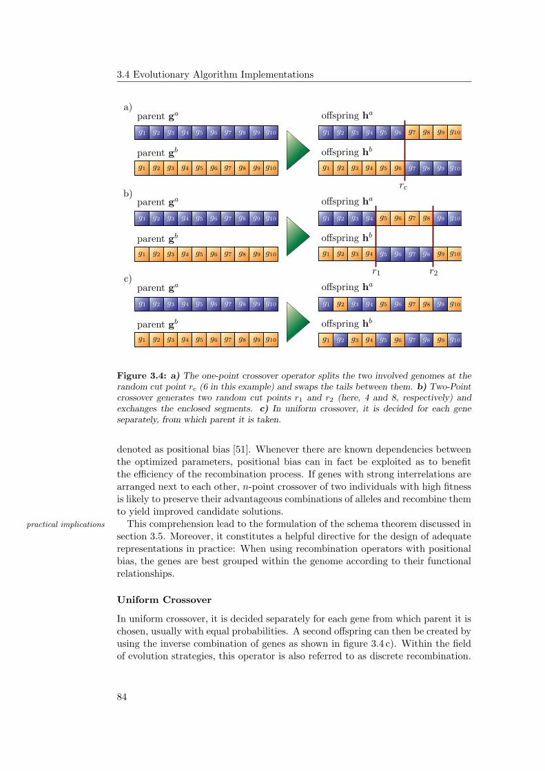
3.4 Evolutionary Algorithm Implementations
PSfrag replacements
a)
b)
c)
g1g1
g1g1
g1g1
g2
g2
g2g2
g2g2
g3g3
g3g3
g3g3
g4g4
g4g4
g4g4
g5
g5
g5
g5
g5g5
g6g6
g6
g6
g6g6
g7
g7
g7
g7
g7
g7
g8
g8
g8
g8
g8
g8
g9g9
g9g9
g9
g9
g10
g10
g10g10
g10
g10
g1
g1
g1
g1
g1
g1 g2
g2
g2
g2
g2
g2 g3
g3
g3
g3
g3
g3 g4
g4
g4
g4
g4
g4
g5
g5
g5
g5
g5
g5
g6
g6
g6
g6
g6
g6
g7
g7
g7
g7
g7
g7
g8
g8
g8
g8
g8
g8 g9
g9
g9
g9
g9
g9 g10
g10
g10
g10
g10
g10
offspring ha
offspring ha
offspring ha
offspring hb
offspring hb
offspring hb
parent ga
parent ga
parent ga
parent gb
parent gb
parent gb
rc
r1 r2
Figure 3.4: a) The one-point crossover operator splits the two involved genomes at therandom cut point rc (6 in this example) and swaps the tails between them. b) Two-Pointcrossover generates two random cut points r1 and r2 (here, 4 and 8, respectively) andexchanges the enclosed segments. c) In uniform crossover, it is decided for each geneseparately, from which parent it is taken.
denoted as positional bias [51]. Whenever there are known dependencies betweenthe optimized parameters, positional bias can in fact be exploited as to benefitthe efficiency of the recombination process. If genes with strong interrelations arearranged next to each other, n-point crossover of two individuals with high fitnessis likely to preserve their advantageous combinations of alleles and recombine themto yield improved candidate solutions.
This comprehension lead to the formulation of the schema theorem discussed inpractical implications
section 3.5. Moreover, it constitutes a helpful directive for the design of adequaterepresentations in practice: When using recombination operators with positionalbias, the genes are best grouped within the genome according to their functionalrelationships.
Uniform Crossover
In uniform crossover, it is decided separately for each gene from which parent it ischosen, usually with equal probabilities. A second offspring can then be created byusing the inverse combination of genes as shown in figure 3.4 c). Within the fieldof evolution strategies, this operator is also referred to as discrete recombination.
84
Evolutionary Algorithms
The uniform crossover operator does not exhibit any positional bias. On the distributional bias
other hand, it tends to yield offspring that contains the genetic material of bothparents in an approximately equal amount. Such a behavior is known as distribu-tional bias [51].
Bearing in mind the propositions of the No Free Lunch theorem brought forward selecting adequatecrossover schemesin section 3.3.3, it can be concluded that if no knowledge is available about the
dependencies between the optimized parameters — and their arrangement withinthe genome is thus random — there is no a priori reason to favor any of the abovecrossover operators over the others. Empirical and theoretical studies suggestthat uniform crossover is superior to the one or two-point operators on severalartificial problems [197] [203]. But it should not be underestimated that thenumber of necessary random values is far greater in the uniform case than forn-point crossover with moderate n. Furthermore, when the genes can be groupedas to account for relationships between the parameters, recombination operatorswith positional bias might generally be the better choice.
A Note on the Organization of the Genome
So far, it has been assumed that all genes of a candidate solution are arranged partitioning intochromosomeswithin one single vector that constitutes the entire genome of the individual. Like
in biological systems, the genetic material of a genome can be partitioned intomultiple chromosomes, each being a string or vector of genes as considered above.
Any Recombination operators are then applied to each parental pair of chro-mosomes separately. As in the case of operators with positional bias, this schemeis considered useful if the distribution of genes between the chromosomes reflectsthe organizational characteristics of the optimized system.
Moreover, a segmentation into chromosomes suggests a new form of crossover swappingchromosomeswhere whole chromosomes are swapped between two mating individuals with a
given probability. Whether they are exchanged or not is individually decided foreach chromosomal pair. Finally, the actually applied recombination operator canbe different for each chromosome. The respective choice might depend on thepresence or absence of functional relationships between the contained genes.
Another Note on Mixed Representations
Returning to the subject of genetic representations discussed in section 3.4.2, it isto be expected that a given optimization task incorporates a variety of parametersof different kinds. Rather than trying to find a common representation to beapplied to all attributes, it seems reasonable to code each parameter in the waythat best suits its characteristics. The resulting genomes will contain genes ofdifferent types and each gene can assume alleles gi of its individual set Gi, gi ∈ Gi.
As long as all genomes in a population are structurally equivalent, a mixed mixed representationsand variationrepresentation does not necessarily give rise to further complications. The pre-
sented mutation operators all operate on single genes. Like in case of the usedencoding, the applied mutation operator can readily be chosen for each gene sepa-rately. Furthermore, all discussed recombinational models are independent of the
85
3.5 Theoretical Analysis: The Schema Theorem
specific nature of the single genes. Hence, all of the above exchange operators canimmediately be applied to any mixed representation without further modification.
3.5 Theoretical Analysis: The Schema Theorem
A considerable amount of theoretical work has been undertaken to model andobjectives
analyze the behavior of evolutionary algorithms. Ultimately, these efforts aimfor a prediction of the performance of a given algorithm on a specific task. Ifsuccessful, this would allow for the selection of the most suitable algorithm — andthe most adequate choice of parameters — for a desired optimization problem inadvance.
A variety of theoretical techniques have been employed in pursuit of this goalmethodologic variety
such as, e.g., the analysis with Markov Chains [173] [174], the dynamical systemsapproach [217] [214], and the application of methods that originate from statisticalmechanics [164] [165]. Although these investigations provide valuable insights intoseveral different aspects of how evolutionary algorithms work, they are in themajority of cases concerned with comparably simple binary genetic algorithms onsimplified artificial problems.
Evolutionary algorithms are complex dynamic systems involving numerous ran-limitations
dom factors and it can be argued that the ultimate goal of precisely predicting thebehavior of an arbitrary algorithm on a realistic task might not ever be achiev-able [50]. Nevertheless, the reported results at least provide useful hints for theconstruction and tuning of efficient evolutionary algorithms in practice.
A thorough examination of these various theoretical approaches and their resultsthe schema theorem
cannot be given here. Instead, the following sections will confine themselves withthe discussion of an early result found by Holland which is commonly known as theschema theorem [96]. Holland’s analysis has not only been of vital importance forthe development of genetic algorithms in general but will also prove to be usefulwhen investigating the feasibility of evolutionary algorithms for the training ofneural networks (chapter 4).
3.5.1 Schemata
A schema is simply an affine subspace in the search space. The agreed notation fordefinition
a schema uses the “don’t care” symbol #, such that in a 5-dimensional genotypespace G consisting of genome vectors g = (g1, g2, g3, g4, g5), the exemplary schemaH = (1, #, #, #, 1) denotes the affine subspace in G which is defined by all pointsthat exhibit ones in the first and last component. All vectors that meet thisrequirement are called examples or instances of this schema. This allows to definethe fitness of a schema to be the mean fitness of all its instances.
Two measures characterize a schema. First, its order is defined as the number ofdefining length andorder its specified positions, i.e., those positions that do not show the # sign. Second,
the defining length is taken to be the number of crossover points between theoutermost fixed genes. The schema defined above has order 2 and defining length4, whereas the schema (1, #, 0, #, 1) also has defining length 4 but exhibits anorder of 3.
86
Evolutionary Algorithms
Holland’s initial analysis is concerned with the so-called standard genetic al- the standard geneticalgorithmgorithm (SGA) that uses a binary representation, fitness proportional parent se-
lection, one-point crossover, a single-gene bit-flipping mutation operator, and agenerational replacement scheme. In this case, a genome g is given by a sim-ple binary string and the above schema — which is now conveniently written as1###1 — includes 23 = 8 instances.
3.5.2 The Processing of Schemata
Holland showed that a given string of length ng is an example of 2ng schemata. implicit parallelism
Although a finite population of µ genomes will not in general contain µ · 2ng
different schemata, he derived that it can nevertheless usefully process about O(µ3)of them. This feature of genetic algorithms is known as implicit parallelism andhas widely been regarded as one of the main reasons for their efficiency.
During the execution of an evolutionary algorithm, the number of instances of a schemata andvariation operatorsschema that are present in the current population will depend on the schemata’s
fitness value as well as on the effects of the applied variation operators. Recom-bination and mutation can create new instances but can also destroy previouslyexisting examples.
In the case of the SGA, the probability of a schema H to be disrupted by mathematicalformulationcrossover and mutation can be calculated and expressed in terms of its order o(H),
its defining length d(H), and the length of the genome ng. Let f(H) denote theeffective fitness of the schema, i.e., the average fitness of all its instances in thecurrent generation. If <f > is taken to be the mean fitness of all present indi-viduals, then the on average expected number of instances in the next generationm(H, t + 1) can be estimated from the number of examples m(H, t) in the currentpopulation according to
m(H, t + 1) ≥ m(H, t) · f(H)
<f>·[1 −
(pc ·
d(H)
ng − 1
)]· [pm · o(H)] (3.7)
where pm and pc are the respective probabilities for applying the mutation andcrossover operators [96]. The common interpretation of this result is that therepresentations of schemata which exhibit a sufficiently high fitness and also standa reasonable chance to be preserved under mutation and crossover will continuallygrow from generation to generation.
Schemata and Variation Operators
The fact that equation 3.7 can merely estimate a lower bound on the number destructive andconstructive effectsof instances of a given schema H is ultimately owed to the circumstance that
Holland’s derivation does not account for the constructive effect of the variationoperators. Only the probabilities of crossover and mutation to destroy a givenexample of a schema are considered. Analyzing the constructive potential of thevariation operators is considerably more difficult, since these effects depend on theexplicit composition of the current population. But it has later been shown thatunder some simplifying conditions and for an arbitrary recombination operator,
87
3.5 Theoretical Analysis: The Schema Theorem
the expected number of instances of a schema that are destroyed are in fact equalto the expected number of examples that are created [198].
Besides that, the evaluation of variation operators in terms of their destructivepositional anddistributional bias effect on schemata provides a more solid foundation for the concepts of positional
and distributional bias (see section 3.4.4) [51]. Regarding two schemata H1 and H2
with equal fitness f(H1) = f(H2) but different defining lengths d(H1) < d(H2),an operator is denoted to exhibit positional bias if it is less likely to destroythe schema with the shorter defining length H1. This, e.g., applies to one-pointcrossover.
On the other hand, a variation operator is said to show distributional bias ifits probability to disrupt a schema H is a function of the schema’s order o(H).Uniform crossover as well as every single-gene mutation operator fall into thiscategory.
3.5.3 Building Blocks, Deception and Challenges to the SchemaTheorem
A closer investigation of equation 3.7 reveals that assuming equal fitness values,estimated growth ofrepresentations short low-order schemata generally have a higher probability to be preserved in the
next generation of an SGA than longer schemata or those with higher order. It hasbeen argued that by virtue of equation 3.7, the representations of short schematawith low order are in fact expected to grow approximately exponentially.
This comprehension forms the basis of what has become widely known as thethe building blockhypothesis building block hypothesis [71]. According to this model, a genetic algorithm starts
by selecting short, low-order schemata and successively combines them to buildlonger, higher-order schemata until, in the ideal case, a schema of order ng isfound that represents the globally optimal solution. The building block hypothesisstresses the role of recombination and in the field of genetic algorithms, crossoveris regarded to be the primary force behind the optimization process, whereasmutation is merely regarded as a background mechanism that is to warrant thenecessary genetic diversity [71].
Deceptive Problems
Analyzing the operation of genetic algorithms in terms of building blocks even-characterization
tually gives rise to the question of what is expected to happen once the globalsolution to a given problem is not an instance of the low-order schemata that ex-hibit a high mean fitness. To illustrate this, consider an exemplary three-bit prob-example problem
lem where the fitness values of the possible bit-strings are given as follows [225]:
f(000) = 28
f(010) = 22
f(110) = 0
f(101) = 0
f(001) = 26
f(100) = 14
f(011) = 0
f(111) = 30
In this artificial problem, all schemata of order n < 3 that have a 1 in one
88
Evolutionary Algorithms
of their defining positions exhibit a lower mean fitness than their correspondingcounterparts that show a 0 in the same position. More specifically, the averagedfitness values f(h) of the different schemata H obey:
f(0##) > f(1##)
f(#0#) > f(#1#)
f(##0) > f(##1)
f(00#) > f(11#), f(10#), f(01#)
f(0#0) > f(1#1), f(1#0), f(0#1)
f(#00) > f(#11), f(#10), f(#01)
Yet, the global optimum is represented by the string 111. In other words, allschemata of order n < 3 effectively lead the search away from the perfect solutionand towards the suboptimal string 000. Problems of this kind are commonly de-noted as deceptive, although this term is not unambiguously defined [76] [195] [225].
It could be apprehended that such deceptive problems considerably challenge practical relevance
conventional genetic algorithms since no appropriate building blocks are present.However, experimental investigations have been reported that do not reveal adirect correlation between the probability of an optimization problem to be de-ceptive and the ability of the SGA to find the global solution [195]. Also, it isnot generally agreed whether deceptive problems are to be regarded as adequatemodels of realistic tasks in practice [76] [225].
Challenges to the Schema Theorem
It shall not remain unmentioned that the Schema Theorem and the building blockhypothesis have faced some criticism. As stated above, the schema theorem islimited in so far as it does not consider the potential of the variation operators tocreate new instances of a schema but only accounts for their destructive effects.
Furthermore, the estimated fitness f(H) of a schema is exclusively based on finite populationeffectsthe fitness values of those instances that are present in the current population
and might therefore not be representative of the schema as a whole. In so far,equation 3.7 is restricted to make predictions only for the following generation.Since the representation of H and all other present schemata will have changedin the next generation, so will the estimated fitness values, and the compositionof the current population cannot reliably be employed to yield sound estimatesfor later generations [50]. In particular, the rate by which the representation estimated growth of
representationsof a given schema H increases is not exponential: As soon as its share of thepopulation grows, its selective advantage f(H)/ <f> decreases accordingly dueto the increased mean fitness of the whole population.
The experimentally verified efficiency of operators with a high distributional experimentalcounter-argumentsbias, most notably uniform crossover [197] [203], as well as the SGA’s apparent
ability to tackle deceptive problems [195] cannot satisfactorily be reconciled withthe propositions of the schema theorem and the building block hypothesis. Con-sidering the recombination of building blocks to be the main force behind geneticsearch can only insufficiently explain the success of those approaches that do notincorporate recombination at all, e.g., most forms of evolution strategies.
Nevertheless, it shall be repeated that analyzing evolutionary algorithms interms of schemata persists to provide valuable insights into at least some aspects
89

3.5 Theoretical Analysis: The Schema Theorem
of how this kind of optimization procedures work. Among other things, the dis-cussed results considerably affect the applicability of evolutionary algorithms tothe training of neural networks. This will be the topic of the following chapter.
90
Chapter 4
Evolving Artificial NeuralNetworks
Human beings, who are almost unique in having the abilityto learn from the experience of others, are also remarkablefor their apparent disinclination to do so.
Douglas Adams, Last Chance to See
Evolutionary algorithms have the ability to cope with complex, multimodal searchspaces and do not depend on a detailed model of the system to be optimized(chapter 3). In particular, they do not require the applied performance measureto be differentiable with respect to the free parameters. A such, they represent apromising approach to train neural networks, even those kinds of neural systemsfor which no other feasible training algorithm is immediately available, e.g., re-current networks, multi-layer networks of binary threshold neurons or networksimplemented in analog VLSI (see section 2.4).
Several examples in the preceeding chapter have already hinted at some suitable possible combinations
approaches for optimizing the synaptic weights of a network, but besides that,evolutionary algorithms have been combined with artificial neural networks alsoin various other ways (for a comprehensive overview see, e.g., [26] and [234]).Most notably, they can be employed to optimize the architecture of a network,i.e., the number of neurons and the available connections. Often, the training ofthe weight values and the construction of the architecture are combined. Furtherapplications of evolutionary algorithms within the field of neural computationinclude the evolutionary tuning of learning rules [13] [36] or the optimization ofneuron transfer functions [234].
This chapter will focus on the evolution of the synaptic weights and brieflydiscuss the evolutionary design of architectures. Since this thesis is primarily con-cerned with training strategies for hardware-implemented, feedforward networksthat cannot be trained via conventional algorithms and which exhibit fixed neurontransfer functions (see chapter 5), the evolution of learning rules and activationfunctions will not be covered.
Instead, two alternative methods for the optimization of neural network weights
91
4.1 Evolving Synaptic Weights
shall be discussed that do not depend on a differentiable performance measure anda detailed model of the network operation as well: Simulated annealing and theweight perturbation algorithm.
4.1 Evolving Synaptic Weights
If the topology of a neural network is fixed, training its synaptic weights can beregarded as an optimization process that aims to minimize the network’s erroron the training patterns (see sections 1.2.4, 2.1.2, 2.1.3, and 2.2.2). In so far,evolutionary algorithms could be expected to be readily applicable to this kind oftask without major modifications.
Indeed, compared to most gradient-based training approaches like, e.g., thebenefits
backpropagation algorithm discussed in section 2.2.2, evolutionary algorithmsyield the advantage of not posing any restrictions on the architecture of the op-timized network. Given a suitable fitness function that appropriately quantifiesthe performance of the network on the task in question (section 4.1.1), the sameevolutionary algorithm can in principle be applied to feedforward networks, radialbasis function networks, or recurrent networks [74]. In the following sections, em-phasis is placed on feedforward networks, but most of the results can readily betransferred to different architectures.
On the other hand, it turns out that the structural features of neural networkschallenges
call for special precautions during the design of suitable genetic representationsand corresponding variation operators. These issues are closely related to whatis commonly known as the permutation problem which will be addressed in sec-tion 4.1.2
4.1.1 Performance Evaluation and Fitness Function
Equations 2.15 and 2.16 represent suitable means for quantifying the performancenetwork error
of a network on a given task and it seems reasonable to utilize them for evolution-ary algorithms as well. If the fitness of an individual is desired to increase withimproving performance, the network error E on the training patterns can easily betransformed into an adequate fitness function that meets this requirement. Com-mon approaches are to choose 1/E, 1/(1 + E), or (Emax − E)/Emax as the usedfitness measure.
Apart from that, evolutionary algorithms allow to incorporate additional de-additional constraints
mands to the trained network into the formulation of the fitness function. In thecase of highly recurrent architectures, for example, the fitness function could beformulated as to penalize networks that exhibit an undesirable oscillating behavior(see sections 2.3.3 and 2.3.4).
Although there are no direct limitations concerning the special requirementsthat might be accounted for by the fitness measure, it is to be remembered thatthe exact form of the fitness function can have considerable impact on the successof the evolutionary search (see section 3.2.1). More elaborate forms of perfor-mance measures might run a greater risk of assuming multiple local optima on
92
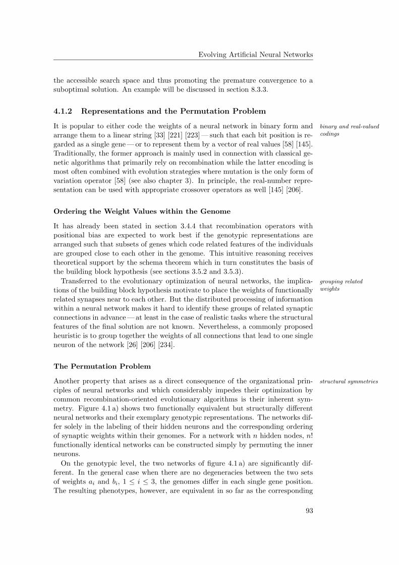
Evolving Artificial Neural Networks
the accessible search space and thus promoting the premature convergence to asuboptimal solution. An example will be discussed in section 8.3.3.
4.1.2 Representations and the Permutation Problem
It is popular to either code the weights of a neural network in binary form and binary and real-valuedcodingsarrange them to a linear string [33] [221] [223] — such that each bit position is re-
garded as a single gene — or to represent them by a vector of real values [58] [145].Traditionally, the former approach is mainly used in connection with classical ge-netic algorithms that primarily rely on recombination while the latter encoding ismost often combined with evolution strategies where mutation is the only form ofvariation operator [58] (see also chapter 3). In principle, the real-number repre-sentation can be used with appropriate crossover operators as well [145] [206].
Ordering the Weight Values within the Genome
It has already been stated in section 3.4.4 that recombination operators withpositional bias are expected to work best if the genotypic representations arearranged such that subsets of genes which code related features of the individualsare grouped close to each other in the genome. This intuitive reasoning receivestheoretical support by the schema theorem which in turn constitutes the basis ofthe building block hypothesis (see sections 3.5.2 and 3.5.3).
Transferred to the evolutionary optimization of neural networks, the implica- grouping relatedweightstions of the building block hypothesis motivate to place the weights of functionally
related synapses near to each other. But the distributed processing of informationwithin a neural network makes it hard to identify these groups of related synapticconnections in advance — at least in the case of realistic tasks where the structuralfeatures of the final solution are not known. Nevertheless, a commonly proposedheuristic is to group together the weights of all connections that lead to one singleneuron of the network [26] [206] [234].
The Permutation Problem
Another property that arises as a direct consequence of the organizational prin- structural symmetries
ciples of neural networks and which considerably impedes their optimization bycommon recombination-oriented evolutionary algorithms is their inherent sym-metry. Figure 4.1 a) shows two functionally equivalent but structurally differentneural networks and their exemplary genotypic representations. The networks dif-fer solely in the labeling of their hidden neurons and the corresponding orderingof synaptic weights within their genomes. For a network with n hidden nodes, n!functionally identical networks can be constructed simply by permuting the innerneurons.
On the genotypic level, the two networks of figure 4.1 a) are significantly dif-ferent. In the general case when there are no degeneracies between the two setsof weights ai and bi, 1 ≤ i ≤ 3, the genomes differ in each single gene position.The resulting phenotypes, however, are equivalent in so far as the corresponding
93
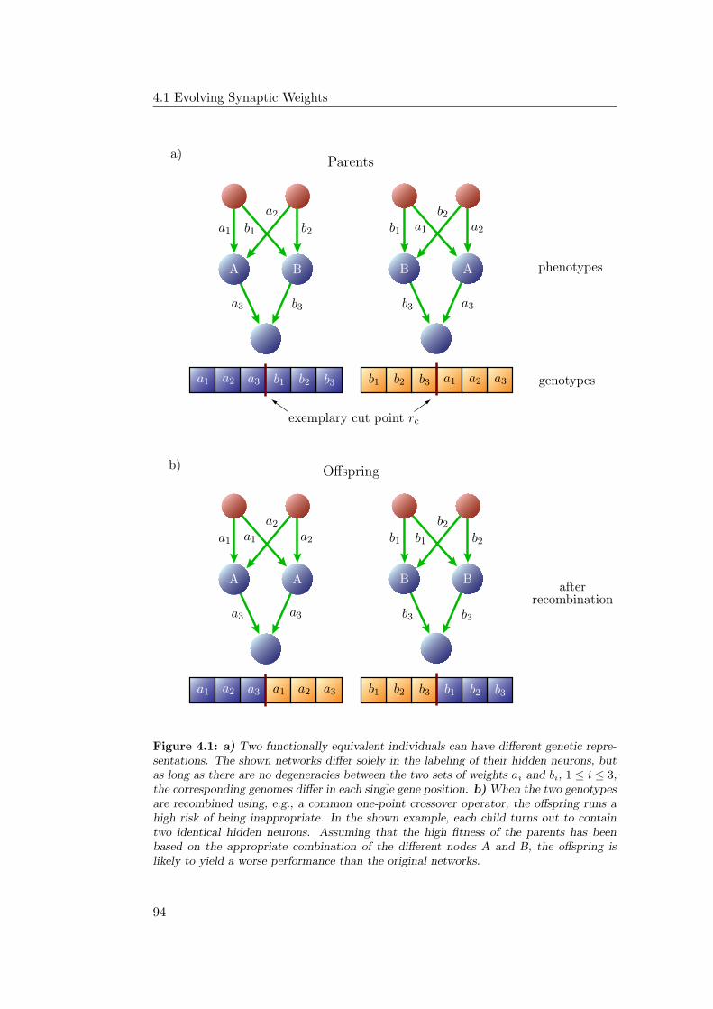
4.1 Evolving Synaptic Weights
PSfrag replacements
phenotypes
genotypes
afterrecombination
a1
a1a1
a1
a1
a1
a2
a2
a2
a2
a2
a2
a3
a3a3
a3
a3
a3
b1b1
b1
b1
b1
b1
b2
b2
b2
b2
b2
b2
b3
b3b3
b3
b3b3
a1
a1
a2
a2
a3
a3
b1
b1
b2
b2
b3
b3
AA
AA
BB
BB
a)
b)
exemplary cut point rc
Parents
Offspring
Figure 4.1: a) Two functionally equivalent individuals can have different genetic repre-sentations. The shown networks differ solely in the labeling of their hidden neurons, butas long as there are no degeneracies between the two sets of weights ai and bi, 1 ≤ i ≤ 3,the corresponding genomes differ in each single gene position. b) When the two genotypesare recombined using, e.g., a common one-point crossover operator, the offspring runs ahigh risk of being inappropriate. In the shown example, each child turns out to containtwo identical hidden neurons. Assuming that the high fitness of the parents has beenbased on the appropriate combination of the different nodes A and B, the offspring islikely to yield a worse performance than the original networks.
94
Evolving Artificial Neural Networks
networks yield equal responses when being applied the same input, i.e., they im-plement the same functional mapping. In fact, with the numbering of the hiddennodes being initially arbitrary, one would usually regard the two individuals asone and the same network.
Using the genetic representation shown in figure 4.1 a), the evolutionary algo- symmetries andrecombinationrithm is bound to ignore this symmetry. As illustrated in figure 4.1 b) a recom-
bination of the genomes that involves a common one-point crossover operator islikely to produce inappropriate offspring. This phenomenon is commonly knownas the permutation problem (also: competing conventions problem) [17] [80] [81].
There is a related but somewhat more subtle issue that is connected to the weight symmetries
special symmetry of neurons with odd activation functions [26]: A neuron of thiskind retains its effective influence on the receiving nodes when the signs of theweights of all its incoming and outgoing connections are flipped simultaneously.For the types of activation function presented in section 1.2.3, this requires anadditional adjustment of the receiving neurons’ bias values, but the general sym-metry abides. Within a network of n hidden neurons, one is free to flip the signsof any of these nodes which gives rise to
∑ni=0
(ni
)= 2n different, but functionally
identical networks.
Implications of the Permutation Problem
Each of the different conventions — i.e., the individual numbering of the neurons speciation
in connection with the agreed signs of the weights — is represented by a distinctregion of the search space. Only a recombination of individuals from the sameregion promises to yield improved offspring. Therefore, it is reasonable to assumethat the impact of the permutation problem could be alleviated by employingone of the speciation mechanisms introduced in section 3.3.4 (e.g., [199] [200] orsee [26]).
In the light of the schema theorem, it is a direct consequence of the permutation schemata
problem that there exist multiple competing schemata with high average fitnessthat each specify the values of the same genes but exhibit different alleles onthese positions. When multiple such building blocks are recombined, they do notautomatically yield better individuals. On the contrary, given the high degreeof symmetry in large networks, a combination of these building blocks stands aconsiderable chance to produce worse offspring. Seen from this angle, the trainingof neural networks can be regarded as a deceptive optimization task in terms ofsection 3.5.3. The simplest way to avoid the negative impact of the permutationproblem would thus be to use no recombination at all.
It has been argued that the effects of the permutation problem are not as severe population sizing andselective pressureas widely supposed [80] [81] and that they will most probably depend on param-
eters like the sizes of the network and the population [80] [81] [224]. Small pop-ulation sizes in combination with strong selection and more aggressive mutationshould prevent the algorithm from exploring multiple alternative but equivalentregions of the search space in parallel. On the other hand, this strategy runs therisk of promoting premature convergence and can be expected to be feasible onlyfor small networks.
95
4.1 Evolving Synaptic Weights
Several approaches have been proposed that try to match the hidden neurons ofimprovingrecombination two networks and either appropriately reorder the genotypes before recombination
or confine themselves to merely swapping corresponding hidden nodes betweenthe two mating individuals (for an overview see [26]). Finally, the permutationproblem can be circumvented by evolving the weights and the architecture of thenetwork simultaneously (section 4.2).
4.1.3 Comparison with Gradient Based Training
Evolutionary algorithms are comparably expensive in terms of computational ef-speed considerations
fort. In each generation, multiple new networks have to be implemented, testedand evaluated. Compared to fast variants of backpropagation or other gradient-based training algorithms, an evolutionary optimization of the weight values isoften found to be measurably slower (see [234]).
Nevertheless, some reported results suggest that evolutionary training can besignificantly faster than backpropagation at least on some problems (e.g., [188]).The apparent discrepancy between these observations can partly be attributed tothe different evolutionary algorithm and backpropagation implementations com-pared.
Evolutionary Training of Hardware Neural Networks
As already indicated above, the rationale behind the application of evolutionaryoptimizationalcapabilities algorithms to neural network training is not initially given by speed considerations.
Rather, evolutionary algorithms lend themselves to the optimization of synapticweights primarily due to their ability to find global optima in complex, multi-modal search spaces and their insensitiveness to starting conditions. Furthermore,they can successfully and reliably train even those kinds of neural networks thatcannot be optimized by common gradient-based approaches.
In this respect, evolutionary algorithms do not directly compete with traditionallearning algorithms in terms of speed, but are to be seen to complement these ap-proaches, especially considering those types of networks that cannot immediatelybe trained via common gradient-based optimization. Besides highly recurrent net-works, this particularly applies to neural networks implemented in analog VLSI(see section 2.4).
For the latter case, the evolutionary approach is deemed to be feasible also withtraining speed
regard to the absolute speed of the training, since a parallel hardware realizationpotentially allows to evaluate multiple different networks in a short time. Whenbeing realized as chip-in-the-loop algorithms, evolutionary strategies therefore rep-resent a competitive training approach for fast analog or hybrid hardware neuralnetworks (section 2.4.5).
Combined Approaches
Several strategies have been reported in literature that aim to combine the prin-combining evolutionand gradient descent ciples of simulated evolution with gradient-based training (e.g. [17], or see [26]
96
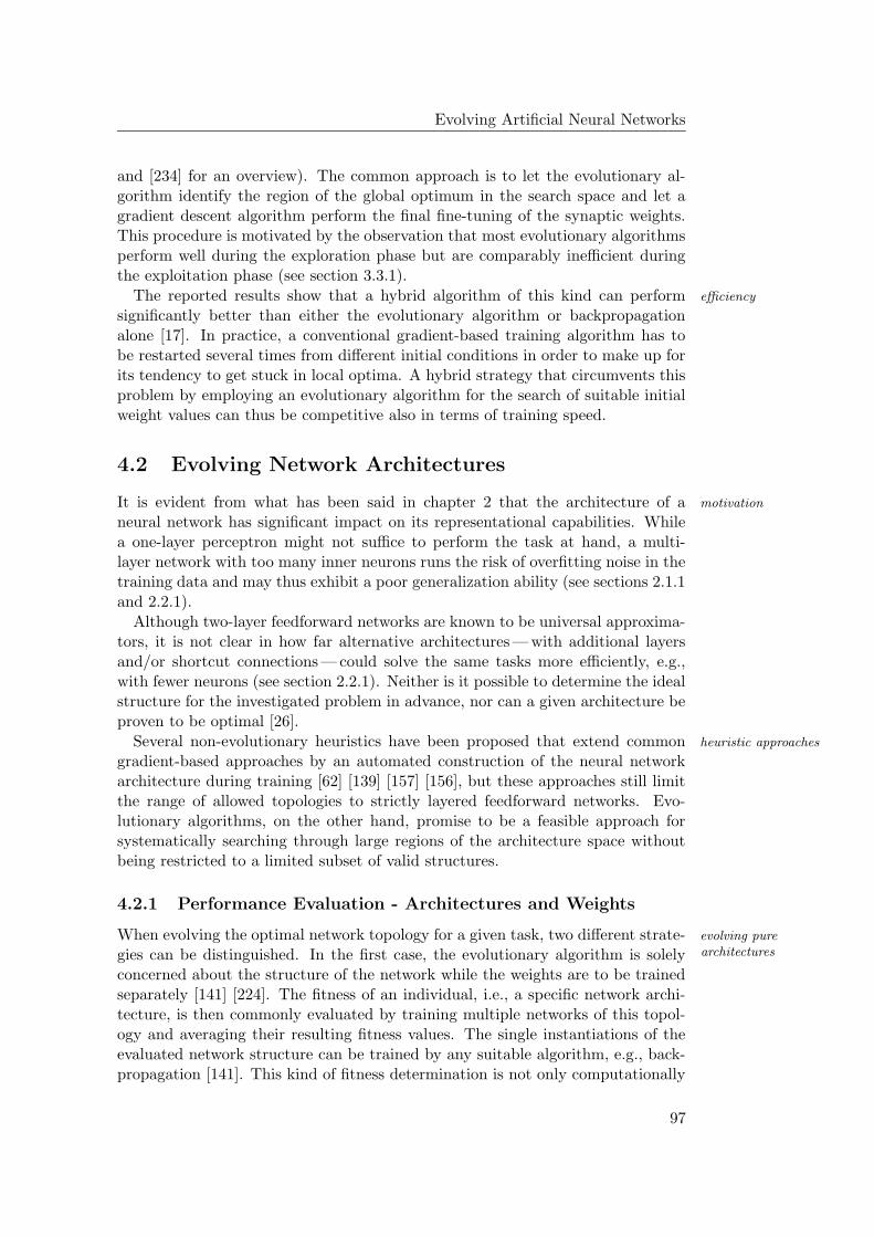
Evolving Artificial Neural Networks
and [234] for an overview). The common approach is to let the evolutionary al-gorithm identify the region of the global optimum in the search space and let agradient descent algorithm perform the final fine-tuning of the synaptic weights.This procedure is motivated by the observation that most evolutionary algorithmsperform well during the exploration phase but are comparably inefficient duringthe exploitation phase (see section 3.3.1).
The reported results show that a hybrid algorithm of this kind can perform efficiency
significantly better than either the evolutionary algorithm or backpropagationalone [17]. In practice, a conventional gradient-based training algorithm has tobe restarted several times from different initial conditions in order to make up forits tendency to get stuck in local optima. A hybrid strategy that circumvents thisproblem by employing an evolutionary algorithm for the search of suitable initialweight values can thus be competitive also in terms of training speed.
4.2 Evolving Network Architectures
It is evident from what has been said in chapter 2 that the architecture of a motivation
neural network has significant impact on its representational capabilities. Whilea one-layer perceptron might not suffice to perform the task at hand, a multi-layer network with too many inner neurons runs the risk of overfitting noise in thetraining data and may thus exhibit a poor generalization ability (see sections 2.1.1and 2.2.1).
Although two-layer feedforward networks are known to be universal approxima-tors, it is not clear in how far alternative architectures — with additional layersand/or shortcut connections — could solve the same tasks more efficiently, e.g.,with fewer neurons (see section 2.2.1). Neither is it possible to determine the idealstructure for the investigated problem in advance, nor can a given architecture beproven to be optimal [26].
Several non-evolutionary heuristics have been proposed that extend common heuristic approaches
gradient-based approaches by an automated construction of the neural networkarchitecture during training [62] [139] [157] [156], but these approaches still limitthe range of allowed topologies to strictly layered feedforward networks. Evo-lutionary algorithms, on the other hand, promise to be a feasible approach forsystematically searching through large regions of the architecture space withoutbeing restricted to a limited subset of valid structures.
4.2.1 Performance Evaluation - Architectures and Weights
When evolving the optimal network topology for a given task, two different strate- evolving purearchitecturesgies can be distinguished. In the first case, the evolutionary algorithm is solely
concerned about the structure of the network while the weights are to be trainedseparately [141] [224]. The fitness of an individual, i.e., a specific network archi-tecture, is then commonly evaluated by training multiple networks of this topol-ogy and averaging their resulting fitness values. The single instantiations of theevaluated network structure can be trained by any suitable algorithm, e.g., back-propagation [141]. This kind of fitness determination is not only computationally
97
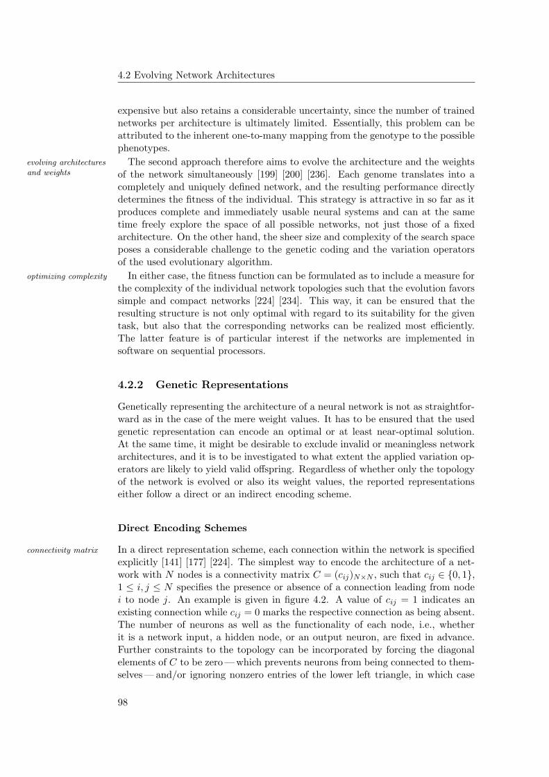
4.2 Evolving Network Architectures
expensive but also retains a considerable uncertainty, since the number of trainednetworks per architecture is ultimately limited. Essentially, this problem can beattributed to the inherent one-to-many mapping from the genotype to the possiblephenotypes.
The second approach therefore aims to evolve the architecture and the weightsevolving architecturesand weights of the network simultaneously [199] [200] [236]. Each genome translates into a
completely and uniquely defined network, and the resulting performance directlydetermines the fitness of the individual. This strategy is attractive in so far as itproduces complete and immediately usable neural systems and can at the sametime freely explore the space of all possible networks, not just those of a fixedarchitecture. On the other hand, the sheer size and complexity of the search spaceposes a considerable challenge to the genetic coding and the variation operatorsof the used evolutionary algorithm.
In either case, the fitness function can be formulated as to include a measure foroptimizing complexity
the complexity of the individual network topologies such that the evolution favorssimple and compact networks [224] [234]. This way, it can be ensured that theresulting structure is not only optimal with regard to its suitability for the giventask, but also that the corresponding networks can be realized most efficiently.The latter feature is of particular interest if the networks are implemented insoftware on sequential processors.
4.2.2 Genetic Representations
Genetically representing the architecture of a neural network is not as straightfor-ward as in the case of the mere weight values. It has to be ensured that the usedgenetic representation can encode an optimal or at least near-optimal solution.At the same time, it might be desirable to exclude invalid or meaningless networkarchitectures, and it is to be investigated to what extent the applied variation op-erators are likely to yield valid offspring. Regardless of whether only the topologyof the network is evolved or also its weight values, the reported representationseither follow a direct or an indirect encoding scheme.
Direct Encoding Schemes
In a direct representation scheme, each connection within the network is specifiedconnectivity matrix
explicitly [141] [177] [224]. The simplest way to encode the architecture of a net-work with N nodes is a connectivity matrix C = (cij)N×N , such that cij ∈ 0, 1,1 ≤ i, j ≤ N specifies the presence or absence of a connection leading from nodei to node j. An example is given in figure 4.2. A value of cij = 1 indicates anexisting connection while cij = 0 marks the respective connection as being absent.The number of neurons as well as the functionality of each node, i.e., whetherit is a network input, a hidden node, or an output neuron, are fixed in advance.Further constraints to the topology can be incorporated by forcing the diagonalelements of C to be zero — which prevents neurons from being connected to them-selves— and/or ignoring nonzero entries of the lower left triangle, in which case
98
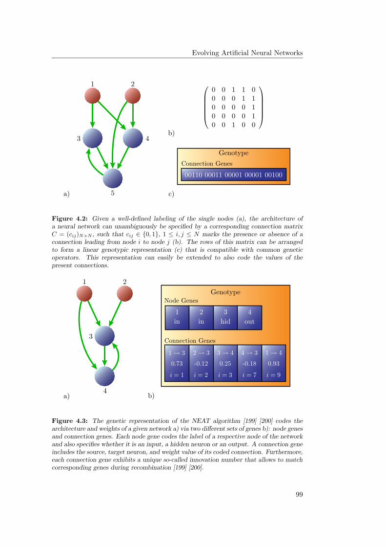
Evolving Artificial Neural NetworksPSfrag replacements
1 2
3 4
5
Genotype
Connection Genes
0 0 1 1 00 0 0 1 10 0 0 0 10 0 0 0 10 0 1 0 0
00110 00011 00001 00001 00100
a)
b)
c)
Figure 4.2: Given a well-defined labeling of the single nodes (a), the architecture ofa neural network can unambiguously be specified by a corresponding connection matrixC = (cij)N×N , such that cij ∈ 0, 1, 1 ≤ i, j ≤ N marks the presence or absence of aconnection leading from node i to node j (b). The rows of this matrix can be arrangedto form a linear genotypic representation (c) that is compatible with common geneticoperators. This representation can easily be extended to also code the values of thepresent connections.
PSfrag replacements
1 2
3
4a) b)
GenotypeNode Genes
Connection Genes
1 2 3 4
inin outhid
1 → 3 2 → 3 3 → 4 4 → 3 1 → 4
0.73 -0.12 0.25 -0.18 0.93
i = 1 i = 2 i = 3 i = 7 i = 9
Figure 4.3: The genetic representation of the NEAT algorithm [199] [200] codes thearchitecture and weights of a given network a) via two different sets of genes b): node genesand connection genes. Each node gene codes the label of a respective node of the networkand also specifies whether it is an input, a hidden neuron or an output. A connection geneincludes the source, target neuron, and weight value of its coded connection. Furthermore,each connection gene exhibits a unique so-called innovation number that allows to matchcorresponding genes during recombination [199] [200].
99
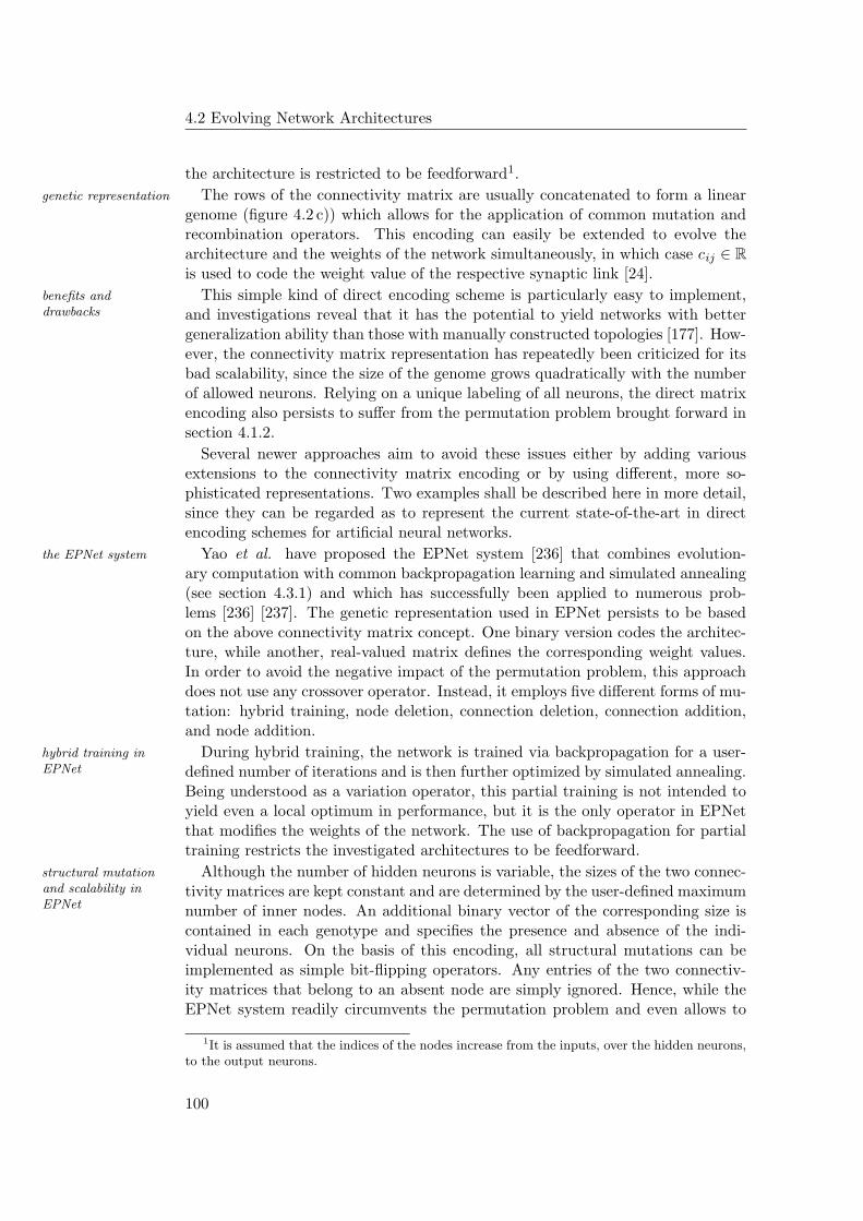
4.2 Evolving Network Architectures
the architecture is restricted to be feedforward1.
The rows of the connectivity matrix are usually concatenated to form a lineargenetic representation
genome (figure 4.2 c)) which allows for the application of common mutation andrecombination operators. This encoding can easily be extended to evolve thearchitecture and the weights of the network simultaneously, in which case cij ∈ R
is used to code the weight value of the respective synaptic link [24].
This simple kind of direct encoding scheme is particularly easy to implement,benefits anddrawbacks and investigations reveal that it has the potential to yield networks with better
generalization ability than those with manually constructed topologies [177]. How-ever, the connectivity matrix representation has repeatedly been criticized for itsbad scalability, since the size of the genome grows quadratically with the numberof allowed neurons. Relying on a unique labeling of all neurons, the direct matrixencoding also persists to suffer from the permutation problem brought forward insection 4.1.2.
Several newer approaches aim to avoid these issues either by adding variousextensions to the connectivity matrix encoding or by using different, more so-phisticated representations. Two examples shall be described here in more detail,since they can be regarded as to represent the current state-of-the-art in directencoding schemes for artificial neural networks.
Yao et al. have proposed the EPNet system [236] that combines evolution-the EPNet system
ary computation with common backpropagation learning and simulated annealing(see section 4.3.1) and which has successfully been applied to numerous prob-lems [236] [237]. The genetic representation used in EPNet persists to be basedon the above connectivity matrix concept. One binary version codes the architec-ture, while another, real-valued matrix defines the corresponding weight values.In order to avoid the negative impact of the permutation problem, this approachdoes not use any crossover operator. Instead, it employs five different forms of mu-tation: hybrid training, node deletion, connection deletion, connection addition,and node addition.
During hybrid training, the network is trained via backpropagation for a user-hybrid training inEPNet defined number of iterations and is then further optimized by simulated annealing.
Being understood as a variation operator, this partial training is not intended toyield even a local optimum in performance, but it is the only operator in EPNetthat modifies the weights of the network. The use of backpropagation for partialtraining restricts the investigated architectures to be feedforward.
Although the number of hidden neurons is variable, the sizes of the two connec-structural mutationand scalability inEPNet
tivity matrices are kept constant and are determined by the user-defined maximumnumber of inner nodes. An additional binary vector of the corresponding size iscontained in each genotype and specifies the presence and absence of the indi-vidual neurons. On the basis of this encoding, all structural mutations can beimplemented as simple bit-flipping operators. Any entries of the two connectiv-ity matrices that belong to an absent node are simply ignored. Hence, while theEPNet system readily circumvents the permutation problem and even allows to
1It is assumed that the indices of the nodes increase from the inputs, over the hidden neurons,to the output neurons.
100
Evolving Artificial Neural Networks
evolve individually sized networks, it retains an unfavorable scaling behavior.
Recently, a more elaborate direct encoding scheme has been proposed which the NEAT algorithm
is referred to as the NEAT method (NeuroEvolution of Augmenting Topolo-gies) [199] [200]. It incorporates two different kinds of genetic units: node genesand connection genes. Like in a common connectivity matrix encoding, eachconnection gene specifies the presence/absence and the weight value of a singlesynaptic connection. But in contrast to the above representations, the genes arenot arranged according to a fixed order. Rather, each connection gene internallycodes the source and target nodes of the represented synapse. Beyond that, thegenotype also contains a list of node genes that encode the labels of the presentinput nodes, hidden neurons, and outputs (see figure 4.3).
In addition to the traditional random modifications of the weight values, a spe- structural mutationin NEATcial mutation operator adds a new connection between two previously unconnected
nodes. The number of neurons in the network is variable as well. A third dedicatedmutation operator adds neurons to the network by splitting an existing connec-tion in two and inserting the new node where the old connection used to be. Asan important result, the numbers of the connection genes and node genes in thegenotype are not fixed and will in general differ between the processed individuals.
In order to match corresponding genes within two mating genomes, each connec- recombination andspeciation in NEATtion gene contains a fixed, population-wide index (the “global innovation number”)
that is increased with every newly introduced connection in any genome of thewhole population. Among other things, this allows for the implementation of afeasible crossover operator that can handle the varying size of the genotypes. It isnot the purpose of this work to examine the elaborate details of the NEAT algo-rithm and the applied recombination operators. The interested reader is referredto the original publications [199] [200]. But it is worth noting that NEAT incorpo-rates a specific distance measure to evaluate the similarity between two genomes.This measure is employed to implement speciation through fitness sharing as it isdescribed in section 3.3.4.
It turns out that given the variability of the genome and the complexity ofthe search space, the implemented speciation mechanism is vitally necessary toefficiently explore different competing architectures. Otherwise, networks withmore complex structures which might prove to be beneficial in the long run wouldsoon be outperformed and suppressed by simpler networks that can be optimizedmore easily and thus reach higher fitness values considerably faster [200].
Apart from that, it is a striking feature of the NEAT encoding scheme that it permutation problem:solveddoes not suffer from the permutation problem. This is primarily due to the fact
that the source and target nodes of each connection are coded within the respectivegene and that corresponding genes can be identified via similar values of the globalinnovation number. Similar, yet not as sophisticated, approaches that partlydecouple the effect of a gene from its exact position in the genome and/or allow forgenotypes of varying size have also been proposed by other authors [24] [166] [148].
101
4.2 Evolving Network Architectures
Indirect Encoding Schemes
The undesirable scaling properties of most direct encoding schemes and their com-mon susceptibility to the effects of the permutation problem have motivated thedevelopment of several indirect encoding methods [82] [117]. The basic idea be-hind an indirect representation is that it does not specify each single node orconnection of the network explicitly but rather codes either general characteris-tics of the neural network architecture itself or specifications of a suitable networkconstruction procedure.
One approach that has been proposed by Harp et al. lets dedicated segmentsparametric encodings
of the genotype code the features of corresponding subareas (layers) of the net-work [82]. Each segment primarily contains information about the number ofneurons included in the respective area as well as their average connectivity to thenodes in other regions of the network. According to the rather coarse structuralspecifications that are contained in the genome, networks are then built via anautomated, and partly stochastic construction rule. In order to yield a completelyspecified network, the synaptic weights of the resulting connections are finallytrained by a suitable algorithm. The training parameters for each area, e.g., thelearning rate η and the momentum ν of the backpropagation algorithm, are codedin the genome as well.
An even simpler variant of the indirect encoding would be to assume a strictlybenefits andlimitations layered, homogeneously connected feedforward architecture and merely code the
number of layers and their individual sizes. Coding schemes like these two ex-amples which contain only certain parameters of the final network are commonlydenoted as parametric representations. Although a parametric encoding methodcan significantly reduce the length of the genotype, the resulting network archi-tectures are usually limited to a subset of the whole feasible architecture space.
According to another indirect representation that has originally been introduceddevelopmental rulerepresentations by Kitano, the genotype codes the rules of a deterministic graph grammar which
is then used to build the connectivity matrix C [117]. In other words, instead ofincluding only the parameters of a fixed building rule that is used to constructthe final network, the genome also codes the development rule itself. Such anencoding scheme is therefore referred to as a developmental rule representation.
Like parametric encodings, developmental rule representations usually exhibitcompact genotypes
a good scaling behavior. Depending on the evolved set of rules, the resultingnetworks can become very complex without requiring the genotype to grow ac-cordingly. The coding of construction rules also facilitates the definition of suit-able representations that yield useful building blocks and can thus efficiently becombined with corresponding crossover operators. Some good results have beenreported with this encoding method [117].
On the other hand, developmental rule representations favor regular networklimited architecturerange architectures [26]. It can generally be said that depending on the used way of
encoding, not every structure is equally probable, and this inherent bias mayeffectively prevent the algorithm from finding the optimal topology as it has ac-tually been desired in the first place. Finally, the developmental rule encodingcan only efficiently be employed for the evolution of architectures while the weight
102
Evolving Artificial Neural Networks
values have to be trained separately. Experimental results suggest that it is notautomatically superior to common direct encodings per se [191].
4.2.3 Fixed vs. Evolved Architectures
In summary, it can be concluded that using either of the representational ap- feasibility of topologyevolutionproaches, the evolutionary search for optimal network architectures ultimately
faces adherent challenges. Simple direct encoding schemes exhibit poor scalabilityand persist to suffer from the permutation problem. The latter can be circum-vented by abstaining from the use of recombination like it is done in EPNet,but even then, the poor scaling behavior remains. More elaborate variants likethe NEAT algorithm constitute promising approaches. But they also require ad-ditional computational and organizational overhead in order to implement validrecombination operators and the necessary speciation mechanisms.
While indirect encodings allow for compact representations, they are inherentlylimited in the range of resulting architectures. Moreover, they have to defer thetraining of the weight values to separate algorithms which results in a computa-tionally expensive an noisy fitness evaluation of the individuals.
Against the background of these issues it is worthwhile to reflect the initial mo- evolving architectures:necessary?tivation for evolving the topologies of neural networks: First, it is desired to find a
network structure that yields the best performance on the investigated task, morespecifically, that leads to an optimal generalization ability of the final network.Second, in order to feasibly implement the resulting networks on ordinary sequen-tial computers, they are preferably compact and simple, i.e., comprise of as fewneurons and connections as possible. It can be concluded that if sufficiently largeand complex networks could efficiently be realized on a suitable substrate andif these networks could simultaneously be trained to yield the desired generaliza-tion performance — even when being limited to a predetermined architecture — anautomated optimization of the topology might not be worth the effort.
Evolving Architectures for Neural Networks Implemented in Hardware
It has been motivated in section 2.4 that analog and/or hybrid CMOS VLSItechnologies have the potential to provide efficient means of realizing such large,yet fast neural networks. The evolutionary training approach can greatly benefitfrom the high configuration and evaluation speeds of these systems and in so farideally complements dedicated hardware implementations.
Yet, if the training algorithm is not to compromise the speed advantage of the speed vs.computationalcomplexity
hardware substrate, it must itself be implemented efficiently (see also sections 6.2.6and 6.3.3). From what has been said above, it can thus be deduced that anevolutionary training strategy for fast hardware neural networks should ratheraim to keep up pace with the network implementation instead of dedicating majorcomputational effort to the unnecessary minimization and optimization of thenetwork topology. As long as the algorithm can succeed in producing networkswith competitive generalization capability, abandoning the search for an idealarchitecture does not necessarily constitute a limitation in practice.
103
4.3 Alternative Black-Box Approaches
On the other hand, the arguments brought forward in sections 2.1.1 and 2.2.1suggest that improving the generalization ability of a neural network ultimatelyboils down to the optimization of its architecture, primarily the appropriate adap-tation of its size. It has repeatedly been argued that the former does not seemto be achievable without the latter (e.g. [12] [139] [141]). In so far, it still awaitsdemonstration that fast and simple training algorithms which refrain from op-timizing the network architecture can efficiently exploit the speed and potentialsize of hardware implemented networks while simultaneously yielding the desiredgeneralization performance. This will be investigated more closely in chapters 8and 9.
4.3 Alternative Black-Box Approaches
One of the main features of evolutionary algorithms that qualifies them for thetraining of highly recurrent and/or hardware implemented neural networks is thatthey do not require the used performance measure to be differentiable with respectto the free parameters, i.e., the weight values. In fact, the fitness needs not tobe consistently expressible as a function of the synaptic weights at all. As notedin section 3.3.3, optimization algorithms with this characteristic are denoted asmodel-free or black-box approaches.
Although all of the experiments presented in this thesis employ evolutionaryalgorithms, other model-free, stochastic optimization algorithms have been pro-posed that should in principle be capable of training neural networks implementedon the used hardware substrate (chapter 5) as well. Since the main aspects of theresults presented in part III are deemed to be transferable also to these alternativetraining algorithms, the two most prominent examples — simulated annealing andweight perturbation — shall briefly be discussed in the following.
4.3.1 Simulated Annealing
Similar to evolutionary algorithms, simulated annealing is inspired by an opti-physical annealing
mization process in nature. In condensed matter physics, annealing is a procedureto obtain the low-energy states of a solid. Initially, the material exhibits multipleimperfections in its crystalline structure, and it is the aim of the annealing pro-cess to yield the perfect regular structure that corresponds to the energetic groundstate: First, the temperature of the solid is raised to the material’s melting point.Then, the temperature is slowly lowered according to a predetermined coolingscheme until the desired low-energy state of the solid is reached.
Statistical Mechanics and the Metropolis Algorithm
In statistical mechanics, the behavior of a many-particle system is commonlystatistical ensembles
analyzed by regarding large ensembles of identical systems and averaging theirproperties [54]. If the system is in thermal equilibrium with its environment at atemperature T , the contribution of each possible state2 ri that exhibits the energy
2The vector ri specifies the values of all free parameters of the system in the represented state.
104
Evolving Artificial Neural Networks
Ei is weighted by its Boltzmann probability factor
pB(ri) = exp− Ei
kBT(4.1)
where kB is the Boltzmann constant.In 1953, Metropolis et al. introduced a simple iterative algorithm to simulate the Metropolis
algorithmthe behavior of a collection of atoms in thermal equilibrium at a given temperatureT [138]. In each step, one of the atoms is applied a small random displacementin the phase space which results in a corresponding change ∆E of the overallsystems energy E. If ∆E ≤ 0, the displacement is immediately accepted and thealgorithm proceeds with the resulting new configuration of the system. Otherwise,the displacement is only accepted with a probability P (∆E) calculated accordingto equation 4.1 with Ei being replaced by ∆E. When this procedure is iterated,it efficiently simulates the thermal motion of atoms in thermal equilibrium. Theparticular choice of P (∆E) eventually causes the system to evolve into a Boltz-mann distribution [54] [138], i.e., the probability PT(si) to find the system in agiven state si with energy Ei is given by
PT(si) =exp− Ei
kBT∑j
exp− Ej
kBT
(4.2)
where the sum in the denominator runs over all possible states.
Optimization by Simulated Annealing
The basic idea behind solving optimization problems by simulated annealing is to basic idea
combine the Metropolis algorithm with a slow decrease of the temperature param-eter T [116].Here, the energy Ei of a given state is replaced by the performancemeasure E(si) of the candidate solution si. Unlike in common evolutionary al-gorithms, the used performance measure is reasonably formulated such that thebetter the candidate solution si, the lower the value of E(si). For neural net-works, the error on the training set (equations 2.15 and 2.16) thus represents asuitable choice. Following the common nomenclature of simulated annealing, theused performance measure E is also referred to as the energy function.
The optimization process starts with an arbitrary initial system of energy E0 iterative procedure
and a sufficiently high temperature parameter T0. For a given number N I(T0)of iterations, the Metropolis algorithm is applied, i.e., the candidate solution isrepeatedly subject to random modifications — comparable to the mutations in anevolutionary algorithm — and the changes are accepted or rejected according tothe scheme described above.
Once the N I(T0) iterations have been performed, the temperature parameter temperature variation
T is lowered to a new value T1 < T0 and the Metropolis algorithm is continuedfor a number of N I(T1) iterations, this time using the new temperature T1 tocalculate the transition probabilities from one candidate solution to another. Thiswhole procedure is repeated until after the nth temperature step, the resultingtemperature Tn has decreased below a given threshold. In analogy to physical
105
4.3 Alternative Black-Box Approaches
annealing, this algorithm is expected to exhibit a high probability of convergingto the global minimum of the energy function E on the search space.
Discussing Simulated Annealing
In order to be successfully applied to a specific optimization task, several aspectsadjustable parameters
of the simulated annealing algorithm have to be tuned: The initial temperature T0,the number of iterations per temperature step N I(T ), N I : R → N, the size of theith temperature step ∆T (i), ∆T : N → R, the termination temperature Tt, and,finally, the stochastic perturbation mechanism that modifies a given candidatesolution to yield a new one. The first four parameters are commonly denoted asthe applied cooling scheme.
The initial temperature T0 is preferably chosen high enough as to allow allpossible modifications of the candidate solution to be accepted with approximatelyequal probabilities. This corresponds to the liquid state of a physical systemwhere the particles are arranged totally randomly. If the temperature is loweredthermal equilibrium
sufficiently slowly — as determined by N I(T ) and ∆T (i) — the algorithm can ateach temperature Ti reach a state that corresponds to the thermal equilibrium ina physical system, i.e., the probability PT(si) to encounter a specific candidatesolution si with energy Ei will be given by equation 4.2. Besides the capability ofthe applied perturbation mechanism to create every possible candidate solutionfrom any previous one, the thermal equilibrium condition is essential for provingthe asymptotic convergence of simulated annealing to the optimal solution [102].
Depending on the current temperature T , even disadvantageous modifications ofefficiency
the candidate solution stand a chance to be accepted. This way, simulated anneal-ing can in effectively escape local minima of the energy function E and thereforeexhibits an increased capability of finding the true optimal solution compared toordinary local search schemes [102]. Unfortunately, its warranted asymptotic con-heuristic character
vergence merely guarantees that the optimal solution is found in the limit of aninfinite number of steps. In practice, one is naturally interested in finding a goodsolution within a finite time. On the other hand, like evolutionary algorithms,simulated annealing has proven to be readily and successfully applicable to a mul-titude of different problems, and in so far, it constitutes another example for aheuristic (see section 3.3.3).
4.3.2 Weight Perturbation
As described in sections 2.1.3 and 2.2.2, common gradient descent training ap-gradient descent
proaches iteratively calculate the modification of a synaptic weight wij on thebasis of the corresponding derivative of the network error E:
∆wij = −η∂E
∂wij(4.3)
where η is an adjustable learning rate and E quantifies the difference betweenthe network response and the target output on a fixed set of training examples(equations 2.15 and 2.16).
106
Evolving Artificial Neural Networks
In the case of strictly feedforward networks of neurons with continuous activa-tion functions, the necessary derivatives can readily be calculated. This eventuallyleads to the formulation of the delta-rule and the backpropagation algorithm forsingle-layer and multi-layer networks, respectively.
Derivative Approximation
When the gradient of the error function is either costly to obtain or cannot be de- evaluatingperturbationstermined analytically at all, it stands to reason to avoid its calculation by probing
the dependence of the error on the single weights directly. The derivative of theerror E with respect to a single weight wij can be approximated by applying asmall perturbation ∆pwij to the current weight value and evaluating the resultingchange in the error ∆E = E(wij + ∆pwij) − E(wij):
∂E
∂wik=
E(wij + ∆pwij) − E(wij)
∆pwij+ O(∆pwij) (4.4)
As long as ∆pwij is sufficiently small, a good approximation of the optimal weightchange is then given by
∆wij = −ηE(wij + ∆pwij) − E(wij)
∆pwij. (4.5)
This weight update rule does not require any information beyond the size of training with weightperturbationsthe applied perturbation and the respective performance of the original and mod-
ified network. The iterative training procedure that adopts this update schemeis referred to as the weight perturbation algorithm [106]. Originally, it has beensuggested as an efficient training procedure for recurrent neural networks imple-mented in analog VLSI. Several similar algorithms have been proposed which alsoapproximate the derivative of the error function by measuring the differences be-tween slightly perturbed versions (e.g., [34] [47] [55] [226]).
Discussing Weight Perturbation
Since it allows to apply the general principles of gradient descent to any opti- generality
mization problem, even those for which the necessary derivatives cannot be ob-tained analytically, the concept of approximating the desired gradients by finitedifferences is not limited to neural network training. On the other hand, weight local optima
perturbation naturally inherits all problems of the gradient descent approach, i.e.,it is highly susceptible to local optima of the error function.
While they solely rely on the network’s response to the applied set of training efficiency
examples— an information which is reasonably available for any network imple-mentation — weight perturbation and most related approaches lead to a consid-erably larger amount of network evaluations than true gradient descent methods.Each single weight update requires to measure the error E of a new, slightly modi-fied network. In this respect, these algorithms are optimally suited for the on-chipor chip-in-the-loop training of dedicated hardware implementations that do notprovide detailed information about their internal state but have the capability ofefficiently implementing multiple networks with high speed (see section 2.4.5).
107
4.3 Alternative Black-Box Approaches
4.3.3 Comparison to Evolutionary Algorithms
In the light of the No Free Lunch theorem (see section 3.3.3), none of the threedescribed black-box approaches for neural network training — evolutionary algo-rithms, weight perturbation, and simulated annealing — can initially be deemedto be superior to the remaining two. Furthermore, either approach representsfeasible means of training neural networks implemented in analog CMOS VLSI.
Nevertheless, compared to evolutionary algorithms and simulated annealing,global and local search
weight perturbation is more likely to get trapped in local optima of the perfor-mance measure. Like true gradient descent algorithms, it is good at fine-tuningthe weight values but is less effective in reliably finding the global optimum.
Evolutionary algorithms and simulated annealing exhibit some important sim-simulated annealingvs. evolutionaryalgorithms
ilarities. Both incorporate random changes of the candidate solutions, and theprobabilistic acceptance scheme of the Metropolis algorithm can be seen in anal-ogy to the survivor selection process in evolutionary algorithms. In so far, simu-lated annealing could even be viewed as a special kind of evolutionary algorithmwith a population size of 1, a generational replacement scheme, a probabilisticsurvivor selection process, and an automated adjustment of the selection pressure(given by the slow decrease of the temperature parameter T ). But while com-mon evolutionary algorithms do not incorporate an automated adaption of theselection parameters, they usually benefit from the parallel processing of morethan one individual and potentially draw additional computational power fromthe appropriate recombination of different candidate solutions.
Due to these considerations and motivated by the multitude of reported suc-cesses in combining evolutionary computation with artificial neural networks (seeabove), the experiments described in this thesis exclusively employ the evolution-ary approach. However, the discussed results do by no means aim to suggest thegeneral superiority of evolutionary algorithms over alternative model-free train-ing algorithms. In fact, the presented observations are regarded to be of moreuniversal nature, and this topic will be returned to in section 9.5.
108
Part II
Hardware Neural NetworkFramework
109

Chapter 5
The HAGEN Chip
Any sufficiently advanced technologyis indistinguishable from magic.
Arthur C. Clarke
The investigations presented in this thesis explore the applicability of evolutionaryalgorithms (see chapters 3 and 4) to the training of large hardware neural networks(see chapters 1 and 2). The central part of the hardware platform that is usedthroughout all of the presented experiments is the HAGEN chip (Heidelberg Ana-loG Evolvable Neural network). HAGEN is a mixed-signal1 ASIC that allows forthe efficient implementation of fast, low power consuming, and nearly arbitrarilyscalable networks. It has been designed by Dr. Johannes Schemmel [179].
Although the majority of the results presented in chapters 8 and 9 is regardedto be of general nature and should readily be transferable to other network im-plementations as well — regardless of whether they be realized in hardware or insoftware (see also section 10.4) — the introduced training strategy has been de-vised with particular regard to the characteristics of the used network chip. Inturn, the concepts that underlie the design of HAGEN pay special tribute to thecompatibility with highly-iterative chip-in-the-loop training algorithms like theyare, e.g., represented by evolutionary strategies2.
While the HAGEN prototype demonstrates the general feasibility of its under-lying ideas, the proposed model for the realization of fast and scalable hardwareneural networks is also deemed to be a promising basis for more evolved futureASICs that take full advantage of contemporary CMOS technologies. Therefore,this chapter does not only intend to introduce the HAGEN prototype itself butalso to discuss and motivate some of the general considerations that form the basisof its design.
The chapter will be concluded with an investigation of how the inevitable devicevariations introduced during fabrication of an analog ASIC affect the networkoperation of the HAGEN chip. Procedures for the evaluation of these deviations
1That is, it follows a hybrid approach that combines analog computing with digital signaling(see section 2.4).
2Hence the name.
111
5.1 Design Considerations
are devised, experimental results are presented, and strategies for the efficientcompensation of the observed effects are proposed.
5.1 Design Considerations
The development of the HAGEN ASIC has been driven by the goal of imple-menting a general-purpose, mixed-signal VLSI neurochip in a standard CMOStechnology that combines the high speed and efficiency of analog devices with thescalability and flexibility of digital computing (see section 2.4).
5.1.1 Speed and Efficiency
A high operational speed of the network as well as a fast reconfigurability ofspeed considerations
its weights and architecture are vital preconditions for the efficient applicationof highly iterative training strategies such as evolutionary algorithms. However,given the ongoing progress in computer technology, the absolute speed of a systemhas proven to be a short-lived quality. The presented design concept rather pursuesto exploit the fundamental speed advantage of analog computing in comparisonto digital solutions.
Apart from speed considerations, the aim to make optimal use of the siliconchallenges to analogVLSI substrate also implies to minimize area and power consumption. While analog
VLSI has the potential to fulfill all of these requirements, the automation of analogintegrated circuit design is considerably harder than in the case of purely digitalimplementations. The feasibility of an analog solution will thus be judged againstthe background of the increased design times and non recurring engineering (NRE)costs. It has been argued that any analog approach needs to exhibit an enhancedefficiency in performance, size, or power consumption of at least one order ofmagnitude to become more commercially attractive than digital ones [122].
This is most unlikely to be achieved for general purpose analog processors butcan realistically be targeted at for specific applications. In the particular caseof neural networks, several analog implementations have been proposed in litera-ture [137] [16] [215] [216].
The characteristic curves of transistors provide a wide range of functionalityexploiting transistorphysics (nonlinear amplification, linear amplification, thresholding, etc.) [215]. In order
to take full advantage of the capabilities of the CMOS technology, the used neuralnetwork model has to be mapped onto the analog properties of these elementarycomponents instead of using them merely as binary switches. This is not a trivialtask and requires the application of a model that explicitly allows for an efficientrepresentation by physical quantities [16] [215] [216].
5.1.2 Scalability
The need for scalability towards larger networks usually arises from the complexityof the tasks to be solved. Up-scaling constitutes a challenge not only to thetechnical realization of the network but also to the underlying model and theapplied training strategies.
112
The HAGEN Chip
It has to be taken into account that analog designs are potentially more vulner- up-scaling and analognoiseable to noise and offsets than digital systems. Digital quantities can be stored and
transmitted far easier than analog signals. The reliable propagation of informa-tion across large distances is of vital importance for the available connectivity ina large-scale network. In this respect, purely analog implementations can hardlybe anticipated to provide satisfactory scalability.
On the other hand, for a large-scale realization of the network to be feasible at miniaturization
all, the elementary operations must be implemented efficiently. Again, this refersto power consumption as well as area requirements and militates in favor of analogimplementations.
5.1.3 The Mixed-Signal Approach
The aim for high performance, low power consumption and feasible miniaturiza-tion is to be reconciled with the desire for good scalability to larger systems. Thismotivates a mixed-signal design that combines analog computing with digital sig-naling. While all computationally expensive tasks are to be implemented in analogVLSI, digital circuits will provide reliable communication and flexible routing toallow for the implementation of large networks.
It has been proposed that the analog operation is preferably organized in a array-based structures
regular, array-based structure with digital interface [25] [122] [68]. This representsan efficient way to implement vector-matrix multiplications that form the basisfor various neural network paradigms such as feedforward networks (chapter 2) orsupport vector machines (section 2.3.1).
5.1.4 Trainability
When arguing in favor of a mixed-signal implementation, it cannot be ignoredthat inevitable device mismatches introduced during manufacturing as well asfluctuations in the analog signals during operation persist to impose restrictionson the applicable training algorithms. As motivated in section 2.4.5, off-chiplearning can deal with such unreliable substrates only to a limited extent, andthis leaves either on-chip or chip-in-the-loop algorithms as viable alternatives.
Compared to on-chip learning, the chip-in-the-loop approach naturally provides chip-on-the-loop vs.on-chip trainingenhanced flexibility. Hence, as long as the design of appropriate training algo-
rithms remains a subject of research by itself, network models and implementationsthat are suited for chip-in-the-loop algorithms are deemed the more appropriatealternative.
5.2 Network Model
The chosen network model is designed as to account for the prescriptions summa- McCulloch-Pittsneuronsrized in the preceeding paragraphs. Its basic computational unit is the McCulloch-
Pitts neuron described in section 1.2.3, and multiple neurons are arranged to formso-called network blocks as shown in figure 5.1. One network block implements a fully connected
perceptronfully connected, single-layer perceptron with multiple outputs by connecting each
113
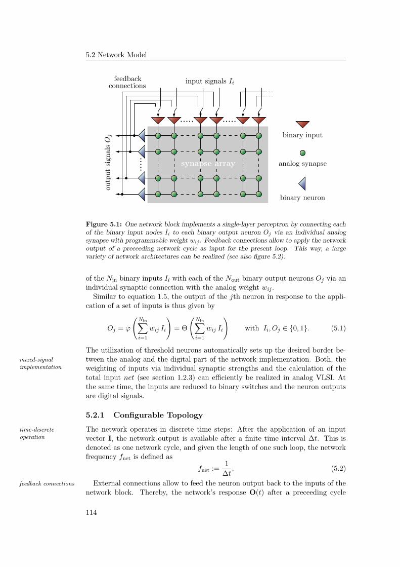
5.2 Network Model
PSfrag replacements
binary input
binary neuron
analog synapse
feedbackconnections
outp
ut
sign
als
Oj
input signals Ii
synapse array
Figure 5.1: One network block implements a single-layer perceptron by connecting eachof the binary input nodes Ii to each binary output neuron Oj via an individual analogsynapse with programmable weight wij . Feedback connections allow to apply the networkoutput of a preceeding network cycle as input for the present loop. This way, a largevariety of network architectures can be realized (see also figure 5.2).
of the Nin binary inputs Ii with each of the Nout binary output neurons Oj via anindividual synaptic connection with the analog weight wij .
Similar to equation 1.5, the output of the jth neuron in response to the appli-cation of a set of inputs is thus given by
Oj = ϕ
(Nin∑
i=1
wij Ii
)= Θ
(Nin∑
i=1
wij Ii
)with Ii, Oj ∈ 0, 1. (5.1)
The utilization of threshold neurons automatically sets up the desired border be-tween the analog and the digital part of the network implementation. Both, themixed-signal
implementation weighting of inputs via individual synaptic strengths and the calculation of thetotal input net (see section 1.2.3) can efficiently be realized in analog VLSI. Atthe same time, the inputs are reduced to binary switches and the neuron outputsare digital signals.
5.2.1 Configurable Topology
The network operates in discrete time steps: After the application of an inputtime-discreteoperation vector I, the network output is available after a finite time interval ∆t. This is
denoted as one network cycle, and given the length of one such loop, the networkfrequency fnet is defined as
fnet :=1
∆t. (5.2)
External connections allow to feed the neuron output back to the inputs of thefeedback connections
network block. Thereby, the network’s response O(t) after a preceeding cycle
114
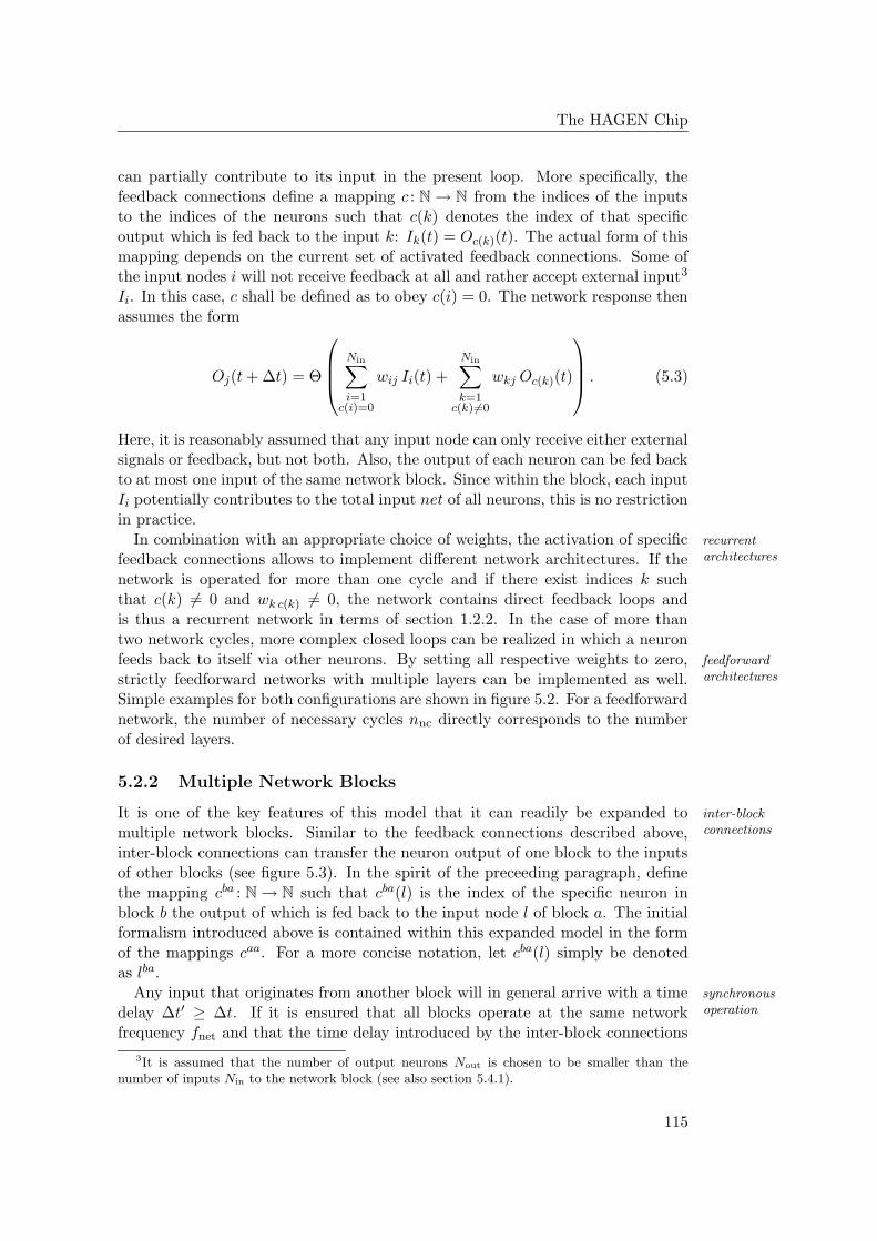
The HAGEN Chip
can partially contribute to its input in the present loop. More specifically, thefeedback connections define a mapping c : N → N from the indices of the inputsto the indices of the neurons such that c(k) denotes the index of that specificoutput which is fed back to the input k: Ik(t) = Oc(k)(t). The actual form of thismapping depends on the current set of activated feedback connections. Some ofthe input nodes i will not receive feedback at all and rather accept external input3
Ii. In this case, c shall be defined as to obey c(i) = 0. The network response thenassumes the form
Oj(t + ∆t) = Θ
Nin∑
i=1c(i)=0
wij Ii(t) +
Nin∑
k=1c(k)6=0
wkj Oc(k)(t)
. (5.3)
Here, it is reasonably assumed that any input node can only receive either externalsignals or feedback, but not both. Also, the output of each neuron can be fed backto at most one input of the same network block. Since within the block, each inputIi potentially contributes to the total input net of all neurons, this is no restrictionin practice.
In combination with an appropriate choice of weights, the activation of specific recurrentarchitecturesfeedback connections allows to implement different network architectures. If the
network is operated for more than one cycle and if there exist indices k suchthat c(k) 6= 0 and wk c(k) 6= 0, the network contains direct feedback loops andis thus a recurrent network in terms of section 1.2.2. In the case of more thantwo network cycles, more complex closed loops can be realized in which a neuronfeeds back to itself via other neurons. By setting all respective weights to zero, feedforward
architecturesstrictly feedforward networks with multiple layers can be implemented as well.Simple examples for both configurations are shown in figure 5.2. For a feedforwardnetwork, the number of necessary cycles nnc directly corresponds to the numberof desired layers.
5.2.2 Multiple Network Blocks
It is one of the key features of this model that it can readily be expanded to inter-blockconnectionsmultiple network blocks. Similar to the feedback connections described above,
inter-block connections can transfer the neuron output of one block to the inputsof other blocks (see figure 5.3). In the spirit of the preceeding paragraph, definethe mapping cba : N → N such that cba(l) is the index of the specific neuron inblock b the output of which is fed back to the input node l of block a. The initialformalism introduced above is contained within this expanded model in the formof the mappings caa. For a more concise notation, let cba(l) simply be denotedas lba.
Any input that originates from another block will in general arrive with a time synchronousoperationdelay ∆t′ ≥ ∆t. If it is ensured that all blocks operate at the same network
frequency fnet and that the time delay introduced by the inter-block connections
3It is assumed that the number of output neurons Nout is chosen to be smaller than thenumber of inputs Nin to the network block (see also section 5.4.1).
115
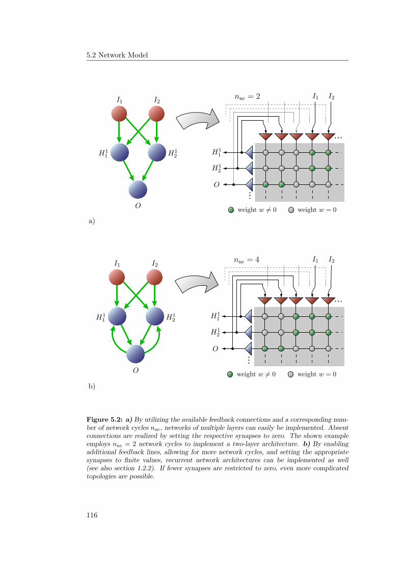
5.2 Network Model
PSfrag replacements
I1I1I2I2
H11H1
1
H12
H12
O
O
a)
nnc = 2
weight w = 0weight w 6= 0
PSfrag replacements
I1I1I2I2
H11H1
1 H12
H12
O
O
b)
nnc = 4
weight w = 0weight w 6= 0
Figure 5.2: a) By utilizing the available feedback connections and a corresponding num-ber of network cycles nnc, networks of multiple layers can easily be implemented. Absentconnections are realized by setting the respective synapses to zero. The shown exampleemploys nnc = 2 network cycles to implement a two-layer architecture. b) By enablingadditional feedback lines, allowing for more network cycles, and setting the appropriatesynapses to finite values, recurrent network architectures can be implemented as well(see also section 1.2.2). If fewer synapses are restricted to zero, even more complicatedtopologies are possible.
116
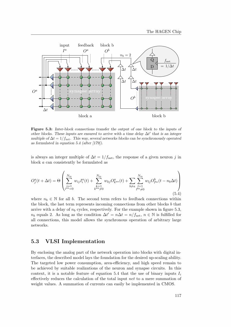
The HAGEN ChipPSfrag replacements
Q
D
block a block b
fnet
= 1/∆t
∆t
∆t∆t
∆t∆t
nb = 2Oa
Oa
Ob
ObIa
feedback block binput
synapse array
synapse array
Figure 5.3: Inter-block connections transfer the output of one block to the inputs ofother blocks. These inputs are ensured to arrive with a time delay ∆t′ that is an integermultiple of ∆t = 1/fnet. This way, several networks blocks can be synchronously operatedas formulated in equation 5.4 (after [179]).
is always an integer multiple of ∆t = 1/fnet, the response of a given neuron j inblock a can consistently be formulated as
Oaj (t + ∆t) = Θ
Nin∑
i=1iaa=0
wijIai (t) +
Nin∑
k=1kaa 6=0
wkjOakaa(t) +
∑
b6=a
Nin∑
l=1lba 6=0
wljOblba(t − nb∆t)
(5.4)where nb ∈ N for all b. The second term refers to feedback connections withinthe block, the last term represents incoming connections from other blocks b thatarrive with a delay of nb cycles, respectively. For the example shown in figure 5.3,nb equals 2. As long as the condition ∆t′ = n∆t = n/fnet, n ∈ N is fulfilled forall connections, this model allows the synchronous operation of arbitrary largenetworks.
5.3 VLSI Implementation
By enclosing the analog part of the network operation into blocks with digital in-terfaces, the described model lays the foundation for the desired up-scaling ability.The targeted low power consumption, area-efficiency, and high speed remain tobe achieved by suitable realizations of the neuron and synapse circuits. In thiscontext, it is a notable feature of equation 5.4 that the use of binary inputs Ii
effectively reduces the calculation of the total input net to a mere summation ofweight values. A summation of currents can easily be implemented in CMOS.
117
5.3 VLSI Implementation
5.3.1 Binary Neurons, Trainability, and VLSI Design Implica-tions
Many hardware implementations of feedforward networks do not restrict them-multi-valued inputs
selves to binary inputs and outputs. If the inherent parallelism in the networkoperation is to be fully exploited, the necessary multiplier circuits do in this casehave to be incorporated within each synapse [79]. This naturally leads to increasedarea requirements of the synapse implementations. Another disadvantage of thisapproach is the difficulty for analog multiplier circuits to achieve simultaneouslya high dynamic range, a good noise resistance and a low power consumption [79].
Multi-valued inputs can be simulated by using binary inputs in connection withappropriately dimensioned weights as will be described in section 8.2.2. In sofar, the use of binary input nodes does not inhibit the processing of multi-valuedinputs. At the same time, it allows to reduce the complexity of the synapticcircuits and thus promotes smaller and faster synapse implementations.
There is another important advantage of using binary inputs that arises from theanalog multiplication
fact that an analog summation is only affected by additive offset mismatches [122].In contrast, analog multiplication potentially suffers from offsets in the inputs aswell as additional variations in the gain. A purely additive offset can easily be com-pensated, since it is independent of the inputs and the weights (see section 5.5).This does not hold for the gain and offset mismatches in a multiplication cir-cuit [144].
Nevertheless, the use of binary neurons also restricts the range of suitable train-training networks ofthreshold neurons ing approaches: It has been discussed in section 2.2.2 that due to the credit
assignment problem, the formulation of efficient training algorithms for networksof simple threshold neurons with more than one layer remains a considerable chal-lenge. The popular backpropagation training algorithm for multi-layer networks(section 2.2.2) vitally depends on the neurons to exhibit a continuous output andis thus not viable in this case. But it has repeatedly been motivated (chapters 2, 3,and 4) that adequate black-box optimization strategies, most notably evolutionaryalgorithms, can successfully be utilized for this kind of task.
The efficient application of these highly iterative generate-and-test approachesbenefits ofchip-in-the-looptraining
requires a high speed of the network operation. On the other hand, when being im-plemented either on-chip or as chip-in-the-loop training, evolutionary algorithmscan adequately cope with potential device mismatches and high noise levels. Con-sequently, a network implementation that is intended for use in conjunction withevolutionary algorithms or other model-free strategies should be able to exploitthe small feature sizes of contemporary CMOS technologies to the fullest withoutrunning the risk of compromising its trainability.
Finally, striving to benefit from the high degree of parallelism that is inherent inlocal weight storage
the concepts of neural information processing does not only imply to include thenecessary computational circuitry within each single synapse. It also requires thesynapses to have direct access to their predetermined weight values and thus toincorporate an adequate means of weight storage into the synapse implementation.
118
The HAGEN Chip
5.3.2 Circuit Design
The proposed synapse and neuron circuits are designed in consideration of the mixed-mode operation
above conclusions and are schematically illustrated in figure 5.4. The synapsecombines voltage mode and current mode operation: While the postsynaptic ac-tivity is represented by a current Ips( | w | ) > 0 that is sank into the synapseaccording to the absolute value of its weight w, the weight value itself is stored ascharge on a capacitor. On a general level, the synapse acts like a voltage controlledcurrent sink (for details see [179]).
The sign of the weight is stored in a dynamic latch. Depending on the state of excitatory andinhibitory currentsthis latch, a synapse is either connected to the excitatory line I+ or the inhibitory
line I− of the postsynaptic neuron. By virtue of Kirchhoff’s law, the total exci-tatory and inhibitory input currents Ipos and Ineg to the neuron that result fromthe contribution of all its activated synapses become
Ineg =∑
i
Ips( |wi |) ∀ i ∈ j | wj < 0 (5.5)
Ipos =∑
i
Ips( |wi |) ∀ i ∈ j | wj > 0 (5.6)
As long as the input node of a specific synapse is not activated, it gets connectedto the third current line Ipark (see next section). The Resistors R+ and R− ofthe neuron circuit convert the respective sums of the excitatory and inhibitorycurrents to voltages Upos and Uneg according to Ohm’s law:
Uneg = Vdd − R− · Ineg (5.7)
Upos = Vdd − R+ · Ipos (5.8)
A comparator amplifies the resulting difference Upos − Uneg to logic levels.
5.3.3 Implementation Properties
Since the synapses continuously sink a current to either I+ I− or Ipark, the power constant powerconsumptionconsumption of this design is independent of the input activity and solely deter-
mined by the programmed weights. From a technical point of view, a constantpower consumption is advantageous in so far as it also implies a constant tem-perature and thus largely avoids temperature induced side effects on the circuitoperation. Besides that, it suppresses power supply noise [178]. Finally, the cho-sen concept allows to adjust the overall power consumption via the programmingof appropriate weights.
The proposed weight storage circuit not only fulfills the demands for a small, weight storage andweight refreshfast, and energy-saving synapse as well as a truly parallel synapse operation. It
also admits frequent changes in the weight values, e.g., during training. On theother hand, leakage currents in the synapse circuit will cause the weight capacitorto discharge over time. The actual time scale on which these weight deteriorationeffects measurably occur depends on the utilized CMOS process. In the explicitcase of the 0.35 µm process used for the HAGEN prototype, the leakage time isin the order of 10 to 100 ms and therefore several orders of magnitude larger than
119
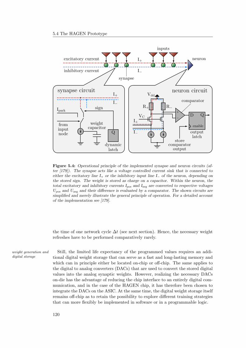
5.4 The HAGEN Prototype
+
-
PSfrag replacements
excitatory current
inhibitory current
synapse
synapse circuit neuron circuit
neuron
inputs
Q
Q
D
I+
I+
I+
I−
I−
I−
Ipark
Vdd
R+ R−
VC
sign
weightcapacitor enablefrom
inputnode
dynamic
latch
latch
storecomparator
comparator
output
output
Figure 5.4: Operational principle of the implemented synapse and neuron circuits (af-ter [179]). The synapse acts like a voltage controlled current sink that is connected toeither the excitatory line I+ or the inhibitory input line I− of the neuron, depending onthe stored sign. The weight is stored as charge on a capacitor. Within the neuron, thetotal excitatory and inhibitory currents Ipos and Ineg are converted to respective voltagesUpos and Uneg and their difference is evaluated by a comparator. The shown circuits aresimplified and merely illustrate the general principle of operation. For a detailed accountof the implementation see [179].
the time of one network cycle ∆t (see next section). Hence, the necessary weightrefreshes have to be performed comparatively rarely.
Still, the limited life expectancy of the programmed values requires an addi-weight generation anddigital storage tional digital weight storage that can serve as a fast and long-lasting memory and
which can in principle either be located on-chip or off-chip. The same applies tothe digital to analog converters (DACs) that are used to convert the stored digitalvalues into the analog synaptic weights. However, realizing the necessary DACson-die has the advantage of reducing the chip interface to an entirely digital com-munication, and in the case of the HAGEN chip, it has therefore been chosen tointegrate the DACs on the ASIC. At the same time, the digital weight storage itselfremains off-chip as to retain the possibility to explore different training strategiesthat can more flexibly be implemented in software or in a programmable logic.
120
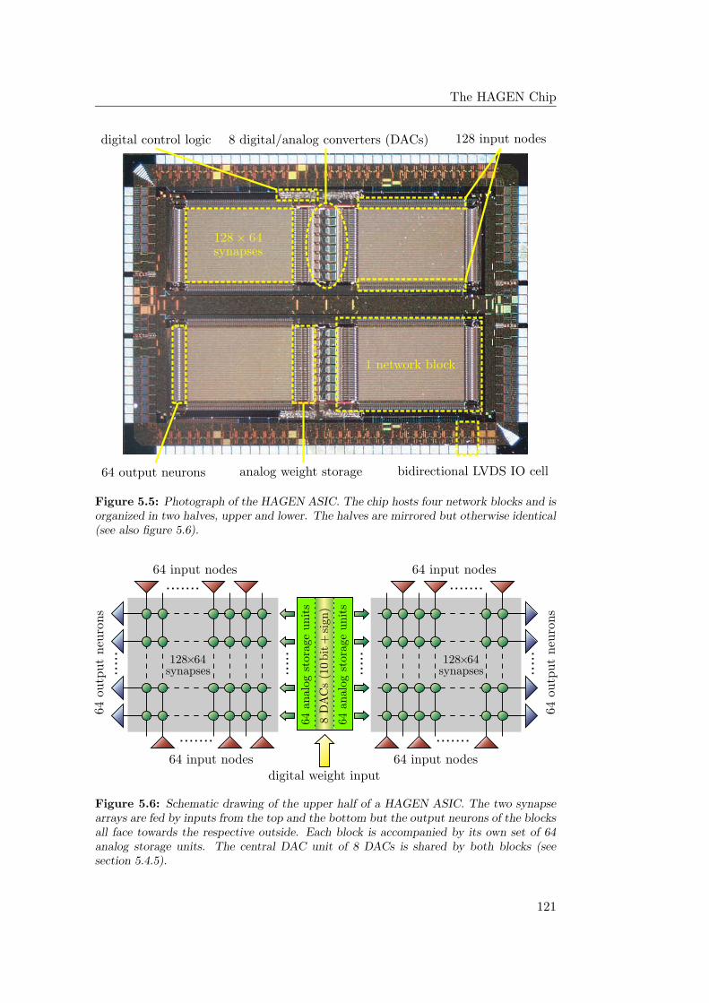
The HAGEN Chip
PSfrag replacements
digital control logic 8 digital/analog converters (DACs) 128 input nodes
64 output neurons analog weight storage bidirectional LVDS IO cell
128 × 64synapses
1 network block
Figure 5.5: Photograph of the HAGEN ASIC. The chip hosts four network blocks and isorganized in two halves, upper and lower. The halves are mirrored but otherwise identical(see also figure 5.6).
PSfrag replacements
64 input nodes
64 input nodes
64 input nodes
64 input nodes
64ou
tput
neu
rons
64ou
tput
neu
rons
digital weight input
64an
alog
stor
age
units
64an
alog
stor
age
units
8D
AC
s(1
0bit
+si
gn)
128×64128×64synapsessynapses
Figure 5.6: Schematic drawing of the upper half of a HAGEN ASIC. The two synapsearrays are fed by inputs from the top and the bottom but the output neurons of the blocksall face towards the respective outside. Each block is accompanied by its own set of 64analog storage units. The central DAC unit of 8 DACs is shared by both blocks (seesection 5.4.5).
121
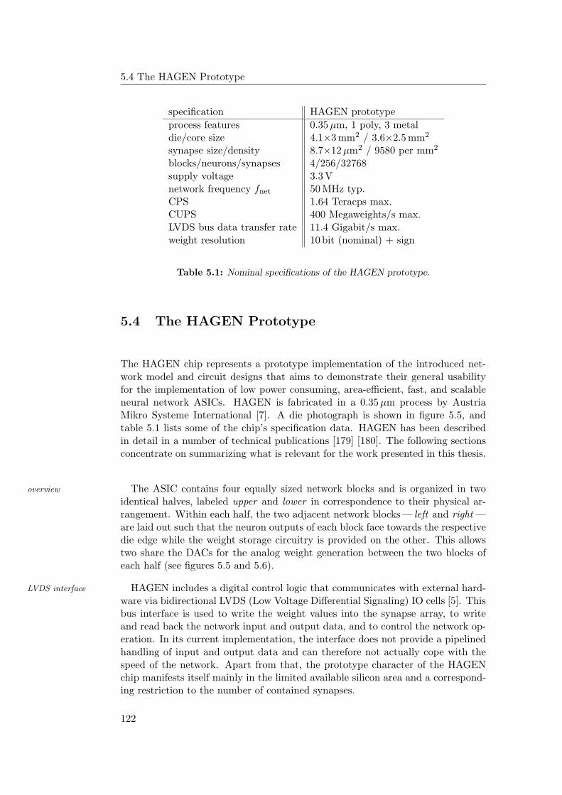
5.4 The HAGEN Prototype
specification HAGEN prototype
process features 0.35 µm, 1 poly, 3 metaldie/core size 4.1×3 mm2 / 3.6×2.5 mm2
synapse size/density 8.7×12 µm2 / 9580 per mm2
blocks/neurons/synapses 4/256/32768supply voltage 3.3 Vnetwork frequency fnet 50 MHz typ.CPS 1.64 Teracps max.CUPS 400 Megaweights/s max.LVDS bus data transfer rate 11.4 Gigabit/s max.weight resolution 10 bit (nominal) + sign
Table 5.1: Nominal specifications of the HAGEN prototype.
5.4 The HAGEN Prototype
The HAGEN chip represents a prototype implementation of the introduced net-work model and circuit designs that aims to demonstrate their general usabilityfor the implementation of low power consuming, area-efficient, fast, and scalableneural network ASICs. HAGEN is fabricated in a 0.35 µm process by AustriaMikro Systeme International [7]. A die photograph is shown in figure 5.5, andtable 5.1 lists some of the chip’s specification data. HAGEN has been describedin detail in a number of technical publications [179] [180]. The following sectionsconcentrate on summarizing what is relevant for the work presented in this thesis.
The ASIC contains four equally sized network blocks and is organized in twooverview
identical halves, labeled upper and lower in correspondence to their physical ar-rangement. Within each half, the two adjacent network blocks — left and right —are laid out such that the neuron outputs of each block face towards the respectivedie edge while the weight storage circuitry is provided on the other. This allowstwo share the DACs for the analog weight generation between the two blocks ofeach half (see figures 5.5 and 5.6).
HAGEN includes a digital control logic that communicates with external hard-LVDS interface
ware via bidirectional LVDS (Low Voltage Differential Signaling) IO cells [5]. Thisbus interface is used to write the weight values into the synapse array, to writeand read back the network input and output data, and to control the network op-eration. In its current implementation, the interface does not provide a pipelinedhandling of input and output data and can therefore not actually cope with thespeed of the network. Apart from that, the prototype character of the HAGENchip manifests itself mainly in the limited available silicon area and a correspond-ing restriction to the number of contained synapses.
122
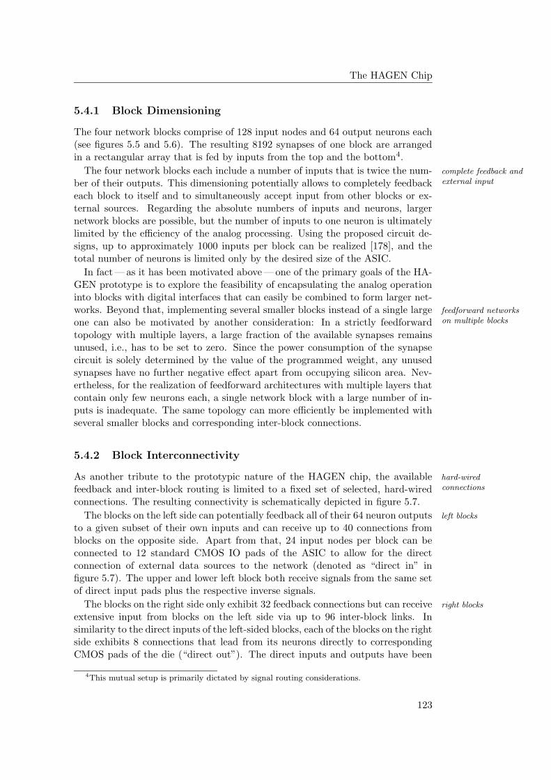
The HAGEN Chip
5.4.1 Block Dimensioning
The four network blocks comprise of 128 input nodes and 64 output neurons each(see figures 5.5 and 5.6). The resulting 8192 synapses of one block are arrangedin a rectangular array that is fed by inputs from the top and the bottom4.
The four network blocks each include a number of inputs that is twice the num- complete feedback andexternal inputber of their outputs. This dimensioning potentially allows to completely feedback
each block to itself and to simultaneously accept input from other blocks or ex-ternal sources. Regarding the absolute numbers of inputs and neurons, largernetwork blocks are possible, but the number of inputs to one neuron is ultimatelylimited by the efficiency of the analog processing. Using the proposed circuit de-signs, up to approximately 1000 inputs per block can be realized [178], and thetotal number of neurons is limited only by the desired size of the ASIC.
In fact — as it has been motivated above — one of the primary goals of the HA-GEN prototype is to explore the feasibility of encapsulating the analog operationinto blocks with digital interfaces that can easily be combined to form larger net-works. Beyond that, implementing several smaller blocks instead of a single large feedforward networks
on multiple blocksone can also be motivated by another consideration: In a strictly feedforwardtopology with multiple layers, a large fraction of the available synapses remainsunused, i.e., has to be set to zero. Since the power consumption of the synapsecircuit is solely determined by the value of the programmed weight, any unusedsynapses have no further negative effect apart from occupying silicon area. Nev-ertheless, for the realization of feedforward architectures with multiple layers thatcontain only few neurons each, a single network block with a large number of in-puts is inadequate. The same topology can more efficiently be implemented withseveral smaller blocks and corresponding inter-block connections.
5.4.2 Block Interconnectivity
As another tribute to the prototypic nature of the HAGEN chip, the available hard-wiredconnectionsfeedback and inter-block routing is limited to a fixed set of selected, hard-wired
connections. The resulting connectivity is schematically depicted in figure 5.7.
The blocks on the left side can potentially feedback all of their 64 neuron outputs left blocks
to a given subset of their own inputs and can receive up to 40 connections fromblocks on the opposite side. Apart from that, 24 input nodes per block can beconnected to 12 standard CMOS IO pads of the ASIC to allow for the directconnection of external data sources to the network (denoted as “direct in” infigure 5.7). The upper and lower left block both receive signals from the same setof direct input pads plus the respective inverse signals.
The blocks on the right side only exhibit 32 feedback connections but can receive right blocks
extensive input from blocks on the left side via up to 96 inter-block links. Insimilarity to the direct inputs of the left-sided blocks, each of the blocks on the rightside exhibits 8 connections that lead from its neurons directly to correspondingCMOS pads of the die (“direct out”). The direct inputs and outputs have been
4This mutual setup is primarily dictated by signal routing considerations.
123
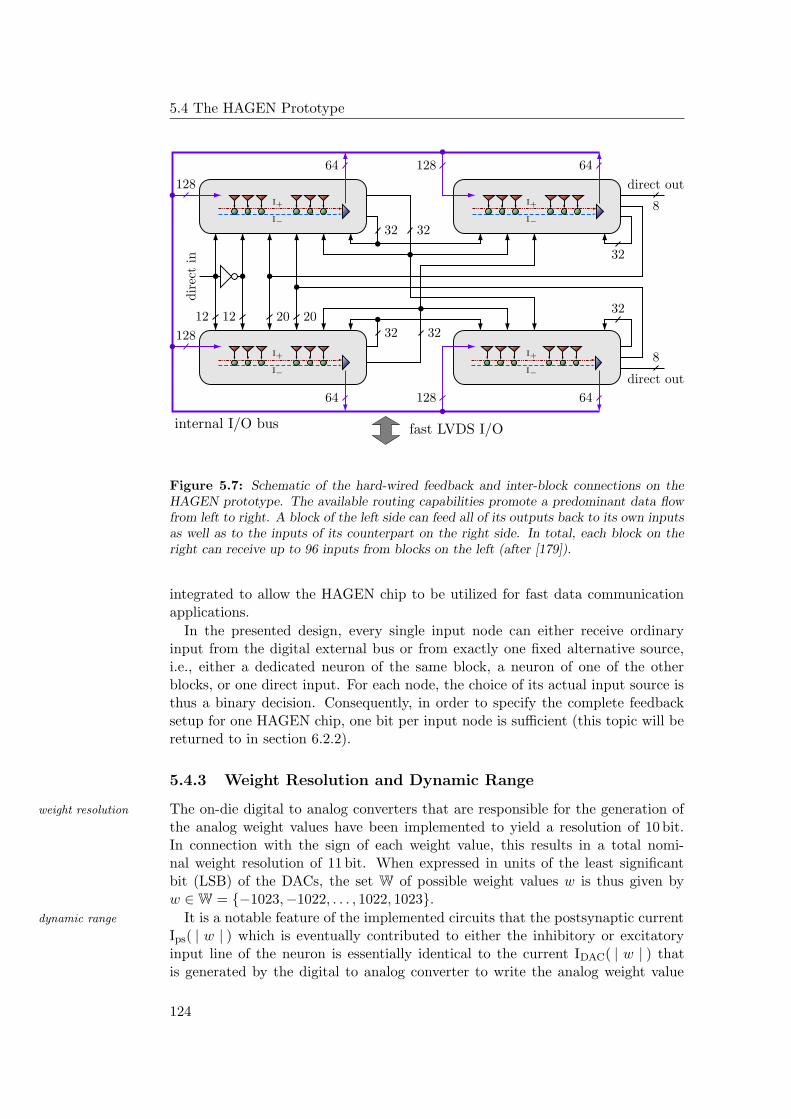
5.4 The HAGEN Prototype
PSfrag replacements
8
8
1212 20 2032
32
3232
3232
64
6464
64
128
128
128
128
dir
ect
in
direct out
direct out
internal I/O bus fast LVDS I/O
I+ I+
I+I+
I−
I−
I−
I−
Figure 5.7: Schematic of the hard-wired feedback and inter-block connections on theHAGEN prototype. The available routing capabilities promote a predominant data flowfrom left to right. A block of the left side can feed all of its outputs back to its own inputsas well as to the inputs of its counterpart on the right side. In total, each block on theright can receive up to 96 inputs from blocks on the left (after [179]).
integrated to allow the HAGEN chip to be utilized for fast data communicationapplications.
In the presented design, every single input node can either receive ordinaryinput from the digital external bus or from exactly one fixed alternative source,i.e., either a dedicated neuron of the same block, a neuron of one of the otherblocks, or one direct input. For each node, the choice of its actual input source isthus a binary decision. Consequently, in order to specify the complete feedbacksetup for one HAGEN chip, one bit per input node is sufficient (this topic will bereturned to in section 6.2.2).
5.4.3 Weight Resolution and Dynamic Range
The on-die digital to analog converters that are responsible for the generation ofweight resolution
the analog weight values have been implemented to yield a resolution of 10 bit.In connection with the sign of each weight value, this results in a total nomi-nal weight resolution of 11 bit. When expressed in units of the least significantbit (LSB) of the DACs, the set W of possible weight values w is thus given byw ∈ W = −1023,−1022, . . . , 1022, 1023.
It is a notable feature of the implemented circuits that the postsynaptic currentdynamic range
Ips( | w | ) which is eventually contributed to either the inhibitory or excitatoryinput line of the neuron is essentially identical to the current IDAC( | w | ) thatis generated by the digital to analog converter to write the analog weight value
124
The HAGEN Chip
into the synapse [179] (possible deviations will be discussed in section 5.5). Theeffective dynamic range of the synapse currents is therefore determined by thedynamic range of the DACs and can be adjusted externally. The synapse imple-mentation itself is designed for a maximum current Imax
ps = Ips(1023) of at most50 µA which corresponds to a resolution of approximately 50 nA. The comparatorof the neuron circuit also achieves a resolution of 50 nA and exhibits a dynamicrange of ±300 µA for each input line.
Hence, if the maximum synapse current Imaxps is set to the largest allowed value, neuron saturation
six activated synapses with maximum weights that are all connected to either I+or I− will cause the respective neuron input branch to reach saturation. Thisis deemed to be no severe restriction in practice: First, in common networks,synapses with maximum weight are expected to be the exception rather than therule. Second, for most of the time, only parts of the neuron inputs will be activatedsimultaneously. Finally, chip-in-the-loop training algorithms can automaticallyaccount for these general restrictions and adjust the magnitudes of the weightvalues accordingly.
Apart from that, Imaxps is usually chosen to be smaller than the allowed max- dynamic range and
noiseimum value. This is not only reasonable with respect to a better exploitationof the dynamic range of the neuron, but also yields a lower power consumption(section 5.3.3). On the other hand, changes in the dynamic range of the synapsecurrent also affect its signal to noise ratio and thereby influence the effective res-olution of the synaptic weights (see section 5.5.4).
5.4.4 Weight Configuration
A network block cannot be used for data processing while its weights are written.Therefore, a fast weight transfer is desired. Each of the respective DAC units thatare located between the two opposing blocks of the upper and lower half (see fig-ure 5.6) comprises of 8 single digital to analog converters. Each one of these DACsis employed for the conversion of the synaptic weights of 2 · 8 neurons, 8 in eachof the two adjacent network blocks. This setup constitutes a compromise betweenthe resulting area consumption and the maximum achievable weight update rate.
The analog values of the single weights are written into the synapse array accord- two stage setup
ing to a column-wise pattern. In order to retain a high transfer speed, a two stagestructure is employed and combined with an alternating transfer scheme [179]:Every DAC has two banks of digital input latches that are capable of the fullspeed of the LVDS interface. While the DAC converts the weights for one block,the buffers for the other side can already be filled with the corresponding digitalweight values. Furthermore, each DAC is accompanied by 2 · 8 analog storageunits, 8 per side. Unlike the sign bits of the weights that are transferred directlyinto the synapses of the currently served column, the analog weight values are firstwritten into these current memory units. Once all eight buffers are filled, theircontents are finally being transferred into the respective synapses. Simultaneously,the DACs can fill the analog storage units of the opposite side.
The conversion time of a single digital to analog converter is 40 ns. With eightDACs, eight conversion cycles are necessary to fill the 64 current memories of one
125
5.4 The HAGEN Prototype
side. The implemented circuitry can transfer the analog weights from the cur-rent storage units into the synapses within 320 ns. Together with the alternatingscheme described above, this allows for a continuous DAC operation.
In summary, the weights of all 32768 synapses of all four blocks on a HAGENhigh configurationalspeed chip can be updated within 82 µs which corresponds to a maximum achievable
CUPS value during training (section 2.4.3) of about 400 Megaweights/s. Using aweight refresh rate of 10 ms, the network speed is thus reduced by less than 1 %.
5.4.5 Performance and Scalability
The network operates at a maximum frequency fnet of 50 MHz. Assuming that ahigh network speed
given network configuration can fully exploit the parallel operation of one block,the resulting performance becomes
8192 synapses · 50 MHz = 4.1·1011 CPS. (5.9)
A direct comparison to standard microprocessors is not unproblematic, since thecomparison tostandardmicroprocessors
utilized 0.35 µm process has been used by manufacturers in the years around1995–1997. At the time of writing of this thesis, contemporary microprocessorsof commercially available PCs have become strong competitors in terms of mereperformance. Consider the exemplary case of a 3.6 GHz processor with SIMD(Single Instruction, Multiple Data), e.g. a 0.09 µm Pentium IV processor. If it isassumed that an optimum of eight 16-bit integer instructions can be performedin each clock-cycle and that the processor is used to simulate the operationalprinciples of the HAGEN block, the resulting performance turns out to be
8 integer additions · 3.6 GHz = 2.88·1010 CPS. (5.10)
It is understood that the 16 bit precision of the used integer representation isnot the most efficient way to code the 11 bit weights of HAGEN. But even interms of the achievable connection primitives per second (see section 2.4.3), theperformance of a HAGEN block and the Pentium IV microprocessor become4.5·1012 CPPS and 4.6·1011 CPPS, respectively.
Besides providing a gain in computational performance of about one order oflow powerconsumption magnitude, the second main advantage of the neural hardware approach is given by
its superior power efficiency: While the peak power consumption of a Pentium IVis in the order of 100 W, a single HAGEN block reaches a maximum of onlyapproximately 1 W [179] [178]. Achieving a two orders of magnitude lower powerconsumption particularly facilitates the efficient realization of large networks.
Admittedly, these are rather coarse calculations. The above considerations areprimarily intended to convey a general feeling for the high potential of the conceptsthat underlie the desing of the HAGEN prototype. A thorough discussion of thecomputational performance and power consumption of the HAGEN ASIC liesbeyond the scope of this thesis. A more detailed account of these topics can befound in [185].
The utilized network model (equation 5.1) allows for a feasible up-scaling offeasible up-scaling
the implemented networks not only by integrating more network blocks on future
126
The HAGEN Chip
ASICs or by increasing the size of the blocks itself. The digital chip interfacein connection with the clocked network operation and the fast LVDS bus readilyallows to distribute suitable neural network architectures over multiple intercon-nected HAGEN chips [52]. As long as it can be ensured that connections fromnetwork blocks on different ASICs always retain a time delay ∆t′ that is an integermultiple of the time of one network cycle ∆t = 1/fnet, the synchronous operationof the whole network is ensured (see equation 5.4). A corresponding hardwaresetup will briefly be introduced in section 6.3.
5.5 Network Calibration
The presented synapse and neuron circuit implementations ensure that the device motivation
mismatches introduced during manufacturing of the ASIC primarily lead to mereadditive offsets in the analog operation [179]. Hence, the major part of the staticvariations can be compensated for by adequately modifying the desired weightsbefore they are programmed into the synapse arrays. Within certain limitations,this even allows to train the networks off-chip. While for some applications, thismight be a feasible or even necessary alternative to chip-in-the-loop training ap-proaches, the main motivation to calibrate the static variations of the used networkASIC is the ability to transfer the obtained sets of weights from one chip to an-other without a severe loss in performance. In any case, detailed knowledge of thesources and magnitudes of the involved offsets is required.
5.5.1 Types of Fixed Pattern Offsets
Three types of static variations can be distinguished that affect the calculation ofthe network output:
Neuron offset The switching points of the single neurons do not consistentlyequal 0. In general, each neuron exhibits an individual threshold Inoff such that itwill only be activated if Ipos−Ineg ≥ Inoff and remain inactivated otherwise. Theseneuron offsets can be be positive or negative.
An easy way to compensate for this deviation is to reserve one column of neuron calibration
synapses per block for the neuron calibration: The corresponding input nodeis permanently activated and the synapses are each assigned an individual weightσnoff , such that the resulting synaptic current equals the offset Inoff of their re-spective neuron. Regarding only the contributions I′pos and I′neg of the remainingsynapses, the firing condition of a given neuron then becomes I′pos − I′neg ≥ 0 asdesired. Hence, while the calibration of the neuron offset is comparably unprob-lematic, it effectively reduces the available inputs of a block to 127 (or less, seesection 5.5.4).
Weight generation error A second type of of static deviation has its origin inthe special operation of the on-chip DACs (see sections 5.4.3 and 5.4.4). In order tospeed up the transfer of the generated weight to the intermediate current memory,
127
5.5 Network Calibration
a fixed offset has to be added to its analog value (for technical details see [179]).Dedicated circuitry is included in the weight generation unit that accounts forthis effect by subtracting the temporary offset before the desired weight value iseventually written into the synapse. But due to the present device variations,this compensation is not entirely perfect, and a small deviation from the originalweight remains. Although this effect is the result of an imprecise operation of thecompensation circuit rather than being caused by the DAC itself, it shall in thefollowing be denoted as DAC offset for simplicity.
The DAC offset can be positive or negative and its exact magnitude cannot reli-ably and exactly be predicted in advance. But since all synapses of a given neuronare served by the same DAC, they all suffer from the same, initially unknown offset∆IDAC. If w is the desired weight expressed in LSB units, the actually generatedcurrent IDAC(|w|) that is written into the synapse via the current memory buffer(section 5.4.4) obeys
IDAC( |w|) = J( |w|) + ∆IDAC. (5.11)
Here, J(w) is the part of the DAC output that is exclusively determined by theprogrammed weight and fulfills J(0) = 0.
Individual synapse offset In addition to the above deviation which is the samefor all synapses of a given neuron, each single synapse exhibits its own individualoffset due to charge injection [4] [179]. The postsynaptic current Ips( | w | ) thatis eventually contributed to either the inhibitory or excitatory input line of theneuron will differ from the generated value IDAC(|w|) (see equation 5.11) accordingto
Ips( |w|) = IDAC( |w|) + ∆Isyn. (5.12)
The offsets ∆Isyn are generally positive. Furthermore, considering all synapsesof one specific neuron, the single values ∆Isyn can be described in terms of arow-specific mean offset ∆Iavg
syn and an individual offset ∆Iindsyn:
Ips( |w|) = IDAC( |w|) + ∆Iavgsyn + ∆Iind
syn (5.13)
While the DAC offset ∆IDAC and the individual synapse offset ∆Iindsyn can be posi-
tive or negative, the absolute value of their sum is guaranteed to be smaller thanthe row-wise synapse offset mean, |∆IDAC + ∆Iind
syn |< ∆Iavgsyn. In other words, the
resulting total deviation
∆I = IDAC + ∆Iavgsyn + ∆Iind
syn > 0 (5.14)
remains to be always positive. Depending on whether a synapse is connected toI+ or I−, the excitatory or inhibitory effect of the synapse will be enlarged.
Regarding the different terms in equation 5.14, only the last summand dif-fers between the individual synapses. The first two offsets are common to allsynapses of a neuron and can therefore be combined to a row-specific mean offset∆Irow = IDAC + ∆Iavg
syn. In summary, the final postsynaptic current can then bewritten in the form
Ips( |w|) = J( |w|) + ∆Irow + ∆Iindsyn. (5.15)
128
The HAGEN Chip
The HAGEN prototype provides special functionality for the compensation of row-wise offsetcalibrationany deviations that are common to all synapses of a given neuron. Additional
dedicated circuitry is included in the weight storage setup that allows to store anexternally defined offset which is then automatically subtracted from all weightsthat are being copied from the intermediate current memories into the final synap-tic storage capacitances [179]. This circuitry can be used to balance the effect ofthe row-wise offsets ∆Irow, once their respective values have been determined.
Furthermore, given that the magnitudes of all individual synapse offsets ∆Iindsyn synapse offset
calibrationare known, they can in principle be compensated by subtracting correspondingvalues from the respective programmed weights w. Unlike in the cases of the neu-ron offsets and the row-specific deviations that can be accounted for by constantvalues and independently of the desired weights, the calibration of the individ-ual synaptic deviations requires to readjust every single value in each new set ofweights that is to be transferred into the synapse array. Such a procedure leadsto unwanted additional costs in the weight generation and is preferably avoided.
Finally, since the weight storage capacitor of a given synapse cannot be charged limitations
with less than no current at all, subtracting the necessary offset from the absolutevalue |w| of the desired weight must not yield a negative number. If this situationdoes occur, the weight value is reasonably set to zero. In other words, even if itis decided to calibrate the single synapse offsets individually, only those weightscan reliably and accurately be stored in the synapse array whose absolute valuesexceed a given threshold that is determined by the magnitude of the synapticfixed-pattern noise.
In either case, it is desired that the single synapse offsets are reasonably smalland therefore do not compromise the achievable resolution of the weights tooseverely. In order to verify that the HAGEN prototype fulfills this requirement —and to actually allow for the calibration of the chip — it is necessary to devisemeans of determining the magnitudes of the discussed types of offsets. This willbe the topic of the following sections.
5.5.2 Determining the Offset Values
The HAGEN ASIC does not provide any means for measuring the DAC output,the individual neuron thresholds, or the single weight values directly. The onlyinformation that is provided by the network is its response to a given input pat-tern. In the course of the work presented in this thesis, a calibration method hasbeen developed that allows to deduce the values of the above fixed pattern offsetssolely by evaluating how the neurons’ responses to a specific input depend on thespecified weight values.
The involved measurements are based on the following basic procedure: The basic setup
inputs of the examined block are deactivated entirely except for two selected nodes.For a given neuron, the two corresponding synapses are set to opposite weightvalues w and −w which would ideally result in Ipos = Ineg. In the general case,however, the individual effective offsets of the two synapses will cause the resultingtotal neuron input to be different from zero and the offset of the neuron will havemoved its threshold to negative or positive values. Consequently, the neuron may
129
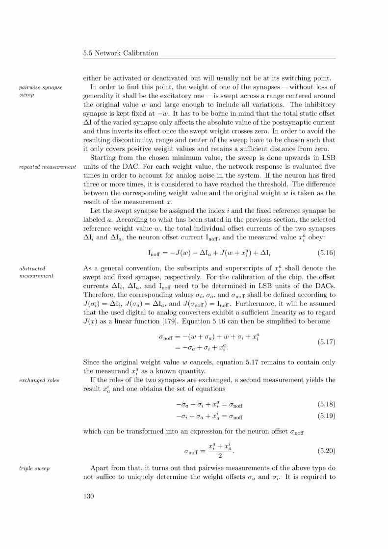
5.5 Network Calibration
either be activated or deactivated but will usually not be at its switching point.In order to find this point, the weight of one of the synapses — without loss ofpairwise synapse
sweep generality it shall be the excitatory one — is swept across a range centered aroundthe original value w and large enough to include all variations. The inhibitorysynapse is kept fixed at −w. It has to be borne in mind that the total static offset∆I of the varied synapse only affects the absolute value of the postsynaptic currentand thus inverts its effect once the swept weight crosses zero. In order to avoid theresulting discontinuity, range and center of the sweep have to be chosen such thatit only covers positive weight values and retains a sufficient distance from zero.
Starting from the chosen minimum value, the sweep is done upwards in LSBunits of the DAC. For each weight value, the network response is evaluated fiverepeated measurement
times in order to account for analog noise in the system. If the neuron has firedthree or more times, it is considered to have reached the threshold. The differencebetween the corresponding weight value and the original weight w is taken as theresult of the measurement x.
Let the swept synapse be assigned the index i and the fixed reference synapse belabeled a. According to what has been stated in the previous section, the selectedreference weight value w, the total individual offset currents of the two synapses∆Ii and ∆Ia, the neuron offset current Inoff , and the measured value xa
i obey:
Inoff = −J(w) − ∆Ia + J(w + xai ) + ∆Ii (5.16)
As a general convention, the subscripts and superscripts of xai shall denote theabstracted
measurement swept and fixed synapse, respectively. For the calibration of the chip, the offsetcurrents ∆Ii, ∆Ia, and Inoff need to be determined in LSB units of the DACs.Therefore, the corresponding values σi, σa, and σnoff shall be defined according toJ(σi) = ∆Ii, J(σa) = ∆Ia, and J(σnoff) = Inoff . Furthermore, it will be assumedthat the used digital to analog converters exhibit a sufficient linearity as to regardJ(x) as a linear function [179]. Equation 5.16 can then be simplified to become
σnoff = −(w + σa) + w + σi + xai
= −σa + σi + xai .
(5.17)
Since the original weight value w cancels, equation 5.17 remains to contain onlythe measurand xa
i as a known quantity.If the roles of the two synapses are exchanged, a second measurement yields theexchanged roles
result xia and one obtains the set of equations
−σa + σi + xai = σnoff (5.18)
−σi + σa + xia = σnoff (5.19)
which can be transformed into an expression for the neuron offset σnoff
σnoff =xa
i + xia
2. (5.20)
Apart from that, it turns out that pairwise measurements of the above type dotriple sweep
not suffice to uniquely determine the weight offsets σa and σi. It is required to
130
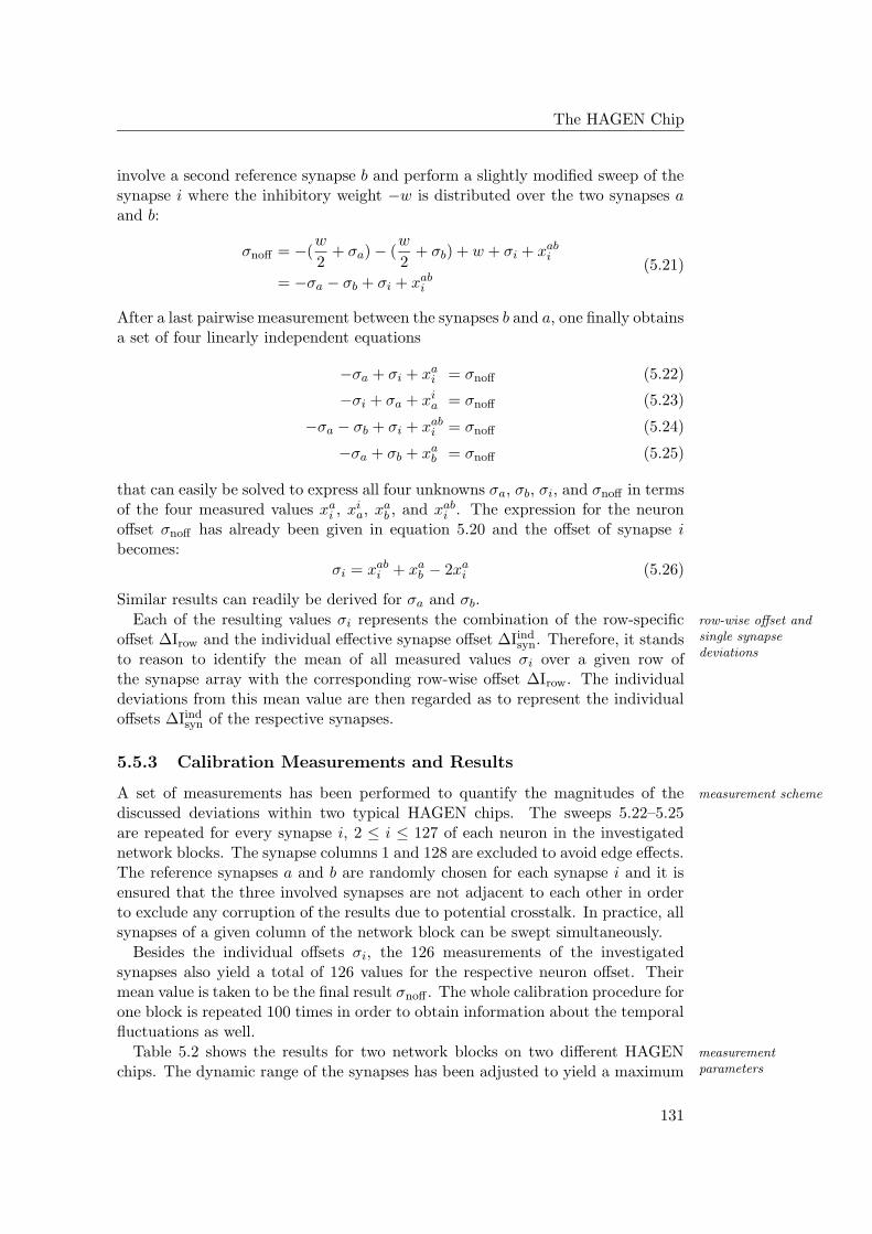
The HAGEN Chip
involve a second reference synapse b and perform a slightly modified sweep of thesynapse i where the inhibitory weight −w is distributed over the two synapses aand b:
σnoff = −(w
2+ σa) − (
w
2+ σb) + w + σi + xab
i
= −σa − σb + σi + xabi
(5.21)
After a last pairwise measurement between the synapses b and a, one finally obtainsa set of four linearly independent equations
−σa + σi + xai = σnoff (5.22)
−σi + σa + xia = σnoff (5.23)
−σa − σb + σi + xabi = σnoff (5.24)
−σa + σb + xab = σnoff (5.25)
that can easily be solved to express all four unknowns σa, σb, σi, and σnoff in termsof the four measured values xa
i , xia, xa
b , and xabi . The expression for the neuron
offset σnoff has already been given in equation 5.20 and the offset of synapse ibecomes:
σi = xabi + xa
b − 2xai (5.26)
Similar results can readily be derived for σa and σb.
Each of the resulting values σi represents the combination of the row-specific row-wise offset andsingle synapsedeviations
offset ∆Irow and the individual effective synapse offset ∆Iindsyn. Therefore, it stands
to reason to identify the mean of all measured values σi over a given row ofthe synapse array with the corresponding row-wise offset ∆Irow. The individualdeviations from this mean value are then regarded as to represent the individualoffsets ∆Iind
syn of the respective synapses.
5.5.3 Calibration Measurements and Results
A set of measurements has been performed to quantify the magnitudes of the measurement scheme
discussed deviations within two typical HAGEN chips. The sweeps 5.22–5.25are repeated for every synapse i, 2 ≤ i ≤ 127 of each neuron in the investigatednetwork blocks. The synapse columns 1 and 128 are excluded to avoid edge effects.The reference synapses a and b are randomly chosen for each synapse i and it isensured that the three involved synapses are not adjacent to each other in orderto exclude any corruption of the results due to potential crosstalk. In practice, allsynapses of a given column of the network block can be swept simultaneously.
Besides the individual offsets σi, the 126 measurements of the investigatedsynapses also yield a total of 126 values for the respective neuron offset. Theirmean value is taken to be the final result σnoff . The whole calibration procedure forone block is repeated 100 times in order to obtain information about the temporalfluctuations as well.
Table 5.2 shows the results for two network blocks on two different HAGEN measurementparameterschips. The dynamic range of the synapses has been adjusted to yield a maximum
131
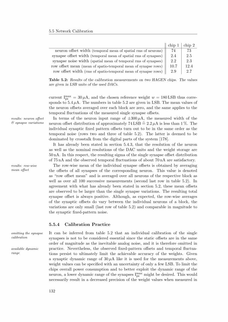
5.5 Network Calibration
chip 1 chip 2
neuron offset width (temporal mean of spatial rms of neurons) 74 73synapse offset width (temporal mean of spatial rms of synapses) 2.4 2.5synapse noise width (spatial mean of temporal rms of synapses) 2.2 2.3
row offset mean (mean of spatio-temporal mean of synapse rows) 10.7 12.4row offset width (rms of spatio-temporal mean of synapse rows) 2.9 2.7
Table 5.2: Results of the calibration measurements on two HAGEN chips. The valuesare given in LSB units of the used DACs.
current Imaxps = 30 µA, and the chosen reference weight w = 180 LSB thus corre-
sponds to 5.4 µA. The numbers in table 5.2 are given in LSB. The mean values ofthe neuron offsets averaged over each block are zero, and the same applies to thetemporal fluctuations of the measured single synapse offsets.
In terms of the neuron input range of ±300 µA, the measured width of theresults: neuron offset& synapse variations neuron offset distribution of approximately 74 LSB = 2.2 µA is less than 1 %. The
individual synaptic fixed pattern offsets turn out to be in the same order as thetemporal noise (rows two and three of table 5.2). The latter is deemed to bedominated by crosstalk from the digital parts of the system [178].
It has already been stated in section 5.4.3, that the resolution of the neuronas well as the nominal resolutions of the DAC units and the weight storage are50 nA. In this respect, the resulting sigma of the single synapse offset distributionof 75 nA and the observed temporal fluctuations of about 70 nA are satisfactory.
The row-wise mean of the individual synapse offsets is obtained by averagingresults: row-wisemean offset the offsets of all synapses of the corresponding neuron. This value is denoted
as “row offset mean” and is averaged over all neurons of the respective block aswell as over all 100 successive measurements (second last row in table 5.2). Inagreement with what has already been stated in section 5.2, these mean offsetsare observed to be larger than the single synapse variations. The resulting totalsynapse offset is always positive. Although, as expected, the row-wise averagesof the synaptic offsets do vary between the individual neurons of a block, thevariations are only small (last row of table 5.2) and comparable in magnitude tothe synaptic fixed-pattern noise.
5.5.4 Calibration Practice
It can be inferred from table 5.2 that an individual calibration of the singleomitting the synapsecalibration synapses is not to be considered essential since the static offsets are in the same
order of magnitude as the inevitable analog noise, and it is therefore omitted inpractice. Nevertheless, the observed fixed-pattern offsets and temporal fluctua-available dynamic
range tions persist to ultimately limit the achievable accuracy of the weights. Givena synaptic dynamic range of 30 µA like it is used for the measurements above,weight values can be specified with an uncertainty of only a few LSB. To limit thechips overall power consumption and to better exploit the dynamic range of theneuron, a lower dynamic range of the synapses Imax
ps might be desired. This wouldnecessarily result in a decreased precision of the weight values when measured in
132
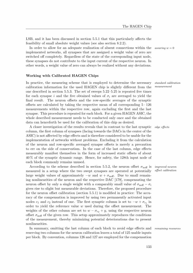
The HAGEN Chip
LSB, and it has been discussed in section 5.5.1 that this particularly affects thefeasibility of small absolute weight values (see also section 8.2.2).
In order to allow for an adequate realization of absent connections within the assuring w = 0
implemented networks, all synapses that are assigned a weight value of zero areswitched off completely. Regardless of the state of the corresponding input node,these synapses do not contribute to the input current of the respective neuron. Inother words, a weight value of zero can always be realized without any deviations.
Working with Calibrated HAGEN Chips
In practice, the measuring scheme that is employed to determine the necessary standard calibrationmeasurementcalibration information for the used HAGEN chip is slightly different from the
one described in section 5.5.3. The set of sweeps 5.22–5.25 is repeated five timesfor each synapse i and the five obtained values of σi are averaged to yield thefinal result. The neuron offsets and the row-specific averages of the synapticoffsets are calculated by taking the respective mean of all corresponding 5 · 126measurements within the respective row, again excluding the first and the lastsynapse. This procedure is repeated for each block. For a given HAGEN ASIC, thewhole described measurement needs to be conducted only once and the obtaineddata can henceforth be used for the calibration of this chip as desired.
A closer investigation of the results reveals that in contrast to the last synaptic edge effects
column, the first column of synapses (facing towards the DACs in the center of theASIC) is not affected by edge effects and is therefore considered to be usable for theimplementation of networks without problems. Excluding it from the calculationof the neuron and row-specific averaged synapse offsets is merely a precautionto err on the side of conservatism. In the case of the last column, edge effectsmeasurably manifest themselves in the form of increased static offsets of about40 % of the synaptic dynamic range. Hence, for safety, the 128th input node ofeach block commonly remains unused.
According to the scheme described in section 5.5.2, the neuron offset σnoff is improved neuronoffset calibrationmeasured in a setup where the two swept synapses are operated at potentially
large weight values of approximately −w and w + σnoff . Due to small remain-ing nonlinearities of the neuron and the respective DAC [179], compensating theneuron offset by only a single weight with a comparably small value of σnoff − σi
gives rise to slight but measurable deviations. Therefore, the proposed procedurefor the neuron offset calibration (section 5.5.1) is modified in practice: The accu-racy of the compensation is improved by using two permanently activated inputnodes c1 and c2 instead of one. The first synaptic column is set to −w + σc1 inorder to yield the reference value w used during the offset measurement. Theweights of the other column are set to w − σc2 + y, using the respective neuronoffset σnoff of the given row. This setup approximately reproduces the conditionsof the measurement, thereby minimizing potential deteriorations due to presentnonlinearities.
In summary, omitting the last column of each block to avoid edge effects and remaining resources
reserving two columns for the neuron calibration leaves a total of 125 usable inputsper block. By convention, columns 126 and 127 are employed for the compensation
133
5.5 Network Calibration
of the neuron offset. As described in section 5.5.1, the calibration of all row-wisesynapse offsets is performed in hardware. The operation of a calibrated chipremaining deviations
then deviates from the ideal model formulated in equation 5.4 merely by thelimited dynamic range of the neurons, the slight nonlinearities of the implementedDACs [179], as well as the analog noise and the static individual synapse offsets.For typical values of the maximum synapse current Imax
ps ≈ 22–30 µA, the static andtemporal weight variations are in the order of less than 1 %. The same applies toall potential deviations that are caused by slight imperfections of the used digitalto analog converters [179].
Implications for Training and Reusability
It can be concluded that the use of calibrated HAGEN chips in principle allowsoff-chip training
for the utilization of suitable off-chip training approaches, provided that severalprecautions are taken. First, the theoretically calculated weight values have tobe feasible also in the presence of random static and temporal variations in theorder of up to 1 %. Second, the used training model has to account for the limiteddynamic range of the neurons (section 5.4.3).
While it is possible to incorporate these aspects into the formulation of dedicatedchip-in-the-looptraining off-chip training algorithms, it is evident that chip-in-the-loop approaches persist
to be advantageous in so far as they automatically account for these peculiaritiesof the hardware substrate. Most notably, training the networks directly on theASIC will favor systems that inherently exhibit an improved robustness against thepresent analog noise. From this point of view, the use of calibrated chips remainsto be attractive mainly in one respect: the reusability of the trained networks ondifferent ASICs.
Since the neuron offsets and the row-wise deviations are readily accounted forimproving chiptransferability by the calibration, the main issue that remains to potentially impede the usability
of a given set of weights on several different ASICs is given by the individualsynaptic variations that differ from chip to chip. This problem can be overcomein at least three conceivable ways.
- Although a compensation of the single synaptic deviations is not feasibleone-time calibration
during iterative training, the measured offset values can be used to modifythe weights of an already trained network as to reduce their specialization tothe chip they have been optimized on. In turn, before the resulting genericset of weights is used in another ASIC, it can once be corrected by theindividually measured offset values of the target synapses.
- The magnitudes of the single synapse offsets are only in the order of 1 %re-training
of the total weight range. Therefore, if the network’s performance shows ameasurable deterioration after being transferred to another chip, it is rea-sonable to assume that the original quality can be restored by a short andcautious re-training.
134
The HAGEN Chip
- Similar to the robustness against temporal fluctuations that is automatically promoting inherentrobustnesspromoted by chip-in-the-loop approaches, the utilized network structures
and employed training strategies could be optimized to yield networks thatinherently exhibit the required insensitivity to spatial variations as well.
The best results can be expected from the combination of all three approaches.However, if successful, the last strategy is particularly attractive in so far as itpotentially renders the first two procedures unnecessary. Moreover, aiming forneural networks that are robust against unreliable substrates by construction isnot only motivated by the properties of biological neural systems. If feasiblemeans of generating such networks could be devised, the underlying conceptsmight also be applicable to other systems, even those for which the first twosolutions do not constitute available alternatives. It remains to be demonstratedthat corresponding strategies for the construction and training of neural networkson the HAGEN ASIC can be found. A promising approach will be investigated inchapters 9 and 10.
135

Chapter 6
The Hardware Environment
Any technology distinguishable from magicis insufficiently advanced.
Gregory Benford
The preceeding chapter has introduced the HAGEN neural network chip as afeasible substrate for the flexible implementation of fast, massively parallel, andscalable neural networks in a low power, mixed-signal hardware. In order to beapplicable to desired information-processing tasks, the ASIC itself needs to be em-bedded within a complete neurocomputer framework (see section 2.4.2) that pro-vides the necessary functionality to interface and train the implemented networks.The following sections will describe the corresponding hardware environment thatis used for all experiments presented in this thesis.
Due to its fast reconfigurability, the HAGEN ASIC is particularly well suited forhighly iterative chip-in-the-loop training and it has been motivated in section 2.4.5that model-free algorithms like, e.g., evolutionary strategies represent promisingapproaches. Still, from what has been discussed in chapters 3 and 4 it can beinferred that efficient evolutionary neural network training strategies persist to bea topic of research themselves. Hence, the flexibility of a hardware neural networkframework to implement and evaluate different training algorithms constitutes animportant aspect.
At the same time, the configurational speed and the fast network operationof the used HAGEN ASIC (see sections 5.4.4 and 5.4.5) can only efficiently beexploited during training if the algorithm itself is capable of generating new can-didate solutions at a sufficient rate. Apart from that, it has been stated in sec-tion 2.4.5 that chip-in-the-loop training gives rise to considerable data transferbetween the algorithm implementation and the neural network ASIC. Therefore,in order to best exploit the potential of the HAGEN chip also during training,both, the used algorithm and the required data transfer need to be realized asefficient as possible.
Among other things, the presented hardware setup features a specialized co-processor architecture that is implemented in a configurable logic and allows tospeed up the execution of evolutionary algorithms by performing the data inten-
137
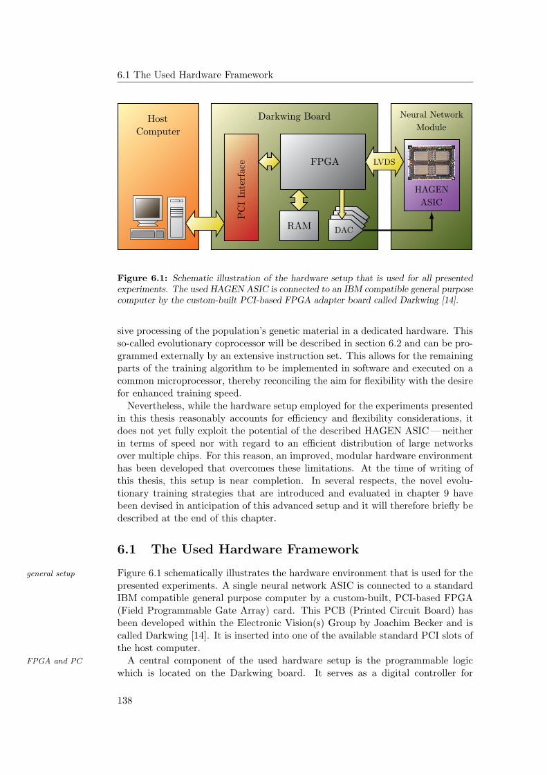
6.1 The Used Hardware Framework
PSfrag replacements
Darkwing Board
FPGA
PC
IIn
terf
ace
RAM DAC
LVDS
HAGEN
ASIC
Neural Network
ModuleHost
Computer
Figure 6.1: Schematic illustration of the hardware setup that is used for all presentedexperiments. The used HAGEN ASIC is connected to an IBM compatible general purposecomputer by the custom-built PCI-based FPGA adapter board called Darkwing [14].
sive processing of the population’s genetic material in a dedicated hardware. Thisso-called evolutionary coprocessor will be described in section 6.2 and can be pro-grammed externally by an extensive instruction set. This allows for the remainingparts of the training algorithm to be implemented in software and executed on acommon microprocessor, thereby reconciling the aim for flexibility with the desirefor enhanced training speed.
Nevertheless, while the hardware setup employed for the experiments presentedin this thesis reasonably accounts for efficiency and flexibility considerations, itdoes not yet fully exploit the potential of the described HAGEN ASIC — neitherin terms of speed nor with regard to an efficient distribution of large networksover multiple chips. For this reason, an improved, modular hardware environmenthas been developed that overcomes these limitations. At the time of writing ofthis thesis, this setup is near completion. In several respects, the novel evolu-tionary training strategies that are introduced and evaluated in chapter 9 havebeen devised in anticipation of this advanced setup and it will therefore briefly bedescribed at the end of this chapter.
6.1 The Used Hardware Framework
Figure 6.1 schematically illustrates the hardware environment that is used for thegeneral setup
presented experiments. A single neural network ASIC is connected to a standardIBM compatible general purpose computer by a custom-built, PCI-based FPGA(Field Programmable Gate Array) card. This PCB (Printed Circuit Board) hasbeen developed within the Electronic Vision(s) Group by Joachim Becker and iscalled Darkwing [14]. It is inserted into one of the available standard PCI slots ofthe host computer.
A central component of the used hardware setup is the programmable logicFPGA and PC
which is located on the Darkwing board. It serves as a digital controller for
138
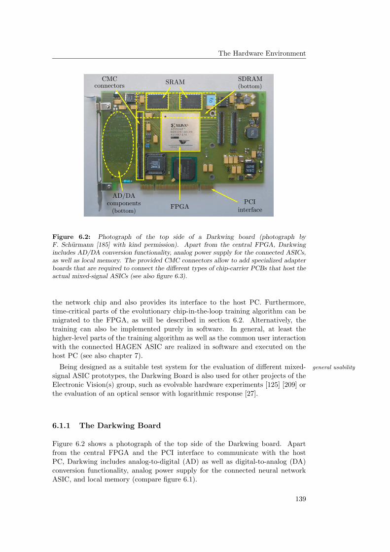
The Hardware Environment
PSfrag replacements
AD/DAcomponents
(bottom)
(bottom)SDRAM
FPGA
CPLD
PLX
CMCconnectors
PCIinterface
SRAM
Figure 6.2: Photograph of the top side of a Darkwing board (photograph byF. Schurmann [185] with kind permission). Apart from the central FPGA, Darkwingincludes AD/DA conversion functionality, analog power supply for the connected ASICs,as well as local memory. The provided CMC connectors allow to add specialized adapterboards that are required to connect the different types of chip-carrier PCBs that host theactual mixed-signal ASICs (see also figure 6.3).
the network chip and also provides its interface to the host PC. Furthermore,time-critical parts of the evolutionary chip-in-the-loop training algorithm can bemigrated to the FPGA, as will be described in section 6.2. Alternatively, thetraining can also be implemented purely in software. In general, at least thehigher-level parts of the training algorithm as well as the common user interactionwith the connected HAGEN ASIC are realized in software and executed on thehost PC (see also chapter 7).
Being designed as a suitable test system for the evaluation of different mixed- general usability
signal ASIC prototypes, the Darkwing Board is also used for other projects of theElectronic Vision(s) group, such as evolvable hardware experiments [125] [209] orthe evaluation of an optical sensor with logarithmic response [27].
6.1.1 The Darkwing Board
Figure 6.2 shows a photograph of the top side of the Darkwing board. Apartfrom the central FPGA and the PCI interface to communicate with the hostPC, Darkwing includes analog-to-digital (AD) as well as digital-to-analog (DA)conversion functionality, analog power supply for the connected neural networkASIC, and local memory (compare figure 6.1).
139
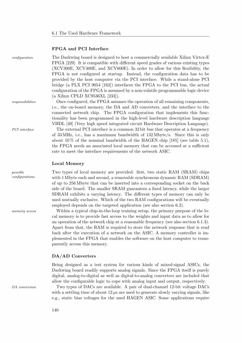
6.1 The Used Hardware Framework
FPGA and PCI Interface
The Darkwing board is designed to host a commercially available Xilinx Virtex-Econfiguration
FPGA [229]. It is compatible with different speed grades of various existing types(XCV300E, XCV400E, and XCV600E). In order to allow for this flexibility, theFPGA is not configured at startup. Instead, the configuration data has to beprovided by the host computer via the PCI interface. While a stand-alone PCIbridge (a PLX PCI 9054 [162]) interfaces the FPGA to the PCI bus, the actualconfiguration of the FPGA is assumed by a non-volatile programmable logic device(a Xilinx CPLD XC9536XL [233]).
Once configured, the FPGA assumes the operation of all remaining components,responsibilities
i.e., the on-board memory, the DA and AD converters, and the interface to theconnected network chip. The FPGA configuration that implements this func-tionality has been programmed in the high-level hardware description languageVHDL [49] (Very high speed integrated circuit Hardware Description Language).
The external PCI interface is a common 32 bit bus that operates at a frequencyPCI interface
of 33 MHz, i.e., has a maximum bandwidth of 132 Mbyte/s. Since this is onlyabout 10 % of the nominal bandwidth of the HAGEN chip [185] (see table 5.1),the FPGA needs an associated local memory that can be accessed at a sufficientrate to meet the interface requirements of the network ASIC.
Local Memory
Two types of local memory are provided: first, two static RAM (SRAM) chipspossibleconfigurations with 1 Mbyte each and second, a removable synchronous dynamic RAM (SDRAM)
of up to 256 Mbyte that can be inserted into a corresponding socket on the backside of the board. The smaller SRAM guarantees a fixed latency, while the largerSDRAM exhibits a varying latency. The different types of memory can only beused mutually exclusive. Which of the two RAM configurations will be eventuallyemployed depends on the targeted application (see also section 6.2).
Within a typical chip-in-the-loop training setup, the primary purpose of the lo-memory access
cal memory is to provide fast access to the weights and input data as to allow foran operation of the network chip at a reasonable frequency (see also section 6.1.3).Apart from that, the RAM is required to store the network response that is readback after the execution of a network on the ASIC. A memory controller is im-plemented in the FPGA that enables the software on the host computer to trans-parently access this memory.
DA/AD Converters
Being designed as a test system for various kinds of mixed-signal ASICs, theDarkwing board readily supports analog signals. Since the FPGA itself is purelydigital, analog-to-digital as well as digital-to-analog converters are included thatallow the configurable logic to cope with analog input and output, respectively.
Two types of DACs are available. A pair of dual-channel 12-bit voltage DACsDA conversion
with a settling time of about 12 µs are used to generate slowly varying signals, likee.g., static bias voltages for the used HAGEN ASIC. Some applications require
140
The Hardware Environment
PSfrag replacements
chip-carrier PCB LVDS interface adapter
HAGEN prototype(packaged)
SCSIconnectors connectors
CMC
LVDS bus
supply voltages
Figure 6.3: Photograph of the HAGEN carrier PCB and the LVDS interface adapterboard (photograph by F. Schurmann [185] with kind permission). The LVDS extensionboard gets connected to the Darkwing card via the shown CMC connectors. Apart fromthe LVDS signals, the SCSI interface to the chip-carrier PCB also conveys the digital andanalog supply voltages for the HAGEN ASIC (see text).
a faster generation of analog values and therefore, one 16-bit current DAC isincluded on the board that has a conversion time of only 25 ns. For the operationof the HAGEN ASIC, this DAC remains unused.
Besides that, a 12-bit ADC (Analog to Digital Converter) with a sampling rate AD conversion
of 40 MHz allows to perform the necessary analog-to-digital conversions wheneveranalog signals need to be connected to the FPGA. With the inputs and outputsof the used HAGEN chip being entirely digital, no AD conversion is required forits operation. In the employed setup, the ADC thus remains unused as well.
Analog Power Supply
The primary power supply for the Darkwing board is provided by the PCI interface(3.3 V, 5 V, and ±12V are available). These power supplies are shared between allcomponents of the PC and are electrically noisy. Besides special power suppliesthat meet the requirements of the various digital components, the board includesextra power supplies with adequate blocking capacitors that serve its analog com-ponents. The DACs and the ADC are fed by an analog 5 V power supply that canalso be used for the connected ASIC.
Peripheral Bus and Connection to the HAGEN chip
The employed Xilinx FPGAs provide enough I/O capabilities not only to manage connecting ASICs
the local memory, serve the PCI interface, and control the AD/DA converters, but
141
6.1 The Used Hardware Framework
also — and most importantly — to serve the peripheral bus to the connected neuralnetwork chip. Dedicated CMC (Common Mezzanine Card) connectors allow toconnect special PCB extensions to the Darkwing board that translate its genericinterface to the specific hot-plug interface of the particular chip-carrier PCBs thathost the different mixed-signal ASICs.
A photograph of both, the HAGEN carrier PCB and the special LVDS interfaceconnecting HAGEN
adapter that forms the corresponding extension to the Darkwing board is shown infigure 6.3. Due to the generic features that are already provided by the Darkwingcard itself, the functionality of the chip-carrier PCB is mainly reduced to passiveelectronics and mechanical adapters. In the case of the HAGEN ASIC, the con-nectors of the carrier PCB and the interface adapter are mechanically compatiblewith the SCSI Parallel Interface connector 2 type P [159]. Electrically, the pinconfiguration is adapted to suit the purpose of interfacing to the HAGEN pro-totype (for details see [185]). In addition to the necessary supply voltages, theinterface mediates 16 bi-directional and 5 uni-directional LVDS links that can beoperated at up to 300 MHz. Voltage regulators on the carrier PCB derive therequired analog voltage of 3.3 V (see table 5.1) from the 5 V that are provided bythe Darkwing board.
6.1.2 The Host Computer
Within the described hardware configuration, the Darkwing card is inserted intoone of the PCI extensions slots of the used IBM compatible general purpose com-puter. Since contemporary PCs provide multiple slots, this in principle allows tooperate several boards simultaneously in one machine.
At present, the used host computers execute a Linux operating system withoperating system
kernel 2.4.x. As it will be discussed in section 7.1.4, the software that is employedfor the operation and training of the HAGEN chip is largely platform independentand is deemed to be easily portable to other operating systems as well.
For the various investigations within the Electronic Vision(s) group, a totalused setup
of 11 similar configurations are currently in operation that include either IntelPentium IV or AMD Athlon XP processors. The three setups that are used forthe presented experiments feature Intel Pentium IV CPUs with 2.4GHz. Onesingle Darkwing board is connected to each computer.
6.1.3 Common Chip-in-the-Loop Operation
In general, the following three basic steps are iterated during a common chip-in-basic scheme ofiteration the-loop training process (see also figure 2.11): First, the algorithm generates a
new candidate solution, i.e., a new network configuration for the HAGEN ASICthat is to be used to solve the task in question. Besides the individual weightvalues, the unambiguous definition of a network on the HAGEN chip requires thespecification of the activated feedback and inter-block connections as well as thenumber of network cycles that are operated for each applied input pattern (seesection 5.2).
142
The Hardware Environment
Second, the generated network configuration is sent to the HAGEN ASIC forimplementation and the desired set of input patterns is applied successively. Afterthe network has finished processing all its input patterns, the resulting networkresponses are stored in the local memory of the FPGA such that, third, the al-gorithm can read back this data for evaluation. As long as the observed perfor-mance of the evaluated network is not satisfactory — and all potential additionaltermination conditions remain unfulfilled — the algorithm proceeds with the nextiteration, i.e., starts by generating a new candidate solution, etc.
Data Handling
If the training algorithm is purely implemented in software, all parts of the network required data transfer
configuration that potentially change between the single candidate solutions (e.g.,the weight values) need to be retransmitted from the host PC over the PCI busto the local memory of the FPGA for each tested network. The same applies tothe network response that needs to be read back from the memory of the FPGAinto the RAM of the host computer for evaluation.
In contrast, the input patterns that are applied to the single candidate solutions input data handling
during training are usually the same for all networks. Within the experimentspresented in part III, these input patterns are therefore transferred to the localmemory of the FPGA only once at the beginning of a given training run andremain there to be applied to all tested candidate networks.
Speed Considerations
In the used setup, the HAGEN chip can be operated at frequencies of up to HAGEN interfacespeed100 MHz which yields a maximum bandwidth of the data transfer between the
FPGA and the HAGEN ASIC of about 500 Mbyte/s [185]. This is about 4 timesthe nominal maximum speed of the PCI bus (see section 6.1.1). If the completenetwork specification and the desired input patterns are available in the localmemory, an exemplary network that requires two network cycles and utilizes all33k synapses in all four blocks can be loaded into the HAGEN chip and process1000 input patterns within less than 1 ms.
Using a software implemented algorithm, the speed of the system during training PCI bottleneck
is limited by the considerable amount of data that has to be transmitted via thePCI bus from the host PC to the local memory on the Darkwing board or viceversa. According to what has been stated above, this primarily refers to the weightvalues and the output data of the network.
In order to avoid this bottleneck, it suggests itself to at least partly implementthe generation of new candidate solutions and/or the evaluation of the networkoutputs within the FPGA and thereby to cut down the data that needs to beexchanged with the host computer. Ultimately, it would be desirable to entirelyavoid any significant data transfer over the PCI bus, e.g., by reducing the parts ofthe training algorithm that need to be executed on the host PC to mere controllingand user interaction. A feasible approach is described in the next section.
143
6.2 The Evolutionary Coprocessor
6.2 The Evolutionary Coprocessor
During the experiments presented in this thesis, the HAGEN chip is trained withevolutionary chip-in-the-loop algorithms (see chapters 3 and 4). Apart from thefitness calculation that needs to be performed for each new individual in everygeneration, one of the most time-critical aspects of evolutionary optimization isthe processing of the genetic material in the population. Using a generationalreplacement scheme (see section 3.4.1), a whole generation of new genotypes needsto be created from the genomes of the previous population in each iteration.
Depending on the number of free parameters, the creation of offspring can in-data-intensive geneticoperations volve large amounts of data. For example, even if only the weights of half of the
synapses in one network block of the HAGEN ASIC were to be optimized, a singlegenome would still contain 4096 genes. On the other hand, given a desired setof mutation and recombination operators, all pairs of mating individuals are pro-cessed in a similar way, and all genes within the genome are usually regarded asequivalent. Tasks that require a similar set of simple operations to be repeatedlyperformed on large sequences of data are particularly well suited for a pipelinedimplementation in a specialized hardware.
This section introduces a dedicated coprocessor architecture that speeds upgenetic operations inhardware evolutionary training algorithms by performing the required genetic variation op-
erations within a configurable logic. This so-called evolutionary coprocessor iscoded in VHDL [49] and has been designed by Tillmann Schmitz [182]. A detaileddescription of the coprocessor will be given in Tillmann Schmitz’ PhD thesis1.The following sections confine themselves with discussing those aspects that arerelevant for the work presented in this thesis.
6.2.1 Coprocessor Setup Overview
In the described hardware setup, the coprocessor resides within the FPGA ofgeneral setup
the Darkwing board. In order to retain a sufficient flexibility in the realizableevolutionary training approaches, the remaining parts of the training algorithmpersist to be implemented in software and are executed on the microprocessorof the host computer. At the same time, the coprocessor completely takes overthe management and processing of the genomes in the evolved population and iscontrolled by the software via a given set of instructions. Figure 6.4 schematicallyillustrates the data flow within this setup.
The genomes that are being processed by the coprocessor are stored within thelocal memory of the FPGA. In order to allow for reasonably sized populationsof genomes of the required size, the used hardware setup employs a 64 MbyteSDRAM module that is inserted into the corresponding socket of the Darkwingboard (see section 6.1.1).
Since the genetic material that defines a given candidate solution is stored withinadvantages
the local memory, the evaluation of individual networks on the HAGEN ASIC doesnot require this configuration data to be transmitted over the PCI bus. In additionto the acceleration of the genetic operations, this yields a substantial speed gain
1At the time of this writing, the mentioned thesis has not yet been finalized.
144
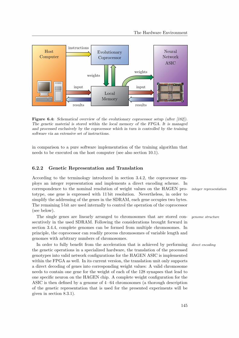
The Hardware EnvironmentPSfrag replacements
weightsweights
inputinput
resultsresults
instructionsEvolutionaryCoprocessor
Local
Memory
NeuralNetwork
ASIC
HostComputer
Figure 6.4: Schematical overview of the evolutionary coprocessor setup (after [182]).The genetic material is stored within the local memory of the FPGA. It is managedand processed exclusively by the coprocessor which in turn is controlled by the trainingsoftware via an extensive set of instructions.
in comparison to a pure software implementation of the training algorithm thatneeds to be executed on the host computer (see also section 10.1).
6.2.2 Genetic Representation and Translation
According to the terminology introduced in section 3.4.2, the coprocessor em-ploys an integer representation and implements a direct encoding scheme. Incorrespondence to the nominal resolution of weight values on the HAGEN pro- integer representation
totype, one gene is expressed with 11 bit resolution. Nevertheless, in order tosimplify the addressing of the genes in the SDRAM, each gene occupies two bytes.The remaining 5 bit are used internally to control the operation of the coprocessor(see below).
The single genes are linearly arranged to chromosomes that are stored con- genome structure
secutively in the used SDRAM. Following the considerations brought forward insection 3.4.4, complete genomes can be formed from multiple chromosomes. Inprinciple, the coprocessor can readily process chromosomes of variable length andgenomes with arbitrary numbers of chromosomes.
In order to fully benefit from the acceleration that is achieved by performing direct encoding
the genetic operations in a specialized hardware, the translation of the processedgenotypes into valid network configurations for the HAGEN ASIC is implementedwithin the FPGA as well. In its current version, the translation unit only supportsa direct decoding of genes into corresponding weight values: A valid chromosomeneeds to contain one gene for the weight of each of the 128 synapses that lead toone specific neuron on the HAGEN chip. A complete weight configuration for theASIC is then defined by a genome of 4 · 64 chromosomes (a thorough descriptionof the genetic representation that is used for the presented experiments will begiven in section 8.3.1).
145
6.2 The Evolutionary Coprocessor
Architecture Specification
Apart from the mere weight values, the additional parts of a complete chip config-fixed architecture
uration that are required to uniquely define the architecture of the final network —i.e., the activated feedback and inter-block connections in combination with theused number of network cycles— can, as yet, not be coded within the genome.Hence, in the current setup, the potential of the coprocessor can only be exploitedif the architecture of all networks is fixed during training. At the beginning ofthe training run, the specification of the corresponding parameters can then betransferred to the local memory of the FPGA in order to be used for all individ-uals that will be evaluated during the following simulated evolution. Otherwise,the individual architecture specification for each new candidate solution has to betransferred from the host PC which significantly impedes a fast execution of thetraining procedure.
Given a desired architecture, not all neurons and synapses of the HAGEN ASICdetermining thearchitecture are necessarily used for the actually implemented network. Those genes of a chro-
mosome that correspond to unused synapses of the coded neuron are reasonablyset to zero. The coprocessor allows to mark single genes as deactivated such thatthey are not affected by mutation (internally, this involves one of the 5 spare bitsin each gene, see below). In other words, any genes that are set to zero and arealso marked as deactivated within all genomes of the initial population, will re-main zero in all individuals throughout the whole evolution. In combination withthe fixed feedback and inter-block connections as well as the specified number ofnetwork cycles, this allows to optimize the weight values of networks with anydesired architecture that can be implemented on the HAGEN ASIC.
6.2.3 Pipeline Operation Overview
The design of the coprocessor pursues two aims: First, it needs to process ahigh throughput of genetic data. Second, it is desired to allow for a wide rangeof conceivable evolutionary algorithms to be implemented without changing thehardware configuration. In consideration of these requirements, the coprocessoris implemented as a pipeline whose single stages can be managed and controlledby a given set of instructions.
A simplified schematic of this pipeline is shown in figure 6.5. Given the addressesprocessing scheme
of the two parent chromosomes “parent 1” and “parent 2” in the local memory, therespective genetic material is fed through the pipeline successively. According tothe instructions that control each stage of the pipeline, the offspring chromosomeis constructed gene by gene and is written to a specified target address.
In fact, the pipeline is designed fourfold parallel, i.e., four genes can be processedprocessing speed
in each clock cycle. At a clock frequency of 80 MHz, this leads to a nominalmaximum rate of 320 · 106 processed genes per second. However, the followingdescription will only assume a single pipeline for simplicity; the generalization tofour pipelines is straight forward.
Each of the single stages shown in figure 6.5 involves numerous decisions thatare partly random and can partly be controlled via instructions. For the random
146
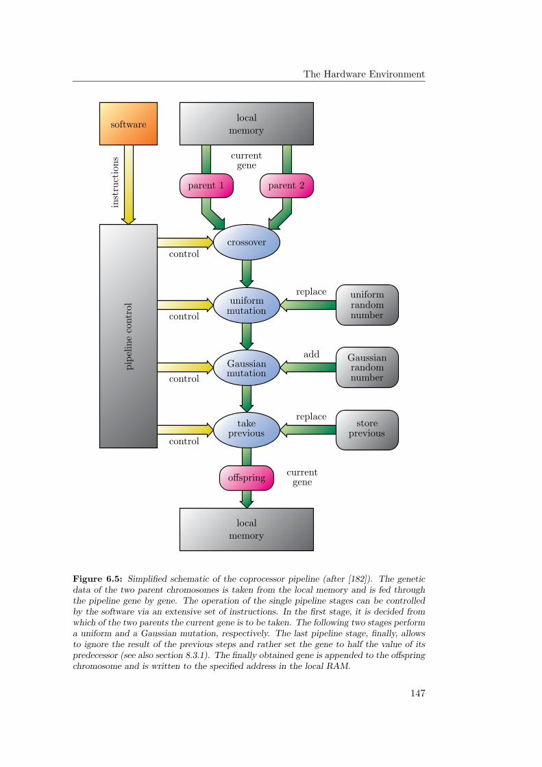
The Hardware Environment
PSfrag replacements
softwarein
stru
ctio
ns
pip
elin
eco
ntr
ol
parent 1 parent 2
current
current
gene
gene
local
local
memory
memory
crossover
control
control
control
control
replace
replace
add
uniformuniform
GaussianGaussian
mutation
mutationrandom
random
number
number
storetakeprevious previous
offspring
Figure 6.5: Simplified schematic of the coprocessor pipeline (after [182]). The geneticdata of the two parent chromosomes is taken from the local memory and is fed throughthe pipeline gene by gene. The operation of the single pipeline stages can be controlledby the software via an extensive set of instructions. In the first stage, it is decided fromwhich of the two parents the current gene is to be taken. The following two stages performa uniform and a Gaussian mutation, respectively. The last pipeline stage, finally, allowsto ignore the result of the previous steps and rather set the gene to half the value of itspredecessor (see also section 8.3.1). The finally obtained gene is appended to the offspringchromosome and is written to the specified address in the local RAM.
147
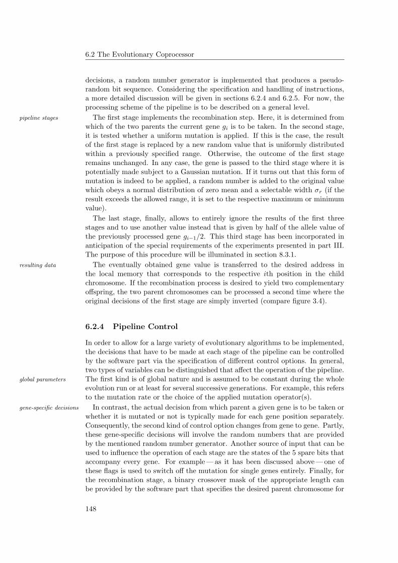
6.2 The Evolutionary Coprocessor
decisions, a random number generator is implemented that produces a pseudo-random bit sequence. Considering the specification and handling of instructions,a more detailed discussion will be given in sections 6.2.4 and 6.2.5. For now, theprocessing scheme of the pipeline is to be described on a general level.
The first stage implements the recombination step. Here, it is determined frompipeline stages
which of the two parents the current gene gi is to be taken. In the second stage,it is tested whether a uniform mutation is applied. If this is the case, the resultof the first stage is replaced by a new random value that is uniformly distributedwithin a previously specified range. Otherwise, the outcome of the first stageremains unchanged. In any case, the gene is passed to the third stage where it ispotentially made subject to a Gaussian mutation. If it turns out that this form ofmutation is indeed to be applied, a random number is added to the original valuewhich obeys a normal distribution of zero mean and a selectable width σr (if theresult exceeds the allowed range, it is set to the respective maximum or minimumvalue).
The last stage, finally, allows to entirely ignore the results of the first threestages and to use another value instead that is given by half of the allele value ofthe previously processed gene gi−1/2. This third stage has been incorporated inanticipation of the special requirements of the experiments presented in part III.The purpose of this procedure will be illuminated in section 8.3.1.
The eventually obtained gene value is transferred to the desired address inresulting data
the local memory that corresponds to the respective ith position in the childchromosome. If the recombination process is desired to yield two complementaryoffspring, the two parent chromosomes can be processed a second time where theoriginal decisions of the first stage are simply inverted (compare figure 3.4).
6.2.4 Pipeline Control
In order to allow for a large variety of evolutionary algorithms to be implemented,the decisions that have to be made at each stage of the pipeline can be controlledby the software part via the specification of different control options. In general,two types of variables can be distinguished that affect the operation of the pipeline.The first kind is of global nature and is assumed to be constant during the wholeglobal parameters
evolution run or at least for several successive generations. For example, this refersto the mutation rate or the choice of the applied mutation operator(s).
In contrast, the actual decision from which parent a given gene is to be taken orgene-specific decisions
whether it is mutated or not is typically made for each gene position separately.Consequently, the second kind of control option changes from gene to gene. Partly,these gene-specific decisions will involve the random numbers that are providedby the mentioned random number generator. Another source of input that can beused to influence the operation of each stage are the states of the 5 spare bits thataccompany every gene. For example — as it has been discussed above — one ofthese flags is used to switch off the mutation for single genes entirely. Finally, forthe recombination stage, a binary crossover mask of the appropriate length canbe provided by the software part that specifies the desired parent chromosome for
148
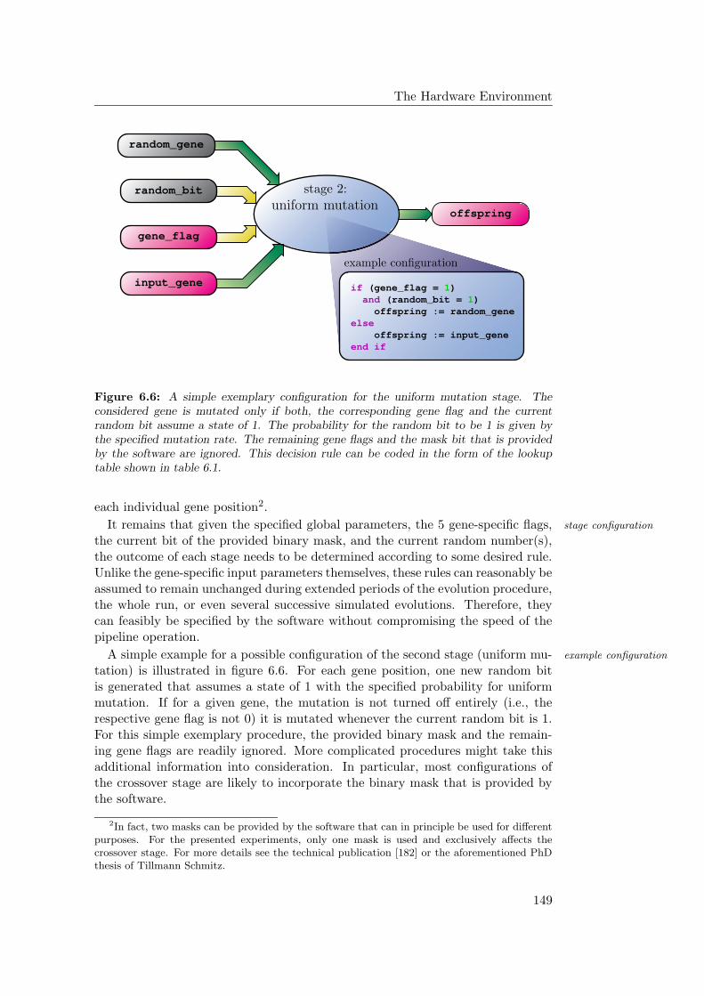
The Hardware Environment
random_gene
gene_flag
random_bit
input_gene
offspring
if (gene_flag = 1) and (random_bit = 1) offspring := random_geneelse offspring := input_geneend if
PSfrag replacements
stage 2:
uniform mutation
example configuration
Figure 6.6: A simple exemplary configuration for the uniform mutation stage. Theconsidered gene is mutated only if both, the corresponding gene flag and the currentrandom bit assume a state of 1. The probability for the random bit to be 1 is given bythe specified mutation rate. The remaining gene flags and the mask bit that is providedby the software are ignored. This decision rule can be coded in the form of the lookuptable shown in table 6.1.
each individual gene position2.
It remains that given the specified global parameters, the 5 gene-specific flags, stage configuration
the current bit of the provided binary mask, and the current random number(s),the outcome of each stage needs to be determined according to some desired rule.Unlike the gene-specific input parameters themselves, these rules can reasonably beassumed to remain unchanged during extended periods of the evolution procedure,the whole run, or even several successive simulated evolutions. Therefore, theycan feasibly be specified by the software without compromising the speed of thepipeline operation.
A simple example for a possible configuration of the second stage (uniform mu- example configuration
tation) is illustrated in figure 6.6. For each gene position, one new random bitis generated that assumes a state of 1 with the specified probability for uniformmutation. If for a given gene, the mutation is not turned off entirely (i.e., therespective gene flag is not 0) it is mutated whenever the current random bit is 1.For this simple exemplary procedure, the provided binary mask and the remain-ing gene flags are readily ignored. More complicated procedures might take thisadditional information into consideration. In particular, most configurations ofthe crossover stage are likely to incorporate the binary mask that is provided bythe software.
2In fact, two masks can be provided by the software that can in principle be used for differentpurposes. For the presented experiments, only one mask is used and exclusively affects thecrossover stage. For more details see the technical publication [182] or the aforementioned PhDthesis of Tillmann Schmitz.
149
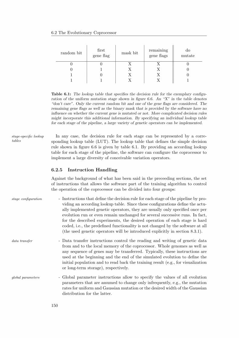
6.2 The Evolutionary Coprocessor
random bitfirst
gene flagmask bit
remaininggene flags
domutate
0 0 X X 00 1 X X 01 0 X X 01 1 X X 1
Table 6.1: The lookup table that specifies the decision rule for the exemplary configu-ration of the uniform mutation stage shown in figure 6.6. An “X” in the table denotes“don’t care”. Only the current random bit and one of the gene flags are considered. Theremaining gene flags as well as the binary mask that is provided by the software have noinfluence on whether the current gene is mutated or not. More complicated decision rulesmight incorporate this additional information. By specifying an individual lookup tablefor each stage of the pipeline, a large variety of genetic operators can be implemented.
In any case, the decision rule for each stage can be represented by a corre-stage-specific lookuptables sponding lookup table (LUT). The lookup table that defines the simple decision
rule shown in figure 6.6 is given by table 6.1. By providing an according lookuptable for each stage of the pipeline, the software can configure the coprocessor toimplement a large diversity of conceivable variation operators.
6.2.5 Instruction Handling
Against the background of what has been said in the preceeding sections, the setof instructions that allows the software part of the training algorithm to controlthe operation of the coprocessor can be divided into four groups:
- Instructions that define the decision rule for each stage of the pipeline by pro-stage configuration
viding an according lookup table. Since these configurations define the actu-ally implemented genetic operators, they are usually only specified once perevolution run or even remain unchanged for several successive runs. In fact,for the described experiments, the desired operation of each stage is hardcoded, i.e., the predefined functionality is not changed by the software at all(the used genetic operators will be introduced explicitly in section 8.3.1).
- Data transfer instructions control the reading and writing of genetic datadata transfer
from and to the local memory of the coprocessor. Whole genomes as well asany sequence of genes may be transferred. Typically, these instructions areused at the beginning and the end of the simulated evolution to define theinitial population and to read back the training result (e.g., for visualizationor long-term storage), respectively.
- Global parameter instructions allow to specify the values of all evolutionglobal parameters
parameters that are assumed to change only infrequently, e.g., the mutationrates for uniform and Gaussian mutation or the desired width of the Gaussiandistribution for the latter.
150
The Hardware Environment
- A given set of recombination instructions is used to define the addresses of recombination
the two parent chromosomes, their respective lengths, the target address forthe offspring, and the desired crossover mask. Typically, a new correspond-ing set of information is provided for each recombination.
Using a control software that is executed on the host PC, these instructionsneed to be transferred via the PCI bus. The first three types of instructions areuncritical in terms of speed since they are only used infrequently. In contrast, therecombination instructions need to be issued for each mating process. Consideringgenomes with N chromosomes, a total of 2N parent addresses, N chromosomelengths, N crossover masks, and N target addresses need to be specified for eachcrossover procedure.
For an efficient handling of these instructions, a dedicated data and instruction instruction buffer
buffer is provided that can be utilized to pool instructions and store frequentlyused data. After an entire list of instructions has been written into this buffer,a corresponding start command transmits all instructions to the coprocessor andinitiates the execution of the whole sequence. During the following operation ofthe coprocessor, the software can address other tasks (e.g., calculating the fitnessof previously evaluated individuals).
Parts of the instruction buffer are reserved to allow for the generation of an data buffer
internal address table. Frequently used chromosome addresses and/or chromosomelengths can be stored in this list such that instead of specifying all source andtarget addresses directly, the corresponding instructions merely need to includethe index of the respective information in the internal address list. Using onlya fixed set of addresses for all individuals that are created throughout the wholeevolution run, this indirect addressing scheme effectively reduces the amount ofdata that needs to be exchanged between the software and the coprocessor duringtraining. In principle, the same indirect addressing can also be used to repeatedlyswitch between different lookup tables for the individual stages of the pipeline.Within the current state of the setup, the buffer allows to store a total of 2048instructions, chromosome address, and/or chromosome lengths.
The evolutionary coprocessor is subject to constant development and improve- advanced features
ment. Since its original version, several advanced features have been added thatprovide more efficient ways of transmitting recombination instructions. For exam-ple, having specified the number, addresses, and lengths of multiple chromosomepairs, special loop functionality allows to iteratively apply predefined recombina-tion operators, like, e.g., one-point crossover, to the whole set of chromosomes viaeffectively only one single instruction. New random crossover masks are createdautomatically and autonomously by the coprocessor for each mating pair. Theusage of such pre-set recombination operators further minimizes the amount ofdata and instructions that needs to be exchanged between the software and thecoprocessor. However, this novel functionality has not yet been employed for theexperiments presented in this thesis. The detailed description of these additionalfeatures is therefore deferred to later publications.
151
6.3 An Advanced Hardware Environment
6.2.6 The Evolutionary Coprocessor: Reflection and Outlook
The advantages of using the evolutionary coprocessor for the training of networkson the HAGEN chip are twofold: First, performing the required genetic operationsin a dedicated hardware can potentially yield a significant speed gain compared topure software solutions, especially for large genomes. Second, having the geneticmaterial of the whole population available in the local memory allows to evaluatethe different candidate solutions without the need to repeatedly transmit largeamounts of configuration data over the PCI bus.
In order to further reduce the required data transfer between the host PC andfitness calculation inhardware the memory of the coprocessor, the calculation of the fitness could be implemented
in the FPGA as well. In the current state of the system where suitable trainingalgorithms and appropriate fitness functions are a topic of research themselves, thefitness calculation remains to be realized in software. A hardware implementationof the fitness calculation is planned for future investigations.
Apart from that, the coprocessor persists to impose certain restrictions on thelimited complexity
complexity of the realizable genetic operators. The present version can only beused to evolve the synaptic weights of networks with a fixed architecture using adirect encoding scheme, an 11 bit integer representation, and two simple single-gene mutation operators.
More complex encoding schemes and operators could in principle be realized byimplications fortraining processing the same set of chromosomes multiple times using different configura-
tions for the single stages of the pipeline. Alternatively, the functionality of thetranslation unit could be improved to allow for more abstracted genotypic repre-sentations. In both cases, the increase in complexity would most likely be paid forby a reduction in training speed. Also with regard to the fitness function, it canthus generally be said that in order to fully benefit from hardware accelerationand to be capable of keeping up pace with the used neural network hardware,all time-critical parts of the evolutionary training algorithm are preferably keptsimple. While the next section introduces an advanced hardware environmentthat successfully avoids some of the drawbacks of the current setup, the aboveconsiderations will turn out to hold also for this improved system.
6.3 An Advanced Hardware Environment
By confining the analog network operation into blocks with an entirely digitalinterface, the employed network model of the mixed-signal HAGEN prototypelays the foundation for a feasible up-scaling to larger networks (see sections 5.2and 5.4.5). Apart from including more blocks in future ASICs, this can also beachieved by interconnecting a desired number of the existing HAGEN chips.
Regarding the hardware infrastructure that has been described in the preceedingscalabilityconsiderations sections, multiple Darkwing boards could be used in the same host computer to
operate several HAGEN prototypes simultaneously. However, if the different chipsare to be interconnected to form one enlarged network, considerable amounts ofdata will have to be transmitted isynchronously from one ASIC to the other viathe PCI bus (see also equation 5.4). Apart from the fact that the latency of a
152
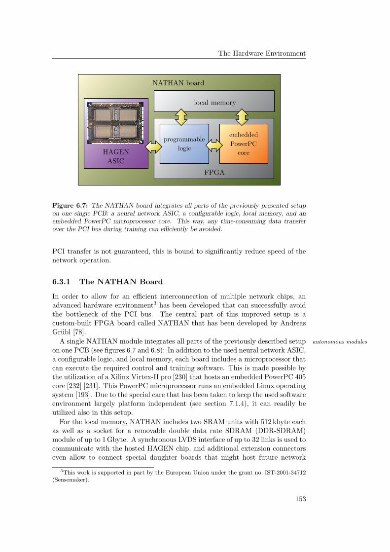
The Hardware Environment
PSfrag replacementsNATHAN board
local memory
FPGA
programmable
logic
embedded
PowerPC
coreHAGEN
ASIC
Figure 6.7: The NATHAN board integrates all parts of the previously presented setupon one single PCB: a neural network ASIC, a configurable logic, local memory, and anembedded PowerPC microprocessor core. This way, any time-consuming data transferover the PCI bus during training can efficiently be avoided.
PCI transfer is not guaranteed, this is bound to significantly reduce speed of thenetwork operation.
6.3.1 The NATHAN Board
In order to allow for an efficient interconnection of multiple network chips, anadvanced hardware environment3 has been developed that can successfully avoidthe bottleneck of the PCI bus. The central part of this improved setup is acustom-built FPGA board called NATHAN that has been developed by AndreasGrubl [78].
A single NATHAN module integrates all parts of the previously described setup autonomous modules
on one PCB (see figures 6.7 and 6.8): In addition to the used neural network ASIC,a configurable logic, and local memory, each board includes a microprocessor thatcan execute the required control and training software. This is made possible bythe utilization of a Xilinx Virtex-II pro [230] that hosts an embedded PowerPC 405core [232] [231]. This PowerPC microprocessor runs an embedded Linux operatingsystem [193]. Due to the special care that has been taken to keep the used softwareenvironment largely platform independent (see section 7.1.4), it can readily beutilized also in this setup.
For the local memory, NATHAN includes two SRAM units with 512 kbyte eachas well as a socket for a removable double data rate SDRAM (DDR-SDRAM)module of up to 1 Gbyte. A synchronous LVDS interface of up to 32 links is used tocommunicate with the hosted HAGEN chip, and additional extension connectorseven allow to connect special daughter boards that might host future network
3This work is supported in part by the European Union under the grant no. IST-2001-34712(Sensemaker).
153
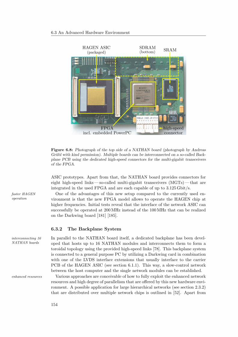
6.3 An Advanced Hardware Environment
PSfrag replacements
SRAMSDRAM(bottom)
HAGEN ASIC(packaged)
FPGAincl. embedded PowerPC
high-speedconnector
Figure 6.8: Photograph of the top side of a NATHAN board (photograph by AndreasGrubl with kind permission). Multiple boards can be interconnected on a so-called Back-plane PCB using the dedicated high-speed connectors for the multi-gigabit transceiversof the FPGA.
ASIC prototypes. Apart from that, the NATHAN board provides connectors foreight high-speed links — so-called multi-gigabit transceivers (MGTs) — that areintegrated in the used FPGA and are each capable of up to 3.125 Gbit/s.
One of the advantages of this new setup compared to the currently used en-faster HAGENoperation vironment is that the new FPGA model allows to operate the HAGEN chip at
higher frequencies. Initial tests reveal that the interface of the network ASIC cansuccessfully be operated at 200 MHz instead of the 100 MHz that can be realizedon the Darkwing board [181] [185].
6.3.2 The Backplane System
In parallel to the NATHAN board itself, a dedicated backplane has been devel-interconnecting 16NATHAN boards oped that hosts up to 16 NATHAN modules and interconnects them to form a
toroidal topology using the provided high-speed links [78]. This backplane systemis connected to a general purpose PC by utilizing a Darkwing card in combinationwith one of the LVDS interface extensions that usually interface to the carrierPCB of the HAGEN ASIC (see section 6.1.1). This way, a slow-control networkbetween the host computer and the single network modules can be established.
Various approaches are conceivable of how to fully exploit the enhanced networkenhanced resources
resources and high degree of parallelism that are offered by this new hardware envi-ronment. A possible application for large hierarchical networks (see section 2.3.2)that are distributed over multiple network chips is outlined in [52]. Apart from
154
The Hardware Environment
implementing larger networks on several HAGEN ASICs, the use of multiple dif-ferent network chips also provides the possibility to speed up the training processby evaluating several candidate solutions in parallel. If the training algorithm it-self can benefit from parallelization, it could even be distributed over the multiplePowerPC processors of the single NATHAN modules itself.
The introduced advanced hardware environment is a conjoint work with J. Fieres, operational readiness
A. Grubl, S. Philipp, Dr. J. Schemmel, T. Schmitz, F. Schurmann and A. Sinsel.At the time of writing of this thesis, the single components of this system havepassed the initial test stage and are demonstrated to be fully functional. Theused software environment (see chapter 7) is successfully migrated to the embed-ded Linux that is executed on PowerPC core of the employed Xilinx FPGA. Thewhole framework will be fully functional in the near future. Although its operationand further development is beyond the scope of this thesis, the evolutionary train-ing strategies presented in part III are partially designed in special considerationof the advantages and limitations of this new hardware setup.
6.3.3 Implications for Network Training
With regard to the training process, the NATHAN/Backplane environment will advantages
allow to exploit the speed of the HAGEN ASIC more efficiently than it is possiblewith the current Darkwing setup: The chip itself can be interfaced at higher speedsand the bottleneck of the PCI bus is efficiently avoided by executing the trainingsoftware locally on the embedded PowerPC. A clever distribution of adequatetraining approaches over multiple NATHAN boards might even promote furtheracceleration due to parallelization.
It remains to be a noticeable limitation of this setup, that the featured PowerPC limitations
core operates at a maximum clock frequency of only 350 MHz4 [232] [231] anddoes, e.g., not provide special floating-point units. Compared to the currentlyused 2.4 GHz Pentium IV, this breeds a substantial reduction in speed and isthus bound to affect the training process. Aiming to make best use of both, theaccelerated network ASIC operation and the faster data transfer, the used trainingalgorithm will be challenged to keep up pace with the implemented networks evenmore than in the present setup.
Considering the application of evolutionary training algorithms, it will therefore feasible hardwareaccelerationbecome inevitable to employ the evolutionary coprocessor and thereby release
the PowerPC from performing the time-consuming genetic operations in software.Ultimately, the calculation of the fitness is preferably migrated to the FPGA aswell, and the software part is best reduced to only a minimum of controllingfunctionality.
As it has already been discussed in section 6.2 this implies to use simple ge- simple trainingalgorithmsnetic codings, variation operators, and fitness functions that allow for an efficient
realization within a configurable logic. In summary, it can be concluded thatwithin either of the described hardware setups, feasible evolutionary training ap-
4Three different speed grades are available with maximum clock frequencies of 300, 350 and450MHz, respectively [232] [231]. All those models are compatible with the NATHAN board.The eventual choice is determined by cost considerations.
155

6.3 An Advanced Hardware Environment
proaches need to contend themselves with simple components and — in anticipa-tion of the NATHAN/Backplane system — should rather aim to efficiently benefitfrom potential parallelization. A promising training approach will be introducedin chapter 9.
156
Chapter 7
The HANNEE Software
Real Programmers don’t comment their code. If itwas hard to write, it should be hard to understand.
Anonymous
The HAGEN neural network chip introduced in chapter 5 is optimized for highlyiterative chip-in-the-loop training algorithms. This motivates the application ofevolutionary strategies (chapters 3 and 4), and it has been discussed in section 6.2that this kind of optimization procedure can greatly benefit from hardware ac-celeration. Nevertheless, as long as adequate training approaches remain to be asubject of investigation in their own right, the arising need for flexibility advisesto implement at least part of the training in software.
Even if the training was completely realized on-chip or within a configurablelogic, the user interaction with the hardware — either for mere system testing orthe visualization and evaluation of training results and network responses — wouldeventually involve a dedicated software. Within the two neural network hardwaresetups presented in the preceeding chapter, the corresponding software compo-nents are executed on either the standard PC and/or the embedded PowerPCcores of the used Xilinx FPGAs.
In parallel to the HAGEN ASIC and the described hardware frameworks, asoftware environment has been developed that allows the user to test, analyzeand train neural networks on the HAGEN chip for desired tasks. This software iscalled HANNEE (Heidelberg Analog Neural Network Evolution Environment). Ithas been designed in co-operation with Johannes Fieres and also received majorcontributions from Eilif Mueller, Johannes Schemmel, Tillmann Schmitz, and FelixSchurmann.
Regarding the prototype state of both, the neural network hardware as well as design goals
the appropriate training algorithms, the design of HANNEE had to fulfill at leasttwo important requirements. First, the software has to be usable in connectionwith different, present and future hardware configurations (e.g., new generationsof network ASICs or alternative PCB environments) with only minor additionalprogramming effort. Second, it has to facilitate the integration of new softwarecomponents contributed by different researchers with diverging research interests.
157
7.1 Overview
With respect to the evaluation of evolutionary algorithms as suitable train-ing approaches, the second point also comprises the concrete desire for an easycombination of different evolutionary algorithm components (see sections 3.3.2and 3.3.4).
As a basic consequence of these considerations, the HANNEE software follows anplatformindependence object-oriented approach and is implemented in C++ [202]. At the time of writing
of this thesis, it is primarily used on Unix-based systems, but special care hasbeen taken to keep the source code largely platform-independent. Earlier versionshave been used under the Windows operating system, and it is apprehended toconstitute no major effort to port current and future versions to Windows as well.
The succeeding sections will describe HANNEE in more detail and outline howthe main design goals formulated above are realized. Being written by a workgroupof scientists to serve as a tool for their ongoing research, the HANNEE platformis subject to constant development and improvement. Any detailed discussion ofits implementation would be outdated within weeks and would in any case missthe purpose of this thesis.
In this sense, the present chapter is not intended to serve as an outright HAN-NEE manual or an exhaustive source code documentation (the latter is included asa doxygen [213] documentation within the source files). Rather, the main designconcepts that establish HANNEE as a flexible and efficient software environmentfor the presented neural network hardware and as a valuable tool for the researchon evolutionary training strategies will be investigated on a general and structurallevel.
Since the following sections are concerned with object-oriented software design,it is assumed that the reader is familiar with the philosophy of object-orientedprogramming and the concepts of classes, objects and inheritance. An introduc-tion to this field can be found in literature [155] [202].
7.1 Overview
Figure 7.1 schematically illustrates the structure of the HANNEE software and itsinteraction with the neural network hardware. As it has already been discussedin section 6.1, any communication between the software and the HAGEN chip ismediated by a configurable logic. Within the software, the access to the FPGAis completely encapsulated by a set of dedicated hardware access classes. Besidesproviding the functionality to configure the FPGA and to control the operationof the neural network ASICs, these classes also manage the communication withthe evolutionary coprocessor (see section 6.2).
7.1.1 Standardized Hardware Access
Realizing parts of the training algorithm in software gives rise to frequent dataefficiencyrequirements transfer between the neural network chips and the software environment (see sec-
tions 2.4.5 and 6.1.3). Therefore, an efficient implementation of the hardwareaccess is vital if the speed benefits of using a fast neural network hardware are
158
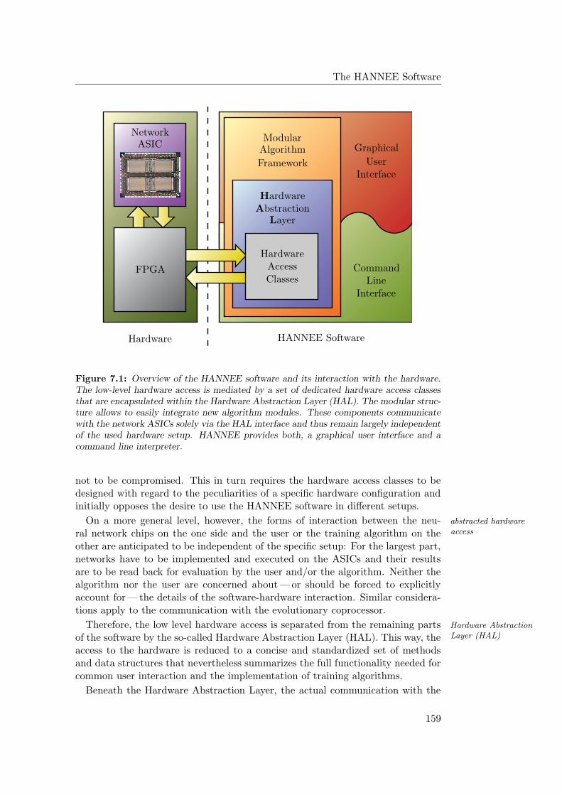
The HANNEE Software
PSfrag replacements
NetworkASIC
Hardware HANNEE Software
FPGA
ModularAlgorithm
Framework
HardwareAbstraction
Layer
HardwareAccessClasses
CommandLine
Graphical
User
Interface
Interface
Figure 7.1: Overview of the HANNEE software and its interaction with the hardware.The low-level hardware access is mediated by a set of dedicated hardware access classesthat are encapsulated within the Hardware Abstraction Layer (HAL). The modular struc-ture allows to easily integrate new algorithm modules. These components communicatewith the network ASICs solely via the HAL interface and thus remain largely independentof the used hardware setup. HANNEE provides both, a graphical user interface and acommand line interpreter.
not to be compromised. This in turn requires the hardware access classes to bedesigned with regard to the peculiarities of a specific hardware configuration andinitially opposes the desire to use the HANNEE software in different setups.
On a more general level, however, the forms of interaction between the neu- abstracted hardwareaccessral network chips on the one side and the user or the training algorithm on the
other are anticipated to be independent of the specific setup: For the largest part,networks have to be implemented and executed on the ASICs and their resultsare to be read back for evaluation by the user and/or the algorithm. Neither thealgorithm nor the user are concerned about — or should be forced to explicitlyaccount for — the details of the software-hardware interaction. Similar considera-tions apply to the communication with the evolutionary coprocessor.
Therefore, the low level hardware access is separated from the remaining parts Hardware AbstractionLayer (HAL)of the software by the so-called Hardware Abstraction Layer (HAL). This way, the
access to the hardware is reduced to a concise and standardized set of methodsand data structures that nevertheless summarizes the full functionality needed forcommon user interaction and the implementation of training algorithms.
Beneath the Hardware Abstraction Layer, the actual communication with the
159
7.1 Overview
network ASICs or the evolutionary coprocessor is delegated to an exchangeableset of hardware access objects that is specifically designed for the currently usedhardware setup. Apart from selecting the present configuration, the user is notinvolved in the details of the hardware access. Furthermore, by exclusively ad-dressing the network chip or the coprocessor via the HAL interface, all remainingparts of the HANNEE software retain the flexibility to be used with any presentand future hardware configurations. The Hardware Abstraction Layer will bedescribed in more detail in section 7.3.
7.1.2 Modular Structure
Besides providing a standardized hardware interface, the HANNEE software ex-easy extensibility
hibits additional features that facilitate the implementation of new training strate-gies or other experimental setups. The modular structure of the HANNEE plat-form allows to easily integrate new components into the project and to efficientlycombine them with existing modules.
Basic functionality — like the ability to store parameters and results on disk, abuilt-in functionality
user friendly interface, and the possibility of automated batch scripting, etc. — isprovided in the form of carefully designed base classes. Building on this founda-tion, the effort of developing new modules that can readily be used within theHANNEE framework and benefit from its various features is reduced to a mini-mum.
In order to promote the fast realization and testing of novel chip-in-the-loopstandardizedalgorithm interface training approaches, special care has been taken to warrant the easy interchange-
ability of different algorithmic components. This is achieved by introducing adedicated standardized interface class which is used as the basis for all algorithmimplementations in HANNEE. The main concepts of the modular approach areoutlined in section 7.2.
Evolutionary strategies are deemed to be a particularly feasible approach forevolutionaryalgorithm framework the training of mixed-signal neural network ASICs like the HAGEN chip and
can gain considerable acceleration from the evolutionary coprocessor (section 6.2).Therefore, HANNEE has been equipped with an additional set of base classes thatare designed to ease the realization of different evolutionary algorithm modelsfor neural network training. The entirety of these classes forms the HANNEEEvolutionary Algorithm Framework (HEAF) that will exhaustively be discussedin section 7.4.
7.1.3 Automatically Generated User Interfaces
HANNEE can be controlled via two user interfaces, a graphical one and a com-GUI andcommand-lineinterpreter
mand line interpreter. The latter proves to be convenient when automated pro-cedures are processed in batch mode or when only a terminal connection can beopened to the executing machine. The graphical interface is implemented usingthe Qt library [210] which is available for multiple platforms.
While an intuitive user interface is important for a software to be of reason-user interfacegeneration able use in practice, research on new algorithmic concepts which requires the
160
The HANNEE Software
frequent implementation and modification of new software components is not tobe decelerated by the cumbersome details of creating corresponding graphical rep-resentations. It is one of the outstanding features of the HANNEE software thatthe user interface for new modules is to a large extent generated automatically.This refers to the graphical as well as the command line interface.
The creation of a solid software infrastructure that can serve as a convenientbasis for development and as an easily expandable tool for scientific research isa demanding and time-consuming exercise by itself. This particularly includes,but is not limited to, the automatization of user interface generation and theimplementation of scripting functionality. Nevertheless, although a lot of work hasbeen dedicated to these subjects, they are not of direct relevance for the scientificwork presented in this thesis. The elaborate details of how these conveniencefeatures are implemented will therefore not be described here.
7.1.4 Platform Independence
Within the currently used hardware setup (see section 6.1), HANNEE is executed compatibilityconsiderationson the IBM compatible general purpose computer that hosts the Darkwing board.
At present, the primary development platform is Linux with a 2.4.x kernel anda GCC 3.3 compiler [67]. But apart from the usage of the QT library that canbe compiled for both, Unix and Windows operating systems, several additionalprecautions have been taken in order to warrant an easy migration of the HANNEEsoftware also to other compilers and platforms:
- All used libraries are openly available and can be compiled for any platformthat is supported by the GCC.
- It has been abstained from using any compiler specific extensions to theC++ standard. This readily allows to employ a variety of compilers thatcan automatically optimize the code for the targeted CPU. For example,regarding the used Intel Pentium IV processor, HANNEE can alternativelybe compiled by the dedicated Intel Compiler [104] (see also [185]).
- The low-level hardware access is mediated by the WinDriver 6.x productby Jungo, Inc. [114] which is available for all major platforms. Under Unixand Windows, it encapsulates the hardware device by a kernel module or adevice driver, respectively.
Most notably, HANNEE can readily be compiled for the embedded Linux that HANNEE onNATHANis executed on the PowerPC 405 microprocessor of the NATHAN board. Cur-
rently, only the command-line interface is available when executing the programon NATHAN, but if desired, the graphical user interface can be included in futureversions. The MacOs X operating system is supported as well and apart fromsome minor bugfixes that might potentially be required when the code is actu-ally tested on other platforms, it is expected that HANNEE will immediately beoperable also under Windows NT/XP.
161
7.2 HObjects and the HAlgorithm Concept
7.2 HObjects and the HAlgorithm Concept
HANNEE, as an extendible software framework, provides a set of powerful basepowerful base classes
classes with general functionality and a common interface. By inheriting theseclasses, the developer of new modules can readily use this basic functionality,and the such created new components are seamlessly integrated and interoperablewithin the overall HANNEE software.
Two examples of these base classes will be introduced here in more detail. First,the HObject class, since it represents the least specialized case and is in factthe common basis for all other classes that are to be inherited by new modules.Second, the HAlgorithm class, since it serves as the appropriate base class for allcomponents that implement some kind of executable procedure like, e.g., neuralnetwork training algorithms.
7.2.1 The HObject Framework
Algorithms in general and neural network training strategies in particular usuallygeneral requirements
include numerous free parameters (see chapters 2, 3, and 4). One of the mainchallenges of successful training is posed by the appropriate tuning of these vari-ables. Hence in practice, a neural network training software is required to allowfor an easy adjusting of parameters via a suitable user interface and to providemeans for storing previously found settings on disk. This can be extended to otherparts of the HANNEE software as well. For example, the smooth operation of thehardware requires the specification of several parameters like clock frequencies,reference currents, etc. (see section 5.4.3).
Parameter Management via HElements and HValues
Being derived from HObject, a new class automatically inherits the functional-HObjectfunctionality ity to manage internal variables such that their contents can be stored on disk
in XML (Extensible Markup Language [167]) format and are also automaticallyrecognized as parameters that require an adequate representation in the user in-terface. Figure 7.2 shows a simplified UML (Unified Modeling Language [155])diagram of the HObject class. Like most of the UML schematics shown in thischapter, figure 7.2 omits parts of the class specification for clarity. Only thoseattributes and methods are shown that are relevant for this discussion. For adetailed account of the presented classes, the interested reader is referred to thesource code documentation.
Any internal variables of an HObject that need to appear in the user interfaceHElements assubelements and have to be included in the XML description are each encapsulated within
a so-called HElement. A given HObject can contain multiple HElements assubelements that are also referred to as its children. New children are added toand removed from the object via different overloaded forms of addElement(·)and removeElement(·).
Some basic features of HElement are shown in figure 7.3. Most notably, objectsHElementfunctionality of this class exhibit the ability to convert their contents to valid XML strings. The
settings of a specific HElement can be identified in an XML document via the
162
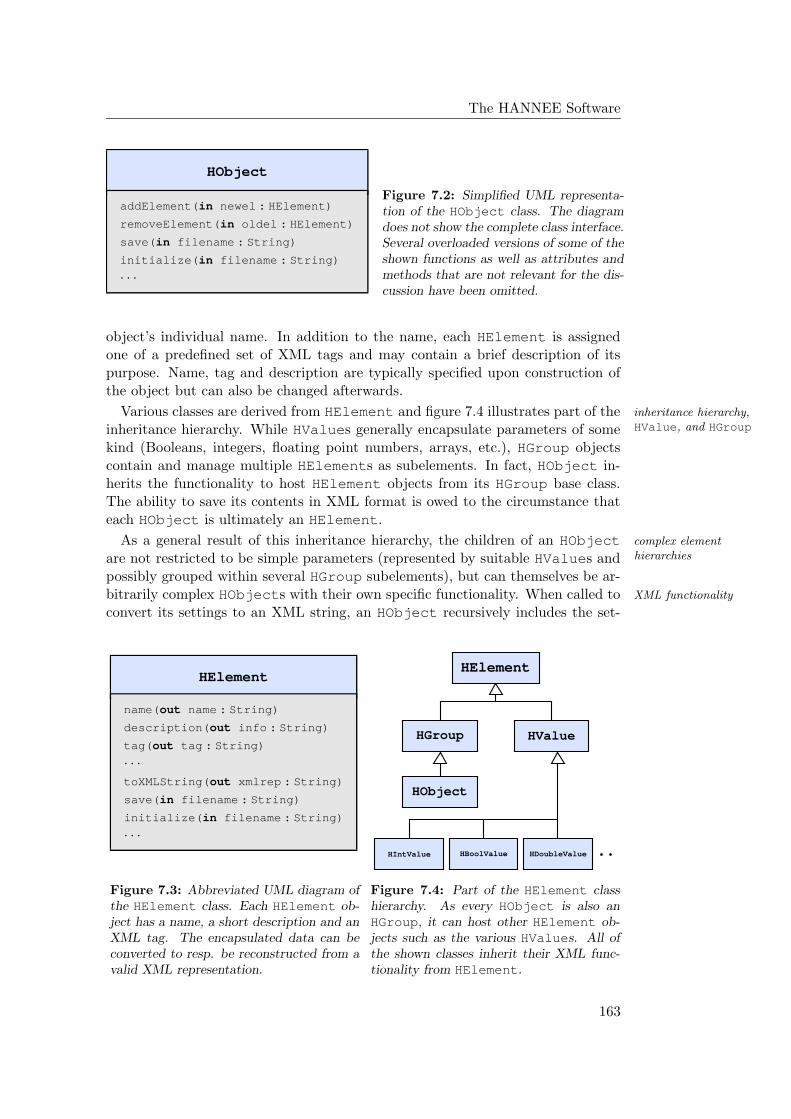
The HANNEE Software
HObject
addElement(in newel : HElement)
removeElement(in oldel : HElement)
save(in filename : String)
initialize(in filename : String)
· · ·
Figure 7.2: Simplified UML representa-tion of the HObject class. The diagramdoes not show the complete class interface.Several overloaded versions of some of theshown functions as well as attributes andmethods that are not relevant for the dis-cussion have been omitted.
object’s individual name. In addition to the name, each HElement is assignedone of a predefined set of XML tags and may contain a brief description of itspurpose. Name, tag and description are typically specified upon construction ofthe object but can also be changed afterwards.
Various classes are derived from HElement and figure 7.4 illustrates part of the inheritance hierarchy,HValue, and HGroupinheritance hierarchy. While HValues generally encapsulate parameters of some
kind (Booleans, integers, floating point numbers, arrays, etc.), HGroup objectscontain and manage multiple HElements as subelements. In fact, HObject in-herits the functionality to host HElement objects from its HGroup base class.The ability to save its contents in XML format is owed to the circumstance thateach HObject is ultimately an HElement.
As a general result of this inheritance hierarchy, the children of an HObject complex elementhierarchiesare not restricted to be simple parameters (represented by suitable HValues and
possibly grouped within several HGroup subelements), but can themselves be ar-bitrarily complex HObjects with their own specific functionality. When called to XML functionality
convert its settings to an XML string, an HObject recursively includes the set-
HElement
name(out name : String)
description(out info : String)
tag(out tag : String)
· · ·toXMLString(out xmlrep : String)
save(in filename : String)
initialize(in filename : String)
· · ·
Figure 7.3: Abbreviated UML diagram ofthe HElement class. Each HElement ob-ject has a name, a short description and anXML tag. The encapsulated data can beconverted to resp. be reconstructed from avalid XML representation.
PSfrag replacements
HElement
HGroup
HObject
HValue
HIntValue HBoolValue HDoubleValue
Figure 7.4: Part of the HElement classhierarchy. As every HObject is also anHGroup, it can host other HElement ob-jects such as the various HValues. All ofthe shown classes inherit their XML func-tionality from HElement.
163
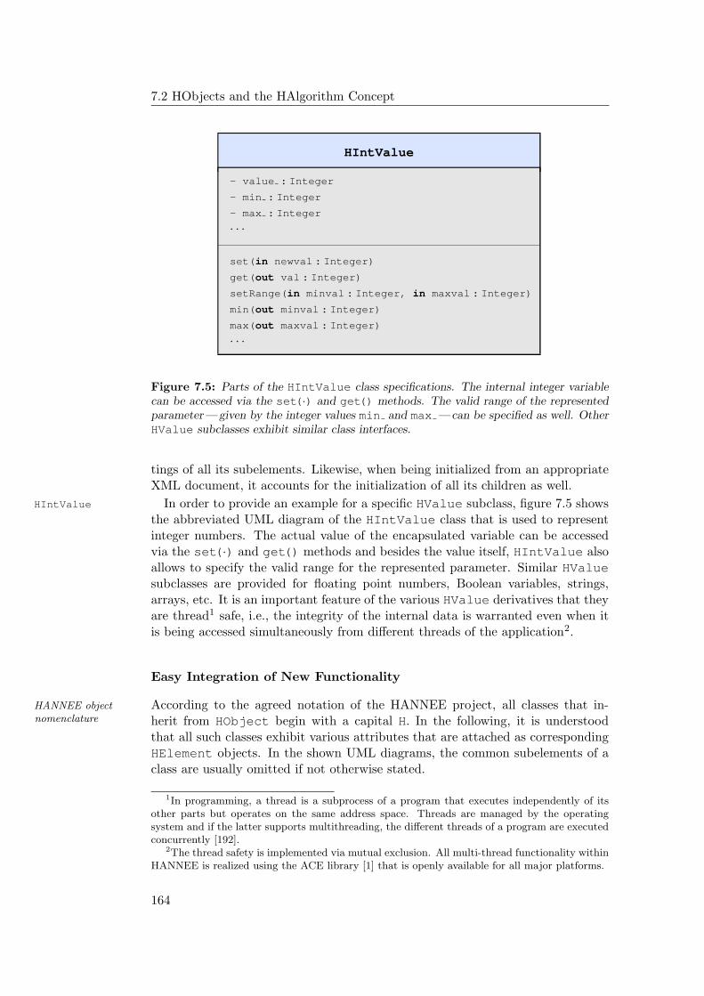
7.2 HObjects and the HAlgorithm Concept
HIntValue
- value : Integer
- min : Integer
- max : Integer
· · ·
set(in newval : Integer)
get(out val : Integer)
setRange(in minval : Integer, in maxval : Integer)
min(out minval : Integer)
max(out maxval : Integer)
· · ·
Figure 7.5: Parts of the HIntValue class specifications. The internal integer variablecan be accessed via the set(·) and get() methods. The valid range of the representedparameter — given by the integer values min and max —can be specified as well. OtherHValue subclasses exhibit similar class interfaces.
tings of all its subelements. Likewise, when being initialized from an appropriateXML document, it accounts for the initialization of all its children as well.
In order to provide an example for a specific HValue subclass, figure 7.5 showsHIntValue
the abbreviated UML diagram of the HIntValue class that is used to representinteger numbers. The actual value of the encapsulated variable can be accessedvia the set(·) and get() methods and besides the value itself, HIntValue alsoallows to specify the valid range for the represented parameter. Similar HValuesubclasses are provided for floating point numbers, Boolean variables, strings,arrays, etc. It is an important feature of the various HValue derivatives that theyare thread1 safe, i.e., the integrity of the internal data is warranted even when itis being accessed simultaneously from different threads of the application2.
Easy Integration of New Functionality
According to the agreed notation of the HANNEE project, all classes that in-HANNEE objectnomenclature herit from HObject begin with a capital H. In the following, it is understood
that all such classes exhibit various attributes that are attached as correspondingHElement objects. In the shown UML diagrams, the common subelements of aclass are usually omitted if not otherwise stated.
1In programming, a thread is a subprocess of a program that executes independently of itsother parts but operates on the same address space. Threads are managed by the operatingsystem and if the latter supports multithreading, the different threads of a program are executedconcurrently [192].
2The thread safety is implemented via mutual exclusion. All multi-thread functionality withinHANNEE is realized using the ACE library [1] that is openly available for all major platforms.
164
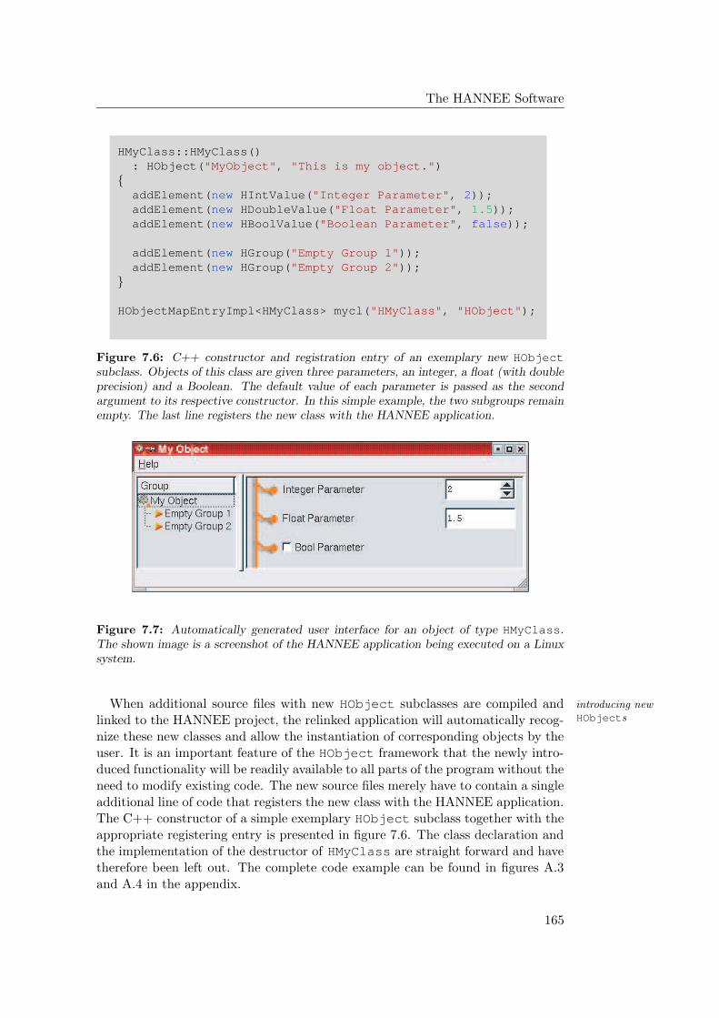
The HANNEE Software
HMyClass::HMyClass(): HObject("MyObject", "This is my object.")
addElement(new HIntValue("Integer Parameter", 2));addElement(new HDoubleValue("Float Parameter", 1.5));addElement(new HBoolValue("Boolean Parameter", false));
addElement(new HGroup("Empty Group 1"));addElement(new HGroup("Empty Group 2"));
HObjectMapEntryImpl<HMyClass> mycl("HMyClass", "HObject");
Figure 7.6: C++ constructor and registration entry of an exemplary new HObjectsubclass. Objects of this class are given three parameters, an integer, a float (with doubleprecision) and a Boolean. The default value of each parameter is passed as the secondargument to its respective constructor. In this simple example, the two subgroups remainempty. The last line registers the new class with the HANNEE application.
Figure 7.7: Automatically generated user interface for an object of type HMyClass.The shown image is a screenshot of the HANNEE application being executed on a Linuxsystem.
When additional source files with new HObject subclasses are compiled and introducing newHObjectslinked to the HANNEE project, the relinked application will automatically recog-
nize these new classes and allow the instantiation of corresponding objects by theuser. It is an important feature of the HObject framework that the newly intro-duced functionality will be readily available to all parts of the program without theneed to modify existing code. The new source files merely have to contain a singleadditional line of code that registers the new class with the HANNEE application.The C++ constructor of a simple exemplary HObject subclass together with theappropriate registering entry is presented in figure 7.6. The class declaration andthe implementation of the destructor of HMyClass are straight forward and havetherefore been left out. The complete code example can be found in figures A.3and A.4 in the appendix.
165
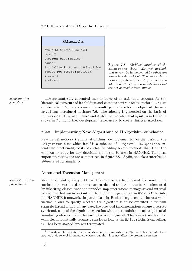
7.2 HObjects and the HAlgorithm Concept
HAlgorithm
start(in thread : Boolean)
reset()
busy(out busy : Boolean)
pause()
initialize(in former : HAlgorithm)
result(out result : HNetData)
# exec()
# clear()
· · ·
Figure 7.8: Abridged interface of theHAlgorithm class. Abstract methodsthat have to be implemented by subclassesare set in a slanted font. The last two func-tions are protected, i.e., they are only vis-ible inside the class and in subclasses butare not accessible from outside.
The automatically generated user interface of an HObject accounts for theautomatic GUIgeneration hierarchical structure of its children and contains controls for its various HValue
subelements. Figure 7.7 shows the resulting interface for an object of the newHMyClass introduced in figure 7.6. The labeling is generated on the basis ofthe various HElements’ names and it shall be repeated that apart from the codeshown in 7.6, no further development is necessary to create this user interface.
7.2.2 Implementing New Algorithms as HAlgorithm subclasses
New neural network training algorithms are implemented on the basis of theHAlgorithm class which itself is a subclass of HObject3. HAlgorithm ex-tends the functionality of its base class by adding several methods that define thecommon interface for any algorithm module to be used in HANNEE. The mostimportant extensions are summarized in figure 7.8. Again, the class interface isabbreviated for simplicity.
Automated Execution Management
Most prominently, every HAlgorithm can be started, paused and reset. Thebasic HAlgorithmfunctionality methods start(·) and reset() are predefined and are not to be reimplemented
by inheriting classes since the provided implementations manage several internalprocedures that are important for the smooth integration of an HAlgorithm intothe HANNEE framework. In particular, the Boolean argument to the start(·)method allows to specify whether the algorithm is to be executed in its ownseparate thread or not. In any case, the provided implementations ensure a correctsynchronization of the algorithm execution with other modules — such as potentialmonitoring objects — and the user interface in general. The busy() method, forexample, automatically returns true for as long as the HAlgorithm is executing,i.e., has been started but not terminated.
3In reality, the situation is somewhat more complicated as HAlgorithm inherits fromHObject via several intermediate classes, but that does not affect the present discussion.
166
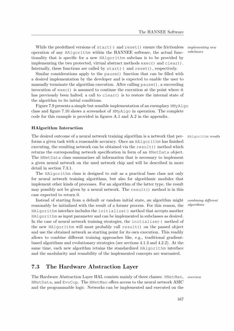
The HANNEE Software
While the predefined versions of start(·) and reset() ensure the frictionless implementing newsubclassesoperation of any HAlgorithm within the HANNEE software, the actual func-
tionality that is specific for a new HAlgorithm subclass is to be provided byimplementing the two protected, virtual abstract methods exec() and clear().Internally, these functions are called by start(·) and reset(), respectively.
Similar considerations apply to the pause() function that can be filled witha desired implementation by the developer and is expected to enable the user tomanually terminate the algorithm execution. After calling pause(), a succeedinginvocation of exec() is assumed to continue the execution at the point where ithas previously been halted; a call to clear() is to restore the internal state ofthe algorithm to its initial conditions.
Figure 7.9 presents a simple but sensible implementation of an exemplary HMyAlgoclass and figure 7.10 shows a screenshot of HMyAlgo in operation. The completecode for this example is provided in figures A.1 and A.2 in the appendix.
HAlgorithm Interaction
The desired outcome of a neural network training algorithm is a network that per- HAlgorithm results
forms a given task with a reasonable accuracy. Once an HAlgorithm has finishedexecuting, the resulting network can be obtained via the result() method whichreturns the corresponding network specification in form of an HNetData object.The HNetData class summarizes all information that is necessary to implementa given neural network on the used network chip and will be described in moredetail in section 7.3.1.
The HAlgorithm class is designed to suit as a practical base class not onlyfor neural network training algorithms, but also for algorithmic modules thatimplement other kinds of processes. For an algorithm of the latter type, the resultmay possibly not be given by a neural network. The result() method is in thiscase expected to return 0.
Instead of starting from a default or random initial state, an algorithm might combining differentalgorithmsreasonably be initialized with the result of a former process. For this reason, the
HAlgorithm interface includes the initialize(·) method that accepts anotherHAlgorithm as input parameter and can be implemented in subclasses as desired.In the case of neural network training strategies, the initialize(·) method ofthe new HAlgorithm will most probably call result() on the passed objectand use the obtained network as starting point for its own execution. This readilyallows to combine different training approaches like, e.g., traditional gradient-based algorithms and evolutionary strategies (see sections 4.1.3 and 4.2.2). At thesame time, each new algorithm retains the standardized HAlgorithm interfaceand the modularity and reusability of the implemented concepts are warranted.
7.3 The Hardware Abstraction Layer
The Hardware Abstraction Layer HAL consists mainly of three classes: HNetMan, overview
HNetData, and EvoCop. The HNetMan offers access to the neural network ASICand the programmable logic. Networks can be implemented and executed on the
167
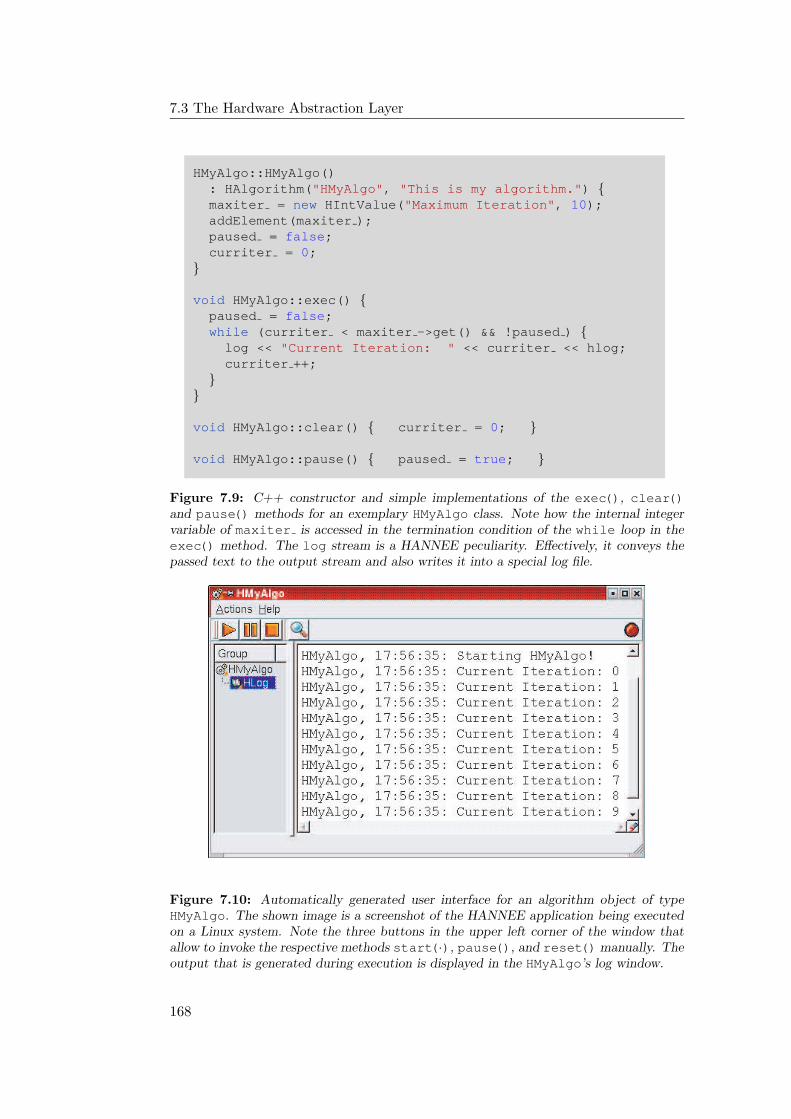
7.3 The Hardware Abstraction Layer
HMyAlgo::HMyAlgo(): HAlgorithm("HMyAlgo", "This is my algorithm.") maxiter = new HIntValue("Maximum Iteration", 10);addElement(maxiter );paused = false;curriter = 0;
void HMyAlgo::exec() paused = false;while (curriter < maxiter ->get() && !paused ) log << "Current Iteration: " << curriter << hlog;curriter ++;
void HMyAlgo::clear() curriter = 0;
void HMyAlgo::pause() paused = true;
Figure 7.9: C++ constructor and simple implementations of the exec(), clear()and pause() methods for an exemplary HMyAlgo class. Note how the internal integervariable of maxiter is accessed in the termination condition of the while loop in theexec() method. The log stream is a HANNEE peculiarity. Effectively, it conveys thepassed text to the output stream and also writes it into a special log file.
Figure 7.10: Automatically generated user interface for an algorithm object of typeHMyAlgo. The shown image is a screenshot of the HANNEE application being executedon a Linux system. Note the three buttons in the upper left corner of the window thatallow to invoke the respective methods start(·), pause(), and reset() manually. Theoutput that is generated during execution is displayed in the HMyAlgo’s log window.
168
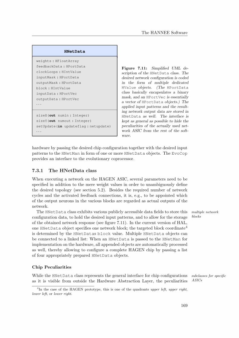
The HANNEE Software
HNetData
weights : HFloatArray
feedbackData : HPortData
clockLoops : HIntValue
inputMask : HPortData
outputMask : HPortData
block : HIntValue
inputData : HPortVec
outputData : HPortVec
· · ·
sizeX(out numin : Integer)
sizeY(out numout : Integer)
setUpdate(in updateflag : netupdate)
· · ·
Figure 7.11: Simplified UML de-scription of the HNetData class. Thedesired network configuration is codedin the form of multiple dedicatedHValue objects. (The HPortDataclass basically encapsulates a binarymask, and an HPortVec is essentiallya vector of HPortData objects.) Theapplied input patterns and the result-ing network output data are stored inHNetData as well. The interface iskept as general as possible to hide thepeculiarities of the actually used net-work ASIC from the rest of the soft-ware.
hardware by passing the desired chip configuration together with the desired inputpatterns to the HNetMan in form of one or more HNetData objects. The EvoCopprovides an interface to the evolutionary coprocessor.
7.3.1 The HNetData class
When executing a network on the HAGEN ASIC, several parameters need to bespecified in addition to the mere weight values in order to unambiguously definethe desired topology (see section 5.2). Besides the required number of networkcycles and the activated feedback connections, it is, e.g., to be appointed whichof the output neurons in the various blocks are regarded as actual outputs of thenetwork.
The HNetData class exhibits various publicly accessible data fields to store this multiple networkblocksconfiguration data, to hold the desired input patterns, and to allow for the storage
of the obtained network response (see figure 7.11). In the current version of HAL,one HNetData object specifies one network block; the targeted block coordinate4
is determined by the HNetDatas block value. Multiple HNetData objects canbe connected to a linked list: When an HNetData is passed to the HNetMan forimplementation on the hardware, all appended objects are automatically processedas well, thereby allowing to configure a complete HAGEN chip by passing a listof four appropriately prepared HNetData objects.
Chip Peculiarities
While the HNetData class represents the general interface for chip configurations subclasses for specificASICsas it is visible from outside the Hardware Abstraction Layer, the peculiarities
4In the case of the HAGEN prototype, this is one of the quadrants upper left, upper right,lower left, or lower right.
169
7.3 The Hardware Abstraction Layer
of different past, present, and future ASICs are to be accounted for by derivingcorresponding subclasses. For example, the configuration of one HAGEN block isgiven by an object of the HHagenData class. For the reasons discussed at thebeginning of this chapter, the actual nature of the currently used network chip isto be hidden from the rest of the program, and the HNetData interface has to bekept as general as possible. Therefore, the dimensions of the weight matrix — beingone of the specifications that is most likely to be changed for future chips — canbe inferred via sizeX() and sizeY() that return the number of input nodes andoutput neurons, respectively.
In addition to the network configuration, each type of network ASIC is antici-analog parameters
pated to require the specification of several analog parameters (reference currents,bias voltages, etc. — see also section 5.4.3) that are likely to differ between theindividual chip models. These settings do therefore not appear in the HNetDatainterface, but are defined in the chip specific subclasses where they are coded viaadequate HValues. As such, these parameters are not initially visible from out-side HAL. But due to the functionality of the HObject framework, they can, e.g.,be manually adjusted via the user interface.
Network Evaluation
Implementing and evaluating a neural network on the hardware proceeds as fol-executing networks onthe hardware lows: First, the desired network configuration is translated into a linked list of
HNetData objects — including the feedback connections, the weight values, andthe desired input patterns. Second, the list is sent to the hardware for execu-tion. Third, the resulting response of the network can be obtained from theoutputData fields of the respective HNetData objects and can be evaluatedas required. The second step is the only part that involves the hardware and isaccomplished by using the HNetMan class (section 7.3.2).
During the execution of chip-in-the-loop training algorithms, multiple networksrepeated execution
are iteratively evaluated on the chip that usually only differ in a few aspects,e.g., the weight values. It is thus undesirable to retransfer the whole set of un-changed settings to the hardware over and over again. In fact, weights, feedbackinformation, and input patterns are stored in the local memory of the FPGA andpotentially get updated whenever a new HNetData is sent (see section 6.1.3). Adedicated set of update flags in HNetData allows for a differentiated specificationof the information that actually needs to be retransmitted. In the case of theHAGEN/Darkwing setup, this can particularly speed up the network evaluationif the used input patterns are the same for all tested networks and only the weightvalues have to be updated for each run (see section 6.1.3).
7.3.2 The HNetMan class
For all classes outside the hardware abstraction layer, the access to the used neuralnetwork ASIC is mediated by one or more objects of the HNetMan class. Fig-ure 7.12 shows a simplified UML representation of its interface. Besides severalfunctions for the configuration of the FPGA, the testing of the hardware setup,
170
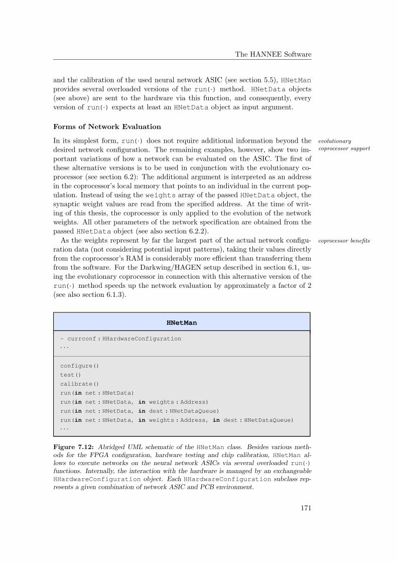
The HANNEE Software
and the calibration of the used neural network ASIC (see section 5.5), HNetManprovides several overloaded versions of the run(·) method. HNetData objects(see above) are sent to the hardware via this function, and consequently, everyversion of run(·) expects at least an HNetData object as input argument.
Forms of Network Evaluation
In its simplest form, run(·) does not require additional information beyond the evolutionarycoprocessor supportdesired network configuration. The remaining examples, however, show two im-
portant variations of how a network can be evaluated on the ASIC. The first ofthese alternative versions is to be used in conjunction with the evolutionary co-processor (see section 6.2): The additional argument is interpreted as an addressin the coprocessor’s local memory that points to an individual in the current pop-ulation. Instead of using the weights array of the passed HNetData object, thesynaptic weight values are read from the specified address. At the time of writ-ing of this thesis, the coprocessor is only applied to the evolution of the networkweights. All other parameters of the network specification are obtained from thepassed HNetData object (see also section 6.2.2).
As the weights represent by far the largest part of the actual network configu- coprocessor benefits
ration data (not considering potential input patterns), taking their values directlyfrom the coprocessor’s RAM is considerably more efficient than transferring themfrom the software. For the Darkwing/HAGEN setup described in section 6.1, us-ing the evolutionary coprocessor in connection with this alternative version of therun(·) method speeds up the network evaluation by approximately a factor of 2(see also section 6.1.3).
HNetMan
- currconf : HHardwareConfiguration
· · ·
configure()
test()
calibrate()
run(in net : HNetData)
run(in net : HNetData, in weights : Address)
run(in net : HNetData, in dest : HNetDataQueue)
run(in net : HNetData, in weights : Address, in dest : HNetDataQueue)
· · ·
Figure 7.12: Abridged UML schematic of the HNetMan class. Besides various meth-ods for the FPGA configuration, hardware testing and chip calibration, HNetMan al-lows to execute networks on the neural network ASICs via several overloaded run(·)functions. Internally, the interaction with the hardware is managed by an exchangeableHHardwareConfiguration object. Each HHardwareConfiguration subclass rep-resents a given combination of network ASIC and PCB environment.
171
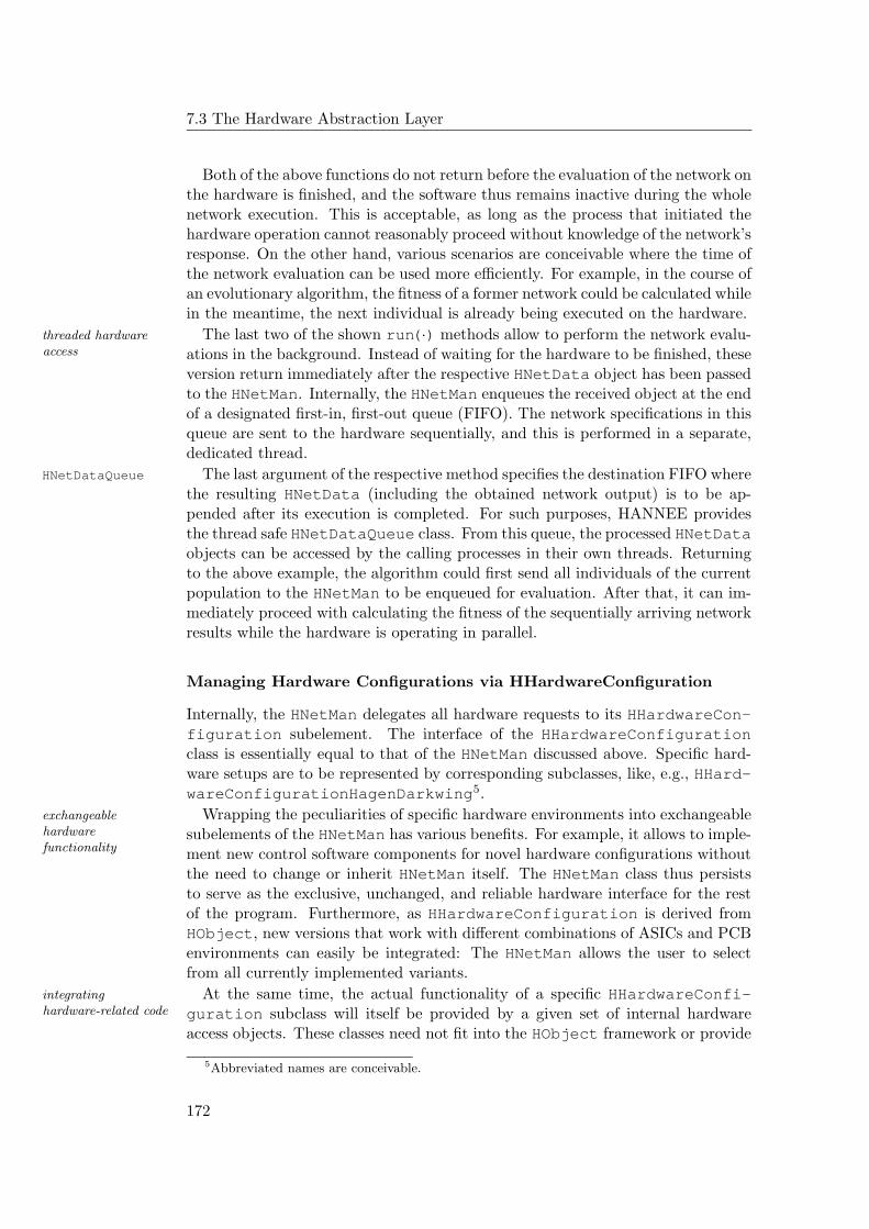
7.3 The Hardware Abstraction Layer
Both of the above functions do not return before the evaluation of the network onthe hardware is finished, and the software thus remains inactive during the wholenetwork execution. This is acceptable, as long as the process that initiated thehardware operation cannot reasonably proceed without knowledge of the network’sresponse. On the other hand, various scenarios are conceivable where the time ofthe network evaluation can be used more efficiently. For example, in the course ofan evolutionary algorithm, the fitness of a former network could be calculated whilein the meantime, the next individual is already being executed on the hardware.
The last two of the shown run(·) methods allow to perform the network evalu-threaded hardwareaccess ations in the background. Instead of waiting for the hardware to be finished, these
version return immediately after the respective HNetData object has been passedto the HNetMan. Internally, the HNetMan enqueues the received object at the endof a designated first-in, first-out queue (FIFO). The network specifications in thisqueue are sent to the hardware sequentially, and this is performed in a separate,dedicated thread.
The last argument of the respective method specifies the destination FIFO whereHNetDataQueue
the resulting HNetData (including the obtained network output) is to be ap-pended after its execution is completed. For such purposes, HANNEE providesthe thread safe HNetDataQueue class. From this queue, the processed HNetDataobjects can be accessed by the calling processes in their own threads. Returningto the above example, the algorithm could first send all individuals of the currentpopulation to the HNetMan to be enqueued for evaluation. After that, it can im-mediately proceed with calculating the fitness of the sequentially arriving networkresults while the hardware is operating in parallel.
Managing Hardware Configurations via HHardwareConfiguration
Internally, the HNetMan delegates all hardware requests to its HHardwareCon-figuration subelement. The interface of the HHardwareConfigurationclass is essentially equal to that of the HNetMan discussed above. Specific hard-ware setups are to be represented by corresponding subclasses, like, e.g., HHard-wareConfigurationHagenDarkwing5.
Wrapping the peculiarities of specific hardware environments into exchangeableexchangeablehardwarefunctionality
subelements of the HNetMan has various benefits. For example, it allows to imple-ment new control software components for novel hardware configurations withoutthe need to change or inherit HNetMan itself. The HNetMan class thus persiststo serve as the exclusive, unchanged, and reliable hardware interface for the restof the program. Furthermore, as HHardwareConfiguration is derived fromHObject, new versions that work with different combinations of ASICs and PCBenvironments can easily be integrated: The HNetMan allows the user to selectfrom all currently implemented variants.
At the same time, the actual functionality of a specific HHardwareConfi-integratinghardware-related code guration subclass will itself be provided by a given set of internal hardware
access objects. These classes need not fit into the HObject framework or provide
5Abbreviated names are conceivable.
172
The HANNEE Software
EvoCop
writeBlkSdram(in addr : Address, in dest : Address, in size : Integer)
allocIbuf(in num : Integer, out addr : Address)
allocCmd(in num : Integer, out addr : Address))
writePcIbuf(in addr : Address, in data : Integer)
start()
finito(out fin : Boolean)
setProbabUni(in prob : Integer)
sourceOne(in addr : Address)
maskNull(in len : Integer)
target(in addr : Address)
· · ·
Figure 7.13: Abbreviated UML interface of the EvoCop class. Apart from dedicatedmethods that implement the transfer of genetic data between the memory of the softwareand the local RAM of the coprocessor, the EvoCop class provides several functions tomanage and fill the coprocessor’s data and instruction buffer. A call to start() transmitsthe contents of this buffer to the local memory of the FPGA and initiates the executionof the defined instruction sequence.
any functionality beyond the interaction with the hardware. This way, the devel-oper of new hardware access software can concentrate on the optimization of thehardware related code. The resulting functionality can then easily be wrappedinto an HHardwareConfiguration subclass that provides all the convenientfeatures of the HObject framework, can readily be integrated into the HANNEEsoftware, and is therefore immediately available for use.
7.3.3 The EvoCop class
As it has been discussed in section 6.2.1, the evolutionary coprocessor that isimplemented in the configurable logic of the used hardware environment can becontrolled via an extensive set of instructions. Within HANNEE, the access to thecoprocessor is encapsulated by an object of the EvoCop class which provides thefunctionality to read and write genetic data to and from the local memory of theFPGA, to define a desired sequence of commands, and to initiate the successiveexecution of these instructions by the coprocessor itself. The abridged interfaceof the EvoCop class is shown in figure 7.13.
According to what has been stated in section 6.2.5, the provided set of in- types of commands
structions can roughly be divided into four groups: instructions that define theconfiguration for each stage of the pipeline, data transfer commands, instructionsthat specify the global evolution parameters, and those that control a single re-combination process, e.g., by specifying the source and target addresses of theprocessed genetic material in the local memory of the FPGA.
173
7.3 The Hardware Abstraction Layer
In the current stage of the used neural network framework, neither the copro-fixed configurations
cessor nor the HANNEE software allow to modify the basic operation of the singlestages of the coprocessor pipeline. In other words, the first type of instructions isnot yet supported and the lookup table (see section 6.2.4) for each of the stagesshown in figure 6.5 is predefined (see also section 6.2.5).
The transfer of genetic data from the software’s RAM space to the local memorydata transfer
of the coprocessor is implemented by the writeBlkSdram(·) method. Thisfunction requires the specification of the source address in the local memory of theCPU, the target address within the SDRAM of the coprocessor, and the numberof bytes to be transferred. A corresponding readBlkSdram(·) method (notshown in figure 7.13) transmits a defined number of bytes from the memory of thecoprocessor into the memory of the CPU .
Instruction Buffer Management
While the above commands are issued to the coprocessor directly and executedpooling instructions
immediately, the majority of instructions that control the processing of the hostedgenetic material are temporarily pooled inside an instruction buffer that residesin the RAM space of the software (see section 6.2.5). Once this buffer has beencoprocessor execution
filled with the desired set of instructions, an invocation of the start() commandtransfers the whole sequence to the coprocessor for execution. The start()method returns as soon as the respective data has been transmitted, i.e., duringthe processing of the genetic data, the software can in principle address othertasks. The state of the coprocessor can be inferred at any time via the finito()function which returns true as soon as the coprocessor has finished executing.
Apart from the actual instructions, dedicated parts of the buffer can also storebuffer management
frequently used data like, e.g., an available set of valid chromosome addressesand lengths (see section 6.2.5). The buffer space for the desired number of com-mands and data entries is allocated via the corresponding allocCmd(·) andallocIbuf(·) method, respectively (buffer space that is not required any longercan be released by according freeCmd(·) and freeIbuf(·) methods not shownin figure 7.13). While any desired data can then be written to a given address inthe buffer using the writePcIbuf(·) function, all specified instructions are con-secutively stored in the reserved command buffer in the order in which they havebeen issued. After a call to start(), the thus defined sequence of commands isbe executed by the coprocessor in the same order.
Evolution Commands
Three global evolution parameters can be specified externally: the respective prob-global parameters
abilities for each single gene to be subject to uniform and Gaussian mutation aswell as the width of the Gaussian distribution that is used to generate the randomnumbers for the latter. As an example, the probability for uniform mutation canbe set by the setProbabUni(·) method. Corresponding functions are providedfor the remaining two parameters. Typically, these methods are only executed
174
The HANNEE Software
once at the beginning of the training run6.
For each recombination process, the two source addresses of the parent chro- recombinationinstructionsmosomes in the local memory of the coprocessor, the target address of the off-
spring chromosome, as well as the desired crossover mask need to be specified (seesections 6.2.3 and 6.2.4). The required address information can be provided bythe sourceOne(·), sourceTwo(·) (not shown), and target(·) methods. Thepassed values do not directly spcify the adresses of the chromosomes in the RAMbut always refer to entries in the data buffer.
Crossover masks can be defined in a runlength encoding using the maskNull(·) crossover masks
and maskOne(·) functions (the latter method is not included in figure 7.13 forsimplicity). Initially, the mask has length 0. Using the above methods, it cansuccessively be extended by adding corresponding sequences of ones and zeroswith the respectively specified lengths.
During evolution, the software-implemented training algorithm will typicallypool a whole sequence of instructions that defines the recombination of multiplechromosome pairs — e.g., those that form two entire genomes or even several mat-ing pairs — before the actual processing of the genetic data is initiated by a callto start(). A simple code example for how the methods of the EvoCop classcan be used to program the coprocessor in practice is given in figure A.5 in theappendix.
At the time of writing of this thesis, the evolutionary coprocessor is still under additional features
development and subject to ongoing improvement. A variety of novel featureshas been added since its original version that allow for a more efficient control ofthe recombination process (see section 6.2.5). While this additional functionalityis already supported by the HANNEE software, it has not yet been thoroughlytested and is not used for the experiments presented in this thesis. A thoroughdiscussion of these features is therefore deferred to later publications that willdescribe the coprocessor in more detail7.
7.4 HEAF: An Object-Oriented Framework for Evo-lutionary Algorithms
It has been motivated in section 7.2.2 that implementing new network trainingalgorithms in the form of individual HAlgorithm subclasses greatly simplifies theprocess of integrating and testing new algorithmic concepts and allows to easilycombine different training strategies. Regarding the special case of evolutionaryalgorithms, the modularity concept can even be taken further.
As outlined in sections 3.3.2 and 3.3.4, the different parts of an evolutionary evolutionaryalgorithms and objectorientation
algorithm — the fitness calculation, the selection scheme and the genetic repre-sentation in combination with the variation operators — are inherently indepen-
6Note, however, that the specification of the global parameters nevertheless requires to allocatespace for a corresponding number of commands in the instruction buffer and is to be executedwith a call to start() (see also figure A.5 in the appendix).
7This primarily refers to the aforementioned PhD thesis of Tillmann Schmitz that has notbeen finalized at the time of this writing.
175
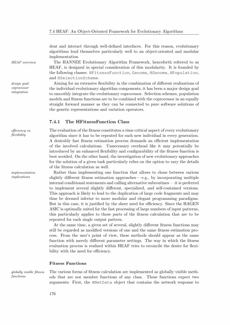
7.4 HEAF: An Object-Oriented Framework for Evolutionary Algorithms
dent and interact through well-defined interfaces. For this reason, evolutionaryalgorithms lend themselves particularly well to an object-oriented and modularimplementation.
The HANNEE Evolutionary Algorithm Framework, henceforth referred to asHEAF overview
HEAF, is designed in special consideration of this modularity. It is founded bythe following classes: HFitnessFunction, Genome, HGenome, HPopulation,and HSelectionScheme.
Aiming for an extensive flexibility in the combination of different realizations ofdesign goal:coprocessorintegration
the individual evolutionary algorithm components, it has been a major design goalto smoothly integrate the evolutionary coprocessor. Selection schemes, populationmodels and fitness functions are to be combined with the coprocessor in an equallystraight forward manner as they can be connected to pure software solutions ofthe genetic representations and variation operators.
7.4.1 The HFitnessFunction Class
The evaluation of the fitness constitutes a time critical aspect of every evolutionaryefficiency vs.flexibility algorithm since it has to be repeated for each new individual in every generation.
A desirably fast fitness estimation process demands an efficient implementationof the involved calculations. Unnecessary overhead like it may potentially beintroduced by an enhanced flexibility and configurability of the fitness function isbest avoided. On the other hand, the investigation of new evolutionary approachesfor the solution of a given task particularly relies on the option to vary the detailsof the fitness calculation as well.
Rather than implementing one function that allows to chose between variousimplementationimplications slightly different fitness estimation approaches — e.g., by incorporating multiple
internal conditional statements and calling alternative subroutines — it is preferredto implement several slightly different, specialized, and self-contained versions.This approach is likely to lead to the duplication of large code fragments and maythus be deemed inferior to more modular and elegant programming paradigms.But in this case, it is justified by the sheer need for efficiency. Since the HAGENASIC is optimally suited for the fast processing of large numbers of input patterns,this particularly applies to those parts of the fitness calculation that are to berepeated for each single output pattern.
At the same time, a given set of several, slightly different fitness functions maystill be regarded as modified versions of one and the same fitness estimation pro-cess. From the user’s point of view, these methods should appear as the samefunction with merely different parameter settings. The way in which the fitnessevaluation process is realized within HEAF tries to reconcile the desire for flexi-bility with the need for efficiency.
Fitness Functions
The various forms of fitness calculation are implemented as globally visible meth-globally visible fitnessfunctions ods that are not member functions of any class. These functions expect two
arguments: First, the HNetData object that contains the network response to
176
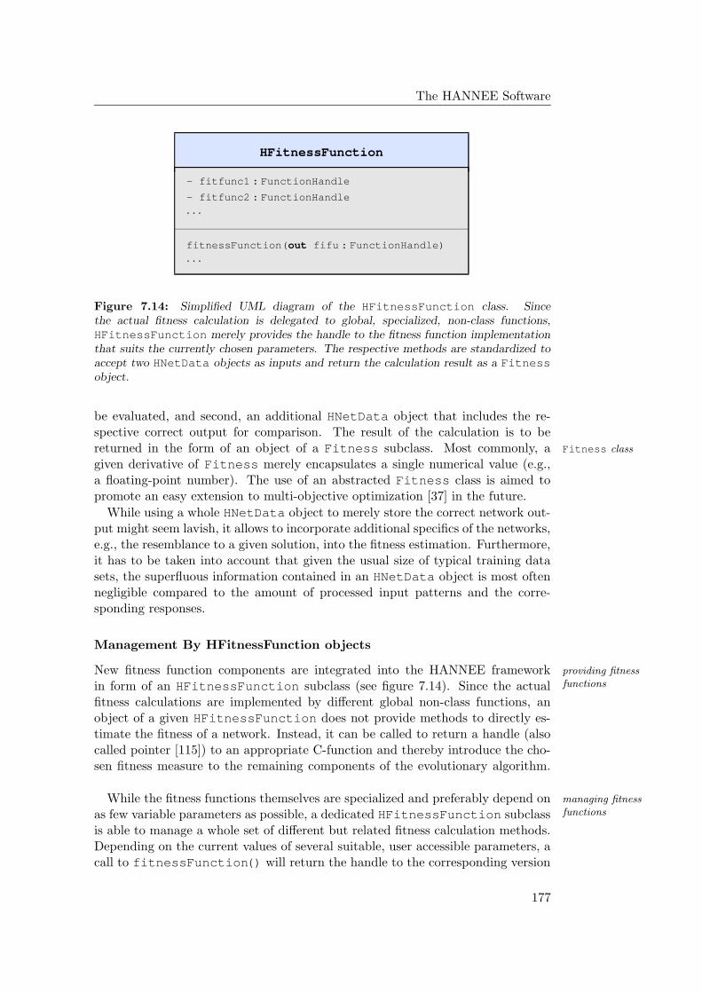
The HANNEE Software
HFitnessFunction
- fitfunc1 : FunctionHandle
- fitfunc2 : FunctionHandle
· · ·
fitnessFunction(out fifu : FunctionHandle)
· · ·
Figure 7.14: Simplified UML diagram of the HFitnessFunction class. Sincethe actual fitness calculation is delegated to global, specialized, non-class functions,HFitnessFunction merely provides the handle to the fitness function implementationthat suits the currently chosen parameters. The respective methods are standardized toaccept two HNetData objects as inputs and return the calculation result as a Fitnessobject.
be evaluated, and second, an additional HNetData object that includes the re-spective correct output for comparison. The result of the calculation is to bereturned in the form of an object of a Fitness subclass. Most commonly, a Fitness class
given derivative of Fitness merely encapsulates a single numerical value (e.g.,a floating-point number). The use of an abstracted Fitness class is aimed topromote an easy extension to multi-objective optimization [37] in the future.
While using a whole HNetData object to merely store the correct network out-put might seem lavish, it allows to incorporate additional specifics of the networks,e.g., the resemblance to a given solution, into the fitness estimation. Furthermore,it has to be taken into account that given the usual size of typical training datasets, the superfluous information contained in an HNetData object is most oftennegligible compared to the amount of processed input patterns and the corre-sponding responses.
Management By HFitnessFunction objects
New fitness function components are integrated into the HANNEE framework providing fitnessfunctionsin form of an HFitnessFunction subclass (see figure 7.14). Since the actual
fitness calculations are implemented by different global non-class functions, anobject of a given HFitnessFunction does not provide methods to directly es-timate the fitness of a network. Instead, it can be called to return a handle (alsocalled pointer [115]) to an appropriate C-function and thereby introduce the cho-sen fitness measure to the remaining components of the evolutionary algorithm.
While the fitness functions themselves are specialized and preferably depend on managing fitnessfunctionsas few variable parameters as possible, a dedicated HFitnessFunction subclass
is able to manage a whole set of different but related fitness calculation methods.Depending on the current values of several suitable, user accessible parameters, acall to fitnessFunction() will return the handle to the corresponding version
177
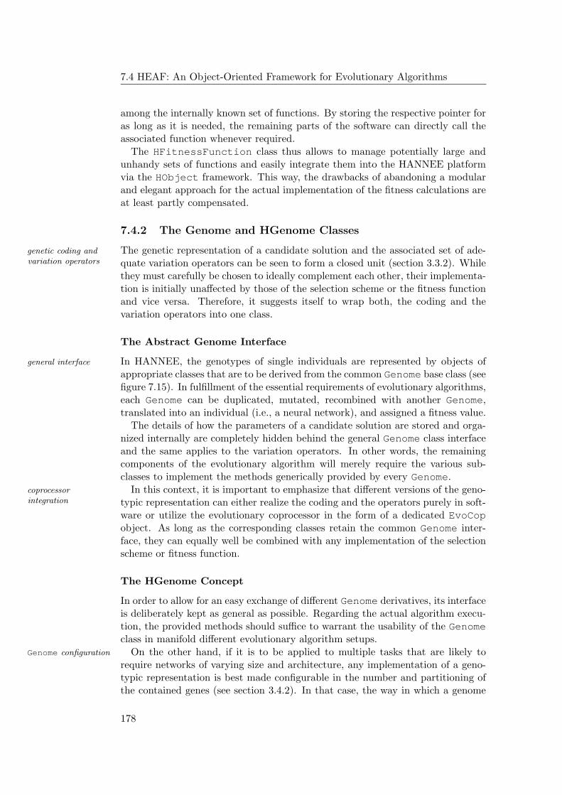
7.4 HEAF: An Object-Oriented Framework for Evolutionary Algorithms
among the internally known set of functions. By storing the respective pointer foras long as it is needed, the remaining parts of the software can directly call theassociated function whenever required.
The HFitnessFunction class thus allows to manage potentially large andunhandy sets of functions and easily integrate them into the HANNEE platformvia the HObject framework. This way, the drawbacks of abandoning a modularand elegant approach for the actual implementation of the fitness calculations areat least partly compensated.
7.4.2 The Genome and HGenome Classes
The genetic representation of a candidate solution and the associated set of ade-genetic coding andvariation operators quate variation operators can be seen to form a closed unit (section 3.3.2). While
they must carefully be chosen to ideally complement each other, their implementa-tion is initially unaffected by those of the selection scheme or the fitness functionand vice versa. Therefore, it suggests itself to wrap both, the coding and thevariation operators into one class.
The Abstract Genome Interface
In HANNEE, the genotypes of single individuals are represented by objects ofgeneral interface
appropriate classes that are to be derived from the common Genome base class (seefigure 7.15). In fulfillment of the essential requirements of evolutionary algorithms,each Genome can be duplicated, mutated, recombined with another Genome,translated into an individual (i.e., a neural network), and assigned a fitness value.
The details of how the parameters of a candidate solution are stored and orga-nized internally are completely hidden behind the general Genome class interfaceand the same applies to the variation operators. In other words, the remainingcomponents of the evolutionary algorithm will merely require the various sub-classes to implement the methods generically provided by every Genome.
In this context, it is important to emphasize that different versions of the geno-coprocessorintegration typic representation can either realize the coding and the operators purely in soft-
ware or utilize the evolutionary coprocessor in the form of a dedicated EvoCopobject. As long as the corresponding classes retain the common Genome inter-face, they can equally well be combined with any implementation of the selectionscheme or fitness function.
The HGenome Concept
In order to allow for an easy exchange of different Genome derivatives, its interfaceis deliberately kept as general as possible. Regarding the actual algorithm execu-tion, the provided methods should suffice to warrant the usability of the Genomeclass in manifold different evolutionary algorithm setups.
On the other hand, if it is to be applied to multiple tasks that are likely toGenome configuration
require networks of varying size and architecture, any implementation of a geno-typic representation is best made configurable in the number and partitioning ofthe contained genes (see section 3.4.2). In that case, the way in which a genome
178
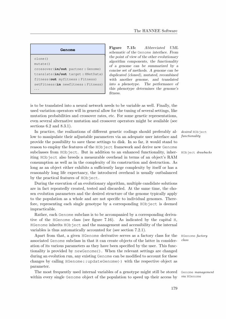
The HANNEE Software
Genome
clone()
mutate()
crossover(in/out partner : Genome)
translate(in/out target : HNetData)
fitness(out myfitness : Fitness)
setFitness(in newfitness : Fitness)
· · ·
Figure 7.15: Abbreviated UMLschematic of the Genome interface. Fromthe point of view of the other evolutionaryalgorithm components, the functionalityof a genome can be summarized by aconcise set of methods. A genome can beduplicated (cloned), mutated, recombinedwith another genome, and translatedinto a phenotype. The performance ofthis phenotype determines the genome’sfitness.
is to be translated into a neural network needs to be variable as well. Finally, theused variation operators will in general allow for the tuning of several settings, likemutation probabilities and crossover rates, etc. For some genetic representations,even several alternative mutation and crossover operators might be available (seesections 6.2 and 8.3.1).
In practice, the realizations of different genetic codings should preferably al- desired HObjectfunctionalitylow to manipulate their adjustable parameters via an adequate user interface and
provide the possibility to save these settings to disk. In so far, it would stand toreason to employ the features of the HObject framework and derive new Genomesubclasses from HObject. But in addition to an enhanced functionality, inher- HObject drawbacks
iting HObject also breeds a measurable overhead in terms of an object’s RAMconsumption as well as in the complexity of its construction and destruction. Aslong as an object either exhibits a sufficiently large complexity by itself or has areasonably long life expectancy, the introduced overhead is usually outbalancedby the practical features of HObject.
During the execution of an evolutionary algorithm, multiple candidate solutionsare in fact repeatedly created, tested and discarded. At the same time, the cho-sen evolution parameters and the desired structure of the genome typically applyto the population as a whole and are not specific to individual genomes. There-fore, representing each single genotype by a corresponding HObject is deemedimpracticable.
Rather, each Genome subclass is to be accompanied by a corresponding deriva-tive of the HGenome class (see figure 7.16). As indicated by the capital H,HGenome inherits HObject and the management and accessibility of the internalvariables is thus automatically accounted for (see section 7.2.1).
Apart from that, a given HGenome derivative serves as a factory class for the HGenome factoryclassassociated Genome subclass in that it can create objects of the latter in consider-
ation of its various parameters as they have been specified by the user. This func-tionality is provided by newGenome(). When the relevant settings are changedduring an evolution run, any existing Genome can be modified to account for thesechanges by calling HGenome::updateGenome(·) with the respective object asparameter.
The most frequently used internal variables of a genotype might still be stored Genome managementvia HGenomewithin every single Genome object of the population to speed up their access by
179
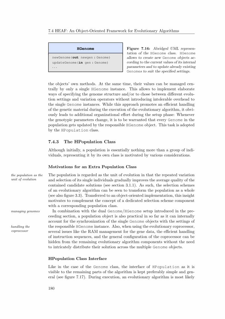
7.4 HEAF: An Object-Oriented Framework for Evolutionary Algorithms
HGenome
newGenome(out newgen : Genome)
updateGenome(in gen : Genome)
· · ·
Figure 7.16: Abridged UML represen-tation of the HGenome class. HGenomeallows to create new Genome objects ac-cording to the current values of its internalparameters and to update already existingGenomes to suit the specified settings.
the objects’ own methods. At the same time, their values can be managed cen-trally by only a single HGenome instance. This allows to implement elaborateways of specifying the genome structure and/or to chose between different evolu-tion settings and variation operators without introducing intolerable overhead tothe single Genome instances. While this approach promotes an efficient handlingof the genetic material during the execution of the evolutionary algorithm, it obvi-ously leads to additional organizational effort during the setup phase: Wheneverthe genotypic parameters change, it is to be warranted that every Genome in thepopulation gets updated by the responsible HGenome object. This task is adoptedby the HPopulation class.
7.4.3 The HPopulation Class
Although initially, a population is essentially nothing more than a group of indi-viduals, representing it by its own class is motivated by various considerations.
Motivations for an Extra Population Class
The population is regarded as the unit of evolution in that the repeated variationthe population as theunit of evolution and selection of its single individuals gradually improves the average quality of the
contained candidate solutions (see section 3.1.1). As such, the selection schemesof an evolutionary algorithm can be seen to transform the population as a whole(see also figure 3.3). Transferred to an object-oriented implementation, this insightmotivates to complement the concept of a dedicated selection scheme componentwith a corresponding population class.
In combination with the dual Genome/HGenome setup introduced in the pre-managing genomes
ceeding section, a population object is also practical in so far as it can internallyaccount for the synchronization of the single Genome objects with the settings ofthe responsible HGenome instance. Also, when using the evolutionary coprocessor,handling the
coprocessor several issues like the RAM management for the gene data, the efficient handlingof instruction sequences, and the general configuration of the coprocessor can behidden from the remaining evolutionary algorithm components without the needto intricately distribute their solution across the multiple Genome objects.
HPopulation Class Interface
Like in the case of the Genome class, the interface of HPopulation as it isvisible to the remaining parts of the algorithm is kept preferably simple and gen-eral (see figure 7.17). During execution, an evolutionary algorithm is most likely
180
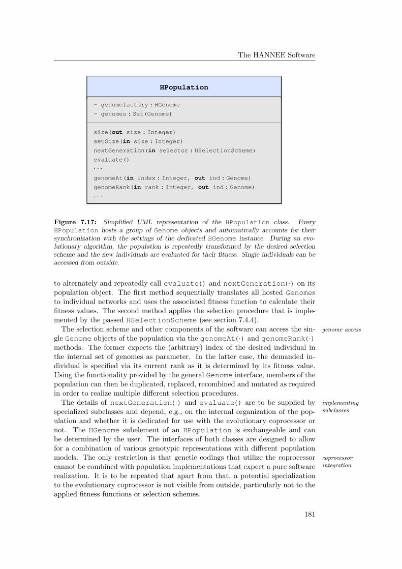
The HANNEE Software
HPopulation
- genomefactory : HGenome
- genomes : Set(Genome)
size(out size : Integer)
setSize(in size : Integer)
nextGeneration(in selector : HSelectionScheme)
evaluate()
· · ·genomeAt(in index : Integer, out ind : Genome)
genomeRank(in rank : Integer, out ind : Genome)
· · ·
Figure 7.17: Simplified UML representation of the HPopulation class. EveryHPopulation hosts a group of Genome objects and automatically accounts for theirsynchronization with the settings of the dedicated HGenome instance. During an evo-lutionary algorithm, the population is repeatedly transformed by the desired selectionscheme and the new individuals are evaluated for their fitness. Single individuals can beaccessed from outside.
to alternately and repeatedly call evaluate() and nextGeneration(·) on itspopulation object. The first method sequentially translates all hosted Genomesto individual networks and uses the associated fitness function to calculate theirfitness values. The second method applies the selection procedure that is imple-mented by the passed HSelectionScheme (see section 7.4.4).
The selection scheme and other components of the software can access the sin- genome access
gle Genome objects of the population via the genomeAt(·) and genomeRank(·)methods. The former expects the (arbitrary) index of the desired individual inthe internal set of genomes as parameter. In the latter case, the demanded in-dividual is specified via its current rank as it is determined by its fitness value.Using the functionality provided by the general Genome interface, members of thepopulation can then be duplicated, replaced, recombined and mutated as requiredin order to realize multiple different selection procedures.
The details of nextGeneration(·) and evaluate() are to be supplied by implementingsubclassesspecialized subclasses and depend, e.g., on the internal organization of the pop-
ulation and whether it is dedicated for use with the evolutionary coprocessor ornot. The HGenome subelement of an HPopulation is exchangeable and canbe determined by the user. The interfaces of both classes are designed to allowfor a combination of various genotypic representations with different populationmodels. The only restriction is that genetic codings that utilize the coprocessor coprocessor
integrationcannot be combined with population implementations that expect a pure softwarerealization. It is to be repeated that apart from that, a potential specializationto the evolutionary coprocessor is not visible from outside, particularly not to theapplied fitness functions or selection schemes.
181
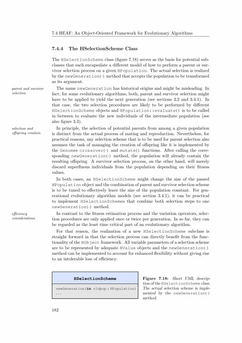
7.4 HEAF: An Object-Oriented Framework for Evolutionary Algorithms
7.4.4 The HSelectionScheme Class
The HSelectionScheme class (figure 7.18) serves as the basis for potential sub-classes that each encapsulate a different model of how to perform a parent or sur-vivor selection process on a given HPopulation. The actual selection is realizedby the newGeneration(·) method that accepts the population to be transformedas its argument.
The name newGeneration has historical origins and might be misleading. Inparent and survivorselection fact, for some evolutionary algorithms, both, parent and survivor selection might
have to be applied to yield the next generation (see sections 3.2 and 3.4.1). Inthat case, the two selection procedures are likely to be performed by differentHSelectionScheme objects and HPopulation::evaluate() is to be calledin between to evaluate the new individuals of the intermediate population (seealso figure 3.3).
In principle, the selection of potential parents from among a given populationselection andoffspring creation is distinct from the actual process of mating and reproduction. Nevertheless, for
practical reasons, any selection scheme that is to be used for parent selection alsoassumes the task of managing the creation of offspring like it is implemented bythe Genomes crossover(·) and mutate() functions. After calling the corre-sponding newGeneration(·) method, the population will already contain theresulting offspring. A survivor selection process, on the other hand, will merelydiscard superfluous individuals from the population depending on their fitnessvalues.
In both cases, an HSelectionScheme might change the size of the passedHPopulation object and the combination of parent and survivor selection schemeis to be tuned to effectively leave the size of the population constant. For gen-erational evolutionary algorithm models (see section 3.4.1), it can be practicalto implement HSelectionSchemes that combine both selection steps to onenewGeneration(·) method.
In contrast to the fitness estimation process and the variation operators, selec-efficiencyconsiderations tion procedures are only applied once or twice per generation. In so far, they can
be regarded as the least time critical part of an evolutionary algorithm.
For that reason, the realization of a new HSelectionScheme subclass isstraight forward in that the selection process can directly benefit from the func-tionality of the HObject framework. All variable parameters of a selection schemeare to be represented by adequate HValue objects and the newGeneration(·)method can be implemented to account for enhanced flexibility without giving riseto an intolerable loss of efficiency.
HSelectionScheme
newGeneration(in oldpop : HPopulation)
· · ·
Figure 7.18: Short UML descrip-tion of the HSelectionScheme class.The actual selection scheme is imple-mented by the newGeneration(·)method.
182
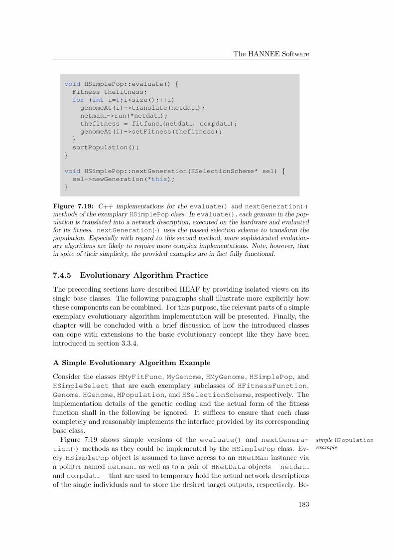
The HANNEE Software
void HSimplePop::evaluate() Fitness thefitness;for (int i=1;i<size();++i)genomeAt(i)->translate(netdat );netman ->run(*netdat );thefitness = fitfunc (netdat , compdat );genomeAt(i)->setFitness(thefitness);
sortPopulation();
void HSimplePop::nextGeneration(HSelectionScheme* sel) sel->newGeneration(*this);
Figure 7.19: C++ implementations for the evaluate() and nextGeneration(·)methods of the exemplary HSimplePop class. In evaluate(), each genome in the pop-ulation is translated into a network description, executed on the hardware and evaluatedfor its fitness. nextGeneration(·) uses the passed selection scheme to transform thepopulation. Especially with regard to this second method, more sophisticated evolution-ary algorithms are likely to require more complex implementations. Note, however, thatin spite of their simplicity, the provided examples are in fact fully functional.
7.4.5 Evolutionary Algorithm Practice
The preceeding sections have described HEAF by providing isolated views on itssingle base classes. The following paragraphs shall illustrate more explicitly howthese components can be combined. For this purpose, the relevant parts of a simpleexemplary evolutionary algorithm implementation will be presented. Finally, thechapter will be concluded with a brief discussion of how the introduced classescan cope with extensions to the basic evolutionary concept like they have beenintroduced in section 3.3.4.
A Simple Evolutionary Algorithm Example
Consider the classes HMyFitFunc, MyGenome, HMyGenome, HSimplePop, andHSimpleSelect that are each exemplary subclasses of HFitnessFunction,Genome, HGenome, HPopulation, and HSelectionScheme, respectively. Theimplementation details of the genetic coding and the actual form of the fitnessfunction shall in the following be ignored. It suffices to ensure that each classcompletely and reasonably implements the interface provided by its correspondingbase class.
Figure 7.19 shows simple versions of the evaluate() and nextGenera- simple HPopulationexampletion(·) methods as they could be implemented by the HSimplePop class. Ev-
ery HSimplePop object is assumed to have access to an HNetMan instance viaa pointer named netman as well as to a pair of HNetData objects —netdatand compdat — that are used to temporary hold the actual network descriptionsof the single individuals and to store the desired target outputs, respectively. Be-
183
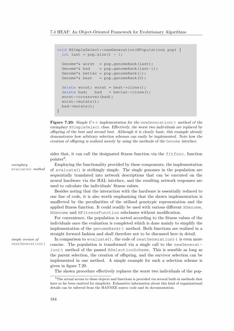
7.4 HEAF: An Object-Oriented Framework for Evolutionary Algorithms
void HSimpleSelect::newGeneration(HPopulation& pop) int last = pop.size() - 1;
Genome*& worst = pop.genomeRank(last);Genome*& bad = pop.genomeRank(last-1);Genome*& better = pop.genomeRank(1);Genome*& best = pop.genomeRank(0);
delete worst; worst = best->clone();delete bad; bad = better->clone();worst->crossover(bad);worst->mutate();bad->mutate();
Figure 7.20: Simple C++ implementation for the newGeneration(·) method of theexemplary HSimpleSelect class. Effectively, the worst two individuals are replaced byoffspring of the best and second best. Although it is clearly basic, this example alreadydemonstrates how arbitrary selection schemes can easily be implemented. Note how thecreation of offspring is realized merely by using the methods of the Genome interface.
sides that, it can call the designated fitness function via the fitfunc functionpointer8.
Employing the functionality provided by these components, the implementationexemplaryevaluate() method of evaluate() is strikingly simple. The single genomes in the population are
sequentially translated into network descriptions that can be executed on theneural hardware via the HAL interface, and the resulting network responses areused to calculate the individuals’ fitness values.
Besides noting that the interaction with the hardware is essentially reduced toone line of code, it is also worth emphasizing that the shown implementation isunaffected by the peculiarities of the utilized genotypic representation and theapplied fitness function. It could readily be used with various different HGenome,HGenome and HFitnessFunction subclasses without modification.
For convenience, the population is sorted according to the fitness values of theindividuals once the evaluation is completed which is done mainly to simplify theimplementation of the genomeRank(·) method. Both functions are realized in astraight forward fashion and shall therefore not to be discussed here in detail.
In comparison to evaluate(), the code of nextGeneration(·) is even moresimple version ofnextGeneration(·) concise. The population is transformed via a single call to the newGenerat-
ion(·) method of the passed HSelectionScheme. This is sensible as long asthe parent selection, the creation of offspring, and the survivor selection can beimplemented in one method. A simple example for such a selection scheme isgiven in figure 7.20.
The shown procedure effectively replaces the worst two individuals of the pop-
8The actual access to these objects and functions is provided via several built-in methods thathave so far been omitted for simplicity. Exhaustive information about this kind of organizationaldetails can be inferred from the HANNEE source code and its documentation.
184
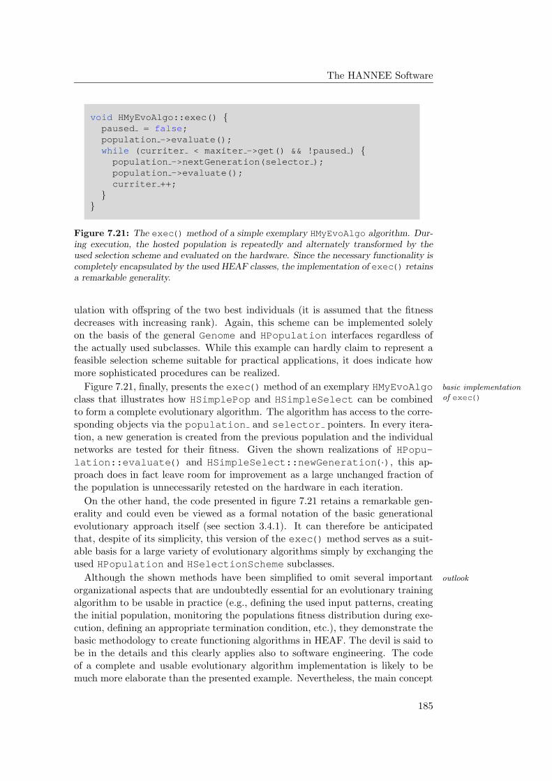
The HANNEE Software
void HMyEvoAlgo::exec() paused = false;population ->evaluate();while (curriter < maxiter ->get() && !paused ) population ->nextGeneration(selector );population ->evaluate();curriter ++;
Figure 7.21: The exec() method of a simple exemplary HMyEvoAlgo algorithm. Dur-ing execution, the hosted population is repeatedly and alternately transformed by theused selection scheme and evaluated on the hardware. Since the necessary functionality iscompletely encapsulated by the used HEAF classes, the implementation of exec() retainsa remarkable generality.
ulation with offspring of the two best individuals (it is assumed that the fitnessdecreases with increasing rank). Again, this scheme can be implemented solelyon the basis of the general Genome and HPopulation interfaces regardless ofthe actually used subclasses. While this example can hardly claim to represent afeasible selection scheme suitable for practical applications, it does indicate howmore sophisticated procedures can be realized.
Figure 7.21, finally, presents the exec() method of an exemplary HMyEvoAlgo basic implementationof exec()class that illustrates how HSimplePop and HSimpleSelect can be combined
to form a complete evolutionary algorithm. The algorithm has access to the corre-sponding objects via the population and selector pointers. In every itera-tion, a new generation is created from the previous population and the individualnetworks are tested for their fitness. Given the shown realizations of HPopu-lation::evaluate() and HSimpleSelect::newGeneration(·), this ap-proach does in fact leave room for improvement as a large unchanged fraction ofthe population is unnecessarily retested on the hardware in each iteration.
On the other hand, the code presented in figure 7.21 retains a remarkable gen-erality and could even be viewed as a formal notation of the basic generationalevolutionary approach itself (see section 3.4.1). It can therefore be anticipatedthat, despite of its simplicity, this version of the exec() method serves as a suit-able basis for a large variety of evolutionary algorithms simply by exchanging theused HPopulation and HSelectionScheme subclasses.
Although the shown methods have been simplified to omit several important outlook
organizational aspects that are undoubtedly essential for an evolutionary trainingalgorithm to be usable in practice (e.g., defining the used input patterns, creatingthe initial population, monitoring the populations fitness distribution during exe-cution, defining an appropriate termination condition, etc.), they demonstrate thebasic methodology to create functioning algorithms in HEAF. The devil is said tobe in the details and this clearly applies also to software engineering. The codeof a complete and usable evolutionary algorithm implementation is likely to bemuch more elaborate than the presented example. Nevertheless, the main concept
185
7.4 HEAF: An Object-Oriented Framework for Evolutionary Algorithms
of exploiting the inherent modularity of evolutionary computation for the realiza-tion of a flexible evolutionary algorithm software framework holds. It remains tobe investigated whether the proposed design withstands a confrontation with theextensions to the basic evolutionary approach that have been brought forward insection 3.3.4.
Extensions to the Basic Concept
Among other things, encapsulating the details of the population management intoisland-modelalgorithms a dedicated HPopulation class yields the advantage that multiple populations
can easily be combined to implement various forms of island-model approaches(section 3.3.4). In contrast, the realization of diffusion-model algorithms re-diffusion-model
algorithms quires to extend the functionality of the HPopulation and HSelectionSchemeclasses by deriving appropriate subclasses. A corresponding HPopulation deriva-tive needs to account for the desired topology such that the hereby defined neigh-borhood of a given individual is well-defined and can readily inferred by thenewGeneration(·) method of the used HSelectionScheme object.
One possible way to introduce this functionality is to expand the interface ofthe HPopulation subclass by a dedicated method, e.g.,
neighborhood(in ind : Integer, out neigh : Set(Integer)),
which returns the set of indices neigh of all population members that form theneighborhood of a given individual ind. This is probably the most intuitiveapproach but it is limited in so far as an accompanying HSelectionSchemesubclass has to be implemented as well that actually employs this function duringthe selection process. Hence, although the new HPopulation class would providethe necessary topology information, the actual implementation of the diffusion-model concept would be deferred to the new HSelectionScheme derivative.
An alternative approach exploits the fact that the HPopulation::nextGen-eration(·) function is designed as a callback routine (see also figure 7.19): In-stead of calling HSelectionScheme::newGeneration(·) on itself, a special-ized diffusion-model population can repeatedly apply the desired selection proce-dure to appropriate subpopulations. These neighborhoods can be represented byinternal objects of another specialized HPopulation subclass that do not actu-ally host their own genomes. Instead, their genomeAt(·) and genomeRank(·)methods are to return handles to the corresponding genotypes of the original pop-ulation. This second solution is advantageous in so far as it allows to employexisting HSelectionScheme classes unchanged.
Note that for both variants, the peculiarities of the diffusion-model concept areretained modularityand generality completely hidden from the actual algorithm implementation. For example, the
code presented in figure 7.21 would not need to be changed at all. This insight canbe regarded as an additional support for the claim that the inherent modularityof evolutionary algorithms (section 3.3.2) is not compromised by the extensionsintroduced in section 3.3.4.
186
The HANNEE Software
Analog considerations apply to the concept of a similarity metric used for spe- similarity measuresand speciationciation schemes. As suggested in section 3.3.4, the task of quantifying the resem-
blance between two individuals can be assigned to the genetic representation. Inother words, subclasses of Genome can provide the necessary information in formof an additional method, e.g.,
similarity(in comp : Genome, out sim : Float),
which returns the similarity sim between the regarded object and the specifiedpartner comp in adequate units. Alternatively, a special HFitnessFunctionobject could be used to provide functions that do not actually evaluate the per-formance of a network in consideration of the target output but calculate somemeasure for the resemblance between the two passed HNetData objects. Thissecond variant can conveniently be used with already existing Genome classes,but an estimation of the similarity based on the final networks runs the risk ofbeing less efficient.
While the first method measures the distance in the genotype space, the second again: retainedmodularity andgenerality
quantifies the similarity in the phenotype space. In both cases, the thus providedinformation can be used by dedicated HSelectionScheme subclasses and again,the algorithm implementation remains unaffected on the higher level.
The above reflections do not only underline the modularity of the evolutionarycomputation concept itself. They also demonstrate that HEAF has the potentialto serve as a practical and flexible foundation for the efficient implementation ofevolutionary training algorithms for mixed-signal neural networks. This function-ality constitutes the basis for the development of the efficient evolutionary trainingstrategies introduced in the following chapters.
187


Part III
Experiments and Results
189

Chapter 8
A Simple EvolutionaryApproach
Whenever you are asked if you can do a job,tell ’em, ’Certainly I can!’ Then get busy andfind out how to do it.
Theodore Roosevelt
The hardware neural network framework presented in the preceeding chaptersallows to implement networks with in the order of 104 synapses that can efficientlyexploit the inherent parallelism of neural information processing. Networks ofthe achievable scale and performance constitute a promising approach to tacklechallenging real-world problems that involve the processing of large amounts ofdata. But in order to fully benefit from the potential of the provided hardwareresources, suitable training algorithms have to be devised first that can cope withthe size of the implemented networks and the complexity of the investigated tasks.
Several strategies have been considered for the design of neural systems that aimto make best use of the available resources and the featured parallelism. Both, theconcept of computing without stable states (section 2.3.4) as well as the hierarchi-cal approach (section 2.3.2) have been demonstrated to be successfully applicableto the construction of networks on the presented hardware platform [52] [184].
The experiments described in this and the following chapters investigate thepotential of the more traditional chip-in-the-loop training approach. As it has beenstated before, highly iterative generate-and-test algorithms ideally complement therealization of neural networks on the HAGEN chip since they can on the one handaccount for the peculiarities of the CMOS substrate and the inevitable noise inthe analog circuits (sections 2.4.5 and 5.5.1) and can on the other hand take fulladvantage of HAGEN’s high configurational speed (section 5.4.4). Beyond that,the utilization of evolutionary algorithms or any other black-box approaches (seesection 4.3) readily avoids the credit assignment problem (see section 2.2.2) thatusually impedes the training of multilayer networks of threshold neurons.
It remains that in order to keep up pace with the speed of the networks, thetraining algorithm itself has to be implemented efficiently. This insight drove the
191
8.1 Classification Benchmarks
design of the evolutionary coprocessor that provides flexible means of acceleratinga large diversity of evolutionary strategies (see section 6.2). In its current state,the coprocessor supports codings and operators that are primarily suited for theevolution of the mere synaptic weights. More sophisticated representations — likethey have been discussed in section 4.2.2— that allow to simultaneously optimizealso the network architecture can, as yet, not fully benefit from hardware acceler-ation. In general, it can be said that the desire for fast algorithm implementationsmotivates the use of simple algorithms. Elaborate speciation schemes, computa-tionally expensive fitness measures, and/or ingenious genetic representations runthe risk of compromising the speed advantage of the neural network hardwareduring training.
In turn, the desire for simple algorithms interferes with the ultimate goal oftraining complex networks for demanding real-world tasks. Besides describing thegeneral training setup that is to serve as the basis for all presented experiments,this chapter will investigate in how far the restriction to simple evolutionary algo-rithms limits the achievable training success. The obtained results will motivatethe development of the improved training strategies introduced in the next chap-ter.
8.1 Classification Benchmarks
Pattern classification (see section 1.2.4) is one of the most important types ofbenchmark problems
applications for neural networks [20] [163]. There are a large number of real-worldclassification problems originating from a variety of application areas that areaccepted throughout the neural network community as suitable benchmarks forevaluating the feasibility of network models and novel training approaches.
Within the experiments described in this thesis, evolutionary training algo-rithms are tested for their ability to train neural networks on the HAGEN chipfor a selected set of these common classification benchmarks. This readily allowsfor a direct comparison of the achieved results with other neural network imple-mentations, training algorithms, or classification procedures. The selected tasksall represent real-world data and are therefore anticipated to capture the mainfeatures that characterize realistic pattern categorization applications in practice.The data sets have been obtained from the UCI KDD online archive [90], but someare also included in the “Proben1” collection compiled by Lutz Prechelt [163].
8.1.1 The Classification Tasks
A total of nine well-established classification benchmarks are used within the de-the selected tasks
scribed experiments: the breast cancer, diabetes, heart disease, liver disorder, irisplant, wine, glass, E.coli, and yeast problems. Each task is represented by a finiteset E of Ne exemplary instances eα, 1 ≤ α ≤ Ne, that each belong to one of Nc
classes Ck, 1 ≤ k ≤ Nc. Every instance eα of the respective problem is describedby a set of Na attributes whose values are used to form the corresponding inputvectors Iα for the network (see also section 1.2.4).
192
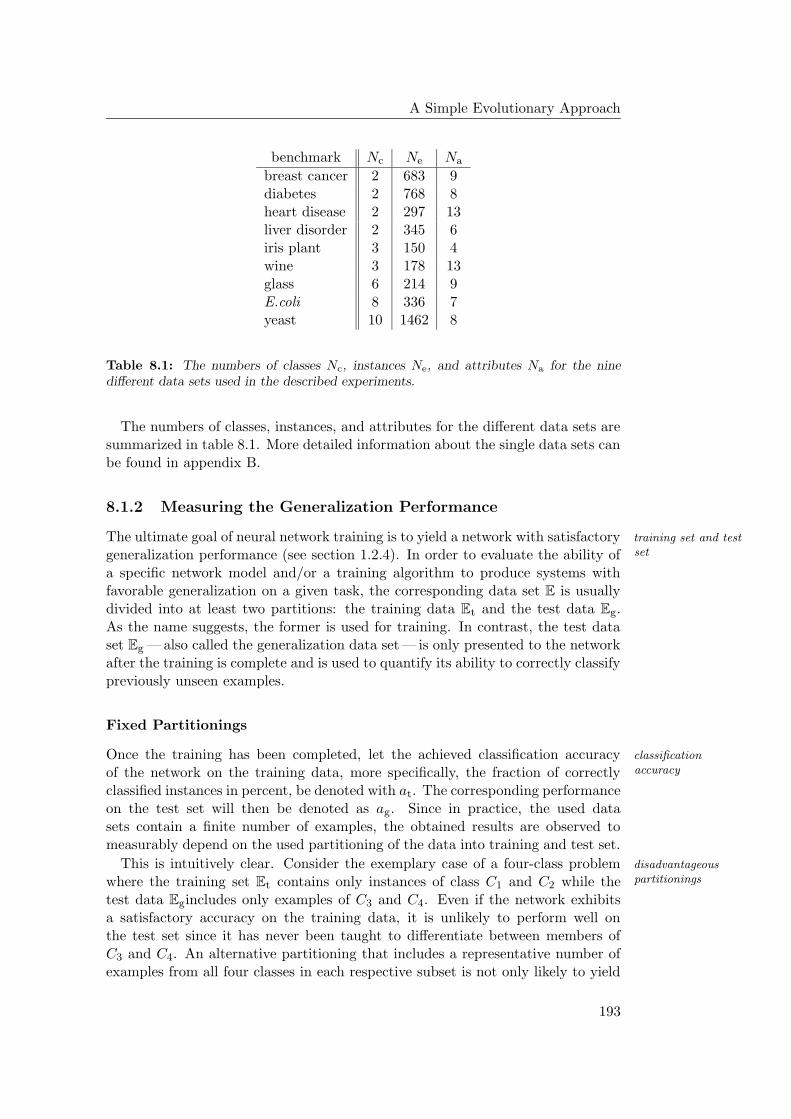
A Simple Evolutionary Approach
benchmark Nc Ne Na
breast cancer 2 683 9diabetes 2 768 8heart disease 2 297 13liver disorder 2 345 6iris plant 3 150 4wine 3 178 13glass 6 214 9E.coli 8 336 7yeast 10 1462 8
Table 8.1: The numbers of classes Nc, instances Ne, and attributes Na for the ninedifferent data sets used in the described experiments.
The numbers of classes, instances, and attributes for the different data sets aresummarized in table 8.1. More detailed information about the single data sets canbe found in appendix B.
8.1.2 Measuring the Generalization Performance
The ultimate goal of neural network training is to yield a network with satisfactory training set and testsetgeneralization performance (see section 1.2.4). In order to evaluate the ability of
a specific network model and/or a training algorithm to produce systems withfavorable generalization on a given task, the corresponding data set E is usuallydivided into at least two partitions: the training data Et and the test data Eg.As the name suggests, the former is used for training. In contrast, the test dataset Eg — also called the generalization data set — is only presented to the networkafter the training is complete and is used to quantify its ability to correctly classifypreviously unseen examples.
Fixed Partitionings
Once the training has been completed, let the achieved classification accuracy classificationaccuracyof the network on the training data, more specifically, the fraction of correctly
classified instances in percent, be denoted with at. The corresponding performanceon the test set will then be denoted as ag. Since in practice, the used datasets contain a finite number of examples, the obtained results are observed tomeasurably depend on the used partitioning of the data into training and test set.
This is intuitively clear. Consider the exemplary case of a four-class problem disadvantageouspartitioningswhere the training set Et contains only instances of class C1 and C2 while the
test data Egincludes only examples of C3 and C4. Even if the network exhibitsa satisfactory accuracy on the training data, it is unlikely to perform well onthe test set since it has never been taught to differentiate between members ofC3 and C4. An alternative partitioning that includes a representative number ofexamples from all four classes in each respective subset is not only likely to yield
193
8.1 Classification Benchmarks
networks with better generalization ability, but also permits a more meaningfulinterpretation of the results.
But even then, the actual compositions of the training and test set remainto influence the observed classification and generalization accuracies. Some ofthe instances are usually harder to classify than others, e.g., if the classes partlyoverlap in the input space (compare figures 2.3 a) – c)). Including the majorityof these problematic cases in the generalization data is likely to lead to a betterperformance on the training data and thus to higher values of at but will also yielda lower observed generalization accuracy ag and vice versa.
In summary, it can be said that a given partitioning of the data into trainingreproduciblepartitionings and test set inevitably imposes an unwanted bias to the evaluation of the gener-
alization performance. Hence, for a quantitative comparison with the results ofother investigations, it is of vital importance to use exactly the same partition-ing [163]. In fact, to achieve representative and sufficiently unbiased estimates,multiple different partitionings should be used. The “Proben1” collection accountsfor this issue by specifying three randomly created but fixed partitionings for eachtask [163].
Cross-Validation
A better estimate for the generalization ability of a classifier system is provided bymultiple randompartitionings a more elaborate method commonly known as N-fold cross-validation or rotation
estimation. First, the whole data set is randomly divided into Np mutually exclu-sive and equally sized subsets Er, 1 ≤ r ≤ Np. Second, based on these subsets,Np different partitionings are constructed that divide the whole data set E intotraining and test data: According to the rth partitioning, subset Er representsthe test patterns while E \ Er is used as the training set. The classification andgeneralization accuracies ar
t and arg of the investigated classifier system are then
evaluated once for each partitioning r and the results are averaged to yield themean classification and generalization accuracies at and ag.
Each single instance of the task is contained in the generalization set of exactlystratified subsets
one partitioning and appears in the training data of the remaining Np − 1 cases.This way, all instances are treated equally. Taking the average over all obtainedgeneralization accuracies effectively compensates for the unfavorable bias that islikely to be introduced by each partitioning individually. The reliability of theestimate can be improved further by ensuring that the proportion of classes inall Np subsets is approximately equal. In each subset, the fraction of instancesbelonging to class Ck then roughly corresponds to Ck’s share of the whole dataset. This is called stratified N-fold cross-validation.
In the extreme case, the number Np of subsets equals the number Ne of ex-leave-one-outvalidation amples in E which is commonly known as leave-one-out validation or jackknifing.
Depending on the size of the used data set, it can be very expensive to train Ne
different networks. While it might be apprehended that the quality of the estima-tion grows with an increasing number Np of partitions, it can actually be shownthat leave-one-out validation does not necessarily yield the most accurate estimatefor the generalization ability of the investigated system [119]. Choosing a number
194
A Simple Evolutionary Approach
of partitionings in the order of ten is generally supposed to yield a sufficient ac-curacy of the obtained results and also constitutes a compromise with regard tothe necessary computational effort.
In particular, the results of a random, stratified 10-fold cross-validation can beexpected to be sufficiently accurate as to compare them with other investigationsthat also employ the same scheme but with a different set of random partition-ings. Therefore, most of the presented experiments follow a stratified 10-fold crossvalidation scheme. Only if the obtained results are to be directly compared withpreviously published results, the experiments are conducted with the same parti-tionings as reported in the respective publications.
Indeterministic Algorithms and Repeated Validation
The averages at and ag obtained by a stratified 10-fold cross-validation are deemed the random nature ofevolutionto be largely independent of the actually used random subsets, and the respective
standard deviations ∆at and ∆ag can be interpreted as to reflect the variance indifficulty between the individual partitionings. However, for highly indeterministicalgorithms such as evolutionary strategies which involve a large number of randomdecisions, even the results of multiple training runs on one and the same trainingand test data configuration are observed to show a measurable variance. No pairof evolutionary optimization processes yield the same network. Even commongradient-based approaches suffer from a similar problem since the outcome of thetraining can significantly depend on the random initializations of the weight values.When applying neural networks to real-world applications, it is therefore commonpractice to train multiple networks on the same data and keep only the best one.
In order to evaluate the expected generalization performance of the resulting modifiedcross-validationnetworks, the used stratified 10-fold cross-validation scheme is easily modified such
that on each of the 10 partitionings, a number of Nn networks are trained andonly the ones with the best performance on the respective training set are usedfor the calculation of at and ag. For a realistic estimate, it is evidently necessarythat the choice of the best network on each combination of training and test datais exclusively based on the respective training set.
But it remains that given a specific network model and training algorithm, it isnot initially known in how far a high performance on the training data also impliesa high generalization accuracy. Especially in the case of highly indeterministictraining algorithms, the latter might therefore show a measurable variance betweentwo experiments, even if only the best of Nn networks is considered in each case.Neither does the used cross-validation scheme account for this variance, nor canthe measured standard deviations ∆at and ∆ag serve to quantify its magnitude.
For this reason, the described cross-validation scheme is applied multiple times. repeatedcross-validationSuch a procedure is frequently encountered in literature and widely known as re-
peated cross-validation. Usually, it is intended to further minimize the impact ofthe partition bias and therefore, different random divisions of the data are em-ployed for each repetition. In the case of the presented experiments, repeatingthe measurement rather aims to quantify the effects of the inherently indeter-ministic nature of the training algorithms. Hence, the single repetitions of the
195
8.2 Network Setup
cross-validation scheme all use the same set of fixed but random partitionings.In summary, the performance on a specific task that is to be expected from athe used evaluation
scheme given combination of network model and evolutionary training strategy is chosento be evaluated as follows: A stratified 10-fold cross-validation is performed, suchthat for each of the 10 partitionings, Nn = 10 networks are trained and onlythe one with the best performance on the training data is taken to contributeto the averaged accuracies at and ag. Using the same set of partitionings, thewhole process is repeated Nr = 5 times. The respectively achieved accuracies at
and ag are averaged once more to yield the final results At and Ag together withthe respective standard errors of the mean ∆At and ∆Ag. Note that in order toobtain these values, a total of 500 networks is trained. It is therefore expected thatthey do not only represent a sufficiently unbiased estimate of the generalizationperformance of the investigated system, but also reasonably quantify the reliabilityof the used evolutionary training algorithms.
8.2 Network Setup
The HAGEN chip supports a wide range of neural network architectures (seesection 5.2). Several experimental investigations have shown that highly recur-rent networks [184], strictly layered feedforward topologies with multiple lay-ers [52] [94], as well as architectures with shortcuts [93] or feedback connections [95]can feasibly be implemented. Among other things, the reported results demon-strate that large networks can successfully be distributed over multiple networkblocks (see section 5.4.2), thereby paving the way for future experiments that areto spread even larger networks over several chips (see also section 6.3).
8.2.1 General Architecture and Number of Hidden Nodes
It has repeatedly been stated in the preceeding chapters that choosing the opti-fixed architecture
mal topology or size of a neural network for a given task is anything but trivial.Rather than striving for a thorough optimization of the network architecture, theinvestigations presented in this thesis aim to provide a proof of principle for theclaim that simple and fast algorithms can successfully train networks implementedon the HAGEN chip for realistic pattern recognition task. Therefore, the architec-ture of the trained network is fixed in advance and the training algorithm merelyoptimizes the synaptic weights. It is to be emphasized, though, that this is byno means due to any principle restriction of the used hardware neural networkframework.
Strictly layered, feedforward neural networks with one hidden layer are proventwo-layer networks
to be universal approximators (see section 2.2.1), and it has therefore been cho-sen to employ feedforward architectures with at most one hidden layer for allpresented experiments. Given one of the classification benchmarks introduced inthe foregoing section, the necessary number of input nodes Nin is related to thenumber of attributes Na, while the size of the output layer Nout depends on thenumber of classes Nc. The exact values are eventually determined by the way inwhich the individual input attributes are presented to the network and by how
196
A Simple Evolutionary Approach
the network is desired to code its output. These topics will be addresses in thefollowing sections.
The number of hidden nodes in each network is decided to be scaled according to number of hiddenneuronsthe number of classes in the investigated benchmark. For simplicity, all networks
contain a fixed number of N chid = 6 inner neurons per category, such that the total
size of the hidden layer is in each case given by Nc · N chid. This is intended to
account for the fact that with an increasing number of classes, more complicatedpartitionings of the input space need to be performed which in turn implies alarger required number of hidden neurons.
The particular choice of N chid = 6 neurons per class is motivated by practical
considerations rather than theoretical predictions: Given a maximum of ten classes(like they are included in the yeast problem), the hidden layers of all networks fiton one network block of the HAGEN chip (see section 8.2.4). Apart from that,it is understood that the employed network sizes do not necessarily represent therespective optimal choice (see also section 8.4.3).
8.2.2 Input Representation
With only a few exceptions, all attributes that characterize the individual instances types of attributes
of the investigated classification tasks fall in one of three categories: binary, nomi-nal, or (quasi-)continuous numerical variables. Attributes of the first kind assumeonly two different states and are therefore adequately represented by one bit.Nominal attributes can take one of m > 2 possible values that do not necessarilyobey an ordering relation (like, e.g., north, south, east, and west). The valuesof numerical attributes, finally, are specified by either integer or floating-pointnumbers.
There do appear some ordinal attributes within the data sets that assume oneof m > 2 alternative values which actually show a qualitative order (like, e.g.,small, medium, and large). Attributes of this type could reasonably be mappedonto corresponding numeric variables, but in all encountered cases, the respectivenumber m of potential values turns out to be lower than 4. For simplicity andin agreement with other investigations [163] it has therefore been chosen to treatthese parameters like nominal attributes.
If the values of numerical or nominal attributes are to be presented to a networkon the HAGEN chip, they first have to be mapped onto the binary inputs of theused network blocks. Nominal and continuous attributes are coded in differentways.
Nominal attributes
Although a nominal parameter with m possible values can in principle be coded 1-of-m encoding
as an integer number, e.g., between 0 and m − 1, it is common practice to use adifferent representation known as 1-of-m encoding. According to this approach,m binary inputs are reserved for the attribute. In order to specify the jth value,the jth input node is activated, while the remaining nodes are kept deactivated.
Effectively, this procedure could be seen as to replace a nominal attribute of
197
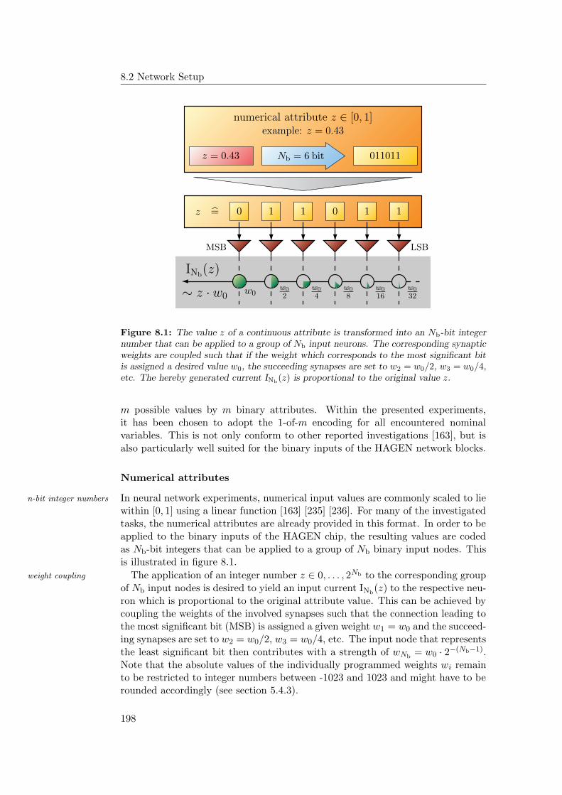
8.2 Network Setup
PSfrag replacements
00 1111
numerical attribute z ∈ [0, 1]
z = 0.43
example: z = 0.43
Nb = 6 bit27 = 011011
011011
z =
w0w0
2w0
4w0
8w0
16w0
32
INb(z)
∼ z · w0
MSB LSB
Figure 8.1: The value z of a continuous attribute is transformed into an Nb-bit integernumber that can be applied to a group of Nb input neurons. The corresponding synapticweights are coupled such that if the weight which corresponds to the most significant bitis assigned a desired value w0, the succeeding synapses are set to w2 = w0/2, w3 = w0/4,etc. The hereby generated current INb
(z) is proportional to the original value z.
m possible values by m binary attributes. Within the presented experiments,it has been chosen to adopt the 1-of-m encoding for all encountered nominalvariables. This is not only conform to other reported investigations [163], but isalso particularly well suited for the binary inputs of the HAGEN network blocks.
Numerical attributes
In neural network experiments, numerical input values are commonly scaled to lien-bit integer numbers
within [0, 1] using a linear function [163] [235] [236]. For many of the investigatedtasks, the numerical attributes are already provided in this format. In order to beapplied to the binary inputs of the HAGEN chip, the resulting values are codedas Nb-bit integers that can be applied to a group of Nb binary input nodes. Thisis illustrated in figure 8.1.
The application of an integer number z ∈ 0, . . . , 2Nb to the corresponding groupweight coupling
of Nb input nodes is desired to yield an input current INb(z) to the respective neu-
ron which is proportional to the original attribute value. This can be achieved bycoupling the weights of the involved synapses such that the connection leading tothe most significant bit (MSB) is assigned a given weight w1 = w0 and the succeed-ing synapses are set to w2 = w0/2, w3 = w0/4, etc. The input node that representsthe least significant bit then contributes with a strength of wNb
= w0 · 2−(Nb−1).Note that the absolute values of the individually programmed weights wi remainto be restricted to integer numbers between -1023 and 1023 and might have to berounded accordingly (see section 5.4.3).
198
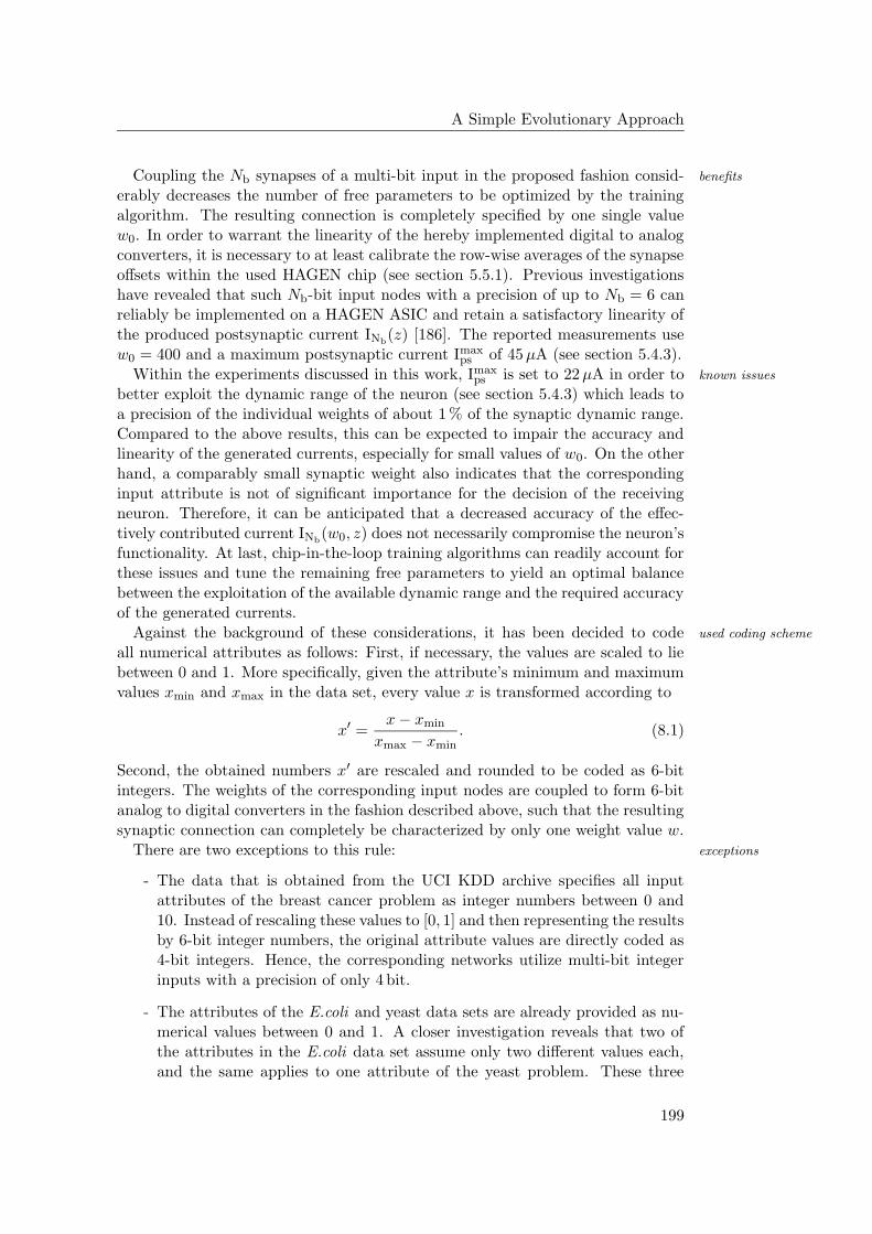
A Simple Evolutionary Approach
Coupling the Nb synapses of a multi-bit input in the proposed fashion consid- benefits
erably decreases the number of free parameters to be optimized by the trainingalgorithm. The resulting connection is completely specified by one single valuew0. In order to warrant the linearity of the hereby implemented digital to analogconverters, it is necessary to at least calibrate the row-wise averages of the synapseoffsets within the used HAGEN chip (see section 5.5.1). Previous investigationshave revealed that such Nb-bit input nodes with a precision of up to Nb = 6 canreliably be implemented on a HAGEN ASIC and retain a satisfactory linearity ofthe produced postsynaptic current INb
(z) [186]. The reported measurements usew0 = 400 and a maximum postsynaptic current Imax
ps of 45 µA (see section 5.4.3).Within the experiments discussed in this work, Imax
ps is set to 22 µA in order to known issues
better exploit the dynamic range of the neuron (see section 5.4.3) which leads toa precision of the individual weights of about 1 % of the synaptic dynamic range.Compared to the above results, this can be expected to impair the accuracy andlinearity of the generated currents, especially for small values of w0. On the otherhand, a comparably small synaptic weight also indicates that the correspondinginput attribute is not of significant importance for the decision of the receivingneuron. Therefore, it can be anticipated that a decreased accuracy of the effec-tively contributed current INb
(w0, z) does not necessarily compromise the neuron’sfunctionality. At last, chip-in-the-loop training algorithms can readily account forthese issues and tune the remaining free parameters to yield an optimal balancebetween the exploitation of the available dynamic range and the required accuracyof the generated currents.
Against the background of these considerations, it has been decided to code used coding scheme
all numerical attributes as follows: First, if necessary, the values are scaled to liebetween 0 and 1. More specifically, given the attribute’s minimum and maximumvalues xmin and xmax in the data set, every value x is transformed according to
x′ =x − xmin
xmax − xmin. (8.1)
Second, the obtained numbers x′ are rescaled and rounded to be coded as 6-bitintegers. The weights of the corresponding input nodes are coupled to form 6-bitanalog to digital converters in the fashion described above, such that the resultingsynaptic connection can completely be characterized by only one weight value w.
There are two exceptions to this rule: exceptions
- The data that is obtained from the UCI KDD archive specifies all inputattributes of the breast cancer problem as integer numbers between 0 and10. Instead of rescaling these values to [0, 1] and then representing the resultsby 6-bit integer numbers, the original attribute values are directly coded as4-bit integers. Hence, the corresponding networks utilize multi-bit integerinputs with a precision of only 4 bit.
- The attributes of the E.coli and yeast data sets are already provided as nu-merical values between 0 and 1. A closer investigation reveals that two ofthe attributes in the E.coli data set assume only two different values each,and the same applies to one attribute of the yeast problem. These three
199
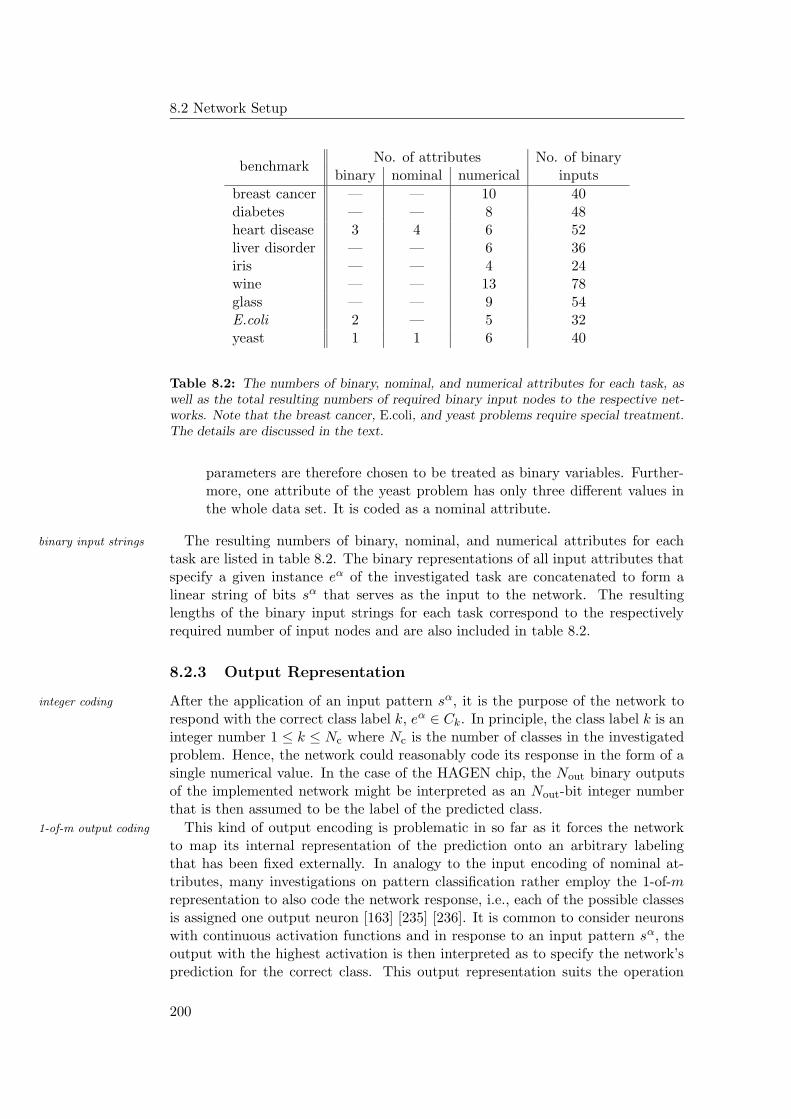
8.2 Network Setup
benchmarkNo. of attributes No. of binary
binary nominal numerical inputs
breast cancer — — 10 40diabetes — — 8 48heart disease 3 4 6 52liver disorder — — 6 36iris — — 4 24wine — — 13 78glass — — 9 54E.coli 2 — 5 32yeast 1 1 6 40
Table 8.2: The numbers of binary, nominal, and numerical attributes for each task, aswell as the total resulting numbers of required binary input nodes to the respective net-works. Note that the breast cancer, E.coli, and yeast problems require special treatment.The details are discussed in the text.
parameters are therefore chosen to be treated as binary variables. Further-more, one attribute of the yeast problem has only three different values inthe whole data set. It is coded as a nominal attribute.
The resulting numbers of binary, nominal, and numerical attributes for eachbinary input strings
task are listed in table 8.2. The binary representations of all input attributes thatspecify a given instance eα of the investigated task are concatenated to form alinear string of bits sα that serves as the input to the network. The resultinglengths of the binary input strings for each task correspond to the respectivelyrequired number of input nodes and are also included in table 8.2.
8.2.3 Output Representation
After the application of an input pattern sα, it is the purpose of the network tointeger coding
respond with the correct class label k, eα ∈ Ck. In principle, the class label k is aninteger number 1 ≤ k ≤ Nc where Nc is the number of classes in the investigatedproblem. Hence, the network could reasonably code its response in the form of asingle numerical value. In the case of the HAGEN chip, the Nout binary outputsof the implemented network might be interpreted as an Nout-bit integer numberthat is then assumed to be the label of the predicted class.
This kind of output encoding is problematic in so far as it forces the network1-of-m output coding
to map its internal representation of the prediction onto an arbitrary labelingthat has been fixed externally. In analogy to the input encoding of nominal at-tributes, many investigations on pattern classification rather employ the 1-of-mrepresentation to also code the network response, i.e., each of the possible classesis assigned one output neuron [163] [235] [236]. It is common to consider neuronswith continuous activation functions and in response to an input pattern sα, theoutput with the highest activation is then interpreted as to specify the network’sprediction for the correct class. This output representation suits the operation
200
A Simple Evolutionary Approach
of neural networks far better than an encoding of the class label by an integernumber (compare figures 2.2, 2.4, 2.5, 2.6, 2.7, and 2.8).
Using neurons with sigmoidal activation functions (see section 1.2.3), the indi-vidual output values Ok can be interpreted as the predicted probabilities P α
k =P (Ck | eα) that the applied instance belongs to the respective class Ck [20] (seealso section 2.1.3). It is a notable advantage of this approach that it allows toinfer the confidence of the network’s prediction. If multiple output neurons exhibitnearly equal values or if even the one with the highest activation yields only a neg-ligible response, the classification of the respective instance is evidently difficult(see also figure 2.5). For practical applications, this information can be of vitalimportance for the user.
In the case of binary outputs like they are implemented on the HAGEN chip, multiple outputs perclassthe response of the network can only unambiguously be interpreted if exactly one
output neuron is activated and all others remain silent. In order to promote a moredifferentiated network response, it stands to reason to assign a number N c
out > 1of outputs to each class. It then remains to be specified, how these output neuronsare desired to quantify the individual probabilities P α
k .
Similar to the combination of input nodes for multi-bit integer inputs, it ispossible to group N c
out binary output neurons to act as an integer output. UsingN c
out−1 feedback connections and (N cout−1)N c
out appropriately tuned weights, sucha group of output neurons can measure its analog input activity and represent it asan integer number between 0 and 2(Nc
out−1) [186]. For the investigations presented used coding scheme
in this work, a simpler approach has been chosen: After the application of aninput pattern sα, the class with the highest number of activated output neuronsis considered to be the prediction of the network. Given a fixed number N c
out
of outputs per class, this encoding does not achieve the same resolution as therepresentation by an N c
out-bit integer, but it yields the advantage of not bindingadditional resources and being straight-forward to implement.
The number of outputs per class is fixed to N cout = 4. It is expected that this
number constitutes a good compromise between the achievable resolution andthe required resources. Still, this initial choice retains a certain arbitrariness. Athorough optimization of the network parameters might yield another value andthis topic will returned to in section 10.3.1.
8.2.4 Implementation on the HAGEN ASIC
Summarizing the considerations of the preceeding sections, figure 8.2 a) schemat- overall network setup
ically illustrates the chosen network setup. For a given categorization problemwith Nc classes, the network contains a single hidden layer of 6 · Nc inner neu-rons — N c
hid = 6 per class— that are homogeneously connected to all input nodesas well as to all outputs. While each class is assigned its own group of N c
out = 4output neurons, the exact number of binary input nodes is determined by thenumbers and types of input attributes that characterize an individual instance ofthe investigated task (see table 8.2). As described in section 8.2.2, some or allof the input nodes are associated in groups to form Nb-bit integer inputs for thecorresponding numerical attribute values. By convention, Nb is set to 6 for all
201
8.3 The Evolutionary Training Algorithm
tasks, except for the breast cancer problem where Nb = 4 (see section 8.2.2).
In order to be implemented on the HAGEN chip, the resulting networks aremulti-block setup
distributed over multiple blocks as it is shown in figure 8.2 b). The first layeris realized on block a. The output states of the involved neurons after the firstnetwork cycle are fed into the input nodes of block b which implements the outputlayer. Hence, the actual network response is available after the second cycle.For tasks with only a few classes, the resulting networks could easily be fit onsingle blocks and use appropriate feedback connections. But in anticipation ofthe extensions introduced in the next chapter and in order to treat all tasks in asimilar fashion, the shown multi-block setup is used for all investigated problems.
The choice of N chid = 6 hidden neurons per class allows to fit all involved net-
works on a maximum of two blocks. For the yeast problem with its ten classes,nearly all outputs of block a have to be connected to the corresponding inputs ofblock b. Regarding the limited, hard-coded inter-block connections of the HAGENprototype (see section 5.4.2), this implies to use a block of the left side for blocka and its counterpart on the right side for block b (compare figure 5.7).
Not all input nodes and neurons of the two blocks are needed to implementunused resources
the desired networks. Output neurons of block b that do not contribute to theresponse of the implemented network are ignored. Any redundant feedback orinter-block connections are switched off and the weights of all unused synapses areset to 0. The unused inputs of both blocks are permanently deactivated1.
In this context, it is to be noted that apart from those input nodes that are usedinternal neuron bias
to code the actual attributes of the respective task, one input per block is reservedfor the implementation of internal bias values for the neurons (see section 1.2.3and figure 1.8). These nodes are permanently set to an input of one and theweights of the corresponding synapses are allowed to be adjusted by the trainingalgorithm.
8.3 The Evolutionary Training Algorithm
With the architecture of the networks being fixed, it remains the task of thetraining algorithm to find a suitable set of weight values that yields a satisfactoryclassification performance on the training data. It has repeatedly been argued inthe preceeding sections that in order to best exploit the speed of the used neuralnetwork hardware, the training is preferably implemented as fast as possible.
Within the used training setup, the synaptic weights are optimized by an evo-use evolutionarycoprocessor lutionary chip-in-the-loop algorithm that is partly implemented in software but
employs the evolutionary coprocessor (see section6.2) for the genetic representa-tion of the individuals and the application of suitable variation operators.
1Note that this does not apply to the respective input nodes with indices 126 and 127 thatare used for the neuron offset calibration (see section 5.5.4).
202
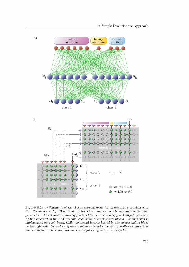
A Simple Evolutionary Approach
PSfrag replacementsa)
O1 O4 O5 O8
H11
H16
H17 H1
12
binarynumerical nominalattributeattributeattribute
class 1 class 2PSfrag replacements
bias
biasbin.
numerical
nominal H11
H14
H112
O1
O4
O5
O8
b)
nnc = 4
class 1
class 2 weight w = 0
weight w 6= 0
block a (left)
block b (right)
nnc = 2
Figure 8.2: a) Schematic of the chosen network setup for an exemplary problem withNc = 2 classes and Na = 3 input attributes: One numerical, one binary, and one nominalparameter. The network contains N c
hid = 6 hidden neurons and N cout = 4 outputs per class.
b) Implemented on the HAGEN chip, each network employs two blocks. The first layer isimplemented on a left block, while the second layer is hosted by the corresponding blockon the right side. Unused synapses are set to zero and unnecessary feedback connectionsare deactivated. The chosen architecture requires nnc = 2 network cycles.
203
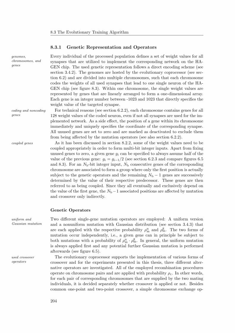
8.3 The Evolutionary Training Algorithm
8.3.1 Genetic Representation and Operators
Every individual of the processed population defines a set of weight values for allgenomes,chromosomes, andgenes
synapses that are utilized to implement the corresponding network on the HA-GEN chip. The used genetic representation follows a direct encoding scheme (seesection 3.4.2). The genomes are hosted by the evolutionary coprocessor (see sec-tion 6.2) and are divided into multiple chromosomes, such that each chromosomecodes the weights of all used synapses that lead to one single neuron of the HA-GEN chip (see figure 8.3). Within one chromosome, the single weight values arerepresented by genes that are linearly arranged to form a one-dimensional array.Each gene is an integer number between -1023 and 1023 that directly specifies theweight value of the targeted synapse.
For technical reasons (see section 6.2.2), each chromosome contains genes for allcoding and noncodinggenes 128 weight values of the coded neuron, even if not all synapses are used for the im-
plemented network. As a side effect, the position of a gene within its chromosomeimmediately and uniquely specifies the coordinate of the corresponding synapse.All unused genes are set to zero and are marked as deactivated to exclude themfrom being affected by the mutation operators (see also section 6.2.2).
As it has been discussed in section 8.2.2, some of the weight values need to becoupled genes
coupled appropriately in order to form multi-bit integer inputs. Apart from fixingunused genes to zero, a given gene gi can be specified to always assume half of thevalue of the previous gene: gi = gi−1/2 (see section 6.2.3 and compare figures 6.5and 8.3). For an Nb-bit integer input, Nb consecutive genes of the correspondingchromosome are associated to form a group where only the first position is actuallysubject to the genetic operators and the remaining Nb − 1 genes are successivelydetermined by the value of their respective predecessor. These genes are thenreferred to as being coupled. Since they all eventually and exclusively depend onthe value of the first gene, the Nb−1 associated positions are affected by mutationand crossover only indirectly.
Genetic Operators
Two different single-gene mutation operators are employed: A uniform versionuniform andGaussian mutation and a nonuniform mutation with Gaussian distribution (see section 3.4.3) that
are each applied with the respective probability ρum and ρg
m. The two forms ofmutation occur independently, i.e., a given gene can in principle be subject toboth mutations with a probability of ρu
m · ρgm. In general, the uniform mutation
is always applied first and any potential further Gaussian mutation is performedafterwards (see figure 6.5).
The evolutionary coprocessor supports the implementation of various forms ofused crossoveroperators crossover and for the experiments presented in this thesis, three different alter-
native operators are investigated. All of the employed recombination proceduresoperate on chromosome pairs and are applied with probability ρc. In other words,for each pair of corresponding chromosomes that are supplied by the two matingindividuals, it is decided separately whether crossover is applied or not. Besidescommon one-point and two-point crossover, a simple chromosome exchange op-
204
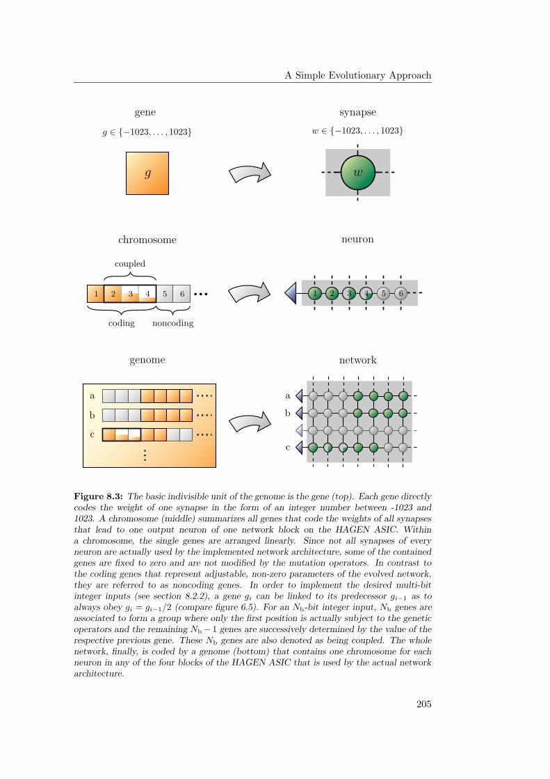
A Simple Evolutionary Approach
PSfrag replacements
synapse
neuron
network
coupled
coding noncoding
gene
chromosome
genome
g ∈ −1023, . . . , 1023 w ∈ −1023, . . . , 1023
11 22 3 34 4 55 66
g w
a a
b b
c
c
Figure 8.3: The basic indivisible unit of the genome is the gene (top). Each gene directlycodes the weight of one synapse in the form of an integer number between -1023 and1023. A chromosome (middle) summarizes all genes that code the weights of all synapsesthat lead to one output neuron of one network block on the HAGEN ASIC. Withina chromosome, the single genes are arranged linearly. Since not all synapses of everyneuron are actually used by the implemented network architecture, some of the containedgenes are fixed to zero and are not modified by the mutation operators. In contrast tothe coding genes that represent adjustable, non-zero parameters of the evolved network,they are referred to as noncoding genes. In order to implement the desired multi-bitinteger inputs (see section 8.2.2), a gene gi can be linked to its predecessor gi−1 as toalways obey gi = gi−1/2 (compare figure 6.5). For an Nb-bit integer input, Nb genes areassociated to form a group where only the first position is actually subject to the geneticoperators and the remaining Nb − 1 genes are successively determined by the value of therespective previous gene. These Nb genes are also denoted as being coupled. The wholenetwork, finally, is coded by a genome (bottom) that contains one chromosome for eachneuron in any of the four blocks of the HAGEN ASIC that is used by the actual networkarchitecture.
205
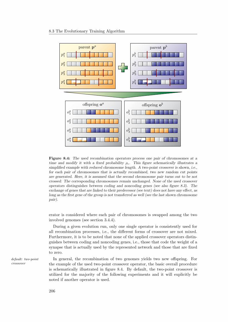
8.3 The Evolutionary Training Algorithm
PSfrag replacements
parent pa parent pb
offspring oa offspring ob
pa1
pa2
pa3
pa4
pb1
pb2
pb3
pb4
oa1
oa2
oa3
oa4
ob1
ob2
ob3
ob4
Figure 8.4: The used recombination operators process one pair of chromosomes at atime and modify it with a fixed probability ρc. This figure schematically illustrates asimplified example with reduced chromosome length. A two-point crossover is shown, i.e.,for each pair of chromosomes that is actually recombined, two new random cut pointsare generated. Here, it is assumed that the second chromosome pair turns out to be notcrossed: The corresponding chromosomes remain unchanged. None of the used crossoveroperators distinguishes between coding and noncoding genes (see also figure 8.3). Theexchange of genes that are linked to their predecessor (see text) does not have any effect, aslong as the first gene of the group is not transferred as well (see the last shown chromosomepair).
erator is considered where each pair of chromosomes is swapped among the twoinvolved genomes (see section 3.4.4).
During a given evolution run, only one single operator is consistently used forall recombination processes, i.e., the different forms of crossover are not mixed.Furthermore, it is to be noted that none of the applied crossover operators distin-guishes between coding and noncoding genes, i.e., those that code the weight of asynapse that is actually used by the represented network and those that are fixedto zero.
In general, the recombination of two genomes yields two new offspring. Fordefault: two-pointcrossover the example of the used two-point crossover operator, the basic overall procedure
is schematically illustrated in figure 8.4. By default, the two-point crossover isutilized for the majority of the following experiments and it will explicitly benoted if another operator is used.
206
A Simple Evolutionary Approach
8.3.2 Selection Scheme and Evolution Parameters
While the actual genetic material of the population is hosted and processed bythe evolutionary coprocessor, the hereby defined genetic representation is encap-sulated into a dedicated HGenome subclass of the HEAF software framework (seesection 7.4). Within the used setup, both, the fitness calculation and the selec-tion scheme are realized purely in software and are wrapped into correspondingHFitnessFunction and HSelectionScheme subclasses.
The implemented algorithm processes a population of µ individuals and follows generationalreplacementa generational replacement scheme (see section 3.4.1). Since several theoretical
investigations suggest that algorithms with elitist selection exhibit more favorableconvergence properties than those without [50] [174], the best nel genomes of thecurrent population can be taken over to the next generation unchanged. For thedescribed experiments, nel is fixed to 1.
The rest of the new generation is generated as follows: First, a common tour- tournament selection
nament selection process with a tournament size of τ = 2 is used to fill a matingpool of µ − nel genomes drawn from the preceeding population. The membersof the mating pool are then randomly grouped into pairs and each mating pairis recombined with a probability ρr =90 % using the selected crossover operator.Finally, the respective offspring are made subject to mutation2. Together withthe nel unmodified genomes from the previous population, the resulting genotypesform the new generation.
Against the background of what has been discussed in section 4.1.2 and given small populations andstrong mutationthe simplicity of the utilized genetic coding, it is to be anticipated that the de-
scribed evolutionary approach will potentially suffer from the negative impact ofthe permutation problem. Aiming for a minimization of these effects, a compa-rably small population size of µ = 20 is chosen (see also section 4.1.2). In orderto compensate for the emergent increased susceptibility to premature convergence(see section 3.3.1), the probabilities of uniform and nonuniform mutation are setto relatively high values of ρu
m = 3 % and ρgm = 7 %, respectively. Choosing small
population sizes in combination with comparably high mutation rates has alsobeen motivated by previous investigations with a preceeding neural network ASICprototype [93].
8.3.3 Fitness Estimation
The calculation of the fitness needs to be repeated for each new individual in everygeneration. Besides the genetic variation operators, the fitness estimation processtherefore constitutes one of the most time critical aspects of an evolutionary algo-rithm. This particularly applies to the training of neural networks for the selectedbenchmark problems, since quantifying the performance of a network on one ofthese tasks involves the evaluation of its response to a potentially large number ofinput patterns (see table 8.1).
On the other hand, common measures for the network performance reasonably planned hardwareimplementationtreat all input instances — and the corresponding network outputs — in a uniform
2If µ − nel is an odd number, the remaining genome is not recombined but only mutated.
207
8.3 The Evolutionary Training Algorithm
fashion (see equations 2.15 and 2.16). With regard to a fast implementation ofthe fitness calculation, this eventually motivates a pipelined and possibly evenparallelized processing of the involved data within a configurable logic (see sec-tion 6.2.6). In the future, it is therefore planned to transfer the calculation of thefitness to the FPGAs on the Darkwing or NATHAN boards of the used hardwaresetup (see sections 6.1 and 6.3). For this approach to be feasible, the necessarycomputations for each single pattern need to be simple enough as to warranttheir efficient realization with the available logic blocks of the used configurablesubstrate.
A Basic Approach
From what has been said above, it can be concluded that regardless of whetherthe fitness calculation is implemented in software or within an FPGA, it is prefer-ably kept simple. Initially, this restriction seems to be easily reconciled with thechosen output representation. In response to an input pattern sα of class Ck, thenetwork is desired to activate the corresponding group of N c
out = 4 output neuronsand keep the remaining outputs deactivated. A simple bitwise comparison of allsimple scoring scheme
neuron outputs Oαi , 1 ≤ i ≤ Nc · N c
out with the corresponding target responsesTα
i yields the number of agreeing positions λ(eα). After the individual scores forall processed inputs have been added up, the resulting total value Λ =
∑α λ(eα)
readily fulfills the general requirements to a suitable fitness function: First, itassumes its maximum value only for a network that always responds with the cor-rect output. Second, due to the large numbers of instances and output neurons,Λ is expected to be a sufficiently smooth measure as to allow for a differentiatedcomparison between two competing individuals.
In practice, the continuity of the hereby defined fitness function is further im-repeated applicationof patterns proved by duplicating each of the training patterns mp > 1 times and applying
the total resulting total data set in a random order. Originally, this procedure isintended to account for the analog noise in the system: Due to the present tem-poral fluctuations, the repeated application of the same input can cause differentnetwork responses. Considering each pattern multiple times does not only yield asmoother fitness measure but also allows to quantify the stability of the respectivecandidate solution. Within the described set of experiments, mp is set to 5.
A Refined Version
It is an outstanding feature of the proposed fitness calculation that it confinesitself with simple bitwise comparisons and integer summations and can thereforebe implemented efficiently either in software or within a configurable logic. Un-fortunately, it turns out that in its original, simple form, the described procedurecannot serve as a suitable fitness estimation procedure in practice. The reasonsfor this are twofold.
Weighted Outputs A considerable fraction of the used classification bench-marks includes a number of classes Nc that is larger than two (see table 8.1). As
208
A Simple Evolutionary Approach
a consequence, the correct output Oα in response to an applied input pattern sα
contains more zeros than ones. When the described fitness measure is employedfor the evolutionary training of networks for such tasks, it can be observed thatafter only a few generations, the population has evolved to be comprised of net-works that always respond with Oi = 0, 1 ≤ i ≤ Nout, regardless of the presentedinput. This especially affects the glass, E.coli, and yeast problems (see table 8.1).
Although evidently undesired, this behavior can easily be understood. Consider problem: unbalancedoutputthe E.coli problem with its Nc = 8 classes. Each target output Tα contains
only N cout = 4 ones but 7 · 4 zeros. A network that permanently produces a
response of zero with all its output neurons achieves a fitness that is 7/8 of thepossible maximum. This breeds a critical evolutionary advantage over networksthat exhibit a large number of false activations, even although they might actuallyconstitute more promising candidate solutions in terms of the original classificationtask.
For this reason, the fitness calculation is modified as follows: After a bitwise modified scoringschemecomparison with the target output Tα, the single outputs are weighted according
to whether they are required to be activated or not. Every neuron that correctlyshows an output of one is rewarded with a score of Nc − 1, those that correctlyrespond with zero contribute with a score of 1. As before, neurons that producean incorrect output do not increase λ(eα) at all. This scoring scheme ensuresthat the activation of the correct neurons and the deactivation of the remainingoutputs are effectively weighted equally.
Finally, if no other class exhibits a larger number of activated output neuronsthan the correct one, the network is awarded an overall bonus of 2(Nc − 1)N c
out
which corresponds to the maximally achievable value of λ(eα) without bonus. Intotal, the resulting single pattern scores thus range between 0 and 4(Nc − 1)N c
out.
Normalized Class Distributions In the majority of the investigated data sets,the different classes are not represented by equal numbers of instances (see ap-pendix B). For example, the most common classes of the E.coli and yeast problemscontribute 42.6 % and 31.2 % of the data, respectively. Even after incorporatingthe above modifications into the fitness function, the evolutionary algorithm turnsout to produce networks that always predict the most frequently occurring classof the current problem, independently of the presented instance.
In analogy to the considerations of the preceeding paragraph, this problem weighted class-specificscorescan be overcome by an appropriate weighting of the different classes. The single
pattern scores λ(eα) are added up separately for each class Ck to obtain the class-specific fitness values Λk which are then divided by the respective square root ofthe number of instances Nk
e in each category. The sum of these normalized classscores forms the fitness of the individual.
209
8.4 First Training Experiments
In terms of the notations introduced above, the fitness function F that is usedfinal fitness function
for the experiments presented in this chapter assumes the final explicit form:
F =
Nc∑
k=1
(Λk√Nk
e
)=
Nc∑
k=1
1√
Nke
∑
eα∈Ck
λ(eα)
(8.2)
If desired, the resulting quantity can be normalized by(∑
k
√Nk
e
)4(Nc − 1)N c
out
to yield a fitness measure between 0 and 1.
Although this refined version does not retain the same simplicity as the originalpreserved hardwaresuitability form, it is still suited for an implementation in a configurable logic. Apart from
the normalization of the single class scores Λk by the square roots√
Nke , the
calculation persists to merely involve comparisons and summations. The divisionshave to be performed only once per individual, and the required values
√Nk
e arefixed throughout the training process. They can be calculated in advance and, e.g.,be stored in a lookup table. Since contemporary configurable logic substrates donot commonly incorporate floating-point units, the used weighting scheme mighthave to be modified to exclusively involve integer numbers, but the basic conceptpersists to be fit for realization within an FPGA.
8.4 First Training Experiments
It remains to be investigated whether the described evolutionary algorithm incombination with the predefined feedforward architecture can succeed in produc-ing networks that achieve a satisfactory generalization performance on demand-ing real-world pattern categorization problems. To this end, a set of stratifiedcross-validation measurements (see section 8.1.2) is performed on each of the nineselected tasks.
8.4.1 Experimental Setup
All trained neural networks are implemented on a HAGEN chip and employ thechip parameters
architecture defined in section 8.2.4. The used ASICs are operated in calibratedmode such that both, the row-wise averages of the synapse offsets and the neuronoffsets are compensated for (see section 5.5.1). The synaptic dynamic range ischosen to be limited to a maximum postsynaptic current of Imax
ps = 22 µA (seesections 5.4.3, 5.5.4, and 8.2.2).
The experiments utilize the hardware configuration described in section 6.1.hardware setup
The software part of the evolutionary algorithm is implemented within the HEAFframework of the HANNEE software (section 7.4) and is executed on a 2.4 GHzPentium IV. The software communicates with a single HAGEN chip via one Dark-wing board. Three identical setups are used, but all networks for one specificbenchmark are always trained on the same chip. In all setups, the interface of theASIC is operated at a frequency of 84 MHz (see section 6.1.3) which determinesthe the effective network frequency fnet (see section 5.2) to be 14 MHz [185] [181].
210
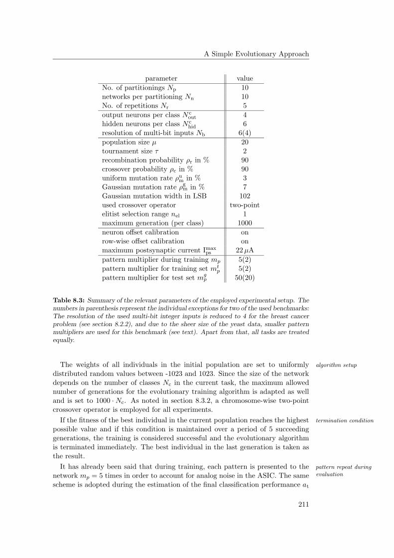
A Simple Evolutionary Approach
parameter value
No. of partitionings Np 10networks per partitioning Nn 10No. of repetitions Nr 5
output neurons per class N cout 4
hidden neurons per class N chid 6
resolution of multi-bit inputs Nb 6(4)
population size µ 20tournament size τ 2recombination probability ρr in % 90crossover probability ρc in % 90uniform mutation rate ρu
m in % 3Gaussian mutation rate ρg
m in % 7Gaussian mutation width in LSB 102used crossover operator two-pointelitist selection range nel 1maximum generation (per class) 1000
neuron offset calibration onrow-wise offset calibration onmaximum postsynaptic current Imax
ps 22 µA
pattern multiplier during training mp 5(2)pattern multiplier for training set mt
p 5(2)
pattern multiplier for test set mgp 50(20)
Table 8.3: Summary of the relevant parameters of the employed experimental setup. Thenumbers in parenthesis represent the individual exceptions for two of the used benchmarks:The resolution of the used multi-bit integer inputs is reduced to 4 for the breast cancerproblem (see section 8.2.2), and due to the sheer size of the yeast data, smaller patternmultipliers are used for this benchmark (see text). Apart from that, all tasks are treatedequally.
The weights of all individuals in the initial population are set to uniformly algorithm setup
distributed random values between -1023 and 1023. Since the size of the networkdepends on the number of classes Nc in the current task, the maximum allowednumber of generations for the evolutionary training algorithm is adapted as welland is set to 1000 · Nc. As noted in section 8.3.2, a chromosome-wise two-pointcrossover operator is employed for all experiments.
If the fitness of the best individual in the current population reaches the highest termination condition
possible value and if this condition is maintained over a period of 5 succeedinggenerations, the training is considered successful and the evolutionary algorithmis terminated immediately. The best individual in the last generation is taken asthe result.
It has already been said that during training, each pattern is presented to the pattern repeat duringevaluationnetwork mp = 5 times in order to account for analog noise in the ASIC. The same
scheme is adopted during the estimation of the final classification performance at
211
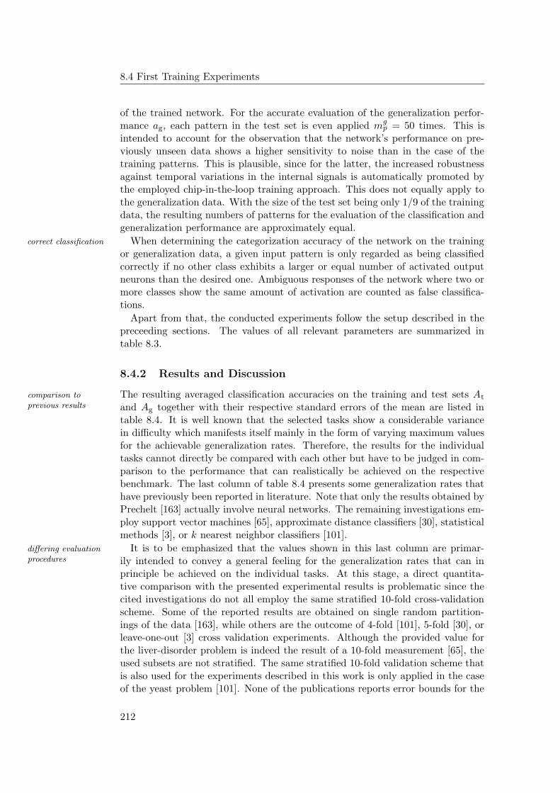
8.4 First Training Experiments
of the trained network. For the accurate evaluation of the generalization perfor-mance ag, each pattern in the test set is even applied mg
p = 50 times. This isintended to account for the observation that the network’s performance on pre-viously unseen data shows a higher sensitivity to noise than in the case of thetraining patterns. This is plausible, since for the latter, the increased robustnessagainst temporal variations in the internal signals is automatically promoted bythe employed chip-in-the-loop training approach. This does not equally apply tothe generalization data. With the size of the test set being only 1/9 of the trainingdata, the resulting numbers of patterns for the evaluation of the classification andgeneralization performance are approximately equal.
When determining the categorization accuracy of the network on the trainingcorrect classification
or generalization data, a given input pattern is only regarded as being classifiedcorrectly if no other class exhibits a larger or equal number of activated outputneurons than the desired one. Ambiguous responses of the network where two ormore classes show the same amount of activation are counted as false classifica-tions.
Apart from that, the conducted experiments follow the setup described in thepreceeding sections. The values of all relevant parameters are summarized intable 8.3.
8.4.2 Results and Discussion
The resulting averaged classification accuracies on the training and test sets Atcomparison toprevious results and Ag together with their respective standard errors of the mean are listed in
table 8.4. It is well known that the selected tasks show a considerable variancein difficulty which manifests itself mainly in the form of varying maximum valuesfor the achievable generalization rates. Therefore, the results for the individualtasks cannot directly be compared with each other but have to be judged in com-parison to the performance that can realistically be achieved on the respectivebenchmark. The last column of table 8.4 presents some generalization rates thathave previously been reported in literature. Note that only the results obtained byPrechelt [163] actually involve neural networks. The remaining investigations em-ploy support vector machines [65], approximate distance classifiers [30], statisticalmethods [3], or k nearest neighbor classifiers [101].
It is to be emphasized that the values shown in this last column are primar-differing evaluationprocedures ily intended to convey a general feeling for the generalization rates that can in
principle be achieved on the individual tasks. At this stage, a direct quantita-tive comparison with the presented experimental results is problematic since thecited investigations do not all employ the same stratified 10-fold cross-validationscheme. Some of the reported results are obtained on single random partition-ings of the data [163], while others are the outcome of 4-fold [101], 5-fold [30], orleave-one-out [3] cross validation experiments. Although the provided value forthe liver-disorder problem is indeed the result of a 10-fold measurement [65], theused subsets are not stratified. The same stratified 10-fold validation scheme thatis also used for the experiments described in this work is only applied in the caseof the yeast problem [101]. None of the publications reports error bounds for the
212
A Simple Evolutionary Approach
benchmarkNo. ofclasses
Nc
classification accuracy in %
training set test set reported takenfromAt Ag Ag
breast cancer 2 98.26 ± 0.01 96.27 ± 0.13 98.85 [163]diabetes 2 78.27 ± 0.02 73.17 ± 0.58 78.5 [163]heart disease 2 89.06 ± 0.09 81.94 ± 0.48 96.8 [163]liver disorder 2 75.94 ± 0.20 67.09 ± 0.78 73.7 [65]iris plant 3 98.80 ± 0.05 94.30 ± 0.26 96–98 [30]wine 3 91.10 ± 0.45 87.36 ± 1.37 100 [3]glass 6 52.66 ± 0.68 46.07 ± 1.15 67.92 [163]E.coli 8 57.13 ± 0.70 54.55 ± 0.45 86 [101]yeast 10 8.52 ± 0.59 8.70 ± 0.68 60 [101]
Table 8.4: Training results obtained with the described combination of network setupand evolutionary training algorithm. For problems with two or three classes, the resultsare promising. With an increasing number of classes, the gap between the best reportedresults and the accuracies that are obtained by networks on the HAGEN chip widenssignificantly. The yeast problem is not reasonably learned at all (see text).
cited values. For a reasonable quantitative comparison with the measurementsdiscussed in this thesis, the different validation schemes of the other investigationswould have to be reproduced. A corresponding set of experiments will be discussedin section 9.4.5.
Against the background of these considerations, it can be inferred from table 8.4 promising results
that — for most of the used benchmarks — the results are promising. In the caseof the breast cancer and iris plant problems, the obtained averaged accuracies onthe test sets are approximately in the order of those reported by other authors.As expected, the performance on the test set is generally lower than the respectiveaccuracy on the training data (except for the yeast problem, see below) but is highenough as to imply a satisfactory generalization ability of the trained networks.Nevertheless, the absolute values of the achieved accuracies clearly leave room comparably low
accuraciesfor improvement: Apart from the liver disorder and iris plant data, not even therespective performance on the training set can exceed the generalization accuracyof other systems.
The gap between the achieved generalization performance and the accuracy that remainingdeficienciescan approximately be expected in the ideal case turns out to be considerably wide
for problems that incorporate larger numbers of classes. It is an important resultthat being trained on the glass and E.coli data sets, the final networks do notsimply predict the most common class as it has been encountered in preliminaryexperiments (in the case of the glass problem, the largest class represents 35.5 % ofthe whole data). But compared to the results that have previously been reportedby other authors, the performance of the trained networks is not satisfactory.
In the case of the yeast problem, finally, the networks completely fail to produce yeast problem: clearfailureany reasonable response at all. A closer investigation reveals that they persist to
213
8.4 First Training Experiments
yield an output which is largely independent of the actually applied input pat-tern, and that the single networks each tend to specialize on only one of the threemost common classes (which contain 31.2 %, 28.9 %, and 16.4 % of the whole data,respectively). But even this specific class rarely exhibits a number of activatedoutputs that exceeds those of all others. Against the background of these observa-tions and given the low absolute accuracies, it is not surprising that the averagedperformance on the test data does not differ significantly from the classificationrate on the training set.
8.4.3 Modified Training Setups
For categorization tasks with three, six, or up to eight classes, the normalizationof the class scores that has been incorporated into the used fitness function (seesection 8.3.3) seems to at least partially yield the desired improvements. Nev-ertheless, the eventually achieved generalization accuracies do not live up to theexpectations and this particularly applies to tasks with more than three classes.The training of networks for the yeast problem evidently exceeds the capability ofthe used evolutionary algorithm setup. With respect to the initial goal of trainingnetworks on the HAGEN ASIC for demanding real-world applications — that arelikely to involve large numbers of classes— it might thus be concluded that simpleevolutionary algorithms and networks with a fixed architecture do not appear tobe a feasible approach.
Before this conclusion can be drawn with certainty, it is to be ensured that thepossible limitations
achieved training success is not in fact limited by the chosen particular evolution-ary algorithm setup, i.e., the used mutation and crossover operators. In the lightof the permutation problem, the mere application of crossover might itself impedea satisfactory outcome of the evolutionary training. Furthermore, since the exper-iments presented in this thesis are the first to consistently utilize the evolutionarycoprocessor, it is to be verified that no hitherto unobserved deficiencies of thisdevice are the reason for the achieved results.
Therefore, a set of experiments similar to the ones discussed above is conductedmodified evolutionparameters where some of the parameters of the described setup are modified. In the first
experiment, the Gaussian mutation is disabled completely and the probability foruniform mutation is raised to 4 %. The next three experiments use the original mu-varying crossover
operators tation probabilities but employ different crossover strategies: one-point crossover,no crossover, and chromosome exchange. In the latter case, the recombination op-erator simply swaps each pair of corresponding chromosomes between the two mat-ing genomes with a modified probability of ρc = 50 % (see sections 3.4.4 and 8.3.2).Another experiment is performed that uses the unmodified evolution settings butpure software
algorithm utilizes a software implementation of the genetic coding and the variance operatorsinstead of the coprocessor.
Finally, it is understood that the used network architecture, most notably thepredetermined size of the respective hidden layer, can generally be suspected ofconstituting an unfavorable choice that eventually limits the achievable general-ization performance. Indeed, it is to be expected that a systematic examinationof multiple network sizes will yield an optimal number of hidden units per class
214
A Simple Evolutionary Approach
that is different from the chosen value N cout = 6 and depends on the particular
task at hand. But although a corresponding set of experiments can easily be con-ducted, this would ultimately contradict the original intention of abandoning theoptimization of the network architecture in favor of high training speeds. Thesole existence of an optimal network size does not support the feasibility of thesimple evolutionary approach, even if it resulted in an improved generalizationcapability of the trained networks. Moreover, the following chapter will present atraining approach that does not require a thorough optimization of the networkarchitectures in order to achieve competitive classification rates.
For these reasons, an exploration of different network sizes is deferred to sec- decoupled weightvaluestion 10.3.1. The last experiment in this campaign rather investigates whether the
enforced coupling of the weights to predefined multi-bit integer inputs (see sec-tion 8.2.2) might in fact prevent the training algorithm from discovering bettersolutions. In this experimental setup, all synaptic weights of the network are al-lowed to be optimized by the algorithm independently of each other. While thisconsiderably increases the number of free parameters, it also permits to explorehitherto inaccessible regions of the search space.
8.4.4 Results Obtained with the Modified Setups
The results are listed in tables 8.5 and 8.6. Only the obtained generalizationaccuracies are shown, since the classification rates on the training sets are onlyof minor interest in practice. A complete summary of the results can be foundin table C.1 in the appendix. Repeatedly training 500 networks for the E.coliand yeast problems is particularly time-consuming due to the large number ofclasses and — in case of the yeast benchmark — the sheer size of the data set.An investigation of single, exemplary evolution runs indicates that neither of theabove modifications to the original setup can actually compensate for the generalincapability of the used evolutionary approach to train networks for the yeastproblem. Preliminary measurements with the E.coli data yield results that aresimilar to those obtained with the other tasks. Therefore, it is decided to excludethe last two benchmarks from this second set of experiments.
A comparison with table 8.4 immediately reveals that also in the cases of all unchanged results
other data sets, no significant improvement of the classification success can beachieved. For the breast cancer, liver disorder, and iris plant problems, the aban-donment of the Gaussian mutation leads to a slight increase of the averaged gener-alization accuracy, but the respective difference to the original result is in no caselarger than the estimated error. For all other benchmarks, the use of a Gaussianmutation has lead to a measurably better generalization.
Considering the various forms of recombination, none of the tested alternatives crossover operators:equivalentseems to exhibit a distinct superiority over the others. Using no crossover at
all only yields a better performance on the glass problem. For all other tasks, iteither deteriorates the generalization rate or does not lead to an improvement thatexceeds the estimated uncertainty. Similar conclusions are to be drawn for the one-point crossover and the chromosome exchange operator. Each of the investigatedrecombination methods shows favorable results on some of the benchmarks but
215
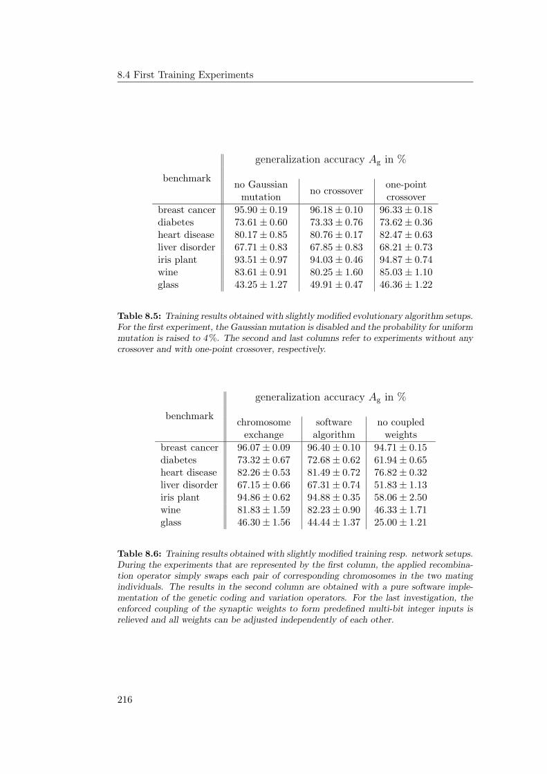
8.4 First Training Experiments
benchmark
generalization accuracy Ag in %
no Gaussianmutation
no crossoverone-pointcrossover
breast cancer 95.90 ± 0.19 96.18 ± 0.10 96.33 ± 0.18diabetes 73.61 ± 0.60 73.33 ± 0.76 73.62 ± 0.36heart disease 80.17 ± 0.85 80.76 ± 0.17 82.47 ± 0.63liver disorder 67.71 ± 0.83 67.85 ± 0.83 68.21 ± 0.73iris plant 93.51 ± 0.97 94.03 ± 0.46 94.87 ± 0.74wine 83.61 ± 0.91 80.25 ± 1.60 85.03 ± 1.10glass 43.25 ± 1.27 49.91 ± 0.47 46.36 ± 1.22
Table 8.5: Training results obtained with slightly modified evolutionary algorithm setups.For the first experiment, the Gaussian mutation is disabled and the probability for uniformmutation is raised to 4 %. The second and last columns refer to experiments without anycrossover and with one-point crossover, respectively.
benchmark
generalization accuracy Ag in %
chromosomeexchange
softwarealgorithm
no coupledweights
breast cancer 96.07 ± 0.09 96.40 ± 0.10 94.71 ± 0.15diabetes 73.32 ± 0.67 72.68 ± 0.62 61.94 ± 0.65heart disease 82.26 ± 0.53 81.49 ± 0.72 76.82 ± 0.32liver disorder 67.15 ± 0.66 67.31 ± 0.74 51.83 ± 1.13iris plant 94.86 ± 0.62 94.88 ± 0.35 58.06 ± 2.50wine 81.83 ± 1.59 82.23 ± 0.90 46.33 ± 1.71glass 46.30 ± 1.56 44.44 ± 1.37 25.00 ± 1.21
Table 8.6: Training results obtained with slightly modified training resp. network setups.During the experiments that are represented by the first column, the applied recombina-tion operator simply swaps each pair of corresponding chromosomes in the two matingindividuals. The results in the second column are obtained with a pure software imple-mentation of the genetic coding and variation operators. For the last investigation, theenforced coupling of the synaptic weights to form predefined multi-bit integer inputs isrelieved and all weights can be adjusted independently of each other.
216
A Simple Evolutionary Approach
yields inferior generalization rates on others. On most problems, the differencesbetween the various crossover operators are within the estimated error bounds.The only exception is given by the wine benchmark where the initial two-pointcrossover is observed to lead to significantly better results than the alternativeoperators.
Especially with regard to the performance that is achieved without any recom-bination, these results can be seen as to support previous suggestions that thepermutation problem might not in fact be as severe as widely supposed [80] [81](see section 4.1.2). But they could also be accredited to the circumstance thatin the presence of the used high mutation rates and small population sizes, theapplied recombination operator might not have a significant impact on the opti-mization process at all.
It can be argued that especially for the larger networks, stronger selection incombination with even further increased mutation rates could potentially improvethe performance of the evolutionary algorithm [93]. But similar to an explorationof the optimal architecture, the need to tune the evolution parameters to optimallysuit the task at hand would rather militate in favor of an automatic adaptation ofthe free parameters during training than support the employed simple evolutionaryapproach.
Beyond that, it is important to note that compared to the training performance coprocessor:functionalof the software algorithm, the evolutionary coprocessor does not show any sign
of a general insufficiency. While on the iris problem, the pure software algorithmyields a slightly better performance of the final networks, the utilization of thecoprocessor leads to better results on the wine and glass benchmarks. Regardingall investigated data sets and within the remaining statistical uncertainties of thepresented generalization rates, it can be said that both, the evolutionary copro-cessor and the pure software implementation of the genetic coding and variationoperators tend to perform approximately equally well. This is good news in so faras it supports the claim that the introduced coprocessor implementation allows toefficiently accelerate the evolutionary training algorithm without loss in trainingsuccess.
Finally, it turns out that the original strategy to couple the weights of a multi- weight coupling:necessarybit integer input to suit the used binary coding of the attribute values does indeed
give rise to a remarkable improvement of the training performance compared tothe case where all weights need to be adjusted independently. Using the lat-ter approach, the achieved generalization accuracies are in some cases (e.g., theiris plant, wine and glass data sets) dramatically reduced compared to those ob-tained with all other investigated training setups. When appropriately couplingthe weight values, the resulting reduction of the search space evidently yields sucha significant simplification of the eventual optimization problem that it more thancompensates for the reduced flexibility in adjusting the weight values.
8.4.5 Concluding Remarks
It is to be emphasized that regardless of the dissatisfying results that are obtainedon benchmarks with more than three classes, the presented experiments success-
217
8.4 First Training Experiments
fully demonstrate the general functionality of the used hardware neural networkframework, most notably the evolutionary coprocessor. The latter is demonstratedto achieve the same training performance as a slower software implementation.The generalization rates that are eventually obtained by comparably small net-works for classification task with two or three classes are promising.
The observation that extensive modifications to the applied variation operatorssimple approach:insufficient or their probabilities do not on average yield a significant change in the achieved
results remains to indicate that the inherent robustness of the simple evolutionaryapproach might also give rise to a partial insensitivity against small changes ofthe evolution parameters, especially the used recombination operators. Initially,this can be seen as a favorable feature of the heuristic evolutionary approach, butit also indicates that the observed deficiency of the training setup is of a rathergeneral nature: The used simple evolutionary algorithm is not fit for optimizingthe weight values of large networks for demanding classification tasks with morethan two or three classes.
This is also problematic in so far as even the largest of the trained networks —dedicated for the classification of yeast proteins — utilizes only a fraction of theresources offered by one HAGEN chip (see section 5.4.1). Aiming for an efficientexploitation of the parallelism that is provided by the implemented network model,it will ultimately be required to train even larger and more complex networks.
It is evident that more sophisticated evolutionary training strategies need to berequired: improvedtraining devised that can readily benefit from the functionality of the coprocessor and at
the same time succeed in training complex networks for realistic applications. Afeasible approach will be introduced in the following chapter.
218
Chapter 9
Stepwise Evolutionary TrainingStrategies
Prediction is very difficult, especially about the future.
Niels Bohr
The experimental results presented in the foregoing chapter indicate that simpleevolutionary algorithms do not suffice to successfully train large and complex neu-ral networks on the HAGEN chip for challenging classification tasks. Regardingthe sheer dimensionality of the resulting search spaces, the ubiquitous threat ofpremature convergence, and the various issues that are known to especially af-fect the evolutionary training of neural networks — like the permutation problembrought forward in section 4.1.2 — it is not surprising that the capability of simpleevolutionary algorithms to train large neural networks is ultimately limited.
Common ways to face up to these challenges are to extend the basic evolution-ary approach by incorporating sophisticated speciation schemes and/or elaborategenetic encodings. Several potential extensions to the described algorithm, suchas an automatic adaptation of the evolution parameters, the optimization of thenetwork architecture during training, or a further improved fitness function havealready been suggested in the previous chapter. Numerous feasible extensionsare also reported in literature and some of the more recent and most promisingapproaches to train neural networks by simulated evolution like the NEAT andEPNet algorithms have been discussed in section 4.2.2.
It has been motivated in section 7.4.5 that, in principle, such refined and im-proved algorithms can readily be implemented within the HEAF framework forevolutionary algorithms. Nevertheless, increasingly complex training algorithmsnecessarily introduce additional computational effort (see section 4.2.3). It persiststhat aiming for an efficient exploitation of the speed of the used network ASIC, anappropriate hardware neural network framework requires simple and fast trainingalgorithms that can in the ideal case benefit from hardware acceleration and/orparallelization themselves (see sections 6.2.6 and 6.3.3).
In pursuit of a training strategy that can fulfill these demands, the followingchapter introduces and evaluates a novel approach that aims to solve the com-
219
9.1 The Divide-and-Conquer Approach
plex task of training large networks for difficult problems without introducingadditional, time-consuming calculations. Instead, it follows an intuitive divide-and-conquer heuristic.
9.1 The Divide-and-Conquer Approach
When trying to solve a large and complex task by simple means, it is a commonapproach to divide the whole problem into several, easier to solve subproblemsthat can be dealt with independently. If the available tools suffice to cope withthe smaller problems, the original task can easily be accomplished by completingthe individual parts separately, i.e., either sequentially or in parallel. It remainsthat depending on the problem at hand, finding a reasonable partitioning intoindependent subproblems and/or determining an adequate combination of theobtained partial solutions to successfully solve the entire problem often turns outto be highly nontrivial.
9.1.1 Stepwise Network Training
Regarding the training of neural networks for a pattern recognition task withdividing classificationtasks Nc classes, it is comparably straight forward to split the original problem into
Nc problems with two classes each: For every class Ck, one separate network istrained to distinguish its instances eα ∈ Ck from those that belong to any otherclass eα ∈ E \ Ck. This is illustrated schematically in figure 9.1 for an exemplarytask with three classes. The shown networks are simplified to only exhibit N sn
hid = 4hidden neurons and N sn
out = 2 outputs.The first stage of the training is then divided into Nc phases such that in the kthtraining stages and
training phases phase, 1 ≤ k ≤ Nc, one dedicated network is trained for class Ck. In response tothe binary representation sα of an arbitrary instance of the problem, this networkis demanded to activate all of its outputs if the presented instance belongs to classCk and to produce an output of zero otherwise.
Two important observations can be made. First, the training of the single net-simple training ofsubnetworks works can be performed independently. In each case, the entire available training
data can be used. Only the desired target outputs differ between the networks.Second, since they expect the same kind of input patterns, all networks can beconnected to the same set of input nodes and can thus in fact be regarded assubnetworks of one large network. If every subnetwork can successfully be trainedto fulfill its individual requirements, the whole network readily solves the originaltask.
Compared to the architecture that has been chosen for the experiments in theuncompletedarchitecture preceeding chapter, the second layer of the final network does not exhibit the full
connectivity. The outputs of one specific class Ck are not connected to the hiddenneurons of the other subnetworks. Being trained to each distinguish a differentclass l 6= k from the respective rest, the other subnetworks do in particular providemeans of differentiating between instances of their own class l and the consideredclass k. In so far, the information that is coded by the inner neurons of thoseremaining subnetworks might be useful also for the output neurons of this class.
220
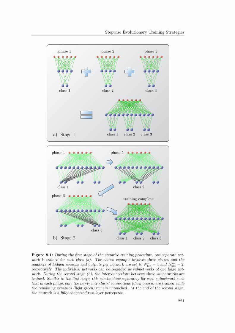
Stepwise Evolutionary Training Strategies
PSfrag replacements
class 1
class 1
class 1
class 1
class 2
class 2
class 2
class 2
class 3
class 3
class 3
class 3
phase 1 phase 2 phase 3
phase 4 phase 5
phase 6
a) Stage 1
b) Stage 2
training complete
Figure 9.1: During the first stage of the stepwise training procedure, one separate net-work is trained for each class (a). The shown example involves three classes and thenumbers of hidden neurons and outputs per network are set to N sn
hid = 4 and N snout = 2,
respectively. The individual networks can be regarded as subnetworks of one large net-work. During the second stage (b), the interconnections between these subnetworks aretrained. Similar to the first stage, this can be done separately for each subnetwork suchthat in each phase, only the newly introduced connections (dark brown) are trained whilethe remaining synapses (light green) remain untouched. At the end of the second stage,the network is a fully connected two-layer perceptron.
221
9.1 The Divide-and-Conquer Approach
Therefore, it suggests itself to interconnect the single subnetworks in order tointerconnecting thesubnetworks yield a homogeneously connected two-layer architecture. This is done in the second
training stage shown in the lower half of figure 9.1. Similar to the first stage, theprocess can be divided into several independent phases: In each step, the outputsof one specific subnetwork k are connected to the hidden neurons of all others.While the synaptic weights that have been optimized in the preceeding phasesremain fixed, the weight values of the new connections are optimized to improvethe recognition accuracy of the respective class k.
As before, the single phases can be performed independently. During the train-independent trainingphases ing of the synapses that lead to the outputs of subnetwork k, the connections
to all other outputs remain untouched. Furthermore, the iterative modificationsof the optimized weight values are based solely on the response of the respectivesubnetwork — the outputs of the other subnetworks can readily be ignored. Inthis respect, the phases of the second stage are similar to those of the first stagewhich particularly allows to apply the same training algorithm.
9.1.2 Implications for Training
Once the second stage has been completed, the final network exhibits the sameoutput encoding
connectivity and is trained to perform the same task as the network proposedin section 8.2. When being presented an instance of the respective problem, itis expected to activate the outputs that indicate the correct class and deactivateall others. In practice, the class with the largest number of activated neurons inresponse to an input pattern sα is regarded as the prediction of the network.
However, compared to the training process described in the foregoing chapter,the single phases of the stepwise approach involve optimization problems that areconsiderably simpler in several respects. First, in every phase, the amount of freesmaller search spaces
parameters, i.e., weight values, is significantly reduced. Regarding the trainingresults that can be achieved on small networks (see table 8.4) it is reasonable toassume that the used simple evolutionary algorithm can successfully cope withsearch spaces of the resulting dimensionalities. Second, the task that remains tosimple subproblems
be solved by each subnetwork is a mere two-class problem. Again, the resultsshown in table 8.4 indicate that the capability of simple training algorithms canbe expected to suffice for this kind of task. Third, the desired network responsesimpler fitness
function demands all output neurons to behave equally. Against the background of whathas been discussed in section 8.3.3, this allows for a considerable simplificationof the fitness calculation. A weighting of the output neurons according to therespective target outputs becomes obsolete, and for each pattern sα, the scoreλ(eα) can simply be calculated as the number of output neurons that show thedesired state of activation.
In summary, it is anticipated that the simple evolutionary algorithm describedtraining times andparallelization in section 8.3 can successfully be utilized for the single optimization problems
that remain to be solved in each phase. On the other hand, for a problem withNc classes, the whole training process now involves 2Nc single evolution runs. De-pending on the number of generations that are allowed per phase, the resultingtotal number of iterations might exceed that of the simple approach used in the
222
Stepwise Evolutionary Training Strategies
preceeding chapter. But compared to a simultaneous optimization of the wholenetwork, the stepwise approach inherently promotes an immediate parallelizationof the training process: Within each stage, the single phases can readily be per-formed in parallel. This particularly suits a hardware neural network platformthat allows to evaluate multiple neural networks simultaneously. This aspect willbe examined more closely in section 10.1.2.
9.1.3 Stepwise Training and Mixtures of Experts
The concept of dividing a given task into smaller subproblems that are to bedealt with independently by specialized modules has already been considered inthe context of neural network training in another form. In 1991, Jacobs et al.proposed the so-called adaptive mixture of local experts approach [108]. It is animportant difference between the introduced stepwise training strategy and themixture of experts model that the latter performs a partitioning of the investigatedtask in the input space.
In the case of the stepwise training procedure described above, the single net- dividing the outputspaceworks are each specialized in recognizing a different class. Hence, it can be said
that they are each specialized on a different dimension of the output space. At thesame time, all subnetworks are trained on the complete set of training instances.In contrast, within the mixture of experts approach, the individual networks are dividing the input
spacetrained to specialize on different regions of the input space. When a new vectorIα is applied to the final system, it is not processed by all networks alike but onlyby the expert that is responsible for the respective region of the input space thatcontains Iα.
Since a suitable corresponding partitioning of the input space will in general not learning the inputpartitioningbe known in advance, it needs to be determined during training. Apart from the
single expert networks, the system proposed by Jacobs et al. therefore includesan additional, dedicated gating network that individually decides for each inputpattern which of the experts is applicable. As a consequence, all expert networks simultaneous training
requiredand the gating network have to be trained simultaneously. During training, thesingle networks specialize on different areas of the input space, and the gatingnetwork iteratively learns how to best allocate the different instances to the singleexperts. A detailed account of the used training algorithm can be found in the citedpublications and shall not be given here. But it is to be noted that this strategyand related approaches are reported to be successfully applicable to demandingvowel discrimination and visual recognition tasks [107] [108].
In the case of a classification task with Nc categories, the individual networks of advantages ofstepwise trainingthe mixture of experts approach are in principle required to distinguish between
all Nc classes — even if only for a reduced set of instances. According to theintroduced stepwise strategy, each network merely has to solve a simple two-class problem and can be trained on all available input vectors. The necessarypartitioning of the output space is automatically implied by the formulation of theactual classification problem and does not have to be learned. Besides allowing forthe application of a simple algorithm to the training of the individual subnetworks,this eventually yields the advantage that all of the single training phases within
223
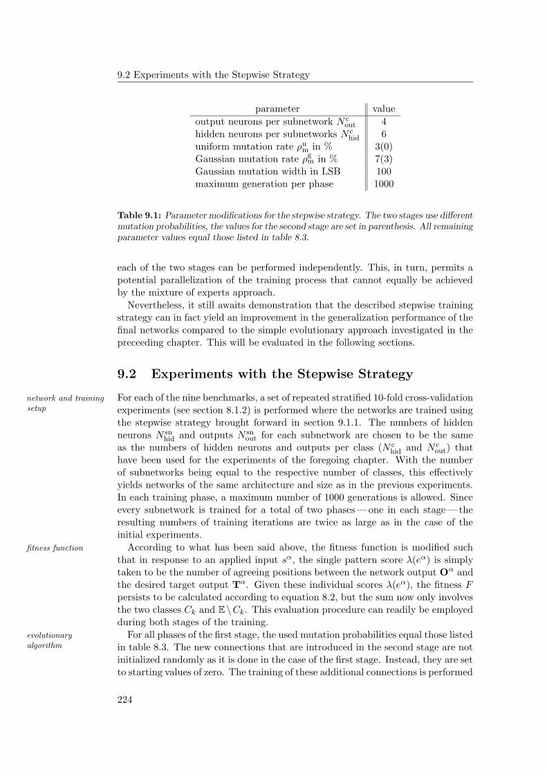
9.2 Experiments with the Stepwise Strategy
parameter value
output neurons per subnetwork N cout 4
hidden neurons per subnetworks N chid 6
uniform mutation rate ρum in % 3(0)
Gaussian mutation rate ρgm in % 7(3)
Gaussian mutation width in LSB 100maximum generation per phase 1000
Table 9.1: Parameter modifications for the stepwise strategy. The two stages use differentmutation probabilities, the values for the second stage are set in parenthesis. All remainingparameter values equal those listed in table 8.3.
each of the two stages can be performed independently. This, in turn, permits apotential parallelization of the training process that cannot equally be achievedby the mixture of experts approach.
Nevertheless, it still awaits demonstration that the described stepwise trainingstrategy can in fact yield an improvement in the generalization performance of thefinal networks compared to the simple evolutionary approach investigated in thepreceeding chapter. This will be evaluated in the following sections.
9.2 Experiments with the Stepwise Strategy
For each of the nine benchmarks, a set of repeated stratified 10-fold cross-validationnetwork and trainingsetup experiments (see section 8.1.2) is performed where the networks are trained using
the stepwise strategy brought forward in section 9.1.1. The numbers of hiddenneurons N sn
hid and outputs N snout for each subnetwork are chosen to be the same
as the numbers of hidden neurons and outputs per class (N chid and N c
out) thathave been used for the experiments of the foregoing chapter. With the numberof subnetworks being equal to the respective number of classes, this effectivelyyields networks of the same architecture and size as in the previous experiments.In each training phase, a maximum number of 1000 generations is allowed. Sinceevery subnetwork is trained for a total of two phases — one in each stage — theresulting numbers of training iterations are twice as large as in the case of theinitial experiments.
According to what has been said above, the fitness function is modified suchfitness function
that in response to an applied input sα, the single pattern score λ(eα) is simplytaken to be the number of agreeing positions between the network output Oα andthe desired target output Tα. Given these individual scores λ(eα), the fitness Fpersists to be calculated according to equation 8.2, but the sum now only involvesthe two classes Ck and E\Ck. This evaluation procedure can readily be employedduring both stages of the training.
For all phases of the first stage, the used mutation probabilities equal those listedevolutionaryalgorithm in table 8.3. The new connections that are introduced in the second stage are not
initialized randomly as it is done in the case of the first stage. Instead, they are setto starting values of zero. The training of these additional connections is performed
224
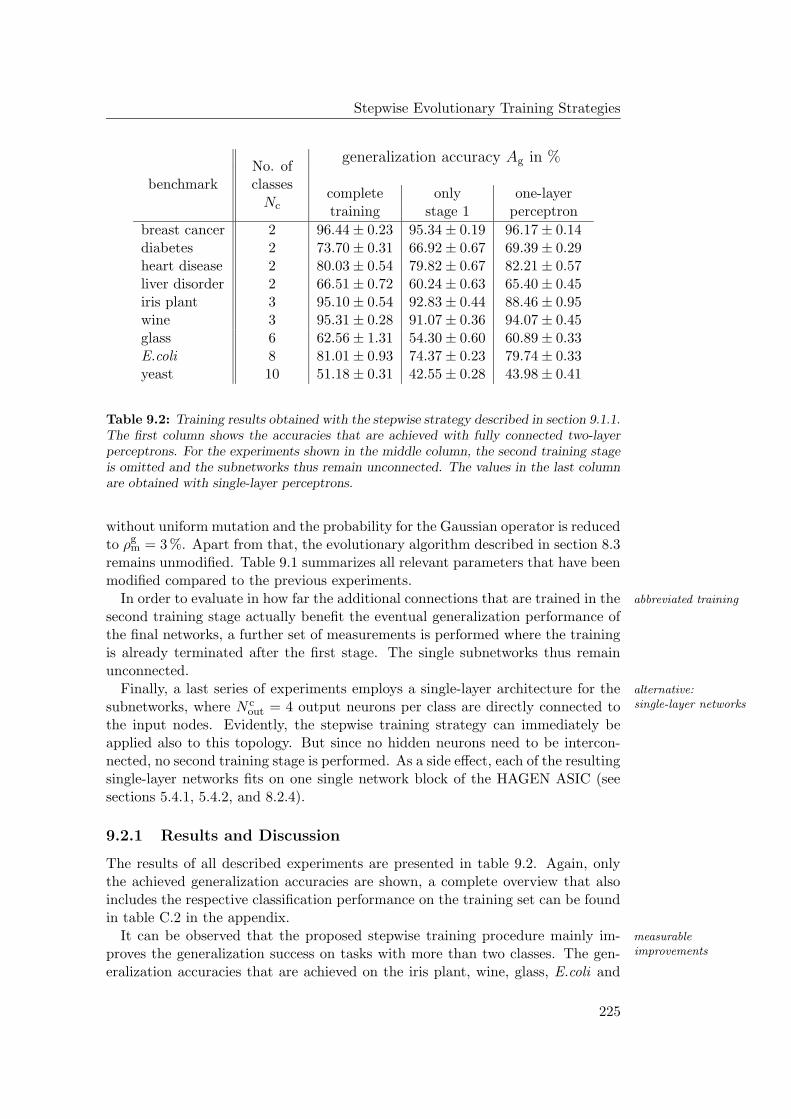
Stepwise Evolutionary Training Strategies
benchmarkNo. ofclasses
Nc
generalization accuracy Ag in %
completetraining
onlystage 1
one-layerperceptron
breast cancer 2 96.44 ± 0.23 95.34 ± 0.19 96.17 ± 0.14diabetes 2 73.70 ± 0.31 66.92 ± 0.67 69.39 ± 0.29heart disease 2 80.03 ± 0.54 79.82 ± 0.67 82.21 ± 0.57liver disorder 2 66.51 ± 0.72 60.24 ± 0.63 65.40 ± 0.45iris plant 3 95.10 ± 0.54 92.83 ± 0.44 88.46 ± 0.95wine 3 95.31 ± 0.28 91.07 ± 0.36 94.07 ± 0.45glass 6 62.56 ± 1.31 54.30 ± 0.60 60.89 ± 0.33E.coli 8 81.01 ± 0.93 74.37 ± 0.23 79.74 ± 0.33yeast 10 51.18 ± 0.31 42.55 ± 0.28 43.98 ± 0.41
Table 9.2: Training results obtained with the stepwise strategy described in section 9.1.1.The first column shows the accuracies that are achieved with fully connected two-layerperceptrons. For the experiments shown in the middle column, the second training stageis omitted and the subnetworks thus remain unconnected. The values in the last columnare obtained with single-layer perceptrons.
without uniform mutation and the probability for the Gaussian operator is reducedto ρg
m = 3 %. Apart from that, the evolutionary algorithm described in section 8.3remains unmodified. Table 9.1 summarizes all relevant parameters that have beenmodified compared to the previous experiments.
In order to evaluate in how far the additional connections that are trained in the abbreviated training
second training stage actually benefit the eventual generalization performance ofthe final networks, a further set of measurements is performed where the trainingis already terminated after the first stage. The single subnetworks thus remainunconnected.
Finally, a last series of experiments employs a single-layer architecture for the alternative:single-layer networkssubnetworks, where N c
out = 4 output neurons per class are directly connected tothe input nodes. Evidently, the stepwise training strategy can immediately beapplied also to this topology. But since no hidden neurons need to be intercon-nected, no second training stage is performed. As a side effect, each of the resultingsingle-layer networks fits on one single network block of the HAGEN ASIC (seesections 5.4.1, 5.4.2, and 8.2.4).
9.2.1 Results and Discussion
The results of all described experiments are presented in table 9.2. Again, onlythe achieved generalization accuracies are shown, a complete overview that alsoincludes the respective classification performance on the training set can be foundin table C.2 in the appendix.
It can be observed that the proposed stepwise training procedure mainly im- measurableimprovementsproves the generalization success on tasks with more than two classes. The gen-
eralization accuracies that are achieved on the iris plant, wine, glass, E.coli and
225
9.2 Experiments with the Stepwise Strategy
yeast data sets are measurably increased compared to networks that are trainedas a whole (see table 8.4). For the iris plant problem, the improvement in gen-eralization performance just exceeds the estimated error, but in case of the winedata set, the number of misclassification is reduced by more than a half.
For large networks and problems with large numbers of classes, the stepwise ap-benefits for largernetworks proach naturally yields a substantial reduction of the search space in comparison
to a simultaneous optimization of all weights. This is observed to lead to a drasticincrease in generalization accuracy for the glass, E.coli and yeast problems. Com-pared to the results that are reported by other authors (see table 8.4) the obtainedgeneralization rates now exhibit approximately the same slight inferiority as thoseachieved on problems with three or two classes. This is particularly satisfactory inthe case of the yeast problem for which networks could not reasonably be trainedwith the simple evolutionary approach at all.
Given the observed measurement uncertainty, the results obtained on the breastresults for smallnetworks cancer, diabetes, and liver disorder data sets are not significantly different to those
reported in the preceeding chapter. Splitting the respective networks into twoindependently trained halves and thereby reducing the number of simultaneouslyoptimized parameters does in these cases not yield a substantial improvementof the training. As suspected earlier, it can reasonably be concluded that forthese benchmarks, the achieved generalization performance is not limited by thesimplicity of the used evolutionary algorithm and/or the size of the networks. Theonly task where the stepwise strategy yields a measurably worse generalizationperformance than the naive approach of the previous chapter is the heart diseaseproblem.
It can furthermore be inferred from the third column of table 9.2 that the ad-favorable: twotraining stages ditional connections between the subnetworks which are introduced during the
second stage of the training measurably benefit the performance of the final net-works. An abandonment of the second stage leads to a decrease of the generaliza-tion accuracy for all tasks. With the exception of the heart disease problem, theobserved deterioration always exceeds the estimated statistical uncertainty.
The last column, finally, reveals that the feasibility of a single-layer architectureoptimal architecture:task dependent strongly depends on the investigated task. The single-layer perceptrons that are
trained for the heart disease problem actually seem to perform better on aver-age than the networks with one hidden layer (see also table 8.4). Against thebackground of the above observation that even the simple evolutionary approachachieved better generalization on this benchmark, it can be concluded that thegiven number of 12 hidden neurons in combination with the extended trainingtimes of the stepwise strategy does in this case lead to an unfavorable overfittingof the data (see also figure 2.3 c)).
Comparing the second last and last columns, it becomes clear that when onlyone training stage is performed, networks with just one single layer tend to achievebetter generalization accuracies than those with two layers. The only exceptionsare the iris and wine problem.
Although it can generally be observed that — apart from the heart disease prob-suitability ofsingle-layer networks lem — the generalization rates of the single-layer networks are lower than those of
the two-layer perceptrons, it can also be seen that the respective difference turns
226
Stepwise Evolutionary Training Strategies
out to be remarkably small for most tasks. It is well known that two of the threeclasses that form the iris problem are definitely not linearly separable. This isconsistent with the achieved results. Given the obtained accuracies on the otherbenchmarks, it is to be concluded that the respective classes actually contain alarge fraction of linearly separable data. This seems to particularly apply to theheart disease problem where a linear partitioning of the input space is in fact su-perior to more complex class separations. This has already been observed duringprevious investigations by other authors [163].
The dimensionalities of the investigated problems inhibit a reasonable display intwo or even three dimensions. But it is plausible to assume that when consideringany pair of classes from one of these problem, their arrangement in the input spacemight be similar to the situation illustrated in figure 2.3 c).
Implications for Further Improvements
In summary, it can be concluded that the introduced stepwise training strategy stepwise training:feasibletends to promote a measurable improvement in the achievable classification per-
formance compared to the simple evolutionary approach that has been describedin the foregoing chapter. In each phase of the training, a simple and fast evolu-tionary training algorithm can be used and the individual subnetworks for eachclass can in principle be trained in parallel. In so far, the stepwise training ap-proach is particularly well suited for fast and massively parallel neural networkhardware platforms (a possible way of exploiting this parallelism will be discussedin section 10.1.2).
Still, the achieved results can, as yet, not compete with those that are obtained remaining issues
by other systems, and the gained improvements primarily affect problems withmore than two classes. Furthermore, considering the observations that are madeon the heart disease benchmark, it must be stated that the restriction to a fixedand predefined, two-layer network architecture runs the risk of yielding suboptimalresults on some problems.
Finally, it is to be considered that a number of N chid = 6 hidden neurons and/or unused resources
N cout = 4 outputs per class, does — for most of the investigated benchmarks — by
far not exploit the resources that are provided by even only a single HAGEN chip.Therefore, it would be desired to extend the proposed stepwise training procedureto allow for an efficient training of larger networks that can make best use ofthe offered hardware resources and achieve competitive generalization rates ona variety of problems without requiring an individual adaptation of the networkarchitecture. The following sections will present a promising approach.
9.3 The Generalized Stepwise Strategy
In the spirit of an intuitive divide-and-conquer heuristic, the proposed stepwisetraining strategy performs a partitioning of the whole network that is inspiredby the combinatorial structure of the actual categorization task: The resultingsubnetworks are each trained for a different class. The experiments describedin the preceeding section demonstrate that the resulting division of the training
227
9.3 The Generalized Stepwise Strategy
process into the independent optimization of several single subnetworks is indeedfeasible.
In pursuit of larger networks, the size of the individual subnetworks could beincreased until the capability of the training algorithm to successfully optimizethe resulting set of weights reaches its limit. But given the apparent success of thedivide-and-conquer approach, it also suggests itself to compensate for increasednetwork sizes by further dividing the thus enlarged subnetworks themselves.
9.3.1 Training Multiple Networks per Class
The original stepwise strategy shown in figure 9.1 can easily be extended by train-generalizing thestepwise strategy ing multiple networks for each class instead of one. Figure 9.2 schematically illus-
trates a simple example where a number of N cnet = 2 subnetworks is trained for
each of the Nc = 2 possible classes. Effectively, each of the Nc phases of the firststage is simply repeated N c
net times. Again, the resulting set of Nc · N cnet networks
can readily be regarded as to form one large network.
The second training stage then proceeds as before: During a number of Nc · N cneteffect: increased
networks training phases, the outputs of each subnetwork are connected to the hidden neu-rons of all other subnetworks. Once again, the resulting network turns out to ex-hibit a fully connected two-layer architecture, the only change being an increasednumber of hidden neurons N c
net · N chid and outputs N c
net · N cout.
Multiple Subnetworks vs. Increased Subnetwork Size
Initially, generalizing the original strategy to the training of multiple subnetworksper class does not automatically seem to yield an advantage over a simple increaseof the subnetwork size. As long as the used training algorithm can cope withthe resulting dimensionality of the search space, a further division of the enlargedsubnetwork is not necessarily expected to increase the training performance. Atleast, this is suggested by the results that are obtained with the original stepwiseapproach on two-class problems (see table 9.2).
Nevertheless, the proposed extended strategy promises to be advantageous inincreased trainingtimes several respects. Both, the training of larger subnetworks and the optimization of
multiple subnetworks per class eventually increase the required number of trainingiterations. In the latter case, the total number of performed generations of the evo-lutionary algorithm linearly scales with the number of subnetworks per class — ifit is assumed that the maximum number of allowed generations per phase remainsunchanged. Given a fixed size of the individual subnetworks, the overall numberof iterations is then proportional to the total number of hidden neurons in thefinal network. For an alternative training of larger subnetworks, the number oftraining iterations in each phase is reasonably increased in approximately the samefashion.
Having said that, it remains an important difference between the two approachespotentialparallelization that the training of multiple networks per class can readily be performed in par-
allel. Evidently, this does not apply to the additional generations that will haveto be processed for the training of the larger networks. The parallelization of the
228
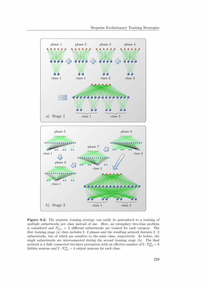
Stepwise Evolutionary Training Strategies
PSfrag replacements
class 1
class 1
class 1class 1
class 2
class 2
class 2
class 2
class 1
class 1
class 2
class 2
phase 1 phase 2 phase 3 phase 4
phase 5
phase 6
phase 7
phase 8
a) Stage 1
b) Stage 2training complete
Figure 9.2: The stepwise training strategy can easily be generalized to a training ofmultiple subnetworks per class instead of one. Here, an exemplary two-class problemis considered and N c
net = 2 different subnetworks are trained for each category. Thefirst training stage (a) then includes 2 · 2 phases and the resulting network features 2 · 2subnetworks, two of which are sensitive to the same class, respectively. As before, thesingle subnetworks are interconnected during the second training stage (b). The finalnetwork is a fully connected two-layer perceptron with an effective number of 2 ·N sn
hid = 8hidden neurons and 2 · N sn
out = 4 output neurons for each class.
229
9.3 The Generalized Stepwise Strategy
stepwise strategy will more thoroughly be discussed in section 10.1.2.
Beyond that, increasing the size of the single subnetworks will eventually befeasibility of simplealgorithms limited by the capabilities of the used simple training algorithm. Indeed, com-
paring the results of the previous chapter with the performance of the stepwisestrategy (tables 8.4 and 9.2), it can be expected that a measurable deteriorationof the training success already occurs for networks with 3 · 6 hidden neurons (e.g.,the networks for the iris and wine problems). In contrast, repeatedly trainingand interconnecting multiple networks of a fixed size is limited only by the avail-able network resources, the achievable degree of parallelization, and the allowedtraining time.
9.3.2 Network Ensembles: Theoretical Considerations
In addition to the above considerations, training multiple subnetworks per classsubnetwork diversity
instead of a single large one is also anticipated to be beneficial with respect to theachievable generalization accuracy. It has been discussed earlier that the eventualoutcome of an evolutionary training run is influenced by numerous random deci-sions, and the multiple subnetworks i, 1 ≤ i ≤ N c
net that are trained for a givenclass Ck are therefore expected to be slightly different. Due to their individualpartitionings of the input space, the number of outputs ν i
k(sα) ∈ 1, . . . , N sn
out thatare activated in response to the application of the same input pattern sα is likelyto vary between the single networks — at least for some of the instances (comparefigure 2.3 c)).
Following the proposed strategy, the binary output patterns of these subnet-averaged outputs
works are simply concatenated such that the total number of activated outputneurons per class immediately becomes
νk(sα) =
Ncnet∑
i=1
νik(s
α) k ∈ 1, . . . , Nc (9.1)
and eventually obeys νk ∈ 1, . . . , N snout · N c
net, 1 ≤ k ≤ Nc. As long as the samenumber of subnetworks N c
net is trained for each category, this procedure effectivelyyields the same response of the entire network as when the averaged numbers ofoutputs νk = νk/N
cnet for each class were compared.
So-called ensembles of networks whose outputs are appropriately combined tonetwork ensembles
yield a collective prediction of the whole committee have already been examinedrepeatedly in literature [105] [111] [124] [154] [153] [160] [189] [190].
Perrone and Cooper [160] consider a group of N networks with the respectivefunctionapproximation output functions yi(I), 1 ≤ i ≤ N that each approximate a given target function
f(I) with a specific individual error εi(I), f(I) = yi(I) + εi(I). The expected sum-of-squares error of network yi(I) can then be written as
Ei = 〈 (yi(I) − f(I))2 〉 = 〈 ε2i 〉 (9.2)
(compare equations 2.15 and 2.16) and the on average expected error of any single
230
Stepwise Evolutionary Training Strategies
network in the committee simply becomes
E =1
N
N∑
i=1
〈 ε2i 〉 (9.3)
where 〈 · 〉 denotes the expectation value on the input space I ∈ I.Instead of considering only the output of a single network, one can regard the ensemble prediction
collective prediction of the whole ensemble y(I) to be the average over all individualnetwork responses
y(I) =1
N
N∑
i=1
yi(I). (9.4)
The expected sum-of-squares error of this ensemble output is then given by
Eens =
⟨ (1
N
N∑
i=1
yi(I) − f(I)
)2 ⟩=
⟨ (1
N
N∑
i=1
εi
)2 ⟩. (9.5)
Perrone and Cooper derive the important result that if the errors εi(I) of the improved accuracy
different networks are assumed to be uncorrelated and to have zero mean, thenthe estimated error of the ensemble Eens and the averaged estimated error of thesingle networks E obey
Eens =1
NE. (9.6)
At first sight, this is a remarkable observation in so far as it suggests that limitations
the sum-of-squares error of the ensemble prediction can be reduced below anydesired threshold ε > 0 simply by regarding committees of sufficient size. Inpractice, however, the assumption that the errors εi(I) of the single networksare uncorrelated does not hold. In fact, the errors are anticipated to be highlycorrelated, since they are strongly influenced by the used network architecture,the employed training algorithm, and the structure of the available training data.In general, when networks with equal architectures are trained on the same datain a more or less deterministic fashion (see sections 2.1.3 and 2.2.2), the remainingerrors of the individual networks are likely to occur on approximately the samesubset of problematic input values.
Therefore, equation 9.6 can merely serve as a lower bound on the actually guaranteed: preservedaccuracyobserved ensemble error Eens. On the other hand, it can also be shown quite
easily [20] that the use of an ensemble can never increase the on average expectederror, i.e.,
Eens ≤ E. (9.7)
Experimental results suggest that some measurable improvement in performancewill generally be observed [20] [160].
231
9.3 The Generalized Stepwise Strategy
Network Ensembles and Diversity
It remains that in order for an ensemble to be superior over a single network,ensemble diversity
the members of the committee need to exhibit a sufficient diversity, i.e., theymust not behave equally on all input patterns. Even an arbitrary number ofidentical networks will not yield any improvement over a single instance of thesame network. This intuitively plausible insight has been formalized by Kroghand Vedelsby [124]. For each network i, they consider the deviation di(I) of itsoutput from the ensemble mean
di(I) = (yi(I) − y(I))2 (9.8)
and define the on average expected ensemble diversity (or “ambiguity”) to be
Dens =1
N
N∑
i=1
〈 di(I) 〉. (9.9)
On the basis of this definition, a simple relation between the estimated ensemblediversity andaccuracy error Eens, the expected error of the single networks E, and the ensemble diversity
Dens is obtained:
Eens = E − Dens (9.10)
Again, it turns out that the error of the ensemble is guaranteed to be not largerthan the average error of the single networks. The achieved reduction is deter-mined by the diversity Dens of the networks within the committee.
Aiming for the construction of an efficient ensemble, it is thus necessary topromoting diversity
not only optimize the accuracy, but also the diversity of the contained networks.Various approaches to promote a sufficient disagreement between the differentcommittee members are conceivable and have been investigated in literature.Prominent strategies are to vary the used training data between the individualnetworks [124] [153], to employ different architectures, start from different ini-tializations of the weights [130], or to apply varying training algorithms (for anoverview see [189]).
More recent approaches aim to actively minimize the similarity between theactively enforcingdiversity individual ensemble members. For example, Opitz and Shavlik use a genetic al-
gorithm to construct a diverse set of networks [154]. Other procedures start witha minimal ensemble of only one or two networks and successively add and trainnew members in a way that ensures these newly introduced networks to be dif-ferent from the others [73] [105]. The algorithm proposed by Islam et al. [105]additionally incorporates the automatic adjustment of the architectures and thenumber of networks in the ensemble. While this last approach promises to maxi-mize the diversity within the committee most efficiently and yields excellent resultson various benchmark problems (see section 9.4.5), it also requires elaborate pro-cedures to ensure the diversity of the networks. In general, for all of the aboveapproaches, the training of each individual network needs to incorporate knowl-edge of the current performance of all others, i.e., the networks can no longer betrained independently.
232
Stepwise Evolutionary Training Strategies
The Stepwise Strategy and Diversity
It is understood that equations 9.6, 9.7, and 9.10 have been derived for networks threshold neurons andclassificationwith continuous outputs that are being applied to function approximation tasks
and can as such not directly be transferred to networks on the HAGEN chip thatare trained to solve classification problems. Still, when using a number N c
out ofoutput neurons per class, the task to activate them all whenever an applied inputpattern belongs to a given class and to deactivate them otherwise can be seen asthe approximation of a function that only assumes values of either 0 or N c
out. Thedifference between the number of actually activated outputs and the respectivelydesired value can thus serve as an — admittedly coarse — error measure similar tothe quantity εi(I) considered above.
As it has been argued before, concatenating the outputs of several networks qualitative similarity
that are trained to recognize the same class is effectively equivalent to an averag-ing over the single network responses. In so far, the propositions of the preceedingsections are assumed to at least qualitatively hold also for the introduced gener-alized stepwise strategy.
It remains that the final response of the whole network is obtained by a majorityvoting among the different classes. This ultimately impedes an equally straightforward theoretical investigation of the situation as in the case of the originallyconsidered function approximation tasks. A thorough discussion of these topicslies beyond the scope of this thesis. But it is reasonable to expect that an improved improved accuracy
expectedperformance of the single parts which each specialize on a different class Ck willalso lead to an increased classification accuracy of the whole network. Trainingmultiple subnetworks for the same category is therefore anticipated to yield bettergeneralization results — as long as it can be ensured that the different subnetworksexhibit a sufficient diversity (see equation 9.10).
In the case of the proposed stepwise strategy, the diversity of the multiple sub- diversity throughindependent evolutionnetworks that are trained for the same class is expected to automatically arise from
the intrinsic random nature of the evolutionary training algorithm. Initially, it isnot at all clear whether this suffices to yield a satisfactory reduction of the simi-larity between the individual network responses. But in contrast to the previouslymentioned strategies that actively enforce the diversity within the constructed en-sembles, the introduced stepwise approach allows for a truly independent trainingof the single subnetworks. This even holds for the second training stage that oc-curs for two-layer networks: When optimizing the interconnections that lead toone specific subnetwork, only its own output needs to be evaluated. The modifica-tions that are applied to the corresponding weights do in no way affect the othersubnetworks. As stated before, this permits the training procedure to be remark-ably simple and allows for a degree of parallelization that cannot be achieved bythe more elaborate procedures discussed above. The only remaining restriction isthat all phases of the first stage need to be completed before the second stage canbe initiated.
Furthermore, it is to be considered that the additional interconnections that information sharingvia interconnectionsare established in the second training stage allow the single subnetworks to share
useful information. In addition to the benefits that automatically arise due to
233
9.4 Experiments with the Extended Stepwise Strategy
the use of an ensemble of separate networks, this might even permit a more ef-ficient exploitation of the thus increased network resources. Still, it remains tobe verified whether the introduced generalized stepwise strategy can ultimatelyyield a measurable gain in classification accuracy or whether it can compete witha simple enlargement of the single subnetworks. These questions are addressed inthe following sections.
9.4 Experiments with the Extended Stepwise Strategy
An extensive campaign of measurements is performed to evaluate in how far thefixed subnetwork size
classification performance of networks on the HAGEN chip can be increased bytraining multiple subnetworks N c
net per class. For simplicity, the size of eachsubnetwork remains fixed to N c
hid = 6 and N cout = 4, and the number of al-
lowed generations per training phase is consistently set to 1000 generations (seetable 9.1).
Similar to the preceeding investigations, a repeated stratified 10-fold cross-varied number ofsubnetworks validation measurement is conducted for each benchmark and for several different
numbers N cnet of subnetworks per class. Besides the described two-layer architec-
ture, this is also done for networks with only one layer where the second trainingstage is naturally omitted.
In each phase, the training is performed by the evolutionary algorithm that hasunmodified training
also been employed for the experiments of the foregoing section, and the usedparameters equal those listed in tables 9.1 and 8.3. Apart from a different initial-ization of the adjustable weight values and the modified mutation probabilities,the training algorithms of the two successive stages that are used for the two-layerarchitectures are essentially equal (see section 9.2). In consideration of the resultsshown in table 9.2, both training stages are completed and the final networks arefully-connected two-layer perceptrons.
9.4.1 General Observations
As an introductory example, the results obtained on the liver disorder benchmarkare presented in figure 9.3. The diagrams show the averaged classification rates onthe training and test data At and Ag as a function of the number of subnetworksper class N c
net. The upper part refers to two-layer networks while the lower partpresents the accuracies of the single-layer perceptrons (see also figure C.1 in theappendix). It shall be repeated that each pair of data points involves the trainingof 500 networks.
For the achieved performance of both, the single-layer and two-layer networks,liver disorder
a clear dependence on the number of subnetworks per class can be observed: Withincreasing N c
net, the classification accuracies At and Ag measurably improve. Thegain in performance is distinct for N c
net = 2 and 3 but is seen to abate for largernumbers of subnetworks. Around approximately N c
net = 5, any potential furtherincrease in the generalization rate begins to founder in the remaining statisticalfluctuations. This behavior is commonly encountered for most of the benchmarks.
Figure 9.4 shows the outcome of the corresponding set of experiments with thewine
234

Stepwise Evolutionary Training Strategies
PSfrag replacements
Liver Disorder
training set
training set
test set
test set
two-layer networks
single-layer networks
two-layer networksingle-layer network
multiple subnetworksenlarged subnetworks
clas
sifica
tion
accu
racy
in%
generalization accuracy Ag in %mean absolute difference D in percentage points
number of subnetworks per class N cnet
number of output neurons per class N cout
chip Achip Bchip C
simulation0
10
1
11
2
12
3
13
4
14
5
15
6
167
178
189
192050215122522353245425552656275728582959304031413242334334443545364637473848394960
70
70
6171627263736474
65
65
75
75
6676677768786979
80
80
908191829283938494
85
85
958696879788988999
100500
1000150020002500300035004000450050005500
0.51.52.53.54.55.56.57.58.59.5
96.25
96.5
96.75
Figure 9.3: The achieved classification accuracies on the training sets At and test sets Ag
as a function of the number N cnet of subnetworks per class for the liver disorder problem.
The upper diagram presents the results of the two-layer networks, the lower diagram refersto single-layer perceptrons. Each pair of data points is the result of a repeated stratified10-fold cross-validation. The results for N c
net = 1 correspond to those listed in table 9.2.The shown dashed lines are the result of a heuristic fit (see equation 9.11) and are merelyintended to serve as a guide to the eye (see text). For the classification accuracies on thetraining set, the error bars are very small and are partly covered by the markers.
235
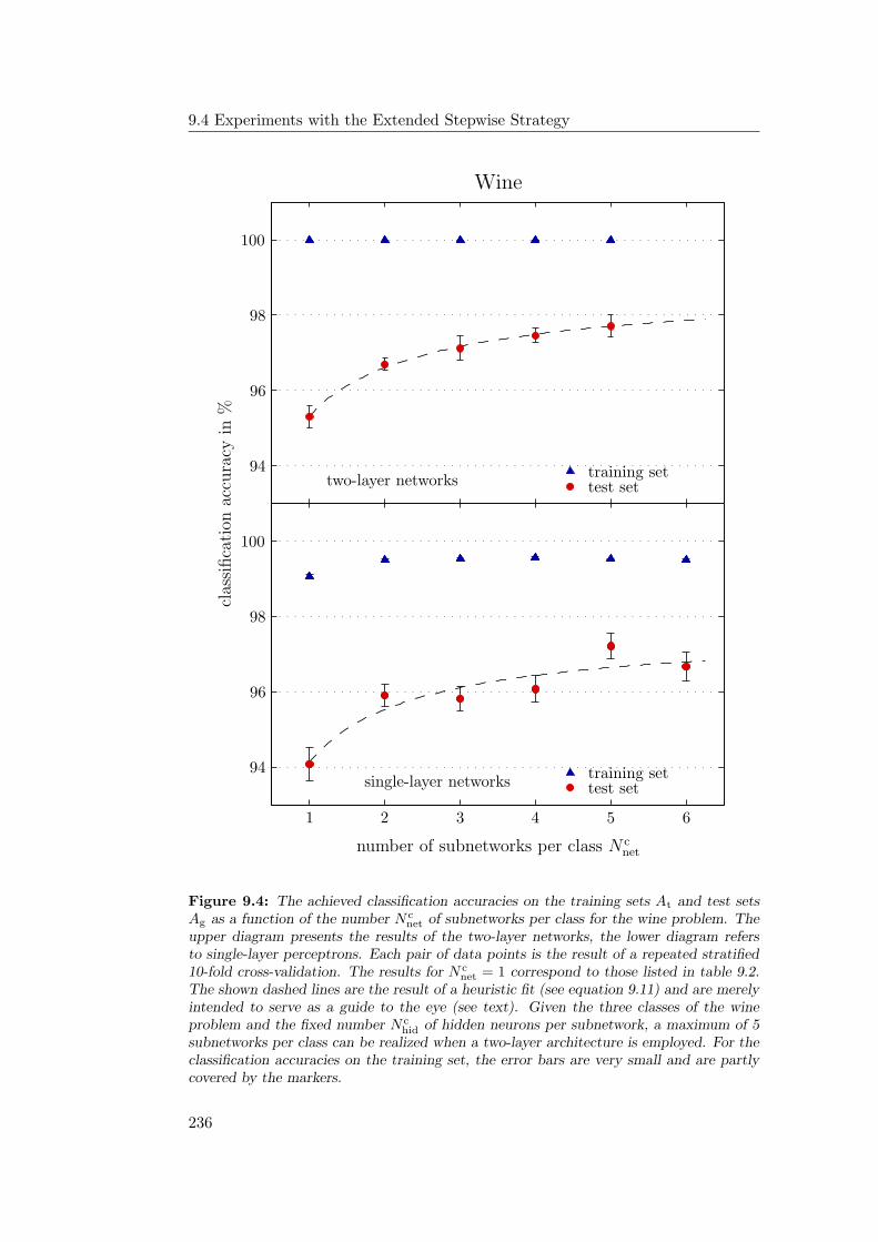
9.4 Experiments with the Extended Stepwise Strategy
PSfrag replacements
Wine
training set
training set
test set
test settwo-layer networks
single-layer networks
two-layer networksingle-layer network
multiple subnetworksenlarged subnetworks
clas
sifica
tion
accu
racy
in%
generalization accuracy Ag in %mean absolute difference D in percentage points
number of subnetworks per class N cnet
number of output neurons per class N cout
chip Achip Bchip C
simulation0
10
1
11
2
12
3
13
4
14
5
15
6
167
178
189
19205021512252235324542555265627572858295930403141324233433444354536463747384839496070617162726373647465756676677768786979809081918292839384
94
94
859586
96
96
879788
98
988999
100
100
5001000150020002500300035004000450050005500
0.51.52.53.54.55.56.57.58.59.5
96.25
96.5
96.75
Figure 9.4: The achieved classification accuracies on the training sets At and test setsAg as a function of the number N c
net of subnetworks per class for the wine problem. Theupper diagram presents the results of the two-layer networks, the lower diagram refersto single-layer perceptrons. Each pair of data points is the result of a repeated stratified10-fold cross-validation. The results for N c
net = 1 correspond to those listed in table 9.2.The shown dashed lines are the result of a heuristic fit (see equation 9.11) and are merelyintended to serve as a guide to the eye (see text). Given the three classes of the wineproblem and the fixed number N c
hid of hidden neurons per subnetwork, a maximum of 5subnetworks per class can be realized when a two-layer architecture is employed. For theclassification accuracies on the training set, the error bars are very small and are partlycovered by the markers.
236
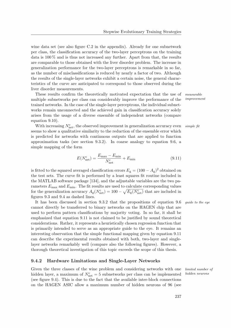
Stepwise Evolutionary Training Strategies
wine data set (see also figure C.2 in the appendix). Already for one subnetworkper class, the classification accuracy of the two-layer perceptrons on the trainingdata is 100 % and is thus not increased any further. Apart from that, the resultsare comparable to those obtained with the liver disorder problem. The increase ingeneralization performance for the two-layer perceptrons is remarkable in so far,as the number of misclassifications is reduced by nearly a factor of two. Althoughthe results of the single-layer networks exhibit a certain noise, the general charac-teristics of the curve are anticipated to correspond to those observed during theliver disorder measurements.
These results confirm the theoretically motivated expectation that the use of measurableimprovementmultiple subnetworks per class can considerably improve the performance of the
trained networks. In the case of the single-layer perceptrons, the individual subnet-works remain unconnected and the achieved gain in classification accuracy solelyarises from the usage of a diverse ensemble of independent networks (compareequation 9.10).
With increasing N cnet, the observed improvement in generalization accuracy even simple fit
seems to show a qualitative similarity to the reduction of the ensemble error whichis predicted for networks with continuous outputs that are applied to functionapproximation tasks (see section 9.3.2). In coarse analogy to equation 9.6, asimple mapping of the form
E(N cnet) =
Emax − Emin
N cnet
+ Emin (9.11)
is fitted to the squared averaged classification errors Eg = (100 − Ag)2 obtained on
the test sets. The curve fit is performed by a least squares fit routine included inthe MATLAB software package [134], and the adjustable variables are the two pa-rameters Emax and Emin. The fit results are used to calculate corresponding valuesfor the generalization accuracy Ag(N
cnet) = 100 −
√Eg(N c
net) that are included infigures 9.3 and 9.4 as dashed lines.
It has been discussed in section 9.3.2 that the propositions of equation 9.6 guide to the eye
cannot directly be transferred to binary networks on the HAGEN chip that areused to perform pattern classifications by majority voting. In so far, it shall beemphasized that equation 9.11 is not claimed to be justified by sound theoreticalconsiderations. Rather, it represents a heuristically chosen regression function thatis primarily intended to serve as an appropriate guide to the eye. It remains aninteresting observation that the simple functional mapping given by equation 9.11can describe the experimental results obtained with both, two-layer and single-layer networks remarkably well (compare also the following figures). However, athorough theoretical investigation of this topic exceeds the scope of this thesis.
9.4.2 Hardware Limitations and Single-Layer Networks
Given the three classes of the wine problem and considering networks with one limited number ofhidden neuronshidden layer, a maximum of N c
net = 5 subnetworks per class can be implemented(see figure 9.4). This is due to the fact that the available inter-block connectionson the HAGEN ASIC allow a maximum number of hidden neurons of 96 (see
237
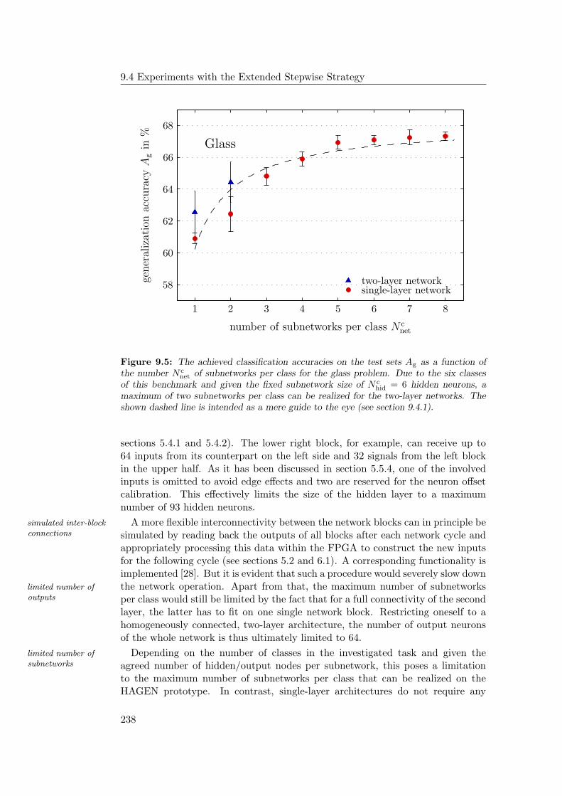
9.4 Experiments with the Extended Stepwise Strategy
PSfrag replacements
Glass
training set
test settwo-layer networks
single-layer networks
two-layer networksingle-layer network
multiple subnetworksenlarged subnetworks
classification accuracy in %
gener
aliz
atio
nac
cura
cyA
gin
%
mean absolute difference D in percentage points
number of subnetworks per class N cnet
number of output neurons per class N cout
chip Achip Bchip C
simulation0
10
1
11
2
12
3
13
4
14
5
15
6
16
7
17
8
189
192050215122522353245425552656275728
58
29593040314132423343344435453646374738483949
60
706171
62
726373
64
746575
66
766777
68
7869798090819182928393849485958696879788988999
100500
1000150020002500300035004000450050005500
0.51.52.53.54.55.56.57.58.59.5
96.25
96.5
96.75
Figure 9.5: The achieved classification accuracies on the test sets Ag as a function ofthe number N c
net of subnetworks per class for the glass problem. Due to the six classesof this benchmark and given the fixed subnetwork size of N c
hid = 6 hidden neurons, amaximum of two subnetworks per class can be realized for the two-layer networks. Theshown dashed line is intended as a mere guide to the eye (see section 9.4.1).
sections 5.4.1 and 5.4.2). The lower right block, for example, can receive up to64 inputs from its counterpart on the left side and 32 signals from the left blockin the upper half. As it has been discussed in section 5.5.4, one of the involvedinputs is omitted to avoid edge effects and two are reserved for the neuron offsetcalibration. This effectively limits the size of the hidden layer to a maximumnumber of 93 hidden neurons.
A more flexible interconnectivity between the network blocks can in principle besimulated inter-blockconnections simulated by reading back the outputs of all blocks after each network cycle and
appropriately processing this data within the FPGA to construct the new inputsfor the following cycle (see sections 5.2 and 6.1). A corresponding functionality isimplemented [28]. But it is evident that such a procedure would severely slow downthe network operation. Apart from that, the maximum number of subnetworkslimited number of
outputs per class would still be limited by the fact that for a full connectivity of the secondlayer, the latter has to fit on one single network block. Restricting oneself to ahomogeneously connected, two-layer architecture, the number of output neuronsof the whole network is thus ultimately limited to 64.
Depending on the number of classes in the investigated task and given thelimited number ofsubnetworks agreed number of hidden/output nodes per subnetwork, this poses a limitation
to the maximum number of subnetworks per class that can be realized on theHAGEN prototype. In contrast, single-layer architectures do not require any
238
Stepwise Evolutionary Training Strategies
PSfrag replacements
E.coli
training set
test settwo-layer networks
single-layer networks
two-layer networksingle-layer network
multiple subnetworksenlarged subnetworks
classification accuracy in %
gener
aliz
atio
nac
cura
cyA
gin
%
mean absolute difference D in percentage points
number of subnetworks per class N cnet
number of output neurons per class N cout
chip Achip Bchip C
simulation0
10
1
11
2
12
3
13
4
14
5
15
6
16
7
178
189
19205021512252235324542555265627572858295930403141324233433444354536463747384839496070617162726373647465756676677768786979
80
908191
82
928393
84
948595
86
96879788988999
100500
1000150020002500300035004000450050005500
0.51.52.53.54.55.56.57.58.59.5
96.25
96.5
96.75
Figure 9.6: The achieved classification accuracies on the test sets Ag as a function ofthe number N c
net of subnetworks per class for the E.coli problem. Due to the eight classesof this benchmark and given the fixed subnetwork size of N c
hid = 6 hidden neurons, onlyone subnetworks per class can be realized for the two-layer networks. The shown dashedline is intended as a mere guide to the eye (see section 9.4.1).
feedback connections and since the desired input patterns can easily be appliedsimultaneously to multiple blocks, single-layer networks can be distributed over single-layer networks:
unrestrictedthe different blocks of the HAGEN chip without restrictions. Here, the size of thenetwork is only limited by the total number of available output neurons. Withregard to a feasible increase of the number of subnetworks per class, the useof single-layer networks therefore constitutes an important potential alternative,especially for task with many classes.
Figures 9.5 and 9.6 present the results obtained with the glass and E.coli prob- glass and E.coli
lems. In these and all following diagrams, the classification rates on the trainingsets are omitted and only the generalization rates for two-layer and single-layernetworks are compared. The complete data is shown in figures C.3, and C.4 inthe appendix.
For the glass and E.coli problems, the networks with hidden layer can at most single-layer networks:efficientinclude two respectively one subnetwork of the agreed size per class. Compared to
the generalization rates that are initially achieved with these two-layer architec-tures, the single-layer networks show a remarkable improvement in performancewhen the number of subnetworks is increased. In the cases of the previouslydiscussed liver disorder and wine benchmarks, the accuracies of the one-layer net-works are observed to converge to approximately the accuracy of a two-layer net-work with two subnetworks per class. For the glass and E.coli problems, the
239
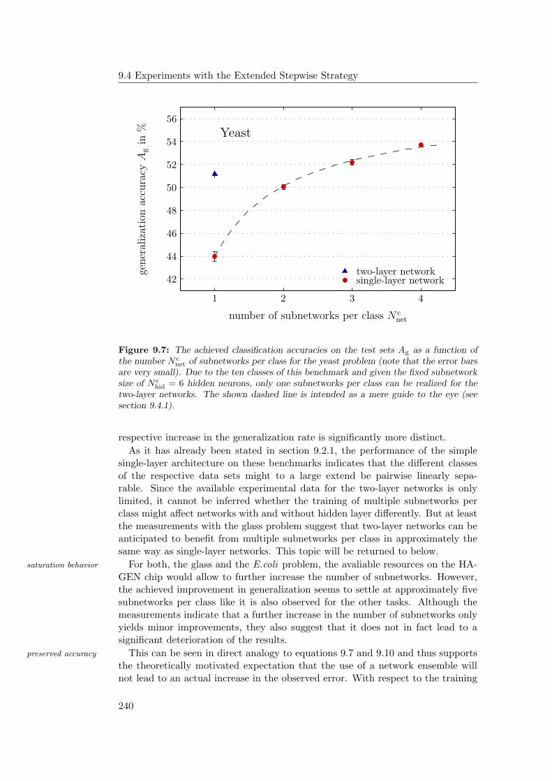
9.4 Experiments with the Extended Stepwise Strategy
PSfrag replacements
Yeast
training set
test settwo-layer networks
single-layer networks
two-layer networksingle-layer network
multiple subnetworksenlarged subnetworks
classification accuracy in %
gener
aliz
atio
nac
cura
cyA
gin
%
mean absolute difference D in percentage points
number of subnetworks per class N cnet
number of output neurons per class N cout
chip Achip Bchip C
simulation0
10
1
11
2
12
3
13
4
145
156
167
178
189
1920
50
215122
52
235324
54
255526
56
2757285829593040314132
42
334334
44
354536
46
374738
48
394960706171627263736474657566766777687869798090819182928393849485958696879788988999
100500
1000150020002500300035004000450050005500
0.51.52.53.54.55.56.57.58.59.5
96.25
96.5
96.75
Figure 9.7: The achieved classification accuracies on the test sets Ag as a function ofthe number N c
net of subnetworks per class for the yeast problem (note that the error barsare very small). Due to the ten classes of this benchmark and given the fixed subnetworksize of N c
hid = 6 hidden neurons, only one subnetworks per class can be realized for thetwo-layer networks. The shown dashed line is intended as a mere guide to the eye (seesection 9.4.1).
respective increase in the generalization rate is significantly more distinct.
As it has already been stated in section 9.2.1, the performance of the simplesingle-layer architecture on these benchmarks indicates that the different classesof the respective data sets might to a large extend be pairwise linearly sepa-rable. Since the available experimental data for the two-layer networks is onlylimited, it cannot be inferred whether the training of multiple subnetworks perclass might affect networks with and without hidden layer differently. But at leastthe measurements with the glass problem suggest that two-layer networks can beanticipated to benefit from multiple subnetworks per class in approximately thesame way as single-layer networks. This topic will be returned to below.
For both, the glass and the E.coli problem, the avaliable resources on the HA-saturation behavior
GEN chip would allow to further increase the number of subnetworks. However,the achieved improvement in generalization seems to settle at approximately fivesubnetworks per class like it is also observed for the other tasks. Although themeasurements indicate that a further increase in the number of subnetworks onlyyields minor improvements, they also suggest that it does not in fact lead to asignificant deterioration of the results.
This can be seen in direct analogy to equations 9.7 and 9.10 and thus supportspreserved accuracy
the theoretically motivated expectation that the use of a network ensemble willnot lead to an actual increase in the observed error. With respect to the training
240
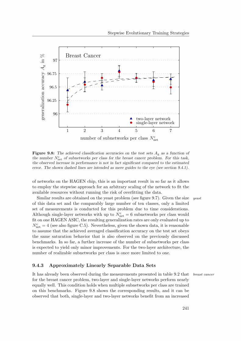
Stepwise Evolutionary Training Strategies
PSfrag replacements
Breast Cancer
training set
test settwo-layer networks
single-layer networks
two-layer networksingle-layer network
multiple subnetworksenlarged subnetworks
classification accuracy in %
gener
aliz
atio
nac
cura
cyA
gin
%
mean absolute difference D in percentage points
number of subnetworks per class N cnet
number of output neurons per class N cout
chip Achip Bchip C
simulation0
10
1
11
2
12
3
13
4
14
5
15
6
16
7
178
189
1920502151225223532454255526562757285829593040314132423343344435453646374738483949607061716272637364746575667667776878697980908191829283938494859586
96
87
97
88988999
100500
1000150020002500300035004000450050005500
0.51.52.53.54.55.56.57.58.59.5
96.25
96.5
96.75
Figure 9.8: The achieved classification accuracies on the test sets Ag as a function ofthe number N c
net of subnetworks per class for the breast cancer problem. For this task,the observed increase in performance is not in fact significant compared to the estimatederror. The shown dashed lines are intended as mere guides to the eye (see section 9.4.1).
of networks on the HAGEN chip, this is an important result in so far as it allowsto employ the stepwise approach for an arbitrary scaling of the network to fit theavailable resources without running the risk of overfitting the data.
Similar results are obtained on the yeast problem (see figure 9.7). Given the size yeast
of this data set and the comparably large number of ten classes, only a limitedset of measurements is conducted for this problem due to time considerations.Although single-layer networks with up to N c
net = 6 subnetworks per class wouldfit on one HAGEN ASIC, the resulting generalization rates are only evaluated up toN c
net = 4 (see also figure C.5). Nevertheless, given the shown data, it is reasonableto assume that the achieved averaged classification accuracy on the test set obeysthe same saturation behavior that is also observed on the previously discussedbenchmarks. In so far, a further increase of the number of subnetworks per classis expected to yield only minor improvements. For the two-layer architecture, thenumber of realizable subnetworks per class is once more limited to one.
9.4.3 Approximately Linearly Separable Data Sets
It has already been observed during the measurements presented in table 9.2 that breast cancer
for the breast cancer problem, two-layer and single-layer networks perform nearlyequally well. This condition holds when multiple subnetworks per class are trainedon this benchmarks. Figure 9.8 shows the corresponding results, and it can beobserved that both, single-layer and two-layer networks benefit from an increased
241
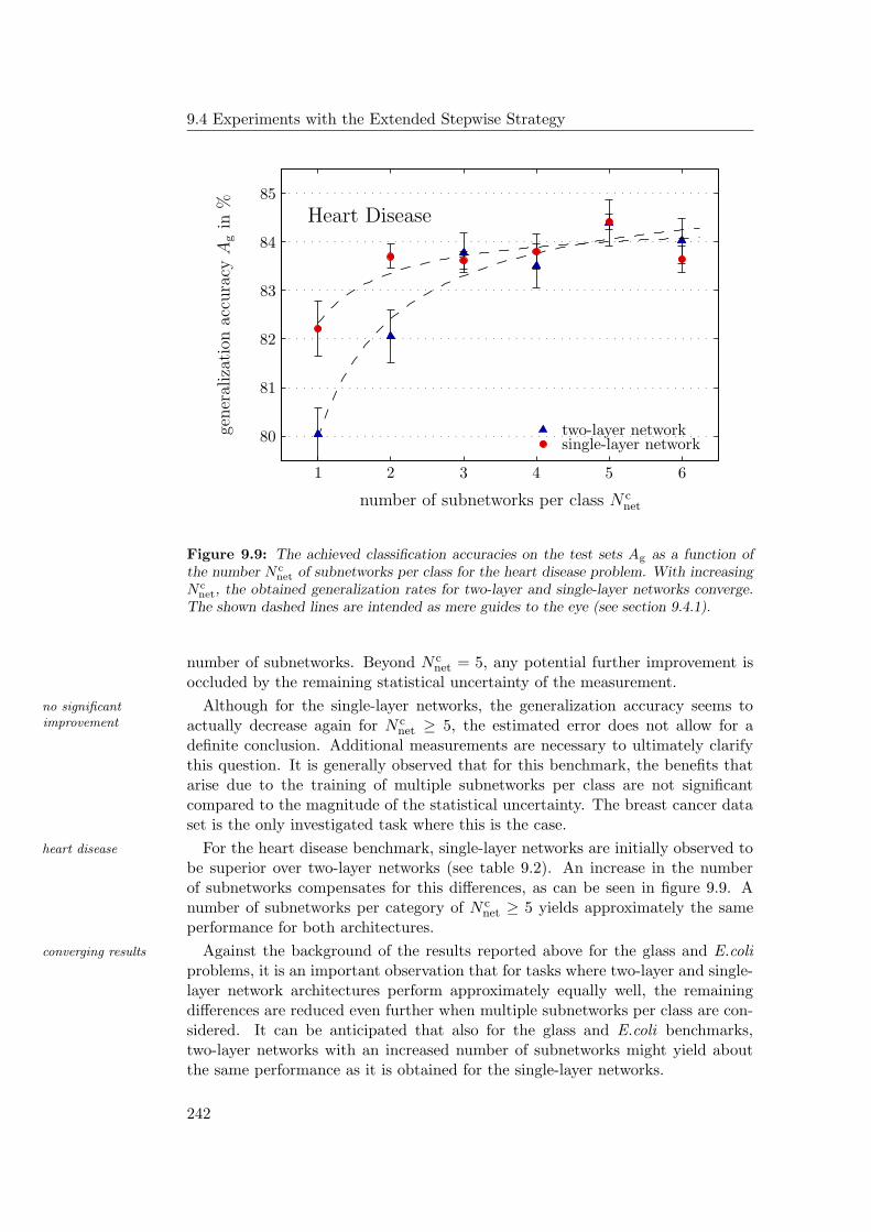
9.4 Experiments with the Extended Stepwise Strategy
PSfrag replacements
Heart Disease
training set
test settwo-layer networks
single-layer networks
two-layer networksingle-layer network
multiple subnetworksenlarged subnetworks
classification accuracy in %
gener
aliz
atio
nac
cura
cyA
gin
%
mean absolute difference D in percentage points
number of subnetworks per class N cnet
number of output neurons per class N cout
chip Achip Bchip C
simulation0
10
1
11
2
12
3
13
4
14
5
15
6
167
178
189
19205021512252235324542555265627572858295930403141324233433444354536463747384839496070617162726373647465756676677768786979
80
90
81
91
82
92
83
93
84
94
85
958696879788988999
100500
1000150020002500300035004000450050005500
0.51.52.53.54.55.56.57.58.59.5
96.25
96.5
96.75
Figure 9.9: The achieved classification accuracies on the test sets Ag as a function ofthe number N c
net of subnetworks per class for the heart disease problem. With increasingN c
net, the obtained generalization rates for two-layer and single-layer networks converge.The shown dashed lines are intended as mere guides to the eye (see section 9.4.1).
number of subnetworks. Beyond N cnet = 5, any potential further improvement is
occluded by the remaining statistical uncertainty of the measurement.
Although for the single-layer networks, the generalization accuracy seems tono significantimprovement actually decrease again for N c
net ≥ 5, the estimated error does not allow for adefinite conclusion. Additional measurements are necessary to ultimately clarifythis question. It is generally observed that for this benchmark, the benefits thatarise due to the training of multiple subnetworks per class are not significantcompared to the magnitude of the statistical uncertainty. The breast cancer dataset is the only investigated task where this is the case.
For the heart disease benchmark, single-layer networks are initially observed toheart disease
be superior over two-layer networks (see table 9.2). An increase in the numberof subnetworks compensates for this differences, as can be seen in figure 9.9. Anumber of subnetworks per category of N c
net ≥ 5 yields approximately the sameperformance for both architectures.
Against the background of the results reported above for the glass and E.coliconverging results
problems, it is an important observation that for tasks where two-layer and single-layer network architectures perform approximately equally well, the remainingdifferences are reduced even further when multiple subnetworks per class are con-sidered. It can be anticipated that also for the glass and E.coli benchmarks,two-layer networks with an increased number of subnetworks might yield aboutthe same performance as it is obtained for the single-layer networks.
242
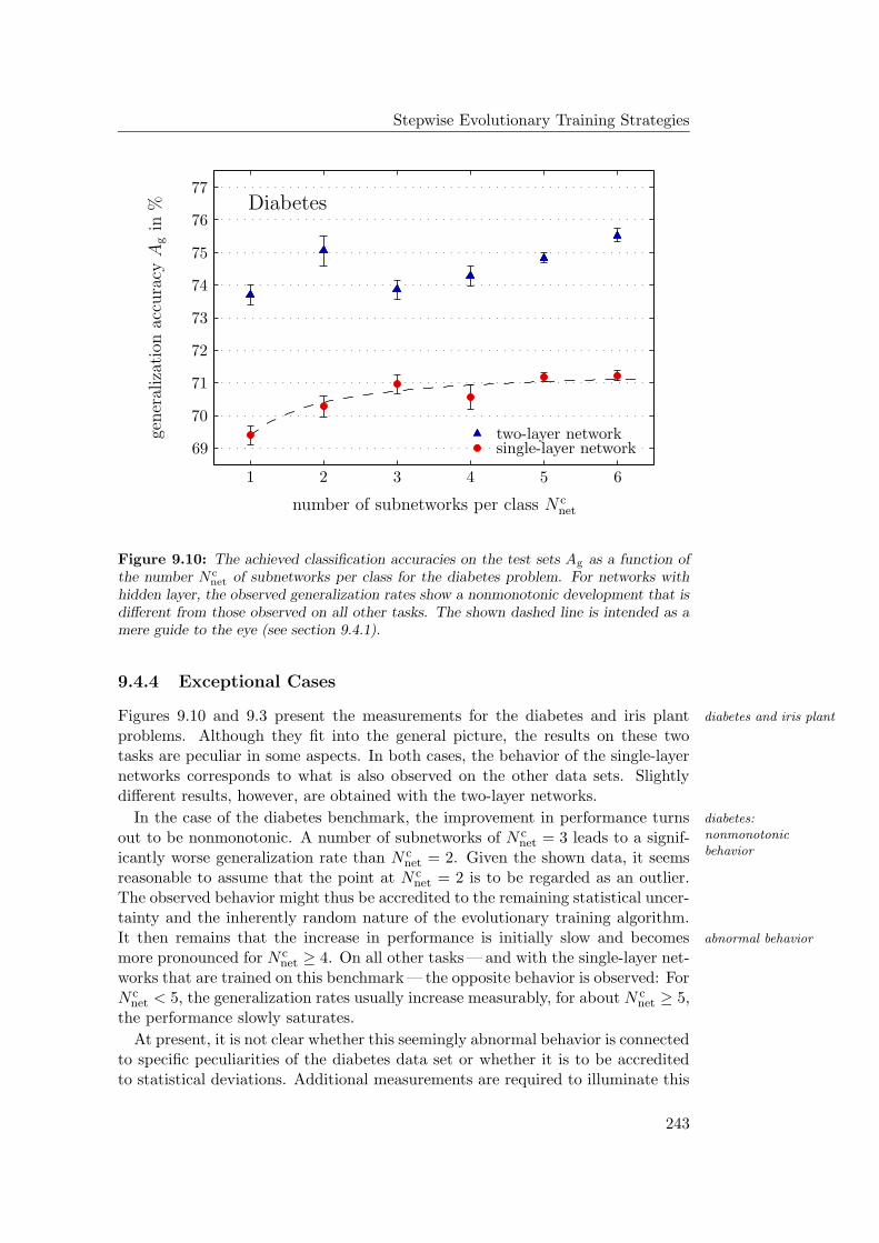
Stepwise Evolutionary Training Strategies
PSfrag replacements
Diabetes
training set
test settwo-layer networks
single-layer networks
two-layer networksingle-layer network
multiple subnetworksenlarged subnetworks
classification accuracy in %
gener
aliz
atio
nac
cura
cyA
gin
%
mean absolute difference D in percentage points
number of subnetworks per class N cnet
number of output neurons per class N cout
chip Achip Bchip C
simulation0
10
1
11
2
12
3
13
4
14
5
15
6
167
178
189
192050215122522353245425552656275728582959304031413242334334443545364637473848394960
70
61
71
62
72
63
73
64
74
65
75
66
76
67
77
6878
69
798090819182928393849485958696879788988999
100500
1000150020002500300035004000450050005500
0.51.52.53.54.55.56.57.58.59.5
96.25
96.5
96.75
Figure 9.10: The achieved classification accuracies on the test sets Ag as a function ofthe number N c
net of subnetworks per class for the diabetes problem. For networks withhidden layer, the observed generalization rates show a nonmonotonic development that isdifferent from those observed on all other tasks. The shown dashed line is intended as amere guide to the eye (see section 9.4.1).
9.4.4 Exceptional Cases
Figures 9.10 and 9.3 present the measurements for the diabetes and iris plant diabetes and iris plant
problems. Although they fit into the general picture, the results on these twotasks are peculiar in some aspects. In both cases, the behavior of the single-layernetworks corresponds to what is also observed on the other data sets. Slightlydifferent results, however, are obtained with the two-layer networks.
In the case of the diabetes benchmark, the improvement in performance turns diabetes:nonmonotonicbehavior
out to be nonmonotonic. A number of subnetworks of N cnet = 3 leads to a signif-
icantly worse generalization rate than N cnet = 2. Given the shown data, it seems
reasonable to assume that the point at N cnet = 2 is to be regarded as an outlier.
The observed behavior might thus be accredited to the remaining statistical uncer-tainty and the inherently random nature of the evolutionary training algorithm.It then remains that the increase in performance is initially slow and becomes abnormal behavior
more pronounced for N cnet ≥ 4. On all other tasks — and with the single-layer net-
works that are trained on this benchmark — the opposite behavior is observed: ForN c
net < 5, the generalization rates usually increase measurably, for about N cnet ≥ 5,
the performance slowly saturates.
At present, it is not clear whether this seemingly abnormal behavior is connectedto specific peculiarities of the diabetes data set or whether it is to be accreditedto statistical deviations. Additional measurements are required to illuminate this
243
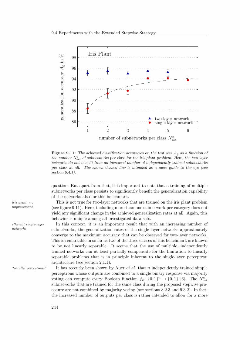
9.4 Experiments with the Extended Stepwise Strategy
PSfrag replacements
Iris Plant
training set
test settwo-layer networks
single-layer networks
two-layer networksingle-layer network
multiple subnetworksenlarged subnetworks
classification accuracy in %
gener
aliz
atio
nac
cura
cyA
gin
%
mean absolute difference D in percentage points
number of subnetworks per class N cnet
number of output neurons per class N cout
chip Achip Bchip C
simulation0
10
1
11
2
12
3
13
4
14
5
15
6
167
178
189
1920502151225223532454255526562757285829593040314132423343344435453646374738483949607061716272637364746575667667776878697980
90
819182
92
839384
94
8595
86
96
8797
88
98
8999
100500
1000150020002500300035004000450050005500
0.51.52.53.54.55.56.57.58.59.5
96.25
96.5
96.75
Figure 9.11: The achieved classification accuracies on the test sets Ag as a function ofthe number N c
net of subnetworks per class for the iris plant problem. Here, the two-layernetworks do not benefit from an increased number of independently trained subnetworksper class at all. The shown dashed line is intended as a mere guide to the eye (seesection 9.4.1).
question. But apart from that, it is important to note that a training of multiplesubnetworks per class persists to significantly benefit the generalization capabilityof the networks also for this benchmark.
This is not true for two-layer networks that are trained on the iris plant problemiris plant: noimprovement (see figure 9.11). Here, including more than one subnetwork per category does not
yield any significant change in the achieved generalization rates at all. Again, thisbehavior is unique among all investigated data sets.
In this context, it is an important result that with an increasing number ofefficient single-layernetworks subnetworks, the generalization rates of the single-layer networks approximately
converge to the maximum accuracy that can be observed for two-layer networks.This is remarkable in so far as two of the three classes of this benchmark are knownto be not linearly separable. It seems that the use of multiple, independentlytrained networks can at least partially compensate for the limitation to linearlyseparable problems that is in principle inherent to the single-layer perceptronarchitecture (see section 2.1.1).
It has recently been shown by Auer et al. that n independently trained simple“parallel perceptrons”
perceptrons whose outputs are combined to a single binary response via majorityvoting can compute every Boolean function fB : 0, 1n → 0, 1 [6]. The N c
net
subnetworks that are trained for the same class during the proposed stepwise pro-cedure are not combined by majority voting (see sections 8.2.3 and 9.3.2). In fact,the increased number of outputs per class is rather intended to allow for a more
244
Stepwise Evolutionary Training Strategies
differentiated comparison with the remaining networks that are trained for theother classes. In so far, it is understood that the above universal approximationtheorem for “parallel perceptrons” [6] cannot directly be applied. But the experi-mental data shown in figure 9.11 suggests that similar propositions might also holdfor single-layer networks that are trained by the generalized stepwise strategy. Amore detailed theoretical investigation of this question exceeds the scope of thisthesis but promises to be an interesting topic for future investigations.
Summarizing Remarks
For all investigated benchmark problems — except for the breast cancer problem — improved results
the training of multiple subnetworks per class yields some kind of measurableimprovement of the achieved classification accuracies. At the same time, both, thesimplicity of the evolutionary training algorithm that is used in each phase andthe favorable inherent parallelism of the original stepwise approach are preserved.
Furthermore, given the results that are obtained on the breast cancer, heart single-layer networks:feasibledisease, iris plant, glass, and E.coli data sets, it can be concluded that the gen-
eralized stepwise training strategy also allows for the application of single-layerperceptrons to demanding, real-world tasks — partly even for those problems thatcannot ordinarily be solved satisfactorily by such simple networks. Apart frombeing an interesting observation by itself, this particularly suits the used HAGENprototype, since single-layer networks are not affected by the restrictions that arisefrom the limited set of available, hard-wired feedback connections or the fixed sizeof the network blocks.
It is another important outcome of the presented measurements that the train- results for differentarchitecturesing of multiple subnetworks per class tends to compensate for the differences in
performance between the investigated two-layer and single-layer architectures. Es-pecially in the case of the heart disease problem, the choice of a network withhidden layer has initially been encountered to be problematic (see section 9.2.1).But when it is possible to train a sufficient number of subnetworks per class, thetwo-layer architecture is seen to be at least as efficient as the simple single-layertopology on all respective benchmarks.
These results indicate that the generalized stepwise strategy can largely relieve architectureoptimization: largelyredundant
the user — or the training algorithm — from determining the optimal architecturefor a specific task: If the number of classes in the considered problem allows torealize a number of two-layer subnetworks of about N c
net = 5, the two-layer ar-chitecture is to be chosen. Otherwise, satisfactory generalization rates can stillbe achieved with the single-layer architecture. At this point, having experimen-tally investigated only a limited number of exemplary benchmarks, this directiveis admittedly nothing more than an empirical rule of thumb. Nevertheless, itpersists that in all examined cases where a sufficient number of subnetworks canbe implemented on the HAGEN chip, the two-layer architectures never performmeasurably worse than the single-layer networks.
In summary, the proposed generalized stepwise strategy suggests itself as afeasible way of training enlarged networks that can efficiently exploit the resourcesof the HAGEN ASIC. But it remains to be investigated whether the performance
245
9.4 Experiments with the Extended Stepwise Strategy
of the hereby constructed networks can eventually compete with those of othersystems.
9.4.5 Comparison to Previous Results
It has already been stated in section 8.4.2 that most of the reported experimentsthat evaluate the performance of other neural network setups or classification sys-tems on the selected benchmarks do not employ a stratified 10-fold cross-validationscheme. In order to allow for a direct comparison with these results, an additionalset of experiments is performed where for each benchmark, the same evaluationscheme is employed that is also used in a corresponding earlier publication. Apartfrom alternative training setups for single neural networks, the performance of theintroduced stepwise strategy is compared also to other classification algorithms —such as support vector machines and k nearest neighbor classifiers— as well as tocontemporary approaches for the training of neural network ensembles.
Fixed Partitionings and Single Neural Networks
Among numerous other benchmarks, Prechelt [163] examines multiple feedforward“Proben1”
neural network architectures on the breast cancer, diabetes, heart disease and glassproblems. For each task, a set of three different partitionings into training andtest data is provided. Since these partitionings are all included in the “Proben1”benchmark suite that is introduced in the same publication, the respective combi-nations of training and test data shall be denoted as “Proben1 a)”, “Proben1 b)”,and “Proben1 c)”.
The breast cancer and diabetes problem are also investigated by Yao and Liu [236]EPNet
who evaluate the performance of their EPNet system (see section 4.2.2) on thesetasks. They use one fixed partitioning of the data for each benchmark, and theirinvestigations also include the heart disease problem. But unfortunately, the pre-cise compositions of training and test set for this task cannot unambiguously bereconstructed.
In both publications, the training data is divided further into an actual trainingtraining set andvalidation set set and a so-called validation set [163] [236]. The training of the network then only
employs the former while the latter is exclusively used to determine the termina-tion of the algorithm: During training, the network is periodically tested on thevalidation set, usually after a fixed number of iterations. While the classificationaccuracy on the training set is expected to improve approximately monotonically,the performance on the validation set might stagnate or even deteriorate due tooverfitting of the data. If this is the case, the training is terminated. The evolu-tionary stepwise strategy introduced in this thesis does not employ any validationdata during training. The subsets of the data that are marked as the validationsets are therefore appended to the respective training sets.
Table 9.3 compares the results of the cited publications with the generalizationtraining setup
rates that are obtained by neural networks on the HAGEN chip. The networksare trained with the same algorithm and network setup that is also used duringthe investigations described in the previous sections. The only exception is that
246
Stepwise Evolutionary Training Strategies
during the evaluation of a network’s classification accuracy on the test data, eachpattern is applied only mg
p = 20 times instead of the 50 repetitions used for theprevious experiments (see section 8.4.1 and table 8.3). This accounts for the factthat according to the used fixed partitionings, the different test sets now containabout 25 % of the total instances in the respective data set.
In case of the glass problem, the network architecture comprises only one single network architecture
layer; for the other tasks, the networks have two layers. The numbers of sub-networks per class that are contained in the trained networks are included in thetable.
For each of the used fixed partitionings, a total of Nn = 10 entire networks evaluation procedure
is trained, and the one with the best classification rate on the training data isregarded as the result. This is repeated Nr = 5 times for each partitioning andthe obtained averaged generalization accuracies Ag together with the correspond-ing standard deviations are listed in table 9.3. Only the classification rates onthe test data are compared. For the networks trained on the HAGEN chip, theperformance on the training data At can be found in table C.3 in the appendix.
A variety of results are reported in the “Proben1” collection that each employ compared networks
slightly different network architectures and transfer functions [163]. The networksare trained with a variant of the backpropagation algorithm (see section 2.2.2).For each individual partitioning of the individual data sets, table 9.3 lists the bestrespective result that can be found in this publication regardless of the employednetwork setup. Since some of these values represent the generalization rates ofindividual, outstanding networks, the respective results include no error estimates.The remaining values represent the mean of 60 independent training runs (10 inthe case of the heart disease problem) and the provided error measures are given bythe corresponding standard error of the mean1. Within the experiments reportedby Yao and Liu, the network topology is optimized by the training algorithm (seealso section 4.2.2). Here, the cited results each represent the mean of 30 trainingruns with the EPNet system. The generalization rates that are obtained by thesetwo previous investigations represent the best results of single neural networks onthe considered benchmarks that have been found in literature and that can alsoexactly be reproduced due to an unambiguous specification of the used trainingand test data. The performance of recent neural network ensemble approacheswill be discussed below.
A comparison to the generalization accuracies that are obtained with networks results: competitive
on the HAGEN chip reveals that the introduced stepwise training strategy incombination with the used strictly layered, feedforward perceptron architectureconstitutes a competitive approach to tackle the investigated problems. In mostcases, the trained networks either achieve better generalization rates than thoseobtained by the previous setups (marked red in table 9.3) or perform approxi-mately equally well (blue entries).
This result is particularly remarkable in so far, as neither the various parametersof the used evolutionary training algorithm nor the settings of the generalized
1The provided standard errors of the mean are calculated from the respective standard devi-ations and the number of experiments that are reported in the two cited publications.
247
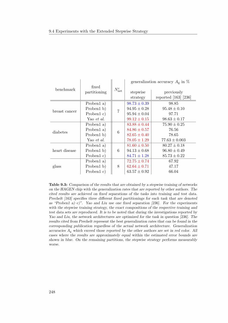
9.4 Experiments with the Extended Stepwise Strategy
benchmarkfixed
partitioningN c
net
generalization accuracy Ag in %
stepwisestrategy
previouslyreported [163] [236]
breast cancer
Proben1 a)
7
98.73 ± 0.39 98.85Proben1 b) 94.95 ± 0.28 95.48 ± 0.10Proben1 c) 95.94 ± 0.04 97.71Yao et al. 99.12 ± 0.15 98.63 ± 0.17
diabetes
Proben1 a)
6
83.88 ± 0.44 75.90 ± 0.25Proben1 a) 84.86 ± 0.57 76.56Proben1 b) 82.65 ± 0.40 78.65Yao et al. 78.05 ± 1.29 77.63 ± 0.003
heart diseaseProben1 a)
681.60 ± 0.50 80.27 ± 0.18
Proben1 b) 94.13 ± 0.68 96.80 ± 0.49Proben1 c) 84.71 ± 1.28 85.73 ± 0.22
glassProben1 a)
872.75 ± 0.74 67.92
Proben1 b) 62.64 ± 0.71 47.17Proben1 c) 63.57 ± 0.92 66.04
Table 9.3: Comparison of the results that are obtained by a stepwise training of networkson the HAGEN chip with the generalization rates that are reported by other authors. Thecited results are achieved on fixed separations of the tasks into training and test data.Prechelt [163] specifies three different fixed partitionings for each task that are denotedas “Proben1 a)–c)”. Yao and Liu use one fixed separation [236]. For the experimentswith the stepwise training strategy, the exact compositions of the respective training andtest data sets are reproduced. It is to be noted that during the investigations reported byYao and Liu, the network architectures are optimized for the task in question [236]. Theresults cited from Prechelt represent the best generalization rates that can be found in thecorresponding publication regardless of the actual network architecture. Generalizationaccuracies Ag which exceed those reported by the other authors are set in red color. Allcases where the results are approximately equal within the estimated error bounds areshown in blue. On the remaining partitions, the stepwise strategy performs measurablyworse.
248
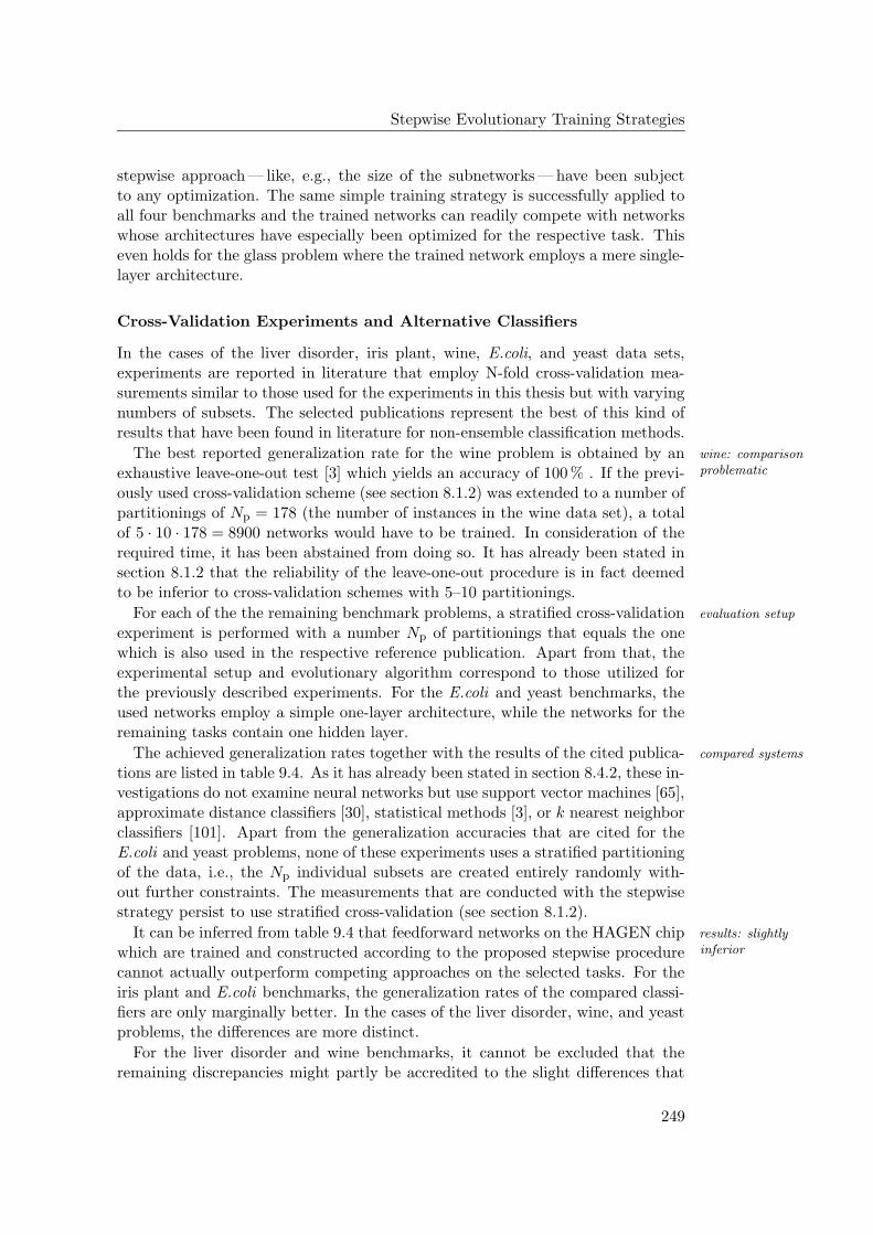
Stepwise Evolutionary Training Strategies
stepwise approach — like, e.g., the size of the subnetworks — have been subjectto any optimization. The same simple training strategy is successfully applied toall four benchmarks and the trained networks can readily compete with networkswhose architectures have especially been optimized for the respective task. Thiseven holds for the glass problem where the trained network employs a mere single-layer architecture.
Cross-Validation Experiments and Alternative Classifiers
In the cases of the liver disorder, iris plant, wine, E.coli, and yeast data sets,experiments are reported in literature that employ N-fold cross-validation mea-surements similar to those used for the experiments in this thesis but with varyingnumbers of subsets. The selected publications represent the best of this kind ofresults that have been found in literature for non-ensemble classification methods.
The best reported generalization rate for the wine problem is obtained by an wine: comparisonproblematicexhaustive leave-one-out test [3] which yields an accuracy of 100 % . If the previ-
ously used cross-validation scheme (see section 8.1.2) was extended to a number ofpartitionings of Np = 178 (the number of instances in the wine data set), a totalof 5 · 10 · 178 = 8900 networks would have to be trained. In consideration of therequired time, it has been abstained from doing so. It has already been stated insection 8.1.2 that the reliability of the leave-one-out procedure is in fact deemedto be inferior to cross-validation schemes with 5–10 partitionings.
For each of the the remaining benchmark problems, a stratified cross-validation evaluation setup
experiment is performed with a number Np of partitionings that equals the onewhich is also used in the respective reference publication. Apart from that, theexperimental setup and evolutionary algorithm correspond to those utilized forthe previously described experiments. For the E.coli and yeast benchmarks, theused networks employ a simple one-layer architecture, while the networks for theremaining tasks contain one hidden layer.
The achieved generalization rates together with the results of the cited publica- compared systems
tions are listed in table 9.4. As it has already been stated in section 8.4.2, these in-vestigations do not examine neural networks but use support vector machines [65],approximate distance classifiers [30], statistical methods [3], or k nearest neighborclassifiers [101]. Apart from the generalization accuracies that are cited for theE.coli and yeast problems, none of these experiments uses a stratified partitioningof the data, i.e., the Np individual subsets are created entirely randomly with-out further constraints. The measurements that are conducted with the stepwisestrategy persist to use stratified cross-validation (see section 8.1.2).
It can be inferred from table 9.4 that feedforward networks on the HAGEN chip results: slightlyinferiorwhich are trained and constructed according to the proposed stepwise procedure
cannot actually outperform competing approaches on the selected tasks. For theiris plant and E.coli benchmarks, the generalization rates of the compared classi-fiers are only marginally better. In the cases of the liver disorder, wine, and yeastproblems, the differences are more distinct.
For the liver disorder and wine benchmarks, it cannot be excluded that theremaining discrepancies might partly be accredited to the slight differences that
249
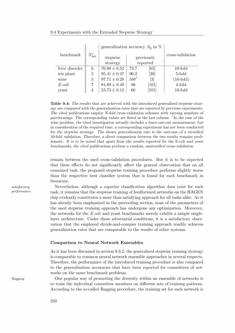
9.4 Experiments with the Extended Stepwise Strategy
benchmark N cnet
generalization accuracy Ag in %
cross-validationstepwisestrategy
previouslyreported
liver disorder 6 70.98 ± 0.52 73.7 [65] 10-foldiris plant 5 95.41 ± 0.47 96.2 [30] 5-fold
wine 5 97.71 ± 0.28 100 * [3] (10-fold)E.coli 7 84.89 ± 0.49 86 [101] 4-foldyeast 4 53.73 ± 0.12 60 [101] 10-fold
Table 9.4: The results that are achieved with the introduced generalized stepwise strat-egy are compared with the generalization rates that are reported by previous experiments.The cited publications employ N-fold cross-validation schemes with varying numbers ofpartitionings. The corresponding values are listed in the last column. *In the case of thewine problem, the cited investigation actually includes a leave-one-out measurement, butin consideration of the required time, a corresponding experiment has not been conductedfor the stepwise strategy. The shown generalization rate is the outcome of a stratified10-fold validation. Therefore, a direct comparison between the two results remains prob-lematic. It is to be noted that apart from the results reported for the E.coli and yeastbenchmarks, the cited publications perform a random, unstratified cross-validation.
remain between the used cross-validation procedures. But it is to be expectedthat these effects do not significantly affect the general observation that on allexamined task, the proposed stepwise training procedure performs slightly worsethan the respective best classifier system that is found for each benchmark inliterature.
Nevertheless, although a superior classification algorithm does exist for eachsatisfactoryperformance task, it remains that the stepwise training of feedforward networks on the HAGEN
chip evidently constitutes a more than satisfying approach for all tasks alike. As ithas already been emphasized in the preceeding section, none of the parameters ofthe used stepwise training approach has undergone any optimization. Moreover,the networks for the E.coli and yeast benchmarks merely exhibit a simple single-layer architecture. Under these adversarial conditions, it is a satisfactory obser-vation that the employed divide-and-conquer training approach readily achievesgeneralization rates that are comparable to the results of other systems.
Comparison to Neural Network Ensembles
As it has been discussed in section 9.3.2, the generalized stepwise training strategyis comparable to common neural network ensemble approaches in several respects.Therefore, the performance of the introduced training procedure is also comparedto the generalization accuracies that have been reported for committees of net-works on the same benchmark problems.
One popular way of promoting the diversity within an ensemble of networks isBagging
to train the individual committee members on different sets of training patterns.According to the so-called Bagging procedure, the training set for each network is
250
Stepwise Evolutionary Training Strategies
benchmark N cnet
generalization accuracy Ag in %
stepwisestrategy
Bagging [153] CNNE [105]
breast cancer 7 96.65 ± 0.10 96.6 98.9diabetes 6 75.52 ± 0.21 77.2 82.2heart disease 6 84.03 ± 0.46 83.0 88.8glass 8 67.33 ± 0.26 66.9 75.4
Table 9.5: The results that are achieved with the introduced generalized stepwise strategyare compared to the generalization rates that are reported by other investigations onneural network ensembles. The cited publications both employ an unstratified 10-foldcross-validation scheme. Bagging is a popular approach where the individual members ofthe ensemble are trained on different training sets [153]. The CNNE algorithm proposed byIslam et al. incorporates elaborate schemes of adjusting the number and architecture of thesingle networks and promoting the diversity within the ensemble by negative correlationlearning [105]. The generalization rates that are achieved by this latter approach are byfar the best that have been encountered for the investigated tasks in literature.
generated by randomly drawing, with replacement, Nt examples from the originaltraining data, where Nt is the number of instances in the whole training set [153].Some of the instances will then appear multiple times in the training data of agiven network, while others will be left out. Since each network in the ensemble istrained on a new, randomly created training set, it is expected that their responseswill exhibit a measurable disagreement.
It has been discussed in section 9.3.2 that more recent approaches actively en- compared ensembles
force the diversity of the networks in the ensemble during training. Among otherbenchmarks, Islam et al. [105] test their proposed CNNE (Constructive NeuralNetwork Ensemble) algorithm also on the breast cancer, diabetes, heart disease,and glass problem and compare it to the results that are reported for a Baggingensemble by Opitz et al. [153].
In both investigations, a 10-fold cross-validation scheme is employed and the evaluation procedure
reported results can therefore directly be compared to the generalization ratesthat are achieved by the introduced stepwise strategy. The respectively obtainedclassification accuracies on the test sets are summarized in table 9.5.
Compared to the results of the Bagging ensemble, the stepwise strategy is once comparison
more observed to exhibit a competitive performance. Still, the generalization ratesthat are achieved by the CNNE approach are not only significantly better thanthose of the Bagging ensemble, to the author’s best knowledge they also representby far the best results that are reported for N-fold cross-validation measurementson the respective benchmarks in literature. It can be inferred from table 9.5,that the generalization accuracies that are achieved with the introduced stepwisestrategy cannot compete with these results.
As it has already been stated in section 9.3.2, the CNNE model involves a CNNE
complex learning procedure that actively promotes the diversity of the individualnetworks in the ensemble. During training, the weight modifications that are
251
9.4 Experiments with the Extended Stepwise Strategy
applied to each single network are affected not only by its own output but also bythe current performance of the other networks, such that any correlation betweenthe responses of the different networks can effectively be reduced [105]. In otherwords, the networks need to be trained simultaneously and cannot be consideredindependently. Furthermore, elaborate construction schemes are applied in orderto optimize the individual architectures as well as the number of networks in thecommittee during training.
Given the complexity of this approach, it is not surprising that the training ofcomplexity vs. speed
networks via the generalized stepwise strategy — which is optimized for simplic-ity, fast training speeds, and inherent parallelism— is eventually outperformed bythe CNNE algorithm. On the other hand, an elaborate approach like the CNNEprocedure is unlikely to achieve an efficient exploitation of the speed benefits thatarise from the use of a neural network hardware. In particular, the interdependen-cies that remain between the networks during training do not allow for the samedegree of parallelism that can readily be achieved by the proposed stepwise strat-egy. In so far, it is a more than satisfying observation that the stepwise training iscomparable in performance to common neural network ensemble approaches andat the same time allows to efficiently utilize the evolutionary coprocessor for thefast training of neural networks on the HAGEN chip.
9.4.6 Multiple Subnetworks vs. Increased Subnetwork Size
Having demonstrated the potential of the generalized stepwise approach, the chap-ter is to be concluded by an investigation of whether an alternative increase of thesubnetwork size might actually yield an equal or even better performance. A setof experiments is conducted where only one subnetwork is trained for each classof the investigated problem and where the classification accuracies of the finalnetworks on the used test sets are evaluated as a function of the number of hiddenneurons N sn
hid and outputs N snout per subnetwork.
In order to allow for a direct comparison with the training of multiple sub-equal network size
networks per class, the enlarged subnetworks are scaled to contain numbers ofhidden nodes and outputs that are simple integer multiples ms of the agreed ini-tial parameters N sn
hid = 6 and N snout = 4, respectively. Therefore, the resulting
networks comprise an equal total number of neurons as those that are obtained byan independent training of ms subnetworks for each category. The allowed num-equal training time
ber of generations of the evolutionary training algorithm in each phase is scaledaccordingly, i.e., an increase of the network size by a factor of ms is accountedfor by multiplying the number of training iterations per phase by the same fac-tor. Hence, the total amount of processed generations is the same as for thecorresponding experiment with the generalized stepwise strategy described in thepreceeding sections. Apart from the increased subnetwork size and the extendedtraining time, the experiments follow the same setup as described in section 9.2.
252
Stepwise Evolutionary Training Strategies
General Observations
In figure 9.12, the results that are obtained on the liver disorder problem are com- liver disorder
pared with the performance of the generalized stepwise strategy investigated insection 9.4.1. For both results to be displayed in the same diagram, the achievedclassification accuracies on the test sets Ag are shown as a function of the numberof output neurons of the networks. The circular dots refer to networks with in-creased subnetwork size, the triangles represent those with multiple subnetworksper class. It is to be repeated that each pair of corresponding data points ef-fectively represents networks with the same size that have been trained for thesame total number of iterations. Merely the training procedures are different.The upper diagram corresponds to two-layer networks, the lower part refers tosingle-layer networks.
The presented results immediately reveal that a straight-forward increase of enlarged subnetworks:inferiorthe subnetwork size is measurably inferior to the alternative training of multiple
subnetworks with fixed numbers of neurons. For the two-layer networks, an en-largement of the class specific subnetworks is indeed observed to yield a slightincrease in the achieved generalization rates. But these improvements cannotcompete with the benefits that arise due to a training of multiple subnetworks perclass.
In the case of the single-layer architecture, an increased subnetwork size leadsto only slightly improved generalization rates, and an enlargement to the fifefoldor sixfold of the original size even yields a distinct deterioration of the observedaccuracy. The efficient training of enlarged single-layer networks for this bench-mark obviously exceeds the capability of the used simple evolutionary algorithm.The independent training of multiple subnetworks per class does not equally sufferfrom such limitations of the employed training procedure.
A similar behavior is commonly observed on all examined data sets. Figure 9.13 wine
shows the outcome of corresponding experiments with the wine benchmark. Here,an increase of the subnetwork size turns out to leave the obtained generalizationrates at best unaffected. For several specific numbers of hidden neurons and/oroutputs, the performance even seems to be significantly reduced. However, in thelight of the estimated errors, it is to be said that these effects do not necessarilyneed to follow any systematics. Nevertheless, against the background of this be-havior and comparing the magnitudes of the estimated errors with those obtainedfor the networks with multiple subnetworks per class, it can be concluded that thetraining of enlarged subnetworks is also disadvantageous in terms of reliability—at least on this data set.
Examining Different Benchmarks
As an example for a problem with more than three classes, figure 9.14 presents E.coli
the results for the E.coli data set. Due the constraints of the HAGEN prototype,only single-layer networks are considered for this task. The results are comparableto those obtained with the liver disorder benchmark. Increasing the subnetworksize does indeed yield a measurable improvement in performance, but the training
253
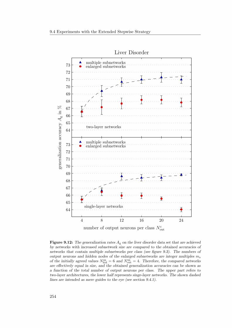
9.4 Experiments with the Extended Stepwise Strategy
PSfrag replacements
Liver Disorder
training set
test set
two-layer networks
single-layer networks
two-layer networksingle-layer network
multiple subnetworks
multiple subnetworks
enlarged subnetworks
enlarged subnetworks
classification accuracy in %
gener
aliz
atio
nac
cura
cyA
gin
%
mean absolute difference D in percentage pointsnumber of subnetworks per class N c
net
number of output neurons per class N cout
chip Achip Bchip C
simulation0
101
112
12
313
4
145
156
16
717
8
189
19
20
50215122522353
24
5425552656275728582959304031413242334334443545364637473848394960
70
70
61
71
71
62
72
72
63
73
73
64
64
74
65
65
75
66
66
76
67
67
77
68
68
78
69
69
798090819182928393849485958696879788988999
100500
1000150020002500300035004000450050005500
0.51.52.53.54.55.56.57.58.59.5
96.25
96.5
96.75
Figure 9.12: The generalization rates Ag on the liver disorder data set that are achievedby networks with increased subnetwork size are compared to the obtained accuracies ofnetworks that contain multiple subnetworks per class (see figure 9.3). The numbers ofoutput neurons and hidden nodes of the enlarged subnetworks are integer multiples ms
of the initially agreed values N snhid = 6 and N sn
out = 4. Therefore, the compared networksare effectively equal in size, and the obtained generalization accuracies can be shown asa function of the total number of output neurons per class. The upper part refers totwo-layer architectures, the lower half represents singe-layer networks. The shown dashedlines are intended as mere guides to the eye (see section 9.4.1).
254
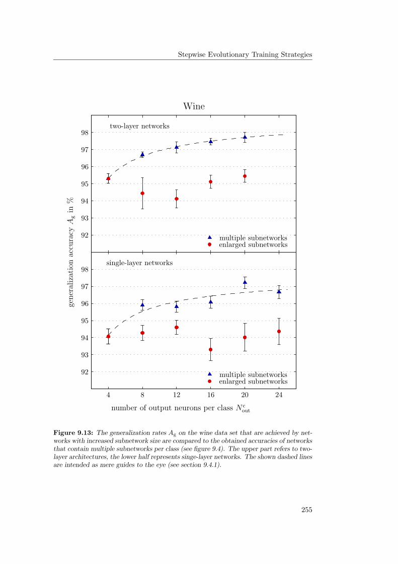
Stepwise Evolutionary Training Strategies
PSfrag replacements
Wine
training set
test set
two-layer networks
single-layer networks
two-layer networksingle-layer network
multiple subnetworks
multiple subnetworks
enlarged subnetworks
enlarged subnetworks
classification accuracy in %
gener
aliz
atio
nac
cura
cyA
gin
%
mean absolute difference D in percentage pointsnumber of subnetworks per class N c
net
number of output neurons per class N cout
chip Achip Bchip C
simulation0
101
112
12
313
4
145
156
16
717
8
189
19
20
50215122522353
24
5425552656275728582959304031413242334334443545364637473848394960706171627263736474657566766777687869798090819182
92
92
83
93
93
84
94
94
85
95
95
86
96
96
87
97
9788
98
98
8999
100500
1000150020002500300035004000450050005500
0.51.52.53.54.55.56.57.58.59.5
96.25
96.5
96.75
Figure 9.13: The generalization rates Ag on the wine data set that are achieved by net-works with increased subnetwork size are compared to the obtained accuracies of networksthat contain multiple subnetworks per class (see figure 9.4). The upper part refers to two-layer architectures, the lower half represents singe-layer networks. The shown dashed linesare intended as mere guides to the eye (see section 9.4.1).
255
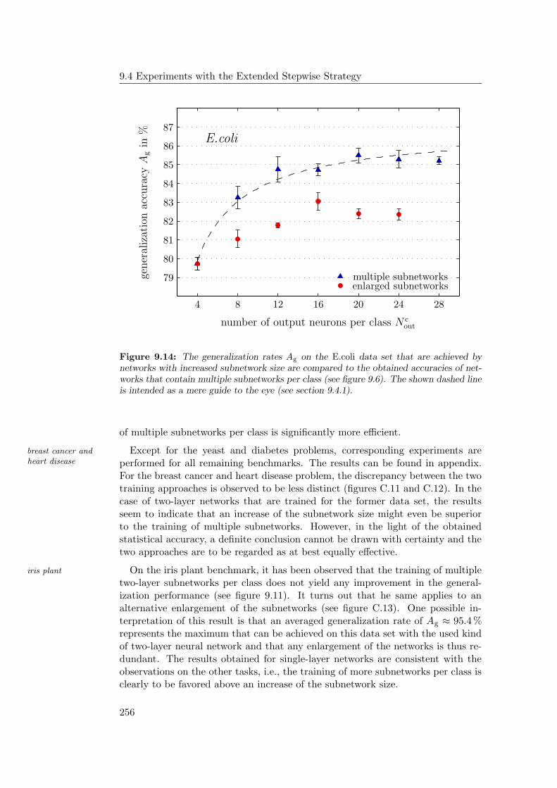
9.4 Experiments with the Extended Stepwise Strategy
PSfrag replacements
E.coli
training set
test settwo-layer networks
single-layer networkstwo-layer network
single-layer network
multiple subnetworksenlarged subnetworks
classification accuracy in %
gener
aliz
atio
nac
cura
cyA
gin
%
mean absolute difference D in percentage pointsnumber of subnetworks per class N c
net
number of output neurons per class N cout
chip Achip Bchip C
simulation0
101
112
12
313
4
145
156
16
717
8
189
19
20
50215122522353
24
54255526562757
28
582959304031413242334334443545364637473848394960706171627263736474657566766777687869
79
80
90
81
91
82
92
83
93
84
94
85
95
86
96
87
9788988999
100500
1000150020002500300035004000450050005500
0.51.52.53.54.55.56.57.58.59.5
96.25
96.5
96.75
Figure 9.14: The generalization rates Ag on the E.coli data set that are achieved bynetworks with increased subnetwork size are compared to the obtained accuracies of net-works that contain multiple subnetworks per class (see figure 9.6). The shown dashed lineis intended as a mere guide to the eye (see section 9.4.1).
of multiple subnetworks per class is significantly more efficient.
Except for the yeast and diabetes problems, corresponding experiments arebreast cancer andheart disease performed for all remaining benchmarks. The results can be found in appendix.
For the breast cancer and heart disease problem, the discrepancy between the twotraining approaches is observed to be less distinct (figures C.11 and C.12). In thecase of two-layer networks that are trained for the former data set, the resultsseem to indicate that an increase of the subnetwork size might even be superiorto the training of multiple subnetworks. However, in the light of the obtainedstatistical accuracy, a definite conclusion cannot be drawn with certainty and thetwo approaches are to be regarded as at best equally effective.
On the iris plant benchmark, it has been observed that the training of multipleiris plant
two-layer subnetworks per class does not yield any improvement in the general-ization performance (see figure 9.11). It turns out that he same applies to analternative enlargement of the subnetworks (see figure C.13). One possible in-terpretation of this result is that an averaged generalization rate of Ag ≈ 95.4 %represents the maximum that can be achieved on this data set with the used kindof two-layer neural network and that any enlargement of the networks is thus re-dundant. The results obtained for single-layer networks are consistent with theobservations on the other tasks, i.e., the training of more subnetworks per class isclearly to be favored above an increase of the subnetwork size.
256
Stepwise Evolutionary Training Strategies
9.5 The Stepwise Strategy: Conclusion
The presented strategy of independently optimizing and interconnecting multiple successful training
subnetworks for each class of the investigated categorization task is shown to be afeasible approach to successfully train large neural networks on the HAGEN ASICfor demanding real-world problems. Each of the single training phases can be ac-complished by a simple evolutionary algorithm that is itself well suited for hard-ware acceleration. The presented experiments demonstrate — for the first time —that networks on the HAGEN chip provide more than competitive means forsolving challenging classification benchmarks compared to software-implementedneural networks (see table 9.3).
It is shown that by increasing the number of subnetworks per category, the entire exploited resources
network can readily be scaled to the desired extent, limited only by the availableresources on the HAGEN ASIC. The hereby increased network size does not lead toa measurable overfitting of the data, i.e., the proposed stepwise training approachexhibits a favorable up-scaling behavior. Although an alternative increase of thesubnetwork size can yield an improvement of the network performance as well, itis observed to be clearly inferior to the training of multiple subnetworks per classon the majority of examined benchmarks.
Theoretical considerations suggest that a sufficient dissimilarity between the alternative black-boxapproachesindividual subnetworks of the same class constitutes a vital precondition for the
success of the generalized stepwise strategy. Apart from that, it is reasonable toexpect that other model-free chip-in-the-loop training algorithms can be employedfor the single training phases as well. In so far, the simulated annealing and weightperturbation algorithms which have been introduced in section 4.3 provide poten-tial alternatives to the evolutionary training approach. However, while simulatedannealing — similar to evolutionary optimization — is highly indeterministic andcan therefore be assumed to automatically promote a reasonable diversity, theweight-perturbation approach might not be able to yield a sufficient disagreementbetween the subnetworks that are trained for each class. A thorough examina-tion of alternative optimization algorithms exceeds the scope of this thesis and isdeferred to future investigations.
Having demonstrated the potential of the stepwise evolutionary training strat-egy in principle, several aspects remain to deserve further evaluation, e.g., howto efficiently exploit its inherent parallelism or in how far the performance of thefinal network can be optimized by appropriately adjusting the subnetwork size.These and some other topics will be investigated in the following chapter.
257

Chapter 10
Hardware Implications
The trouble with facts is that there are so many of them.
Samuel McChord Crothers, The Gentle Reader
There are several important aspects of the used hardware neural network frame-work in general (see chapter 6) and the introduced stepwise evolutionary trainingstrategy in particular (see chapter 9) that deserve further consideration but havenot yet been examined in detail. This final chapter is to provide a more thoroughdiscussion of these topics.
Most notably, the succeeding sections will discuss the training speed that can beachieved within the currently used neural network framework. It will be demon-strated that — as it has repeatedly been claimed in the foregoing chapter — theproposed stepwise strategy allows for an efficient parallelization of the trainingprocedure. Furthermore, it has already been discussed in section 5.5 that theutilization of calibrated HAGEN chips in principle allows to transfer the net-work configurations that have been trained for one ASIC also to other chips. Insection 10.2, it will be evaluated in how far this affects the performance of thetransferred networks.
The remaining sections of this chapter will present several preliminary investi-gations that are not as exhaustive as the other measurements and are primarilyintended to provide an outlook to future experiments: Section 10.3 examines howthe eventual success of the proposed stepwise strategy is affected by modificationsto the size and architecture of the single subnetworks (see sections 9.1.1 and 9.3.1).Section 10.4, finally, is concerned with software-implemented networks. It is in-vestigated whether the concepts of the stepwise approach might also be applicableto an ideal network that accurately obeys equation 5.4 and does not suffer fromthe inevitable device variations and temporal fluctuations that are present in theused HAGEN ASIC.
10.1 Training Speed and Parallelization
During evolutionary chip-in-the-loop training, the testing of individual networks parallelized networkevaluationon the used HAGEN ASIC and the evaluation of their fitness values on the basis of
259
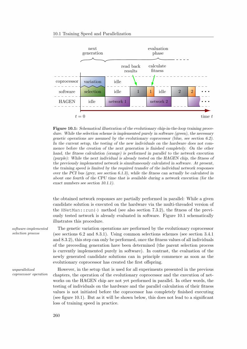
10.1 Training Speed and Parallelization
PSfrag replacements
timetraining set
test settwo-layer networks
single-layer networkstwo-layer network
single-layer networkmultiple subnetworksenlarged subnetworks
classification accuracy in %generalization accuracy Ag in %
mean absolute difference D in percentage pointsnumber of subnetworks per class N c
net
number of output neurons per class N cout
chip Achip Bchip C
simulation0
101
112
123
134
145
156
167
178
189
192050215122522353245425552656275728582959304031413242334334443545364637473848394960706171627263736474657566766777687869798090819182928393849485958696879788988999
100500
1000150020002500300035004000450050005500
0.51.52.53.54.55.56.57.58.59.5
96.25
96.5
96.75
nextgeneration
evaluationphase
evolutionary
coprocessor
software
HAGEN
idle
idleidle
idle
time tt = 0
evaluate
network 1 network 2
variation
selection 1 1 2 2
read backresults
calculatefitness
Figure 10.1: Schematical illustration of the evolutionary chip-in-the-loop training proce-dure. While the selection scheme is implemented purely in software (green), the necessarygenetic operations are assumed by the evolutionary coprocessor (blue, see section 6.2).In the current setup, the testing of the new individuals on the hardware does not com-mence before the creation of the next generation is finished completely. On the otherhand, the fitness calculation (orange) is performed in parallel to the network execution(purple): While the next individual is already tested on the HAGEN chip, the fitness ofthe previously implemented network is simultaneously calculated in software. At present,the training speed is limited by the required transfer of the individual network responsesover the PCI bus (grey, see section 6.1.3), while the fitness can actually be calculated inabout one fourth of the CPU time that is available during a network execution (for theexact numbers see section 10.1.1).
the obtained network responses are partially performed in parallel: While a givencandidate solution is executed on the hardware via the multi-threaded version ofthe HNetMan::run(·) method (see also section 7.3.2), the fitness of the previ-ously tested network is already evaluated in software. Figure 10.1 schematicallyillustrates this procedure.
The genetic variation operations are performed by the evolutionary coprocessorsoftware-implementedselection process (see sections 6.2 and 8.3.1). Using common selections schemes (see section 3.4.1
and 8.3.2), this step can only be performed, once the fitness values of all individualsof the preceeding generation have been determined (the parent selection processis currently implemented purely in software). In contrast, the evaluation of thenewly generated candidate solutions can in principle commence as soon as theevolutionary coprocessor has created the first offspring.
However, in the setup that is used for all experiments presented in the previousunparallelizedcoprocessor operation chapters, the operation of the evolutionary coprocessor and the execution of net-
works on the HAGEN chip are not yet performed in parallel. In other words, thetesting of individuals on the hardware and the parallel calculation of their fitnessvalues is not initiated before the coprocessor has completely finished executing(see figure 10.1). But as it will be shown below, this does not lead to a significantloss of training speed in practice.
260
Hardware Implications
10.1.1 Time Measurements
Within the present hardware framework, performing the fitness calculation in soft-ware requires to transfer the output data of each tested network from the localmemory of the FPGA to the RAM of the host PC over the PCI bus (see sec-tion 6.1.3 and compare figure 10.1). Being currently executed on a Pentium IVwith 2.4 GHz, the actual evaluation of the fitness can then be performed compa-rably fast. Considering the exemplary case of the liver disorder problem where liver disorder
a number of 1550 patterns needs to be processed by both, the tested networkand the fitness function, the latter requires 0.28 ± 0.01 ms, while the execution ofthe network on the hardware — including the transfer of the output data over thePCI bus — takes 2.04 ± 0.01 ms. If the time-consuming exchange of output databetween the memory of the FPGA and the host computer is omitted, this time isreduced to 1.26 ± 0.01ms1.
The reported numbers are obtained by measuring the amount of time that is measurementprocedurespent in the HNetMan::run(·) function and the fitness calculation method2 (see
section 7.4.1), respectively. The given values each represent the mean of 100measurements and the respective standard deviation. Similar to all previouslypresented experiments, the interface of the HAGEN chip is operated at a frequencyof 84 MHz (see section 6.1.3) and the network frequency fnet (see section 5.2) isthus determined to be 14 MHz [181] [185]. The first phase of the first stage of theproposed stepwise strategy is considered (see sections 9.1 and 9.2). The trainednetwork comprises N c
hid = 6 hidden units and N cout = 4 outputs.
It is to be noted that in the case of the HNetMan::run(·) method, the re- communicationoverheadported time does not only include the network operation on the hardware: Even
if the output data is not read back over the PCI bus, the measured value persiststo be increased by the remaining communication between the PC and the FPGAthat is necessary to synchronize their operation. Given the used base frequencyof 84 MHz and the processed number of patterns of 1550, the time that is ex-clusively spent for the actual execution of the network can be estimated to beapproximately 1.1 ms [181].
It remains that in the present state of the system, the calculation of the fitness remaining idle time
only occupies about one fourth of the time that effectively elapses until the resultsof the next network can be read back from the memory of the FPGA. Since thetimes for the fitness evaluation and the network execution each grow linearly withthe number of processed patterns, similar conditions are expected to apply alsoto the other investigated tasks (see below). This generally leads to a considerableamount of idle time for the CPU, and a strategy of how this time can be usedmore efficiently will be introduced in section 10.1.2.
1In the current setup, such a procedure is evidently not practical, since the fitness calculationcan in this case not yield reasonable results.
2For these measurements, the network execution and the fitness evaluation are performedsequentially and not in parallel. The standard built-in C-functionality for time measurements isused as it is provided by the ctime library.
261
10.1 Training Speed and Parallelization
Averaged Individual Processing Time
In order convey a general feeling for the speed of the current training setup, mea-experimental setup
surements are performed where the average overall processing time for one individ-ual network is estimated. This is done for all of the nine investigated benchmarks.Again, all networks contain N c
hid = 6 hidden units and N cout = 4 outputs, and the
effective number of adjustable genes within the genome merely varies accordingto the number of inputs required for the respective benchmarks. The processingof the genetic material is taken over by the evolutionary coprocessor. Apart fromthat, the evaluation time of each network depends on the respective number ofinput patterns that needs to be processed.
For each task, it is evaluated how much time is spent in one generation step of theaveraged processingtime per individual evolutionary algorithm, i.e., the time that elapses between the moment when the
HPopulation::newGeneration(·) function is invoked and the point when thesucceeding HPopulation::evaluate() method returns (compare figure 7.21and see sections 7.4.3, 7.4.4, and 7.4.5). Similar to the experiments presented inthe previous chapters, the population size is set to µ = 20 and the average timefor one individual is thus obtained by dividing the resulting numbers by 20. Themeasurements are repeated for a respective number of 1000 generations and thecorresponding average is taken as the final result.
According to the scheme depicted in figure 10.1, the fitness calculation is per-a complete iteration
formed in parallel to the network execution. Still, apart from the actual imple-mentation of the networks on the HAGEN ASIC, the operation of the evolution-ary coprocessor, and the necessary communication via the PCI bus (see above),the measured times also include the sorting of the population according to theindividuals’ fitness values, the selection process, the generation of the desired re-combination instructions for the coprocessor (see section 7.3.3), and the generalorganizational overhead for the parallelized execution of networks on the hardware(see section 7.3.2). The latter four parts are all implemented in software.
In so far, it is to be emphasized that the presented numbers do not claim to bean accurate estimate for the actual speed of the hardware itself. Rather, they areto serve as a practical measure for the speed of the training as it is experiencedby the user. A second set of measurement evaluates the time that is exclusivelycreating the new
generation spent in the HPopulation::newGeneration(·) method. These times remainto include the selection process, the generation of appropriate instructions for theevolutionary coprocessor in software, the transmission of these commands over thePCI bus, and the operation of the coprocessor itself. Again, the resulting numbersare normalized by the number of individuals in the population.
The obtained values are presented in figure 10.2. The results are given in mil-results
liseconds and are shown as a function of the number of processed patterns. Theoverall times per individual for one complete generation step are represented bycircular markers, the data points that correspond to only the creation of the nextpopulation are shown as squares.
The averaged overall time per individual shows the expected dependence on thelinear dependence
number of processed patterns: The times for both, the execution of the actualnetwork and the calculation of its fitness should grow linearly with the number
262
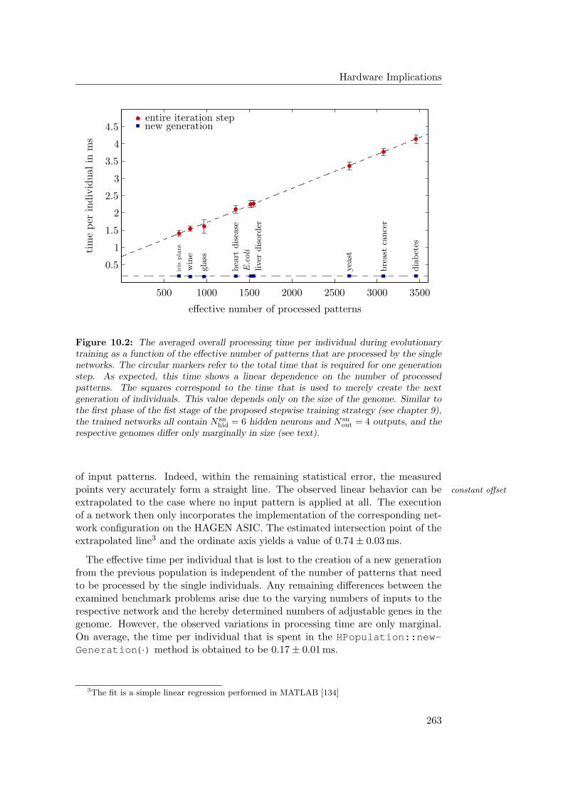
Hardware Implications
PSfrag replacements
timetraining set
test settwo-layer networks
single-layer networkstwo-layer network
single-layer networkmultiple subnetworksenlarged subnetworks
classification accuracy in %generalization accuracy Ag in %
mean absolute difference D in percentage pointsnumber of subnetworks per class N c
net
number of output neurons per class N cout
chip Achip Bchip C
simulation0
10
1
11
2
12
3
13
4
145
156
167
178
189
192050215122522353245425552656275728582959304031413242334334443545364637473848394960706171627263736474657566766777687869798090819182928393849485958696879788988999
100
500 1000 1500 2000 2500 3000 3500
4000450050005500
0.5
1.5
2.5
3.5
4.5
5.56.57.58.59.5
96.25
96.5
96.75
bre
ast
cance
r
dia
bet
es
hea
rtdis
ease
liver
dis
ord
er
iris
pla
nt
win
e
gla
ss
E.coli
yea
st
effective number of processed patterns
tim
eper
indiv
idual
inm
s
entire iteration stepnew generation
Figure 10.2: The averaged overall processing time per individual during evolutionarytraining as a function of the effective number of patterns that are processed by the singlenetworks. The circular markers refer to the total time that is required for one generationstep. As expected, this time shows a linear dependence on the number of processedpatterns. The squares correspond to the time that is used to merely create the nextgeneration of individuals. This value depends only on the size of the genome. Similar tothe first phase of the fist stage of the proposed stepwise training strategy (see chapter 9),the trained networks all contain N sn
hid = 6 hidden neurons and N snout = 4 outputs, and the
respective genomes differ only marginally in size (see text).
of input patterns. Indeed, within the remaining statistical error, the measuredpoints very accurately form a straight line. The observed linear behavior can be constant offset
extrapolated to the case where no input pattern is applied at all. The executionof a network then only incorporates the implementation of the corresponding net-work configuration on the HAGEN ASIC. The estimated intersection point of theextrapolated line3 and the ordinate axis yields a value of 0.74 ± 0.03 ms.
The effective time per individual that is lost to the creation of a new generationfrom the previous population is independent of the number of patterns that needto be processed by the single individuals. Any remaining differences between theexamined benchmark problems arise due to the varying numbers of inputs to therespective network and the hereby determined numbers of adjustable genes in thegenome. However, the observed variations in processing time are only marginal.On average, the time per individual that is spent in the HPopulation::new-Generation(·) method is obtained to be 0.17 ± 0.01 ms.
3The fit is a simple linear regression performed in MATLAB [134]
263
10.1 Training Speed and Parallelization
Outlook: Speeding up the Training
Especially for large problems it can be inferred from figure 10.2 that the trainingcurrent limitations
speed is presently limited by the the time that is required for the network execu-tion. But it is to be emphasized that while the evaluation time for each networkwill persist to grow linearly with the number of applied input patterns, the abso-lute value of the execution time as well as the slope of the observed linear increaseare specific to the currently used hardware environment which cannot in fact fullyexploit the potential of the HAGEN ASIC.
It has already been stated in section 6.3 that within the new NATHAN/Back-advanced setup
plane setup, the interface to the HAGEN chip can be operated at higher fre-quencies and no data transfer over the PCI bus is required during training. Assoon as this more advanced setup is fully operable, it will serve as the primaryplatform for future applications and training experiments. Regarding the lineardependence of the averaged overall processing time per individual on the numberof input patterns (see figure 10.2), both, its slope and its offset will then be consid-erably decreased. At the same time, given the frequency of the featured PowerPCmicroprocessor of only 350 MHz (see section 6.3.3), all parts of the iteration stepthat are implemented in software — most notably the fitness calculation and theselection process — will be slowed down significantly. Under these circumstances,the roles of the fitness calculation and the network execution are likely to beexchanged in so far as the former will require more time than the latter.
Finally, it is to be noted that the way in which incoming and outgoing data isfuture ASICs
managed within the HAGEN prototype leaves some room for improvement [178].Future neural network ASICs will provide additional functionality that will allowfor a more efficient, pipelined handling of input and output data directly on thechip. This is bound to speed up the execution of the networks even further.
At present, exact quantitative predictions for the eventual training speed offast algorithms
the NATHAN/Backplane setup are difficult [181] and do not actually fall intothe scope of this work. But as it has already been discussed in sections 6.2.6and 6.3.3, the above considerations remain to fuel the desire for simple evolutionaryalgorithms that can keep up pace with the used neural network ASICs and canpreferably benefit from hardware acceleration and/or parallelization themselves.
10.1.2 Parallelization of the Generalized Stepwise Strategy
During evolutionary training, the calculation of the former individual’s fitnessunexploited potential
value currently takes only about one fourth of the time that is required for thenext candidate network to finish executing on the hardware (see also section 10.1.1and compare figure 10.1). The remaining intermediate CPU time is bound to bewasted. It is true that due to the high degree of parallelism in the network oper-ation of the HAGEN prototype, the execution time for, e.g., a two-layer networkdoes not increase with a growing size of its single layers. This allows for a feasiblescaling to large networks. But for comparably small networks like those that aretrained during the single phases of the proposed stepwise strategy (see chapter 9)and which occupy merely a small fraction of the offered network resources each,
264
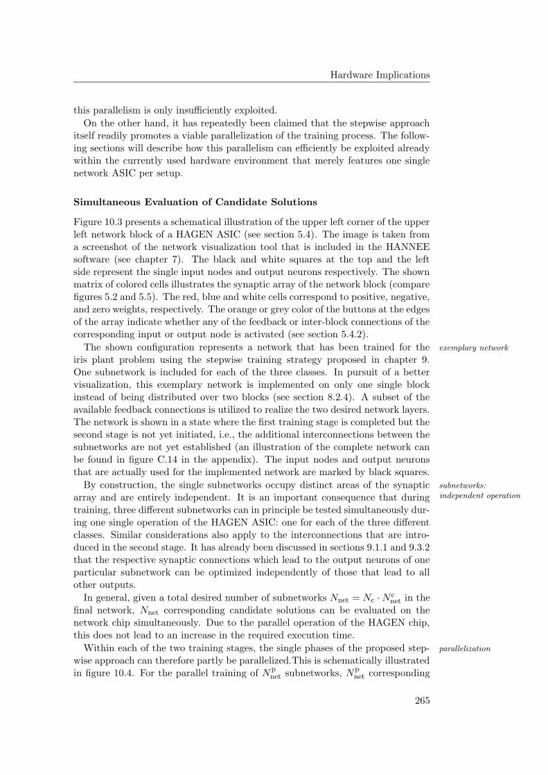
Hardware Implications
this parallelism is only insufficiently exploited.
On the other hand, it has repeatedly been claimed that the stepwise approachitself readily promotes a viable parallelization of the training process. The follow-ing sections will describe how this parallelism can efficiently be exploited alreadywithin the currently used hardware environment that merely features one singlenetwork ASIC per setup.
Simultaneous Evaluation of Candidate Solutions
Figure 10.3 presents a schematical illustration of the upper left corner of the upperleft network block of a HAGEN ASIC (see section 5.4). The image is taken froma screenshot of the network visualization tool that is included in the HANNEEsoftware (see chapter 7). The black and white squares at the top and the leftside represent the single input nodes and output neurons respectively. The shownmatrix of colored cells illustrates the synaptic array of the network block (comparefigures 5.2 and 5.5). The red, blue and white cells correspond to positive, negative,and zero weights, respectively. The orange or grey color of the buttons at the edgesof the array indicate whether any of the feedback or inter-block connections of thecorresponding input or output node is activated (see section 5.4.2).
The shown configuration represents a network that has been trained for the exemplary network
iris plant problem using the stepwise training strategy proposed in chapter 9.One subnetwork is included for each of the three classes. In pursuit of a bettervisualization, this exemplary network is implemented on only one single blockinstead of being distributed over two blocks (see section 8.2.4). A subset of theavailable feedback connections is utilized to realize the two desired network layers.The network is shown in a state where the first training stage is completed but thesecond stage is not yet initiated, i.e., the additional interconnections between thesubnetworks are not yet established (an illustration of the complete network canbe found in figure C.14 in the appendix). The input nodes and output neuronsthat are actually used for the implemented network are marked by black squares.
By construction, the single subnetworks occupy distinct areas of the synaptic subnetworks:independent operationarray and are entirely independent. It is an important consequence that during
training, three different subnetworks can in principle be tested simultaneously dur-ing one single operation of the HAGEN ASIC: one for each of the three differentclasses. Similar considerations also apply to the interconnections that are intro-duced in the second stage. It has already been discussed in sections 9.1.1 and 9.3.2that the respective synaptic connections which lead to the output neurons of oneparticular subnetwork can be optimized independently of those that lead to allother outputs.
In general, given a total desired number of subnetworks Nnet = Nc · N cnet in the
final network, Nnet corresponding candidate solutions can be evaluated on thenetwork chip simultaneously. Due to the parallel operation of the HAGEN chip,this does not lead to an increase in the required execution time.
Within each of the two training stages, the single phases of the proposed step- parallelization
wise approach can therefore partly be parallelized.This is schematically illustratedin figure 10.4. For the parallel training of Np
net subnetworks, Npnet corresponding
265
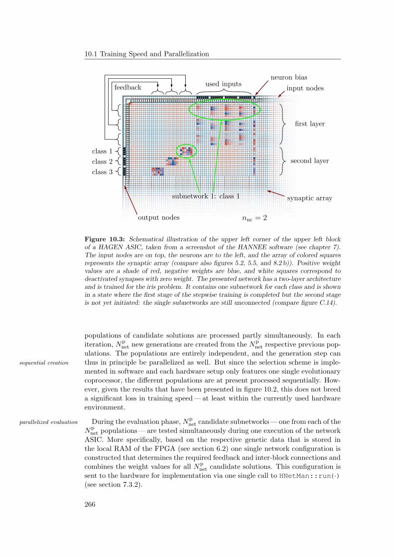
10.1 Training Speed and Parallelization
PSfrag replacements
timetraining set
test settwo-layer networks
single-layer networkstwo-layer network
single-layer networkmultiple subnetworksenlarged subnetworks
classification accuracy in %generalization accuracy Ag in %
mean absolute difference D in percentage pointsnumber of subnetworks per class N c
net
number of output neurons per class N cout
chip Achip Bchip C
simulation0
101
112
123
134
145
156
167
178
189
192050215122522353245425552656275728582959304031413242334334443545364637473848394960706171627263736474657566766777687869798090819182928393849485958696879788988999
100500
1000150020002500300035004000450050005500
0.51.52.53.54.55.56.57.58.59.5
96.25
96.5
96.75
used inputsneuron bias
input nodes
output nodes
first layer
second layer
feedback
upper left block
synaptic arraysubnetwork 1: class 1
class 1
class 2
class 3
nnc = 2
Figure 10.3: Schematical illustration of the upper left corner of the upper left blockof a HAGEN ASIC, taken from a screenshot of the HANNEE software (see chapter 7).The input nodes are on top, the neurons are to the left, and the array of colored squaresrepresents the synaptic array (compare also figures 5.2, 5.5, and 8.2 b)). Positive weightvalues are a shade of red, negative weights are blue, and white squares correspond todeactivated synapses with zero weight. The presented network has a two-layer architectureand is trained for the iris problem. It contains one subnetwork for each class and is shownin a state where the first stage of the stepwise training is completed but the second stageis not yet initiated: the single subnetworks are still unconnected (compare figure C.14).
populations of candidate solutions are processed partly simultaneously. In eachiteration, Np
net new generations are created from the Npnet respective previous pop-
ulations. The populations are entirely independent, and the generation step canthus in principle be parallelized as well. But since the selection scheme is imple-sequential creation
mented in software and each hardware setup only features one single evolutionarycoprocessor, the different populations are at present processed sequentially. How-ever, given the results that have been presented in figure 10.2, this does not breeda significant loss in training speed — at least within the currently used hardwareenvironment.
During the evaluation phase, Npnet candidate subnetworks — one from each of theparallelized evaluation
Npnet populations — are tested simultaneously during one execution of the network
ASIC. More specifically, based on the respective genetic data that is stored inthe local RAM of the FPGA (see section 6.2) one single network configuration isconstructed that determines the required feedback and inter-block connections andcombines the weight values for all Np
net candidate solutions. This configuration issent to the hardware for implementation via one single call to HNetMan::run(·)(see section 7.3.2).
266
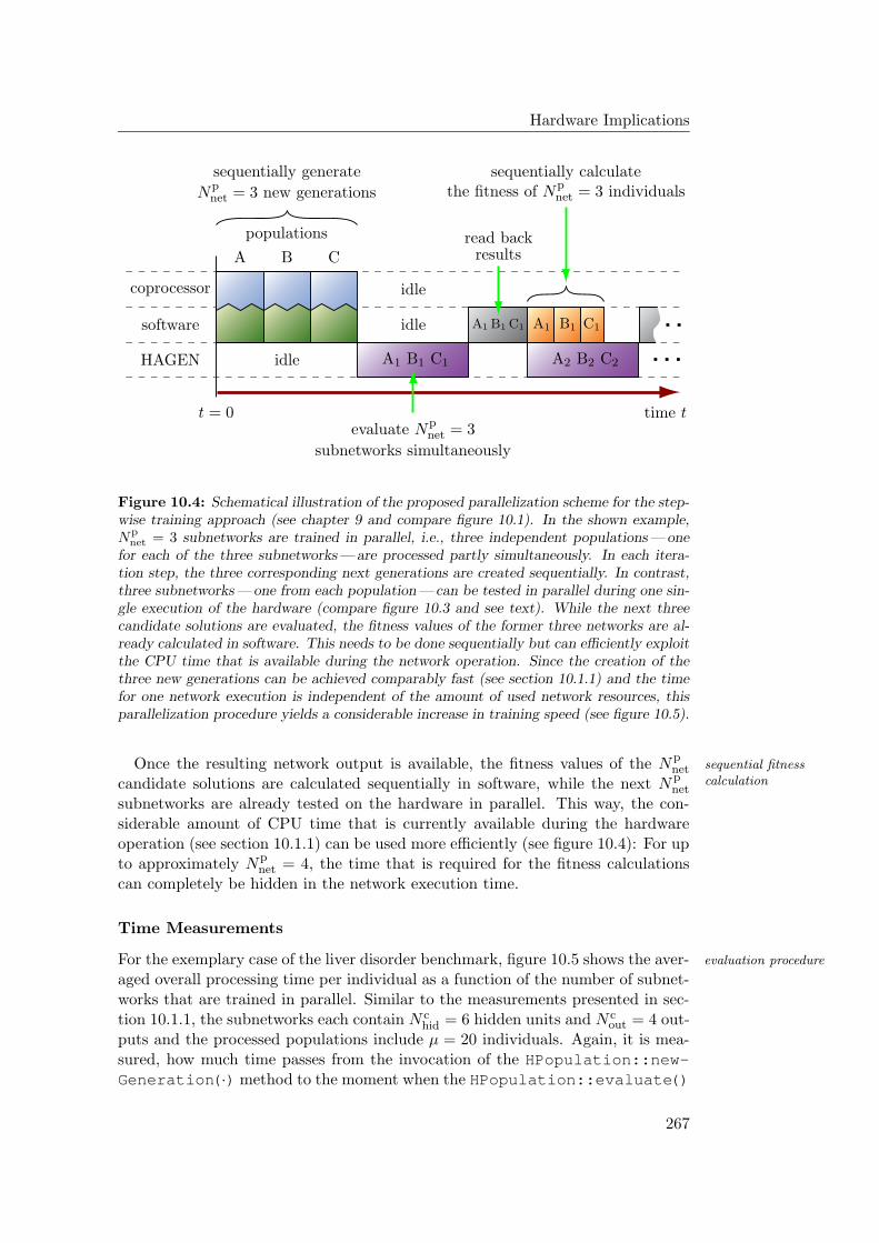
Hardware Implications
PSfrag replacements
timetraining set
test settwo-layer networks
single-layer networkstwo-layer network
single-layer networkmultiple subnetworksenlarged subnetworks
classification accuracy in %generalization accuracy Ag in %
mean absolute difference D in percentage pointsnumber of subnetworks per class N c
net
number of output neurons per class N cout
chip Achip Bchip C
simulation0
101
112
123
134
145
156
167
178
189
192050215122522353245425552656275728582959304031413242334334443545364637473848394960706171627263736474657566766777687869798090819182928393849485958696879788988999
100500
1000150020002500300035004000450050005500
0.51.52.53.54.55.56.57.58.59.5
96.25
96.5
96.75
next
sequentially generate
Npnet = 3 new generations
populations
A B C
idle
coprocessor
software
HAGEN
idle
idle
idle
time tt = 0evaluate Np
net = 3
subnetworks simultaneously
A1 B1 C1 A2 B2 C2
A1 B1 C1 A1 B1 C1
read backresults
sequentially calculatethe fitness of Np
net = 3 individuals
Figure 10.4: Schematical illustration of the proposed parallelization scheme for the step-wise training approach (see chapter 9 and compare figure 10.1). In the shown example,Np
net = 3 subnetworks are trained in parallel, i.e., three independent populations —onefor each of the three subnetworks —are processed partly simultaneously. In each itera-tion step, the three corresponding next generations are created sequentially. In contrast,three subnetworks —one from each population —can be tested in parallel during one sin-gle execution of the hardware (compare figure 10.3 and see text). While the next threecandidate solutions are evaluated, the fitness values of the former three networks are al-ready calculated in software. This needs to be done sequentially but can efficiently exploitthe CPU time that is available during the network operation. Since the creation of thethree new generations can be achieved comparably fast (see section 10.1.1) and the timefor one network execution is independent of the amount of used network resources, thisparallelization procedure yields a considerable increase in training speed (see figure 10.5).
Once the resulting network output is available, the fitness values of the N pnet sequential fitness
calculationcandidate solutions are calculated sequentially in software, while the next N pnet
subnetworks are already tested on the hardware in parallel. This way, the con-siderable amount of CPU time that is currently available during the hardwareoperation (see section 10.1.1) can be used more efficiently (see figure 10.4): For upto approximately Np
net = 4, the time that is required for the fitness calculationscan completely be hidden in the network execution time.
Time Measurements
For the exemplary case of the liver disorder benchmark, figure 10.5 shows the aver- evaluation procedure
aged overall processing time per individual as a function of the number of subnet-works that are trained in parallel. Similar to the measurements presented in sec-tion 10.1.1, the subnetworks each contain N c
hid = 6 hidden units and N cout = 4 out-
puts and the processed populations include µ = 20 individuals. Again, it is mea-sured, how much time passes from the invocation of the HPopulation::new-Generation(·) method to the moment when the HPopulation::evaluate()
267
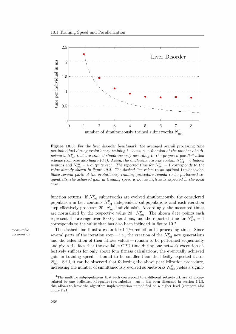
10.1 Training Speed and Parallelization
PSfrag replacements
Liver Disorder
training set
test settwo-layer networks
single-layer networkstwo-layer network
single-layer networkmultiple subnetworksenlarged subnetworks
classification accuracy in %generalization accuracy Ag in %
mean absolute difference D in percentage pointsnumber of subnetworks per class N c
net
number of output neurons per class N cout
chip Achip Bchip C
simulation
00
10
1
1
11
2
2
12
3
13
4
14
5
15
6
16
7
17
8
189
192050215122522353245425552656275728582959304031413242334334443545364637473848394960706171627263736474657566766777687869798090819182928393849485958696879788988999
100500
1000150020002500300035004000450050005500
0.5
1.5
2.5
3.54.55.56.57.58.59.5
96.25
96.5
96.75
number of simultaneously trained subnetworks Npnet
tim
eper
indiv
idual
inm
s
Figure 10.5: For the liver disorder benchmark, the averaged overall processing timeper individual during evolutionary training is shown as a function of the number of sub-networks Np
net that are trained simultaneously according to the proposed parallelizationscheme (compare also figure 10.4). Again, the single subnetworks contain N sn
hid = 6 hiddenneurons and N sn
out = 4 outputs each. The reported time for Npnet = 1 corresponds to the
value already shown in figure 10.2. The dashed line refers to an optimal 1/n-behavior.Since several parts of the evolutionary training procedure remain to be performed se-quentially, the achieved gain in training speed is not as high as is expected in the idealcase.
function returns. If Npnet subnetworks are evolved simultaneously, the considered
population in fact contains Npnet independent subpopulations and each iteration
step effectively processes 20 · Npnet individuals4. Accordingly, the measured times
are normalized by the respective value 20 · Npnet. The shown data points each
represent the average over 1000 generations, and the reported time for N pnet = 1
corresponds to the value that has also been included in figure 10.2.
The dashed line illustrates an ideal 1/n-reduction in processing time. Sincemeasurableacceleration several parts of the iteration step — i.e., the creation of the N p
net new generationsand the calculation of their fitness values — remain to be performed sequentiallyand given the fact that the available CPU time during one network execution ef-fectively suffices for only about four fitness calculations, the eventually achievedgain in training speed is bound to be smaller than the ideally expected factorNp
net. Still, it can be observed that following the above parallelization procedure,increasing the number of simultaneously evolved subnetworks N p
net yields a signifi-
4The multiple subpopulations that each correspond to a different subnetwork are all encap-sulated by one dedicated HPopulation subclass. As it has been discussed in section 7.4.5,this allows to leave the algorithm implementation unmodified on a higher level (compare alsofigure 7.21).
268
Hardware Implications
cant reduction in the effective processing time that is on average required for eachindividual. For Np
net = 6, the training time is reduced by approximately a factorof 3. Training more than 6 subnetworks in parallel only yields minor improvementsin training speed.
Parallelization in Practice
Leaving hardware limitations aside, the maximum number of subnetworks that remaining limitations
can actually be trained simultaneously is ultimately limited by the given num-ber of classes in the examined categorization problem times the desired numberof subnetworks per class. Apart from that, it is understood that the proposedscheme does not exploit the inherent parallelism of the stepwise training strategyto the fullest possible extent: Several parts of the iteration step remain to be per-formed sequentially that could in principle be parallelized as well. But on the otherhand, the presented measurements do not only provide a first demonstration forthe claim that the stepwise training approach is indeed suited for a parallel imple-mentation, the proposed scheme can also readily be employed within the currentlyused hardware setup. In fact, the exhaustive investigations presented in the fore-going chapter have successfully utilized the proposed parallelized implementationof the training process.
For future investigations, it is planned to also perform the execution of the evolu- parallelization infuture setupstionary coprocessor in parallel to the evaluation of networks on the HAGEN ASIC.
With regard to the upcoming NATHAN/Backplane framework (see section 6.3),the faster operational speed of the network hardware and the reduced performanceof the featured PowerPC microprocessor will render the proposed parallelizationscheme infeasible, since the fitness calculation will under these conditions mostlikely take longer than the actual network execution (see also section 6.3.3). Onthe other hand, the advanced hardware setup will allow to efficiently benefit fromthe parallel nature of the stepwise training strategy by distributing both, the fi-nal networks5 and the simultaneous training of multiple subnetworks over severalNATHAN boards (see also section 6.3.3).
10.2 Network Transferability
It is one of the important advantages of chip-in-the-loop training that it can substrate deficiencies
automatically cope with the potential deficiencies and peculiarities of the usedhardware neural network substrate (see section 2.4.5). Beyond that, it has beendiscussed in section 5.5 that the device variations which affect the network op-eration on the HAGEN prototype can to a large extend be compensated for byan appropriate calibration. During the experiments presented in the preceedingsections, the used HAGEN chips have always been operated in calibrated modesuch that the single neuron offsets and the row-specific averages of the individualsynapse offsets are accounted for (see sections 5.5.1 and 5.5.4). Under these con-ditions, it remains the primary task of the evolutionary training algorithm to deal
5It has already been discussed in section 9.4.2 that at least for single-layer architectures, thetrained networks can be distributed over an arbitrary number of blocks without restrictions.
269
10.2 Network Transferability
with the single static synapse offsets and to appropriately adjust the individualweights as to best exploit the dynamic ranges of the neurons and synapses (seealso section 5.4.3).
Given the allowed maximum postsynaptic current Imaxps = 22 µA (section 5.4.3)network transfer
that is used for all presented experiments, the magnitudes of the individual synapseoffsets are in the order of only 1 % of the total weight range (see also section 5.5.3).In so far — as it has already been discussed in section 5.5.4— any network config-urations that are obtained during the training of networks on one HAGEN ASICshould to some extent also be usable on other HAGEN chips. It is not expected,however, that the transfer of a network configuration to another chip will yieldexactly the same performance as on the original ASIC it has been trained on.Therefore, it is worthwhile to investigate if and in how far the performance of anetwork configuration that has been trained with the generalized stepwise strat-egy deteriorates once it is being loaded into a chip that it has not originally beenoptimized for.
10.2.1 Transfer Experiments
For the liver disorder, wine and E.coli benchmarks, the different network configu-rations that have been obtained during the experiments presented in the preceed-ing chapter are each transferred to two different HAGEN ASICs. This is done forall investigated numbers of networks per class N c
net and for both, single-layer andtwo-layer networks.
In this context, it is to be repeated that the classification accuracies on theabsolute differences
training and test sets At and Ag reported in the preceeding chapters each representthe respective average over a total of 50 different networks — five for each of theten stratified random partitionings of the data into training and test set (seesection 8.1.2). Based on the original accuracies ar
t and arg of a specific network
configuration that has been trained on the rth partitioning and given the respectivevalues ar
t and arg that are obtained on the same training and test data once this
very network is implemented on another chip, consider the absolute differences
drt =|ar
t − art | (10.1)
drg =|ar
g − arg | . (10.2)
Since drt and dr
g quantify the respective difference in the fraction of correctlyclassified training and test patterns, they are given in percentage points. Af-ter measuring these quantities for all of the ten networks that have originally beenaveraged results
considered for one single 10-fold cross-validation, the resulting values are aver-aged to yield the mean differences dt and dg. This is repeated for each of the fiveperformed repetitions of the cross-validation measurement (see section 8.1.2), andthe achieved values are averaged once more to yield the final results Dt and Dg
together with the corresponding standard errors of the mean ∆Dt and ∆Dg.The outcome of this measurement for the liver disorder benchmark is presentedliver disorder
in figure 10.6. The networks are originally trained on the HAGEN ASIC denotedas “chip A” and are once transferred to “chip B” (left plot) and once to “chip C”(right plot). The three chips are operated in calibrated mode, work at the same
270
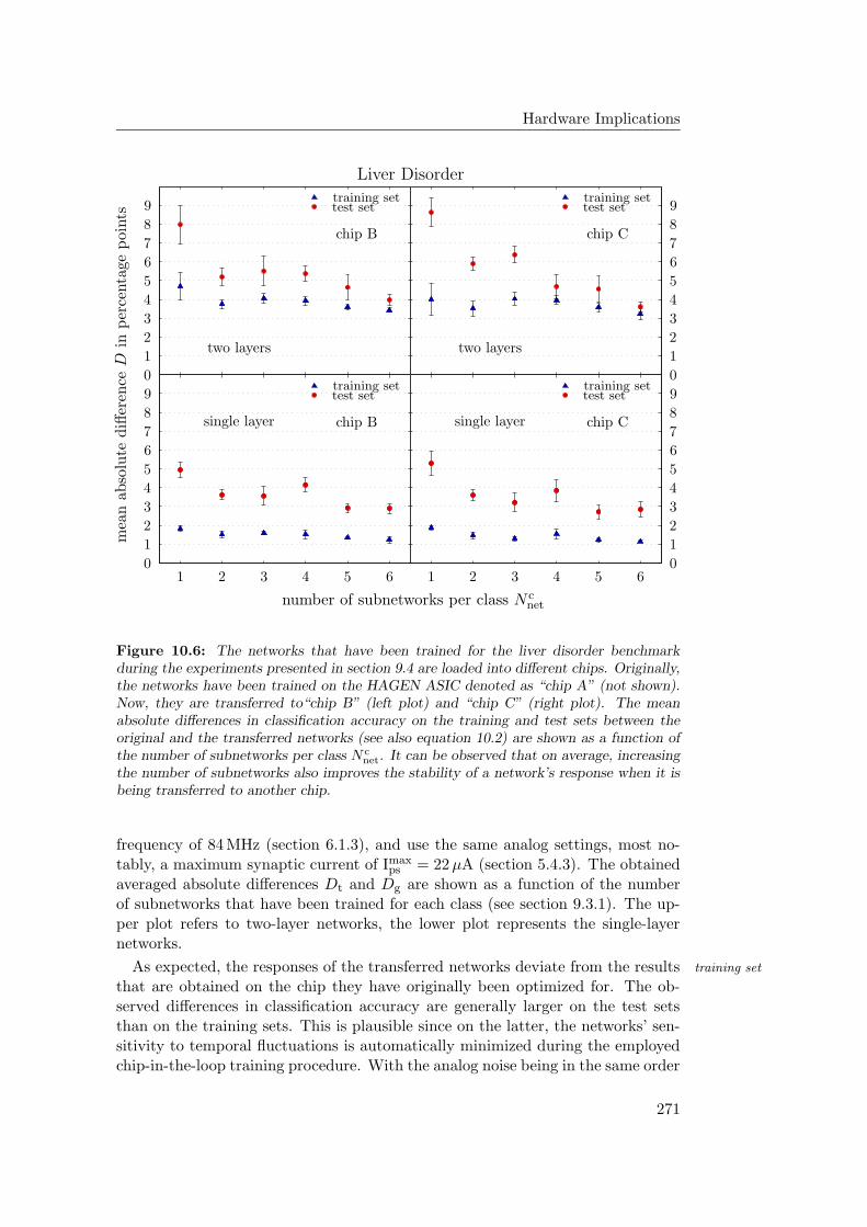
Hardware Implications
PSfrag replacements
Liver Disorder
training set
training set
training set
training set
test set
test set
test set
test set
two layerstwo layers
single layersingle layer
mea
nab
solu
tediff
eren
ceD
inper
centa
gepoi
nts
number of subnetworks per class N cnet
chip A
chip B
chip B
chip C
chip C
simulation
0
0
10
1
1
11
2
2
12
3
3
13
4
4
14
5
5
15
6
6
16
7
7
17
8
8
18
9
9
19
0
10
11
11
22
12
33
13
44
14
55
15
66
16
7
17
8
18
9
19
0
0
10
1
1
11
2
212
3
3
13
4
4
14
5
5
15 6
6
16
7
7
17
8
8
18
9
9
19
Figure 10.6: The networks that have been trained for the liver disorder benchmarkduring the experiments presented in section 9.4 are loaded into different chips. Originally,the networks have been trained on the HAGEN ASIC denoted as “chip A” (not shown).Now, they are transferred to“chip B” (left plot) and “chip C” (right plot). The meanabsolute differences in classification accuracy on the training and test sets between theoriginal and the transferred networks (see also equation 10.2) are shown as a function ofthe number of subnetworks per class N c
net. It can be observed that on average, increasingthe number of subnetworks also improves the stability of a network’s response when it isbeing transferred to another chip.
frequency of 84 MHz (section 6.1.3), and use the same analog settings, most no-tably, a maximum synaptic current of Imax
ps = 22 µA (section 5.4.3). The obtainedaveraged absolute differences Dt and Dg are shown as a function of the numberof subnetworks that have been trained for each class (see section 9.3.1). The up-per plot refers to two-layer networks, the lower plot represents the single-layernetworks.
As expected, the responses of the transferred networks deviate from the results training set
that are obtained on the chip they have originally been optimized for. The ob-served differences in classification accuracy are generally larger on the test setsthan on the training sets. This is plausible since on the latter, the networks’ sen-sitivity to temporal fluctuations is automatically minimized during the employedchip-in-the-loop training procedure. With the analog noise being in the same order
271
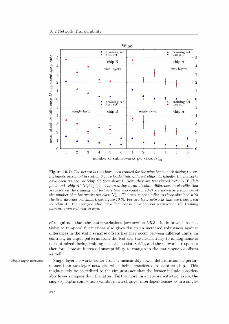
10.2 Network Transferability
PSfrag replacements
Wine
training set
training set
training set
training set
test set
test set
test set
test set
two layerstwo layers
single layersingle layer
mea
nab
solu
tediff
eren
ceD
inper
centa
gepoi
nts
number of subnetworks per class N cnet
chip A
chip A
chip B
chip B
chip C
simulation
0
0
10
1
1
11
2
2
12
3
3
13
4
4
14
5
5
15
6
16
7
17
8
18
9
19
0
10
11
11
22
12
33
13
44
14
55
15
66
16
7
17
8
18
9
19
0
0
10
1
1
11
2
212
3
3
13
4
4
14 5
5
15
6
16
7
17
8
18
9
19
Figure 10.7: The networks that have been trained for the wine benchmark during the ex-periments presented in section 9.4 are loaded into different chips. Originally, the networkshave been trained on “chip C” (not shown). Now, they are transferred to“chip B” (leftplot) and “chip A” (right plot). The resulting mean absolute differences in classificationaccuracy on the training and test sets (see also equation 10.2) are shown as a function ofthe number of subnetworks per class N c
net. The results are similar to those obtained withthe liver disorder benchmark (see figure 10.6). For two-layer networks that are transferredto “chip A”, the averaged absolute differences in classification accuracy on the trainingdata are even reduced to zero.
of magnitude than the static variations (see section 5.5.3) the improved insensi-tivity to temporal fluctuations also gives rise to an increased robustness againstdifferences in the static synapse offsets like they occur between different chips. Incontrast, for input patterns from the test set, the insensitivity to analog noise isnot optimized during training (see also section 8.4.1), and the networks’ responsestherefore show an increased susceptibility to changes in the static synapse offsetsas well.
Single-layer networks suffer from a measurably lower deterioration in perfor-single-layer networks
mance than two-layer networks when being transferred to another chip. Thismight partly be accredited to the circumstance that the former include consider-ably fewer synapses than the latter. Furthermore, in a network with two layers, thesingle synaptic connections exhibit much stronger interdependencies as in a single-
272
Hardware Implications
layer network. Due to the highly nonlinear behavior of the employed thresholdneurons, only small variations of the weights in the input layer can lead to signifi-cant changes in the responses of the hidden nodes and are thus likely to cause evenlarger deviations in the final output of the second layer. Finally, it can be inferredfrom figure 9.3 that single-layer networks generally perform worse on this task thantwo-layer networks in the first place. With a linear partitioning of the input spaceobviously not being the appropriate separation to reliably differentiate betweenthe two classes, it is reasonable to assume that multiple linear partitionings existwhich yield approximately the same — suboptimal — classification performance.In so far, it seems plausible that the eventual classification accuracies of networkswith only one layer are less sensitive to perturbations of the single weight valuesthan those of two-layer networks.
Apart from that, it is an important observation that with an increasing number multiple subnetworks:improved stabilityof subnetworks per class, the averaged absolute difference in accuracy on the test
set Dg is significantly reduced. This also applies to the difference in performanceDt that is obtained on the training data but here, the effect is not as distinct.
Similar results are obtained with the wine and E.coli data sets, as it is shown in wine and E.coli
figures 10.7 and 10.8. The networks for these two benchmarks have been trained on“chip C” and are transferred to both, “chip A” and “chip B”. Compared to the liverdisorder data set, the initial differences between the original and the transferrednetworks are smaller, and the observed decrease in Dt is more pronounced. In thecase of the wine data set, the average difference in performance on the trainingdata observed for two-layer networks that are transferred to “chip A” is evenreduced to zero.
Initially, it could have been expected that with an increasing size, the networks’ possible explanation
susceptibility to variations in the static offsets becomes more severe, since a largernumber of mutually dependent synaptic weights is affected. But it can be inferredfrom the presented measurements that the redundancy that results from the train-ing of multiple subnetworks per class actually gives rise to an improved stability ofthe final networks once they are confronted with the peculiarities of another chipthan the one they have been trained on. It might be a possible explanation forthis phenomenon that the deviations which occur when a network is transferredto a different chip promote an improved diversity among the single subnetworksthat are dedicated to the same class. It has been argued in section 9.3.2 that anincreased dissimilarity between the members of a network ensemble yields a betterperformance of the whole committee. It is reasonable to assume that this bene-ficial effect can at least partly compensate for the perturbations that inevitablyoccur when the network is transfered to another HAGEN ASIC.
The results that are achieved on the E.coli data set reveal that the stability of saturation behavior
the final networks is not improved any further when more than approximately 5subnetworks per class are trained (see figure 10.8). This can be seen in analogyto the saturation behavior of the generalization accuracy that has already beenobserved during the actual training of an increasing number of subnetworks perclass (compare figure 9.6).
For N cnet > 5, the difference in accuracy on the training data even seems to in- remaining differences
crease again, but given the estimated statistical uncertainty, a definite conclusion
273
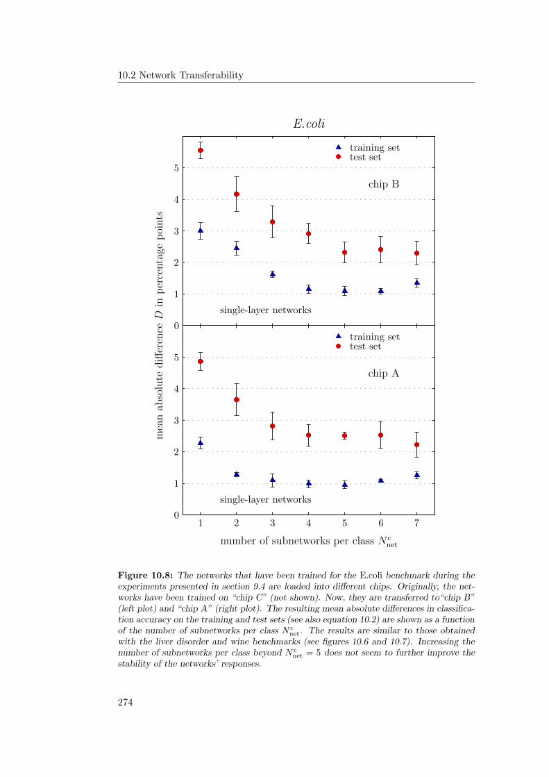
10.2 Network Transferability
PSfrag replacements
E.coli
training set
training set
test set
test set
two-layer networks
single-layer networks
single-layer networks
two-layer networksingle-layer network
multiple subnetworksenlarged subnetworks
classification accuracy in %generalization accuracy Ag in %
mea
nab
solu
tediff
eren
ceD
inper
centa
gepoi
nts
number of subnetworks per class N cnet
number of output neurons per class N cout
chip A
chip B
chip C
simulation
0
0
10
1
1
1
11
2
2
2
12
3
3
3
13
4
4
4
14
5
5
5
15
6
16
7
178
189
192050215122522353245425552656275728582959304031413242334334443545364637473848394960706171627263736474657566766777687869798090819182928393849485958696879788988999
100500
1000150020002500300035004000450050005500
0.51.52.53.54.55.56.57.58.59.5
96.25
96.5
96.75
Figure 10.8: The networks that have been trained for the E.coli benchmark during theexperiments presented in section 9.4 are loaded into different chips. Originally, the net-works have been trained on “chip C” (not shown). Now, they are transferred to“chip B”(left plot) and “chip A” (right plot). The resulting mean absolute differences in classifica-tion accuracy on the training and test sets (see also equation 10.2) are shown as a functionof the number of subnetworks per class N c
net. The results are similar to those obtainedwith the liver disorder and wine benchmarks (see figures 10.6 and 10.7). Increasing thenumber of subnetworks per class beyond N c
net = 5 does not seem to further improve thestability of the networks’ responses.
274
Hardware Implications
cannot be drawn. Still, the measurements suggest that the differences in perfor-mance between the original and the transferred networks are not reduced to zerowhen more subnetworks per class are trained. It is to be expected that a givenminimum deviation will remain.
Having hitherto considered only the absolute values of the observed deviations(see equation 10.2), it is to be noted that especially on the test data, the finalclassification accuracy of a transferred network can in some cases actually be betterthan the performance of the respective original. In practice, however, this effectcannot directly be exploited since the behavior of a network under chip transferis effectively unpredictable. In so far, the mean absolute differences Dt and Dg
persist to be the adequate measures for evaluating the stability of a network.
10.2.2 Discussion and Further Improvements
Regarding the measurements for each of the three benchmarks, the results that are different ASICs
achieved on the two different respective target chips are very similar. It can thusreasonably be assumed that the obtained results are of general validity and arenot caused by specific peculiarities of any of the three involved HAGEN ASICs.
It is a satisfying observation that apart from producing networks with compet- improved stability
itive generalization accuracies on realistic problems (see table 9.3), the proposedstepwise training strategy also promotes an improved stability of the final networksonce they are being transferred to different chips. But it persists that the individ-ual characteristics of the used ASICs remain to lead to measurable deviations inthe network response. The perturbative effects that occur when a network con-figuration is loaded into another chip are not actually compensated for. Rather,their negative impact on the network’s eventual classification accuracy is reduced.
Some promising approaches to further improve the network transferability have further improvement
been discussed in section 5.5.4. Most notably, it is expected that the originalperformance of a transferred network can be reproduced by a short and cautiousretraining. However, corresponding investigations are beyond the scope of thiswork and have to be deferred to further investigations.
10.3 Outlook: Coping with Chip Limitations
The limited size of the single network blocks on the HAGEN prototype (see sec- current limitations
tion 5.4.1) as well as the fixed set of available, hard-wired feedback and inter-blockconnections (section 5.4.2) remain to impose certain restrictions on the size andarchitecture of the realizable networks. It has already been discussed in sec-tion 9.4.2 that in the case of the generalized stepwise strategy, this eventuallydefines an upper limit to the number of subnetworks that can be trained for eachclass. Single-layer networks are not as severely affected by these restrictions ashomogeneously connected two-layer architectures since they do not require anyfeedback connections and can thus more easily be distributed over multiple net-work blocks.
275
10.3 Outlook: Coping with Chip Limitations
Having observed that an increased number of subnetworks per class is generallysmaller subnetworks
expected to lead to an improvement in the final network’s performance (see sec-tion 9.4) and given the result that an alternative increase in the subnetwork size isnot equally beneficial (section 9.4.6), it suggests itself to investigate the feasibilityof smaller subnetworks that in turn allow for a larger number of subnetworks perclass to simultaneously fit on one HAGEN chip. Although it is actually regardedas a favorable feature of the proposed generalized stepwise training strategy thatnetworks with competitive performance can be produced even without any adjust-ment of the subnetwork size, the pragmatically chosen numbers of N c
hid = 6 hiddenneurons and/or N c
out = 4 outputs per subnetwork are not necessarily optimal.
There is another limitation of the HAGEN prototype that arises from the fixedlimited number ofinputs number of 128 inputs to each block. For classification problems with large numbers
of input attributes, the resulting lengths of the binary input strings sα mightexceed the number of available input nodes. In such cases, it will be required todistribute the input layer over several network blocks. For a given neuron, it willthus no longer be possible to directly be connected to all inputs.
As it has been stated in section 5.4.1, potential future network ASICs can partlydistributed inputlayers overcome these restrictions by featuring more and/or larger network blocks. The
employed circuit designs should allow for about 1000 input nodes per neuron, andthe maximum number of outputs is solely limited by the desired size of the en-tire ASIC. Still, aiming for an application of the implemented networks to dataintensive problems with high-dimensional input spaces — like, e.g., image pro-cessing tasks — the available number of inputs might nevertheless turn out to beinsufficient. In so far, it is worthwhile to examine whether partially connectedarchitectures, where the single neurons are not equally connected to all inputs,can retain a satisfying performance.
The following sections will present a set of initial measurements that aim toilluminate these questions. However, the reported experiments do not claim tobe exhaustive. Rather, they intend to provide a first estimation of how an opti-mization of the subnetwork size or a distribution of the input nodes over multiplenetwork blocks affect the performance of the final networks. As such, these mea-surements primarily serve as a basis for future investigations that are to addressthese topics more systematically.
10.3.1 Varied Subnetwork Size
For the liver disorder benchmark, two additional sets of experiments are performedvaried subnetworksize where the numbers N sn
hid and N snout of hidden neurons and outputs per subnetwork
are modified compared to the setup that is used for the experiments presented inthe foregoing chapter. For the first campaign of measurements, each subnetworkcontains only N sn
hid = 3 hidden nodes but persists to include N snout = 4 outputs. In
the second case, both, the numbers of hidden units and outputs are reduced andare set to N sn
hid = 3 and N snout = 2, respectively. The former set of measurements
shall in the following be denoted as experiment M (medium) and the latter willbe referred to as experiment S (small).
276
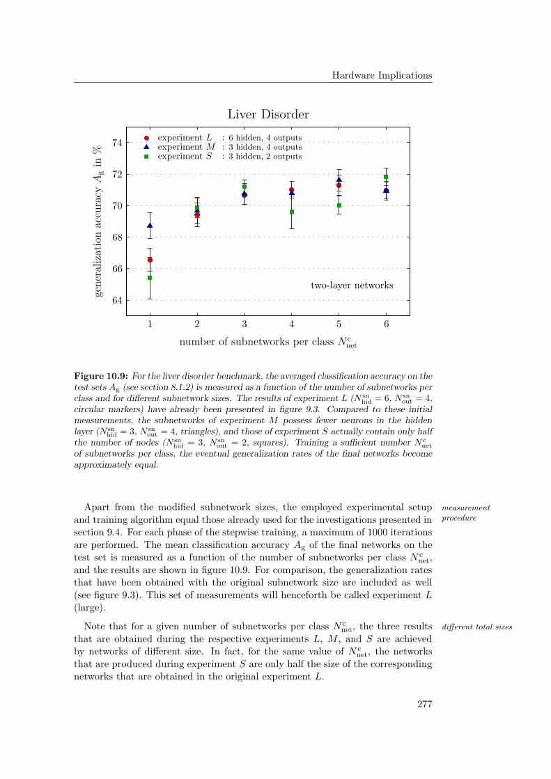
Hardware Implications
PSfrag replacements
Liver Disorder
training set
test set
two-layer networks
single-layer networkstwo-layer network
single-layer networkmultiple subnetworksenlarged subnetworks
classification accuracy in %
gener
aliz
atio
nac
cura
cyA
gin
%
mean absolute difference D in percentage points
number of subnetworks per class N cnet
number of output neurons per class N cout
chip Achip Bchip C
simulation0
10
1
11
2
12
3
13
4
14
5
15
6
167
178
189
192050215122522353245425552656275728582959304031413242334334443545364637473848394960
70
617162
72
6373
64
74
6575
66
766777
68
7869798090819182928393849485958696879788988999
100500
1000150020002500300035004000450050005500
0.51.52.53.54.55.56.57.58.59.5
96.25
96.5
96.75classification accuracy At in %
experiment L : 6 hidden, 4 outputsexperiment M : 3 hidden, 4 outputsexperiment S : 3 hidden, 2 outputs
Figure 10.9: For the liver disorder benchmark, the averaged classification accuracy on thetest sets Ag (see section 8.1.2) is measured as a function of the number of subnetworks perclass and for different subnetwork sizes. The results of experiment L (N sn
hid = 6, N snout = 4,
circular markers) have already been presented in figure 9.3. Compared to these initialmeasurements, the subnetworks of experiment M possess fewer neurons in the hiddenlayer (N sn
hid = 3, N snout = 4, triangles), and those of experiment S actually contain only half
the number of nodes (N snhid = 3, N sn
out = 2, squares). Training a sufficient number N cnet
of subnetworks per class, the eventual generalization rates of the final networks becomeapproximately equal.
Apart from the modified subnetwork sizes, the employed experimental setup measurementprocedureand training algorithm equal those already used for the investigations presented in
section 9.4. For each phase of the stepwise training, a maximum of 1000 iterationsare performed. The mean classification accuracy Ag of the final networks on thetest set is measured as a function of the number of subnetworks per class N c
net,and the results are shown in figure 10.9. For comparison, the generalization ratesthat have been obtained with the original subnetwork size are included as well(see figure 9.3). This set of measurements will henceforth be called experiment L(large).
Note that for a given number of subnetworks per class N cnet, the three results different total sizes
that are obtained during the respective experiments L, M , and S are achievedby networks of different size. In fact, for the same value of N c
net, the networksthat are produced during experiment S are only half the size of the correspondingnetworks that are obtained in the original experiment L.
277
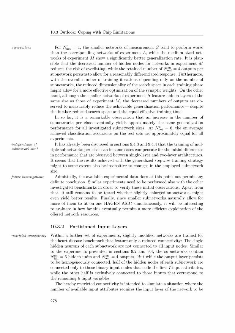
10.3 Outlook: Coping with Chip Limitations
For N cnet = 1, the smaller networks of measurement S tend to perform worseobservations
than the corresponding networks of experiment L, while the medium sized net-works of experiment M show a significantly better generalization rate. It is plau-sible that the decreased number of hidden nodes for networks in experiment Mreduces the risk of overfitting, while the retained number of N sn
out = 4 outputs persubnetwork persists to allow for a reasonably differentiated response. Furthermore,with the overall number of training iterations depending only on the number ofsubnetworks, the reduced dimensionality of the search space in each training phasemight allow for a more effective optimization of the synaptic weights. On the otherhand, although the smaller networks of experiment S feature hidden layers of thesame size as those of experiment M , the decreased numbers of outputs are ob-served to measurably reduce the achievable generalization performance— despitethe further reduced search space and the equal effective training time.
In so far, it is a remarkable observation that an increase in the number ofsubnetworks per class eventually yields approximately the same generalizationperformance for all investigated subnetwork sizes. At N c
net = 6, the on averageachieved classification accuracies on the test sets are approximately equal for allexperiments.
It has already been discussed in sections 9.4.3 and 9.4.4 that the training of mul-independence ofsubnetwork size? tiple subnetworks per class can in some cases compensate for the initial differences
in performance that are observed between single-layer and two-layer architectures.It seems that the results achieved with the generalized stepwise training strategymight to some extent also be insensitive to changes in the employed subnetworksize.
Admittedly, the available experimental data does at this point not permit anyfuture investigations
definite conclusion. Similar experiments need to be performed also with the otherinvestigated benchmarks in order to verify these initial observations. Apart fromthat, it still remains to be tested whether slightly enlarged subnetworks mighteven yield better results. Finally, since smaller subnetworks naturally allow formore of them to fit on one HAGEN ASIC simultaneously, it will be interestingto evaluate in how far this eventually permits a more efficient exploitation of theoffered network resources.
10.3.2 Partitioned Input Layers
Within a further set of experiments, slightly modified networks are trained forrestricted connectivity
the heart disease benchmark that feature only a reduced connectivity: The singlehidden neurons of each subnetwork are not connected to all input nodes. Similarto the experiments presented in sections 9.2 and 9.4, the subnetworks containN sn
hid = 6 hidden units and N snout = 4 outputs. But while the output layer persists
to be homogeneously connected, half of the hidden nodes of each subnetwork areconnected only to those binary input nodes that code the first 7 input attributes,while the other half is exclusively connected to those inputs that correspond tothe remaining 6 input variables.
The hereby restricted connectivity is intended to simulate a situation where thenumber of available input attributes requires the input layer of the network to be
278
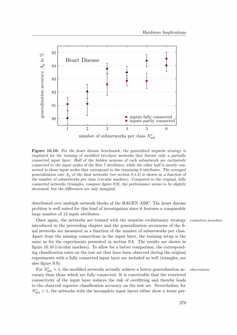
Hardware Implications
PSfrag replacements
Heart Disease
training set
test settwo-layer networks
single-layer networkstwo-layer network
single-layer networkmultiple subnetworksenlarged subnetworks
classification accuracy in %
gener
aliz
atio
nac
cura
cyA
gin
%
mean absolute difference D in percentage points
number of subnetworks per class N cnet
number of output neurons per class N cout
chip Achip Bchip C
simulation0
10
1
11
2
12
3
13
4
14
5
15
6
167
178
189
19205021512252235324542555265627572858295930403141324233433444354536463747384839496070617162726373647465756676677768786979
80
90
81
91
82
92
83
93
84
94
85
958696879788988999
100500
1000150020002500300035004000450050005500
0.51.52.53.54.55.56.57.58.59.5
96.25
96.5
96.75
inputs fully connectedinputs partly connected
Figure 10.10: For the heart disease benchmark, the generalized stepwise strategy isemployed for the training of modified two-layer networks that feature only a partiallyconnected input layer: Half of the hidden neurons of each subnetwork are exclusivelyconnected to the input nodes of the first 7 attributes, while the other half is merely con-nected to those input nodes that correspond to the remaining 6 attributes. The averagedgeneralization rate Ag of the final networks (see section 8.1.2) is shown as a function ofthe number of subnetworks per class (circular markers). Compared to the original, fullyconnected networks (triangles, compare figure 9.9), the performance seems to be slightlydecreased, but the differences are only marginal.
distributed over multiple network blocks of the HAGEN ASIC. The heart diseaseproblem is well suited for this kind of investigation since it features a comparablylarge number of 13 input attributes.
Once again, the networks are trained with the stepwise evolutionary strategy evaluation procedure
introduced in the preceeding chapter and the generalization accuracies of the fi-nal networks are measured as a function of the number of subnetworks per class.Apart from the missing connections in the input layer, the training setup is thesame as for the experiments presented in section 9.4. The results are shown infigure 10.10 (circular markers). To allow for a better comparison, the correspond-ing classification rates on the test set that have been observed during the originalexperiments with a fully connected input layer are included as well (triangles, seealso figure 9.9).
For N cnet = 1, the modified networks actually achieve a better generalization ac- observations
curacy than those which are fully connected. It is conceivable that the restrictedconnectivity of the input layer reduces the risk of overfitting and thereby leadsto the observed superior classification accuracy on the test set. Nevertheless, forN c
net > 1, the networks with the incomplete input layers either show a worse per-
279
10.4 Outlook: Software Simulations
formance than their homogeneously connected pendants or the respective valuesare approximately equal within the estimated error.
All in all, the results seem to suggest that a reduced connectivity of the first layermarginaldeterioration indeed tends to slightly decrease the achievable performance of the final networks
on this task. Still, given that the remaining statistical uncertainty ultimatelyimpedes a clear decision, it is important to note that any potential deteriorationin generalization accuracy is evidently only marginal. Furthermore, it can beinferred from figure 10.10 that even if the input layers needed to be distributedover several blocks, the hereby restricted networks would persist to measurablybenefit from an independent training of multiple subnetworks per class.
Having investigated only a single exemplary benchmark problem, it cannot bepredicted with certainty in how far these observations hold also for other classifi-cation tasks. But in the light of the presented measurements, it is reasonable toassume that the restricted number of input nodes of the featured network blocksdoes not necessarily prevent the HAGEN chip from being successfully applicableto problems with high-dimensional input spaces. Ultimately, this question willhave to be clarified by future experiments.
10.4 Outlook: Software Simulations
The numerous networks that have been trained during all hitherto presented ex-periments are each optimized for the specific HAGEN ASIC they have been trainedon. The particular deficiencies and peculiarities of the used chip are partly com-pensated for by the calibration procedure described in section 5.5.4, and the re-maining deviations from the ideal network model (see section 5.2) are dealt with bythe used chip-in-the-loop training algorithm. It has already been investigated insection 10.2, in how far this procedure allows for a viable transfer of the resultingnetwork configurations to other calibrated HAGEN chips.
Apart from the static device variations and the present analog noise, the op-hardware networks insoftware eration of the implemented network obeys equation 5.4. This in principle allows
to use the obtained configurations also for software simulations of the utilizednetwork model. Like in the case of a transfer from chip to chip, a simulation insoftware is not assumed to entirely preserve the network’s performance, but theobservations of section 10.2 are expected to hold also in this scenario.
Furthermore, the applicability of the proposed stepwise training strategy is not atraining softwarenetworks priori restricted to hardware implementations. It is true that the usage of multiple
subnetworks per class naturally leads to larger networks. Software simulationsthat usually persist to be implemented on ordinary sequential computers rathercall for preferably small systems, but this does not inhibit the utilization of thegeneralized stepwise approach for training in principle. On the other hand, it isconceivable that the demonstrated success of this strategy actually relies on thecharacteristics of the used hardware substrate. The inherent static variations andtemporal fluctuations might promote the diversity of the multiple subnetworksthat are trained for each class (see also sections 9.3.2 and 10.2.1). Finally, it willsoftware networks in
hardware be interesting to evaluate the performance of network configurations that have
280
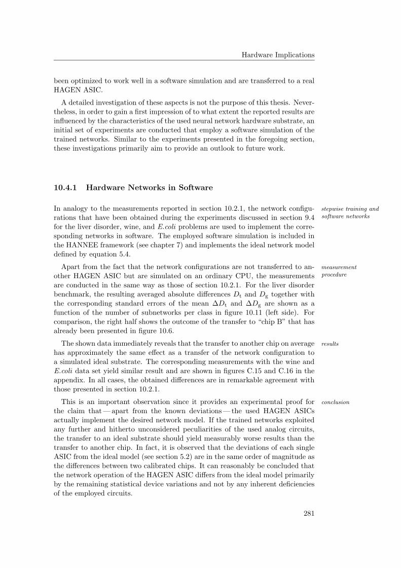
Hardware Implications
been optimized to work well in a software simulation and are transferred to a realHAGEN ASIC.
A detailed investigation of these aspects is not the purpose of this thesis. Never-theless, in order to gain a first impression of to what extent the reported results areinfluenced by the characteristics of the used neural network hardware substrate, aninitial set of experiments are conducted that employ a software simulation of thetrained networks. Similar to the experiments presented in the foregoing section,these investigations primarily aim to provide an outlook to future work.
10.4.1 Hardware Networks in Software
In analogy to the measurements reported in section 10.2.1, the network configu- stepwise training andsoftware networksrations that have been obtained during the experiments discussed in section 9.4
for the liver disorder, wine, and E.coli problems are used to implement the corre-sponding networks in software. The employed software simulation is included inthe HANNEE framework (see chapter 7) and implements the ideal network modeldefined by equation 5.4.
Apart from the fact that the network configurations are not transferred to an- measurementprocedureother HAGEN ASIC but are simulated on an ordinary CPU, the measurements
are conducted in the same way as those of section 10.2.1. For the liver disorderbenchmark, the resulting averaged absolute differences Dt and Dg together withthe corresponding standard errors of the mean ∆Dt and ∆Dg are shown as afunction of the number of subnetworks per class in figure 10.11 (left side). Forcomparison, the right half shows the outcome of the transfer to “chip B” that hasalready been presented in figure 10.6.
The shown data immediately reveals that the transfer to another chip on average results
has approximately the same effect as a transfer of the network configuration toa simulated ideal substrate. The corresponding measurements with the wine andE.coli data set yield similar result and are shown in figures C.15 and C.16 in theappendix. In all cases, the obtained differences are in remarkable agreement withthose presented in section 10.2.1.
This is an important observation since it provides an experimental proof for conclusion
the claim that — apart from the known deviations — the used HAGEN ASICsactually implement the desired network model. If the trained networks exploitedany further and hitherto unconsidered peculiarities of the used analog circuits,the transfer to an ideal substrate should yield measurably worse results than thetransfer to another chip. In fact, it is observed that the deviations of each singleASIC from the ideal model (see section 5.2) are in the same order of magnitude asthe differences between two calibrated chips. It can reasonably be concluded thatthe network operation of the HAGEN ASIC differs from the ideal model primarilyby the remaining statistical device variations and not by any inherent deficienciesof the employed circuits.
281
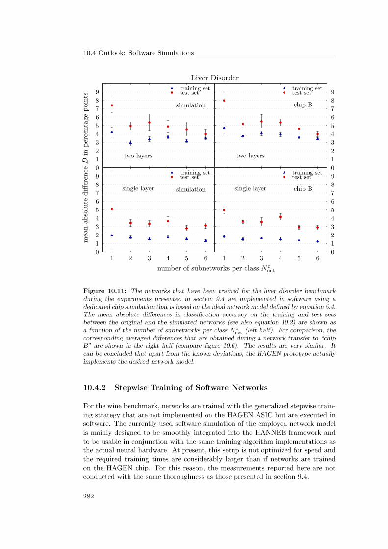
10.4 Outlook: Software Simulations
PSfrag replacements
Liver Disorder
training set
training set
training set
training set
test set
test set
test set
test set
two layerstwo layers
single layersingle layer
mea
nab
solu
tediff
eren
ceD
inper
centa
gepoi
nts
number of subnetworks per class N cnet
chip A
chip B
chip B
chip C
simulation
simulation
0
0
10
1
1
11
2
2
12
3
3
13
4
4
14
5
5
15
6
6
16
7
7
17
8
8
18
9
9
19
0
10
11
11
22
12
33
13
44
14
55
15
66
16
7
17
8
18
9
19
0
0
10
1
1
11
2
212
3
3
13
4
4
14
5
5
15 6
6
16
7
7
17
8
8
18
9
9
19
Figure 10.11: The networks that have been trained for the liver disorder benchmarkduring the experiments presented in section 9.4 are implemented in software using adedicated chip simulation that is based on the ideal network model defined by equation 5.4.The mean absolute differences in classification accuracy on the training and test setsbetween the original and the simulated networks (see also equation 10.2) are shown asa function of the number of subnetworks per class N c
net (left half). For comparison, thecorresponding averaged differences that are obtained during a network transfer to “chipB” are shown in the right half (compare figure 10.6). The results are very similar. Itcan be concluded that apart from the known deviations, the HAGEN prototype actuallyimplements the desired network model.
10.4.2 Stepwise Training of Software Networks
For the wine benchmark, networks are trained with the generalized stepwise train-ing strategy that are not implemented on the HAGEN ASIC but are executed insoftware. The currently used software simulation of the employed network modelis mainly designed to be smoothly integrated into the HANNEE framework andto be usable in conjunction with the same training algorithm implementations asthe actual neural hardware. At present, this setup is not optimized for speed andthe required training times are considerably larger than if networks are trainedon the HAGEN chip. For this reason, the measurements reported here are notconducted with the same thoroughness as those presented in section 9.4.
282
Hardware Implications
PSfrag replacements
Wine
training set
test settwo-layer networks
single-layer networkstwo-layer network
single-layer networkmultiple subnetworksenlarged subnetworks
classification accuracy in %generalization accuracy Ag in %
mean absolute difference D in percentage points
number of subnetworks per class N cnet
number of output neurons per class N cout
chip Achip Bchip C
simulation0
10
1
11
2
12
3
13
4
145
156
167
178
189
192050215122522353245425552656275728582959304031413242334334443545364637473848394960706171627263736474657566766777687869798090819182
92
83
93
84
94
85
95
86
96
87
97
88
98
89
99
100500
1000150020002500300035004000450050005500
0.51.52.53.54.55.56.57.58.59.5
96.25
96.5
96.75 gener
aliz
atio
nra
tea
g(A
g)
in%
chip Csimulation
Figure 10.12: The generalized stepwise strategy is employed for the training of networksfor the wine problem that are purely implemented in software. For each number of sub-networks per class N c
net, a single 10-fold cross-validation (see section 8.1.2) is performedand the resulting averaged accuracy on the test sets ag is shown (circular markers). Forcomparison, the mean generalization rates Ag that have been obtained during the corre-sponding measurements with hardware implemented networks (see section 9) are presentedas well (triangles, compare figure 9.4).
Most of the parameters of the training setup equal those already used for the measurement setup
original investigations of chapter 9 (see tables 8.3 and 9.1). The networks exhibita two-layer architecture and contain N sn
hid = 6 hidden nodes and N snout = 4 outputs
per subnetwork. However, the following modifications to the experimental proce-dure are made: Since the software simulation is deterministic and does not sufferfrom any analog noise, each training pattern is only processed once by each net-work in each iteration. The same applies to the evaluation of the final network’sclassification performance on the training and test sets. To further reduce theexpenditure of time, only a single 10-fold cross-validation is performed for eachmeasurement, and the maximum number of training iterations in each phase ofthe stepwise training procedure is reduced to 500.
Figure 10.12 shows the obtained averaged classification accuracy on the testset ag as a function of the number of subnetworks that are trained per class.The standard error of the mean that is on average obtained on the 10 networksthat are trained for each of the 10 partitionings (see section 8.1.2) is in the orderof ±1 % (corresponding error bars are included in figure 10.12). Although it is estimated uncertainty
understood that this quantity is not the adequate error measure to be consultedfor a comparison between the shown data points (see section 8.1.2), it is expectedto provide a realistic upper limit to the remaining statistical uncertainty that willbe observed when multiple cross-validations are performed. For comparison, the
283
10.4 Outlook: Software Simulations
corresponding accuracies Ag that have been obtained during the experiments ofsection 9.4 (see figure 9.4) are included in figure 10.12 as well.
For N cnet = 1, the software simulation performs measurably worse than the net-comparison
works that are implemented on the hardware. Given the used setup, this mightpartly be accredited to the reduced training times. But it is also conceivable thatsince the temporal fluctuations within the HAGEN chip and the resulting noisynetwork response might yield a smoother fitness measure (see also section 8.3.3),the evolutionary training algorithm could optimize networks on the hardware moreefficiently. In so far, the present analog noise might even be beneficial for the even-tual training success. Still, the available experimental data does not yet suffice tosupport this conclusion, and further measurements will be necessary to illuminatethis interesting question.
Apart from that, it can be observed that training multiple subnetworks per classimprovinggeneralization also improves the performance of software-implemented networks. For a number
of 3 subnetworks per class, the simulated networks even seem to achieve a betterperformance than those on the HAGEN ASIC. Due to the limited amount of dataand the remaining uncertainty, this result should not be over-interpreted. Still,the shown data suggests that with growing N c
net, the simulated networks mightbecome at least as good as the networks that are trained on the hardware.
It is a satisfying observation that the concepts of the proposed stepwise trainingstrategy seem to be readily transferable to ideal, software-implemented networksof threshold neurons as well. Although it can reasonably be assumed that theseobservations will hold also for the other benchmark problems, this will ultimatelyhave to be confirmed by additional experiments.
10.4.3 Software Networks in Hardware
Within a final set of measurements, the software networks that are trained forevaluation procedure
the wine problem during the investigations discussed in the preceeding section areloaded into the HAGEN ASIC formerly denoted as “chip B” to be implemented inhardware. The observed differences in performance between the original softwarenetworks and their hardware implemented pendants are evaluated according to theprocedure described in section 10.2.1. But since only one 10-fold cross-validationis performed for each value of N c
net, no final averaging over multiple repetitions isdone.
The resulting averaged absolute differences dt and dg are shown in figure 10.13.observations
With only the networks of one cross-validation measurement being considered, noerror measures can be provided that are reasonably comparable to those includedin figure 10.7 (see also section 8.1.2). It is expected that a repetition of the cross-validation will reveal statistical fluctuations in the same order of magnitude asthose obtained during the previously presented experiments. In comparison to theresults that have been presented in sections 10.2.1 and 10.4.1 (see also figure C.15),it can be observed that training a network for the ideal substrate and transferringit to a real HAGEN chip on average yields approximately the same difference inperformance as it is obtained in the inverse case or when networks are transferredbetween different ASICs. Again, this can be seen as to support the claim that
284
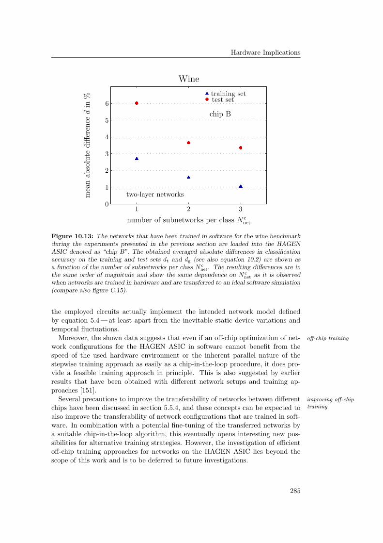
Hardware Implications
PSfrag replacements
Wine
training settest set
two-layer networks
single-layer networkstwo-layer network
single-layer networkmultiple subnetworksenlarged subnetworks
classification accuracy in %generalization accuracy Ag in %
mean absolute difference D in percentage points
number of subnetworks per class N cnet
number of output neurons per class N cout
chip A
chip B
chip C
simulation
0
10
1
1
11
2
2
12
3
3
13
4
14
5
15
6
167
178
189
192050215122522353245425552656275728582959304031413242334334443545364637473848394960706171627263736474657566766777687869798090819182928393849485958696879788988999
100500
1000150020002500300035004000450050005500
0.51.52.53.54.55.56.57.58.59.5
96.25
96.5
96.75
mea
nab
solu
tediff
eren
ced
in%
Figure 10.13: The networks that have been trained in software for the wine benchmarkduring the experiments presented in the previous section are loaded into the HAGENASIC denoted as “chip B”. The obtained averaged absolute differences in classificationaccuracy on the training and test sets dt and dg (see also equation 10.2) are shown asa function of the number of subnetworks per class N c
net. The resulting differences are inthe same order of magnitude and show the same dependence on N c
net as it is observedwhen networks are trained in hardware and are transferred to an ideal software simulation(compare also figure C.15).
the employed circuits actually implement the intended network model definedby equation 5.4 — at least apart from the inevitable static device variations andtemporal fluctuations.
Moreover, the shown data suggests that even if an off-chip optimization of net- off-chip training
work configurations for the HAGEN ASIC in software cannot benefit from thespeed of the used hardware environment or the inherent parallel nature of thestepwise training approach as easily as a chip-in-the-loop procedure, it does pro-vide a feasible training approach in principle. This is also suggested by earlierresults that have been obtained with different network setups and training ap-proaches [151].
Several precautions to improve the transferability of networks between different improving off-chiptrainingchips have been discussed in section 5.5.4, and these concepts can be expected to
also improve the transferability of network configurations that are trained in soft-ware. In combination with a potential fine-tuning of the transferred networks bya suitable chip-in-the-loop algorithm, this eventually opens interesting new pos-sibilities for alternative training strategies. However, the investigation of efficientoff-chip training approaches for networks on the HAGEN ASIC lies beyond thescope of this work and is to be deferred to future investigations.
285

Summary and Outlook
You cannot depend on your eyes whenyour imagination is out of focus.
Mark Twain
The HAGEN neural network ASIC provides flexible means for the implementation the HAGEN chip
of fast and massively parallel neural networks with in the order of 104 synapsesin a low power, mixed-signal hardware. By confining the analog operation toblocks with an entirely digital interface, the employed network model allows fora feasible up-scaling to even larger networks. On the other hand, the binarynature of the neurons in combination with the inevitable analog noise that remainsto affect the operation of the network impede a direct application of traditionalgradient-based training algorithms. Chip-in-the-loop training approaches can notonly automatically cope with these peculiarities of the HAGEN chip, but can alsomake best use of its high reconfigurational speed and fast operation.
Within this thesis, it has been investigated in how far evolutionary chip-in-the- classificationbenchmarksloop algorithms can successfully be applied to the training of neural networks on
the HAGEN ASIC for demanding classification tasks. To this end, the performanceof the examined evolutionary strategies has been tested on a set of nine well-knownclassification benchmarks: the breast cancer, diabetes, heart disease, liver disorder,iris plant, wine, glass, E.coli, and yeast problems.
In order to efficiently train neural networks on the HAGEN chip, the evolu- evolutionarycoprocessortionary algorithm itself needs to be realized in a way such that it can keep up
with the speed of the networks. The used hardware environment features a ded-icated evolutionary coprocessor that is implemented within a configurable logicand accelerates evolutionary algorithms by performing the time-consuming ge-netic operations in hardware. In its current version, the coprocessor persists toimpose certain restrictions on the complexity of the used genetic representationand the applied variation operators. At present, only direct encoding schemes aresupported and the architecture of the trained networks needs to be fixed duringtraining. In general, to be suited for use within the introduced hardware environ-ment, the training algorithm is preferably kept simple and should rather aim toefficiently benefit from parallelization.
Experiments have been presented that examine a simple evolutionary algorithm the simpleevolutionary approachthat utilizes the evolutionary coprocessor for the genetic operations. While this
algorithm allows for a fast implementation and therefore ideally suits the used
287
Summary and Outlook
hardware neural network framework, it turns out to be not capable of training net-works on the HAGEN ASIC to achieve a satisfactory performance on the selectedclassification benchmarks. This particularly applies to problems that include morethan two classes.
Therefore, a stepwise training strategy has been developed that divides thethe stepwise trainingstrategy original task of training one large network for the entire categorization problem
into the separate optimization of multiple, smaller subnetworks that each addressonly a part of the whole task: Each of the subnetworks is trained to differentiatethe members of only one specific class against all remaining instances. Usinga two-layer architecture, it is a notable feature of this strategy that additionalinterconnections between the single subnetworks can be introduced and optimizedwithin a second training stage. This can be done separately for all subnetworks.As an important consequence, the single training steps of the whole procedurecan be performed in parallel. Furthermore, it has been verified experimentallythat each of the independent training phases can successfully be accomplished bysimple and fast evolutionary algorithms that benefit from the functionality of theevolutionary coprocessor.
It is straight forward to generalize the proposed stepwise strategy to incorpo-multiple subnetworksper class rate the training of multiple subnetworks for the same class instead of one. An
exhaustive campaign of measurements has been conducted that evaluates in howfar an increased number of subnetworks per category improves the classificationperformance of the final networks. This has been done for all investigated bench-marks and for both, single-layer and two-layer networks. The results reveal thatthe use of multiple subnetworks per class never leads to a decrease of the achievedclassification rate.
For all considered tasks — except for the breast cancer and iris plant problems —improved accuracy
an increased number of subnetworks has been observed to lead to a significantimprovement of the network performance. In the case of the breast cancer dataset, the achieved gain in generalization accuracy does not exceed the estimatedstatistical uncertainty and for the iris data set, a measurable improvement hasonly been obtained with single-layer networks.
Apart from that, single-layer and two-layer networks have been shown to equallysingle-layer networks
benefit from an enlarged number of subnetworks. For the heart disease and irisplant benchmarks, it has even been observed that any initial differences in per-formance between the two architectures tend to vanish once a sufficient numberof subnetworks is trained. It is an important aspect of the proposed generalizedstepwise strategy that it allows for an efficient application of simple single-layernetworks to challenging classification tasks. Single-layer architectures can moreeasily be scaled to fully exploit the resources of the currently used HAGEN pro-totype than two-layer networks.
For the breast cancer, diabetes, heart disease, and glass benchmarks, the finallycomparison toprevious results obtained generalization rates have been compared with the accuracies of software-
implemented networks that have previously been reported by other authors. It isa satisfying observation that in comparison to these results, the networks on theHAGEN ASIC show a more than competitive performance (see table 9.3). Theachieved generalization rates have been shown to be even comparable to those of
288
Summary and Outlook
common neural network ensemble approaches (see table 9.5). Although for each ofthe nine investigated task, a better classifier— not necessarily a neural network —can eventually be found in literature (see tables 9.4 and 9.5), networks on theHAGEN ASIC that are being trained by the introduced stepwise strategy havebeen shown to achieve a satisfying performance on all benchmarks.
The presented experiments are the first to demonstrate that networks on the successful training
HAGEN chip can actually be trained to outperform other neural network imple-mentations on realistic classification tasks. This is remarkable in so far as each ofthe independent training phases is performed by a simple evolutionary algorithmand none of the training parameters has been subject to an exhaustive optimiza-tion. Most notably, the size of the independently trained subnetworks has beenfixed to 6 hidden neurons and/or 4 output nodes.
The proposed strategy of training multiple subnetworks per class has been com- an alternativeapproachpared to an alternative approach where only a single subnetwork is included for
each category that contains a larger number of neurons instead. It has been ob-served that although an improvement in generalization accuracy can be obtainedon some benchmarks, this latter procedure tends to be inferior to the training ofmultiple subnetworks.
Moreover, it has been demonstrated that the inherent parallelism of the stepwise parallelization
approach can be exploited already within the currently used hardware environmentthat includes only a single ASIC and one evolutionary coprocessor within eachtraining setup. In this configuration, the proposed parallelization scheme canspeed up the training by up to a factor of 3. The upcoming NATHAN/Backplanesystem will allow to make even better use of both, the speed of the neural networkASIC and the parallel nature of the presented training approach. Since it cansuccessfully employ simple and fast evolutionary algorithms and is readily suitedfor a parallel implementation, the stepwise training strategy can be seen to ideallycomplement the introduced hardware neural network framework.
For the liver disorder, wine, and E.coli benchmarks, the trained network con- network transfer
figurations have been transferred to other HAGEN chips than the one they hadoriginally been trained on, and it has been evaluated how this affects the networkoperation. As expected, the response of a transferred network deviates from theoutput of the original. But it has been observed that the training of multiplesubnetworks per class improves the stability of the networks: Although the dif-ferences to the respective original do not vanish completely, they are measurablyreduced. Transferring the network configurations to a software simulation of theideal network model has been shown to yield similar results as if these networksare tested on different chips.
As an outlook to future investigations, it has been examined whether a mod- varied subnetworksizeerately reduced size of the single subnetworks affects the generalization rates of
networks that are trained for the liver disorder problem. If only one subnetworkis included for each class, the numbers of hidden neurons and outputs per subnet-work have indeed been observed to affect the performance of the final network.These differences have been seen to disappear as soon as multiple subnetworksper class are trained. Apart from that, it has been shown that the connectivity ofnetworks which are trained for the heart disease problem can be restricted — such
289
Summary and Outlook
that not all hidden neurons are connected to all inputs — without leading to a sig-nificant reduction in classification accuracy. This is a satisfying observation in sofar as more complex problems with large numbers of input attributes will requirethe input layer of the network to be distributed over multiple network blocks ofthe HAGEN ASIC or even multiple chips. The obtained results suggest that thisis not necessarily bound to cause a deterioration in performance.
Preliminary measurements have been performed that test the applicability ofsoftware simulations
the stepwise training strategy to software simulations of the used network model.The training of multiple subnetworks per class has been observed to be beneficialalso for software-implemented networks that do not suffer from static offsets oranalog noise. The resulting network configurations have been loaded into a realHAGEN chip. The observed differences in performance are similar to those thathave been obtained with networks that are originally trained on the hardware andtransferred to the software simulation. This opens interesting new possibilities forsuitable off-chip training approaches.
It persists that evolutionary chip-in-the-loop algorithms represent an ideal wayoutlook
to benefit from the speed of the neural hardware during training and at the sametime automatically compensate for the peculiarities of the mixed-signal networkimplementation. The presented results establish the stepwise evolutionary strat-egy as an efficient approach to successfully train complex networks on the HAGENASIC for real-world classification tasks. Due to its inherent scalability and paral-lelism, the proposed training procedure promises to be readily applicable to theenlarged networks that can be realized within the upcoming advanced hardwareenvironment and on future ASICs. In combination with hierarchical network ap-proaches that are also investigated in the Electronic Vision(s) group [52], it isplanned to employ the stepwise strategy for the training of large and massivelyparallel networks for complex real-time image recognition tasks in the future.
290

Appendix
i

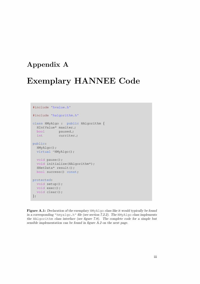
Appendix A
Exemplary HANNEE Code
#include "hvalue.h"
#include "halgorithm.h"
class HMyAlgo : public HAlgorithm HIntValue* maxiter ;bool paused ;int curriter ;
public:HMyAlgo();virtual ˜HMyAlgo();
void pause();void initialize(HAlgorithm*);HNetData* result();bool success() const;
protected:void setup();void exec();void clear();
;
Figure A.1: Declaration of the exemplary HMyAlgo class like it would typically be foundin a corresponding "hmyalgo.h" file (see section 7.2.2). The HMyAlgo class implementsthe HAlgorithm class interface (see figure 7.8). The complete code for a simple butsensible implementation can be found in figure A.2 on the next page.
iii
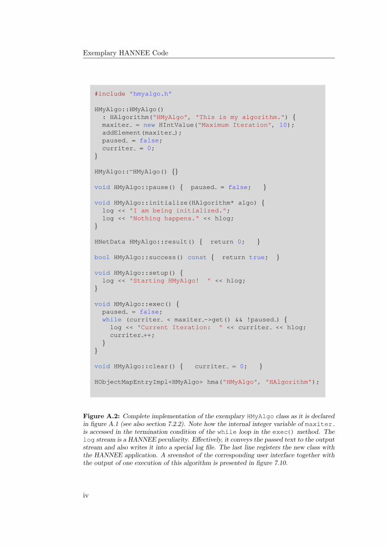
Exemplary HANNEE Code
#include "hmyalgo.h"
HMyAlgo::HMyAlgo(): HAlgorithm("HMyAlgo", "This is my algorithm.") maxiter = new HIntValue("Maximum Iteration", 10);addElement(maxiter );paused = false;curriter = 0;
HMyAlgo::˜HMyAlgo()
void HMyAlgo::pause() paused = false;
void HMyAlgo::initialize(HAlgorithm* algo) log << "I am being initialized.";log << "Nothing happens." << hlog;
HNetData HMyAlgo::result() return 0;
bool HMyAlgo::success() const return true;
void HMyAlgo::setup() log << "Starting HMyAlgo! " << hlog;
void HMyAlgo::exec() paused = false;while (curriter < maxiter ->get() && !paused ) log << "Current Iteration: " << curriter << hlog;curriter ++;
void HMyAlgo::clear() curriter = 0;
HObjectMapEntryImpl<HMyAlgo> hma("HMyAlgo", "HAlgorithm");
Figure A.2: Complete implementation of the exemplary HMyAlgo class as it is declaredin figure A.1 (see also section 7.2.2). Note how the internal integer variable of maxiteris accessed in the termination condition of the while loop in the exec() method. Thelog stream is a HANNEE peculiarity. Effectively, it conveys the passed text to the outputstream and also writes it into a special log file. The last line registers the new class withthe HANNEE application. A sreenshot of the corresponding user interface together withthe output of one execution of this algorithm is presented in figure 7.10.
iv
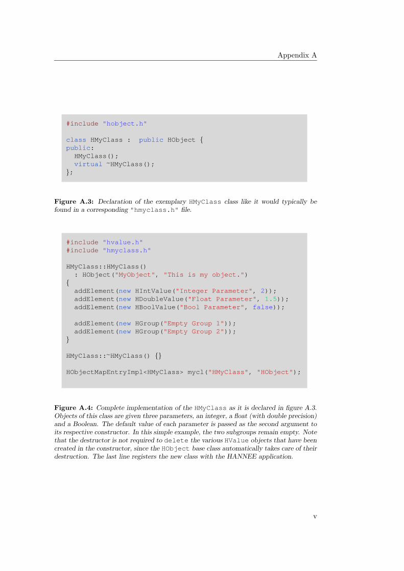
Appendix A
#include "hobject.h"
class HMyClass : public HObject public:HMyClass();virtual ˜HMyClass();
;
Figure A.3: Declaration of the exemplary HMyClass class like it would typically befound in a corresponding "hmyclass.h" file.
#include "hvalue.h"#include "hmyclass.h"
HMyClass::HMyClass(): HObject("MyObject", "This is my object.")
addElement(new HIntValue("Integer Parameter", 2));addElement(new HDoubleValue("Float Parameter", 1.5));addElement(new HBoolValue("Bool Parameter", false));
addElement(new HGroup("Empty Group 1"));addElement(new HGroup("Empty Group 2"));
HMyClass::˜HMyClass()
HObjectMapEntryImpl<HMyClass> mycl("HMyClass", "HObject");
Figure A.4: Complete implementation of the HMyClass as it is declared in figure A.3.Objects of this class are given three parameters, an integer, a float (with double precision)and a Boolean. The default value of each parameter is passed as the second argument toits respective constructor. In this simple example, the two subgroups remain empty. Notethat the destructor is not required to delete the various HValue objects that have beencreated in the constructor, since the HObject base class automatically takes care of theirdestruction. The last line registers the new class with the HANNEE application.
v
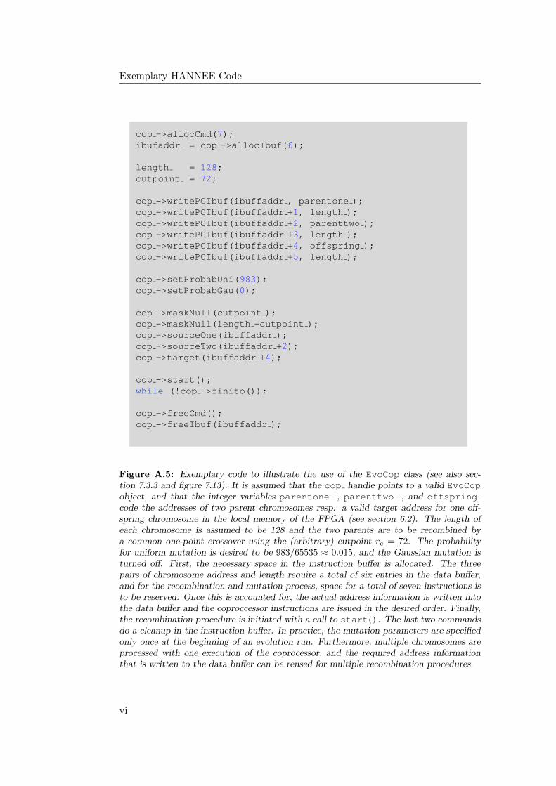
Exemplary HANNEE Code
cop ->allocCmd(7);ibufaddr = cop ->allocIbuf(6);
length = 128;cutpoint = 72;
cop ->writePCIbuf(ibuffaddr , parentone );cop ->writePCIbuf(ibuffaddr +1, length );cop ->writePCIbuf(ibuffaddr +2, parenttwo );cop ->writePCIbuf(ibuffaddr +3, length );cop ->writePCIbuf(ibuffaddr +4, offspring );cop ->writePCIbuf(ibuffaddr +5, length );
cop ->setProbabUni(983);cop ->setProbabGau(0);
cop ->maskNull(cutpoint );cop ->maskNull(length -cutpoint );cop ->sourceOne(ibuffaddr );cop ->sourceTwo(ibuffaddr +2);cop ->target(ibuffaddr +4);
cop ->start();while (!cop ->finito());
cop ->freeCmd();cop ->freeIbuf(ibuffaddr );
Figure A.5: Exemplary code to illustrate the use of the EvoCop class (see also sec-tion 7.3.3 and figure 7.13). It is assumed that the cop handle points to a valid EvoCopobject, and that the integer variables parentone , parenttwo , and offspringcode the addresses of two parent chromosomes resp. a valid target address for one off-spring chromosome in the local memory of the FPGA (see section 6.2). The length ofeach chromosome is assumed to be 128 and the two parents are to be recombined bya common one-point crossover using the (arbitrary) cutpoint rc = 72. The probabilityfor uniform mutation is desired to be 983/65535 ≈ 0.015, and the Gaussian mutation isturned off. First, the necessary space in the instruction buffer is allocated. The threepairs of chromosome address and length require a total of six entries in the data buffer,and for the recombination and mutation process, space for a total of seven instructions isto be reserved. Once this is accounted for, the actual address information is written intothe data buffer and the coproccessor instructions are issued in the desired order. Finally,the recombination procedure is initiated with a call to start(). The last two commandsdo a cleanup in the instruction buffer. In practice, the mutation parameters are specifiedonly once at the beginning of an evolution run. Furthermore, multiple chromosomes areprocessed with one execution of the coprocessor, and the required address informationthat is written to the data buffer can be reused for multiple recombination procedures.
vi
Appendix B
The Investigated BenchmarkProblems
All data sets that are used for the presented experiments have been obtainedfrom the UCI KDD online archive [90]. Some are also included in the “Proben1”benchmark collection compiled by Lutz Prechelt [163]. The numbers of classes,instances, and attributes for the different classification tasks are summarized intable 8.1. The following paragraphs are intended to provide additional informationabout the origins, compositions, and relative difficulties of the different problems.
The breast cancer problem This data set was originally obtained from theUniversity of Wisconsin Hospital, Madison, from Dr. William H. Wolberg [133].The task is to classify a tumor as either benign or malignant based on cell de-scriptions gathered by microscopic examination (e.g., clump thickness, cell sizeuniformity, the frequency of bare nuclei, etc.). The original data set contains699 instances but 16 include missing attribute values and are therefore omitted.65 % of the used examples are benign.
The diabetes problem The data in this set was originally donated by VincentSigillito from the Johns Hopkins University. Based on various personal data andmedical examinations (age, blood pressure, body mass index, etc.), it is to bedecided whether a female patient of Pima Indian1 heritage and age above 21would test positive for diabetes according to the criteria of the World HealthOrganization or not. 65.1 % of the patients are tested negative for diabetes.
The heart disease problem The experiments presented in this thesis onlyuse the specific part of this data set that originates from the Cleveland Clinicfoundation (this corresponds to the heartc data set of the “Proben1” collectionby Prechelt [163]). It was supplied by Robert Dotrano of the V.A. Medical Center,Long Beach, CA. On the basis of personal data (age, sex, smoking habits, etc.)and various medical examinations such as blood pressure and electro cardiogram
1The Pima Indians live near Phoenix, Arizona, USA.
vii
The Investigated Benchmark Problems
results, it is to be decided whether at least one major vessel is reduced in diameterby more than 50 %. The whole data set comprises 303 instances, 6 of which exhibitmissing attribute values and have therefore been omitted. 53.81 % of the patientshave “no vessel reduced”.
The liver disorder problem This data set was created by BUPA Medical Re-search Ltd. and donated by Richard S. Forsyth, 8 Grosvenor Avenue, MapperleyPark, Nottingham. The task is to predict the presence of liver disorder for a malepatient on the basis of several blood tests and the number of half-pint equivalentsof alcoholic beverages drunk per day. It appears that a value larger than five forthe latter attribute is some sort of a selector on this data set. The first classcontains 42 % of all instances.
It is to be noted that the above four data sets are commonly considered to rep-resent some of the most challenging problems in the neural network and machinelearning field since they all feature a comparably small sample size and high noiselevel [236].
The iris plant problem This is perhaps the best known database to be foundin the pattern recognition literature. It was created by R.A. Fisher and donatedby Michael Marshall. The three classes each refer to a type of iris plant (IrisSetosa, Iris Versicolour, and Iris Virginica) that are to be distinguished on thebasis of the respective dimensions of the sepal and petal. Each class contains 50instances (33.3 %) and one class is known to be linearly separable from the othertwo. The latter are not linearly separable. The iris plant benchmark is widelyregarded as a comparably simple task.
The wine problem The data in this set was originally donated by M. Forina,Institute of Pharmaceutical and Food Analysis and Technologies, Via BrigataSalerno, Genoa, Italy and was first used as a benchmark for pattern recognitionby Aeberhard et al. [3]. The data represents the results of a chemical analysis ofwines grown in the same region in Italy but derived from three different cultivars.The analysis determined the quantities of 13 constituents found in each of thethree types of wines. The three classes contain 33.1 %, 39.9 %, and 27 % of thedata, respectively. In a classification context, this is a well posed problem whichis commonly considered as a good data set for first testing a new classifier, but itis not truly challenging (see also table 9.4).
The glass problem This data set was created by B. German from the Cen-tral Research Establishment, Home Office Forensic Science Service, Aldermaston,Reading, Berkshire and was donated by Vina Spehler, PhD., DABFT Diagnos-tic Products Corporation. The task is to distinguish glass types. The results ofa chemical analysis of glass splinters (percent content of eight different elements)plus the refractive index are used to classify the sample to be either float processedor non float processed building windows, vehicle windows, containers, tableware,
viii

Appendix B
or head lamps. This is motivated by forensic needs in criminal investigation. Thelargest class (non float processed building windows) contributes 35.5 % of all in-stances. The remaining classes contain 32.7 %, 13.6 %, 7.9 %, 6.1 %, and 4.2 % ofthe data set, respectively.
The E.coli and yeast problems These two data sets were created by KentaNakai, Institute of Molecular and Cellular Biology, Osaka University, Japan andwere donated by Paul Horton. The task is to predict the cellular localization sitesof E.coli resp. yeast proteins. The decision is to be made on the basis of a set offeature values that are calculated from the protein’s amino acid sequence. Thesetwo data sets contain comparably large numbers of classes (compare table 8.1).For the E.coli benchmark, the single classes contain 42.6 %, 22.9 %, 15.5 %, 10.4 %,6.0%, 1.5 %, 0.6 %, and 0.6 % of the instances, respectively. For the yeast bench-mark, the most common class contributes 32.2 %, and the remaining categoriescomprise 28.9 %, 16.4 %, 11.0 %, 3.4 %, 3.4 %, 2.4 %, 2.0 %, 1.3 %, and 0.3 % of thedata, respectively.
ix


Appendix C
Experimental Data
This page remains empty. The presentation of the experimental data starts onthe next page.
xi
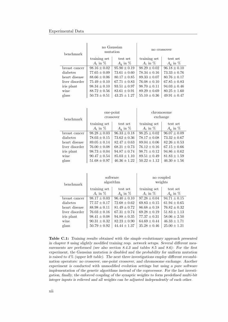
Experimental Data
benchmark
no Gaussianmutation
no crossover
training set test set training set test setAt in % Ag in % At in % Ag in %
breast cancer 98.16 ± 0.02 95.90 ± 0.19 98.29 ± 0.02 96.18 ± 0.10diabetes 77.65 ± 0.09 73.61 ± 0.60 78.34 ± 0.16 73.33 ± 0.76heart disease 88.66 ± 0.06 80.17 ± 0.85 89.33 ± 0.07 80.76 ± 0.17liver disorder 75.49 ± 0.10 67.71 ± 0.83 76.08 ± 0.10 67.85 ± 0.83iris plant 98.34 ± 0.10 93.51 ± 0.97 98.70 ± 0.11 94.03 ± 0.46wine 88.72 ± 0.56 83.61 ± 0.91 89.29 ± 0.69 80.25 ± 1.60glass 50.73 ± 0.51 43.25 ± 1.27 55.10 ± 0.36 49.91 ± 0.47
benchmark
one-pointcrossover
chromosomeexchange
training set test set training set test setAt in % Ag in % At in % Ag in %
breast cancer 98.28 ± 0.03 96.33 ± 0.18 98.25 ± 0.02 96.07 ± 0.09diabetes 78.03 ± 0.15 73.62 ± 0.36 78.17 ± 0.08 73.32 ± 0.67heart disease 89.05 ± 0.14 82.47 ± 0.63 89.04 ± 0.06 82.26 ± 0.53liver disorder 76.00 ± 0.08 68.21 ± 0.73 76.12 ± 0.16 67.15 ± 0.66iris plant 98.73 ± 0.04 94.87 ± 0.74 98.71 ± 0.12 94.86 ± 0.62wine 90.47 ± 0.54 85.03 ± 1.10 89.51 ± 0.49 81.83 ± 1.59glass 51.68 ± 0.97 46.36 ± 1.22 50.22 ± 1.12 46.30 ± 1.56
benchmark
softwarealgorithm
no coupledweights
training set test set training set test setAt in % Ag in % At in % Ag in %
breast cancer 98.17 ± 0.03 96.40 ± 0.10 97.28 ± 0.04 94.71 ± 0.15diabetes 77.57 ± 0.17 72.68 ± 0.62 69.83 ± 0.15 61.94 ± 0.65heart disease 88.98 ± 0.11 81.49 ± 0.72 86.68 ± 0.18 76.82 ± 0.32liver disorder 76.03 ± 0.16 67.31 ± 0.74 69.28 ± 0.19 51.83 ± 1.13iris plant 98.41 ± 0.08 94.88 ± 0.35 77.37 ± 0.31 58.06 ± 2.50wine 90.31 ± 0.32 82.23 ± 0.90 64.69 ± 0.44 46.33 ± 1.71glass 50.79 ± 0.92 44.44 ± 1.37 35.28 ± 0.46 25.00 ± 1.21
Table C.1: Training results obtained with the simple evolutionary approach presentedin chapter 8 using slightly modified training resp. network setups. Several different mea-surements are performed (see also section 8.4.3 and tables 8.5 and 8.6): For the firstexperiment, the Gaussian mutation is disabled and the probability for uniform mutationis raised to 4 % (upper left table). The next three investigations employ different recombi-nation operators: no crossover, one-point crossover, and chromosome exchange. Anotherexperiment is conducted with unmodified evolution settings but using a pure softwareimplementation of the genetic algorithms instead of the coprocessor. For the last investi-gation, finally, the enforced coupling of the synaptic weights to form predefined multi-bitinteger inputs is relieved and all weights can be adjusted independently of each other.
xii
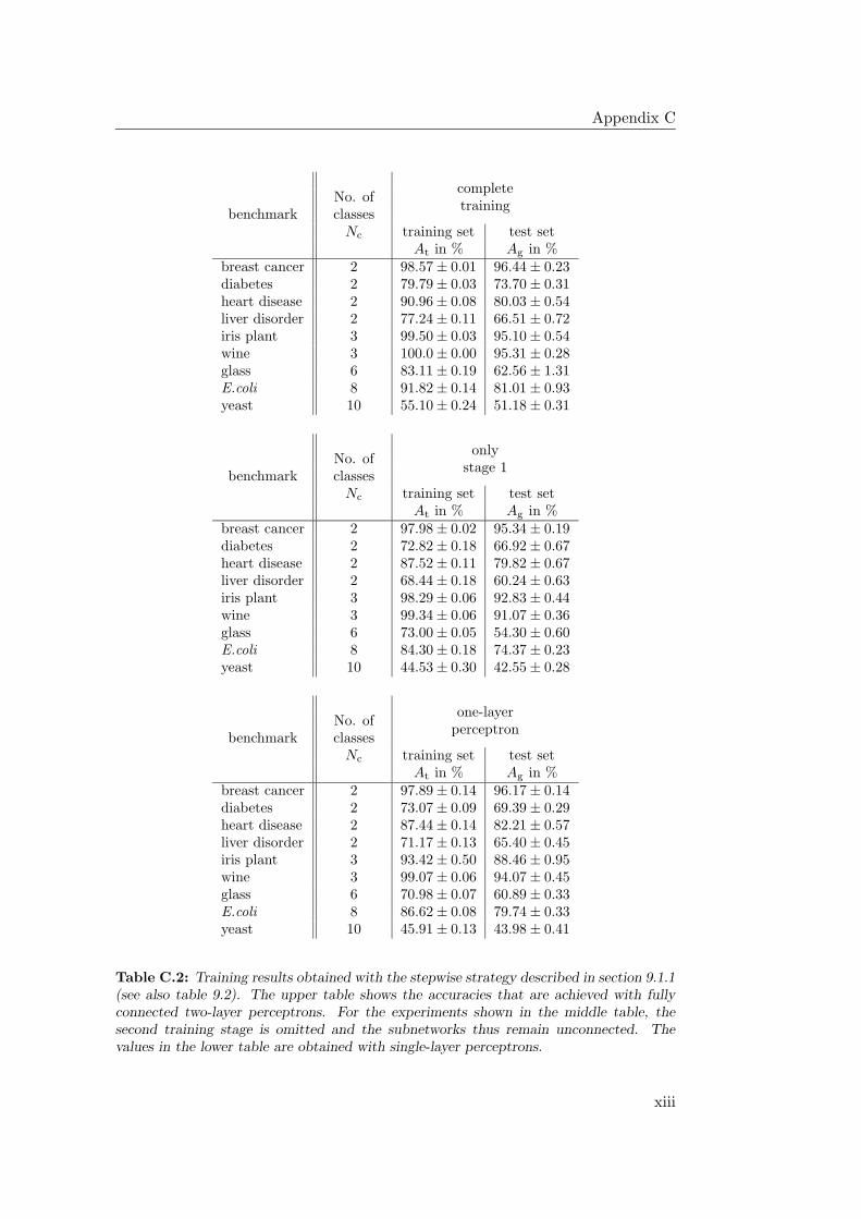
Appendix C
benchmarkNo. ofclasses
Nc
completetraining
training set test setAt in % Ag in %
breast cancer 2 98.57 ± 0.01 96.44 ± 0.23diabetes 2 79.79 ± 0.03 73.70 ± 0.31heart disease 2 90.96 ± 0.08 80.03 ± 0.54liver disorder 2 77.24 ± 0.11 66.51 ± 0.72iris plant 3 99.50 ± 0.03 95.10 ± 0.54wine 3 100.0 ± 0.00 95.31 ± 0.28glass 6 83.11 ± 0.19 62.56 ± 1.31E.coli 8 91.82 ± 0.14 81.01 ± 0.93yeast 10 55.10 ± 0.24 51.18 ± 0.31
benchmarkNo. ofclasses
Nc
onlystage 1
training set test setAt in % Ag in %
breast cancer 2 97.98 ± 0.02 95.34 ± 0.19diabetes 2 72.82 ± 0.18 66.92 ± 0.67heart disease 2 87.52 ± 0.11 79.82 ± 0.67liver disorder 2 68.44 ± 0.18 60.24 ± 0.63iris plant 3 98.29 ± 0.06 92.83 ± 0.44wine 3 99.34 ± 0.06 91.07 ± 0.36glass 6 73.00 ± 0.05 54.30 ± 0.60E.coli 8 84.30 ± 0.18 74.37 ± 0.23yeast 10 44.53 ± 0.30 42.55 ± 0.28
benchmarkNo. ofclasses
Nc
one-layerperceptron
training set test setAt in % Ag in %
breast cancer 2 97.89 ± 0.14 96.17 ± 0.14diabetes 2 73.07 ± 0.09 69.39 ± 0.29heart disease 2 87.44 ± 0.14 82.21 ± 0.57liver disorder 2 71.17 ± 0.13 65.40 ± 0.45iris plant 3 93.42 ± 0.50 88.46 ± 0.95wine 3 99.07 ± 0.06 94.07 ± 0.45glass 6 70.98 ± 0.07 60.89 ± 0.33E.coli 8 86.62 ± 0.08 79.74 ± 0.33yeast 10 45.91 ± 0.13 43.98 ± 0.41
Table C.2: Training results obtained with the stepwise strategy described in section 9.1.1(see also table 9.2). The upper table shows the accuracies that are achieved with fullyconnected two-layer perceptrons. For the experiments shown in the middle table, thesecond training stage is omitted and the subnetworks thus remain unconnected. Thevalues in the lower table are obtained with single-layer perceptrons.
xiii
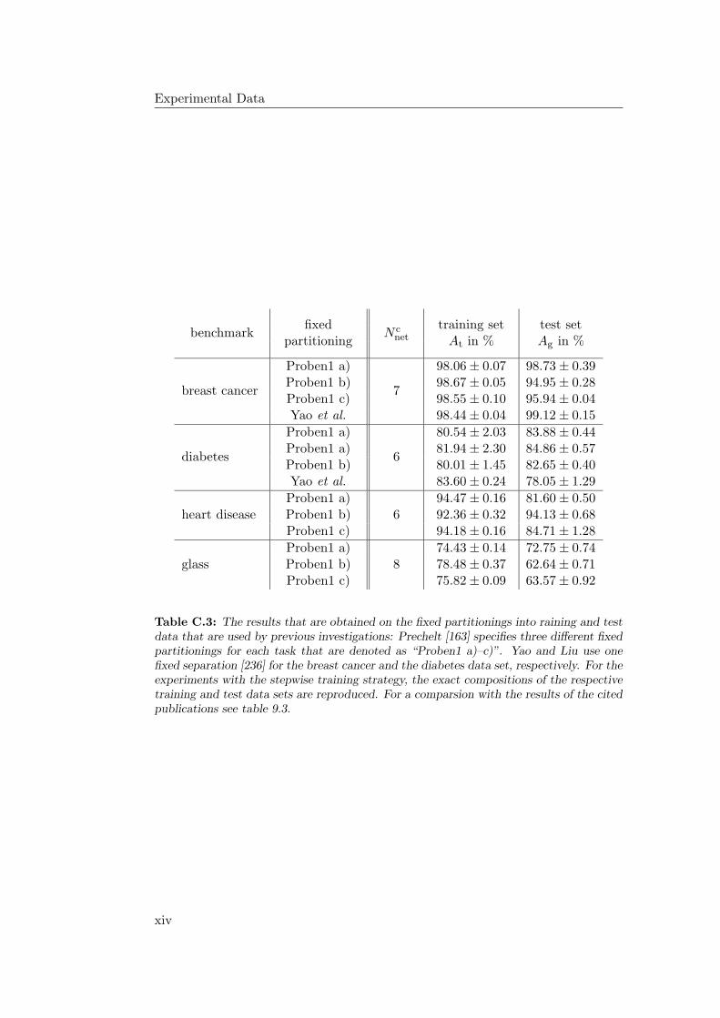
Experimental Data
benchmarkfixed
partitioningN c
nettraining set
At in %test setAg in %
breast cancer
Proben1 a)
7
98.06 ± 0.07 98.73 ± 0.39Proben1 b) 98.67 ± 0.05 94.95 ± 0.28Proben1 c) 98.55 ± 0.10 95.94 ± 0.04Yao et al. 98.44 ± 0.04 99.12 ± 0.15
diabetes
Proben1 a)
6
80.54 ± 2.03 83.88 ± 0.44Proben1 a) 81.94 ± 2.30 84.86 ± 0.57Proben1 b) 80.01 ± 1.45 82.65 ± 0.40Yao et al. 83.60 ± 0.24 78.05 ± 1.29
heart diseaseProben1 a)
694.47 ± 0.16 81.60 ± 0.50
Proben1 b) 92.36 ± 0.32 94.13 ± 0.68Proben1 c) 94.18 ± 0.16 84.71 ± 1.28
glassProben1 a)
874.43 ± 0.14 72.75 ± 0.74
Proben1 b) 78.48 ± 0.37 62.64 ± 0.71Proben1 c) 75.82 ± 0.09 63.57 ± 0.92
Table C.3: The results that are obtained on the fixed partitionings into raining and testdata that are used by previous investigations: Prechelt [163] specifies three different fixedpartitionings for each task that are denoted as “Proben1 a)–c)”. Yao and Liu use onefixed separation [236] for the breast cancer and the diabetes data set, respectively. For theexperiments with the stepwise training strategy, the exact compositions of the respectivetraining and test data sets are reproduced. For a comparsion with the results of the citedpublications see table 9.3.
xiv
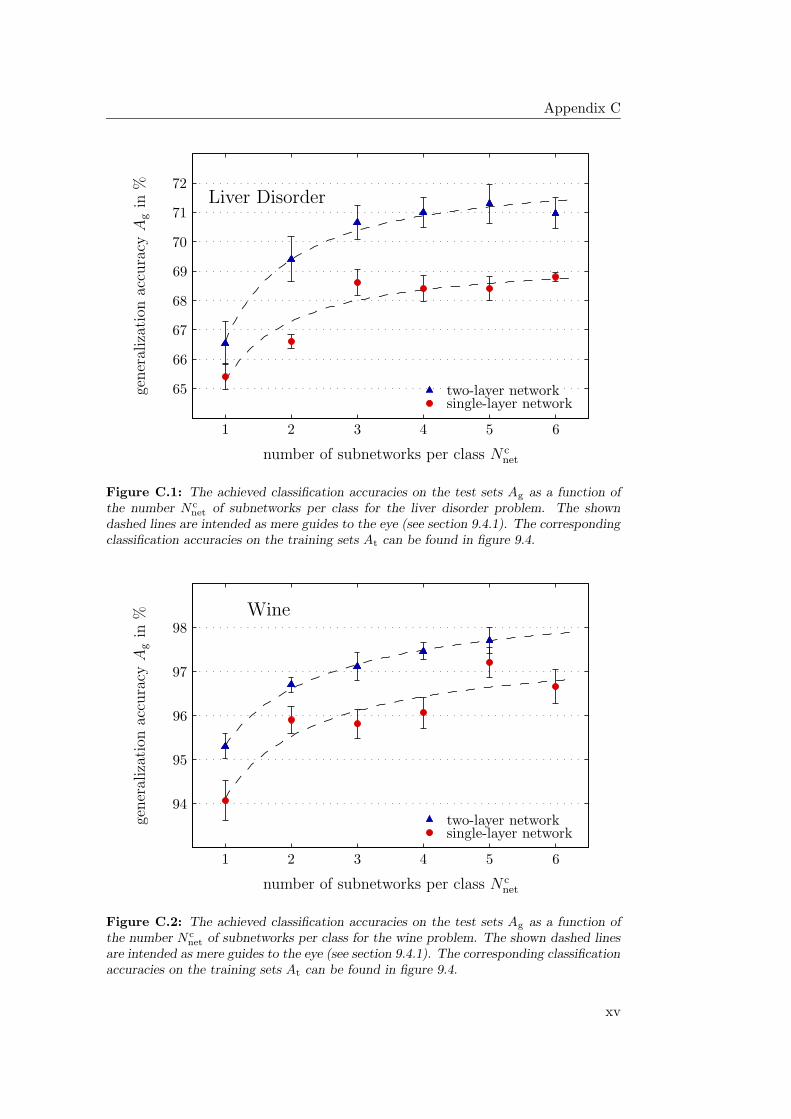
Appendix C
PSfrag replacements
Liver Disorder
training set
test settwo-layer networks
single-layer networks
two-layer networksingle-layer network
multiple subnetworksenlarged subnetworks
classification accuracy in %
gener
aliz
atio
nac
cura
cyA
gin
%
mean absolute difference D in percentage points
number of subnetworks per class N cnet
number of output neurons per class N cout
chip Achip Bchip C
simulation0
10
1
11
2
12
3
13
4
14
5
15
6
167
178
189
192050215122522353245425552656275728582959304031413242334334443545364637473848394960
70
61
71
62
72
63736474
65
75
66
76
67
77
68
78
69
798090819182928393849485958696879788988999
100500
1000150020002500300035004000450050005500
0.51.52.53.54.55.56.57.58.59.5
96.25
96.5
96.75
Figure C.1: The achieved classification accuracies on the test sets Ag as a function ofthe number N c
net of subnetworks per class for the liver disorder problem. The showndashed lines are intended as mere guides to the eye (see section 9.4.1). The correspondingclassification accuracies on the training sets At can be found in figure 9.4.
PSfrag replacements
Wine
training set
test settwo-layer networks
single-layer networks
two-layer networksingle-layer network
multiple subnetworksenlarged subnetworks
classification accuracy in %
gener
aliz
atio
nac
cura
cyA
gin
%
mean absolute difference D in percentage points
number of subnetworks per class N cnet
number of output neurons per class N cout
chip Achip Bchip C
simulation0
10
1
11
2
12
3
13
4
14
5
15
6
167
178
189
19205021512252235324542555265627572858295930403141324233433444354536463747384839496070617162726373647465756676677768786979809081918292839384
94
85
95
86
96
87
97
88
98
8999
100500
1000150020002500300035004000450050005500
0.51.52.53.54.55.56.57.58.59.5
96.25
96.5
96.75
Figure C.2: The achieved classification accuracies on the test sets Ag as a function ofthe number N c
net of subnetworks per class for the wine problem. The shown dashed linesare intended as mere guides to the eye (see section 9.4.1). The corresponding classificationaccuracies on the training sets At can be found in figure 9.4.
xv
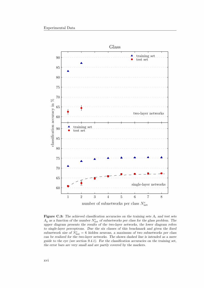
Experimental Data
PSfrag replacements
Glass
training set
training set
test set
test set
two-layer networks
single-layer networks
two-layer networksingle-layer network
multiple subnetworksenlarged subnetworks
clas
sifica
tion
accu
racy
in%
generalization accuracy Ag in %mean absolute difference D in percentage points
number of subnetworks per class N cnet
number of output neurons per class N cout
chip Achip Bchip C
simulation0
10
1
11
2
12
3
13
4
14
5
15
6
16
7
17
8
189
1920502151225223532454255526562757285829593040314132423343344435453646374738483949
60
60
70
70
6171627263736474
65
65
75
75
6676677768786979
80
80
90
90
8191829283938494
85
85
958696879788988999
100500
1000150020002500300035004000450050005500
0.51.52.53.54.55.56.57.58.59.5
96.25
96.5
96.75
Figure C.3: The achieved classification accuracies on the training sets At and test setsAg as a function of the number N c
net of subnetworks per class for the glass problem. Theupper diagram presents the results of the two-layer networks, the lower diagram refersto single-layer perceptrons. Due the six classes of this benchmark and given the fixedsubnetwork size of N c
hid = 6 hidden neurons, a maximum of two subnetworks per classcan be realized for the two-layer networks. The shown dashed line is intended as a mereguide to the eye (see section 9.4.1). For the classification accuracies on the training set,the error bars are very small and are partly covered by the markers.
xvi
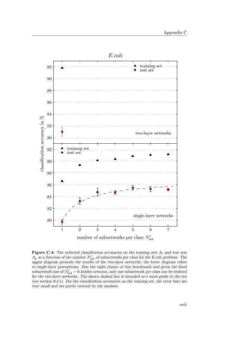
Appendix C
PSfrag replacements
E.coli
training set
training set
test set
test set
two-layer networks
single-layer networks
two-layer networksingle-layer network
multiple subnetworksenlarged subnetworks
clas
sifica
tion
accu
racy
in%
generalization accuracy Ag in %mean absolute difference D in percentage points
number of subnetworks per class N cnet
number of output neurons per class N cout
chip Achip Bchip C
simulation0
10
1
11
2
12
3
13
4
14
5
15
6
16
7
178
189
19205021512252235324542555265627572858295930403141324233433444354536463747384839496070617162726373647465756676677768786979
80
80
90
90
8191
82
82
92
92
8393
84
84
948595
86
86
968797
88
88988999
100500
1000150020002500300035004000450050005500
0.51.52.53.54.55.56.57.58.59.5
96.25
96.5
96.75
Figure C.4: The achieved classification accuracies on the training sets At and test setsAg as a function of the number N c
net of subnetworks per class for the E.coli problem. Theupper diagram presents the results of the two-layer networks, the lower diagram refersto single-layer perceptrons. Due the eight classes of this benchmark and given the fixedsubnetwork size of N c
hid = 6 hidden neurons, only one subnetwork per class can be realizedfor the two-layer networks. The shown dashed line is intended as a mere guide to the eye(see section 9.4.1). For the classification accuracies on the training set, the error bars arevery small and are partly covered by the markers.
xvii
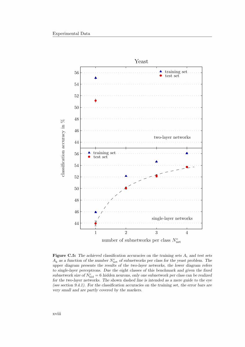
Experimental Data
PSfrag replacements
Yeast
training set
training set
test set
test set
two-layer networks
single-layer networks
two-layer networksingle-layer network
multiple subnetworksenlarged subnetworks
clas
sifica
tion
accu
racy
in%
generalization accuracy Ag in %mean absolute difference D in percentage points
number of subnetworks per class N cnet
number of output neurons per class N cout
chip Achip Bchip C
simulation0
10
1
11
2
12
3
13
4
145
156
167
178
189
1920
50
50
215122
52
52
235324
54
54
255526
56
56
275728582959304031413242334334
44
44
354536
46
46
374738
48
48
394960706171627263736474657566766777687869798090819182928393849485958696879788988999
100500
1000150020002500300035004000450050005500
0.51.52.53.54.55.56.57.58.59.5
96.25
96.5
96.75
Figure C.5: The achieved classification accuracies on the training sets At and test setsAg as a function of the number N c
net of subnetworks per class for the yeast problem. Theupper diagram presents the results of the two-layer networks, the lower diagram refersto single-layer perceptrons. Due the eight classes of this benchmark and given the fixedsubnetwork size of N c
hid = 6 hidden neurons, only one subnetwork per class can be realizedfor the two-layer networks. The shown dashed line is intended as a mere guide to the eye(see section 9.4.1). For the classification accuracies on the training set, the error bars arevery small and are partly covered by the markers.
xviii
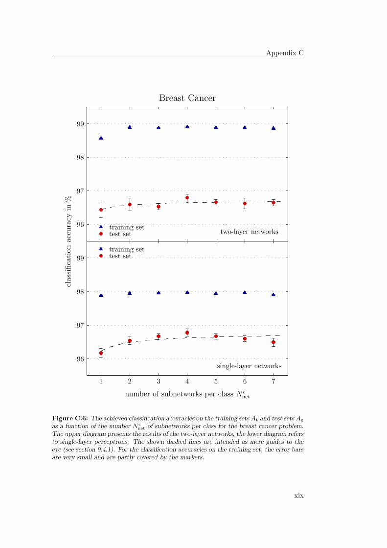
Appendix C
PSfrag replacements
Breast Cancer
training set
training set
test set
test set two-layer networks
single-layer networks
two-layer networksingle-layer network
multiple subnetworksenlarged subnetworks
clas
sifica
tion
accu
racy
in%
generalization accuracy Ag in %mean absolute difference D in percentage points
number of subnetworks per class N cnet
number of output neurons per class N cout
chip Achip Bchip C
simulation0
10
1
11
2
12
3
13
4
14
5
15
6
16
7
178
189
1920502151225223532454255526562757285829593040314132423343344435453646374738483949607061716272637364746575667667776878697980908191829283938494859586
96
96
87
97
97
88
98
98
89
99
99
100500
1000150020002500300035004000450050005500
0.51.52.53.54.55.56.57.58.59.5
96.25
96.5
96.75
Figure C.6: The achieved classification accuracies on the training sets At and test sets Ag
as a function of the number N cnet of subnetworks per class for the breast cancer problem.
The upper diagram presents the results of the two-layer networks, the lower diagram refersto single-layer perceptrons. The shown dashed lines are intended as mere guides to theeye (see section 9.4.1). For the classification accuracies on the training set, the error barsare very small and are partly covered by the markers.
xix
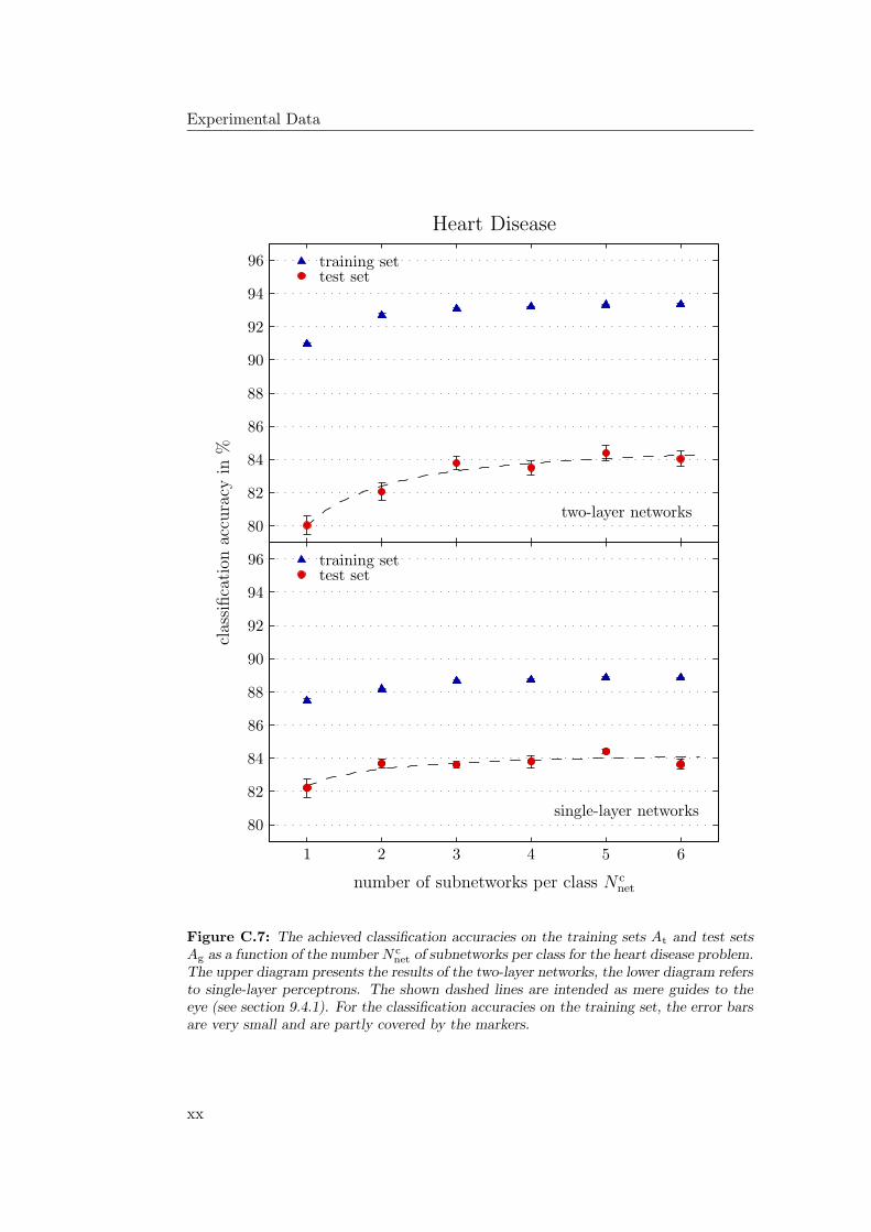
Experimental Data
PSfrag replacements
Heart Disease
training set
training set
test set
test set
two-layer networks
single-layer networks
two-layer networksingle-layer network
multiple subnetworksenlarged subnetworks
clas
sifica
tion
accu
racy
in%
generalization accuracy Ag in %mean absolute difference D in percentage points
number of subnetworks per class N cnet
number of output neurons per class N cout
chip Achip Bchip C
simulation0
10
1
11
2
12
3
13
4
14
5
15
6
167
178
189
19205021512252235324542555265627572858295930403141324233433444354536463747384839496070617162726373647465756676677768786979
80
80
90
90
8191
82
82
92
92
8393
84
84
94
94
8595
86
86
96
96
8797
88
88
988999
100500
1000150020002500300035004000450050005500
0.51.52.53.54.55.56.57.58.59.5
96.25
96.5
96.75
Figure C.7: The achieved classification accuracies on the training sets At and test setsAg as a function of the number N c
net of subnetworks per class for the heart disease problem.The upper diagram presents the results of the two-layer networks, the lower diagram refersto single-layer perceptrons. The shown dashed lines are intended as mere guides to theeye (see section 9.4.1). For the classification accuracies on the training set, the error barsare very small and are partly covered by the markers.
xx
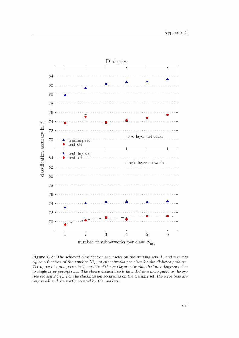
Appendix C
PSfrag replacements
Diabetes
training set
training set
test set
test set
two-layer networks
single-layer networks
two-layer networksingle-layer network
multiple subnetworksenlarged subnetworks
clas
sifica
tion
accu
racy
in%
generalization accuracy Ag in %mean absolute difference D in percentage points
number of subnetworks per class N cnet
number of output neurons per class N cout
chip Achip Bchip C
simulation0
10
1
11
2
12
3
13
4
14
5
15
6
167
178
189
192050215122522353245425552656275728582959304031413242334334443545364637473848394960
70
70
617162
72
72
637364
74
74
657566
76
76
677768
78
78
6979
80
80
908191
82
82
928393
84
84
9485958696879788988999
100500
1000150020002500300035004000450050005500
0.51.52.53.54.55.56.57.58.59.5
96.25
96.5
96.75
Figure C.8: The achieved classification accuracies on the training sets At and test setsAg as a function of the number N c
net of subnetworks per class for the diabetes problem.The upper diagram presents the results of the two-layer networks, the lower diagram refersto single-layer perceptrons. The shown dashed line is intended as a mere guide to the eye(see section 9.4.1). For the classification accuracies on the training set, the error bars arevery small and are partly covered by the markers.
xxi
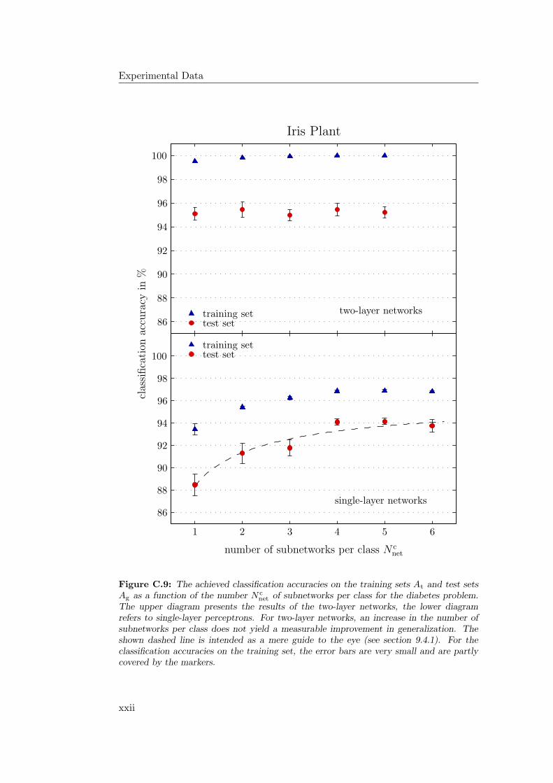
Experimental Data
PSfrag replacements
Iris Plant
training set
training set
test set
test set
two-layer networks
single-layer networks
two-layer networksingle-layer network
multiple subnetworksenlarged subnetworks
clas
sifica
tion
accu
racy
in%
generalization accuracy Ag in %mean absolute difference D in percentage points
number of subnetworks per class N cnet
number of output neurons per class N cout
chip Achip Bchip C
simulation0
10
1
11
2
12
3
13
4
14
5
15
6
167
178
189
1920502151225223532454255526562757285829593040314132423343344435453646374738483949607061716272637364746575667667776878697980
90
90
819182
92
92
839384
94
94
8595
86
86
96
96
8797
88
88
98
98
8999
100
100
5001000150020002500300035004000450050005500
0.51.52.53.54.55.56.57.58.59.5
96.25
96.5
96.75
Figure C.9: The achieved classification accuracies on the training sets At and test setsAg as a function of the number N c
net of subnetworks per class for the diabetes problem.The upper diagram presents the results of the two-layer networks, the lower diagramrefers to single-layer perceptrons. For two-layer networks, an increase in the number ofsubnetworks per class does not yield a measurable improvement in generalization. Theshown dashed line is intended as a mere guide to the eye (see section 9.4.1). For theclassification accuracies on the training set, the error bars are very small and are partlycovered by the markers.
xxii
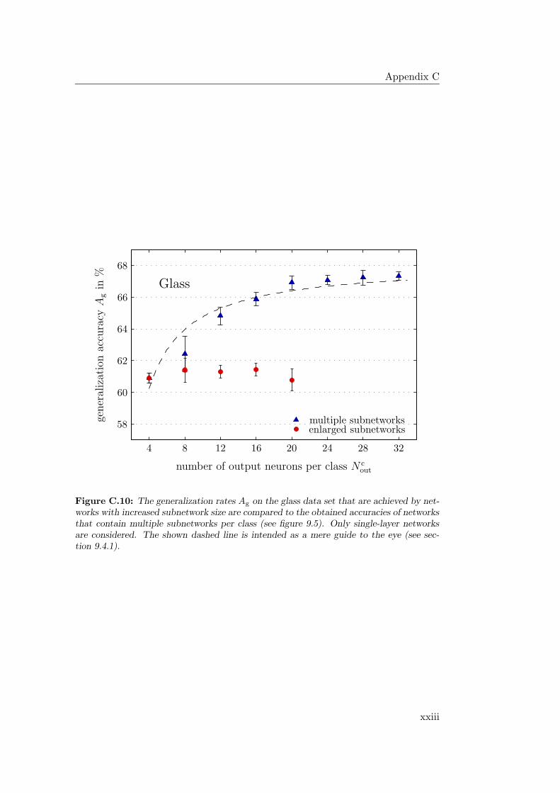
Appendix C
PSfrag replacements
Glass
training set
test settwo-layer networks
single-layer networkstwo-layer network
single-layer network
multiple subnetworksenlarged subnetworks
classification accuracy in %
gener
aliz
atio
nac
cura
cyA
gin
%
mean absolute difference D in percentage pointsnumber of subnetworks per class N c
net
number of output neurons per class N cout
chip Achip Bchip C
simulation0
101
112
12
313
4
145
156
16
717
8
189
19
20
50215122522353
24
54255526562757
28
58
295930403141
32
423343344435453646374738483949
60
706171
62
726373
64
746575
66
766777
68
7869798090819182928393849485958696879788988999
100500
1000150020002500300035004000450050005500
0.51.52.53.54.55.56.57.58.59.5
96.25
96.5
96.75
Figure C.10: The generalization rates Ag on the glass data set that are achieved by net-works with increased subnetwork size are compared to the obtained accuracies of networksthat contain multiple subnetworks per class (see figure 9.5). Only single-layer networksare considered. The shown dashed line is intended as a mere guide to the eye (see sec-tion 9.4.1).
xxiii
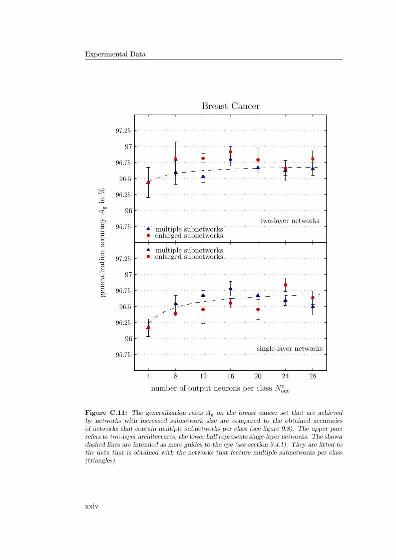
Experimental Data
PSfrag replacements
Breast Cancer
training set
test set
two-layer networks
single-layer networks
two-layer networksingle-layer network
multiple subnetworks
multiple subnetworks
enlarged subnetworks
enlarged subnetworks
classification accuracy in %
gener
aliz
atio
nac
cura
cyA
gin
%
mean absolute difference D in percentage pointsnumber of subnetworks per class N c
net
number of output neurons per class N cout
chip Achip Bchip C
simulation0
101
112
12
313
4
145
156
16
717
8
189
19
20
50215122522353
24
54255526562757
28
5829593040314132423343344435453646374738483949607061716272637364746575667667776878697980908191829283938494859586
96
96
87
97
97
88988999
100500
1000150020002500300035004000450050005500
0.51.52.53.54.55.56.57.58.59.5
96.25
96.5
96.75
95.75
95.75
96.25
96.25
96.5
96.5
96.75
96.75
97.25
97.25
Figure C.11: The generalization rates Ag on the breast cancer set that are achievedby networks with increased subnetwork size are compared to the obtained accuraciesof networks that contain multiple subnetworks per class (see figure 9.8). The upper partrefers to two-layer architectures, the lower half represents singe-layer networks. The showndashed lines are intended as mere guides to the eye (see section 9.4.1). They are fitted tothe data that is obtained with the networks that feature multiple subnetworks per class(triangles).
xxiv
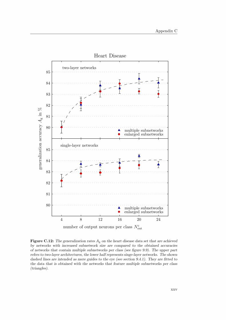
Appendix C
PSfrag replacements
Heart Disease
training set
test set
two-layer networks
single-layer networks
two-layer networksingle-layer network
multiple subnetworks
multiple subnetworks
enlarged subnetworks
enlarged subnetworks
classification accuracy in %
gener
aliz
atio
nac
cura
cyA
gin
%
mean absolute difference D in percentage pointsnumber of subnetworks per class N c
net
number of output neurons per class N cout
chip Achip Bchip C
simulation0
101
112
12
313
4
145
156
16
717
8
189
19
20
50215122522353
24
542555265627572858295930403141324233433444354536463747384839496070617162726373647465756676677768786979
80
80
90
81
81
91
82
82
92
83
83
93
84
84
94
85
85
958696879788988999
100500
1000150020002500300035004000450050005500
0.51.52.53.54.55.56.57.58.59.5
96.25
96.5
96.75
Figure C.12: The generalization rates Ag on the heart disease data set that are achievedby networks with increased subnetwork size are compared to the obtained accuraciesof networks that contain multiple subnetworks per class (see figure 9.9). The upper partrefers to two-layer architectures, the lower half represents singe-layer networks. The showndashed lines are intended as mere guides to the eye (see section 9.4.1). They are fitted tothe data that is obtained with the networks that feature multiple subnetworks per class(triangles).
xxv
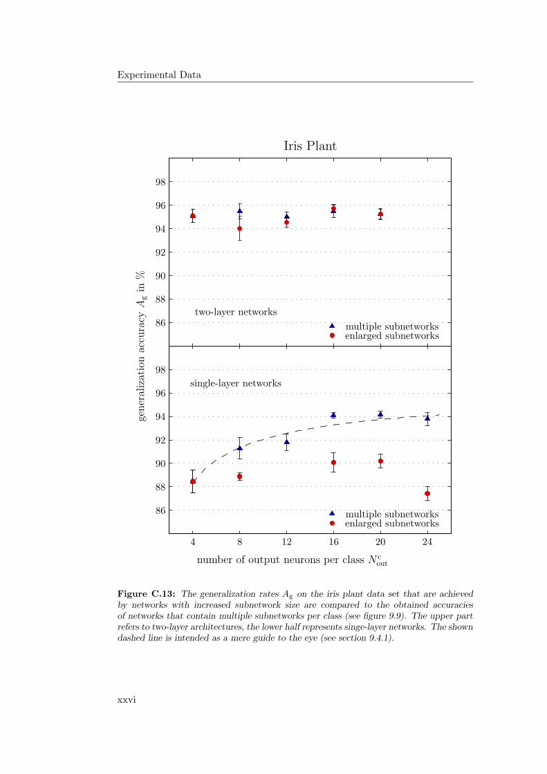
Experimental Data
PSfrag replacements
Iris Plant
training set
test set
two-layer networks
single-layer networks
two-layer networksingle-layer network
multiple subnetworks
multiple subnetworks
enlarged subnetworks
enlarged subnetworks
classification accuracy in %
gener
aliz
atio
nac
cura
cyA
gin
%
mean absolute difference D in percentage pointsnumber of subnetworks per class N c
net
number of output neurons per class N cout
chip Achip Bchip C
simulation0
101
112
12
313
4
145
156
16
717
8
189
19
20
50215122522353
24
54255526562757285829593040314132423343344435453646374738483949607061716272637364746575667667776878697980
90
90
819182
92
92
839384
94
94
8595
86
86
96
96
8797
88
88
98
98
8999
100500
1000150020002500300035004000450050005500
0.51.52.53.54.55.56.57.58.59.5
96.25
96.5
96.75
Figure C.13: The generalization rates Ag on the iris plant data set that are achievedby networks with increased subnetwork size are compared to the obtained accuraciesof networks that contain multiple subnetworks per class (see figure 9.9). The upper partrefers to two-layer architectures, the lower half represents singe-layer networks. The showndashed line is intended as a mere guide to the eye (see section 9.4.1).
xxvi
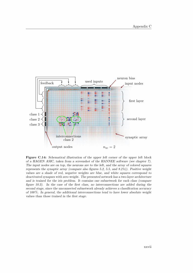
Appendix C
PSfrag replacements
timetraining set
test settwo-layer networks
single-layer networkstwo-layer network
single-layer networkmultiple subnetworksenlarged subnetworks
classification accuracy in %generalization accuracy Ag in %
mean absolute difference D in percentage pointsnumber of subnetworks per class N c
net
number of output neurons per class N cout
chip Achip Bchip C
simulation0
101
112
123
134
145
156
167
178
189
192050215122522353245425552656275728582959304031413242334334443545364637473848394960706171627263736474657566766777687869798090819182928393849485958696879788988999
100500
1000150020002500300035004000450050005500
0.51.52.53.54.55.56.57.58.59.5
96.25
96.5
96.75
used inputsneuron bias
input nodes
output nodes
first layer
second layer
feedback
upper left block
synaptic arrayinterconnections
class 1
class 2
class 2
class 3
nnc = 2
Figure C.14: Schematical illustration of the upper left corner of the upper left blockof a HAGEN ASIC, taken from a screenshot of the HANNEE software (see chapter 7).The input nodes are on top, the neurons are to the left, and the array of colored squaresrepresents the synaptic array (compare also figures 5.2, 5.5, and 8.2 b)). Positive weightvalues are a shade of red, negative weights are blue, and white squares correspond todeactivated synapses with zero weight. The presented network has a two-layer architectureand is trained for the iris problem. It contains one subnetwork for each class (comparefigure 10.3). In the case of the first class, no interconnections are added during thesecond stage, since the unconnected subnetwork already achieves a classification accuracyof 100 %. In general, the additional interconnections tend to have lower absolute weightvalues than those trained in the first stage.
xxvii
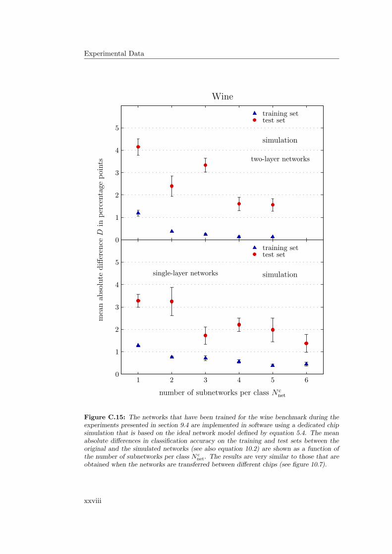
Experimental Data
PSfrag replacements
Wine
training set
training set
test set
test set
two-layer networks
single-layer networks
two-layer networksingle-layer network
multiple subnetworksenlarged subnetworks
classification accuracy in %generalization accuracy Ag in %
mea
nab
solu
tediff
eren
ceD
inper
centa
gepoi
nts
number of subnetworks per class N cnet
number of output neurons per class N cout
chip Achip Bchip C
simulation
simulation
0
0
10
1
1
1
11
2
2
2
12
3
3
3
13
4
4
4
14
5
5
5
15
6
167
178
189
192050215122522353245425552656275728582959304031413242334334443545364637473848394960706171627263736474657566766777687869798090819182928393849485958696879788988999
100500
1000150020002500300035004000450050005500
0.51.52.53.54.55.56.57.58.59.5
96.25
96.5
96.75
Figure C.15: The networks that have been trained for the wine benchmark during theexperiments presented in section 9.4 are implemented in software using a dedicated chipsimulation that is based on the ideal network model defined by equation 5.4. The meanabsolute differences in classification accuracy on the training and test sets between theoriginal and the simulated networks (see also equation 10.2) are shown as a function ofthe number of subnetworks per class N c
net. The results are very similar to those that areobtained when the networks are transferred between different chips (see figure 10.7).
xxviii
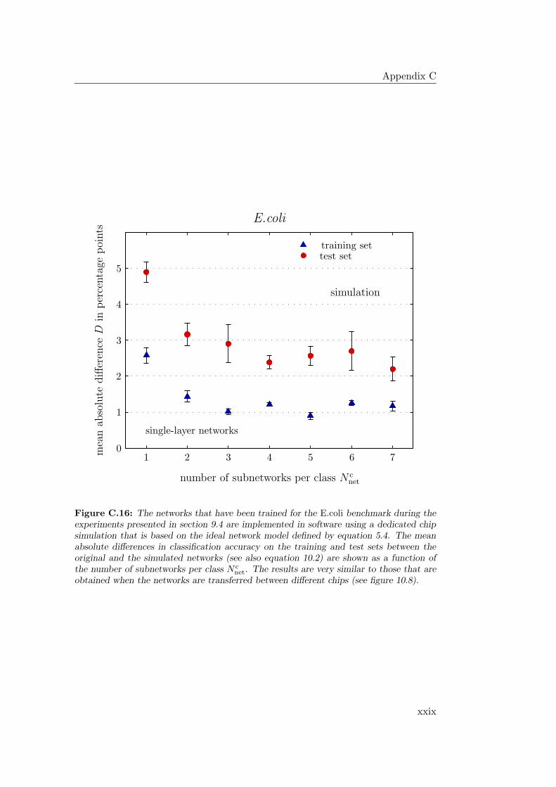
Appendix C
PSfrag replacements
E.coli
training settest set
two-layer networks
single-layer networks
two-layer networksingle-layer network
multiple subnetworksenlarged subnetworks
classification accuracy in %generalization accuracy Ag in %
mea
nab
solu
tediff
eren
ceD
inper
centa
gepoi
nts
number of subnetworks per class N cnet
number of output neurons per class N cout
chip Achip Bchip C
simulation
0
10
1
1
11
2
2
12
3
3
13
4
4
14
5
5
15
6
16
7
178
189
192050215122522353245425552656275728582959304031413242334334443545364637473848394960706171627263736474657566766777687869798090819182928393849485958696879788988999
100500
1000150020002500300035004000450050005500
0.51.52.53.54.55.56.57.58.59.5
96.25
96.5
96.75
Figure C.16: The networks that have been trained for the E.coli benchmark during theexperiments presented in section 9.4 are implemented in software using a dedicated chipsimulation that is based on the ideal network model defined by equation 5.4. The meanabsolute differences in classification accuracy on the training and test sets between theoriginal and the simulated networks (see also equation 10.2) are shown as a function ofthe number of subnetworks per class N c
net. The results are very similar to those that areobtained when the networks are transferred between different chips (see figure 10.8).
xxix

Bibliography
[1] ACE: The Adaptive Communication Environment. Distributed Object Com-puting (DOC) group, Vanderbilt University, Nashville, Washington Univer-sity, and University of California, Irvine,http://www.cs.wustl.edu/ schmidt/ACE.html.
[2] D. H. Ackley, G. E. Hinton, and T. J. Sejnowski. A learning algorithm forBoltzmann machines. Cognitive Science, 9:147–169, 1985.
[3] S. Aeberhard, D. Coomans, and O. de Vel. The performance of statisticalpattern recognition methods in high dimensional settings. Technical Re-port 4, James Cook University, Australia, 1993.
[4] P. E. Allen and D. R. Holberg. CMOS Analog Circuit Design. OxfordUniversity Press, Inc., 198 Madison Avenue, New York, 2002.
[5] ANSI/TIA/EIA-644. Electrical Characteristics of Low Voltage DifferentialSignalling (LVDS), March 1996.
[6] P. Auer, H. Burgsteiner, and W. Maass. Reducing communication fordistributed learning in neural networks. In Proceedings of the Interna-tional Conference on Artificial Neural Networks ICANN’02, pages 123–128.Springer Verlag, 2002.
[7] Austria Mikro Systeme International AG. austriamicrosystems AG. SchlossPremstatten, A-8141 Unterpremstatten, Austria,http://www.austriamicrosystems.com.
[8] T. Back. Optimal mutation rates in genetic search. In Forrest, editor, Pro-ceedings of the 5th International Conference on Genetic Algorithms, pages2–8. Morgan Kauffman, June 1993.
[9] T. Back, F. Hoffmeister, and H. Schwefel. A survey of evolution strategies. InR. K. Belew and L. B. booker, editors, Proceedings of the 4th InternationalConference on Genetic Algorithms, pages 2–9, San Diego, CA, July 1991.Morgan Kaufmann.
[10] J. E. Baker. Reducing bias and inefficiency in the selection algorithm. InJ. J. Grefenstette, editor, Proceedings of the 2nd International Conferenceon Genetic Algorithms, pages 14–21, Hillsdale, New Jersey, 1987. LawrenceErlbaum.
xxxi
Bibliography
[11] E. B. Baum. On the capabilities of multilayer perceptrons. Journal ofComplexity, 4:193–215, 1988.
[12] E. B. Baum and D. Haussler. What size nets gives valid generalization?Neural Computation, 1:151–160, 1989.
[13] J. Baxter. The evolution of learning algorithms for artificial neural networks.Complex Systems, pages 313–326, 1992.
[14] J. Becker. Ein FPGA-basiertes Testsystem fur gemischt analog/digitaleASICs. Diploma thesis (german), University of Heidelberg, HD-KIP-01-11,2001.
[15] V. Beiu. Digitial integrated circuit implementations. In E. Fiesler andR. Beale, editors, The Handbook of Neural Computation, New York, January1997. Institute of Physics Publishing and Oxford University Publishing.
[16] V. Beiu. VLSI implementations of threshold logic – a comprehensive survey.IEEE Transactions on Neural Networks, 14(5):1217–1243, 2003.
[17] R. K. Belew, J. McInerney, and N. M. Schraudolph. Evolving networks:Using the genetic algorithm with connectionist learning. Technical ReportCS90-174 (Revised), Computer Science & Engr. Dept. (C-104), Univ. ofCalifornia, San Diego, La Jolla, CA 92093, USA, February 1991.
[18] N. Bertschinger and T. Natschlager. Real-time computation at the edge ofchaos in recurrent neural networks. Neural Computation, 16(7):1413 – 1436,July 2004.
[19] B. Bhanu and Y. Lin. Learning composite operators for object detection.In W. Langdon et al., editors, Proceedings of the Genetic and EvolutionaryComputation Conference GECCO 2002, pages 1003–1010. Morgan Kauf-mann Publishers, July 2002.
[20] C. M. Bishop. Neural Networks for Pattern Recognition. Oxford UniversityPress, Walton Street, Oxford, 1995.
[21] T. Blickle and L. Thiele. A comparison of selection schemes used in geneticalgorithms. Technical Report 11, Computer Engineering and Communica-tions Networks Lab (TIK), Swiss Federal Institute of Technology (ETH),Gloriastrasse 35, 8092 Zurich, Switzerland, 1995.
[22] H. D. Block. The perceptron: a model for brain functioning. Reviews ofModern Physics, 34:123–135, 1962.
[23] E. K. Blum and L. K. Li. Approximation theory and feedforward networks.Neural Networks, 4(4):511–515, 1991.
[24] S. Bornholdt and D. Graudez. General asymmetric neural networks andstructure design by genetic algorithms. Neural Networks, 5(1):327–334, 1992.
xxxii
Bibliography
[25] Boser et al. An analog neural network processor with programmable topol-ogy. IEEE Journal of Solid-State Circuits, pages 2017–2025, December 1991.
[26] J. Branke. Evolutionary algorithms in neural network design and training –A review. In J. T. Alander, editor, Proceedings of the First Nordic Work-shop on Genetic Algorithms and their Applications (1NWGA), number 95-1,pages 145–163, Vaasa, Finnland, 1995.
[27] A. Breidenassel, K. Meier, and J. Schemmel. A flexible scheme for adaptiveintegration time control. In Proceedings of the Third IEEE Conference onSensors, pages 280–283, Vienna, October 2004.
[28] D. Bruderle. Implementing spike-based computation on a hardware percep-tron. Diploma thesis, University of Heidelberg, HD-KIP-04-16, 2004.
[29] C. J. C. Burges. A tutorial on support vector machines for pattern recogni-tion. Data Mining and Knowledge Discovery, 2(2):121–167, 1998.
[30] A. H. Cannon, L. J. Cowen, and C. E. Priebe. Approximate distance clas-sification. In Proceedings of the 1998 Symposium on the Interface betweenComputer Science and Statistics, number 30-1, pages 544–549, 1998.
[31] B. Carr, W. Hart, N. Krasnogor, J. Hirst, E. Burke, and J. Smith. Alignmentof protein structures with a memetic evolutionary algorithm. In W. Langdonet al., editors, Proceedings of the Genetic and Evolutionary ComputationConference GECCO 2002, pages 1027–1034. Morgan Kaufmann Publishers,July 2002.
[32] J. P. Cater. Successfully using peak learning rates of 10 (and greater) in back-propagation networks with the heuristic learning algorithm. In M. Caudilland C. Butler, editors, Proceedings of the IEEE First International Con-ference on Neural Networks, volume II, pages 645–651, San Diego, 1987.IEEE.
[33] T. P. Caudell and C. P. Dolan. Parametric connectivity: Training of con-strained networks using genetic algorithms. In J. D. Schaffer, editor, Pro-ceedings of the Third International Conference on Genetic Algorithms, pages370–374. Morgan Kaufmann, 1989.
[34] G. Cauwenberghs. A fast stochastic error-descent algorithm for supervisedlearning and optimization. Advances in Neural Information Processing Sys-tems, 5:244–251, 1993.
[35] G. Cauwenberghs. Learning on silicon: A survey. In G. Cauwenberghsand M. A. Bayoumi, editors, Learning on Silicon: Adaptive VLSI NeuralSystems, pages 1–29, Norwell, MA, 1999. Kluwer Academic Publisher.
[36] D. J. Chalmers. The evolution of learning: An experiment in genetic con-nectionism. In D. S. Touretzky, J. L. Elman, and G. E. Hinten, editors,Proceedings of the 1990 Connectionist Models Summer School, pages 81–90,San Mateo, CA, 1990. Morgan Kaufmann.
xxxiii
Bibliography
[37] C. A. Coello Coello, D. A. Van Veldhuizen, and G. B. Lamont. EvolutionaryAlgorithms for Solving Multi-Objective Problems. Kluwer Academic/PlenumPublishers, New York, 2002.
[38] J. P. Cohoon, S. U. Hedge, W. N. Martin, and D. Richards. Punctuatedequilibria: A parallel genetic algorithm. In J. J. Grefenstette, editor, Pro-ceedings of the 2nd International Conference on Genetic Algorithms, pages148–154, Hillsdale, New Jersey, 1987. Lawrence Erlbaum.
[39] J. P. Cohoon, W. N. Martin, and D. S. Richards. Genetic algorithms andpunctuated equilibria in VLSI. In H.-P. Schwefel and R. Manner, editors,Proceedings of the 1st International Conference on Parallel Problem Solvingfrom Nature, volume 496, pages 134–141. Springer Verlag, 1991.
[40] C. Cortez and V. Vapnik. Support-vector networks. Machine Learning,20:273–297, 1995.
[41] T. Cover. Geometrical and statistical properties of systems of linear inequal-ities with applications in pattern recognition. IEEE Trans. on ElectronicComputers, EC-14:326–334, 1965.
[42] C. R. Darwin. On the Origin of Species. John Murray, London, 1859.
[43] L. Davis. Adapting operator probabilities in genetic algorithms. In J. D.Schaffer, editor, Proceedings of the Third International Conference on Ge-netic Algorithms, pages 61–69. Morgan Kaufmann, 1989.
[44] P. Dayan and L. F. Abott. Theoretical Neuroscience: Computational andMathematical Modeling of Neural Systems. The MIT press, Cambride, Mas-sachusetts, London, England, 2001.
[45] K. Deb and D. E. Goldberg. An investigation of niche and species formationin genetic function optimization. In J. D. Schaffer, editor, Proceedings of theThird International Conference on Genetic Algorithms, pages 42–50, SanFrancisco, 1989. Morgan Kaufmann.
[46] K. DeJong. The analysis and behaviour of a class of genetic adaptive sys-tems. PhD thesis, 1975.
[47] A. Dembo and T. Kailath. Model-free distributed learning. IEEE Transac-tions on Neural Networks, 1(1):58–70, 1990.
[48] B. Denby, P. Garda, B. Dranado, C. Kiesling, J.-C. Prevotet, and A. Was-satsch. Fast triggering in high-energy physics experiments using hardwareneural network. IEEE Transactions on Neural Networks, 14(5):1010–1026,2003.
[49] Design Automation Standards Committee of the IEEE Computer Society,New York. VHDL Language Reference Manual, IEEE Std. 1076.1, 1997.
xxxiv
Bibliography
[50] A. E. Eiben and J. E. Smith. Introduction to Evolutionary Computing.Springer Verlag, Berlin, Heidelberg, New York, 2003.
[51] L. J. Eshelmann, R. A. Caruana, and J. D. Schaffer. Biases in crossoverlandscape. In J. D. Schaffer, editor, Proceedings of the Third InternationalConference on Genetic Algorithms, pages 10–19. Morgan Kaufmann, 1989.
[52] J. Fieres, A. Grubl, S. Philipp, K. Meier, J. Schemmel, and F. Schurmann.A platform for parallel operation of VLSI neural networks. In Proc. of the2004 Brain Inspired Cognitive Systems Conference (BICS2004), Universityof Stirling, Scotland, UK, 2004.
[53] G. Fischer. Lineare Algebra. Friedrich Vieweg und Sohn VerlagsgesellschaftmbH, Braunschweig, Wiesbaden, 1986.
[54] T. Fließbach. Statistische Physik. Spektrum Akademischer Verlag GmbH,Heidelberg, 1995.
[55] B. Flower and M. Jabri. Summed weight neuron perturbation: An O(n)improvement over weight perturbation. Advances in Neural InformationProcessing Systems, 5:212–219, 1993.
[56] D. B. Fogel. Evolutionary Computation – Toward a New Philosophy ofMachine Intelligence. IEEE Press, New York, 1995.
[57] D. B. Fogel, editor. Evolutionary Computation: the Fossil Record. IEEEPress, Piscataway, NJ, 1998.
[58] D. B. Fogel, L. J. Fogel, and V. W. Porto. Evolving neural networks. Bio-logical Cybernetics, 63:487–493, 1990.
[59] O. Forster. Analysis 2. Friedrich Vieweg und Sohn Verlagsgesellschaft mbH,Braunschweig, Wiesbaden, 1984.
[60] O. Forster. Analysis 3. Friedrich Vieweg und Sohn Verlagsgesellschaft mbH,Braunschweig, Wiesbaden, 1992.
[61] O. Forster. Analysis 1. Friedrich Vieweg und Sohn Verlagsgesellschaft mbH,Braunschweig, Wiesbaden, 2000.
[62] M. Frean. The upstart algorithm: A method for constructing and trainingfeedforward neural networks. Neural Computation, 2:198–209, 1990.
[63] K. Fukushima. Neocognitron: A hierarchical neural network capable ofvisual pattern recognition. Neural Networks, 1:119–130, 1988.
[64] K. Fukushima, S. Miyake, and T. Ito. Neocognitron: A neural networkmodel for a mechanism of visual pattern recognition. IEEE Transactions onSystems, Man and Cybernetics, SMC-13:826–834, 1983.
xxxv
Bibliography
[65] G. Fung and O. L. Mangasarian. Proximal support vector machine classi-fiers. In F. Provost and R. Srikant, editors, Proceedings of the Seventh ACMSIGKDD International Conference on Knowledge Discovery and Data Min-ing, pages 77–86, 2001.
[66] D. J. Futuyma. Evolutionary Biology. Sinauer Associates, Inc., Sunderland,Massachusetts, USA, 1986.
[67] The GNU Compiler Collection. Free Software Foundation, Inc., 59 TemplePlace, Boston, MA, USA, http://gcc.gnu.org/.
[68] R. Genov. Kerneltron: Support vector “machine” in silicon. IEEE Trans-actions on Neural Networks, 14(5):1426–1434, 2003.
[69] W. Gerstner and W. Kistler. Spiking Neuron Models: Single Neurons, Pop-ulations, Plasticity. Cambridge University Press, 2002.
[70] D. E. Goldberg. Genetic algorithms with sharing for multimodal functionapproximation. In J. J. Grefenstette, editor, Proceedings of the 2nd Inter-national Conference on Genetic Algorithms, pages 41–49, Hillsdale, NewJersey, 1987. Lawrence Erlbaum.
[71] D. E. Goldberg. Genetic Algorithms in Search, Optimization and MachineLearning. Addison Wesley Longman Inc., 1989.
[72] M. Gorges-Schleuter. ASPARAGOS an asynchronous parallel genetic opti-mization strategy. In J. D. Schaffer, editor, Proceedings of the Third Inter-national Conference on Genetic Algorithms, pages 422–427, San Francisco,1989. Morgan Kaufmann.
[73] P. M. Granitto, H. Navone, and H. A. Ceccatto. A stepwise algorithm forconstruction of neural network ensembles. In VII Argentine Congress ofComputer Science, Calafate, Argentina, 2001.
[74] G. W. Greenwood. Training partially recurrent neural networks using evo-lutionary strategies. IEEE Transactions on Speech and Audio Processing,5(2):192–194, 1997.
[75] J. J. Grefenstette. Optimization of control parameters for genetic algorithms.IEEE Transactions on Systems, Man, and Cybernetics, SMC-16(1):122–128,1986.
[76] J. J. Grefenstette. Deception considered harmful. In L. D. Whitley, editor,Foundations of Genetic Algorithms, volume 2, pages 75–91, 1993.
[77] J. J. Grefenstette and J. E. Baker. How genetic algorithms work: A criticallook at implicit parallelism. In J. D. Schaffer, editor, Proceedings of theThird International Conference on Genetic Algorithms, pages 20–27. MorganKaufmann, 1989.
xxxvi
Bibliography
[78] A. Grubl. Eine FPGA-basierte platform fur neuronala netze. Diploma thesis(german), University of Heidelberg, HD-KIP-03-2, 2003.
[79] G. Han and E. Sanchez. CMOS transconductance multipliers: A tutorial.IEEE Transactions on Circuits and Systems II; Analog and Digital SignalProcessing, 45(12):1550–1563, 1998.
[80] P. J. B. Hancock. Genetic algorithms and permutation problems: A com-parison of recombination operators for neural net structure specification. InD. Whitley, editor, Proceedings of the IEEE Workshop on Combinations ofGenetic Algorithms and Neural Network, pages 108–121. IEEE Press, 1992.
[81] P. J. B. Hancock. Recombination operators for the design of neural nets bygenetic algorithm. In R. Manner and B. Manderick, editors, Proceedings ofthe Conference on Parallel Problem Solving from Nature, volume 2, pages441–450. Elsevier Science Publishers B.V., 1992.
[82] S. A. Harp, T. Samad, and A. Guha. Towards the genetic synthesis of neuralnetworks. In J. D. Schaffer, editor, Proceedings of the Third InternationalConference on Genetic Algorithms, pages 360–369. Morgan Kaufmann, 1989.
[83] J. C. Hay, F. C. Martin, and C. W. Wightman. The MARK I perceptron- design and performance. In IRE National Convention Record, volume 2,pages 78–87, 1960.
[84] S. Haykin. Neural Networks: A Comprehensive Foundation. Prentice Hall,Upper Saddle River, New Jersey, 1999.
[85] D. O. Hebb. The Organization of Behaviour. Wiley, New York, 1949.
[86] R. Hecht-Nielsen. Neurocomputing. Addison-Wesley, 1989.
[87] J. N. H. Heemskerk. Overview of neural hardware. In: Neurocomputersfor Brain-Style Processing. Design, Implementation and Application, PhDthesis, 1995.
[88] J. Hertz, A. Krogh, and R. G. Palmer. Introduction to the theory of neuralcomputation. Addison Wesley Publishing Company, Redwood City, CA,1991.
[89] J. Hesser and R. Manner. Towards an optimal mutation probability forgenetic algorithms. In H.-P. Schwefel and R. Manner, editors, Proceedingsof the 1st International Conference on Parallel Problem Solving from Nature,volume 496, pages 23–32. Springer Verlag, 1991.
[90] S. Hettich and S. D. Bay. The UCI KDD archive. University of Cal-ifornia, Department of Information and Computer Science, Irvine, USA,http://kdd.ics.uci.edu, 1999.
xxxvii
Bibliography
[91] R. Hinterding, Z. Michalewicz, and A. E. Eiben. Adaptation in evolutionarycomputation: A survey. In IEEECEP: Proceedings of The IEEE Conferenceon Evolutionary Computation, IEEE World Congress on Computational In-telligence, 1997.
[92] A. Hohmann and W. Hielscher. Lehrbuch der Zahntechnik, Band I.Quintessenz Verlags-GmbH, Berlin, 2001.
[93] S. Hohmann, J. Schemmel, F. Schurmann, and K. Meier. Exploring theparameter space of a genetic algorithm for training an analog neural network.In W. e. a. Langdon, editor, Proceedings of the Genetic and EvolutionaryComputation Conference GECCO 2002, pages 375–382. Morgan KaufmannPublishers, July 2002.
[94] S. Hohmann, J. Fieres, K. Meier, J. Schemmel, T. Schmitz, andF. Schurmann. Training fast mixed-signal neural networks for data clas-sification. In Proceedings of the 2004 International Joint Conference onNeural Networks (IJCNN’04), pages 2647–2652. IEEE Press, 2004.
[95] S. G. Hohmann, J. Schemmel, F. Schurmann, and K. Meier. Predictingprotein cellular localization sites with a hardware analog neural network.In Proceedings of the Int. Joint Conf. on Neural Networks, pages 381–386.IEEE Press, July 2003.
[96] J. H. Holland. Genetic algorithms and the optimal allocation of trials. SIAMJ. of Computing, 2:88–105, 1973.
[97] M. Holler. VLSI implementation of learning and memory systems: A review.Advances in Neural Information Processing Systems, 3, 1991.
[98] J. J. Hopfield. Neural networks and physical systems with emergent collec-tive computational abilities. Proceedings of the National Academy of Sci-ences, 79:2554–2558, 1982.
[99] J. J. Hopfield. Neurons with graded response have collective computa-tional properties like those of two-state neurons. Proceedings of the NationalAcademy of Sciences, 81:3088–3092, 1984.
[100] K. Hornik, M. Stinchcombe, and H. White. Multilayer feedforward networksare universal approximators. Neural Networks, 4(2):359–366, 1989.
[101] P. Horton and K. Nakai. Better prediction of protein cellular localizationsites with the k nearest neighbors classifier. In Proceedings of the 5th In-ternational Conference on Intelligent Systems in Molecular Biology, pages147–152. AAAIPress, 1997.
[102] J. Hromkovic. Algorithmics for Hard Problems. Springer Verlag, Berlin,Heidelberg, New York, 2004.
xxxviii
Bibliography
[103] P. Husbands. Distributed co-evolutionary genetic algorithms for multi-criteria and multi-constraint optimisation. In T. C. Fogarty, editor, Evo-lutionary Computing: Proceedings of the AISB workshop, pages 150–165,Berlin, Heidelberg, New York, 1994. Springer Verlag.
[104] Intel Compiler for Linux. Intel Inc.,http://www.intel.com/software/products/compilers/clin/.
[105] M. M. Islam, X. Yao, and K. Murase. A constructive algorithm for train-ing cooperative neural network ensembles. IEEE Transactions on NeuralNetworks, 14(4):820–834, 2003.
[106] M. Jabri and B. Flower. Weight perturbation: An optimal architecture andlearning technique for analog VLSI feedforward and recurrent multilayernetworks. IEEE Transactions on Neural Networks, 3(1):154–157, 1992.
[107] R. A. Jacobs, M. I. Jordan, and A. G. Barto. Task decomposition throughcompetition in a modular connectionist architecture: The what and wherevision tasks. Cognitive Science, 15:219–250, 1991.
[108] R. A. Jacobs, M. I. Jordan, S. J. Nowlan, and G. E. Hinton. Adaptivemixtures of local experts. Neural Computation, 3:79–87, 1991.
[109] R. Jacobs. Increased rates of convergence through learning rate adaption.Neural Networks, 1:295–307, 1988.
[110] H. Jaeger. The ”echo state” approach to analysing and training recurrentneural networks. Technical Report GMD Report 148, German NationalResearch Center for Information Technology, 2001.
[111] D. Jimenez and N. Walsh. Dynamically weighted ensemble neural networksfor classification. In Proceedings of the 1998 International Joint Conferenceon Neural Networks (IJCNN), 1998.
[112] T. Joachims. Text categorization with support vector machines: learningwith many relevant features. In C. Nedellec and C. Rouveirol, editors,Proceedings of ECML-98, 10th European Conference on Machine Learning,pages 137–142, Chemnitz, DE, 1998. Springer Verlag, Heidelberg, DE.
[113] L. K. Jones. A simple lemma on greedy approximation in hilbert spaceand convergence rates for projection pursuit regression and neural networktraining. Annals of Statistics, 20(1):608–613, 1992.
[114] Jungo Ltd., Netanya. Windriver 6 User’s Manual, 2003.
[115] B. W. Kernighan and D. M. Ritchie. The C Programming Language.Prentice-Hall International Inc., London, 1978.
[116] S. Kirkpatrick, C. D. Gelatt, and M. P. Vecchi. Optimization by simulatedannealing. Science, 220(4598):671–680, 1983.
xxxix
Bibliography
[117] H. Kitano. Designing neural networks using genetic algorithms with graphgeneration system. Complex Systems, 4(4):461–476, 1990.
[118] C. Koch. Biophysics of Computation: Information Processing in SingleNeurons. Oxford University Press, 1999.
[119] R. Kohavi. A study of cross-validation and bootstrap for accuracy estima-tion and model selection. In The 1995 International Joint Conference onArtificial Intelligence IJCAI, pages 1137–1145, Montreal, Quebec, Canada,August 1995.
[120] T. Kohonen. Self-organized formation of topologically correct feature maps.Biological Cybernetics, 43:59–69, 1982.
[121] J. R. Koza, F. H. Bennet III, D. Andre, and M. A. Keane. Genetic Program-ming III - Darwinian Invention and Problem Solving. Morgan KaufmannPublishers, San Francisko, CA, USA, 1999.
[122] A. Kramer. Array-based analog computation. IEEE Micro, pages 20–29,October 1996.
[123] T. Kristensen and R. Patel. Classification of eukariotic and prokariotic cellsby a backpropagation network. In Proceedings of the International JointConference on Neural Networks, pages 1718–1723. IEEE Press, 2003.
[124] A. Krogh and J. Vedelsby. Neural network ensembles, cross validation andactive learning. Advances in Neural Information Processing Systems, 7:299–314, 1995.
[125] J. Langeheine, K. Meier, and J. Schemmel. Intrinsic Evolution of Quasi DCSolutions for Transistor Level Analog Electronic Circuits Using a CMOSFPTA chip. In Proceedings of the 2002 NASA/DoD Conference an EvolvableHardware, 2002.
[126] C. Lindsey and T. Lindblad. Survey of neural network hardware. SPIE,1995(2492):1194–1205, April 1995.
[127] R. P. Lippmann. An introduction to computing with neural nets. IEEEASSP Magazine, 4(2):4–22, 1987.
[128] R. Lohmann. Application of evolution strategy in parallel populations. InH.-P. Schwefel and R. Manner, editors, Proceedings of the 1st InternationalConference on Parallel Problem Solving from Nature, volume 496, pages198–208. Springer Verlag, 1991.
[129] W. Maass, T. Natschlager, and H. Markram. Real-time computing withoutstable states: A new framework for neural computation based on perturba-tions. Neural Computation, 14(11):2531–2560, 2002.
xl
Bibliography
[130] R. Maclin and J. W. Shavlik. Combining the predictions of multiple classi-fiers: Using competitive learning to initialize neural networks. In Proceedingsof the Fourteenth International Joint Conference on Artificial Intelligence,pages 524–530, Montreal, Canada, 1995.
[131] S. W. Mahfoud. Niching methods for genetic algorithms. PhD thesis, 1995.
[132] B. Manderick and P. Spiessens. Fine-grained parallel genetic algorithms. InJ. D. Schaffer, editor, Proceedings of the Third International Conference onGenetic Algorithms, pages 428–433, San Francisco, 1989. Morgan Kaufmann.
[133] O. L. Mangasarian and W. H. Wolberg. Cancer diagnosis via linear pro-gramming. SIAM News, 23(5):1–18, September 1990.
[134] MATLAB. version 6, release 12.1, The Mathworks Inc., 3 Apple Hill Drive,Natick, MA, USA,http://www.mathworks.com/products/matlab/.
[135] W. S. McCulloch and W. Pitts. A logical calculus of the ideas immanent innervous activity. Bulletin of Mathematical Biophysics, pages 127–147, 1943.
[136] M. R. J. McQuoid. Neural ensembles: Simultaneous recognition of multiple2-D visual objects. Neural Networks, 6:907–917, 1993.
[137] C. A. Mead. Analog VLSI and Neural Systems. Addison Wesley, Reading,MA, 1989.
[138] N. Metropolis, A. W. Rosenbluth, M. N. Rosenbluth, and A. H. Theller.Equation of state calculations by fast computing machines. Journal of Chem-ical Physics, 21(6):1087–1092, 1953.
[139] M. Mezard and J.-P. Nadal. Learning inf feedforward layered networks: thetiling algorithm. Journal of Physics A, 22:2191–2203, 1989.
[140] Z. Michalewicz. Genetic Algorithms + Data Structures = Evolution Pro-gramms. Springer Verlag, Berlin, Heidelberg, New York, 1999.
[141] G. F. Miller and P. M. Todd. Designing neural networks using geneticalgorithms. In J. D. Schaffer, editor, Proceedings of the Third InternationalConference on Genetic Algorithms, pages 379–384. Morgan Kaufmann, 1989.
[142] M. Minsky. Neural nets and the brain model problem. PhD thesis, 1954.
[143] M. Minsky and S. Papert. Perceptrons. MIT Press, Cambridge, MA, 1969.
[144] P. Moerland and E. Fiesler. Neural network adaptions to hardware imple-mentations. In E. Fiesler and R. Beale, editors, The Handbook of NeuralComputation, New York, January 1997. Institute of Physics Publishing andOxford University Publishing.
xli

Bibliography
[145] D. Montana and L. Davis. Training feedforward neural networks using ge-netic algorithms. In Proceedings of the 11th International Joint Conferenceon Artificial Intelligence, pages 762–767, San Mateo, CA, 1989. MorganKaufmann.
[146] J. Moody and C. J. Darken. Fast learning in networks of locally-tunedprocessing units. Neural Computation, 1:281–294, 1989.
[147] G. E. Moore. Cramming more components onto integrated circuits. Elec-tronics, 38(8), April 1965.
[148] D. Moriarty and R. Miikkulainen. Discovering complex othello strategiesthrough evolutionary neural networks. Connection Science, 7(3/4):195–210,1995.
[149] Y. S. Mostafa and J. St. Jaques. Information capacity of the hopfield model.IEEE Transactions on Information Theory, IT-31(4):461–464, 1985.
[150] H. Muhlenbein. Parallel genetic algorithms, population genetics and com-binatorial optimization. In J. D. Schaffer, editor, Proceedings of the ThirdInternational Conference on Genetic Algorithms, pages 416–421, San Fran-cisco, 1989. Morgan Kaufmann.
[151] D. Niedenzu. Aufbau eines binaren Neocognitrons. Diploma thesis (german),University of Heidelberg, HD-KIP-03-11, 2003.
[152] A. R. Omondi. Neurocomputers: A dead end ? International Journal ofNeural Systems, 10(6):475–481, 2000.
[153] D. W. Opitz and R. Maclin. Popular ensemble methods: An empirical study.Journal of Artificial Intelligence Research, 11:337–353, 1999.
[154] D. W. Opitz and J. W. Shavlik. Actively searching for an effective neuralnetwork ensemble. Connection Science, 8(3/4):337–353, 1996.
[155] M. Page-Jones. Fundamentals of Object-Oriented Design in UML. AddisonWesley, Reading, MA, 2000.
[156] R. Parekh, J. Yang, and V. Honavar. Mupstart - a constructive neural net-work learning algorithm for multi-category pattern classification. In Proceed-ings of the IEEE International Conference on Neural Networks (ICNN’97),pages 1924–1929, Houston, TX, USA, 1997.
[157] R. Parekh, J. Yang, and V. Honavar. Pruning strategies for the mtilingconstructive learning algorithm. In Proceedings of the IEEE InternationalConference on Neural Networks (ICNN’97), volume 3, pages 1960 – 1965,Houston, TX, USA, 1997.
[158] E. Pasero and M. Perri. Hw-sw codesign of a flexible neural controllerthrough a fpga-based neural network programmed in vhdl. In Proceedingsof the International Joint Conference on Neural Networks IJCNN’04, pages3161–3166. IEEE Press, 2004.
xlii

Bibliography
[159] G. O. Penokie. Working Draft SCSI Parallel Interface-2 (SPI-2). AmericanNational Standard of Accredited Standards Committee NCITS, Washington,DC, revision 20b edition, April 1998.
[160] M. P. Peronne and L. N. Cooper. When networks disagree: Ensemble meth-ods for hybrid neural networks. Artificial Neural Networks for Speech andVision, pages 126–142, 1993.
[161] C. B. Pettey, M. R. Leuze, and G. J. J. A parallel genetic algorithm. InJ. J. Grefenstette, editor, Proceedings of the 2nd International Conference onGenetic Algorithms, pages 155–161, Hillsdale, New Jersey, 1987. LawrenceErlbaum.
[162] PLX Technology, Inc., Sunnyvale. PLX 9054 Data Book, version 2.1 edition,January 2000.
[163] L. Prechelt. Proben1 — A set of neural network benchmark problems andbenchmarking rules. Technical Report 21/94, 38 pages, Fakultat fur Infor-matik, Universitat Karlsruhe, 1994.
[164] A. Prugel-Bennet and A. Rogers. Modelling GA dynamics. Proceedings ofTheoretical Aspects of Evolutionary Computation, pages 59–86, 2001.
[165] A. Prugel-Bennet and J. L. Shapiro. Analysis of genetic algorithms usingstatistical mechanics. Physical Review Letters, 72(9):1305–1309, February1994.
[166] J. Pujol and R. Poli. Evolving neural networks using a dual representationwith a combined crossover operator. In Proceedings of the IEEE Inter-national Conference on Evolutionary Computation (ICEC), pages 416–421,1998.
[167] E. T. Ray. Learning XML. O’Reilly & Associates, Inc., 101 Morris Street,Sebastopol, CA, 2001.
[168] L. Reyneri. Implementation issues of neuro-fuzzy hardware: Going towardHW/SW codesign. IEEE Transactions on Neural Networks, 14(1):176–194,January 2003.
[169] P. Rojas. Theorie der neuronalen Netze: Eine systematische Einfuhrung.Springer Verlag, Berlin, Heidelberg, New York, 1996.
[170] F. Rosenblatt. The perceptron: a probabilistic model for information storageand organization in the brain. Psychological Review, 65:386–408, 1958.
[171] F. Rosenblatt. Perceptron simulation experiments. In Proceedings of theIRE, pages 301–309, 1960.
[172] G. Rudolph. Global optimization by means of distributed evolution strate-gies. In H.-P. Schwefel and R. Manner, editors, Proceedings of the 1st Inter-national Conference on Parallel Problem Solving from Nature, volume 496,pages 209–213. Springer Verlag, 1991.
xliii
Bibliography
[173] G. Rudolph. Convergence of evolutionary algorithms in general searchspaces. In Proceedings of the IEEE Conference on Evolutionary Compu-tation, pages 50–54, Piscataway, NJ, 1996. IEEE Press.
[174] G. Rudolph. Convergence Properties of Evolutionary Algorithms. Verlag Dr.Kovac, Hamburg, 1997.
[175] D. E. Rumelhart, G. E. Hinton, and W. R.J. Learning internal representa-tions by error propagation. Parallel Distributed Processing: Explorations inthe Microstructures of Cognition, I:318–362, 1986.
[176] D. E. Rumelhart, G. E. Hinton, and W. R.J. Learning representations ofback-propagation errors. Nature, 323:533–536, 1986.
[177] J. D. Schaffer, R. A. Caruana, and L. J. Eshelmann. Using genetic search toexploit the emergent behavior of neural networks. Physica D, 42:244–248,1990.
[178] J. Schemmel. personal communication, 2005.
[179] J. Schemmel, S. Hohmann, K. Meier, and F. Schurmann. A mixed-modeanalog neural network using current-steering synapses. Analog IntegratedCircuits and Signal Processing, 38(2-3):233–244, 2004.
[180] J. Schemmel, F. Schurmann, S. Hohmann, and K. Meier. An integratedmixed-mode neural network architecture for megasynapse ANNs. In Pro-ceedings of the 2002 International Joint Conference on Neural NetworksIJCNN’02, pages 2704–2710. IEEE Press, 2002.
[181] T. Schmitz. personal communication, 2005.
[182] T. Schmitz, S. Hohmann, K. Meier, J. Schemmel, and F. Schurmann. Speed-ing up Hardware Evolution: A Coprocessor for Evolutionary Algorithms. InA. M. Tyrrell, P. C. Haddow, and J. Torresen, editors, Proceedings of the 5thInternational Conference on Evolvable Systems ICES 2003, pages 274–285.Springer Verlag, 2003.
[183] R. Schuffny, A. Graupner, and J. Schreiter. Hardware for neural networks.In Proceedings of the 4th International Workshop on Neural Networks inApplications, pages 1–6, 1999.
[184] F. Schurmann, K. Meier, and J. Schemmel. Edge of Chaos Computation inMixed Mode VLSI – “A Hard Liquid”. In L. Saul, Y. Weiss, and L. Bottou,editors, Advances in Neural Information Processing Systems 17, Cambride,2005. MIT Press.
[185] F. Schurmann. PhD thesis, University of Heidelberg, in preparation, 2005.
[186] F. Schurmann, S. G. Hohmann, K. Meier, and J. Schemmel. Interfacingbinary networks to multi-valued signals. In Supplementary Proceedings ofthe Joint International Conference ICANN/ICONIP, pages 430–433. IEEEPress, 2003.
xliv
Bibliography
[187] T. J. Sejnowski and C. R. Rosenberg. NETtalk: a parallel network thatlearns to read aloud. Technical Report JHU/EECS-86/01, John HopkinsUniversity, Electrical Engineering and Computer Science, 1986.
[188] R. S. Sexton, R. E. Dorsez, and J. J. D. Toward global optimization of neu-ral networks: A comparison of the genetic algorithm and backpropagation.Decision Support Systems, 22(2):171–185, 1998.
[189] A. J. C. Sharkey. On combining artificial neural nets. Connection Science,8(3/4):299–314, 1996.
[190] A. J. C. Sharkey and N. E. Sharkey. Combining diverse neural nets. Knowl-egde Engineering Review, 12(3):1–17, 1997.
[191] A. A. Siddiqi and S. M. Lucas. A comparison of matrix rewriting versusdirect encoding for evolving neural networks. In Proceedings of the 1998IEEE International Conference on Evolutionary Computation (ICEC’98),pages 392–397, Piscataway, NJ, 1998. IEEE Press.
[192] H.-J. Siegert and U. Baumgarten. Betriebssysteme: Eine Einfuhrung. R.Oldenbourg Verlag, Munchen, 1998.
[193] A. Sinsel. Linuxportierung auf einen eingebetteten powerpc 405 zursteuerung eines neuronalen netzwerkes. Diploma thesis (german), Universityof Heidelberg, HD-KIP-03-14, 2001.
[194] R. E. Smith, C. Bonacina, P. Kearney, and W. Merlat. Embodiment ofevolutionary computation in general agents. Evolutionary Computation,8(4):475–493, 2001.
[195] R. E. Smith and J. E. Smith. New methods for tunable, random landscapes.In W. N. Martin and W. Spears, editors, Foundations of Genetic Algorithms,volume 6, pages 47–67, 2001.
[196] W. M. Spears. Simple subpopulation schemes. In A. V. Sebald and L. J.Fogel, editors, Proceedings of the Third Annual Conference on EvolutionaryProgramming, pages 296–307. World Scientific, 1994.
[197] W. M. Spears and K. A. De Jong. On the virtues of parametrized uniformcrossover. In R. K. Belew and L. K. booker, editors, Proceedings of the 4thInternational Conference on Genetic Algorithms, pages 230–236, San Diego,CA, 1991. Morgan Kaufmann.
[198] W. M. Spears and K. DeJong. Dining withGAs: Operator lunch theorems.In W. Banzhaf and C. Reeves, editors, Foundations of Genetic Algorithms,volume 5, pages 85–101, 1999.
[199] K. O. Stanley and R. Miikkulainen. Continual coevolution through com-plexification. In W. Langdon et al., editors, Proceedings of the Genetic andEvolutionary Computation Conference GECCO 2002, pages 113–120. Mor-gan Kaufmann Publishers, July 2002.
xlv
Bibliography
[200] K. O. Stanley and R. Miikkulainen. Efficient reinforcement learning throughevolving neural network topologies. In W. Langdon et al., editors, Pro-ceedings of the Genetic and Evolutionary Computation Conference GECCO2002, pages 569–577. Morgan Kaufmann Publishers, July 2002.
[201] V. Storch, U. Welsch, and M. Wink. Evolutionsbiologie. Springer Verlag,Berlin, Heidelberg, New York, 2001.
[202] B. Stroustrup. The C++ Programming Language. Addison Wesley, Reading,MA, August 1997.
[203] G. Syswerda. Uniform crossover in genetic algorithms. In J. D. Schaffer,editor, Proceedings of the Third International Conference on Genetic Algo-rithms, pages 2–9, San Francisco, 1989. Morgan Kaufmann.
[204] R. Tanese. Parallel genetic algorithm for a hypercube. In J. J. Grefen-stette, editor, Proceedings of the 2nd International Conference on GeneticAlgorithms, pages 177–183, Hillsdale, New Jersey, 1987. Lawrence Erlbaum.
[205] J. Teichert and R. Malaka. An association architecture for the detection ofobjects with changing topologies. In Proceedings of the International JointConference on Neural Networks IJCNN’03, pages 125–130. IEEE Press, July2003.
[206] D. Thierens, J. Suykens, J. Vandewalle, and B. DeMoor. Genetic weightoptimization of a feedforward neural network controller. In Proceedings ofthe Conference on Artificial Neural Nets and Genetic Algorithms, pages 658–663, Berlin, Heidelberg, New York, 1993. Springer Verlag.
[207] R. F. Thompson. The Brain. W. H. Freeman and Company, New York andOxford, 1985.
[208] S. J. Thorpe, D. Fize, and C. Marlot. Speed of processing in the humanvisual system. Nature, 381:520–522, 1996.
[209] M. Trefzer, J. Langeheine, K. Meier, and J. Schemmel. New genetic opera-tors to facilitate understanding of evolved transistor circuits. In Proceedingsof the 2004 NASA/DoD Conference an Evolvable Hardware (EH2004), 2004.
[210] Trolltech AS. The Qt application development framework. WaldemarThranes gate, 98, NO-0175 Oslo, Norway,http://www.trolltech.com/products/qt/.
[211] A. Turing. On computable numbers, with an application to the Entschei-dungsproblem. Proceedings of the London Mathematical Society, 42:230–265,1937.
[212] M. Valle. Analog VLSI implementations of neural networks with supervisedon-chip-learning. Analog Integrated Circuits and Signal Processing, 33:263–287, 2002.
xlvi
Bibliography
[213] D. van Heesch. The doxygen documentation system. 2004,http://www.stack.nl/˜dimitri/doxygen.
[214] E. van Nimwegen, J. P. Crutchfield, and M. Mitchell. Statistical dynamicsof the Royal Road genetic algorithm. Theoretical Computer Science, 229:41–102, 1999.
[215] E. A. Vittoz. Analog VLSI signal processing: Why, where and how? AnalogIntegrated Circuits and Signal Processing, 8(1):27–44, 1994.
[216] E. A. Vittoz. Analog VLSI implementation of neural networks. In E. Fieslerand R. Beale, editors, The Handbook of Neural Computation, New York,January 1997. Institute of Physics Publishing and Oxford University Pub-lishing.
[217] M. D. Vose and G. E. Liepins. Punctuated equilibria in genetic search.Complex Systems, 5(1):31–44, 1992.
[218] R. L. Watrous. Learning algorithms for connectionist networks: Appliedgradient methods for nonlinear optimization. In M. Caudill and C. Butler,editors, Proceedings of the IEEE First International Conference on NeuralNetworks, volume II, pages 619–627, San Diego, 1987. IEEE.
[219] H. White. Connectionist nonparametric regression: Multilayer feedforwardnetworks can learn arbitrary mappings. Neural Networks, 3(5):535–549,1990.
[220] P. M. White and C. C. Pettey. Double selection vs. single selection in dif-fusion model GAs. In T. Back, editor, Proceedings of the 7th InternationalConference on Genetic Algorithms, pages 174–180, San Fransiso, 1997. Mor-gan Kaufmann.
[221] D. Whitley. The GENITOR algorithm and selection pressure: Why rank-based allocation of reproductive trials is best. In J. D. Schaffer, editor,Proceedings of the Third International Conference on Genetic Algorithms,pages 116–121. Morgan Kaufmann, 1989.
[222] D. Whitley. Cellular genetic algorithms. In S. Forrest, editor, Proceedingsof the 5th International Conference on Genetic Algorithms, page 658, SanFrancisco, 1993. Morgan Kaufmann.
[223] D. Whitley and T. Hanson. Optimizing neural networks using faster, moreaccurate genetic search. In J. D. Schaffer, editor, Proceedings of the ThirdInternational Conference on Genetic Algorithms, pages 391–395, 1989.
[224] D. Whitley, T. Starkweather, and C. Bogart. Genetic algorithms and neuralnetworks: Optimizing connections and connectivity. Parallel Computing,14(3):347–361, 1990.
xlvii
Bibliography
[225] L. D. Whitley. Fundamental principles of deception in genetic search. InG. Rawlins, editor, Foundations of Genetic Algorithms, volume 1, pages221–241, 1991.
[226] B. Widrow and M. A. Lehr. 30 years of adaptive neural networks: Percep-tron, Madaline, and backpropagation. Proceedings of the IEEE, 78(9):1415–1442, 1990.
[227] B. Widrow and M. E. Hoff. Adaptive switching circuits. In IRE WESCONConvention Record, pages 96–104, New York, 1960. IRE.
[228] D. H. Wolpert and W. G. Macready. No free lunch theorems for optimization.IEEE Transactions on Evolutionary Computation, 1(1):67–82, April 1997.
[229] Xilinx, Inc., 2100 Logic Drive, San Jose, CA 95124-3400, USA. Virtex EDatasheet.
[230] Xilinx, Inc., www.xilinx.com. Virtex-II Pro Platform FPGA Handbook,2002.
[231] Xilinx, Inc., www.xilinx.com. PowerPC processor reference guide, Septem-ber 2003.
[232] Xilinx, Inc., www.xilinx.com. PowerPC 405 processor block reference guide,August 2004.
[233] Xilinx Inc., San Jose. Xilinx XC9536XL High Performance CPLD, Septem-ber 2004.
[234] X. Yao. Evolving artificial neural networks. Proceedings of the IEEE,87(9):1423–1447, 1999.
[235] X. Yao and Y. Liu. Ensemble structure of evolutionary artificial neuralnetworks. In Proceedings of the Third IEEE International Conference onEvolutionary Computation (ICEC’96), pages 659–664, Nagoya, Japan, May1996.
[236] X. Yao and Y. Liu. A new evolutionary system for evolving artificial neuralnetworks. IEEE Transactions on Neural Networks, 8(3):694–713, May 1997.
[237] X. Yao and Y. Liu. Making use of population information in evolutionaryneural networks. IEEE Transactions on Systems, Man and Cybernetics,Part B: Cybernetics, 28(3):417–425, 1998.
xlviii

Danksagung(Acknowledgements)
We are not an endangered species ourselves yet,but this is not for lack of trying.
Douglas Adams, Last Chance to See
Abschließend mochte ich all jenen, die zum Gelingen dieser Arbeit beigetragen haben, einherzliches Dankeschon aussprechen. Mein Dank gilt vor allem
- Herrn Prof. Dr. K. Meier fur die freundliche Aufnahme in seine Arbeitsgruppe unddie Moglichkeit, an einem so interessanten Projekt mitarbeiten zu konnen.
- Herrn Prof. Dr. F. A. Hamprecht, der freundlicherweise das Zweitgutachten uber-nommen hat.
- Dr. Johannes Schemmel, der nicht nur mit der Entwicklung des HAGEN Chipseinen wesentlichen Grundstein fur diese Arbeit gelegt hat, auf dessen umfassendesfachliches Wissen und visionaren Ideenreichtum ich auch in unzahligen Diskussionenzuruckgreifen durfte, der immer auf alle Probleme eine Antwort wusste und dessenfreundliche Art mir die Arbeit stets angenehm machte.
- Felix Schurmann fur die jahrelange kollegiale Zusammenarbeit, viele fruchtbareDiskussionen, bereitwillige Hilfe in allen Hardware-Fragen, wertvolles inspirieren-des Material fur die Kapitel 5 und 6 und die immer geduldige Unterstutzung beiunzahligen Linux-Problemen.
- Johannes Fieres fur weitaus mehr als ich hier aufzahlen konnte, vor allem jedochfur enorme Mengen genialen C++ Codes, objekt-orientiertes Denken in allen Le-benslagen, viele erhellende fachliche und (mindestens ebenso viele) nichtfachlicheDiskussionen, des ofteren Schokolade, Abendessen im Botanik, gute Stimmung imBuro, diverse Schulertage, bei denen ich nicht zu erscheinen brauchte, die aufmerk-same Korrektur des Manuskripts und vor allem seine trotz alledem andauerndeFreundschaft.
- Eilif Mueller, nicht nur weil sein ehemaliges VisWidget immer noch toll aussieht,sondern auch fur seinen wesentlichen Beitrag zur netten Atmosphare im Buro, vieleinspirierende Gedanken zu theoretischen Fragen und dafur, dass er mich so oft anseinen Englischkenntnissen hat teilhaben lassen.
- Tillmann Schmitz, der es nicht nur geschafft hat, einen schnellen evolutionaren Ko-prozessor zu zaubern und stetig zu verbessern, sondern der ihn auch bereitwilligselbst den abstrusesten Vorstellungen der Jungs aus dem Softwarezimmer anzupas-sen bereit war.
xlix

Danksagung (Acknowledgements)
- Allen Mitgliedern der Electronic Vision(s) Gruppe fur die vielen lustigen Arbeits-gruppen-Meetings, die immerwahrende Hilfsbereitschaft — egal, wen man fragt —ein harmonisches Arbeitsklima, das nahezu vollstandige Erscheinen auf allen WG-und Geburtstagsparties und dass man auch, wenn man nicht um 12 Uhr essen gehtund nur ein klapperiges altes Schrottfahrrad fahrt, das Gefuhl hat dazuzugehoren.
- meinem ersten und leider einzigen Diplomanden Dominik”Bon“ Niedenzu fur seine
vielfaltige konstruktive Kritik am HANNEE Programm, seine erfrischend andereSichtweise der Dinge und dafur, dass er es geschafft hat, Diplomand zu sein undgleichzeitig Kumpel zu bleiben.
- Kristoffer Lerch und Ulf Bissbort, deren vorbildliches Engagement sie im Rahmenihrer Projektarbeiten wertvolle Beitrage zur HANNEE Software bzw. der Forschungan den schrittweisen Trainingsmethoden hat liefern lassen.
Abgesehen von der fachlichen und anderweitig arbeitsbezogenen Unterstutzung, diemir im Laufe dieses Projekts zuteil wurde, haben insbesondere auch der freundschaftlicheund emotionale Beistand mehrerer lieber Menschen die letzten Jahre fur mich zu einerwertvollen Erfahrung werden lassen, die ich nicht mehr missen mochte. An dieser Stellewill ich auch hierfur ein herzliches Dankeschon loswerden an:
- alle Mitglieder (die ehemaligen wie die aktuellen) der Kultband”Fake It“: Ani,
Hanni, Kranky, Mad und Merd dafur, dass sie ihren despotischen”Frontman“ auch
nach Jahren immer noch ertragen, fur einmal in der Woche rumschreien durfen, tolleMusik, bombastische Auftritte, jede Menge Spass, kein Rauchen im Proberaum unduberhaupt das ganze Rockband-Lebensgefuhl.
- Martin”Desboth“ Both, Gunnar
”the Gunner“ Schramm, Thomas
”the Killer“
Kunsting und Blizzard Entertainment fur wiederholtes wildes gezocke, Proseccound viel zu viel Pizza. Ab demnachst bin ich wieder voll dabei:
”That’s it. I’m
dead.“
- den Mensaclub: Annika, Franzi, Fred, Gunnar, Johannes, Kristin, Kristine, Martin,Nicole, Stefan, Thomas und alle gelegentlichen Besucher fur das unangefochtenesoziale Highlight meines Arbeitstages, interessante und nicht immer so bierernst zunehmende Diskussionen uber Gott und die Welt und das Tolle Gefuhl, Mitglied ineinem der erlesensten und elitarsten Intellektuellenclubs der Welt zu sein.
- meine WG— Angelika, Beate und Michael — sowie meine Lieblings-Ex-MitbewohnerNicole und Sven fur ein trautes und harmonisches Heim, auch wenn ich nicht oftgenug dort war um immer mein Zeug abzuspulen.
- meine allerliebste Verena fur ihre nicht enden wollende Geduld mit ihrem standigarbeitenden Freund, ihre aufopferungsvolle Unterstutzung in den letzten Wochenund vor allem dafur, dass mit ihr das Leben so viel schoner ist.
- meine lieben Eltern, die inhaltlich vielleicht nicht so viel zu dieser Doktorarbeitbeigetragen haben, die es mir aber durch ihre stete liebevolle Unterstutzung injeglicher Hinsicht uberhaupt erst ermoglicht haben, es bis hierhin zu schaffen.
l