Embed Size (px)
Citation preview
Ramsey Theory for Product Spaces
Pandelis Dodos
Vassilis Kanellopoulos

Preface
I. Ramsey theory is the general area of combinatorics devoted to the study of
the pigeonhole principles that appear in mathematical practice. It originates from
the works of Ramsey [Ra] and van der Waerden [vdW], and at the early stages of
its development the focus was on structural properties of graphs and hypergraphs.
However, the last 40 years or so, Ramsey theory has expanded significantly, both
in scope and in depth, and is now constantly interacting with analysis, ergodic
theory, logic, number theory, probability theory, theoretical computer science, and
topological dynamics.
This book (which inherits, to some extent, the diversity of the field) is a detailed
exposition of a number of Ramsey-type results concerning product spaces or, more
accurately, finite Cartesian products F1×· · ·×Fn where the factors F1, . . . , Fn may
be equipped with an additional structure depending upon the context. Product
spaces are ubiquitous in mathematics and are admittedly elementary objects, yet
they exhibit a variety of Ramsey properties which depend on the dimension n and
the size of each factor. Quantifying properly this dependence is one of the main
goals of Ramsey theory, a goal which can sometimes be quite challenging.
I.1. The first example of a product space of interest to us in this book is the
discrete hypercube
An := A× · · · ×A︸ ︷︷ ︸n−times
where n is a positive integer and A is a nonempty finite set. In fact, we will
be mostly interested in the high-dimensional case (that is, when the dimension n
is large compared with the cardinality of A), but apart from this assumption no
further constraints will be imposed on the set A.
A classical result concerning the structure of high-dimensional hypercubes was
discovered in 1963 by Hales and Jewett [HJ]. It asserts that for every partition of
An into, say, two pieces, one can always find a “sub-cube” of An which is entirely
contained in one of the pieces of the partition. The Hales–Jewett theorem paved
the way for a thorough study of the Ramsey properties of discrete hypercubes and
related structures, and it triggered the development of several infinite-dimensional
extensions. This material is the content of Chapters 2, 4 and 5.
Around 30 years after the work of Hales and Jewett, another fundamental
result of Ramsey theory was proved by Furstenberg and Katznelson [FK4]. It
is a natural, yet quite deep, refinement of the Hales–Jewett theorem and asserts
that every dense subset of An (that is, every subset of An whose cardinality is
iii
iv PREFACE
proportional to that of An) must contain a “sub-cube” of An. Much more recently,
the work of Furstenberg and Katznelson was revisited by several authors and a
number of different proofs of this important result have been found. This line of
research eventually led to a better understanding of the structure of dense subsets
of hypercubes both in the finite and the infinite dimensional setting. We present
these developments in Chapters 8 and 9.
I.2. A second example relevant to the theme of this book is the product space
T1× · · · × Td
where d is a positive integer and T1, . . . , Td are nonempty trees. Partitions of
products spaces of this form appear in the context of Ramsey theory for trees.
However, in this case we are interested in the somewhat different regime where the
dimension d is regarded as being fixed while the trees T1, . . . , Td are assumed to be
sufficiently large and even possibly infinite. Chapter 3 is devoted to this topic.
I.3. The last main example of a product space which we are considering in this
book is of the form
Ω1× · · · × Ωn
where n is a positive integer and for each i ∈ 1, . . . , n the set Ωi is the sample
space of a probability space (Ωi,Σi, µi). We view, in this case, the set Ω1×· · ·×Ωnalso as a probability space equipped with the product measure µ1× · · · × µn.
A powerful result concerning products of probability spaces, with several con-
sequences in Ramsey theory, was proved around 10 years ago. It asserts that for
every finite family F of measurable events of Ω1× · · · ×Ωn whose joint probability
is negligible, one can approximate the members of F by lower-complexity events
(that is, by events which depend on fewer coordinates) whose intersection is empty.
This result is known as the removal lemma and in this generality is due to Tao
[Tao1], though closely related discrete analogues were obtained earlier by Gowers
[Go5] and, independently, by Nagle, Rodl, Schacht and Skokan [NRS, RSk]. We
present these results in Chapter 7.
Finally, in Chapter 6 we discuss certain aspects of the regularity method. It
originates from the work of Szemeredi [Sz1, Sz2] and is used to show that dense
subsets of discrete structures are inherently pseudorandom. We follow a probabilis-
tic approach in the presentation of the method, emphasizing its relevance not only in
the context of graphs and hypergraphs, but also in the analysis of high-dimensional
product spaces.
II. This book is addressed to researchers in combinatorics, but also working
mathematicians and advanced graduate students who are interested in this part of
Ramsey theory. The prerequisites for reading this book are rather minimal; it only
requires familiarity, at the graduate level, with probability theory and real analysis.
Some familiarity with the basics of Ramsey theory (as exposed, for instance, in the
book of Graham, Rothschild and Spencer [GRS]) would also be beneficial, though
it is not necessary.
PREFACE v
To assist the reader we have included six appendices, thus making this book
essentially self-contained. In Appendix A we briefly discuss some properties of
primitive recursive functions, while in Appendix B we present a classical estimate for
the Ramsey numbers due to Erdos and Rado [ER]. In Appendix C we recall some
results related to the Baire property which are needed in Section 3.2. Appendix
D contains an exposition of a part of the theory of ultrafilters and idempotents in
compact semigroups; we note that this material is used only in Section 4.1. Finally,
in Appendix E we present the necessary background from probability theory, and
in Appendix F we discuss open problems.
It is needless to say that this book is based on the work of many researchers
who made Ramsey theory a rich and multifaceted area. Several new results are also
included. Bibliographical information on the content of each chapter is contained
in its final section named as “Notes and remarks”.
Acknowledgments. During the preparation of this book we have been greatly
helped from the comments and remarks of Thodoris Karageorgos and Kostas Tyros.
We extend our warm thanks to both of them.
Athens Pandelis Dodos
January 2015 Vassilis Kanellopoulos

Contents
Preface iii
Chapter 1. Basic concepts 1
1.1. General notation 1
1.2. Words over an alphabet 2
1.3. Combinatorial spaces 4
1.4. Reduced and extracted words 6
1.5. Carlson–Simpson spaces 8
1.6. Trees 11
1.7. Notes and remarks 15
Part 1. Coloring theory 17
Chapter 2. Combinatorial spaces 19
2.1. The Hales–Jewett theorem 19
2.2. The multidimensional Hales–Jewett theorem 24
2.3. Colorings of combinatorial spaces 27
2.4. Notes and remarks 37
Chapter 3. Strong subtrees 39
3.1. The Halpern–Lauchli theorem 39
3.2. Milliken’s tree theorem 44
3.3. Homogeneous trees 54
3.4. Notes and remarks 58
Chapter 4. Variable words 61
4.1. Carlson’s theorem 61
4.2. Applications 65
4.3. Finite versions 69
4.4. Carlson–Simpson spaces 77
4.5. Notes and remarks 79
Chapter 5. Finite sets of words 81
5.1. Subsets of combinatorial spaces 81
5.2. Subsets of Carlson–Simpson spaces 86
5.3. Notes and remarks 92
vii
viii CONTENTS
Part 2. Density theory 93
Chapter 6. Szemeredi’s regularity method 95
6.1. Decompositions of random variables 95
6.2. Szemeredi’s regularity lemma 105
6.3. A concentration inequality for product spaces 109
6.4. Notes and remarks 115
Chapter 7. The removal lemma 117
7.1. A multidimensional version of Theorem 6.5 118
7.2. A regularity lemma for hypergraph systems 120
7.3. A counting lemma for hypergraph systems 123
7.4. Proof of Theorem 7.2 133
7.5. Applications 136
7.6. Notes and remarks 141
Chapter 8. The density Hales–Jewett theorem 143
8.1. Sperner’s theorem 143
8.2. Preliminary tools 144
8.3. Proof of Theorem 8.1 147
8.4. Applications 155
8.5. Notes and remarks 164
Chapter 9. The density Carlson–Simpson theorem 165
9.1. The convolution operation 166
9.2. Iterated convolutions 171
9.3. Some basic estimates 174
9.4. A probabilistic version of Theorem 9.2 183
9.5. An exhaustion procedure: achieving the density increment 192
9.6. Proof of Theorem 9.2 211
9.7. Proof of Theorem 9.1 212
9.8. Applications 214
9.9. Notes and remarks 221
Appendix A. Primitive recursive functions 223
Appendix B. Ramsey’s theorem 225
Appendix C. The Baire property 227
Appendix D. Ultrafilters 229
Appendix E. Probabilistic background 237
Appendix F. Open problems 243
Bibliography 249
Index 255
CHAPTER 1
Basic concepts
1.1. General notation
1.1.1. Throughout this book, by N = 0, 1, . . . we shall denote the set of all
natural numbers. Moreover, for every positive integer n we set [n] := 1, . . . , n.For every set X by |X| we shall denote its cardinality. If k ∈ N with k 6 |X|,
then by(Xk
)we shall denote the set of all subsets of X of cardinality k, that is,(
X
k
)= Y ⊆ X : |Y | = k. (1.1)
On the other hand, if X is infinite, then [X]∞ stands for the set of all infinite
subsets of X. The powerset of X will be denoted by P(X).
1.1.2. If X and Y are nonempty sets, then a map c : X → Y will be called a
Y -coloring of X, or simply a coloring if X and Y are understood. A finite coloring
of X is a coloring c : X → Y where Y is finite, and if |Y | = r for some positive
integer r, then c will be called an r-coloring. The nature of the set Y is irrelevant
from a Ramsey theoretic perspective, and so we will view every r-coloring of X as
a map c : X → [r].
Given a coloring c : X → Y, a subset Z of X is said to be monochromatic
(with respect to the coloring c) provided that c(z1) = c(z2) for every z1, z2 ∈ Z, or
equivalently, that Z ⊆ c−1(y) for some y ∈ Y .
1.1.3. Let X be a (possibly infinite) nonempty set and Y a nonempty finite
subset of X. For every A ⊆ X the density of A relative to Y is defined by
densY (A) =|A ∩ Y ||Y |
. (1.2)
If it is clear from the context which set Y we are referring to (for instance, if Y
coincides with X), then we shall drop the subscript Y and we shall denote the
above quantity simply by dens(A). More generally, for every f : X → R we set
Ey∈Y f(y) =1
|Y |∑y∈Y
f(y). (1.3)
Notice that for every A ⊆ X we have densY (A) = Ey∈Y 1A(y) where 1A stands for
the characteristic function of A, that is,
1A(x) =
1 if x ∈ A,0 otherwise.
(1.4)
1
2 1. BASIC CONCEPTS
The quantities densY (A) and Ey∈Y f(y) have a natural probabilistic interpretation
which is very important in the context of density Ramsey theory. Specifically,
denoting by µY the uniform probability measure on X concentrated on Y , we see
that densY (A) = µY (A) and Ey∈Y f(y) =∫f dµY . A review of those tools from
probability theory which are needed in this book can be found in Appendix E.
1.1.4. Recall that a hypergraph is a pair H = (V,E) where V is a nonempty set
and E ⊆ P(V ). The elements of V are called the vertices of H while the elements
of E are called its edges. If E is a nonempty subset of(Vr
)for some r ∈ N, then
the hypergraph H will be called r-uniform. Thus, a 2-uniform hypergraph is just a
graph with at least one edge.
1.1.5. For every function f : N→ N and every ` ∈ N by f (`) : N→ N we shall
denote the `-th iteration of f defined recursively by the rulef (0)(n) = n,
f (`+1)(n) = f(f (`)(n)
).
(1.5)
Note that this is a basic example of primitive recursion (see Appendix A).
1.2. Words over an alphabet
Let A be a nonempty alphabet, that is, a nonempty set. For every n ∈ N by An
we shall denote the set of all sequences of length n having values in A. Precisely,
A0 contains just the empty sequence while if n > 1, then
An =
(a0, . . . , an−1) : ai ∈ A for every i ∈ 0, . . . , n− 1. (1.6)
Also let
A<n+1 =
n⋃i=0
Ai and A<N =⋃n∈N
An. (1.7)
The elements of A<N are called words over A, or simply words if A is understood.
The length of a word w over A, denoted by |w|, is defined to be the unique natural
number n such that w ∈ An. For every i ∈ N with i 6 |w| by w i we shall denote
the word of length i which is an initial segment of w. (In particular, we have that
w 0 is the empty word.) More generally, if X is a nonempty subset of A<N such
that for every w ∈ X we have i 6 |w|, then we set
X i = w i : w ∈ X. (1.8)
If w and u are two words over A, then the concatenation of w and u will be denoted
by wau. Moreover, for every pair X,Y of nonempty subsets of A<N we set
XaY = wau : w ∈ X and u ∈ Y . (1.9)
The infimum of w and u, denoted by w ∧ u, is defined to be the greatest common
initial segment of w and u. Note that the infimum operation can be extended to
nonempty sets of words. Specifically, for every nonempty subset X of A<N the
infimum of X, denoted by ∧X, is the word over A of greatest length which is an
initial segment of every w ∈ X. Observe that w∧u = ∧w, u for every w, u ∈ A<N.
1.2. WORDS OVER AN ALPHABET 3
If<A is a linear order on A, then for every distinct w, u ∈ A<N we write w <lex u
provided that: (i) |w| = |u| > 1, and (ii) if w = (w0, . . . , wn−1), u = (u0, . . . , un−1)
and i0 = |w ∧ u|, then wi0 <A ui0 . Notice that for every positive integer n the
partial order <lex restricted on An is the usual lexicographical order.
1.2.1. Located words. Let A be a nonempty alphabet. For every (possibly
empty) finite subset J of N by AJ we shall denote the set of all functions from J
into A. An element of the set ⋃J⊆N finite
AJ (1.10)
is called a located word over A. Clearly, every word over A is a located word over
A. Indeed, notice that for every n ∈ N we have
Ai∈N: i<n = An. (1.11)
Conversely, we may identify located words over A with words over A as follows.
Definition 1.1. Let A be a nonempty alphabet and let J be a nonempty finite
subset of N. Set j = |J | and let n0 < · · · < nj−1 be the increasing enumeration
of J . The canonical isomorphism associated with J is the bijection IJ : Aj → AJ
defined by the rule
IJ(w)(ni) = wi (1.12)
for every i ∈ 0, . . . , j − 1 and every w = (w0, . . . , wj−1) ∈ Aj.Moreover, observing that A∅ = A0 = ∅, we define the canonical isomorphism
I∅ associated with the empty set to be the identity.
If J,K are two finite subsets of N with J ⊆ K and w ∈ AK is a located word
over A, then by w J we shall denote the restriction of w on J . Notice that
w J ∈ AJ . Moreover, if I, J is a pair of finite subsets of N with I ∩ J = ∅, then
for every u ∈ AI and every v ∈ AJ by (u, v) we shall denote the unique element z
of AI∪J such that z I = u and z J = v.
1.2.2. Variable words. Let A be a nonempty alphabet and let n be a positive
integer. We fix a set x0, . . . , xn−1 of distinct letters which is disjoint from A. We
view x0, . . . , xn−1 as a set of variables. An n-variable word over A is a word v over
the alphabet A∪x0, . . . , xn−1 such that: (i) for every i ∈ 0, . . . , n−1 the letter
xi appears in v at least once, and (ii) if n > 2, then for every i, j ∈ 0, . . . , n − 1with i < j all occurrences of xi precede all occurrences of xj .
If A is understood and n > 2, then n-variable words over A will be referred
to as n-variable words. On the other hand, 1-variable words over A will be called
simply as variable words and their variable will be denoted by x. A left variable
word (over A) is a variable word whose leftmost letter is x.
Remark 1.1. The concept of a variable word is closely related to the notion
of a parameter word introduced by Graham and Rothschild [GR]. Specifically, an
n-parameter word over A is also a finite sequence having values in the alphabet
A ∪ x0, . . . , xn−1 which satisfies (i) above and such that: (ii)′ if n > 2, then for
every i, j ∈ 0, . . . , n − 1 with i < j the first occurrence of xi precedes the first
4 1. BASIC CONCEPTS
occurrence of xj . In particular, every n-variable word is an n-parameter word. Of
course, when n = 1 the two notions coincide.
Now let A,B be nonempty alphabets. If v is a variable word over A and b ∈ B,
then by v(b) we shall denote the unique word over A ∪B obtained by substituting
in v all appearances of the variable x with b. Notice that if b ∈ A, then v(b) is
a word over A, while v(x) = v. More generally, let v be an n-variable word over
A and let b0, . . . , bn−1 ∈ B. By v(b0, . . . , bn−1) we shall denote the unique word
over A∪B obtained by substituting in v all appearances of the letter xi with bi for
every i ∈ 0, . . . , n− 1. Observe that if B = A∪x0, . . . , xm−1 for some m ∈ [n],
then v(b0, . . . , bn−1) is a word over A if and only if (b0, . . . , bn−1) is a word over
A; on the other hand, v(b0, . . . , bn−1) is an m-variable word over A if and only if
(b0, . . . , bn−1) is an m-variable word over A. Taking into account these remarks, for
every m ∈ [n] we set
Subwm(v)=v(b0, . . . , bn−1) : (b0, . . . , bn−1) is an m-variable word over A
(1.13)
and we call an element of Subwm(v) as an m-variable subword of v. Note that for
every u ∈ Subwm(v) and every ` ∈ [m] we have Subw`(u) ⊆ Subw`(v).
1.3. Combinatorial spaces
Throughout this section, let A be a finite alphabet with |A| > 2. A combina-
torial space of A<N is a set of the form
V =v(a0, . . . , an−1) : a0, . . . , an−1 ∈ A
(1.14)
where n is a positive integer and v is a n-variable word over A. (Note that both
n and v are unique since |A| > 2.) The positive integer n is called the dimension
of V and is denoted by dim(V ). The 1-dimensional combinatorial spaces will be
called combinatorial lines.
Now let V be a combinatorial space of A<N and set n = dim(V ). Also let v
be the (unique) n-variable word over A which generates V via formula (1.14) and
notice that v induces a bijection between An and V . We will give this bijection a
special name as follows.
Definition 1.2. Let V be a combinatorial space of A<N. Set n = dim(V ) and
let v be the n-variable word which generates V via formula (1.14). The canonical
isomorphism associated with V is the bijection IV : An → V defined by the rule
IV((a0, . . . , an−1)
)= v(a0, . . . , an−1) (1.15)
for every (a0, . . . , an−1) ∈ An.
We will view an n-dimensional combinatorial space V as a “copy” of An and,
using the canonical isomorphism, we will identify V with An for most practical pur-
poses. This identification is very convenient and will be constantly used throughout
this book.
1.3. COMBINATORIAL SPACES 5
We proceed to discuss two alternative ways to define combinatorial spaces.
First, for every nonempty finite sequence (vi)n−1i=0 of variable words over A we set
V =v0(a0)a. . .a vn−1(an−1) : a0, . . . , an−1 ∈ A
(1.16)
and we call V the combinatorial space of A<N generated by (vi)n−1i=0 . Observe that
two different finite sequences of variable words over A might generate the same
combinatorial space of A<N.
Next, let V be a combinatorial space of A<N, set n = dim(V ) and let v be the
n-variable word over A which generates V via formula (1.14). Recall that v is a
nonempty word over the alphabet A∪ x0, . . . , xn−1 and write v = (v0, . . . , vm−1)
where m = |v|. For every j ∈ 0, . . . , n− 1 we set
Xj =i ∈ 0, . . . ,m− 1 : vi = xj
. (1.17)
Clearly, X0, . . . , Xn−1 are nonempty subsets of 0, . . . ,m − 1 and if n > 2, then
max(Xi) < min(Xi+1) for every i ∈ 0, . . . , n − 2. The sets X0, . . . , Xn−1 are
called the wildcard sets of V . We also set
S = 0, . . . ,m− 1 \( n−1⋃j=1
Xi
)(1.18)
and we call S the set of fixed coordinates of V . Finally, the constant part of V is the
located word v S ∈ AS . Note that the wildcard sets, the set of fixed coordinates
and the constant part completely determine a combinatorial space.
1.3.1. Subspaces. If V and U are two combinatorial spaces of A<N, then
we say that U is a combinatorial subspace of V if U is contained in V . For every
combinatorial space V of A<N and every m ∈ [dim(V )] by Subspm(V ) we shall
denote the set of all m-dimensional combinatorial subspaces of V .
We will present two different representations of the set Subspm(V ) which are
both straightforward consequences of the relevant definitions. The first representa-
tion relies on the canonical isomorphism IV associated with V .
Fact 1.3. Let V be a combinatorial space of A<N and set n = dim(V ). Then
for every m ∈ [n] the map
Subspm(An) 3 R 7→ IV (R) ∈ Subspm(V ) (1.19)
is a bijection.
The second representation will enable us to identify combinatorial subspaces
with subwords. Specifically, we have the following fact.
Fact 1.4. Let V be a combinatorial space of A<N. Set n = dim(V ) and let v be
the n-variable word over A which generates V via formula (1.14). Then for every
m ∈ [n] the map
Subwm(v) 3 u 7→ u(a0, . . . , am−1) : a0, . . . , am−1 ∈ A ∈ Subspm(V ) (1.20)
is a bijection.
6 1. BASIC CONCEPTS
1.3.2. Restriction on smaller alphabets. Let V be a combinatorial space
of A<N and let IV be the canonical isomorphism associated with V . For every
B ⊆ A with |B| > 2 we define the restriction of V on B by the rule
V B =
IV (u) : u ∈ Bdim(V ). (1.21)
Notice that the map IV : Bdim(V ) → V B is a bijection, and so we may identify the
restriction of V on B with a combinatorial space of B<N. Having this identification
in mind, for every m ∈ [dim(V )] we set
Subspm(V B) =
IV (X) : X ∈ Subspm(Bdim(V )). (1.22)
By Definition 1.2 and (1.21), we have the following fact.
Fact 1.5. Let V be a combinatorial space of A<N and let m ∈ [dim(V )]. Also
let B ⊆ A with |B| > 2. Then for every R ∈ Subspm(V B) there exists a unique
U ∈ Subspm(V ) such that R = U B.
In particular, we have Subspm(V B) ⊆ U B : U ∈ Subspm(V ).
1.4. Reduced and extracted words
We are about to introduce two classes of combinatorial objects which are gen-
erated from sequences of variable words. In what follows, let A denote a finite
alphabet with at least two letters.
1.4.1. Reduced words and variable words. Let (wi)n−1i=0 be a nonempty
finite sequence of variable words over A.
A reduced word1 of (wi)n−1i=0 is a word w over A of the form
w = w0(a0)a. . .a wn−1(an−1) (1.23)
where (a0, . . . , an−1) is a word over A. The set of all reduced words of (wi)n−1i=0 will
be denoted by [(wi)n−1i=0 ]. Observe that [(wi)
n−1i=0 ] coincides with the combinatorial
space of A<N generated by (wi)n−1i=0 .
A reduced variable word of (wi)n−1i=0 is a variable word v over A of the form
v = w0(α0)a. . .a wn−1(αn−1) (1.24)
where (α0, . . . , αn−1) is a variable word over A. (Notice, in particular, that there
exists i ∈ 0, . . . , n− 1 such that αi = x.) The set of all reduced variable words of
(wi)n−1i=0 will be denoted by V[(wi)
ni=0].
More generally, a finite sequence (vi)m−1i=0 of variable words over A is said to
be a reduced subsequence of (wi)n−1i=0 if m ∈ [n] and there exist a strictly increasing
sequence (ni)mi=0 in N with n0 = 0 and nm = n, and a sequence (αj)
n−1j=0 in A∪ x
such that for every i ∈ 0, . . . ,m− 1 we have x ∈ αj : ni 6 j 6 ni+1 − 1 and
vi = wni(αni)a. . .a wni+1−1(αni+1−1). (1.25)
For everym ∈ [n] by Vm[(wi)n−1i=0 ] we shall denote the set of all reduced subsequences
of (wi)n−1i=0 of length m. Note that V1[(wi)
n−1i=0 ] = V[(wi)
n−1i=0 ].
1This terminology is, of course, group theoretic. The reader should have in mind though that
it has somewhat different meaning in the present combinatorial context.
1.4. REDUCED AND EXTRACTED WORDS 7
The above notions can be extended to infinite sequences of variable words.
Specifically, let w = (wi) be a sequence of variable words over A. For every positive
integer n let w n = (wi)n−1i=0 and set
[w] =
∞⋃n=1
[w n] and V[w] =
∞⋃n=1
V[w n]. (1.26)
An element of [w] will be called a reduced word of w while an element of V[w] will
be called a reduced variable word of w. Moreover, for every positive integer m we
define the set of all reduced subsequences of w of length m by the rule
Vm[w] =
∞⋃n=m
Vm[w n] (1.27)
Finally, we say that an infinite sequence v = (vi) of variable words over A is a
reduced subsequence of w if for every integer m > 1 we have v m ∈ Vm[w]. The
set of all reduced subsequences of w of infinite length will be denoted by V∞[w].
We proceed to discuss some basic properties of reduced words and variable
words. We first observe that if (wi)n−1i=0 is a finite sequence of variable words over A,
then every reduced subsequence of (wi)n−1i=0 corresponds to a combinatorial subspace
[(wi)n−1i=0 ]. More precisely, we have the following fact.
Fact 1.6. Let (wi)n−1i=0 be a nonempty finite sequence of variable words over A
and set W = [(wi)n−1i=0 ]. Then for every m ∈ [n] the map
Vm[(wi)n−1i=0 ] 3 (vi)
m−1i=0 7→ [(vi)
m−1i=0 ] ∈ Subspm(W ) (1.28)
is onto. Moreover, this map is a bijection between V1[(wi)n−1i=0 ] and Subsp1(W ).
We also have the following coherence properties.
Fact 1.7. Let v,w be two nonempty sequences (of finite or infinite length) of
variable words over A and assume that v is a reduced subsequence of w. Then we
have [v] ⊆ [w], V[v] ⊆ V[w] and Vm[v] ⊆ Vm[w] for every positive integer m which
is less than or equal to the length of v. Moreover, if both v and w are infinite
sequences, then we have V∞[v] ⊆ V∞[w].
1.4.2. Extracted words and variable words. As in the previous subsec-
tion, let (wi)n−1i=0 be a nonempty finite sequence of variable words over A.
An extracted word of (wi)n−1i=0 is a reduced word of a subsequence of (wi)
n−1i=0
while an extracted variable word of (wi)n−1i=0 is a reduced variable word of a sub-
sequence of (wi)n−1i=0 . (Thus, an extracted variable word of (wi)
n−1i=0 is of the form
wi0(α0)a. . .a wi`(α`) where ` ∈ N, 0 6 i0 < · · · < i` 6 n − 1 and (α0, . . . , α`) is
a variable word over A.) An extracted subsequence of (wi)n−1i=0 is a reduced sub-
sequence of a subsequence of (wi)n−1i=0 . By E[(wi)
n−1i=0 ] and EV[(wi)
n−1i=0 ] we shall
denote the sets of all extracted words and all extracted variable words of (wi)n−1i=0
respectively. Moreover, for every m ∈ [n] the set of all extracted subsequences of
(wi)n−1i=0 of length m will be denoted by EVm[(wi)
n−1i=0 ].
8 1. BASIC CONCEPTS
Next, let w = (wi) be an infinite sequence of variable words over A. We set
E[w] =
∞⋃n=1
E[w n] and EV[w] =
∞⋃n=1
EV[w n] (1.29)
and for every positive integer m let
EVm[w] =
∞⋃n=m
EVm[w n]. (1.30)
On the other hand, by EV∞[w] we shall denote the set of all infinite extracted
subsequences of w, that is, the set of all (infinite) sequences of variable words over
A which are reduced subsequences of a subsequence of w.
We close this section with the following analogue of Fact 1.7.
Fact 1.8. Let v,w be two nonempty sequences (of finite or infinite length) of
variable words over A and assume that v is an extracted subsequence of w. Then
we have E[v] ⊆ E[w], EV[v] ⊆ EV[w] and EVm[v] ⊆ EVm[w] for every positive
integer m which is less than or equal to the length of v. Moreover, if both v and w
are infinite sequences, then we have EV∞[v] ⊆ EV∞[w].
1.5. Carlson–Simpson spaces
Let A be a finite alphabet with |A| > 2. This alphabet will be fixed through-
out this section. A finite-dimensional Carlson–Simpson system over A is a pair
〈t, (wi)d−1i=0 〉 where t is a word over A and (wi)
d−1i=0 a nonempty finite sequence of left
variable words over A. The length d of the finite sequence (wi)d−1i=0 will be called
the dimension of the system.
A finite-dimensional Carlson–Simpson space of A<N is a set of the form
W = t ∪taw0(a0)a. . .a wm−1(am−1) : m ∈ [d] and a0, . . . , am−1 ∈ A
(1.31)
where 〈t, (wi)d−1i=0 〉 is a finite-dimensional Carlson–Simpson system over A. Note
that the system 〈t, (wi)d−1i=0 〉 which generates W via formula (1.31) is unique; it
will be called the generating system of W . The dimension of W , denoted by
dim(W ), is the dimension of its generating system (that is, the length of the fi-
nite sequence (wi)d−1i=0 ). The 1-dimensional Carlson–Simpson spaces will be called
Carlson–Simpson lines.
Let W be a finite-dimensional Carlson–Simpson space of A<N, set d = dim(W )
and let 〈t, (wi)d−1i=0 〉 be its generating system. For every m ∈ 0, . . . , d we define
the m-level W (m) of W by setting W (0) = t and
W (m) =taw0(a0)a. . .a wm−1(am−1) : a0, . . . , am−1 ∈ A
(1.32)
if m ∈ [d]. Observe that W = W (0) ∪ · · · ∪W (d) and notice that for every m ∈ [d]
the m-level W (m) of W is an m-dimensional combinatorial subspace of Anm where
nm = |t|+∑m−1i=0 |wi|. The level set of W , denoted by L(W ), is defined by
L(W ) =n ∈ N : W (m) ⊆ An for some m ∈ 0, . . . , d
. (1.33)
Equivalently, we have L(W ) =|t| ∪
|t|+
∑m−1i=0 |wi| : m ∈ [d]
.
1.5. CARLSON–SIMPSON SPACES 9
1.5.1. Subsystems and subspaces. Let d,m be positive integers, and let
w = 〈t, (wi)d−1i=0 〉 and u = 〈s, (vi)m−1
i=0 〉 be two Carlson–Simpson systems over A of
dimensions d and m respectively. We say that u is a subsystem of w if m 6 d
and there exist a strictly increasing sequence (ni)mi=0 in 0, . . . , d and a sequence
(aj)nm−1j=0 in A ∪ x such that the following conditions are satisfied.
(C1) If n0 = 0, then s = t. Otherwise, we have a0, . . . , an0−1 ∈ A and
s = taw0(a0)a. . .a wn0−1(an0−1).
(C2) For every i ∈ 0, . . . ,m− 1 we have ani = x and
vi = wni(ani)a. . .a wni+1−1(ani+1−1).
The set of all m-dimensional subsystems of w will be denoted by Subsysm(w).
On the other hand, if W and U are two finite-dimensional Carlson–Simpson
spaces of A<N, then we say that U is a (Carlson–Simpson) subspace of W if U
is contained in W . (This implies, in particular, that dim(U) 6 dim(W ).) For
every m ∈ [dim(W )] by SubCSm(W ) we shall denote the set of all m-dimensional
Carlson–Simpson subspaces of W . Notice that, setting
W m+ 1 = W (0) ∪ · · · ∪W (m), (1.34)
we have W m+ 1 ∈ SubCSm(W ).
There is a natural correspondence between subsystems and subspaces. Indeed,
let W and U be two finite-dimensional Carlson–Simpson spaces of A<N generated
by the systems w and u respectively, and observe that U is a subspace of W if and
only if u is a subsystem of w. More precisely, we have the following fact.
Fact 1.9. Let W be a finite-dimensional Carlson–Simpson space of A<N and
let w be its generating system. For every Carlson–Simpson subspace U of W let
wU be its generating system. Then for every m ∈ [dim(W )] the map
SubCSm(W ) 3 U 7→ wU ∈ Subsysm(w) (1.35)
is a bijection.
1.5.2. Canonical isomorphisms. Let d be a positive integer and note that
the archetypical example of a d-dimensional Carlson–Simpson space of A<N is the
set A<d+1 of all finite sequences in A of length less than or equal to d. In fact,
every d-dimensional Carlson–Simpson space of A<N can be viewed as a “copy” of
A<d+1. The philosophy is identical to that in Section 1.3.
Definition 1.10. Let W be a finite-dimensional Carlson–Simpson space of
A<N, set d = dim(W ) and let 〈t, (wi)d−1i=0 〉 be its generating system. The canonical
isomorphism associated with W is the bijection IW : A<d+1 →W defined by setting
IW (∅) = t and
IW((a0, . . . , am−1)
)= taw0(a0)a. . .a wm−1(am−1) (1.36)
for every m ∈ [d] and every (a0, . . . , am−1) ∈ Am.
10 1. BASIC CONCEPTS
The canonical isomorphism preserves all structural properties one is interested
in while working in the category of Carlson–Simpson spaces. In particular, we have
the following analogue of Fact 1.3.
Fact 1.11. Let W be a finite-dimensional Carlson–Simpson space of A<N and
set d = dim(W ). Then for every m ∈ [d] the map
SubCSm(A<d+1) 3 R 7→ IW (R) ∈ SubCSm(W ) (1.37)
is a bijection.
Another basic property of canonical isomorphisms is that they preserve infima.
Fact 1.12. Let W be a finite-dimensional Carlson–Simpson space of A<N.
Then for every nonempty subset F of A<dim(W )+1 we have IW (∧F ) = ∧IW (F ).
We continue by presenting a method to produce Carlson–Simpson spaces from
combinatorial spaces. The method is based on canonical isomorphisms. Specifically,
let W be a finite-dimensional Carlson–Simpson space of A<N and let m ∈ [dim(W )].
Recall that for every U ∈ SubCSm(W ) the m-level U(m) of U is an m-dimensional
combinatorial space of A<N. Let d = dim(W ), and set
SubCSmaxm (W ) =
U ∈ SubCSm(W ) : U(m) ⊆W (d)
. (1.38)
That is, SubCSmaxm (W ) is the set of all m-dimensional Carlson–Simpson subspaces
of W whose last level is contained in the last level of W .
Lemma 1.13. Let W a finite-dimensional Carlson–Simpson space of A<N and
set d = dim(W ). Then for every m ∈ [d] the map
SubCSmaxm (W ) 3 U 7→ U(m) ∈ Subspm
(W (d)
)(1.39)
is a bijection.
Proof. Notice that every V ∈ Subspm(Ad) is of the form V = R(m) for some
unique R ∈ SubCSmaxm (A<d+1). By Fact 1.11 and taking into account this remark,
the result follows.
1.5.3. Restriction on smaller alphabets. Let W be a finite-dimensional
Carlson–Simpson space of A<N and let IW be the canonical isomorphism associated
with W . As in Subsection 1.3.2, for every B ⊆ A with |B| > 2 we define the
restriction of W on B by the rule
W B =
IW (u) : u ∈ B<dim(W )+1
(1.40)
and for every m ∈ [dim(W )] we set
SubCSm(W B) =
IW (X) : X ∈ SubCSm(B<dim(W )+1). (1.41)
Observe that the map IW : B<dim(W )+1 →W B is a bijection. Moreover, we have
the following fact.
Fact 1.14. Let W be a finite-dimensional Carlson–Simpson space of A<N. Also
let m ∈ [dim(W )] and B ⊆ A with |B| > 2. Then for every R ∈ SubCSm(W B)
there exists a unique U ∈ SubCSm(W ) such that R = U B.
In particular, we have SubCSm(W B) ⊆ U B : U ∈ SubCSm(W ).
1.6. TREES 11
1.5.4. Infinite-dimensional Carlson–Simpson spaces. We proceed to dis-
cuss the infinite versions of the concepts introduced in this section so far.
An infinite-dimensional Carlson–Simpson system over A is a pair 〈t, (wi)〉where t is a word over A and (wi) is a sequence of left variable words over A.
On the other hand, an infinite-dimensional Carlson–Simpson space of A<N is a set
of the form
W = t ∪taw0(a0)a. . .a wm(am) : m ∈ N and a0, . . . , am ∈ A
(1.42)
where 〈t, (wi)〉 is an infinite-dimensional Carlson–Simpson system over A. This
system is clearly unique and will also be called the generating system of W . Re-
spectively, for every m ∈ N the m-level W (m) of W is defined by setting W (0) = t
and W (m) = taw0(a0)a. . .a wm−1(am−1) : a0, . . . , am−1 ∈ A if m > 1, while the
level set of W is defined by
L(W ) = n ∈ N : W (m) ⊆ An for some m ∈ N. (1.43)
We have the following analogue of Definition 1.10.
Definition 1.15. Let W be an infinite-dimensional Carlson–Simpson space of
A<N and let 〈t, (wi)〉 be its generating system. The canonical isomorphism associ-
ated with W is the bijection IW : A<N →W defined by setting IW (∅) = t and
IW((a0, . . . , am)
)= taw0(a0)a. . .a wm(am) (1.44)
for every m ∈ N and every a0, . . . , am ∈ A.
Now let W be an infinite-dimensional Carlson–Simpson space of A<N. A
Carlson–Simpson subspace of W is a finite or infinite dimensional Carlson–Simpson
space of A<N which is contained in W . For every positive integer m by SubCSm(W )
we shall denote the set of all m-dimensional Carlson–Simpson subspaces of W while
SubCS∞(W ) stands for the set of all infinite-dimensional Carlson–Simpson sub-
spaces of W . We close this section with the following analogue of Fact 1.11.
Fact 1.16. Let W be an infinite-dimensional Carlson–Simpson space of A<N.
Also let m be a positive integer. Then the maps
SubCSm(A<N) 3 R 7→ IW (R) ∈ SubCSm(W ) (1.45)
and
SubCS∞(A<N) 3 R 7→ IW (R) ∈ SubCS∞(W ) (1.46)
are both bijections.
1.6. Trees
By the term tree we mean a (possibly empty) partially ordered set (T,<T ) such
that the set s ∈ T : s <T t is finite and linearly ordered under <T for every t ∈ T .
The cardinality of this set is defined to be the length of t in T and will be denoted
by |t|T . For every n ∈ N the n-level of T , denoted by T (n), is defined to be the set
T (n) = t ∈ T : |t|T = n. (1.47)
12 1. BASIC CONCEPTS
The height of T , denoted by h(T ), is defined as follows. First, we set h(T ) = 0 if T
is empty. If T is nonempty and there exists n ∈ N such that T (n) = ∅, then we set
h(T ) = maxn ∈ N : T (n) 6= ∅+ 1;
otherwise, we set h(T ) =∞. Notice that the height of a nonempty finite tree T is
the cardinality of the set of all nonempty levels of T .
An element of a tree T is called a node of T . For every node t of T by SuccT (t)
we shall denote the set of all successors of t in T , that is,
SuccT (t) = s ∈ T : t = s or t <T s. (1.48)
The set of immediate successors of t in T is the subset of SuccT (t) defined by
ImmSuccT (t) = s ∈ T : t <T s and |s|T = |t|T + 1. (1.49)
A node t of T is called maximal if ImmSuccT (t) is empty.
A nonempty tree T is said to be finitely branching (respectively, pruned) if
for every t ∈ T the set of immediate successors of t in T is finite (respectively,
nonempty). It is said to be rooted if T (0) is a singleton; in this case, the unique
node of T (0) is called the root of T .
A chain of a tree T is a subset of T which is linearly ordered under <T . A
maximal (with respect to inclusion) chain of T is called a branch of T . The tree T
is said to be balanced if all branches of T have the same cardinality. Note that a
tree of infinite height is balanced if and only if it is pruned.
Now let T be a tree and let D be a subset of T . The level set of D in T ,
denoted by LT (D), is defined to be the set
LT (D) = n ∈ N : D ∩ T (n) 6= ∅. (1.50)
Moreover, for every n ∈ N let
D n =⋃
m∈N:m<n
D ∩ T (m). (1.51)
(In particular, D 0 is the empty tree.) Note that if D = T and n > 1, then
T n = T (0) ∪ · · · ∪ T (n− 1). (1.52)
More generally, for every M ⊆ N we set
D M =⋃m∈M
D ∩ T (m). (1.53)
Finally, if D is finite, then we define the depth of D in T , denoted by depthT (D),
to be the least n ∈ N such that D ⊆ T n. Observe that for every nonempty finite
subset D of T we have depthT (D) = max(LT (D)
)+ 1.
1.6.1. Strong subtrees. A subtree of a tree (T,<T ) is a subset of T viewed
as a tree equipped with the induced partial ordering. An initial subtree of T is a
subtree of T of the form T n for some n ∈ N with n < h(T ). The following class
of subtrees is of particular importance in the context of Ramsey theory.
Definition 1.17. A subtree S of a tree T is said to be strong if either S is
empty, or S is nonempty and satisfies the following conditions.
1.6. TREES 13
(a) The tree S is rooted and balanced.
(b) Every level of S is a subset of some level of T , that is, for every n ∈ Nwith n < h(S) there exists m ∈ N such that S(n) ⊆ T (m).
(c) For every non-maximal node s ∈ S and every t ∈ ImmSuccT (s) the set
ImmSuccS(s) ∩ SuccT (t) is a singleton.
For every k ∈ N with k < h(T ) by Strk(T ) we shall denote the set of all strong
subtrees of T of height k. Notice that Str0(T ) contains only the empty tree; on
the other hand, we have Str1(T ) =t : t ∈ T
and so we may identify the set
Str1(T ) with T . If T has infinite height, then by Str<∞(T ) and Str∞(T ) we shall
denote the set of all strong subtrees of T of finite and infinite height respectively.
We isolate below some elementary (though basic) properties of strong subtrees.
Fact 1.18. Let T be a tree and let S be a strong subtree of T .
(a) Every strong subtree of S is also a strong subtree of T .
(b) If T is pruned and S ∈ Strk(T ) for some k ∈ N, then there is R ∈ Str∞(T )
(not necessarily unique) such that S = R k.
1.6.2. Homogeneous trees. Let b ∈ N with b > 2 and recall that [b]<N
stands for the set of all finite sequences having values in [b]. We view [b]<N as a
tree equipped with the (strict) partial order @ of end-extension. In particular, for
every positive integer n the set [b]<n is the initial subtree of [b]<N of height n.
A homogeneous tree is a nonempty strong subtree T of [b]<N for some b ∈ Nwith b > 2. The (unique) integer b is called the branching number of T and is
denoted by bT . Note that a homogeneous tree T of height k is just a “copy” of
[bT ]<k inside [bT ]<N. More precisely, we have the following definition.
Definition 1.19. Let T be a homogeneous tree of finite height. The canonical
isomorphism associated with T is the unique bijection IT : [bT ]<h(T ) → T such that
for every t, t′ ∈ [bT ]<h(T ) we have
(P1) |t| = |t′| if and only if |IT (t)|T = |IT (t′)|T ,
(P2) t @ t′ if and only if IT (t) @ IT (t′), and
(P3) t <lex t′ if and only if IT (t) <lex IT (t′).
Respectively, the canonical isomorphism associated with a homogeneous tree T of
infinite height is the unique bijection IT : [bT ]<N → T satisfying (P1), (P2) and
(P3) for every t, t′ ∈ [bT ]<N.
1.6.3. Vector trees. A vector tree is a finite sequence T = (T1, . . . , Td) of
trees having common height. This common height is defined to be the height of T
and will be denoted by h(T). A vector tree T = (T1, . . . , Td) is said to be finitely
branching (respectively, pruned, rooted, balanced) if for every i ∈ [d] the tree Ti is
finitely branching (respectively, pruned, rooted, balanced).
If T = (T1, . . . , Td) is a vector tree, then a vector subset of T is a finite sequence
D = (D1, . . . , Dd) where Di ⊆ Ti for every i ∈ [d]. As in (1.51), for every n ∈ N let
D n = (D1 n, . . . ,Dd n) (1.54)
14 1. BASIC CONCEPTS
and, more generally, for every M ⊆ N let
D M = (D1 M, . . . ,Dd M). (1.55)
In particular, if D = T and n > 1, then we have T n = (T1 n, . . . , Td n).
Now let D = (D1, . . . , Dd) be a vector subset of T = (T1, . . . , Td). If Di is finite
for every i ∈ [d], then the depth of D in T, denoted by depthT(D), is defined by
depthT(D) = minn ∈ N : D is a vector subset of T n. (1.56)
On the other hand, we say that D is level compatible if there exists L ⊆ N such
that LTi(Di) = L for every i ∈ [d]. The (unique) set L will be denoted by LT(D)
and will be called the level set of D in T. Moreover, for every n ∈ LT(D) we set
⊗D(n) =(D1 ∩ T1(n)
)× · · · ×
(Dd ∩ Td(n)
)(1.57)
and we define the level product of D by the rule
⊗D =⋃
n∈LT(D)
⊗D(n). (1.58)
In particular, for every n ∈ N with n < h(T) we have
⊗T(n) = T1(n)× · · · × Td(n)
and
⊗T =⋃
n<h(T)
⊗T(n).
Finally, for every t = (t1, . . . , td) ∈ ⊗T by |t|T we shall denote the unique natural
number n such that t ∈ ⊗T(n).
1.6.4. Vector strong subtrees. The concept of a strong subtree is naturally
extended to vector trees. Specifically, we have the following definition.
Definition 1.20. Let T = (T1, . . . , Td) be a vector tree. A vector strong
subtree of T is a vector subset S = (S1, . . . , Sd) of T which is level compatible
(that is, there exists L ⊆ N with LTi(Si) = L for every i ∈ [d]) and such that Si is
a strong subtree of Ti for every i ∈ [d].
Notice that every vector strong subtree S of a vector tree T is a vector tree
on its own, and observe that its height h(S) coincides with the common height of
S1, . . . , Sd. For every k ∈ N with k < h(T) by Strk(T) we shall denote the set of all
vector strong subtrees of T of height k. If, in addition, T is of infinite height, then
by Str<∞(T) and Str∞(T) we shall denote the set of all vector strong subtrees of
T of finite and infinite height respectively.
We close this subsection with the following analogue of Fact 1.18.
Fact 1.21. Let T be a vector tree and let S be a vector strong subtree of T.
(a) Every vector strong subtree of S is also a vector strong subtree of T.
(b) If T is pruned and S∈Strk(T) for some k ∈ N, then there is R ∈ Str∞(T)
(not necessarily unique) such that S = R k.
1.7. NOTES AND REMARKS 15
1.6.5. Vector homogeneous trees. A vector homogeneous tree is a vector
tree T = (T1, . . . , Td) such that Ti is homogeneous for every i ∈ [d]. Observe
that a vector homogeneous tree T = (T1, . . . , Td) is a vector strong subtree of
([bT1 ]<N, . . . , [bTd ]<N) with h(T) > 1.
1.7. Notes and remarks
1.7.1. The notion of a combinatorial line originates from the classical paper
of Hales and Jewett [HJ]. On the other hand, the concepts of a reduced and an
extracted word appeared first in the work of Carlson [C]. Carlson–Simpson spaces
were introduced in [CS]; however, our exposition follows later presentations (see,
e.g., [DKT3, McC1]).
1.7.2. There are several (essentially) equivalent ways to define trees. We fol-
lowed the set theoretic approach mainly for historical reasons (see, in particular,
the discussion in Section 3.4). We also note that the notion of a strong subtree was
introduced by Laver in the late 1960s (see also [M2, M3]).


Part 1
Coloring theory

CHAPTER 2
Combinatorial spaces
2.1. The Hales–Jewett theorem
The following theorem is due to Hales and Jewett [HJ] and the corresponding
bounds are due to Shelah [Sh1].
Theorem 2.1. For every pair k, r of positive integers with k > 2 there exists
a positive integer N with the following property. If n > N , then for every alphabet
A with |A| = k and every r-coloring of An there exists a variable word w over A
of length n such that the set w(a) : a ∈ A is monochromatic. The least positive
integer with this property will be denoted by HJ(k, r).
Moreover, the numbers HJ(k, r) are upper bounded by a primitive recursive
function belonging to the class E5.
The Hales–Jewett theorem is considered to be one of the cornerstones of modern
Ramsey theory, for several good reasons. We will single out two of these reasons
which appear to be the most substantial.
First, the Hales–Jewett theorem is at the right level of generality, and as such,
it is applicable to a wide range of problems. This is ultimately related to the
rich combinatorial nature of the hypercube An which can encode both algebraic
and geometric information. For example, looking at the expansion of the natural
numbers in base ` (where ` > 2 is a fixed integer), one sees that the Hales–Jewett
theorem implies the theorem of van der Waerden on arithmetic progressions [vdW].
In fact, with a bit more effort (see [GRS] for details) one sees that the Hales–Jewett
theorem also implies the higher-dimensional analogue1 of this classical result. The
penetrating power of the Hales–Jewett theorem is unique and there are numerous
more examples some of which we will encounter later on in this book.
Beyond the scope of applications, the Hales–Jewett theorem is a constant source
of inspiration in Ramsey theory. In particular, there are several different proofs (as
well as extensions) of this result. We will follow Shelah’s proof [Sh1] which proceeds
by induction on the cardinality of the finite alphabet A. The general inductive step
splits into two parts. First, given a finite coloring c of An, one finds a combinatorial
subspace W of An of large dimension such that the coloring c restricted on W is
“simple”. Once the coloring has been made “simple”, the proof is completed with
an application of the inductive assumptions. This method is very fruitful and many
of the results that we present in this book are proved following this general scheme.
1The higher-dimensional version of the van der Waerden theorem is known as Gallai’s theorem
(see [GRS]).
19
20 2. COMBINATORIAL SPACES
Of course, to implement this strategy, one has to define what a “simple” coloring
actually is, and this is usually the most interesting part of the proof. In the context
of the Hales–Jewett theorem, the definition of the proper concept of “simplicity”
was undoubtedly a significant conceptual breakthrough in the work of Shelah and
has proven to be very influential. This is the notion of an insensitive coloring which
we are about to introduce.
2.1.1. Insensitive sets and insensitive colorings. Let A be a finite al-
phabet with |A| > 2 and a, b ∈ A with a 6= b. Also let z, y be two words
over A. We say that z and y are (a, b)-equivalent provided that: (i) |z| = |y|,and (ii) if z = (z0, . . . , zn−1) and y = (y0, . . . , yn−1) with n > 1, then for every
i ∈ 0, . . . , n− 1 and every γ ∈ A \ a, b we have
zi = γ if and only if yi = γ.
That is, the words z and y are (a, b)-equivalent if they have the same length and
possibly differ only in the coordinates taking values in a, b.
Definition 2.2. Let A be a finite alphabet with |A| > 2 and a, b ∈ A with
a 6= b. Also let S be a set of words over A.
(a) We say that S is (a, b)-insensitive provided that for every z ∈ S and every
y ∈ A<N if z and y are (a, b)-equivalent, then y ∈ S.
(b) We say that S is (a, b)-insensitive in a combinatorial space W of A<N if
I−1W (S∩W ) is an (a, b)-insensitive subset of A<N where IW is the canonical
isomorphism associated with W (see Definition 1.2).
Notice that the family of all (a, b)-insensitive subsets of A<N is an algebra of
sets. In particular, it is closed under intersections, unions and complements. The
same remark applies to the family of all (a, b)-insensitive sets in a combinatorial
space W of A<N.
The notion of an insensitive set is naturally extended to colorings as follows.
Definition 2.3. Let A be a finite alphabet with |A| > 2 and a, b ∈ A with
a 6= b. Also let r be a positive integer, W a combinatorial space of A<N and c an
r-coloring of W . We say that the coloring c is (a, b)-insensitive in W if for every
p ∈ [r] the set c−1(p) is (a, b)-insensitive in W .
Notice that if W is a combinatorial space of A<N of dimension d and c is an
r-coloring of W , then for every z ∈ Ad and every p ∈ [r] we have c(IW (z)
)= p if
and only if z ∈ I−1W
(c−1(p) ∩W
). Using this observation we obtain the following
characterization of insensitive colorings.
Fact 2.4. Let A be a finite alphabet with |A| > 2 and a, b ∈ A with a 6= b. Also
let W be a combinatorial space of A<N of dimension d and c a finite coloring of W .
Then the coloring c is (a, b)-insensitive in W if and only if c(IW (z)
)= c(IW (y)
)for every z, y ∈ Ad which are (a, b)-equivalent.
2.1. THE HALES–JEWETT THEOREM 21
2.1.2. Shelah’s insensitivity lemma. We are now in a position to state the
key result in Shelah’s proof of the Hales–Jewett theorem.
Lemma 2.5 (Shelah’s insensitivity lemma). For every triple k, d, r of positive
integers there exists a positive integer N with the following property. If n > N ,
then for every alphabet A with |A| = k + 1, every a, b ∈ A with a 6= b and every
coloring c : An → [r] there exists a d-dimensional combinatorial subspace W of An
such that the coloring c is (a, b)-insensitive in W . The least positive integer with
this property will be denoted by Sh(k, d, r).
Moreover, the numbers Sh(k, d, r) are upper bounded by a primitive recursive
function belonging to the class E4.
The first step towards the proof of Lemma 2.5 is an extension of Fact 2.4. It will
enable us to reduce Lemma 2.5 to the construction of a d-dimensional combinatorial
subspace W on which the coloring c satisfies a property seemingly weaker than
insensitivity.
Sublemma 2.6. Let A be an alphabet with |A| > 2 and a, b ∈ A with a 6= b.
Also let W be a combinatorial space of A<N of dimension d and c a finite coloring
of W . Then the coloring c is (a, b)-insensitive in W if and only if
c(IW (vaaau)
)= c(IW (vabau)
)for every i ∈ 0, . . . , d− 1, every v ∈ Ai and every u ∈ Ad−i−1.
Proof. First we notice that for every i ∈ 0, . . . , d − 1, every v ∈ Ai and
every u ∈ Ad−i−1 the words vaaau and vabau are (a, b)-equivalent. Therefore the
“only if” part follows readily by Fact 2.4.
Conversely, let z, y ∈ Ad and assume that z and y are (a, b)-equivalent. By Fact
2.4, it is enough to show that c(IW (z)
)= c(IW (y)
). To this end, let ` be the number
of coordinates where z and y differ. We select a finite sequence (z0, . . . , z`) in Ad
such that: (i) z0 = z, (ii) z` = y, and (iii) for every i ∈ [`−1] the words zi−1 and zidiffer in exactly one coordinate at which one of them takes the value a and the other
the value b. Invoking our assumption we see that c(IW (z0)
)= · · · = c
(IW (z`)
),
and since z0 = z and z` = y, we conclude that c(IW (z)
)= c(IW (y)
). The proof of
Sublemma 2.6 is completed.
It is convenient to introduce the following notation. For every nonempty al-
phabet A, every a ∈ A and every positive integer i we set
ai = (a, . . . , a︸ ︷︷ ︸i−times
). (2.1)
Also let a0 denote the empty word.
The next result is the combinatorial core of Shelah’s insensitivity lemma and
deals with the first nontrivial case, namely when “d = 1”.
Sublemma 2.7. For every pair k, r of positive integers we have Sh(k, 1, r) = r.
22 2. COMBINATORIAL SPACES
Proof. First we observe that Sh(k, 1, r) > r. This is obvious if r = 1, and so,
we may assume that r > 2. Let A be a finite alphabet with |A| > 2 and fix a, b ∈ Awith a 6= b. Define c : Ar−1 → 0, . . . , r − 1 by
c((a0, . . . , ar−2)
)= |i ∈ 0, . . . , r − 2 : ai = a|
and notice that c(w(a)
)6= c(w(b)
)for every variable word w over A of length r−1.
This implies, of course, that Sh(k, 1, r) > r.We proceed to show that Sh(k, 1, r) 6 r. Fix an integer n > r, an alphabet A
with |A| = k + 1 and a coloring c : An → [r]. We also fix a, b ∈ A with a 6= b. We
need to find a variable word w over A of length n such that c(w(a)
)= c(w(b)
). To
this end we define
D(a, b, n) = aiabn−i : 0 6 i 6 n ⊆ An. (2.2)
The set D(a, b, n) satisfies the following crucial property: every pair of distinct
elements of D(a, b, n) forms a combinatorial line over the alphabet a, b of length
n. Indeed, let z, y ∈ D(a, b, n) with z 6= y and write z = aiabn−i and y = ajabn−j
where 0 6 i < j 6 n. Setting w = aiaxj−iabn−j , we see that w is a variable word
over a, b of length n such that w(a) = y and w(b) = z.
Now observe that |D(a, b, n)| = n+1 > r. Therefore, by the classical pigeonhole
principle, there exist z1, z2 ∈ D(a, b, n) with z1 6= z2 and such that c(z1) = c(z2).
By the previous discussion, there exists a variable word w over a, b of length n
such that w(a), w(b) = z1, z2. Clearly, w is as desired. The proof of Sublemma
2.7 is completed.
We need to introduce some numerical invariants. Specifically, let f : N5 → Nbe defined by
f(k, d, r, i, n) =
r(k+1)n+d−i−1
if n+ d− i− 1 > 0,
0 otherwise(2.3)
and define g : N4 → N recursively by the ruleg(k, d, r, 0) = 0,
g(k, d, r, i+ 1) = g(k, d, r, i) + f(k, d, r, i, g(k, d, r, i)
).
(2.4)
Finally, we define φ : N3 → N by
φ(k, d, r) = g(k, d, r, d). (2.5)
The function f has double exponential growth and so it is majorized by a function
belonging to the class E3. It follows that both g and φ are upper bounded by
primitive recursive functions belonging to the class E4. Moreover, notice that
φ(k, 1, r) = r. (2.6)
We are ready to give the proof of Lemma 2.5.
Proof of Lemma 2.5. We fix a pair k, r of positive integers. It is enough to
show that for every positive integer d we have
Sh(k, d, r) 6 φ(k, d, r). (2.7)
2.1. THE HALES–JEWETT THEOREM 23
Notice, first, that the case “d = 1” follows from Sublemma 2.7 and (2.6). So assume
that d > 2. For every i ∈ 0, . . . , d we set Ni = g(k, d, r, i). Observe that N0 = 0,
Nd = g(k, d, r, d) = φ(k, d, r) and
Ni+1 = Ni + f(k, d, r, i,Ni) = Ni + r(k+1)Ni+d−i−1
(2.8)
for every i ∈ 0, . . . , d− 1. In particular, the estimate in (2.7) will follow once we
show that Sh(k, d, r) 6 Nd.To this end, let n > Nd and A an alphabet with |A| = k+1. Also let c : An → [r]
be a coloring and fix a, b ∈ A with a 6= b. First we claim that we may assume that
n = Nd. Indeed, we select an element z0 ∈ An−Nd and we define c′ : ANd → [r] by
the rule c′(z) = c(zaz0) for every z ∈ ANd . If W is a d-dimensional combinatorial
subspace of ANd such that the coloring c′ is (a, b)-insensitive in W, then so is the
coloring c in the d-dimensional combinatorial subspace Waz0 of An.
The desired d-dimensional combinatorial subspace W of ANd will be generated
by a sequence (wi)d−1i=0 of variable words over A (actually over the smaller alphabet
a, b). This sequence of variable words will be selected by backwards induction
subject to the following conditions.
(C1) For every i ∈ 0, . . . , d− 1 the length of wi is ni where
ni = Ni+1 −Ni = r(k+1)Ni+d−i−1
. (2.9)
(C2) For every z ∈ ANd−1 we have c(zawd−1(a)
)= c(zawd−1(b)
).
(C3) For every i ∈ 0, . . . , d− 2, every z ∈ ANi and every y ∈ Ad−i−1 we have
c(zawi(a)aIWi+1
(y))
= c(zawi(b)
aIWi+1(y))
where Wi+1 is the combinatorial subspace of ANd−Ni+1 generated by the
finite sequence (wj)d−1j=i+1 via formula (1.16) and IWi+1
is the canonical
isomorphism associated with Wi+1.
The first step is identical to the general one, and so let i ∈ 0, . . . , d − 2 and
assume that the variable words wi+1, . . . , wd−1 have been selected so that the above
conditions are satisfied. By (2.9), we may identify [r]ANi×Ad−i−1
with [ni]. We
define a coloring C : Ani → [ni] by the rule
C(u) =⟨c(zauaIWi+1
(y))
: (z, y) ∈ ANi ×Ad−i−1⟩
for every u ∈ Ani . (For the first step we set C(u) = 〈c(zau) : z ∈ ANd−1〉.) By
Sublemma 2.7 applied to the coloring C, there exists a variable word w over A of
length ni such that C(w(a)
)= C
(w(b)
). We set wi = w and we observe that with
this choice the above conditions are satisfied. The selection of the sequence (wi)d−1i=0
is thus completed.
It remains to check that the coloring c is (a, b)-insensitive in the combinatorial
subspace W of ANd generated by the sequence (wi)d−1i=0 . Indeed, by conditions (C2)
and (C3), we see that c(IW (vaaau)
)= c(IW (vabau)
)for every i ∈ 0, . . . , d− 1,
every v ∈ Ai and every u ∈ Ad−i−1. By Sublemma 2.6, we conclude that the
coloring c is (a, b)-insensitive in W and the proof of Lemma 2.5 is completed.
24 2. COMBINATORIAL SPACES
2.1.3. Proof of Theorem 2.1. As we have already mentioned, the proof
proceeds by induction on k. The initial case “k = 2” follows from Sublemma 2.7.
Indeed, for every positive integer r we have HJ(2, r) = Sh(1, 1, r) and so
HJ(2, r) = r. (2.10)
Next, let k > 2 and assume that the result has been proved up to k. The following
lemma is the second main step of the proof of Theorem 2.1.
Lemma 2.8. Let k, r be positive integers with k > 2 and assume that the number
HJ(k, r) has been estimated. Also let A be an alphabet with |A| = k+1 and a, b ∈ Awith a 6= b. Finally, let n, d be positive integers with n > d > HJ(k, r), c an
r-coloring of An and W a d-dimensional combinatorial subspace of An. If the
coloring c is (a, b)-insensitive in W , then there exists a combinatorial line of An
which is monochromatic with respect to c.
Proof. Set B = A \ b and define c′ : Bd → [r] by c′(z) = c(IW (z)
)where
IW is the canonical isomorphism associated with W (see Definition 1.2). Since
|B| = k and d > HJ(k, r), there exists a variable word w over B of length d such
that the combinatorial line w(β) : β ∈ B of Bd is monochromatic with respect
to c′. Therefore, the set IW(w(β)
): β ∈ B
(2.11)
is contained in W and is monochromatic with respect to c. Next observe that
w(a) and w(b) are (a, b)-equivalent words of Ad and recall that the coloring c is
(a, b)-insensitive in W . By Fact 2.4, we obtain that c(IW (w(a))
)= c(IW (w(b))
).
It follows from the previous discussion that the set
U =
IW(w(β)
): β ∈ B
∪
IW(w(b)
)(2.12)
is a combinatorial line of An which is monochromatic with respect to c. The proof
of Lemma 2.8 is completed.
We are now ready to estimate the numbers HJ(k+1, r). Specifically, by Lemmas
2.5 and 2.8, we see that
HJ(k + 1, r) 6 Sh(k,HJ(k, r), r
)(2.13)
for every positive integer r. This completes, of course, the proof of the general
inductive step.
Finally, the fact that the Hales–Jewett numbers are upper bounded by a prim-
itive recursive function belonging to the class E5 is an immediate consequence of
(2.10) and (2.13), and the upper bounds for the numbers Sh(k, d, r) obtained by
Lemma 2.5. The proof of Theorem 2.1 is completed.
2.2. The multidimensional Hales–Jewett theorem
The following result is known as the multidimensional Hales–Jewett theorem
and is a natural refinement of Theorem 2.1.
2.2. THE MULTIDIMENSIONAL HALES–JEWETT THEOREM 25
Theorem 2.9. For every triple k, d, r of positive integers with k > 2 there exists
a positive integer N with the following property. If A is an alphabet with |A| = k,
then for every combinatorial space W of A<N of dimension at least N and every
r-coloring of W there exists a monochromatic d-dimensional combinatorial subspace
of W . The least positive integer with this property will be denoted by MHJ(k, d, r).
Moreover, the numbers MHJ(k, d, r) are upper bounded by a primitive recursive
function belonging to the class E5.
We will present two proofs of Theorem 2.9. The first proof is a modification of
Shelah’s proof of the Hales–Jewett theorem.
First proof of Theorem 2.9. It is enough to observe that for every triple
k, d, r of positive integers with k > 2 we have MHJ(2, d, r) = Sh(1, d, r) and
MHJ(k + 1, d, r) 6 Sh(k,MHJ(k, d, r), r
). (2.14)
The estimate in (2.14) is, of course, the analogue of (2.13) and can be easily proved
using Shelah’s insensitivity lemma and arguing as in Lemma 2.8. The first proof of
Theorem 2.9 is completed.
The second proof of Theorem 2.9 is more general and relies on a direct appli-
cation of the Hales–Jewett theorem. In particular, given an alphabet A, the idea is
to use words over an appropriately selected finite Cartesian product Ad of A. We
will see, later on, more applications of this technique.
We proceed to the details. Let A be a finite alphabet with |A| > 2 and let d, `
be positive integers. Notice that the finite alphabets (Ad)` and Ad·` have the same
cardinality, and so, they can be identified in many ways. In the following definition
we fix a convenient, for our purposes, identification.
Definition 2.10. Let A be a finite alphabet with |A| > 2 and d, ` positive
integers. We define a map T: (Ad)` → Ad·` as follows. Let b0, . . . , b`−1 ∈ Ad be
arbitrary. For every i ∈ 0, . . . , d − 1 and every j ∈ 0, . . . , ` − 1 denote by bi,jthe i-th coordinate of bj and define
T((b0, . . . , b`−1)
)= (b0,0, . . . , b0,`−1)a. . .a(bd−1,0, . . . , bd−1,`−1). (2.15)
The next fact is straightforward.
Fact 2.11. Let A, d, ` and T be as in Definition 2.10. If m ∈ 0, . . . , d · `− 1,then let im ∈ 0, . . . , d − 1 and jm ∈ 0, . . . , ` − 1 be the unique integers such
that m = im · ` + jm. Finally, let b0, . . . , b`−1 ∈ Ad and a0, . . . , ad·`−1 ∈ A. Then
T((b0, . . . , b`−1)
)= (a0, . . . , ad·`−1) if and only if am is the im-th coordinate of bjm
for every m ∈ 0, . . . , d · `− 1.
The main property of the map T is described in the following lemma.
Lemma 2.12. Let A be a finite alphabet with |A| > 2 and d, ` positive integers,
and set B = Ad and N = d · `. Let T: B` → AN be as in Definition 2.10.
Then the image under the map T of a combinatorial line of B` is a d-dimensional
combinatorial subspace of AN .
26 2. COMBINATORIAL SPACES
Proof. Fix a combinatorial line L of B`. Let X be the wildcard set of L,
S the set of its fixed coordinates and (fj)j∈S ∈ BS its constant part. For every
i ∈ 0, . . . , d−1 let Xi = x+i·` : x ∈ X and observe that max(Xi) < min(Xi+1).
Moreover, for every a ∈ A set
Sa = i · `+ j : j ∈ S and the i-th coordinate of fj is a.
Now let w = (w0, . . . , wN−1) ∈ AN be arbitrary. By Fact 2.11, we see that w ∈ T(L)
if and only if: (i) for every i ∈ 0, . . . , d− 1 the located word w Xi is constant,
and (ii) for every a ∈ A and every m ∈ Sa we have wm = a. Therefore, the set T(L)
is a d-dimensional combinatorial subspace of AN with wildcard sets X0, . . . , Xd−1.
The proof of Lemma 2.12 is completed.
We are ready to give the second proof of Theorem 2.9.
Second proof of Theorem 2.9. Fix a triple k, d, r of positive integers with
k > 2. We will show that
MHJ(k, d, r) 6 d ·HJ(kd, r). (2.16)
To this end, set ` = HJ(kd, r) and N = d · `. Also fix an alphabet A with |A| = k
and set B = Ad. Finally, let W be an N -dimensional combinatorial space of A<N
and c : W → [r] an r-coloring of W . We set c′ = c IW T where IW : AN →W is
the canonical isomorphism associated with W (see Definition 1.2) and T: B` → AN
is as in Definition 2.10. Notice that c′ is an r-coloring of B`. Since |B| = kd and
` = HJ(kd, r), there exists a combinatorial line L of B` which is monochromatic
with respect to c′. We set V = IW(T(L)
). By Lemma 2.12 and Fact 1.3, we see
that V is a d-dimensional combinatorial subspace of W which is monochromatic
with respect to c. This shows that the estimate in (2.16) is satisfied and the second
proof of Theorem 2.9 is completed.
We close this section with the following proposition which provides significantly
better upper bounds for the multidimensional Hales–Jewett numbers when “k = 2”.
Proposition 2.13. For every pair d, r of positive integers we have
MHJ(2, d, r) 6 d · r3d−1
. (2.17)
Proof. It is similar to the proof of Sublemma 2.7. The choice of the alphabet
is irrelevant, and so we may assume that A = 0, 1. It is also convenient to
introduce the following terminology. We say that a variable word w over 0, 1 is
simple if there exist i, j, k ∈ N with j 6= 0 such that w = 0iaxja1k. Respectively,
we say that a combinatorial line over 0, 1 is simple if it is generated by a simple
variable word. Finally, for every n ∈ N let
D(n) = 0ia1n−i : 0 6 i 6 n ⊆ 0, 1n. (2.18)
Notice that |D(n)| = n+1. Arguing as in the proof of Sublemma 2.7, it is easy to see
that there exists a bijection between(D(n)
2
)and the set of all simple combinatorial
lines of 0, 1n. In particular, for every positive integer n there are exactly(n+1
2
)simple combinatorial lines of 0, 1n.
2.3. COLORINGS OF COMBINATORIAL SPACES 27
Claim 2.14. Let d, r be positive integers and define a sequence (ni) in N recur-
sively by the rule n0 = r,
ni+1 = r∏ij=0
(nj+1
2
).
(2.19)
If Nd =∑d−1i=0 ni, then for every coloring c : 0, 1Nd → [r] there exists a finite
sequence (wi)d−1i=0 of simple variable words over 0, 1 such that: (i) wi has length
ni for every i ∈ 0, . . . , d−1, and (ii) the combinatorial subspace of ANd generated
by (wi)d−1i=0 is monochromatic.
Proof of Claim 2.14. By induction on d. The case “d = 1” follows from
Sublemma 2.7. Let d > 1 and assume that the result has been proved up to d. Write
Nd+1 =∑di=0 ni = Nd + nd and let c : 0, 1Nd+1 → [r] be an arbitrary coloring.
For every s ∈ D(nd) we define cs : 0, 1Nd → [r] by the rule cs(y) = c(yas) for
every y ∈ 0, 1Nd . Notice that the cardinality of the set of all finite sequences
(vi)d−1i=0 such that vi is a simple variable word over 0, 1 of length ni for every
i ∈ 0, . . . , d− 1, is equal to(n0 + 1
2
)· · ·(nd−1 + 1
2
)=
d−1∏i=0
(ni + 1
2
).
Moreover,
|D(nd)| = nd + 1(2.19)
= r
d−1∏i=0
(ni + 1
2
)+ 1.
Taking into account the above remarks, applying our inductive assumption to each
coloring in the family cs : s ∈ D(nd) and using the classical pigeonhole principle,
we select s, t ∈ D(nd) with s 6= t and a sequence (v0, . . . , vd−1) of simple variable
words over 0, 1 such that vi has length ni for every i ∈ 0, . . . , d−1 and satisfying
the following property. If V is the d-dimensional combinatorial subspace of 0, 1Ndgenerated by the sequence (v0, . . . , vd−1), then c(yas) = c(zat) for every y, z ∈ V .
Finally, let vd be the unique simple variable word over 0, 1 of length nd such that
vd(0), vd(1) = s, t. Clearly, the finite sequence (v0, . . . , vd−1, vd) is as desired.
The proof of Claim 2.14 is completed.
Fix a pair d, r of positive integers. By (2.19), we have ni+1 = ni(ni+1
2
)6 n3
i
and so ni 6 r3i for every i ∈ N. Therefore, by Claim 2.14, we conclude that
MHJ(2, d, r) 6d−1∑i=0
ni 6d−1∑i=0
r3i 6 d · r3d−1
and the proof of Proposition 2.13 is completed.
2.3. Colorings of combinatorial spaces
So far we have been dealing with colorings of points of combinatorial spaces.
We will now change our perspective and we will consider colorings of combinatorial
spaces of a fixed dimension. Specifically, this section is devoted to the proof of the
following result which is a significant extension of the Hales–Jewett theorem.
28 2. COMBINATORIAL SPACES
Theorem 2.15. For every quadruple k, d,m, r of positive integers with k > 2
and d > m there exists a positive integer N with the following property.
If n > N and A is an alphabet with |A| = k, then for every n-variable word w
over A and every r-coloring of Subwm(w) there exists v ∈ Subwd(w) such that the
set Subwm(v) is monochromatic. The least positive integer with this property will
be denoted by GR(k, d,m, r).
Moreover, the numbers GR(k, d,m, r) are upper bounded by a primitive recur-
sive function belonging to the class E6.
We remark that Theorem 2.15 is a variant2 of the Graham–Rothschild theorem
[GR] which refers to m-parameter words instead of m-variable words. We will not
use the Graham–Rothschild theorem in this book, and so our choice of the acronym
“GR” will not cause confusion. However, the reader should have in mind that these
two results refer to different types of structures.
Also note that, taking into account the correspondence between m-variable
words and m-dimensional combinatorial spaces (see Fact 1.4), Theorem 2.15 is
equivalently formulated as follows.
Theorem 2.15′. Let k, d,m, r be positive integers with k > 2 and d > m. If
A is an alphabet with |A| = k, then for every combinatorial space W of A<N of
dimension at least GR(k, d,m, r) and every r-coloring of Subspm(W ) there exists
V ∈ Subspd(W ) such that the set Subspm(V ) is monochromatic.
The proof of Theorem 2.15 will be given in Subsection 2.3.3. It follows the
general scheme we discussed in Section 2.1. More precisely, given a finite coloring
c of Subwm(w), the strategy is to find u ∈ Subw`(w), where ` is sufficiently large,
such that for every v ∈ Subwm(u) the color c(v) of v depends only on the position
of its variables. In this way, Theorem 2.15 is effectively reduced to a simpler
statement which is a finite version of the Milliken–Taylor theorem [M1, Tay1].
The finite version of the Milliken–Taylor theorem, as well as some related results
of independent interest, are presented in Subsections 2.3.1 and 2.3.2.
2.3.1. The disjoint unions theorem. A disjoint sequence is a nonempty
finite sequence F = (F0, . . . , Fn−1) of nonempty finite subsets of N with the prop-
erty that Fi ∩ Fj = ∅ for every i, j ∈ 0, . . . , n − 1 with i 6= j. A disjoint se-
quence F = (F0, . . . , Fn−1) is said to be block if max(Fi) < min(Fj) for every
i, j ∈ 0, . . . , n− 1 with i < j. The set of nonempty unions of a disjoint sequence
F = (F0, . . . , Fn−1) is defined by
NU(F) = ⋃s∈S
Fs : S is a nonempty subset of 0, . . . , n− 1. (2.20)
2In fact, not only are Theorem 2.15 and the Graham–Rothschild theorem similar statements
but also the corresponding known bounds are of the same order of magnitude. Specifically, Shelah
has shown (see [Sh1, page 687]) that the original Graham–Rothschild numbers are also upper
bounded by a primitive recursive function belonging to the class E6.
2.3. COLORINGS OF COMBINATORIAL SPACES 29
The following result is known as the disjoint unions theorem3 and appeared first in
[GR]. The corresponding primitive recursive bounds are taken from [Tay2].
Theorem 2.16. For every pair d, r of positive integers there exists a positive
integer N with the following property. If n > N , then for every disjoint sequence
F = (F0, . . . , Fn−1) and every r-coloring of NU(F) there exists a disjoint sequence
G = (G0, . . . , Gd−1) in NU(F) such that the set NU(G) is monochromatic. The
least positive integer with this property will be denoted by T(d, r).
Moreover, the numbers T(d, r) are upper bounded by a primitive recursive func-
tion belonging to the class E4.
The proof of the disjoint unions theorem is based on the following lemma which
is an appropriate interpretation of the multidimensional Hales–Jewett theorem for
the alphabet A = 0, 1.
Lemma 2.17. Let n, r be positive integers and set N = MHJ(2, n+ 1, r). Also
let F = (F0, . . . , FN−1) be a disjoint sequence and c : NU(F)→ [r] a coloring. Then
there exist a set E ∈ NU(F) and a disjoint sequence G = (G0, . . . , Gn−1) in NU(F)
with E ∩(⋃n−1
i=0 Gi)
= ∅ and such that the set E ∪ E ∪ H : H ∈ NU(G) is
monochromatic.
Proof. For every set X let X(0) = ∅ and X(1) = X. We identify 0, 1N with
the set of all unions (not necessarily nonempty) of F via the map
0, 1N 3 (ε0, . . . , εN−1) 7→N−1⋃j=0
F(εj)j
and we extend the coloring c to an r-coloring of 0, 1N . By the choice of N ,
there exists a combinatorial subspace V of 0, 1N of dimension n + 1 which is
monochromatic. Let X0, . . . , Xn be the wildcard sets of V, S the set of its fixed
coordinates and (fj)j∈S ∈ 0, 1S its constant part. We set
E =( ⋃j∈S
F(fj)j
)∪( ⋃j∈X0
Fj
).
Also for every i ∈ 0, . . . , n− 1 let
Gi =⋃
j∈Xi+1
Fj .
It is easy to check that the set E and the disjoint sequence G = (G0, . . . , Gn−1) are
as desired. The proof of Lemma 2.17 is completed.
We are ready to give the proof of Theorem 2.16.
Proof of Theorem 2.16. We define f : N2 → N recursively by the rulef(r, 0) = 1,
f(r, i+ 1) = MHJ(2, f(r, i) + 1, r
).
(2.21)
3The disjoint unions theorem has a number theoretic counterpart which is known as the
non-repeating sums theorem and is attributed to Rado [Rado1, Rado2], Folkman (unpublished)
and J. H. Sanders [Sa1].
30 2. COMBINATORIAL SPACES
By Proposition 2.13, we see that f is upper bounded by a primitive recursive
function belonging to the class E4. Hence, the proof will be completed once we
show that
T(d, r) 6 f(r, (d− 1) · r + 1) (2.22)
for every pair d, r of positive integers. To this end we need the following claim.
Claim 2.18. Let r, ` ∈ N with r > 1 and ` > 2, and set N = f(r, `). Also
let F = (F0, . . . , FN−1) be a disjoint sequence and c : NU(F) → [r] a coloring.
Then there exists a disjoint sequence E = (E0, . . . , E`−1) in NU(F) such that for
every i ∈ 0, . . . , ` − 2 the set Ei ∪Ei ∪ H : H ∈ NU
((Ei+1, . . . , E`−1)
)is
monochromatic.
Granting Claim 2.18, the estimate in (2.22) follows from the classical pigeonhole
principle.
It remains to prove Claim 2.18. Fix the parameters r and ` and for every
i ∈ 0, . . . , `− 1 set ni = f(r, i). By (2.21), we have ni+1 = MHJ(2, ni + 1, r) for
every i ∈ 0, . . . , `− 2. Hence, by Lemma 2.17 and backwards induction, we may
select a disjoint sequence (Ei)`−1i=0 in NU(F) and a finite sequence (Gi)`i=0 of disjoint
sequences with G` = F and satisfying the following conditions for every i ∈ [`− 1].
(C1) The set Ei belongs to NU(Gi+1). Moreover, the sequence Gi is a disjoint
sequence in NU(Gi+1) of length ni such that Ei ∩(⋃Gi)
= ∅.(C2) The set Ei ∪ Ei ∪H : H ∈ NU(Gi) is monochromatic.
We set E = (E0, . . . , E`−1). Using conditions (C1) and (C2), we see that E is as
desired. This completes the proof of Claim 2.18, and as we have indicated, the
proof of Theorem 2.16 is also completed.
The second result in this subsection is the following variant of Theorem 2.16. It
refers to block, instead of disjoint, sequences and is the finite analogue of Hindman’s
theorem [H].
Proposition 2.19. For every pair d, r of positive integers there exists a positive
integer N with the following property. If n > N , then for every block sequence
F = (F0, . . . , Fn−1) and every r-coloring of NU(F) there exists a block sequence
G = (G0, . . . , Gd−1) in NU(F) such that the set NU(G) is monochromatic. The
least positive integer with this property will be denoted by H(d, r).
Moreover, the numbers H(d, r) are upper bounded by a primitive recursive func-
tion belonging to the class E4.
As in Appendix B, for every triple d,m, r of positive integers by R(d,m, r) we
denote the corresponding Ramsey number. Recall that R(d,m, r) is defined to be
the least integer n > d such that for every n-element set X and every r-coloring of(Xm
)there exists Z ∈
(Xd
)such that the set
(Zm
)is monochromatic. For the proof of
Proposition 2.19 we need the following consequence of Ramsey’s theorem.
Fact 2.20. Let m, r be positive integers. Also let X be a set with
|X| > R(2m,m, rm) (2.23)
2.3. COLORINGS OF COMBINATORIAL SPACES 31
and c : F ⊆ X : 1 6 |F | 6 m → [r] an r-coloring of the family of all nonempty
subsets of X of cardinality at most m. Then there exists Y ∈(Xm
)such that for
every i ∈ [m] the set(Yi
)is monochromatic.
Proof. Clearly we may assume that X ⊆ N. For every nonempty subset F of
X and every i ∈ 1, . . . , |F | we denote by F i the set of the first i elements of F .
We define C :(Xm
)→ [r]m by the rule C(F ) = 〈c(F i) : i ∈ [m]〉. By (2.23), there
exists a subset Z of X with |Z| = 2m such that the set(Zm
)is monochromatic with
respect to C. We set Y = Z m. It is easy to see that Y is as desired. The proof
of Fact 2.20 is completed.
We proceed to the proof of Proposition 2.19.
Proof of Proposition 2.19. By Theorems 2.16 and B.1, it is enough to
show that for every pair d, r of positive integers we have
H(d, r) 6 R(2T(d, r),T(d, r), rT(d,r)
). (2.24)
To this end, fix the parameters d, r and set m = T(d, r) and N = R(2m,m, rm).
Let n > N and F = (F0, . . . , Fn−1) a block sequence. Also let c : NU(F) → [r] be
a coloring. Notice that the map
S ⊆ 0, . . . , n− 1 : 1 6 |S| 6 m 3 S 7→⋃s∈S
Fs ∈ NU(F)
is an injection. Hence, by Fact 2.20, there is a block sequence E = (E0, . . . , Em−1)
in NU(F) such that c(⋃
s∈S Es)
= c(⋃
t∈T Et)
for every pair S, T of nonempty
subsets of 0, . . . ,m − 1 with |S| = |T |. By the choice of m, there is a disjoint
sequenceH = (H0, . . . ,Hd−1) in NU(E) such that the set NU(H) is monochromatic.
For every j ∈ 0, . . . , d− 1 let Sj be the unique subset of 0, . . . ,m− 1 such that
Hj =⋃s∈Sj Es. Notice that (S0, . . . , Sd−1) is a disjoint sequence of nonempty
subsets of 0, . . . ,m−1. Therefore, we may select a block sequence (T0, . . . , Td−1)
such that Tj ⊆ 0, . . . ,m− 1 and |Tj | = |Sj | for every j ∈ 0, . . . , d− 1. We set
G = (G0, . . . , Gd−1) where Gj =⋃t∈Tj Et for every j ∈ 0, . . . , d− 1. Clearly G is
as desired. The proof of Proposition 2.19 is thus completed.
2.3.2. The finite version of the Milliken–Taylor theorem. First we
introduce some pieces of notation and some terminology. Given two block sequences
F = (F0, . . . , Fn−1) and G = (G0, . . . , Gm−1), we say that G is a block subsequence
of F if for every i ∈ 0, . . . ,m− 1 we have Gi ∈ NU(F). For every block sequence
F of length n and every integer m ∈ [n] we denote by Blockm(F) the set of all
block subsequences of F of length m. Also let F m = (F0, . . . , Fm−1) and notice
that F m ∈ Blockm(F). If G is a block subsequence of F , then the depth of G in
F , denoted by depthF (G), is defined to be the least integer d ∈ [n] such that G is
a block subsequence of F d. Finally, for every m ∈ [n] we define
Blockmaxm (F) = G ∈ Blockm(F) : depthF (G) = n. (2.25)
That is, Blockmaxm (F) is the set of all block subsequences of F of length m and of
maximal depth.
32 2. COMBINATORIAL SPACES
This subsection is devoted to the proof of the following theorem which is the
finite version of the Milliken–Taylor theorem [M1, Tay1].
Theorem 2.21. For every triple d,m, r of positive integers with d > m there
exists a positive integer N with the following property. For every block sequence Fof length at least N and every r-coloring of Blockm(F) there exists G ∈ Blockd(F)
such that the set Blockm(G) is monochromatic. The least positive integer with this
property will be denoted by MT(d,m, r).
Moreover, the numbers MT(d,m, r) are upper bounded by a primitive recursive
function belonging to the class E6.
For the proof of Theorem 2.21 we need to do some preparatory work. Specifi-
cally, we define h : N4 → N recursively by the ruleh(`,m, r, 0) = 1,
h(`,m, r, i+ 1) = H(h(`,m, r, i), r2`m
)+ 1
(2.26)
where `,m and r vary over all positive integers. If some of the parameters `,m, r
happens to be zero, then we set h(`,m, r, i) = 0. By Proposition 2.19, we see that
the function h is upper bounded by a primitive recursive function belonging to the
class E5. The following lemma is the main step of the proof of Theorem 2.21.
Lemma 2.22. Let `,m,N, r be positive integers with ` > m+ 1 and such that
N = m− 1 + h(`,m, r, `−m). (2.27)
Also let F = (F0, . . . , FN−1) be a block sequence and c : Blockm+1(F) → [r] a
coloring. Then there exists G ∈ Block`(F) such that for every X ,Y ∈ Blockm+1(G)
with X m = Y m we have c(X ) = c(Y).
Proof. For every i ∈ m − 1, . . . , ` − 1 set Ni = h(`,m, r, ` − 1 − i) and
observe that 1 = N`−1 6 Ni 6 Nm−1 = N − (m− 1). Also notice that
Ni−1 = H(Ni, r
2`m)
+ 1 (2.28)
for every i ∈ m, . . . , `− 1.Recursively we will select two sequences (Gi)`−1
i=m−1 and (Hi)`−1i=m−1 of block
subsequences of F and a sequence (Ei)`−1i=m−1 in NU(F) such that the following
conditions are satisfied for every i ∈ m− 1, . . . , `− 1.(C1) We have |Gi| = i, |Hi| = Ni − 1 and
max(⋃Gi)< min(Ei) 6 max(Ei) < min
(⋃Hi).
(C2) If i > m, then Gi = Gi−1aEi−1.
(C3) If i > m, then EiaHi is a block subsequence of Hi−1.
(C4) If i > m, then c(ZaX
)= c(ZaY
)for every Z ∈ Blockmax
m (Gi) and every
X,Y ∈ NU(EiaHi
).
For the first step of the recursive selection we set Gm−1 = F (m−1), Em−1 = Fm−1
and Hm−1 = (Fm, . . . , FN−1). By (2.27), we see that with these choices condition
(C1) is satisfied. The other conditions are superfluous in this case, and so the first
step of the selection is completed.
2.3. COLORINGS OF COMBINATORIAL SPACES 33
Let i ∈ m, . . . , ` − 1 and assume that the block sequences Gm−1, . . . ,Gi−1
and Hm−1, . . . ,Hi−1 as well as the sets Em−1, . . . , Ei−1 have been selected. First
we set Gi = Gi−1aEi−1. For notational convenience let B = Blockmax
m (Gi). We
define a coloring C : NU(Hi−1) → [r]B by the rule C(X) = 〈c(ZaX) : Z ∈ B〉.Notice that |B| < 2im < 2`m. Moreover, by our inductive assumptions, we have
that |Hi−1| = Ni−1 − 1 and so, by (2.28), the length of Hi−1 is H(Ni, r
2`m). By
Proposition 2.19, there exists a block subsequence V = (V0, . . . , VNi−1) of Hi−1
such that NU(V) is monochromatic with respect to the coloring C. We set Ei = V0
and Hi = (V1, . . . , VNi−1). It is easy to check that with these choices conditions
(C1) up to (C4) are fulfilled. The recursive selection is thus completed.
We set G = G`−1 and we claim that G is as desired. Indeed, notice first that G is
a block subsequence of F of length `. Let X ,Y ∈ Blockm+1(G) with X m = Y mand write X = ZaX and Y = ZaY where Z = X m = Y m. There exists
a unique i ∈ m, . . . , ` − 1 such that Z ∈ Blockmaxm (Gi) and X,Y ∈ NU(Ei
aHi).Therefore, by condition (C4), we conclude that c(X ) = c(ZaX) = c(ZaY ) = c(Y).
The proof of Lemma 2.22 is completed.
We are ready to give the proof of Theorem 2.21.
Proof of Theorem 2.21. Notice first that
MT(d, 1, r) = H(d, r). (2.29)
On the other hand, by Lemma 2.22, we see that
MT(d,m+ 1, r) 6 m− 1 + h(MT(d,m, r),m, r,MT(d,m, r)−m
)(2.30)
for every triple d,m, r of positive integers with d > m+ 1.
Finally, recall that the function h is upper bounded by a primitive recursive
function belonging to the class E5. Therefore, by (2.29), (2.30) and Proposition 2.19,
we see that the numbers MT(d,m, r) are upper bounded by a primitive recursive
function belonging to the class E6. The proof of Theorem 2.21 is completed.
2.3.3. Proof of Theorem 2.15. We begin by introducing some numerical
invariants. First, let f : N6 → N be defined by
f(k, `,m, r, i, n) = HJ(k, r(k+m)n+`−i−1)
(2.31)
if k > 2, r > 1 and n+ `− i− 1 > 0; otherwise, we set f(k, `,m, r, i, n) = 0. Next,
we define g : N5 → N recursively by the ruleg(k, `,m, r, 0) = 0,
g(k, `,m, r, i+ 1) = g(k, `,m, r, i) + f(k, `,m, r, i, g(k, `,m, r, i)
).
(2.32)
By Theorem 2.1, we see that the function g is upper bounded by a primitive recur-
sive function belonging to the class E6.
We also need to introduce some pieces of notation. Specifically, let A be a finite
alphabet with |A| > 2 and n,m ∈ N with n > m > 1. For every m-variable word
w = (w0, . . . , wn−1) over A of length n and every j ∈ 0, . . . ,m− 1 let
Xj =i ∈ 0, . . . , n− 1 : wi = xj
. (2.33)
34 2. COMBINATORIAL SPACES
That is, Xj is the set of coordinates where the j-th variable xj appears in w. Set
X (w) = (X0, . . . , Xm−1) (2.34)
and notice that X (w) is a block sequence.
As we have already pointed out, the strategy of the proof is to reduce Theorem
2.15 to Theorem 2.21. This is achieved with the following lemma.
Lemma 2.23. Let k, `,m, r be positive integers with k > 2 and ` > m, and set
N = g(k, `,m, r, `).
Then for every alphabet A with |A| = k and every r-coloring c of the set of all
m-variable words over A of length N there exists an `-variable word w over A of
length N such that c(y) = c(z) for every y, z ∈ Subwm(w) with X (y) = X (z).
The following result is the analogue of Sublemma 2.6 and its proof is identical
to that of Sublemma 2.6.
Sublemma 2.24. Let `,m be positive integers with ` > m and A a finite alphabet
with |A| > 2. Also let w be an `-variable word over A and c a finite coloring of
Subwm(w). Then the following are equivalent.
(a) We have c(y) = c(z) for every y, z ∈ Subwm(w) with X (y) = X (z).
(b) For every m-variable word (α0, . . . , α`−1) over A, if i ∈ 0, . . . , `− 1 is
such that αi ∈ A, then
c(w(α0, . . . , αi−1, a, αi+1, . . . , α`−1)
)= c(w(α0, . . . , αi−1, b, αi+1, . . . , α`−1)
)for every a, b ∈ A.
We proceed to the proof of Lemma 2.23.
Proof of Lemma 2.23. Clearly, we may assume that ` > m + 1. For every
i ∈ 0, . . . , ` set Ni = g(k, `,m, r, i). Moreover, for every i ∈ 0, . . . , ` − 1 let
Mi = Ni + `− i− 1. Notice that N0 = 0, M0 = `− 1, N` = N , M`−1 = N`−1 and
Ni+1 = Ni + HJ(k, r(k+m)Mi
)(2.35)
for every i ∈ 0, . . . , `− 1.Let A be an alphabet with |A| = k and c an r-coloring of the set of allm-variable
words over A of lengthN . By backwards induction, we will select a sequence (wi)`−1i=0
of variable words over A such that the following conditions are satisfied.
(C1) For every i ∈ 0, . . . , `− 1 the variable word wi has length ni where
ni = Ni+1 −Ni(2.35)
= HJ(k, r(k+m)Mi
). (2.36)
(C2) For every m-variable word v over A of length M`−1 and every a, b ∈ A we
have c(vaw`−1(a)
)= c(vaw`−1(b)
).
(C3) For every i ∈ 0, . . . , `−2 and every m-variable word v = (v0, . . . , vMi−1)
over A of length Mi, setting
v(i) = v Ni and v(i+1) = wi+1(vNi)awi+2(vNi+1)a. . .a w`−1(vMi−1), (2.37)
we have c(v(i)awi(a)av(i+1)
)= c(v(i)awi(b)
av(i+1))
for every a, b ∈ A.
2.3. COLORINGS OF COMBINATORIAL SPACES 35
The first step is identical to the general one, and so let i ∈ 0, . . . , ` − 2 and
assume that the variable words wi+1, . . . , w`−1 have been selected so that the above
conditions are satisfied. For every m-variable word v = (v0, . . . , vMi−1) over A of
length Mi let v(i) and v(i+1) be as in (2.37) and observe that v(i)azav(i+1) is an
m-variable word over A of length N for every z ∈ Ani . We define a coloring C of
Ani by the rule
C(z) =⟨c(v(i)azav(i+1)) : v is an m-variable word over A of length Mi
⟩.
(We set C(z) = 〈c(vaz) : v is an m-variable word over A of length M`−1〉 for the
case “i = `− 1”.) Notice that the number of all m-variable words over A of length
Mi is less than (k+m)Mi . Hence, by (2.36), there exists a variable word w over A of
length ni such that the combinatorial line w(a) : a ∈ A of Ani is monochromatic
with respect to C. We set wi = w and we observe that with this choice the above
conditions are satisfied. The selection of the sequence (wi)d−1i=0 is thus completed.
We set w = w0(x0)a. . .a w`−1(x`−1). It is clear that w is an `-variable word
over A of length N` = N . Moreover, by conditions (C1) and (C2), it satisfies
the following property. For every i ∈ 0, . . . , ` − 1 and every pair (α0, . . . , α`−1)
and (β0, . . . , β`−1) of m-variable words over A of length `, if αj = βj for every
j ∈ 0, . . . , `−1\i and αi, βi ∈ A, then c(w(α0, . . . , α`−1)
)= c(w(β0, . . . , β`−1)
).
By Sublemma 2.24 and taking into account the previous remarks, we see that w is
as desired. The proof of Lemma 2.23 is completed.
We are now ready for the last step of the proof of Theorem 2.15. By Lemma
2.23 and Theorem 2.21, we see that
GR(k, d,m, r) 6 g(k,MT(d,m, r),m, r,MT(d,m, r)
). (2.38)
Hence, by (2.38), Theorem 2.21 and the fact that g is dominated by a function
belonging to the class E6, we conclude that the numbers GR(k, d,m, r) are upper
bounded by a primitive recursive function also belonging to the class E6. The proof
of Theorem 2.15 is completed.
2.3.4. Colorings of combinatorial lines. We close this section with the
following result due to Tyros [Ty] which provides better upper bounds for the
Graham–Rothschild numbers for the important special case “m = 1”.
Proposition 2.25. There exists a primitive recursive function ψ : N3 → Nbelonging to the class E5 such that
GR(k, d, 1, r) 6 ψ(k, d, r) (2.39)
for every triple k, d, r of positive integers with k > 2.
The proof of Proposition 2.25 is a modification of Shelah’s proof of the
Hales–Jewett theorem and relies on the following analogue of Definition 2.2 in the
context of variable words.
Definition 2.26. Let A be a finite alphabet with |A| > 2 and a, b ∈ A with
a 6= b. Also let n, d be positive integers with n > d and c a finite coloring of the
set of all variable words over A of length n. Finally, let w be a d-variable word
36 2. COMBINATORIAL SPACES
over A of length n. We say that the coloring c is (a, b)-insensitive in Subw1(w) if
c(u) = c(v) for every u, v ∈ Subw1(w) which are (a, b)-equivalent when viewed as
words over the alphabet A ∪ x.
We have the following analogue of Shelah’s insensitivity lemma.
Lemma 2.27. For every triple k, d, r of positive integers there exists a positive
integer N with the following property. If n > N , then for every alphabet A with
|A| = k+1, every a, b ∈ A with a 6= b and every r-coloring c of the set of all variable
words over A of length n, there exists a d-variable word w over A of length n such
that the coloring c is (a, b)-insensitive in Subw1(w). The least positive integer with
this property will be denoted by Shv(k, d, r).
Moreover, the numbers Shv(k, d, r) are upper bounded by a primitive recursive
function belonging to the class E4.
For the proof of Lemma 2.27 we need to introduce some slight variants of the
functions f, g and φ defined in (2.3), (2.4) and (2.5) respectively. Specifically, we
define f ′ : N5 → N by
f ′(k, d, r, i, n) =
r(k+2)n+d−i−1
if n+ d− i− 1 > 0,
1 otherwise.(2.40)
Also let g′ : N4 → N be defined recursively by the ruleg′(k, d, r, 0) = 0,
g′(k, d, r, i+ 1) = g′(k, d, r, i) + f ′(k, d, r, i, g′(k, d, r, i)
) (2.41)
and define φ′ : N3 → N by setting
φ′(k, d, r) = g′(k, d, r, d). (2.42)
Notice that g′ and φ′ are both upper bounded by primitive recursive functions
belonging to the class E4.
Proof of Lemma 2.27. We will show that for every triple k, d, r of positive
integers we have
Shv(k, d, r) 6 φ′(k, d, r). (2.43)
Notice, first, that Shv(k, 1, r) = 1 = φ′(k, 1, r), and so we may assume that d > 2.
For every i ∈ 0, . . . , d let Ni = g′(k, d, r, i) and Mi = Ni+d− i−1. Observe that
N0 = 0, M0 = d− 1 and
Ni+1 = Ni + r(k+2)Mi (2.44)
for every i ∈ 0, . . . , d− 1. Therefore, it is enough to show that Shv(k, d, r) 6 Nd.To this end let n > Nd, A an alphabet with |A| = k + 1 and a, b ∈ A with a 6= b.
Also let c be an r-coloring of the set of all variable words over A of length n. Clearly,
we may assume that n = Nd. By backwards induction and arguing as in the proof
of Lemma 2.5, we select a sequence (wi)d−1i=0 of variable words over A such that the
following conditions are satisfied.
2.4. NOTES AND REMARKS 37
(C1) For every i ∈ 0, . . . , d− 1 the variable word wi has length ni where
ni = Ni+1 −Ni(2.44)
= r(k+2)Mi .
(C2) We have c(vawd−1(a)
)= c(vawd−1(b)
)for every variable word v over A
of length N`−1.
(C3) For every i ∈ 0, . . . , d − 2 and every variable word v over A of length
Mi, writing v = (v0, . . . , vMi−1) and setting
v(i) = v Ni and v(i+1) = wi+1(vNi)awi+2(vNi+1)a. . .a wd−1(vMi−1),
we have c(v(i)awi(a)av(i+1)
)= c(v(i)awi(b)
av(i+1)).
We define w = w0(x0)a. . .a wd−1(xd−1). By conditions (C1)–(C3), it is clear that
w is as desired. The proof of Lemma 2.27 is completed.
We are ready to complete the proof of Proposition 2.25.
Proof of Proposition 2.25. First observe that, by Proposition 2.19 and
Lemma 2.27, for every pair d, r of positive integers we have
GR(2, d, 1, r) 6 Shv
(1,H(d, r), r
). (2.45)
On the other hand, invoking Lemma 2.27 once again, we see that
GR(k + 1, d, 1, r) 6 Shv
(k,GR(k, d, 1, r), r
)(2.46)
for every triple k, d, r of positive integers with k > 2.
Now recall that, by Proposition 2.19, the numbers H(d, r) are upper bounded
by a primitive recursive function belonging to the class E4. Therefore, by (2.45),
(2.46) and Lemma 2.27, we conclude that the numbers GR(k, d, 1, r) are upper
bounded by a primitive recursive function belonging to the class E5. The proof of
Proposition 2.25 is completed.
2.4. Notes and remarks
2.4.1. We have already pointed out that there are several different proofs of
the Hales–Jewett theorem. The original proof was combinatorial in nature and was
based on a color focusing argument, a method invented by van der Waerden [vdW].
The color focusing argument is very flexible, but has the drawback that it yields
upper bounds of Ackermann type. Nevertheless, it is still influential and there are
some interesting recent results which are proved using this method (see, e.g., [W]).
There is a second approach which utilizes the structure of the Stone–Cech
compactification βX of a discrete topological space X, a classical construction which
can also be identified with the set of all ultrafilters on X. The use of ultrafilters in
the context of the Hales–Jewett theorem was first implemented by Carlson [C] and
further developed by several authors (see, e.g., [BBH, B2, HM1, McC2]). This
is a very fruitful approach which in addition leads to elegant proofs.
A third approach (closely related to the work of Carlson) was developed by
Furstenberg and Katznelson in [FK3]. It uses tools from topological dynamics (the
branch of the theory of dynamical systems which studies the behavior of iterations of
continuous transformations acting on sufficiently regular spaces) and was motivated
38 2. COMBINATORIAL SPACES
by Furstenberg’s proof [F] of Szemeredi’s theorem on arithmetic progressions [Sz1].
As such, it is naturally placed in the general context of ergodic Ramsey theory (see,
e.g., [McC1]).
In spite of their diversity, the aforementioned proofs shed no light on the be-
havior of the Hales–Jewett numbers. In particular, the best known general upper
bounds for these invariants are the ones obtained by Shelah, but still they are huge
when compared to the known lower bounds. It is one of the central open prob-
lems of Ramsey theory to obtain tight estimates for the numbers HJ(k, r) and any
significant improvement on Shelah’s bounds would be of fundamental importance.
2.4.2. We note that the proof of Theorem 2.15 that we presented, follows the
method developed by Shelah in his proof of the Graham–Rothschild theorem (see
[Sh1, Theorem 2.2]). Working with m-variable words instead of m-parameter words
makes the argument slightly more involved, but the overall strategy is identical. We
also note that Theorem 2.15 has several infinite-dimensional extensions4. We will
discuss in detail these extensions in Chapter 4.
4Theorem 2.15 can be derived, of course, from these extensions via a standard compactness
argument. However, this reduction is ineffective and gives no quantitative information for the
numbers GR(k, d,m, r).
CHAPTER 3
Strong subtrees
3.1. The Halpern–Lauchli theorem
The topic of this section is the study of partitions of finite Cartesian products
of trees. Specifically, given a coloring of the product of a finite tuple (T1, . . . , Td)
of rooted, pruned and finitely branching trees, the goal is to find for each i ∈ [d]
a “structured” subset Si of the tree Ti such that the product S1 × · · · × Sd is
monochromatic. This problem is, of course, interesting on its own, but is also
essential for the development of Ramsey theory for trees.
It is easy to see that some restriction has to be imposed on the colorings under
consideration. Indeed, let T and S be two, say, dyadic trees of infinite height and
color red an element (t, s) of T ×S if |t|T > |s|S ; otherwise, color it blue. Clearly, if
A and B are infinite subsets of T and S respectively, then A×B contains elements
of both colors. To avoid this pathological behavior, it is thus necessary to restrict
our attention to colorings of certain subsets of products of trees. In this context,
the most natural (and practically useful) choice is to consider colorings of level
products. It turns out that once this restriction is imposed, one can obtain a very
satisfactory positive answer to the aforementioned problem. This is the content of
the following theorem. General notation and terminology about trees can be found
in Section 1.6.
Theorem 3.1. Let T = (T1, . . . , Td) be a rooted, pruned and finitely branching
vector tree. Then for every finite coloring of the level product ⊗T of T there exists a
vector strong subtree S of T of infinite height whose level product is monochromatic.
Theorem 3.1 is known as the strong subtree version of the Halpern–Lauchli
theorem and its formulation is due to Laver. It is a consequence of a slightly more
general result due to Halpern and Lauchli [HL]. However, from a combinatorial
perspective, Theorem 3.1 is the most important result of this kind.
The aforementioned result of Halpern and Lauchli can be stated in several
equivalent ways. We will state the “dominating set version” which is quite close to
the original formulation of Halpern and Lauchli. It also deals with colorings of level
products of vector trees but it does not refer to vector strong subtrees. Instead it
refers to dominating sets, a concept which we are about to introduce.
Let T = (T1, . . . , Td) be a rooted, pruned and finitely branching vector tree.
Also let D = (D1, . . . , Dd) be a vector subset of T and t = (t1, . . . , td) ∈ ⊗T. We
say that D is t-dominating provided that: (i) D is level compatible (that is, the
sets D1, . . . , Dd have a common level set), and (ii) for every n ∈ N with n > |t|T39
40 3. STRONG SUBTREES
there exists m ∈ N such that for every i ∈ [d] and every s ∈ SuccTi(ti) ∩ Ti(n)
there exists w ∈ Di ∩ Ti(m) with s 6Ti w. If D is T(0)-dominating, then it will be
referred to simply as dominating.
We are now ready to state the dominating set version of the Halpern–Lauchli
theorem.
Theorem 3.2. Let d be a positive integer and T = (T1, . . . , Td) a rooted, pruned
and finitely branching vector tree. Also let D be a dominating vector subset of T
and P a subset of the level product ⊗D of D. Then, either
(a) there exists a vector subset X of D which is dominating and whose level
product is contained in P, or
(b) there exists a vector subset Y of D which is t-dominating for some t ∈ ⊗T
and whose level product is contained in the complement of P.
The proof of Theorem 3.2 will be given in Subsection 3.1.1. As we have already
indicated, Theorem 3.1 follows from Theorem 3.2. The argument is simple and
we will present it at this point. To this end, notice the following consequence of
Theorem 3.2: if c is a finite coloring of the level product of a rooted, pruned and
finitely branching vector tree T, then one of the colors contains the level product
of a vector subset D of T which is t-dominating for some t ∈ ⊗T. Using this
observation, Theorem 3.1 follows from the following general fact.
Fact 3.3. Let T be a rooted, pruned and finitely branching vector tree, and
t ∈ ⊗T. Also let D = (D1, . . . , Dd) be a t-dominating vector subset of T. Then for
every s = (s1, . . . , sd) ∈ ⊗SuccT(t) ∩ ⊗D there exists S ∈ Str∞(T) with S(0) = s
and such that Si ⊆ Di for every i ∈ [d].
Proof. Recursively and invoking the definition of a t-dominating vector set,
we select a strictly increasing sequence (mn) in LT(D) with m0 = |s|T and such
that for every n ∈ N, every i ∈ [d] and every s ∈ SuccTi(si) ∩ Ti(mn + 1) there
exists w ∈ Di ∩Ti(mn+1) with s 6Ti w. It is then easy to construct for each i ∈ [d]
a strong subtree Si of Ti such that Si(n) ⊆ Di ∩ Ti(mn) for every n ∈ N.
3.1.1. Proof of Theorem 3.2. We follow the proof from [AFK] which
proceeds by induction on the number of trees. First, we need to introduce some
pieces of notation concerning dominating sets.
Let T = (T1, . . . , Td) be a rooted, pruned and finitely branching vector tree.
If A = (A1, . . . , Ad) and B = (B1, . . . , Bd) are vector subsets of T, then we say
that B dominates A if for every i ∈ [d] and every a ∈ Ai there exists b ∈ Bi with
ai 6Ti bi. For every vector subset D = (D1, . . . , Dd) of T and every m ∈ N let
D(m) =(D1 ∩ T1(m), . . . , Dd ∩ Td(m)
). (3.1)
(In particular, if D is a subset of a pruned tree T , then D(m) stands for the set
D ∩ T (m) for every m ∈ N.) Moreover, for every t = (t1, . . . , td) ∈ ⊗T we set
SuccT(t,D) =(SuccT1
(t1) ∩D1, . . . ,SuccTd(td) ∩Dd
). (3.2)
Notice that SuccT(t,D) is a vector subset of SuccT(t). The following fact is
straightforward.
3.1. THE HALPERN–LAUCHLI THEOREM 41
Fact 3.4. Let T be a rooted, pruned and finitely branching vector tree, and
t ∈ ⊗T. Also let D be a vector subset of T.
(a) The vector set D is t-dominating if and only if SuccT(t,D) is dominating
in the vector tree SuccT(t).
(b) If D is t-dominating, then there is a dominating vector subset E of T
such that D is a vector subset of E, LT(E) = LT(D) and satisfying
SuccT(t,E) = SuccT(t,D).
We will also need the following fact.
Fact 3.5. Let T be a rooted, pruned and finitely branching vector tree, and
t ∈ ⊗T. Also let D be a t-dominating vector subset of T. Then there exists an
infinite subset L of its level set LT(D) such that for every infinite subset M of L
the restriction D M is t-dominating.
Proof. Clearly, we may assume that D is dominating. We select a strictly
increasing sequence (`n) in LT(D) such that D(`n) dominates T(n) for every n ∈ N,
and we set L = `n : n ∈ N. The proof of Fact 3.5 is completed.
We now proceed to the details of the proof of Theorem 3.2. The initial case
“d = 1” is the content of the following lemma.
Lemma 3.6. Let T be a rooted, pruned and finitely branching tree, and D a
dominating subset of T . If P is a subset of D, then either P is dominating, or
there exists t ∈ T such that D \ P is t-dominating.
Proof. Assume that P is not dominating. Then there exists n0 ∈ N such that
T (n0) is not dominated by P (m) for every m ∈ N. Let L ⊆ LT (D) be as in Fact
3.5. The set T (n0) is finite since the tree T is finitely branching. Therefore, by the
classical pigeonhole principle, there exist a node t0 ∈ T (n0) and an infinite subset
M of L such that P ∩ T (m) ∩ SuccT (t0) = ∅ for every m ∈M .
We will show that D \ P is t0-dominating. Indeed, let n > |t0|T be arbi-
trary. Since D M is dominating, there exists m ∈ M such that D(m) domi-
nates SuccT (t0) ∩ T (n). On the other hand, by the previous discussion, we see
that D ∩ T (m) ∩ SuccT (t0) = (D \ P ) ∩ T (m) ∩ SuccT (t0). This implies that
(D \ P ) ∩ T (m) dominates SuccT (t0) ∩ T (n). Since n was arbitrary, we conclude
that D \ P is t0-dominating and the proof of Lemma 3.6 is completed.
The rest of this subsection is devoted to the proof of the general inductive
step. Specifically, let d be a positive integer and assume that the result has been
proved for any d-tuple (T1, . . . , Td) of rooted, pruned and finitely branching trees.
We emphasize that, in what follows, this positive integer d will be fixed. Also it is
convenient to denote a (d + 1)-tuple of trees as (T,W ) where T = (T1, . . . , Td) is
a d-tuple of trees and W is a tree. Respectively, a vector subset of (T,W ) will be
denoted as (D, E) where D is a vector subset of T and E is a subset of W . Notice,
in particular, that (D, E) is dominating if and only if both D and E are dominating
and have a common level set.
42 3. STRONG SUBTREES
Lemma 3.7. Let T1, . . . , Td,W be rooted, pruned and finitely branching trees
and set T = (T1, . . . , Td). Also let D be a dominating vector subset of T and C an
infinite chain of W with LT(D) = LW (C). Then for every subset P of ⊗(T,W )
one of the following is satisfied.
(a) There exist a vector subset X of D and an infinite subchain A of C such
that X is dominating, LT(X) = LW (A) and ⊗(X, A) ⊆ P.
(b) There exist a vector subset Y of D, an infinite subchain B of C and
t ∈ ⊗T such that Y is dominating, LT
(SuccT(t,Y)
)= LW (B) and
⊗(SuccT(t,Y), B
)∩ P = ∅.
Proof. Let (wn) be the 6W -increasing enumeration of C and set
R =⋃n∈N
t ∈ ⊗D : |t|T = |wn|W and (t, wn) ∈ P
.
By our inductive assumptions, one of the following alternatives is satisfied.
(A1) There exists a vector subset X of D which is dominating and whose level
product is contained in R.
(A2) There exist t ∈ ⊗T and a vector subset Z of D which is t-dominating and
whose level product is contained in ⊗D \ R.
If alternative (A1) holds true, then we set A = C LT(X). It is easy to check
that the first part of the lemma is satisfied for X and A. Otherwise, by Fact
3.4, we may select a dominating vector subset Y of T such that LT(Y) = LT(Z)
and SuccT(t,Y) = SuccT(t,Z). Therefore, setting B = C LT(Y), we see that
⊗(SuccT(t,Y), B) = ⊗(SuccT(t,Z), B) ⊆ ⊗(Z, B) ⊆ ⊗(T,W ) \ P. The proof of
Lemma 3.7 is completed.
We are about to introduce a family of sets which plays a crucial role in the
proof of Theorem 3.2.
Definition 3.8. Let T and W be as in Lemma 3.7. Also let t ∈ ⊗T, w ∈ Wand P ⊆ ⊗(T,W ). By D(t, w,P) we denote the family of all dominating vector
subsets (D, E) of (T,W ) satisfying the following property. For every dominating
vector subset Y of D and every v ∈ SuccW (w)∩E there exist a dominating vector
subset X of Y and an infinite chain C ⊆ SuccW (v) ∩ E such that
LT
(SuccT(t,X)
)= LW (C) and ⊗
(SuccT
(t,X), C
)⊆ P. (3.3)
Note that in Definition 3.8 we do not demand that t and w have necessarily
the same length. This will be crucial in the following lemma.
Lemma 3.9. Let T and W be as in Lemma 3.7. Also let (D, E) be a dominating
vector subset of (T,W ) and P ⊆ ⊗(D, E). Then one of the following is satisfied.
(a) There exists an infinite subset L of L(T,W )(D, E) such that (D L,E L)
belongs to D(T(0),W (0),P
).
(b) There exist t′ ∈ ⊗T, w′ ∈W and a vector subset (D′, E′) of (D, E) such
that (D′, E′) belongs to D(t′, w′,Q) where Q = ⊗(D, E) \ P.
3.1. THE HALPERN–LAUCHLI THEOREM 43
Proof. Assume that neither (a) nor (b) is satisfied. We will derive a contra-
diction using Lemma 3.7. To this end fix an enumeration (tn) of the level product
⊗T of T. By Fact 3.5, we also fix an infinite subset M of L(T,W )(D, E) such that
(D N,E N) is dominating for every infinite subset N of M . Recursively, we
will select two sequences (w∗n) and (wn) in E M , a sequence (Dn) of dominating
vector subsets of D M and two strictly increasing sequences (`n) and (mn) of
natural numbers such that the following conditions are satisfied.
(C1) If X is a dominating vector subset D0 and C ⊆ SuccW (w∗0) ∩ (E M) is
an infinite chain with LW (C) = LT(X), then ⊗(X, C) * P.
(C2) For every n ∈ N we have |w∗n|W = `n < mn. Moreover,(Dn(mn), E(mn)
)dominates
(T(`n),W (`n)
)and wn ∈ E(mn) ∩ SuccW (w∗n).
(C3) For every n ∈ N we have that Dn+1 is a dominating vector subset of
Dn and w∗n+1 ∈ SuccW (wn) ∩ En where En = E LT(Dn). More-
over, for every dominating vector subset X of Dn+1 and every infinite
chain C ⊆ SuccW (w∗n+1) ∩ En with LW (C) = LT(X) we have that
⊗(SuccT(tn,X), C
)* Q.
The first step of the recursive selection (i.e., the choice of D0, w∗0 , w0, `0 and m0)
follows from our assumption that part (a) is not satisfied. The next steps are carried
out using the negation of part (b).
We set
D∞ =⋃n∈N
Dn(mn) and C∞ = wn : n ∈ N.
By conditions (C2) and (C3), we see that D∞ is a dominating vector subset of D0
and C∞ is an infinite chain of SuccW (w∗0) ∩ (E M) with LW (C∞) = LT(D∞).
Therefore, by (C1) and Lemma 3.7, there exist a dominating vector subset Y of D∞,
an infinite subchain B of C∞ and t ∈ ⊗T such that LT
(SuccT(t,Y)
)= LW (B)
and ⊗(SuccT(t,Y), B
)⊆ Q.
We are now in a position to derive the contradiction. Let n0 ∈ N be such that
tn0= t and set N = mn : n > n0 + 1, C = B N and X = Y N . First observe
that ⊗(SuccT(tn0
,X), C)⊆ ⊗
(SuccT(t,Y), B
)⊆ Q. Next, by (C2) and (C3),
notice that X is a dominating vector subset of Dn0+1 and C ⊆ SuccW (w∗n0+1)∩En0
is an infinite chain with LW (C) = LT(X) = N . Therefore, invoking condition
(C3) once again, we conclude that ⊗(SuccT(tn0
,X), C)* Q. This is clearly a
contradiction. The proof of Lemma 3.9 is thus completed.
The following lemma is the last step of the proof.
Lemma 3.10. Let T and W be as in Lemma 3.7, t′ ∈ ⊗T and w′ ∈ W . Also
let Q ⊆ ⊗(T,W ) and (D′, E′) ∈ D(t′, w′,Q). Then for every (s, v) ∈ ⊗(T,W )
with s ∈ ⊗SuccT(t′) and v ∈ SuccW (w′) there exists a vector subset (D′′, E′′) of
(D′, E′) which is (s, v)-dominating and such that ⊗(D′′, E′′) ⊆ Q.
Proof. We fix (s, v) ∈ ⊗(T,W ) with s ∈ ⊗SuccT(t′) and v ∈ SuccW (w′), and
we set ` = |s|T = |v|W . The proof is based on the following claim.
44 3. STRONG SUBTREES
Claim 3.11. For every integer n > ` there exist m ∈ N, a dominating vec-
tor subset X of D′ and a subset H of E′ such that(X(m), H(m)
)dominates(
T(n),SuccW (v) ∩W (n))
and ⊗(SuccT
(s,X(m)
), H(m)
)⊆ Q.
Granting Claim 3.11 the proof of the lemma is completed as follows. Recur-
sively and using Claim 3.11, we may select a strictly increasing sequence (mn) in
N with m0 > `, a sequence (Xn) of vector subsets of D′ and a sequence (Hn) of
subsets of E′ such that for every n ∈ N we have that(Xn(mn), Hn(mn)
)dominates(
T(n),SuccW (v) ∩W (n))
and ⊗(SuccT
(s,X(mn)
), H(mn)
)⊆ Q. Hence, setting
D′′ =⋃n∈N
SuccT
(s,X(mn)
)and E′′ =
⋃n∈N
Hn(mn),
we see that D′′ and E′′ satisfy the requirements of the lemma.
It remains to prove Claim 3.11. Notice first that (D′, E′) ∈ D(s, v,Q). Fix an
integer n > ` and let (wk)rk=1 be an enumeration of the set SuccW (v) ∩W (n). By
repeated applications of Definition 3.8, we obtain a sequence (Xk)rk=1 of dominating
vector subsets of D′ and a sequence (Ck)rk=1 of infinite chains of E′ such that the
following conditions are satisfied.
(C1) For every k ∈ [r] we have that Ck ⊆ SuccW (wk)∩E′, LT(Xk) = LW (Ck)
and ⊗(SuccT(s,Xk), Ck
)⊆ P.
(C2) For every k ∈ 2, . . . , r we have that Xk is a vector subset of Xk−1.
Let L = LT(Xr) = LW (Cr). We set m = min(L), X = Xr and H =⋃rk=1(Ck L).
It is easy to check that with these choices the result follows. This completes the
proof of Claim 3.11, and as we have already indicated, the proof of Lemma 3.10 is
also completed.
We are in a position to complete the proof of the general inductive step of the
theorem. Let T1, . . . , Td,W be rooted, pruned and finitely branching trees and set
T = (T1, . . . , Td). Also let (D, E) be a dominating subset of (T,W ) and P a subset
of ⊗(D, E), and assume that P does not contain the level product of a dominating
vector subset of (D, E). This assumption implies, in particular, that for every
infinite subset L of L(T,W )(D, E) we have that (D L,E L) /∈ D(T(0),W (0),P).
By Lemmas 3.9 and 3.10, we see that the complement of P must contain the level
product of a vector subset (D′′, E′′) of (D, E) which is (s, v)-dominating for some
(s, v) ∈ ⊗(T,W ). This completes the proof of the inductive step and so the entire
proof of Theorem 3.2 is completed.
3.2. Milliken’s tree theorem
We now turn our attention to finite colorings of strong subtrees. These ques-
tions were investigated in detail by Milliken in [M2, M3]. His results, collectively
known as Milliken’s tree theorem, are naturally categorized according to the height
of the strong subtrees that we color. To state them, it is convenient to introduce
some pieces of notation.
3.2. MILLIKEN’S TREE THEOREM 45
Let T be a rooted, balanced and finitely branching vector tree. For every k ∈ N,
every A ∈ Strk(T) and every integer m > k let
Strm(A,T) = S ∈ Strm(T) : S k = A. (3.4)
If, in addition, T has infinite height1, then we set
Str<∞(A,T) = S ∈ Str<∞(T) : S k = A (3.5)
and
Str∞(A,T) = S ∈ Str∞(T) : S k = A. (3.6)
In the special case where A = T k, the above sets will be denoted simply by
Strm(k,T), Str<∞(k,T) and Str∞(k,T) respectively. Notice, in particular, that
Strm(0,T) = Strm(T), Str<∞(0,T) = Str<∞(T) and Str∞(0,T) = Str∞(T). Fi-
nally, recall that for every vector subset X of T the depth of X in T is the least
n ∈ N such that X is a vector subset of T n; it is denoted by depthT(X).
3.2.1. Colorings of strong subtrees of finite height. The first instance
of the circle of results that we present in this section deals with colorings of strong
subtrees of a fixed finite height. Specifically, we have the following theorem.
Theorem 3.12. For every rooted, pruned and finitely branching vector tree T,
every positive integer k and every finite coloring of Strk(T) there is S ∈ Str∞(T)
such that the set Strk(S) is monochromatic.
Note that there is also a finite version of Theorem 3.12 which is obtained with
a standard compactness argument. A quantitative refinement of this finite version
will be presented in Section 3.3.
The proof of Theorem 3.12 is based on the following lemma.
Lemma 3.13. Let T = (T1, . . . , Td) be a rooted, pruned and finitely branching
vector tree. Also let k ∈ N and A ∈ Strk(T), and set n = depthT(A). Then for
every F ⊆ Strk+1(T) there exists S ∈ Str∞(n,T) such that either Strk+1(A,S) ⊆ For Strk+1(A,S) ∩ F = ∅.
Proof. Notice that the case “k = 0” is a restatement of the strong subtree
version of the Halpern–Lauchli theorem. Therefore, in what follows, we may assume
that k > 1.
First we will deal with the case “d = 1”. Specifically, let T be a rooted,
pruned and finitely branching tree, k a positive integer and A ∈ Strk(T ). Set
n = depthT (A) and fix F ⊆ Strk+1(T ). Let t1, . . . , t` be an enumeration of the
n-level T (n) of T . For every i ∈ [`] let Si = SuccT (ti) and set S = (S1, . . . , S`).
For every s ∈ ⊗S we define E(A, s) ∈ Strk+1(A, T ) as follows. Let A(k − 1) be the
(k − 1)-level of A and notice that A(k − 1) ⊆ T (n− 1). For every t ∈ A(k − 1) set
I(t) =i ∈ [`] : ti ∈ ImmSuccT (t)
and let
I(A) =⋃
t∈A(k−1)
I(t).
1Notice that a balanced vector tree T has infinite height if and only if it is pruned.
46 3. STRONG SUBTREES
Finally, for every s = (s1, . . . , s`) ∈ ⊗S we define
E(A, s) = A ∪ si : i ∈ I(A).
It is easy to see that the map
⊗S 3 s 7→ E(A, s) ∈ Strk+1(A, T )
is a surjection. Therefore, by Theorem 3.1, there exists R = (R1, . . . , R`) ∈ Str∞(S)
such that either E(A, s) : s ∈ ⊗R ⊆ F or E(A, s) : s ∈ ⊗R ∩ F = ∅. We set
S = (T n) ∪⋃i=1
Ri.
Clearly, we have S ∈ Str(n, T ) and either Strk+1(A,S) ⊆ F or Strk+1(A,S)∩F = ∅.We now proceed to the general case. Let d > 2 and let T = (T1, . . . , Td),
k, A, n and F be as in the statement of the lemma. We fix an element τ with
τ /∈ Ti for every i ∈ [d] and for every vector subset W = (W1, . . . ,Wd) of T we
set τ(W) = τ ∪⋃di=1Wi. We set T = τ(T) and A = τ(A). Notice that T is
naturally viewed as a pruned and finitely branching tree with root τ . Moreover,
A is a strong subtree of T of height k + 1 and of depth n + 1. Finally, observe
that the sets Strk+1(A,T) and Strk+2(A, T ), as well as the sets Str∞(n,T) and
Str∞(n + 1, T ), can be identified via the map W 7→ τ(W). Taking into account
these remarks, we see that the general case is reduced to the case “d = 1”. The
proof of Lemma 3.13 is thus completed.
Notice that for every rooted, pruned and finitely branching vector tree T and
every n ∈ N the set of all vector strong subtrees of T of depth n is finite. Therefore,
by repeated applications of Lemma 3.13, we obtain the following corollary.
Corollary 3.14. Let T be a rooted, pruned and finitely branching vector tree.
Then for every n ∈ N and every finite coloring of Str<∞(T) there is S ∈ Str∞(n,T)
such that for every vector strong subtree A of T with depthT(A) = n the set
Strh(A)+1(A,S) is monochromatic.
We are now ready to give the proof of Theorem 3.12.
Proof of Theorem 3.12. By induction on k. The case “k = 1” follows from
the strong subtree version of the Halpern–Lauchli theorem, and so let k > 1 and
assume that the result has been proved up to k. Fix a rooted, pruned and finitely
branching vector tree T and let c be a finite coloring of Strk+1(T). Recursively and
using Corollary 3.14, we select a sequence (Tn) in Str∞(T) such that: (i) T0 = T,
(ii) Tn+1 ∈ Str∞(n+ k,Tn) for every n ∈ N, and (iii) the family Strk+1(A,Tn+1)
is monochromatic for every A ∈ Strk(Tn) with depthTn(A) = n + k. For every
n ∈ N write Tn = (T(n)1 , . . . , T
(n)d ) and for every i ∈ [d] set
Ri = (T(0)i k) ∪
∞⋃n=1
T(n)i (n+ k − 1).
Notice that R = (R1, . . . , Rd) is a vector strong subtree of T of infinite height.
Also observe that c(B) = c(C) for every B,C ∈ Strk+1(R) with B k = C k.
3.2. MILLIKEN’S TREE THEOREM 47
In other words, the coloring of Strk+1(R) is reduced to a coloring of Strk(R). By
our inductive assumptions, there exists S ∈ Str∞(R) ⊆ Str∞(T) such that the set
Strk+1(S) is monochromatic. The proof of Theorem 3.12 is completed.
3.2.2. Colorings of strong subtrees of infinite height. Let T be a rooted,
pruned and finitely branching vector tree. A subset F of Str∞(T) is called Ramsey
if for every S ∈ Str∞(T) there exists R ∈ Str∞(S) such that either Str∞(R) ⊆ For Str∞(R) ∩ F = ∅. It is called completely Ramsey if for every S ∈ Str∞(T) and
every A ∈ Str<∞(S) there exists R ∈ Str∞(A,S) such that either Str∞(A,R) ⊆ For Str∞(A,R) ∩ F = ∅. Clearly, if F is completely Ramsey, then it is Ramsey.
Using the axiom of choice one can easily construct subsets of Str∞(T) which
are not Ramsey. However, these examples are by no means “canonical” and one
expects to be able to prove that “simple” subsets of Str∞(T) are not only Ramsey
but in fact completely Ramsey. This basic intuition turns out to be correct. The
proper concept of “simplicity” in this context is related to the complexity of a given
subset of Str∞(T) with respect to an appropriate topology on Str∞(T) which we
are about to introduce.
Let
E =
Str∞(A,S) : S ∈ Str∞(T) and A ∈ Str<∞(S)
(3.7)
and define the Ellentuck topology on Str∞(T) to be the topology generated by E ,
that is, the smallest topology on Str∞(T) that contains every member of E . It is
easy to see that the family E is actually a basis for the Ellentuck topology.
We are ready to state the main result of this section. General facts about the
Baire property can be found in Appendix C.
Theorem 3.15. Let T be a rooted, pruned and finitely branching vector tree.
Then a subset of Str∞(T) is completely Ramsey if and only if it has the Baire
property in the Ellentuck topology.
Although the Ellentuck topology on Str∞(T) is somewhat exotic2, Theorem
3.15 has some consequences which refer to another, more natural, topology on the
set Str∞(T). Specifically, for every S,R ∈ Str∞(T) with S 6= R let
dT(S,R) = 2−n (3.8)
where n is the least natural number with S n 6= R n. Also let dT(S,S) = 0 for
every S ∈ Str∞(T). It is easy to see that dT is a metric on Str∞(T) and the metric
space (Str∞(T), dT) is separable and complete. Moreover, the family
M = Str∞(A,T) : A is a finite vector strong subtree of T (3.9)
is a basis for this metric topology on Str∞(T). In particular, by (3.7) and (3.9),
we see that the metric topology on Str∞(T) is coarser than the Ellentuck topology,
and as a consequence we obtain the following corollary.
Corollary 3.16. Let T be a rooted, pruned and finitely branching vector tree.
Then every C-set of (Str∞(T), dT) is completely Ramsey.
2For instance, the Ellentuck topology on Str∞(T) is neither second countable nor metrizable.
48 3. STRONG SUBTREES
Proof. First recall that the family of C-sets of (Str∞(T), dT) is the smallest
σ-algebra on Str∞(T) containing all metrically open sets and closed under the
Souslin operation (see Appendix C). Since every metrically open set is open in the
Ellentuck topology, by Proposition C.2 and Theorem C.3, we see that every C-set
of (Str∞(T), dT) has the Baire property in the Ellentuck topology. By Theorem
3.15, the result follows.
The rest of this section is devoted to the proof of Theorem 3.15. The argument
is somewhat lengthy and so we will comment on it for the benefit of the reader.
After some initial reductions, Theorem 3.15 boils down to showing that every open
set in the Ellentuck topology is completely Ramsey. Let O be such a set and fix
S ∈ Str∞(T) and A ∈ Str<∞(S). Since O is open, we may find a basic open set
Str∞(B,R) which is contained in Str∞(A,S) and such that either Str∞(B,R) ⊆ Oor Str∞(B,R) ∩ O = ∅. Note that this fact barely misses to prove that the set Ois completely Ramsey, and observe that what we actually need to ensure is that
the aforementioned basic open set Str∞(B,R) can be chosen so that B = A. This
selection is the combinatorial core of the proof and is achieved by implementing, as
pigeonhole principle, the strong subtree version of the Halpern–Lauchli theorem in
a powerful method discovered by Galvin and Prikry [GR] and further developed
by Ellentuck [E]. The following definitions are the main conceptual tools.
Definition 3.17. Let T be a rooted, pruned and finitely branching vector tree.
Also let F ⊆ Str∞(T), S ∈ Str∞(T) and A ∈ Str<∞(S). We say that S accepts
A into F if Str∞(A,S) ⊆ F . We say that S rejects A from F if there is no
R ∈ Str∞(A,S) accepting A into F . Finally, we say that S decides A relative to
F if either S accepts A into F or S rejects A from F .
If the family F is understood, then we will simply say that S accepts, rejects
and decides A respectively.
We need some basic properties concerning the above notions which are gathered
in the following fact.
Fact 3.18. Let T, F , S and A be as in Definition 3.17. Also let R ∈ Str∞(S)
such that A ∈ Str<∞(R). Then the following hold.
(a) If S accepts A, then R accepts A.
(b) If S rejects A, then R rejects A.
(c) If S decides A, then R decides A in the same way that S does.
(d) There exists Y ∈ Str∞(depthS(A),S) which decides A.
Proof. Parts (a), (b) and (c) are straightforward consequences of the relevant
definitions. For part (d) notice that if S rejects A, then we may set Y = S.
Otherwise, there exists R ∈ Str∞(A,S) such that Str∞(A,R) ⊆ F . We select
Y ∈ Str∞(depthS(A),S) so that Str∞(A,Y) = Str∞(A,R). Clearly, Y is as
desired. The proof of Fact 3.18 is completed.
We proceed with the following lemma.
3.2. MILLIKEN’S TREE THEOREM 49
Lemma 3.19. Let T, F , S and A be as in Definition 3.17. Then there exists
Y ∈ Str∞(A,S) which decides every B ∈ Str<∞(A,Y).
Proof. By passing to a vector strong subtree of S of infinite height, we may
assume that A is an initial vector subtree of S. Hence, setting n0 = h(A), we
have A = S n0. Recursively, we select a sequence (Yn) in Str∞(S) such that the
following conditions are satisfied.
(C1) We have that Y0 ∈ Str∞(A,S) and Y0 decides A.
(C2) For every n > 1 we have that Yn ∈ Str∞(n0 + n,Yn−1). Moreover, Yn
decides every B ∈ Str<∞(A,Yn−1) with depthYn−1(B) = n0 + n.
The above construction can be easily carried out using part (d) of Fact 3.18. By
condition (C1), there exists Y ∈ Str∞(S) such that Y ∈ Str∞(n0 +n,Yn) for every
n ∈ N. Using conditions (C1) and (C2) and Fact 3.18, we see that Y is as desired.
The proof of Lemma 3.19 is completed.
The heart of the proof of Theorem 3.15 lies in the following lemma.
Lemma 3.20. Let T, F , S and A be as in Definition 3.17. Assume that S re-
jects A. Then there is R ∈ Str∞(A,S) such that R rejects every B ∈ Str<∞(A,R).
Proof. By Lemma 3.19, there exists Y ∈ Str∞(A,S) which decides every
B ∈ Str<∞(A,Y). Since S rejects A, by Fact 3.18, we see that Y also rejects A.
We set n0 = h(A). Recursively, we will select a sequence (Rn) in Str∞(A,Y) such
that the following conditions are satisfied for every n ∈ N.
(C1) Setting
An =A′ ∈ Str<∞(A,Rn) : depthRn
(A′) = n0 + n, (3.10)
we have that Rn rejects every A′ ∈ An.
(C2) We have Rn+1 ∈ Str∞(n0 + n,Rn).
(C3) Let An be as in (3.10). Then, setting
Bn+1 =⋃
A′∈An
B ∈ Str<∞(A′,Rn+1) : h(B) = h(A′) + 1
, (3.11)
we have that Rn+1 rejects every B ∈ Bn+1.
Assuming that the above selection has been carried out, the proof of the lemma
is completed as follows. First we observe that, by condition (C2), there exists a
unique R ∈ Str∞(A,S) such that R ∈ Str∞(n0 + n,Rn) for every n ∈ N. We
claim that R is as desired. Indeed, let A′ ∈ Str<∞(A,R) be arbitrary. Then
depthR(A′) = n0 + n for some n ∈ N. Since R ∈ Str∞(n0 + n,Rn) we have
A′ ∈ An. Hence, by condition (C1) and Fact 3.18, we conclude that R rejects A′.
It remains to carry out the recursive selection. First we set R0 = Y . Since
A0 = A and Y rejects A, we see that with this choice condition (C1) is satisfied.
The other conditions are superfluous for “n = 0” and so the first step of the
recursive selection is completed. Let n ∈ N and assume that R0, . . . ,Rn have
been selected so that the above conditions are satisfied. Recall that Y decides
every B ∈ Str<∞(A,Y). Since Rn ∈ Str∞(A,Y), by Fact 3.18, we see that every
50 3. STRONG SUBTREES
B ∈ Str<∞(A,Rn) is either accepted or rejected by Rn. Hence, by Corollary 3.14
and Fact 3.18, we may select Z ∈ Str∞(n0 + n,Rn) such that for every A′ ∈ Anwe have that either: (i) Z accepts every B ∈ Str<∞(A′,Z) with h(B) = h(A′) + 1,
or (ii) Z rejects every B ∈ Str<∞(A′,Z) with h(B) = h(A′) + 1. We claim that
alternative (ii) is satisfied for every A′ ∈ An. Indeed, let A′ ∈ An and assume that
for A′ the first alternative holds true. Then for every X ∈ Str∞(A′,Z) we have
that Z accepts X (h(A′) + 1) which implies, in particular, that X ∈ F . Thus we
see that Str∞(A′,Z) ⊆ F , which is equivalent to saying that Z accepts A′. Since
Z ∈ Str∞(Rn), this contradicts our inductive assumption that Rn rejects A′.
We set Rn+1 = Z and we claim that with this choice conditions (C1), (C2)
and (C3) are satisfied. To this end notice, first, that Rn+1 ∈ Str∞(n0 + n,Rn).
Moreover, by the discussion in the previous paragraph, we have that Rn+1 rejects
every member of Bn+1. Therefore, we only need to check that condition (C1) is
satisfied. Let A′ ∈ An+1 be arbitrary. Looking at the initial vector subtree of A′ of
height h(A′)− 1, we see that there exists a unique i ∈ [n+ 1] such that A′ belongs
to Bi. If i = n + 1, then we are done. Otherwise, by our inductive assumptions,
we have that Ri rejects A′. Since Rn+1 ∈ Str∞(Ri), by Fact 3.18, we conclude
that Rn+1 rejects A′. The recursive selection is completed, and as we have already
indicated, the proof of Lemma 3.20 is also completed.
We are now ready to give the proof of Theorem 3.15.
Proof of Theorem 3.15. We emphasize that in what follows all topological
notions refer to the Ellentuck topology. For every subset X of Str∞(T) by X and
Int(X ) we denote the closure and the interior of X respectively.
The proof is based on a series of claims. We start with the following.
Claim 3.21. If X is completely Ramsey, then X \ Int(X ) is nowhere dense.
Proof of Claim 3.21. Assume not. It is then possible to find S ∈ Str∞(T)
and A ∈ Str<∞(S) such that Str∞(A,S) ⊆ X \ Int(X ). The set X is completely
Ramsey, and so there exists R ∈ Str∞(A,S) such that either Str∞(A,R) ⊆ X or
Str∞(A,R)∩X = ∅. If the second alternative holds true, then Str∞(A,R)∩X = ∅which implies that Str∞(A,R)∩X \ Int(X ) = ∅. Note that this is impossible, since
Str∞(A,R) ⊆ Str∞(A,S) ⊆ X \ Int(X ). It follows that the first alternative must
be satisfied, that is, Str∞(A,R) ⊆ X . But then Str∞(A,R) ⊆ Int(X ) which also
implies that Str∞(A,R) ∩ X \ Int(X ) = ∅. Having arrived to a contradiction, the
proof of Claim 3.21 is completed.
We proceed with the following crucial claim.
Claim 3.22. Every open set is completely Ramsey.
Proof of Claim 3.22. Fix an open subset O of Str∞(T). Let S ∈ Str∞(T)
and A ∈ Str<∞(S) be arbitrary. We need to find R ∈ Str∞(A,S) such that either
Str∞(A,R) ⊆ O or Str∞(A,R) ∩ O = ∅.
3.2. MILLIKEN’S TREE THEOREM 51
We set n0 = h(A). By Fact 3.18, we may assume that A = S n0 and
that S decides A relative to O. If S accepts A into O, then we are done. Oth-
erwise, by Lemma 3.20, there exists R ∈ Str∞(A,S) such that R rejects every
B ∈ Str<∞(A,R) from O. We will show that Str∞(A,R) ∩ O = ∅. Indeed, let
X ∈ Str∞(A,R) be arbitrary. Also let n ∈ N and set Bn = X (n0 + n). Notice
that R rejects Bn fromO since Bn ∈ Str<∞(A,R). This implies, in particular, that
Str∞(n0 + n,X) = Str∞(Bn,X) * O and so there is Yn ∈ Str∞(n0 + n,X) such
that Yn /∈ O. In this way we select a sequence (Yn) in the complement of O such
that Yn ∈ Str∞(n0 +n,X) for every n ∈ N. The family Str∞(n+n0,X) : n ∈ Nis a neighborhood basis for X. Hence, the sequence (Yn) converges to X. Since
the complement of O is closed, we conclude that X /∈ O which implies, of course,
that Str∞(A,R) ∩ O = ∅. The proof of Claim 3.22 is completed.
It is convenient to introduce the following terminology. We say that a subset
N of Str∞(T) is Ramsey null if for every S ∈ Str∞(T) and every A ∈ Str<∞(S)
there exists R ∈ Str∞(A,S) such that Str∞(A,R) ∩N = ∅.Also recall that a family I of subsets of a set X is called a σ-ideal provided
that: (i) for every A ∈ I and every B ⊆ A we have B ∈ I, and (ii) for every
sequence (An) in I we have⋃nAn ∈ I.
Claim 3.23. The family of Ramsey null subsets of Str∞(T) is a σ-ideal.
Proof of Claim 3.23. It is easy to see that if N is Ramsey null, then so is
every subset of N . Therefore, it is enough to prove that the family of Ramsey null
subsets of Str∞(T) is closed under countable unions. To this end, let (Nn) be a
sequence of Ramsey null sets and denote by N their union. Also let S ∈ Str∞(T)
and A ∈ Str<∞(S) be arbitrary. We set n0 = h(A). Notice that we may assume
that S n0 = A. We need to find R ∈ Str∞(A,S) such that Str∞(A,R) ∩N = ∅.Recursively and using our assumption that every set Nn is Ramsey null, we select a
sequence (Rn) in Str∞(A,S) with R0 = S and satisfying the following conditions
for every n ∈ N.
(C1) We have Rn+1 ∈ Str∞(n0 + n,Rn).
(C2) For every B ∈ Str<∞(A,Rn) with depthRn(B) = n0 + n we have that
Str∞(B,Rn+1) ∩Nn = ∅.By (C1), there exists R ∈ Str∞(A,S) such that R ∈ Str∞(n0 + n,Rn+1) for every
n ∈ N. We will show that Str∞(A,R)∩N = ∅. Indeed, let X ∈ Str∞(A,R). Also
let n ∈ N be arbitrary and set C = X (n0 + n). By our construction, we have
Str∞(C,Rn+1) ∩ Nn = ∅. This yields, in particular, that X /∈ Nn. Since n was
arbitrary, we see that X /∈ N which implies, of course, that Str∞(A,R∞)∩N = ∅.The proof of Claim 3.23 is completed.
The following claim is the final step of the argument.
Claim 3.24. A subset of Str∞(T) is meager if and only if it is Ramsey null.
Proof of Claim 3.24. LetM be a meager subset of Str∞(T). We will show
that M is Ramsey null. By Claim 3.23, we may assume that M is nowhere

52 3. STRONG SUBTREES
dense. Let S ∈ Str∞(T) and A ∈ Str<∞(S) be arbitrary. By Claim 3.22, the
set M is completely Ramsey. Hence, there exists R ∈ Str∞(A,S) such that either
Str∞(A,R) ⊆ M or Str∞(A,R) ∩M = ∅. Since M is nowhere dense, we have
Int(M)
= ∅. This implies that Str∞(A,R) ∩M = ∅ and so Str∞(A,R) ∩M = ∅.Conversely, let N be a Ramsey null subset of Str∞(T). We will show that N
is nowhere dense in Str∞(T). Indeed, if not, then there exist S ∈ Str∞(T) and
A ∈ Str<∞(S) such that Str∞(A,S) ⊆ N . Since N is Ramsey null, we may find
R ∈ Str∞(A,S) such that Str∞(A,R) ∩ N = ∅. This, of course, implies that
Str∞(A,R) ∩N = ∅, a contradiction. The proof of Claim 3.24 is completed.
We are now ready to complete the proof of Theorem 3.15. First we observe that,
by Claim 3.21, every completely Ramsey set has the Baire property. Conversely
assume that X has the Baire property and write X = O4M where O is open
and X is meager. Let S ∈ Str∞(T) and A ∈ Str<∞(S) be arbitrary. By Claim
3.24, there exists R ∈ Str∞(A,S) such that Str∞(A,R) ∩ M = ∅. Next, by
Claim 3.22, we may select W ∈ Str∞(A,R) such that either Str∞(A,W) ⊆ Oor Str∞(A,W) ∩ O = ∅. The first case implies that Str∞(A,W) ⊆ X while the
second case yields that Str∞(A,W) ∩ X = ∅. Therefore, the set X is completely
Ramsey, and so, the entire proof of Theorem 3.15 is completed.
3.2.3. Applications. Let T be a rooted, pruned and finitely branching vector
tree. Also let k be a positive integer. With every finite coloring c of(Nk
)we associate
a finite coloring C of Strk(T) defined by the rule
C(A) = c(LT(A)
).
Moreover, notice that for every S ∈ Str∞(T) the map
Strk(S) 3 A 7→ LT(A) ∈(LT(S)
k
)is a surjection. Taking into account these remarks, we see that Theorem 3.12
implies the infinite version of Ramsey’s classical theorem [Ra]. Using essentially
the same arguments, we also see that Theorem 3.15 implies Ellentuck’s theorem [E]
on definable partitions of infinite subsets of N.
The next result is an extension of Theorem 3.12 in the spirit of the work of
Nash-Williams [NW] and Galvin [Ga1].
Corollary 3.25. Let T be a rooted, pruned and finitely branching vector tree,
and F a family of vector strong subtrees of T of finite height. Then there exists
S ∈ Str∞(T) such that either: (i) Str<∞(S)∩F = ∅, or (ii) for every R ∈ Str∞(S)
there exists n ∈ N such that R n ∈ F .
Proof. We set O =⋃
A∈F Str∞(A,T) and we observe that O is open both
in the Ellentuck and in the metric topology of Str∞(T). By Theorem 3.15, there
exists S ∈ Str∞(T) such that either Str∞(S) ∩ O = ∅ or Str∞(S) ⊆ O. Notice
that every vector strong subtree of S of finite height is the initial vector subtree of
some vector strong subtree of S of infinite height. Therefore, the first alternative
3.2. MILLIKEN’S TREE THEOREM 53
is equivalent to saying that Str<∞(S) ∩F = ∅. The proof of Corollary 3.25 is thus
completed.
Our last application deals with colorings of infinite chains of dyadic trees. We
will use as a model the tree [2]<N, henceforth denoted for simplicity by D. Given
a subset S of D, we denote by Chains∞(S) the set of all infinite chains of D which
are contained in S. Notice that the set Chains∞(S) can be identified with the set
of all sequences (sn) in S such that sn @ sn+1 for every n ∈ N. In particular, if
D is endowed with the discrete topology and DN with the product topology, then
Chains∞(D) is a closed (hence, Polish) subspace DN. All topological notions below
refer to the relative topology on Chains∞(D).
Now let C be a definable subset of Chain∞(D). We address the question
whether there exists a “nice” subtree S of D such that either Chains∞(S) ⊆ Cor Chains∞(S)∩ C = ∅. It is initially unsettling to observe that this problem has a
negative answer in the category of strong subtrees of D. Indeed, color an infinite
chain (sn) of D red if s0a1 v s1; otherwise, color it blue. Notice that this is a
clopen partition of Chains∞(D). However, every strong subtree of D of infinite
height contains chains of both colors.
It turns out that the right category for studying this problem is that of regular
dyadic subtrees of D (see [Ka2]). Recall that a subtree R of D is said to be regular
dyadic provided that: (i) every t ∈ R has exactly two immediate successors in R,
and (ii) for every n ∈ N there exists m ∈ N such that the n-level R(n) of R is
contained in T (m).
We have the following theorem, essentially due to Stern [St] (see also [Paw]).
Theorem 3.26. Let C ⊆ Chains∞(D) be a C-set. Then there exists a regular
dyadic subtree R of D such that either Chains∞(R) ⊆ C or Chains∞(R) ∩ C = ∅.
Proof. In spite of the examples mentioned above, we will reduce the result
to Corollary 3.16. To this end, first we will “extend” C to a color of Str∞(D).
Specifically, for every S ∈ Str∞(D) let (sn) be the leftmost branch of S. (Recall
that the leftmost branch of S is the unique sequence (sn) such that for every n ∈ Nthe node sn is the lexicographically least element of the n-level S(n) of S.) Notice
that the leftmost branch of S is an infinite chain of D. Also observe that the
map Φ: Str∞(D) → Chains∞(D) which assigns to each S ∈ Str∞(D) its leftmost
branch, is continuous when Str∞(D) is equipped with the metric topology. By
Proposition C.5, we see that Φ−1(C) is a C-set with respect to the metric topology
of Str∞(D). Therefore, by Corollary 3.16, there exists a strong subtree S of D of
infinite height such that either Str∞(S) ⊆ Φ−1(C) or Str∞(S)∩Φ−1(C) = ∅. Notice
that this monochromatic subtree is not the desired one since the image of Str∞(S)
under the map Φ is not onto Chains∞(S).
However, this is not a serious problem and can be easily bypassed if we appro-
priately “trim” the tree S. Specifically, let
R0 = ∅ ∪∞⋃n=1
(a0, . . . , a2n−1) ∈ [2]2n : ai = 1 if i is even
. (3.12)
54 3. STRONG SUBTREES
Also let IS : D → S be the canonical isomorphism associated with the homogeneous
tree S (see Definition 1.19) and define R = IS(R0). Observe that R is a regular
dyadic subtree of D. Moreover, note that every infinite chain of R is the leftmost
branch of a strong subtree of S. It follows, in particular, that Chains∞(R) ⊆ C if
Str∞(S) ⊆ Φ−1(C), while Chains∞(R)∩C = ∅ if Str∞(S)∩Φ−1(C) = ∅. The proof
of Theorem 3.26 is completed.
3.3. Homogeneous trees
In this section we study colorings of strong subtrees of a homogeneous tree of
finite, but sufficiently large, height. Our main objective is to obtain quantitative
information for the corresponding “Milliken numbers” for this important special
class of trees.
To this end we will not rely on the strong subtree version of the Halpern–Lauchli
theorem as we did in Section 3.2. Instead, we will use the following finite version
of Theorem 3.1 which is, essentially, a consequence of the Hales–Jewett theorem.
The relation between the Hales–Jewett theorem and the Halpern–Lauchli theorem
for homogeneous trees is well understood and can be traced back to the work of
Carlson and Simpson [CS].
Proposition 3.27. For every integer d > 1, every b1, . . . , bd ∈ N with bi > 2
for all i ∈ [d] and every pair `, r of positive integers there exists a positive integer
N with the following property. If T = (T1, . . . , Td) is a vector homogeneous tree
with bTi = bi for all i ∈ [d] and h(T) > N, then for every r-coloring of ⊗T there
exists S ∈ Str`(T) such that the level product ⊗S of S is monochromatic. The least
positive integer with this property will be denoted by HL(b1, . . . , bd | `, r).Moreover, there exists a primitive recursive function φ : N3 → N belonging to
the class E5 such that
HL(b1, . . . , bd | `, r) 6 φ( d∏i=1
bi, `, r)
(3.13)
for every d > 1, every b1, . . . , bd > 2 and every `, r > 1.
Proof. We have already pointed out that the result is a consequence of the
Hales–Jewett theorem, but we will give a streamlined proof using Proposition 2.25
instead. Specifically, we will show that
HL(b1, . . . , bd | `, r) 6 GR( d∏i=1
bi, `, 1, r). (3.14)
Clearly, by Proposition 2.25, this is enough to complete the proof.
To see that the estimate in (3.14) is satisfied, fix the “dimension” d and the
parameters b1, . . . , bd, `, r. Set N = GR(∏d
i=1 bi, `, 1, r)
and let T = (T1, . . . , Td)
be a vector homogeneous tree with bTi = bi for all i ∈ [d] and h(T) > N . Notice
that we may assume that Ti = [bi]<N for every i ∈ [d].
The main observation of the proof is that we can “code” the level product of T
with words over the alphabet A = [b1]× · · · × [bd]. Specifically, for every i ∈ [d] let
3.3. HOMOGENEOUS TREES 55
πi : A→ [bi] be the natural projection. We extend πi to a map πi : A<N → [bi]<N
by the rule πi(∅) = ∅ and πi((a0, . . . , an−1)
)=(πi(a0), . . . , πi(an−1)
)for every
n ∈ [N − 1] and every a0, . . . , an−1 ∈ A. Finally, we define I : A<N → ⊗T by
I(w) =(π1(w), . . . , πd(w)
)for every w ∈ A<N . It is easy to see that the map I is a bijection. Moreover, for
every natural number n < N we have I(An) = [b1]n × · · · × [bd]n.
Now let c : ⊗T → [r] be a coloring. We will associate with c an r-coloring C
of Subsp1(AN ). First we define a map Φ: Subsp1(AN ) → A<N as follows. Let L
be a combinatorial line of AN and let X be its wildcard set. We select w ∈ L and
we set Φ(L) = w min(X) ∈ A<N . Notice that Φ(L) is independent of the choice
of w. Next, we define C : Subsp1(AN )→ [r] by C = c I Φ. By the choice of N ,
there exists W ∈ Subsp`(AN ) such that the set Subsp1(W ) is monochromatic with
respect to C. Let X0, . . . , X`−1 be the wildcard sets of W and set
S =
`−1⋃i=0
w min(Xi) : w ∈W.
Also for every i ∈ [d] let Si = πi(S) and set S = (S1, . . . , Sd). Notice that
Φ(Subsp1(W )
)= S, I(S) = ⊗S and S ∈ Str`(T). Moreover, by the definition
of the coloring C and the choice of W , the level product of S is monochromatic
with respect to c. This shows that the estimate in (3.14) is satisfied, and the proof
of Proposition 3.27 is completed.
We are now ready to state the main result of this section.
Theorem 3.28. For every integer d > 1, every b1, . . . , bd ∈ N with bi > 2 for
all i ∈ [d] and every triple `, k, r of positive integers with ` > k there exists a positive
integer N with the following property. If T = (T1, . . . , Td) is a vector homogeneous
tree with bTi = bi for all i ∈ [d] and h(T) > N, then for every r-coloring of Strk(T)
there exists S ∈ Str`(T) such that the set Strk(S) is monochromatic. The least
positive integer with this property will be denoted by Mil(b1, . . . , bd | `, k, r).
Moreover, for every integer d > 1 the numbers Mil(b1, . . . , bd | `, k, r) are upper
bounded by a primitive recursive function belonging to the class E7.
The proof of Theorem 3.28 proceeds by induction on k and follows the general
scheme we discussed in Section 2.1. The main tool is Lemma 3.30 below, which
will enable us to “simplify” a given finite coloring of Strk(T) by passing to a vector
strong subtree of T of sufficiently large height.
We start with the following lemma.
Lemma 3.29. Let d > 1 and let b1, . . . , bd, k, r, n,M be positive integers with
bi > 2 for all i ∈ [d] and n > k. Also let T = (T1, . . . , Td) be a vector homogeneous
tree such that bTi = bi for all i ∈ [d] and c : Strk+1(T)→ [r] a coloring. We set
q = q(b1, . . . , bd, k, n) = |A ∈ Strk(T) : depthT(A) = n|. (3.15)
56 3. STRONG SUBTREES
Assume that
h(T) > n+ φ( d∏i=1
bbnii ,M, rq
)(3.16)
where φ : N3 → N is as in Proposition 3.27. Then there exists W ∈ Strn+M (n,T)
such that the set Strk+1(A,W) is monochromatic for every A ∈ Strk(W) with
depthW(A) = n.
Proof. It is similar to the proof of Lemma 3.13. Unfortunately the notation
is more cumbersome since we need to work with vector trees. However, the general
strategy is identical.
We proceed to the details. Let i ∈ [d] be arbitrary and fix an enumeration
ti1, . . . , tibni of the n-level Ti(n) of Ti. For every j ∈ [bni ] let Sij = SuccTi(tij) and
set Si = (Si1, . . . , Sibni
). Observe that bSij = bi for every j ∈ [bni ]. Also let
S = (S1, . . . ,Sd) = (S11 , . . . , S
1bni, . . . , Sd1 , . . . , S
dbnd
)
and notice that
h(S) = h(T)− n(3.16)
> φ( d∏i=1
bbnii ,M, rq
)(3.13)
> HL(b1, . . . , b1︸ ︷︷ ︸bn1−times
, . . . , bd, . . . , bd︸ ︷︷ ︸bnd−times
|M, rq). (3.17)
Next, for every A ∈ Strk(T) with depthT(A) = n and every s ∈ ⊗S we define
E(A, s) ∈ Strk+1(A,T) as follows. Write A = (A1, . . . , Ad) and s = (s1, . . . , sd)
where si = (si1, . . . , sibni
) ∈ ⊗Si for every i ∈ [d]. For every i ∈ [d] and every
t ∈ Ai(k − 1) let
I(t) =j ∈ [bni ] : tij ∈ ImmSuccTi(t)
and set
E(Ai, si) = Ai ∪sij : j ∈ I(t) for some t ∈ Ai(k − 1)
.
Finally, we define E(A, s) =(E(A1, s1), . . . , E(Ad, sd)
).
Now set F = A ∈ Strk(T) : depthT(A) = n. Observe that |F| = q by the
choice of q in (3.15). Also let C : ⊗ S→ [r]F be defined by the rule
C(s) =⟨c(E(A, s)
): A ∈ F
⟩.
By (3.17), there exists a vector strong subtree R of S with h(R) = M such that
⊗R is monochromatic with respect to C. Notice that R is of the form
R = (R1, . . . ,Rd) = (R11, . . . , R
1bni, . . . , Rd1, . . . , R
dbnd
)
where Rij is a strong subtree of Sij for every i ∈ [d] and every j ∈ [bni ].
For every i ∈ [d] let
Wi = (Ti n) ∪bni⋃j=1
Rij .
We set W = (W1, . . . ,Wd) and we claim that W is as desired. Indeed, first observe
that W ∈ Strn+M (n,T). Next, let A ∈ Strk(T) with depthT(A) = n be arbitrary.
3.3. HOMOGENEOUS TREES 57
Note that A ∈ F and Strk+1(A,W) = E(A, s) : s ∈ ⊗R. By the definition
of C and the choice of R, we conclude that Strk+1(A,W) is monochromatic with
respect to the coloring c. The proof of Lemma 3.29 is completed.
We need to introduce some numerical invariants. For every positive integer d
we define a function gd : Nd+4 → N recursively by the rulegd(b, `, k, r, 0) = 1,
gd(b, `, k, r, j + 1) = φ(∏d
i=1 bb|`−j−1|ii , gd(b, `, k, r, j), r
2∑di=1 b
`i
)+ 1
(3.18)
where b = (b1, . . . , bd) ∈ Nd with bi > 2 for all i ∈ [d], `, k, r are positive integers
and φ : N3 → N is as in Proposition 3.27. If bi 6 1 for some i ∈ [d] or if some of
the parameters `, k, r happens to be zero, then we set gd(b1, . . . , bd, `, k, r, j) = 0.
Since φ belongs to the class E5, we see that the function gd is upper bounded by
a primitive recursive function belonging to the class E6. Note that this bound is
uniform with respect to d.
As we have already pointed out, the following lemma is the main step towards
the proof of Theorem 3.28.
Lemma 3.30. Let d > 1 and let b1, . . . , bd, `, k, r be positive integers with bi > 2
for all i ∈ [d] and ` > k + 1. Also let T = (T1, . . . , Td) be a vector homogeneous
tree such that bTi = bi for all i ∈ [d] and
h(T) = k − 1 + gd(b1, . . . , bd, `, k, r, `− k). (3.19)
Finally, let c : Strk+1(T) → [r] be a coloring. Then there exists S ∈ Str`(T) such
that c(B) = c(C) for every B,C ∈ Strk+1(S) with B k = C k.
Proof. For every n ∈ k−1, . . . , `−1 let Mn = gd(b1, . . . , bd, `, k, r, `−1−n).
Notice that 1 = M`−1 6Mn 6Mk−1 = h(T)− (k − 1) and if n > k, then
Mn−1 = φ( d∏i=1
bbnii ,Mn, r
2∑di=1 b
`i)
+ 1. (3.20)
Recursively, we will select a sequence (Sn)`−1n=k−1 of vector strong subtrees of T with
Sk−1 = T such that the following conditions are satisfied.
(C1) We have h(Sn) = n+Mn.
(C2) If n > k, then Sn ∈ Strn+Mn(n,Sn−1).
(C3) If n > k, then for every A ∈ Strk(Sn) with depthSn(A) = n the set
Strk+1(A,Sn) is monochromatic.
Let n ∈ k, . . . , `− 1 and assume that the vector trees Sk−1, . . . ,Sn−1 have been
selected. Set q = |A ∈ Strk(Sn−1) : depthSn−1(A) = n| and notice that
d∑i=1
b`i >d∑i=1
bni > log2 q. (3.21)
58 3. STRONG SUBTREES
By Corollary A.4, we may assume that for every b,m, r, r′ ∈ N with r > r′ we have
φ(b,m, r) > φ(b,m, r′). Hence,
h(Sn−1)(C1)= (n− 1) +Mn−1
(3.20)= n+ φ
( d∏i=1
bbnii ,Mn, r
2∑di=1 b
`i)
(3.21)
> n+ φ( d∏i=1
bbnii ,Mn, r
q). (3.22)
By Lemma 3.29, there exists a vector strong subtree Sn of Sn−1 satisfying conditions
(C1), (C2) and (C3). The recursive selection is completed.
We set S = S`−1 and we claim that S is as desired. To this end notice, first, that
h(S) = ` − 1 + M`−1 = `. Let B,C ∈ Strk+1(S) with B k = C k be arbitrary.
Set A = B k = C k and n = depthS(A). Observe that n ∈ k, . . . , ` − 1.By condition (C2), we see that S ∈ Str`(n,Sn). This implies, in particular, that
A ∈ Strk(Sn), depthSn(A) = n and B,C ∈ Strk+1(A,Sn). By condition (C3), we
conclude that c(B) = c(C) and the proof of Lemma 3.30 is completed.
We are ready to give the proof of Theorem 3.28.
Proof of Theorem 3.28. Fix the positive integer d. Observe that
Mil(b1, . . . , bd | `, 1, r)
= HL(b1, . . . , bd | `, r). (3.23)
On the hand, by Lemma 3.30, we see that
Mil(b | `, k + 1, r) 6 k − 1 + gd(b,Mil(b | `, k, r), k, r,Mil(b | `, k, r)− k
)(3.24)
for every b = (b1, . . . , bd) ∈ Nd with bi > 2 for all i ∈ [d] and every triple `, k, r of
positive integers with ` > k + 1. Now recall that the function gd is upper bounded
by a primitive recursive function belonging to the class E6. Hence, by (3.23), (3.24)
and Proposition 3.27, we conclude that the numbers Mil(b1, . . . , bd | `, k, r)
are upper
bounded by a primitive recursive function in the class E7. The proof of Theorem
3.28 is completed.
3.4. Notes and remarks
3.4.1. Theorem 3.2 was discovered in 1966 as a result needed for the construc-
tion of a model of set theory in which the Boolean prime ideal theorem is true but
not the full axiom of choice (see [HLe]). The original proof was based on tools from
logic and somewhat later a second proof was found by Harrington (unpublished)
using set theoretic techniques. Purely combinatorial proofs were given much later
by Argyros, Felouzis and Kanellopoulos [AFK], and by Todorcevic [To].
Theorem 3.1 was first formulated in the late 1960s by Laver who also obtained
in [L] an extension of this result that concerns partitions of products of infinitely
many trees. Yet another proof of Theorem 3.1 was given by Milliken [M2] using
methods developed by Halpern and Lauchli in [HL].
3.4. NOTES AND REMARKS 59
3.4.2. As we have already mentioned, all the results in Subsections 3.2.1 and
3.2.2 are due to Milliken. Milliken also addressed the natural problem of getting
quantitative refinements of Theorem 3.12 (see, in particular, [M2, Section 5]). In
this direction, the primitive recursive bounds obtained by Theorem 3.28 are new
and encompass all cases considered by Milliken.
We also note that Theorem 3.15 is naturally placed in the general context
of topological Ramsey spaces. This theory, initiated by Carlson [C] and further
developed by Todorcevic [To], is an extension of the works of Galvin and Prikry
[GP], and Ellentuck [E].
3.4.3. Besides the work of Milliken [M2, M3] and Stern [St], there is a large
number of results in the literature dealing with Ramsey properties of trees and
perfect sets of reals. Examples include the work of Galvin [Ga2] and Blass [B1] on
colorings of finite subsets of the reals, the work of Louveau, Shelah and Velickovic
[LSV] on colorings of “rapidly increasing” sequences of reals, and the work of
Kanellopoulos [Ka2] on colorings of “rapidly increasing” dyadic trees. These results
are based on the strong subtree version of the Halpern–Lauchli theorem and can
be derived from Milliken’s tree theorem arguing as in the proof of Theorem 3.26.

CHAPTER 4
Variable words
4.1. Carlson’s theorem
The central theme of this chapter is the study of Ramsey properties of sequences
of variable words. Most of the results that we present can be roughly classified as
infinite-dimensional extensions of the Hales–Jewett theorem and its consequences,
though there are finite-dimensional phenomena in this context not covered by the
analysis in Chapter 2 (see, in particular, Section 4.3). The present section is entirely
devoted to the proof of the following theorem due to Carlson [C]. General facts
about extracted variable words can be found in Section 1.4.
Theorem 4.1. Let A be a finite alphabet with |A| > 2 and w = (wn) a sequence
of variable words over A. Then for every finite coloring of the set EV[w] of all
extracted variable words of w there exists an extracted subsequence v = (vn) of w
such that the set EV[v] is monochromatic.
Carlson’s theorem is, arguably, one of the finest results in Ramsey theory. It
unifies and extends several strong results, including the Carlson–Simpson theorem,
Hindman’s theorem and many more. We present in detail a number of its conse-
quences in Section 4.2.
We also note that no combinatorial proof of Carlson’s theorem has been found
so far1 and all known proofs are based on the use of ultrafilters and/or methods
from topological dynamics. Proofs of this sort were first discovered by Galvin and
Glazer. This line of research was subsequently further developed by several authors
and is now an active part of Ramsey theory. We review this theory, and in particular
those tools needed for the proof of Carlson’s theorem, in Appendix D.
Proof of Theorem 4.1. We follow the proof from [HS]. We fix a letter x
not belonging to A which we view as a variable, and we set S = (A ∪ x)<N.
Notice that the set S equipped with the operation of concatenation is a semigroup.
Therefore, by Proposition D.5, the space βS of all ultrafilters on S equipped with
the binary operation a defined by
R ∈ VaW ⇔ (Vv)(Ww) [vaw ∈ R]
is a compact semigroup. We recall that a basic open set of βS is of the form
(R)βS = V ∈ βS : R ∈ V for some R ⊆ S.
1We remark, however, that most of the consequences of Carlson’s theorem can be proved by
purely combinatorial means.
61
62 4. VARIABLE WORDS
We fix a sequence w = (wn) of variable words over A. For every m ∈ N let
Cm = E[(wn)∞n=m], Vm = EV[(wn)∞n=m] and Sm = Cm ∪ Vm (4.1)
and define
γC =
∞⋂m=0
(Cm)βS , γV =
∞⋂m=0
(Vm)βS and γS =
∞⋂m=0
(Sm)βS . (4.2)
We have the following claim.
Claim 4.2. The following hold.
(a) The spaces γS and γC are compact subsemigroups of βS. Moreover, γV
is a two-sided ideal of γS.
(b) For every a ∈ A the semigroup homomorphism S 3 v 7→ v(a) ∈ S (with
the convention that v(a) = v if v ∈ A<N) is extended to a continuous
homomorphism Ta : γS → γC which is the identity on γC.
Proof of Claim 4.2. (a) As in Appendix D, for every R ⊆ S by C`βS(R)
we denote the closure of the set eS(R) = eS(r) : r ∈ R in βS. By (D.2), we
have C`βS(R) = (R)βS for every R ⊆ S. Hence, the family (Sm)βS : m ∈ N is
a decreasing sequence of nonempty closed subsets of βS which implies that the set
γS =⋂∞m=0(Sm)βS is a nonempty compact subset of βS. Arguing similarly we see
that γC and γV are both nonempty compact subsets of βS.
We proceed to show that γS is a subsemigroup of βS. Let V,W ∈ γS be
arbitrary. Notice that
VaW ∈ γS ⇔ (∀m ∈ N) [Sm ∈ VaW]. (4.3)
Therefore, it is enough to prove that Sm ∈ VaW for every m ∈ N. We first observe
that
(∀m ∈ N)(∀v ∈ Sm)(∃` ∈ N) [S` ⊆ w ∈ S : vaw ∈ Sm]. (4.4)
Indeed, let m ∈ N and v ∈ Sm. Then v ∈ E[(wn)`−1n=m] ∪ EV[(wn)`−1
n=m] for some
` > m + 1. Clearly vaS` ⊆ Sm and so S` ⊆ w ∈ S : vaw ∈ Sm. Since S` ∈ W,
we see that w ∈ S : vaw ∈ Sm ∈ W. Hence,
Sm ⊆ v ∈ S : w ∈ S : vaw ∈ Sm ∈ W.
This implies that v ∈ S : w ∈ S : vaw ∈ Sm ∈ W ∈ V which is equivalent to
saying that Sm ∈ VaW.
With identical arguments we see that γC is a compact subsemigroup of βS.
Therefore, the proof of this part of the claim will be completed once we show that
γV is a two-sided ideal of γS. So let V ∈ γV and W ∈ γS. Arguing as in the proof
of (4.4), we see that
(∀m ∈ N)(∀v ∈ Vm)(∃` ∈ N) [S` ⊆ w ∈ S : vaw ∈ Vm] (4.5)
which is easily seen to imply that Vm ∈ VaW for every m ∈ N. This shows, of
course, that VaW ∈ γV . Conversely notice that
(∀m ∈ N)(∀w ∈ Sm)(∃` ∈ N) [V` ⊆ v ∈ S : wav ∈ Vm]. (4.6)
4.1. CARLSON’S THEOREM 63
This yields that Vm ∈ WaV for every m ∈ N and so WaV ∈ γV . Thus γV is a
two-sided ideal of γS.
(b) Fix a ∈ A. By Proposition D.9, there exists a unique continuous semigroup
homomorphism Ta : βS → βS such that Ta(v) = v(a) for every v ∈ S. Let W ∈ γSand recall that Ta(W) = X ⊆ S : T−1
a (X) ∈ W. Also let m ∈ N be arbitrary. It
is easy to see that Sm ⊆ T−1a (Cm). Since Sm ∈ W, we have T−1
a (Cm) ∈ W. Hence,
Cm ∈ Ta(W) for every m ∈ N which implies that Ta(W) ∈ γC.
Now let W ∈ γC. We will show that Ta(W) = W. By the maximality of
ultrafilters, it is enough to prove that X ∈ Ta(W) for every X ∈ W. To this end,
let X ∈ W. Set Y = X ∩ C0 and notice that Y ∈ W. Moreover, Y ⊆ T−1a (Y ) and
so T−1a (Y ) ∈ W which is equivalent to saying that Y ∈ Ta(W). Since Y ⊆ X we
conclude that X ∈ Ta(W). The proof of Claim 4.2 is completed.
The following claim is the main step of the proof.
Claim 4.3. There exists an idempotent V ∈ γV such that for every a ∈ A we
have Ta(V)aV = VaTa(V) = V.
Proof of Claim 4.3. The space γC is a compact semigroup on its own.
Hence, by Lemma D.11 and Proposition D.12, there exists a minimal idempotent
W of γC. Note thatW is also an idempotent of γS. Next recall that, by Claim 4.2,
γV is a two-sided ideal of γS. Therefore, by Corollary D.15, there exists an idem-
potent V ∈ γV with V 4 W. This implies, in particular, that WaV = VaW = V.
Fix a ∈ A. Since Ta(W) =W we have
Ta(V) = Ta(WaV) = Ta(W)aTa(V) =WaTa(V) (4.7)
and
Ta(V) = Ta(VaW) = Ta(V)aTa(W) = Ta(V)aW. (4.8)
Moreover,
Ta(V) = Ta(VaV) = Ta(V)aTa(V). (4.9)
It follows that Ta(V) is an idempotent of γC and Ta(V) 4 W. The ultrafilter Wis a minimal idempotent of γC and so Ta(V) = W. Hence, Ta(V)aV = WaV = Vand VaTa(V) = VaW = V. The proof of Claim 4.3 is completed.
We proceed with the following claim.
Claim 4.4. Let V be as in Claim 4.3. Also let X ∈ V. Then there exists an
extracted subsequence v of w such that EV[v] ⊆ X.
Proof of Claim 4.4. Since V ∈ γV and EV[w] = EV[(wn)∞n=0] = V0 ∈ V,
we may assume that V consists of subsets of EV[w]. Let Y ∈ V be arbitrary. By
Claim 4.3, for every a ∈ A we have Ta(V)aV = VaTa(V) = V which implies that
(Vv)(Vu)(∀a ∈ A) [v(a)au ∈ Y ∧ vau(a) ∈ Y ].
On the other hand, we have VaV = V and so
(Vv)(Vu) [v ∈ Y ∧ u ∈ Y ∧ vau ∈ Y ].
64 4. VARIABLE WORDS
Since EV[(v, u)] = v(a)au : a ∈ A ∪ vau(a) : a ∈ A ∪ v, u, vau for every
v, u ∈ EV[w], we conclude that
(Vv)(Vu)[EV[(v, u)] ⊆ Y
]. (4.10)
In what follows for every v, u ∈ EV[w] we write v < u if there exists a positive
integer m such that v ∈ EV[(wn)m−1n=0 ] and u ∈ Vm = EV[(wn)∞n=m].
Now let X ∈ V. Recursively, we will select a decreasing sequence (Xn) of
subsets of X and a sequence (vn) in EV[w] such that for every n ∈ N we have
(C1) vn ∈ Xn, Xn ∈ V, vn < vn+1 and Xn+1 = u ∈ V0 : EV[(vn, u)] ⊆ Xn.First we set X0 = X. By (4.10) applied for “Y = X0”, there exists v0 ∈ V0 such
that, setting X1 = u ∈ V0 : EV[(v0, u)] ⊆ X0, we have X1 ∈ V. Next, let n
be a positive integer and assume that the sets X0, . . . , Xn and the variable words
v0, . . . , vn−1 have been selected. Let m > 1 be such that vn−1 ∈ EV[(wn)m−1n=0 ].
Notice that EV[(wn)∞n=m] = Vm ∈ V. Therefore, by (4.10) applied for “Y = Xn”,
we may select vn ∈ Vm such that u ∈ V0 : EV[(vn, u)] ⊆ Xn ∈ V. Finally, let
Xn+1 = u ∈ V0 : EV[(vn, u)] ⊆ Xn and observe that with these choices the
recursive selection is completed.
We set v = (vn). Since vn ∈ V0 and vn < vn+1 for every n ∈ N, we see that
v is an extracted subsequence of (wn). We will show that EV[v] ⊆ X. To this
end, for every m, i ∈ N let EV(v,m, i) be the set of all variable words of the form
vi0(a0)a. . .a vim(am) where i0 < · · · < im is a finite strictly increasing sequence in
N with i0 = i and (a0, . . . , am) is a variable word over A. By induction on m, we
will show that EV(v,m, i) ⊆ Xi for every i ∈ N. Notice that EV(v, 0, i) = vi for
every i ∈ N, and so the case “m = 0” follows immediately by the properties of the
above recursive selection. Let m ∈ N and assume that EV(v,m, i) ⊆ Xi for every
i ∈ N. Fix a strictly increasing sequence i0 < · · · < im+1 in N and a variable word
(a0, . . . , am+1) over A. We have to prove that vi0(a0)a. . .a vim+1(am+1) ∈ Xi0 . We
consider the following cases.
Case 1: there exists j ∈ [m + 1] such that aj = x. In this case, setting
v = vi1(a1)a. . .a vim+1(am+1), we have v ∈ EV(v,m, i1) ⊆ Xi1 . Hence,
v ∈ Xi1 ⊆ Xi0+1 = u ∈ V0 : EV[(vi0 , u)] ⊆ Xi0.
Also observe that vi0(a)av ∈ EV[(vi0 , v)] for every a ∈ A ∪ x. Therefore, we
conclude that vi0(a0)a. . .a vim+1(am+1) ∈ Xi0 .
Case 2: we have aj ∈ A for every j ∈ [m+ 1]. Recall that (a0, . . . , am+1) is a
variable word over A. Therefore, by our assumptions, we obtain that a0 = x. We
set v′ = vi1(x)a. . .a vim+1(am+1). Arguing precisely as in the previous case we see
that v′ ∈ u ∈ V0 : EV[(vi0 , u)] ⊆ Xi0. Hence,
vi0(a0)avi1(a1)a. . .a vim+1(am+1) = vi0av′(a1) ∈ EV[(vi0 , v
′)] ⊆ Xi0
as desired.
The above cases are exhaustive, and so this completes the proof of the general
inductive step. Finally, recall that the sequence (Xn) is decreasing and X0 = X.
4.2. APPLICATIONS 65
It follows, in particular, that EV(v,m, i) ⊆ Xi ⊆ X for every m, i ∈ N. Therefore,
EV[v] =⋃
(m,i)∈N2 EV(v,m, i) ⊆ X and the proof of Claim 4.4 is completed.
We are now ready to complete the proof of the theorem. Let V ∈ γV be as in
Claim 4.3 and fix a finite coloring c : EV[w]→ [r]. There exists p ∈ [r] such that the
set c−1(p) belongs to the ultrafilter V. By Claim 4.4, there exists an extracted
sequence v = (vn) of w such that EV[v] ⊆ c−1(p). The proof of Theorem 4.1 is
thus completed.
4.2. Applications
In this section we present several applications of Carlson’s theorem. We start
with the following theorem due to Carlson and Simpson [CS].
Theorem 4.5. Let A be a finite alphabet with |A| > 2. Then for every finite
coloring of the set of all words over A there exist a word w over A and a sequence
(un) of left variable words over A such that the set
w ∪wau0(a0)a. . .a un(an) : n ∈ N and a0, . . . , an ∈ A
is monochromatic.
The Carlson–Simpson theorem is not only an infinite-dimensional extension of
the Hales–Jewett theorem but it also refines the Hales–Jewett theorem by providing
information on the structure of the wildcard set of the monochromatic variable
word. This additional information (namely, that the sequence (un) consists of left
variable words) has further combinatorial consequences. For instance, Theorem 4.5
is easily seen to imply the strong subtree version of the Halpern–Lauchli theorem
for vector homogeneous trees.
The idea to extend the scope of applications of the Hales–Jewett theorem by
providing information on the structure of the wildcard set of the monochromatic
variable word, is quite fruitful and some recent trends in Ramsey theory are pointing
in this direction. A well-known example is the polynomial Hales–Jewett theorem
due to Bergelson and Leibman [BL].
Proof of Theorem 4.5. Let c : A<N → [r] be a finite coloring. Notice that
every variable word v over A is written, uniquely, as v∗av∗∗ where v∗ is a word
over A and v∗∗ is a left variable word over A. (If v is a left variable word, then
v∗ is the empty word and v∗∗ = v.) Using this decomposition we see that the
coloring c corresponds to an r-coloring C of the set of all variable words over A
which is defined by the rule C(v) = c(v∗). By Theorem 4.1, there exist p ∈ [r] and
a sequence v = (vn) of variable words over A such that EV[v] ⊆ C−1(p).Fix α ∈ A and set w = v0(α)av∗1 . Also let un = v∗∗n+1
av∗n+2 for every n ∈ N.
We will show that the word w and the sequence (un) are as desired. Notice, first,
that un is left variable word for every n ∈ N. Next observe that w = (v0(α)av1)∗
and v0(α)av1 ∈ EV[v]. This implies, of course, that c(w) = p. Finally, let n ∈ N
66 4. VARIABLE WORDS
and a0, . . . , an ∈ A be arbitrary. Observe that
wau0(a0)a. . .a un(an) = (v0(α)av∗1)a(v∗∗1 (a0)av∗2)a. . .a (v∗∗n+1(an)av∗n+2)
= v0(α)av1(a0)a. . .a vn+1(an)av∗n+2
= (v0(α)av1(a0)a. . .a vn+1(an)avn+2)∗.
Since v0(α)av1(a0)a. . .a vn+1(an)avn+2 ∈ EV[v] we conclude that
c(wau0(a0)a. . .a un(an)
)= C
(v0(α)av1(a0)a. . .a vn+1(an)avn+2
)= p.
The proof of Theorem 4.5 is completed.
The following result is a version of Theorem 4.1 for extracted words. It was
obtained independently by Carlson [C], and by Furstenberg and Katznelson [FK3].
Theorem 4.6. Let A be a finite alphabet with |A| > 2 and w = (wn) a sequence
of variable words over A. Then for every finite coloring of the set E[w] of all
extracted words of w there exists an extracted subsequence v of w such that the set
E[v] is monochromatic.
Proof. We fix a finite coloring c : E[w] → [r]. We also fix an element α ∈ Aand we define a coloring C : EV[w]→ [r] by the rule C(v) = c
(v(α)
). By Theorem
4.1, there exist p ∈ [r] and an extracted subsequence u = (un) of w such that
EV[u] ⊆ C−1(p). We set vn = u2nau2n+1(α) for every n ∈ N and we observe
that v = (vn) is an extracted subsequence of w. We claim that c(w) = p for every
w ∈ E[v]. Indeed, let w be an extracted word of v. There exist n ∈ N, a finite
strictly increasing sequence i0 < · · · < in in N and a0, . . . , an ∈ A such that
w = vi0(a0)a. . .a vin(an) = u2i0(a0)au2i0+1(α)a. . .a u2in(an)au2in+1(α).
Set v = u2i0(a0)au2i0+1(x)a. . .a u2in(an)au2in+1(x) and observe that v ∈ EV[u]
and v(α) = w. Hence, c(w) = c(v(α)
)= C(v) = p and the proof of Theorem 4.6 is
completed.
The next application is a higher-dimensional extension of Carlson’s theorem.
Theorem 4.7. Let A be a finite alphabet with |A| > 2. Also let m be a positive
integer. Then for every sequence w = (wn) of variable words over A and every
finite coloring of the set EVm[w] there exists an extracted subsequence v of w such
that the set EVm[v] is monochromatic.
For the proof of Theorem 4.7 we need to introduce some pieces of notation.
Specifically, let A be a finite alphabet with |A| > 2 and w = (wn) a sequence of
variable words over A. For every pair `,m of positive integers with ` 6 m and every
(ui)`−1i=0 ∈ EV [w] we set
EVm[(ui)`−1i=0 ,w] =
v ∈ EVm[w] : v ` = (ui)
`−1i=0
. (4.11)
Moreover, for every positive integer n let
EV∞[n,w] = v ∈ EV∞[w] : v n = w n. (4.12)
We are ready to give the proof of Theorem 4.7.
4.2. APPLICATIONS 67
Proof of Theorem 4.7. By induction on m. The case “m = 1” is the con-
tent of Theorem 4.1, and so let m > 1 and assume that the result has been proved up
to m. Fix a sequence w = (wn) of variable words over A and let c : EVm+1[w]→ [r]
be a finite coloring. Recursively, we will select a sequence (wn) of extracted subse-
quences of w with w0 = w and satisfying the following conditions for every n ∈ N.
(C1) We have wn+1 ∈ EV∞[m+ n,wn].
(C2) For every (vi)m−1i=0 ∈ EVm[wn+1 (m+ n)] the set EVm+1[(vi)
m−1i=0 ,wn+1]
is monochromatic.
Assuming that the above selection has been carried out, the proof is completed
as follows. By condition (C1) and the fact that w0 = w, there exists a unique
u ∈ EV∞[w] such that u ∈ EV∞[m + n,wn] for every n ∈ N. By condition (C2),
we see that c((si)
mi=0
)= c((ti)
mi=0
)for every pair (si)
mi=0 and (ti)
mi=0 in EVm+1[u]
with si = ti for every i ∈ 0, . . . ,m−1. It follows, in particular, that the coloring of
EVm+1[u] is reduced to a coloring of EVm[u]. Hence, by our inductive assumptions,
there exists v ∈ EV∞[u] such that EVm+1[v] is monochromatic with respect to c.
It remains to carry out the recursive selection. First we set w0 = w. Let n ∈ Nand assume that the sequences w0, . . . ,wn have been selected so that (C1) and (C2)
are satisfied. Write wn = (w(n)i ) and notice that the set F := EVm[(w
(n)i )m+n−1
i=0 ]
is finite. Define C : EV[(w(n)i )∞i=m+n]→ [r]F by the rule
C(v) =⟨c((v0, . . . , vm−1, v)
): (v0, . . . , vm−1) ∈ F
⟩.
By Theorem 4.1, there exists an extracted subsequence s = (si) of (w(n)i )∞i=m+n
such that the set EV[s] is monochromatic with respect to C. We set w(n+1)i = w
(n)i
if i ∈ 0, . . . ,m + n − 1 and w(n+1)i = si−m−n if i > m + n. It is then clear that
the sequence wn+1 = (w(n+1)i ) is as desired. This completes the recursive selection,
and as we have already indicated, the proof of Theorem 4.7 is also completed.
Recall that a nonempty finite sequence F = (F0, . . . , Fn−1) of nonempty finite
subsets of N is said to be block if max(Fi) < min(Fj) for every i, j ∈ 0, . . . , n− 1with i < j. Respectively, we say that an infinite sequence X = (Xn) of nonempty
finite subsets of N is block if max(Xi) < min(Xj) for every i, j ∈ N with i < j. For
every infinite block sequence X = (Xn) and every positive integer m we denote by
Blockm(X ) the set of all block sequences F = (F0, . . . , Fm−1) of length m such that
for every i ∈ 0, . . . ,m− 1 there exists G ⊆ N with Fi =⋃n∈GXn.
The following result is due, independently, to Milliken [M1] and Taylor [Tay1].
The case “m = 1” is Hindman’s theorem [H].
Theorem 4.8. For every positive integer m and every finite coloring of the set
of all block sequences of length m there exists an infinite block sequence X = (Xn)
such that the set Blockm(X ) is monochromatic.
Proof. Fix an integer m > 1 and a finite coloring c of the set of all block
sequences of length m. Also fix a finite alphabet A with |A| > 2 and a sequence
w of variable words over A. For every ` ∈ [m] and every v = (vi)`−1i=0 ∈ EV [w]
let F (v) be the sequence of wildcard sets of the `-dimensional combinatorial space
68 4. VARIABLE WORDS
[(vi)`−1i=0 ] and notice the F (v) is a block sequence of length `. Thus, we can define
a finite coloring C of EVm[w] by the rule C(v) = c(F (v)
). By Theorem 4.7,
there exists an extracted subsequence u = (un) of w such that the set EVm[u] is
monochromatic with respect to the coloring C. Fix α ∈ A. We set X0 = F (u0) and
Xn = F(u0(α)a. . .a un−1(α)aun
)for every n > 1. It is easy to see that the infinite
block sequence (Xn) is as desired. The proof of Theorem 4.8 is completed.
We close this section with the following analogue of Theorem 4.7 for reduced
variable words (see Subsection 1.4.1 for the relevant definitions).
Theorem 4.9. Let A be a finite alphabet with |A| > 2. Also let m be a positive
integer. Then for every sequence w = (wn) of variable words over A and every
finite coloring of the set Vm[w] of all reduced subsequences of w of length m there
exists a reduced subsequence v of w such that the set Vm[v] is monochromatic.
Although Theorem 4.9 is quite similar to Theorem 4.7, the reader should have
in mind that these two statements refer to different types of structures. Also note
that Theorem 4.9 implies Theorem 2.15 via a standard argument but, of course,
this reduction is ineffective. We proceed to the proof of Theorem 4.9.
Proof of Theorem 4.9. First we select a reduced subsequence u = (un) of
w such that for every t ∈ EV[u] there exist a unique n ∈ N, a unique finite strictly
increasing sequence i0 < · · · < in in N and a unique a variable word (a0, . . . , an) over
A such that t = ui0(a0)a. . .a uin(an). (This property is guaranteed, for example, if
the reduced subsequence (un) of (wn) satisfies |un+1| >∑ni=0 |un| for every n ∈ N.)
For every t ∈ EV[u] we shall denote by suppu(t) the unique set i0, . . . , in of
indices which correspond to t.
Fix α ∈ A. For every t = ui0(a0)a. . .a uin(an) ∈ EV[u] and every m1,m2 ∈ Nwith m1 6 i0 6 in 6 m2 let Qu|m2
m1(t) be the reduced variable word of (ui)
m2i=m1
which is defined by the rule
Qu|m2m1
(t) = um1(bm1
)a. . .a um2(bm2
) (4.13)
where bi0 = a0, . . . , bin = an and bi = α if i ∈ m1, . . . ,m2 \ suppu(t). We view
the word Qu|m2m1
(t) as a “reduced extension” of t. Using these “reduced extensions”
we define a map Qu : EVm[u]→ Vm[u] as follows. Let t = (t0, . . . , tm−1) ∈ EVm[u].
Set p0 = 0 and pi+1 = max(suppu(ti)
)+ 1 for every i ∈ 0, . . . ,m− 1, and let
Qu
(t) =
(Qu|p1−1
p0 (t0), . . . , Qu|pm−1pm−1
(tm−1)). (4.14)
Now fix a finite coloring c : Vm[u] → [r]. We define C : EVm[u] → [r] by the rule
C(t) = c(Qu(t)
)for every t ∈ EVm[u]. By Theorem 4.7, there exist p ∈ [r] and an
extracted subsequence y = (yn) of u such that EVm[y] ⊆ C−1(p). Let m0 = 0
and mn+1 = max(suppu(yn)
)+ 1 for every n ∈ N. We set
vn = Qu|mn+1−1mn (yn) (4.15)
for every n ∈ N and we observe that v = (vn) is a reduced subsequence of u.
Since u is a reduced subsequence of w, we see that v ∈ V∞[w]. We will show
that c(s) = p for every s ∈ Vm[v]. Indeed, let s = (s0, . . . , sm−1) ∈ Vm[v] be
4.3. FINITE VERSIONS 69
arbitrary. There exist a finite strictly increasing sequence 0 = `0 < · · · < `m in Nand a0, . . . , a`m−1 ∈ A ∪ x such that for every i ∈ 0, . . . ,m− 1 we have
si = v`i(a`i)a. . .a v`i+1−1(a`i+1−1) ∈ V[(vj)
`i+1−1j=`i
].
For every i ∈ 0, . . . ,m− 1 set
ti = y`i(a`i)a. . .a y`i+1−1(a`i+1−1)
and notice that t = (t0, . . . , tm−1) ∈ Vm[y] ⊆ EVm[y] and Qu(t) = s. It follows
that c(s) = c(Qu(t)
)= C(t) = p and the proof of Theorem 4.9 is completed.
4.3. Finite versions
We now turn our attention to the study of the finite analogues of the main re-
sults presented in this chapter so far. Our primary objective is to obtain quantita-
tive information for the numerical invariants associated with these finite analogues.
The main tools are the Hales–Jewett theorem and its consequences.
4.3.1. The finite version of the Carlson–Simpson theorem. The fol-
lowing result is the finite version of Theorem 4.5.
Proposition 4.10. For every triple k, d, r of positive integers with k > 2 there
exists a positive integer N with the following property. If A is an alphabet with
|A| = k, then for every Carlson–Simpson space T of A<N of dimension at least N
and every r-coloring of T there exists a d-dimensional Carlson–Simpson subspace
of T which is monochromatic. The least positive integer with this property will be
denoted by cs(k, d, r).
Moreover, the numbers cs(k, d, r) are upper bounded by a primitive recursive
function belonging to the class E5.
Proof. It is similar to the proof of Theorem 4.5. Precisely, we will show that
cs(k, d, r) 6 GR(k, d+ 1, 1, r). (4.16)
By Proposition 2.25, this will complete the proof.
To this end, fix a triple k, d, r of positive integers with k > 2, and let A be an
alphabet with |A| = k. Also let
n > GR(k, d+ 1, 1, r) (4.17)
and T an n-dimensional Carlson–Simpson space of A<N generated by the system
〈t, (vi)n−1i=0 〉. Finally, let c be an r-coloring of T . Set v = (tav0, v1, . . . , vn−1) and
recall that every v ∈ V1[v] is written as v∗av∗∗ where v∗ is a word over A and
v∗∗ is a left variable word over A; moreover, observe that v∗ ∈ T . We define an
r-coloring C of V1[v] by C(v) = c(v∗) and we notice that, by (4.17), there exists
(ui)di=0 ∈ Vd+1[v] such that the set V1[(ui)
di=0] is monochromatic with respect to
C. Set s = u∗0 and wi = u∗∗ai u∗i+1 for every i ∈ 0, . . . , d − 1, and let S be the
Carlson–Simpson space of A<N generated by the system 〈s, (wi)d−1i=0 〉. Clearly, S
is a d-dimensional Carlson–Simpson subspace of T which is monochromatic with
respect to c. The proof of Proposition 4.10 is completed.
70 4. VARIABLE WORDS
We have already pointed out that the Carlson–Simpson theorem implies both
the Hales–Jewett theorem and the strong subtree version of the Halpern–Lauchli
theorem for vector homogeneous trees. The following corollary provides finer quan-
titative information.
Corollary 4.11. The following hold.
(a) For every triple k, d, r of positive integers with k > 2 we have
MHJ(k, d, r) 6 cs(k, d, r). (4.18)
(b) For every integer d > 1, every b1, . . . , bd ∈ N with bi > 2 for all i ∈ [d]
and every pair `, r of positive integers with ` > 2 we have
HL(b1, . . . , bd | `, r) 6 cs( d∏i=1
bi, `− 1, r)
+ 1. (4.19)
Proof. First we argue for part (a). Let k, d, r be positive integers with k > 2
and set N = cs(k, d, r). Also let A be an alphabet with |A| = k and c : AN → [r]
a coloring. Fix an element α ∈ A and for every i ∈ N let αi be as in (2.1). We
define a coloring c′ : A<N+1 → [r] by the rule c′(w) = c(waαN−|w|) for every
w ∈ A<N+1. By the choice of N , there exists a d-dimensional Carlson–Simpson
system 〈s, (wi)d−1i=0 〉 over A such that the Carlson–Simpson space generated by this
system is monochromatic with respect to c′. Setting j = N − |s| −∑d−1i=0 |wi| and
W = saw0(a0)a. . .a wd−1(ad−1)aαj : a0, . . . , ad−1 ∈ A, we see that W is a
monochromatic, with respect to c, d-dimensional combinatorial subspace of AN .
The proof of part (b) is similar to the proof of Proposition 3.27. Fix the
“dimension” d and the parameters b1, . . . , bd, `, r and set N = cs(∏d
i=1 bi, `− 1, r).
Let T = (T1, . . . , Td) be a vector homogeneous tree with bTi = bi for all i ∈ [d] and
h(T) > N + 1. Clearly, we may assume that Ti = [bi]<N+1 for every i ∈ [d]. Also
let c : ⊗T→ [r] be a coloring. We set A = [b1]× · · · × [bd] and for every i ∈ [d] we
define πi : A<N+1 → [bi]<N+1 precisely as in the proof of Proposition 3.27. Next,
define I : A<N+1 → ⊗T by the rule I(w) =(π1(w), . . . , πd(w)
)and recall that the
map I is a bijection. Hence, the coloring c induces a coloring c′ : A<N+1 → [r]
defined by c′ = c I. Let S be a Carlson–Simpson subspace of A<N+1 of dimension
` − 1 which is monochromatic with respect to c′. For every i ∈ [d] set Si = πi(S)
and observe that Si is a Carlson–Simpson subspace of [bi]<N+1 having the same
level set as S. It follows, in particular, that S = (S1, . . . , Sd) is a vector strong
subtree of T. Since I(S) = ⊗S, we conclude that the level product ⊗S of S is
monochromatic with respect to c and the proof of Corollary 4.11 is completed.
4.3.2. Extracted words of finite sequences of variable words. This
subsection is devoted to the proof of the following finite version of Theorem 4.6.
Theorem 4.12. For every triple k, d, r of positive integers with k > 2 there
exists a positive integer N with the following property. If n > N and A is an
alphabet with |A| = k, then for every finite sequence (wi)n−1i=0 of variable words over
A and every r-coloring of the set E[(wi)n−1i=0 ] of all extracted words of (wi)
n−1i=0 there
4.3. FINITE VERSIONS 71
exists an extracted subsequence (vi)d−1i=0 of (wi)
n−1i=0 such that the set E[(vi)
d−1i=0 ] is
monochromatic. The least integer with this property will be denoted by c(k, d, r).
Moreover, the numbers c(k, d, r) are upper bounded by a primitive recursive
function belonging to the class E5.
It is convenient to introduce the following notation. Let F be a nonempty finite
subset of N and A a finite alphabet with |A| > 2. For every n ∈ F let wn be either
a word or a variable word over A. By∏n∈F wn we shall denote the concatenation
of wn : n ∈ F in increasing order of indices. That is, if i0 < · · · < im is the
increasing enumeration of F , then∏n∈F
wn = wi0a. . .a wim . (4.20)
We are ready to give the proof of Theorem 4.12.
Proof of Theorem 4.12. It is similar to the second proof of the multidi-
mensional Hales–Jewett theorem in Section 2.2.
Fix a triple k, d, r of positive integers with k > 2 and set m = H(d, r) where
H(d, r) is as in Proposition 2.19. We will show that
c(k, d, r) 6 m ·HJ(km, r2m−1
). (4.21)
Indeed, let n > m · HJ(km, r2m−1
)and fix an alphabet A with |A| = k. Also let
(wi)n−1i=0 be a finite sequence of variable words over A and let c : E[(wi)
n−1i=0 ] → [r]
be a coloring. For every i ∈ 0, . . . ,m− 1 fix xi /∈ A and set x = (x0, . . . , xm−1).
Observe that for every positive integer p the set of all variable words over Am of
length p is naturally identified with the set (Am ∪ x)p \ (Am)p. Next, set
` = HJ(km, r2m−1
)(4.22)
and for every i ∈ 0, . . . ,m− 1 define πi : Am ∪ x → A ∪ x by
πi((a0, . . . , am−1)
)=
ai if ai ∈ A,x if ai = xi
(4.23)
and Ti : (Am ∪ x)` → [(wi·`+j)`−1j=0] ∪V[(wi·`+j)
`−1j=0] by
Ti((b0, . . . , b`−1)
)=
`−1∏j=0
wi·`+j(πi(bj)
). (4.24)
Notice that for every i ∈ 0, . . . ,m− 1 we have
Ti((Am)`
)= [(wi·`+j)
`−1j=0] and Ti
((Am ∪ x)` \ (Am)`
)⊆ V[(wi·`+j)
`−1j=0].
Also observe that for every v ∈ (Am ∪ x)` \ (Am)` (that is, v is a variable word
over Am of length `) and every (a0, . . . , am−1) ∈ Am, setting ui = Ti(v), we have
Ti
(v((a0, . . . , am−1)
))= ui(ai). (4.25)
We have the following claim.
72 4. VARIABLE WORDS
Claim 4.13. There exists a finite sequence (ui)m−1i=0 of variable words over A
with ui ∈ V[(wi·`+j)`−1j=0] for every i ∈ 0, . . . ,m − 1 and satisfying the following
property. For every nonempty subset F of 0, . . . ,m− 1 there exists pF ∈ [r] such
that c(∏
i∈F ui(ai))
= pF for every (ai)i∈F ∈ AF .
Proof of Claim 4.13. Let F =F ⊆ 0, . . . ,m − 1 : F 6= ∅
and define
C : (Am)` → [r]F by the rule
C((b0, . . . , b`−1)
)=⟨c(∏i∈F
Ti((b0, . . . , b`−1)
)): F ∈ F
⟩. (4.26)
By the choice of ` in (4.22), there exists v ∈ (Am ∪ x)` \ (Am)` such that the
combinatorial line L :=v((a0, . . . , am−1)
): (a0, . . . , am−1) ∈ Am
of (Am)` is
monochromatic with respect to C. It follows, in particular, that for every F ∈ Fthere exists pF ∈ [r] such that for every (a0, . . . , am−1) ∈ Am we have
c(∏i∈F
Ti
(v((a0, . . . , am−1)
)))= pF . (4.27)
For every i ∈ 0, . . . ,m − 1 we set ui = Ti(v). Notice that ui ∈ V[(wi·`+j)`−1j=0].
Moreover, by (4.25) and (4.27), we see that for every F ∈ F and every (ai)i∈F ∈ AFwe have c
(∏i∈F ui(ai)
)= pF . The proof of Claim 4.13 is completed.
The following claim is the second step of the proof. It is a consequence of
Proposition 2.19.
Claim 4.14. Let (ui)m−1i=0 be as in Claim 4.13. Then there exists an extracted
subsequence (vi)d−1i=0 of (ui)
m−1i=0 such that the set E[(vi)
d−1i=0 ] is monochromatic.
Proof of Claim 4.14. For every nonempty F ⊆ 0, . . . ,m − 1 let pF ∈ [r]
be as in Claim 4.13. The map F 7→ pF is, of course, an r-coloring of the set of
all nonempty subsets of 0, . . . ,m − 1. Since m = H(d, r), by Proposition 2.19,
there exist p0 ∈ [r] and a block sequence (F0, . . . , Fd−1) of nonempty subsets of
0, . . . ,m− 1 such that⋃i∈G Fi 7→ p0 for every nonempty G ⊆ 0, . . . , d− 1. We
set vi =∏j∈Fi ui for every i ∈ 0, . . . , d− 1. It is clear that the sequence (vi)
d−1i=0
is as desired. The proof of Claim 4.14 is completed.
By Claims 4.13 and 4.14, we conclude that the estimate in (4.21) is satisfied.
Finally, the fact that the numbers c(k, d, r) are upper bounded by a primitive
recursive function belonging to the class E5 is an immediate consequence of Theorem
2.1, Proposition 2.19 and (4.21). The proof of Theorem 4.12 is completed.
4.3.3. The finite version of Carlson’s theorem. The last result of this
section is the following finite version of Theorem 4.1.
Theorem 4.15. For every triple k, d, r of positive integers with k > 2 there
exists a positive integer N with the following property. If n > N and A is an
alphabet with |A| = k, then for every finite sequence (wi)n−1i=0 of variable words over
A and every r-coloring of the set EV[(wi)n−1i=0 ] of all extracted variable words of
(wi)n−1i=0 there exists an extracted subsequence (vi)
d−1i=0 of (wi)
n−1i=0 such that the set
4.3. FINITE VERSIONS 73
EV[(vi)d−1i=0 ] is monochromatic. The least positive integer with this property will be
denoted by C(k, d, r).
Moreover, the numbers C(k, d, r) are upper bounded by a primitive recursive
function belonging to the class E6.
The proof of Theorem 4.15 is conceptually close to the proof of Theorem 2.15.
However, the argument is slightly more involved since we work with extracted
variable words. The following lemma is the analogue of Lemma 2.23. It is the first
main step of the proof of Theorem 4.15.
Lemma 4.16. Let k, r, L be positive integers with k > 2 and define a finite
sequence (Ni)Li=0 in N recursively by the rule
N0 = 0,
Ni+1 = Ni + HJ(k, r(k+1)2(Ni+L−i−1)
).
(4.28)
Let A be a finite alphabet with |A| = k, w = (wi)NL−1i=0 a finite sequence of vari-
able words over A and c : EV[w] → [r] a coloring. Then there exists a reduced
subsequence u = (ui)L−1i=0 of w with the following property. For every nonempty
subset F of 0, . . . , L − 1 and every (ai)i∈F , (bi)i∈F ∈ (A ∪ x)F \ AF with
i ∈ F : ai = x = i ∈ F : bi = x we have c(∏
i∈F ui(ai))
= c(∏
i∈F ui(bi)).
Proof. By backwards induction, we will select a sequence (ui)L−1i=0 of variable
words over A such that for every i ∈ 0, . . . , L− 1 the following are satisfied.
(C1) We have that ui is a reduced variable word of (wj)Ni+1−1j=Ni
.
(C2) Let F = F1 ∪ F2 where F1 ⊆ 0, . . . , Ni − 1 and F2 ⊆ i+ 1, . . . , L− 1with the convention that F1 = ∅ if i = 0 while F2 = ∅ if i = L−1. Assume
that the set F is nonempty and let (aj)j∈F ∈ (A ∪ x)F \AF . Then for
every a, b ∈ A we have
c( ∏j∈F1
wj(aj)aui(a)a
∏j∈F2
uj(aj))
= c( ∏j∈F1
wj(aj)aui(b)
a∏j∈F2
uj(aj)).
Assuming that the above selection has been carried out, the proof of the lemma is
completed as follows. We set u = (ui)L−1i=0 and we observe that, by condition (C1),
u is a reduced subsequence of w. Moreover, using condition (C2), we see that u
satisfies the requirements of the lemma.
It remains to carry out the above selection. The first step is identical to the
general one, and so let i ∈ 0, . . . , L − 2 and assume that the variable words
ui+1, . . . , uL−1 have been selected so that (C1) and (C2) are satisfied. We set
ni = Ni+1 −Ni(4.28)
= HJ(k, r(k+1)2(Ni+L−i−1))
. (4.29)
Denote by F the family of all pairs (F1, F2) such that: (i) F1 ⊆ 0, . . . , Ni−1 with
F1 = ∅ if i = 0, (ii) F2 ⊆ i+1, . . . , L−1, and (iii) F1∪F2 6= ∅. Moreover, for every
nonempty F ⊆ N let B(F ) = (A ∪ x)F \AF . Finally, set Wi = [(wj)Ni+1−1j=Ni
] and
let IWi: Ani →Wi be the canonical isomorphism associated with the combinatorial
74 4. VARIABLE WORDS
space Wi (see Definition 1.2). We define a coloring C of Ani by the rule
C(z) =⟨c( ∏j∈F1
wj(aj)aIWi(z)
a∏j∈F2
uj(aj))
: (F1, F2) ∈ F and (aj) ∈ B(F1∪F2)⟩.
Notice that |B(F1 ∪ F2)| 6 (k + 1)Ni+L−i−1 for every (F1, F2) ∈ F . Moreover, we
have |F| = 2Ni · 2L−i−1 − 1 6 (k + 1)Ni+L−i−1. Hence, by (4.29), there exists a
variable word u over A of length ni such that the combinatorial line u(a) : a ∈ Aof Ani is monochromatic with respect to C. Let ui be the unique variable word in
V[(wj)Ni+1−1j=Ni
] such that ui(a) = IWi
(u(a)
)for every a ∈ A, and observe that (C1)
and (C2) are satisfied for ui. The proof of Lemma 4.16 is completed.
As in Subsection 2.3.2, for every block sequence X = (X0, . . . , Xn−1) of non-
empty finite subsets of N and every ` ∈ [n] by Block`(X ) we denote the set of all
block subsequences of X of length `. The following fact is a variant of Fact 2.20.
Fact 4.17. Let m, r be positive integers and set
L = MT(2m,m, rm). (4.30)
Also let X = (X0, . . . , XL−1) be a block sequence and c :⋃m`=1 Block`(X ) → [r].
Then there exists Z ∈ Blockm(X ) such that for every ` ∈ [m] the set Block`(Z) is
monochromatic.
Proof. We define C : Blockm(X ) → [r]m by C(H) = 〈c(H `) : ` ∈ [m]〉. By
the choice of L in (4.30) and Theorem 2.21, there exists Y ∈ Block2m(X ) such that
the set Blockm(Y) is monochromatic with respect to C. It is then clear that the
block sequence Z = Y m is as desired. The proof of Fact 4.17 is completed.
We proceed with the following lemma.
Lemma 4.18. Let k,m, r be positive integers with k > 2. Set
L = MT(6m, 3m, r3m)
and let (Ni)Li=0 be as in (4.28). Also let A be a finite alphabet with |A| = k,
w = (wi)NL−1i=0 a finite sequence of variable words over A and c : EV[w]→ [r]. Then
there exist an extracted subsequence v = (vi)m−1i=0 of w and a finite sequence (rn)mn=1
in [r] with the following property. For every nonempty F ⊆ 0, . . . ,m−1 and every
(ai)i∈F ∈ (A ∪ x)F \AF we have c(∏
i∈F vi(ai))
= rn if |i ∈ F : ai = x| = n.
Proof. Let (ui)L−1i=0 be the reduced subsequence of w obtained by Lemma
4.16. For every n ∈ 0, . . . , L− 1 we set Xn = n and we observe that the finite
sequence X = (Xn)L−1n=0 is block. Moreover, for every ` ∈ 2, . . . , 3m and every
H = (H0, . . . ,H`−1) ∈ Block`(X ) denote by Λ(H) the set of all finite sequences
(ai)i∈∪H in A ∪ x such that
(a) ai ∈ A if and only if i ∈⋃Hj : j is even and 0 6 j 6 `− 1 and
(b) ai = x if and only if i ∈⋃Hj : j is odd and 0 6 j 6 `− 1.
4.3. FINITE VERSIONS 75
Notice that, by Lemma 4.16, for every H ∈⋃3m`=2 Block`(X ) there exists pH ∈ [r]
such that for every (ai)i∈∪H ∈ Λ(H) we have
c( ∏i∈∪H
ui(ai))
= pH. (4.31)
Thus, we may define a coloring C :⋃3m`=1 Block`(X )→ [r] by the rule C(H) = pH if
H ∈⋃3m`=2 Block`(X ) and C(H) = r if H is a block sequence of length one. By Fact
4.17, there exists a block sequence Z = (Z0, . . . , Z3m−1) of subsets of 0, . . . , L−1such that for every ` ∈ [3m] the set Block`(Z) is monochromatic with respect to
the coloring C. In particular, for every ` ∈ 2, . . . , 3m there exists p` ∈ [r] such
that pH = p` for every H ∈ Block`(Z).
We fix a letter α ∈ A. For every i ∈ 0, . . . ,m− 1 we set
vi =( ∏j∈Z3i
uj(α))a( ∏
j∈Z3i+1
uj
)a( ∏j∈Z3i+2
uj(α)). (4.32)
We have the following claim.
Claim 4.19. Let n ∈ [m], F ⊆ 0, . . . ,m− 1 and (ai)i∈F ∈ (A ∪ x)F \ AFsuch that |i ∈ F : ai = x| = n. Then we have c
(∏i∈F vi(ai)
)= p2n+1.
Proof of Claim 4.19. First we observe that 2n+1 6 3m and so the number
p2n+1 is well defined. For every i ∈ 0, . . . ,m− 1 we set
Ti = Z3i ∪ Z3i+1 ∪ Z3i+2.
Also let i1 < · · · < in be the increasing enumeration of the set i ∈ F : ai = x.We define H = (Hj)
2nj=0 ∈ Block2n+1(Z) as follows.
(a) If j = 0, then H0 =⋃
Ti : i ∈ F and i < i1∪ Z3i1 .
(b) If j = 2n, then H2n = Z3in+2 ∪⋃
Ti : i ∈ F and in < i
.
(c) If j ∈ [n], then H2j−1 = Z3ij+1.
(d) If n > 2 and j ∈ [n− 1], then
H2j = Z3ij+2 ∪⋃
Ti : i ∈ F and ij < i < ij+1
∪ Z3ij+1
.
We also define (bq)q∈∪H ∈ (A ∪ x)∪H \A∪H by the rule
bq =
x if q ∈
⋃Z3ij+1 : 1 6 j 6 n =
⋃H2j−1 : 1 6 j 6 2n− 1,
ai if q ∈ Z3i+1 for some i ∈ F \ i1, . . . , in,α if q ∈
⋃Z3i ∪ Z3i+2 : i ∈ F.
(4.33)
Notice that
∪H =⋃i∈F
Ti =⋃i∈F
(Z3i ∪ Z3i+1 ∪ Z3i+2)
and bq = x if and only if q ∈⋃Hj : j is odd. Therefore, (bq)q∈∪H ∈ Λ(H).
Moreover, it is easy to see that∏i∈F vi(ai) =
∏q∈∪H uq(bq) and so
c(∏i∈F
vi(ai))
= c( ∏q∈∪H
uq(bq))
(4.31)= pH = p2n+1.
The proof of Claim 4.19 is completed.
76 4. VARIABLE WORDS
For every n ∈ [m] we set rn = p2n+1. By Claim 4.19, we see that the sequences
v = (vi)m−1i=0 and (rn)mn=1 are as desired. The proof of Lemma 4.18 is completed.
The following lemma is the last step of the proof of Theorem 4.15.
Lemma 4.20. Let k, d, r be positive integers with k > 2. Set
L = MT(6H(d, r), 3H(d, r), r3H(d,r)
)(4.34)
and let (Ni)Li=0 be as in (4.28). Also let A be a finite alphabet with |A| = k,
w = (wi)NL−1i=0 a finite sequence of variable words over A and c : EV[w] → [r].
Then there exists an extracted subsequence s = (si)d−1i=0 of w such that the set
EV[s] is monochromatic.
Proof. We set m = H(d, r). By (4.34) and Lemma 4.18, there exist an
extracted subsequence (vi)m−1i=0 of w and a finite sequence (rn)mn=1 in [r] such
that c(∏
i∈F vi(ai))
= rn for every nonempty F ⊆ 0, . . . ,m − 1 and every
(ai)i∈F ∈ (A ∪ x)F \ AF with |i ∈ F : ai = x| = n. By the choice of m
and Proposition 2.19, there exist p ∈ [r] and a block sequence F = (F0, . . . , Fd−1)
of subsets of 0, . . . ,m− 1 such that r|Y | = p for every Y ∈ NU(F). We set
si =∏j∈Fi
vj
for every i ∈ 0, . . . , d − 1 and we claim that s = (si)d−1i=0 is as desired. Indeed,
first observe that s is an extracted subsequence of w. Let H ⊆ 0, . . . , d− 1 and
(ai)i∈H ∈ (A ∪ x)H \ AH be arbitrary. Set Q =⋃i∈H Fi ∈ NU(F). Moreover,
for every q ∈ Q let i(q) be the unique element of H such that q ∈ Fi(q) and set
bq = ai(q). Notice that∏i∈H
si(ai) =∏i∈H
( ∏j∈Fi
vj(ai))
=∏q∈Q
vq(bq).
Also observe that, setting H ′ = i ∈ H : ai = x and Y =⋃i∈H′ Fi, we have
q ∈ Q : bq = x = Y . Since Y ∈ NU(F) we conclude that
c( ∏i∈H
si(ai))
= c( ∏q∈Q
vq(bq))
= r|Y | = p
and the proof of Lemma 4.20 is completed.
We are now ready to complete the proof of Theorem 4.15.
Proof of Theorem 4.15. Fix a triple k, d, r of positive integers with k > 2
and let L be as in (4.34). By Lemma 4.20, we see that
C(k, d, r) 6 NL (4.35)
where the number NL is as in (4.28). Now recall that, by Theorems 2.1 and 2.21
and Proposition 2.19, the Hales–Jewett numbers HJ(k, r) are upper bounded by a
primitive recursive function belonging to the class E5, the Milliken–Taylor numbers
MT(d,m, r) are upper bounded by a primitive recursive function belonging to the
class E6 and, finally, the numbers H(d, r) are upper bounded by a primitive recursive
4.4. CARLSON–SIMPSON SPACES 77
function belonging to the class E4. Hence, by (4.28), (4.34) and (4.35), we conclude
that the numbers C(k, d, r) are upper bounded by a primitive recursive function
belonging to the class E6. The proof of Theorem 4.15 is completed.
4.4. Carlson–Simpson spaces
In this section we will present some basic Ramsey properties of Carlson–Simpson
spaces. These properties are naturally placed in the general context of this chapter,
though their importance will be highlighted in Chapters 5 and 9. The first result
in this direction is the following theorem.
Theorem 4.21. For every quadruple k, d,m, r of positive integers with k > 2
and d > m there exists a positive integer N with the following property. For every
alphabet A with |A| = k, every Carlson–Simpson space T of A<N of dimension at
least N and every r-coloring of SubCSm(T ) there exists S ∈ SubCSd(T ) such that
the set SubCSm(S) is monochromatic. The least positive integer with this property
will be denoted by CS(k, d,m, r).
Moreover, the numbers CS(k, d,m, r) are upper bounded by a primitive recursive
function belonging to the class E6.
As we discussed in Subsection 1.5.1, there is a natural correspondence between
Carlson–Simpson spaces and Carlson–Simpson systems. Using this correspondence,
we see that Theorem 4.21 is equivalently formulated as follows.
Theorem 4.21′. Let k, d,m, r be positive integers with k > 2 and d > m. Also
let n be an integer with n > CS(k, d,m, r). If A is an alphabet with |A| = k, then
for every Carlson–Simpson system w = 〈w, (wi)n−1i=0 〉 over A and every r-coloring of
Subsysm(w) there exists u ∈ Subsysd(w) such that Subsysm(u) is monochromatic.
We proceed to the proof of Theorem 4.21.
Proof of Theorem 4.21. We will show that
CS(k, d,m, r) 6 GR(k, d+ 1,m+ 1, r)− 1 (4.36)
for every choice of admissible parameters. By Theorem 2.15, this is enough to
complete the proof.
First we need to do some preparatory work. Let A be a finite alphabet with
|A| > 2 and define Φ:⋃∞n=1
⋃n`=1 Subsp`+1(An+1) →
⋃∞`=1 SubCS`(A
<N) as fol-
lows. Let n > ` > 1 and V ∈ Subsp`+1(An+1). Let (X0, . . . , X`) be the sequence
of the wildcard sets of V and set Φ(V ) =⋃`i=0v min(Xi) : v ∈ V . Notice that
Φ(V ) is a Carlson–Simpson space of A<N of dimension `. In particular, the map Φ
is well-defined. Also observe that for every i ∈ 0, . . . , ` the i-level of Φ(V ) is the
set v min(Xi) : v ∈ V . We will need the following elementary fact.
Fact 4.22. Let n > ` > 1. Then Φ(An+1) = A<n+1 and
Φ(Subsp`+1
(An+1)
)= SubCS`(A
<n+1). (4.37)
78 4. VARIABLE WORDS
More generally, for every (n + 1)-dimensional combinatorial space W of A<N we
have
Φ(Subsp`+1(W )
)= SubCS`
(Φ(W )
). (4.38)
We are ready to show the estimate in (4.36). Fix the parameters k, d,m, r and
an integer n > GR(k, d+1,m+1, r)−1. Let A be an alphabet with |A| = k. Also let
T be a Carlson–Simpson space of A<N with dim(T ) = n and c : SubCSm(T )→ [r]
a coloring. By Fact 4.22, there exists a (n + 1)-dimensional combinatorial space
W of A<N such that Φ(W ) = T . Notice that n > m and so, by (4.38), we have
Φ(Subspm+1(W )
)= SubCSm(T ). Therefore, by restricting Φ on the set of all
(m + 1)-dimensional combinatorial subspaces of W , we see that the map c Φ is
an r-coloring of Subspm+1(W ). Since dim(W ) = n + 1 > GR(k, d + 1,m + 1, r),
by Theorem 2.15, there exists a (d + 1)-dimensional combinatorial subspace V
of W such that the set Subspm+1(V ) is monochromatic with respect to c Φ.
We set S = Φ(V ). By Fact 4.22, we see that S ∈ SubCSd(T ) and, moreover,
Φ(Subspm+1(V )
)= SubCSm(S). It follows, in particular, that the set SubCSm(S)
is monochromatic with respect to c. The proof of Theorem 4.21 is completed.
We close this section with the following infinite version of Theorem 4.21.
Theorem 4.23. Let A be a finite alphabet with |A| > 2. Also let m be a positive
integer. Then for every infinite-dimensional Carlson–Simpson space T of A<N and
every finite coloring of the set SubCSm(T ) there exists an infinite-dimensional
Carlson–Simpson subspace S of T such that the set SubCSm(S) is monochromatic.
Proof. We fix an infinite-dimensional Carlson–Simpson space T of A<N and
a finite coloring c : SubCSm(T )→ [r]. Let 〈t, (tn)〉 be the Carlson–Simpson system
generating T . We set w0 = tat0 and wn = tn for every n > 1. Clearly w = (wn) is
a sequence of variable words over A.
As in the proof of Theorem 4.5, we write (uniquely) every variable word v
over A as v∗av∗∗ where v∗ is a word over A and v∗∗ is a left variable word over
A. Using this decomposition we define two maps Ψ: V∞[w] → SubCS∞(T ) and
ψ : Vm+1[w] → SubCSm(T ) as follows. If (zn) ∈ V∞[w], then let Ψ((zn)
)be
the infinite-dimensional Carlson–Simpson subspace of T which is generated by the
Carlson–Simpson system 〈z∗0 , (z∗∗an z∗n+1)〉. Respectively, if (un)mn=0 ∈ Vm+1[w],
then let ψ((un)mn=0
)be the m-dimensional Carlson–Simpson subspace of T which
is generated by the Carlson–Simpson system 〈u∗0, (u∗∗an u∗n+1)m−1n=0 〉. Notice that
Ψ(V∞[z]
)= SubCS∞
(Ψ(z)
)and ψ
(Vm+1[z]
)= SubCSm
(Ψ(z)
)(4.39)
for every z ∈ V∞[w]. Moreover, Ψ(w) = T and ψ(Vm+1[w]
)= SubCSm(T ) and
so the map C = c ψ is an r-coloring of Vm+1[w]. By Theorem 4.9, there exist
p ∈ [r] and v ∈ V∞[w] such that Vm+1[v] ⊆ C−1(p). Setting S = Ψ(v), we see
that S ∈ SubCS∞(T ) and SubCSm(S) ⊆ c−1(p). The proof of Theorem 4.23 is
thus completed.
4.5. NOTES AND REMARKS 79
4.5. Notes and remarks
4.5.1. Theorem 4.1 is the content of Lemma 9.6 in [C]. Carlson worked in a
more general context and studied Ramsey properties of sequences of multivariable
words. As such, his arguments are somewhat different. The proof we presented is
more streamlined and is taken from [HS, Theorem 18.23]. Closely related proofs
appear in [FK3] and [BBH].
After the seminal work of Carlson, colorings of variable words have been studied
by several authors; see, e.g., [BBH, HM2, FK3]. Another result in this direction
was obtained by Gowers in [Go1] (see, also, [Ka1]). Gowers’ work was motivated
by a problem concerning the geometry of the Banach space c0.
4.5.2. The Carlson–Simpson theorem was the first infinite-dimensional exten-
sion of the Hales–Jewett and influenced, strongly, all subsequent related advances
in Ramsey theory. It appears as Theorem 6.3 in [CS]. The original proof was
combinatorial in nature and was based on a method invented by Baumgartner in
his proof [Bau] of Hindman’s theorem [H].
We also note that there are several results in the literature related to the
Carlson–Simpson theorem. Theorem 4.6 is of course in this direction, though closer
to the spirit of the Carlson–Simpson theorem is the work of McCutcheon in [McC2].
Other variants appear in [BBH] and [HM1].
4.5.3. All applications of Theorem 4.1 presented in Section 4.2 were observed
in [C]. Carlson also extended Theorems 4.7 and 4.9 for definable partitions of
infinite sequences of variable words (see Theorems 2 and 12 in [C]). These results
are in the spirit of Theorem 3.15 and are obtained by implementing Theorem 4.1
in the method developed by Galvin and Prikry [GP], and Ellentuck [E]. Detailed
presentations can be found in [HS, To].
4.5.4. The primitive recursive bounds obtained by Theorems 4.12 and 4.15
are new. Using these theorems one can obtain, of course, quantitative analogues of
all the results presented in Section 4.2. For instance, we have the following finite
version of Theorem 4.7.
Theorem 4.24. For every quadruple k, d,m, r of positive integers with k > 2
and d > m there exists a positive integer N with the following property. If A is an
alphabet with |A| = k, then for every finite sequence w of variable words over A of
length at least N and every r-coloring of the set EVm[w] there exists v ∈ EVd[w]
such that the set EVm[v] is monochromatic. The least positive integer with this
property will be denoted by C(k, d,m, r).
Moreover, the numbers C(k, d,m, r) are upper bounded by a primitive recursive
function belonging to the class E8.
4.5.5. Theorem 4.21 was observed in [DKT3]. We also note that there is a
version of Theorem 4.23 which is analogous to Theorem 3.15 and concerns defin-
able partitions of infinite-dimensional Carlson–Simpson spaces. This result can be
proved arguing as in the proof of Theorem 4.23 and using [C, Theorem 12] instead
of Theorem 4.9.

CHAPTER 5
Finite sets of words
In this chapter we study colorings of arbitrary nonempty finite sets of words.
Specifically, given a finite alphabet A with at least two letters, we will characterize
the Ramsey classes of finite subsets of A<N. This is achieved by introducing the
type of a nonempty finite subset F of A<N, an isomorphic invariant which encodes
a canonical embedding of F in a substructure of A<N. Substructures of interest
in this context are combinatorial spaces and Carlson–Simpson spaces of sufficiently
large dimension.
5.1. Subsets of combinatorial spaces
5.1.1. Definitions. Let A be a finite alphabet with |A| > 2 and <A a linear
order on A. For every a ∈ A and every integer p > 1 let ap be as in (2.1) and set
∆(Ap) = ap : a ∈ A ⊆ Ap. (5.1)
Also let F be a nonempty subset of An for some n ∈ N and set p = |F |. We are
about to define the following objects related to the set F .
5.1.1.1. The word representation R(F ) of F . If F = w for some w ∈ An,
then we set R(F ) = w. Assume that p > 2 and let w0 <lex · · · <lex wp−1 be the
lexicographical increasing enumeration of F . For every i ∈ 0, . . . , n−1 and every
j ∈ 0, . . . , p− 1 let wi,j be the i-th coordinate of wj and set
αi = (wi,0, . . . , wi,p−1).
We define
R(F ) = (α0, . . . , αn−1). (5.2)
Notice that R(F ) is a word over the alphabet Ap of length n.
5.1.1.2. The type τ(F ) of F . If p = 1, then we define τ(F ) to be the empty
word. If p > 2, then let R(F ) = (α0, . . . , αn−1) be the word representation of F
and set
X(F ) =i ∈ 0, . . . , n− 1 : αi ∈ Ap \∆(Ap)
. (5.3)
Observe that the set X(F ) is nonempty. Also note that there exists a unique
block sequence X (F ) = (X0, . . . , Xm−1) of nonempty subsets of X(F ) satisfying
the following properties.
(P1) We have X(F ) = ∪X (F ).
(P2) For every ` ∈ 0, . . . ,m− 1 the located word R(F ) X` is constant.
(P3) If m > 2, then for every ` ∈ 0, . . . ,m − 2, every i ∈ X` and every
i′ ∈ X`+1 we have αi 6= αi′ .
81
82 5. FINITE SETS OF WORDS
For every ` ∈ 0, . . . ,m − 1 let τ` be the unique letter of Ap \ ∆(Ap) such that
αi = τ` for every i ∈ X` and define
τ(F ) = (τ0, . . . , τm−1). (5.4)
That is, τ(F ) is the word over the alphabet Ap \∆(Ap) of length at most n which
is obtained by erasing first all letters of R(F ) which belong to ∆(Ap), then short-
ening the runs of the same letters of Ap \∆(Ap) to singletons and, finally, pushing
everything back together.
Example 5.1. Let A = [3] equipped with its natural order and let F be the
subset of [3]4 consisting of the words (1, 1, 2, 2), (1, 1, 2, 1), (2, 2, 2, 1) and (2, 2, 2, 3).
Write the set F in lexicographical increasing order as
(1, 1, 2, 1) <lex (1, 1, 2, 2) <lex (2, 2, 2, 1) <lex (2, 2, 2, 3)
and note that α0 = (1, 1, 2, 2), α1 = (1, 1, 2, 2), α2 = (2, 2, 2, 2) and α3 = (1, 2, 1, 3).
Therefore,
R(F ) =((1, 1, 2, 2), (1, 1, 2, 2), (2, 2, 2, 2), (1, 2, 1, 3)
)and τ(F ) =
((1, 1, 2, 2), (1, 2, 1, 3)
).
5.1.2. Basic properties. We first observe that the type is, essentially, inde-
pendent of the choice of the linear order on the alphabet A. Indeed, let <A, <′A
be two linear orders on A. Also let F ⊆ An and G ⊆ Al for some n, l ∈ N and
assume that both are nonempty. Denote by τ(F ), τ(G) the types of F,G when
computed using the linear order <A and by τ ′(F ), τ ′(G) the types of F,G when
computed using the linear order <′A. Then notice that τ(F ) = τ(G) if and only if
τ ′(F ) = τ ′(G). In light of this remark, in what follows we will not refer explicitly
to the linear order which is used to define the type.
We proceed with the following lemma which asserts that the type is preserved
under canonical isomorphisms.
Lemma 5.1. Let A be a finite alphabet with |A| > 2. Also let d ∈ N and F
a nonempty subset of Ad. Finally, let V be a d-dimensional combinatorial space
of A<N and IV the canonical isomorphism associated with V (see Definition 1.2).
Then we have τ(F ) = τ(IV (F )
).
Proof. Let v be the d-variable word over A which generates V and notice
that the set G = v(a0, . . . , ad−1) : (a0, . . . , ad−1) ∈ F has the same type with F .
Since IV (F ) = G, the proof of Lemma 5.1 is completed.
Let A be a finite alphabet with |A| > 2 and set
T = τ(F ) : F is a nonempty subset of An for some n ∈ N.
Let τ = (τ0, . . . , τn−1) ∈ T be nonempty and observe that there exists a unique
positive integer p(τ) such that τ is a word over Ap(τ). Also notice that there is a
canonical way to “decode” τ and produce a set of type τ . Specifically, for every
i ∈ 0, . . . , n− 1 and every j ∈ 0, . . . , p(τ)− 1 let ai,j be the j-th coordinate of
τi and set
[τ ] =
(a0,j , . . . , an−1,j) : 0 6 j 6 p(τ)− 1. (5.5)
5.1. SUBSETS OF COMBINATORIAL SPACES 83
Observe that [τ ] is a subset of A|τ |, has cardinality p(τ) and is of type τ . More
generally, let V be a combinatorial space of A<N with dim(V ) = |τ |. Let IV be the
canonical isomorphism associated with V and define
[V, τ ] = IV([τ ]). (5.6)
By Lemma 5.1 and the previous remarks, we obtain the following fact.
Fact 5.2. Let A be a finite alphabet with |A| > 2. Also let τ ∈ T be nonempty
and V a combinatorial space of A<N with dim(V ) = |τ |. We set F = [V, τ ]. Then
we have F ⊆ V , |F | = p(τ) and τ(F ) = τ .
We will need a converse of Fact 5.2. More precisely, given a nonempty subset
F of An for some n ∈ N, we seek for a combinatorial space V of A<N of dimension
|τ(F )| such that [V, τ(F )] = F . It turns out that, in this context, this problem has
a very satisfactory answer.
Lemma 5.3. Let A be a finite alphabet with |A| > 2. Also let n ∈ N and F ⊆ Anwith |F | > 2, and set m = |τ(F )|. Then there exists a unique m-dimensional
combinatorial space W of A<N such that: (i) [W, τ(F )] = F , and (ii) W ⊆ V for
every combinatorial space V of A<N with F ⊆ V .
We will denote by Env(F ) the combinatorial space obtained by Lemma 5.3 and
we will call it the envelope of F . We proceed to the proof of Lemma 5.3.
Proof of Lemma 5.3. Let R(F ) = (α0, . . . , αn−1) be the word representa-
tion of F . Also let X(F ) be as in (5.3) and set
S(F ) = 0, . . . , n− 1 \X(F ). (5.7)
Notice that if S(F ) 6= ∅, then for every i ∈ S(F ) there exists a unique ai ∈ A such
that αi = api . Finally, let X (F ) = (X0, . . . , Xm−1) be the block sequence satisfying
properties (P1)–(P3) in Subsection 5.1.1. We define W to be the combinatorial
subspace of An with wildcard sets X0, . . . , Xm−1 and constant part (fi)i∈S(F ) where
fi = ai for every i ∈ S(F ). We will show that W is as desired.
To this end notice, first, that dim(W ) = |τ(F )| and [W, τ(F )] = F . Next
let V be a combinatorial space of A<N with F ⊆ V . (This implies, in particular,
that V ⊆ An.) Let Y0, . . . , Yd−1 be the wildcard sets of V , Σ the set of its fixed
coordinates and (gi)i∈Σ ∈ AΣ its constant part. Since F ⊆ V , there exists a block
sequence (H0, . . . ,Hm−1) of nonempty finite subsets of 0, . . . , d− 1 such that
(a) for every ` ∈ 0, . . . ,m− 1 we have X` =⋃j∈H` Yj ,
(b) for every j ∈ 0, . . . , d − 1 if Yj ∩ S(F ) 6= ∅, then Yj ⊆ S(F ) and the
located word f Yj is constant, and
(c) for every i ∈ S(F ) ∩ Σ we have fi = gi.
Using (a), (b) and (c), we conclude that W ⊆ V . Finally, let U be an arbitrary
m-dimensional combinatorial space of A<N satisfying (i) and (ii). Observe that
F = [U, τ(F )] ⊆ U and so, by property (ii) applied for “V = U”, we obtain that
W ⊆ U . With the same reasoning and by switching the roles of U and W , we see
that U ⊆W . Therefore, W = U and the proof of Lemma 5.3 is completed.
84 5. FINITE SETS OF WORDS
We close this subsection with the following result which shows that finite sets
of words of a given type are ubiquitous.
Lemma 5.4. Let A be a finite alphabet with |A| > 2. Also let n ∈ N and F a
nonempty subset of An. Then for every combinatorial space V of A<N of dimension
at least |τ(F )| there exists a subset G of V with τ(G) = τ(F ).
In particular, for every positive integer d the set
Td = τ(F ) : F ⊆ An for some n ∈ N and |τ(F )| 6 d
has cardinality at most 2|A|d
.
Proof. We set p = |F | and m = |τ(F )|. We may assume, of course, that
p > 2 and m > 1. Fix U ∈ Subspm(V ) and set G = [U, τ(F )]. By Fact 5.2, we see
that the set G is as desired.
Now let d be a positive integer and notice that, by the previous discussion, for
every τ ∈ Td we may select a subset Gτ of Ad with τ(Gτ ) = τ . Observe that if
two subsets G,G′ of Ad have different types, then they are distinct. It follows that
the map Td 3 τ 7→ Gτ ∈ P(Ad) is an injection, and so |Td| 6 |P(Ad)| = 2|A|d
. The
proof of Lemma 5.4 is completed.
5.1.3. The main result. It is easy to see that there is no analogue of Ram-
sey’s classical theorem for colorings of subsets of combinatorial spaces of a fixed
cardinality. Indeed, let A be a finite alphabet with |A| > 2 and d, ` ∈ N with
|A|d > ` > 2. Also let W be a combinatorial space of A<N of dimension at least
d + 1 and define a coloring c of(W`
)as follows. Let F ∈
(W`
)be arbitrary and
set c(F ) = τ(F ) if the type of F has length at most d; otherwise set c(F ) = 0.
Regardless of how large the dimension of W is, by Lemma 5.4 we see that for every
V ∈ Subspd+1(W ) the coloring c restricted on(V`
)takes all possible colors.
It turns out, however, that colorings which depend on the type are the only
obstacles to the Ramsey property. Specifically we have the following theorem.
Theorem 5.5. For every triple k, d, r of positive integers with k > 2 there
exists a positive integer N with the following property. If n > N and A is an
alphabet with |A| = k, then for every n-dimensional combinatorial space W of A<N
and every r-coloring of P(W ) there exists V ∈ Subspd(W ) such that every pair of
nonempty subsets of V with the same type is monochromatic. The least positive
integer with this property will be denoted by RamSp(k, d, r).
Moreover, the numbers RamSp(k, d, r) are upper bounded by a primitive recur-
sive function belonging to the class E6.
The proof of Theorem 5.5 is based on the following fact.
Fact 5.6. Let k, d, r be positive integers with k > 2. Also let A be an alphabet
with |A| = k and W a combinatorial space of A<N with
dim(W ) > GR(k, 2d, d, rd+1
). (5.8)
Then for every coloring c : W∪⋃dm=1 Subspm(W )→ [r] there exists V ∈ Subspd(W )
such that: (i) c(v1) = c(v2) for every v1, v2 ∈ V , and (ii) c(X) = c(Y ) for every
m ∈ [d] and every X,Y ∈ Subspm(V ).
5.1. SUBSETS OF COMBINATORIAL SPACES 85
Proof. Fix a ∈ A. For every U ∈ Subspd(W ) and every 0 6 m 6 d let
U(a,m) =
IU (taad−m) : t ∈ Am
(5.9)
where IU is the canonical isomorphism associated with U and ad−m is as in (2.1).
Observe that U(a, 0) ∈ W while U(a,m) ∈ Subspm(W ) for every m ∈ [d]. We
define a coloring C : Subspd(W )→ [rd+1] by the rule
C(U) =⟨c(U(a,m)
): m ∈ 0, . . . , d
⟩.
By Theorem 2.15 and (5.8), there is Y ∈ Subsp2d(W ) such that the set Subspd(Y )
is monochromatic with respect to C. Notice that this is equivalent to saying that
for every m ∈ 0, . . . , d there exists rm ∈ [r] such that c(U(a,m)
)= rm for
every U ∈ Subspd(Y ). Write Y = Y a1 Y2 where Y1 and Y2 are both d-dimensional
combinatorial spaces of A<N and set
V = Y a1 IY2(ad) ∈ Subspd(Y ). (5.10)
We claim that V is as desired. We will argue only for part (ii) since the verification
of part (i) is similar. Fix m ∈ [d] and X ∈ Subspm(V ). By the choice of V in
(5.10), we see that X is of the form XaIY2(ad) for some (unique) X ∈ Subspm(Y1).
Set U = XaIY2(saam) : s ∈ Ad−m and notice that U ∈ Subspd(Y ) and
U(a,m)(5.9)= IX(Am)aIY2(ad−maam) = XaIY2(ad) = X.
Therefore, c(X) = c(U(a,m)
)= rm and the proof of Fact 5.6 is completed.
We proceed to the proof of Theorem 5.5.
Proof of Theorem 5.5. Fix a triple k, d, r of positive integers with k > 2
and set ρ = r2kd
. We will show that
RamSp(k, d, r) 6 GR(k, 2d, d, ρd+1
). (5.11)
By Theorem 2.15, this is enough to complete the proof. To this end, fix an alphabet
A with |A| = k and a combinatorial space W of A<N with
dim(W ) > GR(k, 2d, d, ρd+1
). (5.12)
Let c : P(W )→ [r] be a coloring and let Td be as in Lemma 5.4. For every τ ∈ Td we
will define an r-coloring Cτ of the set W ∪⋃dm=1 Subspm(W ) as follows. Assume,
first, that τ is the empty word. Then for every w ∈ W we set Cτ (w) = c(w); if
X ∈ Subspm(W ) for some m ∈ [d], then we set Cτ (X) = 1. Next assume that τ
is nonempty. Then for every X ∈ Subsp|τ |(W ) we define Cτ (X) = c([X, τ ]
)where
[X, τ ] is as in (5.6). If X ∈W or if X ∈ Subspm(W ) for some m ∈ [d] with m 6= |τ |,then we set Cτ (X) = 1.
Now define C : W ∪⋃dm=1 Subspm(W )→ [r]Td by the rule
C(X) = 〈Cτ (X) : τ ∈ Td〉. (5.13)
By Lemma 5.4, the set Td has cardinality at most 2kd
. This implies, of course, that
C is a ρ-coloring of W ∪⋃dm=1 Subspm(W ). Hence, by Fact 5.6 and (5.12), there
exists V ∈ Subspd(W ) such that: (i) C is constant on V , and (ii) C is constant
on Subspm(V ) for every m ∈ [d]. We claim that V is as desired. Indeed, fix a
86 5. FINITE SETS OF WORDS
pair G,G′ of nonempty subsets of V with τ(G) = τ(G′). Set τ = τ(G) and notice
that τ ∈ Td. If τ is the empty word, then both G and G′ are singletons. Since C
is constant on V , this is easily seen to imply that c(G) = c(G′). So assume that
|τ | > 1. Set m = |τ | and observe that m ∈ [d]. Let X = Env(G), Y = Env(G′) and
notice that, by Lemma 5.3, we have X,Y ∈ Subspm(V ). Using the fact that C is
constant on Subspm(V ) and invoking Lemma 5.3 once again, we conclude that
c(G) = c([X, τ ]
)= Cτ (X) = Cτ (Y ) = c
([Y, τ ]
)= c(G′).
The proof of Theorem 5.5 is completed.
5.2. Subsets of Carlson–Simpson spaces
5.2.1. Definitions. Let A be a finite alphabet with |A| > 2. Fix a linear
order <A on A and a letter χ not belonging to A. For every positive integer p set
Apχ =
p−1⋃q=0
χqaw : w ∈ Ap−q and ∆(Apχ) =
p−1⋃q=0
χqaap−q : a ∈ A (5.14)
where χq and ap−q are as in (2.1). Observe that ∆(Apχ) ⊆ Apχ.
Now let F be a nonempty finite subset of A<N and set p = |F |. We are
about to extend the analysis presented in Subsection 5.1.1 and introduce the word
representation R(F ) and the type τ(F ) associated with F .
To this end let L(F ) = n ∈ N : F ∩ An 6= ∅ be the level set of F and set
L = |L(F )|. Write the set L(F ) in increasing order as n0 < · · · < nL−1 and set
pl = |F ∩ Anl | for every l ∈ 0, . . . , L − 1. Notice that p =∑L−1l=0 pl. Also set
I0 = n ∈ N : n < n0 and Il = n ∈ N : nl−1 6 n < nl if L > 2 and l ∈ [L − 1].
Observe that the family I0, . . . , IL−1 is a partition of the set 0, . . . , nL−1 − 1into successive intervals. (However, note that the set I0 could be empty.)
5.2.1.1. The word representation R(F ) of F . It is a word over the alphabet
Apχ of length nL−1. For every i ∈ 0, . . . , nL−1 − 1 the i-th coordinate αi of R(F )
is defined as follows. Let l(i) ∈ 0, . . . , L − 1 be the unique integer such that
i ∈ Il(i). For every l ∈ l(i), . . . , L− 1 let R(F ∩ Anl) be the word representation
of the set F ∩ Anl computed using the linear order <A. Recall that R(F ∩ Anl)is a word (αl,0, . . . , αl,nl−1) of length nl over the alphabet Apl . Also notice that
nl > nl(i) > i. We set
q(i) = p−L−1∑l=l(i)
pl (5.15)
and we define
αi = χq(i)a( L−1∏l=l(i)
αl,i
)= χq(i)aαl(i),i
a. . .a αL−1,i ∈ Apχ. (5.16)
Observe that if L = 1 (equivalently, if F ⊆ An0), then this definition leads to the
word representation of F as described in Subsection 5.1.1.
5.2. SUBSETS OF CARLSON–SIMPSON SPACES 87
5.2.1.2. The type τ(F ) of F . If L = 1, then the type of F is as defined in
Subsection 5.1.1. So assume that L > 2. Let R(F ) = (α0, . . . , αnL−1−1) be the
word representation of F . For every l ∈ 0, . . . , L− 2 we define Yl ⊆ Il+1 by
i ∈ Yl ⇔ αi = αnl and for every j ∈ nl, . . . , iwe have that either αj ∈ ∆(Apχ) or αj = αnl . (5.17)
Note that for every l ∈ 0, . . . , L − 2 the located word R(F ) Yl is constant
and nl = min(Yl). Moreover, the finite sequence Y(F ) = (Y0, . . . , YL−2) is a block
sequence of subsets of n0, . . . , nL−1 − 1. Next we set
Y (F ) = ∪Y(F ) and X(F ) =i ∈ 0, . . . , nL−1−1\Y (F ) : αi /∈ ∆(Apχ)
. (5.18)
If X(F ) 6= ∅, then there exists a unique block sequence X (F ) = (X0, . . . , XM−1) of
nonempty subsets of X(F ) with the following properties.
(P1) We have X(F ) = ∪X (F ).
(P2) For every j ∈ 0, . . . ,M − 1 the located word R(F ) Xj is constant.
(P3) If M > 2, then for every j ∈ 0, . . . ,M − 2, every i ∈ Xj and every
i′ ∈ Xj+1 we have αi 6= αi′ .
Observe that for every l ∈ 0, . . . , L−2 and every j ∈ 0, . . . ,M−1 we have that
either max(Yl) < min(Xj) or max(Xj) < min(Yl). Therefore, there exists a unique
block sequence Z(F ) = (Z0, . . . , Zm−1), where m = (L− 1) +M , such that each of
the coordinates of Z(F ) is a coordinate of either Y(F ) or X (F ). In particular, for
every ` ∈ 0, . . . ,m − 1 there exists τ` ∈ Apχ such that αi = τ` for every i ∈ Z`.We define the type of F by the rule
τ(F ) = (τ0, . . . , τm−1). (5.19)
Notice that τ(F ) is a word over the alphabet Apχ with L− 1 6 |τ(F )| 6 nL−1.
Example 5.2. Let A = [3] equipped with its natural order and F the subset
of [3]<N consisting of the words (1), (2, 2, 2, 2), (2, 2, 1, 2) and (1, 2, 1, 2, 3). Notice
that L(F ) = 1, 4, 5 and F ∩ [3]1 = (1), F ∩ [3]4 = (2, 2, 1, 2) <lex (2, 2, 2, 2)and F ∩ [3]5 = (1, 2, 1, 2, 3). Therefore,
R(F ) =((1, 2, 2, 1), (χ, 2, 2, 2), (χ, 1, 2, 1), (χ, 2, 2, 2), (χ, χ, χ, 3)
)and τ(F ) =
((1, 2, 2, 1), (χ, 2, 2, 2), (χ, 1, 2, 1), (χ, χ, χ, 3)
).
5.2.2. Basic properties. As in Subsection 5.1.2, we remark that the type
is an intrinsic characteristic in the sense that the question whether two nonempty
finite sets of words over an alphabet A have the same type, is independent of the
particular choice of the linear order <A on A and the letter χ. Thus, we will not
refer explicitly to these data when we talk of properties of types.
The following lemma is the analogue of Lemma 5.1 and shows that the type is
preserved under canonical isomorphisms of Carlson–Simpson spaces.
Lemma 5.7. Let A be a finite alphabet with |A| > 2, d ∈ N and F a nonempty
subset of A<d+1. Also let T be a d-dimensional Carlson–Simpson space of A<N and
let IT be the canonical isomorphism associated with T (see Definition 1.10). Then
we have τ(F ) = τ(IT (F )
).
88 5. FINITE SETS OF WORDS
Proof. We set p = |F | and L = |L(F )|. We may assume that p, L > 2
since the other cases follow from Lemma 5.1. Set G = IT (F ) and observe that
|G| = p and |L(G)| = L. Notice that the d-level T (d) of T is a d-dimensional
combinatorial space of A<N. Let H0, . . . ,Hd−1 be the wildcard sets of T (d), S the
set of its constant coordinates and (cj)j∈S ∈ AS its constant part. Finally, let
R(F ) = (α0, . . . , αn−1) and R(G) = (β0, . . . , β`−1) be the word representations of
F and G respectively. Then observe that
(a) for every i ∈ 0, . . . , d− 1 and every j ∈ Hi we have βj = αi, and
(b) for every j ∈ S we have βj ∈ ∆(Apχ).
Next, let X (F ), Y(F ) and X (G), Y(G) be the block sequences used for the defi-
nition of τ(F ) and τ(G) respectively. Using (a) and (b), we see that the following
properties are satisfied.
(P1) We have |Y(F )| = |Y(G)| = L− 1 and |X (F )| = |X (G)|.(P2) If Y(F ) = (Y0, . . . , YL−2) and Y(G) = (Y ′0 , . . . , Y
′L−2), then for every
l ∈ 0, . . . , L− 2 we have⋃i∈Yl Hi ⊆ Y ′l . Moreover, the constant located
words R(F ) Yl and R(G) Y ′l take the same value.
(P3) If X (F ) = (X0, . . . , XM−1) and X (G) = (X ′0, . . . , X′M−1), then for every
j ∈ 0, . . . ,M − 1 we have X ′j =⋃i∈Xj Hi. Moreover, the constant
located words R(F ) Xj and R(G) X ′j take the same value.
(P4) For every l ∈ 0, . . . , L − 2 and every j ∈ 0, . . . ,M − 1 we have
max(Yl) < min(Xj) if and only if max(Y ′l ) < min(X ′j); respectively, we
have max(Xj) < min(Yl) if and only if max(X ′j) < min(Y ′l ).
By properties (P1)–(P4) and the definition of type, we conclude that τ(F ) = τ(G).
The proof of Lemma 5.7 is completed.
Now let A be a finite alphabet with |A| > 2 and set
T = τ(F ) : F is a nonempty subset of A<N.
Let τ = (τ0, . . . , τn−1) ∈ T be nonempty and notice that there exists a unique
positive integer p(τ) such that τ is a word over Ap(τ)χ . Our goal is to “decode” τ
and produce a set of words of type τ . To this end, for every i ∈ 0, . . . , n− 1 and
every j ∈ 0, . . . , p(τ)− 1 let ai,j be the j-th coordinate of τi. Since τ ∈ T , we see
that for every j ∈ 0, . . . , p(τ)−1 there exists nj ∈ 0, . . . , n such that ai,j ∈ A if
and only if i < nj . Let wj be the empty word if nj = 0 while wj = (a0,j , . . . , anj−1,j)
if nj > 1, and define
[τ ] = w0, . . . , wp(τ)−1. (5.20)
Note that [τ ] is a subset of A<|τ |+1, has cardinality p(τ) and is of type τ . Also
observe that this construction can be performed inside any Carlson–Simpson space.
Indeed, let T be a Carlson–Simpson space of A<N of dimension |τ |, let IT be the
canonical isomorphism associated with T and define
[T, τ ] = IT([τ ]). (5.21)
We have the following fact which follows from Lemma 5.7 taking into account the
previous remarks.
5.2. SUBSETS OF CARLSON–SIMPSON SPACES 89
Fact 5.8. Let A be a finite alphabet with |A| > 2. Also let τ ∈ T be nonempty
and T a Carlson–Simpson space of A<N with dim(T ) = |τ |. We set F = [T, τ ].
Then we have F ⊆ T , |F | = p(τ) and τ(F ) = τ .
As in Section 5.1, we will need a converse of Fact 5.8. This is the content of
the following lemma.
Lemma 5.9. Let A be a finite alphabet with |A| > 2. Also let F be a finite
subset of A<N with |F | > 2 and set m = |τ(F )|. Finally, let S be a (finite or
infinite dimensional) Carlson–Simpson space of A<N with F ⊆ S. Then there
exists T ∈ SubCSm(S) such that [T, τ(F )] = F .
We point out that, in contrast with Lemma 5.3, the Carlson–Simpson space
T obtained by Lemma 5.9 is not necessarily unique. For instance, let F be the
subset of [2]<5 consisting of the words (2), (1, 1, 1, 1) and (1, 1, 1, 2) and notice
that τ(F ) = (2, 1, 1), (χ, 1, 1), (χ, 1, 2). Also let T1 and T2 be the 3-dimensional
Carlson–Simpson subspaces of [2]<5 generated by the systems 〈∅, (x), (x, 1), (x)〉 and
〈∅, (x), (x, x), (x)〉 respectively. Clearly T1 and T2 are incomparable under inclusion,
yet observe that [T1, τ(F )] = [T2, τ(F )] = F .
Proof of Lemma 5.9. Clearly we may assume that S is finite-dimensional.
We set d = dim(S) and we claim that we may also assume that S = A<d+1. Indeed,
let IS be the canonical isomorphism associated with S and set G = I−1S (F ). By
Lemma 5.7, we have G ⊆ A<d+1 and τ(G) = τ(F ). Let R be a Carlson–Simpson
subspace of A<d+1 of dimension m such that [R, τ(G)] = G. We set T = IS(R) and
we observe that T ∈ SubCSm(S). Moreover, note that IT = IS IR and so
[T, τ(F )](5.21)
= IT([τ(F )]
)= IS
(IR([τ(F )]
))= IS
([R, τ(G)]
)= IS(G) = F.
Hence, in what follows we may assume that S = A<d+1.
Let L(F ) be the level set of F and set L = |L(F )|. Also set p = |F |. Assume
that L = 1 or, equivalently, that F ⊆ An for some n ∈ [d]. Consider the envelope
Env(F ) of F and notice that, by Lemma 5.3, we have Env(F ) ∈ Subspm(An)
and [Env(F ), τ(F )] = F . (Here, [Env(F ), τ(F )] is as in (5.6).) By Lemma 1.13,
there exists a unique m-dimensional Carlson–Simpson subspace R of A<n+1 whose
m-level R(m) is Env(F ). Since n ∈ [d], it follows that R ∈ SubCSm(A<d+1) and
[R, τ(F )] = [Env(F ), τ(F )] = F .
It remains to deal with the case |L| > 2. Write the set L(F ) in increasing order
as n0 < · · · < nL−1 and let R(F ) = (α0, . . . , αnL−1−1) be the word representation
of F . Also let Y (F ) and X(F ) be as in (5.18), and let Z(F ) = (Z0, . . . , Zm−1) be
the block sequence of subsets of 0, . . . , nL−1 − 1 which is used to define the type
τ(F ) of F . We set
S(F ) = 0, . . . , nL−1 − 1 \(Y (F ) ∪X(F )
). (5.22)
Observe that if S(F ) 6= ∅, then for every i ∈ S(F ) we have that αi ∈ ∆(Apχ).
Therefore, for every i ∈ S(F ) there exist ai ∈ A and q ∈ 0, . . . , p − 1, both
unique, such that αi = χqaap−qi . Let W be the m-dimensional combinatorial
90 5. FINITE SETS OF WORDS
subspace of AnL−1 with wildcard sets Z0, . . . , Zm−1 and constant part (fi)i∈S(F )
where fi = ai for every i ∈ S(F ). By Lemma 1.13 once again, there exists a unique
m-dimensional Carlson–Simpson subspace R of A<nL−1+1 such that R(m) = W .
Notice that nL−1 6 d and so R ∈ SubCSm(A<d+1). Moreover, by the definition of
τ(F ) and the choice of W , we see that [R, τ(F )] = F . The proof of Lemma 5.9 is
completed.
We close this section with the following analogue of Lemma 5.4.
Lemma 5.10. Let A be a finite alphabet with |A| > 2. Also let F be a nonempty
subset of A<N. Then for every Carlson–Simpson space T of A<N of dimension at
least |τ(F )| there exists a subset G of T with τ(G) = τ(F ).
In particular, for every positive integer d the set
Td = τ(F ) : F ⊆ A<N and |τ(F )| 6 d
has cardinality at most 2|A|d+1
.
Proof. We set p = |F | and m = |τ(F )|. We may assume that p > 2. Let T
be a Carlson–Simpson space of A<N with dim(T ) > m. We select S ∈ SubCSm(T )
and we set G = [S, τ(F )]. By Fact 5.8, the set G is as desired.
Using this property we see that for every positive integer d there exists an
injection Td 3 τ 7→ Gτ ∈ P(A<d+1). Therefore, |Td| 6 |P(A<d+1)| 6 2|A|d+1
and
the proof of Lemma 5.10 is completed.
5.2.3. The main result. We are now in a position to state the main result
of this section.
Theorem 5.11. For every triple k, d, r of positive integers with k > 2 there
exists a positive integer N with the following property. If n > N and A is an
alphabet with |A| = k, then for every n-dimensional Carlson–Simpson space T of
A<N and every r-coloring of P(T ) there exists S ∈ SubCSd(T ) such that every pair
of nonempty subsets of S with the same type is monochromatic. The least positive
integer with this property will be denoted by RamCS(k, d, r).
Moreover, the numbers RamCS(k, d, r) are upper bounded by a primitive recur-
sive function belonging to the class E6.
Theorem 5.11 is optimal, of course, as can be seen by coloring the subsets of T
according to their type. The proof of Theorem 5.11 is based on the following fact.
Fact 5.12. Let k, d, r be positive integers with k > 2. Also let A be an alphabet
with |A| = k and T a Carlson–Simpson space of A<N with
dim(T ) > CS(k, 2d, d, rd+1). (5.23)
Then for every coloring c : T ∪⋃dm=1 SubCSm(T )→ [r] there exists S ∈ SubCSd(T )
such that: (i) c(s1) = c(s2) for every s1, s2 ∈ S, and (ii) c(R) = c(R′) for every
m ∈ [d] and every R,R′ ∈ SubCSm(S).
5.2. SUBSETS OF CARLSON–SIMPSON SPACES 91
Proof. Fix c and define a coloring C : SubCSd(T )→ [rd+1] by the rule
C(U) =⟨c(U m+ 1
): m ∈ 0, . . . , d
⟩where U m+1 = U(0)∪· · ·∪ U(m) for every U ∈ SubCSd(T ) and m ∈ 0, . . . , d.By Theorem 4.21 and (5.23), there exists a 2d-dimensional Carlson–Simpson sub-
space Y of T such that the set SubCSd(Y ) is monochromatic with respect to C. In
particular, for everym ∈ 0, . . . , d there exists rm ∈ [r] such that c(U m+1) = rmfor every U ∈ SubCSd(Y ).
We set S = Y d+ 1 ∈ SubCSd(T ) and we claim that S is as desired. Indeed,
let X ∈ S ∪⋃dm=1 SubCSm(S). We set m = 0 if X ∈ S; otherwise let m = dim(X).
Observe that there exists U ∈ SubCSd(Y ) such that X = U m + 1. Therefore,
c(X) = c(U m+ 1
)= rm and the proof of Fact 5.12 is completed.
We proceed to the proof of Theorem 5.11.
Proof of Theorem 5.11. It is similar to the proof of Theorem 5.5. Fix a
triple k, d, r of positive integers with k > 2 and set ρ = r2kd+1
. We will show that
RamCS(k, d, r) 6 CS(k, 2d, d, ρd+1). (5.24)
By Theorem 4.21, this is enough to complete the proof. To this end, let A be an
alphabet with |A| = k and let T be a Carlson–Simpson space of A<N of dimension
at least CS(k, 2d, d, ρd+1). Fix a coloring c : P(T )→ [r] and let Td be as in Lemma
5.10. For every τ ∈ Td we define an r-coloring Cτ of T∪⋃dm=1 SubCSm(T ) as follows.
If τ is nonempty and R ∈ SubCS|τ |(T ), then we set Cτ (R) = c([R, τ ]
)where [R, τ ]
is as in (5.21). If τ is the empty word and t ∈ T , then we set Cτ (t) = c(t). In all
other cases we define Cτ to be constantly equal to 1.
Now define C : T ∪⋃dm=1 SubCSm(T ) → [r]Td by C(X) = 〈Cτ (X) : τ ∈ Td〉.
By Lemma 5.10, the set Td has cardinality at most 2kd+1
and so C is an ρ-coloring
of T ∪⋃dm=1 SubCSm(T ). Therefore, by Fact 5.12, there exists S ∈ SubCSd(T )
such that: (i) C is constant on S, and (ii) C is constant on SubCSm(S) for every
m ∈ [d]. We will show that S is as desired. Let G,G′ be a pair of nonempty subsets
of S with τ(G) = τ(G′) and set τ = τ(G). Notice that τ ∈ Td. Assume that τ is
the empty word or, equivalently, that both G and G′ are singletons. In this case,
using the fact that C is constant of S, we see that c(G) = c(G′). Next assume
that |τ | > 1. Set m = |τ | and observe that m ∈ [d]. By Lemma 5.9, there exist
R1, R2 ∈ SubCSm(S) such that [R1, τ ] = G and [R2, τ ] = G′. Hence,
c(G) = c([R1, τ ]
)= Cτ (R1) = Cτ (R2) = c
([R2, τ ]
)= c(G′)
and the proof of Theorem 5.11 is completed.
5.2.4. Infinite-dimensional Carlson–Simpson spaces. Let A be a finite
alphabet A with |A| > 2 and, as in Subsection 5.2.2, let
T = τ(F ) : F is a nonempty subset of A<N.
We have the following infinite version of Theorem 5.11.
92 5. FINITE SETS OF WORDS
Theorem 5.13. Let A be a finite alphabet with |A| > 2 and let τ ∈ T . Also let
T be an infinite-dimensional Carlson–Simpson space of A<N. Then for every finite
coloring of P(T ) there exists an infinite-dimensional Carlson–Simpson subspace S
of T such that every pair of subsets of S with type τ is monochromatic.
Of course, by repeated applications of Theorem 5.13, one can deal simultane-
ously with any nonempty finite subset of T . However, we point out that an exact
infinite-dimensional extension of Theorem 5.11 does not hold true, as is shown in
the following example.
Example 5.3. Fix a finite alphabet A with |A| > 2. For every nonempty subset
F of A<N let ∧F be the infimum of F . (Recall that ∧F is the maximal common
initial segment of every w ∈ F .) We define a 2-coloring c of P(A<N) by the rule
c(F ) =
0 if F is nonempty and |∧F | < |τ(F )|,1 otherwise.
Fix an infinite subset S of T and an infinite-dimensional Carlson–Simpson space
T of A<N. We will show that the set Pτ (T ) := F ⊆ T : τ(F ) = τ is not
monochromatic with respect to c for all but finitely many τ ∈ S. Indeed, let
`0 < `1 < · · · be the increasing enumeration of the level set of T . By Lemma
5.10, the set T`0 = τ ∈ T : |τ | 6 `0 is finite. Let τ ∈ S \ T`0 be arbitrary and
set m = |τ |. Notice that m > 1 and so τ = τ(F ) for some F ⊆ A<N with |F | > 2.
We select a ∈ A and we set F0 = [τ ] and F1 = ama[τ ] where [τ ] is as in (5.20). By
Fact 5.8, we have τ(F0) = τ(F1) = τ . Also notice that ∧F0 = ∅ and ∧F1 = am.
Now let T0 = T 2m+ 1 and set G0 = IT0(F0) and G1 = IT0(F1). By Lemma 5.7,
we see that τ(G0) = τ(G1) = τ . Moreover, |∧ G0| = |IT0(∧F0)| = `0 < |τ | and
|∧G2| = |IT0(∧F1)| = `m > m = |τ | which implies that c(G0) = 0 and c(G1) = 1.
Hence, the set Pτ (T ) is not monochromatic.
We proceed to the proof of Theorem 5.13.
Proof of Theorem 5.13. If τ is the empty word, then the result follows
from (and is, in fact, equivalent to) the Carlson–Simpson theorem. So assume
that τ is nonempty and set m = |τ |. Let c : P(T ) → [r] be a finite coloring
and define C : SubCSm(T ) → [r] by the rule C(R) = c([R, τ ]
). By Theorem 4.23,
there exists an infinite-dimensional Carlson–Simpson subspace S of T such that the
set SubCSm(S) is monochromatic with respect to the coloring C. Let F, F ′ be two
subsets of S with τ(F ) = τ(F ′) = τ . By Lemma 5.9, there exist U,U ′ ∈ SubCSm(S)
such that [U, τ ] = F and [U ′, τ ] = F ′. Therefore, c(F ) = C(U) = C(U ′) = c(F ′)
and the proof of Theorem 5.13 is completed.
5.3. Notes and remarks
The material in Section 5.1 is due to Dodos, Kanellopoulos and Tyros and is
taken from [DKT4]. The analysis in Section 5.2 is new. Closely related results
have been also obtained by Furstenberg and Katznelson in [FK3].
Part 2
Density theory

CHAPTER 6
Szemeredi’s regularity method
In this chapter we will discuss certain aspects of Szemeredi’s regularity method,
a remarkable discovery of Szemeredi [Sz2] asserting that dense sets of discrete struc-
tures are inherently pseudorandom. The method was first developed in the context
of graphs (see, e.g., [KS]), but it was realized recently that it can be formulated as
an abstract probabilistic principle. This abstraction yields streamlined proofs and,
more important, broadly extends the scope of applications of the method. In our
exposition we will follow this probabilistic approach.
6.1. Decompositions of random variables
6.1.1. Semirings and their uniformity norms. We are about to present
a decomposition of a given random variable into significantly simpler (and, conse-
quently, more manageable) components. To this end, we will need the following
slight strengthening of the classical concept of a semiring of sets (see also [BN]).
Definition 6.1. Let Ω be a nonempty set and k a positive integer. Also let Sbe a collection of subsets of Ω. We say that S is a k-semiring on Ω if the following
properties are satisfied.
(P1) We have that ∅,Ω ∈ S.
(P2) For every S, T ∈ S we have that S ∩ T ∈ S.
(P3) For every S, T ∈ S there exist ` ∈ [k] and R1, . . . , R` ∈ S which are
pairwise disjoint and such that S \ T = R1 ∪ · · · ∪R`.
We view every element of a k-semiring S as a “structured” set and a linear
combination of few characteristic functions of elements of S as a “simple” function.
We will use the following norm in order to quantify how far from being “simple” a
given function is.
Definition 6.2. Let (Ω,Σ, µ) be a probability space, k a positive integer and
S a k-semiring on Ω with S ⊆ Σ. For every f ∈ L1(Ω,Σ, µ) we set
‖f‖S = sup∣∣ ∫
S
f dµ∣∣ : S ∈ S
. (6.1)
The quantity ‖f‖S will be called the S-uniformity norm of f .
Note that, in general, the S-uniformity norm is a seminorm. However, observe
that if the k-semiring S is sufficiently rich, then the function ‖·‖S is indeed a norm.
Specifically, the function ‖ · ‖S is a norm if and only if the family 1S : S ∈ S
95
96 6. SZEMEREDI’S REGULARITY METHOD
separates points in L1(Ω,Σ, µ), that is, for every f, g ∈ L1(Ω,Σ, µ) with f 6= g
there exists S ∈ S with∫Sf dµ 6=
∫Sg dµ.
The simplest example of a k-semiring on a nonempty set Ω, is an algebra of
subsets of Ω. Indeed, notice that a family of subsets of Ω is a 1-semiring if and only
if it is an algebra. Another standard example is the collection of all intervals1 of a
linearly ordered set, a family which is easily seen to be a 2-semiring. The following
lemma will enable us to construct a variety of k-semirings.
Lemma 6.3. Let Ω be a nonempty set. Also let m, k1, . . . , km be positive integers
and set k =∑mi=1 ki. If Si is a ki-semiring on Ω for every i ∈ [m], then the family
S = m⋂i=1
Si : Si ∈ Si for every i ∈ [m]
(6.2)
is a k-semiring on Ω.
Proof. We may assume, of course, that m > 2. Notice that the family Ssatisfies properties (P1) and (P2) in Definition 6.1. To see that property (P3) is
also satisfied, fix S, T ∈ S and write S =⋂mi=1 Si and T =
⋂mi=1 Ti where Si, Ti ∈ Si
for every i ∈ [m]. We set P1 = Ω \ T1 and Pj = T1 ∩ · · · ∩ Tj−1 ∩ (Ω \ Tj) if
j ∈ 2, . . . ,m. Observe that the sets P1, . . . , Pm are pairwise disjoint. Moreover,
Ω \( m⋂i=1
Ti
)=
m⋃j=1
Pj
and so
S \ T =( m⋂i=1
Si
)\( m⋂i=1
Ti
)=
m⋃j=1
( m⋂i=1
Si ∩ Pj).
Let j ∈ [m] be arbitrary. Since Sj is a kj-semiring, there exist `j ∈ [kj ] and pairwise
disjoint sets Rj1, . . . , Rj`j∈ Sj such that Sj \ Tj = Rj1 ∪ · · · ∪R
j`j
. Thus, setting
(a) B1 = Ω and Bj =⋂
16i<j(Si ∩ Ti) if j ∈ 2, . . . ,m,(b) Cj =
⋂j<i6m Si if j ∈ 1, . . . ,m− 1 and Cm = Ω,
and invoking the definition of the sets P1, . . . , Pm we obtain that
S \ T =
m⋃j=1
( `j⋃n=1
(Bj ∩Rjn ∩ Cj
)). (6.3)
Now set I =⋃mj=1
(j × [`j ]
)and observe that |I| 6 k. For every (j, n) ∈ I let
U jn = Bj ∩ Rjn ∩ Cj and notice that U jn ∈ S, U jn ⊆ Rjn and U jn ⊆ Pj . This implies,
in particular, that the family U jn : (j, n) ∈ I is contained in S and consists of
pairwise disjoint sets. Moreover, by (6.3), we have
S \ T =⋃
(j,n)∈I
U jn.
Hence, the family S satisfies property (P3) in Definition 6.1 and the proof of Lemma
6.3 is completed.
1Recall that a subset I of a linearly ordered set (L,<) is said to be an interval if for every
x, y ∈ I and every z ∈ L with x < z < y we have z ∈ I.
6.1. DECOMPOSITIONS OF RANDOM VARIABLES 97
Next we isolate some basic properties of the S-uniformity norm. Recall that,
if (Ω,Σ, µ) is a probability space and Σ′ is a sub-σ-algebra of Σ, then for every
random variable f ∈ L1(Ω,Σ, µ) by E(f |Σ′) we denote the conditional expectation
of f relative to Σ′.
Lemma 6.4. Let (Ω,Σ, µ) be a probability space, k a positive integer and S a
k-semiring on Ω with S ⊆ Σ. Also let f ∈ L1(Ω,Σ, µ). Then the following hold.
(a) We have ‖f‖S 6 ‖f‖L1 .
(b) If Σ′ is a σ-algebra on Ω with Σ′ ⊆ S, then ‖E(f |Σ′)‖S 6 ‖f‖S .
(c) If S is a σ-algebra, then ‖f‖S 6 ‖E(f | S)‖L16 2‖f‖S .
Proof. Part (a) is straightforward. For part (b), fix a σ-algebra Σ′ on Ω with
Σ′ ⊆ S, and set P = ω ∈ Ω : E(f |Σ′)(ω) > 0 and N = Ω \ P . Notice that
P,N ∈ Σ′ ⊆ S. Hence, for every S ∈ S we have∣∣ ∫S
E(f |Σ′) dµ∣∣ 6 max
∫P∩S
E(f |Σ′) dµ,−∫N∩S
E(f |Σ′) dµ
6 max∫
P
E(f |Σ′) dµ,−∫N
E(f |Σ′) dµ
= max∫
P
f dµ,−∫N
f dµ6 ‖f‖S
which yields that ‖E(f |Σ′)‖S 6 ‖f‖S .
Finally, assume that S is a σ-algebra and observe that∫Sf dµ =
∫SE(f | S) dµ
for every S ∈ S. In particular, we have ‖f‖S 6 ‖E(f | S)‖L1. Also let, as above,
P = ω ∈ Ω : E(f | S)(ω) > 0 and N = Ω \ P . Since P,N ∈ S, we obtain that
‖E(f | S)‖L16 2 ·max
∫P
E(f | S) dµ,−∫N
E(f | S) dµ6 2‖f‖S
and the proof of Lemma 6.4 is completed.
We close this subsection by presenting some examples of k-semirings which
are relevant from a combinatorial perspective. In the first example the underlying
space is the product of a finite sequence of probability spaces. The corresponding
k-semirings are closely related to the development of Szemeredi’s regularity method
for hypergraphs and will be of particular importance in Chapter 7.
Example 6.1. Let n be a positive integer and (Ω1,Σ1, µ1), . . . , (Ωn,Σn, µn) a
finite sequence of probability spaces. By (Ω,Σ,µ) we shall denote their product
(see Appendix E). Moreover, if I ⊆ [n] is nonempty, then the product of the spaces
〈(Ωi,Σi, µi) : i ∈ I〉 will be denoted by (ΩI ,ΣI ,µI). In particular, we have
Ω =
n∏i=1
Ωi and ΩI =∏i∈I
Ωi.
(By convention, Ω∅ stands for the empty set.) Notice that the σ-algebra ΣI is not
comparable with Σ, but it may be “lifted” to the full product Ω using the natural
projection πI : Ω→ ΩI . Specifically, let
BI =π−1I (A) : A ∈ ΣI
(6.4)

98 6. SZEMEREDI’S REGULARITY METHOD
and observe that BI is a sub-σ-algebra of Σ.
Now assume that n > 2 and let I be a family of nonempty subsets of [n]. Set
k = |I| and observe that, by Lemma 6.3, we may associate with the family I a
k-semiring SI on Ω defined by the rule
S ∈ SI ⇔ S =⋂I∈I
AI where AI ∈ BI for every I ∈ I. (6.5)
Note that if the family I satisfies [n] /∈ I and ∪I = [n], then it gives rise to a
non-trivial semiring whose corresponding uniformity norm is a genuine norm.
It turns out that there is a minimal non-trivial semiring Smin one can obtain
in this way. It corresponds to the family Imin =(
[n]1
)and is particularly easy to
grasp since it consists of all measurable rectangles of Ω. The Smin-uniformity norm
is known as the cut norm and was introduced by Frieze and Kannan [FrK].
At the other extreme, this construction also yields a maximal non-trivial semir-
ing Smax on Ω. It corresponds to the family Imax =(
[n]n−1
)and consists of those
subsets of the product which can be written as A1 ∩ · · · ∩ An where for every
i ∈ [n] the set Ai is measurable and does not depend on the i-th coordinate. The
Smax-uniformity norm is known as the Gowers box norm and was introduced by
Gowers [Go4, Go5].
In the second example the underlying space is a combinatorial space of A<N
where A is a finite alphabet with at least two letters. The building blocks of the
corresponding k-semirings are the insensitive sets introduced in Subsection 2.1.1.
Example 6.2. Let A be a finite alphabet with |A| > 2. Also let W be a
combinatorial space of A<N. We view W as a discrete probability space equipped
with the uniform probability measure. For every a, b ∈ A with a 6= b we set
Aa,b = X ⊆W : X is (a, b)-insensitive in W. (6.6)
We have already pointed out in Subsection 2.1.1 that the family Aa,b is an algebra
of subsets of W . These algebras can then be used to construct various semirings
on W . Specifically, let I ⊆(A2
)and set k = |I|. By Lemma 6.3, we see that the
family constructed from the algebras Aa,b : a, b ∈ I via formula (6.2) is a
k-semiring on W . The maximal semiring obtained in this way corresponds to the
family(A2
). We shall denote it by S(W ). Notice, in particular, that S(W ) is a
K-semiring on W where K = |A|(|A| − 1)2−1. Also observe that if |A| > 3, then
the S(W )-uniformity norm is actually a norm.
6.1.2. The main result. First we introduce some terminology and some
pieces of notation. We say that a function F : N→ R is a growth function provided
that: (i) F is increasing, and (ii) F (n) > n + 1 for every n ∈ N. Moreover, as in
Appendix E, for every nonempty set Ω and every finite partition P of Ω by APwe shall denote the finite algebra on Ω generated by P. Recall that the nonempty
atoms of AP are precisely the members of P, and notice that a finite partition Qof Ω is a refinement2 of P if and only if AQ ⊇ AP .
2If Q and P are two finite partitions of a nonempty set Ω, then recall that Q is said to be a
refinement of P if for every Q ∈ Q there exists P ∈ P with Q ⊆ P .
6.1. DECOMPOSITIONS OF RANDOM VARIABLES 99
Now for every pair k, ` of positive integers, every 0 < σ 6 1 and every growth
function F : N→ R we define h : N→ N recursively by ruleh(0) = 1
h(i+ 1) = h(i) · (k + 1)dσ2F (h(i))2`e
(6.7)
and we set
RegSz(k, `, σ, F ) = h(dσ−2`e
). (6.8)
Observe that if σ is rational and F : N→ N is a primitive recursive growth function
belonging to the class En for some n ∈ N, then the function h is also primitive
recursive and belongs to the class Em where m = max4, n+ 1.The following theorem is the main result of this section and is essentially due
to Tao [Tao1, Tao2]. General facts about the conditional expectation relative to
a σ-algebra can be found in Appendix E.
Theorem 6.5. Let k, ` be positive integers, 0 < σ 6 1 and F : N→ R a growth
function. Also let (Ω,Σ, µ) be a probability space and S a k-semiring on Ω with
S ⊆ Σ. Finally, let F be a family in L2(Ω,Σ, µ) such that ‖f‖L26 1 for every
f ∈ F and with |F| = `. Then there exist
(i) a positive integer M with M 6 RegSz(k, `, σ, F ),
(ii) a partition P of Ω with P ⊆ S and |P| = M , and
(iii) a finite refinement Q of P with Q ⊆ S
such that for every f ∈ F , writing f = fstr + ferr + funf where
fstr = E(f | AP), ferr = E(f | AQ)− E(f | AP) and funf = f − E(f | AQ), (6.9)
we have the estimates
‖ferr‖L26 σ and ‖funf‖S 6
1
F (M). (6.10)
In particular, for every f ∈ F the following hold.
(a) The function fstr is constant on each S ∈ P.
(b) The functions fstr and fstr + ferr are non-negative if f is non-negative.
If, in addition, f is [0, 1]-valued, then ferr and funf take values in [−1, 1]
while fstr and fstr + ferr take values in [0, 1].
(c) If Σ′ is a sub-σ-algebra of Σ with S ⊆ Σ′ and f is Σ′-measurable, then
the functions fstr, ferr and funf are also Σ′-measurable.
The proof of Theorem 6.5 will be given in the next subsection. We also note
that in Section 7.1 we will present a multidimensional version of Theorem 6.5 which
will enable us to decompose, simultaneously, a finite family of random variables with
respect to an arbitrary finite collection of k-semirings. This additional feature is
needed in the context of hypergraphs and related combinatorial structures. How-
ever, in all applications in this chapter there will be only one relevant k-semiring.
100 6. SZEMEREDI’S REGULARITY METHOD
6.1.3. Proof of Theorem 6.5. First we need to do some preparatory work.
Recall that a finite sequence (fi)ni=0 of integrable random variables on a proba-
bility space (Ω,Σ, µ) is said to be a martingale if there exists an increasing se-
quence (Ai)ni=0 of sub-σ-algebras of Σ such that: (i) fi ∈ L1(Ω,Ai, µ) for every
i ∈ 0, . . . , n, and (ii) fi = E(fi+1 | Ai) if n > 1 and i ∈ 0, . . . , n− 1. Note that
this is equivalent to saying that there exists f ∈ L1(Ω,Σ, µ) such that
fi = E(f | Ai) (6.11)
for every i ∈ 0, . . . , n. We have the following basic property of successive differ-
ences3 of square-integrable finite martingales.
Fact 6.6. Let (Ω,Σ, µ) be a probability space. Also let n be a positive integer
and (Ai)ni=0 an increasing finite sequence of sub-σ-algebras of Σ. Then for every
f ∈ L2(Ω,Σ, µ) we have( n∑i=1
‖E(f | Ai)− E(f | Ai−1)‖2L2
)1/2
6 ‖E(f | An)‖L2. (6.12)
Proof. We set d0 = E(f | A0) and di = E(f | Ai) − E(f | Ai−1) if i ∈ [n]. By
Proposition E.1, the sequence (di)ni=0 is orthogonal in L2(Ω,Σ, µ). Therefore,( n∑
i=1
‖E(f | Ai)− E(f | Ai−1)‖2L2
)1/2
6( n∑i=0
‖di‖2L2
)1/2
=∥∥ n∑i=0
di∥∥L2
= ‖E(f | An)‖L2
and the proof of Fact 6.6 is completed.
The following lemma is the first main step of the proof of Theorem 6.5.
Lemma 6.7. Let k be a positive integer and 0 < δ 6 1. Also let (Ω,Σ, µ) be a
probability space, S a k-semiring on Ω with S ⊆ Σ and Q a finite partition of Ω
with Q ⊆ S. Finally, let f ∈ L2(Ω,Σ, µ) be such that ‖f − E(f | AQ)‖S > δ. Then
there exists a refinement R of Q such that: (i) R ⊆ S, (ii) |R| 6 |Q|(k + 1), and
(iii) ‖E(f | AR)− E(f | AQ)‖L2> δ.
Proof. By our assumptions, there exists S ∈ S such that∣∣ ∫S
(f − E(f | AQ)
)dµ∣∣ > δ. (6.13)
Since S is a k-semiring on Ω, there exists a refinement R of Q such that: (i) R ⊆ S,
(ii) |R| 6 |Q|(k + 1), and (iii) S ∈ AR. In particular, it follows that∫S
E(f | AR) dµ =
∫S
f dµ. (6.14)
3Successive differences of martingales are known as martingale difference sequences.
6.1. DECOMPOSITIONS OF RANDOM VARIABLES 101
Therefore, by the monotonicity of the Lp norms, we obtain that
δ(6.13)<
∣∣ ∫S
(f − E(f | AQ)
)dµ∣∣ (6.14)
=∣∣ ∫S
(E(f | AR)− E(f | AQ)
)dµ∣∣
6 ‖E(f | AR)− E(f | AQ)‖L1
6 ‖E(f | AR)− E(f | AQ)‖L2
and the proof of Lemma 6.7 is completed.
Let k be a positive integer, Ω a nonempty set and S a k-semiring on Ω. For
every N ∈ N and every finite partition P of Ω with P ⊆ S by ΠNS (P) we shall denote
the set of all refinements Q of P which satisfy Q ⊆ S and |Q| 6 |P|(k + 1)N . We
proceed with the following lemma.
Lemma 6.8. Let k, ` be positive integers, 0 < δ, σ 6 1 and set N = dσ2δ−2`e.Also let (Ω,Σ, µ) be a probability space, S a k-semiring on Ω with S ⊆ Σ, P a finite
partition of Ω with P ⊆ S and F a family in L2(Ω,Σ, µ) with |F| = `. Then there
exists Q ∈ ΠNS (P) such that either
(a) ‖E(f | AQ)− E(f | AP)‖L2 > σ for some f ∈ F , or
(b) ‖E(f | AQ)−E(f | AP)‖L2 6 σ and ‖f−E(f | AQ)‖S 6 δ for every f ∈ F .
Proof. Assume that there is no Q ∈ ΠNS (P) which satisfies the first part of
the lemma. Observe that this is equivalent to saying that
(H1) ‖E(f | AQ)− E(f | AP)‖L26 σ for every Q ∈ ΠN
S (P) and every f ∈ F .
We will use hypothesis (H1) to show that there exists Q ∈ ΠNS (P) which satisfies
the second part of the lemma.
To this end we will argue by contradiction. Let Q ∈ ΠNS (P) be arbitrary. By
hypothesis (H1) and our assumption that part (b) does not hold true, there exists
f ∈ F (possibly depending on the partition Q) such that ‖f − E(f | AQ)‖S > δ.
Hence, by Lemma 6.7, we obtain that
(H2) for every Q ∈ ΠNS (P) there exist R ∈ Π1
S(Q) and f ∈ F such that
‖E(f | AR)− E(f | AQ)‖L2> δ.
Recursively and using hypothesis (H2), we select a finite sequence P0, . . . ,PN of
finite partitions of Ω with P0 = P and a finite sequence f1, . . . , fN in F such that
for every i ∈ [N ] we have Pi ∈ Π1S(Pi−1) and ‖E(fi | APi) − E(fi | APi−1
)‖L2> δ.
The first property implies that Pj ∈ ΠNS (Pi) for every i, j ∈ 0, . . . , N with i < j.
In particular, we have PN ∈ ΠNS (P). On the other hand, by the fact that |F| = `
and the classical pigeonhole principle, there exist g ∈ F and I ⊆ [N ] with |I| > N/`and such that g = fi for every i ∈ I. Hence, ‖E(g | APi)− E(g | APi−1
)‖L2> δ for
every i ∈ I. By Fact 6.6 applied to the random variable “f = g − E(g | AP)” and
the sequence (APi)Ni=0, we obtain that
σ 6 δ(N/`)1/2 6 δ|I|1/2 < ‖E(g | APN )− E(g | AP)‖L2. (6.15)
Summing up we see that PN ∈ ΠNS (P) and ‖E(g | APN )− E(g | AP)‖L2
> σ which
contradicts hypothesis (H1). The proof of Lemma 6.8 is thus completed.
The last step of the proof of Theorem 6.5 is the content of the following lemma.
102 6. SZEMEREDI’S REGULARITY METHOD
Lemma 6.9. Let k, ` be positive integers, 0 < σ 6 1 and F : N → R a growth
function. Set L = dσ−2`e and define two sequences (Ni) and (Mi) in N recursively
by the rule N0 = 0 and M0 = 1,
Ni+1 = dσ2F (Mi)2`e and Mi+1 = Mi(k + 1)Ni+1 .
(6.16)
Let (Ω,Σ, µ) be a probability space, S a k-semiring on Ω with S ⊆ Σ and F a family
in L2(Ω,Σ, µ) such that ‖f‖L2 6 1 for every f ∈ F and with |F | = `. Then there
exist i ∈ 0, . . . , L − 1 and two finite partitions P and Q of Ω with: (i) P ⊆ S,
(ii) |P| 6 Mi, (iii) Q ∈ ΠNi+1
S (P), and (iv) ‖E(f | AQ) − E(f | AP)‖L26 σ and
‖f − E(f | AQ)‖S 6 1/F (Mi) for every f ∈ F .
Proof. It is similar to the proof of Lemma 6.8. Let i ∈ 0, . . . , L− 1 and let
P be a finite partition of Ω with P ⊆ S and |P| 6Mi. By Lemma 6.8, we see that
one of the following alternatives is satisfied.
(A1) There exists Q ∈ ΠNi+1
S (P) such that ‖E(f | AQ)− E(f | AP)‖L26 σ and
‖f − E(f | AQ)‖S 6 1/F (Mi) for every f ∈ F .
(A2) There exist Q ∈ ΠNi+1
S (P) and f ∈ F with ‖E(f | AQ)−E(f | AP)‖L2> σ.
Of course, the proof of the lemma will be completed once we show that the first
alternative holds true for some i ∈ 0, . . . , L − 1 and some finite partition P as
described above.
Assume, towards a contradiction, that such a pair cannot be found. Recursively
and invoking alternative (A2), we select a finite sequence P0, . . . ,PL of finite parti-
tions of Ω with P0 = Ω and a finite sequence f1, . . . , fL in F such that for every
i ∈ [L] we have Pi ∈ ΠNi+1
S (Pi−1) and ‖E(fi | APi)− E(fi | APi−1)‖L2 > σ. By the
classical pigeonhole principle, there exist g ∈ F and I ⊆ [L] with |I| > L/` > σ−2
and such that g = fi for every i ∈ I. By Fact 6.6, the previous discussion and the
fact that ‖g‖L26 1, we conclude that
1 6 σ|I|1/2 < ‖E(g | APL)‖L26 ‖g‖L2
6 1
which is clearly a contradiction. The proof of Lemma 6.9 is completed.
We are now ready to complete the proof of Theorem 6.5.
Proof of Theorem 6.5. Fix the positive integers k and `, the constant σ
and the growth function F . Set L = dσ−2`e. Also let i ∈ 0, . . . , L − 1 and P,Qbe as in Lemma 6.9, and set M = |P|. We will show that the positive integer M
and the finite partitions P and Q are as desired.
To this end, let h be the function defined in (6.7) for the fixed data k, `, σ and
F . By (6.16), we have Mi = h(i) for every i ∈ N and so
M = |P| 6Mi 6Mdσ−2`e = h(dσ−2`e) (6.8)= RegSz(k, `, σ, F ). (6.17)
Since P,Q ⊆ S and Q is a finite refinement of P, we see that M,P and Q satisfy
the requirements of the theorem. Next, let f ∈ F be arbitrary and set
fstr = E(f | AP), ferr = E(f | AQ)− E(f | AP) and funf = f − E(f | AQ).
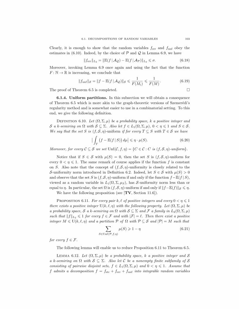
6.1. DECOMPOSITIONS OF RANDOM VARIABLES 103
Clearly, it is enough to show that the random variables ferr and funf obey the
estimates in (6.10). Indeed, by the choice of P and Q in Lemma 6.9, we have
‖ferr‖L2= ‖E(f | AQ)− E(f | AP)‖L2
6 σ. (6.18)
Moreover, invoking Lemma 6.9 once again and using the fact that the function
F : N→ R is increasing, we conclude that
‖funf‖S = ‖f − E(f | AQ)‖S 61
F (Mi)6
1
F (M). (6.19)
The proof of Theorem 6.5 is completed.
6.1.4. Uniform partitions. In this subsection we will obtain a consequence
of Theorem 6.5 which is more akin to the graph-theoretic versions of Szemeredi’s
regularity method and is somewhat easier to use in a combinatorial setting. To this
end, we give the following definition.
Definition 6.10. Let (Ω,Σ, µ) be a probability space, k a positive integer and
S a k-semiring on Ω with S ⊆ Σ. Also let f ∈ L1(Ω,Σ, µ), 0 < η 6 1 and S ∈ S.
We say that the set S is (f,S, η)-uniform if for every T ⊆ S with T ∈ S we have∣∣ ∫T
(f − E(f |S)
)dµ∣∣ 6 η · µ(S). (6.20)
Moreover, for every C ⊆ S we set Unf(C, f, η) = C ∈ C : C is (f,S, η)-uniform.
Notice that if S ∈ S with µ(S) = 0, then the set S is (f,S, η)-uniform for
every 0 < η 6 1. The same remark of course applies if the function f is constant
on S. Also note that the concept of (f,S, η)-uniformity is closely related to the
S-uniformity norm introduced in Definition 6.2. Indeed, let S ∈ S with µ(S) > 0
and observe that the set S is (f,S, η)-uniform if and only if the function f−E(f |S),
viewed as a random variable in L1(Ω,Σ, µS), has S-uniformity norm less than or
equal to η. In particular, the set Ω is (f,S, η)-uniform if and only if ‖f−E(f)‖S 6 η.
We have the following proposition (see [TV, Section 11.6]).
Proposition 6.11. For every pair k, ` of positive integers and every 0 < η 6 1
there exists a positive integer U(k, `, η) with the following property. Let (Ω,Σ, µ) be
a probability space, S a k-semiring on Ω with S ⊆ Σ and F a family in L2(Ω,Σ, µ)
such that ‖f‖L2 6 1 for every f ∈ F and with |F| = `. Then there exist a positive
integer M 6 U(k, `, η) and a partition P of Ω with P ⊆ S and |P| = M such that∑S∈Unf(P,f,η)
µ(S) > 1− η (6.21)
for every f ∈ F .
The following lemma will enable us to reduce Proposition 6.11 to Theorem 6.5.
Lemma 6.12. Let (Ω,Σ, µ) be a probability space, k a positive integer and Sa k-semiring on Ω with S ⊆ Σ. Also let C be a nonempty finite subfamily of Sconsisting of pairwise disjoint sets, f ∈ L1(Ω,Σ, µ) and 0 < η 6 1. Assume that
f admits a decomposition f = fstr + ferr + funf into integrable random variables
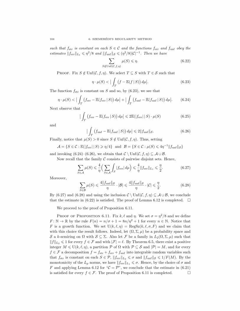
104 6. SZEMEREDI’S REGULARITY METHOD
such that fstr is constant on each S ∈ C and the functions ferr and funf obey the
estimates ‖ferr‖L16 η2/8 and ‖funf‖S 6 (η2/8)|C|−1. Then we have∑
S/∈Unf(C,f,η)
µ(S) 6 η. (6.22)
Proof. Fix S /∈ Unf(C, f, η). We select T ⊆ S with T ∈ S such that
η · µ(S) <∣∣ ∫T
(f − E(f |S)
)dµ∣∣. (6.23)
The function fstr is constant on S and so, by (6.23), we see that
η · µ(S) <∣∣ ∫T
(ferr − E(ferr |S)
)dµ∣∣+∣∣ ∫T
(funf − E(funf |S)
)dµ∣∣. (6.24)
Next observe that∣∣ ∫T
(ferr − E(ferr |S)
)dµ∣∣ 6 2E(|ferr| |S) · µ(S) (6.25)
and ∣∣ ∫T
(funf − E(funf |S)
)dµ∣∣ 6 2‖funf‖S . (6.26)
Finally, notice that µ(S) > 0 since S /∈ Unf(C, f, η). Thus, setting
A = S ∈ C : E(|ferr| |S) > η/4 and B = S ∈ C : µ(S) 6 4η−1‖funf‖S
and invoking (6.24)–(6.26), we obtain that C \Unf(C, f, η) ⊆ A ∪ B.
Now recall that the family C consists of pairwise disjoint sets. Hence,∑S∈A
µ(S) 64
η
(∑S∈A
∫S
|ferr| dµ)6
4
η‖ferr‖L1
6η
2. (6.27)
Moreover, ∑S∈B
µ(S) 64‖funf‖S
η· |B| 6 4‖funf‖S
η· |C| 6 η
2. (6.28)
By (6.27) and (6.28) and using the inclusion C \Unf(C, f, η) ⊆ A∪ B, we conclude
that the estimate in (6.22) is satisfied. The proof of Lemma 6.12 is completed.
We proceed to the proof of Proposition 6.11.
Proof of Proposition 6.11. Fix k, ` and η. We set σ = η2/8 and we define
F : N → R by the rule F (n) = n/σ + 1 = 8n/η2 + 1 for every n ∈ N. Notice that
F is a growth function. We set U(k, `, η) = RegSz(k, `, σ, F ) and we claim that
with this choice the result follows. Indeed, let (Ω,Σ, µ) be a probability space and
S a k-semiring on Ω with S ⊆ Σ. Also let F be a family in L2(Ω,Σ, µ) such that
‖f‖L26 1 for every f ∈ F and with |F| = `. By Theorem 6.5, there exist a positive
integer M 6 U(k, `, η), a partition P of Ω with P ⊆ S and |P| = M , and for every
f ∈ F a decomposition f = fstr + ferr + funf into integrable random variables such
that fstr is constant on each S ∈ P, ‖ferr‖L2 6 σ and ‖funf‖S 6 1/F (M). By the
monotonicity of the Lp norms, we have ‖ferr‖L16 σ. Hence, by the choice of σ and
F and applying Lemma 6.12 for “C = P”, we conclude that the estimate in (6.21)
is satisfied for every f ∈ F . The proof of Proposition 6.11 is completed.
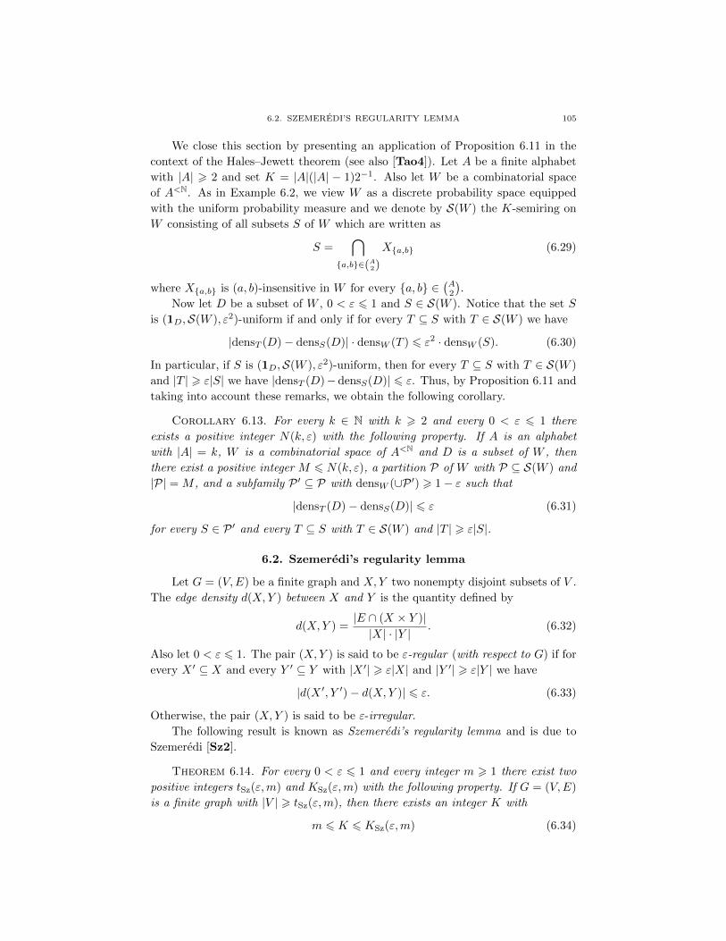
6.2. SZEMEREDI’S REGULARITY LEMMA 105
We close this section by presenting an application of Proposition 6.11 in the
context of the Hales–Jewett theorem (see also [Tao4]). Let A be a finite alphabet
with |A| > 2 and set K = |A|(|A| − 1)2−1. Also let W be a combinatorial space
of A<N. As in Example 6.2, we view W as a discrete probability space equipped
with the uniform probability measure and we denote by S(W ) the K-semiring on
W consisting of all subsets S of W which are written as
S =⋂
a,b∈(A2)
Xa,b (6.29)
where Xa,b is (a, b)-insensitive in W for every a, b ∈(A2
).
Now let D be a subset of W , 0 < ε 6 1 and S ∈ S(W ). Notice that the set S
is (1D,S(W ), ε2)-uniform if and only if for every T ⊆ S with T ∈ S(W ) we have
|densT (D)− densS(D)| · densW (T ) 6 ε2 · densW (S). (6.30)
In particular, if S is (1D,S(W ), ε2)-uniform, then for every T ⊆ S with T ∈ S(W )
and |T | > ε|S| we have |densT (D)−densS(D)| 6 ε. Thus, by Proposition 6.11 and
taking into account these remarks, we obtain the following corollary.
Corollary 6.13. For every k ∈ N with k > 2 and every 0 < ε 6 1 there
exists a positive integer N(k, ε) with the following property. If A is an alphabet
with |A| = k, W is a combinatorial space of A<N and D is a subset of W , then
there exist a positive integer M 6 N(k, ε), a partition P of W with P ⊆ S(W ) and
|P| = M , and a subfamily P ′ ⊆ P with densW (∪P ′) > 1− ε such that
|densT (D)− densS(D)| 6 ε (6.31)
for every S ∈ P ′ and every T ⊆ S with T ∈ S(W ) and |T | > ε|S|.
6.2. Szemeredi’s regularity lemma
Let G = (V,E) be a finite graph and X,Y two nonempty disjoint subsets of V .
The edge density d(X,Y ) between X and Y is the quantity defined by
d(X,Y ) =|E ∩ (X × Y )||X| · |Y |
. (6.32)
Also let 0 < ε 6 1. The pair (X,Y ) is said to be ε-regular (with respect to G) if for
every X ′ ⊆ X and every Y ′ ⊆ Y with |X ′| > ε|X| and |Y ′| > ε|Y | we have
|d(X ′, Y ′)− d(X,Y )| 6 ε. (6.33)
Otherwise, the pair (X,Y ) is said to be ε-irregular.
The following result is known as Szemeredi’s regularity lemma and is due to
Szemeredi [Sz2].
Theorem 6.14. For every 0 < ε 6 1 and every integer m > 1 there exist two
positive integers tSz(ε,m) and KSz(ε,m) with the following property. If G = (V,E)
is a finite graph with |V | > tSz(ε,m), then there exists an integer K with
m 6 K 6 KSz(ε,m) (6.34)
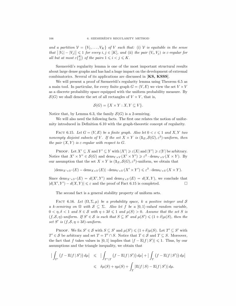
106 6. SZEMEREDI’S REGULARITY METHOD
and a partition V = V1, . . . , VK of V such that: (i) V is equitable in the sense
that∣∣ |Vi| − |Vj |∣∣ 6 1 for every i, j ∈ [K], and (ii) the pair (Vi, Vj) is ε-regular for
all but at most ε(K2
)of the pairs 1 6 i < j 6 K.
Szemeredi’s regularity lemma is one of the most important structural results
about large dense graphs and has had a huge impact on the development of extremal
combinatorics. Several of its applications are discussed in [KS, KSSS].
We will present a proof of Szemeredi’s regularity lemma using Theorem 6.5 as
a main tool. In particular, for every finite graph G = (V,E) we view the set V ×Vas a discrete probability space equipped with the uniform probability measure. By
S(G) we shall denote the set of all rectangles of V × V , that is,
S(G) = X × Y : X,Y ⊆ V .
Notice that, by Lemma 6.3, the family S(G) is a 2-semiring.
We will also need the following facts. The first one relates the notion of unifor-
mity introduced in Definition 6.10 with the graph-theoretic concept of regularity.
Fact 6.15. Let G = (V,E) be a finite graph. Also let 0 < ε 6 1 and X,Y two
nonempty disjoint subsets of V . If the set X × Y is (1E ,S(G), ε3)-uniform, then
the pair (X,Y ) is ε-regular with respect to G.
Proof. LetX ′ ⊆ X and Y ′ ⊆ Y with |X ′| > ε|X| and |Y ′| > ε|Y | be arbitrary.
Notice that X ′ × Y ′ ∈ S(G) and densV×V (X ′ × Y ′) > ε2 · densV×V (X × Y ). By
our assumption that the set X × Y is (1E ,S(G), ε3)-uniform, we obtain that
|densX′×Y ′(E)− densX×Y (E)| · densV×V (X ′ × Y ′) 6 ε3 · densV×V (X × Y ).
Since densX′×Y ′(E) = d(X ′, Y ′) and densX×Y (E) = d(X,Y ), we conclude that
|d(X ′, Y ′)− d(X,Y )| 6 ε and the proof of Fact 6.15 is completed.
The second fact is a general stability property of uniform sets.
Fact 6.16. Let (Ω,Σ, µ) be a probability space, k a positive integer and Sa k-semiring on Ω with S ⊆ Σ. Also let f be a [0, 1]-valued random variable,
0 < η, δ < 1 and S ∈ S with η + 3δ 6 1 and µ(S) > 0. Assume that the set S is
(f,S, η)-uniform. If S′ ∈ S is such that S ⊆ S′ and µ(S′) 6 (1 + δ)µ(S), then the
set S′ is (f,S, η + 3δ)-uniform.
Proof. We fix S′ ∈ S with S ⊆ S′ and µ(S′) 6 (1 + δ)µ(S). Let T ′ ⊆ S′ with
T ′ ∈ S be arbitrary and set T = T ′ ∩ S. Notice that T ∈ S and T ⊆ S. Moreover,
the fact that f takes values in [0, 1] implies that |f − E(f |S′)| 6 1. Thus, by our
assumptions and the triangle inequality, we obtain that∣∣ ∫T ′
(f − E(f |S′)
)dµ∣∣ 6 ∣∣ ∫
T ′\T
(f − E(f |S′)
)dµ∣∣+∣∣ ∫T
(f − E(f |S′)
)dµ∣∣
6 δµ(S) + ηµ(S) +
∫T
|E(f |S)− E(f |S′)| dµ.
6.2. SZEMEREDI’S REGULARITY LEMMA 107
Invoking once again the fact that the random variable f is [0, 1]-valued, we see that
|E(f |S)− E(f |S′)| 6 2µ(S′ \ S)/µ(S′). Therefore,∫T
|E(f |S)− E(f |S′)| dµ 6 2µ(S′ \ S)
µ(S′)· µ(T ) 6 2µ(S′ \ S) 6 2δµ(S).
Summing up, we conclude that∣∣ ∫T ′
(f − E(f |S′)
)dµ∣∣ 6 δµ(S) + ηµ(S) + 2δµ(S) 6 (η + 3δ)µ(S′)
and the proof of Fact 6.16 is completed.
The third, and last, fact will enable us to produce an equitable partition of the
vertex set V of a finite graph from a given partition of V × V .
Fact 6.17. Let M be a positive integer and 0 < θ 6 1/2. Also let V be a finite
set with |V | > 4Mθ−3 and P a partition of V × V into M sets of the form X × Ywhere X,Y ⊆ V . Then there exist a positive integer K with
(1− θ)θ−14M 6 K 6 2θ−14M , (6.35)
a family U = U1, . . . , UK of pairwise disjoint subsets of V and a partition
V = V1, . . . , VK of V such that: (i) |Ui| = bθ|V | · 4−Mc for every i ∈ [K],
(ii) the set Ui × Uj is contained in a (necessarily unique) element of P for every
i, j ∈ [K], (iii)∣∣ |Vi| − |Vj |∣∣ 6 1 for every i, j ∈ [K], (iv) Ui ⊆ Vi for every i ∈ [K],
and (v) |Vi| 6 (1 + 3θ)|Ui| for every i ∈ [K].
Proof. We write the partition P as Xi × Yi : i ∈ [M ]. Let A and B be the
sets of all nonempty atoms of the algebras generated by the families Xi : i ∈ [M ]and Yi : i ∈ [M ] respectively. We set R0 = A ∩ B : A ∈ A and B ∈ B and
we observe that R0 is a partition of V with |R0| 6 4M and such that the family
P ′ := X × Y : X,Y ∈ R0 is a refinement of P. Next, we partition every X ∈ R0
into disjoint sets of size N = bθ|V | ·4−Mc plus an error set of size at most N . (Since
|V | > 4Mθ−3 we have N > 1, and so such a partition is possible.) Let E0 be the
union of all the error sets and let U1, . . . , UK be the remaining sets. Notice that
|E0| 6 |R0|N 6 4MN 6 θ|V |.
In particular, we have
|V | − θ|V | 6 KN 6 |V | (6.36)
which is easily seen to imply the estimate on K in (6.35). Also observe that for
every i, j ∈ [K] there exist X,Y ∈ R0 such that Ui ⊆ X and Uj ⊆ Y . This implies,
of course, that Ui × Uj ⊆ X × Y ∈ P ′. Using the fact that P ′ is a refinement of
P, we obtain that Ui ×Uj is contained in a unique element of P. Thus, the family
U := U1, . . . , UK satisfies parts (i) and (ii).
We proceed to define the partition V. We break up the set E0 arbitrarily into K
sets E1, . . . , EK such that∣∣ |Ei|−|Ej |∣∣ 6 1 for every i, j ∈ [K] and we set Vi = Ui∪Ei
for every i ∈ [K]. It is then clear that the partition V := V1, . . . , VK satisfies parts
(iii) and (iv). To see that part (v) is also satisfied, let x = min|Ei| : i ∈ [K] and
108 6. SZEMEREDI’S REGULARITY METHOD
observe that x 6 |Ei| 6 x+1 for every i ∈ [K]. Notice that the family E1, . . . , EKis a partition of E0 and recall that 0 < θ 6 1/2. Hence,
Kx 6 θ|V |(6.36)
6 θ(1− θ)−1KN 6 2θKN.
which implies that 0 6 x 6 2θN . Using again the fact that 0 < θ 6 1/2 we see that
θ−2 − θ−1 > 1 and, in particular, that θ−1 6 bθ−2c. Since |V | > 4Mθ−3 we have
θN = θbθ|V | · 4−Mc > θbθ−2c > 1. Therefore, for every i ∈ [K] we obtain that
|Vi| = |Ui|+ |Vi \ Ui| = N + |Ei| 6 N + x+ 1 6 N + 3θN = (1 + 3θ)|Ui|.
The proof of Fact 6.17 is completed.
We are ready to give the proof of Theorem 6.14.
Proof of Theorem 6.14. We follow the proof from [Tao2]. Fix 0 < ε 6 1
and a positive integer m. Let
η =ε3
64, θ =
η
45mand σ =
η2
8(6.37)
and define F : N → R by the rule F (n) = σ−1(2θ−14n)2 for every n ∈ N. Notice
that F is a growth function. Finally, let
M0 = RegSz(2, 1, σ, F ) (6.38)
and set
tSz(ε,m) = d4M0θ−3e and KSz(ε,m) = b2θ−14M0c. (6.39)
We will show that tSz(ε,m) and KSz(ε,m) are as desired.
Let G = (V,E) be an arbitrary finite graph with |V | > tSz(ε,m). By Theorem
6.5 applied for the 2-semiring S(G) and the family F = 1E, there exist a positive
integer M 6 M0, a partition P of V × V with P ⊆ S(G) and |P| = M , and a
decomposition 1E = fstr + ferr + funf such that fstr is constant on each S ∈ P,
‖ferr‖L26 σ and ‖funf‖S 6 1/F (M). By the choice of tSz(ε,m) in (6.39) and the
fact that |P| = M 6 M0, we have |V | > 4Mθ−3. Thus, by Fact 6.17, there exist a
positive integer K with
(1− θ)θ−14M 6 K 6 2θ−14M , (6.40)
a family U = U1, . . . , UK of pairwise disjoint subsets of V and a partition
V = V1, . . . , VK of V satisfying parts (i)–(v) of Fact 6.17.
We claim that K and V satisfy the requirements of the theorem. Indeed, notice
first that, by (6.40) and the choice of θ and KSz(ε,m) in (6.37) and (6.39), we have
m 6 K 6 KSz(ε,m). Also let
D = Vi × Vj : 1 6 i < j 6 K and C = Ui × Uj : 1 6 i < j 6 K.
As in Definition 6.10, by Unf(D,1E , 2η) we denote the set of all Vi × Vj ∈ D such
that Vi×Vj is (1E ,S(G), 2η)-uniform. Respectively, Unf(C,1E , η) stands for set of
all Ui × Uj ∈ C such that Ui × Uj is (1E ,S(G), η)-uniform.
Let 1 6 i < j 6 K and assume that the pair (Vi, Vj) is ε-irregular. By (6.37),
we have 2η 6 ε3 and so, by Fact 6.15, we obtain that Vi × Vj /∈ Unf(D,1E , 2η).
Next observe that, by the choice of U and V, we have Ui × Uj ⊆ Vi × Vj and
6.3. A CONCENTRATION INEQUALITY FOR PRODUCT SPACES 109
|Vi × Vj | 6 (1 + 15θ)|Ui × Uj |. On the other hand, by (6.37), we have 45θ 6 η
and η+ 45θ 6 1. Thus, by Fact 6.16 and the previous discussion, we conclude that
Ui × Uj /∈ Unf(C,1E , η). Therefore, it is enough to show that
|C \Unf(C,1E , η)| 6 ε(K
2
). (6.41)
To this end, notice that C ⊆ S(G) is a collection of pairwise disjoint sets. Moreover,
for every Ui × Uj ∈ C we have
densV×V (Ui × Uj) =bθ|V | · 4−Mc2
|V |2>(θ4−M
2
)2 (6.40)
>(1− θ
2K
)2 (6.37)
> (4K)−2.
Invoking the definition of the growth function F , we also have
|C| 6 K2(6.40)
6 (2θ−14M )2 = σF (M)
and so ‖funf‖S 6 1/F (M) 6 σ|C|−1 = (η2/8)|C|−1. On the other hand, observe
that ‖ferr‖L16 ‖ferr‖L2
6 σ = η2/8. Hence, by Lemma 6.12 and the previous
estimates, we obtain that
|C \Unf(C,1E , η)| · (4K)−2 6∑
Ui×Uj /∈Unf(C,1E ,η)
densV×V (Ui × Uj) 6 η. (6.42)
Finally, by (6.37) and (6.40), we see that K > 2 which implies that K2 6 4(K2
).
Therefore, we conclude that
|C \Unf(C,1E , η)|(6.42)
6 16ηK2(6.37)
6ε
4K2 6 ε
(K
2
).
The proof of Theorem 6.14 is completed.
6.3. A concentration inequality for product spaces
6.3.1. The main result. In this section we will present a concentration
inequality for product spaces which asserts that every square-integrable random
variable defined on the product of sufficiently many probability spaces exhibits
pseudorandom behavior. Combinatorial applications will be discussed in Subsec-
tions 6.3.2 and 6.3.3.
First we introduce some notation concerning product spaces. Let n be a pos-
itive integer and let (Ω1,Σ1, µ1), . . . , (Ωn,Σn, µn) be a finite sequence of proba-
bility spaces. As in Example 6.1, by (Ω,Σ,µ) we shall denote their product,
while for every nonempty I ⊆ [n] by (ΩI ,ΣI ,µI) we shall denote the product
of the spaces 〈(Ωi,Σi, µi) : i ∈ I〉. (Recall that, by convention, Ω∅ stands for
the empty set.) If I ⊆ [n], x ∈ ΩI and y ∈ Ω[n]\I , then by (x,y) we shall de-
note the unique element z of Ω such that πI(z) = x and π[n]\I(z) = y. (Here,
πI : Ω → ΩI and π[n]\I : Ω → Ω[n]\I are the natural projections.) Finally, for
every function f : Ω → R and every x ∈ ΩI by fx : Ω[n]\I → R we shall denote
the map defined by fx(y) = f((x,y)
). Notice, in particular, that for every subset
A of Ω the function (1A)x coincides with the characteristic function of the section
Ax = y ∈ Ω[n]\I : (x,y) ∈ A of A at x.
110 6. SZEMEREDI’S REGULARITY METHOD
Now for every positive integer `, every 0 < σ 6 1 and every F : N→ N we set
ConcProd(`, σ, F ) = F (dσ−3`e)(1). (6.43)
The following theorem is the main result of this section.
Theorem 6.18. Let ` be a positive integer, 0 < σ 6 1 and F : N → N such
that F (m) > m + 1 for every m ∈ N. Also let n be a positive integer with
n > F(ConcProd(`, σ, F )
)+1 and let (Ω,Σ,µ) be the product of a finite sequence
(Ω1,Σ1, µ1), . . . , (Ωn,Σn, µn) of probability spaces. If F is a family in L2(Ω,Σ,µ)
such that ‖f‖L26 1 for every f ∈ F and with |F| = `, then there exists a positive
integer M with
M 6 ConcProd(`, σ, F ) (6.44)
such that for every nonempty I ⊆ M + 1, . . . , F (M) and every f ∈ F we have
µI(x ∈ ΩI : |E(fx)− E(f)| 6 σ
)> 1− σ. (6.45)
The proof of Theorem 6.18 is also based on Fact 6.6. Specifically, let m ∈ [n]
and recall that (Ω[m],Σ[m],µ[m]) stands for the product of the probability spaces
(Ω1,Σ1, µ1), . . . , (Ωm,Σm, µm). As in Example 6.1, we may “extend” the σ-algebra
Σ[m] to the full product Ω using the projection π[m]. Indeed, for every m ∈ [n] let
Bm =π−1
[m](A) : A ∈ Σ[m]
(6.46)
and observe that Bm = A × Ω[n]\[m] : A ∈ Σ[m] if m < n while Bn = Σ. It
follows that (Bm)nm=1 is an increasing finite sequence of sub-σ-algebras of Σ, and
so for every f ∈ L2(Ω,Σ,µ) with ‖f‖L2 6 1 the sequence E(f | B1), . . . ,E(f | Bn)
is a finite martingale which is contained in the unit ball of L2(Ω,Σ,µ). We have
the following property which is satisfied by all finite martingales of this form.
Lemma 6.19. Let l be a positive integer, 0 < η 6 1 and Φ: N → N such
that Φ(m) > m + 1 for every m ∈ N. Also let n ∈ N with n > Φ(dη−1le+1)(1).
Finally, let (Ω,Σ, µ) be a probability space, (Am)nm=1 an increasing finite sequence
of sub-σ-algebras of Σ and F a family in L2(Ω,Σ, µ) such that ‖f‖L2 6 1 for every
f ∈ F and with |F| = l. Then there exists a positive integer M with
M 6 Φ(dη−1le)(1) (6.47)
such that for every f ∈ F we have
‖E(f | AΦ(M))− E(f | AM )‖2L26 η. (6.48)
Proof. Assume that there is no positive integer M which satisfies (6.47) and
(6.48). This implies that for every M ∈ 1, . . . ,Φ(dη−1le)(1) there exists f ∈ F such
that ‖E(f | AΦ(M)) − E(f | AM )‖2L2> η. Therefore, for every i ∈ 1, . . . , dη−1le
we may select fi ∈ F such that ‖E(fi | AΦ(Mi))−E(fi | AMi)‖2L2
> η where M1 = 1
and Mi = Φ(Mi−1) = Φ(i−1)(1) if i > 2. By the classical pigeonhole principle,
there exist g ∈ F and a subset I of 1, . . . , dη−1le with |I| > dη−1le/|F| and such
that fi = g for every i ∈ I. Hence, by Fact 6.6, we obtain that
1 6 η|I| < ‖E(g | An)‖2L26 ‖g‖2L2
6 1
which is clearly a contradiction. The proof of Lemma 6.19 is completed.
6.3. A CONCENTRATION INEQUALITY FOR PRODUCT SPACES 111
We will also need the following lemma. In its proof, and in the rest of this
subsection, we will follow the common practice when proving inequalities and we
will ignore measurability issues since they can be easily resolved with standard
arguments.
Lemma 6.20. Let I ⊆ [n] and assume that both I and [n] \ I are nonempty.
Then for every g, h ∈ L2(Ω,Σ,µ) we have∫‖gx − hx‖2L1
dµI 6 ‖g − h‖2L2. (6.49)
Proof. By Fubini’s theorem, we see that
‖g − h‖2L2=
∫ (∫|gx − hx|2 dµ[n]\I
)dµI . (6.50)
On the other hand, by Jensen’s inequality, for every x ∈ ΩI we have
‖gx − hx‖2L1=(∫|gx − hx| dµ[n]\I
)2
6∫|gx − hx|2 dµ[n]\I (6.51)
and so, taking the average over all x ∈ ΩI and using (6.50), we conclude that the
estimate in (6.49) is satisfied. The proof of Lemma 6.20 is completed.
We are ready to give the proof of Theorem 6.18.
Proof of Theorem 6.18. Fix a family F in L2(Ω,Σ,µ) with ‖f‖L26 1 for
every f ∈ F and |F| = `. We apply Lemma 6.19 to the sequence (Bm)nm=1 defined
in (6.46), the family F and the constant “η = σ3”, and we obtain a positive integer
M 6 ConcProd(`, σ, F ) such that
‖E(f | BF (M))− E(f | BM )‖2L26 σ3 (6.52)
for every f ∈ F . We will show that the positive integer M is as desired.
Notice, first, that the estimate in (6.44) is satisfied. Next, fix a nonempty
subset I of M + 1, . . . , F (M) and let f ∈ F be arbitrary. We set
g = E(f | BF (M)) and h = E(f | BM ). (6.53)
We have the following claim.
Claim 6.21. For every x ∈ ΩI we have E(gx) = E(fx) and E(hx) = E(f).
Proof of Claim 6.21. Fix x ∈ ΩI . Since I ⊆ [F (M)], by (6.53) and Fubini’s
theorem, we see that for every y ∈ Ω[F (M)]\I the function g(x,y) : Ω[n]\[F (M)] → Ris constant and equal to E(f(x,y)). Therefore,
E(gx) =
∫gx dµ[n]\I =
∫ (∫g(x,y) dµ[n]\[F (M)]
)dµ[F (M)]\I
=
∫E(f(x,y)) dµ[F (M)]\I
=
∫ (∫f(x,y) dµ[n]\[F (M)]
)dµ[F (M)]\I
=
∫fx dµ[n]\I = E(fx).
112 6. SZEMEREDI’S REGULARITY METHOD
We proceed to show that E(hx) = E(f). As above we observe that, by (6.53) and
Fubini’s theorem, for every z ∈ Ω[M ] the function hz : Ω[n]\[M ] → R is constant
and equal to E(fz). Since I ∩ [M ] = ∅, the function h(x,z) : Ω[n]\(I∪[M ]) → R is also
constant and equal to E(fz). Hence,
E(hx) =
∫hx dµ[n]\I =
∫ (∫h(x,z) dµ[n]\(I∪[M ])
)dµ[M ]
=
∫E(fz) dµ[M ] = E(f).
The proof of Claim 6.21 is completed.
By Claim 6.21, for every x ∈ ΩI we have
|E(fx)− E(f)| =∣∣ ∫ (gx − hx) dµ[n]\I
∣∣ 6 ‖gx − hx‖L1
and so, by (6.52), (6.53) and Lemma 6.20, we obtain that∫|E(fx)− E(f)|2 dµI 6 σ3. (6.54)
By Markov’s inequality, we conclude that
µI(x ∈ ΩI : |E(fx)− E(f)| 6 σ
)> 1− σ (6.55)
and the proof of Theorem 6.18 is completed.
6.3.2. Combinatorial spaces. In the last two subsections we will present
two combinatorial applications of Theorem 6.18. The first one is in the context of
the Hales–Jewett theorem and asserts that every dense subset of a high-dimensional
hypercube can be effectively modeled as a family of measurable events indexed by
the elements of another hypercube of smaller, but large enough, dimension. Related
results will also be obtained in Chapters 8 and 9.
We proceed to the details. Let k, `,m be positive integers with k > 2 and
0 < ε 6 1. We set
σ = minε, k−m/2 (6.56)
and we define F : N→ N by the rule F (n) = n+m for every n ∈ N. Finally, let
RegSp(k, `,m, ε) = F(ConcProd(`, σ, F )
)+ 1. (6.57)
We have the following lemma.
Lemma 6.22. Let k, `,m be positive integers with k > 2 and 0 < ε 6 1. Also
let A be an alphabet with |A| = k and n > RegSp(k, `,m, ε). If F is a family of
subsets of An with |F| = `, then there exists an interval I ⊆ l ∈ N : l < n with
|I| = m such that for every D ∈ F and every t ∈ AI we have
|dens(Dt)− dens(D)| 6 ε (6.58)
where Dt = s ∈ Al∈N : l<n\I : (t, s) ∈ D is the section of D at t.
6.3. A CONCENTRATION INEQUALITY FOR PRODUCT SPACES 113
Proof. We view the sets A and An as discrete probability spaces equipped
with their uniform probability measures. Notice, in particular, that the probability
space An is the product of n many copies of A. Hence, by (6.57) and Theorem
6.18, if F is a family of subsets of An with |F| = `, then there exists an interval
I ⊆ l ∈ N : l < n with |I| = m such that for every D ∈ F we have
dens(t ∈ AI : |dens(Dt)− dens(D)| 6 σ
)> 1− σ
(6.56)
> 1− k−m/2
which implies, of course, that |dens(Dt) − dens(D)| 6 σ for every t ∈ AI . Since
σ 6 ε we conclude that the estimate in (6.58) is satisfied and the proof of Lemma
6.22 is completed.
6.3.3. Carlson–Simpson spaces. We proceed to discuss the analogue of
Lemma 6.22 in the context of the Carlson–Simpson theorem. To this end, we need
the following definition.
Definition 6.23. Let A be a finite alphabet with |A| > 2 and F a family of
subsets of A<N. Also let 0 < ε 6 1 and J a nonempty finite subset of N. We say
that the family F is (ε, J)-regular provided that for every D ∈ F , every n ∈ J ,
every (possibly empty) I ⊆ j ∈ J : j < n and every t ∈ AI we have
|dens(s ∈ Al∈N : l<n\I : (t, s) ∈ D
)− densAn(D)| 6 ε. (6.59)
Notice that for every t ∈ AI the set s ∈ Al∈N : l<n\I : (t, s) ∈ D is just the
section of the set D ∩An at t. Therefore, Definition 6.23 guarantees that for every
D ∈ F, every n ∈ J and every I ⊆ j ∈ J : j < n the density of the sections of
D ∩An along elements of AI are essentially equal to the density of D ∩An.
We also need to introduce some numerical invariants. Specifically, let k, `,m
be positive integers with k > 2 and 0 < ε 6 1. We define h : N→ N recursively by
the rule h(0) = h(1) = 1,
h(i+ 1) = RegSp(k, `, h(i), ε)(6.60)
where RegSp(k, `, h(i), ε) is as in (6.57), and we set
RegCS(k, `,m, ε) = h(m). (6.61)
The following lemma is the main result of this subsection.
Lemma 6.24. Let k, `,m be positive integers with k > 2 and 0 < ε 6 1.
Also let A be an alphabet with |A| = k and let J0 be a finite subset of N with
|J0| > RegCS(k, `,m, ε). If F a family of subsets of A<N with |F| = `, then there
exists a subset J of J0 with |J | = m such that the family F is (ε, J)-regular.
The proof of Lemma 6.24 is based on the following refinement of Lemma 6.22.
Sublemma 6.25. Let k, `, r be positive integers with k > 2 and 0 < ε 6 1.
Also let A be an alphabet with |A| = k and let J be a finite subset of N with
|J | > RegSp(k, `, r, ε). We set p = max(J). If F is a family of subsets of Ap with
114 6. SZEMEREDI’S REGULARITY METHOD
|F| = `, then there exists a subset J ′ of J \ p with |J ′| = r such that for every
D ∈ F , every subset I of J ′ and every t ∈ AI we have
|dens(s ∈ Al∈N : l<p\I : (t, s) ∈ D
)− densAp(D)| 6 ε. (6.62)
Proof. First, recall that RegSp(k, `, r, ε) = F(ConcProd(`, σ, F )
)+ 1 where
σ = minε, k−r/2 and F : N→ N is defined by F (i) = i+ r for every i ∈ N. Next
let n = |J | and observe that
n > RegSp(k, `, r, ε) = F(ConcProd
(`, σ, F )
)+ 1. (6.63)
In particular, we have n > 2. Let j1 < · · · < jn be the increasing enumeration of J
and set J∗ = J \ p = j1, . . . , jn−1. We view the sets Ap, Aji, . . . , Ajn−1 and
Al∈N : l<p\J∗ as discrete probability spaces equipped with their uniform probabil-
ity measures and, as in the proof of Lemma 6.22, we observe that the probability
space Ap is naturally identified with the product of the spaces Aji, . . . , Ajn−1
and Al∈N : l<p\J∗ . By Theorem 6.18 and (6.63), if F is a family of subsets of Ap
with |F| = `, then there exists J ′ ⊆ j1, . . . , jn−1 = J \ p with |J ′| = r such
that for every D ∈ F and every nonempty I ⊆ J ′, the set of all t ∈ AI satisfying
|dens(s ∈ Al∈N : l<p\I : (t, s) ∈ D
)− densAp(D)| 6 σ.
has density at least 1−σ. Using the fact that σ = minε, k−r/2, we conclude that
for every D ∈ F , every nonempty I ⊆ J ′ and every t ∈ AI we have
|dens(s ∈ Al∈N : l<p\I : (t, s) ∈ D
)− densAp(D)| 6 ε.
Since the estimate in (6.62) is automatically satisfied if I is empty, the proof of
Sublemma 6.25 is completed.
We are ready to give the proof of Lemma 6.24.
Proof of Lemma 6.24. Clearly, we may assume that m > 2. We fix a family
F of subsets of A<N with |F| = `. Recursively and using Sublemma 6.25, we select
a finite sequence J1, . . . , Jm−1 of subsets of J0 such that for every i ∈ [m − 1] the
following are satisfied.
(C1) We have |Ji| = h(m− i) where h is as in (6.60).
(C2) The set Ji is a subset of Ji−1 \ max(Ji−1).(C3) For every D ∈ F , every subset I of Ji and every t ∈ AI we have
|dens(s ∈ Al∈N : l<pi−1\I : (t, s) ∈ D
)− densApi−1 (D)| 6 ε
where pi−1 = max(Ji−1).
We set J = max(Jm−1), . . . ,max(J0)
. Using (C2) and (C3), we see that J is a
subset of J0 with |J | = m and such that the family F is (ε, J)-regular. The proof
of Lemma 6.24 is thus completed.
6.4. NOTES AND REMARKS 115
6.4. Notes and remarks
6.4.1. As we have already mentioned, Theorem 6.5 is due to Tao [Tao1, Tao2].
His approach, however, is somewhat different since he works with σ-algebras instead
of k-semirings. Our presentation follows [DKKa].
The idea to obtain uniformity estimates with respect to an arbitrary growth
function appeared first in [AFKS] and has been also considered by several other
authors (see, e.g., [LS, RSc1]). This particular feature of Theorem 6.5 is essential
when one needs to iterate this structural decomposition.
6.4.2. A weaker version of Theorem 6.14, restricted to bipartite graphs, was
first introduced in [Sz1] where it was used as a tool in the proof of Szemeredi’s
theorem on arithmetic progressions. The current form of Szemeredi’s regularity
lemma was obtained somewhat later in [Sz2].
We also note that the proof of Theorem 6.14 that we presented yields that the
numbers KSz(ε,m) are upper bounded by a primitive recursive function belonging
to the class E4. It is possible to obtain slightly better estimates by proceeding
with a more direct—but still probabilistic—argument (see, e.g., [ASp]). We point
out, however, that this tower-type dependence is actually necessary. Specifically, in
[Go2] examples were given of graphs for which any equitable partition satisfying
the second part of Theorem 6.14 has cardinality at least γ, where γ is a tower of
twos of height proportional to ε−1/16.
6.4.3. Theorem 6.18 is an abstract version of Lemma 3.2 in [DKT3]. Lemmas
6.22 and 6.24 are taken from [DKT3].
6.4.4. We remark that Theorems 6.5 and 6.18 can be extended to finite families
of random variables in Lp for any p > 1. (Of course, the corresponding bounds
will also depend upon the choice p.) These extensions are based on inequalities for
martingale difference sequences in Lp spaces (see [DKKa] and [DKT5] for details).

CHAPTER 7
The removal lemma
The removal lemma is a powerful result with several consequences in Ramsey
theory. It originates from the work of Ruzsa and Szemeredi in [RS], though its
full combinatorial strength was obtained much later by Gowers [Go5] and, inde-
pendently, by Nagle, Rodl, Schacht and Skokan [NRS, RSk]. However, as in the
case of Szemeredi’s regularity lemma, it also has a probabilistic formulation which
refers to the following natural measure-theoretic structures.
Definition 7.1. A hypergraph system is a triple
H = (n, 〈(Ωi,Σi, µi) : i ∈ [n]〉,H) (7.1)
where n is a positive integer, 〈(Ωi,Σi, µi) : i ∈ [n]〉 is a finite sequence of probability
spaces and H is a hypergraph on [n]. If the hypergraph H is r-uniform, then H
will be called an r-uniform hypergraph system.
For every hypergraph system H = (n, 〈(Ωi,Σi, µi) : i ∈ [n]〉,H) by (Ω,Σ,µ)
we shall denote the product of the spaces 〈(Ωi,Σi, µi) : i ∈ [n]〉. Moreover, as in
Example 6.1, for every nonempty e ⊆ [n] let (Ωe,Σe,µe) be the product of the
spaces 〈(Ωi,Σi, µi) : i ∈ e〉 and recall that the σ-algebra Σe can be “lifted” to the
full product Ω via the formula
Be =π−1e (A) : A ∈ Σe
(7.2)
where πe : Ω → Ωe is the natural projection. By convention, we set B∅ = ∅,Ω.The following theorem is the main result of this chapter and is due to Tao [Tao1].
Theorem 7.2. For every n, r ∈ N with n > r > 2 and every 0 < ε 6 1
there exist a strictly positive constant δ(n, r, ε) and a positive integer K(n, r, ε) with
the following property. Let H = (n, 〈(Ωi,Σi, µi) : i ∈ [n]〉,H) be an r-uniform
hypergraph system and for every e ∈ H let Ee ∈ Be such that
µ( ⋂e∈H
Ee
)6 δ(n, r, ε). (7.3)
Then for every e ∈ H there exists Fe ∈ Be with
µ(Ee \ Fe) 6 ε and⋂e∈H
Fe = ∅. (7.4)
Moreover, there exists a collection 〈Pe′ : e′ ⊆ e for some e ∈ H〉 of partitions of Ω
such that: (i) Pe′ ⊆ Be′ and |Pe′ | 6 K(n, r, ε) for every e′ ⊆ e ∈ H, and (ii) for
every e ∈ H the set Fe belongs to the algebra generated by the family⋃e′ e Pe′ .
117
118 7. THE REMOVAL LEMMA
The proof of Theorem 7.2 is effective and follows a method first implemented
by Ruzsa and Szemeredi [RS]. It consists of two parts. The first part is a regular-
ity lemma for hypergraph systems which follows from a multidimensional version
of Theorem 6.5. The second part is a “counting lemma” which enables us to esti-
mate the probability of various events similar to those that appear in (7.3). These
preparatory steps are presented in Sections 7.1, 7.2 and 7.3. The proof of Theorem
7.2 is completed in Section 7.4 while in Section 7.5 we discuss applications.
7.1. A multidimensional version of Theorem 6.5
Let Ω be a nonempty set. As in Appendix E, for every finite partition P of Ω
by AP we shall denote the algebra on Ω generated by P. Moreover, for every finite
tuple C = (C1, . . . , Cd) of families of subsets of Ω and every nonempty I ⊆ [d] set
CI =⋂i∈I
Ci : Ci ∈ Ci for every i ∈ I. (7.5)
Note that, by Lemma 6.3, if S = (S1, . . . ,Sd) consists of k-semirings on Ω (where
k is a positive integer), then SI is a (k · |I|)-semiring on Ω. On the other hand, if
P = (P1, . . . ,Pd) is a tuple of finite partitions of Ω with Pi ⊆ Si for every i ∈ [d],
then the family PI is also a finite partition of Ω which is contained in SI .The following theorem is a multidimensional version of Theorem 6.5 and is the
main result in this section. Recall that a growth function is an increasing function
F : N→ R which satisfies F (n) > n+ 1 for every n ∈ N.
Theorem 7.3. Let k, d, ` be positive integers, 0 < σ 6 1 and F : N → R a
growth function. Also let (Ω,Σ, µ) be a probability space and S = (S1, . . . ,Sd) a
d-tuple of k-semirings on Ω with Si ⊆ Σ for every i ∈ [d]. Finally, let F be a family
in L2(Ω,Σ, µ) with ‖f‖L26 1 for every f ∈ F and |F| = `. Then there exist
(a) a positive integer M with M 6 RegSz(k, ` · 2d, σ, F ),
(b) a d-tuple P = (P1, . . . ,Pd) of finite partitions of Ω with Pi ⊆ Si and
|Pi| 6M for every i ∈ [d], and
(c) a d-tuple Q = (Q1, . . . ,Qd) where Qi is a finite refinement of Pi with
Qi ⊆ Si for every i ∈ [d]
with the following property. For every f ∈ F and every nonempty subset I of [d],
letting SI , PI and QI be as in (7.5) and writing f = f Istr + f Ierr + f Iunf where
f Istr = E(f | API ), fIerr = E(f | AQI
)−E(f | API ) and f Iunf = f−E(f | AQI), (7.6)
we have the estimates
‖f Ierr‖L26 σ and ‖f Iunf‖SI 6
1
F (M)(7.7)
where ‖ · ‖SI is the uniformity norm associated with the (k · |I|)-semiring SI .
The main point in Theorem 7.3 is that one can decompose a finite family of
random variables by using two collections of partitions which are implicated in the
same way as the corresponding semirings. This additional coherence property is
needed for the proof of Theorem 7.2.
7.1. A MULTIDIMENSIONAL VERSION OF THEOREM 6.5 119
In spite of being stronger, Theorem 7.3 follows the same strategy as the proof
of Theorem 6.5. In particular, the reader is advised to review at this point the
material in Subsection 6.1.3.
It is convenient to introduce the following notation. Let k, d be positive integers,
Ω a nonempty set and S = (S1, . . . ,Sd) a d-tuple of k-semirings on Ω. Also let
P = (P1, . . . ,Pd) be a d-tuple of finite partitions of Ω with Pi ⊆ Si for every i ∈ [d].
For every N ∈ N by ΠNS (P) we shall denote the set of all d-tuples Q = (Q1, . . . ,Qd)
such that for every i ∈ [d] we have: (i) Qi ⊆ Si, (ii) Qi is a refinement of Pi, and
(iii) |Qi| 6 |Pi|(k + 1)N . We have the following variant of Lemma 6.7.
Lemma 7.4. Let k, d be positive integers and 0 < δ 6 1. Also let (Ω,Σ, µ) be a
probability space, S = (S1, . . . ,Sd) a d-tuple of k-semirings on Ω with Si ⊆ Σ for
every i ∈ [d] and Q = (Q1, . . . ,Qd) a d-tuple of finite partitions of Ω with Qi ⊆ Sifor every i ∈ [d]. Finally, let f ∈ L2(Ω,Σ, µ) and let I ⊆ [d] be nonempty, and
assume that ‖f − E(f | AQI)‖SI > δ. Then there exists R ∈ Π1
S(Q) such that
‖E(f | ARI)− E(f | AQI
)‖L2 > δ.
Proof. We select S ∈ SI such that∣∣ ∫S
(f − E(f | AQI
))dµ∣∣ > δ. (7.8)
By (7.5), for every i ∈ I there exists Si ∈ Si such that
S =⋂i∈I
Si.
The d-tuple S = (S1, . . . ,Sd) consists of k-semirings on Ω, and so there exists
R = (R1, . . . ,Rd) ∈ Π1S(Q) such that Si ∈ ARi for every i ∈ I. Therefore, we
have S ∈ ARIand, consequently,∫
S
E(f | ARI) dµ =
∫S
f dµ. (7.9)
By (7.8), (7.9) and the monotonicity of the Lp norms, we conclude that
‖E(f | ARI)− E(f | AQI
)‖L2 > δ
and the proof of Lemma 7.4 is completed.
The next lemma follows arguing precisely as in the proof of Lemma 6.8 and
using Lemma 7.4 instead of Lemma 6.7.
Lemma 7.5. Let k, d, ` be positive integers, 0<δ, σ 6 1 and set N=dσ2δ−2` 2de.Also let (Ω,Σ, µ) be a probability space, S = (S1, . . . ,Sd) a d-tuple of k-semirings on
Ω with Si ⊆ Σ for every i ∈ [d] and P = (P1, . . . ,Pd) a d-tuple of finite partitions
of Ω with Pi ⊆ Si for every i ∈ [d]. Finally, let F be a family in L2(Ω,Σ, µ) with
|F| = `. Then there exists Q ∈ ΠNS (P) such that either
(a) ‖E(f | AQI) − E(f | API )‖L2
> σ for some f ∈ F and some nonempty
subset I of [d], or
(b) ‖E(f | AQI) − E(f | API )‖L2 6 σ and ‖f − E(f | AQI
)‖SI 6 δ for every
f ∈ F and every nonempty subset I of [d].
120 7. THE REMOVAL LEMMA
The last step towards the proof of Theorem 7.3 is the following analogue of
Lemma 6.9. Its proof is identical to that of Lemma 6.9.
Lemma 7.6. Let k, d, ` be positive integers, 0 < σ 6 1 and F : N → R a
growth function. Set L = dσ−2` 2de and define two sequences (Nj) and (Mj) in Nrecursively by the rule
N0 = 0 and M0 = 1,
Nj+1 = dσ2F (Mj)2` 2de and Mj+1 = Mj(k + 1)Nj+1 .
(7.10)
Let (Ω,Σ, µ) be a probability space and S = (S1, . . . ,Sd) a d-tuple of k-semirings
on Ω with Si ⊆ Σ for every i ∈ [d]. Also let F be a family in L2(Ω,Σ, µ) such that
‖f‖L2 6 1 for every f ∈ F and with |F| = `. Then there exist j ∈ 0, . . . , L − 1,a d-tuple P = (P1, . . . ,Pd) of partitions of Ω with Pi ⊆ Si and |Pi| 6 Mj for
every i ∈ [d], and Q ∈ ΠNj+1
S (P) such that ‖E(f | AQI) − E(f | API )‖L2
6 σ and
‖f − E(f | AQI)‖SI 6 1/F (Mj) for every f ∈ F and every nonempty I ⊆ [d].
We are ready to give the proof of Theorem 7.3.
Proof of Theorem 7.3. Fix the positive integers k, d, `, the constant σ and
the growth function F . Let j,P and Q be as in Lemma 7.6 and set M = Mj . We
claim that M,P and Q are as desired. Indeed, let h : N → N be the map defined
in (6.7) for the parameters k, ` · 2d, σ and F . By (7.10), we have Mj = h(j) and so
M = Mj 6Mdσ−2` 2de = h(dσ−2` 2de) (6.8)= RegSz(k, ` · 2d, σ, F ).
Therefore, by Lemma 7.6, we see that M,P and Q satisfy the requirements of the
theorem. Finally, notice the estimate in (7.7) is an immediate consequence of (7.6)
and Lemma 7.6. The proof of Theorem 7.3 is completed.
7.2. A regularity lemma for hypergraph systems
In this section we will present the first main step of the proof of Theorem
7.2. Specifically, given a uniform hypergraph system H and a finite collection Cof measurable events of its product space Ω, we will produce a sequence of finite
partitions which can be considered as “approximations” of the given events. These
partitions are contained in gradually smaller σ-algebras (hence, we improve upon
the measurability of the members of C), while at the same time we keep strong
control on the error terms of the “approximations”.
We proceed to the details. For every hypergraph G and every e ∈ G let
∂e = e′ ⊆ e : |e′| = |e| − 1 (7.11)
and set
∂G = e′ : e′ ∈ ∂e for some e ∈ G. (7.12)
Clearly, if G is k-uniform for some k > 1, then ∂G is (k − 1)-uniform. Next, for
every r-uniform hypergraph system H = (n, 〈(Ωi,Σi, µi) : i ∈ [n]〉,H) we define a
finite sequence H0, . . . ,Hr of hypergraphs on [n] recursively by the rule
Hr = H and Hj = ∂Hj+1. (7.13)
7.2. A REGULARITY LEMMA FOR HYPERGRAPH SYSTEMS 121
Notice that Hj is j-uniform for every j ∈ 0, . . . , r. Moreover, if r > 2, then as in
Example 6.1 for every j ∈ 2, . . . , r and every e ∈ Hj let
S∂e = ⋂e′∈∂e
Ae′ : Ae′ ∈ Be′ for every e′ ∈ ∂e
(7.14)
and recall that S∂e is a j-semiring on Ω. Note that S∂e ⊆ Be.We also need to introduce some numerical invariants. Let n be an integer with
n > 2 and let F : N→ R be a growth function. First, for every m ∈ N we define a
function Gm,F : N→ R by setting Gm,F (x) = F (F (m) +x) for every x ∈ N. Notice
that Gm,F is a growth function. Next, for every r ∈ 2, . . . , n and every 0 < σ 6 1
we define a growth function φn,r,σ,F : N→ R by
φn,r,σ,F (m) = F (m) + RegSz(1,m · nr · 2n
r−1
, σ,Gm,F)
(7.15)
where RegSz(1,m · nr · 2nr−1
, σ,Gm,F ) is as in (6.8). Finally, we define two finite
sequences of growth functions (Fn,r)nr=2 and (Φn,r,F )nr=2 recursively by the rule
Fn,2(m) = F (2)(m) and Φn,2,F (m) = φn,2,1/F (m),Fn,2(m),
Fn,r(m) = F (2)(Φn,r−1,F (m)
),
Φn,r,F (m) = Φn,r−1,F
(φn,r,1/F (m),Fn,r(m)
).
(7.16)
We have the following lemma.
Lemma 7.7. Let n, r ∈ N with n > r > 2 and F : N → R a growth function.
Also let H = (n, 〈(Ωi,Σi, µi) : i ∈ [n]〉,H) be an r-uniform hypergraph system and
let H0, . . . ,Hr be as in (7.13). Finally, let Mr be a positive integer and for every
e ∈ Hr let Pe be a partition of Ω with Pe ⊆ Be and |Pe| 6 Mr. Then there exist:
(i) a finite sequence (Mj)r−1j=1 of positive integers with
Mr 6 F (Mr) 6Mr−1 6 F (Mr−1) 6 · · · 6M1 6 Φn,r,F (Mr), (7.17)
(ii) for every j ∈ [r − 1] and every e′ ∈ Hj a partition Pe′ of Ω with Pe′ ⊆ Be′ and
|Pe′ | 6Mj, and (iii) for every j ∈ [r− 1] and every e′ ∈ Hj a finite refinement Qe′of Pe′ with Qe′ ⊆ Be′ , such that the following hold. Fix j ∈ 2, . . . , r and e ∈ Hj.Let S∂e be the j-semiring defined in (7.14) and consider the finite partitions
P∂e = ⋂e′∈∂e
Ae′ : Ae′ ∈ Pe′ for every e′ ∈ ∂e
(7.18)
and
Q∂e = ⋂e′∈∂e
Ae′ : Ae′ ∈ Qe′ for every e′ ∈ ∂e. (7.19)
Then for every A ∈ Pe, writing 1A = sA + bA + uA with
sA = E(1A | AP∂e), bA = E(1A | AQ∂e)− E(1A | AP∂e)and uA = 1A − E(1A | AQ∂e), (7.20)
we have the estimates
‖bA‖L26
1
F (Mj)and ‖uA‖S∂e 6
1
F (M0)(7.21)
where M0 = F (M1).
122 7. THE REMOVAL LEMMA
Proof. By induction on r. The initial case “r = 2” is identical to the general
one, and so let r > 3 and assume that the result has been proved up to r − 1.
Let n be a positive integer with n > r and fix an r-uniform hypergraph system
H = (n, 〈(Ωi,Σi, µi) : i ∈ [n]〉,H). Also let F be a growth function, Mr a positive
integer and for every e ∈ Hr let Pe be a partition of Ω with Pe ⊆ Be and |Pe| 6Mr.
Set F = 1A : A ∈ Pe for some e ∈ Hr and observe that F is a family in
L2(Ω,Σ,µ) with ‖f‖L26 1 for every f ∈ F and |F| 6Mr · |Hr| 6Mr · nr. Next,
let B = 〈Be′ : e′ ∈ Hr−1〉 and notice that B is a collection of 1-semirings on Ω;
moreover, |Hr−1| 6 nr−1. Finally, let Fn,r be as in (7.16) and recall that GMr,Fn,r
stands for the growth function defined by GMr,Fn,r(x) = Fn,r(Fn,r(Mr) + x). We
apply Theorem 7.3 for σ = 1/F (Mr), the growth function GMr,Fn,r , the collection
B and the family F and we obtain: (i) a positive integer M with
M 6 RegSz(1,Mr · nr · 2n
r−1
, 1/F (Mr), GMr,Fn,r
), (7.22)
(ii) two collections 〈Pe′ : e′ ∈ Hr−1〉 and 〈Qe′ : e′ ∈ Hr−1〉 of finite partitions
of Ω, and (iii) for every f ∈ F and every nonempty I ⊆ Hr−1 a decomposition
f = f Istr + f Ierr + f Iunf as described Theorem 7.3. Note that if e ∈ Hr and A ∈ Pe,then the family B∂e defined in (7.5) for I = ∂e coincides with the r-semiring S∂edefined in (7.14) and, moreover, (1A)∂estr = sA, (1A)∂eerr = bA and (1A)∂eunf = uA. Set
Mr−1 = Fn,r(Mr) +M. (7.23)
Since GMr,Fn,r (M) = Fn,r(Mr−1), it follows from the previous discussion and (7.7)
that for every e ∈ Hr and every A ∈ Pe we have
‖bA‖L26
1
F (Mr)and ‖uA‖S∂e 6
1
Fn,r(Mr−1). (7.24)
On the other hand, by (7.15), (7.22) and (7.23), we obtain that
Mr 6 F (Mr) 6Mr−1 6 φn,r,1/F (Mr),Fn,r(Mr). (7.25)
Next, we apply our inductive assumptions to the (r − 1)-uniform hypergraph
system Hr−1 = (n, 〈(Ωi,Σi, µi) : i ∈ [n]〉,Hr−1), the positive integer Mr−1 and
the collection of partitions 〈Pe′ : e′ ∈ Hr−1〉 and we obtain: (iv) a finite sequence
(Mj)r−2j=1 of positive integers with
Mr−1 6 F (Mr−1) 6 · · · 6M1 6 Φn,r−1,F (Mr−1), (7.26)
(v) two collections 〈Pe′ : e′ ∈ H1 ∪ · · · ∪ Hr−2〉 and 〈Qe′ : e′ ∈ H1 ∪ · · · ∪ Hr−2〉 of
finite partitions of Ω, and (vi) for every j ∈ 2, . . . , r− 1, every e′ ∈ Hj and every
A ∈ Pe′ a decomposition 1A = sA + bA + uA where sA, bA, and uA are as in (7.20)
and satisfy the estimates in (7.21). By (7.24) and (7.26), it is enough to show that
F (M0) 6 Fn,r(Mr−1) and M1 6 Φn,r,F (Mr). Indeed, since F is increasing, we have
F (M0) = F (2)(M1)(7.26)
6 F (2)(Φn,r−1,F (Mr−1)
) (7.16)= Fn,r(Mr−1).
Moreover,
M1
(7.26)
6 Φn,r−1,F (Mr−1)(7.25)
6 Φn,r−1,F
(φn,r,1/F (Mr),Fn,r(Mr)
) (7.16)= Φn,r,F (Mr)
and the proof of Lemma 7.7 is completed.
7.3. A COUNTING LEMMA FOR HYPERGRAPH SYSTEMS 123
7.3. A counting lemma for hypergraph systems
First we introduce some terminology and some pieces of notation. We say that
a hypergraph G is closed under set inclusion if for every g ∈ G and every g′ ⊆ g we
have g′ ∈ G. Moreover, we define the downwards closure of G by the rule
G = g′ : g′ ⊆ g for some g ∈ G. (7.27)
That is, G is the smallest hypergraph containing G and closed under set inclusion.
Now let n, r ∈ N with n > r > 2 and H = (n, 〈(Ωi,Σi, µi) : i ∈ [n]〉,H) an
r-uniform hypergraph system. Write H = H0 ∪ · · · ∪ Hr where H0, . . . ,Hr are as
in (7.13), and let P∅ = Ω. These data will be fixed throughout this section.
Assume that we are given a growth function F , a positive integer Mr and for
every e ∈ Hr a partition Pe of Ω with Pe ⊆ Be and |Pe| 6 Mr. Then, by applying
Lemma 7.7 to F,Mr and 〈Pe : e ∈ Hr〉, we obtain: (i) a finite sequence (Mj)r−1j=1
of positive integers, (ii) a collection 〈Pe′ : e′ ∈ H1 ∪ · · · ∪ Hr−1〉 of partitions of Ω,
and (iii) for every j ∈ 2, . . . , r, every e ∈ Hj and every A ∈ Pe a decomposition
1A = sA + bA + uA as described in Lemma 7.7. We enlarge the collection in (ii) by
attaching the initial partitions 〈Pe : e ∈ Hr〉 and P∅, and we obtain a new collection
〈Pe : e ∈ H〉 which is indexed by the downwards closure of H. This new collection
in turn generates a finite partition of Ω whose atoms are of the form⋂e∈H
Ae (7.28)
where Ae ∈ Pe for every e ∈ H. Our goal in this section is to estimate the size of
these atoms. Note that this task is particularly easy if the decomposition in Lemma
7.7 was perfect, that is, if bAe = uAe = 0 for every j ∈ 2, . . . , r and every e ∈ Hj .Indeed, proceeding by induction and using (7.20), in this case we have
µ( ⋂e∈H
Ae
)=
r∏j=1
∏e∈Hj
E(1Ae
∣∣∣ ⋂e′∈∂e
Ae′). (7.29)
(This identity also follows from the proof of Lemma 7.9 below.) Although the
decomposition in Lemma 7.7 does have error terms, we will see that an approximate
version of (7.29) holds true provided that the atom in (7.28) is not degenerate in
the sense of the following definition.
Definition 7.8. Fix a growth function F , a positive integer Mr and for every
e ∈ Hr a partition Pe of Ω with Pe ⊆ Be and |Pe| 6Mr. Let (Mj)r−1j=1, 〈Pe : e ∈ H〉
and 〈sA,bA,uA : A ∈ Pe for some e ∈ H2 ∪ · · · ∪ Hr〉 be as in Lemma 7.7 when
applied to F,Mr and 〈Pe : e ∈ Hr〉. Also let 〈Ae : e ∈ H〉 with Ae ∈ Pe for every
e ∈ H. We say that the family 〈Ae : e ∈ H〉 is good provided that the following
conditions are satisfied.
(C1) For every j ∈ [r] and every e ∈ Hj we have
E(1Ae
∣∣∣ ⋂e′∈∂e
Ae′)>
1
logF (Mj). (7.30)
124 7. THE REMOVAL LEMMA
(C2) For every j ∈ 2, . . . , r and every e ∈ Hj we have
E(
b2Ae
∣∣∣ ⋂e′ e
Ae′)6
1
F (Mj). (7.31)
Observe that a good family 〈Ae : e ∈ H〉 does not necessarily represent an atom
via formula (7.28), since in Definition 7.8 we do not demand that the intersection of
the members of the family is nonempty. Note, however, that condition (C1) implies
that for every j ∈ 2, . . . , r and every e ∈ Hj the constant value of the function
sAe on⋂e′∈∂eAe′ is at least 1/ logF (Mj).
Now let ζ : N → R be defined by ζ(`) = supx−1/4(log x)` : x > 1 and notice
that ζ(`) 6 (4`)` for every ` > 1. Moreover, for every pair m, k of positive integers
and every %, ` ∈ N we define c(m, k, %, `) and C(m, k, %, `) recursively by the rulesc(m, k, 0, `) = c(m, k, 1, `) = 0,
c(m, k, %+ 2, 0) = c(m, 2k, %+ 1, 2k%+1), (7.32)
c(m, k, %+ 2, `+ 1) = c(m, k, %+ 2, `) +(1 + c(m, k, %+ 2, 0)
)·m−1/4 · ζ(`+ 1)
and C(m, k, 0, `) = C(m, k, 1, `) = 0,
C(m, k, %+ 2, 0) = C(m, 2k, %+ 1, 2k%+1), (7.33)
C(m, k, %+ 2, `+ 1) = C(m, k, %+ 2, `) + C(m, k, %+ 2, 0) ·m2k + 1.
We isolate, for future use, the following basic properties.
(P1) For every k > 1 and every %, ` ∈ N we have c(m, k, %, `)→ 0 as m→ +∞.
(P2) For every m > 1 and every % ∈ N we have c(m, k, %, `) 6 c(m, k′, %, `′) and
C(m, k, %, `) 6 C(m, k′, %, `′) whenever 1 6 k 6 k′ and ` 6 `′.
The following lemma is the second main step of the proof of Theorem 7.2.
Lemma 7.9. Fix a growth function F , a positive integer Mr and for every
e ∈ Hr a partition Pe of Ω with Pe ⊆ Be and |Pe| 6Mr. Let (Mj)r−1j=1, 〈Pe : e ∈ H〉
and 〈sA,bA,uA : A ∈ Pe for some e ∈ H2 ∪ · · · ∪ Hr〉 be as in Lemma 7.7 when
applied to F,Mr and 〈Pe : e ∈ Hr〉. Also let 〈Ae : e ∈ H〉 with Ae ∈ Pe for every
e ∈ H and assume that the family 〈Ae : e ∈ H〉 is good. Set p∅ = 1 and for every
nonempty e ∈ H let
pe = E(1Ae
∣∣∣ ⋂e′∈∂e
Ae′). (7.34)
Then, setting M0 = F (M1), we have∣∣µ( ⋂e∈H
Ae
)−∏e∈H
pe∣∣ 6 c(Mr, n, r, n
r) ·∏e∈H
pe +C(M0, n, r, n
r)
F (M0). (7.35)
7.3.1. Proof of Lemma 7.9. As above, let n, r ∈ N with n > r > 2 and
H = (n, 〈(Ωi,Σi, µi) : i ∈ [n]〉,H) an r-uniform hypergraph system. Also write
H = H0 ∪ · · · ∪Hr where H0, . . . ,Hr are as in (7.13), and let P∅ = Ω. Again we
emphasize that these data will be fixed in what follows.
7.3. A COUNTING LEMMA FOR HYPERGRAPH SYSTEMS 125
Although for the proof of Theorem 7.2 we need precisely the estimate in (7.35),
we will actually prove a slightly stronger estimate which is much more amenable to
an inductive argument. To this end, we introduce the following definition.
Definition 7.10. A hypergraph bundle over H is a triple (k,G, ϕ) where k is
a positive integer, G is a nonempty, closed under set inclusion hypergraph on [k]
and ϕ : [k] → [n] is a homomorphism from G into H, that is, for every nonempty
g ∈ G the restriction of ϕ on g is an injection and, moreover, ϕ(g) ∈ H.
With every hypergraph bundle (k,G, ϕ) over H we associate a new hypergraph
system G = (k, 〈(Ω′j ,Σ′j , µ′j) : j ∈ [k]〉,G) where
(Ω′j ,Σ′j , µ′j) = (Ωϕ(j),Σϕ(j), µϕ(j)) (7.36)
for every j ∈ [k]. Attached to the hypergraph system G , we have the product
(Ω′,Σ′,µ′) of the spaces 〈(Ω′j ,Σ′j , µ′j) : j ∈ [k]〉 as well as the product (Ω′g,Σ′g,µ
′g)
of the spaces 〈(Ω′j ,Σ′j , µ′j) : j ∈ g〉 for every nonempty g ⊆ [k]. Recall that the
σ-algebra Σ′g can be “lifted” to the full product Ω′ via the natural projection
π′g : Ω′ → Ω′g. Specifically, for every nonempty g ⊆ [k] let
B′g =
(π′g)−1(A′) : A′ ∈ Σ′g
(7.37)
and note that B′g is a sub-σ-algebra of Σ′. Next, let g ∈ G be nonempty and define
Ig : (Ω′g,Σ′g,µ
′g)→ (Ωϕ(g),Σϕ(g),µϕ(g)) (7.38)
by setting Ig((ω′j)j∈g
)= (ωi)i∈ϕ(g) where ωi = ω′j if i = ϕ(j). Since the restriction
of ϕ on g is an injection, by (7.36), we see that the map Ig is an isomorphism. That
is, Ig is a bijection, both Ig and I−1g are measurable and µϕ(g)(A) = µ′g
(I−1g (A)
)for every A ∈ Σϕ(g). These isomorphisms will be used to transfer information from
the hypergraph system H to the hypergraph system G as follows.
Fix a nonempty g ∈ G. Let A ∈ Bϕ(g) be arbitrary and notice that, by (7.2),
we have A = π−1ϕ(g)
(πϕ(g)(A)
). Thus, setting
A = πϕ(g)(A) ∈ Σϕ(g), A′ = I−1g (A) ∈ Σ′g and A′ = (π′g)
−1(A′) ∈ B′g, (7.39)
we see that the map Bϕ(g) 3 A 7→ A′ ∈ B′g is a bijection and, moreover,
µ(A) = µϕ(g)(A) = µ′g(A′) = µ′(A′). (7.40)
More generally, let f ∈ L1(Ω,Bϕ(g),µ). Also let f be the unique random variable
in L1(Ωϕ(g),Σϕ(g),µϕ(g)) such that f = f πϕ(g) and set
f ′ = f Ig ∈ L1(Ω′g,Σ′g,µ
′g) and f ′ = f ′ π′g ∈ L1(Ω′,B′g,µ′). (7.41)
Observe that for every A ∈ Bϕ(g) we have∫A
f dµ =
∫A
f dµϕ(g) =
∫A′
f ′ dµ′g =
∫A′f ′ dµ′. (7.42)
Hence, the map f 7→ f ′ is a linear isometry from L1(Ω,Bϕ(g),µ) onto L1(Ω′,B′g,µ′).We are now in a position to state the aforementioned variant of Lemma 7.9.
126 7. THE REMOVAL LEMMA
Lemma 7.9′. Fix a growth function F , a positive integer Mr and for every
e ∈ Hr a partition Pe of Ω with Pe ⊆ Be and |Pe| 6Mr. Let (Mj)r−1j=1, 〈Pe : e ∈ H〉
and 〈sA,bA,uA : A ∈ Pe for some e ∈ H2 ∪ · · · ∪ Hr〉 be as in Lemma 7.7 when
applied to F,Mr and 〈Pe : e ∈ Hr〉. Also let 〈Ae : e ∈ H〉 with Ae ∈ Pe for every
e ∈ H and assume that the family 〈Ae : e ∈ H〉 is good. Set p∅ = 1 and for every
nonempty e ∈ H let pe be as in (7.34).
Finally, let (k,G, ϕ) be a hypergraph bundle over H. Let r′ = max|g| : g ∈ Gbe the order of G and set ` = |g ∈ G : |g| = r′|. Also set A′∅ = Ω′ and for every
nonempty g ∈ G let A′g ∈ B′g be as in (7.39) for the set Aϕ(g) ∈ Pϕ(g) ⊆ Bϕ(g).
Then, setting M0 = F (M1), we have∣∣µ′( ⋂g∈G
A′g
)−∏g∈G
pϕ(g)
∣∣ 6 c(Mr, k, r′, `) ·
∏g∈G
pϕ(g) +C(M0, k, r
′, `)
F (M0). (7.43)
It is clear that Lemma 7.9 follows by applying Lemma 7.9′ to the hypergraph
bundle (n, H, Id) over H. We proceed to the proof.
Proof of Lemma 7.9′. First observe that the cases “r′ = 0” and “r′ = 1”
are straightforward. Indeed, if r′ = 0, then G consists only of the empty set. On
the other hand, if r′ = 1, then the family 〈A′g : g ∈ G〉 is independent and satisfies
pϕ(g) = µ′(A′g) for every g ∈ G; these facts imply, of course, the estimate in (7.43).
We now enter the main part of the proof which proceeds by double induction.
Specifically, fix r′ ∈ 2, . . . , r and assume that
(A1) the estimate in (7.43) has been proved for every hypergraph bundle over
H of order at most r′ − 1.
Next, let k, ` be positive integers with r′ 6 k and 1 6 ` 6(kr′
)and assume that
(A2) the estimate in (7.43) has been proved for every hypergraph bundle
(k,Z, ψ) over H of order at most r′ and with |z ∈ Z : |z| = r′| 6 `− 1.
Finally, let (k,G, ϕ) be a hypergraph bundle over H of order r′ and satisfying
|g ∈ G : |g| = r′| = `. We need to show that (7.43) is satisfied for (k,G, ϕ).
To this end, fix g0 ∈ G with |g0| = r′. Since Aϕ(g0) ∈ Bϕ(g0), by (7.20), we see
that sAϕ(g0),bAϕ(g0)
,uAϕ(g0)∈ L1(Ω,Bϕ(g0),µ). Let
s′g0 ,b′g0 ,u
′g0 ∈ L1(Ω′,B′g0 ,µ
′) (7.44)
be as in (7.41) for the random variables sAϕ(g0), bAϕ(g0)
and uAϕ(g0)respectively.
Then, by Lemma 7.7, Definition 7.8, (7.41) and (7.42), the following hold.
(P3) We have 1A′g0 = s′g0 + b′g0 + u′g0 .
(P4) The function s′g0 is constant on the set⋂g∈∂g0 A
′g and equals to pϕ(g0).
(P5) The functions b′g0 and u′g0 are B′g0-measurable.
(P6) If ‖ · ‖S′∂g0 is the uniformity norm associated with the r′-semiring
S ′∂g0 = ⋂g∈∂g0
B′g : B′g ∈ B′g for every g ∈ ∂g0
,
then we have ‖b′g0‖L2 6 1/F (Mr′) and ‖u′g0‖S′∂g0 6 1/F (M0).
(P7) We have pϕ(g0) > 1/ logF (Mr′) and E(|b′g0 |
2 |⋂g g0 A
′g
)6 1/F (Mr′).
7.3. A COUNTING LEMMA FOR HYPERGRAPH SYSTEMS 127
We set
D =∣∣µ′( ⋂
g∈GA′g
)−∏g∈G
pϕ(g)
∣∣.By property (P3), we have
1 ⋂g∈G
A′g=( ∏g∈G\g0
1A′g
)· (s′g0 + b′g0 + u′g0)
and so, setting
D1 =∣∣ ∫ ( ∏
g∈G\g0
1A′g
)· s′g0 dµ
′ −∏g∈G
pϕ(g)
∣∣,R1 =
∫ ( ∏g∈G\g0
1A′g
)· |b′g0 | dµ
′ and R2 =∣∣ ∫ ( ∏
g∈G\g0
1A′g
)· u′g0 dµ
′∣∣,we see that D 6 D1 + R1 + R2. Thus, it suffices to estimate D1, R1 and R2. We
will first deal with D1 and R2, and then we will concentrate on R1 which requires
some more work.
Before we proceed to the details, we need to introduce some pieces of notation.
For every nonempty g, h ⊆ [k] with g ⊆ h by π′h,g : Ω′h → Ω′g we shall denote the
natural projection map. (Notice, in particular, that π′[k],g = π′g for every nonempty
g ⊆ [k].) Moreover, as in Subsection 6.3.1, we write Ω′ = Ω′[k]\g0 × Ω′g0 and for
every ω′ ∈ Ω′ let ω′ = (x,y) where x = π′[k]\g0(ω′) and y = π′g0(ω′). We will use
the representation of Ω′ as the product Ω′[k]\g0 × Ω′g0 in order to apply Fubini’s
theorem. In these applications, we will follow the convention in Subsection 6.3.1 and
we will ignore issues related to the measurability of sections of sets and functions,
since they can be easily resolved with standard arguments.
Estimation of D1. By Definition 7.10, the hypergraph G is closed under set
inclusion. It follows that ∂g0 ⊆ G \ g0 which implies, by property (P4), that( ∏g∈G\g0
1A′g
)· s′g0 =
( ∏g∈G\g0
1A′g
)· pϕ(g0).
Consequently,
D1 =∣∣µ′( ⋂
g∈G\g0
A′g
)−
∏g∈G\g0
pϕ(g)
∣∣ · pϕ(g0)
and so, by (A2), property (P2) and the fact that 0 < pϕ(g0) 6 1, we conclude that
D1 6 c(Mr, k, r′, `− 1) ·
∏g∈G
pϕ(g) +C(M0, k, r
′, `− 1)
F (M0). (7.45)
Estimation of R2. This step is based on the fact that ‖u′g0‖S′∂g0 6 1/F (M0).
We will assume that [k] \ g0 is nonempty. (If [k] = g0, then the proof is similar.)
By Fubini’s theorem, we have∫ ( ∏g∈G\g0
1A′g
)· u′g0 dµ
′ =
∫ (∫ ( ∏g∈G\g0
1(A′g)x
)· (u′g0)x dµ
′g0
)dµ′[k]\g0
128 7. THE REMOVAL LEMMA
where (A′g)x and (u′g0)x are the sections at x of A′g and u′g0 respectively. We will
show that for every x ∈ Ω′[k]\g0 there exists a family 〈B′h : h ∈ ∂g0〉 (possibly
depending on x) with B′h ∈ B′h for every h ∈ ∂g0, and such that∫ ( ∏g∈G\g0
1(A′g)x
)· (u′g0)x dµ
′g0 =
∫ ( ∏h∈∂g0
1B′h
)· u′g0 dµ
′. (7.46)
Once this is done then, by property (P6) and taking the average over all x ∈ Ω′[k]\g0 ,
we obtain that
R2 61
F (M0). (7.47)
So, let x ∈ Ω′[k]\g0 be arbitrary. The selection of the family 〈B′h : h ∈ ∂g0〉 relies on
the following claim.
Claim 7.11. For every g ∈ G \ g0 there exist h ∈ ∂g0 and C′g,h ∈ Σ′h (not
necessarily unique) such that (A′g)x = (π′g0,h)−1(C′g,h).
Proof of Claim 7.11. If g = ∅ or, more generally, if g∩g0 = ∅, then we have
(A′g)x = Ω′g0 . In these cases we select an arbitrary h ∈ ∂g0 and we set C′g,h = Ω′h.
Next, assume that g g0 is nonempty. By (7.39), there exists A′g ∈ Σ′g such
that A′g = (π′g)−1(A′g). Notice that (A′g)x = (π′g0,g)
−1(A′g). Fix h ∈ ∂g0 with g ⊆ hand observe that (π′g0,g)
−1(A′g) = (π′g0,h)−1((π′h,g)
−1(A′g)). Thus, the edge h and
the set C′g,h := (π′h,g)−1(A′g) ∈ Σ′h satisfy the requirements of the claim.
Finally, assume that g \g0 and g∩g0 are nonempty. Write Ω′g = Ω′g∩g0×Ω′g\g0and let x′ = π′[k]\g0,g\g0(x) ∈ Ω′g\g0 . Also let (A′g)x′ be the section of A′g at
x′, and note that (A′g)x′ ∈ Σ′g∩g0 and (A′g)x = (π′g0,g∩g0)−1((A′g)x′
). On the
other hand, since g 6= g0 and |g0| = max|g′| : g′ ∈ G, we see that g ∩ g0 is a
nonempty proper subset of g0. We select h ∈ ∂g0 with g ∩ g0 ⊆ h and we set
C′g,h := (π′h,g∩g0)−1((A′g)x′
)∈ Σ′h. Clearly, h and C′g,h are as desired. The proof
of Claim 7.11 is completed.
We are ready to define the family 〈B′h : h ∈ ∂g0〉. Specifically, by Claim 7.11,
for every h ∈ ∂g0 there exists C′′h ∈ Σ′h such that⋂g∈G\g0
(A′g)x =⋂
h∈∂g0
(π′g0,h)−1(C′′h). (7.48)
Set B′h = (π′h)−1(C′′h) and observe that B′h ∈ B′h and 1(π′g0,h)−1(C′′h) π′g0 = 1B′h .
Moreover, by property (P5), let u′g0 be the unique Σ′g0 -measurable function such
that u′g0 = u′g0 π′g0 and notice that (u′g0)x = u′g0 . Then we have∫ ( ∏
g∈G\g0
1(A′g)x
)· (u′g0)x dµ
′g0
(7.48)=
∫ ( ∏h∈∂g0
1(π′g0,h)−1(C′′h)
)· u′g0 dµ
′g0 =
=
∫ (( ∏h∈∂g0
1(π′g0,h)−1(C′′h)
)· u′g0
) π′g0 dµ
′ =
∫ ( ∏h∈∂g0
1B′h
)· u′g0 dµ
′
and the proof of (7.46) is completed.
7.3. A COUNTING LEMMA FOR HYPERGRAPH SYSTEMS 129
Estimation of R1. We set
G<g0 = g ∈ G : g g0 and G′ = g ∈ G \ G<g0 : |g| 6 r′ − 1.
As before, to simplify the exposition, we will assume that G′ is nonempty. (If G′is empty, then the proof is simpler since Claim 7.13 below is superfluous.) Let
A′<g0 =⋂g∈G<g0
A′g and observe that A′<g0 ∈ B′g0 . In particular, there exists a
unique A′<g0 ∈ Σ′g0 with A′<g0 = (π′g0)−1(A′<g0). The set A′<g0 can also be written
as the intersection of a family of events indexed by G<g0 . Indeed, we have
A′<g0 =⋂
g∈G<g0
π′g0(A′g) =⋂
g∈G<g0
(π′g0,g)−1(A′g) (7.49)
where, as above, A′g = π′g(A′g) for every nonempty g ∈ G<g0 and, by convention,
A′∅ = Ω′g0 . In the following claim we obtain a first estimate for R1 by eliminating
the contribution of b′g0 .
Claim 7.12. We have
R1 6(µ′(A′<g0)
F (Mr′)
)1/2
·(∫
1A′<g0·( ∫
(∏g∈G′
1A′g )y dµ′[k]\g0
)2dµ′g0
)1/2
(7.50)
where for every y ∈ Ω′g0 by (∏g∈G′ 1A′g )y we denote the section of
∏g∈G′ 1A′g at y.
Proof of Claim 7.12. Since G<g0∪ G′ ⊆ G \ g0 we have
R1 6∫ ( ∏
g∈G<g0∪G′1A′g
)· |b′g0 | dµ
′
and so, by Fubini’s theorem,
R1 6∫ (∫
(∏
g∈G<g0∪G′1A′g )y · (|b′g0 |)y dµ
′[k]\g0
)dµ′g0 . (7.51)
We will write (7.51) in a more manageable form. Fix y ∈ Ω′g0 and, by property (P5),
let b′g0 be the unique Σ′g0-measurable function such that b′g0 = b′g0π′g0 . Notice that
(b′g0)y(x) = b′g0((x,y)
)= (b′g0 π
′g0)(x,y) = b′g0(y) for every x ∈ Ω′[k]\g0 . Hence,
(b′g0)y is constantly equal to b′g0(y). Moreover, (1A′g )y(x) = 1(π′g0,g)−1(A′g)(y) for
every nonempty g ∈ G<g0 and every x ∈ Ω′[k]\g0 and so, by (7.49),
(∏
g∈G<g0
1A′g )y(x) = 1A′<g0(y).
Thus, if G : Ω′g0 → R is the random variable defined by the rule
G(y) =
∫(∏g∈G′
1A′g )y dµ′[k]\g0 ,
then we may write (7.51) as
R1 6∫
(1A′<g0· |b′g0 | ·G) dµ′g0 =
∫(1A′<g0
· |b′g0 |) · (1A′<g0·G) dµ′g0 .
130 7. THE REMOVAL LEMMA
Therefore, by the Cauchy–Schwarz inequality, we obtain that1
R1 6(∫
1A′<g0· |b′g0 |
2 dµ′g0
)1/2
·(∫
1A′<g0·G2 dµ′g0
)1/2
. (7.52)
On the other hand, by (7.42) and property (P7), we have∫1A′<g0
· |b′g0 |2 dµ′g0 = E
(|b′g0 |
2 |A′<g0)· µ′(A′<g0) 6
µ′(A′<g0)
F (Mr′).
By the choice of G and the previous estimates, we conclude that (7.50) is satisfied
and the proof of Claim 7.12 is completed.
The second step of this part of the proof is based on an application of assump-
tion (A1). To this end, we will represent the double integral in the right-hand side
of (7.50) as the probability of the intersection of a family of events which correspond
to a hypergraph bundle over H. Specifically, for every g ⊆ [k] let
i(g) = (g ∩ g0) ∪ j + k : j ∈ g \ g0 (7.53)
and set W = G<g0 ∪ G′ ∪ i(g) : g ∈ G′. Clearly, W is a nonempty, closed under
set inclusion hypergraph on [2k] of order r′ − 1. Also let ψ : [2k] → [k] be defined
by ψ(j) = j if j ∈ [k] and ψ(j) = j − k if j ∈ [2k] \ [k]. Notice that for every
nonempty w ∈ W the restriction of ψ on w is an injection and, moreover, for every
g ∈ G<g0 ∪ G′ we have
ψ(g) = ψ(i(g)
)= g. (7.54)
It follows that the triple (2k,W, ϕ ψ) is a hypergraph bundle over H and so it
defines a new hypergraph system W = (2k, 〈(Ω′′j ,Σ′′j , µ′′j ) : j ∈ [2k]〉,W) where
(Ω′′j ,Σ′′j , µ′′j ) = (Ω′ψ(j),Σ
′ψ(j), µ
′ψ(j)) = (Ωϕ(ψ(j)),Σϕ(ψ(j)), µϕ(ψ(j))) (7.55)
for every j ∈ [2k]. Recall that associated with W we have the product (Ω′′,Σ′′,µ′′)
of the spaces 〈(Ω′′j ,Σ′′j , µ′′j ) : j ∈ [2k]〉 as well as the product (Ω′′w,Σ′′w,µ
′′w) of the
spaces 〈(Ω′′j ,Σ′′j , µ′′j ) : j ∈ w〉 for every nonempty w ⊆ [2k]. Note that, by (7.53)
and (7.55), for every nonempty g ⊆ [k] the following hold.
(P8) We have (Ω′′g ,Σ′′g ,µ
′′g ) = (Ω′g,Σ
′g,µ
′g); in particular, Ω′′[k] = Ω′ and
Ω′′g0 = Ω′g0 . Moreover, the spaces (Ω′′i(g),Σ′′i(g),µ
′′i(g)) and (Ω′g,Σ
′g,µ
′g)
are isomorphic via the bijection Ω′′i(g) 3 (ω′′l )l∈i(g) 7→ (ω′j)j∈g ∈ Ω′g where
ω′j = ω′′l if l = i(j).
Next, as in (7.2), for every nonempty w ⊆ [2k] let B′′w = (π′′w)−1(A′′) : A′′ ∈ Σ′′wwhere π′′w : Ω′′ → Ω′′w is the natural projection, and let 〈A′′w : w ∈ W〉 be the
family of events described in the statement of the lemma for the hypergraph bundle
(2k,W, ϕ ψ). Then observe that for every nonempty g ∈ G<g0 ∪ G′ we have
A′′g = (π′′[k])−1(A′g) ∈ B′′g (7.56)
and, respectively, for every g ∈ G′
A′′i(g) = (π′′i([k]))−1(A′g) ∈ B′′i(g) (7.57)
1The doubling of the characteristic function of A′<g0in (7.52) is needed in order to prevent
some critical losses in (7.65) below. Similar technical maneuvers are present and in other proofs
of the hypergraph removal lemma (see, e.g., [Go5]).
7.3. A COUNTING LEMMA FOR HYPERGRAPH SYSTEMS 131
where, by (P8), we view π′′[k] and π′′i([k]) as projections from Ω′′ onto Ω′. We have
the following claim.
Claim 7.13. We have
µ′′( ⋂w∈W
A′′w
)=
∫1A′<g0
·( ∫
(∏g∈G′
1A′g )y dµ′[k]\g0
)2dµ′g0 . (7.58)
Proof of Claim 7.13. We set W ′ =W \ G<g0 . Moreover, by (P8), write
Ω′′ = Ω′′[2k]\g0 ×Ω′′g0 = Ω′′[2k]\g0 ×Ω′g0
and for every ω′′ ∈ Ω′′ let ω′′ = (x,y) where x = π′′[2k]\g0(ω′′) and y = π′′g0(ω′′).
By Fubini’s theorem, we have
µ( ⋂w∈W
A′′w
)=
∫ (∫(∏w∈W
1A′′w)y dµ′′[2k]\g0
)dµ′g0
=
∫ (∫(∏
g∈G<g0
1A′′g )y · (∏w∈W′
1A′′w)y dµ′′[2k]\g0
)dµ′g0 . (7.59)
Since⋂g∈G<g0
A′g = (π′g0)−1(A′<g0), by (7.56), we have⋂g∈G<g0
A′′g = (π′′g0)−1(A′<g0).
Thus, we may rewrite (7.59) as
µ( ⋂w∈W
A′′w
)=
∫1A′<g0
·(∫
(∏g∈G′
1A′′g )y · (∏g∈G′
1A′′i(g)
)y dµ′′[2k]\g0
)dµ′g0 . (7.60)
Now fix y ∈ Ω′′g0 . Set I = [k]\g0 and recall that, by (P8), we may view π′′I and π′′i(I)as projections from Ω′′ onto Ω′I . Also let g ∈ G′ and observe that, by (7.56) and
(7.57), we have (A′′g )y = (π′′I )−1((A′g)y
)and (A′′i(g))y = (π′′i(I))
−1((A′g)y
). Since I
and i(I) are disjoint, it follows that the sets (⋂g∈G′ A
′′g )y and (
⋂g∈G′ A
′′i(g))y are
independent in (Ω′′[2k]\g0 ,Σ′′[2k]\g0 ,µ
′′[2k]\g0) and both have measure equal to
µ′[k]\g0
((⋂g∈G′
A′g)y
)=
∫(∏g∈G′
1A′g )y dµ′[k]\g0 .
Hence, (7.58) is satisfied and the proof of Claim 7.13 is completed.
We are ready to estimate R1. First, we set
c = c(Mr, k, r′, 0) and C = C(M0, k, r
′, 0). (7.61)
Next, observe that the triple (k,G<g0 , ϕ) is a hypergraph bundle over H, the order
of G<g0 is r′ − 1 and |g ∈ G<g0 : |g| = r′ − 1| = |∂g0| = |g0| = r′. Hence, by
assumption (A1), (7.32), (7.33) and property (P2), we have
µ′( ⋂g∈G<g0
A′g
)6 (1 + c) ·
∏g∈G<g0
pφ(g) +C
F (M0). (7.62)
On the other hand, as we have already mentioned, the triple (2k,W, ϕ ψ) is a
hypergraph bundle over H and the order of W is r′ − 1. Note that, by the choice
of W, we have |w ∈ W : |w| = r′ − 1| 6 2(
kr′−1
)6 2kr
′−1. Moreover, by (7.54),∏w∈W
pϕ(ψ(w)) =∏
g∈G<g0
pφ(g) ·∏g∈G′
p2φ(g).
132 7. THE REMOVAL LEMMA
Thus, using assumption (A1), (7.32), (7.33) and (P2) once again, we see that
µ′′( ⋂w∈W
A′′w
)6 (1 + c) ·
∏g∈G<g0
pφ(g) ·∏g∈G′
p2φ(g) +
C
F (M0). (7.63)
Now since |ϕ(g)| = |g| > 1 for every g ∈ G′, by (7.17) and (7.30), we have∏g∈G′
pφ(g) >∏g∈G′
1
logF (M|g|)> (logM0)−2k >M−2k
0 . (7.64)
Combining (7.62)–(7.64), we obtain that
µ′( ⋂g∈G<g0
A′g
)· µ′′
( ⋂w∈W
A′′w
)6(
(1 + c) ·∏
g∈G<g0∪G′pφ(g) +
C ·M2k
0
F (M0)
)2
and so, by Claims 7.12 and 7.13,
R1 6 F (Mr′)−1/2 ·
((1 + c) ·
∏g∈G<g0∪G′
pφ(g) +C ·M2k
0
F (M0)
).
This estimate is already strong enough but we need to write it in a form which is
suitable for the induction. Specifically, by (7.17) and (7.30) once again, we have(logF (Mr′)
)` · ( ∏g∈G:|g|=r′
pϕ(g)
)> 1
and, consequently,
R1 6 F (Mr′)−1/2 ·
(logF (Mr′)
)` · (1 + c) ·∏g∈G
pφ(g) +C ·M2k
0
F (M0). (7.65)
Since ζ(`) = supx−1/4(log x)` : x > 1 and Mr 6Mr′ 6 F (Mr′), we get that
F (Mr′)−1/2 ·
(logF (Mr′)
)`= F (Mr′)
−1/4 ·(
logF (Mr′))`
F (Mr′)1/46M−1/4
r · ζ(`).
Hence, by (7.61) and (7.65), we conclude that
R1 6(1 + c(Mr, k, r
′, 0))·M−1/4
r · ζ(`) ·∏g∈G
pφ(g) +C(M0, k, r
′, 0) ·M2k
0
F (M0). (7.66)
Verification of the inductive assumptions. We are ready for the last step of
the argument. Specifically, by (7.45), (7.47) and (7.66), and using the definition of
the numbers c(Mr, k, r′, `) and C(M0, k, r
′, `) in (7.32) and (7.33) respectively, we
obtain that∣∣µ′( ⋂g∈G
A′g
)−∏g∈G
pϕ(g)
∣∣ 6 D1 +R1 +R2
6 c(Mr, k, r′, `) ·
∏g∈G
pϕ(g) +C(M0, k, r
′, `)
F (M0).
That is, the estimate in (7.43) is satisfied for the hypergraph bundle (k,G, ϕ). This
completes the proof of the general inductive step and so the entire proof of Lemma
7.9′ is completed.
7.4. PROOF OF THEOREM 7.2 133
7.4. Proof of Theorem 7.2
Fix n, r ∈ N with n > r > 2 and 0 < ε 6 1. For every positive integer m let
c(m,n, r, nr) and C(m,n, r, nr) be as (7.32) and (7.33) respectively, and set
m0(n, r) = minm > 1 : c(m′, n, r, nr) < 1/4 for every m′ > m. (7.67)
(Note that, by property (P1), m0(n, r) is well-defined.) Moreover, set
Mr = max2,m0(n, r), ε−1 and F (m) = 4m2n · C(m,n, r, nr) + em2 2n+1
(7.68)
and let F (0) = 1. Observe that the map F : N → R is a growth function. Finally,
let Φn,r,F be as in (7.16) and define
δ(n, r, ε) = 2−1 · F (Φn,r,F (Mr))−2n and K(n, r, ε) = Φn,r,F (Mr). (7.69)
We will show that δ(n, r, ε) and K(n, r, ε) are as desired.
Indeed, let H = (n, 〈(Ωi,Σi, µi) : i ∈ [n]〉,H) be an r-uniform hypergraph
system and for every e ∈ H let Ee ∈ Be such that
µ( ⋂e∈H
Ee
)6 δ(n, r, ε). (7.70)
Clearly, we may assume that for every e ∈ H the sets Ee and Ω \Ee are nonempty.
Write H = H0 ∪ · · · ∪ Hr where H0, . . . ,Hr are as in (7.13), and set P∅ = Ω.Moreover, set Pe = Ee,Ω \ Ee for every e ∈ Hr. We apply Lemma 7.7 to F,Mr
and 〈Pe : e ∈ Hr〉 and we obtain: (i) a finite sequence (Mj)r−1j=1 of positive integers,
(ii) a collection 〈Pe′ : e′ ∈ H1 ∪ · · · ∪ Hr−1〉 of partitions of Ω, and (iii) for every
j ∈ 2, . . . , r, every e ∈ Hj and every A ∈ Pe a decomposition 1A = sA + bA + uAas described in Lemma 7.7. As in Section 7.3, we enlarge the collection in (ii) by
attaching the initial partitions 〈Pe : e ∈ Hr〉 and P∅. Recall that the new collection
〈Pe : e ∈ H〉 generates a finite partition of Ω whose atoms are of the form⋂e∈HAe
where Ae ∈ Pe for every e ∈ H. We have the following estimate for the measure of
the atoms which correspond to good families in the sense of Definition 7.8.
Claim 7.14. For every good family 〈Ae : e ∈ H〉 we have
µ( ⋂e∈H
Ae
)> δ(n, r, ε). (7.71)
Proof. Set M0 = F (M1). For every nonempty e ∈ H let pe be as in (7.34)
and notice that, by (7.17) and (7.30), we have pe > (logF (M1))−1 >M−10 . Hence,
by Lemma 7.9, we see that
µ( ⋂e∈H
Ae
)>(1− c(Mr, n, r, n
r))·M−2n
0 − C(M0, n, r, nr)
F (M0)
which implies, by the choice of Mr and F in (7.68), that
µ( ⋂e∈H
Ae
)> 2−1 ·M−2n
0 .
Finally, by (7.17), we have M1 6 Φn,r,F (Mr). Therefore, by (7.69), we obtain that
2−1M−2n
0 > δ(n, r, ε) and the proof of Claim 7.14 is completed.
134 7. THE REMOVAL LEMMA
Our next goal is to obtain an upper bound for the measure of the union of
all atoms which are not generated by good families. Specifically, for every j ∈ [r],
every e ∈ Hj and every A ∈ Pe let BA,e be the set of all families 〈Ae′ : e′ e〉 with
Ae′ ∈ Pe′ for every e′ e and such that
E(1A
∣∣∣ ⋂e′∈∂e
Ae′)6
1
logF (Mj)or E
(b2A
∣∣∣ ⋂e′ e
Ae′)>
1
F (Mj). (7.72)
Also set
BA,e =⋃
〈Ae′ :e′ e〉∈BA,e
⋂e′ e
Ae′ (7.73)
and notice that if a family 〈Ae : e ∈ H〉 is not good, then there exists a nonempty
e ∈ H such that the set⋂e′ eAe′ is contained in BAe,e.
Claim 7.15. Let j ∈ [r], e ∈ Hj and A ∈ Pe. Then the following hold.
(a) The set BA,e belongs to the algebra generated by the family⋃e′ e Pe′ .
(b) We have µ(A ∩BA,e) 6 2/ logF (Mj).
Proof. Part (a) is straightforward and so we only need to show part (b). To
this end, let B1 be the set of all families 〈Ae′ : e′ ∈ ∂e〉 with Ae′ ∈ Pe′ for every
e′ ∈ ∂e and such that E(1A |
⋂e′∈∂eAe′
)6 1/ logF (Mj). Next, let B2 be the
set of all families 〈Ae′ : e′ e〉 with Ae′ ∈ Pe′ for every e′ e and such that
E(b2A |⋂e′ eAe′
)> 1/F (Mj). Finally, set
B1 =⋃
〈Ae′ :e′∈∂e〉∈B1
⋂e′∈∂e
Ae′ and B2 =⋃
〈Ae′ :e′ e〉∈B2
⋂e′ e
Ae′
and notice that BA,e ⊆ B1 ∪B2. Therefore, it is enough to estimate the quantities
µ(A ∩B1) and µ(A ∩B2). Indeed, let 〈Ae′ : e′ ∈ ∂e〉 ∈ B1 and observe that
µ(A ∩
⋂e′∈∂e
Ae′)6
1
logF (Mj)· µ( ⋂e′∈∂e
Ae′).
Note that if 〈Ae′ : e′ ∈ ∂e〉 and 〈Ce′ : e′ ∈ ∂e〉 are two distinct families in B1, then
the sets⋂e′∈∂eAe′ and
⋂e′∈∂e Ce′ are disjoint. It follows that
µ(A ∩B1) 61
logF (Mj)· µ(B1) 6
1
logF (Mj). (7.74)
Moreover, for every 〈Ae′ : e′ e〉 ∈ B2 we have
µ(A ∩
⋂e′ e
Ae′)6 F (Mj) ·
∫ ( ∏e′ e
1Ae′
)· b2A dµ.
Again observe that for any pair 〈Ae′ : e′ e〉 and 〈Ce′ : e′ e〉 of distinct families
in B2 the sets⋂e′ eAe′ and
⋂e′ e Ce′ are disjoint. Hence, by (7.21),
µ(A ∩B2) 6 F (Mj) ·∫B2
b2A dµ 6 F (Mj) · ‖bA‖2L2
61
F (Mj)(7.75)
and the proof of Claim 7.15 is completed.
7.4. PROOF OF THEOREM 7.2 135
Now for every e ∈ H we define
Fe = Ω \(BEe,e ∪
⋃∅6=e′ e
⋃A∈Pe′
(A ∩BA,e′
))(7.76)
and we claim that the sets 〈Fe : e ∈ H〉 and the partitions 〈Pe : e ∈ H〉 satisfy the
requirements of the theorem. First observe that, by Claim 7.15, for every e ∈ Hthe set Fe belongs to the algebra generated by the family
⋃e′ e Pe′ . Moreover, by
Lemma 7.7 and (7.69), we see that Pe ⊆ Be and |Pe| 6 K(n, r, ε) for every e ∈ H.
(Recall that, by convention, B∅ = ∅,Ω.) On the other hand, by Lemma 7.7 and
Claim 7.15, for every e ∈ H we have
µ(Ee \ Fe)(7.76)
6 µ(Ee ∩BEe,e) +
r−1∑j=1
∑e′∈Hj
∑A∈Pe′
µ(A ∩BA,e′)
62
logF (Mr)+
r−1∑j=1
|Hj | ·Mj · 2logF (Mj)
(7.68)
6 ε.
Thus, it is enough to show that⋂e∈H Fe = ∅. Assume, towards a contradiction,
that this set is nonempty. Then there exists a family 〈Ae′ : e′ ∈ H \ H〉 with
Ae′ ∈ Pe′ for every e′ ∈ H \ H and such that
∅ 6=⋂
e′∈H\H
Ae′ ⊆⋂e∈H
Fe. (7.77)
We enlarge the collection 〈Ae′ : e′ ∈ H \H〉 by setting Ae = Ee for every e ∈ H. It
follows that ⋂e∈H
Ae ⊆⋂e∈H
Ee (7.78)
and, consequently, the family 〈Ae : e ∈ H〉 is not good. (For if not, by Claim 7.14,
we would have
δ(n, r, ε) < µ( ⋂e∈H
Ae
) (7.78)
6 µ( ⋂e∈H
Ee
) (7.70)
6 δ(n, r, ε)
which is clearly impossible.) Hence, there exists a nonempty e0 ∈ H such that⋂e′ e0
Ae′ ⊆ BAe0 ,e0 . (7.79)
Fix e1 ∈ H with e0 ⊆ e1. If e0 = e1, then Ae0 = Ee1 and so, by (7.77) and (7.79),
∅ 6=⋂
e′∈H\H
Ae′ ⊆ Fe1 ∩BEe1 ,e1(7.76)
= ∅.
On the other hand, if e0 e1, then, invoking (7.77) and (7.79) once again, we have
∅ 6=⋂
e′∈H\H
Ae′ ⊆ Fe1 ∩(Ae0 ∩
⋂e′ e0
Ae′)⊆ Fe1 ∩ (Ae0 ∩BAe0 ,e0)
(7.76)= ∅.
Therefore, we have⋂e∈H Fe = ∅ and the proof of Theorem 7.2 is completed.
136 7. THE REMOVAL LEMMA
7.5. Applications
7.5.1. The hypergraph removal lemma. Let X,Y be nonempty finite sets
with |X| 6 |Y |, and letH,G be hypergraphs onX and Y respectively. A hypergraph
(Z,Z) is said to be a copy of H in G if Z = ϕ(X) and Z = ϕ(e) : e ∈ H where
ϕ : X → Y is an injection satisfying ϕ(e) ∈ G for every e ∈ H. The hypergraph Gis called H-free if there is no copy of H in G.
The following result is known as the hypergraph removal lemma and is the main
result in this subsection.
Theorem 7.16. For every n, r ∈ N with n > r > 2 and every 0 < ε 6 1 there
exist a strictly positive constant %(n, r, ε) and a positive integer N(n, r, ε) with the
following property. Let H be an r-uniform hypergraph on [n] and G an r-uniform
hypergraph on [N ] with N > N(n, r, ε). If G contains at most %(n, r, ε)Nn copies
of H, then one can delete εNr edges of G to make it H-free.
The first instance of Theorem 7.16 is for H = K3 (that is, when H is the
complete graph on 3 vertices) and can be traced back to the work of Ruzsa and
Szemeredi in [RS]. This particular case is already non-trivial and is known as the
triangle removal lemma. The case of a general graph H appeared in the literature
somewhat later (see [ADLRY, Fu]). On the other hand, the first important con-
tribution in the context of hypergraphs was made by Frankl and Rodl [FR1, FR2].
Theorem 7.16 was finally proved in full generality by Gowers [Go5] and, indepen-
dently, by Nagle, Rodl, Schacht and Skokan [NRS, RSk].
We will give a proof of Theorem 7.16 using Theorem 7.2. To this end, we first
observe that Theorem 7.2 immediately yields the following version of Theorem 7.16
which deals with copies of simplices in uniform partite hypergraphs2. Although less
general, this version is needed in applications in Ramsey theory.
Corollary 7.17. Let r ∈ N with r > 2 and 0 < ε 6 1, and let δ(r+ 1, r, ε) be
as in Theorem 7.2. Also let V1, . . . , Vr+1 be pairwise disjoint nonempty finite sets
and G an (r + 1)-partite r-uniform hypergraph on V1, . . . , Vr+1. If G contains at
most δ(r + 1, r, ε)∏r+1i=1 |Vi| copies of the r-simplex K
(r)r+1 =
([r+1]r
), then for every
e ∈(
[r+1]r
)one can delete ε
∏i∈e |Vi| edges of G ∩
∏i∈eVi to make it simplex-free.
We proceed to the proof of Theorem 7.16.
Proof of Theorem 7.16. Let δ(n, r, ε/nr) be as in Theorem 7.2 and set
%(n, r, ε) =δ(n, r, ε/nr)
2n!and N(n, r, ε) =
⌈ n2
δ(n, r, ε/nr)
⌉. (7.80)
We will show that with these choices the result follows. Indeed, fix N > N(n, r, ε)
and let H,G be r-uniform hypergraphs on [n] and [N ] respectively. Also let
cop(H,G) be the number of copies of H in G and assume that
cop(H,G) 6 %(n, r, ε)Nn. (7.81)
2Let n, r ∈ N with n > r > 2 and V1, . . . , Vn pairwise disjoint nonempty sets, and recall
that an n-partite r-uniform hypergraph on the vertex sets V1, . . . , Vn is a collection of r-element
subsets F of V1 ∪ · · · ∪ Vn such that |F ∩ Vi| 6 1 for every i ∈ [n].
7.5. APPLICATIONS 137
We view the set [N ] as a discrete probability space equipped with the uniform
probability measure, and we define an r-uniform hypergraph system
H = (n, 〈(Ωi,Σi, µi) : i ∈ [n]〉,H)
where Ωi = [N ] for every i ∈ [n]. Next, for every e ∈ H let
Ee =
(yi)ni=1 ∈ [N ]n : yi : i ∈ e ∈ G
(7.82)
and set
E =⋂e∈H
Ee. (7.83)
Observe that
cop(H,G) 6 |E| 6 n! · cop(H,G) +
(n
2
)Nn−1. (7.84)
The first inequality is straightforward. On the other hand, denoting by E∗ the set
of all (yi)ni=1 ∈ E such that yi 6= yj for every i, j ∈ [n] with i 6= j, we have
|E| −(n
2
)Nn−1 6 |E∗| 6 n! · cop(H,G)
which implies, of course, the second inequality in (7.84).
By (7.81), (7.84) and the choice of %(n, r, ε) and N(n, r, ε) in (7.80), we see that
|E| 6 δ(n, r, ε/nr)Nn. Therefore, by Theorem 7.2, for every e ∈ H there exists a
set Fe ⊆ [N ]e such that, setting Fe = π−1e (Fe) (where, as usual, πe : [N ]n → [N ]e
is the natural projection), we have
|Ee \ Fe|Nn
6ε
nrand
⋂e∈H
Fe = ∅. (7.85)
For every e ∈ H let Ee = πe(Ee) =
(yi)i∈e ∈ [N ]e : yi : i ∈ e ∈ G
and define
G′ = G \⋃e∈H
yi : i ∈ e : (yi)i∈e ∈ Ee \ Fe
.
We claim that G′ is as desired. First observe that G′ is contained in G. Moreover,
|G \ G′| 6∣∣ ⋃e∈H
Ee \ Fe∣∣ 6∑
e∈H|Ee \ Fe| = Nr ·
∑e∈H
|Ee \ Fe|Nn
(7.85)
6 εNr.
Finally, notice that G′ isH-free. Indeed, assume, towards a contradiction, that there
is a copy (Z,Z) of H in G′. Recall that Z = ϕ([n]) and Z = ϕ(e) : e ∈ H where
ϕ : [n]→ [N ] is an injection satisfying ϕ(e) ∈ G′ for every e ∈ H. If (yi)ni=1 ∈ [N ]n
is defined by yi = ϕ(i) for every i ∈ [n], then we have
(yi)ni=1 ∈
⋂e∈H
(Ee ∩ Fe) ⊆⋂e∈H
Fe
which contradicts, of course, (7.85). The proof of Theorem 7.16 is completed.
138 7. THE REMOVAL LEMMA
7.5.2. Ramsey-theoretic consequences. We start with the following “geo-
metric” version of Corollary 7.17. For every integer r > 2 by e1, . . . , er we denote
the standard basis of Rr.
Theorem 7.18. For every integer r > 2 and every 0 < δ 6 1 there exists a
positive integer Smp(r, δ) with the following property. If n > Smp(r, δ), then every
D ⊆ [n]r with |D| > δnr contains a set of the form e ∪ e + λei : 1 6 i 6 r for
some e ∈ [n]r and some positive integer λ.
The case “r = 2” in Theorem 7.18 is known as the corners theorem and is
due to Ajtai and Szemeredi [ASz]. The general case is due to Furstenberg and
Katznelson [FK1].
Proof of Theorem 7.18. We follow the proof from [So]. Fix an integer
r > 2 and 0 < δ 6 1. Set ε = 2−r−1(1 + r2)−1δ2 and define
Smp(r, δ) = dδ(r + 1, r, ε)−1e (7.86)
where δ(r + 1, r, ε) is as in Theorem 7.2. We will show that with this choice the
result follows. Indeed, let n > Smp(r, δ) and D ⊆ [n]r with |D| > δnr. We have
the following claim.
Claim 7.19. There exist x0 ∈ [2n]r and D′ ⊆ D with |D′| > 2−rδ2nr and such
that D′ = x0 −D′.
Proof of Claim 7.19. Set X = [2n]r and Y = [n]r. Also let µX and µYbe the uniform probability measures on X and Y respectively. Note that for every
y ∈ Y we have y +D ⊆ X, and so µX(y +D) = µX(D) > 2−rδ. Moreover,∫µY(D ∩ (x−D)
)dµX =
∫ (∫1D(y) · 1x−D(y) dµY
)dµX
=
∫ (∫1D(y) · 1y+D(x) dµY
)dµX
=
∫1D(y) ·
(∫1y+D(x) dµX
)dµY
> 2−rδ ·∫
1D(y) dµY > 2−rδ2.
We select x0 ∈ X with µY(D ∩ (x0 −D)
)> 2−rδ2 and we set D′ = D ∩ (x0 −D).
Clearly, x0 and D′ are as desired. The proof of Claim 7.19 is completed.
Let x0 and D′ be as in Claim 7.19. Since D′ = x0 −D′, it is enough to show
that D′ contains a set of the form e′ ∪ e′ + λ′ei : 1 6 i 6 r for some e′ ∈ [n]r
and some nonzero λ′ ∈ Z.
Assume, towards a contradiction, that no such configuration is contained in D′.
We define an (r + 1)-partite r-uniform hypergraph G with vertex sets V1, . . . , Vr+1
as follows. First, for every i ∈ [r] set
Vi = Him : m ∈ Ji
7.5. APPLICATIONS 139
where Ji = [n] and Him = (x1, . . . , xr) ∈ Rr : xi = m for every m ∈ Ji. Also let
Vr+1 = Hr+1m : m ∈ Jr+1
where Jr+1 = r, . . . , rn and Hr+1m = (x1, . . . , xr) ∈ Rr : x1 + · · · + xr = m
for every m ∈ Jr+1. Notice that for every 1 6 i1 < · · · < ir 6 r + 1 and every
Hi1m1∈ Vi1 , . . . ,H
irmr ∈ Vir the hyperplanes Hi1
m1, . . . ,Hir
mr intersect in a unique
point of [n]r. We define the edges of G to be those sets Hi1m1, . . . ,Hir
mr for which
the unique common point of Hi1m1, . . . ,Hir
mr belongs to D′.
Now observe that our assumption for the set D′ implies that all r-simplices of Gare degenerate in the following sense. Let S = H1
m1, . . . ,Hr+1
mr+1 where Hi
mi ∈ Vifor every i ∈ [r + 1], and assume that S is an r-simplex of G. By the definition of
G, we see that
(m1, . . . ,mr) ∪
(m1, . . . ,mr) +(mr+1 −
r∑l=1
ml
)· ei : 1 6 i 6 r
⊆ D′
and so we must have mr+1−(m1+· · ·+mr) = 0. In other words, all the hyperplanes
H1m1, . . . ,Hr+1
mr+1must contain the point (m1, . . . ,mr) ∈ D′.
It follows from the previous discussion that there is a natural bijection between
the set of all r-simplices of G and the set D′. In particular, if s is the number of
r-simplices of G, then we have
s = |D′| 6 nr(7.86)
6 δ(r + 1, r, ε) · nr+1 6 δ(r + 1, r, ε) ·r+1∏i=1
|Vi|.
By Corollary 7.17, Claim 7.19 and the choice of ε, we may remove
ε · nr + r · (ε · r · nr) = 2−r−1δ2 · nr 6 |D′|/2
edges of G to make it simplex-free. On the other hand, note that the r-simplices of
G are pairwise edge-disjoint. Indeed, if S = H1m1, . . . ,Hr+1
mr+1 is an r-simplex of
G, then every edge of S determines the unique common point of H1m1, . . . ,Hr+1
mr+1.
Thus, we have to remove at least |D′| edges of G in order to make it simplex-free.
This is clearly a contradiction and the proof of Theorem 7.18 is completed.
The following theorem is due to Szemeredi [Sz1].
Theorem 7.20. For every integer k > 2 and every 0 < δ 6 1 there exists a
positive integer Sz(k, δ) with the following property. If n > Sz(k, δ), then every
D ⊆ [n] with |D| > δn contains an arithmetic progression of length k.
Szemeredi’s theorem is a deep and remarkably influential result. In particular,
there are numerous different proofs of Theorem 7.20 some of which are discussed in
[TV, Chapter 11]. The best known general upper bounds for the numbers Sz(k, δ)
are due to Gowers [Go3]:
Sz(k, δ) 6 22δ−22
k+9
. (7.87)
We will present a proof of Szemeredi’s theorem using Theorem 7.18. The argument
is amenable to generalizations, but has the drawback that it offers very poor upper
bounds for the numbers Sz(k, δ).
140 7. THE REMOVAL LEMMA
We will need the following lemma. For every positive integer d and every
u = (u1, . . . , ud) ∈ Rd we set ‖u‖∞ = max|u1|, . . . , |ud|.
Lemma 7.21. Let d,m be positive integers and u1, . . . ,um nonzero vectors in
Nd, and set M = max‖ui‖∞ : 1 6 i 6 m. Define Φ: Nd+m → Nd by
Φ(x, (y1, . . . , ym)
)= x + y1 · u1 + · · ·+ ym · um (7.88)
for every x ∈ Nd and every (y1, . . . , ym) ∈ Nm. Also let n be a positive integer,
0 < δ 6 1 and D ⊆ [n]d with |D| > δnd. Then there exists z0 ∈ Zd+m such that
|(z0 + Φ−1(D)
)∩ [n]d+m| >
( δ
(1 +Mm)d
)· nd+m. (7.89)
Proof. It is similar to the proof of Claim 7.19. Set X = −Mmn+1, . . . , nd,Y = [n]m and let µX and µY be the uniform probability measures on X and Y .
Also set Z = X×Y and let µZ be the uniform probability measure on Z. Moreover,
define φ : Nm → Nd by φ((y1, . . . , ym)
)= y1 · u1 + · · ·+ ym · um. For every y ∈ Y
we have D − φ(y) ⊆ X and so µX(D − φ(y)
)= µX(D) > δ/(1 +Mm)d. Hence,
µZ(Φ−1(D)
)=
∫1D(Φ(x,y)
)dµZ =
∫1D(x + φ(y)
)dµZ
=
∫ (∫1D−φ(y)(x) dµX
)dµY
=
∫µX(D − φ(y)
)dµY >
δ
(1 +Mm)d.
Finally, observe that Z can be partitioned into translates of [n]d+m. Therefore,
there exists z′0 ∈ Zd+m such that |Φ−1(D)∩(z′0 + [n]d+m
)| > δ (1 +Mm)−d nd+m.
The vector z0 = −z′0 is as desired. The proof of Lemma 7.21 is completed.
We proceed to the proof of Theorem 7.20.
Proof of Theorem 7.20. We will show that
Sz(k, δ) 6 Smp(k − 1, δ/k2) (7.90)
for every integer k > 3 and every 0 < δ 6 1. Indeed, fix k > 3 and 0 < δ 6 1, and
let n > Smp(k − 1, δ/k2) and D ⊆ [n] with |D| > δn. We define Φ: Nk−1 → N by
Φ(x1, x2, . . . , xk−1) = x1 + 2x2 + · · ·+ (k − 1)xk−1.
By Lemma 7.21 applied for “d = 1” and “m = k − 2”, there exists z0 ∈ Zk−1 such
that dens[n]k−1
(z0 + Φ−1(D)
)> δ/k2. Next, we apply Theorem 7.18 and we select
e ∈ [n]k−1 and λ > 0 such that e ∪ e + λei : 1 6 i 6 k − 1 ⊆ z0 + Φ−1(D).
Observe that Φ(ei) = i for every i ∈ [k − 1]. Therefore, setting c = Φ(e − z0), we
see that the arithmetic progression c+ i · λ : 0 6 i 6 k − 1 is contained D. The
proof of Theorem 7.20 is completed.
Our last application is known as the multidimensional Szemeredi theorem and
is due to Furstenberg and Katznelson [FK1].
7.6. NOTES AND REMARKS 141
Theorem 7.22. For every pair k, d of positive integers with k > 2 and every
0 < δ 6 1 there exists a positive integer MSz(k, d, δ) with the following property. If
n > MSz(k, d, δ), then every D ⊆ [n]d with |D| > δnd contains a set of the formc + λx : x ∈ 0, . . . , k − 1d
for some c ∈ Nd and some positive integer λ.
The first quantitative information for the numbers MSz(k, d, δ) became avail-
able as a consequence of the hypergraph removal lemma, but there are now several
different effective proofs of Theorem 7.22 (we will present an alternative approach
in Section 8.4). In spite this progress, the best known upper bounds for the num-
bers MSz(k, d, δ) have an Ackermann-type dependence with respect to k for each
fixed d > 2 and 0 < δ 6 1. We proceed to the proof.
Proof of Theorem 7.22. It is similar to the proof of Theorem 7.20. The
case “d = 1” is the content of Theorem 7.20, and so we may assume that d > 2.
We claim that
MSz(k, d, δ) 6 Smp(kd − 1, δ/kd+1). (7.91)
To see this, fix n > Smp(kd − 1, δ/kd+1) and let D ⊆ [n]d with |D| > δnd. Set
m = kd−1−d and enumerate the set 0, . . . , k−1d \0, e1, . . . , ed as u1, . . . ,um.
Finally, define Φ: Nd+m → Nd by
Φ(x, (y1, . . . , ym)
)= x + y1u1 + · · ·+ ymum.
By Lemma 7.21, we have
dens[n]kd−1
(z0 + Φ−1(D)
)> δ/kd+1
for some z0 ∈ Zkd−1. Therefore, by Theorem 7.18 and the choice of n, there exist
e ∈ [n]kd−1 and λ > 0 such that e ∪ e + λei : 1 6 i 6 kd − 1 ⊆ z0 + Φ−1(D).
Note that Φ(ei) = ei if i ∈ [d], while Φ(ed+i) = ui if i ∈ [kd − 1]. Hence, setting
c = Φ(e − z0), we see thatc + λx : x ∈ 0, . . . , k − 1d
⊆ D. The proof of
Theorem 7.22 is completed.
7.6. Notes and remarks
7.6.1. Theorem 7.2 and its proof are due to Tao [Tao1]. Actually, Tao consid-
ered only those probability spaces which are relevant in the context of graphs and
hypergraphs (namely, nonempty finite sets equipped with their uniform probability
measures), but his approach works in full generality. Theorem 7.3 is new.
7.6.2. Theorem 7.16 was conjectured by Erdos, Frankl and Rodl [EFR] in
the mid-1980s. There is now a variety of different proofs and extensions of this
important result; see, e.g., [AT, ES, RSc1, RSc2, RSc3, Tao3]. Nevertheless,
all effective proofs of Theorem 7.16 follow the same strategy as the proof of Theo-
rem 7.2 and proceed by establishing a version of the regularity lemma for uniform
hypergraphs and a corresponding counting lemma. In particular, the best known
lower bounds for the constant %(n, r, ε) in Theorem 7.16 have an Ackermann-type
dependence with respect to r. The problem of improving upon these estimates is of
fundamental importance and has been asked by several authors (see, e.g., [Tao1]).

CHAPTER 8
The density Hales–Jewett theorem
The following result is known as the density Hales–Jewett theorem and is due
to Furstenberg and Katznelson [FK4].
Theorem 8.1. For every integer k > 2 and every 0 < δ 6 1 there exists a
positive integer N with the following property. If n > N and A is an alphabet with
|A| = k, then every D ⊆ An with |D| > δ|An| contains a combinatorial line of An.
The least positive integer with this property will be denoted by DHJ(k, δ).
The density Hales–Jewett theorem is a fundamental result of Ramsey theory. It
has several strong results as consequences, including Szemeredi’s theorem on arith-
metic progressions [Sz1], its multidimensional version [FK1] and the IPr-Szemeredi
theorem [FK2]. We present these applications, among others, in Section 8.4.
The rest of this chapter is devoted to the proof of Theorem 8.1. The case
“k = 2” follows from a classical result in extremal combinatorics due to Sperner
[Sp]. Sperner’s theorem and its relation with the density Hales–Jewett theorem are
discussed in Section 8.1. In Section 8.2 we present some preliminary tools which
are needed for the proof of Theorem 8.1 but are not directly related to the main
argument. The proof of Theorem 8.1 is completed in Section 8.3.
8.1. Sperner’s theorem
A family A of subsets of a nonempty set X is called an antichain if none of the
sets is contained in any other, that is, if A 6⊂ B for every A,B ∈ A with A 6= B.
Notice that for every positive integer k 6 |X| the family(Xk
)is an antichain of
subsets of X. It follows, in particular, that there exists an antichain of subsets of
[n] of cardinality(
nbn/2c
)for every integer n > 1. The following theorem due to
Sperner [Sp] asserts that this is the largest antichain of subsets of [n].
Theorem 8.2. Let n be a positive integer and A an antichain of subsets of [n].
Then we have |A| 6(
nbn/2c
).
Proof. We follow the proof from [Lu]. The case “n = 1” is straightforward,
and so we may assume that n > 2. Let C be the set of all finite sequences (Si)ni=1 of
subsets of [n] such that |Si| = i for every i ∈ [n] and Si ⊆ Si+1 for every i ∈ [n−1].
Note that |C| = n!. For every nonempty subset S of [n] let C(S) be the set of all
sequences from C which contain S. Observe that if |S| = r, then
|C(S)| = r! (n− r)! > bn/2c! (n− bn/2c)!.
143
144 8. THE DENSITY HALES–JEWETT THEOREM
Finally, notice that if A is an antichain of subsets of [n], then C(A) ∩ C(B) = ∅ for
every A,B ∈ A with A 6= B. Therefore,
n! = |C| > |⋃A∈AC(A)| =
∑A∈A|C(A)| > |A|
(bn/2c!
(n− bn/2c
)!)
which yields that |A| 6(
n[n/2]
). The proof of Theorem 8.2 is completed.
Now let n be a positive integer and observe that we may identify every subset
of [n] with a word over 0, 1 of length n via its characteristic function. Note that
this particular bijection
P([n]) 3 F 7→ 1F ∈ 0, 1n
has the following property. It maps pairs of subsets of [n] which are compara-
ble under inclusion, to combinatorial lines of 0, 1n. Taking into account these
observations and using Sperner’s theorem we obtain the following corollary.
Corollary 8.3. For every 0 < δ 6 1 we have DHJ(2, δ) 6 4/δ2.
Proof. By a standard approximation related to Stirling’s formula, we have
e7/8 <n!
(n/e)n√n< e
for every n > 2 (see, e.g., [Ru, page 200]). Hence,(n
bn/2c
)< 2
1√n
2n
for every positive integer n. Using this estimate and Theorem 8.2, we see that
|A|/2n < 2/√n for every antichain A of subsets of [n]. Therefore, if δ > 2/
√n,
then every collection of subsets of [n] of cardinality at least δ2n contains two subsets
S and T with S 6= T and S ⊆ T . The proof of Corollary 8.3 is completed.
8.2. Preliminary tools
The first result in this section asserts that the density Hales–Jewett theorem
implies its multidimensional version.
Proposition 8.4. Let k ∈ N with k > 2 and assume that for every 0 < % 6 1
the number DHJ(k, %) has been estimated. Then for every integer m > 1 and every
0 < δ 6 1 there exists a positive integer MDHJ(k,m, δ) with the following property.
If n > MDHJ(k,m, δ) and A is an alphabet with |A| = k, then every subset of An
with density at least δ contains an m-dimensional combinatorial subspace of An.
Proof. By induction on m. The case “m = 1” follows, of course, from our
assumptions. Let m ∈ N with m > 1 and assume that the result has been proved
up to m. For every 0 < δ 6 1 let M = DHJ(k, δ/2) and set
MDHJ(k,m+ 1, δ) = M + MDHJ(k,m, δ2−1(k + 1)−M ). (8.1)
We will show that the positive integer MDHJ(k,m+1, δ) is as desired. To this end,
let n > MDHJ(k,m+1, δ). Also let A be an alphabet with |A| = k and fix a subset
8.2. PRELIMINARY TOOLS 145
D of An with dens(D) > δ. For every w ∈ An−M set Dw = y ∈ AM : way ∈ Dand observe that
Ew∈An−Mdens(Dw) = dens(D) > δ.
Therefore, there exists a subset E of An−M with dens(E) > δ/2 such that for
every w ∈ E we have dens(Dw) > δ/2. By the choice of M , for every w ∈ E
there exists a combinatorial line Lw of AM such that Lw ⊆ Dw. The number of
combinatorial lines of AM is (k + 1)M − kM , and so, less than (k + 1)M . Hence,
by the classical pigeonhole principle, there exist a combinatorial line L of AM and
a subset F of E with dens(F ) > δ2−1(k + 1)−M and such that L ⊆ Dw for every
w ∈ F . Since n−M > MDHJ(k,m, δ2−1(k+ 1)−M ) there exists an m-dimensional
combinatorial subspace W of An−M with W ⊆ F . We set V = WaL. Then V
is an (m + 1)-dimensional combinatorial subspace of An and clearly V ⊆ D. The
proof of Proposition 8.4 is completed.
The next result is a simpler version of Lemma 6.22 and asserts that every dense
subset of a hypercube of sufficiently large dimension, becomes extremely uniformly
distributed when restricted on a suitable combinatorial space.
Lemma 8.5. Let A be a finite alphabet with |A| > 2, m a positive integer and
0 < ε < 1. Also let n > ε−1|A|mm and let D be a subset of An with dens(D) > ε.
Then there exist an integer l with m 6 l < n and an m-dimensional combinatorial
subspace W of Al such that for every w ∈ W we have dens(Dw) > dens(D) − εwhere Dw = y ∈ An−l : way ∈ D is the section of D at w.
Proof. We set % = ε(|A|m − 1)−1. Also let W1 = Am and observe that
Ew∈W1dens(Dw) = dens(D). Note that if W1 does not satisfy the requirements of
the lemma, then there exists w1 ∈W1 such that dens(Dw1) > dens(D)+%. Next we
set W2 = wa1 Am and we observe that Ew∈W2
dens(Dw) = dens(Dw1) > dens(D)+%.
Again we note that if W2 is not the desired combinatorial subspace, then there exists
w2 ∈ W2 such that dens(Dw2) > dens(D) + 2%. This process must terminate, of
course, after at most b%−1c iterations. Noticing that (b%−1c + 1)m < n the proof
of Lemma 8.5 is completed.
By Proposition 8.4 and Lemma 8.5, we obtain the following corollary.
Corollary 8.6. Let k ∈ N with k > 2 and assume that for every 0 < % 6 1
the number DHJ(k, %) has been estimated. Then for every integer m > 1 and
every 0 < δ 6 1 there exists a positive integer MDHJ∗(k,m, δ) with the following
property. If n > MDHJ∗(k,m, δ) and A is an alphabet with |A| = k + 1, then for
every D ⊆ An with density at least δ and every B ⊆ A with |B| = k there exists an
m-dimensional combinatorial subspace V of An such that V B is contained in D,
where V B is as in (1.21).
Proof. Let M = MDHJ(k,m, δ/2) and set
MDHJ∗(k,m, δ) = (δ/2)−1(k + 1)MM. (8.2)
We claim that with this choice the result follows. Indeed, let n > MDHJ∗(k,m, δ)
and let A be an alphabet with |A| = k + 1. Also let D be a subset of An with
146 8. THE DENSITY HALES–JEWETT THEOREM
dens(D) > δ and fix B ⊆ A with |B| = k. By Lemma 8.5 and (8.2), there exist
some l ∈ N with M 6 l < n and an M -dimensional combinatorial subspace W
of Al such that dens(Dw) > δ/2 for every w ∈ W . We set Z = W B. On
the one hand, we have |D ∩ (ZaAn−l)| > (δ/2)|ZaAn−l| since dens(Dz) > δ/2
for every z ∈ Z. On the other hand, the family Zay : y ∈ An−l forms a
partition of ZaAn−l into sets of equal size. Hence, there exists y0 ∈ An−l such that
|D∩ (Zay0)| > (δ/2)|Zay0|. Let IW be the canonical isomorphism associated with
the combinatorial space W (see Definition 1.2) and define Φ: BM → Zay0 by the
rule Φ(w) = IW (w)ay0. Notice that Φ is a bijection. By the choice of M , there
exists an m-dimensional combinatorial subspace U of BM with U ⊆ Φ−1(D). If
V is the unique m-dimensional combinatorial subspace of An with V B = Φ(U),
then V is as desired. The proof of Corollary 8.6 is completed.
We close this section with the following measure-theoretic consequence of the
density Hales–Jewett theorem.
Proposition 8.7. Let k ∈ N with k > 2 and assume that for every 0 < % 6 1
the number DHJ(k, %) has been estimated. Let 0 < δ 6 1 and set
n0 = n0(k, δ) = DHJ(k, δ/2) and ζ(k, δ) =δ/2
(k + 1)n0 − kn0. (8.3)
If A is an alphabet with |A| = k, then for every combinatorial space W of A<N of
dimension at least n0 and every familyDw : w ∈ W
of measurable events in a
probability space (Ω,Σ, µ) satisfying µ(Dw) > δ for every w ∈ W , there exists a
combinatorial line L of W such that
µ( ⋂w∈L
Dw
)> ζ(k, δ). (8.4)
Proposition 8.7 appears as Proposition 2.1 in [FK4], though the argument in
its proof can be traced in an old paper of Erdos and Hajnal [EH]. In Subsection
8.4.3 we will present an extension of this result.
Proof of Proposition 8.7. Clearly, we may assume that W is of the form
An for some n > n0. LetDw : w ∈ An
be as in the statement of the lemma. We
select y0 ∈ An−n0 and we set
X =ω ∈ Ω : dens
(v ∈ An0 : ω ∈ Dvay0
)> δ/2
.
Notice that µ(X) > δ/2 since µ(Dvay0
)> δ for every v ∈ An0 . Let ω ∈ X be
arbitrary. By the choice of n0 in (8.3), there exists a combinatorial line Lω of An0
such that Lω ⊆v ∈ An0 : ω ∈ Dvay0
. In other words, for every ω ∈ X there
exists a combinatorial line Lω of An0 with
ω ∈⋂v∈Lω
Dvay0 .
The number of combinatorial lines of An0 is equal to (k + 1)n0 − kn0 and so there
exist a combinatorial line L0 of An0 and a measurable subset X0 of X with
µ(X0) >δ/2
(k + 1)n0 − kn0(8.5)
8.3. PROOF OF THEOREM 8.1 147
and such that Lω = L0 for every ω ∈ X0. We set L = way0 : w ∈ L0 and we
observe that L is a combinatorial line of An. Moreover,
µ( ⋂w∈L
Dw
)= µ
( ⋂v∈L0
Dvay0
)> µ(X0)
(8.5)
>δ/2
(k + 1)n0 − kn0
(8.3)= ζ(k, δ).
The proof of Proposition 8.7 is completed.
8.3. Proof of Theorem 8.1
The proof proceeds by induction on k and is based on a density increment
strategy, a method invented by Roth [Ro]. The case “k = 2” is, of course, the
content of Corollary 8.3. Let k ∈ N with k > 2 and assume that for every 0 < % 6 1
the number DHJ(k, %) has been estimated. This assumption permits us to introduce
some numerical invariants. Specifically, for every 0 < δ 6 1 we set
m0 = DHJ(k, δ/4), θ =δ/4
(k + 1)m0 − km0, η =
δθ
48and γ =
η2
2k. (8.6)
The main step of the proof of Theorem 8.1 is the following dichotomy.
Proposition 8.8. Let k ∈ N with k > 2 and assume that for every 0 < % 6 1
the number DHJ(k, %) has been estimated. Then for every 0 < δ 6 1 and every
integer d > 1 there exists a positive integer N(k, d, δ) with the following property.
If n > N(k, d, δ) and A is an alphabet with |A| = k+ 1, then for every subset D of
An with dens(D) > δ we have that either: (i) D contains a combinatorial line of
An, or (ii) there exists a d-dimensional combinatorial subspace V of An such that
densV (D) > dens(D) + γ where γ is as in (8.6).
Using Proposition 8.8 the numbers DHJ(k+1, δ) can be estimated easily with a
standard iteration. Indeed, fix 0 < δ 6 1 and define a sequence (ni) in N recursively
by the rule n0 = 1,
ni+1 = N(k, ni, δ).(8.7)
Then, by Proposition 8.8, we have
DHJ(k + 1, δ) 6 ndγ−1e.
It remains to prove Proposition 8.8. This is our goal in the next subsection.
8.3.1. Proof of Proposition 8.8. We follow the proof from [DKT2]. First
we introduce some pieces of notation. Specifically, for every integer m > 1 and
every 0 < ε 6 1 we set
n(m, ε) = ε−1(k + 1)mm. (8.8)
Notice that the number n(m, ε) is the threshold appearing in Lemma 8.5 for an
alphabet of cardinality k + 1. We also fix an alphabet A with k + 1 letters and, in
what follows, we will assume that for every 0 < % 6 1 the number DHJ(k, %) has
been estimated.
Our objective in the first part of the proof is to obtain a “probabilistic”
strengthening of our assumptions. This “probabilistic” strengthening refers to the
148 8. THE DENSITY HALES–JEWETT THEOREM
natural question whether a dense subset of Γn, where Γ is an alphabet with k
letters and n is sufficiently large, not only will contain a combinatorial line but
actually a non-trivial portion of them. Unfortunately this is not true, as is shown
in the following example.
Example 8.1. Let 0 < ε < 1 be arbitrary. Also let Γ be a finite alphabet with
|Γ| > 2. We will show that for every sufficiently large integer n there exists D ⊆ Γn
with dens(D) > 1− ε and such that |L ∈ Subsp1(Γn) : L ⊆ D| 6 ε|Subsp1(Γn)|.For every g ∈ Γ, every integer n > 1 and every w = (w0, . . . , wn−1) ∈ Γn we
set Ng(w) = |i ∈ 0, . . . , n− 1 : wi = g|. Moreover, let
E(Γ, g, n) =w ∈ Γn : |Ng(w)− n
|Γ|| > n2/3
and define
D(Γ, n) = Γn \( ⋃g∈Γ
E(Γ, g, n)).
We have the following properties.
(P1) For every g ∈ Γ and every n > 1 we have dens(E(Γ, g, n)
)6 n−1/3.
(P2) For every n > 1 we have dens(D(Γ, n)
)> 1− |Γ|n−1/3.
(P3) For every n > 27(|Γ|+ 1)3 we have
|L ∈ Subsp1(Γn) : L ⊆ D(Γ, n)| 6 (n/2)−1/3|Subsp1(Γn)|.
By (P2) and (P3), it is clear that the set D(Γ, n) is as desired as long as n is
sufficiently large depending on |Γ| and ε.
To see that the above properties are satisfied, fix g ∈ Γ and n > 1. For every
i ∈ 0, . . . , n − 1 define Xg,i : Γn → 0, 1 by Xg,i
((w0, . . . , wn−1)
)= 1 if wi = g
and Xg,i
((w0, . . . , wn−1)
)= 0 otherwise. Also let Xg =
∑n−1i=0 Xg,i. Note that the
sequence (Xg,i)n−1i=0 is an independent sequence of random variables. (Here, we view
Γn as a discrete probability space equipped with the uniform probability measure.)
Moreover, E(Xg,i) = 1/|Γ| and Var(Xg,i) = E(X2g,i)−E(Xg,i)
2 = 1/|Γ|−1/|Γ|2 < 1
for every i ∈ 0, . . . , n − 1. Therefore, E(Xg) =∑n−1i=0 E(Xg,i) = n/|Γ| and,
because of independence, Var(Xg) =∑n−1i=0 Var(Xg,i) < n. Finally, observe that
Xg(w) = Ng(w) for every w ∈ Γn and n2/3 = n1/6n1/2 > n1/6√
Var(Xg). Hence,
E(Γ, g, n) ⊆w ∈ Γn : |Xg(w)− E(Xg)| > n1/6
√Var(Xg)
.
By Chebyshev’s inequality, this inclusion implies property (P1). Property (P2)
follows immediately by (P1) and the definition of D(Γ, n). The last property is
also an easy consequence of (P1). Indeed, fix an integer n > 27(|Γ| + 1)3. Also
fix a letter x not belonging to Γ which we view as a variable, and identify every
combinatorial line of Γn with a word over Γ ∪ x of length n. Note that the
cardinality of the wildcard set of every combinatorial line contained in D(Γ, n) is
less than 2n2/3. By the choice of n, we see that 2n2/3 6 n|Γ|+1 − n
1/3 and so the
set L ∈ Subsp1(Γn) : L ⊆ D(Γ, n) is contained in the set E(Γ ∪ x, x, n). Thus,
by property (P1) applied for the alphabet “Γ ∪ x” and “g = x”, we obtain that
|L ∈ Subsp1(Γn) : L ⊆ D(Γ, n)| 6 n−1/3(|Γ|+ 1)n. Taking into account the fact
8.3. PROOF OF THEOREM 8.1 149
that n > 27(|Γ|+ 1)3 we see that |Subsp1(Γn)| = (|Γ|+ 1)n− |Γ|n > 21/3(|Γ|+ 1)n.
Combining the previous estimates we conclude that property (P3) is satisfied.
In spite of the above example, we will show that dense subsets of hypercubes
indeed contain plenty of combinatorial lines, but when restricted on appropriately
chosen combinatorial spaces. The main tools for locating these combinatorial spaces
are Proposition 2.25, Lemma 8.5 and Proposition 8.7.
We start with the following lemma.
Lemma 8.9. Let 0 < δ 6 1 and m > m0. If n > n(GR(k,m, 1, 2), η2/2), then
for every D ⊆ An with dens(D) > δ and every B ⊆ A with |B| = k there exist
some l ∈ N with m 6 l < n and an m-dimensional subspace U of Al such that
(a) for every u ∈ U we have dens(Du) > dens(D)− η2/2, and
(b) for every combinatorial line L of U B we have dens(⋂
u∈LDu
)> θ
where U B is as in (1.21) and Du = y ∈ An−l : uay ∈ D for every u ∈ U .
Proof. By Lemma 8.5, there exist an integer l with GR(k,m, 1, 2) 6 l < n
and a combinatorial subspace W of Al with dim(W ) = GR(k,m, 1, 2) such that
dens(Dw) > dens(D)− η2/2 for every w ∈W . We set
L =L ∈ Subsp1(W B) : dens
( ⋂w∈L
Dw
)> θ.
As in Subsection 1.3.2, using the canonical isomorphism IW associated with W , we
identify W B with Bdim(W ) and Subsp1(W B) with Subsp1(Bdim(W )). Hence,
by Proposition 2.25, there is an m-dimensional combinatorial subspace V of W Bsuch that either Subsp1(V ) ⊆ L or Subsp1(V )∩L = ∅. If Subsp1(V ) ⊆ L, then let
U be the unique combinatorial subspace of Al with U B = V . Clearly, U satisfies
the requirements of the lemma.
Therefore, it is enough to show that Subsp1(V ) ∩ L 6= ∅. Indeed, notice that
since V ⊆ W , we have dens(Dv) > dens(D) − η2/2 > δ/2 for every v ∈ V .
Moreover, dim(V ) = m > m0 = DHJ(k, δ/4) and so, by Proposition 8.7, there
exists L ∈ Subsp1(V ) ∩ L. The proof of Lemma 8.9 is completed.
The next lemma completes the first part of the proof.
Lemma 8.10. Let 0 < δ 6 1 and m > m0. Also let n > n(GR(k,m, 1, 2), η2/2)
and D ⊆ An with dens(D) > δ. Then either: (i) there exists an m-dimensional
combinatorial subspace X of An such that densX(A) > dens(D) + η2/2, or (ii) for
every B ⊆ A with |B| = k there exists an m-dimensional combinatorial subspace
W of An such that densW (D) > dens(D)− 2η and
|L ∈ Subsp1(W B) : L ⊆ D| > (θ/2)|Subsp1(W B)|. (8.9)
Proof. Assume that part (i) is not satisfied, that is, for every m-dimensional
combinatorial subspace X of An we have densX(D) < dens(D) + η2/2. Fix B ⊆ Awith |B| = k. By Lemma 8.5, there exist l ∈ m, . . . , n− 1 and an m-dimensional
combinatorial subspace U of Al such that dens(Du) > dens(D) − η2/2 for every
150 8. THE DENSITY HALES–JEWETT THEOREM
u ∈ U and dens(⋂
u∈LDu
)> θ for every L ∈ Subsp1(U B). The first property
implies, in particular, that
Ey∈An−ldensUay(D) > dens(D)− η2/2. (8.10)
Observe that for every y ∈ An−l the set Uay is an m-dimensional combinatorial
subspace of An. Hence, by our assumption, we have densUay(D) < dens(D) +η2/2
for every y ∈ An−l. By Lemma E.3 and (8.10), there exists H1 ⊆ An−l with
dens(H1) > 1− η and such that densUay(D) > dens(D)− 2η for every y ∈ H1.
Now for every y ∈ An−l let Ly = L ∈ Subsp1(U B) : y ∈⋂u∈LDu. Since
dens(⋂
u∈LDu
)> θ for every L ∈ Subsp1(U B) we have
Ey∈An−l|Ly|
|Subsp1(U B)|= EL∈Subsp1(UB)dens
( ⋂u∈L
Du
)> θ. (8.11)
Therefore, there exists a subset H2 of An−l with dens(H2) > θ/2 and such that
|Ly| > (θ/2)|Subsp1(U B)| for every y ∈ H2. By the choice of θ and η in (8.6), we
have η < θ/2. It follows that the set H1 ∩H2 is nonempty. We select y0 ∈ H1 ∩H2
and we set W = Uay0. It is clear that W is as desired. The proof of Lemma 8.10
is completed.
In the second part of the proof we will show that if a dense subset of An contains
no combinatorial line, then it must correlate more than expected with a “simple”
subset of An. The proper concept of “simplicity” in this context is related to the
notion of an insensitive set introduced by Shelah in [Sh1]. In particular, the reader
is advised to review the material in Subsection 2.1.1.
We also need to introduce some more numerical invariants. Specifically, let
λ =k + 1
kand M0 = max
m0,
log η−1
log λ
. (8.12)
where m0 and η are as in (8.6). We have the following lemma.
Lemma 8.11. Let 0 < δ 6 1 and m >M0. Also let n > n(GR(k,m, 1, 2), η2/2)
and D ⊆ An with dens(D) > δ. Finally, let a ∈ A and set B = A \ a. Assume
that D contains no combinatorial line of An and densX(A) < dens(D) + η2/2
for every m-dimensional combinatorial subspace X of An. Then there exist an
m-dimensional combinatorial subspace W of An and a subset C of W satisfying the
following properties.
(a) We have densW (C) > θ/4 and C =⋂b∈B Cb where Cb is (a, b)-insensitive
in W for every b ∈ B.
(b) We have densW(D ∩ (W \ C)
)>(dens(D) + 6η
)densW (W \ C) and,
moreover, densW(D ∩ (W \ C)
)> dens(D)− 3η.
Proof. By Lemma 8.10 and our assumptions, there exists an m-dimensional
combinatorial subspace W of An with densW (D) > dens(D) − 2η and satisfying
(8.9). For every L ∈ Subsp1(W B) let vL be the unique variable word over A
such that L = uL(b) : b ∈ B and define
C =(D ∩ (W B)
)∪ uL(a) : L ∈ Subsp1(W B) and L ⊆ D. (8.13)
8.3. PROOF OF THEOREM 8.1 151
We will show that W and C are as desired.
First observe that the map Subsp1(W B) 3 L 7→ vL(a) ∈ W is one-to-one.
Therefore, by (8.9), we have
|vL(a) : L ∈ Subsp1(W B) and L ⊆ D| > (θ/2)|Subsp1(W B)|. (8.14)
Hence,
|C| > |vL(a) : L ∈ Subsp1(W B) and L ⊆ D|(8.14)
> (θ/2)|Subsp1(W B)|
= (θ/2)((k + 1)m − km
) (8.12)
> (θ(1− η)/2)(k + 1)m(8.6)
> (θ/4)|W |
which is equivalent to saying that densW (C) > θ/4. Next let IW : Am →W be the
canonical isomorphism associated with W . For every b ∈ B and every w ∈ Am let
wa→b be the unique element of Bm obtained by replacing all appearances of the
letter a in w by b. (Notice that wa→b = w if w ∈ Bm.) We set
Cb =
IW (w) : w ∈ Am and wa→b ∈ I−1W (D)
.
Then observe that Cb is (a, b)-insensitive in W for every b ∈ B, and C =⋂b∈B Cb.
We proceed to the proof of the second part of the lemma. Our assumption that
D contains no combinatorial line of An implies that D∩C ⊆W B. In particular,
we have densW (D ∩ C) 6 λ−m 6 λ−M0 6 η by the choice of λ and M0 in (8.12).
Since densW (D) > dens(D)−2η, we see that densW(D∩ (W \C)
)> dens(D)−3η.
Therefore,
densW(D ∩ (W \ C)
)densW (W \ C)
>dens(D)− 3η
1− θ/4>(dens(D)− 3η
)(1 + θ/4)
(8.6)
> dens(D) + 6η.
The proof of Lemma 8.11 is completed.
The following corollary completes the second part of the proof.
Corollary 8.12. Let 0 < δ 6 1 and m >M0. Let n > n(GR(k,m, 1, 2), η2/2)
and D ⊆ An with dens(D) > δ. Finally, let a ∈ A and set B = A \ a. Assume
that D contains no combinatorial line of An. Then there exist an m-dimensional
combinatorial subspace W of An and a family Sb : b ∈ B of subsets of W such that
Sb is (a, b)-insensitive in W for every b ∈ B and, moreover, setting S =⋂b∈B Sb
we have densW (S) > γ and densW (D ∩ S) >(dens(D) + 2γ
)densW (S).
Proof. Assume that there exists an m-dimensional combinatorial subspace
X of An such that densX(D) > δ + η2/2. Then we set W = X and Sb = X
for every b ∈ B. Since η2/2 > 2γ, it is clear that with these choices the result
follows. Otherwise, by Lemma 8.11, there exist an m-dimensional combinatorial
subspace W of An and a set C =⋂b∈B Cb, where Cb is (a, b)-insensitive in W
for every b ∈ B, such that densW(D ∩ (W \ C)
)> (dens(D) + 6η) densW (W \ C)
and densW(D ∩ (W \ C)
)> δ − 3η. Let b1, . . . , bk be an enumeration of B.
We set P1 = W \ Cb1 and Pi = Cb1 ∩ · · · ∩ Cbi−1∩ (W \ Cbi) if i ∈ 2, . . . , k.
Notice that the family P1, . . . , Pk is a partition of W \ C. Therefore, setting
152 8. THE DENSITY HALES–JEWETT THEOREM
λi = densW (Pi)/densW (W \ C) and δi = densW (D ∩ Pi)/densW (Pi) for every
i ∈ [k] (with the convention that δi = 0 if Pi happens to be empty), we see that
k∑i=1
λiδi =densW
(D ∩ (W \ C)
)densW (W \ C)
> dens(D) + 6η.
Hence, there exists i0 ∈ [k] such that δi0 > dens(D) + 3η > dens(D) + 2γ and
λi0 > 3η/k. We define Sbi = Cbi if i < i0, Sbi0 = W \ Cbi0 and Sbi = W if i > i0.
Clearly Sb is (a, b)-insensitive in W for every b ∈ B. Moreover, setting S =⋂b∈B Sb
we see that S = Pi0 , and so, densW (S) = λi0densW (W \ C) > (3η/k)(δ − 3η) > γ
and densW (D ∩ S) = δi0densW (S) >(dens(D) + 2γ
)densW (S). The proof of
Corollary 8.12 is completed.
In the third, and last, part of the proof our goal is to almost entirely partition
the set S obtained by Corollary 8.12 into combinatorial spaces of sufficiently large
dimension. This is achieved by appropriately modifying an argument of Ajtai and
Szemeredi [ASz].
First we deal with the case of an arbitrary insensitive set. For every 0 < β 6 1
and every integer m > 1 we set
M1 = MDHJ∗(k,m, β) and F (m,β) = dβ−1(k+1+m)M1(k+1)M1−mM1e (8.15)
where MDHJ∗(k,m, β) is as in Corollary 8.6. We have the following lemma.
Lemma 8.13. Let 0 < β 6 1/2 and m > 1. If n > F (m,β), then for every
a, b ∈ A with a 6= b and every (a, b)-insensitive subset S of An with dens(S) > 2β
there exists a family V of pairwise disjoint m-dimensional combinatorial subspaces
of An which are all contained in S and are such that dens(S \ ∪V) < 2β.
Proof. We set Θ = β(k + 1 +m)−M1(k + 1)m−M1 . Notice that Θ < β and
n > F (m,β) = dΘ−1M1e > Θ−1M1. (8.16)
Fix a, b ∈ A with a 6= b and set B = A \ a. We will determine a positive
integer r0 6 bΘ−1c and we will select, recursively, a strictly decreasing sequence
S = S0 ! S1 ! · · · ! Sr0 of subsets of S and a sequence V1, . . . ,Vr0 of families of
m-dimensional combinatorial subspaces of An subject to the following conditions.
(C1) For every r ∈ [r0] the family Vr consists of pairwise disjoint m-dimensional
combinatorial subspaces of An which are contained in Sr−1\Sr. Moreover,
we have dens(∪Vr) > Θ.
(C2) For every r ∈ 0, . . . , r0 and every z ∈ ArM1 the set
Szr = t ∈ An−rM1 : taz ∈ Sr
is (a, b)-insensitive.
(C3) If r ∈ 0, . . . , r0 − 1, then we have 2β 6 dens(Sr) 6 dens(S) − rΘ. On
the other hand, we have dens(Sr0) < 2β.
The first step is identical to the general one, and so let r be a positive integer with
r 6 bΘ−1c and assume that the sequences (Sj)rj=0 and (Vj)rj=1 have been selected.
If dens(Sr) < 2β, then we set “r0 = r” and we terminate the recursive selection.
8.3. PROOF OF THEOREM 8.1 153
Otherwise, we have dens(Sr) > 2β. Note that this estimate and condition (C1)
yield that rΘ + 2β 6 1. Since Θ < β we see that bΘ−1c > (r + 1) and so
n− (r + 1)M1
(8.16)
> Θ−1M1 − bΘ−1cM1 > 0. (8.17)
It follows, in particular, that we may write An as An−(r+1)M1 ×AM1 ×ArM1 . For
every (t, z) ∈ An−(r+1)M1 × ArM1 let S(t,z)r = y ∈ AM1 : tayaz ∈ Sr. By our
inductive assumptions, the set Szr is (a, b)-insensitive for every z ∈ ArM1 . Noticing
that S(t,z)r is section of Szr at t, we see that S
(t,z)r is (a, b)-insensitive for every
(t, z) ∈ An−(r+1)M1 ×ArM1 . Also observe that
E(t,z)∈An−(r+1)M1×ArM1 dens(S(t,z)r
)= dens(Sr) > 2β.
Hence, there exists a subset Γ0 of An−(r+1)M1×ArM1 of density at least β such that
dens(S(t,z)r ) > β for every (t, z) ∈ Γ0. Let (t, z) ∈ Γ0 be arbitrary. By Corollary
8.6 and the choice of M1 in (8.15), there exists an m-dimensional combinatorial
subspace V(t,z) of AM1 such that V(t,z) B ⊆ S(t,z)r , and so, V(t,z) ⊆ S
(t,z)r since
S(t,z)r is (a, b)-insensitive. The number of m-dimensional combinatorial subspaces
of AM1 is less than (k+ 1 +m)M1 . Therefore, by the classical pigeonhole principle,
there exists an m-dimensional combinatorial subspace V of AM1 such that, setting
Γ =
(t, z) ∈ An−(r+1)M1 ×ArM1 : taV az ⊆ Sr, (8.18)
we have
dens(Γ) >dens(Γ0)
(k + 1 +m)M1> β(k + 1 +m)−M1 . (8.19)
We define
Vr+1 = taV az : (t, z) ∈ Γ and Sr+1 = Sr \ ∪Vr+1. (8.20)
We will show that Vr+1 and Sr+1 are as desired. Indeed, notice first that
| ∪ Vr+1| = dens(Γ)(k + 1)n−M1(k + 1)m
(8.19)
> β(k + 1 +m)−M1(k + 1)m−M1(k + 1)n = Θ(k + 1)n.
Using this estimate and invoking the definition of Vr+1 and Sr+1 we see that condi-
tion (C1) is satisfied. To see that condition (C2) is also satisfied, fix z1 ∈ A(r+1)M1 .
We need to prove that the set Sz1r+1 = t ∈ An−(r+1)M1 : taz1 ∈ Sr+1 is
(a, b)-insensitive. By (8.20), it is enough to show that
t0az1 ∈ Sr ⇔ t1
az1 ∈ Sr (8.21)
and
t0az1 ∈ ∪Vr+1 ⇔ t1
az1 ∈ ∪Vr+1 (8.22)
for every t0, t1 ∈ An−(r+1)M1 which are (a, b)-equivalent. Fix such a pair t0, t1 and
write z1 = y0az0 where (y0, z0) ∈ AM1 ×ArM1 . By our inductive assumptions, the
set Sz0r is (a, b)-insensitive. Since t0ay0 and t1
ay0 are (a, b)-equivalent, we have
t0az1 ∈ Sr ⇔ t0
ay0 ∈ Sz0r ⇔ t1ay0 ∈ Sz0r ⇔ t1
az1 ∈ Srand so (8.21) is satisfied. Next observe that, by the definition of the set Γ in (8.18),
we have t ∈ An−(r+1)M1 : (t, z0) ∈ Γ = t ∈ An−(r+1)M1 : taV ⊆ Sz0r . Invoking
154 8. THE DENSITY HALES–JEWETT THEOREM
the (a, b)-insensitivity of Sz0r , we obtain that the set t ∈ An−(r+1)M1 : (t, z0) ∈ Γis also (a, b)-insensitive. Therefore,
t0az1 ∈ ∪Vr+1 ⇔ t0
ay0az0 ∈ ∪taV az : (t, z) ∈ Γ
⇔ (t0, z0) ∈ Γ and y0 ∈ V ⇔ (t1, z0) ∈ Γ and y0 ∈ V⇔ t1
ay0az0 ∈ ∪taV az : (t, z) ∈ Γ ⇔ t1
az1 ∈ ∪Vr+1.
It follows that (8.22) is also satisfied, and thus condition (C2) is fulfilled. Since
condition (C3) for the set Sr+1 will be checked in the next iteration, the recursive
selection is completed.
Now, by (8.16) and condition (C1), we see that the above algorithm will even-
tually terminate after at most bΘ−1c iterations. We set V = V1 ∪ · · · ∪ Vr0 . By
conditions (C1) and (C3), the family V is as desired. The proof of Lemma 8.13 is
completed.
By recursion on r ∈ [k], for every 0 < β 6 1 and every integer m > 1 we define
F (r)(m,β) by the rule
F (1)(m,β) = F (m,β) and F (r+1)(m,β) = F (r)(F (m,β), β
). (8.23)
We have the following corollary.
Corollary 8.14. Let r ∈ [k], 0 < β 6 1/2r and m > 1. Let n > F (r)(m,β),
a ∈ A and b1, . . . , br distinct elements of A \ a. For every i ∈ [r] let Si be an
(a, bi)-insensitive subset of An. We set S = S1 ∩ · · · ∩ Sr. If dens(S) > 2rβ, then
there exists a family V of pairwise disjoint m-dimensional combinatorial subspaces
of An which are all contained in S and are such that dens(S \ ∪V) < 2rβ.
Proof. By induction on r. The case “r = 1” follows from Lemma 8.13. Let
r ∈ [k−1] and assume that the result has been proved up to r. Fix n > F (r+1)(m,β),
a ∈ A and b1, . . . , br+1 distinct elements of A \ a. Also let S1, . . . , Sr+1 be as in
the statement of the corollary. By our inductive assumptions, there exists a family
V ′ of pairwise disjoint F (m,β)-dimensional combinatorial subspaces of An which
are all contained in S′ := S1 ∩ · · · ∩ Sr and are such that dens(S′ \ ∪V ′) < 2rβ.
Let V ′′ = V ∈ V ′ : densV (Sr+1) > 2β. Notice that for every V ∈ V ′′ the set
V ∩Sr+1 is (a, br+1)-insensitive in V and dim(V ) = F (m,β). Hence, by identifying
each V ∈ V ′′ with AF (m,β) via the canonical isomorphism IV and applying Lemma
8.13, we obtain for every V ∈ V ′′ a collection VV of pairwise disjoint m-dimensional
combinatorial subspaces of V which are all contained in V ∩Sr+1 and are such that
densV (Sr+1 \∪VV ) < 2β. We set V = W : V ∈ V ′′ and W ∈ VV . Clearly, V is as
desired. The proof of Corollary 8.14 is completed.
We are now ready to give the proof of Proposition 8.8.
Proof of Proposition 8.8. For every d ∈ N with d > 1 and every 0 < δ 6 1
let β = γ2/2k and m(d) = maxM0, F(k)(d, β). We define
N(k, d, δ) = n(GR(k,m(d), 1, 2
), η2/2
). (8.24)
8.4. APPLICATIONS 155
Let n > N(k, d, δ), an alphabet A with |A| = k + 1 and a subset D of An with
dens(D) > δ. Assume that D contains no combinatorial line of An. Fix a ∈ A
and set B = A \ a. By Corollary 8.12, there exist a combinatorial subspace W
of An of dimension m(d) and a family Sb : b ∈ B of subsets of W such that
Sb is (a, b)-insensitive in W for every b ∈ B and, setting S =⋂b∈B Sb, we have
densW (S) > γ and densW (D ∩ S) >(dens(D) + 2γ
)densW (S). By Corollary 8.14,
there exists a family V of pairwise disjoint d-dimensional combinatorial subspaces
of W such that ∪V ⊆ S and densW (S \ ∪V) < 2kβ = γ2. Therefore,
densW (D ∩ ∪V) > densW (D ∩ S)− densW (S \ ∪V)
>(dens(D) + 2γ
)densW (S)− γ2
>(dens(D) + γ
)densW (S) >
(dens(D) + γ
)densW (∪V).
Hence, there exists V ∈ V such that densW (D∩V ) >(dens(D)+γ
)densW (V ) which
is equivalent to saying that densV (D) > dens(D) + γ. The proof of Proposition 8.8
is thus completed.
8.4. Applications
8.4.1. Main applications. We start by presenting a proof of Szemeredi’s
theorem using the density Hales–Jewett theorem. The argument can be traced
in [HJ] and can be easily generalized, but gives very weak upper bounds for the
numbers Sz(k, δ).
Second proof of Theorem 7.20. We fix k > 2 and 0 < δ 6 1, and we set
r = DHJ(k, δ/2). We will show that Sz(k, δ) 6 kr. Let n > kr and D ⊆ [n] with
|D| > δn. Note that there exists an interval I of [n] with |I| = kr and such that
|D ∩ I| > (δ/2)|I|. By translating, simultaneously, the interval I and the set D,
we may assume that I = 0, . . . , kr − 1. We set A = 0, . . . , k − 1 and we define
φ : Ar → 0, . . . , kr−1 by the rule φ((w0, . . . , wr−1)
)=∑r−1j=0 wjk
j . Observe that
φ is a bijection and has the following property. It maps combinatorial lines of Ar to
arithmetic progressions of 0, . . . , kr−1 of length k. By the choice of r and taking
into account these remarks, the second proof of Theorem 7.20 is completed.
The above reasoning also applies in higher dimensions. In particular, we have
the following proof of the multidimensional Szemeredi theorem.
Second proof of Theorem 7.22. Let k, d be positive integers with k > 2
and 0 < δ 6 1. We set r = DHJ(kd, δ/2d) and we claim that MSz(k, d, δ) 6 kr.
Indeed, fix n > kr and let D ⊆ [n]d with |D| > δnd. It is easy to see that
there exist subintervals I1, . . . , Id of [n] with |I1| = · · · = |Id| = kr and such
that |D ∩ (I1 × · · · × Id)| > (δ/2d)|I1| · · · |Id|. We may assume, of course, that
Ii = 0, . . . , kr − 1 for every i ∈ [d]. Set A = 0, . . . , k − 1d and observe that
every w ∈ Ar can be written as (wi,j)d r−1i=1,j=0 where wi,j ∈ 0, . . . , k − 1 for every
i ∈ [d] and every j ∈ 0, . . . , r − 1. We define Φ: Ar → 0, . . . , kr − 1d by
Φ(w) =( r−1∑j=0
w1,jkj , . . . ,
r−1∑j=0
wd,jkj).
156 8. THE DENSITY HALES–JEWETT THEOREM
The map Φ is a bijection and so, by the density Hales–Jewett theorem and the
choice of r, there exists a combinatorial line L of Ar such that Φ(L) ⊆ D. Let F
be the wildcard set of L, S the set of its fixed coordinates and f ∈ AS its constant
part. Write f = (fi,j)di=1,j∈S with fi,j ∈ 0, . . . , k − 1 for every i ∈ [d] and every
j ∈ S, and set c = (c1, . . . , cd) ∈ Nd where ci =∑j∈S fi,jk
j for every i ∈ [d]. Also
let λ =∑j∈F k
j and observe that Φ(L) =c + λx : x ∈ 0, . . . , k − 1d
. The
second proof of Theorem 7.22 is completed.
The last result in this subsection is due to Furstenberg and Katznelson [FK2].
To state it we need to introduce some terminology. Let r ∈ N with r > 1 and
denote by Fr the set of all nonempty subsets of 0, . . . , r − 1. An IPr-system is a
family (Tα)α∈Fr of transformations on a nonempty set X (that is, Tα : X → X for
every α ∈ Fr) such that T0, . . . , Tr−1 are pairwise commuting, and
Ti0,...,im = Ti0 · · · Tim (8.25)
for every 0 6 m 6 r−1 and every 0 6 i0 < · · · < im 6 r−1. Notice that if α, β ∈ Frwith α ∩ β = ∅, then Tα Tβ = Tα∪β . Two IPr-systems (Tα)α∈Fr and (Sα)α∈Frof transformations on the same set X are called commuting if Sβ Tα = Tα Sβfor every α, β ∈ Fr. Also recall that a measure preserving transformation on a
probability space (X,Σ, µ) is a measurable map T : X → X with the property that
µ(T−1(A)
)= µ(A) for every A ∈ Σ.
Theorem 8.15. For every positive integer k and every 0 < δ 6 1 there exist a
positive integer IP-Sz(k, δ) and a strictly positive constant η(k, δ) with the following
property. Let r > IP-Sz(k, δ) and let (T(1)α )α∈Fr , . . . , (T
(k)α )α∈Fr be commuting
IPr-systems of measure preserving transformations on a probability space (X,Σ, µ).
If D ∈ Σ with µ(D) > δ, then there exists α ∈ Fr such that
µ(D ∩ T (1)
α
−1(D) ∩ · · · ∩ T (k)
α
−1(D)
)> η(k, δ). (8.26)
Theorem 8.15 is known as the IPr-Szemeredi theorem and is a far-reaching
extension of the multidimensional Szemeredi theorem. The first effective proof of
Theorem 8.15 became available as a consequence of the quantitative information
on the density Hales–Jewett numbers obtained in [P]. We proceed to the proof.
Proof of Theorem 8.15. We fix a positive integer k and 0 < δ 6 1. Let
n0(k + 1, δ) and ζ(k + 1, δ) be as in (8.3) and set IP-Sz(k, δ) = n0(k + 1, δ) and
η(k, δ) = ζ(k+1, δ). We will show that with these choices the result follows. Indeed,
let r > IP-Sz(k, δ) and let (T(1)α )α∈Fr , . . . , (T
(k)α )α∈Fr be commuting IPr-systems of
measure preserving transformations on a probability space (X,Σ, µ). We enlarge
this family of commuting IPr-systems by adding the IPr-system (T(0)α )α∈Fr where
T(0)α is the identity on X for every α ∈ Fr. We set A = 0, . . . , k and for every
w = (w0, . . . , wr−1) ∈ Ar we define Rw = T(w0)0 T
(w1)1 · · · T
(wr−1)r−1 . Notice that
Rw is a measure preserving transformation on (X,Σ, µ).
Now let D ∈ Σ with µ(D) > δ. The fact that Rw is measure preserving yields
that µ(R−1w (D)
)> δ for every w ∈ Ar. Hence, by Proposition 8.7 and the choice
8.4. APPLICATIONS 157
of r and η(k, δ), there exists a combinatorial line L of Ar such that
µ( ⋂w∈L
R−1w (D)
)> η(k, δ). (8.27)
Let α be the wildcard set of the combinatorial line L, S the set of its fixed coor-
dinates and (fj)j∈S ∈ AS its constant part. We set Q =∏j∈S T
(fj)
j . Since the
IPr-systems (T(0)α )α∈Fr , (T
(1)α )α∈Fr , . . . , (T
(k)α )α∈Fr are commuting, we have⋂
w∈LR−1w (D) =
k⋂i=0
(T (i)α Q
)−1(D) = Q−1
( k⋂i=0
T (i)α
−1(D)
). (8.28)
Observe that Q is measure preserving. Therefore,
µ(D ∩ T (1)
α
−1(D) ∩ · · · ∩ T (k)
α
−1(D)
)= µ
( k⋂i=0
T (i)α
−1(D)
)= µ
(Q−1
( k⋂i=0
T (i)α
−1(D)
))(8.28)
= µ( ⋂w∈L
R−1w (D)
) (8.27)
> η(k, δ)
and the proof of Theorem 8.15 is completed.
8.4.2. Combinatorial consequences for finite fields and abelian groups.
In this subsection we will present some combinatorial results of geometric and
algebraic nature which are due to Furstenberg and Katznelson [FK2]. They were
originally obtained as consequences of the IPr-Szemeredi theorem, but can also been
proved using the hypergraph removal lemma (see, e.g., [RSTT]). In our exposition
we will rely on the density Hales–Jewett theorem. We start with the following
density version of the affine Ramsey theorem [GLR].
Theorem 8.16. For every pair q, d of positive integers and every 0 < δ 6 1
there exists a positive integer N(q, d, δ) with the following property. If Fq is a finite
field with q elements and V is a vector space over Fq of dimension at least N(q, d, δ),
then every D ⊆ V with |D| > δ|V | contains an affine d-dimensional subspace.
Proof. Let q, d be a pair of positive integers and 0 < δ 6 1, and notice that
we may assume that q = pk for some prime p and some positive integer k. We
will show that the positive integer MDHJ(q, d, δ) is as desired. Let V be a vector
space over Fq of dimension at least MDHJ(q, d, δ). Also let v0, . . . ,vn−1 be a basis
of V and D ⊆ V with |D| > δ|V |. We set A = Fq and we define T : An → V by
T (w) =∑n−1j=0 wjvj for every w = (w0, . . . , wn−1) ∈ An. Clearly, T is a bijection.
Hence, by Proposition 8.4, there exists a d-dimensional combinatorial subspace W
of An which contained in T−1(D). Let F0, . . . , Fd−1 be the wildcard sets of W ,
S the set of its fixed coordinates and (fj)j∈S ∈ AS its constant part. Then observe
that T (W ) = c + U where c =∑j∈S fj vj and U is the d-dimensional subspace of
V generated by the vectors∑j∈F0
vj , . . . ,∑j∈Fd−1
vj . The proof of Theorem 8.16
is completed.
158 8. THE DENSITY HALES–JEWETT THEOREM
Now let G be an abelian group (written additively) and r a positive integer.
As is Subsection 8.4.1, we shall denote by Fr the set of all nonempty subsets of
0, . . . , r − 1. An IPr-set in G is a family (gα)α∈Fr of elements of G such that
gα∪β = gα + gβ whenever α∩ β = ∅. Notice that (gα)α∈Fr is an IPr-set in G if and
only if gα =∑m∈α gm for every α ∈ Fr. We have the following theorem.
Theorem 8.17. For every positive integer k and every 0 < δ 6 1 there exist
a positive integer G(k, δ) and a strictly positive constant ε(k, δ) with the following
property. Let G be an abelian group, r > G(k, δ) and (g(0)α )α∈Fr , . . . , (g
(k−1)α )α∈Fr
IPr-sets in G. Also let J be a nonempty finite subset of G such that
max|(g(i)m + J)4 J | : 0 6 i 6 k − 1 and 0 6 m 6 r − 1
6 ε(k, δ)|J |. (8.29)
If D ⊆ J with |D| > δ|J |, then D contains a set of the form g+g(i)α : 0 6 i 6 k−1
for some g ∈ G and some α ∈ Fr.
Of course, if G is a finite abelian group, then we may set “J = G” and apply
Theorem 8.17 directly to dense subsets of G. On the other hand, we note that if
G is countable, then for every finite subset X of G and every ε > 0 there exists a
nonempty finite subset J of G such that |(x+J)4 J | 6 ε|J | for every x ∈ X. This
property follows from—and is in fact equivalent to—the amenability of countable
abelian groups (see, e.g., [Pat]). Thus, Theorem 8.17 is also applicable to all
countable abelian groups.
Proof of Theorem 8.17. We may assume, of course, that k > 2. We fix
0 < δ 6 1 and we set
G(k, δ) = DHJ(k, δ/2) and ε(k, δ) =δ
2G(k, δ). (8.30)
We will show that with these choices the result follows. Indeed, let r > G(k, δ) and
let (g(0)α )α∈Fr , . . . , (g
(k−1)α )α∈Fr be IPr-sets in G. Also let J satisfying (8.29) and
fix D ⊆ J with |D| > δ|J |. We need to find g ∈ G and α ∈ Fr such that the set
g + g(i)α : 0 6 i 6 k − 1 is contained in D. Clearly, we may assume that
r = G(k, δ).
Let A = 0, . . . , k − 1 and for every w = (w0, . . . , wr−1) ∈ Ar set
sw =
r−1∑m=0
g(wm)m and Dw = (D − sw) ∩ J.
We need the following simple fact in order to estimate the size of each Dw.
Fact 8.18. Let n be a positive integer. If h0, . . . , hn−1 ∈ G and F is a nonempty
finite subset of G, then we have
∣∣( n−1∑m=0
hm + F)4F
∣∣ 6 n−1∑m=0
|(hm + F )4F |. (8.31)
8.4. APPLICATIONS 159
Now let w = (w0, . . . , wr−1) ∈ Ar. By Fact 8.18, we have
|(sw + J)4 J | =∣∣( r−1∑
m=0
g(wm)m + J
)4 J
∣∣(8.31)
6r−1∑m=0
|(g(wm)m + J)4 J |
(8.29),(8.30)
6 (δ/2)|J |.
Therefore,
|Dw| = |(D − sw) ∩ J | = |D ∩ (J + sw)| = |D \((J + sw)4 J
)|
> |D| − |(J + sw)4 J | > (δ/2)|J |. (8.32)
By the choice of r, there exists a combinatorial line L of Ar such that⋂w∈LDw 6= ∅.
We fix g′ ∈⋂w∈LDw. Also let α be the wildcard set of L, S the set of its fixed
coordinates and (fm)m∈S ∈ AS its constant part. If g′′ =∑m∈S g
(fm)m , then
⋂w∈L
Dw =( k−1⋂i=0
(D − g(i)α ))− g′′.
Therefore, setting g = g′+ g′′, we see that g+ g(i)α ∈ D for every i ∈ 0, . . . , k− 1.
The proof of Theorem 8.17 is completed.
Theorem 8.17 yields the following beautiful refinement of Szemeredi’s theorem.
Corollary 8.19. For every integer k > 2 and every 0 < δ 6 1 there exist
two positive integers r = r(k, δ) and N0 = N0(k, δ) with the following property. If
(λm)r−1m=0 is a finite sequence in Z and n > N0 · max|λm| : 0 6 m < r, then
every D ⊆ [n] with |D| > δn contains an arithmetic progression of length k whose
common difference is of the form∑m∈α λm for some nonempty α ⊆ 0, . . . , r−1.
Proof. Fix an integer k > 2 and 0 < δ 6 1, and let G(k, δ) and ε(k, δ) be
as in Theorem 8.17. We set r = G(k, δ) and N0 = d2k/ε(k, δ)e. We claim that
with these choices the result follows. Indeed, let (λm)r−1m=0 be a finite sequence in
Z. For every i ∈ 0, . . . , k− 1 and every α ∈ Fr let λ(i)α = i ·
∑m∈α λm and notice
that (λ(i)α )α∈Fr is an IPr-set in Z. Also let n > N0 · max|λm| : 0 6 m < r and
observe that, by the choice of N0, the set (λ(i)m+ [n])4 [n] has cardinality at most
ε(k, δ) · n for every i ∈ 0, . . . , k − 1 and every m ∈ 0, . . . , r − 1. Therefore,
by Theorem 8.17, every subset D of [n] with |D| > δn contains a set of the form
a+ λ(i)α : 0 6 i 6 k − 1 =
a+ i ·
∑m∈α λm : 0 6 i 6 k − 1
for some a ∈ Z and
some α ∈ Fr. The proof of Corollary 8.19 is completed.
Recall that for every positive integer d and every u = (u1, . . . , ud) ∈ Rd we set
‖u‖∞ = max|u1|, . . . , |ud|
.
We have the following multidimensional version of Corollary 8.19. It follows from
Theorem 8.17 arguing precisely as above.
160 8. THE DENSITY HALES–JEWETT THEOREM
Corollary 8.20. For every pair k, d of positive integers with k > 2 and every
0 < δ 6 1 there exist two positive integers r = r(k, d, δ) and N0 = N0(k, d, δ) with
the following property. Let u0, . . . ,uk−1 ⊆ Zd and (λα)α∈Fr an IPr-set in Z.
Also let n > N0 ·max‖u0‖∞, . . . , ‖uk−1‖∞ ·max|λj| : 0 6 j < r. Then every
D ⊆ [n]d with |D| > δnd contains a set of the form c + λαui : 0 6 i 6 k − 1 for
some c ∈ Zd and some α ∈ Fr.
8.4.3. Measurable events indexed by combinatorial spaces. Our last
application is an extension of Proposition 8.7. Specifically, for every 0 < δ 6 1 set
ζ(1, δ) = δ and let ζ(p, δ) be as in (8.3) if p is an integer with p > 2. We have the
following theorem due to Dodos, Kanellopoulos and Tyros [DKT4].
Theorem 8.21. For every pair k,m of positive integers with k > 2 and every
0 < δ 6 1 there exists a positive integer CorSp(k,m, δ) with the following property.
If A is an alphabet with |A| = k, then for every combinatorial space W of A<N with
dim(W ) > CorSp(k,m, δ) and every family Dw : w ∈ W of measurable events
in a probability space (Ω,Σ, µ) satisfying µ(Dw) > δ for every w ∈ W , there exists
an m-dimensional combinatorial subspace V of W such that for every nonempty
F ⊆ V we have
µ( ⋂w∈F
Dw
)> ζ(|F |, δ). (8.33)
The proof of Theorem 8.21 is based on the notion of the type of a nonempty
subset of a combinatorial space, introduced in Subsection 5.1.1. Recall that the def-
inition of this invariant requires the existence of a linear order on the finite alphabet
we are working with. However, in what follows, we will follow the convention in
Subsection 5.1.2 and we will not refer explicitly to the linear order which is used to
define the type.
We start with the following lemma.
Lemma 8.22. Let A be a finite alphabet with |A| > 2, d a positive integer and
G ⊆ Ad with |G| > 2. Let τ(G) be the type of G, and set p = |G| and m = |τ(G)|.Then there exists an alphabet B ⊆ Am with |B| = p and a map T : B<N → A<N
with the following properties.
(a) For every n ∈ N we have T (Bn) ⊆ Am·n.
(b) For every positive integer n and every combinatorial line L of Bn the
image T (L) = T (w) : w ∈ L of L is a subset of Am·n of type τ(G).
Proof. By the definition of the type, we have τ(G) = (τi)m−1i=0 where m ∈ [d]
and τi ∈ Ap \ ∆(Ap) for every i ∈ 0, . . . ,m − 1. (Here, ∆(Ap) is as in (5.1).)
Fix j ∈ 0, . . . , p − 1 and for every i ∈ 0, . . . ,m − 1 let τi,j ∈ A be the j-th
coordinate of τi. We set βj = (τi,j)m−1i=0 ∈ Am and we define
B = β0, . . . , βp−1. (8.34)
We proceed to define the map T which is a variant of the map T in Definition 2.10.
Specifically, let t ∈ B<N be arbitrary. If t = ∅, then we set T (∅) = ∅. Otherwise,
8.4. APPLICATIONS 161
write t = (t`)n−1`=0 ∈ Bn ⊆ (Am)n. For every i ∈ 0, . . . ,m − 1 let ti,` ∈ A be the
i-th coordinate of t` and set
T (t) = (t0,0, . . . , t0,n−1)a. . .a (tm−1,0, . . . , tm−1,n−1). (8.35)
We claim that B and T are as desired. Indeed, notice first that T (Bn) ⊆ Am·n
for every n ∈ N. To see that the second part of the lemma is also satisfied, fix a
positive integer n and let L be a combinatorial line of Bn. Let v be the variable
word over B of length n such that L = v(β) : β ∈ B. Also let X be the wildcard
set of L, S the set of its fixed coordinates and (fs)s∈S ∈ BS its constant part. For
every i ∈ 0, . . . ,m− 1 and every s ∈ S let fi,s ∈ A be the i-th coordinate of fs.
We set Xi = x+ i · n : x ∈ X and Si = s+ i · n : s ∈ S, and we observe that
Xi ∩ Si = ∅ and Xi ∪ Si = i · n, . . . , (i+ 1) · n− 1. (8.36)
It follows, in particular, that for every r ∈ 0, . . . ,m · n− 1 there exists a unique
i(r) ∈ 0, . . . ,m−1 such that r ∈ i(r)·n, . . . , (i(r)+1)·n−1 = Xi(r)∪Si(r). If, in
addition, r ∈ Si(r), then there exists a unique s(r) ∈ S such that r = s(r) + i(r) ·n.
Now, fix j ∈ 0, . . . , p − 1 and write T(v(βj)
)= (ajr)
m·n−1r=0 ∈ Am·n. By the
definition of T , for every r ∈ 0, . . . ,m · n− 1 we have
ajr =
τi(r),j if r ∈ Xi(r)
fi(r),s(r) if r ∈ Si(r)and, therefore,
(a0r, . . . , a
p−1r ) =
(τi(r),0, . . . , τi(r),p−1) = τi(r) if r ∈ Xi(r)
fpi(r),s(r) ∈ ∆(Ap) if r ∈ Si(r).(8.37)
Finally, by (8.36), we see that max(Xi) < min(Xi+1) for every i ∈ 0, . . . ,m − 2provided, of course, that m > 2. Using this fact and (8.37), we conclude that T (L)
and G have the same type. The proof of Lemma 8.22 is completed.
We proceed with the following lemma.
Lemma 8.23. Let 0 < δ 6 1 and A a finite alphabet with |A| > 2. Also let U
be a combinatorial space of A<N and Du : u ∈ U a family of measurable events
in a probability space (Ω,Σ, µ) satisfying µ(Du) > δ for every u ∈ U . Finally, let d
be a positive integer and G ⊆ Ad with |G| > 2. Assume that
dim(U) > |τ(G)| ·DHJ(|G|, δ/2) (8.38)
where τ(G) is the type of G. Then there exists H ⊆ U with τ(H) = τ(G) such that
µ( ⋂u∈H
Du
)> ζ(|G|, δ)
where ζ(|G|, δ) is as in (8.3).
Proof. We set p = |G|, m = |τ(G)|, n0 = DHJ(p, δ/2) and N = dim(U). Also
fix α ∈ A and let B ⊆ Am and T : B<N → A<N be as in Lemma 8.22 when applied
to the set G. We define Φ: Bn0 → U by the rule
Φ(t) = IU(T (t)aαN−m·n0
)
162 8. THE DENSITY HALES–JEWETT THEOREM
where IU is the canonical isomorphism associated with U (see Definition 1.2) and
αN−m·n0 is as in (2.1). (By Lemma 8.22, we have T (t) ∈ Am·n0 and so the map Φ
is well-defined.) Next, we set D′t = DΦ(t) for every t ∈ Bn0 and we observe that
µ(D′t) > δ. Since |B| = p, by the choice of n0 and Proposition 8.7, there exists a
combinatorial line L of Bn0 such that
µ( ⋂t∈L
D′t
)> ζ(p, δ). (8.39)
We will show that the set H = Φ(L) is as desired. Indeed, by the definition of Φ,
we have H =
IU(T (t)aαN−m·n0
): t ∈ L
and so, by Lemma 5.1, we obtain that
τ(H) = τ(T (t)aαN−m·n0 : t ∈ L
). (8.40)
Next observe that
τ(T (t)aαN−m·n0 : t ∈ L
)= τ
(T (L)
). (8.41)
On the other hand, by Lemma 8.22, we have
τ(T (L)
)= τ(G). (8.42)
By (8.40)–(8.42), we see that τ(H) = τ(G). Finally, notice that
µ( ⋂u∈H
Du
)= µ
( ⋂t∈L
D′t
) (8.39)
> ζ(p, δ)
and the proof of Lemma 8.23 is completed.
The last ingredient of the proof of Theorem 8.21 is the following estimate for
the “density Hales–Jewett numbers” which is of independent interest.
Lemma 8.24. For every k ∈ N with k > 2 and every 0 < δ 6 1 we have
DHJ(k, δ) 6 DHJ(k + 1, δ). (8.43)
Proof. Let k ∈ N with k > 2 and 0 < δ 6 1, and let A be an alphabet with
|A| = k + 1. We select an element α ∈ A and we set B = A \ α. For every b ∈ Bwe define πb : A→ B by the rule πb(α) = b and πb(β) = β if β ∈ B. More generally,
for every positive integer n and every w = (w0, . . . , wn−1) ∈ Bn we define a map
πw : An → Bn by setting
πw((a0, . . . , an−1)
)=(πw0
(a0), . . . , πwn−1(an−1)
). (8.44)
Notice that πw is a surjection, and so it induces a probability measure µw on Bn
defined by
µw(X) = densAn(π−1w (X)
)(8.45)
for every X ⊆ Bn. We have the following claim.
Claim 8.25. The following hold.
(a) For every w ∈ Bn and every combinatorial line L of An the set πw(L B)
is a combinatorial line of Bn where L B is as in (1.21).
(b) For every X ⊆ Bn we have densBn(X) = Ew∈Bnµw(X).
8.4. APPLICATIONS 163
Proof of Claim 8.25. Part (a) is an immediate consequence of the relevant
definitions. For part (b) it is enough to show that Ew∈Bnµw(y) = k−n for every
y = (y0, . . . , yn−1) ∈ Bn. To this end, fix y = (y0, . . . , yn−1) ∈ Bn and for every
w = (w0, . . . , wn−1) ∈ Bn let ∆(w, y) =i ∈ 0, . . . , n− 1 : wi = yi
. Note that
µw(y) =2|∆(w,y)|
(k + 1)n. (8.46)
Also observe that for every F ⊆ 0, . . . , n− 1 we have
|w ∈ Bn : ∆(w, y) = F| = (k − 1)n−|F |. (8.47)
Therefore,
Ew∈Bnµw(y) (8.46)= k−n(k + 1)−n
∑w∈Bn
2|∆(w,y)|
(8.47)= k−n(k + 1)−n
n∑i=0
(n
i
)(k − 1)n−i2i = k−n
and the proof of Claim 8.25 is completed.
Now let n > DHJ(k + 1, δ) and fix a subset D of Bn with densBn(D) > δ.
By Claim 8.25, there exists w ∈ Bn such that µw(D) > densBn(D). This implies
that densAn(π−1w (D)
)> δ and so, by the choice of n, the set π−1
w (D) contains a
combinatorial line L of An. Invoking Claim 8.25 once again, we conclude that the
set πw(L B) is a combinatorial line of Bn which is contained in D. This shows that
the estimate in (8.43) is satisfied and the proof of Lemma 8.24 is completed.
We are now ready to give the proof of Theorem 8.21.
Proof of Theorem 8.21. Fix a pair k,m of positive integers with k > 2 and
0 < δ 6 1, and set d = m ·DHJ(km, δ/2). We will show that
CorSp(k,m, δ) 6 RamSp(k, d, 2) (8.48)
where RamSp(k, d, 2) is as in Theorem 5.5.
Let n > RamSp(k, d, 2) and let A be an alphabet with |A| = k. Also let W
be an n-dimensional combinatorial space of A<N and Dw : w ∈ W a family of
measurable events in a probability space (Ω,Σ, µ) satisfying µ(Dw) > δ for every
w ∈W . We define a coloring c : P(W )→ [2] by setting c(F ) = 1 if F is nonempty
and µ(⋂
w∈F Dw
)> ζ(|F |, δ). By the choice of n and Theorem 5.5, there exists
a d-dimensional combinatorial subspace U of W such that every pair of nonempty
subsets of U with the same type is monochromatic. We select V ∈ Subspm(U)
and we claim that V is as desired. Indeed, let F be a nonempty subset of V and
observe that, by the definition of the coloring c, it is enough to show that c(F ) = 1.
Set p = |F | and let τ(F ) be the type of F . Clearly, we may assume that p > 2.
Also notice that |τ(F )| 6 m and p 6 km. We set G = I−1U (F ) where IU is the
canonical isomorphism associated with U . By Lemma 5.1, we see that G ⊆ Ad and
τ(G) = τ(F ). Therefore,
dim(U) = d = m ·DHJ(km, δ/2) > |τ(G)| ·DHJ(p, δ/2)
164 8. THE DENSITY HALES–JEWETT THEOREM
where the last inequality follows from Lemma 8.24. By Lemma 8.23, there exists
H ⊆ U with τ(H) = τ(G) and such that µ(⋂
u∈H Du
)> ζ(p, δ). It follows, in
particular, that c(H) = 1 and τ(H) = τ(F ). Since every pair of nonempty subsets
of U with the same type is monochromatic, we conclude that c(F ) = 1 and the
proof of Theorem 8.21 is completed.
We close this section with the following extension1 of Corollary 8.6.
Corollary 8.26. Let 0 < δ 6 1, A a finite alphabet with |A| > 2, d a positive
integer and G a subset of Ad with |G| > 2. Let τ(G) be the type of G and set
M = d ·DHJ(|G|, δ/4). If W is a combinatorial space of A<N with
dim(W ) > 2δ−1|A|MM, (8.49)
then every D ⊆W with densW (D) > δ contains a set F with τ(F ) = τ(G).
Proof. We may assume that W is of the form An for some n > d2δ−1|A|MMe.By Lemma 8.5, there exist an integer l with M 6 l < N and an M -dimensional
combinatorial subspace U of Al such that for every u ∈ U we have dens(Du) > δ/2where Du = y ∈ An−l : uay ∈ D is the section of D at u. Since |τ(G)| 6 d, by
the choice of M and Lemma 8.23, there exists H ⊆ U with τ(H) = τ(G) and such
that µ(⋂
u∈H Du
)> ζ(|H|, δ/2). In particular, the set
⋂u∈H Du is nonempty. We
select y ∈⋂u∈H Du and we set F = way : w ∈ H. Clearly, F is as desired. The
proof of Corollary 8.26 is completed.
8.5. Notes and remarks
The density Hales–Jewett theorem was, undoubtedly, the culmination of the
ergodic-theoretic methods gradually developed by Furstenberg and Katznelson in
[F, FK1, FK2]. The original proof was also based on several results from coloring
Ramsey theory, including the Carlson–Simpson theorem and Carlson’s theorem. A
different ergodic proof was given in [A].
The first combinatorial proof of the density Hales–Jewett theorem was discov-
ered by Polymath [P]. This proof also yields the best known upper bounds for the
numbers DHJ(k, δ). Another combinatorial proof was outlined by Tao in [Tao4].
Tao’s approach was motivated by the graph-theoretic proofs of Szemeredi’s theorem
and was based on a variant of Corollary 6.13. The proof we presented is due to
Dodos, Kanellopoulos and Tyros [DKT2]. It was found in the course of obtaining
a density version of the Carlson–Simpson theorem—a result that we will discuss in
detail in Chapter 9—and gives essentially the same upper bounds for the numbers
DHJ(k, δ) as in Polymath’s proof. However, these upper bounds are admittedly
weak and have an Ackermann-type dependence with respect to k. It is one of the
central open problems of Ramsey theory to decide whether the numbers DHJ(k, δ)
are upper bounded by a primitive recursive function.
1The main point in Corollary 8.26 is, of course, the estimate in (8.49). Notice, in particular,
that if the cardinality of the set G is fixed, then the lower bound in (8.49) is controlled by a
primitive recursive function of the parameters δ, |A| and d.
CHAPTER 9
The density Carlson–Simpson theorem
The following result is the density version of the Carlson–Simpson theorem and
is due to Dodos, Kanellopoulos and Tyros [DKT3].
Theorem 9.1. Let A be a finite alphabet with |A| > 2. Then for every set D
of words over A satisfying
lim supn→∞
|D ∩An||An|
> 0
there exist a word w over A and a sequence (un) of left variable words over A such
that the set
w ∪wau0(a0)a. . .a un(an) : n ∈ N and a0, . . . , an ∈ A
is contained in D.
Although Theorem 9.1 is genuinely infinite-dimensional, it will be reduced to
an appropriate finite version. This finite version is the content of the following
theorem whose proof will occupy the bulk of this chapter. General facts about
Carlson–Simpson spaces can be found in Section 1.5.
Theorem 9.2. For every pair k,m of positive integers with k > 2 and every
0 < δ 6 1 there exists a positive integer N with the following property. If A is an
alphabet with |A| = k, L is a finite subset of N of cardinality at least N and D is a
set of words over A satisfying |D ∩ An| > δ|An| for every n ∈ L, then D contains
an m-dimensional Carlson–Simpson space of A<N. The least positive integer with
this property will be denoted by DCS(k,m, δ).
The main point in Theorem 9.2 is that the result is independent of the position
of the finite set L. Note, in particular, that this structural property does not follow
from Theorem 9.1 with standard arguments based on compactness.
We now briefly describe the contents of this chapter. The first six sections
are devoted to the proof of Theorem 9.2. Sections 9.1 and 9.2 contain, mostly,
supporting material and the main part of the argument is given in Sections 9.3,
9.4 and 9.5. The proof of Theorem 9.2 is completed in Section 9.6. It proceeds
by induction on the cardinality of the finite alphabet A and is based on a density
increment strategy. The argument is effective and yields explicit, albeit weak, upper
bounds for the numbers DCS(k,m, δ). Specific features of the proof are discussed
in Subsections 9.4.1 and 9.5.1. Finally, in Section 9.7 we derive Theorem 9.1 from
Theorem 9.2 while in Section 9.8 we present some applications.
165
166 9. THE DENSITY CARLSON–SIMPSON THEOREM
9.1. The convolution operation
9.1.1. Definitions. We are about to introduce a method of “gluing” a pair
of words over a nonempty finite alphabet A. This method can be thought of as
a natural extension of the familiar operation of concatenation, and is particularly
easy to grasp for pairs of words of given length. Specifically, let n,m be two positive
integers and fix a subset L of 0, . . . , n+m− 1 of cardinality n. Given an element
x of An and an element y of Am, the outcome of the “gluing” method for the pair
x, y is the unique element z of An+m which is “equal” to x on L and to y on the
rest of the coordinates. This simple process can be extended to arbitrary pairs of
words over A.
Definition 9.3. Let A be a finite alphabet with |A| > 2 and let L be a nonempty
finite subset of N. We set
nL = max(L)− |L|+ 1 and ΩL = AnL . (9.1)
Also let l0 < · · · < l|L|−1 be the increasing enumeration of the set L and for every
i ∈ 0, . . . , |L| − 1 set
Li = l ∈ L : l < li, Ki = n ∈ N : n < li and n /∈ Li and κi = |Ki|. (9.2)
We define the convolution operation cL : A<|L| × ΩL → A<N associated with L as
follows. For every i ∈ 0, . . . , |L| − 1, every t ∈ Ai and every ω ∈ ΩL we set
cL(t, ω) =(ILi(t), IKi(ω κi)
)∈ Ali (9.3)
where ILi and IKi are the canonical isomorphisms associated with the sets Li and
Ki respectively (see Definition 1.1).
More generally, let V be a finite-dimensional Carlson–Simpson space of A<N
such that L ⊆ 0, . . . ,dim(V ). The convolution operation cL,V : A<|L| ×ΩL → V
associated with (L, V ) is defined by the rule
cL,V (t, ω) = IV(cL(t, ω)
)(9.4)
where IV is the canonical isomorphism associated with V (see Definition 1.10).
For a specific example, consider the alphabet A = a, b, c, d, e and let L be the
set 1, 3, 7, 9. Notice that nL = 6 and ΩL = A6. In particular, the convolution
operation cL associated with L is defined for pairs in A<4 ×A6. Then for the pair
t = (a, b) and ω = (c, e, d, b, d, a) we have
cL(t, ω) = (c,a, e,b, d, b, d) (9.5)
where in (9.5) we indicated with boldface letters the contribution of t.
We also note the asymmetric role of A<|L| and ΩL in Definition 9.3. Indeed,
while the set A<|L| is the structured part of the domain of cL, the set ΩL will be
regarded merely as a “sample” space. Specifically, we will view ΩL as a discrete
probability space equipped with the uniform probability measure. Because of this
asymmetricity, we may consider the convolution operation as a noncommutative
analogue of concatenation.
9.1. THE CONVOLUTION OPERATION 167
9.1.2. Basic properties. In this subsection we will present some basic prop-
erties of convolution operations. We start with the following fact.
Fact 9.4. Let A be a finite alphabet with |A| > 2, V a finite-dimensional
Carlson–Simpson space of A<N and L = l0 < · · · < l|L|−1 a nonempty finite
subset of 0, . . . ,dim(V ). For every t ∈ A<|L| we set
Ct = cL,V (t, ω) : ω ∈ ΩL. (9.6)
Then for every t, t′ ∈ A<|L| with t 6= t′ we have Ct ∩ Ct′ = ∅. Moreover, for every
i ∈ 0, . . . , |L| − 1 the family Ct : t ∈ Ai forms an equipartition of V (li).
Proof. Let i ∈ 0, . . . , |L| − 1 and t ∈ Ai. By (9.6) and the definition of the
convolution operation, we see that
Ct(9.4)= IV
(cL(t, ω) : ω ∈ ΩL
) (9.3)= IV
(z ∈ Ali : z Li = ILi(t)
)(9.7)
and the proof of Fact 9.4 is completed.
The next fact is the “dual” version of Fact 9.4.
Fact 9.5. Let A, V and L be as in Fact 9.4. For every t ∈ A<|L| and every
s ∈ A<N we set
Ωst = ω ∈ ΩL : cL,V (t, ω) = s. (9.8)
Then for every t ∈ A<|L| and every s, s′ ∈ Ct with s 6= s′, where Ct is as in (9.6),
the sets Ωst and Ωs′
t are nonempty disjoint subsets of ΩL. Moreover, the family
Ωst : s ∈ Ct forms an equipartition of ΩL.
Proof. First observe that the set Ωst is a nonempty subset of ΩL for every
t ∈ A<|L| and every s ∈ Ct. Also notice that if s′ ∈ Ct with s′ 6= s, then Ωst∩Ωs′
t = ∅.Next, fix t ∈ Ai for some i ∈ 0, . . . , |L| − 1. By (9.6), it is clear that the
family Ωst : s ∈ Ct is a partition of ΩL, and so we only have to show that this
family is actually an equipartition. To this end, recall that l0 < · · · < l|L|−1 is the
increasing enumeration of the set L. Let s ∈ Ct and let z be the unique element of
Ali such that IV (z) = s. Then observe that
Ωst = ω ∈ ΩL : IKi(ω κi) = z Ki (9.9)
which implies that |Ωst | = |A|nL−κi . The proof of Fact 9.5 is completed.
Now let A, V and L be as in Fact 9.4. Also let i ∈ 0, . . . , |L|−1 and t, t′ ∈ Ai.For every s ∈ Ct we select ωs ∈ Ωst (where Ct and Ωts are as in (9.6) and (9.8)
respectively) and we define
rt,t′(s) = cL,V (t′, ωs). (9.10)
Notice, first, that rt,t′(s) is independent of the choice of ωs. Indeed, if z is the
unique element of Ali such that IV (z) = s, then we have
rt,t′(s)(9.10)
= cL,V (t′, ωs)(9.4)= IV
(cL(t′, ωs)
)(9.3)= IV
((ILi(t
′), IKi(ωs κi)))
= IV
((ILi(t
′), z Ki
)). (9.11)
168 9. THE DENSITY CARLSON–SIMPSON THEOREM
Next observe that, by (9.6) and (9.10), we have rt,t′(s) ∈ Ct′ . It follows, in partic-
ular, that the assignment Ct 3 s 7→ rt,t′(s) ∈ Ct′ is well-defined. We gather below
some properties of this map. They are all straightforward consequences of (9.6),
(9.8) and (9.11).
Fact 9.6. Let A, V and L be as in Fact 9.4. Also let i ∈ 0, . . . , |L| − 1 and
t, t′ ∈ Ai, and consider the map rt,t′ : Ct → Ct′ . Then the following hold.
(a) The map rt,t′ is a bijection.
(b) For every s ∈ Ct we have Ωst = Ωrt,t′ (s)
t′ .
(c) Let a, b ∈ A with a 6= b and assume that t and t′ are (a, b)-equivalent
(see Subsection 2.1.1). Then for every s ∈ Ct the words s and rt,t′(s) are
(a, b)-equivalent.
We close this subsection with the following lemma.
Lemma 9.7. Let A, V and L be as in Fact 9.4. Also let D ⊆ A<N and set
D = c−1L,V (D). Then the following hold.
(a) For every t ∈ A<|L| we have densCt(D) = denst×ΩL(D) where Ct is as
in (9.6).
(b) For every i ∈ 0, . . . , |L| − 1 we have densV (li)(D) = densAi×ΩL(D).
Proof. Fix t ∈ A<|L| and for every s ∈ Ct let Ωst be as in (9.8). By the
definition of D and Ct, we see that
D ∩ (t × ΩL) = (t, ω) : cL,V (t, ω) ∈ D ∩ Ct
=⋃
s∈D∩Ct
(t, ω) : cL,V (t, ω) = s
=⋃
s∈D∩Ct
t × Ωst . (9.12)
Moreover, by Fact 9.5, for every s ∈ Ct we have |Ωst |/|ΩL| = 1/|Ct|. Therefore,
denst×ΩL(D) =|D ∩ (t × ΩL)||t × ΩL|
(9.12)=
∑s∈D∩Ct
|t × Ωst ||t × ΩL|
=∑
s∈D∩Ct
|Ωst ||ΩL|
=|D ∩ Ct||Ct|
= densCt(D). (9.13)
To see that the second part of the lemma is satisfied, let i ∈ 0, . . . , |L| − 1 be
arbitrary and observe that, by Fact 9.4, we have
densV (li)(D) = Et∈Ai densCt(D). (9.14)
Hence, by (9.14) and the first part of the lemma, we conclude that
densV (li)(D) = Et∈Ai denst×ΩL(D) = densAi×ΩL(D).
The proof of Lemma 9.7 is completed.
9.1. THE CONVOLUTION OPERATION 169
9.1.3. Coherence properties. We continue the analysis of convolution op-
erations with the following lemma which asserts that all convolution operations
preserve Carlson–Simpson spaces.
Lemma 9.8. Let A be a finite alphabet with |A| > 2, V a finite-dimensional
Carlson–Simpson space of A<N and L a nonempty finite subset of 0, . . . ,dim(V )with |L| > 2. Also let U be a Carlson–Simpson subspace of A<|L| and ω ∈ ΩL.
Then, setting
Uω = cL,V (u, ω) : u ∈ U, (9.15)
we have that Uω is a Carlson–Simpson subspace of V of dimension dim(U). More-
over, for every i ∈ 0, . . . ,dim(U) we have
Uω(i) = cL,V (u, ω) : u ∈ U(i). (9.16)
Proof. We set X = L|L|−1 and Y = K|L|−1 where L|L|−1 and K|L|−1 are as in
(9.2). Notice, in particular, that X = L \ max(L), Y = 0, . . . ,max(L)− 1 \X,
X∪Y = 0, . . . ,max(L)−1 and |Y | = nL. Let x0 < · · · < x|L|−2 be the increasing
enumeration of X and let W be the (|L| − 1)-dimensional combinatorial subspace
of Amax(L) with wildcard sets x0, . . . , x|L|−2 and constant part IY (ω) ∈ AY .
(Here, IY is the canonical isomorphism associated with Y ; see Definition 1.1.) By
Lemma 1.13, there exists a unique Carlson–Simpson subspace Sω of A<max(L)+1
with dim(Sω) = |L| − 1 and whose last level Sω(|L| − 1) is W . Then observe that,
by Definition 9.3, we have cL(t, ω) = ISω (t) for every t ∈ A<|L| where ISω stands
for the canonical isomorphism associated with Sω. Thus, we obtain that
cL,V (t, ω) = IV(ISω (t)
)(9.17)
for every t ∈ A<|L| which implies, of course, that Uω is as desired. The proof of
Lemma 9.8 is completed.
The next result will enable us to transfer quantitative information from the
space A<N to the space on which the convolution operations are acting.
Lemma 9.9. Let A, V and L be as in Lemma 9.8 and U a Carlson–Simpson
subspace of A<|L|. Also let ω ∈ ΩL and define Uω as in (9.15). Finally, let D be a
subset of A<N and set D = c−1L,V (D). Then for every i ∈ 0, . . . ,dim(U) we have
densUω(i)(D) = densU(i)×ω(D). (9.18)
Proof. Let i ∈ 0, . . . ,dim(U) be arbitrary. By Fact 9.4, we have that
cL,V (t, ω) 6= cL,V (t′, ω) for every t, t′ ∈ Uω(i) with t 6= t′. Hence, by (9.16),
|Uω(i)| = |U(i)| = |U(i)× ω|. (9.19)
Next observe that for every t ∈ A<|L| we have (t, ω) ∈ D ∩(U(i)×ω
)if and only
if cL,V (t, ω) ∈ D ∩ Uω(i). Therefore,
|D ∩ Uω(i)| = |D ∩(U(i)× ω
)|. (9.20)
Combining (9.19) and (9.20), we see that (9.18) is satisfied and the proof of Lemma
9.9 is completed.
170 9. THE DENSITY CARLSON–SIMPSON THEOREM
We close this subsection with the following lemma.
Lemma 9.10. Let A, V and L be as in Lemma 9.8 and U a Carlson–Simpson
subspace of A<|L|. Also let D ⊆ A<N. Then for every i ∈ 0, . . . ,dim(U) we have
denscL,V (U(i)×ΩL)(D) = Eω∈ΩLdensUω(i)(D) (9.21)
where Uω is as in (9.15). In particular, for every i ∈ 0, . . . , |L| − 1 we have
densV (li)(D) = Eω∈ΩLdensRω(i)(D) (9.22)
where Rω = cL,V (t, ω) : t ∈ A<|L| for every ω ∈ ΩL.
Proof. Fix i ∈ 0, . . . ,dim(U). There exists a unique l ∈ 0, . . . , |L| − 1such that U(i) is contained in Al. By Fact 9.4, the family Ct : t ∈ U(i) forms an
equipartition of cL,V (U(i)× ΩL). Therefore, setting D = c−1L,V (D), by Lemma 9.7,
we obtain that
denscL,V (U(i)×ΩL)(D) = Et∈U(i) densCt(D)
= Et∈U(i) denst×ΩL(D)
= densU(i)×ΩL(D)
= Eω∈ΩLdensU(i)×ω(D)
(9.18)= Eω∈ΩLdensUω(i)(D). (9.23)
Finally, notice that V (li) = cL,V (Ai × ΩL) for every i ∈ 0, . . . , |L| − 1. Hence,
(9.22) follows from (9.21) and the proof of Lemma 9.10 is completed.
9.1.4. Convolution operations and regularity. The last result of this
section relates the concept of (ε, L)-regularity introduced in Definition 6.23 with
convolution operations. This result is, to a large extent, the main motivation for
the definition of convolution operations and will be used throughout this chapter.
Lemma 9.11. Let A be a finite alphabet with |A| > 2 and F a family of subsets
of A<N. Also let 0 < ε 6 1 and L = l0 < · · · < l|L|−1 a nonempty finite subset of
N such that the family F is (ε, L)-regular. Finally, let cL : A<|L| × ΩL → A<N be
the convolution operation associated with L and set D = c−1L (D) for every D ∈ F .
Then for every i ∈ 0, . . . , |L| − 1, every D ∈ F and every t ∈ Ai we have
|densΩL(Dt)− densAli (D)| 6 ε (9.24)
where Dt = ω ∈ ΩL : (t, ω) ∈ D is the section of D at t.
Proof. We fix i ∈ 0, . . . , |L| − 1 and D ∈ F . Let Li and Ki be as in (9.2).
The family F is (ε, L)-regular, and so for every y ∈ ALi we have
|dens(w ∈ AKi : (y, w) ∈ D ∩Ali
)− densAli (D)| 6 ε. (9.25)
Now let t ∈ Ai be arbitrary. By the definition of cL, we see that
Ct(9.6)= cL(t, ω) : ω ∈ ΩL = z ∈ Ali : z Li = ILi(t)
9.2. ITERATED CONVOLUTIONS 171
where ILi stands for the canonical isomorphism associated with the set Li. Thus,
by identifying Ct with ILi(t) ×AKi ,
densCt(D) = dens(w ∈ AKi : (ILi(t), w) ∈ D ∩Ali
). (9.26)
On the other hand, by Lemma 9.7, we have
densCt(D) = denst×ΩL(D) = densΩL(Dt). (9.27)
Combining (9.26) and (9.27), we obtain that
dens(w ∈ AKi :
(ILi(t), w
)∈ D ∩Ali
)= densΩL(Dt). (9.28)
Therefore, by (9.25) applied for “y = ILi(t)” and (9.28), we conclude that the
estimate in (9.24) is satisfied and the proof of Lemma 9.11 is completed.
9.2. Iterated convolutions
In this section we study iterations of convolution operations. We point out
that this material will be used only in Section 9.5. We start with the following
definition.
Definition 9.12. Let A be a finite alphabet with |A| > 2, let L = (Ln)dn=0 be a
nonempty finite sequence of nonempty finite subsets of N and let V = (Vn)dn=0
be a finite sequence of finite-dimensional Carlson–Simpson spaces of A<N with
the same length as L. We say that the pair (L,V) is A-compatible, or simply
compatible if A is understood, provided that for every n ∈ 0, . . . , d we have
Ln ⊆ 0, . . . ,dim(Vn) and, if n < d, then Vn+1 ⊆ A<|Ln|.
Observe that if (L,V) is a compatible pair and L′,V′ are initial subsequences of
L,V with a common length, then the pair (L′,V′) is compatible. Also notice that
for every compatible pair (L,V) =((Ln)dn=0, (Vn)dn=0
)and every n ∈ 0, . . . , d we
can define the convolution operation cLn,Vn : A<|Ln| × ΩLn → Vn associated with
(Ln, Vn). The main point in Definition 9.12 is that for compatible pairs we can
iterate these operations. This is the content of the following definition.
Definition 9.13. Let A be a finite alphabet with |A| > 2. Also let d ∈ N and
(L,V) =((Ln)dn=0, (Vn)dn=0
)an A-compatible pair. We set
ΩL =
d∏n=0
ΩLn . (9.29)
By recursion on d, we define the iterated convolution operation
cL,V : A<|Ld| ×ΩL → V0 (9.30)
associated with (L,V) as follows.
If d = 0, then this is the cL0,V0convolution operation defined in (9.4). Next let
d > 1, set L′ = (Ln)d−1n=0 and V′ = (Vn)d−1
n=0 and assume that the operation cL′,V′
has been defined. Then we set
cL,V(t, ω0, . . . , ωd) = cL′,V′(cLd,Vd(t, ωd), ω0, . . . , ωd−1
)(9.31)
172 9. THE DENSITY CARLSON–SIMPSON THEOREM
for every t ∈ A<|Ld| and every (ω0, . . . , ωd) ∈ ΩL. Moreover, we define the quotient
map
qL,V : A<|Ld| ×ΩL → A<|Ld−1| ×ΩL′ (9.32)
associated with (L,V) by the rule
qL,V(t,ω, ω) =(cLd,Vd(t, ω),ω
)(9.33)
for every t ∈ A<|Ld| and every (ω, ω) ∈ ΩL′ × ΩLd .
In the rest of this section we will present several properties of iterated convo-
lutions. Most of these properties are based on the results in Section 9.1. We begin
with the following elementary fact.
Fact 9.14. Let A be a finite alphabet with |A| > 2. Also let d be a positive
integer and let (L,V) =((Ln)dn=0, (Vn)dn=0
)be an A-compatible pair. Then, setting
(L′,V′) =((Ln)d−1
n=0, (Vn)d−1n=0
), we have cL,V = cL′,V′ qL,V.
The following lemma is the multidimensional analogue of Lemma 9.8.
Lemma 9.15. Let A be a finite alphabet with |A| > 2. Consider an A-compatible
pair (L,V) =((Ln)dn=0, (Vn)dn=0
)and let U be a Carlson–Simpson subspace of
A<|Ld| and ω ∈ ΩL. Then the set
Uω = cL,V(u,ω) : u ∈ U (9.34)
is a Carlson–Simpson subspace of V0 with the same dimension as U . Moreover, for
every i ∈ 0, . . . ,dim(U) we have
Uω(i) = cL,V(u,ω) : u ∈ U(i). (9.35)
Proof. By induction on d. The case “d = 0” is the content of Lemma 9.8. Let
d > 1 and assume that the result has been proved up to d−1. Fix a compatible pair
(L,V) =((Ln)dn=0, (Vn)dn=0
)and let U and ω be as in the statement of the lemma.
Write ω = (ω0, . . . , ωd) and set ω′ = (ω0, . . . , ωd−1). Also let L′ = (Ln)d−1n=0 and
V′ = (Vn)d−1n=0 and notice that the pair (L′,V′) is compatible. Therefore, setting
Uωd = cLd,Vd(u, ωd) : u ∈ U, we see that
Uω = cL,V(u,ω) : u ∈ U (9.31)=
cL′,V′
(cLd,Vd(u, ωd),ω
′) : u ∈ U
= cL′,V′(s,ω′) : s ∈ Uωd. (9.36)
By Lemma 9.8, we have that Uωd is a Carlson–Simpson subspace of Vd with
dim(Uωd) = dim(U). This implies, in particular, that Uωd ⊆ Vd ⊆ A<|Ld−1|.
Therefore, by (9.36) and our inductive assumptions applied for the compatible pair
(L′,V′), the Carlson–Simpson space Uωd and the element ω′ ∈ ΩL′ , we conclude
that Uω is a Carlson–Simpson subspace of V0 of dimension dim(U). The equality
in (9.35) is verified similarly. The proof of Lemma 9.15 is completed.
The next result is an extension of Lemma 9.9.
9.2. ITERATED CONVOLUTIONS 173
Lemma 9.16. Let A be a finite alphabet with |A| > 2. Consider an A-compatible
pair (L,V) =((Ln)dn=0, (Vn)dn=0
)and let U be a Carlson–Simpson subspace of
A<|Ld| and ω ∈ ΩL. Also let D be a subset of A<N and set D = c−1L,V(D). Then
for every i ∈ 0, . . . ,dim(W ) we have
densUω(i)(D) = densU(i)×ω(D). (9.37)
Proof. Let h : A<|Ld| → V0 be defined by the rule h(t) = cL,V(t,ω). By
induction on d, we see that the map h is an injection. Also let i ∈ 0, . . . ,dim(V )and notice that, by (9.35), we have Uω(i) = h
(U(i)
). Therefore,
|Uω(i)| = |h(U(i)
)| = |U(i)| = |U(i)× ω|. (9.38)
Next observe that
h−1(Uω(i) ∩D
)× ω =
(U(i)× ω
)∩ c−1
L,V(D)
and so
|Uω(i) ∩D| = |h−1(Uω(i) ∩D
)× ω| = |
(U(i)× ω
)∩D |. (9.39)
By (9.38) and (9.39), we conclude that
densUω(i)(D) =|Uω(i) ∩D||Uω(i)|
=|(U(i)× ω
)∩D |
|U(i)× ω|= densU(i)×ω(D)
and the proof of Lemma 9.16 is completed.
We proceed with the following lemma.
Lemma 9.17. Let A be a finite alphabet with |A| > 2. Consider an A-compatible
pair (L,V) =((Ln)dn=0, (Vn)dn=0
)and for every t ∈ A<|Ld| set
Ct = cLd,Vd(t, ω) : ω ∈ ΩLd. (9.40)
Assume that d > 1 and set (L′,V′)=((Ln)d−1
n=0, (Vn)d−1n=0
). Then the following hold.
(a) For every t ∈ A<|Ld| we have q−1L,V(Ct ×ΩL′) = t ×ΩL.
(b) For every t ∈ A<|Ld| and every D ⊆ A<|Ld−1| ×ΩL′ we have
densCt×ΩL′ (D) = denst×ΩL
(q−1
L,V(D)). (9.41)
Proof. Let t ∈ A<|Ld| be arbitrary. By the definition of the quotient map
qL,V in (9.33), we have
q−1L,V(Ct ×ΩL′) = c−1
Ld,Vd(Ct)×ΩL′ .
On the other hand, by Fact 9.4, we see that c−1Ld,Vd
(Ct) = t × ΩLd . Therefore,
q−1L,V(Ct ×ΩL′) =
(t × ΩLd
)×ΩL′ = t ×ΩL
and the proof of the first part of the lemma is completed.
We proceed to the proof of part (b). We fix a subset D of A<|Ld−1| ×ΩL′ and
we set D = q−1L,V(D). For every ω′ ∈ ΩL′ let Dω′ = t ∈ A<|Ld| : (t,ω′) ∈ D and
Dω′ = (t, ω) ∈ A<|Ld| × ΩLd : (t,ω′, ω) ∈ D be the sections at ω′ of D and D
respectively. Observe that Dω′ = c−1Ld,Vd
(Dω′). Hence, by Lemma 9.7, we have
denst×ΩLd(Dω′) = densCt(Dω′). (9.42)
174 9. THE DENSITY CARLSON–SIMPSON THEOREM
Taking the average over all ω′ ∈ ΩL′ we conclude that
denst×ΩL
(q−1
L,V(D))
= denst×ΩL(D) = Eω′∈ΩL′denst×ΩLd
(Dω′)
(9.42)= Eω′∈ΩL′densCt(Dω′) = densCt×ΩL′ (D).
The proof of Lemma 9.17 is completed.
We close this section with the following consequence of Lemma 9.17.
Corollary 9.18. Let A be a finite alphabet with |A| > 2 and let d be a positive
integer. Also let (L,V) =((Ln)dn=0, (Vn)dn=0
)be an A-compatible pair and set
(L′,V′) =((Ln)d−1
n=0, (Vn)d−1n=0
). Finally, let D ⊆ A<N and set D = c−1
L,V(D) and
D = c−1L′,V′(D). Then for every t ∈ A<|Ld| we have
densΩL(Dt) = Es∈CtdensΩL′ (Ds) (9.43)
where Dt is the section of D at t, Ct ⊆ Vd ⊆ A<|Ld−1| is as in (9.40) and Ds is the
section of D at s.
Proof. By Fact 9.14, we see that
D = c−1L,V(D) = q−1
L,V
(c−1L′,V′(D)
)= q−1
L,V(D). (9.44)
Now let t ∈ A<|Ld| be arbitrary and observe that
densΩL(Dt) = denst×ΩL
(D)(9.44)
= denst×ΩL
(q−1
L,V(D))
(9.41)= densCt×ΩL′ (D) = Es∈CtdensΩL′ (Ds).
The proof of Corollary 9.18 is completed.
9.3. Some basic estimates
In this section we will present three results which are needed for the proof of
Theorem 9.2 and are independent of the rest of the argument. The first of these
results is a measure-theoretic consequence of Theorem 9.2. It is the analogue of
Proposition 8.7 in the context of the density Carlson–Simpson theorem and will be
presented in Subsection 9.3.1 together with some related material of probabilistic
nature. The next two results are part of a general inductive scheme that we will
discuss in Subsection 9.4.1. Specifically, in Subsection 9.3.2 we prove the first
instance of Theorem 9.2 which can be seen as a variant of Sperner’s theorem.
Finally, in Subsection 9.3.3 we estimate the numbers DCS(k,m + 1, δ) assuming
that the numbers DCS(k,m, β) have been estimated for every 0 < β 6 1.
9.3.1. Probabilistic tools. We start by introducing the following classes of
probability measures.
Definition 9.19. Let A be a finite alphabet with |A| > 2, V a finite-dimensional
Carlson–Simpson space of A<N and L a nonempty finite subset of N.
(a) The Furstenberg–Weiss measure dVFW associated with V is the probability
measure on A<N defined by the rule
dVFW(D) = En∈0,...,dim(V ) densV (n)(D). (9.45)
9.3. SOME BASIC ESTIMATES 175
(b) The generalized Furstenberg–Weiss measure dL associated with L is the
probability measure on A<N defined by
dL(D) = En∈L densAn(D). (9.46)
We point out that the class of generalized Furstenberg–Weiss measures is closed
under averages. Specifically, if L is a nonempty finite subset of N, then for every
n ∈ 1, . . . , |L| and every set D of words over A we have
dL(D) = EM∈(Ln) dM (D). (9.47)
However, the Furstenberg–Weiss measures associated with Carlson–Simpson spaces
do not have this important property. Also observe that if ` is an integer with ` > 2
and L = 0, . . . , ` − 1 is the initial interval of N of size `, then the probabil-
ity measure dL coincides with the Furstenberg–Weiss measure associated with the
Carlson–Simpson space A<`. More generally, we have the following lemma which
relates these two classes of measures.
Lemma 9.20. Let A be a finite alphabet with |A| > 2 and L a finite subset of Nwith |L| > 2. Then for every subset D of A<N there exists a Carlson–Simpson space
V of A<N of dimension |L| − 1 such that dVFW(D) > dL(D) and with L(V ) = L
where, as in (1.33), L(V ) is the level set V .
Proof. We fix a subset D of A<N. Let l0 < · · · < l|L|−1 be the increasing enu-
meration of the set L and let cL : A<|L| ×ΩL → A<N be the convolution operation
associated with L. Moreover, for every ω ∈ ΩL set
Rω = cL(t, ω) : t ∈ A<|L|
and recall that, by Lemma 9.8, the set Rω is a Carlson–Simpson space of A<N of
dimension |L| − 1. Also notice that L(Rω) = L. On the other hand, by Lemma
9.10, for every i ∈ 0, . . . , |L| − 1 we have
densAli (D) = Eω∈ΩLdensRω(i)(D)
and so, by averaging over all i ∈ 0, . . . , |L| − 1, we obtain that
dL(D) = Eω∈ΩL dRωFW(D).
Therefore, there exists ω0 ∈ ΩL with dRω0
FW (D) > dL(D) and the proof of Lemma
9.20 is completed.
Now let k and m be positive integers with k > 2 and assume that for every
0 < β 6 1 the number DCS(k,m, β) has been estimated. This assumption permits
us to introduce some numerical invariants. Specifically, for every 0 < η 6 1 we set
Λ(k,m, η) = dη−1DCS(k,m, η)e (9.48)
and
Θ(k,m, η) =2η
|SubCSm([k]<Λ(k,m,η)
)|. (9.49)
The following proposition is the main result of this subsection.
176 9. THE DENSITY CARLSON–SIMPSON THEOREM
Proposition 9.21. Let k,m be positive integers with k > 2 and assume that
for every 0 < β 6 1 the number DCS(k,m, β) has been estimated.
Let A be an alphabet with |A| = k and 0 < δ, ε 6 1. Also let L be a finite subset
of N with |L| > Λ(k,m, δε/4) where Λ(k,m, δε/4) is as in (9.48). Finally, let E be
a subset of A<N such that dL(E) > ε. If Dt : t ∈ E is a family of measurable
events in a probability space (Ω,Σ, µ) satisfying µ(Dt) > δ for every t ∈ E, then
there exists an m-dimensional Carlson–Simpson space S of A<N which is contained
in E and such that
µ( ⋂t∈S
Dt
)> Θ(k,m, δε/4)
where Θ(k,m, δε/4) is as in (9.49).
For the proof of Proposition 9.21 we need the following simple fact.
Fact 9.22. Let k,m be positive integers with k > 2, 0 < η 6 1/2 and as-
sume that the number DCS(k,m, η) has been estimated. Let A be an alphabet
with |A| = k and V a finite-dimensional Carlson–Simpson space of A<N with
dim(V ) > Λ(k,m, η) − 1. Then every D ⊆ A<N with dVFW(D) > 2η contains
an m-dimensional Carlson–Simpson subspace of V .
Proof. Let L = n ∈ 0, . . . ,dim(V ) : densV (n)(D) > η. By identifying
V with A<dim(V )+1 via the canonical isomorphism IV (see Definition 1.10), it is
enough to show that |L| > DCS(k,m, η). Indeed, by Markov’s inequality and the
fact that dVFW(D) > 2η, we obtain that
|L| > η(dim(V ) + 1) > ηΛ(k,m, η)(9.48)
> DCS(k,m, η)
and the proof of Fact 9.22 is completed.
We proceed to the proof of Proposition 9.21.
Proof of Proposition 9.21. We set Λ = Λ(k,m, δε/4). By (9.47) and by
passing to an appropriate subset of L if necessary, we may assume that |L| = Λ. By
Lemma 9.20, there exists a Carlson–Simpson space V of A<N with dim(V ) = Λ−1,
L(V ) = L and such that dVFW(E) > dL(E) > ε. For every ω ∈ Ω let
Eω = t ∈ E ∩ V : ω ∈ Dt
and set
Y = ω ∈ Ω : dVFW(Eω) > δε/2.Since dVFW(E) > ε and µ(Dt) > δ for every t ∈ E, we see that µ(Y ) > δε/2. On
the other hand, by the choice of Λ and Fact 9.22, for every ω ∈ Y there exists an
m-dimensional Carlson–Simpson subspace Sω of V with Sω ⊆ Eω. Noticing that
|SubCSm(V )| = |SubCSm([k]<Λ
)|, we conclude that there exist S ∈ SubCSm(V )
and G ∈ Σ with Sω = S for every ω ∈ G and such that
µ(G) >µ(Y )
|SubCSm(V )|>
δε/2
|SubCSm([k]<Λ
)|
(9.49)= Θ(k,m, δε/4).
The proof of Proposition 9.21 is completed.
9.3. SOME BASIC ESTIMATES 177
We isolate, for future use, the following consequence of Proposition 9.21.
Corollary 9.23. Let k,m be positive integers with k > 2 and assume that for
every 0 < β 6 1 the number DCS(k,m, β) has been estimated.
Let 0 < δ 6 1 and d ∈ N with d > Λ(k,m, δ/4) − 1 where Λ(k,m, δ/4) is as
in (9.48). Also let A be an alphabet with |A| = k + 1 and V a Carlson–Simpson
space of A<N with dim(V ) > CS(k + 1, d,m, 2). If B is a subset of A with |B| = k
and Dt : t ∈ V is a family of measurable events in a probability space (Ω,Σ, µ)
satisfying µ(Dt) > δ for every t ∈ V , then there exists W ∈ SubCSd(V ) such that
for every U ∈ SubCSm(W ) we have
µ( ⋂t∈UB
Dt
)> Θ(k,m, δ/4)
where Θ(k,m, δ/4) is as in (9.49) and U B is as in (1.40).
Proof. We set
U =U ∈ SubCSm(V ) : µ
( ⋂t∈UB
Dt
)> Θ(k,m, δ/4)
.
By Theorem 4.21, there exists W ∈ SubCSd(V ) such that either SubCSm(W ) ⊆ Uor SubCSm(W )∩U = ∅. Therefore, it is enough to show that SubCSm(W )∩U 6= ∅.To this end we argue as follows. Let IW : A<d+1 →W be the canonical isomorphism
associated with W and for every t ∈ B<d+1 set D′t = DIW (t). By Proposition 9.21,
there exists S ∈ SubCSm(B<d+1) such that
µ( ⋂t∈S
D′t
)> Θ(k,m, δ/4). (9.50)
If U is the unique element of SubCSm(W ) such that U B = IW (S), then, by
(9.50), we see that U ∈ U . The proof of Corollary 9.23 is completed.
We will also need the following variant of Corollary 9.23.
Corollary 9.24. Let k,m be positive integers with k > 2 and assume that for
every 0 < β 6 1 the number DCS(k,m, β) has been estimated.
Let 0 < δ 6 1 and d ∈ N with d > Λ(k,m, δ/4) − 1 where Λ(k,m, δ/4) is as
in (9.48). Also let A be an alphabet with |A| = k + 1 and V a Carlson–Simpson
space of A<N with dim(V ) > CS(k + 1, d,m, 2). Finally, let Dt : t ∈ V be a
family of measurable events in a probability space (Ω,Σ, µ) such that: (i) µ(Dt) > δfor every t ∈ V , and (ii) there exist a, b ∈ A with a 6= b such that Dt = Dt′ for
every t, t′ ∈ V which are (a, b)-equivalent (see Subsection 2.1.1). Then there exists
W ∈ SubCSd(V ) such that for every U ∈ SubCSm(W ) we have
µ( ⋂t∈U
Dt
)> Θ(k,m, δ/4)
where Θ(k,m, δ/4) is as in (9.49).
178 9. THE DENSITY CARLSON–SIMPSON THEOREM
Proof. Set B = A\a. Observe that our assumption that Dt = Dt′ for every
t, t′ which are (a, b)-equivalent, implies that for every Carlson–Simpson subspace R
of V we have ⋂t∈R
Dt =⋂
t∈RB
Dt.
Using this observation, the result follows from Corollary 9.23.
9.3.2. Estimation of the numbers DCS(2, 1, δ). This subsection is devoted
to the proof of the following proposition which deals with the first non-trivial case
of Theorem 9.2.
Proposition 9.25. Let A be an alphabet with |A| = 2 and 0 < δ 6 1. Also let
D be a subset of A<N and L0 a finite subset of N such that
|L0| > RegCS(2, 1,CS(2, d17δ−2e, 1, 2) + 1, δ/4
). (9.51)
If |D ∩An| > δ2n for every n ∈ L0, then there exists a Carlson–Simpson line R of
A<N which is contained in D. In particular,
DCS(2, 1, δ) 6 RegCS(2, 1,CS(2, d17δ−2e, 1, 2) + 1, δ/4
). (9.52)
We point out that the estimate for the numbers DCS(2, 1, δ) obtained in (9.52)
is far from being optimal. However, the proof of Proposition 9.25 is conceptually
close to the proof of the general case of Theorem 9.2 and can serve as a motivating
introduction to the main argument.
Proof of Proposition 9.25. Write the alphabet A as a, b, and let D and
L0 be as in the statement of the proposition. We start with the following claim.
Claim 9.26. There exists a subset L of L0 with
|L| = CS(2, d17δ−2e, 1, 2) + 1 (9.53)
and satisfying the following property. Let cL : A<|L|×ΩL → A<N be the convolution
operation associated with L and set D = c−1L (D). Then for every t ∈ A<|L| we have
dens(Dt) > 3δ/4 where Dt = ω ∈ ΩL : (t, ω) ∈ D is the section of D at t.
Proof of Claim 9.26. By (9.51) and Lemma 6.24, there exists L ⊆ L0 with
|L| = CS(2, d17δ−2e, 1, 2) + 1 such that the family F := D is (δ/4, L)-regular. By
Lemma 9.11, the set L is as desired. The proof of Claim 9.26 is completed.
We introduce some terminology. Let W be a Carlson–Simpson space of A<N of
finite dimension. Set m = dim(W ) and let 〈c, (wn)m−1n=0 〉 be the Carlson–Simpson
system over A which generates W . Also let t, t′ ∈W . We say that t′ is a successor
of t in W provided that there exist i, j ∈ 0, . . . ,m−1 with i 6 j and ai, . . . , aj ∈ Asuch that t′ = tawi(ai)
a. . .a wj(aj). If, in addition, we have ai = a, then we say
that t′ is an a-successor of t in W .
Claim 9.27. Let L and Dt : t ∈ A<|L| be as in Claim 9.26. Then there
exists a Carlson–Simpson subspace W of A<|L| with dim(W ) = d17δ−2e such that
dens(Dt ∩Dt′) > δ2/16 for every t, t′ ∈W with t′ an a-successor of t in W .
9.3. SOME BASIC ESTIMATES 179
Proof of Claim 9.27. We define a subset L of SubCS1
(A<|L|
)by the rule
S ∈ L ⇔ if 〈s, s0〉 is the Carlson–Simpson system generating S,
then dens(Ds ∩Dsas0(a)) > δ2/16.
By (9.53) and Theorem 4.21, there exists a Carlson–Simpson subspace W of A<|L|
with dim(W ) = d17δ−2e such that either SubCS1(W ) ⊆ L or SubCS1(W )∩L = ∅.Let t, t′ ∈W and observe that t′ is an a-successor of t in W if and only if there exists
a Carlson–Simpson line S of W such that, denoting by 〈s, s0〉 the system generating
S, we have t = s and t′ = sas0(a). Therefore, the proof will be completed once
we show that SubCS1(W ) ∩ L 6= ∅. To this end, set d = dim(W ) = d17δ−2eand let 〈w, (wn)d−1
n=0〉 be the Carlson–Simpson system which generates W . We set
t0 = w and ti = waw0(a)a. . .a wi−1(a) for every i ∈ [d]. By our assumptions,
we have dens(Dti) > 3δ/4 for every i ∈ 0, . . . , d. Hence, by Lemma E.5 applied
for “ε = 3δ/4” and “θ = δ/4”, there exist i, j ∈ 0, . . . , d with i < j such that
dens(Dti ∩ Dtj ) > δ2/16. If R is the Carlson–Simpson line of W generated by the
system 〈ti, wia. . .a wj−1〉, then the previous discussion implies that R ∈ L. The
proof of Claim 9.27 is completed.
The following claim is the last step of the proof of Proposition 9.25.
Claim 9.28. Let W be the Carlson–Simpson space obtained by Claim 9.27.
Then W contains a Carlson–Simpson line S such that⋂t∈S Dt 6= ∅.
Proof of Claim 9.28. As in Claim 9.27, we set d = dim(W ) = d17δ−2e.Also let 〈w, (wn)d−1
n=0〉 be the Carlson–Simpson system which generates W . For
every i ∈ 0, . . . , d− 2 set
ti = waw0(b)a. . .awi(b) and si = tiawi+1(a)a. . .awd−1(a)
and observe that si is an a-successor of ti in W . Therefore, by Claim 9.27, setting
Ci = Dti ∩ Dsi we have dens(Ci) > δ2/16 for every i ∈ 0, . . . , d − 2. Also let
sd−1 = waw0(b)a . . .a wd−1(b) and Cd−1 = Dsd−1and notice that, by Claim 9.26,
we have dens(Cd−1) > 3δ/4 > δ2/16. Since d > 16/δ2, there exist 0 6 i < j 6 d−1
such that Ci ∩ Cj 6= ∅. We define
s = ti and s0 = wi+1a. . .awj
ay
where y = wj+1(a)a. . .a wd−1(a) if j < d − 1 and y = ∅ otherwise. Let S be
the Carlson–Simpson line of W generated by the system 〈s, s0〉 and observe that
S = ti ∪ si, sj. Hence, ⋂t∈S
Dt ⊇ Ci ∩ Cj 6= ∅
and the proof of Claim 9.28 is completed.
We are now in a position to complete the proof of the proposition. Let S be
the Carlson–Simpson line obtained by Claim 9.28. We select ω0 ∈ ΩL such that
ω0 ∈ Dt for every t ∈ S, and we set
R =
cL(t, ω0) : t ∈ S.
180 9. THE DENSITY CARLSON–SIMPSON THEOREM
By Lemma 9.8, we see that R is a Carlson–Simpson line of A<N. Finally, recall that
D = c−1L (D). Since (t, ω0) ∈ D for every t ∈ S, we conclude that R is contained in
D and the proof of Proposition 9.25 is completed.
9.3.3. Estimation of the numbers DCS(k,m + 1, δ). Let k,m be positive
integers with k > 2 and assume that for every 0 < β 6 1 the number DCS(k,m, β)
has been estimated. This assumption implies, of course, that for every ` ∈ [m]
and every 0 < β 6 1 the number DCS(k, `, β) has also been estimated. For every
0 < δ 6 1 we set
Λ0 = Λ0(k, δ) = Λ(k, 1, δ2/16) and Θ0 = Θ0(k, δ) = Θ(k, 1, δ2/16) (9.54)
where Λ(k, 1, δ2/16) and Θ(k, 1, δ2/16) are as in (9.48) and (9.49) respectively. Also
let hk,δ : N→ N be defined by the rule
hk,δ(n) = Λ0 + d2Θ−10 ne. (9.55)
Notice that for the definition of Λ0, Θ0 and hk,δ we only need to have the number
DCS(k, 1, δ2/16) at our disposal.
The following theorem is the main result of this subsection.
Theorem 9.29. Let k,m be positive integers with k > 2 and assume that for
every 0 < β 6 1 the number DCS(k,m, β) has been estimated. Then for every
0 < δ 6 1 we have
DCS(k,m+ 1, δ) 6 h(d8δ−2e)k,δ
(DCS(k,m,Θ0/2)
)(9.56)
where Θ0 and hk,δ are as in (9.54) and (9.55) respectively.
The proof of Theorem 9.29 is based on the following dichotomy.
Lemma 9.30. Let k ∈ N with k > 2 and assume that for every 0 < β 6 1 the
number DCS(k, 1, β) has been estimated.
Let 0 < δ 6 1 and let Λ0 and Θ0 be as in (9.54). Also let A be an alphabet with
|A| = k, L a nonempty finite subset of N and D ⊆ A<N such that densA`(D) > δ
for every ` ∈ L. Finally, let n be a positive integer and assume that |L| > hk,δ(n)
where hk,δ is as in (9.55). Then, denoting by L0 the set of the first Λ0 elements of
L, we have that either
(i) there exist a subset L′ of L \ L0 with |L′| > n and a word t0 ∈ A`0 for
some `0 ∈ L0 such that
densA`−`0(s ∈ A<N : t0
as ∈ D)> δ + δ2/8 (9.57)
for every ` ∈ L′, or
(ii) there exist a subset L′′ of L \ L0 with |L′′| > n and a Carlson–Simpson
line S of A<N with S ⊆ D and L(S) ⊆ L0 (as in (1.33), L(S) is the level
set of S) such that if `1 is the unique integer with S(1) ⊆ A`1 , then
densA`−`1(s ∈ A<N : tas ∈ D for every t ∈ S(1)
)> Θ0/2 (9.58)
for every ` ∈ L′′.
9.3. SOME BASIC ESTIMATES 181
Proof. Let M = L \ L0 and set M` = m − ` : m ∈ M for every ` ∈ L0.
Moreover, for every t ∈⋃`∈L0
A` let
Dt = s ∈ A<N : tas ∈ D. (9.59)
Observe that for every ` ∈ L0 we have
Et∈A`dM`(Dt) = dM (D) (9.60)
while the fact that densA`(D) > δ for every ` ∈ L implies that
dM (D) > δ and dL0(D) > δ. (9.61)
(Here, dM`, dM and dL0
are the generalized Furstenberg–Weiss measures on A<N
associated with the sets M`, M and L0 respectively.) On the other hand, since
|L| > hk,δ(n)(9.55)
= Λ0 + d2Θ−10 ne and |L0| = Λ0, we obtain that
|M`| = |M | > 2Θ−10 n (9.62)
for every ` ∈ L0. We consider the following cases.
Case 1: there exist `0 ∈ L0 and t0 ∈ A`0 such that dM`0(Dt0) > δ + δ2/4. By
(9.49) and (9.54), we see that Θ0 6 δ2/8. Hence, in this case we have
|m ∈M`0 : densAm(Dt0) > δ + δ2/8| > (δ2/8) |M`0 |(9.62)
> n.
We set L′ = m ∈ M : densAm−`0 (Dt0) > δ + δ2/8 and we observe that with this
choice the first alternative of the lemma holds true.
Case 2: for every ` ∈ L0 and every t ∈ A` we have dM`(Dt) < δ + δ2/4.
Combining (9.60) and (9.61) we see that Et∈A`dM`(Dt) > δ for every ` ∈ L0. Thus,
by Lemma E.3, in this case we have
|t ∈ A` : dM`(Dt) > δ/2| > (1− δ/2)k`
for every ` ∈ L0. Therefore, setting
E =⋃`∈L0
t ∈ A` : t ∈ D and dM`(Dt) > δ/2, (9.63)
we obtain that
dL0(E) > δ/2. (9.64)
Now let
(Ω,µ) =∏`∈L0
(A<N,dM`
)be the product of the discrete probability spaces
(A<N,dM`
) : ` ∈ L0
. For every
t ∈ E we define an event Dt of Ω as follows. We set
Dt =∏`∈L0
Xt` (9.65)
where Xt` = Dt if ` = |t| and Xt
` = A<N otherwise. Notice that for every ` ∈ L0
and every t ∈ E ∩A` we have
µ(Dt) = dM`(Dt)
(9.63)
> δ/2. (9.66)
182 9. THE DENSITY CARLSON–SIMPSON THEOREM
Also recall that |L0| = Λ0(9.54)
= Λ(k, 1, δ2/16). Hence, by (9.64), (9.66) and Propo-
sition 9.21, there exists a Carlson–Simpson line S of A<N which is contained in E
and such that
µ( ⋂t∈S
Dt
)> Θ(k, 1, δ2/16)
(9.54)= Θ0. (9.67)
Notice, in particular, that the level set L(S) of S is contained in L0, and so if `1 is
the unique integer with S(1) ⊆ A`1 , then we have `1 ∈ L0. By the definition of the
events Dt : t ∈ E in (9.65), we obtain that
dM`1
( ⋂t∈S(1)
Dt)
= µ( ⋂t∈S(1)
Dt
) (9.67)
> Θ0. (9.68)
Thus, setting
M ′`1 =m ∈M`1 : densAm
( ⋂t∈S(1)
Dt)> Θ0/2
, (9.69)
by (9.68) and Markov’s inequality we have
|M ′`1 | > (Θ0/2)|M`1 |(9.62)
> n. (9.70)
Finally, let L′′ = `1 + m : m ∈ M ′`1. We will show that L′′ and S satisfy the
second alternative of the lemma. Indeed, notice first that L′′ is contained in L \L0
and |L′′| > n. Since `1 ∈ L0 we see, in particular, that `1 < min(L′′). Also observe
that for every ` ∈ L′′ we have ` − `1 ∈ M ′`1 . Hence, by (9.59) and (9.69), we
conclude that
densA`−`1(s ∈ A<N : tas ∈ D for every t ∈ S(1)
)> Θ0/2 (9.71)
for every ` ∈ L′′ which implies, of course, that the second alternative is satisfied.
The above cases are exhaustive, and so the proof of Lemma 9.30 is completed.
We proceed to the proof of Theorem 9.29.
Proof of Theorem 9.29. Fix 0 < δ 6 1 and set N0 = DCS(k,m,Θ0/2).
Let L be an arbitrary finite subset of N with |L| > h(d8δ−2e)k,δ (N0) and let D be a
subset of A<N such that densA`(D) > δ for every ` ∈ L. By our assumption for the
size of the set L and repeated applications of Lemma 9.30, there exist a subset L′′
of L with |L′′| > N0 and a Carlson–Simpson line V of A<N with V ⊆ D, such that
if `1 is the unique integer with V (1) ⊆ A`1 , then we have `1 < min(L′′) and
densA`−`1(s ∈ A<N : tas ∈ D for every t ∈ V (1)
)> Θ0/2 (9.72)
for every ` ∈ L′′. By the choice of N0 and (9.72), there exists an m-dimensional
Carlson–Simpson space U of A<N such that
U ⊆ s ∈ A<N : tas ∈ D for every t ∈ V (1). (9.73)
Therefore, setting
S = V (0) ∪⋃
t∈V (1)
tau : u ∈ U, (9.74)
9.4. A PROBABILISTIC VERSION OF THEOREM 9.2 183
we see that S is a Carlson–Simpson space of A<N of dimension m + 1 which is
contained in D. The proof of Theorem 9.29 is completed.
9.4. A probabilistic version of Theorem 9.2
9.4.1. Overview. In this subsection we will give an outline of the proof of
Theorem 9.2. As we have already mentioned, it proceeds by induction on the
cardinality of the finite alphabet A and is based on a density increment strategy.
The initial case—that is, the estimation of the numbers DCS(2, 1, δ)—is the content
of Proposition 9.25. The next step is given in Theorem 9.29. Indeed, by Theorem
9.29, the proof of Theorem 9.2 reduces to the task of estimating the numbers
DCS(k, 1, δ). To achieve this goal we follow an inductive scheme which can be
described as follows:
DCS(k,m, β) for every m and every β ⇒ DCS(k + 1, 1, δ). (9.75)
Specifically, fix a positive integer k and 0 < δ 6 1 and assume, as in (9.75),
that the numbers DCS(k,m, β) have been estimated for every choice of admissible
parameters. Also let A be an alphabet with |A| = k + 1 and let D be a subset of
A<N not containing a Carlson–Simpson line such that densAn(D) > δ for sufficiently
many n ∈ N. Our objective is to find a Carlson–Simpson space W of A<N such that
the density of D has been significantly increased in sufficiently many levels of W .
Once this is done the numbers DCS(k + 1, 1, δ) can be estimated with a standard
iteration. This is enough, of course, to complete the proof of Theorem 9.2.
To this end we argue as follows. First, we will select a Carlson–Simpson space
V of A<N and a subset S of V which is the intersection of relatively few insensitive
sets and correlates with the set D more than expected in many levels of V . (As
in Subsection 8.3.1, we view S as a “simple” subset of V .) This is the content
of Corollary 9.37 below. Next, we use this information to achieve the density
increment. We will comment on this part of the proof in Subsection 9.5.1. At this
point we simply mention that the statement of main interest is Corollary 9.55.
Concerning the proof of the first part, we note that it is reduced, essentially,
to a “probabilistic” strengthening of our inductive assumptions. A straightforward
modification of Example 8.1 shows that a global “probabilistic” version of Theorem
9.2 does not hold true, in the sense that there exist highly dense sets of words
containing just a tiny portion of Carlson–Simpson lines. However, this problem
can be effectively resolved locally, that is, by passing to an appropriately chosen
Carlson–Simpson space. The philosophy is identical to that in Subsection 8.3.1 and
the argument proceeds by applying the following three basic steps.
Step 1. By Szemeredi’s regularity method, we show that a given dense set D of
words over A is sufficiently pseudorandom. This enables us to model the set D as
a family of measurable events Dt : t ∈ V in a probability space (Ω,Σ, µ) indexed
by a Carlson–Simpson space V of A<N of sufficiently large dimension. The main
tools in this step are Lemmas 6.24 and 9.11.
184 9. THE DENSITY CARLSON–SIMPSON THEOREM
Step 2. We use coloring arguments and our inductive assumptions to show that
there exists a Carlson–Simpson subspace V ′ of V of prescribed dimension such that
the events in the subfamily Dt : t ∈ V ′ are highly correlated. This step is based
on Theorem 4.21 and Proposition 9.21.
Step 3. Let B be a sub-alphabet of A with k letters. We use a double counting
argument to locate a Carlson–Simpson space U of A<N with dim(U) = dim(V ′)
and satisfying one of the following alternatives. Either the density of D in U is
increased (and so, we can directly proceed to the next iteration), or the density of
D in U is preserved and, moreover, the set D contains plenty of Carlson–Simpson
lines of U B.
Finally, regarding the effectiveness of the proof, we notice that there exist
primitive recursive (and fairly reasonable) upper bounds for all the results used in
the steps described above. However, the argument yields very poor lower bounds
for the correlation of the events Dt : t ∈ V ′ in the second step. These lower
bounds are partly responsible for the weak estimate of the numbers DCS(k,m, δ).
9.4.2. The main dichotomy. Let k,m be positive integers with k > 2 and
assume that for every 0 < β 6 1 the number DCS(k,m, β) has been estimated.
Hence, for every 0 < δ 6 1 we may set
ϑ = ϑ(k,m, δ) = Θ(k,m, δ/8) and η = η(k,m, δ) =δϑ
30k(9.76)
where Θ(k,m, δ/8) is as in (9.49). Moreover, let
Λ′ = Λ(k,m, δ/8)(9.48)
= d8δ−1DCS(k,m, δ/8)e (9.77)
and for every n ∈ N set
`(n,m) = CS(k + 1, n+ Λ′,m, 2) + 1. (9.78)
Next, define g : N× N× (0, 1]→ N by the rule
g(n,m, ε) = RegCS(k + 1, 1, `(n,m), ε). (9.79)
Finally, if A is a finite alphabet with |A| > 2, then for every finite-dimensional
Carlson–Simpson space V of A<N and every 1 6 m 6 i 6 dim(V ) we set
SubCS0m(V, i) =
U ∈ SubCSm(V ) : U(0) = V (0) and U(m) ⊆ V (i)
. (9.80)
As in Subsection 1.5.3, for every sub-alphabet B of A with |B| > 2 and every
finite-dimensional Carlson–Simpson space V of A<N let V B be the restriction of
V on B. Recall that if IV is the canonical isomorphism associated with V , then the
map IV : B<dim(V )+1 → V B is a bijection, and so we may identify V B with
B<dim(V )+1. Taking into account these remarks, we set
SubCS0m(V B, i) =
IV (U) : U ∈ SubCS0
m(B<dim(V )+1, i).
We are now ready to state the main result of this section.
9.4. A PROBABILISTIC VERSION OF THEOREM 9.2 185
Proposition 9.31. Let k,m be positive integers with k > 2 and assume that
for every 0 < β 6 1 the number DCS(k,m, β) has been estimated.
Let 0 < δ 6 1 and define ϑ, η and Λ′ as in (9.76) and (9.77) respectively. Also
let n ∈ N with n > 1 and L0 a finite subset of N such that
|L0| > g(dη−4ne,m, η2/2
)(9.81)
where g is as in (9.79). If A is an alphabet with |A| = k + 1, B is a subset of
A with |B| = k and D ⊆ A<N satisfies densAl(D) > δ for every l ∈ L0, then
there exist a Carlson–Simpson space W of A<N with dim(W ) = dη−4ne + Λ′ and
I ⊆ m, . . . ,dim(W ) with |I| > n such that either
(a) for every i ∈ I we have densW (i)(D) > δ + η2/2, or
(b) for every i ∈ I we have densW (i)(D) > δ − 2η and, moreover,
dens(V ∈ SubCS0
m(W B, i) : V ⊆ D)> ϑ/2.
The following lemma is the first step of the proof of Proposition 9.31.
Lemma 9.32. Let k,m, δ, ϑ, η,Λ′, n and L0 be as in Proposition 9.31. Also let
A be an alphabet with |A| = k + 1, B ⊆ A with |B| = k and D ⊆ A<N such
that densAl(D) > δ for every l ∈ L0. Then there exist a subset L of L0 and a
Carlson–Simpson subspace S of A<|L| of dimension dη−4ne+Λ′ such that, denoting
by cL : A<|L| × ΩL → A<N the convolution operation associated with L and setting
D = c−1L (D), the following are satisfied.
(a) For every t ∈ A<|L| we have densΩL(Dt) > δ−η2/2 where Dt is the section
of D at t.
(b) For every U ∈ SubCSm(S B) we have
densΩL
( ⋂t∈U
Dt
)> ϑ.
Proof. By (9.81), the definition of the function g in (9.79) and Lemma 6.24,
there exists a subset L of L0 with
|L| = `(dη−4ne,m)(9.78)
= CS(k + 1, dη−4ne+ Λ′,m, 2) + 1 (9.82)
and such that the family F := A is (η2/2, L)-regular. Hence, by Lemma 9.11, we
see that part (a) is satisfied for the set L.
Next, let V = A<|L| and d = dη−4ne+ Λ′. By (9.77) and (9.82), we have
d > Λ(k,m, δ/8)− 1 and dim(V ) = |L| − 1 = CS(k + 1, d,m, 2).
Moreover, by part (a), for every t ∈ V we have
densΩL(Dt) > δ − η2/2(9.76)
> δ/2.
Therefore, by Corollary 9.23, there exists a d-dimensional Carlson–Simpson sub-
space S of A<|L| such that for every U ∈ SubCSm(S) we have
densΩL
( ⋂t∈UB
Dt
)> Θ(k,m, δ/8)
186 9. THE DENSITY CARLSON–SIMPSON THEOREM
where Θ(k,m, δ/8) is as in (9.49). Since
SubCSm(S B) ⊆ U B : U ∈ SubCSm(S)
and ϑ(9.76)
= Θ(k,m, δ/8), we conclude that part (b) is also satisfied. The proof of
Lemma 9.32 is completed.
Now let L be a finite subset of N with |L| > 2 and consider the convolution op-
eration cL : A<|L|×ΩL → A<N associated with L. Also let S be a Carlson–Simpson
subspace of A<|L|. As in Lemma 9.8, for every ω ∈ ΩL we set
Sω = cL(t, ω) : t ∈ S (9.83)
and we recall that Sω is a Carlson–Simpson space of A<N with dim(Sω) = dim(S).
We have the following lemma.
Lemma 9.33. Let k ∈ N with k > 2 and A an alphabet with |A| = k + 1. Also
let L be a finite subset of N with |L| > 2 and cL : A<|L|×ΩL → A<N the convolution
operation associated with L. Finally, let S be a Carlson–Simpson subspace of A<|L|
and D ⊆ A<N. For every ω ∈ ΩL let Sω be as in (9.83), set D = c−1L (D) and for
every t ∈ A<|L| let Dt be the section of D at t. Then the following hold.
(a) For every i ∈ 0, . . . ,dim(S) we have
Eω∈ΩLdensSω(i)(D) = Et∈S(i)densΩL(Dt).
(b) For every 1 6 m 6 i 6 dim(S) and every B ⊆ A with |B| > 2 we have
Eω∈ΩLdens(V ∈SubCS0
m(Sω B, i) : V ⊆D)
=
EU∈SubCS0m(SB,i) densΩL
( ⋂t∈U
Dt
).
Proof. (a) Let i ∈ 0, . . . ,dim(S) be arbitrary. By Lemma 9.10, we have
Eω∈ΩLdensSω(i)(D) = denscL(S(i)×ΩL)(D). (9.84)
As in (9.6), for every t ∈ A<|L| we set Ct = cL(t, ω) : ω ∈ ΩL. Notice that
cL(S(i)× ΩL) =⋃
t∈S(i)
cL(t × ΩL) =⋃
t∈S(i)
Ct. (9.85)
Next observe that S(i) ⊆ Al for some l ∈ 0, . . . , |L| − 1. Therefore, by Fact 9.4,
we have |Ct| = |Ct′ | for every t, t′ ∈ S(i). It follows that the family Ct : t ∈ S(i)is an equipartition of cL(S(i)× ΩL) and so
denscL(S(i)×ΩL)(D) = Et∈S(i) densCt(D). (9.86)
Finally, by Lemma 9.7, for every t ∈ S(i) we have
densCt(D) = denst×ΩL(D) = densΩL(Dt). (9.87)
Combining (9.84), (9.86) and (9.87), we conclude that part (a) is satisfied.
(b) Fix 1 6 m 6 i 6 dim(S) and B ⊆ A with |B| > 2. We set
P =
(U, ω) ∈ SubCS0m(S B, i)× ΩL : Uω ⊆ D
9.4. A PROBABILISTIC VERSION OF THEOREM 9.2 187
where, as in (9.83), we have Uω = cL(u, ω) : u ∈ U. Moreover, for every
U ∈ SubCS0m(S B, i) and every ω ∈ ΩL let
PU = ω ∈ ΩL : (U, ω) ∈ P and Pω =U ∈ SubCS0
m(S B, i) : (U, ω) ∈ P
be the sections of P at U and ω respectively. Notice that
ω ∈ PU ⇔ (U, ω) ∈ P ⇔ Uω ⊆ D ⇔ ω ∈⋂t∈U
Dt
which implies that for every U ∈ SubCS0m(S B, i) we have
PU =⋂t∈U
Dt. (9.88)
Also observe that for every ω ∈ ΩL the map
SubCS0m(S B, i) 3 U 7→ Uω ∈ SubCS0
m(Sω B, i)
is a bijection. Hence, for every ω ∈ ΩL we have
dens(V ∈ SubCS0
m(Sω B, i) : V ⊆ D)
=
=|V ∈ SubCS0
m(Sω B, i) : V ⊆ D||SubCS0
m(Sω B, i)|
=|U ∈ SubCS0
m(S B, i) : Uω ⊆ D||SubCS0
m(S B, i)|= dens(Pω). (9.89)
Therefore, we conclude that
Eω∈ΩLdens(V ∈SubCS0
m(Sω B, i) : V ⊆D)
=
(9.89)= Eω∈ΩL dens(Pω) = EU∈SubCS0
m(SB,i) densΩL(PU )
(9.88)= EU∈SubCS0
m(SB,i) densΩL
( ⋂t∈U
Dt
).
The proof of Lemma 9.33 is completed.
We are now ready to give the proof of Proposition 9.31.
Proof of Proposition 9.31. We fix D ⊆ A<N such that densAl(D) > δ for
every l ∈ L0. Set d = dη−4ne + Λ′ and let L and S be as in Lemma 9.32 when
applied to the set D. Notice, in particular, that dim(S) = d. Invoking the first
parts of Lemmas 9.32 and 9.33, for every i ∈ 0, . . . , d we have
Eω∈ΩLdensSω(i)(D) > δ − η2/2. (9.90)
On the other hand, by the second parts of the aforementioned lemmas, we see that
Eω∈ΩLdens(V ∈ SubCS0
m(Sω B, i) : V ⊆ D)> ϑ (9.91)
for every i ∈ m, . . . , d.Now set J = m, . . . , d and observe that
|J | = d−m+ 1 > dη−4ne. (9.92)
Moreover, for every i ∈ J set
188 9. THE DENSITY CARLSON–SIMPSON THEOREM
(a) Ωi,0 = ω ∈ ΩL : densSω(i)(D) > δ + η2/2,(b) Ωi,1 = ω ∈ ΩL : densSω(i)(D) > δ − 2η, and
(c) Ωi,2 =ω ∈ ΩL : dens
(V ∈ SubCS0
m(Sω B, i) : V ⊆ D)> ϑ/2
.
Finally, let J0 = i ∈ J : densΩL(Ωi,0) > η3. We consider the following cases.
Case 1: we have |J0| > |J |/2. By Lemma E.4, there exists ω0 ∈ ΩL such that
|i ∈ J0 : ω0 ∈ Ωi,0| > η3|J0| > η3 |J |2
(9.92)
>η3dη−4ne
2
(9.76)
> n.
We set I = i ∈ J : ω0 ∈ Ωi,0 and W = Sω0. Clearly, with these choices the first
part of the proposition is satisfied.
Case 2: we have |J0| < |J |/2. In this case we set K0 = J \ J0. Let i ∈ K0 be
arbitrary and notice that
densΩL(Ωi,0) = dens(ω ∈ ΩL : densSω(i)(D) > δ + η2/2
)< η3. (9.93)
By (9.90), (9.93) and Lemma E.3, we obtain that densΩL(Ωi,1) > 1 − η. On the
other hand, by (9.91), we have densΩL(Ωi,2) > ϑ/2. Therefore, by the choice of η
in (9.76), we conclude that densΩL(Ωi,1 ∩Ωi,2) > ϑ/4 for every i ∈ K0. By another
application of Lemma E.4, we see that there exists ω1 ∈ ΩL such that
|i ∈ K0 : ω1 ∈ Ωi,1 ∩ Ωi,2| >ϑ
4|K0| >
ϑ|J |8
(9.92)
>ϑdη−4ne
8
(9.76)
> n.
We set I = i ∈ K0 : ω1 ∈ Ωi,1 ∩Ωi,2 and W = Sω1and we notice that with these
choices part (b) is satisfied. The above cases are exhaustive and so the proof of
Proposition 9.31 is completed.
9.4.3. Obtaining insensitive sets. Let A be a finite alphabet with |A| > 2
and a, b ∈ A with a 6= b. Recall that, by Definition 2.2, a set S of words over A
is said to (a, b)-insensitive provided that for every z ∈ S and every y ∈ A<N if z
and y are (a, b)-equivalent, then y ∈ S. This concept can be relativized to any
Carlson–Simpson space of A<N as follows.
Definition 9.34. Let A be a finite alphabet with |A| > 2 and a, b ∈ A with
a 6= b. Also let S ⊆ A<N and V a Carlson–Simpson space of A<N. We say that S
is (a, b)-insensitive in V if I−1V (S ∩ V ) is an (a, b)-insensitive subset of A<N where
IV is the canonical isomorphism associated with V (see Definition 1.10).
Now let k ∈ N with k > 2 and assume that for every 0 < β 6 1 the number
DCS(k, 1, β) has been estimated. For every 0 < δ 6 1 we set
ϑ1 = ϑ1(k, δ) = ϑ(k, 1, δ) and η1 = η1(k, δ) = η(k, 1, δ) (9.94)
where ϑ(k, 1, δ) and η(k, 1, δ) are as in (9.76). Also define g1 : N× (0, 1]→ N by
g1(n, ε) = g(n, 1, ε) (9.95)
where g is as in (9.79). We have the following lemma.
9.4. A PROBABILISTIC VERSION OF THEOREM 9.2 189
Lemma 9.35. Let k ∈ N with k > 2 and assume that for every 0 < β 6 1 the
number DCS(k, 1, β) has been estimated.
Let 0 < δ 6 1, n ∈ N with n > 1 and L0 a finite subset of N such that
|L0| > g1
(dη−4
1 (k + 1)ne, η21/2)
where η1 and g1 are as in (9.94) and (9.95) respectively. Also let A be an alphabet
with |A| = k + 1, a ∈ A and set B = A \ a. Finally, let D ⊆ A<N be such that
densAl(D) > δ for every l ∈ L0 and assume that D contains no Carlson–Simpson
line of A<N. Assume, moreover, that for every finite-dimensional Carlson–Simpson
space W of A<N we have
|i ∈ 0, . . . ,dim(W ) : densW (i)(D) > δ + η2
1/2| < n (9.96)
Then there exist a finite-dimensional Carlson–Simpson space V of A<N, a subset
C of V and a subset J of 0, . . . ,dim(V ) with the following properties.
(a) We have |J | > n.
(b) We have C =⋂b∈B Cb where Cb is (a, b)-insensitive in V for every b ∈ B.
Moreover, densV (j)(C) > ϑ1/2 for every j ∈ J where ϑ1 is as in (9.94).
(c) The sets D and C are disjoint.
(d) For every j ∈ J we have densV (j)(D) > δ − 5kη1.
The proof of Lemma 9.35 is based on Proposition 9.31. Before we proceed to
the details we need to introduce some pieces of notation and some terminology.
Let A be an alphabet with |A| = k + 1 and fix a ∈ A. Also let d be a positive
integer and let W be a d-dimensional Carlson–Simpson space of A<N. Consider the
canonical isomorphism IW : A<d+1 →W associated with W and set
W [a] =
IW (s) : s ∈ A<d+1 with |s| > 1 and s(0) = a. (9.97)
Notice that if dim(W ) > 2, then W [a] is a Carlson–Simpson subspace of W with
dim(W [a]) = dim(W )−1. On the other hand, if W is a Carlson–Simpson line, then
W [a] is the singleton IW (a); we will identify in this case W [a] with IW (a). Next,
set B = A \ a and note that, by Fact 1.14, for every Carlson–Simpson subspace1
R of W B there exists a unique Carlson–Simpson subspace U of W such that
R = U B. We will call this unique Carlson–Simpson space U as the extension of
R and we will denote it by R. We have the following elementary fact.
Fact 9.36. Let A, a and B be as in Lemma 9.35 and W a finite-dimensional
Carlson–Simpson space of A<N with dim(W ) > 2. We set V = W [a]. Then
for every j ∈ 0, . . . ,dim(V ) and every R ∈ SubCS01(W B, j + 1) we have
R[a] ∈ V (j). Moreover, the map
SubCS01(W B, j + 1) 3 R 7→ R[a] ∈ V (j)
is a bijection.
We are ready to give the proof of Lemma 9.35.
1Recall that, by (1.41), every Carlson–Simpson subspace of W B is of the form IW (S) for
some (unique) Carlson–Simpson subspace S of B<d+1.
190 9. THE DENSITY CARLSON–SIMPSON THEOREM
Proof of Lemma 9.35. By our assumptions and Proposition 9.31 applied to
the set D and “m = 1”, there exist a finite-dimensional Carlson–Simpson space W
of A<N and I ⊆ 1, . . . ,dim(W ) with |I| > (k + 1)n such that
densW (i)(D) > δ − 2η1 and dens(R ∈ SubCS0
1(W B, i) : R ⊆ D)> ϑ1/2
for every i ∈ I. For every b ∈ B let Vb = W [b]. We set
V = W [a], (9.98)
C =⋃i∈I
R[a] : R ∈ SubCS0
1(W B, i) with R ⊆ D
(9.99)
and
J =j ∈ 0, . . . ,dim(V ) : densV (j)(D) > δ − 5kη1 and j + 1 ∈ I
(9.100)
and we claim that V , C and J are as desired. First we will show that |J | > n. To
this end, set J0 = j ∈ 0, . . . ,dim(V ) : j + 1 ∈ I and observe that J ⊆ J0 and
|J0| > (k + 1)n. (9.101)
Let j ∈ J0 \ J be arbitrary. Notice that densV (j)(D) < δ − 5kη1. On the other
hand, we have j + 1 ∈ I and so, by the choice of I,
1
k + 1
(densV (j)(D) +
∑b∈B
densVb(j)(D))
= densW (j+1)(D) > δ − 2η1.
It follows that there exists bj ∈ B such that densVbj (j)(D) > δ + η1. Since |B| = k,
by the classical pigeonhole principle, there exists b0 ∈ B such that
|j ∈ J0 \ J : densVb0 (j)(D) > δ + η1| >|J0 \ J |k
(9.101)
> n+n− |J |k
. (9.102)
Moreover, by (9.96), we have
|j ∈ J0 \ J : densVb0 (j)(D) > δ + η1| < n. (9.103)
Combining (9.102) and (9.103) we conclude that |J | > n.
We continue with the proof of part (b). Let b ∈ B be arbitrary. For every l ∈ Nand every s ∈ Al let sa→b be the unique element of Bl obtained by replacing all
appearances of a in s by b. We set
Cb =
IV (s) : s ∈⋃i∈I
Ai−1 and sa→b ∈ I−1Vb
(D)
where IV and IVb are the canonical isomorphisms associated with V and Vb respec-
tively (see Definition 1.10). Observe that Cb is (a, b)-insensitive in V . We will show
that C coincides with⋂b∈B Cb. Indeed, notice first that C ⊆
⋂b∈B Cb. To see the
other inclusion, fix t ∈⋂b∈B Cb and set s = I−1
V (t). Let i be the unique element of
I such that s ∈ Ai−1 and define
Rt = W (0) ∪
IVb(sa→b) : b ∈ B
.
Observe that Rt ∈ SubCS01(W B, i). By the choice of W , we have W (0) ∈ D
while the fact that t ∈⋂b∈B Cb yields that IVb(s
a→b) ∈ D for every b ∈ B. Thus,
9.4. A PROBABILISTIC VERSION OF THEOREM 9.2 191
we see that Rt ⊆ D. Since t = Rt[a] we conclude that t ∈ C. Finally, let j ∈ J .
Recall that j + 1 ∈ I and notice that
densV (j)(C) = densV (j)
(R[a] : R ∈ SubCS0
1(W B, j + 1) with R ⊆ D).
Hence, by Fact 9.36 and the choice of I, we obtain that
densV (j)(C) = dens(R ∈ SubCS0
1(W B, j + 1) : R ⊆ D)> ϑ1/2
as desired.
Now the fact that D and C are disjoint follows from our assumption that the
set D contains no Carlson–Simpson line of A<N and the definition of C in (9.99).
Finally, part (d) is an immediate consequence of (9.100). The proof of Lemma 9.35
is completed.
9.4.4. Consequences. In this subsection we will summarize what we have
achieved in Proposition 9.31 and Lemma 9.35. The resulting statement is the first
main step of the proof of the inductive scheme described in (9.75).
Corollary 9.37. Let k ∈ N with k > 2 and assume that for every 0 < β 6 1
the number DCS(k, 1, β) has been estimated.
Let 0 < δ 6 1, n ∈ N with n > 1 and L0 a finite subset of N such that
|L0| > g1
(dη−4
1 (k + 1)kne, η21/2)
(9.104)
where η1 and g1 are as in (9.94) and (9.95) respectively. Also let A be an alphabet
with |A| = k + 1, a ∈ A and set B = A \ a. Finally, let D ⊆ A<N be such that
densAl(D) > δ for every l ∈ L0. Assume that D contains no Carlson–Simpson line
of A<N. Then there exist a finite-dimensional Carlson–Simpson space V of A<N, a
subset S of V and a subset I of 0, . . . ,dim(V ) with the following properties.
(a) We have |I| > n.
(b) We have S =⋂b∈B Sb where Sb is (a, b)-insensitive in V for every b ∈ B.
(c) For every i ∈ I we have densV (i)(D ∩ S) > (δ + η21/2) densV (i)(S) and
densV (i)(S) > η21/2.
Proof. Assume, first, that there exists a finite-dimensional Carlson–Simpson
space W of A<N such that
|i ∈ 0, . . . ,dim(W ) : densW (i)(D) > δ + η2
1/2| > kn.
In this case we set V = W , I = i ∈ 0, . . . ,dim(W ) : densW (i)(D) > δ + η21/2
and Sb = V for every b ∈ B. It is clear that with these choices the result follows.
Otherwise, by Lemma 9.35, there exist a finite-dimensional Carlson–Simpson
space V of A<N, a subset J of 0, . . . ,dim(V ) with |J | > kn and a set C =⋂b∈B Cb
such that: (i) D ∩ C = ∅, (ii) Cb is (a, b)-insensitive in V for every b ∈ B and
densV (j)(C) > ϑ1/2 for every j ∈ J , and (iii) densV (j)(D) > δ − 5kη1 for every
j ∈ J . (Here, ϑ1 and η1 are as in (9.94).) In particular, for every j ∈ J we have
densV (j)(D)
densV (j)(V \ C)>δ − 5kη1
1− ϑ1/2> (δ − 5kη1)(1 + ϑ1/2) > δ + 7kη1.
192 9. THE DENSITY CARLSON–SIMPSON THEOREM
Let b1, . . . , bk be an enumeration of the alphabet B. We set Q1 = V \ Cb1 and
Qr = Cb1 ∩ · · · ∩Cbr−1∩ (V \Cbr ) for every r ∈ 2, . . . , k, and we observe that the
family Q1, . . . , Qr is a partition of V \C. Let j ∈ J be arbitrary. By Lemma E.6
applied for “ε = kη1”, there exists rj ∈ [k] such that
densV (j)(D ∩Qrj ) > (δ + 6kη1) densV (j)(Qrj ) (9.105)
and
densV (j)(Qrj ) > (δ − 5kη1) η1/4. (9.106)
Hence, by the classical pigeonhole principle, there exist r0 ∈ [k] and I ⊆ J with
|I| > |J |/k > n and such that ri = r0 for every i ∈ I. We set S = Qr0 , Sr = Cr if
r < r0, Sr0 = V \Cr0 and Sr = V if r > r0. Notice, first, that Sr is (a, br)-insensitive
in V for every r ∈ [k]. Also observe that S1 ∩ · · · ∩ Sk = S. Finally, by the choice
of η1 in (9.94), for every i ∈ I we have
densV (i)(D ∩ S)(9.105)
> (δ + 6kη1) densV (i)(S) > (δ + η21/2) densV (i)(S)
and
densV (i)(S)(9.106)
> (δ − 5kη1) η1/4 > η21/2.
The proof of Corollary 9.37 is completed.
9.5. An exhaustion procedure: achieving the density increment
9.5.1. Motivation. This section is devoted to the proof of the second part of
the inductive scheme described in (9.75). Recall that the first part of this inductive
scheme is the content of Corollary 9.37. Specifically, by Corollary 9.37, if A is an
alphabet with k + 1 letters and D is a dense set of words over A not containing a
Carlson–Simpson line, then there exist a finite-dimensional Carlson–Simpson space
V of A<N and a “simple” subset S of V (precisely, S is the intersection of few
insensitive sets) which correlates with D more than expected in many levels of V .
Our goal in this section is to use this information to achieve density increment for
the set D. In order to do so, a natural strategy is to produce an “almost tiling” of
S, that is, to construct a collection V of pairwise disjoint Carlson–Simpson spaces
of sufficiently large dimension which are all contained in S and are such that the
set S \ ∪V is essentially negligible2. Once this is done, one then expects to be able
to find a Carlson–Simpson space W which belongs to the family V and is such that
the density of D has been increased in sufficiently many levels of W . However, this
is not possible in general, as is shown in the following example.
Example 9.1. Fix a positive integer m and 0 < ε 6 1. Let A be a finite
alphabet with |A| > 2 and set k = |A|. Also let q, ` be positive integers with q > `and such that (k` − 1)k`−q 6 ε. With these choices it is possible to select for
every t ∈ A<` an element st ∈ Aq−` such that st 6= st′ for every t, t′ ∈ A<` with
2This method was invented by Ajtai and Szemeredi [ASz]. It was used, for instance, in
Section 8.3 in the proof of the density Hales–Jewett theorem.
9.5. AN EXHAUSTION PROCEDURE: ACHIEVING THE DENSITY INCREMENT 193
t 6= t′. Next, for every i ∈ 0, . . . , ` − 1, every t ∈ Ai and every a ∈ A we set
zat = ta(a`−i)ast where a`−i is as in (2.1). Moreover, set
Z = zat : t ∈ A<` and a ∈ A.
and notice that Z ⊆ Aq and dens(Z) 6 ε. Also observe that if t 6= t′, then we have
zat : a ∈ A ∩ zat′ : a ∈ A = ∅. Finally, set
S = A<` ∪q+m−1⋃i=q
Ai and D = A<` ∪⋃
y∈Aq\Z
yas : s ∈ A<m.
It is clear that S is a highly structured subset of A<N (it is the union of certain
levels of A<N) and D is a subset of S of relative density at least 1 − ε. Now for
every t ∈ A<` let
Vt = t ∪ zatas : a ∈ A and s ∈ A<m
and observe that V := Vt : t ∈ A<` is a family of pairwise disjoint m-dimensional
Carlson–Simpson spaces which are all contained in S. Also notice that, regardless
of how large ` is, V is maximal, that is, the set S \∪V contains no Carlson–Simpson
space of dimension m. Nevertheless, Vt ∩D is the singleton t for every t ∈ A<`.
The above example shows that, in the context of the density Carlson–Simpson
theorem, one cannot achieve the density increment merely by producing an almost
tiling of the “simple” set S. (In particular, a greedy algorithm will be inefficient.)
To overcome this obstacle, an exhaustion procedure is used which can be roughly
described as follows. At each step of the process, we are given a subset S′ of
S and we produce a collection U of Carlson–Simpson spaces of sufficiently large
dimension which are all contained in S′. These Carlson–Simpson spaces are not
pairwise disjoint since we are not aiming at producing a tiling. Instead, we are
mainly interested in whether a sufficient portion of them behaves as expected, in
the sense that for “many” U ∈ U the density of the set D in U is close enough to
the relative density of D in S. If this is the case, then we can easily achieve the
density increment. Otherwise, using coloring arguments, we show that for “almost
every” Carlson–Simpson space U ∈ U the restriction of D on U is quite “thin”.
We then remove from S′ an appropriately chosen subset of ∪U and we repeat this
process for the resulting set. Finally, it is shown that this algorithm will indeed
terminate, thus completing the proof of this step.
We also note that in order to execute the steps described above, we will rep-
resent any finite subset of A<N as a family of measurable events indexed by an
appropriately chosen finite-dimensional Carlson–Simpson space of A<N. The phi-
losophy is identical to that in Section 9.4, though the details are somewhat different
since we need to work with iterated convolutions. In particular, the reader is ad-
vised to review the material in Section 9.2.
9.5.2. The main result. Let k ∈ N with k > 2 and assume that for every
positive integer l and every 0 < β 6 1 the number DCS(k, l, β) has been estimated.
194 9. THE DENSITY CARLSON–SIMPSON THEOREM
This assumption permits us to introduce some numerical invariants. Specifically,
for every positive integer m and every 0 < γ 6 1 we set
m = m(m, γ) = d256γ−3me (9.107)
and
M = Λ(k, m, γ2/32)(9.48)
= d32γ−2DCS(k, m, γ2/32)e. (9.108)
Also let
α = α(k,m, γ) = Θ(k, m, γ2/32) and p0 = p0(k,m, γ) = bα−1c (9.109)
where Θ(k, m, γ2/32) is as in (9.49). Finally, we define three sequences (np), (νp)
and (Np) in N—also depending on the parameters k,m and γ—recursively by the
rule n0 = ν0 = N0 = 0 andnp+1 = m+ (m+ 1)Np,
νp+1 = CS(k + 1, np+1, m, m+ 1),
Np+1 = CS(k + 1,maxνp+1,M, m, 2).
(9.110)
The following theorem is the main result of this section.
Theorem 9.38. Let k ∈ N with k > 2 and assume that for every positive
integer l and every 0 < β 6 1 the number DCS(k, l, β) has been estimated.
Let 0 < γ, δ 6 1, A an alphabet with |A| = k + 1 and a, b ∈ A with a 6= b. Also
let V be a finite-dimensional Carlson–Simpson space of A<N and I a nonempty
subset of 0, . . . ,dim(V ). Assume that we are given three subsets S, T and D of
A<N with the following properties.
(a) The set S is (a, b)-insensitive in V .
(b) For every i ∈ I we have densV (i)(S ∩ T ∩D) > (δ + 2γ) densV (i)(S ∩ T )
and densV (i)(S ∩ T ) > 2γ.
Finally, let m be a positive integer and suppose that
|I| > RegCS(k + 1, 2, Np0 + 1, γ2/2)
where p0 and Np0 are defined in (9.109) and (9.110) respectively for the parameters
k,m and γ. Then there exist a finite-dimensional Carlson–Simpson subspace W of
V and a subset I ′ of 0, . . . ,dim(W ) of cardinality m such that
densW (i)(T ∩D) > (δ + γ/2) densW (i)(T )
and
densW (i)(T ) >γ3
256
for every i ∈ I ′.
The proof of Theorem 9.38 occupies the bulk of the present section and is given
in Subsections 9.5.3 and 9.5.4. Finally, in Subsection 9.5.5 we use Theorem 9.38 to
complete the proof of the second step of the inductive scheme described in (9.75).
9.5. AN EXHAUSTION PROCEDURE: ACHIEVING THE DENSITY INCREMENT 195
9.5.3. Preliminary lemmas. We are about to present some results which are
part of the proof of Theorem 9.38 but are independent of the rest of the argument.
We start with the following variant of Lemma 9.11.
Lemma 9.39. Let 0 < γ, δ 6 1. Also let A be a finite alphabet with |A| > 2, V a
finite-dimensional Carlson–Simpson space of A<N, N ∈ N and I ⊆ 0, . . . ,dim(V )such that
|I| > RegCS(|A|, 2, N + 1, γ2/2). (9.111)
Finally, let E,D be subsets of A<N such that for every i ∈ I we have
densV (i)(E ∩D) > (δ + 2γ) densV (i)(E) and densV (i)(E) > 2γ. (9.112)
Then there exists L ⊆ I with |L| = N + 1 and satisfying the following property. Let
cL,V be the convolution operation associated with (L, V ), and set E = c−1L,V (E) and
D = c−1L,V (D). Then for every t ∈ A<|L| we have
densΩL(Et ∩ Dt) > (δ + γ) densΩL(Et) and densΩL(Et) > γ (9.113)
where Et and Dt are the sections at t of E and D respectively.
Proof. We set F =
I−1V (E), I−1
V (E ∩D)
where IV is the canonical isomor-
phism associated with V (see Definition 1.10). By Lemma 6.24 and (9.111), there
exists a subset L = l0 < · · · < l|L|−1 of I with |L| = N + 1 such that the family
F is (γ2/2, L)-regular. We will show that the set L is as desired. Indeed, by (9.4),
we have E ∩ D = c−1L
(I−1V (E ∩D)
)and E = c−1
L
(I−1V (E)
). Fix i ∈ 0, . . . , |L| − 1
and let t ∈ Ai be arbitrary. By Lemma 9.11, we see that
(a) |densΩL(Et ∩ Dt)− densAli(I−1V (E ∩D)
)| 6 γ2/2 and
(b) |densΩL(Et)− densAli(I−1V (E)
)| 6 γ2/2.
Since densAli(I−1V (X)
)= densV (li)(X) for every X ⊆ V (li), we obtain that
|densΩL(Et ∩ Dt)− densV (li)(E ∩D)| 6 γ2/2 (9.114)
and
|densΩL(Et)− densV (li)(E)| 6 γ2/2. (9.115)
Combining (9.112), (9.114) and (9.115), we conclude that the two estimates in
(9.113) are satisfied. The proof of Lemma 9.39 is completed.
The next lemma asserts that certain metric properties are preserved by iterated
convolutions operations.
Lemma 9.40. Let A be a finite alphabet with |A| > 2, d a positive integer
and (L,V) =((Ln)dn=0, (Vn)dn=0
)an A-compatible pair. Also let E,D ⊆ A<N.
For every p ∈ 0, . . . , d set (Lp,Vp) =((Ln)pn=0, (Vn)pn=0
), Ep = c−1
Lp,Vp(E) and
Dp = c−1Lp,Vp
(D), and for every t ∈ A<|Lp| let Ept and Dpt be the sections at t of Epand Dp respectively. Finally, let λ > 0 and 0 < γ 6 1. Then the following hold.
(a) If densΩL0(E0s ∩D0
s) > λ ·densΩL0(E0s ) for every s ∈ A<|L0|, then for every
p ∈ [d] and every t ∈ A<|Lp| we have densΩLp(Ept ∩D
pt ) > λ ·densΩLp
(Ept ).
(b) If densΩL0(E0s ) > γ for every s ∈ A<|L0|, then for every p ∈ [d] and every
t ∈ A<|Lp| we have densΩLp(Ept ) > γ.
196 9. THE DENSITY CARLSON–SIMPSON THEOREM
Proof. Let p ∈ [d] and t ∈ A<|Lp| be arbitrary. By Corollary 9.18, we have
densΩLp(Ept ∩ D
pt ) = Es∈CtdensΩLp−1
(Ep−1s ∩ Dp−1
s ) (9.116)
and
densΩLp(Ept ) = Es∈CtdensΩLp−1
(Ep−1s ) (9.117)
where, as in (9.40), Ct = cLp,Vp(t, ω) : ω ∈ ΩLp. Therefore, the result follows by
induction on p and using (9.116) and (9.117).
We proceed with the following variant of Lemma 9.17.
Lemma 9.41. Let A, d and (L,V) be as in Lemma 9.40. Let p ∈ 0, . . . , d− 1and set (Lp,Vp) =
((Ln)pn=0, (Vn)pn=0
)and (Lp+1,Vp+1) =
((Ln)p+1
n=0, (Vn)p+1n=0
).
Denote by qp+1 the quotient map associated with (Lp+1,Vp+1) defined in (9.33).
Let X be a subset of A<|Lp|×ΩLp . Also let t ∈ A<|Lp+1| and Y a nonempty subset
of Ct ×ΩLp where Ct = cLp+1,Vp+1(t, ω) : ω ∈ ΩLp+1
. We set X = q−1p+1(X ) and
Y = q−1p+1(Y). Then Y is a subset of t ×ΩLp+1
and
densY (X ) = densY(X ). (9.118)
In particular, for every X ⊆ V0 we have
densY
(c−1Lp+1,Vp+1
(X))
= densY(c−1Lp,Vp
(X)). (9.119)
Proof. Recall that, by Lemma 9.17, we have q−1p+1(Ct ×ΩLp) = t ×ΩLp+1 .
This implies that Y ⊆ t ×ΩLp+1 . Moreover, X ∩ Y = q−1p+1(X ∩ Y) and so
densY (X ) =|X ∩ Y ||Y |
=denst×ΩLp+1
(X ∩ Y )
denst×ΩLp+1(Y )
(9.41)=
densCt×ΩLp(X ∩ Y)
densCt×ΩLp(Y)
=|X ∩ Y||Y|
= densY(X ).
Finally, by Fact 9.14, we have c−1Lp+1,Vp+1
(X) = q−1p+1
(c−1Lp,Vp
(X))
for every X ⊆ V0,
and so (9.119) follows from (9.118). The proof of Lemma 9.41 is completed.
The last result of this subsection shows that iterated convolutions operations
are compatible with the notion of (a, b)-equivalence introduced in Subsection 2.1.1.
Lemma 9.42. Let A, d and (L,V) be as in Lemma 9.40. Let p ∈ 0, . . . , d and
set (Lp,Vp) =((Ln)pn=0, (Vn)pn=0
). Also let t, t′ ∈ A<|Lp| and a, b ∈ A with a 6= b.
Then the following hold.
(a) Let ω ∈ ΩLp and set s = cLp,Vp(t,ω) and s′ = cLp,Vp
(t′,ω). Then t and
t′ are (a, b)-equivalent if and only if s and s′ are (a, b)-equivalent.
(b) Let S be a subset of A<N. Set Sp = c−1Lp,Vp
(S) and let Spt and Spt′ be the
sections of Sp at t and t′ respectively. If S is (a, b)-insensitive in V0 and
t, t′ are (a, b)-equivalent, then Spt and Spt′ coincide.
9.5. AN EXHAUSTION PROCEDURE: ACHIEVING THE DENSITY INCREMENT 197
Proof. (a) By induction on p. The initial case “p = 0” follows immediately
by Definition 9.3. Let p ∈ 0, . . . , d−1 and assume that the result has been proved
up to p. Fix ω ∈ ΩLp+1and write ω as (ω0, ω) where ω0 ∈ ΩLp and ω ∈ ΩLp+1
.
Set y = cLp+1,Vp(t, ω) and y′ = cLp+1,Vp(t′, ω) and notice that
t, t′ are (a, b)-equivalent⇔ y, y′ are (a, b)-equivalent. (9.120)
On the other hand, by (9.31), we have s = cLp,Vp(y,ω0) and s′ = cLp,Vp(y′,ω0).
Thus, invoking our inductive assumptions, we obtain that
y, y′ are (a, b)-equivalent⇔ s, s′ are (a, b)-equivalent. (9.121)
By (9.120) and (9.121), the proof of the first part of the lemma is completed.
(b) Let ω ∈ ΩLp be arbitrary. By part (a) and using the fact that S is
(a, b)-insensitive in V0, we see that cLp,Vp(t,ω) ∈ S if and only if cLp,Vp(t′,ω) ∈ S,
which is equivalent to saying that ω ∈ Spt if and only if ω ∈ Spt′ . It follows that
Spt = Spt′ and the proof of Lemma 9.42 is completed.
9.5.4. Proof of Theorem 9.38. First we apply Lemma 9.39 and we obtain
L ⊆ I with |L| = Np0 + 1 such that, setting S = c−1L,V (S), T = c−1
L,V (T ) and
D = c−1L,V (D), for every s ∈ A<|L| we have
densΩL(Ss ∩ Ts ∩ Ds) > (δ + γ) densΩL(Ss ∩ Ts) (9.122)
and
densΩL(Ss ∩ Ts) > γ (9.123)
where Ss, Ts and Ds are the sections at s of S, T and D respectively.
We now argue by contradiction. Specifically, if Theorem 9.38 is not satisfied,
then we will determine an integer d ∈ [p0] and we will select
(a) an A-compatible pair((Ln)dn=0, (Vn)dn=0
)with L0 = L and V0 = V , and
(b) for every p ∈ [d], every ` ∈ [p] and every s ∈ A<|Lp| a family Q`,ps of
subsets of ΩLp where Lp = (Ln)pn=0 and Vp = (Vn)pn=0.
The selection is done recursively so that, setting
Sp = c−1Lp,Vp
(S), T p = c−1Lp,Vp
(T ) and Dp = c−1Lp,Vp
(D)
for every p ∈ [d], the following conditions are satisfied.
(C1) The set Lp has cardinality Np0−p + 1.
(C2) For every s ∈ A<|Lp| and every ` ∈ [p] the family Q`,ps consists of pairwise
disjoint subsets of the section Sps of Sp at s.
(C3) If p > 2, then for every s ∈ A<|Lp| the sets ∪Q1,ps , . . . ,∪Qp,ps are pairwise
disjoint.
(C4) For every s, s′ ∈ A<|Lp| with |s| = |s′|, every ` ∈ [p] and every Q ∈ Q`,psand Q′ ∈ Q`,ps′ we have densΩLp
(Q) = densΩLp(Q′).
(C5) For every s ∈ A<|Lp| and every ` ∈ [p] we say that an element Q of Q`,psis good provided that
densQ(Sps ∩ T ps ∩ Dps) > (δ + γ/2) densQ(Sps ∩ T ps )
198 9. THE DENSITY CARLSON–SIMPSON THEOREM
and
densQ(Sps ∩ T ps ) > γ3/256.
Then, setting
G`,ps = Q ∈ Q`,ps : Q is good,
we have|G`,ps ||Q`,ps |
<γ3
256. (9.124)
(C6) For every s ∈ A<|Lp| and every ` ∈ [p] we have densΩLp(∪Q`,ps ) > α where
α is as in (9.109).
(C7) For every s, s′ ∈ A<|Lp| if s and s′ are (a, b)-equivalent, then for every
` ∈ [p] we have Q`,ps = Q`,ps′ .
(C8) If p = d, then there exists t0 ∈ A<|Ld| such that
densΩLd
(Sdt0 \
d⋃`=1
∪Q`,dt0)< γ2/8. (9.125)
Assuming that the above selection has been carried out, the proof of the theorem
is completed as follows. Let t0 be as in condition (C8). Since L0 = L and V0 = V ,
by (9.122), (9.123) and Lemma 9.40, we see that
densΩLd(Sdt0 ∩ T
dt0 ∩ D
dt0) > (δ + γ) densΩLd
(Sdt0 ∩ Tdt0) (9.126)
and
densΩLd(Sdt0 ∩ T
dt0) > γ. (9.127)
For every ` ∈ [d] we set Q` = ∪Q`,dt0 . By (9.125), the family Q` : ` ∈ [d] is an
“almost cover” of Sdt0 , and a fortiori an “almost cover” of Sdt0 ∩ Tdt0 . Therefore, by
(9.126), (9.127) and applying Lemma E.6 for “λ = δ + γ”, “β = γ” and “ε = γ/4”,
there exists `0 ∈ [d] such that
densQ`0(Sdt0 ∩ T
dt0 ∩ D
dt0) > (δ + 3γ/4) densQ`0
(Sdt0 ∩ Tdt0) (9.128)
and
densQ`0(Sdt0 ∩ T
dt0) > γ2/16. (9.129)
Next observe that, by conditions (C2) and (C4), the family Q`0,dt0 is a partition of
Q`0 into sets of equal size. Taking into account this observation and the estimates
in (9.128) and (9.129), by a second application of Lemma E.6 for “λ = δ + 3γ/4”,
“β = γ2/16” and “ε = γ/4”, we conclude that
|G`0,dt0 ||Q`0,dt0 |
>γ3
256.
This contradicts (9.124), as desired.
The rest of the proof is devoted to the description of the recursive selection.
For “p = 0” we set L0 = L and V0 = V . Let p ∈ 0, . . . , p0 and assume that the
selection has been carried out up to p. We consider the following cases.
Case 1: we have p = p0. Notice first that, by condition (C1), the set Lp is a
singleton, and so A<|Lp| consists only of the empty word. We set t0 = ∅ and d = p0.
9.5. AN EXHAUSTION PROCEDURE: ACHIEVING THE DENSITY INCREMENT 199
With these choices the recursive selection will be completed once we show that the
estimate in (9.125) is satisfied. Indeed, by conditions (C3) and (C6), we have
densΩLd
( d⋃`=1
∪Q`,dt0)> d · α = p0 · α
(9.109)> 1− γ2/8
which implies, of course, the estimate in (9.125).
Case 2: we have 1 6 p < p0 and there exists t0 ∈ A<|Lp| such that
densΩLp
(Spt0 \
p⋃`=1
∪Q`,pt0)< γ2/8.
In this case we set d = p and we terminate the construction.
Case 3: either p = 0, or 1 6 p < p0 and
densΩLp
(Sps \
p⋃`=1
∪Q`,ps)> γ2/8 (9.130)
for every s ∈ A<|Lp|. If p = 0, then for every s ∈ A<|L0| we set
Γs = S0s . (9.131)
Otherwise, for every s ∈ A<|Lp| let
Γs = Sps \( p⋃`=1
∪Q`,ps). (9.132)
We have the following fact.
Fact 9.43. For every s ∈ A<|Lp| we have densΩLp(Γs) > γ2/8. Moreover, if
s, s′ ∈ A<|Lp| are (a, b)-equivalent, then Γs = Γs′ .
Proof. Let s ∈ A<|Lp|. If p = 0, then we have
densΩLp(Γs) = densΩL0
(S0s ) > densΩL0
(S0s ∩ T 0
s )(9.123)
> γ > γ2/8.
On the other hand, if p > 1, then the desired estimate follows from (9.130). Finally,
let s, s′ ∈ A<|Lp| be (a, b)-equivalent. By Lemma 9.42 (and condition (C7) if p > 1),
we obtain that Sps = Sps′ . The proof of Fact 9.43 is completed.
For every Carlson–Simpson subspace U of A<|Lp| we set
ΓU =⋂s∈U
Γs. (9.133)
Also let m and M be as in (9.107) and (9.108) respectively and notice that, by
condition (C1), we have
|Lp| = Np0−p + 1(9.110)
= CS(k + 1,maxνp0−p,M, m, 2) + 1. (9.134)
Therefore, by Fact 9.43 and (9.134), we may apply Corollary 9.24 and we obtain a
Carlson–Simpson subspace X of A<|Lp| with dim(X) = νp0−p such that
densΩLp(ΓU ) > Θ(k, m, γ2/32)
(9.109)= α (9.135)
200 9. THE DENSITY CARLSON–SIMPSON THEOREM
for every m-dimensional Carlson–Simpson subspace U of X.
Next, for every i ∈ 0, . . . , m and every Carlson–Simpson subspace U of X
with dim(U) = m let Gi,U be the set of all ω ∈ ΓU satisfying
(P1) densU(i)×ω(Sp ∩ T p ∩ Dp) > (δ + γ/2) densU(i)×ω(Sp ∩ T p), and
(P2) densU(i)×ω(Sp ∩ T p) > γ3/256.
Our assumption that Theorem 9.38 does not hold true, reduces to the following
property of the sets Gi,U .
Fact 9.44. For every m-dimensional Carlson–Simpson subspace U of X there
exists i ∈ 0, . . . , m such that densΓU (Gi,U ) < γ3/256.
Proof. Assume, towards a contradiction, that there exists a m-dimensional
Carlson–Simpson subspace U of X such that for every i ∈ 0, . . . , m we have
densΓU (Gi,U ) > γ3/256. For every ω ∈ ΓU we set
Iω =i ∈ 0, . . . , m : ω ∈ Gi,U
.
By Lemma E.4, there exists ω0 ∈ ΓU such that |Iω0| > (m+1)γ3/256. Hence, by the
choice of m in (9.107), we have |Iω0 | > m. We define Uω0 = cLp,Vp(s,ω0) : s ∈ Uand we observe that, by Lemma 9.15, the set Uω0 is a Carlson–Simpson subspace
of V0 = V of dimension m. By Lemma 9.16 applied to the sets S∩T ∩D and S∩T ,
for every i ∈ 0, . . . , m we have
densUω0(i)(S ∩ T ∩D) = densU(i)×ω0(S
p ∩ T p ∩ Dp)
and
densUω0(i)(S ∩ T ) = densU(i)×ω0(S
p ∩ T p).The above equalities and the fact that ω0 ∈ Gi,U for every i ∈ Iω0
yield that
densUω0(i)(S ∩ T ∩D) > (δ + γ/2) densUω0
(i)(S ∩ T )
and
densUω0(i)(S ∩ T ) >
γ3
256for every i ∈ Iω0
. Finally, observe that Uω0is contained in S since ω0 ∈ ΓU .
Therefore, the Carlson–Simpson space Uω0and the set Iω0
satisfy the conclusion
of Theorem 9.38, in contradiction with our assumption. The proof of Fact 9.44 is
completed.
We are now in a position to define the new objects of the recursive selection.
Step 1: selection of Vp+1 and Lp+1. First, we will use a coloring argument to
control the integer i obtained by Fact 9.44. Specifically, by Theorem 4.21 and the
fact that
dim(X) = νp0−p(9.110)
= CS(k + 1, np0−p, m, m+ 1),
there exist i0 ∈ 0, . . . , m and a Carlson–Simpson subspace Y of X with
dim(Y ) = np0−p(9.110)
= m+ (m+ 1)Np0−(p+1) (9.136)
and such that for every m-dimensional Carlson–Simpson subspace U of Y we have
densΓU (Gi0,U ) < γ3/256.
9.5. AN EXHAUSTION PROCEDURE: ACHIEVING THE DENSITY INCREMENT 201
We define
Vp+1 = Y and Lp+1 = i0 + (i0 + 1)i : 0 6 i 6 Np0−(p+1). (9.137)
Notice that
|Lp+1| = Np0−(p+1) + 1 (9.138)
and so with these choices condition (C1) is satisfied. Also observe that, by (9.136)
and (9.137), we have Lp+1 ⊆ 0, . . . ,dim(Vp+1) and Vp+1 ⊆ X ⊆ A<|Lp|. Thus,
the pair (Lp+1,Vp+1) =((Ln)p+1
n=0, (Vn)p+1n=0
)is A-compatible. In what follows, for
notational simplicity, we shall denote by qp+1 the quotient map associated with the
pair (Lp+1,Vp+1) defined in (9.33).
Step 2: selection of the families Qp+1,p+1t . This is the most important part of
the recursive selection. The members of the families Qp+1,p+1t are, essentially, the
sets ΓU where U varies over all m-dimensional Carlson–Simpson subspaces of Vp+1.
However, in order to carry out the next steps of the selection, we have to group
them in a canonical way.
We proceed to the details. Let t ∈ A<|Lp+1| and let i ∈ 0, . . . , |Lp+1| − 1 be
the unique integer such that t ∈ Ai. As in (9.6), we set
Ct =
cLp+1,Vp+1(t, ω) : ω ∈ ΩLp+1
. (9.139)
By Fact 9.4, we have Ct ⊆ Vp+1
(i0 + (i0 + 1)i
). If i > 1, then let
Zt =
cLp+1(t (i− 1), ω)at(i− 1) : ω ∈ ΩLp+1
(9.140)
and observe that Zt ⊆ A(i0+1)i. On the other hand, if i = 0 (that is, if t is the
empty word), then we set Z∅ = A0 = ∅. Next, for every z ∈ Zt let
Rz = zax : x ∈ A<m+1. (9.141)
Notice that the family Rz : z ∈ Zt consists of pairwise disjoint m-dimensional
Carlson–Simpson spaces and observe that for every z ∈ Zt we have
Rz ⊆ A<m+(i0+1)i+1(9.136)
⊆ A<dim(Vp+1)+1.
We also set
Ut =
IVp+1(Rz) : z ∈ Zt
(9.142)
where IVp+1is the canonical isomorphism associated with Vp+1 (see Definition 1.10).
Before we analyze the above definitions, let us give a specific example. Consider
the alphabet A = a, b, c, d and assume for simplicity that Vp+1 = A<n+1 where
the integer n is large enough compared to i0 (hence, the map IVp+1is the identity).
Let t = (a, b, a) ∈ A3 and observe that t 2 = (a, b). Also notice that Ct is
the set of all z ∈ A4i0+3 such that z(i0) = t(0) = a, z(2i0 + 1) = t(1) = b and
z(3i0 + 2) = t(2) = a. On the other hand, the set Zt consists of all z ∈ A3i0+3 such
that z(i0) = t(0) = a, z(2i0 + 1) = t(1) = b and z(3i0 + 2) = t(2) = a. It is easy
to see that in this example the family U(i0) : U ∈ Ut is a partition of the set Ct.This is actually a general property as is shown in the following fact.
202 9. THE DENSITY CARLSON–SIMPSON THEOREM
Fact 9.45. Let t ∈ A<|Lp+1|. Then we have
cLp+1(t, ω) : ω ∈ ΩLp+1
= zax : z ∈ Zt and x ∈ Ai0. (9.143)
Moreover, the set Ut consists of pairwise disjoint m-dimensional Carlson–Simpson
subspaces of Vp+1 and
Ct =⋃U∈Ut
U(i0). (9.144)
Proof. By Definition 9.3, we see that (9.143) is satisfied. It is also clear that
Ut consists of pairwise disjoint m-dimensional Carlson–Simpson subspaces of Vp+1.
Finally, notice that
Ct(9.139)
= IVp+1
(cLp+1
(t, ω) : ω ∈ ΩLp+1)
(9.143)=
⋃z∈Zt
IVp+1
(zax : x ∈ Ai0
)(9.141)
=⋃z∈Zt
IVp+1
(Rz(i0)
) (9.142)=
⋃U∈Ut
U(i0)
and the proof of Fact 9.45 is completed.
We are now ready to define the families Qp+1,p+1t . Specifically, let t ∈ A<|Lp+1|
and for every U ∈ Ut and every ω ∈ ΓU we define
Qω,Ut = ω ×
ω ∈ ΩLp+1
: cLp+1,Vp+1(t, ω) ∈ U(i0)
⊆ ΩLp+1
. (9.145)
We isolate, for future use, the following two representations of the sets Qω,Ut .
(R1) Let Ct be as in (9.139). Moreover, as in (9.8), for every s ∈ Ct we set
Ωst = ω ∈ ΩLp+1: cLp+1,Vp+1
(t, ω) = s. Then observe that
Qω,Ut = ω ×
⋃s∈U(i0)
Ωst . (9.146)
(R2) By Fact 9.45, the set U(i0) is contained in Ct. Therefore,
t ×Qω,Ut = q−1
p+1
(U(i0)× ω
). (9.147)
Finally, we define
Qp+1,p+1t = Qω,U
t : U ∈ Ut and ω ∈ ΓU. (9.148)
The second step of the recursive selection is completed.
Step 3: selection of the families Q`,p+1t for every ` ∈ [p]. In this step we will
not introduce something new, but only “copy” in the space ΩLp+1what we have
constructed so far. In particular, this step is meaningful only if p > 1.
So let p > 1. Fix t ∈ A<|Lp+1| and let Ct be as in (9.139). For every s ∈ Ct,every ` ∈ [p] and every Q ∈ Q`,ps we define
Cs,`,Qt = Q× ω ∈ ΩLp+1: cLp+1,Vp+1
(t, ω) = s ⊆ ΩLp+1. (9.149)
As in the previous step, we have the following representations of these sets.
9.5. AN EXHAUSTION PROCEDURE: ACHIEVING THE DENSITY INCREMENT 203
(R3) Since Ωst = ω ∈ ΩLp+1: cLp+1,Vp+1
(t, ω) = s, we see that
Cs,`,Qt = Q× Ωst . (9.150)
(R4) We have
t × Cs,`,Qt = q−1p+1
(s ×Q
). (9.151)
Finally, let
Q`,p+1t = Cs,`,Qt : s ∈ Ct and Q ∈ Q`,ps . (9.152)
The recursive selection is completed.
Step 4: verification of the inductive assumptions. Recall that condition (C1)
has already been checked in Step 1. Conditions (C2)–(C7) will be verified in the
following series of claims.
Claim 9.46. Let t ∈ A<|Lp+1|. Then for every ` ∈ [p + 1] the family Q`,p+1t
consists of pairwise disjoint subsets of Sp+1t . That is, condition (C2) is satisfied.
Proof. Assume that p > 1 and ` ∈ [p]. First we will show that the family
Q`,p+1t consists of pairwise disjoint sets. To this end, let s, s′ ∈ Ct, Q ∈ Q`,ps and
Q′ ∈ Q`,ps′ such that (s,Q) 6= (s′, Q′). If s = s′, then we have Q 6= Q′ which
implies, by our inductive assumptions, that Q∩Q′ = ∅. By (9.150), we obtain that
Cs,`,Qt ∩ Cs′,`,Q′
t = ∅. Otherwise, if s 6= s′, then by Fact 9.5 we have Ωst ∩ Ωs′
t = ∅.Invoking (9.150) once again, we conclude that Cs,`,Qt ∩ Cs
′,`,Q′
t = ∅. Next, let
Cs,`,Qt ∈ Q`,p+1t for some s ∈ Ωt and Q ∈ Q`,ps . By our inductive assumptions, we
have Q ⊆ Sps or equivalently s ×Q ⊆ Sp. Hence, by Fact 9.14,
t × Cs,`,Qt
(9.151)= qp+1
(s ×Q
)⊆ q−1
p+1(Sp) = Sp+1.
We now consider the case “` = p + 1”. Let U,U ′ ∈ Ut, ω ∈ ΓU and ω′ ∈ ΓU ′ ,
and assume that (U,ω) 6= (U ′,ω′). We need to show that the sets Qω,Ut and Qω′,U ′
t
are disjoint. Indeed, if U = U ′, then we have ω 6= ω′ which implies, by (9.146),
that Qω,Ut ∩ Qω′,U ′
t = ∅. Otherwise, by Fact 9.45, the Carlson–Simpson spaces U
and U ′ are disjoint. This implies, in particular, that U(i0) ∩ U ′(i0) = ∅ and so, by
(9.147), we see that Qω,Ut ∩Qω′,U ′
t = ∅. Finally, let U ∈ Ut and ω ∈ ΓU . By (9.132)
and (9.133), we have U(i0)× ω ⊆ Sp. Therefore, by Fact 9.14, we conclude that
t ×Qω,Ut
(9.147)= qp+1
(U(i0)× ω
)⊆ q−1
p+1(Sp) = Sp+1.
The proof of Claim 9.46 is completed.
Claim 9.47. Let t ∈ A<|Lp+1|. If p > 1, then the sets ∪Q1,p+1t , . . . ,∪Qp+1,p+1
t
are pairwise disjoint. That is, condition (C3) is satisfied.
Proof. Let ` ∈ [p]. Also let `′ ∈ [p + 1] with `′ 6= `. We need to show that
the sets ∪Q`,p+1t and ∪Q`
′,p+1t are disjoint. If `′ 6 p, then this follows immediately
from (9.150) and our inductive assumptions. Next, assume that `′ = p+ 1 and let
U ∈ Ut and ω ∈ ΓU be arbitrary. By (9.132) and (9.133), we see that ω 6∈ ∪Q`,ps for
every s ∈ U . Using this observation, the result follows from (9.147) and (9.151).
204 9. THE DENSITY CARLSON–SIMPSON THEOREM
Claim 9.48. Let t, t′ ∈ A<|Lp+1| with |t| = |t′|. Then for every ` ∈ [p + 1],
every Q ∈ Q`,p+1t and every Q′ ∈ Q`,p+1
t′ we have densΩLp+1(Q) = densΩLp+1
(Q′).
That is, condition (C4) is satisfied.
Proof. Fix ` ∈ [p+ 1], Q ∈ Q`,p+1t and Q′ ∈ Q`,p+1
t′ . Assume that p > 1 and
` ∈ [p]. By (9.150), there exist s ∈ Ct, s′ ∈ Ct′ , Q0 ∈ Q`,ps and Q′0 ∈ Q`,ps′ such that
Q = Q0 × Ωst and Q′ = Q′0 × Ωs′
t′ .
Since |t| = |t′|, by Fact 9.4, we see that |Ct| = |Ct′ | and |s| = |s′|. By our inductive
assumptions, this implies that
densΩLp(Q0) = densΩLp
(Q′0) (9.153)
and moreover, by Fact 9.5,
densΩLp+1(Ωst ) =
1
|Ct|=
1
|Ct′ |= densΩLp+1
(Ωs′
t′ ). (9.154)
Therefore, combining (9.153) and (9.154), we obtain that
densΩLp+1(Q) = densΩLp+1
(Q0 × Ωst )
= densΩLp(Q0) · densΩLp+1
(Ωst )
= densΩLp(Q′0) · densΩLp+1
(Ωs′
t′ ) = densΩLp+1(Q′).
Next we deal with the case “` = p+1”. By (9.146), there exist U ∈ Ut, U ′ ∈ Ut′ ,ω ∈ ΓU and ω′ ∈ ΓU ′ such that
Q = ω ×⋃
s∈U(i0)
Ωst and Q′ = ω′ ×⋃
s′∈U ′(i0)
Ωs′
t′ .
By Fact 9.45, we have U(i0) ⊆ Ct, U ′(i0) ⊆ Ct′ and |U(i0)| = |U ′(i0)| = |Ai0 |. On
the other hand, by Fact 9.5, the families Ωst : s ∈ Ct and Ωs′t′ : s′ ∈ Ct′ consist
of pairwise disjoint sets. Also recall that |Ct| = |Ct′ |. Thus, by (9.154),
densΩLp+1
( ⋃s∈U(i0)
Ωst
)=|U(i0)||Ct|
=|U ′(i0)||Ct′ |
= densΩLp+1
( ⋃s′∈U ′(i0)
Ωs′
t′
)which implies that
densΩLp+1(Q) = densΩLp+1
(ω ×
⋃s∈U(i0)
Ωst
)= densΩLp
(ω
)· densΩLp+1
( ⋃s∈U(i0)
Ωst
)= densΩLp
(ω′
)· densΩLp+1
( ⋃s′∈U ′(i0)
Ωs′
t′
)= densΩLp+1
(Q′).
The proof of Claim 9.48 is completed.
Claim 9.49. Let t ∈ A<|Lp+1|. Then for every ` ∈ [p+ 1] we have
|G`,p+1t ||Q`,p+1
t |<
γ3
256.
That is, condition (C5) is satisfied.
9.5. AN EXHAUSTION PROCEDURE: ACHIEVING THE DENSITY INCREMENT 205
Proof. First assume that p > 1 and ` ∈ [p]. For every s ∈ Ct let
Qs =Cs,`,Qt : Q ∈ Q`,ps
and Gs = G`,p+1
t ∩Qs.
By (9.151), the family Qs : s ∈ Ct is a partition of Q`,p+1t . Also notice that the
family Gs : s ∈ Ct is the induced partition of G`,p+1t . Therefore,
|Q`,p+1t | =
∑s∈Ct
|Qs| and |G`,p+1t | =
∑s∈Ct
|Gs|. (9.155)
We have the following representation of the family Gs.
Subclaim 9.50. For every s ∈ Ct we have Gs = Cs,`,Qt : Q ∈ G`,ps .
Proof of Subclaim 9.50. Fix s ∈ Ct and let C ∈ Qs be arbitrary. By
(9.150), we see that the map Q`,ps 3 Q 7→ Cs,`,Qt ∈ Qs is a bijection. Hence, there
exists a unique Q ∈ Q`,ps such that C = C`,s,Qt . In particular, by (9.151), we have
t × C = q−1p+1
(s ×Q
)and so, by Fact 9.14 and Lemma 9.41, we obtain that
densC(Sp+1t ∩ T p+1
t ∩ Dp+1t ) = denst×C(Sp+1 ∩ T p+1 ∩ Dp+1)
= densq−1p+1(s×Q)
(q−1p+1(Sp ∩ T p ∩ Dp)
)= denss×Q(Sp ∩ T p ∩ Dp)= densQ(Sps ∩ T ps ∩ Dps)
and, similarly,
densC(Sp+1t ∩ T p+1
t ) = densQ(Sps ∩ T ps ).
By the above equalities and the definition of a good set described in condition (C5),
we conclude that C ∈ Gs if and only if Q ∈ G`,ps which is equivalent to saying that
Gs = Cs,`,Qt : Q ∈ G`,ps . The proof of Subclaim 9.50 is completed.
We are in a position to complete the proof for the case “` ∈ [p]”. As we have
already mentioned, for every s ∈ Ct the map Q`,ps 3 Q 7→ Cs,`,Qt ∈ Qs is a bijection
and so |Qs| = |Q`,ps |. Moreover, by Subclaim 9.50, we have |Gs| = |G`,ps | for every
s ∈ Ct. Hence, by (9.155), we see that
|Q`,p+1t | =
∑s∈Ct
|Q`,ps | and |G`,p+1t | =
∑s∈Ct
|G`,ps |. (9.156)
On the other hand, by our inductive assumptions, for every s ∈ Ct we have
|G`,ps | < (γ3/256) · |Q`,ps |. (9.157)
Therefore,
|G`,p+1t ||Q`,p+1
t |(9.156)
=
∑s∈Ct |G
`,ps |∑
s∈Ct |Q`,ps |
(9.157)<
γ3
256.
Next we consider the case “` = p + 1”. The argument is similar. Specifically,
for every U ∈ Ut let
QU =Qω,Ut : ω ∈ ΓU and GU = Gp+1,p+1
t ∩QU .
206 9. THE DENSITY CARLSON–SIMPSON THEOREM
By Fact 9.45 and (9.147), the family QU : U ∈ Ut is a partition of Qp+1,p+1t while
the family GU : U ∈ Ut is the induced partition of Gp+1,p+1t . Hence,
|Qp+1,p+1t | =
∑U∈Ut
|QU | and |Gp+1,p+1t | =
∑U∈Ut
|GU |. (9.158)
Also recall that Gi0,U is the set of all ω ∈ ΓU satisfying properties (P1) and (P2).
We have the following analogue of Subclaim 9.50.
Subclaim 9.51. For every U ∈ Ut we have GU = Qω,Ut : ω ∈ Gi0,U.
Proof of Subclaim 9.51. Fix U ∈ Ut and let C ∈ QU be arbitrary. By
(9.146), the map ΓU 3 ω 7→ Qω,Ut ∈ QU is a bijection and so there exists a unique
ω ∈ ΓU such that C = Qω,Ut . By (9.147), we see that t×C = q−1
p+1
(U(i0)×ω
).
Moreover, by Fact 9.45, we have U(i0) ⊆ Ct. By Fact 9.14, Lemma 9.41 and arguing
precisely as in the proof of Subclaim 9.50, we conclude that C ∈ GU if and only if
ω ∈ Gi0,U . The proof of Subclaim 9.51 is completed.
We are ready to estimate the size of Gp+1,p+1t . By Subclaim 9.51 and the fact
that for every U ∈ Ut the map ΓU 3 ω 7→ Qω,Ut ∈ QU is a bijection, we obtain that
|QU | = |ΓU | and |GU | = |Gi0,U | for every U ∈ Ut. Hence, by (9.158),
|Qp+1,p+1t | =
∑U∈Ut
|ΓU | and |Gp+1,p+1t | =
∑U∈Ut
|Gi0,U |. (9.159)
By the choice of i0 in Step 1, we have |Gi0,U | < (γ3/256) · |ΓU | for every U ∈ Ut.Therefore,
|Gp+1,p+1t ||Qp+1,p+1
t |(9.159)
=
∑U∈Ut |Gi0,U |∑U∈Ut |ΓU |
<γ3
256
and the proof of Claim 9.49 is completed.
Claim 9.52. Let t ∈ A<|Lp+1|. Then for every ` ∈ [p+ 1] we have
densΩLp+1(∪Q`,p+1
t ) > α.
That is, condition (C6) is satisfied.
Proof. First assume that p > 1 and ` ∈ [p]. By our inductive assumptions,
densCt×ΩLp
( ⋃s∈Ct
s × ∪Q`,ps)> α. (9.160)
On the other hand,
q−1p+1
( ⋃s∈Ct
s × ∪Q`,ps)
= q−1p+1
( ⋃s∈Ct
⋃Q∈Q`,ps
s ×Q)
=⋃s∈Ct
⋃Q∈Q`,ps
q−1p+1
(s ×Q
)(9.151)
=⋃s∈Ct
⋃Q∈Q`,ps
t × Cs,`,Qt
(9.152)= t × ∪Q`,p+1
t . (9.161)
9.5. AN EXHAUSTION PROCEDURE: ACHIEVING THE DENSITY INCREMENT 207
By (9.160), (9.161) and Lemma 9.17, we obtain that
densΩLp+1(∪Q`,p+1
t ) = denst×ΩLp+1
(t × ∪Q`,p+1
t
)> α.
Next assume that ` = p + 1. By Fact 9.45, the family U(i0) : U ∈ Ut is a
partition of Ct and, by (9.135), we have densΩLp(ΓU ) > α for every U ∈ Ut. Hence,
densCt×ΩLp
( ⋃U∈Ut
U(i0)× ΓU
)> α. (9.162)
Notice that
q−1p+1
( ⋃U∈Ut
U(i0)× ΓU
)= q−1
p+1
( ⋃U∈Ut
⋃ω∈ΓU
U(i0)× ω)
=⋃U∈Ut
⋃ω∈ΓU
q−1p+1
(U(i0)× ω
)(9.147)
=⋃U∈Ut
⋃ω∈ΓU
t ×Qω,Ut
(9.148)= t × ∪Qp+1,p+1
t . (9.163)
Combining (9.162) and (9.163) and applying Lemma 9.17, we conclude that
densΩLp+1(∪Qp+1,p+1
t ) = denst×ΩLp+1
(t × ∪Qp+1,p+1
t
)> α.
The proof of Claim 9.52 is completed.
Claim 9.53. Let t, t′ ∈ A<|Lp+1| such that t and t′ are (a, b)-equivalent. Then
for every ` ∈ [p+ 1] we have Q`,p+1t = Q`,p+1
t′ . That is, condition (C7) is satisfied.
Proof. Assume that p > 1 and ` ∈ [p]. For every s ∈ Ct and every s′ ∈ Ct′ let
Qts = Cs,`,Qt : Q ∈ Q`,ps and Qt′
s′ = Cs′,`,Q′
t′ : Q′ ∈ Q`,ps′ . (9.164)
By (9.151), the families Qts : s ∈ Ct and Qt′s′ : s′ ∈ Ct′ are partitions of Q`,p+1t
and Q`,p+1t′ respectively. Let rt,t′ : Ct → Ct′ be the bijection defined in (9.10) and
let s ∈ Ct be arbitrary. By Fact 9.6, we have
Ωst = Ωrt,t′ (s)
t′ (9.165)
and moreover, since t and t′ are (a, b)-equivalent, the words s and rt,t′(s) are
(a, b)-equivalent. Thus, invoking our inductive assumptions, we obtain that
Q`,ps = Q`,prt,t′ (s). (9.166)
Therefore,
Qts(9.164)
= Cs,`,Qt : Q ∈ Q`,ps (9.150)
= Q× Ωst : Q ∈ Q`,ps (9.165)
= Q× Ωrt,t′ (s)
t′ : Q ∈ Q`,ps (9.166)
= Q× Ωrt,t′ (s)
t′ : Q ∈ Q`,prt,t′ (s)(9.150)
= Crt,t′ (s),`,Qt′ : Q ∈ Q`,prt,t′ (s)(9.164)
= Qt′
rt,t′ (s).
Since the map rt,t′ : Ct → Ct′ is a bijection, we conclude that Q`,p+1t = Q`,p+1
t′ .
We proceed to the case “` = p+1”. To this end, we need to do some preparatory
work. Specifically, let U and U ′ be two finite-dimensional Carlson–Simpson spaces
208 9. THE DENSITY CARLSON–SIMPSON THEOREM
of A<N with dim(U) = dim(U ′) and let IU and IU ′ be the canonical isomorphisms
associated with U and U ′ respectively (see Definition 1.10). Notice that the map
U 3 u 7→ IU ′(I−1U (u)
)∈ U ′
is a bijection. This bijection will be called the canonical isomorphism associated
with the pair U,U ′ and will be denoted by IU,U ′ . Observe that IU,U ′(U(i)
)= U ′(i)
for every i ∈ 0, . . . ,dim(U).
Subclaim 9.54. Let Ut and Ut′ be as in (9.142). Then there exists a map
ft,t′ : ∪ Ut → ∪Ut′ with the following properties.
(a) The map ft,t′ is a bijection. Moreover, for every s ∈ ∪Ut the words s and
ft,t′(s) are (a, b)-equivalent.
(b) For every U ∈ Ut we have ft,t′(U) ∈ Ut′ and the restriction of ft,t′ on U co-
incides with the canonical isomorphism associated with the pair U, ft,t′(U).
(c) For every s ∈ Ct we have ft,t′(s) = rt,t′(s).
Proof of Subclaim 9.54. Let i ∈ 0, . . . , |Lp+1| − 1 be the unique integer
such that t, t′ ∈ Ai. If i = 0 (that is, if t = t′ = ∅), then the desired map is the
identity. So assume that i > 1 and let Zt and Zt′ be as in (9.140). First we define
a map h0t,t′ : Zt → Zt′ as follows. For every z ∈ Zt we select ωz ∈ ΩLp+1
such that
z = cLp+1(t (i− 1), ωz)
at(i− 1) and we set
h0t,t′(z) = cLp+1
(t′ (i− 1), ωz)at′(i− 1).
Note that: (i) h0t,t′(z) is independent of the choice of ωz, and (ii) the map h0
t,t′ is
a bijection. Also observe that, since t and t′ are (a, b)-equivalent, for every z ∈ Ztthe words z and h0
t,t′(z) are (a, b)-equivalent too.
Next we set
Rt = Rz : z ∈ Zt and Rt′ = Rz′
: z′ ∈ Zt′
where, as in (9.141), Rz = zax : x ∈ A<m+1 and Rz′
= z′ax : x ∈ A<m+1 for
every z ∈ Zt and every z′ ∈ Zt′ respectively. We define ht,t′ : ∪Rt → ∪Rt′ by the
rule ht,t′(zax) = h0
t,t′(z)ax. Using the aforementioned properties of h0
t,t′ , we see
that the following are satisfied.
(H1) The map ht,t′ is a bijection. Moreover, for every r ∈ ∪Rt the words r
and ht,t′(r) are (a, b)-equivalent.
(H2) For every z ∈ Zt the restriction of ht,t′ on Rz is onto Rh0t,t′ (z) and coincides
with the canonical isomorphism associated with the pair Rz, Rh0t,t′ (z).
(H3) For every ω ∈ ΩLp+1we have ht,t′
(cLp+1
(t, ω))
= cLp+1(t′, ω).
We are in a position to define the map ft,t′ . Specifically, let IVp+1be the
canonical isomorphism associated with Vp+1 and for every s ∈ ∪Ut we set
ft,t′(s) = IVp+1
(ht,t′
(I−1Vp+1
(s))). (9.167)
(Notice that, by (9.142), ft,t′(s) is well-defined.) It follows readily from properties
(H1)–(H3) isolated above that the map ft,t′ is as desired. The proof of Subclaim
9.54 is completed.
9.5. AN EXHAUSTION PROCEDURE: ACHIEVING THE DENSITY INCREMENT 209
Now let U ∈ Ut be arbitrary. By Subclaim 9.54, we have ft,t′(U) ∈ Ut′ .Moreover, for every s ∈ U the words s and ft,t′(s) are (a, b)-equivalent. Thus,
by Fact 9.43 and (9.133), we obtain that
ΓU = Γft,t′ (U). (9.168)
Next recall that, by Fact 9.45, we have U(i0) ⊆ Ct. Hence, invoking Subclaim 9.54
once again, we conclude that
ft,t′(U)(i0) = ft,t′(U(i0)
)= rt,t′(s) : s ∈ U(i0). (9.169)
We are ready for the last step of the argument. For every U ∈ Ut and every U ′ ∈ Ut′we set
QtU = Qω,Ut : ω ∈ ΓU and Qt
′
U ′ = Qω′,U ′
t′ : ω′ ∈ ΓU ′. (9.170)
By Fact 9.45 and (9.147), the families QtU : U ∈ Ut and Qt′U ′ : U ′ ∈ Ut′ are
partitions of Qp+1,p+1t and Qp+1,p+1
t′ respectively. Moreover, for every U ∈ Ut,
QtU(9.170)
= Qω,Ut : ω ∈ ΓU
(9.146)=
ω ×
⋃s∈U(i0)
Ωst : ω ∈ ΓU
(9.168)
=ω′ ×
⋃s∈U(i0)
Ωst : ω′ ∈ Γft,t′ (U)
(9.165)
=ω′ ×
⋃s∈U(i0)
Ωrt,t′ (s)
t′ : ω′ ∈ Γft,t′ (U)
(9.169)
=ω′ ×
⋃s′∈ft,t′ (U)(i0)
Ωs′
t′ : ω′ ∈ Γft,t′ (U)
= Qt
′
ft,t′ (U). (9.171)
Finally, observe that, by Subclaim 9.54, the map Ut 3 U 7→ ft,t′(U) ∈ Ut′ is a
bijection. Hence, by (9.171), we conclude that Qp+1,p+1t = Qp+1,p+1
t′ and the proof
of Claim 9.53 is completed.
By Claims 9.46 up to 9.53, the pair (Vp+1, Lp+1) and the families Q`,p+1t con-
structed in Steps 1, 2 and 3, satisfy all required conditions. This completes the
recursive selection, and as we have already indicated, the entire proof of Theorem
9.38 is completed.
9.5.5. Consequences. Let k ∈ N with k > 2 and assume that for every
positive integer l and every 0 < β 6 1 the number DCS(k, l, β) has been estimated.
We define H : N× (0, 1]→ N by H(0, γ) = 0 and
H(m, γ) = RegCS(k + 1, 2, Np0 + 1, γ2/2) (9.172)
if m > 1, where p0 and Np0 are as in (9.109) and (9.110) respectively for the
parameters k,m and γ. Next, for every n ∈ 0, . . . , k we define, recursively,
H(n) : N× (0, 1]→ N by the rule H(0)(m, γ) = m and
H(n+1)(m, γ) = H(H(n)(m, γ), γ
). (9.173)
210 9. THE DENSITY CARLSON–SIMPSON THEOREM
Finally, for every 0 < γ 6 1 let
ξ = ξ(γ) =γ3k(
21/2 · 32)3k−1
. (9.174)
We have the following corollary. This result together with Corollary 9.37 form the
basis of the proof of Theorem 9.2.
Corollary 9.55. Let k ∈ N with k > 2 and assume that for every positive
integer l and every 0 < β 6 1 the number DCS(k, l, β) has been estimated.
Let 0 < γ, δ 6 1. Also let A be an alphabet with |A| = k + 1, a ∈ A, V
a finite-dimensional Carlson–Simpson space of A<N and I a nonempty subset of
0, . . . ,dim(V ). Set B = A\a and assume that we are given a subset D of A<N
and a family Sb : b ∈ B of subsets of A<N with the following properties.
(a) For every b ∈ B the set Sb is (a, b)-insensitive in V .
(b) For every i ∈ I we have densV (i)
(⋂b∈B Sb∩D
)> (δ+γ)densV (i)
(⋂b∈B Sb
)and densV (i)
(⋂b∈B Sb
)> γ.
Finally, let m ∈ N with m > 1 and suppose that
|I| > H(k)(m, ξ) (9.175)
where H(k) and ξ are defined in (9.173) and (9.174) respectively for the parameters
k,m and γ. Then there exist a finite-dimensional Carlson–Simpson subspace W of
V and a subset I ′ of 0, . . . ,dim(W ) of cardinality m such that
densW (i)(D) > δ + ξ (9.176)
for every i ∈ I ′.
Proof. We define a sequence (γr) in R recursively by the rule γ0 = γ/2 and
γr+1 = γ3r/512. Note that for every r ∈ N we have
γr =γ3r
2 ·(21/2 · 32
)3r−1 . (9.177)
In particular, by (9.174) and (9.177), we see that 2γk = ξ.
Next let b1, . . . , bk be an enumeration of B and let, for notational simplicity,
Sr = Sbr for every r ∈ [k]. We also set Sk+1 = V . Using Theorem 9.38, we select a
finite sequence V0 ⊇ V1 ⊇ · · · ⊇ Vk of Carlson–Simpson subspaces of V and a finite
sequence I0, I1 . . . , Ik of finite subsets of N with V0 = V and I0 = I, and satisfying
the following conditions for every r ∈ 0, . . . , k.(C1) We have Ir ⊆ 0, . . . ,dim(Vr) and |Ir| = H(k−r)(m, ξ).
(C2) For every i ∈ Ir we have
densVr(i)
( k+1⋂j=r+1
Sj ∩D)> (δ + 2γr) densVr(i)
( k+1⋂j=r+1
Sj
)and
densVr(i)
( k+1⋂j=r+1
Sj
)> 2γr.
9.6. PROOF OF THEOREM 9.2 211
Finally, we set W = Vk and I ′ = Ik and we claim that with these choices the result
follows. Indeed notice first that, by condition (C3), we have I ′ ⊆ 0, . . . ,dim(W )and |I ′| = H(0)(m, ξ) = m. On the other hand, by condition (C2), we see that
densW (i)(V ∩D) > (δ+ 2γk) densW (i)(V ) for every i ∈ I ′. Since W = Vk ⊆ V , this
implies that densW (i)(D) > δ+ 2γk = δ+ ξ for every i ∈ I ′. The proof of Corollary
9.55 is thus completed.
9.6. Proof of Theorem 9.2
In this section we will complete the proof of Theorem 9.2 following the inductive
scheme outlined in Subsection 9.4.1. First we recall that the numbers DCS(2, 1, δ)
are estimated in Proposition 9.25. By induction on m and using Theorem 9.29, we
may also estimate the numbers DCS(2,m, δ).
Next we argue for the general inductive step. Let k ∈ N with k > 2 and assume
that for every positive integer l and every 0 < β 6 1 the number DCS(k, l, β) has
been estimated. We fix 0 < δ 6 1. Let η1 be as in (9.94). Recall that
η1 =δ2
120k · |SubCS1
([k]<Λ
)|
where Λ = d8δ−1DCS(k, 1, δ/8)e. We set
% = ξ(η21/2)
(9.174)=
(η21/2)3k(
21/2 · 32)3k−1
(9.178)
and we define Fδ : N→ N by the rule
Fδ(m) = g1
(⌈η−4
1 (k + 1)k ·H(k)(m, %)⌉, η2
1/2)
(9.179)
where g1 and H(k)(m, %) are as in (9.95) and (9.173) respectively. The following
proposition is the heart of the density increment strategy. It is a straightforward
consequence of Corollaries 9.37 and 9.55.
Proposition 9.56. Let k ∈ N with k > 2 and assume that for every positive
integer l and every 0 < β 6 1 the number DCS(k, l, β) has been estimated.
Let 0 < δ 6 1, A an alphabet with |A| = k + 1 and L a nonempty finite subset
of N. Also let D ⊆ A<N such that densAl(D) > δ for every l ∈ L and assume that
D contains no Carlson–Simpson line of A<N. Finally, let m be a positive integer
and suppose that |L| > Fδ(m) where Fδ is as in (9.179). Then there exist a finite-
dimensional Carlson–Simpson space W of A<N and a subset I of 0, . . . ,dim(W )with |I| = m such that densW (i)(D) > δ+% for every i ∈ I where % is as in (9.178).
With Proposition 9.56 at our disposal, the numbers DCS(k + 1, 1, δ) can be
estimated easily. Specifically, we have the following corollary.
Corollary 9.57. Let k ∈ N with k > 2 and assume that for every positive
integer l and every 0 < β 6 1 the number DCS(k, l, β) has been estimated. Then
for every 0 < δ 6 1 we have
DCS(k + 1, 1, δ) 6 F (d%−1e)δ (1). (9.180)
212 9. THE DENSITY CARLSON–SIMPSON THEOREM
Finally, as in the case “k = 2”, the numbers DCS(k+ 1,m, δ) can be estimated
using Theorem 9.29 and Corollary 9.57. This completes the proof of the general
inductive step, and so the entire proof of Theorem 9.2 is completed.
9.7. Proof of Theorem 9.1
As we have already mentioned, the proof is based on Theorem 9.2. Specifically,
for every k ∈ N with k > 2 and every 0 < δ 6 1 let Λ0(k, δ) and Θ0(k, δ) be as in
(9.54). Also let hk,δ(n) : N→ N be as in (9.55). Recall that
Λ0(k, δ) = d16δ−2DCS(k, 1, δ2/16)e and Θ0(k, δ) =δ2/8
|SubCS1
([k]<Λ0(k,δ)
)|
and
hk,δ(n) = Λ0(k, δ) + d2Θ0(k, δ)−1ne.We have the following variant of Lemma 9.30.
Lemma 9.58. Let k ∈ N with k > 2 and 0 < δ 6 1. Also let A be an alphabet
with |A| = k, M an infinite subset of N and D ⊆ A<N such that densAm(D) > δ
for every m ∈M . Then there exist a Carlson–Simpson line V of A<N with V ⊆ Dand an infinite subset M ′ of M with the following property. If m1 is the unique
integer with V (1) ⊆ Am1 , then m1 < min(M ′) and for every m ∈M ′ we have
densAm−m1
(w ∈ A<N : vaw ∈ D for every v ∈ V (1)
)> 2−1Θ0(k, δ/2)
where Θ0(k, δ/2) is as in (9.54).
Proof. For every s ∈ A<N let Ds = w ∈ A<N : saw ∈ D and define
δs = lim supm∈M
densAm−|s|(Ds).
Set δ∗ = supδs : s ∈ A<N and note that δ 6 δ∗ 6 1. We fix 0 < δ0 6 1 with
δ/2 < δ0 < δ∗ < δ0 + δ20/8 (9.181)
and we select s0 ∈ A<N and an infinite subset N of m ∈M : m > |s0| such that
δ0 6 densAm−|s0|(Ds0) (9.182)
for every m ∈ N . Let I0 be the initial segment of N with |I0| = Λ0(k, δ0) where
Λ0(k, δ0) is as in (9.54). By the definition of δ∗ and (9.181), there exists m0 ∈ Nwith m0 > max(I0) such that for every t ∈
⋃m∈I0 A
m−|s0| and every m ∈ N with
m > m0 we have
densAm−|s0
at|(Ds0at) < δ0 + δ20/8. (9.183)
We also fix a sequence (Jn) of pairwise disjoint subsets of m ∈ N : m > m0 such
that |Jn| = d2Θ0(k, δ0)−1e for every n ∈ N.
Let n ∈ N be arbitrary. We set Kn = I0 ∪ Jn and we observe that
|Kn| = |I0|+ |Jn| = Λ0(k, δ0) + d2Θ0(k, δ0)−1e = hk,δ0(1). (9.184)
Set D′ = Ds0 , L0 = m − |s0| : m ∈ I0 and L = m − |s0| : m ∈ Kn and notice
that, by (9.182), we have densA`(D′) > δ0 for every ` ∈ L. Moreover, L0 is the
initial segment of L with |L0| = Λ0(k, δ0) and, by (9.184), we have |L| = hk,δ0(1).
9.7. PROOF OF THEOREM 9.1 213
It follows, in particular, that Lemma 9.30 can be applied to D′, L and L0. The
first alternative of Lemma 9.30 does not hold true since, by (9.183), we have
densA`−|t|(w ∈ A<N : taw ∈ D′
)< δ0 + δ2
0/8
for every t ∈⋃`∈L0
A` and every ` ∈ L \L0. Therefore, there exist ln ∈ L \L0 and
a Carlson–Simpson line Sn of A<N contained in D′ with L(Sn) ⊆ L0 (where, as
in (1.33), L(Sn) is the level set of Sn) and such that, denoting by `1,n the unique
integer in L0 with Sn(1) ⊆ A`1,n , we have
densAln−`1,n(w ∈ A<N : saw ∈ D′ for every s ∈ Sn(1)
)> 2−1Θ0(k, δ0).
Set Vn = s0as : s ∈ Sn, in = `1,n+|s0| and jn = ln+|s0|. Notice that: (i) Vn ⊆ D,
(ii) in ∈ I0, (iii) jn ∈ Jn, (iv) L(Vn) ⊆ I0, (v) Vn(1) ⊆ Ain and (vi) in < jn. On
the other hand, the fact that δ/2 < δ0 yields that Θ0(k, δ0) > Θ0(k, δ/2). Hence,
we obtain that
densAjn−in(w ∈ A<N : vaw ∈ D for every v ∈ Vn(1)
)> 2−1Θ0(k, δ/2).
By the classical pigeonhole principle, there exist an infinite subset P of N and a
Carlson–Simpson line V of A<N such that Vn = V for every n ∈ P . Thus, setting
M ′ = jn : n ∈ P, we see that V and M ′ are as desired. The proof of Lemma
9.58 is completed.
We are now in a position to complete the proof of Theorem 9.1. Let A be an
alphabet with |A| > 2. Also let 0 < δ 6 1 and D ⊆ A<N such that
lim supn→∞
|D ∩An||An|
> δ.
We fix an infinite subset M of N such that densAm(D) > δ for every m ∈M . Also,
we define a sequence (δn) in (0, 1] by the rule
δ0 = δ and δn+1 = 2−1Θ0(|A|, δn/2) (9.185)
where Θ0(|A|, δn/2) is as in (9.54). Using Lemma 9.58 we select, recursively,
(a) a sequence (Dn) of subsets of A<N with D0 = D,
(b) a sequence (Vn) of Carlson–Simpson lines of A<N, and
(c) two sequences (Mn) and (M ′n) of infinite subsets of N with M0 = M ,
such that for every n ∈ N the following conditions are satisfied.
(C1) For every m ∈Mn we have densAm(Dn
)> δn.
(C2) We have Vn ⊆ Dn.
(C3) If mn is the unique integer with Vn(1) ⊆ Amn , then
M ′n ⊆ m ∈Mn : m > mn and Mn+1 = m′ −mn : m′ ∈M ′n.
(C4) We have Dn+1 =w ∈ A<N : vaw ∈ Dn for every v ∈ Vn(1)
.
Next, for every n ∈ N let 〈vn, vn0 〉 be the Carlson–Simpson system generating Vnand set w = v0 and un = vn0
avn+1. Observe that un is a left variable word over A
for every n ∈ N. We will show that
w ∪wau0(a0)a. . .a un(an) : n ∈ N and a0, . . . , an ∈ A
⊆ D.
214 9. THE DENSITY CARLSON–SIMPSON THEOREM
To this end notice first that, by condition (C2), we have w ∈ D0 = D. Moreover,
by condition (C4), we see that Vn(1)aDn+1 ⊆ Dn for every n ∈ N. By induction,
this inclusion yields that
V0(1)a. . .a Vn(1)aDn+1 ⊆ D. (9.186)
Now let n ∈ N and a0, . . . , an ∈ A be arbitrary. By the choice of w and u0, . . . , un,
we obtain that
wau0(a0)a. . .a un(an) ∈ V0(1)a. . .a Vn(1)aVn+1(0). (9.187)
On the other hand, by condition (C2), we have Vn+1(0) ⊆ Dn+1. Thus, combining
(9.186) and (9.187), we conclude that wau0(a0)a . . .a un(an) ∈ D. The proof of
Theorem 9.1 is completed.
9.8. Applications
9.8.1. Connections with other results. In this section we will present some
applications of Theorems 9.1 and 9.2. We begin with a discussion on the relation
of the density Carlson–Simpson theorem with other results in Ramsey theory. In
this direction, we first observe that the density Hales–Jewett theorem follows from
Theorem 9.1 with a standard compactness argument. In fact, we have the following
finer quantitative information.
Proposition 9.59. For every integer k > 2 and every 0 < δ 6 1 we have
DHJ(k, δ) 6 DCS(k, 1, δ). (9.188)
Proof. Fix an integer k > 2 and 0 < δ 6 1, and let A be an alphabet with
|A| = k. Also let n ∈ N with n > DCS(k, 1, δ) and D ⊆ An with |D| > δ|An|. For
every ` ∈ [n] and every t ∈ An−` let Dt = s ∈ A` : tas ∈ D be the section of D
at t and observe that
Et∈An−` dens(Dt) = dens(D) > δ.
Hence, for every ` ∈ [n] we may select t` ∈ An−` such that dens(Dt`) > δ. Let
D′ =⋃`∈[n]
Dt`
and notice that densA`(D′) = densA`(Dt`) > δ for every ` ∈ [n]. By the choice of
n, there exists a Carlson–Simpson line W of A<N which is contained in D′. Let
〈w,w0〉 be the Carlson–Simpson system generating W . Also let ` ∈ [n] be the
unique integer such that W (1) ⊆ A` and set
V = t`awaw0(a) : a ∈ A.
Then observe that V is a combinatorial line of An and V ⊆ D. This shows that the
estimate in (9.188) is satisfied and the proof of Proposition 9.59 is completed.
The next result deals with dense subsets of products of homogeneous trees and
is due to Dodos, Kanellopoulos and Tyros [DKT1].
9.8. APPLICATIONS 215
Theorem 9.60. For every integer d > 1, every b1, . . . , bd ∈ N with bi > 2 for
all i ∈ [d], every integer ` > 1 and every 0 < δ 6 1 there exists a positive integer
N with the following property. If T = (T1, . . . , Td) is a vector homogeneous tree
with h(T) > N and bTi = bi for all i ∈ [d], L is a subset of 0, . . . , h(T)− 1 with
|L| > N and D is a subset of the level product ⊗T of T satisfying
|D ∩(T1(n)× · · · × Td(n)
)| > δ|T1(n)× · · · × Td(n)|
for every n ∈ L, then there exists S ∈ Str`(T) such that ⊗S ⊆ D. The least positive
integer with this property will be denoted by UDHL(b1, . . . , bd | `, δ).
Of course, the main point in Theorem 9.60 is that the result is independent
of the position of the finite set L. As in Proposition 9.59, we will obtain upper
bounds for the numbers UDHL(b1, . . . , bd | `, δ) which are expressed in terms of the
numbers DCS(k,m, δ).
Proof of Theorem 9.60. It is similar to the proof of Corollary 4.11. Fix
the parameters d, b1, . . . , bd, `, δ. Since UDHL(b1, . . . , bd | 1, δ) = 1, we may assume
that ` > 2. We claim that
UDHL(b1, . . . , bd | `, δ) 6 DCS( d∏i=1
bi, `− 1, δ). (9.189)
Indeed, set N = DCS(∏d
i=1 bi, ` − 1, δ)
and let T = (T1, . . . , Td) be a vector
homogeneous tree with h(T) > N and bTi = bi for all i ∈ [d]. Clearly, we may
additionally assume that h(T) is finite and Ti = [bi]<h(T) for every i ∈ [d]. For
every i ∈ [d] let πi : A → [bi] and πi : A<h(T) → [bi]<h(T) be as in Corollary 4.11
and define the map I : A<h(T) → ⊗T by I(w) =(π1(w), . . . , πd(w)
). Recall that I
is a bijection and satisfies I(An) = [b1]n×· · ·× [bd]n for every n ∈ 0, . . . , h(T)−1.
Now let D ⊆ ⊗T and L ⊆ 0, . . . , h(T) − 1 with |L| > N and assume that
|D ∩ ⊗T(n)| > δ|⊗ T(n)| for every n ∈ L. We set D′ = I−1(D) and we observe
that |D′ ∩ An| > δ|An| for every n ∈ L. Hence, by the choice of N , there exists a
Carlson–Simpson space of A<N of dimension ` − 1 which is contained in D′. For
every i ∈ [d] set Si = πi(S) and notice that Si is a Carlson–Simpson subspace of
[bi]<N having the same level set as S. Therefore, S = (S1, . . . , Sd) is a vector strong
subtree of T with h(S) = `. Since I(S) = ⊗S, we conclude that ⊗S is contained in
D and the proof of Theorem 9.60 is completed.
By Theorem 9.1 and arguing precisely as above, we obtain the following infinite
version of Theorem 9.60 due to Dodos, Kanellopoulos and Karagiannis [DKK].
Theorem 9.61. For every vector homogeneous tree T = (T1, . . . , Td) of infinite
height and every subset D of the level product ⊗T of T satisfying
lim supn→∞
|D ∩(T1(n)× · · · × Td(n)
)|
|T1(n)× · · · × Td(n)|> 0
there exists a vector strong subtree S of T of infinite height whose level product is
contained in D.

216 9. THE DENSITY CARLSON–SIMPSON THEOREM
9.8.2. Homogeneous trees. Let H : [0, 1] → [0, 1] be the binary entropy
function—see (E.21)—and for every integer b > 2 and every 0 < δ 6 1 let c(b, δ)
be the unique3 real in (0, 1/2] such that
c(b, δ) = H−1(δ · log2
( b
b− 1
)). (9.190)
The following theorem is the main result of this subsection. It is a quantitative
refinement of Theorem 9.60 for the case of a single homogeneous tree.
Theorem 9.62. Let b ∈ N with b > 2 and 0 < δ 6 1. Also let T be a nonempty
homogeneous tree of finite height and with branching number b. Then for every
nonempty subset L of 0, . . . , h(T )− 1 and every D ⊆ T satisfying
En∈L densT (n)(D) > δ
there exists a strong subtree S of T which is contained in D and satisfies LT (S) ⊆ Land |h(S)| > c(b, δ)|L| where c(b, δ) is as in (9.190).
In particular, for every positive integer ` we have
UDHL(b | `, δ) 6 `
c(b, δ). (9.191)
For the proof of Theorem 9.62 we need to do some preparatory work. First, we
will introduce two invariants which are associated with subsets of trees and are of
independent interest. Specifically, let T be a nonempty tree of finite height and for
every subset D of T we set
LT (D) = LT (S) : S is a strong subtree of T with S ⊆ D (9.192)
and
wT (D) =
h(T )−1∑n=0
densT (n)(D). (9.193)
(Notice that |LT (D)| > 1 since the empty tree is a strong subtree of any tree T .)
The following lemma is due to Pach, Solymosi and Tardos [PST] and relates the
quantities |LT (D)| and wT (D). It is the main tool for the proof of Theorem 9.62.
Lemma 9.63. Let T be a nonempty homogeneous tree of finite height and let b
be the branching number of T . Then for every D ⊆ T we have
|LT (D)| >( b
b− 1
)wT (D)
. (9.194)
Proof. By induction on the height of the tree T . The initial case “h(T ) = 1”
is straightforward, and so let n be a positive integer and assume that the result has
been proved for every nonempty homogeneous tree with height less than or equal
to n. Fix a homogeneous tree T with h(T ) = n + 1 and let b be the branching
3Recall that the restriction of H on [0, 1/2] is strictly increasing and onto [0, 1], and so the
constant c(b, δ) is well-defined.
9.8. APPLICATIONS 217
number of T . Also let t1, . . . , tb be an enumeration of the 1-level T (1) of T . For
every i ∈ [b] set Ti = SuccT (ti) and Di = D ∩ Ti, and notice that
LT( b⋃i=1
Di
)=
b⋃i=1
LT (Di) and wT
( b⋃i=1
Di
)=
b∑i=1
wT (Di). (9.195)
Also observe that for every i ∈ [b] we have: (i) h(Ti) = n, (ii) |LTi(Di)| = |LT (Di)|,and (iii) wTi(Di) = b · wT (Di). Hence, by our inductive assumptions, we have
|LT (Di)|=|LTi(Di)| >( b
b− 1
)wTi (Di)=( b
b− 1
)b·wT (Di)
(9.196)
for every i ∈ [b]. Let T (0) be the root of T and consider the following cases.
Case 1: we have T (0) /∈ D. In this case we see that D = D1 ∪ · · · ∪Db and
wT (D) = wT (D1) + · · ·+ wT (Db). Therefore,
|LT (D)| (9.195)= |
b⋃i=1
LT (Di)| > max|LT (Di)| : 1 6 i 6 b
(9.196)
=( b
b− 1
)b·maxwT (Di):16i6b
>( b
b− 1
)∑bi=1 wT (Di)
=( b
b− 1
)wT (D)
as desired.
Case 2: we have T (0) ∈ D. Our assumption in this case implies that
|LT (D)| = |b⋃i=1
LT (Di)|+ |d⋂i=1
LT (Di)| (9.197)
and
wT (D) = 1 +
b∑i=1
wT (Di) = 1 +1
b
b∑i=1
wTi(Di). (9.198)
We will need the following simple fact in order to estimate the size of LT (D).
Fact 9.64. Let b be a positive integer. Also let X be a set and let L1, . . . ,Lbbe subsets of X. Then we have
b∑i=1
|Li| 6 (b− 1)|b⋃i=1
Li|+ |b⋂i=1
Li|. (9.199)
Proof of Fact 9.64. We may assume, of course, that b > 2. Notice that
|Lb| − |b⋂i=1
Li| 6b−1∑i=1
|Lb \ Li| 6b−1∑i=1
|b⋃j=1
Lj \ Li|
=
b−1∑i=1
(|b⋃j=1
Lj | − |Li|)
= (b− 1)|b⋃i=1
Li| −b−1∑i=1
|Li|
and the proof of Fact 9.64 is completed.
218 9. THE DENSITY CARLSON–SIMPSON THEOREM
Now, using the convexity of the function f(x) =(
bb−1
)xand our inductive
assumptions, we obtain that( b
b− 1
)wT (D) (9.198)=
( b
b− 1
)·( b
b− 1
)b−1·∑bi=1 wTi (Di)
6b
b− 1· 1
b·b∑i=1
( b
b− 1
)wTi (Di) (9.196)
61
b− 1
b∑i=1
|LT (Di)|
and so, by Fact 9.64, we conclude that( b
b− 1
)wT (D)
6 |b⋃i=1
LT (Di)|+1
b− 1· |
b⋂i=1
LT (Di)|
6 |b⋃i=1
LT (Di)|+ |b⋂i=1
LT (Di)|(9.197)
= |LT (D)|.
The above cases are exhaustive and the proof of Lemma 9.63 is completed.
We are ready to give the proof of Theorem 9.62.
Proof of Theorem 9.62. We fix a nonempty subset L of 0, . . . , h(T )− 1and a subset D of T such that En∈L densT (n)(D) > δ. Clearly, we may assume that
D is contained in⋃n∈L T (n), and in particular, that the set LT (D) is a collection
of subsets of L. Next observe that
wT (D)(9.193)
=(En∈L densT (n)(D)
)· |L| > δ|L|
and so, by Lemma 9.63,
log2
(|LT (D)|
) (9.194)
> log2
( b
b− 1
)· wT (D)
>(δ · log2
( b
b− 1
))· |L| (9.190)
= H(c(b, δ)
)· |L|.
This estimate and Lemma E.7 yield that
|LT (D)| >bc(b,δ)·|L|c∑
i=0
(|L|i
).
It follows that the family LT (D) must contain a subset of L of cardinality at least
bc(b, δ) · |L|c+ 1 and the proof of Theorem 9.62 is completed.
We close this subsection with the following “parameterized” version of Sze-
meredi’s theorem due to Furstenberg and Weiss [FW].
Theorem 9.65. Let b, ` be a pair of integers with b, ` > 2 and 0 < δ 6 1. Also
let T be a homogeneous tree of finite height, with branching number b and such that
h(T ) > Sz(`, c(b, δ)
)where c(b, δ) is as in (9.190). Then every D ⊆ T satisfying
En∈0,...,h(T )−1 densT (n)(D) > δ (9.200)
contains a strong subtree S of T of height ` whose level set is an arithmetic pro-
gression.
9.8. APPLICATIONS 219
For the proof of Theorem 9.65 we need the following fact. It follows from basic
properties of strong subtrees.
Fact 9.66. Let T be a nonempty finite tree of finite height. Also let R be a
strong subtree of T and L′ ⊆ LT (R). Then there exists a strong subtree S of R such
that LT (R) = L′. In particular, for every D ⊆ T the family LT (D) is hereditary,
that is, for every L ∈ LT (D) and every L′ ⊆ L we have L′ ∈ LT (D).
We proceed to the proof of Theorem 9.65.
Proof of Theorem 9.65. We follow the proof from [PST]. We fix D ⊆ T
satisfying (9.200). By Theorem 9.62 applied for “L = 0, . . . , h(T ) − 1”, there
exists a strong subtree R of T with R ⊆ D and such that h(R) > c(b, δ)h(T ). In
particular, we have LT (R) ⊆ 0, . . . , h(T ) − 1 and |LT (R)| > c(b, δ)h(T ). Since
h(T ) > Sz(`, c(b, δ)
), by Szemeredi’s theorem, the set LT (R) contains an arithmetic
progression P of length `. Noticing that LT (R) ∈ LT (D), by Fact 9.66, we conclude
that there exists S ∈ LT (D) with LT (S) = P . Clearly, S is as desired. The proof
of Theorem 9.65 is completed.
9.8.3. Patterns. Our goal in this subsection is to prove an extension of
Theorem 9.2 which does not refer to left variable words but to a wider classes of
variable words. Specifically, let A be a finite alphabet with |A| > 2 and let u, p be
two variable words over A. We say that u is of pattern p if p is an initial segment
of u. (Notice that if p = (v), then u is of pattern p if and only if u is a left variable
word.) More generally, given two nonempty finite sequences (un)m−1n=0 and (pn)m−1
n=0
of variable words over A, we say that (un)m−1n=0 is of pattern (pn)m−1
n=0 if pn is an
initial segment of un for every n ∈ 0, . . . ,m− 1. We have the following theorem.
Theorem 9.67. Let m, r be positive integers and 0 < δ 6 1. Also let A be a
finite alphabet with |A| > 2 and L a finite subset of N with
|L| > d2rδ−1DCS(|Ar|,m, δ/2)e. (9.201)
If D is a subset of A<N with |D ∩A`| > δ|A`| for every ` ∈ L, then for every finite
sequence (pn)m−1n=0 of variable words over A with max|pn| : 0 6 n < m 6 r there
exist a word w over A and a finite sequence (un)m−1n=0 of variable words over A of
pattern (pn)m−1n=0 such that the set
w ∪wau0(a0)a. . .a un(an) : n ∈ 0, . . . ,m− 1 and a0, . . . , an ∈ A
is contained in D.
We will give a proof of Theorem 9.67 which is a variant of the second proof of
the multidimensional Hales–Jewett theorem presented in Section 2.2 and relies on
an application of Theorem 9.2 for an appropriately chosen finite Cartesian product
of A. We start with the following definition.
Definition 9.68. Let A be a finite alphabet with |A| > 2 and r a positive
integer. We set B = Ar and we define Φr : B<N → A<N by setting Φr(∅) = ∅ and
Φr((β0, . . . , βn−1)
)= β0
a. . .a βn−1
220 9. THE DENSITY CARLSON–SIMPSON THEOREM
for every n > 1 and every (β0, . . . , βn−1) ∈ Bn. Moreover, for every t ∈ A<N let
Φt,r : B<N → A<N be defined by Φt,r(s) = taΦr(s) for every s ∈ B<N.
In the following fact we collect some basic properties of the maps Φr and Φt,r.
They are all straightforward consequences of the relevant definitions.
Fact 9.69. Let A be a finite alphabet with |A| > 2 and t ∈ A<N. Also let r be
a positive integer and set B = Ar. Then the following hold.
(a) If t = ∅, then Φt,r = Φr.
(b) For every v1, v2 ∈ B<N we have
Φt,r(va1 v2) = Φt,r(v1)aΦr(v2). (9.202)
(c) The map Φt,r is an injection and satisfies Φt,r(Bn)
= tas : s ∈ Ar·nfor every n ∈ N. In particular, for every D ⊆ A<N and every n ∈ N
densBn(Φ−1t,r (D)
)= densAn·r (Dt)
where Dt = s ∈ A<N : tas ∈ D.(d) Let v be a left variable word over B and let p be a variable word over A
with |p| = r. Then there exists a variable word w over A of pattern p such
that w(a) = Φr(v(p(a))
)for every a ∈ A.
We proceed with the following lemma.
Lemma 9.70. Let r be a positive integer and 0 < δ 6 1. Also let A be a finite
alphabet with |A| > 2, L a nonempty finite subset of N and D ⊆ A<N such that
densA`(D) > δ for every ` ∈ L. Then there exist an integer i0 ∈ 0, . . . , r − 1, a
word t0 ∈ Ai0 and a finite subset M of N with |M | > (2r)−1δ|L| such that, setting
B = Ar, we have densBm(Φ−1t0,r(D)
)> δ/2 for every m ∈M .
Proof. For every i ∈ 0, . . . , r − 1 we set Li = ` ∈ L : ` = i mod r and
we select i0 ∈ 0, . . . , r − 1 such that |Li0 | > |L|/r. Next, for every t ∈ Ai0 we
set Lti0 = ` ∈ Li0 : densA`−i0 (Dt) > δ/2 where Dt = s ∈ A<N : tas ∈ D. Let
` ∈ Li0 be arbitrary. Notice that Et∈Ai0 densA`−i0 (Dt) = densA`(D) > δ and so,
by Markov’s inequality, we have
dens(t ∈ Ai0 : densA`−i0 (Dt) > δ/2
)> δ/2.
Hence, by Lemma E.4, there exists t0 ∈ Ai0 such that |Lt0i0 | > (δ/2)|Li0 |. We set
M = m ∈ N : mr + i0 ∈ Lt0i0 and we observe that |M | = |Lt0i0 | > (2r)−1δ|L|.Finally, let m ∈ M and set ` = mr + i0 ∈ Lt0i0 . By Fact 9.69, we see that
densBm(Φ−1t0,r(D)
)= densAm·r (Dt0) = densA`−i0 (Dt0) > δ/2 and the proof of
Lemma 9.70 is completed.
We are ready to give the proof of Theorem 9.67.
Proof of Theorem 9.67. Fix a pair m, r of positive integers and 0 < δ 6 1.
Let A be a finite alphabet with |A| > 2 and L a finite subset of N satisfying (9.201).
Also let D ⊆ A<N such that densA`(D) > δ for every ` ∈ L. We set B = Ar. By
9.9. NOTES AND REMARKS 221
Lemma 9.70 and (9.201), there exist an integer i0 ∈ 0, . . . , r− 1, a word t0 ∈ Ai0and a subset M of N with
|M | > (2r)−1δ|L| > DCS(|Ar|,m, δ/2)
and such that densBm(Φ−1t0,r(D)
)> δ/2 for every m ∈ M . Thus, by Theorem 9.2,
there exists an m-dimensional Carlson–Simpson space V of B<N with V ⊆ Φ−1t0,r(D).
Let 〈s, (vn)m−1n=0 〉 be the Carlson–Simpson system generating V . Also let (pn)m−1
n=0
be a finite sequence of variable words over A with max|pn| : 0 6 n 6 m− 1 6 r.Fix α ∈ A and for every n ∈ 0, . . . ,m− 1 set
p′n = pnaαr−|pn|. (9.203)
(Here, αr−|pn| is as in (2.1).) Notice that each p′n is a variable word over A of
length r and of pattern pn. By Fact 9.69, there exists a finite sequence (un)m−1n=0 of
variable words over A of pattern (p′n)m−1n=0 such that
un(a) = Φr(vn(p′n(a))
)(9.204)
for every n ∈ 0, . . . ,m − 1 and every a ∈ A. By (9.203), we see that (un)m−1n=0
is of pattern (pn)m−1n=0 . Next, set w = Φt0,r(s) and observe that w = Φt0,r
(V (0)
).
Moreover, for every n ∈ 0, . . . ,m− 1 and every a0, . . . , an ∈ A we have
wau0(a0)a. . .a un(an)(9.204)
= Φt0,r(s)aΦr(v0(p′0(a0)))a. . .aΦr
(vn(p′n(an))
)(9.202)
= Φt0,r(sav0(p′0(a0))a. . .avn(p′n(an))
)which implies that wau0(a0)a. . .a un(an) ∈ Φt0,r
(V (n)
). Since V ⊆ Φ−1
t0,r(D), we
conclude that the set
w ∪wau0(a0)a . . .a un(an) : n ∈ 0, . . . ,m− 1 and a0, . . . , an ∈ A
is contained in D and the proof of Theorem 9.67 is completed.
9.9. Notes and remarks
9.9.1. The material in Sections 9.1 up to 9.7 is taken from [DKT3]. We notice,
however, that the class of Furstenberg–Weiss measures, introduced in Definition
9.19, appeared first in [FW] in a slightly less general form.
9.9.2. As we have already mentioned, Proposition 9.21 is the analogue of
Proposition 8.7. In this direction, we also have the following extension of Proposi-
tion 9.21 in the spirit of Theorem 8.21.
Theorem 9.71. For every positive integer p and every 0 < δ 6 1 there exists
a strictly positive constant Θ(p, δ) with the following property. If k,m are positive
integers with k > 2, then there exists a positive integer CorCS(k,m, δ) such that
for every alphabet A with |A| = k, every Carlson–Simpson space T of A<N with
dim(T ) > CorCS(k,m, δ) and every family Dt : t ∈ T of measurable events in
a probability space (Ω,Σ, µ) satisfying µ(Dt) > δ for every t ∈ T , there exists an
222 9. THE DENSITY CARLSON–SIMPSON THEOREM
m-dimensional Carlson–Simpson subspace S of T such that for every nonempty
subset F of S we have
µ( ⋂t∈F
Dt
)> Θ(|F |, δ). (9.205)
Theorem 9.71 is based on Theorems 5.11 and 9.2. It follows the same strategy
as the proof of Theorem 8.21, though the argument for the case of Carlson–Simpson
spaces is somewhat more involved (see [DKT4] for details).
9.9.3. Theorem 9.61 is a density version of the Halpern–Lauchli theorem and
was conjectured by Laver in the late 1960s. We also point out that the assumption
in Theorem 9.61 that the trees are homogeneous is essentially optimal (see [BV]).
9.9.4. We remark that Theorem 9.67 has an infinite-dimensional version which
extends Theorem 9.1 to wider classes of sequences of variable words. This extension
can be found in [DKT3].
APPENDIX A
Primitive recursive functions
Throughout this appendix we deal with number theoretic functions, that is,
functions from a nonempty finite Cartesian product of the natural numbers to the
natural numbers. If f : Nk → N is a number theoretic function, then the (unique)
positive integer k is called the arity of f . Two simple examples of number theoretic
functions, which are relevant to our discussion, are the successor function S : N→ Ndefined by S(n) = n + 1, and the projection functions P ki : Nk → N (1 6 i 6 k)
defined by P ki (x1, . . . , xk) = xi.
Let g, h and f be number theoretic functions of arities k, k + 2 and k + 1
respectively. Recall that f is said to be defined by primitive recursion from g and
h provided that for every x ∈ Nk and every n ∈ N we havef(0, x) = g(x),
f(n+ 1, x) = h(f(n, x), n, x).(A.1)
There is a simpler kind of primitive recursion appropriate for defining unary func-
tions, namely f(0) = m,
f(n+ 1) = h(f(n), n)(A.2)
where m ∈ N and h : N2 → N. We will include this simpler scheme when we talk of
definition by primitive recursion.
Also recall that if ψ is a number theoretic function of arity k and g1, . . . , gk are
number theoretic functions all of arity m, then the composition of ψ with g1, . . . , gkis the function φ of arity m defined by φ(y) = ψ
(g1(y), . . . , gk(y)
)where y varies
over Nm.
Definition A.1. The class of primitive recursive functions is the smallest set
of number theoretic functions that contains the constant zero function, the successor
function and the projection functions, and is closed under composition and primitive
recursion.
We will not need the fine structure of primitive recursive functions, only their
basic properties. They will be used as effective tools in order to estimate the growth
of number theoretic functions coming from various inductive arguments. This point
of view is very convenient from a Ramsey theoretic perspective, especially when
combined with a natural hierarchy of primitive recursive functions, introduced by
Grzegorczyk [Grz], which we are about to recall.
223
224 A. PRIMITIVE RECURSIVE FUNCTIONS
Let E0 and E1 be the number theoretic functions defined by E0(x, y) = x+ y
and E1(x) = x2 + 2 (thus E0 is binary while E1 is unary). Next, for every n ∈ Nlet En+2 be the unary number theoretic function defined recursively by the rule
En+2(0) = 2,
En+2(x+ 1) = En+1
(En+2(x)
).
(A.3)
Observe that each En is primitive recursive. Also notice that for every n > 1 the
function En is increasing.
Definition A.2. For every n ∈ N the Grzegorczyk’s class En is the smallest
set of number theoretic functions that contains the functions Ek for k < n, the
constant zero function, the successor function and the projection functions, and is
closed under composition and limited primitive recursion (that is, if g, h, j ∈ Enand f is defined by primitive recursion from g and h, has the same arity as j and
is pointwise bounded by j, then f belongs to En).
As we have already indicated, much of our interest in Grzegorczyk’s classes
stems from the fact that they possess strong stability properties. We gather, below,
these properties that are used throughout this book. For a proof, as well as for a
detailed exposition of this material, we refer to [Ros].
Proposition A.3. The following hold.
(a) For every n ∈ N we have En ⊆ En+1. Moreover, a number theoretic
function f is primitive recursive if and only if f ∈ En for some n ∈ N.
(b) If g, h ∈ En for some n ∈ N and f is defined by primitive recursion from
g and h, then f ∈ En+1.
(c) For every integer n > 2 and every f ∈ En there exists m ∈ N such that
f(x1, . . . , xk) 6 E(m)n−1(maxx1, . . . , xk) where k is the arity of f and
x1, . . . , xk vary over N.
One consequence of Proposition A.3 is that every unary function in the class
En (n ∈ N) is majorized by a unary increasing function also belonging to En. More
generally we have the following corollary.
Corollary A.4. For every n ∈ N and every f ∈ En of arity k there exists
F ∈ En of arity k which dominates f pointwise and satisfies
F (x1, . . . , xk) 6 F (y1, . . . , yk) (A.4)
for every x1, . . . , xk, y1, . . . , yk ∈ N with xi 6 yi for all i ∈ [k].
In light of Corollary A.4 we may assume that all primitive recursive functions
we are dealing with satisfy the monotonicity property described in (A.4). We will
follow this assumption throughout this book, sometimes without giving an explicit
reference to Corollary A.4.
APPENDIX B
Ramsey’s theorem
For every triple d,m, r of positive integers with d > m let R(d,m, r) be the
Ramsey number for the parameters d,m, r, that is, the least integer n > d such
that for every n-element set X and every r-coloring of(Xm
)there exists Z ∈
(Xd
)such that the set
(Zm
)is monochromatic. The existence of the numbers R(d,m, r)
for every choice of admissible parameters is, of course, the content of Ramsey’s
famous theorem [Ra].
It is obvious that R(d,m, 1) = d for every d > m > 1. The case “m = 1” is a
consequence of the classical pigeonhole principle. Indeed, notice that
R(d, 1, r) = r(d− 1) + 1 (B.1)
for every d > 1 and every r > 1. Our goal in this appendix is to present the proof
of the following general estimate for the Ramsey numbers, essentially due to Erdos
and Rado [ER].
Theorem B.1. For every triple d,m, r of positive integers with d > m+ 1 and
r > 2 we have
R(d,m+ 1, r) 6 m− 1 + r(R(d,m,r)−1
m ). (B.2)
In particular, the numbers R(d,m, r) are upper bounded by a primitive recursive
functions belonging to the class E4.
The proof of Theorem B.1 follows the scheme we discussed in Section 2.1. It
is based on the following lemma which will enable us to reduce a finite coloring of(Xm+1
)to a “simpler” one.
Lemma B.2. Let `,m, r be positive integers with ` > m+ 1 and r > 2. Also let
X be a subset of N and c :(Xm+1
)→ [r], and assume that
|X| = m− 1 + r(`−1m ). (B.3)
Then there exists Y ∈(X`
)such that c(F ) = c(G) for every F,G ∈
(Y
m+1
)satisfying
F \ max(F ) = G \ max(G).
Proof. If m > 2, then let Y0 = x0, . . . , xm−2 be the subset of X consisting
of the first m − 1 elements of X; otherwise, let Y0 = ∅. Also set Xm−1 = X \ Y0
and xm−1 = min(Xm−1). By (B.3), we have |Xm−1| = r(`−1m ). Recursively, we will
select a decreasing sequence Xm ⊇ · · · ⊇ X`−1 of subsets of Xm−1 and an increasing
sequence xm < · · · < x`−1 of elements of X such that the following conditions are
satisfied.
225
226 B. RAMSEY’S THEOREM
(C1) For every i ∈ m, . . . , `− 1 we have |Xi| = r(`−1m )−( im) and xi ∈ Xi.
(C2) For every i ∈ m, . . . , ` − 1 we have Xi ⊆ Xi−1 \ xi−1. Moreover, for
every G ⊆ x0, . . . , xi−2 with |G| = m− 1 and every z1, z2 ∈ Xi we have
c(G ∪ xi−1 ∪ z1
)= c(G ∪ xi−1 ∪ z2
).
The first step is identical to the general one, and so let i ∈ m, . . . , ` − 2 and
assume that the sets Xm, . . . , Xi and the elements xm, . . . , xi have been selected so
that the above conditions are satisfied. We set
G =
(x0, . . . , xi−1
m− 1
)and we define a coloring C : Xi \ xi → [r]G by the rule
C(z) =⟨c(G ∪ xi ∪ z
): G ∈ G
⟩.
Since r > 2 and |Xi| = r(`−1m )−( im), by the classical pigeonhole principle, there exists
a subset Z of Xi \ xi which is monochromatic with respect to C and satisfies
|Z| >⌈ |Xi| − 1
r(i
m−1)
⌉> r(
`−1m )−( im)−( i
m−1) = r(`−1m )−(i+1
m ).
We set Xi+1 = Z and xi+1 = min(Xi+1) and we observe that conditions (C1) and
(C2) are satisfied. The recursive selection is thus completed.
Finally, we set Y = Y0 ∪ xm−1, . . . , x`−1 = x0, . . . , x`−1 and we claim that
this set satisfies the requirements of the lemma. Indeed, first observe that |Y | = `.
Also notice that for every F ∈(Y
m+1
)there exists i ∈ m, . . . , ` − 1 such that F
is written as G ∪ xi−1 ∪ z where G is the set of the first m − 1 elements of F
and z = max(F ) ∈ Xi. Using this remark and condition (C2), we see that Y is as
desired. The proof of lemma B.2 is completed.
We are ready to give the proof of Theorem B.1.
Proof of Theorem B.1. The estimate in (B.2) is an immediate consequence
of Lemma B.2. On the other hand, the fact that the Ramsey numbers are upper
bounded by a function belonging to the class E4 follows by (B.1), (B.2) and ele-
mentary properties of primitive recursive functions. The proof of Theorem B.1 is
completed.
APPENDIX C
The Baire property
We recall the following classical topological notions.
Definition C.1. Let (X, τ) be a topological space. A subset N of X is said
to be nowhere dense if its closure has empty interior. A subset M of X is called
meager if it is the countable union of nowhere dense subsets of X. Finally, a subset
A of X is said to have the Baire property if it is equal to an open set modulo a
meager set, that is, if there exists an open subset U of X such that the symmetric
difference
A4U = (A \ U) ∪ (U \A)
of A and U is meager.
Notice that the collection of all subsets of a topological space with the Baire
property is a σ-algebra and contains all open and all meager sets. In fact, we have
the following finer information (see, e.g., [Ke]).
Proposition C.2. The class of sets with the Baire property of a topological
space (X, τ) is the smallest σ-algebra on X containing all open and all meager sets.
We proceed to discuss yet another important closure property of the class of
sets with the Baire property. To this end we recall some definitions.
Let X be a set. A Souslin scheme on X is a collection 〈Fs : s ∈ N<N〉 of subsets
of X indexed by the set N<N of all finite sequences in N. The Souslin operation
applied to such a scheme produces the set
AsFs =⋃x∈NN
⋂n∈N
Fxn. (C.1)
A family F of subsets of X is said to be closed under the Souslin operation if
AsFs ∈ F for every Souslin scheme 〈Fs : s ∈ N<N〉 with Fs ∈ F for every s ∈ N<N.
The Souslin operation is of fundamental importance in classical descriptive set
theory. Its relation with the Baire property is described in the following theorem
(see, e.g., [Ke]).
Theorem C.3. The class of sets with the Baire property of a topological space
(X, τ) is closed under the Souslin operation.
Note that, as opposed to Proposition C.2, the above result does not characterize
the family of all sets with the Baire property. Precisely, if (X, τ) is a topological
space, then the smallest σ-algebra on X containing all open sets and closed under
the Souslin operation may be strictly smaller than the class of all sets with the
Baire property. This motivates the following definition.
227
228 C. THE BAIRE PROPERTY
Definition C.4. Let (X, τ) be a topological space. A subset of X is said to be
a C-set if it belongs to the smallest σ-algebra on X containing all open sets and
closed under the Souslin operation.
The family of C-sets is quite extensive and contains most sets that appear in
mathematical practice. Also it enjoys, by its very definition, all stability properties
of the class of sets with the Baire property. We close this appendix by noting
another important property of the family of C-sets (see, e.g., [Ke]).
Proposition C.5. Let X and Y be topological spaces and f : X → Y a Borel
measurable function. If A ⊆ Y is a C-set, then so is f−1(A).
APPENDIX D
Ultrafilters
D.1. Definitions. We recall the following notion.
Definition D.1. Let X be a nonempty set. An ultrafilter on X is a family Uof subsets of X which satisfies the following properties.
(U1) The empty set does not belong to U .
(U2) If A ∈ U and A ⊆ B ⊆ X, then B ∈ U .
(U3) If A,B ∈ U , then A ∩B ∈ U .
(U4) For every A ⊆ X we have that either A ∈ U or X \A ∈ U .
The set of all ultrafilters on X will be denoted by βX.
A family of subsets of X satisfying (U1)–(U3) is called a filter on X. By (U4),
we see that every ultrafilter on X is, in fact, a maximal filter on X. An ultrafilter
U on X is called principal if there exists x ∈ X such that U = A ⊆ X : x ∈ A.The existence of non-principal ultrafilters on an infinite set X is a straightforward
consequence of Zorn’s lemma. More generally, we have the following fact.
Fact D.2. Let X be an infinite set. Then the following hold.
(a) Every family F of nonempty subsets of X with the finite intersection prop-
erty (that is, every finite subfamily of F has a nonempty intersection) is
extended to an ultrafilter on X.
(b) Let F = F : X \ F is finite be the family of all cofinite subsets of X.
Then F is extended to a non-principal ultrafilter on X. Conversely, every
non-principal ultrafilter on X contains the family F .
In the rest of this appendix we review some basic properties of the space βX.
A more complete treatment of this material can be found in [HS, B2, To].
D.2. The topology of βX. Let X be a nonempty set. For every A ⊆ X let
(A)βX = U ∈ βX : A ∈ U. (D.1)
Also let eX : X → βX be defined by eX(x) = A ⊆ X : x ∈ A. We have the
following proposition.
Proposition D.3. Let X be a nonempty set and set B = (A)βX : A ⊆ X.Then B is a basis for a Hausdorff topology on βX with the following properties.
(a) For every A ⊆ X the set eX(A) is a dense open subset of (A)βX . In
particular, eX(X) is a dense open subset of βX.
(b) The topological space βX is compact.
229
230 D. ULTRAFILTERS
Proof. Notice that (X)βX = βX. Moreover, βX \ (A)βX = (X \ A)βX and
(A)βX ∩ (B)βX = (A∩B)βX for every A,B ⊆ X. It follows, in particular, that the
family B is a basis for a topology on βX consisting of clopen sets. To see that this
topology is Hausdorff let U ,W ∈ βX with U 6=W. By the maximality of U , there
exists A ∈ U \W. Hence, U ∈ (A)βX and W ∈ (X \A)βX .
Next observe that for every x ∈ X we have (x)βX = eX(x). This im-
plies that the singleton eX(x) is a basic open set, and as a consequence, the set
eX(A) =⋃x∈AeX(x) is open for every A ⊆ X. We will show that the set eX(A)
is dense in (A)βX . Indeed, let U ∈ (A)βX be arbitrary. Also let (B)βX be a basic
open neighborhood of U . Then A,B ∈ U and so A∩B ∈ U . In particular, A∩B 6= ∅which implies that (B)βX ∩ eX(A) = eX(A ∩B) 6= ∅.
It remains to show that the space βX is compact. To this end it is enough to
show that every cover of βX by a family of basic sets has a finite subcover. So let
G be a family of subsets of X such that βX =⋃A∈G(A)βX . Assume, towards a
contradiction, that there is no finite subfamilyH of G such that βX =⋃A∈H(A)βX .
Taking complements and using the identity βX \ (A)βX = (X \A)βX , we see that
the family F = X \ A : A ∈ G has the finite intersection property. By Fact D.2,
there exists an ultrafilter U on X such that F ⊆ U . It follows that U /∈⋃A∈G(A)βX ,
a contradiction. The proof of Proposition D.3 is thus completed.
In what follows all topological properties of the space βX will refer to the
topology described in Proposition D.3. Moreover, we will identify X with the set
of all principal ultrafilters on X via the map X 3 x 7→ eX(x) ∈ βX. Having this
identification in mind, for every A ⊆ X we will write C`βX(A) to denote the closure
of the set eX(A) in βX. Notice that, by Proposition D.3,
C`βX(A) = (A)βX (D.2)
for every A ⊆ X.
It turns out that the space βX is homeomorphic to the Stone–Cech compacti-
fication of the set X equipped with the discrete topology. In particular, the space
βX satisfies the following universal property.
Proposition D.4. Let X be a nonempty set. Also let Y be a nonempty set and
f : X → Y . Then the function f has a unique continuous extension f : βX → βY
which is defined by the rule
f(U) = B ⊆ Y : f−1(B) ∈ U (D.3)
for every U ∈ βX.
Proof. It is easy to see that for every U ∈ βX the set f(U) is an ultrafilter
on Y . Therefore the map f is well defined. Now let B ⊆ Y and observe that
f−1((B)βY
)= U ∈ βX : f(U) ∈ (B)βY = U ∈ βX : B ∈ f(U)= U ∈ βX : f−1(B) ∈ U = (f−1(B))βX .
Hence, the map f : βX → βY is continuous. Also notice that
f(x) = f(eX(x)) = B ⊆ Y : f(x) ∈ B = eY (f(x)) = f(x)
D. ULTRAFILTERS 231
which implies, of course, that f is indeed an extension of f . Finally, observe that
the uniqueness of f follows by the fact that the set X is dense in βX. The proof
of Proposition D.4 is completed.
For notational simplicity, for every function f : X → Y we will still denote by f
the unique extension obtained by Proposition D.4. We will also write f(U) instead
of f(U) for every U ∈ βX.
D.3. Ultrafilters as quantifiers. There is an alternative description of ultra-
filters as quantifiers which is extremely convenient from a combinatorial perspective.
Specifically, with every ultrafilter U on a nonempty set X we associate a quantifier
(Ux) as follows. If P (x) is a property of elements x ∈ X, then we write
(Ux) P (x)⇔ x ∈ X : P (x) ∈ U . (D.4)
That is, the formula (Ux) P (x) is satisfied if and only if the set of all x ∈ X which
satisfy P is “large” in the sense that it belongs to the ultrafilter U . For example, if
A is a subset of X and P (x) is the statement “x ∈ A”, then
(Ux) [x ∈ A]⇔ A ∈ U . (D.5)
Using basic properties of ultrafilters it is easy to see the quantifier (Ux) commutes
with conjunction and negation. Namely, if P (x) and Q(x) are properties of elements
of X, then we have((Ux) P (x)
)∧((Ux) Q(x)
)⇔ (Ux) [P (x) ∧Q(x)] (D.6)
and
¬((Ux) P (x)
)⇔ (Ux) [¬P (x)]. (D.7)
Notice that if f : X → Y and U ∈ βX, then the quantifier associated with the
ultrafilter f(U) satisfies (f(U)y
)P (y)⇔ (Ux) P
(f(x)
)(D.8)
for every property P (y) of elements of the set Y . In particular, we have
B ∈ f(U)⇔(f(U)y
)[y ∈ B]⇔ (Ux) [f(x) ∈ B] (D.9)
for every B ⊆ Y .
D.4. Algebraic properties of βX. Let (X, ∗) be a semigroup, that is, a
nonempty set X equipped with an associative binary relation ∗ on X. Our goal is
to extend the semigroup structure of X on βX. To this end, for every V,W ∈ βXwe define
V ∗W =A ⊆ X : (Vx)(Wy) [x ∗ y ∈ A]
. (D.10)
Setting
Ax = y ∈ X : x ∗ y ∈ A (D.11)
for every A ⊆ X and every x ∈ X, we see that
A ∈ V ∗W ⇔x ∈ X : y ∈ X : x ∗ y ∈ A ∈ W
∈ V
⇔ x ∈ X : Ax ∈ W ∈ V. (D.12)
232 D. ULTRAFILTERS
Recall that a compact semigroup is a semigroup (S, ∗) together with a topology τ
on S such that: (i) the topological space (S, τ) is compact and Hausdorff, and (ii)
for every s ∈ S the map
S 3 t 7→ t ∗ s ∈ S
is continuous. We have the following proposition.
Proposition D.5. If (X, ∗) is a semigroup, then the space (βX, ∗) is a com-
pact semigroup. Moreover, the binary operation ∗ on βX is an extension of the
semigroup operation ∗ on X.
Proof. The proof is based on a series of claims. First we will show that the
binary operation ∗ on βX is well defined.
Claim D.6. For every V,W ∈ βX we have V ∗W ∈ βX.
Proof of Claim D.6. We fix V,W ∈ βX. It is easy to see that ∅ /∈ V ∗ W.
Hence, property (U1) in Definition D.1 is satisfied. To see that property (U2) is
satisfied, let A ⊆ B ⊆ X. Notice that Ax ⊆ Bx for every x ∈ X. Therefore,
A ∈ V ∗W ⇔ x ∈ X : Ax ∈ W ∈ V⇒ x ∈ X : Bx ∈ W ∈ V ⇔ B ∈ V ∗W.
We proceed to show that property (U3) is satisfied. Let A,B ∈ V ∗ W. Observe
that (A ∩B)x = Ax ∩Bx for every x ∈ X, and so,
x ∈ X : (A ∩B)x ∈ W = x ∈ X : Ax ∩Bx ∈ W= x ∈ X : Ax ∈ W ∩ x ∈ X : Bx ∈ W.
Hence,
A,B ∈ V ∗W ⇔ x ∈ X : Ax ∈ W ∈ V and x ∈ X : Bx ∈ W ∈ V⇔
(x ∈ X : Ax ∈ W ∩ x ∈ X : Bx ∈ W
)∈ V
⇔ x ∈ X : (A ∩B)x ∈ W ∈ V ⇔ A ∩B ∈ V ∗W.
It remains to verify that V ∗ W satisfies property (U4). To this end let A ⊆ X be
arbitrary. Notice that X \Ax = (X \A)x for every x ∈ X. Thus,
A /∈ V ∗W ⇔ x ∈ X : Ax ∈ W /∈ V ⇔ x ∈ X : Ax /∈ W ∈ V⇔ x ∈ X : X \Ax ∈ W ∈ V⇔ x ∈ X : (X \A)x ∈ W ∈ V ⇔ X \A ∈ V ∗W.
The proof of Claim D.6 is completed.
Next we will show that the binary operation ∗ on βX is associative.
Claim D.7. For every U ,V,W ∈ βX we have U ∗ (V ∗W) = (U ∗ V) ∗W.
D. ULTRAFILTERS 233
Proof of Claim D.7. Fix U ,V,W ∈ βX. Let A be an arbitrary subset of
X. Notice that (Ax)y = Ax∗y for every x, y ∈ X. Hence,
A ∈ U ∗ (V ∗W) ⇔ x ∈ X : Ax ∈ V ∗W ∈ U⇔
x ∈ X : y ∈ Y : (Ax)y ∈ W ∈ V
∈ U
⇔x ∈ X : y ∈ Y : Ax∗y ∈ W ∈ V
∈ U . (D.13)
On the other hand,
A ∈ (U ∗ V) ∗W ⇔ z ∈ X : Az ∈ W ∈ U ∗ V⇔
x ∈ X : z ∈ X : Az ∈ Wx ∈ V
∈ U . (D.14)
Notice that for every x ∈ X we have
z ∈ X : Az ∈ Wx = y ∈ X : Ax∗y ∈ W. (D.15)
Indeed,
w ∈ z ∈ X : Az ∈ Wx ⇔ x ∗ w ∈ z ∈ X : Az ∈ W⇔ Ax∗w ∈ W ⇔ w ∈ y ∈ X : Ax∗y ∈ W.
Therefore, by (D.14) and (D.15), we obtain that
A ∈ (U ∗ V) ∗W ⇔x ∈ X : y ∈ Y : Ax∗y ∈ W ∈ V
∈ U . (D.16)
Summing up, by (D.13) and (D.16), we conclude that A ∈ U ∗ (V ∗W) if and only if
A ∈ (U ∗ V) ∗W. Since A was arbitrary, this shows that U ∗ (V ∗W) = (U ∗ V) ∗Wand the proof of Claim D.7 is completed.
We proceed with the following claim.
Claim D.8. For every W ∈ βX the map V 7→ V ∗W is continuous.
Proof of Claim D.8. Fix W ∈ βX and let φ : βX → βX be defined by the
rule φ(V) = V ∗W. Also let A ⊆ X be arbitrary and observe that
φ−1((A)βX
)= V ∈ βX : φ(V) ∈ (A)βX = V ∈ βX : A ∈ φ(V)= V ∈ βX : A ∈ V ∗W =
V ∈ βX : x ∈ X : Ax ∈ W ∈ V
.
Therefore, setting B = x ∈ X : Ax ∈ W, we see that φ−1((A)βX
)= (B)βX .
This implies, of course, that the map φ is continuous. The proof of Claim D.8 is
completed.
We are now ready to complete the proof of the proposition. Notice first that,
by Proposition D.3 and Claims D.6, D.7 and D.8, the space (βX, ∗) is a compact
topological semigroup. So, it remains to show that for every y, z ∈ X we have
eX(y) ∗ eX(z) = eX(y ∗ z). Indeed, let A ⊆ X be arbitrary and observe that
A ∈ eX(y) ∗ eX(z) ⇔ y ∈ x ∈ X : z ∈ Ax⇔ z ∈ Ay ⇔ y ∗ z ∈ A⇔ A ∈ eX(y ∗ z).
The proof of Proposition D.5 is thus completed.
We close this subsection with the following proposition.
234 D. ULTRAFILTERS
Proposition D.9. Let (X, ∗) be a semigroup. Also let (Y, ·) be a semigroup and
T : (X, ∗)→ (Y, ·) a semigroup homomorphism, that is, T (x1 ∗ x2) = T (x1) · T (x2)
for every x1, x2 ∈ X. Then the unique extension T : βX → βY is also a semigroup
homomorphism.
Proof. Let V,W ∈ βX and fix B ⊆ Y . Since T : X → Y is a semigroup
homomorphism, we see that (T−1(B))x = T−1(BT (x)
)for every x ∈ X. Therefore,
B ∈ T (V ∗W) ⇔ T−1(B) ∈ V ∗W ⇔ x ∈ X : (T−1(B))x ∈ W ∈ V⇔ x ∈ X : T−1(BT (x)) ∈ W ∈ V⇔ x ∈ X : BT (x) ∈ T (W) ∈ V⇔ T−1
(y ∈ Y : By ∈ T (W)
)∈ V
⇔ y ∈ Y : By ∈ T (W) ∈ T (V)⇔ B ∈ T (V) · T (W)
and the proof of Proposition D.9 is completed.
D.5. Compact semigroups. In this section we present some basic proper-
ties of compact semigroups. This material is somewhat more general and is not
intrinsically related to ultrafilters. However, it is conceptually quite close to the
context of this appendix.
Let (S, ∗) be a compact semigroup. Recall that a subset J of S is said to be a
left ideal (respectively, right ideal) provided that S∗J ⊆ J (respectively, J ∗S ⊆ J).
A minimal left ideal is a left ideal J of S not containing any left ideal of S other
than itself. Finally, a subset I of S is said to be a two-sided ideal if I is both left
and right ideal of S. We gather, below, some basic properties of left ideals (and
related structures) of compact semigroups.
Proposition D.10. Let (S, ∗) be a compact semigroup.
(a) Every left ideal of S contains a minimal left ideal.
(b) Every minimal left ideal is closed.
(c) Let J be a minimal left ideal of S and s ∈ S. Then J ∗ s is a minimal left
ideal. In particular, we have that J ∗ s = J if s ∈ J .
(d) Every minimal left ideal is contained in every two-sided ideal of S.
Proof. (a) Fix a left ideal J of S and set
M = I ⊆ J : I is closed left ideal of S.
Since S ∗ s ∈ M for every s ∈ J , we see that M 6= ∅. By Zorn’s lemma, there
exists a minimal (with respect to inclusion) element I0 of M. We claim that I0 is
a minimal left ideal. Indeed, let I ⊆ I0 be a left ideal, and let s ∈ I be arbitrary.
Notice that S ∗ s ⊆ I ⊆ I0. Since S ∗ s is a closed left ideal of S, the minimality of
I0 yields that S ∗ s = I0 which implies, of course, that I = I0.
(b) Let J be a minimal left ideal of S and fix s0 ∈ J . Notice that S ∗ s0 is a
left ideal of S which is contained in J . The minimality of J yields, in particular,
that S ∗ s0 = J . Invoking the continuity of the map t 7→ t ∗ s0, we conclude that J
is compact and hence closed.
D. ULTRAFILTERS 235
(c) Notice, first, that J ∗s is a left ideal of S since S ∗(J ∗s) = (S ∗J)∗s ⊆ J ∗s.So we only need to show that the left ideal J ∗ s is actually minimal. To this end,
let I be a minimal left ideal contained in J ∗ s (it exists by part (a) above). Fix
t ∈ I. Then t ∈ J ∗ s and so t = w ∗ s for some w ∈ J . Observe that S ∗ t = I and
S ∗ w = J , since I and J are both minimal left ideals of S. Therefore,
I = S ∗ t = S ∗ (w ∗ s) = (S ∗ w) ∗ s = J ∗ s
which implies that is J ∗ s is a minimal left ideal.
Finally, let s ∈ J and notice that J ∗ s is a left ideal of S with J ∗ s ⊆ J .
Invoking the minimality of J , we see that J ∗ s = J .
(d) Let J be a minimal left ideal of S. Also let I be a two-sided ideal of S.
In particular, I is a left ideal of S and so S ∗ (I ∗ J) ⊆ I ∗ J . Hence, I ∗ J is a
left ideal. On the other hand, J is a left ideal S which implies that I ∗ J ⊆ J .
Summing up, we see that I ∗J is a left ideal of S which is contained in J . Invoking
the minimality of J we get that I ∗J = J . Since I is also a right ideal, we conclude
that J = I ∗ J ⊆ I. The proof of Proposition D.10 is completed.
An element p of a compact semigroup S is said to be an idempotent if p∗p = p.
The existence of idempotents in arbitrary compact semigroups is a fundamental
result which is known as Ellis’s lemma.
Lemma D.11. Every compact semigroup contains an idempotent.
Proof. Let (S, ∗) be a compact semigroup and let C be the family of all
compact subsemigroups of S ordered by inclusion. By Zorn’s lemma, there exists
a minimal element T0 of C. Let p ∈ T0 be arbitrary. We will show that p is an
idempotent. To this end, notice that T0 ∗ p is a compact subsemigroup of T0. By
the minimality of T0, we see that T0 ∗ p = T0. It follows, in particular, that the
set T = t ∈ T0 : t ∗ p = p is nonempty. Next observe that T is a compact
subsemigroup of T0. Invoking the minimality of T0 once again, we get that T = T0.
Therefore, p ∈ T which implies, of course, that p∗p = p. The proof of Lemma D.11
is completed.
Now let S be a compact semigroup. On the set of all idempotents of S we
define a (partial) binary relation 4 by the rule
p 4 q ⇔ p ∗ q = q ∗ p = p. (D.17)
It is easy to see that the relation 4 is a partial order. An idempotent p of S is said
to be minimal if for every idempotent q ∈ S with q 4 p we have q = p. We have
the following proposition.
Proposition D.12. Let (S, ∗) be a compact semigroup.
(a) For every idempotent q of S there is a minimal idempotent p with p 4 q.(b) An idempotent of S is minimal if and only if it belongs to some minimal
left ideal of S.
Proof. We start with the following claim.
236 D. ULTRAFILTERS
Claim D.13. Let J be a closed left ideal of S. Also let q be an idempotent of
S. Then J ∗ q contains an idempotent p with p 4 q.
Proof of Claim D.13. Notice that (J ∗ q) ∗ (J ∗ q) ⊆ J ∗ q and so J ∗ q is a
subsemigroup of S. Moreover, by the continuity of the map t 7→ t ∗ q, we have that
J ∗ q is a compact subsemigroup of S. By Lemma D.11, there exists an idempotent
r contained in J ∗ q. Let t ∈ J be such that r = t∗ q and set p = q ∗ t∗ q = q ∗ r. We
will show that p is as desired. Indeed, p = q∗ t∗q ∈ S ∗J ∗q ⊆ J ∗q and so p ∈ J ∗q.Moreover, p ∗ p = (q ∗ t ∗ q) ∗ (q ∗ t ∗ q) = q ∗ (t ∗ q) ∗ (t ∗ q) = q ∗ r ∗ r = q ∗ r = p.
Therefore, p is an idempotent. Finally, notice that p ∗ q = q ∗ t ∗ q ∗ q = q ∗ t ∗ q = p
and q ∗ p = q ∗ q ∗ t ∗ q = q ∗ t ∗ q = p. Hence, p 4 q and the proof of Claim D.13 is
completed.
We proceed with the following claim.
Claim D.14. Every idempotent of a minimal left ideal is minimal.
Proof of Claim D.14. Let J be a minimal left ideal. Also let p ∈ J be an
idempotent and fix an idempotent q ∈ S with q 4 p. Since q = q ∗p ∈ S ∗J ⊆ J we
see that q ∈ J . By Proposition D.10, we have J ∗ q = J and so there exists r ∈ Jsuch that r ∗ q = p. Therefore, q = p ∗ q = r ∗ q ∗ q = r ∗ q = p. The proof of Claim
D.14 is completed.
We are now ready to complete the proof of the proposition. To this end, let
q be an idempotent of S. Also let J be an arbitrary minimal left ideal of S. By
part (b) of Proposition D.10 and Claim D.13, there exists an idempotent p ∈ J ∗ qwith p 4 q. By part (c) of Proposition D.10, we have that J ∗ q is also a minimal
left ideal. Hence, by Claim D.14, the idempotent p is minimal. Summing up, we
see that for every idempotent q the idempotent p selected above satisfies p 4 q
and is minimal; in particular, the first part of the proposition is satisfied. If, in
addition, the idempotent q is minimal, then q = p which implies that q belongs to
the minimal left ideal J ∗ q. On the other hand, by Claim D.14, every idempotent
of a minimal left ideal is minimal. This shows that part (b) is also satisfied. The
proof of Proposition D.12 is thus completed.
We close this appendix with the following result. It is an immediate conse-
quence of Propositions D.10 and D.12.
Corollary D.15. Let (S, ∗) be a compact semigroup. Then every two-sided
ideal contains all minimal idempotents of S. In particular, if I is a two-sided ideal
and q is an idempotent of S, then there is a minimal idempotent p ∈ I with p 4 q.
APPENDIX E
Probabilistic background
Let (Ω,Σ, µ) be a probability space. Also let A ∈ Σ with µ(A) > 0. For every
B ∈ Σ the conditional probability of B given A is the quantity
µ(B |A) =µ(B ∩A)
µ(A). (E.1)
The conditional probability measure of µ relative to A is the probability measure
µA on (Ω,Σ) defined by the rule
µA(B) = µ(B |A) (E.2)
for every B ∈ Σ. More generally, let f : Ω → R be an integrable random variable
and let E(f) denote the expected value of f , that is,
E(f) =
∫f dµ. (E.3)
The conditional expectation of f with respect to A is defined by
E(f |A) =
∫Af dµ
µ(A). (E.4)
Notice that the conditional expectation of f with respect to Ω coincides with the
expected value of f and observe that E(f |A) =∫f dµA and E(1B |A) = µ(B |A)
for every B ∈ Σ. By convention we set E(f |A) = 0 if µ(A) = 0.
E.1. Main probabilistic inequalities. The following basic inequality relates
the distribution of a non-negative random variable with its expected value.
Markov’s inequality. Let (Ω,Σ, µ) be a probability space. Then for every
non-negative random variable f and every λ > 0 we have
µ(ω ∈ Ω : f(ω) > λ
)6E(f)
λ. (E.5)
Markov’s inequality can be used to control the order of magnitude of a given
random variable f . Note, however, that this control is insufficient when one needs
to know whether f does not deviate significantly from its expected value. This
information can be obtained from the higher moments of f . Specifically, for every
random variable f let Var(f) denote the variance of f , that is,
Var(f) =
∫|f − E(f)|2 dµ. (E.6)
We have the following general large deviation inequality.
237
238 E. PROBABILISTIC BACKGROUND
Chebyshev’s inequality. Let (Ω,Σ, µ) be a probability space. Then for every
random variable f and every λ > 0 we have
µ(ω ∈ Ω : |f(ω)− E(f)| > λ
)6
Var(f)
λ2. (E.7)
E.2. The Lp spaces. Let (Ω,Σ, µ) be a probability space and 1 6 p < +∞.
By Lp(Ω,Σ, µ) we denote the vector space of all random variables f : Ω → R for
which the quantity∫|f |p dµ is finite (modulo, of course, µ-a.e. equality). For every
f ∈ Lp(Ω,Σ, µ) the Lp norm of f is the quantity
‖f‖Lp =(∫|f |p dµ
)1/p
. (E.8)
(If f /∈ Lp(Ω,Σ, µ), then we set ‖f‖Lp = +∞.) The vector space Lp(Ω,Σ, µ)
equipped with the Lp norm is a Banach space. Of particular importance is the
space L2(Ω,Σ, µ) which is a Hilbert space.
Many structural properties of the spaces Lp(Ω,Σ, µ) follow from the following
fundamental inequality.
Holder’s inequality. Let 1 < p 6 q < +∞ with 1/p + 1/q = 1. Then for
every pair f, g of random variables on a probability space (Ω,Σ, µ) we have
‖fg‖L16 ‖f‖Lp · ‖g‖Lq . (E.9)
Notice that the case “p = q = 2” in (E.9) is the Cauchy–Schwarz inequality.
Another important consequence of Holder’s inequality is the monotonicity of the Lpnorms. More precisely, observe that for every 1 6 p 6 q < +∞ and every random
variable f we have
‖f‖Lp 6 ‖f‖Lq . (E.10)
This fact also follows from the following powerful inequality.
Jensen’s inequality. Let I be an interval of R and φ : I → R a convex
function. Then for every I-valued integrable random variable f on a probability
space (Ω,Σ, µ) we have
φ(∫
f dµ)6∫
(φ f) dµ. (E.11)
E.3. Algebras and conditional expectation. Let Ω be a nonempty set and
let A be an algebra of subsets of Ω. A set A ∈ A is said to be an atom of A if for
every nonempty B ∈ A with B ⊆ A we have that B = A. The set of all nonempty
atoms of A will be denoted by Atoms(A). Although an infinite algebra may be
atomless, note that every finite algebra has plenty of atoms. Specifically, for every
finite algebra A on Ω the set Atoms(A) is a finite partition of Ω. Conversely, let
P be a finite partition of Ω and denote by AP the algebra generated by P. Notice
that the algebra AP is finite and coincides with the set of all finite (possibly empty)
unions of elements of P. Also observe that Atoms(AP) = P.
Now let (Ω,Σ, µ) be a probability space and Σ′ a σ-algebra on Ω with Σ′ ⊆ Σ.
For every f ∈ L1(Ω,Σ, µ) by E(f |Σ′) we shall denote the conditional expectation
E. PROBABILISTIC BACKGROUND 239
of f relative to Σ′. If A is a finite algebra on Ω with A ⊆ Σ, then the conditional
expectation E(f | A) has a particularly simple description, namely
E(f | A) =∑
A∈Atoms(A)
E(f |A) · 1A. (E.12)
In the following proposition we recall some basic properties of the conditional ex-
pectation. For a detailed presentation of this material see, e.g., [Bi].
Proposition E.1. Let (Ω,Σ, µ) be a probability space and Σ′ a σ-algebra on
Ω with Σ′ ⊆ Σ. Then the following hold.
(a) Let 1 6 p < +∞. Also let f, g ∈ Lp(Ω,Σ, µ) and a, b ∈ R. Then we have
(i) E(af + bg |Σ′) = aE(f |Σ′) + bE(g |Σ′),(ii) ‖E(f |Σ′)‖Lp 6 ‖f‖Lp ,
(iii) E(E(f |Σ′) |Σ′) = E(f |Σ′), and
(iv) if f ∈ Lp(Ω,Σ′, µ), then E(f |Σ′) = f .
Hence, the map f 7→ E(f |Σ′) is a linear, norm-one projection from Lp(Ω,Σ, µ)
onto Lp(Ω,Σ′, µ).
(b) For every f, g ∈ L2(Ω,Σ, µ) we have∫f · E(g |Σ′) dµ =
∫E(f |Σ′) · g dµ.
That is, the projection f 7→ E(f |Σ′) is self-adjoint on L2(Ω,Σ, µ). In particular,
we have ‖f‖2L2= ‖E(f |Σ′)‖2L2
+ ‖f − E(f |Σ′)‖2L2for every f ∈ L2(Ω,Σ, µ).
(c) If Σ′′ is a σ-algebra on Ω with Σ′ ⊆ Σ′′ ⊆ Σ, then for every f ∈ L1(Ω,Σ, µ)
we have E(E(f |Σ′′) |Σ′) = E(f |Σ′). Therefore, for every 1 6 p < +∞ the projec-
tions f 7→ E(f |Σ′) and f 7→ E(f |Σ′′) in Lp(Ω,Σ, µ) are commuting.
E.4. Products of probability spaces. Let (Ω1,Σ1, µ1) and (Ω2,Σ2, µ2) be
two probability spaces. We endow the Cartesian product Ω1 × Ω2 with the tensor
product σ-algebra Σ1⊗Σ2 of Σ1 and Σ2, that is, the σ-algebra on Ω1×Ω2 generated
by the sets
A1 ×A2 : A1 ∈ Σ1 and A2 ∈ Σ2.
The product measure µ1×µ2 of µ1 and µ2 is the unique probability measure on the
measurable space (Ω1 × Ω2,Σ1 ⊗ Σ2) satisfying
(µ1 × µ2)(A1 ×A2) = µ1(A1) · µ2(A2)
for every A1 ∈ Σ1 and every A2 ∈ Σ2. Finally, the product of the spaces (Ω1,Σ1, µ1)
and (Ω2,Σ2, µ2) is the probability space (Ω1×Ω2,Σ1⊗Σ2, µ1×µ2). The product of
an arbitrary nonempty finite family of probability spaces is constructed by iterating
this basic operation.
Now let f : Ω1 × Ω2 → R be a function. Given x ∈ Ω1 we define fx : Ω2 → Rby the rule fx(y) = f(x, y). Respectively, for every y ∈ Ω2 we define fy : Ω1 → Rby fy(x) = f(x, y). The following result is known as Fubini’s theorem and is a
fundamental property of product spaces (see, e.g., [Bi]).
240 E. PROBABILISTIC BACKGROUND
Theorem E.2. Let (Ω1,Σ1, µ1) and (Ω2,Σ2, µ2) be two probability spaces and
f ∈ L1(Ω1 × Ω2,Σ1 ⊗ Σ2, µ1 × µ2). Then the following hold.
(a) We have fx ∈ L1(Ω2,Σ2, µ2) for µ1-almost all x ∈ Ω1.
(b) We have fy ∈ L1(Ω1,Σ1, µ1) for µ2-almost all y ∈ Ω2.
(c) The random variables x 7→ E(fx) and y 7→ E(fy) are integrable and∫f d(µ1 × µ2) =
∫E(fx) dµ1 =
∫E(fy) dµ2. (E.13)
E.5. General lemmas. We close this appendix by presenting some basic
facts, of probabilistic nature, which are used throughout this book. We start with
the following variant of Markov’s inequality.
Lemma E.3. Let 0 < ε < δ 6 1 and (δi)ni=1 a nonempty finite sequence in [0, 1].
Assume that Ei∈[n] δi > δ and |i ∈ [n] : δi > δ + ε2| 6 ε3n. Then we have
|i ∈ [n] : δi > δ − ε| > (1− ε)n. (E.14)
Proof. We set I = i ∈ [n] : δi > δ − ε and J = [n] \ I. Moreover, let
I1 = i ∈ [n] : δ− ε 6 δi < δ+ ε2 and I2 = i ∈ [n] : δ+ ε2 6 δi 6 1. Notice that
I = I1 ∪ I2 and |I2| 6 ε3n. Therefore,
δn 6n∑i=1
δi =∑i∈I1
δi +∑i∈I2
δi +∑i∈J
δi
6 (δ + ε2)|I1|+ |I2|+ (δ − ε)(n− |I|)6 (δ + ε2)|I|+ ε3n+ (δ − ε)(n− |I|)
which implies that |I| > (1− ε)n.
We proceed with the following lemma.
Lemma E.4. Let (Ω,Σ, µ) be a probability space. Also let 0 < δ 6 1 and (Ai)ni=1
a nonempty finite sequence of measurable events in (Ω,Σ, µ) such that µ(Ai) > δ
for every i ∈ [n]. For every ω ∈ Ω we set Lω = i ∈ [n] : ω ∈ Ai. Then there
exists ω0 ∈ Ω such that |Lω0 | > δn. Moreover,
µ(ω ∈ Ω : |Lω| > (δ/2)n
)> δ/2. (E.15)
Proof. Set f = 1n
∑ni=1 1Ai and notice that |Lω| = f(ω) · n for every ω ∈ Ω.
Since E(f) > δ there exists ω0 ∈ Ω with f(ω0) > δ which is equivalent to saying
that |Lω0| > δn. Moreover, the random variable f takes values in [0, 1] and so
δ 6 E(f) 6 µ(ω ∈ Ω : f(ω) > (δ/2)n
)+δ
2.
The proof of Lemma E.4 is completed.
The next result asserts that any sufficiently large family of measurable events
in a probability space contains two events which are at least as correlated as if they
were independent.
E. PROBABILISTIC BACKGROUND 241
Lemma E.5. Let 0 < θ < ε 6 1 and n ∈ N with n > (ε2 − θ2)−1. If (Ai)ni=1
is a finite sequence of measurable events in a probability space (Ω,Σ, µ) satisfying
µ(Ai) > ε for every i ∈ [n], then there exist i, j ∈ [n] with i 6= j and µ(Ai∩Aj) > θ2.
Proof. Let f =∑ni=1 1Ai . Then E(f) > εn and so, by Jensen’s inequality,∑
i∈[n]
∑j∈[n]\i
µ(Ai ∩Aj) = E(f2 − f) > ε2n2 − εn.
Therefore, there exist i, j ∈ [n] with i 6= j such that µ(Ai ∩Aj) > θ2.
The following lemma concerns, essentially, the distribution of a measurable
event in the sets of a partition of the sample space, though the precise statement
is somewhat more general. This more general form will be needed in Chapter 9.
Lemma E.6. Let (Ω,Σ, µ) be a probability space and 0 < λ, β, ε 6 1. Let A and
B be two measurable events in (Ω,Σ, µ) with A ⊆ B and such that µ(A) > λµ(B)
and µ(B) > β. Suppose that Q = Q1, . . . , Qn is a nonempty finite family of
pairwise disjoint measurable events in (Ω,Σ, µ) such that µ(B \ ∪Q) 6 εβ/2 and
µ(Qi) > 0 for every i ∈ [n]. Then, setting
I =i ∈ [n] : µQi(A) > (λ− ε)µQi(B) and µQi(B) > βε/4
, (E.16)
we have ∑i∈I
µ(Qi) > βε/4. (E.17)
In particular, if µ(Qi) = µ(Qj) for every i, j ∈ [n], then |I| > (βε/4)n.
Proof. Notice, first, that µ(A \∪Q) 6 εβ/2. This is easily seen to imply that
n∑i=1
µ(A ∩Qi)µ(B)
> λ− ε/2. (E.18)
For every i ∈ [n] let ai = µQi(A)/µQi(B), bi = µQi(B) and ci = µ(Qi)/µ(B)
with the convention that ai = 0 if µ(B ∩ Qi) = 0. Then inequality (E.18) can be
reformulated asn∑i=1
aibici > λ− ε/2. (E.19)
Notice thatn∑i=1
bici 6 1 and
n∑i=1
ci 61
β. (E.20)
Also observe that I = i ∈ [n] : ai > λ − ε and bi > βε/4. Since 0 6 ai, bi 6 1
for every i ∈ [n], by (E.19) and (E.20) and the previous remarks, we conclude that∑i∈I ci > ε/4. The proof of Lemma E.6 is completed.
The last result is a classical estimate for the tail of the binomial distribution.
Specifically, let H : [0, 1] → R be the binary entropy function (see, e.g., [Re]).
Recall that H(0) = H(1) = 0 and
H(x) = −x log2(x)− (1− x) log2(1− x) (E.21)
242 E. PROBABILISTIC BACKGROUND
for every 0 < x < 1. Observe that H(1/2 − z) = H(1/2 + z) for all 0 6 z 6 1/2.
Also notice that H is continuous and its restriction on the interval [0, 1/2] is strictly
increasing and onto [0, 1]. We have the following lemma.
Lemma E.7. Let 0 < ε 6 1/2. Then for every positive integer n we have
bε·nc∑i=0
(n
i
)< 2H(ε)·n. (E.22)
Proof. Since 2H(ε)·n = ε−ε·n(1− ε)−(1−ε)·n it is enough to show that
bε·nc∑i=0
(n
i
)εε·n(1− ε)(1−ε)·n < 1.
Using the fact that 0 < ε 6 1/2 we see that εε·n(1 − ε)(1−ε)·n 6 εi(1 − ε)n−i for
every 0 6 i 6 bε · nc. Therefore,
bε·nc∑i=0
(n
i
)εε·n(1− ε)(1−ε)·n 6
bε·nc∑i=0
(n
i
)εi(1− ε)n−i
<
n∑i=0
(n
i
)εi(1− ε)n−i =
(ε+ (1− ε)
)n= 1
and the proof of Lemma E.7 is completed.
APPENDIX F
Open problems
F.1. Hales–Jewett numbers and related problems. We start with the
following classical problem in Ramsey theory.
Problem 1. Which is the asymptotic behavior of the Hales–Jewett numbers?
There is no reasonable conjecture in this direction, partly because it is very
difficult to predict the growth of the numbers HJ(k, r). As we have pointed out in
Section 2.4, any significant improvement on Shelah’s bound would be of fundamen-
tal importance.
The understanding of the growth of the density Hales–Jewett numbers is even
less satisfactory. Indeed, the best known upper bounds for the numbers DHJ(k, δ)
have an Ackermann-type dependence with respect to k.
Problem 2. Which is the asymptotic behavior of the density Hales–Jewett
numbers? In particular, is it true that the numbers DHJ(k, δ) are upper bounded
by a primitive recursive function?
It is quite likely that the second part of Problem 2 has an affirmative answer.
In fact, it is natural to expect stronger results in this direction.
Conjecture 3. The density Carlson–Simpson numbers, DCS(k,m, δ), are up-
per bounded by a primitive recursive function.
Note that, by Proposition 9.59, an affirmative answer to Conjecture 3 also
yields an affirmative answer to the second part of Problem 2.
F.2. Carlson’s theorem. As we have mentioned in Section 4.1, all known
proofs of Carlson’s theorem rely on the use of ultrafilters and/or methods from
topological dynamics. (Note, however, that most of its consequences can be proved
by combinatorial means.)
Problem 4. Find a purely combinatorial proof of Carlson’s theorem.
F.3. Extensions of the Furstenberg–Weiss theorem. The following prob-
lem asks whether a multidimensional version of the Furstenberg–Weiss theorem
(Theorem 9.65) holds true.
Problem 5. Let ` > 3 and 0 < δ 6 1. Also let T = (T1, . . . , Td) be a vector
homogeneous tree of finite height and D a subset of the level product of T satisfying
En∈0,...,h(T)−1|D ∩
(T1(n)× · · · × Td(n)
)|
|T1(n)× · · · × Td(n)|> δ.
243
244 F. OPEN PROBLEMS
If the height h(T) of T is sufficiently large (depending on `, δ, d and the branching
numbers of T1, . . . , Td), then does there exist a vector strong subtree S of T of
height ` with ⊗S ⊆ D and whose level set LT(S) is an arithmetic progression?
There is a stronger (and in a sense more complete) version of Problem 5 which
refers to Carlson–Simpson spaces.
Problem 6. Let m > 3 and 0 < δ 6 1, and let A be a finite alphabet with
|A| > 2. Also let N be a positive integer and D a subset of A<N+1 satisfying
En∈0,...,N|D ∩An||An|
> δ.
If N is sufficiently large (depending on m, δ and the cardinality of A), then does
there exist an m-dimensional Carlson–Simpson subspace W of A<N+1 which is
contained in D and whose level set L(W ) is an arithmetic progression?
Not much is known in this direction. In fact, even the following coloring version
of Problem 6 is open, and is already quite interesting.
Problem 6′. Let m > 3 and r > 2, and let A be a finite alphabet with |A| > 2.
Also let N be a positive integer and c : A<N+1 → [r] a coloring. If N is suffi-
ciently large (depending on m, r and the cardinality of A), then does there exist
a monochromatic m-dimensional Carlson–Simpson subspace W of A<N+1 whose
level set L(W ) is an arithmetic progression?
F.4. Bounds for the hypergraph removal lemma. As we have already
pointed out in Section 7.6, all known effective proofs of the hypergraph removal
lemma yield lower bounds for the constant %(n, r, ε) in Theorem 7.16 which have
an Ackermann-type dependence with respect to r.
Problem 7. Which is the asymptotic behavior of the constants %(n, r, ε)? In
particular, is it true that there exist primitive recursive bounds for the hypergraph
removal lemma?
We notice that Problem 7 and instances thereof have been asked by several
authors (see, e.g., [Tao1]).
∗ ∗ ∗
We close this appendix with a brief discussion on three long-standing open
problems in Ramsey theory. Although these problems are somewhat distinct from
the main theme of this book, they are certainly in line with the general context of
this appendix.
F.5. Diagonal Ramsey numbers. For every k ∈ N with k > 2 let R(k) be
the k-th diagonal Ramsey number, that is, the least integer n > k such that for
every n-element set X and every 2-coloring of(X2
)there exists Z ∈
(Xk
)such that
the set(Z2
)is monochromatic. The existence of these numbers follows, of course,
from the work of Ramsey [Ra], but the standard upper bound, R(k) 6(
2k−2k−1
), is
due to Erdos and Szekeres [ErdS]. On the other hand, the first non-trivial lower
F. OPEN PROBLEMS 245
bound was obtained by Erdos [Erd1] who showed that 2k/2 6 R(k). Combining
these classical estimates, we see that√
2 6 R(k)1/k 6 4. (F.1)
Currently, the best known general estimates for the diagonal Ramsey numbers are(1 + o(1)
)√2
ek 2k/2 6 R(k) 6 (k − 1)−C
log(k−1)log log(k−1)
(2k − 2
k − 1
)(F.2)
where C > 0 is an absolute constant. The lower bound in (F.2) is due to Spencer
[Spe], while the upper bound is due to Conlon [Co] who improved previous work
of Thomason [Th]. Although (F.2) is an important advance, it has a minor impact
on (F.1) since it yields that√
2 6 lim infk→∞
R(k)1/k 6 lim supk→∞
R(k)1/k 6 4.
The question of determining the exact asymptotic behavior of the sequence
〈R(k)1/k : k > 2〉 is of fundamental importance in Ramsey theory and has been
asked by several authors (see, e.g., [Erd2, GRo, GRS]). This is the content of
the following problem due to Erdos.
Problem 8. Is it true that the sequence 〈R(k)1/k : k > 2〉 converges? And if
yes, then what is its limit?
F.6. Bounds for Szemeredi’s theorem. For every pair N, k of positive
integers with N > k > 3 let rk(N) be the cardinality of the largest subset of
[N ] not containing an arithmetic progression of length k. Note that Szemeredi’s
theorem is equivalent to saying that
limN→∞
rk(N)
N= 0
for every integer k > 3.
Problem 9. Which is the asymptotic behavior of rk(N)?
Problem 9 is discussed in detail in [Go6]. The case “k = 3” is among the most
heavily investigated questions in combinatorial number theory. A classical lower
bound for r3(N) is due to Behrend [Beh], while the first upper bound was obtained
by Roth [Ro]. Currently, the best known estimates for r3(N) are1
Ne−√
8 logN (logN)1/4 r3(N) N
(logN)1−o(1)(F.3)
due to Elkin [Elk] and T. Sanders [Sa2] respectively (see also [Blo]). The estima-
tion of rk(N) becomes harder as k increases, and as such, progress for k > 4 has
been much slower. In particular, the best known general estimates are
Ne−ck(logN)1/dlog2 ke(logN)1/2dlog2 ke rk(N) N(log logN)−1/22k+9
. (F.4)
1We write f(N) g(N) to denote that there exists an absolute constant C > 0 such that
f(N) 6 Cg(N) for all sufficiently large N ∈ N.
246 F. OPEN PROBLEMS
The lower bound in (F.4) is due to O’Bryant [OBr]. The upper bound is due to
Gowers [Go3] and is the only “reasonable” upper bound for rk(N).
Problem 9 is closely related to the following famous conjecture of Erdos.
Conjecture 10 (Erdos’ conjecture on arithmetic progressions). Let A be a
subset of N such that∑n∈A n
−1 =∞. Then A contains arbitrarily long arithmetic
progressions.
It is not difficult to see that to prove Erdos’ conjecture it is sufficient to show
that rk(N) N(logN)−1(log logN)−2 for every k > 3. Also note that an affirma-
tive answer to Erdos’s conjecture would imply the celebrated result of Green and
Tao [GT] that the set of primes contains arbitrarily long arithmetic progressions.
F.7. The density polynomial Hales–Jewett conjecture. Let A be a finite
alphabet with |A| > 2, and fix a letter x not belonging to A which we view as a
variable. For every pair n, d of positive integers let A[n]d be the set of all maps
from the d-fold Cartesian product [n]d to A. A polynomial variable word of A[n]d
is a map v : [n]d → A∪ x such that v−1(x) = Xd for some nonempty subset X
of [n]. If v is a polynomial word of A[n]d and a ∈ A, then v(a) denotes the unique
element of A[n]d obtained by substituting in v all appearances of the variable x
with a. A polynomial line of A[n]d is a set of the form v(a) : a ∈ A where v is a
polynomial variable word of A[n]d .
The following result is known as the polynomial Hales–Jewett theorem and is
due to Bergelson and Leibman [BL].
Theorem F.1. For every triple k, d, r of positive integers with k > 2 there
exists a positive integer N with the following property. If n > N , then for every
alphabet A with |A| = k and every r-coloring of A[n]d there exists a polynomial
variable word v of A[n]d such that the set v(a) : a ∈ A is monochromatic. The
least positive integer with this property will be denoted by PHJ(k, d, r).
The original proof of Theorem F.1 was based on tools from topological dynam-
ics, but soon after its discovery a combinatorial proof was given in [W]. The best
known upper bounds for the numbers PHJ(k, d, r) were obtained slightly later by
Shelah [Sh2].
The polynomial Hales–Jewett theorem has a number of beautiful consequences
in Ramsey theory, several of which are discussed in detail in [McC1]. However, it
is not known whether there exists a density version of the polynomial Hales–Jewett
theorem. This is the content of the following conjecture of Bergelson [Ber].
Conjecture 11. For every pair k, d of positive integers with k > 2 and every
0 < δ 6 1 there exists a positive integer N with the following property. If n > N
and A is an alphabet with |A| = k, then every subset of A[n]d with cardinality at
least δknd
contains a polynomial line of A[n]d .
Note that the case “d = 1” of Conjecture 11 is just the density Hales–Jewett
theorem, but even the simplest higher-dimensional case, “k = d = 2”, is open. This
F. OPEN PROBLEMS 247
particular case is equivalent to a conjectural two-dimensional extension of Sperner’s
theorem and is very interesting on its own.
Problem 12. For every 0 < δ 6 1 there exists a positive integer N with the
following property. If n > N and D is a family of subsets of [n]2 with cardinality
at least δ2n2
, then there exist A,B ∈ D with A ⊆ B such that B \A is of the form
X ×X for some nonempty subset X of [n].

Bibliography
[ASz] M. Ajtai and E. Szemeredi, Sets of lattice points that form no squares, Stud. Sci. Math.
Hungar. 9 (1974), 9–11.
[ADLRY] N. Alon, R. A. Duke, H. Lefmann, V. Rodl and R. Yuster, The algorithmic aspects of
the regularity lemma, J. Algorithms 16 (1994), 80–109.
[AFKS] N. Alon, E. Fischer, M. Krivelevich and M. Szegedy, Efficient testing of large graphs,
Combinatorica 20 (2000), 451–476.
[ASp] N. Alon and J. Spencer, The Probabilistic Method, 2nd edition, John Wiley & Sons, 2000.
[AFK] S. A. Argyros, V. Felouzis and V. Kanellopoulos, A proof of Halpern–Lauchli partition
theorem, Eur. J. Comb. 23 (2002), 1–10.
[A] T. Austin, Deducing the density Hales–Jewett theorem from an infinitary removal lemma, J.
Theor. Probab. 24 (2011), 615–633.
[AT] T. Austin and T. Tao, On the testability and repair of hereditary hypergraph properties,
Random Struct. Algorithms 36 (2010), 373–463.
[Bau] J. E. Baumgartner, A short proof of Hindman’s theorem, J. Comb. Theory, Ser. A 17
(1974), 384–386.
[Beh] F. A. Behrend, On sets of integers which contain no three in arithmetic progression, Proc.
Natl. Acad. Sci. USA 23 (1946), 331–332.
[Ber] V. Bergelson, Ergodic Ramsey theory—an update, in “Ergodic Theory of Zd-Actions”, Lon-
don Mathematical Society Lecture Note Series, Vol. 228, Cambridge University Press, 1996,
1–61.
[BBH] V. Bergelson, A. Blass and N. Hindman, Partition theorems for spaces of variable words,
Proc. London Math. Soc. 68 (1994), 449–476.
[BL] V. Bergelson and A. Leibman, Set-polynomials and polynomial extension of the Hales–Jewett
theorem, Ann. Math. 150 (1999), 33–75.
[B1] A. Blass, A partition theorem for perfect sets, Proc. Amer. Math. Soc. 82 (1981), 271–277.
[B2] A. Blass, Ultrafilters: where topological dynamics = algebra = combinatorics, Topology Proc.
18 (1993), 33–56.
[Blo] T. F. Bloom, A quantitative improvement for Roth’s theorem on arithmetic progressions,
J. London Math. Soc. 93 (2016), 643–663.
[BV] R. Bicker and B. Voigt, Density theorems for finitistic trees, Combinatorica 3 (1983), 305–
313.
[Bi] P. Billingsley, Probability and Measure, 3rd edition, John Wiley & Sons, 1995.
[BN] B. Bollobas and V. Nikiforov, An abstract regularity lemma, in “Building Bridges”, Bolyai
Society Mathematical Studies, Vol. 19, Springer, 2008, 219–240.
[C] T. J. Carlson, Some unifying principles in Ramsey theory, Discr. Math. 68 (1988), 117–169.
[CS] T. J. Carlson and S. G. Simpson, A dual form of Ramsey’s theorem, Adv. Math. 53 (1984),
265–290.
[Co] D. Conlon, A new upper bound for diagonal Ramsey numbers, Ann. Math. 170 (2009),
941–960.
[DKK] P. Dodos, V. Kanellopoulos and N. Karagiannis, A density version of the Halpern–Lauchli
theorem, Adv. Math. 244 (2013), 955–978.
[DKKa] P. Dodos, V. Kanellopoulos and Th. Karageorgos, Szemeredi’s regularity lemma via
martingales, Electron. J. Comb. 23 (2016), Research Paper P3.11, 1–24.
249
250 BIBLIOGRAPHY
[DKT1] P. Dodos, V. Kanellopoulos and K. Tyros, Dense subsets of products of finite trees, Int.
Math. Res. Not. 4 (2013), 924–970.
[DKT2] P. Dodos, V. Kanellopoulos and K. Tyros, A simple proof of the density Hales–Jewett
theorem, Int. Math. Res. Not. 12 (2014), 3340–3352.
[DKT3] P. Dodos, V. Kanellopoulos and K. Tyros, A density version of the Carlson–Simpson
theorem, J. Eur. Math. Soc. 16 (2014), 2097–2164.
[DKT4] P. Dodos, V. Kanellopoulos and K. Tyros, Measurable events indexed by words, J. Comb.
Theory, Ser. A 127 (2014), 176–223.
[DKT5] P. Dodos, V. Kanellopoulos and K. Tyros, A concentration inequality for product spaces,
J. Funct. Anal. 270 (2016), 609–620.
[ES] G. Elek and B. Szegedy, A measure-theoretic approach to the theory of dense hypergraphs,
Adv. Math. 231 (2012), 1731–1772.
[Elk] M. Elkin, An improved construction of progression-free sets, Israel J. Math. 184 (2011),
93–128.
[E] E. Ellentuck, A new proof that analytic sets are Ramsey, J. Symb. Logic 39 (1974), 163–165.
[Erd1] P. Erdos, Some remarks on the theory of graphs, Bull. Amer. Math. Soc. 53 (1947), 292–
294.
[Erd2] P. Erdos, Problems and results on graphs and hypergraphs: similarities and differences,
in “Mathematics of Ramsey Theory”, Algorithms and Combinatorics, Vol. 5, Springer, 1990,
12–28.
[EFR] P. Erdos, P. Frankl and V. Rodl, The asymptotic number of graphs not containing a fixed
subgraph and a problem for hypergraphs having no exponent, Graphs Comb. 2 (1986), 113–
121.
[EH] P. Erdos and A. Hajnal, Some remarks on set theory, IX. Combinatorial problems in mea-
sure theory and set theory, Mich. Math. Journal 11 (1964), 107–127.
[ER] P. Erdos and R. Rado, Combinatorial theorems on classifications of subsets of a given set,
Proc. London Math. Soc. 2 (1952), 417–439.
[ErdS] P. Erdos and G. Szekeres, A combinatorial problem in geometry, Compos. Math. 2 (1935),
463–470.
[FR1] P. Frankl and V. Rodl, The uniformity lemma for hypergraphs, Graphs Comb. 8 (1992),
309–312.
[FR2] P. Frankl and V. Rodl, Extremal problems on set systems, Random Struct. Algorithms 20
(2002), 131–164.
[FrK] A. Frieze and R. Kannan, Quick approximation to matrices and applications, Combinatorica
19 (1999), 175–220.
[Fu] Z. Furedi, Extremal hypergraphs and combinatorial geometry, in “Proceedings of the Inter-
national Congress of Mathematicians”, Vol. 2, Birkhauser, 1995, 1343–1352.
[F] H. Furstenberg, Ergodic behavior of diagonal measures and a theorem of Szemeredi on arith-
metic progressions, J. Anal. Math. 31 (1977), 204–256.
[FK1] H. Furstenberg and Y. Katznelson, An ergodic Szemeredi theorem for commuting trans-
formations, J. Anal. Math. 31 (1978), 275–291.
[FK2] H. Furstenberg and Y. Katznelson, An ergodic Szemeredi theorem for IP-systems and
combinatorial theory, J. Anal. Math. 45 (1985), 117–168.
[FK3] H. Furstenberg and Y. Katznelson, Idempotents in compact semigroups and Ramsey theory,
Israel J. Math. 68 (1989), 257–270.
[FK4] H. Furstenberg and Y. Katznelson, A density version of the Hales–Jewett theorem, J. Anal.
Math. 57 (1991), 64–119.
[FW] H. Furstenberg and B. Weiss, Markov processes and Ramsey theory for trees, Comb. Prob.
Comput. 12 (2003), 547–563.
[Ga1] F. Galvin, A generalization of Ramsey’s theorem, Notices Amer. Math. Soc. 15 (1968),
548.
[Ga2] F. Galvin, Partition theorems for the real line, Notices Amer. Math. Soc. 15 (1968), 660.
BIBLIOGRAPHY 251
[GP] F Galvin and K. Prikry, Borel sets and Ramsey’s theorem, J. Symb. Logic 38 (1973), 193–
198.
[Go1] W. T. Gowers, Lipschitz functions on classical spaces, Eur. J. Comb. 13 (1992), 141–151.
[Go2] W. T. Gowers, Lower bounds of tower type for Szemeredi’s uniformity lemma, Geom.
Funct. Anal. 7 (1997), 322–337.
[Go3] W. T. Gowers, A new proof of Szemeredi’s theorem, Geom. Funct. Anal. 11 (2001), 465–
588.
[Go4] W. T. Gowers, Quasirandomness, counting and regularity for 3-uniform hypergraphs,
Comb. Prob. Comput. 15 (2006), 143–184.
[Go5] W. T. Gowers, Hypergraph regularity and the multidimensional Szemeredi theorem, Ann.
Math. 166 (2007), 897–946.
[Go6] W. T. Gowers, Erdos and arithmetic progressions, in “Erdos Centennial”, Bolyai Society
Mathematical Studies, Vol. 25, Springer, 2013, 265–287.
[GLR] R. L. Graham, K. Leeb and B. L. Rothschild, Ramsey’s theorem for a class of categories,
Adv. Math. 8 (1972), 417–433.
[GRo] R. L. Graham and V. Rodl, Numbers in Ramsey theory, in “Surveys in Combinatorics,
1987”, London Mathematical Society Lecture Note Series, Vol. 123, Cambridge University
Press, 1987, 111–153.
[GR] R. L. Graham and B. L. Rothschild, Ramsey’s theorem for n-parameter sets, Trans. Amer.
Math. Soc. 159 (1971), 257–292.
[GRS] R. L. Graham, B. L. Rothschild and J. H. Spencer, Ramsey Theory, 2nd edition, John
Wiley & Sons, 1980.
[GT] B. Green and T. Tao, The primes contain arbitrarily long arithmetic progressions, Ann.
Math. 167 (2008), 481–547.
[Grz] A. Grzegorczyk, Some classes of recursive functions, Diss. Math. 4 (1953), 1–45.
[HJ] A. H. Hales and R. I. Jewett, Regularity and positional games, Trans. Amer. Math. Soc. 106
(1963), 222–229.
[HL] J. D. Halpern and H. Lauchli, A partition theorem, Trans. Amer. Math. Soc. 124 (1966),
360–367.
[HLe] J. D. Halpern and A. Levy, The boolean prime ideal theorem does not imply the axiom
of choice, Proceedings of the Symposium in Pure Mathematics, Vol. 13, part I, American
Mathematical Society, Providence, R. I., 1967, 83–134.
[H] N. Hindman, Finite sums from sequences within cells of a partition of N, J. Comb. Theory,
Ser. A 17 (1974), 1–11.
[HM1] N. Hindman and R. McCutcheon, Partition theorems for left and right variable words,
Combinatorica 24 (2004), 271–286.
[HM2] N. Hindman and R. McCutcheon, One sided ideals and Carlson’s theorem, Proc. Amer.
Math. Soc. 130 (2002), 2559–2567.
[HS] N. Hindman and D. Strauss, Algebra in the Stone–Cech compactification: theory and appli-
cations, Walter de Gruyter, Berlin, 1998.
[Ka1] V. Kanellopoulos, A proof of W. T. Gowers’ c0 theorem, Proc. Amer. Math. Soc. 132
(2004), 3231–3242.
[Ka2] V. Kanellopoulos, Ramsey families of subtrees of the dyadic tree, Trans. Amer. Math. Soc.
357 (2005), 3865–3886.
[Ke] A. S. Kechris, Classical Descriptive Set Theory, Graduate Texts in Mathematics, Vol. 156,
Springer, 1995.
[KSSS] J. Komlos, A. Shokoufandeh, M. Simonovits, and E. Szemeredi, The regularity lemma
and its applications in graph theory, in “Theoretical Aspects of Computer Science”, Lecture
Notes in Computer Science, Vol. 2292, Springer, 2002, 84–112.
[KS] J. Komlos and M. Simonovits, Szemeredi’s regularity lemma and its applications in graph
theory, in “Combinatorics: Paul Erdos is Eighty”, Vol. 2 (Keszthely, 1993), Bolyai Society
Mathematical Studies, Vol. 2, Janos Bolyai Mathematical Society, 1996, 295–352.
[L] R. Laver, Products of infinitely many perfect trees, J. London Math. Soc. 29 (1984), 385–396.
252 BIBLIOGRAPHY
[LSV] A. Louveau, S. Shelah and B. Velickovic, Borel partitions of infinite trees of a perfect tree,
Ann. Pure App. Logic 63 (1993), 271–281.
[LS] L. Lovasz and B. Szegedy, Szemeredi’s lemma for the analyst, Geom. Funct. Anal. 17 (2007),
252–270.
[Lu] D. Lubell, A short proof of Sperner’s lemma, J. Comb. Theory 1 (1966), 299.
[McC1] R. McCutcheon, Elemental Methods in Ergodic Ramsey Theory, Lecture Notes in Math-
ematics, Vol. 1722, Springer, 1999.
[McC2] R. McCutcheon, Two new extensions of the Hales–Jewett theorem, Electron. J. Comb. 7
(2000), Research Paper R49, 1–18.
[M1] K. Milliken, Ramsey’s theorem with sums or unions, J. Comb. Theory, Ser. A 18 (1975),
276–290.
[M2] K. Milliken, A Ramsey theorem for trees, J. Comb. Theory, Ser. A 26 (1979), 215–237.
[M3] K. Milliken, A partition theorem for the infinite subtrees of a tree, Trans. Amer. Math. Soc.
263 (1981), 137–148.
[NRS] B. Nagle, V. Rodl and M. Schacht, The counting lemma for regular k-uniform hypergraphs
Random Struct. Algorithms 28 (2006), 113–179.
[NW] C. St. J. A. Nash-Williams, On well-quasi-ordering transfinite sequences, Proc. Camb.
Philos. Soc. 61 (1965), 33–39.
[OBr] K. O’Bryant, Sets of integers that do not contain long arithmetic progressions, Electron.
J. Comb. 18 (2011), Research Paper P59, 1–15.
[PST] J. Pach, J. Solymosi and G. Tardos, Remarks on a Ramsey theory for trees, Combinatorica
32 (2012), 473–482.
[Pat] A. L. T. Paterson, Amenability, Mathematical Surveys and Monographs, Vol. 29, Amereri-
can Mathematical Society, 1988.
[Paw] J. Pawlikowski, Parameterized Ellentuck theorem, Topology Appl. 37 (1990), 65–73.
[P] D. H. J. Polymath, A new proof of the density Hales–Jewett theorem, Ann. Math. 175 (2012),
1283–1327.
[Rado1] R. Rado, Studien zur Kombinatorik, Math Z. 36 (1933), 424–480.
[Rado2] R. Rado, Note on combinatorial analysis, Proc. London Math. Soc. 48 (1943), 122–160.
[Ra] F. P. Ramsey, On a problem of formal logic, Proc. London Math. Soc. 30 (1930), 264–286.
[Re] A. Renyi, Foundations of Probability, Holden-Day Series in Probability and Statistics, 1970.
[RSc1] V. Rodl and M. Schacht, Regular partitions of hypergraphs: regularity lemmas, Combin.
Probab. Comput. 16 (2007), 833–885.
[RSc2] V. Rodl and M. Schacht, Regular partitions of hypergraphs: counting lemmas, Combin.
Probab. Comput. 16 (2007), 887–901.
[RSc3] V. Rodl and M. Schacht, Generalizations of the removal lemma, Combinatorica 29 (2009),
467–501.
[RSTT] V. Rodl, M. Schacht, E. Tengan and N. Tokushige, Density theorems and extremal hy-
pergraph problems, Israel J. Math. 152 (2006), 371–380.
[RSk] V. Rodl and J. Skokan, Regularity lemma for k-uniform hypergraphs Random Struct. Al-
gorithms 25 (2004), 1–42.
[Ros] H. E. Rose, Subrecursion: functions and hierarchies, Oxford Logic Guide 9, Oxford Uni-
versity Press, Oxford, 1984.
[Ro] K. F. Roth, On certain sets of integers, J. London Math. Soc. 28 (1953), 104–109.
[Ru] W. Rudin, Principles of Mathematical Analysis, 3rd edition, International Series in Pure
and Applied Mathematics, McGraw–Hill, 1976.
[RS] I. Z. Ruzsa and E. Szemeredi, Triple systems with no six points carrying three triangles, in
“Combinatorics” (Keszthely, 1976), Colloquia Mathematics Societies Janos Bolyai, Vol. 18,
1978, 939–945.
[Sa1] J. H. Sanders, A generalization of Schur’s theorem, Thesis, Yale University, 1968.
[Sa2] T. Sanders, On Roth’s theorem on progressions, Ann. Math. 174 (2011), 619–636.
[Sh1] S. Shelah, Primitive recursive bounds for van der Waerden numbers, J. Amer. Math. Soc.
1 (1988), 683–697.
BIBLIOGRAPHY 253
[Sh2] S. Shelah, A partition theorem, Sci. Math. Jpn. 56 (2002), 413–438.
[So] J. Solymosi, A note on a question of Erdos and Graham, Combin. Probab. Comput. 13
(2004), 263–267.
[Spe] J. Spencer, Ramsey’s theorem—A new lower bound, J. Comb. Theory, Ser. A 18 (1975),
108115.
[Sp] E. Sperner, Ein Satz uber Untermengen einer endlichen Menge, Math. Z. 27 (1928) 544–548.
[St] J. Stern, A Ramsey theorem for trees with an application to Banach spaces, Israel J. Math.
29 (1978), 179–188.
[Sz1] E. Szemeredi, On sets of integers containing no k elements in arithmetic progression, Acta
Arith. 27 (1975), 199–245.
[Sz2] E. Szemeredi, Regular partitions of graphs, in “Problemes combinatoires et theorie des
graphes” (Colloq. Internat. du CNRS, Univ. Orsay, Orsay, 1976), Colloques Internationaux
du CNRS, Vol. 260, CNRS, 1978, 399–401.
[Tao1] T. Tao, A variant of the hypergraph removal lemma, J. Comb. Theory, Ser. A 113 (2006),
1257–1280.
[Tao2] T. Tao, Szemeredi’s regularity lemma revisited, Contrib. Discrete Math. 1 (2006), 8–28.
[Tao3] T. Tao, A correspondence principle between (hyper)graph theory and probability theory,
and the (hyper)graph removal lemma, J. Anal. Math. 103 (2007), 1–45.
[Tao4] T. Tao, An Epsilon of Room, II: Pages from Year Three of a Mathematical Blog, American
Mathematical Society, 2011.
[TV] T. Tao and V. Vu, Additive Combinatorics, Cambridge Studies in Advanced Mathematics,
Vol. 105, Cambridge University Press, 2006.
[Tay1] A. D. Taylor, A canonical partition relation for the finite subsets of ω, J. Comb. Theory,
Ser. A 21 (1976), 137–146.
[Tay2] A. D. Taylor, Bounds for the disjoint unions theorem, J. Comb. Theory, Ser. A 30 (1981),
339–344.
[Th] A. Thomason, An upper bound for some Ramsey numbers, J. Graph Theory 12 (1988),
509–517.
[To] S. Todorcevic, Introduction to Ramsey Spaces, Annals of Mathematics Studies, No. 174,
Princeton University Press, 2010.
[Ty] K. Tyros, On colorings of variable words, Discr. Math. 338 (2015), 1025–1028.
[vdW] B. L. van der Waerden, Beweis einer Baudetschen Vermutung, Nieuw. Arch. Wisk. 15
(1927), 212–216.
[W] M. Walters, Combinatorial proofs of the polynomial van der Waerden and the polynomial
Hales–Jewett theorem, J. London Math. Soc. 61 (2000), 1–12.


Index
En, En, 224
LT (D), depthT (D), 12
LT(D), depthT(D), 14
S, Pki , 223
[(wi)n−1i=0 ], V[(wi)
ni=0], Vm[(wi)
n−1i=0 ], 6
[w], V[w], Vm[w], V∞[w], 7
βX, 229
δ(n, r, ε), K(n, r, ε), 117
E(f), E(f | A), 237
E(f | Σ), 239
D(t, w,P), 42
LT (D), wT (D), 216
Atoms(A), 238
Blockm(F), 31
CS(k, d,m, r), 77
Chains∞(D), 53
ConcProd(`, σ, F ), 110
CorCS(k,m, δ), 221
CorSp(k,m, δ), 160
C(k, d,m, r), 79
C(k, d, r), 72
DCS(k,m, δ), 165
DHJ(k, δ), 143
EVm[(ui)`−1i=0 ,w], EV∞[n,w], 66
E[(wi)n−1i=0 ], EV[(wi)
n−1i=0 ], EVm[(wi)
n−1i=0 ], 7
E[w], EV[w], EVm[w], EV∞[w], 8
GR(k, d,m, r), 28
HJ(k, r), 19
HL(b1, . . . , bd | `, r), 54
H(d, r), 30
IP-Sz(k, δ), 156
MDHJ(k,m, δ), 144
MDHJ∗(k,m, δ), 145
MHJ(k, d, r), 25
MSz(k, d, δ), 141
MT(d,m, r), 32
Mil(b1, . . . , bd | `, k, r), 55
NU(F), 28
RamCS(k, d, r), 90
RamSp(k, d, r), 84
RegCS(k, `,m, ε), 113
RegSp(k, `,m, ε), 112
RegSz(k, `, σ, F ), 99
R(d,m, r), 225
Sh(k, d, r), 21
Shv(k, d, r), 36
Smp(r, δ), 138
Strk(T ), Str<∞(T ), Str∞(T ), 13
Strk(T), Str<∞(T), Str∞(T), 14
Strm(k,T), Strm(A,T), 45
Str<∞(k,T), Str<∞(A,T), 45
Str∞(k,T), Str∞(A,T), 45
SubCSm(W ), 9
SubCSm(W B), 10
SubCSmaxm (W ), 10
SubCS∞(W ), 11
Subspm(V ), 5
Subspm(V B), 6
Subsysm(w), 9
Subwm(v), 4
SuccT (t), ImmSuccT (t), 12
SuccT(t,D), 40
Sz(k, δ), 139
T(d, r), 29
UDHL(b1, . . . , bd | `, δ), 215
Unf(C, f, η), 103
U(k, `, η), 103
Var(f), 237
cs(k, d, r), 69
c(k, d, r), 70
densY (A), dense(A), Ey∈Y f(y), 1A, 1
dVFW, dL, 174
µ(B | A), µA, 237
⊗T(n), ⊗T, 14
dT(S,R), 47
p 4 q, 235
tSz(ε,m), KSz(ε,m), 105
w <lex u, 3
wau, w ∧ u, XaY , X ∧ Y , 2(Xk
), [X]∞, P(X), 1
255
256 INDEX
a vector tree S
accepts A into F , 48
decides A relative to F , 48
rejects A from F , 48
alphabet, 2
antichain of sets, 143
atom of an algebra, 238
Baire property, 227
binary entropy function, 241
block sequence, 28
block subsequence, 31
C-set, 228
canonical isomorphism associated with
a Carlson–Simpson space, 9, 11
a combinatorial space, 4
a finite set J , 3
a homogeneous tree, 13
Carlson–Simpson space
Carlson–Simpson line, 8
dimension, 8
generating system, 8
infinite-dimensional, 11
level, 8
level set, 8
restriction, 10
subspace, 9
Carlson–Simpson system
dimension, 8
infinite-dimensional, 11
subsystem, 9
coloring, 1
r-coloring, 1
finite coloring, 1
monochromatic set with respect to a
coloring, 1
combinatorial space, 4
combinatorial line, 4
constant part, 5
dimension, 4
restriction, 6
set of fixed coordinates, 5
subspace, 5
wildcard sets, 5
compact semigroup, 232
A-compatible pair, 171
completely Ramsey subset of Str∞(T), 47
conditional expectation with respect to a
σ-algebra, 239
conditional expectation with respect to an
event, 237
conditional probability measure, 237
convolution operation, 166
density increment strategy, 147
disjoint sequence, 28
edge density d(X,Y ), 105
Ellentuck topology on Str∞(T), 47
Ellis’s lemma, 235
envelope Env(F ), 83
equivalent words, 20
expected value of a random variable, 237
extracted subsequence, 7
extracted variable word, 7
extracted word, 7
filter on a set X, 229
Furstenberg–Weiss measures, 174
growth function, 98
hypergraph, 2
closed under set inclusion, 123
downwards closure of a hypergraph, 123
hypergraph bundle, 125
r-uniform, 2
hypergraph removal lemma, 136
partite version, 136
hypergraph system, 117
ideal
left, 234
minimal left, 234
right, 234
two-sided, 234
idempotent, 235
minimal, 235
insensitive
coloring, 20
set in a Carlson–Simpson space, 188
set in a combinatorial space, 20
set of words, 20
iterated convolution operation, 171
located word, 3
martingale, 100
meager set, 227
measure preserving transformation, 156
nowhere dense set, 227
parameter word, 3
primitive recursive function, 223
En, 224
Grzegorczyk’s class En, 224
projection function Pki , 223
INDEX 257
successor function S, 223
Ramsey null subset of Str∞(T), 51
Ramsey subset of Str∞(T), 47
reduced subsequence, 6
reduced variable word, 6
reduced word, 6
ε-regular pair, 105
(ε, J)-regular family of sets of words, 113
semigroup, 231
k-semiring, 95
IPr-set in an abelian group, 158
Shelah’s insensitivity lemma, 21
Souslin operation, 227
Souslin scheme, 227
IPr-system of transformations, 156
Szemeredi’s regularity lemma, 105
theorem
Carlson’s theorem, 61
Carlson’s theorem (finite version), 72
Carlson–Simpson theorem, 65
Carlson–Simpson theorem (finite
version), 69
corners theorem, 138
density affine Ramsey theorem, 157
density Carlson–Simpson theorem, 165
density Carlson–Simpson theorem (finite
version), 165
density Hales–Jewett theorem, 143
density Halpern–Lauchli theorem, 215
density Halpern–Lauchli theorem (finite
version), 215
disjoint unions theorem, 29
Furstenberg–Weiss theorem, 218
Hales–Jewett theorem, 19
Halpern–Lauchli theorem (dominating
set version), 40
Halpern–Lauchli theorem (strong subtree
version), 39
Hindman’s theorem, 67
Hindman’s theorem (finite version), 30
Milliken’s tree theorem, 45, 47
Milliken’s tree theorem (finite version),
55
Milliken–Taylor theorem, 67
Milliken–Taylor theorem (finite version),
32
multidimensional Hales–Jewett theorem,
25
multidimensional Szemeredi theorem,
141, 155
Ramsey’s theorem, 225
Sperner’s theorem, 143
Stern’s theorem, 53
Szemeredi’s theorem, 139, 155
IPr-Szemeredi theorem, 156
Szemeredi’s theorem for abelian groups,
158
tree/vector tree, 12, 13
balanced, 12, 13
branch of a tree, 12
branching number of a homogeneous
tree, 13
chain of a tree, 12
depth, 12, 14
dominating vector subset, 39
finitely branching, 12, 13
height, 12, 13
homogeneous tree, 13
immediate successors of a node, 12
initial subtree, 12
length of a node, 12
level compatible vector subset, 14
level of a tree, 12
level product, 14
level set, 12, 14
maximal node, 12
node of a tree, 12
pruned, 12, 13
regular dyadic tree, 53
rooted, 12, 13
strong subtree, 12
successors of a node, 12
vector homogeneous tree, 15
vector strong subtree, 14
vector subset, 14
type τ(F ) of
a subset of a Carlson–Simpson space, 87
a subset of a combinatorial space, 82
ultrafilter, 229
principal, 229
(f,S, η)-uniform set, 103
S-uniformity norm, 95
variable word
left variable word, 3
of pattern p, 219
n-variable subword, 4
n-variable word, 3
variance of a random variable, 237
word over an alphabet, 2
word representation R(F ) of
a subset of a Carlson–Simpson space, 86
a subset of a combinatorial space, 81


![A Stringy Product on Twisted Orbifold K-theory · A stringy product on twisted orbifold K-theory 35 ... Our main reference is the book [1], but [24] is also a useful introduction](https://img.pdfslide.tips/doc/110x75/5ea7006d1bd83510726585c6/a-stringy-product-on-twisted-orbifold-k-a-stringy-product-on-twisted-orbifold-k-theory.jpg)