Embed Size (px)
Citation preview
Algebra2Unit9PracticeTest
RATIONAL FUNCTIONS – Introductory Material from Earl – Please read this!
In working with rational functions, I tend to split them up into two types:
Simple rational functions are of the form or an equivalent form that does not contain
a polynomial of degree higher than 1 (i.e., no , , . – just ’s and constants).
General rational functions are of the form where either or (or both) is a
polynomial of degree 2 or higher (i.e., contains an , , .).
In general, I like to find the asymptotes for a function first, and then find points that help me graph the curve. The domain and any holes typically fall out during this process. The range and the end behavior become identifiable once the function is graphed.
Now, let’s look at the two types of rational functions!
Type 1: SIMPLE RATIONAL FUNCTIONS
First, a couple of thoughts about simple rational functions. If you can put a rational function in the form
, here’s what you get:
Vertical Asymptote: Occurs at . Generally I find the vertical asymptote first. It’s easy to find because it occurs at . The reason for this is that gives a denominator of 0, and you
cannot divide by zero. Hence, as your ‐values approach , the denominator of becomes very
small, so becomes very large, and the graph shoots off either up or down.
Horizontal Asymptote: Occurs at . The function cannot have a value of because that would
require the lead term, to be zero, which can never happen since 0. Hence, the function can
approach , but will never reach it.
Domain: All Real . No value of exists at a vertical asymptote.
Range: All Real . No value of exists at a horizontal asymptote in simple rational functions.
Holes: None, ever for a simple rational function.
End Behavior: Both ends of the function tend toward the horizontal asymptote, so:
→ ∞,
→ and
→ ∞,
→
Page 1 of 20
Algebra2Unit9PracticeTest
Type 2: GENERAL RATIONAL FUNCTIONS
Now, a couple of thoughts about general rational functions: .
The easiest way to graph a general rational function is to factor both the numerator and denominator and simplify by eliminating identical factors in the numerator and denominator.
For example, if the 2 in the numerator and denominator can be eliminated to
obtain the function to be graphed: . You must remember, however, any terms removed from
the denominator, because this is where the holes in the graph will be located. In this example 2 will define the location of a hole. See more below.
Vertical Asymptotes and Holes: Any root (also called a “zero”) of the denominator of a rational function will produce either a vertical asymptote or a hole.
Vertical Asymptote: If is a root of the denominator and remains a root of the denominator after eliminating identical factors in the numerator and denominator of the given function, then
is a vertical asymptote of the function.
Hole: If is a root of the denominator and is eliminated from the denominator when eliminating identical factors in the numerator and denominator of the given function, then defines the location of a hole in the function.
Horizontal Asymptote: Horizontal asymptotes can be found by eliminating all terms of the polynomials in both the numerator and denominator except the ones with the greatest exponents. Then, take the limit as
→ ∞ and simplify the result. See the following examples.
If the variable disappears from only the numerator of the simplified function, the horizontal
asymptote occurs at 0. Example: let . Then,
lim→
35 6
lim→
lim→
. So, thereisahorizontalasymptoteat .
If the variable disappears from both the numerator and denominator of the simplified function,
the horizontal asymptote occurs at the numerical result. Example: let . Then,
lim→
35 6
lim→
lim→
. So, thereisahorizontalasymptoteat .
If the variable disappears from only the denominator of the simplified function, the function
does not have a horizontal asymptote. Example: let . Then,
lim→
5 63
lim→
lim→
∞. So, thereisnohorizontalasymptoteforthis
function.
Page 2 of 20
Algebra2Unit9PracticeTest
Domain: The domain is always all Real except where there is a vertical asymptote or a hole. No function value is associated with at either a vertical asymptote or a hole.
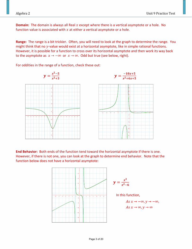
Range: The range is a bit trickier. Often, you will need to look at the graph to determine the range. You might think that no ‐value would exist at a horizontal asymptote, like in simple rational functions. However, it is possible for a function to cross over its horizontal asymptote and then work its way back to the asymptote as
→ ∞ or
→ ∞. Odd but true (see below, right).
For oddities in the range of a function, check these out:
End Behavior: Both ends of the function tend toward the horizontal asymptote if there is one. However, if there is not one, you can look at the graph to determine end behavior. Note that the function below does not have a horizontal asymptote:
In this function,
→ ∞,
→ ∞,
→ ∞,
→ ∞
Page 3 of 20
Algebra2Unit9PracticeTest
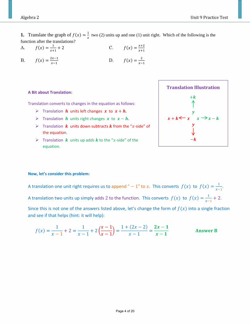
TranslationIllustration
1. Translate the graph of two (2) units up and one (1) unit right. Which of the following is the
function after the translations? A. 2 C.
B. D.
A Bit about Translation:
Translation converts to changes in the equation as follows:
Translation units left changes to .
Translation units right changes to .
Translation units down subtracts from the “ ‐side” of
the equation.
Translation units up adds to the “ ‐side” of the
equation.
Now, let’s consider this problem:
A translation one unit right requires us to append “ 1” to . This converts to .
A translation two units up simply adds2 to the function. This converts to 2.
Since this is not one of the answers listed above, let’s change the form of into a single fraction
and see if that helps (hint: it will help):
11
211
211
1 2 21
Page 4 of 20
Algebra2Unit9PracticeTest
-8
-8 8
8
y
x
-8
-8 8
8
y
x
-8
-8 8
8
y
-8
8
8
y
x-8
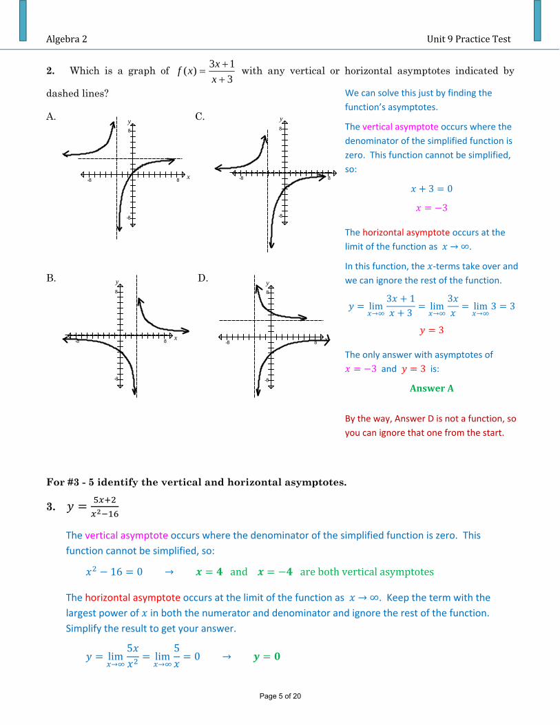
2. Which is a graph of 3
13)(
x
xxf with any vertical or horizontal asymptotes indicated by
dashed lines?
A. C.
B. D.
For #3 - 5 identify the vertical and horizontal asymptotes.
3.
The vertical asymptote occurs where the denominator of the simplified function is zero. This
function cannot be simplified, so:
16 0→ and arebothverticalasymptotes
The horizontal asymptote occurs at the limit of the function as → ∞. Keep the term with the
largest power of in both the numerator and denominator and ignore the rest of the function.
Simplify the result to get your answer.
lim→
5lim→
50
→
3 0
3
lim→
3 13
lim→
3lim→
3 3
3
We can solve this just by finding the
function’s asymptotes.
The vertical asymptote occurs where the
denominator of the simplified function is
zero. This function cannot be simplified,
so:
The horizontal asymptote occurs at the
limit of the function as → ∞.
In this function, the ‐terms take over and
we can ignore the rest of the function.
The only answer with asymptotes of
3 and 3 is:
AnswerA
By the way, Answer D is not a function, so
you can ignore that one from the start.
Page 5 of 20
Algebra2Unit9PracticeTest
4. 4
The vertical asymptote occurs where the denominator of the simplified function is zero. This
function cannot be simplified, so:
2 0→
The horizontal asymptote occurs at the limit of the function as → ∞. In this equation, the term
with in the denominator will approach zero as → ∞. The “ 4” term is not affected by
becoming larger and larger.
lim→
52
4 0 4 4→
5.
The vertical asymptote occurs where the denominator of the simplified function is zero. Let’s see if
this function can be simplified (hint: yes, it can):
47 10
2 22 5
25
0→
Note that in the original equation, 2makes the curve blow up as well. However, since
2 is a factor in both the numerator and denominator, and factors out completely in the
simplified form of the function, it will form a “hole” in our graph and not a vertical asymptote.
The horizontal asymptote occurs at the limit of the function as → ∞. Keep the term with the
largest power of in both the numerator and denominator and ignore the rest of the function.
Simplify the result to get your answer.
lim→
lim→
1 1→
6.
The vertical asymptote occurs where the denominator of the simplified function is zero. This function
cannot be simplified, so:
2 5 0→
The horizontal asymptote occurs at the limit of the function as → ∞. Keep the term with the largest
power of in both the numerator and denominator and ignore the rest of the function. Simplify the result to
get your answer.
lim→
32
32
∞→ .
Page 6 of 20
Algebra2Unit9PracticeTest
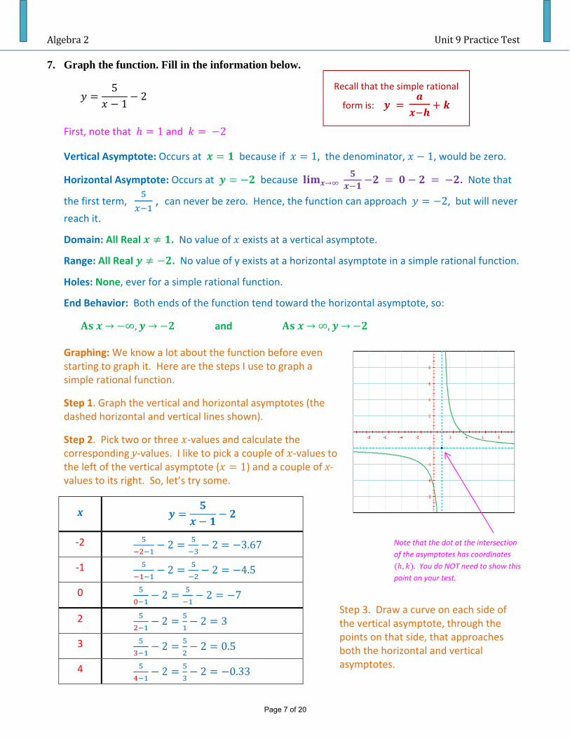
7. Graph the function. Fill in the information below.
51
2
First, note that 1 and 2
Vertical Asymptote: Occurs at because if 1, the denominator, 1, would be zero.
Horizontal Asymptote: Occurs at because → . Note that
the first term, , can never be zero. Hence, the function can approach 2, but will never
reach it.
Domain: All Real . No value of exists at a vertical asymptote.
Range: All Real . No value of y exists at a horizontal asymptote in a simple rational function.
Holes: None, ever for a simple rational function.
End Behavior: Both ends of the function tend toward the horizontal asymptote, so:
→ ∞,
→ and
→ ∞,
→
Graphing: We know a lot about the function before even starting to graph it. Here are the steps I use to graph a simple rational function.
Step 1. Graph the vertical and horizontal asymptotes (the dashed horizontal and vertical lines shown).
Step 2. Pick two or three ‐values and calculate the corresponding y‐values. I like to pick a couple of ‐values to the left of the vertical asymptote ( 1) and a couple of x‐values to its right. So, let’s try some.
x
‐2 2 2 3.67
‐1 2 2 4.5
0 2 2 7
2 2 2 3
3 2 2 0.5
4 2 2 0.33
Step 3. Draw a curve on each side of the vertical asymptote, through the points on that side, that approaches both the horizontal and vertical asymptotes.
Note that the dot at the intersection
of the asymptotes has coordinates
, . You do NOT need to show this point on your test.
Recall that the simple rational
form is:
Page 7 of 20
Algebra2Unit9PracticeTest
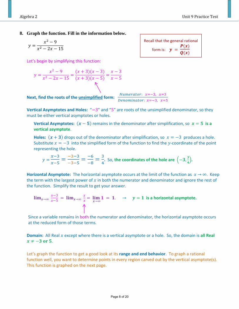
8. Graph the function. Fill in the information below.
92 15
Let’s begin by simplifying this function:
92 15
3 33 5
35
Next, find the roots of the unsimplified form: : ,
: ,
Vertical Asymptotes and Holes: “ 3” and “5” are roots of the unsimplified denominator, so they must be either vertical asymptotes or holes.
Vertical Asymptotes: remains in the denominator after simplification, so is a vertical asymptote.
Holes: drops out of the denominator after simplification, so 3 produces a hole. Substitute 3 into the simplified form of the function to find the ‐coordinate of the point representing the hole.
. So, the coordinates of the hole are , .
Horizontal Asymptote: The horizontal asymptote occurs at the limit of the function as → ∞. Keep
the term with the largest power of in both the numerator and denominator and ignore the rest of the function. Simplify the result to get your answer.
→ 3
5
→ →
.→ is a horizontal asymptote.
Since a variable remains in both the numerator and denominator, the horizontal asymptote occurs at the reduced form of those terms.
Domain: All Real except where there is a vertical asymptote or a hole. So, the domain is all Real .
Let’s graph the function to get a good look at its range and end behavior. To graph a rational function well, you want to determine points in every region carved out by the vertical asymptote(s). This function is graphed on the next page.
Recall that the general rational
form is:
Page 8 of 20
Algebra2Unit9PracticeTest
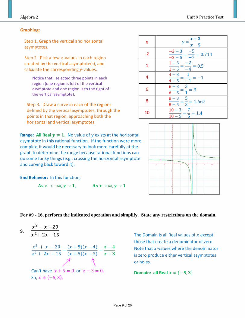
Step 1. Graph the vertical and horizontal asymptotes.
Step 2. Pick a few ‐values in each region created by the vertical asymptote(s), and calculate the corresponding y‐values.
Step 3. Draw a curve in each of the regions defined by the vertical asymptotes, through the points in that region, approaching both the horizontal and vertical asymptotes.
Notice that I selected three points in each region (one region is left of the vertical asymptote and one region is to the right of the vertical asymptote).
Graphing:
Range: All Real . No value of exists at the horizontal asymptote in this rational function. If the function were more complex, it would be necessary to look more carefully at the graph to determine the range because rational functions can do some funky things (e.g., crossing the horizontal asymptote and curving back toward it).
End Behavior: In this function,
→ ∞,
→ ,
→ ∞,
→
For #9 - 16, perform the indicated operation and simplify. State any restrictions on the domain.
9.
202 15
5 45 3
x
‐2 2 32 5
57
0.714
1 1 31 5
24
0.5
4 4 34 5
11
1
6 6 36 5
31
3
8 8 38 5
53
1.667
10 10 310 5
75
1.4
The Domain is all Real values of except
those that create a denominator of zero.
Note that ‐values where the denominator
is zero produce either vertical asymptotes
or holes.
Domain: all Real , Can’t have 5 0 or 3 0.So, 5, 3 .
Page 9 of 20
Algebra2Unit9PracticeTest
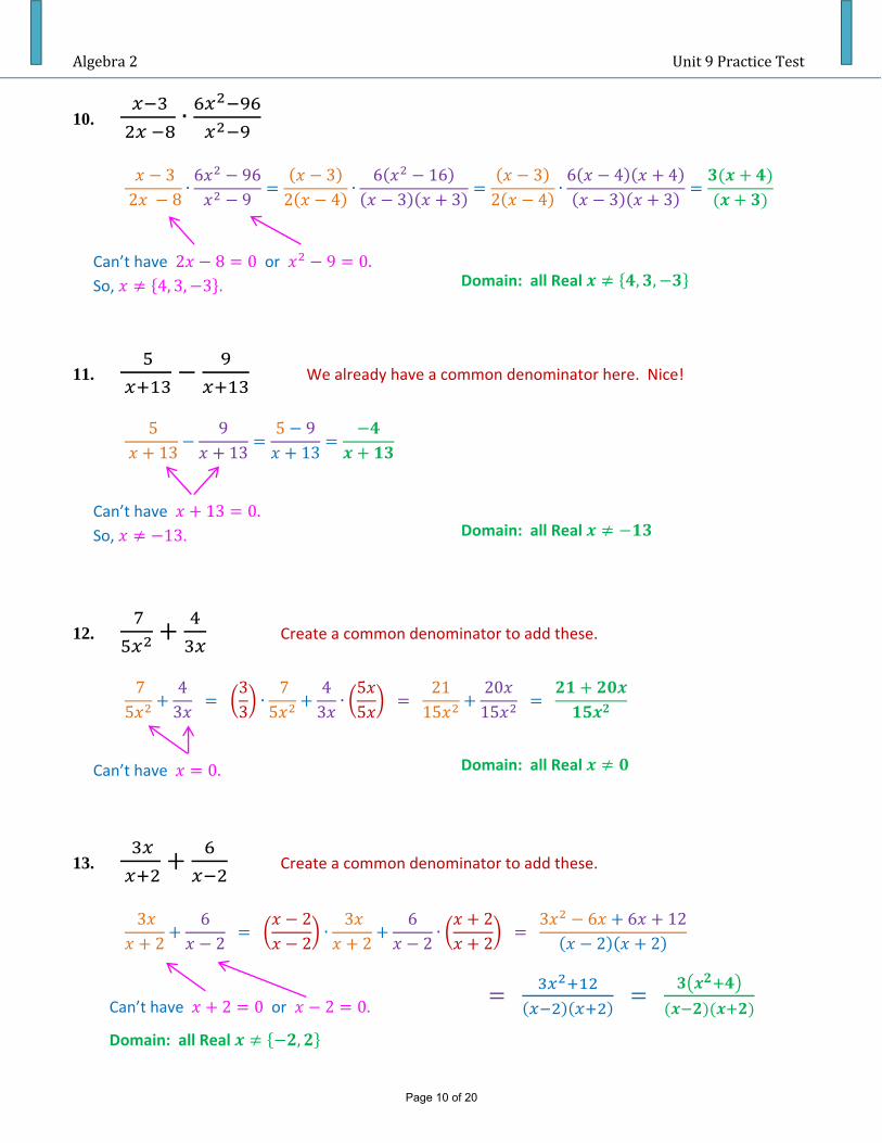
10.
∙
32 8
∙6 96
93
2 4∙6 16
3 33
2 4∙6 4 4
3 3
11.
We already have a common denominator here. Nice!
5 13
913
5 913
12.
Create a common denominator to add these.
75
43
33
∙75
43
∙55
2115
2015
13.
Create a common denominator to add these.
32
62
22
∙3
262∙
22
3 6 6 122 2
Can’t have 2 8 0 or 9 0. So, 4, 3, 3 . Domain: all Real , ,
Can’t have 13 0.So, 13. Domain: all Real
Can’t have 0. Domain: all Real
Can’t have 2 0 or 2 0.
Domain: all Real ,
Page 10 of 20
Algebra2Unit9PracticeTest
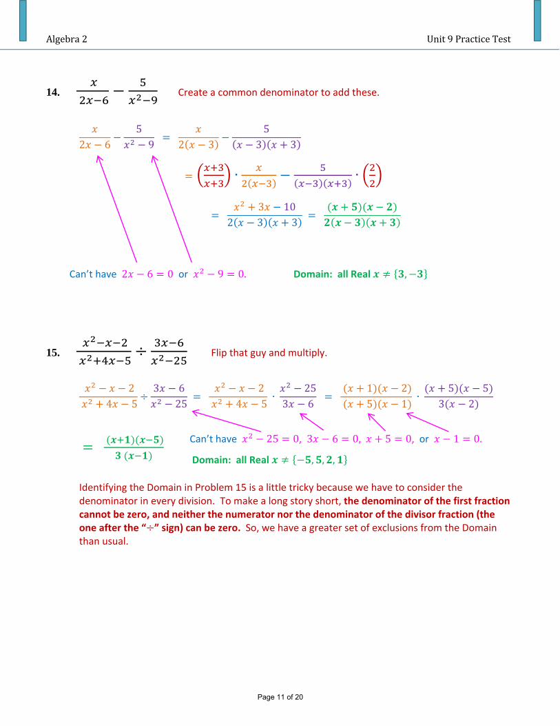
14.
Create a common denominator to add these.
2 659
2 35
3 3
∙ ∙
3 10
2 3 3
15.
Flip that guy and multiply.
2 4 5
3 625
2 4 5
∙ 25
3 6
1 2 5 1
∙ 5 5
3 2
Identifying the Domain in Problem 15 is a little tricky because we have to consider the denominator in every division. To make a long story short, the denominator of the first fraction cannot be zero, and neither the numerator nor the denominator of the divisor fraction (the one after the “ ” sign) can be zero. So, we have a greater set of exclusions from the Domain than usual.
Can’t have 2 6 0 or 9 0. Domain: all Real ,
Can’t have 25 0, 3 6 0, 5 0, or 1 0.
Domain: all Real , , ,
Page 11 of 20
Algebra2Unit9PracticeTest
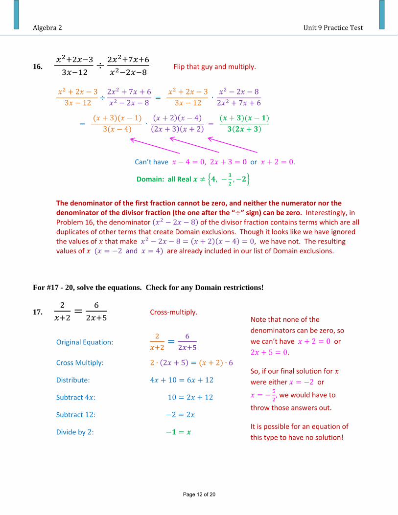
16.
Flip that guy and multiply.
2 33 12
2 7 62 8
2 33 12
∙ 2 8
2 7 6
3 1
3 4 ∙
2 42 3 2
The denominator of the first fraction cannot be zero, and neither the numerator nor the denominator of the divisor fraction (the one after the “ ” sign) can be zero. Interestingly, in Problem 16, the denominator 2 8 of the divisor fraction contains terms which are all duplicates of other terms that create Domain exclusions. Though it looks like we have ignored the values of that make 2 8 2 4 0, we have not. The resulting values of 2 and 4 are already included in our list of Domain exclusions.
For #17 - 20, solve the equations. Check for any Domain restrictions!
17. Cross‐multiply.
Original Equation:
Cross Multiply: 2 ∙ 2 5 2 ∙ 6
Distribute: 4 10 6 12
Subtract 4 : 10 2 12
Subtract 12: 2 2
Divide by 2:
Can’t have 4 0, 2 3 0 or 2 0.
Domain: all Real , ,
Note that none of the
denominators can be zero, so
we can’t have 2 0 or 2 5 0.
So, if our final solution for
were either 2 or
, we would have to
throw those answers out.
It is possible for an equation of
this type to have no solution!
Page 12 of 20
Algebra2Unit9PracticeTest
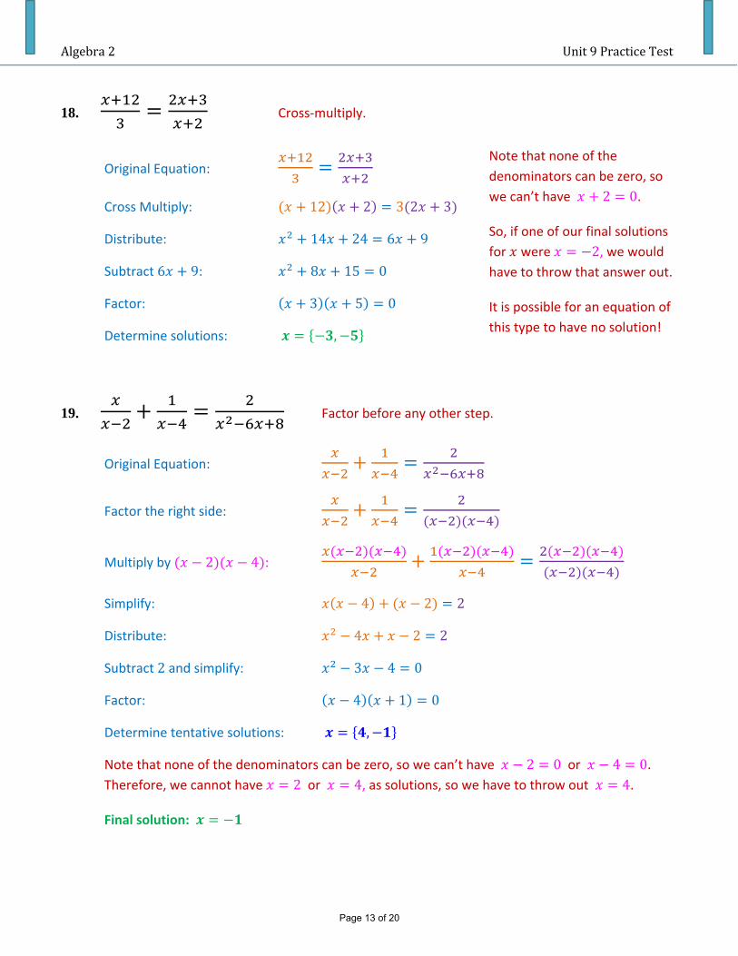
18. Cross‐multiply.
Original Equation:
Cross Multiply: 12 2 3 2 3
Distribute: 14 24 6 9
Subtract 6 9: 8 15 0
Factor: 3 5 0
Determine solutions: ,
19. Factor before any other step.
Original Equation:
Factor the right side:
Multiply by 2 4 :
Simplify: 4 2 2
Distribute: 4 2 2
Subtract 2 and simplify: 3 4 0
Factor: 4 1 0
Determine tentative solutions: ,
Note that none of the denominators can be zero, so we can’t have 2 0 or 4 0. Therefore, we cannot have 2 or 4, as solutions, so we have to throw out 4.
Final solution:
Note that none of the
denominators can be zero, so
we can’t have 2 0.
So, if one of our final solutions
for were 2, we would have to throw that answer out.
It is possible for an equation of
this type to have no solution!
Page 13 of 20
Algebra2Unit9PracticeTest
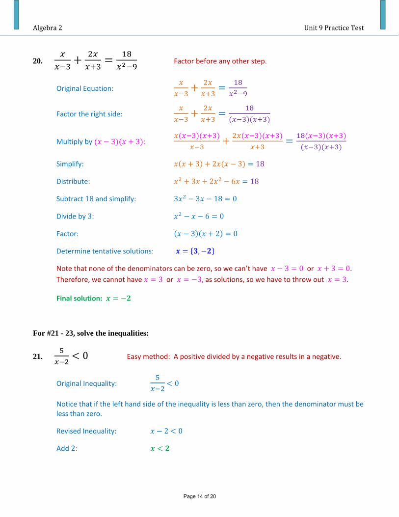
20. Factor before any other step.
Original Equation:
Factor the right side:
Multiply by 3 3 :
Simplify: 3 2 3 18
Distribute: 3 2 6 18
Subtract 18 and simplify: 3 3 18 0
Divide by 3: 6 0
Factor: 3 2 0
Determine tentative solutions: ,
Note that none of the denominators can be zero, so we can’t have 3 0 or 3 0. Therefore, we cannot have 3 or 3, as solutions, so we have to throw out 3.
Final solution:
For #21 - 23, solve the inequalities:
21. 0 Easy method: A positive divided by a negative results in a negative.
Original Inequality: 0
Notice that if the left hand side of the inequality is less than zero, then the denominator must be less than zero.
Revised Inequality: 2 0
Add 2:
Page 14 of 20
Algebra2Unit9PracticeTest
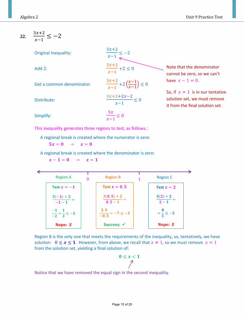
22. 2
Original Inequality: 2
Add 2: 2 0
Get a common denominator: 2 11 0
Distribute: 0
Simplify: 0
This inequality generates three regions to test, as follows.:
A regional break is created where the numerator is zero:
→
A regional break is created where the denominator is zero:
→
Region B is the only one that meets the requirements of the inequality, so, tentatively, we have solution: 0 . However, from above, we recall that 1, so we must remove 1 from the solution set, yielding a final solution of:
Notice that we have removed the equal sign in the second inequality.
Test
Nope:X
Region A
..
..
Test .
Success:
Test
Nope:X
Region B Region C 0 1
Note that the denominator
cannot be zero, so we can’t
have 1 0.
So, if 1 is in our tentative solution set, we must remove
it from the final solution set.
Page 15 of 20
Algebra2Unit9PracticeTest
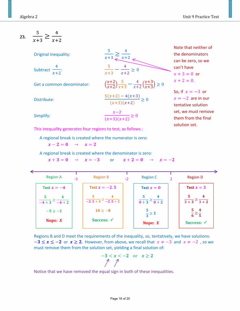
23.
Original Inequality:
Subtract : 0
Get a common denominator: 22
53
42
33 0
Distribute:
0
Simplify: 0
This inequality generates four regions to test, as follows.:
A regional break is created where the numerator is zero:
→
A regional break is created where the denominator is zero:
→ or
→
Regions B and D meet the requirements of the inequality, so, tentatively, we have solutions: or . However, from above, we recall that 3 and 2 , so we
must remove them from the solution set, yielding a final solution of:
or
Notice that we have removed the equal sign in both of these inequalities.
Test
Nope:X
Region A
. .
Test .
Success:
Test
Nope:X
Region B Region C ‐3 ‐2
Note that neither of
the denominators
can be zero, so we
can’t have
3 0 or 2 0.
So, if 3 or 2 are in our
tentative solution
set, we must remove
them from the final
solution set.
Region D
Test
Success:
2
Page 16 of 20
Algebra2Unit9PracticeTest
For #24-25: Graph the function. Fill in the information below.
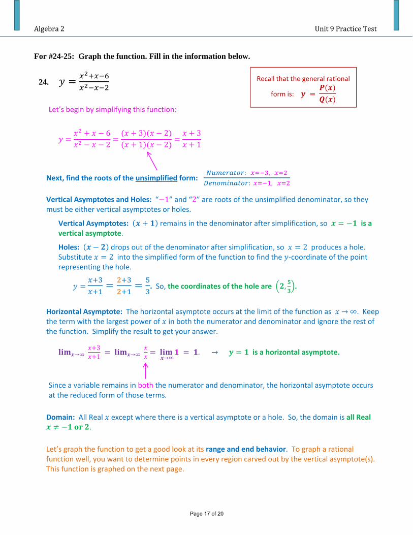
24.
Let’s begin by simplifying this function:
62
3 21 2
31
Next, find the roots of the unsimplified form: : ,
: ,
Vertical Asymptotes and Holes: “ 1” and “2” are roots of the unsimplified denominator, so they must be either vertical asymptotes or holes.
Vertical Asymptotes: remains in the denominator after simplification, so is a vertical asymptote.
Holes: drops out of the denominator after simplification, so 2 produces a hole. Substitute 2 into the simplified form of the function to find the ‐coordinate of the point representing the hole.
. So, the coordinates of the hole are , .
Horizontal Asymptote: The horizontal asymptote occurs at the limit of the function as → ∞. Keep
the term with the largest power of in both the numerator and denominator and ignore the rest of the function. Simplify the result to get your answer.
→ 3
1
→ →
.→ is a horizontal asymptote.
Since a variable remains in both the numerator and denominator, the horizontal asymptote occurs at the reduced form of those terms.
Domain: All Real except where there is a vertical asymptote or a hole. So, the domain is all Real .
Let’s graph the function to get a good look at its range and end behavior. To graph a rational function well, you want to determine points in every region carved out by the vertical asymptote(s). This function is graphed on the next page.
Recall that the general rational
form is:
Page 17 of 20
Algebra2Unit9PracticeTest
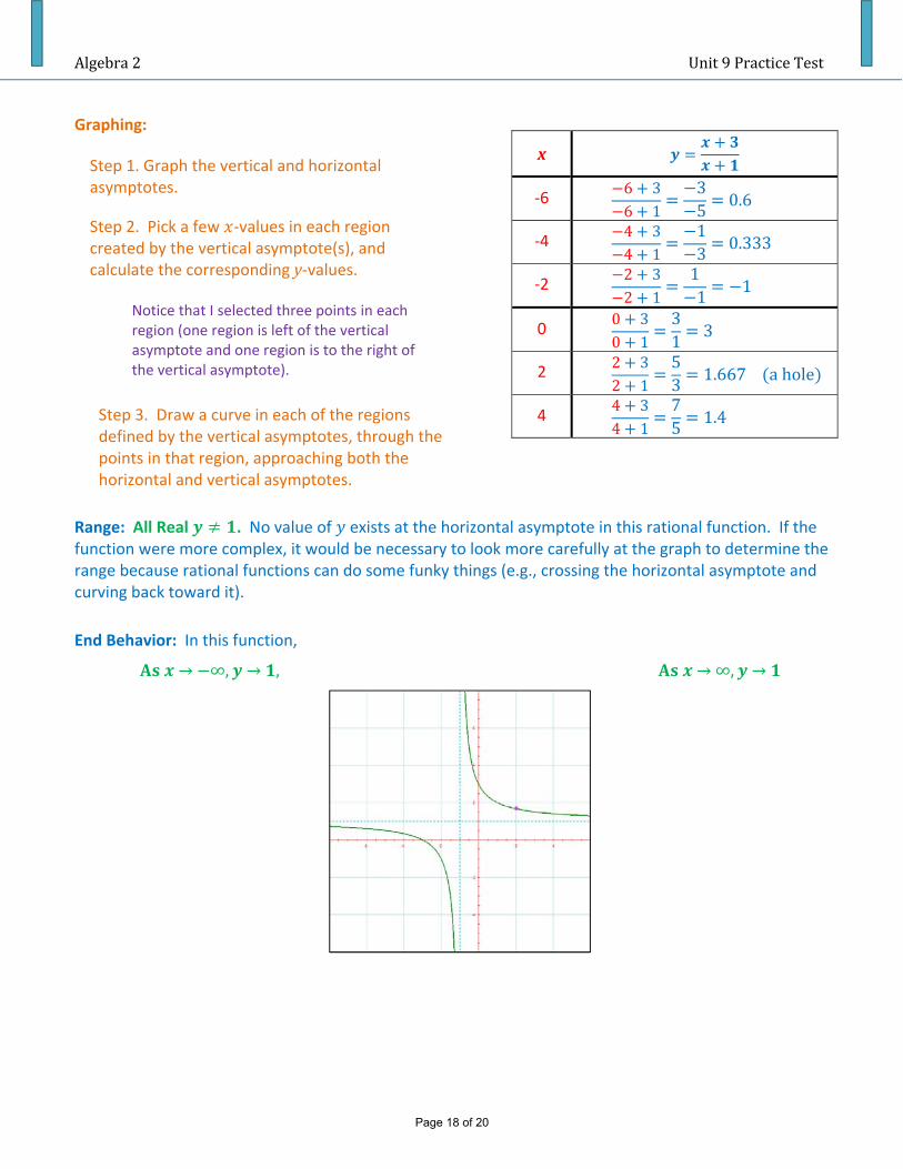
Step 1. Graph the vertical and horizontal asymptotes.
Step 2. Pick a few ‐values in each region created by the vertical asymptote(s), and calculate the corresponding y‐values.
Step 3. Draw a curve in each of the regions defined by the vertical asymptotes, through the points in that region, approaching both the horizontal and vertical asymptotes.
Notice that I selected three points in each region (one region is left of the vertical asymptote and one region is to the right of the vertical asymptote).
Graphing:
Range: All Real . No value of exists at the horizontal asymptote in this rational function. If the function were more complex, it would be necessary to look more carefully at the graph to determine the range because rational functions can do some funky things (e.g., crossing the horizontal asymptote and curving back toward it).
End Behavior: In this function,
→ ∞,
→ ,
→ ∞,
→
x
‐6 6 36 1
35
0.6
‐4 4 34 1
13
0.333
‐2 2 32 1
11
1
0 0 30 1
31
3
2 2 32 1
53
1.667 a hole
4 4 34 1
75
1.4
Page 18 of 20
Algebra2Unit9PracticeTest
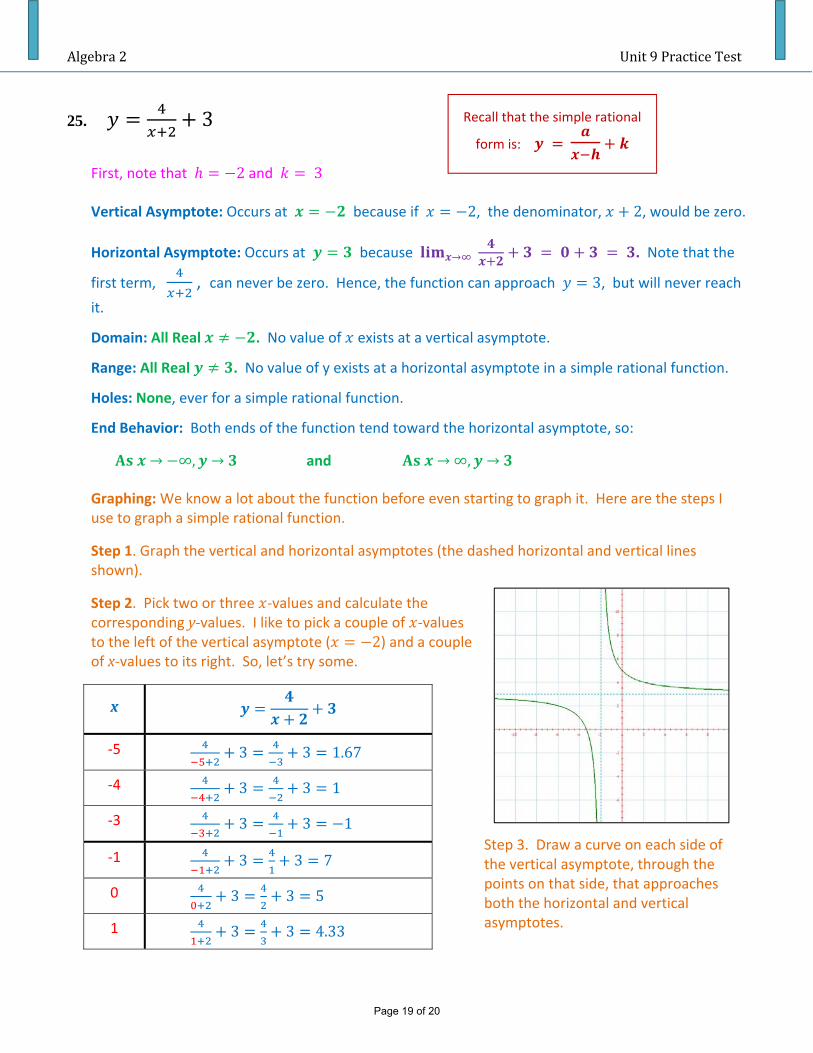
25. 3
First, note that 2 and 3
Vertical Asymptote: Occurs at because if 2, the denominator, 2, would be zero.
Horizontal Asymptote: Occurs at because → . Note that the
first term, , can never be zero. Hence, the function can approach 3, but will never reach
it.
Domain: All Real . No value of exists at a vertical asymptote.
Range: All Real . No value of y exists at a horizontal asymptote in a simple rational function.
Holes: None, ever for a simple rational function.
End Behavior: Both ends of the function tend toward the horizontal asymptote, so:
→ ∞,
→ and
→ ∞,
→
Graphing: We know a lot about the function before even starting to graph it. Here are the steps I use to graph a simple rational function.
Step 1. Graph the vertical and horizontal asymptotes (the dashed horizontal and vertical lines shown).
Step 2. Pick two or three ‐values and calculate the corresponding y‐values. I like to pick a couple of ‐values to the left of the vertical asymptote ( 2) and a couple of x‐values to its right. So, let’s try some.
x
‐5 3 3 1.67
‐4 3 3 1
‐3 3 3 1
‐1 3 3 7
0 3 3 5
1 3 3 4.33
Step 3. Draw a curve on each side of the vertical asymptote, through the points on that side, that approaches both the horizontal and vertical asymptotes.
Recall that the simple rational
form is:
Page 19 of 20
Algebra2Unit9PracticeTest
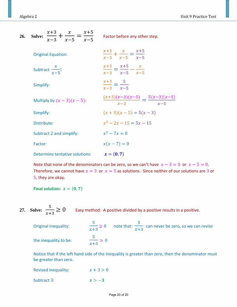
26. Solve: Factor before any other step.
Original Equation:
Subtract :
Simplify:
Multiply by 3 5 :
Simplify: 3 5 5 3
Distribute: 2 15 5 15
Subtract 2 and simplify: 7 0
Factor: 7 0
Determine tentative solutions: ,
Note that none of the denominators can be zero, so we can’t have 3 0 or 5 0. Therefore, we cannot have 3 or 5 as solutions. Since neither of our solutions are 3 or 5, they are okay.
Final solution: ,
27. Solve: 0 Easy method: A positive divided by a positive results in a positive.
Original Inequality: 0 note that: can never be zero, so we can revise
the inequality to be: 0
Notice that if the left hand side of the inequality is greater than zero, then the denominator must be greater than zero.
Revised Inequality: 3 0
Subtract 3:
Page 20 of 20