Regional US carbon sinks from three-dimensionalatmospheric CO2 samplingCyril Crevoisiera,b,1, Colm Sweeneyc,d, Manuel Gloore, Jorge L. Sarmientob, and Pieter P. Tansd

aLaboratoire de Météorologie Dynamique, Centre National de la Recherche Scientifique, Institut Pierre Simon Laplace, Ecole Polytechnique, 91128Palaiseau Cedex, France; bAtmospheric and Oceanic Sciences Program, Princeton University, Princeton, NJ 08544; cCooperative Institute for Research inEnvironmental Sciences, University of Colorado at Boulder, Boulder, CO; dNational Oceanic and Atmospheric Administration/Earth System ResearchLaboratory, Boulder, CO 80305; and eEarth and Biosphere Institute and School of Geography, University of Leeds, Leeds, United Kingdom

Edited by Bev E. Law, Oregon State University, and accepted by the Editorial Board August 10, 2010 (received for review January 6, 2009)

Studies diverge substantially on the actual magnitude of the NorthAmerican carbon budget. This is due to the lack of appropriate dataandalso stems from thedifficulty to properlymodel all thedetails ofthe flux distribution and transport inside the region of interest. Tosidestep thesedifficulties,weuseherea simplebudgetingapproachto estimate land-atmosphere fluxes across North America by balan-cing the inflow and outflow of CO2 from the troposphere. We baseour study on the unique sampling strategy of atmospheric CO2

vertical profiles over North America from the National Oceanicand Atmospheric Administration/Earth System Research Labora-tory aircraft network, from which we infer the three-dimensionalCO2 distribution over the continent. We find a moderate sink of0.5� 0.4 PgCy−1 for the period 2004–2006 for the coterminousUnited States, in good agreement with the forest-inventory-basedestimate of the first North American State of the Carbon CycleReport, and averaged climate conditions. We find that the highestuptakeoccurs in theMidwest and in theSoutheast. This partitioningagrees with independent estimates of crop uptake in the Midwest,whichproves to be a significant part of theUSatmospheric sink, andof secondary forest regrowth in the Southeast. Provided that verti-cal profile measurements are continued, our study offers an inde-pendent means to link regional carbon uptake to climate drivers.

atmospheric composition ∣ biogeochemistry ∣ carbon cycle ∣greenhouse gases

Knowledge of today’s carbon sources and sinks, their spatialdistribution, and their variability in time is one of the essen-

tial ingredients for predicting future carbon dioxide (CO2) atmo-spheric levels, and in turn the anthropogenic perturbation ofradiative forcing by CO2. Ocean uptake of anthropogenic carboncan be estimated with fairly high accuracy, implying a global netland sink of ∼1 PgC y−1 over the past two decades when com-bined with atmospheric records and fossil fuel emissions (1; seealso SI Text). However, the location and understanding of under-lying mechanisms of this land sink remain controversial. Untilrecently, the dominant consensus has been that a strong land sinkis located in the northern hemisphere midlatitudes, althoughattempts (2–9) to partition the sink further between Eurasiaand North America have yielded diverse values ranging from0.4 to 1.4 PgC y−1 for the temperate North American sink, withassociated formal uncertainties ranging from 0.4 to 0.8 PgC y−1(Table 1). This large spread in the estimates comes partiallyfrom temporal variability of the sink, but also stems from the lackof appropriate observations, which strongly impacts “top-down”atmospheric approaches.

The traditional top-down approach exploits, in essence, theaccumulation or depletion of CO2 in the overlying air as aconstraint on carbon sources and sinks at the surface. It usesatmospheric transport models in an inverse mode to determinethe spatiotemporal land-air surface flux distribution that givesthe best match to a set of atmospheric CO2 data. Strong biasesin the estimates may arise from (i) the specific nature of surfacefluxes originating from a strong diurnal and seasonal cycle in land

vegetation; (ii) limitations in state-of-the-art atmospheric trans-port models, particularly in terms of near-surface to midtropo-sphere air exchange, with the choice of the transport modelused in the estimation critically influencing the results (10–12);and (iii) limitations in atmospheric CO2 sampling (4, 5, 13). Inparticular, atmospheric concentration measurements have beenpredominantly made at remote locations to avoid the vicinityof large point sources or rapidly varying fluxes such as those dueto photosynthesis and respiration on land, and fossil fuel emis-sions. Point source flux signals are thus strongly diluted. Also,being mostly made at the surface, the measurements also lackinformation in the vertical dimension that is not only necessaryto characterize the surface fluxes but also essential to validateand calibrate model transport. Given that the spread in the fluxestimates obtained with the traditional atmospheric inverseapproach comes largely from the difficulty in modeling properlyall the details of the flux distribution and transport inside theregion of interest, a reasonable alternative approach would beto not try to model that detail at all, but to just look at the inflowand outflow at the boundaries of this region.

To that end, we leverage a unique vertical profile samplingstrategy that was implemented by National Oceanic and Atmo-spheric Administration/Earth System Research Laboratory(NOAA/ESRL) to extract signatures of the exchange of CO2

and other trace gases over the continent and their associatedvariability, and to constrain representations of atmospheric mix-ing in chemical transport models. The use of such data in a dataassimilation system or in a traditional atmospheric approach mayresult in a powerful constraint on carbon budgets, even whenusing weaker or no a priori constraints on fluxes (8). However,this would involve solving the problem of the design of an appro-priate error covariance structure that would be assigned tovertical transport models. In this paper, we focus on a particularstrength of these data, which is the opportunity they provide todesign a method avoiding the need for detailed modeling offluxes and transport processes to estimate the North Americantemperate sink. Here, we use the vertical profile sampling strat-egy to estimate the full three-dimensional tropospheric CO2

distribution over North America and use analyzed winds to studymass exchange pathways over the continent. Relying on a simplebudgeting approach and the assumption that large-scale temporaland spatial variability dominate the change in the three-dimen-sional CO2 distribution, we derive a previously undescribed

Author contributions: M.G. and P.P.T. designed research; C.C. performed research; C.S.contributed data; C.C., M.G., J.L.S., and P.P.T. interpreted results; C.C. and C.S. analyzeddata; and C.C. wrote the paper.

The authors declare no conflict of interest.

This article is a PNAS Direct Submission. B.E.L. is a guest editor invited by the EditorialBoard.

Freely available online through the PNAS open access option.1To whom correspondence should be addressed. E-mail: cyril.crevoisier@lmd.polytechnique.fr.

This article contains supporting information online at www.pnas.org/lookup/suppl/doi:10.1073/pnas.0900062107/-/DCSupplemental.

18348–18353 ∣ PNAS ∣ October 26, 2010 ∣ vol. 107 ∣ no. 43 www.pnas.org/cgi/doi/10.1073/pnas.0900062107

estimate of the North American sink with results at a regionallevel that we compare with previously published estimates.

A Three-Dimensional CO2 DistributionThe data consist of regular aircraft-based measurements ofvertical CO2 profiles up to a height of 8 km performed byNOAA/ESRL as part of the North American Carbon Program(14) at 20 locations (Table S1) covering most of North America,including Hawaii, once to twice a month, for the three-year per-iod 2004–2006. Most measurements were performed around

noon, which is the time most representative of the daily averageCO2 column (10). All together, about 25,000 measurementscovering the three-year period are used in this study.

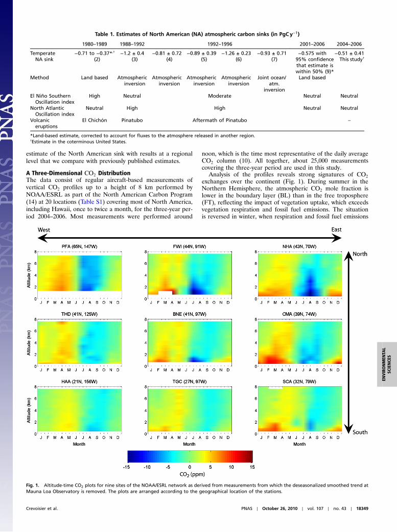
Analysis of the profiles reveals strong signatures of CO2

exchanges over the continent (Fig. 1). During summer in theNorthern Hemisphere, the atmospheric CO2 mole fraction islower in the boundary layer (BL) than in the free troposphere(FT), reflecting the impact of vegetation uptake, which exceedsvegetation respiration and fossil fuel emissions. The situationis reversed in winter, when respiration and fossil fuel emissions

Table 1. Estimates of North American (NA) atmospheric carbon sinks (in PgCy−1)

1980–1989 1988–1992 1992–1996 2001–2006 2004–2006

TemperateNA sink

−0.71 to −0.37*,†

(2)−1.2 ± 0.4

(3)−0.81 ± 0.72

(4)−0.89 ± 0.39

(5)−1.26 ± 0.23

(6)−0.93 ± 0.71

(7)−0.575 with95% confidencethat estimate iswithin 50% (9)*

−0.51 ± 0.41This study†

Method Land based Atmosphericinversion

Atmosphericinversion

Atmosphericinversion

Atmosphericinversion

Joint ocean/atm.

inversion

Land based

El Niño SouthernOscillation index

High Neutral Moderate Neutral Neutral

North AtlanticOscillation index

Neutral High High Neutral Neutral

Volcaniceruptions

El Chichón Pinatubo Aftermath of Pinatubo –

*Land-based estimate, corrected to account for fluxes to the atmosphere released in another region.†Estimate in the coterminous United States.

Fig. 1. Altitude-time CO2 plots for nine sites of the NOAA/ESRL network as derived from measurements from which the deseasonalized smoothed trend atMauna Loa Observatory is removed. The plots are arranged according to the geographical location of the stations.

Crevoisier et al. PNAS ∣ October 26, 2010 ∣ vol. 107 ∣ no. 43 ∣ 18349

ENVIRONMEN

TAL

SCIENCE

S

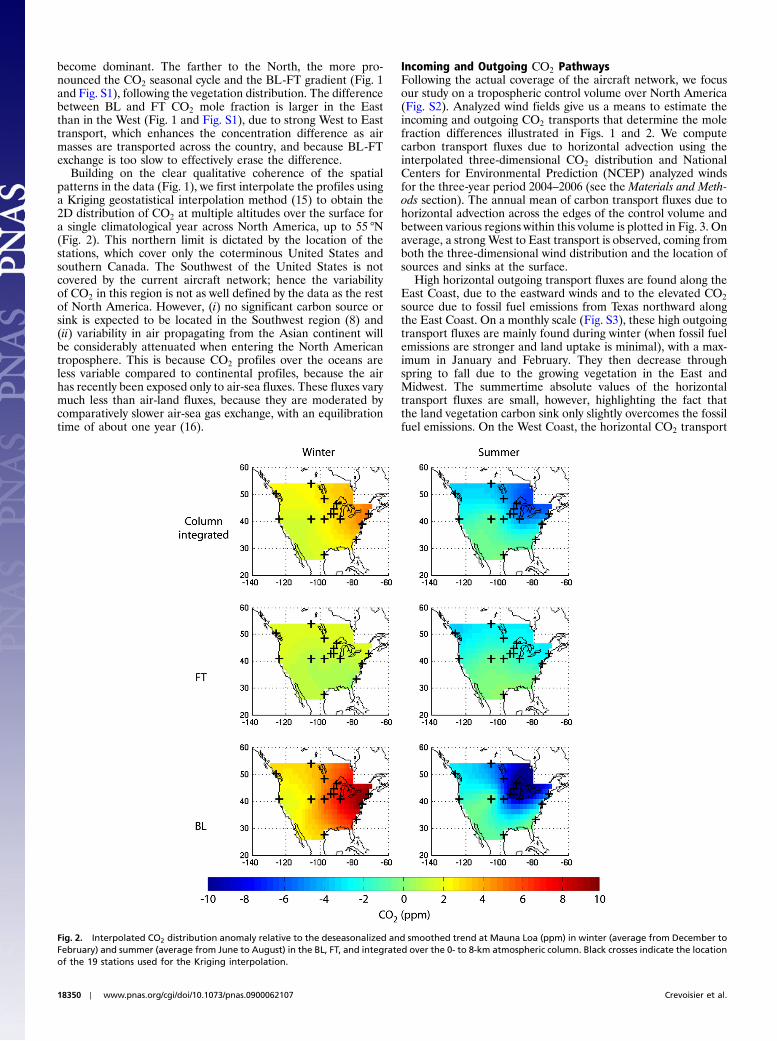
become dominant. The farther to the North, the more pro-nounced the CO2 seasonal cycle and the BL-FT gradient (Fig. 1and Fig. S1), following the vegetation distribution. The differencebetween BL and FT CO2 mole fraction is larger in the Eastthan in the West (Fig. 1 and Fig. S1), due to strong West to Easttransport, which enhances the concentration difference as airmasses are transported across the country, and because BL-FTexchange is too slow to effectively erase the difference.

Building on the clear qualitative coherence of the spatialpatterns in the data (Fig. 1), we first interpolate the profiles usinga Kriging geostatistical interpolation method (15) to obtain the2D distribution of CO2 at multiple altitudes over the surface fora single climatological year across North America, up to 55 °N(Fig. 2). This northern limit is dictated by the location of thestations, which cover only the coterminous United States andsouthern Canada. The Southwest of the United States is notcovered by the current aircraft network; hence the variabilityof CO2 in this region is not as well defined by the data as the restof North America. However, (i) no significant carbon source orsink is expected to be located in the Southwest region (8) and(ii) variability in air propagating from the Asian continent willbe considerably attenuated when entering the North Americantroposphere. This is because CO2 profiles over the oceans areless variable compared to continental profiles, because the airhas recently been exposed only to air-sea fluxes. These fluxes varymuch less than air-land fluxes, because they are moderated bycomparatively slower air-sea gas exchange, with an equilibrationtime of about one year (16).

Incoming and Outgoing CO2 PathwaysFollowing the actual coverage of the aircraft network, we focusour study on a tropospheric control volume over North America(Fig. S2). Analyzed wind fields give us a means to estimate theincoming and outgoing CO2 transports that determine the molefraction differences illustrated in Figs. 1 and 2. We computecarbon transport fluxes due to horizontal advection using theinterpolated three-dimensional CO2 distribution and NationalCenters for Environmental Prediction (NCEP) analyzed windsfor the three-year period 2004–2006 (see the Materials and Meth-ods section). The annual mean of carbon transport fluxes due tohorizontal advection across the edges of the control volume andbetween various regions within this volume is plotted in Fig. 3. Onaverage, a strongWest to East transport is observed, coming fromboth the three-dimensional wind distribution and the location ofsources and sinks at the surface.

High horizontal outgoing transport fluxes are found along theEast Coast, due to the eastward winds and to the elevated CO2

source due to fossil fuel emissions from Texas northward alongthe East Coast. On a monthly scale (Fig. S3), these high outgoingtransport fluxes are mainly found during winter (when fossil fuelemissions are stronger and land uptake is minimal), with a max-imum in January and February. They then decrease throughspring to fall due to the growing vegetation in the East andMidwest. The summertime absolute values of the horizontaltransport fluxes are small, however, highlighting the fact thatthe land vegetation carbon sink only slightly overcomes the fossilfuel emissions. On the West Coast, the horizontal CO2 transport

Fig. 2. Interpolated CO2 distribution anomaly relative to the deseasonalized and smoothed trend at Mauna Loa (ppm) in winter (average from December toFebruary) and summer (average from June to August) in the BL, FT, and integrated over the 0- to 8-km atmospheric column. Black crosses indicate the locationof the 19 stations used for the Kriging interpolation.

18350 ∣ www.pnas.org/cgi/doi/10.1073/pnas.0900062107 Crevoisier et al.

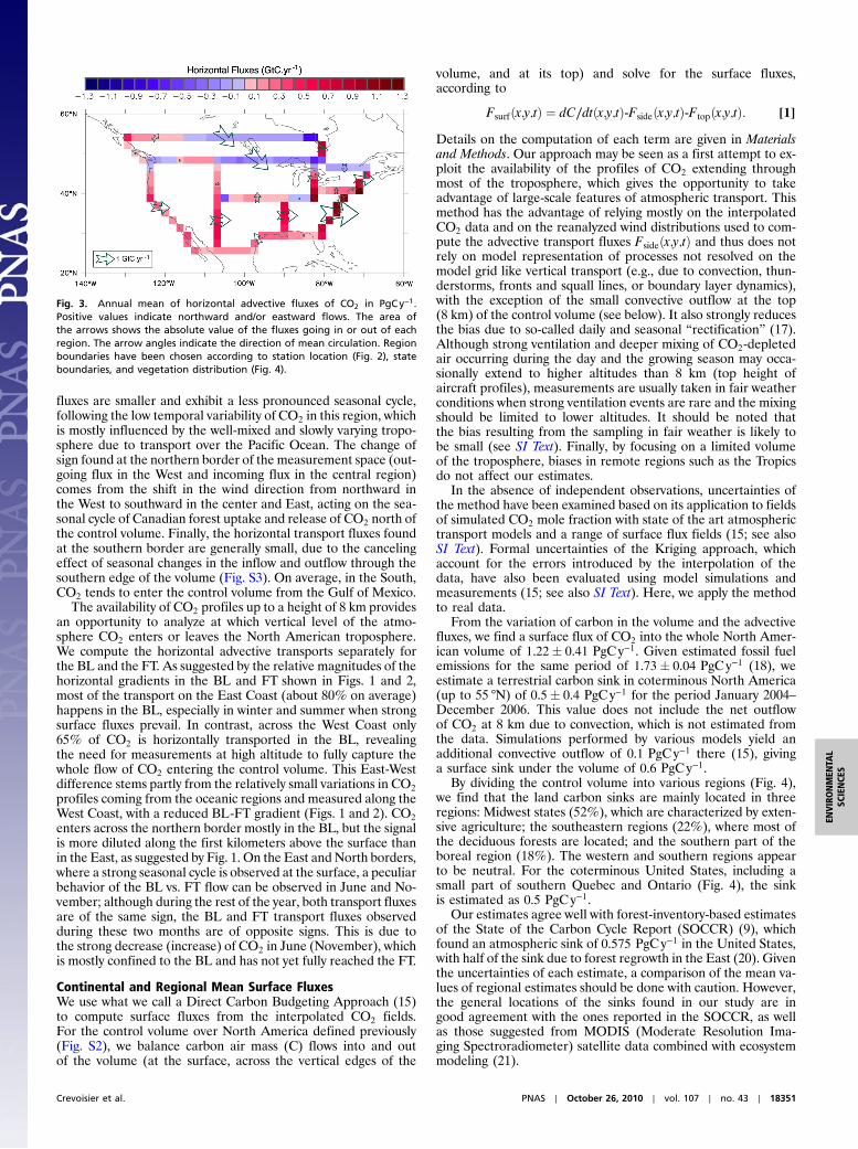
fluxes are smaller and exhibit a less pronounced seasonal cycle,following the low temporal variability of CO2 in this region, whichis mostly influenced by the well-mixed and slowly varying tropo-sphere due to transport over the Pacific Ocean. The change ofsign found at the northern border of the measurement space (out-going flux in the West and incoming flux in the central region)comes from the shift in the wind direction from northward inthe West to southward in the center and East, acting on the sea-sonal cycle of Canadian forest uptake and release of CO2 north ofthe control volume. Finally, the horizontal transport fluxes foundat the southern border are generally small, due to the cancelingeffect of seasonal changes in the inflow and outflow through thesouthern edge of the volume (Fig. S3). On average, in the South,CO2 tends to enter the control volume from the Gulf of Mexico.

The availability of CO2 profiles up to a height of 8 km providesan opportunity to analyze at which vertical level of the atmo-sphere CO2 enters or leaves the North American troposphere.We compute the horizontal advective transports separately forthe BL and the FT. As suggested by the relative magnitudes of thehorizontal gradients in the BL and FT shown in Figs. 1 and 2,most of the transport on the East Coast (about 80% on average)happens in the BL, especially in winter and summer when strongsurface fluxes prevail. In contrast, across the West Coast only65% of CO2 is horizontally transported in the BL, revealingthe need for measurements at high altitude to fully capture thewhole flow of CO2 entering the control volume. This East-Westdifference stems partly from the relatively small variations in CO2

profiles coming from the oceanic regions and measured along theWest Coast, with a reduced BL-FT gradient (Figs. 1 and 2). CO2

enters across the northern border mostly in the BL, but the signalis more diluted along the first kilometers above the surface thanin the East, as suggested by Fig. 1. On the East and North borders,where a strong seasonal cycle is observed at the surface, a peculiarbehavior of the BL vs. FT flow can be observed in June and No-vember; although during the rest of the year, both transport fluxesare of the same sign, the BL and FT transport fluxes observedduring these two months are of opposite signs. This is due tothe strong decrease (increase) of CO2 in June (November), whichis mostly confined to the BL and has not yet fully reached the FT.

Continental and Regional Mean Surface FluxesWe use what we call a Direct Carbon Budgeting Approach (15)to compute surface fluxes from the interpolated CO2 fields.For the control volume over North America defined previously(Fig. S2), we balance carbon air mass (C) flows into and outof the volume (at the surface, across the vertical edges of the

volume, and at its top) and solve for the surface fluxes,according to

Fsurfðx;y;tÞ ¼ dC∕dtðx;y;tÞ-Fsideðx;y;tÞ-Ftopðx;y;tÞ: [1]

Details on the computation of each term are given in Materialsand Methods. Our approach may be seen as a first attempt to ex-ploit the availability of the profiles of CO2 extending throughmost of the troposphere, which gives the opportunity to takeadvantage of large-scale features of atmospheric transport. Thismethod has the advantage of relying mostly on the interpolatedCO2 data and on the reanalyzed wind distributions used to com-pute the advective transport fluxes Fsideðx;y;tÞ and thus does notrely on model representation of processes not resolved on themodel grid like vertical transport (e.g., due to convection, thun-derstorms, fronts and squall lines, or boundary layer dynamics),with the exception of the small convective outflow at the top(8 km) of the control volume (see below). It also strongly reducesthe bias due to so-called daily and seasonal “rectification” (17).Although strong ventilation and deeper mixing of CO2-depletedair occurring during the day and the growing season may occa-sionally extend to higher altitudes than 8 km (top height ofaircraft profiles), measurements are usually taken in fair weatherconditions when strong ventilation events are rare and the mixingshould be limited to lower altitudes. It should be noted thatthe bias resulting from the sampling in fair weather is likely tobe small (see SI Text). Finally, by focusing on a limited volumeof the troposphere, biases in remote regions such as the Tropicsdo not affect our estimates.

In the absence of independent observations, uncertainties ofthe method have been examined based on its application to fieldsof simulated CO2 mole fraction with state of the art atmospherictransport models and a range of surface flux fields (15; see alsoSI Text). Formal uncertainties of the Kriging approach, whichaccount for the errors introduced by the interpolation of thedata, have also been evaluated using model simulations andmeasurements (15; see also SI Text). Here, we apply the methodto real data.

From the variation of carbon in the volume and the advectivefluxes, we find a surface flux of CO2 into the whole North Amer-ican volume of 1.22� 0.41 PgC y−1. Given estimated fossil fuelemissions for the same period of 1.73� 0.04 PgC y−1 (18), weestimate a terrestrial carbon sink in coterminous North America(up to 55 °N) of 0.5� 0.4 PgC y−1 for the period January 2004–December 2006. This value does not include the net outflowof CO2 at 8 km due to convection, which is not estimated fromthe data. Simulations performed by various models yield anadditional convective outflow of 0.1 PgC y−1 there (15), givinga surface sink under the volume of 0.6 PgC y−1.

By dividing the control volume into various regions (Fig. 4),we find that the land carbon sinks are mainly located in threeregions: Midwest states (52%), which are characterized by exten-sive agriculture; the southeastern regions (22%), where most ofthe deciduous forests are located; and the southern part of theboreal region (18%). The western and southern regions appearto be neutral. For the coterminous United States, including asmall part of southern Quebec and Ontario (Fig. 4), the sinkis estimated as 0.5 PgC y−1.

Our estimates agree well with forest-inventory-based estimatesof the State of the Carbon Cycle Report (SOCCR) (9), whichfound an atmospheric sink of 0.575 PgC y−1 in the United States,with half of the sink due to forest regrowth in the East (20). Giventhe uncertainties of each estimate, a comparison of the mean va-lues of regional estimates should be done with caution. However,the general locations of the sinks found in our study are ingood agreement with the ones reported in the SOCCR, as wellas those suggested from MODIS (Moderate Resolution Ima-ging Spectroradiometer) satellite data combined with ecosystemmodeling (21).

Fig. 3. Annual mean of horizontal advective fluxes of CO2 in PgC y−1.Positive values indicate northward and/or eastward flows. The area ofthe arrows shows the absolute value of the fluxes going in or out of eachregion. The arrow angles indicate the direction of mean circulation. Regionboundaries have been chosen according to station location (Fig. 2), stateboundaries, and vegetation distribution (Fig. 4).

Crevoisier et al. PNAS ∣ October 26, 2010 ∣ vol. 107 ∣ no. 43 ∣ 18351

ENVIRONMEN

TAL

SCIENCE

S

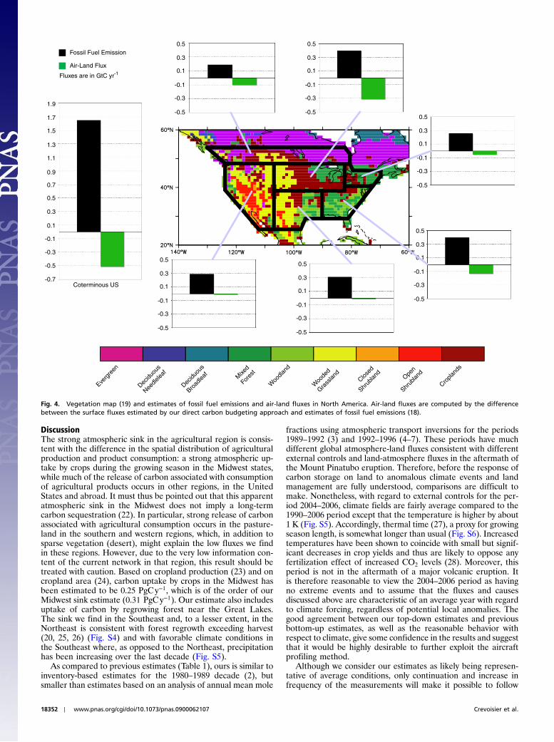
DiscussionThe strong atmospheric sink in the agricultural region is consis-tent with the difference in the spatial distribution of agriculturalproduction and product consumption: a strong atmospheric up-take by crops during the growing season in the Midwest states,while much of the release of carbon associated with consumptionof agricultural products occurs in other regions, in the UnitedStates and abroad. It must thus be pointed out that this apparentatmospheric sink in the Midwest does not imply a long-termcarbon sequestration (22). In particular, strong release of carbonassociated with agricultural consumption occurs in the pasture-land in the southern and western regions, which, in addition tosparse vegetation (desert), might explain the low fluxes we findin these regions. However, due to the very low information con-tent of the current network in that region, this result should betreated with caution. Based on cropland production (23) and oncropland area (24), carbon uptake by crops in the Midwest hasbeen estimated to be 0.25 PgC y−1, which is of the order of ourMidwest sink estimate (0.31 PgC y−1). Our estimate also includesuptake of carbon by regrowing forest near the Great Lakes.The sink we find in the Southeast and, to a lesser extent, in theNortheast is consistent with forest regrowth exceeding harvest(20, 25, 26) (Fig. S4) and with favorable climate conditions inthe Southeast where, as opposed to the Northeast, precipitationhas been increasing over the last decade (Fig. S5).

As compared to previous estimates (Table 1), ours is similar toinventory-based estimates for the 1980–1989 decade (2), butsmaller than estimates based on an analysis of annual mean mole

fractions using atmospheric transport inversions for the periods1989–1992 (3) and 1992–1996 (4–7). These periods have muchdifferent global atmosphere-land fluxes consistent with differentexternal controls and land-atmosphere fluxes in the aftermath ofthe Mount Pinatubo eruption. Therefore, before the response ofcarbon storage on land to anomalous climate events and landmanagement are fully understood, comparisons are difficult tomake. Nonetheless, with regard to external controls for the per-iod 2004–2006, climate fields are fairly average compared to the1990–2006 period except that the temperature is higher by about1 K (Fig. S5). Accordingly, thermal time (27), a proxy for growingseason length, is somewhat longer than usual (Fig. S6). Increasedtemperatures have been shown to coincide with small but signif-icant decreases in crop yields and thus are likely to oppose anyfertilization effect of increased CO2 levels (28). Moreover, thisperiod is not in the aftermath of a major volcanic eruption. Itis therefore reasonable to view the 2004–2006 period as havingno extreme events and to assume that the fluxes and causesdiscussed above are characteristic of an average year with regardto climate forcing, regardless of potential local anomalies. Thegood agreement between our top-down estimates and previousbottom-up estimates, as well as the reasonable behavior withrespect to climate, give some confidence in the results and suggestthat it would be highly desirable to further exploit the aircraftprofiling method.

Although we consider our estimates as likely being represen-tative of average conditions, only continuation and increase infrequency of the measurements will make it possible to follow

0.5

0.3

0.1

-0.1

-0.3

-0.5

0.5

0.3

0.1

-0.1

-0.3

-0.50.5

0.3

0.1

-0.1

-0.3

-0.5

0.5

0.3

0.1

-0.1

-0.3

-0.5

0.5

0.3

0.1

-0.1

-0.3

-0.5

0.5

0.3

0.1

-0.1

-0.3

-0.5

1.9

1.7

1.5

1.3

1.1

0.9

0.7

0.5

0.3

0.1

-0.1

-0.3

-0.5

-0.7Coterminous US

Fossil Fuel Emission

Air-Land Flux

Fluxes are in GtC yr-1

Cropla

nds

Decidu

ous

Needle

leaf

Decidu

ous

Broad

leaf

Mixe

d

Fore

st

Woo

dland

Woo

ded

Grass

land

C

losed

Shrub

land

Open

Shrub

land

Everg

reen

Fig. 4. Vegetation map (19) and estimates of fossil fuel emissions and air-land fluxes in North America. Air-land fluxes are computed by the differencebetween the surface fluxes estimated by our direct carbon budgeting approach and estimates of fossil fuel emissions (18).

18352 ∣ www.pnas.org/cgi/doi/10.1073/pnas.0900062107 Crevoisier et al.

the evolution of the North American sink. Moreover, the avail-ability of multiple profile sampling of CO2, combined here withour direct carbon budgeting approach, provides a means topartition the sink in different regions and to thus link variationsin carbon uptake to vegetation, climate and human drivers, awell-defined priority of the North American Carbon Program(NACP). Given the promise of the simple mass balance methodand given the particular strength of using multiple profile mea-surements as opposed to only surface measurements in an atmo-spheric inversion (8), we would recommend expanding thecoverage of appropriate observations with (i) more observationsat all sites to allow us to detect interannual variability and (ii) anincrease in site locations both in the coterminous United Statesand in other terrestrial regions where the method can work andthe carbon budget is poorly understood, namely the Amazonbasin or, more generally, the tropical region, although this wouldrequire a better understanding of the convective outflow acrossthe 8-km level because these regions have much stronger anddeeper convection compared to midlatitudes. In our view, theinitial results presented here demonstrate a feasible strategyfor constraining the large-scale carbon budgets of these regions.

Materials and MethodsWe interpolate the profiles using a Kriging technique (29). We take intoaccount the spatial continuity of the CO2 field using modeled spatial covar-iance (15). The subgrid variability is taken from ref. 30. We estimate thehorizontal CO2-carbon advective transport fluxes across the edges of thecontrol volume V shown in Fig. S2 from

Fhorizontal ¼ −ZZ

Sρχu · ndS;

where χ is the CO2 dry air mole fraction, ρ is air density, u is the 3D-wind field,S is the surface vertically bounding V (extending from the surface to 8 km),and n is the normal to S. Here, χ is the interpolated CO2 profile anomalyrelative to Mauna Loa. The wind distribution u used in our study and shownin Fig. S2 is taken from the NCEP (31) reanalysis. Nearly identical resultshave been obtained with the European Centre for Medium-Range WeatherForecasts wind distribution (32).

We estimate the surface fluxes using the volume-integrated continuityequation, which gives the carbon budget in the control volume V shownin Fig. S2,

∂C∂t

����V¼ ∂

∂t

ZZZVρχdV ¼ −

ZZSρχu:ndSþ Fvertical þ Fsurf ;

where C is the CO2-carbon mass content inside V , S is the surface envelopingV (including the top at 8 km and the bottom, with a surface wind velocityequal to zero), t is time, Fvertical is the carbon flux, other than vertical advec-tion, at the top of V , and Fsurf is the carbon surface flux. Terms of the equa-tion represent (i) the change of carbon inside V ; (ii) carbon fluxes due toadvection; (iii) vertical carbon fluxes, other than vertical advection, betweenV and the upper atmosphere, at 8 km; and (iv) carbon exchanges betweenV and the ground, which are the sum of natural vegetation, fossil fuelemissions, and nonvegetation fluxes such as CO2 stored in reservoirs andgoing into rivers.

All themeasurements were made by the NOAA/ESRL Aircraft Project usingautomated portable flask packages. A separate portable compressor packageis used to flush the air samples through a 0.7-L borosilicate glass flaskat 10–18 L∕min. Measurement was done by first cryogenically drying thesample gas and measuring the mole fraction using a nondispersive infraredanalyzer and three World Meteorological Organization CO2 reference stan-dards. Samples are collected at weekly to monthly intervals from 500 mabove ground to 8 km and analyzed at NOAA/ESRL within a week of collec-tion. Aircraft are equipped with single air inlets extending more than 6 in. offthe fuselage to avoid contamination from aircraft emissions. Simultaneousmeasurements of a variety of halocarbons and CO provide an independentindication of cabin air or engine exhaust contamination.

ACKNOWLEDGMENTS. This research was funded by the Cooperative Institutefor Climate Science under award NA17RJ2612 from the National Oceanic andAtmospheric Administration, U.S. Department of Commerce, by the CarbonMitigation Initiative, with support provided by the FordMotor Company, andby the U.S. Department of Energy’s Office of Science (BER) through theNortheastern Regional Center of the National Institute for Climatic ChangeResearch. The statements, findings, conclusions, and recommendations arethose of the authors and do not necessarily reflect the views of the NationalOceanic and Atmospheric Administration, or the U.S. Department ofCommerce.

1. Sabine CL, et al. (2004) The oceanic sink for anthropogenic CO2 . Science 305:367–371.2. Pacala SW, et al. (2001) Consistent land- and atmosphere-based U.S. carbon sink

estimates. Science 292:2316–2320.3. Fan S-M, Sarmiento JL, Gloor M, Pacala SW (1999) On the use of regularization

techniques in the inverse modeling of atmospheric carbon dioxide. J Geophys Res104:21503–21512.

4. Gurney KR, et al. (2002) Towards robust estimates of CO2 sources and sinks usingatmospheric transport models. Nature 415:626–630.

5. Gurney KR, et al. (2004) Transcom 3 inversion intercomparison: Model mean resultsfor the estimation of seasonal carbon sources and sinks. Global Biogeochem Cycles18:GB1010.

6. Baker DF, et al. (2006) Transcom 3 inversion intercomparison: Impact of transportmodel errors on the interannual variability of regional CO2 fluxes, 1988–2003. GlobalBiogeochem Cycles 20:GB1002.

7. Jacobson AR, Mikaloff Fletcher SE, Gruber N, Sarmiento JL, Gloor M (2007) A jointatmosphere-ocean inversion for surface fluxes of carbon dioxide: 1. Methods andglobal-scale fluxes. Global Biogeochem Cycles 21:GB1019.

8. Peters W, et al. (2007) An atmospheric perspective on North American carbon dioxideexchange: CarbonTracker. Proc Natl Acad Sci USA 104:18925–18930.

9. Pacala SW, et al. (2007) The First State of the Carbon Cycle Report (SOCCR), edsAW King et al. (U.S. Climate Change Science Program, Washington, DC), pp 69–91.

10. Stephens BB, et al. (2007) Weak northern and strong tropical land carbon uptake fromvertical profiles of atmospheric CO2. Science 316:1732–1735.

11. Yang Z, et al. (2007) New constraints on Northern Hemisphere growing season netflux. Geophys Res Lett 34:L12807.

12. Prather MJ, Zhu X, Strahan SE, Steenrod SD, Rodriguez JM (2008) Quantifying errors intrace species transport modeling. Proc Natl Acad Sci USA 105:19617–19621.

13. Gloor M, et al. (2001) What is the concentration footprint of a tall tower? J GeophysRes 106:17831–17840.

14. North American Carbon Program Implementation Strategy Group (2005) ScienceImplementation Strategy for the North American Carbon Program, http://www.isse.ucar.edu/nacp/.

15. Crevoisier C, et al. (2006) A direct carbon budgeting approach to infer carbon sourcesand sinks. Design and synthetic application to complement the NACP observationnetwork. Tellus 58B:366–375.

16. Lynch-Stieglitz J, Stocker TF, Broecker WS, Fairbanks RG (1995) The influence of air-seaexchange on the isotopic composition of oceanic carbon: Observations and modeling.Global Biogeochem Cycles 9:653–665.

17. Denning AS, Fung IY, Randall AD (1995) Latitudinal gradient of atmospheric CO2 dueto seasonal exchange with land biota. Nature 376:240–243.

18. Marland G, Boden T, Andres RJ (2007) National CO2 emissions from fossil-fuelburning, cement manufacture, and gas flaring. http://cdiac.ornl.gov/trends/emis_mon/stateemis/emis_state.html.

19. Hansen M, DeFries R, Townshend JRG, Sohlberg R (1998) UMD Global Land CoverClassification, 1 Kilometer, 1.0, Department of Geography, University of Maryland,College Park, Maryland, 1981–1994.

20. Houghton RA, Hackler JL (2000) Changes in terrestrial carbon storage in the UnitedStates 1. The roles of agriculture and forestry. Global Ecol Biogeogr 9:125–144.

21. Potter C, Klooster S, Huete A, Genovese V (2007) Terrestrial carbon sinks for the unitedstates predicted from MODIS satellite data and ecosystem modeling. Earth Interact11:1–21.

22. Verma SB, et al. (2005) Annual carbon dioxide exchange in irrigated and rainfedmaize-based agroecosystems. Agr Forest Meteorol 131:77–96.

23. United States Department of Agriculture (2006) Crop Production 2006 Summary(National Agricultural Statistics Service report).

24. Waisanen PJ, Bliss NB (2002) Changes in population and agricultural land inconterminous United States countries. Global Biogeochem Cycles 16:1137.

25. Hurtt GC, et al. (2002) Projecting the future of the U.S. carbon sink. Proc Natl Acad SciUSA 99:1389–1394.

26. Hurtt GC, et al. (2006) The underpinnings of land-use history: Three centuries of globalgridded land-use transitions, wood harvest activity, and resulting secondary lands.Glob Change Biol 12:1208–1229.

27. Masle J, Doussinault G, Farquhar GD, Sun B (1989) Foliar stage in wheat correlatesbetter to photothermal time than to thermal time. Plant Cell Environ 12:235–247.

28. Lobell DB, Field CW (2007) Global scale climate-crop yield relationships and theimpacts of recent warming. Environ Res Lett 2:014002.

29. Matheron G (1965) Regionalized Variables and Their Estimation (Les Variablesrégionalisées et leur estimation) (Masson, Paris) p 306.

30. Lin JC, et al. (2004) An empirical analysis of the spatial variability of atmospheric CO2 :Implications for inverse analyses and space-borne sensors.Geophys Res Lett 31:L23104.

31. Kalnay E, et al. The NCEP/NCAR 40-year reanalysis project. Bull Am Meteorol Soc77:437–470.

32. Uppala SM, et al. (2005) The ERA-40 re-analysis. Quart J Roy Meteorol Soc131:2961–3012.

Crevoisier et al. PNAS ∣ October 26, 2010 ∣ vol. 107 ∣ no. 43 ∣ 18353

ENVIRONMEN

TAL

SCIENCE

S