Embed Size (px)
Citation preview
Relais User’s Guide – Version 3.0
Page 1
RELREL ISISRELREL ISIS
User’s Guide
Version 3.0
Editors:
Monica Scannapieco (Istat) Nicoletta Cibella (Istat)
Laura Tosco (Istat) Tiziana Tuoto (Istat)
Luca Valentino (Istat) Marco Fortini (Istat)
Luca Mancini (Istat)
RELREL ISISRELREL ISIS
Relais User’s Guide – Version 3.0
Page 2
RELREL ISISRELREL ISIS
Index
1 Introduction ......................................................................................................................... 4
1.1 Add-ons of RELAIS 3.0 ............................................................................................... 5
2 Record Linkage Processes in RELAIS ............................................................................... 5
2.1 Phases ........................................................................................................................... 5 2.2 RELAIS Techniques..................................................................................................... 7
2.2.1 Phase 1: Choice of Matching Variables ................................................................ 8 2.2.2 Phase 2: Choice of Comparison Functions ........................................................... 8
2.2.3 Phase 3: Creation and Reduction of the Search Space of Link Candidate Pairs .. 9 2.2.4 Phase 4: Choice of Decision Model ................................................................... 10 2.2.5 Phase 5: Selection of Unique Links .................................................................... 10
2.3 Examples of Record Linkage Work-flows ................................................................. 10
3 Installation ......................................................................................................................... 11
3.1 Windows Environment: Requirements ...................................................................... 11 3.2 Windows Environment: Installation and Execution ................................................... 12 3.3 Linux Environment: Requirements ............................................................................ 13
3.4 Linux Environment: Installation and Execution ........................................................ 13 3.5 Training Data Sets ...................................................................................................... 15
4 The RELAIS Menu ........................................................................................................... 15
5 Project ............................................................................................................................... 16
6 Dataset ............................................................................................................................... 17
7 Pre-processing Functionalities .......................................................................................... 20
7.1 Check Functions ......................................................................................................... 20
7.2 Conversion Functions ................................................................................................. 21 7.2.1 Field Standardization .......................................................................................... 21 7.2.2 Fields Merge ....................................................................................................... 22
7.2.3 Field Parse ........................................................................................................... 23
7.2.4 Inaccuracy Repair ............................................................................................... 24 7.2.5 Schema Reconciliation ........................................................................................ 26
8 Data Profiling .................................................................................................................... 27
8.1 Methodological Aspects ............................................................................................. 27 8.2 Diagnostics for Selecting Blocking Variables............................................................ 28 8.3 Diagnostics for Selecting Matching Variables ........................................................... 29
9 Creation and Reduction of the Search Space .................................................................... 30
9.1 Methodological Aspects ............................................................................................. 30 9.2 Search Space Creation ................................................................................................ 31
9.3 Search Space Reduction ............................................................................................. 31 9.3.1 Blocking .............................................................................................................. 32
9.3.2 Blocking Union ................................................................................................... 33 9.3.3 Sorted Neighbourhood Method ........................................................................... 34 9.3.4 Nested Blocking .................................................................................................. 35 9.3.5 SimHash .............................................................................................................. 35 9.3.6 Blocked SimHash ................................................................................................ 38
9.4 Read from external file ............................................................................................... 38
10 Decisional models ............................................................................................................. 39

Relais User’s Guide – Version 3.0
Page 3
RELREL ISISRELREL ISIS
10.1 Methodological aspects .......................................................................................... 39
10.2 Selection of Comparison Functions ........................................................................ 40 10.3 Deterministic Decision Models .............................................................................. 42 10.4 Probabilistic Model ................................................................................................. 46
10.4.1 Contingency Table .............................................................................................. 48 10.4.2 Parameter Estimation of the Probabilistic Model and the Table MU ................. 49
11 Reduction to matching 1:1 ................................................................................................ 51
11.1 Methodological Aspects ......................................................................................... 51 11.2 Optimized Solution ................................................................................................. 52 11.3 Greedy Solution ...................................................................................................... 52
12 Linkage Result .................................................................................................................. 52
12.1 Choice of the Thresholds ........................................................................................ 52 12.2 The Linkage Result menu ....................................................................................... 56
13 Save ................................................................................................................................... 57
14 Utility ................................................................................................................................ 60
15 Batch Execution ........................................................ Errore. Il segnalibro non è definito.
16 Bibliography...................................................................................................................... 63
17 Appendix : Parameter Estimation of the Probabilistic Model via the EM Algorithm ...... 66
Relais User’s Guide – Version 3.0
Page 4
RELREL ISISRELREL ISIS
1 Introduction
RELAIS (REcord Linkage At IStat) is a toolkit providing a set of techniques for dealing with record
linkage projects.
The purpose of record linkage is to identify the same real world entity that can be differently
represented in data sources [3], even if unique identifiers are not available or are affected by errors. In
statistics, record linkage is needed for several applications, including: enriching the information stored
in different data-sets; de-duplicating data-sets; improving the data quality of a source; measuring a
population amount by capture-recapture method; checking the confidentiality of public-use micro data.
Starting from the earliest contributions, dated back to 1959 [13], there has been a proliferation of
different approaches based on statistics, databases, machine learning, knowledge representation.
However, despite this proliferation, no particular record linkage technique has emerged as the best
solution for all cases. We believe that such a solution does not actually exist, and that an alternative
strategy should be adopted [5]. In fact, record linkage can be seen as a complex process consisting of
several phases involving different knowledge areas; moreover, several different techniques can be
adopted for each phase. We believe that the choice of the most appropriate technique not only depends
on the practitioner‟s skill but, most of all, it is application specific. Moreover, in some applications,
there is no evidence to prefer a given method to others or of the fact that different choices, at some
linkage stage, could bring to the same results. This is why it could be reasonable to dynamically select
the most appropriate technique for each phase and to combine the selected techniques for building a
record linkage work-flow of a given application. RELAIS is a toolkit relying on these ideas.
The principal features of RELAIS are [5, 9, 11, 12]:
It is designed and developed to allow the combination of different techniques for each of the
record linkage phases, so that the resulting work-flow is actually built on the basis of
application and data specific requirements.
It has been developed as an open source project, so several solutions already available for
record linkage in the scientific community can be easily re-used. It is released under the EUPL
license (European Union Public License).
It has been implemented by using two languages based on different paradigms: Java, an object-
oriented language, and R, a functional language. This choice depends on our belief that a
record linkage process is composed of techniques for manipulating data, for which Java is
more appropriate, and of calculation-oriented techniques for which R is a preferable choice.
The choice of Java and R is also in line with the open source philosophy of the RELAIS
project.
It has been implemented using a relational database architecture, in particular it is based on a
mySql environment that is also in line with the open source philosophy of the RELAIS project.
Relais User’s Guide – Version 3.0
Page 5
RELREL ISISRELREL ISIS
The RELAIS project aims to provide record linkage techniques easily accessible to not-expert users.
Indeed, the developed system has a GUI (Graphical User Interface) that on the one hand permits to
build record linkage work-flows with a good flexibility. On the other hand it checks the execution
order among the different provided techniques whereas precedence rules must be controlled.
The current version of RELAIS provides a set of techniques to execute record linkage applications
according to the decomposition described in Section 2.
1.1 Add-ons of RELAIS 3.0
With respect to RELAIS version 2.2, RELAIS 3.0 has the following new features:
Pre-processing functionalities
Schema reconciliation
New methods for search space reduction: SimHash and Blocked SimHash
New functions for string comparison
Graphical choice of thresholds
And other minor innovations.
2 Record Linkage Processes in RELAIS The complexity of the whole linking process relies on several aspects of different nature. If unique
identifiers are available in the considered data sources the problem can be quite easily treated because
its complexity is reduced only to computational constraints. But, generally, unique identifiers are not
available and more sophisticated statistical procedures, relying on “matching variables” chosen for
linking data, are requested.
However, data sources are often hard to combine since errors or lacking information in the record
identifiers may complicate the integrated use of the information, in order to overcome such obstacles
record linkage techniques provide multidisciplinary set of methods and practices whose purpose is to
identify the same real world entity, which can be differently represented in one or more data sources.
RELAIS aims to join the statistical and computational essence of the linkage problem.
2.1 Phases
The idea of decomposing the record linkage process in its phases is the core of the RELAIS toolkit and
makes the whole process easier to manage; each phase has its own windows. Now, a general overview
on the main phases is given while more details are added later in the specific paragraph devoted to the
considered phase.
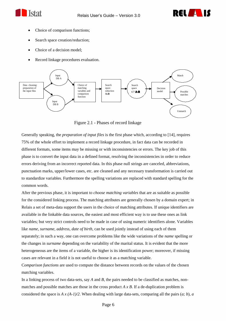
The main phases (shown in Figure 2.1) are:
Data cleaning - preparation of the input files (pre-processing);
Choice of the common identifying attributes (matching variables);
Relais User’s Guide – Version 3.0
Page 6
RELREL ISISRELREL ISIS
Choice of comparison functions;
Search space creation/reduction;
Choice of a decision model;
Record linkage procedures evaluation.
Generally speaking, the preparation of input files is the first phase which, according to [14], requires
75% of the whole effort to implement a record linkage procedure, in fact data can be recorded in
different formats, some items may be missing or with inconsistencies or errors. The key job of this
phase is to convert the input data in a defined format, resolving the inconsistencies in order to reduce
errors deriving from an incorrect reported data. In this phase null strings are canceled, abbreviations,
punctuation marks, upper/lower cases, etc. are cleaned and any necessary transformation is carried out
to standardize variables. Furthermore the spelling variations are replaced with standard spelling for the
common words.
After the previous phase, it is important to choose matching variables that are as suitable as possible
for the considered linking process. The matching attributes are generally chosen by a domain expert; in
Relais a set of meta-data support the users in the choice of matching attributes. If unique identifiers are
available in the linkable data sources, the easiest and most efficient way is to use these ones as link
variables; but very strict controls need to be made in case of using numeric identifiers alone. Variables
like name, surname, address, date of birth, can be used jointly instead of using each of them
separately; in such a way, one can overcome problems like the wide variations of the name spelling or
the changes in surname depending on the variability of the marital status. It is evident that the more
heterogeneous are the items of a variable, the higher is its identification power; moreover, if missing
cases are relevant in a field it is not useful to choose it as a matching variable.
Comparison functions are used to compute the distance between records on the values of the chosen
matching variables.
In a linking process of two data-sets, say A and B, the pairs needed to be classified as matches, non-
matches and possible matches are those in the cross product A x B. If a de-duplication problem is
considered the space is A x (A-1)/2. When dealing with large data-sets, comparing all the pairs (a; b), a
Input
DB A
Data cleaning:
preparation of
the input files
Input
DB B
Choice of
matching
variables and
comparison
function
Search
space
reduction
AxB
Search
space
C? AxB
Decision
model
Match
Unmatch
Possible
matches
Figure 2.1 - Phases of record linkage
Relais User’s Guide – Version 3.0
Page 7
RELREL ISISRELREL ISIS
belonging to A and b belonging to B, in the cross product is almost impracticable, in fact while the
number of possible matches increases linearly, the computational problem raises quadratic, being the
complexity O(n2) [15]. To reduce this complexity it is necessary to reduce the number of pairs (a; b) to
be compared. There are many different techniques that can be applied to reduce the search space;
blocking and sorted neighbourhood are the two main methods. Blocking consists of partitioning the two
sets into blocks and of considering linkable only records within each block. The partition is made
through blocking keys; two records belong to the same block if all the blocking keys are equal or if a
hash function applied to the blocking keys of the two records gives the same result. Sorted
neighbourhood sorts the two input files on a blocking key and searches possible matching records only
inside a window of a fixed dimension which slides on the two ordered record sets.
Starting from the reduced search space, we can apply different decision models that define the rules
used to determine whether a pair of records (a; b) is a match, a non-match or a possible match.
The core of a record linkage process is the choice of a decision model that enables to classify pairs into
M, the set of matches and U, the set of non-matches. The decision rule can be empirical or
probabilistic. In the deterministic approach, a pair is a match if it agrees completely on all the
matching variables chosen or satisfies a defined rule-base system, that is if it reaches a score that is
beyond a threshold when applying the comparison function.
The probabilistic approach, based on the Fellegi and Sunter model [4], requires an estimation of the
model parameters that can be performed via the EM algorithm, Bayesian methods, etc.
A linkage process can be also classified as: (i) one-to-one problem, if one record in the set A links to
only one record in B and also the other way around, (ii) one-to-many problem if a record in a set can be
matched with more than one of the compared file, (iii) many-to-many problem if more than one record
in each file match with more than one record in the other. The latter two problems may imply the
existence of duplicate records in the linkable data sources.
Finally, as not every record matched in the linkage process refers to the same identity, in “the record
linkage procedure evaluation”, it‟s important to establish whether a match is a “true one” or not. In
other words, during a linkage project is necessary to classify records as true link or true non link,
minimizing the two types of possible errors: false matches and false non-matches. The first type of
error refers to matched records which do not represent the same entity, while the latter indicates
unmatched records not correctly classified, that imply truly matched entities were not linked.
2.2 RELAIS Techniques
Each of the phases described in the previous section can be performed according to different
techniques; depending on specific applications and features of the data at hand, it can be suitable to
iterate and/or omit some phases, as well as it could be better to choose some techniques rather than
others. In the current version, RELAIS provides some of the most widespread methods and techniques
for the following phases:
Relais User’s Guide – Version 3.0
Page 8
RELREL ISISRELREL ISIS
Data cleaning - preparation of the input files (pre-processing);
Choice of matching variables;
Choice of comparison functions;
Creation and reduction of the search space of link candidate pairs;
Choice of the decision model;
Selection of unique links.
In the following, for each of the implemented phase, we briefly detail the available techniques.
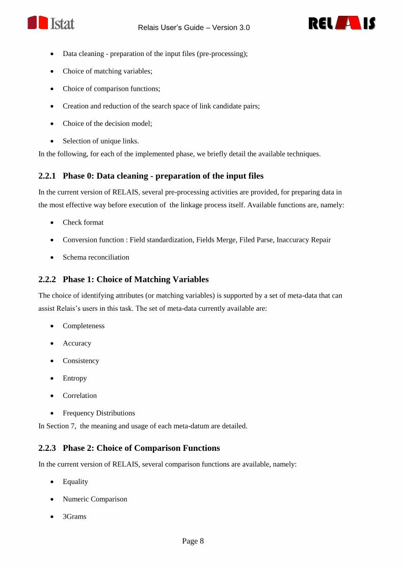
2.2.1 Phase 0: Data cleaning - preparation of the input files
In the current version of RELAIS, several pre-processing activities are provided, for preparing data in
the most effective way before execution of the linkage process itself. Available functions are, namely:
Check format
Conversion function : Field standardization, Fields Merge, Filed Parse, Inaccuracy Repair
Schema reconciliation
2.2.2 Phase 1: Choice of Matching Variables
The choice of identifying attributes (or matching variables) is supported by a set of meta-data that can
assist Relais‟s users in this task. The set of meta-data currently available are:
Completeness
Accuracy
Consistency
Entropy
Correlation
Frequency Distributions
In Section 7, the meaning and usage of each meta-datum are detailed.
2.2.3 Phase 2: Choice of Comparison Functions
In the current version of RELAIS, several comparison functions are available, namely:
Equality
Numeric Comparison
3Grams
Relais User’s Guide – Version 3.0
Page 9
RELREL ISISRELREL ISIS
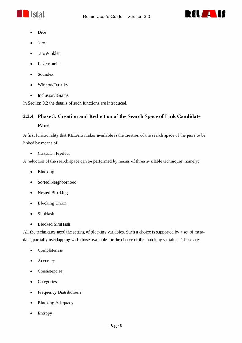
Dice
Jaro
JaroWinkler
Levenshtein
Soundex
WindowEquality
Inclusion3Grams
In Section 9.2 the details of such functions are introduced.
2.2.4 Phase 3: Creation and Reduction of the Search Space of Link Candidate
Pairs
A first functionality that RELAIS makes available is the creation of the search space of the pairs to be
linked by means of:
Cartesian Product
A reduction of the search space can be performed by means of three available techniques, namely:
Blocking
Sorted Neighborhood
Nested Blocking
Blocking Union
SimHash
Blocked SimHash
All the techniques need the setting of blocking variables. Such a choice is supported by a set of meta-
data, partially overlapping with those available for the choice of the matching variables. These are:
Completeness
Accuracy
Consistencies
Categories
Frequency Distributions
Blocking Adequacy
Entropy
Relais User’s Guide – Version 3.0
Page 10
RELREL ISISRELREL ISIS
In paragraph 8, a detailed discussion on such meta-data is available.
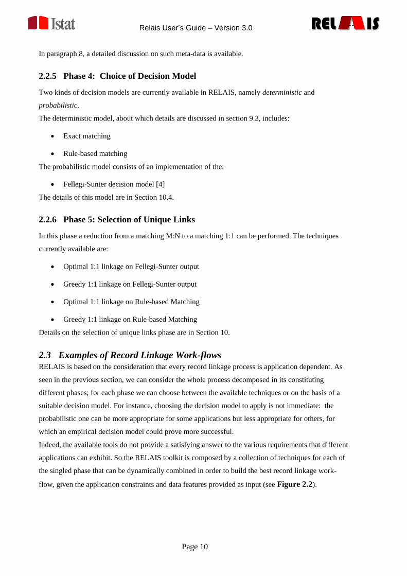
2.2.5 Phase 4: Choice of Decision Model
Two kinds of decision models are currently available in RELAIS, namely deterministic and
probabilistic.
The deterministic model, about which details are discussed in section 9.3, includes:
Exact matching
Rule-based matching
The probabilistic model consists of an implementation of the:
Fellegi-Sunter decision model [4]
The details of this model are in Section 10.4.
2.2.6 Phase 5: Selection of Unique Links
In this phase a reduction from a matching M:N to a matching 1:1 can be performed. The techniques
currently available are:
Optimal 1:1 linkage on Fellegi-Sunter output
Greedy 1:1 linkage on Fellegi-Sunter output
Optimal 1:1 linkage on Rule-based Matching
Greedy 1:1 linkage on Rule-based Matching
Details on the selection of unique links phase are in Section 10.
2.3 Examples of Record Linkage Work-flows
RELAIS is based on the consideration that every record linkage process is application dependent. As
seen in the previous section, we can consider the whole process decomposed in its constituting
different phases; for each phase we can choose between the available techniques or on the basis of a
suitable decision model. For instance, choosing the decision model to apply is not immediate: the
probabilistic one can be more appropriate for some applications but less appropriate for others, for
which an empirical decision model could prove more successful.
Indeed, the available tools do not provide a satisfying answer to the various requirements that different
applications can exhibit. So the RELAIS toolkit is composed by a collection of techniques for each of
the singled phase that can be dynamically combined in order to build the best record linkage work-
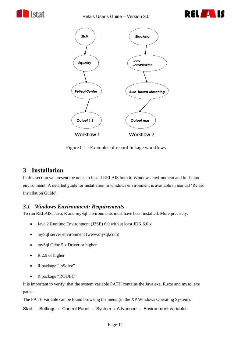
flow, given the application constraints and data features provided as input (see Figure 2.2).
Relais User’s Guide – Version 3.0
Page 11
RELREL ISISRELREL ISIS
3 Installation In this section we present the notes to install RELAIS both in Windows environment and in Linux
environment. A detailed guide for installation in windows environment is available in manual „Relais
Installation Guide‟.
3.1 Windows Environment: Requirements
To run RELAIS, Java, R and mySql environments must have been installed. More precisely:
Java 2 Runtime Environment (J2SE) 6.0 with at least JDK 6.0.x
mySql server environment (www.mysql.com)
mySql Odbc 5.x Driver or higher
R 2.9 or higher
R package “lpSolve”
R package “RODBC”
It is important to verify that the system variable PATH contains the Java.exe, R.exe and mysql.exe
paths.
The PATH variable can be found browsing the menu (in the XP Windows Operating System):
Start → Settings → Control Panel → System → Advanced → Environment variables
Fellegi-Sunter
SNM
Equality
Output 1:1
Workflow 1
Fellegi-Sunter
SNM
Equality
Output 1:1
Workflow 1
Rule-based Matching
Blocking
Jaro
JaroWinkler
Output m:n
Workflow 2
Rule-based Matching
Blocking
Jaro
JaroWinkler
Output m:n
Workflow 2
Figure 0.1 - Examples of record linkage workflows
Relais User’s Guide – Version 3.0
Page 12
RELREL ISISRELREL ISIS
To modify the system variable PATH it is necessary to be PC administrator.
If different version of Java and/or R are installed on the PC, the new paths of Java and/or R must be
written in the PATH variable string before the paths of the previous version; we recommend to insert
the new paths at the beginning of the PATH variable.
An example of how to set the PATH variable follows:
PATH=C:\Programs\Java\jre1.6.0_03\bin;C:\Programs\R\R-2.5.1\bin;C:\Programs\mysql\MySql Server 5.0\bin
Finally, it is important to check that the operating system is updated at least to Service Pack 2. To
verify this requirement, click with the right button of the mouse on the Computer Resources icon and
select the Properties menu, in the General menu is described the Service Pack version currently
installed. If an update is needed, just click on the Windows Update icon (on the Start menu) and follow
the instructions.
3.2 Windows Environment: Installation and Execution
To install RELAIS, starting from the Relais_setup.exe file, just execute this file and follow the
instruction. The directory, in which RELAIS has been installed, will contain the following files:
Relais.bat
Relais2.2.jar
mu_gen_embedded.R
LP.R
mu_from_marginals.R
RelaisBatch.bat
batchParameters.txt
and the lib directory which contains the files my-sql-connector-java-5.1.10-bin.jar and ojdbc14.jar that
are necessary for the connection to the databases (MySQL and Oracle).
It is recommended to check the RELAIS directory permissions: the read-write permissions must be
enabled for all users.
To run the program just double click on the Relais.bat file.
While installing mySql environment it is necessary to create an anonymous account besides the system
account.
After the installation it is necessary, for using RODBC package, to create a new data source. After
creating relais data base in mySql environment, browse the menu (in the XP Windows Operating
System):
Start → Settings → Control Panel → Administration Tools → Data Sources (ODBC)
Relais User’s Guide – Version 3.0
Page 13
RELREL ISISRELREL ISIS
In the window that will be opened the User DSN menu must be chosen; in this menu clicking on the
Add button, a new window will be open, in this window the mySql ODBC driver must be chosen. In
the new window that will be opened, the following settings must be done:
data source = relais
server = localhost
database = relais
To install R packages, run the R environment and browse the menu:
Packages → Install packages
After choosing a CRAN, a list of packages will be displayed. In this list, click on the lpSolve package
and on the RODBC package1.
3.3 Linux Environment: Requirements
To run RELAIS, Java, R and mySql environments must have been installed. More precisely:
Java 2 Runtime environment (J2SE) 6.0 with at least JDK 6.0.x
mySql server environment (www.mysql.com)
mySql Odbc 5.x Driver or higher
R 2.9 or higher
R package “lpSolve”
R package “RODBC”
3.4 Linux Environment: Installation and Execution
To install RELAIS starting from the RELAIS2.2.zip file, it is necessary to unzip this file in a directory,
for example C:\RELAIS. This directory will contain the following files:
Relais.bat
Relais2.2.jar
mu_gen_embedded.R
LP.R
mu_from_marginals.R
1 If there are problems to reach a CRAN, click with the right button of the mouse on the R icon and select the
Properties menu, in the Connection menu write –internet2 at the end of the destination. For example:
C:\Programs\R\R-2.8.1\bin\Rgui.exe –internet2.
Relais User’s Guide – Version 3.0
Page 14
RELREL ISISRELREL ISIS
RelaisBatch.bat
batchParameters.txt
and the lib directory which contains the files my-sql-connecotr-java-5.1.10-bin.jar and ojdbc14.jar that
are necessary for the connection to the databases (MySQL and Oracle).
During the installation of mySql environment it is necessary to create the user “root” specifying a
password. Moreover, it is necessary to create an anonymous user “” giving him all the grants on the
following schema:
information_schema
mysql
relais
Thus the relais schema must have been created using the instruction:
CREATE DATABASE relais
It is important to notice that the data base name relais must be written in lower cases being the Linux
operating system case sensitive.
If no specific knowledge about the Linux operating system is held, it could be useful to install the
mySql Gui tool that gives a graphical interface to the data base and make easier to perform all the
operations described below.
Moreover, it is important to check that the libmyODBC library has been installed, this library contains
the header necessary for a correct running of mySql.
Moreover, the libraries:
unixODBC_dev
unixODBC
must have been installed, these are necessary to connect to the data base starting from a R program.
Finally, it is necessary to modify the hidden file .ODBC.ini (that can be found in the own home folder)
writing the following instructions:
[ODBC Data Sources]
relais = Connector/ODBC 3.51 Driver DSN
[relais]
Driver = /usr/lib/odbc/libmyodbc.so
Description = Connector/ODBC 3.51 Driver DSN
Server = localhost
Relais User’s Guide – Version 3.0
Page 15
RELREL ISISRELREL ISIS
DSN = relais
Port = 3306
User =
Password =
Database = relais
ServerType = MySql
Option =
TraceFile = /var/log/mysql_test_trace.log
Trace = 0
To run the program just use the following command:
java –jar relais.jar
or after changing the Relais.bat file making an executable file (chmod 777 Relais.bat), just double click
on the Relais.bat file icon.
To install R packages, run the R environment and write the instruction:
install.packages(“name_of_package”, dependencies=TRUE)
For example, to install lpSolve package write the following instruction:
install.packages(“lpSolve”, dependencies=TRUE)
3.5 Training Data Sets
The RELAIS installation directory also contains a directory named “training_data” with two datasets of
synthetic census like records, stored in the files census_a.txt and census_b.txt. The two datasets,
originally provided by W. Winkler, are available also with the SECONDSTRING package:
www.cs.utexas.edu/users/ml/riddle/data/secondstring.tar.gz
Census_a and census_b contain respectively 449 and 392 records. The true matches (327) can be found
by the IDENTIFIER field.
4 The RELAIS Menu As shown in Figure 5.1, the RELAIS menu is composed by the following items:
Project
Dataset
Relais User’s Guide – Version 3.0
Page 16
RELREL ISISRELREL ISIS
Preprocessing
Data Profiling
Search Space Creation
Decision Model
Linkage 1:1
Linkage Result
Save
Utility
In following sections, each of this menu will be detailed.
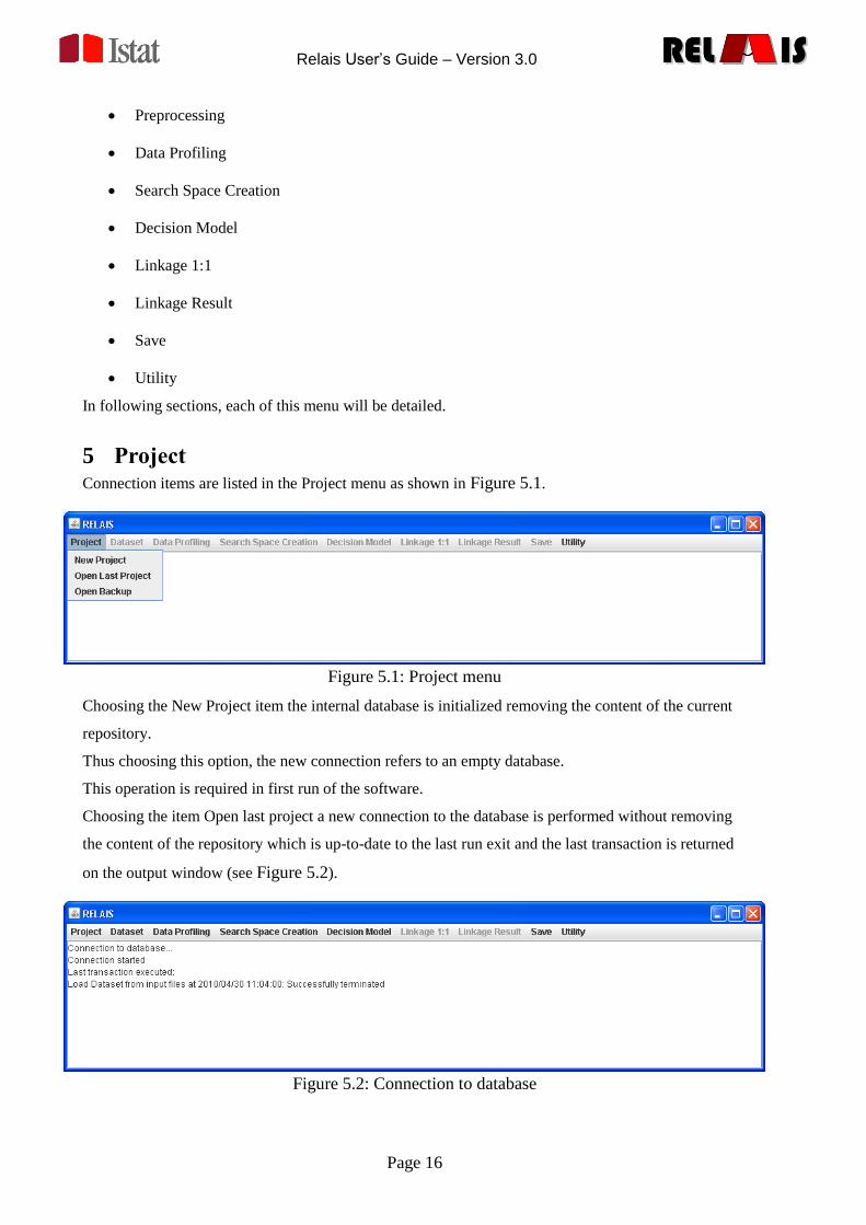
5 Project Connection items are listed in the Project menu as shown in Figure 5.1.
Figure 5.1: Project menu
Choosing the New Project item the internal database is initialized removing the content of the current
repository.
Thus choosing this option, the new connection refers to an empty database.
This operation is required in first run of the software.
Choosing the item Open last project a new connection to the database is performed without removing
the content of the repository which is up-to-date to the last run exit and the last transaction is returned
on the output window (see Figure 5.2).
Figure 5.2: Connection to database
Relais User’s Guide – Version 3.0
Page 17
RELREL ISISRELREL ISIS
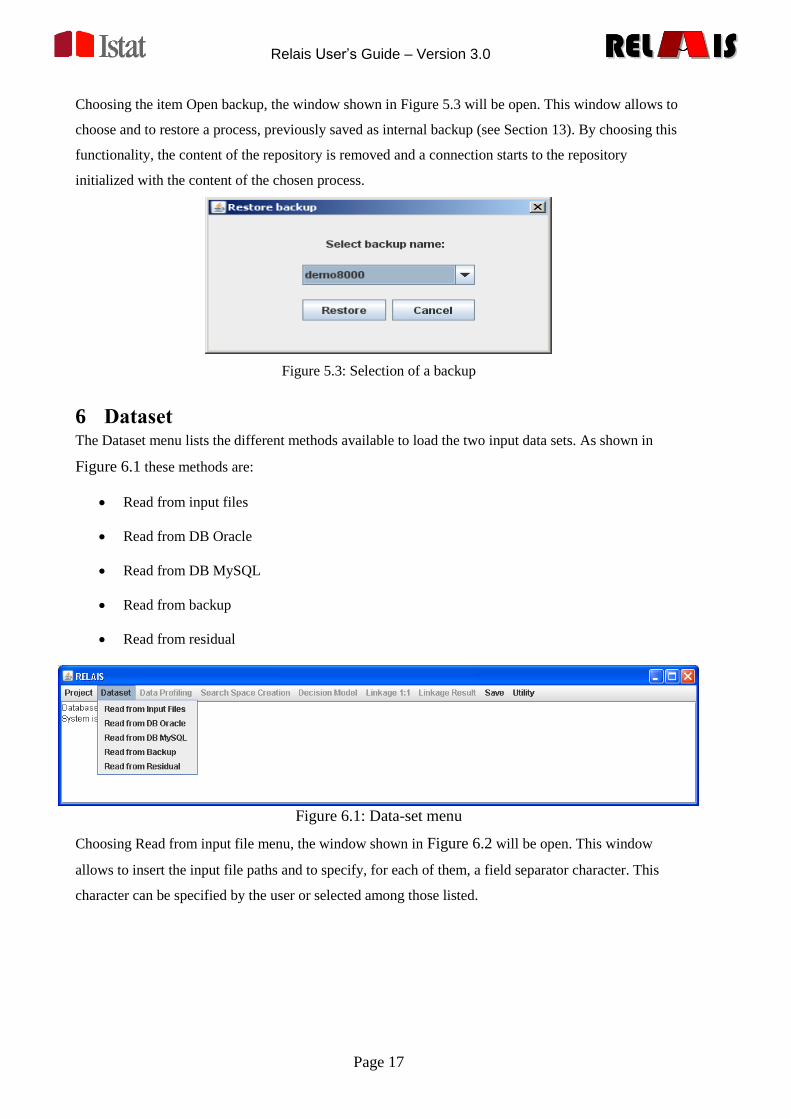
Choosing the item Open backup, the window shown in Figure 5.3 will be open. This window allows to
choose and to restore a process, previously saved as internal backup (see Section 13). By choosing this
functionality, the content of the repository is removed and a connection starts to the repository
initialized with the content of the chosen process.
Figure 5.3: Selection of a backup
6 Dataset The Dataset menu lists the different methods available to load the two input data sets. As shown in
Figure 6.1 these methods are:
Read from input files
Read from DB Oracle
Read from DB MySQL
Read from backup
Read from residual
Figure 6.1: Data-set menu
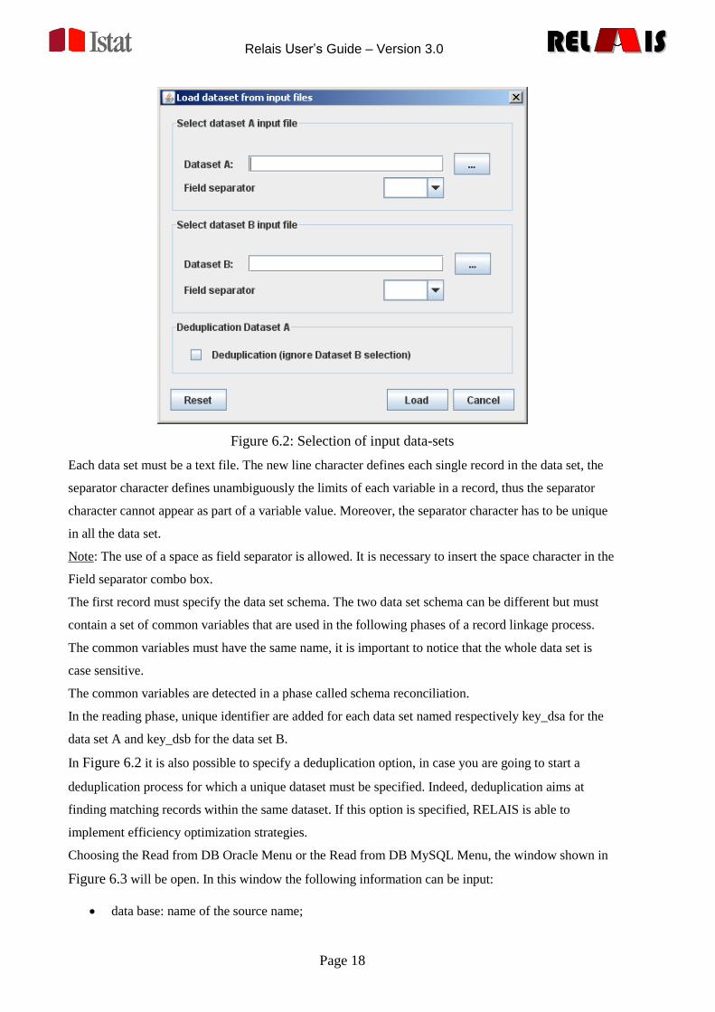
Choosing Read from input file menu, the window shown in Figure 6.2 will be open. This window
allows to insert the input file paths and to specify, for each of them, a field separator character. This
character can be specified by the user or selected among those listed.
Relais User’s Guide – Version 3.0
Page 18
RELREL ISISRELREL ISIS
Figure 6.2: Selection of input data-sets
Each data set must be a text file. The new line character defines each single record in the data set, the
separator character defines unambiguously the limits of each variable in a record, thus the separator
character cannot appear as part of a variable value. Moreover, the separator character has to be unique
in all the data set.
Note: The use of a space as field separator is allowed. It is necessary to insert the space character in the
Field separator combo box.
The first record must specify the data set schema. The two data set schema can be different but must
contain a set of common variables that are used in the following phases of a record linkage process.
The common variables must have the same name, it is important to notice that the whole data set is
case sensitive.
The common variables are detected in a phase called schema reconciliation.
In the reading phase, unique identifier are added for each data set named respectively key_dsa for the
data set A and key_dsb for the data set B.
In Figure 6.2 it is also possible to specify a deduplication option, in case you are going to start a
deduplication process for which a unique dataset must be specified. Indeed, deduplication aims at
finding matching records within the same dataset. If this option is specified, RELAIS is able to
implement efficiency optimization strategies.
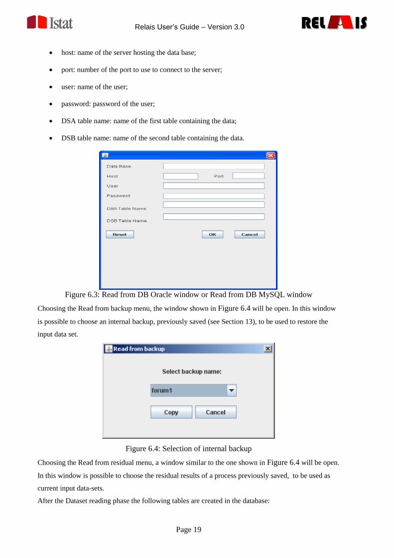
Choosing the Read from DB Oracle Menu or the Read from DB MySQL Menu, the window shown in
Figure 6.3 will be open. In this window the following information can be input:
data base: name of the source name;
Relais User’s Guide – Version 3.0
Page 19
RELREL ISISRELREL ISIS
host: name of the server hosting the data base;
port: number of the port to use to connect to the server;
user: name of the user;
password: password of the user;
DSA table name: name of the first table containing the data;
DSB table name: name of the second table containing the data.
Figure 6.3: Read from DB Oracle window or Read from DB MySQL window
Choosing the Read from backup menu, the window shown in Figure 6.4 will be open. In this window
is possible to choose an internal backup, previously saved (see Section 13), to be used to restore the
input data set.
Figure 6.4: Selection of internal backup
Choosing the Read from residual menu, a window similar to the one shown in Figure 6.4 will be open.
In this window is possible to choose the residual results of a process previously saved, to be used as
current input data-sets.
After the Dataset reading phase the following tables are created in the database:
Relais User’s Guide – Version 3.0
Page 20
RELREL ISISRELREL ISIS
DSA : contains the data-set A with the generated variable key_dsa;
DSB : contains the data-set B with the generated variable key_dsb;
RECONCILED_SCHEMA : contains the list of the common variables between the two data-
sets.
7 Pre-processing Functionalities Preprocessing functionalities are available in the menu named “Preprocessing”. This menu is enabled
after the dataset loading.
We distinguish two types of functions:
Check functions
Conversion functions
The detail of each function is described in the following sections.
7.1 Check Functions
Given a variable for which a format rule is available, a check function in RELAIS allows to create a
list of the variable values that do not match the expected format rule.
This list is saved in a text file where the first line is the name of the variable and the remaining lines
report inaccurate values. The inaccurate value list does not contain duplicated values or, if present, the
NA value.
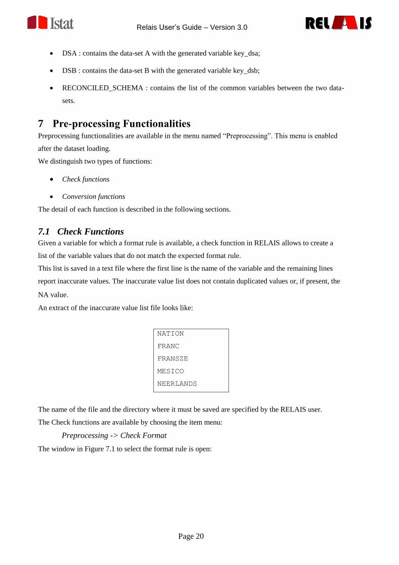
An extract of the inaccurate value list file looks like:
NATION
FRANC
FRANSZE
MESICO
NEERLANDS
The name of the file and the directory where it must be saved are specified by the RELAIS user.
The Check functions are available by choosing the item menu:
Preprocessing -> Check Format
The window in Figure 7.1 to select the format rule is open:
Relais User’s Guide – Version 3.0
Page 21
RELREL ISISRELREL ISIS
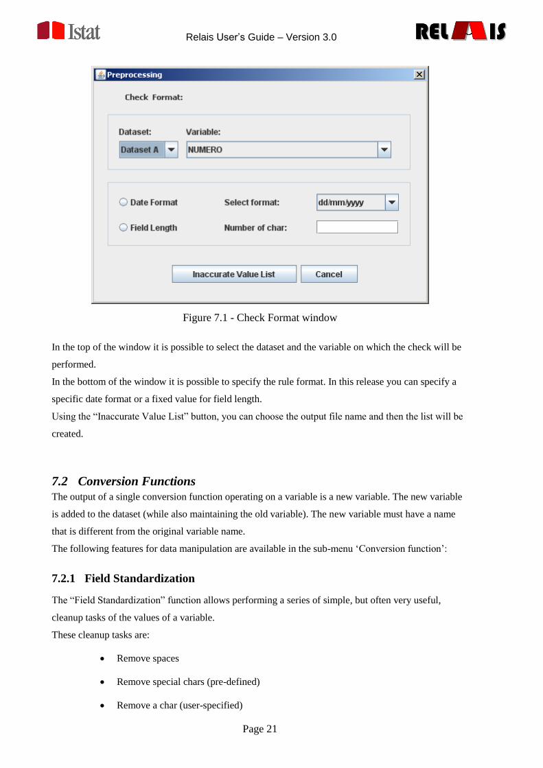
Figure 7.1 - Check Format window
In the top of the window it is possible to select the dataset and the variable on which the check will be
performed.
In the bottom of the window it is possible to specify the rule format. In this release you can specify a
specific date format or a fixed value for field length.
Using the “Inaccurate Value List” button, you can choose the output file name and then the list will be
created.
7.2 Conversion Functions
The output of a single conversion function operating on a variable is a new variable. The new variable
is added to the dataset (while also maintaining the old variable). The new variable must have a name
that is different from the original variable name.
The following features for data manipulation are available in the sub-menu „Conversion function‟:
7.2.1 Field Standardization
The “Field Standardization” function allows performing a series of simple, but often very useful,
cleanup tasks of the values of a variable.
These cleanup tasks are:
Remove spaces
Remove special chars (pre-defined)
Remove a char (user-specified)
Relais User’s Guide – Version 3.0
Page 22
RELREL ISISRELREL ISIS
Case conversion
The Field Standardization functions are available by choosing the item menu:
Preprocessing -> Conversion Functions -> Field Standardization
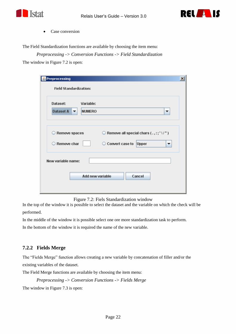
The window in Figure 7.2 is open:
Figure 7.2: Fiels Standardization window In the top of the window it is possible to select the dataset and the variable on which the check will be
performed.
In the middle of the window it is possible select one ore more standardization task to perform.
In the bottom of the window it is required the name of the new variable.
7.2.2 Fields Merge
The “Fields Merge” function allows creating a new variable by concatenation of filler and/or the
existing variables of the dataset.
The Field Merge functions are available by choosing the item menu:
Preprocessing -> Conversion Functions -> Fields Merge
The window in Figure 7.3 is open:
Relais User’s Guide – Version 3.0
Page 23
RELREL ISISRELREL ISIS
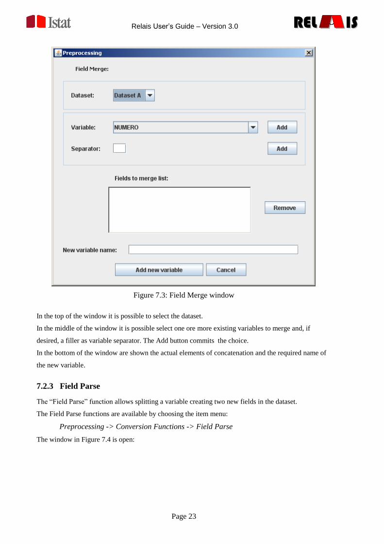
Figure 7.3: Field Merge window
In the top of the window it is possible to select the dataset.
In the middle of the window it is possible select one ore more existing variables to merge and, if
desired, a filler as variable separator. The Add button commits the choice.
In the bottom of the window are shown the actual elements of concatenation and the required name of
the new variable.
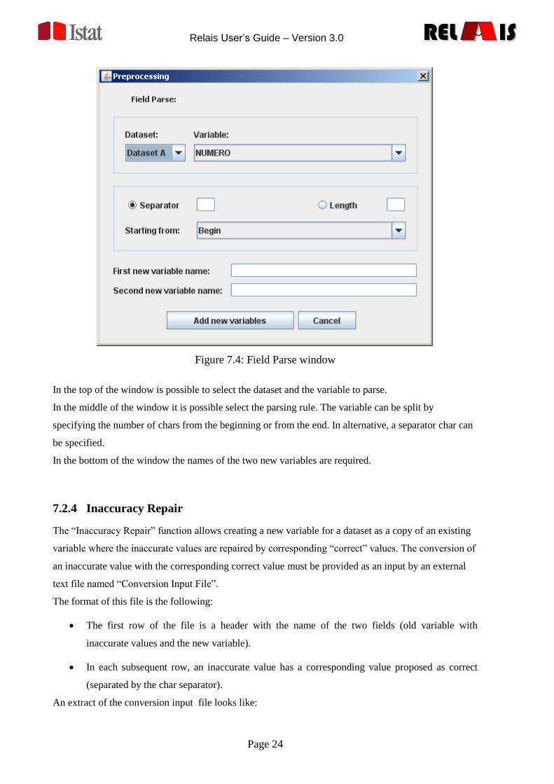
7.2.3 Field Parse
The “Field Parse” function allows splitting a variable creating two new fields in the dataset.
The Field Parse functions are available by choosing the item menu:
Preprocessing -> Conversion Functions -> Field Parse
The window in Figure 7.4 is open:
Relais User’s Guide – Version 3.0
Page 24
RELREL ISISRELREL ISIS
Figure 7.4: Field Parse window
In the top of the window is possible to select the dataset and the variable to parse.
In the middle of the window it is possible select the parsing rule. The variable can be split by
specifying the number of chars from the beginning or from the end. In alternative, a separator char can
be specified.
In the bottom of the window the names of the two new variables are required.
7.2.4 Inaccuracy Repair
The “Inaccuracy Repair” function allows creating a new variable for a dataset as a copy of an existing
variable where the inaccurate values are repaired by corresponding “correct” values. The conversion of
an inaccurate value with the corresponding correct value must be provided as an input by an external
text file named “Conversion Input File”.
The format of this file is the following:
The first row of the file is a header with the name of the two fields (old variable with
inaccurate values and the new variable).
In each subsequent row, an inaccurate value has a corresponding value proposed as correct
(separated by the char separator).
An extract of the conversion input file looks like:
Relais User’s Guide – Version 3.0
Page 25
RELREL ISISRELREL ISIS
NATION;NATION_CORRECT
FRANC;FRANCE
FRANSZE;FRANCE
MESICO;MEXICO
NEERLANDS;NETHERLANDS
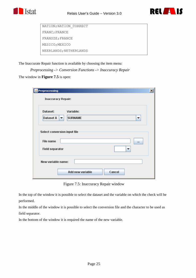
The Inaccurate Repair function is available by choosing the item menu:
Preprocessing -> Conversion Functions -> Inaccuracy Repair
The window in Figure 7.5 is open:
Figure 7.5: Inaccuracy Repair window
In the top of the window it is possible to select the dataset and the variable on which the check will be
performed.
In the middle of the window it is possible to select the conversion file and the character to be used as
field separator.
In the bottom of the window it is required the name of the new variable.
Relais User’s Guide – Version 3.0
Page 26
RELREL ISISRELREL ISIS
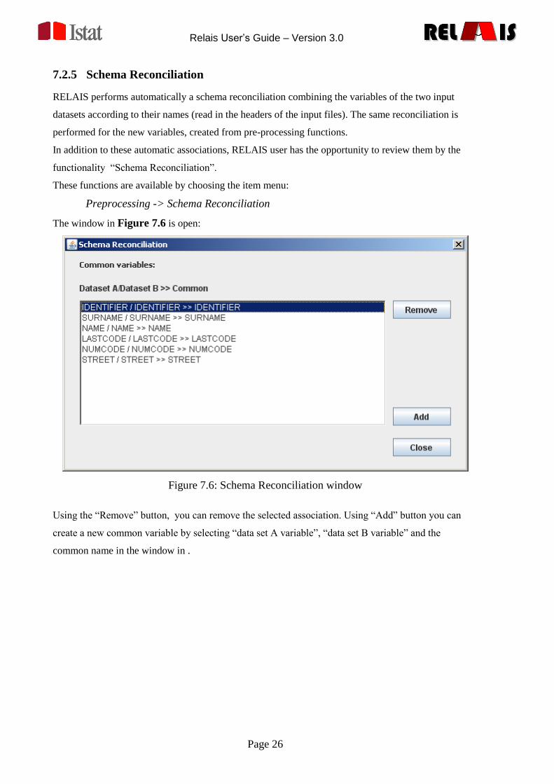
7.2.5 Schema Reconciliation
RELAIS performs automatically a schema reconciliation combining the variables of the two input
datasets according to their names (read in the headers of the input files). The same reconciliation is
performed for the new variables, created from pre-processing functions.
In addition to these automatic associations, RELAIS user has the opportunity to review them by the
functionality “Schema Reconciliation”.
These functions are available by choosing the item menu:
Preprocessing -> Schema Reconciliation
The window in Figure 7.6 is open:
Figure 7.6: Schema Reconciliation window
Using the “Remove” button, you can remove the selected association. Using “Add” button you can
create a new common variable by selecting “data set A variable”, “data set B variable” and the
common name in the window in .
Relais User’s Guide – Version 3.0
Page 27
RELREL ISISRELREL ISIS
Figure 7.7: Add common variable window
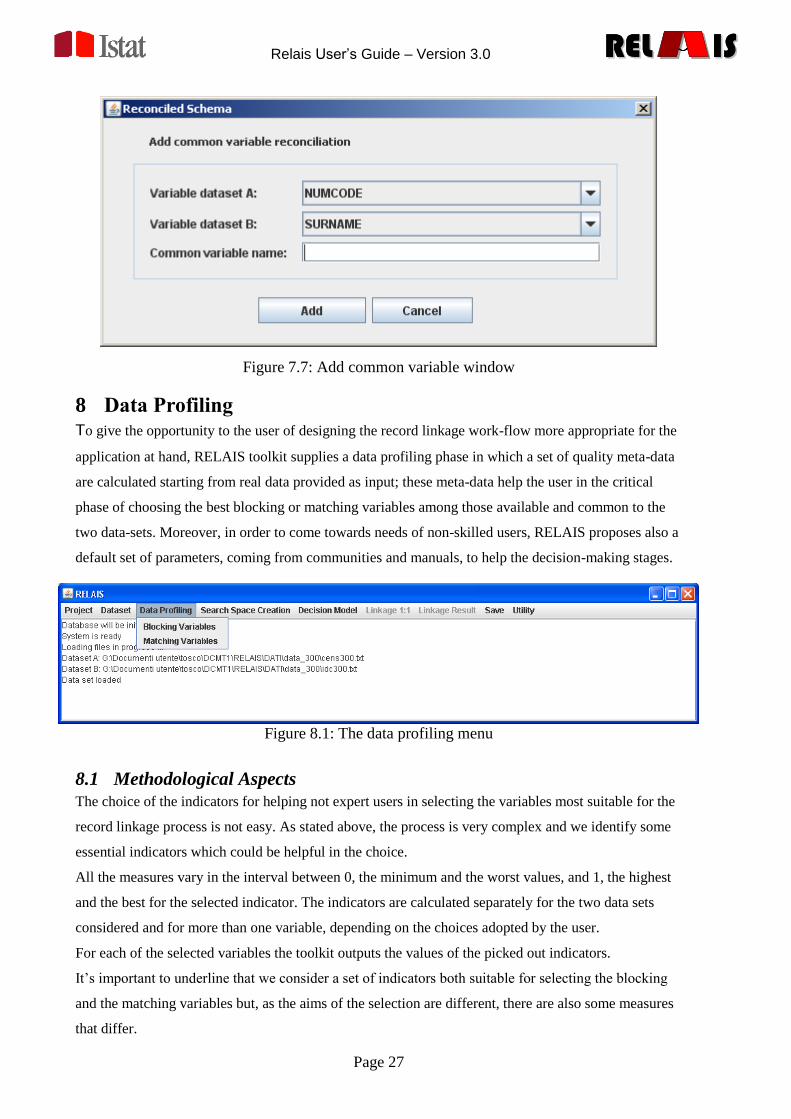
8 Data Profiling To give the opportunity to the user of designing the record linkage work-flow more appropriate for the
application at hand, RELAIS toolkit supplies a data profiling phase in which a set of quality meta-data
are calculated starting from real data provided as input; these meta-data help the user in the critical
phase of choosing the best blocking or matching variables among those available and common to the
two data-sets. Moreover, in order to come towards needs of non-skilled users, RELAIS proposes also a
default set of parameters, coming from communities and manuals, to help the decision-making stages.
Figure 8.1: The data profiling menu
8.1 Methodological Aspects
The choice of the indicators for helping not expert users in selecting the variables most suitable for the
record linkage process is not easy. As stated above, the process is very complex and we identify some
essential indicators which could be helpful in the choice.
All the measures vary in the interval between 0, the minimum and the worst values, and 1, the highest
and the best for the selected indicator. The indicators are calculated separately for the two data sets
considered and for more than one variable, depending on the choices adopted by the user.
For each of the selected variables the toolkit outputs the values of the picked out indicators.
It‟s important to underline that we consider a set of indicators both suitable for selecting the blocking
and the matching variables but, as the aims of the selection are different, there are also some measures
that differ.
Relais User’s Guide – Version 3.0
Page 28
RELREL ISISRELREL ISIS
In particular, the indicators common in the selection of blocking and matching variable are:
1. completeness;
2. accuracy;
3. consistency;
4. categories;
5. frequency distribution;
6. entropy.
In detail, the completeness (1) is the proportion of non-missing records on the overall (NA or NB) for
the considered variable in data-set A and B, respectively. A completeness equal to 1 means no missing
value in the variables (blocking or matching one).
The accuracy (2) implies the comparison of the recorded value of a variable with a dictionary or a set
of reference values that are known to be correct for the variable; this measure provides the number of
correct - not out of range - values on the overall.
The consistency (3) gives information on how well each item of the selected variable relates to the
items of a selected variable (e.g. province and region). It is necessary to indicate the variable that you
want to compare the item with and to give the set of values that the associated variable can assume.
The categories (4) report the number of different categories in the selected variable for both data-sets,
A and B.
The frequency distribution (5) returns in output the tables (for A and B) related to the frequency
distribution of the variable, sorted by frequency.
The entropy (6) calculates the Gini index for the selected variables, both for A and B data-sets. An
index equal to 0 means that all the frequencies are concentrated in a single item of the variables,
instead, a value of the index equal to 1 means a complete heterogeneity in the variable (all the i items
have the same relative frequencies, fi=1/K). The formula adopted is:
K
i
iKi ffG1
log
where i , i = 1,2,..K, are the items of the selected variable.
8.2 Diagnostics for Selecting Blocking Variables
In order to reduce the search space of the candidate pairs, the most suitable variables are generally
those most discriminating and accurate, i.e., not affected by errors or missing values. Usually, variables
as zip code, municipality, geographic area, year of birth can be chosen as blocking variables when
dealing with individual records. Then, links are searched only within the blocks, assuming that there
are no matches out of them; therefore, if the blocking variable is error affected, some true links could
be missed. Furthermore, it is useful to avoid blocking variables which create too small groups (i.e.
blocking variable with a large amount of values) in order to reduce risk of errors in the blocking
Relais User’s Guide – Version 3.0
Page 29
RELREL ISISRELREL ISIS
variable; in addition, also blocking variables which create too large groups must be avoided, generally
because they do not allow to reduce enough the search space. Generally speaking, it is suitable to
create blocks of the same size, selecting one or more variables, which present a consistent number of
values uniformly distributed among the units (for instance, the day and month of birth).
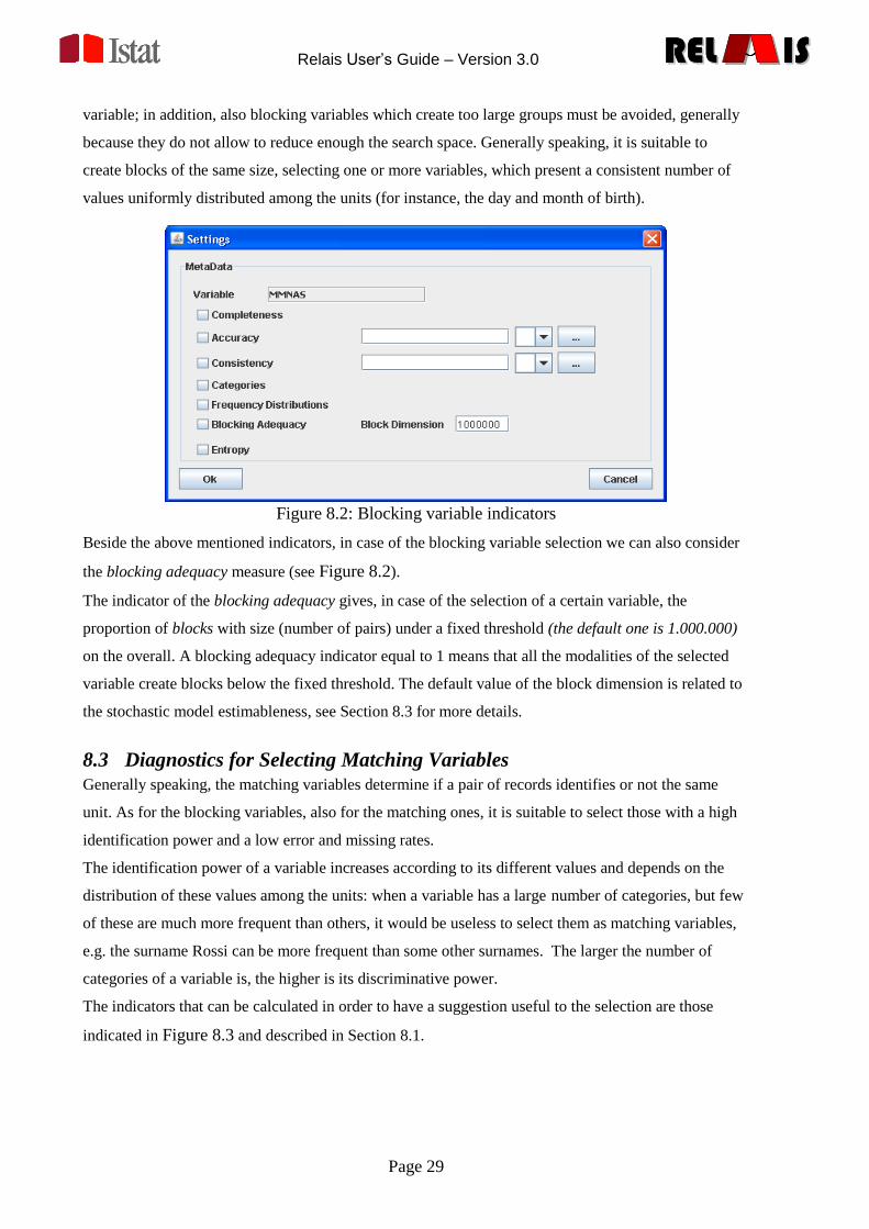
Figure 8.2: Blocking variable indicators
Beside the above mentioned indicators, in case of the blocking variable selection we can also consider
the blocking adequacy measure (see Figure 8.2).
The indicator of the blocking adequacy gives, in case of the selection of a certain variable, the
proportion of blocks with size (number of pairs) under a fixed threshold (the default one is 1.000.000)
on the overall. A blocking adequacy indicator equal to 1 means that all the modalities of the selected
variable create blocks below the fixed threshold. The default value of the block dimension is related to
the stochastic model estimableness, see Section 8.3 for more details.
8.3 Diagnostics for Selecting Matching Variables
Generally speaking, the matching variables determine if a pair of records identifies or not the same
unit. As for the blocking variables, also for the matching ones, it is suitable to select those with a high
identification power and a low error and missing rates.
The identification power of a variable increases according to its different values and depends on the
distribution of these values among the units: when a variable has a large number of categories, but few
of these are much more frequent than others, it would be useless to select them as matching variables,
e.g. the surname Rossi can be more frequent than some other surnames. The larger the number of
categories of a variable is, the higher is its discriminative power.
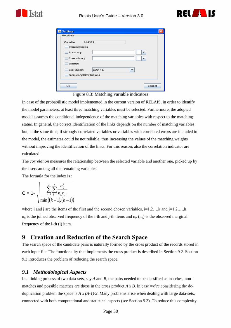
The indicators that can be calculated in order to have a suggestion useful to the selection are those
indicated in Figure 8.3 and described in Section 8.1.
Relais User’s Guide – Version 3.0
Page 30
RELREL ISISRELREL ISIS
Figure 8.3: Matching variable indicators
In case of the probabilistic model implemented in the current version of RELAIS, in order to identify
the model parameters, at least three matching variables must be selected. Furthermore, the adopted
model assumes the conditional independence of the matching variables with respect to the matching
status. In general, the correct identification of the links depends on the number of matching variables
but, at the same time, if strongly correlated variables or variables with correlated errors are included in
the model, the estimates could be not reliable, thus increasing the values of the matching weights
without improving the identification of the links. For this reason, also the correlation indicator are
calculated.
The correlation measures the relationship between the selected variable and another one, picked up by
the users among all the remaining variables.
The formula for the index is :
C = 1-
1,1min
1 1 ..
2
hk
nn
nk
i
h
j ji
ij
where i and j are the items of the first and the second chosen variables, i=1,2…,k and j=1,2,…,h
nij is the joined observed frequency of the i-th and j-th items and ni. (n.j) is the observed marginal
frequency of the i-th (j) item.
9 Creation and Reduction of the Search Space The search space of the candidate pairs is naturally formed by the cross product of the records stored in
each input file. The functionality that implements the cross product is described in Section 9.2. Section
9.3 introduces the problem of reducing the search space.
9.1 Methodological Aspects
In a linking process of two data-sets, say A and B, the pairs needed to be classified as matches, non-
matches and possible matches are those in the cross product A x B. In case we‟re considering the de-
duplication problem the space is A x (A-1)/2. Many problems arise when dealing with large data-sets,
connected with both computational and statistical aspects (see Section 9.3). To reduce this complexity
Relais User’s Guide – Version 3.0
Page 31
RELREL ISISRELREL ISIS
it is necessary to reduce the number of pairs (a; b), a belonging to A and b belonging to B so as to have
a set of pairs of manageable size. Starting from this reduced search space, we can apply different
decision models that define the rules used to determine whether a pair of records (a; b) is a match, a
non-match or a possible match.
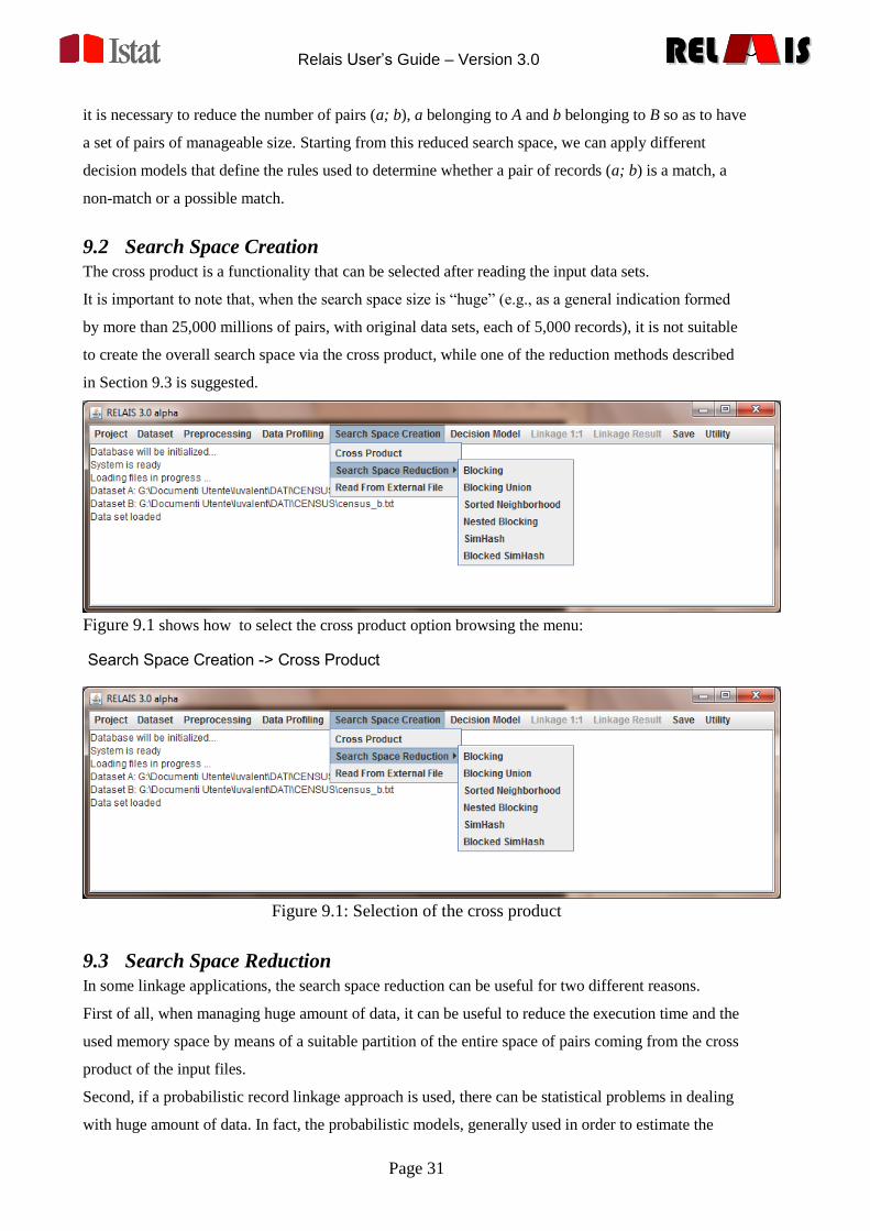
9.2 Search Space Creation
The cross product is a functionality that can be selected after reading the input data sets.
It is important to note that, when the search space size is “huge” (e.g., as a general indication formed
by more than 25,000 millions of pairs, with original data sets, each of 5,000 records), it is not suitable
to create the overall search space via the cross product, while one of the reduction methods described
in Section 9.3 is suggested.
Figure 9.1 shows how to select the cross product option browsing the menu:
Search Space Creation -> Cross Product
Figure 9.1: Selection of the cross product
9.3 Search Space Reduction
In some linkage applications, the search space reduction can be useful for two different reasons.
First of all, when managing huge amount of data, it can be useful to reduce the execution time and the
used memory space by means of a suitable partition of the entire space of pairs coming from the cross
product of the input files.
Second, if a probabilistic record linkage approach is used, there can be statistical problems in dealing
with huge amount of data. In fact, the probabilistic models, generally used in order to estimate the
Relais User’s Guide – Version 3.0
Page 32
RELREL ISISRELREL ISIS
conditional probabilities of being link or being non-link, do not allow to correctly identify such
probabilities when the number of possible links is too small with respect to the whole set of candidate
pairs. The statistical problem can be overcome by means of the creation of suitable groups or partitions
of the whole cross product set of pairs, so as in each sub-group the number of expected links is not
much smaller than the number of candidate pairs. In particular, when the probabilistic model assumes
that the overall candidate pairs are a mixture of the two unknown distributions of the true links and of
the true non-links, as in the current version of the probabilistic decision model implemented by
RELAIS, if one of the two unknown populations (the matches) is really too small with respect to the
other (the non-matches), it is possible that the estimation mechanism is not able to identify it: in fact,
the estimation algorithm could still converge, but it could estimate another latent phenomenon different
from the linkage. In this situations, some authors [10] suggest to apply a reduction of the pairs space so
that the expected number of links is not below 5% of the overall compared pairs. The 5% is just a
suggestion, actually a prudential suggestion; in practice, if the matching variables have a high
identification power, good results can be achieved even if the expected number of links was around the
1‰ of the overall compared pairs.
Among the several reduction techniques, the current version RELAIS provides the Blocking method
and the Sorted Neighbourhood Method. The first step required in RELAIS is the selection of the
variables for the reduction. This task can be supported by the data profiling activity (See Section 7.2).
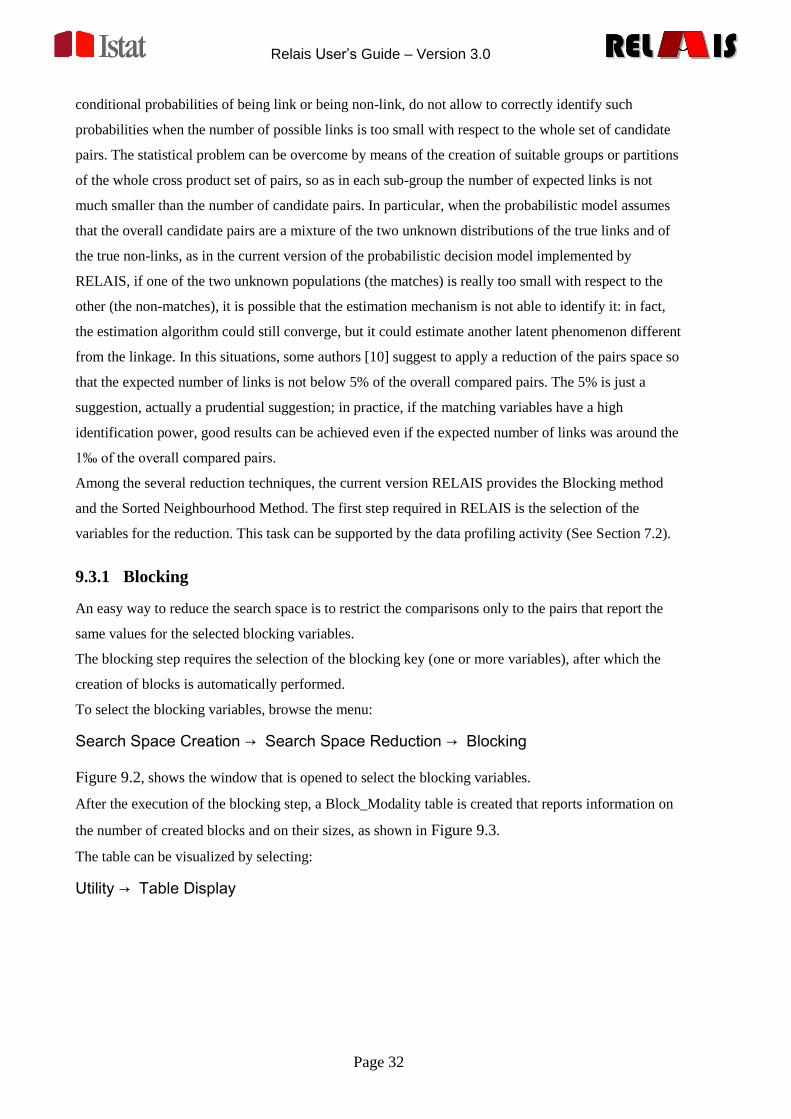
9.3.1 Blocking
An easy way to reduce the search space is to restrict the comparisons only to the pairs that report the
same values for the selected blocking variables.
The blocking step requires the selection of the blocking key (one or more variables), after which the
creation of blocks is automatically performed.
To select the blocking variables, browse the menu:
Search Space Creation → Search Space Reduction → Blocking
Figure 9.2, shows the window that is opened to select the blocking variables.
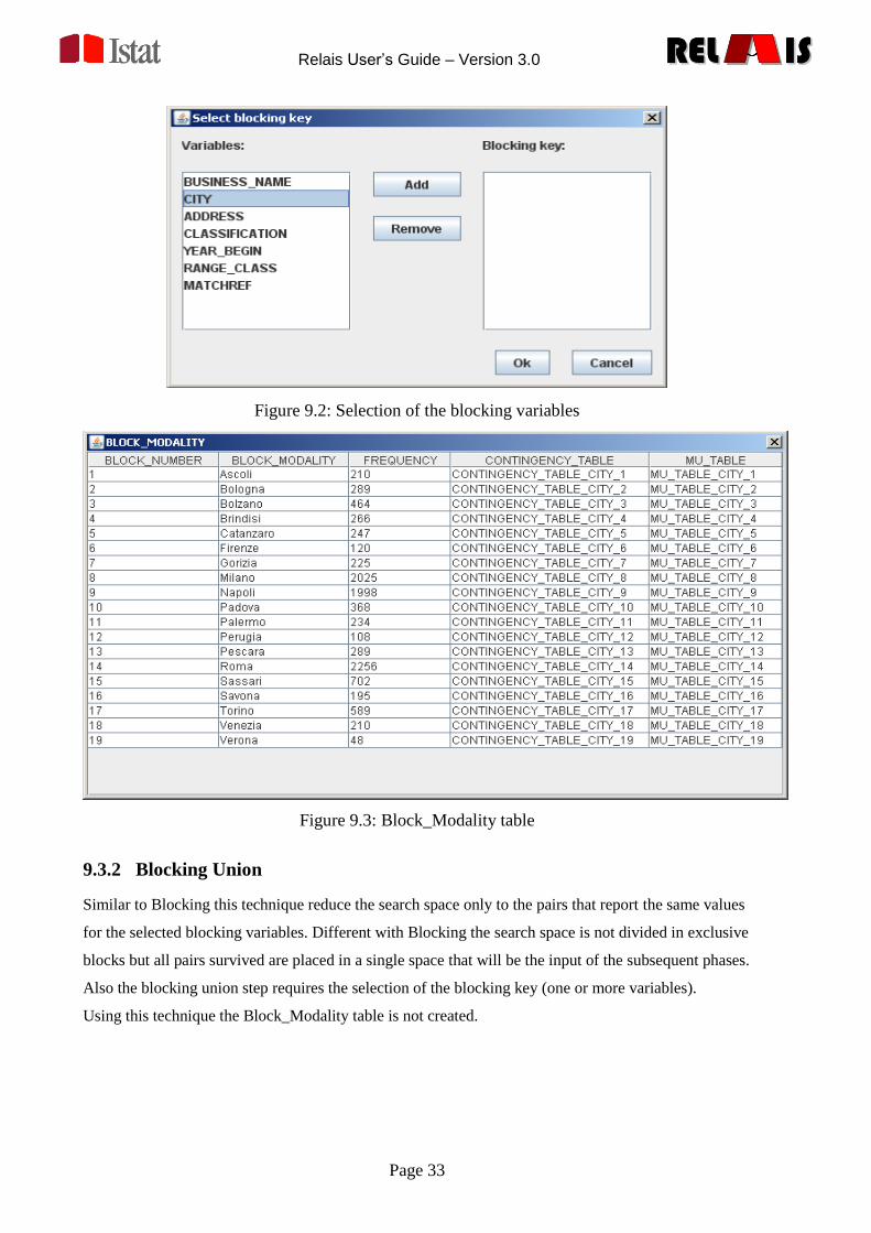
After the execution of the blocking step, a Block_Modality table is created that reports information on
the number of created blocks and on their sizes, as shown in Figure 9.3.
The table can be visualized by selecting:
Utility → Table Display
Relais User’s Guide – Version 3.0
Page 33
RELREL ISISRELREL ISIS
Figure 9.2: Selection of the blocking variables
Figure 9.3: Block_Modality table
9.3.2 Blocking Union
Similar to Blocking this technique reduce the search space only to the pairs that report the same values
for the selected blocking variables. Different with Blocking the search space is not divided in exclusive
blocks but all pairs survived are placed in a single space that will be the input of the subsequent phases.
Also the blocking union step requires the selection of the blocking key (one or more variables).
Using this technique the Block_Modality table is not created.
Relais User’s Guide – Version 3.0
Page 34
RELREL ISISRELREL ISIS
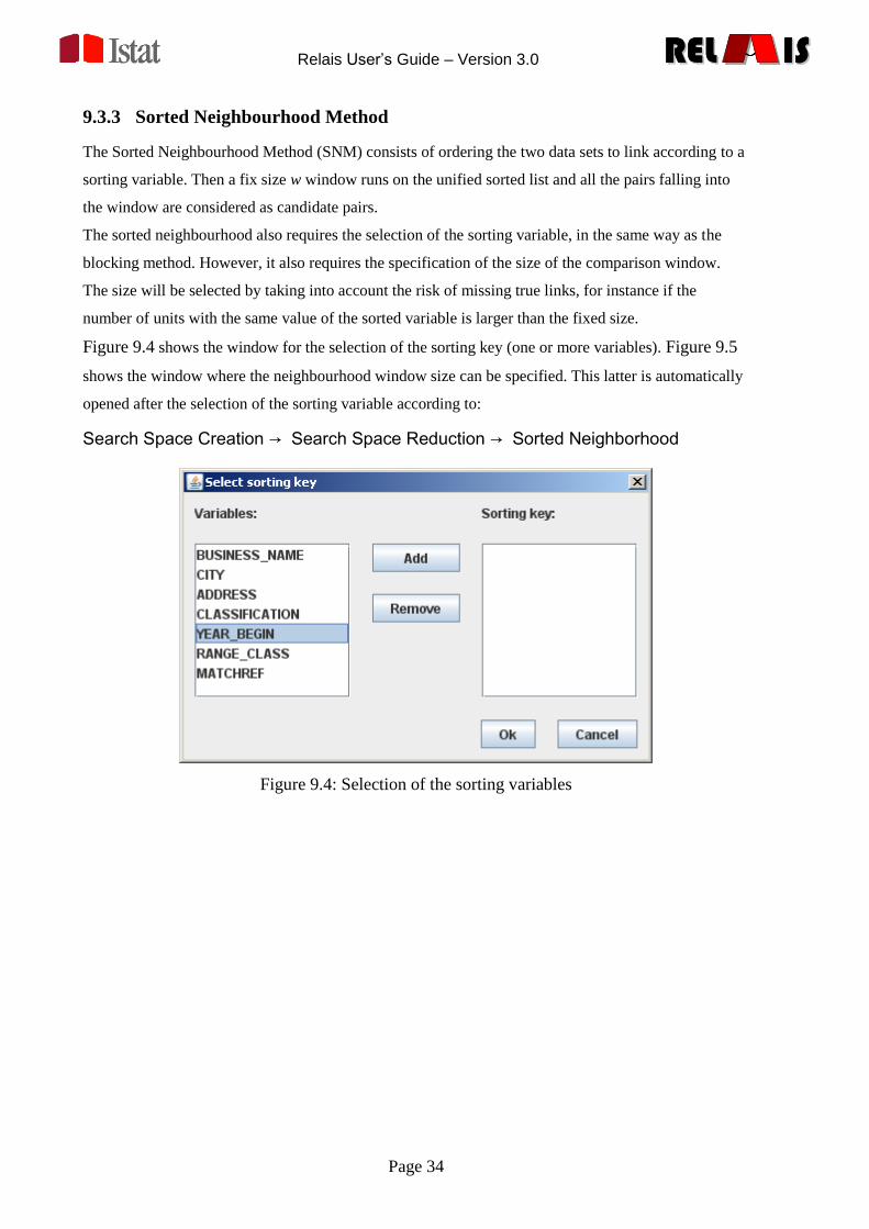
9.3.3 Sorted Neighbourhood Method
The Sorted Neighbourhood Method (SNM) consists of ordering the two data sets to link according to a
sorting variable. Then a fix size w window runs on the unified sorted list and all the pairs falling into
the window are considered as candidate pairs.
The sorted neighbourhood also requires the selection of the sorting variable, in the same way as the
blocking method. However, it also requires the specification of the size of the comparison window.
The size will be selected by taking into account the risk of missing true links, for instance if the
number of units with the same value of the sorted variable is larger than the fixed size.
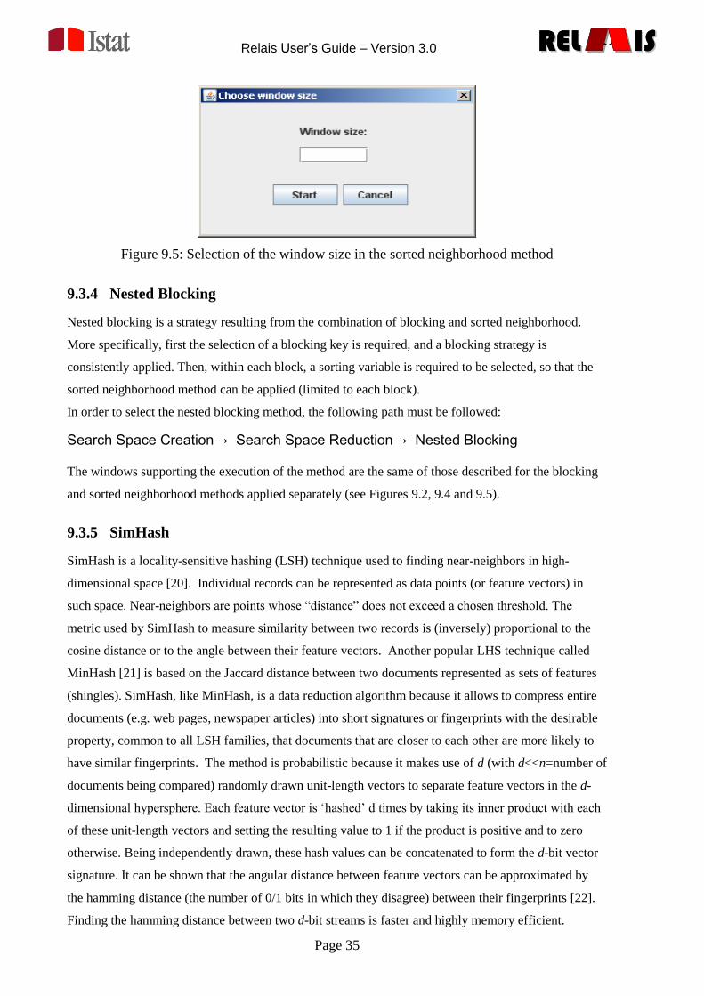
Figure 9.4 shows the window for the selection of the sorting key (one or more variables). Figure 9.5
shows the window where the neighbourhood window size can be specified. This latter is automatically
opened after the selection of the sorting variable according to:
Search Space Creation → Search Space Reduction → Sorted Neighborhood
Figure 9.4: Selection of the sorting variables
Relais User’s Guide – Version 3.0
Page 35
RELREL ISISRELREL ISIS
Figure 9.5: Selection of the window size in the sorted neighborhood method
9.3.4 Nested Blocking
Nested blocking is a strategy resulting from the combination of blocking and sorted neighborhood.
More specifically, first the selection of a blocking key is required, and a blocking strategy is
consistently applied. Then, within each block, a sorting variable is required to be selected, so that the
sorted neighborhood method can be applied (limited to each block).
In order to select the nested blocking method, the following path must be followed:
Search Space Creation → Search Space Reduction → Nested Blocking
The windows supporting the execution of the method are the same of those described for the blocking
and sorted neighborhood methods applied separately (see Figures 9.2, 9.4 and 9.5).
9.3.5 SimHash
SimHash is a locality-sensitive hashing (LSH) technique used to finding near-neighbors in high-
dimensional space [20]. Individual records can be represented as data points (or feature vectors) in
such space. Near-neighbors are points whose “distance” does not exceed a chosen threshold. The
metric used by SimHash to measure similarity between two records is (inversely) proportional to the
cosine distance or to the angle between their feature vectors. Another popular LHS technique called
MinHash [21] is based on the Jaccard distance between two documents represented as sets of features
(shingles). SimHash, like MinHash, is a data reduction algorithm because it allows to compress entire
documents (e.g. web pages, newspaper articles) into short signatures or fingerprints with the desirable
property, common to all LSH families, that documents that are closer to each other are more likely to
have similar fingerprints. The method is probabilistic because it makes use of d (with d<<n=number of
documents being compared) randomly drawn unit-length vectors to separate feature vectors in the d-
dimensional hypersphere. Each feature vector is „hashed‟ d times by taking its inner product with each
of these unit-length vectors and setting the resulting value to 1 if the product is positive and to zero
otherwise. Being independently drawn, these hash values can be concatenated to form the d-bit vector
signature. It can be shown that the angular distance between feature vectors can be approximated by
the hamming distance (the number of 0/1 bits in which they disagree) between their fingerprints [22].
Finding the hamming distance between two d-bit streams is faster and highly memory efficient.

Relais User’s Guide – Version 3.0
Page 36
RELREL ISISRELREL ISIS
Fast Search Algorithm
Once the n fingerprints have been created the search for near-neighbors is performed by first jumbling
their bits using a random permutation function and then arranging the permuted signatures in
lexicographic order to create a sorted list [23]. A number r of such random permutation functions is
chosen resulting in r alternative sorted lists. The search algorithm is then similar to the SNM presented
in 9.3.3, with one key difference: rather than using a scanning window of fixed size w, close neighbors
in each sorted list are considered candidates and inserted in the reduced search space iff their hamming
distance does not exceed a predefined threshold k. It can be shown that the time complexity of creating
the search space improves from O(n2) to O(n).
Implementation of SimHash in Relais 3.0
The current version of SimHash implemented in Relais 3.0 has been tested extensively on large
population registers as well as on census data [24]. The algorithm uses d=128-bit signatures generated
by decomposing the original records (strings) into feature vectors made of s-letter shingles (partially-
overlapping s-grams). The features are weighted using two alternative sets of weights: a) linear,
where the weight is equal to the number of times a given shingle appears in a given record, and b)
TF-IDF, where shingle frequency is scaled up or down depending on the rarity/ubiquity with which
they occur in the whole dataset (all records). The fast search algorithm performs 2(r +1) bit
permutations thus creating as many sorted lists of fingerprints. A number of choices for r and k
(hamming distance threshold) is available.
Permutations simply consist of head-to-tail rotations of contiguous q-bit streams. The rotation
parameter r is determined by d/q. For instance, with d=128 and q=8, r is equal to 16. In this case 34
(16+16+2) different sorted lists of signatures will be created and searched. The additional 16 lists are
generated by applying r q-bit rotations to the inverse of the original signatures, while the last two
sorted lists arrange the signatures according to the alphabetical order of the original (33rd
round) and
inverted (34th
round) strings they were constructed from. These two last searches only use a threshold
which is about 25% tighter than k because the target is to find those residual strong candidates which
may have gone undetected in the earlier searches. For every sorted list the search algorithm only inserts
in the final search space the newly found candidate pairs, i.e. those not yet found in the sorted lists
already searched.
To use SimHash select the following path from the menu:
Search Space Creation → Search Space Reduction → SimHash
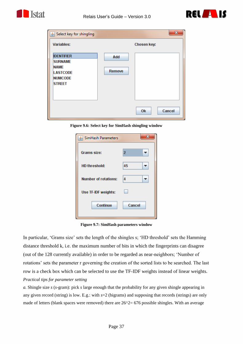
The next window, shown in Figure 9.6, allows the selection of the fields (keys) to be concatenated
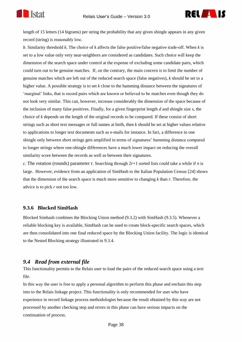
and then shingled to construct the LSH fingerprints. Finally, from the window shown in Figure 9.7
the user can set the SimHash parameters.
Relais User’s Guide – Version 3.0
Page 37
RELREL ISISRELREL ISIS
Figure 9.6: Select key for SimHash shingling window
Figure 9.7: SimHash parameters window
In particular, „Grams size‟ sets the length of the shingles s; „HD threshold‟ sets the Hamming
distance threshold k, i.e. the maximum number of bits in which the fingerprints can disagree
(out of the 128 currently available) in order to be regarded as near-neighbors; „Number of
rotations‟ sets the parameter r governing the creation of the sorted lists to be searched. The last
row is a check box which can be selected to use the TF-IDF weights instead of linear weights.
Practical tips for parameter setting
a. Shingle size s (s-gram): pick s large enough that the probability for any given shingle appearing in
any given record (string) is low. E.g.: with s=2 (bigrams) and supposing that records (strings) are only
made of letters (blank spaces were removed) there are 26^2= 676 possible shingles. With an average
Relais User’s Guide – Version 3.0
Page 38
RELREL ISISRELREL ISIS
length of 15 letters (14 bigrams) per string the probability that any given shingle appears in any given
record (string) is reasonably low.
b. Similarity threshold k. The choice of k affects the false positive/false negative trade-off. When k is
set to a low value only very near-neighbors are considered as candidates. Such choice will keep the
dimension of the search space under control at the expense of excluding some candidate pairs, which
could turn out to be genuine matches. If, on the contrary, the main concern is to limit the number of
genuine matches which are left out of the reduced search space (false negatives), k should be set to a
higher value. A possible strategy is to set k close to the hamming distance between the signatures of
„marginal‟ links, that is record pairs which are known or believed to be matches even though they do
not look very similar. This can, however, increase considerably the dimension of the space because of
the inclusion of many false positives. Finally, for a given fingerprint length d and shingle size s, the
choice of k depends on the length of the original records to be compared. If these consist of short
strings such as short text messages or full names at birth, then k should be set at higher values relative
to applications to longer text documents such as e-mails for instance. In fact, a difference in one
shingle only between short strings gets amplified in terms of signatures‟ hamming distance compared
to longer strings where one-shingle differences have a much lower impact on reducing the overall
similarity score between the records as well as between their signatures.
c. The rotation (rounds) parameter r. Searching through 2r+1 sorted lists could take a while if n is
large. However, evidence from an application of SimHash to the Italian Population Census [24] shows
that the dimension of the search space is much more sensitive to changing k than r. Therefore, the
advice is to pick r not too low.
9.3.6 Blocked SimHash
Blocked Simhash combines the Blocking Union method (9.3.2) with SimHash (9.3.5). Whenever a
reliable blocking key is available, SimHash can be used to create block-specific search spaces, which
are then consolidated into one final reduced space by the Blocking Union facility. The logic is identical
to the Nested Blocking strategy illustrated in 9.3.4.
9.4 Read from external file
This functionality permits to the Relais user to load the pairs of the reduced search space using a text
file.
In this way the user is free to apply a personal algorithm to perform this phase and enchain this step
into to the Relais linkage project. This functionality is only recommended for user who have
experience in record linkage process methodologies because the result obtained by this way are not
processed by another checking step and errors in this phase can have serious impacts on the
continuation of process.
Relais User’s Guide – Version 3.0
Page 39
RELREL ISISRELREL ISIS
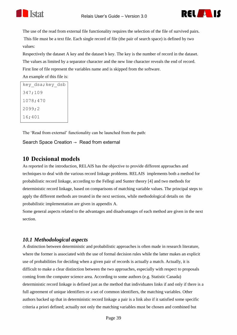
The use of the read from external file functionality requires the selection of the file of survived pairs.
This file must be a text file. Each single record of file (the pair of search space) is defined by two
values:
Respectively the dataset A key and the dataset b key. The key is the number of record in the dataset.
The values as limited by a separator character and the new line character reveals the end of record.
First line of file represent the variables name and is skipped from the software.
An example of this file is:
key_dsa;key_dsb
347;109
1078;470
2099;2
16;401
The „Read from external‟ functionality can be launched from the path:
Search Space Creation → Read from external
10 Decisional models As reported in the introduction, RELAIS has the objective to provide different approaches and
techniques to deal with the various record linkage problems. RELAIS implements both a method for
probabilistic record linkage, according to the Fellegi and Sunter theory [4] and two methods for
deterministic record linkage, based on comparisons of matching variable values. The principal steps to
apply the different methods are treated in the next sections, while methodological details on the
probabilistic implementation are given in appendix A.
Some general aspects related to the advantages and disadvantages of each method are given in the next
section.
10.1 Methodological aspects
A distinction between deterministic and probabilistic approaches is often made in research literature,
where the former is associated with the use of formal decision rules while the latter makes an explicit
use of probabilities for deciding when a given pair of records is actually a match. Actually, it is
difficult to make a clear distinction between the two approaches, especially with respect to proposals
coming from the computer science area. According to some authors (e.g. Statistic Canada)
deterministic record linkage is defined just as the method that individuates links if and only if there is a
full agreement of unique identifiers or a set of common identifiers, the matching variables. Other
authors backed up that in deterministic record linkage a pair is a link also if it satisfied some specific
criteria a priori defined; actually not only the matching variables must be chosen and combined but
Relais User’s Guide – Version 3.0
Page 40
RELREL ISISRELREL ISIS
also a threshold has to be fixed in order to establish whether a pair should be considered a link or not,
that is this kind of linkage is almost-exact but not exact in the strict sense [14]. In the deterministic
approach, both exact and almost-exact, the uncertainty in the match between two different databases is
minimized but the linkage rate could be very low.
Deterministic record linkage can be adopted, instead of probabilistic method, in presence of error-free
unique identifiers (such a social security number or fiscal code) or when matching variables with high
quality and discriminating power are available and can be combined so as to establish the pairs link
status; in this case the deterministic approach is very fast and effective and its adoption is appropriate.
From the other side, the rule definition is strictly dependent on the data and on the knowledge of the
practitioners. Moreover, due to the strong importance of the matching variable quality, in the
deterministic procedure, some links can be missed due to presence of errors or missing values in the
matching variables; so the choice between the deterministic and probabilistic methods must take into
account “the availability, the stability and the uniqueness of the variables in the files” [14]. It is
important also to underline that, in a deterministic context, the linkage quality can be assessed only by
means of re-linkage procedures or accurate and expensive clerical reviews. The probabilistic approach
is more complex and formal abut can solve problems caused by bad quality data. In particular it can be
helpful when differently spelled, swapped or misreported variables are stored in the two data files. In
addition the probabilistic procedure allows to evaluate the linkage errors, calculating the likelihood of
the correct match.
Generally speaking, the deterministic and the probabilistic approaches can be combined in a two step
process: firstly the deterministic method can be performed on the high quality variables then the
probabilistic approach can be adopted on the residuals, the units not linked in the first step; however
the joint use of the two techniques depends on the aims of the whole linkage project.
10.2 Selection of Comparison Functions
Comparison functions measure the “similarity” between two fields. Many of them are proposed in
literature and provided in RELAIS, as described below. Generally speaking, the results of a
comparison function can be also composed of categorical or continuous values. In RELAIS each
comparison function is normalized and its results are in the range [0,1]. Moreover, it is requested to the
user to choose a threshold, between 0 and 1, consequently RELAIS converts the results in binary
elements, treating all the results above the threshold as 1 and all results below the threshold as 0. The
higher distance for two strings is, the more similar the strings are.
A part the equality function, hereafter, we list of the comparison function available in RELAIS with a
short description. Some of the included functions are part of the Java package StringMetrics
(http://www.dcs.shef.ac.uk/~sam/stringmetrics.html ).
1. Numeric Comparison
This metric compare two strings by their numeric value. Thus named Nx and Ny the numeric value of
the two string Sx and Sy the numeric comparison is:
Relais User’s Guide – Version 3.0
Page 41
RELREL ISISRELREL ISIS
|)N||,N(|max
|)N||,Nmin(| )S,NC(S
yx
yx
yx
If the strings are not numeric or the two numbers have different signs the comparison‟s result is 0.
2. Levenshtein comparison function
This is the basic edit distance function whereby the distance is given simply as the minimum edit
operations which transforms string1 into string2. Edit operations are: copy a character from string1
over to string2; delete a character in string1; insert a character in string2; substitute one character for
another . Some other comparison functions reported below are extensions of the Levenshtein distance
function, and typically they alter the cost of the edit operation, while in the Levenshtein function all the
operations have the same cost.
3. Dice comparison function
Dice comparison function is a term based similarity measure and is defined as twice the number of
terms common to compared entities divided by the total number of terms in both tested entities.
String2in termsofNumber String1in termsofNumber
TermsCommon *2 Dice
4. Jaro comparison function [16]
The Jaro comparison function takes into account typical spelling deviations. Briefly, for two strings s
and t, let s' be the characters in s that are “common with” t, and let t' be the characters in t that are
"common with" s; roughly speaking, a character a in s is “in common” with t if the same character a
appears in about the place in t.
Let Ts′,t′ measure the number of transpositions of characters in s' relative to t'. The Jaro similarity metric
for s and t is
'2
'''
3
1),(
','
s
Ts
t
t
s
stsJaro
ts
5. Jaro-Winkler comparison function [17]
This metric, an extension of the Jaro comparison function (4), tends to modify the weights of the pairs
s,t with a common prefix; the Jaro-Winkler distance metric is particularly suitable in case of short
strings such as person names.
The Jaro-Winkler function for s and t is
tsJarolptsJarotsWinklerJaro ,1*,),(
where l is the length of common prefix at the beginning of the string; p is a constant scaling factor for
how much the score is adjusted upwards for having common prefixes. In Relais the value of constant p
is the standard used in Winkler's work[17]: p = 0.1 and the value of l can not exceed 6. This adjustment
gives more favorable ratings to strings that match from the beginning for a set prefix length.
6. 3-Grams [18]
Relais User’s Guide – Version 3.0
Page 42
RELREL ISISRELREL ISIS
Q-grams are generally used in approximate string matching by “sliding” a window of length q over the
characters of a string s to create a number of 'q' length grams (in the case of RELAIS we considered q
equal to 3) for matching.
A match is then rated as number of q-gram matches within the second string, t, over possible q-grams.
When two strings s and t have a small edit distance, they also have a large number of q-grams in
common.
7. Soundex comparison function
The Soundex function is a rude phonetic indexing scheme that generally focuses on individuals names;
with this metric the errors in phonetic are easily recognized, e.g. the names John, Johne and Jon
referred to the same person.
This is a term based evaluation where each term is given a Soundex code, each Soundex code consists
of a letter, the first one of the string, and five numbers between 0 and 6. The numbers are based on the
consonants as in the following table:
1) B,P,F,V
2) C,S,K,G,J,Q,X,Z
3) D,T
4) L
5) M,N
6) R
The vowels are not used. If two or more adjacent (not separated by a vowel) letters have the same
numeric value, only one is used. This also applies if the first letter and the second one have the same
value; the second letter would not be used to generate a digit. If there are less then six consonants in the
string, the code is filled out with zeros. This approach is very promising for disambiguation of
transliterated/misspell names.
8. Window Equality
The window equality function compares integer numbers.
Been x and y two integers to be compared, been w the window size defined by the user, x and
y are considered equals if and only if (|x-y| <= w).
9. Inclusion3Grams
Similarly to 3-Grams, the Inclusion3Grams depends on number of 3-length grams common to the two
strings, however in this case the target is the 3-grams amount of the shortest string. This difference
implies high scores when the shortest string is contained, completely or in part, in the longest one.
10.3 Deterministic Decision Models
The deterministic record linkage is associated with the use of formal decision rules and it can be
adopted, instead of probabilistic method, in presence of error-free unique identifiers (such a fiscal
code) or when suitable matching variables with high quality and discriminating power are available
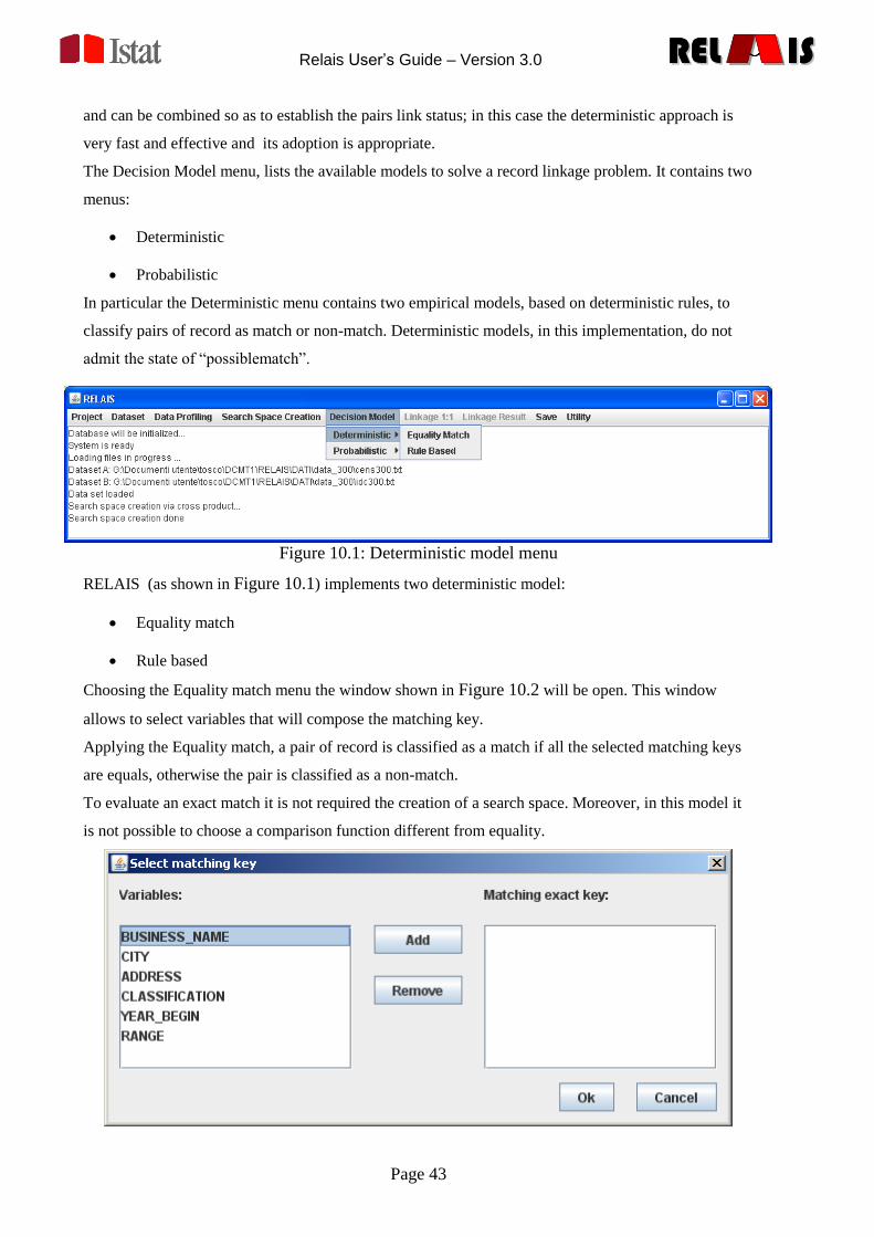
Relais User’s Guide – Version 3.0
Page 43
RELREL ISISRELREL ISIS
and can be combined so as to establish the pairs link status; in this case the deterministic approach is
very fast and effective and its adoption is appropriate.
The Decision Model menu, lists the available models to solve a record linkage problem. It contains two
menus:
Deterministic
Probabilistic
In particular the Deterministic menu contains two empirical models, based on deterministic rules, to
classify pairs of record as match or non-match. Deterministic models, in this implementation, do not
admit the state of “possiblematch”.
Figure 10.1: Deterministic model menu
RELAIS (as shown in Figure 10.1) implements two deterministic model:
Equality match
Rule based
Choosing the Equality match menu the window shown in Figure 10.2 will be open. This window
allows to select variables that will compose the matching key.
Applying the Equality match, a pair of record is classified as a match if all the selected matching keys
are equals, otherwise the pair is classified as a non-match.
To evaluate an exact match it is not required the creation of a search space. Moreover, in this model it
is not possible to choose a comparison function different from equality.
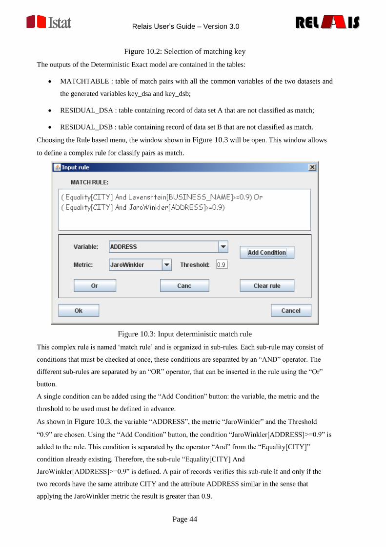
Relais User’s Guide – Version 3.0
Page 44
RELREL ISISRELREL ISIS
Figure 10.2: Selection of matching key
The outputs of the Deterministic Exact model are contained in the tables:
MATCHTABLE : table of match pairs with all the common variables of the two datasets and
the generated variables key_dsa and key_dsb;
RESIDUAL_DSA : table containing record of data set A that are not classified as match;
RESIDUAL_DSB : table containing record of data set B that are not classified as match.
Choosing the Rule based menu, the window shown in Figure 10.3 will be open. This window allows
to define a complex rule for classify pairs as match.
Figure 10.3: Input deterministic match rule
This complex rule is named „match rule‟ and is organized in sub-rules. Each sub-rule may consist of
conditions that must be checked at once, these conditions are separated by an “AND” operator. The
different sub-rules are separated by an “OR” operator, that can be inserted in the rule using the “Or”
button.
A single condition can be added using the “Add Condition” button: the variable, the metric and the
threshold to be used must be defined in advance.
As shown in Figure 10.3, the variable “ADDRESS”, the metric “JaroWinkler” and the Threshold
“0.9” are chosen. Using the “Add Condition” button, the condition “JaroWinkler[ADDRESS]>=0.9” is
added to the rule. This condition is separated by the operator “And” from the “Equality[CITY]”
condition already existing. Therefore, the sub-rule “Equality[CITY] And
JaroWinkler[ADDRESS]>=0.9” is defined. A pair of records verifies this sub-rule if and only if the
two records have the same attribute CITY and the attribute ADDRESS similar in the sense that
applying the JaroWinkler metric the result is greater than 0.9.
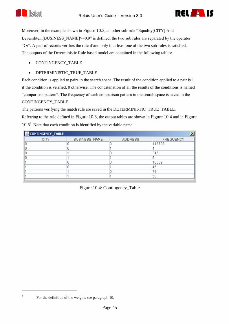
Relais User’s Guide – Version 3.0
Page 45
RELREL ISISRELREL ISIS
Moreover, in the example shown in Figure 10.3, an other sub-rule “Equality[CITY] And
Levenshtein[BUSINESS_NAME]>=0.9” is defined; the two sub rules are separated by the operator
“Or”. A pair of records verifies the rule if and only if at least one of the two sub-rules is satisfied.
The outputs of the Deterministic Rule based model are contained in the following tables:
CONTINGENCY_TABLE
DETERMINISTIC_TRUE_TABLE
Each condition is applied to pairs in the search space. The result of the condition applied to a pair is 1
if the condition is verified, 0 otherwise. The concatenation of all the results of the conditions is named
“comparison pattern”. The frequency of each comparison pattern in the search space is saved in the
CONTINGENCY_TABLE.
The patterns verifying the match rule are saved in the DETERMINISTIC_TRUE_TABLE.
Referring to the rule defined in Figure 10.3, the output tables are shown in Figure 10.4 and in Figure
10.52. Note that each condition is identified by the variable name.
Figure 10.4: Contingency_Table
2 For the definition of the weights see paragraph 10.
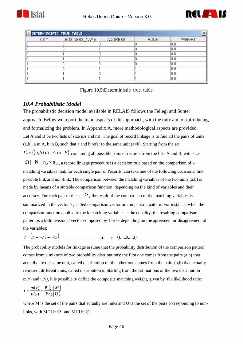
Relais User’s Guide – Version 3.0
Page 46
RELREL ISISRELREL ISIS
Figure 10.5:Deterministic_true_table
10.4 Probabilistic Model
The probabilistic decision model available in RELAIS follows the Fellegi and Sunter
approach. Below we report the main aspects of this approach, with the only aim of introducing
and formalizing the problem. In Appendix A, more methodological aspects are provided.
Let A and B be two lists of size nA and nB. The goal of record linkage is to find all the pairs of units
(a,b), a in A, b in B, such that a and b refer to the same unit (a=b). Starting from the set
BbAaba ,;, containing all possible pairs of records from the lists A and B, with size
BA nnN|| , a record linkage procedure is a decision rule based on the comparison of k
matching variables that, for each single pair of records, can take one of the following decisions: link,
possible link and non-link. The comparison between the matching variables of the two units (a,b) is
made by means of a suitable comparison function, depending on the kind of variables and their
accuracy. For each pair of the set , the result of the comparison of the matching variables is
summarized in the vector , called comparison vector or comparison pattern. For instance, when the
comparison function applied to the k matching variables is the equality, the resulting comparison
pattern is a k-dimensional vector composed by 1 or 0, depending on the agreement or disagreement of
the variables:
kj ,...,,...,1 1,...,0,...,1 .
The probability models for linkage assume that the probability distribution of the comparison pattern
comes from a mixture of two probability distributions: the first one comes from the pairs (a,b) that
actually are the same unit, called distribution m; the other one comes from the pairs (a,b) that actually
represent different units, called distribution u. Starting from the estimations of the two distribution
m() and u(), it is possible to define the composite matching weight, given by the likelihood ratio:
U
M
u
mr
Pr
|Pr
)(
)(
where M is the set of the pairs that actually are links and U is the set of the pairs corresponding to non-
links, with M∩U= and MUU= .
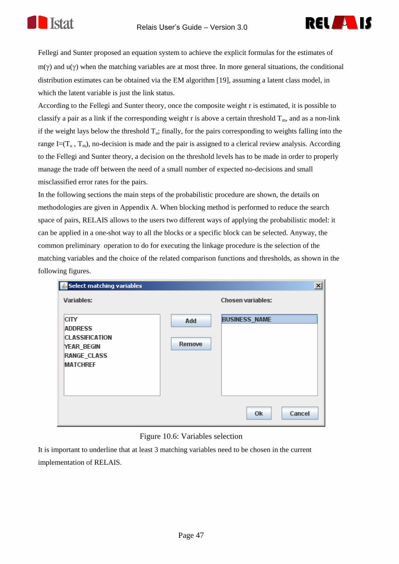
Relais User’s Guide – Version 3.0
Page 47
RELREL ISISRELREL ISIS
Fellegi and Sunter proposed an equation system to achieve the explicit formulas for the estimates of
m() and u() when the matching variables are at most three. In more general situations, the conditional
distribution estimates can be obtained via the EM algorithm [19], assuming a latent class model, in
which the latent variable is just the link status.
According to the Fellegi and Sunter theory, once the composite weight r is estimated, it is possible to
classify a pair as a link if the corresponding weight r is above a certain threshold Tm, and as a non-link
if the weight lays below the threshold Tu; finally, for the pairs corresponding to weights falling into the
range I=(Tu , Tm), no-decision is made and the pair is assigned to a clerical review analysis. According
to the Fellegi and Sunter theory, a decision on the threshold levels has to be made in order to properly
manage the trade off between the need of a small number of expected no-decisions and small
misclassified error rates for the pairs.
In the following sections the main steps of the probabilistic procedure are shown, the details on
methodologies are given in Appendix A. When blocking method is performed to reduce the search
space of pairs, RELAIS allows to the users two different ways of applying the probabilistic model: it
can be applied in a one-shot way to all the blocks or a specific block can be selected. Anyway, the
common preliminary operation to do for executing the linkage procedure is the selection of the
matching variables and the choice of the related comparison functions and thresholds, as shown in the
following figures.
Figure 10.6: Variables selection
It is important to underline that at least 3 matching variables need to be chosen in the current
implementation of RELAIS.
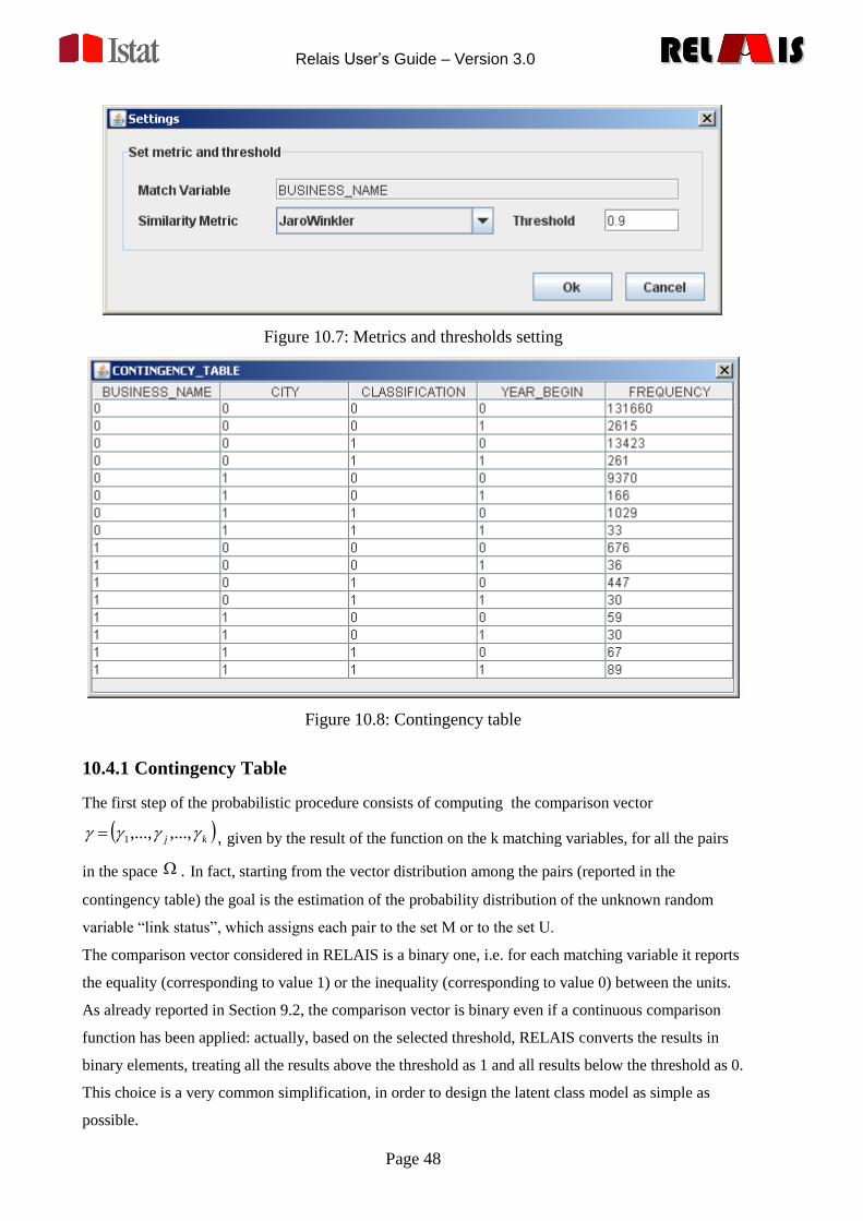
Relais User’s Guide – Version 3.0
Page 48
RELREL ISISRELREL ISIS
Figure 10.7: Metrics and thresholds setting
Figure 10.8: Contingency table
10.4.1 Contingency Table
The first step of the probabilistic procedure consists of computing the comparison vector
kj ,...,,...,1 , given by the result of the function on the k matching variables, for all the pairs
in the space . In fact, starting from the vector distribution among the pairs (reported in the
contingency table) the goal is the estimation of the probability distribution of the unknown random
variable “link status”, which assigns each pair to the set M or to the set U.
The comparison vector considered in RELAIS is a binary one, i.e. for each matching variable it reports
the equality (corresponding to value 1) or the inequality (corresponding to value 0) between the units.
As already reported in Section 9.2, the comparison vector is binary even if a continuous comparison
function has been applied: actually, based on the selected threshold, RELAIS converts the results in
binary elements, treating all the results above the threshold as 1 and all results below the threshold as 0.
This choice is a very common simplification, in order to design the latent class model as simple as
possible.
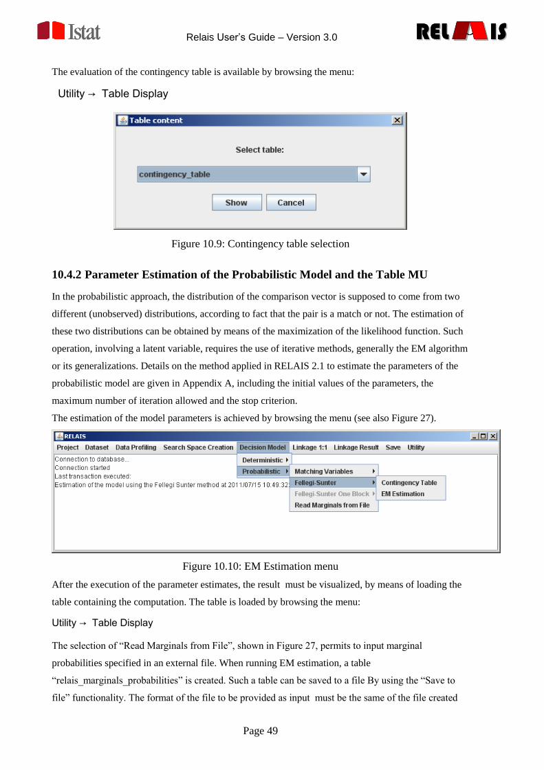
Relais User’s Guide – Version 3.0
Page 49
RELREL ISISRELREL ISIS
The evaluation of the contingency table is available by browsing the menu:
Utility → Table Display
Figure 10.9: Contingency table selection
10.4.2 Parameter Estimation of the Probabilistic Model and the Table MU
In the probabilistic approach, the distribution of the comparison vector is supposed to come from two
different (unobserved) distributions, according to fact that the pair is a match or not. The estimation of
these two distributions can be obtained by means of the maximization of the likelihood function. Such
operation, involving a latent variable, requires the use of iterative methods, generally the EM algorithm
or its generalizations. Details on the method applied in RELAIS 2.1 to estimate the parameters of the
probabilistic model are given in Appendix A, including the initial values of the parameters, the
maximum number of iteration allowed and the stop criterion.
The estimation of the model parameters is achieved by browsing the menu (see also Figure 27).
Figure 10.10: EM Estimation menu
After the execution of the parameter estimates, the result must be visualized, by means of loading the
table containing the computation. The table is loaded by browsing the menu:
Utility → Table Display
The selection of “Read Marginals from File”, shown in Figure 27, permits to input marginal
probabilities specified in an external file. When running EM estimation, a table
“relais_marginals_probabilities” is created. Such a table can be saved to a file By using the “Save to
file” functionality. The format of the file to be provided as input must be the same of the file created
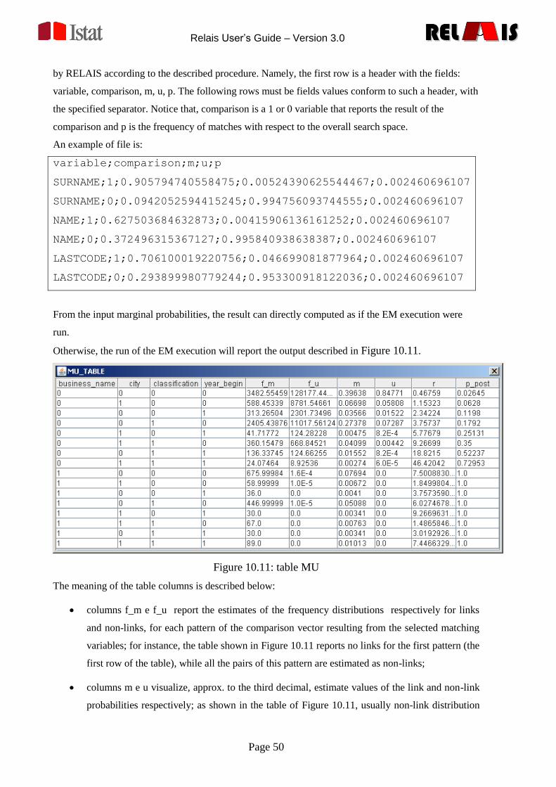
Relais User’s Guide – Version 3.0
Page 50
RELREL ISISRELREL ISIS
by RELAIS according to the described procedure. Namely, the first row is a header with the fields:
variable, comparison, m, u, p. The following rows must be fields values conform to such a header, with
the specified separator. Notice that, comparison is a 1 or 0 variable that reports the result of the
comparison and p is the frequency of matches with respect to the overall search space.
An example of file is:
variable;comparison;m;u;p
SURNAME;1;0.905794740558475;0.00524390625544467;0.002460696107
SURNAME;0;0.0942052594415245;0.994756093744555;0.002460696107
NAME;1;0.627503684632873;0.00415906136161252;0.002460696107
NAME;0;0.372496315367127;0.995840938638387;0.002460696107
LASTCODE;1;0.706100019220756;0.046699081877964;0.002460696107
LASTCODE;0;0.293899980779244;0.953300918122036;0.002460696107
From the input marginal probabilities, the result can directly computed as if the EM execution were
run.
Otherwise, the run of the EM execution will report the output described in Figure 10.11.
Figure 10.11: table MU
The meaning of the table columns is described below:
columns f_m e f_u report the estimates of the frequency distributions respectively for links
and non-links, for each pattern of the comparison vector resulting from the selected matching
variables; for instance, the table shown in Figure 10.11 reports no links for the first pattern (the
first row of the table), while all the pairs of this pattern are estimated as non-links;
columns m e u visualize, approx. to the third decimal, estimate values of the link and non-link
probabilities respectively; as shown in the table of Figure 10.11, usually non-link distribution
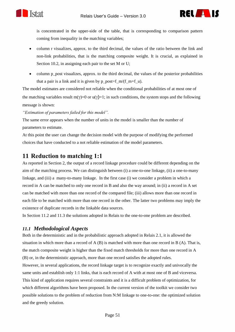
Relais User’s Guide – Version 3.0
Page 51
RELREL ISISRELREL ISIS
is concentrated in the upper-side of the table, that is corresponding to comparison pattern
coming from inequality in the matching variables;
column r visualizes, approx. to the third decimal, the values of the ratio between the link and
non-link probabilities, that is the matching composite weight. It is crucial, as explained in
Section 10.2, in assigning each pair to the set M or U;
column p_post visualizes, approx. to the third decimal, the values of the posterior probabilities
that a pair is a link and it is given by p_post=f_m/(f_m+f_u).
The model estimates are considered not reliable when the conditional probabilities of at most one of
the matching variables result m()=0 or u()=1; in such conditions, the system stops and the following
message is shown:
“Estimation of parameters failed for this model”.
The same error appears when the number of units in the model is smaller than the number of
parameters to estimate.
At this point the user can change the decision model with the purpose of modifying the performed
choices that have conducted to a not reliable estimation of the model parameters.
11 Reduction to matching 1:1 As reported in Section 2, the output of a record linkage procedure could be different depending on the
aim of the matching process. We can distinguish between (i) a one-to-one linkage, (ii) a one-to-many
linkage, and (iii) a many-to-many linkage. In the first case (i) we consider a problem in which a
record in A can be matched to only one record in B and also the way around; in (ii) a record in A set
can be matched with more than one record of the compared file; (iii) allows more than one record in
each file to be matched with more than one record in the other. The latter two problems may imply the
existence of duplicate records in the linkable data sources.
In Section 11.2 and 11.3 the solutions adopted in Relais to the one-to-one problem are described.
11.1 Methodological Aspects
Both in the deterministic and in the probabilistic approach adopted in Relais 2.1, it is allowed the
situation in which more than a record of A (B) is matched with more than one record in B (A). That is,
the match composite weight is higher than the fixed match thresholds for more than one record in A
(B) or, in the deterministic approach, more than one record satisfies the adopted rules.
However, in several applications, the record linkage target is to recognize exactly and univocally the
same units and establish only 1:1 links, that is each record of A with at most one of B and viceversa.
This kind of application requires several constraints and it is a difficult problem of optimization, for
which different algorithms have been proposed. In the current version of the toolkit we consider two
possible solutions to the problem of reduction from N:M linkage to one-to-one: the optimized solution
and the greedy solution.
Relais User’s Guide – Version 3.0
Page 52
RELREL ISISRELREL ISIS
11.2 Optimized Solution
In this first alternative we consider an optimal solution for the reduction 1 to 1. Once the matching
weight, r, is assigned to each pair, the identification of 1 to 1 links can be solved as a linear
programming problem, where the objective function to maximize is the sum of weights for the linked
pairs, under the constraints given by the fact that each unit of A must be linked with only one unit in B.
In the current version of RELAIS, the solution of such a problem is obtained by means of the simplex
algorithm, available in the R package “lpSolve”.
With respect to linkage process using probabilistic model, the original algorithm has been modified in
order to exclude all pairs with linkage probabilities less than 0.5; in such a way the number of
constraints is reduced (as well as the complexity of the problem) when the number of units belonging
to pairs with linkage probability less than 0.5 is large. If such a condition is not verified, huge amount
of data can required large data structure that can reach the maximum allocation of memory permitted
by R. Experiments show that the algorithm can solve problems with input data of some thousands of
records.
When linkage process is based on deterministic approach, the optimized reduction to 1:1 links can be
obtained usign a system of weights, which can be assigned by the user giving the maximum positive
weight for the most important rule and the subsequent ones in descending order according to the
relevance of the rule. Nevertheless the system gives its own default weights: the maximum is given to
the first rule defined by the user.
11.3 Greedy Solution
If the optimal solution is not able to reach a result due to computational limitations, we can apply a
“greedy solution” in order to select, from the N : M cluster, the one-to-one linkage. Also in this
context, we consider firstly the r weight (for deterministic approach see par. 10.2) and we sort all the
record pairs by r. Then we consider as one-to-one pairs those that have the higher r. With this strategy,
it is not guaranteed that we reach an optimal solution because we perform local choices.
12 Linkage Result The last phase of the record linkage process is the selection of the desired output data. In the following
paragraphs the choices to be adopted are described and also all the available outputs in order not only
to better end the whole process but also to have the residual to begin the new process with.
12.1 Choice of the Thresholds
At this point the unmatch threshold (Tu) and the match threshold (Tm) are selected. If the weight value
p_post is higher than Tu and lower than Tm, the pair is assigned to the set of the Possible Match, if the
value p_post is higher than Tm, the pair is assigned to the set of Match.
When the same value is chosen for Tu and Tm, the resulting set of Possible Match is empty.
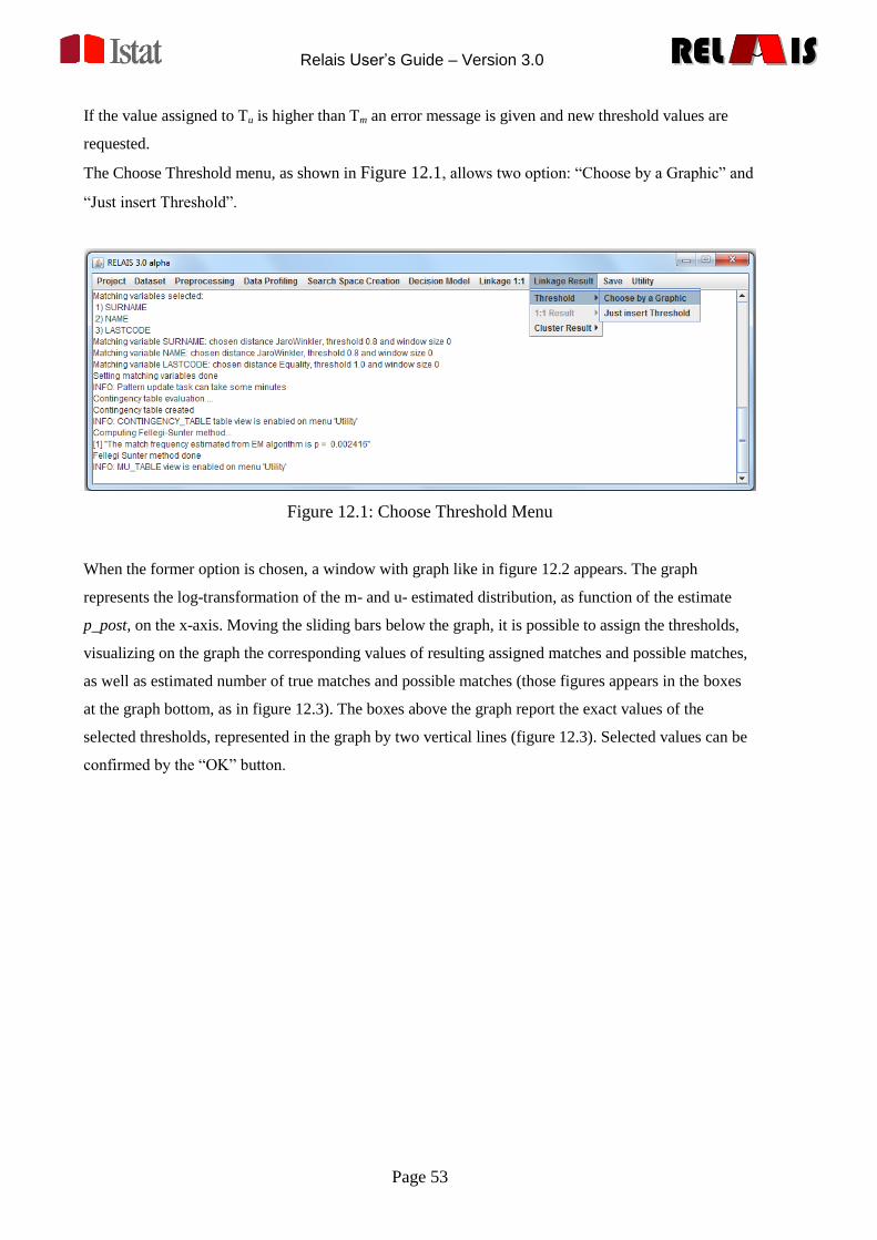
Relais User’s Guide – Version 3.0
Page 53
RELREL ISISRELREL ISIS
If the value assigned to Tu is higher than Tm an error message is given and new threshold values are
requested.
The Choose Threshold menu, as shown in Figure 12.1, allows two option: “Choose by a Graphic” and
“Just insert Threshold”.
Figure 12.1: Choose Threshold Menu
When the former option is chosen, a window with graph like in figure 12.2 appears. The graph
represents the log-transformation of the m- and u- estimated distribution, as function of the estimate
p_post, on the x-axis. Moving the sliding bars below the graph, it is possible to assign the thresholds,
visualizing on the graph the corresponding values of resulting assigned matches and possible matches,
as well as estimated number of true matches and possible matches (those figures appears in the boxes
at the graph bottom, as in figure 12.3). The boxes above the graph report the exact values of the
selected thresholds, represented in the graph by two vertical lines (figure 12.3). Selected values can be
confirmed by the “OK” button.
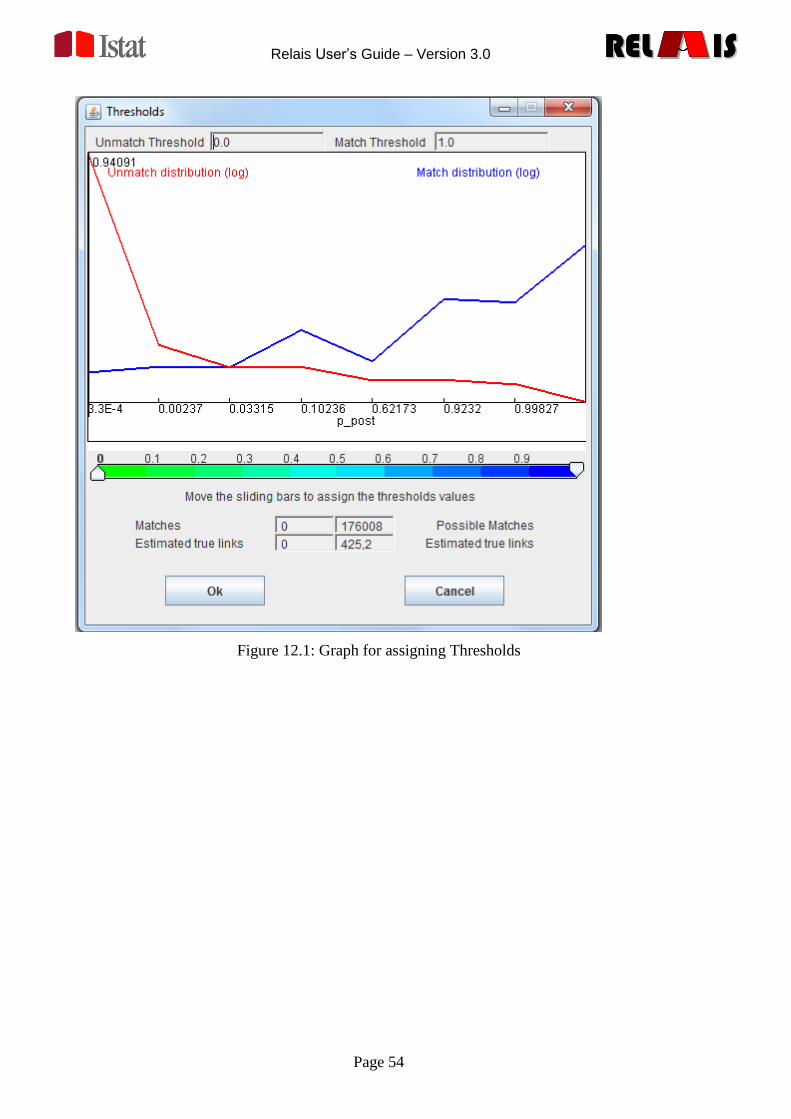
Relais User’s Guide – Version 3.0
Page 54
RELREL ISISRELREL ISIS
Figure 12.1: Graph for assigning Thresholds

Relais User’s Guide – Version 3.0
Page 55
RELREL ISISRELREL ISIS
Figure 12.3: Using the graph for assigning Thresholds
Thresholds can be assigned also directly, by the latter option in the Choose Threshold Menu. In this
case a window appears, as shown in Figure 12.4, allowing to insert the two thresholds: Unmatch
threshold and Match Threshold. The two thresholds take two default values:
Unmatch threshold = 0.90
Match threshold = 0.95
It is possible to change these values with the most appropriate depending on the data.
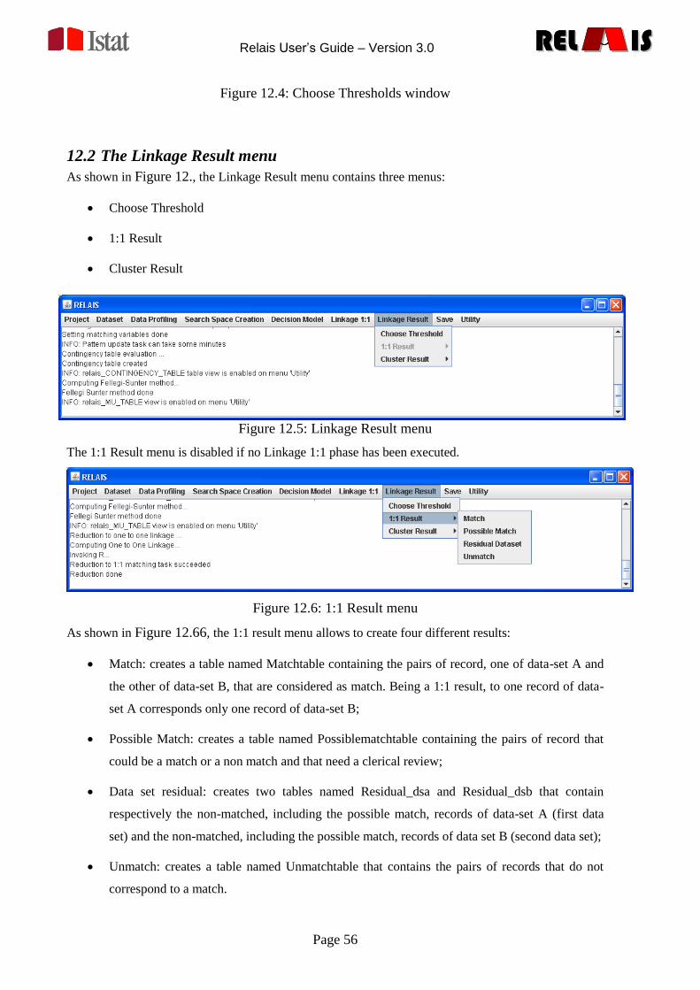
Relais User’s Guide – Version 3.0
Page 56
RELREL ISISRELREL ISIS
Figure 12.4: Choose Thresholds window
12.2 The Linkage Result menu
As shown in Figure 12., the Linkage Result menu contains three menus:
Choose Threshold
1:1 Result
Cluster Result
Figure 12.5: Linkage Result menu
The 1:1 Result menu is disabled if no Linkage 1:1 phase has been executed.
Figure 12.6: 1:1 Result menu
As shown in Figure 12.66, the 1:1 result menu allows to create four different results:
Match: creates a table named Matchtable containing the pairs of record, one of data-set A and
the other of data-set B, that are considered as match. Being a 1:1 result, to one record of data-
set A corresponds only one record of data-set B;
Possible Match: creates a table named Possiblematchtable containing the pairs of record that
could be a match or a non match and that need a clerical review;
Data set residual: creates two tables named Residual_dsa and Residual_dsb that contain
respectively the non-matched, including the possible match, records of data-set A (first data
set) and the non-matched, including the possible match, records of data set B (second data set);
Unmatch: creates a table named Unmatchtable that contains the pairs of records that do not
correspond to a match.
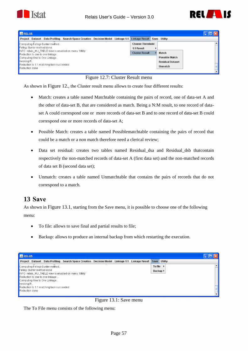
Relais User’s Guide – Version 3.0
Page 57
RELREL ISISRELREL ISIS
Figure 12.7: Cluster Result menu
As shown in Figure 12., the Cluster result menu allows to create four different results:
Match: creates a table named Matchtable containing the pairs of record, one of data-set A and
the other of data-set B, that are considered as match. Being a N:M result, to one record of data-
set A could correspond one or more records of data-set B and to one record of data-set B could
correspond one or more records of data-set A;
Possible Match: creates a table named Possiblematchtable containing the pairs of record that
could be a match or a non match therefore need a clerical review;
Data set residual: creates two tables named Residual_dsa and Residual_dsb thatcontain
respectively the non-matched records of data-set A (first data set) and the non-matched records
of data set B (second data set);
Unmatch: creates a table named Unmatchtable that contains the pairs of records that do not
correspond to a match.
13 Save As shown in Figure 13.1, starting from the Save menu, it is possible to choose one of the following
menu:
To file: allows to save final and partial results to file;
Backup: allows to produce an internal backup from which restarting the execution.
Figure 13.1: Save menu
The To File menu consists of the following menu:
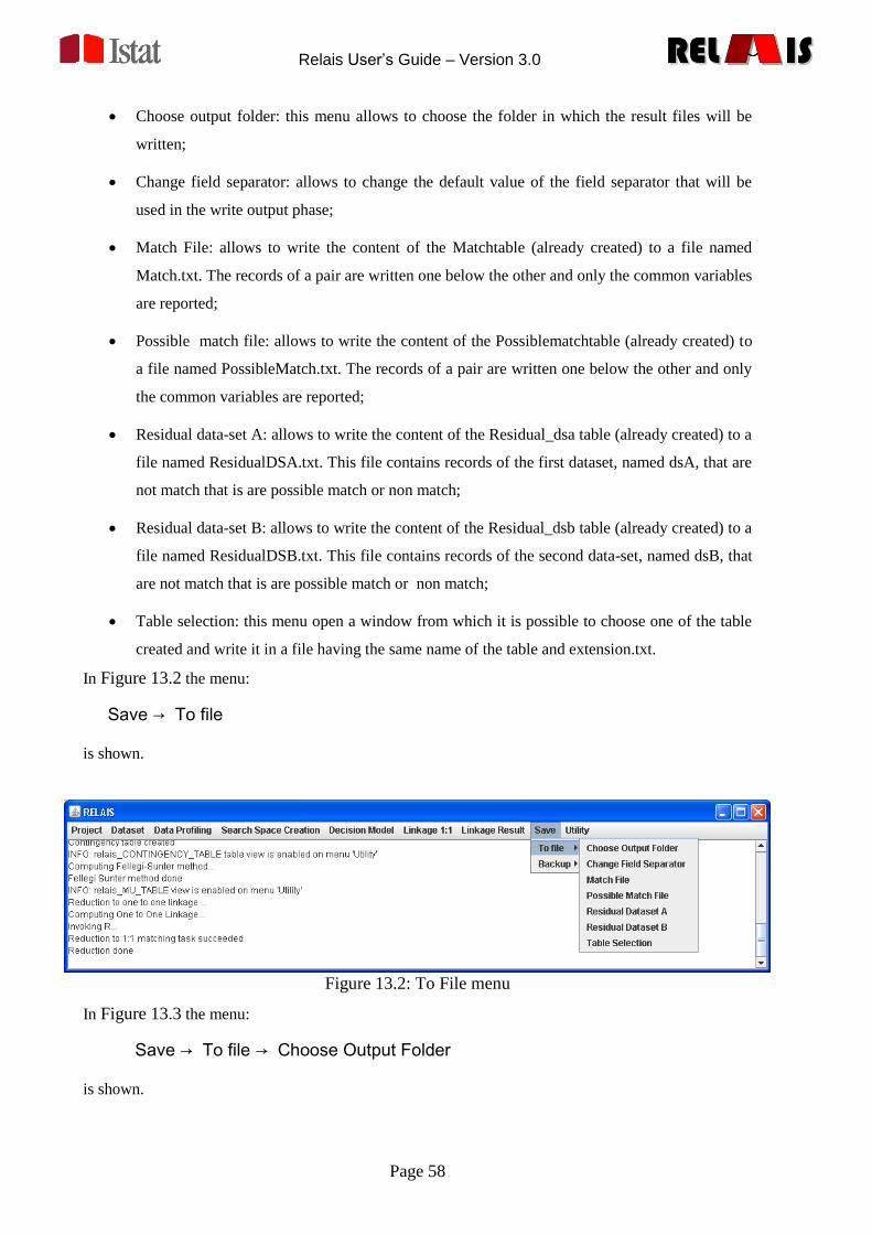
Relais User’s Guide – Version 3.0
Page 58
RELREL ISISRELREL ISIS
Choose output folder: this menu allows to choose the folder in which the result files will be
written;
Change field separator: allows to change the default value of the field separator that will be
used in the write output phase;
Match File: allows to write the content of the Matchtable (already created) to a file named
Match.txt. The records of a pair are written one below the other and only the common variables
are reported;
Possible match file: allows to write the content of the Possiblematchtable (already created) to
a file named PossibleMatch.txt. The records of a pair are written one below the other and only
the common variables are reported;
Residual data-set A: allows to write the content of the Residual_dsa table (already created) to a
file named ResidualDSA.txt. This file contains records of the first dataset, named dsA, that are
not match that is are possible match or non match;
Residual data-set B: allows to write the content of the Residual_dsb table (already created) to a
file named ResidualDSB.txt. This file contains records of the second data-set, named dsB, that
are not match that is are possible match or non match;
Table selection: this menu open a window from which it is possible to choose one of the table
created and write it in a file having the same name of the table and extension.txt.
In Figure 13.2 the menu:
Save → To file
is shown.
Figure 13.2: To File menu
In Figure 13.3 the menu:
Save → To file → Choose Output Folder
is shown.
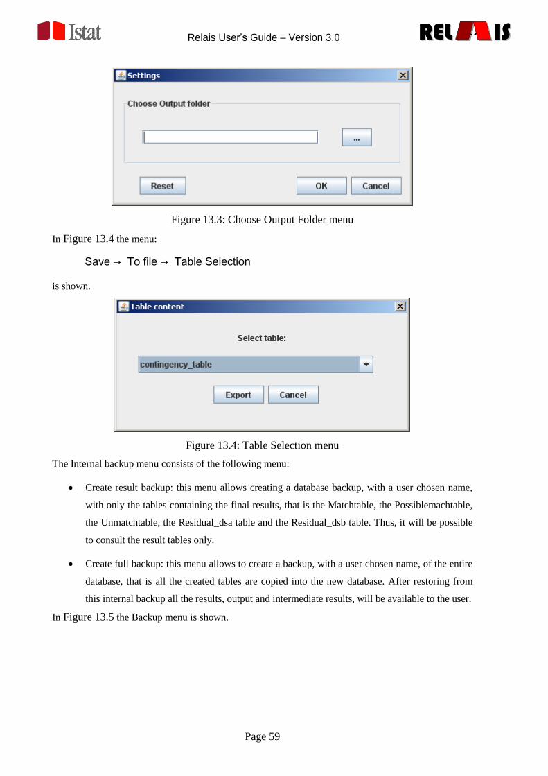
Relais User’s Guide – Version 3.0
Page 59
RELREL ISISRELREL ISIS
Figure 13.3: Choose Output Folder menu
In Figure 13.4 the menu:
Save → To file → Table Selection
is shown.
Figure 13.4: Table Selection menu
The Internal backup menu consists of the following menu:
Create result backup: this menu allows creating a database backup, with a user chosen name,
with only the tables containing the final results, that is the Matchtable, the Possiblemachtable,
the Unmatchtable, the Residual_dsa table and the Residual_dsb table. Thus, it will be possible
to consult the result tables only.
Create full backup: this menu allows to create a backup, with a user chosen name, of the entire
database, that is all the created tables are copied into the new database. After restoring from
this internal backup all the results, output and intermediate results, will be available to the user.
In Figure 13.5 the Backup menu is shown.
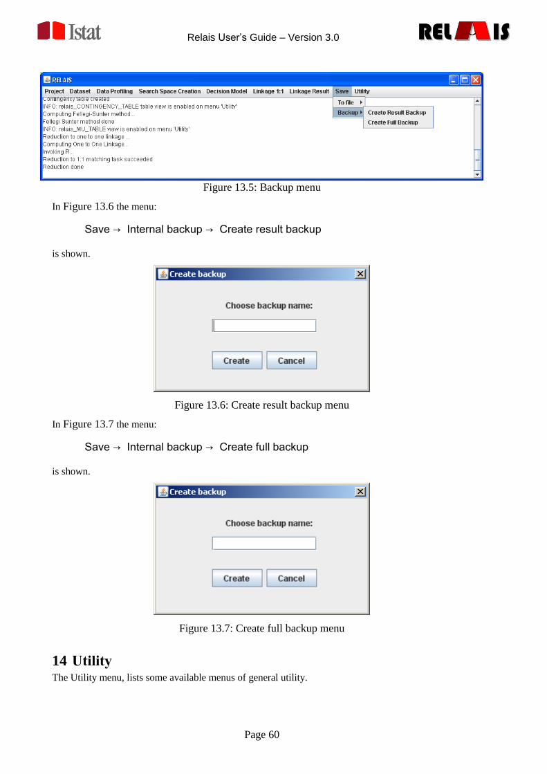
Relais User’s Guide – Version 3.0
Page 60
RELREL ISISRELREL ISIS
Figure 13.5: Backup menu
In Figure 13.6 the menu:
Save → Internal backup → Create result backup
is shown.
Figure 13.6: Create result backup menu
In Figure 13.7 the menu:
Save → Internal backup → Create full backup
is shown.
Figure 13.7: Create full backup menu
14 Utility The Utility menu, lists some available menus of general utility.
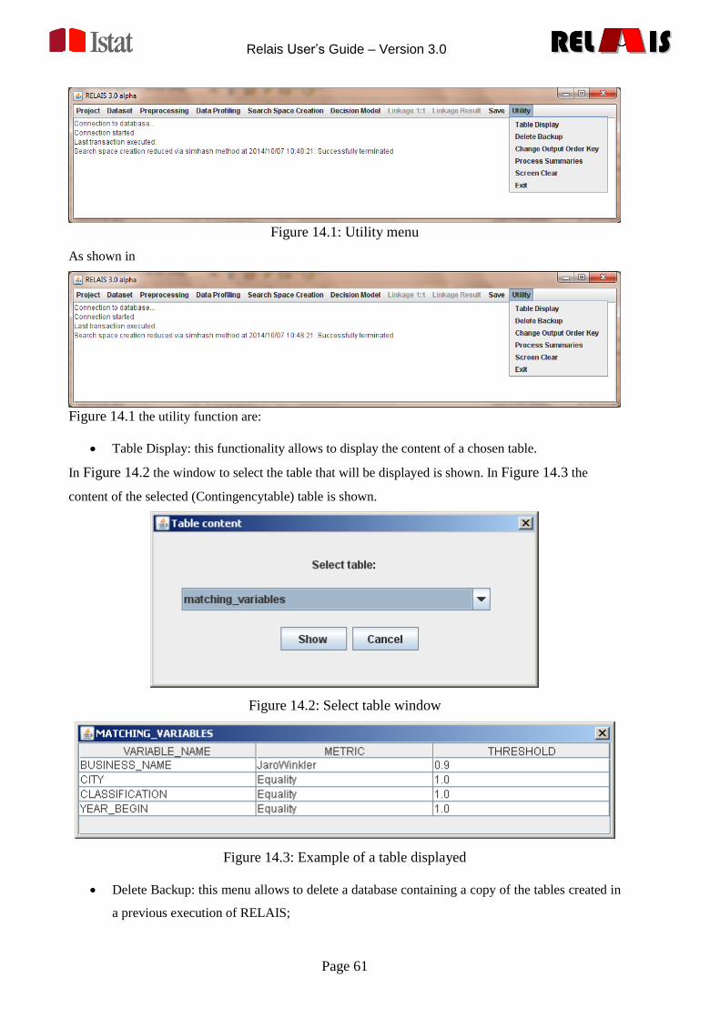
Relais User’s Guide – Version 3.0
Page 61
RELREL ISISRELREL ISIS
Figure 14.1: Utility menu
As shown in
Figure 14.1 the utility function are:
Table Display: this functionality allows to display the content of a chosen table.
In Figure 14.2 the window to select the table that will be displayed is shown. In Figure 14.3 the
content of the selected (Contingencytable) table is shown.
Figure 14.2: Select table window
Figure 14.3: Example of a table displayed
Delete Backup: this menu allows to delete a database containing a copy of the tables created in
a previous execution of RELAIS;
Relais User’s Guide – Version 3.0
Page 62
RELREL ISISRELREL ISIS
Change Output Order Key: allows to change the order of the data-set A and data-set B used in
the results. By default the first data-set is the data-set A;
Process Summaries: shows to user the principal parameters applied in the current linkage
project;
Screen Clear: this functionality allows to clear the output window;
Exit: this menu allows to close the application and freeze the current repository.
15 Batch Execution Instead of using RELAIS GUI, in some applications it is needed to run RELAIS in a batch mode, by
specifying all the input parameters once before the record linkage process execution.
The first step is the specification of the input parameters file, named “batchparam.txt”.
Such a file requires the specification of the following parameters:
dsaFile, path to the file of dataset A
dsaSep, separator of dataset A
dsbFile, , path to the file of dataset B
dsbSep, separator of dataset B
dedup, Y if needed, empty otherwise
Method, search space reduction method. If empty, cross product is performed. Otherwise the
possible values are “Blocking”, “Blocking Union”, ”Sorted Neighborhood”,”Nested
Blocking”, “SimHash” and “Blocked SimHash”.
BKey, name of the blocking key. If more than one, variables must be comma separated.
SKey, name of the sorting key. If more than one, variables must be comma separated.
WSize, size of the SNM window if SNM is specified as search space reduction method.
SHParam (optional), to modify parameters for the SimHash reduction method (and Blocked
SimHash). The ordered list of parameters, comma separated, is: Grams Size (the admitted
values are 2,3 and 4), HD threshold (the admitted values are 30, 35, 40, 45 and 50), number of
rotations (the admitted values are 2, 4, 8, 16 and 32), use of weights (the admitted values are 0
and 1). The default value for this parameter is “2,45,2,0”.
MVar, list of matching variables comma separated.
Relais User’s Guide – Version 3.0
Page 63
RELREL ISISRELREL ISIS
MMet, list of matching metrics comma separated, in the corresponding order of the matching
variables. The possible values are: “Equality”, “NumericComparison”, “3grams”, “Dice”,
“Jaro”, “JaroWinkler”, “Levenshtein”, “Soundex”. If empty, equality is used.
MThr, list of matching thresholds comma separated, in the corresponding order of the
matching variables.
Model, it is the decision model to be adopted. Current possible values are “Equality Match”
and “Fellegi Sunter”.
1to1 if empty no reduction 1:1 is performed. Possible values are “Greedy” or “Optimal”.
TU, Unmatch Threshold.
TM, Match Threshold.
Folder, path to the directory where output results will be saved.
Residuals, if set to “Y” (or “Yes”) also the residual datasets will be saved.
One the input parameters file is specified, RELAIS batch can be run:
Double-clicking RelaisBatch.bat file
From command line, by typing : java -jar relais3.0.jar
paramfilename.txt
16 Bibliography [1] Belin T.R., Rubin D.B.: A Method for Calibrating False-Match Rates in Record Linkage.
Journal of the American Statistical Association, Vol. 90, pp. 694-707, 1985.
[2] Dempster A.P., Laird N.M., Rubin D.B.: Maximum Likelihood from Incomplete Data via
EM Algorithm. Journal of the Royal Statistical Society, Series A, Vol.153, pp.287-320, 1977.
[3] Elmagarmid A. K., Ipeirotis P. G., Verykios V. S. Duplicate Record Detection: A Survey.
IEEE Transaction on Knowledge and Data Engineering, Vol. 19, N. 1, pp.1-16, 2007.
[4] Fellegi, I. P., and A. B. Sunter: A Theory for Record Linkage. Journal of the American
Statistical Association, Vol. 64, pp. 1183-1210, 1969.
[5] Fortini, M., Scannapieco, M., Tosco, L. and Tuoto, T.: Towards an Open Source Toolkit
for Building Record Linkage Workflows, In Proc. of SIGMOD 2006 Workshop on
Information Quality in Information Systems (IQIS'06), Chicago, USA, 2006.
[6] Hernandez, M. and Stolfo, S.: Real-world Data is Dirty: Data Cleansing and the
Merge/Purge Problem. Journal of Data Mining and Knowledge Discovery, Vol. 1, N. 2, 1998.
Relais User’s Guide – Version 3.0
Page 64
RELREL ISISRELREL ISIS
[7] Jaro, M.A.: Advances in Record Linkage Methodology as Applied to Matching the 1985
Census of Tampa, Florida. Journal of the American Statistical Association, Vol. 84, pp. 414-
420, 1989.
[8] Koudas, N. and Srivastava, D.: Approximate Joins: Concepts and Techniques. In Proc. of
International Conference on Very Large Data Bases (VLDB), Trondheim, Norway, 2005.
[9] Tuoto, T. , Cibella, N., Fortini, M., Scannapieco, M. and Tosco, L.: RELAIS: Don't Get
Lost in a Record Linkage Project, In Proc. of the Federal Committee on Statistical
Methodologies (FCSM 2007) Research Conference, Arlington, VA, USA, 2007.
[10] Yancey, W. E. Improving EM Algorithm Estimates for Record Linkage Parameters,
RESEARCH REPORT SERIES (Statistics #2004-01)
[11] Cibella N, Fortini M, Scannapieco M, Tosco L, Tuoto T.: Theory and practice of
developing a record linkage software, In Proc. Of the Combination of surveys and
administrative data Workshop of the CENEX Statistical Methodology Project Area
"Integration of survey and administrative data", Vienna, Austria, 2008
[12] Cibella N., Fernandez G.L., Fortini M., Guigò M., Hernandez F., Scannapieco M., Tosco
L., Tuoto T.: Sharing Solutions for Record Linkage: the RELAIS Software and the Italian and
Spanish Experiences, In Proc. Of the NTTS (New Techniques and Technologies for Statistics)
Conference, Bruxelles, Belgium 2009
[13] Newcombe H, Kennedy J, Axford S and James A.: Automatic Linkage of Vital Records,
Science, Vol.130 pp. 954-959
[14] Gill, L.: Methods for Automatic Record Matching and Linkage and their Use in National
Statistics. National Statistics Methodological Series no. 25, HMSO Norwich, UK (2001)
[15] Christen, P. & Goiser, K. (2005), Assessing deduplication and data linkage quality: What
to measure?, in 'Proceedings of the fourth Australasian Data Mining Conference (AusDM
2005)', Sydney.
[16] Jaro, M. A. 1995 "Probabilistic linkage of large public health data file" Statistics in
Medicine 14:491-498
[17] Winkler, W. E. (1999). "The state of record linkage and current research problems".
Statistics of Income Division, Internal Revenue Service Publication R99/04.
http://www.census.gov/srd/papers/pdf/rr99-04.pdf.
[18] "Using q-grams in a DBMS for Approximate String Processing" by Luis Gravano,
Panagiotis G, Ipeirotis H. V, Jagadish, Nick Koudas S. Muthukrishnan, Lauri Pietarinen and
Divesh Srivastava.
Relais User’s Guide – Version 3.0
Page 65
RELREL ISISRELREL ISIS
[19] Jaro, M.A., “Advances in record linkage methodology as applied to matching the 1985
Census of Tampa, Florida”, Journal of the American Statistical Association, 1989, 84, 414-420
[20] Charikar, M.S. (2002), “Similarity estimation techniques from rounding algorithms”,
Proceedings ACM STOC ‟02, May 19-21 2002, Montreal, Quebec,Canada, 380–388.
[21] Broder, A. (1997), “On the resemblance and containment of documents”. Proceedings of
the Compression and Complexity of Sequences.
[22] Goemans, M.X. and Williamson, D.P. (1995), “Improved approximation algorithms for
maximum cut and satisfiability problems using semidefinite programming”, Journal of the
ACM 42(6), p.1115-1145.
[23] Indik, P. and Motwani, R. (1998), “Approximate nearest-neighbors: Towards removing
the curse of dimensionality”, Proceedings of the 30th
STOC, p. 604-613.
[24] Mancini, L., Valentino, L., Borrelli, F. and Marcone, L. (2012). “Record linkage between
large dataset: Evidence from the 15th
Italian Population Census”, Quaderni di Statistica,Vol.
14, p. 149-152.
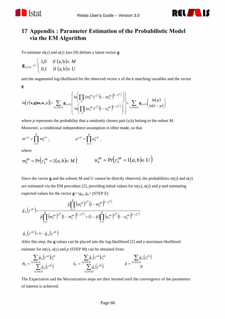
Relais User’s Guide – Version 3.0
Page 66
RELREL ISISRELREL ISIS
17 Appendix : Parameter Estimation of the Probabilistic Model
via the EM Algorithm
To estimate m() and u() Jaro [9] defines a latent vector g:
and the augmented log-likelihood for the observed vector x of the k matching variables and the vector
g
where p represents the probability that a randomly chosen pair (a,b) belong to the subset M.
Moreover, a conditional independence assumption is often made, so that
K
k
bak
ba mm1
,,
;
K
k
bak
ba uu1
,,
.
where
Since the vector g and the subsets M and U cannot be directly observed, the probabilities m() and u()
are estimated via the EM procedure [2], providing initial values for m(), u() and p and estimating
expected values for the vector g=<gm, gu> (STEP E)
After this step, the g values can be placed into the log-likelihood [2] and a maximum likelihood
estimate for m(), u() and p (STEP M) can be obtained from:
The Expectation and the Maximization steps are then iterated until the convergence of the parameters
of interest is achieved.
U
Mba
ba, if1,0
ba, if0,1),(g
ba
ba
ba
k
abk
abk
k
abk
abk
bap
p
uu
mm
pfabk
abk
abk
abk
,
,
, 1
1
,1ln
ln
1)(ln
1)(ln
ln ggu,m,gx,
Mbam abk
abk ,1Pr Ubau ab
kabk ,1Pr
abm
abu
K
k
abk
abk
K
k
abk
abk
K
k
abk
abk
abm
gg
uupmmp
mmp
gabk
abk
abk
abk
abk
abk
ˆ1ˆ
1ˆ11ˆ
1ˆ
ˆ
1
1
1
1
1
1
),(
),(
ˆ
ˆ
ˆ
ba
abm
ba
abk
abm
kg
g
m
),(
),(
ˆ
ˆ
ˆ
ba
abu
ba
abk
abu
kg
g
u
N
g
pba
abkm
),(
ˆ
ˆ
Relais User’s Guide – Version 3.0
Page 67
RELREL ISISRELREL ISIS
In the current version of RELAIS, the routine "mu_gen_embedded.R" applies the R optimizer
for loglinear model during the M step,equivalent to the conditional independence model
defined above. The loglinear model parametrisation allows for a more flexible model
definition in which the independence hypothesis can be relaxed in some extent. The initial
values of the parameters are m()=0.8 , u()=0.2 and p=0.1; the maximum number of iteration
is 5.000 and the stop criterion is achieved when the difference between the estimates of two
iteration is 0.000001.
The model estimates are considered not reliable when the estimated conditional probabilities m() and
u() of at least one of the matching variables have the same trend both for matches and for non-matches
populations. In such conditions, the system stops and the following message is shown:
"ERROR: one or more variables give inconsistent estimates. Please, check the variables in the model or
try to reduce the search space."
"See FSFail.Rout for more details."
The estimated conditional probabilities m() and u() can be verified in file FSFail.Rout in the RELAIS
folder.
A warning message is given when the estimates conditional probabilities of at least one of the
matching variables are nearly the boundary (m()>0.99999 or u()>0.99999). In such a situations, the
following message is shown:
"WARNING: one or more nearly boundary parameters. See FSFail.Rout for more details.";
the estimation results are saved in the MU_table and the estimated conditional probabilities can be
verified in the file FSFail.Rout in the RELAIS folder.
When the probabilistic model is applied on several blocks, a FSFail.Rout file is created for each block
giving erroneous or warning results.