Robots Ctr Tro

IEEE TRANSACTIONS ON ROBOTICS, VOL. 26, NO. 2, APRIL 2010 209

Design and Control of Concentric-Tube RobotsPierre E. Dupont, Senior Member, IEEE, Jesse Lock, Brandon Itkowitz, and Evan Butler, Student Member, IEEE

Abstract—A novel approach toward construction of robots isbased on a concentric combination of precurved elastic tubes. Byrotation and extension of the tubes with respect to each other, theircurvatures interact elastically to position and orient the robot’s tip,as well as to control the robot’s shape along its length. In this ap-proach, the flexible tubes comprise both the links and the joints ofthe robot. Since the actuators attach to the tubes at their proximalends, the robot itself forms a slender curve that is well suited forminimally invasive medical procedures. This paper demonstratesthe potential of this technology. Design principles are presentedand a general kinematic model incorporating tube bending andtorsion is derived. Experimental demonstration of real-time posi-tion control using this model is also described.

Index Terms—Continuum robots, flexible arms, kinematics,medical robots and systems, telerobotics.

I. INTRODUCTION

M INIMALLY invasive medical procedures involve themanipulation of tools, sensors, and prosthetic devices

inside the body that lead to minimum damage of surroundingtissue structures. In many cases, navigation to the surgical siterequires the instrument to be steered along 3-D curves throughtissue to avoid bony or sensitive structures (percutaneous pro-cedures) or following the interior contours of a body orifice(e.g., the nasal passages) or body cavity (e.g., the heart). Onceat the surgical site, it is often necessary to control the positionand orientation of the instrument’s distal tip while the proximalinserted length is held relatively immobile.

The instruments used in minimally invasive procedures canbe grouped into three general categories. The first category in-

Manuscript received January 31, 2009; revised September 15, 2009. Firstpublished December 31, 2009; current version published April 7, 2010. Thispaper was recommended for publication by Associate Editor A. Albu-Schafferand Editor G. Oriolo upon evaluation of the reviewers’ comments. This work wassupported in part by the National Institutes of Health under Grant R01HL073647and Grant R01HL087797 and by the Wallace H. Coulter Foundation. This pa-per was presented in part at the IEEE International Conference on Roboticsand Automation, Kobe, Japan, May 2009. This paper was submitted in part tothe forthcoming IEEE International Conference on Robotics and Automation,Anchorage, AK, May 2010.

P. E. Dupont was with the Department of Mechanical Engineering, BostonUniversity, Boston, MA 02215 USA. He is now with the Department of Cardio-vascular Surgery, Children’s Hospital Boston, Harvard Medical School, Boston,MA 02115 USA (e-mail: [email protected]).

J. Lock is with the Department of Biomedical Engineering, Boston Univer-sity, Boston, MA 02215 USA (e-mail: [email protected]).

B. Itkowitz was with the Department of Electrical and Computer Sys-tems Engineering, Boston University, Boston, MA 02215 USA. He is nowwith Intuitive Surgical, Inc., Sunnyvale, CA 94086-5304 USA (e-mail:[email protected]).

E. Butler is with the Department of Mechanical Engineering, Boston Univer-sity, Boston, MA 02215 USA (e-mail: [email protected]).

This paper has supplementary downloadable material available athttp://ieeexplore.ieee.org, provided by the authors.

Color versions of one or more of the figures in this paper are available onlineat http://ieeexplore.ieee.org.

Digital Object Identifier 10.1109/TRO.2009.2035740

cludes straight flexible needles that are used for percutaneousprocedures in solid tissue. The needle is steered along a curvedinsertion path by the application of lateral forces at the needlebase or tip as the needle is advanced into the tissue. Since theneedle is initially straight, both base- and tip-steering methodsrely on tissue reaction forces to flex the needle along a curvedinsertion path. Consequently, these instruments possess no abil-ity to produce lateral tip motion without further penetration intosolid tissue.

The second category of instruments is composed of a straight,stiff shaft with an articulated tip-mounted tool (e.g., forceps).Both hand-held and robotic instruments (e.g., da Vinci, IntuitiveSurgical, Inc.) [1] of this type are in common use for minimallyinvasive access of body cavities (e.g., chest or abdomen). Theshaft must follow a straight-line path from the entry point of thebody to the surgical site. Lateral motion of the tip depends onpivoting the straight shaft about a fulcrum typically located atthe insertion point into the body. This pivoting motion producestissue deformation proportional to the thickness of tissue fromthe entry point to the body cavity.

The third category of instruments includes elongated, steer-able devices, such as multistage microrobot devices, which aretypically used for entry through a body orifice, and steerablecatheters, which are most often used for percutaneous accessof the circulatory system. Multistage microrobot devices aretypically mounted at the distal end of a rigid shaft and includea flexible backbone that has a series of regularly spaced plat-forms. Control elements, e.g., wires or tubes, attach to the distalplatform and slide through all proximal platforms. For exam-ple, in [2], the control elements are tubes that act as secondarybackbones and enable shape control through push–pull actu-ation. These devices are typically sufficiently rigid to supporttheir own weight as well as to apply appreciable lateral forces tothe surrounding tissue. An alternate novel technology enablesextension along an arbitrary 3-D curve [3]. This technology is,however, nonholonomic in that lateral motion of the tip is onlyaccomplished in combination with tangential motion.

In contrast, steerable catheters include an elongate memberof sufficient flexibility to conform to the curvature of the vesselthrough which it is advanced. Steering is achieved by the useof one or more wires attached to the distal end of the elongatemember disposed along the catheter’s length [4]. User actuation(e.g., pulling) of the wires causes the distal portion of the elon-gate member to flex in one or more directions. Alternately, anexternal magnetic field can be used to position the catheter tip(Stereotaxis, Inc.) [5].

Concentric tube robots possess the best properties of all threetypes of instruments. With cross sections comparable with nee-dles and catheters, they are nevertheless capable of substantialactively controlled lateral motion and force application alongtheir length. Since robot shape can be controlled, they enable

1552-3098/$26.00 © 2009 IEEE

Authorized licensed use limited to: BOSTON UNIVERSITY. Downloaded on June 04,2010 at 18:05:20 UTC from IEEE Xplore. Restrictions apply.

210 IEEE TRANSACTIONS ON ROBOTICS, VOL. 26, NO. 2, APRIL 2010

Fig. 1. Concentric-tube robot comprising four telescoping sections that canbe rotated and translated with respect to each other.

navigation through the body along 3-D curves. Furthermore,the lumen of the tubes can house additional tubes and wires forcontrol of articulated tip-mounted tools. An example is shownin Fig. 1.

Thus, the technology holds the potential to enable many newminimally invasive interventions. An important class of appli-cations for such a device would be to enter a body lumen bysteering through tissue or through a body orifice. Once inside thelumen, the proximal portion can remain relatively fixed whilethe distal portion manipulates tools within the lumen to performminimally invasive surgery.

The kinematic modeling for real-time control of these robotsis a challenge in comparison to that of traditional robots whoselinks are relatively rigid and whose joints are discrete. The for-ward kinematics can be cast as a 3-D beam-bending problemin which the kinematic input variables (tube rotations and dis-placements at the proximal end) enter the problem as a subsetof the boundary conditions. The remaining boundary conditionscomprise point forces and torques applied to the distal ends ofthe tubes. Contact along the robot’s length (e.g., with tissue)generates additional distributed and point loads.

Thus, it can be anticipated that the most general kinematicmodel can be expressed as a two-point boundary-value problemthat involves a differential equation with respect to arc lengthalong the common centerline of the tubes. Phenomena that maybe included in the model are bending, torsion, friction, shear,axial elongation, and nonlinear constitutive behavior.

Since real-time control necessitates the balance of the accu-racy of the model with efficiency of its computation, efforts todate have modeled curved portions of the tubes as torsionallyrigid [10]–[15]. The torsionally rigid model, which was first de-rived in [10], results in an algebraic expression for curvature ofthe combined tubes that can be analytically integrated to yieldposition and orientation of the robot’s tip. Models of this typehave been demonstrated to provide reasonable performance incombination with real-time sensing of the tip frame (teleopera-tion in [13] and image servoing in [15]).

Including torsional twist in the straight-transmission lengthsof the tubes has also been proposed in [11] and implementedby the use of online root finding in [15]. Instabilities that arisefrom the interaction of transmission-length torsion and curved-length bending have been investigated using an energy approachin [14].

While it was shown in [12] that closed-form inverse kinematicsolutions can be derived for simple concentric-tube robots, they

Fig. 2. Dominating-stiffness tube pair. (a) When retracted, tubes conform toshape of stiff outer tube. (b) Portion of extended inner tube relaxes to its initialcurvature.

are difficult to obtain in general. Jacobian-based inverse kine-matics that use the algebraic curvature model were first formu-lated in [12] and experimentally implemented in [13]. Inclusionof torsional twist in straight transmission lengths is reportedin [15].

The contribution of this paper is to provide a framework forthe design and kinematic modeling of concentric-tube robotsthat enables accurate real-time position control. The paper isarranged as follows. Section II presents design guidelines forthe production of clinically relevant robots and describes theorigins of concentric-tube technology. Section III derives anew kinematic model that is more accurate than prior mod-els since it includes torsion along the entire lengths of thetubes and is also able to predict torsion-bending instabilitiesfor curved tubes [16]. Implementation of closed-loop positioncontrol based on the kinematic model is described in Section IVand its experimental evaluation appears in Section V. Conclu-sions are given in Section VI.

II. DESIGN OF CONCENTRIC-TUBE ROBOTS

A. Overview

When curved tubes are inserted inside each other, their com-mon axis conforms to a mutually resultant curvature. By relativetranslations and rotations of the tubes, both the curvature as wellas the overall length of the robot can be varied. The first robotsof this type composed of two tubes were presented in [7]–[9].Robots composed from three or more tubes were first proposedin [10] and [11].

To understand the capabilities of the technology, it is useful toconsider the interaction of two concentrically combined tubes.Limiting cases of their interaction correspond to when the ratioof bending stiffnesses for the two tubes is 1) very large, suchthat the shape of one tube dominates that of the other, and 2) theratio is approximately one, such that the tubes’ shapes interactequally to determine the overall shape. Each of these cases isdescribed next.

1) Domination-Stiffness Tube Pair: Since the bending stiff-ness of one tube is much larger than that of the other, the pairof concentric tubes conforms to the curvature of the stiffer tube.When the more flexible tube is translated such that it extendsbeyond the end of the stiff tube, the extended portion relaxes toits original curvature.

This is illustrated in Fig. 2 for the case of a stiff, straight outertube and a curved, inner flexible tube. As shown in Fig. 2(b),once the flexible tube is extended, the pair has two independentdegrees of freedom (DOFs) associated with relative translation


DUPONT et al.: DESIGN AND CONTROL OF CONCENTRIC-TUBE ROBOTS 211

Fig. 3. Balanced-stiffness tube pair. (a) Rotating tube pair with curvaturesaligned. (b) Rotating-tube pair with curvatures opposed.

and relative rotation of the tubes. Cardiologists routinely employthis technique with catheters and guide wires to manually ne-gotiate branches in the vasculature. Tube pairs of this type havepreviously been used to steer joystick-controlled tip of straightneedles [7].

2) Balanced-Stiffness Tube Pair: Since the tubes are of sim-ilar stiffness, their unstressed curvatures interact to determinetheir combined curvature. Relative rotation of the tubes causesthe combined curvature to vary. An example is depicted in Fig. 3in which the unstressed curvatures of the two tubes have beendesigned such that the pair is straight when the unstressed curva-tures oppose each other and possesses maximum curvature whenthe individual curvatures are aligned. A balanced-stiffness tubepair was first proposed and constructed as a steerable needlein [9].

When either type of tube pair is used as a robot, the rela-tive displacements of the tubes are produced by the applicationof forces and torques at the proximal end. When inertial ef-fects are ignored, the magnitudes of the forces and torques arethose necessary to deform the tubes from their combined min-imum energy configuration and to overcome friction betweenthe tubes.

Possible modes of tube deformation are bending, torsion,cross-section shear, and axial elongation. For the prediction oftip displacement, bending and torsion are the dominant contrib-utors. The effect of bending on tube pairs has been describedearlier. As will be derived in Section III, torsional twisting oc-curs whenever two curved tubes are rotated from the alignedconfiguration of Fig. 3(a).

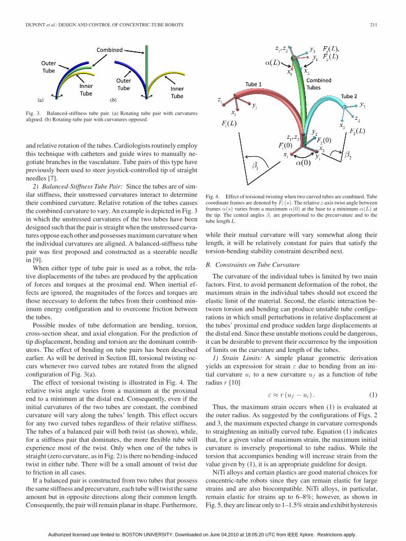
The effect of torsional twisting is illustrated in Fig. 4. Therelative twist angle varies from a maximum at the proximalend to a minimum at the distal end. Consequently, even if theinitial curvatures of the two tubes are constant, the combinedcurvature will vary along the tubes’ length. This effect occursfor any two curved tubes regardless of their relative stiffness.The tubes of a balanced pair will both twist (as shown), while,for a stiffness pair that dominates, the more flexible tube willexperience most of the twist. Only when one of the tubes isstraight (zero curvature, as in Fig. 2) is there no bending-inducedtwist in either tube. There will be a small amount of twist dueto friction in all cases.

If a balanced pair is constructed from two tubes that possessthe same stiffness and precurvature, each tube will twist the sameamount but in opposite directions along their common length.Consequently, the pair will remain planar in shape. Furthermore,

Fig. 4. Effect of torsional twisting when two curved tubes are combined. Tubecoordinate frames are denoted by Fi (s). The relative z-axis twist angle betweenframes α(s) varies from a maximum α(0) at the base to a minimum α(L) atthe tip. The central angles βi are proportional to the precurvature and to thetube length L.

while their mutual curvature will vary somewhat along theirlength, it will be relatively constant for pairs that satisfy thetorsion-bending stability constraint described next.

B. Constraints on Tube Curvature

The curvature of the individual tubes is limited by two mainfactors. First, to avoid permanent deformation of the robot, themaximum strain in the individual tubes should not exceed theelastic limit of the material. Second, the elastic interaction be-tween torsion and bending can produce unstable tube configu-rations in which small perturbations in relative displacement atthe tubes’ proximal end produce sudden large displacements atthe distal end. Since these unstable motions could be dangerous,it can be desirable to prevent their occurrence by the impositionof limits on the curvature and length of the tubes.

1) Strain Limits: A simple planar geometric derivationyields an expression for strain ε due to bending from an ini-tial curvature ui to a new curvature uf as a function of tuberadius r [10]

ε ≈ r (uf − ui) . (1)

Thus, the maximum strain occurs when (1) is evaluated atthe outer radius. As suggested by the configurations of Figs. 2and 3, the maximum expected change in curvature correspondsto straightening an initially curved tube. Equation (1) indicatesthat, for a given value of maximum strain, the maximum initialcurvature is inversely proportional to tube radius. While thetorsion that accompanies bending will increase strain from thevalue given by (1), it is an appropriate guideline for design.

NiTi alloys and certain plastics are good material choices forconcentric-tube robots since they can remain elastic for largestrains and are also biocompatible. NiTi alloys, in particular,remain elastic for strains up to 6–8%; however, as shown inFig. 5, they are linear only to 1–1.5% strain and exhibit hysteresis



Fig. 5. Stress versus strain curve for NiTi showing characteristic elastic load-ing and unloading plateaus.

at higher strain. While a complete discussion is beyond the scopeof this paper, the effect of this behavior on robot design can besummarized by taking into account its effect on tube pairs.

Bending stiffness is given by EI in which E is elastic mod-ulus, which corresponds to the slope of the stress–strain curve,and I is the cross-sectional moment of inertia. For a pair oftubes in which the maximum strain is less than the linear elas-tic limit, the ratio of bending stiffness is given by the ratio ofcross-sectional moduli.

From (1), strain varies linearly with distance from the cen-ter of the tube. As the change in tube curvature increases, thecross section will transition from the linear elastic region to thestress plateau starting with the outer fibers. In this transition, theeffective elastic modulus and, thus, bending stiffness decreases.

In a dominating-stiffness tube pair, the less stiff tube experi-ences higher strains, and therefore, its cross section transitionsto the stress plateau first. This works in favor of the designersince it means that the effective stiffness ratio is larger than whatis predicted from the ratio of cross-sectional inertias.

For balanced stiffness-tube pairs, the outer tube, which pos-sesses a larger outer radius, will always start the transition to thestress plateau first given the same change in curvature. This isnot an impediment to implementation of a balanced pair, how-ever, and the effect can be incorporated in the kinematic modelas needed.

2) Torsion-Bending Instabilities: The second limitation ontube curvature arises from the torsional twisting associated withrotating curved tubes. This effect will be derived in Section III;however, it is possible to provide a simple explanation here byreference to Figs. 3 and 4. As the tubes are rotated from theiraligned configuration, the rotation angle at the distal end ini-tially lags the rotation angle at the proximal end. If the lag islarge enough that tip rotation fails to catch up as the proximalrotation angle approaches π [which corresponds to the config-uration of Fig. 3(b)], the tubes will subsequently snap throughthis configuration to one in which the distal rotation leads theproximal value. The implications of instability for design arediscussed next.

Fig. 6. Example five-tube robot design composed of three telescoping sectionsof variable, fixed, and variable curvature, respectively. Tube pairs comprisingvariable-curvature sections are rotated individually but extended simultaneously.Each section dominates the shape of those sections retracted inside it.

C. Robot Design

Based on the discussion of Section I, two desirable propertiesof a minimally invasive robotic instrument are as follows.

1) the ability to manipulate distal links independent of prox-imal links, i.e., to decouple the robot’s links;

2) the ability to navigate narrow curved passages and, if tissueis penetrated, exert minimal lateral forces.

A design strategy that provides these properties is encapsu-lated in the following four design rules and illustrated in Fig. 6.

1) Telescoping Dominant Stiffness: The stiffnesses of thetubes are selected such that each telescoping section dominatesall those sections extending from it. This is equivalent to aconcatenation of dominating-stiffness tube pairs (recall Fig. 2).The result is that each telescoping section corresponds to a linkwhose shape and displacement are approximately kinematicallydecoupled from all other sections.

2) Fixed and Variable Curvature Sections: Each telescopingsection behaves as a dominating (fixed curvature) or balanced(variable curvature) tube pair. Thus, the shape of each telescop-ing section is dominated by its outermost tubes and is of fixedcurvature (if the outer tube dominates all inner tubes) or is ofvariable curvature (if the outer tube pair dominates all innertubes). Tube curvatures are selected as per the constraints de-scribed in Section II-B.

3) Piecewise-Constant Initial Tube Curvatures: To avoidproducing lateral motion or forces during telescopic extension,the order of extension must proceed from the proximal sectionto the distal one. In addition, the curvature of each section mustbe constant. By precurving each tube such that its curvature ispiecewise constant, the combined telescoping curvature is alsoapproximately piecewise constant. This is true even when tor-sion is considered. Telescopically extended fixed-curvature sec-tions assume the shape of their precurvature since they dominateall inner tubes. In addition, as described at the end of Section I,a, stable variable-curvature section composed of balanced tubesremains planar and of almost-constant curvature.

4) Increasing Curvature From Base to Tip: While the shapeof the proximal sections may be tightly constrained by the de-sired navigation path to the surgical site, it is often desirableto employ larger curvatures for the distal section(s). In thisway, the proximal sections function as the links of a typicalrobot arm produce most of the tip displacement. The tightlycurved distal sections function as the robot’s wrist to controlmost of the tip orientation as well as small displacements. Fur-thermore, since the distal sections’ tubes are comprised of the



smaller diameter inner tubes, they can be given larger precur-vatures without exceeding the elastic strain limit. Stable pre-curvature is limited, however, since the inner tubes are alsothe longest, and therefore, most prone to torsion-bendinginstabilities.

In summary, tube cross sections and initial curvatures are se-lected such that the robot behaves as a concatenation of kinemat-ically independent dominating stiffness (constant curvature) andbalanced stiffness (variable curvature) tube pairs. Each constant-curvature section has two kinematic input variables {l, θ} andcontributes two DOFs that correspond to the extension lengthand rotation of the section (see Fig. 6). Each variable-curvaturesection has three kinematic input variables {θ1 , θ2 , l} and con-tributes three DOFs. The angles {θ1 , θ2} control rotation andcurvature of the section and l controls arc length (see Fig. 3).

The kinematic model developed in the next section providesthe tools for computation of the displacements of the proposedtelescopic concatenation of constant- and variable-curvaturesections. It also dictates how closely these design goals canbe achieved in practice.

III. KINEMATIC MODELING

In this section, we present a general kinematic model thatincludes bending and torsion for an arbitrary number of tubeswhose curvature and stiffness can vary with arc length. (Notethat this is more general than what is needed to model the designsproposed earlier.) Effects that are neglected include shear of thecross section, axial elongation, nonlinear constitutive behavior,friction between the tubes, and deformation due to externalloading (including gravity). Note that while neglected, theseeffects may not be negligible but are beyond the scope of thispaper.

For ease of exposition, the model is developed in severalsteps. First, coordinate frames and curvature are defined fol-lowed by a concise derivation of the torsionally rigid algebraicmodel. Next, the differential equation model for two torsionally-compliant tubes is developed. Its analytic solution is given, andthe torsion-bending stability condition is derived. Finally, thegeneral multitube torsion-bending model is presented. The vari-ables used in the paper are enumerated in Table I.

A. Coordinate Frames and Curvature

In the remainder of the paper, subscript indices i = 1, 2, . . . , nare used to refer to individual tubes with tube 1 being outermostand tube n being innermost. Arc length s is measured such thats = 0 at the proximal end of the tubes. As shown in Fig. 4,material coordinate frames for each cross section can be definedas a function of arc length s along tube i by the definitionof a single frame at the proximal end Fi(0), such that its z-axis is tangent to the tube’s centerline. Under the unrestrictiveassumption that the tubes do not possess initial material torsion,the frame Fi(s) is obtained by sliding Fi(0) along the tubecenterline without rotation about its z-axis (i.e., a Bishop frame[17]). As the tubes move, bend, and twist, these material framesact as body frames that track the displacements of their crosssections.

TABLE INOMENCLATURE

It is also useful to define a reference frame F0(s) (not shown)which displaces with the cross sections but does not rotate aboutits z-axis. When needed for clarity, superscripts will be used toindicate the coordinate frame of vectors and transforms.

As the ith tube’s coordinate frame Fi(s) slides down itscenterline, it experiences a body-frame angular rate of changeper unit arc length given by

uFi (s)i (s) = [uix(s) uiy (s) uiz (s) ]T (2)

in which (uix , uiy ) are the components of curvature due tobending, and uiz is the curvature component due to torsion. Acircumflex on a curvature component is used to designate theinitial precurvature of a tube.

Curvatures transform between coordinate frames like angu-lar velocities. Thus, with the definition of θi(s) as the z-axis



rotation angle from frame F0(s) to frame Fi(s) and Rz (θi) asthe corresponding rotation matrix, the curvature vectors trans-form as

uF0 (s)i = Rz (θi(s))u

Fi (s)i . (3)

B. Torsionally Rigid Model

An algebraic curvature model can be derived by the combina-tion of three equations: 1) a constitutive model relates bendingmoments to changes in curvature of individual tubes; 2) theequilibrium of bending moments for the assembled tubes; and3) a compatibility equation that relates the individual curvaturesof the assembled tubes. These are described next.

1) Constitutive Model: When a tube with initial curvatureu

Fi (s)i (s) is deformed to a different curvature u

Fi (s)i (s), a bend-

ing moment is generated. On the assumption of linear elasticbehavior, i.e., that strains remain in the linear elastic region ofFig. 5, the bending moment vector m

Fi (s)i (s) at any point s

along tube i is given by

mFi (s)i (s) = Ki

(u

Fi (s)i (s) − u

Fi (s)i (s)

)(4)

in which Ki is the frame-invariant stiffness tensor given by

Ki =

kix 0 0

0 kiy 0

0 0 kiz

=

EiIi 0 0

0 EiIi 0

0 0 JiGi

(5)

and Ei is the modulus of elasticity, Ii is the area moment ofinertia, Ji is the polar moment of inertia, and Gi is the shearmodulus. While not explicitly noted, all variables in (5) can befunctions of arc length in the derivations that follow.

2) Equilibrium of Bending Moments: In a concentric tuberobot, forces and torques must be applied at the proximal end ofthe individual tubes to maintain any desired configuration. If noother wrenches are applied, the net force and torque applied tothe tubes by the actuators is zero. Consequently, the net bendingmoment on every cross section is also zero

n∑i=1

mF0 (s)i (s) = 0. (6)

In this equation, all moments must be expressed in the samecoordinate frame. Recall that the transformation of momentsbetween collocated coordinate frames consists of a pure rotation[6]. Thus, they transform identically to curvatures as given by(3).

3) Compatibility of Deformations: On the assumption thatthe clearance between each pair of adjacent tubes is just suffi-cient to enable relative motion, all tubes must conform to thesame final x–y (bending) curvature when assembled. On the as-sumption of torsional rigidity, the z-component of curvature iszero, and the compatibility equation is given by

uF0 (s)1 (s)=u

F0 (s)2 (s)= · · · =

u

F0 (s)ix (s)

uF0 (s)iy (s)

0

= · · · = uF0 (s)

n (s).

(7)

Fig. 7. Three-tube example illustrating that torsionally-rigid model predictstubes of piecewise-constant curvature combine to form a robot of piecewise-constant curvature.

Combining (3)–(7) yields an expression for the resultant cur-vature as a function of arc length s [10]

uF0 (s)i (s) =

(n∑

i=1

Ki

)−1 n∑i=1

KiuF0 (s)i (s). (8)

If the initial curvatures of the tubes uF0 (s)i (s) are piecewise-

constant curvature, (4) and (8) indicate that the bending momentand curvature are constant over each segment of the robot inwhich all of the tubes in that segment have constant initialcurvature and stiffness. This is illustrated in Fig. 7. There isan implicit assumption here that, over negligible lengths at theboundaries of these segments, (4) and (7) are violated to producediscontinuities in curvature and bending moment.

Using this model, tubes of piecewise-constant curvature com-bine to form robots of piecewise-constant curvature. The tip-coordinate frame can be computed by analytic integration ofthe curvature of each constant-curvature segment and then con-catenation of the resultant set of relative transformations [10].While this model is computationally efficient, torsion must beincluded to obtain an accurate model as described next.

C. Torsionally Compliant Model for Two Tubes

In this derivation, we employ the special Cosserat rod modelto account for torsional twisting of the tubes. The same resultscan be obtained by the use of the calculus of variations, as de-scribed in [16]. For clarity of presentation, the model is derivedhere for two tubes of constant curvature and length L.

It is convenient to define the relative twist angle α(s) betweentubes as a function of arc length

α(s) = θ2(s) − θ1(s) (9)

where θi(s) is the z-axis rotation between frames F0(s) andFi(s) at arc length s. Equilibrium of moments (6) can be writtenin the body frame of tube 1 as

mF1 (s)1 (s) = −Rz (α(s)) m

F2 (s)2 . (10)

To include torsional twisting, the compatibility equation (7)enforcing the coincidence of tube centerlines becomes

uF1 (s)1 (s) = Rz (α)uF2 (s)

2 (s) − α(s)eF2 (s)z (11)



in which eF1 (s)z = e

F2 (s)z = [0, 0, 1]T , and α = dα/ds. This

equation ensures that the tubes experience the same curvaturein the plane of the cross section but allows different rates oftorsional twist.

In the subsequent presentation, all tube variables are definedin their respective frame, and we omit reference to the frame.Thus, u

F2 (s)2 (s) is written as u2(s).

1) Bending Curvature: Combining the moment equilibriumequation (10) with the constitutive model (4) and the compati-bility equation (11) leads to an expression for the curvature oftube 2. On the assumption of circular cross sections, Rz (α) andKi commute, yielding

u2 = (K1 + K2)−1 (

RTz (α)K1 u1 + K2 u2 + αK1ez

). (12)

The x and y components of this equation mirror those of thetorsionally-rigid case and provide explicit algebraic equationsfor curvature as a function of initial curvature and twist angleα(s). The difference here is that twist angle α(s) is a functionof arc length

u2(s)|x,y = (K1 + K2)−1x,y

(RT

z (α(s))K1 u1(s)+ K2 u2(s))x,y

(13)

u1(s)|x,y = (Rz (α(s))u2(s))x,y . (14)

2) Torsional Curvature: The z-component of (12) providesan expression for twist-angle rate α

α = (1 + k2z /k1z ) u2z . (15)

Here, we have used the fact that precurvature does not includetorsional twist. To solve this expression, we need to be able toevaluate u2z .

We can obtain such an expression from the equilibrium equa-tion of the special Cosserat rod model [18]–[20]. When time-dependent terms are set to zero, the body-frame equilibriumequations for a curved rod undergoing distributed loading ofτ ∈3

R torque per unit length and f ∈ R3 force per unit length

are given by [m

n

]=

[τ

f

]−

[[u] [v]

0 [u]

][m

n

]. (16)

Derivatives are with respect to arc length along the rod sand m,n ∈ R

3 are the bending moment and shear force vectorsacting on the rod’s cross section. Here, and in the remainder ofthe paper, the square brackets on the vectors u and v denote theskew-symmetric form

[u] =

0 −uz uy

uz 0 −ux

−uy ux 0

. (17)

Consistent with the previous notation, u, v ∈ R3 are the an-

gular and linear strain rates per unit arc length. If one imaginessliding along a curved rod, these vectors can be interpreted aslinear and angular velocities (twist velocities) with arc lengththat corresponds to time. Wrenches applied at either end of therod enter the equations as boundary conditions.

Equation (16) can be interpreted as body-frame force andmoment-equilibrium equations for a differential length ds ofa curved beam or rod. The cross-product terms involving [u]are needed to account for rotation of the body frame along thelength of the differential element.

This equation can be used to predict the shape and forcesexerted when two or more precurved tubes are combined con-centrically. Since we anticipate that bending and twisting willbe the dominant forms of deformation of the tubes, we continueto assume that shear strain and axial strain are negligible. In(16), this results in vT = [0, 0, 1]. Furthermore, we assume thatcontact between the tubes is frictionless and that tubes can onlyexert distributed reaction forces, but not torques, on each other.As with the torsionally-rigid model, we assume that concen-trated moments are generated over negligibly short lengths atdiscontinuities in precurvature and at the ends of tubes in orderto satisfy compatibility [see (13) and (14)]. These moments aretreated as boundary conditions in (16).

Since tube interaction is limited to distributed forces, τ = 0in (16), and for each tube, it reduces to

mi = − [ui ] mi − [vi ] ni. (18)

To eliminate moments from these equations, we can use theconstitutive model for moments (4) and its derivative with re-spect to arc length

mi = Kiui. (19)

In the derivative, we have taken Ki and ui to be independentof s for simplicity, but this is not necessary. Equation (18) cannow be rewritten in terms of curvature

ui = −K−1i [ui ] Ki (ui − ui) − K−1

i [vi ] ni. (20)

Recalling vi = [0, 0, 1]T and assuming equal bending stiff-ness in the x- and y-directions kix = kiy , the z-component of(20) provides an expression for the derivative of torsional-twistrate as a function of bending curvature

u2z =(

k2x

k2z

)(u2x u2y − u2y u2x). (21)

This simple equation indicates that the derivative of twist rateis given by the cross product between actual and initial bendingcurvature multiplied by the ratio of bending to torsional stiffness.For tubes, this ratio is given by

kxi

kzi=

EiIi

GiJi= 1 + ν (22)

in which ν is Poisson’s ratio. By equilibrium of torsional mo-ments, we need only integrate for u1z or u2z since

u1z = −(

k2z

k1z

)u2z . (23)

Equations (13), (15), and (21) comprise the set of equationsthat must be solved to compute curvature along the length of thetubes. Equations (15) and (21) are two first-order differentialequations that can be equivalently described by a second-orderequation in α. If we assume that the cross-sectional precurvatureof both tubes is in the same direction (e.g., both in x direction or



both in y direction) when α = 0, then the three equations reduceto the following simple expression for precurvature magnitudes‖u1‖ and ‖u2‖

α(s) = (1 + ν) ‖u1‖ ‖u2‖ sinα(s) = c sin α(s). (24)

This equation indicates that the second derivative of twist an-gle has a simple dependence on a constant c, given by Poission’sratio multiplied by the initial tube curvatures.

Two boundary conditions are needed for the two state vari-ables, (α, α) or (α, u2z ). Since the tube angles at the proximalend θi(0) are the kinematic input variables

α(0) = θ2(0) − θ1(0). (25)

In addition, the torsional bending moment at the distal end ofeach tube is zero

m2z (L) = k2z (u2z (L) − u2z (L)) = k2z u2z (L) = 0. (26)

This yields a second boundary condition

α(L) = u2z (L) = 0. (27)

This is a two-point boundary value problem that can be inte-grated analytically, as shown next.

D. Analytical Solution for Two Tubes

The differential equation (24) governing the twist of twoconstant-curvature tubes has two trivial equilibrium solutions

α(s) = {0, π}, s ∈ [0, L]. (28)

These correspond to the situations in which the cross-sectional curvature vectors of the tubes have the same and op-posite directions, respectively (see Fig. 3). In neither case is anexternal torque needed to maintain the configuration. One canguess, however, that the solution α(s) = π is not a minimum-energy solution for the kinematic input value α(0) = π, andthus, it is likely that additional solutions to (24) share the initialcondition α(0) = π. To study solution multiplicity, we seek ananalytic solution to (24).

1) Analytic Integration: To integrate by separation of vari-ables, we use α = α dα

dα and write∫ α(s)

α(0)ada = c

∫ α(s)

α(0)sin ada (29)

in which a and a are variables of integration. This results in thefollowing expression for α(s):

α2(s) = α2(0) + 2c (cos(α(0)) − cos(α(s))) . (30)

Evaluating this equation using the boundary conditionα(L) = 0 and substituting the result in (30) yields

α2(s) = 2c (cos(α(L)) − cos(α(s))) . (31)

Separation of variables can be used again to obtain

s =±1√2c

∫ α(s)

α(0)

da√cos(α(L)) − cos(a)

. (32)

In (32), the sign is selected to match the sign of the integrationinterval sgn (α(s) − α(0)). Recognizing (32) as an incomplete

Fig. 8. Relative twist angle of tubes at base versus tip for three values of L√

c.Only the curve with L

√c < π/2 exhibits stable rotation.

elliptic integral of the first kind, we desire an expression for theupper limit of integration α(s). This can be obtained in termsof Jacobi elliptic functions by a variety of methods, includingconverting the integral of (32) to standard form or by assuminga solution and showing that it satisfies (31). This results in

sin(α(s)/2) = sin(α(L)/2) · nd((L − s)√

c|cos2(α(L)/2))

cos(α(s)/2) = cos(α(L)/2) · cd((L − s)√

c|cos2(α(L)/2))

(33)

in which nd (u|m)and cd (u|m) are Jacobi elliptic functions[21]. See Appendices A and B for a brief description of thesefunctions, as well as a proof that (33) satisfies (24).

Equation (33) expresses relative twist angle in terms of thetwist angle at the distal end. We are specifically interested inthe value at the proximal end since it is the kinematic inputα(0) = θ2(0) − θ1(0)

sin(α(0)/2) = sin(α(L)/2) · nd(L√

c|cos2(α(L)/2))

cos(α(0)/2) = cos(α(L)/2) · cd(L√

c|cos2(α(L)/2)). (34)

These expressions involve a single dimensionless parameterL√

c. Fig. 8 plots (34) for several values of this parameter.2) Solution Multiplicity: It can be seen from the figure that

at least one value of α(L) exists for each value of α(0) ∈ [0, 2π],but it is also apparent that there can be multiple solutions. So-lution multiplicity produces sudden changes in tube twist inresponse to incremental changes in the kinematic input α(0).These “snap through” instabilities are indicated as dotted linesin the figure and correspond to the tubes traversing betweenminimum energy branches of the curve.

To determine the dependence of the instability on the param-eter Lc1/2 , we count the solutions for α(L) given α(0) = π.Identical results are obtained using either the sine or cosineequation of (34). The sine equation reduces to

sin (α(L)/2) = dn(L√

c∣∣cos2 (α(L)/2)

). (35)



Since dn (u|0) = 1, (35) always has at least one solution{α(0), α(L)} = {π, π} corresponding to the case of zero twistalong the tubes’ length. To determine when additional solutionsexist, we use the identity [21]

dn(K(m)|m) =√

m1

m + m1 = 1, 0 ≤ m ≤ 1 (36)

and note that dn is periodic in its first argument with period2K(m). Here, K(m) is the complete elliptic integral of thefirst kind, which is a monotonically increasing function of mwith K(0) = π/2 and K(1) = +∞. Combining (35) and (36)results in

L√

c = nK(m), n = 1, 3, 5, . . . . (37)

This equation has no solutions for L√

c < π/2. For L√

c =π/2, the n = 1 solution is identical to the original solution{α(0), α(L)} = {π, π}. For π/2 < L

√c ≤ 3π/2, one new so-

lution to (37) exists. Since m = sin2 (α(L)/2), this yields twonew solutions sin (α(L)/2) = ±√

m. As seen in Fig. 8, thesesolutions are symmetric about α(L) = π. Similarly, 3π/2 <L√

c ≤ 5π/2 yields four solutions to (37).The dimensionless parameter L

√c = π/2 is very important

from a design perspective. The model predicts stable behaviorfor tubes satisfying

L√

c < π/2. (38)

As this parameter increases, however, additional solutionsexist which lie on unstable branches of the relation. The criticalvalues of α(0) at which “snap through” occurs correspond tothe extrema of α(0) adjacent to the n = 1 solution of (37).

A geometric interpretation of (38) can be obtained by notingthat

L√

c =√

(1 + ν)(L‖u1‖)(L‖u2‖) =√

(1 + ν)β1β2 (39)

in which β1 and β2 are the central angles swept out by theinitial curvatures of the tubes, as shown in Fig. 4. Thus, if twofrictionless tubes of the same length L possess initial curvatureswith central angles β1 and β2 , they can be combined and rotatedat their proximal end without instability as long as the geometricmean of their central angles satisfies√

β1β2 <

(1√

1 + ν

)π

2. (40)

Assuming that ν ≈ 0.3 and that the tubes have the same ini-tial curvature, their maximum stable central angle is limitedto about 1.38 rad (79◦). This equation must be modified andthe maximum central angle reduced if the curved sections arelocated at the distal ends of straight transmission lengths.

E. General Model for an Arbitrary Number of Tubes

The equations of Section III-C can easily be extended toinclude any number of tubes of arbitrary stiffness and initialcurvature [16]. For n tubes, the equations can be written in termsof 2n − 2 state variables {αi, uiz}, i = 2, . . . , n. The relativetwist angles are defined by

αi(s) = θi(s) − θ1(s), i = 2, . . . , n (41)

where θi(s) is the angular displacement of the ith tube at arclength s. The resulting equations are

dαi

ds= uiz − u1z , i = 2, . . . , n

u1z = (−1/k1z )(k2z u2z + · · · + knzunz )

duiz

ds= (kixy /kiz )(uixuiy − uiy uix)

ui |x,y =

n∑

j=1

Kj

−1

RTz (αi)

n∑

j=1

Rz (αj )Kj uj

∣∣∣∣∣∣x,y

(42)

and can be directly compared to those for two tubes given by(13), (15), and (21).

As before, half of the boundary conditions are obtained fromthe kinematic input variables θi(0)

αi(0) = θi(0) − θ1(0), i = 2, . . . , n. (43)

The remainder are defined by the torque applied at the distalends of the tubes. Assuming no external torque, the torsionalbending moments and, thus, curvature are zero at this location

uiz (Li) = 0, i = 2, . . . , n. (44)

Equations (42)–(44) are easily applied to any combination ofprecurved tubes—regardless of whether or not the tubes followthe design guidelines of Section II-C. The stiffness and precur-vature of each tube can be an arbitrary function of arc length.This includes discontinuities in both stiffness and precurvature.Consequently, there is no need to subdivide the domain duringintegration over a telescoping arrangement of tubes. Distal tothe physical end of each tube, its stiffness and curvature can bedefined as zero. Details of the numerical solution are presentednext.

IV. CLOSED-LOOP POSITION CONTROL

Tool-frame position control involves solving the forward andinverse kinematic problems at real-time rates. The forward kine-matic model (42)–(44) presents a challenge in this regard sinceit is both a nonlinear second-order differential equation, andit has split boundary conditions. Furthermore, these equationsyield curvature as a function of arc length. Curvature must beintegrated once more to yield tip-frame orientation and a secondtime to obtain tip-frame position.

To achieve a real-time implementation, the approach takenhere is to precompute the model’s forward-kinematic solutionover the robot’s workspace and then to approximate it by a prod-uct of truncated Fourier series. The inverse kinematic solutionis solved at each time step using a root-finding method appliedto the functional approximation. These techniques are describedin the following sections.

A. Forward-Kinematic Functional Approximation

To solve (42)–(44), we note that robot shape is indepen-dent of rigid-body translation and rotation. Since rotation or



translation of all tubes simultaneously produces rigid-body mo-tion, the number of independent kinematic inputs can be reducedby two. Given the form of (42), we choose the rotation andtranslation of the first tube θ1 and l1 as references to measureall tubes’ angles and linear displacements. Thus, the reduced setof kinematic input variables is {α2−n (0), l2−n} = {αi(0), li},i = 2, . . . , n, and the desired output is the tip-frame positionand orientation relative to the base g1(α2−n (0), l2−n ). Here,subscript 1 indicates that the displacement is for the referencevalues of θ1 = l1 = 0. The transformation for nonzero values isgiven by

g0(α2−n (0), l2−n , θ1 , l1) =

Rz (θ1)

0

0l1

0 1

g1(α2−n (0), l2−n ).

(45)To precompute the forward-kinematic solution over a grid of

kinematic input values, it is convenient to define the grid at therobot’s tip in terms of {αi(L), li}, i = 2, . . . , n and thereforesolve (42) and (44) as an initial value problem by integratingbackward in arc length from L to 0. This yields the curvaturealong the robot as well as the input twist angles αi(0), i =2, . . . , n. Curvature can then be integrated along the robot’slength to yield tip position and orientation relative to the baseg1(α(0), l), as defined earlier. Integrating curvature is analogousto integrating body-frame twist velocity. A variety of numericalintegration methods are available that preserve group structureon SE(3) [22], [23].

A dense discretization of {α2−n (0), l2−n} yields a large dataset of g1(α2−n (0), l2−n ). While one approach is to store thisdata as a lookup table, functional approximations offer reducedstorage requirements at modest computational cost. Since theinput variables have a periodic effect on the tip frame, each ofthe tip-frame coordinates can be modeled using a product oftruncated Fourier series.

Define a scalar Fourier series H of order q as

H(α, q) =+q∑

j=−q

cj ei(jα) (46)

in which cj ∈ C, c−j = c∗j , where the asterisk indicates com-plex conjugate. We model each of the tip coordinates inp1 = [x1 , y1 , z1 ]T using a product of series in the form of (46).For example, assuming n tubes that can be rotated and translatedand using the same order series for all input variables, x1 is ofthe form

x1 =

(n∏

i=2

H(αi, q)

) n∏

j=2

H(lj /λj , q)

(47)

in which the linear displacement variables li are scaled by ap-propriate wavelength parameters λi .

Tip orientation can be modeled in a similar fashion. For ex-ample, for the 5-DOF robot used in the experiments, roll an-gle is undefined and a tangent vector can define orientationt1 = [tx1 , ty1 , tz1 ]T with components modeled by (47).

Multiplying out the product expansion for each componentof tip position and direction produces sets of unknown con-stant coefficients that can be estimated using linear least squaresfrom the dataset g1(α2−n (0), l2−n ). The resulting approxima-tion is denoted as g1(α2−n (0), l2−n ), and it can be used in(45) to produce the approximated forward kinematic solutiong0(α2−n (0), l2−n , θ1 , s1).

B. Real-Time Inverse Kinematics

Given the desired tip frame gdes0 , the inverse-kinematics prob-

lem can be posed as a root-finding problem. The desired jointvalues correspond to the zero of a scalar- or vector-valued func-tion d(g0 , g

des0 ) representing the distance between the actual and

desired tip frames. One example of d(g0 , gdes0 ) is the twist vec-

tor corresponding to the screw motion between g0 and gdes0 . In

this context, the standard Jacobian-inverse approach is an onlineimplementation of Newton’s root-finding method.

For the 5-DOF robot used in the experimental implementationdescribed next, tip-frame roll angle is undefined, and therefore,the function d(g0 , g

des0 ) ∈ R

6 is selected as

d(g0 , gdes0 ) =

[p0 − pdes

0(γ sin−1

∥∥t0 × tdes0

∥∥) (t0 × tdes

0)]

. (48)

Here, tip position is given by p0 and tip-tangent directionby unit vector t0 . The scaling factor γ is given by the ratioof maximum tip-position error to maximum orientation-angleerror

γ =

(p0 − pdes

0)max(

sin−1∥∥t0 × tdes

0

∥∥)max . (49)

Root finding is accomplished using the Gauss–Newtonmethod. The method requires the Jacobian of (48) with respectto the joint variables. This can be evaluated numerically usingadditional function evaluations of (48) or computed from theanalytic form of the Jacobian. The latter is easily obtained sincethe partial derivatives of (47) with respect to the joint variableshave the same functional form as (47).

The number of iterations needed to converge to the inverse so-lution depends on the initial magnitude of (48). In teleoperation,the current joint values and tip location can be used to initiateroot finding for the next time step. Thus, the maximum mag-nitude is usually small and can be estimated from the desiredtip-motion bandwidth and controller-cycle time. For example,a 10-mm-amplitude sinusoidal tip displacement at 10 Hz hasa maximum displacement of less than 1 mm during a 1 kHzcontrol cycle. Consequently, the algorithm typically convergeswithin a controller time step. For those cases when convergenceis not obtained within a control cycle, motion is still well be-haved since the implementation is such that error decreases witheach iteration. As described next, our current unoptimized im-plementation can compute up to eight iterations during the 1 mstime step of our 1 kHz controller.



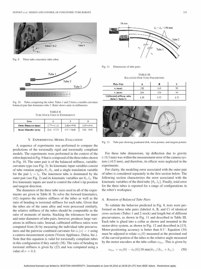
Fig. 9. Three-tube concentric-tube robot.

Fig. 10. Tubes comprising the robot. Tubes 1 and 2 form a variable-curvaturebalanced pair that dominates tube 3. Ruler shows units in millimeters.

TABLE IITUBE STOCK USED IN EXPERIMENTS

V. EXPERIMENTAL MODEL EVALUATION

A sequence of experiments was performed to compare thepredictions of the torsionally rigid and torsionally compliantmodels. The experiments were performed in the context of therobot depicted in Fig. 9 that is composed of the three tubes shownin Fig. 10. The outer pair is of the balanced stiffness, variable-curvature type (see Fig. 3). Its kinematic input variables consistof tube rotation angles θ1 , θ2 , and a single translation variablefor the pair l1 = l2 . The innermost tube is dominated by theouter pair (see Fig. 2) and its kinematic variables are θ3 , l3 . Thefive kinematic inputs are used to control the robot’s tip positionand tangent direction.

The diameters of the three tube sizes used in all of the exper-iments are given in Table II. To solve the forward kinematics,(42) requires the relative stiffness of the tubes as well as theratio of bending to torsional stiffness for each tube. Given thatthe tubes are of the same alloy and were processed similarly,the relative stiffness of the tubes should be computable as theratio of moments of inertia. Stacking the tolerances for innerand outer diameters of tube pairs, however, produces large vari-ations in stiffness ratio. Instead, calibrated stiffness ratios werecomputed from (8) by measuring the individual tube precurva-tures and the pairwise combined curvature for αi(s) = π usinga camera-measurement system (Vision Appliance, Dalsa, Inc.).Note that this equation is valid for torsionally compliant tubesin this configuration if they satisfy (38). The ratio of bending totorsional stiffness is given by (22) and was computed using avalue of ν = 0.3.

Fig. 11. Dimensions of tube pairs.

TABLE IIIBALANCED-PAIR TUBE PARAMETERS

Fig. 12. Tube pair showing graduated disk, twist pointer, and tangent pointer.

For these tube dimensions, tip deflection due to gravity(<0.3 mm) was within the measurement error of the camera sys-tem (±0.5 mm), and therefore, its effects were neglected in theexperiments.

For clarity, the modeling error associated with the outer pairof tubes is considered separately in the first section below. Thefollowing section characterizes the error associated with thekinematic variables of the third tube {θ3 , l3}. Finally, total errorfor the three tubes is reported for a range of configurations inthe robot’s workspace.

A. Rotation of Balanced Tube Pairs

To validate the behavior predicted in Fig. 8, tests were per-formed on three tube pairs (labeled A, B, and C) of identicalcross sections (Tubes 1 and 2 stock) and length but of differentprecurvatures, as shown in Fig. 11 and described in Table III.Each tube is glued into a collar as shown and mounted in themotor-drive system, as shown in Fig. 12 and described in [13].Motor-positioning accuracy is better than 0.1◦. Equation (34)must be adjusted to relate α2(0) measured at the proximal endof the curved portion of the tubes to the relative angle measuredby the motor encoders at the tube collars α2m . This is given by

α2m = α2(0) − α2(0)(18 mm)k1z /(k1z + k2z ). (50)



Fig. 13. Tip versus motor twist angle for tube pair A.

Fig. 14. Tip versus motor twist angle for tube pair B.

Unlike (34), this computation requires the stiffness ratio ofthe tubes. This ratio was computed using the method describedearlier, and as reported in Table III, it was found to differ betweentube pairs.

To measure the twist at the distal end of the tubes α2(L), acircular graduated disk was attached over the last 2 mm of theouter tube (see Fig. 12). A 2-cm-long straight wire was attachedto the tip of the inner tube to enable measurement of the tiptangent direction. A twist pointer was attached perpendicularto this wire adjacent to the disk for twist measurement andzeroed for the configuration in which the curvature of the tubesis aligned. The error in measuring tip angle was estimated to be±2◦.

1) Torsional Twisting: Figs. 13–15 compare the torsionally-rigid and -compliant models with experiment for the three tubepairs. The torsionally-rigid model is a line of unit slope whilethe torsionally-compliant model obtained from (34) and (50)predicts s-shaped curves. Experimental data was collected byrotating the tube pairs quasistatically through a complete revo-lution in the positive and negative directions. This data producedan envelope of the possible reachable values of (α2m , α2(L)).The envelope is due to unmodeled phenomena. While notshown, it was demonstrated experimentally that the entire inte-rior of the envelopes in Figs. 13 and 14, including the point

Fig. 15. Tip versus motor twist angle for tube pair C.

(α2m , α2(L)) = (π, π), is reachable and stable. In contrast,there are stable and unstable portions of the envelope in Fig. 15.

These figures clearly demonstrate the predictive capabilityof the torsionally compliant model in comparison with the rigidmodel. They also validate that twist, and thus, deviation from therigid model increases with increasing curvature. Stable rotationis also successfully predicted for the tube pairs of Figs. 13and 14.

In each direction of rotation, α2(L) initially lags α2m , but,in agreement with the torsional model, α2(L) subsequently in-creases faster than α2m such that α2m = α2(L) = π is a validsolution. In contrast, Fig. 15 exhibits a “snap-through” instabil-ity. In this case, the lag in α2(L) continues beyond α2m = πuntil α2(L) suddenly transitions through π to reach the otherstable branch of solutions.

In contrast to both models, however, experiment shows thatevery nonzero value of α2m (excluding the unstable region ofFig. 15) can produce the range of values of α2(L) that lie insidethe experimental envelope. The specific value achieved dependson the history of motion of α2m . Identifying the physical originof this phenomena and modeling it is beyond the scope of thispaper. For the purpose of evaluating tube-tip location error be-low, the average tip location is computed from the boundariesof the envelope.

2) Tip-Location Error: While Figs. 13–15 show that tor-sional twisting of the tubes does occur, they do not revealthe relative error of the models in predicting tube-tip positionand tangent direction. These quantities were measured usinga stereo-camera system (Vision Appliance, Dalsa, Inc.) duringthe twist experiments described earlier. The tangent direction atthe tip was computed from the coordinates of the points at thebase and tip of the tangent pointer of Fig. 12. To evaluate modelerror, the average location of the tip is computed from the twoboundaries of the envelope and compared to the predicted value.

Table IV reports position- and tangent-direction error for thethree sets of tubes at six values of α2m . The mean, standard de-viation, and maxima are also reported for the complete datasetsof Figs. 13–15. To visualize the workspace of the tube pairs,Fig. 16 depicts the torsionally rigid solutions for tube pair B atthe six values of α2m reported in the table.



TABLE IVTUBE-PAIR TIP POSITION AND TANGENT ERROR

Fig. 16. Tube pair B workspace. Depicted configurations are computed usingthe torsionally rigid model.

As can be seen from Figs. 13 and 14 and Table IV, thetorsionally rigid and compliant models are in agreement forstable tube pairs at α2m = {0, π, 2π}. For those values ofα2m at which torsional twisting is largest α2m ≈ {120, 240}◦,the model predictions diverge significantly, and as shown inTable IV, the torsional model is much more accurate. For exam-ple, at α2m = 240◦, the rigid- and torsional-modeling errors oftube pair B are 12.3 versus 4.4 mm in position and 10.1 versus1.0◦ in tangent direction.

The effect of tube curvature on the models can be observedby comparing the increasing divergence between the modelsacross Figs. 13–15. The effect on model error can be seen bycomparing the columns of the three tube pairs in Table IV.While error grows with increasing curvature for both models,the torsionally compliant model is substantially more accurate.

Figs. 13 and 14 also show how the magnitude of the experi-mentally observed, but unmodeled, twist envelope varies fromzero when α2m = {0, 2π} to a maximum when α2m = π. Thisenvelope is the major source of error observed in the compliantmodel.

TABLE VTUBE PARAMETERS

Fig. 17. Workspace generated by rotating and translating tube 3 with respectto the outer pair.

B. Rotation and Translation of Tube 3

The models were evaluated for tube 3 inserted inside tubepair B of Table III. For convenience, the parameters of all threetubes are given in Table V. As depicted in Fig. 10, the proximalsection of the third tube is straight while its distal section is ofconstant curvature. As noted in the table, the curved portion ofTube 3 was found to have a lower measured stiffness than itsstraight portion.

The workspace generated by the translation and rotation of thethird tube relative to the outer pair is illustrated in Fig. 17. Sincethe outer pair is substantially stiffer, tube 3 does not deform theouter pair very much as it rotates with respect to them, and thus,its tip traces out a path that is close to circular.

Twist in the third tube was experimentally measured withα2m = 0 for three extension lengths l3 = 0, 30, 57 mm, corre-sponding to the tube being fully retracted, partially extended,and fully extended. Results are shown in Fig. 18, together withthe predictions of the torsionally compliant model. As before,data were recorded for both directions of rotation revealing anenvelope of reachable, stable solutions.

In agreement with Fig. 18, the torsionally compliant modelpredicts that, for any fixed values of α2m and α3m , twist in thethird tube should increase from zero, when its curved sectionis fully extended beyond the tip of the outer tube pair (l3 =57 mm) to a maximum, when its curved length is fully retractedinside the curved outer pair (l3 = 0 mm). Thus, the rigid andcompliant models are in agreement at full extension but predictsubstantially different results as the inner tube is retracted intothe outer pair.



Fig. 18. Tube 3 tip twist angle versus motor twist angle and extended lengthfor α2m = 0. Circles are experimental data points. Surface denotes predictionof torsionally compliant model.

TABLE VIROBOT TIP ERROR

C. Modeling Error Over 3-Tube Robot Workspace

This section reports overall model error for the robot of Fig. 9using the tubes of Table V. As described earlier, the kinematicinput variables associated with deformation of the tubes are{α2m , α3m , l3}. The workspace associated with these variablescan be envisioned by combining the motion of the outer tubepair in Fig. 16 with that of the inner tube depicted in Fig. 17.Robot tip position and tangent direction were measured at 128configurations in this workspace for the following values of{α2m , α3m , l3}:

α2m = {0, 45, 90, 135, 180, 225, 270, 315}◦

α3m = {0, 45, 90, 135, 180, 225, 270, 315}◦

l3 = {0, 30} (in millimeters). (51)

The two values of l3 correspond to the curved portion of thethird tube being fully retracted and half extended from the outer-tube pair. To take into account the effect of motion history on tiplocation, two measurements were taken at each configurationcorresponding to positive rotations of α2m and both positiveand negative rotations of α3m . Values associated with negativerotations of α2m were calculated assuming symmetry. Modelerror was computed at each configuration using the averageexperimental tip location calculated from the two measured andthe two calculated locations.

Table VI compares tip position and tangent errors for thetorsionally-rigid model (8) and the torsionally compliant model(42)–(44). The inclusion of torsion substantially reduces themean, variance, and maximum of the position error. As can beinferred from Table IV, substituting more highly curved tubeswould produce a larger difference between the models.

Fig. 19. Teleoperator block diagram.

The largest contributor to error in the torsionally compliantmodel is the experimentally observed history dependence oftube twist. It is likely that this dependence is due to one ofthe modeling simplifications, e.g., ignoring cross-section shear,axial elongation, nonlinear elasticity, and friction.

Additional sources of error include uncertainty in tube pa-rameters and the finite clearance between tubes 2 and 3 at thedistal end of tube 2.

VI. REAL-TIME POSITION CONTROL

To demonstrate real-time implementation of the compliantmodel, as described in Section IV-A, a teleoperation system us-ing the robot shown in Fig. 9 and tube properties of Table V wasimplemented using the controller shown in Fig. 19. The systemincludes a master arm comprised of a PHANTOM Omnihapticdevice (Sensable Technologies, Inc.), a slave arm consisting ofthe concentric tube robot, and master and slave controllers. Inthe case shown and described here, the robot consists of the threetubes shown in Fig. 10 and possesses 5-DOFs. As described ear-lier, the outer pair is of the balanced stiffness, variable-curvaturetype (see Fig. 3). Its kinematic input variables consist of tube ro-tation angles θ1 , θ2 , and a single translation variable for the pairl1 = l2 . The innermost tube is dominated by the outer pair (seeFig. 2) and its kinematic variables are θ3 , l3 . The five kinematicinputs are used to control the robot’s tip position and tangentdirection.

In Fig. 19, the slave controller receives the position and tan-gent direction of the tip of the master arm (represented by gm

0 )and calculates the inverse kinematics of the concentric-tuberobot using the method described in the preceding section. Then,a set of PID controllers calculate the torques/forces applied tothe tubes of the robot. The master controller reads the tube con-figuration of the robot and calculates the position and tangentvectors of its tip. The force feedback provided to the master isgoverned by a proportional-control law based on the Cartesianposition error between the master- and slave-tip positions.

The teleoperator system of Fig. 19 is implemented by a mul-tithreaded process under Windows 2000. While Windows 2000does not natively support hard real-time scheduling, it does sup-port soft real-time scheduling with a time-critical thread priority.When used appropriately, a time-critical thread may be used to



maintain a regular 1 kHz update rate with sufficiently low timingvariations to be used for closed-loop control. For this particularcontroller, the slave mechanism bandwidth is less than 10 Hz,and therefore, soft real-time implementation of a 1 kHz controlloop was more than sufficient.

The process includes two time-critical user-mode threads run-ning at 1 kHz that implement the controllers and an applicationthread that updates a graphical user interface (not shown). Oneof the time-critical threads executes the PID controller of theslave arm, and the other executes the master controller andinverse-kinematics block of the slave controller. The separa-tion of threads eases integration between the master with itsIEEE-1394-based interface and the slave controlled through aQuanser Q8 data acquisition board with its real-time input–output subsystem support accessed through the hardware in theloop software development kit (HIL SDK).

A. Forward Kinematic Model

The method of Section IV-A was used to arrive at a functionalapproximation of the forward-kinematic model. Removing therigid-body degrees of freedom, the reduced set of kinematic in-put variables is given by {α2 , α3 , l3}. Solving (42) and (44) asan initial value problem, the resulting curvature was integratedbackward in arc length from L to 0 to get g1(α2(0), α3(0), l3)for a uniform 40 × 40 × 40 grid of {α2(L), α3(L), l3}. Thisdataset was used to construct a second-order product series (47)for each component of the position and tangent vectors using awavelength of λ3 = 2π/lmax

3 . The resulting functional approx-imations, where each is defined by 125 constant coefficients,were evaluated against a second dataset constructed using gridvalues midway between those of the original set. In this eval-uation, the average tip-position error was 0.025 mm (0.1 mmmaximum), and the average tip-tangent error was 0.02◦ (0.06◦

maximum). This approximation error is insignificant in com-parison to modeling error.

B. Inverse-Kinematic Model

Inverse kinematics were implemented, as described inSection IV-B. Tube lengths and precurvatures limit maximumtip position and orientation errors to approximately 200 mmand π rad, respectively. For convenience of interpretation, thescaling factor of γ = (180 mm)/(π rad) was selected yielding atangent error magnitude in degrees.

Our current unoptimized implementation of the Gauss–Newton method can perform eight iterations in 0.5 ms; however,convergence to the accuracy of the functional approximation isusually achieved in five or fewer iterations. This fits easily withinthe 1 ms cycle time of our controller.

In addition, the inverse kinematic implementation enforcescontinuity of the inverse solution and enforces joint limits onthe tube extension variables l1 = l2 and l3 .

C. Results

Performance of the teleoperation system was evaluated fora task that consisted of touching a sequence of nine 2-mm-diameter beads embedded in the faces of three dodecahedral

Fig. 20. Teleoperated real-time position control task. Touching sequence ofnine silver beads embedded in dice involves controlling both position and tan-gent direction of robot tip.

dice suspended on posts, as shown in Fig. 20. This task requiresthe operator to control both the tip position and tangent directionto contact the beads. As shown in the accompanying video,teleoperation is smooth and responsive.

Since the inverse kinematic solver converges within each timestep, trajectory-following error is due to kinematic-modeling er-ror and drive-system bandwidth limitations. Steady-state controlerror is due only to modeling error.

VII. CONCLUSION

Concentric tube robots are a novel technology that has broadpotential in minimally invasive surgery. The design principlespresented in Section II provide the tools to produce concentric-tube robots that exhibit stable motion, possess kinematicallydecoupled links, and are capable of snaking through curved pas-sages. The authors are currently using the principles describedin this paper to design such robots for surgery inside the beatingheart and inside the brain.

The new torsion-flexure kinematic model of Section III iscompletely general. It can be used to compute the resultantshape of any number of tubes of arbitrary cross section andprecurvature while also predicting unstable tube configurations.Furthermore, it is substantially more accurate than prior mod-els with its comparative accuracy increasing with both tubelength and curvature. Using only geometric and mechanical pa-rameters obtained from simple static measurements, the newmodel reduced tip-position error by 50% to 4.2 ± 2.0 mm for a200-mm-long robot. The major remaining source of error is anexperimentally observed dependence on motion history that isthe subject of future research.

While the kinematic model is a two-point boundary-valuedifferential equation, Section IV provides a technique for pre-computing an accurate functional approximation. This sectionalso details an online root-finding method for implementing real-time position control. Unoptimized control code running on aPC was easily able to compute the three-tube inverse-kinematic



solution at 1 kHz rate. Thus, both analytically and numerically,the approach provides the capacity for extension to robots withgreater numbers of tubes. It can also be easily adapted to futurekinematic models that include currently neglected effects suchas friction and nonlinear constitutive behavior.

APPENDIX A

Following the presentation of [21], the Jacobi elliptic func-tions can be defined in terms of the integral

u =∫ φ

0

dθ√1 − m sin2 θ

(52)

with u,m ∈ R. The following three Jacobi elliptic functions canbe used to generate the remaining nine functions:

sn(u|m) = sin φ

cn(u|m) = cos φ

dn(u|m) =√

1 − m sin2 φ. (53)

The functions used in the paper and Appendix B are

sd = sn /dn

cd = cn /dn

nd = 1/dn. (54)

Since Jacobi elliptic functions involving any real values of mcan be expressed in terms of Jacobi-elliptic functions with 0 ≤m ≤ 1, it is sufficient to consider m in this interval. Using theterminology of [21], m and m1 are referred to as the parameterand complementary parameter, respectively, and

m + m1 = 10 ≤ m,m1 ≤ 1.

(55)

Additional insight into the functions of (54) can be gained byevaluating them at the limiting values of the parameter m

sd(u|0) = sin u, sd(u|1) = sinhu

cd(u|0) = cos u, cd(u|1) = 1

nd(u|0) = 1, nd(u|1) = cosh u. (56)

In the derivation next, the following formulas for derivativesare used [21]:

d

du(nd (u|m)) = m sd (u|m) cd (u|m) (57)

d

du(sd (u|m)) = cd (u|m) nd (u|m) (58)

APPENDIX B

Equation (33) is shown here to satisfy differential equation(24). For brevity, (33) is rewritten here in the compact form

sin (α(s)/2) =√

m1 nd (u|m) (59)

cos (α(s)/2) =√

m cd (u|m) (60)

in which

m = cos2 (α(L/2)) (61)

m1 = sin2 (α(L/2)) (62)

u =√

c (L − s) . (63)

Differentiation of (59) is performed using (57)

d

ds(sin (α(s)/2)) =

√m1

d

ds(nd (u|m)) (64)

12

cos (α(s)/2) α =√

m1 (m sd (u|m) cd (u|m)) u. (65)

Substituting (60) and the derivative of (63) into (65) yields

α(s) = −2√

cmm1 sd (u|m) . (66)

Note that differentiating (60) instead of (59) also produces(66). Differentiating a second time using (58) and (63) resultsin

α(s) = 2c (√

m1 nd (u|m))(√

m cd (u|m)). (67)

Recognizing the expressions in parentheses as (59) and (60)gives the differential equation (24)

α(s) = 2c sin (α(s)/2) cos (α(s)/2)

= c sin α(s). (68)

REFERENCES

[1] A. Madhanir, G. Niemeyer, and J. K. SalisburyJr., “The black falcon: Ateleoperated surgical instrument for minimally invasive surgery,” in Proc.IEEE/RSJ Int. Conf. Intell. Robots Syst., Victoria, BC, Canada, 1998,pp. 936–944.

[2] K. Xu and N. Simaan, “An investigation of the intrinsic force sensingcapabilities of continuum robots,” IEEE Trans. Robot., vol. 24, no. 3,pp. 576–587, Jun. 2008.

[3] A. Degani, H. Choset, A. Wolf, and M. Zenati, “Highly articulated roboticprobe for minimally invasive surgery,” in Proc. IEEE Int. Conf. Robot.Autom., Orlando, FL, 2006, pp. 4167–4172.

[4] D. Camarillo, C. Milne, C. Carlson, M. Zinn, and J. K. Salisbury, “Mechan-ics modeling of tendon-driven continuum manipulators,” IEEE Trans.Robot., vol. 24, no. 6, pp. 1262–1273, Dec. 2008.

[5] D. C. Meeker, E. H. Maslen, R. C. Ritter, and F. M. Creighton, “Optimalrealization of arbitrary forces in a magnetic stereotaxis system,” IEEETrans. Magn., vol. 32, no. 2, pp. 320–328, Mar. 1996.

[6] R. Murray, Z. Li, and S. Sastry, A Mathematical Introduction to RoboticManipulation. Boca Raton, FL: CRC, 1994.

[7] R. Ebrahimi, S. Okzawa, R. Rohling, and S. E. Salcudean, “Handheldsteerable needle device,” in Proc. Med. Image Comput. Comput. Assist.Intervent., 2003, pp. 223–230.

[8] M. Loser and N. Navab, “A new robotic system for visually controlledpercutaneous interventions under CT fluoroscopy,” in Proc. Med. ImageComput. Comput.-Assist. Intervent., 2000, pp. 887–896.

[9] M. Loser, “A new robotic system for visually controlled percutaneous in-terventions under X-ray fluoroscopy or CT-imaging,” Dr. Ing. dissertation,Microsystems Technol., Univ. Freiburg, Freiburg, Germany, 2005.

[10] P. Sears and P. Dupont, “A steerable needle technology using curved con-centric tubes,” in Proc. IEEE RSJ Int. Conf. Intell. Robots Syst., Beijing,China, 2006, pp. 2850–2856.

[11] R. J. Webster, A. M. Okamura, and N. J. Cowan, “Toward active cannulas:Miniature snake-like surgical robots,” in Proc. IEEE/RSJ Int. Conf. Intell.Robots Syst., Beijing, China, 2006, pp. 2857–2863.

[12] P. Sears and P. Dupont, “Inverse kinematics of concentric tube steerableneedles,” in Proc. IEEE Int. Conf. Robot. Autom., Roma, Italy, 2007,pp. 1887–1892.

[13] B. Itkowitz, “Teleoperation of concentric tube manipulators,” M. S. thesis,Dept. Elect. Comput. Eng., Boston Univ., Boston, MA, 2007.



[14] R. J. Webster, III, J. M. Romano, and N. J. Cowan, “Kinematics andcalibration of active cannulas,” in Proc. IEEE Int. Conf. Robot. Autom.,2008, pp. 3888–3895.

[15] R. J. Webster, III, J. P. Swensen, J. M. Romano, and N. J. Cowan, “Closed-form differential kinematics for concentric-tube continuum robots withapplication to visual servoing,” presented at the 11th Int. Symp. Exp.Robot., Athens, Greece, 2008.

[16] P. E. Dupont, J. Lock, and E. Butler, “Torsional kinematic model forconcentric tube robots,” in Proc. IEEE Int. Conf. Robot. Autom., Kobe,Japan, 2009, pp. 3851–3858.

[17] R. L. Bishop, “There is more than one way to frame a curve,” Amer. Math.Monthly, vol. 82, no. 3, pp. 246–251, Mar. 1975.

[18] S. S. Antman, Nonlinear Problems of Elasticity. New York: Springer-Verlag, 1995.

[19] D. Pai, “Strands: Interactive simulation of thin solids using Cosserat mod-els,” in Proc. Eurographics 2002, vol. 21, no. 8, pp. 347–352.

[20] D. Trivedi, A. Lofti, and C. Rahn, “Geometrically exact models for softrobotic manipulators,” IEEE Trans. Robot., vol. 24, no. 4, pp. 773–780,Aug. 2008.

[21] M. Abramowitz and I. A. Stegun, Handbook of Mathematical Functionswith Formulas, Graphs and Mathematical Tables, 9th printing. NewYork: Dover, 1970.

[22] P. E. Crouch and R. Grossman, “Numerical integration of ordinary differ-ential equations on manifolds,” J. Nonlinear Sci., vol. 3, no. 1, pp. 1–33,1993.

[23] J. Park and W.-K. Chung, “Geometric integration on Euclidean groupwith application to articulated multibody systems,” IEEE Trans. Robot.,vol. 21, no. 5, pp. 850–863, Oct. 2005.

Pierre E. Dupont (M’99–SM’03) received the B.S.,M.S., and Ph.D. degrees in mechanical engineeringfrom Rensselaer Polytechnic Institute, Troy, NY, in1982, 1984, and 1988, respectively.

From 1988 to 1990, he was with the School of En-gineering and Applied Sciences, Harvard University,Cambridge, MA, as Postdoctoral Fellow. He subse-quently was with Boston University, Boston, MA,where, until recently, he was a Professor of mechan-ical engineering and biomedical engineering. He iscurrently with the Children’s Hospital Boston and

Harvard Medical School, Boston, as Director of Pediatric Cardiac Bioengi-neering and is engaged in the development of instrumentation and imagingtechnology for minimally invasive surgery.

Prof. Dupont has served on many committees of the IEEE Robotics and Au-tomation Society, including the Administrative Committee. He has also servedas an Associate Editor for the TRANSACTIONS ON ROBOTICS and AUTOMATION

and the TRANSACTIONS ON ROBOTICS. He is currently an Associate Vice Presi-dent for Publications and a member of the Management Committee of the IEEETRANSACTIONS ON HAPTICS.

Jesse Lock received the B.A. degree in english fromAmherst College, Amherst, MA, in 1997 and theM.D. degree from Albany Medical College, Albany,NY, in 2002. He is currently working toward the Ph.D.degree in biomedical engineering with Boston Uni-versity, Boston, MA.

He spent a year of clinical pediatric research atStanford University, Stanford, CA. He completed hisresidency in pediatrics at Oregon Health SciencesUniversity, Portland, in 2005. He subsequently en-rolled in a transitional engineering program at Boston

University. His research interests include robotics and medical devices as theypertain to pediatric health care.

Dr. Lock is a recipient of a National Institutes of Health National ResearchService Award Fellowship.

Brandon Itkowitz received the B.S. degree in com-puter systems engineering and the M.S. degreein electrical engineering from Boston University,Boston, MA, in 1999 and 2008, respectively.

From 1999 to 2008, he was with SensAble Tech-nologies, Woburn, MA, as a Lead Software Engineer.He has two patents pending related to the OpenHap-tics Toolkit. He is currently with the Applied Re-search Group of Intuitive Surgical, Inc., Sunnyvale,CA, as a Senior Software Engineer. His research in-terests include human–computer interaction, surgical

robotics, haptic rendering, computer graphics, and computational geometry.

Evan Butler (S’08) received the B.S. degree inphysics in 2007 from Boston University, Boston, MA,where he is currently working toward the M.S. degreein mechanical engineering with special focus on con-trol systems.

His research interests include medical robotics andintelligent flight-control systems.

Mr. Butler is a recipient of the National Aero-nautics and Space Administration Graduate StudentsResearch Projects Fellowship.


Documents

Robots Ctr Tro