Embed Size (px)
Citation preview
千葉大学
ROBUST CONTROL THEORY
CHIBA UNIVERSITY
KANG-ZHI LIU
千葉大学劉 康志
1
千葉大学
Contents of SeminarIntroductory course to robust control theory of linear systems
1. Mathematical tools
2. Fundamentals of robust control
3. Parameterization of stabilizing controllers
4. Riccati equation
5. H2 control
6. H∞ control
7. Gain-scheduled control
2
千葉大学
Chapter 1 Mathematical Tools
• Eigenvalue and eigenvector
• Calculus of vector and matrix
• Vector norm
• Inner product
• Matrix norm
• Singular value and SVD
• Pseudo-inverse
• Positive definite matrix
• Introduction to LMI
• From BMI to LMI
3
千葉大学
1 Notations• R, Rn: set of real numbers, n dimensional real space
• C, Cn: set of complex numbers, n dimensional complex space
• Rm×p, Cm×p: set of m row, n column real/complex matrices
• sup: supermum (may be regarded as maximum)
• u(s) = L[u(t)]: Laplace transform of u(t)
• := defined as
• ∈ belong to
• ∀ for all
• ⊂ included in
• Im(A) = y ∈ Cn | y = Ax, x ∈ Cm image of matrix map A
• Ker(A) = x | Ax = 0, x ∈ Rn kernel of matrix map A
4
千葉大学
• A = [aij ] matrix with (i, j) element aij
• X∗ := XT
• F (s)∼ = F (−s)T
• λi(A) i-th eigenvalue of matrix A
• σ(A) = λ1, . . . , λn set of all eigenvalues
• ρ(A) = maxi |λi(A)| spectral radius
• Tr (A) =∑n
i=1 aii trace of square matrix A = [aij ] ∈ Cn×n
• A⊥ orthogonal matrix of A, Im A⊥ = Ker A
5
千葉大学
2 Eigenvalue and eigenvector
Given square A, if scalar λ ∈ C and vector u ∈ Cn satisfy
Au = λu, u 6= 0 (1)
λ is called an eigenvalue of A, u the corresponding eigenvector.
Equivalent definition
(A− λI)u = 0, u 6= 0 (2)
Alsodet(λI −A) = 0 (3)
Eigenvalues are computed by solving this characteristic polynomial.
6
千葉大学
Example 1
A =[
0 18 2
]
Its characteristic polynomial is
det(λI −A) = (λ− 4)(λ + 2) ⇒ λ = −2, 4
Computation of eigenvectors:
Let the eigenvector of λ1 = −2 be u = [α β]T
(A− λ1I)u = 0 ⇒ β = −2α ⇒ u = [1/2 − 1]T
Let the eigenvector of λ2 = 4 be v = [γ δ]T
(A− λ2I)v = 0 ⇒ v = [1/4 1]T
7
千葉大学
u
v
Au
Av
O
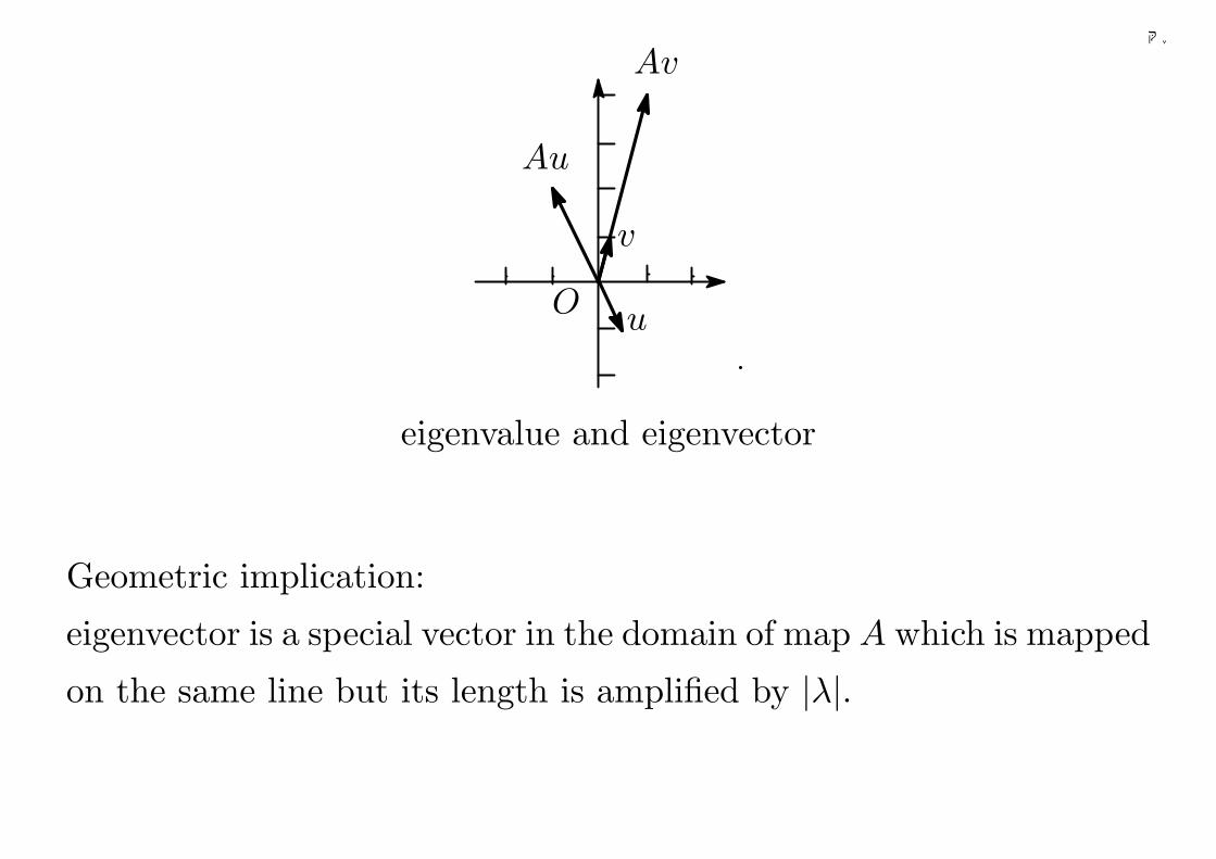
eigenvalue and eigenvector
Geometric implication:
eigenvector is a special vector in the domain of map A which is mapped
on the same line but its length is amplified by |λ|.
8
千葉大学
3 Spectrum and spectral radius
Spectrum σ(A):
set of eigenvalues of matrix A.
σ(A) := λ1, λ2, . . . , λn (4)
When all eigenvalues of A are real, λmax(A) denotes the largest eigen-
value of A and λmin(A) denotes the smallest one.
Spectrual radius of A
ρ(A) := max1≤i≤n
|λi|
9
千葉大学
4 Calculus of vector and matrix
x(t) :=
x1(t)...
xn(t)
, A(t) := [aij(t)] (5)
∫A(t)dt :=
[∫aij(t)dt
](6)
d
dt(AB) =
dA
dtB + A
dB
dt(7)
∫ b
a
dA
dtBdt = AB|ba −
∫ b
a
AdB
dtdt (8)
10
千葉大学
Given a scalar function f(x) of vector x = [x1, . . . , xn]T
∂f
∂x:=
[∂f
∂x1, · · · , ∂f
∂xn
](9)
∂2f
∂x2:=
∂2f∂x2
1· · · ∂2f
∂xn∂x1
......
∂2f∂x1∂xn
· · · ∂2f∂x2
n
(10)
In particular, for b ∈ Rn and AT = A ∈ Rn×n
∂
∂xbT x = bT ,
∂
∂xxT Ax = 2xT A,
∂2
∂x2= 2A
11
千葉大学
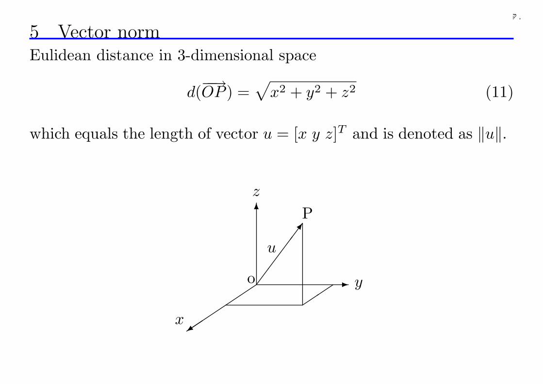
5 Vector normEulidean distance in 3-dimensional space
d(−−→OP ) =√
x2 + y2 + z2 (11)
which equals the length of vector u = [x y z]T and is denoted as ‖u‖.
´´
´´+x
z
y
P
u
-¶¶
¶¶7
6
o´
´
12
千葉大学
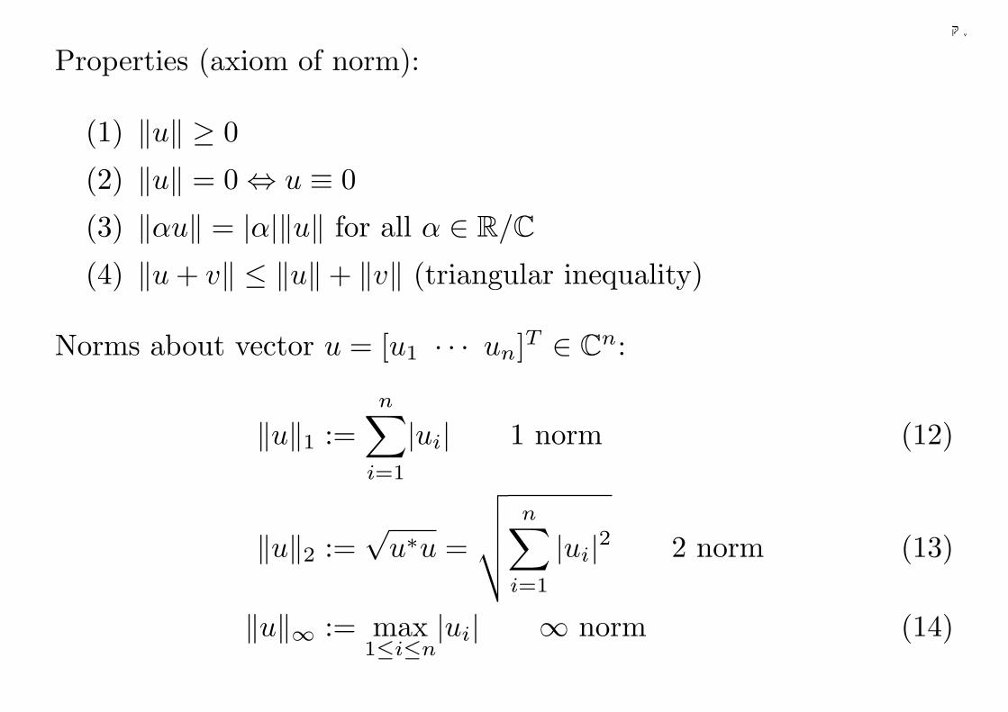
Properties (axiom of norm):
(1) ‖u‖ ≥ 0
(2) ‖u‖ = 0 ⇔ u ≡ 0
(3) ‖αu‖ = |α|‖u‖ for all α ∈ R/C(4) ‖u + v‖ ≤ ‖u‖+ ‖v‖ (triangular inequality)
Norms about vector u = [u1 · · · un]T ∈ Cn:
‖u‖1 :=n∑
i=1
|ui| 1 norm (12)
‖u‖2 :=√
u∗u =
√√√√n∑
i=1
|ui|2 2 norm (13)
‖u‖∞ := max1≤i≤n
|ui| ∞ norm (14)
13
千葉大学
Example 2 Let us show that the function f(u) =n∑
i=1
|ui| is a norm.
First, f(u) ≥ 0 is trival. Second,
f(u) = 0 ⇔ |ui| = 0 ∀i ⇔ ui = 0 ∀i ⇔ u = 0
holds. Further
f(αu) =n∑
i=1
|αui| = |α|n∑
i=1
|ui| = |α|f(u)
as well as
f(u + v) =n∑
i=1
|ui + vi| ≤n∑
i=1
(|ui|+ |vi|) = f(u) + f(v)
hold due to |ui + vi| ≤ |ui|+ |vi|. Hence, f(u) is a norm.
14
千葉大学
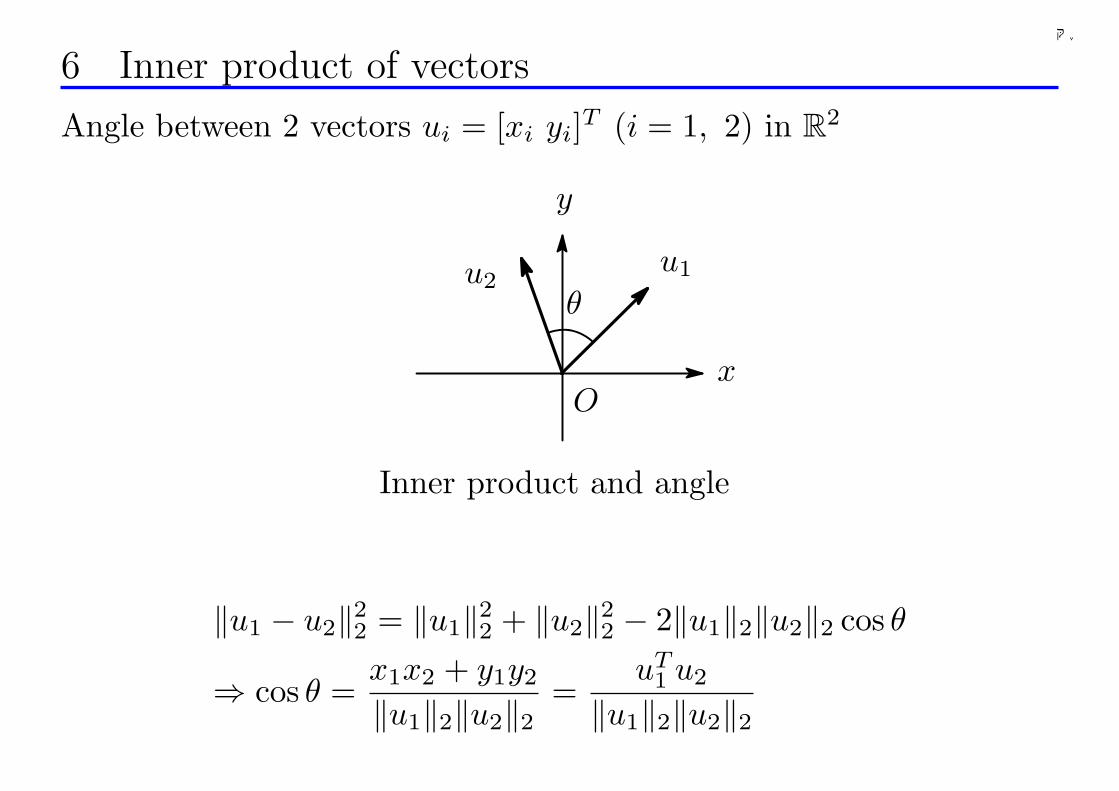
6 Inner product of vectors
Angle between 2 vectors ui = [xi yi]T (i = 1, 2) in R2
Ox
y
u1u2θ
Inner product and angle
‖u1 − u2‖22 = ‖u1‖22 + ‖u2‖22 − 2‖u1‖2‖u2‖2 cos θ
⇒ cos θ =x1x2 + y1y2
‖u1‖2‖u2‖2 =uT
1 u2
‖u1‖2‖u2‖2
15
千葉大学
uT1 u2 is a map of vector to scalar, called inner product
〈u1, u2〉 := uT1 u2 (15)
By using this notion
cos θ =〈u1, u2〉
‖u1‖2‖u2‖2 , θ ∈ [0, π] (16)
There is an 1-to-1 correspondance between inner product and angle.
For high dimensional space, angle must be defined in terms of inner
product.
16
千葉大学
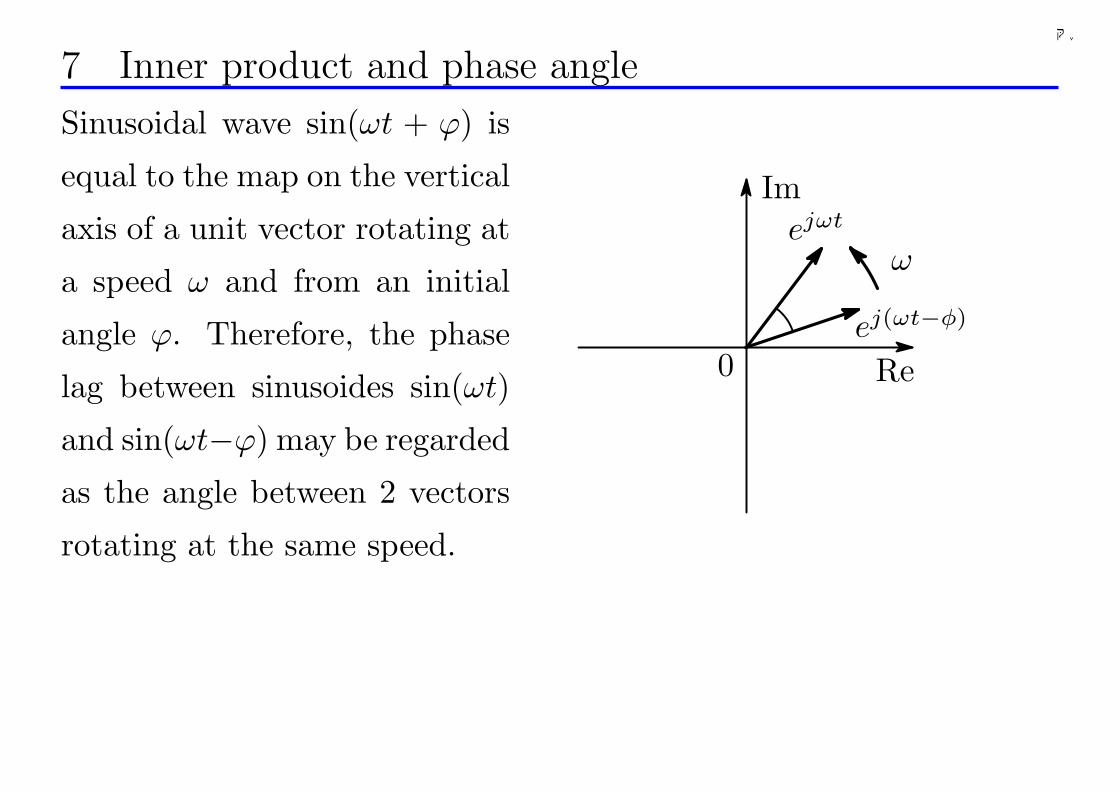
7 Inner product and phase angle
Sinusoidal wave sin(ωt + ϕ) is
equal to the map on the vertical
axis of a unit vector rotating at
a speed ω and from an initial
angle ϕ. Therefore, the phase
lag between sinusoides sin(ωt)
and sin(ωt−ϕ) may be regarded
as the angle between 2 vectors
rotating at the same speed.
ωejωt
ej(ωt−φ)
0 Re
Im
17
千葉大学
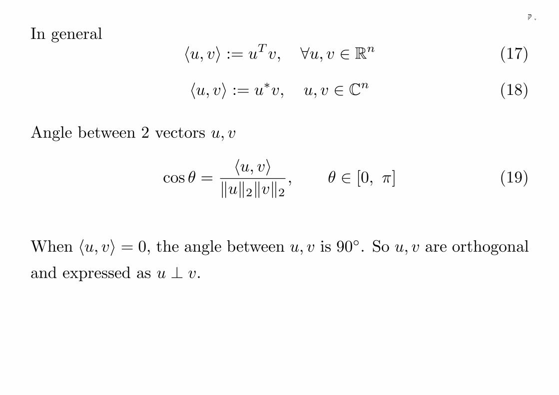
In general〈u, v〉 := uT v, ∀u, v ∈ Rn (17)
〈u, v〉 := u∗v, u, v ∈ Cn (18)
Angle between 2 vectors u, v
cos θ =〈u, v〉
‖u‖2‖v‖2 , θ ∈ [0, π] (19)
When 〈u, v〉 = 0, the angle between u, v is 90. So u, v are orthogonal
and expressed as u ⊥ v.
18
千葉大学
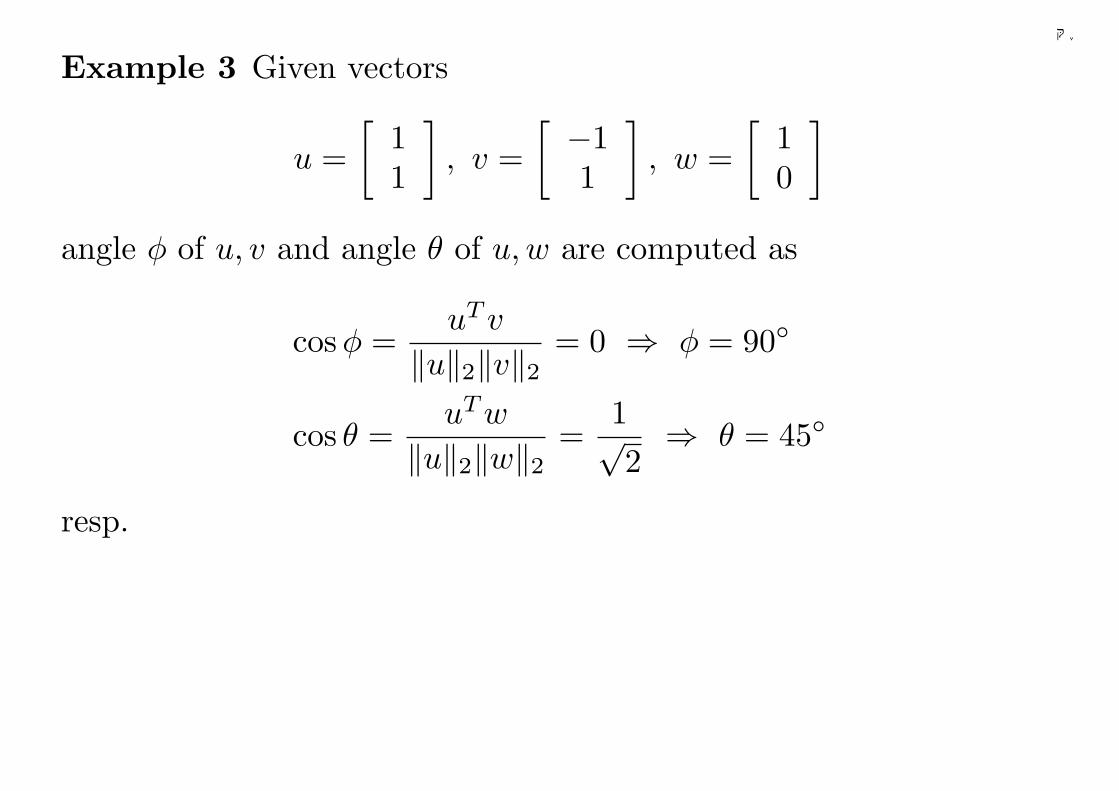
Example 3 Given vectors
u =[
11
], v =
[ −11
], w =
[10
]
angle φ of u, v and angle θ of u,w are computed as
cos φ =uT v
‖u‖2‖v‖2 = 0 ⇒ φ = 90
cos θ =uT w
‖u‖2‖w‖2 =1√2⇒ θ = 45
resp.
19
千葉大学
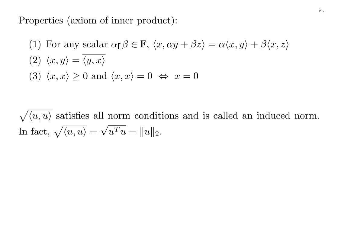
Properties (axiom of inner product):
(1) For any scalar α,β ∈ F, 〈x, αy + βz〉 = α〈x, y〉+ β〈x, z〉(2) 〈x, y〉 = 〈y, x〉(3) 〈x, x〉 ≥ 0 and 〈x, x〉 = 0 ⇔ x = 0
√〈u, u〉 satisfies all norm conditions and is called an induced norm.
In fact,√〈u, u〉 =
√uT u = ‖u‖2.
20
千葉大学
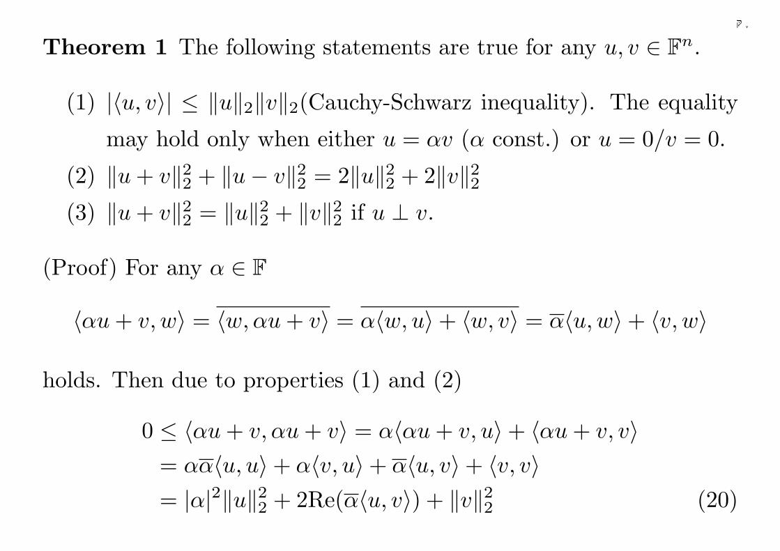
Theorem 1 The following statements are true for any u, v ∈ Fn.
(1) |〈u, v〉| ≤ ‖u‖2‖v‖2(Cauchy-Schwarz inequality). The equality
may hold only when either u = αv (α const.) or u = 0/v = 0.
(2) ‖u + v‖22 + ‖u− v‖22 = 2‖u‖22 + 2‖v‖22(3) ‖u + v‖22 = ‖u‖22 + ‖v‖22 if u ⊥ v.
(Proof) For any α ∈ F
〈αu + v, w〉 = 〈w, αu + v〉 = α〈w, u〉+ 〈w, v〉 = α〈u,w〉+ 〈v, w〉
holds. Then due to properties (1) and (2)
0 ≤ 〈αu + v, αu + v〉 = α〈αu + v, u〉+ 〈αu + v, v〉= αα〈u, u〉+ α〈v, u〉+ α〈u, v〉+ 〈v, v〉= |α|2‖u‖22 + 2Re(α〈u, v〉) + ‖v‖22 (20)
21
千葉大学
Substitution of α = t〈u, v〉 (t ∈ R) into this equation leads to
‖u‖22|〈u, v〉|2t2 + 2|〈u, v〉|2t + ‖v‖22 ≥ 0, ∀t (21)
which requires
‖v‖22 −4|〈u, v〉|4
4‖u‖22|〈u, v〉|2 ≥ 0 ⇒ |〈u, v〉| ≤ ‖u‖2‖v‖2 (22)
(∵ at2 + bt + c = a(t + b/2a)2 + (c− b2/4a) ≥ 0 ⇒ c− b2/4a ≥ 0)
Statement (2) is obtained via substitutions of α = 1 and α = −1 into
〈αu + v, αu + v〉 = |α|2‖u‖22 + 2Re(α〈u, v〉) + ‖v‖22,
then adding them together.
Statement (3) is obtained by the substitutions of α = 1 and 〈u, v〉 = 0.
22
千葉大学
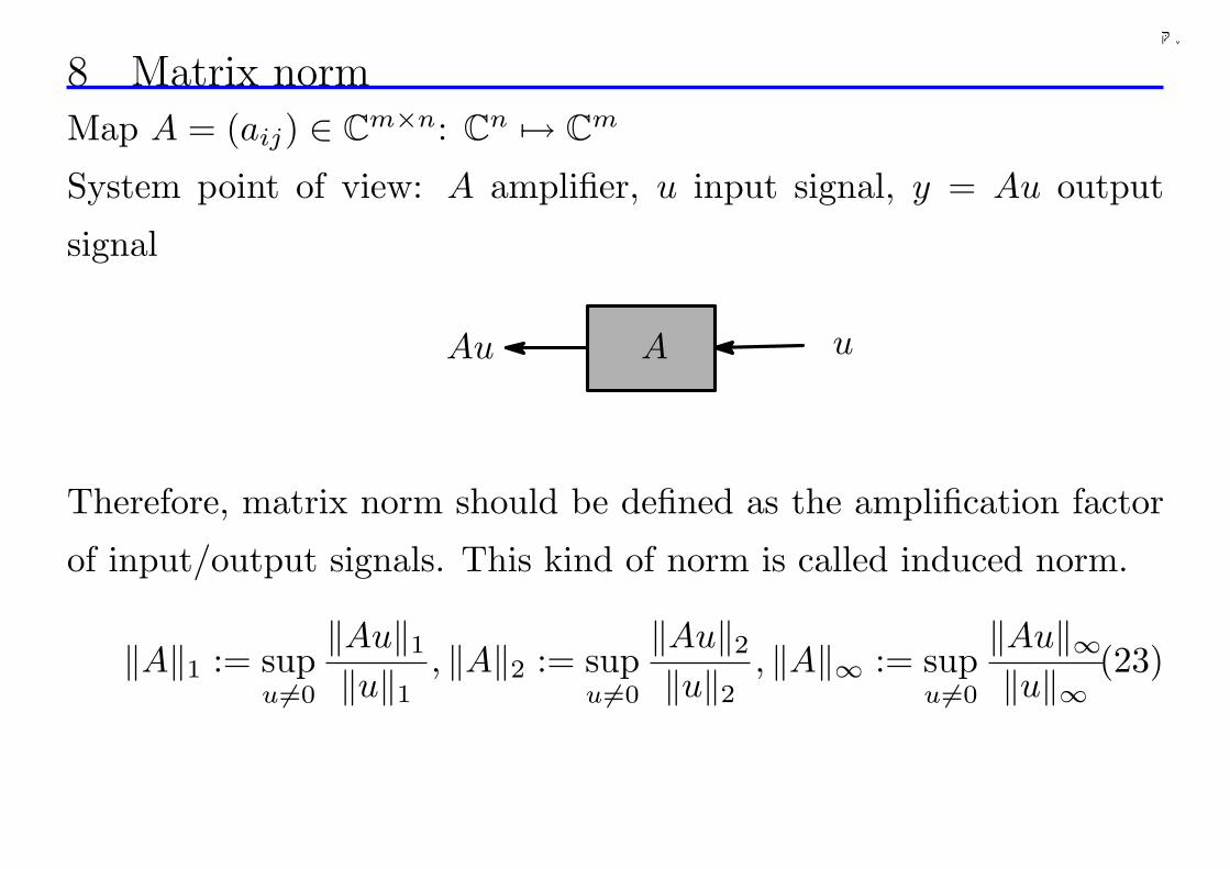
8 Matrix normMap A = (aij) ∈ Cm×n: Cn 7→ Cm
System point of view: A amplifier, u input signal, y = Au output
signal
A uAu
Therefore, matrix norm should be defined as the amplification factor
of input/output signals. This kind of norm is called induced norm.
‖A‖1 := supu 6=0
‖Au‖1‖u‖1 , ‖A‖2 := sup
u 6=0
‖Au‖2‖u‖2 , ‖A‖∞ := sup
u 6=0
‖Au‖∞‖u‖∞ (23)
23
千葉大学
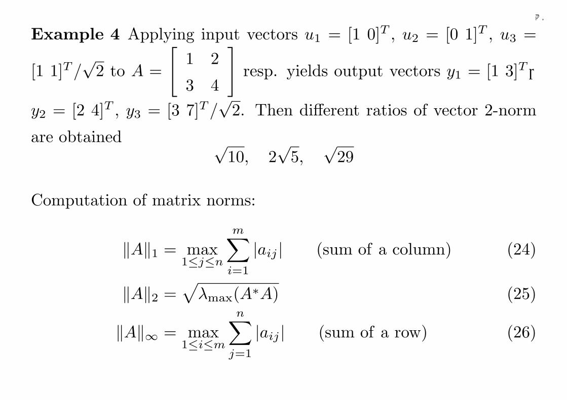
Example 4 Applying input vectors u1 = [1 0]T , u2 = [0 1]T , u3 =
[1 1]T /√
2 to A =
[1 2
3 4
]resp. yields output vectors y1 = [1 3]T,
y2 = [2 4]T , y3 = [3 7]T /√
2. Then different ratios of vector 2-norm
are obtained √10, 2
√5,
√29
Computation of matrix norms:
‖A‖1 = max1≤j≤n
m∑
i=1
|aij | (sum of a column) (24)
‖A‖2 =√
λmax(A∗A) (25)
‖A‖∞ = max1≤i≤m
n∑
j=1
|aij | (sum of a row) (26)
24
千葉大学
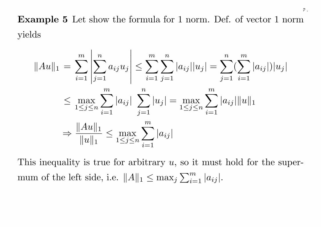
Example 5 Let show the formula for 1 norm. Def. of vector 1 norm
yields
‖Au‖1 =m∑
i=1
∣∣∣∣∣∣
n∑
j=1
aijuj
∣∣∣∣∣∣≤
m∑
i=1
n∑
j=1
|aij ||uj | =n∑
j=1
(m∑
i=1
|aij |)|uj |
≤ max1≤j≤n
m∑
i=1
|aij |n∑
j=1
|uj | = max1≤j≤n
m∑
i=1
|aij |‖u‖1
⇒ ‖Au‖1‖u‖1 ≤ max
1≤j≤n
m∑
i=1
|aij |
This inequality is true for arbitrary u, so it must hold for the super-
mum of the left side, i.e. ‖A‖1 ≤ maxj
∑mi=1 |aij |.
25
千葉大学
Next, suppose the maximum is taken at the sum of j∗-th column
m∑
i=1
|aij∗ | = max1≤j≤n
m∑
i=1
|aij |
Let u∗ = ej∗ (all elemnts are zeros except the j∗-th element), then
‖u∗‖ = 1 and
‖Au∗‖1 =m∑
i=1
|aij∗ | = max1≤j≤n
m∑
i=1
|aij | = max1≤j≤n
m∑
i=1
|aij |‖u∗‖1
⇒ ‖Au∗‖1‖u∗‖1 = max
1≤j≤n
m∑
i=1
|aij | ⇒ ‖A‖1 ≥ ‖Au∗‖1‖u∗‖1 = max
1≤j≤n
m∑
i=1
|aij |
So (24) holds.
26
千葉大学
9 Sub-multiplicative property of induced norm
‖AB‖ ≤ ‖A‖‖B‖ (27)
This is easily obtained from
y = Av, v = Bu
‖y‖‖u‖ =
‖y‖‖v‖
‖v‖‖u‖ ≤ sup
‖y‖‖v‖ sup
‖v‖‖u‖ ⇒ sup
‖y‖‖u‖ ≤ sup
‖y‖‖v‖ sup
‖v‖‖u‖
⇒ ‖AB‖ ≤ ‖A‖‖B‖
27
千葉大学
10 Singular value and SVD
Observations:
• For nonsquare matrix, its magnitude cannot be measured by the
abstract value of eigenvalue because eigenvalue is not defined.
• Matrix norm measures the largest possible amplification for in-
puts in all directions, but it is not useful as the measure of input
amplification in a specified direction.
• For A of any sizes, A∗A is sqaure and positive semi-definite. So
its eigenvalues are all real and nonnegative, thus may be used
as a measure of input amplification in some specified directions.
28
千葉大学
Singular values of matrix A ∈ Cm×n:
σi(A) :=√
λi(A∗A) (28)
σi(A) is the i-th largest singular value of matrix A.
Singular vector vi:
A∗Avi = σ2i vi, vi 6= 0 (29)
‖Avi‖2‖vi‖2 = σi
implies that a singular value denotes the amplification of input in the
corresponding singular vector direction, in the sense of 2 norm.
σmax(A): maximal singular value, σmin(A): minimal singular value
Further, σmax(A) = ‖A‖2.
29
千葉大学
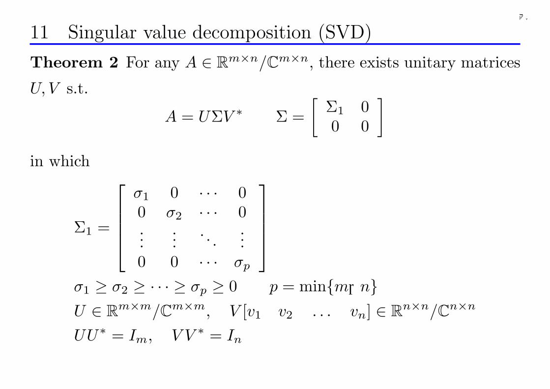
11 Singular value decomposition (SVD)
Theorem 2 For any A ∈ Rm×n/Cm×n, there exists unitary matrices
U, V s.t.
A = UΣV ∗ Σ =[
Σ1 00 0
]
in which
Σ1 =
σ1 0 · · · 00 σ2 · · · 0...
.... . .
...0 0 · · · σp
σ1 ≥ σ2 ≥ · · · ≥ σp ≥ 0 p = minm,nU ∈ Rm×m/Cm×m, V [v1 v2 . . . vn] ∈ Rn×n/Cn×n
UU∗ = Im, V V ∗ = In
30
千葉大学
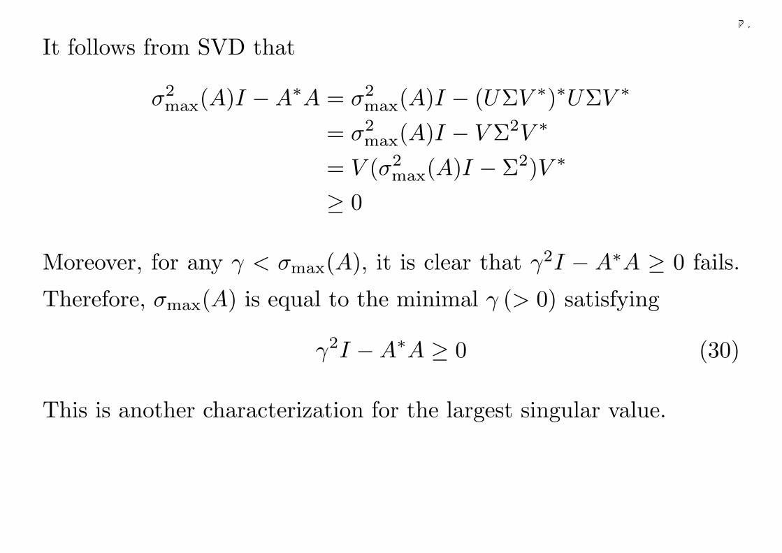
It follows from SVD that
σ2max(A)I −A∗A = σ2
max(A)I − (UΣV ∗)∗UΣV ∗
= σ2max(A)I − V Σ2V ∗
= V (σ2max(A)I − Σ2)V ∗
≥ 0
Moreover, for any γ < σmax(A), it is clear that γ2I − A∗A ≥ 0 fails.
Therefore, σmax(A) is equal to the minimal γ (> 0) satisfying
γ2I −A∗A ≥ 0 (30)
This is another characterization for the largest singular value.
31
千葉大学
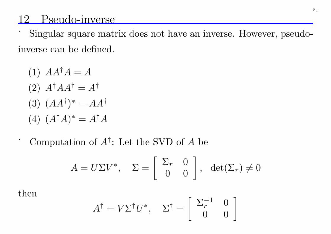
12 Pseudo-inverse Singular square matrix does not have an inverse. However, pseudo-
inverse can be defined.
(1) AA†A = A
(2) A†AA† = A†
(3) (AA†)∗ = AA†
(4) (A†A)∗ = A†A
Computation of A†: Let the SVD of A be
A = UΣV ∗, Σ =[
Σr 00 0
], det(Σr) 6= 0
then
A† = V Σ†U∗, Σ† =[
Σ−1r 00 0
]
32
千葉大学
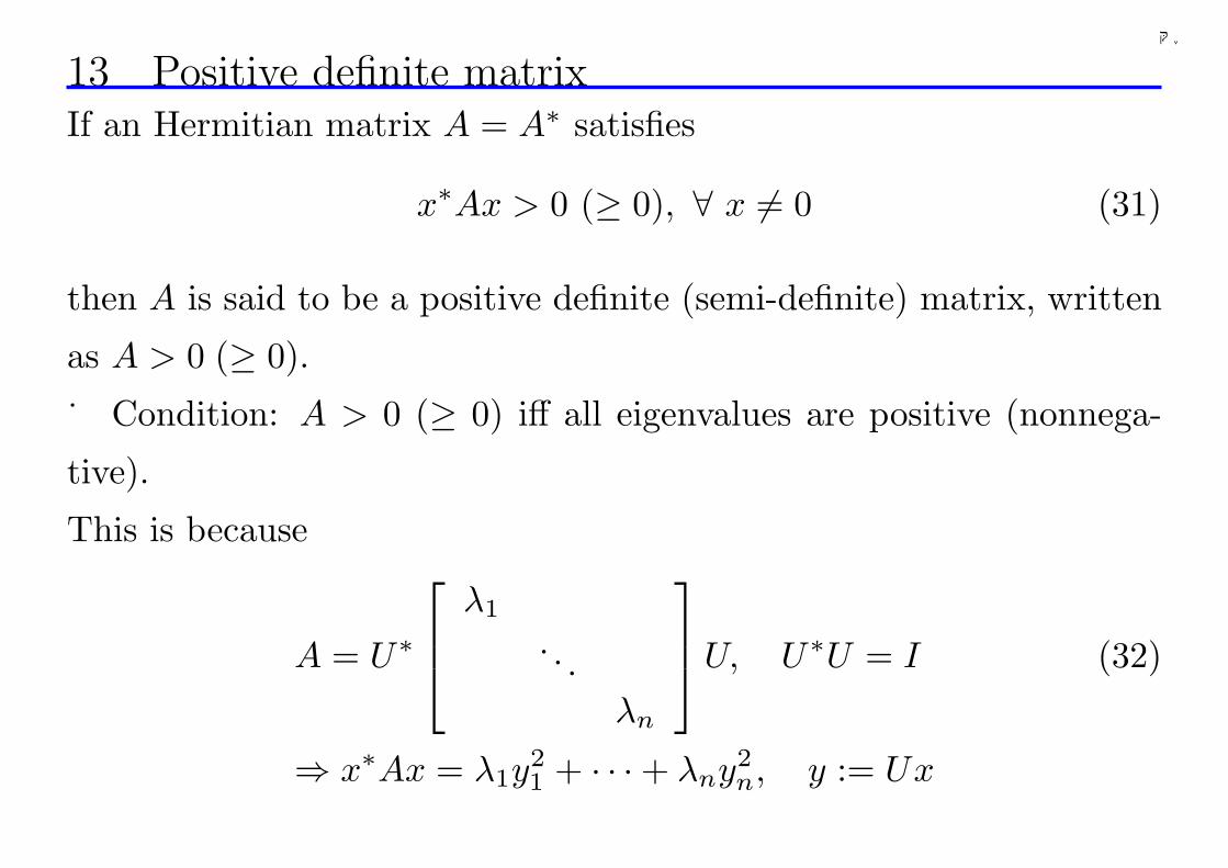
13 Positive definite matrixIf an Hermitian matrix A = A∗ satisfies
x∗Ax > 0 (≥ 0), ∀ x 6= 0 (31)
then A is said to be a positive definite (semi-definite) matrix, written
as A > 0 (≥ 0).
Condition: A > 0 (≥ 0) iff all eigenvalues are positive (nonnega-
tive).
This is because
A = U∗
λ1
. . .λn
U, U∗U = I (32)
⇒ x∗Ax = λ1y21 + · · ·+ λny2
n, y := Ux
33
千葉大学
Lemma 1 Partition an Hermitian matrix X = X∗ as
X =[
X11 X12
X∗12 X22
]
The following statements hold.
(1) X > 0 iff either of the conditions below holds.
(a) X11 −X12X−122 X∗
12 > 0 and X22 > 0
(b) X22 −X∗12X
−111 X12 > 0 and X11 > 0
(2) When X22 ≥ 0, X ≥ 0 iff
Ker(X22) ⊂ Ker(X12), X11 −X12X†22X
∗12 ≥ 0
(3) When X11 ≥ 0, X ≥ 0 iff
Ker(X11) ⊂ Ker(X∗12), X22 −X∗
12X†11X12 ≥ 0
34
千葉大学
(Proof) Condition (1a) follows immediately from[
I −X12X−122
0 I
] [X11 X12
X∗12 X22
] [I 0
−X−122 X∗
12 I
]
=[
X11 −X12X−122 X∗
12 00 X22
](33)
(2): If X22 > 0, then by (33) X ≥ 0 iff X11 −X12X−122 X∗
12 ≥ 0.
Meanwhile, when det(X22) = 0, Ker(X22) is not empty and there
exists a nonzero u ∈ Ker(X22). Set v = X12u, we prove v = 0.
If not, v∗X12u = ‖X12u‖2 6= 0. Then for any α ∈ R
[v∗ αu∗]X[
vαu
]= v∗X11v + 2α‖X12u‖2
Let α → −∞, this quadratic function becomes negative which contra-
dicts with X ≥ 0. ∴ u ∈ Ker(X12), i.e. Ker(X22) ⊂ Ker(X12).
35
千葉大学
Then X12 = Y X22 has a solution Y . So
X12X†22X22 = Y X22X
†22X22 = Y X22 = X12
Then (33) holds even if X−122 is replaced by X†
22. And the conlusion is
obtained.
(1b) and (3) are proved similarly.
36
千葉大学
14 Introduction to LMI
LMI(linear matrix inequality)
F (x) = F0 +m∑
i=1
xiFi > 0 (34)
in which x ∈ Rm is the variable, Fi = FTi ∈ Rn×n (i = 1, . . .,m) are
const. matrices.
F (x) is linear in variable vector x.
Numerical computation of LMI: interior point algorithm
37
千葉大学
15 LMI formulation of control problems
In many control problems, the variable is a matrix. Although it is dif-
ferent from LMI (34) in form, it, however, can be transformed equiv-
alently into (34) through the introduction of basis matrices.
Example 6 Consider a 2nd order system
x(t) = Ax(t), x(0) 6= 0.
It is stable iff ∃ P > 0 s.t.
AP + PAT < 0.
The symmetric basis for any 2× 2 symmetric matrix P is given by
P1 =[
1 00 0
], P2 =
[0 11 0
], P3 =
[0 00 1
]
38
千葉大学
And P is expressed as
P =[
x1 x2
x2 x3
]= x1P1 + x2P2 + x3P3
Substituion of this P into the inquality gives LMI
0 > AP +PAT = x1(AP1+P1AT )+x2(AP2+P2A
T )+x3(AP3+P3AT )
For n dimensional symmetric matrix P , the number of basis matrix
is n(n + 1)/2.
THEREFORE, linear inquality in matrices will also be called as LMI.
39
千葉大学
16 From BMI to LMIConsider a stabilization problem.
Example 7 Stabilize linear system
x = Ax + Bu
by state feedback u = Fx. The closed loop system is given by
x = (A + BF )x
Stabilization condition: ∃ P > 0, F s.t.
(A + BF )P + P (A + BF )T < 0.
Product FP of variables F and P exists. So this is not an LMI, but
a BMI (bilinear matrix inequality). BMI is not convex and it is very
difficult to solve numerically.
40
千葉大学
Many BMI may be transformed to LMI’s via 2 techniques:
1. Variable transformation
2. Variable elimination
Variable transformation: note that P > 0 is nonsingular, so
M := FP ⇔ F = MP−1 (35)
i.e. there is an 1-to-1 correspondance between F and M .
Via this variable transformation, the inequality is written as
AP + PAT + BM + MT BT < 0
which is an LMI in (P, M).
41
千葉大学
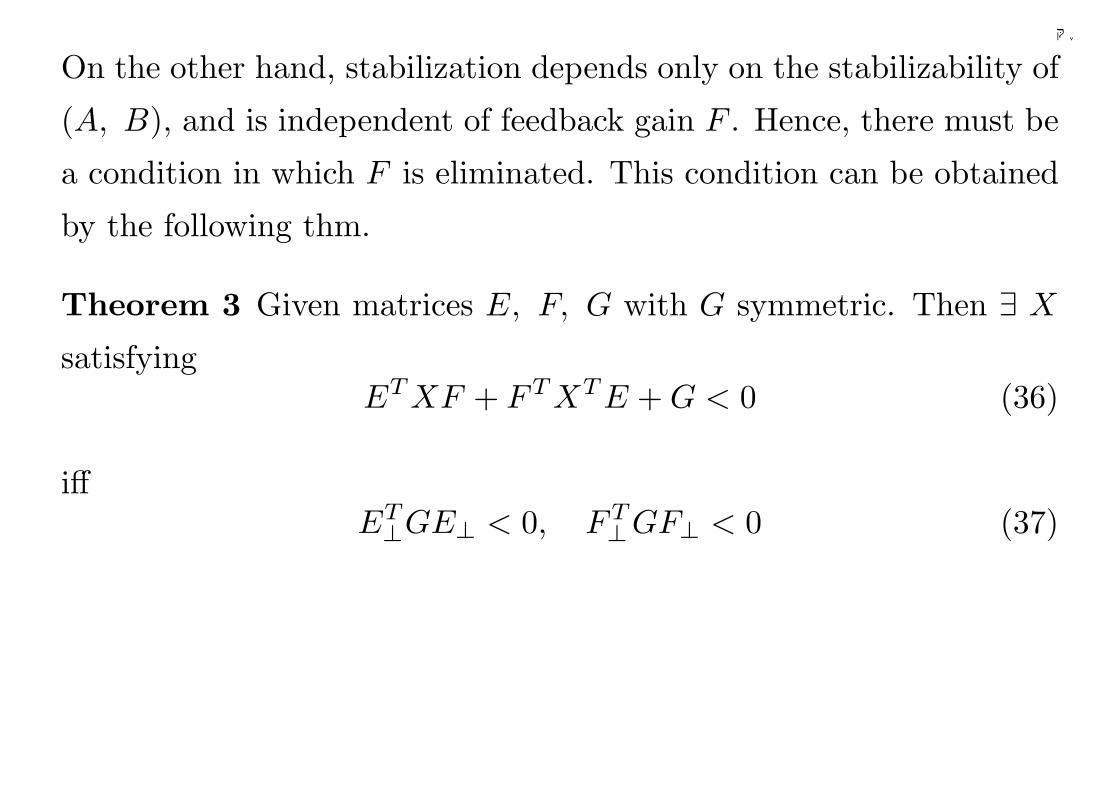
On the other hand, stabilization depends only on the stabilizability of
(A, B), and is independent of feedback gain F . Hence, there must be
a condition in which F is eliminated. This condition can be obtained
by the following thm.
Theorem 3 Given matrices E, F, G with G symmetric. Then ∃ X
satisfyingET XF + FT XT E + G < 0 (36)
iffET⊥GE⊥ < 0, FT
⊥GF⊥ < 0 (37)
42
千葉大学
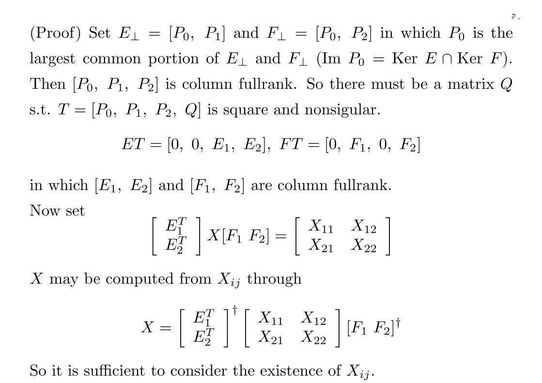
(Proof) Set E⊥ = [P0, P1] and F⊥ = [P0, P2] in which P0 is the
largest common portion of E⊥ and F⊥ (Im P0 = Ker E ∩ Ker F ).
Then [P0, P1, P2] is column fullrank. So there must be a matrix Q
s.t. T = [P0, P1, P2, Q] is square and nonsigular.
ET = [0, 0, E1, E2], FT = [0, F1, 0, F2]
in which [E1, E2] and [F1, F2] are column fullrank.
Now set [ET
1
ET2
]X[F1 F2] =
[X11 X12
X21 X22
]
X may be computed from Xij through
X =[
ET1
ET2
]† [X11 X12
X21 X22
][F1 F2]†
So it is sufficient to consider the existence of Xij .
43
千葉大学
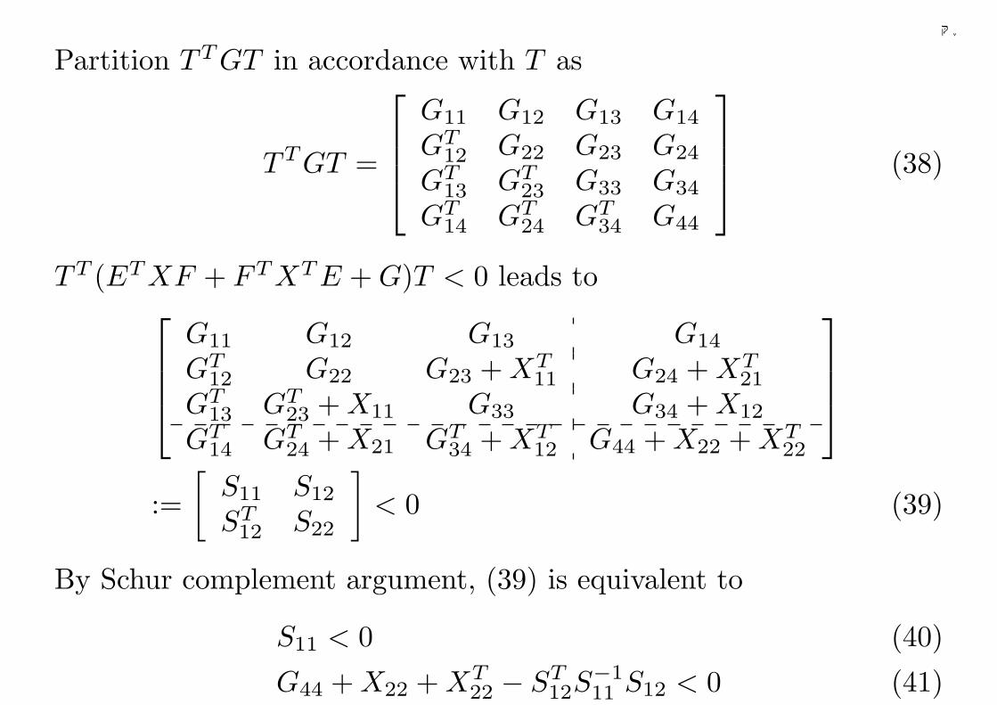
Partition TT GT in accordance with T as
TT GT =
G11 G12 G13 G14
GT12 G22 G23 G24
GT13 GT
23 G33 G34
GT14 GT
24 GT34 G44
(38)
TT (ET XF + FT XT E + G)T < 0 leads to
G11 G12 G13 G14
GT12 G22 G23 + XT
11 G24 + XT21
GT13 GT
23 + X11 G33 G34 + X12
GT14 GT
24 + X21 GT34 + XT
12 G44 + X22 + XT22
:=[
S11 S12
ST12 S22
]< 0 (39)
By Schur complement argument, (39) is equivalent to
S11 < 0 (40)
G44 + X22 + XT22 − ST
12S−111 S12 < 0 (41)
44
千葉大学
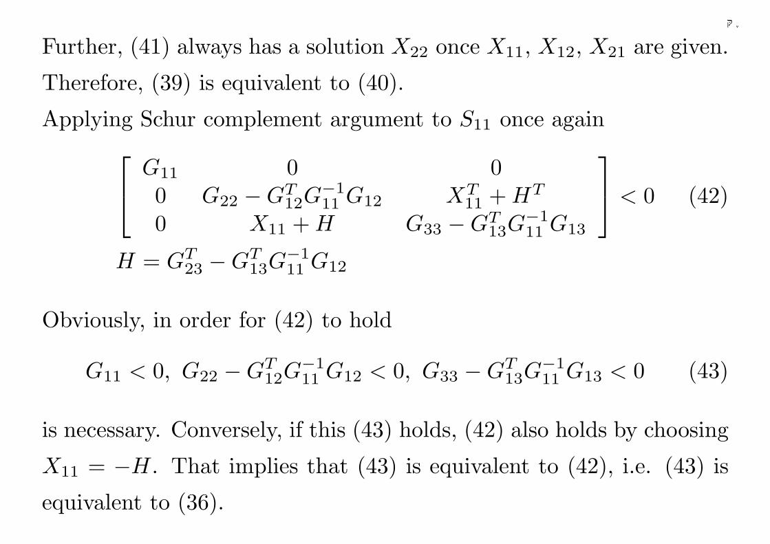
Further, (41) always has a solution X22 once X11, X12, X21 are given.
Therefore, (39) is equivalent to (40).
Applying Schur complement argument to S11 once again
G11 0 00 G22 −GT
12G−111 G12 XT
11 + HT
0 X11 + H G33 −GT13G
−111 G13
< 0 (42)
H = GT23 −GT
13G−111 G12
Obviously, in order for (42) to hold
G11 < 0, G22 −GT12G
−111 G12 < 0, G33 −GT
13G−111 G13 < 0 (43)
is necessary. Conversely, if this (43) holds, (42) also holds by choosing
X11 = −H. That implies that (43) is equivalent to (42), i.e. (43) is
equivalent to (36).
45
千葉大学
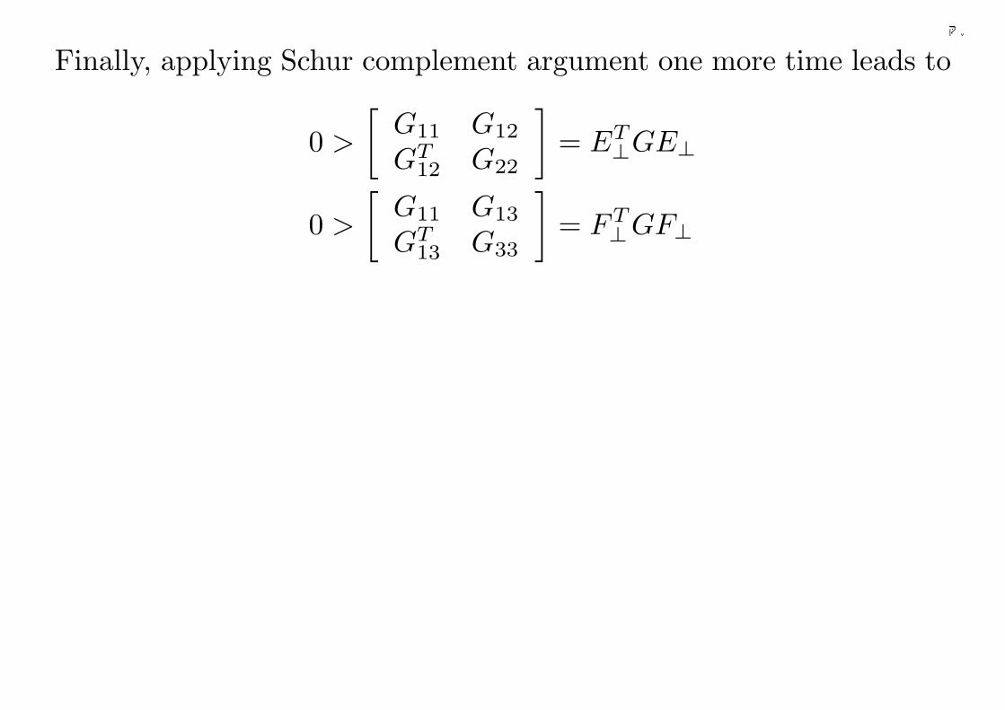
Finally, applying Schur complement argument one more time leads to
0 >
[G11 G12
GT12 G22
]= ET
⊥GE⊥
0 >
[G11 G13
GT13 G33
]= FT
⊥GF⊥
46
千葉大学
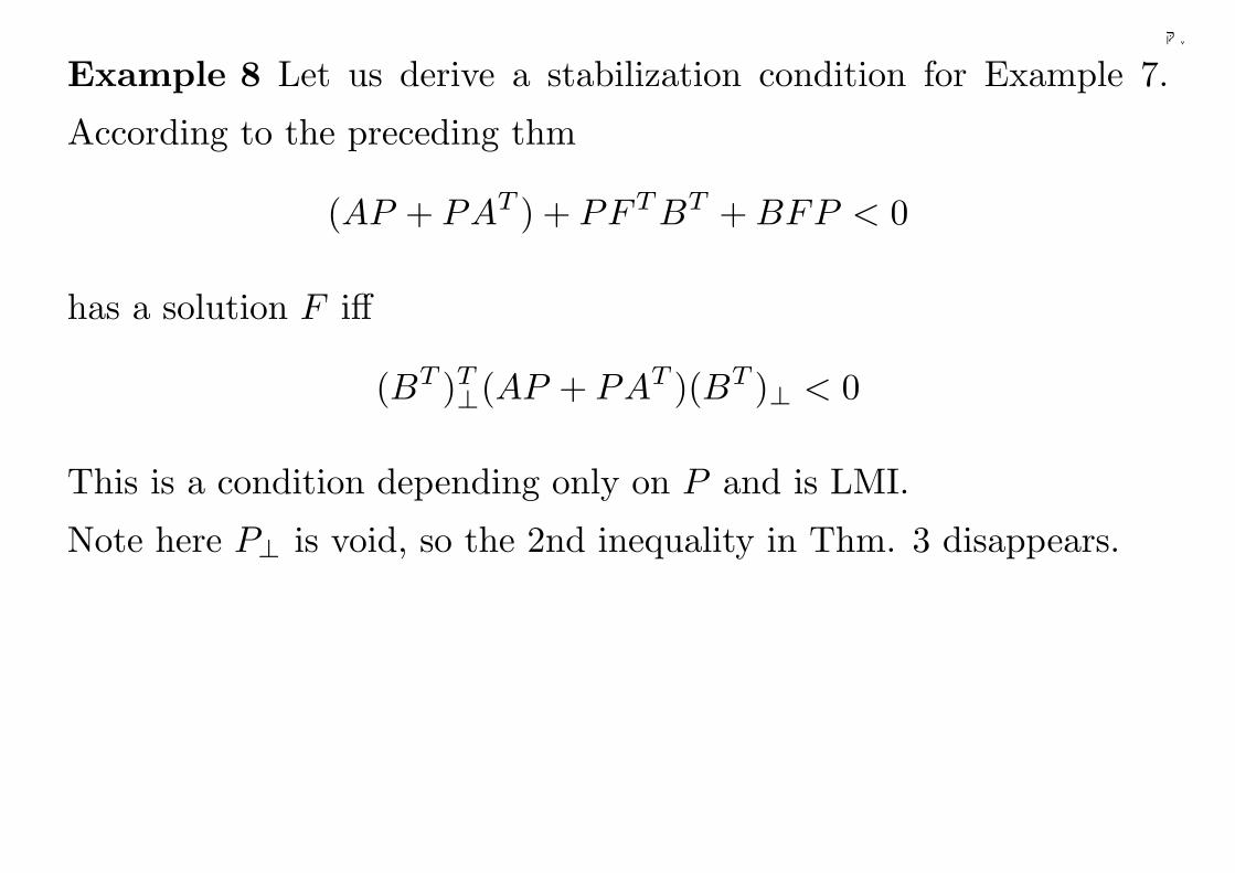
Example 8 Let us derive a stabilization condition for Example 7.
According to the preceding thm
(AP + PAT ) + PFT BT + BFP < 0
has a solution F iff
(BT )T⊥(AP + PAT )(BT )⊥ < 0
This is a condition depending only on P and is LMI.
Note here P⊥ is void, so the 2nd inequality in Thm. 3 disappears.
47
千葉大学
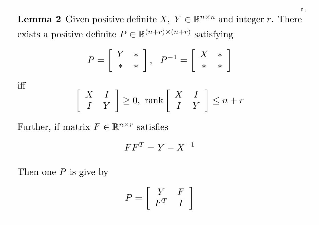
Lemma 2 Given positive definite X, Y ∈ Rn×n and integer r. There
exists a positive definite P ∈ R(n+r)×(n+r) satisfying
P =[
Y ∗∗ ∗
], P−1 =
[X ∗∗ ∗
]
iff [X II Y
]≥ 0, rank
[X II Y
]≤ n + r
Further, if matrix F ∈ Rn×r satisfies
FFT = Y −X−1
Then one P is give by
P =[
Y FFT I
]
48
千葉大学
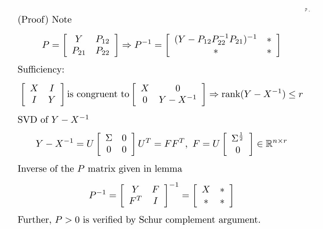
(Proof) Note
P =[
Y P12
P21 P22
]⇒ P−1 =
[(Y − P12P
−122 P21)−1 ∗∗ ∗
]
Sufficiency:[
X II Y
]is congruent to
[X 00 Y −X−1
]⇒ rank(Y −X−1) ≤ r
SVD of Y −X−1
Y −X−1 = U
[Σ 00 0
]UT = FFT , F = U
[Σ
12
0
]∈ Rn×r
Inverse of the P matrix given in lemma
P−1 =[
Y FFT I
]−1
=[
X ∗∗ ∗
]
Further, P > 0 is verified by Schur complement argument.
49
千葉大学
Necessity: When such P > 0 exists, inversion formula gives
X−1 = Y − P12P−122 PT
12
Hence, Y − X−1 = P12P−122 PT
12 ≥ 0 and rank(Y − X−1) =
rank(P12P−122 PT
12) ≤ r. Moreover, conditions on
[X I
I Y
]can be
derived via Schur complement argument.
50
千葉大学
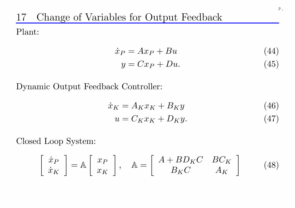
17 Change of Variables for Output Feedback
Plant:
xP = AxP + Bu (44)y = CxP + Du. (45)
Dynamic Output Feedback Controller:
xK = AKxK + BKy (46)u = CKxK + DKy. (47)
Closed Loop System:[
xP
xK
]= A
[xP
xK
], A =
[A + BDKC BCK
BKC AK
](48)
51
千葉大学
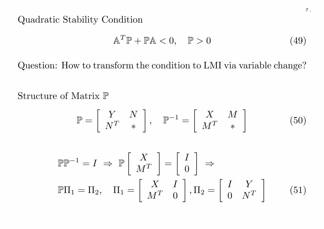
Quadratic Stability Condition
ATP+ PA < 0, P > 0 (49)
Question: How to transform the condition to LMI via variable change?
Structure of Matrix P
P =[
Y NNT ∗
], P−1 =
[X M
MT ∗]
(50)
PP−1 = I ⇒ P[
XMT
]=
[I0
]⇒
PΠ1 = Π2, Π1 =[
X IMT 0
],Π2 =
[I Y0 NT
](51)
52
千葉大学
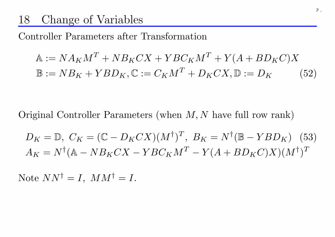
18 Change of Variables
Controller Parameters after Transformation
A := NAKMT + NBKCX + Y BCKMT + Y (A + BDKC)X
B := NBK + Y BDK ,C := CKMT + DKCX,D := DK (52)
Original Controller Parameters (when M, N have full row rank)
DK = D, CK = (C−DKCX)(M†)T , BK = N†(B− Y BDK) (53)
AK = N†(A−NBKCX − Y BCKMT − Y (A + BDKC)X)(M†)T
Note NN† = I, MM† = I.
53
千葉大学
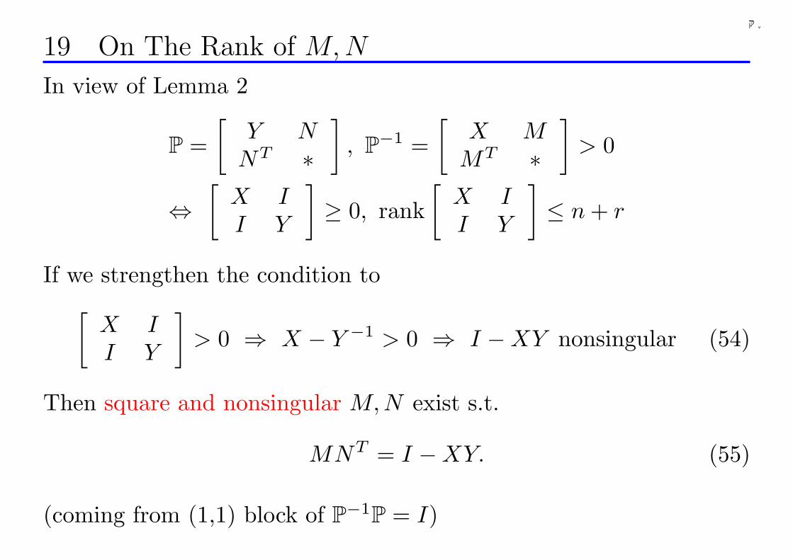
19 On The Rank of M,N
In view of Lemma 2
P =[
Y NNT ∗
], P−1 =
[X M
MT ∗]
> 0
⇔[
X II Y
]≥ 0, rank
[X II Y
]≤ n + r
If we strengthen the condition to[
X II Y
]> 0 ⇒ X − Y −1 > 0 ⇒ I −XY nonsingular (54)
Then square and nonsingular M, N exist s.t.
MNT = I −XY. (55)
(coming from (1,1) block of P−1P = I)
54
千葉大学
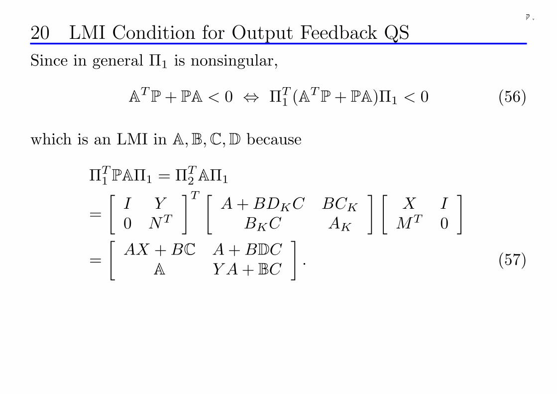
20 LMI Condition for Output Feedback QS
Since in general Π1 is nonsingular,
ATP+ PA < 0 ⇔ ΠT1 (ATP+ PA)Π1 < 0 (56)
which is an LMI in A,B,C,D because
ΠT1 PAΠ1 = ΠT
2 AΠ1
=[
I Y0 NT
]T [A + BDKC BCK
BKC AK
] [X I
MT 0
]
=[
AX + BC A + BDCA Y A + BC
]. (57)
55
千葉大学
Chapter 2 Introduction to Robust Control
• Norm (Signal, System, Relationship)
• Model Uncertainty
• Fundamental Idea of Robust Control
• How to describe model uncertainty
• How to model the range of uncertainty
• Basic notions: Robust stabilty/Robust performance
• Small-gain theorem
• Conditions of robust stability
• Equivalence between H∞ nominal performance and robust sta-
bility
• Conditions of robust performance
56
千葉大学
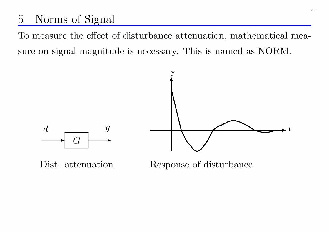
5 Norms of Signal
To measure the effect of disturbance attenuation, mathematical mea-
sure on signal magnitude is necessary. This is named as NORM.
G- -yd
Dist. attenuation
t
y
Response of disturbance
57
千葉大学
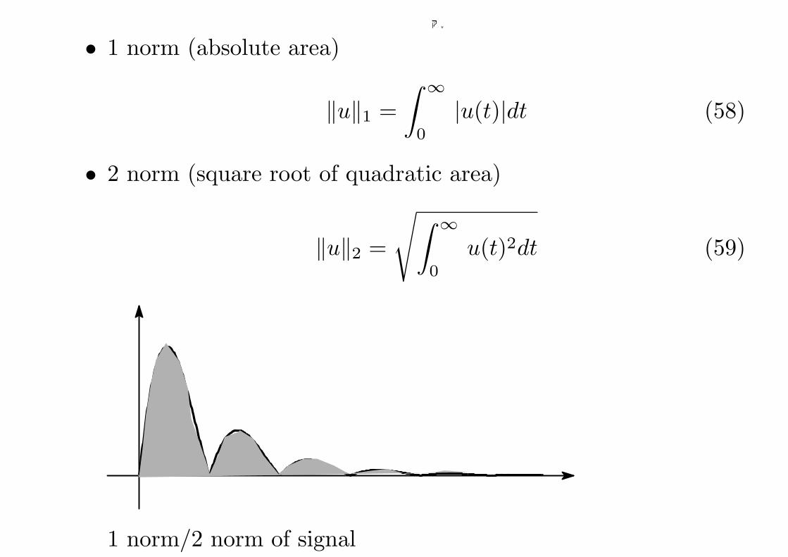
• 1 norm (absolute area)
‖u‖1 =∫ ∞
0
|u(t)|dt (58)
• 2 norm (square root of quadratic area)
‖u‖2 =
√∫ ∞
0
u(t)2dt (59)
1 norm/2 norm of signal
58
千葉大学
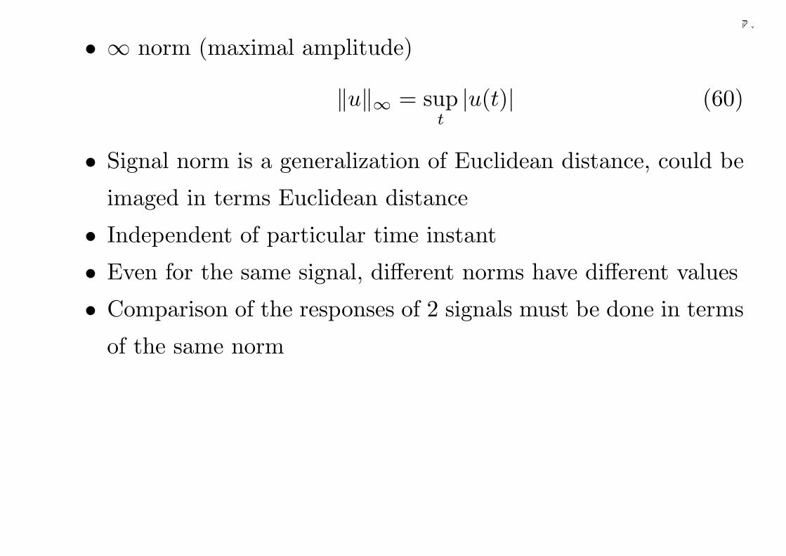
• ∞ norm (maximal amplitude)
‖u‖∞ = supt|u(t)| (60)
• Signal norm is a generalization of Euclidean distance, could be
imaged in terms Euclidean distance
• Independent of particular time instant
• Even for the same signal, different norms have different values
• Comparison of the responses of 2 signals must be done in terms
of the same norm
59
千葉大学
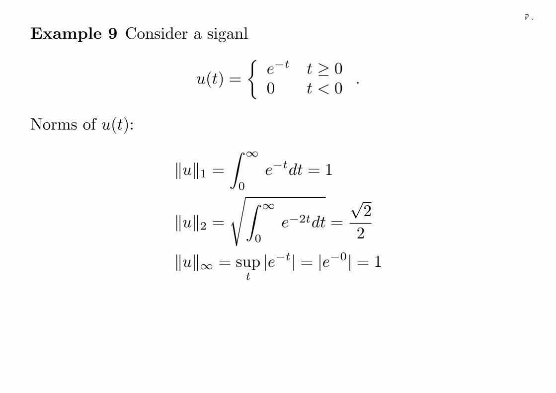
Example 9 Consider a siganl
u(t) =
e−t t ≥ 00 t < 0 .
Norms of u(t):
‖u‖1 =∫ ∞
0
e−tdt = 1
‖u‖2 =
√∫ ∞
0
e−2tdt =√
22
‖u‖∞ = supt|e−t| = |e−0| = 1
60
千葉大学
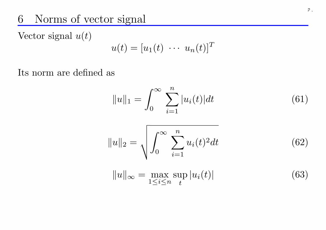
6 Norms of vector signal
Vector signal u(t)u(t) = [u1(t) · · · un(t)]T
Its norm are defined as
‖u‖1 =∫ ∞
0
n∑
i=1
|ui(t)|dt (61)
‖u‖2 =
√√√√∫ ∞
0
n∑
i=1
ui(t)2dt (62)
‖u‖∞ = max1≤i≤n
supt|ui(t)| (63)
61
千葉大学
Comparison of The Gains of 2 Systems
ω
dB
1 2ωω
|G |1
2|G |
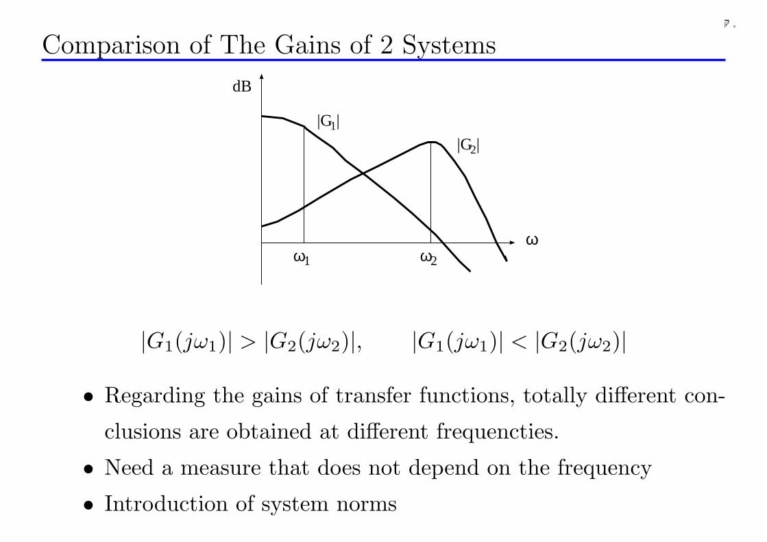
|G1(jω1)| > |G2(jω2)|, |G1(jω1)| < |G2(jω2)|
• Regarding the gains of transfer functions, totally different con-
clusions are obtained at different frequencties.
• Need a measure that does not depend on the frequency
• Introduction of system norms
62
千葉大学
7 System Norms: SISO case
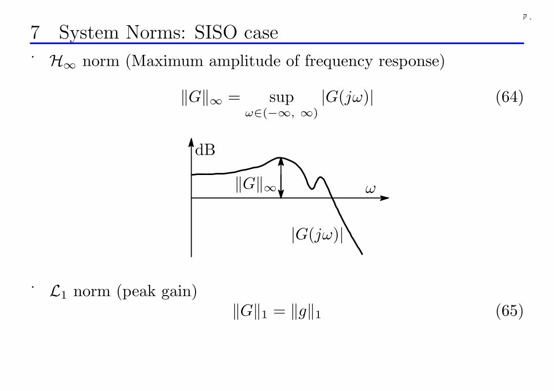
H∞ norm (Maximum amplitude of frequency response)
‖G‖∞ = supω∈(−∞, ∞)
|G(jω)| (64)
‖G‖∞
dB
|G(jω)|
ω
L1 norm (peak gain)‖G‖1 = ‖g‖1 (65)
63
千葉大学
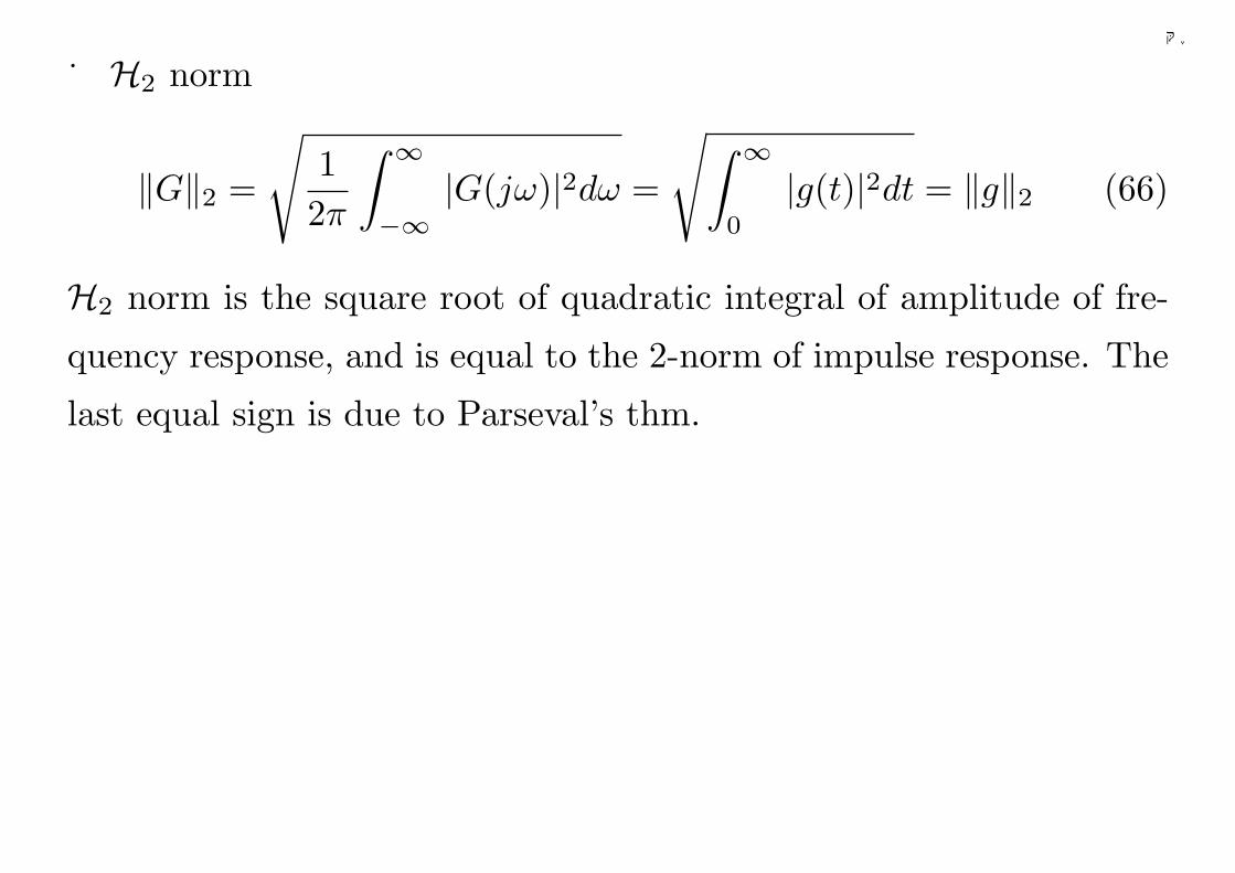
H2 norm
‖G‖2 =
√12π
∫ ∞
−∞|G(jω)|2dω =
√∫ ∞
0
|g(t)|2dt = ‖g‖2 (66)
H2 norm is the square root of quadratic integral of amplitude of fre-
quency response, and is equal to the 2-norm of impulse response. The
last equal sign is due to Parseval’s thm.
64
千葉大学
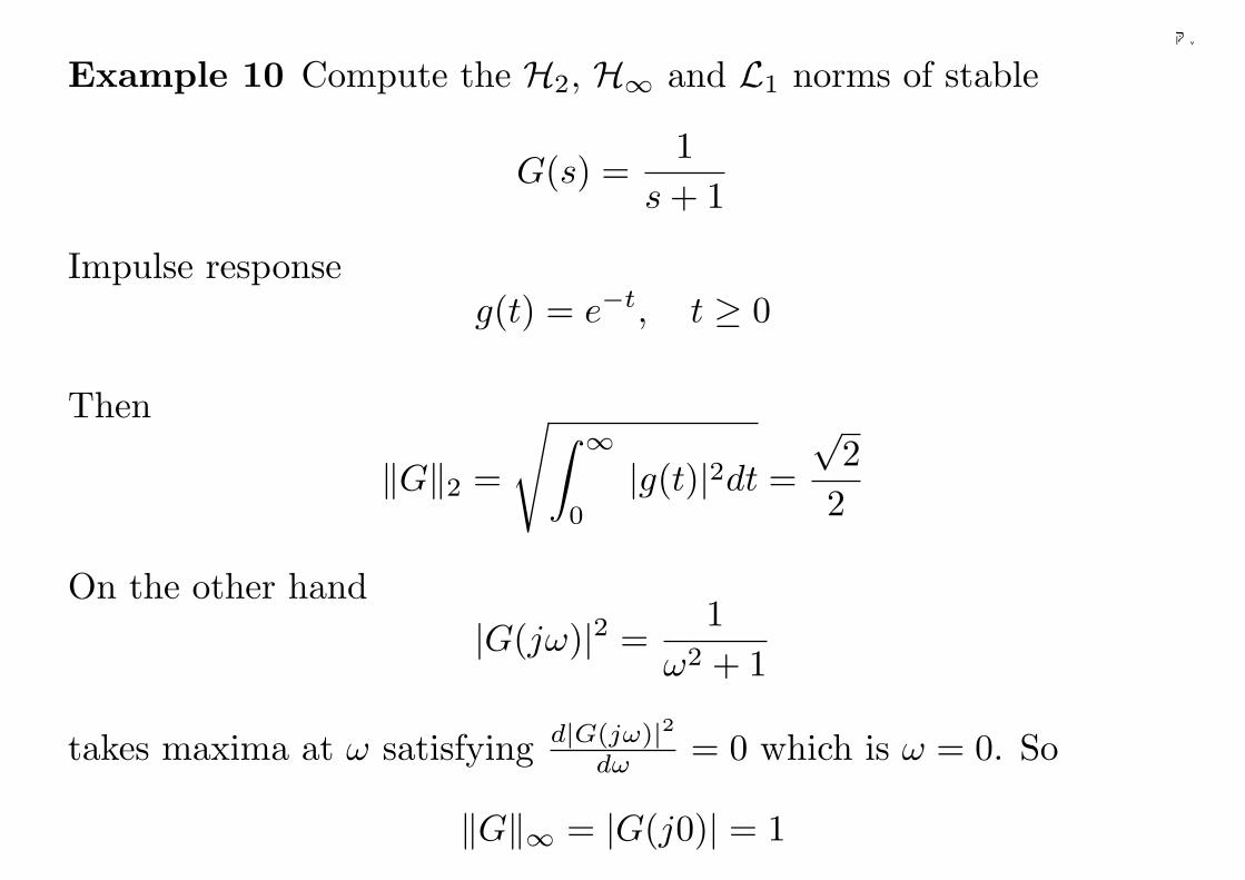
Example 10 Compute the H2, H∞ and L1 norms of stable
G(s) =1
s + 1
Impulse responseg(t) = e−t, t ≥ 0
Then
‖G‖2 =
√∫ ∞
0
|g(t)|2dt =√
22
On the other hand|G(jω)|2 =
1ω2 + 1
takes maxima at ω satisfying d|G(jω)|2dω = 0 which is ω = 0. So
‖G‖∞ = |G(j0)| = 1
65
千葉大学
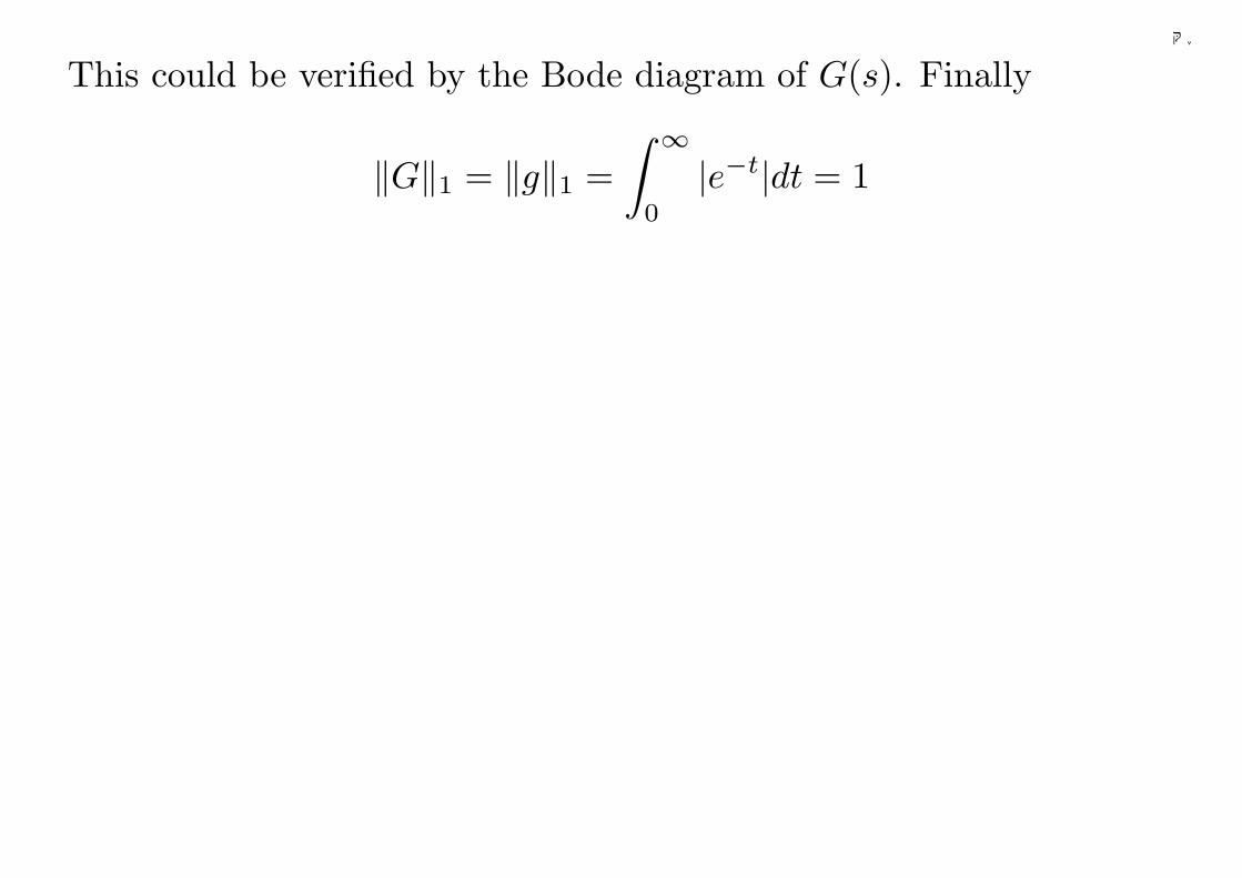
This could be verified by the Bode diagram of G(s). Finally
‖G‖1 = ‖g‖1 =∫ ∞
0
|e−t|dt = 1
66
千葉大学
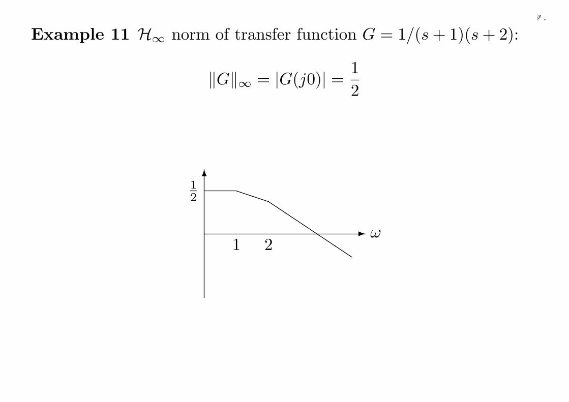
Example 11 H∞ norm of transfer function G = 1/(s + 1)(s + 2):
‖G‖∞ = |G(j0)| = 12
-
6PP
Q
12
ω1 2
67
千葉大学
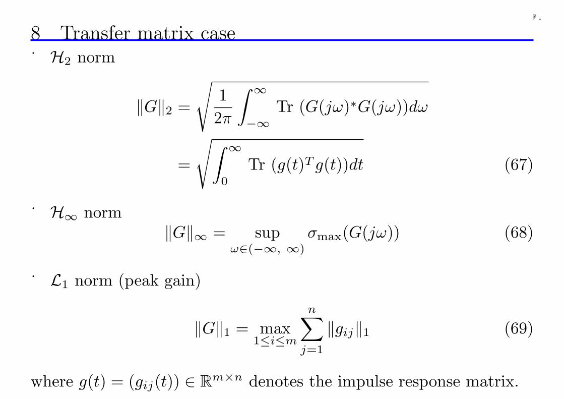
8 Transfer matrix caseH2 norm
‖G‖2 =
√12π
∫ ∞
−∞Tr (G(jω)∗G(jω))dω
=
√∫ ∞
0
Tr (g(t)T g(t))dt (67)
H∞ norm‖G‖∞ = sup
ω∈(−∞, ∞)
σmax(G(jω)) (68)
L1 norm (peak gain)
‖G‖1 = max1≤i≤m
n∑
j=1
‖gij‖1 (69)
where g(t) = (gij(t)) ∈ Rm×n denotes the impulse response matrix.
68
千葉大学
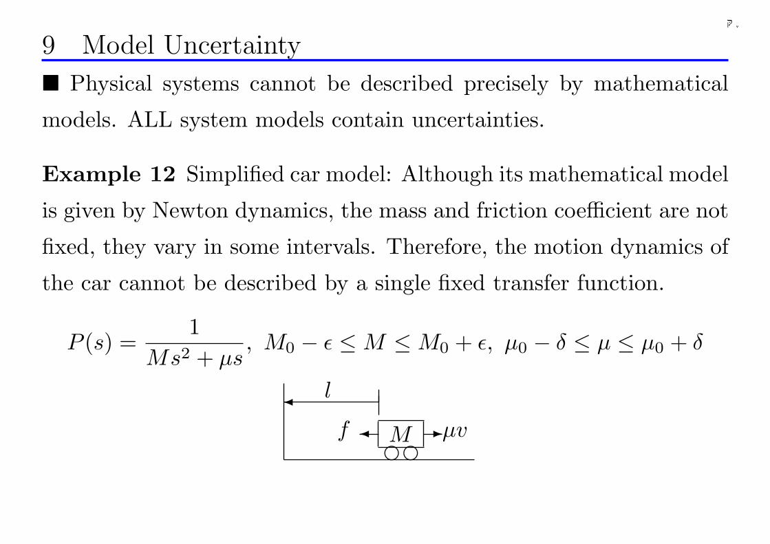
9 Model Uncertainty
¥ Physical systems cannot be described precisely by mathematical
models. ALL system models contain uncertainties.
Example 12 Simplified car model: Although its mathematical model
is given by Newton dynamics, the mass and friction coefficient are not
fixed, they vary in some intervals. Therefore, the motion dynamics of
the car cannot be described by a single fixed transfer function.
P (s) =1
Ms2 + µs, M0 − ε ≤ M ≤ M0 + ε, µ0 − δ ≤ µ ≤ µ0 + δ
e e-µv¾f
l
M
¾
69
千葉大学
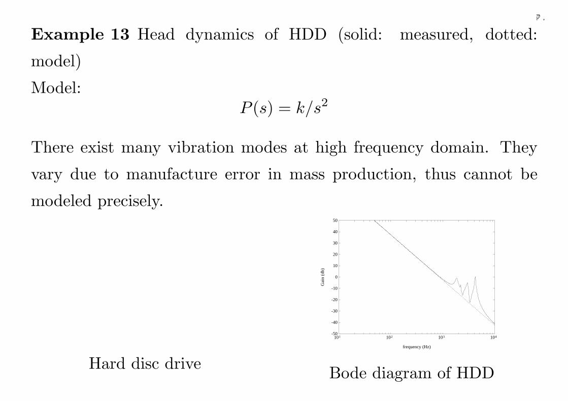
Example 13 Head dynamics of HDD (solid: measured, dotted:
model)
Model:P (s) = k/s2
There exist many vibration modes at high frequency domain. They
vary due to manufacture error in mass production, thus cannot be
modeled precisely.
Hard disc drive
-50
-40
-30
-20
-10
0
10
20
30
40
50
101 102 103 104
frequency (Hz)
Gai
n (d
b)
Bode diagram of HDD
70
千葉大学
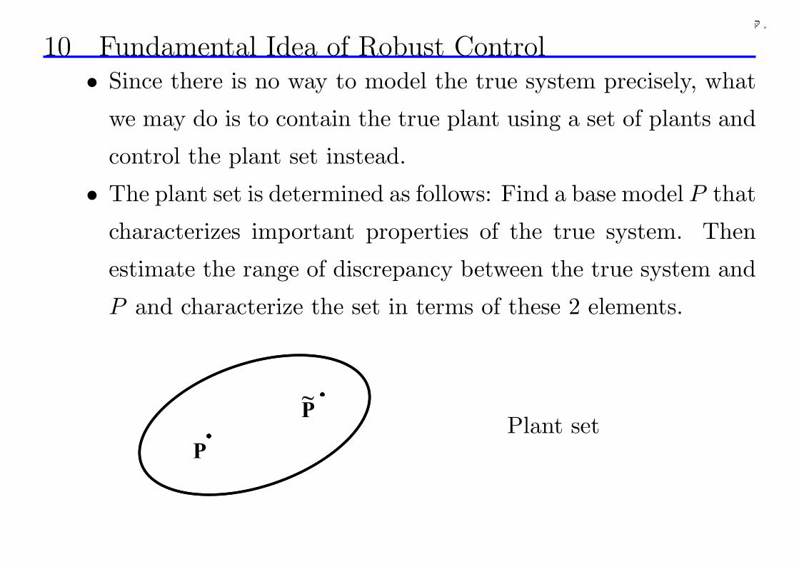
10 Fundamental Idea of Robust Control• Since there is no way to model the true system precisely, what
we may do is to contain the true plant using a set of plants and
control the plant set instead.
• The plant set is determined as follows: Find a base model P that
characterizes important properties of the true system. Then
estimate the range of discrepancy between the true system and
P and characterize the set in terms of these 2 elements.
P
~P
Plant set
71

千葉大学
• P is called ”the Nominal Plant”
• If the required stability and performance are guaranteed for the
plant set, then for the true system the required stability and
performance are guaranteed automatically.
• Issues to be addressed
– Description of plant set
– Modeling of uncertainty
– Stability condition for the plant set
– Performance condition for the plant set
72
千葉大学
11 Category of Uncertainties
• Parameter uncertainty
• Dynamic uncertainty
– Unidentified high frequency modes
– Ignored dynamics for the sake of simplification of analysis
and design
– Variation due to aging and time-varying parameter
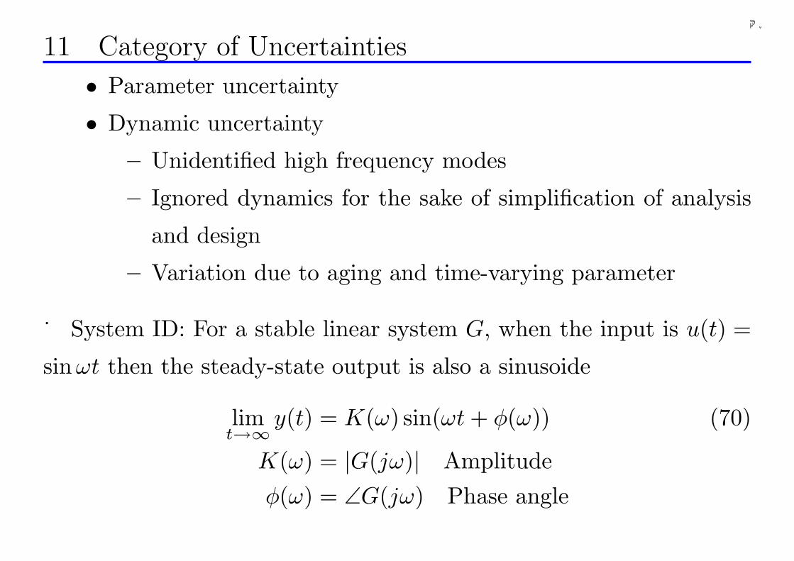
System ID: For a stable linear system G, when the input is u(t) =
sinωt then the steady-state output is also a sinusoide
limt→∞
y(t) = K(ω) sin(ωt + φ(ω)) (70)
K(ω) = |G(jω)| Amplitudeφ(ω) = ∠G(jω) Phase angle
73
千葉大学
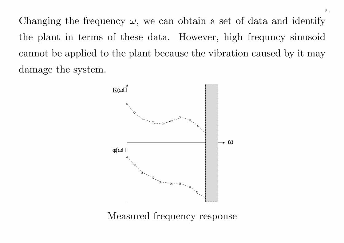
Changing the frequency ω, we can obtain a set of data and identify
the plant in terms of these data. However, high frequncy sinusoid
cannot be applied to the plant because the vibration caused by it may
damage the system.
x
xx x x
x
x
xx
oo
ooo
ooo
o
o
x
φ(ω)
K(ω)
ω
Measured frequency response
74
千葉大学
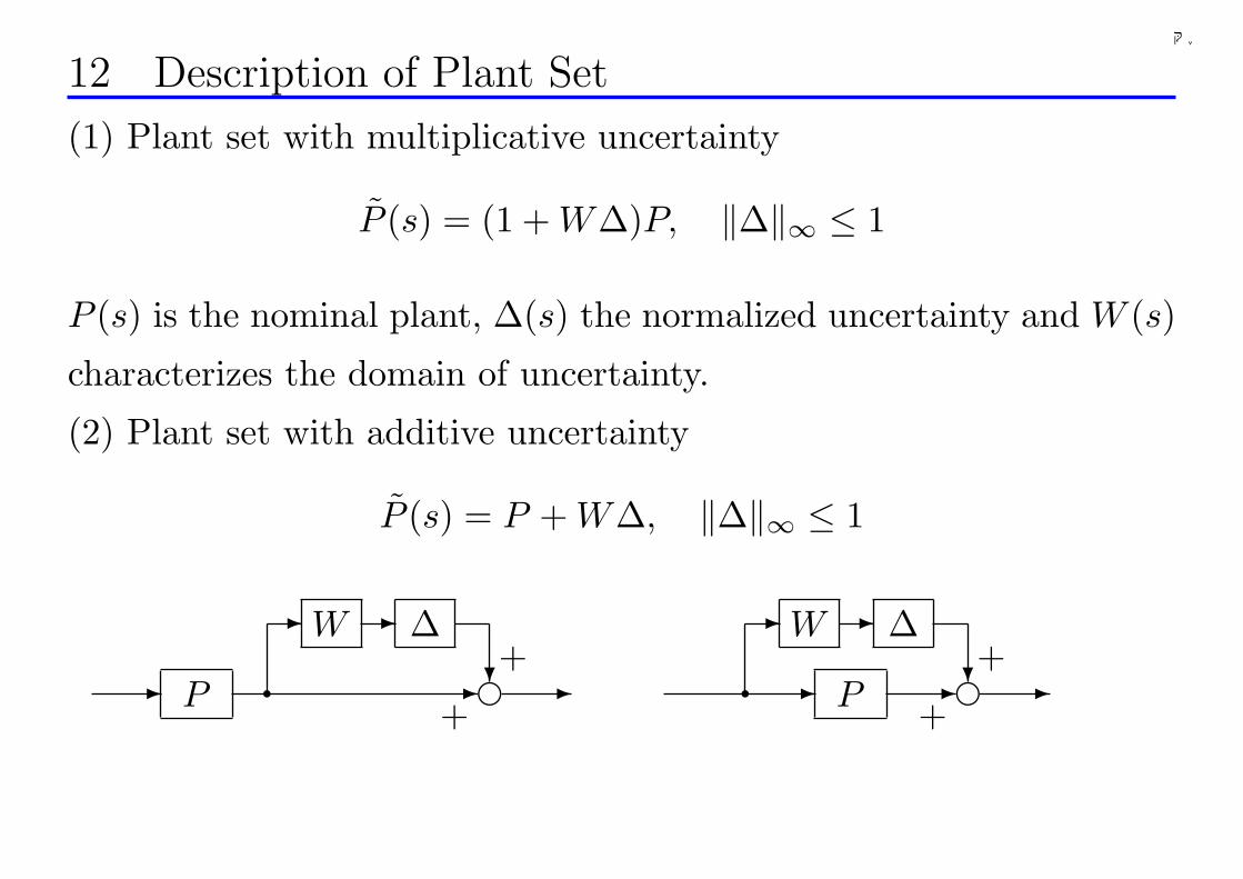
12 Description of Plant Set
(1) Plant set with multiplicative uncertainty
P (s) = (1 + W∆)P, ‖∆‖∞ ≤ 1
P (s) is the nominal plant, ∆(s) the normalized uncertainty and W (s)
characterizes the domain of uncertainty.
(2) Plant set with additive uncertainty
P (s) = P + W∆, ‖∆‖∞ ≤ 1
P -e∆--
?-+
+q -
W
-e∆-- W
?+
+q -- P
75
千葉大学
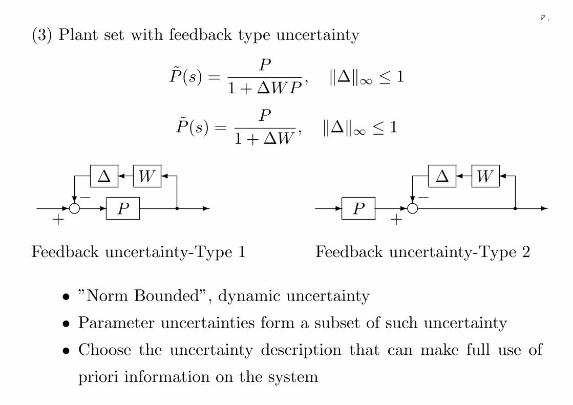
(3) Plant set with feedback type uncertainty
P (s) =P
1 + ∆WP, ‖∆‖∞ ≤ 1
P (s) =P
1 + ∆W, ‖∆‖∞ ≤ 1
P- e?−+
- -q∆ W ¾¾
Feedback uncertainty-Type 1
P - e?−+
- -q∆ W ¾¾
Feedback uncertainty-Type 2
• ”Norm Bounded”, dynamic uncertainty
• Parameter uncertainties form a subset of such uncertainty
• Choose the uncertainty description that can make full use of
priori information on the system
76
千葉大学
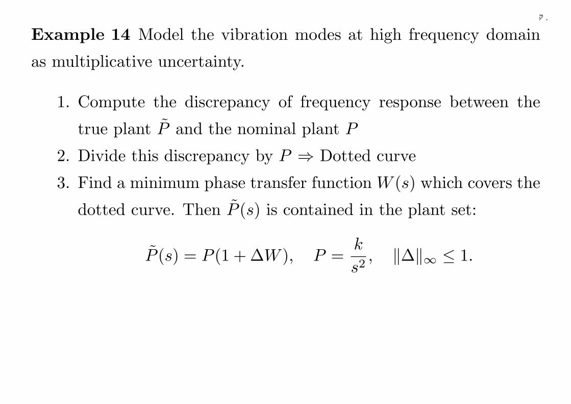
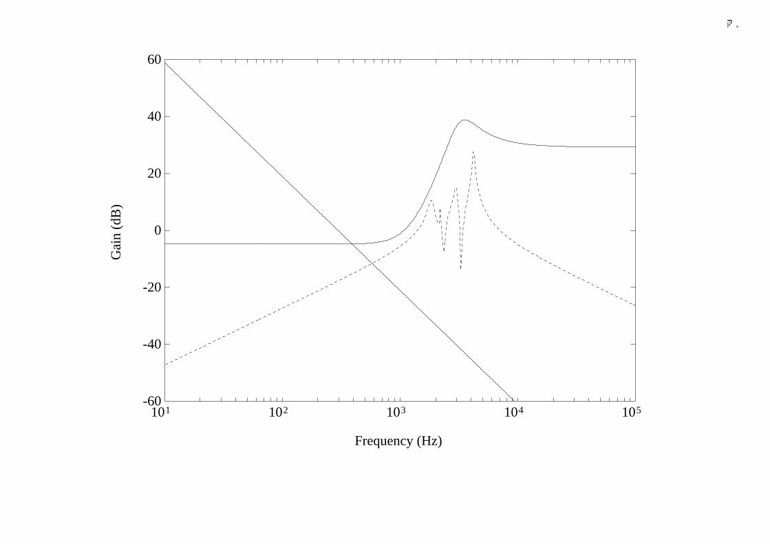
Example 14 Model the vibration modes at high frequency domain
as multiplicative uncertainty.
1. Compute the discrepancy of frequency response between the
true plant P and the nominal plant P
2. Divide this discrepancy by P ⇒ Dotted curve
3. Find a minimum phase transfer function W (s) which covers the
dotted curve. Then P (s) is contained in the plant set:
P (s) = P (1 + ∆W ), P =k
s2, ‖∆‖∞ ≤ 1.
77
千葉大学
-60
-40
-20
0
20
40
60
101 102 103 104 105
Frequency (Hz)
Gai
n (d
B)
78
千葉大学
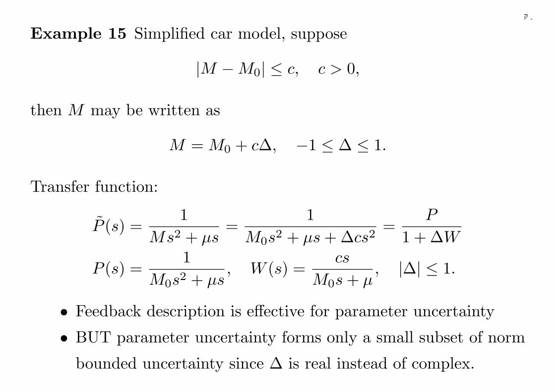
Example 15 Simplified car model, suppose
|M −M0| ≤ c, c > 0,
then M may be written as
M = M0 + c∆, −1 ≤ ∆ ≤ 1.
Transfer function:
P (s) =1
Ms2 + µs=
1M0s2 + µs + ∆cs2
=P
1 + ∆W
P (s) =1
M0s2 + µs, W (s) =
cs
M0s + µ, |∆| ≤ 1.
• Feedback description is effective for parameter uncertainty
• BUT parameter uncertainty forms only a small subset of norm
bounded uncertainty since ∆ is real instead of complex.
79
千葉大学
13 Modeling of The Domain of Uncertainty
PRICIPLE:
• Bound of uncertainty is called as a ”weight”
• Lower order weight of uncertainty is desired, in order to simplify
the design.
• Since the control performance is related to the frequency re-
sponse property at Low-Middle frequency domain, the weight
should be determined in such a way that it is not so greater
than the uncertainty in domain. The reason is that if the sys-
tem dynamics is characterized more precisely, it is more possible
to achieve better performance in control design.
80
千葉大学
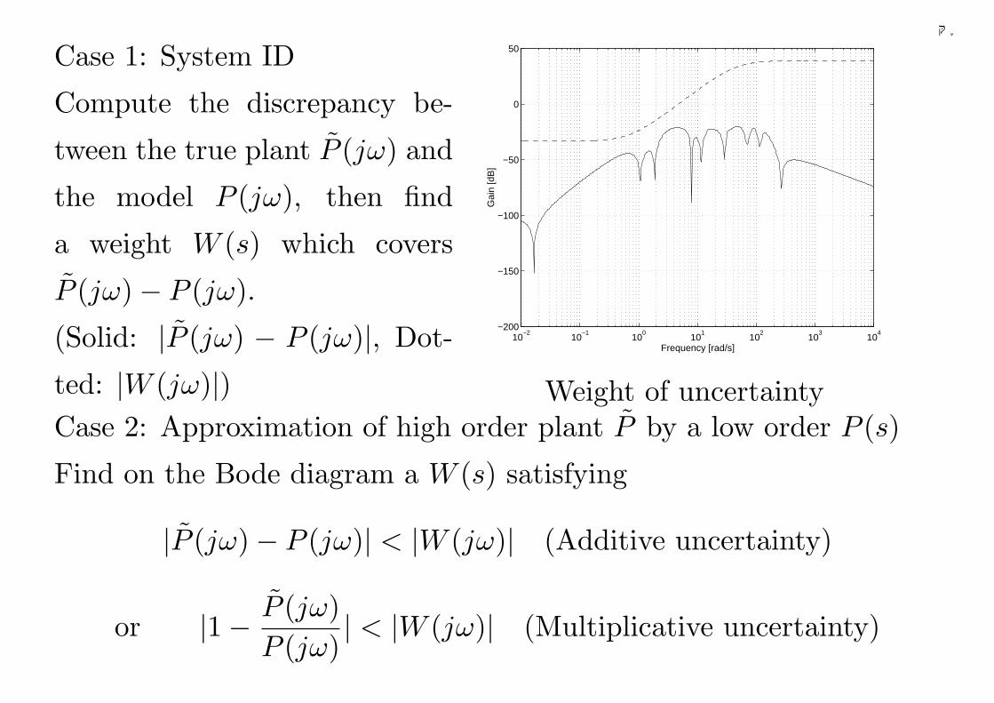
Case 1: System ID
Compute the discrepancy be-
tween the true plant P (jω) and
the model P (jω), then find
a weight W (s) which covers
P (jω)− P (jω).
(Solid: |P (jω) − P (jω)|, Dot-
ted: |W (jω)|)10
−210
−110
010
110
210
310
4−200
−150
−100
−50
0
50
Frequency [rad/s]
Gai
n [d
B]
Weight of uncertaintyCase 2: Approximation of high order plant P by a low order P (s)
Find on the Bode diagram a W (s) satisfying
|P (jω)− P (jω)| < |W (jω)| (Additive uncertainty)
or |1− P (jω)P (jω)
| < |W (jω)| (Multiplicative uncertainty)
81
千葉大学
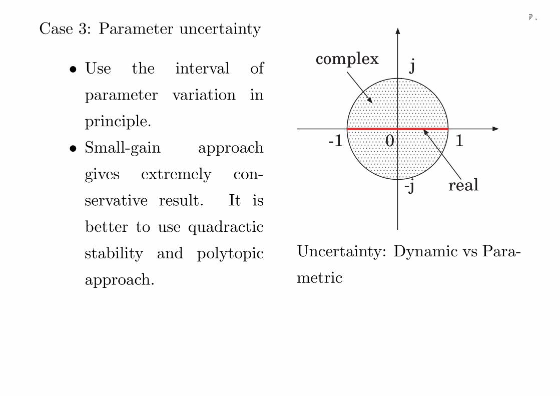
Case 3: Parameter uncertainty
• Use the interval of
parameter variation in
principle.
• Small-gain approach
gives extremely con-
servative result. It is
better to use quadractic
stability and polytopic
approach.
-1 1
-j
j
0
complex
real
Uncertainty: Dynamic vs Para-
metric
82
千葉大学
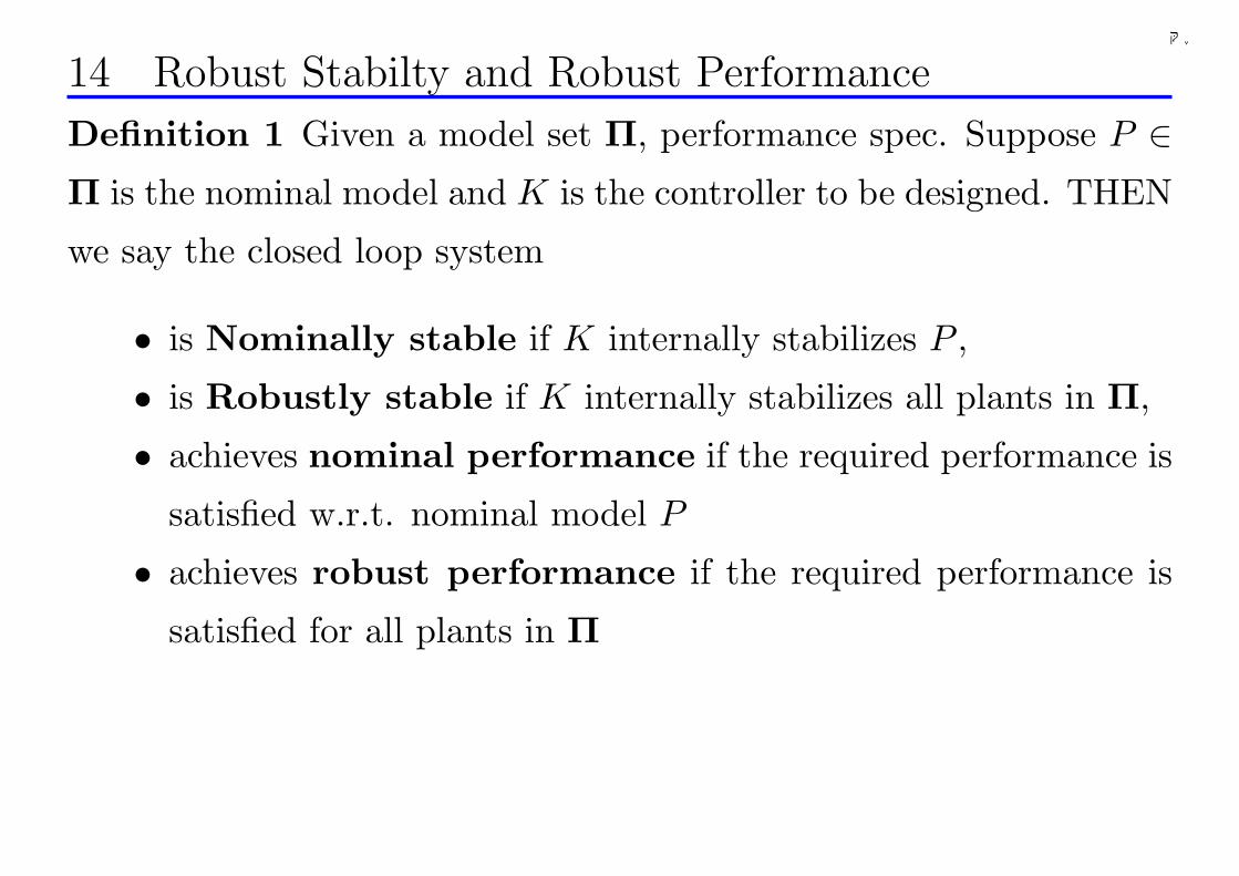
14 Robust Stabilty and Robust Performance
Definition 1 Given a model set Π, performance spec. Suppose P ∈Π is the nominal model and K is the controller to be designed. THEN
we say the closed loop system
• is Nominally stable if K internally stabilizes P ,
• is Robustly stable if K internally stabilizes all plants in Π,
• achieves nominal performance if the required performance is
satisfied w.r.t. nominal model P
• achieves robust performance if the required performance is
satisfied for all plants in Π
83
千葉大学
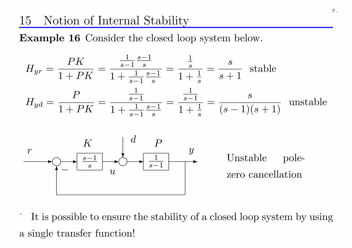
15 Notion of Internal Stability
Example 16 Consider the closed loop system below.
Hyr =PK
1 + PK=
1s−1
s−1s
1 + 1s−1
s−1s
=1s
1 + 1s
=s
s + 1stable
Hyd =P
1 + PK=
1s−1
1 + 1s−1
s−1s
=1
s−1
1 + 1s
=s
(s− 1)(s + 1)unstable
1s−1
- --g-6
s−1s
-−
g?rd
y
u
PK
Unstable pole-
zero cancellation
It is possible to ensure the stability of a closed loop system by using
a single transfer function!
84
千葉大学
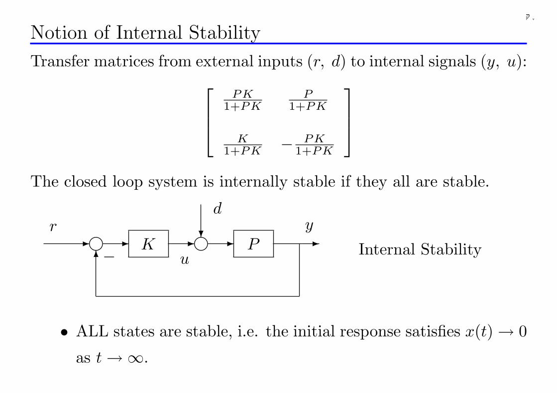
Notion of Internal Stability
Transfer matrices from external inputs (r, d) to internal signals (y, u):
PK1+PK
P1+PK
K1+PK − PK
1+PK
The closed loop system is internally stable if they all are stable.
P- --g-6
K-−
g?rd
y
uInternal Stability
• ALL states are stable, i.e. the initial response satisfies x(t) → 0
as t →∞.
85
千葉大学
• Internall stability = stability of Hyr and there is no unstable
pole-zero cancellation in (P, K).
86
千葉大学
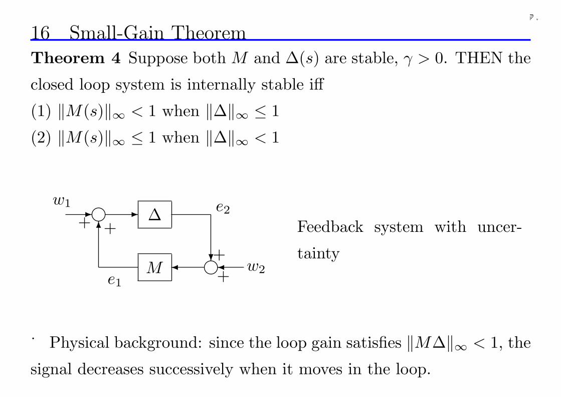
16 Small-Gain TheoremTheorem 4 Suppose both M and ∆(s) are stable, γ > 0. THEN the
closed loop system is internally stable iff
(1) ‖M(s)‖∞ < 1 when ‖∆‖∞ ≤ 1
(2) ‖M(s)‖∞ ≤ 1 when ‖∆‖∞ < 1
++
++
e2
e1
w2
w1∆
M
--6g
g¾ ?¾
Feedback system with uncer-
tainty
Physical background: since the loop gain satisfies ‖M∆‖∞ < 1, the
signal decreases successively when it moves in the loop.
87
千葉大学
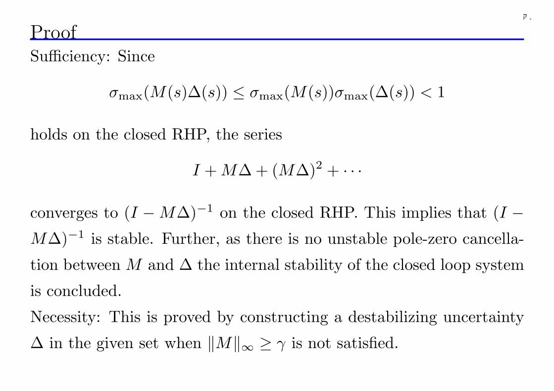
ProofSufficiency: Since
σmax(M(s)∆(s)) ≤ σmax(M(s))σmax(∆(s)) < 1
holds on the closed RHP, the series
I + M∆ + (M∆)2 + · · ·
converges to (I −M∆)−1 on the closed RHP. This implies that (I −M∆)−1 is stable. Further, as there is no unstable pole-zero cancella-
tion between M and ∆ the internal stability of the closed loop system
is concluded.
Necessity: This is proved by constructing a destabilizing uncertainty
∆ in the given set when ‖M‖∞ ≥ γ is not satisfied.
88
千葉大学
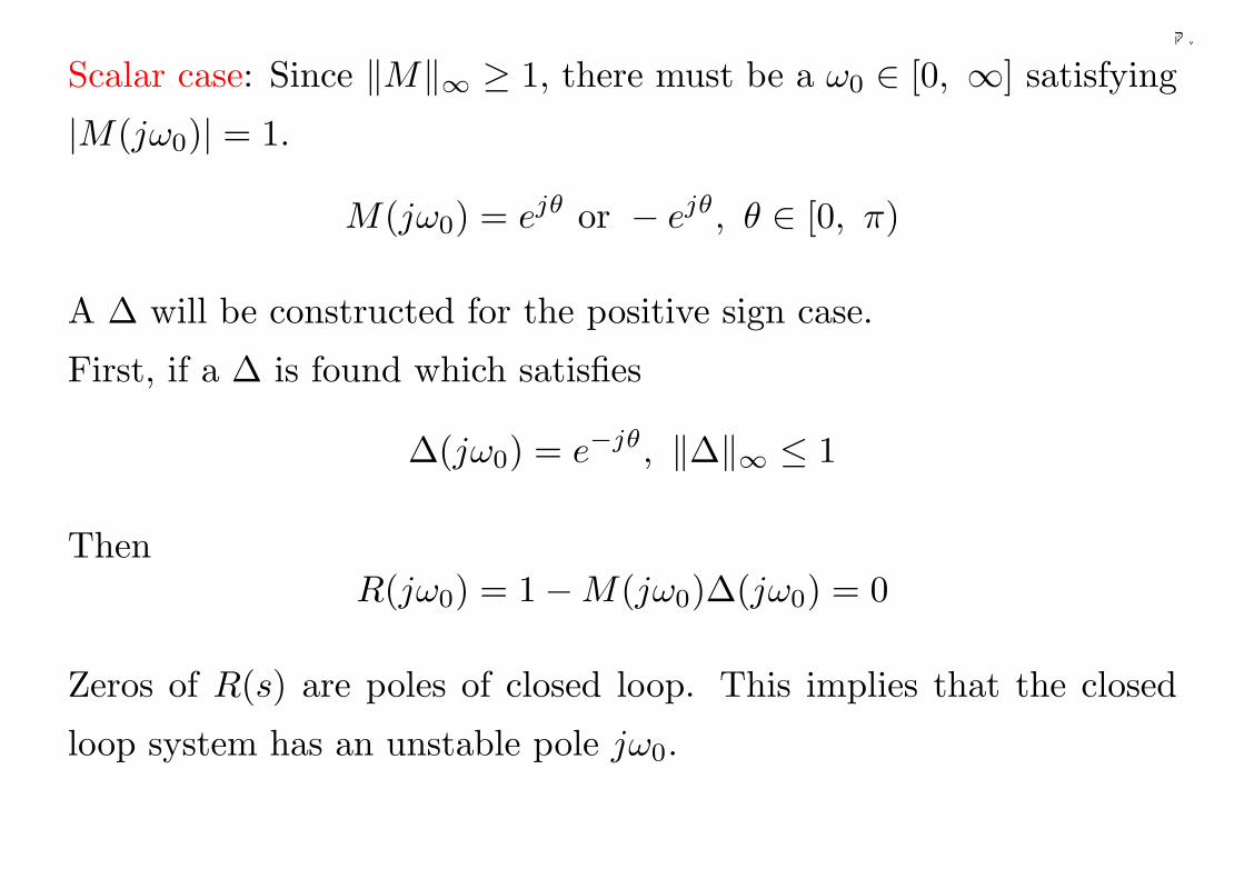
Scalar case: Since ‖M‖∞ ≥ 1, there must be a ω0 ∈ [0, ∞] satisfying
|M(jω0)| = 1.
M(jω0) = ejθ or − ejθ, θ ∈ [0, π)
A ∆ will be constructed for the positive sign case.
First, if a ∆ is found which satisfies
∆(jω0) = e−jθ, ‖∆‖∞ ≤ 1
ThenR(jω0) = 1−M(jω0)∆(jω0) = 0
Zeros of R(s) are poles of closed loop. This implies that the closed
loop system has an unstable pole jω0.
89
千葉大学
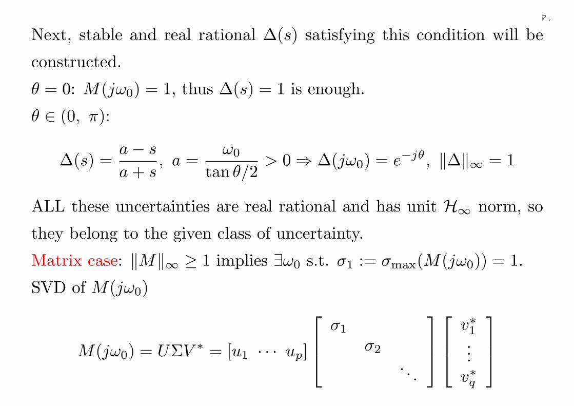
Next, stable and real rational ∆(s) satisfying this condition will be
constructed.
θ = 0: M(jω0) = 1, thus ∆(s) = 1 is enough.
θ ∈ (0, π):
∆(s) =a− s
a + s, a =
ω0
tan θ/2> 0 ⇒ ∆(jω0) = e−jθ, ‖∆‖∞ = 1
ALL these uncertainties are real rational and has unit H∞ norm, so
they belong to the given class of uncertainty.
Matrix case: ‖M‖∞ ≥ 1 implies ∃ω0 s.t. σ1 := σmax(M(jω0)) = 1.
SVD of M(jω0)
M(jω0) = UΣV ∗ = [u1 · · · up]
σ1
σ2
. . .
v∗1...
v∗q
90
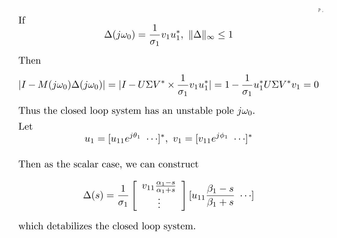
千葉大学
If∆(jω0) =
1σ1
v1u∗1, ‖∆‖∞ ≤ 1
Then
|I −M(jω0)∆(jω0)| = |I −UΣV ∗× 1σ1
v1u∗1| = 1− 1
σ1u∗1UΣV ∗v1 = 0
Thus the closed loop system has an unstable pole jω0.
Letu1 = [u11e
jθ1 · · ·]∗, v1 = [v11ejφ1 · · ·]∗
Then as the scalar case, we can construct
∆(s) =1σ1
[v11
α1−sα1+s...
][u11
β1 − s
β1 + s· · ·]
which detabilizes the closed loop system.
91
千葉大学
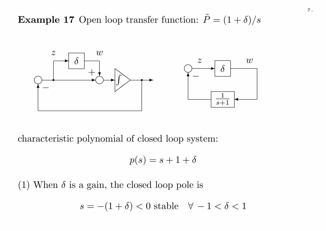
Example 17 Open loop transfer function: P = (1 + δ)/s
δ
ZZg g- -6
q−
-?
-
q +
wz
½½
∫ δ- wz
¾1s+1
g6−
characteristic polynomial of closed loop system:
p(s) = s + 1 + δ
(1) When δ is a gain, the closed loop pole is
s = −(1 + δ) < 0 stable ∀ − 1 < δ < 1
92
千葉大学
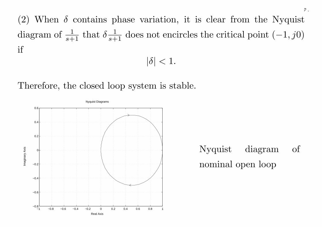
(2) When δ contains phase variation, it is clear from the Nyquist
diagram of 1s+1 that δ 1
s+1 does not encircles the critical point (−1, j0)
if|δ| < 1.
Therefore, the closed loop system is stable.
Real Axis
Imag
inar
y A
xis
Nyquist Diagrams
−1 −0.8 −0.6 −0.4 −0.2 0 0.2 0.4 0.6 0.8 1−0.8
−0.6
−0.4
−0.2
0
0.2
0.4
0.6
Nyquist diagram of
nominal open loop
93
千葉大学
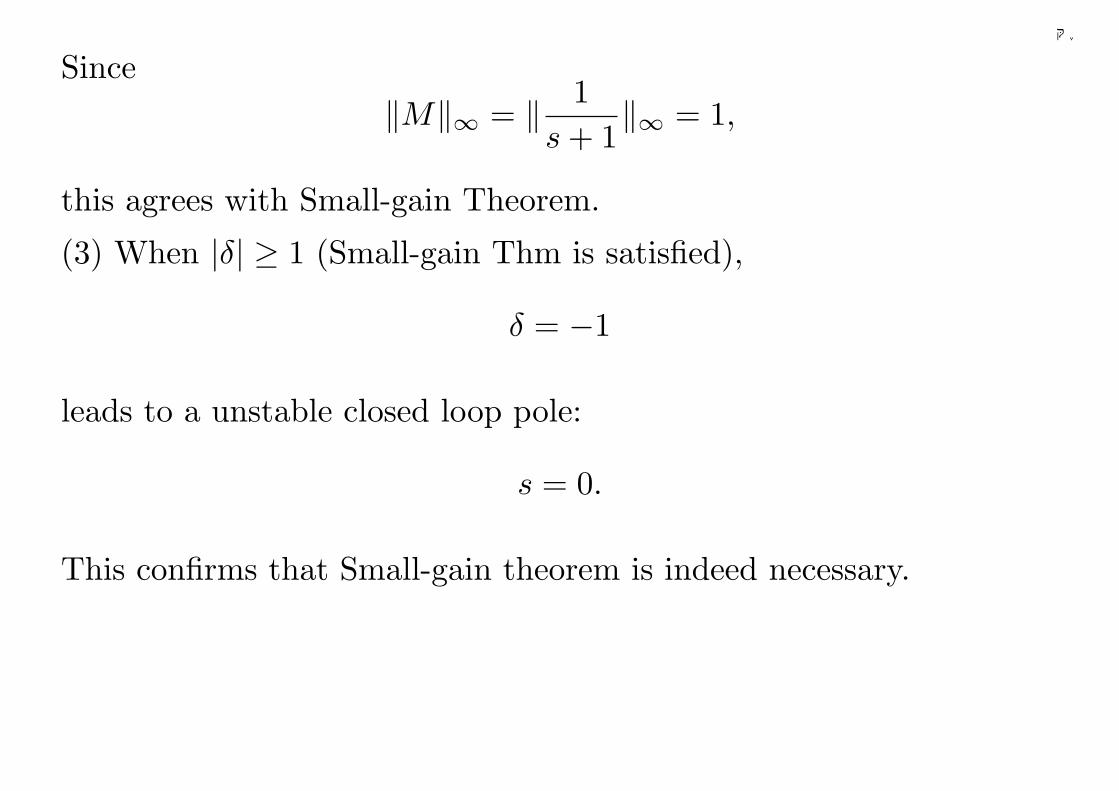
Since‖M‖∞ = ‖ 1
s + 1‖∞ = 1,
this agrees with Small-gain Theorem.
(3) When |δ| ≥ 1 (Small-gain Thm is satisfied),
δ = −1
leads to a unstable closed loop pole:
s = 0.
This confirms that Small-gain theorem is indeed necessary.
94
千葉大学
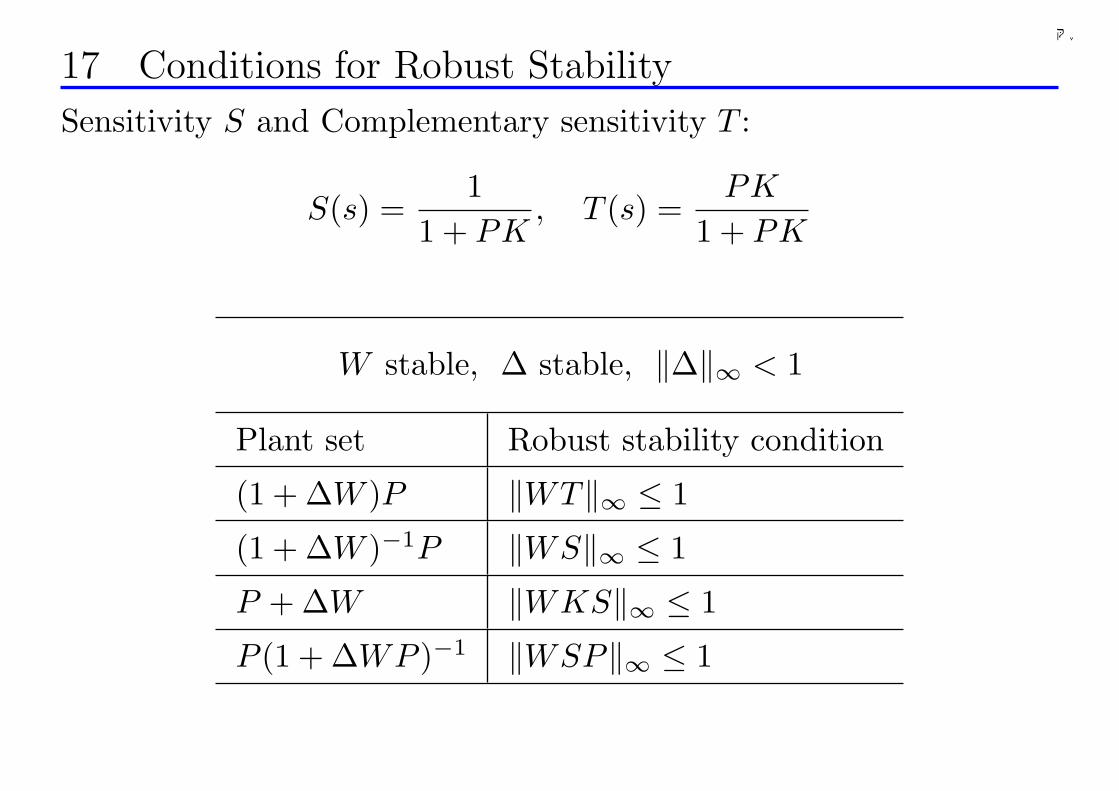
17 Conditions for Robust Stability
Sensitivity S and Complementary sensitivity T :
S(s) =1
1 + PK, T (s) =
PK
1 + PK
W stable, ∆ stable, ‖∆‖∞ < 1
Plant set Robust stability condition
(1 + ∆W )P ‖WT‖∞ ≤ 1
(1 + ∆W )−1P ‖WS‖∞ ≤ 1
P + ∆W ‖WKS‖∞ ≤ 1
P (1 + ∆WP )−1 ‖WSP‖∞ ≤ 1
95
千葉大学
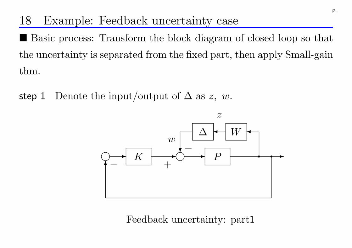
18 Example: Feedback uncertainty case
¥ Basic process: Transform the block diagram of closed loop so that
the uncertainty is separated from the fixed part, then apply Small-gain
thm.
step 1 Denote the input/output of ∆ as z, w.
K-g6
- g?−+
- -q∆ W ¾¾
P−
z
w
q
Feedback uncertainty: part1
96
千葉大学
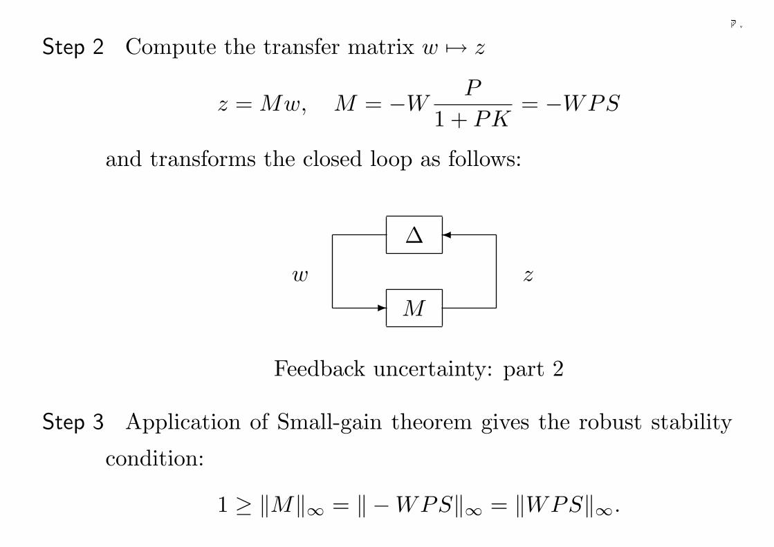
Step 2 Compute the transfer matrix w 7→ z
z = Mw, M = −WP
1 + PK= −WPS
and transforms the closed loop as follows:
∆
M
¾
-zw
Feedback uncertainty: part 2
Step 3 Application of Small-gain theorem gives the robust stability
condition:
1 ≥ ‖M‖∞ = ‖ −WPS‖∞ = ‖WPS‖∞.
97
千葉大学
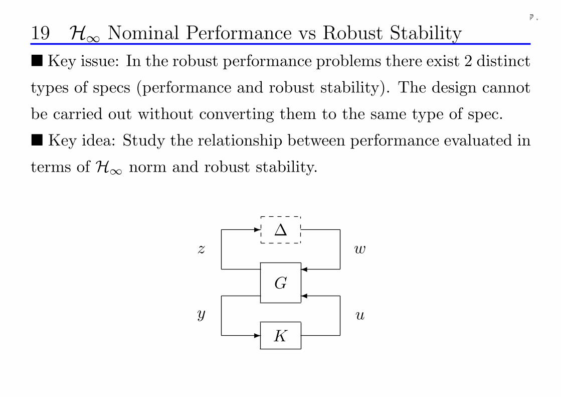
19 H∞ Nominal Performance vs Robust Stability
¥ Key issue: In the robust performance problems there exist 2 distinct
types of specs (performance and robust stability). The design cannot
be carried out without converting them to the same type of spec.
¥ Key idea: Study the relationship between performance evaluated in
terms of H∞ norm and robust stability.
G
K
-
¾
¾
-
∆w
u
z
y
98
千葉大学
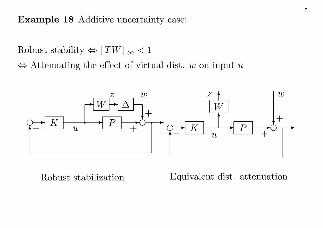
Example 18 Additive uncertainty case:
Robust stability ⇔ ‖TW‖∞ < 1
⇔ Attenuating the effect of virtual dist. w on input u
K-e6−
wz
q-∆-- W
?+
+q --
ueP
Robust stabilization
K-e6−
wz
-eW
+
+-
6 ?u
P-
6
Equivalent dist. attenuation
99
千葉大学
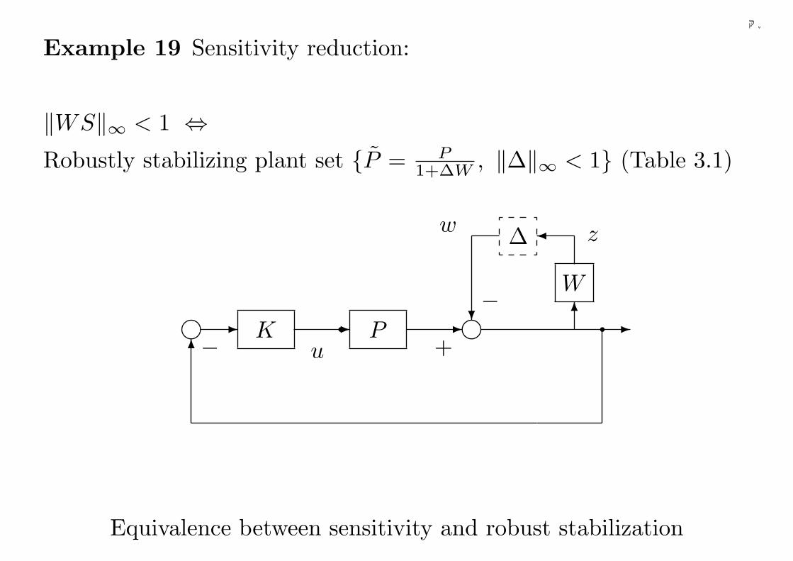
Example 19 Sensitivity reduction:
‖WS‖∞ < 1 ⇔Robustly stabilizing plant set P = P
1+∆W , ‖∆‖∞ < 1 (Table 3.1)
-g6−
w z
-g−
q --u
PK
∆
W
¾
? 6 q+
Equivalence between sensitivity and robust stabilization
100
千葉大学
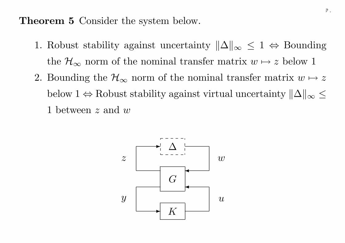
Theorem 5 Consider the system below.
1. Robust stability against uncertainty ‖∆‖∞ ≤ 1 ⇔ Bounding
the H∞ norm of the nominal transfer matrix w 7→ z below 1
2. Bounding the H∞ norm of the nominal transfer matrix w 7→ z
below 1⇔ Robust stability against virtual uncertainty ‖∆‖∞ ≤1 between z and w
G
K
-
¾
¾
-
∆w
u
z
y
101
千葉大学
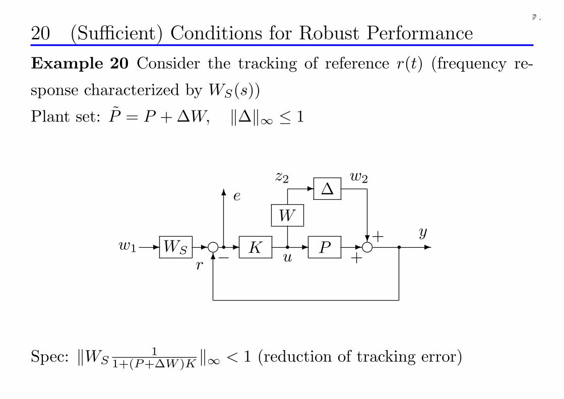
20 (Sufficient) Conditions for Robust Performance
Example 20 Consider the tracking of reference r(t) (frequency re-
sponse characterized by WS(s))
Plant set: P = P + ∆W, ‖∆‖∞ ≤ 1
-e6−
w2z2
-e++
W
-
∆
WS
-
?
6
r
e
q qq-y
-PKu-w1
Spec: ‖WS1
1+(P+∆W )K ‖∞ < 1 (reduction of tracking error)
102
千葉大学
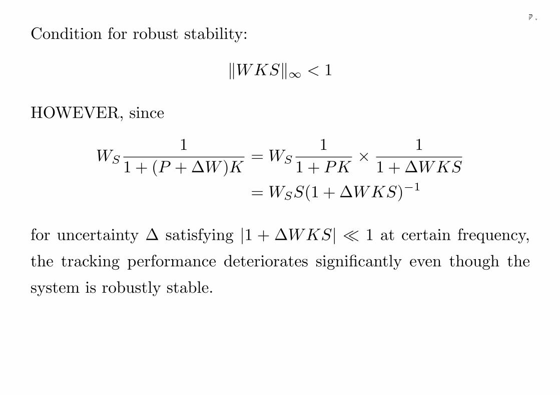
Condition for robust stability:
‖WKS‖∞ < 1
HOWEVER, since
WS1
1 + (P + ∆W )K= WS
11 + PK
× 11 + ∆WKS
= WSS(1 + ∆WKS)−1
for uncertainty ∆ satisfying |1 + ∆WKS| ¿ 1 at certain frequency,
the tracking performance deteriorates significantly even though the
system is robustly stable.
103
千葉大学
In the end, we need
‖WKS‖∞ < 1 and ‖WSS(1 + ∆WKS)−1‖∞ < 1
to be satisifed simultaneously.
• Both conditions are given in terms of H∞ norm. One contains
uncertainty and cannot be used in design directly.
• Need to convert both conditions into some condition w/o un-
certainty
104
千葉大学
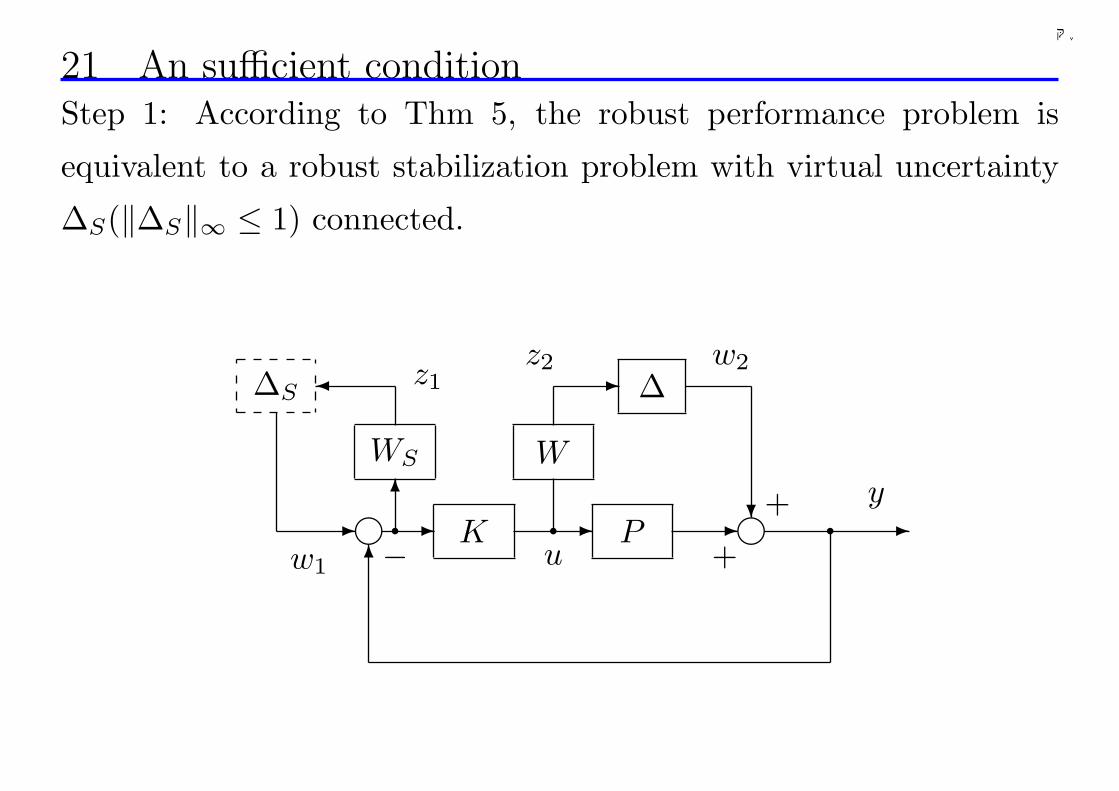
21 An sufficient conditionStep 1: According to Thm 5, the robust performance problem is
equivalent to a robust stabilization problem with virtual uncertainty
∆S(‖∆S‖∞ ≤ 1) connected.
-g6−
w2z2
-g++-
∆S
W
-
∆
WS
-
?
¾
w1
z1
q qqy
Pu-
6K
105
千葉大学
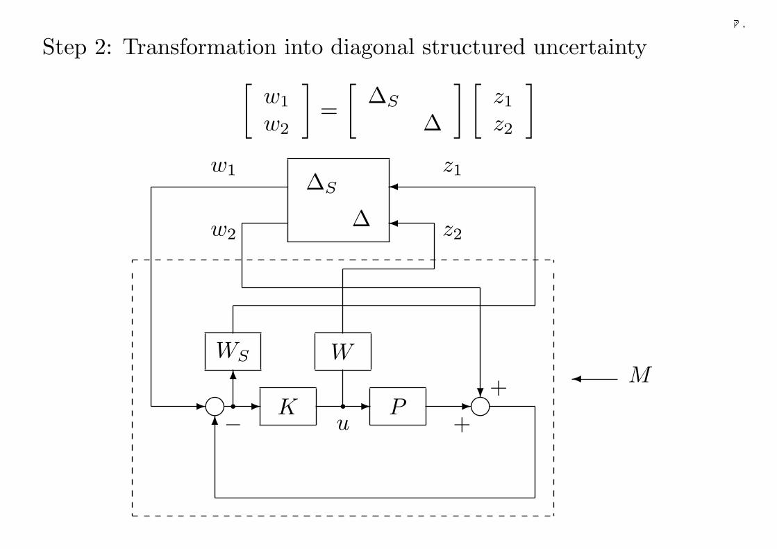
Step 2: Transformation into diagonal structured uncertainty[
w1
w2
]=
[∆S
∆
] [z1
z2
]
-g6−
g++-K
W
-
WS
6q q- ?
¾
¾
z2
z1
w2
w1
u
M¾
∆S
∆
P
106
千葉大学
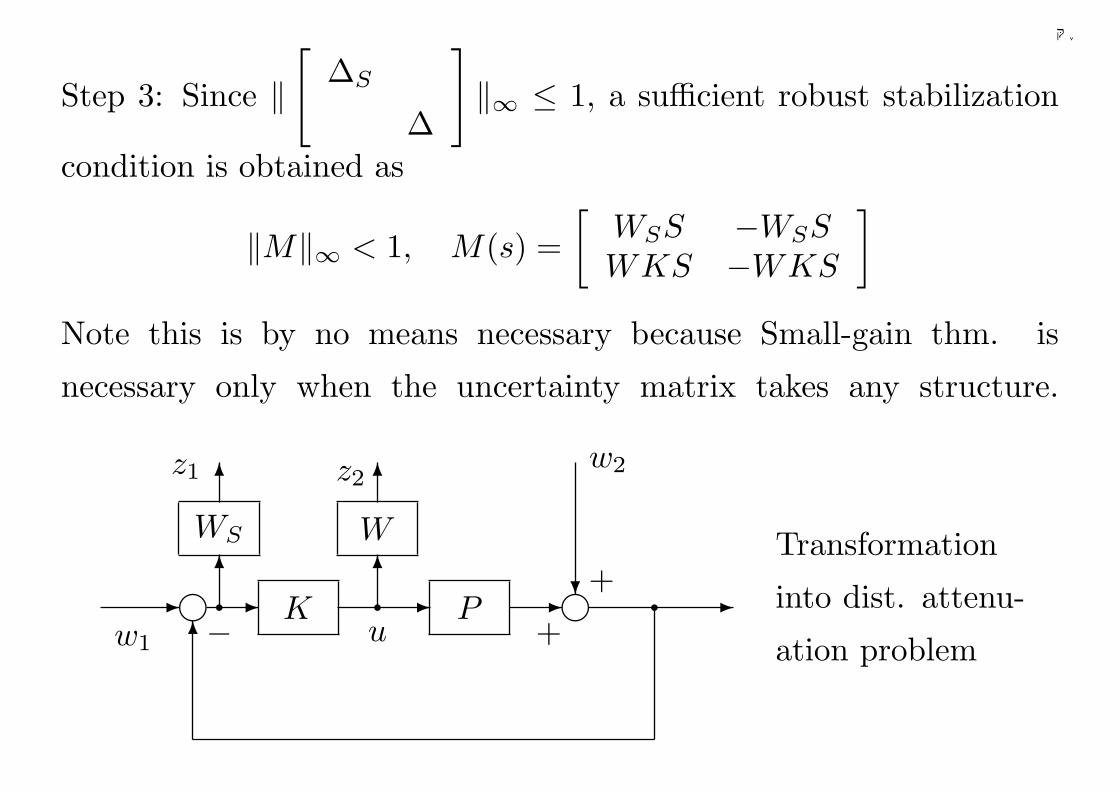
Step 3: Since ‖[
∆S
∆
]‖∞ ≤ 1, a sufficient robust stabilization
condition is obtained as
‖M‖∞ < 1, M(s) =[
WSS −WSSWKS −WKS
]
Note this is by no means necessary because Small-gain thm. is
necessary only when the uncertainty matrix takes any structure.
-g6−
w2z2
-+
+- PK-
WS
?6
w1
z1
q qq -6
6
gW
6
u
Transformation
into dist. attenu-
ation problem
107
千葉大学
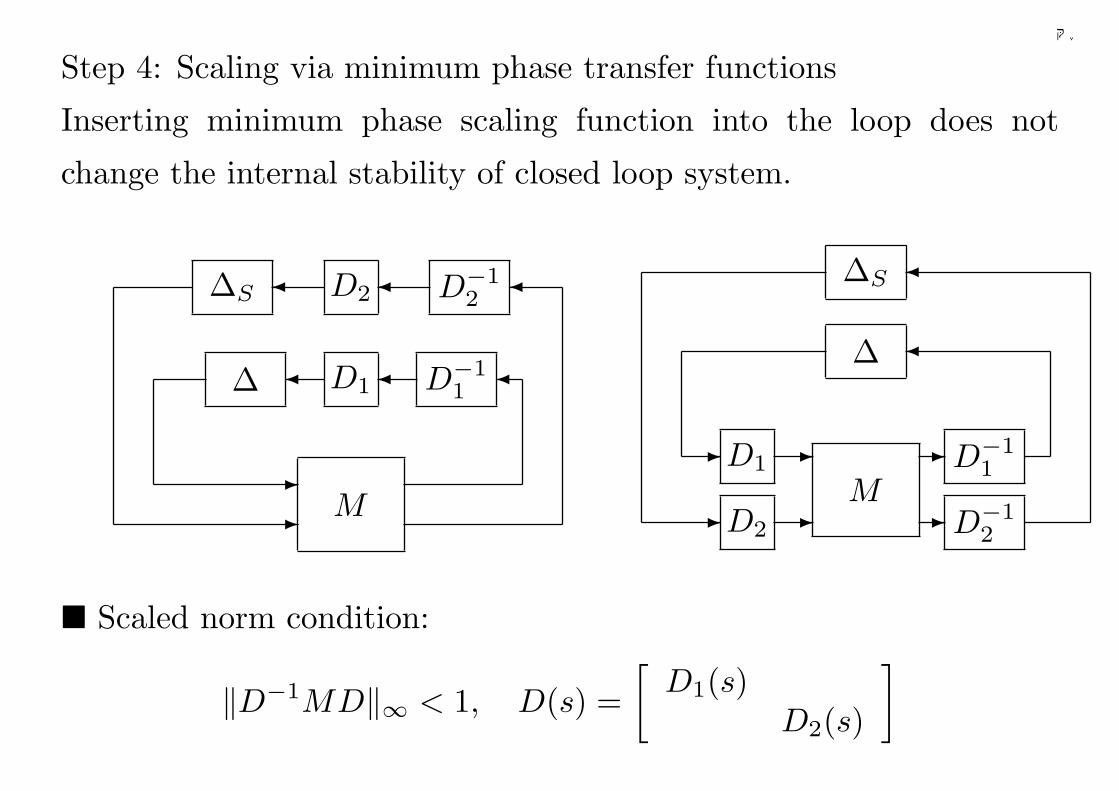
Step 4: Scaling via minimum phase transfer functions
Inserting minimum phase scaling function into the loop does not
change the internal stability of closed loop system.
∆S
∆
D2 D−12
D−11
¾¾
¾¾ ¾
¾
-- M
D1
∆S
D1 D−11
D2 D−12
¾
¾
-
-
--
- -
∆
M
¥ Scaled norm condition:
‖D−1MD‖∞ < 1, D(s) =[
D1(s)D2(s)
]
108
千葉大学
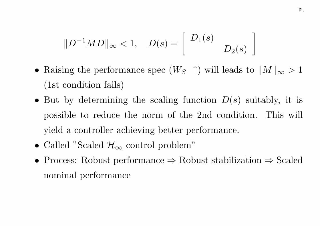
‖D−1MD‖∞ < 1, D(s) =[
D1(s)D2(s)
]
• Raising the performance spec (WS ↑) will leads to ‖M‖∞ > 1
(1st condition fails)
• But by determining the scaling function D(s) suitably, it is
possible to reduce the norm of the 2nd condition. This will
yield a controller achieving better performance.
• Called ”Scaled H∞ control problem”
• Process: Robust performance ⇒ Robust stabilization ⇒ Scaled
nominal performance
109
千葉大学
-i6−
w2z2
-+
+- PK-
WS
?6
w1
z1
r rr -6
6
i
W
6
u
D−1
D
6
-
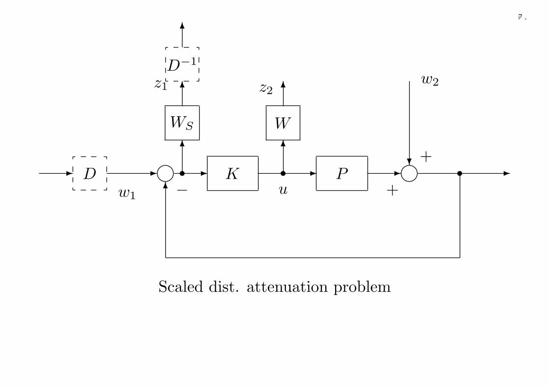
Scaled dist. attenuation problem
110
千葉大学
Chapter 3: Parameterization of Stabilizing Controllers
Describe all stabilzing controllers in terms of a closed form formula
Useful in system optimization, structure analysis, performance lim-
itation analysis, etc.
Contents
1. Introduction of generalized feedback system
2. Parameterization of all controllers
3. Structural analysis of 2 DOF systems
111
千葉大学
5 Introduction of Generalized Feedback System
G
K
z
y
w
u
¾ ¾¾
-
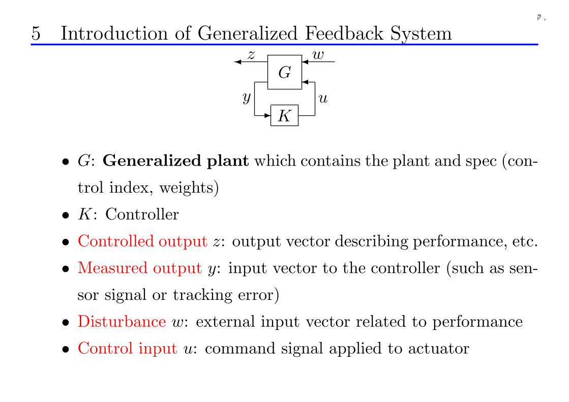
• G: Generalized plant which contains the plant and spec (con-
trol index, weights)
• K: Controller
• Controlled output z: output vector describing performance, etc.
• Measured output y: input vector to the controller (such as sen-
sor signal or tracking error)
• Disturbance w: external input vector related to performance
• Control input u: command signal applied to actuator
112
千葉大学
Introduction of Generalized Feedback System
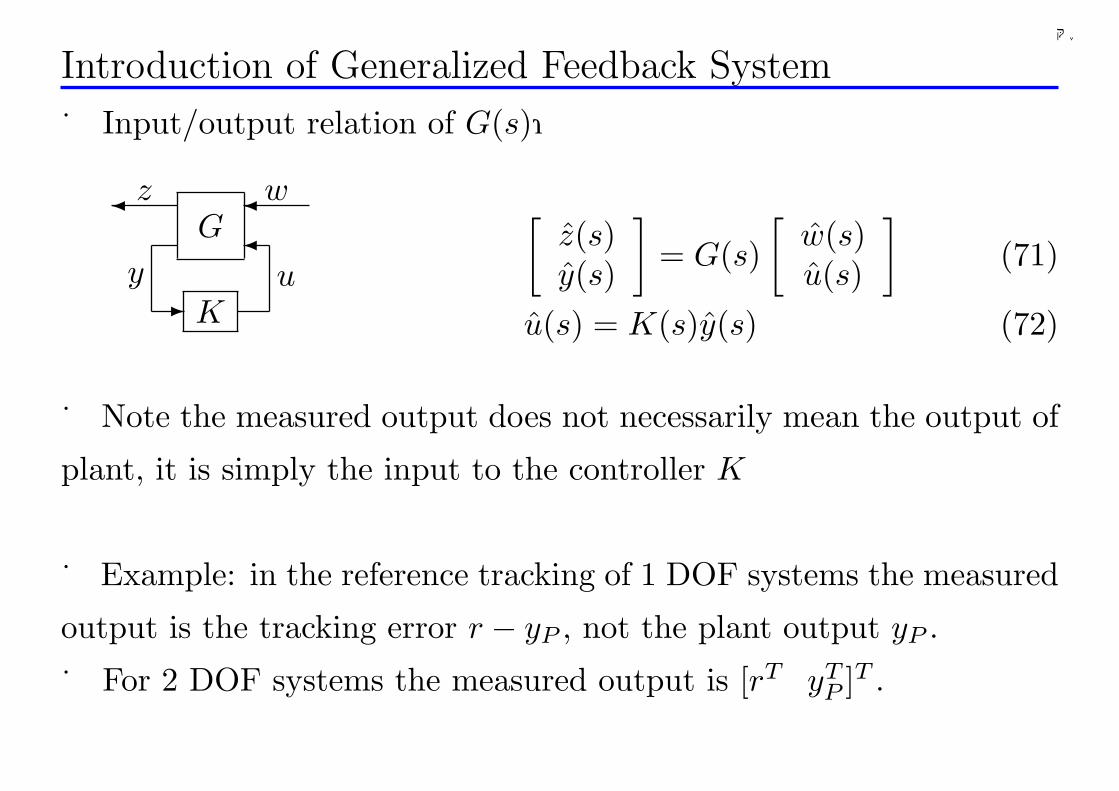
Input/output relation of G(s):
G
K
z
y
w
u
¾ ¾¾
-
[z(s)y(s)
]= G(s)
[w(s)u(s)
](71)
u(s) = K(s)y(s) (72)
Note the measured output does not necessarily mean the output of
plant, it is simply the input to the controller K
Example: in the reference tracking of 1 DOF systems the measured
output is the tracking error r − yP , not the plant output yP .
For 2 DOF systems the measured output is [rT yTP ]T .
113
千葉大学
6 2 DOF Control System
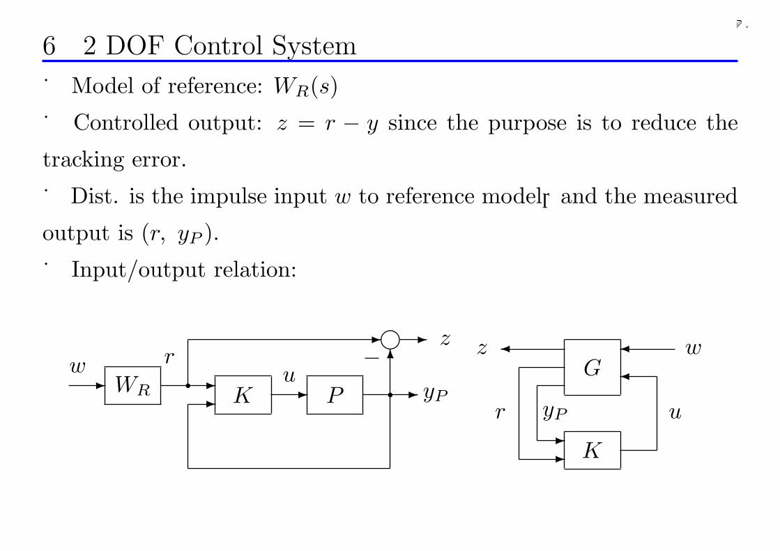
Model of reference: WR(s)
Controlled output: z = r − y since the purpose is to reduce the
tracking error.
Dist. is the impulse input w to reference model,and the measured
output is (r, yP ).
Input/output relation:
WR--
- - -6
- -g
qq−
yP
zw r
u
K
¾¾¾
--
Gw
uyPr
z
PK
114
千葉大学
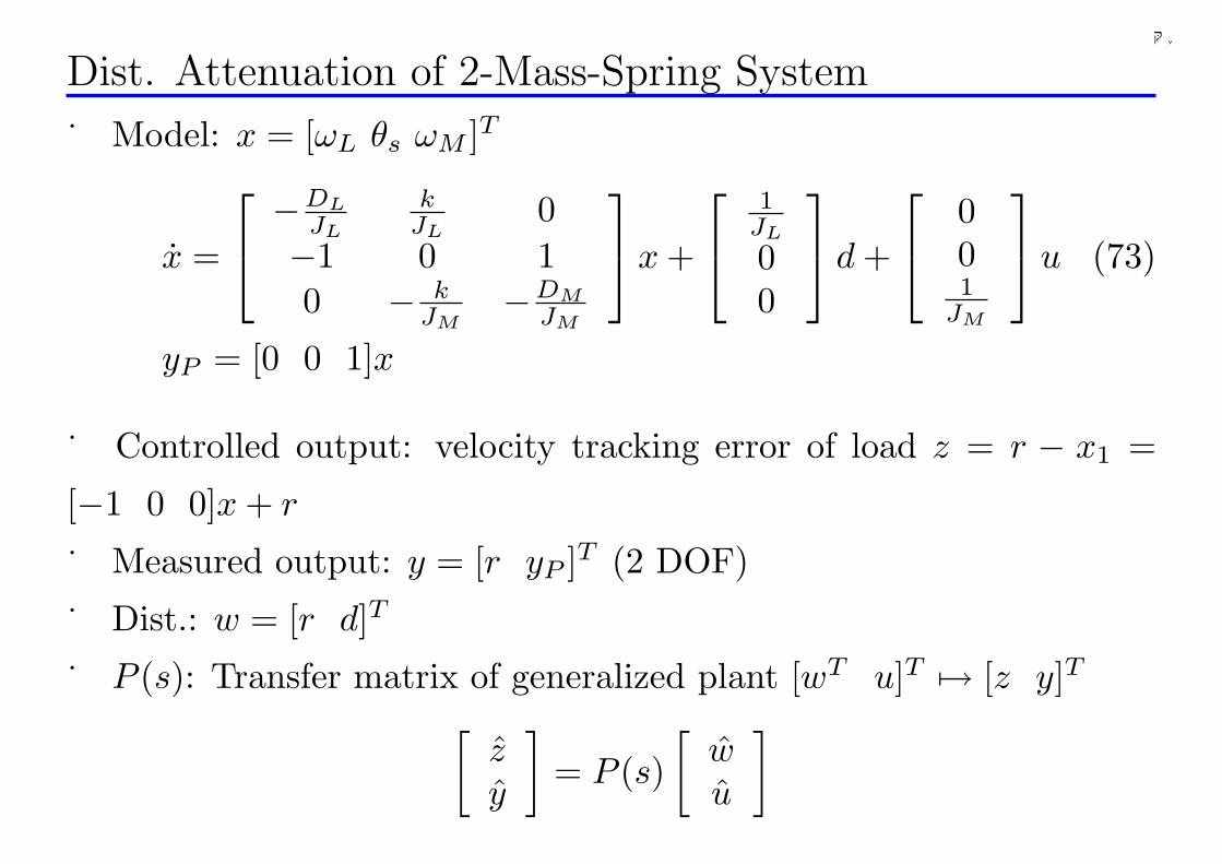
Dist. Attenuation of 2-Mass-Spring System
Model: x = [ωL θs ωM ]T
x =
−DL
JL
kJL
0−1 0 10 − k
JM−DM
JM
x +
1JL
00
d +
001
JM
u (73)
yP = [0 0 1]x
Controlled output: velocity tracking error of load z = r − x1 =
[−1 0 0]x + r
Measured output: y = [r yP ]T (2 DOF)
Dist.: w = [r d]T
P (s): Transfer matrix of generalized plant [wT u]T 7→ [z y]T
[zy
]= P (s)
[wu
]
115
千葉大学
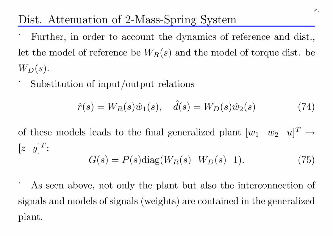
Dist. Attenuation of 2-Mass-Spring System
Further, in order to account the dynamics of reference and dist.,
let the model of reference be WR(s) and the model of torque dist. be
WD(s).
Substitution of input/output relations
r(s) = WR(s)w1(s), d(s) = WD(s)w2(s) (74)
of these models leads to the final generalized plant [w1 w2 u]T 7→[z y]T :
G(s) = P (s)diag(WR(s) WD(s) 1). (75)
As seen above, not only the plant but also the interconnection of
signals and models of signals (weights) are contained in the generalized
plant.
116
千葉大学
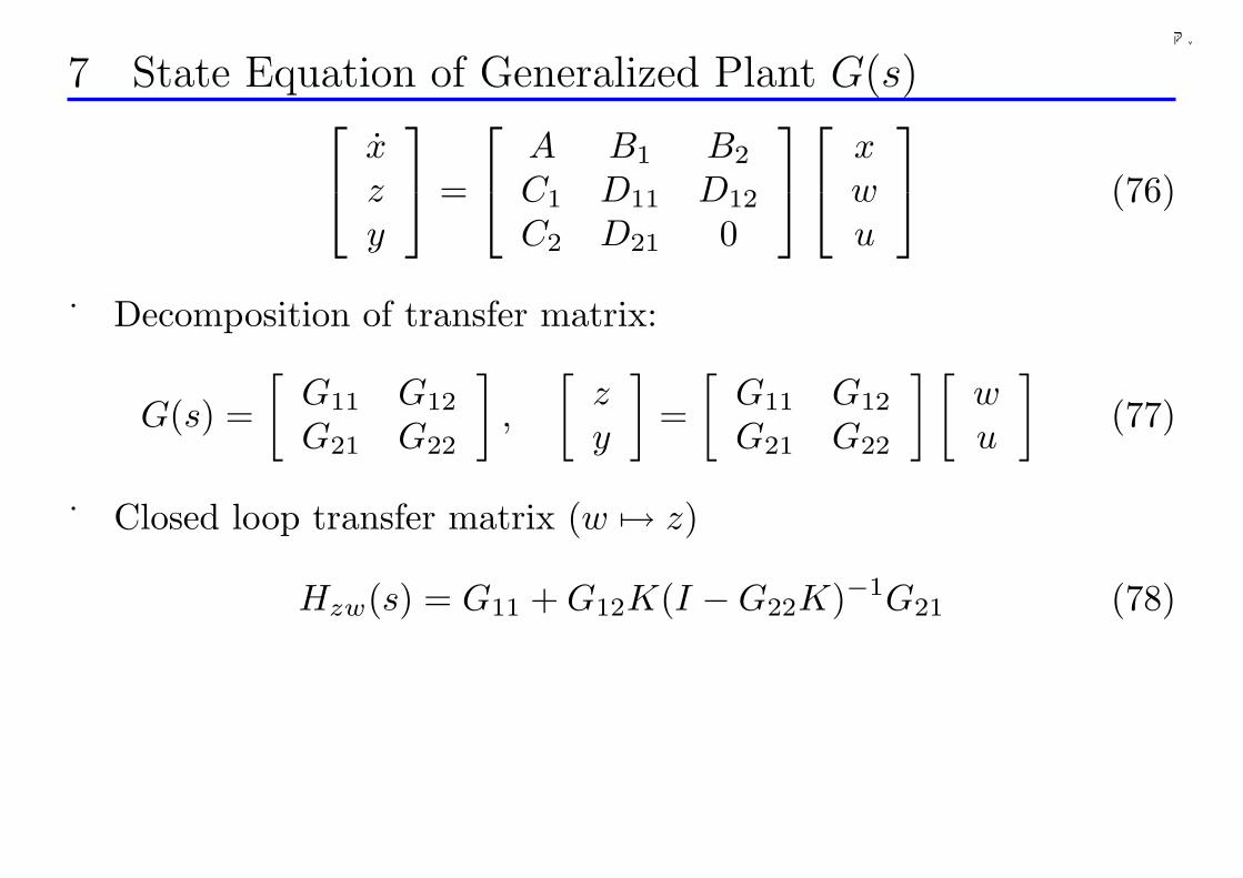
7 State Equation of Generalized Plant G(s)
xzy
=
A B1 B2
C1 D11 D12
C2 D21 0
xwu
(76)
Decomposition of transfer matrix:
G(s) =[
G11 G12
G21 G22
],
[zy
]=
[G11 G12
G21 G22
] [wu
](77)
Closed loop transfer matrix (w 7→ z)
Hzw(s) = G11 + G12K(I −G22K)−1G21 (78)
117
千葉大学
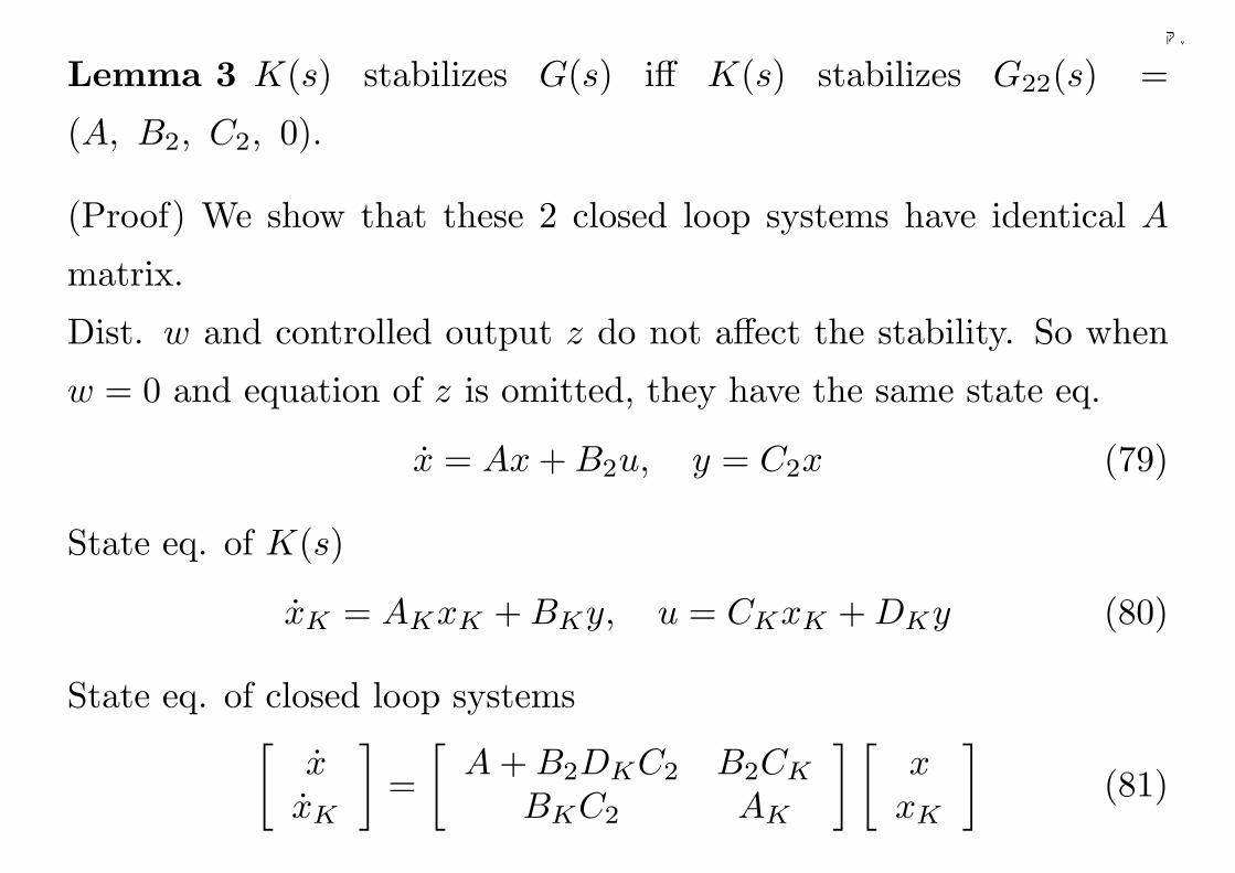
Lemma 3 K(s) stabilizes G(s) iff K(s) stabilizes G22(s) =
(A, B2, C2, 0).
(Proof) We show that these 2 closed loop systems have identical A
matrix.
Dist. w and controlled output z do not affect the stability. So when
w = 0 and equation of z is omitted, they have the same state eq.
x = Ax + B2u, y = C2x (79)
State eq. of K(s)
xK = AKxK + BKy, u = CKxK + DKy (80)
State eq. of closed loop systems[
xxK
]=
[A + B2DKC2 B2CK
BKC2 AK
] [x
xK
](81)
118
千葉大学
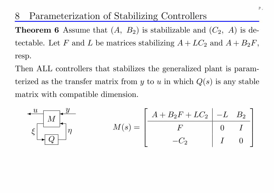
8 Parameterization of Stabilizing Controllers
Theorem 6 Assume that (A, B2) is stabilizable and (C2, A) is de-
tectable. Let F and L be matrices stabilizing A + LC2 and A + B2F ,
resp.
Then ALL controllers that stabilizes the generalized plant is param-
terized as the transfer matrix from y to u in which Q(s) is any stable
matrix with compatible dimension.
M
Q
u
ξ
y
η
¾ ¾¾
-M(s) =
A + B2F + LC2 −L B2
F 0 I
−C2 I 0
119
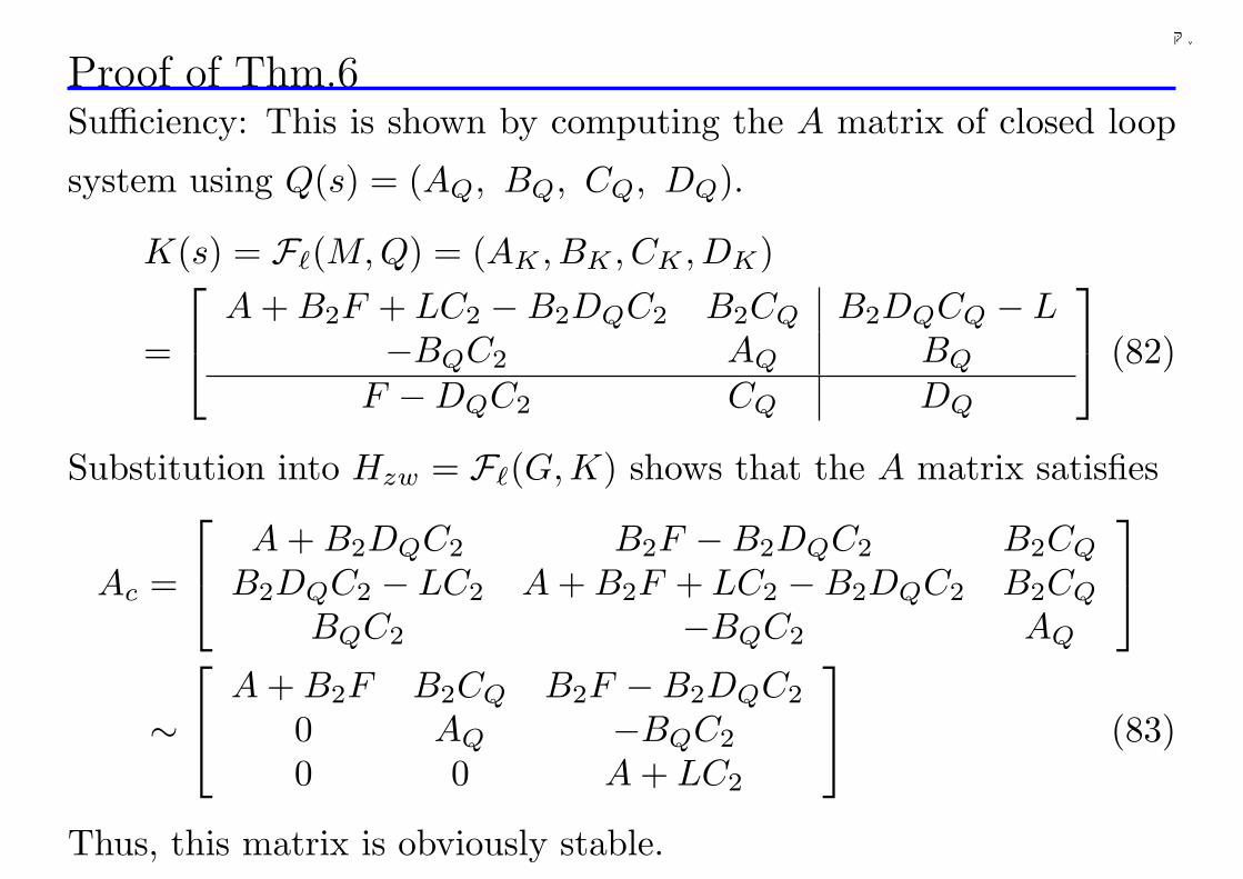
千葉大学
Proof of Thm.6Sufficiency: This is shown by computing the A matrix of closed loop
system using Q(s) = (AQ, BQ, CQ, DQ).
K(s) = F`(M, Q) = (AK , BK , CK , DK)
=
A + B2F + LC2 −B2DQC2 B2CQ B2DQCQ − L−BQC2 AQ BQ
F −DQC2 CQ DQ
(82)
Substitution into Hzw = F`(G,K) shows that the A matrix satisfies
Ac =
A + B2DQC2 B2F −B2DQC2 B2CQ
B2DQC2 − LC2 A + B2F + LC2 −B2DQC2 B2CQ
BQC2 −BQC2 AQ
∼
A + B2F B2CQ B2F −B2DQC2
0 AQ −BQC2
0 0 A + LC2
(83)
Thus, this matrix is obviously stable.
120
千葉大学
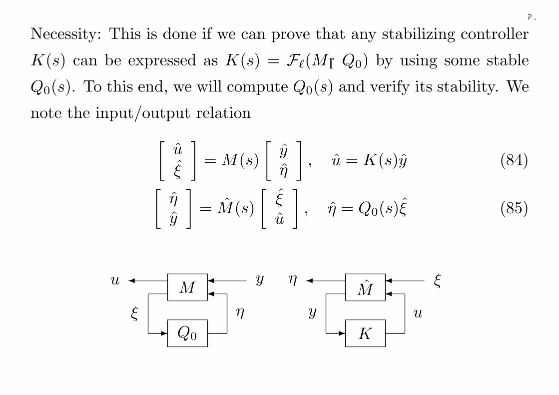
Necessity: This is done if we can prove that any stabilizing controller
K(s) can be expressed as K(s) = F`(M,Q0) by using some stable
Q0(s). To this end, we will compute Q0(s) and verify its stability. We
note the input/output relation[
u
ξ
]= M(s)
[yη
], u = K(s)y (84)
[ηy
]= M(s)
[ξu
], η = Q0(s)ξ (85)
M
Q0
¾¾¾
-
y
ηξ
uM
K
¾¾¾
-
ξ
uy
η
121
千葉大学
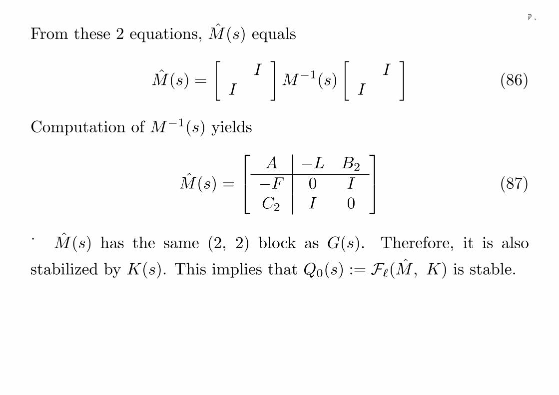
From these 2 equations, M(s) equals
M(s) =[
II
]M−1(s)
[I
I
](86)
Computation of M−1(s) yields
M(s) =
A −L B2
−F 0 IC2 I 0
(87)
M(s) has the same (2, 2) block as G(s). Therefore, it is also
stabilized by K(s). This implies that Q0(s) := F`(M, K) is stable.
122
千葉大学
9 Formula of Stabilizing Controller: Stable G(s)
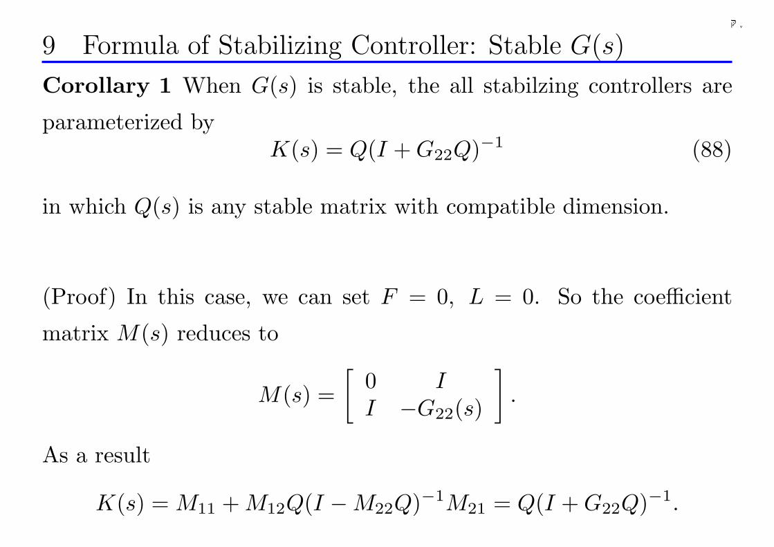
Corollary 1 When G(s) is stable, the all stabilzing controllers are
parameterized byK(s) = Q(I + G22Q)−1 (88)
in which Q(s) is any stable matrix with compatible dimension.
(Proof) In this case, we can set F = 0, L = 0. So the coefficient
matrix M(s) reduces to
M(s) =[
0 II −G22(s)
].
As a result
K(s) = M11 + M12Q(I −M22Q)−1M21 = Q(I + G22Q)−1.
123
千葉大学
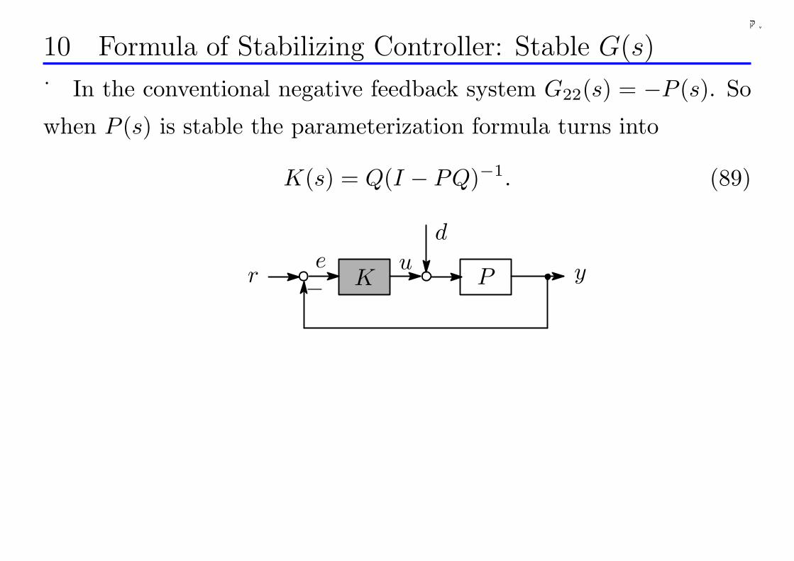
10 Formula of Stabilizing Controller: Stable G(s)
In the conventional negative feedback system G22(s) = −P (s). So
when P (s) is stable the parameterization formula turns into
K(s) = Q(I − PQ)−1. (89)
PK−ue y
d
r
124
千葉大学
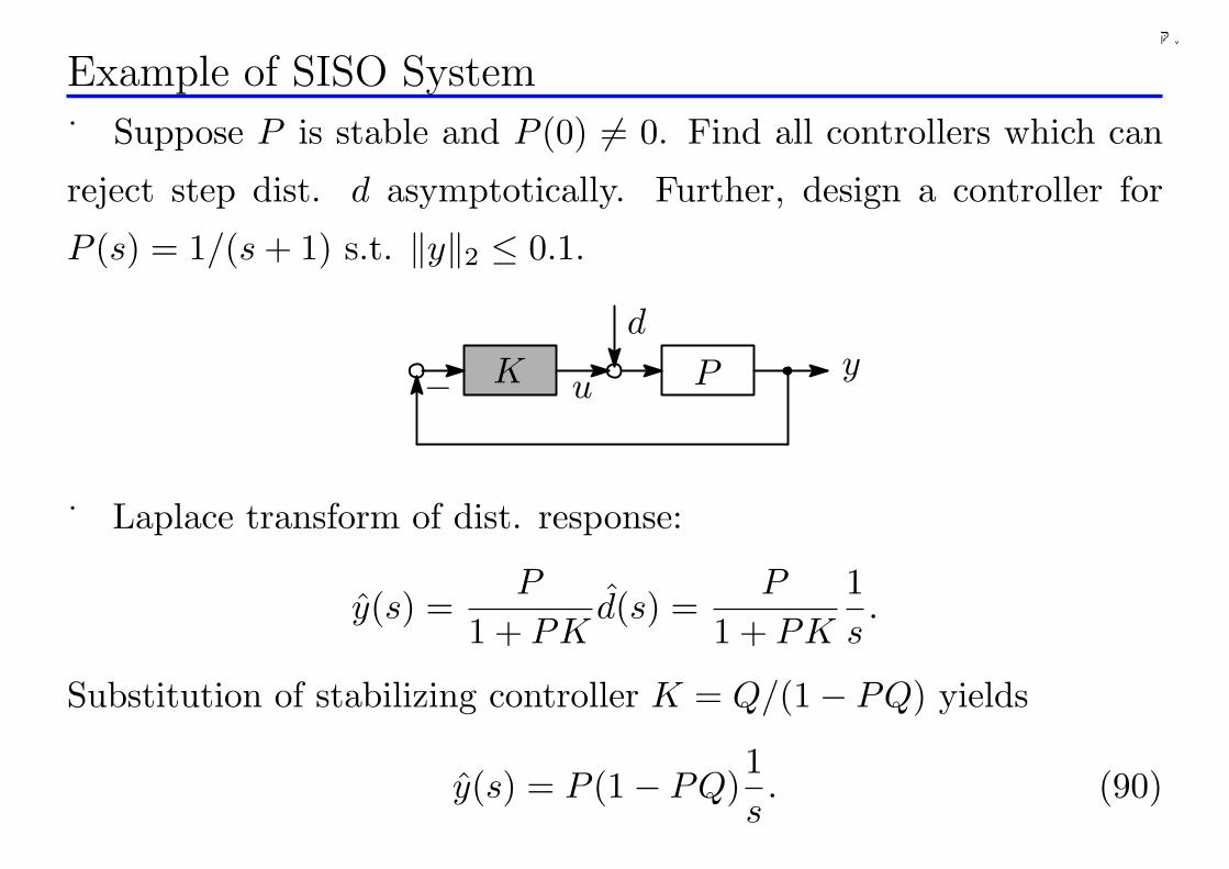
Example of SISO System
Suppose P is stable and P (0) 6= 0. Find all controllers which can
reject step dist. d asymptotically. Further, design a controller for
P (s) = 1/(s + 1) s.t. ‖y‖2 ≤ 0.1.
d
uK P y−
Laplace transform of dist. response:
y(s) =P
1 + PKd(s) =
P
1 + PK
1s.
Substitution of stabilizing controller K = Q/(1− PQ) yields
y(s) = P (1− PQ)1s. (90)
125
千葉大学
According to the final value thm of Laplace transform,
y(∞) = lims→0
sy(s) = P (0)[1− P (0)Q(0)] = 0
must hold. Since P (0) 6= 0, this implies that
Q(0) =1
P (0). (91)
Class of controllers:
K =Q
1− PQ: Q stable and Q(0) =
1P (0)
. (92)
Obviously,
K(0) = lims→0
Q
1− PQ→∞ (93)
holds which means that K(s) has at least an integrator 1/s.
126
千葉大学
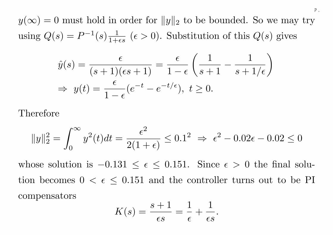
y(∞) = 0 must hold in order for ‖y‖2 to be bounded. So we may try
using Q(s) = P−1(s) 11+εs (ε > 0). Substitution of this Q(s) gives
y(s) =ε
(s + 1)(εs + 1)=
ε
1− ε
(1
s + 1− 1
s + 1/ε
)
⇒ y(t) =ε
1− ε(e−t − e−t/ε), t ≥ 0.
Therefore
‖y‖22 =∫ ∞
0
y2(t)dt =ε2
2(1 + ε)≤ 0.12 ⇒ ε2 − 0.02ε− 0.02 ≤ 0
whose solution is −0.131 ≤ ε ≤ 0.151. Since ε > 0 the final solu-
tion becomes 0 < ε ≤ 0.151 and the controller turns out to be PI
compensators
K(s) =s + 1εs
=1ε
+1εs
.
127
千葉大学
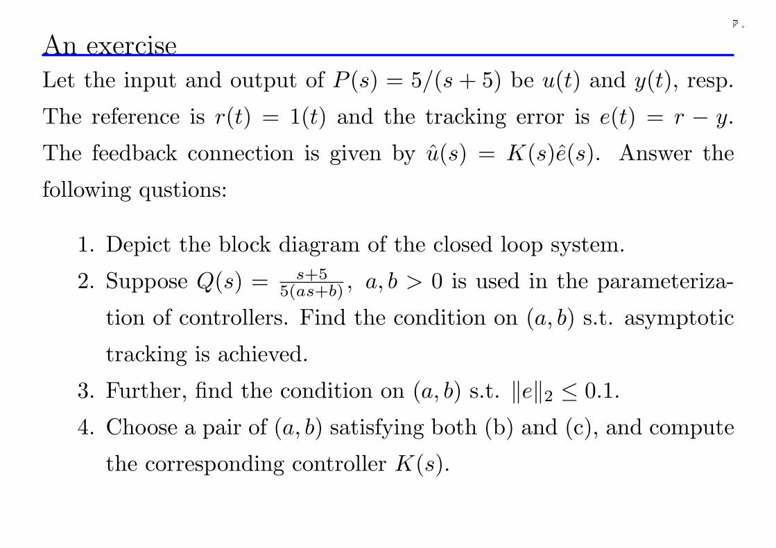
An exerciseLet the input and output of P (s) = 5/(s + 5) be u(t) and y(t), resp.
The reference is r(t) = 1(t) and the tracking error is e(t) = r − y.
The feedback connection is given by u(s) = K(s)e(s). Answer the
following qustions:
1. Depict the block diagram of the closed loop system.
2. Suppose Q(s) = s+55(as+b) , a, b > 0 is used in the parameteriza-
tion of controllers. Find the condition on (a, b) s.t. asymptotic
tracking is achieved.
3. Further, find the condition on (a, b) s.t. ‖e‖2 ≤ 0.1.
4. Choose a pair of (a, b) satisfying both (b) and (c), and compute
the corresponding controller K(s).
128
千葉大学
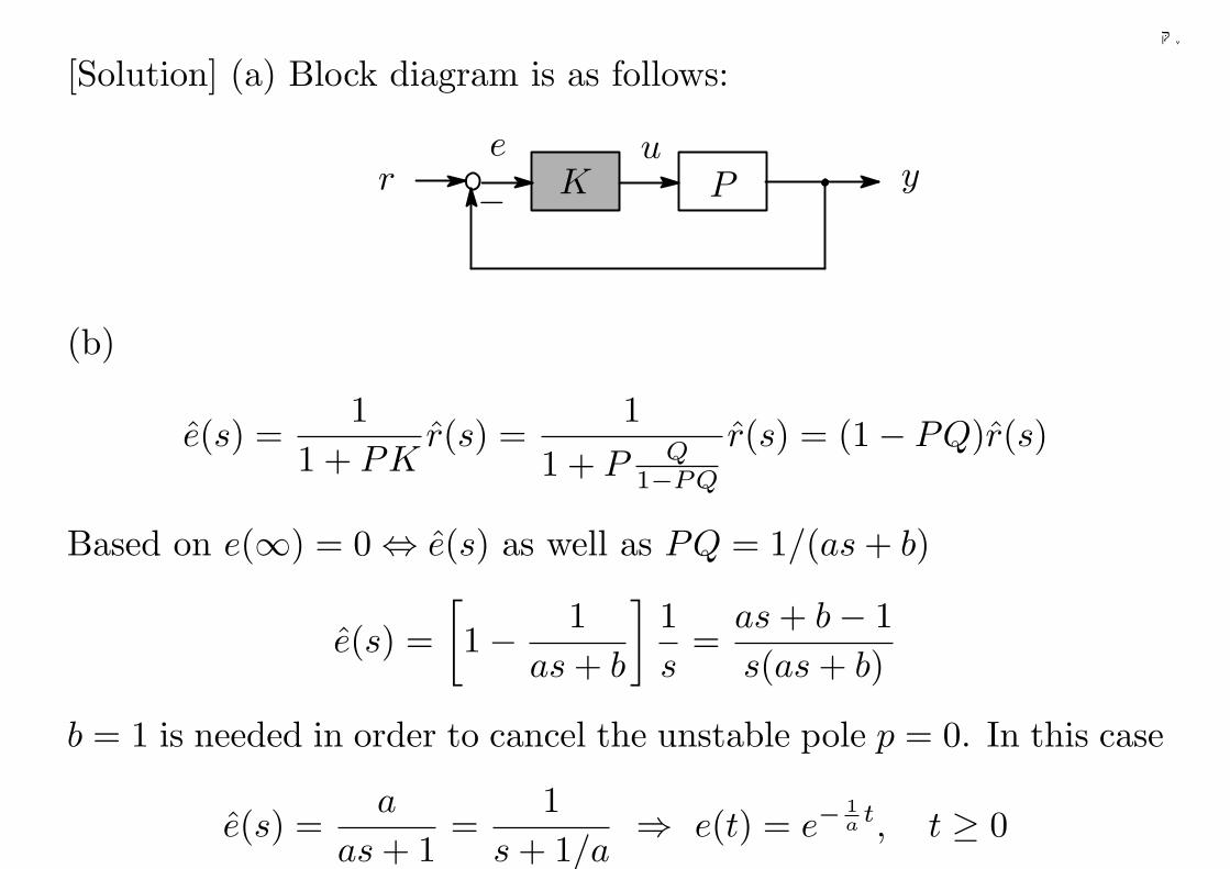
[Solution] (a) Block diagram is as follows:
−r yPKe u
(b)
e(s) =1
1 + PKr(s) =
11 + P Q
1−PQ
r(s) = (1− PQ)r(s)
Based on e(∞) = 0 ⇔ e(s) as well as PQ = 1/(as + b)
e(s) =[1− 1
as + b
]1s
=as + b− 1s(as + b)
b = 1 is needed in order to cancel the unstable pole p = 0. In this case
e(s) =a
as + 1=
1s + 1/a
⇒ e(t) = e−1a t, t ≥ 0
129
千葉大学
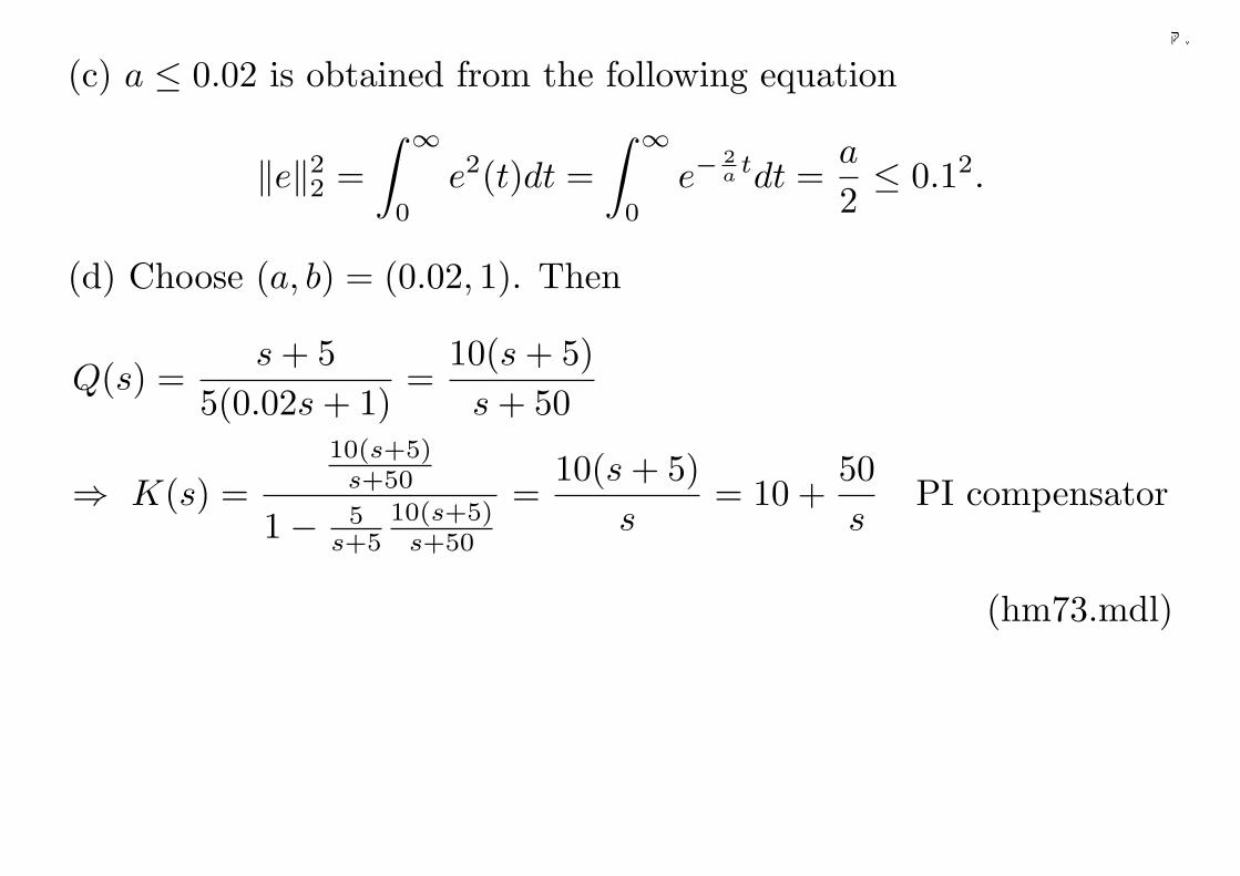
(c) a ≤ 0.02 is obtained from the following equation
‖e‖22 =∫ ∞
0
e2(t)dt =∫ ∞
0
e−2a tdt =
a
2≤ 0.12.
(d) Choose (a, b) = (0.02, 1). Then
Q(s) =s + 5
5(0.02s + 1)=
10(s + 5)s + 50
⇒ K(s) =10(s+5)
s+50
1− 5s+5
10(s+5)s+50
=10(s + 5)
s= 10 +
50s
PI compensator
(hm73.mdl)
130
千葉大学
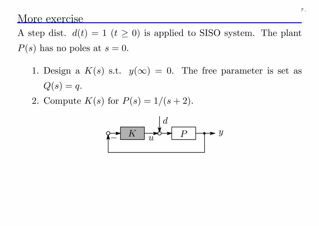
More exerciseA step dist. d(t) = 1 (t ≥ 0) is applied to SISO system. The plant
P (s) has no poles at s = 0.
1. Design a K(s) s.t. y(∞) = 0. The free parameter is set as
Q(s) = q.
2. Compute K(s) for P (s) = 1/(s + 2).
d
uK P y−
131
千葉大学
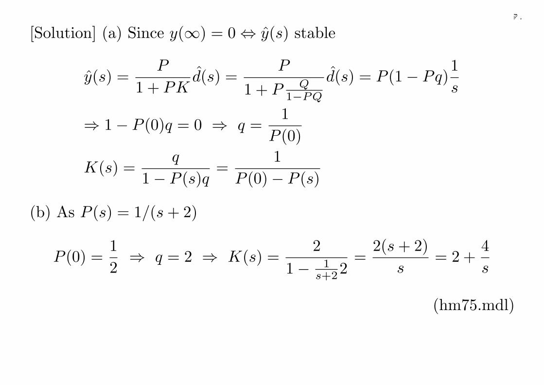
[Solution] (a) Since y(∞) = 0 ⇔ y(s) stable
y(s) =P
1 + PKd(s) =
P
1 + P Q1−PQ
d(s) = P (1− Pq)1s
⇒ 1− P (0)q = 0 ⇒ q =1
P (0)
K(s) =q
1− P (s)q=
1P (0)− P (s)
(b) As P (s) = 1/(s + 2)
P (0) =12⇒ q = 2 ⇒ K(s) =
21− 1
s+22=
2(s + 2)s
= 2 +4s
(hm75.mdl)
132
千葉大学
11 Structure of Closed Loop System
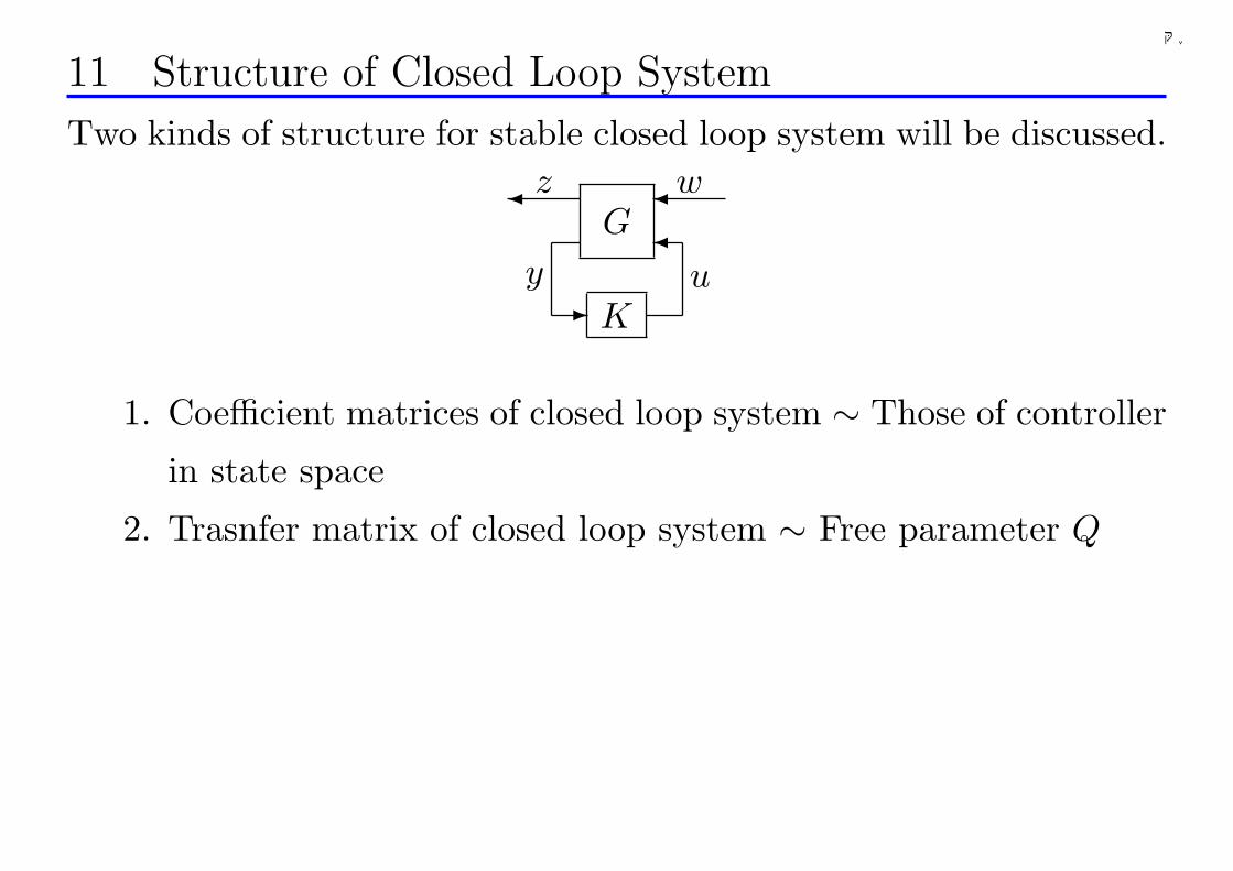
Two kinds of structure for stable closed loop system will be discussed.
G
K
z
y
w
u
¾ ¾¾
-
1. Coefficient matrices of closed loop system ∼ Those of controller
in state space
2. Trasnfer matrix of closed loop system ∼ Free parameter Q
133
千葉大学
12 Affine strcuture in parameter matrix of controller
Controller realization:
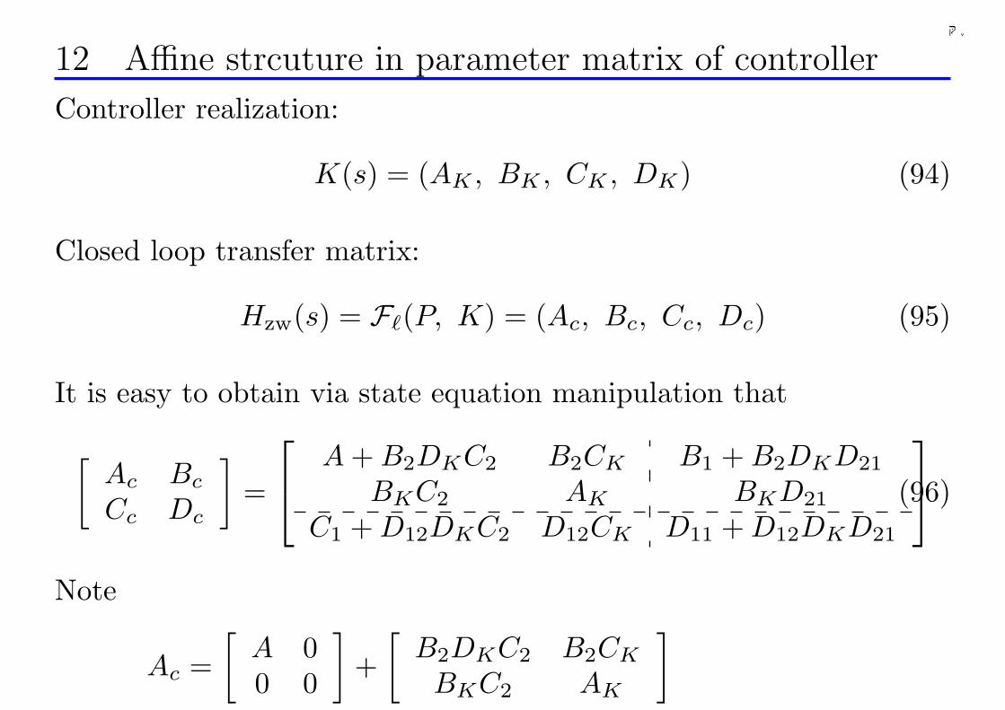
K(s) = (AK , BK , CK , DK) (94)
Closed loop transfer matrix:
Hzw(s) = F`(P, K) = (Ac, Bc, Cc, Dc) (95)
It is easy to obtain via state equation manipulation that
[Ac Bc
Cc Dc
]=
A + B2DKC2 B2CK B1 + B2DKD21
BKC2 AK BKD21
C1 + D12DKC2 D12CK D11 + D12DKD21
(96)
Note
Ac =[
A 00 0
]+
[B2DKC2 B2CK
BKC2 AK
]
134
千葉大学
=[
A 00 0
]+
[B2 00 I
] [DK CK
BK AK
] [C2 00 I
]
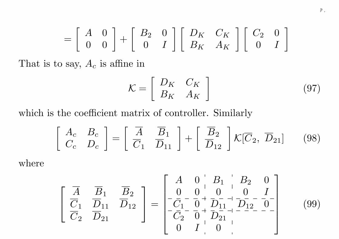
That is to say, Ac is affine in
K =[
DK CK
BK AK
](97)
which is the coefficient matrix of controller. Similarly[
Ac Bc
Cc Dc
]=
[A B1
C1 D11
]+
[B2
D12
]K[C2, D21] (98)
where
A B1 B2
C1 D11 D12
C2 D21
=
A 0 B1 B2 00 0 0 0 IC1 0 D11 D12 0C2 0 D21
0 I 0
(99)
135
千葉大学
• Closed loop transfer matrix Hzw is a nonlinear (fractional) func-
tion of K
• BUT the relation between coefficient matrices of state space
realization is linear (affine)! A much simpler structure that
makes the state space an extremely effective paradiam for the
development of optimization methods.
136
千葉大学
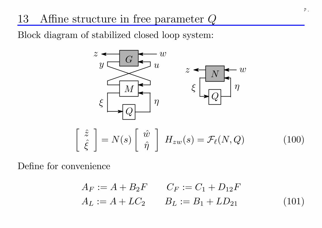
13 Affine structure in free parameter Q
Block diagram of stabilized closed loop system:
N
Qξ η
wz
ηξ
uyw
Q
M
Gz
[z
ξ
]= N(s)
[wη
]Hzw(s) = F`(N, Q) (100)
Define for convenience
AF := A + B2F CF := C1 + D12F
AL := A + LC2 BL := B1 + LD21 (101)
137
千葉大学
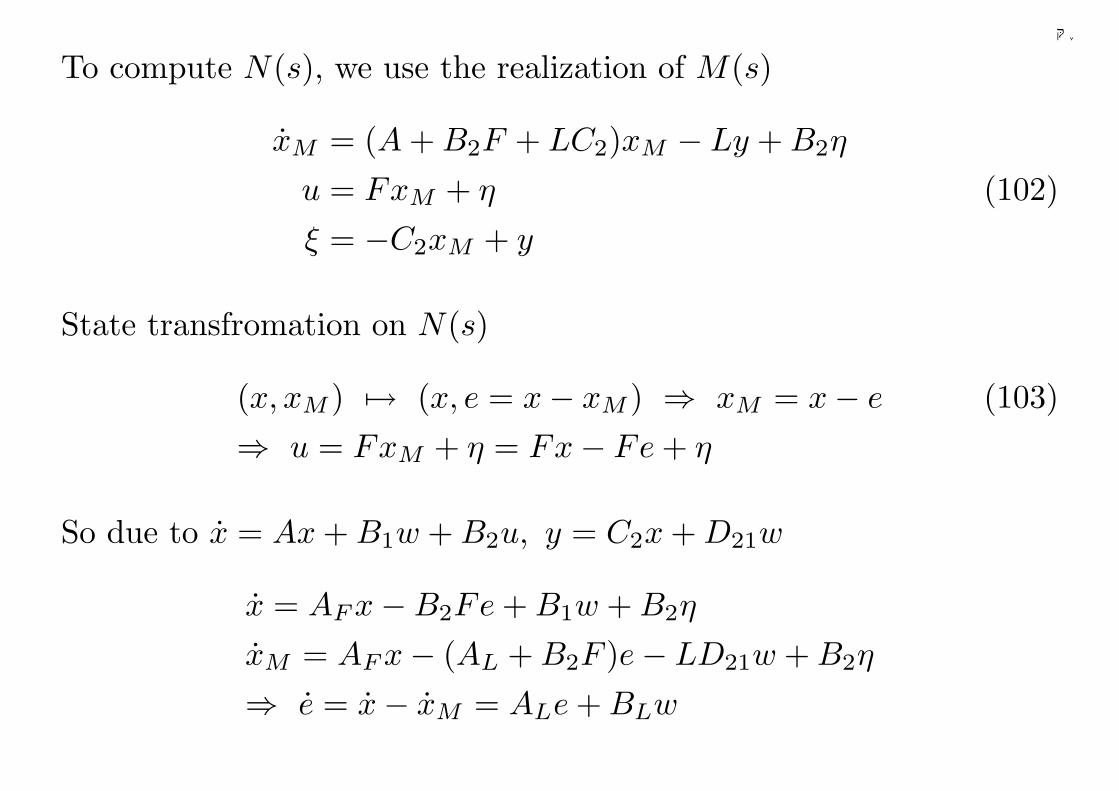
To compute N(s), we use the realization of M(s)
xM = (A + B2F + LC2)xM − Ly + B2η
u = FxM + η (102)ξ = −C2xM + y
State transfromation on N(s)
(x, xM ) 7→ (x, e = x− xM ) ⇒ xM = x− e (103)⇒ u = FxM + η = Fx− Fe + η
So due to x = Ax + B1w + B2u, y = C2x + D21w
x = AF x−B2Fe + B1w + B2η
xM = AF x− (AL + B2F )e− LD21w + B2η
⇒ e = x− xM = ALe + BLw
138
千葉大学
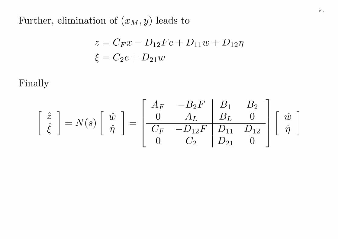
Further, elimination of (xM , y) leads to
z = CF x−D12Fe + D11w + D12η
ξ = C2e + D21w
Finally
[z
ξ
]= N(s)
[wη
]=
AF −B2F B1 B2
0 AL BL 0CF −D12F D11 D12
0 C2 D21 0
[wη
]
139
千葉大学
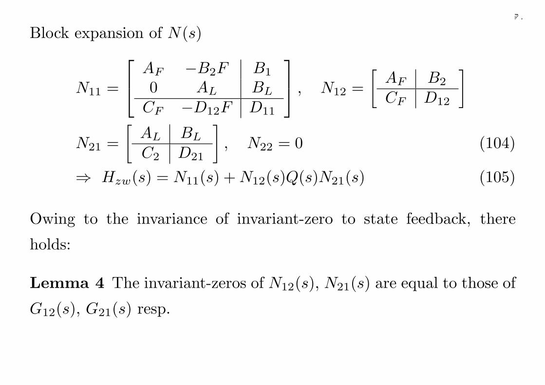
Block expansion of N(s)
N11 =
AF −B2F B1
0 AL BL
CF −D12F D11
, N12 =
[AF B2
CF D12
]
N21 =[
AL BL
C2 D21
], N22 = 0 (104)
⇒ Hzw(s) = N11(s) + N12(s)Q(s)N21(s) (105)
Owing to the invariance of invariant-zero to state feedback, there
holds:
Lemma 4 The invariant-zeros of N12(s), N21(s) are equal to those of
G12(s), G21(s) resp.
140
千葉大学
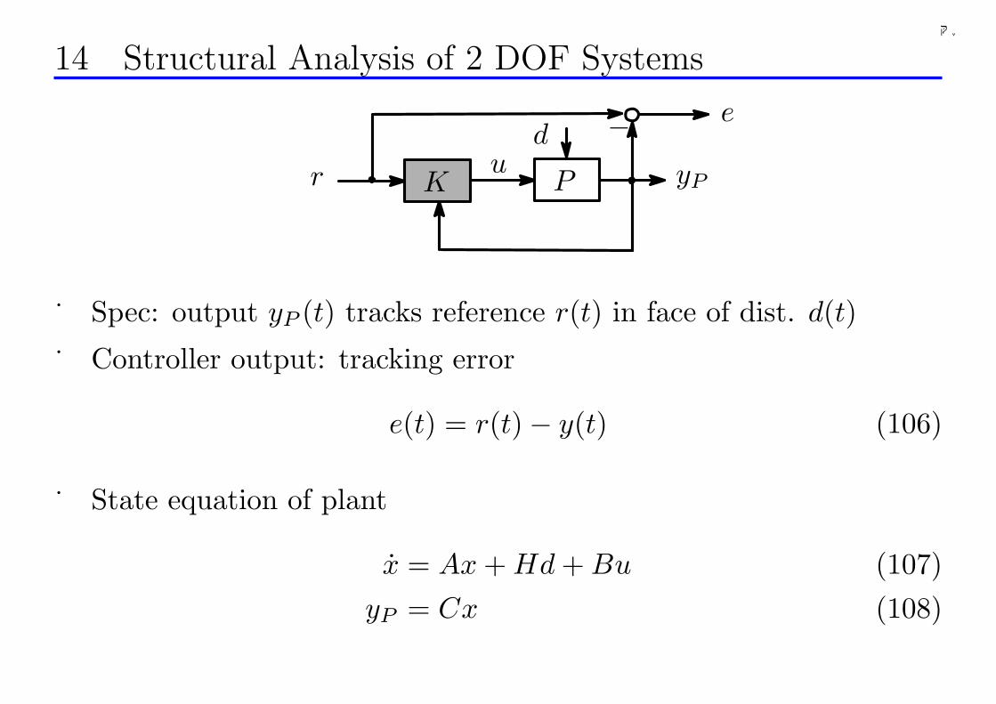
14 Structural Analysis of 2 DOF Systems
K Pr yPu
e−d
Spec: output yP (t) tracks reference r(t) in face of dist. d(t)
Controller output: tracking error
e(t) = r(t)− y(t) (106)
State equation of plant
x = Ax + Hd + Bu (107)yP = Cx (108)
141
千葉大学
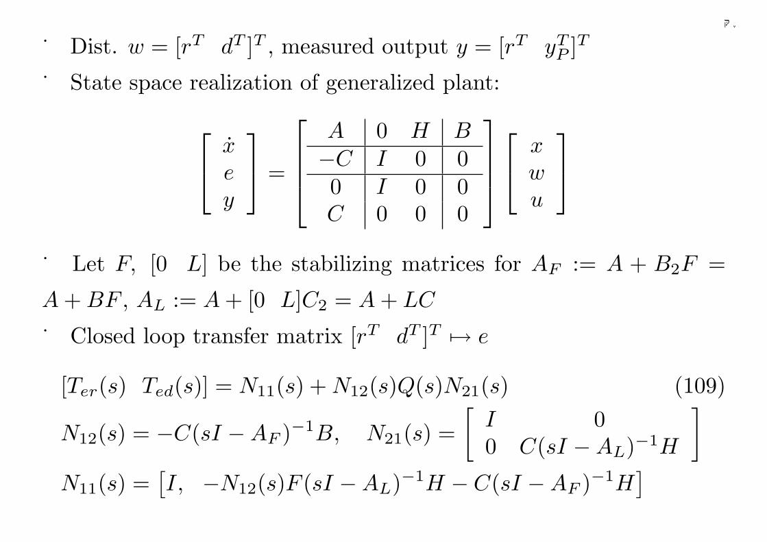
Dist. w = [rT dT ]T , measured output y = [rT yTP ]T
State space realization of generalized plant:
xey
=
A 0 H B−C I 0 00 I 0 0C 0 0 0
xwu
Let F, [0 L] be the stabilizing matrices for AF := A + B2F =
A + BF , AL := A + [0 L]C2 = A + LC
Closed loop transfer matrix [rT dT ]T 7→ e
[Ter(s) Ted(s)] = N11(s) + N12(s)Q(s)N21(s) (109)
N12(s) = −C(sI −AF )−1B, N21(s) =[
I 00 C(sI −AL)−1H
]
N11(s) =[I, −N12(s)F (sI −AL)−1H − C(sI −AF )−1H
]
142
千葉大学
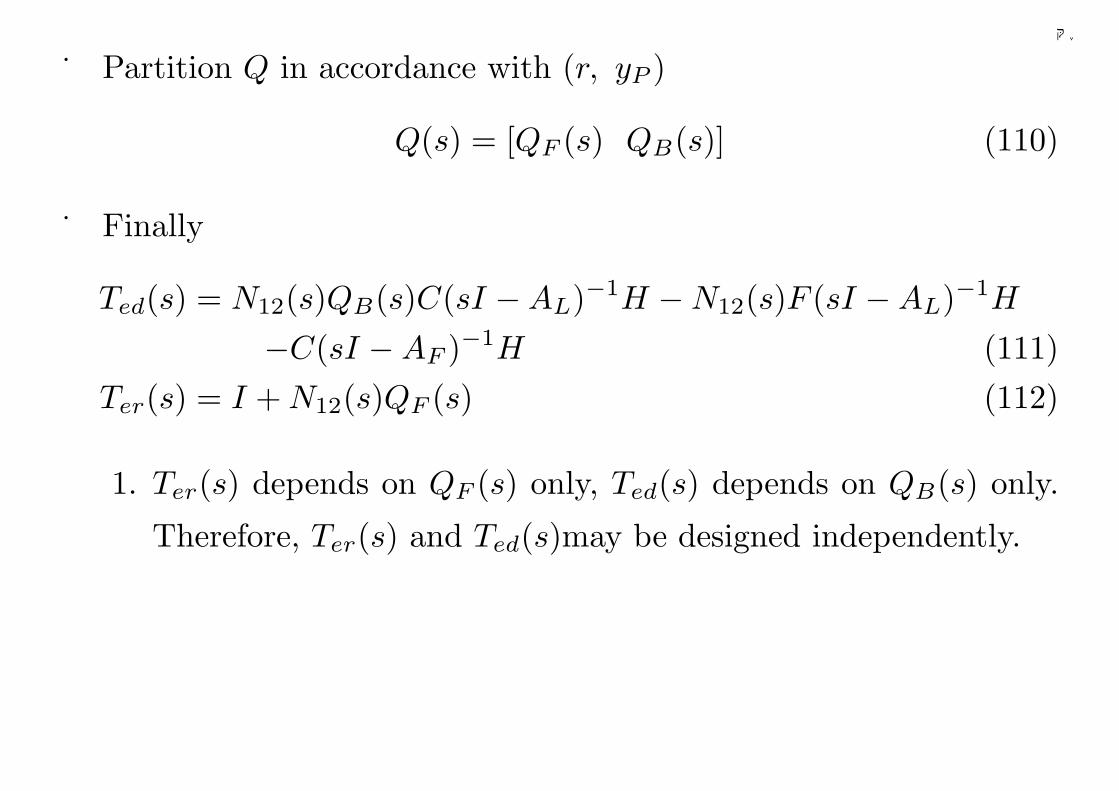
Partition Q in accordance with (r, yP )
Q(s) = [QF (s) QB(s)] (110)
Finally
Ted(s) = N12(s)QB(s)C(sI −AL)−1H −N12(s)F (sI −AL)−1H
−C(sI −AF )−1H (111)Ter(s) = I + N12(s)QF (s) (112)
1. Ter(s) depends on QF (s) only, Ted(s) depends on QB(s) only.
Therefore, Ter(s) and Ted(s)may be designed independently.
143
千葉大学
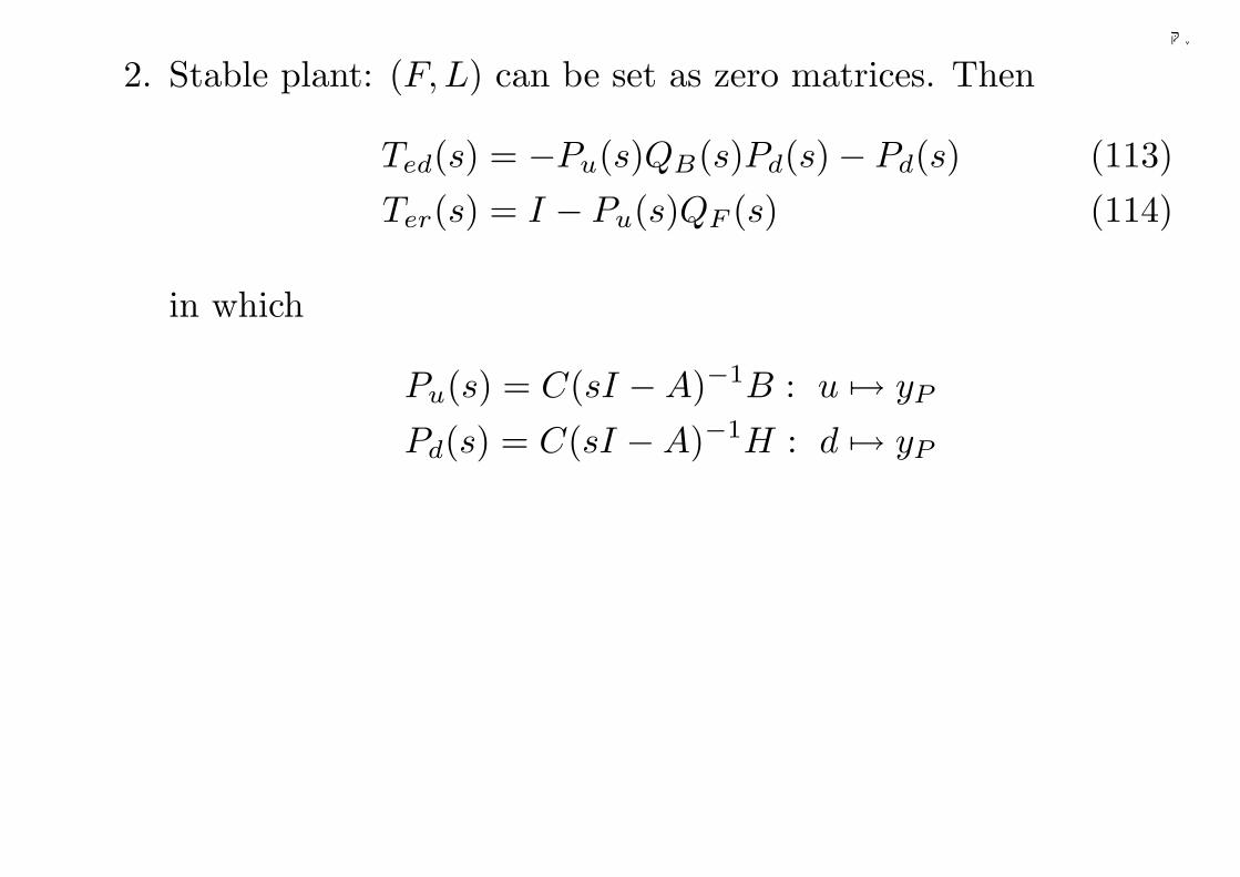
2. Stable plant: (F, L) can be set as zero matrices. Then
Ted(s) = −Pu(s)QB(s)Pd(s)− Pd(s) (113)Ter(s) = I − Pu(s)QF (s) (114)
in which
Pu(s) = C(sI −A)−1B : u 7→ yP
Pd(s) = C(sI −A)−1H : d 7→ yP
144
千葉大学
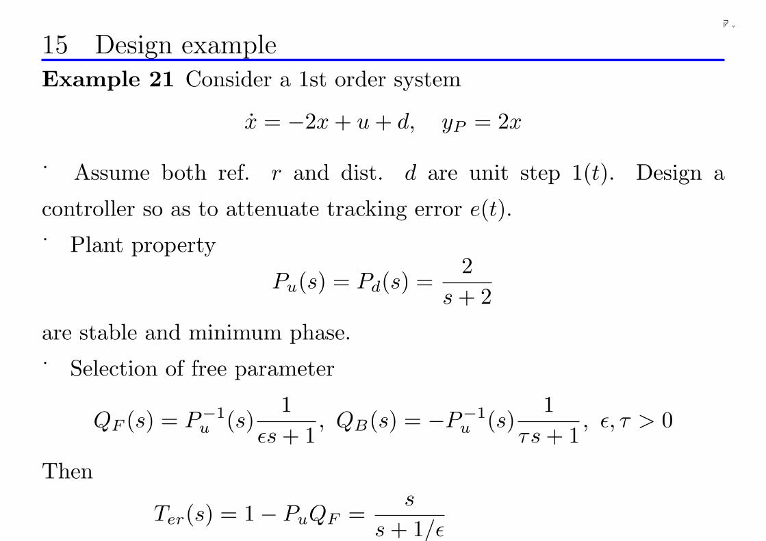
15 Design exampleExample 21 Consider a 1st order system
x = −2x + u + d, yP = 2x
Assume both ref. r and dist. d are unit step 1(t). Design a
controller so as to attenuate tracking error e(t).
Plant property
Pu(s) = Pd(s) =2
s + 2
are stable and minimum phase.
Selection of free parameter
QF (s) = P−1u (s)
1εs + 1
, QB(s) = −P−1u (s)
1τs + 1
, ε, τ > 0
Then
Ter(s) = 1− PuQF =s
s + 1/ε
145
千葉大学
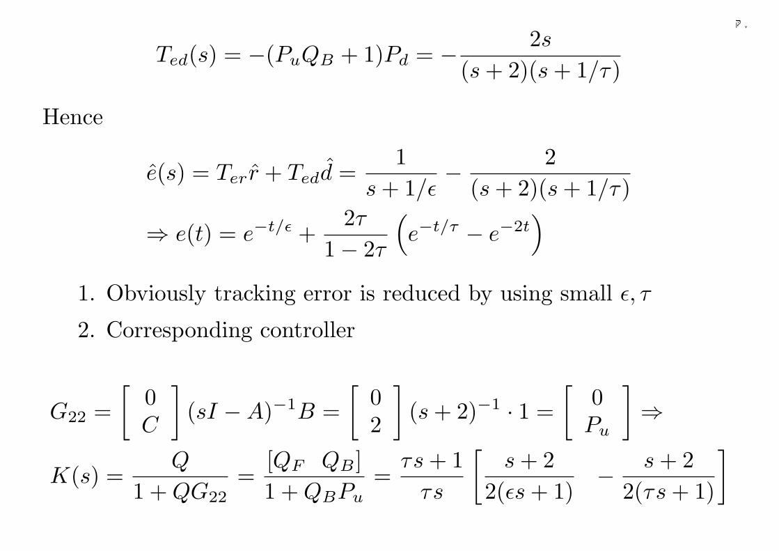
Ted(s) = −(PuQB + 1)Pd = − 2s
(s + 2)(s + 1/τ)
Hence
e(s) = Ter r + Tedd =1
s + 1/ε− 2
(s + 2)(s + 1/τ)
⇒ e(t) = e−t/ε +2τ
1− 2τ
(e−t/τ − e−2t
)
1. Obviously tracking error is reduced by using small ε, τ
2. Corresponding controller
G22 =[
0C
](sI −A)−1B =
[02
](s + 2)−1 · 1 =
[0Pu
]⇒
K(s) =Q
1 + QG22=
[QF QB ]1 + QBPu
=τs + 1
τs
[s + 2
2(εs + 1)− s + 2
2(τs + 1)
]
146
千葉大学
Chapter 4 Algebraic Riccati equation (ARE)
• ARE plays an extremly important role in optimal design
• Properties and computation of solution to ARE
• Bounded real lemma
AREAT X + XA + XRX + Q = 0 (115)
A, Q, R are in Rn×n and QT = Q, RT = R
Since ARE is nonlinear, its solution is not unique!
147
千葉大学
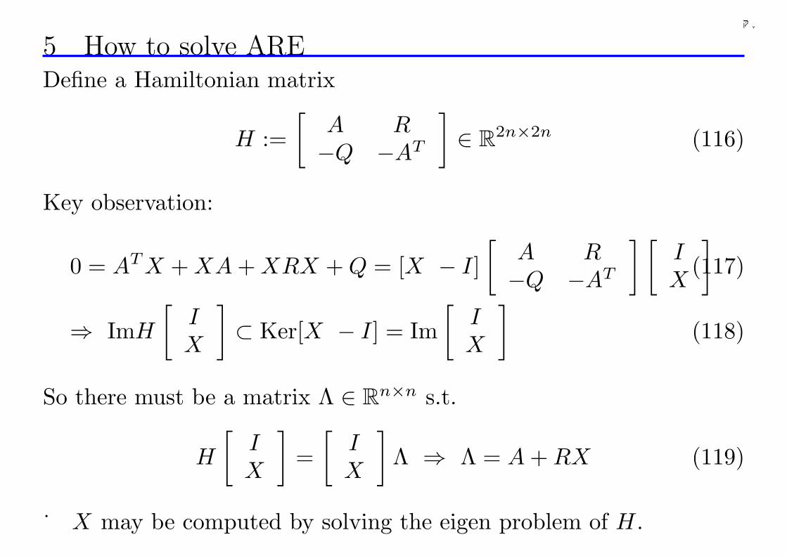
5 How to solve AREDefine a Hamiltonian matrix
H :=[
A R−Q −AT
]∈ R2n×2n (116)
Key observation:
0 = AT X + XA + XRX + Q = [X − I][
A R−Q −AT
] [IX
](117)
⇒ ImH
[IX
]⊂ Ker[X − I] = Im
[IX
](118)
So there must be a matrix Λ ∈ Rn×n s.t.
H
[IX
]=
[IX
]Λ ⇒ Λ = A + RX (119)
X may be computed by solving the eigen problem of H.
148
千葉大学
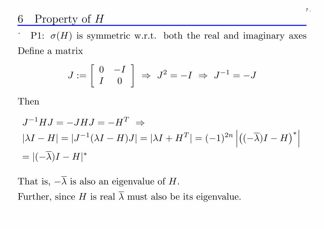
6 Property of H
P1: σ(H) is symmetric w.r.t. both the real and imaginary axes
Define a matrix
J :=[
0 −II 0
]⇒ J2 = −I ⇒ J−1 = −J
Then
J−1HJ = −JHJ = −HT ⇒|λI −H| = |J−1(λI −H)J | = |λI + HT | = (−1)2n
∣∣∣((−λ)I −H
)∗∣∣∣= |(−λ)I −H|∗
That is, −λ is also an eigenvalue of H.
Further, since H is real λ must also be its eigenvalue.
149
千葉大学
-
6
××
× ×
o Re
Im
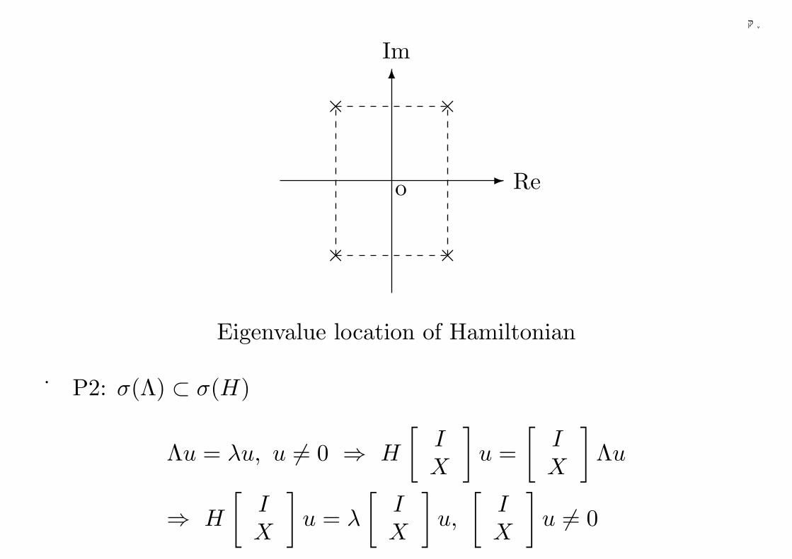
Eigenvalue location of Hamiltonian
P2: σ(Λ) ⊂ σ(H)
Λu = λu, u 6= 0 ⇒ H
[IX
]u =
[IX
]Λu
⇒ H
[IX
]u = λ
[IX
]u,
[IX
]u 6= 0
150
千葉大学
7 Property of X
(JH)T = JH =[
Q AT
A R
], H
[IX
]=
[IX
]Λ
⇒ [I XT ]JH
[IX
]= [I XT ]J
[IX
]Λ = (XT −X)Λ
Due to the symmetry of JH, if
λi(Λ) + λj(Λ) 6= 0,∀i 6= j
then
(XT −X)Λ = [(XT −X)Λ]T
⇒ (XT −X)Λ + ΛT (XT −X) = 0 ⇒ XT −X = 0 (120)
That is, X is symmetric.
151
千葉大学
8 Geometric viewpoint
H
[IX
]=
[IX
]Λ
⇔ ∃|X1| 6= 0, H
[X1
X2
]=
[X1
X2
]X−1
1 ΛX1, X2 = XX1
⇔ HIm[
X1
X2
]⊂ Im
[X1
X2
]
This means that ∃X satisfying (115) iff
∃(X1, X2), |X1| 6= 0 s.t. V := Im[
X1
X2
]is H invariant (121)
Obviously σ(Λ) = σ(X−11 ΛX1) ⊂ σ(H).
152
千葉大学
9 Stabilizing solution X: A + RX stable
Stabilizing solution exists only if H has no eigenvalue on jω axis
∵ σ(A + RX) ⊂ σ(H) and σ(H) is symmetric w.r.t. jω axis
When this condition holds, the eigen space of H w.r.t. all eigenvalues
in LHP forms an invariant subspace X−(H) of H
X−(H) = Im[
X1
X2
], X1, X2 ∈ Rn×n, H
[X1
X2
]=
[X1
X2
]Λ, Λ stable
We know that a solution to ARE exists iff X1 is nonsingular, i.e.
X−(H)⊕ Im[
0I
]= R2n×2n (122)
and the solution is computed as
X := X2X−11 (123)
153
千葉大学
Hence H 7−→ X is a function which will be denoted as Ric
X = Ric(H) (124)
dom(Ric), domain of Ric is composed of such H that satisfies
1. H has no eigenvalue on jω axis
2. The following eq. holds
X−(H)⊕ Im[
0I
]= R2n×2n
154
千葉大学
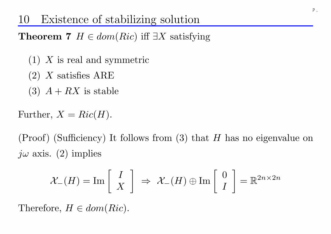
10 Existence of stabilizing solution
Theorem 7 H ∈ dom(Ric) iff ∃X satisfying
(1) X is real and symmetric
(2) X satisfies ARE
(3) A + RX is stable
Further, X = Ric(H).
(Proof) (Sufficiency) It follows from (3) that H has no eigenvalue on
jω axis. (2) implies
X−(H) = Im[
IX
]⇒ X−(H)⊕ Im
[0I
]= R2n×2n
Therefore, H ∈ dom(Ric).
155
千葉大学
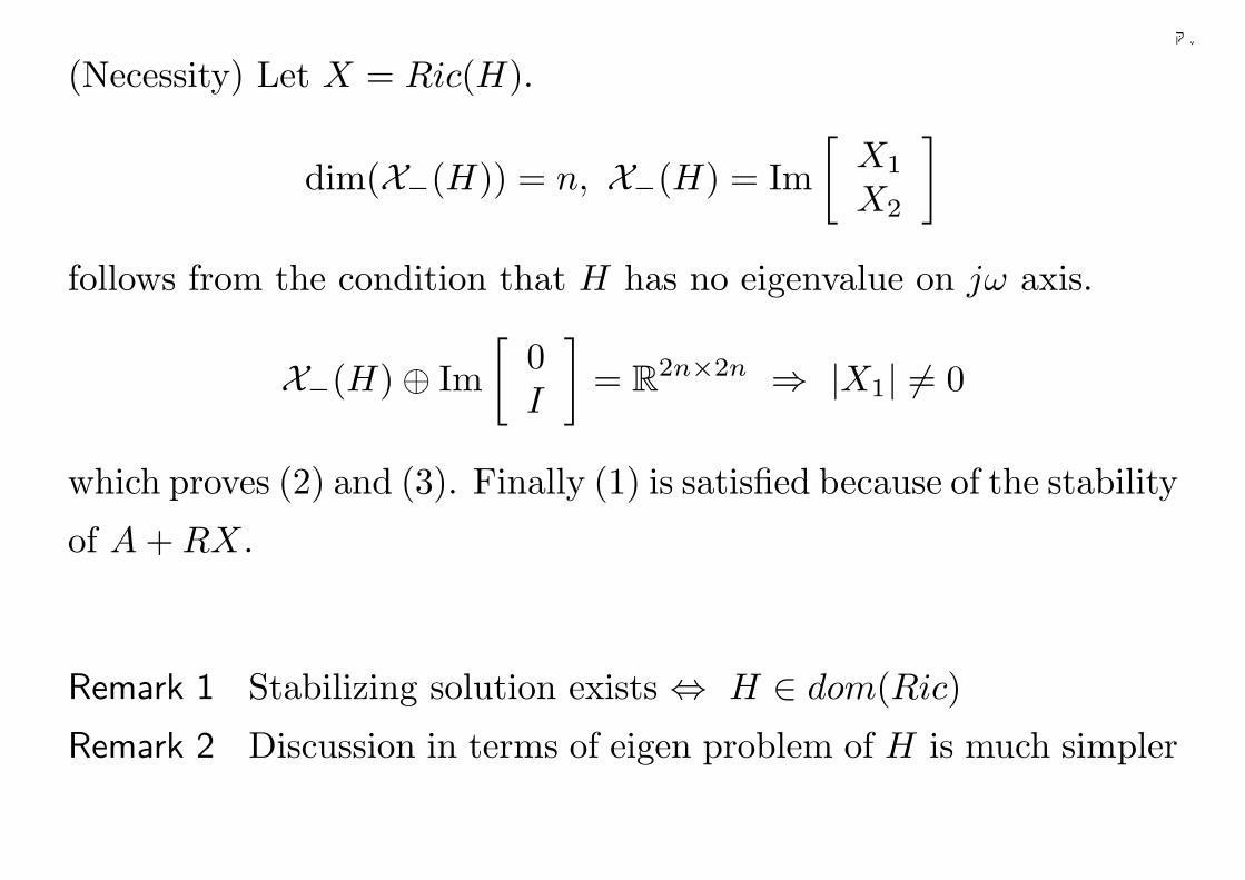
(Necessity) Let X = Ric(H).
dim(X−(H)) = n, X−(H) = Im[
X1
X2
]
follows from the condition that H has no eigenvalue on jω axis.
X−(H)⊕ Im[
0I
]= R2n×2n ⇒ |X1| 6= 0
which proves (2) and (3). Finally (1) is satisfied because of the stability
of A + RX.
Remark 1 Stabilizing solution exists ⇔ H ∈ dom(Ric)
Remark 2 Discussion in terms of eigen problem of H is much simpler
156
千葉大学
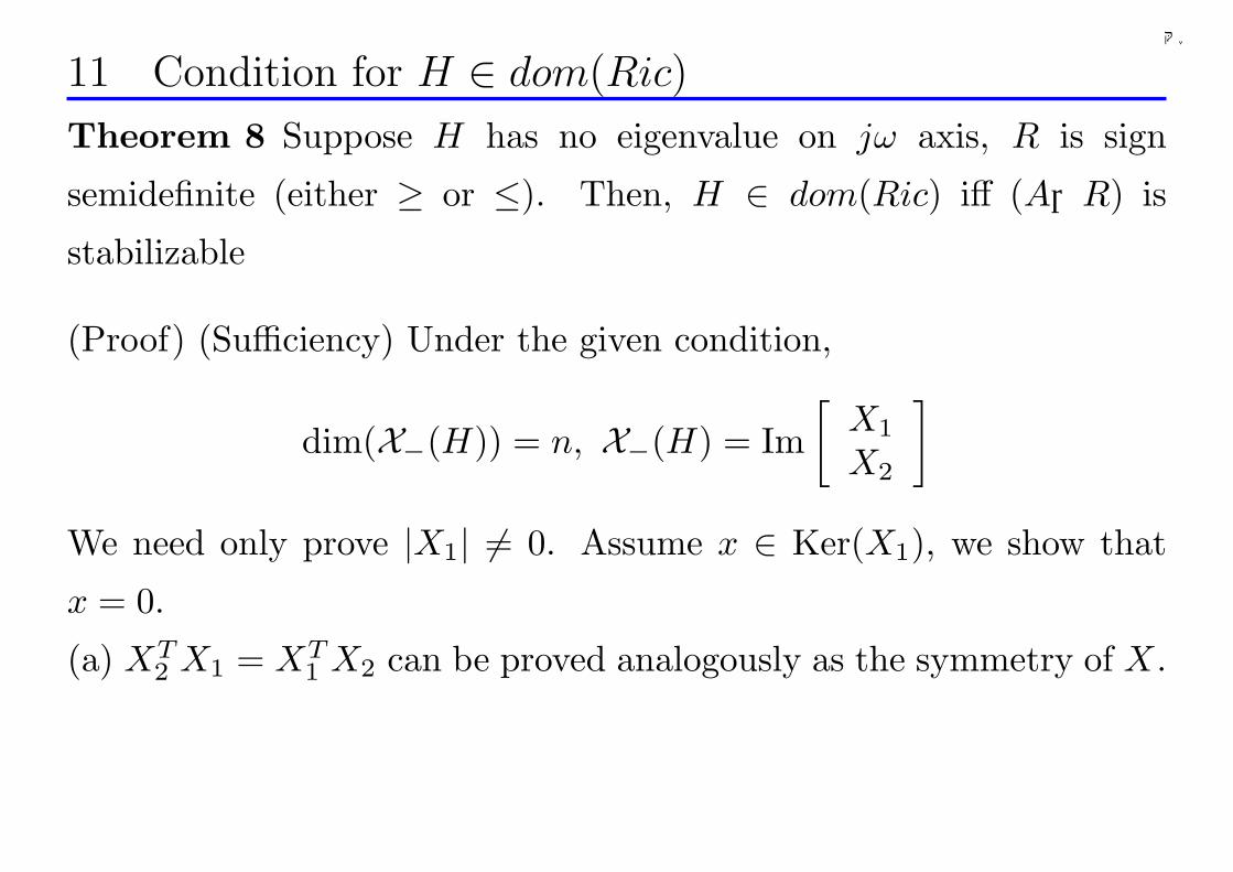
11 Condition for H ∈ dom(Ric)
Theorem 8 Suppose H has no eigenvalue on jω axis, R is sign
semidefinite (either ≥ or ≤). Then, H ∈ dom(Ric) iff (A,R) is
stabilizable
(Proof) (Sufficiency) Under the given condition,
dim(X−(H)) = n, X−(H) = Im[
X1
X2
]
We need only prove |X1| 6= 0. Assume x ∈ Ker(X1), we show that
x = 0.
(a) XT2 X1 = XT
1 X2 can be proved analogously as the symmetry of X.
157
千葉大学
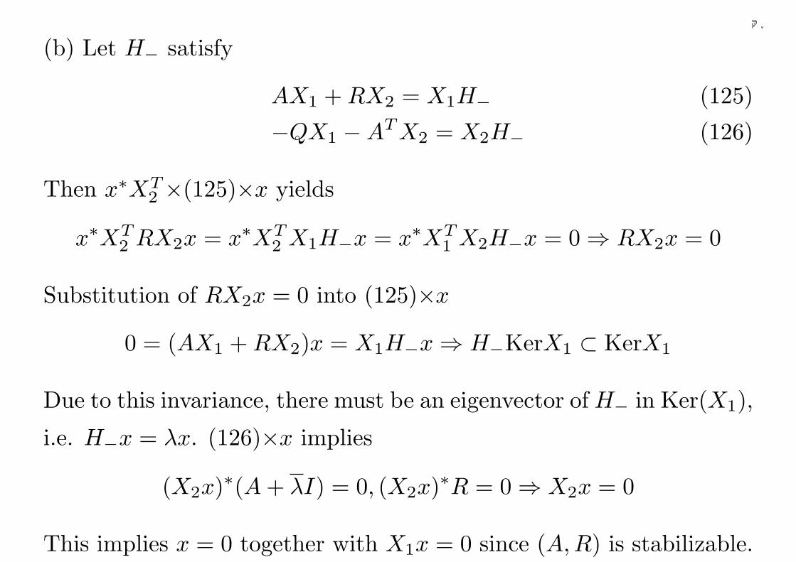
(b) Let H− satisfy
AX1 + RX2 = X1H− (125)
−QX1 −AT X2 = X2H− (126)
Then x∗XT2 ×(125)×x yields
x∗XT2 RX2x = x∗XT
2 X1H−x = x∗XT1 X2H−x = 0 ⇒ RX2x = 0
Substitution of RX2x = 0 into (125)×x
0 = (AX1 + RX2)x = X1H−x ⇒ H−KerX1 ⊂ KerX1
Due to this invariance, there must be an eigenvector of H− in Ker(X1),
i.e. H−x = λx. (126)×x implies
(X2x)∗(A + λI) = 0, (X2x)∗R = 0 ⇒ X2x = 0
This implies x = 0 together with X1x = 0 since (A,R) is stabilizable.
158
千葉大学
(Necessity) H ∈ dom(Ric) ⇒ A + RX is stable which requires the
stabilizability of (A, R).
159
千葉大学
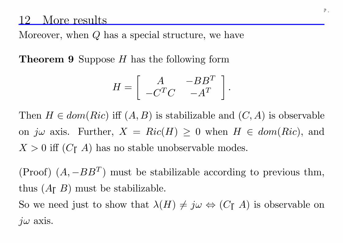
12 More resultsMoreover, when Q has a special structure, we have
Theorem 9 Suppose H has the following form
H =[
A −BBT
−CT C −AT
].
Then H ∈ dom(Ric) iff (A,B) is stabilizable and (C, A) is observable
on jω axis. Further, X = Ric(H) ≥ 0 when H ∈ dom(Ric), and
X > 0 iff (C,A) has no stable unobservable modes.
(Proof) (A,−BBT ) must be stabilizable according to previous thm,
thus (A,B) must be stabilizable.
So we need just to show that λ(H) 6= jω ⇔ (C,A) is observable on
jω axis.
160
千葉大学
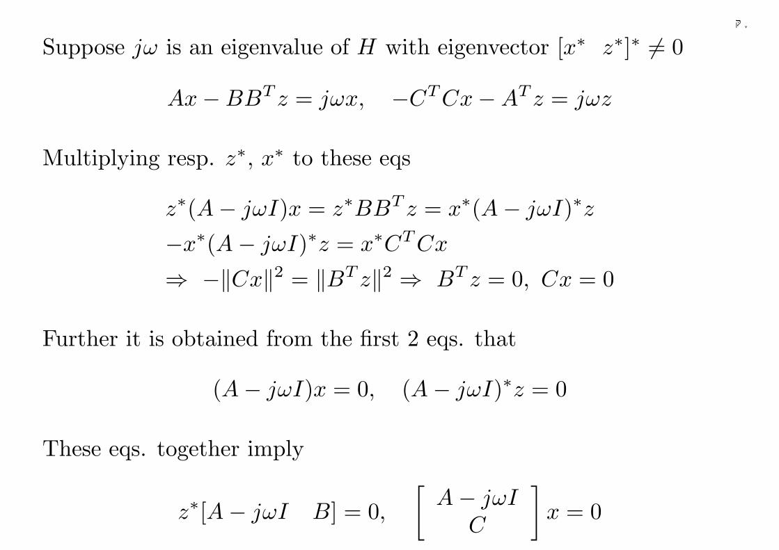
Suppose jω is an eigenvalue of H with eigenvector [x∗ z∗]∗ 6= 0
Ax−BBT z = jωx, −CT Cx−AT z = jωz
Multiplying resp. z∗, x∗ to these eqs
z∗(A− jωI)x = z∗BBT z = x∗(A− jωI)∗z
−x∗(A− jωI)∗z = x∗CT Cx
⇒ −‖Cx‖2 = ‖BT z‖2 ⇒ BT z = 0, Cx = 0
Further it is obtained from the first 2 eqs. that
(A− jωI)x = 0, (A− jωI)∗z = 0
These eqs. together imply
z∗[A− jωI B] = 0,
[A− jωI
C
]x = 0
161
千葉大学
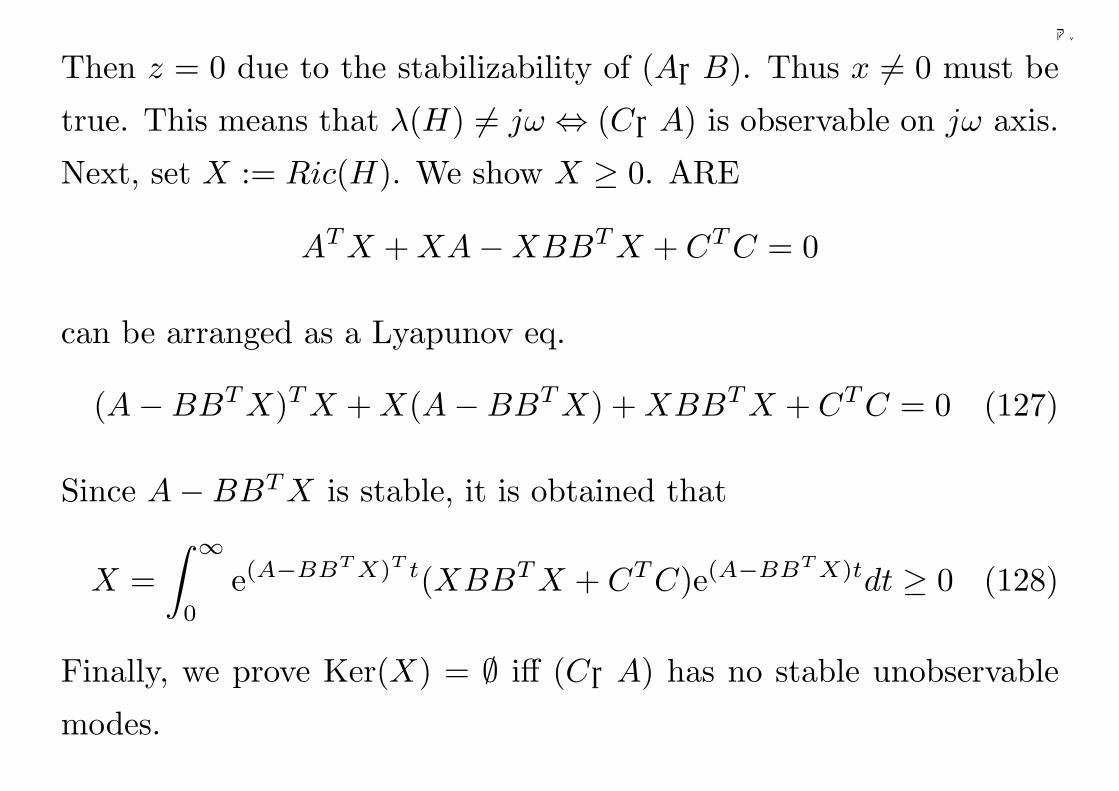
Then z = 0 due to the stabilizability of (A,B). Thus x 6= 0 must be
true. This means that λ(H) 6= jω ⇔ (C,A) is observable on jω axis.
Next, set X := Ric(H). We show X ≥ 0. ARE
AT X + XA−XBBT X + CT C = 0
can be arranged as a Lyapunov eq.
(A−BBT X)T X + X(A−BBT X) + XBBT X + CT C = 0 (127)
Since A−BBT X is stable, it is obtained that
X =∫ ∞
0
e(A−BBT X)T t(XBBT X + CT C)e(A−BBT X)tdt ≥ 0 (128)
Finally, we prove Ker(X) = ∅ iff (C,A) has no stable unobservable
modes.
162
千葉大学
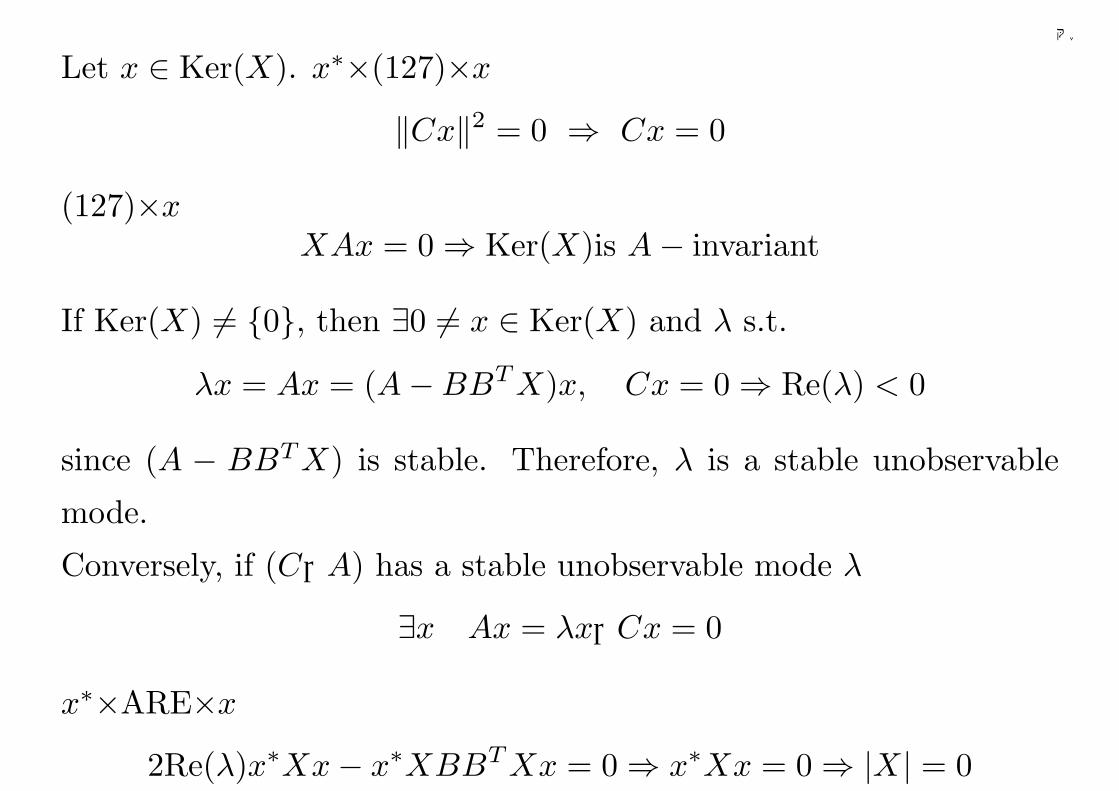
Let x ∈ Ker(X). x∗×(127)×x
‖Cx‖2 = 0 ⇒ Cx = 0
(127)×xXAx = 0 ⇒ Ker(X)is A− invariant
If Ker(X) 6= 0, then ∃0 6= x ∈ Ker(X) and λ s.t.
λx = Ax = (A−BBT X)x, Cx = 0 ⇒ Re(λ) < 0
since (A − BBT X) is stable. Therefore, λ is a stable unobservable
mode.
Conversely, if (C,A) has a stable unobservable mode λ
∃x Ax = λx,Cx = 0
x∗×ARE×x
2Re(λ)x∗Xx− x∗XBBT Xx = 0 ⇒ x∗Xx = 0 ⇒ |X| = 0
163
千葉大学
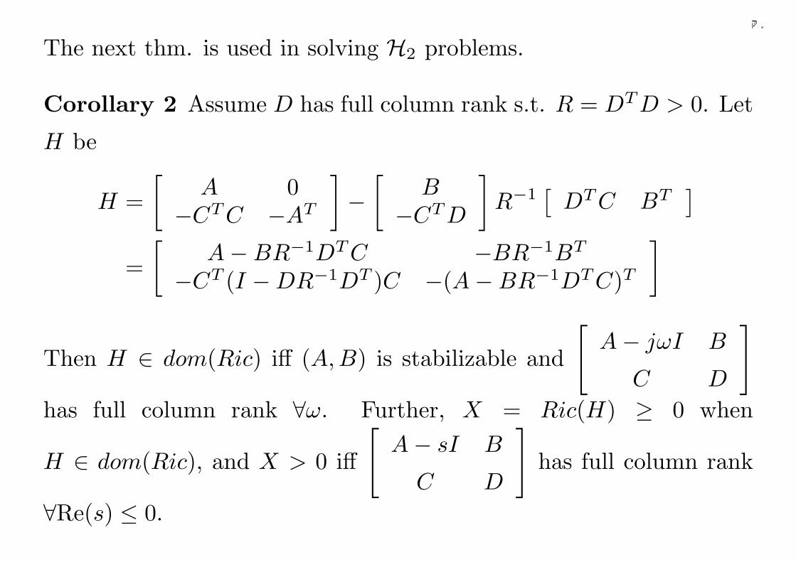
The next thm. is used in solving H2 problems.
Corollary 2 Assume D has full column rank s.t. R = DT D > 0. Let
H be
H =[
A 0−CT C −AT
]−
[B
−CT D
]R−1
[DT C BT
]
=[
A−BR−1DT C −BR−1BT
−CT (I −DR−1DT )C −(A−BR−1DT C)T
]
Then H ∈ dom(Ric) iff (A,B) is stabilizable and
[A− jωI B
C D
]
has full column rank ∀ω. Further, X = Ric(H) ≥ 0 when
H ∈ dom(Ric), and X > 0 iff
[A− sI B
C D
]has full column rank
∀Re(s) ≤ 0.
164
千葉大学
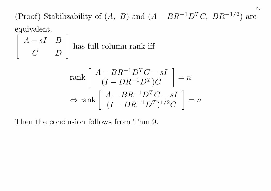
(Proof) Stabilizability of (A, B) and (A − BR−1DT C, BR−1/2) are
equivalent.[A− sI B
C D
]has full column rank iff
rank[
A−BR−1DT C − sI(I −DR−1DT )C
]= n
⇔ rank[
A−BR−1DT C − sI(I −DR−1DT )1/2C
]= n
Then the conclusion follows from Thm.9.
165
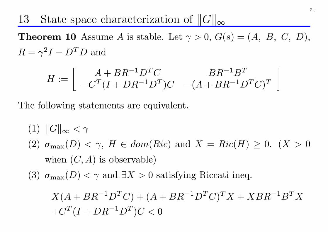
千葉大学
13 State space characterization of ‖G‖∞Theorem 10 Assume A is stable. Let γ > 0, G(s) = (A, B, C, D),
R = γ2I −DT D and
H :=[
A + BR−1DT C BR−1BT
−CT (I + DR−1DT )C −(A + BR−1DT C)T
]
The following statements are equivalent.
(1) ‖G‖∞ < γ
(2) σmax(D) < γ, H ∈ dom(Ric) and X = Ric(H) ≥ 0. (X > 0
when (C, A) is observable)
(3) σmax(D) < γ and ∃X > 0 satisfying Riccati ineq.
X(A + BR−1DT C) + (A + BR−1DT C)T X + XBR−1BT X
+CT (I + DR−1DT )C < 0
166
千葉大学
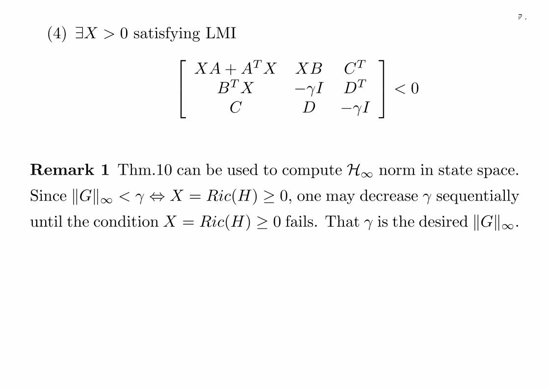
(4) ∃X > 0 satisfying LMI
XA + AT X XB CT
BT X −γI DT
C D −γI
< 0
Remark 1 Thm.10 can be used to compute H∞ norm in state space.
Since ‖G‖∞ < γ ⇔ X = Ric(H) ≥ 0, one may decrease γ sequentially
until the condition X = Ric(H) ≥ 0 fails. That γ is the desired ‖G‖∞.
167
千葉大学
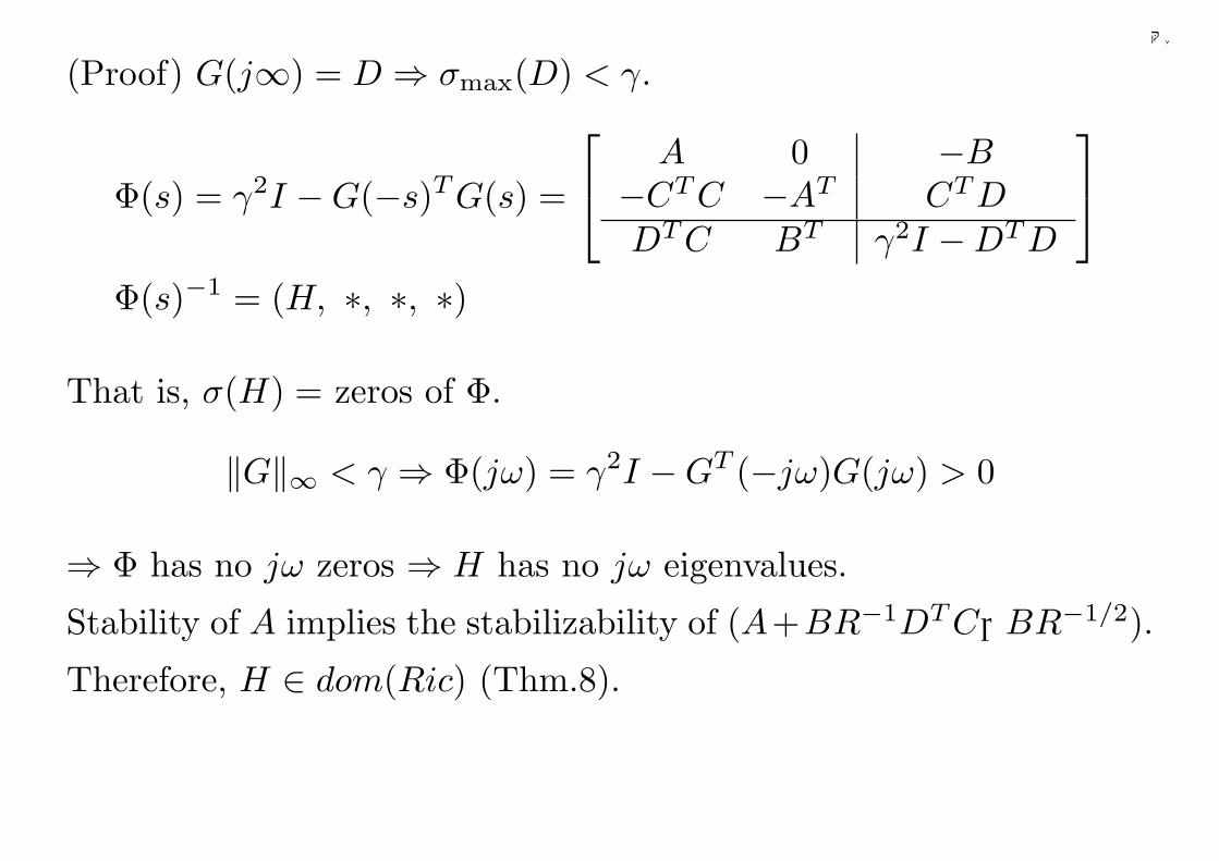
(Proof) G(j∞) = D ⇒ σmax(D) < γ.
Φ(s) = γ2I −G(−s)T G(s) =
A 0 −B−CT C −AT CT DDT C BT γ2I −DT D
Φ(s)−1 = (H, ∗, ∗, ∗)
That is, σ(H) = zeros of Φ.
‖G‖∞ < γ ⇒ Φ(jω) = γ2I −GT (−jω)G(jω) > 0
⇒ Φ has no jω zeros ⇒ H has no jω eigenvalues.
Stability of A implies the stabilizability of (A+BR−1DT C,BR−1/2).
Therefore, H ∈ dom(Ric) (Thm.8).
168
千葉大学
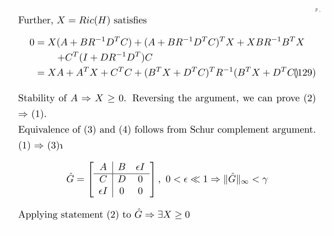
Further, X = Ric(H) satisfies
0 = X(A + BR−1DT C) + (A + BR−1DT C)T X + XBR−1BT X
+CT (I + DR−1DT )C
= XA + AT X + CT C + (BT X + DT C)T R−1(BT X + DT C)(129)
Stability of A ⇒ X ≥ 0. Reversing the argument, we can prove (2)
⇒ (1).
Equivalence of (3) and (4) follows from Schur complement argument.
(1) ⇒ (3):
G =
A B εIC D 0εI 0 0
, 0 < ε ¿ 1 ⇒ ‖G‖∞ < γ
Applying statement (2) to G ⇒ ∃X ≥ 0
169
千葉大学
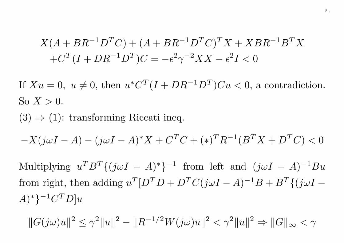
X(A + BR−1DT C) + (A + BR−1DT C)T X + XBR−1BT X
+CT (I + DR−1DT )C = −ε2γ−2XX − ε2I < 0
If Xu = 0, u 6= 0, then u∗CT (I + DR−1DT )Cu < 0, a contradiction.
So X > 0.
(3) ⇒ (1): transforming Riccati ineq.
−X(jωI −A)− (jωI −A)∗X + CT C + (∗)T R−1(BT X + DT C) < 0
Multiplying uT BT (jωI − A)∗−1 from left and (jωI − A)−1Bu
from right, then adding uT [DT D + DT C(jωI −A)−1B + BT (jωI −A)∗−1CT D]u
‖G(jω)u‖2 ≤ γ2‖u‖2 − ‖R−1/2W (jω)u‖2 < γ2‖u‖2 ⇒ ‖G‖∞ < γ
170
千葉大学
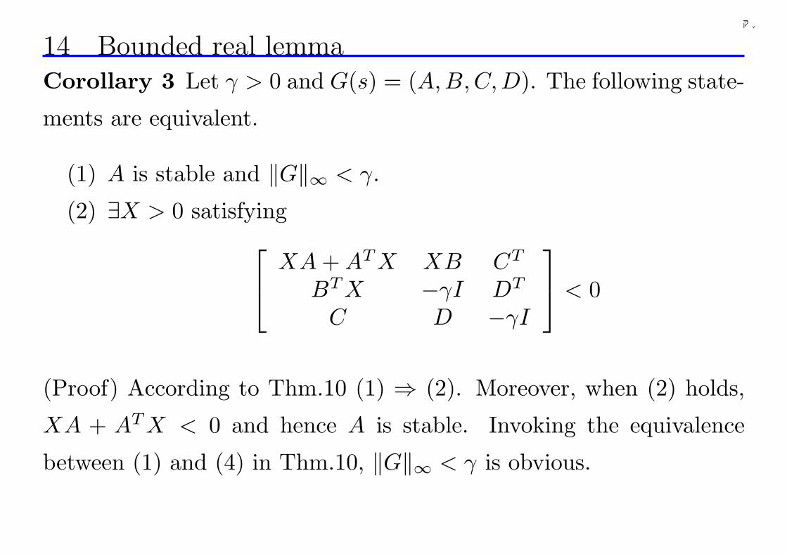
14 Bounded real lemmaCorollary 3 Let γ > 0 and G(s) = (A,B, C, D). The following state-
ments are equivalent.
(1) A is stable and ‖G‖∞ < γ.
(2) ∃X > 0 satisfying
XA + AT X XB CT
BT X −γI DT
C D −γI
< 0
(Proof) According to Thm.10 (1) ⇒ (2). Moreover, when (2) holds,
XA + AT X < 0 and hence A is stable. Invoking the equivalence
between (1) and (4) in Thm.10, ‖G‖∞ < γ is obvious.
171
千葉大学
Remark 2 This corollary is called the bounded real lemma which
plays the central role in solving H∞ directly in state space.
172
千葉大学
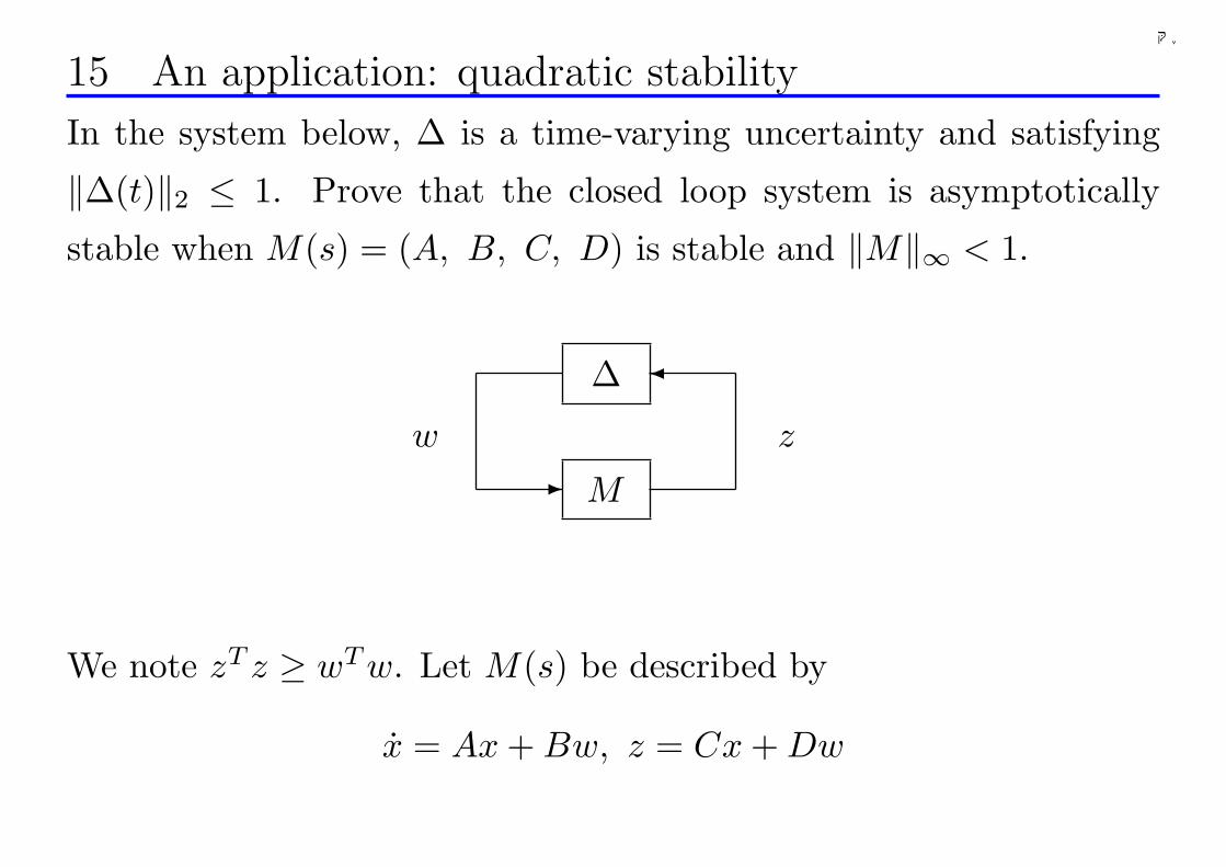
15 An application: quadratic stability
In the system below, ∆ is a time-varying uncertainty and satisfying
‖∆(t)‖2 ≤ 1. Prove that the closed loop system is asymptotically
stable when M(s) = (A, B, C, D) is stable and ‖M‖∞ < 1.
∆
M
¾
-zw
We note zT z ≥ wT w. Let M(s) be described by
x = Ax + Bw, z = Cx + Dw
173
千葉大学
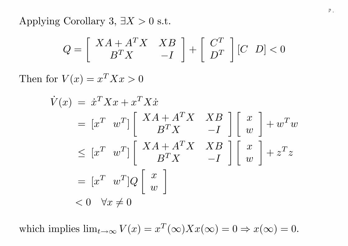
Applying Corollary 3, ∃X > 0 s.t.
Q =[
XA + AT X XBBT X −I
]+
[CT
DT
][C D] < 0
Then for V (x) = xT Xx > 0
V (x) = xT Xx + xT Xx
= [xT wT ][
XA + AT X XBBT X −I
] [xw
]+ wT w
≤ [xT wT ][
XA + AT X XBBT X −I
] [xw
]+ zT z
= [xT wT ]Q[
xw
]
< 0 ∀x 6= 0
which implies limt→∞ V (x) = xT (∞)Xx(∞) = 0 ⇒ x(∞) = 0.
174
千葉大学
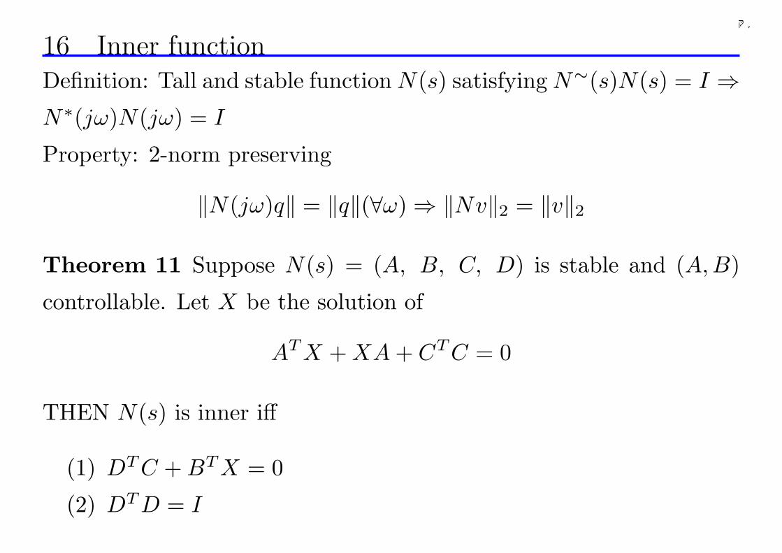
16 Inner functionDefinition: Tall and stable function N(s) satisfying N∼(s)N(s) = I ⇒N∗(jω)N(jω) = I
Property: 2-norm preserving
‖N(jω)q‖ = ‖q‖(∀ω) ⇒ ‖Nv‖2 = ‖v‖2
Theorem 11 Suppose N(s) = (A, B, C, D) is stable and (A,B)
controllable. Let X be the solution of
AT X + XA + CT C = 0
THEN N(s) is inner iff
(1) DT C + BT X = 0
(2) DT D = I
175
千葉大学
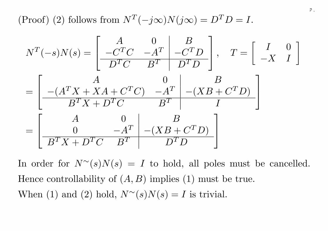
(Proof) (2) follows from NT (−j∞)N(j∞) = DT D = I.
NT (−s)N(s) =
A 0 B−CT C −AT −CT DDT C BT DT D
, T =
[I 0−X I
]
=
A 0 B−(AT X + XA + CT C) −AT −(XB + CT D)
BT X + DT C BT I
=
A 0 B0 −AT −(XB + CT D)
BT X + DT C BT DT D
In order for N∼(s)N(s) = I to hold, all poles must be cancelled.
Hence controllability of (A,B) implies (1) must be true.
When (1) and (2) hold, N∼(s)N(s) = I is trivial.
176
千葉大学
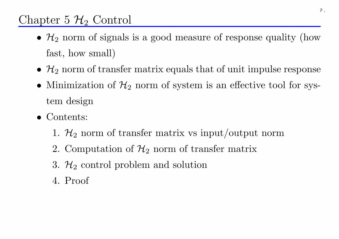
Chapter 5 H2 Control
• H2 norm of signals is a good measure of response quality (how
fast, how small)
• H2 norm of transfer matrix equals that of unit impulse response
• Minimization of H2 norm of system is an effective tool for sys-
tem design
• Contents:
1. H2 norm of transfer matrix vs input/output norm
2. Computation of H2 norm of transfer matrix
3. H2 control problem and solution
4. Proof
177
千葉大学
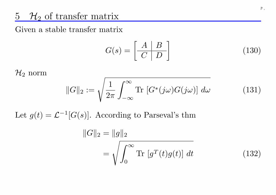
5 H2 of transfer matrix
Given a stable transfer matrix
G(s) =[
A BC D
](130)
H2 norm
‖G‖2 :=
√12π
∫ ∞
−∞Tr [G∗(jω)G(jω)] dω (131)
Let g(t) = L−1[G(s)]. According to Parseval’s thm
‖G‖2 = ‖g‖2
=
√∫ ∞
0
Tr [gT (t)g(t)] dt (132)
178
千葉大学
6 Input/output relationship
SISO case:
Output response to unit impulse is y(t) = g(t). So ‖G‖2 = ‖g‖2implies that the H2 norm of a transfer function is equal to that of its
impulse response.
MIMO case:
Consider a system having m inputs. Let ui (i = 1, . . . , m) be an
orthonormal set in Rm, i.e.
U = [u1, · · · , um], UT U = UUT = I
Output response to impulse input wi(t) = uiδ(t) is yi(t) = g(t)ui.
179
千葉大学
m∑
i=1
‖yi‖22 =m∑
i=1
∫ ∞
0
yTi (t)yi(t) dt =
m∑
i=1
∫ ∞
0
uTi gT (t)g(t)ui dt
=∫ ∞
0
m∑
i=1
Tr(gT (t)g(t)uiu
Ti
)dt
=∫ ∞
0
Tr(gT (t)g(t)UUT
)dt =
∫ ∞
0
Tr(gT (t)g(t)
)dt
= ‖G‖22
(Tr (AB) = Tr (BA) and∑
Tr (Ai) = Tr (∑
Ai) used)
⇒ H2 norm square of transfer matrix equals sum of H2 norm square
of responses to orthonormal impulse input set.
Further,
‖G‖22 =∫ ∞
0
Tr(g(t)gT (t)
)dt
180
千葉大学
7 Alternative interpretation
H2 norm of a trasnfer matrix equals steady-state square-mean of re-
sponse to unit vector white noise
White noise:
E[u(t)] = 0 ∀t, E[u(t)u(τ)T ] = δ(t− τ)I (133)
Then E[y(t)] = 0 and
E(y(t)T y(t)
)= E
(∫ t
0
∫ t
0
(g(t− α)u(α))T g(t− β)u(β)dαdβ
)
= E(∫ t
0
∫ t
0
Tr(g(t− α)T g(t− β)u(β)u(α)T
)dαdβ
)
=∫ t
0
∫ t
0
Tr(g(t− α)T g(t− β)E
(u(β)u(α)T
))dαdβ
181
千葉大学
=∫ t
0
∫ t
0
Tr(g(t− α)T g(t− β)× δ(β − α)I
)dαdβ
=∫ t
0
Tr(g(t− β)T g(t− β)
)dβ
=∫ t
0
Tr(g(τ)T g(τ)
)dτ (τ = t− β)
(∫ t
0f(τ)δ(τ − α)dτ = f(α) (α ∈ [0, t]) used)
Thereforelim
t→∞E
(y(t)T y(t)
)= ‖G‖22 (134)
For this reason, in the design of filters whose main purpose is to to filter
out noise from measuered data, H2 method is extremely powerful.
182
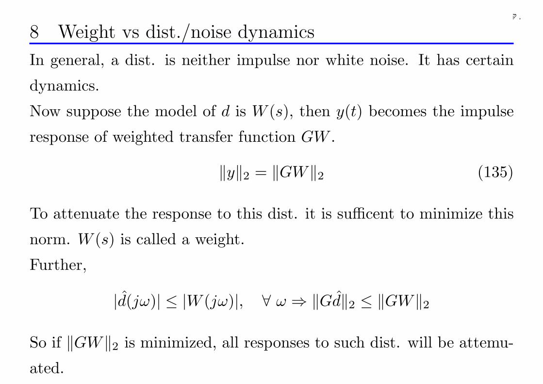
千葉大学
8 Weight vs dist./noise dynamics
In general, a dist. is neither impulse nor white noise. It has certain
dynamics.
Now suppose the model of d is W (s), then y(t) becomes the impulse
response of weighted transfer function GW .
‖y‖2 = ‖GW‖2 (135)
To attenuate the response to this dist. it is sufficent to minimize this
norm. W (s) is called a weight.
Further,
|d(jω)| ≤ |W (jω)|, ∀ ω ⇒ ‖Gd‖2 ≤ ‖GW‖2
So if ‖GW‖2 is minimized, all responses to such dist. will be attemu-
ated.
183
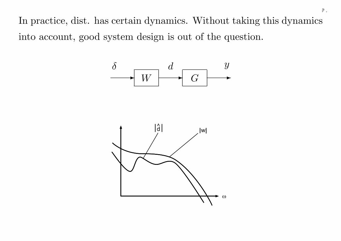
千葉大学
In practice, dist. has certain dynamics. Without taking this dynamics
into account, good system design is out of the question.
G- -yd
W-δ
w
w
^d
184
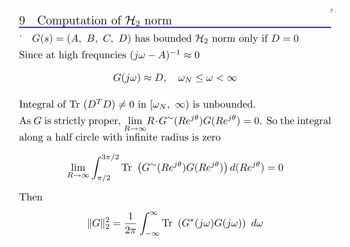
千葉大学
9 Computation of H2 norm
G(s) = (A, B, C, D) has bounded H2 norm only if D = 0
Since at high frequncies (jω −A)−1 ≈ 0
G(jω) ≈ D, ωN ≤ ω < ∞
Integral of Tr (DT D) 6= 0 in [ωN , ∞) is unbounded.
As G is strictly proper, limR→∞
R·G∼(Rejθ)G(Rejθ) = 0. So the integral
along a half circle with infinite radius is zero
limR→∞
∫ 3π/2
π/2
Tr(G∼(Rejθ)G(Rejθ)
)d(Rejθ) = 0
Then
‖G‖22 =12π
∫ ∞
−∞Tr (G∗(jω)G(jω)) dω
185
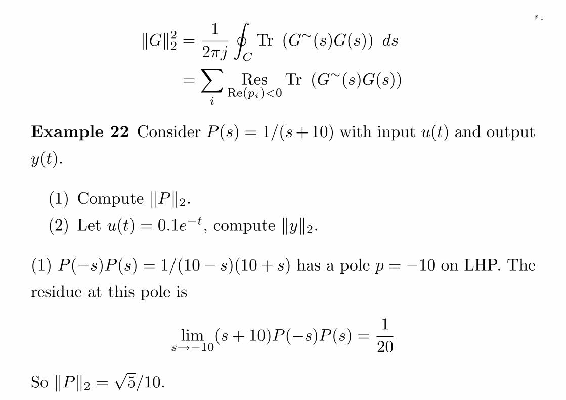
千葉大学
‖G‖22 =1
2πj
∮
C
Tr (G∼(s)G(s)) ds
=∑
i
ResRe(pi)<0
Tr (G∼(s)G(s))
Example 22 Consider P (s) = 1/(s+10) with input u(t) and output
y(t).
(1) Compute ‖P‖2.(2) Let u(t) = 0.1e−t, compute ‖y‖2.
(1) P (−s)P (s) = 1/(10− s)(10 + s) has a pole p = −10 on LHP. The
residue at this pole is
lims→−10
(s + 10)P (−s)P (s) =120
So ‖P‖2 =√
5/10.
186
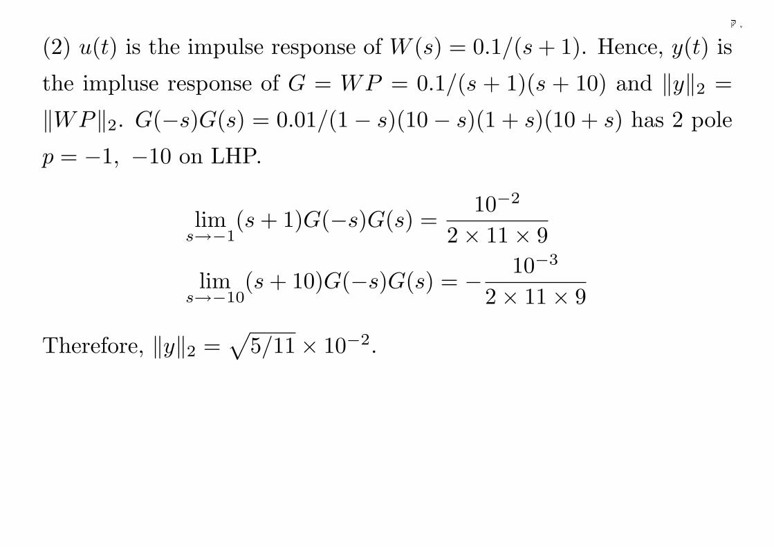
千葉大学
(2) u(t) is the impulse response of W (s) = 0.1/(s + 1). Hence, y(t) is
the impluse response of G = WP = 0.1/(s + 1)(s + 10) and ‖y‖2 =
‖WP‖2. G(−s)G(s) = 0.01/(1− s)(10− s)(1 + s)(10 + s) has 2 pole
p = −1, −10 on LHP.
lims→−1
(s + 1)G(−s)G(s) =10−2
2× 11× 9
lims→−10
(s + 10)G(−s)G(s) = − 10−3
2× 11× 9
Therefore, ‖y‖2 =√
5/11× 10−2.
187
千葉大学
10 State space method
Lemma 5 Suppose A is stable in G(s) = (A, B, C, 0). Then
‖G‖22 = Trace(BT LoB) = Trace(CLcCT ) (136)
in which Lc/Lo are controllability/observability gramian satisfying
Lyapunov eqs.
ALc + LcAT + BBT = 0 AT Lo + LoA + CT C = 0
(Proof) Inverse Laplace transform of G
g(t) = L−1(G) = CeAtB (t ≥ 0)
So
‖G‖22 =∫ ∞
0
Tr(g(t)gT (t)
)dt =
∫ ∞
0
Tr(CeAtBBT eAT tCT
)dt
= Tr (C(∫ ∞
0
eAtBBT eAT t dt
)CT ) = Tr (CLcC
T )
188
千葉大学
Controllability gramian
Lc =∫ ∞
0
eAtBBT eAT t dt ⇒
ALc + LcAT + BBT
=∫ ∞
0
AeAtBBT eAT t dt +∫ ∞
0
eAtBBT eAT tAT dt + BBT
=∫ ∞
0
d
dt(eAtBBT eAT t) dt + BBT
= −e0BBT e0 + BBT
= 0
The other formula follows from ‖G‖22 =∫∞0
Tr(gT g
)dt.
189
千葉大学
11 Condition for ‖G‖2 < γ
The next lemma is fundamental for solving singular H2 problems.
Lemma 6 The following statements are equivalent.
(1) A is stable and ‖C(sI −A)−1B‖2 < γ.
(2) ∃X = XT > 0 satisfying
XA + AT X + CT C < 0 (137)
Tr (BT XB) < γ2 (138)
(3) ∃X = XT ,W = WT satisfying[
XA + AT X CT
C −I
]< 0 (139)
[W BT
B X−1
]> 0 (140)
Tr (W ) < γ2 (141)
190
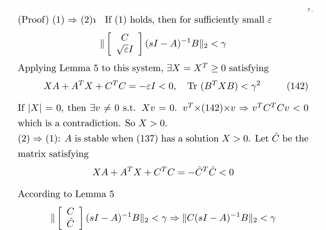
千葉大学
(Proof) (1) ⇒ (2): If (1) holds, then for sufficiently small ε
‖[
C√εI
](sI −A)−1B‖2 < γ
Applying Lemma 5 to this system, ∃X = XT ≥ 0 satisfying
XA + AT X + CT C = −εI < 0, Tr (BT XB) < γ2 (142)
If |X| = 0, then ∃v 6= 0 s.t. Xv = 0. vT×(142)×v ⇒ vT CT Cv < 0
which is a contradiction. So X > 0.
(2) ⇒ (1): A is stable when (137) has a solution X > 0. Let C be the
matrix satisfying
XA + AT X + CT C = −CT C < 0
According to Lemma 5
‖[
C
C
](sI −A)−1B‖2 < γ ⇒ ‖C(sI −A)−1B‖2 < γ
191
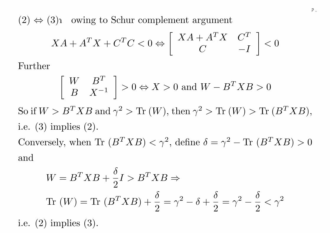
千葉大学
(2) ⇔ (3): owing to Schur complement argument
XA + AT X + CT C < 0 ⇔[
XA + AT X CT
C −I
]< 0
Further [W BT
B X−1
]> 0 ⇔ X > 0 and W −BT XB > 0
So if W > BT XB and γ2 > Tr (W ), then γ2 > Tr (W ) > Tr (BT XB),
i.e. (3) implies (2).
Conversely, when Tr (BT XB) < γ2, define δ = γ2 − Tr (BT XB) > 0
and
W = BT XB +δ
2I > BT XB ⇒
Tr (W ) = Tr (BT XB) +δ
2= γ2 − δ +
δ
2= γ2 − δ
2< γ2
i.e. (2) implies (3).
192
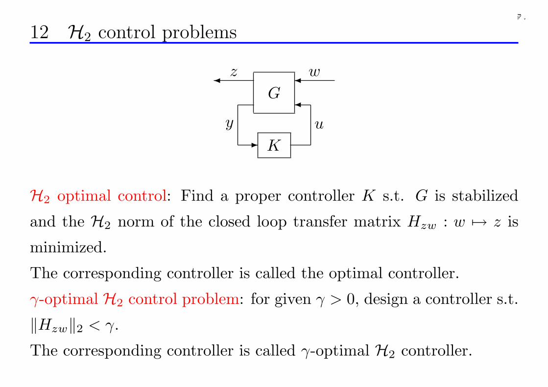
千葉大学
12 H2 control problems
G
K
z
y
w
u
¾ ¾
¾
-
H2 optimal control: Find a proper controller K s.t. G is stabilized
and the H2 norm of the closed loop transfer matrix Hzw : w 7→ z is
minimized.
The corresponding controller is called the optimal controller.
γ-optimal H2 control problem: for given γ > 0, design a controller s.t.
‖Hzw‖2 < γ.
The corresponding controller is called γ-optimal H2 controller.
193
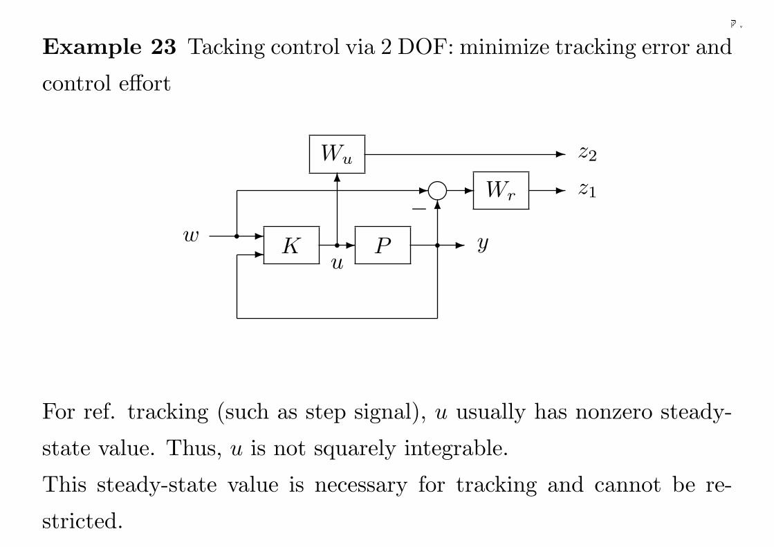
千葉大学
Example 23 Tacking control via 2 DOF: minimize tracking error and
control effort
Wr
--
-
- -6
- -g
qq−
y
z1
wu
PK
Wu
6
q
- z2
For ref. tracking (such as step signal), u usually has nonzero steady-
state value. Thus, u is not squarely integrable.
This steady-state value is necessary for tracking and cannot be re-
stricted.
194
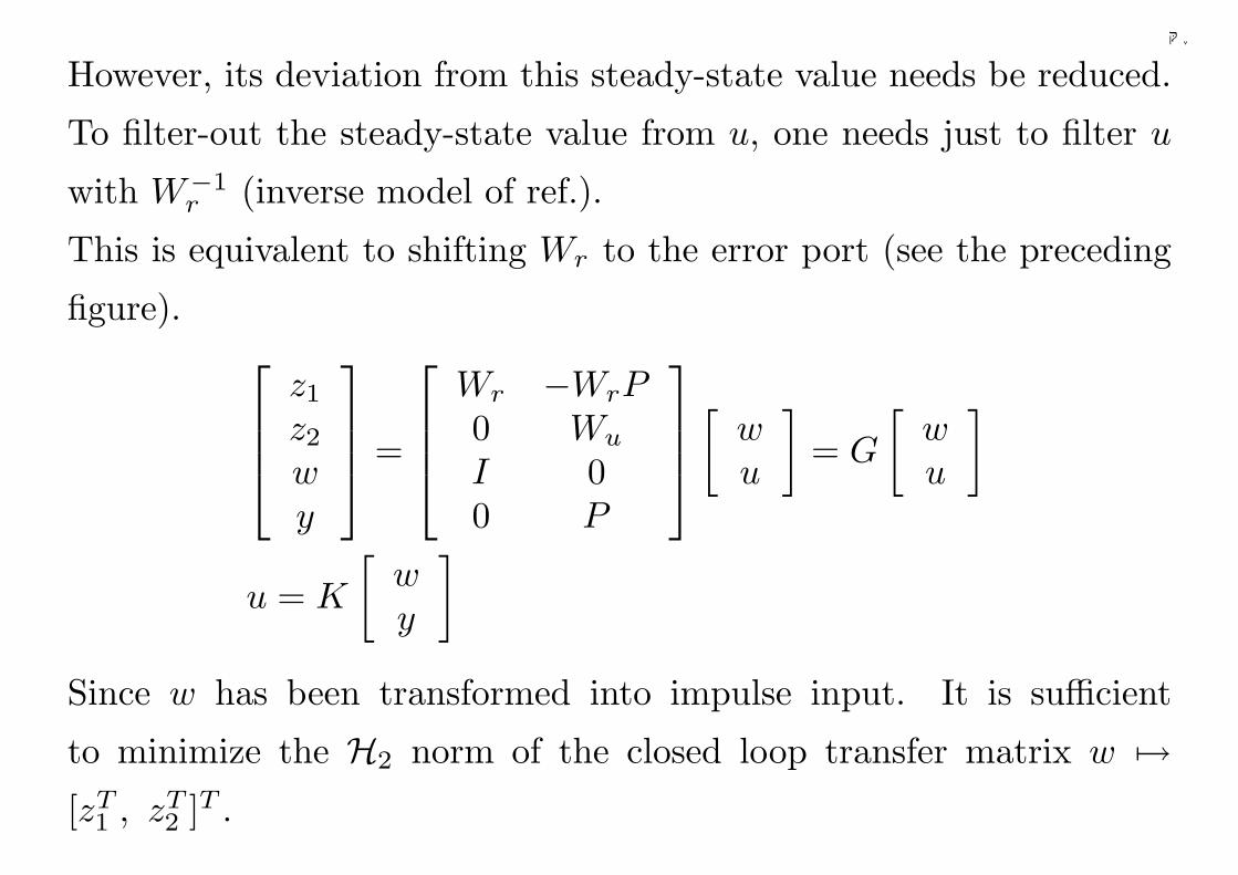
千葉大学
However, its deviation from this steady-state value needs be reduced.
To filter-out the steady-state value from u, one needs just to filter u
with W−1r (inverse model of ref.).
This is equivalent to shifting Wr to the error port (see the preceding
figure).
z1
z2
wy
=
Wr −WrP0 Wu
I 00 P
[wu
]= G
[wu
]
u = K
[wy
]
Since w has been transformed into impulse input. It is sufficient
to minimize the H2 norm of the closed loop transfer matrix w 7→[zT
1 , zT2 ]T .
195
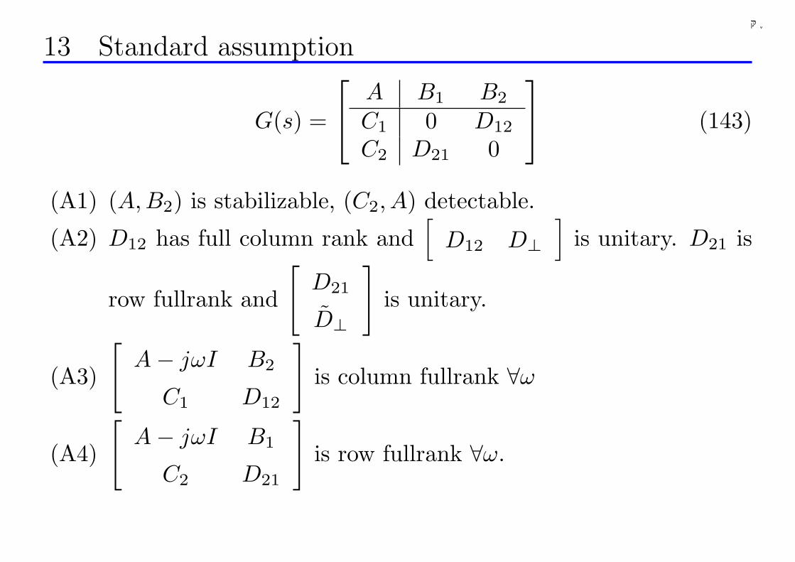
千葉大学
13 Standard assumption
G(s) =
A B1 B2
C1 0 D12
C2 D21 0
(143)
(A1) (A,B2) is stabilizable, (C2, A) detectable.
(A2) D12 has full column rank and[
D12 D⊥]
is unitary. D21 is
row fullrank and
[D21
D⊥
]is unitary.
(A3)
[A− jωI B2
C1 D12
]is column fullrank ∀ω
(A4)
[A− jωI B1
C2 D21
]is row fullrank ∀ω.
196
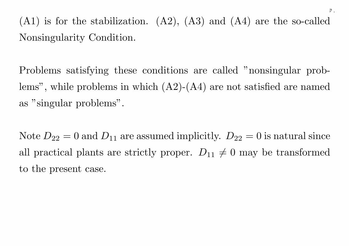
千葉大学
(A1) is for the stabilization. (A2), (A3) and (A4) are the so-called
Nonsingularity Condition.
Problems satisfying these conditions are called ”nonsingular prob-
lems”, while problems in which (A2)-(A4) are not satisfied are named
as ”singular problems”.
Note D22 = 0 and D11 are assumed implicitly. D22 = 0 is natural since
all practical plants are strictly proper. D11 6= 0 may be transformed
to the present case.
197
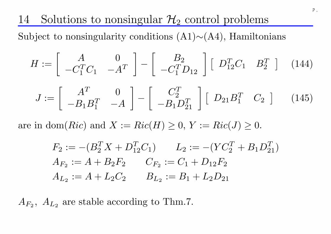
千葉大学
14 Solutions to nonsingular H2 control problems
Subject to nonsingularity conditions (A1)∼(A4), Hamiltonians
H :=[
A 0−CT
1 C1 −AT
]−
[B2
−CT1 D12
] [DT
12C1 BT2
](144)
J :=[
AT 0−B1B
T1 −A
]−
[CT
2
−B1DT21
] [D21B
T1 C2
](145)
are in dom(Ric) and X := Ric(H) ≥ 0, Y := Ric(J) ≥ 0.
F2 := −(BT2 X + DT
12C1) L2 := −(Y CT2 + B1D
T21)
AF2 := A + B2F2 CF2 := C1 + D12F2
AL2 := A + L2C2 BL2 := B1 + L2D21
AF2 , AL2 are stable according to Thm.7.
198
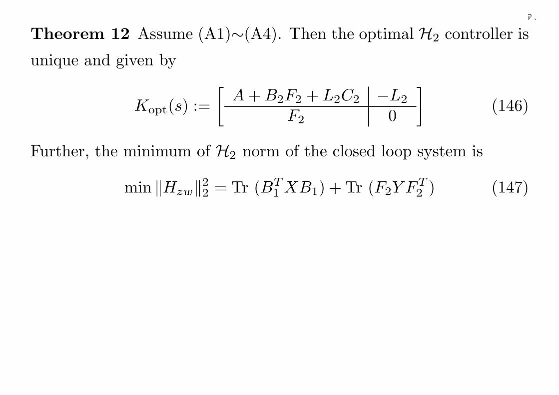
千葉大学
Theorem 12 Assume (A1)∼(A4). Then the optimal H2 controller is
unique and given by
Kopt(s) :=[
A + B2F2 + L2C2 −L2
F2 0
](146)
Further, the minimum of H2 norm of the closed loop system is
min ‖Hzw‖22 = Tr (BT1 XB1) + Tr (F2Y FT
2 ) (147)
199
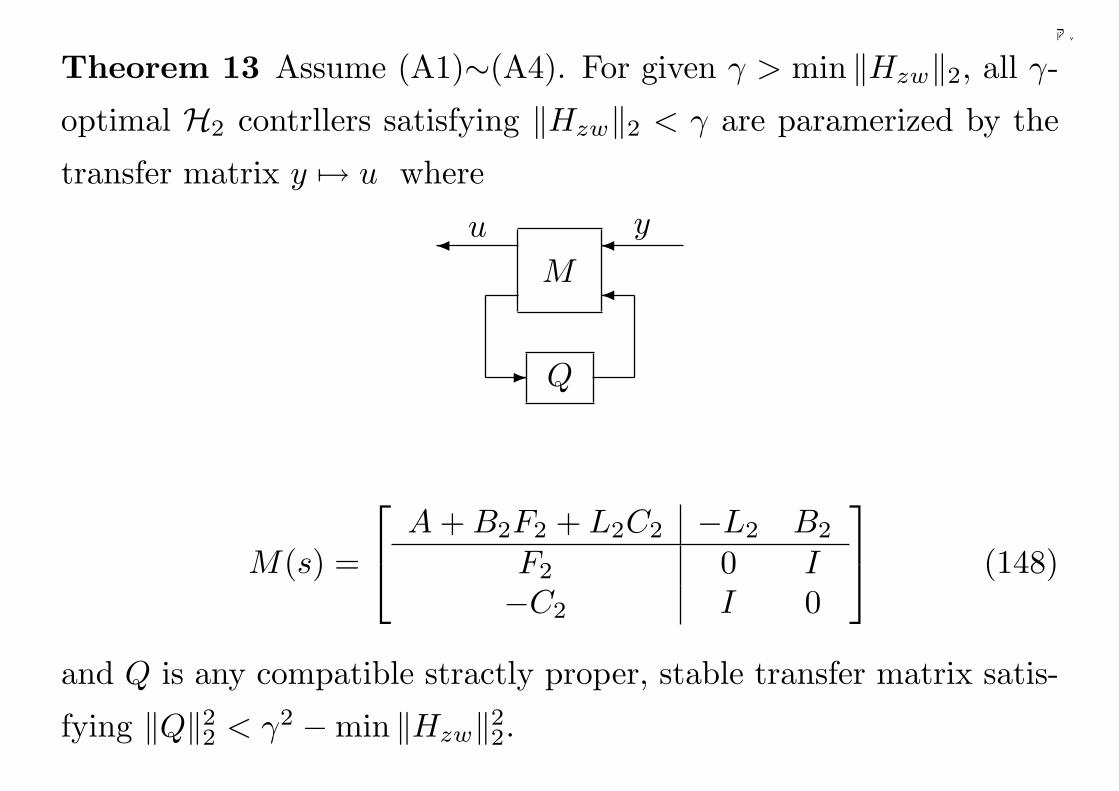
千葉大学
Theorem 13 Assume (A1)∼(A4). For given γ > min ‖Hzw‖2, all γ-
optimal H2 contrllers satisfying ‖Hzw‖2 < γ are paramerized by the
transfer matrix y 7→ u where
M
Q
u y¾ ¾
¾
-
M(s) =
A + B2F2 + L2C2 −L2 B2
F2 0 I−C2 I 0
(148)
and Q is any compatible stractly proper, stable transfer matrix satis-
fying ‖Q‖22 < γ2 −min ‖Hzw‖22.
200
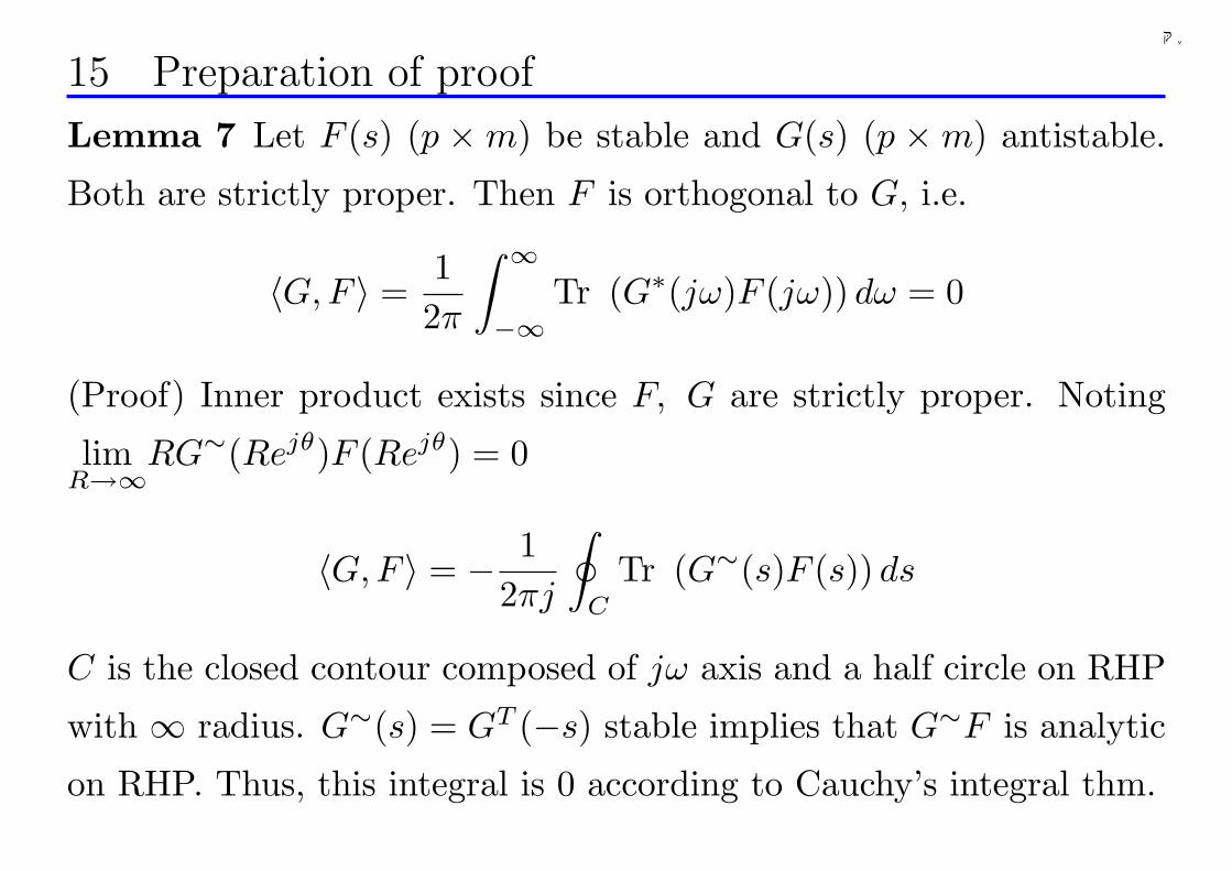
千葉大学
15 Preparation of proof
Lemma 7 Let F (s) (p ×m) be stable and G(s) (p ×m) antistable.
Both are strictly proper. Then F is orthogonal to G, i.e.
〈G,F 〉 =12π
∫ ∞
−∞Tr (G∗(jω)F (jω)) dω = 0
(Proof) Inner product exists since F, G are strictly proper. Noting
limR→∞
RG∼(Rejθ)F (Rejθ) = 0
〈G,F 〉 = − 12πj
∮
C
Tr (G∼(s)F (s)) ds
C is the closed contour composed of jω axis and a half circle on RHP
with ∞ radius. G∼(s) = GT (−s) stable implies that G∼F is analytic
on RHP. Thus, this integral is 0 according to Cauchy’s integral thm.
201
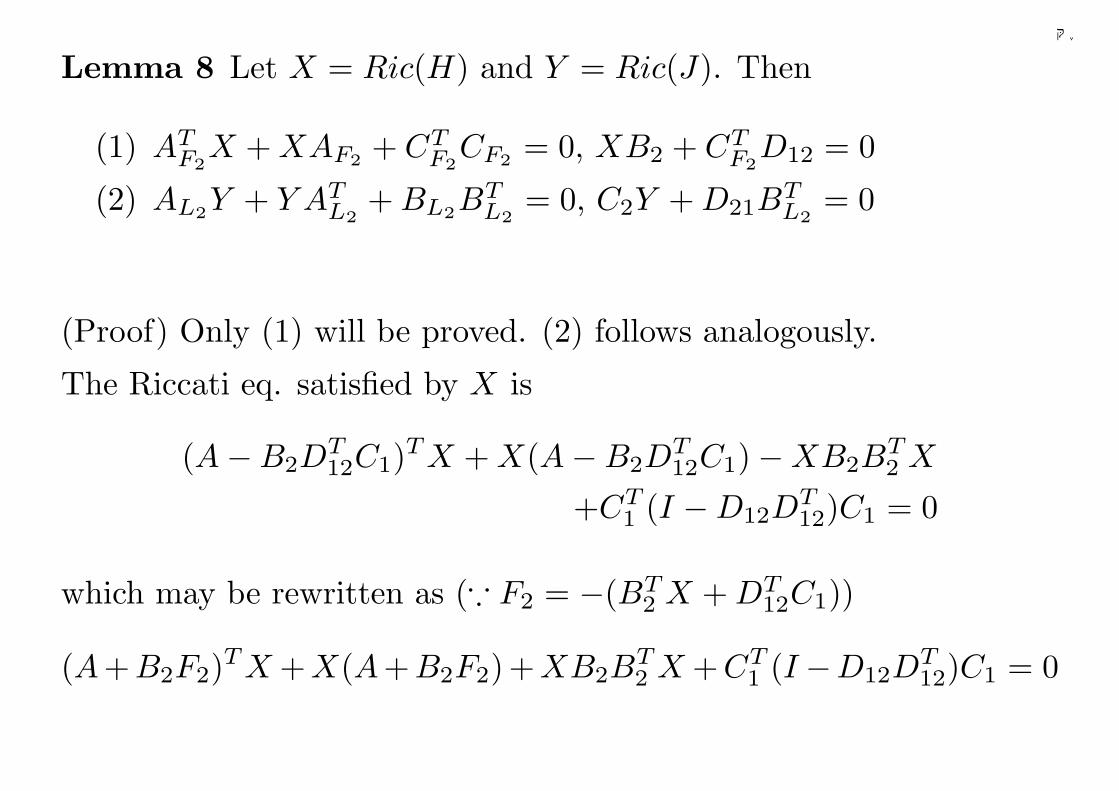
千葉大学
Lemma 8 Let X = Ric(H) and Y = Ric(J). Then
(1) ATF2
X + XAF2 + CTF2
CF2 = 0, XB2 + CTF2
D12 = 0
(2) AL2Y + Y ATL2
+ BL2BTL2
= 0, C2Y + D21BTL2
= 0
(Proof) Only (1) will be proved. (2) follows analogously.
The Riccati eq. satisfied by X is
(A−B2DT12C1)T X + X(A−B2D
T12C1)−XB2B
T2 X
+CT1 (I −D12D
T12)C1 = 0
which may be rewritten as (∵ F2 = −(BT2 X + DT
12C1))
(A+B2F2)T X +X(A+B2F2)+XB2BT2 X +CT
1 (I −D12DT12)C1 = 0
202
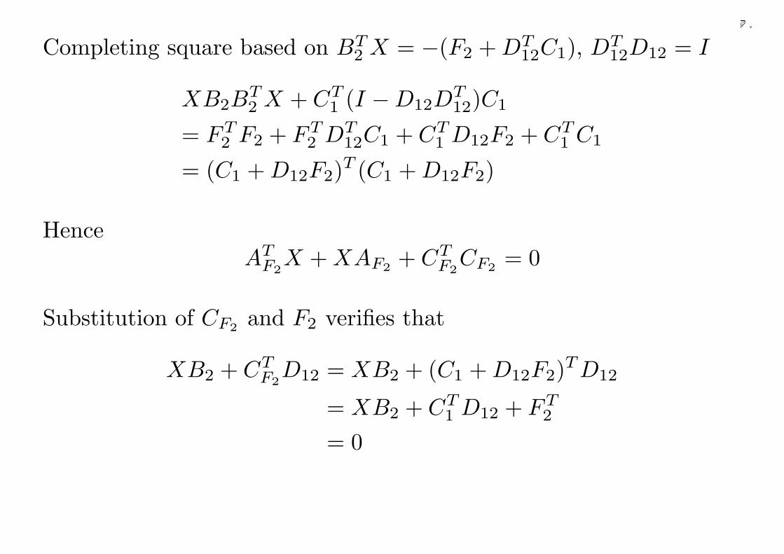
千葉大学
Completing square based on BT2 X = −(F2 + DT
12C1), DT12D12 = I
XB2BT2 X + CT
1 (I −D12DT12)C1
= FT2 F2 + FT
2 DT12C1 + CT
1 D12F2 + CT1 C1
= (C1 + D12F2)T (C1 + D12F2)
HenceAT
F2X + XAF2 + CT
F2CF2 = 0
Substitution of CF2 and F2 verifies that
XB2 + CTF2
D12 = XB2 + (C1 + D12F2)T D12
= XB2 + CT1 D12 + FT
2
= 0
203
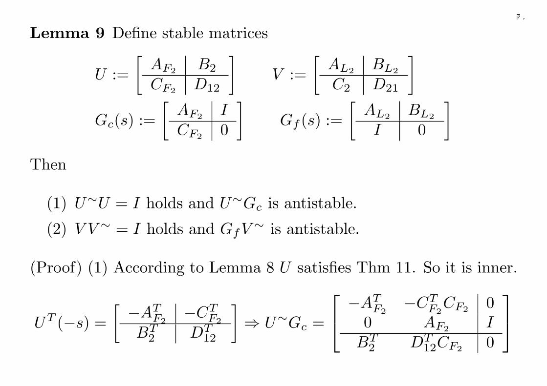
千葉大学
Lemma 9 Define stable matrices
U :=[
AF2 B2
CF2 D12
]V :=
[AL2 BL2
C2 D21
]
Gc(s) :=[
AF2 ICF2 0
]Gf (s) :=
[AL2 BL2
I 0
]
Then
(1) U∼U = I holds and U∼Gc is antistable.
(2) V V ∼ = I holds and GfV ∼ is antistable.
(Proof) (1) According to Lemma 8 U satisfies Thm 11. So it is inner.
UT (−s) =[ −AT
F2−CT
F2
BT2 DT
12
]⇒ U∼Gc =
−AT
F2−CT
F2CF2 0
0 AF2 IBT
2 DT12CF2 0
204
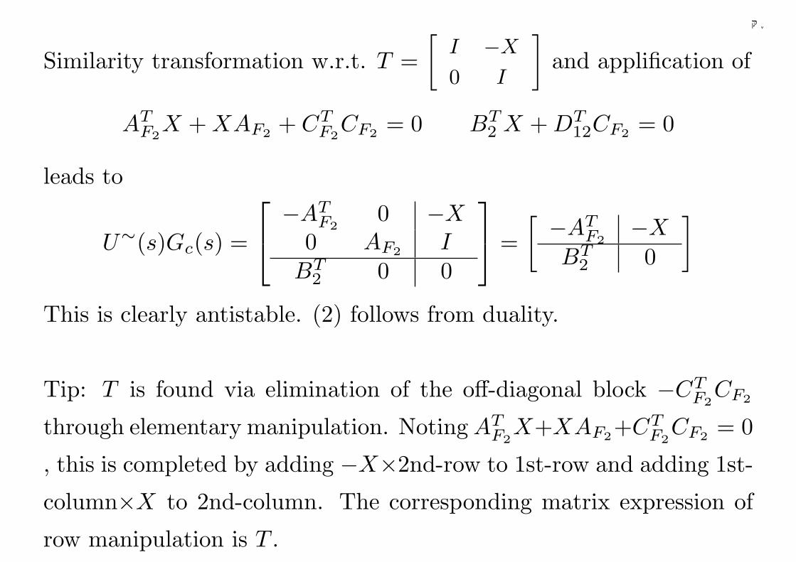
千葉大学
Similarity transformation w.r.t. T =[
I −X
0 I
]and applification of
ATF2
X + XAF2 + CTF2
CF2 = 0 BT2 X + DT
12CF2 = 0
leads to
U∼(s)Gc(s) =
−AT
F20 −X
0 AF2 IBT
2 0 0
=
[ −ATF2
−X
BT2 0
]
This is clearly antistable. (2) follows from duality.
Tip: T is found via elimination of the off-diagonal block −CTF2
CF2
through elementary manipulation. Noting ATF2
X+XAF2+CTF2
CF2 = 0
, this is completed by adding −X×2nd-row to 1st-row and adding 1st-
column×X to 2nd-column. The corresponding matrix expression of
row manipulation is T .
205
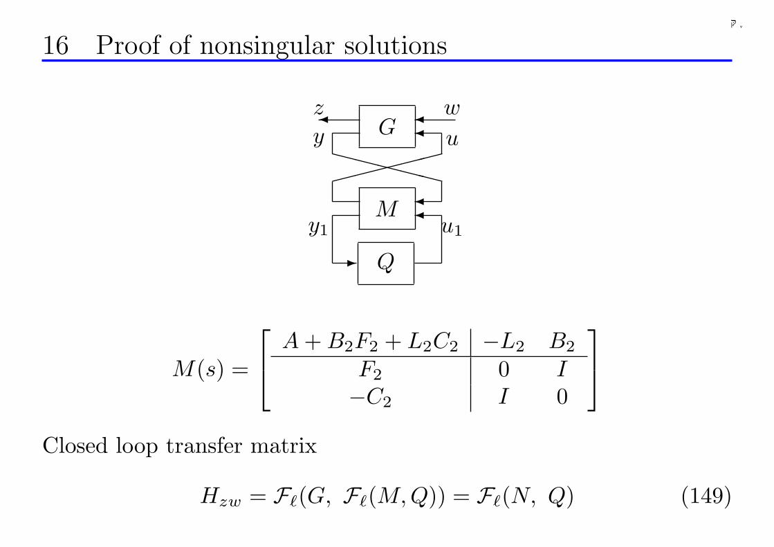
千葉大学
16 Proof of nonsingular solutions
u1y1
y u
wz
-
¾
¾
»»»»»¾
XXXXX¾
¾
Q
M
G
M(s) =
A + B2F2 + L2C2 −L2 B2
F2 0 I−C2 I 0
Closed loop transfer matrix
Hzw = F`(G, F`(M, Q)) = F`(N, Q) (149)
206
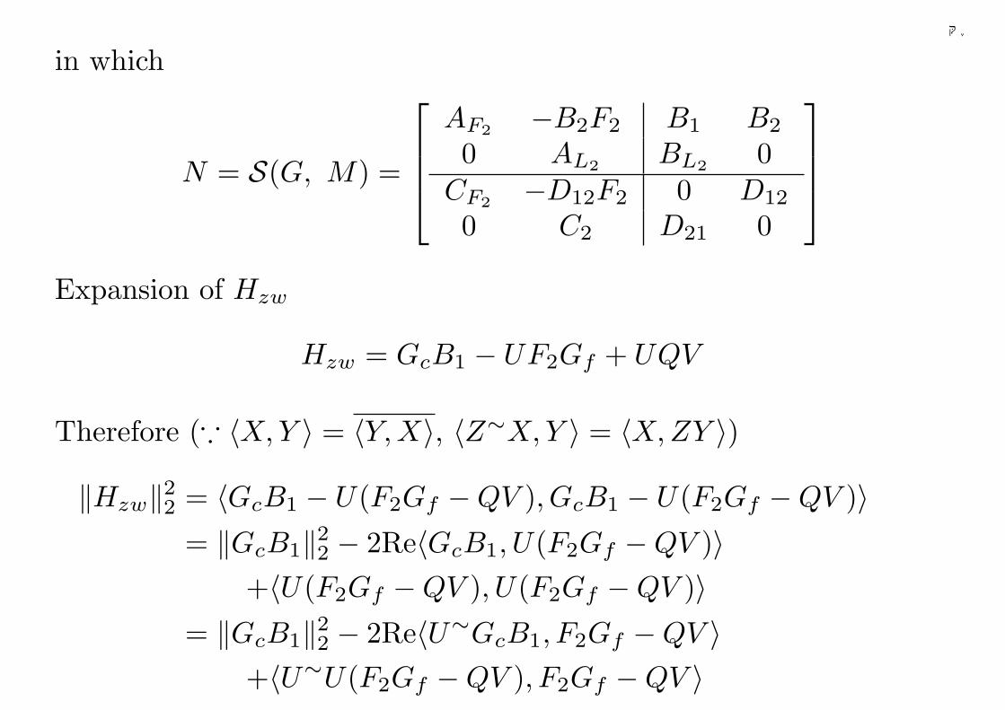
千葉大学
in which
N = S(G, M) =
AF2 −B2F2 B1 B2
0 AL2 BL2 0CF2 −D12F2 0 D12
0 C2 D21 0
Expansion of Hzw
Hzw = GcB1 − UF2Gf + UQV
Therefore (∵ 〈X, Y 〉 = 〈Y, X〉, 〈Z∼X, Y 〉 = 〈X, ZY 〉)
‖Hzw‖22 = 〈GcB1 − U(F2Gf −QV ), GcB1 − U(F2Gf −QV )〉= ‖GcB1‖22 − 2Re〈GcB1, U(F2Gf −QV )〉
+〈U(F2Gf −QV ), U(F2Gf −QV )〉= ‖GcB1‖22 − 2Re〈U∼GcB1, F2Gf −QV 〉
+〈U∼U(F2Gf −QV ), F2Gf −QV 〉207
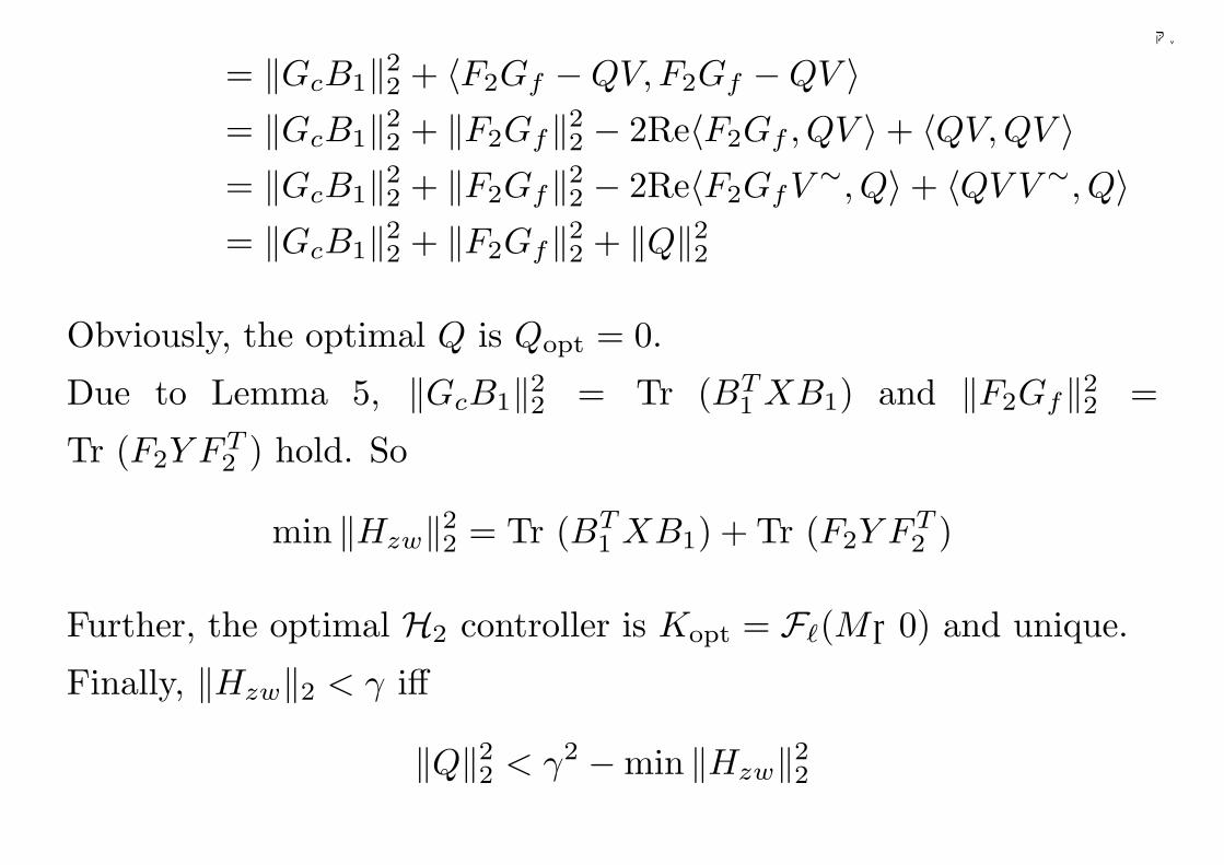
千葉大学
= ‖GcB1‖22 + 〈F2Gf −QV, F2Gf −QV 〉= ‖GcB1‖22 + ‖F2Gf‖22 − 2Re〈F2Gf , QV 〉+ 〈QV, QV 〉= ‖GcB1‖22 + ‖F2Gf‖22 − 2Re〈F2GfV ∼, Q〉+ 〈QV V ∼, Q〉= ‖GcB1‖22 + ‖F2Gf‖22 + ‖Q‖22
Obviously, the optimal Q is Qopt = 0.
Due to Lemma 5, ‖GcB1‖22 = Tr (BT1 XB1) and ‖F2Gf‖22 =
Tr (F2Y FT2 ) hold. So
min ‖Hzw‖22 = Tr (BT1 XB1) + Tr (F2Y FT
2 )
Further, the optimal H2 controller is Kopt = F`(M,0) and unique.
Finally, ‖Hzw‖2 < γ iff
‖Q‖22 < γ2 −min ‖Hzw‖22
208
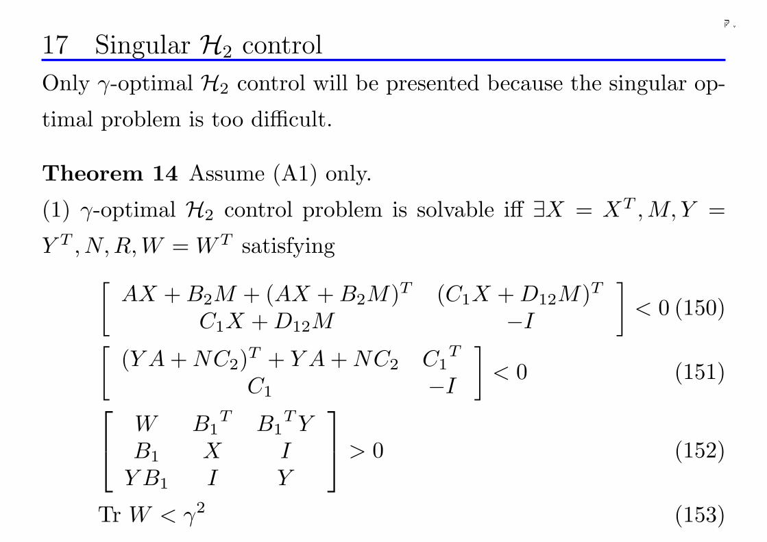
千葉大学
17 Singular H2 control
Only γ-optimal H2 control will be presented because the singular op-
timal problem is too difficult.
Theorem 14 Assume (A1) only.
(1) γ-optimal H2 control problem is solvable iff ∃X = XT ,M, Y =
Y T , N,R, W = WT satisfying[
AX + B2M + (AX + B2M)T (C1X + D12M)T
C1X + D12M −I
]< 0 (150)
[(Y A + NC2)T + Y A + NC2 C1
T
C1 −I
]< 0 (151)
W B1T B1
T YB1 X I
Y B1 I Y
> 0 (152)
Tr W < γ2 (153)
209
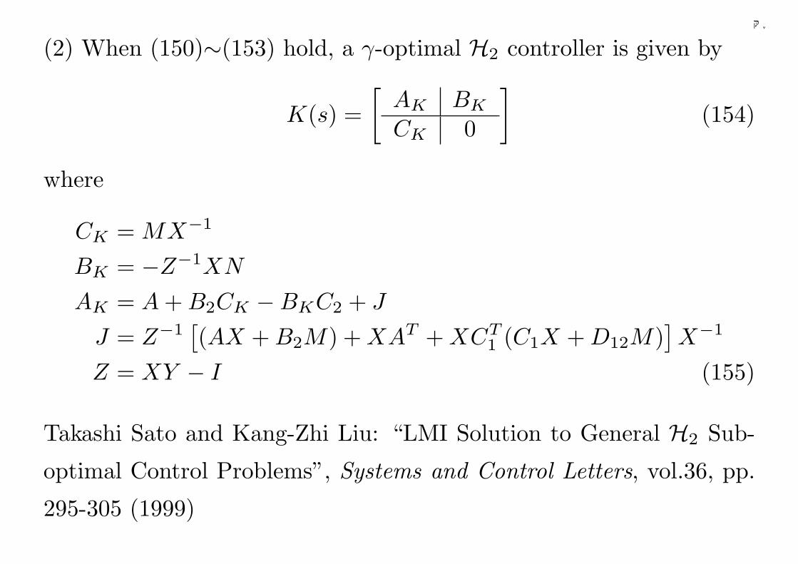
千葉大学
(2) When (150)∼(153) hold, a γ-optimal H2 controller is given by
K(s) =[
AK BK
CK 0
](154)
where
CK = MX−1
BK = −Z−1XN
AK = A + B2CK −BKC2 + J
J = Z−1[(AX + B2M) + XAT + XCT
1 (C1X + D12M)]X−1
Z = XY − I (155)
Takashi Sato and Kang-Zhi Liu: “LMI Solution to General H2 Sub-
optimal Control Problems”, Systems and Control Letters, vol.36, pp.
295-305 (1999)
210
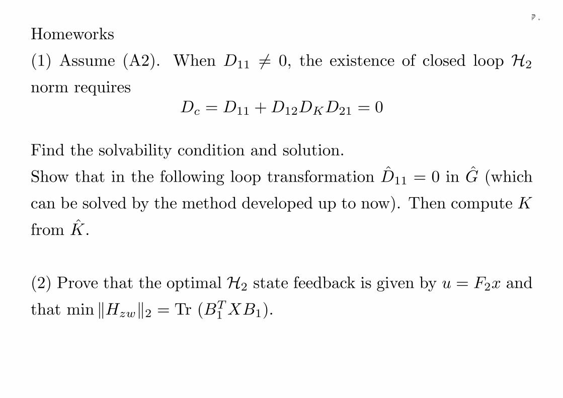
千葉大学
Homeworks
(1) Assume (A2). When D11 6= 0, the existence of closed loop H2
norm requiresDc = D11 + D12DKD21 = 0
Find the solvability condition and solution.
Show that in the following loop transformation D11 = 0 in G (which
can be solved by the method developed up to now). Then compute K
from K.
(2) Prove that the optimal H2 state feedback is given by u = F2x and
that min ‖Hzw‖2 = Tr (BT1 XB1).
211
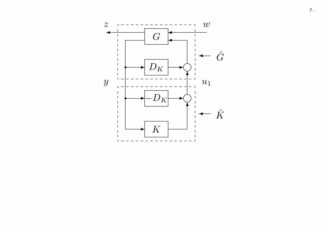
千葉大学
G
DK
−DK
K
¾¾¾
- g
-
-
-
-
6
6
g
q
q¾
¾ G
K
wz
u1y
212
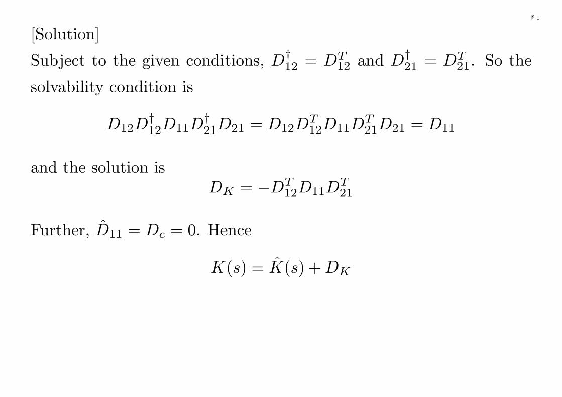
千葉大学
[Solution]
Subject to the given conditions, D†12 = DT
12 and D†21 = DT
21. So the
solvability condition is
D12D†12D11D
†21D21 = D12D
T12D11D
T21D21 = D11
and the solution isDK = −DT
12D11DT21
Further, D11 = Dc = 0. Hence
K(s) = K(s) + DK
213
千葉大学
Chapter 6 H∞ control
• Motivation
• Dist. control and H∞ norm of transfer matrix
• H∞ control problem
• ARE solution
• Treatment of non-standard probelm
• LMI solution
• Selection of generalized plant
• How to choose weights
• Case study 1: head positioning control of HDD
• case study 3: shock control of automa
214
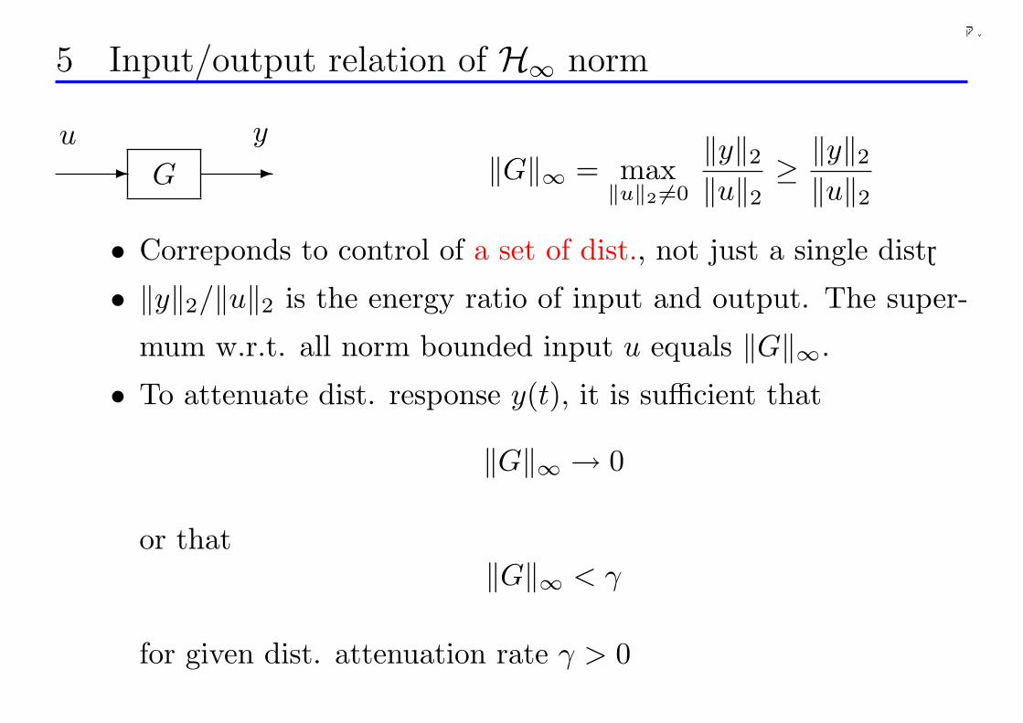
千葉大学
5 Input/output relation of H∞ norm
G- -yu
‖G‖∞ = max‖u‖2 6=0
‖y‖2‖u‖2 ≥
‖y‖2‖u‖2
• Correponds to control of a set of dist., not just a single dist.
• ‖y‖2/‖u‖2 is the energy ratio of input and output. The super-
mum w.r.t. all norm bounded input u equals ‖G‖∞.
• To attenuate dist. response y(t), it is sufficient that
‖G‖∞ → 0
or that‖G‖∞ < γ
for given dist. attenuation rate γ > 0
215
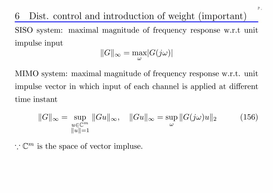
千葉大学
6 Dist. control and introduction of weight (important)
SISO system: maximal magnitude of frequency response w.r.t unit
impulse input‖G‖∞ = max
ω|G(jω)|
MIMO system: maximal magnitude of frequency response w.r.t. unit
impulse vector in which input of each channel is applied at different
time instant
‖G‖∞ = supu∈Cm
‖u‖=1
‖Gu‖∞, ‖Gu‖∞ = supω‖G(jω)u‖2 (156)
∵ Cm is the space of vector impluse.
216
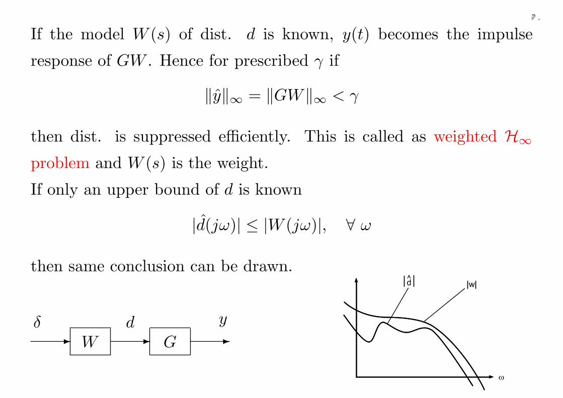
千葉大学
If the model W (s) of dist. d is known, y(t) becomes the impulse
response of GW . Hence for prescribed γ if
‖y‖∞ = ‖GW‖∞ < γ
then dist. is suppressed efficiently. This is called as weighted H∞problem and W (s) is the weight.
If only an upper bound of d is known
|d(jω)| ≤ |W (jω)|, ∀ ω
then same conclusion can be drawn.
G- -yd
W-δ
w
w
^d
217
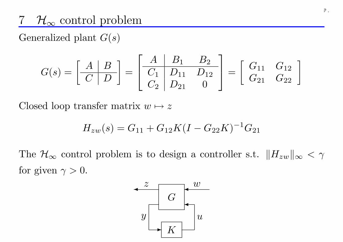
千葉大学
7 H∞ control problem
Generalized plant G(s)
G(s) =[
A BC D
]=
A B1 B2
C1 D11 D12
C2 D21 0
=
[G11 G12
G21 G22
]
Closed loop transfer matrix w 7→ z
Hzw(s) = G11 + G12K(I −G22K)−1G21
The H∞ control problem is to design a controller s.t. ‖Hzw‖∞ < γ
for given γ > 0.
G
K
z
y
w
u
¾ ¾
¾
-
218
千葉大学
♦ Solutions for H∞ control problem
1. ARE solution: Glover-doyle (88), DGKF (89)
2. LMI solution: Gahinet (94), Iwasaki (94)
219
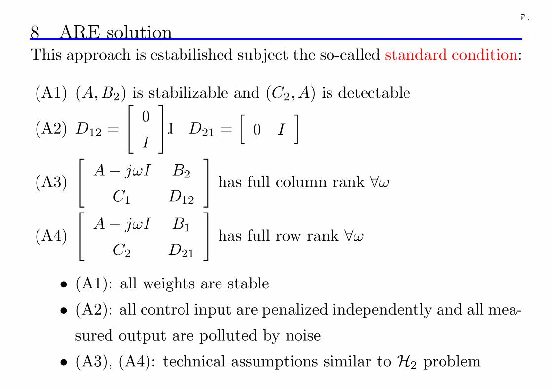
千葉大学
8 ARE solutionThis approach is estabilished subject the so-called standard condition:
(A1) (A,B2) is stabilizable and (C2, A) is detectable
(A2) D12 =
[0
I
]、 D21 =
[0 I
]
(A3)
[A− jωI B2
C1 D12
]has full column rank ∀ω
(A4)
[A− jωI B1
C2 D21
]has full row rank ∀ω
• (A1): all weights are stable
• (A2): all control input are penalized independently and all mea-
sured output are polluted by noise
• (A3), (A4): technical assumptions similar to H2 problem
220
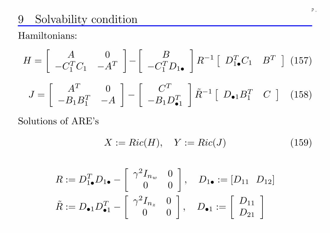
千葉大学
9 Solvability condition
Hamiltonians:
H =[
A 0−CT
1 C1 −AT
]−
[B
−CT1 D1•
]R−1
[DT
1•C1 BT]
(157)
J =[
AT 0−B1B
T1 −A
]−
[CT
−B1DT•1
]R−1
[D•1BT
1 C]
(158)
Solutions of ARE’s
X := Ric(H), Y := Ric(J) (159)
R := DT1•D1• −
[γ2Inw
00 0
], D1• := [D11 D12]
R := D•1DT•1 −
[γ2Inz
00 0
], D•1 :=
[D11
D21
]
221
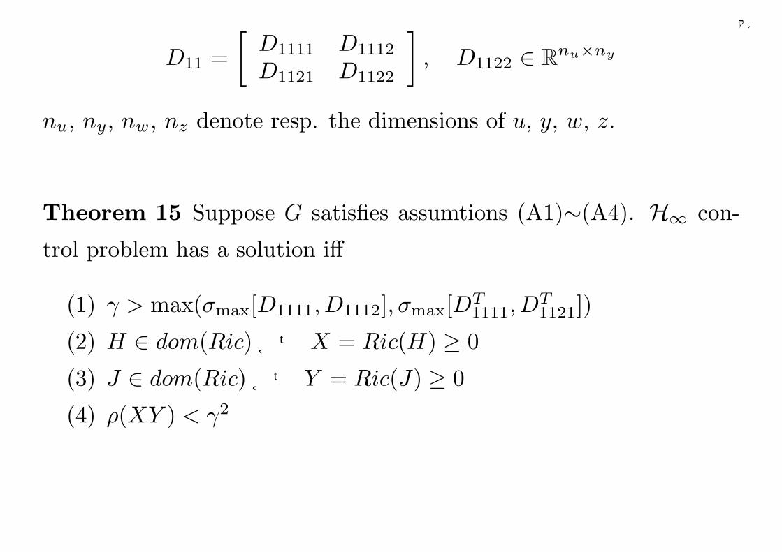
千葉大学
D11 =[
D1111 D1112
D1121 D1122
], D1122 ∈ Rnu×ny
nu, ny, nw, nz denote resp. the dimensions of u, y, w, z.
Theorem 15 Suppose G satisfies assumtions (A1)∼(A4). H∞ con-
trol problem has a solution iff
(1) γ > max(σmax[D1111, D1112], σmax[DT1111, D
T1121])
(2) H ∈ dom(Ric) かつ X = Ric(H) ≥ 0
(3) J ∈ dom(Ric) かつ Y = Ric(J) ≥ 0
(4) ρ(XY ) < γ2
222
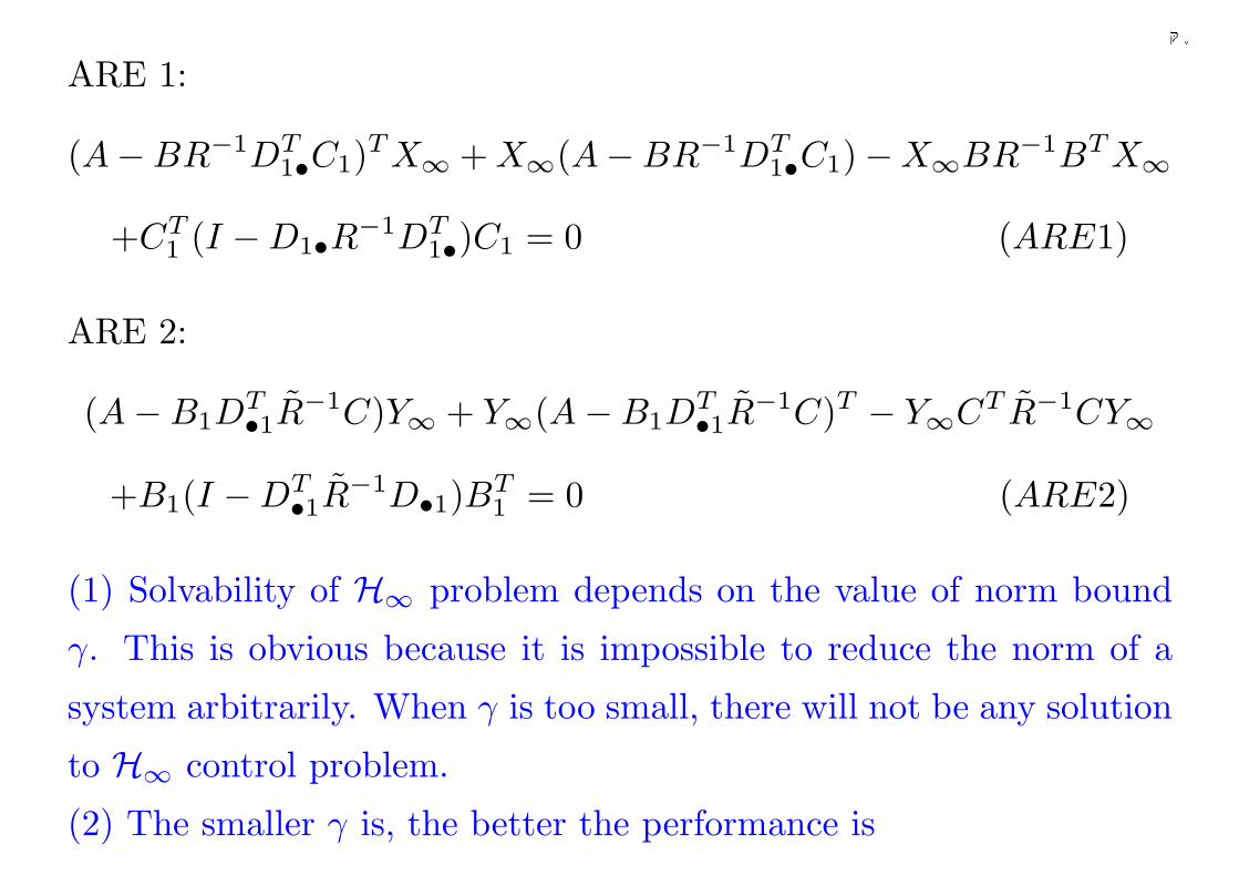
千葉大学
ARE 1:
(A−BR−1DT1•C1)T X∞ + X∞(A−BR−1DT
1•C1)−X∞BR−1BT X∞
+CT1 (I −D1•R−1DT
1•)C1 = 0 (ARE1)
ARE 2:
(A−B1DT•1R
−1C)Y∞ + Y∞(A−B1DT•1R
−1C)T − Y∞CT R−1CY∞
+B1(I −DT•1R
−1D•1)BT1 = 0 (ARE2)
(1) Solvability of H∞ problem depends on the value of norm bound
γ. This is obvious because it is impossible to reduce the norm of a
system arbitrarily. When γ is too small, there will not be any solution
to H∞ control problem.
(2) The smaller γ is, the better the performance is
223
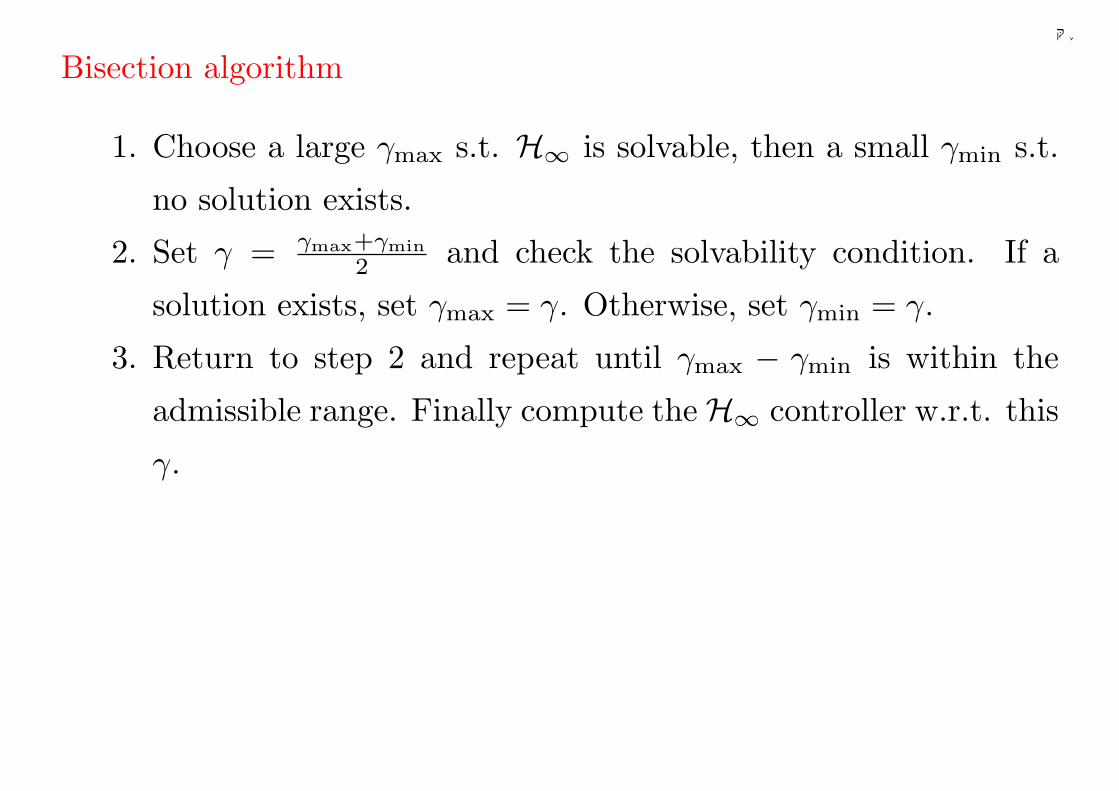
千葉大学
Bisection algorithm
1. Choose a large γmax s.t. H∞ is solvable, then a small γmin s.t.
no solution exists.
2. Set γ = γmax+γmin2 and check the solvability condition. If a
solution exists, set γmax = γ. Otherwise, set γmin = γ.
3. Return to step 2 and repeat until γmax − γmin is within the
admissible range. Finally compute theH∞ controller w.r.t. this
γ.
224
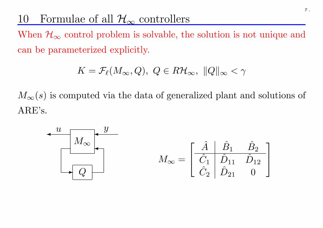
千葉大学
10 Formulae of all H∞ controllers
When H∞ control problem is solvable, the solution is not unique and
can be parameterized explicitly.
K = F`(M∞, Q), Q ∈ RH∞, ‖Q‖∞ < γ
M∞(s) is computed via the data of generalized plant and solutions of
ARE’s.
M∞
Q
u y¾ ¾
¾
-M∞ =
A B1 B2
C1 D11 D12
C2 D21 0
225
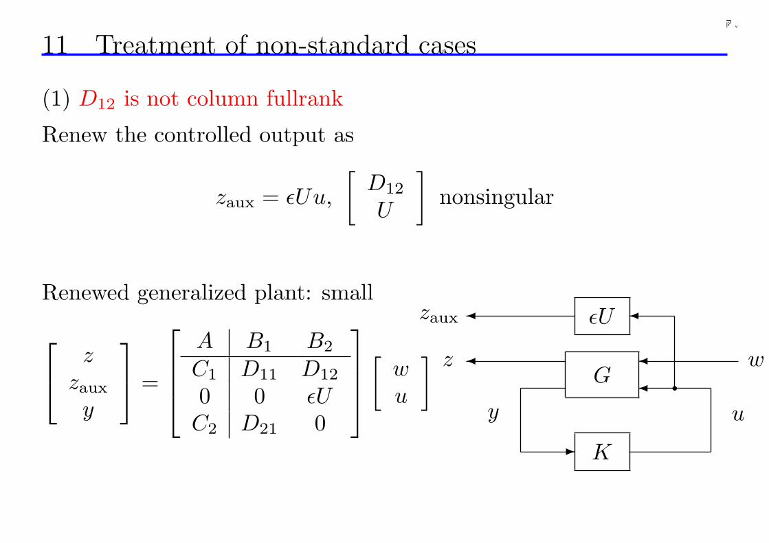
千葉大学
11 Treatment of non-standard cases
(1) D12 is not column fullrank
Renew the controlled output as
zaux = εUu,
[D12
U
]nonsingular
Renewed generalized plant: small
zzaux
y
=
A B1 B2
C1 D11 D12
0 0 εUC2 D21 0
[wu
]
K
¾¾¾
-
qw
uy
z
zaux
G
εU ¾¾
226
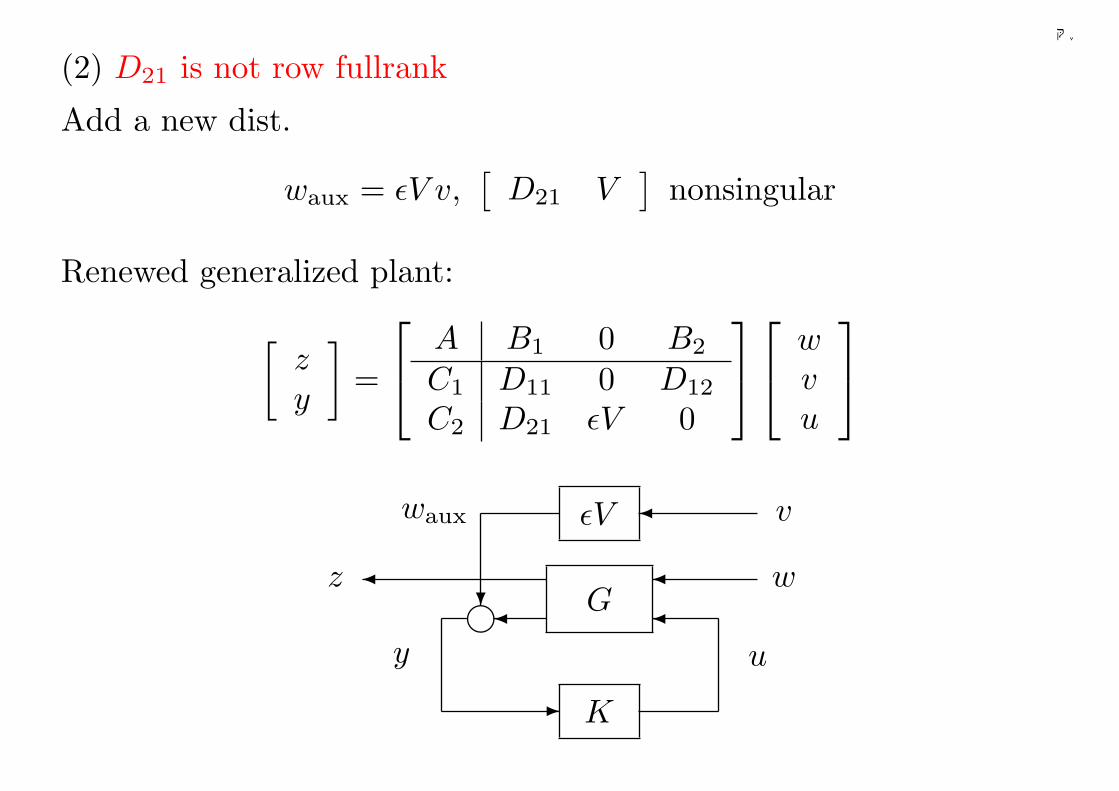
千葉大学
(2) D21 is not row fullrank
Add a new dist.
waux = εV v,[
D21 V]
nonsingular
Renewed generalized plant:
[zy
]=
A B1 0 B2
C1 D11 0 D12
C2 D21 εV 0
wvu
G
K
¾
-
w
uy
z¾
¾g¾?
εV ¾ vwaux
227
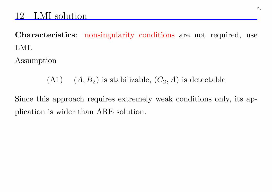
千葉大学
12 LMI solution
Characteristics: nonsingularity conditions are not required, use
LMI.
Assumption
(A1) (A,B2) is stabilizable, (C2, A) is detectable
Since this approach requires extremely weak conditions only, its ap-
plication is wider than ARE solution.
228
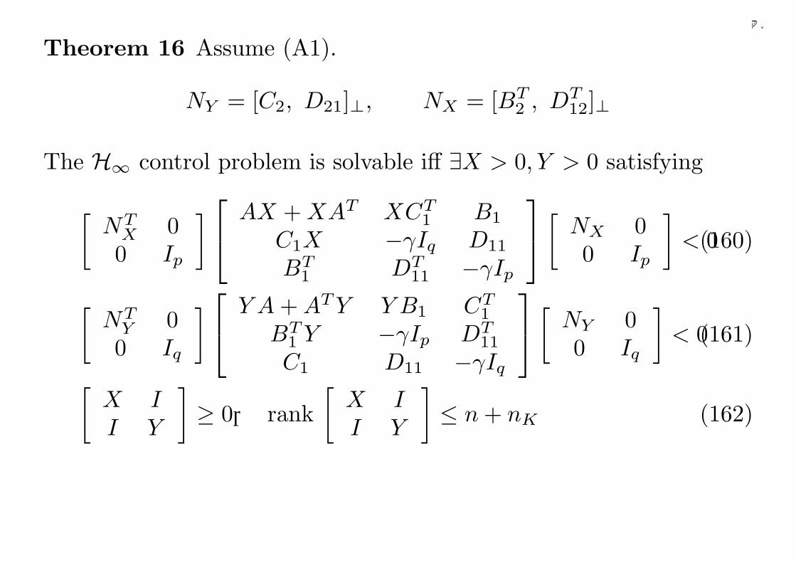
千葉大学
Theorem 16 Assume (A1).
NY = [C2, D21]⊥, NX = [BT2 , DT
12]⊥
The H∞ control problem is solvable iff ∃X > 0, Y > 0 satisfying
[NT
X 00 Ip
]
AX + XAT XCT1 B1
C1X −γIq D11
BT1 DT
11 −γIp
[NX 00 Ip
]< 0(160)
[NT
Y 00 Iq
]
Y A + AT Y Y B1 CT1
BT1 Y −γIp DT
11
C1 D11 −γIq
[NY 00 Iq
]< 0(161)
[X II Y
]≥ 0, rank
[X II Y
]≤ n + nK (162)
229
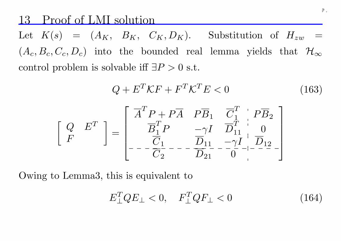
千葉大学
13 Proof of LMI solutionLet K(s) = (AK , BK , CK , DK). Substitution of Hzw =
(Ac, Bc, Cc, Dc) into the bounded real lemma yields that H∞control problem is solvable iff ∃P > 0 s.t.
Q + ETKF + FTKT E < 0 (163)
[Q ET
F
]=
ATP + PA PB1 C
T
1 PB2
BT
1 P −γI DT
11 0C1 D11 −γI D12
C2 D21 0
Owing to Lemma3, this is equivalent to
ET⊥QE⊥ < 0, FT
⊥QF⊥ < 0 (164)
230
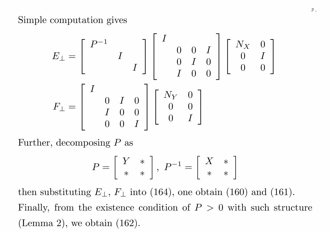
千葉大学
Simple computation gives
E⊥ =
P−1
II
I0 0 I0 I 0I 0 0
NX 00 I0 0
F⊥ =
I0 I 0I 0 00 0 I
NY 00 00 I
Further, decomposing P as
P =[
Y ∗∗ ∗
], P−1 =
[X ∗∗ ∗
]
then substituting E⊥, F⊥ into (164), one obtain (160) and (161).
Finally, from the existence condition of P > 0 with such structure
(Lemma 2), we obtain (162).
231
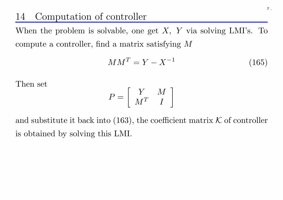
千葉大学
14 Computation of controller
When the problem is solvable, one get X, Y via solving LMI’s. To
compute a controller, find a matrix satisfying M
MMT = Y −X−1 (165)
Then set
P =[
Y MMT I
]
and substitute it back into (163), the coefficient matrix K of controller
is obtained by solving this LMI.
232
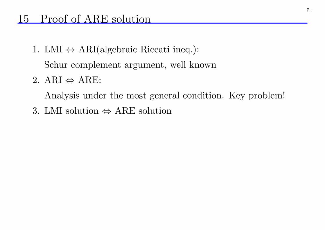
千葉大学
15 Proof of ARE solution
1. LMI ⇔ ARI(algebraic Riccati ineq.):
Schur complement argument, well known
2. ARI ⇔ ARE:
Analysis under the most general condition. Key problem!
3. LMI solution ⇔ ARE solution
233
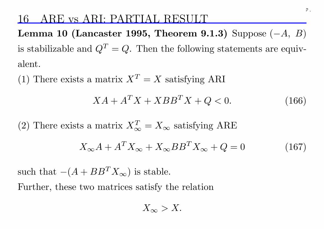
千葉大学
16 ARE vs ARI: PARTIAL RESULTLemma 10 (Lancaster 1995, Theorem 9.1.3) Suppose (−A, B)
is stabilizable and QT = Q. Then the following statements are equiv-
alent.
(1) There exists a matrix XT = X satisfying ARI
XA + AT X + XBBT X + Q < 0. (166)
(2) There exists a matrix XT∞ = X∞ satisfying ARE
X∞A + AT X∞ + X∞BBT X∞ + Q = 0 (167)
such that −(A + BBT X∞) is stable.
Further, these two matrices satisfy the relation
X∞ > X.
234
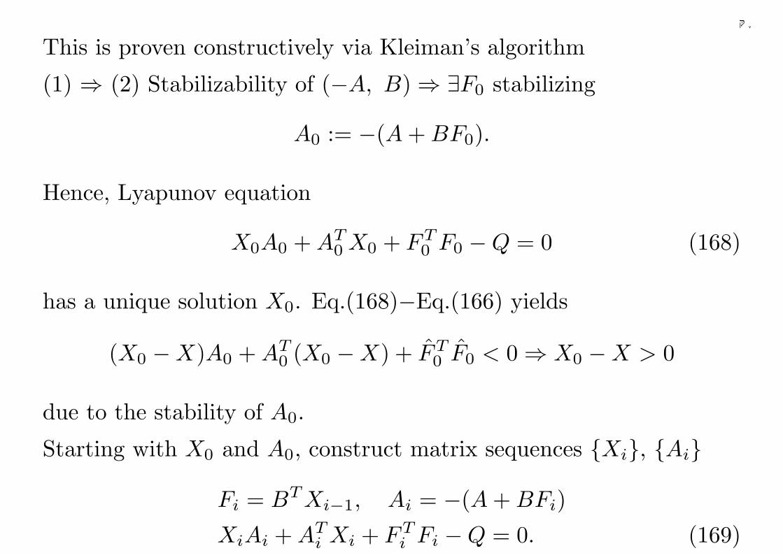
千葉大学
This is proven constructively via Kleiman’s algorithm
(1) ⇒ (2) Stabilizability of (−A, B) ⇒ ∃F0 stabilizing
A0 := −(A + BF0).
Hence, Lyapunov equation
X0A0 + AT0 X0 + FT
0 F0 −Q = 0 (168)
has a unique solution X0. Eq.(168)−Eq.(166) yields
(X0 −X)A0 + AT0 (X0 −X) + FT
0 F0 < 0 ⇒ X0 −X > 0
due to the stability of A0.
Starting with X0 and A0, construct matrix sequences Xi, Ai
Fi = BT Xi−1, Ai = −(A + BFi)
XiAi + ATi Xi + FT
i Fi −Q = 0. (169)
235
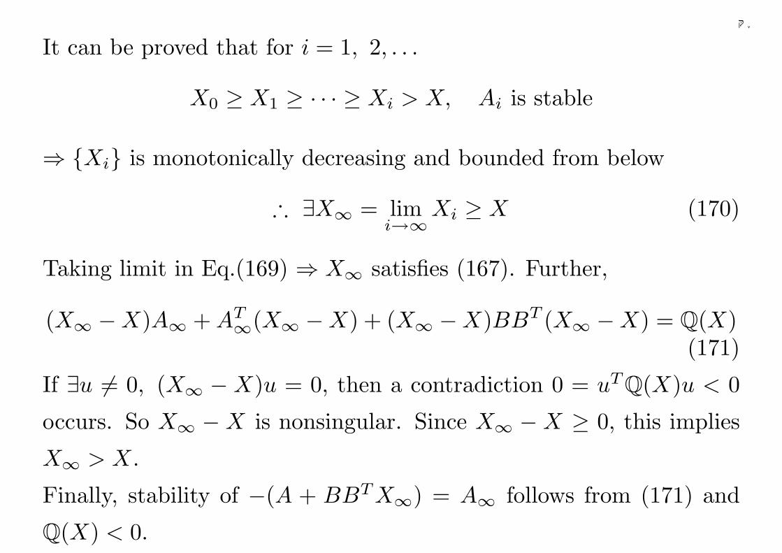
千葉大学
It can be proved that for i = 1, 2, . . .
X0 ≥ X1 ≥ · · · ≥ Xi > X, Ai is stable
⇒ Xi is monotonically decreasing and bounded from below
∴ ∃X∞ = limi→∞
Xi ≥ X (170)
Taking limit in Eq.(169) ⇒ X∞ satisfies (167). Further,
(X∞ −X)A∞ + AT∞(X∞ −X) + (X∞ −X)BBT (X∞ −X) = Q(X)
(171)
If ∃u 6= 0, (X∞ −X)u = 0, then a contradiction 0 = uTQ(X)u < 0
occurs. So X∞ −X is nonsingular. Since X∞ −X ≥ 0, this implies
X∞ > X.
Finally, stability of −(A + BBT X∞) = A∞ follows from (171) and
Q(X) < 0.
236
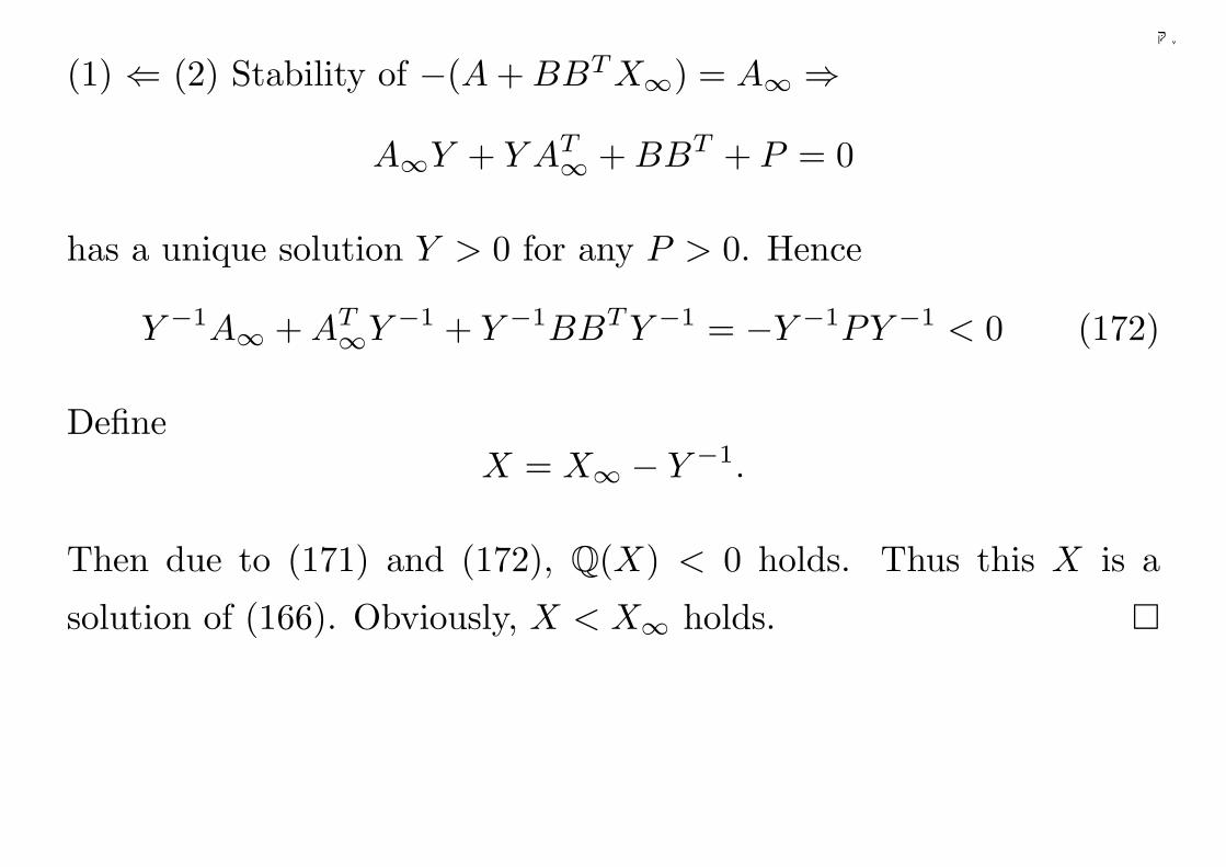
千葉大学
(1) ⇐ (2) Stability of −(A + BBT X∞) = A∞ ⇒
A∞Y + Y AT∞ + BBT + P = 0
has a unique solution Y > 0 for any P > 0. Hence
Y −1A∞ + AT∞Y −1 + Y −1BBT Y −1 = −Y −1PY −1 < 0 (172)
DefineX = X∞ − Y −1.
Then due to (171) and (172), Q(X) < 0 holds. Thus this X is a
solution of (166). Obviously, X < X∞ holds. ¤
237
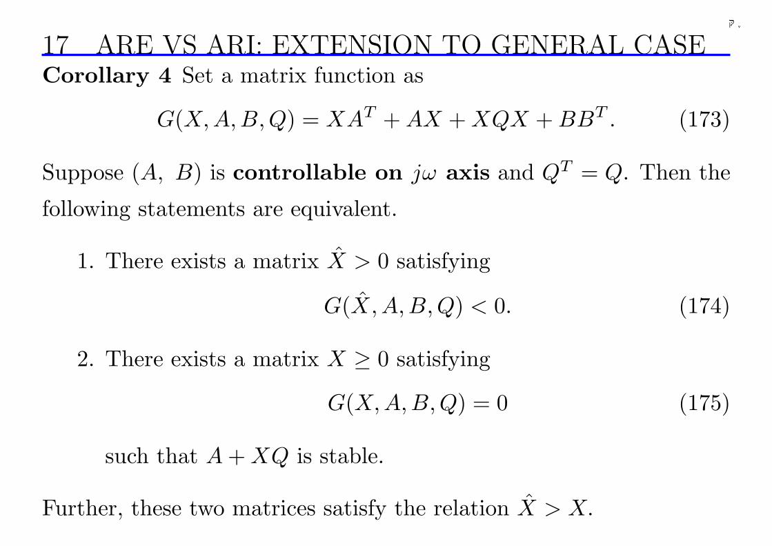
千葉大学
17 ARE VS ARI: EXTENSION TO GENERAL CASECorollary 4 Set a matrix function as
G(X, A, B, Q) = XAT + AX + XQX + BBT . (173)
Suppose (A, B) is controllable on jω axis and QT = Q. Then the
following statements are equivalent.
1. There exists a matrix X > 0 satisfying
G(X, A,B,Q) < 0. (174)
2. There exists a matrix X ≥ 0 satisfying
G(X, A, B, Q) = 0 (175)
such that A + XQ is stable.
Further, these two matrices satisfy the relation X > X.
238
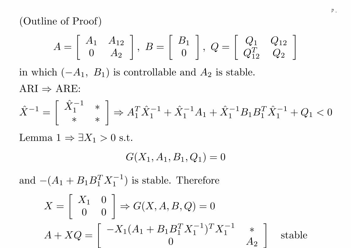
千葉大学
(Outline of Proof)
A =[
A1 A12
0 A2
], B =
[B1
0
], Q =
[Q1 Q12
QT12 Q2
]
in which (−A1, B1) is controllable and A2 is stable.
ARI ⇒ ARE:
X−1 =[
X−11 ∗∗ ∗
]⇒ AT
1 X−11 + X−1
1 A1 + X−11 B1B
T1 X−1
1 + Q1 < 0
Lemma 1 ⇒ ∃X1 > 0 s.t.
G(X1, A1, B1, Q1) = 0
and −(A1 + B1BT1 X−1
1 ) is stable. Therefore
X =[
X1 00 0
]⇒ G(X, A, B, Q) = 0
A + XQ =[ −X1(A1 + B1B
T1 X−1
1 )T X−11 ∗
0 A2
]stable
239
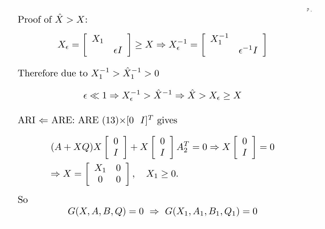
千葉大学
Proof of X > X:
Xε =[
X1
εI
]≥ X ⇒ X−1
ε =[
X−11
ε−1I
]
Therefore due to X−11 > X−1
1 > 0
ε ¿ 1 ⇒ X−1ε > X−1 ⇒ X > Xε ≥ X
ARI ⇐ ARE: ARE (13)×[0 I]T gives
(A + XQ)X[
0I
]+ X
[0I
]AT
2 = 0 ⇒ X
[0I
]= 0
⇒ X =[
X1 00 0
], X1 ≥ 0.
SoG(X, A, B, Q) = 0 ⇒ G(X1, A1, B1, Q1) = 0
240
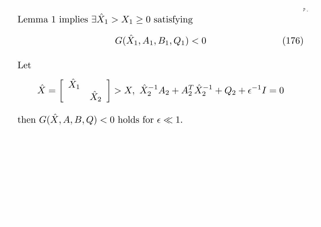
千葉大学
Lemma 1 implies ∃X1 > X1 ≥ 0 satisfying
G(X1, A1, B1, Q1) < 0 (176)
Let
X =[
X1
X2
]> X, X−1
2 A2 + AT2 X−1
2 + Q2 + ε−1I = 0
then G(X, A,B, Q) < 0 holds for ε ¿ 1.
241
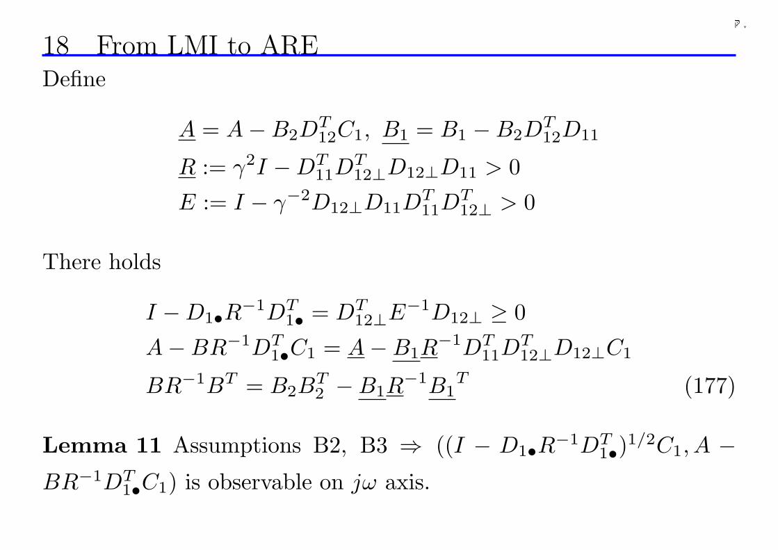
千葉大学
18 From LMI to AREDefine
A = A−B2DT12C1, B1 = B1 −B2D
T12D11
R := γ2I −DT11D
T12⊥D12⊥D11 > 0
E := I − γ−2D12⊥D11DT11D
T12⊥ > 0
There holds
I −D1•R−1DT1• = DT
12⊥E−1D12⊥ ≥ 0
A−BR−1DT1•C1 = A−B1R
−1DT11D
T12⊥D12⊥C1
BR−1BT = B2BT2 −B1R
−1B1T (177)
Lemma 11 Assumptions B2, B3 ⇒ ((I − D1•R−1DT1•)
1/2C1, A −BR−1DT
1•C1) is observable on jω axis.
242
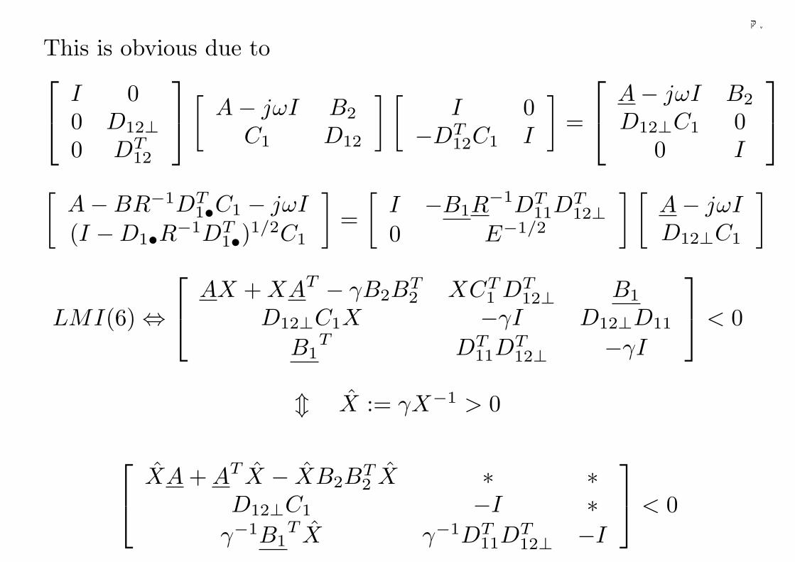
千葉大学
This is obvious due to
I 00 D12⊥0 DT
12
[A− jωI B2
C1 D12
] [I 0
−DT12C1 I
]=
A− jωI B2
D12⊥C1 00 I
[A−BR−1DT
1•C1 − jωI(I −D1•R−1DT
1•)1/2C1
]=
[I −B1R
−1DT11D
T12⊥
0 E−1/2
] [A− jωID12⊥C1
]
LMI(6) ⇔
AX + XAT − γB2BT2 XCT
1 DT12⊥ B1
D12⊥C1X −γI D12⊥D11
B1T DT
11DT12⊥ −γI
< 0
m X := γX−1 > 0
XA + AT X − XB2BT2 X ∗ ∗
D12⊥C1 −I ∗γ−1B1
T X γ−1DT11D
T12⊥ −I
< 0
243
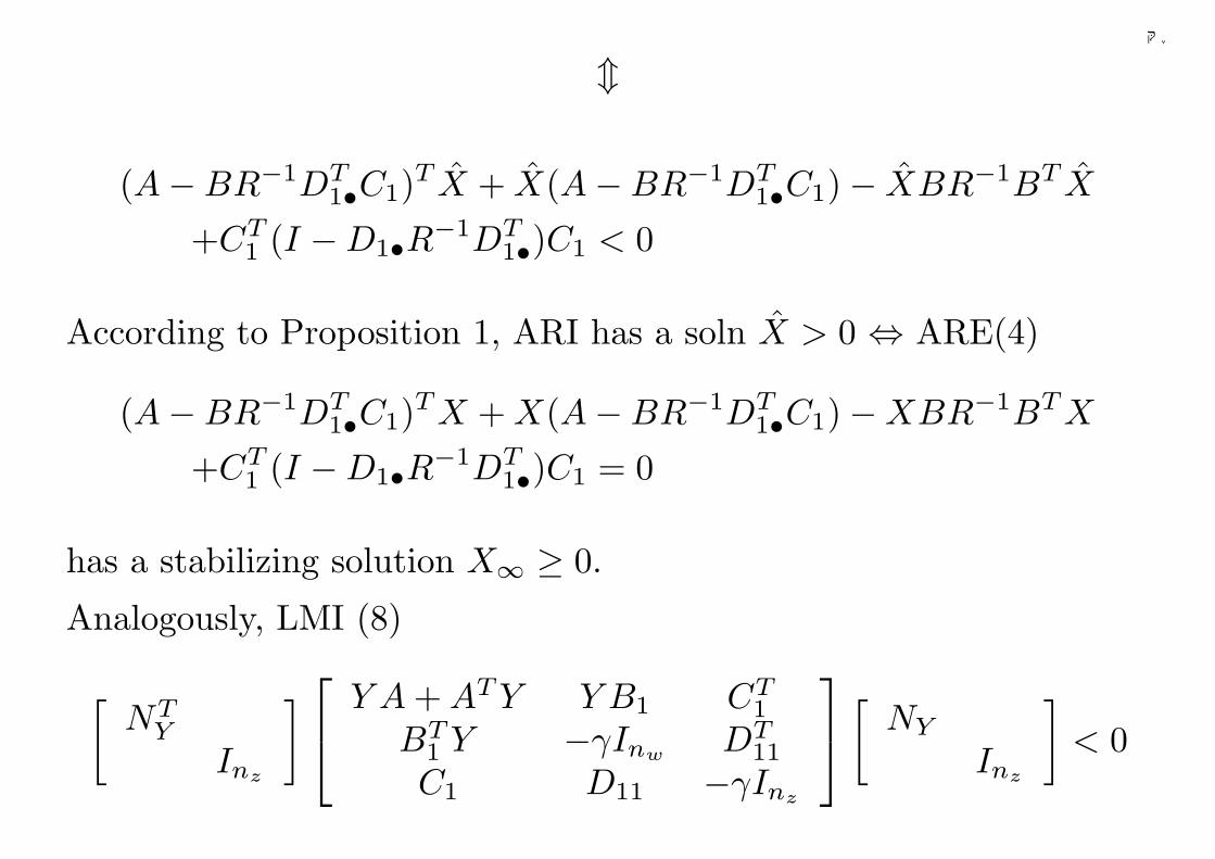
千葉大学
m
(A−BR−1DT1•C1)T X + X(A−BR−1DT
1•C1)− XBR−1BT X
+CT1 (I −D1•R−1DT
1•)C1 < 0
According to Proposition 1, ARI has a soln X > 0 ⇔ ARE(4)
(A−BR−1DT1•C1)T X + X(A−BR−1DT
1•C1)−XBR−1BT X
+CT1 (I −D1•R−1DT
1•)C1 = 0
has a stabilizing solution X∞ ≥ 0.
Analogously, LMI (8)
[NT
Y
Inz
]
Y A + AT Y Y B1 CT1
BT1 Y −γInw
DT11
C1 D11 −γInz
[NY
Inz
]< 0
244
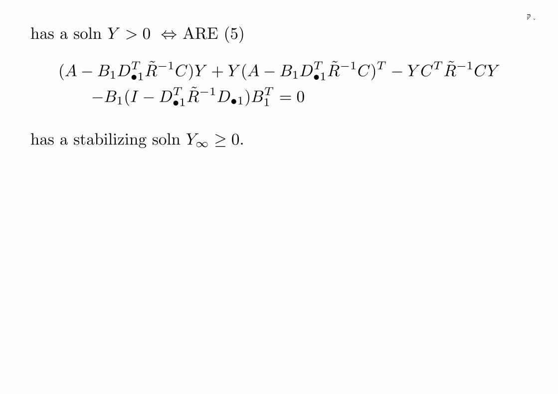
千葉大学
has a soln Y > 0 ⇔ ARE (5)
(A−B1DT•1R
−1C)Y + Y (A−B1DT•1R
−1C)T − Y CT R−1CY
−B1(I −DT•1R
−1D•1)BT1 = 0
has a stabilizing soln Y∞ ≥ 0.
245
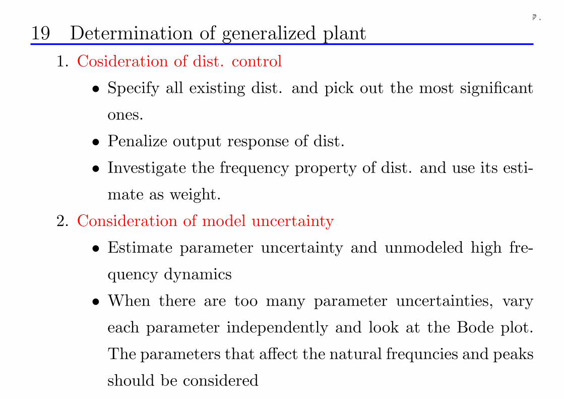
千葉大学
19 Determination of generalized plant
1. Cosideration of dist. control
• Specify all existing dist. and pick out the most significant
ones.
• Penalize output response of dist.
• Investigate the frequency property of dist. and use its esti-
mate as weight.
2. Consideration of model uncertainty
• Estimate parameter uncertainty and unmodeled high fre-
quency dynamics
• When there are too many parameter uncertainties, vary
each parameter independently and look at the Bode plot.
The parameters that affect the natural frequncies and peaks
should be considered
246
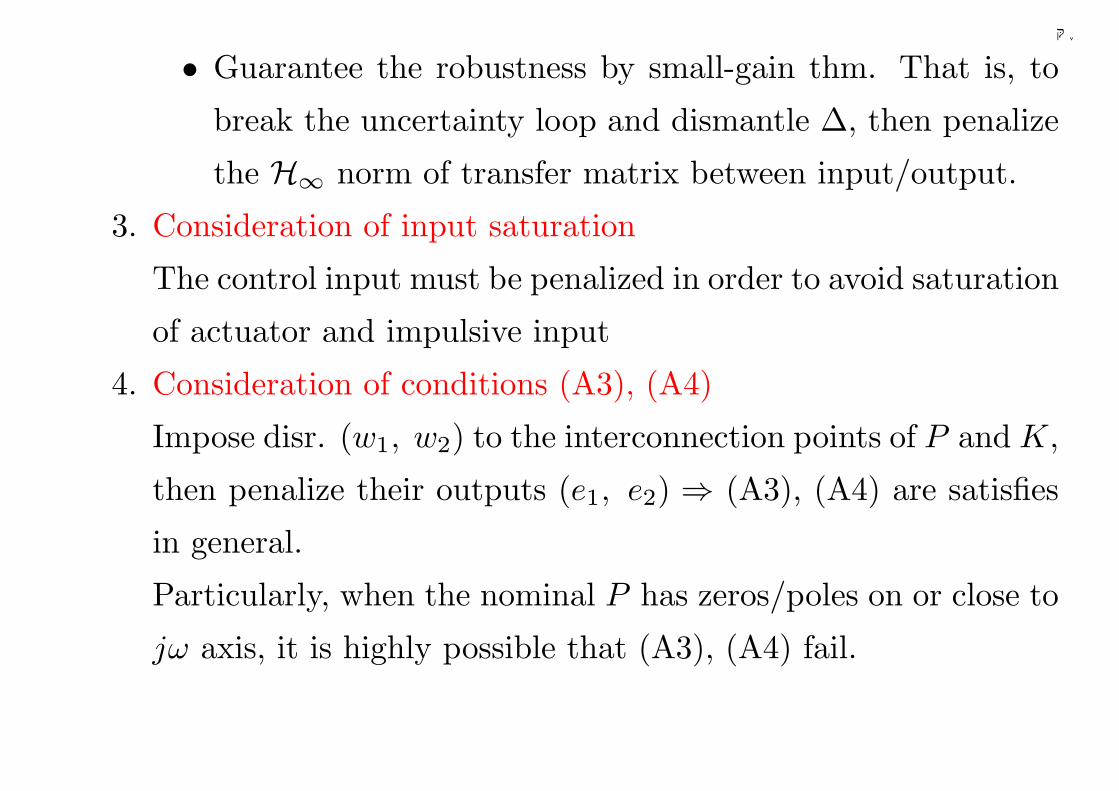
千葉大学
• Guarantee the robustness by small-gain thm. That is, to
break the uncertainty loop and dismantle ∆, then penalize
the H∞ norm of transfer matrix between input/output.
3. Consideration of input saturation
The control input must be penalized in order to avoid saturation
of actuator and impulsive input
4. Consideration of conditions (A3), (A4)
Impose disr. (w1, w2) to the interconnection points of P and K,
then penalize their outputs (e1, e2) ⇒ (A3), (A4) are satisfies
in general.
Particularly, when the nominal P has zeros/poles on or close to
jω axis, it is highly possible that (A3), (A4) fail.
247
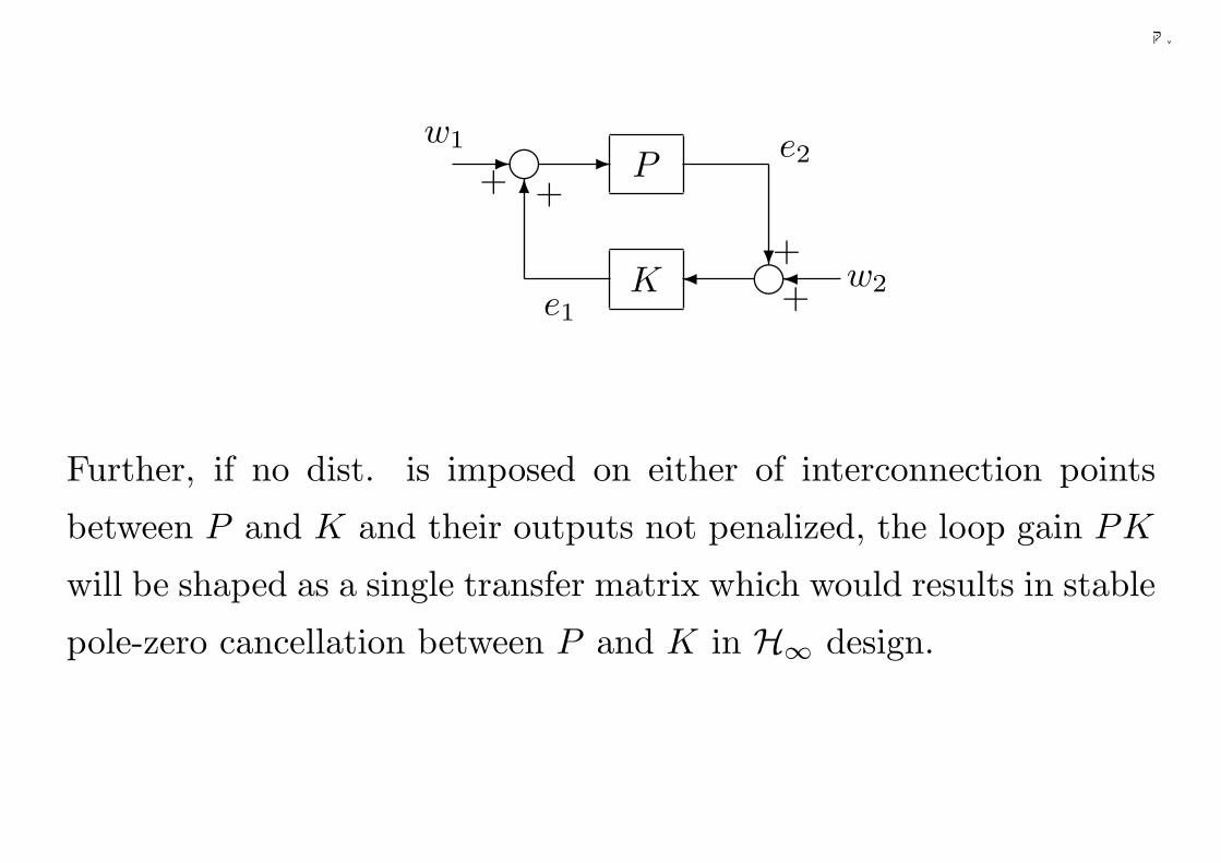
千葉大学
++
++
e2
e1
w2
w1P
K
--6g
g¾ ?¾
Further, if no dist. is imposed on either of interconnection points
between P and K and their outputs not penalized, the loop gain PK
will be shaped as a single transfer matrix which would results in stable
pole-zero cancellation between P and K in H∞ design.
248
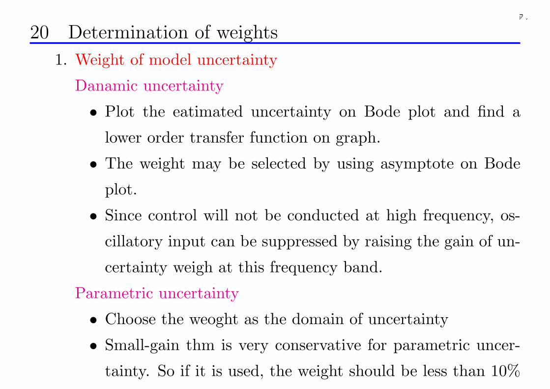
千葉大学
20 Determination of weights
1. Weight of model uncertainty
Danamic uncertainty
• Plot the eatimated uncertainty on Bode plot and find a
lower order transfer function on graph.
• The weight may be selected by using asymptote on Bode
plot.
• Since control will not be conducted at high frequency, os-
cillatory input can be suppressed by raising the gain of un-
certainty weigh at this frequency band.
Parametric uncertainty
• Choose the weoght as the domain of uncertainty
• Small-gain thm is very conservative for parametric uncer-
tainty. So if it is used, the weight should be less than 10%
249
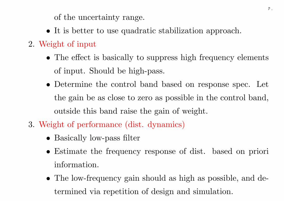
千葉大学
of the uncertainty range.
• It is better to use quadratic stabilization approach.
2. Weight of input
• The effect is basically to suppress high frequency elements
of input. Should be high-pass.
• Determine the control band based on response spec. Let
the gain be as close to zero as possible in the control band,
outside this band raise the gain of weight.
3. Weight of performance (dist. dynamics)
• Basically low-pass filter
• Estimate the frequency response of dist. based on priori
information.
• The low-frequency gain should as high as possible, and de-
termined via repetition of design and simulation.
250
千葉大学
• It is effective to place the dynamics of weight oon the con-
trolled output port and put a tunning gain at the dist. input
port.
4. Order: it is the easiest to determine the weight of uncertainty
and it should be done at first. Then determine the weight of
performance via repetition of design and simulation.
251
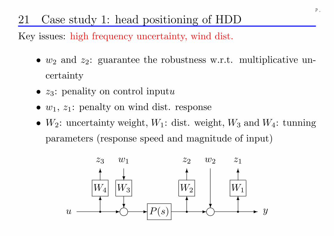
千葉大学
21 Case study 1: head positioning of HDD
Key issues: high frequency uncertainty, wind dist.
• w2 and z2: guarantee the robustness w.r.t. multiplicative un-
certainty
• z3: penality on control inputu
• w1, z1: penalty on wind dist. response
• W2: uncertainty weight, W1: dist. weight, W3 and W4: tunning
parameters (response speed and magnitude of input)
u
W4
- -g-6
6
w1z3
q
?
6
6
q g -? 6
6
w2 z1
q
z2
W1
yP (s)
W2W3
?
252
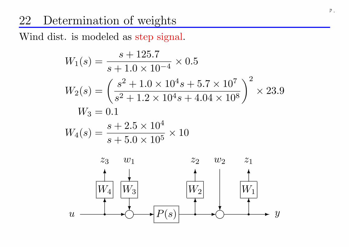
千葉大学
22 Determination of weights
Wind dist. is modeled as step signal.
W1(s) =s + 125.7
s + 1.0× 10−4× 0.5
W2(s) =(
s2 + 1.0× 10⁴s + 5.7× 10⁷
s2 + 1.2× 10⁴s + 4.04× 10⁸
)2
× 23.9
W3 = 0.1
W4(s) =s + 2.5× 10⁴
s + 5.0× 105× 10
u
W4
- -g-6
6
w1z3
q
?
6
6
q g -? 6
6
w2 z1
q
z2
W1
yP (s)
W2W3
?
253
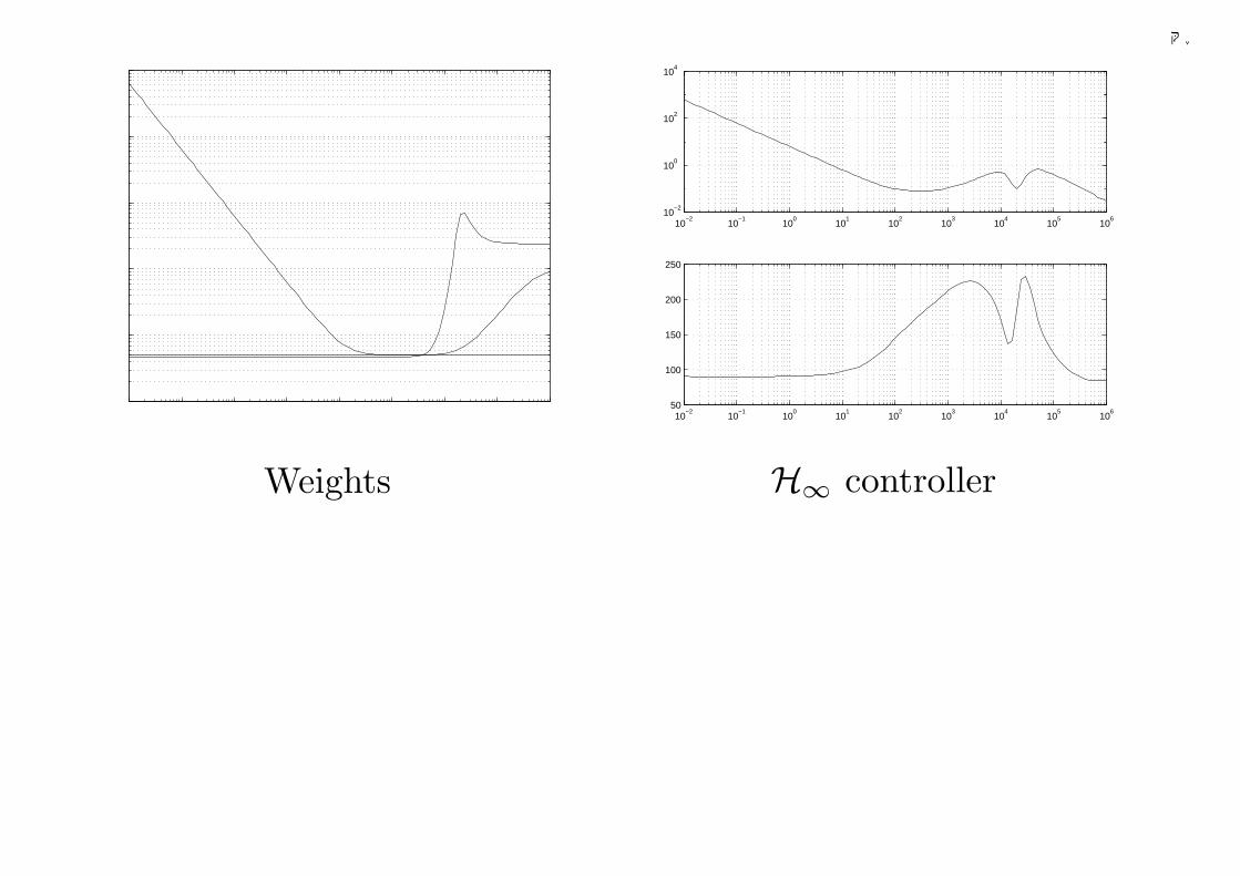
千葉大学
10-2
10-1
100
101
102
103
104
105
106
10-1
100
101
102
103
104
Weighting Functions
Frequency [rad/s]
Gain
Weights
10−2
10−1
100
101
102
103
104
105
106
10−2
100
102
104
Bode plot of Controller
Frequency [rad/s]
Gai
n
10−2
10−1
100
101
102
103
104
105
106
50
100
150
200
250
Frequency [rad/s]
Pha
se(d
egre
es)
H∞ controller
254
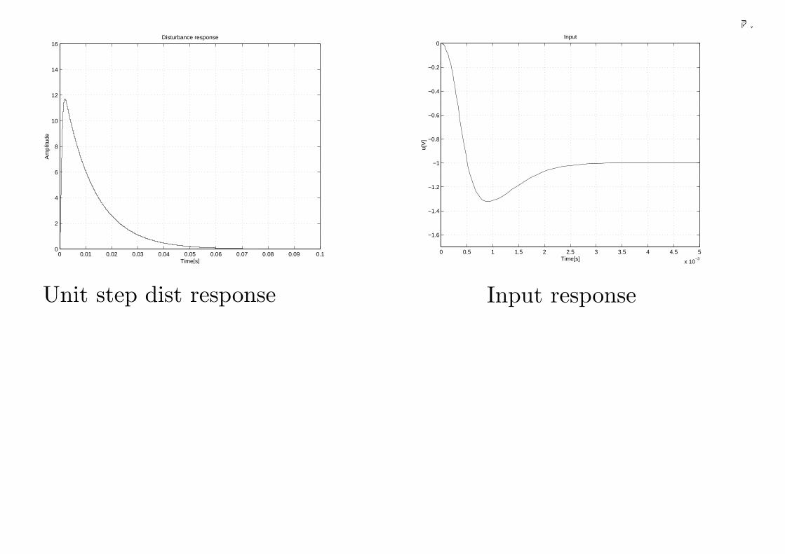
千葉大学
0 0.01 0.02 0.03 0.04 0.05 0.06 0.07 0.08 0.09 0.10
2
4
6
8
10
12
14
16
Time[s]
Am
plitu
de
Disturbance response
Unit step dist response
0 0.5 1 1.5 2 2.5 3 3.5 4 4.5 5
x 10−3
−1.6
−1.4
−1.2
−1
−0.8
−0.6
−0.4
−0.2
0
Time[s]
u[V
]
Input
Input response
255
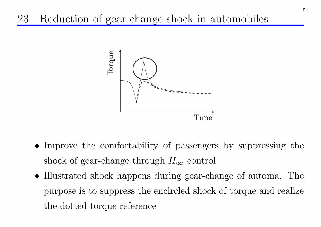
千葉大学
23 Reduction of gear-change shock in automobiles
Torq
ue
Time
• Improve the comfortability of passengers by suppressing the
shock of gear-change through H∞ control
• Illustrated shock happens during gear-change of automa. The
purpose is to suppress the encircled shock of torque and realize
the dotted torque reference
256
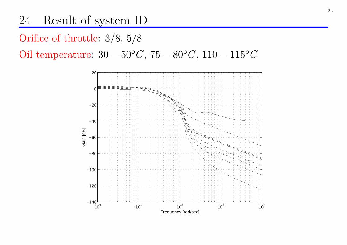
千葉大学
24 Result of system ID
Orifice of throttle: 3/8, 5/8
Oil temperature: 30− 50C, 75− 80C, 110− 115C
100
101
102
103
104
−140
−120
−100
−80
−60
−40
−20
0
20
Frequency [rad/sec]
Gai
n [d
B]
257
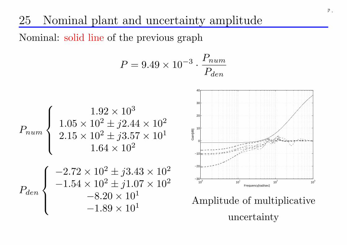
千葉大学
25 Nominal plant and uncertainty amplitude
Nominal: solid line of the previous graph
P = 9.49× 10⁻³ · Pnum
Pden
Pnum
1.92× 10³
1.05× 10² ± j2.44× 102
2.15× 10² ± j3.57× 101
1.64× 10²
Pden
−2.72× 10² ± j3.43× 102
−1.54× 10² ± j1.07× 102
−8.20× 101
−1.89× 101
100
101
102
103
−30
−20
−10
0
10
20
30
40
Frequency[rad/sec]
Gai
n[dB
]
Amplitude of multiplicative
uncertainty
258
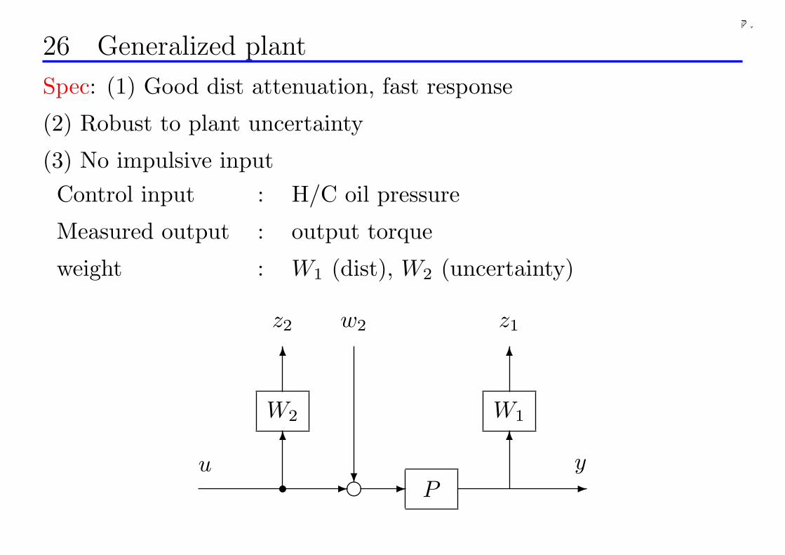
千葉大学
26 Generalized plant
Spec: (1) Good dist attenuation, fast response
(2) Robust to plant uncertainty
(3) No impulsive inputControl input : H/C oil pressure
Measured output : output torque
weight : W1 (dist), W2 (uncertainty)
- e?
w2
y
z2
-
6
W1
6
-
6
6
z1
u r
W2
P
259
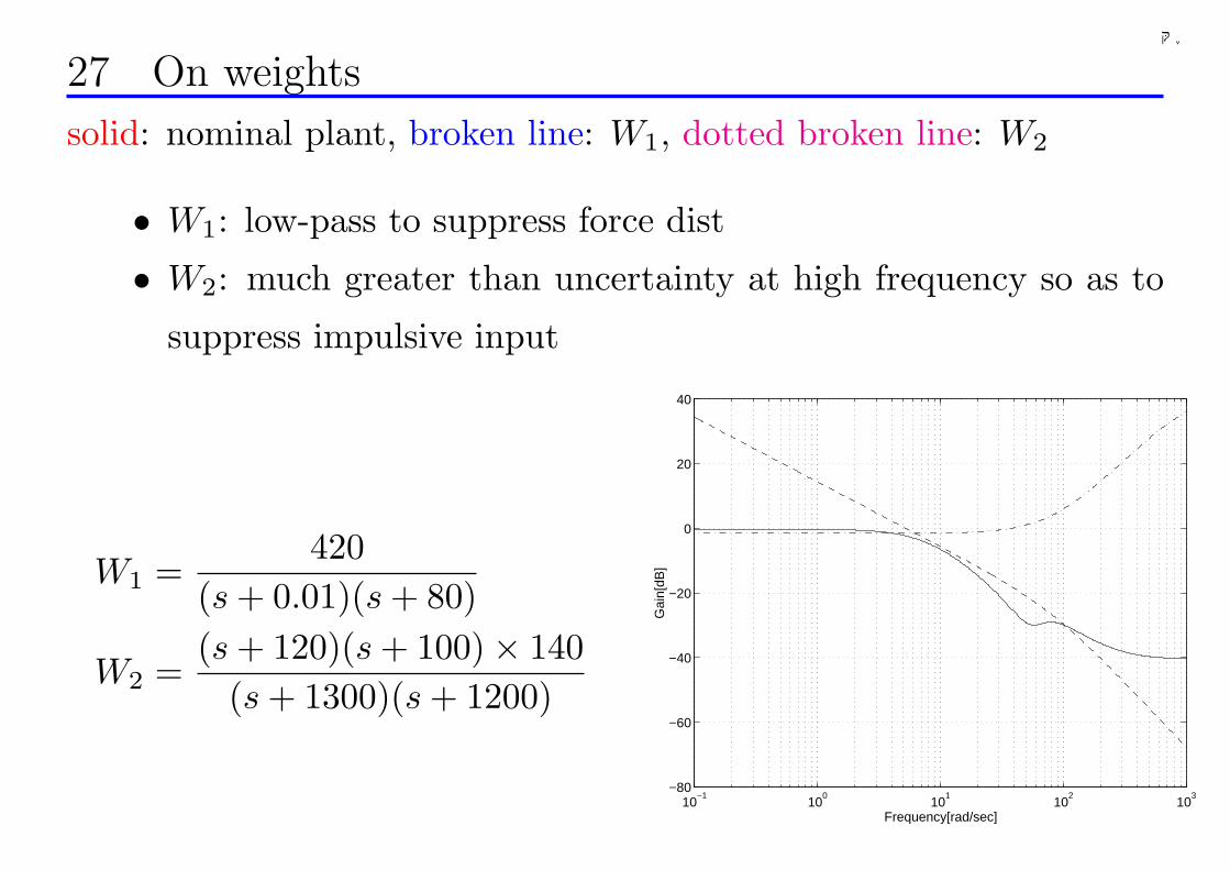
千葉大学
27 On weights
solid: nominal plant, broken line: W1, dotted broken line: W2
• W1: low-pass to suppress force dist
• W2: much greater than uncertainty at high frequency so as to
suppress impulsive input
W1 =420
(s + 0.01)(s + 80)
W2 =(s + 120)(s + 100)× 140
(s + 1300)(s + 1200)
10−1
100
101
102
103
−80
−60
−40
−20
0
20
40
Frequency[rad/sec]
Gai
n[dB
]
260
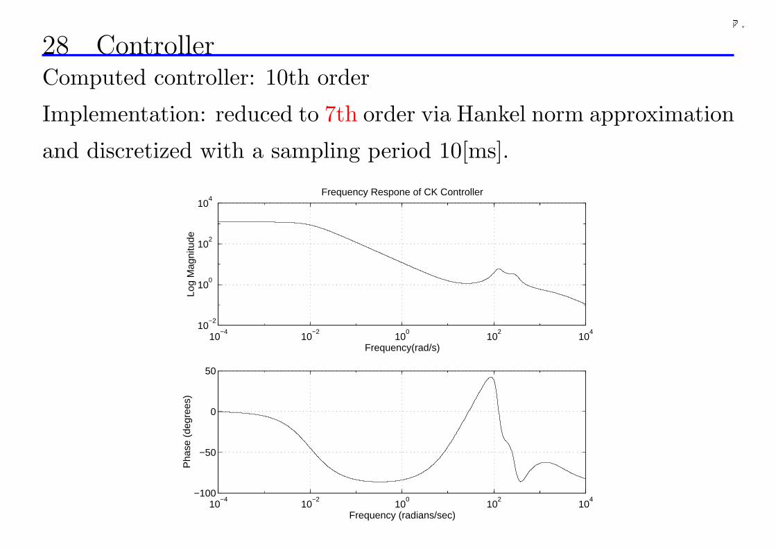
千葉大学
28 ControllerComputed controller: 10th order
Implementation: reduced to 7th order via Hankel norm approximation
and discretized with a sampling period 10[ms].
10−4
10−2
100
102
104
10−2
100
102
104
Log
Mag
nitu
de
Frequency(rad/s)
Frequency Respone of CK Controller
10−4
10−2
100
102
104
−100
−50
0
50
Pha
se (
degr
ees)
Frequency (radians/sec)
261
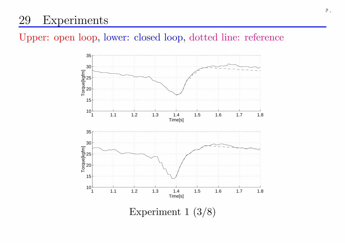
千葉大学
29 Experiments
Upper: open loop, lower: closed loop, dotted line: reference
1 1.1 1.2 1.3 1.4 1.5 1.6 1.7 1.810
15
20
25
30
35
Time[s]
Tor
que[
kgfm
]
1 1.1 1.2 1.3 1.4 1.5 1.6 1.7 1.810
15
20
25
30
35
Time[s]
Tor
que[
kgfm
]
Experiment 1 (3/8)
262

千葉大学
1 1.1 1.2 1.3 1.4 1.5 1.6 1.7 1.810
15
20
25
30
35
Time[s]T
orqu
e[kg
fm]
1 1.1 1.2 1.3 1.4 1.5 1.6 1.7 1.810
15
20
25
30
35
Time[s]
Tor
que[
kgfm
]
Experiment 2 (2/8)
263
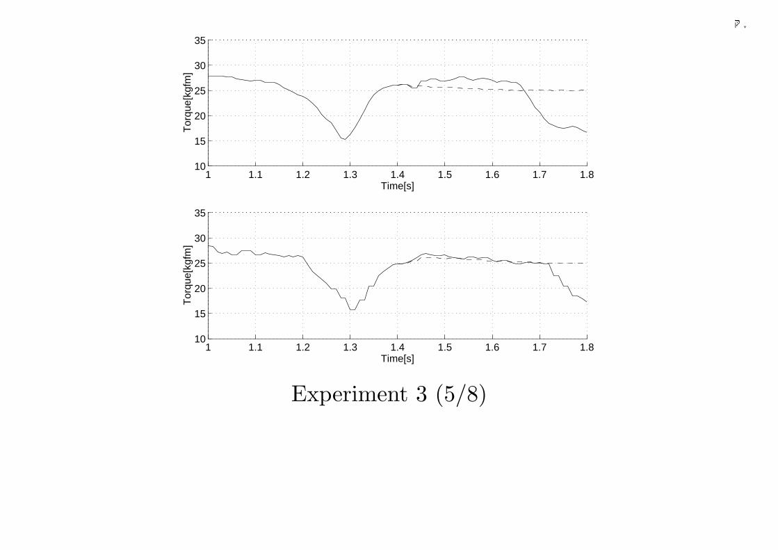
千葉大学
1 1.1 1.2 1.3 1.4 1.5 1.6 1.7 1.810
15
20
25
30
35
Time[s]T
orqu
e[kg
fm]
1 1.1 1.2 1.3 1.4 1.5 1.6 1.7 1.810
15
20
25
30
35
Time[s]
Tor
que[
kgfm
]
Experiment 3 (5/8)
264
千葉大学
Chapter 7 Gain-Scheduled Control
Gain-scheduled control:
Tunning the parameters of controller on-line according to the state of
plant so as to achieve the best performance.
Contents:
Lyapunov stability theory
Quadratic stability
Polytopic description of parameter vector
Quadratic stabilization of polytopic systems
Equivalent transformation: from nonlinear to LPV
Gain-scheduled control
Case study: transient stabilization of power systems
265
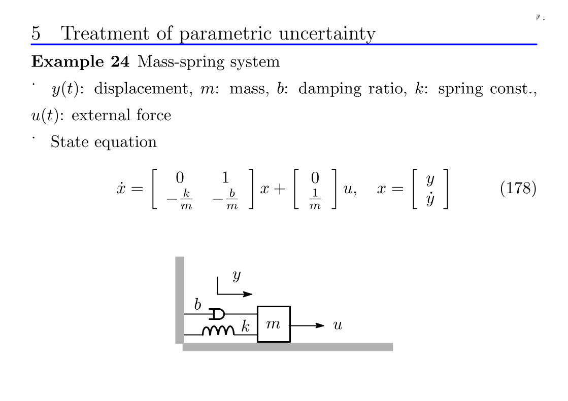
千葉大学
5 Treatment of parametric uncertainty
Example 24 Mass-spring system
y(t): displacement, m: mass, b: damping ratio, k: spring const.,
u(t): external force
State equation
x =[
0 1− k
m − bm
]x +
[01m
]u, x =
[yy
](178)
ub
k
y
m
266
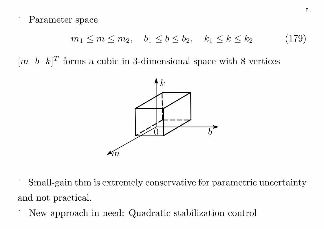
千葉大学
Parameter space
m1 ≤ m ≤ m2, b1 ≤ b ≤ b2, k1 ≤ k ≤ k2 (179)
[m b k]T forms a cubic in 3-dimensional space with 8 vertices
m
b
k
0
Small-gain thm is extremely conservative for parametric uncertainty
and not practical.
New approach in need: Quadratic stabilization control
267
千葉大学
6 Lyapunov stability theory
Basic idea:
Dealing with the asymptotic stability (x(t) → 0) of system
x = Ax, x(0) 6= 0 (180)
via discussion on the convergence of energy function (Lyapunov func-
tion).
Lyapunov function V (x)
Positive quadratic function:
V (x) = xT Px > 0 ∀x 6= 0, V (0) = 0 (181)
Positive definite matrix: square symmetric matrix PT = P associated
with a positive functionP > 0 (182)
268
千葉大学
If the trajectory x(t) of state satisfies
V (x) < 0 ∀x(t) 6= 0 (183)
Then V (x(t)) decreases monotonically with time t.
Due to V (x) ≥ 0
limt→∞
V (x(t)) = x(∞)T Px(∞) = 0 ⇒ x(∞) = 0 (184)
i.e., the system is stable.
269
千葉大学
7 Condition for asymptotic stability of state
Differentiation of V (x) = xT Px along the trajectory of x = Ax
V (x) = xT Px + xT Px
= (Ax)T Px + xT P (Ax)
= xT (AT P + PA)x < 0 ∀x 6= 0 (185)
⇔ AT P + PA < 0 (186)
Therefore, if this LMI has a solution P > 0, the asymptotic stability
of system is guaranteed.
270
千葉大学
8 Condition on convergence rate of state
WhenAT P + PA + 2σP < 0 (187)
has a solution P > 0, then
V (x) = xT (AT P + PA)x < xT (−2σP )x = −2σV (x)⇒ V (x(t)) < e−2σtV (x(0)) (188)
⇒ xT (x)Px(t) < e−2σtxT (0)Px(0)⇒ ‖x(t)‖ < ce−σt‖x(0)‖ (189)
i.e. the state x(t) converges to zero at least at the rate σ.
271
千葉大学
9 Quadratic stability
Plant set
x = A(θ)x, θ : uncertain parameter vector (190)
e.g. in the mass-spring system (u = 0)
x =[
0 1− k
m − bm
]x = A(m, b, k)x, θ = [m b k]
Motivation: to investigate the stability of all systems by using a
single quadratic function V = xT Px (Barmish). When this is possible,
the plant set is said to be quadratically stable.
V (x) = xT Px > 0 ∀x 6= 0, V (x, θ) < 0 ∀x 6= 0, θ (191)
Quadratic stability is a very strong spec, however it proves to be
quite useful in practice.
272
千葉大学
10 Condition for quadratic stability
Since V (x, θ) = xT (AT (θ)P + PA(θ))x, the condition for quadratic
stability becomes
∃P > 0 ⇒ AT (θ)P + PA(θ) < 0 ∀θ (192)
Example 25 Consider a 1st order system
x = −(2 + θ)x, −1 ≤ θ ≤ 1
The following always holds
AT (θ)P + PA(θ) = −(2 + θ)P − P (2 + θ) = −2(2 + θ)P
P = 1 ⇒ AT (θ)P + PA(θ) = −2(2 + θ) < 0 ∀θ
It is equivalent to the asymptotic stability in the usual sense.
273
千葉大学
Question: how to find the solution P > 0 of inequality
AT (θ)P + PA(θ) < 0 ∀θ
The general case is difficult because it depends on the uncertain
parameter vector θ.
Possible if A(θ) has certain special structure in θ
274
千葉大学
11 Polytopic set of parameter vectors
Case 1: one parameter
m ∈ [m1, m2] can be described as a convex combination of its 2
vertices m1,m2
m = λm1 + (1− λ)m2 = m2 − λ(m2 −m1), λ ∈ [0, 1] ⇔ (193)m = α1m1 + α2m2, α1 = λ, α2 = 1− λ ⇒ α1 + α2 = 1, αi ≥ 0(194)
Case 2: two parameters
m ∈ [m1, m2] and b ∈ [b1, b2] are described as
m = α1m1 + α2m2, α1 + α2 = 1, αi ≥ 0 (195)b = β1b1 + β2b2, β1 + β2 = 1, βi ≥ 0 (196)
resp. The vector [m b] is a rectangle with 4 vertices.
275
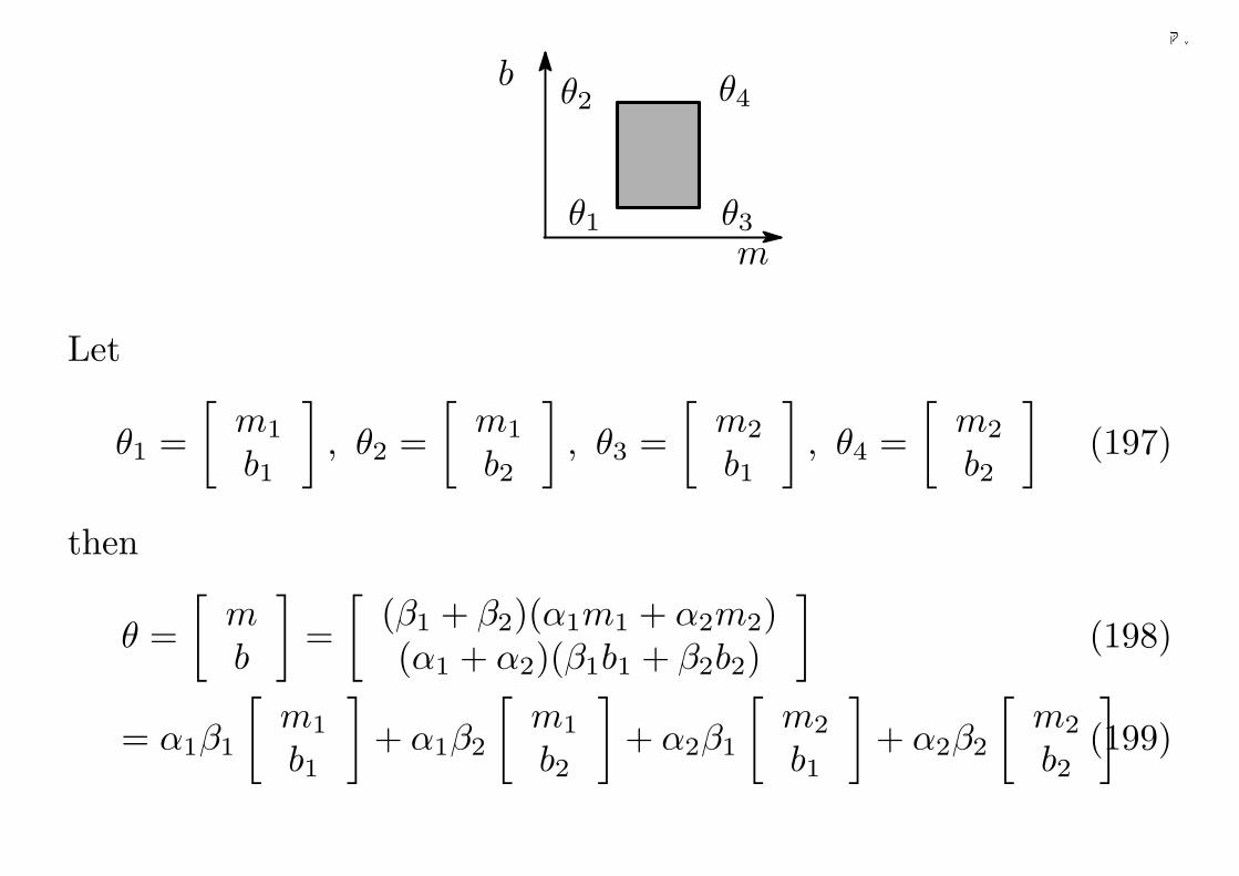
千葉大学
m
b
θ1 θ3
θ4θ2
Let
θ1 =[
m1
b1
], θ2 =
[m1
b2
], θ3 =
[m2
b1
], θ4 =
[m2
b2
](197)
then
θ =[
mb
]=
[(β1 + β2)(α1m1 + α2m2)(α1 + α2)(β1b1 + β2b2)
](198)
= α1β1
[m1
b1
]+ α1β2
[m1
b2
]+ α2β1
[m2
b1
]+ α2β2
[m2
b2
](199)
276
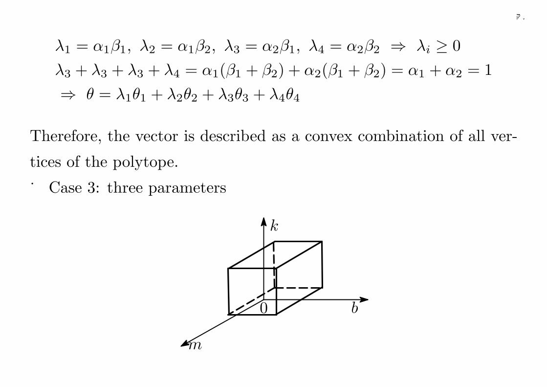
千葉大学
λ1 = α1β1, λ2 = α1β2, λ3 = α2β1, λ4 = α2β2 ⇒ λi ≥ 0λ3 + λ3 + λ3 + λ4 = α1(β1 + β2) + α2(β1 + β2) = α1 + α2 = 1⇒ θ = λ1θ1 + λ2θ2 + λ3θ3 + λ4θ4
Therefore, the vector is described as a convex combination of all ver-
tices of the polytope.
Case 3: three parameters
m
b
k
0
277
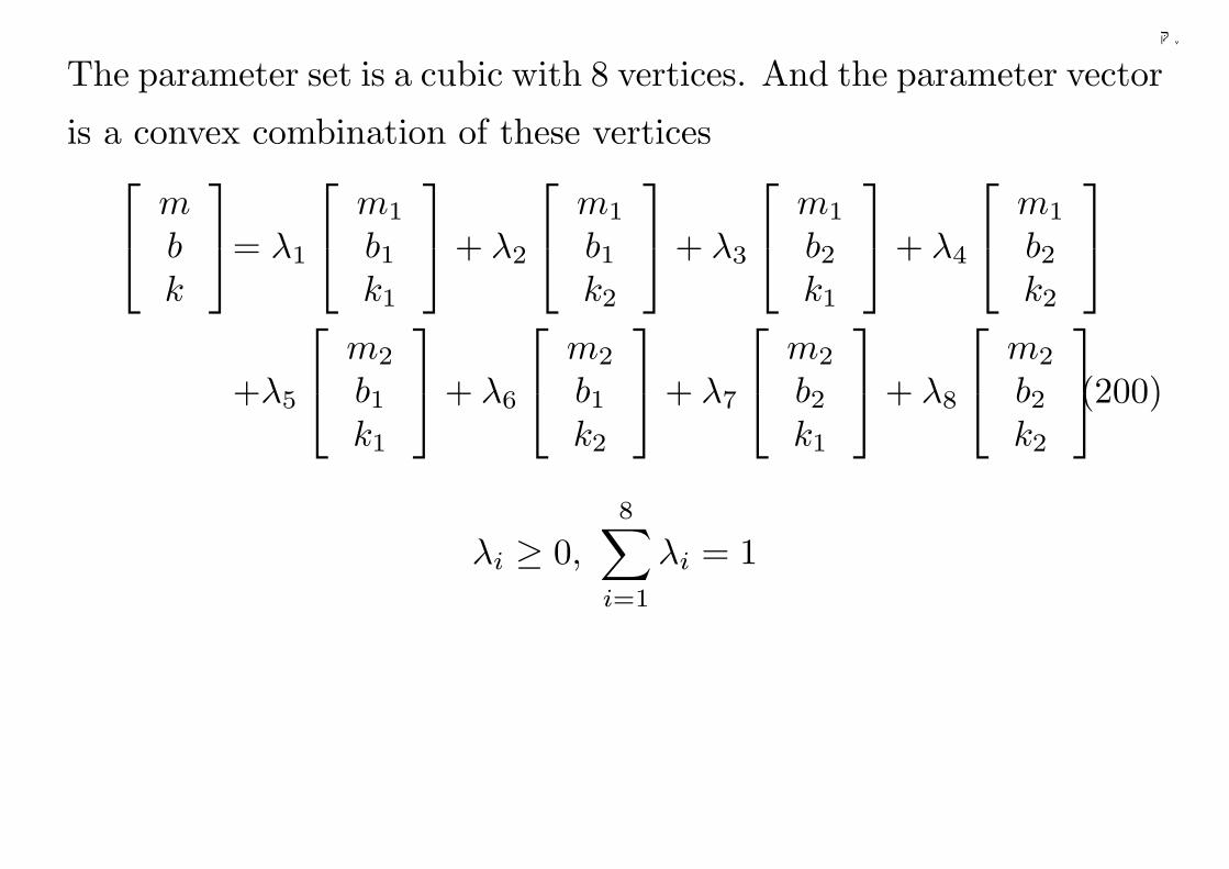
千葉大学
The parameter set is a cubic with 8 vertices. And the parameter vector
is a convex combination of these vertices
mbk
= λ1
m1
b1
k1
+ λ2
m1
b1
k2
+ λ3
m1
b2
k1
+ λ4
m1
b2
k2
+λ5
m2
b1
k1
+ λ6
m2
b1
k2
+ λ7
m2
b2
k1
+ λ8
m2
b2
k2
(200)
λi ≥ 0,
8∑
i=1
λi = 1
278
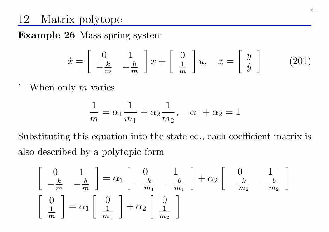
千葉大学
12 Matrix polytope
Example 26 Mass-spring system
x =[
0 1− k
m − bm
]x +
[01m
]u, x =
[yy
](201)
When only m varies
1m
= α11
m1+ α2
1m2
, α1 + α2 = 1
Substituting this equation into the state eq., each coefficient matrix is
also described by a polytopic form[
0 1− k
m − bm
]= α1
[0 1
− km1
− bm1
]+ α2
[0 1
− km2
− bm2
]
[01m
]= α1
[01
m1
]+ α2
[01
m2
]
279
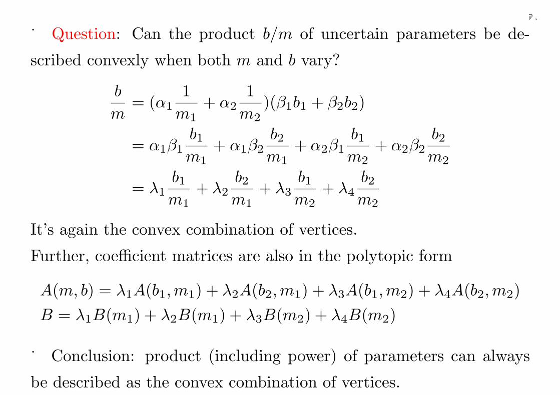
千葉大学
Question: Can the product b/m of uncertain parameters be de-
scribed convexly when both m and b vary?
b
m= (α1
1m1
+ α21
m2)(β1b1 + β2b2)
= α1β1b1
m1+ α1β2
b2
m1+ α2β1
b1
m2+ α2β2
b2
m2
= λ1b1
m1+ λ2
b2
m1+ λ3
b1
m2+ λ4
b2
m2
It’s again the convex combination of vertices.
Further, coefficient matrices are also in the polytopic form
A(m, b) = λ1A(b1,m1) + λ2A(b2,m1) + λ3A(b1,m2) + λ4A(b2,m2)B = λ1B(m1) + λ2B(m1) + λ3B(m2) + λ4B(m2)
Conclusion: product (including power) of parameters can always
be described as the convex combination of vertices.
280
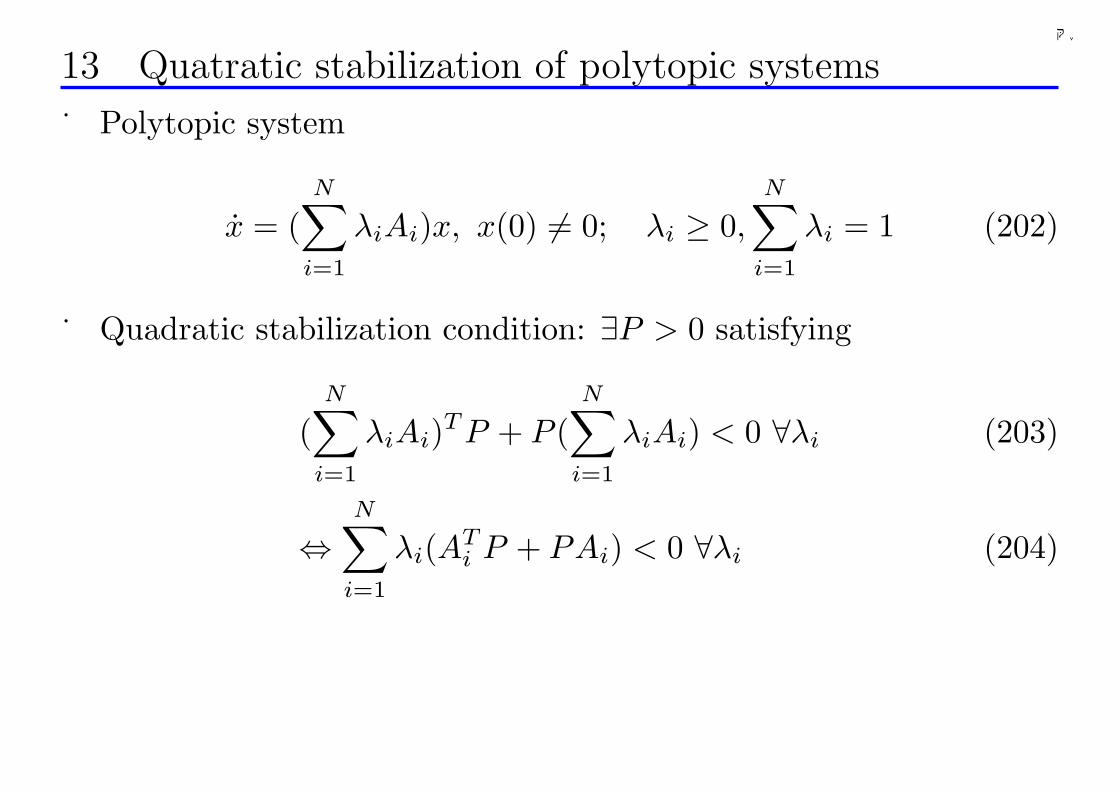
千葉大学
13 Quatratic stabilization of polytopic systems
Polytopic system
x = (N∑
i=1
λiAi)x, x(0) 6= 0; λi ≥ 0,N∑
i=1
λi = 1 (202)
Quadratic stabilization condition: ∃P > 0 satisfying
(N∑
i=1
λiAi)T P + P (N∑
i=1
λiAi) < 0 ∀λi (203)
⇔N∑
i=1
λi(ATi P + PAi) < 0 ∀λi (204)
281
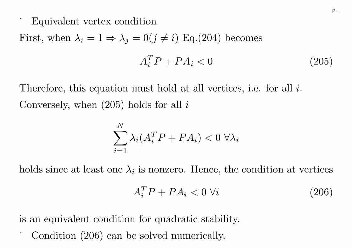
千葉大学
Equivalent vertex condition
First, when λi = 1 ⇒ λj = 0(j 6= i) Eq.(204) becomes
ATi P + PAi < 0 (205)
Therefore, this equation must hold at all vertices, i.e. for all i.
Conversely, when (205) holds for all i
N∑
i=1
λi(ATi P + PAi) < 0 ∀λi
holds since at least one λi is nonzero. Hence, the condition at vertices
ATi P + PAi < 0 ∀i (206)
is an equivalent condition for quadratic stability.
Condition (206) can be solved numerically.
282
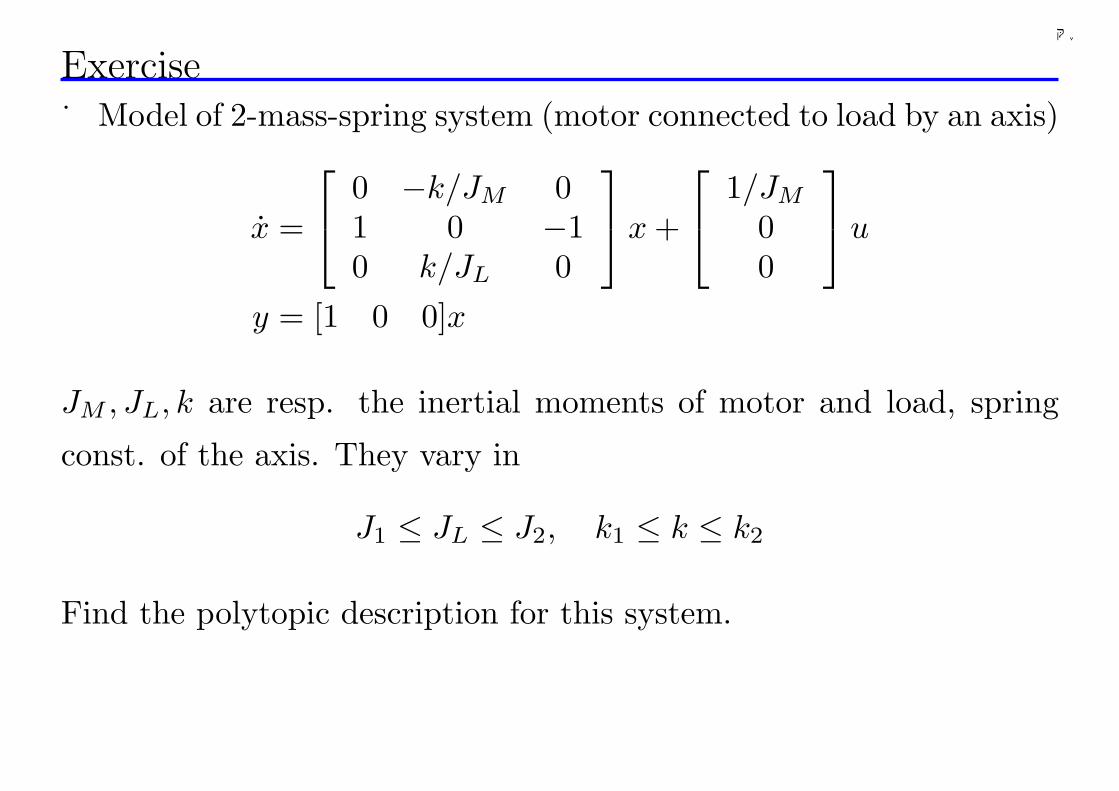
千葉大学
ExerciseModel of 2-mass-spring system (motor connected to load by an axis)
x =
0 −k/JM 01 0 −10 k/JL 0
x +
1/JM
00
u
y = [1 0 0]x
JM , JL, k are resp. the inertial moments of motor and load, spring
const. of the axis. They vary in
J1 ≤ JL ≤ J2, k1 ≤ k ≤ k2
Find the polytopic description for this system.
283
千葉大学
14 Quadratic stabilization via state feedback
Polytopic system
x = (N∑
i=1
λiAi)x + (N∑
i=1
λiBi)u, λi ≥ 0,N∑
i=1
λi = 1 (207)
Const. state feedbacku = Fx (208)
Closed loop system
x = (N∑
i=1
λiAi +N∑
i=1
λiBiF )x =N∑
i=1
λi(Ai + BiF )x (209)
λi ≥ 0,N∑
i=1
λi = 1
284
千葉大学
Quadratic stabilization condition: ∃F, P > 0 s.t.
(Ai + BiF )T P + P (Ai + BiF ) < 0 ∀i (210)
⇔ATi P + PAi + (B1F )T P + PBiF < 0 ∀i (211)
However, the products (BiF )T P, PBiF of unknown matrices appear
in the inequality, it is a BMI (bilnear matrix inequality) not an LMI.
Cannot be solved numerically in this form.
From BMI to LMI: approach of variable transformation
Q = P−1, X = FQ ⇔ F = XQ−1 (212)
In terms of this transformation, the condition turns into
Q(Ai + BiF )T + (Ai + BiF )Q < 0 ∀i (213)
⇔QATi + AiQ + XT BT
i + BiX < 0 ∀i (214)
which is an LMI in Q,X and solvable.
285
千葉大学
15 LPV description of nonlinear systems
LPV (linear parameter varying) system
x = A(p(t))x + B(p(t))u (215)y = C(p(t))x (216)
p(t) is a time-varying vector, each matrix is affine in p(t).
For example, when p(t) = [p1(t) p2(t)]
A(p(t)) = A0 + p1(t)A1 + p2(t)A2, B(p(t)) = B0 + p1(t)B1 + p2(t)B2
C(p(t)) = C0 + p1(t)C1 + p2(t)C2
Transforming a nonlinear system into an LPV system
Many nonlinear systems may be tramsformed equivalently into LPV
systems if the nonlinear terms are regarded as linear terms with time-
varying coefficients.
286
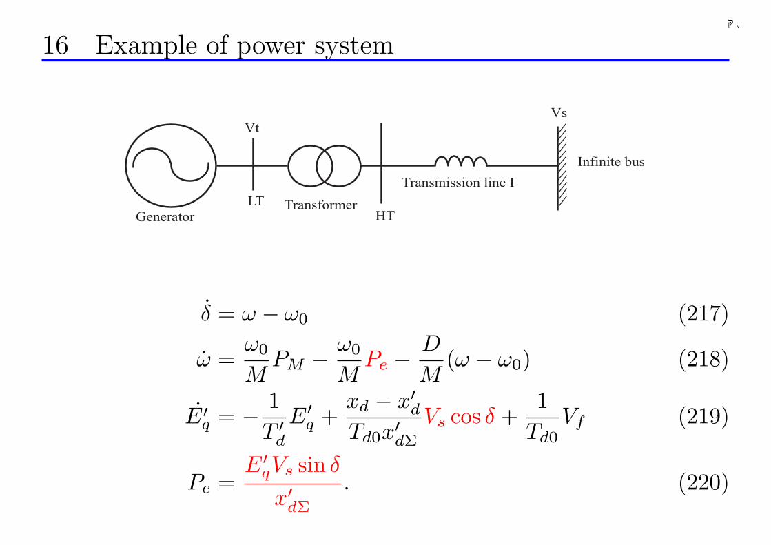
千葉大学
16 Example of power system
GeneratorTransformer
Infinite bus
Vs
Vt
LT
HT
Transmission line I
δ = ω − ω0 (217)
ω =ω0
MPM − ω0
MPe − D
M(ω − ω0) (218)
E′q = − 1
T ′dE′
q +xd − x′dTd0x′dΣ
Vs cos δ +1
Td0Vf (219)
Pe =E′
qVs sin δ
x′dΣ
. (220)
287
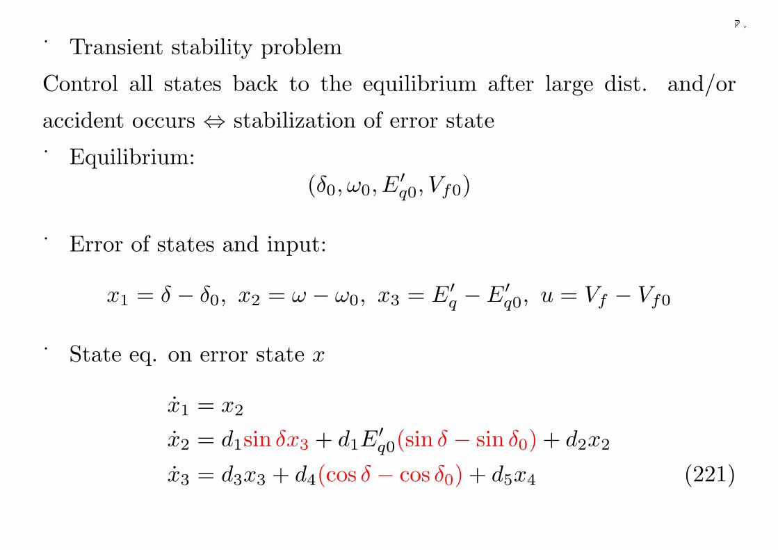
千葉大学
Transient stability problem
Control all states back to the equilibrium after large dist. and/or
accident occurs ⇔ stabilization of error state
Equilibrium:(δ0, ω0, E
′q0, Vf0)
Error of states and input:
x1 = δ − δ0, x2 = ω − ω0, x3 = E′q − E′
q0, u = Vf − Vf0
State eq. on error state x
x1 = x2
x2 = d1sin δx3 + d1E′q0(sin δ − sin δ0) + d2x2
x3 = d3x3 + d4(cos δ − cos δ0) + d5x4 (221)
288
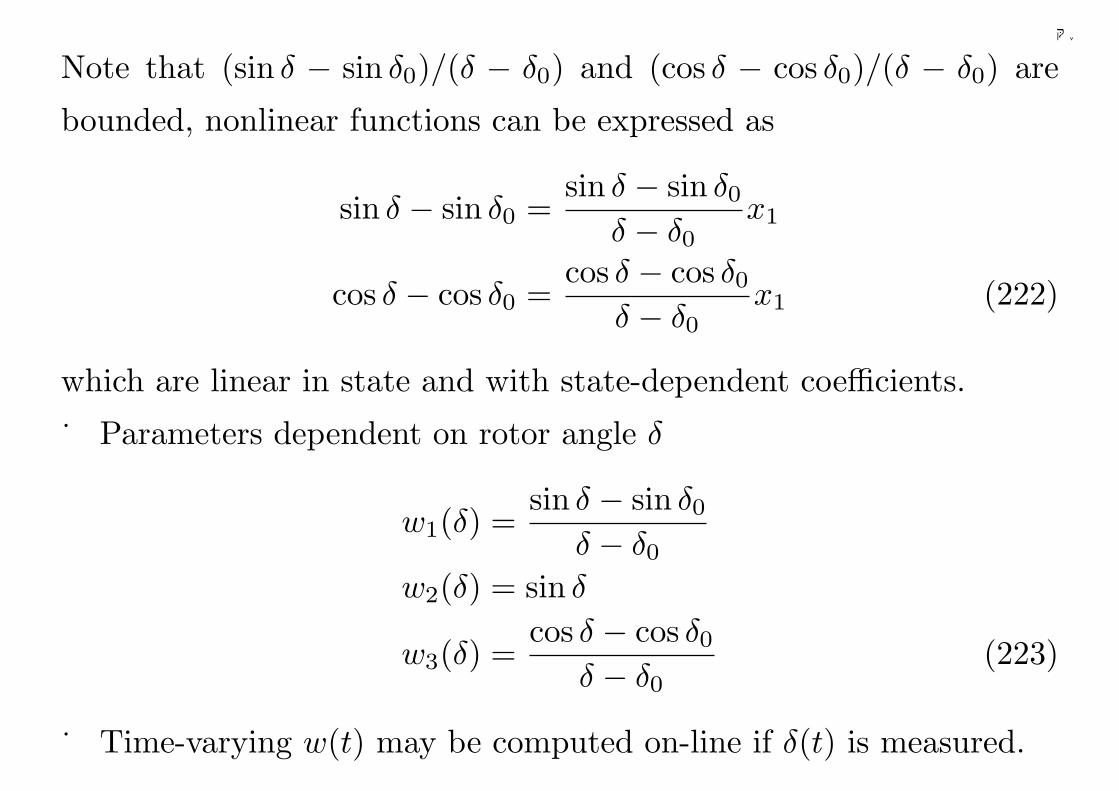
千葉大学
Note that (sin δ − sin δ0)/(δ − δ0) and (cos δ − cos δ0)/(δ − δ0) are
bounded, nonlinear functions can be expressed as
sin δ − sin δ0 =sin δ − sin δ0
δ − δ0x1
cos δ − cos δ0 =cos δ − cos δ0
δ − δ0x1 (222)
which are linear in state and with state-dependent coefficients.
Parameters dependent on rotor angle δ
w1(δ) =sin δ − sin δ0
δ − δ0
w2(δ) = sin δ
w3(δ) =cos δ − cos δ0
δ − δ0(223)
Time-varying w(t) may be computed on-line if δ(t) is measured.
289
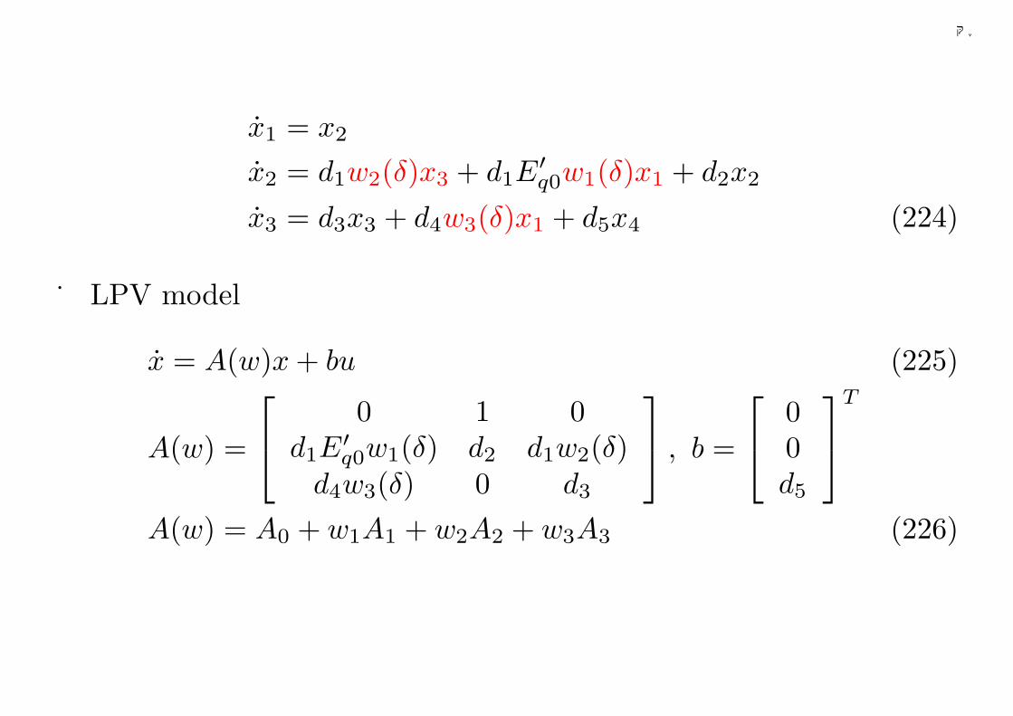
千葉大学
x1 = x2
x2 = d1w2(δ)x3 + d1E′q0w1(δ)x1 + d2x2
x3 = d3x3 + d4w3(δ)x1 + d5x4 (224)
LPV model
x = A(w)x + bu (225)
A(w) =
0 1 0d1E
′q0w1(δ) d2 d1w2(δ)
d4w3(δ) 0 d3
, b =
00d5
T
A(w) = A0 + w1A1 + w2A2 + w3A3 (226)
290
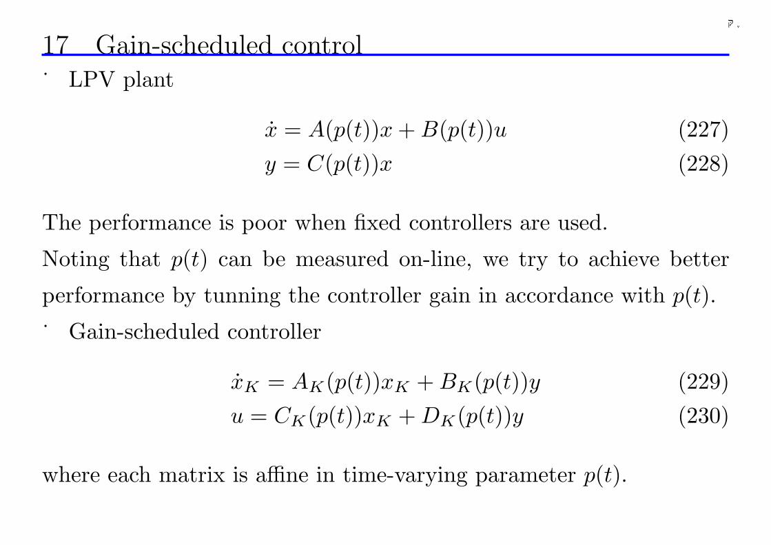
千葉大学
17 Gain-scheduled control LPV plant
x = A(p(t))x + B(p(t))u (227)y = C(p(t))x (228)
The performance is poor when fixed controllers are used.
Noting that p(t) can be measured on-line, we try to achieve better
performance by tunning the controller gain in accordance with p(t).
Gain-scheduled controller
xK = AK(p(t))xK + BK(p(t))y (229)u = CK(p(t))xK + DK(p(t))y (230)
where each matrix is affine in time-varying parameter p(t).
291
千葉大学
18 Case study: stabilization of power systems
¥ Gain-scheduled state feedback
u = F (w)x (231)F (w) = F0 + w1F1 + w2F2 + w3F3. (232)
¥ Design problem: How to find const. matrices F0, F1, F2, F3
¥ Closed Loop Systemx = Acl(w)x (233)
Acl(w) = (A0 + bF0) + w1(A1 + bF1) + w2(A2 + bF2) + w3(A3 + bF3)
292
千葉大学
19 Design specs
Spec 1: ensuring a convergence rate higher than σ
Acl(w)T P + PAcl(w) + 2σP < 0, P > 0 (234)
Spec 2: avoiding input saturation
The excitation voltage Vf (→ u) is limited. In order to avoid satura-
tion, we minimize the feedback gain F (w) indirectly via the minimiza-
tion of ‖F (w)P−12 ‖, i.e. to minimize γ satisfying
||F (w)P−12 ||2 < γ (235)
293
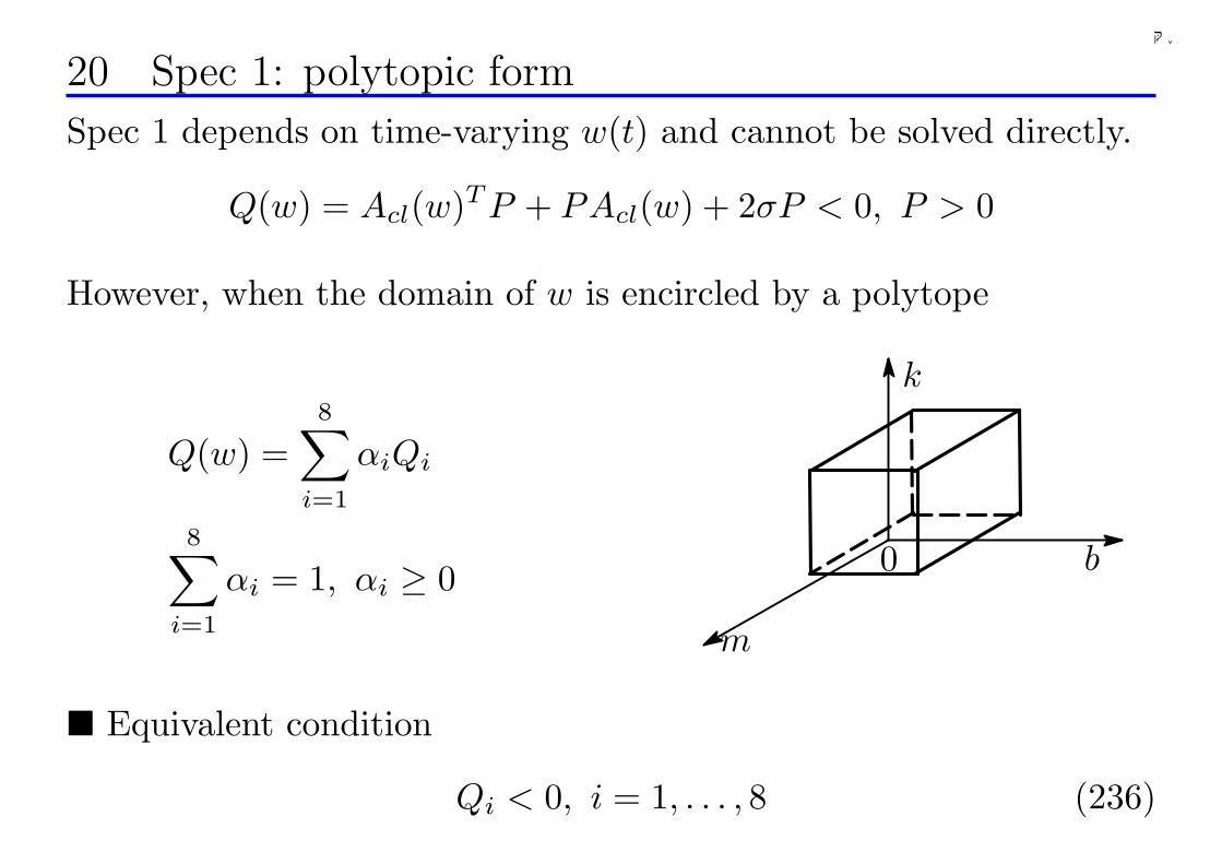
千葉大学
20 Spec 1: polytopic form
Spec 1 depends on time-varying w(t) and cannot be solved directly.
Q(w) = Acl(w)T P + PAcl(w) + 2σP < 0, P > 0
However, when the domain of w is encircled by a polytope
Q(w) =8∑
i=1
αiQi
8∑
i=1
αi = 1, αi ≥ 0
m
b
k
0
¥ Equivalent condition
Qi < 0, i = 1, . . . , 8 (236)
294
千葉大学
21 Reduction to LMIQi is bilinear in unknowns F and P
Q1 = Af0 + w1mAf1 + w2mAf2 + w3mAf3 + 2σP
Af0 = (A0 + bF0)T P + P (A0 + bF0) ...
¥ Variable transformation
X = P−1 > 0, Gi = FiX ⇔ Fi = GiX−1 (237)
reduces Qi < 0 to LMI
Q1 = Af0 + w1mAf1 + w2mAf2 + w3mAf3 + 2σX < 0 (238)...
Af0 = A0X + XAT0 + BG0 + GT
0 BT (239)...
295
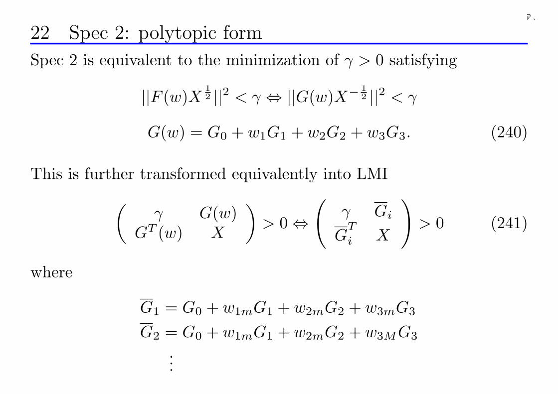
千葉大学
22 Spec 2: polytopic form
Spec 2 is equivalent to the minimization of γ > 0 satisfying
||F (w)X12 ||2 < γ ⇔ ||G(w)X− 1
2 ||2 < γ
G(w) = G0 + w1G1 + w2G2 + w3G3. (240)
This is further transformed equivalently into LMI
(γ G(w)
GT (w) X
)> 0 ⇔
(γ Gi
GT
i X
)> 0 (241)
where
G1 = G0 + w1mG1 + w2mG2 + w3mG3
G2 = G0 + w1mG1 + w2mG2 + w3MG3
...
296
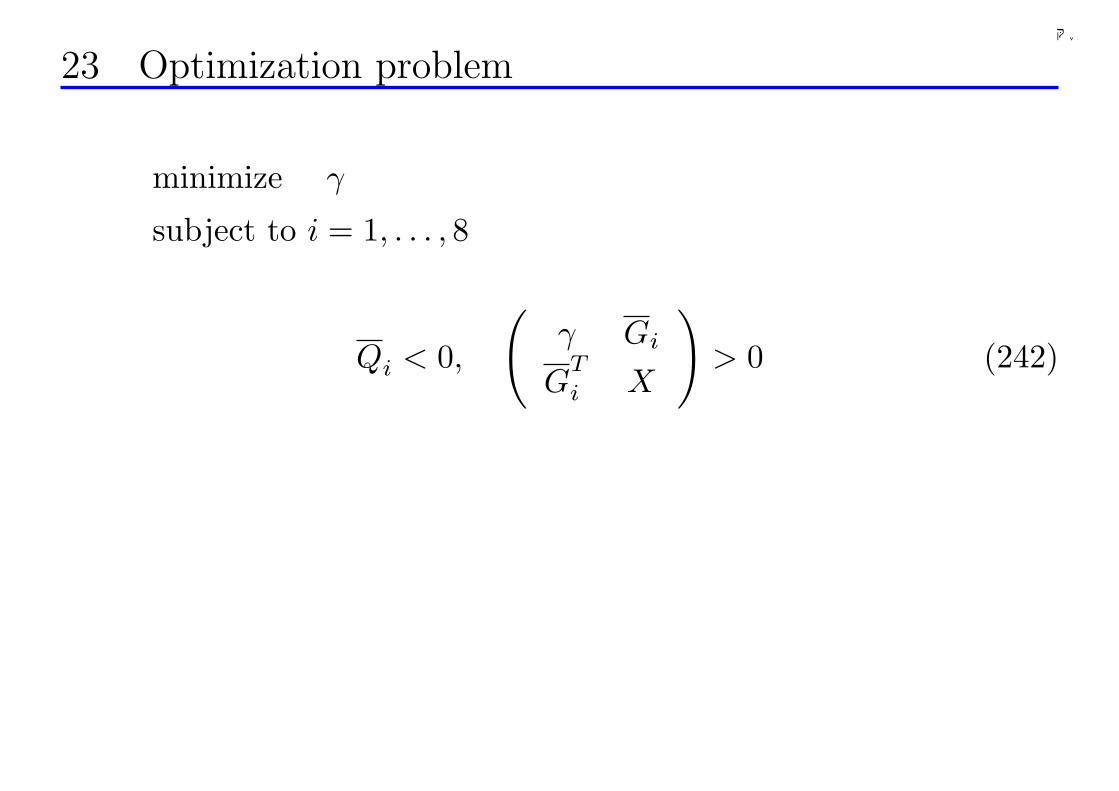
千葉大学
23 Optimization problem
minimize γ
subject to i = 1, . . . , 8
Qi < 0,
(γ Gi
GT
i X
)> 0 (242)
297
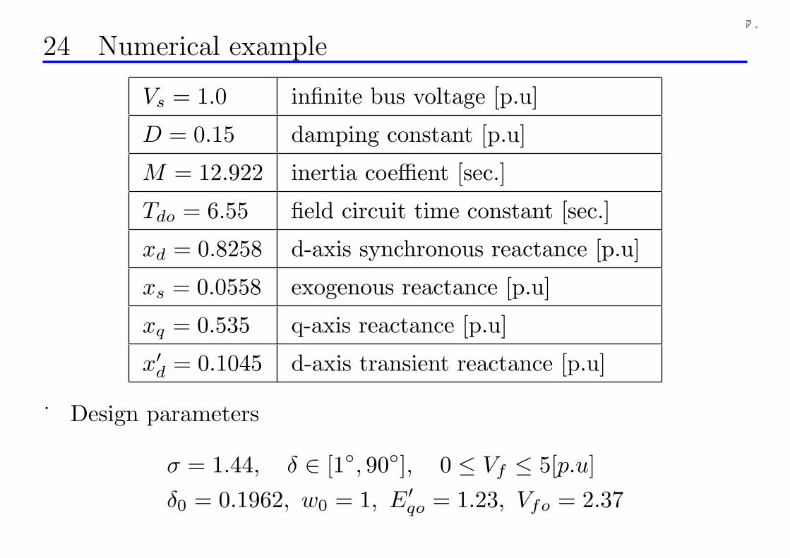
千葉大学
24 Numerical example
Vs = 1.0 infinite bus voltage [p.u]
D = 0.15 damping constant [p.u]
M = 12.922 inertia coeffient [sec.]
Tdo = 6.55 field circuit time constant [sec.]
xd = 0.8258 d-axis synchronous reactance [p.u]
xs = 0.0558 exogenous reactance [p.u]
xq = 0.535 q-axis reactance [p.u]
x′d = 0.1045 d-axis transient reactance [p.u]
Design parameters
σ = 1.44, δ ∈ [1, 90], 0 ≤ Vf ≤ 5[p.u]δ0 = 0.1962, w0 = 1, E′
qo = 1.23, Vfo = 2.37
298
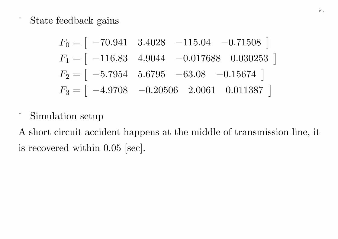
千葉大学
State feedback gains
F0 =[ −70.941 3.4028 −115.04 −0.71508
]
F1 =[ −116.83 4.9044 −0.017688 0.030253
]
F2 =[ −5.7954 5.6795 −63.08 −0.15674
]
F3 =[ −4.9708 −0.20506 2.0061 0.011387
]
Simulation setup
A short circuit accident happens at the middle of transmission line, it
is recovered within 0.05 [sec].
299
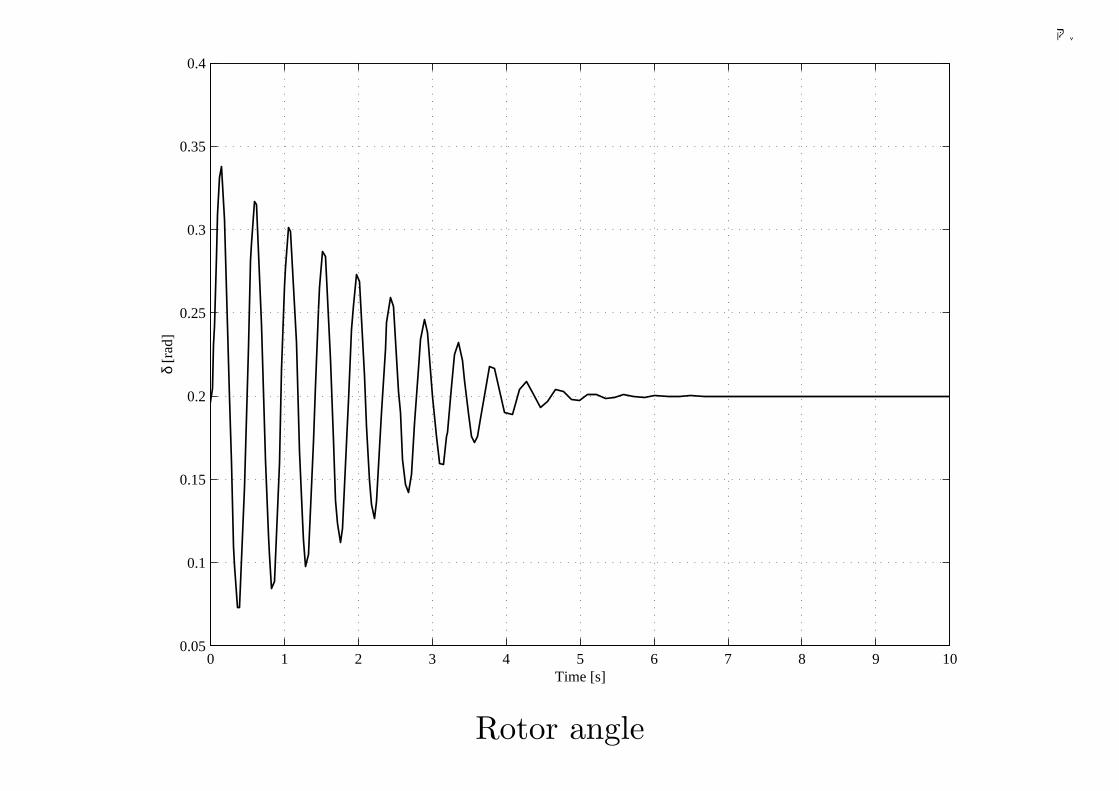
千葉大学
0 1 2 3 4 5 6 7 8 9 100.05
0.1
0.15
0.2
0.25
0.3
0.35
0.4
Time [s]
δ [r
ad]
Rotor angle
300
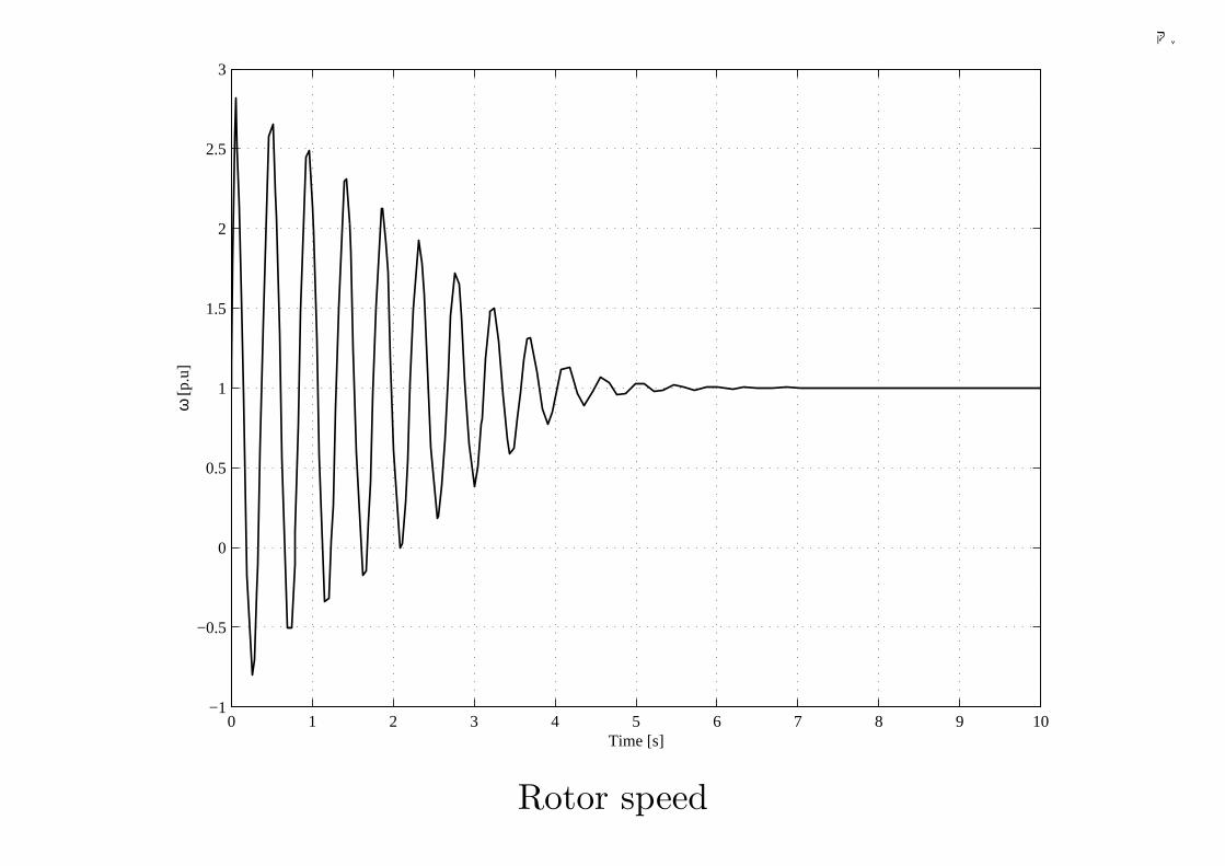
千葉大学
0 1 2 3 4 5 6 7 8 9 10−1
−0.5
0
0.5
1
1.5
2
2.5
3
Time [s]
ω [p
.u]
Rotor speed
301
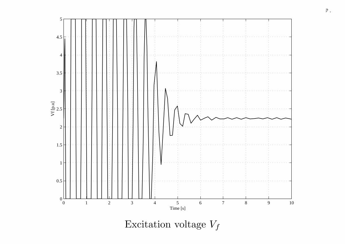
千葉大学
0 1 2 3 4 5 6 7 8 9 100
0.5
1
1.5
2
2.5
3
3.5
4
4.5
5
Time [s]
Vf
[p.u
]
Excitation voltage Vf
302
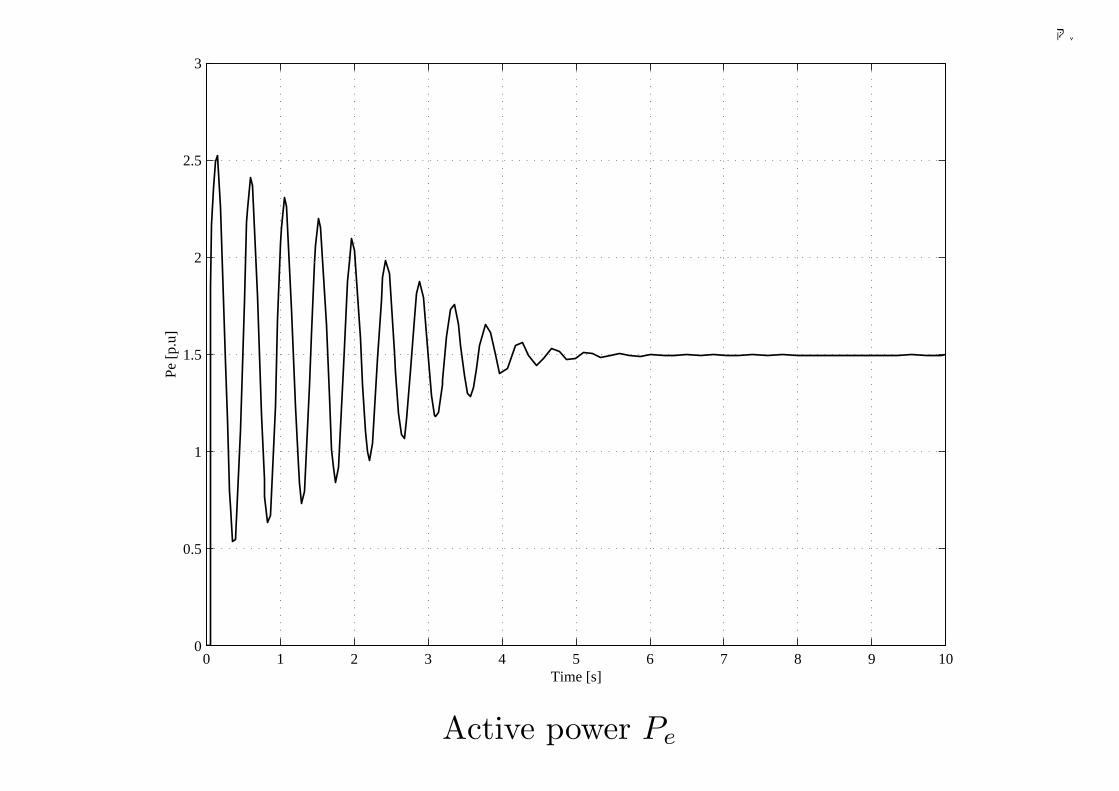
千葉大学
0 1 2 3 4 5 6 7 8 9 100
0.5
1
1.5
2
2.5
3
Time [s]
Pe [
p.u]
Active power Pe
303
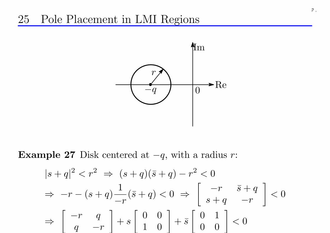
千葉大学
25 Pole Placement in LMI Regions
Im
Re−q
r
0
Example 27 Disk centered at −q, with a radius r:
|s + q|2 < r2 ⇒ (s + q)(s + q)− r2 < 0
⇒ −r − (s + q)1−r
(s + q) < 0 ⇒[ −r s + q
s + q −r
]< 0
⇒[ −r q
q −r
]+ s
[0 01 0
]+ s
[0 10 0
]< 0
304
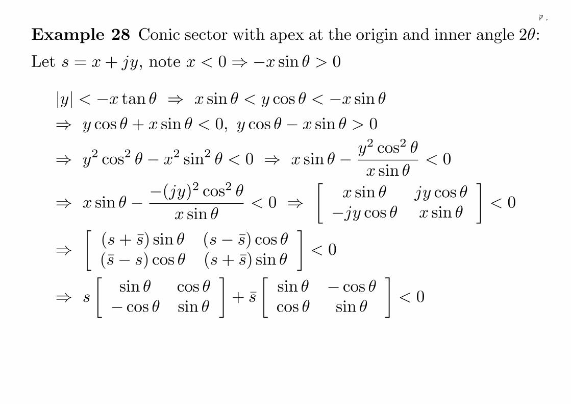
千葉大学
Example 28 Conic sector with apex at the origin and inner angle 2θ:
Let s = x + jy, note x < 0 ⇒ −x sin θ > 0
|y| < −x tan θ ⇒ x sin θ < y cos θ < −x sin θ
⇒ y cos θ + x sin θ < 0, y cos θ − x sin θ > 0
⇒ y2 cos2 θ − x2 sin2 θ < 0 ⇒ x sin θ − y2 cos2 θ
x sin θ< 0
⇒ x sin θ − −(jy)2 cos2 θ
x sin θ< 0 ⇒
[x sin θ jy cos θ−jy cos θ x sin θ
]< 0
⇒[
(s + s) sin θ (s− s) cos θ(s− s) cos θ (s + s) sin θ
]< 0
⇒ s
[sin θ cos θ− cos θ sin θ
]+ s
[sin θ − cos θcos θ sin θ
]< 0
305
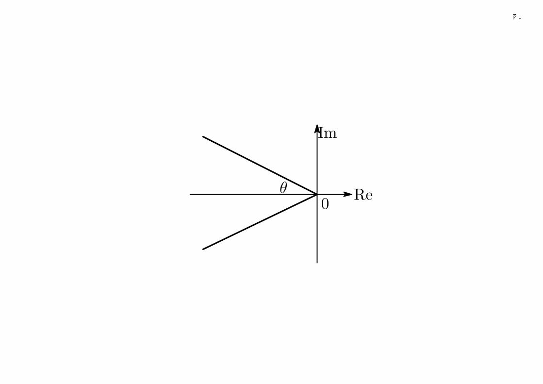
千葉大学
Im
Re0θ
306
千葉大学
26 LMI Condition for Pole PlacementThese examples show that any convex regions symmetric to the real
axis can be described as LMIs in s, s, as follows
D = s ∈ C : fD(s) < 0 (243)
fD(s) = L + sM + sMT (244)
For the eigenvalues of matrix A to be located in D, it is necessary and
sufficent that ∃X > 0 s.t.
MD(A,X) := L⊗X + M ⊗ (XA) + MT ⊗ (AT X) < 0 (245)
307
千葉大学
Example 29 Disk:[ −r q
q −r
]⊗X +
[0 01 0
]⊗ (XA) +
[0 10 0
]⊗ (AT X)
=[ −rX AT X + qX
XA + qX −rX
](246)
Conic sector[
sin θ cos θ− cos θ sin θ
]⊗ (XA) +
[sin θ − cos θcos θ sin θ
]⊗ (AT X)
=[
sin θ(XA + AT X) cos θ(XA−AT X)cos θ(AT X −XA) sin θ(XA + AT X)
](247)
308
千葉大学
Verification of LMI pole placement condition
Disk example: Let z be an eigenvalue of A, u the corresponding eigen-
vector, then Au = zu, u∗AT = zu∗.
[u∗ u∗][ −rX AT X + qX
XA + qX −rX
] [uu
]
=[ −ru∗Xu (Au)∗Xu + qu∗Xu
u∗XAu + qu∗Xu −ru∗Xu
]
=[ −ru∗Xu zu∗Xu + qu∗Xu
zu∗Xu + qu∗Xu −ru∗Xu
]
=[ −r z + q
z + q −r
]u∗Xu
So the negativity of these two matrices are equivalent.
309

Chiba Univ.
Beyond The Small-Gain Paradigm: How to MakeUse of The Phase Information of Uncertainty
Chiba University Kang-Zhi Liu
JAPAN
Chiba Univ.
1 RESEARCH BACKGROUND¥ Small-Gain Paradigm
• Foundation of robust control theory for systems with dynamics
uncertainty
• Uncertainty modeled as norm-bounded dynamics
• Gain information of uncertainty fully used
• Effective in many applications
¥ Drawback
• Phase information of uncertain completely ingored
• Consequence I: class of uncertainty is inevitably enlarged
• Consequence II: unnecessarily lower the controller gain at low and
middle frequency domains, which limits the achievable bandwidth
Chiba Univ.
2 OPEN PROBLEM¥ How to model and use the phase information of uncertainty???
¥ Related resaerches
• KYP Lemma (positive realness): good for passive nominal closed
loop and passive uncertainty, very difficult to realize
• Finite Frequency Positive Realness [Iwasaki, et al.]: positive real
only for frequencies within the control bandwidth, applicable to the
structural design of plant so as to improve control bandwidth
• Requires the passivity of uncertainty: phase being inside
(−90, 90) in all frequency domain/within the bandwidth
• Uncertainty modeling not addressed, not necessarily suitable for
general dynamic uncertainty
Chiba Univ.
3 THIS TALK
• Propose some models for uncertainty phase
• Justification through 3 practical examples
• Establish the robustness condition in frequency domain
• State space characterization of robustness condition

Chiba Univ.
4 OUTLINE OF PRESENTATION
• motivating examples
• modeling of uncertainty phase
• robust stability condition I: frequency domain
• robust stability condition II: state space
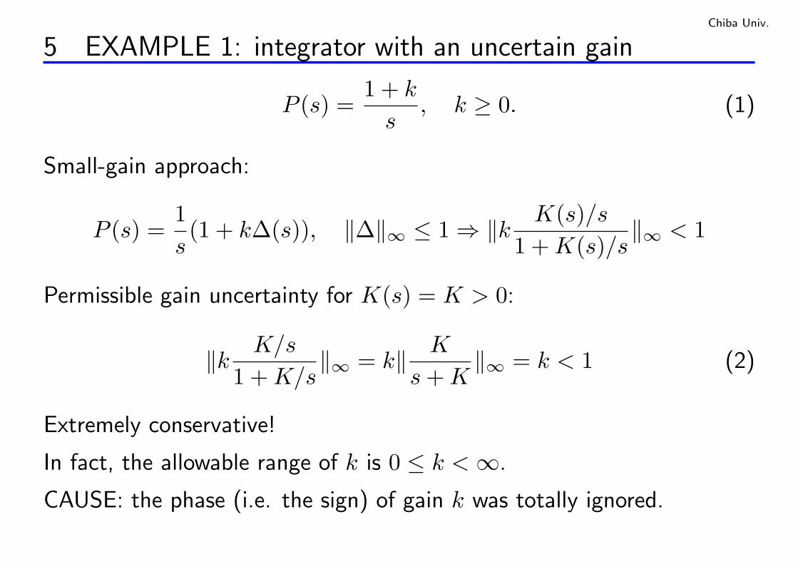
Chiba Univ.
5 EXAMPLE 1: integrator with an uncertain gain
P (s) =1 + k
s, k ≥ 0. (1)
Small-gain approach:
P (s) =1s(1 + k∆(s)), ‖∆‖∞ ≤ 1 ⇒ ‖k K(s)/s
1 + K(s)/s‖∞ < 1
Permissible gain uncertainty for K(s) = K > 0:
‖k K/s
1 + K/s‖∞ = k‖ K
s + K‖∞ = k < 1 (2)
Extremely conservative!
In fact, the allowable range of k is 0 ≤ k < ∞.
CAUSE: the phase (i.e. the sign) of gain k was totally ignored.
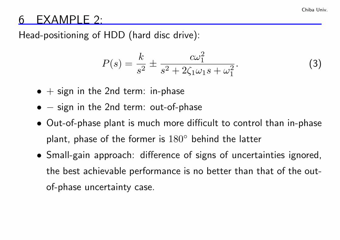
Chiba Univ.
6 EXAMPLE 2:Head-positioning of HDD (hard disc drive):
P (s) =k
s2± cω2
1
s2 + 2ζ1ω1s + ω21
. (3)
• + sign in the 2nd term: in-phase
• − sign in the 2nd term: out-of-phase
• Out-of-phase plant is much more difficult to control than in-phase
plant, phase of the former is 180 behind the latter
• Small-gain approach: difference of signs of uncertainties ignored,
the best achievable performance is no better than that of the out-
of-phase uncertainty case.
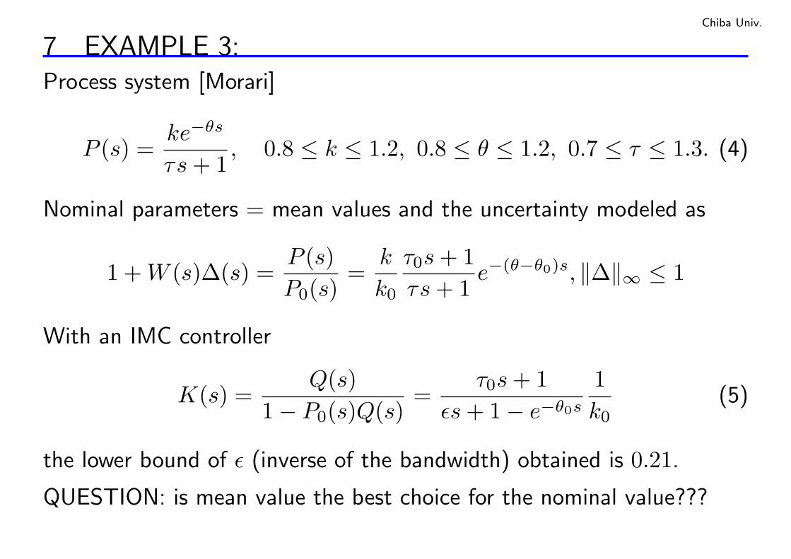
Chiba Univ.
7 EXAMPLE 3:Process system [Morari]
P (s) =ke−θs
τs + 1, 0.8 ≤ k ≤ 1.2, 0.8 ≤ θ ≤ 1.2, 0.7 ≤ τ ≤ 1.3. (4)
Nominal parameters = mean values and the uncertainty modeled as
1 + W (s)∆(s) =P (s)P0(s)
=k
k0
τ0s + 1τs + 1
e−(θ−θ0)s, ‖∆‖∞ ≤ 1
With an IMC controller
K(s) =Q(s)
1− P0(s)Q(s)=
τ0s + 1εs + 1− e−θ0s
1k0
(5)
the lower bound of ε (inverse of the bandwidth) obtained is 0.21.
QUESTION: is mean value the best choice for the nominal value???
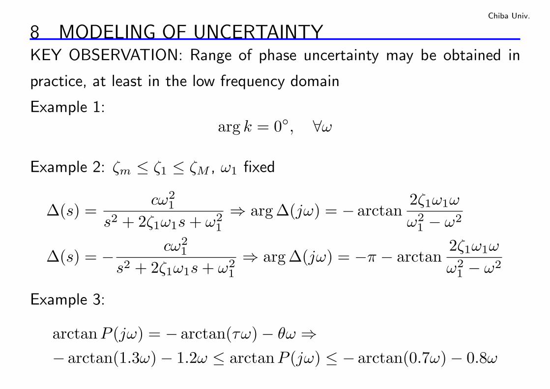
Chiba Univ.
8 MODELING OF UNCERTAINTYKEY OBSERVATION: Range of phase uncertainty may be obtained in
practice, at least in the low frequency domain
Example 1:arg k = 0, ∀ω
Example 2: ζm ≤ ζ1 ≤ ζM , ω1 fixed
∆(s) =cω2
1
s2 + 2ζ1ω1s + ω21
⇒ arg ∆(jω) = − arctan2ζ1ω1ω
ω21 − ω2
∆(s) = − cω21
s2 + 2ζ1ω1s + ω21
⇒ arg ∆(jω) = −π − arctan2ζ1ω1ω
ω21 − ω2
Example 3:
arctanP (jω) = − arctan(τω)− θω ⇒− arctan(1.3ω)− 1.2ω ≤ arctanP (jω) ≤ − arctan(0.7ω)− 0.8ω
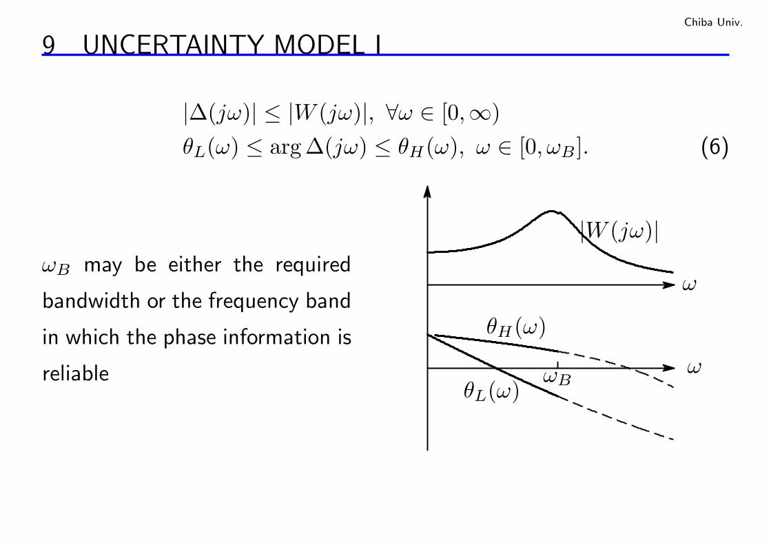
Chiba Univ.
9 UNCERTAINTY MODEL I
|∆(jω)| ≤ |W (jω)|, ∀ω ∈ [0,∞)θL(ω) ≤ arg ∆(jω) ≤ θH(ω), ω ∈ [0, ωB ]. (6)
ωB may be either the required
bandwidth or the frequency band
in which the phase information is
reliable
ω
θH(ω)
θL(ω)ω
|W (jω)|
ωB
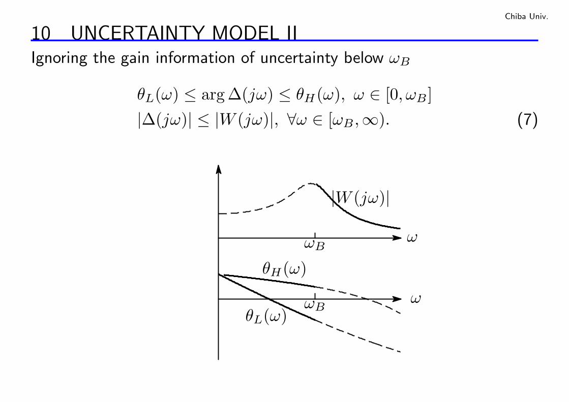
Chiba Univ.
10 UNCERTAINTY MODEL IIIgnoring the gain information of uncertainty below ωB
θL(ω) ≤ arg ∆(jω) ≤ θH(ω), ω ∈ [0, ωB ]|∆(jω)| ≤ |W (jω)|, ∀ω ∈ [ωB ,∞). (7)
ω
θH(ω)
θL(ω)ω
|W (jω)|
ωB
ωB
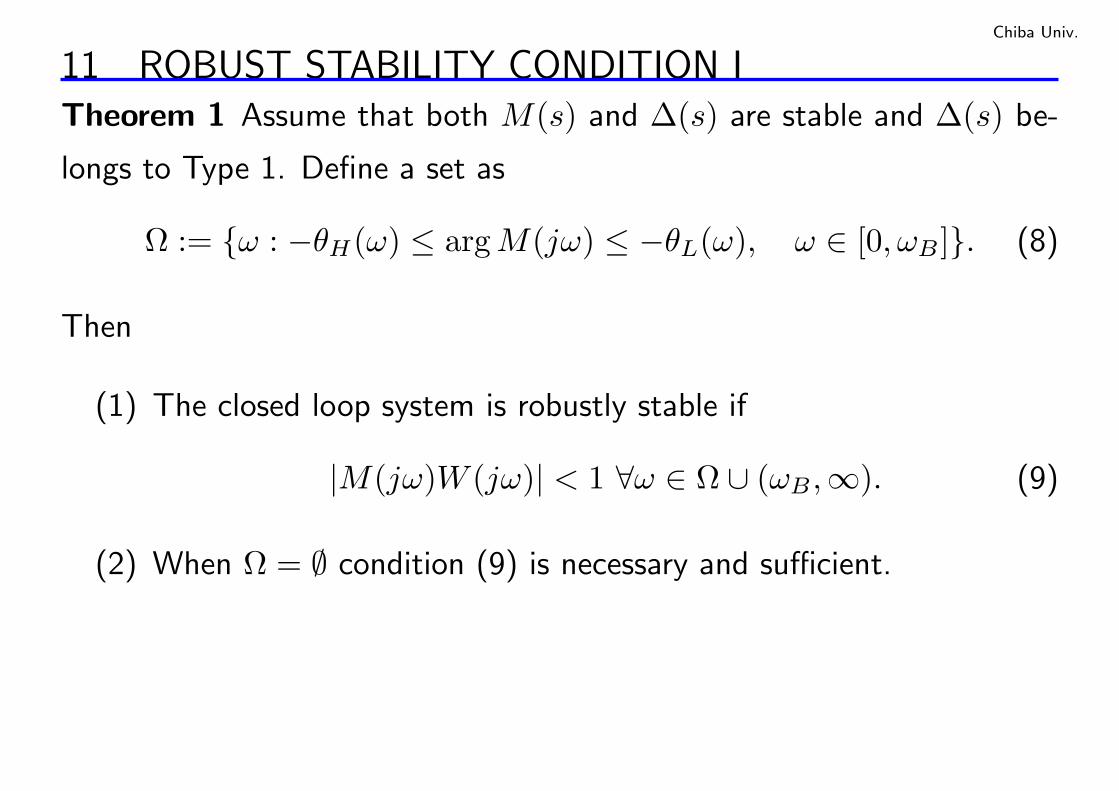
Chiba Univ.
11 ROBUST STABILITY CONDITION ITheorem 1 Assume that both M(s) and ∆(s) are stable and ∆(s) be-
longs to Type 1. Define a set as
Ω := ω : −θH(ω) ≤ arg M(jω) ≤ −θL(ω), ω ∈ [0, ωB ]. (8)
Then
(1) The closed loop system is robustly stable if
|M(jω)W (jω)| < 1 ∀ω ∈ Ω ∪ (ωB ,∞). (9)
(2) When Ω = ∅ condition (9) is necessary and sufficient.
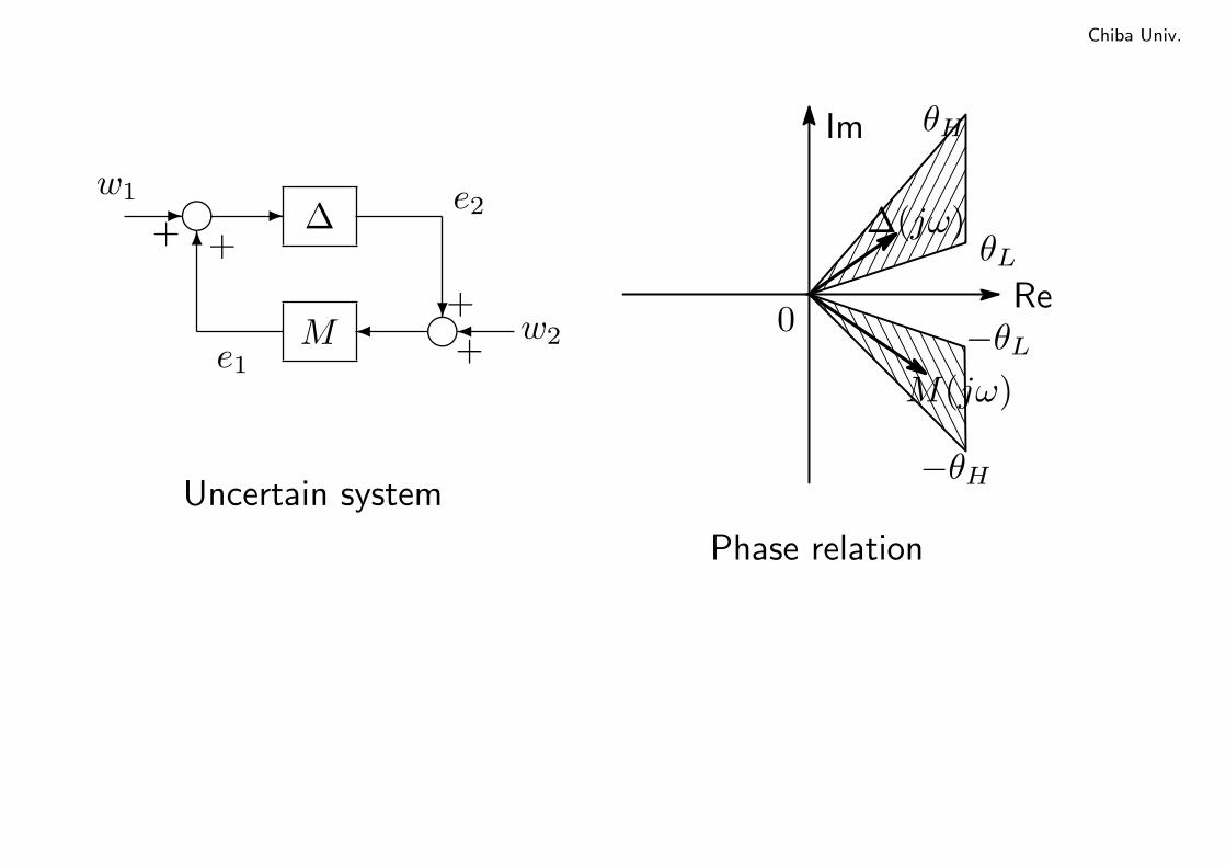
Chiba Univ.
++
++
e2
e1
w2
w1∆
M
--6g
g¾ ?¾
Uncertain system−θH
−θL
θH
θL
0
M(jω)
∆(jω)
Im
Re
Phase relation
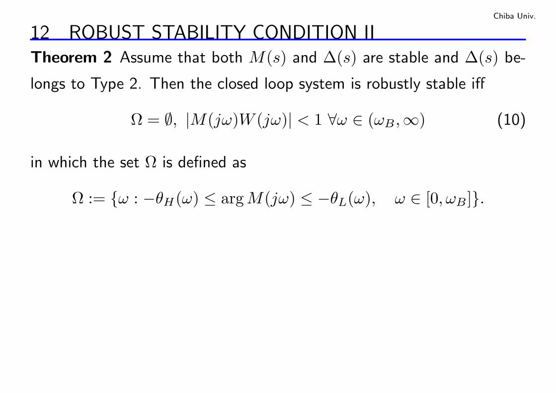
Chiba Univ.
12 ROBUST STABILITY CONDITION IITheorem 2 Assume that both M(s) and ∆(s) are stable and ∆(s) be-
longs to Type 2. Then the closed loop system is robustly stable iff
Ω = ∅, |M(jω)W (jω)| < 1 ∀ω ∈ (ωB ,∞) (10)
in which the set Ω is defined as
Ω := ω : −θH(ω) ≤ arg M(jω) ≤ −θL(ω), ω ∈ [0, ωB ].
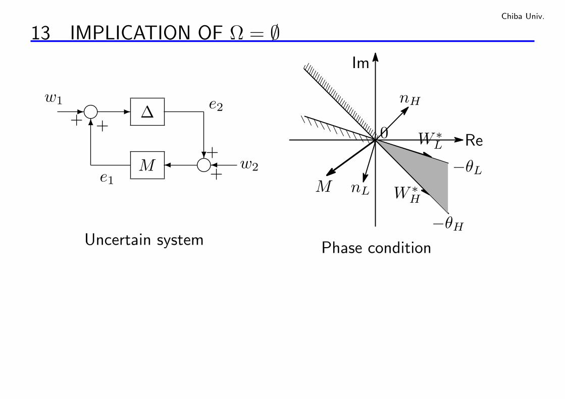
Chiba Univ.
13 IMPLICATION OF Ω = ∅
++
++
e2
e1
w2
w1∆
M
--6g
g¾ ?¾
Uncertain system−θH
−θL
0
M
Im
Re
nH
nL
W ∗L
W ∗H
Phase condition
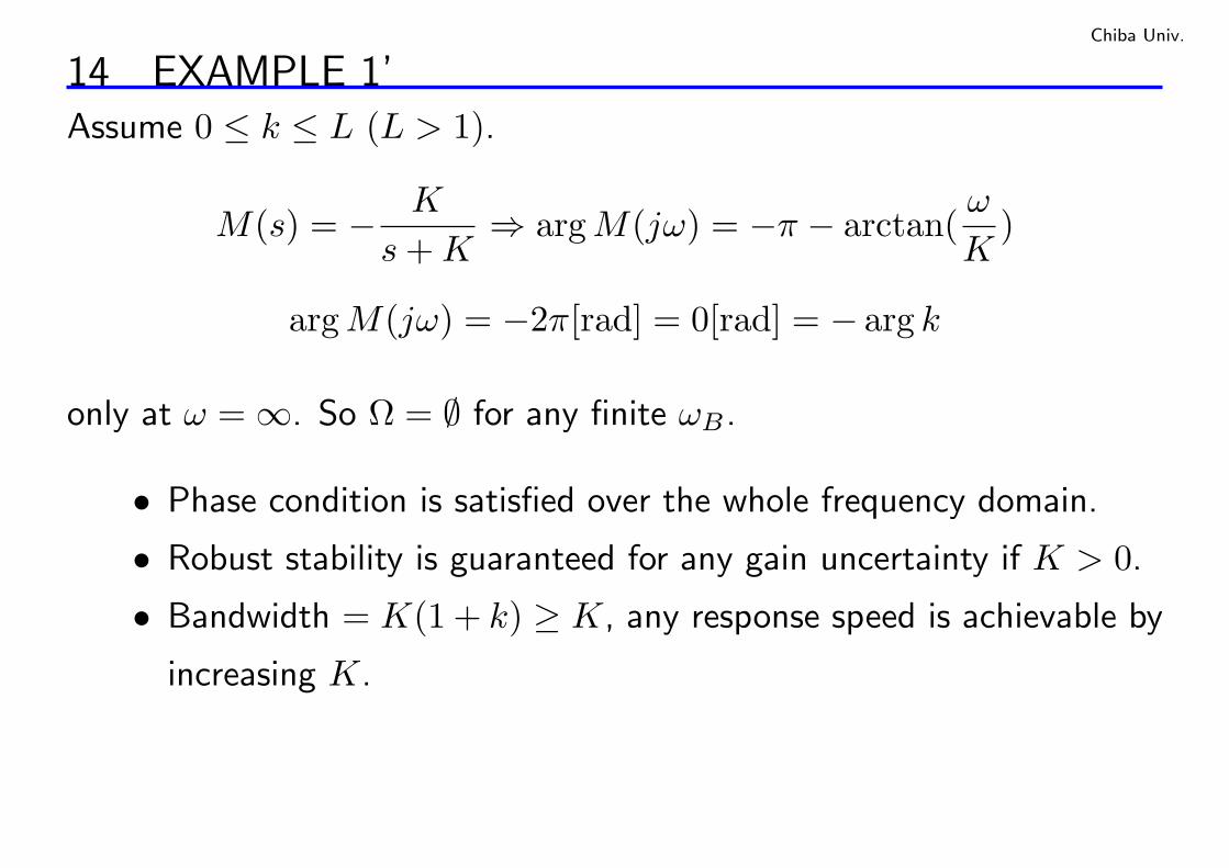
Chiba Univ.
14 EXAMPLE 1’Assume 0 ≤ k ≤ L (L > 1).
M(s) = − K
s + K⇒ arg M(jω) = −π − arctan(
ω
K)
arg M(jω) = −2π[rad] = 0[rad] = − arg k
only at ω = ∞. So Ω = ∅ for any finite ωB .
• Phase condition is satisfied over the whole frequency domain.
• Robust stability is guaranteed for any gain uncertainty if K > 0.
• Bandwidth = K(1 + k) ≥ K, any response speed is achievable by
increasing K.
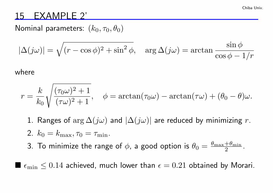
Chiba Univ.
15 EXAMPLE 2’Nominal parameters: (k0, τ0, θ0)
|∆(jω)| =√
(r − cos φ)2 + sin2 φ, arg ∆(jω) = arctansinφ
cos φ− 1/r
where
r =k
k0
√(τ0ω)2 + 1(τω)2 + 1
, φ = arctan(τ0ω)− arctan(τω) + (θ0 − θ)ω.
1. Ranges of arg ∆(jω) and |∆(jω)| are reduced by minimizing r.
2. k0 = kmax, τ0 = τmin.
3. To minimize the range of φ, a good option is θ0 = θmax+θmin2 .
¥ εmin ≤ 0.14 achieved, much lower than ε = 0.21 obtained by Morari.
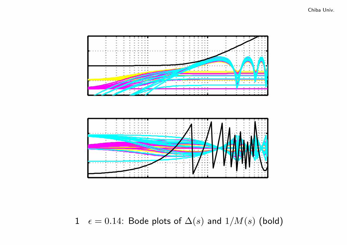
Chiba Univ.
10-1
100
101
102
-20
-10
0
10
20
10-1
100
101
102
-200
-100
0
100
200
図 1 ε = 0.14: Bode plots of ∆(s) and 1/M(s) (bold)
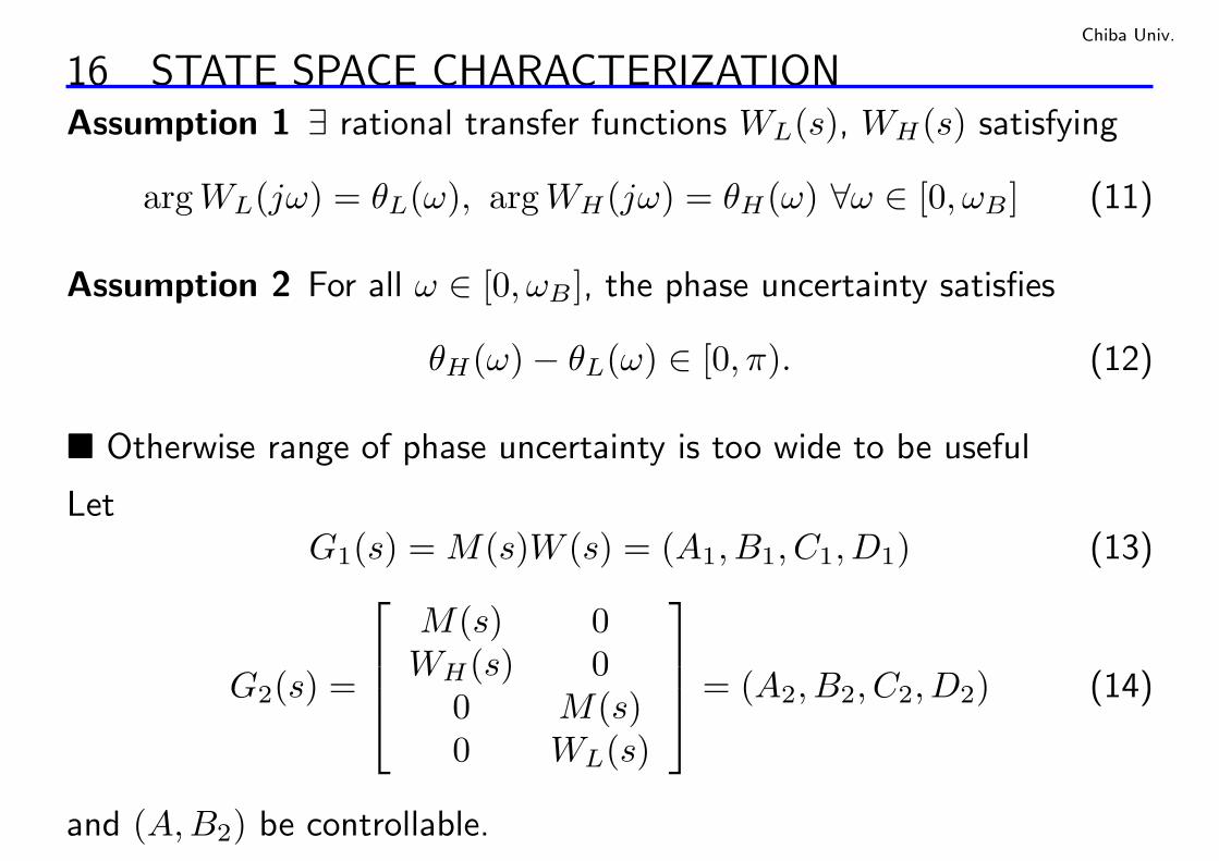
Chiba Univ.
16 STATE SPACE CHARACTERIZATIONAssumption 1 ∃ rational transfer functions WL(s), WH(s) satisfying
arg WL(jω) = θL(ω), arg WH(jω) = θH(ω) ∀ω ∈ [0, ωB ] (11)
Assumption 2 For all ω ∈ [0, ωB ], the phase uncertainty satisfies
θH(ω)− θL(ω) ∈ [0, π). (12)
¥ Otherwise range of phase uncertainty is too wide to be useful
LetG1(s) = M(s)W (s) = (A1, B1, C1, D1) (13)
G2(s) =
M(s) 0WH(s) 0
0 M(s)0 WL(s)
= (A2, B2, C2, D2) (14)
and (A,B2) be controllable.
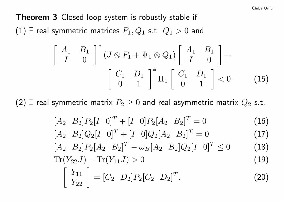
Chiba Univ.
Theorem 3 Closed loop system is robustly stable if
(1) ∃ real symmetric matrices P1, Q1 s.t. Q1 > 0 and
[A1 B1
I 0
]∗(J ⊗ P1 + Ψ1 ⊗Q1)
[A1 B1
I 0
]+
[C1 D1
0 1
]∗Π1
[C1 D1
0 1
]< 0. (15)
(2) ∃ real symmetric matrix P2 ≥ 0 and real asymmetric matrix Q2 s.t.
[A2 B2]P2[I 0]T + [I 0]P2[A2 B2]T = 0 (16)
[A2 B2]Q2[I 0]T + [I 0]Q2[A2 B2]T = 0 (17)
[A2 B2]P2[A2 B2]T − ωB [A2 B2]Q2[I 0]T ≤ 0 (18)
Tr(Y22J)− Tr(Y11J) > 0 (19)[Y11
Y22
]= [C2 D2]P2[C2 D2]T . (20)