Robust Estimator

學生 :范育瑋老師 :王聖智

Outline

Introduction LS-Least Squares LMS-Least Median Squares RANSAC- Random Sample Consequence MLESAC-Maximum likelihood Sample consensus MINPRAN-Minimize the Probability of Randomness

Outline

Introduction LS-Least Squares LMS-Least Median Squares RANSAC- Random Sample Consequence MLESAC-Maximum likelihood Sample consensus MINPRAN-Minimize the Probability of Randomness

Introduction

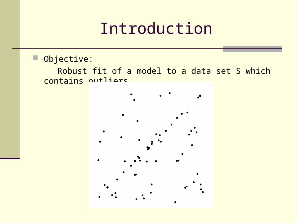
Objective:

Robust fit of a model to a data set S which contains outliers.

Outline

Introduction LS-Least Squares LMS-Least Median Squares RANSAC- Random Sample Consequence MLESAC-Maximum likelihood Sample consensus MINPRAN-Minimize the Probability of Randomness

LS

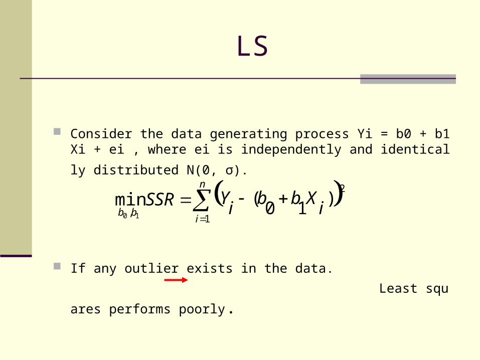
Consider the data generating process Yi = b0 + b1Xi + ei , wher

e ei is independently and identically distributed N(0, σ).

If any outlier exists in the data.

Least squares performs poorly.

n

ibb i

XbbiYSSR

1

2

,)

10(min

10

Outline

Introduction LS-Least Squares LMS-Least Median Squares RANSAC- Random Sample Consequence MLESAC-Maximum likelihood Sample consensus MINPRAN-Minimize the Probability of Randomness

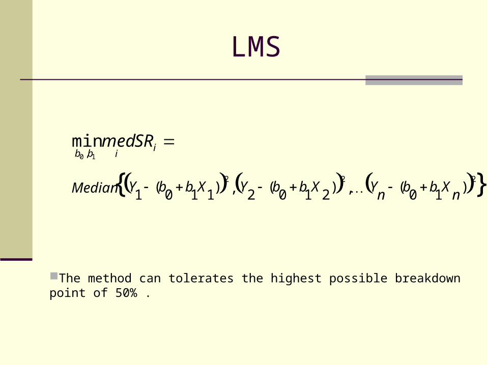
LMS

iibbSRmed

10 ,min

}{ )10

(,)210

(2,)

110(

1222

nXbb

nYXbbYXbbYMedian

The method can tolerates the highest possible breakdown point of 50% .

Outline

Introduction LS-Least Squares LMS-Least Median Squares RANSAC- Random Sample Consequence MLESAC-Maximum likelihood Sample consensus MINPRAN-Minimize the Probability of Randomness

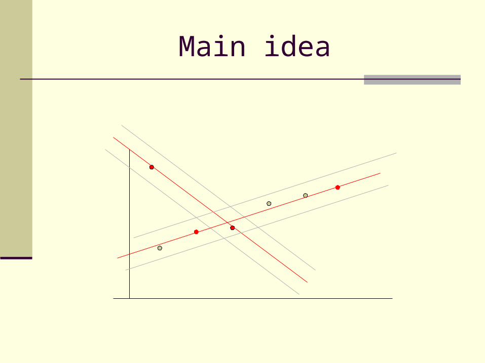
Main idea

Algorithm

a. Randomly select a sample of s data points from S and instantiate the model from this subset.

b. Determine the set of data points Si which are within a distance threshold t of the model.

c. If the size of Si (number of inliers) is greater than threshold T, re-estimate the model using all points in Si and terminate.

d. If the size of Si is less than T , select a new subset and repeat above.

e. After N trials the largest consequence ser Si is selected, and the model is re-estimate the model using all points in the

subset Si.

Algorithm

1. What is the distance threshold?

2. How many sample?

3. How large is an acceptable consensus set?

What is the distance threshold?

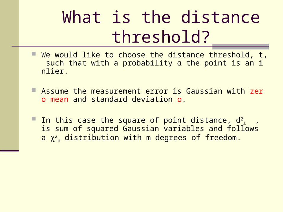
We would like to choose the distance threshold, t, such that with a probability α the point is an inlier.

Assume the measurement error is Gaussian with zero mean and standard deviation σ.

In this case the square of point distance, d2⊥ , is sum of square

d Gaussian variables and follows a χ2m distribution with m degre

es of freedom.

What is the distance threshold?

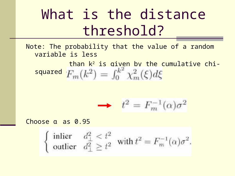
Note: The probability that the value of a random variable is less

than k2 is given by the cumulative chi-squared distribution.

Choose α as 0.95

How many sample?

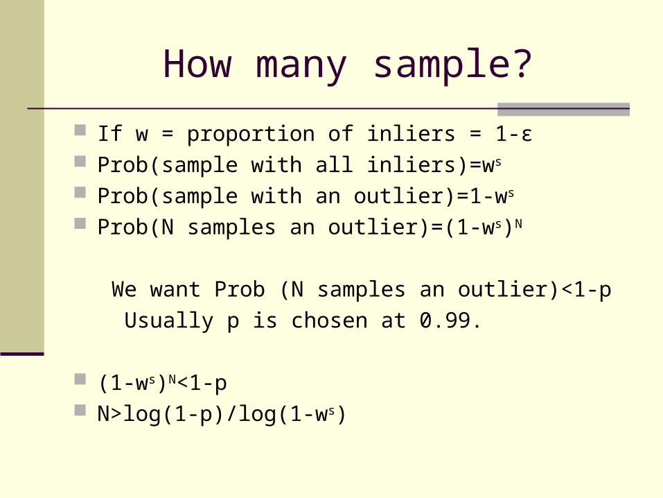
If w = proportion of inliers = 1-ε Prob(sample with all inliers)=ws

Prob(sample with an outlier)=1-ws

Prob(N samples an outlier)=(1-ws)N

We want Prob (N samples an outlier)<1-p

Usually p is chosen at 0.99.

(1-ws)N<1-p N>log(1-p)/log(1-ws)

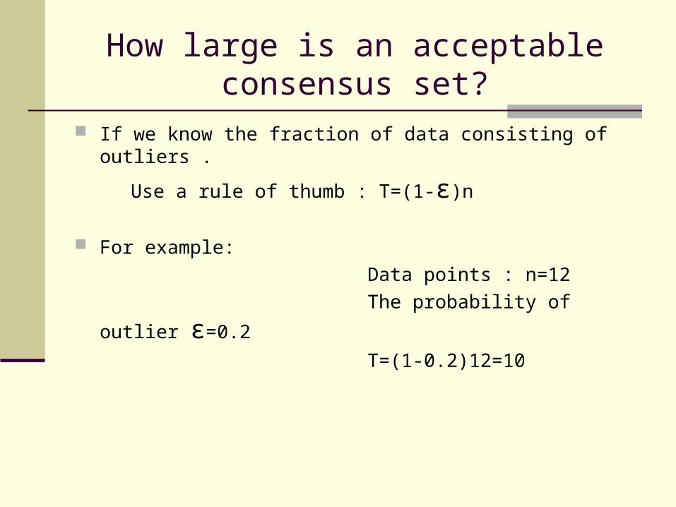
How large is an acceptable consensus set?

If we know the fraction of data consisting of outliers .

Use a rule of thumb : T=(1-ε)n

For example:

Data points : n=12

The probability of outlier ε=0.2

T=(1-0.2)12=10

Outline

Introduction LS-Least Squares LMS-Least Median Squares RANSAC- Random Sample Consequence MLESAC-Maximum likelihood Sample consensus MINPRAN-Minimize the Probability of Randomness

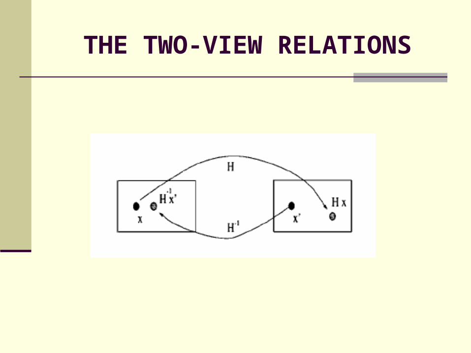
THE TWO-VIEW RELATIONS

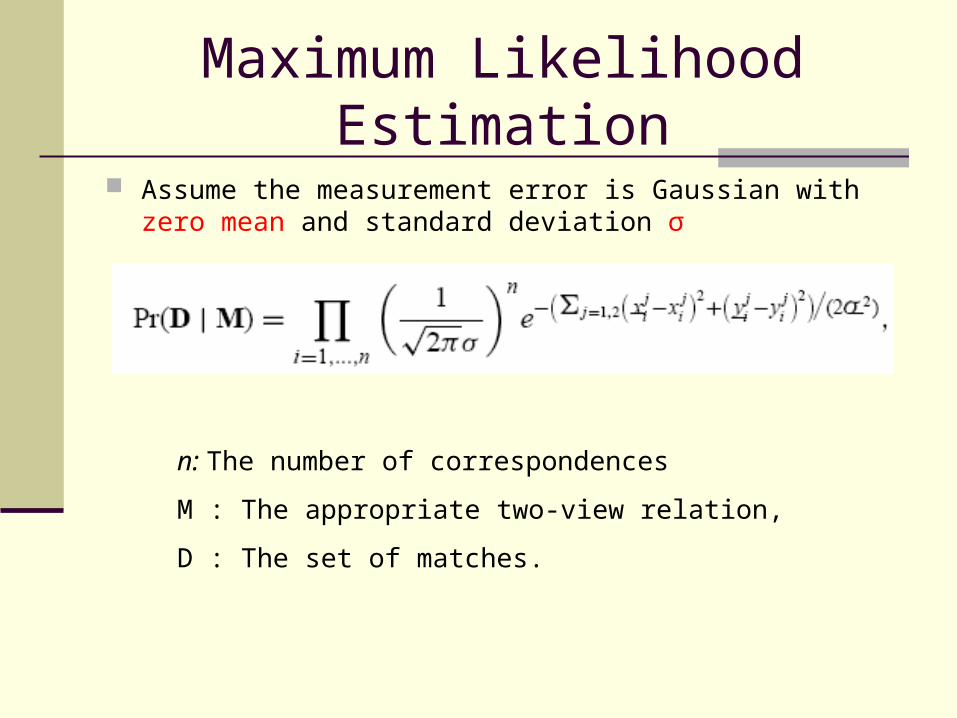
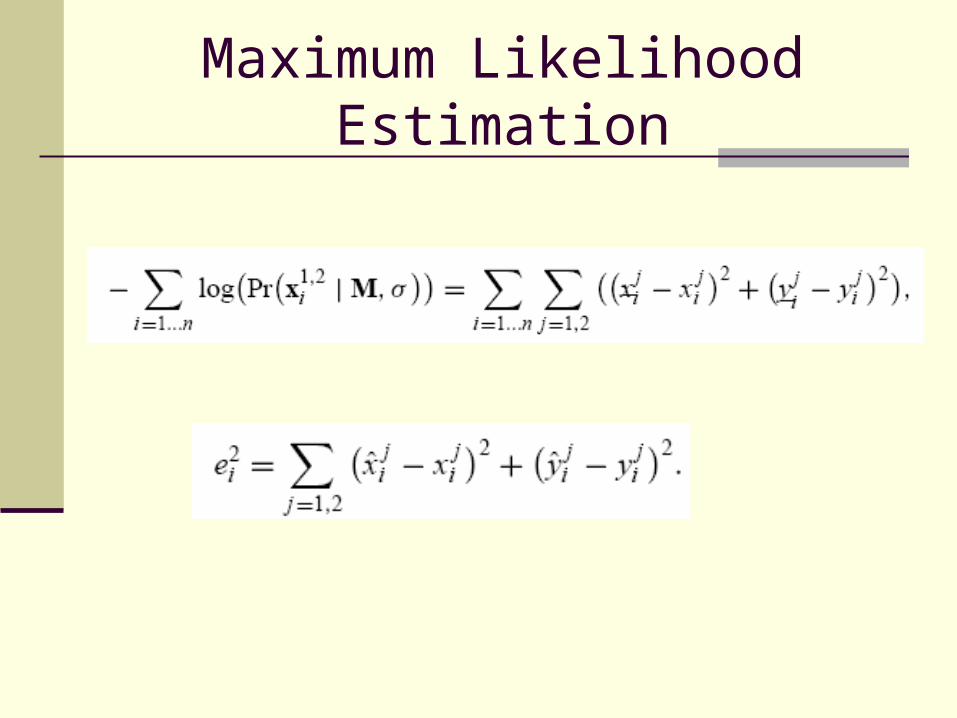
Maximum Likelihood Estimation

Assume the measurement error is Gaussian with zero mean and standard deviation σ

n: The number of correspondences

M : The appropriate two-view relation,

D : The set of matches.

Maximum Likelihood Estimation

Maximum Likelihood Estimation

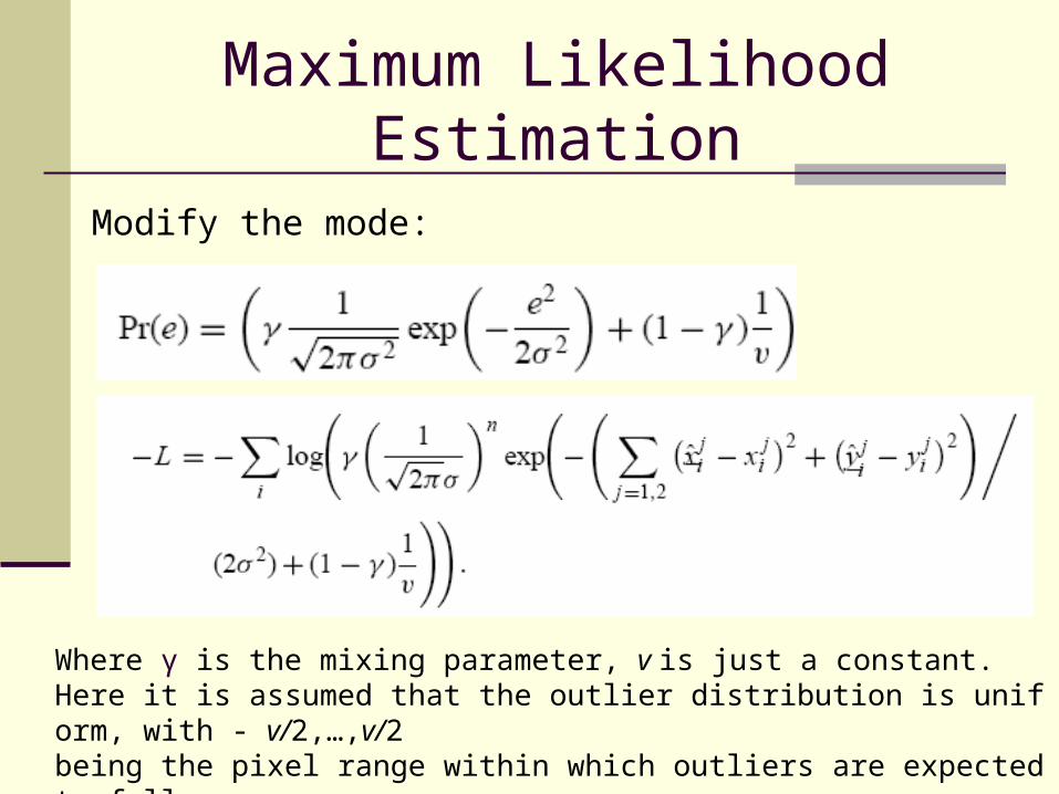
Modify the mode:

Where γ is the mixing parameter, v is just a constant.Here it is assumed that the outlier distribution is uniform, with - v/2,…,v/2 being the pixel range within which outliers are expected to fall.

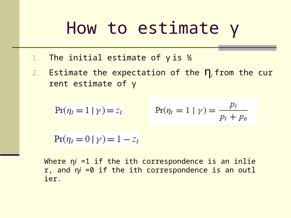
How to estimate γ

1. The initial estimate of γ is ½

2. Estimate the expectation of the ηi from the current estimate of γ

Where ηi =1 if the ith correspondence is an inlier, and ηi =0 if the ith correspondence is an outlier.

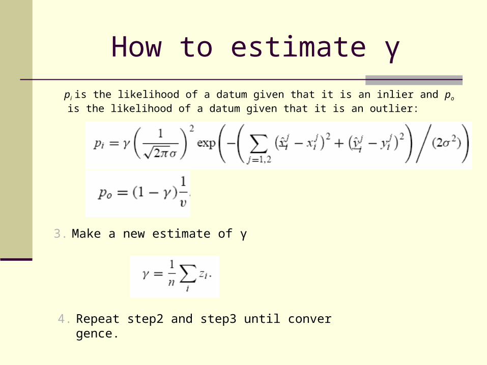
How to estimate γ

pi is the likelihood of a datum given that it is an inlier and po is the likelihood of a datum given that it is an outlier:

3. Make a new estimate of γ

4. Repeat step2 and step3 until convergence.

Outline

Introduction LS-Least Squared LMS-Least Median Squared RANSAC- Random Sample Consequence MLESAC-Maximum likelihood Sample consensus MINPRAN-Minimize the Probability of Randomness

MINPRAN

The first technique that reliably tolerates more than 50% outliers without assuming a know inlier bound.

It only assumes the outliers are uniformly distributed within the dynamic range of the sensor.

MINPRAN

MINPRAN

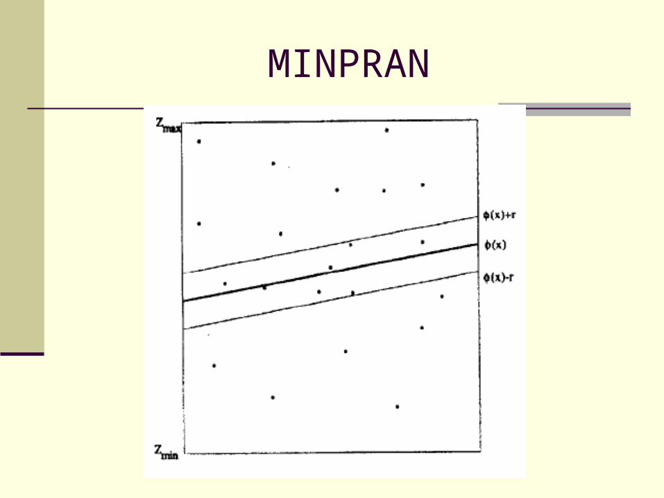
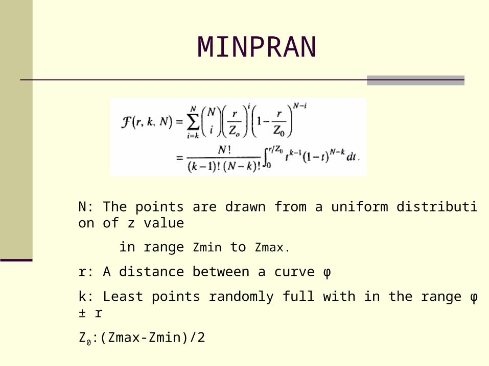
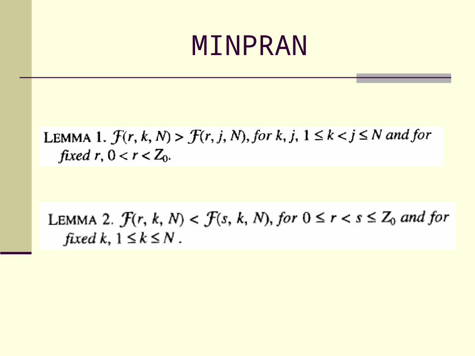
N: The points are drawn from a uniform distribution of z value

in range Zmin to Zmax.

r: A distance between a curve φ

k: Least points randomly full with in the range φ± r

Z0:(Zmax-Zmin)/2

MINPRAN

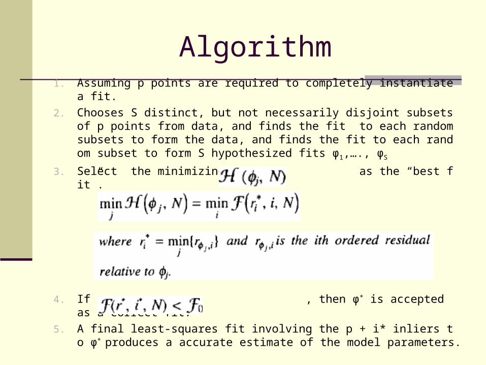
Algorithm1. Assuming p points are required to completely instantiate a fit.

2. Chooses S distinct, but not necessarily disjoint subsets of p points from data, and finds the fit to each random subsets to form the data, and finds the fit to each random subset to form S hypothesized fits φ1,…., φS

3. Select the minimizing as the “best fit”.

4. If , then φ* is accepted as a correct fit.

5. A final least-squares fit involving the p + i* inliers to φ* produces a accurate estimate of the model parameters.

How many sample?

If w = proportion of inliers = 1-ε Prob(sample with all inliers)=wp

Prob(sample with an outlier)=1-wp

Prob(S samples an outlier)=(1-wp)S

We want Prob (S samples an outlier)<1-p

Usually p is chosen at 0.99.

(1-wp)S<1-p S>log(1-p)/log(1-wp)

Randomness Threshold F0

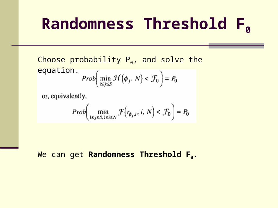
Choose probability P0, and solve the equation.

We can get Randomness Threshold F0.

Randomness Threshold F0

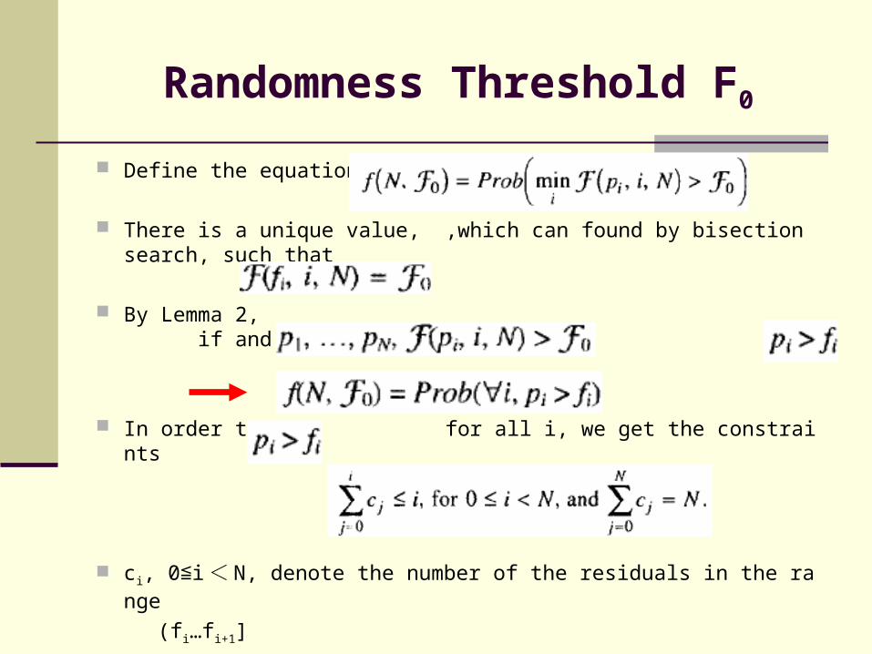
Define the equation

There is a unique value, ,which can found by bisection search, such that

By Lemma 2, if and only if

In order to for all i, we get the constraints

ci, 0 i≦ ＜ N, denote the number of the residuals in the range

(fi…fi+1]

Randomness Threshold F0

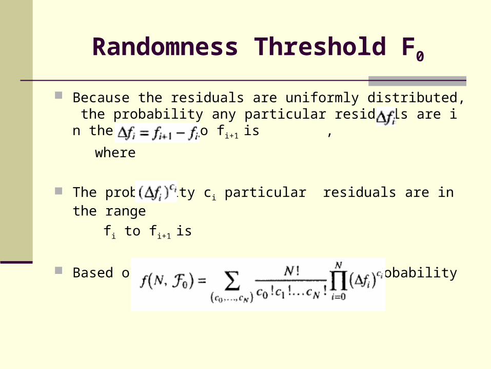
Because the residuals are uniformly distributed, the probability any particular residuals are in the range fi to fi+1 is ,

where

The probability ci particular residuals are in the range

fi to fi+1 is

Based on this, we can calculate the probability

Randomness Threshold F0

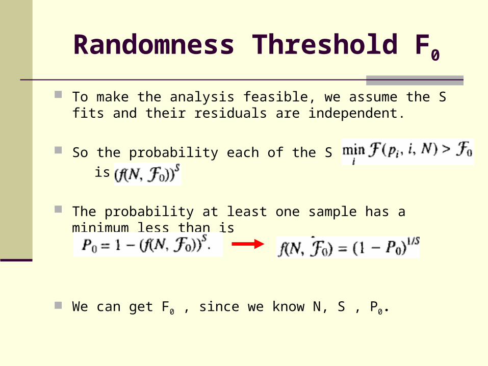
To make the analysis feasible, we assume the S fits and their residuals are independent.

So the probability each of the S samples has

is just

The probability at least one sample has a minimum less than is

We can get F0 , since we know N, S , P0.