Looking at differences: parametric and non-parametric tests

Sealy Gossett, chemist working for Guinness brewery– published work on the t-distribution under the name “student”

Comparing mean difference while accounting for variability in samples

Image: http://www.socialresearchmethods.net/kb/stat_t.php

People with a hot tubPeople without a hot tub

Mean Number of Friends

(D-51 with aluminum tubes)

Why can’t we use a z-test

μ0

σ

μ0

s

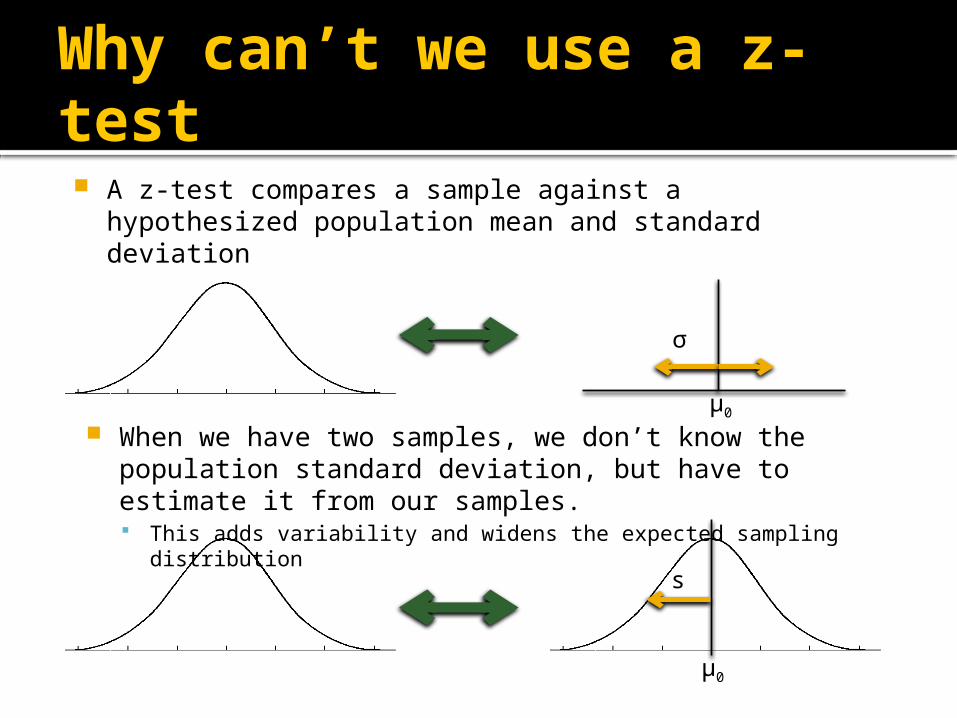
A z-test compares a sample against a hypothesized population mean and standard deviation

When we have two samples, we don’t know the population standard deviation, but have to estimate it from our samples. This adds variability and widens the expected sampling

distribution

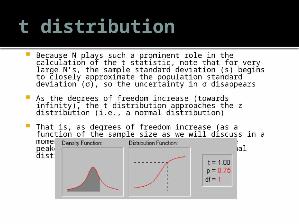
t distribution Because N plays such a prominent role in the calculation of

the t-statistic, note that for very large N’s, the sample standard deviation (s) begins to closely approximate the population standard deviation (σ), so the uncertainty in σ disappears

As the degrees of freedom increase (towards infinity), the t distribution approaches the z distribution (i.e., a normal distribution)

That is, as degrees of freedom increase (as a function of the sample size as we will discuss in a moment), the actual curve itself becomes more peaked and less dispersed– just like the normal distribution.

Why use the t distribution (and the t-test) instead of the z-test?

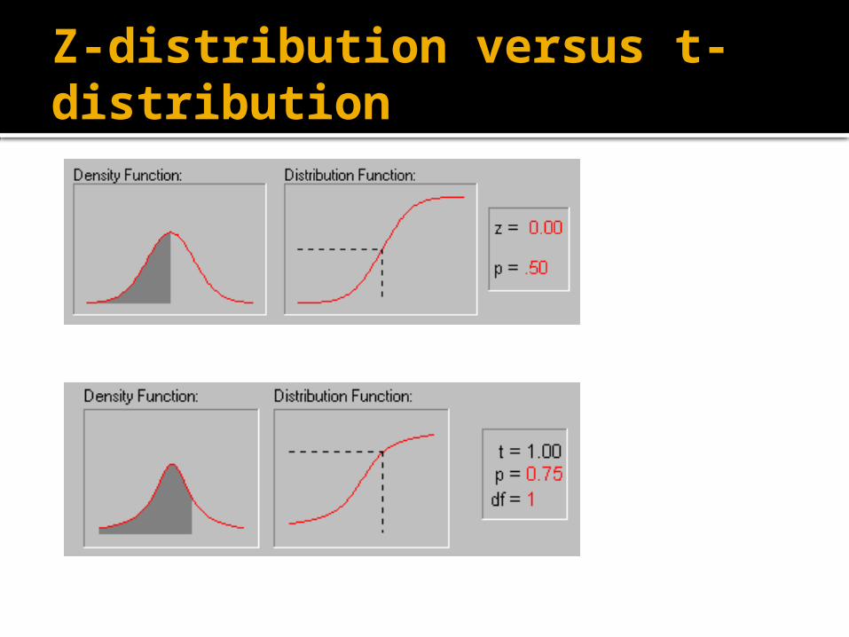
t-test is useful for testing mean differences when the N is not very large

In very large samples, a t-test is the same as a z-test.

Z-distribution versus t-distribution

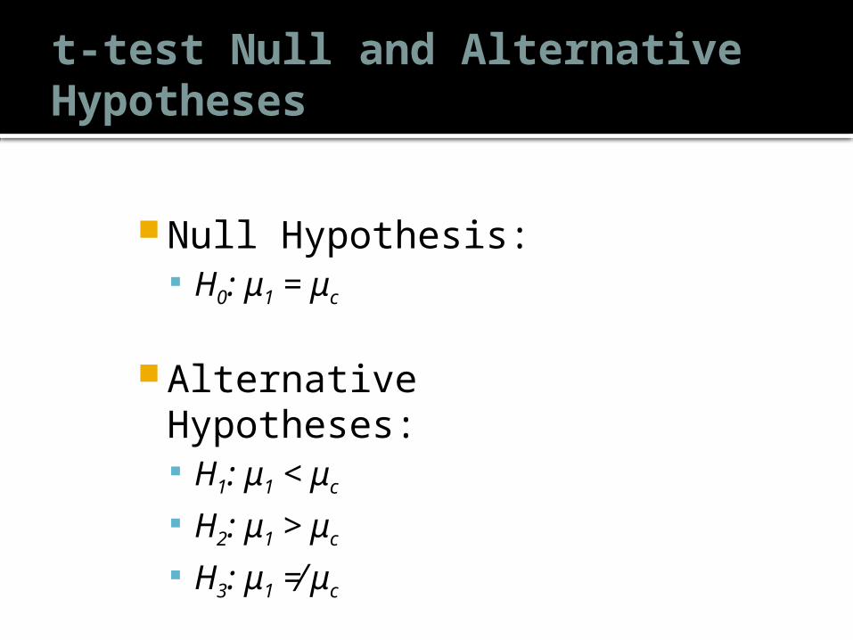
t-test Null and Alternative Hypotheses

Null Hypothesis: H0: μ1 = μc

Alternative Hypotheses: H1: μ1 < μc

H2: μ1 > μc

H3: μ1 ≠ μc

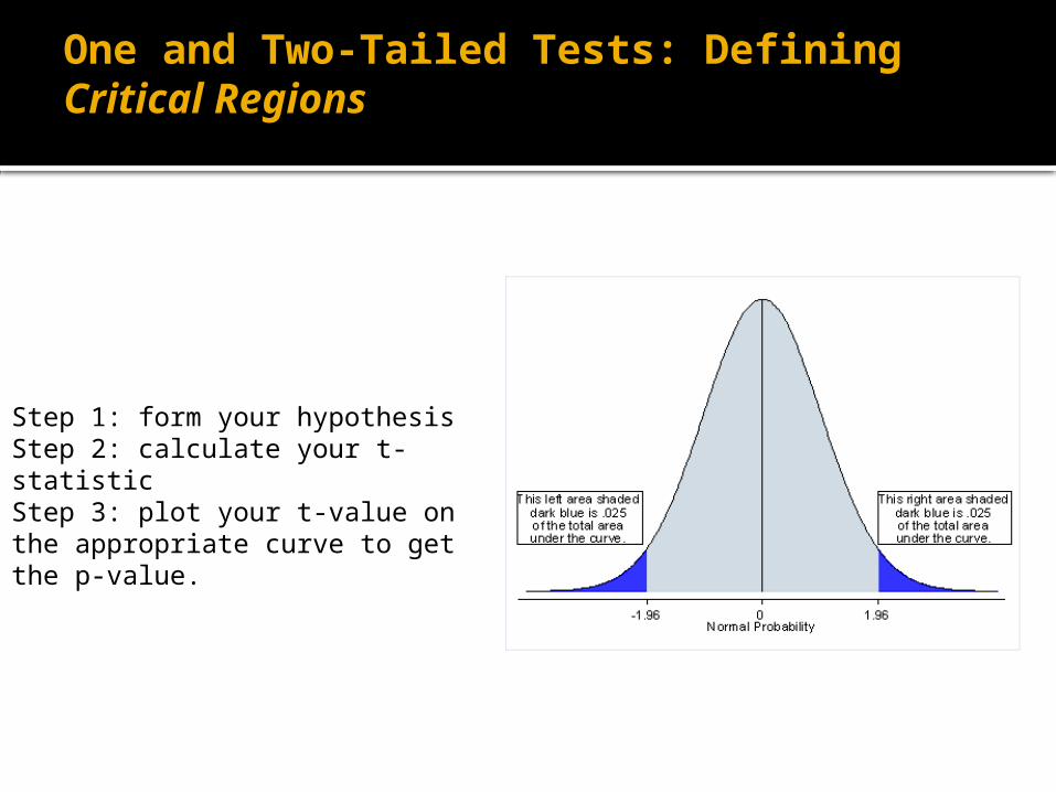
One and Two-Tailed Tests: Defining Critical Regions

Step 1: form your hypothesisStep 2: calculate your t-statisticStep 3: plot your t-value on the appropriate curve to get the p-value.

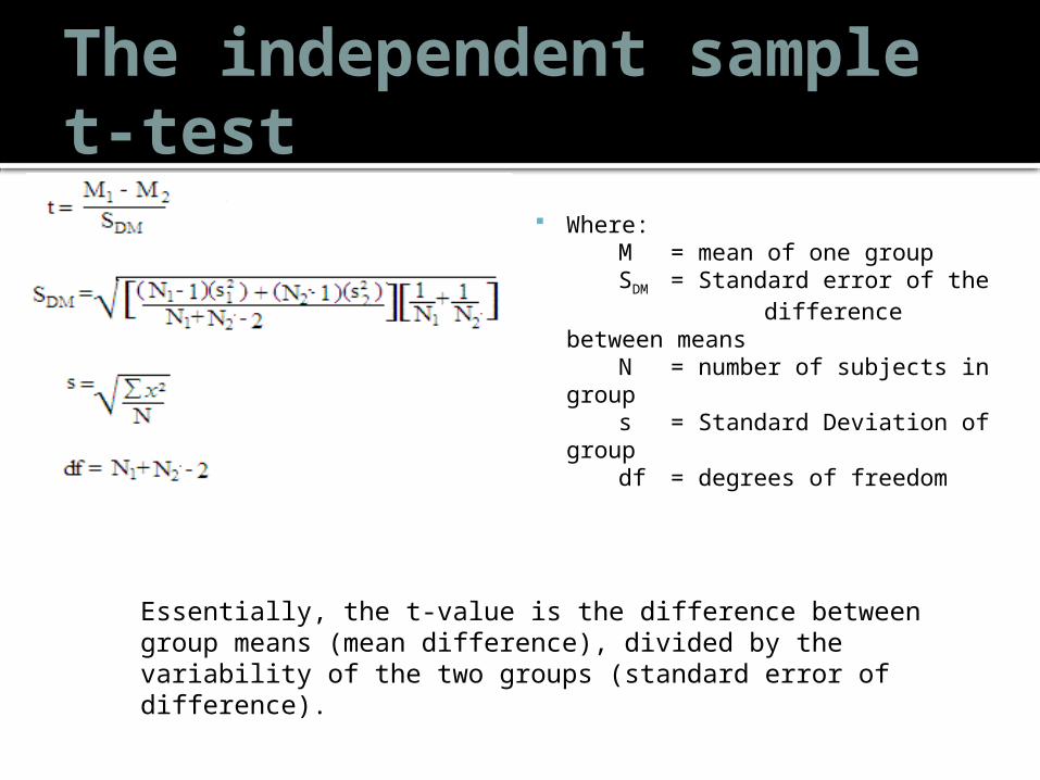
The independent sample t-test

Where: M = mean of one

groupSDM = Standard error of

the difference between means

N = number of subjects in group

s = Standard Deviation of group

df = degrees of freedom

Essentially, the t-value is the difference between group means (mean difference), divided by the variability of the two groups (standard error of difference).

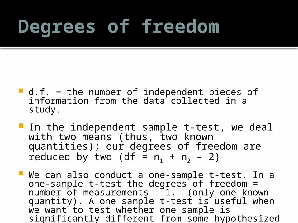
Degrees of freedom

d.f. = the number of independent pieces of information from the data collected in a study.

In the independent sample t-test, we deal with two means (thus, two known quantities); our degrees of freedom are reduced by two (df = n1 + n2 – 2)

We can also conduct a one-sample t-test. In a one-sample t-test the degrees of freedom = number of measurements – 1. (only one known quantity). A one sample t-test is useful when we want to test whether one sample is significantly different from some hypothesized value.

Assumptions Underlying the Independent Sample t-test

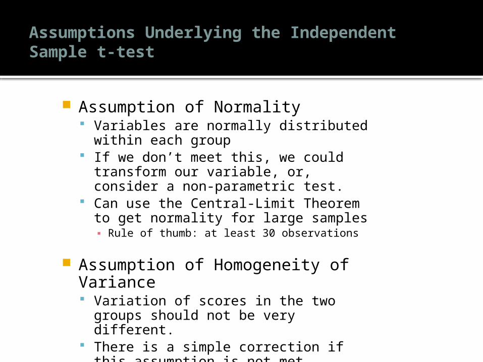
Assumption of Normality Variables are normally distributed within

each group If we don’t meet this, we could transform

our variable, or, consider a non-parametric test.

Can use the Central-Limit Theorem to get normality for large samples▪ Rule of thumb: at least 30 observations

Assumption of Homogeneity of Variance Variation of scores in the two groups

should not be very different. There is a simple correction if this

assumption is not met, automatically applied in R

What if the Variances are not equal?

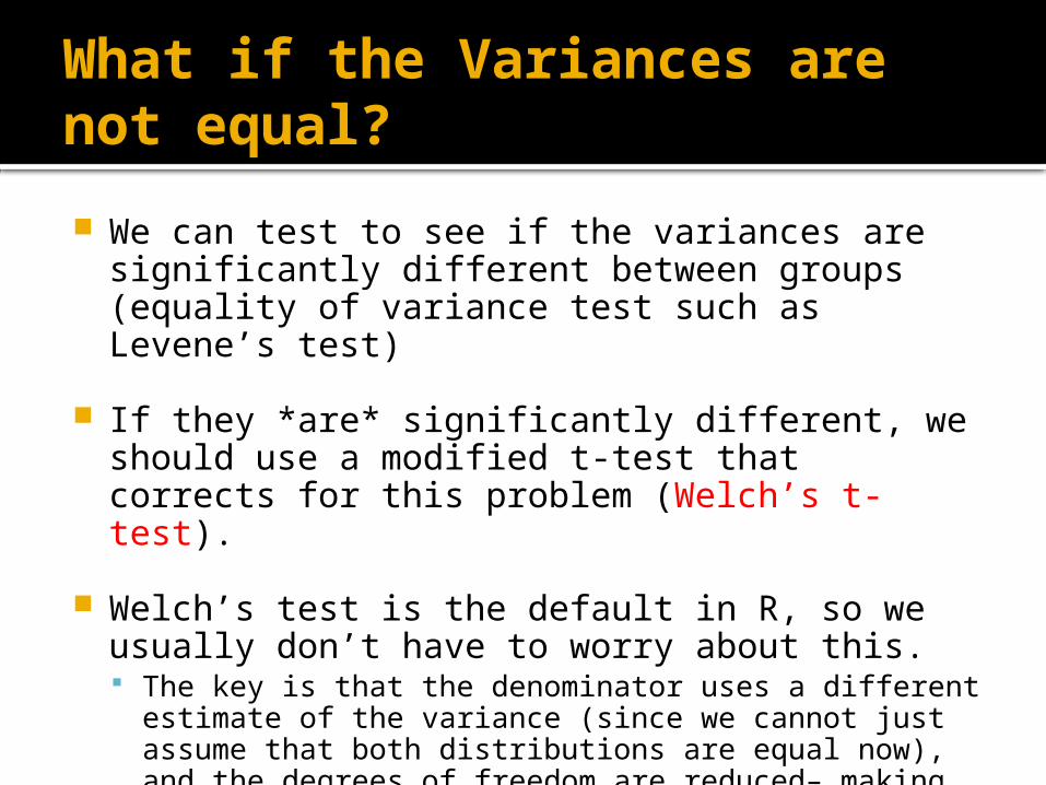
We can test to see if the variances are significantly different between groups (equality of variance test such as Levene’s test)

If they *are* significantly different, we should use a modified t-test that corrects for this problem (Welch’s t-test).

Welch’s test is the default in R, so we usually don’t have to worry about this. The key is that the denominator uses a different estimate

of the variance (since we cannot just assume that both distributions are equal now), and the degrees of freedom are reduced– making this a highly conservative test.

Conducting an independent sample t-test

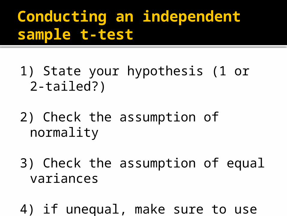
1) State your hypothesis (1 or 2-tailed?)

2) Check the assumption of normality

3) Check the assumption of equal variances

4) if unequal, make sure to use a modified (Welch’s) t-test

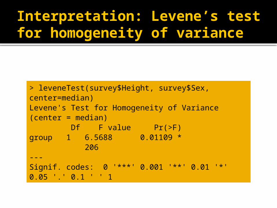
Interpretation: Levene’s test for homogeneity of variance

> leveneTest(survey$Height, survey$Sex, center=median)Levene's Test for Homogeneity of Variance (center = median) Df F value Pr(>F) group 1 6.5688 0.01109 * 206 ---Signif. codes: 0 '***' 0.001 '**' 0.01 '*' 0.05 '.' 0.1 ' ' 1

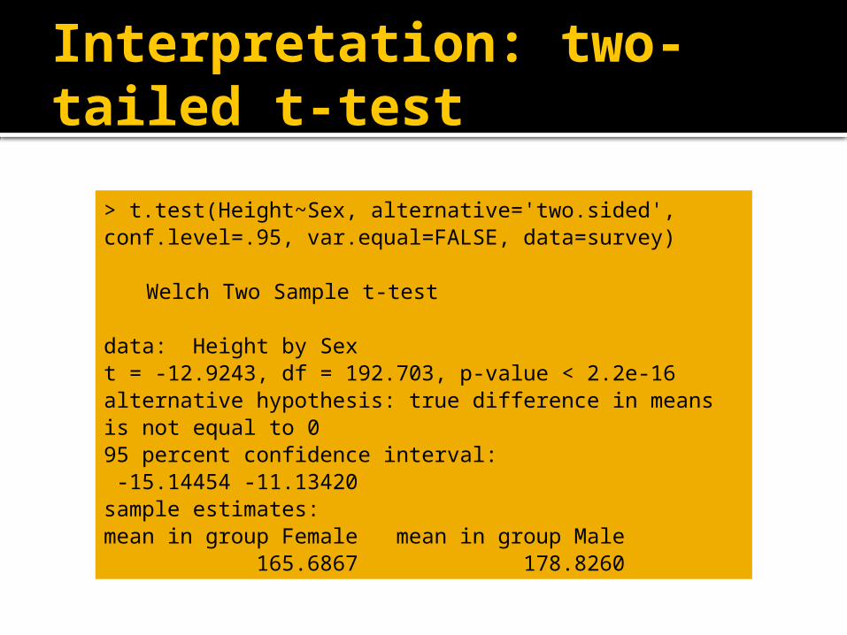
Interpretation: two-tailed t-test

> t.test(Height~Sex, alternative='two.sided', conf.level=.95, var.equal=FALSE, data=survey) 

Welch Two Sample t-test data: Height by Sext = -12.9243, df = 192.703, p-value < 2.2e-16alternative hypothesis: true difference in means is not equal to 095 percent confidence interval: -15.14454 -11.13420sample estimates:mean in group Female mean in group Male 165.6867 178.8260

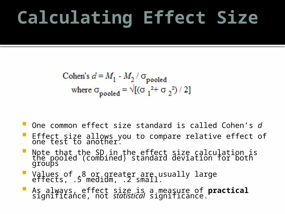
Calculating Effect Size

One common effect size standard is called Cohen’s d Effect size allows you to compare relative effect of one test to

another. Note that the SD in the effect size calculation is the pooled

(combined) standard deviation for both groups Values of .8 or greater are usually large effects, .5 medium, .2

small. As always, effect size is a measure of practical significance,

not statistical significance.

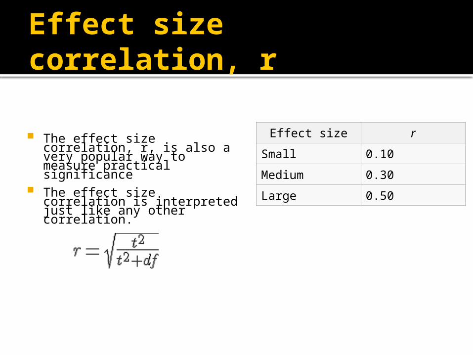
Effect size correlation, r

Effect size r

Small 0.10

Medium 0.30

Large 0.50

The effect size correlation, r, is also a very popular way to measure practical significance

The effect size correlation is interpreted just like any other correlation.

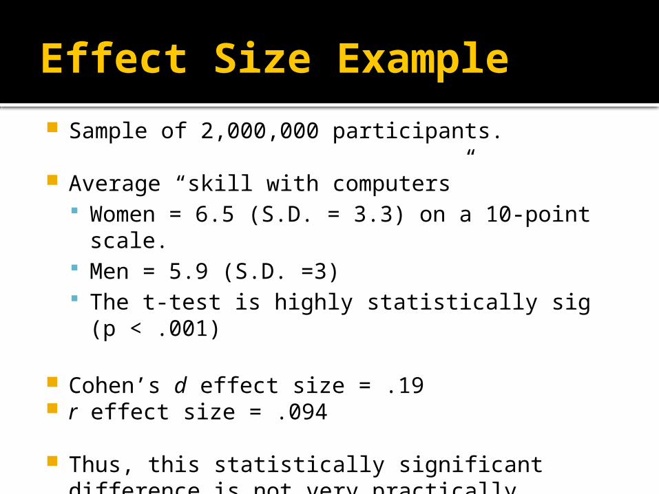
Effect Size Example

Sample of 2,000,000 participants.

Average “skill with computers” Women = 6.5 (S.D. = 3.3) on a 10-point scale. Men = 5.9 (S.D. =3) The t-test is highly statistically sig (p < .001)

Cohen’s d effect size = .19 r effect size = .094

Thus, this statistically significant difference is not very practically significant. This is a small effect size.

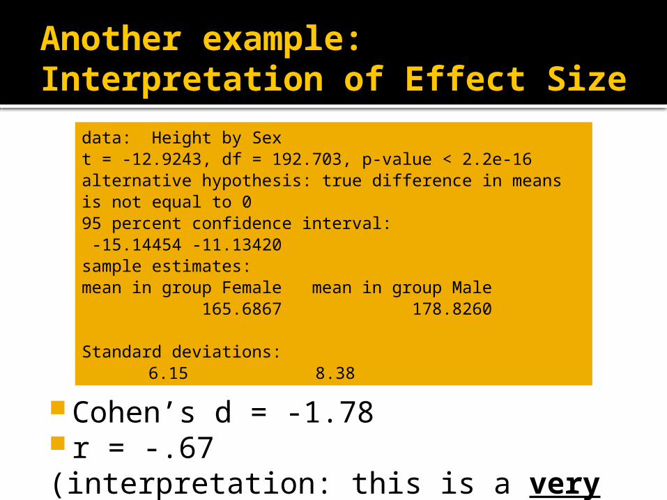
Another example: Interpretation of Effect Size

Cohen’s d = -1.78 r = -.67(interpretation: this is a very large

effect size)

data: Height by Sext = -12.9243, df = 192.703, p-value < 2.2e-16alternative hypothesis: true difference in means is not equal to 095 percent confidence interval: -15.14454 -11.13420sample estimates:mean in group Female mean in group Male 165.6867 178.8260

Standard deviations:6.15 8.38

The dependent t-test

We have already seen that the independent sample t-test allows us to compare means between two different groups.

The dependent t-test allows us to compare the two means (of the same variable) taken at two different time points for the same group of cases. For example, we could use the dependent t-test

to examine how the same class of students performed on the same quiz during the first week and the last week of class.

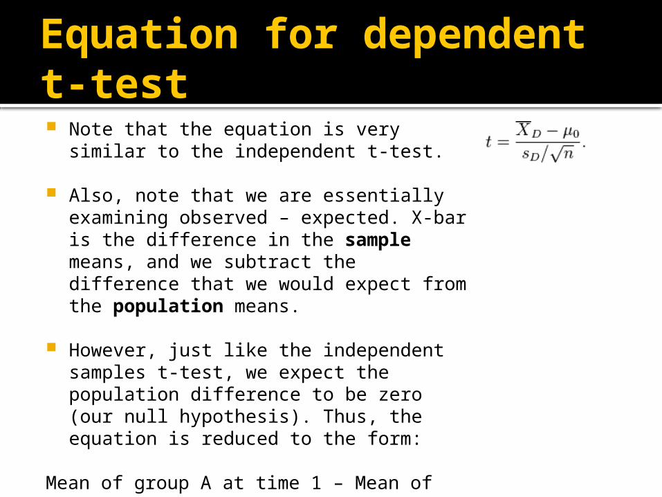
Equation for dependent t-test Note that the equation is very similar to

the independent t-test.

Also, note that we are essentially examining observed – expected. X-bar is the difference in the sample means, and we subtract the difference that we would expect from the population means.

However, just like the independent samples t-test, we expect the population difference to be zero (our null hypothesis). Thus, the equation is reduced to the form:

Mean of group A at time 1 – Mean of group A at time 2

----------------------------------------------------------------Standard error of the differences

Assumptions for the dependent t-test We still assume normality of the sampling distribution, just

as we do with other parametric tests.

However, unlike the independent sample t-test, we are actually only concerned with one distribution rather than two. In the dependent t-test, we want to check the normality of the difference between scores.

Note that it is entirely possible to have two measures that are non-normal, but their differences can be normally distributed.

We can also apply the Central Limit Theorem to get normality for large samples.

Example:

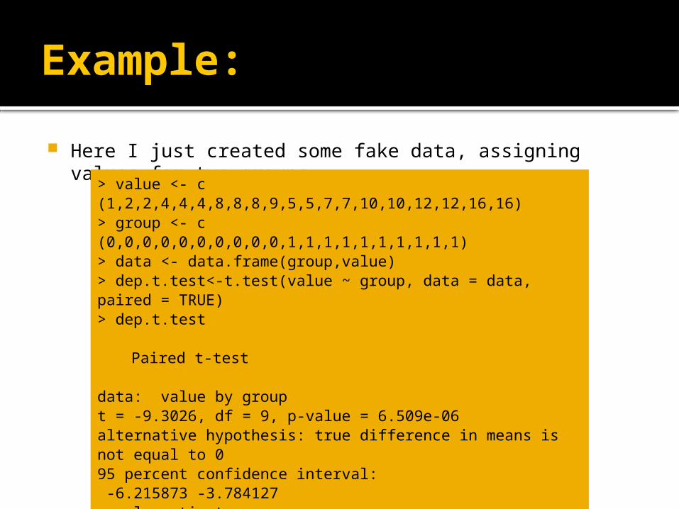
Here I just created some fake data, assigning values for two groups.

> value <- c (1,2,2,4,4,4,8,8,8,9,5,5,7,7,10,10,12,12,16,16)> group <- c (0,0,0,0,0,0,0,0,0,0,1,1,1,1,1,1,1,1,1,1)> data <- data.frame(group,value)> dep.t.test<-t.test(value ~ group, data = data, paired = TRUE)> dep.t.test 

Paired t-test data: value by groupt = -9.3026, df = 9, p-value = 6.509e-06alternative hypothesis: true difference in means is not equal to 095 percent confidence interval: -6.215873 -3.784127sample estimates:mean of the differences -5

Effect size for dependent t-test

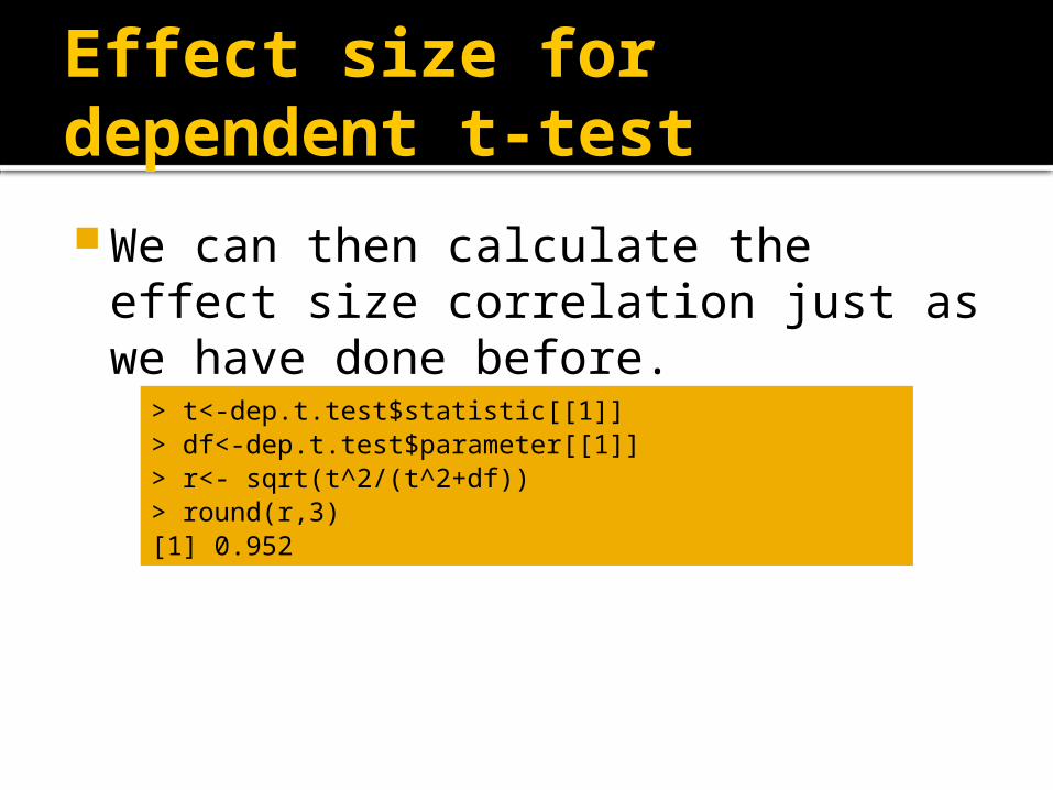
We can then calculate the effect size correlation just as we have done before.

> t<-dep.t.test$statistic[[1]]> df<-dep.t.test$parameter[[1]]> r<- sqrt(t^2/(t^2+df))> round(r,3)[1] 0.952

Non-parametric tests

As we have already discussed, sometimes we do not meet key assumptions, such as the assumption of normality.

We can try to address such problems by transforming variables, but sometimes it might just be best to not make big assumptions in the first place.

Also, non-parametric tests are useful when our key outcome variable is an ordinal variable rather than an interval or ratio variable.

Non-parametric tests, or “assumption-free” tests tend to be much less restrictive.

What do non-parametric tests actually do?

Many non-parametric tests use the principle of ranking data. For example, data are listed from lowest scores to

highest scores. Each score receives a potential rank …1, 2, 3, etc.

Thus, higher scores end up with higher ranks and lower scores have lower ranks.▪ Advantage: we get around the normal distribution

assumption of parametric tests.▪ Disadvantage: we lose some information about the

magnitude of differences between scores. Non-parametric tests often have less power than parametric ones

If our sampling distribution is not normally distributed (which we can only infer from our sample), then a non-parametric test is still a better option than parametric tests (such as t-tests).

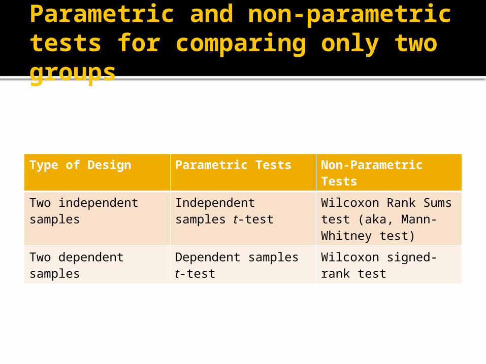
Parametric and non-parametric tests for comparing only two groups

Type of Design Parametric Tests Non-Parametric Tests

Two independent samples

Independent samples t-test

Wilcoxon Rank Sums test (aka, Mann-Whitney test)

Two dependent samples

Dependent samples t-test

Wilcoxon signed-rank test

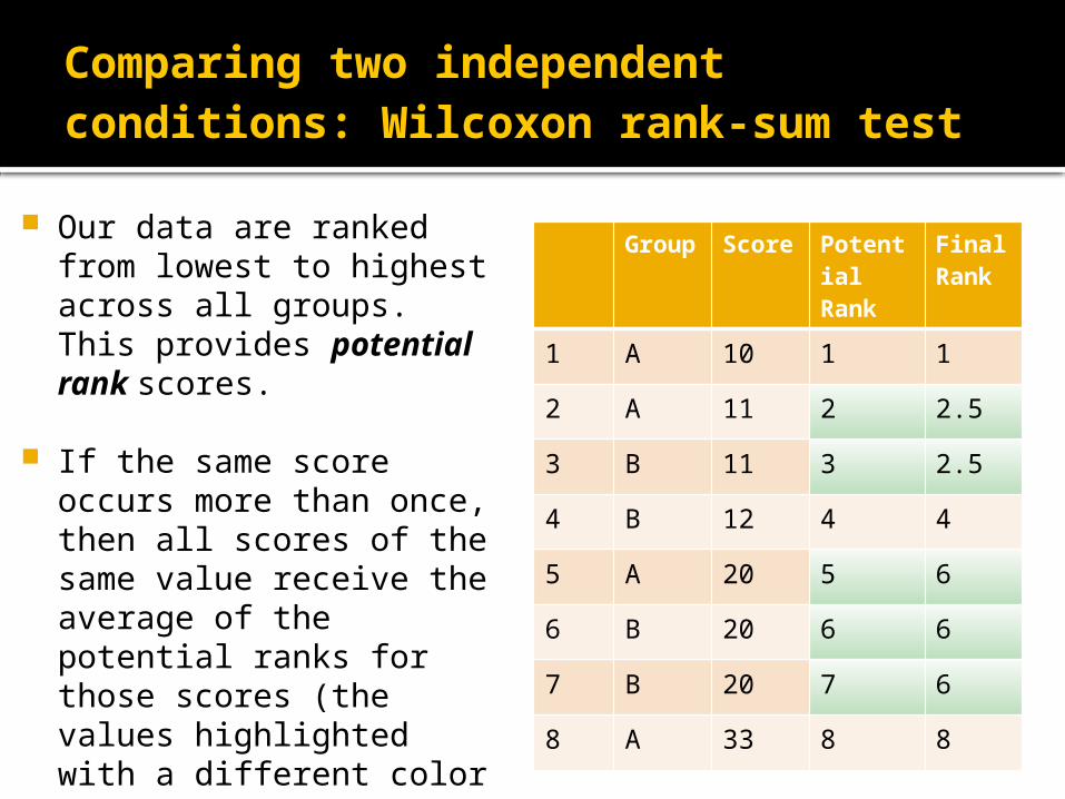
Comparing two independent conditions: Wilcoxon rank-sum test

Our data are ranked from lowest to highest across all groups. This provides potential rank scores.

If the same score occurs more than once, then all scores of the same value receive the average of the potential ranks for those scores (the values highlighted with a different color in the table)

When we are done, we have the final rank scores.

Group

Score Potential Rank

Final Rank

1 A 10 1 1

2 A 11 2 2.5

3 B 11 3 2.5

4 B 12 4 4

5 A 20 5 6

6 B 20 6 6

7 B 20 7 6

8 A 33 8 8

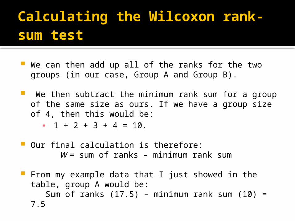
Calculating the Wilcoxon rank-sum test

We can then add up all of the ranks for the two groups (in our case, Group A and Group B).

We then subtract the minimum rank sum for a group of the same size as ours. If we have a group size of 4, then this would be:

▪ 1 + 2 + 3 + 4 = 10.

Our final calculation is therefore:W = sum of ranks – minimum rank sum

From my example data that I just showed in the table, group A would be:

Sum of ranks (17.5) – minimum rank sum (10) = 7.5

Interpretation of Wilcoxon rank-sum test

Just as with a t-test, the default is a two-sided test (where our null hypothesis is that there is no difference in ranks, and the alternative hypothesis is that there is a difference in ranks)

You can also declare a one-directional test if you actually hypothesize that one group will have higher ranks than the other.

There are always two values for W (one for each group), but typically the lowest score for W is used as the test statistic.

Interpretation of Wilcoxon rank-sum test:

Our p-value is calculated with Monte Carlo methods (where simulated data are used to estimate a statistic) if we have a small N (under 40).

For larger samples, R will use a normal approximation method (where we only assume that the sampling distribution of the W statistic is normal– it does not assume that our data are normal).

The normal approximation method is helpful because it also calculates a z-statistic that is used to calculate the p-value.

Effect size for Wilcoxon rank-sum test

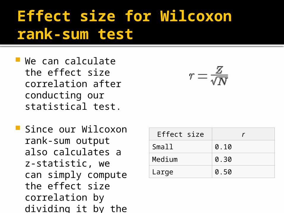
We can calculate the effect size correlation after conducting our statistical test.

Since our Wilcoxon rank-sum output also calculates a z-statistic, we can simply compute the effect size correlation by dividing it by the square root of the total sample size.

Effect size r

Small 0.10

Medium 0.30

Large 0.50

Comparing two related conditions: Wilcoxon signed-rank test The Wilcoxon signed-rank test is the non-

parametric equivalent of the dependent t-test.

We actually use a very similar procedure as the dependent t-test, as we are looking at the difference in scores among the same cases (rather than two separate groups).

But, unlike the dependent t-test, we examine the ranking of the differences in scores, rather than the scores themselves

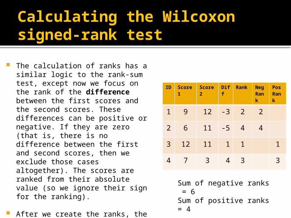
Calculating the Wilcoxon signed-rank test

The calculation of ranks has a similar logic to the rank-sum test, except now we focus on the rank of the difference between the first scores and the second scores. These differences can be positive or negative. If they are zero (that is, there is no difference between the first and second scores, then we exclude those cases altogether). The scores are ranked from their absolute value (so we ignore their sign for the ranking).

After we create the ranks, the positive and negative ranks are summed separately.

Between the positive and the negative sum of ranks, whichever value is smaller is used as the test statistic.

ID Score 1

Score 2

Diff

Rank

NegRank

PosRank

1 9 12 -3 2 2

2 6 11 -5 4 4

3 12 11 1 1 1

4 7 3 4 3 3

Sum of negative ranks = 6Sum of positive ranks = 4

Effect size for Wilcoxon signed-rank test

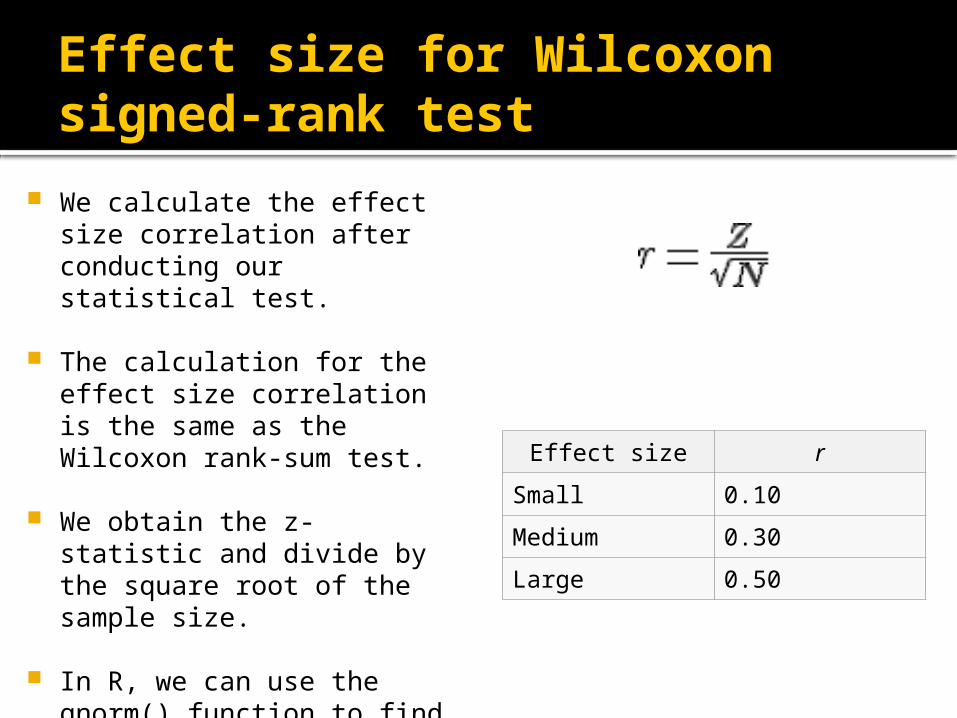
We calculate the effect size correlation after conducting our statistical test.

The calculation for the effect size correlation is the same as the Wilcoxon rank-sum test.

We obtain the z-statistic and divide by the square root of the sample size.

In R, we can use the qnorm() function to find the z-statistic from our p-value.

Effect size r

Small 0.10

Medium 0.30

Large 0.50

In Sum…

Non-parametric tests offer a way to examine differences between different groups or among groups with multiple measures, while avoiding some of the assumptions that are necessary in parametric tests.

Which test you choose (parametric or non-parametric) depends on: (1) the variables and data that you have (e.g.,

do you have a continuous variable of interest, or is it an ordinal variable?)

(2) Whether you meet the necessary assumptions for parametric tests, such as the assumption of normality.