Embed Size (px)
Citation preview
Eur. Phys. J. C (2016) 76:434DOI 10.1140/epjc/s10052-016-4271-x
Regular Article - Experimental Physics
Search for the lepton flavour violating decay μ+ → e+γwith the full dataset of the MEG experiment
MEG Collaboration
A. M. Baldini4a, Y. Bao1, E. Baracchini3,16, C. Bemporad4a,4b, F. Berg1,2, M. Biasotti8a,8b, G. Boca6a,6b,M. Cascella13a,13b,17 , P. W. Cattaneo6a, G. Cavoto7a, F. Cei4a,4b, C. Cerri4a, G. Chiarello13a,13b, C. Chiri13a,13b,A. Corvaglia13a,13b, A. de Bari6a,6b, M. De Gerone8a, T. Doke9, A. D’Onofrio4a,4b, S. Dussoni4a, J. Egger1, Y. Fujii3,L. Galli4a, F. Gatti8a,8b, F. Grancagnolo13a, M. Grassi4a, A. Graziosi7a,7b, D. N. Grigoriev10,14,15, T. Haruyama11,M. Hildebrandt1, Z. Hodge1,2, K. Ieki3, F. Ignatov10,15, T. Iwamoto3, D. Kaneko3, T. I. Kang5, P.-R. Kettle1,B. I. Khazin10,15, N. Khomutov12, A. Korenchenko12, N. Kravchuk12, G. M. A. Lim5, A. Maki11, S. Mihara11,W. Molzon5, Toshinori Mori3, F. Morsani4a, A. Mtchedilishvili1, D. Mzavia12, S. Nakaura3, R. Nardò6a,6b,D. Nicolò4a,4b, H. Nishiguchi11, M. Nishimura3, S. Ogawa3, W. Ootani3, S. Orito3, M. Panareo13a,13b, A. Papa1,R. Pazzi4, A. Pepino13a,13b, G. Piredda7a, G. Pizzigoni8a,8b, A. Popov10,15, F. Raffaelli4a, F. Renga1,7a,7b,E. Ripiccini7a,7b, S. Ritt1, M. Rossella6a, G. Rutar1,2, R. Sawada3, F. Sergiampietri4a, G. Signorelli4a,M. Simonetta6a,6b, G. F. Tassielli13a, F. Tenchini4a,4b, Y. Uchiyama3, M. Venturini4a,4c, C. Voena7a, A. Yamamoto11,K. Yoshida3, Z. You5, Yu. V. Yudin10,15, D. Zanello7
1 Paul Scherrer Institut PSI, 5232 Villigen, Switzerland2 Swiss Federal Institute of Technology ETH, CH-8093 Zurich, Switzerland3 ICEPP, The University of Tokyo, 7-3-1 Hongo, Bunkyo-ku, Tokyo 113-0033, Japan4 (a)INFN Sezione di Pisa, dell’Università, Largo B. Pontecorvo 3, 56127 Pisa, Italy;
(b)Dipartimento di Fisica, dell’Università, Largo B. Pontecorvo 3, 56127 Pisa, Italy;(c)Scuola Normale Superiore, Piazza dei Cavalieri, 56127 Pisa, Italy
5 University of California, Irvine, CA 92697, USA6 (a)INFN Sezione di Pavia, dell’Università, Via Bassi 6, 27100 Pavia, Italy;
(b)Dipartimento di Fisica, dell’Università, Via Bassi 6, 27100 Pavia, Italy7 (a)INFN Sezione di Roma, dell’Università “Sapienza”, Piazzale A. Moro, 00185 Rome, Italy;
(b)Dipartimento di Fisica, dell’Università “Sapienza”, Piazzale A. Moro, 00185 Rome, Italy8 (a)INFN Sezione di Genova, dell’Università, Via Dodecaneso 33, 16146 Genoa, Italy;
(b)Dipartimento di Fisica, dell’Università, Via Dodecaneso 33, 16146 Genoa, Italy9 Research Institute for Science and Engineering, Waseda University, 3-4-1 Okubo, Shinjuku-ku, Tokyo 169-8555, Japan
10 Budker Institute of Nuclear Physics of Siberian Branch of Russian Academy of Sciences, 630090 Novosibirsk, Russia11 KEK, High Energy Accelerator Research Organization, 1-1 Oho, Tsukuba, Ibaraki 305-0801, Japan12 Joint Institute for Nuclear Research, 141980 Dubna, Russia13 (a)INFN Sezione di Lecce, dell’Università del Salento, Via per Arnesano, 73100 Lecce, Italy;
(b)Dipartimento di Matematica e Fisica, dell’Università del Salento, Via per Arnesano, 73100 Lecce, Italy14 Novosibirsk State Technical University, 630092 Novosibirsk, Russia15 Novosibirsk State University, 630090 Novosibirsk, Russia16 Present address: INFN, Laboratori Nazionali di Frascati, Via E. Fermi, 40-00044 Frascati, Rome, Italy17 Present address: Department of Physics and Astronomy, University College London, Gower Street, London WC1E 6BT, UK
Received: 1 June 2016 / Accepted: 11 July 2016 / Published online: 3 August 2016© The Author(s) 2016. This article is published with open access at Springerlink.com
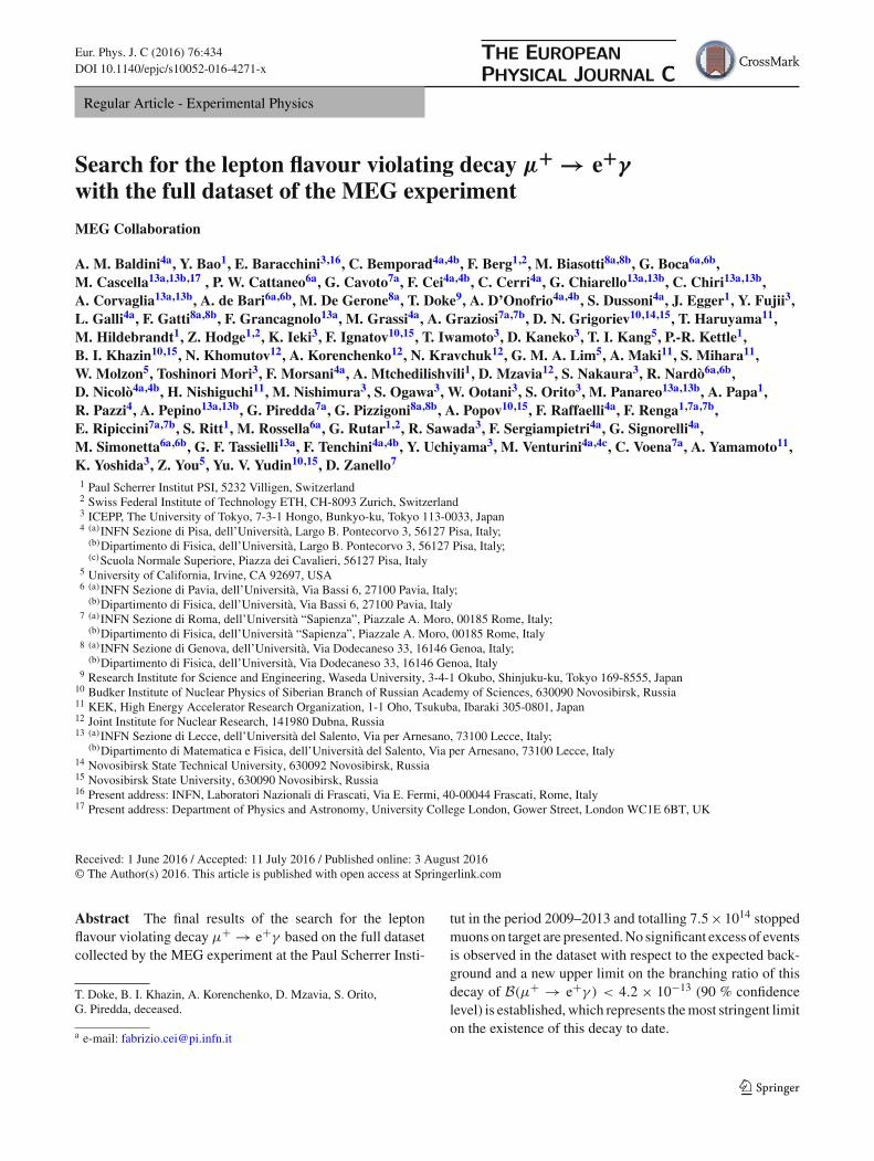
Abstract The final results of the search for the leptonflavour violating decay μ+ → e+γ based on the full datasetcollected by the MEG experiment at the Paul Scherrer Insti-
T. Doke, B. I. Khazin, A. Korenchenko, D. Mzavia, S. Orito,G. Piredda, deceased.
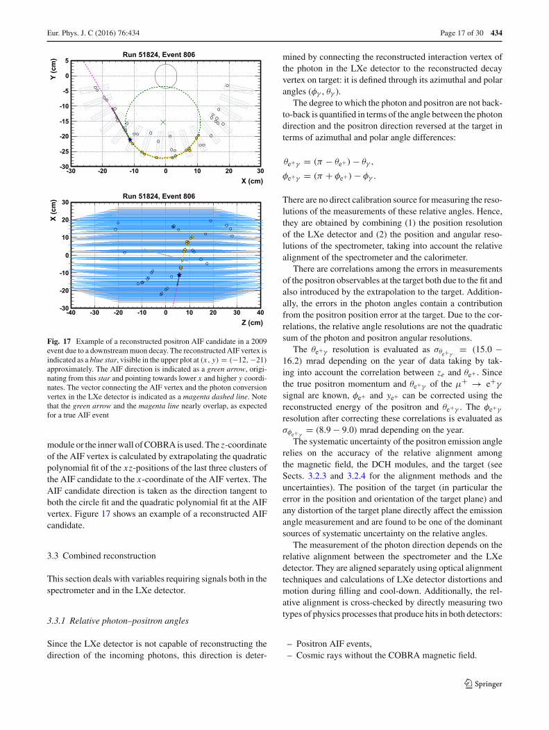
a e-mail: [email protected]
tut in the period 2009–2013 and totalling 7.5 × 10¹⁴ stoppedmuons on target are presented. No significant excess of eventsis observed in the dataset with respect to the expected back-ground and a new upper limit on the branching ratio of thisdecay of B(μ+ → e+γ ) < 4.2 × 10⁻¹³ (90 % confidencelevel) is established, which represents the most stringent limiton the existence of this decay to date.
123
434 Page 2 of 30 Eur. Phys. J. C (2016) 76 :434
Contents
1 Introduction . . . . . . . . . . . . . . . . . . . . . 22 MEG detector . . . . . . . . . . . . . . . . . . . . 33 Reconstruction . . . . . . . . . . . . . . . . . . . . 84 Analysis . . . . . . . . . . . . . . . . . . . . . . . 195 Conclusions . . . . . . . . . . . . . . . . . . . . . 28References . . . . . . . . . . . . . . . . . . . . . . . . 29
1 Introduction
The standard model (SM) of particle physics allowscharged lepton flavour violating (CLFV) processes withonly extremely small branching ratios (�10−50) even whenaccounting for measured neutrino mass differences and mix-ing angles. Therefore, such decays are free from SM physicsbackgrounds associated with processes involving, eitherdirectly or indirectly, hadronic states and are ideal labora-tories for searching for new physics beyond the SM. A pos-itive signal would be an unambiguous evidence for physicsbeyond the SM.
The existence of such decays at measurable rates not farbelow current upper limits is suggested by many SM exten-sions, such as supersymmetry [1]. An extensive review ofthe theoretical expectations for CLFV is provided in [2].CLFV searches with improved sensitivity probe new regionsof the parameter spaces of SM extensions, and CLFV decayμ+ → e+γ is particularly sensitive to new physics. TheMEG collaboration has searched for μ+ → e+γ decay atthe Paul Scherrer Institut (PSI) in Switzerland in the period2008–2013. A detailed report of the experiment motivation,design criteria, and goals is available in reference [3,4] andreferences therein. We have previously reported [5–7] results
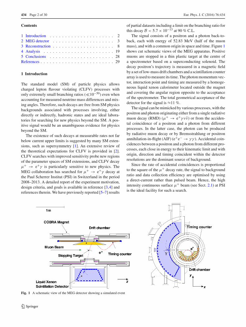
Fig. 1 A schematic view of the MEG detector showing a simulated event
of partial datasets including a limit on the branching ratio forthis decay B < 5.7 × 10⁻¹³ at 90 % C.L.
The signal consists of a positron and a photon back-to-back, each with energy of 52.83 MeV (half of the muonmass), and with a common origin in space and time. Figure 1shows cut schematic views of the MEG apparatus. Positivemuons are stopped in a thin plastic target at the centre ofa spectrometer based on a superconducting solenoid. Thedecay positron’s trajectory is measured in a magnetic fieldby a set of low-mass drift chambers and a scintillation counterarray is used to measure its time. The photon momentum vec-tor, interaction point and timing are measured by a homoge-neous liquid xenon calorimeter located outside the magnetand covering the angular region opposite to the acceptanceof the spectrometer. The total geometrical acceptance of thedetector for the signal is ≈11 %.
The signal can be mimicked by various processes, with thepositron and photon originating either from a single radiativemuon decay (RMD) (μ+ → e+γ νν̄) or from the acciden-tal coincidence of a positron and a photon from differentprocesses. In the latter case, the photon can be producedby radiative muon decay or by Bremsstrahlung or positronannihilation-in-flight (AIF) (e+e− → γ γ ). Accidental coin-cidences between a positron and a photon from different pro-cesses, each close in energy to their kinematic limit and withorigin, direction and timing coincident within the detectorresolutions are the dominant source of background.
Since the rate of accidental coincidences is proportionalto the square of the μ+ decay rate, the signal to backgroundratio and data collection efficiency are optimised by usinga direct-current rather than pulsed beam. Hence, the highintensity continuous surface μ+ beam (see Sect. 2.1) at PSIis the ideal facility for such a search.
123
Eur. Phys. J. C (2016) 76 :434 Page 3 of 30 434
The remainder of this paper is organised as follows. Aftera brief introduction to the detector and to the data acqui-sition system (Sect. 2), the reconstruction algorithms arepresented in detail (Sect. 3), followed by an in-depth dis-cussion of the analysis of the full MEG dataset and of theresults (Sect. 4). Finally, in the conclusions, some prospectsfor future improvements are outlined (Sect. 5).
2 MEG detector
The MEG detector is briefly presented in the following,emphasising the aspects relevant to the analysis; a detaileddescription is available in [8]. Briefly, it consists of the μ+beam, a thin stopping target, a thin-walled, superconductingmagnet, a drift chamber array (DCH), scintillating timingcounters (TC), and a liquid xenon calorimeter (LXe detec-tor).
In this paper we adopt a cylindrical coordinate system(r, φ, z) with origin at the centre of the magnet (see Fig. 1).The z-axis is parallel to the magnet axis and directed along theμ+ beam. The axis defining φ = 90◦ (the y-axis of the corre-sponding Cartesian coordinate system) is directed upwardsand, as a consequence, the x-axis is directed opposite to thecentre of the LXe detector. Positrons move along trajecto-ries with decreasing φ-coordinate. When required, the polarangle θ with respect to the z-axis is also used. The regionwith z < 0 is referred to as upstream, that with z > 0 asdownstream.
2.1 Muon beam
The requirement to stop a large number of μ+ in a thin targetof small transverse size drives the beam requirements: highflux, small transverse size, small momentum spread and smallcontamination, e.g. from positrons. These goals are met bythe 2.2 mA PSI proton cyclotron and πE5 channel in com-bination with the MEG beam line, which produces one ofthe world’s most intense continuous μ+ beams. It is a sur-face muon beam produced by π+ decay near the surface ofthe production target. It can deliver more than 108 μ+/s at28 MeV/c in a momentum bite of 5–7 %. To maximise theexperiment’s sensitivity, the beam is tuned to a μ+ stoppingrate of 3×10⁷, limited by the rate capabilities of the track-ing system and the rate of accidental backgrounds, given theMEG detector resolutions. The ratio of e+ to μ+ flux inthe beam is ≈8, and the positrons are efficiently removedby a combination of a Wien filter and collimator system.The muon momentum distribution at the target is optimisedby a degrader system comprised of a 300 µm thick mylar®
foil and the He-air atmosphere inside the spectrometer infront of the target. The round, Gaussian beam-spot profilehas σx,y ≈10 mm.
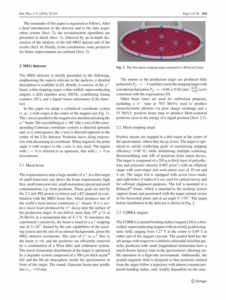
Fig. 2 The thin muon stopping target mounted in a Rohacell frame
The muons at the production target are produced fullypolarized (Pμ+ = −1) and they reach the stopping target witha residual polarization Pμ+ =−0.86 ± 0.02 (stat)+0.05
−0.06 (syst)consistent with the expectations [9].
Other beam tunes are used for calibration purposes,including a π− tune at 70.5 MeV/c used to producemonochromatic photons via pion charge exchange and a53 MeV/c positron beam tune to produce Mott-scatteredpositrons close to the energy of a signal positron (Sect. 2.7).
2.2 Muon stopping target
Positive muons are stopped in a thin target at the centre ofthe spectrometer, where they decay at rest. The target is opti-mised to satisfy conflicting goals of maximising stoppingefficiency (≈80 %) while minimising multiple scattering,Bremsstrahlung and AIF of positrons from muon decays.The target is composed of a 205 µm thick layer of polyethy-lene and polyester (density 0.895 g/cm3) with an ellipticalshape with semi-major and semi-minor axes of 10 cm and4 cm. The target foil is equipped with seven cross marksand eight holes of radius 0.5 cm, used for optical survey andfor software alignment purposes. The foil is mounted in aRohacell® frame, which is attached to the tracking systemsupport frame and positioned with the target normal vectorin the horizontal plane and at an angle θ ≈70◦. The targetbefore installation in the detector is shown in Fig. 2.
2.3 COBRA magnet
The COBRA (constant bending radius) magnet [10] is a thin-walled, superconducting magnet with an axially graded mag-netic field, ranging from 1.27 T at the centre to 0.49 T ateither end of the magnet cryostat. The graded field has theadvantage with respect to a uniform solenoidal field that par-ticles produced with small longitudinal momentum have amuch shorter latency time in the spectrometer, allowing sta-ble operation in a high-rate environment. Additionally, thegraded magnetic field is designed so that positrons emittedfrom the target follow a trajectory with almost constant pro-jected bending radius, only weakly dependent on the emis-
123
434 Page 4 of 30 Eur. Phys. J. C (2016) 76 :434
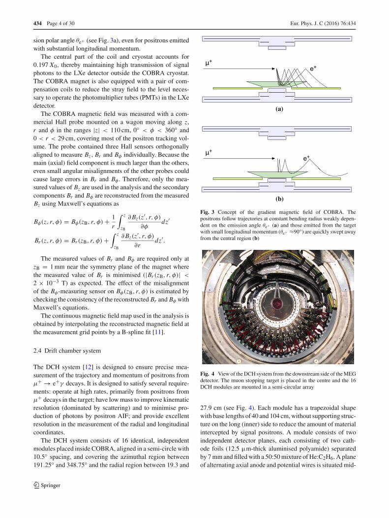
sion polar angle θe+ (see Fig. 3a), even for positrons emittedwith substantial longitudinal momentum.
The central part of the coil and cryostat accounts for0.197 X0, thereby maintaining high transmission of signalphotons to the LXe detector outside the COBRA cryostat.The COBRA magnet is also equipped with a pair of com-pensation coils to reduce the stray field to the level neces-sary to operate the photomultiplier tubes (PMTs) in the LXedetector.
The COBRA magnetic field was measured with a com-mercial Hall probe mounted on a wagon moving along z,r and φ in the ranges |z| < 110 cm, 0◦ < φ < 360◦ and0 < r < 29 cm, covering most of the positron tracking vol-ume. The probe contained three Hall sensors orthogonallyaligned to measure Bz, Br and Bφ individually. Because themain (axial) field component is much larger than the others,even small angular misalignments of the other probes couldcause large errors in Br and Bφ . Therefore, only the mea-sured values of Bz are used in the analysis and the secondarycomponents Br and Bφ are reconstructed from the measuredBz using Maxwell’s equations as
Bφ(z, r, φ) = Bφ(zB, r, φ) + 1
r
∫ z
zB
∂ Bz(z′, r, φ)
∂φdz′
Br (z, r, φ) = Br (zB, r, φ) +∫ z
zB
∂ Bz(z′, r, φ)
∂rdz′.
The measured values of Br and Bφ are required only atzB = 1 mm near the symmetry plane of the magnet wherethe measured value of Br is minimised (|Br (zB, r, φ)| <
2 × 10⁻³ T) as expected. The effect of the misalignmentof the Bφ-measuring sensor on Bφ(zB, r, φ) is estimated bychecking the consistency of the reconstructed Br and Bφ withMaxwell’s equations.
The continuous magnetic field map used in the analysis isobtained by interpolating the reconstructed magnetic field atthe measurement grid points by a B-spline fit [11].
2.4 Drift chamber system
The DCH system [12] is designed to ensure precise mea-surement of the trajectory and momentum of positrons fromμ+ → e+γ decays. It is designed to satisfy several require-ments: operate at high rates, primarily from positrons fromμ+ decays in the target; have low mass to improve kinematicresolution (dominated by scattering) and to minimise pro-duction of photons by positron AIF; and provide excellentresolution in the measurement of the radial and longitudinalcoordinates.
The DCH system consists of 16 identical, independentmodules placed inside COBRA, aligned in a semi-circle with10.5◦ spacing, and covering the azimuthal region between191.25◦ and 348.75◦ and the radial region between 19.3 and
(a)
(b)
Fig. 3 Concept of the gradient magnetic field of COBRA. Thepositrons follow trajectories at constant bending radius weakly depen-dent on the emission angle θe+ (a) and those emitted from the targetwith small longitudinal momentum (θe+ ≈90◦) are quickly swept awayfrom the central region (b)
Fig. 4 View of the DCH system from the downstream side of the MEGdetector. The muon stopping target is placed in the centre and the 16DCH modules are mounted in a semi-circular array
27.9 cm (see Fig. 4). Each module has a trapezoidal shapewith base lengths of 40 and 104 cm, without supporting struc-ture on the long (inner) side to reduce the amount of materialintercepted by signal positrons. A module consists of twoindependent detector planes, each consisting of two cath-ode foils (12.5 µm-thick aluminised polyamide) separatedby 7 mm and filled with a 50:50 mixture of He:C2H6. A planeof alternating axial anode and potential wires is situated mid-
123

Eur. Phys. J. C (2016) 76 :434 Page 5 of 30 434
Fig. 5 Schematic view of the cell structure of a DCH plane
Fig. 6 Schematic view of the Vernier pad method showing the padshape and offsets. Only one of the two cathode pads in each cell isshown
way between the cathode foils with a pitch of 4.5 mm. Thetwo planes of cells are separated by 3 mm and the two wirearrays in the same module are staggered by half a drift cellto help resolve left-right position ambiguities (see Fig. 5). Adouble wedge pad structure is etched on both cathodes witha Vernier pattern of cycle λ = 5 cm as shown in Fig. 6. Thepad geometry is designed to allow a precise measurementof the axial coordinate of the hit by comparing the signalsinduced on the four pads in each cell. The average amount ofmaterial intercepted by a positron track in a DCH module is2.6 × 10−4 X0, with the total material along a typical signalpositron track of 2.0 × 10−3 X0.
2.5 Timing counter
The TC [13,14] is designed to measure precisely the impacttime and position of signal positrons and to infer the muondecay time by correcting for the track length from the targetto the TC obtained from the DCH information.
The main requirements of the TC are:
– provide full acceptance for signal positrons in the DCHacceptance matching the tight mechanical constraintsdictated by the DCH system and COBRA;
– ability to operate at high rate in a high and non-uniformmagnetic field;
– fast and approximate (≈5 cm resolution) determinationof the positron impact point for the online trigger;
– good (≈1 cm) positron impact point position resolutionin the offline event analysis;
– excellent (≈50 ps) time resolution of the positron impactpoint.
The system consists of an upstream and a downstreamsector, as shown in Fig. 1.
Fig. 7 Schematic picture of a TC sector. Scintillator bars are read outby a PMT at each end
Each sector (see Fig. 7) is barrel shaped with full angularcoverage for signal positrons within the photon and positronacceptance of the LXe detector and DCH. It consists of anarray of 15 scintillating bars with a 10.5◦ pitch between adja-cent bars. Each bar has an approximate square cross-sectionof size 4.0 × 4.0 × 79.6 cm3 and is read out by a fine-mesh,magnetic field tolerant, 2” PMT at each end. The inner radiusof a sector is 29.5 cm, such that only positrons with a momen-tum close to that of signal positrons hit the TC.
2.6 Liquid xenon detector
The LXe photon detector [15,16] requires excellent posi-tion, time and energy resolutions to minimise the numberof accidental coincidences between photons and positronsfrom different muon decays, which comprise the dominantbackground process (see Sect. 4.4.1).
It is a homogeneous calorimeter able to contain fully theshower induced by a 52.83 MeV photon and measure thephoton interaction vertex, interaction time and energy withhigh efficiency. The photon direction is not directly measuredin the LXe detector, rather it is inferred by the direction of aline between the photon interaction vertex in the LXe detectorand the intercept of the positron trajectory at the stoppingtarget.
Liquid xenon, with its high density and short radiationlength, is an efficient detection medium for photons; optimalresolution is achieved, at least at low energies, if both theionisation and scintillation signals are detected. In the highrate MEG environment, only the scintillation light with itsvery fast signal, is detected.
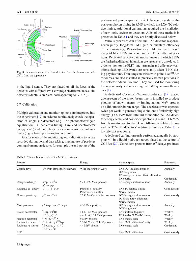
A schematic view of the LXe detector is shown in Fig. 8. Ithas a C-shaped structure fitting the outer radius of COBRA.The fiducial volume is ≈800 , covering 11 % of the solidangle viewed from the centre of the stopping target. Scin-tillation light is detected in 846 PMTs submerged directly
123
434 Page 6 of 30 Eur. Phys. J. C (2016) 76 :434
Fig. 8 Schematic view of the LXe detector: from the downstream side(left), from the top (right)
in the liquid xenon. They are placed on all six faces of thedetector, with different PMT coverage on different faces. Thedetector’s depth is 38.5 cm, corresponding to ≈14 X0.
2.7 Calibration
Multiple calibration and monitoring tools are integrated intothe experiment [17] in order to continuously check the oper-ation of single sub-detectors (e.g. LXe photodetector gainequalisation, TC bar cross-timing, LXe and spectrometerenergy scale) and multiple-detector comparisons simultane-ously (e.g. relative positron-photon timing).
Data for some of the monitoring and calibration tasks arerecorded during normal data taking, making use of particlescoming from muon decays, for example the end-points of the
Table 1 The calibration tools of the MEG experiment
Process Energy Main purpose Frequency
Cosmic rays μ± from atmospheric showers Wide spectrum O(GeV) LXe-DCH relative position AnnuallyDCH alignmentTC energy and time offset calibrationLXe purity On demand
Charge exchange π−p → π0n 55,83,129 MeV photons LXe energy scale/resolution Annuallyπ0 → γ γ
Radiative μ−decay μ+ → e+γ νν̄ Photons > 40 MeV, LXe-TC relative timing ContinuouslyPositrons > 45 MeV Normalisation
Normal μ−decay μ+ → e+νν̄ 52.83 MeV end-point positrons DCH energy scale/resolution ContinuouslyDCH and target alignmentNormalisation
Mott positrons e+ target → e+ target ≈50 MeV positrons DCH energy scale/resolution AnnuallyDCH alignment
Proton accelerator 7Li(p, γ )8Be 14.8, 17.6 MeV photons LXe uniformity/purity Weekly11B(p, γ )12C 4.4, 11.6, 16.1 MeV photons TC interbar/ LXe–TC timing Weekly
Neutron generator 58Ni(n, γ )59Ni 9 MeV photons LXe energy scale WeeklyRadioactive source 241Am(α, γ )237Np 5.5 MeV α’s, 56 keV photons LXe PMT calibration/purity WeeklyRadioactive source 9Be(α241Am, n)12C� 4.4 MeV photons LXe energy scale On demand
12C�(γ )12CLED LXe PMT calibration Continuously
positron and photon spectra to check the energy scale, or thepositron-photon timing in RMD to check the LXe–TC rela-tive timing. Additional calibrations required the installationof new tools, devices or detectors. A list of these methods ispresented in Table 1 and they are briefly discussed below.
Various processes can affect the LXe detector response:xenon purity, long-term PMT gain or quantum efficiencydrifts from ageing, HV variations, etc. PMT gains are trackedusing 44 blue LEDs immersed in the LXe at different posi-tions. Dedicated runs for gain measurements in which LEDsare flashed at different intensities are taken every two days. Inorder to monitor the PMT long-term gain and efficiency vari-ations, flashing LED events are constantly taken (1 Hz) dur-ing physics runs. Thin tungsten wires with point-like 241Amα-sources are also installed in precisely known positions inthe detector fiducial volume. They are used for monitoringthe xenon purity and measuring the PMT quantum efficien-cies [18].
A dedicated Cockcroft–Walton accelerator [19] placeddownstream of the muon beam line is installed to producephotons of known energy by impinging sub-MeV protonson a lithium tetraborate target. The accelerator was operatedtwice per week to generate single photons of relatively highenergy (17.6 MeV from lithium) to monitor the LXe detec-tor energy scale, and coincident photons (4.4 and 11.6 MeVfrom boron) to monitor the TC scintillator bar relative timingand the TC–LXe detectors’ relative timing (see Table 1 forthe relevant reactions).
A dedicated calibration run is performed annually by stop-ping π− in a liquid hydrogen target placed at the centre ofCOBRA [20]. Coincident photons from π0 decays produced
123
Eur. Phys. J. C (2016) 76 :434 Page 7 of 30 434
in the charge exchange (CEX) reaction π−p → π0n aredetected simultaneously in the LXe detector and a dedicatedBGO crystal detector. By appropriate relative LXe and BGOgeometrical selection and BGO energy selection, a nearlymonochromatic sample of 55 MeV (and 83 MeV) photonsincident on the LXe are used to measure the response of theLXe detector at these energies and set the absolute energyscale at the signal photon energy.
A low-energy calibration point is provided by 4.4 MeVphotons from an 241Am/Be source that is moved periodicallyin front of the LXe detector during beam-off periods.
Finally, a neutron generator exploiting the (n, γ ) reactionon nickel shown in Table 1 allows an energy calibration undervarious detector rate conditions, in particular normal MEGand CEX data taking.
Data with Mott-scattered positrons are also acquired annu-ally to monitor and calibrate the spectrometer with all thebenefits associated with the usage of a quasi-monochromaticenergy line at ≈53 MeV [21].
2.8 Front-end electronics
The digitisation and data acquisition system for MEG usesa custom, high frequency digitiser based on the switchedcapacitor array technique, the Domino Ring Sampler 4(DRS4) [22]. For each of the ≈3000 read-out channels witha signal above some threshold, it records a waveform of 1024samples. The sampling rate is 1.6 GHz for the TC and LXedetectors, matched to the precise time measurements in thesedetectors, and 0.8 GHz for the DCH, matched to the driftvelocity and intrinsic drift resolution.
Each waveform is processed offline by applying baselinesubtraction, spectral analysis, noise filtering, digital constantfraction discrimination etc. so as to optimise the extractionof the variables relevant for the measurement. Saving the fullwaveform provides the advantage of being able to reprocessthe full waveform information offline with improved algo-rithms.
2.9 Trigger
An experiment to search for ultra-rare events within a hugebackground due to a high muon stopping rate needs a quickand efficient event selection, which demands the combineduse of high-resolution detection techniques with fast front-end, digitising electronics and trigger. The trigger systemplays an essential role in processing the detector signals inorder to find the signature of μ+ → e+γ events in a high-background environment [23,24]. The trigger must strike acompromise between a high efficiency for signal event selec-tion, high live-time and a very high background rejectionrate. The trigger rate should be kept below 10 Hz so as notto overload the data acquisition (DAQ) system.
The set of observables to be reconstructed at trigger levelincludes:
– the photon energy;– the relative e+γ direction;– the relative e+γ timing.
The stringent limit due to the latency of the read-out electron-ics prevents the use of any information from the DCH, sincethe electron drift time toward the anode wires is too long.Therefore a reconstruction of the positron momentum can-not be obtained at the trigger level even if the requirement ofa TC hit is equivalent to the requirement of positron momen-tum � 45 MeV. The photon energy is the most importantobservable to be reconstructed, due to the steep decrease inthe spectrum at the end-point. For this reason the calibrationfactors for the PMT signals of the LXe detector (such as PMTgains and quantum efficiencies) are continuously monitoredand periodically updated. The energy deposited in the LXedetector is estimated by the weighted linear sum of the PMTpulse amplitudes.
The amplitudes of the inner-face PMT pulses are also sentto comparator stages to extract the index of the PMT collect-ing the highest charge, which provides a robust estimator ofthe photon interaction vertex in the LXe detector. The lineconnecting this vertex and the target centre provides an esti-mate of the photon direction.
On the positron side, the coordinates of the TC interactionpoint are the only information available online. The radialcoordinate is given simply by the radial location of the TC,while, due to its segmentation along φ, this coordinate isidentified by the bar index of the first hit (first bar encounteredmoving along the positron trajectory). The local z-coordinateon the hit bar is measured by the ratio of charges on the PMTson opposite sides of the bar with a resolution ≈5 cm.
On the assumption of the momentum being that of a sig-nal event and the direction opposite to that of the photon, bymeans of Monte Carlo (MC) simulations, each PMT index isassociated with a region of the TC. If the online TC coordi-nates fall into this region, the relative e+γ direction is com-patible with the back-to-back condition.
The interaction time of the photon in the LXe detector isextracted by a fit of the leading edge of PMT pulses with a≈2 ns resolution. The same procedure allows the estimationof the time of the positron hit on the TC with a comparableresolution. The relative time is obtained from their differ-ence; fluctuations due to the time-of-flight of each particleare within the resolutions.
2.10 DAQ system
The DAQ challenge is to perform the complete read-out of alldetector waveforms while maintaining the system efficiency,
123
434 Page 8 of 30 Eur. Phys. J. C (2016) 76 :434
Online efficiency0.65 0.7 0.75 0.8 0.85 0.9 0.95 1
Live
tim
e
0.65
0.7
0.75
0.8
0.85
0.9
0.95
1
0.5
0.6
0.7
0.8
0.9
1
First part
Second part
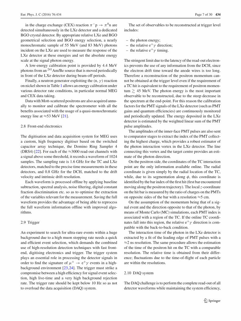
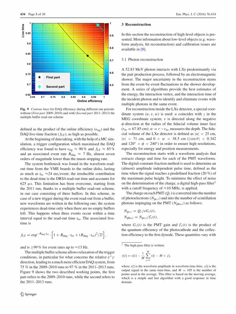
Fig. 9 Contour lines for DAQ efficiency during different run periods:without (First part 2009–2010) and with (Second part 2011–2013) themultiple buffer read-out scheme
defined as the product of the online efficiency (εtrg) and theDAQ live-time fraction ( fLT), as high as possible.
At the beginning of data taking, with the help of a MC sim-ulation, a trigger configuration which maximised the DAQefficiency was found to have εtrg ≈ 90 % and fLT ≈ 85 %and an associated event rate Rdaq ≈ 7 Hz, almost sevenorders of magnitude lower than the muon stopping rate.
The system bottleneck was found in the waveform read-out time from the VME boards to the online disks, lastingas much as tro ≈24 ms/event; the irreducible contributionto the dead-time is the DRS4 read-out time and accounts for625 µs. This limitation has been overcome, starting fromthe 2011 run, thanks to a multiple buffer read-out scheme,in our case consisting of three buffers. In this scheme, incase of a new trigger during the event read-out from a buffer,new waveforms are written in the following one; the systemexperiences dead-time only when there are no empty buffersleft. This happens when three events occur within a timeinterval equal to the read-out time tro. The associated live-time is
fLT = exp−Rdaq·tro ·[1 + Rdaq · tro + (Rdaq · tro)
2/2!],
and is ≥99 % for event rates up to ≈13 Hz.The multiple buffer scheme allows relaxation of the trigger
conditions, in particular for what concerns the relative e+γ
direction, leading to a much more efficient DAQ system, from75 % in the 2009–2010 runs to 97 % in the 2011–2013 runs.Figure 9 shows the two described working points, the firstpart refers to the 2009–2010 runs, while the second refers tothe 2011–2013 runs.
3 Reconstruction
In this section the reconstruction of high-level objects is pre-sented. More information about low-level objects (e.g. wave-form analysis, hit reconstruction) and calibration issues areavailable in [8].
3.1 Photon reconstruction
A 52.83 MeV photon interacts with LXe predominantly viathe pair production process, followed by an electromagneticshower. The major uncertainty in the reconstruction stemsfrom the event-by-event fluctuations in the shower develop-ment. A series of algorithms provide the best estimates ofthe energy, the interaction vertex, and the interaction time ofthe incident photon and to identify and eliminate events withmultiple photons in the same event.
For reconstruction inside the LXe detector, a special coor-dinate system (u, v, w) is used: u coincides with z in theMEG coordinate system; v is directed along the negativeφ-direction at the radius of the fiducial volume inner face(rin = 67.85 cm); w = r −rin, measures the depth. The fidu-cial volume of the LXe detector is defined as |u| < 25 cm,|v| < 71 cm, and 0 < w < 38.5 cm (| cos θ | < 0.342and 120◦ < φ < 240◦) in order to ensure high resolutions,especially for energy and position measurements.
The reconstruction starts with a waveform analysis thatextracts charge and time for each of the PMT waveforms.The digital-constant-fraction method is used to determine an(almost) amplitude independent pulse time, defined as thetime when the signal reaches a predefined fraction (20 %) ofthe maximum pulse height. To minimise the effect of noiseon the determination of the charge, a digital high-pass filter1
with a cutoff frequency of ≈10 MHz, is applied.The charge on each PMT (Qi ) is converted into the number
of photoelectrons (Npe,i ) and into the number of scintillationphotons impinging on the PMT (Npho,i ) as follows:
Npe,i = Qi/eGi (t),
Npho,i = Npe,i/Ei (t),
where Gi (t) is the PMT gain and Ei (t) is the product ofthe quantum efficiency of the photocathode and the collec-tion efficiency to the first dynode. These quantities vary with
1 The high-pass filter is written:
y[i] = x[i] − 1
M
M∑j=1
x[i − M + j],
where x[] is the waveform amplitude in waveform time-bins, y[] is theoutput signal in the same time-bins, and M = 105 is the number ofpoints used in the average. This filter is based on the moving average,which is a simple and fast algorithm with a good response in timedomain.
123
Eur. Phys. J. C (2016) 76 :434 Page 9 of 30 434
time2 and, thus, are continuously monitored and calibratedusing the calibration sources instrumented in the LXe detec-tor (see Sect. 2.7).
The PMT gain is measured using blue LEDs, flashed at dif-ferent intensities by exploiting the statistical relation betweenthe mean and variance of the observed charge,
σ 2Qi
= eGi Q̄i + σ 2noise.
The time variation of the gain is tracked by using the LEDevents collected at ≈1 Hz during physics data taking.
The quantity Ei (t) is evaluated using α-particles producedby 241Am sources within the LXe volume and monochro-matic (17.6-MeV) photons from a p-Li interaction (seeTable 1) by comparing the observed number of photoelec-trons with the expected number of scintillation photons eval-uated with a MC simulation,
Ei = N̄pe,i/N̄ MCpho,i .
This calibration is performed two or three times per weekto monitor the time dependence of this factor. The absoluteenergy scale is not sensitive to the absolute magnitude of thisefficiency, and this calibration serves primarily to equalisethe relative PMT responses and to remove time-dependentdrifts, possibly different from PMT to PMT.
3.1.1 Photon position
The 3D position of the photon interaction vertex rγ =(uγ , vγ , wγ ) is determined by a χ2-fit of the distributionof the numbers of scintillation photons in the PMTs (Npho),taking into account the solid angle subtended by each PMTphotocathode assuming an interaction vertex, to the observedNpho distribution. To minimise the effect of shower fluctua-tions, only PMTs inside a radius of 3.5 times the PMT spac-ing for the initial estimate of the position of the interactionvertex are used in the fit. The initial estimate of the posi-tion is calculated as the amplitude weighted mean positionaround the PMT with the maximum signal. For events result-ing in wγ < 12 cm, the fit is repeated with a further reducednumber of PMTs, inside a radius of twice the PMT spac-ing from the first fit result. The remaining bias on the result,due to the inclined incidence of the photon onto the innerface, is corrected using results from a MC simulation. Theperformance of the position reconstruction is evaluated bya MC simulation and has been verified in dedicated CEXruns by placing lead collimators in front of the LXe detector.The average position resolutions along the two orthogonal
2 Two kinds of instability in the PMT response are observed: one is along-term gain decrease due to decreased secondary emission mainly atthe last dynode with collected charge and the other is a rate-dependentgain shift due to charge build-up on the dynodes.
inner-face coordinates (u, v) and the depth direction (w) areestimated to be ≈5 and ≈6 mm, respectively.
The position is reconstructed in the LXe detector localcoordinate system. The conversion to the MEG coordinatesystem relies on the alignment of the LXe detector with therest of the MEG subsystems. The LXe detector position rel-ative to the MEG coordinate system is precisely surveyedusing a laser survey device at room temperature. After thethermal shrinkage of the cryostat and of the PMT supportstructures at LXe temperature are taken into account, thePMT positions are calculated based on the above informa-tion. The final alignment of the LXe detector with respect tothe spectrometer is described in Sect. 3.3.1.
3.1.2 Photon timing
The determination of the photon emission time from the tar-get tγ starts from the determination of the arrival time of thescintillation photons on the i-th PMT tPMT
γ,i as described inSect. 3.1. To relate this time to the photon conversion time,the propagation time of the scintillation photons must be sub-tracted as well as any hardware-induced time offset (e.g. dueto cable length).
The propagation time of the scintillation photons is eval-uated using the π0 → γ γ events produced in CEX runs inwhich the time of one of the photons is measured by twoplastic scintillator counters with a lead shower converter asa reference time. The primary contribution is expressed as alinear relation with the distance; the coefficient, i.e., the effec-tive light velocity, is measured to be ≈8 cm/ns. A remainingnon-linear dependence is observed and an empirical function(2D function of the distance and incident angle) is calibratedfrom the data. This secondary effect comes from the factthat the fraction of indirect (scattered of reflected) scintil-lation photons increases with a larger incident angle and alarger distance. PMTs that do not directly view the interac-tion vertex rγ , shaded by the inner face wall, are not used inthe following timing reconstruction. After correcting for thescintillation photon propagation times, the remaining (con-stant) time offset is extracted for each PMT from the sameπ0 → γ γ events by comparing the PMT hit time with thereference time.
After correcting for these effects, the photon conversiontime tLXe
γ is obtained by combining the timings of those
PMTs tPMTγ,i which observe more than 50 Npe by a fit that
minimises
χ2 =∑
i
(tPMTγ,i − tLXe
γ
)2
(σ 1-PMT
tγ (Npe,i ))2 .
PMTs with a large contribution to the χ2 are rejected duringthis fitting procedure to remove pile-up effects. The single-
123
434 Page 10 of 30 Eur. Phys. J. C (2016) 76 :434
PMT time resolution is measured in the CEX runs to beσ 1-PMT
tγ (Npe = 500) = 400–540 ps, depending on the loca-
tion of the PMT, and approximately proportional to 1/√
Npe.Typically 150 PMTs with ≈70 000 Npe in total are used toreconstruct 50-MeV photon times.
Finally, the photon emission time from the target tγ isobtained by subtracting the time-of-flight between the pointon the stopping target defined by the intercept of the positrontrajectory at the stopping target and the reconstructed inter-action vertex in the LXe detector from tLXe
γ .The timing resolution σtγ is evaluated as the dispersion of
the time difference between the two photons from π0 decayafter subtracting contributions due to the uncertainty of theπ0 decay position and to the timing resolution of the refer-ence counters. From measurements at 55 and 83 MeV, theenergy dependence is estimated and corrected, resulting inσtγ (Eγ = 52.83 MeV) ≈ 64 ps.
3.1.3 Photon energy
The reconstruction of the photon energy Eγ is based onthe sum of scintillation photons collected by all PMTs. Asummed waveform with the following coefficients over allthe PMTs is formed and the energy is determined by inte-grating it:
Fi = Ai · Wi (rγ )
eGi (t) · Ei (t)· �(rγ ) · U (rγ ) · H(t) · S, (1)
where Ai is a correction factor for the fraction of photocath-ode coverage, which is dependent on the PMT location;3
Wi (rγ ) is a weighting factor for the PMT that is common toall PMTs on a given face and is determined by minimising theresolution in response to 55-MeV photons from CEX. �(rγ )
is a correction factor for the solid angle subtended by photo-cathodes for scintillating photons emitted at the interactionvertex; it is applied only for shallow events (wγ < 3 cm)for which the light collection efficiency is very sensitive tothe relative position of each PMT and the interaction ver-tex. U (rγ ) is a position dependent non-uniformity correctionfactor determined by the responses to the 17.6- and 55-MeVphotons. H(t) is a correction factor for the time-varying LXescintillation light yield and S is a constant conversion factorof the energy scale, determined by the 55- and 83-MeV pho-tons with a precision of 0.3 %.
A potential significant background is due to pile-up eventswith more than one photon in the detector nearly coincidentin time. Approximately 15 % of triggered events suffer frompile-up at the nominal beam rate. The analysis identifies pile-up events and corrects the measured energy, thereby reducing
3 The coverage on the outer face is, for example, 2.6 times less densethan that on the inner face.
background and increasing detection efficiency. Three meth-ods are used to identify and extract the primary photon energyin pile-up events.
The first method identifies multiple photons with differenttiming using the χ2/NDF value in the time fit. In contrast tothe time reconstruction, all the PMTs with more than 50 Npe
are used to identify pile-up events.The second method identifies pile-up events with photons
at different positions by searching for spatially separatedpeaks in the inner and outer faces. If the event has two ormore peaks whose energies cannot be determined using thethird method below, a pile-up removal algorithm is appliedto the PMT charge distribution. It uses a position depen-dent table containing the average charge of each PMT inresponse to 17.6-MeV photons. Once a pile-up event is iden-tified, the energy of the primary photon is estimated by fittingthe PMT charges to the table without using PMTs around thesecondary photon. Then, the PMT charges around the sec-ondary photon are replaced with the charges estimated by thefit. Finally, the energy is reconstructed as a sum of the indi-vidual PMT charges with the coefficients Fi (Eq. 1), insteadof integrating the summed waveform.
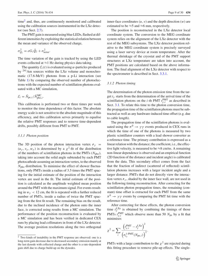
The third method identifies multiple photons and unfoldsthem by combining the information from summed wave-forms and the two methods above. First, the total summedwaveform is searched for temporally separated pulses. Next,if the event is identified as a pile-up event by either of thetwo methods above, a summed waveform over PMTs near thesecondary photon is formed to search for multiple pulses. Thepulse found in the partial summed waveform is added to thelist of pulses if the time is more than 5 ns apart from the otherpulse times. Then, a superimposition of N template wave-forms is fitted to the total summed waveform, where N isthe number of pulses detected in this event. Figure 10 showsan example of the fitting, where three pulses are detected.Finally, the contributions of pile-up photons are subtractedand the remaining waveform is used for the primary energyestimation.
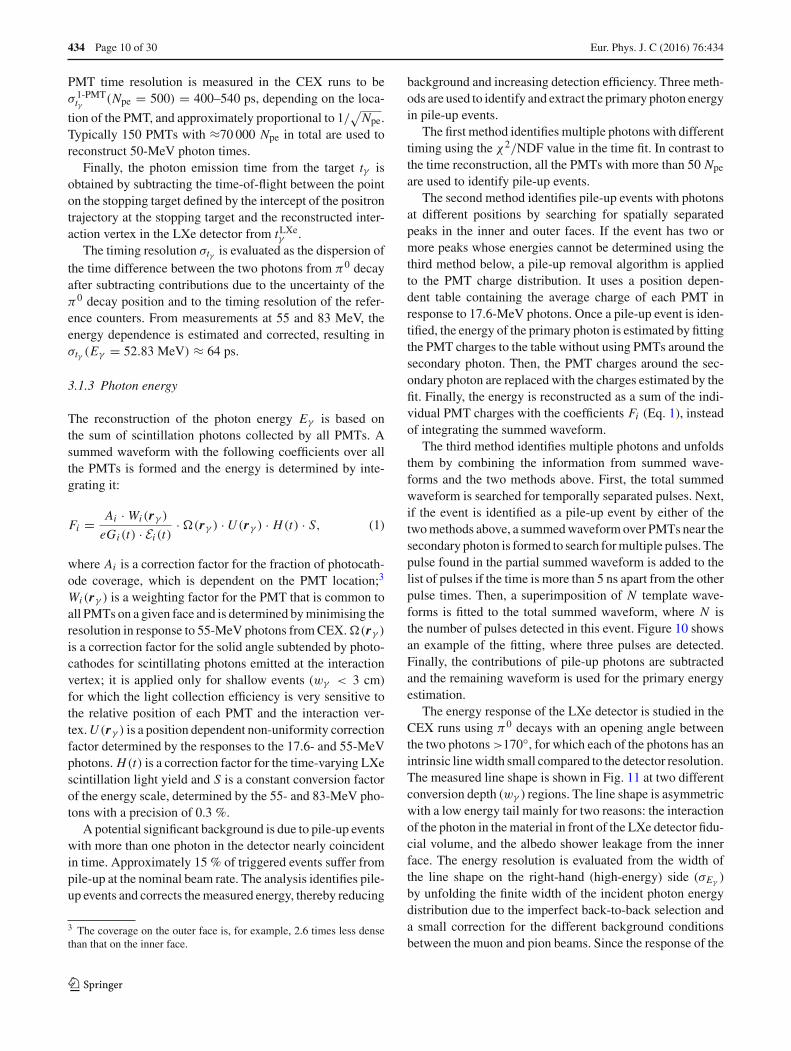
The energy response of the LXe detector is studied in theCEX runs using π0 decays with an opening angle betweenthe two photons >170◦, for which each of the photons has anintrinsic line width small compared to the detector resolution.The measured line shape is shown in Fig. 11 at two differentconversion depth (wγ ) regions. The line shape is asymmetricwith a low energy tail mainly for two reasons: the interactionof the photon in the material in front of the LXe detector fidu-cial volume, and the albedo shower leakage from the innerface. The energy resolution is evaluated from the width ofthe line shape on the right-hand (high-energy) side (σEγ )by unfolding the finite width of the incident photon energydistribution due to the imperfect back-to-back selection anda small correction for the different background conditionsbetween the muon and pion beams. Since the response of the
123
Eur. Phys. J. C (2016) 76 :434 Page 11 of 30 434
Am
plitu
de
-40000
-20000
0
(a)
Time (ns)-600 -550 -500
-40000
-20000
0
(b)
Fig. 10 a Example of a LXe detector waveform for an event withthree photons (2.5, 40.1 and 36.1 MeV). The cross markers show thewaveform (with the digital high-pass filter) summed over all PMTswith the coefficients defined in the text, and the red line shows the fittedsuperposition of three template waveforms. b The unfolded main pulse(solid line) and the pile-up pulses (dashed)
detector depends on the position of the photon conversion,the fitted parameters of the line shape are functions of the 3Dcoordinates, mainly of wγ . The average resolution is mea-sured to be σEγ = 2.3 % (0 < wγ < 2 cm, event fraction42 %) and 1.6 % (wγ > 2 cm, 58 %).
The energy resolutions and energy scale are cross-checkedby fitting the background spectra measured in the muon decaydata with the MC spectra folded with the detector resolutions.
3.2 Positron reconstruction
3.2.1 DCH reconstruction
The reconstruction of positron trajectories in the DCH is per-formed in four steps: hit reconstruction in each single cell,clustering of hits within the same chamber, track finding inthe spectrometer, and track fitting.
In step one, raw waveforms from anodes and cathodes arefiltered in order to remove known noise contributions of fixedfrequencies. A hit is defined as a negative signal appearing inthe waveform collected at each end of the anode wire, withan amplitude of at least −5 mV below the baseline. This leveland its uncertainty σB are estimated from the waveform itself
Num
ber
of e
vent
s /(0
.50
MeV
)
0
50
100
(a)
< 2 cmγw
(MeV)γE30 40 50 60 70
0
100
200
(b)
> 2 cmγw
Fig. 11 Energy response of the LXe detector to 54.9-MeV photons ina restricted range of (uγ , vγ ) for two groups of events with different wγ :a 0 < wγ < 2 cm (event fraction 42 %) and b wγ > 2 cm (58 %)
in the region around 625 ns before the trigger time. The hittime is taken from the anode signal with larger amplitudeas the time of the first sample more than −3σB below thebaseline.
The samples with amplitude below −2σB from the base-line and in a range of [−24,+56] ns around the peak, areused for charge integration. The range is optimised to min-imise the uncertainty produced by the electronic noise. A firstestimate of the z-coordinate, with a resolution of about 1 cm,is obtained from charge division on the anode wire, and itallows the determination of the Vernier cycle (see Sect. 2.4)in which the hit occurred. If one or more of the four cathodepad channels is known to be defective, the z-coordinate fromcharge division is used and is assigned a 1 cm uncertainty.Otherwise, charge integration is performed on the cathodepad waveforms and the resulting charges are combined torefine the z-measurement, exploiting the Vernier pattern. Thecharge asymmetries between the upper and lower sections ofthe inner and outer cathodes are given by
Ain,out = QUPin,out − QDOWN
in,out
QUPin,out + QDOWN
in,out
,
the position within the λ = 5 cm Vernier cycle is given by:
δz = arctan(Ain/Aout) × λ
2π.
123
434 Page 12 of 30 Eur. Phys. J. C (2016) 76 :434
At this stage, a first estimate of the position of the hit in the(x, y) plane is given by the wire position.
Once reconstructed, hits from nearby cells with similarz are grouped into clusters, taking into account that the z-measurement can be shifted by λ if the wrong Vernier cyclehas been selected via charge division. These clusters are thenused to build track seeds.
A seed is defined as a group of three clusters in four adja-cent chambers, at large radius (r > 24 cm) where the cham-ber occupancy is lower and only particles with large momen-tum are found. The clusters are required to satisfy appropriateproximity criteria on their r and z values. A first estimate ofthe track curvature and total momentum is obtained from thecoordinates of the hit wires, and is used to extend the trackand search for other clusters, taking advantage of the adia-batic invariant p2
T /Bz , where pT is the positron transversemomentum, for slowly varying axial magnetic fields. Havingdetermined the approximate trajectory, the left/right ambigu-ity of the hits on each wire can be resolved in most cases. Afirst estimate of the track time (and hence the precise posi-tion of the hit within a cell) and further improvement of theleft/right solutions can be obtained by minimising the χ2 ofa circle fit of the hit positions in the (x, y) plane.
At this stage, in order to retain high efficiency, the samehit can belong to different clusters and the same cluster to dif-ferent track candidates, which can result in duplicated tracks.Only after the track fit, when the best information on the trackis available, independent tracks are defined.
A precise estimate of the (x, y) positions of the hits asso-ciated with the track candidate is then extracted from thedrift time, defined as the difference between the hit and tracktimes. The position is taken from tables relating (x, y) posi-tion to drift time. These are track-angle dependent and arederived using GARFIELD software [25]. The reconstructed(x, y) position is continuously updated during the trackingprocess, as the track information improves.
A track fit is finally performed with the Kalman filter tech-nique [26,27]. The GEANE software [28] is used to accountfor the effect of materials in the spectrometer during the prop-agation of the track and to estimate the error matrix. Exploit-ing the results of the first track fit, hits not initially includedin the track candidate are added if appropriate and hits whichare inconsistent with the fitted track are removed. The trackis then propagated to the TC and matched to the hits in thebars (see Sect. 3.2.7 for details). The time of the matchedTC hit (corrected for propagation delay) is used to providea more accurate estimate of the track time, and hence thedrift times. A final fit is then done with this refined informa-tion. Following the fit, the track is propagated backwards tothe target. The decay vertex (xe+ , ye+ , ze+ ) and the positrondecay direction (φe+ , θe+ ) are defined as the point of inter-section of the track with the target foil and the track directionat the decay vertex. The error matrix of the track parameters
at the decay vertex is computed and used in the subsequentanalysis.
Among tracks sharing at least one hit, a ranking is per-formed based on a linear combination of five variables denot-ing the quality of the track (the momentum, θe+ andφe+ errorsat the target, the number of hits and the reduced χ2). In orderto optimise the performance of the ranking procedure, the lin-ear combination is taken as the first component of a principalcomponent analysis of the five variables. The ranking vari-ables are also used to select tracks, along with other qualitycriteria as (for instance) the request that the backward trackextrapolation intercepts the target within its fiducial volume.Since the subsequent analysis uses the errors associated withthe track parameters event by event, the selection criteria arekept loose in order to preserve high efficiency while removingbadly reconstructed tracks for which the fit and the associ-ated errors might be unreliable. After the selection criteriaare applied, the track quality ranking is used to select onlyone track among the surviving duplicate candidates.
3.2.2 DCH missing turn recovery
A positron can traverse the DCH system multiple timesbefore it exits the spectrometer. An individual crossing ofthe DCH system is referred to as a positron ‘turn’. An inter-mediate merging step in the Kalman fit procedure, describedpreviously, attempts to identify multi-turn positrons by com-bining and refitting individually reconstructed turns into amulti-turn track. However, it is possible that not all turns ofa multi-turn positron are correctly reconstructed or mergedinto a multi-turn track. If this involves the first turn, i.e. theturn closest to the muon stopping target, this will lead to anincorrect determination of the muon decay point and time aswell as an incorrect determination of the positron momentumand direction at the muon decay point, and therefore a lossof signal efficiency.
After the track reconstruction is completed, a missing firstturn (MFT) recovery algorithm, developed and incorporatedin the DCH reconstruction software expressly for this analy-sis, is used to identify and refit positron tracks with an MFT.Firstly, for each track in an event, the algorithm identifiesall hits that may potentially be part of an MFT, based on thecompatibility of their z-coordinates and wire locations in theDCH system with regard to the positron track. The vertexstate vector of the track is propagated backwards to the pointof closest approach with each potential MFT hit, and the hitselection is refined based on the r and z residuals betweenthe potential MFT hits and their propagated state vector posi-tions. Potential MFT candidates are subsequently selected ifthere are MFT hits in at least four DCH modules of whichthree are adjacent to one another, and the average signed z-difference between the hits and their propagated state vectorpositions as well as the standard deviation of the correspond-
123
Eur. Phys. J. C (2016) 76 :434 Page 13 of 30 434
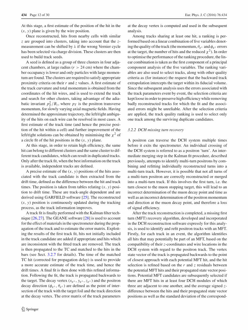
ing unsigned z-difference are smaller than 2.5 cm. A newMFT track is reconstructed using the Kalman filter techniquebased on the selected MFT hits and correspondingly prop-agated state vectors. Finally, the original positron and MFTtracks are combined and refitted using the Kalman filter tech-nique, followed by a recalculation of the track quality rankingand the positron variables and their uncertainties at the target.An example of a multi-turn positron with a recovered MFTis shown in Fig. 12.
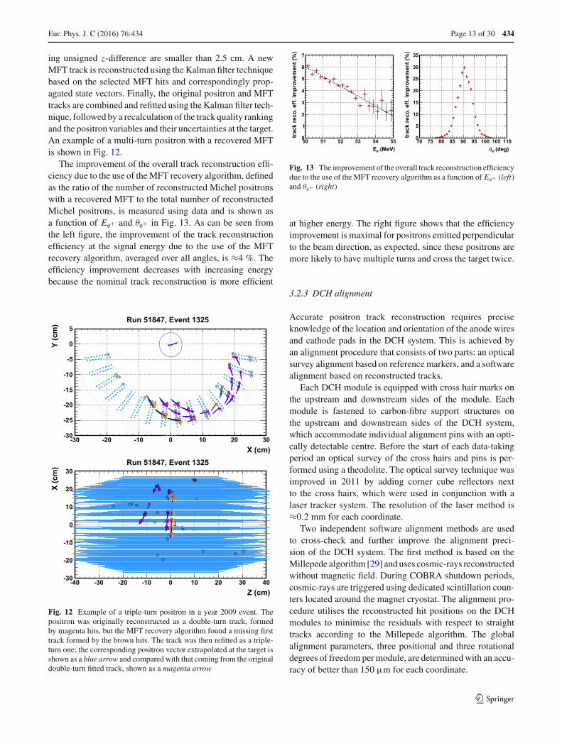
The improvement of the overall track reconstruction effi-ciency due to the use of the MFT recovery algorithm, definedas the ratio of the number of reconstructed Michel positronswith a recovered MFT to the total number of reconstructedMichel positrons, is measured using data and is shown asa function of Ee+ and θe+ in Fig. 13. As can be seen fromthe left figure, the improvement of the track reconstructionefficiency at the signal energy due to the use of the MFTrecovery algorithm, averaged over all angles, is ≈4 %. Theefficiency improvement decreases with increasing energybecause the nominal track reconstruction is more efficient
X (cm)-30 -20 -10 0 10 20 30
Y (c
m)
-30
-25
-20
-15
-10
-5
0
5Run 51847, Event 1325
Z (cm)-40 -30 -20 -10 0 10 20 30 40
X (c
m)
-30
-20
-10
0
10
20
30Run 51847, Event 1325
Fig. 12 Example of a triple-turn positron in a year 2009 event. Thepositron was originally reconstructed as a double-turn track, formedby magenta hits, but the MFT recovery algorithm found a missing firsttrack formed by the brown hits. The track was then refitted as a triple-turn one; the corresponding positron vector extrapolated at the target isshown as a blue arrow and compared with that coming from the originaldouble-turn fitted track, shown as a magenta arrow
(MeV)e+E50 51 52 53 54 55
trac
k re
co. e
ff. im
prov
emen
t (%
)
0
1
2
3
4
5
6
7
(deg)e+θ70 75 80 85 90 95 100 105 110
trac
k re
co. e
ff. im
prov
emen
t (%
)
0
5
10
15
20
25
30
35
Fig. 13 The improvement of the overall track reconstruction efficiencydue to the use of the MFT recovery algorithm as a function of Ee+ (left)and θe+ (right)
at higher energy. The right figure shows that the efficiencyimprovement is maximal for positrons emitted perpendicularto the beam direction, as expected, since these positrons aremore likely to have multiple turns and cross the target twice.
3.2.3 DCH alignment
Accurate positron track reconstruction requires preciseknowledge of the location and orientation of the anode wiresand cathode pads in the DCH system. This is achieved byan alignment procedure that consists of two parts: an opticalsurvey alignment based on reference markers, and a softwarealignment based on reconstructed tracks.
Each DCH module is equipped with cross hair marks onthe upstream and downstream sides of the module. Eachmodule is fastened to carbon-fibre support structures onthe upstream and downstream sides of the DCH system,which accommodate individual alignment pins with an opti-cally detectable centre. Before the start of each data-takingperiod an optical survey of the cross hairs and pins is per-formed using a theodolite. The optical survey technique wasimproved in 2011 by adding corner cube reflectors nextto the cross hairs, which were used in conjunction with alaser tracker system. The resolution of the laser method is≈0.2 mm for each coordinate.
Two independent software alignment methods are usedto cross-check and further improve the alignment preci-sion of the DCH system. The first method is based on theMillepede algorithm [29] and uses cosmic-rays reconstructedwithout magnetic field. During COBRA shutdown periods,cosmic-rays are triggered using dedicated scintillation coun-ters located around the magnet cryostat. The alignment pro-cedure utilises the reconstructed hit positions on the DCHmodules to minimise the residuals with respect to straighttracks according to the Millepede algorithm. The globalalignment parameters, three positional and three rotationaldegrees of freedom per module, are determined with an accu-racy of better than 150 µm for each coordinate.
123
434 Page 14 of 30 Eur. Phys. J. C (2016) 76 :434
The second method is based on an iterative algorithmusing reconstructed Michel positrons and aims to improvethe relative radial and longitudinal alignment of the DCHmodules. The radial and longitudinal differences betweenthe track position and the corresponding hit position at eachmodule are recorded for a large number of tracks. The aver-age hit-track residuals of each module are used to correctthe radial and longitudinal position of the modules, whilekeeping the average correction over all modules equal tozero. This process is repeated several times while refittingthe tracks after each iteration, until the alignment correc-tions converge and an accuracy of better than 50 µm foreach coordinate is reached. The method is cross-checked byusing reconstructed Mott-scattered positrons (see Sect. 2.7),resulting in very similar alignment corrections.
The exact resolution reached by each approach depends onthe resolution of the optical survey used as a starting position.For a low-resolution survey, the Millepede method obtains abetter resolution, while the iterative method obtains a betterresolution for a high-resolution survey. Based on these points,the Millepede method is adopted for the years 2009–2011and the iterative method is used for the years 2012–2013 forwhich the novel optical survey data are available; in 2011,the first year with the novel optical survey data, the resultingresolution of both approaches is comparable.
3.2.4 Target alignment
Precise knowledge of the position of the target foil relative tothe DCH system is crucial for an accurate determination ofthe muon decay vertex and positron direction at the vertex,which are calculated by propagating the reconstructed trackback to the target, particularly when the trajectory of the trackis far from the direction normal to the plane of the target.
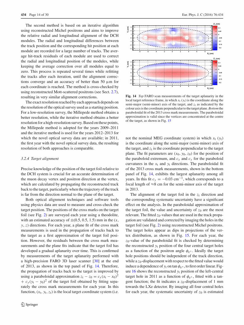
Both optical alignment techniques and software toolsusing physics data are used to measure and cross-check thetarget position. The positions of the cross marks on the targetfoil (see Fig. 2) are surveyed each year using a theodolite,with an estimated accuracy of ±(0.5, 0.5, 1.5) mm in the (x ,y, z) directions. For each year, a plane fit of the cross markmeasurements is used in the propagation of tracks back tothe target as a first approximation of the target foil posi-tion. However, the residuals between the cross mark mea-surements and the plane fits indicate that the target foil hasdeveloped a gradual aplanarity over time. This is confirmedby measurements of the target aplanarity performed witha high-precision FARO 3D laser scanner [30] at the endof 2013, as shown in the top panel of Fig. 14. Therefore,the propagation of tracks back to the target is improved byusing a paraboloidal approximation zt − z0 = cx (xt − x0)
2
+ cy(yt − y0)2 of the target foil obtained by fitting sepa-
rately the cross mark measurements for each year. In thisfunction, (xt, yt, zt) is the local target coordinate system (i.e.
(cm)tX8− 6− 4− 2−
(cm
)tY
3−
2−
1−
0
1
2
3
0.2−
0.15−
0.1−
0.05−
0
0.05
0.1
(cm)tZ
(cm)tX8− 6− 4− 2−
0 2 4 6 8
0 2 4 6 8
(cm
)tY
3−
2−
1−
0
1
2
3
0.2−
0.15−
0.1−
0.05−
0
0.05
0.1
(cm)tZ
Fig. 14 Top FARO scan measurements of the target aplanarity in thelocal target reference frame, in which xt (yt ) is the coordinate along thesemi-major (semi-minor) axis of the target, and zt as indicated by thecolour axis is the coordinate perpendicular to the target plane. Bottom theparaboloidal fit of the 2013 cross mark measurements. The paraboloidalapproximation is valid since the vertices are concentrated at the centreof the target, as shown in Fig. 15
not the nominal MEG coordinate system) in which xt (yt)is the coordinate along the semi-major (semi-minor) axis ofthe target, and zt is the coordinate perpendicular to the targetplane. The fit parameters are (x0, y0, z0) for the position ofthe paraboloid extremum, and cx and cy for the paraboloidcurvatures in the xt and yt directions. The paraboloidal fitof the 2013 cross mark measurements, shown in the bottompanel of Fig. 14, exhibits the largest aplanarity among allyears. In this fit cy = −0.03 cm−1, which corresponds to afocal length of ≈8 cm for the semi-minor axis of the targetin 2013.
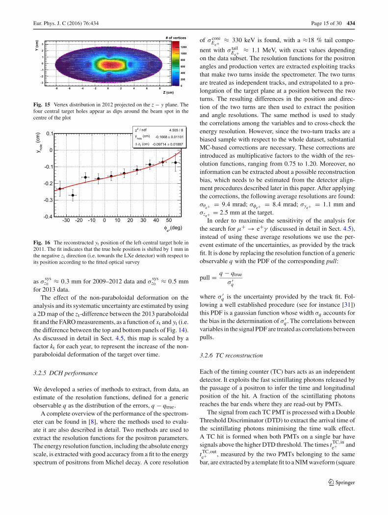
The alignment of the target foil in the zt direction andthe corresponding systematic uncertainty have a significanteffect on the analysis. In the paraboloidal approximation ofthe target foil, the value and uncertainty of z0 are the mostrelevant. The fitted z0-values that are used in the track propa-gation are validated and corrected by imaging the holes in thetarget foil (see Fig. 2) using reconstructed Michel positrons.The target holes appear as dips in projections of the ver-tex distribution, as shown in Fig. 15. For each year, thez0-value of the paraboloidal fit is checked by determiningthe reconstructed yt position of the four central target holesas a function of the positron angle φe+ . Ideally the targethole positions should be independent of the track direction,while a z0-displacement with respect to the fitted value wouldinduce a dependence of yt on tan φe+ , to first order linear. Fig-ure 16 shows the reconstructed yt position of the left-centraltarget hole in 2011 as a function of φe+ , fitted with a tan-gent function; the fit indicates a z0-displacement of 1 mmtowards the LXe detector. By imaging all four central holesfor each year, the systematic uncertainty of z0 is estimated
123
Eur. Phys. J. C (2016) 76 :434 Page 15 of 30 434
Z (cm)8− 6− 4− 2− 0 2 4 6 8
Y (c
m)
3−
2−
1−
0
1
2
3
0
200
400
600
800
1000
1200
# of vertices
Fig. 15 Vertex distribution in 2012 projected on the z − y plane. Thefour central target holes appear as dips around the beam spot in thecentre of the plot
(deg)e+
φ-30 -20 -10 0 10 20 30 40 50
(cm
)ho
ley
-0.4
-0.3
-0.2
-0.1
0
0.1 / ndf 2χ 4.505 / 8
(cm) hole
y 0.01101± -0.1668
(cm) t zΔ 0.01887± -0.09714
/ ndf 2χ 4.505 / 8 (cm)
holey 0.01101± -0.1668
(cm) t zΔ 0.01887± -0.09714
Fig. 16 The reconstructed yt position of the left-central target hole in2011. The fit indicates that the true hole position is shifted by 1 mm inthe negative zt direction (i.e. towards the LXe detector) with respect toits position according to the fitted optical survey
as σsysz0 ≈ 0.3 mm for 2009–2012 data and σ
sysz0 ≈ 0.5 mm
for 2013 data.The effect of the non-paraboloidal deformation on the
analysis and its systematic uncertainty are estimated by usinga 2D map of the zt-difference between the 2013 paraboloidalfit and the FARO measurements, as a function of xt and yt (i.e.the difference between the top and bottom panels of Fig. 14).As discussed in detail in Sect. 4.5, this map is scaled by afactor kt for each year, to represent the increase of the non-paraboloidal deformation of the target over time.
3.2.5 DCH performance
We developed a series of methods to extract, from data, anestimate of the resolution functions, defined for a genericobservable q as the distribution of the errors, q − qtrue.
A complete overview of the performance of the spectrom-eter can be found in [8], where the methods used to evalu-ate it are also described in detail. Two methods are used toextract the resolution functions for the positron parameters.The energy resolution function, including the absolute energyscale, is extracted with good accuracy from a fit to the energyspectrum of positrons from Michel decay. A core resolution
of σ coreEe+
≈ 330 keV is found, with a ≈18 % tail compo-
nent with σ tailEe+
≈ 1.1 MeV, with exact values dependingon the data subset. The resolution functions for the positronangles and production vertex are extracted exploiting tracksthat make two turns inside the spectrometer. The two turnsare treated as independent tracks, and extrapolated to a pro-longation of the target plane at a position between the twoturns. The resulting differences in the position and direc-tion of the two turns are then used to extract the positionand angle resolutions. The same method is used to studythe correlations among the variables and to cross-check theenergy resolution. However, since the two-turn tracks are abiased sample with respect to the whole dataset, substantialMC-based corrections are necessary. These corrections areintroduced as multiplicative factors to the width of the res-olution functions, ranging from 0.75 to 1.20. Moreover, noinformation can be extracted about a possible reconstructionbias, which needs to be estimated from the detector align-ment procedures described later in this paper. After applyingthe corrections, the following average resolutions are found:σθe+ = 9.4 mrad; σφe+ = 8.4 mrad; σye+ = 1.1 mm andσze+ = 2.5 mm at the target.
In order to maximise the sensitivity of the analysis forthe search for μ+ → e+γ (discussed in detail in Sect. 4.5),instead of using these average resolutions we use the per-event estimate of the uncertainties, as provided by the trackfit. It is done by replacing the resolution function of a genericobservable q with the PDF of the corresponding pull:
pull = q − qtrue
σ ′q
where σ ′q is the uncertainty provided by the track fit. Fol-
lowing a well established procedure (see for instance [31])this PDF is a gaussian function whose width σq accounts forthe bias in the determination of σ ′
q . The correlations betweenvariables in the signal PDF are treated as correlations betweenpulls.
3.2.6 TC reconstruction
Each of the timing counter (TC) bars acts as an independentdetector. It exploits the fast scintillating photons released bythe passage of a positron to infer the time and longitudinalposition of the hit. A fraction of the scintillating photonsreaches the bar ends where they are read-out by PMTs.
The signal from each TC PMT is processed with a DoubleThreshold Discriminator (DTD) to extract the arrival time ofthe scintillating photons minimising the time walk effect.A TC hit is formed when both PMTs on a single bar havesignals above the higher DTD threshold. The times tTC,in
e+ and
tTC,oute+ , measured by the two PMTs belonging to the same
bar, are extracted by a template fit to a NIM waveform (square
123
434 Page 16 of 30 Eur. Phys. J. C (2016) 76 :434
wave at level −0.8 V) fired at the lower DTD threshold anddigitised by a DRS.
The hit position along the bar is derived by the followingtechnique. A positron impinging on a TC bar at time t T C
e+ hasa relationship with the measured PMT times given by:
tTC,ine+ = tTC
e+ + bin + Win +L2 + zTC
e+veff
tTC,oute+ = tTC
e+ + bout + Wout +L2 − zTC
e+veff
(2)
where bin,out are the offsets and Win,out are the contributionsfrom the time walk effect from the inner and outer PMT,respectively, veff is the effective velocity of light in the barand L is the bar length; the z-axis points along the main axisof the bar and its origin is taken in the middle of the bar.Adding the two parts of Eq. 2 the result is:
tTCe+ = tTC,in
e+ + tTC,oute+
2− bin + bout
2− Win + Wout
2− L
2veff.
Subtracting the two parts of Eq. 2 the longitudinal coordinateof the impact point along the bar is given by:
zTCe+ = veff
2
((tTC,ine+ − tTC,out
e+)−(bin−bout)−(Win − Wout)
).
The time (longitudinal positions) resolution of TC is deter-mined using tracks hitting multiple bars from the distributionof the time (longitudinal position) difference between hits onneighbouring bars corrected for the path length. The radialand azimuthal coordinates are taken as the correspondingcoordinates of the centre of each bar.
The longitudinal position resolution is σzTCe+
≈ 1.0 cm and
the time resolution is σtTCe+
≈ 65 ps.
The TC, therefore, provides the information required toreconstruct all positron variables necessary to match a DCHtrack (see Sect. 3.2.7) and recover the muon decay time byextrapolating the tTC
e+ along the track trajectory back to thetarget to obtain the positron emission time te+ .
3.2.7 DCH-TC matching
The matching of DCH tracks with hits in the TC is performedas an intermediate step in the track fit procedure, in order toexploit the information from the TC in the track reconstruc-tion.
After being reconstructed within the DCH system, a trackis propagated to the first bar volume it encounters (referencebar). If no bar volume is crossed, the procedure is repeatedwith an extended volume to account for extrapolation uncer-tainties. Then, for each TC hit within ±5 bars from the ref-erence one, the track is propagated to the corresponding barvolume and the hit is matched with the track according to thefollowing ranking:
1. the TC hit belongs to the reference bar, with the longi-tudinal distance between the track and the hit
∣∣�zTC∣∣ <
12 cm (the track position defined as the entrance point ofthe track in the bar volume);
2. the TC hit belongs to another bar whose extended volumeis also crossed by the track, and
∣∣�zTC∣∣ < 12 cm (the
track position defined as the entrance point of the trackin the extended bar volume);
3. the TC hit belongs to a bar whose extended volume is notcrossed by the track, but where the distance of closestapproach of the track to the bar axis is less than 5 cm,and
∣∣�zTC∣∣ < 12 cm (the track position defined as the
point of closest approach of the track to the bar axis).
Among all successful matching candidates, those with thelowest ranking are chosen. Among them, the one with thesmallest �zTC is used.
The time of the matched TC hit is assigned to the track,which is then back-propagated to the chambers in order tocorrect the drift time of the hits for the track length timingcontribution. The Kalman filter procedure is also applied topropagate the track back to the target to get the best estimateof the decay vertex parameters at the target, including thetime te+ .
3.2.8 Positron AIF reconstruction
The photon background in an energy region very close tothe signal is dominated by positron AIF in the detector (seeSect. 4.4.1.1). If the positron crosses part of the DCH beforeit annihilates, it can leave a trace of hits which are corre-lated to the subsequent photon signal. A pattern recognitionalgorithm has been developed that can identify these typesof positron AIF events. Since positron AIF contributes to theaccidental background, this algorithm can help to distinguishaccidental background events from signal and RMD events.The algorithm is summarised in the following.
The procedure starts by building positron AIF seeds fromall reconstructed clusters. An AIF seed is defined as a set ofclusters on adjacent DCH modules which satisfy a numberof minimum proximity criteria. A positron AIF candidate(e+
AIF) is reconstructed from each seed by performing a circlefit based on the xy-coordinates of all clusters in the seed. Thecircle fit is improved by considering the individual hits in allclusters. The xy-coordinates of hits in multi-hit clusters arerefined and left/right solutions based on the initial circle fit aredetermined by taking into account the timing information ofthe individual hits, which also results in an estimate of the AIFtime. The xy-coordinates of the AIF vertex are determinedby the intersection point of the circle fit with the first DCHcathode plane after the last cluster hit. If the circle fit doesnot cross the next DCH cathode plane, the intersection pointof the circle fit with the support structure of the next DCH
123
Eur. Phys. J. C (2016) 76 :434 Page 17 of 30 434
X (cm)-30 -20 -10 0 10 20 30
Y (c
m)
-30
-25
-20
-15
-10
-5
0
5
Z (cm)-40 -30 -20 -10 0 10 20 30 40
X (c
m)
-30
-20
-10
0
10
20
30Run 51824, Event 806
Run 51824, Event 806
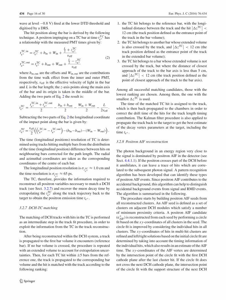
Fig. 17 Example of a reconstructed positron AIF candidate in a 2009event due to a downstream muon decay. The reconstructed AIF vertex isindicated as a blue star, visible in the upper plot at (x, y) = (−12,−21)
approximately. The AIF direction is indicated as a green arrow, origi-nating from this star and pointing towards lower x and higher y coordi-nates. The vector connecting the AIF vertex and the photon conversionvertex in the LXe detector is indicated as a magenta dashed line. Notethat the green arrow and the magenta line nearly overlap, as expectedfor a true AIF event
module or the inner wall of COBRA is used. The z-coordinateof the AIF vertex is calculated by extrapolating the quadraticpolynomial fit of the xz-positions of the last three clusters ofthe AIF candidate to the x-coordinate of the AIF vertex. TheAIF candidate direction is taken as the direction tangent toboth the circle fit and the quadratic polynomial fit at the AIFvertex. Figure 17 shows an example of a reconstructed AIFcandidate.
3.3 Combined reconstruction
This section deals with variables requiring signals both in thespectrometer and in the LXe detector.
3.3.1 Relative photon–positron angles
Since the LXe detector is not capable of reconstructing thedirection of the incoming photons, this direction is deter-
mined by connecting the reconstructed interaction vertex ofthe photon in the LXe detector to the reconstructed decayvertex on target: it is defined through its azimuthal and polarangles (φγ , θγ ).
The degree to which the photon and positron are not back-to-back is quantified in terms of the angle between the photondirection and the positron direction reversed at the target interms of azimuthal and polar angle differences:
θe+γ = (π − θe+) − θγ ,
φe+γ = (π + φe+) − φγ .
There are no direct calibration source for measuring the reso-lutions of the measurements of these relative angles. Hence,they are obtained by combining (1) the position resolutionof the LXe detector and (2) the position and angular reso-lutions of the spectrometer, taking into account the relativealignment of the spectrometer and the calorimeter.
There are correlations among the errors in measurementsof the positron observables at the target both due to the fit andalso introduced by the extrapolation to the target. Addition-ally, the errors in the photon angles contain a contributionfrom the positron position error at the target. Due to the cor-relations, the relative angle resolutions are not the quadraticsum of the photon and positron angular resolutions.
The θe+γ resolution is evaluated as σθe+γ= (15.0 −
16.2) mrad depending on the year of data taking by tak-ing into account the correlation between ze and θe+ . Sincethe true positron momentum and θe+γ of the μ+ → e+γ
signal are known, φe+ and ye+ can be corrected using thereconstructed energy of the positron and θe+γ . The φe+γ
resolution after correcting these correlations is evaluated asσφe+γ
= (8.9 − 9.0) mrad depending on the year.The systematic uncertainty of the positron emission angle
relies on the accuracy of the relative alignment amongthe magnetic field, the DCH modules, and the target (seeSects. 3.2.3 and 3.2.4 for the alignment methods and theuncertainties). The position of the target (in particular theerror in the position and orientation of the target plane) andany distortion of the target plane directly affect the emissionangle measurement and are found to be one of the dominantsources of systematic uncertainty on the relative angles.
The measurement of the photon direction depends on therelative alignment between the spectrometer and the LXedetector. They are aligned separately using optical alignmenttechniques and calculations of LXe detector distortions andmotion during filling and cool-down. Additionally, the rel-ative alignment is cross-checked by directly measuring twotypes of physics processes that produce hits in both detectors:
– Positron AIF events,– Cosmic rays without the COBRA magnetic field.
123
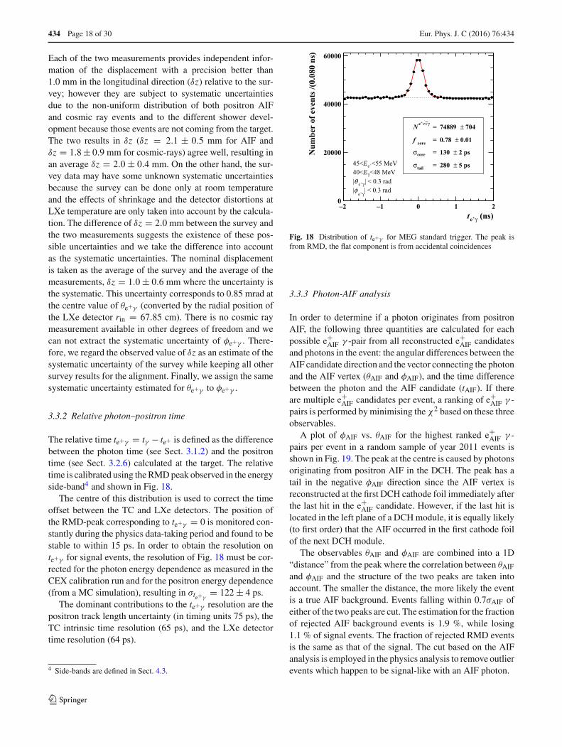
434 Page 18 of 30 Eur. Phys. J. C (2016) 76 :434
Each of the two measurements provides independent infor-mation of the displacement with a precision better than1.0 mm in the longitudinal direction (δz) relative to the sur-vey; however they are subject to systematic uncertaintiesdue to the non-uniform distribution of both positron AIFand cosmic ray events and to the different shower devel-opment because those events are not coming from the target.The two results in δz (δz = 2.1 ± 0.5 mm for AIF andδz = 1.8 ± 0.9 mm for cosmic-rays) agree well, resulting inan average δz = 2.0 ± 0.4 mm. On the other hand, the sur-vey data may have some unknown systematic uncertaintiesbecause the survey can be done only at room temperatureand the effects of shrinkage and the detector distortions atLXe temperature are only taken into account by the calcula-tion. The difference of δz = 2.0 mm between the survey andthe two measurements suggests the existence of these pos-sible uncertainties and we take the difference into accountas the systematic uncertainties. The nominal displacementis taken as the average of the survey and the average of themeasurements, δz = 1.0 ± 0.6 mm where the uncertainty isthe systematic. This uncertainty corresponds to 0.85 mrad atthe centre value of θe+γ (converted by the radial position ofthe LXe detector rin = 67.85 cm). There is no cosmic raymeasurement available in other degrees of freedom and wecan not extract the systematic uncertainty of φe+γ . There-fore, we regard the observed value of δz as an estimate of thesystematic uncertainty of the survey while keeping all othersurvey results for the alignment. Finally, we assign the samesystematic uncertainty estimated for θe+γ to φe+γ .
3.3.2 Relative photon–positron time
The relative time te+γ = tγ − te+ is defined as the differencebetween the photon time (see Sect. 3.1.2) and the positrontime (see Sect. 3.2.6) calculated at the target. The relativetime is calibrated using the RMD peak observed in the energyside-band4 and shown in Fig. 18.
The centre of this distribution is used to correct the timeoffset between the TC and LXe detectors. The position ofthe RMD-peak corresponding to te+γ = 0 is monitored con-stantly during the physics data-taking period and found to bestable to within 15 ps. In order to obtain the resolution onte+γ for signal events, the resolution of Fig. 18 must be cor-rected for the photon energy dependence as measured in theCEX calibration run and for the positron energy dependence(from a MC simulation), resulting in σte+γ
= 122 ± 4 ps.The dominant contributions to the te+γ resolution are the
positron track length uncertainty (in timing units 75 ps), theTC intrinsic time resolution (65 ps), and the LXe detectortime resolution (64 ps).
4 Side-bands are defined in Sect. 4.3.
(ns)γ+et−2 1− 0 1 2
Num
ber
of e
vent
s /(0
.080
ns)
<55 MeV+eE45<<48 MeVγE40<
| < 0.3 radγ+eθ|| < 0.3 rad
γ+eφ|
γνν+eN
coref
coreσ
tailσ
704± = 74889
0.01± = 0.78
2 ps± = 130
5 ps± = 280
0
20000
40000
60000
Fig. 18 Distribution of te+γ for MEG standard trigger. The peak isfrom RMD, the flat component is from accidental coincidences
3.3.3 Photon-AIF analysis
In order to determine if a photon originates from positronAIF, the following three quantities are calculated for eachpossible e+
AIF γ -pair from all reconstructed e+AIF candidates
and photons in the event: the angular differences between theAIF candidate direction and the vector connecting the photonand the AIF vertex (θAIF and φAIF), and the time differencebetween the photon and the AIF candidate (tAIF). If thereare multiple e+
AIF candidates per event, a ranking of e+AIF γ -
pairs is performed by minimising the χ2 based on these threeobservables.
A plot of φAIF vs. θAIF for the highest ranked e+AIF γ -
pairs per event in a random sample of year 2011 events isshown in Fig. 19. The peak at the centre is caused by photonsoriginating from positron AIF in the DCH. The peak has atail in the negative φAIF direction since the AIF vertex isreconstructed at the first DCH cathode foil immediately afterthe last hit in the e+
AIF candidate. However, if the last hit islocated in the left plane of a DCH module, it is equally likely(to first order) that the AIF occurred in the first cathode foilof the next DCH module.
The observables θAIF and φAIF are combined into a 1D“distance” from the peak where the correlation between θAIF
and φAIF and the structure of the two peaks are taken intoaccount. The smaller the distance, the more likely the eventis a true AIF background. Events falling within 0.7σAIF ofeither of the two peaks are cut. The estimation for the fractionof rejected AIF background events is 1.9 %, while losing1.1 % of signal events. The fraction of rejected RMD eventsis the same as that of the signal. The cut based on the AIFanalysis is employed in the physics analysis to remove outlierevents which happen to be signal-like with an AIF photon.
123
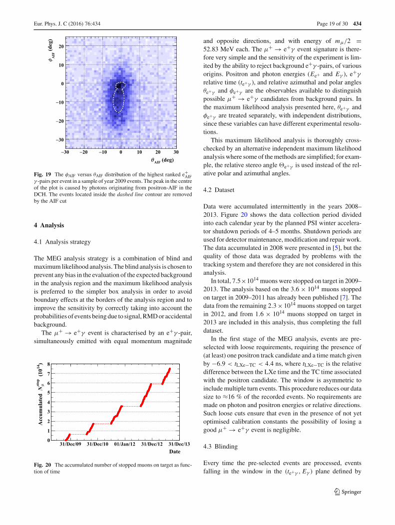
Eur. Phys. J. C (2016) 76 :434 Page 19 of 30 434
(deg)AIFθ−30 −20 −10 0 10 20 30
(deg
)A
IFφ
−30
−20
−10
0
10
20
Fig. 19 The φAIF versus θAIF distribution of the highest ranked e+AIF
γ -pairs per event in a sample of year 2009 events. The peak in the centreof the plot is caused by photons originating from positron-AIF in theDCH. The events located inside the dashed line contour are removedby the AIF cut
4 Analysis
4.1 Analysis strategy
The MEG analysis strategy is a combination of blind andmaximum likelihood analysis. The blind analysis is chosen toprevent any bias in the evaluation of the expected backgroundin the analysis region and the maximum likelihood analysisis preferred to the simpler box analysis in order to avoidboundary effects at the borders of the analysis region and toimprove the sensitivity by correctly taking into account theprobabilities of events being due to signal, RMD or accidentalbackground.
The μ+ → e+γ event is characterised by an e+γ -pair,simultaneously emitted with equal momentum magnitude
Date31/Dec/09 31/Dec/10 01/Jan/12 31/Dec/12 31/Dec/13
)14
(10
stop
μN
Acc
umul
ated
0
1
2
3
4
5
6
7
8
Fig. 20 The accumulated number of stopped muons on target as func-tion of time
and opposite directions, and with energy of mμ/2 =52.83 MeV each. The μ+ → e+γ event signature is there-fore very simple and the sensitivity of the experiment is lim-ited by the ability to reject background e+γ -pairs, of variousorigins. Positron and photon energies (Ee+ and Eγ ), e+γ
relative time (te+γ ), and relative azimuthal and polar anglesθe+γ and φe+γ are the observables available to distinguishpossible μ+ → e+γ candidates from background pairs. Inthe maximum likelihood analysis presented here, θe+γ andφe+γ are treated separately, with independent distributions,since these variables can have different experimental resolu-tions.
This maximum likelihood analysis is thoroughly cross-checked by an alternative independent maximum likelihoodanalysis where some of the methods are simplified; for exam-ple, the relative stereo angle �e+γ is used instead of the rel-ative polar and azimuthal angles.
4.2 Dataset
Data were accumulated intermittently in the years 2008–2013. Figure 20 shows the data collection period dividedinto each calendar year by the planned PSI winter accelera-tor shutdown periods of 4–5 months. Shutdown periods areused for detector maintenance, modification and repair work.The data accumulated in 2008 were presented in [5], but thequality of those data was degraded by problems with thetracking system and therefore they are not considered in thisanalysis.
In total, 7.5×10¹⁴ muons were stopped on target in 2009–2013. The analysis based on the 3.6 × 10¹⁴ muons stoppedon target in 2009–2011 has already been published [7]. Thedata from the remaining 2.3 × 10¹⁴ muons stopped on targetin 2012, and from 1.6 × 10¹⁴ muons stopped on target in2013 are included in this analysis, thus completing the fulldataset.
In the first stage of the MEG analysis, events are pre-selected with loose requirements, requiring the presence of(at least) one positron track candidate and a time match givenby −6.9 < tLXe−TC < 4.4 ns, where tLXe−TC is the relativedifference between the LXe time and the TC time associatedwith the positron candidate. The window is asymmetric toinclude multiple turn events. This procedure reduces our datasize to ≈16 % of the recorded events. No requirements aremade on photon and positron energies or relative directions.Such loose cuts ensure that even in the presence of not yetoptimised calibration constants the possibility of losing agood μ+ → e+γ event is negligible.
4.3 Blinding
Every time the pre-selected events are processed, eventsfalling in the window in the (te+γ , Eγ ) plane defined by
123
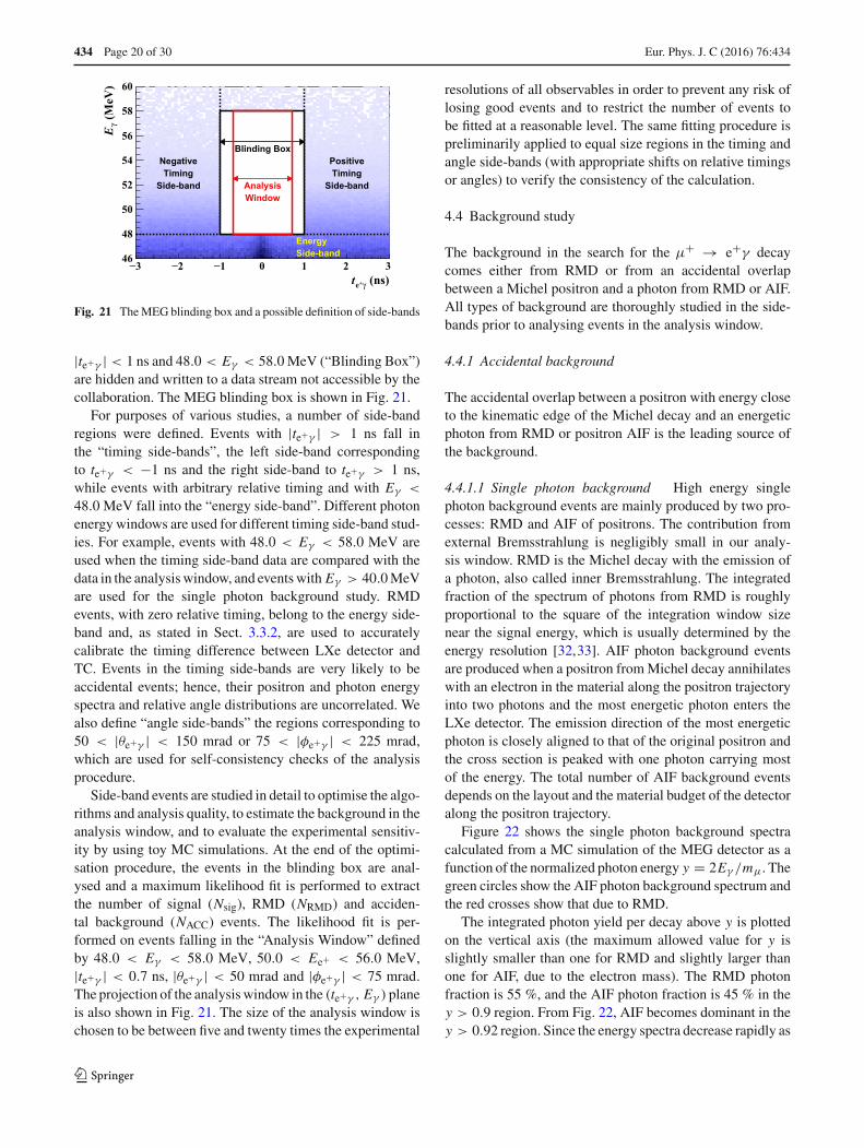
434 Page 20 of 30 Eur. Phys. J. C (2016) 76 :434
(ns)γ+et−3 −2 −1 0 1 2 3
(MeV
)γ
E
46
48
50
52
54
56
58
60
Blinding Box
AnalysisWindow
PositiveTiming
Side-band
NegativeTiming
Side-band
EnergySide-band
Fig. 21 The MEG blinding box and a possible definition of side-bands
|te+γ | < 1 ns and 48.0 < Eγ < 58.0 MeV (“Blinding Box”)are hidden and written to a data stream not accessible by thecollaboration. The MEG blinding box is shown in Fig. 21.
For purposes of various studies, a number of side-bandregions were defined. Events with |te+γ | > 1 ns fall inthe “timing side-bands”, the left side-band correspondingto te+γ < −1 ns and the right side-band to te+γ > 1 ns,while events with arbitrary relative timing and with Eγ <
48.0 MeV fall into the “energy side-band”. Different photonenergy windows are used for different timing side-band stud-ies. For example, events with 48.0 < Eγ < 58.0 MeV areused when the timing side-band data are compared with thedata in the analysis window, and events with Eγ > 40.0 MeVare used for the single photon background study. RMDevents, with zero relative timing, belong to the energy side-band and, as stated in Sect. 3.3.2, are used to accuratelycalibrate the timing difference between LXe detector andTC. Events in the timing side-bands are very likely to beaccidental events; hence, their positron and photon energyspectra and relative angle distributions are uncorrelated. Wealso define “angle side-bands” the regions corresponding to50 < |θe+γ | < 150 mrad or 75 < |φe+γ | < 225 mrad,which are used for self-consistency checks of the analysisprocedure.
Side-band events are studied in detail to optimise the algo-rithms and analysis quality, to estimate the background in theanalysis window, and to evaluate the experimental sensitiv-ity by using toy MC simulations. At the end of the optimi-sation procedure, the events in the blinding box are anal-ysed and a maximum likelihood fit is performed to extractthe number of signal (Nsig), RMD (NRMD) and acciden-tal background (NACC) events. The likelihood fit is per-formed on events falling in the “Analysis Window” definedby 48.0 < Eγ < 58.0 MeV, 50.0 < Ee+ < 56.0 MeV,|te+γ | < 0.7 ns, |θe+γ | < 50 mrad and |φe+γ | < 75 mrad.The projection of the analysis window in the (te+γ , Eγ ) planeis also shown in Fig. 21. The size of the analysis window ischosen to be between five and twenty times the experimental
resolutions of all observables in order to prevent any risk oflosing good events and to restrict the number of events tobe fitted at a reasonable level. The same fitting procedure ispreliminarily applied to equal size regions in the timing andangle side-bands (with appropriate shifts on relative timingsor angles) to verify the consistency of the calculation.
4.4 Background study
The background in the search for the μ+ → e+γ decaycomes either from RMD or from an accidental overlapbetween a Michel positron and a photon from RMD or AIF.All types of background are thoroughly studied in the side-bands prior to analysing events in the analysis window.
4.4.1 Accidental background
The accidental overlap between a positron with energy closeto the kinematic edge of the Michel decay and an energeticphoton from RMD or positron AIF is the leading source ofthe background.
4.4.1.1 Single photon background High energy singlephoton background events are mainly produced by two pro-cesses: RMD and AIF of positrons. The contribution fromexternal Bremsstrahlung is negligibly small in our analy-sis window. RMD is the Michel decay with the emission ofa photon, also called inner Bremsstrahlung. The integratedfraction of the spectrum of photons from RMD is roughlyproportional to the square of the integration window sizenear the signal energy, which is usually determined by theenergy resolution [32,33]. AIF photon background eventsare produced when a positron from Michel decay annihilateswith an electron in the material along the positron trajectoryinto two photons and the most energetic photon enters theLXe detector. The emission direction of the most energeticphoton is closely aligned to that of the original positron andthe cross section is peaked with one photon carrying mostof the energy. The total number of AIF background eventsdepends on the layout and the material budget of the detectoralong the positron trajectory.
Figure 22 shows the single photon background spectracalculated from a MC simulation of the MEG detector as afunction of the normalized photon energy y = 2Eγ /mμ. Thegreen circles show the AIF photon background spectrum andthe red crosses show that due to RMD.
The integrated photon yield per decay above y is plottedon the vertical axis (the maximum allowed value for y isslightly smaller than one for RMD and slightly larger thanone for AIF, due to the electron mass). The RMD photonfraction is 55 %, and the AIF photon fraction is 45 % in they > 0.9 region. From Fig. 22, AIF becomes dominant in they > 0.92 region. Since the energy spectra decrease rapidly as
123
Eur. Phys. J. C (2016) 76 :434 Page 21 of 30 434
y Threshold0.9 0.92 0.94 0.96 0.98 1
Pho
ton
Yie
ld p
er D
ecay
-910
-810
-710
-610
-510
-410
Fig. 22 The RMD (red crosses) and AIF (green circles) photon back-ground spectra in the MEG detector estimated by a MC simulationaround the kinematic end-point. The variable on the horizontal axis isy = 2Eγ /mμ where Eγ is the photon energy and mμ is the muon mass
a function of y near the kinematic end-point, a good energyresolution reduces steeply the single photon background.
In addition to the RMD and AIF components in the analy-sis window, there are contributions from pile-up photons andcosmic-ray components, totalling at most 4–6 %. The pile-uprejection methods are discussed in Sect. 3.1.3. The cosmic-ray events are rejected by using topological cuts based onthe deposited charge ratio of the inner to outer face and thereconstructed depth (w) because these events mostly comefrom the outer face of the LXe detector while signal eventsare expected from the inner face. After applying these cuts,photon background spectra are measured directly from thetiming side-band data, and the measured shape is used in theanalysis window.
4.4.1.2 Single positron background The single positronbackground in the analysis window results from the Micheldecay positrons. Although the theoretical positron energyspectrum of the Michel decay is well known [34], themeasured positron spectrum is severely distorted by thedesign of the spectrometer which tracks only high momen-tum positrons, and therefore introduces a strong momen-tum dependence in the tracking efficiency. The resolution inthe momentum reconstruction also influences the measuredspectrum. The positron spectrum obtained by our detectorwith the resolution function and the acceptance curve areshown in [8]. There is a plateau region near the signal energywhere the measurement rate of the positrons reaches its max-imum, which allows us to extract the shape of the positronbackground precisely from the data with high statistics.
4.4.1.3 Effective branching ratio The effective branchingratio of the accidental background, defined by the back-ground rate normalised to the muon stopping rate, can beapproximately expressed by [35]
50 51 52 53
(MeV
),m
inγ
E
48
49
50
51
52
53
-1310
-1210
-1110
(a)
(MeV),min+eE50 51 52 53
48
49
50
51
52
53-1510
-1410
-1310
-1210
(b)
Fig. 23 Effective branching ratios of the two types of backgroundinto the kinematic window defined by Ee+,min < Ee+ < 53.5 MeV,Eγ,min < Eγ < 53.5 MeV, |te+γ | < 0.24 ns and cos �e+γ < −0.9996.a Accidental background evaluated from the timing side-band. b RMDbackground from μ+ → e+γ νν̄ calculated with theoretical formulafolded with detector responses
Bacc ∝ Rμ δEe+ (δEγ )2 δte+γ δθe+γ δφe+γ ,
where Rμ is the muon stopping rate and δq is the width ofthe integration region defined by the detector resolution forthe observable q. Figure 23a shows the effective branchingratio for the accidental background as a function of the loweredges of the integration regions of Ee+ and Eγ . The sameplot for the RMD background is shown in Fig. 23b, which isdescribed in detail in the Sect. 4.4.2. It can be seen that theaccidental background is much more severe than the RMDbackground.
The rate of the accidental background expected in the anal-ysis window is evaluated using the data from a wider timewindow in the side-bands with larger statistics. The back-ground rate measured in the side-bands is used as a statisticalconstraint in the maximum likelihood analysis. The distribu-tions of the observables relevant for the physics analysis arealso precisely measured in the timing side-bands and used inthe maximum likelihood analysis (Sect. 4.5).
4.4.2 RMD background
A second background source consists of the μ+ → e+γ νν̄
RMD process, producing a time-coincident e+γ -pair. TheRMD events fall into the analysis window when the two neu-trinos have small momentum and are identical to the signalin the limit of neutrino energies equal to zero. Observationof the RMD events provides a strong internal consistencycheck for the μ+ → e+γ analysis since it is a source oftime-coincident e+γ -pairs.
The RMD in the energy side-band defined by 43.0 <
Eγ < 48.0 MeV, 48.0 < Ee+ < 53.0 MeV, |φe+γ | <
0.3 rad, and |θe+γ | < 0.3 rad are studied. The RMD eventsare identified by a peak in the te+γ distribution as shownin Fig. 18. The distribution of RMD in terms of energy andangle is measured by fitting the te+γ -distribution divided into
123
434 Page 22 of 30 Eur. Phys. J. C (2016) 76 :434
(MeV)+eE48 49 50 51 52 53
Num
ber
of e
vent
s
0
2000
4000
< 53 MeVγE43 <| < 0.3 radγ+eθ|| < 0.3 rad
γ+eφ|
(a)
(MeV)γE44 46 48 50 52
Num
ber
of e
vent
s
0
1000
2000
3000
4000
blinded
< 53 MeV+eE48 <| < 0.3 radγ+eθ|| < 0.3 rad
γ+eφ|
(b)
Fig. 24 Projected distributions of μ+ → e+γ νν̄ events measured inthe energy side-band (dots with error bars) compared with the expecta-tions (histograms with the uncertainty specified by the yellow bands).The expectations are calculated with the theoretical formula folded withthe detector responses and a normalisation based on Michel events
energy and angle bins. Figure 24 shows the measured pro-jected distributions. The rates and shapes are compared withthe Standard Model calculation (in lowest order) [35] andfound to be consistent. The measured branching ratio withinthe energy side-band agrees with the expectation to within5 %.
The estimated number of RMD events in the μ+ → e+γ
analysis window is calculated by extrapolating the energyside-band distribution to the analysis window, giving an esti-mate of 〈NRMD〉 = 614 ± 34, which is used as a statisticalconstraint in the likelihood analysis.
The RMD branching ratio is highly suppressed when theintegration region is close to the limit of μ+ → e+γ kine-matics. The effective branching ratio, which is calculated byconsidering the detector resolution, is plotted in Fig. 23b asa function of the lower edges of the integration regions onEe+ and Eγ . For example, the effective branching ratio for52.0 < Eγ < 53.5 MeV and 52.0 < Ee+ < 53.5 MeV is3×10−14, more than twenty times lower than that due to theaccidental background.
4.5 Maximum likelihood analysis
4.5.1 Likelihood function
The numbers of signal, RMD and accidental backgroundevents in the analysis window, (Nsig, NRMD, NACC), are deter-mined by a maximum likelihood analysis. In addition, twotarget parameters t for each year, representing the position(z0) and deformation (kt) of the muon stopping target arealso included as fitting parameters in the likelihood function(see Sect. 3.2.4). Of particular interest is Nsig, while the otherparameters (NRMD, NACC, t) are treated as nuisance param-eters which are profiled in the calculation of the confidenceintervals, as discussed in Sect. 4.5.3. The extended likelihoodfunction is thus defined as
L (Nsig, NRMD, NACC, t
)
= e−N
Nobs!C(NRMD, NACC, t)
×Nobs∏i=1
(NsigS(xi , t) + NRMD R(xi ) + NACC A(xi )
),
(3)
where xi = {Eγ , Ee+ , te+γ , θe+γ , φe+γ } is the vector ofobservables for the i-th event.
S, R and A are the probability density functions (PDFs) forthe signal, RMD and accidental background events, respec-tively. N = Nsig + NRMD + NACC is the total number ofevents in the fit and Nobs is the total number of detectedevents in the analysis window. C is a term for the constraintsof nuisance parameters.
The expected numbers of RMD and accidental back-ground events with their respective uncertainties are evalu-ated in the side-bands and are applied as Gaussian constraintson NRMD and NACC in the C term in Eq. 3.
The target position parameters z0 are subject to Gaussianconstraints whose widths are the year dependent systematicuncertainties; the target deformation parameters kt are con-strained with uniform distributions in year dependent inter-vals.
4.5.2 PDFs
4.5.2.1 Event-by-event PDFs The PDFs for signal, RMDand accidental background events are formed as a functionof the five observables (Eγ , Ee+ , te+γ , θe+γ , φe+γ ) takinginto account the correlations between them and the depen-dence of each of them and of their uncertainties on the pho-ton interaction vertex, the muon decay vertex and the trackreconstruction quality.
Because the detector resolutions depend on the detectorconditions and the hit position in the detector, this approachuses different PDFs for each event (event-by-event PDFs).The energy response, the position resolution and the back-ground spectrum of the LXe detector are evaluated as func-tion of the interaction vertex. For the positron PDF, the fittingerrors of the tracking variables are used to compute the res-olutions; namely the resolution on the observable q (σq ) isreplaced by a product of the pull parameter (sq ) and the fittingerror (σ ′
q ). The pull parameters are extracted from the dataas described in Sect. 3.2.5 and are common to all events ina given DAQ period. The correlations between observablesare also treated on an event-by-event basis. For example, theerrors on the momentum and the angle are correlated becausethe emission angle of positrons is computed by extrapolatingthe fitted tracks to the target plane. Since the true positronmomentum of the signal is known, the mean of the signal
123
Eur. Phys. J. C (2016) 76 :434 Page 23 of 30 434
angle PDF can be corrected as a function of the observedmomentum.
Because the energies, relative timing and angles for thesignal are fixed and known, the signal PDFs are described bythe product of the detector response function for each observ-able. The correlations between the errors of the observablesare implemented in the te+γ , θe+γ and φe+γ PDFs by shift-ing the centres and modifying the resolutions. The possiblereconstruction bias due to errors on the target position anddeformation is included in the signal PDF by shifting thecentre of the φe+γ PDF by an amount computed from t . Theamount of the shift is computed geometrically by shifting thetarget by δz0 + kt · (zt,FARO(xe+ , ye+) − zt,2013(xe+ , ye+))
in the zt direction, where δz0, zt,FARO and zt,2013 are thedeviation of z0 from the nominal value and the coordinatesdefined by the FARO measurements and the 2013 paraboloidfit, respectively (see Fig. 14). For the te+γ PDF, events arecategorised by using qe+ , which consists of the track-fittingquality and the matching quality between the fitted track andthe hit position on the TC. The resolution and the centralvalue are extracted for each category from the observed RMDtiming peak. The dependence on Eγ and Ee+ is taken intoaccount. Most of the parameters used to describe the correla-tions are extracted from data by using the double-turn method(see Sect. 3.2.5), while a few parameters (for instance, theslope parameter for the δte+γ
–δEe+ correlation, where δx isthe difference between the observed and the true value of theobservable x) are extracted from a MC simulation.
The RMD PDF is formed by the convolution of the detec-tor response and the kinematic distribution in the parame-ter space, (Eγ , Ee+ , θe+γ , φe+γ ), expected from the Stan-dard Model [35]. The correlations between the variables areincluded in the kinematic model. The PDF for te+γ is almostthe same as that of the signal PDF, while the correlationbetween δte+γ
and Ee+ is excluded.The accidental background PDFs are extracted from the
timing side-band data. For Ee+ , the spectrum, after applyingthe same event selection on the track reconstruction qualityas for the physics analysis, is fitted with a function formed bythe convolution of the Michel positron spectrum and a param-eterised function describing the detector response. For Eγ ,the energy spectra after applying the pile-up and cosmic-raycuts and a loose selection on the e+γ relative angle, are fittedwith a function to represent background photon, remainingcosmic-ray and the pile-up components convoluted with thedetector response. The θe+γ and φe+γ PDFs are representedby polynomial functions fitted to the data after applying thesame event selection except for the te+γ . For te+γ , a flat PDFis used.
4.5.2.2 Constant PDFs The event-by-event PDFs employthe entire information we have about detector responses andkinematic variable correlations. A slightly less sensitive anal-
ysis, based on an alternative set of PDFs, is used as a crosscheck; this approach was already implemented in [7].
In this alternative set of PDFs the events are characterisedby “categories”, mainly determined by the tracking qualityof positrons and by the reconstructed depth of the interactionvertex in the LXe detector for photons. A constant group ofPDFs is determined year by year, one for each of the cat-egories mentioned above; the relative stereo angle �e+γ istreated as an observable instead of θe+γ and φe+γ separately,while the three other kinematic variables (Ee+ , Eγ and te+γ )are common to the two sets of PDFs. Correlations betweenkinematic variables are also taken into account with a simplerapproach and the systematic uncertainties associated withthe target position are included by shifting �e+γ of eachevent by an appropriate amount, computed by a combina-tion of the corresponding shifts of θe+γ and φe+γ . Signal andRMD PDFs are modelled as in the event-by-event analysisby using calibration data and theoretical distributions, foldedwith detector response. This likelihood function is analogousto Eq. 3 with the inclusion of the Gaussian constraints on theexpected number of RMD and accidental background eventsand of the Poissonian constraint on the expected total num-ber of events. In what follows we refer to this set of PDFs as“constant PDFs” and to the analysis based on it as “constantPDFs’ analysis”.
4.5.3 Confidence interval
The confidence interval of Nsig is calculated following theFeldman-Cousins approach [36] with the profile-likelihoodratio ordering [37]. The test statistic λp for sorting experi-ments is defined by
λp(Nsig) =
⎧⎪⎪⎨⎪⎪⎩
L(Nsig,ˆ̂θ(Nsig))
L(0,ˆ̂θ(0))
if N̂sig < 0
L(Nsig,ˆ̂θ(Nsig))
L(N̂sig,θ̂)if N̂sig ≥ 0,
where θ is a vector of nuisance parameters (NACC, NRMD andt), N̂sig and θ̂ are the values of Nsig and θ which maximise
the likelihood, ˆ̂θ(Nsig) is the value of θ which maximises the
likelihood for the specified Nsig. The confidence interval iscalculated using the distribution of the likelihood ratio foran ensemble of pseudo experiments simulated based on thePDFs.
The following systematic uncertainties are included inthe calculation of the confidence interval: the normalisation(defined in Sect. 4.6), the alignment of the photon and thepositron detectors, the alignment (position and deformation)of the muon stopping target, the photon energy scale, thepositron energy bias, the centre of the signal te+γ PDF, theshapes of the signal and background PDFs, and the corre-lations between the errors of the positron observables. The
123
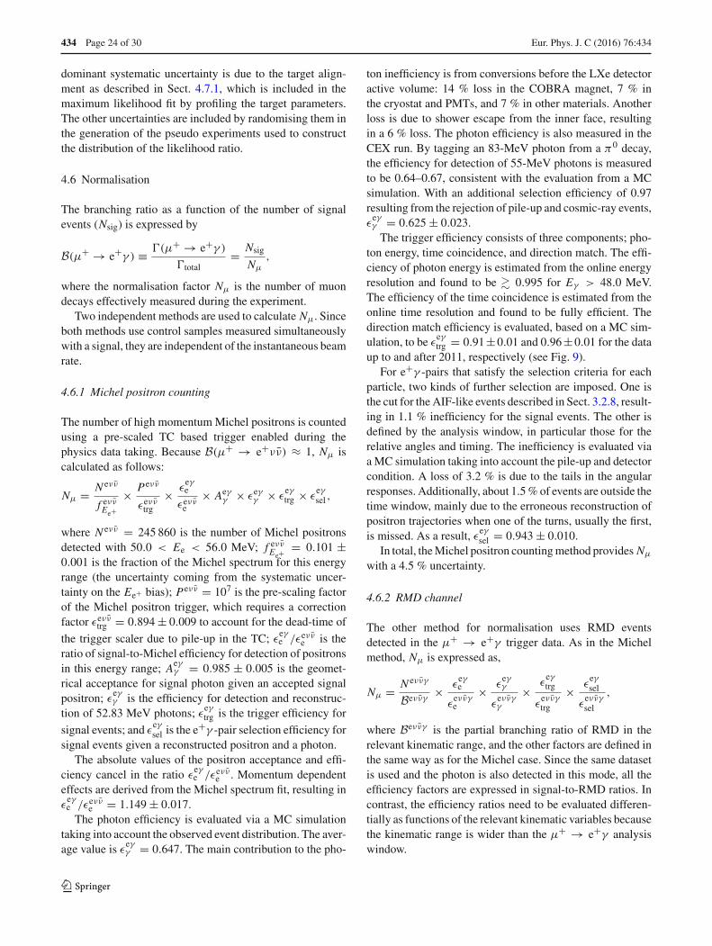
434 Page 24 of 30 Eur. Phys. J. C (2016) 76 :434
dominant systematic uncertainty is due to the target align-ment as described in Sect. 4.7.1, which is included in themaximum likelihood fit by profiling the target parameters.The other uncertainties are included by randomising them inthe generation of the pseudo experiments used to constructthe distribution of the likelihood ratio.
4.6 Normalisation
The branching ratio as a function of the number of signalevents (Nsig) is expressed by
B(μ+ → e+γ ) ≡ �(μ+ → e+γ )
�total= Nsig
Nμ
,
where the normalisation factor Nμ is the number of muondecays effectively measured during the experiment.
Two independent methods are used to calculate Nμ. Sinceboth methods use control samples measured simultaneouslywith a signal, they are independent of the instantaneous beamrate.
4.6.1 Michel positron counting
The number of high momentum Michel positrons is countedusing a pre-scaled TC based trigger enabled during thephysics data taking. Because B(μ+ → e+νν̄) ≈ 1, Nμ iscalculated as follows:
Nμ = N eνν̄
f eνν̄Ee+
× Peνν̄
εeνν̄trg
× εeγe
εeνν̄e
× Aeγγ × εeγ
γ × εeγtrg × ε
eγsel ,
where N eνν̄ = 245 860 is the number of Michel positronsdetected with 50.0 < Ee < 56.0 MeV; f eνν̄
Ee+= 0.101 ±
0.001 is the fraction of the Michel spectrum for this energyrange (the uncertainty coming from the systematic uncer-tainty on the Ee+ bias); Peνν̄ = 107 is the pre-scaling factorof the Michel positron trigger, which requires a correctionfactor εeνν̄
trg = 0.894 ± 0.009 to account for the dead-time of
the trigger scaler due to pile-up in the TC; εeγe /εeνν̄
e is theratio of signal-to-Michel efficiency for detection of positronsin this energy range; Aeγ
γ = 0.985 ± 0.005 is the geomet-rical acceptance for signal photon given an accepted signalpositron; ε
eγγ is the efficiency for detection and reconstruc-
tion of 52.83 MeV photons; εeγtrg is the trigger efficiency for
signal events; and εeγsel is the e+γ -pair selection efficiency for
signal events given a reconstructed positron and a photon.The absolute values of the positron acceptance and effi-
ciency cancel in the ratio εeγe /εeνν̄
e . Momentum dependenteffects are derived from the Michel spectrum fit, resulting inε
eγe /εeνν̄
e = 1.149 ± 0.017.The photon efficiency is evaluated via a MC simulation
taking into account the observed event distribution. The aver-age value is ε
eγγ = 0.647. The main contribution to the pho-
ton inefficiency is from conversions before the LXe detectoractive volume: 14 % loss in the COBRA magnet, 7 % inthe cryostat and PMTs, and 7 % in other materials. Anotherloss is due to shower escape from the inner face, resultingin a 6 % loss. The photon efficiency is also measured in theCEX run. By tagging an 83-MeV photon from a π0 decay,the efficiency for detection of 55-MeV photons is measuredto be 0.64–0.67, consistent with the evaluation from a MCsimulation. With an additional selection efficiency of 0.97resulting from the rejection of pile-up and cosmic-ray events,ε
eγγ = 0.625 ± 0.023.
The trigger efficiency consists of three components; pho-ton energy, time coincidence, and direction match. The effi-ciency of photon energy is estimated from the online energyresolution and found to be � 0.995 for Eγ > 48.0 MeV.The efficiency of the time coincidence is estimated from theonline time resolution and found to be fully efficient. Thedirection match efficiency is evaluated, based on a MC sim-ulation, to be ε
eγtrg = 0.91±0.01 and 0.96±0.01 for the data
up to and after 2011, respectively (see Fig. 9).For e+γ -pairs that satisfy the selection criteria for each
particle, two kinds of further selection are imposed. One isthe cut for the AIF-like events described in Sect. 3.2.8, result-ing in 1.1 % inefficiency for the signal events. The other isdefined by the analysis window, in particular those for therelative angles and timing. The inefficiency is evaluated viaa MC simulation taking into account the pile-up and detectorcondition. A loss of 3.2 % is due to the tails in the angularresponses. Additionally, about 1.5 % of events are outside thetime window, mainly due to the erroneous reconstruction ofpositron trajectories when one of the turns, usually the first,is missed. As a result, ε
eγsel = 0.943 ± 0.010.
In total, the Michel positron counting method provides Nμ
with a 4.5 % uncertainty.
4.6.2 RMD channel
The other method for normalisation uses RMD eventsdetected in the μ+ → e+γ trigger data. As in the Michelmethod, Nμ is expressed as,
Nμ = N eνν̄γ
Beνν̄γ× ε
eγe
εeνν̄γe
× εeγγ
εeνν̄γγ
× εeγtrg
εeνν̄γtrg
× εeγsel
εeνν̄γsel
,
where Beνν̄γ is the partial branching ratio of RMD in therelevant kinematic range, and the other factors are defined inthe same way as for the Michel case. Since the same datasetis used and the photon is also detected in this mode, all theefficiency factors are expressed in signal-to-RMD ratios. Incontrast, the efficiency ratios need to be evaluated differen-tially as functions of the relevant kinematic variables becausethe kinematic range is wider than the μ+ → e+γ analysiswindow.
123
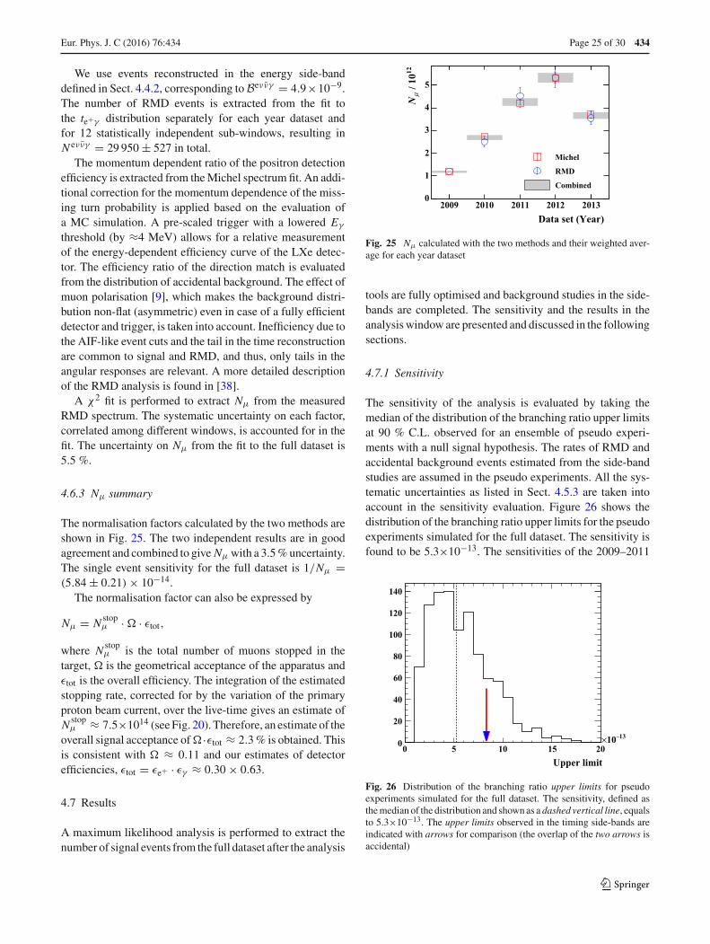
Eur. Phys. J. C (2016) 76 :434 Page 25 of 30 434
We use events reconstructed in the energy side-banddefined in Sect. 4.4.2, corresponding to Beνν̄γ = 4.9×10⁻⁹.The number of RMD events is extracted from the fit tothe te+γ distribution separately for each year dataset andfor 12 statistically independent sub-windows, resulting inN eνν̄γ = 29 950 ± 527 in total.
The momentum dependent ratio of the positron detectionefficiency is extracted from the Michel spectrum fit. An addi-tional correction for the momentum dependence of the miss-ing turn probability is applied based on the evaluation ofa MC simulation. A pre-scaled trigger with a lowered Eγ
threshold (by ≈4 MeV) allows for a relative measurementof the energy-dependent efficiency curve of the LXe detec-tor. The efficiency ratio of the direction match is evaluatedfrom the distribution of accidental background. The effect ofmuon polarisation [9], which makes the background distri-bution non-flat (asymmetric) even in case of a fully efficientdetector and trigger, is taken into account. Inefficiency due tothe AIF-like event cuts and the tail in the time reconstructionare common to signal and RMD, and thus, only tails in theangular responses are relevant. A more detailed descriptionof the RMD analysis is found in [38].
A χ2 fit is performed to extract Nμ from the measuredRMD spectrum. The systematic uncertainty on each factor,correlated among different windows, is accounted for in thefit. The uncertainty on Nμ from the fit to the full dataset is5.5 %.
4.6.3 Nμ summary
The normalisation factors calculated by the two methods areshown in Fig. 25. The two independent results are in goodagreement and combined to give Nμ with a 3.5 % uncertainty.The single event sensitivity for the full dataset is 1/Nμ =(5.84 ± 0.21) × 10−14.
The normalisation factor can also be expressed by
Nμ = N stopμ · � · εtot,
where N stopμ is the total number of muons stopped in the
target, � is the geometrical acceptance of the apparatus andεtot is the overall efficiency. The integration of the estimatedstopping rate, corrected for by the variation of the primaryproton beam current, over the live-time gives an estimate ofN stop
μ ≈ 7.5×10¹⁴ (see Fig. 20). Therefore, an estimate of theoverall signal acceptance of �·εtot ≈ 2.3 % is obtained. Thisis consistent with � ≈ 0.11 and our estimates of detectorefficiencies, εtot = εe+ · εγ ≈ 0.30 × 0.63.
4.7 Results
A maximum likelihood analysis is performed to extract thenumber of signal events from the full dataset after the analysis
Data set (Year)2009 2010 2011 2012 2013
12 /
10μ
N
0
1
2
3
4
5
Michel
RMD
Combined
Fig. 25 Nμ calculated with the two methods and their weighted aver-age for each year dataset
tools are fully optimised and background studies in the side-bands are completed. The sensitivity and the results in theanalysis window are presented and discussed in the followingsections.
4.7.1 Sensitivity
The sensitivity of the analysis is evaluated by taking themedian of the distribution of the branching ratio upper limitsat 90 % C.L. observed for an ensemble of pseudo experi-ments with a null signal hypothesis. The rates of RMD andaccidental background events estimated from the side-bandstudies are assumed in the pseudo experiments. All the sys-tematic uncertainties as listed in Sect. 4.5.3 are taken intoaccount in the sensitivity evaluation. Figure 26 shows thedistribution of the branching ratio upper limits for the pseudoexperiments simulated for the full dataset. The sensitivity isfound to be 5.3×10⁻¹³. The sensitivities of the 2009–2011
Upper limit0 5 10 15 20
13−10×0
20
40
60
80
100
120
140
Fig. 26 Distribution of the branching ratio upper limits for pseudoexperiments simulated for the full dataset. The sensitivity, defined asthe median of the distribution and shown as a dashed vertical line, equalsto 5.3×10⁻¹³. The upper limits observed in the timing side-bands areindicated with arrows for comparison (the overlap of the two arrows isaccidental)
123
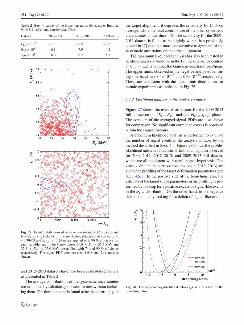
434 Page 26 of 30 Eur. Phys. J. C (2016) 76 :434
Table 2 Best fit values of the branching ratios (Bfit), upper limits at90 % C.L. (B90) and sensitivities (S90)
Dataset 2009–2011 2012–2013 2009–2013
Bfit × 1013 −1.3 −5.5 −2.2
B90 × 1013 6.1 7.9 4.2
S90 × 1013 8.0 8.2 5.3
(MeV)+eE50 51 52 53 54 55 56
(MeV
)γ
E
48
50
52
54
56
58
γ+eΘcos−1 −0.999−0.9995 −0.9985
(ns)
γ+ et
−2
−1.5
−1
−0.5
0
0.5
1
1.5
2
Fig. 27 Event distributions of observed events in the (Ee+ , Eγ )- and(cos �e+γ , te+γ )-planes. In the top figure, selections of cos �e+γ <
−0.99963 and |te+γ | < 0.24 ns are applied with 90 % efficiency foreach variable, and in the bottom figure 51.0 < Eγ < 55.5 MeV and52.4 < Ee+ < 55.0 MeV are applied with 74 and 90 % efficiencyrespectively. The signal PDF contours (1σ , 1.64σ and 2σ ) are alsoshown
and 2012–2013 datasets have also been evaluated separatelyas presented in Table 2.
The average contributions of the systematic uncertaintiesare evaluated by calculating the sensitivities without includ-ing them. The dominant one is found to be the uncertainty on
the target alignment; it degrades the sensitivity by 13 % onaverage, while the total contribution of the other systematicuncertainties is less than 1 %. The sensitivity for the 2009–2011 dataset is found to be slightly worse than previouslyquoted in [7] due to a more conservative assignment of thesystematic uncertainty on the target alignment.
The maximum likelihood analysis has also been tested infictitious analysis windows in the timing side-bands centredat te+γ = ±2 ns without the Gaussian constraint on NRMD.The upper limits observed in the negative and positive tim-ing side-bands are 8.4×10⁻¹³ and 8.3×10⁻¹³, respectively.These are consistent with the upper limit distribution forpseudo experiments as indicated in Fig. 26.
4.7.2 Likelihood analysis in the analysis window
Figure 27 shows the event distributions for the 2009-2013full dataset on the (Ee+ , Eγ )- and (cos �e+γ , te+γ )-planes.The contours of the averaged signal PDFs are also shownfor comparison. No significant correlated excess is observedwithin the signal contours.
A maximum likelihood analysis is performed to evaluatethe number of signal events in the analysis window by themethod described in Sect. 4.5. Figure 28 shows the profile-likelihood ratios as a function of the branching ratio observedfor 2009–2011, 2012–2013, and 2009–2013 full dataset,which are all consistent with a null-signal hypothesis. Thekinks visible in the curves (most obvious in 2012–2013) aredue to the profiling of the target deformation parameters (seeSect. 4.5.1). In the positive side of the branching ratio, theestimate of the target shape parameters in the profiling is per-formed by looking for a positive excess of signal-like eventsin the φe+γ distribution. On the other hand, in the negativeside, it is done by looking for a deficit of signal-like events.
Fig. 28 The negative log-likelihood ratio (λp) as a function of thebranching ratio
123
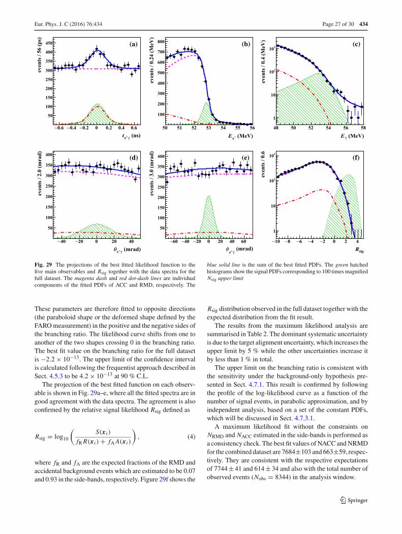
Eur. Phys. J. C (2016) 76 :434 Page 27 of 30 434
(ns)γ+et0.6− 0.4− 0.2− 0 0.2 0.4 0.6
even
ts /
56 (p
s)
50
100
150
200
250
300
350
400
450 (a)
(MeV)+eE50 51 52 53 54 55 56
even
ts /
0.24
(MeV
)
100
200
300
400
500
600
700
800 (b)
(MeV)γE48 50 52 54 56 58
even
ts /
0.4
(MeV
)
1
10
210
310(c)
(mrad)γ+eθ40− 20− 0 20 40
even
ts /
2.0
(mra
d)
50
100
150
200
250
300
350
400 (d)
(mrad)γ+e
φ60− 40− 20− 0 20 40 60
even
ts /
3.0
(mra
d)
50
100
150
200
250
300
350
400 (e)
sigR10− 8− 6− 4− 2− 0 2 4
even
ts /
0.6
1
10
210
310 (f)
Fig. 29 The projections of the best fitted likelihood function to thefive main observables and Rsig together with the data spectra for thefull dataset. The magenta dash and red dot-dash lines are individualcomponents of the fitted PDFs of ACC and RMD, respectively. The
blue solid line is the sum of the best fitted PDFs. The green hatchedhistograms show the signal PDFs corresponding to 100 times magnifiedNsig upper limit
These parameters are therefore fitted to opposite directions(the paraboloid shape or the deformed shape defined by theFARO measurement) in the positive and the negative sides ofthe branching ratio. The likelihood curve shifts from one toanother of the two shapes crossing 0 in the branching ratio.The best fit value on the branching ratio for the full datasetis −2.2 × 10⁻¹³. The upper limit of the confidence intervalis calculated following the frequentist approach described inSect. 4.5.3 to be 4.2 × 10⁻¹³ at 90 % C.L.
The projection of the best fitted function on each observ-able is shown in Fig. 29a–e, where all the fitted spectra are ingood agreement with the data spectra. The agreement is alsoconfirmed by the relative signal likelihood Rsig defined as
Rsig = log10
(S(xi )
fR R(xi ) + fA A(xi )
), (4)
where fR and fA are the expected fractions of the RMD andaccidental background events which are estimated to be 0.07and 0.93 in the side-bands, respectively. Figure 29f shows the
Rsig distribution observed in the full dataset together with theexpected distribution from the fit result.
The results from the maximum likelihood analysis aresummarised in Table 2. The dominant systematic uncertaintyis due to the target alignment uncertainty, which increases theupper limit by 5 % while the other uncertainties increase itby less than 1 % in total.
The upper limit on the branching ratio is consistent withthe sensitivity under the background-only hypothesis pre-sented in Sect. 4.7.1. This result is confirmed by followingthe profile of the log-likelihood curve as a function of thenumber of signal events, in parabolic approximation, and byindependent analysis, based on a set of the constant PDFs,which will be discussed in Sect. 4.7.3.1.
A maximum likelihood fit without the constraints onNRMD and NACC estimated in the side-bands is performed asa consistency check. The best fit values of NACC and NRMDfor the combined dataset are 7684±103 and 663±59, respec-tively. They are consistent with the respective expectationsof 7744 ± 41 and 614 ± 34 and also with the total number ofobserved events (Nobs = 8344) in the analysis window.
123
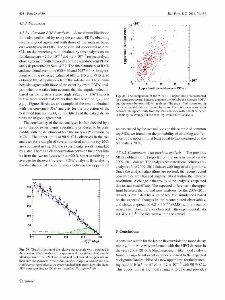
434 Page 28 of 30 Eur. Phys. J. C (2016) 76 :434
4.7.3 Discussion
4.7.3.1 Constant PDFs’ analysis A maximum likelihoodfit is also performed by using the constant PDFs, obtainingresults in good agreement with those of the analysis basedon event-by-event PDFs. The best fit and upper limit at 90 %C.L. on the branching ratio obtained by this analysis on thefull dataset are −2.5×10⁻¹³ and 4.3×10⁻¹³ respectively, inclose agreement with the results of the event-by-event PDFs’analysis presented in Sect. 4.7.2. The fitted numbers of RMDand accidental events are 630±66 and 7927±148, in agree-ment with the expected values of 683 ± 115 and 7915 ± 96obtained by extrapolations from the side-bands. These num-bers also agree with those of the event-by-event PDFs’ anal-ysis when one takes into account that the angular selectionbased on the relative stereo angle (�e+γ > 176◦) selects≈3 % more accidental events than that based on θe+γ andφe+γ . Figure 30 shows an example of the results obtainedwith the constant PDFs’ analysis for the projection of thebest fitted function on �e+γ : the fitted and the data distribu-tions are in good agreement.
The consistency of the two analyses is also checked by aset of pseudo experiments, specifically produced to be com-patible with the structures of both the analyses (“common toyMCs”). The upper limits at 90 % C.L. observed in the twoanalyses for a sample of several hundred common toy MCsare compared in Fig. 31; the experimental result is markedby a star. There is a clear correlation between the upper lim-its from the two analyses with a ≈20 % better sensitivity onaverage for the event-by-event PDFs’ analysis. By analysingthe distribution of the differences between the upper limit
(deg)γ+estereoΘ
176 177 178 179 1800
50
100
150
200
250
Fig. 30 The distribution of the relative stereo angle �e+γ obtained inthe constant PDFs’ analysis for experimental data (black dots) and thefitted spectrum. The RMD and accidental background components andtheir sum are shown with the red dot-dashed, magenta dashed and bluesolid curves, respectively; the green hatched histogram shows the signalPDF corresponding to 100 times magnified Nsig upper limit
Upper limit (event-by-event PDFs)0 5 10 15 20
13−10×
Upp
er li
mt (
cons
tant
PD
Fs)
0
5
10
15
2013−10×
Fig. 31 The comparison of the 90 % C.L. upper limits reconstructedon a sample of several hundred common toy MCs by the constant PDFs’and the event-by-event PDFs’ analyses. The upper limits observed inthe experimental data are marked by a star. There is a clear correlationbetween the upper limits from the two analyses with a ≈20 % bettersensitivity on average for the event-by-event PDFs’ analysis
reconstructed by the two analyses on this sample of commontoy MCs, we found that the probability of obtaining a differ-ence in the upper limit at least equal to that measured on thereal data is 70 %.
4.7.3.2 Comparison with previous analysis The previousMEG publication [7] reported on the analysis based on the2009–2011 dataset. The analysis presented here includes a re-analysis of the 2009–2011 dataset with improved algorithms.Since the analysis algorithms are revised, the reconstructedobservables are changed slightly, albeit within the detectorresolutions. A change in the results of the analysis is expecteddue to statistical effects. The expected difference in the upperlimit between the old and new analyses for the 2009–2011dataset is evaluated by a set of toy MC simulations basedon the expected changes in the reconstructed observables,and shows a spread of 4.2 × 10⁻¹³ (RMS) with a mean ofnearly zero. The difference observed in the experimental datais 0.4 × 10⁻¹³ and lies well within the spread.
5 Conclusions
A sensitive search for the lepton flavour violating muon decaymode μ+ → e+γ was performed with the MEG detector inthe years 2009–2013. A blind, maximum-likelihood analysisfound no significant event excess compared to the expectedbackground and established a new upper limit for the branch-ing ratio of B(μ+ → e+γ ) < 4.2 × 10⁻¹³ with 90 % C.L.This upper limit is the most stringent to date and provides
123
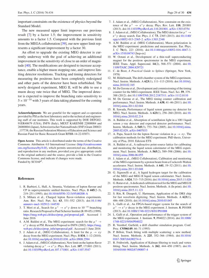
Eur. Phys. J. C (2016) 76 :434 Page 29 of 30 434
important constraints on the existence of physics beyond theStandard Model.
The new measured upper limit improves our previousresult [7] by a factor 1.5; the improvement in sensitivityamounts to a factor 1.5. Compared with the previous limitfrom the MEGA collaboration [39], our new upper limit rep-resents a significant improvement by a factor 30.
An effort to upgrade the existing MEG detector is cur-rently underway with the goal of achieving an additionalimprovement in the sensitivity of close to an order of magni-tude [40]. The modifications are designed to increase accep-tance, enable a higher muon stopping rate, and improve lim-iting detector resolutions. Tracking and timing detectors formeasuring the positrons have been completely redesignedand other parts of the detector have been refurbished. Thenewly designed experiment, MEG II, will be able to use amuon decay rate twice that of MEG. The improved detec-tor is expected to improve the branching ratio sensitivity to5×10−14 with 3 years of data taking planned for the comingyears.
Acknowledgments We are grateful for the support and co-operationprovided by PSI as the host laboratory and to the technical and engineer-ing staff of our institutes. This work is supported by DOE DEFG02-91ER40679 (USA), INFN (Italy), MEXT KAKENHI 22000004 and26000004 (Japan), Schweizerischer Nationalfonds (SNF) Grant 200021_137738, the Russian Federation Ministry of Education and Science andRussian Fund for Basic Research Grant RFBR-14-22-03071.
Open Access This article is distributed under the terms of the CreativeCommons Attribution 4.0 International License (http://creativecommons.org/licenses/by/4.0/), which permits unrestricted use, distribution,and reproduction in any medium, provided you give appropriate creditto the original author(s) and the source, provide a link to the CreativeCommons license, and indicate if changes were made.Funded by SCOAP3.
References
1. R. Barbieri, L. Hall, A. Strumia, Violations of lepton flavour andCP in supersymmetric unified theories. Nucl. Phys. B 445(2–3),219–251 (1995). doi:10.1016/0550-3213(95)00208-A
2. S. Mihara et al., Charged lepton flavor-violation experiments.Ann. Rev. Nucl. Part. Sci. 63, 531–552 (2013). doi:10.1146/annurev-nucl-102912-144530
3. T. Mori et al., Search for μ+ → e+γ down to 10−14 branchingratio. Research Proposal to Paul Scherrer Institut (R-99-05) (1999).https://meg.web.psi.ch/docs/prop_psi/proposal.pdf. Accessed 1June 2016
4. A.M. Baldini et al., The MEG experiment: search for the μ+ →e+γ decay at PSI. Research Proposal to INFN (2002). https://meg.web.psi.ch/docs/prop_infn/nproposal.pdf. Accessed 1 June 2016
5. J. Adam et al., (MEG Collaboration), A limit for the μ → eγdecay from the MEG experiment. Nucl. Phys. B 834, 1–12 (2010).doi:10.1016/j.nuclphysb.2010.03.030. arXiv:0908.2594
6. J. Adam et al., (MEG Collaboration), New limit on the lepton-flavorviolating decay μ+ → e+γ . Phys. Rev. Lett. 107, 171801 (2011).doi:10.1103/PhysRevLett.107.171801. arXiv:1107.5547
7. J. Adam et al., (MEG Collaboration), New constraint on the exis-tence of the μ+ → e+γ decay. Phys. Rev. Lett. 110, 201801(2013). doi:10.1103/PhysRevLett.110.201801. arXiv:1303.0754
8. J. Adam et al., (MEG Collaboration), The MEG detector for μ+ →e+γ decay search. Eur. Phys. J. C 73, 2365 (2013). doi:10.1140/epjc/s10052-013-2365-2. arXiv:1303.2348
9. A.M. Baldini et al. (MEG Collaboration), Muon polarization inthe MEG experiment: predictions and measurements. Eur. Phys.J. C 76(4), 223 (2016). doi:10.1140/epjc/s10052-016-4047-3.arXiv:1510.04743 [hep-ex]
10. W. Ootani et al., Development of a thin-wall superconductingmagnet for the positron spectrometer in the MEG experiment.IEEE Trans. Appl. Supercond. 14(2), 568–571 (2004). doi:10.1109/TASC.2004.829721
11. C. de Boor, A Practical Guide to Splines (Springer, New York,1978)
12. M. Hildebrandt, The drift chamber system of the MEG experiment.Nucl. Instrm. Methods. A 623(1), 111–113 (2010). doi:10.1016/j.nima.2010.02.165
13. M. De Gerone et al., Development and commissioning of the timingcounter for the MEG experiment. IEEE Trans. Nucl. Sci. 59, 379–388 (2012). doi:10.1109/TNS.2012.2187311. arXiv:1112.0110
14. M. De Gerone et al., The MEG timing counter calibration andperformance. Nucl. Instrm. Methods. A 638, 41–46 (2011). doi:10.1016/j.nima.2011.02.044
15. R. Sawada, Performance of liquid xenon gamma ray detector forMEG. Nucl. Instrm. Methods. A 623(1), 258–260 (2010). doi:10.1016/j.nima.2010.02.214
16. A. Baldini et al., Absorption of scintillation light in a 100 l liquidxenon γ -ray detector and expected detector performance. Nucl.Instrm. Methods. A 545(3), 753–764 (2005). doi:10.1016/j.nima.2005.02.029, arXiv:0407033
17. A. Papa, Search for the lepton flavour violation in μ → eγ . Thecalibration methods for the MEG experiment. PhD thesis, Univer-sity of Pisa, 2010. Edizioni ETS
18. A. Baldini et al., A radioactive point-source lattice for calibratingand monitoring the liquid xenon calorimeter of the MEG experi-ment. Nucl. Instrm. Methods. A 565(2), 589–598 (2006). doi:10.1016/j.nima.2006.06.055
19. J. Adam et al., (MEG Collaboration), Calibration and monitoringof the MEG experiment by a proton beam from a Cockcroft-Waltonaccelerator. Nucl. Instrm. Methods. A 641, 19–32 (2011). doi:10.1016/j.nima.2011.03.048
20. G. Signorelli et al., A liquid hydrogen target for the calibrationof the MEG and MEG II liquid xenon calorimeter. Nucl. Instrm.Methods. A 824, 713–715 (2016). doi:10.1016/j.nima.2015.11.026
21. G. Rutar et al., A dedicated calibration tool for the MEG and MEG IIpositron spectrometer. Nucl. Instrm. Methods. A (In print). doi:10.1016/j.nima.2015.11.121
22. S. Ritt, R. Dinapoli, U. Hartmann, Application of the DRS chipfor fast waveform digitizing. Nucl. Instrm. Methods. A 623(1),486–488 (2010). doi:10.1016/j.nima.2010.03.045
23. L. Galli et al., An FPGA-based trigger system for the search ofμ+ → e+γ decay in the MEG experiment. J. Instrum. 8, P01008(2013). doi:10.1088/1748-0221/8/01/P01008
24. L. Galli et al., Operation and performance of the trigger system ofthe MEG experiment. J. Instrum. 9, P04022 (2014). doi:10.1088/1748-0221/9/04/P04022
25. R. Veenhof, Garfield, a drift chamber simulation program. Conf.Proc. C9306149, 66–71 (1993)
26. P. Billoir, Track fitting with multiple scattering: a new method.Nucl. Instrm. Methods. A 225, 352–366 (1984). doi:10.1016/0167-5087(84)90274-6
27. R. Frühwirth, Application of Kalman filtering to track and vertexfitting. Nucl. Instrm. Methods. A 262, 444–450 (1987). doi:10.1016/0168-9002(87)90887-4
123

434 Page 30 of 30 Eur. Phys. J. C (2016) 76 :434
28. A. Fontana et al., Use of GEANE for tracking in virtual MonteCarlo. J. Phys. Conf. Ser. 119, 032018 (2008). doi:10.1088/1742-6596/119/3/032018
29. V. Blobel, Software alignment for tracking detectors. Nucl. Instrm.Methods. A 566, 5–14 (2006). doi:10.1016/j.nima.2006.05.157
30. FARO portable coordinate measuring machines. http://www.faro.com/en-us/products. Accessed 1 Feb 2016
31. Bernard Aubert et al. (BaBar), A study of time dependent CP-violating asymmetries and flavor oscillations in neutral B decaysat the ϒ(4S). Phys. Rev. D66, 032003 (2002). doi:10.1103/PhysRevD.66.032003, arXiv:hep-ex/0201020
32. C. Fronsdal, H. Überall, μ-meson decay with inner bremsstrahlung.Phys. Rev. 113(2), 654–657 (1959). doi:10.1103/PhysRev.113.654
33. S.G. Eckstein, R.H. Pratt, Radiative muon decay. Ann. Phys. 8,297–309 (1959). doi:10.1016/0003-4916(59)90024-7
34. T. Kinoshita, A. Sirlin, Radiative corrections to Fermi interactions.Phys. Rev. 113(6), 1652–1660 (1959). doi:10.1103/PhysRev.113.1652
35. Y. Kuno, Y. Okada, Muon decay and physics beyond the stan-dard model. Rev. Mod. Phys. 73(1), 151–202 (2001). doi:10.1103/RevModPhys.73.151. arXiv:hep-ph/9909265
36. G.J. Feldman, R.D. Cousins, Unified approach to the classical sta-tistical analysis of small signals. Phys. Rev. D 57(7), 3873–3889(1998). doi:10.1103/PhysRevD.57.3873
37. K.A. Olive et al., (Particle Data Group), Review of particle physics.Chin. Phys. C 38, 090001 (2014). doi:10.1088/1674-1137/38/9/090001
38. A.M. Baldini et al., (MEG Collaboration), Measurement of theradiative decay of polarized muons in the MEG experiment. Eur.Phys. J. C 76, 108 (2016). doi:10.1140/epjc/s10052-016-3947-6.arXiv:1312.3217
39. M.L. Brooks et al., (MEGA Collaboration), New limit for thelepton-family-number nonconserving decay μ+ → e+γ . Phys.Rev. Lett. 83(8), 1521–1524 (1999). doi:10.1103/PhysRevLett.83.1521
40. A.M. Baldini et al., MEG upgrade proposal (R-99-05.2) (2013).arXiv:1301.7225
123


![arXiv:1705.10141v2 [hep-ex] 3 Jan 2018 are the ttbb final state with two b jets, the ttbj final state with one b jet and one lighter-flavour jet, the ttcc final state with two](https://img.pdfslide.tips/doc/110x75/5ab40f4e7f8b9a7c5b8b7165/arxiv170510141v2-hep-ex-3-jan-2018-are-the-ttbb-nal-state-with-two-b-jets.jpg)