Embed Size (px)
Citation preview
Sede Amministrativa: Università degli Studi di Padova
Dipartimento di Ingegneria Industriale
SCUOLA DI DOTTORATO DI RICERCA IN : INGEGNERIA INDUSTRIALE
INDIRIZZO: IGEGNERIA CHIMICA DEI MATERIALI E DELLA
PRODUZIONE
CICLO XXVI
NEW MODEL TO ACHIEVE THE WATER MANAGEMENT AS A COMPETITIVE TOOL FOR INDUSTRIAL PROCESSES
Direttore della Scuola : Ch.mo Prof. Paolo Colombo
Coordinatore d’indirizzo: Ch.mo Prof. Enrico Savio
Supervisore :Ch.mo Prof. Antonio Scipioni
Dottorando: Alessandro Manzardo
firma


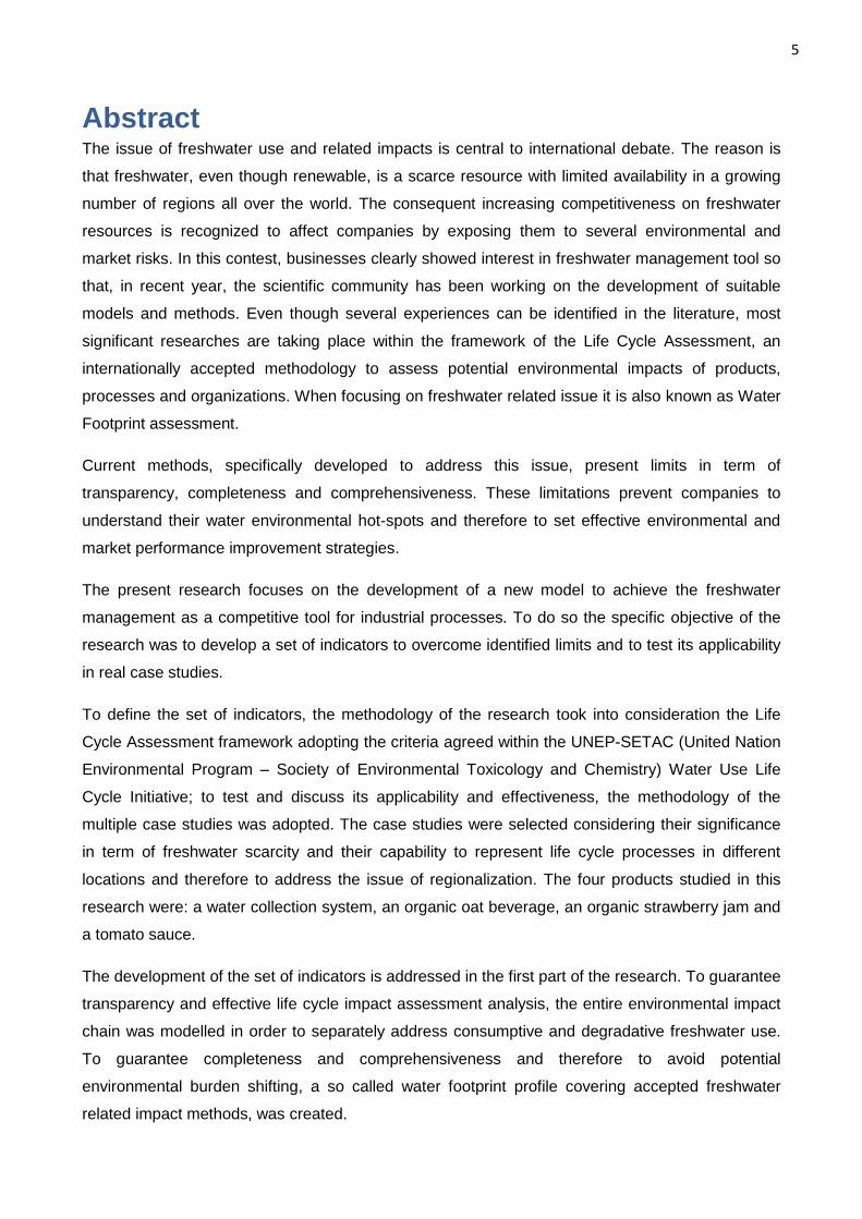
5
Abstract The issue of freshwater use and related impacts is central to international debate. The reason is
that freshwater, even though renewable, is a scarce resource with limited availability in a growing
number of regions all over the world. The consequent increasing competitiveness on freshwater
resources is recognized to affect companies by exposing them to several environmental and
market risks. In this contest, businesses clearly showed interest in freshwater management tool so
that, in recent year, the scientific community has been working on the development of suitable
models and methods. Even though several experiences can be identified in the literature, most
significant researches are taking place within the framework of the Life Cycle Assessment, an
internationally accepted methodology to assess potential environmental impacts of products,
processes and organizations. When focusing on freshwater related issue it is also known as Water
Footprint assessment.
Current methods, specifically developed to address this issue, present limits in term of
transparency, completeness and comprehensiveness. These limitations prevent companies to
understand their water environmental hot-spots and therefore to set effective environmental and
market performance improvement strategies.
The present research focuses on the development of a new model to achieve the freshwater
management as a competitive tool for industrial processes. To do so the specific objective of the
research was to develop a set of indicators to overcome identified limits and to test its applicability
in real case studies.
To define the set of indicators, the methodology of the research took into consideration the Life
Cycle Assessment framework adopting the criteria agreed within the UNEP-SETAC (United Nation
Environmental Program – Society of Environmental Toxicology and Chemistry) Water Use Life
Cycle Initiative; to test and discuss its applicability and effectiveness, the methodology of the
multiple case studies was adopted. The case studies were selected considering their significance
in term of freshwater scarcity and their capability to represent life cycle processes in different
locations and therefore to address the issue of regionalization. The four products studied in this
research were: a water collection system, an organic oat beverage, an organic strawberry jam and
a tomato sauce.
The development of the set of indicators is addressed in the first part of the research. To guarantee
transparency and effective life cycle impact assessment analysis, the entire environmental impact
chain was modelled in order to separately address consumptive and degradative freshwater use.
To guarantee completeness and comprehensiveness and therefore to avoid potential
environmental burden shifting, a so called water footprint profile covering accepted freshwater
related impact methods, was created.
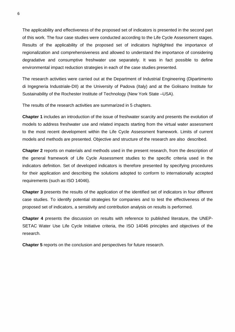
6
The applicability and effectiveness of the proposed set of indicators is presented in the second part
of this work. The four case studies were conducted according to the Life Cycle Assessment stages.
Results of the applicability of the proposed set of indicators highlighted the importance of
regionalization and comprehensiveness and allowed to understand the importance of considering
degradative and consumptive freshwater use separately. It was in fact possible to define
environmental impact reduction strategies in each of the case studies presented.
The research activities were carried out at the Department of Industrial Engineering (Dipartimento
di Ingegneria Industriale-DII) at the University of Padova (Italy) and at the Golisano Institute for
Sustainability of the Rochester Institute of Technology (New York State –USA).
The results of the research activities are summarized in 5 chapters.
Chapter 1 includes an introduction of the issue of freshwater scarcity and presents the evolution of
models to address freshwater use and related impacts starting from the virtual water assessment
to the most recent development within the Life Cycle Assessment framework. Limits of current
models and methods are presented. Objective and structure of the research are also described.
Chapter 2 reports on materials and methods used in the present research, from the description of
the general framework of Life Cycle Assessment studies to the specific criteria used in the
indicators definition. Set of developed indicators is therefore presented by specifying procedures
for their application and describing the solutions adopted to conform to internationally accepted
requirements (such as ISO 14046).
Chapter 3 presents the results of the application of the identified set of indicators in four different
case studies. To identify potential strategies for companies and to test the effectiveness of the
proposed set of indicators, a sensitivity and contribution analysis on results is performed.
Chapter 4 presents the discussion on results with reference to published literature, the UNEP-
SETAC Water Use Life Cycle Initiative criteria, the ISO 14046 principles and objectives of the
research.
Chapter 5 reports on the conclusion and perspectives for future research.
7
Sommario Il tema dell’utilizzo dell’acqua dolce e degli impatti ambientali a esso associati sono centrali
all’interno del dibattitto internazionale. La ragione principale di quest’attenzione sta nel fatto che
l’acqua dolce, sebbene rinnovabile, sia presente in quantità limitata in un numero crescente di
regioni in tutto il pianeta. La conseguente accresciuta competizione per accedere a queste risorse
ha delle conseguenze concrete nel mondo delle imprese che si trovano a dover affrontare rischi di
natura ambientale e di mercato. In questo contesto, le aziende hanno mostrato un notevole
interesse verso gli strumenti per la gestione delle risorse idriche tanto da spingere la comunità
scientifica a moltiplicare gli sforzi per lo sviluppo di modelli e metodi adatti a garantire un utilizzo
più sostenibile di queste risorse. Sebbene si possano identificare diverse esperienze in letteratura,
gli sviluppi più significativi si sono avuti all’interno del contesto del Life Cycle Assessment, una
metodologia ampiamente accettata a livello internazionale per la quantificazione e valutazione dei
potenziali impatti ambientali di prodotti, processi ed organizzazioni. Quando ci si concentra sul
tema risorse idriche questo approccio è conosciuto con il nome di Water Footprint.
I modelli attuali, sviluppati nello specifico per trattare questa problematica, presentano dei limiti in
termini di trasparenza, completezza e comprensività. Queste limitazioni non consentono al mondo
delle imprese di comprendere i propri hot-spot ambientali riguardanti l’acqua e quindi di definire
opportune strategie ambientali e di mercato per il miglioramento della competitività di prodotti e
processi.
La presente ricerca si focalizza sulla creazione di un modello innovativo per tradurre la gestione
dell’acqua dolce in uno strumento per la competitività dei processi. L’obiettivo della ricerca è stato
quello di sviluppare un set di indicatori per superare i limiti evidenziati e quindi verificarne
l’applicabilità in dei casi di studio reali.
Nella definizione del set di indicatori, la metodologia della ricerca ha preso in considerazione il
contesto metodologico del Life Cycle Assessment (analisi di ciclo di vita) nel rispetto dei requisiti
presentati in materia da parte dell’ UNEP-SETAC Water Use Life Cycle Initiative. Per mettere alla
prova e discutere l’efficacia degli indicatori così creati è stata adottata la metodologia del caso di
studio multiplo. La scelta dei casi di studio è stata compiuta in funzione della loro criticità in tema di
utilizzo della risorsa idrica e in funzione della loro capacità di presentare processi localizzati in
regioni con condizioni climatiche e di disponibilità di acqua dolce differenti. I quattro prodotti scelti
per questa ricerca sono: un sistema di collettamento e recupero delle acque piovane, una bevanda
a base di avena biologica, una marmellata di fragole biologiche ed una salsa di pomodoro per il
condimento della pasta.
Lo sviluppo del set di indicatori è affrontato nella prima parte della ricerca. Per garantire la
trasparenza e l’efficacia dell’analisi degli impatti di ciclo di vita, l’intera catena di valutazione
8
ambientale è stata modellata al fine di quantificare separatamente gli effetti del consumo e dell’uso
degradativo dell’acqua dolce. Per garantire completezza e comprensività, così da evitare il
problema del burden-shifting, è stato sviluppato un Water Footprint Profile che considera i metodi
più accettati e diffusi nella quantificazione degli impatti ambientali relativi all’acqua dolce.
L’applicabilità ed efficacia del set di indicatori è presentata nella seconda parte della ricerca. I
quattro casi di studio sono stati condotti nel rispetto dei requisiti del Life Cycle Assessment. I
risultati dell’applicabilità del set di indicatori proposto, ha messo in luce l’importanza della
regionalizzazione e della comprensività e hanno permesso di capire l’importanza di valutare in
modo separato il consumo e l’uso degradativo dell’acqua dolce. In ogni caso di studio è stato
possibile determinare una strategia per la riduzione dei consumi di acqua dolce.
Le attività di ricerca sono state condotte presso il Dipartimento di Ingegneria Industriale
dell’Università di Padova (Italia) e presso il Golisano Institute for Sustainability del Rochester
Institute of Technology (New York State –USA).
I risultati della ricerca sono presentati in cinque capitoli.
Capitolo 1: include un’introduzione al problema della scarsità d’acqua dolce e presenta
l’evoluzione dei modelli per considerare l’utilizzo di acqua dolce ed i relativi impatti a partire dal
concetto di virtual water fino alle recenti evoluzioni all’interno del contesto del Life Cycle
Assessment. Sono quindi chiariti i limiti dei modelli e metodi attuali. Infine sono presentati gli
obiettivi e la metodologia di ricerca.
Capitolo 2: riferisce in merito ai materiali e metodi adottati dalla ricerca, dalla descrizione del
modello generale degli studi di Life Cycle Assessment fino ai criteri considerati per la definizione
degli indicatori. Questi sono poi presentati specificandone procedure applicative e soluzioni di
conformità agli standard accettati a livello internazionale tra cui l’ISO 14046.
Capitolo 3: presenta i risultati dell’applicazione del set di indicatori in quattro diversi casi di studio.
Per la definizione delle strategie di riduzione degli impatti sull’acqua dolce e per verificare
l’efficacia degli indicatori, è stata condotta un’analisi di sensitività e contribuzione specifica in ogni
caso di studio.
Capitolo 4: presenta le discussioni dei risultati ottenutici con riferimento ai modelli pubblicati in
letteratura, ai criteri dell’ UNEP-SETAC Water Use Life Cycle Initiative, dei principi della norma ISO
14046 e degli obiettivi della ricerca.
Capitolo 5 presenta le conclusioni e le indicazioni per futuri sviluppi della ricerca.
9
INDEX 1. Introduction ............................................................................................................................ 13
1.1. Global freshwater resources: the issue of availability ...................................................... 13
1.2. Freshwater use and company competitiveness............................................................... 15
1.3. Impacts related to water and current assessment models ............................................... 17
1.3.1 Water quality degradation: impacts and assessment models ................................... 18
1.3.2 Water availability: impacts and assessment models ................................................ 19
1.3.2.1 The Virtual water model ........................................................................................... 20
1.3.2.2 The Water Footprint Accounting model ................................................................ 21
1.3.3.3 The Water Footprint Sustainability model ................................................................ 24
1.3.2.4 The Water Footprint within Life Cycle Assessment model .................................... 27
1.4. Research needs and limits of current models ................................................................. 34
1.5. Research objectives........................................................................................................ 37
2. Materials and methods ........................................................................................................... 38
2.1. Research structure ......................................................................................................... 38
2.2. General methodological framework: Water Footprint study ............................................. 38
2.3. Criteria used in the definition of the set of water use indicators ....................................... 41
2.4. Definition of the set of water use indicators ..................................................................... 42
2.4.1 Inventory indicators ....................................................................................................... 42
2.4.2 Mid-point indicators ....................................................................................................... 45
2.4.3 End-point indicators ...................................................................................................... 48
2.5. Applicability and effectiveness: methodological approach ............................................... 49
3. Results: applicability and effectiveness .................................................................................. 50
3.1. Case study 1: Water collection system ........................................................................... 50
3.1.1 Goals and scope definition ....................................................................................... 50
3.1.2 Life Cycle Inventory ................................................................................................. 53
3.1.2.1 HDPE selection .................................................................................................... 53
3.1.2.2 HDPE Recycling ................................................................................................... 54
3.1.2.3 Injection molding ........................................................................................................ 55
3.1.3 Life Cycle Inventory Analysis ................................................................................... 55
10
3.1.4 Life Cycle Impact Assessment ................................................................................. 57
3.1.4.1 Water Stress indicator .......................................................................................... 57
3.1.4.2 Degradation profile ............................................................................................... 59
3.1.4.3 End-point impacts on Resources .......................................................................... 60
3.1.5 Life Cycle Interpretation ........................................................................................... 63
3.2. Case study 2: Organic oat beverage ............................................................................... 68
3.2.1 Goals and scope definition ....................................................................................... 68
4.2.2 Life Cycle Inventory ................................................................................................. 72
4.2.2.1 Organic Oat .......................................................................................................... 72
3.2.2.3 Sunflower ................................................................................................................... 74
3.2.2.4 Marine salt ................................................................................................................. 75
3.2.2.5 Organic Oat production .............................................................................................. 75
3.2.2.6 Sunflower oil production ............................................................................................. 75
3.2.2.7 Raw materials transport ............................................................................................. 75
3.2.2.8 Primary packaging materials ...................................................................................... 76
3.2.2.9 Production .................................................................................................................. 76
3.2.2.10 End of life ................................................................................................................. 77
3.2.3 Life Cycle Inventory Analysis ................................................................................... 78
3.2.4 Life Cycle Impact Assessment ................................................................................. 81
3.2.4.1 Water Stress indicator .......................................................................................... 82
3.2.4.2 Degradation profile ............................................................................................... 83
3.2.4.3 End-point impacts on Resources .......................................................................... 84
3.2.4 Life Cycle Interpretation ........................................................................................... 89
3.3. Case study 3: Organic strawberry Jam ........................................................................... 91
3.3.1 Goals and scope definition ....................................................................................... 91
3.3.2 Life Cycle Inventory ................................................................................................. 94
3.3.2.1 Strawberries ......................................................................................................... 95
3.3.2.3 Apple .......................................................................................................................... 96
3.3.2.4 Frozen strawberry ...................................................................................................... 97
3.3.2.5 Apple juice concentrated ............................................................................................ 97
11
3.3.2.6 Packaging .................................................................................................................. 98
3.3.2.7 Transport ................................................................................................................... 98
3.3.2.8 Production .................................................................................................................. 98
3.3.2.9 End of life ................................................................................................................... 99
3.3.3 Life Cycle Inventory Analysis ................................................................................... 99
3.3.4 Life Cycle Impact Assessment ............................................................................... 102
3.3.4.1 Water Stress indicator ........................................................................................ 103
3.3.4.2 Degradation profile ............................................................................................. 104
3.3.4.3 End-point impacts on Resources ........................................................................ 105
3.3.5 Life Cycle Interpretation ......................................................................................... 110
3.4. Case study 4: Tomato Basil Sauce ............................................................................... 112
3.4.1 Goals and scope definition ..................................................................................... 112
3.4.2 Life Cycle Inventory ............................................................................................... 115
3.4.2.1 Tomato ............................................................................................................... 116
3.4.2.2 Olive Oil, Soybean Oil and Sugar ....................................................................... 118
3.4.2.3 Tomato processing ................................................................................................... 119
3.4.2.4 Production ................................................................................................................ 119
3.4.2.5 Use of Francesco Rinaldi Tomato Basil .................................................................... 120
3.4.2.6 End of life ................................................................................................................. 120
3.4.3 Life Cycle Inventory Analysis ................................................................................. 121
3.4.4 Life Cycle Impact Assessment ............................................................................... 125
3.4.4.1 Water Stress Indicator ........................................................................................ 125
3.4.4.2 Degradation profile ............................................................................................. 126
3.4.4.3 End-point impacts on Resources ........................................................................ 128
3.4.5 Life Cycle Interpretation ......................................................................................... 131
4. Discussions.......................................................................................................................... 135
5. Conclusions and future perspectives ................................................................................... 144
6. References .......................................................................................................................... 151
List of Figures ............................................................................................................................. 158
List of Tables .............................................................................................................................. 159

12
Papers and conferences during PhD........................................................................................... 162
ANNEX A: water collection system quality parameters inventory ................................................ 164
ANNEX B: organic oat beverage quality parameters inventory.................................................... 182
ANNEX C: organic strawberry jam quality parameters inventory ................................................. 215
ANNEX D: tomato sauce quality parameters inventory ............................................................... 239
Deposited on the 31st of Jannuary 2014
13
1. Introduction
1.1. Global freshwater resources: the issue of availability
Water is recognized to be one of the most important natural resources to support life of humans
and ecosystems (Falkenmark and Folke, 2003). Its availability is critical to meet basic human
needs and support economic and cultural activities such as agriculture, food, energy and industrial
production, basic sanitation, household uses or sewage water transport (WWAP, 2012). However,
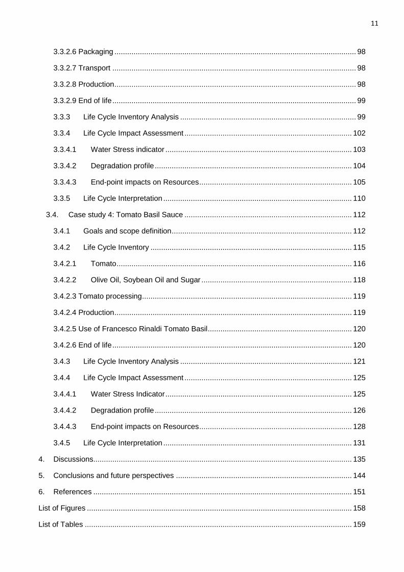
even if water is a renewable resource, it is a limited one. In fact the 70% of planet earth is covered
with water but only the 0,01% is freshwater directly available for the above mentioned human
needs and for life of ecosystems (Revenga et al., 2000) (Fig.1).
Figure 1-1 Global freshwater availability (UNEP, 2008)
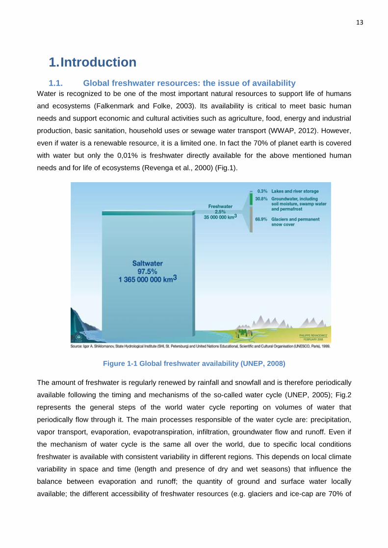
The amount of freshwater is regularly renewed by rainfall and snowfall and is therefore periodically
available following the timing and mechanisms of the so-called water cycle (UNEP, 2005); Fig.2
represents the general steps of the world water cycle reporting on volumes of water that
periodically flow through it. The main processes responsible of the water cycle are: precipitation,
vapor transport, evaporation, evapotranspiration, infiltration, groundwater flow and runoff. Even if
the mechanism of water cycle is the same all over the world, due to specific local conditions
freshwater is available with consistent variability in different regions. This depends on local climate
variability in space and time (length and presence of dry and wet seasons) that influence the
balance between evaporation and runoff; the quantity of ground and surface water locally
available; the different accessibility of freshwater resources (e.g. glaciers and ice-cap are 70% of
14
the world’s freshwater but are located far from human habitation and are not readily accessible for
human use) (UNEP,2008).
Figure 1-2 The Hydrological water cycle (UNEP, 2008)
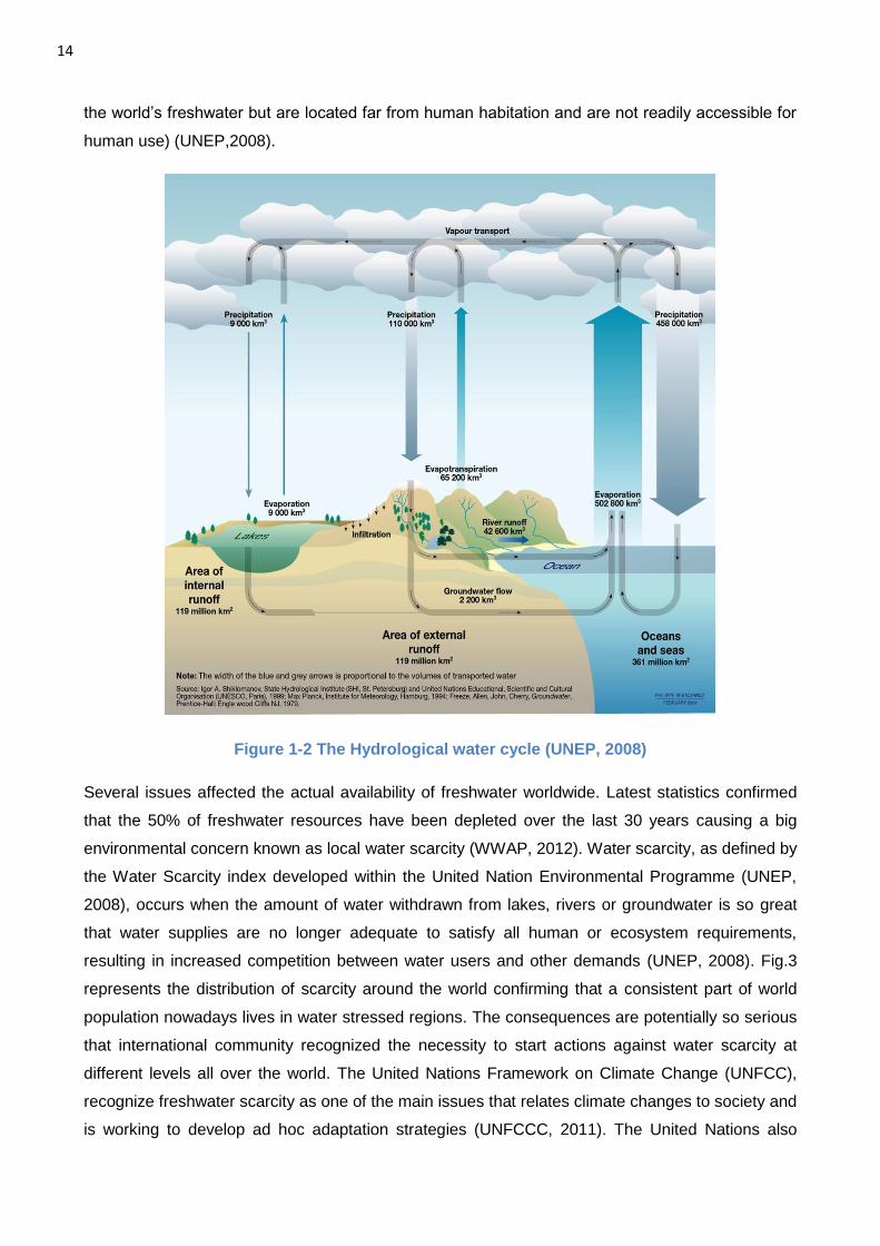
Several issues affected the actual availability of freshwater worldwide. Latest statistics confirmed
that the 50% of freshwater resources have been depleted over the last 30 years causing a big
environmental concern known as local water scarcity (WWAP, 2012). Water scarcity, as defined by
the Water Scarcity index developed within the United Nation Environmental Programme (UNEP,
2008), occurs when the amount of water withdrawn from lakes, rivers or groundwater is so great
that water supplies are no longer adequate to satisfy all human or ecosystem requirements,
resulting in increased competition between water users and other demands (UNEP, 2008). Fig.3
represents the distribution of scarcity around the world confirming that a consistent part of world
population nowadays lives in water stressed regions. The consequences are potentially so serious
that international community recognized the necessity to start actions against water scarcity at
different levels all over the world. The United Nations Framework on Climate Change (UNFCC),
recognize freshwater scarcity as one of the main issues that relates climate changes to society and
is working to develop ad hoc adaptation strategies (UNFCCC, 2011). The United Nations also
15
included water accessibility as one of the Millennium Goals to solve poverty (UN, 2013). The
European Union in 2007 launched the EU water policy in order to ensure access to good quality
water in sufficient quantity for all Europeans, and to ensure the good status of all water bodies
across Europe (EC, 2007). Four main drivers are recognized to have significantly influenced this
issue over time: climate changes, population, urbanization growth and economic development
(WWAP, 2012). The increase of greenhouse gases emission and related climate changes are
affecting the mechanism of hydrological cycles resulting in different local evapotranspiration, soil
moisture, and run-off flow (Bates et al., 2008). Increase of world population results in bigger water
needs for several human uses both from a quantity and improved quality perspective. In the last
century, the world population has tripled and it is expected to rise from the present 6.5 billion to 8.9
billion by 2050, before levelling off; water use has been growing at more than twice the rate of
population increase in the last century resulting in an increasing number of regions that are
chronically short of water. By 2025, 1.8 billion people will be living in countries or regions with
absolute water scarcity, and two-thirds of the world population could be under conditions of water
stress. The situation will be exacerbated as rapidly growing urban areas place heavy pressure on
local water resources (WWAP, 2012) by focusing the demand for water among an ever more
concentrated population and changing the way inland water can be managed and reaches the
gouge. Economic development results in an increased water demand for energy, food and
industrial production that are also known as the main cause for water quality degradation (WWAP,
2012). Another consequence of these drivers is increase competitiveness for water.
Figure 1-3 Water Scarcity Index (UNEP, 2008)
1.2. Freshwater use and company competitiveness
Water is withdrawn from natural environment for several uses that are generally related to five
different categories. The first in term of water consumption is food and agriculture, that is
16
responsible for the 70% of the overall withdrawn water. Crops production followed by livestock
requires huge amount of water and contributes to water quality degradation and therefore to local
water scarcity (FAO, 2009). The greatest water consumption related to this category results from
evaporation and product incorporation of freshwater used for crop irrigation; trends confirms the
importance of this resource also for the future with a growing demand related to the increase
needs of world population (WWAP, 2009; Brunisma, 2009). Another significant water user category
is the human settlements one. This category covers almost the 10% of overall global water
withdrawal (WWAP, 2009) and more often results in over-abstraction leading to higher resource
access competition and challenging ecosystem functioning. Moreover when groundwater
withdrawal is concerned, other related environmental problems shall be considered such as falling
water tables, water quality degradation and land subsidence. Another significant consequence of
human settlements, is the pressure derived from wastewater and water pollution. Recent statistics
confirmed that over the 80% of waste water worldwide is not collected or treated, resulting in high
level of pollution (Corcoran et al., 2010). This situation is especially representative of emerging
countries were water is recognized to be even more scarce (WWAP, 2012). Another user category
to be considered is the ecosystem. This covers a central role in a correct and sustainable
functioning of the hydrological cycle. Recent rethinking of the contribution of ecosystems to water
availability shifts its role from a water demand subject to a water service supplier (WWAP, 2012).
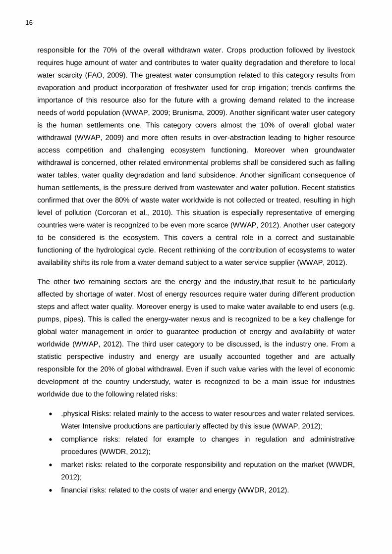
The other two remaining sectors are the energy and the industry,that result to be particularly
affected by shortage of water. Most of energy resources require water during different production
steps and affect water quality. Moreover energy is used to make water available to end users (e.g.
pumps, pipes). This is called the energy-water nexus and is recognized to be a key challenge for
global water management in order to guarantee production of energy and availability of water
worldwide (WWAP, 2012). The third user category to be discussed, is the industry one. From a
statistic perspective industry and energy are usually accounted together and are actually
responsible for the 20% of global withdrawal. Even if such value varies with the level of economic
development of the country understudy, water is recognized to be a main issue for industries
worldwide due to the following related risks:
.physical Risks: related mainly to the access to water resources and water related services.
Water Intensive productions are particularly affected by this issue (WWAP, 2012);
compliance risks: related for example to changes in regulation and administrative
procedures (WWDR, 2012);
market risks: related to the corporate responsibility and reputation on the market (WWDR,
2012);
financial risks: related to the costs of water and energy (WWDR, 2012).
17
When focusing on industries another key issue is recognized to be water quality: different
industries have different water quality needs and differently affect quality of water bodies
(UNEP, 2007). If water resources are not well managed and treated; impacts on humans and
ecosystems can be identified and shall be treated (Ridoutt and Pfister, 2010). The global
business community increasingly recognizes the water challenge, and clearly asked for
guidance, tools, standards and schemes to enable more sustainable practices and to
understand how to reduce impacts on water resources (WBCSD; 2010)
1.3. Impacts related to water and current assessment models
It is worldwide agreed that the sustainable management of freshwater resources should include a
deeper comprehension of human and ecosystems interactions through the analysis of water
related impacts (WWAP, 2012). This analysis shall adopt several dimensions:
a regional one, to understand the effects of freshwater use on local environment (e.g.
basin or watershed level) (Ridoutt and Pfister, 2010);
an international and global dimension: that is described through climate change, trans-
boundary basins, global trade and international investment protection, and equity issues
(Hoekstra, 2011);
a so-called life cycle dimension: to consider all the processes that take place along the
value chain of human related activities (from extraction of raw materials to waste
management) and the potential environmental impacts related to water (Lundqvist et al.,
2008).
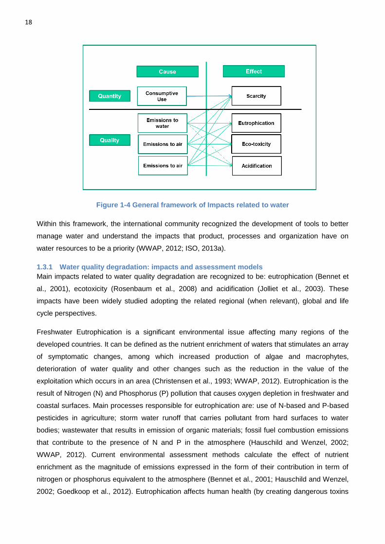
This last dimension proved to be particularly important as 90% of freshwater use is associated with
the life cycles of products and services (Ridoutt and Pfister, 2010). Focusing on environmental
impacts related to water, two big different families can be identified: impacts related to quantity,
also referred as availability, and impacts related to quality (WWAP, 2009) (Figure 4). If the latter
have been widely addressed within several methods by the scientific community, the former, with
the emerging issue of water availability and scarcity, only recently became central to scientific
debate (Kounina et al.2013). Figure 4 represents the two families and their interactions, showing
main causes of impacts and related consequences. In particular, it has to be noticed that
availability results to be influenced both from quantitative use and water quality degradation.
18
Figure 1-4 General framework of Impacts related to water
Within this framework, the international community recognized the development of tools to better
manage water and understand the impacts that product, processes and organization have on
water resources to be a priority (WWAP, 2012; ISO, 2013a).
1.3.1 Water quality degradation: impacts and assessment models
Main impacts related to water quality degradation are recognized to be: eutrophication (Bennet et
al., 2001), ecotoxicity (Rosenbaum et al., 2008) and acidification (Jolliet et al., 2003). These
impacts have been widely studied adopting the related regional (when relevant), global and life
cycle perspectives.
Freshwater Eutrophication is a significant environmental issue affecting many regions of the
developed countries. It can be defined as the nutrient enrichment of waters that stimulates an array
of symptomatic changes, among which increased production of algae and macrophytes,
deterioration of water quality and other changes such as the reduction in the value of the
exploitation which occurs in an area (Christensen et al., 1993; WWAP, 2012). Eutrophication is the
result of Nitrogen (N) and Phosphorus (P) pollution that causes oxygen depletion in freshwater and
coastal surfaces. Main processes responsible for eutrophication are: use of N-based and P-based
pesticides in agriculture; storm water runoff that carries pollutant from hard surfaces to water
bodies; wastewater that results in emission of organic materials; fossil fuel combustion emissions
that contribute to the presence of N and P in the atmosphere (Hauschild and Wenzel, 2002;
WWAP, 2012). Current environmental assessment methods calculate the effect of nutrient
enrichment as the magnitude of emissions expressed in the form of their contribution in term of
nitrogen or phosphorus equivalent to the atmosphere (Bennet et al., 2001; Hauschild and Wenzel,
2002; Goedkoop et al., 2012). Eutrophication affects human health (by creating dangerous toxins
19
and compounds-drinkable water) and ecosystems (such as the so-called death zones and toxins
that enter the food-chain).
Freshwater eco-toxicity refers to the spectrum of effects and impact mechanisms that emissions of
toxic substances have on the environment (Hauschild and Wenzel, 2002; Rosenbaum et al., 2008).
A few important examples are emissions of strongly toxic metals, persistent organic substances or
organic substances. Current methods measure eco-toxicity as the magnitude of the effect on the
functioning of ecosystems. Ecotoxic substances are classified in function of their persistence,
ability to bio accumulate, quantity and human and ecosystem exposure (Hauschild and Wenzel,
2002).
Freshwater acidification is an environmental concern that assumed significant dimension in the last
decades and can be defined as an impact which leads to a fall in the system’s acid neutralizing
capacity (ANC) (De Vries and Breeuwsma, 1987) such as a reduction in substances able to
neutralize hydrogen ions. It is an effect of emissions to the atmosphere and consequent deposition
on water of sulfur dioxide (SO2) and nitrogen oxides (NOx). The main process responsible for the
emission of such compounds is the combustion of fossil fuels (e.g. hard coal) for the production of
energy. Such substances have a limited lifespan, typically of the order of days, therefore their
influence is regional with limited extent from the point source of emissions (Hauschild and Wenzel,
2002). Acidifying substances have actual effects (immediate fall in the ecosystem ANC) and
potential effects (possibility of subsequent release to the ecosystem and subsequent decrease of
ANC). Current methods measure acidification as the sum of this two contribution (Hauschild and
Wenzel, 2002; and Jolliet et al., 2003). Acidification harms ecosystems (such as life of fishes) and
human health (in the form of fine sulfate and nitrate particles that can be transported long
distances by winds and inhaled deep into people’s lungs).
Another consequence of water quality degradation is a reduction of freshwater availability for
humans and ecosystems use (Boulay et al., 2011) (Figure 1-4). This issue will be discussed within
the chapter 1.3.2 that presents the evolution of methods to assess environmental impacts of
freshwater use on water availability.
1.3.2 Water availability: impacts and assessment models
Only in recent years the issue of water availability has become central to international debate
calling for the scientific community to develop methods to better manage water resources and to
understand consequences of freshwater use by human beings (WWAP, 2012). Shortage of water
in fact can result in several impacts that go from humans’ malnutrition to changes in ecosystems
quality.
In this paragraph, the main experiences related to understanding the environmental consequences
of freshwater use are presented: from virtual water, firstly introduced by Allan et al. 1998, to the
20
water footprint concept introduced by Hoekstra et al. 2011, to the recent development within the
framework of Life Cycle Assessment community (Bayart et al. 2010; ISO, 2013a).
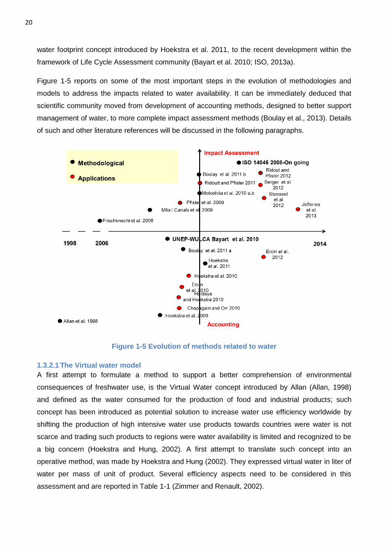
Figure 1-5 reports on some of the most important steps in the evolution of methodologies and
models to address the impacts related to water availability. It can be immediately deduced that
scientific community moved from development of accounting methods, designed to better support
management of water, to more complete impact assessment methods (Boulay et al., 2013). Details
of such and other literature references will be discussed in the following paragraphs.
Figure 1-5 Evolution of methods related to water
1.3.2.1 The Virtual water model
A first attempt to formulate a method to support a better comprehension of environmental
consequences of freshwater use, is the Virtual Water concept introduced by Allan (Allan, 1998)
and defined as the water consumed for the production of food and industrial products; such
concept has been introduced as potential solution to increase water use efficiency worldwide by
shifting the production of high intensive water use products towards countries were water is not
scarce and trading such products to regions were water availability is limited and recognized to be
a big concern (Hoekstra and Hung, 2002). A first attempt to translate such concept into an
operative method, was made by Hoekstra and Hung (2002). They expressed virtual water in liter of
water per mass of unit of product. Several efficiency aspects need to be considered in this
assessment and are reported in Table 1-1 (Zimmer and Renault, 2002).
21
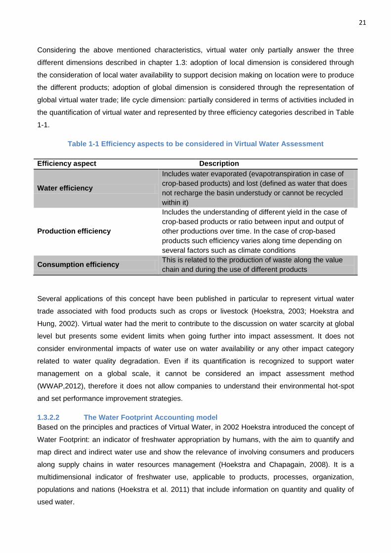
Considering the above mentioned characteristics, virtual water only partially answer the three
different dimensions described in chapter 1.3: adoption of local dimension is considered through
the consideration of local water availability to support decision making on location were to produce
the different products; adoption of global dimension is considered through the representation of
global virtual water trade; life cycle dimension: partially considered in terms of activities included in
the quantification of virtual water and represented by three efficiency categories described in Table
1-1.
Table 1-1 Efficiency aspects to be considered in Virtual Water Assessment
Efficiency aspect Description
Water efficiency
Includes water evaporated (evapotranspiration in case of
crop-based products) and lost (defined as water that does
not recharge the basin understudy or cannot be recycled
within it)
Production efficiency
Includes the understanding of different yield in the case of
crop-based products or ratio between input and output of
other productions over time. In the case of crop-based
products such efficiency varies along time depending on
several factors such as climate conditions
Consumption efficiency This is related to the production of waste along the value
chain and during the use of different products
Several applications of this concept have been published in particular to represent virtual water
trade associated with food products such as crops or livestock (Hoekstra, 2003; Hoekstra and
Hung, 2002). Virtual water had the merit to contribute to the discussion on water scarcity at global
level but presents some evident limits when going further into impact assessment. It does not
consider environmental impacts of water use on water availability or any other impact category
related to water quality degradation. Even if its quantification is recognized to support water
management on a global scale, it cannot be considered an impact assessment method
(WWAP,2012), therefore it does not allow companies to understand their environmental hot-spot
and set performance improvement strategies.
1.3.2.2 The Water Footprint Accounting model
Based on the principles and practices of Virtual Water, in 2002 Hoekstra introduced the concept of
Water Footprint: an indicator of freshwater appropriation by humans, with the aim to quantify and
map direct and indirect water use and show the relevance of involving consumers and producers
along supply chains in water resources management (Hoekstra and Chapagain, 2008). It is a
multidimensional indicator of freshwater use, applicable to products, processes, organization,
populations and nations (Hoekstra et al. 2011) that include information on quantity and quality of
used water.
22
A first operative version of the method to determine Water Footprint has been published in 2009 by
Hoekstra et al. (2009). It is the first method related to water to fully adopt a life cycle dimension on
processes to be considered in the assessment (Boulay et al., 2013). The study consists of three
steps:
the goal and scope definition: in which the objective and the subject of the study are clearly
stated and determined;
the water footprint accounting: that consists in the assessment of the blue, green and grey
water footprint. The sum of these footprints is the final water footprint accounting result.
Three different chains of water use can be identified and contribute to the quantification of the total
water footprint of the object understudy:
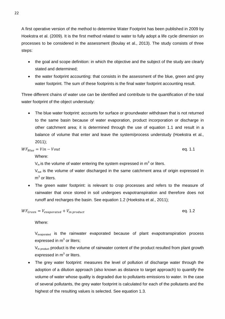
The blue water footprint: accounts for surface or groundwater withdrawn that is not returned
to the same basin because of water evaporation, product incorporation or discharge in
other catchment area; it is determined through the use of equation 1.1 and result in a
balance of volume that enter and leave the system/process understudy (Hoekstra et al.,
2011);
eq. 1.1
Where:
Vin is the volume of water entering the system expressed in m3 or liters.
Vout is the volume of water discharged in the same catchment area of origin expressed in
m3 or liters.
The green water footprint: is relevant to crop processes and refers to the measure of
rainwater that once stored in soil undergoes evapotranspiration and therefore does not
runoff and recharges the basin. See equation 1.2 (Hoekstra et al., 2011);
eq. 1.2
Where:
Vevaporated is the rainwater evaporated because of plant evapotranspiration process
expressed in m3 or liters;
Vin product product is the volume of rainwater content of the product resulted from plant growth
expressed in m3 or liters.
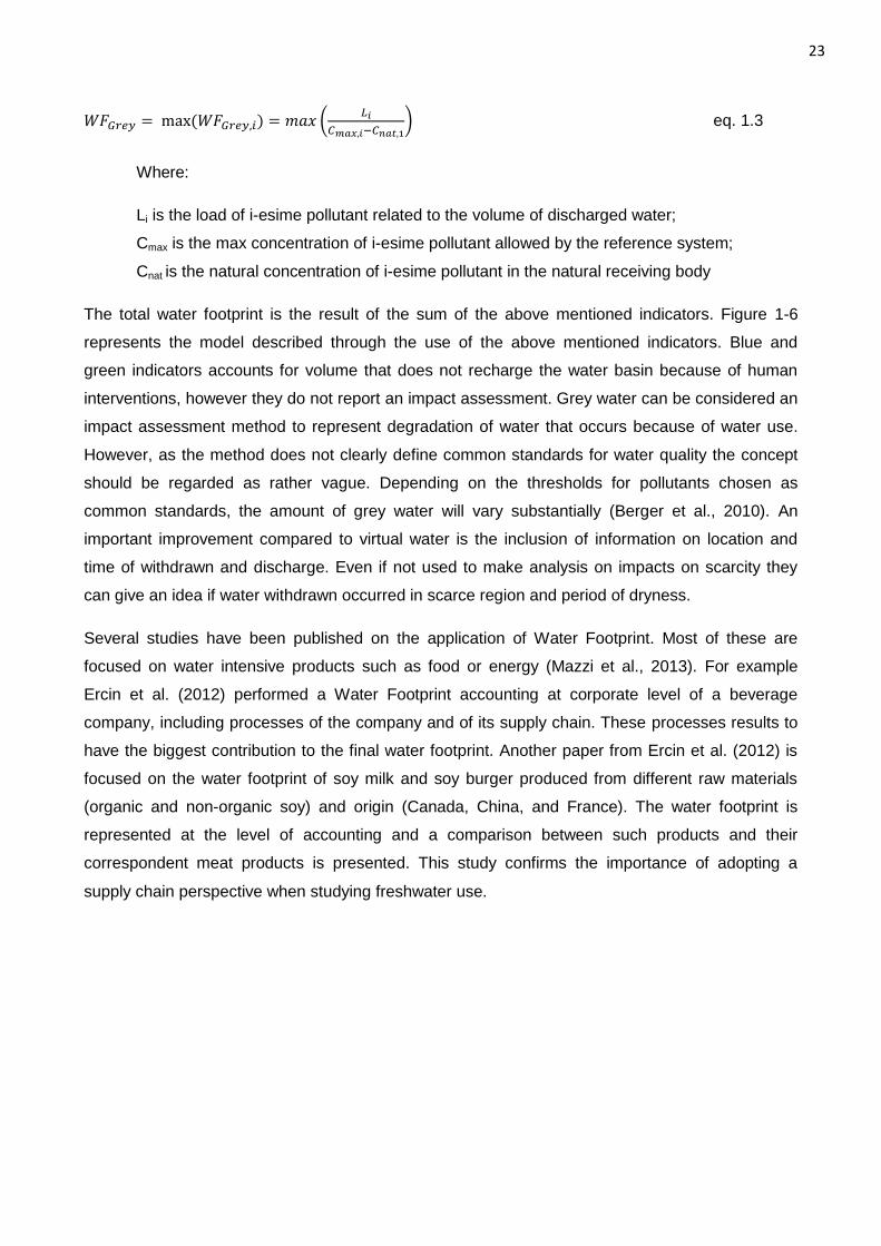
The grey water footprint: measures the level of pollution of discharge water through the
adoption of a dilution approach (also known as distance to target approach) to quantify the
volume of water whose quality is degraded due to pollutants emissions to water. In the case
of several pollutants, the grey water footprint is calculated for each of the pollutants and the
highest of the resulting values is selected. See equation 1.3.
23
(
) eq. 1.3
Where:
Li is the load of i-esime pollutant related to the volume of discharged water;
Cmax is the max concentration of i-esime pollutant allowed by the reference system;
Cnat is the natural concentration of i-esime pollutant in the natural receiving body
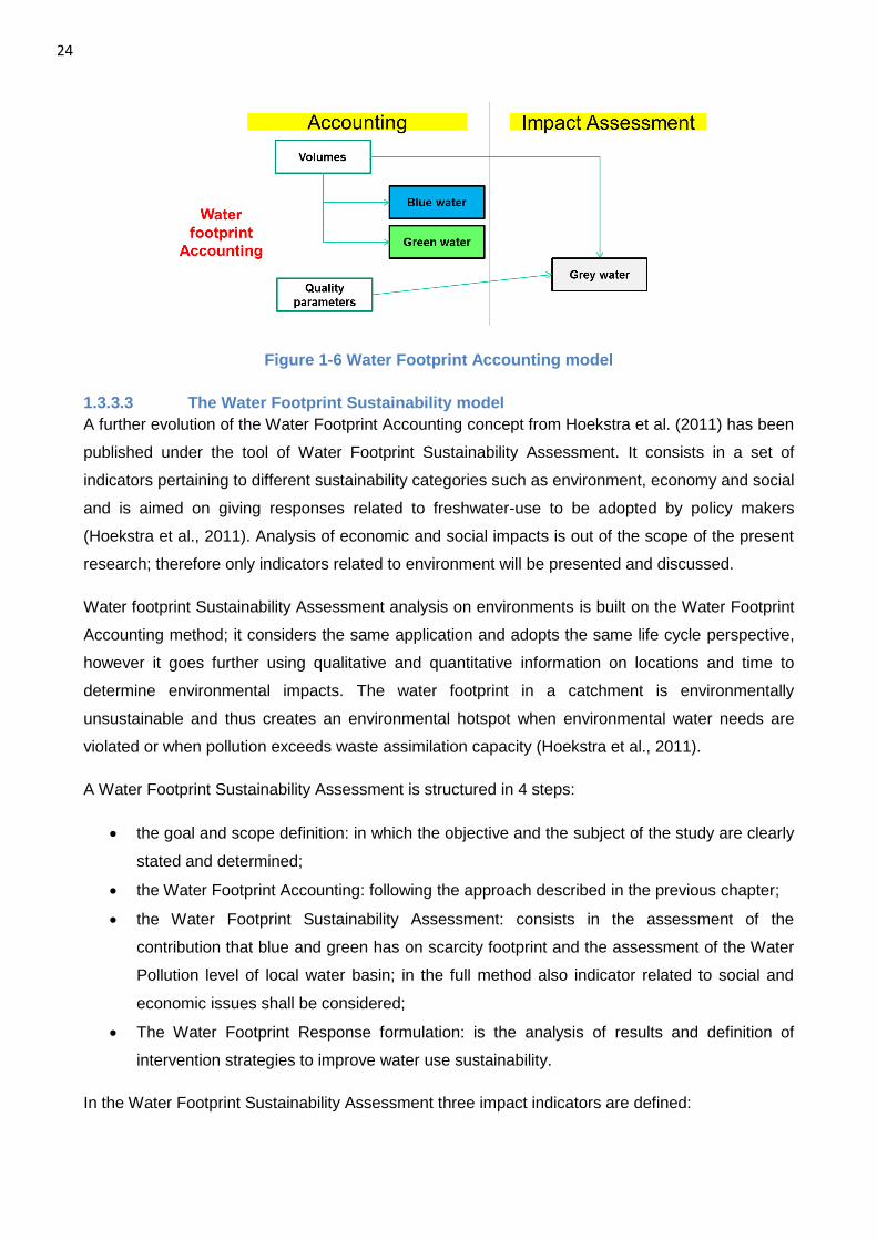
The total water footprint is the result of the sum of the above mentioned indicators. Figure 1-6
represents the model described through the use of the above mentioned indicators. Blue and
green indicators accounts for volume that does not recharge the water basin because of human
interventions, however they do not report an impact assessment. Grey water can be considered an
impact assessment method to represent degradation of water that occurs because of water use.
However, as the method does not clearly define common standards for water quality the concept
should be regarded as rather vague. Depending on the thresholds for pollutants chosen as
common standards, the amount of grey water will vary substantially (Berger et al., 2010). An
important improvement compared to virtual water is the inclusion of information on location and
time of withdrawn and discharge. Even if not used to make analysis on impacts on scarcity they
can give an idea if water withdrawn occurred in scarce region and period of dryness.
Several studies have been published on the application of Water Footprint. Most of these are
focused on water intensive products such as food or energy (Mazzi et al., 2013). For example
Ercin et al. (2012) performed a Water Footprint accounting at corporate level of a beverage
company, including processes of the company and of its supply chain. These processes results to
have the biggest contribution to the final water footprint. Another paper from Ercin et al. (2012) is
focused on the water footprint of soy milk and soy burger produced from different raw materials
(organic and non-organic soy) and origin (Canada, China, and France). The water footprint is
represented at the level of accounting and a comparison between such products and their
correspondent meat products is presented. This study confirms the importance of adopting a
supply chain perspective when studying freshwater use.
24
Figure 1-6 Water Footprint Accounting model
1.3.3.3 The Water Footprint Sustainability model
A further evolution of the Water Footprint Accounting concept from Hoekstra et al. (2011) has been
published under the tool of Water Footprint Sustainability Assessment. It consists in a set of
indicators pertaining to different sustainability categories such as environment, economy and social
and is aimed on giving responses related to freshwater-use to be adopted by policy makers
(Hoekstra et al., 2011). Analysis of economic and social impacts is out of the scope of the present
research; therefore only indicators related to environment will be presented and discussed.
Water footprint Sustainability Assessment analysis on environments is built on the Water Footprint
Accounting method; it considers the same application and adopts the same life cycle perspective,
however it goes further using qualitative and quantitative information on locations and time to
determine environmental impacts. The water footprint in a catchment is environmentally
unsustainable and thus creates an environmental hotspot when environmental water needs are
violated or when pollution exceeds waste assimilation capacity (Hoekstra et al., 2011).
A Water Footprint Sustainability Assessment is structured in 4 steps:
the goal and scope definition: in which the objective and the subject of the study are clearly
stated and determined;
the Water Footprint Accounting: following the approach described in the previous chapter;
the Water Footprint Sustainability Assessment: consists in the assessment of the
contribution that blue and green has on scarcity footprint and the assessment of the Water
Pollution level of local water basin; in the full method also indicator related to social and
economic issues shall be considered;
The Water Footprint Response formulation: is the analysis of results and definition of
intervention strategies to improve water use sustainability.
In the Water Footprint Sustainability Assessment three impact indicators are defined:
25
The blue water scarcity footprint (WSblue): is the measure of the blue water compared to the
blue water availability described through equation 1.4 in function of location x and time t
(Hoekstra et al., 2011);
eq. 1.4
Where:
WFBlue (x,t) is the Blue Water footprint of the product/process/organization under study
related to location x and time t expressed in m3/time or liters/time;
Rnat (x, t) is the natural run-off in location x during the t time expressed in m3/time or
liters/time;
EFR (x,t) is the environmental flow requirement expressed in m3/time or liters/time also
defined as quantity and timing of water flows required to sustain freshwater and estuarine
ecosystems and the human livelihoods and well-being that depend on these ecosystems
(Hoekstra et al., 2011).
The Blue Water Scarcity is expressed in %. Values over 100% mean an unsustainable use
of water resources;
The green scarcity footprint: is the measure of green water that is used with a rate over the
local green water availability (Hoekstra et al., 2011). A green water scarcity of 100 per cent
means that the available green water has been fully consumed. Scarcity values beyond 100
per cent are not sustainable;
eq. 1.5
Where:
WFGreen (x,t) is the Green Water footprint of the product/process/organization under study
related to location x and time t expressed in m3/time or liters/time;
ETGreen (x, t) is the total evapotranspiration of rainwater from land in location x during the t
time expressed in m3/time or liters/time;
ETenv (x, t) is the evapotranspiration from land reserved for natural vegetation in location x
during the t time expressed in m3/time or liters/time;
ETunprod (x, t) is the evapotranspiration from land that cannot be made productive in location
x during the t time expressed in m3/time or liters/time;
The Water Pollution level (WPL): measure the level of pollution of discharge water in
location x during t time. When the water pollution level exceeds 100 per cent, ambient
water quality standards are violated. See equation 1.6
eq.1.6
Where:
26
WFGrey (x,t) is the Grey Water footprint of the product/process/organization under study
related to location x and time t expressed in m3/time or liters/time;
Ract (x, t) is the actual run-off in location x during the t time expressed in m3/time or
liters/time;
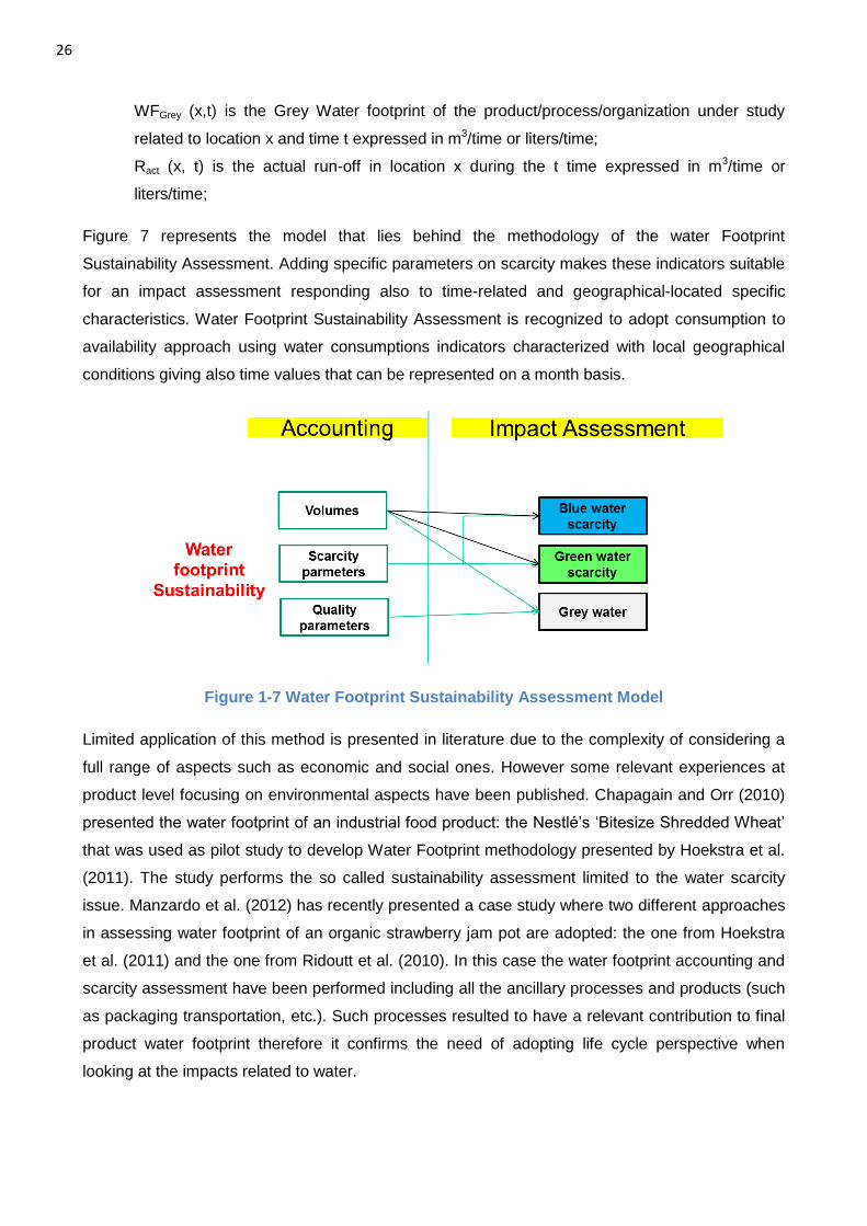
Figure 7 represents the model that lies behind the methodology of the water Footprint
Sustainability Assessment. Adding specific parameters on scarcity makes these indicators suitable
for an impact assessment responding also to time-related and geographical-located specific
characteristics. Water Footprint Sustainability Assessment is recognized to adopt consumption to
availability approach using water consumptions indicators characterized with local geographical
conditions giving also time values that can be represented on a month basis.
Figure 1-7 Water Footprint Sustainability Assessment Model
Limited application of this method is presented in literature due to the complexity of considering a
full range of aspects such as economic and social ones. However some relevant experiences at
product level focusing on environmental aspects have been published. Chapagain and Orr (2010)
presented the water footprint of an industrial food product: the Nestlé’s ‘Bitesize Shredded Wheat’
that was used as pilot study to develop Water Footprint methodology presented by Hoekstra et al.
(2011). The study performs the so called sustainability assessment limited to the water scarcity
issue. Manzardo et al. (2012) has recently presented a case study where two different approaches
in assessing water footprint of an organic strawberry jam pot are adopted: the one from Hoekstra
et al. (2011) and the one from Ridoutt et al. (2010). In this case the water footprint accounting and
scarcity assessment have been performed including all the ancillary processes and products (such
as packaging transportation, etc.). Such processes resulted to have a relevant contribution to final
product water footprint therefore it confirms the need of adopting life cycle perspective when
looking at the impacts related to water.
27
The Water Footprint Sustainability assessment has the merit to advance the analysis toward the
assessment of impacts related to water. However it presents some limits: it does not assess the
comprehensive spectrum of environmental impacts related to water such as eutrophication, eco-
toxicity and acidification (ISO, 2013a; Ridoutt et al., 2010; Jeswani and Azapagic, 2011); the WPL
answer needs to have a measure of degradation footprint, however it does not represent
environmental impacts such as scarcity, moreover it does not give guidance on standard
parameters to be used as reference for the assessment, therefore results are usually subjective
(Jeswani and Azapagic, 2011); even if the environmental relevance of the green water scarcity
footprint is not confirmed, It may be relevant in some cases when land use change occurred (ISO,
2013b), however no methods are able to address these changes therefore green water is usually
not well accepted in the literature (ISO, 2013a).
1.3.2.4 The Water Footprint within Life Cycle Assessment model
Latest development of the Water Footprint concept took place within the Life Cycle Assessment
framework (ISO, 2006; 2013a). LCA methodology, established in the early sixties in order to study
the energetic burdens associated with certain industrial products (Hunt and Franklin 1996), has
evolved over the years to be today the most comprehensive method of potential environmental
impacts assessment of products, services, process or organization adopting a life cycle dimension
(ISO 2006). Environmental impact assessment methods developed to be applied within LCA ,only
partially addressed water issues in the past, focusing only on water quality degradation indexes
such as eco-toxicity (Hauschild and Wenzel, 2002; Rosenbaum et al., 2008), eutrophication
(Bennet et al., 2001; Hauschild and Wenzel, 2002; Goedkoop et al., 2012) and acidification
(Hauschild and Wenzel, 2002; and Jolliet et al., 2003). The introduction of Water Footprint concept
within the LCA methodology is intended to complement and enhance life cycle impact assessment
(LCIA), and to obtain a more complete estimate of life cycle impacts on water introducing methods
to address the issue of water scarcity. In the past few years, to address this challenge, several
studies have been published. The United Nationa Environmental Program (UNEP) and the Society
for Environmental Toxicology and Chemistry (SETAC) Life Cycle Initiative in 2007 launched the
Water Use within LCA project (WULCA) whose goal focuses on providing practitioners, from both
industry and academia, with a coherent framework within which to measure, assess and compare
the environmental performance of products and operations regarding freshwater use (Koehler and
Aoustin, 2008). According to this framework, published methods related to freshwater use can be
categorized according to type of water use or level of assessment (ISO; 2006; Pfister et al. 2009;
Bayart et al. 2010; Kounina et al; 2012). Table 1-2 reports on the definition of such categories.
Description of the most significant published methods within these categories will follow, discussing
on their limits.
28
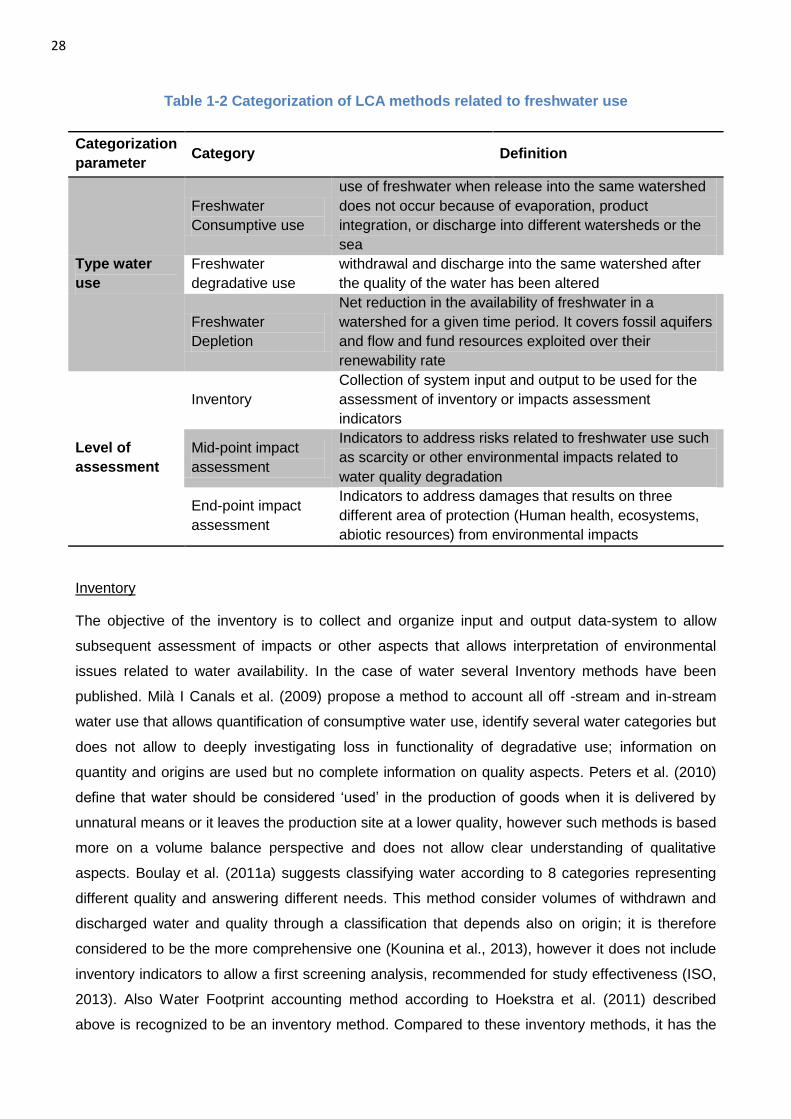
Table 1-2 Categorization of LCA methods related to freshwater use
Categorization
parameter Category Definition
Type water
use
Freshwater
Consumptive use
use of freshwater when release into the same watershed
does not occur because of evaporation, product
integration, or discharge into different watersheds or the
sea
Freshwater
degradative use
withdrawal and discharge into the same watershed after
the quality of the water has been altered
Freshwater
Depletion
Net reduction in the availability of freshwater in a
watershed for a given time period. It covers fossil aquifers
and flow and fund resources exploited over their
renewability rate
Level of
assessment
Inventory
Collection of system input and output to be used for the
assessment of inventory or impacts assessment
indicators
Mid-point impact
assessment
Indicators to address risks related to freshwater use such
as scarcity or other environmental impacts related to
water quality degradation
End-point impact
assessment
Indicators to address damages that results on three
different area of protection (Human health, ecosystems,
abiotic resources) from environmental impacts
Inventory
The objective of the inventory is to collect and organize input and output data-system to allow
subsequent assessment of impacts or other aspects that allows interpretation of environmental
issues related to water availability. In the case of water several Inventory methods have been
published. Milà I Canals et al. (2009) propose a method to account all off -stream and in-stream
water use that allows quantification of consumptive water use, identify several water categories but
does not allow to deeply investigating loss in functionality of degradative use; information on
quantity and origins are used but no complete information on quality aspects. Peters et al. (2010)
define that water should be considered ‘used’ in the production of goods when it is delivered by
unnatural means or it leaves the production site at a lower quality, however such methods is based
more on a volume balance perspective and does not allow clear understanding of qualitative
aspects. Boulay et al. (2011a) suggests classifying water according to 8 categories representing
different quality and answering different needs. This method consider volumes of withdrawn and
discharged water and quality through a classification that depends also on origin; it is therefore
considered to be the more comprehensive one (Kounina et al., 2013), however it does not include
inventory indicators to allow a first screening analysis, recommended for study effectiveness (ISO,
2013). Also Water Footprint accounting method according to Hoekstra et al. (2011) described
above is recognized to be an inventory method. Compared to these inventory methods, it has the
29
advantage of clearly defining inventory indicators that are recognized to be useful in water
management (Boulay et al., 2013), however presents several limits (Jeswani and Azapagic, 2011)
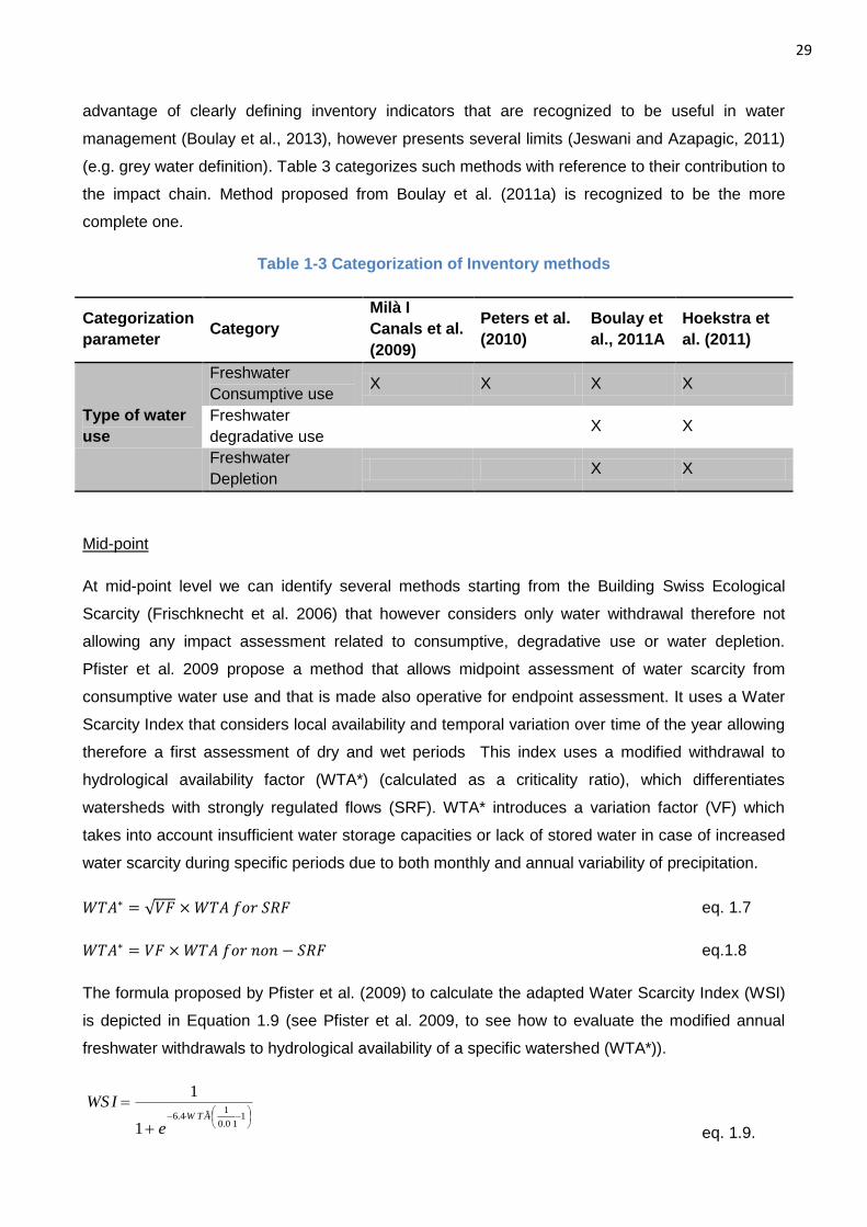
(e.g. grey water definition). Table 3 categorizes such methods with reference to their contribution to
the impact chain. Method proposed from Boulay et al. (2011a) is recognized to be the more
complete one.
Table 1-3 Categorization of Inventory methods
Categorization
parameter Category
Milà I
Canals et al.
(2009)
Peters et al.
(2010)
Boulay et
al., 2011A
Hoekstra et
al. (2011)
Type of water
use
Freshwater
Consumptive use X X X X
Freshwater
degradative use X X
Freshwater
Depletion X X
Mid-point
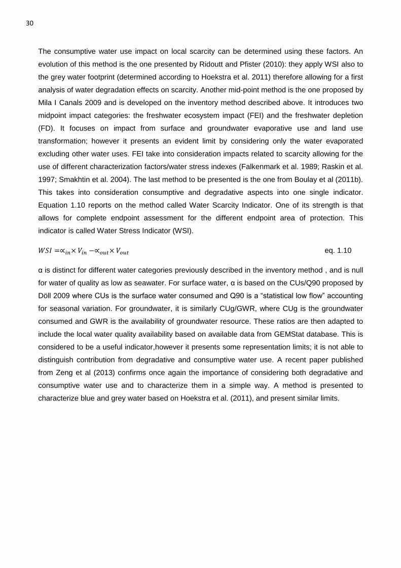
At mid-point level we can identify several methods starting from the Building Swiss Ecological
Scarcity (Frischknecht et al. 2006) that however considers only water withdrawal therefore not
allowing any impact assessment related to consumptive, degradative use or water depletion.
Pfister et al. 2009 propose a method that allows midpoint assessment of water scarcity from
consumptive water use and that is made also operative for endpoint assessment. It uses a Water
Scarcity Index that considers local availability and temporal variation over time of the year allowing
therefore a first assessment of dry and wet periods This index uses a modified withdrawal to
hydrological availability factor (WTA*) (calculated as a criticality ratio), which differentiates
watersheds with strongly regulated flows (SRF). WTA* introduces a variation factor (VF) which
takes into account insufficient water storage capacities or lack of stored water in case of increased
water scarcity during specific periods due to both monthly and annual variability of precipitation.
√ eq. 1.7
eq.1.8
The formula proposed by Pfister et al. (2009) to calculate the adapted Water Scarcity Index (WSI)
is depicted in Equation 1.9 (see Pfister et al. 2009, to see how to evaluate the modified annual
freshwater withdrawals to hydrological availability of a specific watershed (WTA*)).
eq. 1.9.
1
0 1.0
14.6 *
1
1
W T A
e
WSI
30
The consumptive water use impact on local scarcity can be determined using these factors. An
evolution of this method is the one presented by Ridoutt and Pfister (2010): they apply WSI also to
the grey water footprint (determined according to Hoekstra et al. 2011) therefore allowing for a first
analysis of water degradation effects on scarcity. Another mid-point method is the one proposed by
Mila I Canals 2009 and is developed on the inventory method described above. It introduces two
midpoint impact categories: the freshwater ecosystem impact (FEI) and the freshwater depletion
(FD). It focuses on impact from surface and groundwater evaporative use and land use
transformation; however it presents an evident limit by considering only the water evaporated
excluding other water uses. FEI take into consideration impacts related to scarcity allowing for the
use of different characterization factors/water stress indexes (Falkenmark et al. 1989; Raskin et al.
1997; Smakhtin et al. 2004). The last method to be presented is the one from Boulay et al (2011b).
This takes into consideration consumptive and degradative aspects into one single indicator.
Equation 1.10 reports on the method called Water Scarcity Indicator. One of its strength is that
allows for complete endpoint assessment for the different endpoint area of protection. This
indicator is called Water Stress Indicator (WSI).
eq. 1.10
α is distinct for different water categories previously described in the inventory method , and is null
for water of quality as low as seawater. For surface water, α is based on the CUs/Q90 proposed by
Döll 2009 where CUs is the surface water consumed and Q90 is a “statistical low flow” accounting
for seasonal variation. For groundwater, it is similarly CUg/GWR, where CUg is the groundwater
consumed and GWR is the availability of groundwater resource. These ratios are then adapted to
include the local water quality availability based on available data from GEMStat database. This is
considered to be a useful indicator,however it presents some representation limits; it is not able to
distinguish contribution from degradative and consumptive water use. A recent paper published
from Zeng et al (2013) confirms once again the importance of considering both degradative and
consumptive water use and to characterize them in a simple way. A method is presented to
characterize blue and grey water based on Hoekstra et al. (2011), and present similar limits.
31
Table 1-4 Categorization of Mid-point impact assessment methods
Categorization
parameter Category
Frischknecht
et al. (2006)
Pfister
et al.
(2009)
Milà I
Canals
et al.
(2009)
Ridoutt
and
Pfister
(2010)
Boulay
et al.
(2011b)
Zeng et al. (2013)
Type of water
use
Freshwater
Consumptive
use
X partially X X
partially X X X
Freshwater
degradative
use
X X X X
Freshwater
Depletion X
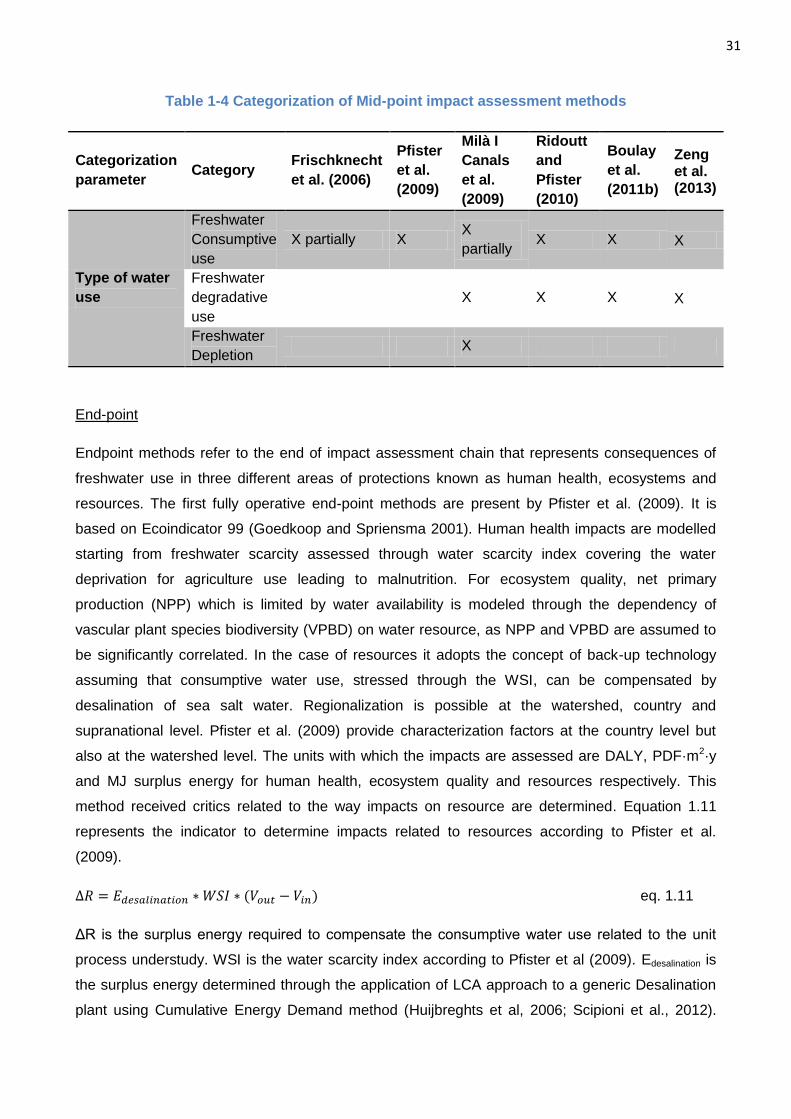
End-point
Endpoint methods refer to the end of impact assessment chain that represents consequences of
freshwater use in three different areas of protections known as human health, ecosystems and
resources. The first fully operative end-point methods are present by Pfister et al. (2009). It is
based on Ecoindicator 99 (Goedkoop and Spriensma 2001). Human health impacts are modelled
starting from freshwater scarcity assessed through water scarcity index covering the water
deprivation for agriculture use leading to malnutrition. For ecosystem quality, net primary
production (NPP) which is limited by water availability is modeled through the dependency of
vascular plant species biodiversity (VPBD) on water resource, as NPP and VPBD are assumed to
be significantly correlated. In the case of resources it adopts the concept of back-up technology
assuming that consumptive water use, stressed through the WSI, can be compensated by
desalination of sea salt water. Regionalization is possible at the watershed, country and
supranational level. Pfister et al. (2009) provide characterization factors at the country level but
also at the watershed level. The units with which the impacts are assessed are DALY, PDF·m2·y
and MJ surplus energy for human health, ecosystem quality and resources respectively. This
method received critics related to the way impacts on resource are determined. Equation 1.11
represents the indicator to determine impacts related to resources according to Pfister et al.
(2009).
eq. 1.11
ΔR is the surplus energy required to compensate the consumptive water use related to the unit
process understudy. WSI is the water scarcity index according to Pfister et al (2009). Edesalination is
the surplus energy determined through the application of LCA approach to a generic Desalination
plant using Cumulative Energy Demand method (Huijbreghts et al, 2006; Scipioni et al., 2012).
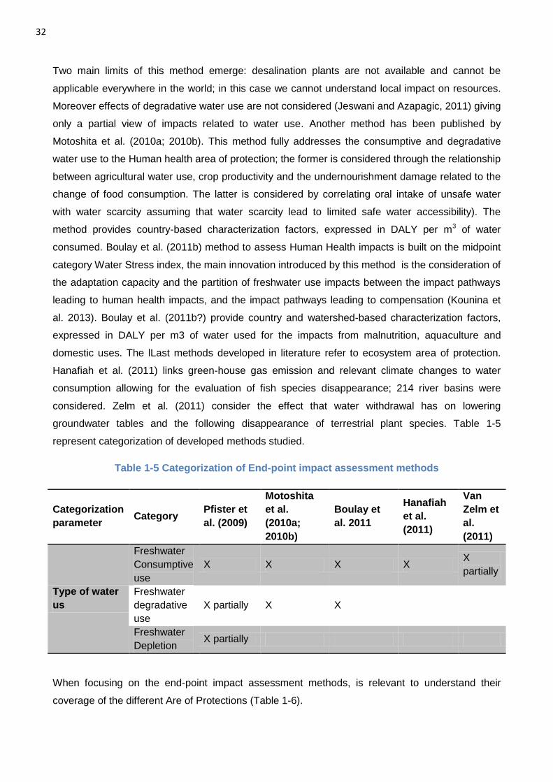
32
Two main limits of this method emerge: desalination plants are not available and cannot be
applicable everywhere in the world; in this case we cannot understand local impact on resources.
Moreover effects of degradative water use are not considered (Jeswani and Azapagic, 2011) giving
only a partial view of impacts related to water use. Another method has been published by
Motoshita et al. (2010a; 2010b). This method fully addresses the consumptive and degradative
water use to the Human health area of protection; the former is considered through the relationship
between agricultural water use, crop productivity and the undernourishment damage related to the
change of food consumption. The latter is considered by correlating oral intake of unsafe water
with water scarcity assuming that water scarcity lead to limited safe water accessibility). The
method provides country-based characterization factors, expressed in DALY per m3 of water
consumed. Boulay et al. (2011b) method to assess Human Health impacts is built on the midpoint
category Water Stress index, the main innovation introduced by this method is the consideration of
the adaptation capacity and the partition of freshwater use impacts between the impact pathways
leading to human health impacts, and the impact pathways leading to compensation (Kounina et
al. 2013). Boulay et al. (2011b?) provide country and watershed-based characterization factors,
expressed in DALY per m3 of water used for the impacts from malnutrition, aquaculture and
domestic uses. The lLast methods developed in literature refer to ecosystem area of protection.
Hanafiah et al. (2011) links green-house gas emission and relevant climate changes to water
consumption allowing for the evaluation of fish species disappearance; 214 river basins were
considered. Zelm et al. (2011) consider the effect that water withdrawal has on lowering
groundwater tables and the following disappearance of terrestrial plant species. Table 1-5
represent categorization of developed methods studied.
Table 1-5 Categorization of End-point impact assessment methods
Categorization
parameter Category
Pfister et
al. (2009)
Motoshita
et al.
(2010a;
2010b)
Boulay et
al. 2011
Hanafiah
et al.
(2011)
Van
Zelm et
al.
(2011)
Type of water
us
Freshwater
Consumptive
use
X X X X X
partially
Freshwater
degradative
use
X partially X X
Freshwater
Depletion X partially
When focusing on the end-point impact assessment methods, is relevant to understand their
coverage of the different Are of Protections (Table 1-6).
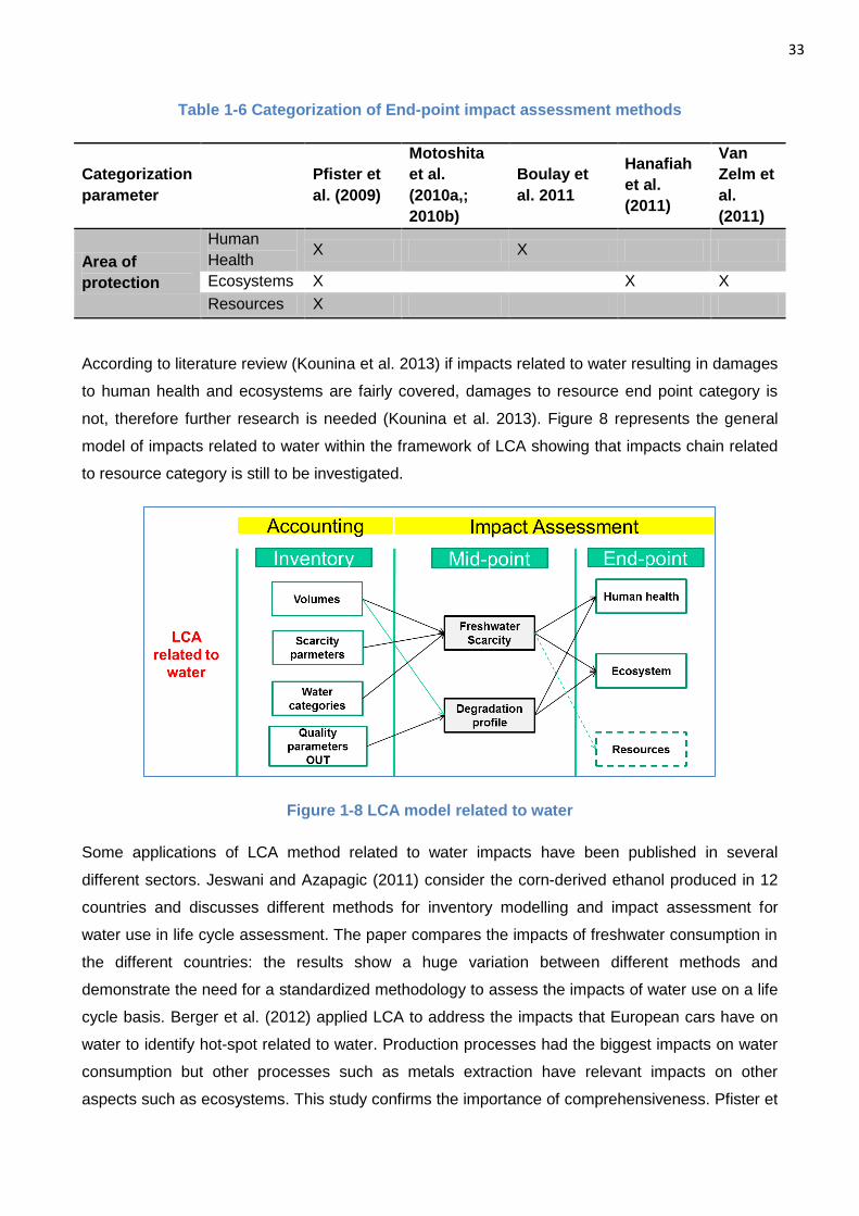
33
Table 1-6 Categorization of End-point impact assessment methods
Categorization
parameter
Pfister et
al. (2009)
Motoshita
et al.
(2010a,;
2010b)
Boulay et
al. 2011
Hanafiah
et al.
(2011)
Van
Zelm et
al.
(2011)
Area of
protection
Human
Health X X
Ecosystems X X X
Resources X
According to literature review (Kounina et al. 2013) if impacts related to water resulting in damages
to human health and ecosystems are fairly covered, damages to resource end point category is
not, therefore further research is needed (Kounina et al. 2013). Figure 8 represents the general
model of impacts related to water within the framework of LCA showing that impacts chain related
to resource category is still to be investigated.
Figure 1-8 LCA model related to water
Some applications of LCA method related to water impacts have been published in several
different sectors. Jeswani and Azapagic (2011) consider the corn-derived ethanol produced in 12
countries and discusses different methods for inventory modelling and impact assessment for
water use in life cycle assessment. The paper compares the impacts of freshwater consumption in
the different countries: the results show a huge variation between different methods and
demonstrate the need for a standardized methodology to assess the impacts of water use on a life
cycle basis. Berger et al. (2012) applied LCA to address the impacts that European cars have on
water to identify hot-spot related to water. Production processes had the biggest impacts on water
consumption but other processes such as metals extraction have relevant impacts on other
aspects such as ecosystems. This study confirms the importance of comprehensiveness. Pfister et
34
al. (2011) applied LCA methods related to water to global power production confirming that this
sector is one of the most water intensive one. Stoessel et al. (2012) applied LCA method including
impacts related to water to the production of different food products. Results of this study were
used by the retailer to support the purchasing decisions and improve the supply chain
management, proving that Water Footprint within LCA can contribute to supply chain efficiency and
therefore companies’ competitiveness. Jefferies et al. (2013) presented a study to compare
different methods proving that water footprint accounting can support better management of water
but impact assessment is mandatory to prevent damages to humans and ecosystems.
1.4. Research needs and limits of current models
According to literature review presented in previous paragraphs, several methods belonging to
different models are available to cover impacts related to freshwater use. From the application of
these methods significant limits emerged negatively impacting on the competitiveness of
companies (ISO, 2013). To make the assessment and reporting of water related impacts more
transparent, ISO launched in 2008 a process of standardization called “Environmental
management — Water footprint — Principles, requirements and guidelines” (ISO, 2013). Actually
in the DIS stage (discussion paper available for stakeholder’s consultation) it gives the principles
and framework to perform a Water Footprint study applicable to products, processes and
organization. Water Footprint according to ISO 14046 is a method that complement LCA standards
ISO 14040 (ISO, 2006) covering specific environmental concerns related to water such as
availability and scarcity. In fact, historically speaking, LCA methodology underestimated impacts
related to freshwater use (ISO, 2013) showing limits at inventory, midpoint and end point
assessment level (Mazzi et al., 2013); focusing on methods, even if effects of degradative water
use are partially covered through eutrophication, eco-toxicity, acidification, there is no clear method
that specifically address the impacts related to scarcity (Zeng et al., 2013)
According to UNEP-SETAC WULCA initiative (Bayart et al., 2010) and other important references
(Berger and Finkbeiner, 2010; Kounina et al., 2013; Boulay et al., 2013), research for new models
related to water, shall be developed within ISO 14046 general framework therefore respecting
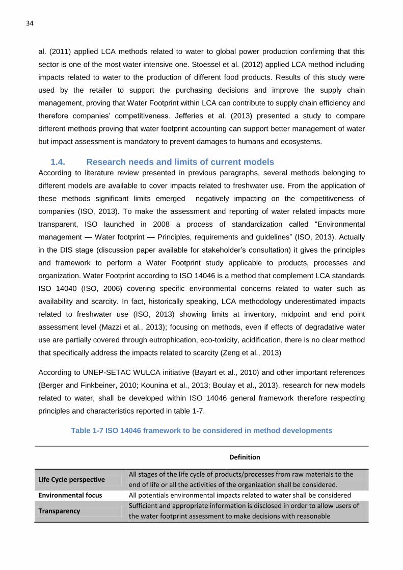
principles and characteristics reported in table 1-7.
Table 1-7 ISO 14046 framework to be considered in method developments
Definition
Life Cycle perspective All stages of the life cycle of products/processes from raw materials to the
end of life or all the activities of the organization shall be considered.
Environmental focus All potentials environmental impacts related to water shall be considered
Transparency Sufficient and appropriate information is disclosed in order to allow users of
the water footprint assessment to make decisions with reasonable
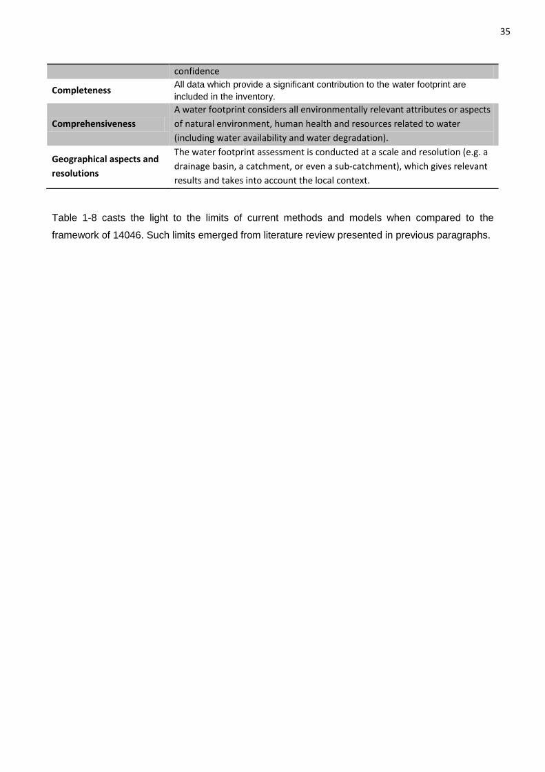
35
confidence
Completeness All data which provide a significant contribution to the water footprint are
included in the inventory.
Comprehensiveness
A water footprint considers all environmentally relevant attributes or aspects
of natural environment, human health and resources related to water
(including water availability and water degradation).
Geographical aspects and
resolutions
The water footprint assessment is conducted at a scale and resolution (e.g. a
drainage basin, a catchment, or even a sub-catchment), which gives relevant
results and takes into account the local context.
Table 1-8 casts the light to the limits of current methods and models when compared to the
framework of 14046. Such limits emerged from literature review presented in previous paragraphs.
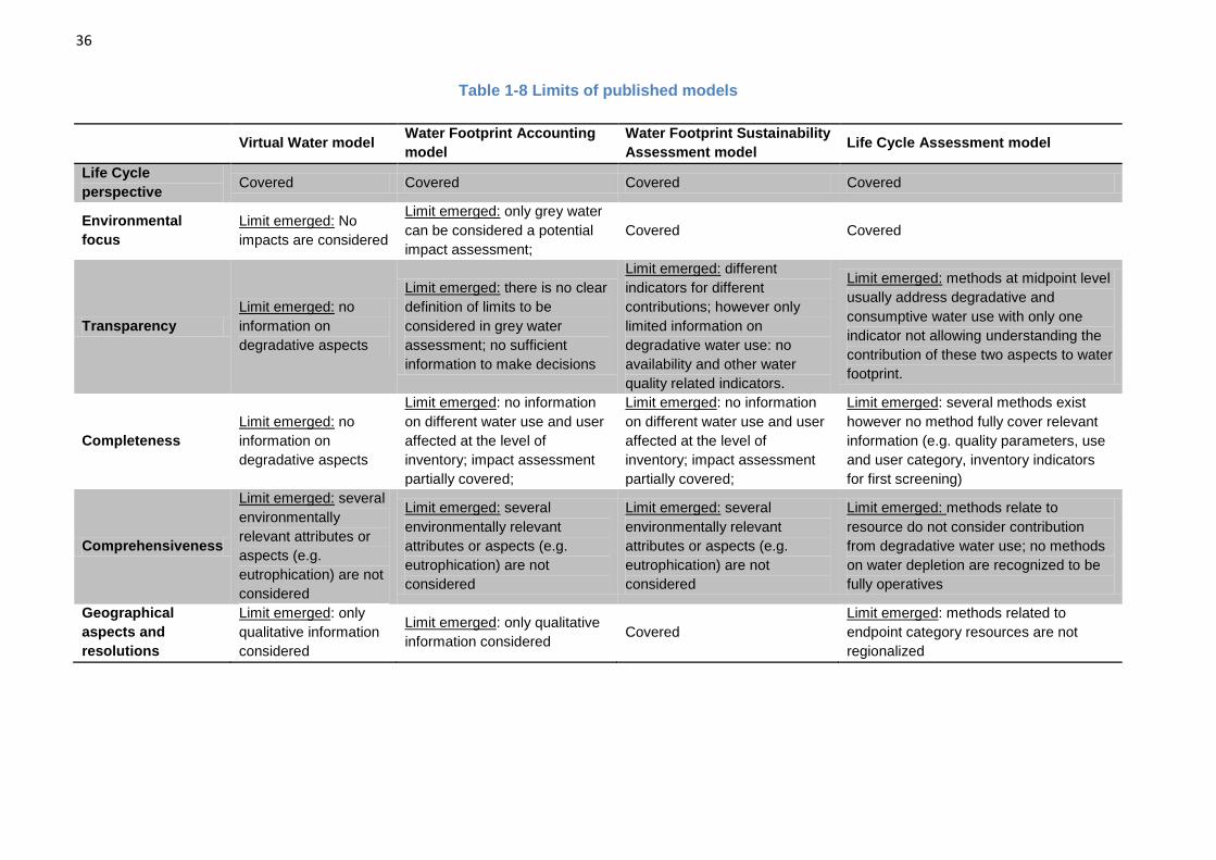
36
Table 1-8 Limits of published models
Virtual Water model Water Footprint Accounting
model
Water Footprint Sustainability
Assessment model Life Cycle Assessment model
Life Cycle
perspective Covered Covered Covered Covered
Environmental
focus
Limit emerged: No
impacts are considered
Limit emerged: only grey water
can be considered a potential
impact assessment;
Covered Covered
Transparency
Limit emerged: no
information on
degradative aspects
Limit emerged: there is no clear
definition of limits to be
considered in grey water
assessment; no sufficient
information to make decisions
Limit emerged: different
indicators for different
contributions; however only
limited information on
degradative water use: no
availability and other water
quality related indicators.
Limit emerged: methods at midpoint level
usually address degradative and
consumptive water use with only one
indicator not allowing understanding the
contribution of these two aspects to water
footprint.
Completeness
Limit emerged: no
information on
degradative aspects
Limit emerged: no information
on different water use and user
affected at the level of
inventory; impact assessment
partially covered;
Limit emerged: no information
on different water use and user
affected at the level of
inventory; impact assessment
partially covered;
Limit emerged: several methods exist
however no method fully cover relevant
information (e.g. quality parameters, use
and user category, inventory indicators
for first screening)
Comprehensiveness
Limit emerged: several
environmentally
relevant attributes or
aspects (e.g.
eutrophication) are not
considered
Limit emerged: several
environmentally relevant
attributes or aspects (e.g.
eutrophication) are not
considered
Limit emerged: several
environmentally relevant
attributes or aspects (e.g.
eutrophication) are not
considered
Limit emerged: methods relate to
resource do not consider contribution
from degradative water use; no methods
on water depletion are recognized to be
fully operatives
Geographical
aspects and
resolutions
Limit emerged: only
qualitative information
considered
Limit emerged: only qualitative
information considered Covered
Limit emerged: methods related to
endpoint category resources are not
regionalized
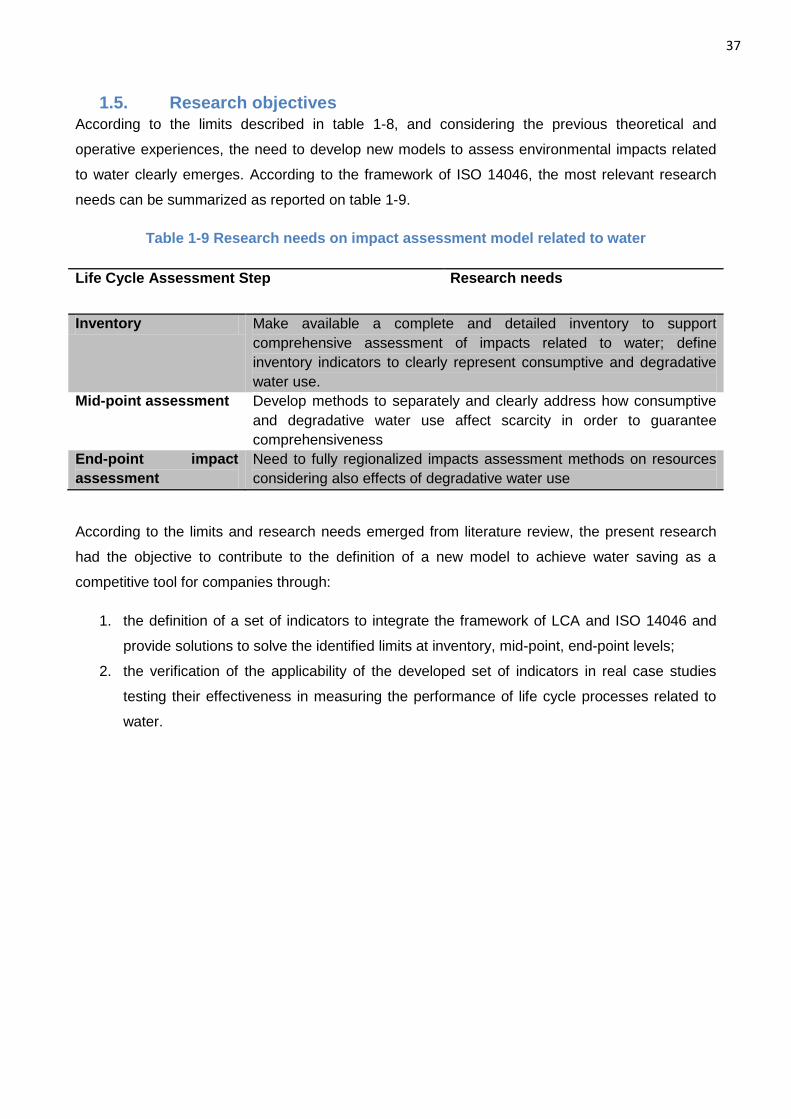
37
1.5. Research objectives
According to the limits described in table 1-8, and considering the previous theoretical and
operative experiences, the need to develop new models to assess environmental impacts related
to water clearly emerges. According to the framework of ISO 14046, the most relevant research
needs can be summarized as reported on table 1-9.
Table 1-9 Research needs on impact assessment model related to water
Life Cycle Assessment Step Research needs
Inventory Make available a complete and detailed inventory to support
comprehensive assessment of impacts related to water; define
inventory indicators to clearly represent consumptive and degradative
water use.
Mid-point assessment Develop methods to separately and clearly address how consumptive
and degradative water use affect scarcity in order to guarantee
comprehensiveness
End-point impact
assessment
Need to fully regionalized impacts assessment methods on resources
considering also effects of degradative water use
According to the limits and research needs emerged from literature review, the present research
had the objective to contribute to the definition of a new model to achieve water saving as a
competitive tool for companies through:
1. the definition of a set of indicators to integrate the framework of LCA and ISO 14046 and
provide solutions to solve the identified limits at inventory, mid-point, end-point levels;
2. the verification of the applicability of the developed set of indicators in real case studies
testing their effectiveness in measuring the performance of life cycle processes related to
water.
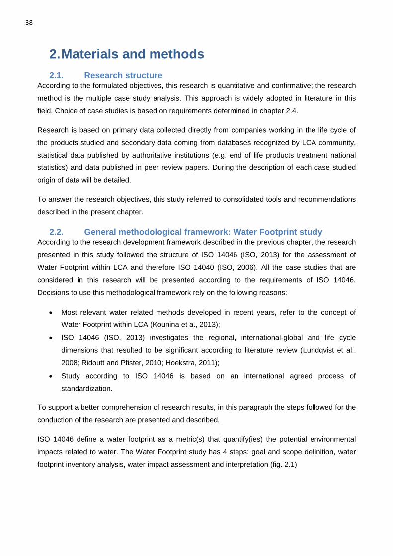
38
2. Materials and methods
2.1. Research structure
According to the formulated objectives, this research is quantitative and confirmative; the research
method is the multiple case study analysis. This approach is widely adopted in literature in this
field. Choice of case studies is based on requirements determined in chapter 2.4.
Research is based on primary data collected directly from companies working in the life cycle of
the products studied and secondary data coming from databases recognized by LCA community,
statistical data published by authoritative institutions (e.g. end of life products treatment national
statistics) and data published in peer review papers. During the description of each case studied
origin of data will be detailed.
To answer the research objectives, this study referred to consolidated tools and recommendations
described in the present chapter.
2.2. General methodological framework: Water Footprint study
According to the research development framework described in the previous chapter, the research
presented in this study followed the structure of ISO 14046 (ISO, 2013) for the assessment of
Water Footprint within LCA and therefore ISO 14040 (ISO, 2006). All the case studies that are
considered in this research will be presented according to the requirements of ISO 14046.
Decisions to use this methodological framework rely on the following reasons:
Most relevant water related methods developed in recent years, refer to the concept of
Water Footprint within LCA (Kounina et a., 2013);
ISO 14046 (ISO, 2013) investigates the regional, international-global and life cycle
dimensions that resulted to be significant according to literature review (Lundqvist et al.,
2008; Ridoutt and Pfister, 2010; Hoekstra, 2011);
Study according to ISO 14046 is based on an international agreed process of
standardization.
To support a better comprehension of research results, in this paragraph the steps followed for the
conduction of the research are presented and described.
ISO 14046 define a water footprint as a metric(s) that quantify(ies) the potential environmental
impacts related to water. The Water Footprint study has 4 steps: goal and scope definition, water
footprint inventory analysis, water impact assessment and interpretation (fig. 2.1)
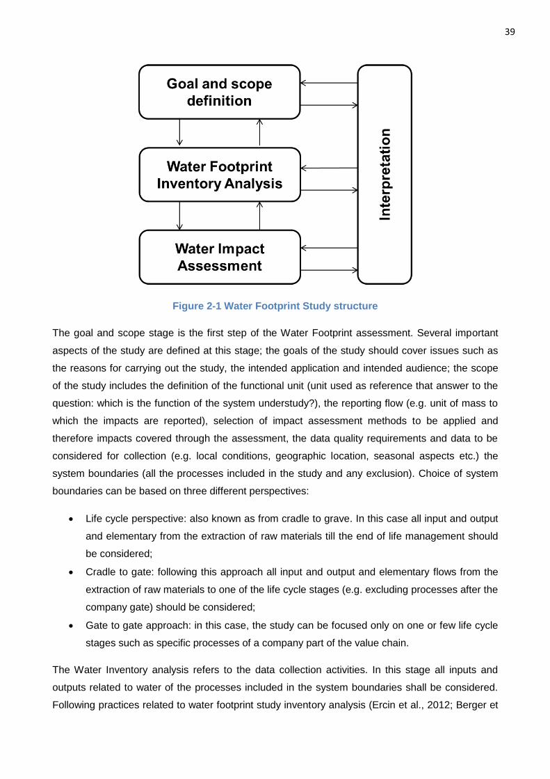
39
Figure 2-1 Water Footprint Study structure
The goal and scope stage is the first step of the Water Footprint assessment. Several important
aspects of the study are defined at this stage; the goals of the study should cover issues such as
the reasons for carrying out the study, the intended application and intended audience; the scope
of the study includes the definition of the functional unit (unit used as reference that answer to the
question: which is the function of the system understudy?), the reporting flow (e.g. unit of mass to
which the impacts are reported), selection of impact assessment methods to be applied and
therefore impacts covered through the assessment, the data quality requirements and data to be
considered for collection (e.g. local conditions, geographic location, seasonal aspects etc.) the
system boundaries (all the processes included in the study and any exclusion). Choice of system
boundaries can be based on three different perspectives:
Life cycle perspective: also known as from cradle to grave. In this case all input and output
and elementary from the extraction of raw materials till the end of life management should
be considered;
Cradle to gate: following this approach all input and output and elementary flows from the
extraction of raw materials to one of the life cycle stages (e.g. excluding processes after the
company gate) should be considered;
Gate to gate approach: in this case, the study can be focused only on one or few life cycle
stages such as specific processes of a company part of the value chain.
The Water Inventory analysis refers to the data collection activities. In this stage all inputs and
outputs related to water of the processes included in the system boundaries shall be considered.
Following practices related to water footprint study inventory analysis (Ercin et al., 2012; Berger et
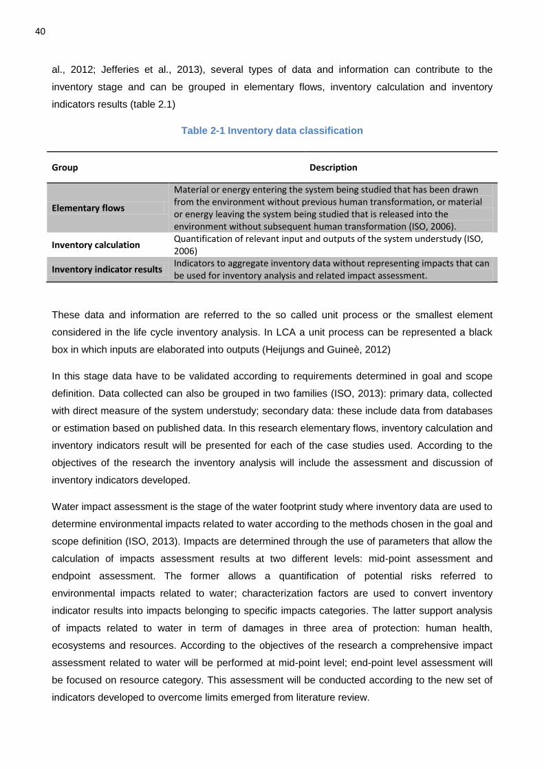
40
al., 2012; Jefferies et al., 2013), several types of data and information can contribute to the
inventory stage and can be grouped in elementary flows, inventory calculation and inventory
indicators results (table 2.1)
Table 2-1 Inventory data classification
Group Description
Elementary flows
Material or energy entering the system being studied that has been drawn from the environment without previous human transformation, or material or energy leaving the system being studied that is released into the environment without subsequent human transformation (ISO, 2006).
Inventory calculation Quantification of relevant input and outputs of the system understudy (ISO, 2006)
Inventory indicator results Indicators to aggregate inventory data without representing impacts that can be used for inventory analysis and related impact assessment.
These data and information are referred to the so called unit process or the smallest element
considered in the life cycle inventory analysis. In LCA a unit process can be represented a black
box in which inputs are elaborated into outputs (Heijungs and Guineè, 2012)
In this stage data have to be validated according to requirements determined in goal and scope
definition. Data collected can also be grouped in two families (ISO, 2013): primary data, collected
with direct measure of the system understudy; secondary data: these include data from databases
or estimation based on published data. In this research elementary flows, inventory calculation and
inventory indicators result will be presented for each of the case studies used. According to the
objectives of the research the inventory analysis will include the assessment and discussion of
inventory indicators developed.
Water impact assessment is the stage of the water footprint study where inventory data are used to
determine environmental impacts related to water according to the methods chosen in the goal and
scope definition (ISO, 2013). Impacts are determined through the use of parameters that allow the
calculation of impacts assessment results at two different levels: mid-point assessment and
endpoint assessment. The former allows a quantification of potential risks referred to
environmental impacts related to water; characterization factors are used to convert inventory
indicator results into impacts belonging to specific impacts categories. The latter support analysis
of impacts related to water in term of damages in three area of protection: human health,
ecosystems and resources. According to the objectives of the research a comprehensive impact
assessment related to water will be performed at mid-point level; end-point level assessment will
be focused on resource category. This assessment will be conducted according to the new set of
indicators developed to overcome limits emerged from literature review.
41
Interpretation stage is the last step of the water footprint study according to ISO 14046 (ISO, 2013)
and includes the analysis of inventory and impact assessment results and formulation of strategies
and recommendation for performance improvement (ISO, 2013). This stage should also include
the analysis of different processes contribution to identify environmental hot-spot, the analysis of
data and results, consideration on assumptions and related limitations (ISO, 2013). This stage is
recognized to contribute to performance improvement and therefore competitiveness of companies
(Boulay et al., 2013). Interpretation of results is performed for all of the case studies included in this
research.
2.3. Criteria used in the definition of the set of water use indicators
To determine the set of indicators to integrate the framework of LCA and solve identified limits at
inventory, mid-point, and end-point level the criteria and requirements of UNEP-SETAC WULCA
initiative (Bayart et al., 2010) reported in this paragraph, have been considered. This framework
has been chosen because it is the result of a process of consensus among several researcher
working ion the modelling of water use related impacts (Bayart; 2010; Heijungs and Guineè, 2012)
Off-stream freshwater use shall be considered when developing impact assessment methods
because it can result in reduced water availability. Two different typology of freshwater use can be
identified and shall be considered:
Consumptive water use: use of freshwater when release into the same watershed does not
occur because of evaporation, product integration, or discharge into different watersheds or
the sea (Bayart et al., 2010);
Degradative water use: withdrawal and discharge into the same watershed after the quality
of the water has been (Pfister et al., 2009).
To develop water-use indicators at inventory level the following criteria are adopted (Bayart et al.,
2010):
The objective of the inventory stage is the analysis of the consumptive and degradative
water use to support the quantification of changes in freshwater availability at mid-point
level (Pfister et al., 2009);
Resources should be classified considering their origin (e.g. groundwater or surface-water)
and resource quality (e.g. suitable for industrial use, agriculture use);
Information of quality of water entering the system should be included;
Information on quantity leaving the system should be included;
Inventory should make possible to express the change in availability for different water
types;
Regionalization should be included;
42
To develop water use indicators at mid-point level the following criteria are adopted (Bayart et al.,
2010):
Should measure change in water availability resulting in increased competition for
freshwater resources for present generations and ecosystems and water depletion for
future generations;
Results should be expressed in volumes of water equivalent (m3equivalent or l equivalent);
Different water types should be weighted considering different parameters in function of
either the water type or the water quality;
State of freshwater scarcity in the area should be considered;
Time and seasonality aspect should be considered;
Distance to target approach or functionality approach should be considered when
assessing degradative water use;
To develop water use indicators at end-point level with specific reference to resource area of
protection, the following criteria are adopted:
Results should be translated in non-renewable primary energy needs;
Use of back-up technology should be adopted;
Results should be expressed following the concept of surplus energy (additional quantity of
energy needed to extract non-renewable resources;
Regionalization at end-point level is necessary.
2.4. Definition of the set of water use indicators
2.4.1 Inventory indicators
ISO defines the inventory analysis (LCI) as the phase of LCA study involving the compilation and
quantification of inputs and outputs for all the processes involved in the life cycle of a product. This
take place through the collection of elementary flows, the calculation of data and the quantification
of indicators results, classification of information and quantification of information are performed.
The proposed inventory indicators set is built on the most representative experiences emerged
from literature review on inventory related to water and the recommendation of UNEP-SETAC
WULCA presented in the previous chapter.
According to literature review current operative methods related to water are based on the
inventory information represented in table 2-2 where an example of an apple growing process is
presented (Ecoinvent, 2010).
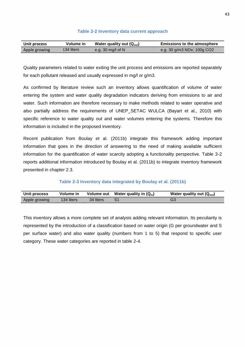
43
Table 2-2 Inventory data current approach
Unit process Volume in Water quality out (Qout) Emissions to the atmosphere
Apple growing 134 liters e.g. 30 mg/l of N e.g. 30 g/m3 NOx; 100g CO2
Quality parameters related to water exiting the unit process and emissions are reported separately
for each pollutant released and usually expressed in mg/l or g/m3.
As confirmed by literature review such an inventory allows quantification of volume of water
entering the system and water quality degradation indicators deriving from emissions to air and
water. Such information are therefore necessary to make methods related to water operative and
also partially address the requirements of UNEP_SETAC WULCA (Bayart et al., 2010) with
specific reference to water quality out and water volumes entering the systems. Therefore this
information is included in the proposed inventory.
Recent publication from Boulay et al. (2011b) integrate this framework adding important
information that goes in the direction of answering to the need of making available sufficient
information for the quantification of water scarcity adopting a functionality perspective. Table 3-2
reports additional information introduced by Boulay et al. (2011b) to integrate inventory framework
presented in chapter 2.3.
Table 2-3 Inventory data integrated by Boulay et al. (2011b)
Unit process Volume in Volume out Water quality in (Qin) Water quality out (Qout)
Apple growing 134 liters 34 liters S1 G3
This inventory allows a more complete set of analysis adding relevant information. Its peculiarity is
represented by the introduction of a classification based on water origin (G per groundwater and S
per surface water) and also water quality (numbers from 1 to 5) that respond to specific user
category. These water categories are reported in table 2-4.
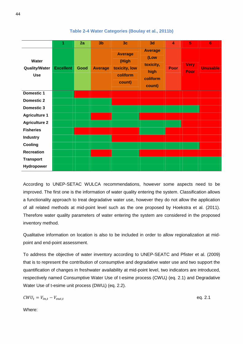
44
Table 2-4 Water Categories (Boulay et al., 2011b)
1 2a 3b 3c 3d 4 5 6
Water
Quality/Water
Use
Excellent Good Average
Average
(High
toxicity, low
coliform
count)
Average
(Low
toxicity,
high
coliform
count)
Poor Very
Poor Unusable
Domestic 1
Domestic 2
Domestic 3
Agriculture 1
Agriculture 2
Fisheries
Industry
Cooling
Recreation
Transport
Hydropower
According to UNEP-SETAC WULCA recommendations, however some aspects need to be
improved. The first one is the information of water quality entering the system. Classification allows
a functionality approach to treat degradative water use, however they do not allow the application
of all related methods at mid-point level such as the one proposed by Hoekstra et al. (2011).
Therefore water quality parameters of water entering the system are considered in the proposed
inventory method.
Qualitative information on location is also to be included in order to allow regionalization at mid-
point and end-point assessment.
To address the objective of water inventory according to UNEP-SEATC and Pfister et al. (2009)
that is to represent the contribution of consumptive and degradative water use and two support the
quantification of changes in freshwater availability at mid-point level, two indicators are introduced,
respectively named Consumptive Water Use of t-esime process (CWUt) (eq. 2.1) and Degradative
Water Use of t-esime unit process (DWUt) (eq. 2.2).
eq. 2.1
Where:
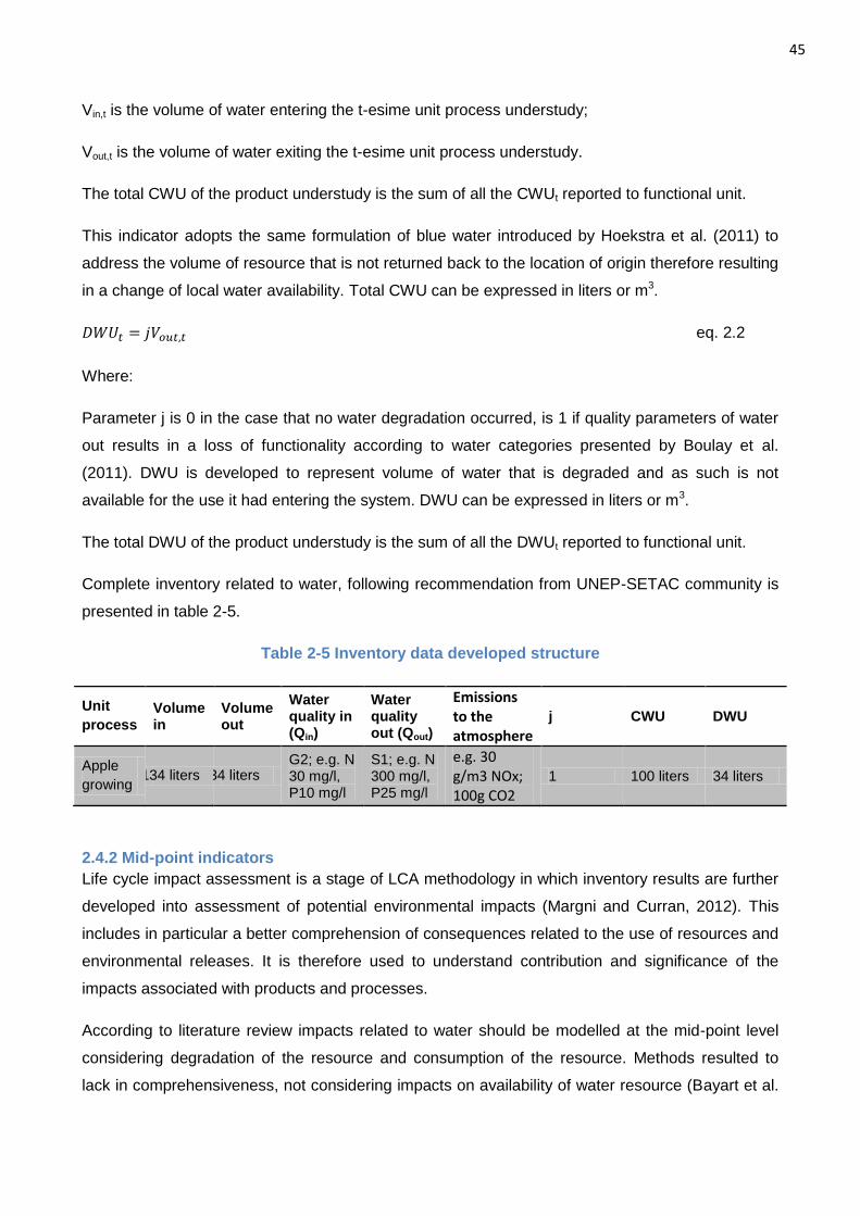
45
Vin,t is the volume of water entering the t-esime unit process understudy;
Vout,t is the volume of water exiting the t-esime unit process understudy.
The total CWU of the product understudy is the sum of all the CWUt reported to functional unit.
This indicator adopts the same formulation of blue water introduced by Hoekstra et al. (2011) to
address the volume of resource that is not returned back to the location of origin therefore resulting
in a change of local water availability. Total CWU can be expressed in liters or m3.
eq. 2.2
Where:
Parameter j is 0 in the case that no water degradation occurred, is 1 if quality parameters of water
out results in a loss of functionality according to water categories presented by Boulay et al.
(2011). DWU is developed to represent volume of water that is degraded and as such is not
available for the use it had entering the system. DWU can be expressed in liters or m3.
The total DWU of the product understudy is the sum of all the DWUt reported to functional unit.
Complete inventory related to water, following recommendation from UNEP-SETAC community is
presented in table 2-5.
Table 2-5 Inventory data developed structure
Unit
process Volume in
Volume out
Water quality in (Qin)
Water quality out (Qout)
Emissions to the atmosphere
j CWU DWU
Apple
growing 134 liters 34 liters
G2; e.g. N 30 mg/l, P10 mg/l
S1; e.g. N 300 mg/l, P25 mg/l
e.g. 30 g/m3 NOx; 100g CO2
1 100 liters 34 liters
2.4.2 Mid-point indicators
Life cycle impact assessment is a stage of LCA methodology in which inventory results are further
developed into assessment of potential environmental impacts (Margni and Curran, 2012). This
includes in particular a better comprehension of consequences related to the use of resources and
environmental releases. It is therefore used to understand contribution and significance of the
impacts associated with products and processes.
According to literature review impacts related to water should be modelled at the mid-point level
considering degradation of the resource and consumption of the resource. Methods resulted to
lack in comprehensiveness, not considering impacts on availability of water resource (Bayart et al.
46
2010; Margni and Curran, 2012; ISO, 2013) not clearly showing contribution from degradative and
consumptive water use to availability.
To address this issue a new method is developed and new indicators are introduced. These are
called: Scarcity Consumptive Water Use (SCWU), Scarcity Degradative Water Use (SDWU), and
Water Stress Indicator (WSI). These indicators, following the principle of life cycle impacts
assessment, are grounded on information and data collected in the inventory stage.
Scarcity Consumptive Water Use of the t-esime unit process (SCWUt) represents the contribution
of consumptive water use to local scarcity. It can be defined as follow:
eq. 2.3
Where:
CWUt is the consumptive water use of the t-esime unit process presented in the previous chapter
and expressed in liters or m3.
αin,t is the characterization factor that represent local water scarcity in the region were water is
withdrawn of the t-esime unit process. αin,t is is determined according the water scarcity factors
developed by Boulay et al. (2011b) and expressed either in [leq/l] or [m3eq/m
3]. This reference was
chosen because it allows quantification of local scarcity parameters developed at watershed level
and because represents the level of competition among users due to the physical stress of the
resource, addressing quality and seasonal variations and distinguishing surface and groundwater.
This answer a functionality approach recommended by UNEP-SETACS WULCA, availability of
water depends on the water category presented in previous chapter: the less functional water is,
the more abundant it will be. αin refers to the scarcity of water entering the system because through
consumptive water use, the availability of that specific water type is affected.
SCWU is expressed in liters equivalent (leq) or m3 equivalent (m3eq) of water.
The total SCWU of the product understudy is the sum of all the SCWUt reported to functional unit.
Scarcity Degradative Water Use (SDWU) represents the contribution of degradative water use to
local scarcity. It can be defined as follow:
(
) eq. 2.4
Where:
DWUt is the degradative water use of the t-esime unit process presented in the previous chapter
and expressed in liters or m3;
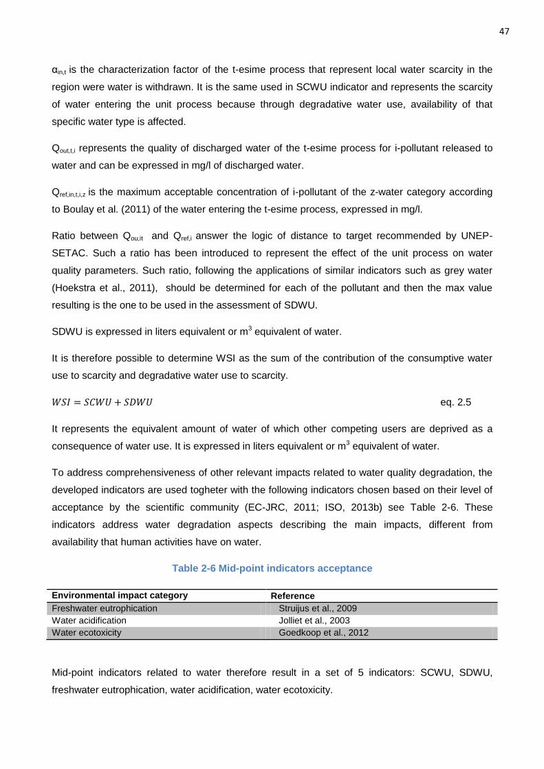
47
αin,t is the characterization factor of the t-esime process that represent local water scarcity in the
region were water is withdrawn. It is the same used in SCWU indicator and represents the scarcity
of water entering the unit process because through degradative water use, availability of that
specific water type is affected.
Qout,t,i represents the quality of discharged water of the t-esime process for i-pollutant released to
water and can be expressed in mg/l of discharged water.
Qref,in,t,i,z is the maximum acceptable concentration of i-pollutant of the z-water category according
to Boulay et al. (2011) of the water entering the t-esime process, expressed in mg/l.
Ratio between Qou,it and Qref,i answer the logic of distance to target recommended by UNEP-
SETAC. Such a ratio has been introduced to represent the effect of the unit process on water
quality parameters. Such ratio, following the applications of similar indicators such as grey water
(Hoekstra et al., 2011), should be determined for each of the pollutant and then the max value
resulting is the one to be used in the assessment of SDWU.
SDWU is expressed in liters equivalent or m3 equivalent of water.
It is therefore possible to determine WSI as the sum of the contribution of the consumptive water
use to scarcity and degradative water use to scarcity.
eq. 2.5
It represents the equivalent amount of water of which other competing users are deprived as a
consequence of water use. It is expressed in liters equivalent or m3 equivalent of water.
To address comprehensiveness of other relevant impacts related to water quality degradation, the
developed indicators are used togheter with the following indicators chosen based on their level of
acceptance by the scientific community (EC-JRC, 2011; ISO, 2013b) see Table 2-6. These
indicators address water degradation aspects describing the main impacts, different from
availability that human activities have on water.
Table 2-6 Mid-point indicators acceptance
Environmental impact category Reference
Freshwater eutrophication Struijus et al., 2009
Water acidification Jolliet et al., 2003
Water ecotoxicity Goedkoop et al., 2012
Mid-point indicators related to water therefore result in a set of 5 indicators: SCWU, SDWU,
freshwater eutrophication, water acidification, water ecotoxicity.
48
2.4.3 End-point indicators
Life Cycle Impact assessment at end point level uses inventory data to express the environmental
impacts in terms of damages into 3 area of protection named human health, eco-systems and non-
renewable resources.
According to literature review impacts related to water in term of non-renewable resources are still
to be investigated and improved (Jeswani and Azapagic, 2009; Bayart et al., 2010; Margni and
Curran, 2012).
Following the recommendations from UNEP-SETAC WULCA (Bayart et al., 2010) the following
end point indicators have been developed.
eq. 2.6
eq. 2.7
eq. 2.8
Where:
Back up CWU is the energy needed to back up the CWU of the product understudy
Back up of DWU is the energy needed to back up the DWU of the product understudy
CWU is the consumptive water use inventory indicator presented in the previous chapters and
expressed in liters or m3.
DWU is the degradative water use inventory indicator presented in the previous chapters and
expressed in liters or m3.
αin is the characterization factor that represent local water scarcity in the region were water is
withdrawn according to Boulay et al. (2011b)
Elocal,i is the surplus energy needed to compensate the consumptive water use through the use of
the i - esime local back-up technologies.
Elocal,j is the surplus energy needed to compensate the degradative water use through the use of
the j - esime local back-up technologies.
Elocal to compensate consumptive and degradative water use is determined following common
practice in the field (Pfister et al. 2009), through the application of LCA methodology using CED
indicators (Huijbreghts et al.,2006; Scipioni et al., 2012). CED represents the surplus energy
related to the product understudy. In the case of water back- up technology this represents the
energy needed to compensate a liter of consumptive or degradative water use. CED follows the
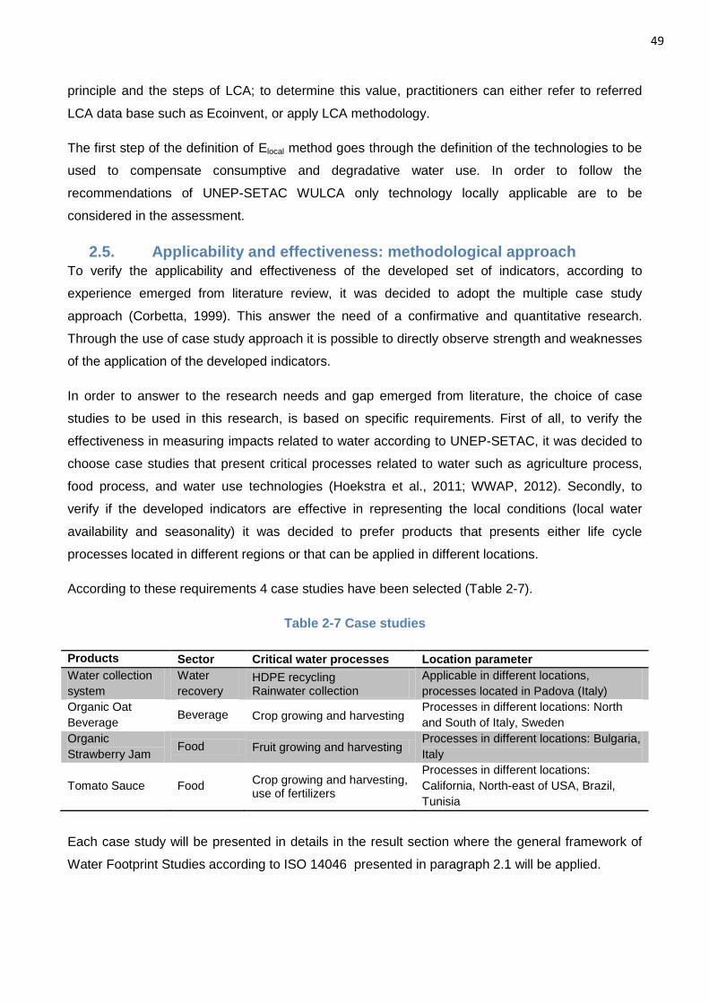
49
principle and the steps of LCA; to determine this value, practitioners can either refer to referred
LCA data base such as Ecoinvent, or apply LCA methodology.
The first step of the definition of Elocal method goes through the definition of the technologies to be
used to compensate consumptive and degradative water use. In order to follow the
recommendations of UNEP-SETAC WULCA only technology locally applicable are to be
considered in the assessment.
2.5. Applicability and effectiveness: methodological approach
To verify the applicability and effectiveness of the developed set of indicators, according to
experience emerged from literature review, it was decided to adopt the multiple case study
approach (Corbetta, 1999). This answer the need of a confirmative and quantitative research.
Through the use of case study approach it is possible to directly observe strength and weaknesses
of the application of the developed indicators.
In order to answer to the research needs and gap emerged from literature, the choice of case
studies to be used in this research, is based on specific requirements. First of all, to verify the
effectiveness in measuring impacts related to water according to UNEP-SETAC, it was decided to
choose case studies that present critical processes related to water such as agriculture process,
food process, and water use technologies (Hoekstra et al., 2011; WWAP, 2012). Secondly, to
verify if the developed indicators are effective in representing the local conditions (local water
availability and seasonality) it was decided to prefer products that presents either life cycle
processes located in different regions or that can be applied in different locations.
According to these requirements 4 case studies have been selected (Table 2-7).
Table 2-7 Case studies
Products Sector Critical water processes Location parameter
Water collection
system
Water
recovery HDPE recycling Rainwater collection
Applicable in different locations,
processes located in Padova (Italy)
Organic Oat
Beverage Beverage Crop growing and harvesting
Processes in different locations: North
and South of Italy, Sweden
Organic
Strawberry Jam Food Fruit growing and harvesting
Processes in different locations: Bulgaria,
Italy
Tomato Sauce Food Crop growing and harvesting, use of fertilizers
Processes in different locations:
California, North-east of USA, Brazil,
Tunisia
Each case study will be presented in details in the result section where the general framework of
Water Footprint Studies according to ISO 14046 presented in paragraph 2.1 will be applied.
50
3. Results: applicability and effectiveness
3.1. Case study 1: Water collection system
The first case study chosen to test the applicability and effectiveness of the developed set of
indicators is related to a water collection system produced by a company located in the area of
Padova (north east of Italy). This system is used to collect rainwater and make it available for
different uses such as gardening or even human use. This product was chosen for several
reasons:
Its function is directly related to water and allows to collect and reuse effective rainwater;
This system can be applied in several contests and regions.
3.1.1 Goals and scope definition
The goal of this study is to apply the developed set of indicators to conduct a contribution and
hotspot analysis of the potential impacts related to water of a unit of water collection system in
order to identify water saving potential and water management practice improvement. The
assessment is intended to assist the company in determining which aspects of the production
processes contribute the most to environmental impacts related to water and, therefore, to identify
potential opportunities to improve water use and management within the company.
The company approached for the first time the analysis of environmental impacts related to their
production and processes. This study has been performed in accordance with the methodologies
and requirements presented in chapter 2.
The Functional Unit (FU) was identified as unit of water collection system of the maximum capacity
of 310 l/m2 that can be applied underground and function as a drening and water collection system.
Volumes of water collected and made available for other uses depend on local climate conditions.
The more it rains the more the capacity of the system to collect water is. Usually this system is
dimensioned on local water needs and rainwater conditions. It is usually applied under impervious
surfaces such as car parks or roads but can be also applied under green surfaces. Table 3-1
reports on the main physical characteristics of the product understudy. Figure 3-1 represents one
unit of the device understudy. The water collection system is made out of these units and can
include water treatment facility and pump according to its use.
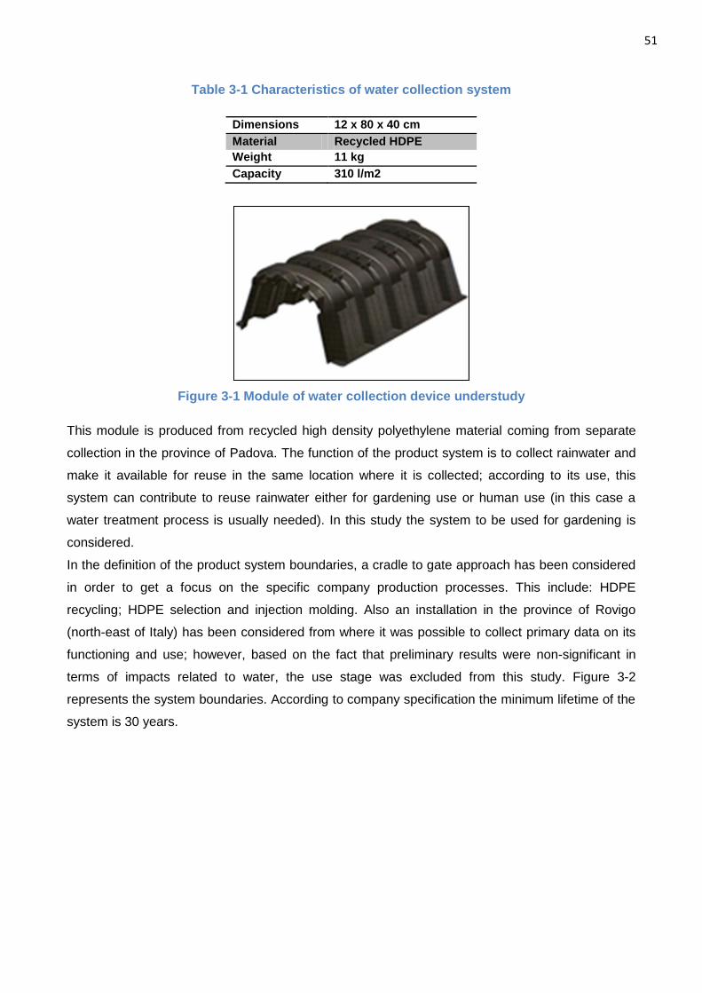
51
Table 3-1 Characteristics of water collection system
Dimensions 12 x 80 x 40 cm
Material Recycled HDPE
Weight 11 kg
Capacity 310 l/m2
Figure 3-1 Module of water collection device understudy
This module is produced from recycled high density polyethylene material coming from separate
collection in the province of Padova. The function of the product system is to collect rainwater and
make it available for reuse in the same location where it is collected; according to its use, this
system can contribute to reuse rainwater either for gardening use or human use (in this case a
water treatment process is usually needed). In this study the system to be used for gardening is
considered.
In the definition of the product system boundaries, a cradle to gate approach has been considered
in order to get a focus on the specific company production processes. This include: HDPE
recycling; HDPE selection and injection molding. Also an installation in the province of Rovigo
(north-east of Italy) has been considered from where it was possible to collect primary data on its
functioning and use; however, based on the fact that preliminary results were non-significant in
terms of impacts related to water, the use stage was excluded from this study. Figure 3-2
represents the system boundaries. According to company specification the minimum lifetime of the
system is 30 years.
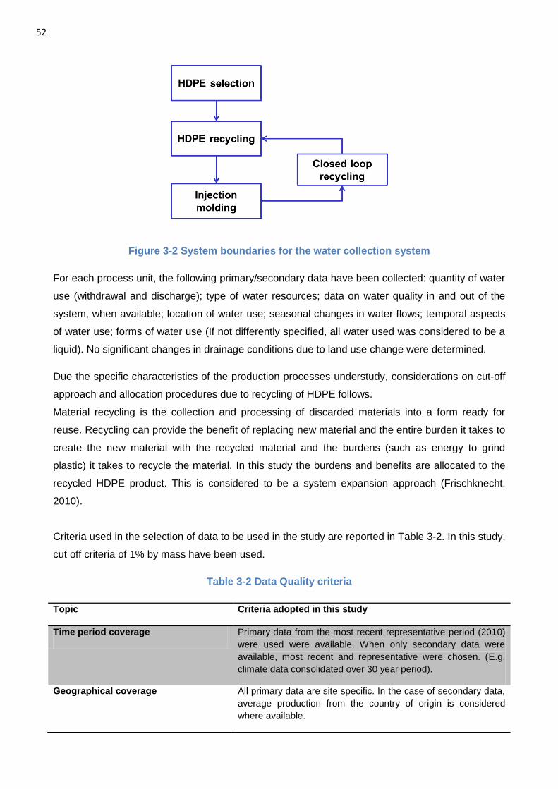
52
Figure 3-2 System boundaries for the water collection system
For each process unit, the following primary/secondary data have been collected: quantity of water
use (withdrawal and discharge); type of water resources; data on water quality in and out of the
system, when available; location of water use; seasonal changes in water flows; temporal aspects
of water use; forms of water use (If not differently specified, all water used was considered to be a
liquid). No significant changes in drainage conditions due to land use change were determined.
Due the specific characteristics of the production processes understudy, considerations on cut-off
approach and allocation procedures due to recycling of HDPE follows.
Material recycling is the collection and processing of discarded materials into a form ready for
reuse. Recycling can provide the benefit of replacing new material and the entire burden it takes to
create the new material with the recycled material and the burdens (such as energy to grind
plastic) it takes to recycle the material. In this study the burdens and benefits are allocated to the
recycled HDPE product. This is considered to be a system expansion approach (Frischknecht,
2010).
Criteria used in the selection of data to be used in the study are reported in Table 3-2. In this study,
cut off criteria of 1% by mass have been used.
Table 3-2 Data Quality criteria
Topic Criteria adopted in this study
Time period coverage Primary data from the most recent representative period (2010)
were used were available. When only secondary data were
available, most recent and representative were chosen. (E.g.
climate data consolidated over 30 year period).
Geographical coverage All primary data are site specific. In the case of secondary data,
average production from the country of origin is considered
where available.
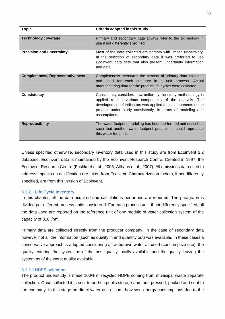
53
Topic Criteria adopted in this study
Technology coverage Primary and secondary data always refer to the technology in
use if not differently specified.
Precision and uncertainty Most of the data collected are primary with limited uncertainty.
In the selection of secondary data it was preferred to use
Ecoinvent data sets that also present uncertainty information
and data.
Completeness, Representativeness Completeness measures the percent of primary data collected
and used for each category in a unit process. Actual
manufacturing data for the product life cycles were collected.
Consistency Consistency considers how uniformly the study methodology is
applied to the various components of the analysis. The
developed set of indicators was applied to all components of the
product under study consistently, in terms of modeling and
assumptions.
Reproducibility The water footprint modeling has been performed and described
such that another water footprint practitioner could reproduce
this water footprint.
Unless specified otherwise, secondary inventory data used in this study are from Ecoinvent 2.2
database. Ecoinvent data is maintained by the Ecoinvent Research Centre. Created in 1997, the
Ecoinvent Research Centre (Frishknet et al., 2005; Althaus et al., 2007). All emissions data used to
address impacts on acidification are taken from Ecoivent. Characterization factors, if not differently
specified, are from this version of Ecoinvent.
3.1.2 Life Cycle Inventory
In this chapter, all the data acquired and calculations performed are reported. The paragraph is
divided per different process units considered. For each process unit, if not differently specified, all
the data used are reported on the reference unit of one module of water collection system of the
capacity of 310 l/m2.
Primary data are collected directly from the producer company. In the case of secondary data
however not all the information (such as quality in and quantity out) was available. In these cases a
conservative approach is adopted considering all withdrawn water as used (consumptive use), the
quality entering the system as of the best quality locally available and the quality leaving the
system as of the worst quality available.
3.1.2.1 HDPE selection
The product understudy is made 100% of recycled HDPE coming from municipal waste separate
collection. Once collected it is sent to ad-hoc public storage and then pressed, packed and sent to
the company. In this stage no direct water use occurs, however, energy consumptions due to the
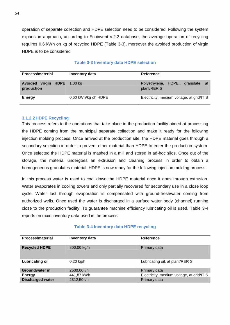
54
operation of separate collection and HDPE selection need to be considered. Following the system
expansion approach, according to Ecoinvent v.2.2 database, the average operation of recycling
requires 0,6 kWh on kg of recycled HDPE (Table 3-3), moreover the avoided production of virgin
HDPE is to be considered
Table 3-3 Inventory data HDPE selection
Process/material Inventory data Reference
Avoided virgin HDPE
production
1,00 kg Polyethylene, HDPE,, granulate, at
plant/RER S
Energy 0,60 kWh/kg oh HDPE Electricity, medium voltage, at grid/IT S
3.1.2.2 HDPE Recycling
This process refers to the operations that take place in the production facility aimed at processing
the HDPE coming from the municipal separate collection and make it ready for the following
injection molding process. Once arrived at the production site, the HDPE material goes through a
secondary selection in order to prevent other material than HDPE to enter the production system.
Once selected the HDPE material is mashed in a mill and stored in ad-hoc silos. Once out of the
storage, the material undergoes an extrusion and cleaning process in order to obtain a
homogeneous granulates material. HDPE is now ready for the following injection molding process.
In this process water is used to cool down the HDPE material once it goes through extrusion.
Water evaporates in cooling towers and only partially recovered for secondary use in a close loop
cycle. Water lost through evaporation is compensated with ground-freshwater coming from
authorized wells. Once used the water is discharged in a surface water body (channel) running
close to the production facility. To guarantee machine efficiency lubricating oil is used. Table 3-4
reports on main inventory data used in the process.
Table 3-4 Inventory data HDPE recycling
Process/material Inventory data Reference
Recycled HDPE 800,00 kg/h Primary data
Lubricating oil 0,20 kg/h Lubricating oil, at plant/RER S
Groundwater in 2500,00 l/h Primary data
Energy 441,87 kWh Electricity, medium voltage, at grid/IT S
Discharged water 2312,50 l/h Primary data
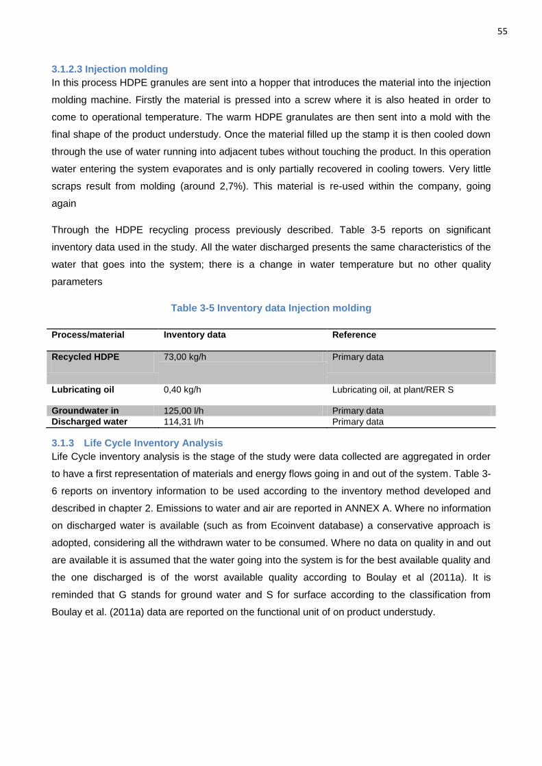
55
3.1.2.3 Injection molding
In this process HDPE granules are sent into a hopper that introduces the material into the injection
molding machine. Firstly the material is pressed into a screw where it is also heated in order to
come to operational temperature. The warm HDPE granulates are then sent into a mold with the
final shape of the product understudy. Once the material filled up the stamp it is then cooled down
through the use of water running into adjacent tubes without touching the product. In this operation
water entering the system evaporates and is only partially recovered in cooling towers. Very little
scraps result from molding (around 2,7%). This material is re-used within the company, going
again
Through the HDPE recycling process previously described. Table 3-5 reports on significant
inventory data used in the study. All the water discharged presents the same characteristics of the
water that goes into the system; there is a change in water temperature but no other quality
parameters
Table 3-5 Inventory data Injection molding
Process/material Inventory data Reference
Recycled HDPE 73,00 kg/h Primary data
Lubricating oil 0,40 kg/h Lubricating oil, at plant/RER S
Groundwater in 125,00 l/h Primary data
Discharged water 114,31 l/h Primary data
3.1.3 Life Cycle Inventory Analysis
Life Cycle inventory analysis is the stage of the study were data collected are aggregated in order
to have a first representation of materials and energy flows going in and out of the system. Table 3-
6 reports on inventory information to be used according to the inventory method developed and
described in chapter 2. Emissions to water and air are reported in ANNEX A. Where no information
on discharged water is available (such as from Ecoinvent database) a conservative approach is
adopted, considering all the withdrawn water to be consumed. Where no data on quality in and out
are available it is assumed that the water going into the system is for the best available quality and
the one discharged is of the worst available quality according to Boulay et al (2011a). It is
reminded that G stands for ground water and S for surface according to the classification from
Boulay et al. (2011a) data are reported on the functional unit of on product understudy.
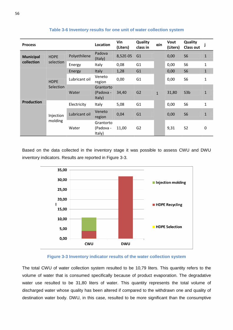
56
Table 3-6 Inventory results for one unit of water collection system
Process Location Vin (Liters)
Quality class in
αin Vout (Liters)
Quality Class out
j
Municipal collection
HDPE selection
Polyethilene Padova (Italy)
8,52E-05 G1
1
0,00 S6 1
Energy Italy 0,08 G1 0,00 S6 1
Production
HDPE Selection
Energy Italy 1,28 G1 0,00 S6 1
Lubricant oil Veneto region
0,00 G1 0,00 S6 1
Water Grantorto (Padova - Italy)
34,40 G2 31,80 S3b 1
Injection molding
Electricity Italy 5,08 G1 0,00 S6 1
Lubricant oil Veneto region
0,04 G1 0,00 S6 1
Water Grantorto (Padova - Italy)
11,00 G2 9,31 S2 0
Based on the data collected in the inventory stage it was possible to assess CWU and DWU
inventory indicators. Results are reported in Figure 3-3.
Figure 3-3 Inventory indicator results of the water collection system
The total CWU of water collection system resulted to be 10,79 liters. This quantity refers to the
volume of water that is consumed specifically because of product evaporation. The degradative
water use resulted to be 31,80 liters of water. This quantity represents the total volume of
discharged water whose quality has been altered if compared to the withdrawn one and quality of
destination water body. DWU, in this case, resulted to be more significant than the consumptive
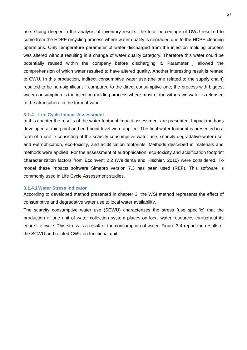
57
use. Going deeper in the analysis of inventory results, the total percentage of DWU resulted to
come from the HDPE recycling process where water quality is degraded due to the HDPE cleaning
operations. Only temperature parameter of water discharged from the injection molding process
was altered without resulting in a change of water quality category. Therefore this water could be
potentially reused within the company before discharging it. Parameter j allowed the
comprehension of which water resulted to have altered quality. Another interesting result is related
to CWU. In this production, indirect consumptive water use (the one related to the supply chain)
resulted to be non-significant if compared to the direct consumptive one; the process with biggest
water consumption is the injection molding process where most of the withdrawn water is released
to the atmosphere in the form of vapor.
3.1.4 Life Cycle Impact Assessment
In this chapter the results of the water footprint impact assessment are presented. Impact methods
developed at mid-point and end-point level were applied. The final water footprint is presented in a
form of a profile consisting of the scarcity consumptive water use, scarcity degradative water use,
and eutrophication, eco-toxicity, and acidification footprints. Methods described in materials and
methods were applied. For the assessment of eutrophication, eco-toxicity and acidification footprint
characterization factors from Ecoinvent 2.2 (Weidema and Hischier, 2010) were considered. To
model these impacts software Simapro version 7.3 has been used (REF). This software is
commonly used in Life Cycle Assessment studies.
3.1.4.1 Water Stress indicator
According to developed method presented in chapter 3, the WSI method represents the effect of
consumptive and degradative water use to local water availability.
The scarcity consumptive water use (SCWU) characterizes the stress (use specific) that the
production of one unit of water collection system places on local water resources throughout its
entire life cycle. This stress is a result of the consumption of water. Figure 3-4 report the results of
the SCWU and related CWU on functional unit.
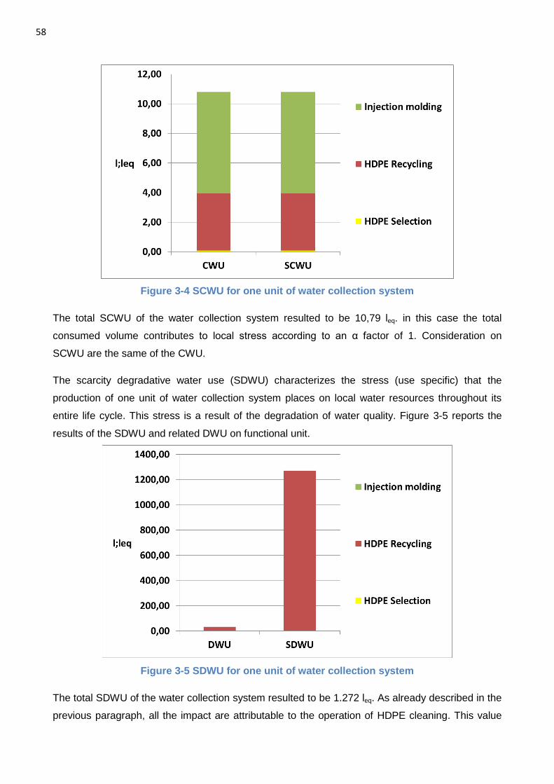
58
Figure 3-4 SCWU for one unit of water collection system
The total SCWU of the water collection system resulted to be 10,79 leq. in this case the total
consumed volume contributes to local stress according to an α factor of 1. Consideration on
SCWU are the same of the CWU.
The scarcity degradative water use (SDWU) characterizes the stress (use specific) that the
production of one unit of water collection system places on local water resources throughout its
entire life cycle. This stress is a result of the degradation of water quality. Figure 3-5 reports the
results of the SDWU and related DWU on functional unit.
Figure 3-5 SDWU for one unit of water collection system
The total SDWU of the water collection system resulted to be 1.272 leq. As already described in the
previous paragraph, all the impact are attributable to the operation of HDPE cleaning. This value
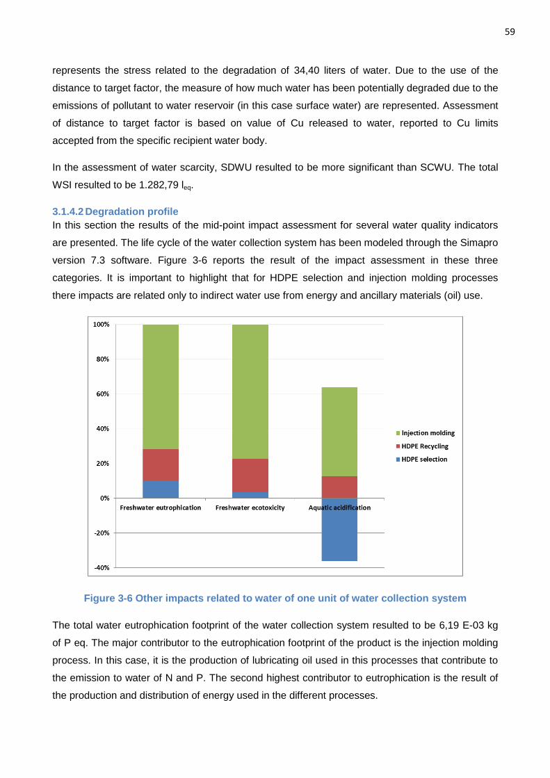
59
represents the stress related to the degradation of 34,40 liters of water. Due to the use of the
distance to target factor, the measure of how much water has been potentially degraded due to the
emissions of pollutant to water reservoir (in this case surface water) are represented. Assessment
of distance to target factor is based on value of Cu released to water, reported to Cu limits
accepted from the specific recipient water body.
In the assessment of water scarcity, SDWU resulted to be more significant than SCWU. The total
WSI resulted to be 1.282,79 leq.
3.1.4.2 Degradation profile
In this section the results of the mid-point impact assessment for several water quality indicators
are presented. The life cycle of the water collection system has been modeled through the Simapro
version 7.3 software. Figure 3-6 reports the result of the impact assessment in these three
categories. It is important to highlight that for HDPE selection and injection molding processes
there impacts are related only to indirect water use from energy and ancillary materials (oil) use.
Figure 3-6 Other impacts related to water of one unit of water collection system
The total water eutrophication footprint of the water collection system resulted to be 6,19 E-03 kg
of P eq. The major contributor to the eutrophication footprint of the product is the injection molding
process. In this case, it is the production of lubricating oil used in this processes that contribute to
the emission to water of N and P. The second highest contributor to eutrophication is the result of
the production and distribution of energy used in the different processes.
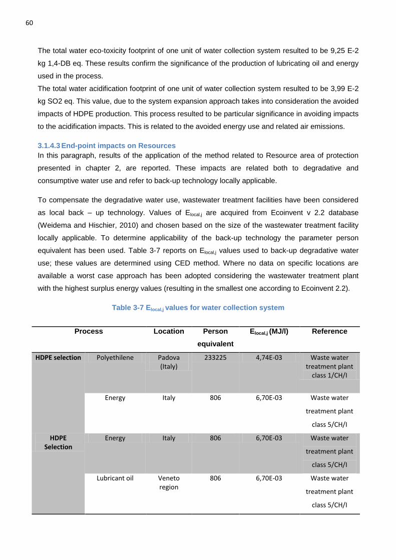
60
The total water eco-toxicity footprint of one unit of water collection system resulted to be 9,25 E-2
kg 1,4-DB eq. These results confirm the significance of the production of lubricating oil and energy
used in the process.
The total water acidification footprint of one unit of water collection system resulted to be 3,99 E-2
kg SO2 eq. This value, due to the system expansion approach takes into consideration the avoided
impacts of HDPE production. This process resulted to be particular significance in avoiding impacts
to the acidification impacts. This is related to the avoided energy use and related air emissions.
3.1.4.3 End-point impacts on Resources
In this paragraph, results of the application of the method related to Resource area of protection
presented in chapter 2, are reported. These impacts are related both to degradative and
consumptive water use and refer to back-up technology locally applicable.
To compensate the degradative water use, wastewater treatment facilities have been considered
as local back – up technology. Values of Elocal,j are acquired from Ecoinvent v 2.2 database
(Weidema and Hischier, 2010) and chosen based on the size of the wastewater treatment facility
locally applicable. To determine applicability of the back-up technology the parameter person
equivalent has been used. Table 3-7 reports on Elocal,j values used to back-up degradative water
use; these values are determined using CED method. Where no data on specific locations are
available a worst case approach has been adopted considering the wastewater treatment plant
with the highest surplus energy values (resulting in the smallest one according to Ecoinvent 2.2).
Table 3-7 Elocal,j values for water collection system
Process Location Person
equivalent
Elocal,j (MJ/l) Reference
HDPE selection Polyethilene Padova (Italy)
233225 4,74E-03 Waste water treatment plant
class 1/CH/I
Energy Italy 806 6,70E-03 Waste water
treatment plant
class 5/CH/I
HDPE Selection
Energy Italy 806 6,70E-03 Waste water
treatment plant
class 5/CH/I
Lubricant oil Veneto region
806 6,70E-03 Waste water
treatment plant
class 5/CH/I
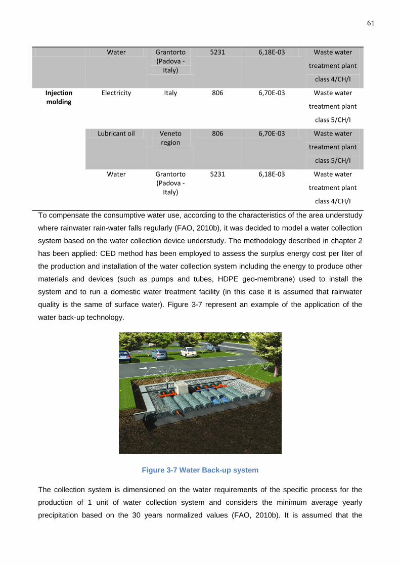
61
To compensate the consumptive water use, according to the characteristics of the area understudy
where rainwater rain-water falls regularly (FAO, 2010b), it was decided to model a water collection
system based on the water collection device understudy. The methodology described in chapter 2
has been applied: CED method has been employed to assess the surplus energy cost per liter of
the production and installation of the water collection system including the energy to produce other
materials and devices (such as pumps and tubes, HDPE geo-membrane) used to install the
system and to run a domestic water treatment facility (in this case it is assumed that rainwater
quality is the same of surface water). Figure 3-7 represent an example of the application of the
water back-up technology.
Figure 3-7 Water Back-up system
The collection system is dimensioned on the water requirements of the specific process for the
production of 1 unit of water collection system and considers the minimum average yearly
precipitation based on the 30 years normalized values (FAO, 2010b). It is assumed that the
Water Grantorto (Padova -
Italy)
5231 6,18E-03 Waste water
treatment plant
class 4/CH/I
Injection molding
Electricity Italy 806 6,70E-03 Waste water
treatment plant
class 5/CH/I
Lubricant oil Veneto region
806 6,70E-03 Waste water
treatment plant
class 5/CH/I
Water Grantorto (Padova -
Italy)
5231 6,18E-03 Waste water
treatment plant
class 4/CH/I
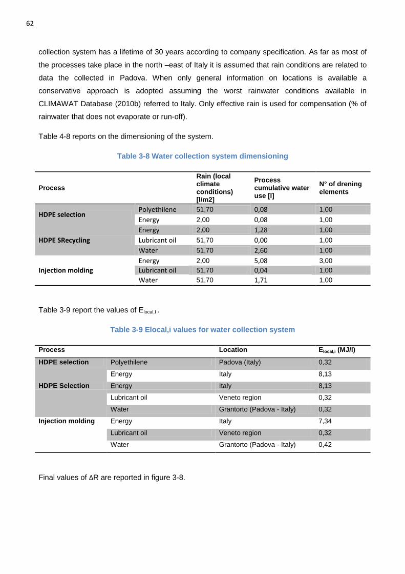
62
collection system has a lifetime of 30 years according to company specification. As far as most of
the processes take place in the north –east of Italy it is assumed that rain conditions are related to
data the collected in Padova. When only general information on locations is available a
conservative approach is adopted assuming the worst rainwater conditions available in
CLIMAWAT Database (2010b) referred to Italy. Only effective rain is used for compensation (% of
rainwater that does not evaporate or run-off).
Table 4-8 reports on the dimensioning of the system.
Table 3-8 Water collection system dimensioning
Process
Rain (local climate conditions) [l/m2]
Process cumulative water use [l]
N° of drening elements
HDPE selection Polyethilene 51,70 0,08 1,00
Energy 2,00 0,08 1,00
HDPE SRecycling
Energy 2,00 1,28 1,00
Lubricant oil 51,70 0,00 1,00
Water 51,70 2,60 1,00
Injection molding
Energy 2,00 5,08 3,00
Lubricant oil 51,70 0,04 1,00
Water 51,70 1,71 1,00
Table 3-9 report the values of Elocal,I .
Table 3-9 Elocal,i values for water collection system
Process Location Elocal,i (MJ/l)
HDPE selection Polyethilene Padova (Italy) 0,32
Energy Italy 8,13
HDPE Selection Energy Italy 8,13
Lubricant oil Veneto region 0,32
Water Grantorto (Padova - Italy) 0,32
Injection molding Energy Italy 7,34
Lubricant oil Veneto region 0,32
Water Grantorto (Padova - Italy) 0,42
Final values of ΔR are reported in figure 3-8.
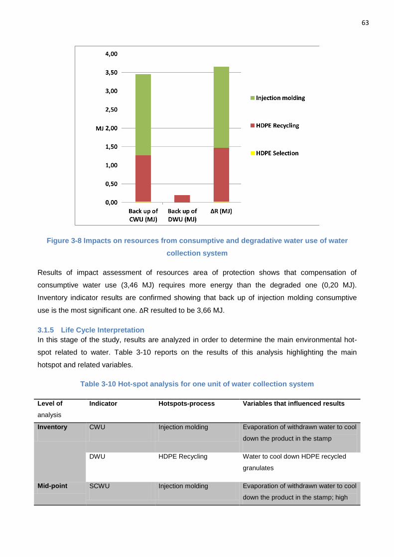
63
Figure 3-8 Impacts on resources from consumptive and degradative water use of water
collection system
Results of impact assessment of resources area of protection shows that compensation of
consumptive water use (3,46 MJ) requires more energy than the degraded one (0,20 MJ).
Inventory indicator results are confirmed showing that back up of injection molding consumptive
use is the most significant one. ΔR resulted to be 3,66 MJ.
3.1.5 Life Cycle Interpretation
In this stage of the study, results are analyzed in order to determine the main environmental hot-
spot related to water. Table 3-10 reports on the results of this analysis highlighting the main
hotspot and related variables.
Table 3-10 Hot-spot analysis for one unit of water collection system
Level of
analysis
Indicator Hotspots-process Variables that influenced results
Inventory CWU Injection molding Evaporation of withdrawn water to cool
down the product in the stamp
DWU HDPE Recycling Water to cool down HDPE recycled
granulates
Mid-point SCWU Injection molding Evaporation of withdrawn water to cool
down the product in the stamp; high
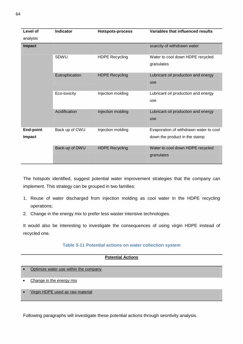
64
Level of
analysis
Indicator Hotspots-process Variables that influenced results
Impact scarcity of withdrawn water
SDWU HDPE Recycling Water to cool down HDPE recycled
granulates
Eutrophication HDPE Recycling Lubricant oil production and energy
use
Eco-toxicity Injection molding Lubricant oil production and energy
use
Acidification Injection molding Lubricant oil production and energy
use
End-point
Impact
Back up of CWU Injection molding Evaporation of withdrawn water to cool
down the product in the stamp
Back-up of DWU HDPE Recycling Water to cool down HDPE recycled
granulates
The hotspots identified, suggest potential water improvement strategies that the company can
implement. This strategy can be grouped in two families:
1. Reuse of water discharged from injection molding as cool water in the HDPE recycling
operations;
2. Change in the energy mix to prefer less waster intensive technologies.
It would also be interesting to investigate the consequences of using virgin HDPE instead of
recycled one.
Table 3-11 Potential actions on water collection system
Potential Actions
Optimize water use within the company
Change in the energy mix
Virgin HDPE used as raw material
Following paragraphs will investigate these potential actions through sesntivity analysis.
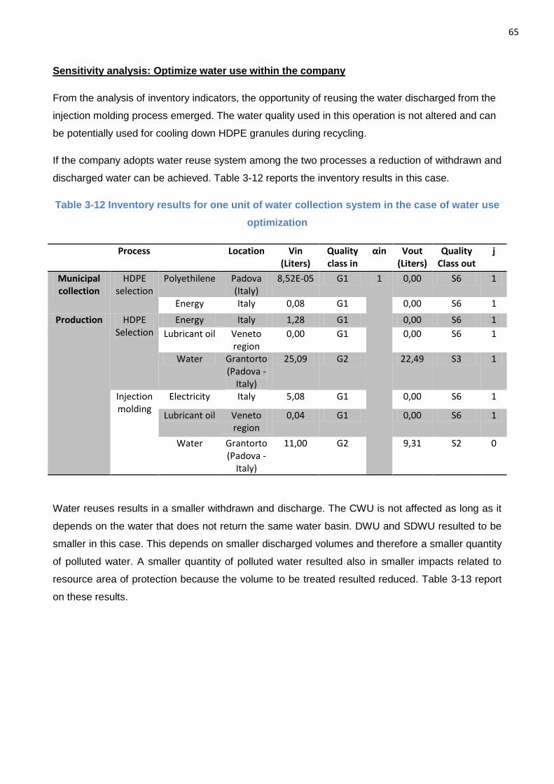
65
Sensitivity analysis: Optimize water use within the company
From the analysis of inventory indicators, the opportunity of reusing the water discharged from the
injection molding process emerged. The water quality used in this operation is not altered and can
be potentially used for cooling down HDPE granules during recycling.
If the company adopts water reuse system among the two processes a reduction of withdrawn and
discharged water can be achieved. Table 3-12 reports the inventory results in this case.
Table 3-12 Inventory results for one unit of water collection system in the case of water use
optimization
Process Location Vin (Liters)
Quality class in
αin Vout (Liters)
Quality Class out
j
Municipal collection
HDPE selection
Polyethilene Padova (Italy)
8,52E-05 G1 1 0,00 S6 1
Energy Italy 0,08 G1 0,00 S6 1
Production HDPE Selection
Energy Italy 1,28 G1 0,00 S6 1
Lubricant oil Veneto region
0,00 G1 0,00 S6 1
Water Grantorto (Padova -
Italy)
25,09 G2 22,49 S3 1
Injection molding
Electricity Italy 5,08 G1 0,00 S6 1
Lubricant oil Veneto region
0,04 G1 0,00 S6 1
Water Grantorto (Padova -
Italy)
11,00 G2 9,31 S2 0
Water reuses results in a smaller withdrawn and discharge. The CWU is not affected as long as it
depends on the water that does not return the same water basin. DWU and SDWU resulted to be
smaller in this case. This depends on smaller discharged volumes and therefore a smaller quantity
of polluted water. A smaller quantity of polluted water resulted also in smaller impacts related to
resource area of protection because the volume to be treated resulted reduced. Table 3-13 report
on these results.
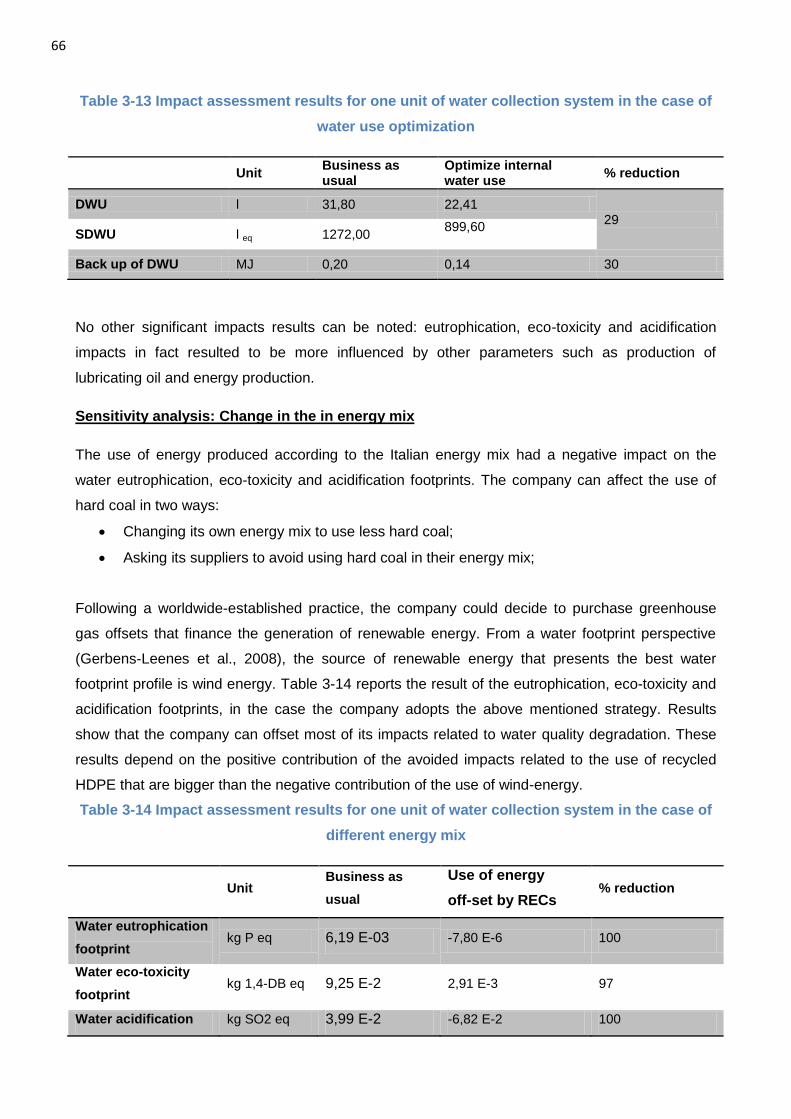
66
Table 3-13 Impact assessment results for one unit of water collection system in the case of
water use optimization
Unit
Business as usual
Optimize internal water use
% reduction
DWU l 31,80 22,41 29
SDWU l eq 1272,00 899,60
Back up of DWU MJ 0,20 0,14 30
No other significant impacts results can be noted: eutrophication, eco-toxicity and acidification
impacts in fact resulted to be more influenced by other parameters such as production of
lubricating oil and energy production.
Sensitivity analysis: Change in the in energy mix
The use of energy produced according to the Italian energy mix had a negative impact on the
water eutrophication, eco-toxicity and acidification footprints. The company can affect the use of
hard coal in two ways:
Changing its own energy mix to use less hard coal;
Asking its suppliers to avoid using hard coal in their energy mix;
Following a worldwide-established practice, the company could decide to purchase greenhouse
gas offsets that finance the generation of renewable energy. From a water footprint perspective
(Gerbens-Leenes et al., 2008), the source of renewable energy that presents the best water
footprint profile is wind energy. Table 3-14 reports the result of the eutrophication, eco-toxicity and
acidification footprints, in the case the company adopts the above mentioned strategy. Results
show that the company can offset most of its impacts related to water quality degradation. These
results depend on the positive contribution of the avoided impacts related to the use of recycled
HDPE that are bigger than the negative contribution of the use of wind-energy.
Table 3-14 Impact assessment results for one unit of water collection system in the case of
different energy mix
Unit
Business as
usual
Use of energy
off-set by RECs % reduction
Water eutrophication
footprint kg P eq 6,19 E-03 -7,80 E-6 100
Water eco-toxicity
footprint kg 1,4-DB eq 9,25 E-2 2,91 E-3 97
Water acidification kg SO2 eq 3,99 E-2 -6,82 E-2 100
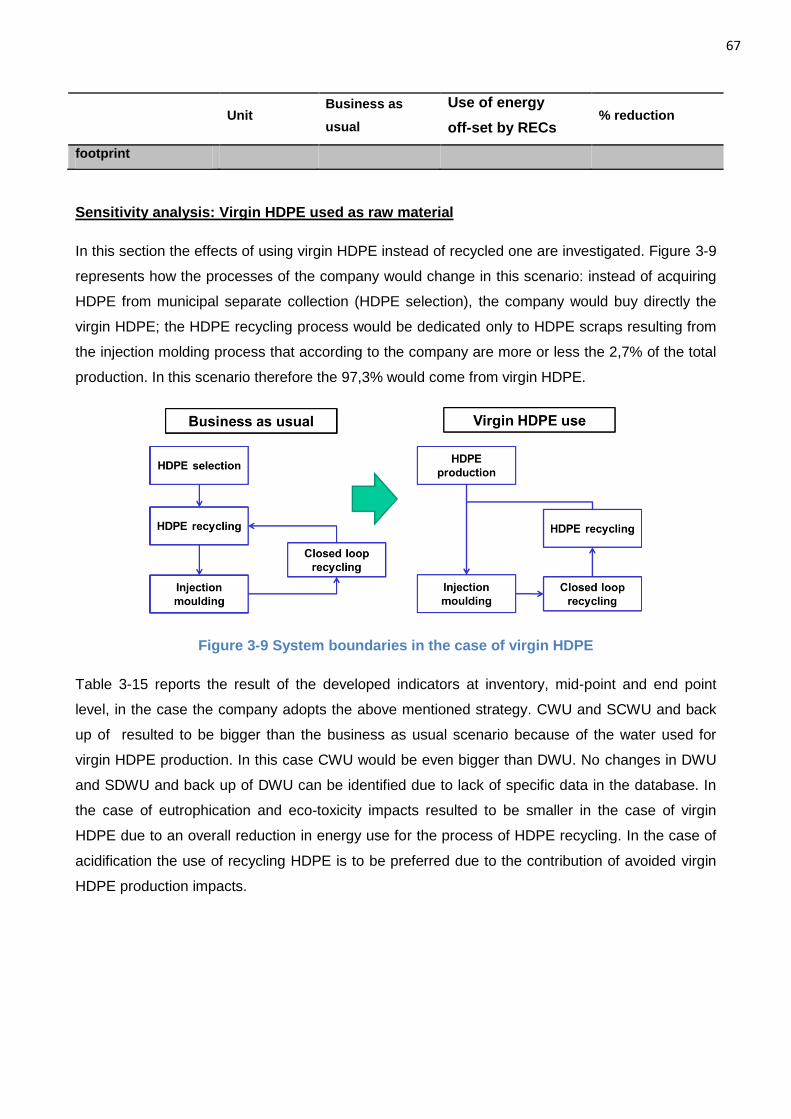
67
Unit
Business as
usual
Use of energy
off-set by RECs % reduction
footprint
Sensitivity analysis: Virgin HDPE used as raw material
In this section the effects of using virgin HDPE instead of recycled one are investigated. Figure 3-9
represents how the processes of the company would change in this scenario: instead of acquiring
HDPE from municipal separate collection (HDPE selection), the company would buy directly the
virgin HDPE; the HDPE recycling process would be dedicated only to HDPE scraps resulting from
the injection molding process that according to the company are more or less the 2,7% of the total
production. In this scenario therefore the 97,3% would come from virgin HDPE.
Figure 3-9 System boundaries in the case of virgin HDPE
Table 3-15 reports the result of the developed indicators at inventory, mid-point and end point
level, in the case the company adopts the above mentioned strategy. CWU and SCWU and back
up of resulted to be bigger than the business as usual scenario because of the water used for
virgin HDPE production. In this case CWU would be even bigger than DWU. No changes in DWU
and SDWU and back up of DWU can be identified due to lack of specific data in the database. In
the case of eutrophication and eco-toxicity impacts resulted to be smaller in the case of virgin
HDPE due to an overall reduction in energy use for the process of HDPE recycling. In the case of
acidification the use of recycling HDPE is to be preferred due to the contribution of avoided virgin
HDPE production impacts.
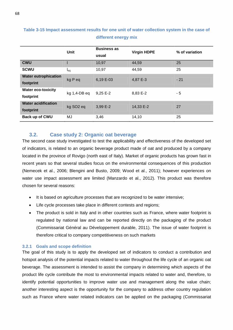
68
Table 3-15 Impact assessment results for one unit of water collection system in the case of
different energy mix
Unit
Business as
usual Virgin HDPE % of variation
CWU l 10,97 44,59 25
SCWU leq 10,97 44,59 25
Water eutrophication
footprint kg P eq 6,19 E-03 4,87 E-3 - 21
Water eco-toxicity
footprint kg 1,4-DB eq 9,25 E-2 8,83 E-2 - 5
Water acidification
footprint kg SO2 eq 3,99 E-2 14,33 E-2 27
Back up of CWU MJ 3,46 14,10 25
3.2. Case study 2: Organic oat beverage
The second case study investigated to test the applicability and effectiveness of the developed set
of indicators, is related to an organic beverage product made of oat and produced by a company
located in the province of Rovigo (north east of Italy). Market of organic products has grown fast in
recent years so that several studies focus on the environmental consequences of this production
(Nemecek et al., 2006; Blengini and Busto, 2009; Wood et al., 2011); however experiences on
water use impact assessment are limited (Manzardo et al., 2012). This product was therefore
chosen for several reasons:
It is based on agriculture processes that are recognized to be water intensive;
Life cycle processes take place in different contests and regions;
The product is sold in Italy and in other countries such as France, where water footprint is
regulated by national law and can be reported directly on the packaging of the product
(Commissariat Général au Développement durable, 2011). The issue of water footprint is
therefore critical to company competitiveness on such markets
3.2.1 Goals and scope definition
The goal of this study is to apply the developed set of indicators to conduct a contribution and
hotspot analysis of the potential impacts related to water throughout the life cycle of an organic oat
beverage. The assessment is intended to assist the company in determining which aspects of the
product life cycle contribute the most to environmental impacts related to water and, therefore, to
identify potential opportunities to improve water use and management along the value chain;
another interesting aspect is the opportunity for the company to address other country regulation
such as France where water related indicators can be applied on the packaging (Commissariat
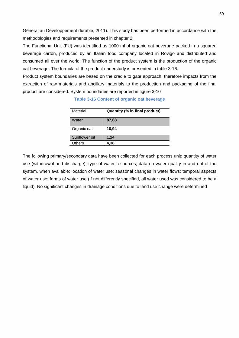
69
Général au Développement durable, 2011). This study has been performed in accordance with the
methodologies and requirements presented in chapter 2.
The Functional Unit (FU) was identified as 1000 ml of organic oat beverage packed in a squared
beverage carton, produced by an Italian food company located in Rovigo and distributed and
consumed all over the world. The function of the product system is the production of the organic
oat beverage. The formula of the product understudy is presented in table 3-16.
Product system boundaries are based on the cradle to gate approach; therefore impacts from the
extraction of raw materials and ancillary materials to the production and packaging of the final
product are considered. System boundaries are reported in figure 3-10
Table 3-16 Content of organic oat beverage
Material Quantity (% in final product)
Water 87,68
Organic oat 10,94
Sunflower oil 1,14
Others 4,38
The following primary/secondary data have been collected for each process unit: quantity of water
use (withdrawal and discharge); type of water resources; data on water quality in and out of the
system, when available; location of water use; seasonal changes in water flows; temporal aspects
of water use; forms of water use (If not differently specified, all water used was considered to be a
liquid). No significant changes in drainage conditions due to land use change were determined
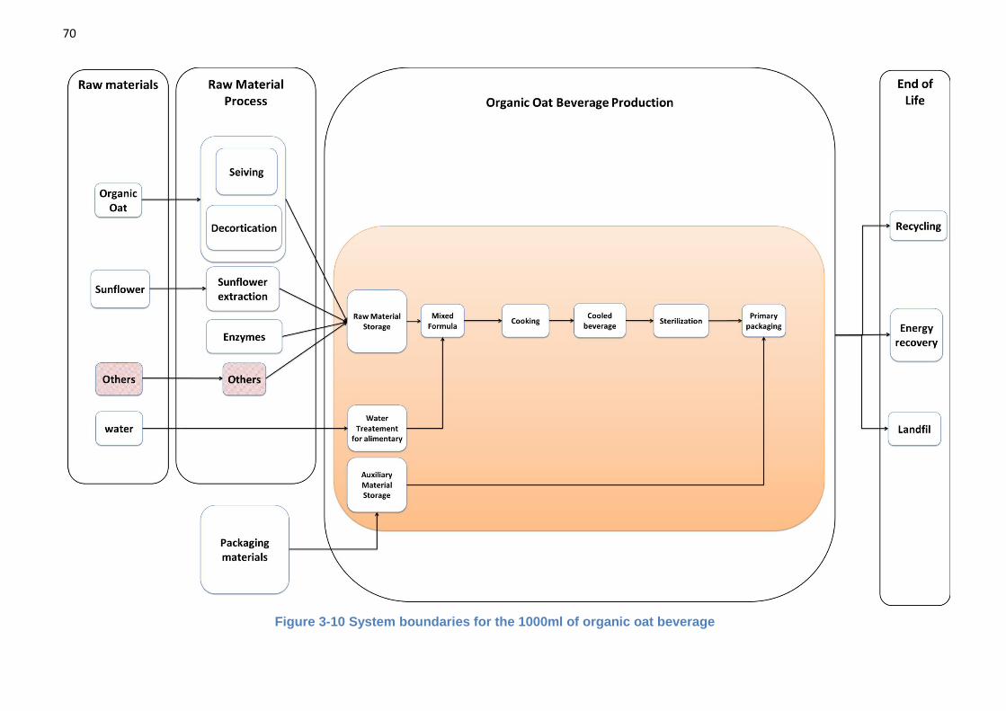
70
Figure 3-10 System boundaries for the 1000ml of organic oat beverage
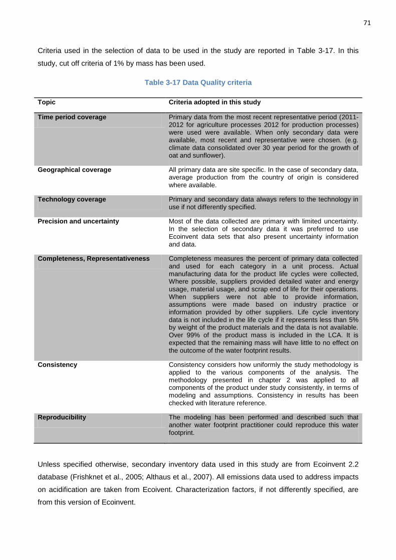
71
Criteria used in the selection of data to be used in the study are reported in Table 3-17. In this
study, cut off criteria of 1% by mass has been used.
Table 3-17 Data Quality criteria
Topic Criteria adopted in this study
Time period coverage Primary data from the most recent representative period (2011-2012 for agriculture processes 2012 for production processes) were used were available. When only secondary data were available, most recent and representative were chosen. (e.g. climate data consolidated over 30 year period for the growth of oat and sunflower).
Geographical coverage All primary data are site specific. In the case of secondary data, average production from the country of origin is considered where available.
Technology coverage Primary and secondary data always refers to the technology in use if not differently specified.
Precision and uncertainty Most of the data collected are primary with limited uncertainty. In the selection of secondary data it was preferred to use Ecoinvent data sets that also present uncertainty information and data.
Completeness, Representativeness Completeness measures the percent of primary data collected and used for each category in a unit process. Actual manufacturing data for the product life cycles were collected, Where possible, suppliers provided detailed water and energy usage, material usage, and scrap end of life for their operations. When suppliers were not able to provide information, assumptions were made based on industry practice or information provided by other suppliers. Life cycle inventory data is not included in the life cycle if it represents less than 5% by weight of the product materials and the data is not available. Over 99% of the product mass is included in the LCA. It is expected that the remaining mass will have little to no effect on the outcome of the water footprint results.
Consistency Consistency considers how uniformly the study methodology is applied to the various components of the analysis. The methodology presented in chapter 2 was applied to all components of the product under study consistently, in terms of modeling and assumptions. Consistency in results has been checked with literature reference.
Reproducibility The modeling has been performed and described such that another water footprint practitioner could reproduce this water footprint.
Unless specified otherwise, secondary inventory data used in this study are from Ecoinvent 2.2
database (Frishknet et al., 2005; Althaus et al., 2007). All emissions data used to address impacts
on acidification are taken from Ecoivent. Characterization factors, if not differently specified, are
from this version of Ecoinvent.
72
4.2.2 Life Cycle Inventory
In this chapter, all the data acquired and calculations performed are reported. The paragraph is
divided per different process unit considered.
Primary data are collected directly from the producer company. In the case of secondary data
however not all the information (such as quality in and quantity out) was available. In these cases a
conservative approach is adopted considering all withdrawn water as used (consumptive use) and
the quality entering the system as of the best quality locally available.
4.2.2.1 Organic Oat
One of the most important raw materials used in the production of the product under study is oat.
This cereal is grown in San Martino Pensile (Campobasso, south of Italy) where the company
owns 270 ha of land dedicated to organic agricultural product growth. Following the common
practice of organic agriculture, oat is grown following the crop-rotation practice; it is usually planted
in the second half of October and harvested in July. Due to local climate conditions, the crops are
mostly rain fed with very little additional water supply requirements. Data reported are primary data
based on the 2011 and 2012. The average yield based on historical company data is 3,2 tons/ha
In order to assess the crop water requirements the CROPWAT model (FAO, 2010a) has been
used. The CROPWAT software developed by FAO is used to model the water requirements of a
crop. The model utilizes data on the climatic conditions, the reference evapotranspiration, the soil
and the specific crop characteristics to determine the irrigation requirements of the crop under
study. ET0 (evapotranspiration in standard condition) is determined using the Penman-Montheit
equation (FAO, 2010a). Effective rain (the rainfall effectively available to the crop) is assessed
through the USDA SCS method (option selected within CROPWAT model). Climatic data are taken
from the climatic stations located in Termoli (the closest one to the location of the production site)
available from (Tab 3-18 and 3-19) and acquired through the use of CLIMAWAT software (FAO,
2010b).
Data on the crop modeling are taken from FAO database (FAO, 2010a) accessible within the
CROPWAT software and then modified with primary parameters such as critical dates of different
processes and specific crop parameters (roots length, crop-coefficients, soil humidity). Medium soil
parameters from CROPWAT are considered.
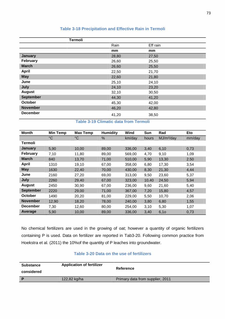
73
Table 3-18 Precipitation and Effective Rain in Termoli
Termoli
Rain Eff rain
mm mm
January 28,80 27,50
February 26,60 25,50
March 26,60 25,50
April 22,50 21,70
May 22,60 21,80
June 25,10 24,10
July 24,10 23,20
August 32,10 30,50
September 44,30 41,20
October 45,30 42,00
November 46,20 42,80
December 41,20 38,50
Table 3-19 Climatic data from Termoli
Month Min Temp Max Temp Humidity Wind Sun Rad Eto
°C °C % km/day hours MJ/m²/day mm/day
Termoli
January 5,90 10,00 89,00 336,00 3,40 6,10 0,73
February 7,10 11,80 89,00 569,00 4,70 9,10 1,09
March 840 13,70 71,00 510,00 5,90 13,30 2.50
April 1310 19,10 67,00 358,00 6,80 17,30 3,54
May 1630 22,40 70,00 430,00 8,30 21,30 4,44
June 2160 27,20 69,00 313,00 9,50 23,60 5,37
July 2260 29,40 67,00 323,00 10,40 24,50 5,94
August 2450 30,90 67,00 236,00 9,60 21,60 5,40
September 2220 29,00 71,00 367,00 7,20 15,80 4,57
October 1490 20,20 81,00 229,00 5,50 10,70 2,06
November 12,90 18,20 78,00 240,00 3,80 6,80 1,55
December 7,30 12,60 80,00 254,00 3,10 5,30 1,07
Average 5,90 10,00 89,00 336,00 3,40 6,1o 0,73
No chemical fertilizers are used in the growing of oat; however a quantity of organic fertilizers
containing P is used. Data on fertilizer are reported in Tab3-20. Following common practice from
Hoekstra et al. (2011) the 10%of the quantity of P leaches into groundwater.
Table 3-20 Data on the use of fertilizers
Substance
considered
Application of fertilizer Reference
P 122,82 kg/ha Primary data from supplier, 2011
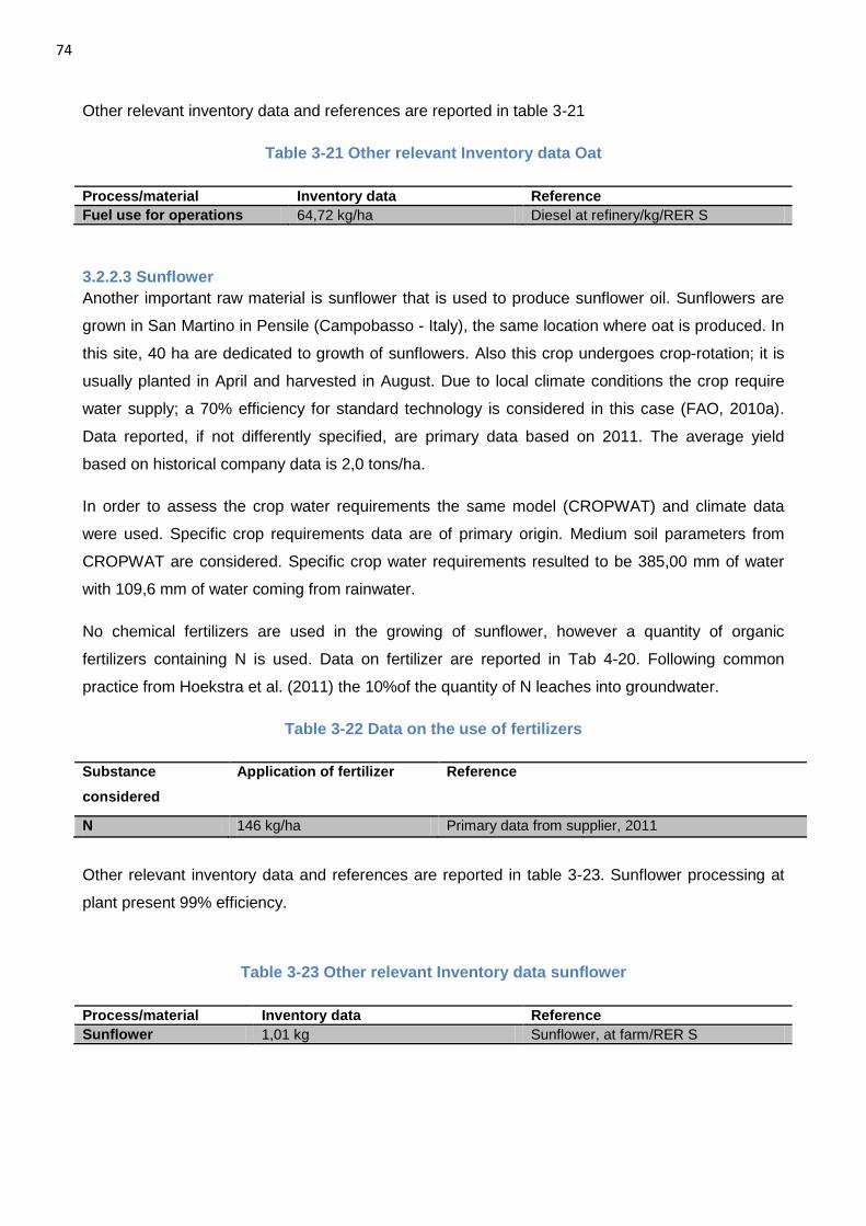
74
Other relevant inventory data and references are reported in table 3-21
Table 3-21 Other relevant Inventory data Oat
Process/material Inventory data Reference
Fuel use for operations 64,72 kg/ha Diesel at refinery/kg/RER S
3.2.2.3 Sunflower
Another important raw material is sunflower that is used to produce sunflower oil. Sunflowers are
grown in San Martino in Pensile (Campobasso - Italy), the same location where oat is produced. In
this site, 40 ha are dedicated to growth of sunflowers. Also this crop undergoes crop-rotation; it is
usually planted in April and harvested in August. Due to local climate conditions the crop require
water supply; a 70% efficiency for standard technology is considered in this case (FAO, 2010a).
Data reported, if not differently specified, are primary data based on 2011. The average yield
based on historical company data is 2,0 tons/ha.
In order to assess the crop water requirements the same model (CROPWAT) and climate data
were used. Specific crop requirements data are of primary origin. Medium soil parameters from
CROPWAT are considered. Specific crop water requirements resulted to be 385,00 mm of water
with 109,6 mm of water coming from rainwater.
No chemical fertilizers are used in the growing of sunflower, however a quantity of organic
fertilizers containing N is used. Data on fertilizer are reported in Tab 4-20. Following common
practice from Hoekstra et al. (2011) the 10%of the quantity of N leaches into groundwater.
Table 3-22 Data on the use of fertilizers
Substance
considered
Application of fertilizer Reference
N 146 kg/ha Primary data from supplier, 2011
Other relevant inventory data and references are reported in table 3-23. Sunflower processing at
plant present 99% efficiency.
Table 3-23 Other relevant Inventory data sunflower
Process/material Inventory data Reference
Sunflower 1,01 kg Sunflower, at farm/RER S
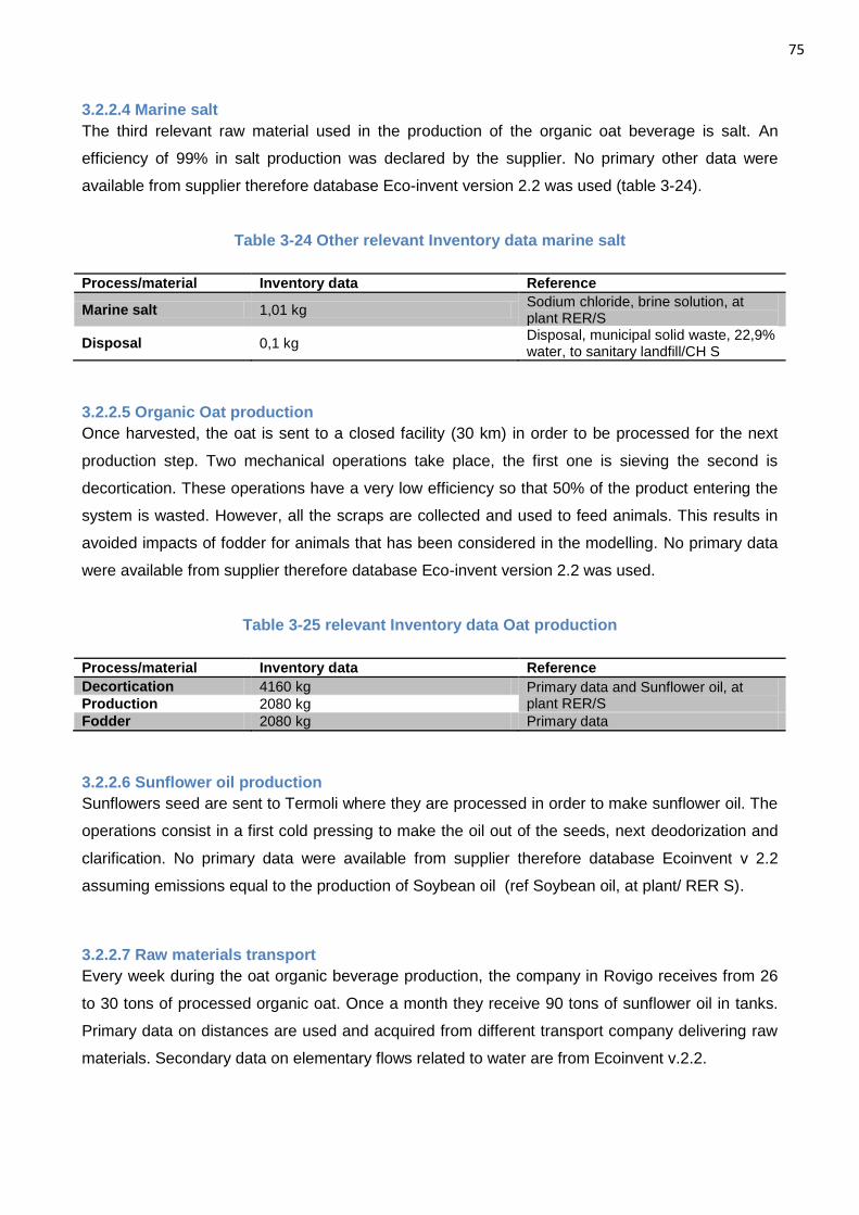
75
3.2.2.4 Marine salt
The third relevant raw material used in the production of the organic oat beverage is salt. An
efficiency of 99% in salt production was declared by the supplier. No primary other data were
available from supplier therefore database Eco-invent version 2.2 was used (table 3-24).
Table 3-24 Other relevant Inventory data marine salt
Process/material Inventory data Reference
Marine salt 1,01 kg Sodium chloride, brine solution, at plant RER/S
Disposal 0,1 kg Disposal, municipal solid waste, 22,9% water, to sanitary landfill/CH S
3.2.2.5 Organic Oat production
Once harvested, the oat is sent to a closed facility (30 km) in order to be processed for the next
production step. Two mechanical operations take place, the first one is sieving the second is
decortication. These operations have a very low efficiency so that 50% of the product entering the
system is wasted. However, all the scraps are collected and used to feed animals. This results in
avoided impacts of fodder for animals that has been considered in the modelling. No primary data
were available from supplier therefore database Eco-invent version 2.2 was used.
Table 3-25 relevant Inventory data Oat production
Process/material Inventory data Reference
Decortication 4160 kg Primary data and Sunflower oil, at plant RER/S Production 2080 kg
Fodder 2080 kg Primary data
3.2.2.6 Sunflower oil production
Sunflowers seed are sent to Termoli where they are processed in order to make sunflower oil. The
operations consist in a first cold pressing to make the oil out of the seeds, next deodorization and
clarification. No primary data were available from supplier therefore database Ecoinvent v 2.2
assuming emissions equal to the production of Soybean oil (ref Soybean oil, at plant/ RER S).
3.2.2.7 Raw materials transport
Every week during the oat organic beverage production, the company in Rovigo receives from 26
to 30 tons of processed organic oat. Once a month they receive 90 tons of sunflower oil in tanks.
Primary data on distances are used and acquired from different transport company delivering raw
materials. Secondary data on elementary flows related to water are from Ecoinvent v.2.2.
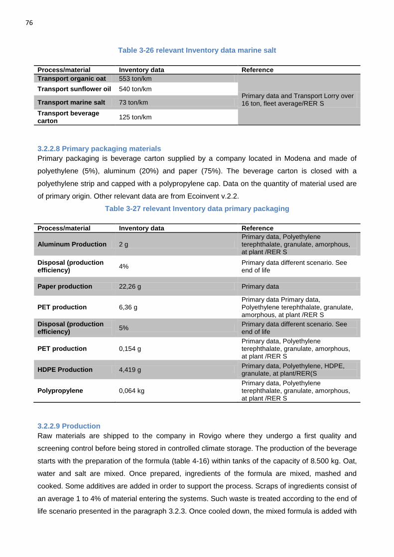
76
Table 3-26 relevant Inventory data marine salt
Process/material Inventory data Reference
Transport organic oat 553 ton/km
Primary data and Transport Lorry over 16 ton, fleet average/RER S
Transport sunflower oil 540 ton/km
Transport marine salt 73 ton/km
Transport beverage carton
125 ton/km
3.2.2.8 Primary packaging materials
Primary packaging is beverage carton supplied by a company located in Modena and made of
polyethylene (5%), aluminum (20%) and paper (75%). The beverage carton is closed with a
polyethylene strip and capped with a polypropylene cap. Data on the quantity of material used are
of primary origin. Other relevant data are from Ecoinvent v.2.2.
Table 3-27 relevant Inventory data primary packaging
Process/material Inventory data Reference
Aluminum Production 2 g Primary data, Polyethylene terephthalate, granulate, amorphous, at plant /RER S
Disposal (production efficiency)
4% Primary data different scenario. See end of life
Paper production 22,26 g Primary data
PET production 6,36 g Primary data Primary data, Polyethylene terephthalate, granulate, amorphous, at plant /RER S
Disposal (production efficiency)
5% Primary data different scenario. See end of life
PET production 0,154 g Primary data, Polyethylene terephthalate, granulate, amorphous, at plant /RER S
HDPE Production 4,419 g Primary data, Polyethylene, HDPE, granulate, at plant/RER(S
Polypropylene 0,064 kg Primary data, Polyethylene terephthalate, granulate, amorphous, at plant /RER S
3.2.2.9 Production
Raw materials are shipped to the company in Rovigo where they undergo a first quality and
screening control before being stored in controlled climate storage. The production of the beverage
starts with the preparation of the formula (table 4-16) within tanks of the capacity of 8.500 kg. Oat,
water and salt are mixed. Once prepared, ingredients of the formula are mixed, mashed and
cooked. Some additives are added in order to support the process. Scraps of ingredients consist of
an average 1 to 4% of material entering the systems. Such waste is treated according to the end of
life scenario presented in the paragraph 3.2.3. Once cooled down, the mixed formula is added with
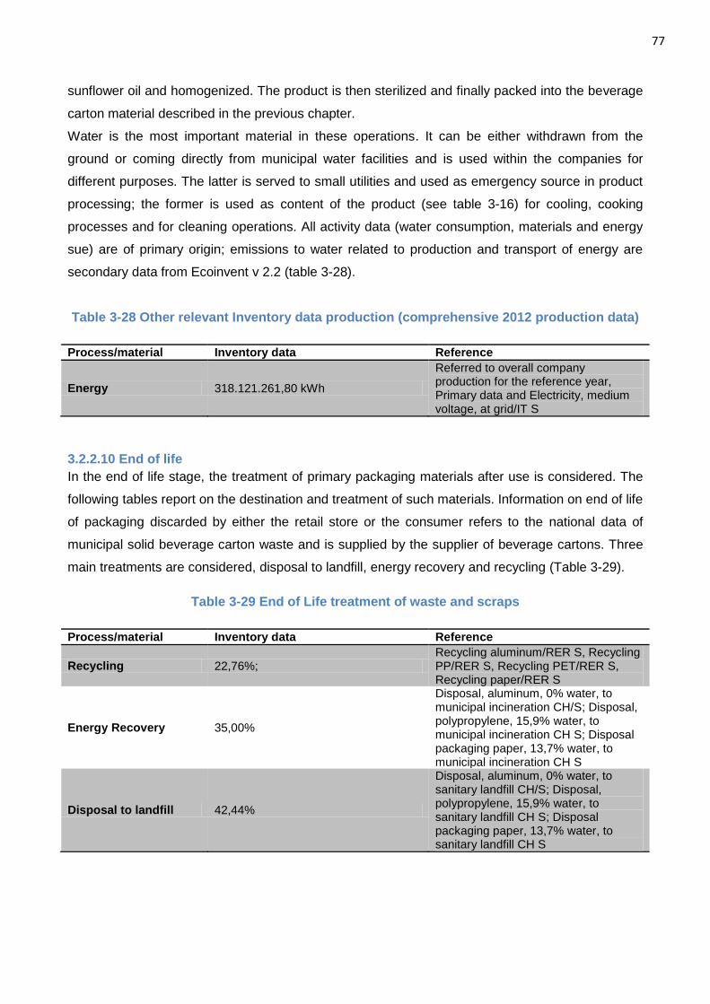
77
sunflower oil and homogenized. The product is then sterilized and finally packed into the beverage
carton material described in the previous chapter.
Water is the most important material in these operations. It can be either withdrawn from the
ground or coming directly from municipal water facilities and is used within the companies for
different purposes. The latter is served to small utilities and used as emergency source in product
processing; the former is used as content of the product (see table 3-16) for cooling, cooking
processes and for cleaning operations. All activity data (water consumption, materials and energy
sue) are of primary origin; emissions to water related to production and transport of energy are
secondary data from Ecoinvent v 2.2 (table 3-28).
Table 3-28 Other relevant Inventory data production (comprehensive 2012 production data)
Process/material Inventory data Reference
Energy 318.121.261,80 kWh
Referred to overall company production for the reference year, Primary data and Electricity, medium voltage, at grid/IT S
3.2.2.10 End of life
In the end of life stage, the treatment of primary packaging materials after use is considered. The
following tables report on the destination and treatment of such materials. Information on end of life
of packaging discarded by either the retail store or the consumer refers to the national data of
municipal solid beverage carton waste and is supplied by the supplier of beverage cartons. Three
main treatments are considered, disposal to landfill, energy recovery and recycling (Table 3-29).
Table 3-29 End of Life treatment of waste and scraps
Process/material Inventory data Reference
Recycling 22,76%; Recycling aluminum/RER S, Recycling PP/RER S, Recycling PET/RER S, Recycling paper/RER S
Energy Recovery 35,00%
Disposal, aluminum, 0% water, to municipal incineration CH/S; Disposal, polypropylene, 15,9% water, to municipal incineration CH S; Disposal packaging paper, 13,7% water, to municipal incineration CH S
Disposal to landfill 42,44%
Disposal, aluminum, 0% water, to sanitary landfill CH/S; Disposal, polypropylene, 15,9% water, to sanitary landfill CH S; Disposal packaging paper, 13,7% water, to sanitary landfill CH S
78
3.2.3 Life Cycle Inventory Analysis
Life Cycle inventory analysis is the stage of the study were data collected are aggregated in order
to have a first representation of materials and energy flows going in and out of the system. Table 4-
23 reports on inventory information to be used according to the inventory method developed and
described in chapter 2. Due to the huge amount of data, discharged water quality parameters and
air emissions parameters are reported in ANNEX B. Where no information on quantity of
discharged water is available (such as from Ecoinvent database) a conservative approach is
adopted, considering all the withdrawn water to be consumed. Where no data on quality in and out
are available it is assumed that the water going into the system is of the best available quality and
the one discharged is of the worst available quality according to the classification of Boulay et al
(2011a). It is reminded that G stands for ground water and S for surface according to the
classification from Boulay et al. (2011a) data are reported on the functional unit of on product
understudy.
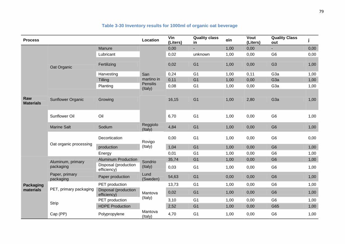
79
Table 3-30 Inventory results for 1000ml of organic oat beverage
Process Location Vin (Liters)
Quality class in
αin Vout (Liters)
Quality Class out
j
Raw Materials
Oat Organic
Manure
San martino in Pensilis (Italy)
0,00 - 1,00 0,00 - 0,00
Lubricant 0,02 unknown 1,00 0,00 G6 0,00
Fertilizing 0,02 G1 1,00 0,00 G3 1,00
Harvesting 0,24 G1 1,00 0,11 G3a 1,00
Tilling 0,11 G1 1,00 0,00 G3a 1,00
Planting 0,08 G1 1,00 0,00 G3a 1,00
Sunflower Organic Growing 16,15 G1 1,00 2,80 G3a 1,00
Sunflower Oil Oil 6,70 G1 1,00 0,00 G6 1,00
Marine Salt Sodium Reggiolo (Italy)
4,84 G1 1,00 0,00 G6 1,00
Oat organic processing
Decortication Rovigo (Italy)
0,00 G1 1,00 0,00 G6 0,00
production 1,04 G1 1,00 0,00 G6 1,00
Energy 0,01 G1 1,00 0,00 G6 1,00
Packaging materials
Aluminum, primary packaging
Aluminum Production Sondrio (Italy)
35,74 G1 1,00 0,00 G6 1,00
Disposal (production efficiency)
0,03 G1 1,00 0,00 G6 1,00
Paper, primary packaging
Paper production Lund (Sweden)
54,63 G1 0,00 0,00 G6 1,00
PET, primary packaging PET production
Mantova (Italy)
13,73 G1 1,00 0,00 G6 1,00
Disposal (production efficiency)
0,02 G1 1,00 0,00 G6 1,00
Strip PET production 3,10 G1 1,00 0,00 G6 1,00
HDPE Production 2,52 G1 1,00 0,00 G65 1,00
Cap (PP) Polypropylene Mantova (Italy)
4,70 G1 1,00 0,00 G6 1,00
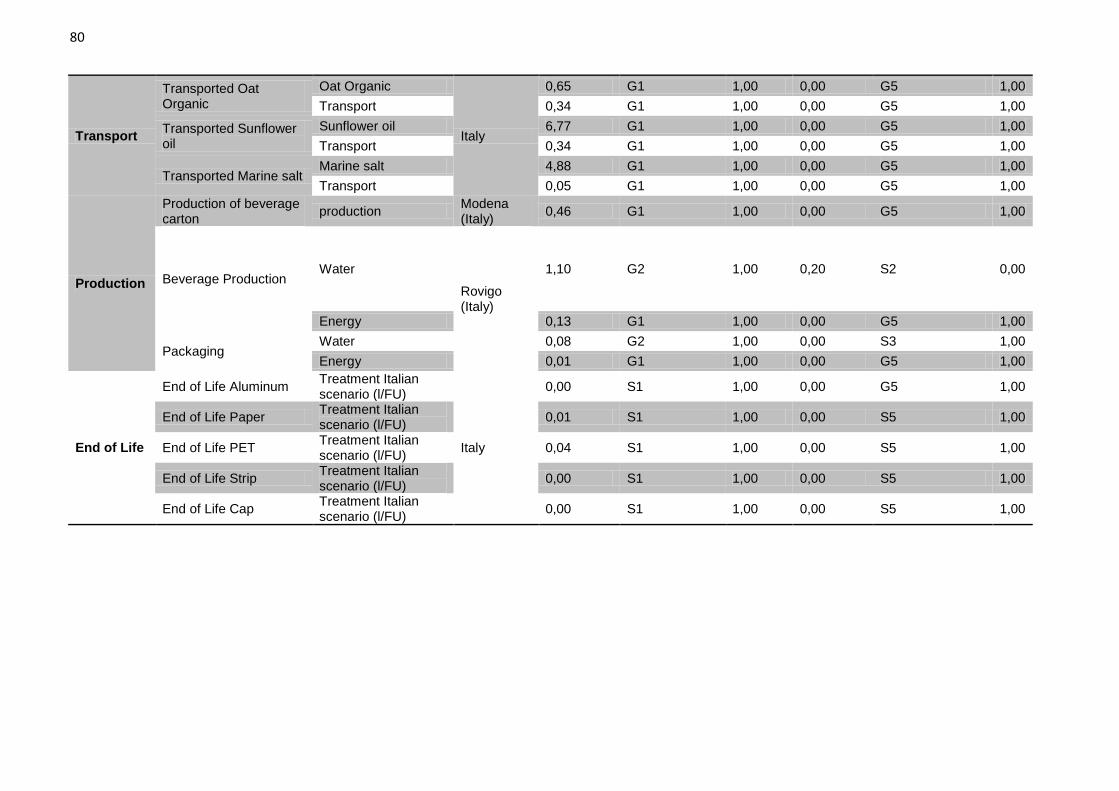
80
Transport
Transported Oat Organic
Oat Organic
Italy
0,65 G1 1,00 0,00 G5 1,00
Transport 0,34 G1 1,00 0,00 G5 1,00
Transported Sunflower oil
Sunflower oil 6,77 G1 1,00 0,00 G5 1,00
Transport 0,34 G1 1,00 0,00 G5 1,00
Transported Marine salt Marine salt 4,88 G1 1,00 0,00 G5 1,00
Transport 0,05 G1 1,00 0,00 G5 1,00
Production
Production of beverage carton
production Modena (Italy)
0,46 G1 1,00 0,00 G5 1,00
Beverage Production Water
Rovigo (Italy)
1,10 G2 1,00 0,20 S2 0,00
Energy 0,13 G1 1,00 0,00 G5 1,00
Packaging Water 0,08 G2 1,00 0,00 S3 1,00
Energy 0,01 G1 1,00 0,00 G5 1,00
End of Life
End of Life Aluminum Treatment Italian scenario (l/FU)
Italy
0,00 S1 1,00 0,00 G5 1,00
End of Life Paper Treatment Italian scenario (l/FU)
0,01 S1 1,00 0,00 S5 1,00
End of Life PET Treatment Italian scenario (l/FU)
0,04 S1 1,00 0,00 S5 1,00
End of Life Strip Treatment Italian scenario (l/FU)
0,00 S1 1,00 0,00 S5 1,00
End of Life Cap Treatment Italian scenario (l/FU)
0,00 S1 1,00 0,00 S5 1,00
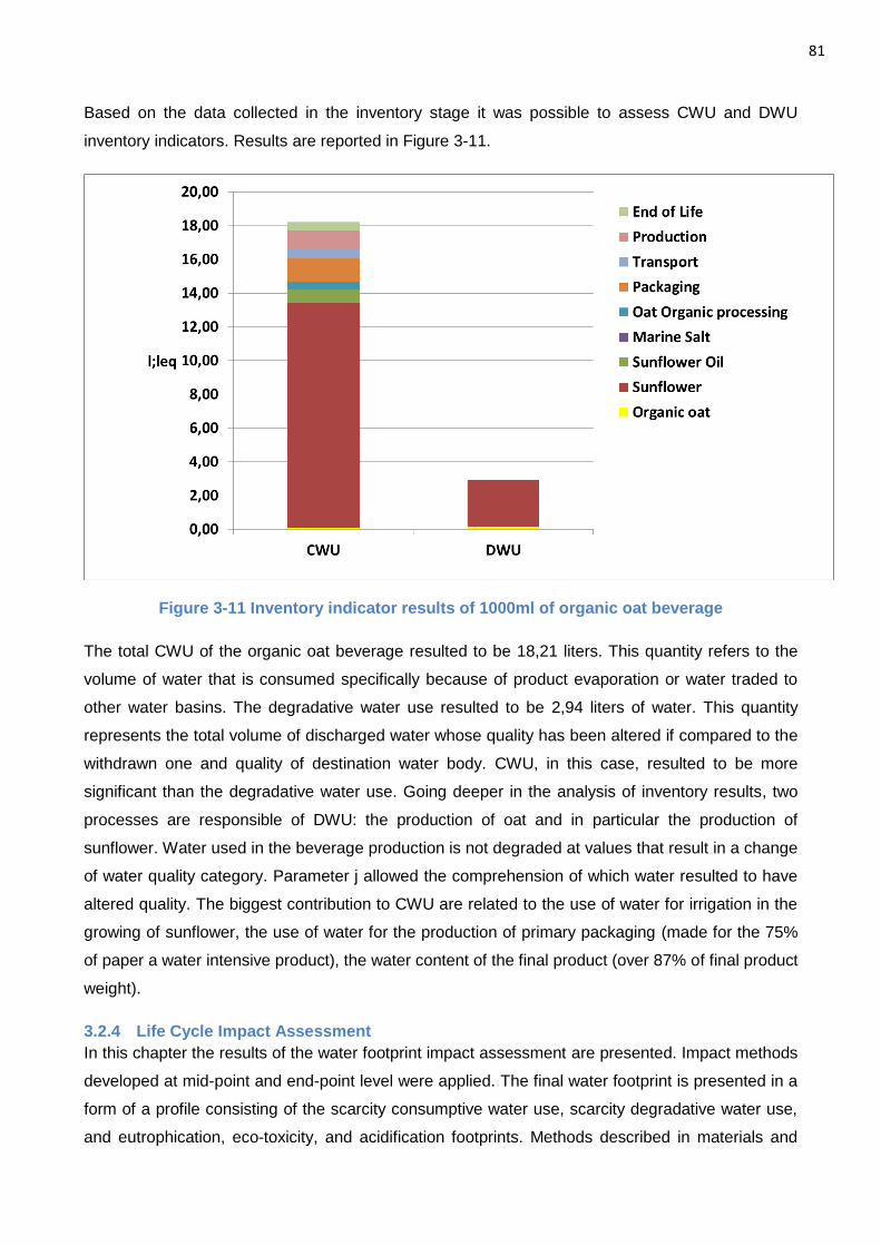
81
Based on the data collected in the inventory stage it was possible to assess CWU and DWU
inventory indicators. Results are reported in Figure 3-11.
Figure 3-11 Inventory indicator results of 1000ml of organic oat beverage
The total CWU of the organic oat beverage resulted to be 18,21 liters. This quantity refers to the
volume of water that is consumed specifically because of product evaporation or water traded to
other water basins. The degradative water use resulted to be 2,94 liters of water. This quantity
represents the total volume of discharged water whose quality has been altered if compared to the
withdrawn one and quality of destination water body. CWU, in this case, resulted to be more
significant than the degradative water use. Going deeper in the analysis of inventory results, two
processes are responsible of DWU: the production of oat and in particular the production of
sunflower. Water used in the beverage production is not degraded at values that result in a change
of water quality category. Parameter j allowed the comprehension of which water resulted to have
altered quality. The biggest contribution to CWU are related to the use of water for irrigation in the
growing of sunflower, the use of water for the production of primary packaging (made for the 75%
of paper a water intensive product), the water content of the final product (over 87% of final product
weight).
3.2.4 Life Cycle Impact Assessment
In this chapter the results of the water footprint impact assessment are presented. Impact methods
developed at mid-point and end-point level were applied. The final water footprint is presented in a
form of a profile consisting of the scarcity consumptive water use, scarcity degradative water use,
and eutrophication, eco-toxicity, and acidification footprints. Methods described in materials and
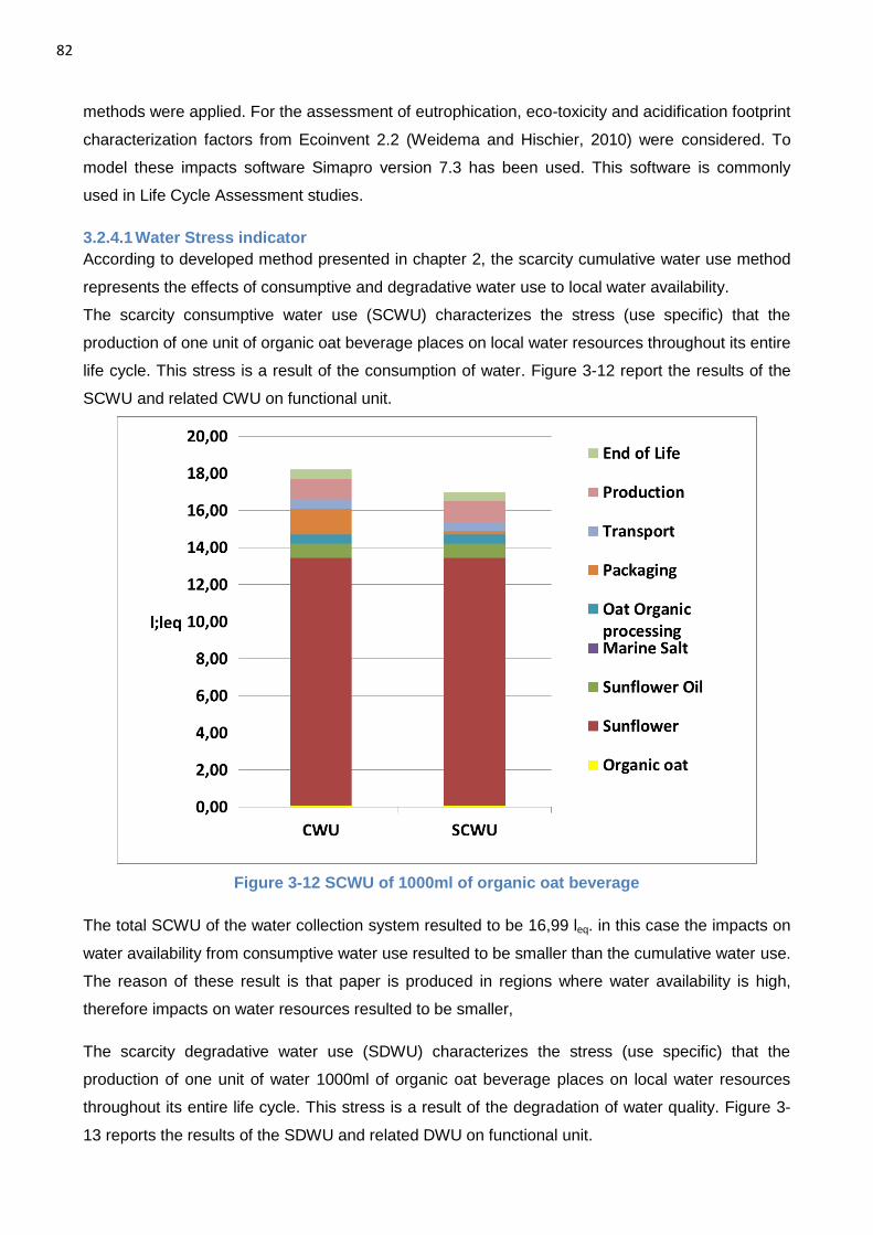
82
methods were applied. For the assessment of eutrophication, eco-toxicity and acidification footprint
characterization factors from Ecoinvent 2.2 (Weidema and Hischier, 2010) were considered. To
model these impacts software Simapro version 7.3 has been used. This software is commonly
used in Life Cycle Assessment studies.
3.2.4.1 Water Stress indicator
According to developed method presented in chapter 2, the scarcity cumulative water use method
represents the effects of consumptive and degradative water use to local water availability.
The scarcity consumptive water use (SCWU) characterizes the stress (use specific) that the
production of one unit of organic oat beverage places on local water resources throughout its entire
life cycle. This stress is a result of the consumption of water. Figure 3-12 report the results of the
SCWU and related CWU on functional unit.
Figure 3-12 SCWU of 1000ml of organic oat beverage
The total SCWU of the water collection system resulted to be 16,99 leq. in this case the impacts on
water availability from consumptive water use resulted to be smaller than the cumulative water use.
The reason of these result is that paper is produced in regions where water availability is high,
therefore impacts on water resources resulted to be smaller,
The scarcity degradative water use (SDWU) characterizes the stress (use specific) that the
production of one unit of water 1000ml of organic oat beverage places on local water resources
throughout its entire life cycle. This stress is a result of the degradation of water quality. Figure 3-
13 reports the results of the SDWU and related DWU on functional unit.
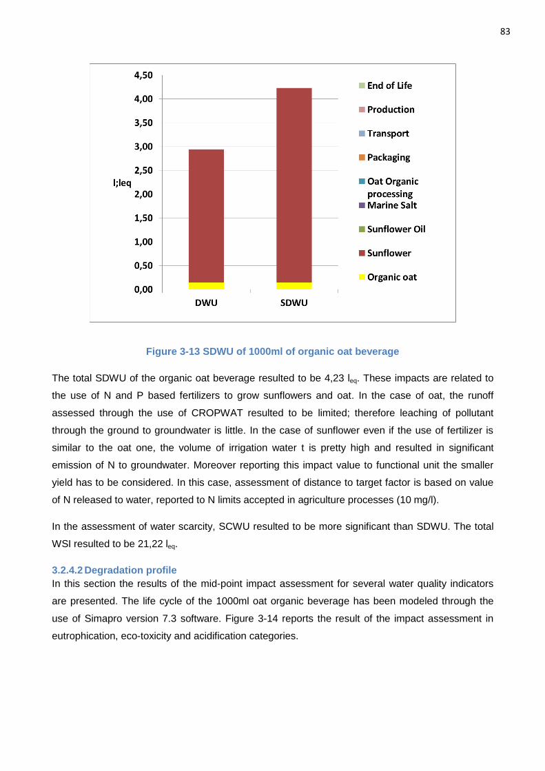
83
Figure 3-13 SDWU of 1000ml of organic oat beverage
The total SDWU of the organic oat beverage resulted to be 4,23 leq. These impacts are related to
the use of N and P based fertilizers to grow sunflowers and oat. In the case of oat, the runoff
assessed through the use of CROPWAT resulted to be limited; therefore leaching of pollutant
through the ground to groundwater is little. In the case of sunflower even if the use of fertilizer is
similar to the oat one, the volume of irrigation water t is pretty high and resulted in significant
emission of N to groundwater. Moreover reporting this impact value to functional unit the smaller
yield has to be considered. In this case, assessment of distance to target factor is based on value
of N released to water, reported to N limits accepted in agriculture processes (10 mg/l).
In the assessment of water scarcity, SCWU resulted to be more significant than SDWU. The total
WSI resulted to be 21,22 leq.
3.2.4.2 Degradation profile
In this section the results of the mid-point impact assessment for several water quality indicators
are presented. The life cycle of the 1000ml oat organic beverage has been modeled through the
use of Simapro version 7.3 software. Figure 3-14 reports the result of the impact assessment in
eutrophication, eco-toxicity and acidification categories.
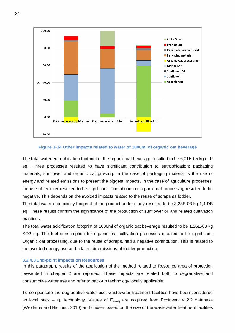
84
Figure 3-14 Other impacts related to water of 1000ml of organic oat beverage
The total water eutrophication footprint of the organic oat beverage resulted to be 6,01E-05 kg of P
eq.. Three processes resulted to have significant contribution to eutrophication: packaging
materials, sunflower and organic oat growing. In the case of packaging material is the use of
energy and related emissions to present the biggest impacts. In the case of agriculture processes,
the use of fertilizer resulted to be significant. Contribution of organic oat processing resulted to be
negative. This depends on the avoided impacts related to the reuse of scraps as fodder.
The total water eco-toxicity footprint of the product under study resulted to be 3,28E-03 kg 1,4-DB
eq. These results confirm the significance of the production of sunflower oil and related cultivation
practices.
The total water acidification footprint of 1000ml of organic oat beverage resulted to be 1,26E-03 kg
SO2 eq. The fuel consumption for organic oat cultivation processes resulted to be significant.
Organic oat processing, due to the reuse of scraps, had a negative contribution. This is related to
the avoided energy use and related air emissions of fodder production.
3.2.4.3 End-point impacts on Resources
In this paragraph, results of the application of the method related to Resource area of protection
presented in chapter 2 are reported. These impacts are related both to degradative and
consumptive water use and refer to back-up technology locally applicable.
To compensate the degradative water use, wastewater treatment facilities have been considered
as local back – up technology. Values of Elocal,j are acquired from Ecoinvent v 2.2 database
(Weidema and Hischier, 2010) and chosen based on the size of the wastewater treatment facilities
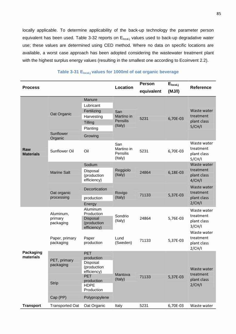
85
locally applicable. To determine applicability of the back-up technology the parameter person
equivalent has been used. Table 3-32 reports on Elocal,j values used to back-up degradative water
use; these values are determined using CED method. Where no data on specific locations are
available, a worst case approach has been adopted considering the wastewater treatment plant
with the highest surplus energy values (resulting in the smallest one according to Ecoinvent 2.2).
Table 3-31 Elocal,j values for 1000ml of oat organic beverage
Process Location Person
equivalent
Elocal,j
(MJ/l) Reference
Raw Materials
Oat Organic
Manure
San Martino in Pensilis (Italy)
5231 6,70E-03
Waste water treatment plant class 5/CH/I
Lubricant
Fertilizing
Harvesting
Tilling
Planting
Sunflower Organic
Growing
Sunflower Oil Oil
San Martino in Pensilis (Italy)
5231 6,70E-03
Waste water treatment plant class 5/CH/I
Marine Salt
Sodium
Reggiolo (Italy)
24864 6,18E-03
Waste water treatment plant class 4/CH/I
Disposal (production efficiency)
Oat organic processing
Decortication Rovigo (Italy)
71133 5,37E-03
Waste water treatment plant class 2/CH/I
production
Energy
Packaging materials
Aluminum, primary packaging
Aluminum Production
Sondrio (Italy)
24864 5,76E-03
Waste water treatment plant class 3/CH/I
Disposal (production efficiency)
Paper, primary packaging
Paper production
Lund (Sweden)
71133 5,37E-03
Waste water treatment plant class 2/CH/I
PET, primary packaging
PET production
Mantova (Italy)
71133 5,37E-03
Waste water treatment plant class 2/CH/I
Disposal (production efficiency)
Strip
PET production HDPE Production
Cap (PP) Polypropylene
Transport Transported Oat Oat Organic Italy 5231 6,70E-03 Waste water
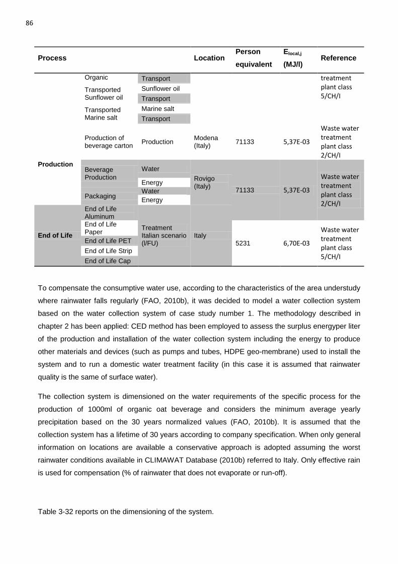
86
Process Location Person
equivalent
Elocal,j
(MJ/l) Reference
Organic Transport treatment plant class 5/CH/I
Transported Sunflower oil
Sunflower oil
Transport
Transported Marine salt
Marine salt
Transport
Production
Production of beverage carton
Production Modena (Italy)
71133 5,37E-03
Waste water treatment plant class 2/CH/I
Beverage Production
Water
Rovigo (Italy)
71133 5,37E-03
Waste water treatment plant class 2/CH/I
Energy
Packaging Water
Energy
End of Life
End of Life Aluminum
Treatment Italian scenario (l/FU)
Italy
End of Life Paper
5231 6,70E-03
Waste water treatment plant class 5/CH/I
End of Life PET
End of Life Strip
End of Life Cap
To compensate the consumptive water use, according to the characteristics of the area understudy
where rainwater falls regularly (FAO, 2010b), it was decided to model a water collection system
based on the water collection system of case study number 1. The methodology described in
chapter 2 has been applied: CED method has been employed to assess the surplus energyper liter
of the production and installation of the water collection system including the energy to produce
other materials and devices (such as pumps and tubes, HDPE geo-membrane) used to install the
system and to run a domestic water treatment facility (in this case it is assumed that rainwater
quality is the same of surface water).
The collection system is dimensioned on the water requirements of the specific process for the
production of 1000ml of organic oat beverage and considers the minimum average yearly
precipitation based on the 30 years normalized values (FAO, 2010b). It is assumed that the
collection system has a lifetime of 30 years according to company specification. When only general
information on locations are available a conservative approach is adopted assuming the worst
rainwater conditions available in CLIMAWAT Database (2010b) referred to Italy. Only effective rain
is used for compensation (% of rainwater that does not evaporate or run-off).
Table 3-32 reports on the dimensioning of the system.
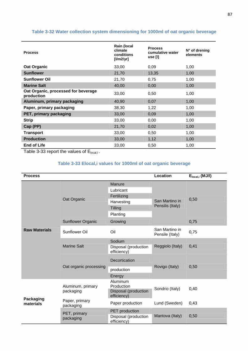
87
Table 3-32 Water collection system dimensioning for 1000ml of oat organic beverage
Process
Rain (local climate conditions [l/m2/yr]
Process cumulative water use [l]
N° of drening elements
Oat Organic 33,00 0,09 1,00
Sunflower 21,70 13,35 1,00
Sunflower Oil 21,70 0,75 1,00
Marine Salt 40,00 0,00 1,00
Oat Organic, processed for beverage production
33,00 0,50 1,00
Aluminum, primary packaging 40,90 0,07 1,00
Paper, primary packaging 38,30 1,22 1,00
PET, primary packaging 33,00 0,09 1,00
Strip 33,00 0,00 1,00
Cap (PP) 21,70 0,02 1,00
Transport 33,00 0,50 1,00
Production 33,00 1,12 1,00
End of Life 33,00 0,50 1,00
Table 3-33 report the values of Elocal,I .
Table 3-33 Elocal,i values for 1000ml of oat organic beverage
Process Location Elocal,i (MJ/l)
Raw Materials
Oat Organic
Manure
San Martino in Pensilis (Italy)
0,50
Lubricant
Fertilizing
Harvesting
Tilling
Planting
Sunflower Organic Growing 0,75
Sunflower Oil Oil San Martino in Pensile (Italy)
0,75
Marine Salt Sodium
Reggiolo (Italy) 0,41 Disposal (production efficiency)
Oat organic processing
Decortication
Rovigo (Italy) 0,50 production
Energy
Packaging materials
Aluminum, primary packaging
Aluminum Production
Sondrio (Italy) 0,40 Disposal (production efficiency)
Paper, primary packaging
Paper production Lund (Sweden) 0,43
PET, primary packaging
PET production Mantova (Italy) 0,50 Disposal (production
efficiency)
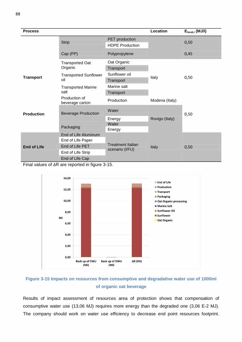
88
Process Location Elocal,i (MJ/l)
Strip PET production
0,50 HDPE Production
Cap (PP) Polypropylene 0,45
Transport
Transported Oat Organic
Oat Organic
Italy 0,50
Transport
Transported Sunflower oil
Sunflower oil
Transport
Transported Marine salt
Marine salt
Transport
Production
Production of beverage carton
Production Modena (Italy)
0,50 Beverage Production Water
Rovigo (Italy) Energy
Packaging Water
Energy
End of Life
End of Life Aluminum
Treatment Italian scenario (l/FU)
Italy 0,50
End of Life Paper
End of Life PET
End of Life Strip
End of Life Cap
Final values of ΔR are reported in figure 3-15.
Figure 3-15 Impacts on resources from consumptive and degradative water use of 1000ml
of organic oat beverage
Results of impact assessment of resources area of protection shows that compensation of
consumptive water use (13,06 MJ) requires more energy than the degraded one (3,06 E-2 MJ).
The company should work on water use efficiency to decrease end point resources footprint.
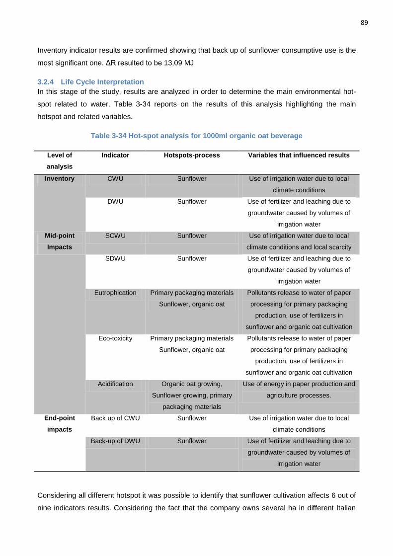
89
Inventory indicator results are confirmed showing that back up of sunflower consumptive use is the
most significant one. ΔR resulted to be 13,09 MJ
3.2.4 Life Cycle Interpretation
In this stage of the study, results are analyzed in order to determine the main environmental hot-
spot related to water. Table 3-34 reports on the results of this analysis highlighting the main
hotspot and related variables.
Table 3-34 Hot-spot analysis for 1000ml organic oat beverage
Level of
analysis
Indicator Hotspots-process Variables that influenced results
Inventory CWU Sunflower Use of irrigation water due to local
climate conditions
DWU Sunflower Use of fertilizer and leaching due to
groundwater caused by volumes of
irrigation water
Mid-point
Impacts
SCWU Sunflower Use of irrigation water due to local
climate conditions and local scarcity
SDWU Sunflower Use of fertilizer and leaching due to
groundwater caused by volumes of
irrigation water
Eutrophication Primary packaging materials
Sunflower, organic oat
Pollutants release to water of paper
processing for primary packaging
production, use of fertilizers in
sunflower and organic oat cultivation
Eco-toxicity Primary packaging materials
Sunflower, organic oat
Pollutants release to water of paper
processing for primary packaging
production, use of fertilizers in
sunflower and organic oat cultivation
Acidification Organic oat growing,
Sunflower growing, primary
packaging materials
Use of energy in paper production and
agriculture processes.
End-point
impacts
Back up of CWU Sunflower Use of irrigation water due to local
climate conditions
Back-up of DWU Sunflower Use of fertilizer and leaching due to
groundwater caused by volumes of
irrigation water
Considering all different hotspot it was possible to identify that sunflower cultivation affects 6 out of
nine indicators results. Considering the fact that the company owns several ha in different Italian
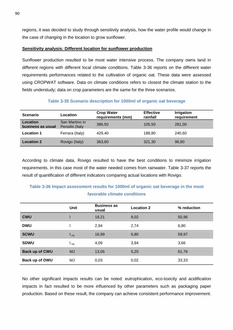
90
regions, it was decided to study through sensitivity analysis, how the water profile would change in
the case of changing in the location to grow sunflower.
Sensitivity analysis: Different location for sunflower production
Sunflower production resulted to be most water intensive process. The company owns land in
different regions with different local climate conditions. Table 3-36 reports on the different water
requirements performances related to the cultivation of organic oat. These data were assessed
using CROPWAT software. Data on climate conditions refers to closest the climate station to the
fields understudy; data on crop parameters are the same for the three scenarios.
Table 3-35 Scenario description for 1000ml of organic oat beverage
Scenario Location Crop Water requirements (mm)
Effective rainfall
Irrigation requirement
Location business as usual
San Martino in Pensilis (Italy
386,50 105,50 281,00
Location 1 Ferrara (Italy) 429,40 188,80 240,60
Location 2 Rovigo (Italy) 363,60 321,30 96,80
According to climate data, Rovigo resulted to have the best conditions to minimize irrigation
requirements. In this case most of the water needed comes from rainwater. Table 3-37 reports the
result of quantification of different indicators comparing actual locations with Rovigo.
Table 3-36 Impact assessment results for 1000ml of organic oat beverage in the most
favorable climate conditions
Unit
Business as usual
Location 2 % reduction
CWU l 18,21 8,02 55,96
DWU l 2,94 2,74 6,80
SCWU l eq 16,99 6,80 59,97
SDWU l eq 4,09 3,94 3,66
Back up of CWU MJ 13,06 5,20 61,76
Back up of DWU MJ 0,03 0,02 33,33
No other significant impacts results can be noted: eutrophication, eco-toxicity and acidification
impacts in fact resulted to be more influenced by other parameters such as packaging paper
production. Based on these result, the company can achieve consistent performance improvement.
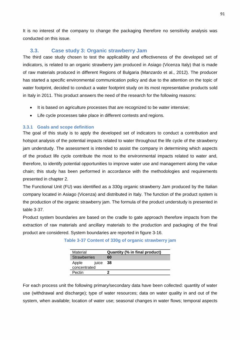
91
It is no interest of the company to change the packaging therefore no sensitivity analysis was
conducted on this issue.
3.3. Case study 3: Organic strawberry Jam
The third case study chosen to test the applicability and effectiveness of the developed set of
indicators, is related to an organic strawberry jam produced in Asiago (Vicenza Italy) that is made
of raw materials produced in different Regions of Bulgaria (Manzardo et al., 2012). The producer
has started a specific environmental communication policy and due to the attention on the topic of
water footprint, decided to conduct a water footprint study on its most representative products sold
in Italy in 2011. This product answers the need of the research for the following reasons:
It is based on agriculture processes that are recognized to be water intensive;
Life cycle processes take place in different contests and regions.
3.3.1 Goals and scope definition
The goal of this study is to apply the developed set of indicators to conduct a contribution and
hotspot analysis of the potential impacts related to water throughout the life cycle of the strawberry
jam understudy. The assessment is intended to assist the company in determining which aspects
of the product life cycle contribute the most to the environmental impacts related to water and,
therefore, to identify potential opportunities to improve water use and management along the value
chain; this study has been performed in accordance with the methodologies and requirements
presented in chapter 2.
The Functional Unit (FU) was identified as a 330g organic strawberry Jam produced by the Italian
company located in Asiago (Vicenza) and distributed in Italy. The function of the product system is
the production of the organic strawberry jam. The formula of the product understudy is presented in
table 3-37.
Product system boundaries are based on the cradle to gate approach therefore impacts from the
extraction of raw materials and ancillary materials to the production and packaging of the final
product are considered. System boundaries are reported in figure 3-16.
Table 3-37 Content of 330g of organic strawberry jam
Material Quantity (% in final product)
Strawberries 60
Apple juice concentrated
38
Pectin 2
For each process unit the following primary/secondary data have been collected: quantity of water
use (withdrawal and discharge); type of water resources; data on water quality in and out of the
system, when available; location of water use; seasonal changes in water flows; temporal aspects

92
of water use; forms of water use (If not differently specified, all water used was considered to be a
liquid). No significant changes in drainage conditions due to land use change were determined.
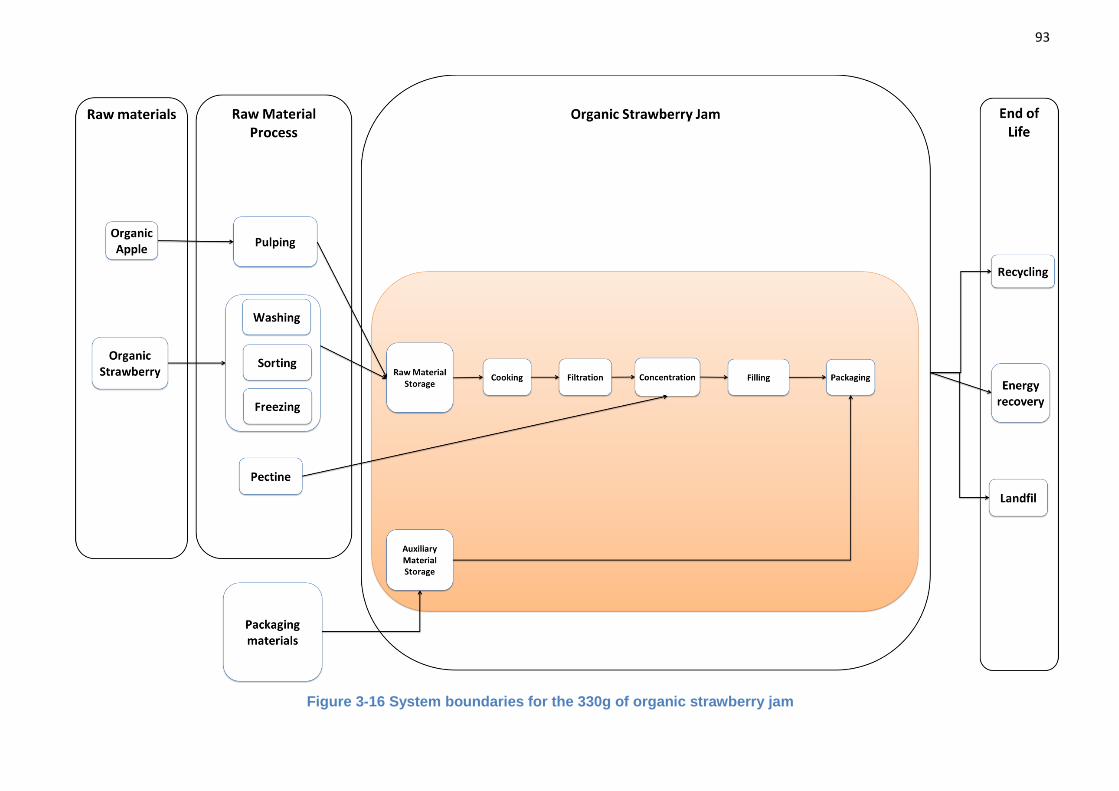
93
Figure 3-16 System boundaries for the 330g of organic strawberry jam
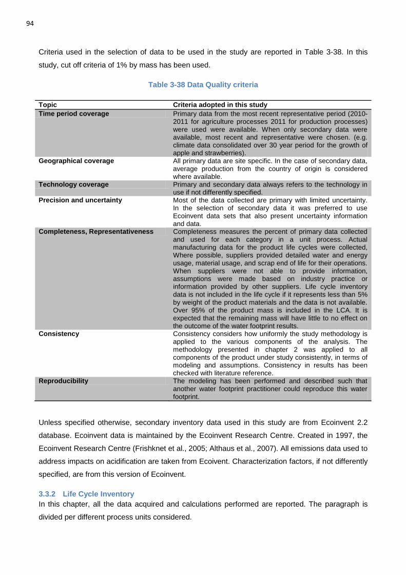
94
Criteria used in the selection of data to be used in the study are reported in Table 3-38. In this
study, cut off criteria of 1% by mass has been used.
Table 3-38 Data Quality criteria
Topic Criteria adopted in this study
Time period coverage Primary data from the most recent representative period (2010-2011 for agriculture processes 2011 for production processes) were used were available. When only secondary data were available, most recent and representative were chosen. (e.g. climate data consolidated over 30 year period for the growth of apple and strawberries).
Geographical coverage All primary data are site specific. In the case of secondary data, average production from the country of origin is considered where available.
Technology coverage Primary and secondary data always refers to the technology in use if not differently specified.
Precision and uncertainty Most of the data collected are primary with limited uncertainty. In the selection of secondary data it was preferred to use Ecoinvent data sets that also present uncertainty information and data.
Completeness, Representativeness Completeness measures the percent of primary data collected and used for each category in a unit process. Actual manufacturing data for the product life cycles were collected, Where possible, suppliers provided detailed water and energy usage, material usage, and scrap end of life for their operations. When suppliers were not able to provide information, assumptions were made based on industry practice or information provided by other suppliers. Life cycle inventory data is not included in the life cycle if it represents less than 5% by weight of the product materials and the data is not available. Over 95% of the product mass is included in the LCA. It is expected that the remaining mass will have little to no effect on the outcome of the water footprint results.
Consistency Consistency considers how uniformly the study methodology is applied to the various components of the analysis. The methodology presented in chapter 2 was applied to all components of the product under study consistently, in terms of modeling and assumptions. Consistency in results has been checked with literature reference.
Reproducibility The modeling has been performed and described such that another water footprint practitioner could reproduce this water footprint.
Unless specified otherwise, secondary inventory data used in this study are from Ecoinvent 2.2
database. Ecoinvent data is maintained by the Ecoinvent Research Centre. Created in 1997, the
Ecoinvent Research Centre (Frishknet et al., 2005; Althaus et al., 2007). All emissions data used to
address impacts on acidification are taken from Ecoivent. Characterization factors, if not differently
specified, are from this version of Ecoinvent.
3.3.2 Life Cycle Inventory
In this chapter, all the data acquired and calculations performed are reported. The paragraph is
divided per different process units considered.
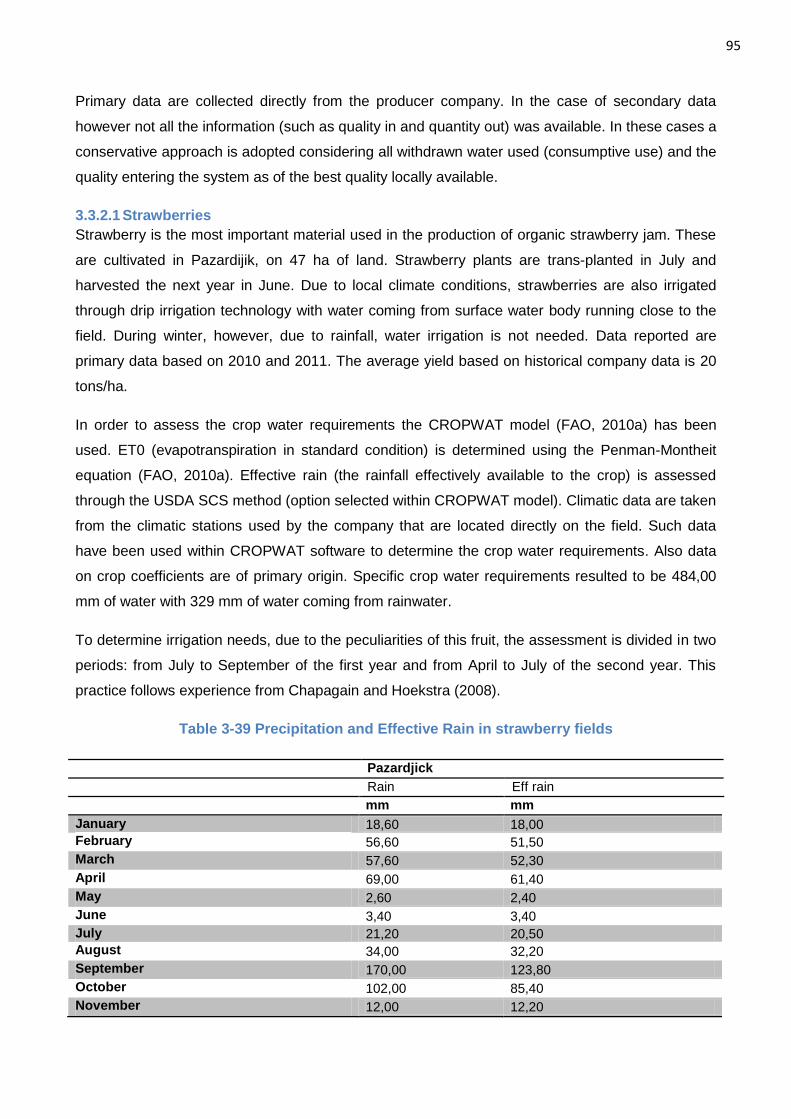
95
Primary data are collected directly from the producer company. In the case of secondary data
however not all the information (such as quality in and quantity out) was available. In these cases a
conservative approach is adopted considering all withdrawn water used (consumptive use) and the
quality entering the system as of the best quality locally available.
3.3.2.1 Strawberries
Strawberry is the most important material used in the production of organic strawberry jam. These
are cultivated in Pazardijik, on 47 ha of land. Strawberry plants are trans-planted in July and
harvested the next year in June. Due to local climate conditions, strawberries are also irrigated
through drip irrigation technology with water coming from surface water body running close to the
field. During winter, however, due to rainfall, water irrigation is not needed. Data reported are
primary data based on 2010 and 2011. The average yield based on historical company data is 20
tons/ha.
In order to assess the crop water requirements the CROPWAT model (FAO, 2010a) has been
used. ET0 (evapotranspiration in standard condition) is determined using the Penman-Montheit
equation (FAO, 2010a). Effective rain (the rainfall effectively available to the crop) is assessed
through the USDA SCS method (option selected within CROPWAT model). Climatic data are taken
from the climatic stations used by the company that are located directly on the field. Such data
have been used within CROPWAT software to determine the crop water requirements. Also data
on crop coefficients are of primary origin. Specific crop water requirements resulted to be 484,00
mm of water with 329 mm of water coming from rainwater.
To determine irrigation needs, due to the peculiarities of this fruit, the assessment is divided in two
periods: from July to September of the first year and from April to July of the second year. This
practice follows experience from Chapagain and Hoekstra (2008).
Table 3-39 Precipitation and Effective Rain in strawberry fields
Pazardjick
Rain Eff rain
mm mm
January 18,60 18,00
February 56,60 51,50
March 57,60 52,30
April 69,00 61,40
May 2,60 2,40
June 3,40 3,40
July 21,20 20,50
August 34,00 32,20
September 170,00 123,80
October 102,00 85,40
November 12,00 12,20
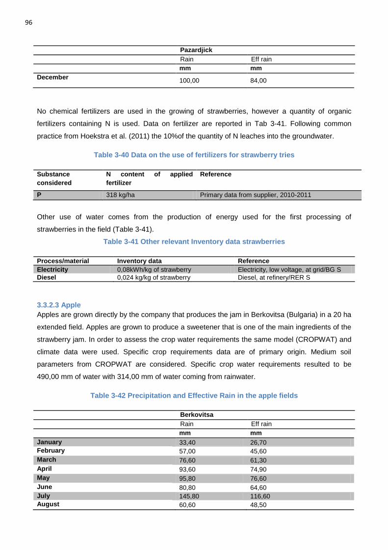
96
Pazardjick
Rain Eff rain
mm mm
December 100,00 84,00
No chemical fertilizers are used in the growing of strawberries, however a quantity of organic
fertilizers containing N is used. Data on fertilizer are reported in Tab 3-41. Following common
practice from Hoekstra et al. (2011) the 10%of the quantity of N leaches into the groundwater.
Table 3-40 Data on the use of fertilizers for strawberry tries
Substance
considered
N content of applied
fertilizer
Reference
P 318 kg/ha Primary data from supplier, 2010-2011
Other use of water comes from the production of energy used for the first processing of
strawberries in the field (Table 3-41).
Table 3-41 Other relevant Inventory data strawberries
Process/material Inventory data Reference
Electricity 0,08kWh/kg of strawberry Electricity, low voltage, at grid/BG S
Diesel 0,024 kg/kg of strawberry Diesel, at refinery/RER S
3.3.2.3 Apple
Apples are grown directly by the company that produces the jam in Berkovitsa (Bulgaria) in a 20 ha
extended field. Apples are grown to produce a sweetener that is one of the main ingredients of the
strawberry jam. In order to assess the crop water requirements the same model (CROPWAT) and
climate data were used. Specific crop requirements data are of primary origin. Medium soil
parameters from CROPWAT are considered. Specific crop water requirements resulted to be
490,00 mm of water with 314,00 mm of water coming from rainwater.
Table 3-42 Precipitation and Effective Rain in the apple fields
Berkovitsa
Rain Eff rain
mm mm
January 33,40 26,70
February 57,00 45,60
March 76,60 61,30
April 93,60 74,90
May 95,80 76,60
June 80,80 64,60
July 145,80 116,60
August 60,60 48,50
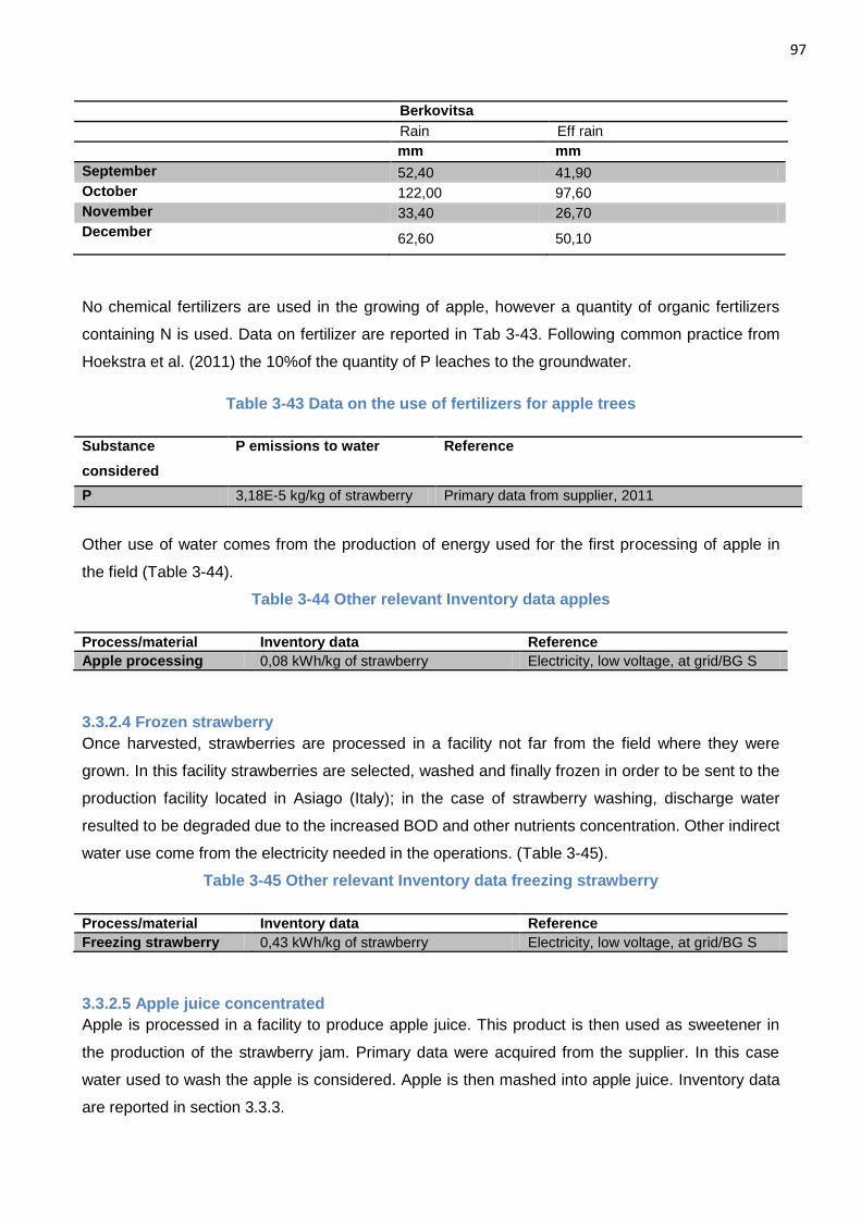
97
Berkovitsa
Rain Eff rain
mm mm
September 52,40 41,90
October 122,00 97,60
November 33,40 26,70
December 62,60 50,10
No chemical fertilizers are used in the growing of apple, however a quantity of organic fertilizers
containing N is used. Data on fertilizer are reported in Tab 3-43. Following common practice from
Hoekstra et al. (2011) the 10%of the quantity of P leaches to the groundwater.
Table 3-43 Data on the use of fertilizers for apple trees
Substance
considered
P emissions to water Reference
P 3,18E-5 kg/kg of strawberry Primary data from supplier, 2011
Other use of water comes from the production of energy used for the first processing of apple in
the field (Table 3-44).
Table 3-44 Other relevant Inventory data apples
Process/material Inventory data Reference
Apple processing 0,08 kWh/kg of strawberry Electricity, low voltage, at grid/BG S
3.3.2.4 Frozen strawberry
Once harvested, strawberries are processed in a facility not far from the field where they were
grown. In this facility strawberries are selected, washed and finally frozen in order to be sent to the
production facility located in Asiago (Italy); in the case of strawberry washing, discharge water
resulted to be degraded due to the increased BOD and other nutrients concentration. Other indirect
water use come from the electricity needed in the operations. (Table 3-45).
Table 3-45 Other relevant Inventory data freezing strawberry
Process/material Inventory data Reference
Freezing strawberry 0,43 kWh/kg of strawberry Electricity, low voltage, at grid/BG S
3.3.2.5 Apple juice concentrated
Apple is processed in a facility to produce apple juice. This product is then used as sweetener in
the production of the strawberry jam. Primary data were acquired from the supplier. In this case
water used to wash the apple is considered. Apple is then mashed into apple juice. Inventory data
are reported in section 3.3.3.
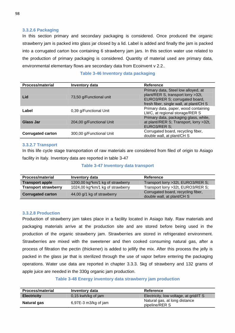
98
3.3.2.6 Packaging
In this section primary and secondary packaging is considered. Once produced the organic
strawberry jam is packed into glass jar closed by a lid. Label is added and finally the jam is packed
into a corrugated carton box containing 6 strawberry jam jars. In this section water use related to
the production of primary packaging is considered. Quantity of material used are primary data,
environmental elementary flows are secondary data from Ecoinvent v 2.2..
Table 3-46 Inventory data packaging
Process/material Inventory data Reference
Lid 73,50 g/Functional unit
Primary data, Steel low alloyed, at plant/RER S, transport lorry >32t, EURO3/RER S; corrugated board, fresh fiber, single wall, at plant/CH S
Label 0,39 g/Functional Unit Primary data, paper, wood containing LWC, at regional storage/RER S
Glass Jar 204,00 g/Functional Unit Primary data, packaging glass, white, at plant//RER S; Transport, lorry >32t, EURO3/RER S;
Corrugated carton 300,00 g/Functional Unit Corrugated board, recycling fiber, double wall, at plant/CH S
3.3.2.7 Transport
In this life cycle stage transportation of raw materials are considered from filed of origin to Asiago
facility in Italy. Inventory data are reported in table 3-47
Table 3-47 Inventory data transport
Process/material Inventory data Reference
Transport apple 1200,00 kg*km/1 kg of strawberry Transport lorry >32t, EURO3/RER S;
Transport strawberry 1024,00 kg*km/1 kg of strawberry Transport lorry >32t, EURO3/RER S;
Corrugated carton 44,00 g/1 kg of strawberry Corrugated board, recycling fiber, double wall, at plant/CH S
3.3.2.8 Production
Production of strawberry jam takes place in a facility located in Asiago Italy. Raw materials and
packaging materials arrive at the production site and are stored before being used in the
production of the organic strawberry jam. Strawberries are stored in refrigerated environment.
Strawberries are mixed with the sweetener and then cooked consuming natural gas, after a
process of filtration the pectin (thickener) is added to jellify the mix. After this process the jelly is
packed in the glass jar that is sterilized through the use of vapor before entering the packaging
operations. Water use data are reported in chapter 3.3.3. 5kg of strawberry and 132 grams of
apple juice are needed in the 330g organic jam production.
Table 3-48 Energy inventory data strawberry jam production
Process/material Inventory data Reference
Electricity 0,15 kwh/kg of jam Electricity, low voltage, at grid/IT S
Natural gas 6,97E-3 m3/kg of jam Natural gas, at long distance pipeline/RER S
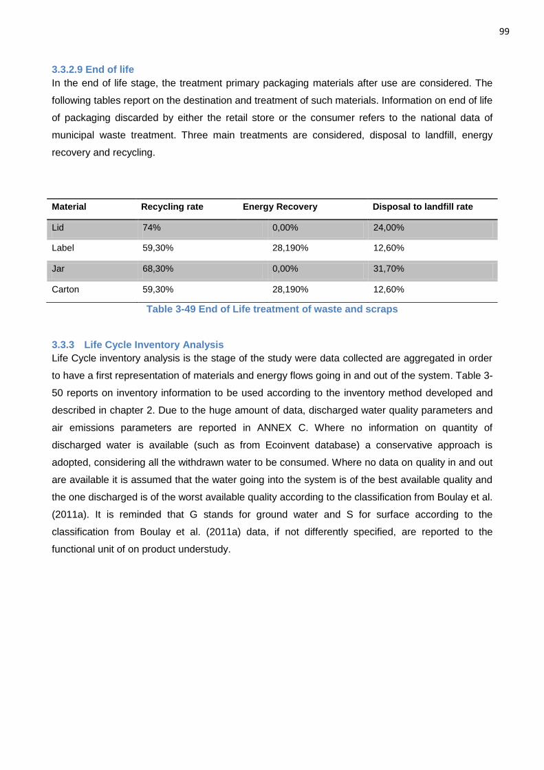
99
3.3.2.9 End of life
In the end of life stage, the treatment primary packaging materials after use are considered. The
following tables report on the destination and treatment of such materials. Information on end of life
of packaging discarded by either the retail store or the consumer refers to the national data of
municipal waste treatment. Three main treatments are considered, disposal to landfill, energy
recovery and recycling.
Table 3-49 End of Life treatment of waste and scraps
3.3.3 Life Cycle Inventory Analysis
Life Cycle inventory analysis is the stage of the study were data collected are aggregated in order
to have a first representation of materials and energy flows going in and out of the system. Table 3-
50 reports on inventory information to be used according to the inventory method developed and
described in chapter 2. Due to the huge amount of data, discharged water quality parameters and
air emissions parameters are reported in ANNEX C. Where no information on quantity of
discharged water is available (such as from Ecoinvent database) a conservative approach is
adopted, considering all the withdrawn water to be consumed. Where no data on quality in and out
are available it is assumed that the water going into the system is of the best available quality and
the one discharged is of the worst available quality according to the classification from Boulay et al.
(2011a). It is reminded that G stands for ground water and S for surface according to the
classification from Boulay et al. (2011a) data, if not differently specified, are reported to the
functional unit of on product understudy.
Material Recycling rate Energy Recovery Disposal to landfill rate
Lid 74% 0,00% 24,00%
Label 59,30% 28,190% 12,60%
Jar 68,30% 0,00% 31,70%
Carton 59,30% 28,190% 12,60%
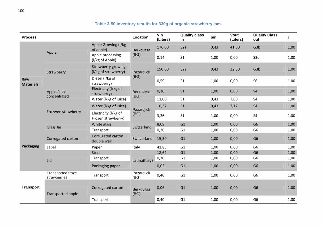
100
Table 3-50 Inventory results for 330g of organic strawberry jam.
Process Location Vin (Liters)
Quality class in
αin Vout (Liters)
Quality Class out
j
Raw Materials
Apple
Apple Growing (l/kg of apple) Berkovitsa
(BG)
176,00 S2a 0,43 41,00 G3b 1,00
Apple processing (l/kg of Apple)
0,14 S1 1,00 0,00 S3c 1,00
Strawberry
Strawberry growing (l/kg of strawberry) Pazardjick
(BG)
150,00 S2a 0,43 22,50 G3b 1,00
Diesel (l/kg of strawberry)
0,59 S1 1,00 0,00 S6 1,00
Apple Juice concentrated
Electricity (l/kg of strawberry) Berkovitsa
(BG)
0,10 S1 1,00 0,00 S4 1,00
Water (l/kg of juice) 11,00 S1 0,43 7,00 S4 1,00
Frozwen strawberry
Water (l/kg of juice) Pazardjick (BG)
10,37 S1 0,43 7,17 S4 1,00
Electricity (l/kg of Frozen strawberry)
3,26 S1 1,00 0,00 S4 1,00
Packaging
Glass Jar White glass
Swtzerland 8,09 G1 1,00 0,00 G6 1,00
Transport 0,20 G1 1,00 0,00 G6 1,00
Corrugated carton Corrugated carton double wall
Switzerland 15,30 G1 1,00 0,00 G6 1,00
Label Paper Italy 41,85 G1 1,00 0,00 G6 1,00
Lid
Steel
Latina(Italy)
18,62 G1 1,00 0,00 G6 1,00
Transport 0,70 G1 1,00 0,00 G6 1,00
Packaging paper 0,02 G1 1,00 0,00 G6 1,00
Transport
Transported froze strawberries
Transport Pazardjick (BG)
0,40 G1 1,00 0,00 G6 1,00
Transported apple
Corrugated carton Berkovitsa (BG)
0,06 G1 1,00 0,00 G6 1,00
Transport 0,40 G1 1,00 0,00 G6 1,00
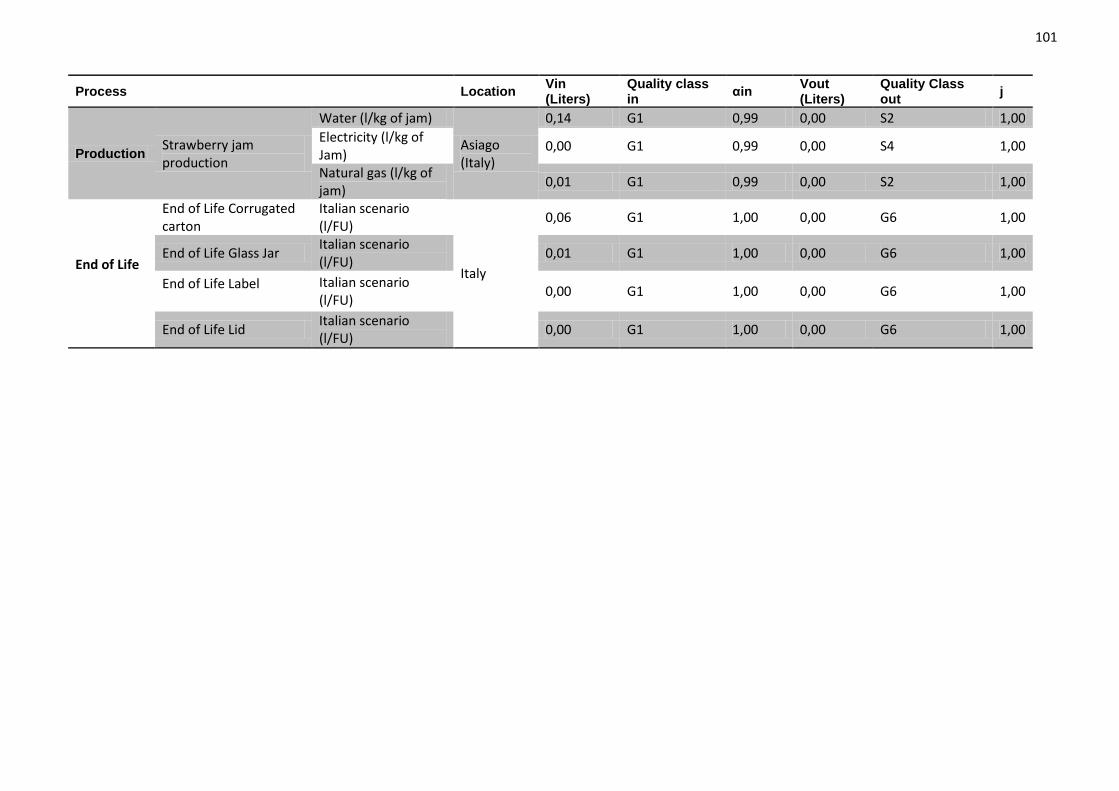
101
Process Location Vin (Liters)
Quality class in
αin Vout (Liters)
Quality Class out
j
Production Strawberry jam production
Water (l/kg of jam)
Asiago (Italy)
0,14 G1 0,99 0,00 S2 1,00
Electricity (l/kg of Jam)
0,00 G1 0,99 0,00 S4 1,00
Natural gas (l/kg of jam)
0,01 G1 0,99 0,00 S2 1,00
End of Life
End of Life Corrugated carton
Italian scenario (l/FU)
Italy
0,06 G1 1,00 0,00 G6 1,00
End of Life Glass Jar Italian scenario (l/FU)
0,01 G1 1,00 0,00 G6 1,00
End of Life Label
Italian scenario (l/FU)
0,00 G1 1,00 0,00 G6 1,00
End of Life Lid Italian scenario (l/FU)
0,00 G1 1,00 0,00 G6 1,00
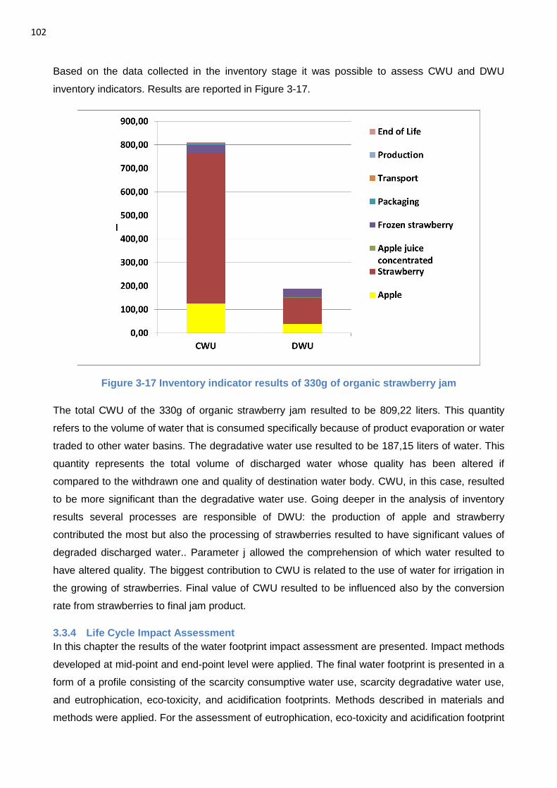
102
Based on the data collected in the inventory stage it was possible to assess CWU and DWU
inventory indicators. Results are reported in Figure 3-17.
Figure 3-17 Inventory indicator results of 330g of organic strawberry jam
The total CWU of the 330g of organic strawberry jam resulted to be 809,22 liters. This quantity
refers to the volume of water that is consumed specifically because of product evaporation or water
traded to other water basins. The degradative water use resulted to be 187,15 liters of water. This
quantity represents the total volume of discharged water whose quality has been altered if
compared to the withdrawn one and quality of destination water body. CWU, in this case, resulted
to be more significant than the degradative water use. Going deeper in the analysis of inventory
results several processes are responsible of DWU: the production of apple and strawberry
contributed the most but also the processing of strawberries resulted to have significant values of
degraded discharged water.. Parameter j allowed the comprehension of which water resulted to
have altered quality. The biggest contribution to CWU is related to the use of water for irrigation in
the growing of strawberries. Final value of CWU resulted to be influenced also by the conversion
rate from strawberries to final jam product.
3.3.4 Life Cycle Impact Assessment
In this chapter the results of the water footprint impact assessment are presented. Impact methods
developed at mid-point and end-point level were applied. The final water footprint is presented in a
form of a profile consisting of the scarcity consumptive water use, scarcity degradative water use,
and eutrophication, eco-toxicity, and acidification footprints. Methods described in materials and
methods were applied. For the assessment of eutrophication, eco-toxicity and acidification footprint
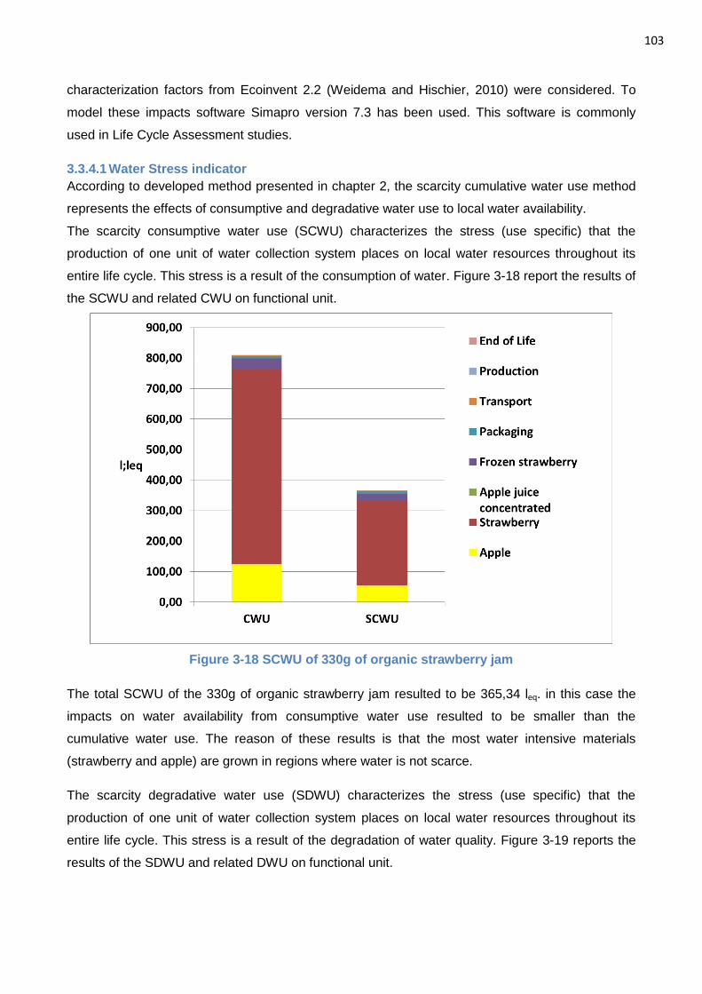
103
characterization factors from Ecoinvent 2.2 (Weidema and Hischier, 2010) were considered. To
model these impacts software Simapro version 7.3 has been used. This software is commonly
used in Life Cycle Assessment studies.
3.3.4.1 Water Stress indicator
According to developed method presented in chapter 2, the scarcity cumulative water use method
represents the effects of consumptive and degradative water use to local water availability.
The scarcity consumptive water use (SCWU) characterizes the stress (use specific) that the
production of one unit of water collection system places on local water resources throughout its
entire life cycle. This stress is a result of the consumption of water. Figure 3-18 report the results of
the SCWU and related CWU on functional unit.
Figure 3-18 SCWU of 330g of organic strawberry jam
The total SCWU of the 330g of organic strawberry jam resulted to be 365,34 leq. in this case the
impacts on water availability from consumptive water use resulted to be smaller than the
cumulative water use. The reason of these results is that the most water intensive materials
(strawberry and apple) are grown in regions where water is not scarce.
The scarcity degradative water use (SDWU) characterizes the stress (use specific) that the
production of one unit of water collection system places on local water resources throughout its
entire life cycle. This stress is a result of the degradation of water quality. Figure 3-19 reports the
results of the SDWU and related DWU on functional unit.
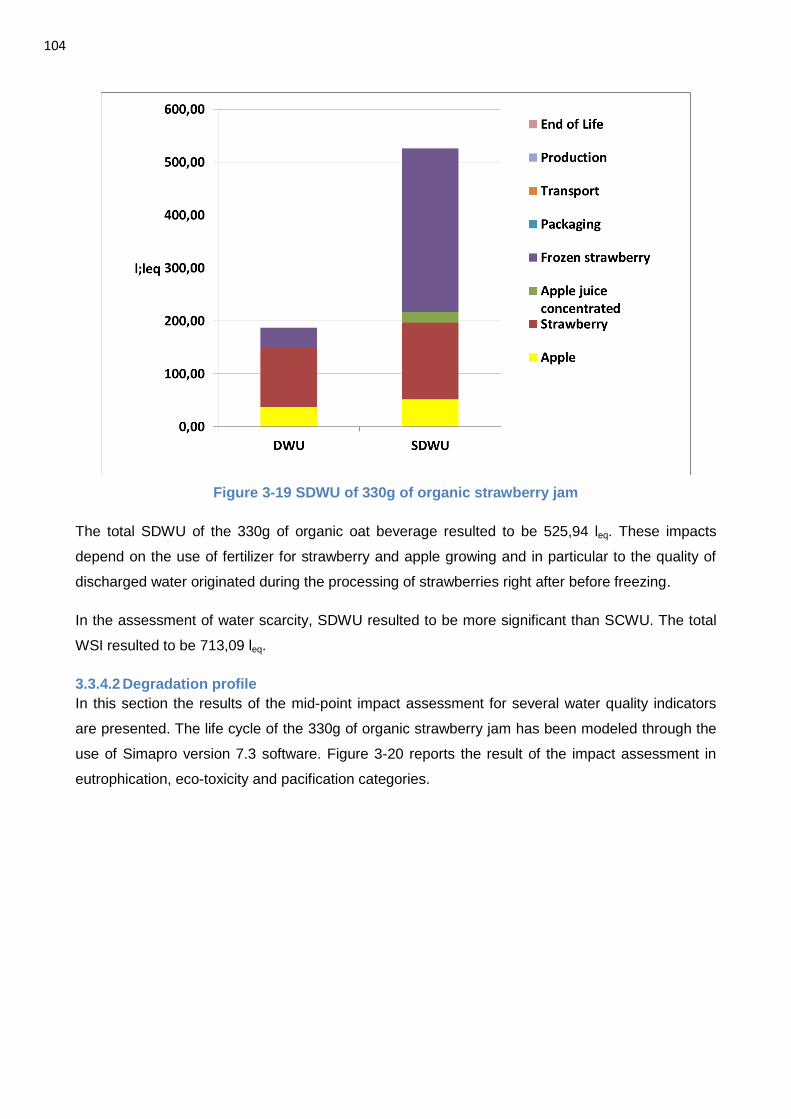
104
Figure 3-19 SDWU of 330g of organic strawberry jam
The total SDWU of the 330g of organic oat beverage resulted to be 525,94 leq. These impacts
depend on the use of fertilizer for strawberry and apple growing and in particular to the quality of
discharged water originated during the processing of strawberries right after before freezing.
In the assessment of water scarcity, SDWU resulted to be more significant than SCWU. The total
WSI resulted to be 713,09 leq.
3.3.4.2 Degradation profile
In this section the results of the mid-point impact assessment for several water quality indicators
are presented. The life cycle of the 330g of organic strawberry jam has been modeled through the
use of Simapro version 7.3 software. Figure 3-20 reports the result of the impact assessment in
eutrophication, eco-toxicity and pacification categories.
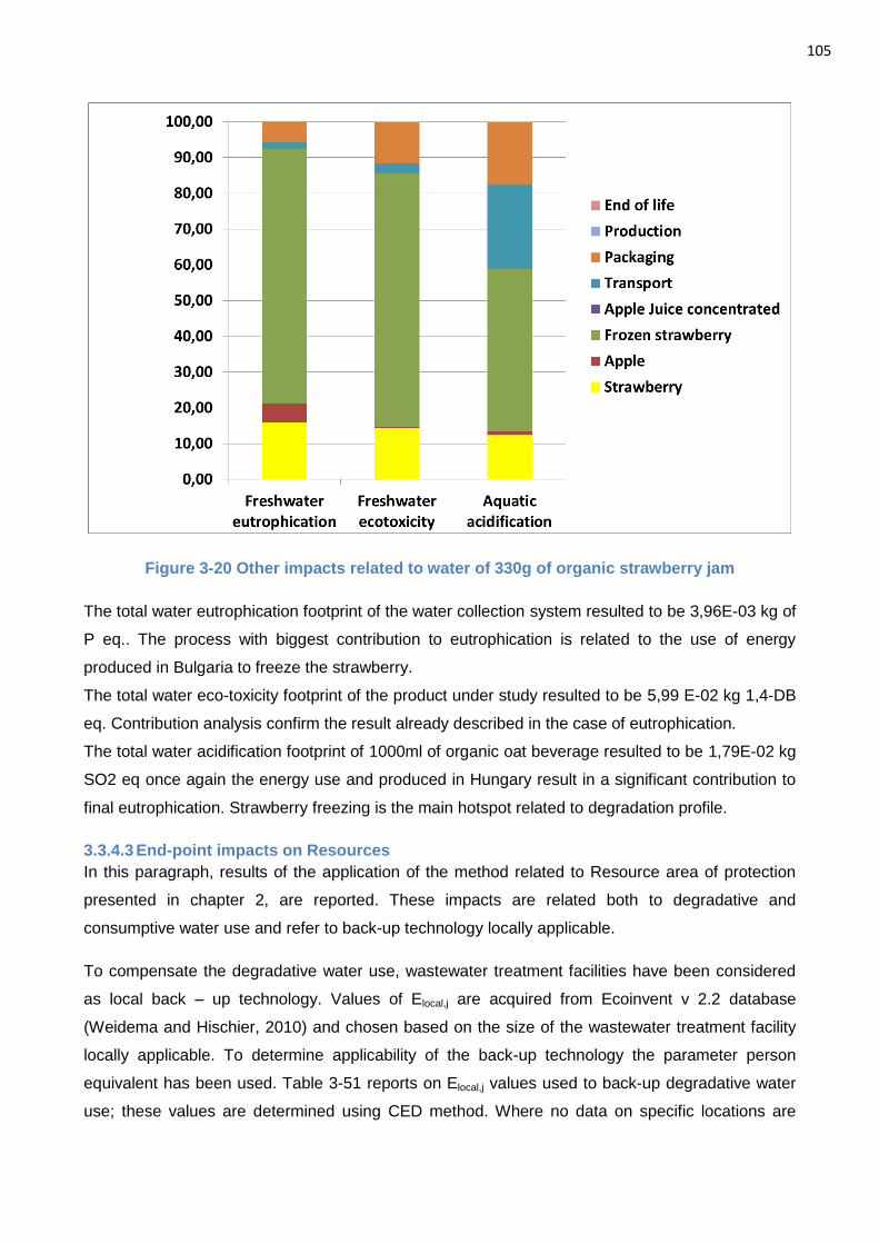
105
Figure 3-20 Other impacts related to water of 330g of organic strawberry jam
The total water eutrophication footprint of the water collection system resulted to be 3,96E-03 kg of
P eq.. The process with biggest contribution to eutrophication is related to the use of energy
produced in Bulgaria to freeze the strawberry.
The total water eco-toxicity footprint of the product under study resulted to be 5,99 E-02 kg 1,4-DB
eq. Contribution analysis confirm the result already described in the case of eutrophication.
The total water acidification footprint of 1000ml of organic oat beverage resulted to be 1,79E-02 kg
SO2 eq once again the energy use and produced in Hungary result in a significant contribution to
final eutrophication. Strawberry freezing is the main hotspot related to degradation profile.
3.3.4.3 End-point impacts on Resources
In this paragraph, results of the application of the method related to Resource area of protection
presented in chapter 2, are reported. These impacts are related both to degradative and
consumptive water use and refer to back-up technology locally applicable.
To compensate the degradative water use, wastewater treatment facilities have been considered
as local back – up technology. Values of Elocal,j are acquired from Ecoinvent v 2.2 database
(Weidema and Hischier, 2010) and chosen based on the size of the wastewater treatment facility
locally applicable. To determine applicability of the back-up technology the parameter person
equivalent has been used. Table 3-51 reports on Elocal,j values used to back-up degradative water
use; these values are determined using CED method. Where no data on specific locations are
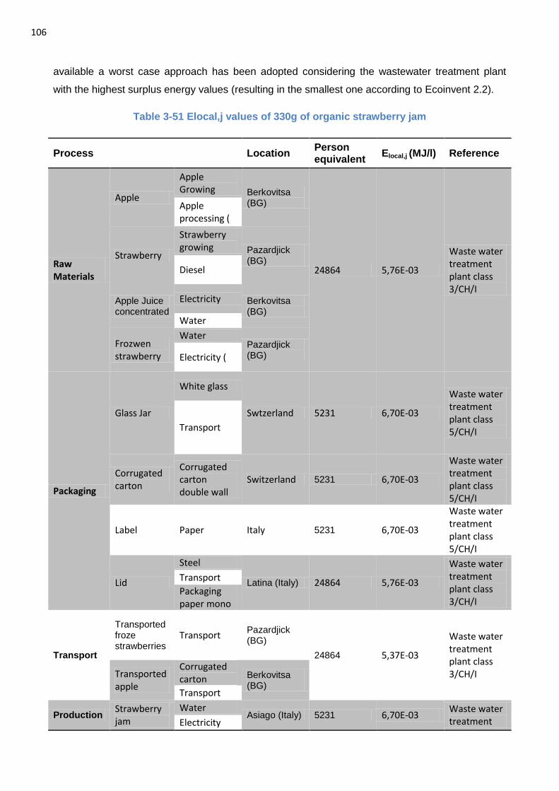
106
available a worst case approach has been adopted considering the wastewater treatment plant
with the highest surplus energy values (resulting in the smallest one according to Ecoinvent 2.2).
Table 3-51 Elocal,j values of 330g of organic strawberry jam
Process Location Person equivalent
Elocal,j (MJ/l) Reference
Raw Materials
Apple
Apple Growing Berkovitsa
(BG)
24864 5,76E-03
Waste water treatment plant class 3/CH/I
Apple processing (
Strawberry
Strawberry growing Pazardjick
(BG) Diesel
Apple Juice concentrated
Electricity Berkovitsa (BG)
Water
Frozwen strawberry
Water Pazardjick (BG) Electricity (
Packaging
Glass Jar
White glass
Swtzerland 5231 6,70E-03
Waste water treatment plant class 5/CH/I Transport
Corrugated carton
Corrugated carton double wall
Switzerland 5231 6,70E-03
Waste water treatment plant class 5/CH/I
Label Paper Italy 5231 6,70E-03
Waste water treatment plant class 5/CH/I
Lid
Steel
Latina (Italy) 24864 5,76E-03
Waste water treatment plant class 3/CH/I
Transport
Packaging paper mono
Transport
Transported froze strawberries
Transport Pazardjick (BG)
24864 5,37E-03
Waste water treatment plant class 3/CH/I Transported
apple
Corrugated carton Berkovitsa
(BG) Transport
Production Strawberry jam
Water Asiago (Italy) 5231 6,70E-03
Waste water treatment Electricity
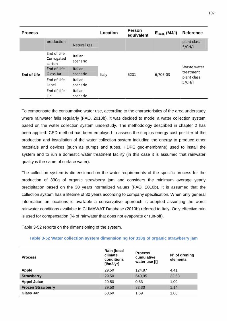
107
Process Location Person equivalent
Elocal,j (MJ/l) Reference
production Natural gas
plant class 5/CH/I
End of Life
End of Life Corrugated carton
Italian scenario
Italy 5231 6,70E-03
Waste water treatment plant class 5/CH/I
End of Life Glass Jar
Italian scenario
End of Life Label
Italian scenario
End of Life Lid
Italian scenario
To compensate the consumptive water use, according to the characteristics of the area understudy
where rainwater falls regularly (FAO, 2010b), it was decided to model a water collection system
based on the water collection system understudy. The methodology described in chapter 2 has
been applied: CED method has been employed to assess the surplus energy cost per liter of the
production and installation of the water collection system including the energy to produce other
materials and devices (such as pumps and tubes, HDPE geo-membrane) used to install the
system and to run a domestic water treatment facility (in this case it is assumed that rainwater
quality is the same of surface water).
The collection system is dimensioned on the water requirements of the specific process for the
production of 330g of organic strawberry jam and considers the minimum average yearly
precipitation based on the 30 years normalized values (FAO, 2010b). It is assumed that the
collection system has a lifetime of 30 years according to company specification. When only general
information on locations is available a conservative approach is adopted assuming the worst
rainwater conditions available in CLIMAWAT Database (2010b) referred to Italy. Only effective rain
is used for compensation (% of rainwater that does not evaporate or run-off).
Table 3-52 reports on the dimensioning of the system.
Table 3-52 Water collection system dimensioning for 330g of organic strawberry jam
Process
Rain (local climate conditions [l/m2/yr]
Process cumulative water use [l]
N° of drening elements
Apple 29,50 124,87 4,41
Strawberry 29,50 640,95 22,63
Appel Juice 29,50 0,53 1,00
Frozen Strawberry 29,50 32,30 1,14
Glass Jar 60,60 1,69 1,00
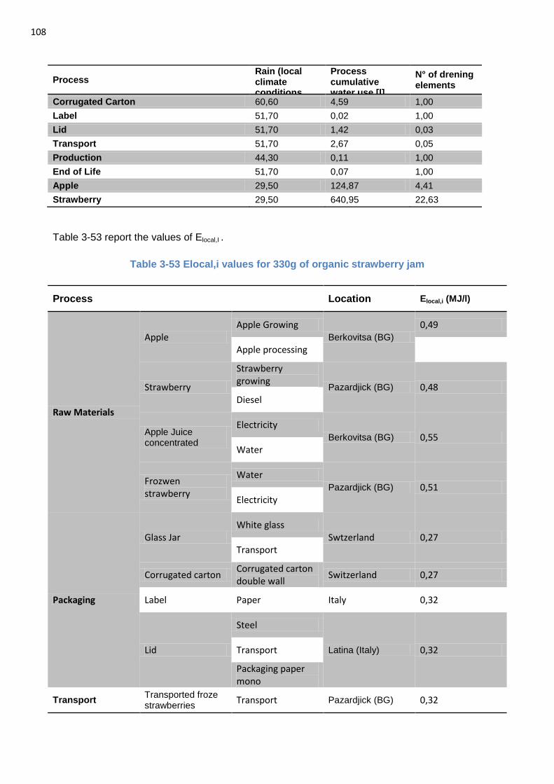
108
Process Rain (local climate conditions [l/m2/yr]
Process cumulative water use [l]
N° of drening elements
Corrugated Carton 60,60 4,59 1,00
Label 51,70 0,02 1,00
Lid 51,70 1,42 0,03
Transport 51,70 2,67 0,05
Production 44,30 0,11 1,00
End of Life 51,70 0,07 1,00
Apple 29,50 124,87 4,41
Strawberry 29,50 640,95 22,63
Table 3-53 report the values of Elocal,I .
Table 3-53 Elocal,i values for 330g of organic strawberry jam
Process Location Elocal,i (MJ/l)
Raw Materials
Apple Apple Growing
Berkovitsa (BG)
0,49
Apple processing
Strawberry
Strawberry growing
Pazardjick (BG) 0,48 Diesel
Apple Juice concentrated
Electricity Berkovitsa (BG) 0,55
Water
Frozwen strawberry
Water Pazardjick (BG) 0,51
Electricity
Packaging
Glass Jar White glass
Swtzerland 0,27 Transport
Corrugated carton Corrugated carton double wall
Switzerland 0,27
Label Paper Italy 0,32
Lid
Steel
Latina (Italy) 0,32 Transport
Packaging paper mono
Transport Transported froze strawberries
Transport Pazardjick (BG) 0,32
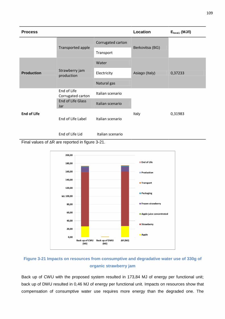
109
Process Location Elocal,i (MJ/l)
Transported apple Corrugated carton
Berkovitsa (BG)
Transport
Production Strawberry jam production
Water
Asiago (Italy) 0,37233 Electricity
Natural gas
End of Life
End of Life Corrugated carton
Italian scenario
Italy 0,31983
End of Life Glass Jar
Italian scenario
End of Life Label Italian scenario
End of Life Lid Italian scenario
Final values of ΔR are reported in figure 3-21.
Figure 3-21 Impacts on resources from consumptive and degradative water use of 330g of
organic strawberry jam
Back up of CWU with the proposed system resulted in 173,84 MJ of energy per functional unit;
back up of DWU resulted in 0,46 MJ of energy per functional unit. Impacts on resources show that
compensation of consumptive water use requires more energy than the degraded one. The
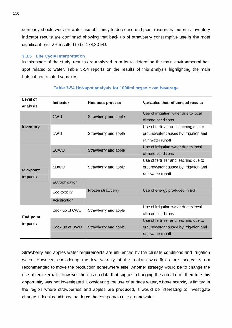
110
company should work on water use efficiency to decrease end point resources footprint. Inventory
indicator results are confirmed showing that back up of strawberry consumptive use is the most
significant one. ΔR resulted to be 174,30 MJ.
3.3.5 Life Cycle Interpretation
In this stage of the study, results are analyzed in order to determine the main environmental hot-
spot related to water. Table 3-54 reports on the results of this analysis highlighting the main
hotspot and related variables.
Table 3-54 Hot-spot analysis for 1000ml organic oat beverage
Level of
analysis Indicator Hotspots-process Variables that influenced results
Inventory
CWU Strawberry and apple Use of irrigation water due to local
climate conditions
DWU Strawberry and apple
Use of fertilizer and leaching due to
groundwater caused by irrigation and
rain water runoff
Mid-point
Impacts
SCWU Strawberry and apple Use of irrigation water due to local
climate conditions
SDWU Strawberry and apple
Use of fertilizer and leaching due to
groundwater caused by irrigation and
rain water runoff
Eutrophication
Frozen strawberry Use of energy produced in BG Eco-toxicity
Acidification
End-point
impacts
Back up of CWU Strawberry and apple Use of irrigation water due to local
climate conditions
Back-up of DWU Strawberry and apple
Use of fertilizer and leaching due to
groundwater caused by irrigation and
rain water runoff
Strawberry and apples water requirements are influenced by the climate conditions and irrigation
water. However, considering the low scarcity of the regions was fields are located is not
recommended to move the production somewhere else. Another strategy would be to change the
use of fertilizer rate; however there is no data that suggest changing the actual one, therefore this
opportunity was not investigated. Considering the use of surface water, whose scarcity is limited in
the region where strawberries and apples are produced, it would be interesting to investigate
change in local conditions that force the company to use groundwater.
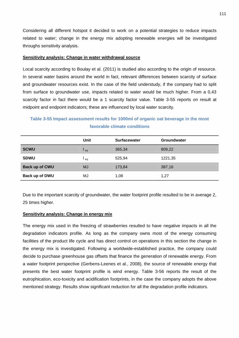
111
Considering all different hotspot it decided to work on a potential strategies to reduce impacts
related to water; change in the energy mix adopting renewable energies will be investigated
throughs sensitivity analysis.
Sensitivity analysis: Change in water withdrawal source
Local scarcity according to Boulay et al. (2011) is studied also according to the origin of resource.
In several water basins around the world in fact, relevant differences between scarcity of surface
and groundwater resources exist. In the case of the field understudy, if the company had to split
from surface to groundwater use, impacts related to water would be much higher. From a 0,43
scarcity factor in fact there would be a 1 scarcity factor value. Table 3-55 reports on result at
midpoint and endpoint indicators; these are influenced by local water scarcity.
Table 3-55 Impact assessment results for 1000ml of organic oat beverage in the most
favorable climate conditions
Unit Surfacewater Groundwater
SCWU l eq 365,34 809,22
SDWU l eq 525,94 1221,35
Back up of CWU MJ 173,84 387,16
Back up of DWU MJ 1,08 1,27
Due to the important scarcity of groundwater, the water footprint profile resulted to be in average 2,
25 times higher.
Sensitivity analysis: Change in energy mix
The energy mix used in the freezing of strawberries resulted to have negative impacts in all the
degradation indicators profile. As long as the company owns most of the energy consuming
facilities of the product life cycle and has direct control on operations in this section the change in
the energy mix is investigated. Following a worldwide-established practice, the company could
decide to purchase greenhouse gas offsets that finance the generation of renewable energy. From
a water footprint perspective (Gerbens-Leenes et al., 2008), the source of renewable energy that
presents the best water footprint profile is wind energy. Table 3-56 reports the result of the
eutrophication, eco-toxicity and acidification footprints, in the case the company adopts the above
mentioned strategy. Results show significant reduction for all the degradation profile indicators.
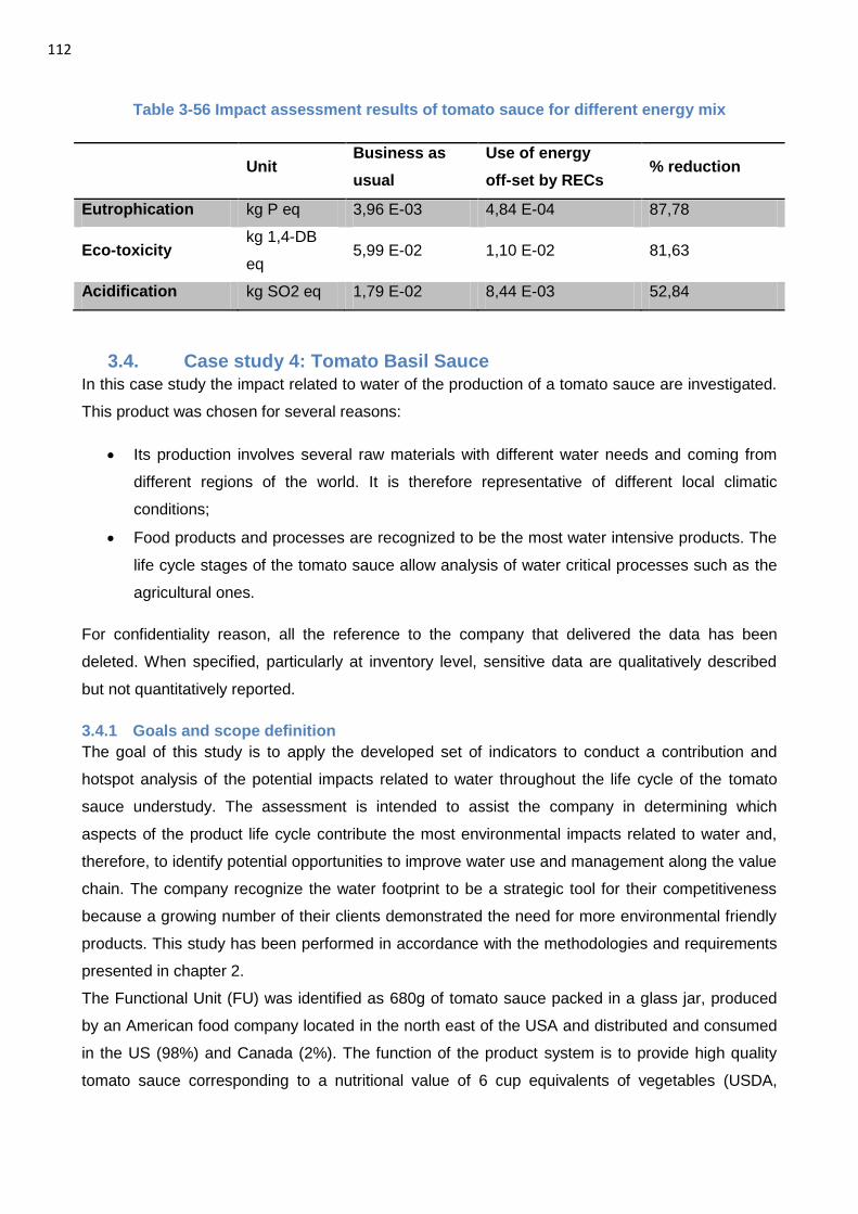
112
Table 3-56 Impact assessment results of tomato sauce for different energy mix
Unit Business as
usual
Use of energy
off-set by RECs % reduction
Eutrophication kg P eq 3,96 E-03 4,84 E-04 87,78
Eco-toxicity kg 1,4-DB
eq 5,99 E-02 1,10 E-02 81,63
Acidification kg SO2 eq 1,79 E-02 8,44 E-03 52,84
3.4. Case study 4: Tomato Basil Sauce
In this case study the impact related to water of the production of a tomato sauce are investigated.
This product was chosen for several reasons:
Its production involves several raw materials with different water needs and coming from
different regions of the world. It is therefore representative of different local climatic
conditions;
Food products and processes are recognized to be the most water intensive products. The
life cycle stages of the tomato sauce allow analysis of water critical processes such as the
agricultural ones.
For confidentiality reason, all the reference to the company that delivered the data has been
deleted. When specified, particularly at inventory level, sensitive data are qualitatively described
but not quantitatively reported.
3.4.1 Goals and scope definition
The goal of this study is to apply the developed set of indicators to conduct a contribution and
hotspot analysis of the potential impacts related to water throughout the life cycle of the tomato
sauce understudy. The assessment is intended to assist the company in determining which
aspects of the product life cycle contribute the most environmental impacts related to water and,
therefore, to identify potential opportunities to improve water use and management along the value
chain. The company recognize the water footprint to be a strategic tool for their competitiveness
because a growing number of their clients demonstrated the need for more environmental friendly
products. This study has been performed in accordance with the methodologies and requirements
presented in chapter 2.
The Functional Unit (FU) was identified as 680g of tomato sauce packed in a glass jar, produced
by an American food company located in the north east of the USA and distributed and consumed
in the US (98%) and Canada (2%). The function of the product system is to provide high quality
tomato sauce corresponding to a nutritional value of 6 cup equivalents of vegetables (USDA,
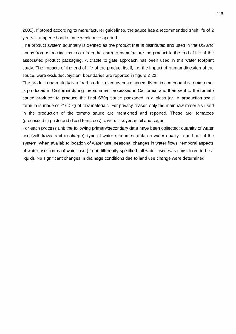
113
2005). If stored according to manufacturer guidelines, the sauce has a recommended shelf life of 2
years if unopened and of one week once opened.
The product system boundary is defined as the product that is distributed and used in the US and
spans from extracting materials from the earth to manufacture the product to the end of life of the
associated product packaging. A cradle to gate approach has been used in this water footprint
study. The impacts of the end of life of the product itself, i.e. the impact of human digestion of the
sauce, were excluded. System boundaries are reported in figure 3-22.
The product under study is a food product used as pasta sauce. Its main component is tomato that
is produced in California during the summer, processed in California, and then sent to the tomato
sauce producer to produce the final 680g sauce packaged in a glass jar. A production-scale
formula is made of 2160 kg of raw materials. For privacy reason only the main raw materials used
in the production of the tomato sauce are mentioned and reported. These are: tomatoes
(processed in paste and diced tomatoes), olive oil, soybean oil and sugar.
For each process unit the following primary/secondary data have been collected: quantity of water
use (withdrawal and discharge); type of water resources; data on water quality in and out of the
system, when available; location of water use; seasonal changes in water flows; temporal aspects
of water use; forms of water use (If not differently specified, all water used was considered to be a
liquid). No significant changes in drainage conditions due to land use change were determined.
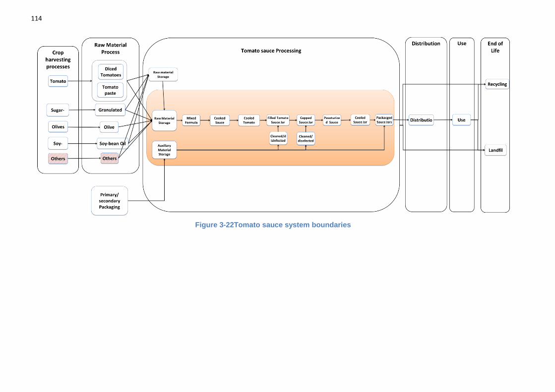
114
Figure 3-22Tomato sauce system boundaries
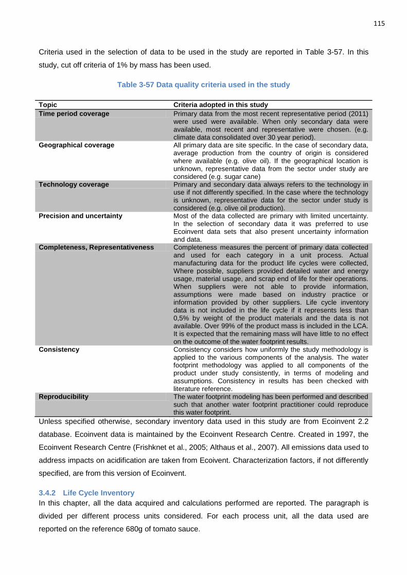
115
Criteria used in the selection of data to be used in the study are reported in Table 3-57. In this
study, cut off criteria of 1% by mass has been used.
Table 3-57 Data quality criteria used in the study
Topic Criteria adopted in this study
Time period coverage Primary data from the most recent representative period (2011) were used were available. When only secondary data were available, most recent and representative were chosen. (e.g. climate data consolidated over 30 year period).
Geographical coverage All primary data are site specific. In the case of secondary data, average production from the country of origin is considered where available (e.g. olive oil). If the geographical location is unknown, representative data from the sector under study are considered (e.g. sugar cane)
Technology coverage Primary and secondary data always refers to the technology in use if not differently specified. In the case where the technology is unknown, representative data for the sector under study is considered (e.g. olive oil production).
Precision and uncertainty Most of the data collected are primary with limited uncertainty. In the selection of secondary data it was preferred to use Ecoinvent data sets that also present uncertainty information and data.
Completeness, Representativeness Completeness measures the percent of primary data collected and used for each category in a unit process. Actual manufacturing data for the product life cycles were collected, Where possible, suppliers provided detailed water and energy usage, material usage, and scrap end of life for their operations. When suppliers were not able to provide information, assumptions were made based on industry practice or information provided by other suppliers. Life cycle inventory data is not included in the life cycle if it represents less than 0,5% by weight of the product materials and the data is not available. Over 99% of the product mass is included in the LCA. It is expected that the remaining mass will have little to no effect on the outcome of the water footprint results.
Consistency Consistency considers how uniformly the study methodology is applied to the various components of the analysis. The water footprint methodology was applied to all components of the product under study consistently, in terms of modeling and assumptions. Consistency in results has been checked with literature reference.
Reproducibility The water footprint modeling has been performed and described such that another water footprint practitioner could reproduce this water footprint.
Unless specified otherwise, secondary inventory data used in this study are from Ecoinvent 2.2
database. Ecoinvent data is maintained by the Ecoinvent Research Centre. Created in 1997, the
Ecoinvent Research Centre (Frishknet et al., 2005; Althaus et al., 2007). All emissions data used to
address impacts on acidification are taken from Ecoivent. Characterization factors, if not differently
specified, are from this version of Ecoinvent.
3.4.2 Life Cycle Inventory
In this chapter, all the data acquired and calculations performed are reported. The paragraph is
divided per different process units considered. For each process unit, all the data used are
reported on the reference 680g of tomato sauce.
116
The inventory is populated with primary data collected directly from companies involved in the
study and secondary data from scientific LCA database. In the case of secondary data however
not all the information (such as quality in and quantity out) are available. In these cases a worst
case approach is adopted considering all withdrawn water as used (consumptive use) and the
quality entering the system as of the best quality locally available).
3.4.2.1 Tomato
One of the most important raw materials used in the production of the product under study are
tomatoes. Tomatoes are grown in California in different sites located within the Sacramento and
the San Joaquin valleys. Following the common practice in California, tomatoes are planted in May
and harvested between September and October. The technology used for irrigation is drip
irrigation. Data reported are primary data from the supplier and are based on the 2011 production
year. The average yield from different production site is 50,43 tons/ha.
In order to assess the crop water requirements the CROPWAT model (FAO, 2010a) has been
used. The CROPWAT software developed by FAO is used to model the water requirements of a
crop. The model utilizes data on the climatic conditions, the reference evapotranspiration, the soil
and the specific crop characteristics to determine the irrigation requirements of the crop under
study. ET0 (evapotranspiration in standard condition) is determined using the Penman-Montheit
equation (FAO, 2010a). Effective rain (the rainfall effectively available to the crop) is assessed
through the USDA SCS method (option selected within CROPWAT model). Climatic data are taken
from standardized average data over the last 30 years acquired through the CLIMAWAT 2.0
database (FAO, 2010b); such database offers observed agroclimatic data of over 5000 stations
worldwide including the locations under study. The data selected for this study comes from the
climatic stations located in Sacramento and Fresno (Tab 3-58 and Tab 3-59). This data was
considered to be representative of the climatic conditions of the locations under study. These are
primary data collected by the National Climate Data Centre (NOAA) of the USA
(http://www.ncdc.noaa.gov/).
Data on the crop modeling are taken from FAO database (FAO, 2010a) accessible within the
CROPWAT software and then modified with primary parameters when available. The soil
considered in the assessment is black clay soil, which is representative of the locations in
California where the tomatoes used in the product under study are grown (primary data from USDA
data base: http://websoilsurvey.nrcs.usda.gov/app/WebSoilSurvey.aspx). Details on drip irrigation
techniques used in California are taken from University of California Division of Agriculture and
Natural Resources (USDA, 2005)
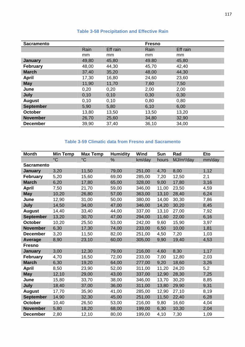
117
Table 3-58 Precipitation and Effective Rain
Sacramento Fresno
Rain Eff rain Rain Eff rain
mm mm mm mm
January 49,80 45,80 49.80 45,80
February 48,00 44,30 45,70 42,40
March 37,40 35,20 48,00 44,30
April 17,30 16,80 24,60 23,60
May 11,90 11,70 7,60 7,50
June 0,20 0,20 2,00 2,00
July 0,10 0,10 0,30 0,30
August 0,10 0,10 0,80 0,80
September 5,90 5,80 6,10 6,00
October 13,80 13,50 13,50 13,20
November 26,70 25,60 34,80 32,90
December 39,90 37,40 36,10 34,00
Table 3-59 Climatic data from Fresno and Sacramento
Month Min Temp Max Temp Humidity Wind Sun Rad Eto
°C °C % km/day hours MJ/m²/day mm/day
Sacramento
January 3,20 11,50 79,00 251,00 4,70 8,00 1,12
February 5,20 15,60 69,00 285,00 7,20 12,50 2,1
March 6,20 17,80 65,00 328,00 9,00 17,80 3,16
April 7,50 21,70 59,00 346,00 11,00 23,50 4,59
May 10,20 26,80 57,00 363,00 13,10 28,40 6,24
June 12,90 31,00 50,00 380,00 14,00 30,30 7,86
July 14,50 34,00 47,00 346,00 14,20 30,20 8,45
August 14,40 33,40 44,00 337,00 13,10 27,00 7,92
September 13,20 30,70 47,00 294,00 11,60 22,00 6,16
October 10,20 25,50 53,00 242,00 9,60 15,90 3,97
November 6,30 17,30 74,00 233,00 6,50 10,00 1,81
December 3,20 11,50 82,00 251,00 4,50 7,20 1,03
Average 8,90 23,10 60,00 305,00 9,90 19,40 4,53
Fresno
January 3,00 12,30 79,00 216,00 4,60 8,30 1,17
February 4,70 16,50 72,00 233,00 7,00 12,80 2,03
March 6,30 19,20 64,00 277,00 9,20 18,60 3,26
April 8,50 23,90 52,00 311,00 11,20 24,20 5,2
May 12,10 29,00 43,00 337,00 12,90 28,30 7,25
June 15,80 33,70 38,00 346,00 13,70 30,20 8,85
July 18,40 37,00 36,00 311,00 13,80 29,90 9,31
August 17,70 35,90 41,00 285,00 12,90 27,10 8,19
September 14,90 32,30 45,00 251,00 11,50 22,40 6,28
October 10,40 26,50 53,00 216,00 9,80 16,60 4,04
November 5,80 18,20 68,00 199,00 6,30 10,30 2,04
December 2,80 12,10 80,00 199,00 4,10 7,30 1,09
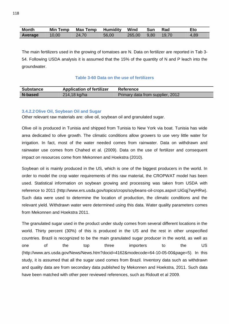
118
Month Min Temp Max Temp Humidity Wind Sun Rad Eto
Average 10,00 24,70 56,00 265,00 9,80 19,70 4,89
The main fertilizers used in the growing of tomatoes are N. Data on fertilizer are reported in Tab 3-
54. Following USDA analysis it is assumed that the 15% of the quantity of N and P leach into the
groundwater.
Table 3-60 Data on the use of fertilizers
Substance
considered
Application of fertilizer
(kg/ha)
Reference
N-based 214,18 kg/ha Primary data from supplier, 2012
3.4.2.2 Olive Oil, Soybean Oil and Sugar
Other relevant raw materials are: olive oil, soybean oil and granulated sugar.
Olive oil is produced in Tunisia and shipped from Tunisia to New York via boat. Tunisia has wide
area dedicated to olive growth. The climatic conditions allow growers to use very little water for
irrigation. In fact, most of the water needed comes from rainwater. Data on withdrawn and
rainwater use comes from Chahed et al. (2009). Data on the use of fertilizer and consequent
impact on resources come from Mekonnen and Hoekstra (2010).
Soybean oil is mainly produced in the US, which is one of the biggest producers in the world. In
order to model the crop water requirements of this raw material, the CROPWAT model has been
used. Statistical information on soybean growing and processing was taken from USDA with
reference to 2011 (http://www.ers.usda.gov/topics/crops/soybeans-oil-crops.aspx#.UiGqj7wyHRw).
Such data were used to determine the location of production, the climatic conditions and the
relevant yield. Withdrawn water were determined using this data. Water quality parameters comes
from Mekonnen and Hoekstra 2011.
The granulated sugar used in the product under study comes from several different locations in the
world. Thirty percent (30%) of this is produced in the US and the rest in other unspecified
countries. Brazil is recognized to be the main granulated sugar producer in the world, as well as
one of the top three importers to the US
(http://www.ars.usda.gov/News/News.htm?docid=4162&modecode=64-10-05-00&page=5). In this
study, it is assumed that all the sugar used comes from Brazil. Inventory data such as withdrawn
and quality data are from secondary data published by Mekonnen and Hoekstra, 2011. Such data
have been matched with other peer reviewed references, such as Ridoutt et al 2009.
119
3.4.2.3 Tomato processing
Tomatoes are processed in two facilities located California. At these two sites, tomatoes are used
to produce the diced tomatoes and the tomato paste. Tomatoes arrive from several locations
presented in the previous chapters.
In the case of diced tomatoes, after a first quality selection that discards almost the 30% of the
incoming raw fruit (unripe tomatoes reused within the site in other productions), the tomatoes are
diced. The final product, diced tomatoes, is made of tomato juice (resulted from the process of
dicing) and diced fruit. The biggest water use in this process is the water used for conveyance and
steam produced for heating the tomatoes during processing. Water is reused throughout the
process as many times as possible until its quality is no longer suitable for the intended use. In this
case, the resultant wastewater is land applied for crop irrigation. Tomato paste is the result of a
process that reduces the water content of tomatoes from 95% average water content to a 31%
equivalent. Water extracted from the product is reused when possible. The production of cooked
and concentrated tomatoes requires a high quantity of energy and steam in order to dry the
tomatoes to the desired water content. Tomato paste is made in both of the facilities.
Once prepared, the diced tomatoes and tomato paste are packed in aseptic plastic bags (300
gallon capacity, made of polyethylene with 5% by weight assumed to be aluminum) and placed into
a wood crate. The packaged product is placed on a wooden pallet (US standard dimension and
capacity) and shipped to the tomato sauce production company by train,
Mots of data comes from direct measure from the two facilities located in California and are related
to withdrawn water, discharged water, quantity in and out. This water balance included the water
content of the tomatoes. In the case of packaging, secondary data from Ecoinvent v.2.2 was used
as primary data was not available.
3.4.2.4 Production
Raw and auxiliary materials are shipped to the tomato sauce producer for the production of the
tomato sauce understudy. The production process starts with the mixing of all the different
ingredients based on the formula). After the sauce is cooked, it is cooled down. In this process,
water is used directly in the product recipe, for cooling, and for the generation of steam (to sterilize
the glass jar). Once cooked and cooled, the tomato sauce goes into packaging process. The sauce
flows into glass jars that are water-lubed conveyed. Once the jar (glass) is full with the right
quantity of product, it is capped (metal lid made of aluminum), pasteurized and cooled. Throughout
these processing steps water is also used for cleaning. Once prepared, the sauce is packed using
stretch wrap and corrugated carton. Packaged products are placed on a wooden pallet (US
standard dimension and capacity) and then distributed to retail stores.
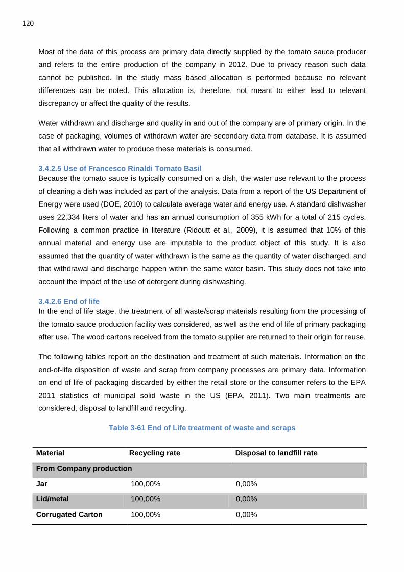
120
Most of the data of this process are primary data directly supplied by the tomato sauce producer
and refers to the entire production of the company in 2012. Due to privacy reason such data
cannot be published. In the study mass based allocation is performed because no relevant
differences can be noted. This allocation is, therefore, not meant to either lead to relevant
discrepancy or affect the quality of the results.
Water withdrawn and discharge and quality in and out of the company are of primary origin. In the
case of packaging, volumes of withdrawn water are secondary data from database. It is assumed
that all withdrawn water to produce these materials is consumed.
3.4.2.5 Use of Francesco Rinaldi Tomato Basil
Because the tomato sauce is typically consumed on a dish, the water use relevant to the process
of cleaning a dish was included as part of the analysis. Data from a report of the US Department of
Energy were used (DOE, 2010) to calculate average water and energy use. A standard dishwasher
uses 22,334 liters of water and has an annual consumption of 355 kWh for a total of 215 cycles.
Following a common practice in literature (Ridoutt et al., 2009), it is assumed that 10% of this
annual material and energy use are imputable to the product object of this study. It is also
assumed that the quantity of water withdrawn is the same as the quantity of water discharged, and
that withdrawal and discharge happen within the same water basin. This study does not take into
account the impact of the use of detergent during dishwashing.
3.4.2.6 End of life
In the end of life stage, the treatment of all waste/scrap materials resulting from the processing of
the tomato sauce production facility was considered, as well as the end of life of primary packaging
after use. The wood cartons received from the tomato supplier are returned to their origin for reuse.
The following tables report on the destination and treatment of such materials. Information on the
end-of-life disposition of waste and scrap from company processes are primary data. Information
on end of life of packaging discarded by either the retail store or the consumer refers to the EPA
2011 statistics of municipal solid waste in the US (EPA, 2011). Two main treatments are
considered, disposal to landfill and recycling.
Table 3-61 End of Life treatment of waste and scraps
Material Recycling rate Disposal to landfill rate
From Company production
Jar 100,00% 0,00%
Lid/metal 100,00% 0,00%
Corrugated Carton 100,00% 0,00%
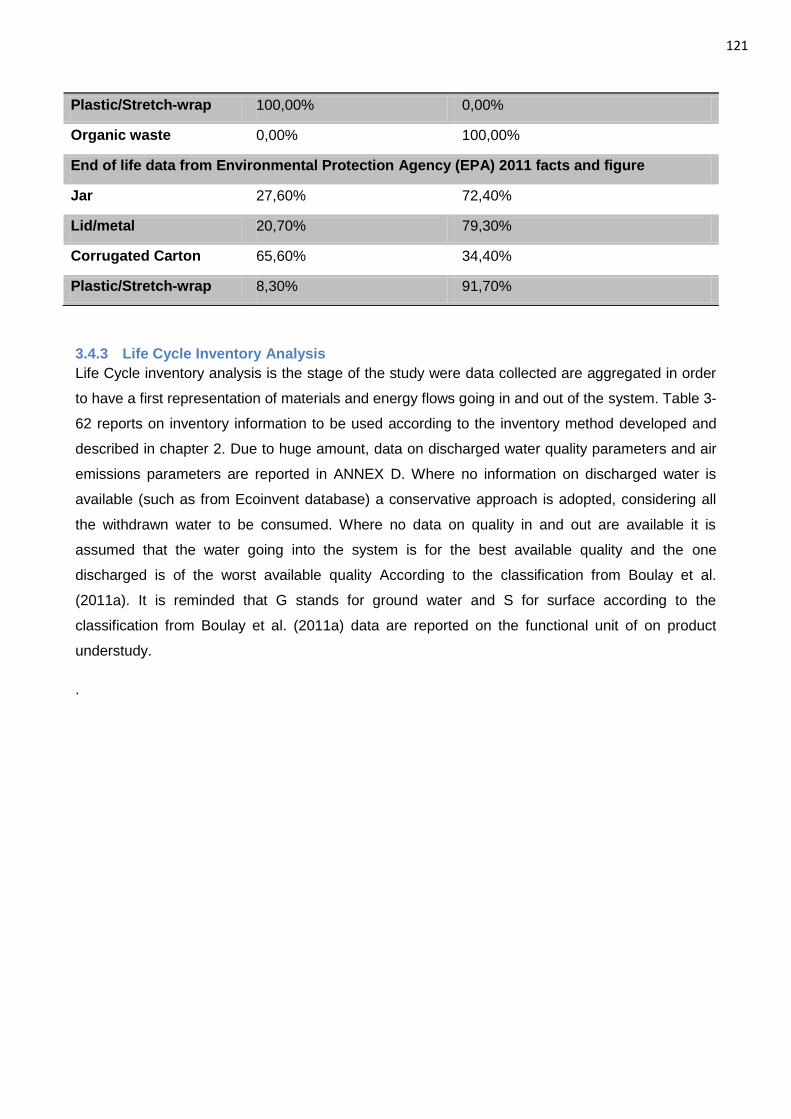
121
3.4.3 Life Cycle Inventory Analysis
Life Cycle inventory analysis is the stage of the study were data collected are aggregated in order
to have a first representation of materials and energy flows going in and out of the system. Table 3-
62 reports on inventory information to be used according to the inventory method developed and
described in chapter 2. Due to huge amount, data on discharged water quality parameters and air
emissions parameters are reported in ANNEX D. Where no information on discharged water is
available (such as from Ecoinvent database) a conservative approach is adopted, considering all
the withdrawn water to be consumed. Where no data on quality in and out are available it is
assumed that the water going into the system is for the best available quality and the one
discharged is of the worst available quality According to the classification from Boulay et al.
(2011a). It is reminded that G stands for ground water and S for surface according to the
classification from Boulay et al. (2011a) data are reported on the functional unit of on product
understudy.
.
Plastic/Stretch-wrap 100,00% 0,00%
Organic waste 0,00% 100,00%
End of life data from Environmental Protection Agency (EPA) 2011 facts and figure
Jar 27,60% 72,40%
Lid/metal 20,70% 79,30%
Corrugated Carton 65,60% 34,40%
Plastic/Stretch-wrap 8,30% 91,70%
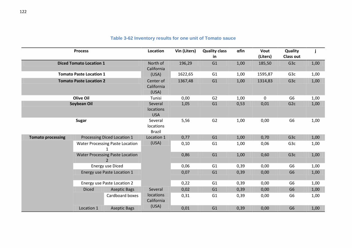
122
Table 3-62 Inventory results for one unit of Tomato sauce
Process Location Vin (Liters) Quality class in
αfin Vout (Liters)
Quality Class out
j
Diced Tomato Location 1 North of California
(USA)
196,29 G1 1,00 185,50 G3c 1,00
Tomato Paste Location 1 1622,65 G1 1,00 1595,87 G3c 1,00
Tomato Paste Location 2 Center of California
(USA)
1367,48 G1 1,00 1314,83 G3c 1,00
Olive Oil Tunisi 0,00 G2 1,00 0 G6 1,00 Soybean Oil Several
locations USA
1,05 G1 0,53 0,01 G2c 1,00
Sugar Several locations
Brazil
5,56 G2 1,00 0,00 G6 1,00
Tomato processing Processing Diced Location 1 Location 1 (USA)
0,77 G1 1,00 0,70 G3c 1,00
Water Processing Paste Location 1
0,10 G1 1,00 0,06 G3c 1,00
Water Processing Paste Location 2
0,86 G1 1,00 0,60 G3c 1,00
Energy use Diced 0,06 G1 0,39 0,00 G6 1,00
Energy use Paste Location 1 0,07 G1 0,39 0,00 G6 1,00
Energy use Paste Location 2 0,22 G1 0,39 0,00 G6 1,00
Diced Aseptic Bags Several locations California
(USA)
0,02 G1 0,39 0,00 G6 1,00
Cardboard boxes 0,31 G1 0,39 0,00 G6 1,00
Location 1 Aseptic Bags 0,01 G1 0,39 0,00 G6 1,00
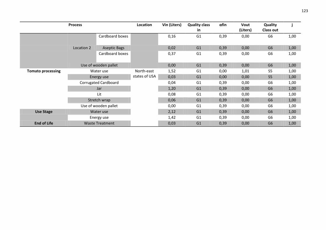
123
Process Location Vin (Liters) Quality class in
αfin Vout (Liters)
Quality Class out
j
Cardboard boxes 0,16 G1 0,39 0,00 G6 1,00
Location 2 Aseptic Bags 0,02 G1 0,39 0,00 G6 1,00
Cardboard boxes 0,37 G1 0,39 0,00 G6 1,00
Use of wooden pallet 0,00 G1 0,39 0,00 G6 1,00
Tomato processing Water use North-east states of USA
1,52 G1 0,00 1,01 S5 1,00
Energy use 0,03 G1 0,00 0,00 S5 1,00
Corrugated Cardboard 0,04 G1 0,39 0,00 G6 1,00
Jar 1,20 G1 0,39 0,00 G6 1,00
Lit 0,08 G1 0,39 0,00 G6 1,00
Stretch wrap 0,06 G1 0,39 0,00 G6 1,00
Use of wooden pallet 0,00 G1 0,39 0,00 G6 1,00
Use Stage Water use 2,12 G1 0,39 0,00 G6 1,00
Energy use 1,42 G1 0,39 0,00 G6 1,00
End of Life Waste Treatment 0,03 G1 0,39 0,00 G6 1,00
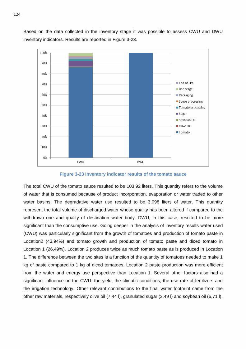
124
Based on the data collected in the inventory stage it was possible to assess CWU and DWU
inventory indicators. Results are reported in Figure 3-23.
Figure 3-23 Inventory indicator results of the tomato sauce
The total CWU of the tomato sauce resulted to be 103,92 liters. This quantity refers to the volume
of water that is consumed because of product incorporation, evaporation or water traded to other
water basins. The degradative water use resulted to be 3,098 liters of water. This quantity
represent the total volume of discharged water whose quality has been altered if compared to the
withdrawn one and quality of destination water body. DWU, in this case, resulted to be more
significant than the consumptive use. Going deeper in the analysis of inventory results water used
(CWU) was particularly significant from the growth of tomatoes and production of tomato paste in
Location2 (43,94%) and tomato growth and production of tomato paste and diced tomato in
Location 1 (26,49%). Location 2 produces twice as much tomato paste as is produced in Location
1. The difference between the two sites is a function of the quantity of tomatoes needed to make 1
kg of paste compared to 1 kg of diced tomatoes. Location 2 paste production was more efficient
from the water and energy use perspective than Location 1. Several other factors also had a
significant influence on the CWU: the yield, the climatic conditions, the use rate of fertilizers and
the irrigation technology. Other relevant contributions to the final water footprint came from the
other raw materials, respectively olive oil (7,44 l), granulated sugar (3,49 l) and soybean oil (6,71 l).
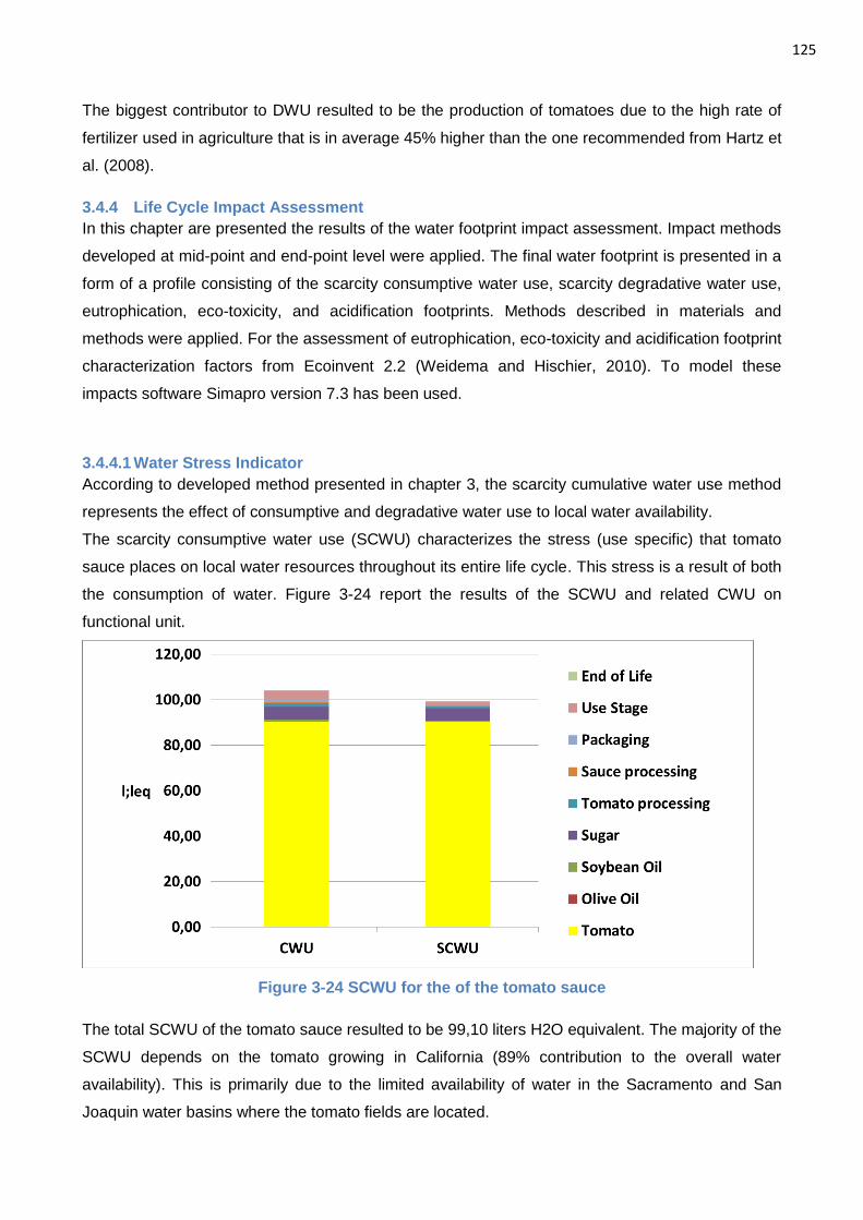
125
The biggest contributor to DWU resulted to be the production of tomatoes due to the high rate of
fertilizer used in agriculture that is in average 45% higher than the one recommended from Hartz et
al. (2008).
3.4.4 Life Cycle Impact Assessment
In this chapter are presented the results of the water footprint impact assessment. Impact methods
developed at mid-point and end-point level were applied. The final water footprint is presented in a
form of a profile consisting of the scarcity consumptive water use, scarcity degradative water use,
eutrophication, eco-toxicity, and acidification footprints. Methods described in materials and
methods were applied. For the assessment of eutrophication, eco-toxicity and acidification footprint
characterization factors from Ecoinvent 2.2 (Weidema and Hischier, 2010). To model these
impacts software Simapro version 7.3 has been used.
3.4.4.1 Water Stress Indicator
According to developed method presented in chapter 3, the scarcity cumulative water use method
represents the effect of consumptive and degradative water use to local water availability.
The scarcity consumptive water use (SCWU) characterizes the stress (use specific) that tomato
sauce places on local water resources throughout its entire life cycle. This stress is a result of both
the consumption of water. Figure 3-24 report the results of the SCWU and related CWU on
functional unit.
Figure 3-24 SCWU for the of the tomato sauce
The total SCWU of the tomato sauce resulted to be 99,10 liters H2O equivalent. The majority of the
SCWU depends on the tomato growing in California (89% contribution to the overall water
availability). This is primarily due to the limited availability of water in the Sacramento and San
Joaquin water basins where the tomato fields are located.
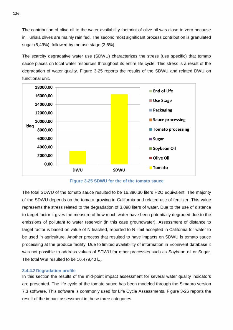
126
The contribution of olive oil to the water availability footprint of olive oil was close to zero because
in Tunisia olives are mainly rain fed. The second most significant process contribution is granulated
sugar (5,49%), followed by the use stage (3,5%).
The scarcity degradative water use (SDWU) characterizes the stress (use specific) that tomato
sauce places on local water resources throughout its entire life cycle. This stress is a result of the
degradation of water quality. Figure 3-25 reports the results of the SDWU and related DWU on
functional unit.
Figure 3-25 SDWU for the of the tomato sauce
The total SDWU of the tomato sauce resulted to be 16.380,30 liters H2O equivalent. The majority
of the SDWU depends on the tomato growing in California and related use of fertilizer. This value
represents the stress related to the degradation of 3,098 liters of water. Due to the use of distance
to target factor it gives the measure of how much water have been potentially degraded due to the
emissions of pollutant to water reservoir (in this case groundwater). Assessment of distance to
target factor is based on value of N leached, reported to N limit accepted in California for water to
be used in agriculture. Another process that resulted to have impacts on SDWU is tomato sauce
processing at the produce facility. Due to limited availability of information in Ecoinvent database it
was not possible to address values of SDWU for other processes such as Soybean oil or Sugar.
The total WSI resulted to be 16.479,40 leq.
3.4.4.2 Degradation profile
In this section the results of the mid-point impact assessment for several water quality indicators
are presented. The life cycle of the tomato sauce has been modeled through the Simapro version
7.3 software. This software is commonly used for Life Cycle Assessments. Figure 3-26 reports the
result of the impact assessment in these three categories.
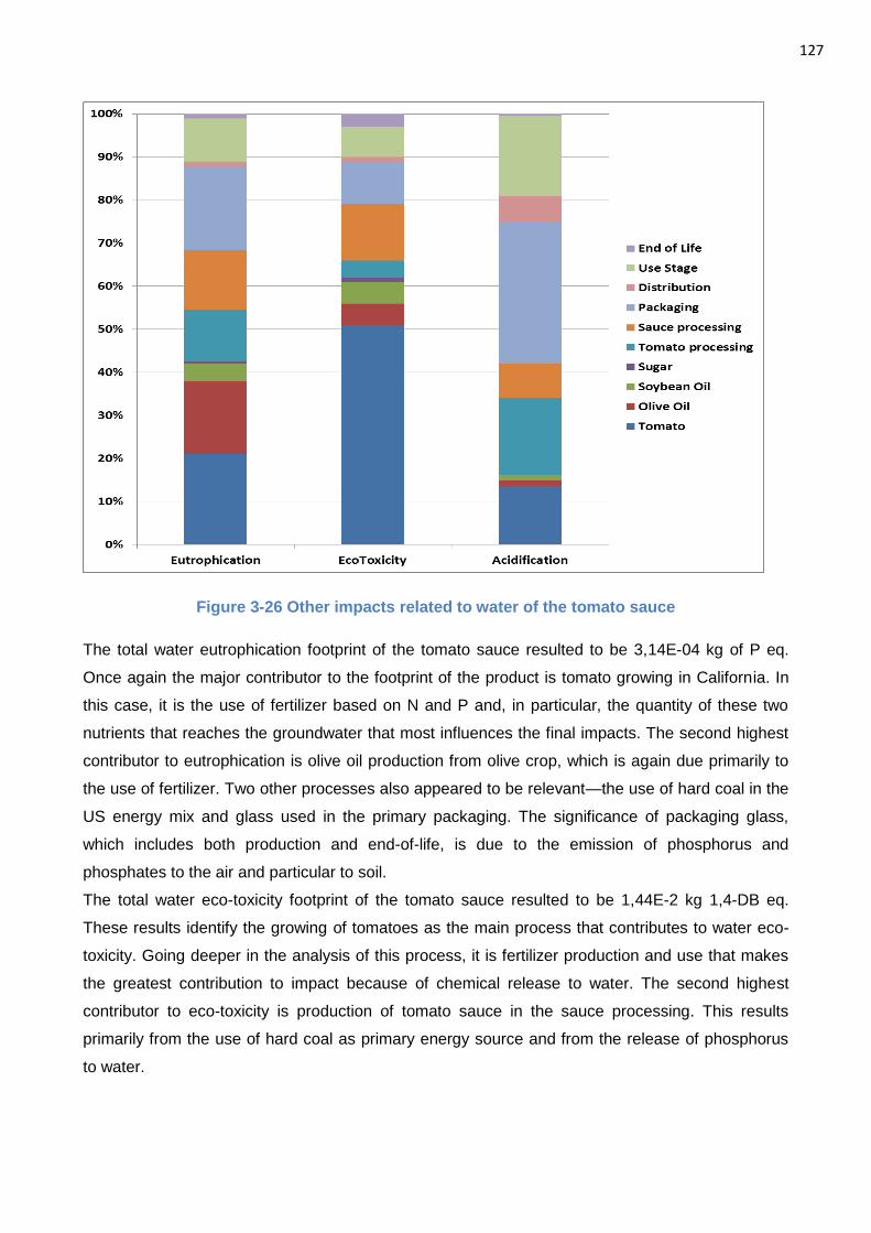
127
Figure 3-26 Other impacts related to water of the tomato sauce
The total water eutrophication footprint of the tomato sauce resulted to be 3,14E-04 kg of P eq.
Once again the major contributor to the footprint of the product is tomato growing in California. In
this case, it is the use of fertilizer based on N and P and, in particular, the quantity of these two
nutrients that reaches the groundwater that most influences the final impacts. The second highest
contributor to eutrophication is olive oil production from olive crop, which is again due primarily to
the use of fertilizer. Two other processes also appeared to be relevant—the use of hard coal in the
US energy mix and glass used in the primary packaging. The significance of packaging glass,
which includes both production and end-of-life, is due to the emission of phosphorus and
phosphates to the air and particular to soil.
The total water eco-toxicity footprint of the tomato sauce resulted to be 1,44E-2 kg 1,4-DB eq.
These results identify the growing of tomatoes as the main process that contributes to water eco-
toxicity. Going deeper in the analysis of this process, it is fertilizer production and use that makes
the greatest contribution to impact because of chemical release to water. The second highest
contributor to eco-toxicity is production of tomato sauce in the sauce processing. This results
primarily from the use of hard coal as primary energy source and from the release of phosphorus
to water.
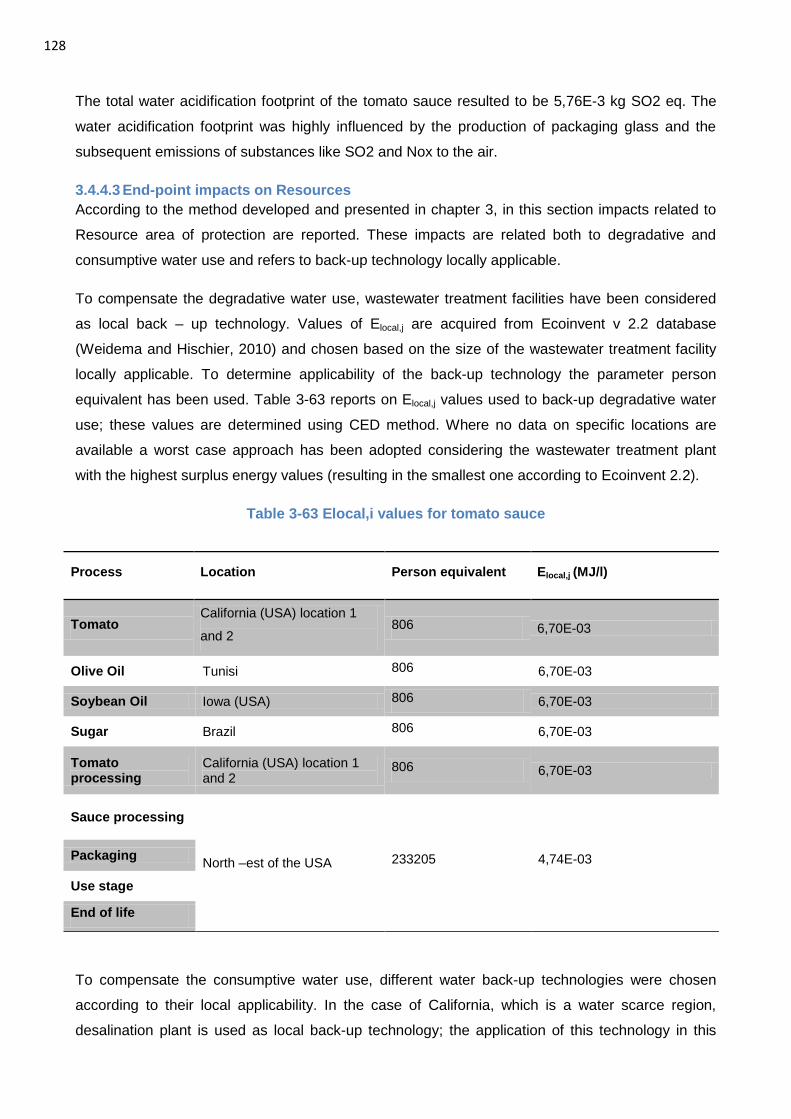
128
The total water acidification footprint of the tomato sauce resulted to be 5,76E-3 kg SO2 eq. The
water acidification footprint was highly influenced by the production of packaging glass and the
subsequent emissions of substances like SO2 and Nox to the air.
3.4.4.3 End-point impacts on Resources
According to the method developed and presented in chapter 3, in this section impacts related to
Resource area of protection are reported. These impacts are related both to degradative and
consumptive water use and refers to back-up technology locally applicable.
To compensate the degradative water use, wastewater treatment facilities have been considered
as local back – up technology. Values of Elocal,j are acquired from Ecoinvent v 2.2 database
(Weidema and Hischier, 2010) and chosen based on the size of the wastewater treatment facility
locally applicable. To determine applicability of the back-up technology the parameter person
equivalent has been used. Table 3-63 reports on Elocal,j values used to back-up degradative water
use; these values are determined using CED method. Where no data on specific locations are
available a worst case approach has been adopted considering the wastewater treatment plant
with the highest surplus energy values (resulting in the smallest one according to Ecoinvent 2.2).
Table 3-63 Elocal,i values for tomato sauce
To compensate the consumptive water use, different water back-up technologies were chosen
according to their local applicability. In the case of California, which is a water scarce region,
desalination plant is used as local back-up technology; the application of this technology in this
Process Location Person equivalent Elocal,j (MJ/l)
Tomato California (USA) location 1
and 2 806 6,70E-03
Olive Oil Tunisi 806 6,70E-03
Soybean Oil Iowa (USA) 806 6,70E-03
Sugar Brazil 806 6,70E-03
Tomato processing
California (USA) location 1 and 2
806 6,70E-03
Sauce processing
North –est of the USA 233205 4,74E-03 Packaging
Use stage
End of life
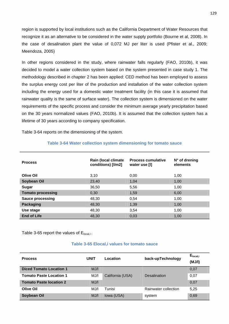
129
region is supported by local institutions such as the California Department of Water Resources that
recognize it as an alternative to be considered in the water supply portfolio (Bourne et al, 2008). In
the case of desalination plant the value of 0,072 MJ per liter is used (Pfister et al., 2009;
Meendoza, 2005)
In other regions considered in the study, where rainwater falls regularly (FAO, 2010b), it was
decided to model a water collection system based on the system presented in case study 1. The
methodology described in chapter 2 has been applied: CED method has been employed to assess
the surplus energy cost per liter of the production and installation of the water collection system
including the energy used for a domestic water treatment facility (in this case it is assumed that
rainwater quality is the same of surface water). The collection system is dimensioned on the water
requirements of the specific process and consider the minimum average yearly precipitation based
on the 30 years normalized values (FAO, 2010b). It is assumed that the collection system has a
lifetime of 30 years according to company specification.
Table 3-64 reports on the dimensioning of the system.
Table 3-64 Water collection system dimensioning for tomato sauce
Process Rain (local climate conditions) [l/m2]
Process cumulative water use [l]
N° of drening elements
Olive Oil 3,10 0,00 1,00
Soybean Oil 23,40 1,04 1,00
Sugar 36,50 5,56 1,00
Tomato processing 0,30 1,59 6,00
Sauce processing 48,30 0,54 1,00
Packaging 48,30 1,39 1,00
Use stage 48,30 3,54 1,00
End of Life 48,30 0,03 1,00
Table 3-65 report the values of Elocal,I .
Table 3-65 Elocal,i values for tomato sauce
Process UNIT Location back-upTechnology Elocal,i
(MJ/l)
Diced Tomato Location 1 MJ/l
California (USA) Desalination
0,07
Tomato Paste Location 1 MJ/l 0,07
Tomato Paste location 2 MJ/l 0,07
Olive Oil MJ/l Tunisi Rainwater collection
system
5,25
Soybean Oil MJ/l Iowa (USA) 0,69
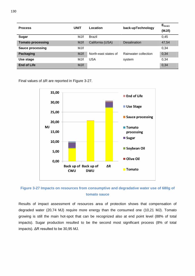
130
Process UNIT Location back-upTechnology Elocal,i
(MJ/l)
Sugar MJ/l Brazil 0,45
Tomato processing MJ/l California (USA) Desalination 47,54
Sauce processing MJ/l
North-east states of
USA
Rainwater collection
system
0,34
Packaging MJ/l 0,34
Use stage MJ/l 0,34
End of Life MJ/l 0,34
Final values of ΔR are reported in Figure 3-27.
Figure 3-27 Impacts on resources from consumptive and degradative water use of 680g of
tomato sauce
Results of impact assessment of resources area of protection shows that compensation of
degraded water (20,74 MJ) require more energy than the consumed one (10,21 MJ). Tomato
growing is still the main hot-spot that can be recognized also at end point level (88% of total
impacts). Sugar production resulted to be the second most significant process (8% of total
impacts). ΔR resulted to be 30,95 MJ.
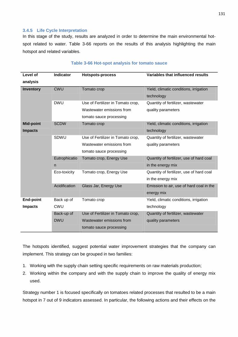
131
3.4.5 Life Cycle Interpretation
In this stage of the study, results are analyzed in order to determine the main environmental hot-
spot related to water. Table 3-66 reports on the results of this analysis highlighting the main
hotspot and related variables.
Table 3-66 Hot-spot analysis for tomato sauce
Level of
analysis
Indicator Hotspots-process Variables that influenced results
Inventory CWU Tomato crop Yield, climatic conditions, irrigation
technology
DWU Use of Fertilizer in Tomato crop,
Wastewater emissions from
tomato sauce processing
Quantity of fertilizer, wastewater
quality parameters
Mid-point
Impacts
SCDW Tomato crop Yield, climatic conditions, irrigation
technology
SDWU Use of Fertilizer in Tomato crop,
Wastewater emissions from
tomato sauce processing
Quantity of fertilizer, wastewater
quality parameters
Eutrophicatio
n
Tomato crop, Energy Use Quantity of fertilizer, use of hard coal
in the energy mix
Eco-toxicity Tomato crop, Energy Use Quantity of fertilizer, use of hard coal
in the energy mix
Acidification Glass Jar, Energy Use Emission to air, use of hard coal in the
energy mix
End-point
Impacts
Back up of
CWU
Tomato crop Yield, climatic conditions, irrigation
technology
Back-up of
DWU
Use of Fertilizer in Tomato crop,
Wastewater emissions from
tomato sauce processing
Quantity of fertilizer, wastewater
quality parameters
The hotspots identified, suggest potential water improvement strategies that the company can
implement. This strategy can be grouped in two families:
1. Working with the supply chain setting specific requirements on raw materials production;
2. Working within the company and with the supply chain to improve the quality of energy mix
used.
Strategy number 1 is focused specifically on tomatoes related processes that resulted to be a main
hotspot in 7 out of 9 indicators assessed. In particular, the following actions and their effects on the
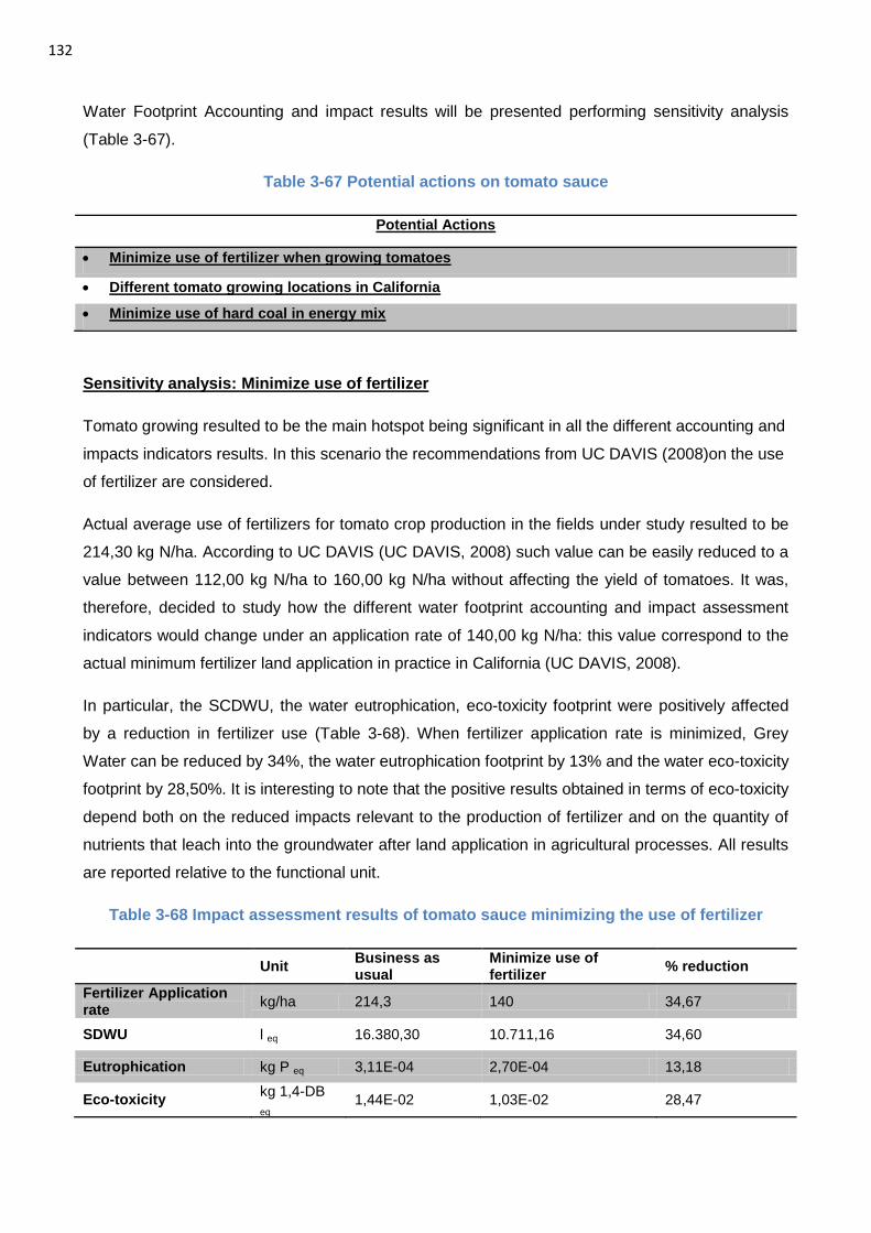
132
Water Footprint Accounting and impact results will be presented performing sensitivity analysis
(Table 3-67).
Table 3-67 Potential actions on tomato sauce
Potential Actions
Minimize use of fertilizer when growing tomatoes
Different tomato growing locations in California
Minimize use of hard coal in energy mix
Sensitivity analysis: Minimize use of fertilizer
Tomato growing resulted to be the main hotspot being significant in all the different accounting and
impacts indicators results. In this scenario the recommendations from UC DAVIS (2008)on the use
of fertilizer are considered.
Actual average use of fertilizers for tomato crop production in the fields under study resulted to be
214,30 kg N/ha. According to UC DAVIS (UC DAVIS, 2008) such value can be easily reduced to a
value between 112,00 kg N/ha to 160,00 kg N/ha without affecting the yield of tomatoes. It was,
therefore, decided to study how the different water footprint accounting and impact assessment
indicators would change under an application rate of 140,00 kg N/ha: this value correspond to the
actual minimum fertilizer land application in practice in California (UC DAVIS, 2008).
In particular, the SCDWU, the water eutrophication, eco-toxicity footprint were positively affected
by a reduction in fertilizer use (Table 3-68). When fertilizer application rate is minimized, Grey
Water can be reduced by 34%, the water eutrophication footprint by 13% and the water eco-toxicity
footprint by 28,50%. It is interesting to note that the positive results obtained in terms of eco-toxicity
depend both on the reduced impacts relevant to the production of fertilizer and on the quantity of
nutrients that leach into the groundwater after land application in agricultural processes. All results
are reported relative to the functional unit.
Table 3-68 Impact assessment results of tomato sauce minimizing the use of fertilizer
Unit Business as usual
Minimize use of fertilizer
% reduction
Fertilizer Application rate
kg/ha 214,3 140 34,67
SDWU l eq 16.380,30 10.711,16 34,60
Eutrophication kg P eq 3,11E-04 2,70E-04 13,18
Eco-toxicity kg 1,4-DB
eq 1,44E-02 1,03E-02 28,47
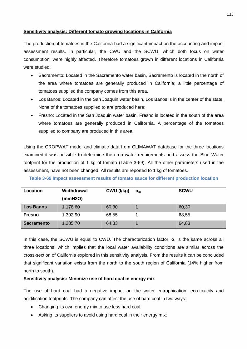
133
Sensitivity analysis: Different tomato growing locations in California
The production of tomatoes in the California had a significant impact on the accounting and impact
assessment results. In particular, the CWU and the SCWU, which both focus on water
consumption, were highly affected. Therefore tomatoes grown in different locations in California
were studied:
Sacramento: Located in the Sacramento water basin, Sacramento is located in the north of
the area where tomatoes are generally produced in California; a little percentage of
tomatoes supplied the company comes from this area.
Los Banos: Located in the San Joaquin water basin, Los Banos is in the center of the state.
None of the tomatoes supplied to are produced here;
Fresno: Located in the San Joaquin water basin, Fresno is located in the south of the area
where tomatoes are generally produced in California. A percentage of the tomatoes
supplied to company are produced in this area.
Using the CROPWAT model and climatic data from CLIMAWAT database for the three locations
examined it was possible to determine the crop water requirements and assess the Blue Water
footprint for the production of 1 kg of tomato (Table 3-69). All the other parameters used in the
assessment, have not been changed. All results are reported to 1 kg of tomatoes.
Table 3-69 Impact assessment results of tomato sauce for different production location
Location Wiithdrawal
(mmH2O)
CWU (l/kg) αin SCWU
Los Banos 1.178,60 60,30 1 60,30
Fresno 1.392,90 68,55 1 68,55
Sacramento 1.285,70 64,83 1 64,83
In this case, the SCWU is equal to CWU. The characterization factor, α, is the same across all
three locations, which implies that the local water availability conditions are similar across the
cross-section of California explored in this sensitivity analysis. From the results it can be concluded
that significant variation exists from the north to the south region of California (14% higher from
north to south).
Sensitivity analysis: Minimize use of hard coal in energy mix
The use of hard coal had a negative impact on the water eutrophication, eco-toxicity and
acidification footprints. The company can affect the use of hard coal in two ways:
Changing its own energy mix to use less hard coal;
Asking its suppliers to avoid using hard coal in their energy mix;
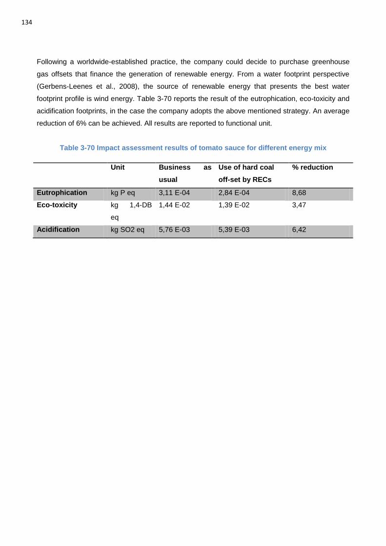
134
Following a worldwide-established practice, the company could decide to purchase greenhouse
gas offsets that finance the generation of renewable energy. From a water footprint perspective
(Gerbens-Leenes et al., 2008), the source of renewable energy that presents the best water
footprint profile is wind energy. Table 3-70 reports the result of the eutrophication, eco-toxicity and
acidification footprints, in the case the company adopts the above mentioned strategy. An average
reduction of 6% can be achieved. All results are reported to functional unit.
Table 3-70 Impact assessment results of tomato sauce for different energy mix
Unit Business as
usual
Use of hard coal
off-set by RECs
% reduction
Eutrophication kg P eq 3,11 E-04 2,84 E-04 8,68
Eco-toxicity kg 1,4-DB
eq
1,44 E-02 1,39 E-02 3,47
Acidification kg SO2 eq 5,76 E-03 5,39 E-03 6,42
135
4. Discussions To address a comprehensive assessment of impacts related to water following the requirements
presented by UNEP-SETAC (Bayart et al., 2010) within the context of LCA and ISO 14046 (ISO
2013), several indicators have been developed and presented in this research.
Focusing at inventory level the CWU and DWU indicators have been introduced; the first one is
aimed at determining the quantity of water that leaves the system because of evaporation, product
incorporation, or different water basin destination. This indicator represents the mass balance
between the water that enters and exit the different unit processes. Following the definitions
introduced by Bayart et al. (2020) such indicator represents the consumptive water use
contribution of a unit process. DWU represents the volume of water that resulted to be discharged
from a unit process with a degraded quality and therefore a limited functionality. It represents the
degradative water use of a specific unit process according to Bayart et al. (2010). To see if a
change in functionality occurred, the classification by Boulay et al. (2011a) was adopted. Moreover,
to allow an easy interpretation, parameter j was introduced in the formulation of DWU. Such
parameter in fact represents with a binary value, 0 or 1, if a loss in functionality occurred in the
specific unit process understudy. Value of j are assigned considering the different water
classification of volumes that enter and exit the system. The use of Boulay et al (2011a) method in
the formulation of the inventory structure developed in this research allowed to answer also other
criteria reported in chapter 2: resources are classified in function of their origin (surface and
groundwater) and it is make possible to understand if a change in water happed with reference to
as specific water category. The adoption of CWU and DWU answers the UNEP-SETAC
requirement of representing consumptive and degradative water use (Bayart et al., 2010);it also
solve the limits of transparency with reference to the framework of ISO 14046 (ISO, 2013) by
separately representing consumptive and degradative use.
To make the two indicators fully operative and to answer UNEP-SEATC criteria (Bayart et al.,
2010) it was necessary to introduce and collect parameters that are usually not considered in life
cycle inventories and international databases. These are: the volume of water leaving the system;
information about the location of withdrawn water that allow regionalization; parameters of air
emissions (see ANNEXES for detailed data). Another parameter that has been included is the
water scarcity index of the water entering the unit process; values of these parameters are
regionalized and acquired from Boulay et al. (2011b). The proposed method uses the scarcity of
the water type entering the system because this is considered the resource category being
affected by consumption and degradation. When compared to the existing method from Hoekstra
et al. (2011) or Boulay et al. (2011) the indicators based water footprint method developed in this
research resulted more complete in fact none of this methods include a first quantification of
136
consumptive and degradative water use (CWU and DWU indicators), moreover thanks to the
additional parameters introduced (such as air emissions), it allowed the quantification of all impacts
considered at mid-point and end-point level (ref. chapter 3). The inclusions of these parameters
answer the principle of completeness from ISO 14046 (ISO, 2013).
At mid-point level UNEP-SETAC requirements (Bayart et al. 2010) were used to develop a water
footprint profile made of 5 indicators named: the Scarcity Consumptive Water Use, SCWU, the
Scarcity Degradative Water Use (SDWU), the water eutrophication, the eco-toxicity and the
acidification footprint. In this research, SCWU and SDWU were introduced to answer the need of
transparently identify the contribution of consumptive and degradative water use to scarcity. SCWU
specifically measures the change in water availability resulting in increased competition for
freshwater resources; and therefore the contribution that a consumptive water use has on local
scarcity; parameter αin is used to represent the scarcity of the water type (considering quality,
origin, location and functionality) entering the specific unit process. SDWU is introduced to address
the contribution of degradative water use to scarcity; it measures how quality degradation limits the
availability of water resources in a specific local context; a distance to target approach is adopted
to measure the magnitude of water pollution by using the ratio between Qou,it and Qref,I; the use of
parameter αin allows to weight the results of degradative water use according to local water
availability. This approach, focusing on degradative use, differs from Hoekstra et al. (2011) where
a dilution factor is used in the quantification of the so-called grey water, and overcome its
recognized limits, by fixing specific water quality threshold represented by the maximum
acceptable concentration of i-pollutant of the z-water category according to Boulay et al. (2011).
This approach differs also from the one presented by Boulay et al. (2011b) that, even if it
addresses the scarcity issue from a qualitative and quantitative perspective, is not able to give a
clear measure of the consumptive and degradative use; SCWU and SDWU allow to do so. The
formulation of these two indicators responds to the other UNEP-SETAC requirements (Bayart et al.
2010): they are expressed in volumes of water equivalent (m3equivalent or l equivalent); they consider
seasonal and local difference in water availability using parameter αin. The water eutrophication,
the eco-toxicity and the acidification footprint were considered using consolidated methods
published in literature based on their acceptance by LCA community (Struijus et al., 2009; Jolliet et
al., 2003; Goedkoop et al., 2012). The use of this set of indicators allowed to get a comprehensive
view of impacts related to water as introduced by ISO 14046 (ISO 2013) and required by UNEP-
SETAC.
At end point level the UNEP-SETAC (Bayart et al. 2010) criteria were adopted to develop two
indicators in the specific resource area of protection; these are the back-up of cumulative water
use and the back-up of degradative water use indicator; these indicators represent the amount of
non-renewable energy that is needed to back up the consumptive and degradative water use. The
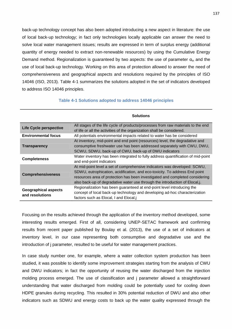
137
back-up technology concept has also been adopted introducing a new aspect in literature: the use
of local back-up technology; in fact only technologies locally applicable can answer the need to
solve local water management issues; results are expressed in term of surplus energy (additional
quantity of energy needed to extract non-renewable resources) by using the Cumulative Energy
Demand method. Regionalization is guaranteed by two aspects: the use of parameter αin and the
use of local back-up technology. Working on this area of protection allowed to answer the need of
comprehensiveness and geographical aspects and resolutions required by the principles of ISO
14046 (ISO, 2013). Table 4-1 summarizes the solutions adopted in the set of indicators developed
to address ISO 14046 principles.
Table 4-1 Solutions adopted to address 14046 principles
Solutions
Life Cycle perspective All stages of the life cycle of products/processes from raw materials to the end
of life or all the activities of the organization shall be considered.
Environmental focus All potentials environmental impacts related to water has be considered
Transparency
At inventory, mid-point and end point (resources) level, the degradative and
consumptive freshwater use has been addressed separately with CWU, DWU,
SCWU, SDWU, back-up of CWU, back-up of DWU indicators
Completeness Water inventory has been integrated to fully address quantification of mid-point
and end-point indicators
Comprehensiveness
At mid-point level a set of comprehensive indicators was developed: SCWU,
SDWU, eutrophication, acidification, and eco-toxicity. To address End point
resources area of protection has been investigated and completed considering
also back-up of degradative water use through the introduction of Elocal,j.
Geographical aspects
and resolutions
Regionalization has been guaranteed at end-point level introducing the
concept of local back-up technology and developing ad-hoc characterization
factors such as Elocal, I and Elocal,j
Focusing on the results achieved through the application of the inventory method developed, some
interesting results emerged. First of all, considering UNEP-SETAC framework and confirming
results from recent paper published by Boulay et al. (2013), the use of a set of indicators at
inventory level, in our case representing both consumptive and degradative use and the
introduction of j parameter, resulted to be useful for water management practices.
In case study number one, for example, where a water collection system production has been
studied, it was possible to identify some improvement strategies starting from the analysis of CWU
and DWU indicators; in fact the opportunity of reusing the water discharged from the injection
molding process emerged. The use of classification and j parameter allowed a straightforward
understanding that water discharged from molding could be potentially used for cooling down
HDPE granules during recycling. This resulted in 30% potential reduction of DWU and also other
indicators such as SDWU and energy costs to back up the water quality expressed through the
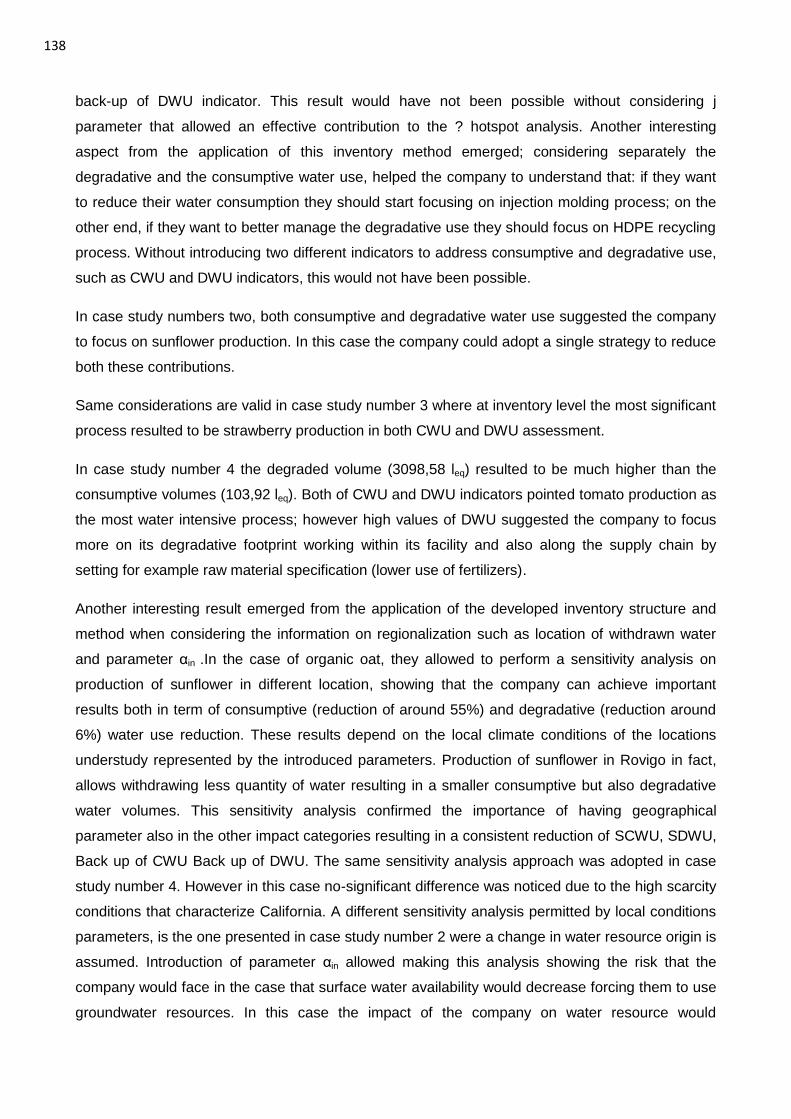
138
back-up of DWU indicator. This result would have not been possible without considering j
parameter that allowed an effective contribution to the ? hotspot analysis. Another interesting
aspect from the application of this inventory method emerged; considering separately the
degradative and the consumptive water use, helped the company to understand that: if they want
to reduce their water consumption they should start focusing on injection molding process; on the
other end, if they want to better manage the degradative use they should focus on HDPE recycling
process. Without introducing two different indicators to address consumptive and degradative use,
such as CWU and DWU indicators, this would not have been possible.
In case study numbers two, both consumptive and degradative water use suggested the company
to focus on sunflower production. In this case the company could adopt a single strategy to reduce
both these contributions.
Same considerations are valid in case study number 3 where at inventory level the most significant
process resulted to be strawberry production in both CWU and DWU assessment.
In case study number 4 the degraded volume (3098,58 leq) resulted to be much higher than the
consumptive volumes (103,92 leq). Both of CWU and DWU indicators pointed tomato production as
the most water intensive process; however high values of DWU suggested the company to focus
more on its degradative footprint working within its facility and also along the supply chain by
setting for example raw material specification (lower use of fertilizers).
Another interesting result emerged from the application of the developed inventory structure and
method when considering the information on regionalization such as location of withdrawn water
and parameter αin .In the case of organic oat, they allowed to perform a sensitivity analysis on
production of sunflower in different location, showing that the company can achieve important
results both in term of consumptive (reduction of around 55%) and degradative (reduction around
6%) water use reduction. These results depend on the local climate conditions of the locations
understudy represented by the introduced parameters. Production of sunflower in Rovigo in fact,
allows withdrawing less quantity of water resulting in a smaller consumptive but also degradative
water volumes. This sensitivity analysis confirmed the importance of having geographical
parameter also in the other impact categories resulting in a consistent reduction of SCWU, SDWU,
Back up of CWU Back up of DWU. The same sensitivity analysis approach was adopted in case
study number 4. However in this case no-significant difference was noticed due to the high scarcity
conditions that characterize California. A different sensitivity analysis permitted by local conditions
parameters, is the one presented in case study number 2 were a change in water resource origin is
assumed. Introduction of parameter αin allowed making this analysis showing the risk that the
company would face in the case that surface water availability would decrease forcing them to use
groundwater resources. In this case the impact of the company on water resource would
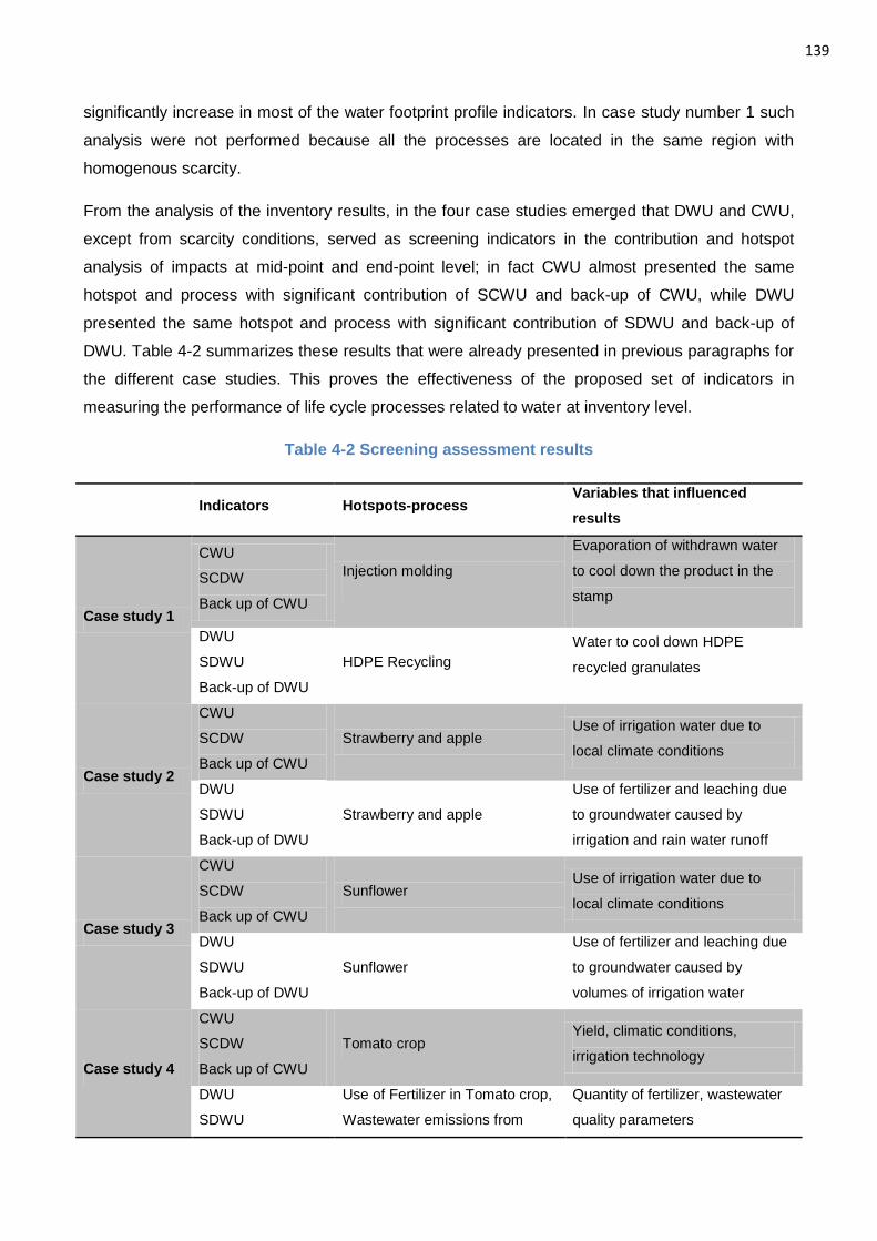
139
significantly increase in most of the water footprint profile indicators. In case study number 1 such
analysis were not performed because all the processes are located in the same region with
homogenous scarcity.
From the analysis of the inventory results, in the four case studies emerged that DWU and CWU,
except from scarcity conditions, served as screening indicators in the contribution and hotspot
analysis of impacts at mid-point and end-point level; in fact CWU almost presented the same
hotspot and process with significant contribution of SCWU and back-up of CWU, while DWU
presented the same hotspot and process with significant contribution of SDWU and back-up of
DWU. Table 4-2 summarizes these results that were already presented in previous paragraphs for
the different case studies. This proves the effectiveness of the proposed set of indicators in
measuring the performance of life cycle processes related to water at inventory level.
Table 4-2 Screening assessment results
Indicators Hotspots-process
Variables that influenced
results
Case study 1
CWU
SCDW
Back up of CWU
Injection molding
Evaporation of withdrawn water
to cool down the product in the
stamp
DWU
SDWU
Back-up of DWU
HDPE Recycling
Water to cool down HDPE
recycled granulates
Case study 2
CWU
SCDW
Back up of CWU
Strawberry and apple Use of irrigation water due to
local climate conditions
DWU
SDWU
Back-up of DWU
Strawberry and apple
Use of fertilizer and leaching due
to groundwater caused by
irrigation and rain water runoff
Case study 3
CWU
SCDW
Back up of CWU
Sunflower Use of irrigation water due to
local climate conditions
DWU
SDWU
Back-up of DWU
Sunflower
Use of fertilizer and leaching due
to groundwater caused by
volumes of irrigation water
Case study 4
CWU
SCDW
Back up of CWU
Tomato crop Yield, climatic conditions,
irrigation technology
DWU
SDWU
Use of Fertilizer in Tomato crop,
Wastewater emissions from
Quantity of fertilizer, wastewater
quality parameters
140
Indicators Hotspots-process
Variables that influenced
results
Back-up of DWU tomato sauce processing
Completeness of inventory, according to UNEP-SEATC criteria, was achieved by introducing also
emissions to air. No specific water inventory method and approaches consider these parameters.
Their use allowed performing a comprehensive water footprint assessment at mid-point level
casting the light also on other indicators such as acidification footprint.
From the application of the developed water footprint profile at mid-point level some interesting
aspects emerged. First of all, the introduction of different indicators to measure consumptive and
degradative aspects resulted to be useful when confronted to other methods published in literature
(Boulay et al., 2011b) because they allowed performing a more complete contribution and hotspot
analysis. This clearly emerged from case study number 1 and number 3. In the former, as already
mentioned, starting from inventory results emerged the need to work both on consumptive and
degradative use focusing respectively on injection molding and HDPE recycling. Adopting the most
used method in literature from Boulay et al (2011b) this would have not been possible. Figure 4-1
shows the contribution results using the two methods. Result of the method from Boulay et al.
(2011b) (Water Scarcity Index WSI) are the same as SCWU in this case study, (this depends on
the scarcity parameters values) but is not able to give us the information that SDWU is giving about
the significance of HDPE recycling process. In case study number 3 the 330g of organic strawberry
jam was studied. Figure 4-2 report on the assessment performed according to Boulay et al (2011b)
and the results achieved through the developed set of indicators. In this case emerged that WSI
from Boulay et al. (2011b) and SCWU are similar, however from the analysis of SDWU emerged
that the process of freezing strawberry is significant. Without considering both consumptive and
degradative impacts separately this information would have been lost. This proves the
effectiveness in measuring the performance of life cycle processes related to water at mid-point
level.
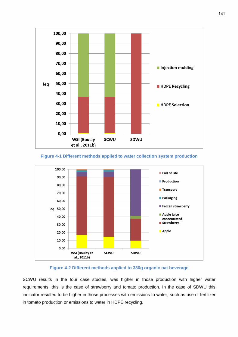
141
Figure 4-1 Different methods applied to water collection system production
Figure 4-2 Different methods applied to 330g organic oat beverage
SCWU results in the four case studies, was higher in those production with higher water
requirements, this is the case of strawberry and tomato production. In the case of SDWU this
indicator resulted to be higher in those processes with emissions to water, such as use of fertilizer
in tomato production or emissions to water in HDPE recycling.

142
Contribution and hotspot analysis was effectively supported by the introduction of the degradation
profile made of the eutrophication, eco-toxicity and acidification footprints. In case study number 1
and 2, the use of these indicators allowed to better understand the positive contributions of
environmental friendly practices active in the product systems understudy: the use of recycling
material (HDPE selection) and the reuse of scraps and secondary products (the case of organic
oat from which animal fodder is derived). With specific reference to case study number 1 a
sensitivity analysis was performed to understand the consequences of using virgin material instead
of recycled one; this analysis allowed to understand that the company would partially improve and
partially worsen its environmental performances. Without adopting a comprehensive approach this
would not have been possible. In case study number 4 the use of these indicators helped to
identify another hotspot such as the glass production. Without considering a comprehensive profile
it would have not been possible to identify these issues. The use of this profile also effectively
helped to determine environmental impact reduction strategies with specific focus on the use of
energy sources. This was true in case study 1, 3 and 4 were the change in the energy mix resulted
in better performances for all the degradation profile indicators. These results prove the
effectiveness of the proposed set of indicators in supporting company performance improvement
and therefore industrial process competitiveness.
The method developed at end-point level was successfully applied in all the different case studies.
In detail, it was possible to study the application of two technologies to back-up water use: a water
collection system dimensioned on specific local back-up needs (based on case study 1, water
collection system) and the desalination system that is usually applied in literature (Pfister et al.
2009). Locally back up of degradative water use, was guaranteed in all the different case studies
using the parameter person equivalent to decide on the wastewater treatment facility locally
applicable. In case study number 1, 2 and 3 back-up of CWU resulted to be bigger than the one of
DWU; from the analysis of contribution same considerations made at inventory level are valid.
When focusing on characterization factors, it can be noted that values are higher in function of the
local climate conditions and the CWU of the specific unit process. Where rainwater volumes are
higher, Elocal,i (MJ/l) resulted to be smaller. This is evident in case study number 3 were values to
back up water in Switzerland (0,27) resulted to be smaller than the energy needed to back up the
water in Italy (0,32) even if in both case the same water collection system dimension has been
used (1 water collection system module). In case study n. 3, Elocal,i (MJ/l) resulted to be higher
with higher CWU values. This is evident in the case of energy needed in Bulgaria than the one
needed in Italy; in fact higher CWU requires bigger water collection system dimensions. Therefore,
these results are highly influenced by the specific water technology used to back up CWU. This
proves the efficacy of using the proposed model in representing local impacts to back-up local
water use. This is also evident in case study number 4. Figure 4-3 reports on the results of back-up
of CWU in three different scenarios: when only desalination plants are used (scenario 1), when
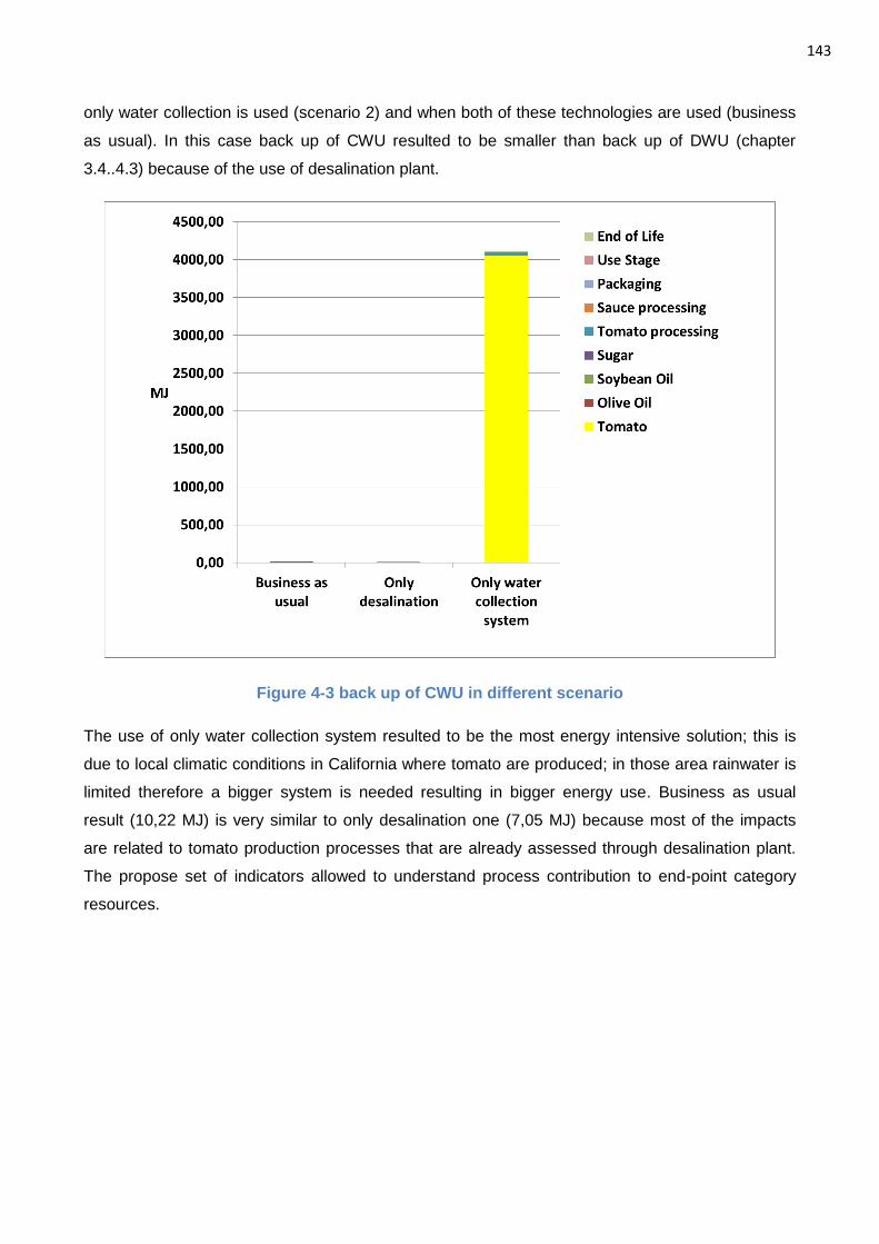
143
only water collection is used (scenario 2) and when both of these technologies are used (business
as usual). In this case back up of CWU resulted to be smaller than back up of DWU (chapter
3.4..4.3) because of the use of desalination plant.
Figure 4-3 back up of CWU in different scenario
The use of only water collection system resulted to be the most energy intensive solution; this is
due to local climatic conditions in California where tomato are produced; in those area rainwater is
limited therefore a bigger system is needed resulting in bigger energy use. Business as usual
result (10,22 MJ) is very similar to only desalination one (7,05 MJ) because most of the impacts
are related to tomato production processes that are already assessed through desalination plant.
The propose set of indicators allowed to understand process contribution to end-point category
resources.
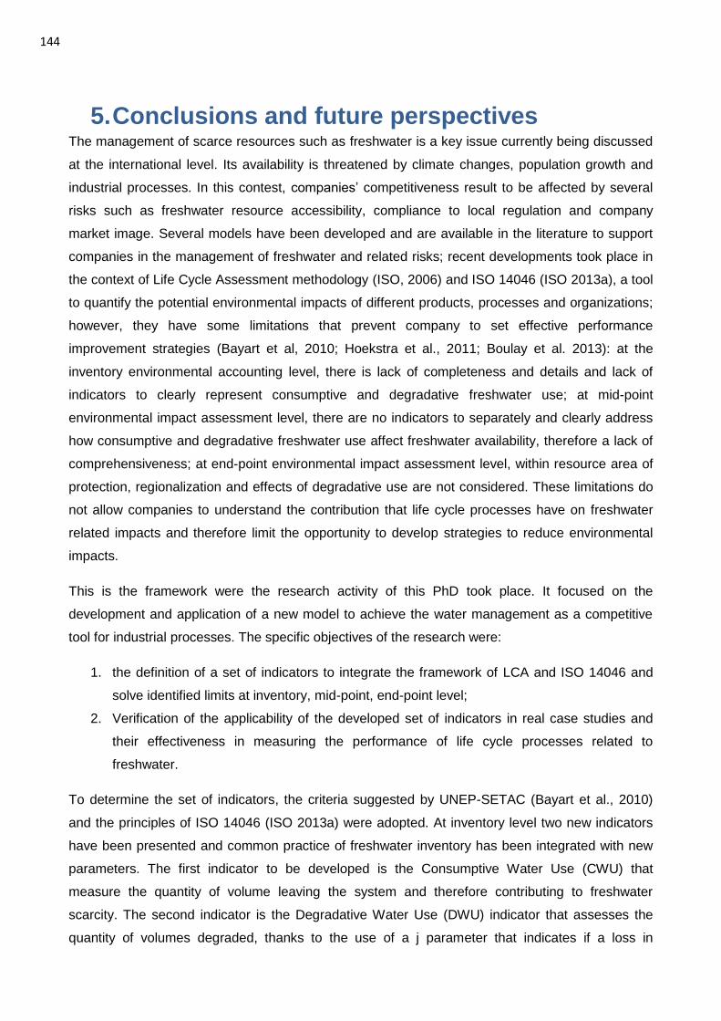
144
5. Conclusions and future perspectives The management of scarce resources such as freshwater is a key issue currently being discussed
at the international level. Its availability is threatened by climate changes, population growth and
industrial processes. In this contest, companies’ competitiveness result to be affected by several
risks such as freshwater resource accessibility, compliance to local regulation and company
market image. Several models have been developed and are available in the literature to support
companies in the management of freshwater and related risks; recent developments took place in
the context of Life Cycle Assessment methodology (ISO, 2006) and ISO 14046 (ISO 2013a), a tool
to quantify the potential environmental impacts of different products, processes and organizations;
however, they have some limitations that prevent company to set effective performance
improvement strategies (Bayart et al, 2010; Hoekstra et al., 2011; Boulay et al. 2013): at the
inventory environmental accounting level, there is lack of completeness and details and lack of
indicators to clearly represent consumptive and degradative freshwater use; at mid-point
environmental impact assessment level, there are no indicators to separately and clearly address
how consumptive and degradative freshwater use affect freshwater availability, therefore a lack of
comprehensiveness; at end-point environmental impact assessment level, within resource area of
protection, regionalization and effects of degradative use are not considered. These limitations do
not allow companies to understand the contribution that life cycle processes have on freshwater
related impacts and therefore limit the opportunity to develop strategies to reduce environmental
impacts.
This is the framework were the research activity of this PhD took place. It focused on the
development and application of a new model to achieve the water management as a competitive
tool for industrial processes. The specific objectives of the research were:
1. the definition of a set of indicators to integrate the framework of LCA and ISO 14046 and
solve identified limits at inventory, mid-point, end-point level;
2. Verification of the applicability of the developed set of indicators in real case studies and
their effectiveness in measuring the performance of life cycle processes related to
freshwater.
To determine the set of indicators, the criteria suggested by UNEP-SETAC (Bayart et al., 2010)
and the principles of ISO 14046 (ISO 2013a) were adopted. At inventory level two new indicators
have been presented and common practice of freshwater inventory has been integrated with new
parameters. The first indicator to be developed is the Consumptive Water Use (CWU) that
measure the quantity of volume leaving the system and therefore contributing to freshwater
scarcity. The second indicator is the Degradative Water Use (DWU) indicator that assesses the
quantity of volumes degraded, thanks to the use of a j parameter that indicates if a loss in
145
functionality of the water entering the system occurred and therefore contribute to limit freshwater
availability. No method published in literature address both consumptive and degradative
freshwater use at inventory level. To guarantee completeness and comprehensiveness the
following parameters have been added to traditional and recent published water inventories: quality
parameters of freshwater entering the system, air emissions and parameter j.
At mid-point level a water footprint profile of 5 indicators has been proposed. It is composed of the
Scarcity Consumptive Water Use (SCWU), Scarcity Degradative Water Use (SDWU),
Eutrophication, Eco-toxicity and Acidification. Considering all these impact indicators, it was
possible to guarantee comprehensiveness of assessment according to ISO 14046 framework (ISO
2013a). No specific current water method takes into considerations all these aspects. In particular
SCWU and SDWU indicators have been developed to address separately the contribution that
consumptive water use and degradative water use have on local freshwater scarcity. This
approach overcomes the limit of transparency of current methods that do not distinguish between
degradative and consumptive water use (Hoekstra et al., 2011; Boulay et al., 2011b). SCWU and
SDWU are reported in the same unit (l equivalent or m3 equivalent) and can be summed into the
Water Scarcity Indicator (WSI).
At end point level the focus has been on resource area of protection and a new approach has been
developed, to consider effects of both degradative (back-up of DWU) and consumptive water use
(back-up of CWU) and to fully address regionalization. The first issue is solved introducing the
back-up of water use concept defined as the surplus energy needed to back-up the quality of water
when degraded; the second issue has been solved by studying local back-up technologies and
weighing water use with αin scarcity parameters from Boulay et al. (2011b). Results of back-up of
DWU and back-up of CWU can be summed into ΔR representing the total amount of energy
needed to back up comprehensive water use. No model presented in literature considers local
back-up technologies and effects of degradative use on resources (Pfister et al., 2009).
To verify the applicability and effectiveness of the proposed set of indicators 4 case studies have
been investigated adopting the methodological framework of LCA (ISO, 2006) and ISO 14046
(ISO, 2013a). Products with critical water processes and with life cycle stages potentially located in
different regions were selected. The 4 case studies dealt with: a water collection system; an
organic oat beverage; an organic oat strawberry jam; a tomato sauce. Applicability of the
developed set of indicators has been confirmed in all the case studies investigated. A summary of
results is reported in table 5-1. In all these case studies the proposed set of indicators allowed to
define comprehensive strategy to reduce the impacts of water use in term of volumes and quality
degradation. This allowed the companies to identify potential actions to improve performances and
therefore competitiveness. At inventory level CWU and DWU resulted to be reliable screening
indicators in all the case studies, giving a first idea of potential hotspots related to water and with
146
specific reference to SCWU, SDWU, back-up of CWU, Back up of DWU. In case study on water
collection system in fact, they allowed to identify injection molding and HDPE recycling hotspots; in
the case of organic oat beverage casted the light on sunflower agriculture processes; in the case of
organic strawberry jam identified apple and strawberry growing as potential hot-spot; in the tomato
sauce production highlighted the importance of tomato growing and agriculture practices. This is
an interesting result because the use of screening indicators is warmly welcomed in literature as it
allows an easy comprehension of environmental related issues with less time and money than
conducting a full analysis (Scipioni et al., 2012). Therefore it facilitates the adoption of water
footprint analysis at the company level.
Another important result of the application of the inventory indicators is their potential support to
water management in response to recent literature needs (Boulay et al., 2011). In fact, for example
in water collection system production, they allowed understanding potential water saving, coming
from the reuse of injection molding discharged water.
The proposed set of inventory indicators supported transparency and comprehension of different
process contribution by giving a measure also of the degraded volume in all the different case
studies (see DWU from Table 5-1).
The inclusion of inventory parameters such as quality in, air emissions and j, allowed to complete
current water inventories (Hoekstra et al; 2011 Boulay et al 2011a) and to apply all the selected
indicators at mid-point and end-point level in all the 4 case studies; in fact without considering
quality in and j, it would not have been possible to quantify SCWU, SDWU, back up of CWU and
back up of SDWU and without considering air emissions it would have not been possible to
quantify acidification.
Results at mid-point level proved the importance of being comprehensive and therefore to consider
more than one impact indicator related to water. These aspects resulted to be central to impact
reduction strategy definition. In the water collection system study, being comprehensive, allowed to
understand the positive contribution of HDPE selection process in acidification and eutrophication
and also to identify several hot-spot (energy use and lubricant oil consumption) that allowed the
definition of water related impact reduction strategies such as the change in the energy-mix.
Similar results are confirmed by the application of the proposed set of indicators also to the other
case studies: in the oat beverage production it allowed to identify avoided impacts coming from the
reuse of oat scraps as fodder and allowed to determine the importance to work on the use of
fertilizer and innovative packaging solutions; in the analysis of organic strawberry jam it suggested
to work on the energy mix and also to consider the negative consequences of changing the
resource use for irrigation therefore suggesting to put particular attention on local water availability;
in the case of tomato sauce allowed to set a comprehensive strategy focused on the company
147
processes and the supply chain one, setting strategies on product specification and energy-mix.
Considering only one or part of the proposed indicators this result would have not been achievable.
The development of water specific indicators support also LCA practice that missed a
comprehensive perspective related to water. Being comprehensive avoid the burden shifting issue
as recommended by LCA standards (ISO, 2006)
The proposed end-point set of indicators allowed to understand the impacts of back-up
consumptive and degradative water use on non-renewable resources. In three out of four case
studies the energy needed to back-up consumptive water use resulted to be higher than the
degradative one and depended on the technology used. These results suggest the importance of
regionalization also in this method in order to allow a better understanding of consequences of
local water use.
Results at mid-point and end-point level confirmed the importance of regionalization. In particular
this emerged in the analysis of impacts related to scarcity. In the case of sunflower and tomato
production sensitivity analysis based on these parameters allowed the companies to better focus
on specific issue to set effective water management strategies. Considering regionalization allowed
understanding the contribution of local climate conditions to final water footprint profile: water
degradation and consumption should be avoided in water scarce regions. Regionalization resulted
to be a key issue also at end-point level: it is more expensive in term of energy to back up water
where it is scarce (e.g. in the case of organic oat beverage where a change in location to produce
sunflower could result from 30 to 60% reduction in terms of energy to back-up degradative water
use).
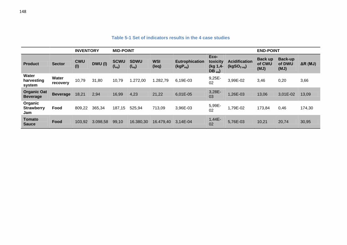
148
Table 5-1 Set of indicators results in the 4 case studies
INVENTORY MID-POINT END-POINT
Product Sector CWU (l)
DWU (l) SCWU (leq)
SDWU (leq)
WSI (leq)
Eutrophication (kgPeq)
Eco-toxicity (kg 1,4-DB eq)
Acidification (kgSO2 eq)
Back up of CWU (MJ)
Back-up of DWU (MJ)
ΔR (MJ)
Water harvesting system
Water recovery
10,79 31,80 10,79 1.272,00 1.282,79 6,19E-03 9,25E-02
3,99E-02 3,46 0,20 3,66
Organic Oat Beverage
Beverage 18,21 2,94 16,99 4,23 21,22 6,01E-05 3,28E-03
1,26E-03 13,06 3,01E-02 13,09
Organic Strawberry Jam
Food 809,22 365,34 187,15 525,94 713,09 3,96E-03 5,99E-02
1,79E-02 173,84 0,46 174,30
Tomato Sauce
Food 103,92 3.098,58 99,10 16.380,30 16.479,40 3,14E-04 1,44E-02
5,76E-03 10,21 20,74 30,95
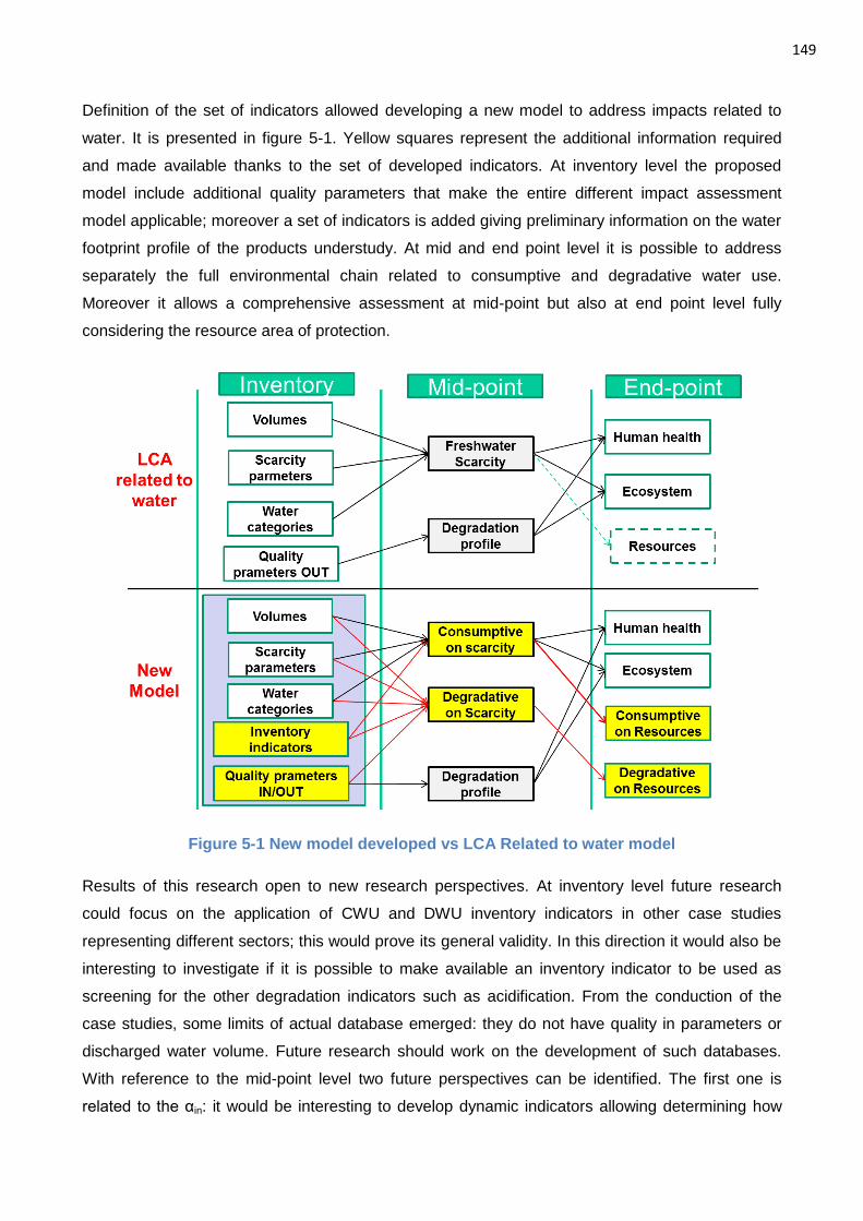
149
Definition of the set of indicators allowed developing a new model to address impacts related to
water. It is presented in figure 5-1. Yellow squares represent the additional information required
and made available thanks to the set of developed indicators. At inventory level the proposed
model include additional quality parameters that make the entire different impact assessment
model applicable; moreover a set of indicators is added giving preliminary information on the water
footprint profile of the products understudy. At mid and end point level it is possible to address
separately the full environmental chain related to consumptive and degradative water use.
Moreover it allows a comprehensive assessment at mid-point but also at end point level fully
considering the resource area of protection.
Figure 5-1 New model developed vs LCA Related to water model
Results of this research open to new research perspectives. At inventory level future research
could focus on the application of CWU and DWU inventory indicators in other case studies
representing different sectors; this would prove its general validity. In this direction it would also be
interesting to investigate if it is possible to make available an inventory indicator to be used as
screening for the other degradation indicators such as acidification. From the conduction of the
case studies, some limits of actual database emerged: they do not have quality in parameters or
discharged water volume. Future research should work on the development of such databases.
With reference to the mid-point level two future perspectives can be identified. The first one is
related to the αin: it would be interesting to develop dynamic indicators allowing determining how
150
present water use will affect future scarcity. The second aspect is related to another environmental
issue that is central to international debates such as climate change (Scipioni et al., 2011). No
model currently addresses how climate change is affecting local water scarcity. Research in this
field is warmed welcome also by the diffusion of another environmental indicator such as Carbon
Footprint (Scipioni et al., 2011). With specific reference to the end-point resource category, future
development can be identified; in this study it was possible to consider a water collection system
and desalination plants, however other water recovery technologies are available on the market
and should be considered when assessing local impacts. It would therefore be interesting to
investigate several potential back-up solutions in order to allow a more effective water impact
reduction strategy definition. To do this the same CED method proposed in this research can be
easily applied. Another need emerged in this research with reference to back-up technology: it
would be useful to develop a set of indicators specifically designed to support the analysis of
optimal back-up of local solutions; for instance, following the wide experience on another limited
resource such as energy, it would be interesting to develop an indicator similar to the Energy Pay-
Back time, that is recognized to support decisions on the best technology to be locally applied.
These future perspectives could also contribute to make LCA database more complete and
support a better water management to guarantee local water availability. Another possible future
research line should focus on expressing the surplus energy at end-point level in economic term as
suggest by the European platform on LCA (EC-JRC, 2011).
151
6. References
Allan, J.A., 1998. Virtual water: a strategic resource. Global solutions to regional deficits.
Groundwater, 36(4):545-546.
Althaus H.J., Bauer C, Doka G., Dones R., Hischier R., Hellweg S., Humbert S., Köllner T.,
Loerincik Y., Margni M., Nemecek T., 2007. Implementation of Life Cycle Impact Assessment
Methods. Eds Frischknecht R., Jungbluth N. Visited online 08/12/2013
http://www.ecoinvent.org/organisation/
Bates, B.C., Z.W. Kundzewicz, S. Wu and J.P. Palutikof, Eds., 2008: Climate Change and Water.
Technical Paper of the Intergovernmental Panel on Climate Change, IPCC Secretariat, Geneva,
210p
Bennet EM, Carpenter SR, Caraco NF (2001) Human impact on 151rodible phosphorus and
eutrophication: A global perspective. Bioscience 51(3):227–234
Berger M., arsen J., Krinke S., Bach V., Finkbeiner M., 2012. Water Footprint of European Cars:
Potential Impacts of Water Consumption along Automobile Life Cycles. Environmental Science and
Technology, 46, 4091−4099
Berger M., Finkbeiner M., 2010. Water Footprinting: How to Address Water Use in Life Cycle
Assessment?. Sustainability, 2, 919-944.
Blangini G.A., Busto M., 2009. The life cycle of rice: LCA of alternative agri-food chain
management systems in Vercelli (Italy). Journal of Environmental Management n. 90 pp1512–
1522.
Boulay A.M., Bouchard C., Bulle C., Deschênes L., Margni M., 2011a. Categorizing water for LCA
inventory. International Journal of Life Cycle Assessment, 16 (7):639-651
Boulay A.M., Cecile B., Bayart J.B., Louise Deschenes L., Margni M., 2011b. Regional
Characterization of Freshwater Use in LCA: Modeling Direct Impacts on Human Health.
Environmental Science and Technology. Dx.doi.org/10.1021/es1030883
Boulay A.M., Hoekstra A.Y., Vionnet S., 2013. Complementarities of Water-Focused Life Cycle
Assessment and Water Footprint Assessment. Environmental Science and Technology DOI:
10.1021/es403928f
Bourne G., Folk-Williams J., McInerny A., Brian Davis B., Chen T., 2008. California Desalination
Planning Handbook. Eds. California State University, Sacramento Center for Collaborative Policy.
Visited online 12/12/2013 http://www.water.ca.gov/desalination/
Bruinsma, J. 2009. The Resource Outlook to 2050: By How Much do Land, Water and Crop Yields
Need to Increase by 2050? Prepared for the FAO Expert Meeting on ‘How to Feed the World in
2050’, 24–26 June 2009, Rome.
Chahed J, Besbes M., Hamdane A. 2009. Water scarcity and food security: A global assessment
152
of water potentiality in Tunisia. 4o Marcelino Botin Water Workshop, Santander, September 22-25
2009.
Chapagain A.K., Orr S., 2010. Water Footprint of Nestlé’s ‘Bitesize Shredded Wheat’. Water
Footprint Pilot Project. Geneva
Chapagain, A.K., Hoekstra, A.Y., 2008. The global component of freshwater demand and supply:
an assessment of virtual water flows between nations as a result of trade in agricoltural and
industrial products. Water International.
Christensen N., Paaby M., Holten-Andersen J.,, 1993. Environment and society – the state of the
environment in Denmark. Professional report n.93, The National Environmental Research Institute.
Commissariat Général au Développement durable, 2011. novembre 2011. Mieux informer les
consummateurs et les producteurs: écolabels, bonnes pratiques de communication et
expérimentation nationale de l’affichage environnmental, Ministère de l’Écologie, de l’Énergie, du
Développement durable et de la Mer, France. Visited online 16/12/2013
http://www.developpement-durable.gouv.fr/IMG/pdf/ Info_environnementale.pdf
Corbetta P., 1999. Metodologia e Tecniche della Ricerca Sociale (Methodology and Methods of the
Social Research). Bologna, Italy: Il Mulino. P. 656.
Corcoran, E., Nellemann, C., Baker, E., Bos, R., Osborn, D. and Savelli, H. (eds). 2010. Sick
Water? The Central Role of Wastewater Management in Sustainable Development. A Rapid
Response Assessment. UN-Habitat/UNEP/GRID-Arendal
De Vires W. and Breeuwsma A., 1987. The relation between soil acidification and element cycling.
Water, Air and Soil Pollution 35, 293-310
DOE (US Department of Energy), 2009. Visited online 09/12/2013
www.femp.energy.gov/procurement/
EC (European Commmission), 2007. Communication from the Commission to the European
Parliament and the Council. Visited on line 27/11/2013 http://eur-
lex.europa.eu/LexUriServ/LexUriServ.do?uri=CELEX:52007DC0414:EN:NOT
EC-JRC, 2011. International Reference Life Cycle Data System (ILCD) Handbook—
recommendations for life cycle impact assessment in the European context. First edition November
2011. European Commission-Joint Research Centre—Institute for Environment and Sustainability:
EUR 24571 EN. Luxemburg. Publications Office of the European Union
EPA (United States Environmental protection Energy), 2012. Facts and Figure 2011. Visited online
16/12/2013 http://www.epa.gov/osw/nonhaz/municipal/msw99.htm
Ercin A., Aldaya M.M., Hoekstra A.Y., 2011. Corporate Water Footprint Accounting and Impact
Assessment: The Case of the Water Footprint of a Sugar-Containing Carbonated Beverage. Water
Resource Management, 25 (2), 721-741
Ercin A., Aldaya M.M., Hoekstra A.Y., 2012. The water footprint of soy milk and soy burger and
153
equivalent animal products. Ecological Indicator, 18, 392-402
Falkenmark M., Lundqvist J., Widstrand C., 1989. Macro-scale water scarcity requires micro-scale
approaches. Aspects of vulnerability in semi-arid development. Natural Resources Forum, 13
(4),258-267
Falkenmark, M. and C.Folke, 2003: Theme issue: Freshwater and welfare fragility: Syndromes,
vulnerabilities and challenges, Royal Society’s Philosophical
Transactions B Biology, 358, p. 1440.
FAO (2010a) ‘CROPWAT 8.0 model’, FAO, Rome, www.fao.org/nr/water/infores_
databases_cropwat.html.
FAO (2010b) ‘CLIMWAT 2.0 database’, FAO, Rome, www.fao.org/nr/water/infores_
databases_climwat.html
FAO (Food and Agriculture Organization of the United Nations). 2011a. The State of the World’s
Land and Water Resources: Managing Systems at Risk. London, Earthscan.
Frischknecht R., 2010. LCI modelling approaches applied on recycling of materials in view of
environmental sustainability, risk perception and eco-efficiency. International Journal of Life Cycle
Assessment DOI 10.1007/s11367-010-0201-6
Frischknecht R., Jungbluth N., Althaus H.J., Doka G., Dones R., Heck T., Hellweg S., Hischer R.,
Nemecek T., Rebitzer G., Spielmann M., 2005, The Eco invent Database: Overview and
Methodological Framework, International Journal of Life Cycle Assessment 10 (1), 3-9.
Gerbens-Leenes P.W., Hoekstra A.Y., van der Mee Th.H.. 2008. Water Footprint of Bio-energy
and other primary carriers. UNESCO research report series n.29.
Goedkoop M., Heijungs R., Huijbregts M., De Schryver A., Struijs J., Zelm Van R., 2013. ReCiPe
2008. A life cycle impact assessment method which comprises armonized category indicators at
the midpoint and the endpoint level.
Goedkoop M., Spriensma R., 2001. The Eco-Indicator 99: a Damage Oriented Method for Life
Cycle Impact Assessment: Methodology Report Publikatiereeks produktenbeleid; nr. 36A;
Ministerie van Volkshiusvesting, Ruimtelijke Ordening en Milieubeheer: Den Haag, the Netherlands
Hanafiah M., Xenopoulos M., Pfister S., Leuven R.S., Huijbregts M., 2011. Characterization factors
for water consumption and greenhouse gas emissions based on freshwater fish species extinction.
Environmental Science technology, 45 (12) 5272–5278.
Hartz T., Miyao G., Mickler J., Lestrange M., Stoddard S., Nuñez J., Aegerter B., 2008. Processing
Tomato Production in California. Eds The Regents of the University of California Division of
Agriculture and Natural Resources. ISBN-13: 978-1-60107-570-3
Hauschild M, Wenzel H (1998): Environmental Assessment of Products – Vol. 2: Scientific
Background, Chapman & Hall, London (UK)
Hauschild M. and Wenzel H., 2002. Environmental assessment of products. Volume 2 the scientific
basis. Published by Chapman and Hall, London pp.565
154
Heijungs R., Guinneè J.B., 2012. An overview of the Life Cycle Assessment Method – Past,
Present and Future; within Life Cycle Assessment Handbook Eds Mary Ann Curran. Wiley
Cincinnati, OH, USA
Hoekstra A.Y., 2003. ‘Virtual water trade between nations: A global mechanism affecting regional
water systems. IGBP Global Change News Letter, No. 54, pp. 2-4.
Hoekstra A.Y., and Hung P.Q., 2002. Virtual water trade: A quantification of virtual water flows
between nations in relation to international crop trade. Value of Water Research Report Series
No.11, IHE, Delft, the Netherlands. Visited online 29/11/2013 from
http://www.ihe.nl/vmp/articles/Projects/PRO-Virtual_Water_Trade.html
Hoekstra A.Y., Hung P.Q., 2002.Virtual water trade, A quantification of virtual water flows between
nations in relation to international crop trade
Hoekstra, A. Y. 2011. The global dimension of water governance: Why the river basin approach is
no longer
sufficient and why cooperative action at global level is needed. Water, Vol. 3, No. 1, pp. 21–46.
Hoekstra, A. Y., Chapagain, A. K., Aldaya, M. M. and Mekonnen, M. M. (2009a) Water Footprint
Manual: State of the Art 2009, Water Footprint Network, Enschede, the Netherlands. Visited online
27/11/2013 www.waterfootprint.org/downloads/WaterFootprintManual2009.pdf
Hoekstra, A. Y.; Chapagain, A. K., 2008. Globalization of Water: Sharing the Planet’S Freshwater
Resources; Oxford: Blackwell Publishing
Hoekstra, A.Y., Chapagain, A.K., Aldaya, M.M., Mekonen, M.M., 2011. The Water Footprint
Assessment Manual. Setting the Global Standard. Earthscan, London: p.228.
Huijbreghts M.A.J., Rombouts L.J., Hellweg S., Frischknecht R., Hendriks, A.J., van de Meent D.,
Ragas, A.M.J. Reijnders, L. Struijs, J., 2006. Is cumulative fossil energy demand a useful indicator
for the environmental performance of products? Environmental Science Technology n.40, 641–
648.
Hunt R.G., Franklin W.E., 1996. How it came about. Personal reflection on the origin and
development of LCA in the USA. International Journal of Life Cycle Assessment, 1 (1), 4-7
ISO, 2006. ISO 14040 .Environmental management – Life cycle assessment – Principle and
framework. International Organization for Standardization, Geneva, Switzerland.
ISO, 2013a. ISO/DIS 14046 Water Footprint. Requirements and guidelines. International
Organization for Standardization, Geneva, Switzerland.
ISO, 2013b. ISO/PDTR 14073. Water Footprint example. International Organization for
Standardization, Geneva, Switzerland.
155
efferies ., Mu oz I., Hodges ., ing . ., Aldaya M, Ercin A.E., Milà I Canals L., Hoekstra H.Y.,
2012. Water Footprint and Life Cycle Assessment as approaches to assess potential impacts of
products on water consumption. Key learning points from pilot studies on tea and margarine.
Journal of Cleaner Production. 33 155-166
efferies ., Mu oz I., Hodges ., ing . ., Aldaya M, Ercin A.E., Milà i Canals L., Hoekstra H. .,
2012. Water Footprint and Life Cycle Assessment as approaches to assess potential impacts of
products on water consumption. Key learning points from pilot studies on tea and margarine.
Journal of Cleaner Production n. 33 155-166.
Jeswani H.K, Azapagic A., 2011. Water footprint: methodologies and a case study for assessing
the impacts of water use. Journal of Cleaner Production, 19, 1288-1299.
Koehler A., Aoustin E., 2008. Assessment of use and depletion of water resources within LCA.
SETAC Europe, Warsaw
Kounina A, Margni M, Bayart JB, Boulay AM, Berger M, Bulle C, Frischknecht R, Koehler A, Milà I
Canals L, Motoshita M, Núñez M, Peters G, Pfister S, Ridoutt B, Van Zelm R, Verones F, Humbert
S. 2013. Review of methods addressing freshwater use in life cycle inventory and impact
assessment. Int J Life Cycle Assess. 18, 707-721.
Lundqvist J., de Fraiture C., Molden D., 2008. Saving Water: From Field to Fork – Curbing Losses
and Wastage in the Food Chain. Policy Brief. Stockholm, Stockholm International Water Institute
(SIWI).
Manzardo A., Mazzi A., Niero M., Toniolo S., Scipioni A., 2012. Water footprint accounting of
organic and non-organic strawberries including ancillary materials: a case study. Corson MS, van
der Werf HMG (eds) Proceedings of 8th International Conference on Life Cycle Assessment in the
Agri-Food sector. (LCA Food 2012). INRA. Rennes: 45-50
Margni M., Curran M.A., 2012. Life Cycle Impact Assessment; withinLife Cycle Assessment
Handbook Eds Mary Ann Curran. Wiley Cincinnati, OH, USA
Mazzi A., Manzardo A., Scipioni A., 2014. Water footprint to support environmental management:
an overview, in Salomone R., Saija G. (edited by) “Pathways to environmental sustainability:
methodologies and experiences” Springer International Publishing AG, Cham, ordrecht, The
Netherlands, ISBN 978-3-319-03825-4
Mekonnen and Hoekstra A. Y.. 2010. The green, blue and grey water footprint of crops and
derived crop products. Hydrological. Earth System Science. 15, 1577–1600,
Milà I Canals L., Chenoweth J, Chapagain A., Orr S., Antón A., Clift R., 2009. Assessing
freshwater use impacts in LCA: Part I — inventory modelling and characterisation factors for the
main impact pathways. International Journal of Life Cycle Assessment 14 (1):28-42
Nemecek T., Dubois D., Huguenin-Elie O., Gaillard G., 2011. Life cycle assessment of Swiss
farming systems: I. Integrated and organic farming. Agricoltural System n. 104 pp 217-232
156
Peters G., Wiedemann S., Rowley H., Tucker R., 2010. Accounting for water use in Australian red
meat production. International Journal of Life Cycle Assessment 15 (3):311-320
Pfister S, Koehler A, Hellweg S (2009) Assessing the environmental impact of freshwater
consumption in LCA. Environmental Science Technology, 43 (11), 4098–4104.
Doi:10.1021/es802423e
Pfister S., Saner D., Koehler A., 2011. The environmental relevance of freshwater consumption in
global power production. International Journal of Life Cycle Assessment.
Raskin P., Gleick P., Kirshen P., Pontius G., Strzepek K., 1997. Water Futures: Assessment of
Long-range Patterns and Prospects. Stockholm, Sweden
Revenga, C., Brunner, J., Henniger, N., Kassem, K., and R. Payne, 2000. Pilot Analysis of Global
Ecosystems, Freshwater Systems, World Resources Institute,Washington, DC.
Ridoutt B., Pfister S., 2010 Reducing humanity’s water footprint. Environmental Science and
Technology, 44, 6019–6021.
Ridoutt B.G., Eady S.J., Sellahewa J., Simons L., Bektash R.. 2009. Water 156ootprinting at the
product brand level: case study and future challenges. Journal of Cleaner Production. 17, 1228–
1235.
Ridoutt B.G., Juliano P., Sanguansr, P., Sellahewa J., 2010. The water footprint of food waste:
case study of fresh mango in Australia. Journal of Cleaner Production 18, (16e17), 1714e1721.
Ridoutt B.G., Pfister S., 2010. A revised approach to water 156ootprinting to make transparent the
impacts of consumption and production on global freshwater scarcity. Global Environmental
Change, 20 (1):113-120
Rosenbaum R.K., Bachmann T.m., Swirsky Gold L.,. Huijbregts M.A.J., Jolliet O., Juraske R.,
Koehler A., Henrik F., MacLeod M.L., Margni M., McKone E.T., Payet J., Schuhmacher M., Meent
V.D., Hauschild M.Z, 2008. USEtox—the UNEP-SETAC toxicity model: recommended
rodibilization factors for human toxicity and freshwater. International Journal of Life Cycle
Assessment 13: 532-546.
Ecotoxicity in life cycle impact assessment
Scipioni A., Manzardo A., Mazzi A., Mastrobuono M.: “Carbon Footprint Management at Product
level. A methodological approach.” ournal of Cleaner Production –2011
Scipioni A., Niero M., Mazzi A., Manzardo A., Piubello S., 2012. Significance of the use of non-
renewable fossil CED as proxy indicator for screening LCA in the beverage packaging sector.
International Journal of Life Cycle Assessment n. 15, 598-607.
Smakhtin V., Revenga C., Döll P., 2004. A Pilot Global Assessment of Environmental Water
Requirements and Scarcity. Water International, 29 (3), 307-317
Stoessel S., Juraske R., Pfister S., Stefanie Hellweg., 2012. Life Cycle Inventory and Carbon and
Water FoodPrint of Fruits and Vegetables: Application to a Swiss Retailer. Environmental Science
and Technology, 46, 3253−3262
157
Struijus J., Beusen A., van Jaarsveld H., Huijbregts M.A.J., 2009. Acquatica Eutrophication. Within
Goedkoop M., Heijungs R., Huijbregts M., De Schryver A., Struijs J., Zelm Van R., 2013. ReCiPe
2008. A life cycle impact assessment method which comprises armonized category indicators at
the midpoint and the endpoint level.
UN (United Nations), 2013. The Millennium Development Goals Report 2013. Visited on line
27/11/2013 http://www.un.org/millenniumgoals/reports.shtml
UNEP (United Nations Environment Programme). 2007. Global Environment Outlook 4. Nairobi,
UNEP.
UNEP, 2005. Ecosystems and human well-being : current state and trends : findings I Condition
and Trends Working Group. Edited by Rashid Hassan, Robert
Scholes, Neville Ash.
UNEP, 2008. Vital Water Graphics – An Overview of the State of the World’s Fresh and Marine
Waters. 2nd Edition. UNEP, Nairobi, Kenya. ISBN: 92-807-2236-0
UNFCC, 2011. United nation Framework on Climate Change. Water and climate change impacts
and adaptation strategies. Visited on line on 27/11/2013
unfccc.int/resource/docs/2009/smsn/ngo/147.pdf
USDA (United States Department of Agriculture), 2005. My Food Pyramid Guidance. Visted online
on 8/12/2013 http://www.mypyramid.gov/pyramid/vegetables_counts.html
Medeazza, M. G. L., 2005. “ irect” and socially-induced environmental impacts of desalination.
Desalination , 185 (1-3), 57–70.
WBCSD, 2010. Water fort businesses. Initiatives guiding the sustainable water management in the
private sector. Visited on line 29/11/2013 http://www.wbcsd.org/work-program/sector-
projects/water.aspx.
Weidema B., and Hischier R., 2010. Ecoinvent data v2.2 the 2010 version of the most
comprehensive and most popular public LCI database. Visited online 03/12/2013
www.ecoinvent.ch
Wood R, Lenzen M, Dey C, Lundie S., 2006. A comparative study of some environmental impacts
of conventional and organic farming in Australia. Agricultural Systems n. 89 pp 324–348.
WWAP (World Water Assessment Programme), 2012. The United Nations World Water
Development Report 4: Managing Water under Uncertainty and Risk. Paris, UNESCO.
WWAP (World Water Assessment Programme). 2009. United Nations World Water Development
Report 3: Water in a Changing World. Paris/London, UNESCO Publishing/ Earthscan.
Zeng Z., Liu J., Savenije H.H.G., 2013. A simple approach to assess water scarcity integrating
water quantity and quality. Ecological Indicators n. 34, pp 441-449.
Zimmer, D. and Renault, D. n.d. Virtual Water in Food Production and Global Trade: Review of
Methodological Issues and Preliminary Results. FAO, Rome.
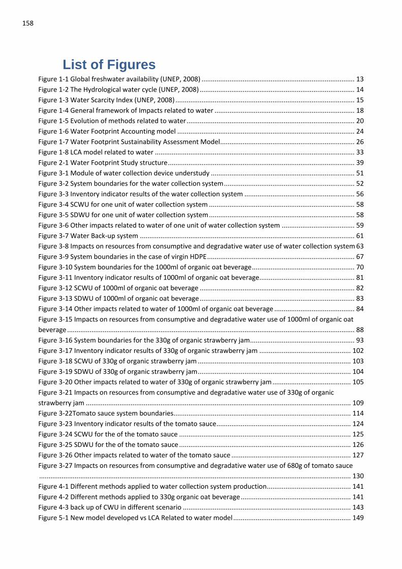
158
List of Figures Figure 1-1 Global freshwater availability (UNEP, 2008) .................................................................................. 13
Figure 1-2 The Hydrological water cycle (UNEP, 2008) ................................................................................... 14
Figure 1-3 Water Scarcity Index (UNEP, 2008) ................................................................................................ 15
Figure 1-4 General framework of Impacts related to water ........................................................................... 18
Figure 1-5 Evolution of methods related to water .......................................................................................... 20
Figure 1-6 Water Footprint Accounting model ............................................................................................... 24
Figure 1-7 Water Footprint Sustainability Assessment Model ........................................................................ 26
Figure 1-8 LCA model related to water ........................................................................................................... 33
Figure 2-1 Water Footprint Study structure .................................................................................................... 39
Figure 3-1 Module of water collection device understudy ............................................................................. 51
Figure 3-2 System boundaries for the water collection system ...................................................................... 52
Figure 3-3 Inventory indicator results of the water collection system ........................................................... 56
Figure 3-4 SCWU for one unit of water collection system .............................................................................. 58
Figure 3-5 SDWU for one unit of water collection system .............................................................................. 58
Figure 3-6 Other impacts related to water of one unit of water collection system ....................................... 59
Figure 3-7 Water Back-up system ................................................................................................................... 61
Figure 3-8 Impacts on resources from consumptive and degradative water use of water collection system 63
Figure 3-9 System boundaries in the case of virgin HDPE ............................................................................... 67
Figure 3-10 System boundaries for the 1000ml of organic oat beverage ....................................................... 70
Figure 3-11 Inventory indicator results of 1000ml of organic oat beverage ................................................... 81
Figure 3-12 SCWU of 1000ml of organic oat beverage ................................................................................... 82
Figure 3-13 SDWU of 1000ml of organic oat beverage ................................................................................... 83
Figure 3-14 Other impacts related to water of 1000ml of organic oat beverage ........................................... 84
Figure 3-15 Impacts on resources from consumptive and degradative water use of 1000ml of organic oat
beverage .......................................................................................................................................................... 88
Figure 3-16 System boundaries for the 330g of organic strawberry jam ........................................................ 93
Figure 3-17 Inventory indicator results of 330g of organic strawberry jam ................................................. 102
Figure 3-18 SCWU of 330g of organic strawberry jam .................................................................................. 103
Figure 3-19 SDWU of 330g of organic strawberry jam .................................................................................. 104
Figure 3-20 Other impacts related to water of 330g of organic strawberry jam .......................................... 105
Figure 3-21 Impacts on resources from consumptive and degradative water use of 330g of organic
strawberry jam .............................................................................................................................................. 109
Figure 3-22Tomato sauce system boundaries ............................................................................................... 114
Figure 3-23 Inventory indicator results of the tomato sauce ........................................................................ 124
Figure 3-24 SCWU for the of the tomato sauce ............................................................................................ 125
Figure 3-25 SDWU for the of the tomato sauce ............................................................................................ 126
Figure 3-26 Other impacts related to water of the tomato sauce ................................................................ 127
Figure 3-27 Impacts on resources from consumptive and degradative water use of 680g of tomato sauce
....................................................................................................................................................................... 130
Figure 4-1 Different methods applied to water collection system production ............................................. 141
Figure 4-2 Different methods applied to 330g organic oat beverage ........................................................... 141
Figure 4-3 back up of CWU in different scenario .......................................................................................... 143
Figure 5-1 New model developed vs LCA Related to water model ............................................................... 149
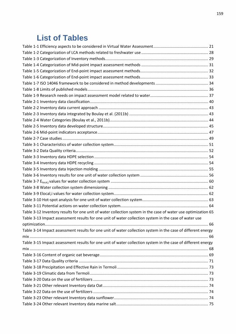
159
List of Tables Table 1-1 Efficiency aspects to be considered in Virtual Water Assessment .................................................. 21
Table 1-2 Categorization of LCA methods related to freshwater use ............................................................. 28
Table 1-3 Categorization of Inventory methods .............................................................................................. 29
Table 1-4 Categorization of Mid-point impact assessment methods ............................................................. 31
Table 1-5 Categorization of End-point impact assessment methods .............................................................. 32
Table 1-6 Categorization of End-point impact assessment methods .............................................................. 33
Table 1-7 ISO 14046 framework to be considered in method developments ................................................ 34
Table 1-8 Limits of published models .............................................................................................................. 36
Table 1-9 Research needs on impact assessment model related to water ..................................................... 37
Table 2-1 Inventory data classification ............................................................................................................ 40
Table 2-2 Inventory data current approach .................................................................................................... 43
Table 2-3 Inventory data integrated by Boulay et al. (2011b) ........................................................................ 43
Table 2-4 Water Categories (Boulay et al., 2011b).......................................................................................... 44
Table 2-5 Inventory data developed structure ................................................................................................ 45
Table 2-6 Mid-point indicators acceptance ..................................................................................................... 47
Table 2-7 Case studies ..................................................................................................................................... 49
Table 3-1 Characteristics of water collection system ...................................................................................... 51
Table 3-2 Data Quality criteria......................................................................................................................... 52
Table 3-3 Inventory data HDPE selection ........................................................................................................ 54
Table 3-4 Inventory data HDPE recycling ........................................................................................................ 54
Table 3-5 Inventory data Injection molding .................................................................................................... 55
Table 3-6 Inventory results for one unit of water collection system .............................................................. 56
Table 3-7 Elocal,j values for water collection system ......................................................................................... 60
Table 3-8 Water collection system dimensioning ........................................................................................... 62
Table 3-9 Elocal,i values for water collection system ...................................................................................... 62
Table 3-10 Hot-spot analysis for one unit of water collection system ............................................................ 63
Table 3-11 Potential actions on water collection system................................................................................ 64
Table 3-12 Inventory results for one unit of water collection system in the case of water use optimization 65
Table 3-13 Impact assessment results for one unit of water collection system in the case of water use
optimization..................................................................................................................................................... 66
Table 3-14 Impact assessment results for one unit of water collection system in the case of different energy
mix ................................................................................................................................................................... 66
Table 3-15 Impact assessment results for one unit of water collection system in the case of different energy
mix ................................................................................................................................................................... 68
Table 3-16 Content of organic oat beverage ................................................................................................... 69
Table 3-17 Data Quality criteria ...................................................................................................................... 71
Table 3-18 Precipitation and Effective Rain in Termoli ................................................................................... 73
Table 3-19 Climatic data from Termoli ............................................................................................................ 73
Table 3-20 Data on the use of fertilizers ......................................................................................................... 73
Table 3-21 Other relevant Inventory data Oat ................................................................................................ 74
Table 3-22 Data on the use of fertilizers ......................................................................................................... 74
Table 3-23 Other relevant Inventory data sunflower ...................................................................................... 74
Table 3-24 Other relevant Inventory data marine salt .................................................................................... 75
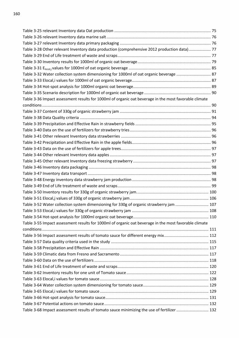
160
Table 3-25 relevant Inventory data Oat production ....................................................................................... 75
Table 3-26 relevant Inventory data marine salt .............................................................................................. 76
Table 3-27 relevant Inventory data primary packaging .................................................................................. 76
Table 3-28 Other relevant Inventory data production (comprehensive 2012 production data) .................... 77
Table 3-29 End of Life treatment of waste and scraps .................................................................................... 77
Table 3-30 Inventory results for 1000ml of organic oat beverage .................................................................. 79
Table 3-31 Elocal,j values for 1000ml of oat organic beverage .......................................................................... 85
Table 3-32 Water collection system dimensioning for 1000ml of oat organic beverage ............................... 87
Table 3-33 Elocal,i values for 1000ml of oat organic beverage ....................................................................... 87
Table 3-34 Hot-spot analysis for 1000ml organic oat beverage...................................................................... 89
Table 3-35 Scenario description for 1000ml of organic oat beverage ............................................................ 90
Table 3-36 Impact assessment results for 1000ml of organic oat beverage in the most favorable climate
conditions ........................................................................................................................................................ 90
Table 3-37 Content of 330g of organic strawberry jam .................................................................................. 91
Table 3-38 Data Quality criteria ...................................................................................................................... 94
Table 3-39 Precipitation and Effective Rain in strawberry fields .................................................................... 95
Table 3-40 Data on the use of fertilizers for strawberry tries ......................................................................... 96
Table 3-41 Other relevant Inventory data strawberries ................................................................................. 96
Table 3-42 Precipitation and Effective Rain in the apple fields ....................................................................... 96
Table 3-43 Data on the use of fertilizers for apple trees ................................................................................. 97
Table 3-44 Other relevant Inventory data apples ........................................................................................... 97
Table 3-45 Other relevant Inventory data freezing strawberry ...................................................................... 97
Table 3-46 Inventory data packaging .............................................................................................................. 98
Table 3-47 Inventory data transport ............................................................................................................... 98
Table 3-48 Energy inventory data strawberry jam production ....................................................................... 98
Table 3-49 End of Life treatment of waste and scraps .................................................................................... 99
Table 3-50 Inventory results for 330g of organic strawberry jam. ................................................................ 100
Table 3-51 Elocal,j values of 330g of organic strawberry jam ....................................................................... 106
Table 3-52 Water collection system dimensioning for 330g of organic strawberry jam .............................. 107
Table 3-53 Elocal,i values for 330g of organic strawberry jam ..................................................................... 108
Table 3-54 Hot-spot analysis for 1000ml organic oat beverage.................................................................... 110
Table 3-55 Impact assessment results for 1000ml of organic oat beverage in the most favorable climate
conditions ...................................................................................................................................................... 111
Table 3-56 Impact assessment results of tomato sauce for different energy mix ........................................ 112
Table 3-57 Data quality criteria used in the study ........................................................................................ 115
Table 3-58 Precipitation and Effective Rain .................................................................................................. 117
Table 3-59 Climatic data from Fresno and Sacramento ................................................................................ 117
Table 3-60 Data on the use of fertilizers ....................................................................................................... 118
Table 3-61 End of Life treatment of waste and scraps .................................................................................. 120
Table 3-62 Inventory results for one unit of Tomato sauce .......................................................................... 122
Table 3-63 Elocal,i values for tomato sauce .................................................................................................. 128
Table 3-64 Water collection system dimensioning for tomato sauce ........................................................... 129
Table 3-65 Elocal,i values for tomato sauce .................................................................................................. 129
Table 3-66 Hot-spot analysis for tomato sauce ............................................................................................. 131
Table 3-67 Potential actions on tomato sauce .............................................................................................. 132
Table 3-68 Impact assessment results of tomato sauce minimizing the use of fertilizer ............................. 132

161
Table 3-69 Impact assessment results of tomato sauce for different production location .......................... 133
Table 3-70 Impact assessment results of tomato sauce for different energy mix ........................................ 134
Table 4-1 Solutions adopted to address 14046 principles ............................................................................ 137
Table 4-2 Screening assessment results ........................................................................................................ 139
Table 5-1 Set of indicators results in the 4 case studies ............................................................................... 148
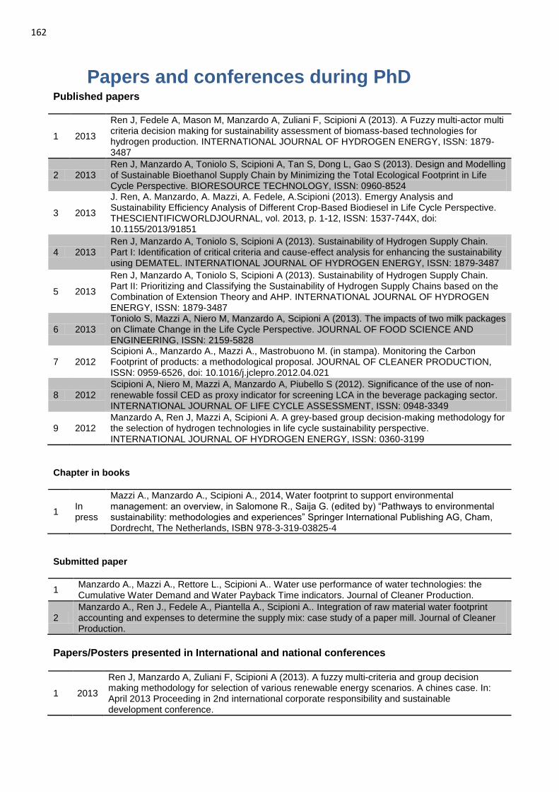
162
Papers and conferences during PhD Published papers
1 2013
Ren J, Fedele A, Mason M, Manzardo A, Zuliani F, Scipioni A (2013). A Fuzzy multi-actor multi criteria decision making for sustainability assessment of biomass-based technologies for hydrogen production. INTERNATIONAL JOURNAL OF HYDROGEN ENERGY, ISSN: 1879-3487
2 2013 Ren J, Manzardo A, Toniolo S, Scipioni A, Tan S, Dong L, Gao S (2013). Design and Modelling of Sustainable Bioethanol Supply Chain by Minimizing the Total Ecological Footprint in Life Cycle Perspective. BIORESOURCE TECHNOLOGY, ISSN: 0960-8524
3 2013
J. Ren, A. Manzardo, A. Mazzi, A. Fedele, A.Scipioni (2013). Emergy Analysis and Sustainability Efficiency Analysis of Different Crop-Based Biodiesel in Life Cycle Perspective. THESCIENTIFICWORLDJOURNAL, vol. 2013, p. 1-12, ISSN: 1537-744X, doi: 10.1155/2013/91851
4 2013 Ren J, Manzardo A, Toniolo S, Scipioni A (2013). Sustainability of Hydrogen Supply Chain. Part I: Identification of critical criteria and cause-effect analysis for enhancing the sustainability using DEMATEL. INTERNATIONAL JOURNAL OF HYDROGEN ENERGY, ISSN: 1879-3487
5 2013
Ren J, Manzardo A, Toniolo S, Scipioni A (2013). Sustainability of Hydrogen Supply Chain. Part II: Prioritizing and Classifying the Sustainability of Hydrogen Supply Chains based on the Combination of Extension Theory and AHP. INTERNATIONAL JOURNAL OF HYDROGEN ENERGY, ISSN: 1879-3487
6 2013 Toniolo S, Mazzi A, Niero M, Manzardo A, Scipioni A (2013). The impacts of two milk packages on Climate Change in the Life Cycle Perspective. JOURNAL OF FOOD SCIENCE AND ENGINEERING, ISSN: 2159-5828
7 2012 Scipioni A., Manzardo A., Mazzi A., Mastrobuono M. (in stampa). Monitoring the Carbon Footprint of products: a methodological proposal. JOURNAL OF CLEANER PRODUCTION, ISSN: 0959-6526, doi: 10.1016/j.jclepro.2012.04.021
8 2012 Scipioni A, Niero M, Mazzi A, Manzardo A, Piubello S (2012). Significance of the use of non-renewable fossil CED as proxy indicator for screening LCA in the beverage packaging sector. INTERNATIONAL JOURNAL OF LIFE CYCLE ASSESSMENT, ISSN: 0948-3349
9 2012 Manzardo A, Ren J, Mazzi A, Scipioni A. A grey-based group decision-making methodology for the selection of hydrogen technologies in life cycle sustainability perspective. INTERNATIONAL JOURNAL OF HYDROGEN ENERGY, ISSN: 0360-3199
Chapter in books
1 In press
Mazzi A., Manzardo A., Scipioni A., 2014, Water footprint to support environmental management: an overview, in Salomone R., Saija G. (edited by) “Pathways to environmental sustainability: methodologies and experiences” Springer International Publishing AG, Cham, Dordrecht, The Netherlands, ISBN 978-3-319-03825-4
Submitted paper
1 Manzardo A., Mazzi A., Rettore L., Scipioni A.. Water use performance of water technologies: the Cumulative Water Demand and Water Payback Time indicators. Journal of Cleaner Production.
2 Manzardo A., Ren J., Fedele A., Piantella A., Scipioni A.. Integration of raw material water footprint accounting and expenses to determine the supply mix: case study of a paper mill. Journal of Cleaner Production.
Papers/Posters presented in International and national conferences
1 2013 Ren J, Manzardo A, Zuliani F, Scipioni A (2013). A fuzzy multi-criteria and group decision making methodology for selection of various renewable energy scenarios. A chines case. In: April 2013 Proceeding in 2nd international corporate responsibility and sustainable development conference.
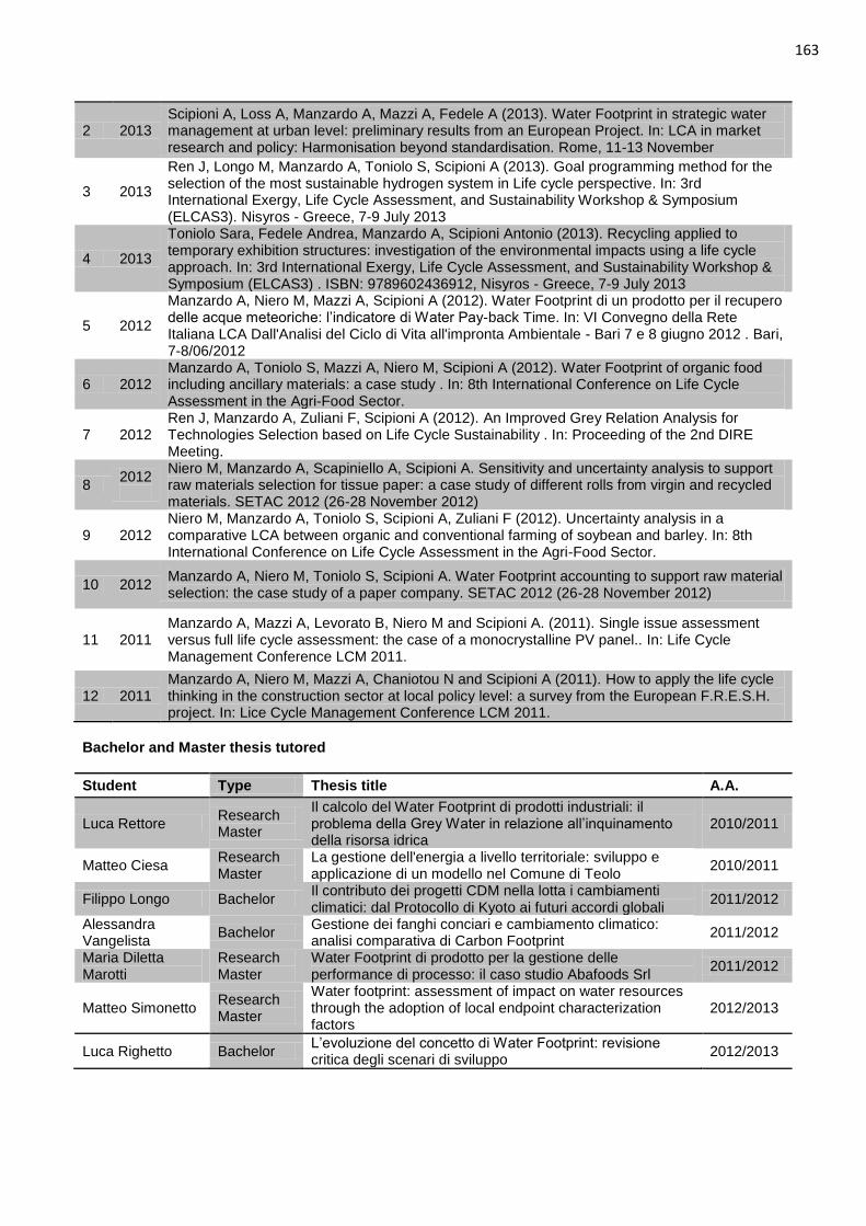
163
2 2013 Scipioni A, Loss A, Manzardo A, Mazzi A, Fedele A (2013). Water Footprint in strategic water management at urban level: preliminary results from an European Project. In: LCA in market research and policy: Harmonisation beyond standardisation. Rome, 11-13 November
3 2013 Ren J, Longo M, Manzardo A, Toniolo S, Scipioni A (2013). Goal programming method for the selection of the most sustainable hydrogen system in Life cycle perspective. In: 3rd International Exergy, Life Cycle Assessment, and Sustainability Workshop & Symposium (ELCAS3). Nisyros - Greece, 7-9 July 2013
4 2013 Toniolo Sara, Fedele Andrea, Manzardo A, Scipioni Antonio (2013). Recycling applied to temporary exhibition structures: investigation of the environmental impacts using a life cycle approach. In: 3rd International Exergy, Life Cycle Assessment, and Sustainability Workshop & Symposium (ELCAS3) . ISBN: 9789602436912, Nisyros - Greece, 7-9 July 2013
5 2012 Manzardo A, Niero M, Mazzi A, Scipioni A (2012). Water Footprint di un prodotto per il recupero delle acque meteoriche: l’indicatore di Water Pay-back Time. In: VI Convegno della Rete Italiana LCA Dall'Analisi del Ciclo di Vita all'impronta Ambientale - Bari 7 e 8 giugno 2012 . Bari, 7-8/06/2012
6 2012 Manzardo A, Toniolo S, Mazzi A, Niero M, Scipioni A (2012). Water Footprint of organic food including ancillary materials: a case study . In: 8th International Conference on Life Cycle Assessment in the Agri-Food Sector.
7 2012 Ren J, Manzardo A, Zuliani F, Scipioni A (2012). An Improved Grey Relation Analysis for Technologies Selection based on Life Cycle Sustainability . In: Proceeding of the 2nd DIRE Meeting.
8 2012
Niero M, Manzardo A, Scapiniello A, Scipioni A. Sensitivity and uncertainty analysis to support raw materials selection for tissue paper: a case study of different rolls from virgin and recycled materials. SETAC 2012 (26-28 November 2012)
9 2012 Niero M, Manzardo A, Toniolo S, Scipioni A, Zuliani F (2012). Uncertainty analysis in a comparative LCA between organic and conventional farming of soybean and barley. In: 8th International Conference on Life Cycle Assessment in the Agri-Food Sector.
10 2012 Manzardo A, Niero M, Toniolo S, Scipioni A. Water Footprint accounting to support raw material selection: the case study of a paper company. SETAC 2012 (26-28 November 2012)
11 2011 Manzardo A, Mazzi A, Levorato B, Niero M and Scipioni A. (2011). Single issue assessment versus full life cycle assessment: the case of a monocrystalline PV panel.. In: Life Cycle Management Conference LCM 2011.
12 2011 Manzardo A, Niero M, Mazzi A, Chaniotou N and Scipioni A (2011). How to apply the life cycle thinking in the construction sector at local policy level: a survey from the European F.R.E.S.H. project. In: Lice Cycle Management Conference LCM 2011.
Bachelor and Master thesis tutored
Student Type Thesis title A.A.
Luca Rettore Research Master
Il calcolo del Water Footprint di prodotti industriali: il problema della Grey Water in relazione all’inquinamento della risorsa idrica
2010/2011
Matteo Ciesa Research Master
La gestione dell'energia a livello territoriale: sviluppo e applicazione di un modello nel Comune di Teolo
2010/2011
Filippo Longo Bachelor Il contributo dei progetti CDM nella lotta i cambiamenti climatici: dal Protocollo di Kyoto ai futuri accordi globali
2011/2012
Alessandra Vangelista
Bachelor Gestione dei fanghi conciari e cambiamento climatico: analisi comparativa di Carbon Footprint
2011/2012
Maria Diletta Marotti
Research Master
Water Footprint di prodotto per la gestione delle performance di processo: il caso studio Abafoods Srl
2011/2012
Matteo Simonetto Research Master
Water footprint: assessment of impact on water resources through the adoption of local endpoint characterization factors
2012/2013
Luca Righetto Bachelor L’evoluzione del concetto di Water Footprint: revisione critica degli scenari di sviluppo
2012/2013
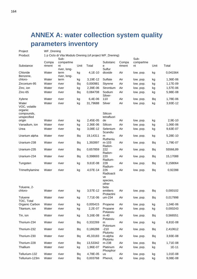
164
ANNEX A: water collection system quality
parameters inventory Project WF_Drening
Product: 1 p Ciclo di Vita Modulo Drening (of project WF_Drening)
Substance Compartment
Sub-compartment Unit Total
Substance
Compartment
Sub-compartment Unit Total
Chloride Water river, long-term kg 4,1E-10
Sulfur dioxide Air low. pop. kg 0,041564
Benzene, chloro- Water
river, long-term kg 3,19E-12 Sulfate Air low. pop. kg 1,36E-06
Zirconium-95 Water river Bq 0,000981 Styrene Air low. pop. kg 1,17E-09
Zinc, ion Water river kg 2,39E-06 Strontium Air low. pop. kg 1,57E-06
Zinc-65 Water river Bq 0,084708 Sodium Air low. pop. kg 5,98E-08
Xylene Water river kg 6,4E-06 Silver-110 Air low. pop. Bq 1,78E-06
Water Water river kg 31,79688 Silver Air low. pop. kg 3,93E-12 VOC, volatile organic compounds, unspecified origin Water river kg 2,45E-05
Silicon tetrafluoride Air low. pop. kg 2,9E-10
Vanadium, ion Water river kg 2,36E-06 Silicon Air low. pop. kg 1,06E-06
Urea Water river kg 3,08E-12 Selenium Air low. pop. kg 9,63E-07
Uranium alpha Water river Bq 19,14311 Scandium Air low. pop. kg 5,28E-10
Uranium-238 Water river Bq 1,392897 Ruthenium-103 Air low. pop. Bq 1,79E-07
Uranium-235 Water river Bq 0,657859 Radon-222 Air low. pop. Bq 55566,89
Uranium-234 Water river Bq 0,398693 Radon-220 Air low. pop. Bq 15,17088
Tungsten Water river kg 9,61E-08 Radium-228 Air low. pop. Bq 0,158064
Trimethylamine Water river kg 4,07E-14 Radium-226 Air low. pop. Bq 0,92288
Toluene, 2-chloro- Water river kg 3,57E-12
Radioactive species, other beta emitters Air low. pop. Bq 0,000102
Toluene Water river kg 7,71E-06 Protactinium-234 Air low. pop. Bq 0,017998
TOC, Total Organic Carbon Water river kg 0,005415 Propene Air low. pop. kg 1,04E-06
Titanium, ion Water river kg 2,2E-07 Propane Air low. pop. kg 0,000243
Tin, ion Water river kg 5,16E-08 Potassium-40 Air low. pop. Bq 0,566551
Thorium-234 Water river Bq 0,332269 Potassium Air low. pop. kg 6,81E-08
Thorium-232 Water river Bq 0,186288 Polonium-210 Air low. pop. Bq 2,410612
Thorium-230 Water river Bq 45,33183 Plutonium-alpha Air low. pop. Bq 3,93E-08
Thorium-228 Water river Bq 13,53342 Plutonium-238 Air low. pop. Bq 1,71E-08
Thallium Water river kg 1,96E-07 Platinum Air low. pop. kg 1E-11
Tellurium-132 Water river Bq 4,78E-05 Phosphorus Air low. pop. kg 1,01E-08
Tellurium-123m Water river Bq 0,003768 Phenol, Air low. pop. kg 9,08E-08
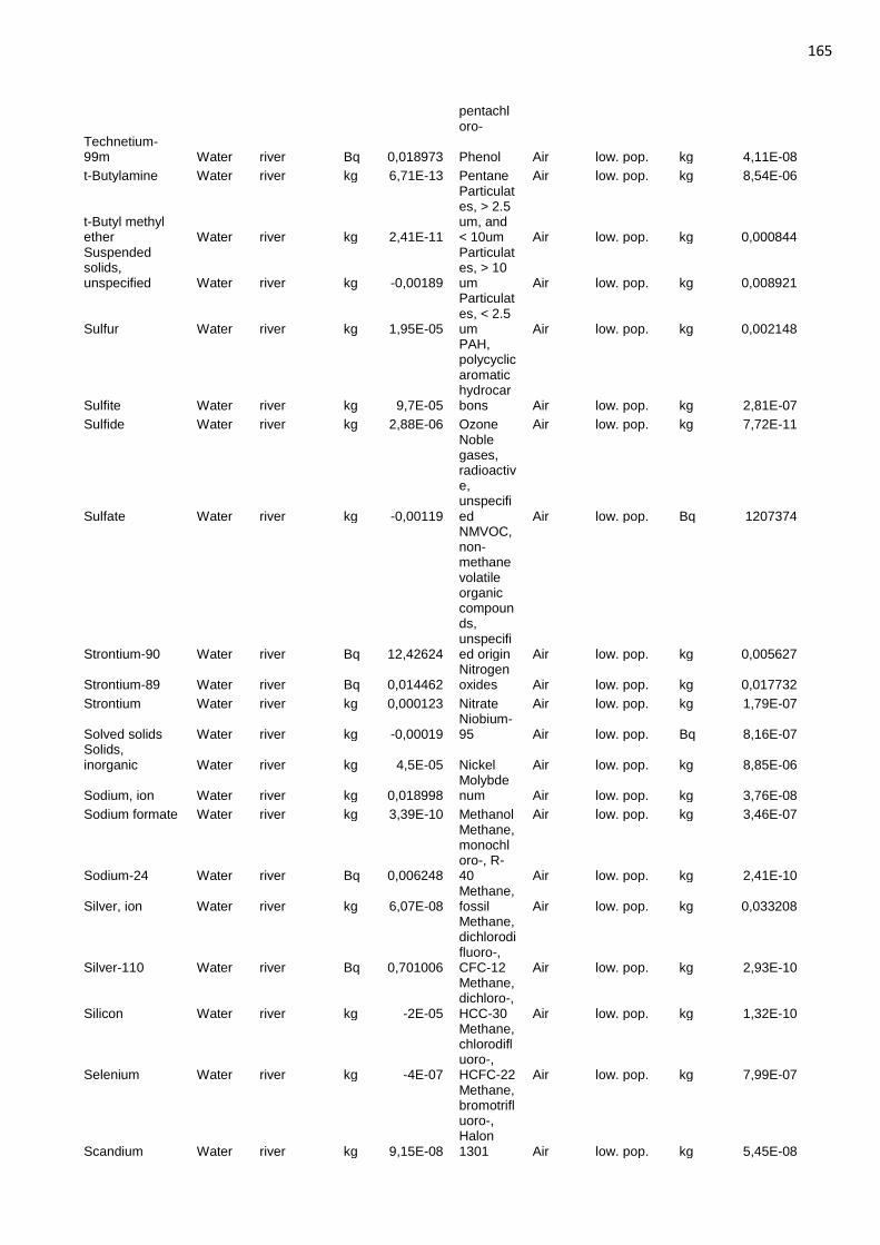
165
pentachloro-
Technetium-99m Water river Bq 0,018973 Phenol Air low. pop. kg 4,11E-08
t-Butylamine Water river kg 6,71E-13 Pentane Air low. pop. kg 8,54E-06
t-Butyl methyl ether Water river kg 2,41E-11
Particulates, > 2.5 um, and < 10um Air low. pop. kg 0,000844
Suspended solids, unspecified Water river kg -0,00189
Particulates, > 10 um Air low. pop. kg 0,008921
Sulfur Water river kg 1,95E-05
Particulates, < 2.5 um Air low. pop. kg 0,002148
Sulfite Water river kg 9,7E-05
PAH, polycyclic aromatic hydrocarbons Air low. pop. kg 2,81E-07
Sulfide Water river kg 2,88E-06 Ozone Air low. pop. kg 7,72E-11
Sulfate Water river kg -0,00119
Noble gases, radioactive, unspecified Air low. pop. Bq 1207374
Strontium-90 Water river Bq 12,42624
NMVOC, non-methane volatile organic compounds, unspecified origin Air low. pop. kg 0,005627
Strontium-89 Water river Bq 0,014462 Nitrogen oxides Air low. pop. kg 0,017732
Strontium Water river kg 0,000123 Nitrate Air low. pop. kg 1,79E-07
Solved solids Water river kg -0,00019 Niobium-95 Air low. pop. Bq 8,16E-07
Solids, inorganic Water river kg 4,5E-05 Nickel Air low. pop. kg 8,85E-06
Sodium, ion Water river kg 0,018998 Molybdenum Air low. pop. kg 3,76E-08
Sodium formate Water river kg 3,39E-10 Methanol Air low. pop. kg 3,46E-07
Sodium-24 Water river Bq 0,006248
Methane, monochloro-, R-40 Air low. pop. kg 2,41E-10
Silver, ion Water river kg 6,07E-08 Methane, fossil Air low. pop. kg 0,033208
Silver-110 Water river Bq 0,701006
Methane, dichlorodifluoro-, CFC-12 Air low. pop. kg 2,93E-10
Silicon Water river kg -2E-05
Methane, dichloro-, HCC-30 Air low. pop. kg 1,32E-10
Selenium Water river kg -4E-07
Methane, chlorodifluoro-, HCFC-22 Air low. pop. kg 7,99E-07
Scandium Water river kg 9,15E-08
Methane, bromotrifluoro-, Halon 1301 Air low. pop. kg 5,45E-08
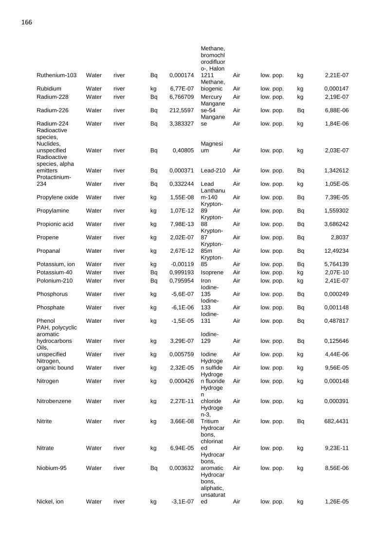
166
Ruthenium-103 Water river Bq 0,000174
Methane, bromochlorodifluoro-, Halon 1211 Air low. pop. kg 2,21E-07
Rubidium Water river kg 6,77E-07 Methane, biogenic Air low. pop. kg 0,000147
Radium-228 Water river Bq 6,766709 Mercury Air low. pop. kg 2,19E-07
Radium-226 Water river Bq 212,5597 Manganese-54 Air low. pop. Bq 6,88E-06
Radium-224 Water river Bq 3,383327 Manganese Air low. pop. kg 1,84E-06
Radioactive species, Nuclides, unspecified Water river Bq 0,40805
Magnesium Air low. pop. kg 2,03E-07
Radioactive species, alpha emitters Water river Bq 0,000371 Lead-210 Air low. pop. Bq 1,342612 Protactinium-234 Water river Bq 0,332244 Lead Air low. pop. kg 1,05E-05
Propylene oxide Water river kg 1,55E-08 Lanthanum-140 Air low. pop. Bq 7,39E-05
Propylamine Water river kg 1,07E-12 Krypton-89 Air low. pop. Bq 1,559302
Propionic acid Water river kg 7,98E-13 Krypton-88 Air low. pop. Bq 3,686242
Propene Water river kg 2,02E-07 Krypton-87 Air low. pop. Bq 2,8037
Propanal Water river kg 2,67E-12 Krypton-85m Air low. pop. Bq 12,49234
Potassium, ion Water river kg -0,00119 Krypton-85 Air low. pop. Bq 5,764139
Potassium-40 Water river Bq 0,999193 Isoprene Air low. pop. kg 2,07E-10
Polonium-210 Water river Bq 0,795954 Iron Air low. pop. kg 2,41E-07
Phosphorus Water river kg -5,6E-07 Iodine-135 Air low. pop. Bq 0,000249
Phosphate Water river kg -6,1E-06 Iodine-133 Air low. pop. Bq 0,001148
Phenol Water river kg -1,5E-05 Iodine-131 Air low. pop. Bq 0,487817
PAH, polycyclic aromatic hydrocarbons Water river kg 3,29E-07
Iodine-129 Air low. pop. Bq 0,125646
Oils, unspecified Water river kg 0,005759 Iodine Air low. pop. kg 4,44E-06 Nitrogen, organic bound Water river kg 2,32E-05
Hydrogen sulfide Air low. pop. kg 9,56E-05
Nitrogen Water river kg 0,000426 Hydrogen fluoride Air low. pop. kg 0,000148
Nitrobenzene Water river kg 2,27E-11
Hydrogen chloride Air low. pop. kg 0,000391
Nitrite Water river kg 3,66E-08
Hydrogen-3, Tritium Air low. pop. Bq 682,4431
Nitrate Water river kg 6,94E-05
Hydrocarbons, chlorinated Air low. pop. kg 9,23E-11
Niobium-95 Water river Bq 0,003632
Hydrocarbons, aromatic Air low. pop. kg 8,56E-06
Nickel, ion Water river kg -3,1E-07
Hydrocarbons, aliphatic, unsaturated Air low. pop. kg 1,26E-05
167
Molybdenum-99 Water river Bq 0,000826
Hydrocarbons, aliphatic, alkanes, unspecified Air low. pop. kg 2,91E-05
Molybdenum Water river kg -8,9E-07
Hydrocarbons, aliphatic, alkanes, cyclic Air low. pop. kg 2,63E-10
Methyl formate Water river kg 2,54E-13 Hexane Air low. pop. kg 1,26E-06
Methyl amine Water river kg 1,1E-12 Helium Air low. pop. kg 3,87E-06
Methyl acrylate Water river kg 1,34E-09 Heat, waste Air low. pop. MJ 64,559
Methyl acetate Water river kg 2,3E-14 Furan Air low. pop. kg 4,46E-09
Methanol Water river kg 3,91E-09 Formic acid Air low. pop. kg 1,57E-08
Methane, dichloro-, HCC-30 Water river kg 1,93E-06
Formaldehyde Air low. pop. kg 3,42E-06
Mercury Water river kg 8,19E-09 Fluorine Air low. pop. kg 3,67E-07
Manganese-54 Water river Bq 0,049654 Ethyne Air low. pop. kg 5,36E-08
Manganese Water river kg 6,33E-06 Ethylene oxide Air low. pop. kg 6,49E-13
Magnesium Water river kg 0,000529
Ethene, tetrachloro- Air low. pop. kg 1,95E-11
m-Xylene Water river kg 3,62E-12 Ethene Air low. pop. kg 1,54E-06
Lithium, ion Water river kg 6,42E-11 Ethanol Air low. pop. kg 1,18E-08
Lead-210 Water river Bq 0,795954
Ethane, 1,2-dichloro-1,1,2,2-tetrafluoro-, CFC-114 Air low. pop. kg 4,01E-08
Lead Water river kg 1,56E-06
Ethane, 1,2-dichloro- Air low. pop. kg 1,82E-11
Lanthanum-140 Water river Bq 0,002395
Ethane, 1,1,1,2-tetrafluoro-, HFC-134a Air low. pop. kg 2,08E-09
Lactic acid Water river kg 2,24E-12
Ethane, 1,1,1-trichloro-, HCFC-140 Air low. pop. kg 9,09E-12
Isopropylamine Water river kg 2,75E-13 Ethane Air low. pop. kg 0,000993
Iron, ion Water river kg 2,94E-05
Dioxin, 2,3,7,8 Tetrachlorodibenzo-p- Air low. pop. kg 7,77E-13
Iron-59 Water river Bq 0,000388
Dinitrogen monoxide Air low. pop. kg 0,000134
Iodine-133 Water river Bq 0,001412 Cyanide Air low. pop. kg 1,17E-07
Iodine-131 Water river Bq 0,010384 Cumene Air low. pop. kg 2,48E-12
Iodide Water river kg 6,82E-06 Copper Air low. pop. kg 1,16E-05
Hypochlorite Water river kg 1,69E-05 Cobalt-60 Air low. pop. Bq 0,000165
Hydroxide Water river kg 6,22E-09 Cobalt- Air low. pop. Bq 1,87E-05
168
58
Hydrogen sulfide Water river kg 1,55E-07 Cobalt Air low. pop. kg 1,2E-07 Hydrogen peroxide Water river kg -1,4E-09
Chromium VI Air low. pop. kg 7,71E-08
Hydrogen-3, Tritium Water river Bq 5107,424
Chromium-51 Air low. pop. Bq 1,34E-05
Hydrocarbons, unspecified Water river kg -0,00015
Chromium Air low. pop. kg 2,49E-06
Hydrocarbons, aromatic Water river kg 3,56E-05
Chloroform Air low. pop. kg 4,46E-11
Hydrocarbons, aliphatic, unsaturated Water river kg 8,12E-07 Chlorine Air low. pop. kg 1,73E-08 Hydrocarbons, aliphatic, alkanes, unspecified Water river kg 8,8E-06
Cesium-137 Air low. pop. Bq 0,000178
Heat, waste Water river MJ 23,26309 Cesium-134 Air low. pop. Bq 1E-05
Formic acid Water river kg 9,77E-13 Cerium-141 Air low. pop. Bq 0,00021
Formate Water river kg 8,61E-11
Carbon monoxide, fossil Air low. pop. kg 0,002923
Formamide Water river kg 3,37E-12
Carbon monoxide, biogenic Air low. pop. kg 7,05E-05
Formaldehyde Water river kg 1,57E-09 Carbon disulfide Air low. pop. kg 8,13E-05
Fluosilicic acid Water river kg 1,25E-07
Carbon dioxide, land transformation Air low. pop. kg 6,86E-05
Fluoride Water river kg -0,00019
Carbon dioxide, fossil Air low. pop. kg 6,36252
Ethylene oxide Water river kg 1,01E-10
Carbon dioxide, biogenic Air low. pop. kg 0,119723
Ethylene diamine Water river kg 4,5E-11
Carbon-14 Air low. pop. Bq 147,1805
Ethylamine Water river kg 2,39E-12 Calcium Air low. pop. kg 8,76E-08
Ethyl acetate Water river kg 4,87E-12 Cadmium Air low. pop. kg 1,21E-06
Ethene, chloro- Water river kg 9,46E-09 Butane Air low. pop. kg 3,79E-05
Ethene Water river kg 1,81E-07 Butadiene Air low. pop. kg 6,72E-14
Ethanol Water river kg 1,02E-09 Bromine Air low. pop. kg 8,9E-06 Ethane, 1,2-dichloro- Water river kg 1,11E-08 Boron Air low. pop. kg 4,4E-05 DOC, Dissolved Organic Carbon Water river kg 0,005473 Beryllium Air low. pop. kg 1,14E-09
Dipropylamine Water river kg 2,85E-12 Benzo(a)pyrene Air low. pop. kg 2,08E-07
Dimethylamine Water river kg 3,69E-12 Benzene, ethyl- Air low. pop. kg 4,28E-11
Diethylamine Water river kg 4,53E-12 Benzene Air low. pop. kg 4,48E-05
Dichromate Water river kg 1,13E-06 Barium-140 Air low. pop. Bq 0,000864
Cyanide Water river kg 3,37E-06 Barium Air low. pop. kg 1,8E-06
Cumene Water river kg 4,92E-07 Arsenic Air low. pop. kg 3,69E-06
Copper, ion Water river kg -2,1E-06 Argon-41 Air low. pop. Bq 1,645646 COD, Chemical Oxygen Water river kg 0,01661
Antimony-125 Air low. pop. Bq 1,33E-05
169
Demand
Cobalt-60 Water river Bq 0,713642 Antimony-124 Air low. pop. Bq 1,27E-06
Cobalt-58 Water river Bq 0,825361 Antimony Air low. pop. kg 4,86E-07
Cobalt-57 Water river Bq 0,005065 Ammonia Air low. pop. kg 8,71E-05
Cobalt Water river kg -4E-06 Aluminium Air low. pop. kg 5,48E-07
Chromium, ion Water river kg 4,76E-07
Aldehydes, unspecified Air low. pop. kg 5,89E-08
Chromium VI Water river kg -1,1E-05
Aerosols, radioactive, unspecified Air low. pop. Bq 0,028213
Chromium-51 Water river Bq 0,173268
Actinides, radioactive, unspecified Air low. pop. Bq 0,000942
Chlorosulfonic acid Water river kg 7,18E-13 Acrolein Air low. pop. kg 1,51E-09
Chloroform Water river kg 8,8E-12 Acetonitrile Air low. pop. kg 2,35E-09
Chloroacetyl chloride Water river kg 9,29E-14 Acetone Air low. pop. kg 1,13E-06 Chloroacetic acid Water river kg 4,24E-09
Acetic acid Air low. pop. kg 5,62E-08
Chlorine Water river kg 8,58E-08 Acetaldehyde Air low. pop. kg 8,55E-09
Chlorinated solvents, unspecified Water river kg -5E-08
Acenaphthene Air low. pop. kg 2,32E-13
Chloride Water river kg 0,03501 Zinc Air high. pop. kg 1,67E-06
Chlorate Water river kg -6,1E-06 Xylene Air high. pop. kg 8,49E-06
Chloramine Water river kg 2,45E-11 Water Air high. pop. kg 2,3E-08
Cesium-137 Water river Bq 0,308592 Vanadium Air high. pop. kg 5,68E-05
Cesium-136 Water river Bq 0,00016 Uranium-238 Air high. pop. Bq 0,002581
Cesium-134 Water river Bq 0,025409 Uranium Air high. pop. kg 6,52E-10
Cesium Water river kg 6,77E-08 Trimethylamine Air high. pop. kg 1,7E-14
Cerium-144 Water river Bq 0,000274 Toluene, 2-chloro- Air high. pop. kg 1,72E-12
Cerium-141 Water river Bq 0,000899 Toluene Air high. pop. kg 1,39E-05 Carboxylic acids, unspecified Water river kg 0,000249 Titanium Air high. pop. kg 9,95E-08
Carbonate Water river kg -0,00032 Tin Air high. pop. kg 1,16E-09
Carbon disulfide Water river kg 8,8E-11 Thorium-232 Air high. pop. Bq 0,000903
Calcium, ion Water river kg 0,003431 Thorium-228 Air high. pop. Bq 0,001419
Cadmium, ion Water river kg 3,94E-08 Thorium Air high. pop. kg 4,9E-10
Butyrolactone Water river kg 9,66E-13 Thallium Air high. pop. kg 4,12E-10
Butyl acetate Water river kg 5,36E-10
t-Butylamine Air high. pop. kg 2,79E-13
Butene Water river kg 1,21E-09
t-Butyl methyl ether Air high. pop. kg 1,47E-09
Bromine Water river kg -3,1E-05 Sulfuric acid Air high. pop. kg 1,3E-10
170
Bromide Water river kg 8,21E-09 Sulfur trioxide Air high. pop. kg 4,57E-11
Bromate Water river kg -7,3E-07 Sulfur dioxide Air high. pop. kg -0,0107
Boron Water river kg 5,94E-06 Sulfate Air high. pop. kg 2,82E-05
Borate Water river kg 1,42E-10 Styrene Air high. pop. kg 2,38E-09 BOD5, Biological Oxygen Demand Water river kg 0,018325 Strontium Air high. pop. kg 4,9E-08
Beryllium Water river kg 1,06E-09
Sodium hydroxide Air high. pop. kg 6,1E-10
Benzene, ethyl- Water river kg 1,62E-06 Sodium formate Air high. pop. kg 1,41E-10
Benzene, chloro- Water river kg 4,03E-09
Sodium dichromate Air high. pop. kg 3,03E-07
Benzene, 1,2-dichloro- Water river kg 2E-10
Sodium chlorate Air high. pop. kg 4,65E-09
Benzene Water river kg 4,55E-06 Sodium Air high. pop. kg 1,84E-05
Barium-140 Water river Bq 0,002249 Silver Air high. pop. kg 2,92E-10
Barium Water river kg 5,92E-05 Silicon Air high. pop. kg -7,1E-06
Arsenic, ion Water river kg -1,5E-06 Selenium Air high. pop. kg 2,99E-07 AOX, Adsorbable Organic Halogen as Cl Water river kg 3,99E-07
Scandium Air high. pop. kg 3,25E-10
Antimony-125 Water river Bq 0,044672 Radon-222 Air high. pop. Bq 0,000259
Antimony-124 Water river Bq 0,049227 Radon-220 Air high. pop. Bq 0,000259
Antimony-122 Water river Bq 0,000513 Radium-228 Air high. pop. Bq 0,016772
Antimony Water river kg -4E-05 Radium-226 Air high. pop. Bq 0,003097
Aniline Water river kg 1,01E-11
Radioactive species, other beta emitters Air high. pop. Bq 0,298223
Ammonium, ion Water river kg -2E-05 Propylene oxide Air high. pop. kg 6,46E-09
Aluminium Water river kg 1,66E-05 Propylamine Air high. pop. kg 4,44E-13
Acrylate, ion Water river kg 1,43E-10 Propionic acid Air high. pop. kg 2,59E-06
Acidity, unspecified Water river kg -2,1E-05 Propene Air high. pop. kg -8,7E-06
Acetyl chloride Water river kg 1,45E-12 Propane Air high. pop. kg 0,000205
Acetonitrile Water river kg 1,97E-13 Propanal Air high. pop. kg -1,8E-09
Acetone Water river kg 2,14E-11 Potassium-40 Air high. pop. Bq 0,003484
Acetic acid Water river kg 5,07E-08 Potassium Air high. pop. kg 2,39E-05
Acetaldehyde Water river kg 8,72E-10
Polychlorinated biphenyls Air high. pop. kg 2,19E-15
Acenaphthylene Water river kg 2,63E-11 Polonium-210 Air high. pop. Bq 0,021938
Acenaphthene Water river kg 4,21E-10 Platinum Air high. pop. kg 4,34E-13
2-Propanol Water river kg 6,36E-13 Phosphorus Air high. pop. kg 2,18E-07
2-Methyl-2-butene Water river kg 3,09E-16
Phosphine Air high. pop. kg 5,21E-14
171
2-Methyl-1-propanol Water river kg 3,35E-12
Phenol, pentachloro- Air high. pop. kg 4,41E-12
2-Aminopropanol Water river kg 6,97E-14
Phenol, 2,4-dichloro- Air high. pop. kg 2,67E-13
1,4-Butanediol Water river kg 7,52E-13 Phenol Air high. pop. kg 8,6E-09
1-Propanol Water river kg 2,74E-12 Pentane Air high. pop. kg 0,0003
1-Pentene Water river kg 1,39E-12
Particulates, > 2.5 um, and < 10um Air high. pop. kg -0,00267
1-Pentanol Water river kg 1,84E-12
Particulates, > 10 um Air high. pop. kg -0,00192
1-Butanol Water river kg 4,12E-10
Particulates, < 2.5 um Air high. pop. kg -0,001
Zinc, ion Water lake kg 7,73E-15
PAH, polycyclic aromatic hydrocarbons Air high. pop. kg 1,4E-06
Nickel, ion Water lake kg 1,07E-14 Ozone Air high. pop. kg 5,48E-09
Mercury Water lake kg 6,79E-17
NMVOC, non-methane volatile organic compounds, unspecified origin Air high. pop. kg -0,04657
Lead Water lake kg 7,85E-15 Nitrogen oxides Air high. pop. kg -0,00923
DOC, Dissolved Organic Carbon Water lake kg 7,78E-09
Nitrobenzene Air high. pop. kg 5,67E-12
Copper, ion Water lake kg 1,2E-13 Nitrate Air high. pop. kg 3,76E-08
Calcium, ion Water lake kg 2,9E-07 Nickel Air high. pop. kg 1,58E-05
Cadmium, ion Water lake kg 2,65E-15
Monoethanolamine Air high. pop. kg 1,75E-08
Arsenic, ion Water lake kg 3,12E-15 Molybdenum Air high. pop. kg 4,46E-07
Zinc, ion Water
groundwater, long-term kg 0,001202
Methyl lactate Air high. pop. kg 1,02E-12
Vanadium, ion Water
groundwater, long-term kg 3,36E-05
Methyl formate Air high. pop. kg 6,35E-13
Tungsten Water
groundwater, long-term kg 2,13E-05
Methyl ethyl ketone Air high. pop. kg 1,14E-07
TOC, Total Organic Carbon Water
groundwater, long-term kg -0,00583
Methyl borate Air high. pop. kg 2,86E-13
Titanium, ion Water
groundwater, long-term kg 0,000202
Methyl amine Air high. pop. kg 4,59E-13
Tin, ion Water
groundwater, long-term kg 1,02E-05
Methyl acrylate Air high. pop. kg 6,84E-11
Thallium Water
groundwater, long-term kg 1,81E-06
Methyl acetate Air high. pop. kg 9,56E-15
Sulfate Water groundwater, long- kg 0,443213 Methanol Air high. pop. kg 2,89E-05
172
term
Strontium Water
groundwater, long-term kg 0,001856
Methanesulfonic acid Air high. pop. kg 2,38E-13
Sodium, ion Water
groundwater, long-term kg 0,049889
Methane, trifluoro-, HFC-23 Air high. pop. kg 1,4E-11
Silver, ion Water
groundwater, long-term kg 8,91E-07
Methane, trichlorofluoro-, CFC-11 Air high. pop. kg 7,12E-14
Silicon Water
groundwater, long-term kg 0,043775
Methane, tetrafluoro-, CFC-14 Air high. pop. kg 9,37E-11
Selenium Water
groundwater, long-term kg 2,52E-05
Methane, tetrachloro-, CFC-10 Air high. pop. kg 2,99E-09
Scandium Water
groundwater, long-term kg 1,64E-05
Methane, monochloro-, R-40 Air high. pop. kg 2,93E-12
Potassium, ion Water
groundwater, long-term kg 0,035577
Methane, fossil Air high. pop. kg -0,15436
Phosphate Water
groundwater, long-term kg 0,015586
Methane, dichlorofluoro-, HCFC-21 Air high. pop. kg 4,39E-14
Nitrogen, organic bound Water
groundwater, long-term kg 1,98E-06
Methane, dichlorodifluoro-, CFC-12 Air high. pop. kg 7,25E-11
Nitrite Water
groundwater, long-term kg 6,6E-08
Methane, dichloro-, HCC-30 Air high. pop. kg 4,5E-10
Nitrate Water
groundwater, long-term kg 0,004954
Methane, chlorodifluoro-, HCFC-22 Air high. pop. kg 2,62E-10
Nickel, ion Water
groundwater, long-term kg 0,000455
Methane, bromotrifluoro-, Halon 1301 Air high. pop. kg 8,84E-15
Molybdenum Water
groundwater, long-term kg 3,66E-05
Methane, biogenic Air high. pop. kg -0,00108
Mercury Water
groundwater, long-term kg 9,21E-07 Mercury Air high. pop. kg -8,6E-09
Manganese Water
groundwater, long-term kg 0,005445
Manganese Air high. pop. kg 7,83E-07
Magnesium Water
groundwater, long-term kg 0,061977
Magnesium Air high. pop. kg 1,25E-06
Lead Water
groundwater, long-term kg 2,82E-06 m-Xylene Air high. pop. kg 1,22E-07
Iron, ion Water
groundwater, long-term kg 0,014904 Lead-210 Air high. pop. Bq 0,012001
Iodide Water
groundwater, long-term kg 4,54E-12 Lead Air high. pop. kg 2E-06
Hydrogen Water groundwat kg 7,62E-06 Lactic Air high. pop. kg 9,32E-13
173
sulfide er, long-term
acid
Heat, waste Water
groundwater, long-term MJ 0,023248
Isopropylamine Air high. pop. kg 1,15E-13
Fluoride Water
groundwater, long-term kg 0,001219
Isocyanic acid Air high. pop. kg 4,18E-08
DOC, Dissolved Organic Carbon Water
groundwater, long-term kg -0,00583 Iron Air high. pop. kg 5,12E-06
Copper, ion Water
groundwater, long-term kg 0,000115 Iodine Air high. pop. kg 2,94E-09
COD, Chemical Oxygen Demand Water
groundwater, long-term kg -0,01492
Hydrogen sulfide Air high. pop. kg -5,5E-08
Cobalt Water
groundwater, long-term kg 0,00014
Hydrogen peroxide Air high. pop. kg 1,66E-10
Chromium VI Water
groundwater, long-term kg 7,03E-06
Hydrogen fluoride Air high. pop. kg -1,8E-05
Chloride Water
groundwater, long-term kg 0,010856
Hydrogen chloride Air high. pop. kg -0,00067
Calcium, ion Water
groundwater, long-term kg 0,111485
Hydrogen Air high. pop. kg -0,00045
Cadmium, ion Water
groundwater, long-term kg 1,77E-05
Hydrocarbons, chlorinated Air high. pop. kg -8,8E-09
Bromine Water
groundwater, long-term kg -1,9E-05
Hydrocarbons, aromatic Air high. pop. kg -0,00094
Boron Water
groundwater, long-term kg 0,000619
Hydrocarbons, aliphatic, unsaturated Air high. pop. kg 6,09E-06
BOD5, Biological Oxygen Demand Water
groundwater, long-term kg -0,00508
Hydrocarbons, aliphatic, alkanes, unspecified Air high. pop. kg 5,97E-05
Beryllium Water
groundwater, long-term kg 1,03E-05
Hydrocarbons, aliphatic, alkanes, cyclic Air high. pop. kg 4,28E-09
Barium Water
groundwater, long-term kg 0,000164 Hexane Air high. pop. kg 0,000172
Arsenic, ion Water
groundwater, long-term kg 4,4E-05 Heptane Air high. pop. kg 2,1E-05
Antimony Water
groundwater, long-term kg -6,3E-05
Heat, waste Air high. pop. MJ -85,485
Ammonium, ion Water
groundwater, long-term kg 1,21E-06
Formic acid Air high. pop. kg 1,35E-10
Aluminium Water
groundwater, long-term kg 0,003793
Formamide Air high. pop. kg 1,4E-12
Zinc, ion Water groundwater kg 2,6E-06
Formaldehyde Air high. pop. kg 4,8E-05
174
Vanadium, ion Water groundwater kg 1,43E-07
Fluosilicic acid Air high. pop. kg 6,94E-08
Uranium-238 Water groundwater Bq 4,75E-05 Fluorine Air high. pop. kg 5,08E-08
Tungsten Water groundwater kg 4,13E-07 Ethyne Air high. pop. kg 1,26E-07
Titanium, ion Water groundwater kg 1,25E-07
Ethylene oxide Air high. pop. kg 2,83E-09
Tin, ion Water groundwater kg 2,45E-08
Ethylene diamine Air high. pop. kg 1,87E-11
Thorium-228 Water groundwater Bq 1,13E-06
Ethylamine Air high. pop. kg 9,95E-13
Thallium Water groundwater kg 3,04E-09
Ethyl cellulose Air high. pop. kg 2,19E-10
Sulfate Water groundwater kg 0,025423
Ethyl acetate Air high. pop. kg 1,14E-07
Strontium Water groundwater kg 2,81E-05
Ethene, tetrachloro- Air high. pop. kg 1,54E-12
Solved solids Water groundwater kg 0,000508
Ethene, chloro- Air high. pop. kg 7,04E-07
Solids, inorganic Water
groundwater kg 0,002416 Ethene Air high. pop. kg -1,2E-05
Sodium, ion Water groundwater kg 0,00045 Ethanol Air high. pop. kg 2,82E-05
Silver, ion Water groundwater kg 1,54E-08
Ethane, hexafluoro-, HFC-116 Air high. pop. kg 2,42E-10
Silicon Water groundwater kg 0,000155
Ethane, 1,2-dichloro- Air high. pop. kg 1,01E-06
Selenium Water groundwater kg 2,71E-07
Ethane, 1,1,2-trichloro-1,2,2-trifluoro-, CFC-113 Air high. pop. kg 2,86E-12
Scandium Water groundwater kg 9,37E-08
Ethane, 1,1,1,2-tetrafluoro-, HFC-134a Air high. pop. kg 1,54E-11
Radium-226 Water groundwater Bq 0,000104
Ethane, 1,1-difluoro-, HFC-152a Air high. pop. kg 1,82E-09
Potassium, ion Water groundwater kg 0,000186 Ethane Air high. pop. kg 0,000242
Potassium-40 Water groundwater Bq 1,12E-05
Dipropylamine Air high. pop. kg 1,19E-12
Polonium-210 Water groundwater Bq 0,000141
Dioxin, 2,3,7,8 Tetrachlorodibenzo-p- Air high. pop. kg 3,25E-13
Phosphorus Water groundwater kg 3,78E-10
Dinitrogen monoxide Air high. pop. kg 0,00041
Phosphate Water groundwater kg 0,003181
Dimethyl malonate Air high. pop. kg 2,96E-13
Nitrate Water groundwater kg 0,000115
Diethylamine Air high. pop. kg 1,89E-12
Nickel, ion Water groundwater kg 1,38E-06
Cyanoacetic acid Air high. pop. kg 2,36E-13
Molybdenum Water groundwater kg 2,38E-06 Cyanide Air high. pop. kg -4,2E-07
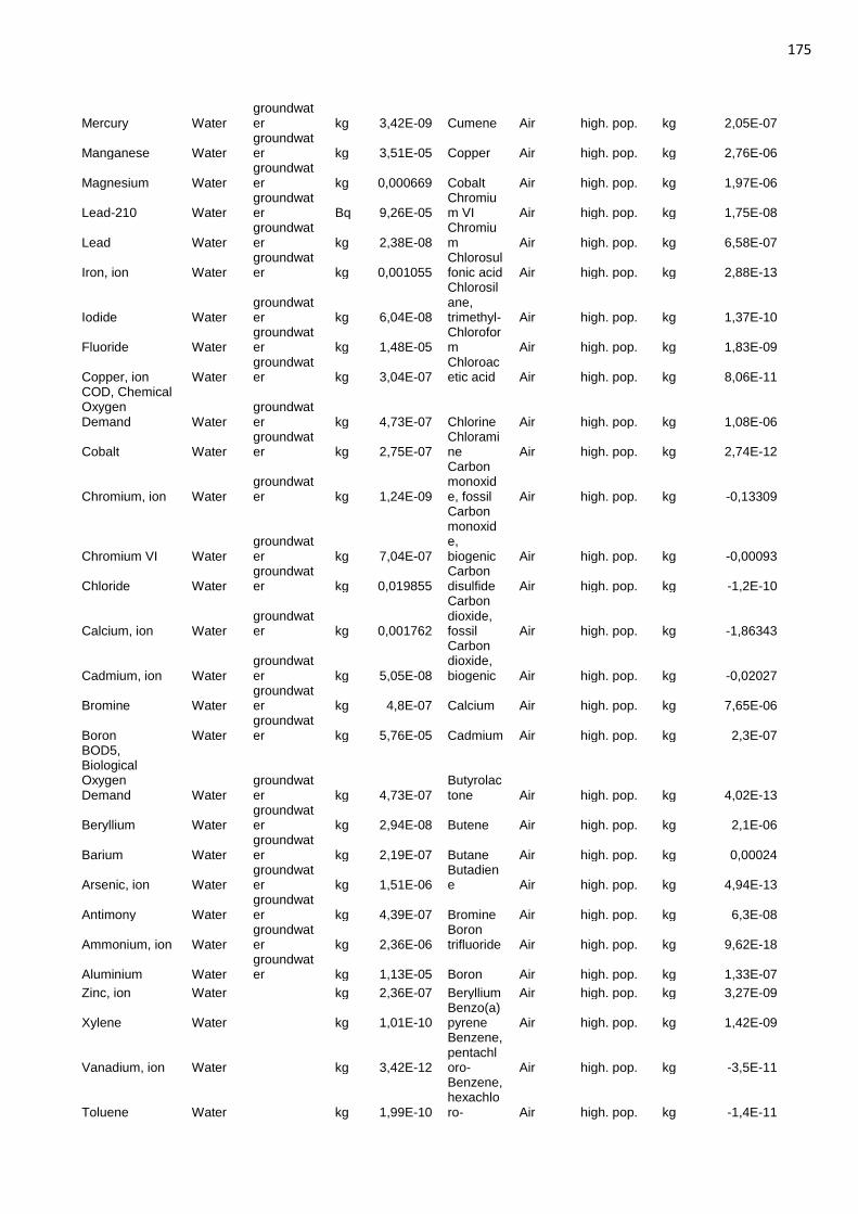
175
Mercury Water groundwater kg 3,42E-09 Cumene Air high. pop. kg 2,05E-07
Manganese Water groundwater kg 3,51E-05 Copper Air high. pop. kg 2,76E-06
Magnesium Water groundwater kg 0,000669 Cobalt Air high. pop. kg 1,97E-06
Lead-210 Water groundwater Bq 9,26E-05
Chromium VI Air high. pop. kg 1,75E-08
Lead Water groundwater kg 2,38E-08
Chromium Air high. pop. kg 6,58E-07
Iron, ion Water groundwater kg 0,001055
Chlorosulfonic acid Air high. pop. kg 2,88E-13
Iodide Water groundwater kg 6,04E-08
Chlorosilane, trimethyl- Air high. pop. kg 1,37E-10
Fluoride Water groundwater kg 1,48E-05
Chloroform Air high. pop. kg 1,83E-09
Copper, ion Water groundwater kg 3,04E-07
Chloroacetic acid Air high. pop. kg 8,06E-11
COD, Chemical Oxygen Demand Water
groundwater kg 4,73E-07 Chlorine Air high. pop. kg 1,08E-06
Cobalt Water groundwater kg 2,75E-07
Chloramine Air high. pop. kg 2,74E-12
Chromium, ion Water groundwater kg 1,24E-09
Carbon monoxide, fossil Air high. pop. kg -0,13309
Chromium VI Water groundwater kg 7,04E-07
Carbon monoxide, biogenic Air high. pop. kg -0,00093
Chloride Water groundwater kg 0,019855
Carbon disulfide Air high. pop. kg -1,2E-10
Calcium, ion Water groundwater kg 0,001762
Carbon dioxide, fossil Air high. pop. kg -1,86343
Cadmium, ion Water groundwater kg 5,05E-08
Carbon dioxide, biogenic Air high. pop. kg -0,02027
Bromine Water groundwater kg 4,8E-07 Calcium Air high. pop. kg 7,65E-06
Boron Water groundwater kg 5,76E-05 Cadmium Air high. pop. kg 2,3E-07
BOD5, Biological Oxygen Demand Water
groundwater kg 4,73E-07
Butyrolactone Air high. pop. kg 4,02E-13
Beryllium Water groundwater kg 2,94E-08 Butene Air high. pop. kg 2,1E-06
Barium Water groundwater kg 2,19E-07 Butane Air high. pop. kg 0,00024
Arsenic, ion Water groundwater kg 1,51E-06
Butadiene Air high. pop. kg 4,94E-13
Antimony Water groundwater kg 4,39E-07 Bromine Air high. pop. kg 6,3E-08
Ammonium, ion Water groundwater kg 2,36E-06
Boron trifluoride Air high. pop. kg 9,62E-18
Aluminium Water groundwater kg 1,13E-05 Boron Air high. pop. kg 1,33E-07
Zinc, ion Water
kg 2,36E-07 Beryllium Air high. pop. kg 3,27E-09
Xylene Water
kg 1,01E-10 Benzo(a)pyrene Air high. pop. kg 1,42E-09
Vanadium, ion Water
kg 3,42E-12
Benzene, pentachloro- Air high. pop. kg -3,5E-11
Toluene Water
kg 1,99E-10
Benzene, hexachloro- Air high. pop. kg -1,4E-11
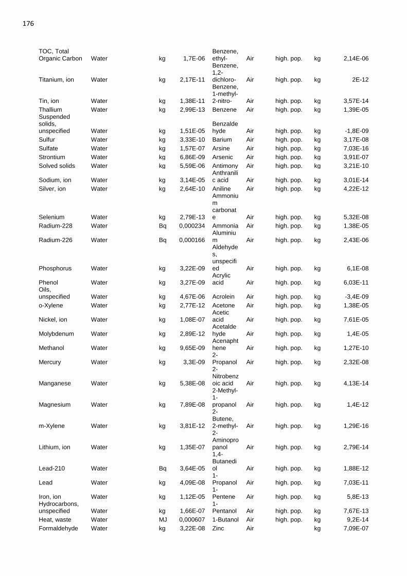
176
TOC, Total Organic Carbon Water
kg 1,7E-06
Benzene, ethyl- Air high. pop. kg 2,14E-06
Titanium, ion Water
kg 2,17E-11
Benzene, 1,2-dichloro- Air high. pop. kg 2E-12
Tin, ion Water
kg 1,38E-11
Benzene, 1-methyl-2-nitro- Air high. pop. kg 3,57E-14
Thallium Water
kg 2,99E-13 Benzene Air high. pop. kg 1,39E-05 Suspended solids, unspecified Water
kg 1,51E-05
Benzaldehyde Air high. pop. kg -1,8E-09
Sulfur Water
kg 3,33E-10 Barium Air high. pop. kg 3,17E-08
Sulfate Water
kg 1,57E-07 Arsine Air high. pop. kg 7,03E-16
Strontium Water
kg 6,86E-09 Arsenic Air high. pop. kg 3,91E-07
Solved solids Water
kg 5,59E-06 Antimony Air high. pop. kg 3,21E-10
Sodium, ion Water
kg 3,14E-05 Anthranilic acid Air high. pop. kg 3,01E-14
Silver, ion Water
kg 2,64E-10 Aniline Air high. pop. kg 4,22E-12
Selenium Water
kg 2,79E-13
Ammonium carbonate Air high. pop. kg 5,32E-08
Radium-228 Water
Bq 0,000234 Ammonia Air high. pop. kg 1,38E-05
Radium-226 Water
Bq 0,000166 Aluminium Air high. pop. kg 2,43E-06
Phosphorus Water
kg 3,22E-09
Aldehydes, unspecified Air high. pop. kg 6,1E-08
Phenol Water
kg 3,27E-09 Acrylic acid Air high. pop. kg 6,03E-11
Oils, unspecified Water
kg 4,67E-06 Acrolein Air high. pop. kg -3,4E-09
o-Xylene Water
kg 2,77E-12 Acetone Air high. pop. kg 1,38E-05
Nickel, ion Water
kg 1,08E-07 Acetic acid Air high. pop. kg 7,61E-05
Molybdenum Water
kg 2,89E-12 Acetaldehyde Air high. pop. kg 1,4E-05
Methanol Water
kg 9,65E-09 Acenaphthene Air high. pop. kg 1,27E-10
Mercury Water
kg 3,3E-09 2-Propanol Air high. pop. kg 2,32E-08
Manganese Water
kg 5,38E-08
2-Nitrobenzoic acid Air high. pop. kg 4,13E-14
Magnesium Water
kg 7,89E-08
2-Methyl-1-propanol Air high. pop. kg 1,4E-12
m-Xylene Water
kg 3,81E-12
2-Butene, 2-methyl- Air high. pop. kg 1,29E-16
Lithium, ion Water
kg 1,35E-07
2-Aminopropanol Air high. pop. kg 2,79E-14
Lead-210 Water
Bq 3,64E-05
1,4-Butanediol Air high. pop. kg 1,88E-12
Lead Water
kg 4,09E-08 1-Propanol Air high. pop. kg 7,03E-11
Iron, ion Water
kg 1,12E-05 1-Pentene Air high. pop. kg 5,8E-13
Hydrocarbons, unspecified Water
kg 1,66E-07
1-Pentanol Air high. pop. kg 7,67E-13
Heat, waste Water
MJ 0,000607 1-Butanol Air high. pop. kg 9,2E-14
Formaldehyde Water
kg 3,22E-08 Zinc Air
kg 7,09E-07
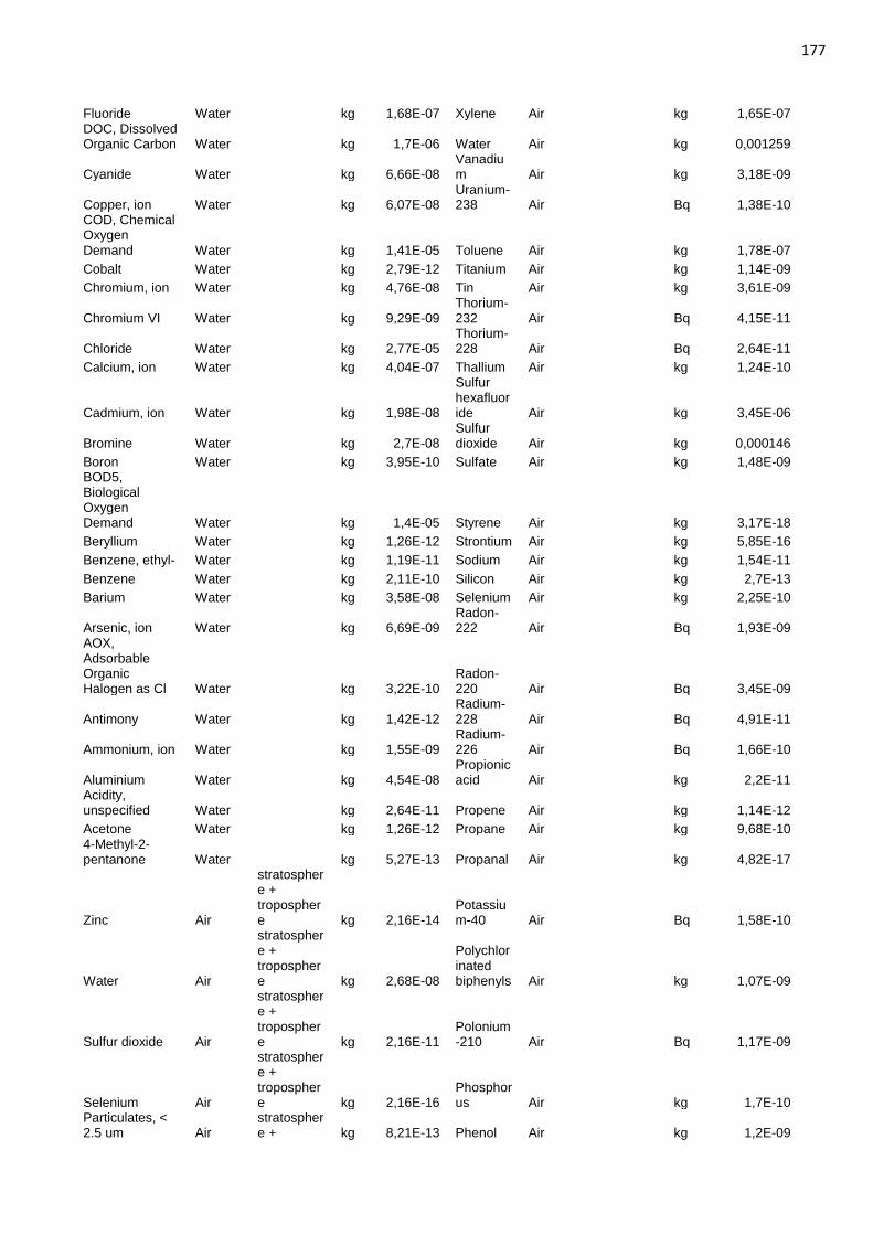
177
Fluoride Water
kg 1,68E-07 Xylene Air
kg 1,65E-07 DOC, Dissolved Organic Carbon Water
kg 1,7E-06 Water Air
kg 0,001259
Cyanide Water
kg 6,66E-08 Vanadium Air
kg 3,18E-09
Copper, ion Water
kg 6,07E-08 Uranium-238 Air
Bq 1,38E-10
COD, Chemical Oxygen Demand Water
kg 1,41E-05 Toluene Air
kg 1,78E-07
Cobalt Water
kg 2,79E-12 Titanium Air
kg 1,14E-09
Chromium, ion Water
kg 4,76E-08 Tin Air
kg 3,61E-09
Chromium VI Water
kg 9,29E-09 Thorium-232 Air
Bq 4,15E-11
Chloride Water
kg 2,77E-05 Thorium-228 Air
Bq 2,64E-11
Calcium, ion Water
kg 4,04E-07 Thallium Air
kg 1,24E-10
Cadmium, ion Water
kg 1,98E-08
Sulfur hexafluoride Air
kg 3,45E-06
Bromine Water
kg 2,7E-08 Sulfur dioxide Air
kg 0,000146
Boron Water
kg 3,95E-10 Sulfate Air
kg 1,48E-09 BOD5, Biological Oxygen Demand Water
kg 1,4E-05 Styrene Air
kg 3,17E-18
Beryllium Water
kg 1,26E-12 Strontium Air
kg 5,85E-16
Benzene, ethyl- Water
kg 1,19E-11 Sodium Air
kg 1,54E-11
Benzene Water
kg 2,11E-10 Silicon Air
kg 2,7E-13
Barium Water
kg 3,58E-08 Selenium Air
kg 2,25E-10
Arsenic, ion Water
kg 6,69E-09 Radon-222 Air
Bq 1,93E-09
AOX, Adsorbable Organic Halogen as Cl Water
kg 3,22E-10
Radon-220 Air
Bq 3,45E-09
Antimony Water
kg 1,42E-12 Radium-228 Air
Bq 4,91E-11
Ammonium, ion Water
kg 1,55E-09 Radium-226 Air
Bq 1,66E-10
Aluminium Water
kg 4,54E-08 Propionic acid Air
kg 2,2E-11
Acidity, unspecified Water
kg 2,64E-11 Propene Air
kg 1,14E-12
Acetone Water
kg 1,26E-12 Propane Air
kg 9,68E-10 4-Methyl-2-pentanone Water
kg 5,27E-13 Propanal Air
kg 4,82E-17
Zinc Air
stratosphere + troposphere kg 2,16E-14
Potassium-40 Air
Bq 1,58E-10
Water Air
stratosphere + troposphere kg 2,68E-08
Polychlorinated biphenyls Air
kg 1,07E-09
Sulfur dioxide Air
stratosphere + troposphere kg 2,16E-11
Polonium-210 Air
Bq 1,17E-09
Selenium Air
stratosphere + troposphere kg 2,16E-16
Phosphorus Air
kg 1,7E-10
Particulates, < 2.5 um Air
stratosphere + kg 8,21E-13 Phenol Air
kg 1,2E-09
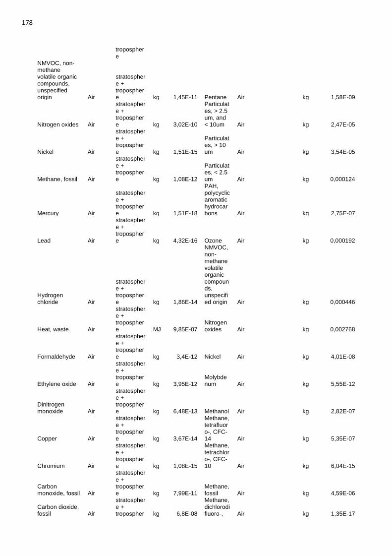
178
troposphere
NMVOC, non-methane volatile organic compounds, unspecified origin Air
stratosphere + troposphere kg 1,45E-11 Pentane Air
kg 1,58E-09
Nitrogen oxides Air
stratosphere + troposphere kg 3,02E-10
Particulates, > 2.5 um, and < 10um Air
kg 2,47E-05
Nickel Air
stratosphere + troposphere kg 1,51E-15
Particulates, > 10 um Air
kg 3,54E-05
Methane, fossil Air
stratosphere + troposphere kg 1,08E-12
Particulates, < 2.5 um Air
kg 0,000124
Mercury Air
stratosphere + troposphere kg 1,51E-18
PAH, polycyclic aromatic hydrocarbons Air
kg 2,75E-07
Lead Air
stratosphere + troposphere kg 4,32E-16 Ozone Air
kg 0,000192
Hydrogen chloride Air
stratosphere + troposphere kg 1,86E-14
NMVOC, non-methane volatile organic compounds, unspecified origin Air
kg 0,000446
Heat, waste Air
stratosphere + troposphere MJ 9,85E-07
Nitrogen oxides Air
kg 0,002768
Formaldehyde Air
stratosphere + troposphere kg 3,4E-12 Nickel Air
kg 4,01E-08
Ethylene oxide Air
stratosphere + troposphere kg 3,95E-12
Molybdenum Air
kg 5,55E-12
Dinitrogen monoxide Air
stratosphere + troposphere kg 6,48E-13 Methanol Air
kg 2,82E-07
Copper Air
stratosphere + troposphere kg 3,67E-14
Methane, tetrafluoro-, CFC-14 Air
kg 5,35E-07
Chromium Air
stratosphere + troposphere kg 1,08E-15
Methane, tetrachloro-, CFC-10 Air
kg 6,04E-15
Carbon monoxide, fossil Air
stratosphere + troposphere kg 7,99E-11
Methane, fossil Air
kg 4,59E-06
Carbon dioxide, fossil Air
stratosphere + tropospher kg 6,8E-08
Methane, dichlorodifluoro-, Air
kg 1,35E-17
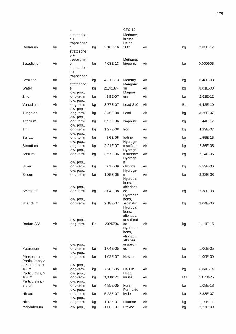
179
e CFC-12
Cadmium Air
stratosphere + troposphere kg 2,16E-16
Methane, bromo-, Halon 1001 Air
kg 2,03E-17
Butadiene Air
stratosphere + troposphere kg 4,08E-13
Methane, biogenic Air
kg 0,000905
Benzene Air
stratosphere + troposphere kg 4,31E-13 Mercury Air
kg 6,48E-08
Water Air stratosphere kg 21,41374
Manganese Air
kg 8,01E-08
Zinc Air low. pop., long-term kg 3,9E-07
Magnesium Air
kg 2,61E-12
Vanadium Air low. pop., long-term kg 3,77E-07 Lead-210 Air
Bq 6,42E-10
Tungsten Air low. pop., long-term kg 2,46E-08 Lead Air
kg 3,26E-07
Titanium Air low. pop., long-term kg 3,97E-06 Isoprene Air
kg 1,44E-17
Tin Air low. pop., long-term kg 1,27E-08 Iron Air
kg 4,23E-07
Sulfate Air low. pop., long-term kg 5,6E-05 Iodine Air
kg 1,55E-15
Strontium Air low. pop., long-term kg 2,21E-07
Hydrogen sulfide Air
kg 2,36E-05
Sodium Air low. pop., long-term kg 3,57E-06
Hydrogen fluoride Air
kg 2,14E-06
Silver Air low. pop., long-term kg 9,1E-09
Hydrogen chloride Air
kg 5,53E-06
Silicon Air low. pop., long-term kg 1,35E-05
Hydrogen Air
kg 3,32E-08
Selenium Air low. pop., long-term kg 3,04E-08
Hydrocarbons, chlorinated Air
kg 2,38E-08
Scandium Air low. pop., long-term kg 2,18E-07
Hydrocarbons, aromatic Air
kg 2,04E-06
Radon-222 Air low. pop., long-term Bq 2325706
Hydrocarbons, aliphatic, unsaturated Air
kg 1,14E-15
Potassium Air low. pop., long-term kg 1,04E-05
Hydrocarbons, aliphatic, alkanes, unspecified Air
kg 1,06E-05
Phosphorus Air low. pop., long-term kg 1,02E-07 Hexane Air
kg 1,09E-09
Particulates, > 2.5 um, and < 10um Air
low. pop., long-term kg 7,28E-05 Helium Air
kg 6,84E-14
Particulates, > 10 um Air
low. pop., long-term kg 0,000121
Heat, waste Air
MJ 10,73625
Particulates, < 2.5 um Air
low. pop., long-term kg 4,85E-05 Furan Air
kg 1,08E-18
Nitrate Air low. pop., long-term kg 5,22E-07
Formaldehyde Air
kg 2,88E-07
Nickel Air low. pop., long-term kg 1,12E-07 Fluorine Air
kg 1,19E-11
Molybdenum Air low. pop., kg 1,06E-07 Ethyne Air
kg 2,27E-09
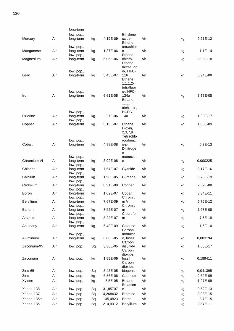
180
long-term
Mercury Air low. pop., long-term kg 4,19E-09
Ethylene oxide Air
kg 9,21E-12
Manganese Air low. pop., long-term kg 1,37E-06
Ethene, tetrachloro- Air
kg 1,1E-14
Magnesium Air low. pop., long-term kg 6,06E-06
Ethene, chloro- Air
kg 5,08E-18
Lead Air low. pop., long-term kg 5,45E-07
Ethane, hexafluoro-, HFC-116 Air
kg 5,94E-08
Iron Air low. pop., long-term kg 6,61E-05
Ethane, 1,1,1,2-tetrafluoro-, HFC-134a Air
kg 3,57E-08
Fluorine Air low. pop., long-term kg 3,7E-06
Ethane, 1,1,1-trichloro-, HCFC-140 Air
kg 1,39E-17
Copper Air low. pop., long-term kg 5,15E-07 Ethane Air
kg 1,88E-09
Cobalt Air low. pop., long-term kg 4,88E-08
Dioxin, 2,3,7,8 Tetrachlorodibenzo-p- Air
kg 6,3E-13
Chromium VI Air low. pop., long-term kg 3,92E-08
Dinitrogen monoxide Air
kg 0,000225
Chlorine Air low. pop., long-term kg 7,54E-07 Cyanide Air
kg 3,17E-16
Calcium Air low. pop., long-term kg 1,98E-05 Cumene Air
kg 6,73E-19
Cadmium Air low. pop., long-term kg 8,31E-09 Copper Air
kg 7,52E-08
Boron Air low. pop., long-term kg 1,02E-07 Cobalt Air
kg 3,84E-11
Beryllium Air low. pop., long-term kg 7,67E-09
Chromium VI Air
kg 5,76E-12
Barium Air low. pop., long-term kg 3,52E-07
Chromium Air
kg 7,63E-08
Arsenic Air low. pop., long-term kg 3,22E-07
Chloroform Air
kg 7,5E-18
Antimony Air low. pop., long-term kg 5,48E-09 Chlorine Air
kg 1,6E-10
Aluminium Air low. pop., long-term kg 6,08E-05
Carbon monoxide, fossil Air
kg 0,003194
Zirconium-95 Air low. pop. Bq 3,36E-05 Carbon disulfide Air
kg 1,65E-17
Zirconium Air low. pop. kg 1,55E-09
Carbon dioxide, fossil Air
kg 0,189411
Zinc-65 Air low. pop. Bq 3,43E-05
Carbon dioxide, biogenic Air
kg 0,041395
Zinc Air low. pop. kg 6,86E-06 Cadmium Air
kg 2,62E-09
Xylene Air low. pop. kg 5,5E-05 Butane Air
kg 1,27E-09
Xenon-138 Air low. pop. Bq 31,85707 Butadiene Air
kg 9,52E-13
Xenon-137 Air low. pop. Bq 4,268432 Bromine Air
kg 3,03E-15
Xenon-135m Air low. pop. Bq 135,4823 Boron Air
kg 3,7E-15
Xenon-135 Air low. pop. Bq 214,9312 Beryllium Air
kg 2,87E-11
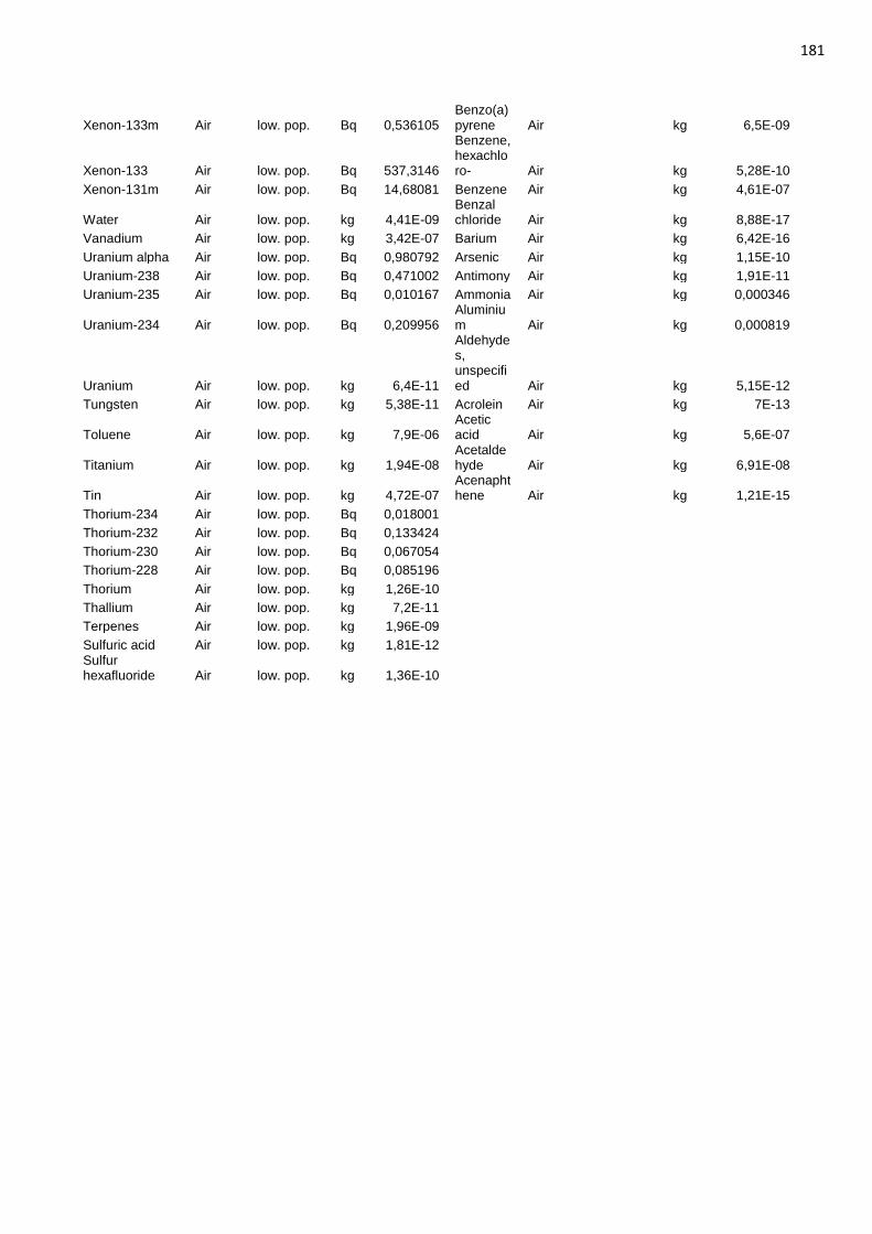
181
Xenon-133m Air low. pop. Bq 0,536105 Benzo(a)pyrene Air
kg 6,5E-09
Xenon-133 Air low. pop. Bq 537,3146
Benzene, hexachloro- Air
kg 5,28E-10
Xenon-131m Air low. pop. Bq 14,68081 Benzene Air
kg 4,61E-07
Water Air low. pop. kg 4,41E-09 Benzal chloride Air
kg 8,88E-17
Vanadium Air low. pop. kg 3,42E-07 Barium Air
kg 6,42E-16
Uranium alpha Air low. pop. Bq 0,980792 Arsenic Air
kg 1,15E-10
Uranium-238 Air low. pop. Bq 0,471002 Antimony Air
kg 1,91E-11
Uranium-235 Air low. pop. Bq 0,010167 Ammonia Air
kg 0,000346
Uranium-234 Air low. pop. Bq 0,209956 Aluminium Air
kg 0,000819
Uranium Air low. pop. kg 6,4E-11
Aldehydes, unspecified Air
kg 5,15E-12
Tungsten Air low. pop. kg 5,38E-11 Acrolein Air
kg 7E-13
Toluene Air low. pop. kg 7,9E-06 Acetic acid Air
kg 5,6E-07
Titanium Air low. pop. kg 1,94E-08 Acetaldehyde Air
kg 6,91E-08
Tin Air low. pop. kg 4,72E-07 Acenaphthene Air
kg 1,21E-15
Thorium-234 Air low. pop. Bq 0,018001 Thorium-232 Air low. pop. Bq 0,133424 Thorium-230 Air low. pop. Bq 0,067054 Thorium-228 Air low. pop. Bq 0,085196 Thorium Air low. pop. kg 1,26E-10 Thallium Air low. pop. kg 7,2E-11 Terpenes Air low. pop. kg 1,96E-09 Sulfuric acid Air low. pop. kg 1,81E-12 Sulfur
hexafluoride Air low. pop. kg 1,36E-10
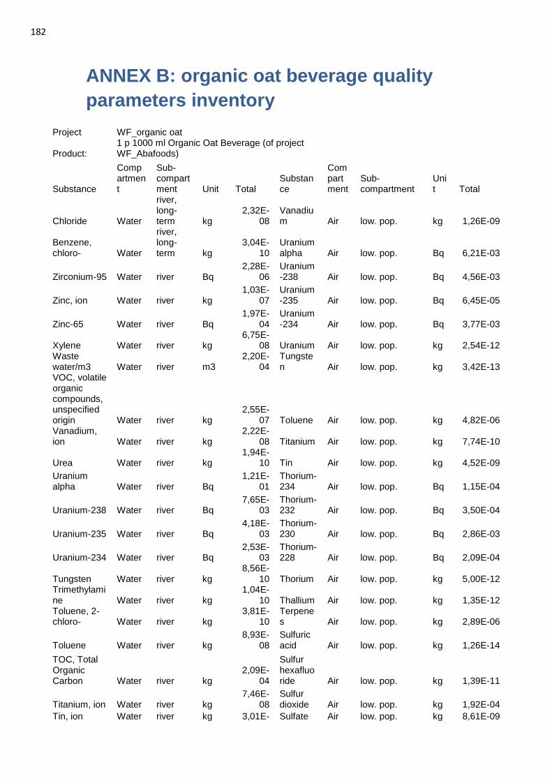
182
ANNEX B: organic oat beverage quality
parameters inventory
Project WF_organic oat
Product: 1 p 1000 ml Organic Oat Beverage (of project WF_Abafoods)
Substance
Compartment
Sub-compartment Unit Total
Substance
Compartment
Sub-compartment
Unit Total
Chloride Water
river, long-term kg
2,32E-08
Vanadium Air low. pop. kg 1,26E-09
Benzene, chloro- Water
river, long-term kg
3,04E-10
Uranium alpha Air low. pop. Bq 6,21E-03
Zirconium-95 Water river Bq 2,28E-
06 Uranium-238 Air low. pop. Bq 4,56E-03
Zinc, ion Water river kg 1,03E-
07 Uranium-235 Air low. pop. Bq 6,45E-05
Zinc-65 Water river Bq 1,97E-
04 Uranium-234 Air low. pop. Bq 3,77E-03
Xylene Water river kg 6,75E-
08 Uranium Air low. pop. kg 2,54E-12 Waste water/m3 Water river m3
2,20E-04
Tungsten Air low. pop. kg 3,42E-13
VOC, volatile organic compounds, unspecified origin Water river kg
2,55E-07 Toluene Air low. pop. kg 4,82E-06
Vanadium, ion Water river kg
2,22E-08 Titanium Air low. pop. kg 7,74E-10
Urea Water river kg 1,94E-
10 Tin Air low. pop. kg 4,52E-09
Uranium alpha Water river Bq
1,21E-01
Thorium-234 Air low. pop. Bq 1,15E-04
Uranium-238 Water river Bq 7,65E-
03 Thorium-232 Air low. pop. Bq 3,50E-04
Uranium-235 Water river Bq 4,18E-
03 Thorium-230 Air low. pop. Bq 2,86E-03
Uranium-234 Water river Bq 2,53E-
03 Thorium-228 Air low. pop. Bq 2,09E-04
Tungsten Water river kg 8,56E-
10 Thorium Air low. pop. kg 5,00E-12 Trimethylamine Water river kg
1,04E-10 Thallium Air low. pop. kg 1,35E-12
Toluene, 2-chloro- Water river kg
3,81E-10
Terpenes Air low. pop. kg 2,89E-06
Toluene Water river kg 8,93E-
08 Sulfuric acid Air low. pop. kg 1,26E-14
TOC, Total Organic Carbon Water river kg
2,09E-04
Sulfur hexafluoride Air low. pop. kg 1,39E-11
Titanium, ion Water river kg 7,46E-
08 Sulfur dioxide Air low. pop. kg 1,92E-04
Tin, ion Water river kg 3,01E- Sulfate Air low. pop. kg 8,61E-09
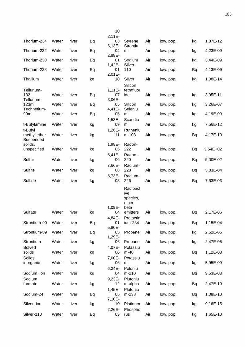
183
10
Thorium-234 Water river Bq 2,11E-
03 Styrene Air low. pop. kg 1,87E-12
Thorium-232 Water river Bq 6,13E-
04 Strontium Air low. pop. kg 4,23E-09
Thorium-230 Water river Bq 2,88E-
01 Sodium Air low. pop. kg 3,44E-09
Thorium-228 Water river Bq 1,42E-
01 Silver-110 Air low. pop. Bq 4,13E-09
Thallium Water river kg 2,01E-
10 Silver Air low. pop. kg 1,08E-14
Tellurium-132 Water river Bq
1,11E-07
Silicon tetrafluoride Air low. pop. kg 3,95E-11
Tellurium-123m Water river Bq
3,06E-05 Silicon Air low. pop. kg 3,26E-07
Technetium-99m Water river Bq
4,41E-05
Selenium Air low. pop. kg 4,19E-09
t-Butylamine Water river kg 1,53E-
09 Scandium Air low. pop. kg 7,56E-12
t-Butyl methyl ether Water river kg
1,26E-11
Ruthenium-103 Air low. pop. Bq 4,17E-10
Suspended solids, unspecified Water river kg
1,98E-05
Radon-222 Air low. pop. Bq 3,54E+02
Sulfur Water river kg 6,41E-
06 Radon-220 Air low. pop. Bq 5,00E-02
Sulfite Water river kg 7,66E-
08 Radium-228 Air low. pop. Bq 3,83E-04
Sulfide Water river kg 5,73E-
08 Radium-226 Air low. pop. Bq 7,53E-03
Sulfate Water river kg 1,09E-
04
Radioactive species, other beta emitters Air low. pop. Bq 2,17E-06
Strontium-90 Water river Bq 4,84E-
01 Protactinium-234 Air low. pop. Bq 1,15E-04
Strontium-89 Water river Bq 5,80E-
05 Propene Air low. pop. kg 2,62E-05
Strontium Water river kg 1,29E-
06 Propane Air low. pop. kg 2,47E-05
Solved solids Water river kg
4,07E-06
Potassium-40 Air low. pop. Bq 1,12E-03
Solids, inorganic Water river kg
7,00E-06
Potassium Air low. pop. kg 5,95E-09
Sodium, ion Water river kg 6,24E-
04 Polonium-210 Air low. pop. Bq 9,53E-03
Sodium formate Water river kg
9,23E-12
Plutonium-alpha Air low. pop. Bq 2,47E-10
Sodium-24 Water river Bq 1,45E-
05 Plutonium-238 Air low. pop. Bq 1,08E-10
Silver, ion Water river kg 7,10E-
10 Platinum Air low. pop. kg 9,16E-15
Silver-110 Water river Bq 2,26E-
03 Phosphorus Air low. pop. kg 1,65E-10
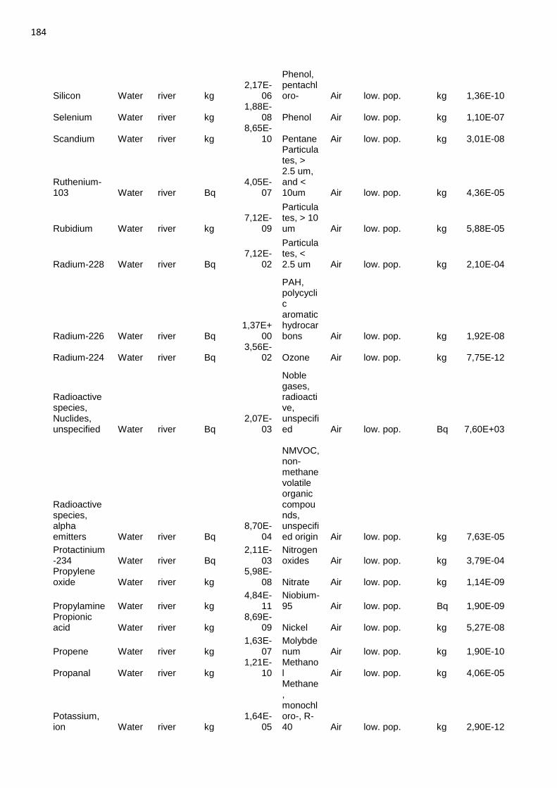
184
Silicon Water river kg 2,17E-
06
Phenol, pentachloro- Air low. pop. kg 1,36E-10
Selenium Water river kg 1,88E-
08 Phenol Air low. pop. kg 1,10E-07
Scandium Water river kg 8,65E-
10 Pentane Air low. pop. kg 3,01E-08
Ruthenium-103 Water river Bq
4,05E-07
Particulates, > 2.5 um, and < 10um Air low. pop. kg 4,36E-05
Rubidium Water river kg 7,12E-
09
Particulates, > 10 um Air low. pop. kg 5,88E-05
Radium-228 Water river Bq 7,12E-
02
Particulates, < 2.5 um Air low. pop. kg 2,10E-04
Radium-226 Water river Bq 1,37E+
00
PAH, polycyclic aromatic hydrocarbons Air low. pop. kg 1,92E-08
Radium-224 Water river Bq 3,56E-
02 Ozone Air low. pop. kg 7,75E-12
Radioactive species, Nuclides, unspecified Water river Bq
2,07E-03
Noble gases, radioactive, unspecified Air low. pop. Bq 7,60E+03
Radioactive species, alpha emitters Water river Bq
8,70E-04
NMVOC, non-methane volatile organic compounds, unspecified origin Air low. pop. kg 7,63E-05
Protactinium-234 Water river Bq
2,11E-03
Nitrogen oxides Air low. pop. kg 3,79E-04
Propylene oxide Water river kg
5,98E-08 Nitrate Air low. pop. kg 1,14E-09
Propylamine Water river kg 4,84E-
11 Niobium-95 Air low. pop. Bq 1,90E-09
Propionic acid Water river kg
8,69E-09 Nickel Air low. pop. kg 5,27E-08
Propene Water river kg 1,63E-
07 Molybdenum Air low. pop. kg 1,90E-10
Propanal Water river kg 1,21E-
10 Methanol Air low. pop. kg 4,06E-05
Potassium, ion Water river kg
1,64E-05
Methane, monochloro-, R-40 Air low. pop. kg 2,90E-12
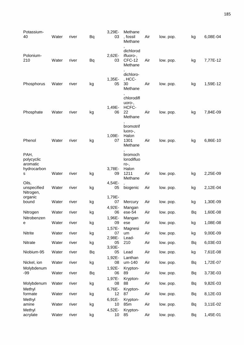
185
Potassium-40 Water river Bq
3,29E-03
Methane, fossil Air low. pop. kg 6,08E-04
Polonium-210 Water river Bq
2,62E-03
Methane, dichlorodifluoro-, CFC-12 Air low. pop. kg 7,77E-12
Phosphorus Water river kg 1,35E-
05
Methane, dichloro-, HCC-30 Air low. pop. kg 1,59E-12
Phosphate Water river kg 1,49E-
06
Methane, chlorodifluoro-, HCFC-22 Air low. pop. kg 7,84E-09
Phenol Water river kg 1,09E-
07
Methane, bromotrifluoro-, Halon 1301 Air low. pop. kg 6,86E-10
PAH, polycyclic aromatic hydrocarbons Water river kg
3,78E-09
Methane, bromochlorodifluoro-, Halon 1211 Air low. pop. kg 2,25E-09
Oils, unspecified Water river kg
4,54E-05
Methane, biogenic Air low. pop. kg 2,12E-04
Nitrogen, organic bound Water river kg
1,79E-07 Mercury Air low. pop. kg 1,30E-09
Nitrogen Water river kg 4,92E-
06 Manganese-54 Air low. pop. Bq 1,60E-08
Nitrobenzene Water river kg
1,96E-09
Manganese Air low. pop. kg 1,08E-08
Nitrite Water river kg 1,57E-
07 Magnesium Air low. pop. kg 9,00E-09
Nitrate Water river kg 2,98E-
05 Lead-210 Air low. pop. Bq 6,03E-03
Niobium-95 Water river Bq 3,93E-
05 Lead Air low. pop. kg 7,61E-08
Nickel, ion Water river kg 1,92E-
08 Lanthanum-140 Air low. pop. Bq 1,72E-07
Molybdenum-99 Water river Bq
1,92E-06
Krypton-89 Air low. pop. Bq 3,73E-03
Molybdenum Water river kg 1,97E-
08 Krypton-88 Air low. pop. Bq 9,82E-03
Methyl formate Water river kg
6,76E-12
Krypton-87 Air low. pop. Bq 8,12E-03
Methyl amine Water river kg
6,91E-10
Krypton-85m Air low. pop. Bq 3,11E-02
Methyl acrylate Water river kg
4,52E-10
Krypton-85 Air low. pop. Bq 1,45E-01
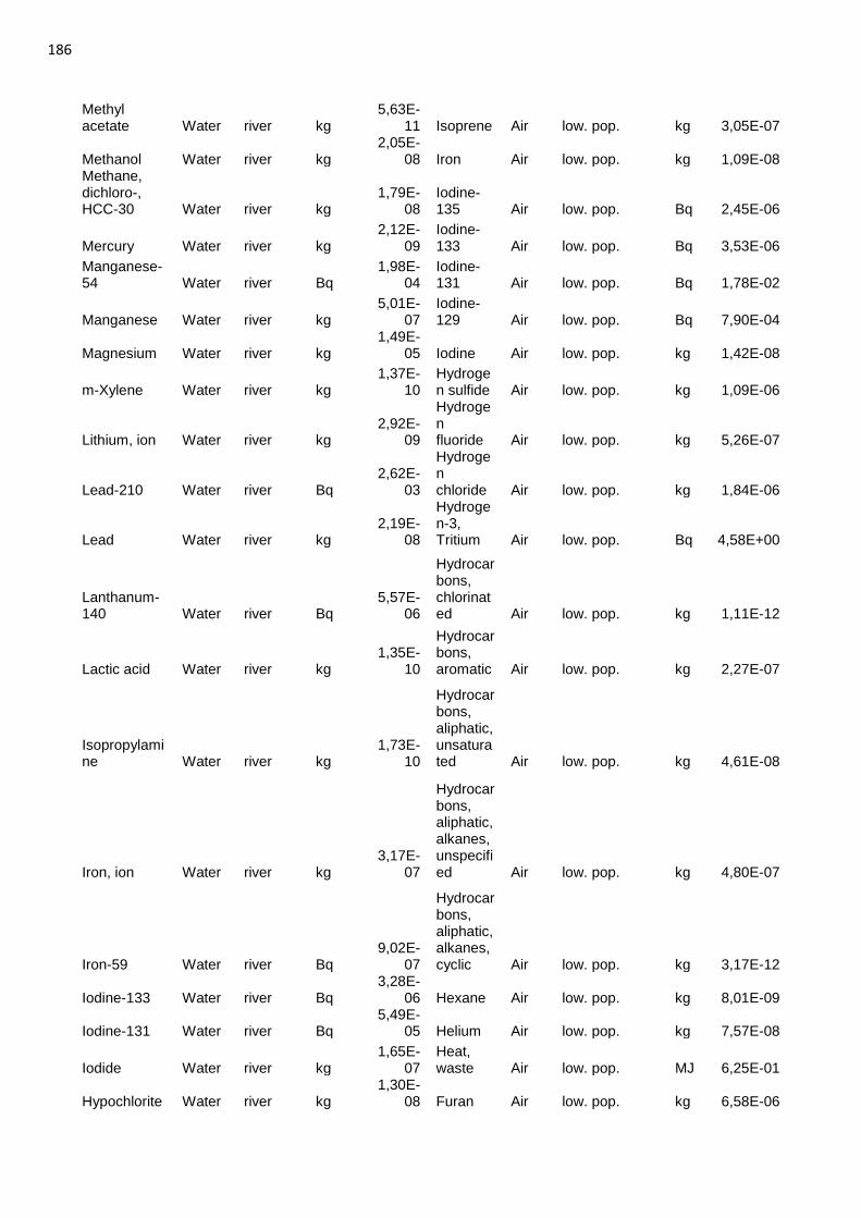
186
Methyl acetate Water river kg
5,63E-11 Isoprene Air low. pop. kg 3,05E-07
Methanol Water river kg 2,05E-
08 Iron Air low. pop. kg 1,09E-08 Methane, dichloro-, HCC-30 Water river kg
1,79E-08
Iodine-135 Air low. pop. Bq 2,45E-06
Mercury Water river kg 2,12E-
09 Iodine-133 Air low. pop. Bq 3,53E-06
Manganese-54 Water river Bq
1,98E-04
Iodine-131 Air low. pop. Bq 1,78E-02
Manganese Water river kg 5,01E-
07 Iodine-129 Air low. pop. Bq 7,90E-04
Magnesium Water river kg 1,49E-
05 Iodine Air low. pop. kg 1,42E-08
m-Xylene Water river kg 1,37E-
10 Hydrogen sulfide Air low. pop. kg 1,09E-06
Lithium, ion Water river kg 2,92E-
09
Hydrogen fluoride Air low. pop. kg 5,26E-07
Lead-210 Water river Bq 2,62E-
03
Hydrogen chloride Air low. pop. kg 1,84E-06
Lead Water river kg 2,19E-
08
Hydrogen-3, Tritium Air low. pop. Bq 4,58E+00
Lanthanum-140 Water river Bq
5,57E-06
Hydrocarbons, chlorinated Air low. pop. kg 1,11E-12
Lactic acid Water river kg 1,35E-
10
Hydrocarbons, aromatic Air low. pop. kg 2,27E-07
Isopropylamine Water river kg
1,73E-10
Hydrocarbons, aliphatic, unsaturated Air low. pop. kg 4,61E-08
Iron, ion Water river kg 3,17E-
07
Hydrocarbons, aliphatic, alkanes, unspecified Air low. pop. kg 4,80E-07
Iron-59 Water river Bq 9,02E-
07
Hydrocarbons, aliphatic, alkanes, cyclic Air low. pop. kg 3,17E-12
Iodine-133 Water river Bq 3,28E-
06 Hexane Air low. pop. kg 8,01E-09
Iodine-131 Water river Bq 5,49E-
05 Helium Air low. pop. kg 7,57E-08
Iodide Water river kg 1,65E-
07 Heat, waste Air low. pop. MJ 6,25E-01
Hypochlorite Water river kg 1,30E-
08 Furan Air low. pop. kg 6,58E-06
187
Hydroxide Water river kg 1,75E-
09 Formic acid Air low. pop. kg 2,32E-05
Hydrogen sulfide Water river kg
3,20E-09
Formaldehyde Air low. pop. kg 2,06E-05
Hydrogen peroxide Water river kg
1,56E-09 Fluorine Air low. pop. kg 3,22E-09
Hydrogen-3, Tritium Water river Bq
3,48E+01 Ethyne Air low. pop. kg 7,74E-06
Hydrocarbons, unspecified Water river kg
3,82E-06
Ethylene oxide Air low. pop. kg 1,26E-13
Hydrocarbons, aromatic Water river kg
3,75E-07
Ethene, tetrachloro- Air low. pop. kg 2,35E-13
Hydrocarbons, aliphatic, unsaturated Water river kg
1,06E-08 Ethene Air low. pop. kg 3,74E-05
Hydrocarbons, aliphatic, alkanes, unspecified Water river kg
9,26E-08 Ethanol Air low. pop. kg 3,28E-07
Heat, waste Water river MJ 9,78E-
02
Ethane, 1,2-dichloro-1,1,2,2-tetrafluoro-, CFC-114 Air low. pop. kg 3,79E-10
Formic acid Water river kg 4,44E-
11
Ethane, 1,2-dichloro- Air low. pop. kg 2,19E-13
Formate Water river kg 1,97E-
07
Ethane, 1,1,1,2-tetrafluoro-, HFC-134a Air low. pop. kg 2,35E-11
Formamide Water river kg 1,53E-
10
Ethane, 1,1,1-trichloro-, HCFC-140 Air low. pop. kg 1,10E-13
Formaldehyde Water river kg
1,94E-09 Ethane Air low. pop. kg 3,61E-05
Fluosilicic acid Water river kg
1,41E-07
Dioxin, 2,3,7,8 Tetrachlorodibenzo-p- Air low. pop. kg 7,24E-15
Fluoride Water river kg 1,28E-
06
Dinitrogen monoxide Air low. pop. kg 4,35E-05
Ethylene oxide Water river kg
3,81E-09 Cyanide Air low. pop. kg 5,78E-06
Ethylene diamine Water river kg
7,73E-11 Cumene Air low. pop. kg 2,98E-14
Ethylamine Water river kg 3,50E-
10 Copper Air low. pop. kg 8,53E-08
188
Ethyl acetate Water river kg 2,70E-
10 Cobalt-60 Air low. pop. Bq 3,84E-07
Ethene, chloro- Water river kg
3,12E-11
Cobalt-58 Air low. pop. Bq 4,34E-08
Ethene Water river kg 1,53E-
08 Cobalt Air low. pop. kg 4,12E-09
Ethanol Water river kg 1,80E-
07 Chromium VI Air low. pop. kg 7,24E-09
Ethane, 1,2-dichloro- Water river kg
5,46E-09
Chromium-51 Air low. pop. Bq 3,12E-08
DOC, Dissolved Organic Carbon Water river kg
5,29E-05
Chromium Air low. pop. kg 2,89E-07
Dipropylamine Water river kg
1,72E-10
Chloroform Air low. pop. kg 5,37E-13
Dimethylamine Water river kg
6,42E-09 Chlorine Air low. pop. kg 1,13E-10
Diethylamine Water river kg 3,59E-
10 Cesium-137 Air low. pop. Bq 4,13E-07
Dichromate Water river kg 1,84E-
09 Cesium-134 Air low. pop. Bq 2,33E-08
Cyanide Water river kg 2,63E-
08 Cerium-141 Air low. pop. Bq 4,87E-07
Cumene Water river kg 8,75E-
08
Carbon monoxide, fossil Air low. pop. kg 2,07E-03
Copper, ion Water river kg 2,00E-
08
Carbon monoxide, biogenic Air low. pop. kg 1,45E-06
COD, Chemical Oxygen Demand Water river kg
4,63E-04
Carbon disulfide Air low. pop. kg 5,12E-07
Cobalt-60 Water river Bq 2,57E-
03
Carbon dioxide, land transformation Air low. pop. kg 4,19E-02
Cobalt-58 Water river Bq 3,13E-
03
Carbon dioxide, fossil Air low. pop. kg 4,47E-02
Cobalt-57 Water river Bq 1,18E-
05
Carbon dioxide, biogenic Air low. pop. kg 1,56E-03
Cobalt Water river kg 6,16E-
09 Carbon-14 Air low. pop. Bq 8,22E-01
Chromium, ion Water river kg
1,46E-08 Calcium Air low. pop. kg 3,52E-09
Chromium VI Water river kg 2,79E-
07 Cadmium Air low. pop. kg 6,83E-09
Chromium-51 Water river Bq
5,49E-04 Butane Air low. pop. kg 1,54E-06
Chlorosulfonic acid Water river kg
2,63E-09
Butadiene Air low. pop. kg 1,30E-14
Chloroform Water river kg 1,31E-
10 Bromine Air low. pop. kg 2,86E-08
189
Chloroacetyl chloride Water river kg
1,35E-10 Boron Air low. pop. kg 2,30E-07
Chloroacetic acid Water river kg
3,26E-08
Beryllium Air low. pop. kg 1,37E-11
Chlorine Water river kg 2,42E-
09 Benzo(a)pyrene Air low. pop. kg 5,38E-10
Chlorinated solvents, unspecified Water river kg
9,05E-10
Benzene, ethyl- Air low. pop. kg 5,15E-13
Chloride Water river kg 8,96E-
04 Benzene Air low. pop. kg 7,89E-06
Chlorate Water river kg 9,07E-
07 Barium-140 Air low. pop. Bq 2,01E-06
Chloramine Water river kg 2,05E-
09 Barium Air low. pop. kg 4,38E-09
Cesium-137 Water river Bq 1,17E-
03 Arsenic Air low. pop. kg 2,27E-08
Cesium-136 Water river Bq 3,71E-
07 Argon-41 Air low. pop. Bq 4,59E-02
Cesium-134 Water river Bq 2,60E-
04 Antimony-125 Air low. pop. Bq 3,09E-08
Cesium Water river kg 7,12E-
10 Antimony-124 Air low. pop. Bq 2,96E-09
Cerium-144 Water river Bq 6,36E-
07 Antimony Air low. pop. kg 2,80E-09
Cerium-141 Water river Bq 2,09E-
06 Ammonia Air low. pop. kg 6,40E-05
Carboxylic acids, unspecified Water river kg
2,62E-06
Aluminium Air low. pop. kg 3,04E-08
Carbonate Water river kg 2,29E-
06
Aldehydes, unspecified Air low. pop. kg 3,76E-10
Carbon disulfide Water river kg
1,95E-10
Aerosols, radioactive, unspecified Air low. pop. Bq 2,01E-04
Calcium, ion Water river kg 3,70E-
05
Actinides, radioactive, unspecified Air low. pop. Bq 1,13E-05
Cadmium, ion Water river kg
3,60E-09 Acrolein Air low. pop. kg 3,65E-12
Butyrolactone Water river kg
2,93E-13
Acetonitrile Air low. pop. kg 3,46E-06
Butyl acetate Water river kg 1,85E-
10 Acetone Air low. pop. kg 1,34E-05
Butene Water river kg 1,76E-
08 Acetic acid Air low. pop. kg 8,28E-05
Bromine Water river kg 7,01E-
07 Acetaldehyde Air low. pop. kg 1,26E-05
Bromide Water river kg 7,38E-
07 Acenaphthene Air low. pop. kg 2,79E-15
Bromate Water river kg 9,32E- Zinc Air high. pop. kg 7,51E-08
190
08
Boron Water river kg 1,01E-
07 Xylene Air high. pop. kg 1,00E-07
Borate Water river kg 1,20E-
08 Water Air high. pop. kg 2,04E-10 BOD5, Biological Oxygen Demand Water river kg
2,01E-04
Vanadium Air high. pop. kg 1,89E-07
Beryllium Water river kg 4,07E-
11 Uranium-238 Air high. pop. Bq 1,84E-04
Benzene, ethyl- Water river kg
1,71E-08 Uranium Air high. pop. kg 4,65E-11
Benzene, chloro- Water river kg
1,47E-07
Trimethylamine Air high. pop. kg 4,32E-11
Benzene, 1,2-dichloro- Water river kg
1,32E-08
Toluene, 2-chloro- Air high. pop. kg 2,40E-10
Benzene Water river kg 2,89E-
07 Toluene Air high. pop. kg 2,33E-07
Barium-140 Water river Bq 5,23E-
06 Titanium Air high. pop. kg 1,26E-08
Barium Water river kg 6,33E-
07 Tin Air high. pop. kg 5,43E-11
Arsenic, ion Water river kg 1,37E-
07 Thorium-232 Air high. pop. Bq 6,43E-05
AOX, Adsorbable Organic Halogen as Cl Water river kg
8,65E-07
Thorium-228 Air high. pop. Bq 1,01E-04
Antimony-125 Water river Bq
3,03E-04 Thorium Air high. pop. kg 3,49E-11
Antimony-124 Water river Bq
2,69E-04 Thallium Air high. pop. kg 4,67E-11
Antimony-122 Water river Bq
1,19E-06
t-Butylamine Air high. pop. kg 6,39E-10
Antimony Water river kg 8,07E-
08
t-Butyl methyl ether Air high. pop. kg 7,32E-10
Aniline Water river kg 7,61E-
10 Sulfuric acid Air high. pop. kg 4,29E-11
Ammonium, ion Water river kg
7,93E-06
Sulfur trioxide Air high. pop. kg 5,19E-09
Aluminium Water river kg 2,50E-
06 Sulfur dioxide Air high. pop. kg 1,38E-04
Acrylate, ion Water river kg 4,83E-
11 Sulfate Air high. pop. kg 5,73E-06 Acidity, unspecified Water river kg
3,09E-08 Styrene Air high. pop. kg 2,58E-10
Acetyl chloride Water river kg
6,56E-11
Strontium Air high. pop. kg 3,58E-09
Acetonitrile Water river kg 7,23E-
10
Sodium hydroxide Air high. pop. kg 2,05E-10
Acetone Water river kg 2,50E-
10 Sodium formate Air high. pop. kg 3,84E-12
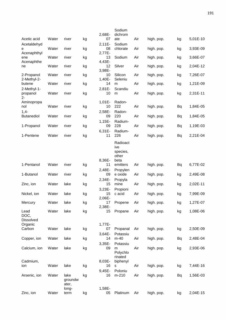
191
Acetic acid Water river kg 2,68E-
07
Sodium dichromate Air high. pop. kg 5,01E-10
Acetaldehyde Water river kg
2,11E-08
Sodium chlorate Air high. pop. kg 3,93E-09
Acenaphthylene Water river kg
2,77E-13 Sodium Air high. pop. kg 3,66E-07
Acenaphthene Water river kg
4,43E-12 Silver Air high. pop. kg 2,04E-12
2-Propanol Water river kg 3,98E-
10 Silicon Air high. pop. kg 7,26E-07 2-Methyl-2-butene Water river kg
1,40E-14
Selenium Air high. pop. kg 1,21E-09
2-Methyl-1-propanol Water river kg
2,81E-10
Scandium Air high. pop. kg 2,31E-11
2-Aminopropanol Water river kg
1,01E-10
Radon-222 Air high. pop. Bq 1,84E-05
1,4-Butanediol Water river kg
2,58E-09
Radon-220 Air high. pop. Bq 1,84E-05
1-Propanol Water river kg 1,15E-
09 Radium-228 Air high. pop. Bq 1,19E-03
1-Pentene Water river kg 6,31E-
11 Radium-226 Air high. pop. Bq 2,21E-04
1-Pentanol Water river kg 8,36E-
11
Radioactive species, other beta emitters Air high. pop. Bq 6,77E-02
1-Butanol Water river kg 2,48E-
09 Propylene oxide Air high. pop. kg 2,49E-08
Zinc, ion Water lake kg 2,34E-
15 Propylamine Air high. pop. kg 2,02E-11
Nickel, ion Water lake kg 3,23E-
15 Propionic acid Air high. pop. kg 7,99E-09
Mercury Water lake kg 2,06E-
17 Propene Air high. pop. kg 1,27E-07
Lead Water lake kg 2,38E-
15 Propane Air high. pop. kg 1,08E-06 DOC, Dissolved Organic Carbon Water lake kg
1,77E-07 Propanal Air high. pop. kg 2,50E-09
Copper, ion Water lake kg 3,64E-
14 Potassium-40 Air high. pop. Bq 2,48E-04
Calcium, ion Water lake kg 3,35E-
09 Potassium Air high. pop. kg 2,93E-06
Cadmium, ion Water lake kg
8,03E-16
Polychlorinated biphenyls Air high. pop. kg 7,44E-16
Arsenic, ion Water lake kg 9,45E-
16 Polonium-210 Air high. pop. Bq 1,56E-03
Zinc, ion Water
groundwater, long-term kg
1,58E-05 Platinum Air high. pop. kg 2,04E-15
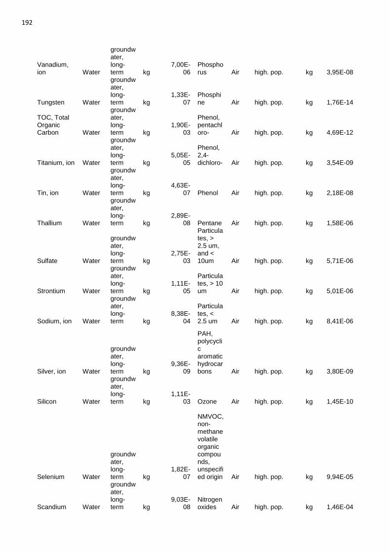
192
Vanadium, ion Water
groundwater, long-term kg
7,00E-06
Phosphorus Air high. pop. kg 3,95E-08
Tungsten Water
groundwater, long-term kg
1,33E-07
Phosphine Air high. pop. kg 1,76E-14
TOC, Total Organic Carbon Water
groundwater, long-term kg
1,90E-03
Phenol, pentachloro- Air high. pop. kg 4,69E-12
Titanium, ion Water
groundwater, long-term kg
5,05E-05
Phenol, 2,4-dichloro- Air high. pop. kg 3,54E-09
Tin, ion Water
groundwater, long-term kg
4,63E-07 Phenol Air high. pop. kg 2,18E-08
Thallium Water
groundwater, long-term kg
2,89E-08 Pentane Air high. pop. kg 1,58E-06
Sulfate Water
groundwater, long-term kg
2,75E-03
Particulates, > 2.5 um, and < 10um Air high. pop. kg 5,71E-06
Strontium Water
groundwater, long-term kg
1,11E-05
Particulates, > 10 um Air high. pop. kg 5,01E-06
Sodium, ion Water
groundwater, long-term kg
8,38E-04
Particulates, < 2.5 um Air high. pop. kg 8,41E-06
Silver, ion Water
groundwater, long-term kg
9,36E-09
PAH, polycyclic aromatic hydrocarbons Air high. pop. kg 3,80E-09
Silicon Water
groundwater, long-term kg
1,11E-03 Ozone Air high. pop. kg 1,45E-10
Selenium Water
groundwater, long-term kg
1,82E-07
NMVOC, non-methane volatile organic compounds, unspecified origin Air high. pop. kg 9,94E-05
Scandium Water
groundwater, long-term kg
9,03E-08
Nitrogen oxides Air high. pop. kg 1,46E-04
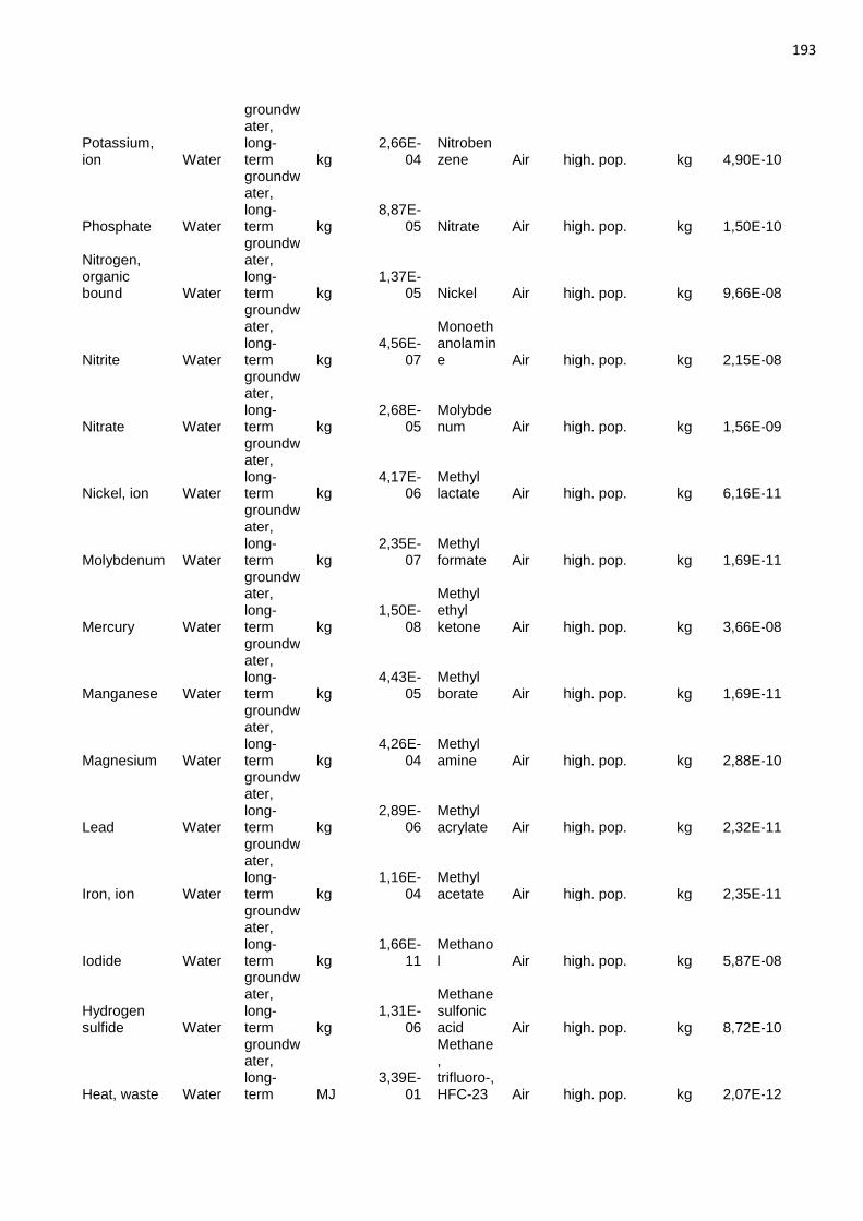
193
Potassium, ion Water
groundwater, long-term kg
2,66E-04
Nitrobenzene Air high. pop. kg 4,90E-10
Phosphate Water
groundwater, long-term kg
8,87E-05 Nitrate Air high. pop. kg 1,50E-10
Nitrogen, organic bound Water
groundwater, long-term kg
1,37E-05 Nickel Air high. pop. kg 9,66E-08
Nitrite Water
groundwater, long-term kg
4,56E-07
Monoethanolamine Air high. pop. kg 2,15E-08
Nitrate Water
groundwater, long-term kg
2,68E-05
Molybdenum Air high. pop. kg 1,56E-09
Nickel, ion Water
groundwater, long-term kg
4,17E-06
Methyl lactate Air high. pop. kg 6,16E-11
Molybdenum Water
groundwater, long-term kg
2,35E-07
Methyl formate Air high. pop. kg 1,69E-11
Mercury Water
groundwater, long-term kg
1,50E-08
Methyl ethyl ketone Air high. pop. kg 3,66E-08
Manganese Water
groundwater, long-term kg
4,43E-05
Methyl borate Air high. pop. kg 1,69E-11
Magnesium Water
groundwater, long-term kg
4,26E-04
Methyl amine Air high. pop. kg 2,88E-10
Lead Water
groundwater, long-term kg
2,89E-06
Methyl acrylate Air high. pop. kg 2,32E-11
Iron, ion Water
groundwater, long-term kg
1,16E-04
Methyl acetate Air high. pop. kg 2,35E-11
Iodide Water
groundwater, long-term kg
1,66E-11
Methanol Air high. pop. kg 5,87E-08
Hydrogen sulfide Water
groundwater, long-term kg
1,31E-06
Methanesulfonic acid Air high. pop. kg 8,72E-10
Heat, waste Water
groundwater, long-term MJ
3,39E-01
Methane, trifluoro-, HFC-23 Air high. pop. kg 2,07E-12
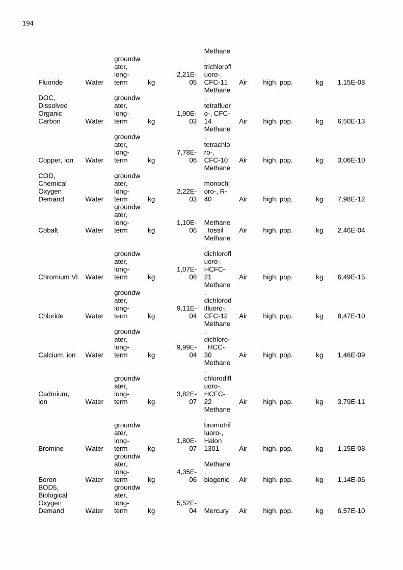
194
Fluoride Water
groundwater, long-term kg
2,21E-05
Methane, trichlorofluoro-, CFC-11 Air high. pop. kg 1,15E-08
DOC, Dissolved Organic Carbon Water
groundwater, long-term kg
1,90E-03
Methane, tetrafluoro-, CFC-14 Air high. pop. kg 6,50E-13
Copper, ion Water
groundwater, long-term kg
7,78E-06
Methane, tetrachloro-, CFC-10 Air high. pop. kg 3,06E-10
COD, Chemical Oxygen Demand Water
groundwater, long-term kg
2,22E-03
Methane, monochloro-, R-40 Air high. pop. kg 7,98E-12
Cobalt Water
groundwater, long-term kg
1,10E-06
Methane, fossil Air high. pop. kg 2,46E-04
Chromium VI Water
groundwater, long-term kg
1,07E-06
Methane, dichlorofluoro-, HCFC-21 Air high. pop. kg 6,49E-15
Chloride Water
groundwater, long-term kg
9,11E-04
Methane, dichlorodifluoro-, CFC-12 Air high. pop. kg 8,47E-10
Calcium, ion Water
groundwater, long-term kg
9,99E-04
Methane, dichloro-, HCC-30 Air high. pop. kg 1,46E-09
Cadmium, ion Water
groundwater, long-term kg
3,82E-07
Methane, chlorodifluoro-, HCFC-22 Air high. pop. kg 3,79E-11
Bromine Water
groundwater, long-term kg
1,80E-07
Methane, bromotrifluoro-, Halon 1301 Air high. pop. kg 1,15E-08
Boron Water
groundwater, long-term kg
4,35E-06
Methane, biogenic Air high. pop. kg 1,14E-06
BOD5, Biological Oxygen Demand Water
groundwater, long-term kg
5,52E-04 Mercury Air high. pop. kg 6,57E-10
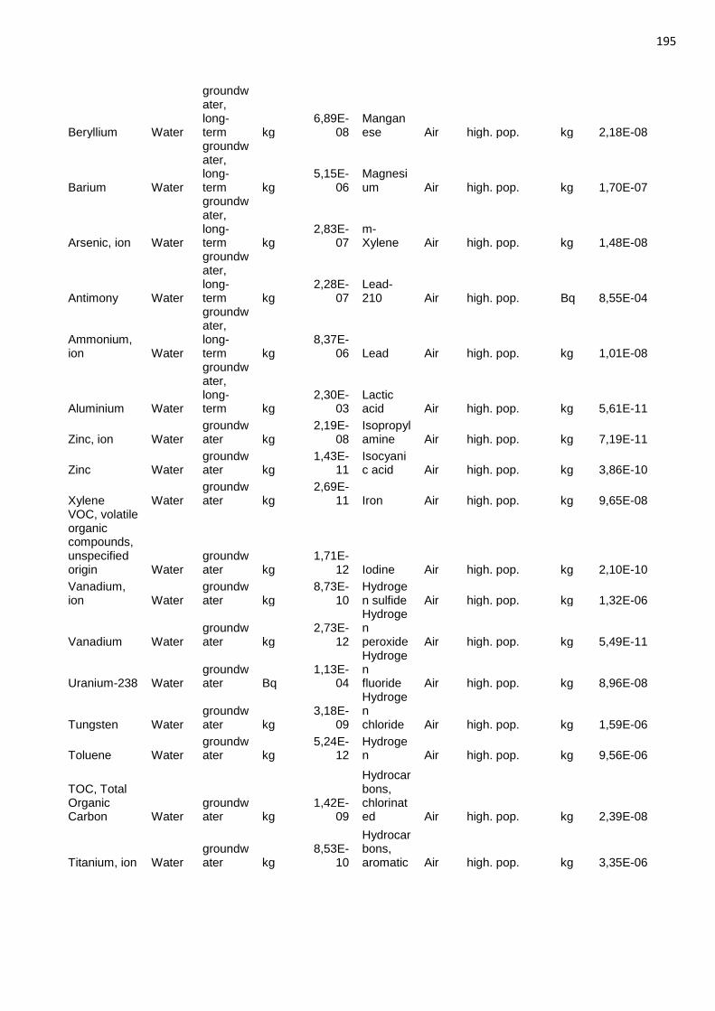
195
Beryllium Water
groundwater, long-term kg
6,89E-08
Manganese Air high. pop. kg 2,18E-08
Barium Water
groundwater, long-term kg
5,15E-06
Magnesium Air high. pop. kg 1,70E-07
Arsenic, ion Water
groundwater, long-term kg
2,83E-07
m-Xylene Air high. pop. kg 1,48E-08
Antimony Water
groundwater, long-term kg
2,28E-07
Lead-210 Air high. pop. Bq 8,55E-04
Ammonium, ion Water
groundwater, long-term kg
8,37E-06 Lead Air high. pop. kg 1,01E-08
Aluminium Water
groundwater, long-term kg
2,30E-03
Lactic acid Air high. pop. kg 5,61E-11
Zinc, ion Water groundwater kg
2,19E-08
Isopropylamine Air high. pop. kg 7,19E-11
Zinc Water groundwater kg
1,43E-11
Isocyanic acid Air high. pop. kg 3,86E-10
Xylene Water groundwater kg
2,69E-11 Iron Air high. pop. kg 9,65E-08
VOC, volatile organic compounds, unspecified origin Water
groundwater kg
1,71E-12 Iodine Air high. pop. kg 2,10E-10
Vanadium, ion Water
groundwater kg
8,73E-10
Hydrogen sulfide Air high. pop. kg 1,32E-06
Vanadium Water groundwater kg
2,73E-12
Hydrogen peroxide Air high. pop. kg 5,49E-11
Uranium-238 Water groundwater Bq
1,13E-04
Hydrogen fluoride Air high. pop. kg 8,96E-08
Tungsten Water groundwater kg
3,18E-09
Hydrogen chloride Air high. pop. kg 1,59E-06
Toluene Water groundwater kg
5,24E-12
Hydrogen Air high. pop. kg 9,56E-06
TOC, Total Organic Carbon Water
groundwater kg
1,42E-09
Hydrocarbons, chlorinated Air high. pop. kg 2,39E-08
Titanium, ion Water groundwater kg
8,53E-10
Hydrocarbons, aromatic Air high. pop. kg 3,35E-06
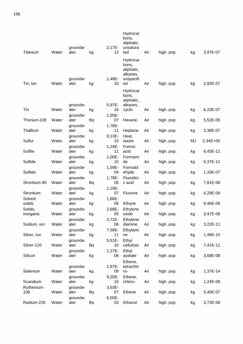
196
Titanium Water groundwater kg
2,17E-12
Hydrocarbons, aliphatic, unsaturated Air high. pop. kg 3,97E-07
Tin, ion Water groundwater kg
1,48E-10
Hydrocarbons, aliphatic, alkanes, unspecified Air high. pop. kg 2,92E-07
Tin Water groundwater kg
5,97E-16
Hydrocarbons, aliphatic, alkanes, cyclic Air high. pop. kg 6,23E-07
Thorium-228 Water groundwater Bq
1,55E-07 Hexane Air high. pop. kg 5,52E-05
Thallium Water groundwater kg
1,78E-11 Heptane Air high. pop. kg 3,38E-07
Sulfur Water groundwater kg
9,13E-15
Heat, waste Air high. pop. MJ 2,34E+00
Sulfite Water groundwater kg
1,24E-11
Formic acid Air high. pop. kg 6,43E-11
Sulfide Water groundwater kg
1,00E-10
Formamide Air high. pop. kg 6,37E-11
Sulfate Water groundwater kg
1,59E-04
Formaldehyde Air high. pop. kg 1,33E-07
Strontium-90 Water groundwater Bq
1,78E-05
Fluosilicic acid Air high. pop. kg 7,81E-08
Strontium Water groundwater kg
1,19E-07 Fluorine Air high. pop. kg 6,29E-09
Solved solids Water
groundwater kg
1,86E-06 Ethyne Air high. pop. kg 9,46E-09
Solids, inorganic Water
groundwater kg
2,68E-05
Ethylene oxide Air high. pop. kg 3,47E-08
Sodium, ion Water groundwater kg
3,72E-06
Ethylene diamine Air high. pop. kg 3,22E-11
Silver, ion Water groundwater kg
7,09E-11
Ethylamine Air high. pop. kg 1,46E-10
Silver-110 Water groundwater Bq
5,51E-10
Ethyl cellulose Air high. pop. kg 7,41E-11
Silicon Water groundwater kg
1,27E-06
Ethyl acetate Air high. pop. kg 3,68E-08
Selenium Water groundwater kg
1,97E-09
Ethene, tetrachloro- Air high. pop. kg 1,37E-14
Scandium Water groundwater kg
9,20E-10
Ethene, chloro- Air high. pop. kg 1,24E-08
Ruthenium-106 Water
groundwater Bq
3,63E-07 Ethene Air high. pop. kg 5,40E-07
Radium-226 Water groundwater Bq
6,00E-03 Ethanol Air high. pop. kg 3,73E-08
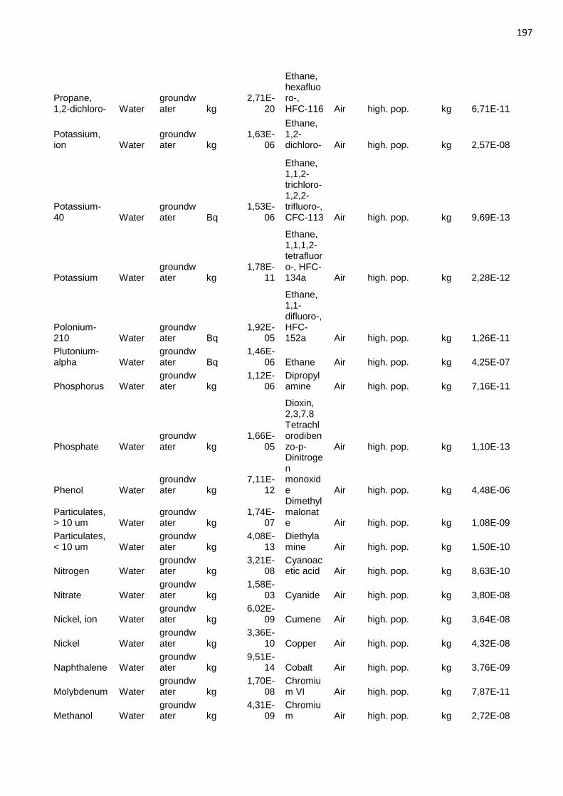
197
Propane, 1,2-dichloro- Water
groundwater kg
2,71E-20
Ethane, hexafluoro-, HFC-116 Air high. pop. kg 6,71E-11
Potassium, ion Water
groundwater kg
1,63E-06
Ethane, 1,2-dichloro- Air high. pop. kg 2,57E-08
Potassium-40 Water
groundwater Bq
1,53E-06
Ethane, 1,1,2-trichloro-1,2,2-trifluoro-, CFC-113 Air high. pop. kg 9,69E-13
Potassium Water groundwater kg
1,78E-11
Ethane, 1,1,1,2-tetrafluoro-, HFC-134a Air high. pop. kg 2,28E-12
Polonium-210 Water
groundwater Bq
1,92E-05
Ethane, 1,1-difluoro-, HFC-152a Air high. pop. kg 1,26E-11
Plutonium-alpha Water
groundwater Bq
1,46E-06 Ethane Air high. pop. kg 4,25E-07
Phosphorus Water groundwater kg
1,12E-06
Dipropylamine Air high. pop. kg 7,16E-11
Phosphate Water groundwater kg
1,66E-05
Dioxin, 2,3,7,8 Tetrachlorodibenzo-p- Air high. pop. kg 1,10E-13
Phenol Water groundwater kg
7,11E-12
Dinitrogen monoxide Air high. pop. kg 4,48E-06
Particulates, > 10 um Water
groundwater kg
1,74E-07
Dimethyl malonate Air high. pop. kg 1,08E-09
Particulates, < 10 um Water
groundwater kg
4,08E-13
Diethylamine Air high. pop. kg 1,50E-10
Nitrogen Water groundwater kg
3,21E-08
Cyanoacetic acid Air high. pop. kg 8,63E-10
Nitrate Water groundwater kg
1,58E-03 Cyanide Air high. pop. kg 3,80E-08
Nickel, ion Water groundwater kg
6,02E-09 Cumene Air high. pop. kg 3,64E-08
Nickel Water groundwater kg
3,36E-10 Copper Air high. pop. kg 4,32E-08
Naphthalene Water groundwater kg
9,51E-14 Cobalt Air high. pop. kg 3,76E-09
Molybdenum Water groundwater kg
1,70E-08
Chromium VI Air high. pop. kg 7,87E-11
Methanol Water groundwater kg
4,31E-09
Chromium Air high. pop. kg 2,72E-08
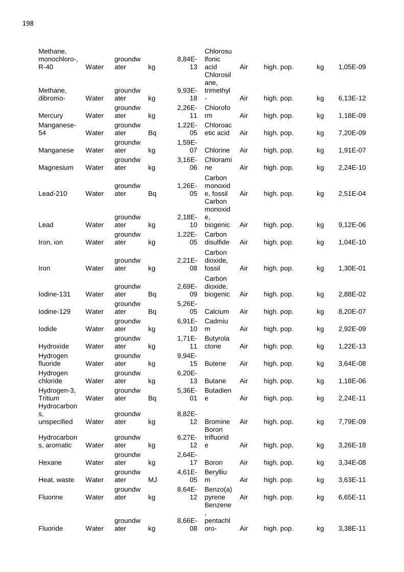
198
Methane, monochloro-, R-40 Water
groundwater kg
8,84E-13
Chlorosulfonic acid Air high. pop. kg 1,05E-09
Methane, dibromo- Water
groundwater kg
9,93E-18
Chlorosilane, trimethyl- Air high. pop. kg 6,13E-12
Mercury Water groundwater kg
2,26E-11
Chloroform Air high. pop. kg 1,18E-09
Manganese-54 Water
groundwater Bq
1,22E-05
Chloroacetic acid Air high. pop. kg 7,20E-09
Manganese Water groundwater kg
1,59E-07 Chlorine Air high. pop. kg 1,91E-07
Magnesium Water groundwater kg
3,16E-06
Chloramine Air high. pop. kg 2,24E-10
Lead-210 Water groundwater Bq
1,26E-05
Carbon monoxide, fossil Air high. pop. kg 2,51E-04
Lead Water groundwater kg
2,18E-10
Carbon monoxide, biogenic Air high. pop. kg 9,12E-06
Iron, ion Water groundwater kg
1,22E-05
Carbon disulfide Air high. pop. kg 1,04E-10
Iron Water groundwater kg
2,21E-08
Carbon dioxide, fossil Air high. pop. kg 1,30E-01
Iodine-131 Water groundwater Bq
2,69E-09
Carbon dioxide, biogenic Air high. pop. kg 2,88E-02
Iodine-129 Water groundwater Bq
5,26E-05 Calcium Air high. pop. kg 8,20E-07
Iodide Water groundwater kg
6,91E-10
Cadmium Air high. pop. kg 2,92E-09
Hydroxide Water groundwater kg
1,71E-11
Butyrolactone Air high. pop. kg 1,22E-13
Hydrogen fluoride Water
groundwater kg
9,94E-15 Butene Air high. pop. kg 3,64E-08
Hydrogen chloride Water
groundwater kg
6,20E-13 Butane Air high. pop. kg 1,18E-06
Hydrogen-3, Tritium Water
groundwater Bq
5,36E-01
Butadiene Air high. pop. kg 2,24E-11
Hydrocarbons, unspecified Water
groundwater kg
8,82E-12 Bromine Air high. pop. kg 7,79E-09
Hydrocarbons, aromatic Water
groundwater kg
6,27E-12
Boron trifluoride Air high. pop. kg 3,26E-18
Hexane Water groundwater kg
2,64E-17 Boron Air high. pop. kg 3,34E-08
Heat, waste Water groundwater MJ
4,61E-05
Beryllium Air high. pop. kg 3,63E-11
Fluorine Water groundwater kg
8,64E-12
Benzo(a)pyrene Air high. pop. kg 6,65E-11
Fluoride Water groundwater kg
8,66E-08
Benzene, pentachloro- Air high. pop. kg 3,38E-11
199
Fluoranthene Water
groundwater kg
4,34E-16
Benzene, hexachloro- Air high. pop. kg 1,35E-11
Ethene, chloro- Water
groundwater kg
4,66E-18
Benzene, ethyl- Air high. pop. kg 3,00E-08
Dioxin, 2,3,7,8 Tetrachlorodibenzo-p- Water
groundwater kg
1,28E-25
Benzene, 1,2-dichloro- Air high. pop. kg 2,66E-09
Decane Water groundwater kg
5,23E-11
Benzene, 1-methyl-2-nitro- Air high. pop. kg 8,75E-11
Cyanide Water groundwater kg
7,09E-14 Benzene Air high. pop. kg 4,11E-07
Curium alpha Water
groundwater Bq
4,81E-07
Benzaldehyde Air high. pop. kg 9,17E-11
Cresol Water groundwater kg
2,36E-16 Barium Air high. pop. kg 4,46E-09
Copper, ion Water groundwater kg
3,53E-09 Arsine Air high. pop. kg 2,38E-16
Copper Water groundwater kg
4,82E-10 Arsenic Air high. pop. kg 3,23E-09
COD, Chemical Oxygen Demand Water
groundwater kg
9,08E-06
Antimony Air high. pop. kg 2,51E-09
Cobalt-60 Water groundwater Bq
7,90E-05
Anthranilic acid Air high. pop. kg 7,49E-11
Cobalt-58 Water groundwater Bq
1,41E-07 Aniline Air high. pop. kg 3,04E-10
Cobalt Water groundwater kg
1,36E-09
Ammonium carbonate Air high. pop. kg 1,06E-10
Chrysene Water groundwater kg
1,05E-15
Ammonia Air high. pop. kg 7,18E-07
Chromium, ion Water
groundwater kg
1,03E-08
Aluminium Air high. pop. kg 4,13E-07
Chromium VI Water groundwater kg
6,69E-09
Aldehydes, unspecified Air high. pop. kg 9,68E-10
Chromium Water groundwater kg
5,07E-12
Acrylic acid Air high. pop. kg 2,04E-11
Chlorine Water groundwater kg
4,26E-10 Acrolein Air high. pop. kg 1,76E-10
Chloride Water groundwater kg
1,08E-04 Acetone Air high. pop. kg 2,83E-08
Cesium-137 Water groundwater Bq
1,70E-04
Acetic acid Air high. pop. kg 1,33E-07
Cesium-134 Water groundwater Bq
1,92E-05
Acetaldehyde Air high. pop. kg 3,30E-08
Carbonate Water groundwater kg
5,38E-10
Acenaphthene Air high. pop. kg 9,51E-14
200
Carbon-14 Water groundwater Bq
1,84E-05
2-Propanol Air high. pop. kg 7,97E-09
Calcium, ion Water groundwater kg
8,60E-06
2-Nitrobenzoic acid Air high. pop. kg 1,01E-10
Cadmium, ion Water
groundwater kg
2,99E-10
2-Methyl-1-propanol Air high. pop. kg 1,17E-10
Cadmium Water groundwater kg
2,50E-11
2-Butene, 2-methyl- Air high. pop. kg 5,84E-15
Bromine Water groundwater kg
5,60E-09
2-Aminopropanol Air high. pop. kg 4,01E-11
Boron Water groundwater kg
3,61E-07
1,4-Butanediol Air high. pop. kg 6,46E-09
BOD5, Biological Oxygen Demand Water
groundwater kg
1,94E-09
1-Propanol Air high. pop. kg 4,87E-09
Beryllium Water groundwater kg
1,45E-10
1-Pentene Air high. pop. kg 2,63E-11
Benzo(b)fluoranthene Water
groundwater kg
1,27E-16
1-Pentanol Air high. pop. kg 3,48E-11
Benzo(a)anthracene Water
groundwater kg
2,37E-16
1-Butanol Air high. pop. kg 9,89E-10
Benzene, ethyl- Water
groundwater kg
8,26E-13
Zirconium-95 Air
Bq -6,33E-11
Benzene Water groundwater kg
7,20E-12
Zirconium Air
kg -3,14E-13
Barium Water groundwater kg
9,93E-10
Zinc oxide Air
kg 1,55E-18
Arsenic, ion Water groundwater kg
1,22E-08 Zinc-65 Air
Bq -4,30E-09
AOX, Adsorbable Organic Halogen as Cl Water
groundwater kg
2,32E-11 Zinc Air
kg 2,96E-08
Antimony-125 Water
groundwater Bq
2,57E-09 Xylene Air
kg 1,31E-08
Antimony-124 Water
groundwater Bq
3,77E-09
Xenon-138 Air
Bq -2,88E-04
Antimony Water groundwater kg
2,52E-09
Xenon-137 Air
Bq -2,80E-05
Anthracene Water groundwater kg
2,79E-15
Xenon-135m Air
Bq -1,14E-03
Ammonium, ion Water
groundwater kg
8,68E-09
Xenon-135 Air
Bq -1,05E-02
Ammonia Water groundwater kg
3,71E-08
Xenon-133m Air
Bq -3,23E-05
Americium-241 Water
groundwater Bq
3,63E-07
Xenon-133 Air
Bq -6,25E-02
201
Aluminium Water groundwater kg
6,88E-08
Xenon-131m Air
Bq -2,16E-04
Acrylonitrile Water groundwater kg
1,98E-15 Water Air
kg 1,21E-03
Acidity, unspecified Water
groundwater kg
1,33E-12
VOC, volatile organic compounds Air
kg 4,13E-10
Acetic acid Water groundwater kg
9,76E-12
Vanadium Air
kg -3,23E-09
Acenaphthylene Water
groundwater kg
7,24E-16 Used air Air
kg 2,86E-03
Acenaphthene Water
groundwater kg
1,83E-15
Uranium alpha Air
Bq -2,08E-05
Zirconium-95 Water
Bq -4,92E-
06 Uranium-238 Air
Bq -4,61E-06
Zinc, ion Water
kg 5,47E-
08 Uranium-235 Air
Bq 2,98E-06
Zinc-65 Water
Bq -8,49E-
07 Uranium-234 Air
Bq -6,08E-06
Yttrium-90 Water
Bq -1,51E-
09 Uranium Air
kg -6,35E-13
Xylene Water
kg -1,44E-
08 Toluene Air
kg 3,33E-08 VOC, volatile organic compounds as C Water
kg
-5,34E-08 Titanium Air
kg -4,40E-11
Vanadium, ion Water
kg
-5,50E-10 Tin oxide Air
kg 7,75E-19
Uranium alpha Water
Bq
-7,02E-04 Tin Air
kg 2,55E-10
Uranium-238 Water
Bq -3,63E-
05 Thorium-234 Air
Bq -5,81E-07
Uranium-235 Water
Bq -2,13E-
05 Thorium-232 Air
Bq -7,69E-07
Uranium-234 Water
Bq -1,43E-
05 Thorium-230 Air
Bq -6,43E-06
Undissolved substances Water
kg
-8,25E-06
Thorium-228 Air
Bq -1,21E-06
Tungsten Water
kg -2,24E-
12 Thorium Air
kg -5,82E-13 Triethylene glycol Water
kg
-1,88E-09 Thallium Air
kg 5,40E-11
Tributyltin compounds Water
kg
-1,33E-10
Tellurium-123m Air
Bq -4,35E-09
Toluene Water
kg -1,66E-
08 Tellurium Air
kg 3,29E-16
TOC, Total Organic Carbon Water
kg
-2,74E-06
Technetium-99 Air
Bq -4,04E-11
Titanium, ion Water
kg -4,95E-
09
t-Butyl methyl ether Air
kg -1,22E-11
Tin, ion Water
kg 1,11E-
12 Sulfur oxides Air
kg -3,90E-06
202
Thorium-234 Water
Bq -1,08E-
05
Sulfur hexafluoride Air
kg 3,67E-09
Thorium-232 Water
Bq -1,65E-
06 Sulfur dioxide Air
kg 6,86E-05
Thorium-230 Water
Bq -1,67E-
03 Sulfate Air
kg 3,17E-11
Thorium-228 Water
Bq -3,05E-
02 Styrene Air
kg 4,72E-17
Thallium Water
kg 3,41E-
14 Strontium-90 Air
Bq -9,54E-07
Terephthalate, dimethyl Water
kg
-8,95E-14
Strontium-89 Air
Bq -1,73E-09
Tellurium-132 Water
Bq
-2,25E-10
Strontium Air
kg -3,19E-11
Tellurium-123m Water
Bq
-5,51E-10 Sodium Air
kg -1,42E-09
Technetium-99m Water
Bq
-6,16E-09
Silver-110 Air
Bq -9,79E-10
Technetium-99 Water
Bq
-6,08E-05 Silver Air
kg 8,53E-22
t-Butyl methyl ether Water
kg
-9,93E-13 Silicon Air
kg -3,20E-11
Suspended solids, unspecified Water
kg
1,61E-06
Silicates, unspecified Air
kg -6,86E-09
Sulfur trioxide Water
kg
-4,12E-10
Selenium Air
kg -4,97E-11
Sulfur Water
kg 3,80E-
11 Scandium Air
kg -3,12E-13
Sulfide Water
kg -4,99E-
09 Ruthenium-106 Air
Bq -5,78E-06
Sulfate Water
kg -3,77E-
06 Ruthenium-103 Air
Bq -9,97E-12
Strontium-90 Water
Bq -1,16E-
04 Rhodium Air
kg 3,68E-21
Strontium-89 Water
Bq -2,94E-
08 Radon-222 Air
Bq
-1,22E+00
Strontium Water
kg -9,24E-
07 Radon-220 Air
Bq -1,30E-04
Solved substances Water
kg
-3,39E-08
Radium-228 Air
Bq -1,43E-06
Solved solids Water
kg
6,37E-07
Radium-226 Air
Bq -2,08E-05
Sodium, ion Water
kg -2,72E-
05
Radioactive species, other beta emitters Air
Bq -1,31E-10
Sodium-24 Water
Bq -4,02E-
07 Protactinium-234 Air
Bq -5,81E-07
Silver, ion Water
kg 3,01E-
11 Propionic acid Air
kg -7,44E-11
Silver-110 Water
Bq -6,65E-
06 Propene Air
kg -1,13E-08
Silver Water
kg -9,30E-
11 Propane Air
kg -2,24E-07
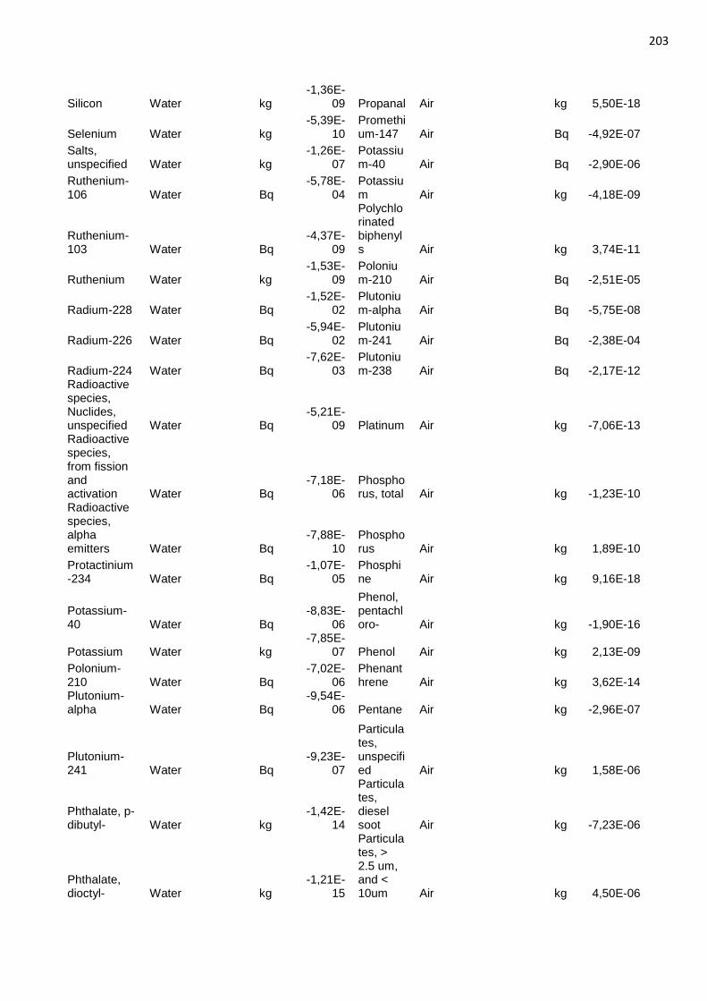
203
Silicon Water
kg -1,36E-
09 Propanal Air
kg 5,50E-18
Selenium Water
kg -5,39E-
10 Promethium-147 Air
Bq -4,92E-07
Salts, unspecified Water
kg
-1,26E-07
Potassium-40 Air
Bq -2,90E-06
Ruthenium-106 Water
Bq
-5,78E-04
Potassium Air
kg -4,18E-09
Ruthenium-103 Water
Bq
-4,37E-09
Polychlorinated biphenyls Air
kg 3,74E-11
Ruthenium Water
kg -1,53E-
09 Polonium-210 Air
Bq -2,51E-05
Radium-228 Water
Bq -1,52E-
02 Plutonium-alpha Air
Bq -5,75E-08
Radium-226 Water
Bq -5,94E-
02 Plutonium-241 Air
Bq -2,38E-04
Radium-224 Water
Bq -7,62E-
03 Plutonium-238 Air
Bq -2,17E-12
Radioactive species, Nuclides, unspecified Water
Bq
-5,21E-09 Platinum Air
kg -7,06E-13
Radioactive species, from fission and activation Water
Bq
-7,18E-06
Phosphorus, total Air
kg -1,23E-10
Radioactive species, alpha emitters Water
Bq
-7,88E-10
Phosphorus Air
kg 1,89E-10
Protactinium-234 Water
Bq
-1,07E-05
Phosphine Air
kg 9,16E-18
Potassium-40 Water
Bq
-8,83E-06
Phenol, pentachloro- Air
kg -1,90E-16
Potassium Water
kg -7,85E-
07 Phenol Air
kg 2,13E-09
Polonium-210 Water
Bq
-7,02E-06
Phenanthrene Air
kg 3,62E-14
Plutonium-alpha Water
Bq
-9,54E-06 Pentane Air
kg -2,96E-07
Plutonium-241 Water
Bq
-9,23E-07
Particulates, unspecified Air
kg 1,58E-06
Phthalate, p-dibutyl- Water
kg
-1,42E-14
Particulates, diesel soot Air
kg -7,23E-06
Phthalate, dioctyl- Water
kg
-1,21E-15
Particulates, > 2.5 um, and < 10um Air
kg 4,50E-06
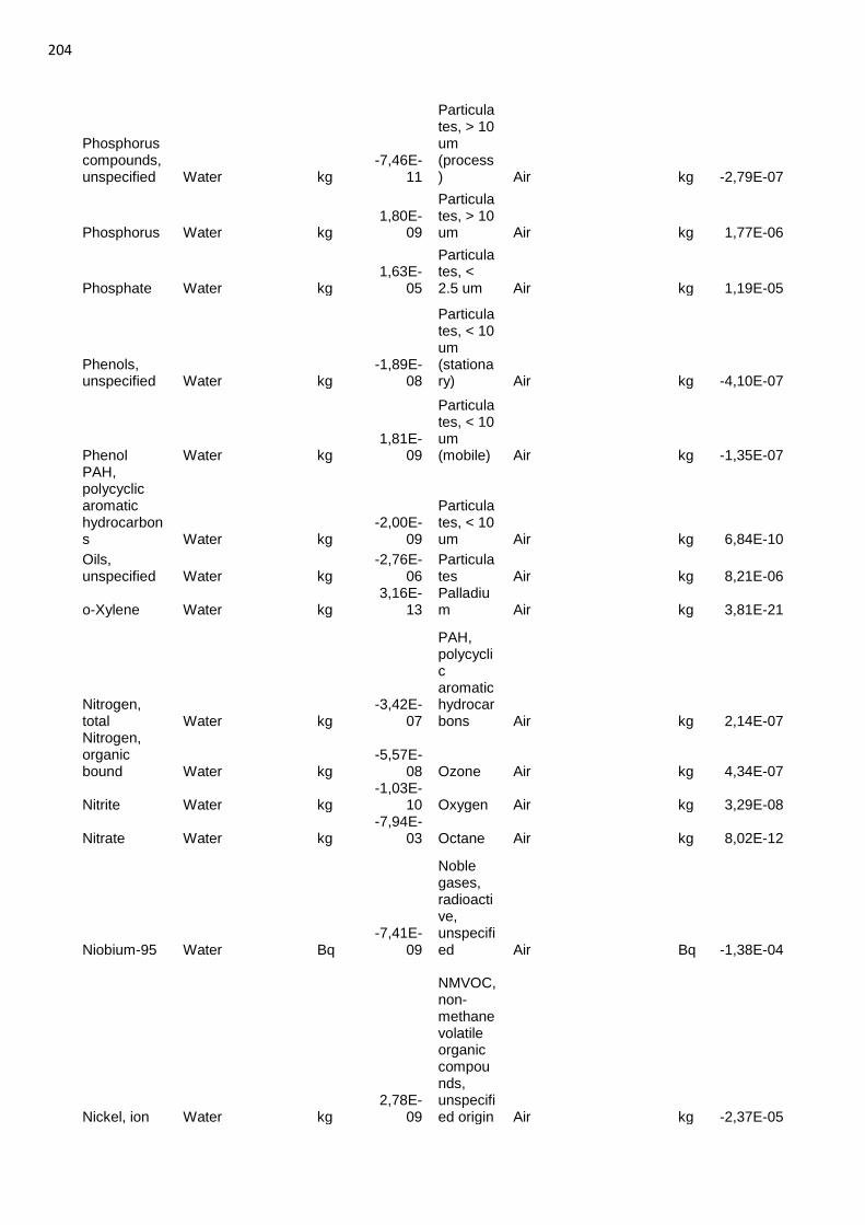
204
Phosphorus compounds, unspecified Water
kg
-7,46E-11
Particulates, > 10 um (process) Air
kg -2,79E-07
Phosphorus Water
kg 1,80E-
09
Particulates, > 10 um Air
kg 1,77E-06
Phosphate Water
kg 1,63E-
05
Particulates, < 2.5 um Air
kg 1,19E-05
Phenols, unspecified Water
kg
-1,89E-08
Particulates, < 10 um (stationary) Air
kg -4,10E-07
Phenol Water
kg 1,81E-
09
Particulates, < 10 um (mobile) Air
kg -1,35E-07
PAH, polycyclic aromatic hydrocarbons Water
kg
-2,00E-09
Particulates, < 10 um Air
kg 6,84E-10
Oils, unspecified Water
kg
-2,76E-06
Particulates Air
kg 8,21E-06
o-Xylene Water
kg 3,16E-
13 Palladium Air
kg 3,81E-21
Nitrogen, total Water
kg
-3,42E-07
PAH, polycyclic aromatic hydrocarbons Air
kg 2,14E-07
Nitrogen, organic bound Water
kg
-5,57E-08 Ozone Air
kg 4,34E-07
Nitrite Water
kg -1,03E-
10 Oxygen Air
kg 3,29E-08
Nitrate Water
kg -7,94E-
03 Octane Air
kg 8,02E-12
Niobium-95 Water
Bq -7,41E-
09
Noble gases, radioactive, unspecified Air
Bq -1,38E-04
Nickel, ion Water
kg 2,78E-
09
NMVOC, non-methane volatile organic compounds, unspecified origin Air
kg -2,37E-05
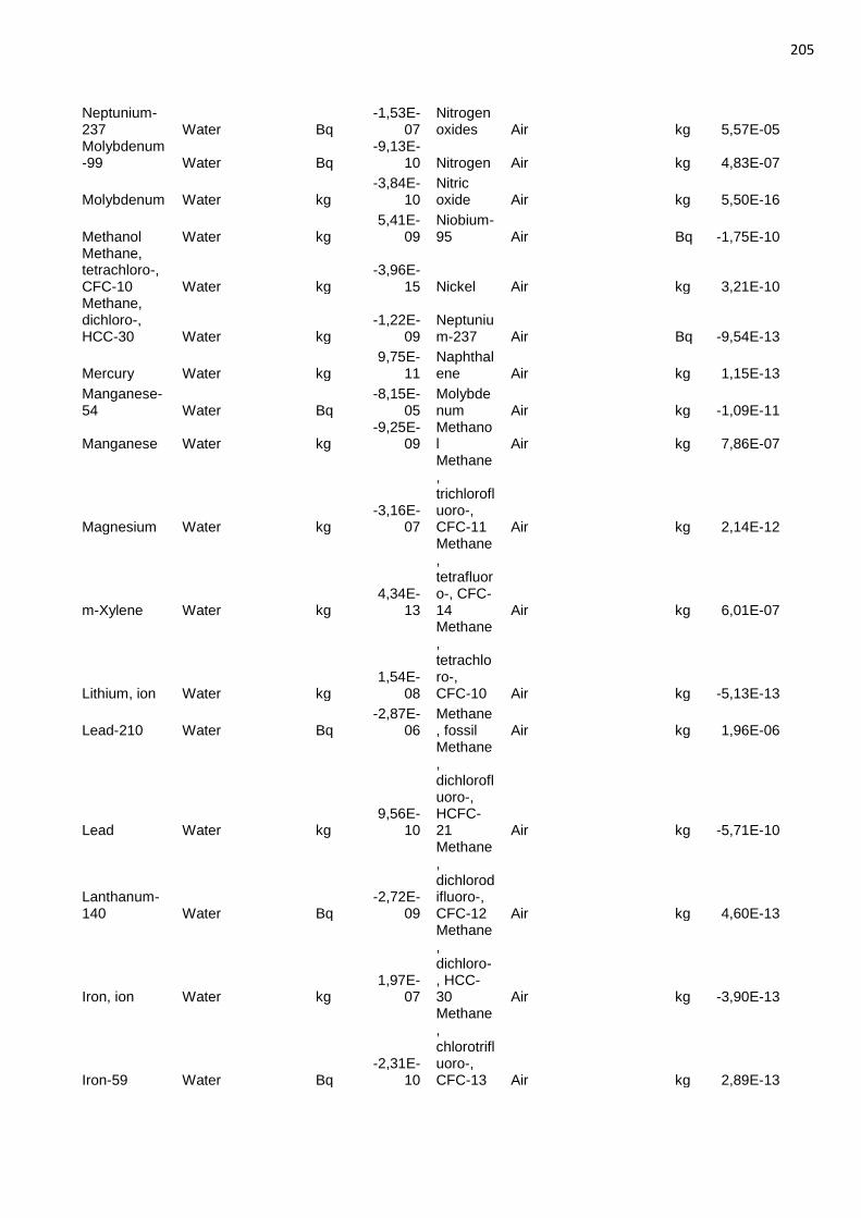
205
Neptunium-237 Water
Bq
-1,53E-07
Nitrogen oxides Air
kg 5,57E-05
Molybdenum-99 Water
Bq
-9,13E-10 Nitrogen Air
kg 4,83E-07
Molybdenum Water
kg -3,84E-
10 Nitric oxide Air
kg 5,50E-16
Methanol Water
kg 5,41E-
09 Niobium-95 Air
Bq -1,75E-10
Methane, tetrachloro-, CFC-10 Water
kg
-3,96E-15 Nickel Air
kg 3,21E-10
Methane, dichloro-, HCC-30 Water
kg
-1,22E-09
Neptunium-237 Air
Bq -9,54E-13
Mercury Water
kg 9,75E-
11 Naphthalene Air
kg 1,15E-13
Manganese-54 Water
Bq
-8,15E-05
Molybdenum Air
kg -1,09E-11
Manganese Water
kg -9,25E-
09 Methanol Air
kg 7,86E-07
Magnesium Water
kg -3,16E-
07
Methane, trichlorofluoro-, CFC-11 Air
kg 2,14E-12
m-Xylene Water
kg 4,34E-
13
Methane, tetrafluoro-, CFC-14 Air
kg 6,01E-07
Lithium, ion Water
kg 1,54E-
08
Methane, tetrachloro-, CFC-10 Air
kg -5,13E-13
Lead-210 Water
Bq -2,87E-
06 Methane, fossil Air
kg 1,96E-06
Lead Water
kg 9,56E-
10
Methane, dichlorofluoro-, HCFC-21 Air
kg -5,71E-10
Lanthanum-140 Water
Bq
-2,72E-09
Methane, dichlorodifluoro-, CFC-12 Air
kg 4,60E-13
Iron, ion Water
kg 1,97E-
07
Methane, dichloro-, HCC-30 Air
kg -3,90E-13
Iron-59 Water
Bq -2,31E-
10
Methane, chlorotrifluoro-, CFC-13 Air
kg 2,89E-13
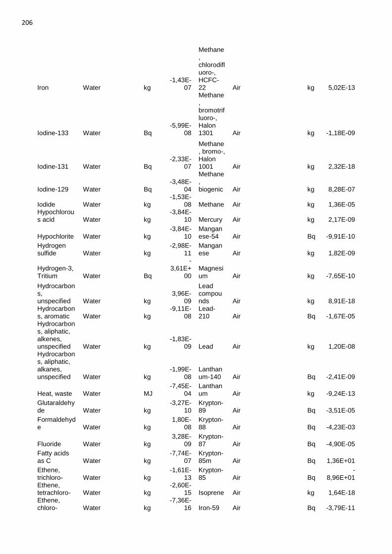
206
Iron Water
kg -1,43E-
07
Methane, chlorodifluoro-, HCFC-22 Air
kg 5,02E-13
Iodine-133 Water
Bq -5,99E-
08
Methane, bromotrifluoro-, Halon 1301 Air
kg -1,18E-09
Iodine-131 Water
Bq -2,33E-
07
Methane, bromo-, Halon 1001 Air
kg 2,32E-18
Iodine-129 Water
Bq -3,48E-
04
Methane, biogenic Air
kg 8,28E-07
Iodide Water
kg -1,53E-
08 Methane Air
kg 1,36E-05 Hypochlorous acid Water
kg
-3,84E-10 Mercury Air
kg 2,17E-09
Hypochlorite Water
kg -3,84E-
10 Manganese-54 Air
Bq -9,91E-10
Hydrogen sulfide Water
kg
-2,98E-11
Manganese Air
kg 1,82E-09
Hydrogen-3, Tritium Water
Bq
-3,61E+
00 Magnesium Air
kg -7,65E-10
Hydrocarbons, unspecified Water
kg
3,96E-09
Lead compounds Air
kg 8,91E-18
Hydrocarbons, aromatic Water
kg
-9,11E-08
Lead-210 Air
Bq -1,67E-05
Hydrocarbons, aliphatic, alkenes, unspecified Water
kg
-1,83E-09 Lead Air
kg 1,20E-08
Hydrocarbons, aliphatic, alkanes, unspecified Water
kg
-1,99E-08
Lanthanum-140 Air
Bq -2,41E-09
Heat, waste Water
MJ -7,45E-
04 Lanthanum Air
kg -9,24E-13
Glutaraldehyde Water
kg
-3,27E-10
Krypton-89 Air
Bq -3,51E-05
Formaldehyde Water
kg
1,80E-08
Krypton-88 Air
Bq -4,23E-03
Fluoride Water
kg 3,28E-
09 Krypton-87 Air
Bq -4,90E-05
Fatty acids as C Water
kg
-7,74E-07
Krypton-85m Air
Bq 1,36E+01
Ethene, trichloro- Water
kg
-1,61E-13
Krypton-85 Air
Bq
-8,96E+01
Ethene, tetrachloro- Water
kg
-2,60E-15 Isoprene Air
kg 1,64E-18
Ethene, chloro- Water
kg
-7,36E-16 Iron-59 Air
Bq -3,79E-11
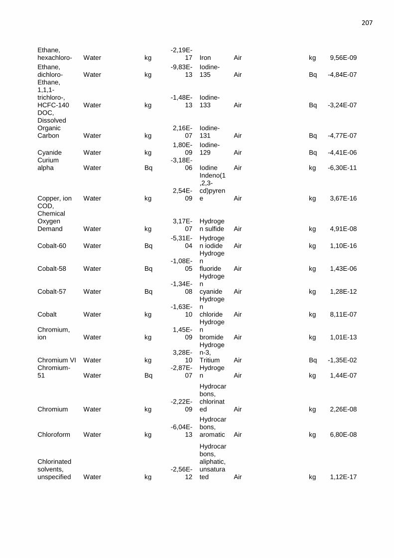
207
Ethane, hexachloro- Water
kg
-2,19E-17 Iron Air
kg 9,56E-09
Ethane, dichloro- Water
kg
-9,83E-13
Iodine-135 Air
Bq -4,84E-07
Ethane, 1,1,1-trichloro-, HCFC-140 Water
kg
-1,48E-13
Iodine-133 Air
Bq -3,24E-07
DOC, Dissolved Organic Carbon Water
kg
2,16E-07
Iodine-131 Air
Bq -4,77E-07
Cyanide Water
kg 1,80E-
09 Iodine-129 Air
Bq -4,41E-06
Curium alpha Water
Bq
-3,18E-06 Iodine Air
kg -6,30E-11
Copper, ion Water
kg 2,54E-
09
Indeno(1,2,3-cd)pyrene Air
kg 3,67E-16
COD, Chemical Oxygen Demand Water
kg
3,17E-07
Hydrogen sulfide Air
kg 4,91E-08
Cobalt-60 Water
Bq -5,31E-
04 Hydrogen iodide Air
kg 1,10E-16
Cobalt-58 Water
Bq -1,08E-
05
Hydrogen fluoride Air
kg 1,43E-06
Cobalt-57 Water
Bq -1,34E-
08
Hydrogen cyanide Air
kg 1,28E-12
Cobalt Water
kg -1,63E-
10
Hydrogen chloride Air
kg 8,11E-07
Chromium, ion Water
kg
1,45E-09
Hydrogen bromide Air
kg 1,01E-13
Chromium VI Water
kg 3,28E-
10
Hydrogen-3, Tritium Air
Bq -1,35E-02
Chromium-51 Water
Bq
-2,87E-07
Hydrogen Air
kg 1,44E-07
Chromium Water
kg -2,22E-
09
Hydrocarbons, chlorinated Air
kg 2,26E-08
Chloroform Water
kg -6,04E-
13
Hydrocarbons, aromatic Air
kg 6,80E-08
Chlorinated solvents, unspecified Water
kg
-2,56E-12
Hydrocarbons, aliphatic, unsaturated Air
kg 1,12E-17
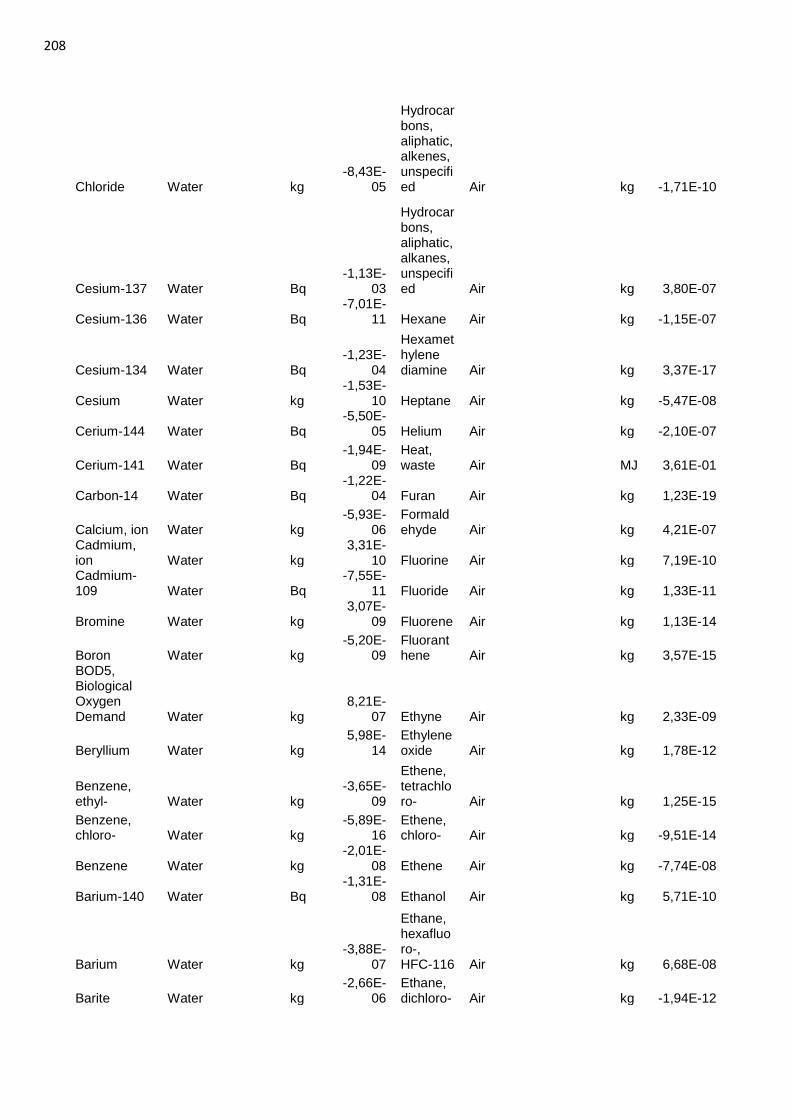
208
Chloride Water
kg -8,43E-
05
Hydrocarbons, aliphatic, alkenes, unspecified Air
kg -1,71E-10
Cesium-137 Water
Bq -1,13E-
03
Hydrocarbons, aliphatic, alkanes, unspecified Air
kg 3,80E-07
Cesium-136 Water
Bq -7,01E-
11 Hexane Air
kg -1,15E-07
Cesium-134 Water
Bq -1,23E-
04
Hexamethylene diamine Air
kg 3,37E-17
Cesium Water
kg -1,53E-
10 Heptane Air
kg -5,47E-08
Cerium-144 Water
Bq -5,50E-
05 Helium Air
kg -2,10E-07
Cerium-141 Water
Bq -1,94E-
09 Heat, waste Air
MJ 3,61E-01
Carbon-14 Water
Bq -1,22E-
04 Furan Air
kg 1,23E-19
Calcium, ion Water
kg -5,93E-
06 Formaldehyde Air
kg 4,21E-07
Cadmium, ion Water
kg
3,31E-10 Fluorine Air
kg 7,19E-10
Cadmium-109 Water
Bq
-7,55E-11 Fluoride Air
kg 1,33E-11
Bromine Water
kg 3,07E-
09 Fluorene Air
kg 1,13E-14
Boron Water
kg -5,20E-
09 Fluoranthene Air
kg 3,57E-15
BOD5, Biological Oxygen Demand Water
kg
8,21E-07 Ethyne Air
kg 2,33E-09
Beryllium Water
kg 5,98E-
14 Ethylene oxide Air
kg 1,78E-12
Benzene, ethyl- Water
kg
-3,65E-09
Ethene, tetrachloro- Air
kg 1,25E-15
Benzene, chloro- Water
kg
-5,89E-16
Ethene, chloro- Air
kg -9,51E-14
Benzene Water
kg -2,01E-
08 Ethene Air
kg -7,74E-08
Barium-140 Water
Bq -1,31E-
08 Ethanol Air
kg 5,71E-10
Barium Water
kg -3,88E-
07
Ethane, hexafluoro-, HFC-116 Air
kg 6,68E-08
Barite Water
kg -2,66E-
06 Ethane, dichloro- Air
kg -1,94E-12
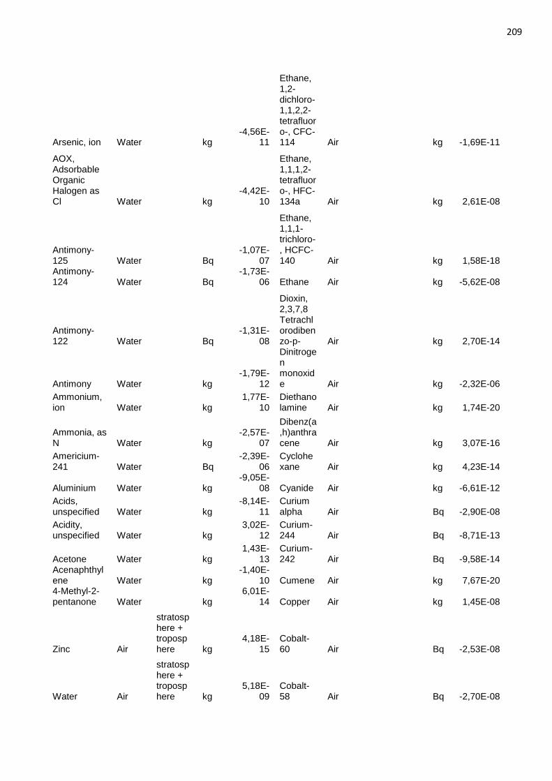
209
Arsenic, ion Water
kg -4,56E-
11
Ethane, 1,2-dichloro-1,1,2,2-tetrafluoro-, CFC-114 Air
kg -1,69E-11
AOX, Adsorbable Organic Halogen as Cl Water
kg
-4,42E-10
Ethane, 1,1,1,2-tetrafluoro-, HFC-134a Air
kg 2,61E-08
Antimony-125 Water
Bq
-1,07E-07
Ethane, 1,1,1-trichloro-, HCFC-140 Air
kg 1,58E-18
Antimony-124 Water
Bq
-1,73E-06 Ethane Air
kg -5,62E-08
Antimony-122 Water
Bq
-1,31E-08
Dioxin, 2,3,7,8 Tetrachlorodibenzo-p- Air
kg 2,70E-14
Antimony Water
kg -1,79E-
12
Dinitrogen monoxide Air
kg -2,32E-06
Ammonium, ion Water
kg
1,77E-10
Diethanolamine Air
kg 1,74E-20
Ammonia, as N Water
kg
-2,57E-07
Dibenz(a,h)anthracene Air
kg 3,07E-16
Americium-241 Water
Bq
-2,39E-06
Cyclohexane Air
kg 4,23E-14
Aluminium Water
kg -9,05E-
08 Cyanide Air
kg -6,61E-12
Acids, unspecified Water
kg
-8,14E-11
Curium alpha Air
Bq -2,90E-08
Acidity, unspecified Water
kg
3,02E-12
Curium-244 Air
Bq -8,71E-13
Acetone Water
kg 1,43E-
13 Curium-242 Air
Bq -9,58E-14
Acenaphthylene Water
kg
-1,40E-10 Cumene Air
kg 7,67E-20
4-Methyl-2-pentanone Water
kg
6,01E-14 Copper Air
kg 1,45E-08
Zinc Air
stratosphere + troposphere kg
4,18E-15
Cobalt-60 Air
Bq -2,53E-08
Water Air
stratosphere + troposphere kg
5,18E-09
Cobalt-58 Air
Bq -2,70E-08
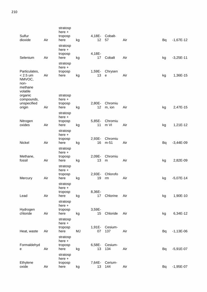
210
Sulfur dioxide Air
stratosphere + troposphere kg
4,18E-12
Cobalt-57 Air
Bq -1,67E-12
Selenium Air
stratosphere + troposphere kg
4,18E-17 Cobalt Air
kg -3,25E-11
Particulates, < 2.5 um Air
stratosphere + troposphere kg
1,59E-13
Chrysene Air
kg 1,36E-15
NMVOC, non-methane volatile organic compounds, unspecified origin Air
stratosphere + troposphere kg
2,80E-12
Chromium, ion Air
kg 2,47E-15
Nitrogen oxides Air
stratosphere + troposphere kg
5,85E-11
Chromium VI Air
kg 1,21E-12
Nickel Air
stratosphere + troposphere kg
2,93E-16
Chromium-51 Air
Bq -3,44E-09
Methane, fossil Air
stratosphere + troposphere kg
2,09E-13
Chromium Air
kg 2,82E-09
Mercury Air
stratosphere + troposphere kg
2,93E-19
Chloroform Air
kg -5,07E-14
Lead Air
stratosphere + troposphere kg
8,36E-17 Chlorine Air
kg 1,90E-10
Hydrogen chloride Air
stratosphere + troposphere kg
3,59E-15 Chloride Air
kg 6,34E-12
Heat, waste Air
stratosphere + troposphere MJ
1,91E-07
Cesium-137 Air
Bq -1,13E-06
Formaldehyde Air
stratosphere + troposphere kg
6,58E-13
Cesium-134 Air
Bq -5,91E-07
Ethylene oxide Air
stratosphere + troposphere kg
7,64E-13
Cerium-144 Air
Bq -1,95E-07
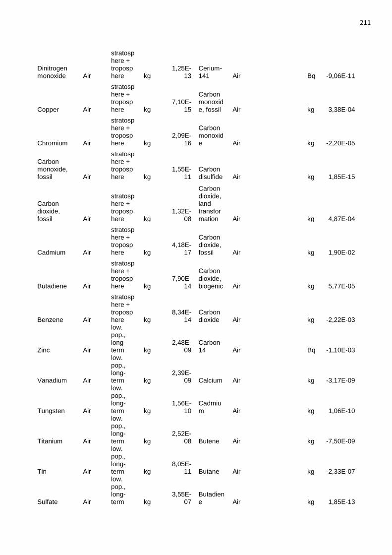
211
Dinitrogen monoxide Air
stratosphere + troposphere kg
1,25E-13
Cerium-141 Air
Bq -9,06E-11
Copper Air
stratosphere + troposphere kg
7,10E-15
Carbon monoxide, fossil Air
kg 3,38E-04
Chromium Air
stratosphere + troposphere kg
2,09E-16
Carbon monoxide Air
kg -2,20E-05
Carbon monoxide, fossil Air
stratosphere + troposphere kg
1,55E-11
Carbon disulfide Air
kg 1,85E-15
Carbon dioxide, fossil Air
stratosphere + troposphere kg
1,32E-08
Carbon dioxide, land transformation Air
kg 4,87E-04
Cadmium Air
stratosphere + troposphere kg
4,18E-17
Carbon dioxide, fossil Air
kg 1,90E-02
Butadiene Air
stratosphere + troposphere kg
7,90E-14
Carbon dioxide, biogenic Air
kg 5,77E-05
Benzene Air
stratosphere + troposphere kg
8,34E-14
Carbon dioxide Air
kg -2,22E-03
Zinc Air
low. pop., long-term kg
2,48E-09
Carbon-14 Air
Bq -1,10E-03
Vanadium Air
low. pop., long-term kg
2,39E-09 Calcium Air
kg -3,17E-09
Tungsten Air
low. pop., long-term kg
1,56E-10
Cadmium Air
kg 1,06E-10
Titanium Air
low. pop., long-term kg
2,52E-08 Butene Air
kg -7,50E-09
Tin Air
low. pop., long-term kg
8,05E-11 Butane Air
kg -2,33E-07
Sulfate Air
low. pop., long-term kg
3,55E-07
Butadiene Air
kg 1,85E-13
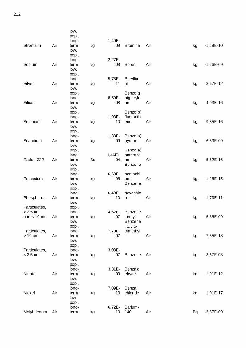
212
Strontium Air
low. pop., long-term kg
1,40E-09 Bromine Air
kg -1,18E-10
Sodium Air
low. pop., long-term kg
2,27E-08 Boron Air
kg -1,26E-09
Silver Air
low. pop., long-term kg
5,78E-11
Beryllium Air
kg 3,67E-12
Silicon Air
low. pop., long-term kg
8,59E-08
Benzo(ghi)perylene Air
kg 4,93E-16
Selenium Air
low. pop., long-term kg
1,93E-10
Benzo(b)fluoranthene Air
kg 9,85E-16
Scandium Air
low. pop., long-term kg
1,38E-09
Benzo(a)pyrene Air
kg 6,53E-09
Radon-222 Air
low. pop., long-term Bq
1,46E+04
Benzo(a)anthracene Air
kg 5,52E-16
Potassium Air
low. pop., long-term kg
6,60E-08
Benzene, pentachloro- Air
kg -1,18E-15
Phosphorus Air
low. pop., long-term kg
6,49E-10
Benzene, hexachloro- Air
kg 1,73E-11
Particulates, > 2.5 um, and < 10um Air
low. pop., long-term kg
4,62E-07
Benzene, ethyl- Air
kg -5,55E-09
Particulates, > 10 um Air
low. pop., long-term kg
7,70E-07
Benzene, 1,3,5-trimethyl- Air
kg 7,55E-18
Particulates, < 2.5 um Air
low. pop., long-term kg
3,08E-07 Benzene Air
kg 3,67E-08
Nitrate Air
low. pop., long-term kg
3,31E-09
Benzaldehyde Air
kg -1,91E-12
Nickel Air
low. pop., long-term kg
7,09E-10
Benzal chloride Air
kg 1,01E-17
Molybdenum Air
low. pop., long-term kg
6,72E-10
Barium-140 Air
Bq -3,87E-09
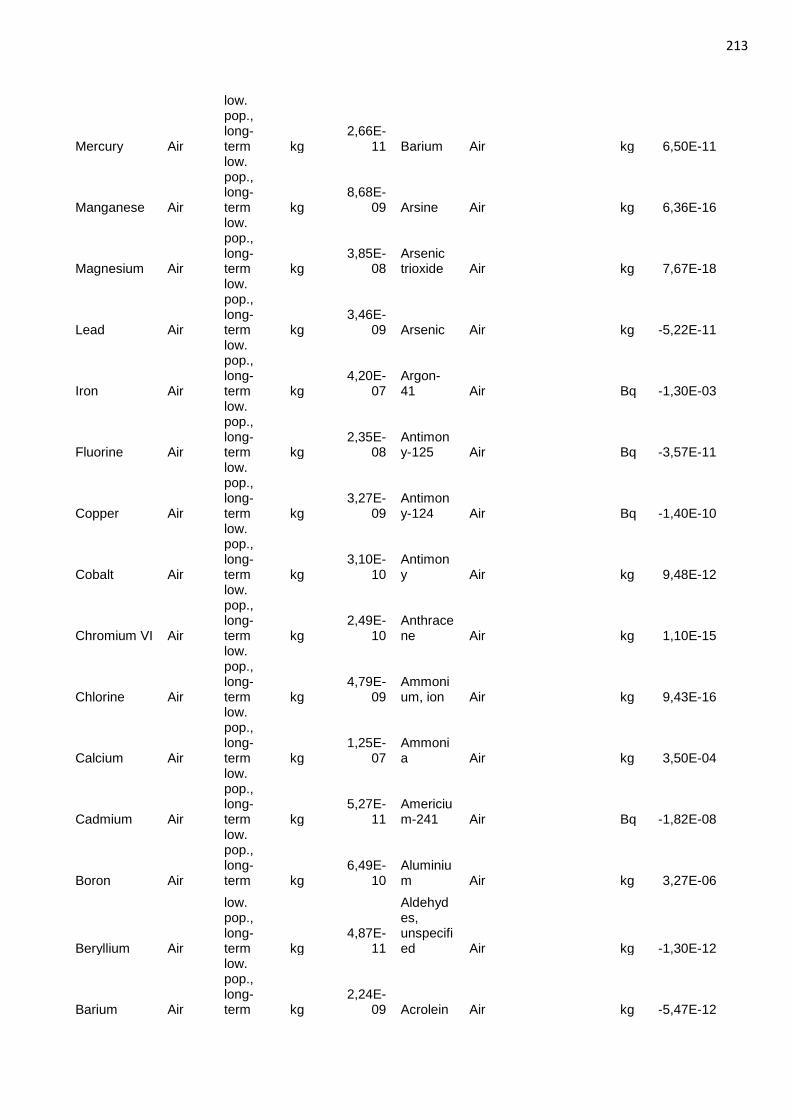
213
Mercury Air
low. pop., long-term kg
2,66E-11 Barium Air
kg 6,50E-11
Manganese Air
low. pop., long-term kg
8,68E-09 Arsine Air
kg 6,36E-16
Magnesium Air
low. pop., long-term kg
3,85E-08
Arsenic trioxide Air
kg 7,67E-18
Lead Air
low. pop., long-term kg
3,46E-09 Arsenic Air
kg -5,22E-11
Iron Air
low. pop., long-term kg
4,20E-07
Argon-41 Air
Bq -1,30E-03
Fluorine Air
low. pop., long-term kg
2,35E-08
Antimony-125 Air
Bq -3,57E-11
Copper Air
low. pop., long-term kg
3,27E-09
Antimony-124 Air
Bq -1,40E-10
Cobalt Air
low. pop., long-term kg
3,10E-10
Antimony Air
kg 9,48E-12
Chromium VI Air
low. pop., long-term kg
2,49E-10
Anthracene Air
kg 1,10E-15
Chlorine Air
low. pop., long-term kg
4,79E-09
Ammonium, ion Air
kg 9,43E-16
Calcium Air
low. pop., long-term kg
1,25E-07
Ammonia Air
kg 3,50E-04
Cadmium Air
low. pop., long-term kg
5,27E-11
Americium-241 Air
Bq -1,82E-08
Boron Air
low. pop., long-term kg
6,49E-10
Aluminium Air
kg 3,27E-06
Beryllium Air
low. pop., long-term kg
4,87E-11
Aldehydes, unspecified Air
kg -1,30E-12
Barium Air
low. pop., long-term kg
2,24E-09 Acrolein Air
kg -5,47E-12
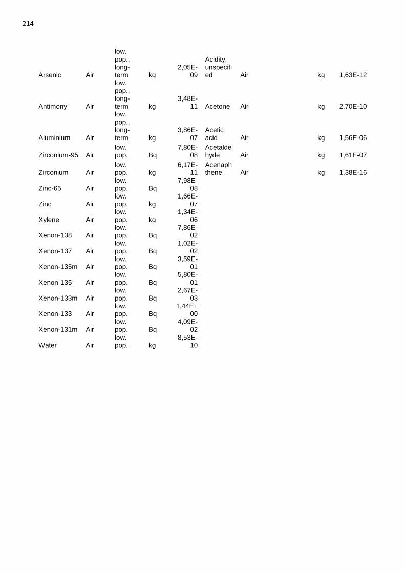
214
Arsenic Air
low. pop., long-term kg
2,05E-09
Acidity, unspecified Air
kg 1,63E-12
Antimony Air
low. pop., long-term kg
3,48E-11 Acetone Air
kg 2,70E-10
Aluminium Air
low. pop., long-term kg
3,86E-07
Acetic acid Air
kg 1,56E-06
Zirconium-95 Air low. pop. Bq
7,80E-08
Acetaldehyde Air
kg 1,61E-07
Zirconium Air low. pop. kg
6,17E-11
Acenaphthene Air
kg 1,38E-16
Zinc-65 Air low. pop. Bq
7,98E-08
Zinc Air
low. pop. kg
1,66E-07
Xylene Air
low. pop. kg
1,34E-06
Xenon-138 Air
low. pop. Bq
7,86E-02
Xenon-137 Air
low. pop. Bq
1,02E-02
Xenon-135m Air
low. pop. Bq
3,59E-01
Xenon-135 Air
low. pop. Bq
5,80E-01
Xenon-133m Air
low. pop. Bq
2,67E-03
Xenon-133 Air
low. pop. Bq
1,44E+00
Xenon-131m Air
low. pop. Bq
4,09E-02
Water Air
low. pop. kg
8,53E-10
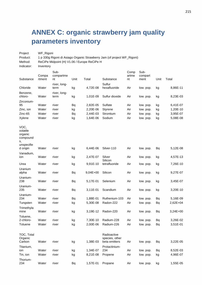
215
ANNEX C: organic strawberry jam quality
parameters inventory
Project WF_Rigoni Product: 1 p 330g Rigoni di Asiago Organic Strawberry Jam (of project WF_Rigoni)
Method: ReCiPe Midpoint (H) V1.06 / Europe ReCiPe H Indicator: Inventory
Substance Compartment
Sub-compartment Unit Total Substance
Compartment
Sub-compartment Unit Total
Chloride Water river, long-term kg 4,72E-08
Sulfur hexafluoride Air low. pop. kg 8,86E-11
Benzene, chloro- Water
river, long-term kg 1,01E-09 Sulfur dioxide Air low. pop. kg 8,23E-03
Zirconium-95 Water river Bq 2,82E-05 Sulfate Air low. pop. kg 6,41E-07
Zinc, ion Water river kg 2,20E-06 Styrene Air low. pop. kg 1,20E-10
Zinc-65 Water river Bq 2,44E-03 Strontium Air low. pop. kg 3,95E-07
Xylene Water river kg 1,64E-06 Sodium Air low. pop. kg 5,08E-08
VOC, volatile organic compounds, unspecified origin Water river kg 6,44E-06 Silver-110 Air low. pop. Bq 5,12E-08
Vanadium, ion Water river kg 2,47E-07 Silver Air low. pop. kg 4,57E-13
Urea Water river kg 9,91E-10 Silicon tetrafluoride Air low. pop. kg 7,26E-10
Uranium alpha Water river Bq 9,04E+00 Silicon Air low. pop. kg 9,27E-07
Uranium-238 Water river Bq 5,17E-01 Selenium Air low. pop. kg 3,45E-07
Uranium-235 Water river Bq 3,11E-01 Scandium Air low. pop. kg 3,20E-10
Uranium-234 Water river Bq 1,88E-01 Ruthenium-103 Air low. pop. Bq 5,16E-09
Tungsten Water river kg 5,30E-08 Radon-222 Air low. pop. Bq 2,62E+04
Trimethylamine Water river kg 3,19E-12 Radon-220 Air low. pop. Bq 3,24E+00
Toluene, 2-chloro- Water river kg 7,30E-10 Radium-228 Air low. pop. Bq 3,26E-02
Toluene Water river kg 2,00E-06 Radium-226 Air low. pop. Bq 3,51E-01
TOC, Total Organic Carbon Water river kg 1,38E-03
Radioactive species, other beta emitters Air low. pop. Bq 3,22E-05
Titanium, ion Water river kg 1,34E-07
Protactinium-234 Air low. pop. Bq 8,52E-03
Tin, ion Water river kg 8,21E-08 Propene Air low. pop. kg 4,96E-07
Thorium-234 Water river Bq 1,57E-01 Propane Air low. pop. kg 1,55E-05
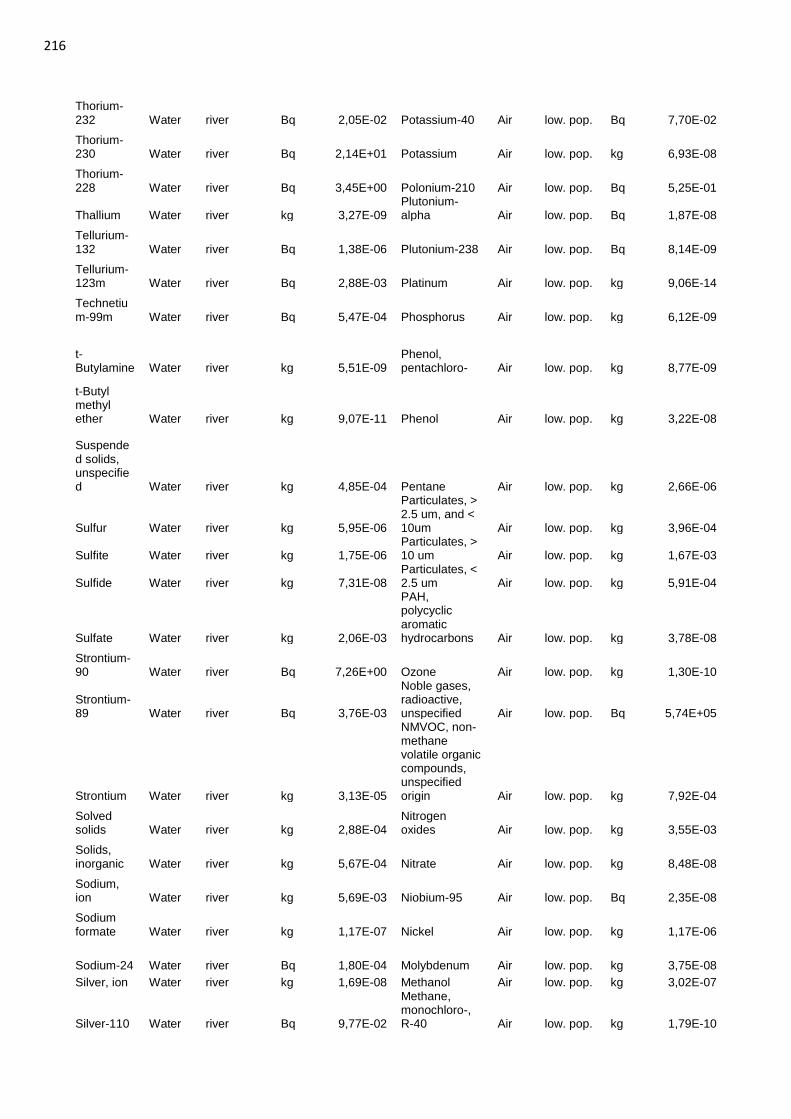
216
Thorium-232 Water river Bq 2,05E-02 Potassium-40 Air low. pop. Bq 7,70E-02
Thorium-230 Water river Bq 2,14E+01 Potassium Air low. pop. kg 6,93E-08
Thorium-228 Water river Bq 3,45E+00 Polonium-210 Air low. pop. Bq 5,25E-01
Thallium Water river kg 3,27E-09 Plutonium-alpha Air low. pop. Bq 1,87E-08
Tellurium-132 Water river Bq 1,38E-06 Plutonium-238 Air low. pop. Bq 8,14E-09
Tellurium-123m Water river Bq 2,88E-03 Platinum Air low. pop. kg 9,06E-14
Technetium-99m Water river Bq 5,47E-04 Phosphorus Air low. pop. kg 6,12E-09
t-Butylamine Water river kg 5,51E-09
Phenol, pentachloro- Air low. pop. kg 8,77E-09
t-Butyl methyl ether Water river kg 9,07E-11 Phenol Air low. pop. kg 3,22E-08
Suspended solids, unspecified Water river kg 4,85E-04 Pentane Air low. pop. kg 2,66E-06
Sulfur Water river kg 5,95E-06
Particulates, > 2.5 um, and < 10um Air low. pop. kg 3,96E-04
Sulfite Water river kg 1,75E-06 Particulates, > 10 um Air low. pop. kg 1,67E-03
Sulfide Water river kg 7,31E-08 Particulates, < 2.5 um Air low. pop. kg 5,91E-04
Sulfate Water river kg 2,06E-03
PAH, polycyclic aromatic hydrocarbons Air low. pop. kg 3,78E-08
Strontium-90 Water river Bq 7,26E+00 Ozone Air low. pop. kg 1,30E-10
Strontium-89 Water river Bq 3,76E-03
Noble gases, radioactive, unspecified Air low. pop. Bq 5,74E+05
Strontium Water river kg 3,13E-05
NMVOC, non-methane volatile organic compounds, unspecified origin Air low. pop. kg 7,92E-04
Solved solids Water river kg 2,88E-04
Nitrogen oxides Air low. pop. kg 3,55E-03
Solids, inorganic Water river kg 5,67E-04 Nitrate Air low. pop. kg 8,48E-08
Sodium, ion Water river kg 5,69E-03 Niobium-95 Air low. pop. Bq 2,35E-08
Sodium formate Water river kg 1,17E-07 Nickel Air low. pop. kg 1,17E-06
Sodium-24 Water river Bq 1,80E-04 Molybdenum Air low. pop. kg 3,75E-08
Silver, ion Water river kg 1,69E-08 Methanol Air low. pop. kg 3,02E-07
Silver-110 Water river Bq 9,77E-02
Methane, monochloro-, R-40 Air low. pop. kg 1,79E-10
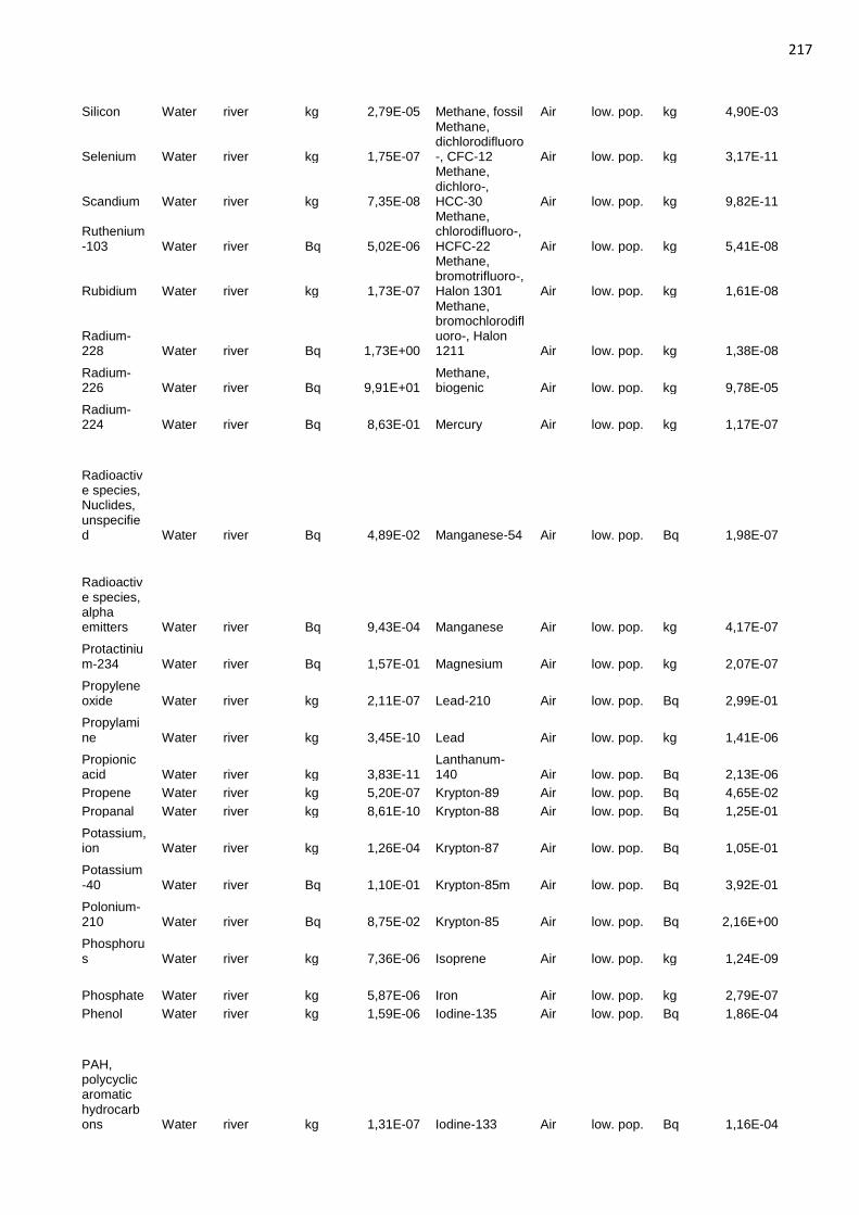
217
Silicon Water river kg 2,79E-05 Methane, fossil Air low. pop. kg 4,90E-03
Selenium Water river kg 1,75E-07
Methane, dichlorodifluoro-, CFC-12 Air low. pop. kg 3,17E-11
Scandium Water river kg 7,35E-08
Methane, dichloro-, HCC-30 Air low. pop. kg 9,82E-11
Ruthenium-103 Water river Bq 5,02E-06
Methane, chlorodifluoro-, HCFC-22 Air low. pop. kg 5,41E-08
Rubidium Water river kg 1,73E-07
Methane, bromotrifluoro-, Halon 1301 Air low. pop. kg 1,61E-08
Radium-228 Water river Bq 1,73E+00
Methane, bromochlorodifluoro-, Halon 1211 Air low. pop. kg 1,38E-08
Radium-226 Water river Bq 9,91E+01
Methane, biogenic Air low. pop. kg 9,78E-05
Radium-224 Water river Bq 8,63E-01 Mercury Air low. pop. kg 1,17E-07
Radioactive species, Nuclides, unspecified Water river Bq 4,89E-02 Manganese-54 Air low. pop. Bq 1,98E-07
Radioactive species, alpha emitters Water river Bq 9,43E-04 Manganese Air low. pop. kg 4,17E-07
Protactinium-234 Water river Bq 1,57E-01 Magnesium Air low. pop. kg 2,07E-07
Propylene oxide Water river kg 2,11E-07 Lead-210 Air low. pop. Bq 2,99E-01
Propylamine Water river kg 3,45E-10 Lead Air low. pop. kg 1,41E-06
Propionic acid Water river kg 3,83E-11
Lanthanum-140 Air low. pop. Bq 2,13E-06
Propene Water river kg 5,20E-07 Krypton-89 Air low. pop. Bq 4,65E-02
Propanal Water river kg 8,61E-10 Krypton-88 Air low. pop. Bq 1,25E-01
Potassium, ion Water river kg 1,26E-04 Krypton-87 Air low. pop. Bq 1,05E-01
Potassium-40 Water river Bq 1,10E-01 Krypton-85m Air low. pop. Bq 3,92E-01
Polonium-210 Water river Bq 8,75E-02 Krypton-85 Air low. pop. Bq 2,16E+00
Phosphorus Water river kg 7,36E-06 Isoprene Air low. pop. kg 1,24E-09
Phosphate Water river kg 5,87E-06 Iron Air low. pop. kg 2,79E-07
Phenol Water river kg 1,59E-06 Iodine-135 Air low. pop. Bq 1,86E-04
PAH, polycyclic aromatic hydrocarbons Water river kg 1,31E-07 Iodine-133 Air low. pop. Bq 1,16E-04
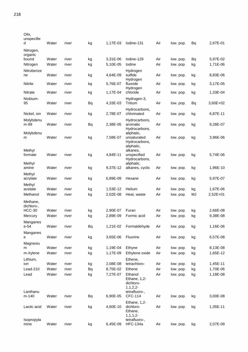
218
Oils, unspecified Water river kg 1,17E-03 Iodine-131 Air low. pop. Bq 2,67E-01
Nitrogen, organic bound Water river kg 3,31E-06 Iodine-129 Air low. pop. Bq 5,97E-02
Nitrogen Water river kg 5,10E-05 Iodine Air low. pop. kg 1,71E-06
Nitrobenzene Water river kg 4,64E-09
Hydrogen sulfide Air low. pop. kg 8,83E-06
Nitrite Water river kg 5,76E-07 Hydrogen fluoride Air low. pop. kg 3,17E-05
Nitrate Water river kg 1,17E-04 Hydrogen chloride Air low. pop. kg 1,33E-04
Niobium-95 Water river Bq 4,33E-03
Hydrogen-3, Tritium Air low. pop. Bq 3,60E+02
Nickel, ion Water river kg 2,78E-07 Hydrocarbons, chlorinated Air low. pop. kg 6,87E-11
Molybdenum-99 Water river Bq 2,38E-05
Hydrocarbons, aromatic Air low. pop. kg 9,28E-07
Molybdenum Water river kg 7,58E-07
Hydrocarbons, aliphatic, unsaturated Air low. pop. kg 3,96E-06
Methyl formate Water river kg 4,84E-11
Hydrocarbons, aliphatic, alkanes, unspecified Air low. pop. kg 5,74E-06
Methyl amine Water river kg 9,37E-12
Hydrocarbons, aliphatic, alkanes, cyclic Air low. pop. kg 1,96E-10
Methyl acrylate Water river kg 6,89E-09 Hexane Air low. pop. kg 5,97E-07
Methyl acetate Water river kg 1,53E-12 Helium Air low. pop. kg 1,67E-06
Methanol Water river kg 2,02E-08 Heat, waste Air low. pop. MJ 2,52E+01
Methane, dichloro-, HCC-30 Water river kg 2,90E-07 Furan Air low. pop. kg 2,66E-08
Mercury Water river kg 2,89E-09 Formic acid Air low. pop. kg 9,38E-08
Manganese-54 Water river Bq 1,21E-02 Formaldehyde Air low. pop. kg 1,16E-06
Manganese Water river kg 3,65E-06 Fluorine Air low. pop. kg 6,57E-08
Magnesium Water river kg 1,19E-04 Ethyne Air low. pop. kg 8,13E-08
m-Xylene Water river kg 1,17E-09 Ethylene oxide Air low. pop. kg 1,65E-12
Lithium, ion Water river kg 2,08E-08
Ethene, tetrachloro- Air low. pop. kg 1,45E-11
Lead-210 Water river Bq 8,75E-02 Ethene Air low. pop. kg 1,70E-06
Lead Water river kg 7,27E-07 Ethanol Air low. pop. kg 1,18E-08
Lanthanum-140 Water river Bq 6,90E-05
Ethane, 1,2-dichloro-1,1,2,2-tetrafluoro-, CFC-114 Air low. pop. kg 3,00E-08
Lactic acid Water river kg 4,60E-10 Ethane, 1,2-dichloro- Air low. pop. kg 1,35E-11
Isopropylamine Water river kg 6,45E-09
Ethane, 1,1,1,2-tetrafluoro-, HFC-134a Air low. pop. kg 2,07E-09
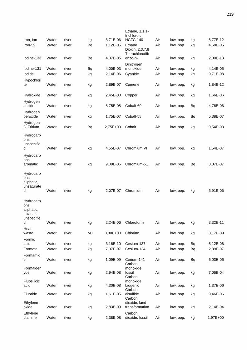
219
Iron, ion Water river kg 8,71E-06
Ethane, 1,1,1-trichloro-, HCFC-140 Air low. pop. kg 6,77E-12
Iron-59 Water river Bq 1,12E-05 Ethane Air low. pop. kg 4,68E-05
Iodine-133 Water river Bq 4,07E-05
Dioxin, 2,3,7,8 Tetrachlorodibenzo-p- Air low. pop. kg 2,00E-13
Iodine-131 Water river Bq 4,00E-03 Dinitrogen monoxide Air low. pop. kg 4,14E-05
Iodide Water river kg 2,14E-06 Cyanide Air low. pop. kg 9,71E-08
Hypochlorite Water river kg 2,89E-07 Cumene Air low. pop. kg 1,84E-12
Hydroxide Water river kg 2,45E-08 Copper Air low. pop. kg 1,66E-06
Hydrogen sulfide Water river kg 8,75E-08 Cobalt-60 Air low. pop. Bq 4,76E-06
Hydrogen peroxide Water river kg 1,75E-07 Cobalt-58 Air low. pop. Bq 5,38E-07
Hydrogen-3, Tritium Water river Bq 2,75E+03 Cobalt Air low. pop. kg 9,54E-08
Hydrocarbons, unspecified Water river kg 4,55E-07 Chromium VI Air low. pop. kg 1,54E-07
Hydrocarbons, aromatic Water river kg 9,09E-06 Chromium-51 Air low. pop. Bq 3,87E-07
Hydrocarbons, aliphatic, unsaturated Water river kg 2,07E-07 Chromium Air low. pop. kg 5,91E-06
Hydrocarbons, aliphatic, alkanes, unspecified Water river kg 2,24E-06 Chloroform Air low. pop. kg 3,32E-11
Heat, waste Water river MJ 3,80E+00 Chlorine Air low. pop. kg 8,17E-09
Formic acid Water river kg 3,16E-10 Cesium-137 Air low. pop. Bq 5,12E-06
Formate Water river kg 7,07E-07 Cesium-134 Air low. pop. Bq 2,89E-07
Formamide Water river kg 1,09E-09 Cerium-141 Air low. pop. Bq 6,03E-06
Formaldehyde Water river kg 2,94E-08
Carbon monoxide, fossil Air low. pop. kg 7,06E-04
Fluosilicic acid Water river kg 4,30E-08
Carbon monoxide, biogenic Air low. pop. kg 1,37E-06
Fluoride Water river kg 1,61E-05 Carbon disulfide Air low. pop. kg 9,46E-06
Ethylene oxide Water river kg 2,83E-09
Carbon dioxide, land transformation Air low. pop. kg 2,14E-04
Ethylene diamine Water river kg 2,38E-08
Carbon dioxide, fossil Air low. pop. kg 1,97E+00
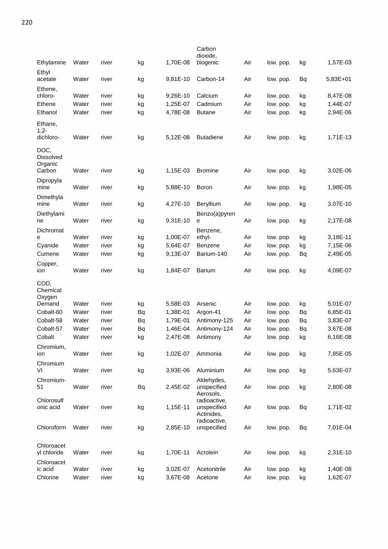
220
Ethylamine Water river kg 1,70E-08
Carbon dioxide, biogenic Air low. pop. kg 1,57E-03
Ethyl acetate Water river kg 9,81E-10 Carbon-14 Air low. pop. Bq 5,83E+01
Ethene, chloro- Water river kg 9,26E-10 Calcium Air low. pop. kg 8,47E-08
Ethene Water river kg 1,25E-07 Cadmium Air low. pop. kg 1,44E-07
Ethanol Water river kg 4,78E-08 Butane Air low. pop. kg 2,94E-06
Ethane, 1,2-dichloro- Water river kg 5,12E-08 Butadiene Air low. pop. kg 1,71E-13
DOC, Dissolved Organic Carbon Water river kg 1,15E-03 Bromine Air low. pop. kg 3,02E-06
Dipropylamine Water river kg 5,88E-10 Boron Air low. pop. kg 1,98E-05
Dimethylamine Water river kg 4,27E-10 Beryllium Air low. pop. kg 3,07E-10
Diethylamine Water river kg 9,31E-10
Benzo(a)pyrene Air low. pop. kg 2,17E-08
Dichromate Water river kg 1,00E-07
Benzene, ethyl- Air low. pop. kg 3,18E-11
Cyanide Water river kg 5,64E-07 Benzene Air low. pop. kg 7,15E-06
Cumene Water river kg 9,13E-07 Barium-140 Air low. pop. Bq 2,49E-05
Copper, ion Water river kg 1,84E-07 Barium Air low. pop. kg 4,09E-07
COD, Chemical Oxygen Demand Water river kg 5,58E-03 Arsenic Air low. pop. kg 5,01E-07
Cobalt-60 Water river Bq 1,38E-01 Argon-41 Air low. pop. Bq 6,85E-01
Cobalt-58 Water river Bq 1,79E-01 Antimony-125 Air low. pop. Bq 3,83E-07
Cobalt-57 Water river Bq 1,46E-04 Antimony-124 Air low. pop. Bq 3,67E-08
Cobalt Water river kg 2,47E-08 Antimony Air low. pop. kg 6,16E-08
Chromium, ion Water river kg 1,02E-07 Ammonia Air low. pop. kg 7,85E-05
Chromium VI Water river kg 3,93E-06 Aluminium Air low. pop. kg 5,63E-07
Chromium-51 Water river Bq 2,45E-02
Aldehydes, unspecified Air low. pop. kg 2,80E-08
Chlorosulfonic acid Water river kg 1,15E-11
Aerosols, radioactive, unspecified Air low. pop. Bq 1,71E-02
Chloroform Water river kg 2,85E-10
Actinides, radioactive, unspecified Air low. pop. Bq 7,01E-04
Chloroacetyl chloride Water river kg 1,70E-11 Acrolein Air low. pop. kg 2,31E-10
Chloroacetic acid Water river kg 3,02E-07 Acetonitrile Air low. pop. kg 1,40E-08
Chlorine Water river kg 3,67E-08 Acetone Air low. pop. kg 1,62E-07
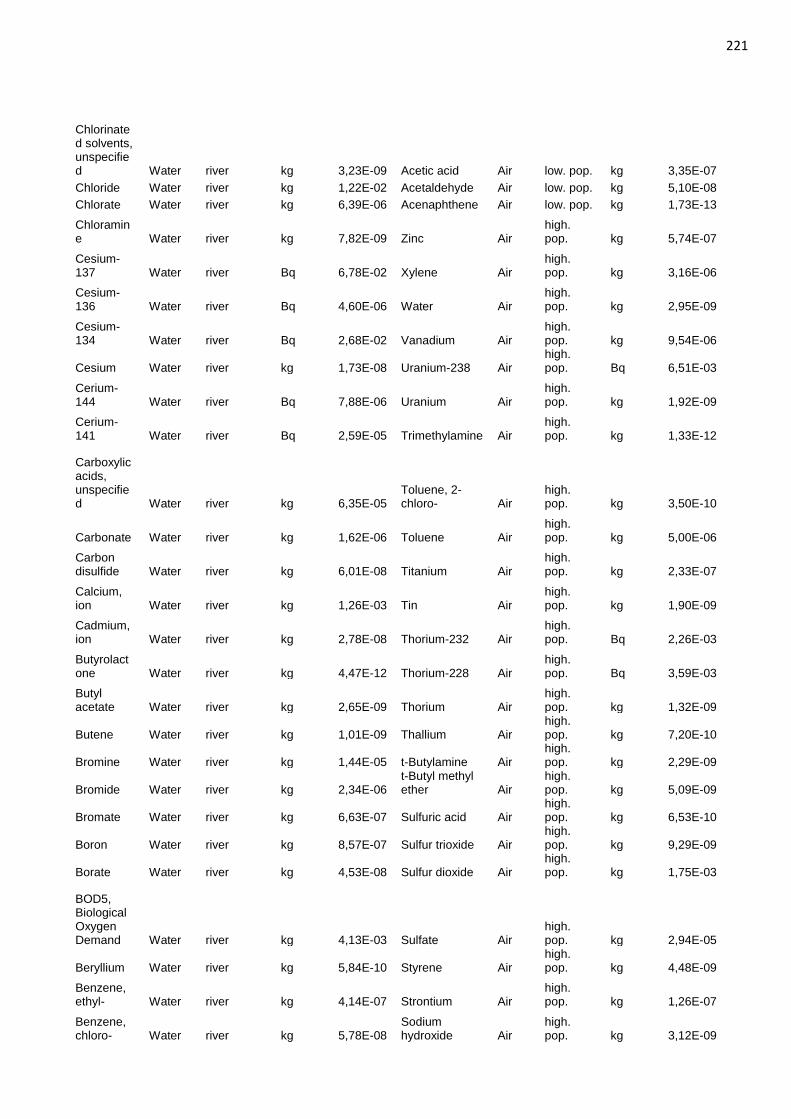
221
Chlorinated solvents, unspecified Water river kg 3,23E-09 Acetic acid Air low. pop. kg 3,35E-07
Chloride Water river kg 1,22E-02 Acetaldehyde Air low. pop. kg 5,10E-08
Chlorate Water river kg 6,39E-06 Acenaphthene Air low. pop. kg 1,73E-13
Chloramine Water river kg 7,82E-09 Zinc Air
high. pop. kg 5,74E-07
Cesium-137 Water river Bq 6,78E-02 Xylene Air
high. pop. kg 3,16E-06
Cesium-136 Water river Bq 4,60E-06 Water Air
high. pop. kg 2,95E-09
Cesium-134 Water river Bq 2,68E-02 Vanadium Air
high. pop. kg 9,54E-06
Cesium Water river kg 1,73E-08 Uranium-238 Air high. pop. Bq 6,51E-03
Cerium-144 Water river Bq 7,88E-06 Uranium Air
high. pop. kg 1,92E-09
Cerium-141 Water river Bq 2,59E-05 Trimethylamine Air
high. pop. kg 1,33E-12
Carboxylic acids, unspecified Water river kg 6,35E-05
Toluene, 2-chloro- Air
high. pop. kg 3,50E-10
Carbonate Water river kg 1,62E-06 Toluene Air high. pop. kg 5,00E-06
Carbon disulfide Water river kg 6,01E-08 Titanium Air
high. pop. kg 2,33E-07
Calcium, ion Water river kg 1,26E-03 Tin Air
high. pop. kg 1,90E-09
Cadmium, ion Water river kg 2,78E-08 Thorium-232 Air
high. pop. Bq 2,26E-03
Butyrolactone Water river kg 4,47E-12 Thorium-228 Air
high. pop. Bq 3,59E-03
Butyl acetate Water river kg 2,65E-09 Thorium Air
high. pop. kg 1,32E-09
Butene Water river kg 1,01E-09 Thallium Air high. pop. kg 7,20E-10
Bromine Water river kg 1,44E-05 t-Butylamine Air high. pop. kg 2,29E-09
Bromide Water river kg 2,34E-06 t-Butyl methyl ether Air
high. pop. kg 5,09E-09
Bromate Water river kg 6,63E-07 Sulfuric acid Air high. pop. kg 6,53E-10
Boron Water river kg 8,57E-07 Sulfur trioxide Air high. pop. kg 9,29E-09
Borate Water river kg 4,53E-08 Sulfur dioxide Air high. pop. kg 1,75E-03
BOD5, Biological Oxygen Demand Water river kg 4,13E-03 Sulfate Air
high. pop. kg 2,94E-05
Beryllium Water river kg 5,84E-10 Styrene Air high. pop. kg 4,48E-09
Benzene, ethyl- Water river kg 4,14E-07 Strontium Air
high. pop. kg 1,26E-07
Benzene, chloro- Water river kg 5,78E-08
Sodium hydroxide Air
high. pop. kg 3,12E-09
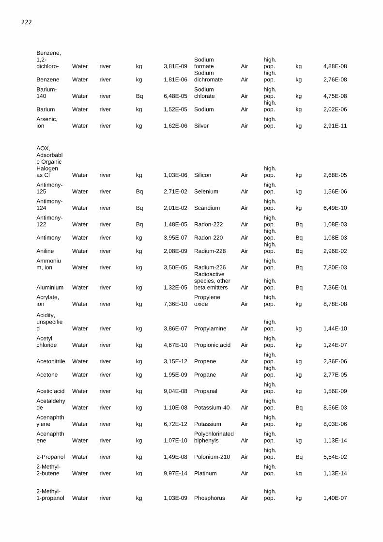
222
Benzene, 1,2-dichloro- Water river kg 3,81E-09
Sodium formate Air
high. pop. kg 4,88E-08
Benzene Water river kg 1,81E-06 Sodium dichromate Air
high. pop. kg 2,76E-08
Barium-140 Water river Bq 6,48E-05
Sodium chlorate Air
high. pop. kg 4,75E-08
Barium Water river kg 1,52E-05 Sodium Air high. pop. kg 2,02E-06
Arsenic, ion Water river kg 1,62E-06 Silver Air
high. pop. kg 2,91E-11
AOX, Adsorbable Organic Halogen as Cl Water river kg 1,03E-06 Silicon Air
high. pop. kg 2,68E-05
Antimony-125 Water river Bq 2,71E-02 Selenium Air
high. pop. kg 1,56E-06
Antimony-124 Water river Bq 2,01E-02 Scandium Air
high. pop. kg 6,49E-10
Antimony-122 Water river Bq 1,48E-05 Radon-222 Air
high. pop. Bq 1,08E-03
Antimony Water river kg 3,95E-07 Radon-220 Air high. pop. Bq 1,08E-03
Aniline Water river kg 2,08E-09 Radium-228 Air high. pop. Bq 2,96E-02
Ammonium, ion Water river kg 3,50E-05 Radium-226 Air
high. pop. Bq 7,80E-03
Aluminium Water river kg 1,32E-05
Radioactive species, other beta emitters Air
high. pop. Bq 7,36E-01
Acrylate, ion Water river kg 7,36E-10
Propylene oxide Air
high. pop. kg 8,78E-08
Acidity, unspecified Water river kg 3,86E-07 Propylamine Air
high. pop. kg 1,44E-10
Acetyl chloride Water river kg 4,67E-10 Propionic acid Air
high. pop. kg 1,24E-07
Acetonitrile Water river kg 3,15E-12 Propene Air high. pop. kg 2,36E-06
Acetone Water river kg 1,95E-09 Propane Air high. pop. kg 2,77E-05
Acetic acid Water river kg 9,04E-08 Propanal Air high. pop. kg 1,56E-09
Acetaldehyde Water river kg 1,10E-08 Potassium-40 Air
high. pop. Bq 8,56E-03
Acenaphthylene Water river kg 6,72E-12 Potassium Air
high. pop. kg 8,03E-06
Acenaphthene Water river kg 1,07E-10
Polychlorinated biphenyls Air
high. pop. kg 1,13E-14
2-Propanol Water river kg 1,49E-08 Polonium-210 Air high. pop. Bq 5,54E-02
2-Methyl-2-butene Water river kg 9,97E-14 Platinum Air
high. pop. kg 1,13E-14
2-Methyl-1-propanol Water river kg 1,03E-09 Phosphorus Air
high. pop. kg 1,40E-07
223
2-Aminopropanol Water river kg 1,27E-11 Phosphine Air
high. pop. kg 2,69E-13
1,4-Butanediol Water river kg 5,68E-12
Phenol, pentachloro- Air
high. pop. kg 1,97E-11
1-Propanol Water river kg 7,99E-10 Phenol, 2,4-dichloro- Air
high. pop. kg 4,25E-12
1-Pentene Water river kg 4,50E-10 Phenol Air high. pop. kg 2,76E-07
1-Pentanol Water river kg 5,95E-10 Pentane Air high. pop. kg 3,89E-05
1-Butanol Water river kg 2,04E-09
Particulates, > 2.5 um, and < 10um Air
high. pop. kg 7,48E-05
Zinc, ion Water lake kg 3,57E-14 Particulates, > 10 um Air
high. pop. kg 7,14E-05
Nickel, ion Water lake kg 4,92E-14 Particulates, < 2.5 um Air
high. pop. kg 2,18E-04
Mercury Water lake kg 3,13E-16
PAH, polycyclic aromatic hydrocarbons Air
high. pop. kg 6,93E-08
Lead Water lake kg 3,62E-14 Ozone Air high. pop. kg 2,32E-09
DOC, Dissolved Organic Carbon Water lake kg 7,24E-09
NMVOC, non-methane volatile organic compounds, unspecified origin Air
high. pop. kg 1,26E-04
Copper, ion Water lake kg 5,55E-13
Nitrogen oxides Air
high. pop. kg 1,86E-03
Calcium, ion Water lake kg 7,10E-08 Nitrobenzene Air
high. pop. kg 1,16E-09
Cadmium, ion Water lake kg 1,22E-14 Nitrate Air
high. pop. kg 2,17E-09
Arsenic, ion Water lake kg 1,44E-14 Nickel Air
high. pop. kg 2,70E-06
Zinc, ion Water
groundwater, long-term kg 4,29E-04
Monoethanolamine Air
high. pop. kg 9,42E-07
Vanadium, ion Water
groundwater, long-term kg 2,83E-05 Molybdenum Air
high. pop. kg 8,46E-08
Tungsten Water
groundwater, long-term kg 3,33E-06 Methyl lactate Air
high. pop. kg 2,11E-10
TOC, Total Organic Carbon Water
groundwater, long-term kg 6,35E-04 Methyl formate Air
high. pop. kg 1,21E-10
Titanium, ion Water
groundwater, long-term kg 1,68E-04
Methyl ethyl ketone Air
high. pop. kg 5,58E-07
Tin, ion Water
groundwater, long-term kg 4,58E-06 Methyl borate Air
high. pop. kg 9,19E-11
224
Thallium Water
groundwater, long-term kg 4,50E-07 Methyl amine Air
high. pop. kg 3,91E-12
Sulfate Water
groundwater, long-term kg 2,70E-01 Methyl acrylate Air
high. pop. kg 3,53E-10
Strontium Water
groundwater, long-term kg 1,19E-03 Methyl acetate Air
high. pop. kg 6,38E-13
Sodium, ion Water
groundwater, long-term kg 3,23E-02 Methanol Air
high. pop. kg 6,57E-07
Silver, ion Water
groundwater, long-term kg 1,94E-07
Methanesulfonic acid Air
high. pop. kg 3,80E-12
Silicon Water
groundwater, long-term kg 5,58E-02
Methane, trifluoro-, HFC-23 Air
high. pop. kg 3,14E-11
Selenium Water
groundwater, long-term kg 1,14E-05
Methane, trichlorofluoro-, CFC-11 Air
high. pop. kg 1,60E-13
Scandium Water
groundwater, long-term kg 7,62E-06
Methane, tetrafluoro-, CFC-14 Air
high. pop. kg 9,28E-12
Potassium, ion Water
groundwater, long-term kg 1,96E-02
Methane, tetrachloro-, CFC-10 Air
high. pop. kg 2,45E-09
Phosphate Water
groundwater, long-term kg 1,03E-02
Methane, monochloro-, R-40 Air
high. pop. kg 1,65E-12
Nitrogen, organic bound Water
groundwater, long-term kg 1,13E-06 Methane, fossil Air
high. pop. kg 1,89E-04
Nitrite Water
groundwater, long-term kg 3,77E-08
Methane, dichlorofluoro-, HCFC-21 Air
high. pop. kg 9,87E-14
Nitrate Water
groundwater, long-term kg 3,32E-03
Methane, dichlorodifluoro-, CFC-12 Air
high. pop. kg 7,14E-11
Nickel, ion Water
groundwater, long-term kg 3,33E-04
Methane, dichloro-, HCC-30 Air
high. pop. kg 8,48E-10
Molybdenum Water
groundwater, long-term kg 1,47E-05
Methane, chlorodifluoro-, HCFC-22 Air
high. pop. kg 5,98E-10
Mercury Water
groundwater, long-term kg 9,75E-07
Methane, bromotrifluoro-, Halon 1301 Air
high. pop. kg 2,18E-14
Manganese Water
groundwater, long-term kg 2,80E-03
Methane, biogenic Air
high. pop. kg 2,01E-06
Magnesium Water
groundwater, long-term kg 3,45E-02 Mercury Air
high. pop. kg 8,07E-09
225
Lead Water
groundwater, long-term kg 9,27E-06 Manganese Air
high. pop. kg 1,75E-07
Iron, ion Water
groundwater, long-term kg 8,20E-03 Magnesium Air
high. pop. kg 3,02E-06
Iodide Water
groundwater, long-term kg 3,47E-12 m-Xylene Air
high. pop. kg 3,75E-08
Hydrogen sulfide Water
groundwater, long-term kg 2,17E-06 Lead-210 Air
high. pop. Bq 3,02E-02
Heat, waste Water
groundwater, long-term MJ 1,57E-02 Lead Air
high. pop. kg 5,39E-07
Fluoride Water
groundwater, long-term kg 2,83E-04 Lactic acid Air
high. pop. kg 1,92E-10
DOC, Dissolved Organic Carbon Water
groundwater, long-term kg 6,35E-04 Isopropylamine Air
high. pop. kg 2,69E-09
Copper, ion Water
groundwater, long-term kg 9,23E-05 Isocyanic acid Air
high. pop. kg 3,59E-08
COD, Chemical Oxygen Demand Water
groundwater, long-term kg 1,45E-03 Iron Air
high. pop. kg 4,30E-06
Cobalt Water
groundwater, long-term kg 7,76E-05 Iodine Air
high. pop. kg 1,23E-08
Chromium VI Water
groundwater, long-term kg 3,45E-05
Hydrogen sulfide Air
high. pop. kg 3,16E-06
Chloride Water
groundwater, long-term kg 7,98E-03
Hydrogen peroxide Air
high. pop. kg 8,36E-10
Calcium, ion Water
groundwater, long-term kg 6,83E-02
Hydrogen fluoride Air
high. pop. kg 4,38E-06
Cadmium, ion Water
groundwater, long-term kg 4,02E-06
Hydrogen chloride Air
high. pop. kg 2,96E-05
Bromine Water
groundwater, long-term kg 5,94E-07 Hydrogen Air
high. pop. kg 3,19E-05
Boron Water
groundwater, long-term kg 1,10E-04
Hydrocarbons, chlorinated Air
high. pop. kg 3,39E-09
BOD5, Biological Oxygen Demand Water
groundwater, long-term kg 4,71E-04
Hydrocarbons, aromatic Air
high. pop. kg 6,36E-07
226
Beryllium Water
groundwater, long-term kg 5,01E-06
Hydrocarbons, aliphatic, unsaturated Air
high. pop. kg 2,05E-06
Barium Water
groundwater, long-term kg 1,41E-04
Hydrocarbons, aliphatic, alkanes, unspecified Air
high. pop. kg 3,18E-06
Arsenic, ion Water
groundwater, long-term kg 1,38E-05
Hydrocarbons, aliphatic, alkanes, cyclic Air
high. pop. kg 9,39E-09
Antimony Water
groundwater, long-term kg 3,30E-06 Hexane Air
high. pop. kg 1,42E-05
Ammonium, ion Water
groundwater, long-term kg 6,93E-07 Heptane Air
high. pop. kg 5,47E-06
Aluminium Water
groundwater, long-term kg 6,99E-03 Heat, waste Air
high. pop. MJ 1,39E+01
Zinc, ion Water groundwater kg 7,96E-07 Formic acid Air
high. pop. kg 8,30E-10
Zinc Water groundwater kg 1,38E-04 Formamide Air
high. pop. kg 4,53E-10
Xylene Water groundwater kg 5,11E-10 Formaldehyde Air
high. pop. kg 1,72E-06
VOC, volatile organic compounds, unspecified origin Water
groundwater kg 3,25E-11 Fluosilicic acid Air
high. pop. kg 2,39E-08
Vanadium, ion Water
groundwater kg 1,30E-07 Fluorine Air
high. pop. kg 1,54E-08
Vanadium Water groundwater kg 5,19E-11 Ethyne Air
high. pop. kg 1,03E-06
Uranium-238 Water
groundwater Bq 2,15E-03 Ethylene oxide Air
high. pop. kg 5,71E-09
Tungsten Water groundwater kg 2,68E-07
Ethylene diamine Air
high. pop. kg 9,90E-09
Toluene Water groundwater kg 9,98E-11 Ethylamine Air
high. pop. kg 7,08E-09
TOC, Total Organic Carbon Water
groundwater kg 2,69E-08 Ethyl cellulose Air
high. pop. kg 1,13E-09
Titanium, ion Water
groundwater kg 1,16E-07 Ethyl acetate Air
high. pop. kg 5,58E-07
Titanium Water groundwater kg 4,13E-11
Ethene, tetrachloro- Air
high. pop. kg 1,98E-13
Tin, ion Water groundwater kg 3,41E-09 Ethene, chloro- Air
high. pop. kg 6,75E-08
Tin Water groundwater kg 1,14E-14 Ethene Air
high. pop. kg 7,44E-06
Thorium-228 Water
groundwater Bq 2,84E-06 Ethanol Air
high. pop. kg 5,46E-07
227
Thallium Water groundwater kg 6,82E-10
Ethane, hexafluoro-, HFC-116 Air
high. pop. kg 1,02E-09
Sulfur Water groundwater kg 1,74E-13
Ethane, 1,2-dichloro- Air
high. pop. kg 1,21E-07
Sulfite Water groundwater kg 2,37E-10
Ethane, 1,1,2-trichloro-1,2,2-trifluoro-, CFC-113 Air
high. pop. kg 1,48E-11
Sulfide Water groundwater kg 1,91E-09
Ethane, 1,1,1,2-tetrafluoro-, HFC-134a Air
high. pop. kg 3,47E-11
Sulfate Water groundwater kg 1,43E-02
Ethane, 1,1-difluoro-, HFC-152a Air
high. pop. kg 1,80E-10
Strontium-90 Water
groundwater Bq 3,39E-04 Ethane Air
high. pop. kg 1,20E-05
Strontium Water groundwater kg 1,03E-05 Dipropylamine Air
high. pop. kg 2,45E-10
Solved solids Water
groundwater kg 5,37E-05
Dioxin, 2,3,7,8 Tetrachlorodibenzo-p- Air
high. pop. kg 5,41E-13
Solids, inorganic Water
groundwater kg 5,29E-03
Dinitrogen monoxide Air
high. pop. kg 2,50E-05
Sodium, ion Water
groundwater kg 7,47E-04
Dimethyl malonate Air
high. pop. kg 4,72E-12
Silver, ion Water groundwater kg 7,71E-09 Diethylamine Air
high. pop. kg 3,88E-10
Silver-110 Water groundwater Bq 1,05E-08
Cyanoacetic acid Air
high. pop. kg 3,76E-12
Silicon Water groundwater kg 2,04E-04 Cyanide Air
high. pop. kg 2,83E-07
Selenium Water groundwater kg 4,96E-07 Cumene Air
high. pop. kg 3,80E-07
Scandium Water groundwater kg 2,50E-07 Copper Air
high. pop. kg 6,85E-07
Ruthenium-106 Water
groundwater Bq 6,90E-06 Cobalt Air
high. pop. kg 3,42E-07
Radium-226 Water
groundwater Bq 1,14E-01 Chromium VI Air
high. pop. kg 1,70E-09
Propane, 1,2-dichloro- Water
groundwater kg 5,15E-19 Chromium Air
high. pop. kg 1,48E-07
Potassium, ion Water
groundwater kg 2,90E-04
Chlorosulfonic acid Air
high. pop. kg 4,59E-12
Potassium-40 Water
groundwater Bq 2,80E-05
Chlorosilane, trimethyl- Air
high. pop. kg 1,11E-10
Potassium Water groundwater kg 3,38E-10 Chloroform Air
high. pop. kg 2,29E-09
Polonium-210 Water
groundwater Bq 3,53E-04
Chloroacetic acid Air
high. pop. kg 1,78E-09
Plutonium-alpha Water
groundwater Bq 2,77E-05 Chlorine Air
high. pop. kg 1,01E-06
Phosphorus, total Water
groundwater kg 2,94E-05 Chloramine Air
high. pop. kg 8,76E-10
Phosphorus Water
groundwater kg 2,26E-09
Carbon monoxide, fossil Air
high. pop. kg 9,21E-04
228
Phosphate Water groundwater kg 1,31E-03
Carbon monoxide, biogenic Air
high. pop. kg 2,29E-05
Phenol Water groundwater kg 1,35E-10
Carbon disulfide Air
high. pop. kg 2,52E-08
Particulates, > 10 um Water
groundwater kg 3,31E-06
Carbon dioxide, fossil Air
high. pop. kg 8,37E-01
Particulates, < 10 um Water
groundwater kg 7,76E-12
Carbon dioxide, biogenic Air
high. pop. kg 2,75E-01
Nitrogen Water groundwater kg 6,11E-07 Calcium Air
high. pop. kg 1,07E-05
Nitrate Water groundwater kg 1,66E-03 Cadmium Air
high. pop. kg 6,35E-08
Nickel, ion Water groundwater kg 6,50E-07 Butyrolactone Air
high. pop. kg 1,86E-12
Nickel Water groundwater kg 6,38E-09 Butene Air
high. pop. kg 5,48E-07
Naphthalene Water
groundwater kg 1,81E-12 Butane Air
high. pop. kg 2,88E-05
Molybdenum Water
groundwater kg 4,49E-06 Butadiene Air
high. pop. kg 1,60E-10
Methanol Water groundwater kg 8,20E-08 Bromine Air
high. pop. kg 2,99E-08
Methane, monochloro-, R-40 Water
groundwater kg 1,68E-11
Boron trifluoride Air
high. pop. kg 4,96E-17
Methane, dibromo- Water
groundwater kg 1,89E-16 Boron Air
high. pop. kg 2,08E-06
Mercury Water groundwater kg 1,95E-09 Beryllium Air
high. pop. kg 1,06E-09
Manganese-54 Water
groundwater Bq 2,33E-04
Benzo(a)pyrene Air
high. pop. kg 3,48E-09
Manganese Water
groundwater kg 1,68E-05
Benzene, pentachloro- Air
high. pop. kg 1,58E-10
Magnesium Water
groundwater kg 3,46E-04
Benzene, hexachloro- Air
high. pop. kg 6,28E-11
Lead-210 Water groundwater Bq 2,32E-04
Benzene, ethyl- Air
high. pop. kg 5,60E-07
Lead Water groundwater kg 5,83E-09
Benzene, 1,2-dichloro- Air
high. pop. kg 4,26E-10
Iron, ion Water groundwater kg 2,42E-03
Benzene, 1-methyl-2-nitro- Air
high. pop. kg 2,38E-12
Iron Water groundwater kg 4,20E-07 Benzene Air
high. pop. kg 6,74E-06
Iodine-131 Water groundwater Bq 5,12E-08 Benzaldehyde Air
high. pop. kg 8,33E-11
Iodine-129 Water groundwater Bq 1,00E-03 Barium Air
high. pop. kg 1,02E-07
Iodide Water groundwater kg 1,20E-07 Arsine Air
high. pop. kg 3,62E-15
Hydroxide Water groundwater kg 3,26E-10 Arsenic Air
high. pop. kg 9,84E-08
Hydrogen fluoride Water
groundwater kg 1,89E-13 Antimony Air
high. pop. kg 1,87E-08
229
Hydrogen chloride Water
groundwater kg 1,18E-11 Anthranilic acid Air
high. pop. kg 2,14E-12
Hydrogen-3, Tritium Water
groundwater Bq 1,02E+01 Aniline Air
high. pop. kg 8,66E-10
Hydrocarbons, unspecified Water
groundwater kg 1,68E-10
Ammonium carbonate Air
high. pop. kg 4,75E-09
Hydrocarbons, aromatic Water
groundwater kg 1,19E-10 Ammonia Air
high. pop. kg 1,83E-05
Hexane Water groundwater kg 5,02E-16 Aluminium Air
high. pop. kg 6,68E-06
Heat, waste Water
groundwater MJ 8,76E-04
Aldehydes, unspecified Air
high. pop. kg 9,25E-09
Fluorine Water groundwater kg 1,64E-10 Acrylic acid Air
high. pop. kg 3,11E-10
Fluoride Water groundwater kg 4,18E-06 Acrolein Air
high. pop. kg 1,60E-10
Fluoranthene Water
groundwater kg 8,26E-15 Acetone Air
high. pop. kg 4,11E-07
Ethene, chloro- Water
groundwater kg 8,86E-17 Acetic acid Air
high. pop. kg 2,08E-06
Dioxin, 2,3,7,8 Tetrachlorodibenzo-p- Water
groundwater kg 2,43E-24 Acetaldehyde Air
high. pop. kg 2,90E-07
Decane Water groundwater kg 9,95E-10 Acenaphthene Air
high. pop. kg 1,91E-12
Cyanide Water groundwater kg 1,35E-12 2-Propanol Air
high. pop. kg 1,23E-07
Curium alpha Water
groundwater Bq 9,14E-06
2-Nitrobenzoic acid Air
high. pop. kg 2,76E-12
Cresol Water groundwater kg 4,50E-15
2-Methyl-1-propanol Air
high. pop. kg 4,29E-10
Copper, ion Water
groundwater kg 9,89E-08
2-Butene, 2-methyl- Air
high. pop. kg 4,15E-14
Copper Water groundwater kg 9,17E-09
2-Aminopropanol Air
high. pop. kg 5,29E-12
COD, Chemical Oxygen Demand Water
groundwater kg 1,73E-04 1,4-Butanediol Air
high. pop. kg 1,42E-11
Cobalt-60 Water groundwater Bq 1,50E-03 1-Propanol Air
high. pop. kg 1,75E-09
Cobalt-58 Water groundwater Bq 2,68E-06 1-Pentene Air
high. pop. kg 1,87E-10
Cobalt Water groundwater kg 1,19E-07 1-Pentanol Air
high. pop. kg 2,48E-10
Chrysene Water groundwater kg 2,00E-14 1-Butanol Air
high. pop. kg 2,31E-12
Chromium, ion Water
groundwater kg 8,11E-08 Zinc oxide Air
kg 2,95E-17
Chromium VI Water
groundwater kg 2,22E-06 Zinc Air
kg 1,49E-06
230
Chromium Water groundwater kg 9,64E-11 Xylene Air
kg 1,33E-07
Chlorine Water groundwater kg 8,10E-09 Xenon-138 Air
Bq 3,85E-04
Chloride Water groundwater kg 4,14E-03 Xenon-137 Air
Bq 2,99E-06
Cesium-137 Water
groundwater Bq 3,24E-03 Xenon-135 Air
Bq 1,14E-02
Cesium-134 Water
groundwater Bq 3,64E-04 Xenon-133 Air
Bq 3,45E-02
Carbonate Water groundwater kg 1,02E-08 Xenon-131m Air
Bq 2,11E-04
Carbon-14 Water groundwater Bq 3,50E-04 Water Air
kg 1,25E+02
Calcium, ion Water
groundwater kg 8,82E-04
VOC, volatile organic compounds Air
kg 7,85E-09
Cadmium, ion Water
groundwater kg 8,15E-09 Vanadium Air
kg 3,62E-09
Cadmium Water groundwater kg 4,76E-10 Used air Air
kg 5,45E-02
Bromine Water groundwater kg 1,08E-06 Uranium-238 Air
Bq 8,44E-05
Boron Water groundwater kg 7,35E-06 Uranium-235 Air
Bq 6,32E-05
BOD5, Biological Oxygen Demand Water
groundwater kg 5,40E-08 Uranium-234 Air
Bq 1,63E-05
Beryllium Water groundwater kg 9,40E-09 Toluene Air
kg 1,81E-07
Benzo(b)fluoranthene Water
groundwater kg 2,42E-15 Titanium Air
kg 1,18E-09
Benzo(a)anthracene Water
groundwater kg 4,50E-15 Tin oxide Air
kg 1,47E-17
Benzene, ethyl- Water
groundwater kg 1,57E-11 Tin Air
kg 3,03E-09
Benzene Water groundwater kg 1,37E-10 Thorium-232 Air
Bq 3,11E-11
Barium Water groundwater kg 9,92E-08 Thorium-228 Air
Bq 1,98E-11
Arsenic, ion Water
groundwater kg 2,53E-06 Thallium Air
kg 9,56E-10
AOX, Adsorbable Organic Halogen as Cl Water
groundwater kg 4,41E-10 Tellurium Air
kg 6,26E-15
Antimony-125 Water
groundwater Bq 4,89E-08
Sulfur hexafluoride Air
kg 3,13E-07
Antimony-124 Water
groundwater Bq 7,17E-08 Sulfur dioxide Air
kg 1,61E-04
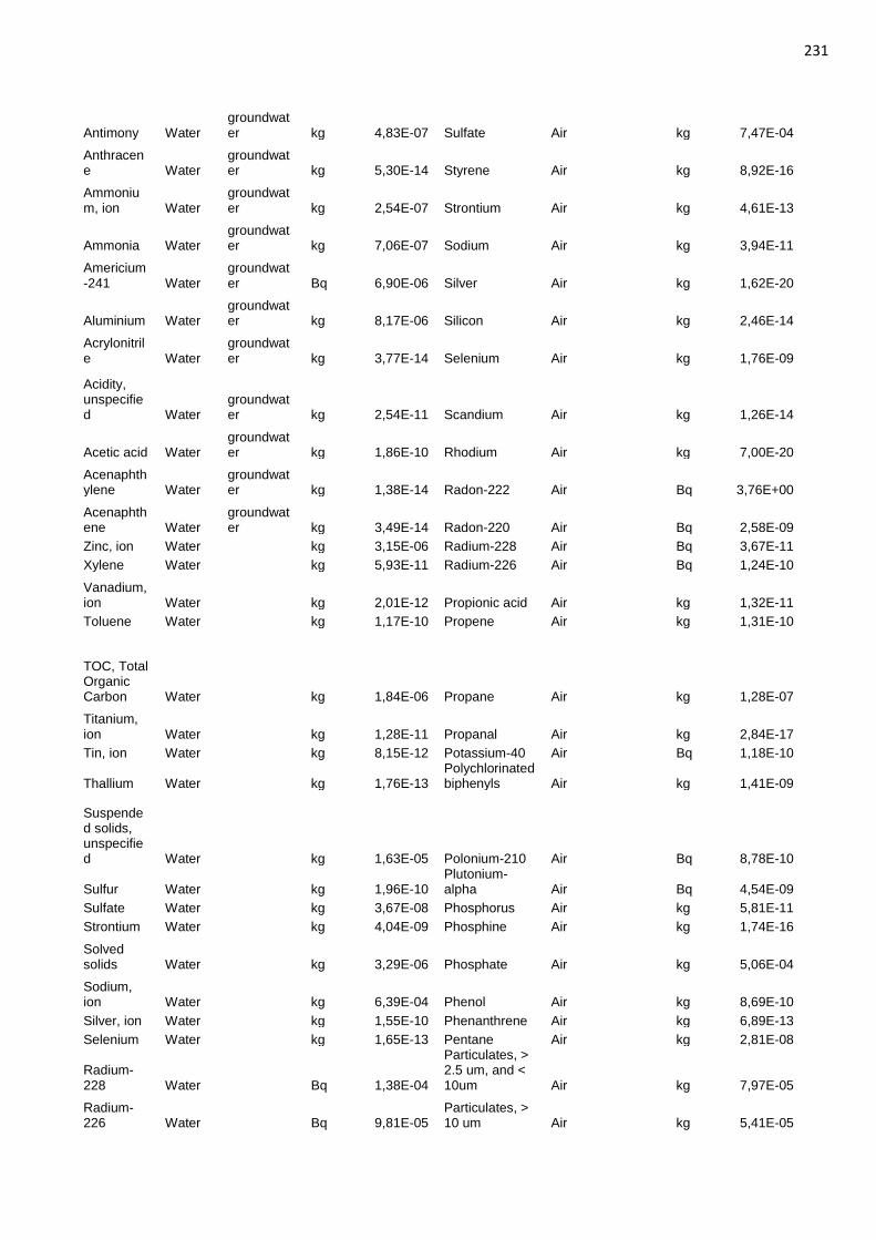
231
Antimony Water groundwater kg 4,83E-07 Sulfate Air
kg 7,47E-04
Anthracene Water
groundwater kg 5,30E-14 Styrene Air
kg 8,92E-16
Ammonium, ion Water
groundwater kg 2,54E-07 Strontium Air
kg 4,61E-13
Ammonia Water groundwater kg 7,06E-07 Sodium Air
kg 3,94E-11
Americium-241 Water
groundwater Bq 6,90E-06 Silver Air
kg 1,62E-20
Aluminium Water groundwater kg 8,17E-06 Silicon Air
kg 2,46E-14
Acrylonitrile Water
groundwater kg 3,77E-14 Selenium Air
kg 1,76E-09
Acidity, unspecified Water
groundwater kg 2,54E-11 Scandium Air
kg 1,26E-14
Acetic acid Water groundwater kg 1,86E-10 Rhodium Air
kg 7,00E-20
Acenaphthylene Water
groundwater kg 1,38E-14 Radon-222 Air
Bq 3,76E+00
Acenaphthene Water
groundwater kg 3,49E-14 Radon-220 Air
Bq 2,58E-09
Zinc, ion Water
kg 3,15E-06 Radium-228 Air
Bq 3,67E-11
Xylene Water
kg 5,93E-11 Radium-226 Air
Bq 1,24E-10
Vanadium, ion Water
kg 2,01E-12 Propionic acid Air
kg 1,32E-11
Toluene Water
kg 1,17E-10 Propene Air
kg 1,31E-10
TOC, Total Organic Carbon Water
kg 1,84E-06 Propane Air
kg 1,28E-07
Titanium, ion Water
kg 1,28E-11 Propanal Air
kg 2,84E-17
Tin, ion Water
kg 8,15E-12 Potassium-40 Air
Bq 1,18E-10
Thallium Water
kg 1,76E-13 Polychlorinated biphenyls Air
kg 1,41E-09
Suspended solids, unspecified Water
kg 1,63E-05 Polonium-210 Air
Bq 8,78E-10
Sulfur Water
kg 1,96E-10 Plutonium-alpha Air
Bq 4,54E-09
Sulfate Water
kg 3,67E-08 Phosphorus Air
kg 5,81E-11
Strontium Water
kg 4,04E-09 Phosphine Air
kg 1,74E-16
Solved solids Water
kg 3,29E-06 Phosphate Air
kg 5,06E-04
Sodium, ion Water
kg 6,39E-04 Phenol Air
kg 8,69E-10
Silver, ion Water
kg 1,55E-10 Phenanthrene Air
kg 6,89E-13
Selenium Water
kg 1,65E-13 Pentane Air
kg 2,81E-08
Radium-228 Water
Bq 1,38E-04
Particulates, > 2.5 um, and < 10um Air
kg 7,97E-05
Radium-226 Water
Bq 9,81E-05
Particulates, > 10 um Air
kg 5,41E-05
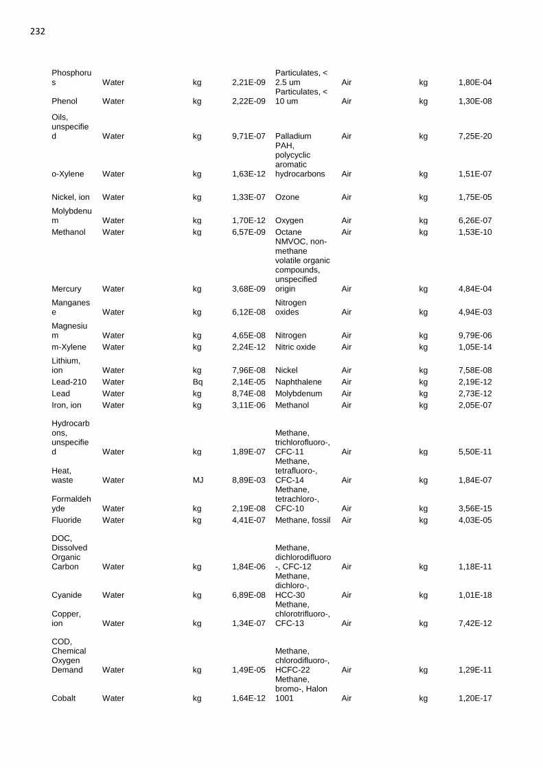
232
Phosphorus Water
kg 2,21E-09
Particulates, < 2.5 um Air
kg 1,80E-04
Phenol Water
kg 2,22E-09 Particulates, < 10 um Air
kg 1,30E-08
Oils, unspecified Water
kg 9,71E-07 Palladium Air
kg 7,25E-20
o-Xylene Water
kg 1,63E-12
PAH, polycyclic aromatic hydrocarbons Air
kg 1,51E-07
Nickel, ion Water
kg 1,33E-07 Ozone Air
kg 1,75E-05
Molybdenum Water
kg 1,70E-12 Oxygen Air
kg 6,26E-07
Methanol Water
kg 6,57E-09 Octane Air
kg 1,53E-10
Mercury Water
kg 3,68E-09
NMVOC, non-methane volatile organic compounds, unspecified origin Air
kg 4,84E-04
Manganese Water
kg 6,12E-08
Nitrogen oxides Air
kg 4,94E-03
Magnesium Water
kg 4,65E-08 Nitrogen Air
kg 9,79E-06
m-Xylene Water
kg 2,24E-12 Nitric oxide Air
kg 1,05E-14
Lithium, ion Water
kg 7,96E-08 Nickel Air
kg 7,58E-08
Lead-210 Water
Bq 2,14E-05 Naphthalene Air
kg 2,19E-12
Lead Water
kg 8,74E-08 Molybdenum Air
kg 2,73E-12
Iron, ion Water
kg 3,11E-06 Methanol Air
kg 2,05E-07
Hydrocarbons, unspecified Water
kg 1,89E-07
Methane, trichlorofluoro-, CFC-11 Air
kg 5,50E-11
Heat, waste Water
MJ 8,89E-03
Methane, tetrafluoro-, CFC-14 Air
kg 1,84E-07
Formaldehyde Water
kg 2,19E-08
Methane, tetrachloro-, CFC-10 Air
kg 3,56E-15
Fluoride Water
kg 4,41E-07 Methane, fossil Air
kg 4,03E-05
DOC, Dissolved Organic Carbon Water
kg 1,84E-06
Methane, dichlorodifluoro-, CFC-12 Air
kg 1,18E-11
Cyanide Water
kg 6,89E-08
Methane, dichloro-, HCC-30 Air
kg 1,01E-18
Copper, ion Water
kg 1,34E-07
Methane, chlorotrifluoro-, CFC-13 Air
kg 7,42E-12
COD, Chemical Oxygen Demand Water
kg 1,49E-05
Methane, chlorodifluoro-, HCFC-22 Air
kg 1,29E-11
Cobalt Water
kg 1,64E-12
Methane, bromo-, Halon 1001 Air
kg 1,20E-17
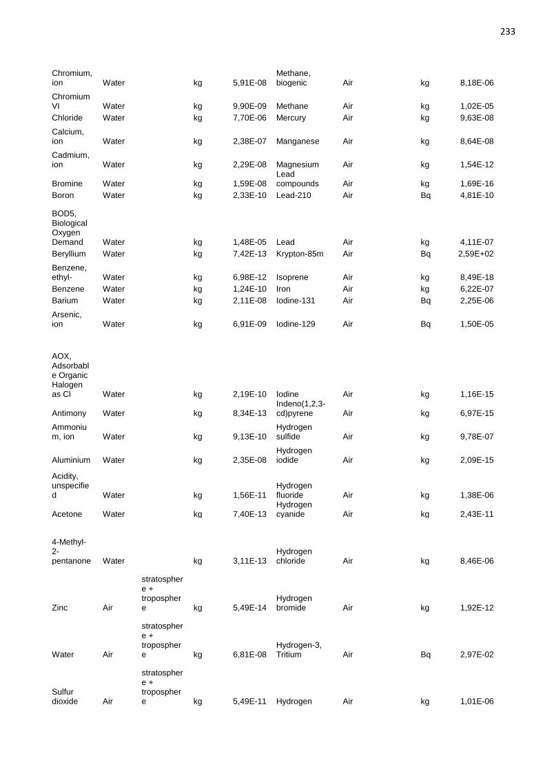
233
Chromium, ion Water
kg 5,91E-08
Methane, biogenic Air
kg 8,18E-06
Chromium VI Water
kg 9,90E-09 Methane Air
kg 1,02E-05
Chloride Water
kg 7,70E-06 Mercury Air
kg 9,63E-08
Calcium, ion Water
kg 2,38E-07 Manganese Air
kg 8,64E-08
Cadmium, ion Water
kg 2,29E-08 Magnesium Air
kg 1,54E-12
Bromine Water
kg 1,59E-08 Lead compounds Air
kg 1,69E-16
Boron Water
kg 2,33E-10 Lead-210 Air
Bq 4,81E-10
BOD5, Biological Oxygen Demand Water
kg 1,48E-05 Lead Air
kg 4,11E-07
Beryllium Water
kg 7,42E-13 Krypton-85m Air
Bq 2,59E+02
Benzene, ethyl- Water
kg 6,98E-12 Isoprene Air
kg 8,49E-18
Benzene Water
kg 1,24E-10 Iron Air
kg 6,22E-07
Barium Water
kg 2,11E-08 Iodine-131 Air
Bq 2,25E-06
Arsenic, ion Water
kg 6,91E-09 Iodine-129 Air
Bq 1,50E-05
AOX, Adsorbable Organic Halogen as Cl Water
kg 2,19E-10 Iodine Air
kg 1,16E-15
Antimony Water
kg 8,34E-13 Indeno(1,2,3-cd)pyrene Air
kg 6,97E-15
Ammonium, ion Water
kg 9,13E-10
Hydrogen sulfide Air
kg 9,78E-07
Aluminium Water
kg 2,35E-08 Hydrogen iodide Air
kg 2,09E-15
Acidity, unspecified Water
kg 1,56E-11
Hydrogen fluoride Air
kg 1,38E-06
Acetone Water
kg 7,40E-13 Hydrogen cyanide Air
kg 2,43E-11
4-Methyl-2-pentanone Water
kg 3,11E-13
Hydrogen chloride Air
kg 8,46E-06
Zinc Air
stratosphere + troposphere kg 5,49E-14
Hydrogen bromide Air
kg 1,92E-12
Water Air
stratosphere + troposphere kg 6,81E-08
Hydrogen-3, Tritium Air
Bq 2,97E-02
Sulfur dioxide Air
stratosphere + troposphere kg 5,49E-11 Hydrogen Air
kg 1,01E-06
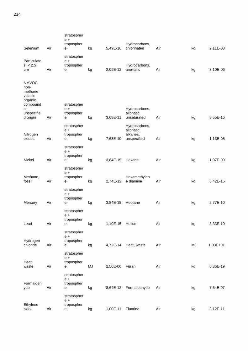
234
Selenium Air
stratosphere + troposphere kg 5,49E-16
Hydrocarbons, chlorinated Air
kg 2,11E-08
Particulates, < 2.5 um Air
stratosphere + troposphere kg 2,09E-12
Hydrocarbons, aromatic Air
kg 3,10E-06
NMVOC, non-methane volatile organic compounds, unspecified origin Air
stratosphere + troposphere kg 3,68E-11
Hydrocarbons, aliphatic, unsaturated Air
kg 8,55E-16
Nitrogen oxides Air
stratosphere + troposphere kg 7,68E-10
Hydrocarbons, aliphatic, alkanes, unspecified Air
kg 1,13E-05
Nickel Air
stratosphere + troposphere kg 3,84E-15 Hexane Air
kg 1,07E-09
Methane, fossil Air
stratosphere + troposphere kg 2,74E-12
Hexamethylene diamine Air
kg 6,42E-16
Mercury Air
stratosphere + troposphere kg 3,84E-18 Heptane Air
kg 2,77E-10
Lead Air
stratosphere + troposphere kg 1,10E-15 Helium Air
kg 3,33E-10
Hydrogen chloride Air
stratosphere + troposphere kg 4,72E-14 Heat, waste Air
MJ 1,03E+01
Heat, waste Air
stratosphere + troposphere MJ 2,50E-06 Furan Air
kg 6,36E-19
Formaldehyde Air
stratosphere + troposphere kg 8,64E-12 Formaldehyde Air
kg 7,54E-07
Ethylene oxide Air
stratosphere + troposphere kg 1,00E-11 Fluorine Air
kg 3,12E-11
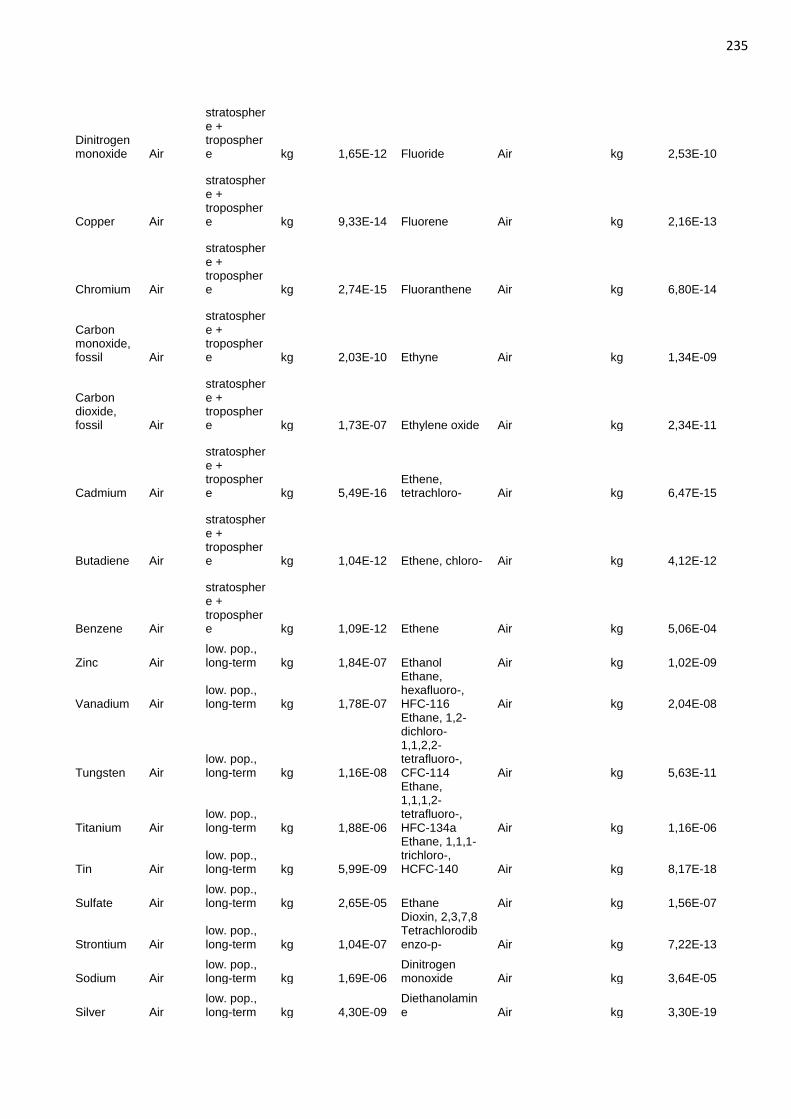
235
Dinitrogen monoxide Air
stratosphere + troposphere kg 1,65E-12 Fluoride Air
kg 2,53E-10
Copper Air
stratosphere + troposphere kg 9,33E-14 Fluorene Air
kg 2,16E-13
Chromium Air
stratosphere + troposphere kg 2,74E-15 Fluoranthene Air
kg 6,80E-14
Carbon monoxide, fossil Air
stratosphere + troposphere kg 2,03E-10 Ethyne Air
kg 1,34E-09
Carbon dioxide, fossil Air
stratosphere + troposphere kg 1,73E-07 Ethylene oxide Air
kg 2,34E-11
Cadmium Air
stratosphere + troposphere kg 5,49E-16
Ethene, tetrachloro- Air
kg 6,47E-15
Butadiene Air
stratosphere + troposphere kg 1,04E-12 Ethene, chloro- Air
kg 4,12E-12
Benzene Air
stratosphere + troposphere kg 1,09E-12 Ethene Air
kg 5,06E-04
Zinc Air low. pop., long-term kg 1,84E-07 Ethanol Air
kg 1,02E-09
Vanadium Air low. pop., long-term kg 1,78E-07
Ethane, hexafluoro-, HFC-116 Air
kg 2,04E-08
Tungsten Air low. pop., long-term kg 1,16E-08
Ethane, 1,2-dichloro-1,1,2,2-tetrafluoro-, CFC-114 Air
kg 5,63E-11
Titanium Air low. pop., long-term kg 1,88E-06
Ethane, 1,1,1,2-tetrafluoro-, HFC-134a Air
kg 1,16E-06
Tin Air low. pop., long-term kg 5,99E-09
Ethane, 1,1,1-trichloro-, HCFC-140 Air
kg 8,17E-18
Sulfate Air low. pop., long-term kg 2,65E-05 Ethane Air
kg 1,56E-07
Strontium Air low. pop., long-term kg 1,04E-07
Dioxin, 2,3,7,8 Tetrachlorodibenzo-p- Air
kg 7,22E-13
Sodium Air low. pop., long-term kg 1,69E-06
Dinitrogen monoxide Air
kg 3,64E-05
Silver Air low. pop., long-term kg 4,30E-09
Diethanolamine Air
kg 3,30E-19
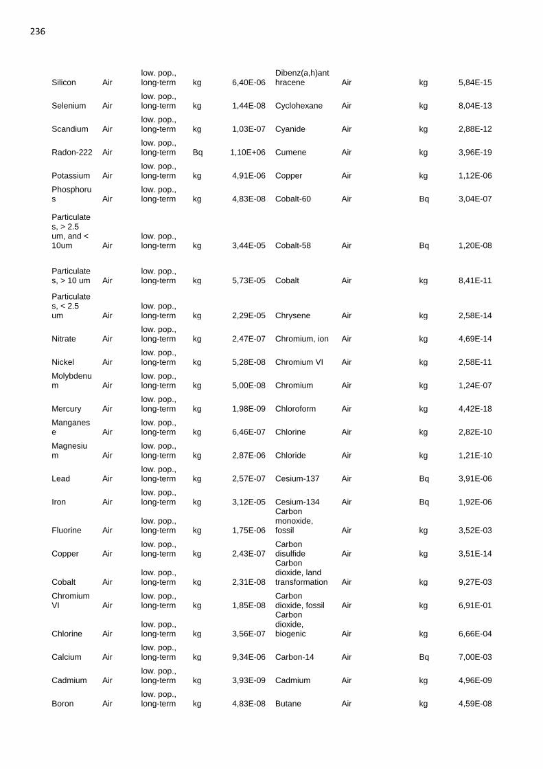
236
Silicon Air low. pop., long-term kg 6,40E-06
Dibenz(a,h)anthracene Air
kg 5,84E-15
Selenium Air low. pop., long-term kg 1,44E-08 Cyclohexane Air
kg 8,04E-13
Scandium Air low. pop., long-term kg 1,03E-07 Cyanide Air
kg 2,88E-12
Radon-222 Air low. pop., long-term Bq 1,10E+06 Cumene Air
kg 3,96E-19
Potassium Air low. pop., long-term kg 4,91E-06 Copper Air
kg 1,12E-06
Phosphorus Air
low. pop., long-term kg 4,83E-08 Cobalt-60 Air
Bq 3,04E-07
Particulates, > 2.5 um, and < 10um Air
low. pop., long-term kg 3,44E-05 Cobalt-58 Air
Bq 1,20E-08
Particulates, > 10 um Air
low. pop., long-term kg 5,73E-05 Cobalt Air
kg 8,41E-11
Particulates, < 2.5 um Air
low. pop., long-term kg 2,29E-05 Chrysene Air
kg 2,58E-14
Nitrate Air low. pop., long-term kg 2,47E-07 Chromium, ion Air
kg 4,69E-14
Nickel Air low. pop., long-term kg 5,28E-08 Chromium VI Air
kg 2,58E-11
Molybdenum Air
low. pop., long-term kg 5,00E-08 Chromium Air
kg 1,24E-07
Mercury Air low. pop., long-term kg 1,98E-09 Chloroform Air
kg 4,42E-18
Manganese Air
low. pop., long-term kg 6,46E-07 Chlorine Air
kg 2,82E-10
Magnesium Air
low. pop., long-term kg 2,87E-06 Chloride Air
kg 1,21E-10
Lead Air low. pop., long-term kg 2,57E-07 Cesium-137 Air
Bq 3,91E-06
Iron Air low. pop., long-term kg 3,12E-05 Cesium-134 Air
Bq 1,92E-06
Fluorine Air low. pop., long-term kg 1,75E-06
Carbon monoxide, fossil Air
kg 3,52E-03
Copper Air low. pop., long-term kg 2,43E-07
Carbon disulfide Air
kg 3,51E-14
Cobalt Air low. pop., long-term kg 2,31E-08
Carbon dioxide, land transformation Air
kg 9,27E-03
Chromium VI Air
low. pop., long-term kg 1,85E-08
Carbon dioxide, fossil Air
kg 6,91E-01
Chlorine Air low. pop., long-term kg 3,56E-07
Carbon dioxide, biogenic Air
kg 6,66E-04
Calcium Air low. pop., long-term kg 9,34E-06 Carbon-14 Air
Bq 7,00E-03
Cadmium Air low. pop., long-term kg 3,93E-09 Cadmium Air
kg 4,96E-09
Boron Air low. pop., long-term kg 4,83E-08 Butane Air
kg 4,59E-08
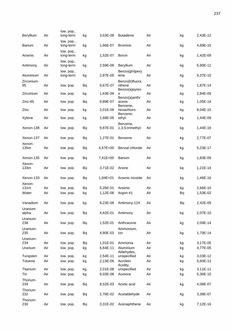
237
Beryllium Air low. pop., long-term kg 3,63E-09 Butadiene Air
kg 2,43E-12
Barium Air low. pop., long-term kg 1,66E-07 Bromine Air
kg 4,69E-10
Arsenic Air low. pop., long-term kg 1,52E-07 Boron Air
kg 1,42E-09
Antimony Air low. pop., long-term kg 2,59E-09 Beryllium Air
kg 5,90E-11
Aluminium Air low. pop., long-term kg 2,87E-05
Benzo(ghi)perylene Air
kg 9,37E-15
Zirconium-95 Air low. pop. Bq 9,67E-07
Benzo(b)fluoranthene Air
kg 1,87E-14
Zirconium Air low. pop. kg 1,63E-09 Benzo(a)pyrene Air
kg 2,84E-09
Zinc-65 Air low. pop. Bq 9,89E-07 Benzo(a)anthracene Air
kg 1,05E-14
Zinc Air low. pop. kg 2,01E-06 Benzene, hexachloro- Air
kg 8,04E-10
Xylene Air low. pop. kg 1,68E-05 Benzene, ethyl- Air
kg 1,44E-09
Xenon-138 Air low. pop. Bq 9,87E-01 Benzene, 1,3,5-trimethyl- Air
kg 1,44E-16
Xenon-137 Air low. pop. Bq 1,27E-01 Benzene Air
kg 2,77E-07
Xenon-135m Air low. pop. Bq 4,57E+00 Benzal chloride Air
kg 5,23E-17
Xenon-135 Air low. pop. Bq 7,41E+00 Barium Air
kg 1,83E-09
Xenon-133m Air low. pop. Bq 3,71E-02 Arsine Air
kg 1,21E-14
Xenon-133 Air low. pop. Bq 1,84E+01 Arsenic trioxide Air
kg 1,46E-16
Xenon-131m Air low. pop. Bq 5,26E-01 Arsenic Air
kg 2,66E-10
Water Air low. pop. kg 1,12E-08 Argon-41 Air
Bq 1,53E-02
Vanadium Air low. pop. kg 9,23E-08 Antimony-124 Air
Bq 2,42E-09
Uranium alpha Air low. pop. Bq 4,62E-01 Antimony Air
kg 2,07E-10
Uranium-238 Air low. pop. Bq 1,52E-01 Anthracene Air
kg 2,09E-14
Uranium-235 Air low. pop. Bq 4,80E-03
Ammonium, ion Air
kg 1,79E-14
Uranium-234 Air low. pop. Bq 1,01E-01 Ammonia Air
kg 3,17E-05
Uranium Air low. pop. kg 6,64E-11 Aluminium Air
kg 4,77E-05
Tungsten Air low. pop. kg 2,54E-11 Aldehydes, unspecified Air
kg 3,03E-12
Toluene Air low. pop. kg 2,13E-06 Acrolein Air
kg 5,60E-13
Titanium Air low. pop. kg 2,01E-08 Acidity, unspecified Air
kg 3,11E-11
Tin Air low. pop. kg 9,03E-08 Acetone Air
kg 5,36E-10
Thorium-234 Air low. pop. Bq 8,52E-03 Acetic acid Air
kg 4,08E-07
Thorium-232 Air low. pop. Bq 2,76E-02 Acetaldehyde Air
kg 3,38E-07
Thorium-230 Air low. pop. Bq 3,31E-02 Acenaphthene Air
kg 7,12E-16

238
Thorium-228 Air low. pop. Bq 1,75E-02
Thorium Air low. pop. kg 1,31E-10 Thallium Air low. pop. kg 3,68E-11 Terpenes Air low. pop. kg 1,17E-08
Sulfuric acid Air low. pop. kg 1,79E-13
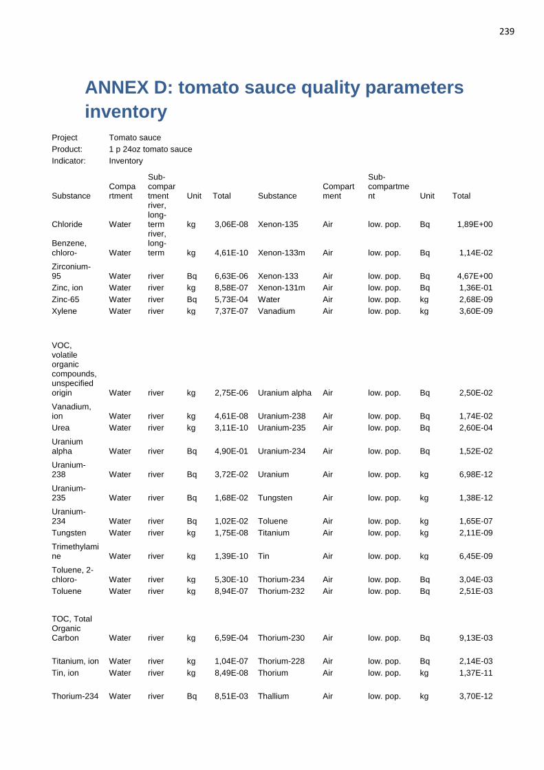
239
ANNEX D: tomato sauce quality parameters
inventory
Project Tomato sauce
Product: 1 p 24oz tomato sauce
Indicator: Inventory
Substance Compartment
Sub-compartment Unit Total Substance
Compartment
Sub-compartment Unit Total
Chloride Water
river, long-term kg 3,06E-08 Xenon-135 Air low. pop. Bq 1,89E+00
Benzene, chloro- Water
river, long-term kg 4,61E-10 Xenon-133m Air low. pop. Bq 1,14E-02
Zirconium-95 Water river Bq 6,63E-06 Xenon-133 Air low. pop. Bq 4,67E+00
Zinc, ion Water river kg 8,58E-07 Xenon-131m Air low. pop. Bq 1,36E-01
Zinc-65 Water river Bq 5,73E-04 Water Air low. pop. kg 2,68E-09
Xylene Water river kg 7,37E-07 Vanadium Air low. pop. kg 3,60E-09
VOC, volatile organic compounds, unspecified origin Water river kg 2,75E-06 Uranium alpha Air low. pop. Bq 2,50E-02
Vanadium, ion Water river kg 4,61E-08 Uranium-238 Air low. pop. Bq 1,74E-02
Urea Water river kg 3,11E-10 Uranium-235 Air low. pop. Bq 2,60E-04
Uranium alpha Water river Bq 4,90E-01 Uranium-234 Air low. pop. Bq 1,52E-02
Uranium-238 Water river Bq 3,72E-02 Uranium Air low. pop. kg 6,98E-12
Uranium-235 Water river Bq 1,68E-02 Tungsten Air low. pop. kg 1,38E-12
Uranium-234 Water river Bq 1,02E-02 Toluene Air low. pop. kg 1,65E-07
Tungsten Water river kg 1,75E-08 Titanium Air low. pop. kg 2,11E-09
Trimethylamine Water river kg 1,39E-10 Tin Air low. pop. kg 6,45E-09
Toluene, 2-chloro- Water river kg 5,30E-10 Thorium-234 Air low. pop. Bq 3,04E-03
Toluene Water river kg 8,94E-07 Thorium-232 Air low. pop. Bq 2,51E-03
TOC, Total Organic Carbon Water river kg 6,59E-04 Thorium-230 Air low. pop. Bq 9,13E-03
Titanium, ion Water river kg 1,04E-07 Thorium-228 Air low. pop. Bq 2,14E-03
Tin, ion Water river kg 8,49E-08 Thorium Air low. pop. kg 1,37E-11
Thorium-234 Water river Bq 8,51E-03 Thallium Air low. pop. kg 3,70E-12
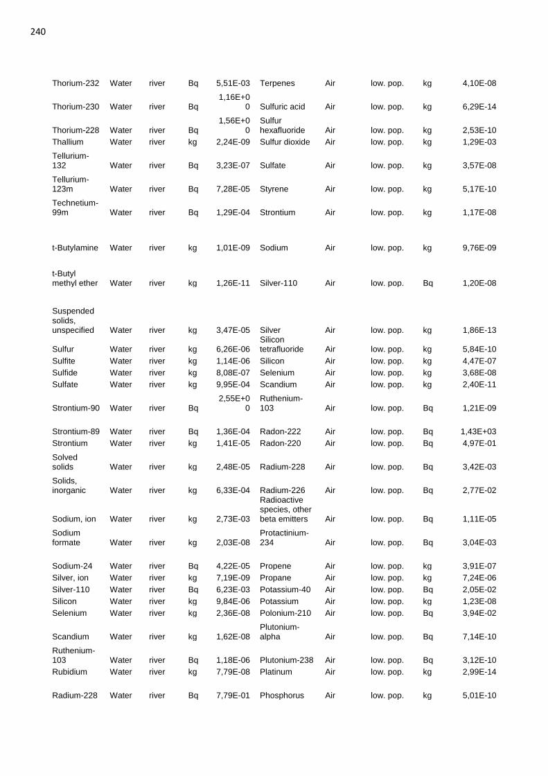
240
Thorium-232 Water river Bq 5,51E-03 Terpenes Air low. pop. kg 4,10E-08
Thorium-230 Water river Bq 1,16E+0
0 Sulfuric acid Air low. pop. kg 6,29E-14
Thorium-228 Water river Bq 1,56E+0
0 Sulfur hexafluoride Air low. pop. kg 2,53E-10
Thallium Water river kg 2,24E-09 Sulfur dioxide Air low. pop. kg 1,29E-03
Tellurium-132 Water river Bq 3,23E-07 Sulfate Air low. pop. kg 3,57E-08
Tellurium-123m Water river Bq 7,28E-05 Styrene Air low. pop. kg 5,17E-10
Technetium-99m Water river Bq 1,29E-04 Strontium Air low. pop. kg 1,17E-08
t-Butylamine Water river kg 1,01E-09 Sodium Air low. pop. kg 9,76E-09
t-Butyl methyl ether Water river kg 1,26E-11 Silver-110 Air low. pop. Bq 1,20E-08
Suspended solids, unspecified Water river kg 3,47E-05 Silver Air low. pop. kg 1,86E-13
Sulfur Water river kg 6,26E-06 Silicon tetrafluoride Air low. pop. kg 5,84E-10
Sulfite Water river kg 1,14E-06 Silicon Air low. pop. kg 4,47E-07
Sulfide Water river kg 8,08E-07 Selenium Air low. pop. kg 3,68E-08
Sulfate Water river kg 9,95E-04 Scandium Air low. pop. kg 2,40E-11
Strontium-90 Water river Bq 2,55E+0
0 Ruthenium-103 Air low. pop. Bq 1,21E-09
Strontium-89 Water river Bq 1,36E-04 Radon-222 Air low. pop. Bq 1,43E+03
Strontium Water river kg 1,41E-05 Radon-220 Air low. pop. Bq 4,97E-01
Solved solids Water river kg 2,48E-05 Radium-228 Air low. pop. Bq 3,42E-03
Solids, inorganic Water river kg 6,33E-04 Radium-226 Air low. pop. Bq 2,77E-02
Sodium, ion Water river kg 2,73E-03
Radioactive species, other beta emitters Air low. pop. Bq 1,11E-05
Sodium formate Water river kg 2,03E-08
Protactinium-234 Air low. pop. Bq 3,04E-03
Sodium-24 Water river Bq 4,22E-05 Propene Air low. pop. kg 3,91E-07
Silver, ion Water river kg 7,19E-09 Propane Air low. pop. kg 7,24E-06
Silver-110 Water river Bq 6,23E-03 Potassium-40 Air low. pop. Bq 2,05E-02
Silicon Water river kg 9,84E-06 Potassium Air low. pop. kg 1,23E-08
Selenium Water river kg 2,36E-08 Polonium-210 Air low. pop. Bq 3,94E-02
Scandium Water river kg 1,62E-08 Plutonium-alpha Air low. pop. Bq 7,14E-10
Ruthenium-103 Water river Bq 1,18E-06 Plutonium-238 Air low. pop. Bq 3,12E-10
Rubidium Water river kg 7,79E-08 Platinum Air low. pop. kg 2,99E-14
Radium-228 Water river Bq 7,79E-01 Phosphorus Air low. pop. kg 5,01E-10
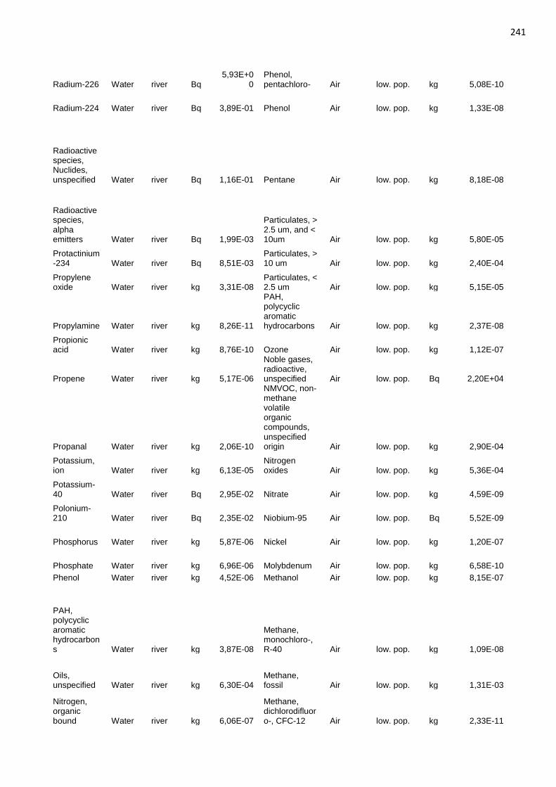
241
Radium-226 Water river Bq 5,93E+0
0 Phenol, pentachloro- Air low. pop. kg 5,08E-10
Radium-224 Water river Bq 3,89E-01 Phenol Air low. pop. kg 1,33E-08
Radioactive species, Nuclides, unspecified Water river Bq 1,16E-01 Pentane Air low. pop. kg 8,18E-08
Radioactive species, alpha emitters Water river Bq 1,99E-03
Particulates, > 2.5 um, and < 10um Air low. pop. kg 5,80E-05
Protactinium-234 Water river Bq 8,51E-03
Particulates, > 10 um Air low. pop. kg 2,40E-04
Propylene oxide Water river kg 3,31E-08
Particulates, < 2.5 um Air low. pop. kg 5,15E-05
Propylamine Water river kg 8,26E-11
PAH, polycyclic aromatic hydrocarbons Air low. pop. kg 2,37E-08
Propionic acid Water river kg 8,76E-10 Ozone Air low. pop. kg 1,12E-07
Propene Water river kg 5,17E-06
Noble gases, radioactive, unspecified Air low. pop. Bq 2,20E+04
Propanal Water river kg 2,06E-10
NMVOC, non-methane volatile organic compounds, unspecified origin Air low. pop. kg 2,90E-04
Potassium, ion Water river kg 6,13E-05
Nitrogen oxides Air low. pop. kg 5,36E-04
Potassium-40 Water river Bq 2,95E-02 Nitrate Air low. pop. kg 4,59E-09
Polonium-210 Water river Bq 2,35E-02 Niobium-95 Air low. pop. Bq 5,52E-09
Phosphorus Water river kg 5,87E-06 Nickel Air low. pop. kg 1,20E-07
Phosphate Water river kg 6,96E-06 Molybdenum Air low. pop. kg 6,58E-10
Phenol Water river kg 4,52E-06 Methanol Air low. pop. kg 8,15E-07
PAH, polycyclic aromatic hydrocarbons Water river kg 3,87E-08
Methane, monochloro-, R-40 Air low. pop. kg 1,09E-08
Oils, unspecified Water river kg 6,30E-04
Methane, fossil Air low. pop. kg 1,31E-03
Nitrogen, organic bound Water river kg 6,06E-07
Methane, dichlorodifluoro-, CFC-12 Air low. pop. kg 2,33E-11
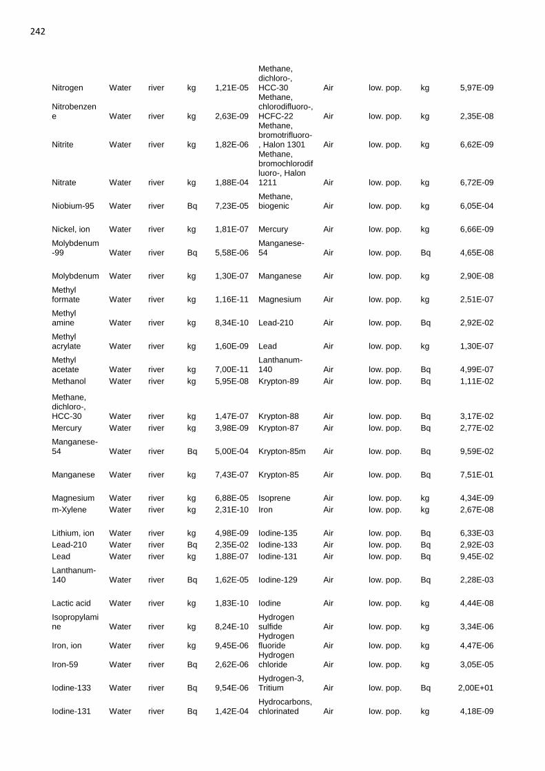
242
Nitrogen Water river kg 1,21E-05
Methane, dichloro-, HCC-30 Air low. pop. kg 5,97E-09
Nitrobenzene Water river kg 2,63E-09
Methane, chlorodifluoro-, HCFC-22 Air low. pop. kg 2,35E-08
Nitrite Water river kg 1,82E-06
Methane, bromotrifluoro-, Halon 1301 Air low. pop. kg 6,62E-09
Nitrate Water river kg 1,88E-04
Methane, bromochlorodifluoro-, Halon 1211 Air low. pop. kg 6,72E-09
Niobium-95 Water river Bq 7,23E-05 Methane, biogenic Air low. pop. kg 6,05E-04
Nickel, ion Water river kg 1,81E-07 Mercury Air low. pop. kg 6,66E-09
Molybdenum-99 Water river Bq 5,58E-06
Manganese-54 Air low. pop. Bq 4,65E-08
Molybdenum Water river kg 1,30E-07 Manganese Air low. pop. kg 2,90E-08
Methyl formate Water river kg 1,16E-11 Magnesium Air low. pop. kg 2,51E-07
Methyl amine Water river kg 8,34E-10 Lead-210 Air low. pop. Bq 2,92E-02
Methyl acrylate Water river kg 1,60E-09 Lead Air low. pop. kg 1,30E-07
Methyl acetate Water river kg 7,00E-11
Lanthanum-140 Air low. pop. Bq 4,99E-07
Methanol Water river kg 5,95E-08 Krypton-89 Air low. pop. Bq 1,11E-02
Methane, dichloro-, HCC-30 Water river kg 1,47E-07 Krypton-88 Air low. pop. Bq 3,17E-02
Mercury Water river kg 3,98E-09 Krypton-87 Air low. pop. Bq 2,77E-02
Manganese-54 Water river Bq 5,00E-04 Krypton-85m Air low. pop. Bq 9,59E-02
Manganese Water river kg 7,43E-07 Krypton-85 Air low. pop. Bq 7,51E-01
Magnesium Water river kg 6,88E-05 Isoprene Air low. pop. kg 4,34E-09
m-Xylene Water river kg 2,31E-10 Iron Air low. pop. kg 2,67E-08
Lithium, ion Water river kg 4,98E-09 Iodine-135 Air low. pop. Bq 6,33E-03
Lead-210 Water river Bq 2,35E-02 Iodine-133 Air low. pop. Bq 2,92E-03
Lead Water river kg 1,88E-07 Iodine-131 Air low. pop. Bq 9,45E-02
Lanthanum-140 Water river Bq 1,62E-05 Iodine-129 Air low. pop. Bq 2,28E-03
Lactic acid Water river kg 1,83E-10 Iodine Air low. pop. kg 4,44E-08
Isopropylamine Water river kg 8,24E-10
Hydrogen sulfide Air low. pop. kg 3,34E-06
Iron, ion Water river kg 9,45E-06 Hydrogen fluoride Air low. pop. kg 4,47E-06
Iron-59 Water river Bq 2,62E-06 Hydrogen chloride Air low. pop. kg 3,05E-05
Iodine-133 Water river Bq 9,54E-06 Hydrogen-3, Tritium Air low. pop. Bq 2,00E+01
Iodine-131 Water river Bq 1,42E-04 Hydrocarbons, chlorinated Air low. pop. kg 4,18E-09
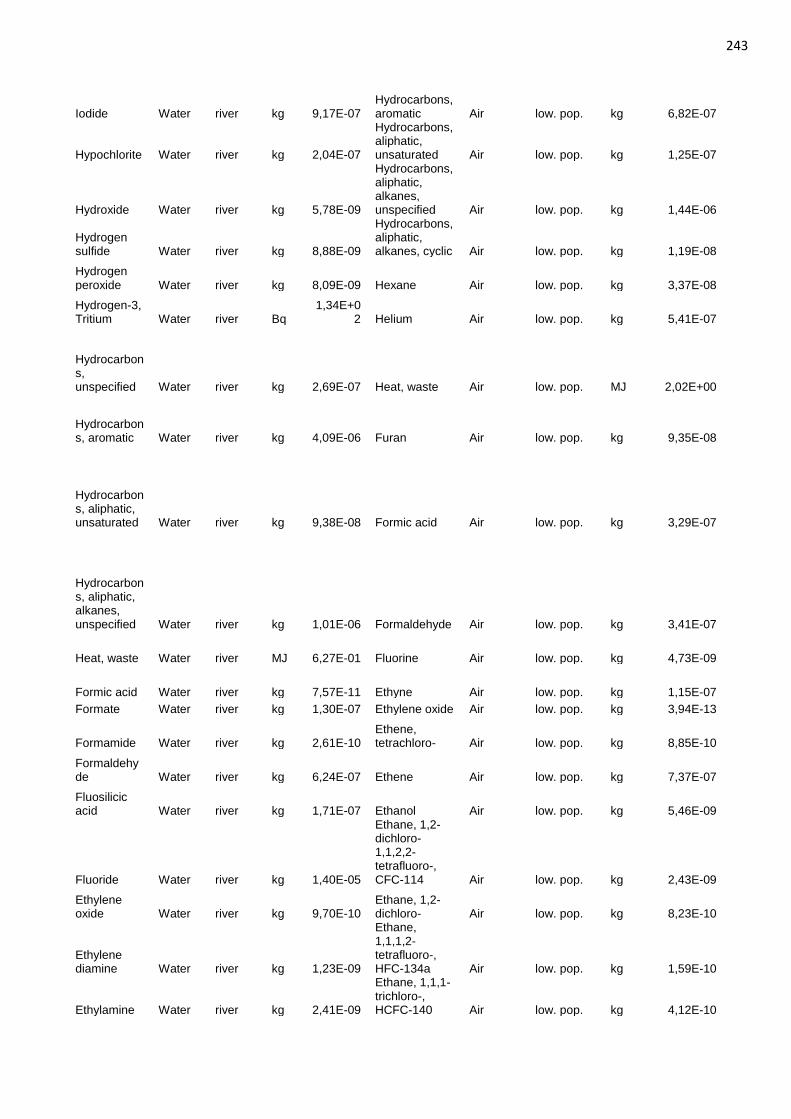
243
Iodide Water river kg 9,17E-07 Hydrocarbons, aromatic Air low. pop. kg 6,82E-07
Hypochlorite Water river kg 2,04E-07
Hydrocarbons, aliphatic, unsaturated Air low. pop. kg 1,25E-07
Hydroxide Water river kg 5,78E-09
Hydrocarbons, aliphatic, alkanes, unspecified Air low. pop. kg 1,44E-06
Hydrogen sulfide Water river kg 8,88E-09
Hydrocarbons, aliphatic, alkanes, cyclic Air low. pop. kg 1,19E-08
Hydrogen peroxide Water river kg 8,09E-09 Hexane Air low. pop. kg 3,37E-08
Hydrogen-3, Tritium Water river Bq
1,34E+02 Helium Air low. pop. kg 5,41E-07
Hydrocarbons, unspecified Water river kg 2,69E-07 Heat, waste Air low. pop. MJ 2,02E+00
Hydrocarbons, aromatic Water river kg 4,09E-06 Furan Air low. pop. kg 9,35E-08
Hydrocarbons, aliphatic, unsaturated Water river kg 9,38E-08 Formic acid Air low. pop. kg 3,29E-07
Hydrocarbons, aliphatic, alkanes, unspecified Water river kg 1,01E-06 Formaldehyde Air low. pop. kg 3,41E-07
Heat, waste Water river MJ 6,27E-01 Fluorine Air low. pop. kg 4,73E-09
Formic acid Water river kg 7,57E-11 Ethyne Air low. pop. kg 1,15E-07
Formate Water river kg 1,30E-07 Ethylene oxide Air low. pop. kg 3,94E-13
Formamide Water river kg 2,61E-10 Ethene, tetrachloro- Air low. pop. kg 8,85E-10
Formaldehyde Water river kg 6,24E-07 Ethene Air low. pop. kg 7,37E-07
Fluosilicic acid Water river kg 1,71E-07 Ethanol Air low. pop. kg 5,46E-09
Fluoride Water river kg 1,40E-05
Ethane, 1,2-dichloro-1,1,2,2-tetrafluoro-, CFC-114 Air low. pop. kg 2,43E-09
Ethylene oxide Water river kg 9,70E-10
Ethane, 1,2-dichloro- Air low. pop. kg 8,23E-10
Ethylene diamine Water river kg 1,23E-09
Ethane, 1,1,1,2-tetrafluoro-, HFC-134a Air low. pop. kg 1,59E-10
Ethylamine Water river kg 2,41E-09
Ethane, 1,1,1-trichloro-, HCFC-140 Air low. pop. kg 4,12E-10
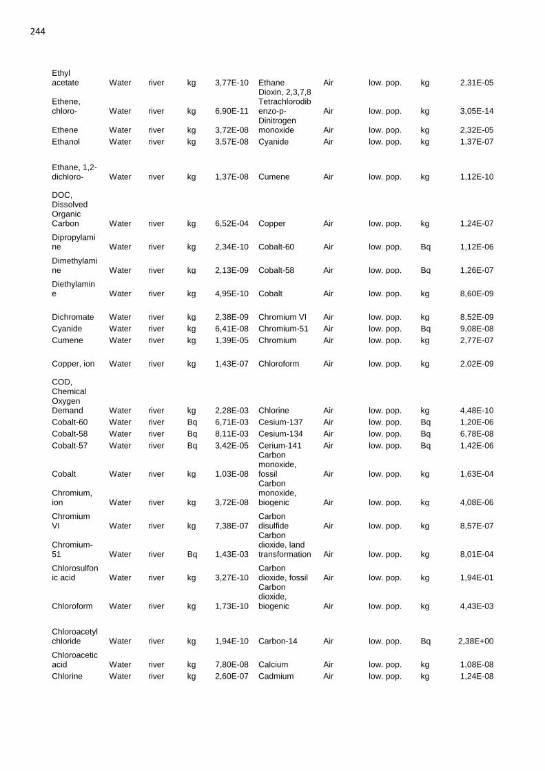
244
Ethyl acetate Water river kg 3,77E-10 Ethane Air low. pop. kg 2,31E-05
Ethene, chloro- Water river kg 6,90E-11
Dioxin, 2,3,7,8 Tetrachlorodibenzo-p- Air low. pop. kg 3,05E-14
Ethene Water river kg 3,72E-08 Dinitrogen monoxide Air low. pop. kg 2,32E-05
Ethanol Water river kg 3,57E-08 Cyanide Air low. pop. kg 1,37E-07
Ethane, 1,2-dichloro- Water river kg 1,37E-08 Cumene Air low. pop. kg 1,12E-10
DOC, Dissolved Organic Carbon Water river kg 6,52E-04 Copper Air low. pop. kg 1,24E-07
Dipropylamine Water river kg 2,34E-10 Cobalt-60 Air low. pop. Bq 1,12E-06
Dimethylamine Water river kg 2,13E-09 Cobalt-58 Air low. pop. Bq 1,26E-07
Diethylamine Water river kg 4,95E-10 Cobalt Air low. pop. kg 8,60E-09
Dichromate Water river kg 2,38E-09 Chromium VI Air low. pop. kg 8,52E-09
Cyanide Water river kg 6,41E-08 Chromium-51 Air low. pop. Bq 9,08E-08
Cumene Water river kg 1,39E-05 Chromium Air low. pop. kg 2,77E-07
Copper, ion Water river kg 1,43E-07 Chloroform Air low. pop. kg 2,02E-09
COD, Chemical Oxygen Demand Water river kg 2,28E-03 Chlorine Air low. pop. kg 4,48E-10
Cobalt-60 Water river Bq 6,71E-03 Cesium-137 Air low. pop. Bq 1,20E-06
Cobalt-58 Water river Bq 8,11E-03 Cesium-134 Air low. pop. Bq 6,78E-08
Cobalt-57 Water river Bq 3,42E-05 Cerium-141 Air low. pop. Bq 1,42E-06
Cobalt Water river kg 1,03E-08
Carbon monoxide, fossil Air low. pop. kg 1,63E-04
Chromium, ion Water river kg 3,72E-08
Carbon monoxide, biogenic Air low. pop. kg 4,08E-06
Chromium VI Water river kg 7,38E-07
Carbon disulfide Air low. pop. kg 8,57E-07
Chromium-51 Water river Bq 1,43E-03
Carbon dioxide, land transformation Air low. pop. kg 8,01E-04
Chlorosulfonic acid Water river kg 3,27E-10
Carbon dioxide, fossil Air low. pop. kg 1,94E-01
Chloroform Water river kg 1,73E-10
Carbon dioxide, biogenic Air low. pop. kg 4,43E-03
Chloroacetyl chloride Water river kg 1,94E-10 Carbon-14 Air low. pop. Bq 2,38E+00
Chloroacetic acid Water river kg 7,80E-08 Calcium Air low. pop. kg 1,08E-08
Chlorine Water river kg 2,60E-07 Cadmium Air low. pop. kg 1,24E-08
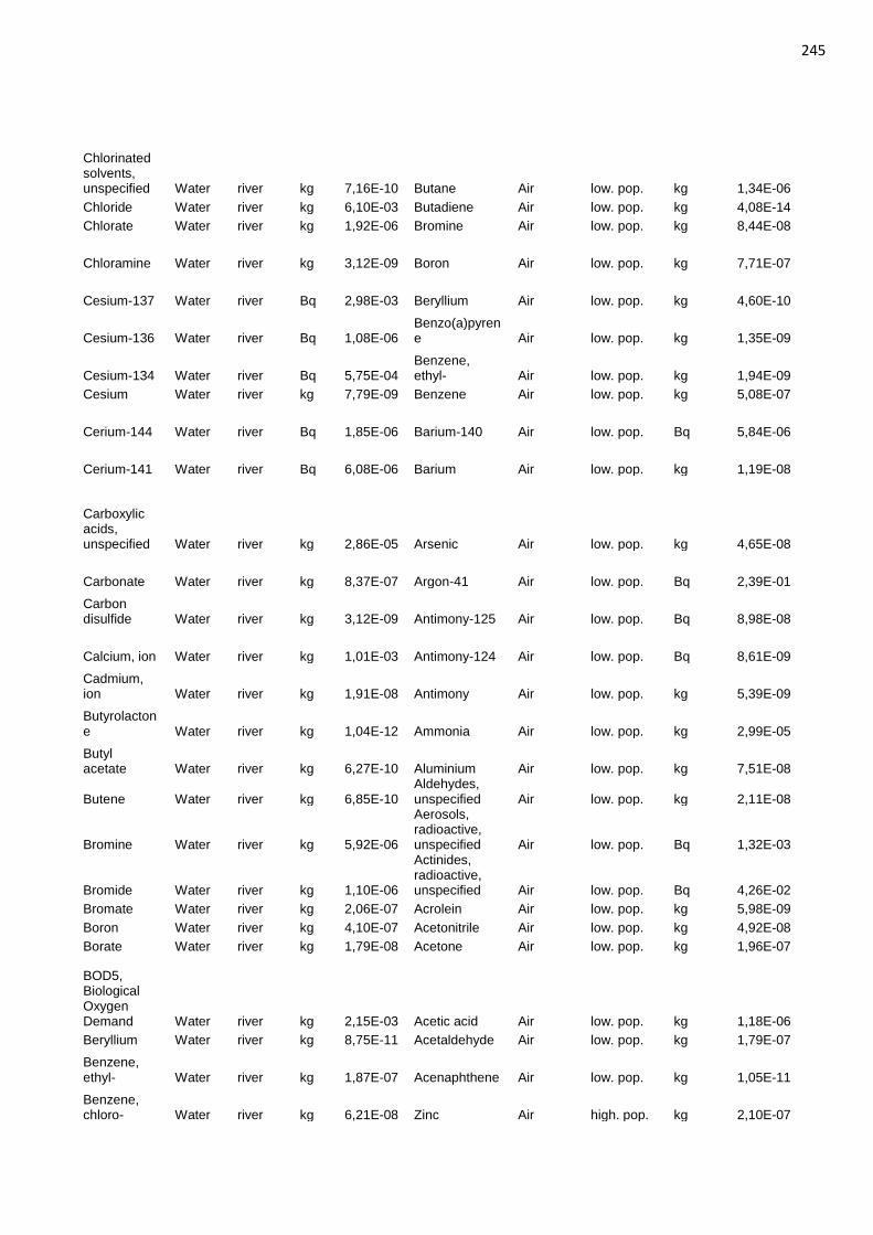
245
Chlorinated solvents, unspecified Water river kg 7,16E-10 Butane Air low. pop. kg 1,34E-06
Chloride Water river kg 6,10E-03 Butadiene Air low. pop. kg 4,08E-14
Chlorate Water river kg 1,92E-06 Bromine Air low. pop. kg 8,44E-08
Chloramine Water river kg 3,12E-09 Boron Air low. pop. kg 7,71E-07
Cesium-137 Water river Bq 2,98E-03 Beryllium Air low. pop. kg 4,60E-10
Cesium-136 Water river Bq 1,08E-06 Benzo(a)pyrene Air low. pop. kg 1,35E-09
Cesium-134 Water river Bq 5,75E-04 Benzene, ethyl- Air low. pop. kg 1,94E-09
Cesium Water river kg 7,79E-09 Benzene Air low. pop. kg 5,08E-07
Cerium-144 Water river Bq 1,85E-06 Barium-140 Air low. pop. Bq 5,84E-06
Cerium-141 Water river Bq 6,08E-06 Barium Air low. pop. kg 1,19E-08
Carboxylic acids, unspecified Water river kg 2,86E-05 Arsenic Air low. pop. kg 4,65E-08
Carbonate Water river kg 8,37E-07 Argon-41 Air low. pop. Bq 2,39E-01
Carbon disulfide Water river kg 3,12E-09 Antimony-125 Air low. pop. Bq 8,98E-08
Calcium, ion Water river kg 1,01E-03 Antimony-124 Air low. pop. Bq 8,61E-09
Cadmium, ion Water river kg 1,91E-08 Antimony Air low. pop. kg 5,39E-09
Butyrolactone Water river kg 1,04E-12 Ammonia Air low. pop. kg 2,99E-05
Butyl acetate Water river kg 6,27E-10 Aluminium Air low. pop. kg 7,51E-08
Butene Water river kg 6,85E-10 Aldehydes, unspecified Air low. pop. kg 2,11E-08
Bromine Water river kg 5,92E-06
Aerosols, radioactive, unspecified Air low. pop. Bq 1,32E-03
Bromide Water river kg 1,10E-06
Actinides, radioactive, unspecified Air low. pop. Bq 4,26E-02
Bromate Water river kg 2,06E-07 Acrolein Air low. pop. kg 5,98E-09
Boron Water river kg 4,10E-07 Acetonitrile Air low. pop. kg 4,92E-08
Borate Water river kg 1,79E-08 Acetone Air low. pop. kg 1,96E-07
BOD5, Biological Oxygen Demand Water river kg 2,15E-03 Acetic acid Air low. pop. kg 1,18E-06
Beryllium Water river kg 8,75E-11 Acetaldehyde Air low. pop. kg 1,79E-07
Benzene, ethyl- Water river kg 1,87E-07 Acenaphthene Air low. pop. kg 1,05E-11
Benzene, chloro- Water river kg 6,21E-08 Zinc Air high. pop. kg 2,10E-07
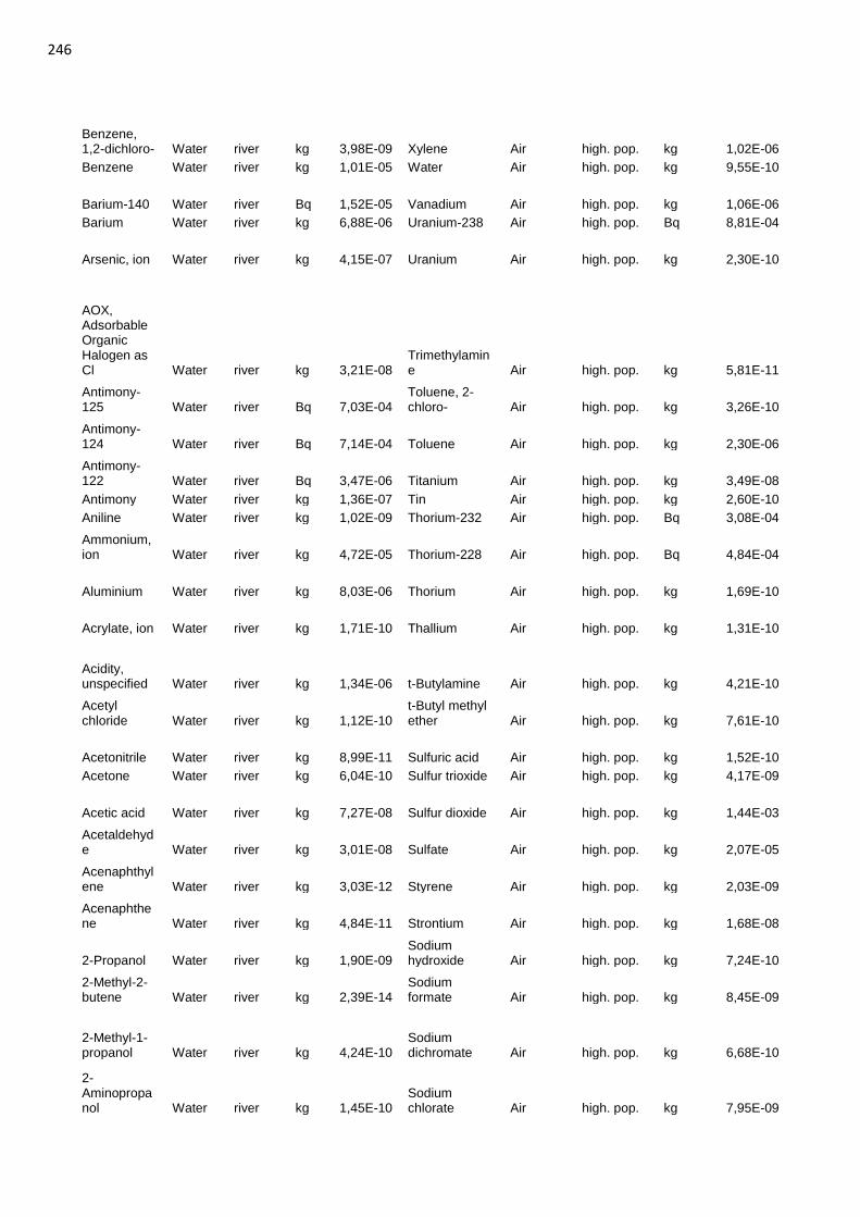
246
Benzene, 1,2-dichloro- Water river kg 3,98E-09 Xylene Air high. pop. kg 1,02E-06
Benzene Water river kg 1,01E-05 Water Air high. pop. kg 9,55E-10
Barium-140 Water river Bq 1,52E-05 Vanadium Air high. pop. kg 1,06E-06
Barium Water river kg 6,88E-06 Uranium-238 Air high. pop. Bq 8,81E-04
Arsenic, ion Water river kg 4,15E-07 Uranium Air high. pop. kg 2,30E-10
AOX, Adsorbable Organic Halogen as Cl Water river kg 3,21E-08
Trimethylamine Air high. pop. kg 5,81E-11
Antimony-125 Water river Bq 7,03E-04
Toluene, 2-chloro- Air high. pop. kg 3,26E-10
Antimony-124 Water river Bq 7,14E-04 Toluene Air high. pop. kg 2,30E-06
Antimony-122 Water river Bq 3,47E-06 Titanium Air high. pop. kg 3,49E-08
Antimony Water river kg 1,36E-07 Tin Air high. pop. kg 2,60E-10
Aniline Water river kg 1,02E-09 Thorium-232 Air high. pop. Bq 3,08E-04
Ammonium, ion Water river kg 4,72E-05 Thorium-228 Air high. pop. Bq 4,84E-04
Aluminium Water river kg 8,03E-06 Thorium Air high. pop. kg 1,69E-10
Acrylate, ion Water river kg 1,71E-10 Thallium Air high. pop. kg 1,31E-10
Acidity, unspecified Water river kg 1,34E-06 t-Butylamine Air high. pop. kg 4,21E-10
Acetyl chloride Water river kg 1,12E-10
t-Butyl methyl ether Air high. pop. kg 7,61E-10
Acetonitrile Water river kg 8,99E-11 Sulfuric acid Air high. pop. kg 1,52E-10
Acetone Water river kg 6,04E-10 Sulfur trioxide Air high. pop. kg 4,17E-09
Acetic acid Water river kg 7,27E-08 Sulfur dioxide Air high. pop. kg 1,44E-03
Acetaldehyde Water river kg 3,01E-08 Sulfate Air high. pop. kg 2,07E-05
Acenaphthylene Water river kg 3,03E-12 Styrene Air high. pop. kg 2,03E-09
Acenaphthene Water river kg 4,84E-11 Strontium Air high. pop. kg 1,68E-08
2-Propanol Water river kg 1,90E-09 Sodium hydroxide Air high. pop. kg 7,24E-10
2-Methyl-2-butene Water river kg 2,39E-14
Sodium formate Air high. pop. kg 8,45E-09
2-Methyl-1-propanol Water river kg 4,24E-10
Sodium dichromate Air high. pop. kg 6,68E-10
2-Aminopropanol Water river kg 1,45E-10
Sodium chlorate Air high. pop. kg 7,95E-09
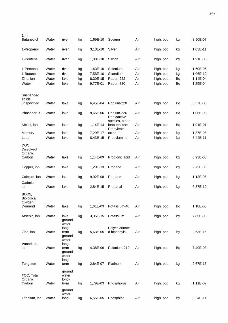
247
1,4-Butanediol Water river kg 1,69E-10 Sodium Air high. pop. kg 8,90E-07
1-Propanol Water river kg 3,18E-10 Silver Air high. pop. kg 1,03E-11
1-Pentene Water river kg 1,08E-10 Silicon Air high. pop. kg 1,91E-06
1-Pentanol Water river kg 1,43E-10 Selenium Air high. pop. kg 1,60E-06
1-Butanol Water river kg 7,58E-10 Scandium Air high. pop. kg 1,06E-10
Zinc, ion Water lake kg 8,30E-15 Radon-222 Air high. pop. Bq 1,14E-04
Water Water lake kg 9,77E-01 Radon-220 Air high. pop. Bq 1,25E-04
Suspended solids, unspecified Water lake kg 6,45E-04 Radium-228 Air high. pop. Bq 5,37E-03
Phosphorus Water lake kg 9,65E-06 Radium-226 Air high. pop. Bq 1,06E-03
Nickel, ion Water lake kg 1,14E-14
Radioactive species, other beta emitters Air high. pop. Bq 1,01E-01
Mercury Water lake kg 7,29E-17 Propylene oxide Air high. pop. kg 1,37E-08
Lead Water lake kg 8,43E-15 Propylamine Air high. pop. kg 3,44E-11
DOC, Dissolved Organic Carbon Water lake kg 1,14E-09 Propionic acid Air high. pop. kg 6,93E-08
Copper, ion Water lake kg 1,29E-13 Propene Air high. pop. kg 2,72E-06
Calcium, ion Water lake kg 9,92E-08 Propane Air high. pop. kg 1,13E-05
Cadmium, ion Water lake kg 2,84E-15 Propanal Air high. pop. kg 6,87E-10
BOD5, Biological Oxygen Demand Water lake kg 1,61E-03 Potassium-40 Air high. pop. Bq 1,18E-03
Arsenic, ion Water lake kg 3,35E-15 Potassium Air high. pop. kg 7,85E-06
Zinc, ion Water
groundwater, long-term kg 5,63E-05
Polychlorinated biphenyls Air high. pop. kg 2,63E-15
Vanadium, ion Water
groundwater, long-term kg 4,38E-06 Polonium-210 Air high. pop. Bq 7,49E-03
Tungsten Water
groundwater, long-term kg 2,84E-07 Platinum Air high. pop. kg 2,67E-15
TOC, Total Organic Carbon Water
groundwater, long-term kg 1,79E-03 Phosphorus Air high. pop. kg 1,11E-07
Titanium, ion Water
groundwater, long- kg 6,55E-05 Phosphine Air high. pop. kg 6,24E-14
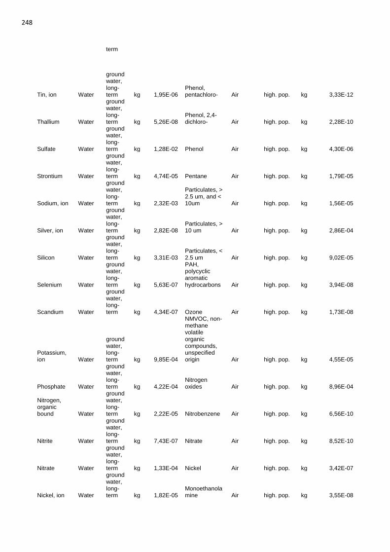
248
term
Tin, ion Water
groundwater, long-term kg 1,95E-06
Phenol, pentachloro- Air high. pop. kg 3,33E-12
Thallium Water
groundwater, long-term kg 5,26E-08
Phenol, 2,4-dichloro- Air high. pop. kg 2,28E-10
Sulfate Water
groundwater, long-term kg 1,28E-02 Phenol Air high. pop. kg 4,30E-06
Strontium Water
groundwater, long-term kg 4,74E-05 Pentane Air high. pop. kg 1,79E-05
Sodium, ion Water
groundwater, long-term kg 2,32E-03
Particulates, > 2.5 um, and < 10um Air high. pop. kg 1,56E-05
Silver, ion Water
groundwater, long-term kg 2,82E-08
Particulates, > 10 um Air high. pop. kg 2,86E-04
Silicon Water
groundwater, long-term kg 3,31E-03
Particulates, < 2.5 um Air high. pop. kg 9,02E-05
Selenium Water
groundwater, long-term kg 5,63E-07
PAH, polycyclic aromatic hydrocarbons Air high. pop. kg 3,94E-08
Scandium Water
groundwater, long-term kg 4,34E-07 Ozone Air high. pop. kg 1,73E-08
Potassium, ion Water
groundwater, long-term kg 9,85E-04
NMVOC, non-methane volatile organic compounds, unspecified origin Air high. pop. kg 4,55E-05
Phosphate Water
groundwater, long-term kg 4,22E-04
Nitrogen oxides Air high. pop. kg 8,96E-04
Nitrogen, organic bound Water
groundwater, long-term kg 2,22E-05 Nitrobenzene Air high. pop. kg 6,56E-10
Nitrite Water
groundwater, long-term kg 7,43E-07 Nitrate Air high. pop. kg 8,52E-10
Nitrate Water
groundwater, long-term kg 1,33E-04 Nickel Air high. pop. kg 3,42E-07
Nickel, ion Water
groundwater, long-term kg 1,82E-05
Monoethanolamine Air high. pop. kg 3,55E-08
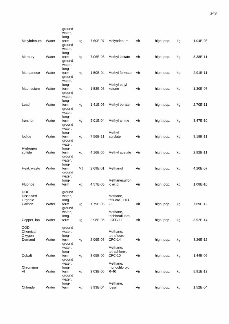
249
Molybdenum Water
groundwater, long-term kg 7,60E-07 Molybdenum Air high. pop. kg 1,04E-08
Mercury Water
groundwater, long-term kg 7,06E-08 Methyl lactate Air high. pop. kg 8,38E-11
Manganese Water
groundwater, long-term kg 1,50E-04 Methyl formate Air high. pop. kg 2,91E-11
Magnesium Water
groundwater, long-term kg 1,53E-03
Methyl ethyl ketone Air high. pop. kg 1,30E-07
Lead Water
groundwater, long-term kg 1,41E-05 Methyl borate Air high. pop. kg 2,70E-11
Iron, ion Water
groundwater, long-term kg 5,01E-04 Methyl amine Air high. pop. kg 3,47E-10
Iodide Water
groundwater, long-term kg 7,56E-11
Methyl acrylate Air high. pop. kg 8,19E-11
Hydrogen sulfide Water
groundwater, long-term kg 4,16E-05 Methyl acetate Air high. pop. kg 2,92E-11
Heat, waste Water
groundwater, long-term MJ 2,69E-01 Methanol Air high. pop. kg 4,20E-07
Fluoride Water
groundwater, long-term kg 4,57E-05
Methanesulfonic acid Air high. pop. kg 1,08E-10
DOC, Dissolved Organic Carbon Water
groundwater, long-term kg 1,79E-03
Methane, trifluoro-, HFC-23 Air high. pop. kg 7,69E-12
Copper, ion Water
groundwater, long-term kg 2,98E-05
Methane, trichlorofluoro-, CFC-11 Air high. pop. kg 3,92E-14
COD, Chemical Oxygen Demand Water
groundwater, long-term kg 2,06E-03
Methane, tetrafluoro-, CFC-14 Air high. pop. kg 3,26E-12
Cobalt Water
groundwater, long-term kg 3,65E-06
Methane, tetrachloro-, CFC-10 Air high. pop. kg 1,44E-09
Chromium VI Water
groundwater, long-term kg 3,03E-06
Methane, monochloro-, R-40 Air high. pop. kg 5,91E-13
Chloride Water
groundwater, long-term kg 9,93E-04
Methane, fossil Air high. pop. kg 1,52E-04
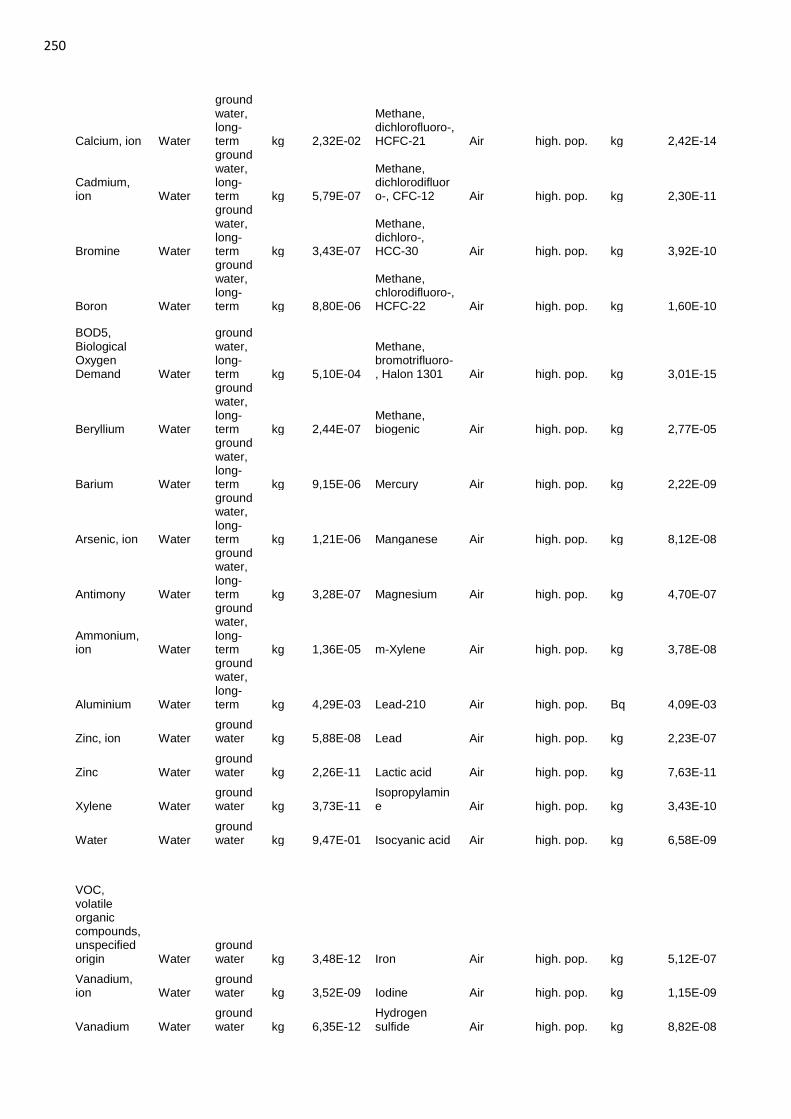
250
Calcium, ion Water
groundwater, long-term kg 2,32E-02
Methane, dichlorofluoro-, HCFC-21 Air high. pop. kg 2,42E-14
Cadmium, ion Water
groundwater, long-term kg 5,79E-07
Methane, dichlorodifluoro-, CFC-12 Air high. pop. kg 2,30E-11
Bromine Water
groundwater, long-term kg 3,43E-07
Methane, dichloro-, HCC-30 Air high. pop. kg 3,92E-10
Boron Water
groundwater, long-term kg 8,80E-06
Methane, chlorodifluoro-, HCFC-22 Air high. pop. kg 1,60E-10
BOD5, Biological Oxygen Demand Water
groundwater, long-term kg 5,10E-04
Methane, bromotrifluoro-, Halon 1301 Air high. pop. kg 3,01E-15
Beryllium Water
groundwater, long-term kg 2,44E-07
Methane, biogenic Air high. pop. kg 2,77E-05
Barium Water
groundwater, long-term kg 9,15E-06 Mercury Air high. pop. kg 2,22E-09
Arsenic, ion Water
groundwater, long-term kg 1,21E-06 Manganese Air high. pop. kg 8,12E-08
Antimony Water
groundwater, long-term kg 3,28E-07 Magnesium Air high. pop. kg 4,70E-07
Ammonium, ion Water
groundwater, long-term kg 1,36E-05 m-Xylene Air high. pop. kg 3,78E-08
Aluminium Water
groundwater, long-term kg 4,29E-03 Lead-210 Air high. pop. Bq 4,09E-03
Zinc, ion Water groundwater kg 5,88E-08 Lead Air high. pop. kg 2,23E-07
Zinc Water groundwater kg 2,26E-11 Lactic acid Air high. pop. kg 7,63E-11
Xylene Water groundwater kg 3,73E-11
Isopropylamine Air high. pop. kg 3,43E-10
Water Water groundwater kg 9,47E-01 Isocyanic acid Air high. pop. kg 6,58E-09
VOC, volatile organic compounds, unspecified origin Water
groundwater kg 3,48E-12 Iron Air high. pop. kg 5,12E-07
Vanadium, ion Water
groundwater kg 3,52E-09 Iodine Air high. pop. kg 1,15E-09
Vanadium Water groundwater kg 6,35E-12
Hydrogen sulfide Air high. pop. kg 8,82E-08
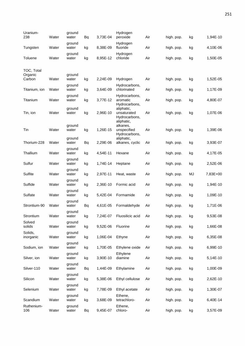
251
Uranium-238 Water
groundwater Bq 3,73E-04
Hydrogen peroxide Air high. pop. kg 1,94E-10
Tungsten Water groundwater kg 8,38E-09
Hydrogen fluoride Air high. pop. kg 4,10E-06
Toluene Water groundwater kg 8,95E-12
Hydrogen chloride Air high. pop. kg 1,50E-05
TOC, Total Organic Carbon Water
groundwater kg 2,24E-09 Hydrogen Air high. pop. kg 1,52E-05
Titanium, ion Water groundwater kg 3,64E-09
Hydrocarbons, chlorinated Air high. pop. kg 1,17E-09
Titanium Water groundwater kg 3,77E-12
Hydrocarbons, aromatic Air high. pop. kg 4,80E-07
Tin, ion Water groundwater kg 2,96E-10
Hydrocarbons, aliphatic, unsaturated Air high. pop. kg 1,07E-06
Tin Water groundwater kg 1,26E-15
Hydrocarbons, aliphatic, alkanes, unspecified Air high. pop. kg 1,39E-06
Thorium-228 Water groundwater Bq 2,29E-06
Hydrocarbons, aliphatic, alkanes, cyclic Air high. pop. kg 3,93E-07
Thallium Water groundwater kg 4,54E-11 Hexane Air high. pop. kg 4,17E-05
Sulfur Water groundwater kg 1,74E-14 Heptane Air high. pop. kg 2,52E-06
Sulfite Water groundwater kg 2,97E-11 Heat, waste Air high. pop. MJ 7,83E+00
Sulfide Water groundwater kg 2,36E-10 Formic acid Air high. pop. kg 1,94E-10
Sulfate Water groundwater kg 5,42E-04 Formamide Air high. pop. kg 1,09E-10
Strontium-90 Water groundwater Bq 4,61E-05 Formaldehyde Air high. pop. kg 1,71E-06
Strontium Water groundwater kg 7,24E-07 Fluosilicic acid Air high. pop. kg 9,53E-08
Solved solids Water
groundwater kg 9,52E-06 Fluorine Air high. pop. kg 1,66E-08
Solids, inorganic Water
groundwater kg 1,06E-04 Ethyne Air high. pop. kg 6,35E-08
Sodium, ion Water groundwater kg 1,70E-05 Ethylene oxide Air high. pop. kg 6,99E-10
Silver, ion Water groundwater kg 3,90E-10
Ethylene diamine Air high. pop. kg 5,14E-10
Silver-110 Water groundwater Bq 1,44E-09 Ethylamine Air high. pop. kg 1,00E-09
Silicon Water groundwater kg 5,38E-06 Ethyl cellulose Air high. pop. kg 2,62E-10
Selenium Water groundwater kg 7,78E-09 Ethyl acetate Air high. pop. kg 1,30E-07
Scandium Water groundwater kg 3,68E-09
Ethene, tetrachloro- Air high. pop. kg 6,40E-14
Ruthenium-106 Water
groundwater Bq 9,45E-07
Ethene, chloro- Air high. pop. kg 3,57E-09
252
Radium-226 Water groundwater Bq 1,58E-02 Ethene Air high. pop. kg 9,21E-07
Propane, 1,2-dichloro- Water
groundwater kg 5,72E-20 Ethanol Air high. pop. kg 3,52E-07
Potassium, ion Water
groundwater kg 6,64E-06
Ethane, hexafluoro-, HFC-116 Air high. pop. kg 2,38E-10
Potassium-40 Water
groundwater Bq 2,26E-05
Ethane, 1,2-dichloro- Air high. pop. kg 1,19E-08
Potassium Water groundwater kg 2,63E-11
Ethane, 1,1,2-trichloro-1,2,2-trifluoro-, CFC-113 Air high. pop. kg 3,43E-12
Polonium-210 Water
groundwater Bq 2,84E-04
Ethane, 1,1,1,2-tetrafluoro-, HFC-134a Air high. pop. kg 8,50E-12
Plutonium-alpha Water
groundwater Bq 3,78E-06
Ethane, 1,1-difluoro-, HFC-152a Air high. pop. kg 6,34E-11
Phosphorus Water groundwater kg 6,73E-05 Ethane Air high. pop. kg 3,06E-06
Phosphate Water groundwater kg 6,36E-05 Dipropylamine Air high. pop. kg 9,74E-11
Phenol Water groundwater kg 1,54E-11
Dioxin, 2,3,7,8 Tetrachlorodibenzo-p- Air high. pop. kg 4,84E-14
Particulates, > 10 um Water
groundwater kg 3,25E-07
Dinitrogen monoxide Air high. pop. kg 1,30E-05
Particulates, < 10 um Water
groundwater kg 5,55E-13
Dimethyl malonate Air high. pop. kg 1,35E-10
Nitrogen Water groundwater kg 3,22E-04 Diethylamine Air high. pop. kg 2,06E-10
Nitrate Water groundwater kg 7,31E-04
Cyanoacetic acid Air high. pop. kg 1,07E-10
Nickel, ion Water groundwater kg 3,64E-08 Cyanide Air high. pop. kg 1,51E-08
Nickel Water groundwater kg 4,51E-10 Cumene Air high. pop. kg 5,80E-06
Naphthalene Water groundwater kg 2,21E-13 Copper Air high. pop. kg 1,54E-07
Molybdenum Water groundwater kg 6,35E-08 Cobalt Air high. pop. kg 4,94E-08
Methanol Water groundwater kg 5,80E-09 Chromium VI Air high. pop. kg 4,81E-10
Methane, monochloro-, R-40 Water
groundwater kg 1,20E-12 Chromium Air high. pop. kg 3,73E-08
Methane, dibromo- Water
groundwater kg 7,20E-17
Chlorosulfonic acid Air high. pop. kg 1,31E-10
Mercury Water groundwater kg 9,93E-11
Chlorosilane, trimethyl- Air high. pop. kg 3,90E-11
Manganese-54 Water
groundwater Bq 3,19E-05 Chloroform Air high. pop. kg 1,65E-09
Manganese Water groundwater kg 8,78E-07
Chloroacetic acid Air high. pop. kg 2,76E-09
253
Magnesium Water groundwater kg 1,62E-05 Chlorine Air high. pop. kg 5,56E-07
Lead-210 Water groundwater Bq 1,87E-04 Chloramine Air high. pop. kg 3,47E-10
Lead Water groundwater kg 4,52E-10
Carbon monoxide, fossil Air high. pop. kg 1,31E-04
Iron, ion Water groundwater kg 4,74E-05
Carbon monoxide, biogenic Air high. pop. kg 2,68E-03
Iron Water groundwater kg 4,24E-08
Carbon disulfide Air high. pop. kg 1,37E-09
Iodine-131 Water groundwater Bq 7,01E-09
Carbon dioxide, fossil Air high. pop. kg 4,41E-01
Iodine-129 Water groundwater Bq 1,37E-04
Carbon dioxide, biogenic Air high. pop. kg 4,61E-02
Iodide Water groundwater kg 2,61E-09 Calcium Air high. pop. kg 2,34E-06
Hydroxide Water groundwater kg 8,10E-09 Cadmium Air high. pop. kg 2,58E-08
Hydrogen fluoride Water
groundwater kg 1,63E-14 Butyrolactone Air high. pop. kg 4,33E-13
Hydrogen chloride Water
groundwater kg 8,31E-13 Butene Air high. pop. kg 2,46E-07
Hydrogen-3, Tritium Water
groundwater Bq
1,40E+00 Butane Air high. pop. kg 1,30E-05
Hydrocarbons, unspecified Water
groundwater kg 2,59E-11 Butadiene Air high. pop. kg 3,83E-11
Hydrocarbons, aromatic Water
groundwater kg 1,17E-11 Bromine Air high. pop. kg 2,16E-08
Hexane Water groundwater kg 5,07E-17
Boron trifluoride Air high. pop. kg 1,15E-17
Heat, waste Water groundwater MJ 1,06E-04 Boron Air high. pop. kg 1,07E-07
Fluorine Water groundwater kg 1,16E-11 Beryllium Air high. pop. kg 1,50E-10
Fluoride Water groundwater kg 3,93E-07
Benzo(a)pyrene Air high. pop. kg 2,95E-10
Fluoranthene Water
groundwater kg 8,90E-16
Benzene, pentachloro- Air high. pop. kg 7,19E-12
Ethene, chloro- Water
groundwater kg 1,36E-17
Benzene, hexachloro- Air high. pop. kg 2,87E-12
Dioxin, 2,3,7,8 Tetrachlorodibenzo-p- Water
groundwater kg 3,73E-25
Benzene, ethyl- Air high. pop. kg 2,57E-07
Decane Water groundwater kg 8,70E-11
Benzene, 1,2-dichloro- Air high. pop. kg 5,72E-10
Cyanide Water groundwater kg 7,46E-13
Benzene, 1-methyl-2-nitro- Air high. pop. kg 1,09E-10
Curium alpha Water
groundwater Bq 1,25E-06 Benzene Air high. pop. kg 6,82E-06
254
Cresol Water groundwater kg 4,51E-16 Benzaldehyde Air high. pop. kg 2,66E-11
Copper, ion Water groundwater kg 6,63E-09 Barium Air high. pop. kg 1,26E-08
Copper Water groundwater kg 6,47E-10 Arsine Air high. pop. kg 8,42E-16
COD, Chemical Oxygen Demand Water
groundwater kg 1,21E-05 Arsenic Air high. pop. kg 2,56E-08
Cobalt-60 Water groundwater Bq 2,06E-04 Antimony Air high. pop. kg 1,50E-08
Cobalt-58 Water groundwater Bq 3,67E-07
Anthranilic acid Air high. pop. kg 9,60E-11
Cobalt Water groundwater kg 6,24E-09 Aniline Air high. pop. kg 4,17E-10
Chrysene Water groundwater kg 2,17E-15
Ammonium carbonate Air high. pop. kg 1,60E-10
Chromium, ion Water
groundwater kg 8,23E-09 Ammonia Air high. pop. kg 2,42E-05
Chromium VI Water
groundwater kg 2,72E-08 Aluminium Air high. pop. kg 1,03E-06
Chromium Water groundwater kg 1,03E-11
Aldehydes, unspecified Air high. pop. kg 1,37E-09
Chlorine Water groundwater kg 9,30E-10 Acrylic acid Air high. pop. kg 7,22E-11
Chloride Water groundwater kg 5,90E-04 Acrolein Air high. pop. kg 5,11E-11
Cesium-137 Water groundwater Bq 4,44E-04 Acetone Air high. pop. kg 2,05E-07
Cesium-134 Water groundwater Bq 4,91E-05 Acetic acid Air high. pop. kg 1,24E-06
Carbonate Water groundwater kg 1,25E-09 Acetaldehyde Air high. pop. kg 1,98E-07
Carbon-14 Water groundwater Bq 4,79E-05 Acenaphthene Air high. pop. kg 1,95E-13
Calcium, ion Water groundwater kg 4,15E-05 2-Propanol Air high. pop. kg 2,83E-08
Cadmium, ion Water
groundwater kg 9,54E-10
2-Nitrobenzoic acid Air high. pop. kg 1,26E-10
Cadmium Water groundwater kg 3,54E-11
2-Methyl-1-propanol Air high. pop. kg 1,77E-10
Bromine Water groundwater kg 2,13E-08
2-Butene, 2-methyl- Air high. pop. kg 9,96E-15
Boron Water groundwater kg 6,56E-07
2-Aminopropanol Air high. pop. kg 5,94E-11
BOD5, Biological Oxygen Demand Water
groundwater kg 9,12E-09 1,4-Butanediol Air high. pop. kg 4,22E-10
Beryllium Water groundwater kg 7,18E-10 1-Propanol Air high. pop. kg 9,81E-10
Benzo(b)fluoranthene Water
groundwater kg 2,34E-16 1-Pentene Air high. pop. kg 4,49E-11
255
Benzo(a)anthracene Water
groundwater kg 5,03E-16 1-Pentanol Air high. pop. kg 5,94E-11
Benzene, ethyl- Water
groundwater kg 1,29E-12 1-Butanol Air high. pop. kg 1,14E-10
Benzene Water groundwater kg 1,29E-11 Zirconium-95 Air
Bq 5,04E-11
Barium Water groundwater kg 6,05E-09 Zirconium Air
kg 1,28E-12
Arsenic, ion Water groundwater kg 4,66E-08 Zinc oxide Air
kg 4,14E-18
AOX, Adsorbable Organic Halogen as Cl Water
groundwater kg 4,33E-11 Zinc-65 Air
Bq 3,43E-09
Antimony-125 Water
groundwater Bq 6,69E-09 Zinc Air
kg 2,04E-07
Antimony-124 Water
groundwater Bq 9,82E-09 Xylene Air
kg 1,72E-06
Antimony Water groundwater kg 9,33E-09 Xenon-138 Air
Bq 3,13E-04
Anthracene Water groundwater kg 6,41E-15 Xenon-137 Air
Bq 2,38E-05
Ammonium, ion Water
groundwater kg 6,41E-08 Xenon-135m Air
Bq 9,60E-04
Ammonia Water groundwater kg 5,00E-08 Xenon-135 Air
Bq 1,05E-02
Americium-241 Water
groundwater Bq 9,45E-07 Xenon-133m Air
Bq 2,56E-05
Aluminium Water groundwater kg 2,94E-07 Xenon-133 Air
Bq 5,61E-02
Acrylonitrile Water groundwater kg 4,18E-15 Xenon-131m Air
Bq 2,17E-04
Acidity, unspecified Water
groundwater kg 3,23E-12 Water Air
kg 1,91E-01
Acetic acid Water groundwater kg 1,71E-11
VOC, volatile organic compounds Air
kg 7,96E-10
Acenaphthylene Water
groundwater kg 1,61E-15 Vanadium Air
kg 2,30E-09
Acenaphthene Water
groundwater kg 4,02E-15 Used air Air
kg 4,04E-03
Zirconium-95 Water
Bq 3,92E-06 Uranium alpha Air
Bq 1,65E-05
Zinc, ion Water
kg 4,72E-07 Uranium-238 Air
Bq 1,90E-05
Zinc-65 Water
Bq 7,47E-07 Uranium-235 Air
Bq 8,91E-06
Yttrium-90 Water
Bq 1,33E-09 Uranium-234 Air
Bq 7,77E-06
Xylene Water
kg 5,72E-08 Uranium Air
kg 5,98E-13
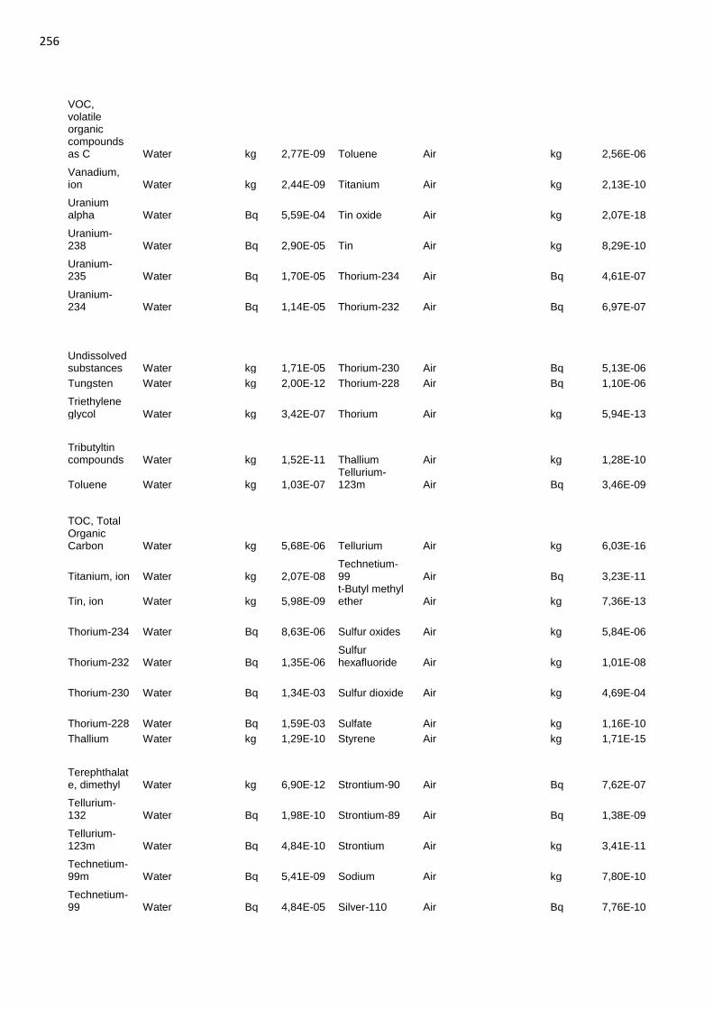
256
VOC, volatile organic compounds as C Water
kg 2,77E-09 Toluene Air
kg 2,56E-06
Vanadium, ion Water
kg 2,44E-09 Titanium Air
kg 2,13E-10
Uranium alpha Water
Bq 5,59E-04 Tin oxide Air
kg 2,07E-18
Uranium-238 Water
Bq 2,90E-05 Tin Air
kg 8,29E-10
Uranium-235 Water
Bq 1,70E-05 Thorium-234 Air
Bq 4,61E-07
Uranium-234 Water
Bq 1,14E-05 Thorium-232 Air
Bq 6,97E-07
Undissolved substances Water
kg 1,71E-05 Thorium-230 Air
Bq 5,13E-06
Tungsten Water
kg 2,00E-12 Thorium-228 Air
Bq 1,10E-06
Triethylene glycol Water
kg 3,42E-07 Thorium Air
kg 5,94E-13
Tributyltin compounds Water
kg 1,52E-11 Thallium Air
kg 1,28E-10
Toluene Water
kg 1,03E-07 Tellurium-123m Air
Bq 3,46E-09
TOC, Total Organic Carbon Water
kg 5,68E-06 Tellurium Air
kg 6,03E-16
Titanium, ion Water
kg 2,07E-08 Technetium-99 Air
Bq 3,23E-11
Tin, ion Water
kg 5,98E-09 t-Butyl methyl ether Air
kg 7,36E-13
Thorium-234 Water
Bq 8,63E-06 Sulfur oxides Air
kg 5,84E-06
Thorium-232 Water
Bq 1,35E-06 Sulfur hexafluoride Air
kg 1,01E-08
Thorium-230 Water
Bq 1,34E-03 Sulfur dioxide Air
kg 4,69E-04
Thorium-228 Water
Bq 1,59E-03 Sulfate Air
kg 1,16E-10
Thallium Water
kg 1,29E-10 Styrene Air
kg 1,71E-15
Terephthalate, dimethyl Water
kg 6,90E-12 Strontium-90 Air
Bq 7,62E-07
Tellurium-132 Water
Bq 1,98E-10 Strontium-89 Air
Bq 1,38E-09
Tellurium-123m Water
Bq 4,84E-10 Strontium Air
kg 3,41E-11
Technetium-99m Water
Bq 5,41E-09 Sodium Air
kg 7,80E-10
Technetium-99 Water
Bq 4,84E-05 Silver-110 Air
Bq 7,76E-10
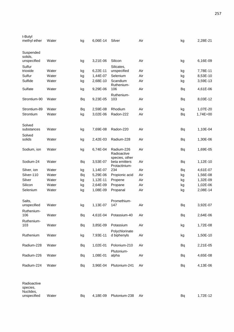
257
t-Butyl methyl ether Water
kg 6,06E-14 Silver Air
kg 2,28E-21
Suspended solids, unspecified Water
kg 3,21E-06 Silicon Air
kg 6,16E-09
Sulfur trioxide Water
kg 6,22E-11
Silicates, unspecified Air
kg 7,78E-11
Sulfur Water
kg 1,44E-07 Selenium Air
kg 8,53E-10
Sulfide Water
kg 2,68E-10 Scandium Air
kg 3,59E-13
Sulfate Water
kg 9,29E-06 Ruthenium-106 Air
Bq 4,61E-06
Strontium-90 Water
Bq 9,23E-05 Ruthenium-103 Air
Bq 8,03E-12
Strontium-89 Water
Bq 2,59E-08 Rhodium Air
kg 1,07E-20
Strontium Water
kg 3,02E-06 Radon-222 Air
Bq 1,74E+00
Solved substances Water
kg 7,69E-08 Radon-220 Air
Bq 1,10E-04
Solved solids Water
kg 2,42E-03 Radium-228 Air
Bq 1,30E-06
Sodium, ion Water
kg 6,74E-04 Radium-226 Air
Bq 1,69E-05
Sodium-24 Water
Bq 3,53E-07
Radioactive species, other beta emitters Air
Bq 1,12E-10
Silver, ion Water
kg 1,14E-07 Protactinium-234 Air
Bq 4,61E-07
Silver-110 Water
Bq 5,29E-06 Propionic acid Air
kg 1,56E-08
Silver Water
kg 1,12E-11 Propene Air
kg 1,32E-09
Silicon Water
kg 2,64E-09 Propane Air
kg 1,02E-06
Selenium Water
kg 1,08E-09 Propanal Air
kg 2,08E-14
Salts, unspecified Water
kg 1,13E-07
Promethium-147 Air
Bq 3,92E-07
Ruthenium-106 Water
Bq 4,61E-04 Potassium-40 Air
Bq 2,64E-06
Ruthenium-103 Water
Bq 3,85E-09 Potassium Air
kg 1,72E-08
Ruthenium Water
kg 7,93E-11 Polychlorinated biphenyls Air
kg 1,50E-10
Radium-228 Water
Bq 1,02E-01 Polonium-210 Air
Bq 2,21E-05
Radium-226 Water
Bq 1,08E-01 Plutonium-alpha Air
Bq 4,65E-08
Radium-224 Water
Bq 3,96E-04 Plutonium-241 Air
Bq 4,13E-06
Radioactive species, Nuclides, unspecified Water
Bq 4,18E-09 Plutonium-238 Air
Bq 1,72E-12
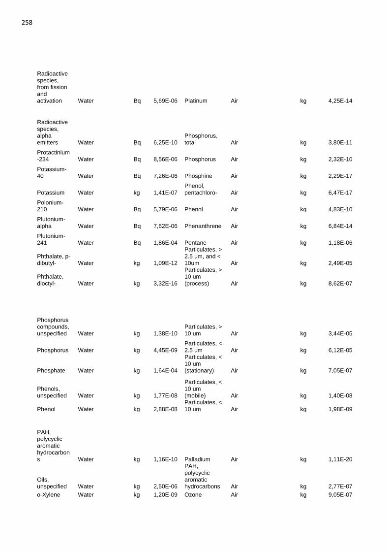
258
Radioactive species, from fission and activation Water
Bq 5,69E-06 Platinum Air
kg 4,25E-14
Radioactive species, alpha emitters Water
Bq 6,25E-10
Phosphorus, total Air
kg 3,80E-11
Protactinium-234 Water
Bq 8,56E-06 Phosphorus Air
kg 2,32E-10
Potassium-40 Water
Bq 7,26E-06 Phosphine Air
kg 2,29E-17
Potassium Water
kg 1,41E-07 Phenol, pentachloro- Air
kg 6,47E-17
Polonium-210 Water
Bq 5,79E-06 Phenol Air
kg 4,83E-10
Plutonium-alpha Water
Bq 7,62E-06 Phenanthrene Air
kg 6,84E-14
Plutonium-241 Water
Bq 1,86E-04 Pentane Air
kg 1,18E-06
Phthalate, p-dibutyl- Water
kg 1,09E-12
Particulates, > 2.5 um, and < 10um Air
kg 2,49E-05
Phthalate, dioctyl- Water
kg 3,32E-16
Particulates, > 10 um (process) Air
kg 8,62E-07
Phosphorus compounds, unspecified Water
kg 1,38E-10
Particulates, > 10 um Air
kg 3,44E-05
Phosphorus Water
kg 4,45E-09 Particulates, < 2.5 um Air
kg 6,12E-05
Phosphate Water
kg 1,64E-04
Particulates, < 10 um (stationary) Air
kg 7,05E-07
Phenols, unspecified Water
kg 1,77E-08
Particulates, < 10 um (mobile) Air
kg 1,40E-08
Phenol Water
kg 2,88E-08 Particulates, < 10 um Air
kg 1,98E-09
PAH, polycyclic aromatic hydrocarbons Water
kg 1,16E-10 Palladium Air
kg 1,11E-20
Oils, unspecified Water
kg 2,50E-06
PAH, polycyclic aromatic hydrocarbons Air
kg 2,77E-07
o-Xylene Water
kg 1,20E-09 Ozone Air
kg 9,05E-07
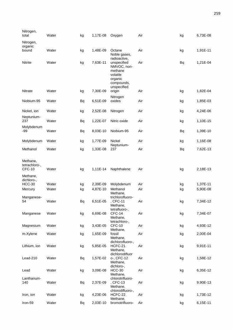
259
Nitrogen, total Water
kg 1,17E-08 Oxygen Air
kg 6,73E-08
Nitrogen, organic bound Water
kg 1,48E-09 Octane Air
kg 1,91E-11
Nitrite Water
kg 7,63E-11
Noble gases, radioactive, unspecified Air
Bq 1,21E-04
Nitrate Water
kg 7,30E-09
NMVOC, non-methane volatile organic compounds, unspecified origin Air
kg 1,82E-04
Niobium-95 Water
Bq 6,51E-09 Nitrogen oxides Air
kg 1,85E-03
Nickel, ion Water
kg 2,52E-08 Nitrogen Air
kg 4,24E-06
Neptunium-237 Water
Bq 1,22E-07 Nitric oxide Air
kg 1,10E-15
Molybdenum-99 Water
Bq 8,03E-10 Niobium-95 Air
Bq 1,39E-10
Molybdenum Water
kg 1,77E-09 Nickel Air
kg 1,16E-08
Methanol Water
kg 1,33E-08 Neptunium-237 Air
Bq 7,62E-13
Methane, tetrachloro-, CFC-10 Water
kg 1,11E-14 Naphthalene Air
kg 2,18E-13
Methane, dichloro-, HCC-30 Water
kg 2,39E-09 Molybdenum Air
kg 1,37E-11
Mercury Water
kg 4,87E-10 Methanol Air
kg 5,90E-08
Manganese-54 Water
Bq 6,51E-05
Methane, trichlorofluoro-, CFC-11 Air
kg 7,34E-12
Manganese Water
kg 6,69E-08
Methane, tetrafluoro-, CFC-14 Air
kg 7,34E-07
Magnesium Water
kg 3,43E-05
Methane, tetrachloro-, CFC-10 Air
kg 4,93E-12
m-Xylene Water
kg 1,65E-09 Methane, fossil Air
kg 2,00E-04
Lithium, ion Water
kg 5,85E-05
Methane, dichlorofluoro-, HCFC-21 Air
kg 9,91E-11
Lead-210 Water
Bq 1,57E-02
Methane, dichlorodifluoro-, CFC-12 Air
kg 1,58E-12
Lead Water
kg 3,09E-08
Methane, dichloro-, HCC-30 Air
kg 6,35E-12
Lanthanum-140 Water
Bq 2,37E-09
Methane, chlorotrifluoro-, CFC-13 Air
kg 9,90E-13
Iron, ion Water
kg 4,23E-06
Methane, chlorodifluoro-, HCFC-22 Air
kg 1,73E-12
Iron-59 Water
Bq 2,03E-10 Methane, bromotrifluoro- Air
kg 6,15E-11
260
, Halon 1301
Iron Water
kg 1,97E-07
Methane, bromo-, Halon 1001 Air
kg 8,79E-15
Iodine-133 Water
Bq 5,24E-08 Methane, biogenic Air
kg 2,70E-06
Iodine-131 Water
Bq 1,90E-07 Methane Air
kg 3,54E-05
Iodine-129 Water
Bq 2,77E-04 Mercury Air
kg 1,08E-08
Iodide Water
kg 7,93E-10 Manganese-54 Air
Bq 7,88E-10
Hypochlorous acid Water
kg 3,08E-10 Manganese Air
kg 1,32E-08
Hypochlorite Water
kg 3,08E-10 Magnesium Air
kg 2,16E-09
Hydrogen sulfide Water
kg 1,25E-10
Lead compounds Air
kg 2,38E-17
Hydrogen-3, Tritium Water
Bq
2,87E+00 Lead-210 Air
Bq 1,45E-05
Hydrocarbons, unspecified Water
kg 2,05E-08 Lead Air
kg 4,60E-08
Hydrocarbons, aromatic Water
kg 3,52E-08
Lanthanum-140 Air
Bq 1,93E-09
Hydrocarbons, aliphatic, alkenes, unspecified Water
kg 1,71E-09 Lanthanum Air
kg 1,02E-12
Hydrocarbons, aliphatic, alkanes, unspecified Water
kg 1,88E-08 Krypton-89 Air
Bq 2,98E-05
Heat, waste Water
MJ 1,61E-03 Krypton-88 Air
Bq 3,36E-03
Glutaraldehyde Water
kg 6,83E-10 Krypton-87 Air
Bq 4,09E-05
Formaldehyde Water
kg 4,44E-08 Krypton-85m Air
Bq 3,54E+01
Fluoride Water
kg 4,06E-07 Krypton-85 Air
Bq 7,16E+01
Fatty acids as C Water
kg 9,66E-08 Isoprene Air
kg 6,23E-15
Ethene, trichloro- Water
kg 4,58E-13 Iron-59 Air
Bq 3,00E-11
Ethene, tetrachloro- Water
kg 7,25E-15 Iron Air
kg 6,67E-08
Ethene, chloro- Water
kg 2,06E-15 Iodine-135 Air
Bq 3,83E-07
261
Ethane, hexachloro- Water
kg 6,11E-17 Iodine-133 Air
Bq 2,57E-07
Ethane, dichloro- Water
kg 3,05E-12 Iodine-131 Air
Bq 8,01E-07
Ethane, 1,1,1-trichloro-, HCFC-140 Water
kg 1,16E-14 Iodine-129 Air
Bq 6,20E-06
DOC, Dissolved Organic Carbon Water
kg 7,94E-07 Iodine Air
kg 5,17E-11
Cyanide Water
kg 7,51E-09 Indeno(1,2,3-cd)pyrene Air
kg 6,93E-16
Curium alpha Water
Bq 2,54E-06
Hydrogen sulfide Air
kg 1,91E-07
Copper, ion Water
kg 2,56E-08 Hydrogen iodide Air
kg 2,45E-16
COD, Chemical Oxygen Demand Water
kg 1,81E-05
Hydrogen fluoride Air
kg 1,87E-06
Cobalt-60 Water
Bq 4,25E-04 Hydrogen cyanide Air
kg 1,72E-12
Cobalt-58 Water
Bq 8,95E-06 Hydrogen chloride Air
kg 2,32E-06
Cobalt-57 Water
Bq 1,18E-08 Hydrogen bromide Air
kg 2,24E-13
Cobalt Water
kg 1,58E-09 Hydrogen-3, Tritium Air
Bq 1,61E-02
Chromium, ion Water
kg 3,83E-08 Hydrogen Air
kg 2,07E-07
Chromium VI Water
kg 1,03E-09
Hydrocarbons, chlorinated Air
kg 3,17E-08
Chromium-51 Water
Bq 2,52E-07
Hydrocarbons, aromatic Air
kg 3,22E-04
Chromium Water
kg 6,51E-12
Hydrocarbons, aliphatic, unsaturated Air
kg 2,90E-14
Chloroform Water
kg 1,68E-12
Hydrocarbons, aliphatic, alkenes, unspecified Air
kg 1,98E-10
Chlorinated solvents, unspecified Water
kg 1,09E-11
Hydrocarbons, aliphatic, alkanes, unspecified Air
kg 1,23E-06
Chloride Water
kg 1,98E-03 Hexane Air
kg 4,77E-07
Cesium-137 Water
Bq 9,02E-04 Hexamethylene diamine Air
kg 7,12E-17
Cesium-136 Water
Bq 6,14E-11 Heptane Air
kg 2,91E-09
Cesium-134 Water
Bq 9,80E-05 Helium Air
kg 1,10E-08
Cesium Water
kg 7,93E-12 Heat, waste Air
MJ 3,01E+00
262
Cerium-144 Water
Bq 4,38E-05 Furan Air
kg 4,67E-16
Cerium-141 Water
Bq 1,71E-09 Formaldehyde Air
kg 7,68E-06
Carbon-14 Water
Bq 9,69E-05 Fluorine Air
kg 4,87E-12
Calcium, ion Water
kg 1,78E-04 Fluoride Air
kg 4,29E-11
Cadmium, ion Water
kg 4,26E-09 Fluorene Air
kg 2,14E-14
Cadmium-109 Water
Bq 6,63E-11 Fluoranthene Air
kg 6,76E-15
Bromine Water
kg 1,17E-05 Ethyne Air
kg 5,63E-10
Boron Water
kg 1,71E-07 Ethylene oxide Air
kg 5,59E-12
BOD5, Biological Oxygen Demand Water
kg 1,15E-05
Ethene, tetrachloro- Air
kg 4,75E-12
Beryllium Water
kg 5,45E-10 Ethene, chloro- Air
kg 1,24E-12
Benzene, ethyl- Water
kg 5,32E-09 Ethene Air
kg 1,25E-08
Benzene, chloro- Water
kg 2,64E-16 Ethanol Air
kg 2,89E-10
Benzene, 1,4-dichloro- Water
kg 7,01E-04
Ethane, hexafluoro-, HFC-116 Air
kg 8,15E-08
Benzene Water
kg 1,10E-07 Ethane, dichloro- Air
kg 5,35E-12
Barium-140 Water
Bq 1,15E-08
Ethane, 1,2-dichloro-1,1,2,2-tetrafluoro-, CFC-114 Air
kg 2,27E-11
Barium Water
kg 1,55E-05
Ethane, 1,1,1,2-tetrafluoro-, HFC-134a Air
kg 1,78E-07
Barite Water
kg 5,53E-06
Ethane, 1,1,1-trichloro-, HCFC-140 Air
kg 6,00E-15
Arsenic, ion Water
kg 1,31E-08 Ethane Air
kg 2,96E-06
AOX, Adsorbable Organic Halogen as Cl Water
kg 4,74E-10
Dioxin, 2,3,7,8 Tetrachlorodibenzo-p- Air
kg 1,77E-13
Antimony-125 Water
Bq 9,35E-08
Dinitrogen monoxide Air
kg 6,04E-06
Antimony-124 Water
Bq 1,39E-06
Diethanolamine Air
kg 3,72E-20
Antimony-122 Water
Bq 1,15E-08
Dibenz(a,h)anthracene Air
kg 5,80E-16
Antimony Water
kg 6,18E-10 Cyclohexane Air
kg 3,06E-13
Ammonium, ion Water
kg 6,70E-07 Cyanide Air
kg 2,97E-11
263
Ammonia, as N Water
kg 6,06E-08 Curium alpha Air
Bq 2,31E-08
Americium-241 Water
Bq 1,91E-06 Curium-244 Air
Bq 6,90E-13
Aluminium Water
kg 1,21E-06 Curium-242 Air
Bq 7,60E-14
Acids, unspecified Water
kg 3,22E-10 Cumene Air
kg 2,91E-16
Acidity, unspecified Water
kg 1,14E-08 Copper Air
kg 1,92E-07
Acetone Water
kg 5,43E-10 Cobalt-60 Air
Bq 7,46E-08
Acenaphthylene Water
kg 1,08E-08 Cobalt-58 Air
Bq 2,36E-08
4-Methyl-2-pentanone Water
kg 2,28E-10 Cobalt-57 Air
Bq 1,33E-12
Zinc Air
stratosphere + troposphere kg 1,31E-14 Cobalt Air
kg 1,16E-10
Water Air
stratosphere + troposphere kg 1,63E-08 Chrysene Air
kg 2,56E-15
Sulfur dioxide Air
stratosphere + troposphere kg 1,31E-11 Chromium, ion Air
kg 4,53E-15
Selenium Air
stratosphere + troposphere kg 1,31E-16 Chromium VI Air
kg 1,34E-11
Particulates, < 2.5 um Air
stratosphere + troposphere kg 4,98E-13 Chromium-51 Air
Bq 2,73E-09
NMVOC, non-methane volatile organic compounds, unspecified origin Air
stratosphere + troposphere kg 8,80E-12 Chromium Air
kg 1,48E-08
Nitrogen oxides Air
stratosphere + troposphere kg 1,84E-10 Chloroform Air
kg 1,44E-13
Nickel Air
stratosphere + troposphere kg 9,18E-16 Chlorine Air
kg 1,28E-08
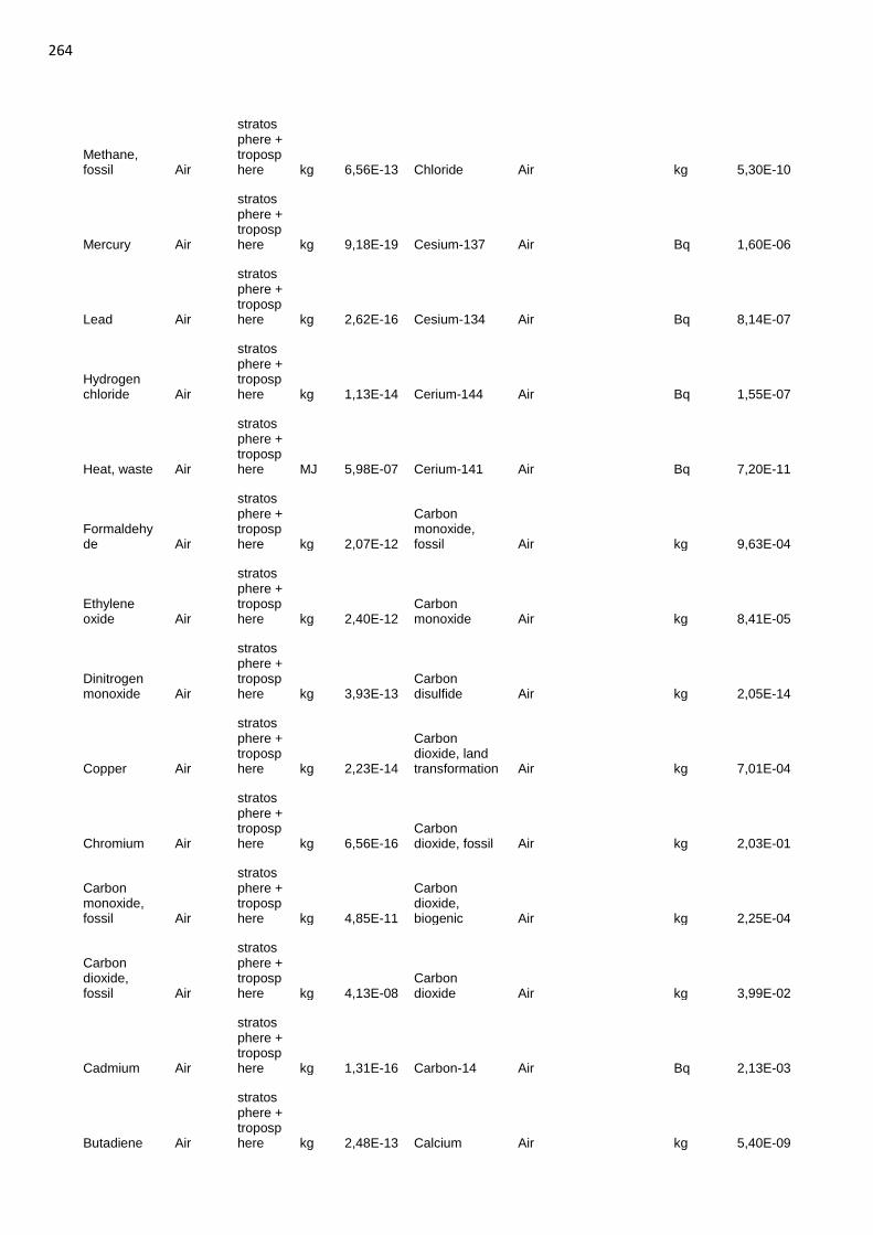
264
Methane, fossil Air
stratosphere + troposphere kg 6,56E-13 Chloride Air
kg 5,30E-10
Mercury Air
stratosphere + troposphere kg 9,18E-19 Cesium-137 Air
Bq 1,60E-06
Lead Air
stratosphere + troposphere kg 2,62E-16 Cesium-134 Air
Bq 8,14E-07
Hydrogen chloride Air
stratosphere + troposphere kg 1,13E-14 Cerium-144 Air
Bq 1,55E-07
Heat, waste Air
stratosphere + troposphere MJ 5,98E-07 Cerium-141 Air
Bq 7,20E-11
Formaldehyde Air
stratosphere + troposphere kg 2,07E-12
Carbon monoxide, fossil Air
kg 9,63E-04
Ethylene oxide Air
stratosphere + troposphere kg 2,40E-12
Carbon monoxide Air
kg 8,41E-05
Dinitrogen monoxide Air
stratosphere + troposphere kg 3,93E-13
Carbon disulfide Air
kg 2,05E-14
Copper Air
stratosphere + troposphere kg 2,23E-14
Carbon dioxide, land transformation Air
kg 7,01E-04
Chromium Air
stratosphere + troposphere kg 6,56E-16
Carbon dioxide, fossil Air
kg 2,03E-01
Carbon monoxide, fossil Air
stratosphere + troposphere kg 4,85E-11
Carbon dioxide, biogenic Air
kg 2,25E-04
Carbon dioxide, fossil Air
stratosphere + troposphere kg 4,13E-08
Carbon dioxide Air
kg 3,99E-02
Cadmium Air
stratosphere + troposphere kg 1,31E-16 Carbon-14 Air
Bq 2,13E-03
Butadiene Air
stratosphere + troposphere kg 2,48E-13 Calcium Air
kg 5,40E-09
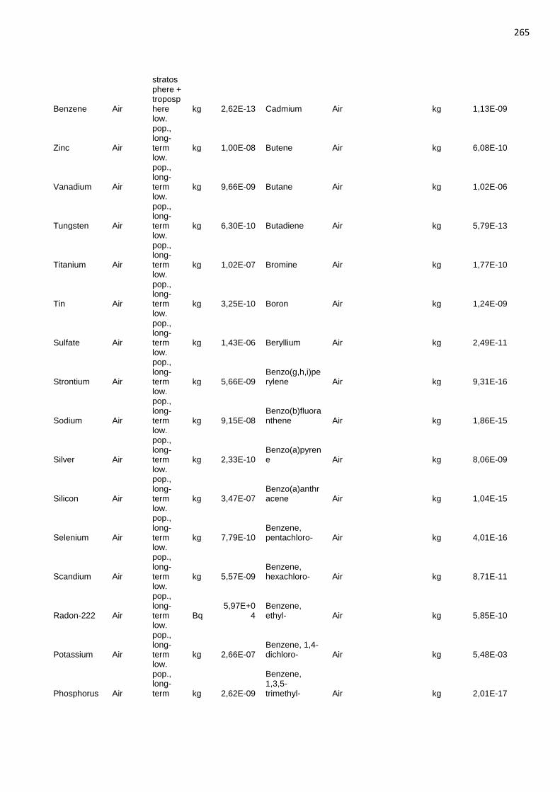
265
Benzene Air
stratosphere + troposphere kg 2,62E-13 Cadmium Air
kg 1,13E-09
Zinc Air
low. pop., long-term kg 1,00E-08 Butene Air
kg 6,08E-10
Vanadium Air
low. pop., long-term kg 9,66E-09 Butane Air
kg 1,02E-06
Tungsten Air
low. pop., long-term kg 6,30E-10 Butadiene Air
kg 5,79E-13
Titanium Air
low. pop., long-term kg 1,02E-07 Bromine Air
kg 1,77E-10
Tin Air
low. pop., long-term kg 3,25E-10 Boron Air
kg 1,24E-09
Sulfate Air
low. pop., long-term kg 1,43E-06 Beryllium Air
kg 2,49E-11
Strontium Air
low. pop., long-term kg 5,66E-09
Benzo(g,h,i)perylene Air
kg 9,31E-16
Sodium Air
low. pop., long-term kg 9,15E-08
Benzo(b)fluoranthene Air
kg 1,86E-15
Silver Air
low. pop., long-term kg 2,33E-10
Benzo(a)pyrene Air
kg 8,06E-09
Silicon Air
low. pop., long-term kg 3,47E-07
Benzo(a)anthracene Air
kg 1,04E-15
Selenium Air
low. pop., long-term kg 7,79E-10
Benzene, pentachloro- Air
kg 4,01E-16
Scandium Air
low. pop., long-term kg 5,57E-09
Benzene, hexachloro- Air
kg 8,71E-11
Radon-222 Air
low. pop., long-term Bq
5,97E+04
Benzene, ethyl- Air
kg 5,85E-10
Potassium Air
low. pop., long-term kg 2,66E-07
Benzene, 1,4-dichloro- Air
kg 5,48E-03
Phosphorus Air
low. pop., long-term kg 2,62E-09
Benzene, 1,3,5-trimethyl- Air
kg 2,01E-17
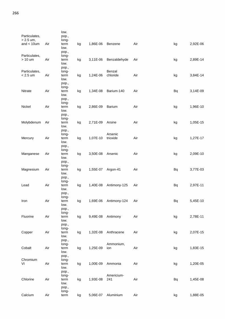
266
Particulates, > 2.5 um, and < 10um Air
low. pop., long-term kg 1,86E-06 Benzene Air
kg 2,92E-06
Particulates, > 10 um Air
low. pop., long-term kg 3,11E-06 Benzaldehyde Air
kg 2,89E-14
Particulates, < 2.5 um Air
low. pop., long-term kg 1,24E-06
Benzal chloride Air
kg 3,84E-14
Nitrate Air
low. pop., long-term kg 1,34E-08 Barium-140 Air
Bq 3,14E-09
Nickel Air
low. pop., long-term kg 2,86E-09 Barium Air
kg 1,96E-10
Molybdenum Air
low. pop., long-term kg 2,71E-09 Arsine Air
kg 1,05E-15
Mercury Air
low. pop., long-term kg 1,07E-10
Arsenic trioxide Air
kg 1,27E-17
Manganese Air
low. pop., long-term kg 3,50E-08 Arsenic Air
kg 2,09E-10
Magnesium Air
low. pop., long-term kg 1,55E-07 Argon-41 Air
Bq 3,77E-03
Lead Air
low. pop., long-term kg 1,40E-08 Antimony-125 Air
Bq 2,97E-11
Iron Air
low. pop., long-term kg 1,69E-06 Antimony-124 Air
Bq 5,45E-10
Fluorine Air
low. pop., long-term kg 9,49E-08 Antimony Air
kg 2,78E-11
Copper Air
low. pop., long-term kg 1,32E-08 Anthracene Air
kg 2,07E-15
Cobalt Air
low. pop., long-term kg 1,25E-09
Ammonium, ion Air
kg 1,83E-15
Chromium VI Air
low. pop., long-term kg 1,00E-09 Ammonia Air
kg 1,20E-05
Chlorine Air
low. pop., long-term kg 1,93E-08
Americium-241 Air
Bq 1,45E-08
Calcium Air
low. pop., long-term kg 5,06E-07 Aluminium Air
kg 1,88E-05
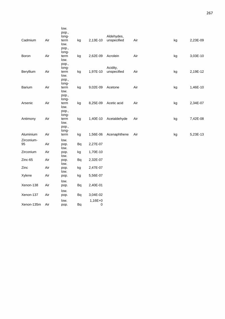
267
Cadmium Air
low. pop., long-term kg 2,13E-10
Aldehydes, unspecified Air
kg 2,23E-09
Boron Air
low. pop., long-term kg 2,62E-09 Acrolein Air
kg 3,03E-10
Beryllium Air
low. pop., long-term kg 1,97E-10
Acidity, unspecified Air
kg 2,19E-12
Barium Air
low. pop., long-term kg 9,02E-09 Acetone Air
kg 1,46E-10
Arsenic Air
low. pop., long-term kg 8,25E-09 Acetic acid Air
kg 2,34E-07
Antimony Air
low. pop., long-term kg 1,40E-10 Acetaldehyde Air
kg 7,42E-08
Aluminium Air
low. pop., long-term kg 1,56E-06 Acenaphthene Air
kg 5,23E-13
Zirconium-95 Air
low. pop. Bq 2,27E-07
Zirconium Air
low. pop. kg 1,70E-10
Zinc-65 Air
low. pop. Bq 2,32E-07
Zinc Air
low. pop. kg 2,47E-07
Xylene Air
low. pop. kg 5,56E-07
Xenon-138 Air low. pop. Bq 2,40E-01
Xenon-137 Air low. pop. Bq 3,04E-02
Xenon-135m Air low. pop. Bq
1,16E+00