SEEMINGLY UNRELATED REGRESSION

INFERENCE AND TESTING

Sunando BaruaBinamrata Haldar

Indranil RathHimanshu Mehrunkar

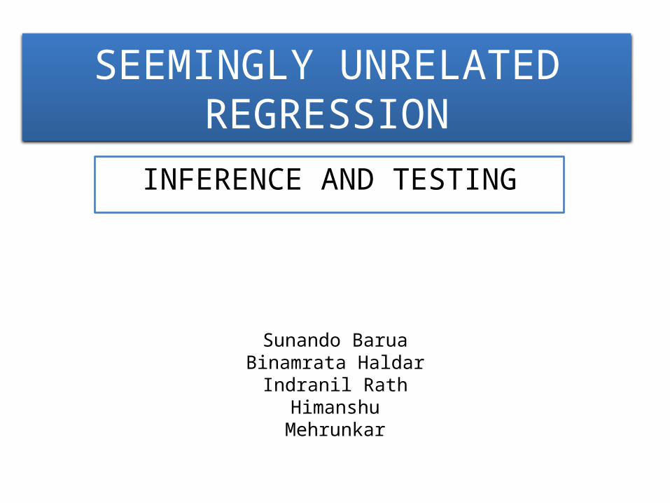
Four Steps of Hypothesis Testing

1. Hypotheses:

• Null hypothesis (H0):

A statement that parameter(s) take specific value (Usually: “no effect”)

• Alternative hypothesis (H1):

States that parameter value(s) falls in some alternative range of values (“an effect”)

2. Test Statistic: Compares data to what H0 predicts, often by finding the number of standard

errors between sample point estimate and H0 value of parameter. For example, the test stastics for Student’s t-test is

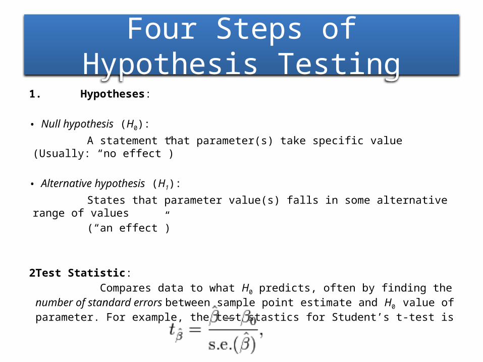
3. P-value (P): • A probability measure of evidence about H0. The probability (under

presumption that H0 is true) the test statistic equals observed value or value even more extreme in direction predicted by H1.

• The smaller the P-value, the stronger the evidence against H0.

4. Conclusion:

• If no decision needed, report and interpret P-value

• If decision needed, select a cutoff point (such as 0.05 or 0.01) and reject H0 if P-value ≤ that value

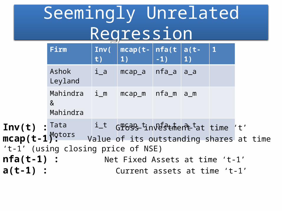
Seemingly Unrelated RegressionFirm Inv(t) mcap(t-1) nfa(t-1) a(t-1) 1

Ashok Leyland

i_a mcap_a nfa_a a_a

Mahindra & Mahindra

i_m mcap_m nfa_m a_m

Tata Motors i_t mcap_t nfa_t a_t

Inv(t) : Gross investment at time ‘t’mcap(t-1): Value of its outstanding shares at time ‘t-1’ (using closing price of NSE)nfa(t-1) : Net Fixed Assets at time ‘t-1’a(t-1) : Current assets at time ‘t-1’

System Specification

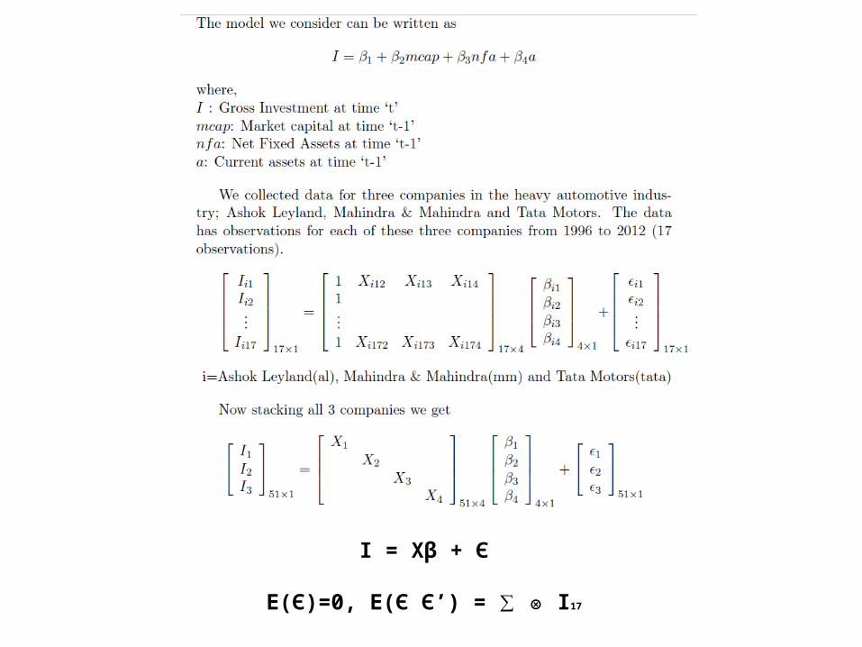
I = Xβ + Є

E(Є)=0, E(Є Є’) = ∑ ⊗ I17

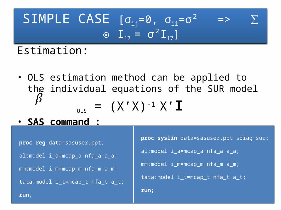
SIMPLE CASE [σij=0, σii=σ² => ∑ ⊗ I17 = σ²I17]

Estimation:

• OLS estimation method can be applied to the individual equations of the SUR model

OLS = (X’X)-1 X’I• SAS command :

proc reg data=sasuser.ppt; al:model i_a=mcap_a nfa_a a_a; mm:model i_m=mcap_m nfa_m a_m; tata:model i_t=mcap_t nfa_t a_t; run;

proc syslin data=sasuser.ppt sdiag sur;

al:model i_a=mcap_a nfa_a a_a;

mm:model i_m=mcap_m nfa_m a_m;

tata:model i_t=mcap_t nfa_t a_t;

run;

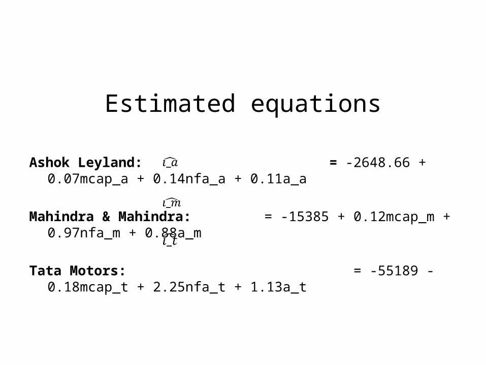
Estimated equations

Ashok Leyland: = -2648.66 + 0.07mcap_a + 0.14nfa_a + 0.11a_a

Mahindra & Mahindra: = -15385 + 0.12mcap_m + 0.97nfa_m + 0.88a_m

Tata Motors: = -55189 - 0.18mcap_t + 2.25nfa_t + 1.13a_t

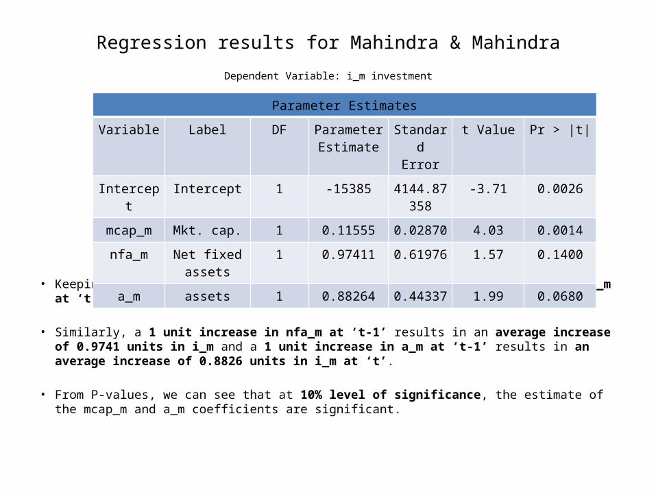
Regression results for Mahindra & Mahindra

Dependent Variable: i_m investment

• Keeping the other explanatory variables constant, a 1 unit increase in mcap_m at ‘t-1’ results in an average increase of 0.1156 units in i_m at ‘t’.

• Similarly, a 1 unit increase in nfa_m at ‘t-1’ results in an average increase of 0.9741 units in i_m and a 1 unit increase in a_m at ‘t-1’ results in an average increase of 0.8826 units in i_m at ‘t’.

• From P-values, we can see that at 10% level of significance, the estimate of the mcap_m and a_m coefficients are significant.

Parameter Estimates

Variable Label DF ParameterEstimate

StandardError

t Value Pr > |t|

Intercept Intercept 1 -15385 4144.87358

-3.71 0.0026

mcap_m Mkt. cap. 1 0.11555 0.02870 4.03 0.0014

nfa_m Net fixed assets

1 0.97411 0.61976 1.57 0.1400

a_m assets 1 0.88264 0.44337 1.99 0.0680

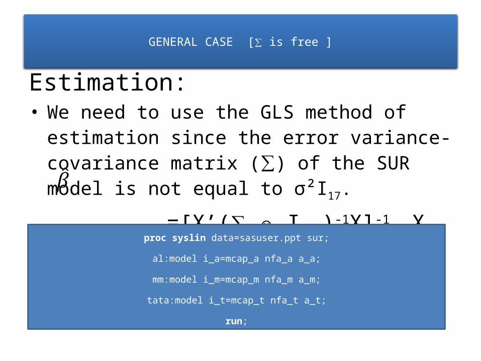
GENERAL CASE [∑ is free ]

• We need to use the GLS method of estimation since the error variance-covariance matrix (∑) of the SUR model is not equal to σ²I17.

GLS=[X’(∑ ⊗ I17 )-1X]-1 X ’(∑ ⊗ I17 )-1 I• SAS command :

proc syslin data=sasuser.ppt sur;

al:model i_a=mcap_a nfa_a a_a;

mm:model i_m=mcap_m nfa_m a_m;

tata:model i_t=mcap_t nfa_t a_t;

run;

Estimation:

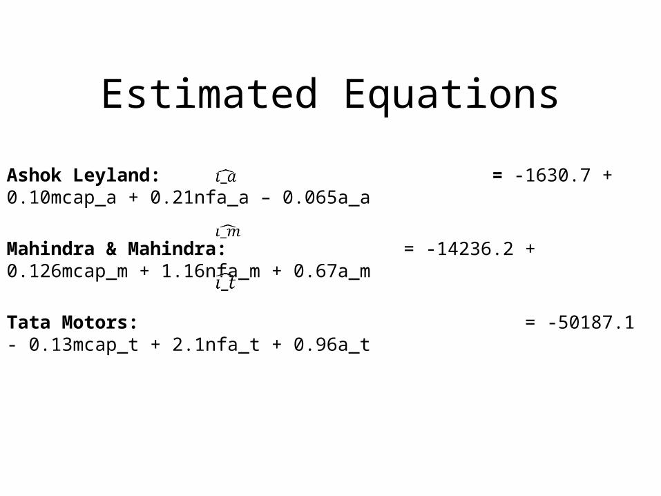
Estimated Equations

Ashok Leyland: = -1630.7 + 0.10mcap_a + 0.21nfa_a – 0.065a_a

Mahindra & Mahindra: = -14236.2 + 0.126mcap_m + 1.16nfa_m + 0.67a_m

Tata Motors: = -50187.1 - 0.13mcap_t + 2.1nfa_t + 0.96a_t

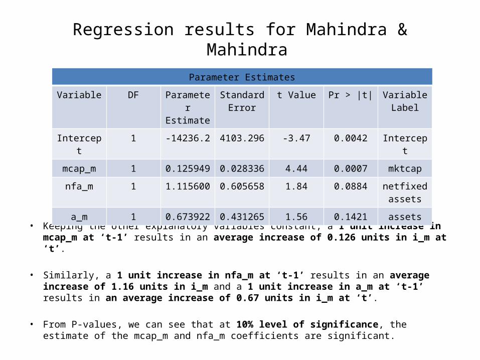
Regression results for Mahindra & Mahindra

Dependent Variable: i_m investment

• Keeping the other explanatory variables constant, a 1 unit increase in mcap_m at ‘t-1’ results in an average increase of 0.126 units in i_m at ‘t’.

• Similarly, a 1 unit increase in nfa_m at ‘t-1’ results in an average increase of 1.16 units in i_m and a 1 unit increase in a_m at ‘t-1’ results in an average increase of 0.67 units in i_m at ‘t’.

• From P-values, we can see that at 10% level of significance, the estimate of the mcap_m and nfa_m coefficients are significant.

Parameter Estimates

Variable DF ParameterEstimate

Standard Error

t Value Pr > |t| VariableLabel

Intercept 1 -14236.2 4103.296 -3.47 0.0042 Intercept

mcap_m 1 0.125949 0.028336 4.44 0.0007 mktcap

nfa_m 1 1.115600 0.605658 1.84 0.0884 netfixedassets

a_m 1 0.673922 0.431265 1.56 0.1421 assets

HYPOTHESIS TESTING

The appropriate framework for the test is the notion of constrained-unconstrained estimation

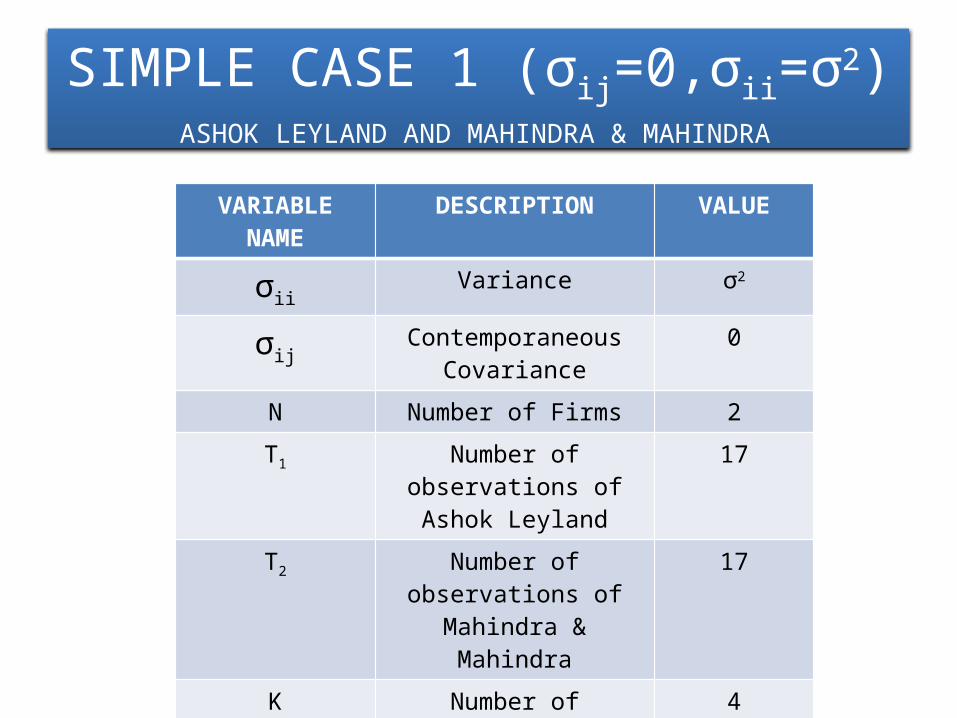
SIMPLE CASE 1 (σij=0,σii=σ2)ASHOK LEYLAND AND MAHINDRA & MAHINDRA

H0 β1 = β2

H1 β1 ≠ β2

VARIABLE NAME DESCRIPTION VALUE

σiiVariance σ2

σijContemporaneous

Covariance0

N Number of Firms 2T1 Number of observations

of Ashok Leyland17

T2 Number of observations of Mahindra & Mahindra

17

K Number of Parameters 4

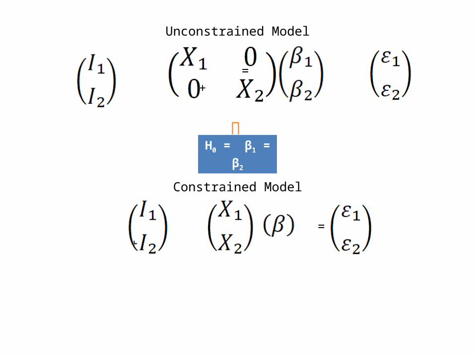
Unconstrained Model

= +

Constrained Model

= +

H0 = β1 = β2

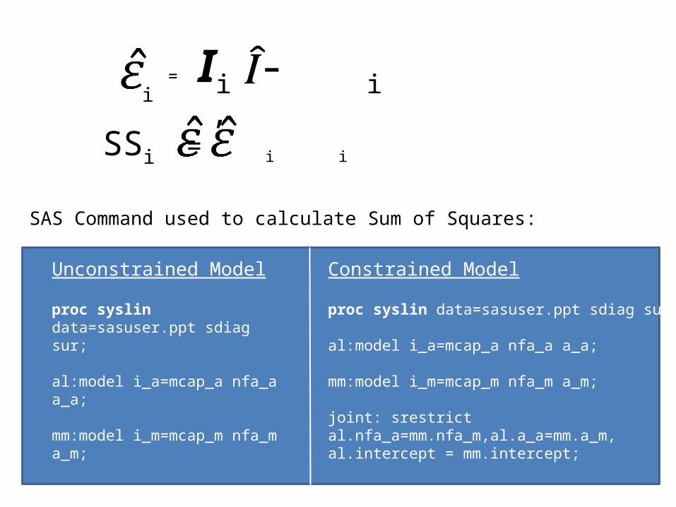
i = Ii - i

SSi = i i ’

SAS Command used to calculate Sum of Squares:

Unconstrained Model

proc syslin data=sasuser.ppt sdiag sur; al:model i_a=mcap_a nfa_a a_a; mm:model i_m=mcap_m nfa_m a_m; run;

Constrained Model

proc syslin data=sasuser.ppt sdiag sur; al:model i_a=mcap_a nfa_a a_a; mm:model i_m=mcap_m nfa_m a_m; joint: srestrict al.nfa_a=mm.nfa_m,al.a_a=mm.a_m, al.intercept = mm.intercept; run;

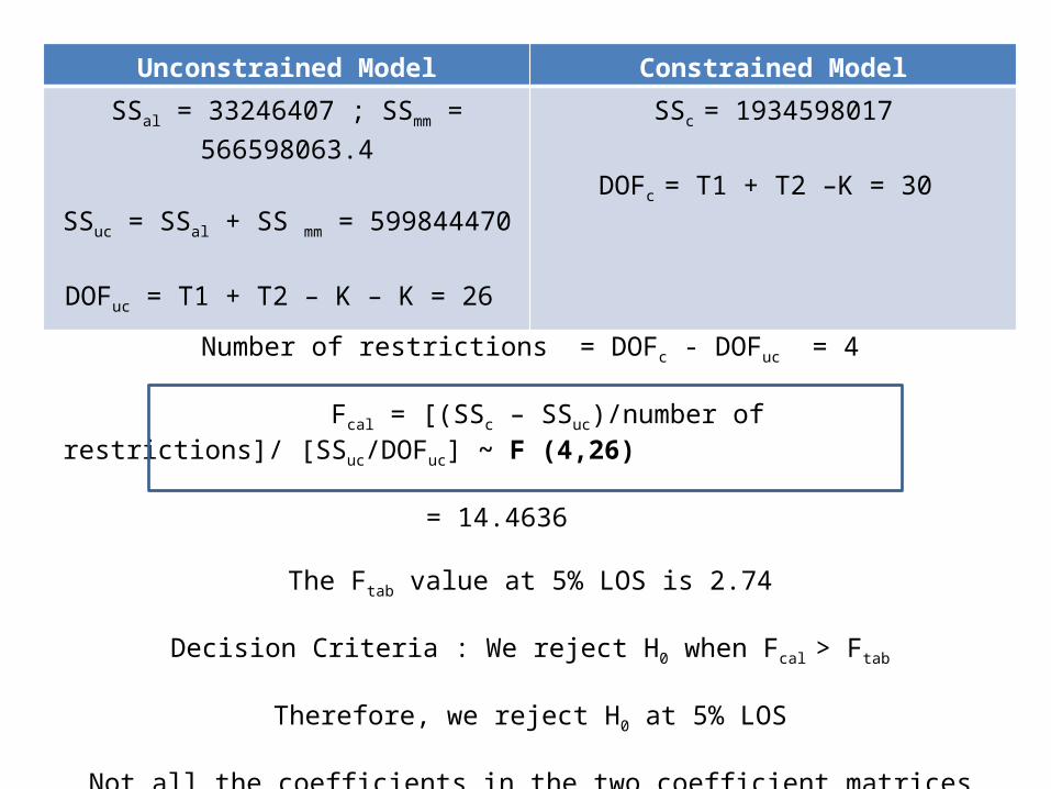
Number of restrictions = DOFc - DOFuc = 4

Fcal = [(SSc – SSuc)/number of restrictions]/ [SSuc/DOFuc] ~ F (4,26) = 14.4636

The Ftab value at 5% LOS is 2.74

Decision Criteria : We reject H0 when Fcal > Ftab

Therefore, we reject H0 at 5% LOS

Not all the coefficients in the two coefficient matrices are equal.

Unconstrained Model Constrained Model

SSal = 33246407 ; SSmm = 566598063.4

SSuc = SSal + SS mm = 599844470

DOFuc = T1 + T2 – K – K = 26

SSc = 1934598017

DOFc = T1 + T2 –K = 30

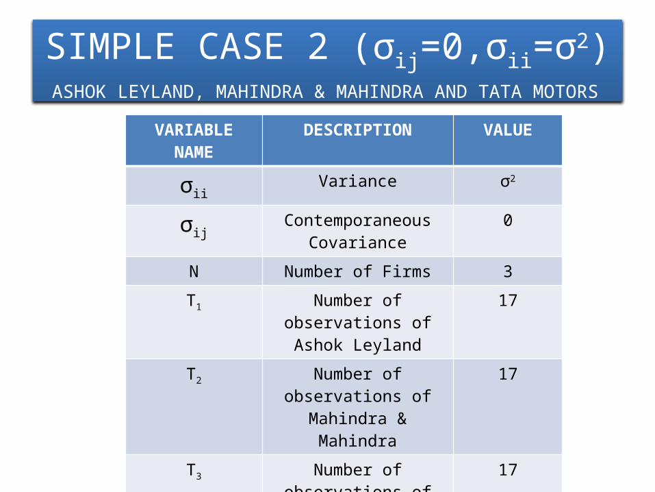
SIMPLE CASE 2 (σij=0,σii=σ2)ASHOK LEYLAND, MAHINDRA & MAHINDRA AND TATA MOTORS

H0 β1 = β2 = β₃

H1 β1 ≠ β2 ≠ β₃

VARIABLE NAME DESCRIPTION VALUE

σiiVariance σ2

σijContemporaneous

Covariance0

N Number of Firms 3T1 Number of observations

of Ashok Leyland17

T2 Number of observations of Mahindra & Mahindra

17

T3 Number of observations of Tata Motors

17

K Number of Parameters 4

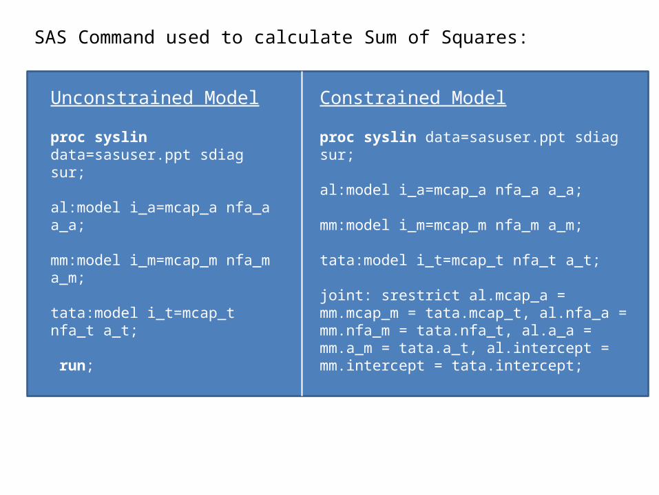
SAS Command used to calculate Sum of Squares:

Unconstrained Model

proc syslin data=sasuser.ppt sdiag sur; al:model i_a=mcap_a nfa_a a_a; mm:model i_m=mcap_m nfa_m a_m;

tata:model i_t=mcap_t nfa_t a_t;

run;

Constrained Model

proc syslin data=sasuser.ppt sdiag sur; al:model i_a=mcap_a nfa_a a_a; mm:model i_m=mcap_m nfa_m a_m;

tata:model i_t=mcap_t nfa_t a_t;

joint: srestrict al.mcap_a = mm.mcap_m = tata.mcap_t, al.nfa_a = mm.nfa_m = tata.nfa_t, al.a_a = mm.a_m = tata.a_t, al.intercept = mm.intercept = tata.intercept;

run;

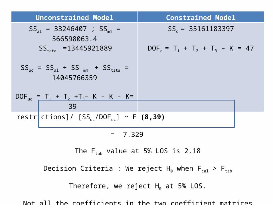
Number of restrictions = DOFc - DOFuc = 8

Fcal = [(SSc – SSuc)/number of restrictions]/ [SSuc/DOFuc] ~ F (8,39) = 7.329

The Ftab value at 5% LOS is 2.18

Decision Criteria : We reject H0 when Fcal > Ftab

Therefore, we reject H0 at 5% LOS.

Not all the coefficients in the two coefficient matrices are equal.

Unconstrained Model Constrained Model

SSal = 33246407 ; SSmm = 566598063.4 SStata =13445921889

SSuc = SSal + SS mm + SStata = 14045766359

DOFuc = T1 + T2 +T3– K – K - K= 39

SSc = 35161183397

DOFc = T1 + T2 + T3 – K = 47

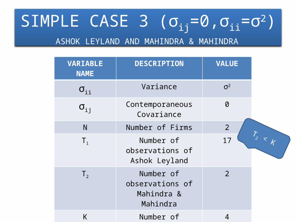
SIMPLE CASE 3 (σij=0,σii=σ2)ASHOK LEYLAND AND MAHINDRA & MAHINDRA

H0 β1 = β2

H1 β1 ≠ β2

VARIABLE NAME DESCRIPTION VALUE

σiiVariance σ2

σijContemporaneous

Covariance0

N Number of Firms 2T1 Number of observations

of Ashok Leyland17

T2 Number of observations of Mahindra & Mahindra

2

K Number of Parameters 4

T2 < K

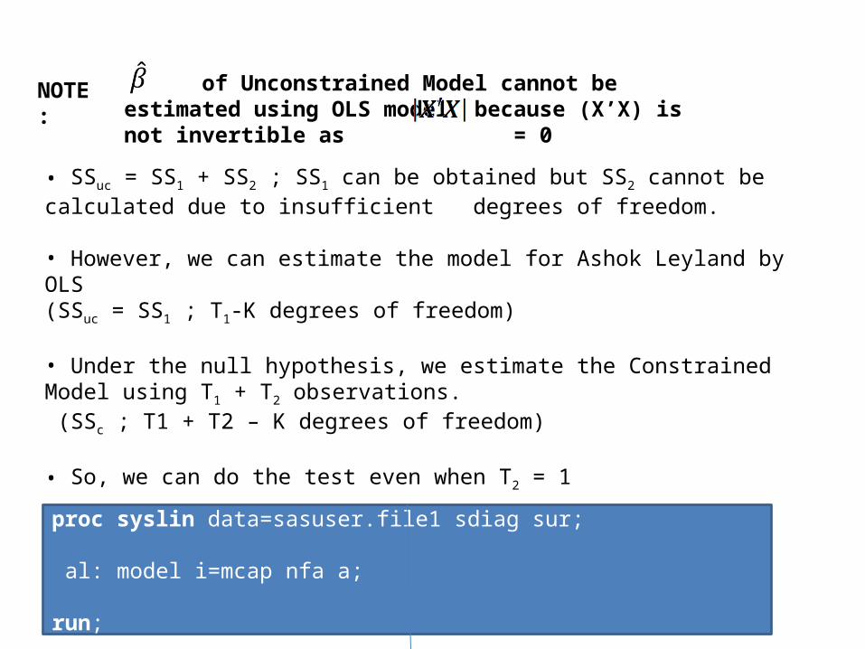
of Unconstrained Model cannot be estimated using OLS model because (X’X) is not invertible as = 0

NOTE:

• SSuc = SS1 + SS2 ; SS1 can be obtained but SS2 cannot be calculated due to insufficient degrees of freedom.

• However, we can estimate the model for Ashok Leyland by OLS (SSuc = SS1 ; T1-K degrees of freedom)

• Under the null hypothesis, we estimate the Constrained Model using T1 + T2 observations. (SSc ; T1 + T2 – K degrees of freedom)

• So, we can do the test even when T2 = 1

SAS Command for Constrained Model:proc syslin data=sasuser.file1 sdiag sur;

al: model i=mcap nfa a;

run;

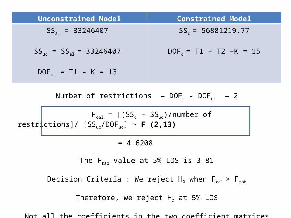
Number of restrictions = DOFc - DOFuc = 2

Fcal = [(SSc – SSuc)/number of restrictions]/ [SSuc/DOFuc] ~ F (2,13) = 4.6208

The Ftab value at 5% LOS is 3.81

Decision Criteria : We reject H0 when Fcal > Ftab

Therefore, we reject H0 at 5% LOS

Not all the coefficients in the two coefficient matrices are equal.

Unconstrained Model Constrained Model

SSal = 33246407

SSuc = SSal = 33246407

DOFuc = T1 – K = 13

SSc = 56881219.77

DOFc = T1 + T2 –K = 15

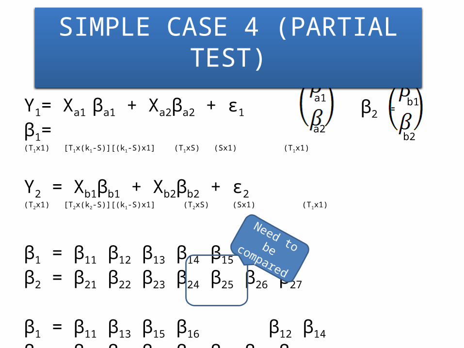
Y1= Xa1 βa1 + Xa2βa2 + ε1 β1= (T1x1) [T1x(k1-S)][(k1-S)x1] (T1xS) (Sx1) (T1x1)

Y2 = Xb1βb1 + Xb2βb2 + ε2 (T2x1) [T2x(k2-S)][(k1-S)x1] (T2xS) (Sx1) (T1x1)

β1 = β11 β12 β13 β14 β15 β16

β2 = β21 β22 β23 β24 β25 β26 β27

β1 = β11 β13 β15 β16 β12 β14

β2 = β21 β23 β24 β25 β26 β22 β27

Need to be compared

a1

a2

β2 = b1

b2

SIMPLE CASE 4 (PARTIAL TEST)

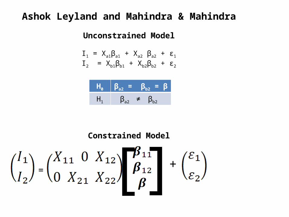
Ashok Leyland and Mahindra & Mahindra

Unconstrained Model

I1 = Xa1βa1 + Xa2 βa2 + ε1

I2 = Xb1βb1 + Xb2βb2 + ε2

Constrained Model

= []+

H0 βa2 = βb2 = β

H1 βa2 ≠ βb2

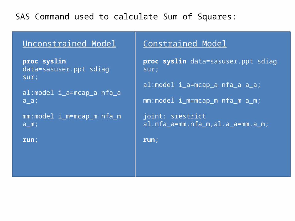
SAS Command used to calculate Sum of Squares:

Unconstrained Model

proc syslin data=sasuser.ppt sdiag sur; al:model i_a=mcap_a nfa_a a_a; mm:model i_m=mcap_m nfa_m a_m; run;

Constrained Model

proc syslin data=sasuser.ppt sdiag sur; al:model i_a=mcap_a nfa_a a_a; mm:model i_m=mcap_m nfa_m a_m; joint: srestrict al.nfa_a=mm.nfa_m,al.a_a=mm.a_m; run;

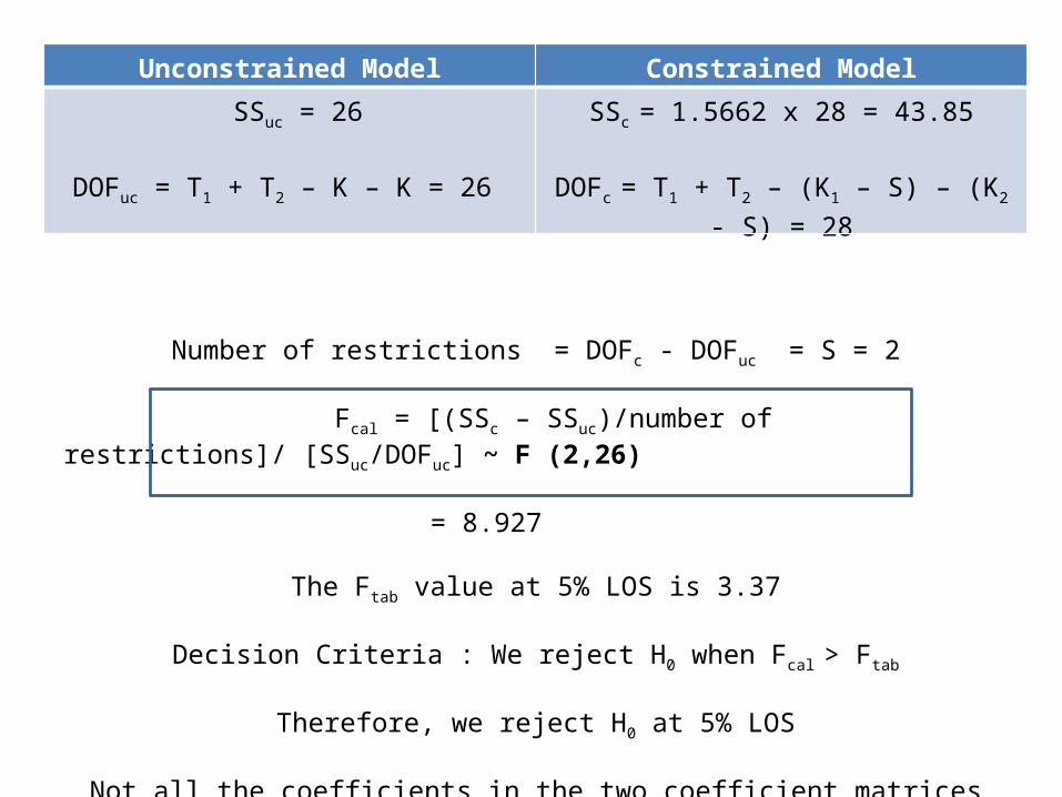
Number of restrictions = DOFc - DOFuc = S = 2

Fcal = [(SSc – SSuc)/number of restrictions]/ [SSuc/DOFuc] ~ F (2,26) = 8.927

The Ftab value at 5% LOS is 3.37

Decision Criteria : We reject H0 when Fcal > Ftab

Therefore, we reject H0 at 5% LOS

Not all the coefficients in the two coefficient matrices are equal.

Unconstrained Model Constrained Model

SSuc = 26

DOFuc = T1 + T2 – K – K = 26

SSc = 1.5662 x 28 = 43.85

DOFc = T1 + T2 – (K1 – S) – (K2 - S) = 28

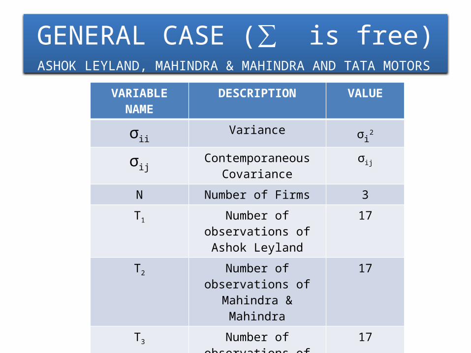
GENERAL CASE (∑ is free)ASHOK LEYLAND, MAHINDRA & MAHINDRA AND TATA MOTORS

H0 β1 = β2 = β₃

H1 Not H0

VARIABLE NAME DESCRIPTION VALUE

σiiVariance σi

2

σijContemporaneous

Covarianceσij

N Number of Firms 3T1 Number of observations

of Ashok Leyland17

T2 Number of observations of Mahindra & Mahindra

17

T3 Number of observations of Tata Motors

17

K Number of Parameters 4

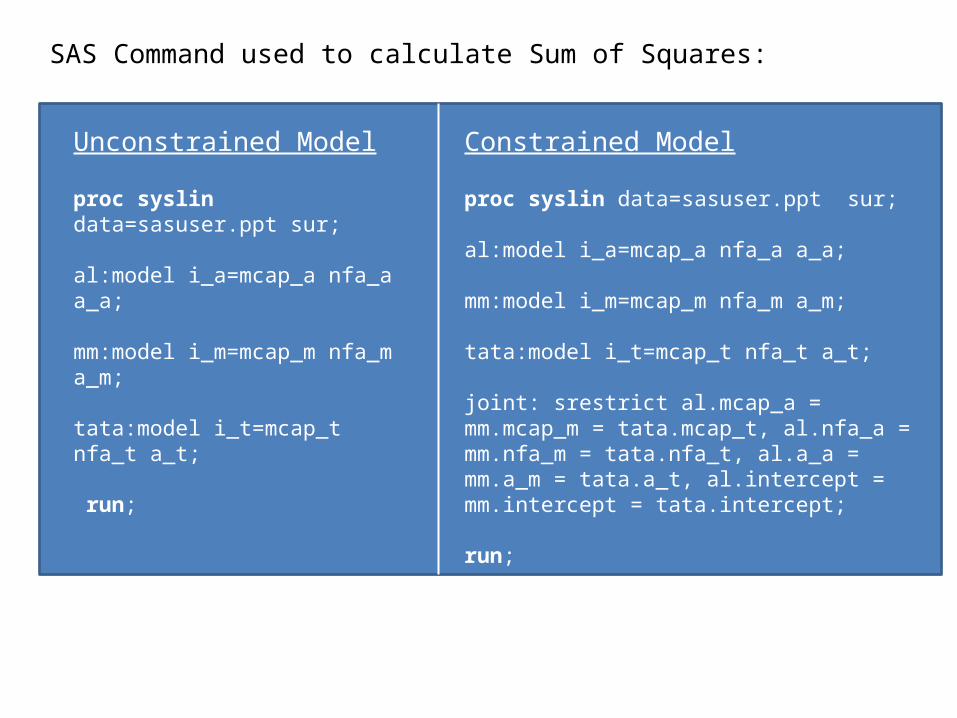
SAS Command used to calculate Sum of Squares:

Unconstrained Model

proc syslin data=sasuser.ppt sur; al:model i_a=mcap_a nfa_a a_a; mm:model i_m=mcap_m nfa_m a_m; tata:model i_t=mcap_t nfa_t a_t;

run;

Constrained Model

proc syslin data=sasuser.ppt sur; al:model i_a=mcap_a nfa_a a_a; mm:model i_m=mcap_m nfa_m a_m;

tata:model i_t=mcap_t nfa_t a_t;

joint: srestrict al.mcap_a = mm.mcap_m = tata.mcap_t, al.nfa_a = mm.nfa_m = tata.nfa_t, al.a_a = mm.a_m = tata.a_t, al.intercept = mm.intercept = tata.intercept;

run;

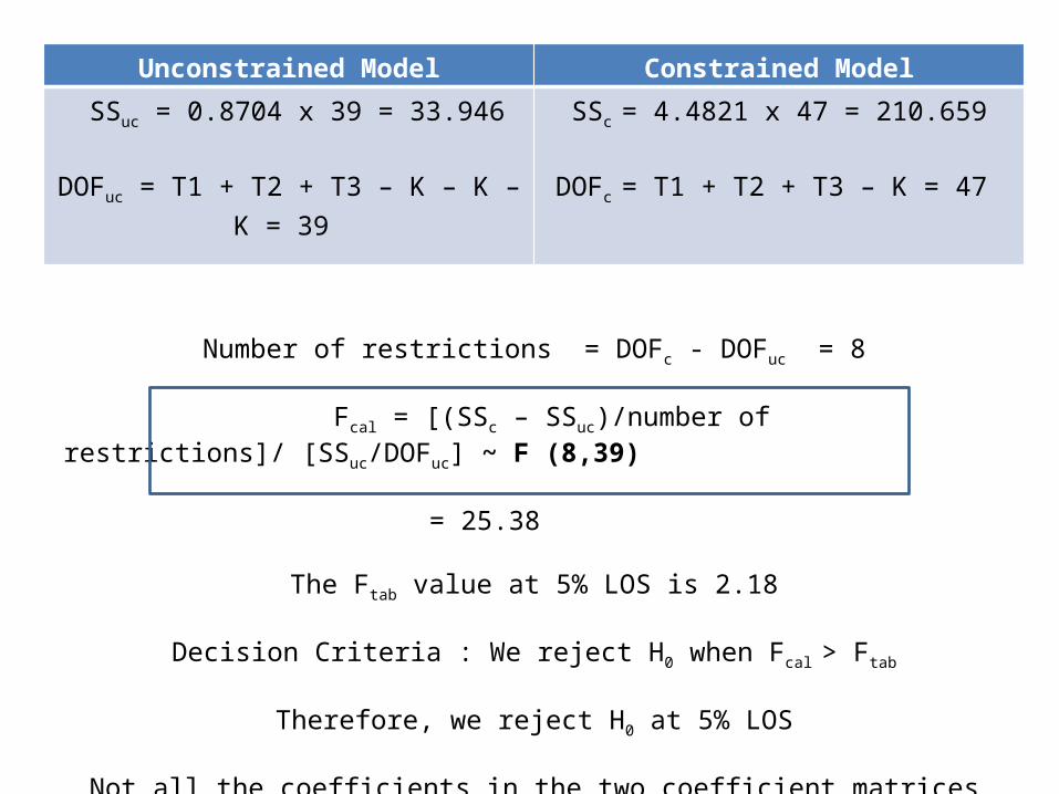
Number of restrictions = DOFc - DOFuc = 8

Fcal = [(SSc – SSuc)/number of restrictions]/ [SSuc/DOFuc] ~ F (8,39) = 25.38

The Ftab value at 5% LOS is 2.18

Decision Criteria : We reject H0 when Fcal > Ftab

Therefore, we reject H0 at 5% LOS

Not all the coefficients in the two coefficient matrices are equal.

Unconstrained Model Constrained Model

SSuc = 0.8704 x 39 = 33.946

DOFuc = T1 + T2 + T3 – K – K – K = 39

SSc = 4.4821 x 47 = 210.659

DOFc = T1 + T2 + T3 – K = 47

CHOW TESTMAHINDRA & MAHINDRA (1996-2005 ; 2006-2012)

H0 β11 = β12

H1 Not H0

VARIABLE NAME DESCRIPTION VALUE

σiiVariance σi

2

σijContemporaneous

Covarianceσij

T1 Number of observations for Period1: 1996-2005

10

T2 Number of observations for Period 2: 2006-2012

7

K Number of Parameters 4

Period 1:1996-2005 as β11

Period 2:2006-2012 as β12

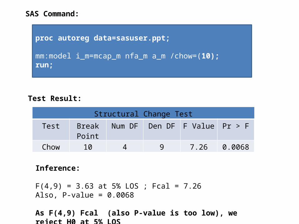
proc autoreg data=sasuser.ppt;

mm:model i_m=mcap_m nfa_m a_m /chow=(10);run;

SAS Command:

Structural Change Test

Test Break Point

Num DF Den DF F Value Pr > F

Chow 10 4 9 7.26 0.0068

Test Result:

Inference:

F(4,9) = 3.63 at 5% LOS ; Fcal = 7.26Also, P-value = 0.0068

As F(4,9) Fcal (also P-value is too low), we reject H0 at 5% LOS

THANK YOU!