Seismic Design for Buried Flexible · PDF fileSeismic Design for Buried Flexible Structures 1 ... various methods used for seismic design of ... conduit/tank. • Stress in buried

By

John M. Clark, MS,PE President of Clark Engineers, Inc.

Presented to Foundation Performance Association June 10, 2015

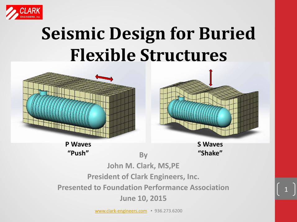
Seismic Design for Buried Flexible Structures

1

www.clark-engineers.com ▪ 936.273.6200

P Waves “Push”

S Waves “Shake”

http://www.clark-engineers.com/



Qualifying Statement

• No original work by this author is included herein. • All information provided herein is from published sources. • References are provided. • Best effort has been made to ensure correct methods;

however all methods should be verified for accuracy before using.

• PDF files of references can be provided upon written request. • Any constructive comments from “those of skill in the art” †

are greatly appreciated and may be sent to [email protected].

†Xerxes Patent US 6,397,168 B1 column 3, line 67 (20) 2


mailto:[email protected]

mailto:[email protected]




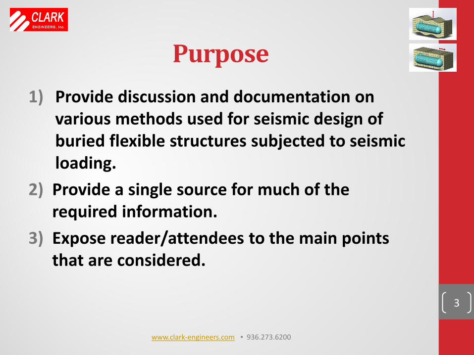
Purpose 1) Provide discussion and documentation on

various methods used for seismic design of buried flexible structures subjected to seismic loading.

2) Provide a single source for much of the required information.

3) Expose reader/attendees to the main points that are considered.

3





Focus of this Presentation

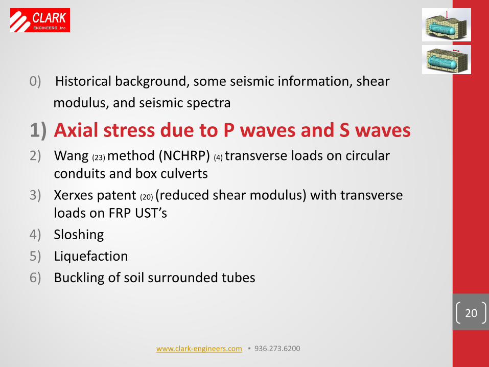
0) Historical background, some seismic information, shear modulus, and seismic spectra

1) Axial stress due to P waves and S waves 2) Wang method (23) (NCHRP) (4) transverse loads on circular

conduits and box culverts 3) Xerxes patent (20) (reduced shear modulus) with transverse

loads on FRP UST’s 4) Sloshing 5) Liquefaction 6) Buckling of soil surrounded tubes

4





Historical Background

• 1980’s customer’s started requiring seismic calculations for underground storage tanks (UST’s). At this time there were no known treatises on this topic.

• Hired local consultant PhD, PE to write paper. ⁻ Results were based on methods used for pipe lines – axial

stress due to P and S waves. Based largely on the work of Newmark (17 & 18) and Yeh (24).

⁻ Method was reviewed and used current Uniform Building Code (~1985). Method relied on confining pressure of the surrounding soil/backfill.

5

0) Historical background, some seismic information, shear modulus





Historical Background

• In 1999 this method was updated to include derivation of equations for stresses due to P and S waves and updated for 1997 UBC and built MathCAD sheet to automate calculations.

• In ~2004 it was again updated to latest International Building Code (IBC).

• Client in New Zealand requested new update in 2015. • Latest literature search revealed alternate methods that

focused on lateral-diametrical stress not previously included. ⁻ Specifically Wang (23) / NCHRP (4) method and Xerxes (20)

method

6






Current method (axial stress) uses soil strain to calculate stress in conduit/tank.

• Stress in buried structures is a function of shear wave velocity (𝑪𝒔).

• Shear wave velocity is a function of shear modulus of surrounding soil – (𝑮𝒎).

• Shear modulus is a function of soil type and confining pressures.

• Resulting stresses are calculated in axial direction e.g. for a pipeline and horizontally (perpendicular to long axis).

• A check for slippage is included for the axial stress condition.

• Sloshing effects are checked.

7

Historical Background 0) Historical background, some seismic information, shear modulus





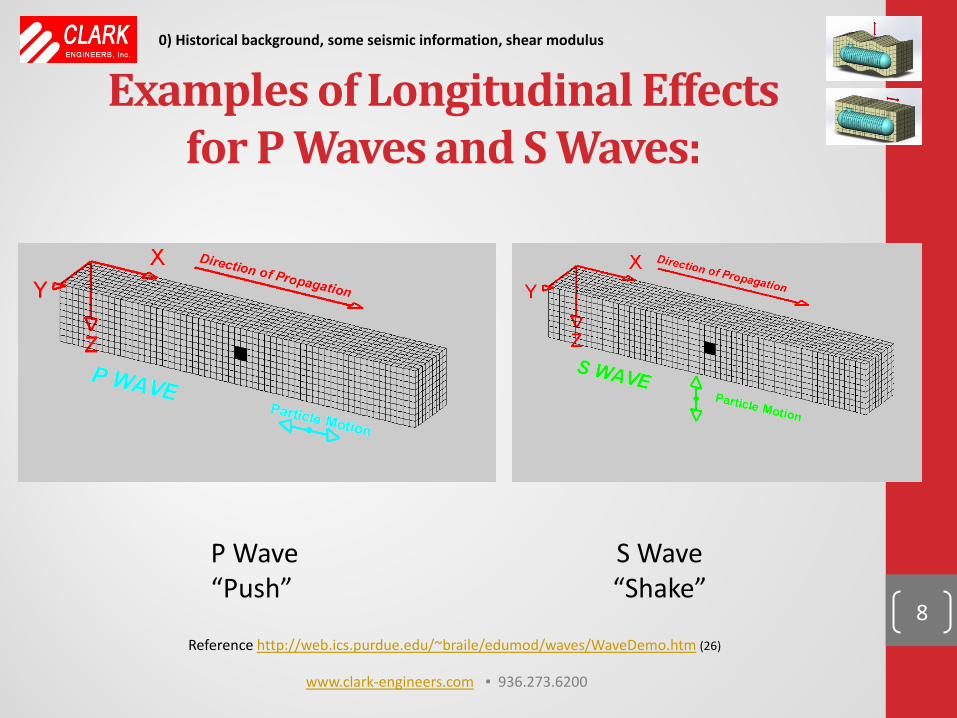
Examples of Longitudinal Effects for P Waves and S Waves:

8

P Wave “Push”

S Wave “Shake”

Reference http://web.ics.purdue.edu/~braile/edumod/waves/WaveDemo.htm (26)



http://web.ics.purdue.edu/~braile/edumod/waves/WaveDemo.htm




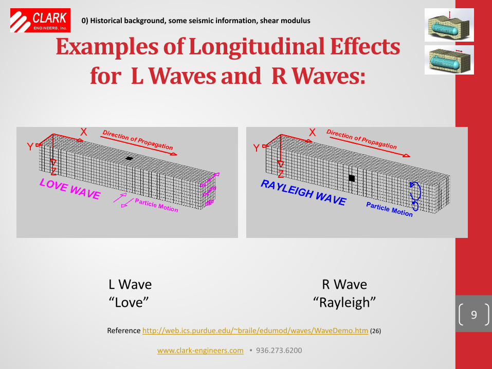
Examples of Longitudinal Effects for L Waves and R Waves:

9

L Wave “Love”

R Wave “Rayleigh”

Reference http://web.ics.purdue.edu/~braile/edumod/waves/WaveDemo.htm (26)



http://web.ics.purdue.edu/~braile/edumod/waves/WaveDemo.htm




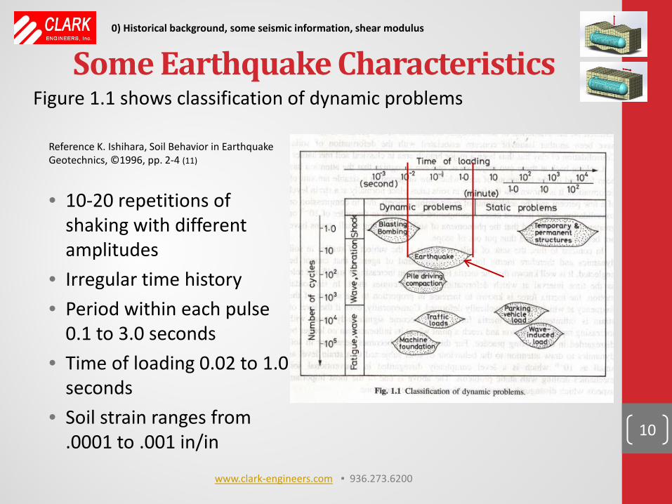
Some Earthquake Characteristics Reference K. Ishihara, Soil Behavior in Earthquake Geotechnics, ©1996, pp. 2-4 (11)

• 10-20 repetitions of shaking with different amplitudes

• Irregular time history • Period within each pulse

0.1 to 3.0 seconds • Time of loading 0.02 to 1.0

seconds • Soil strain ranges from

.0001 to .001 in/in 10

Figure 1.1 shows classification of dynamic problems






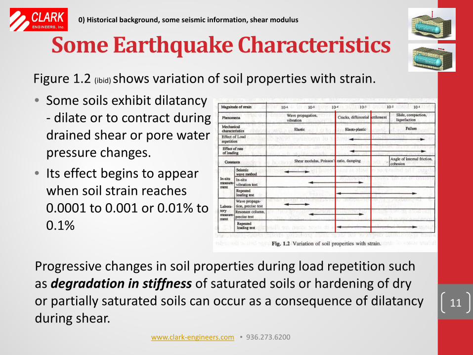
Some Earthquake Characteristics

• Some soils exhibit dilatancy - dilate or to contract during drained shear or pore water pressure changes.

• Its effect begins to appear when soil strain reaches 0.0001 to 0.001 or 0.01% to 0.1%

11

Progressive changes in soil properties during load repetition such as degradation in stiffness of saturated soils or hardening of dry or partially saturated soils can occur as a consequence of dilatancy during shear.

Figure 1.2 (ibid) shows variation of soil properties with strain.







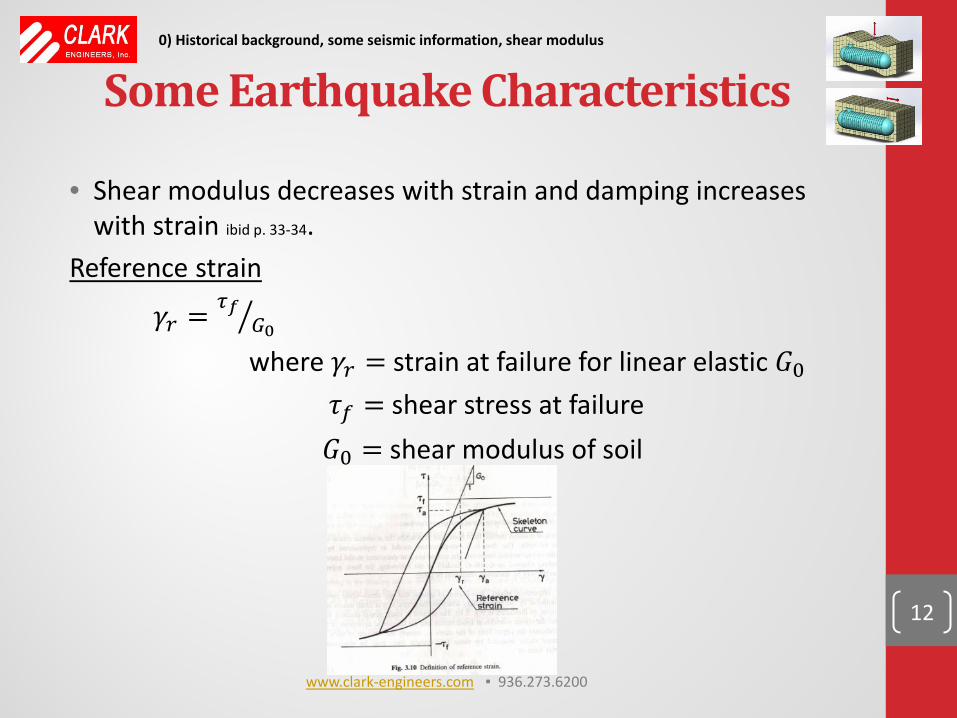
• Shear modulus decreases with strain and damping increases with strain ibid p. 33-34.

Reference strain

𝛾𝑟 = 𝜏𝑓𝐺0�

where 𝛾𝑟 = strain at failure for linear elastic 𝐺0 𝜏𝑓 = shear stress at failure 𝐺0 = shear modulus of soil

12







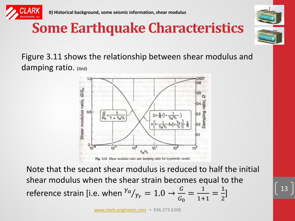
Figure 3.11 shows the relationship between shear modulus and damping ratio. (ibid)

13

Note that the secant shear modulus is reduced to half the initial shear modulus when the shear strain becomes equal to the reference strain [i.e. when 𝛾𝑎 𝛾𝑟⁄ = 1.0 → 𝐺

𝐺0= 1

1+1= 1

2]






Shear Modulus 𝑮𝒐

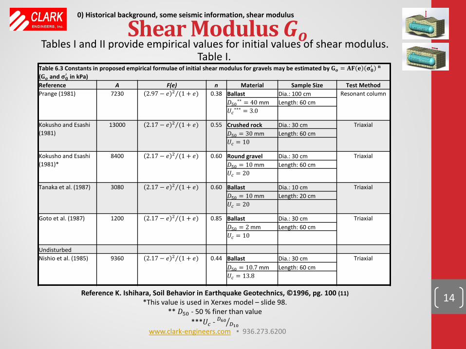
14 Reference K. Ishihara, Soil Behavior in Earthquake Geotechnics, ©1996, pg. 100 (11) *This value is used in Xerxes model – slide 98.

** 𝐷50 - 50 % finer than value ***𝑈𝑐 - 𝐷60 𝐷10�

Table 6.3 Constants in proposed empirical formulae of initial shear modulus for gravels may be estimated by 𝐆𝒐 = 𝐀𝐀 𝐞 𝛔𝟎′ 𝐧 (𝐆𝒐 and 𝛔𝟎′ in kPa) Reference A F(e) n Material Sample Size Test Method Prange (1981) 7230 2.97 − 𝑒 2 (1 + 𝑒)⁄ 0.38 Ballast Dia.: 100 cm Resonant column

𝐷50∗∗ = 40 mm Length: 60 cm 𝑈𝑐∗∗∗ = 3.0

Kokusho and Esashi (1981)

13000 2.17 − 𝑒 2 (1 + 𝑒)⁄ 0.55 Crushed rock Dia.: 30 cm Triaxial 𝐷50 = 30 mm Length: 60 cm 𝑈𝑐 = 10

Kokusho and Esashi (1981)*

8400 2.17 − 𝑒 2 (1 + 𝑒)⁄ 0.60 Round gravel Dia.: 30 cm Triaxial 𝐷50 = 10 mm Length: 60 cm 𝑈𝑐 = 20

Tanaka et al. (1987) 3080 2.17 − 𝑒 2 (1 + 𝑒)⁄ 0.60 Ballast Dia.: 10 cm Triaxial 𝐷50 = 10 mm Length: 20 cm 𝑈𝑐 = 20

Goto et al. (1987) 1200 2.17 − 𝑒 2 (1 + 𝑒)⁄ 0.85 Ballast Dia.: 30 cm Triaxial 𝐷50 = 2 mm Length: 60 cm 𝑈𝑐 = 10

Undisturbed Nishio et al. (1985) 9360 2.17 − 𝑒 2 (1 + 𝑒)⁄ 0.44 Ballast Dia.: 30 cm Triaxial

𝐷50 = 10.7 mm Length: 60 cm 𝑈𝑐 = 13.8

Table I.


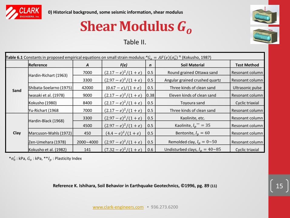
Tables I and II provide empirical values for initial values of shear modulus.





Shear Modulus 𝑮𝒐

15

Reference K. Ishihara, Soil Behavior in Earthquake Geotechnics, ©1996, pg. 89 (11)

Table II.

Table 6.1 Constants in proposed empirical equations on small strain modulus:*𝐺𝑜 = 𝐴𝐴 𝑒 𝜎0′ 𝑛 (Kokusho, 1987)

Reference A F(e) n Soil Material Test Method

Sand

Hardin-Richart (1963) 7000 2.17 − 𝑒 2 (1 + 𝑒)⁄ 0.5 Round grained Ottawa sand Resonant column

3300 2.97 − 𝑒 2 (1 + 𝑒)⁄ 0.5 Angular grained crushed quartz Resonant column

Shibata-Soelarno (1975) 42000 (0.67 − 𝑒) 1 + 𝑒⁄ 0.5 Three kinds of clean sand Ultrasonic pulse

Iwasaki et al. (1978) 9000 2.17 − 𝑒 2 (1 + 𝑒)⁄ 0.38 Eleven kinds of clean sand Resonant column

Kokusho (1980) 8400 2.17 − 𝑒 2 (1 + 𝑒)⁄ 0.5 Toyoura sand Cyclic triaxial

Yu-Richart (1968 7000 2.17 − 𝑒 2 (1 + 𝑒)⁄ 0.5 Three kinds of clean sand Resonant column

Clay

Hardin-Black (1968) 3300 2.97 − 𝑒 2 (1 + 𝑒)⁄ 0.5 Kaolinite, etc. Resonant column

4500 2.97 − 𝑒 2 (1 + 𝑒)⁄ 0.5 Kaolinite, 𝐼𝑝∗∗ = 35 Resonant column

Marcuson-Wahls (1972) 450 4.4 − 𝑒 2 (1 + 𝑒)⁄ 0.5 Bentonite, 𝐼𝑝 = 60 Resonant column

Zen-Umehara (1978) 2000~4000 2.97 − 𝑒 2 (1 + 𝑒)⁄ 0.5 Remolded clay, 𝐼𝑝 = 0~50 Resonant column

Kokusho et al. (1982) 141 7.32 − 𝑒 2 (1 + 𝑒)⁄ 0.6 Undisturbed clays, 𝐼𝑝 = 40~85 Cyclic triaxial

*𝜎0′ : kPa, 𝐺𝑜 : kPa, **𝐼𝑝 : Plasticity Index






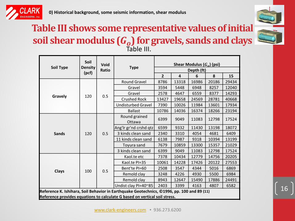
Table III shows some representative values of initial soil shear modulus (𝑮𝒐) for gravels, sands and clays

16

Soil Type Soil

Density (pcf)

Void Ratio Type

Shear Modulus (𝑮𝒐) (psi) Depth (ft)

2 4 6 8 15

Gravely 120 0.5

Round Gravel 8786 13318 16986 20186 29434 Gravel 3594 5448 6948 8257 12040 Gravel 2578 4647 6559 8377 14293

Crushed Rock 13427 19658 24569 28781 40668 Undisturbed Gravel 7390 10026 11984 13601 17934

Ballast 10786 14036 16374 18266 23194

Sands 120 0.5

Round grained Ottawa 6399 9049 11083 12798 17524

Ang'lr gr'nd crshd qtz 6599 9332 11430 13198 18072 3 kinds clean sand 2340 3310 4054 4681 6409

11 kinds clean sand 6138 7987 9318 10394 13199 Toyura sand 7679 10859 13300 15357 21029

3 kinds clean sand 6399 9049 11083 12798 17524

Clays 100 0.5

Kaol.te etc 7378 10434 12779 14756 20205 Kaol.te PI=35 10061 14228 17426 20122 27553 Bent'te PI=60 2508 3547 4344 5016 6869 Remold clay 3248 4226 4930 5500 6984 Remold clay 8943 12647 15490 17886 24491

Undist clay PI=40~85 2403 3399 4163 4807 6582 Reference K. Ishihara, Soil Behavior in Earthquake Geotechnics, ©1996, pp. 100 and 89 (11) Reference provides equations to calculate G based on vertical soil stress.

Table III.






Response Spectra vs. ASCE 7 Design Curves

17


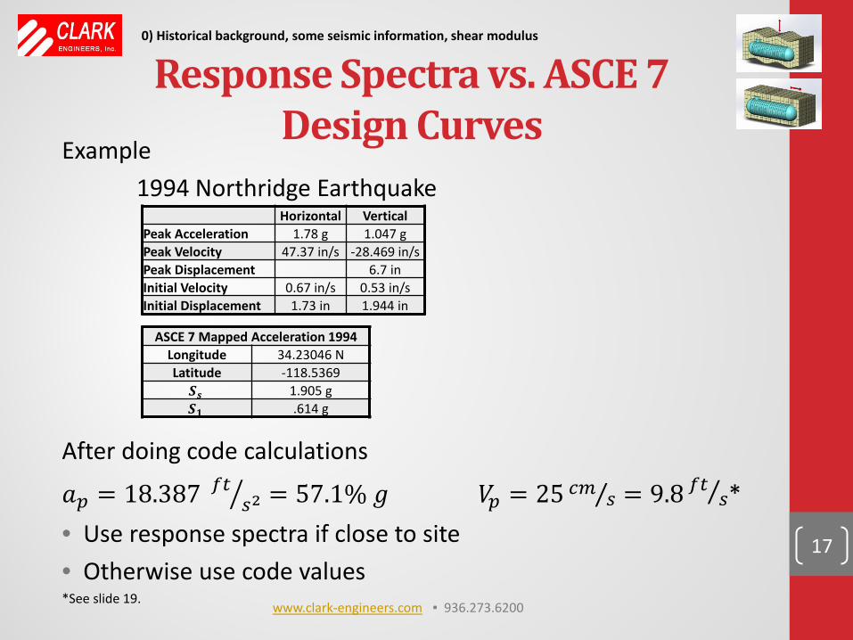
Example 1994 Northridge Earthquake After doing code calculations

𝑎𝑝 = 18.387 𝑓𝑓 𝑠2� = 57.1% 𝑔 𝑉𝑝 = 25 𝑐𝑐 𝑠⁄ = 9.8 𝑓𝑓𝑠⁄ *

• Use response spectra if close to site • Otherwise use code values *See slide 19.

Horizontal Vertical Peak Acceleration 1.78 g 1.047 g Peak Velocity 47.37 in/s -28.469 in/s Peak Displacement 6.7 in Initial Velocity 0.67 in/s 0.53 in/s Initial Displacement 1.73 in 1.944 in

ASCE 7 Mapped Acceleration 1994 Longitude 34.23046 N Latitude -118.5369 𝑺𝒔 1.905 g 𝑺𝟏 .614 g





Example of Response Spectra

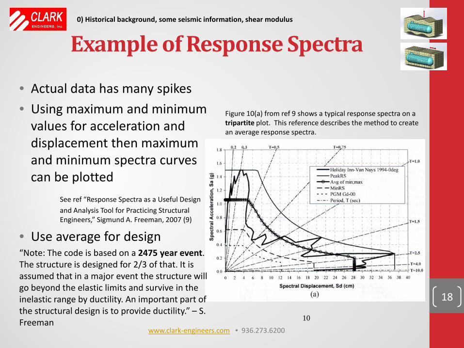
• Actual data has many spikes • Using maximum and minimum

values for acceleration and displacement then maximum and minimum spectra curves can be plotted

See ref “Response Spectra as a Useful Design and Analysis Tool for Practicing Structural Engineers,” Sigmund A. Freeman, 2007 (9)

• Use average for design “Note: The code is based on a 2475 year event. The structure is designed for 2/3 of that. It is assumed that in a major event the structure will go beyond the elastic limits and survive in the inelastic range by ductility. An important part of the structural design is to provide ductility.” – S. Freeman

18


Figure 10(a) from ref 9 shows a typical response spectra on a tripartite plot. This reference describes the method to create an average response spectra.

10 www.clark-engineers.com ▪ 936.273.6200




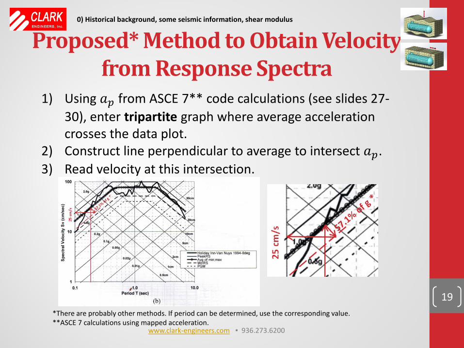
Proposed* Method to Obtain Velocity from Response Spectra

19


*There are probably other methods. If period can be determined, use the corresponding value. **ASCE 7 calculations using mapped acceleration.

1) Using 𝑎𝑝 from ASCE 7** code calculations (see slides 27-30), enter tripartite graph where average acceleration crosses the data plot.

2) Construct line perpendicular to average to intersect 𝑎𝑝. 3) Read velocity at this intersection.





0) Historical background, some seismic information, shear modulus, and seismic spectra

1) Axial stress due to P waves and S waves 2) Wang (23) method (NCHRP) (4) transverse loads on circular


loads on FRP UST’s 4) Sloshing 5) Liquefaction 6) Buckling of soil surrounded tubes

20





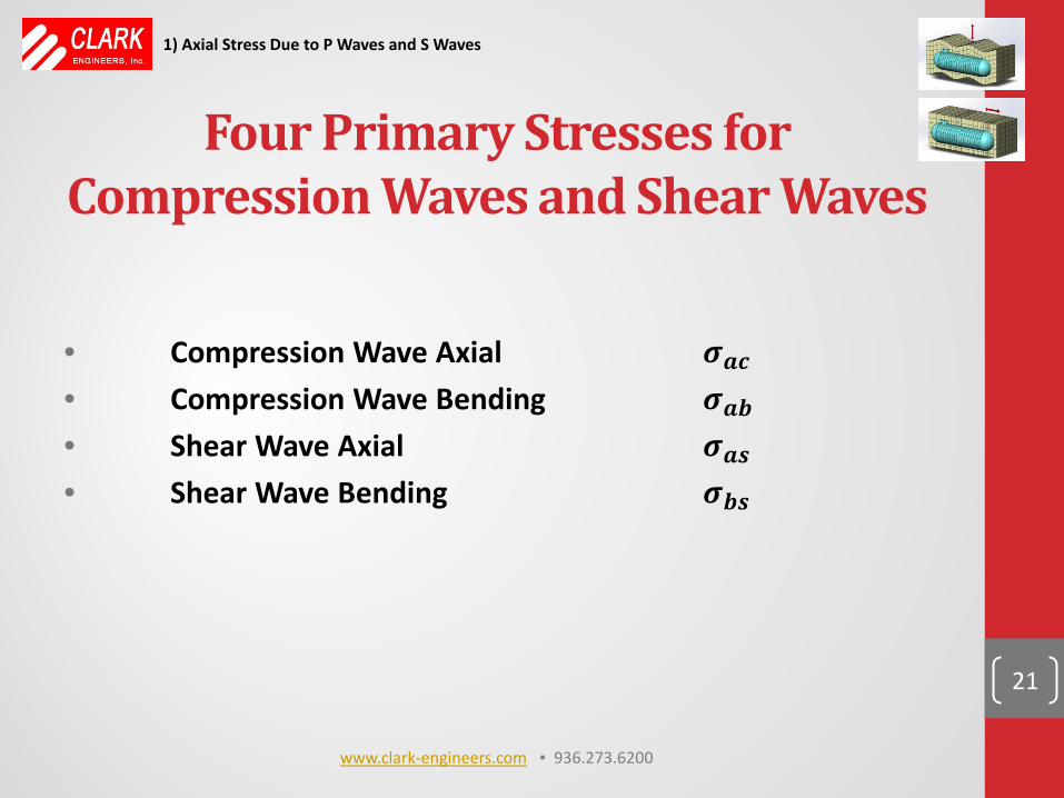
Four Primary Stresses for Compression Waves and Shear Waves

• Compression Wave Axial 𝝈𝒂𝒂 • Compression Wave Bending 𝝈𝒂𝒂 • Shear Wave Axial 𝝈𝒂𝒔 • Shear Wave Bending 𝝈𝒂𝒔

21

1) Axial Stress Due to P Waves and S Waves





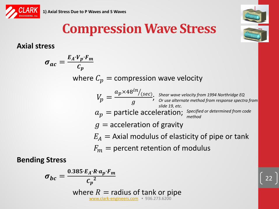
Compression Wave Stress Axial stress

𝝈𝒂𝒂 = 𝑬𝑨∙𝑽𝒑∙𝑭𝒎𝑪𝒑

where 𝐶𝑝 = compression wave velocity

𝑉𝑝 =𝑎𝑝×48𝑖𝑖 (𝑠𝑠𝑠)�

𝑔;

𝑎𝑝 = particle acceleration; 𝑔 = acceleration of gravity 𝐸𝐴 = Axial modulus of elasticity of pipe or tank 𝐴𝑐 = percent retention of modulus Bending Stress

𝝈𝒂𝒂 = 𝟎.𝟑𝟑𝟑∙𝑬𝑨∙𝑹∙𝒂𝒑∙𝑭𝒎𝑪𝒑𝟐

where 𝑅 = radius of tank or pipe

22

Shear wave velocity from 1994 Northridge EQ Or use alternate method from response spectra from slide 19, etc.

Specified or determined from code method






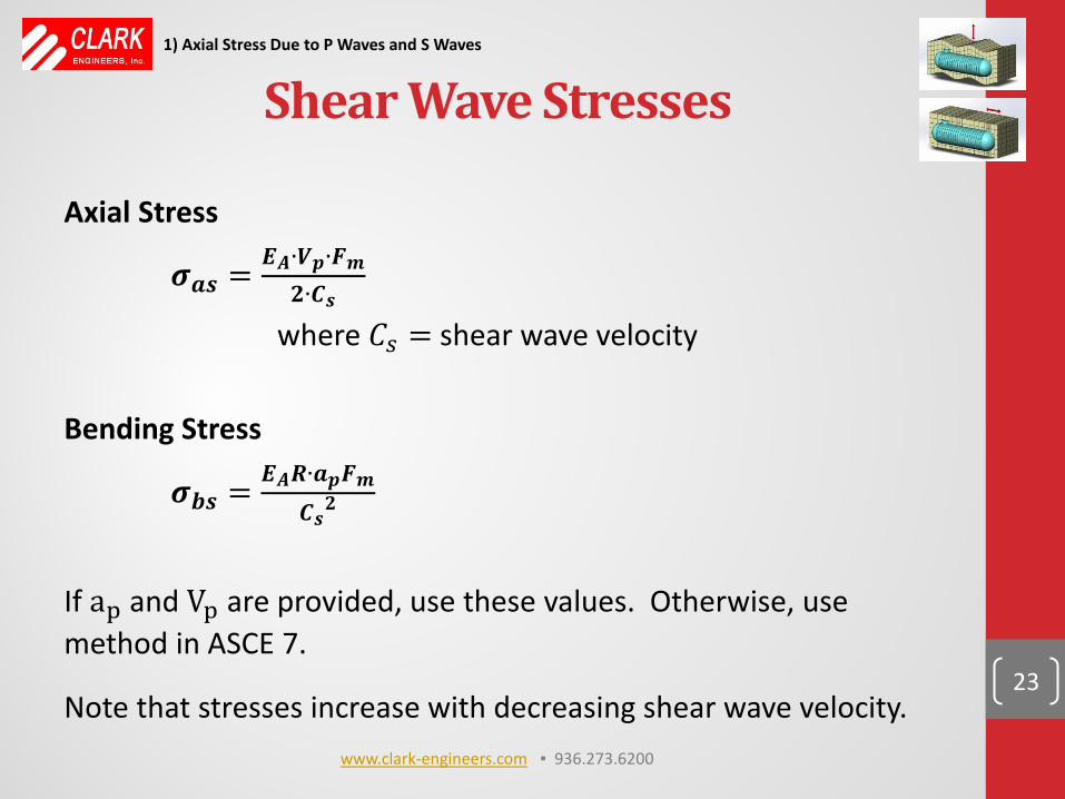
Shear Wave Stresses

Axial Stress

𝝈𝒂𝒔 = 𝑬𝑨∙𝑽𝒑∙𝑭𝒎𝟐∙𝑪𝒔

where 𝐶𝑠 = shear wave velocity Bending Stress

𝝈𝒂𝒔 = 𝑬𝑨𝑹∙𝒂𝒑𝑭𝒎𝑪𝒔𝟐

If ap and Vp are provided, use these values. Otherwise, use method in ASCE 7.

Note that stresses increase with decreasing shear wave velocity.

23



http://earthquake.usgs.gov/hazards/designmaps/downloads/pdfs/2010_ASCE-7_Figure_22-1.pdf





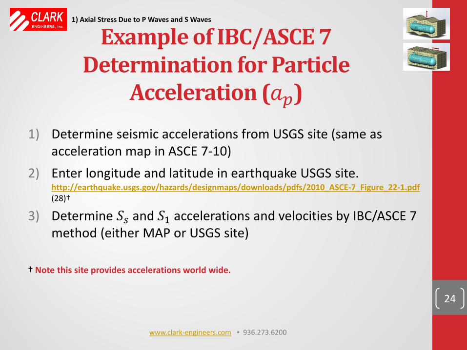
Example of IBC/ASCE 7 Determination for Particle

Acceleration (𝑎𝑝) 1) Determine seismic accelerations from USGS site (same as

acceleration map in ASCE 7-10) 2) Enter longitude and latitude in earthquake USGS site.

http://earthquake.usgs.gov/hazards/designmaps/downloads/pdfs/2010_ASCE-7_Figure_22-1.pdf (28)†

3) Determine 𝑆𝑠 and 𝑆1 accelerations and velocities by IBC/ASCE 7 method (either MAP or USGS site)

† Note this site provides accelerations world wide.

24












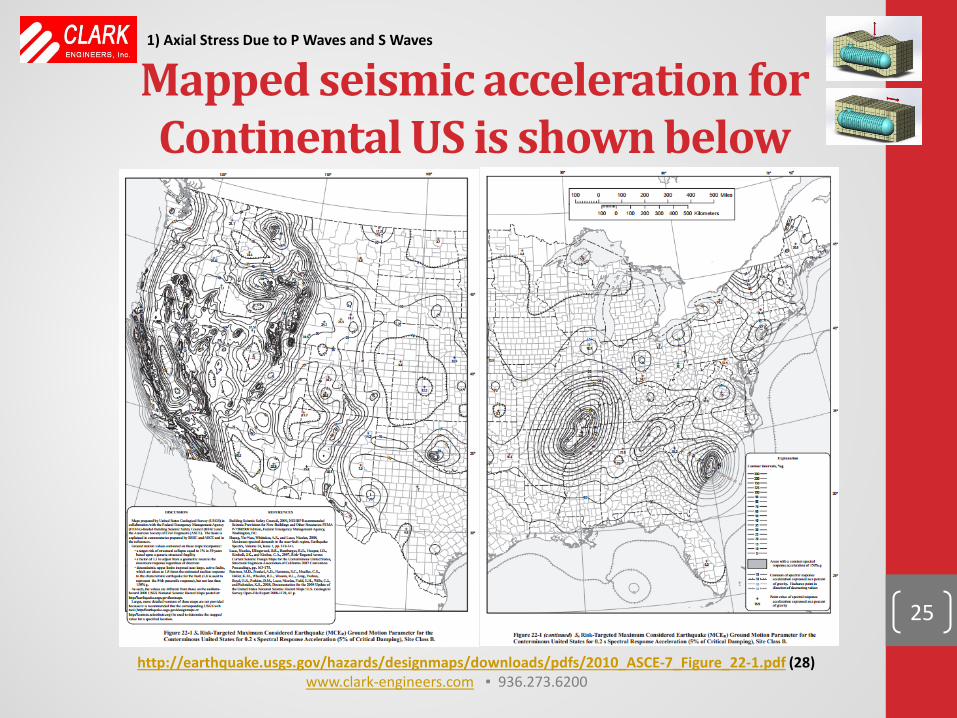
Mapped seismic acceleration for Continental US is shown below

25

http://earthquake.usgs.gov/hazards/designmaps/downloads/pdfs/2010_ASCE-7_Figure_22-1.pdf (28)







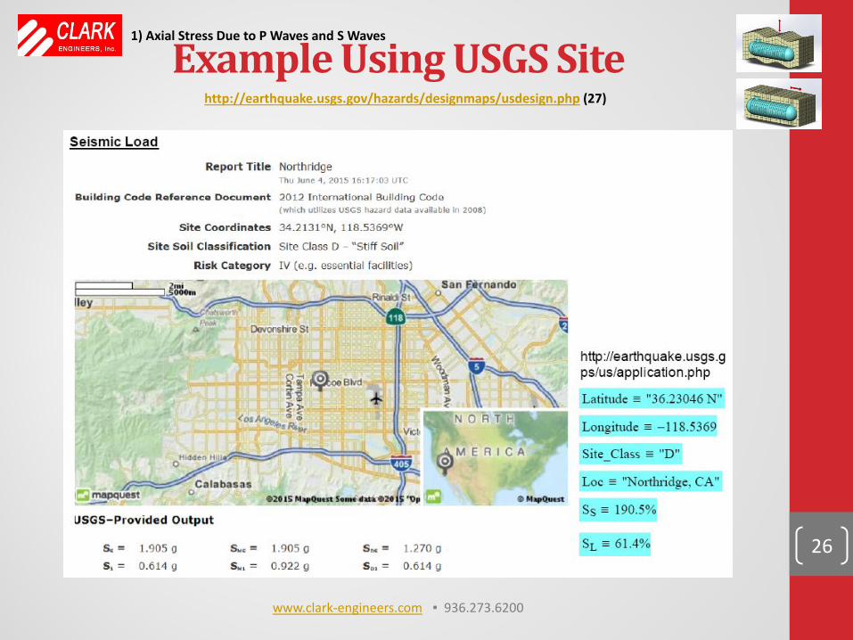
Example Using USGS Site

26

http://earthquake.usgs.gov/hazards/designmaps/usdesign.php (27)



http://earthquake.usgs.gov/hazards/designmaps/usdesign.php




27

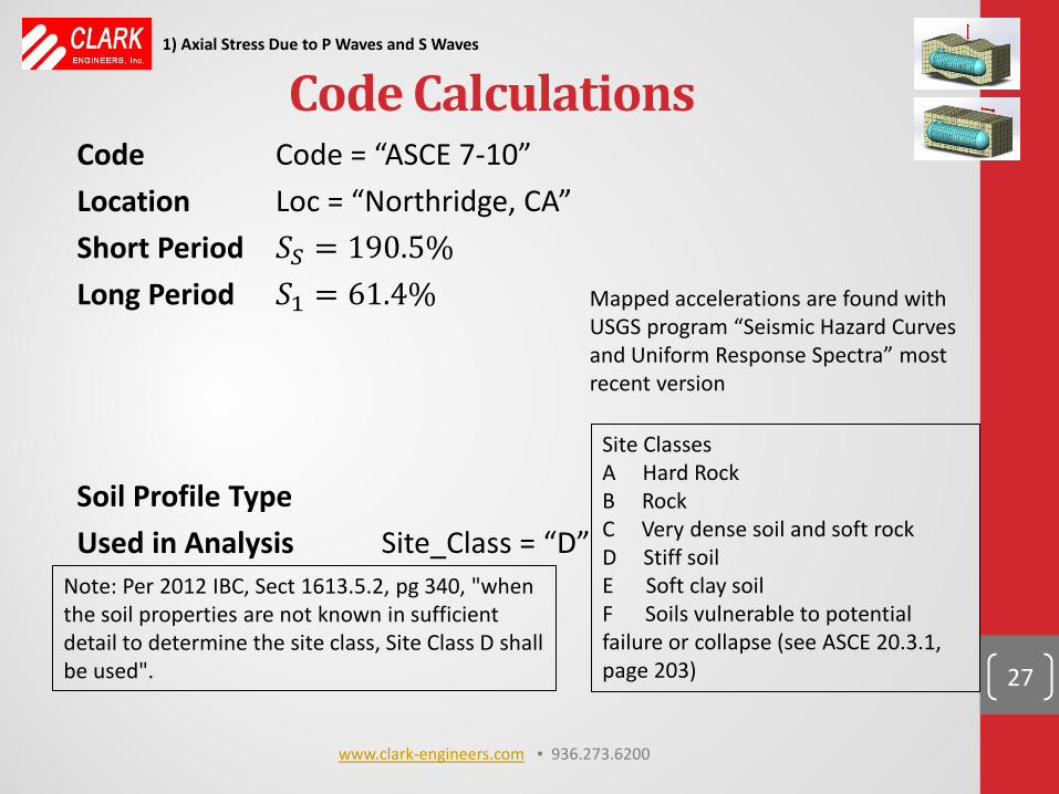
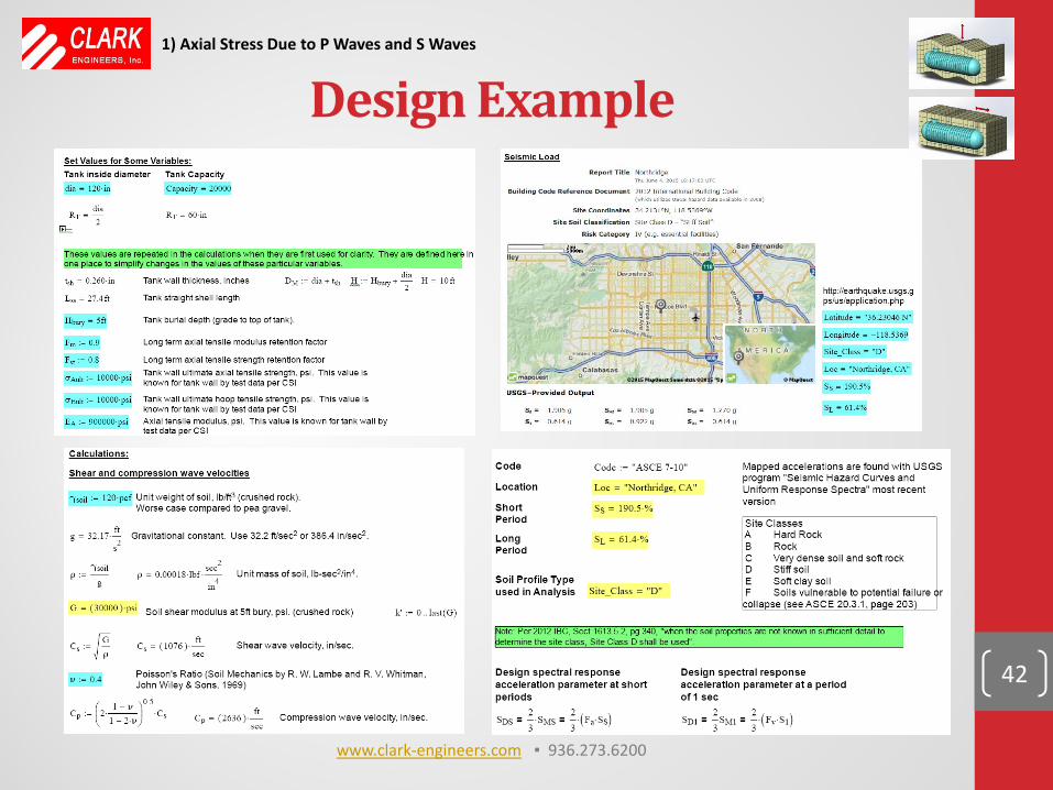
Code Calculations Code Code = “ASCE 7-10” Location Loc = “Northridge, CA” Short Period 𝑆𝑆 = 190.5% Long Period 𝑆1 = 61.4%

Soil Profile Type Used in Analysis Site_Class = “D”

Site Classes A Hard Rock B Rock C Very dense soil and soft rock D Stiff soil E Soft clay soil F Soils vulnerable to potential failure or collapse (see ASCE 20.3.1, page 203)

Note: Per 2012 IBC, Sect 1613.5.2, pg 340, "when the soil properties are not known in sufficient detail to determine the site class, Site Class D shall be used".

Mapped accelerations are found with USGS program “Seismic Hazard Curves and Uniform Response Spectra” most recent version






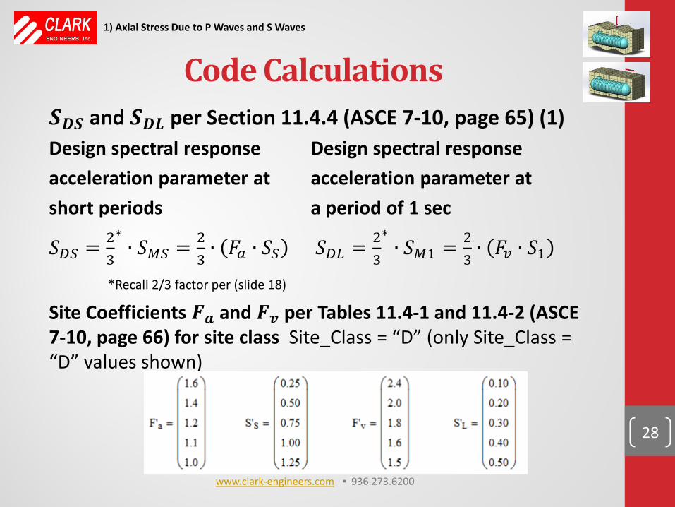
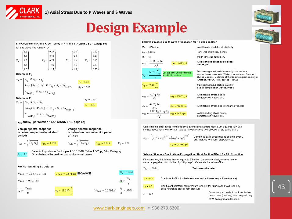
𝑺𝑫𝑺 and 𝑺𝑫𝑫 per Section 11.4.4 (ASCE 7-10, page 65) (1) Design spectral response Design spectral response acceleration parameter at acceleration parameter at short periods a period of 1 sec

𝑆𝐷𝑆 = 23

∗∙ 𝑆𝑀𝑆 = 2

3∙ 𝐴𝑎 ∙ 𝑆𝑆 𝑆𝐷𝐷 = 2

3

∗∙ 𝑆𝑀1 = 2

3∙ 𝐴𝑣 ∙ 𝑆1

*Recall 2/3 factor per (slide 18)

Site Coefficients 𝑭𝒂 and 𝑭𝒗 per Tables 11.4-1 and 11.4-2 (ASCE 7-10, page 66) for site class Site_Class = “D” (only Site_Class = “D” values shown)

28


Code Calculations





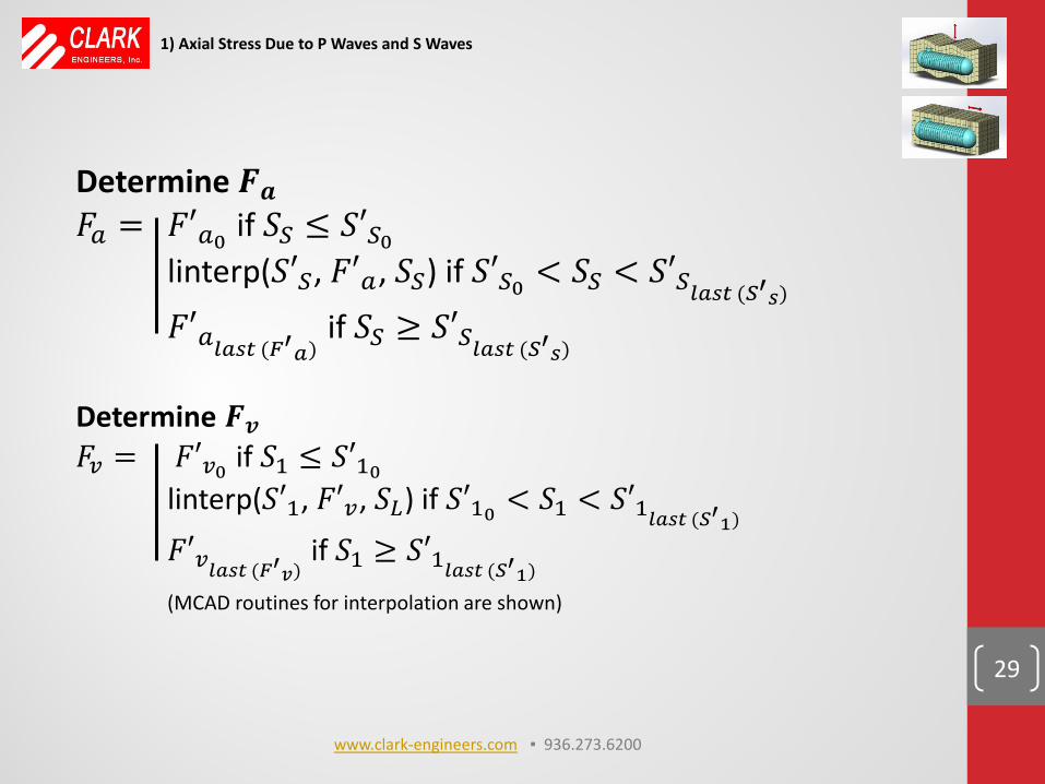
Determine 𝑭𝒂 𝐴𝑎 = 𝐴𝐹𝑎0 if 𝑆𝑆 ≤ 𝑆𝐹𝑆0 linterp(𝑆𝐹𝑆, 𝐴𝐹𝑎, 𝑆𝑆) if 𝑆𝐹𝑆0 < 𝑆𝑆 < 𝑆𝐹𝑆𝑙𝑎𝑠𝑙 (𝑆′𝑠)

𝐴𝐹𝑎𝑙𝑎𝑠𝑙 (𝐹′𝑎) if 𝑆𝑆 ≥ 𝑆𝐹𝑆𝑙𝑎𝑠𝑙 (𝑆′𝑠)

Determine 𝑭𝒗 𝐴𝑣 = 𝐴𝐹𝑣0 if 𝑆1 ≤ 𝑆𝐹10 linterp(𝑆𝐹1, 𝐴𝐹𝑣, 𝑆𝐷) if 𝑆𝐹10 < 𝑆1 < 𝑆𝐹1𝑙𝑎𝑠𝑙 (𝑆′1)

𝐴𝐹𝑣𝑙𝑎𝑠𝑙 (𝐹′𝑣) if 𝑆1 ≥ 𝑆𝐹1𝑙𝑎𝑠𝑙 (𝑆′1)

(MCAD routines for interpolation are shown)

29






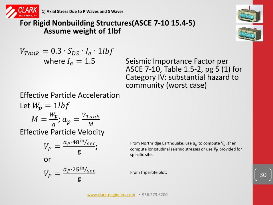
For Rigid Nonbuilding Structures(ASCE 7-10 15.4-5) Assume weight of 1lbf 𝑉𝑇𝑎𝑛𝑇 = 0.3 ∙ 𝑆𝐷𝑆 ∙ 𝐼𝑒 ∙ 1𝑙𝑙𝑙 where 𝐼𝑒 = 1.5 Seismic Importance Factor per ASCE 7-10, Table 1.5-2, pg 5 (1) for Category IV: substantial hazard to community (worst case) Effective Particle Acceleration Let 𝑊𝑝 = 1𝑙𝑙𝑙

𝑀 = 𝑊𝑝

𝑔; 𝑎𝑝 = 𝑉𝑇𝑎𝑖𝑇

𝑀

Effective Particle Velocity

𝑉𝑃 = 𝑎𝑃∙48in sec⁄𝐠

; or

𝑉𝑃 = 𝑎𝑃∙25in sec⁄𝐠

30



From Northridge Earthquake; use ap to compute Vp, then compute longitudinal seismic stresses or use VP provided for specific site.

From tripartite plot.




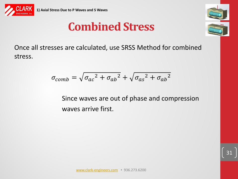
Combined Stress Once all stresses are calculated, use SRSS Method for combined stress.

𝜎𝑐𝑜𝑐𝑐 = 𝜎𝑎𝑐2 + 𝜎𝑎𝑐2 + 𝜎𝑎𝑠2 + 𝜎𝑎𝑐2 Since waves are out of phase and compression waves arrive first.

31






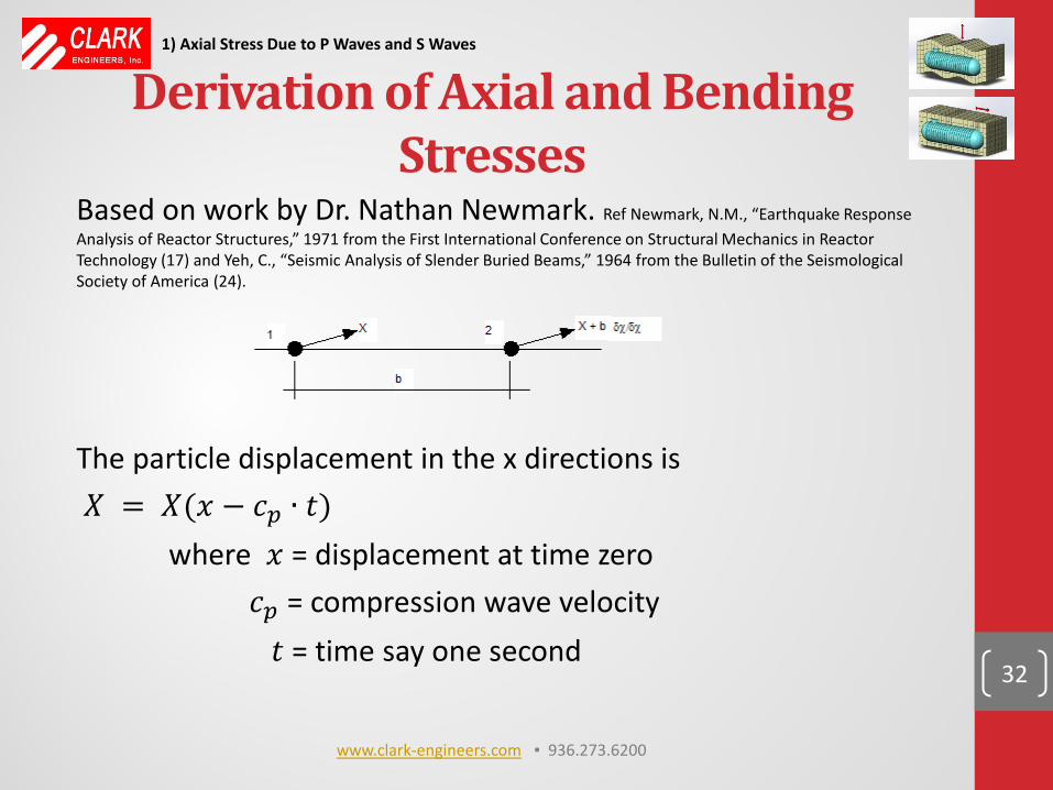
Derivation of Axial and Bending Stresses

Based on work by Dr. Nathan Newmark. Ref Newmark, N.M., “Earthquake Response Analysis of Reactor Structures,” 1971 from the First International Conference on Structural Mechanics in Reactor Technology (17) and Yeh, C., “Seismic Analysis of Slender Buried Beams,” 1964 from the Bulletin of the Seismological Society of America (24).

The particle displacement in the x directions is 𝑋 = 𝑋(𝑥 − 𝑐𝑝 ∙ 𝑡) where 𝑥 = displacement at time zero 𝑐𝑝 = compression wave velocity 𝑡 = time say one second

32






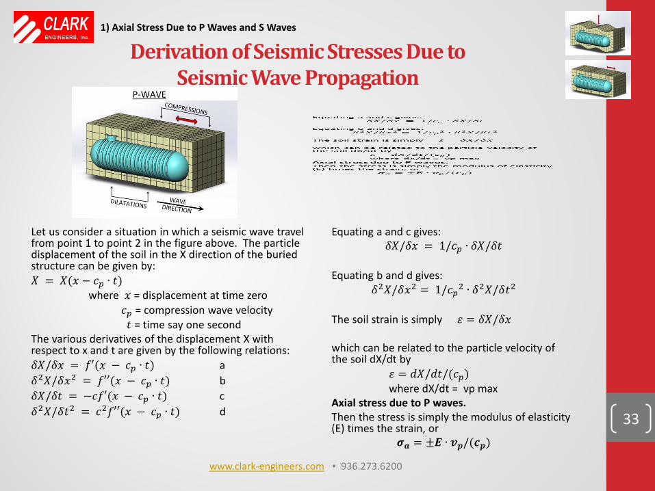
Derivation of Seismic Stresses Due to Seismic Wave Propagation

Let us consider a situation in which a seismic wave travel from point 1 to point 2 in the figure above. The particle displacement of the soil in the X direction of the buried structure can be given by: 𝑋 = 𝑋(𝑥 − 𝑐𝑝 ∙ 𝑡) where 𝑥 = displacement at time zero 𝑐𝑝 = compression wave velocity 𝑡 = time say one second The various derivatives of the displacement X with respect to x and t are given by the following relations: 𝛿𝑋/𝛿𝑥 = 𝑙𝐹(𝑥 − 𝑐𝑝 ∙ 𝑡) a 𝛿2𝑋/𝛿𝑥2 = 𝑙𝐹𝐹(𝑥 − 𝑐𝑝 ∙ 𝑡) b 𝛿𝑋/𝛿𝑡 = −𝑐𝑙𝐹(𝑥 − 𝑐𝑝 ∙ 𝑡) c 𝛿2𝑋/𝛿𝑡2 = 𝑐2𝑙𝐹𝐹(𝑥 − 𝑐𝑝 ∙ 𝑡) d

Equating a and c gives: 𝛿𝑋/𝛿𝑥 = 1/𝑐𝑝 ∙ 𝛿𝑋/𝛿𝑡

Equating b and d gives:

𝛿2𝑋/𝛿𝑥2 = 1/𝑐𝑝2 ∙ 𝛿2𝑋/𝛿𝑡2 The soil strain is simply 𝜀 = 𝛿𝑋/𝛿𝑥 which can be related to the particle velocity of the soil dX/dt by 𝜀 = 𝑑𝑋/𝑑𝑡/(𝑐𝑝) where dX/dt = vp max Axial stress due to P waves. Then the stress is simply the modulus of elasticity (E) times the strain, or

𝝈𝒂 = ±𝑬 ∙ 𝒗𝒑/(𝒂𝒑)

33






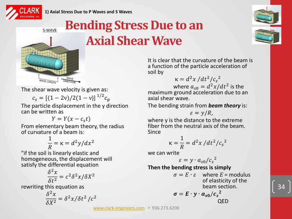
Bending Stress Due to an Axial Shear Wave

The shear wave velocity is given as:

𝑐𝑠 = [(1 − 2ν)/2(1 − ν)] 1/2𝑐𝑝 The particle displacement in the y direction can be written as

𝑌 = 𝑌(𝑥 − 𝑐𝑠𝑡) From elementary beam theory, the radius of curvature of a beam is:

1𝑅

= κ = 𝑑2𝑦/𝑑𝑥2

"if the soil is linearly elastic and homogeneous, the displacement will satisfy the differential equation

𝛿2𝑥𝛿𝑡2

= 𝑐2𝛿2𝑥/𝛿𝑋2

rewriting this equation as 𝛿2𝑥𝛿𝑋2

= 𝛿2𝑥 𝛿𝑡2⁄ /𝑐2

It is clear that the curvature of the beam is a function of the particle acceleration of soil by

κ = 𝑑2𝑥 𝑑𝑡2/𝑐𝑠2⁄ where 𝑎𝑠0 = 𝑑2𝑥/𝑑𝑡2 is the maximum ground acceleration due to an axial shear wave. The bending strain from beam theory is:

𝜀 = 𝑦/𝑅, where y is the distance to the extreme fiber from the neutral axis of the beam. Since

κ =1𝑅

= 𝑑2𝑥 𝑑𝑡2/𝑐𝑠2⁄

we can write 𝜀 = 𝑦 ∙ 𝑎𝑠0/𝑐𝑠2

Then the bending stress is simply 𝜎 = 𝐸 ∙ 𝜀 where E = modulus of elasticity of the beam section. 𝝈 = 𝑬 ∙ 𝒚 ∙ 𝒂𝒔𝟎/𝒂𝒔𝟐 QED

34






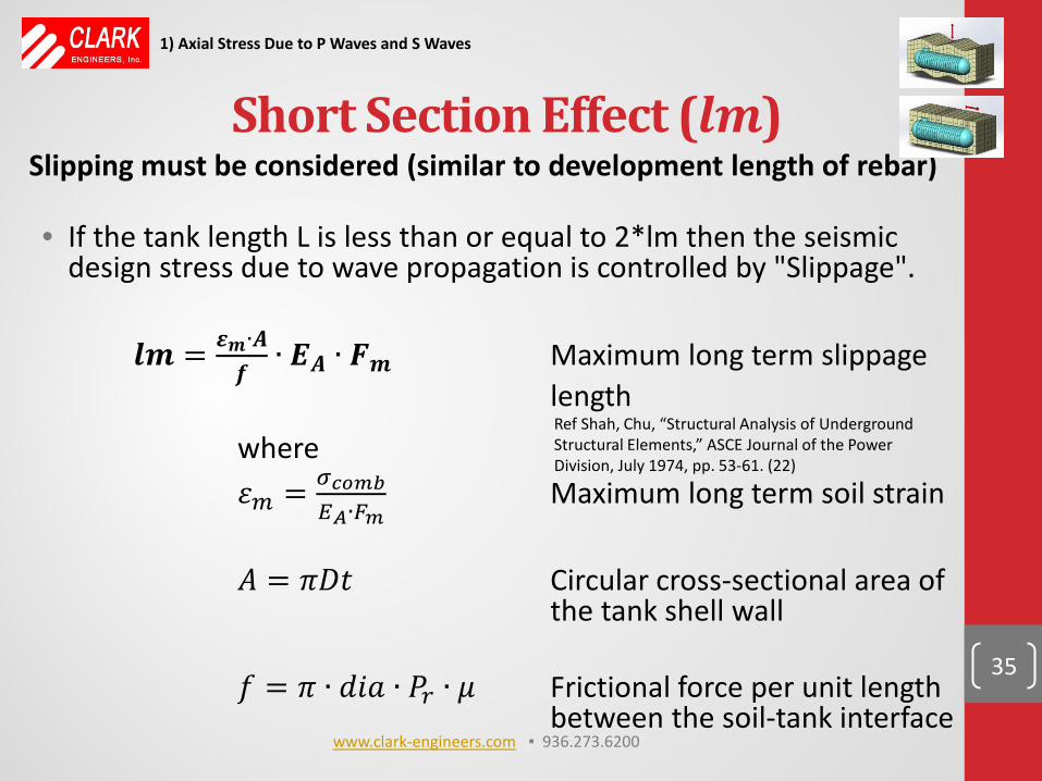
Short Section Effect (𝒍𝒎) Slipping must be considered (similar to development length of rebar) • If the tank length L is less than or equal to 2*lm then the seismic

design stress due to wave propagation is controlled by "Slippage". 𝒍𝒎 = 𝜺𝒎∙𝑨

𝒇∙ 𝑬𝑨 ∙ 𝑭𝒎 Maximum long term slippage

length

where 𝜀𝑐 = 𝜎𝑠𝑐𝑐𝑐

𝐸𝐴∙𝐹𝑐 Maximum long term soil strain

𝐴 = 𝜋𝐷𝑡 Circular cross-sectional area of the tank shell wall 𝑙 = 𝜋 ∙ 𝑑𝑑𝑎 ∙ 𝑃𝑟 ∙ 𝜇 Frictional force per unit length between the soil-tank interface

35


Ref Shah, Chu, “Structural Analysis of Underground Structural Elements,” ASCE Journal of the Power Division, July 1974, pp. 53-61. (22)





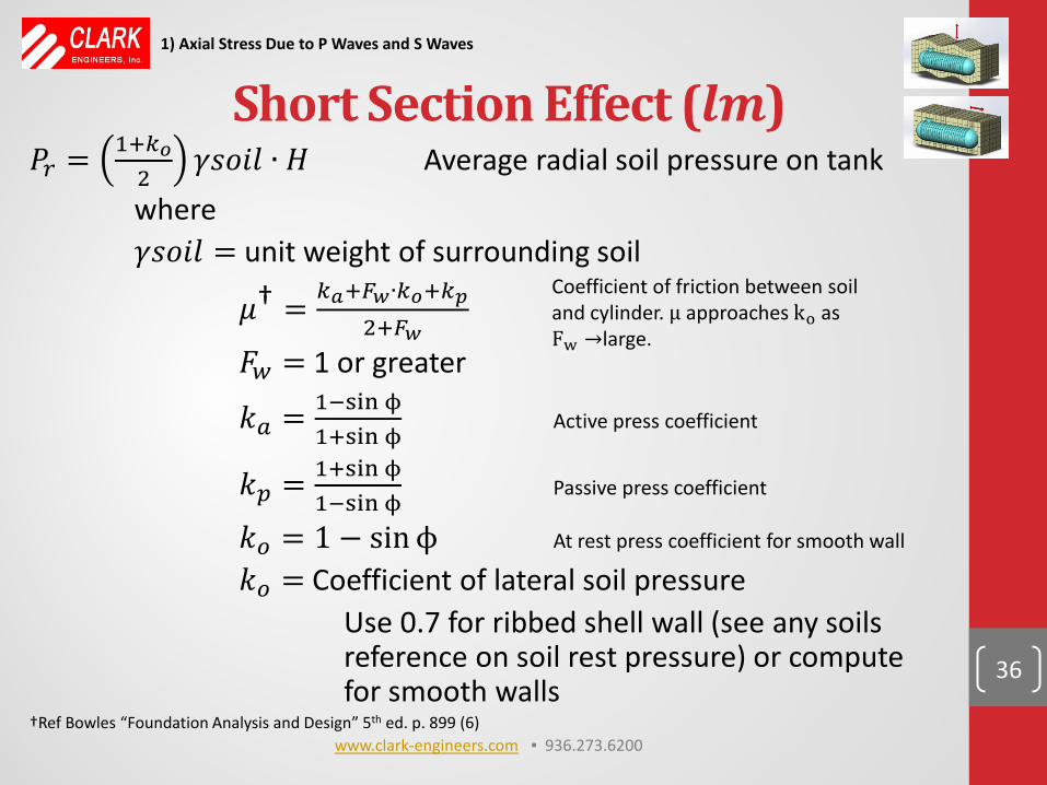
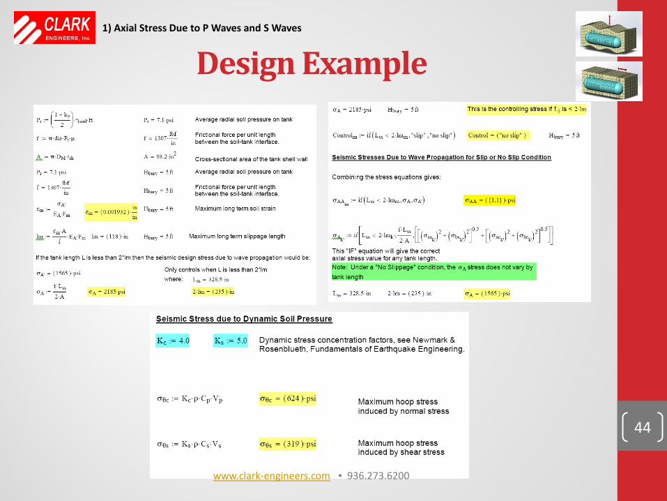
𝑃𝑟 = 1+𝑇𝑐2

𝛾𝛾𝛾𝑑𝑙 ∙ 𝐻 Average radial soil pressure on tank where 𝛾𝛾𝛾𝑑𝑙 = unit weight of surrounding soil

𝜇† = 𝑇𝑎+𝐹𝑤∙𝑇𝑐+𝑇𝑝2+𝐹𝑤

𝐴𝑤 = 1 or greater

𝑘𝑎 = 1−sin ϕ1+sin ϕ

Active press coefficient

𝑘𝑝 = 1+sin ϕ1−sin ϕ

Passive press coefficient

𝑘𝑜 = 1 − sinϕ At rest press coefficient for smooth wall

𝑘𝑜 = Coefficient of lateral soil pressure Use 0.7 for ribbed shell wall (see any soils reference on soil rest pressure) or compute for smooth walls †Ref Bowles “Foundation Analysis and Design” 5th ed. p. 899 (6)

36

Coefficient of friction between soil and cylinder. µ approaches ko as Fw →large.


Short Section Effect (𝒍𝒎)





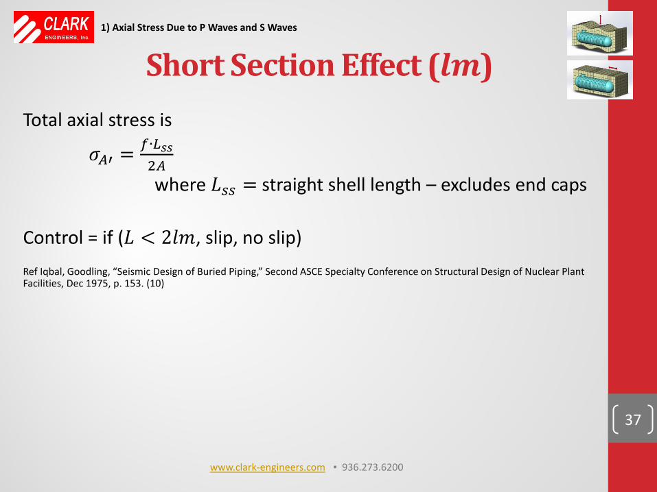
Total axial stress is

𝜎𝐴′ = 𝑓∙𝐷𝑠𝑠2𝐴

where 𝐿𝑠𝑠 = straight shell length – excludes end caps Control = if (𝐿 < 2𝑙𝑙, slip, no slip) Ref Iqbal, Goodling, “Seismic Design of Buried Piping,” Second ASCE Specialty Conference on Structural Design of Nuclear Plant Facilities, Dec 1975, p. 153. (10)

37


Short Section Effect (𝒍𝒎)





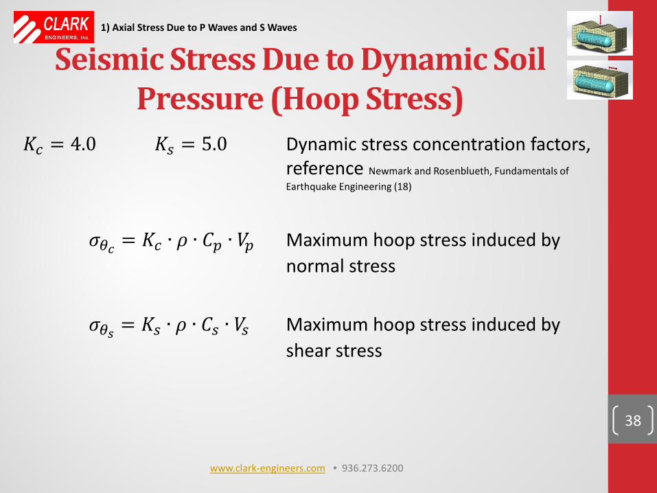
Seismic Stress Due to Dynamic Soil Pressure (Hoop Stress)

𝐾𝑐 = 4.0 𝐾𝑠 = 5.0 Dynamic stress concentration factors, reference Newmark and Rosenblueth, Fundamentals of Earthquake Engineering (18)

𝜎𝜃𝑠 = 𝐾𝑐 ∙ 𝜌 ∙ 𝐶𝑝 ∙ 𝑉𝑝 Maximum hoop stress induced by normal stress 𝜎𝜃𝑠 = 𝐾𝑠 ∙ 𝜌 ∙ 𝐶𝑠 ∙ 𝑉𝑠 Maximum hoop stress induced by shear stress

38






39



Long and Short Period Regions for 𝑻𝑫




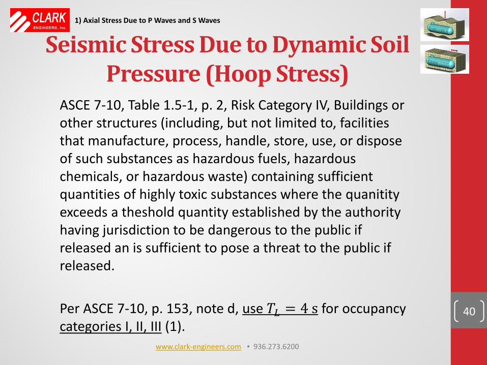
Seismic Stress Due to Dynamic Soil Pressure (Hoop Stress)

ASCE 7-10, Table 1.5-1, p. 2, Risk Category IV, Buildings or other structures (including, but not limited to, facilities that manufacture, process, handle, store, use, or dispose of such substances as hazardous fuels, hazardous chemicals, or hazardous waste) containing sufficient quantities of highly toxic substances where the quanitity exceeds a theshold quantity established by the authority having jurisdiction to be dangerous to the public if released an is sufficient to pose a threat to the public if released. Per ASCE 7-10, p. 153, note d, use 𝑇𝐷 = 4 s for occupancy categories I, II, III (1).

40






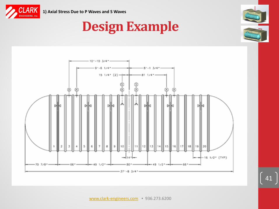
Design Example

41






Design Example

42






Design Example

43






Design Example

44






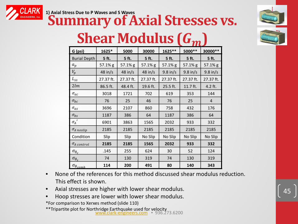
• None of the references for this method discussed shear modulus reduction. This effect is shown. • Axial stresses are higher with lower shear modulus. • Hoop stresses are lower with lower shear modulus. *For comparison to Xerxes method (slide 110) **Tripartite plot for Northridge Earthquake used for velocity

Summary of Axial Stresses vs. Shear Modulus (𝑮𝒎)

45


G (psi) 1625* 5000 30000 1625** 5000** 30000** Burial Depth 5 ft. 5 ft. 5 ft. 5 ft. 5 ft. 5 ft. 𝑎𝑝 57.1% g 57.1% g 57.1% g 57.1% g 57.1% g 57.1% g 𝑉𝑝 48 in/s 48 in/s 48 in/s 9.8 in/s 9.8 in/s 9.8 in/s 𝐿𝑠𝑠 27.37 ft. 27.37 ft. 27.37 ft. 27.37 ft. 27.37 ft. 27.37 ft. 2𝑙𝑙 86.5 ft. 48.4 ft. 19.6 ft. 25.5 ft. 11.7 ft. 4.2 ft. 𝜎𝑎𝑐 3018 1721 702 619 353 144 𝜎𝑐𝑐 76 25 46 76 25 4 𝜎𝑎𝑠 3696 2107 860 758 432 176 𝜎𝑐𝑠 1187 386 64 1187 386 64 𝜎𝐴𝐹 6901 3863 1565 2032 933 332 𝜎𝐴 𝑛𝑜𝑠𝑛𝑛𝑝 2185 2185 2185 2185 2185 2185 Condition Slip Slip No Slip No Slip No Slip No Slip 𝜎𝐴 𝑐𝑜𝑛𝑓𝑟𝑜𝑛 2185 2185 1565 2032 933 332 𝜎𝜃𝑠 .145 255 624 30 52 124 𝜎𝜃𝑠 74 130 319 74 130 319 𝜎𝜃𝑠𝑐𝑐𝑐 114 200 491 80 140 343





0) Historical background, some seismic information, shear modulus, and seismic spectra 1) Axial stress due to P waves and S waves

2) Wang (23) method (NCHRP) (4) transverse loads on circular conduits and box culverts

3) Xerxes (20) patent (reduced shear modulus) with transverse loads on FRP UST’s

4) Sloshing 5) Liquefaction 6) Buckling of soil surrounded tubes

46





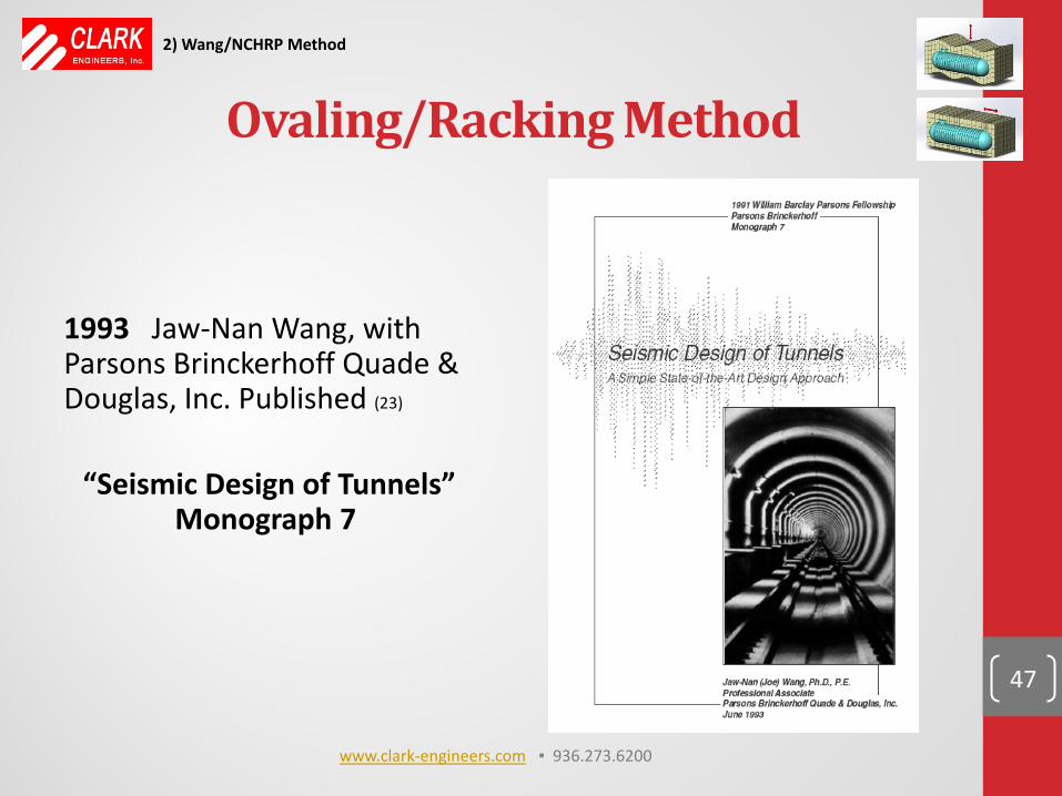
Ovaling/Racking Method 1993 Jaw-Nan Wang, with Parsons Brinckerhoff Quade & Douglas, Inc. Published (23)

“Seismic Design of Tunnels”

Monograph 7

47

2) Wang/NCHRP Method





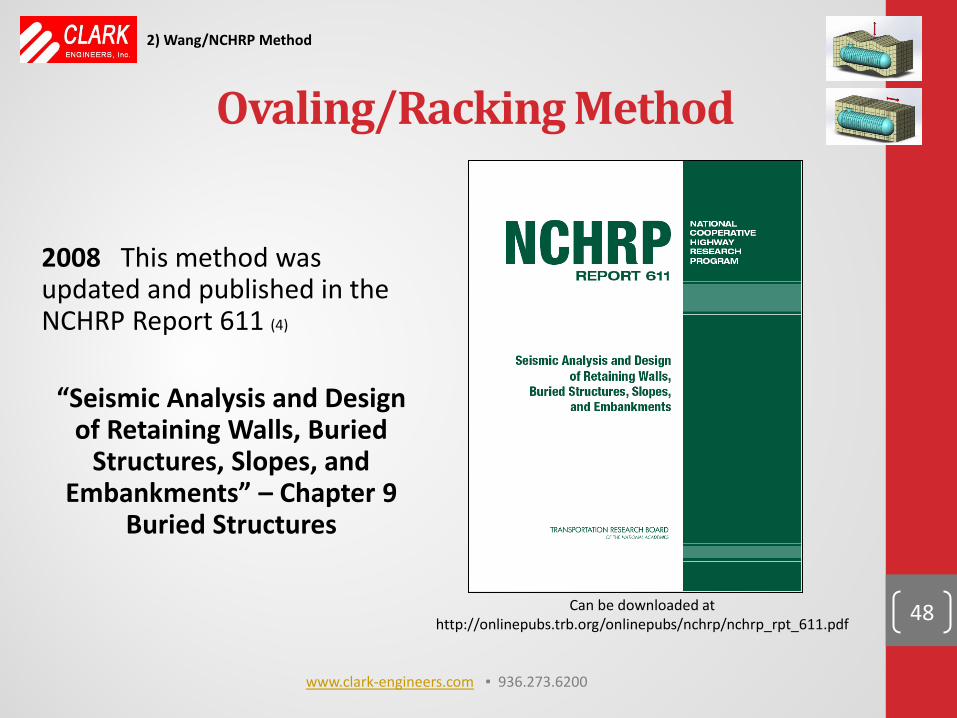
Ovaling/Racking Method 2008 This method was updated and published in the NCHRP Report 611 (4)

“Seismic Analysis and Design

of Retaining Walls, Buried Structures, Slopes, and

Embankments” – Chapter 9 Buried Structures

Can be downloaded at http://onlinepubs.trb.org/onlinepubs/nchrp/nchrp_rpt_611.pdf 48






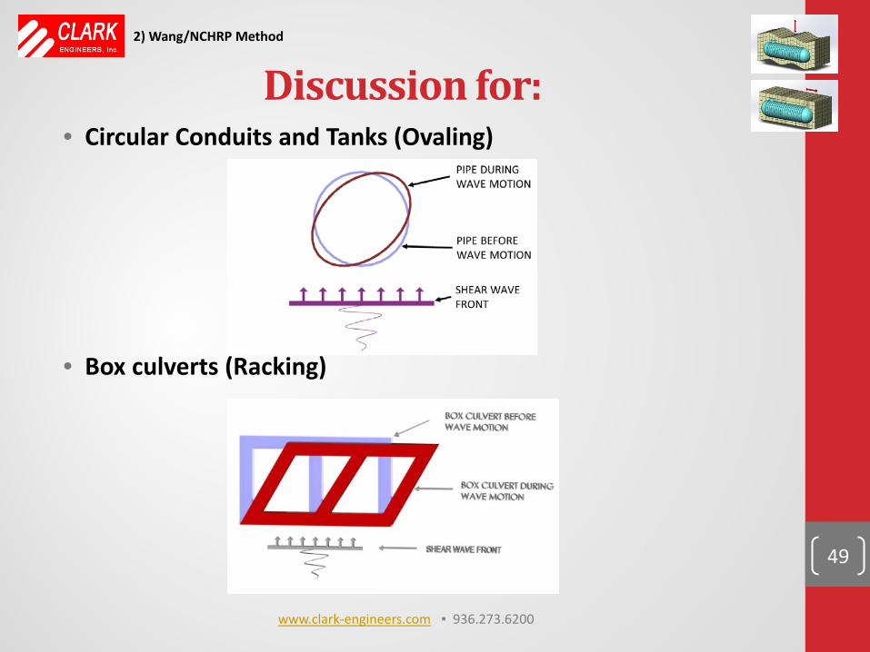
Discussion for:

49

• Circular Conduits and Tanks (Ovaling)

• Box culverts (Racking)






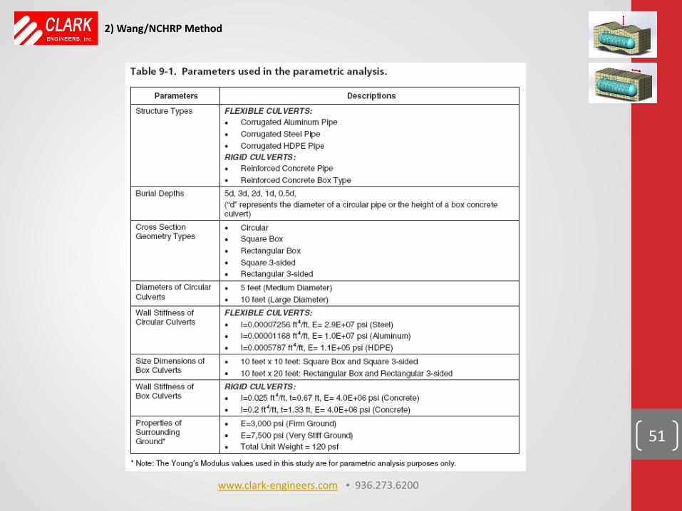
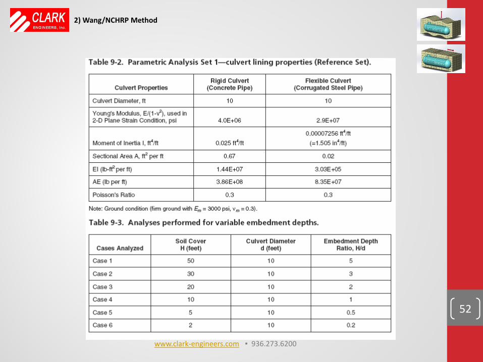
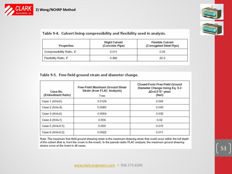
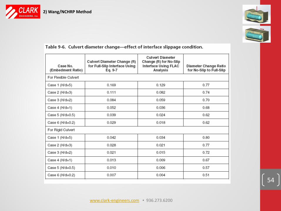
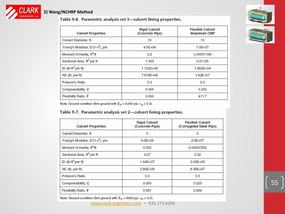
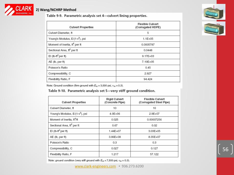
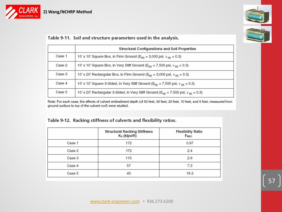
Chapter 9 of Report 611 documents FEA and finite difference studies done on a wide range of soil/structure stiffness ratios and provides “closed form” solutions based on these studies with comparisons to computer results. Wang found that transverse stress were most important for softer soils with caveat that longitudinal stresses can occur with “stiff backfill” e.g. pea gravel or crushed stone as is used in FRP UST’s. It is now recognized that confining pressure can decrease with increasing dynamic strain. This is addressed farther on herein. The following tables show the range of studies done by Wang.

50


NCHRP Report 611, Chapter 9





51






52






53






54






55






56






57






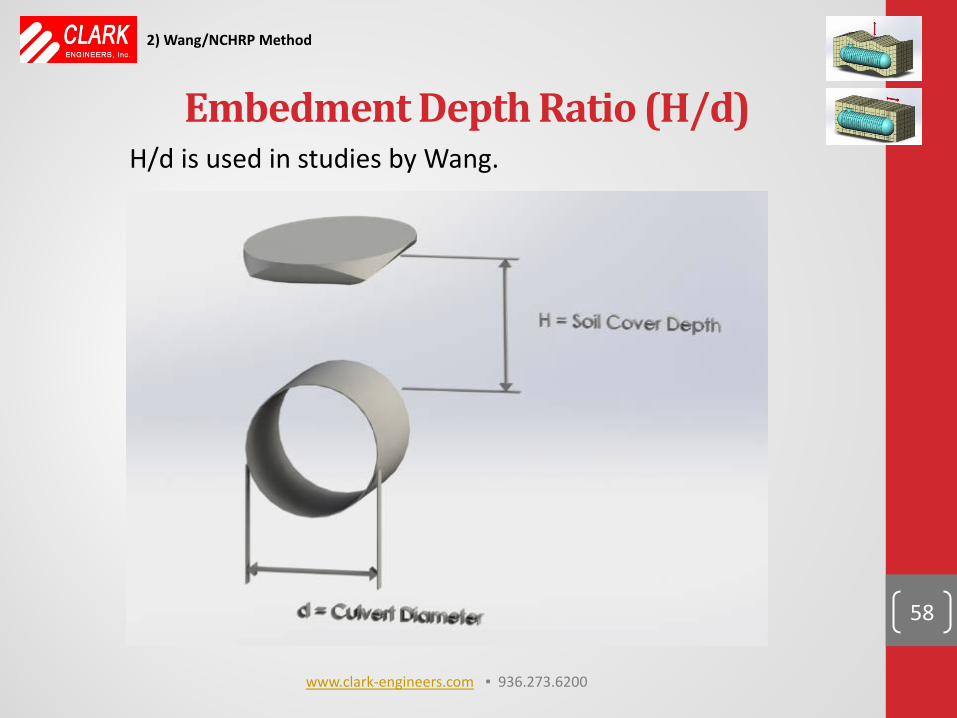
Embedment Depth Ratio (H/d)

58


H/d is used in studies by Wang.





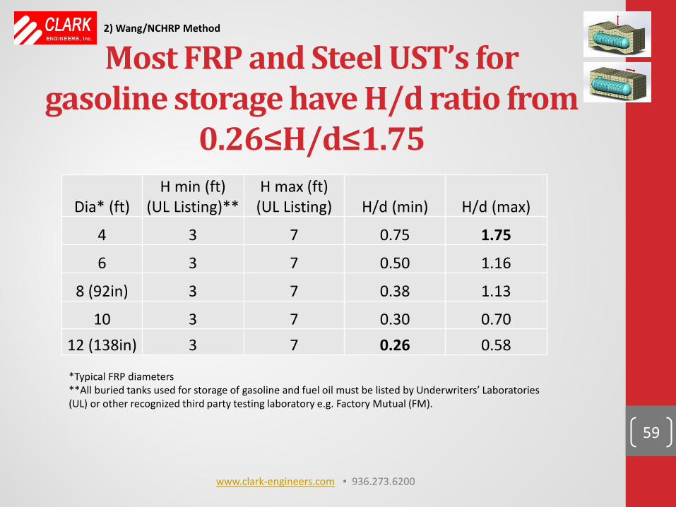
Most FRP and Steel UST’s for gasoline storage have H/d ratio from

0.26≤H/d≤1.75

Dia* (ft) H min (ft)

(UL Listing)** H max (ft)

(UL Listing) H/d (min) H/d (max)

4 3 7 0.75 1.75

6 3 7 0.50 1.16

8 (92in) 3 7 0.38 1.13

10 3 7 0.30 0.70 12 (138in) 3 7 0.26 0.58

59

*Typical FRP diameters **All buried tanks used for storage of gasoline and fuel oil must be listed by Underwriters’ Laboratories (UL) or other recognized third party testing laboratory e.g. Factory Mutual (FM).






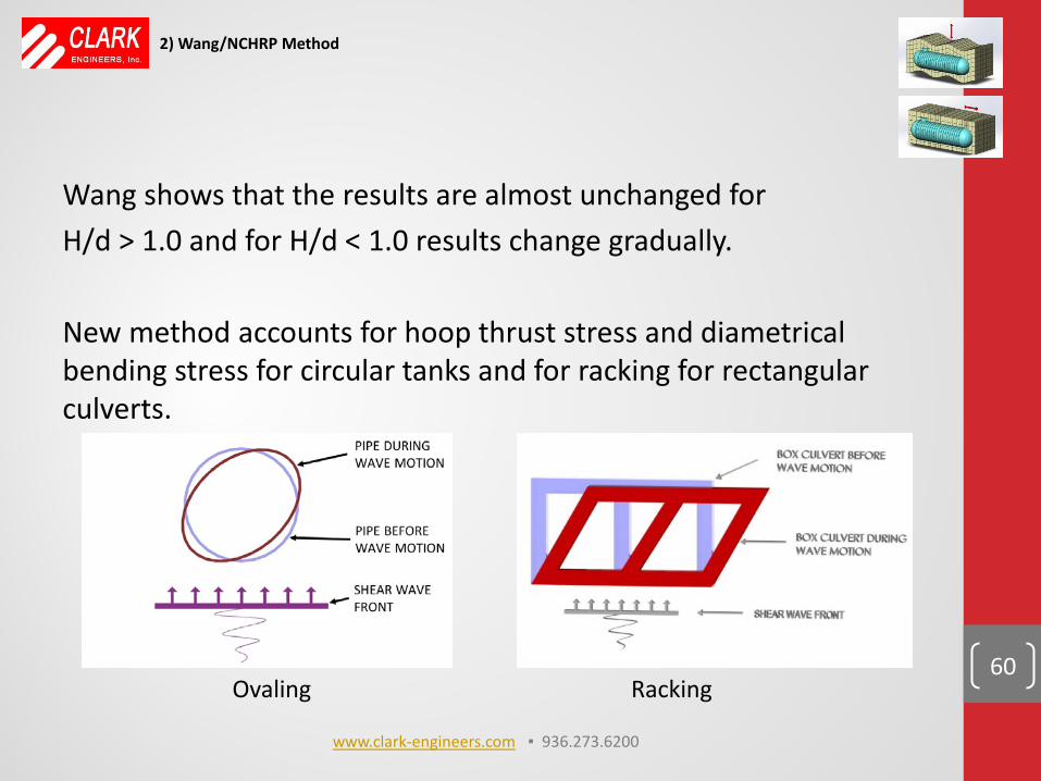
Wang shows that the results are almost unchanged for H/d > 1.0 and for H/d < 1.0 results change gradually. New method accounts for hoop thrust stress and diametrical bending stress for circular tanks and for racking for rectangular culverts.

60 Ovaling Racking






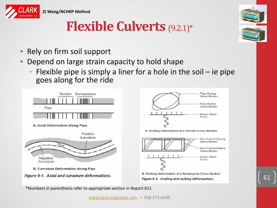
Flexible Culverts (9.2.1)*

• Rely on firm soil support • Depend on large strain capacity to hold shape

• Flexible pipe is simply a liner for a hole in the soil – ie pipe goes along for the ride

61


*Numbers in parenthesis refer to appropriate section in Report 611





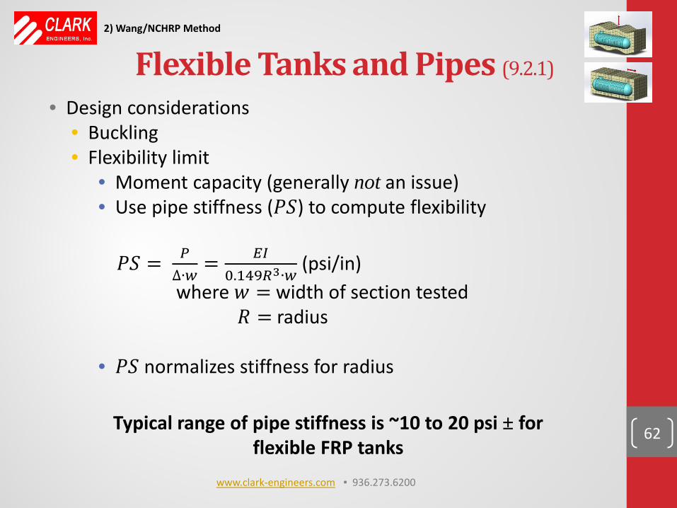
Flexible Tanks and Pipes (9.2.1)

• Design considerations • Buckling • Flexibility limit

• Moment capacity (generally not an issue) • Use pipe stiffness (𝑃𝑆) to compute flexibility 𝑃𝑆 = 𝑃

∆∙𝑤= 𝐸𝐸

0.149𝑅3∙𝑤 (psi/in)

where 𝑤 = width of section tested 𝑅 = radius • 𝑃𝑆 normalizes stiffness for radius

62 Typical range of pipe stiffness is ~10 to 20 psi ± for flexible FRP tanks






Two Main Factors

1) Bending moment and hoop thrust evaluation • Bending demand can be high

2) Soil support is critical for flexible pipe • Can be lost due to liquefaction or other permanent

ground failure mechanisms (see discussion starting on slide 121)

63






General Effects of Earthquakes and Potential “New” Failure Models

Ground Shaking (9.3.1) (See slides 8 and 9 for videos of wave types) • Two different types of waves with two sub types • Body Waves – within Earth’s crust

• Longitudinal compressional: (P) Push waves • Transverse and shear: (S) Shake waves • Travel in any direction

64






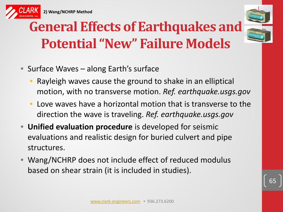
• Surface Waves – along Earth’s surface

• Rayleigh waves cause the ground to shake in an elliptical motion, with no transverse motion. Ref. earthquake.usgs.gov

• Love waves have a horizontal motion that is transverse to the direction the wave is traveling. Ref. earthquake.usgs.gov

• Unified evaluation procedure is developed for seismic evaluations and realistic design for buried culvert and pipe structures.

• Wang/NCHRP does not include effect of reduced modulus based on shear strain (it is included in studies). 65


General Effects of Earthquakes and Potential “New” Failure Models





Rigid Culverts and Pipes • Strain capacity much lower • Not as dependent on soil support as flexible culverts • Must apply soil pressure, active pressure, surcharge pressure,

etc. to obtain total stress condition

66






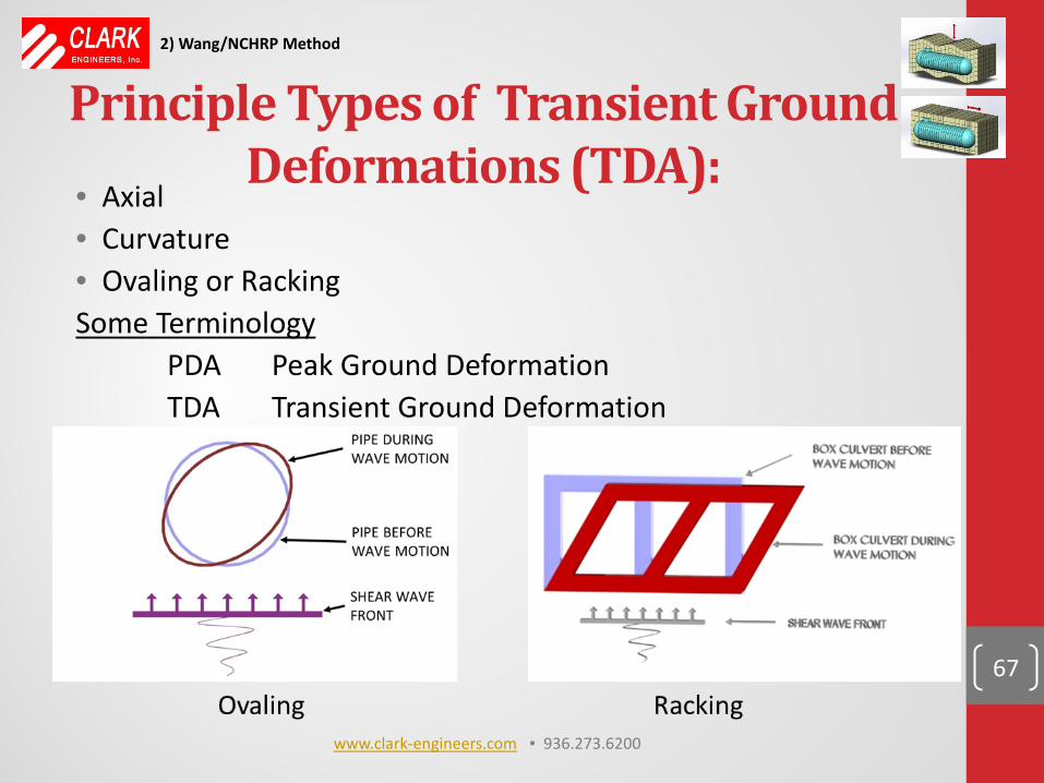
Principle Types of Transient Ground

Deformations (TDA): • Axial • Curvature • Ovaling or Racking Some Terminology PDA Peak Ground Deformation TDA Transient Ground Deformation

67






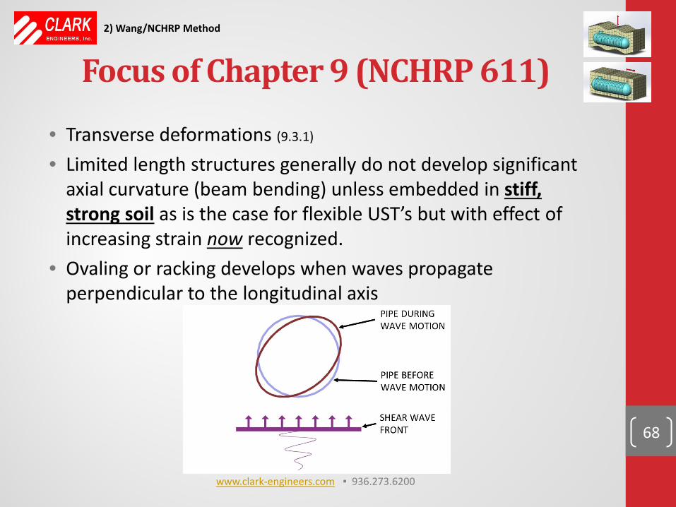
Focus of Chapter 9 (NCHRP 611)

• Transverse deformations (9.3.1)

• Limited length structures generally do not develop significant axial curvature (beam bending) unless embedded in stiff, strong soil as is the case for flexible UST’s but with effect of increasing strain now recognized.

• Ovaling or racking develops when waves propagate perpendicular to the longitudinal axis

68






Vertically propagating shear wave is predominant form of earthquake loading governing ovaling/racking 1) Horizontal component is most severe except for very near

source 2) Vertical ground strains are generally much smaller than shear

strain because shear modulus is lower than constrained modulus

3) Amplification of vertically propagating shear wave is much higher in soft weak soil

Evaluated using under two-dimensional plain strain condition per K. Ishihara

69

Focus of Chapter 9 (NCHRP 611) 2) Wang/NCHRP Method





Ground Failure Modes (Ground Instability)

• Faulting • Landslides • Liquefaction (more on slide 121)

⁻ Induced lateral spread ⁻ Settlement ⁻ Floatation, etc.

• Tectonic uplift and subsidence • Can cause permanent deformations

70






Permanent Deformation • Can be catastrophic to a culvert or pipeline • Usually localized • Typically requires ground improvement

Therefore: Avoid possible ground failure situations or provide an easy means for repair if unavoidable.

71






General Methodology Recommended procedures for ovaling and racking analysis and design. Ovaling

• Change in diameter ∆𝐷= ∆𝐷

• Buckling is key failure mode for flexible conduits • For rigid conduits, thrust and moment are important

72






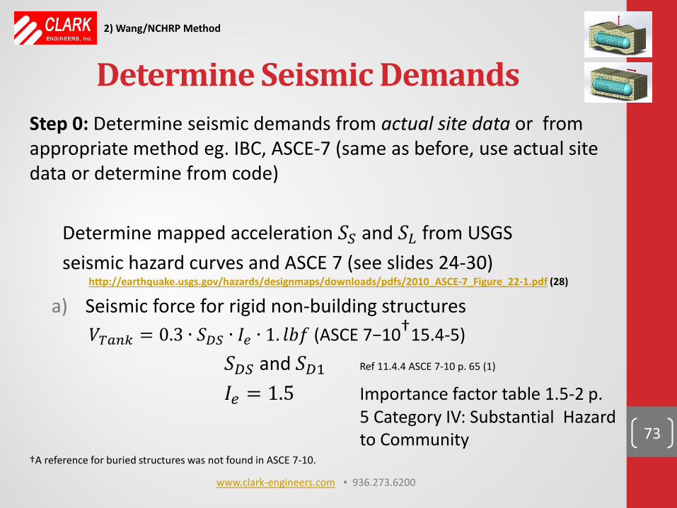
Determine Seismic Demands Step 0: Determine seismic demands from actual site data or from appropriate method eg. IBC, ASCE-7 (same as before, use actual site data or determine from code) Determine mapped acceleration 𝑆𝑆 and 𝑆𝐷 from USGS seismic hazard curves and ASCE 7 (see slides 24-30) http://earthquake.usgs.gov/hazards/designmaps/downloads/pdfs/2010_ASCE-7_Figure_22-1.pdf (28)

a) Seismic force for rigid non-building structures 𝑉𝑇𝑎𝑛𝑇 = 0.3 ∙ 𝑆𝐷𝑆 ∙ 𝐼𝑒 ∙ 1. 𝑙𝑙𝑙 (ASCE 7−10†15.4-5)

𝑆𝐷𝑆 and 𝑆𝐷1 Ref 11.4.4 ASCE 7-10 p. 65 (1)

𝐼𝑒 = 1.5 Importance factor table 1.5-2 p. 5 Category IV: Substantial Hazard to Community †A reference for buried structures was not found in ASCE 7-10.

73







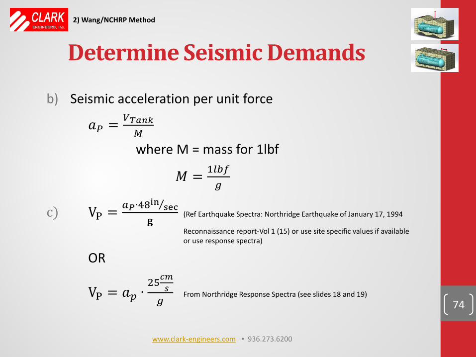
b) Seismic acceleration per unit force

𝑎𝑃 = 𝑉𝑇𝑎𝑖𝑇𝑀

where M = mass for 1lbf

𝑀 = 1𝑛𝑐𝑓𝑔

c) VP = 𝑎𝑃∙48in sec⁄𝐠

(Ref Earthquake Spectra: Northridge Earthquake of January 17, 1994

Reconnaissance report-Vol 1 (15) or use site specific values if available or use response spectra)

OR

VP = 𝑎𝑝 ∙25𝑠𝑐𝑠𝑔

From Northridge Response Spectra (see slides 18 and 19) 74

Determine Seismic Demands 2) Wang/NCHRP Method





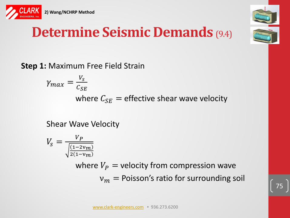
Determine Seismic Demands (9.4)

Step 1: Maximum Free Field Strain

𝛾𝑐𝑎𝑚 = 𝑉𝑠𝐶𝑆𝑆

where 𝐶𝑆𝐸 = effective shear wave velocity Shear Wave Velocity

𝑉𝑠 = 𝑉𝑃1−2ν𝑐2 1−ν𝑐

where 𝑉𝑃 = velocity from compression wave ν𝑐 = Poisson’s ratio for surrounding soil

75






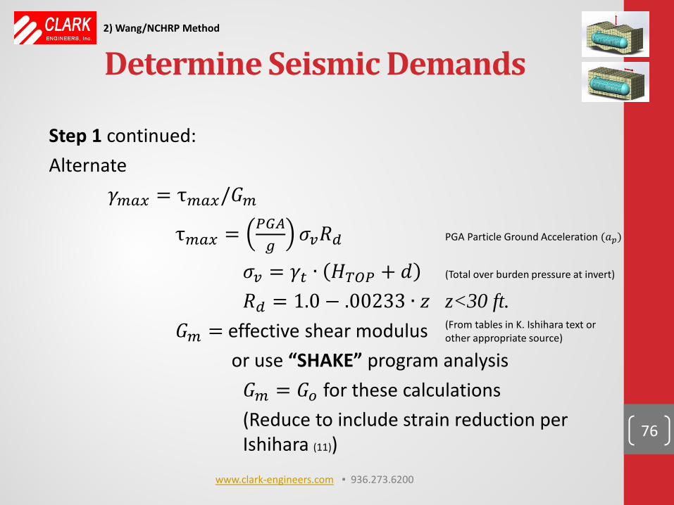
Determine Seismic Demands Step 1 continued: Alternate 𝛾𝑐𝑎𝑚 = τ𝑐𝑎𝑚/𝐺𝑐

τ𝑐𝑎𝑚 = 𝑃𝐺𝐴𝑔

𝜎𝑣𝑅𝑑 PGA Particle Ground Acceleration (𝑎𝑝)

𝜎𝑣 = 𝛾𝑓 ∙ 𝐻𝑇𝑇𝑃 + 𝑑 (Total over burden pressure at invert)

𝑅𝑑 = 1.0 − .00233 ∙ 𝑧 z<30 ft. 𝐺𝑐 = effective shear modulus or use “SHAKE” program analysis 𝐺𝑐 = 𝐺𝑜 for these calculations (Reduce to include strain reduction per Ishihara (11))

76


(From tables in K. Ishihara text or other appropriate source)





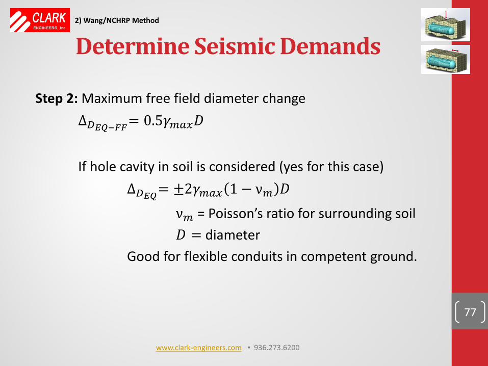
Determine Seismic Demands Step 2: Maximum free field diameter change ∆𝐷𝑆𝐸−𝐹𝐹= 0.5𝛾𝑐𝑎𝑚𝐷

If hole cavity in soil is considered (yes for this case) ∆𝐷𝑆𝐸= ±2𝛾𝑐𝑎𝑚 1 − ν𝑐 𝐷

ν𝑐 = Poisson’s ratio for surrounding soil 𝐷 = diameter Good for flexible conduits in competent ground.

77






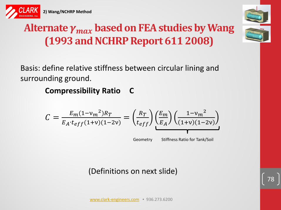
Alternate 𝜸𝒎𝒂𝒎 based on FEA studies by Wang

(1993 and NCHRP Report 611 2008)

Basis: define relative stiffness between circular lining and surrounding ground. Compressibility Ratio C

𝐶 = 𝐸𝑐(1−ν𝑐2)𝑅𝑇 𝐸𝐴∙𝑓𝑠𝑓𝑓(1+ν)(1−2ν)

= 𝑅𝑇𝑓𝑠𝑓𝑓

𝐸𝑐𝐸𝐴

1−ν𝑐2

1+ν 1−2ν

(Definitions on next slide)

78


Stiffness Ratio for Tank/Soil Geometry





Alternate 𝜸𝒎𝒂𝒎 based on FEA studies by Wang

(1993 and NCHRP Report 611 2008)

Flexibility Ratio F

𝐴 = 𝐸𝑐(1−ν𝑐2)𝑅𝑇3 6𝐸𝐸 (1+ν)

= 2𝑅𝑇3

𝑓𝑠𝑓𝑓3𝐸𝑐𝐸

1−ν𝑐2

1+ν

where EI = flexural rigidity of pipe/tank ν = Poisson’s ratio of pipe/tank 𝐸𝑐: strain compatible elastic modulus of surrounding soil (soil report or estimate from available literature) e.g. K. Ishihara, etc. (11)

ν𝑐 = Poisson’s ratio of surrounding soil 𝑅𝑇 = tank or pipe radius Rigid Ring F<1 Flexible Ring F>1

79


Stiffness Ratio for Tank/Soil Geometry





80

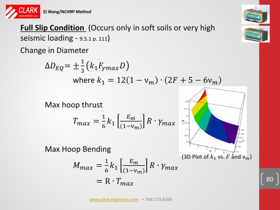
Full Slip Condition (Occurs only in soft soils or very high seismic loading - 9.5.1 p. 111) Change in Diameter

∆𝐷𝐸𝐸= ± 13𝑘1𝐴𝛾𝑐𝑎𝑚𝐷

where 𝑘1 = 12 1 − ν𝑐 ∙ 2𝐴 + 5 − 6ν𝑐 Max hoop thrust

𝑇𝑐𝑎𝑚 = 16𝑘1

𝐸𝑐(1−ν𝑐)

𝑅 ∙ 𝛾𝑐𝑎𝑚

Max Hoop Bending

𝑀𝑐𝑎𝑚 = 16𝑘1

𝐸𝑐(1−ν𝑐)

𝑅 ∙ 𝛾𝑐𝑎𝑚

= R ∙ 𝑇𝑐𝑎𝑚

(3D Plot of 𝑘1 vs. 𝐴 and ν𝑐)






81

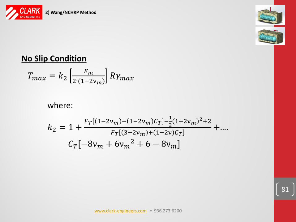
No Slip Condition

𝑇𝑐𝑎𝑚 = 𝑘2𝐸𝑐

2∙(1−2ν𝑐)𝑅𝛾𝑐𝑎𝑚

where:

𝑘2 = 1 +𝐹𝑇 1−2ν𝑐 − 1−2ν𝑐 𝐶𝑇 −12 1−2ν𝑐

2+2

𝐹𝑇 3−2ν𝑐 + 1−2ν 𝐶𝑇+….

𝐶𝑇[−8ν𝑐 + 6ν𝑐2 + 6 − 8ν𝑐]






82

“In most cases the condition at the interface is between slip and no slip,” p. 111. According to Fahimifar and Vakilzadeh in Numerical and Analytical Solutions for Ovaling Deformation in Circular Tunnels Under Seismic Loading (8),

Therefore use full slip method.


“Note that no solution is developed for calculating diametric strain and maximum moment under no-slip condition. It is recommended that the solutions for fullslip condition be used for no-slip condition. The more conservative estimates of the full-slip condition is considered to offset the potential underestimation due to pseudo-static representation of the dynamic problem [1].”





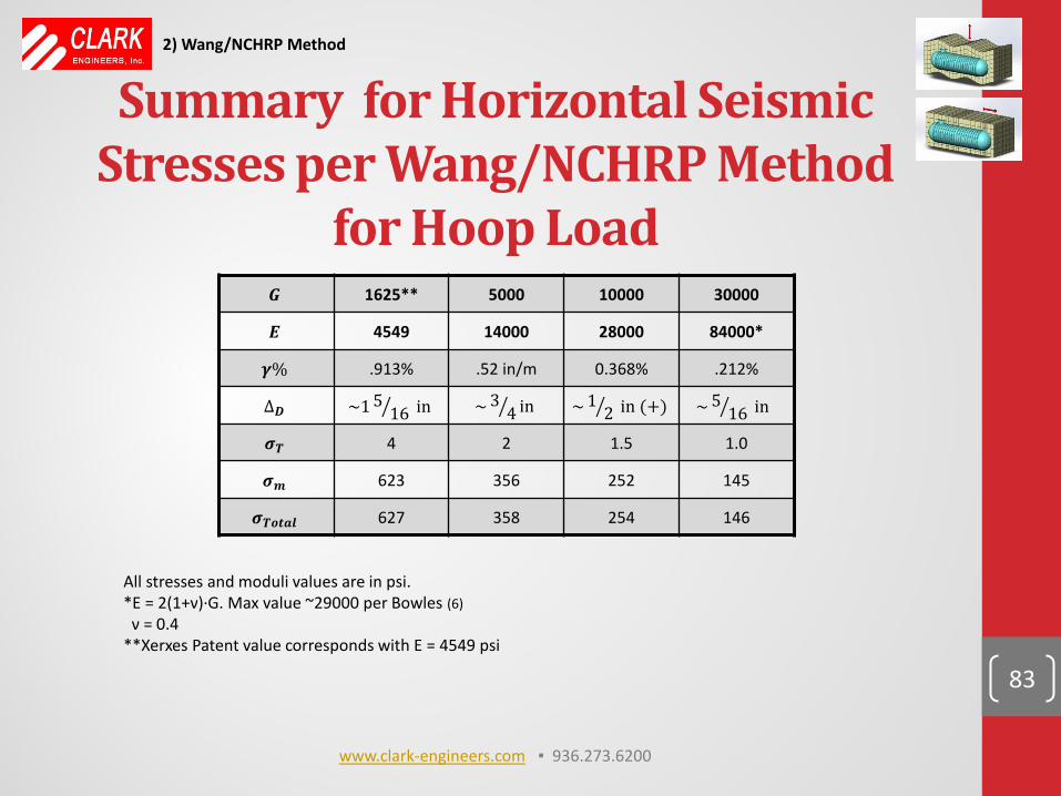
Summary for Horizontal Seismic Stresses per Wang/NCHRP Method

for Hoop Load

83


𝑮 1625** 5000 10000 30000

𝑬 4549 14000 28000 84000*

𝜸𝜸 .913% .52 in/m 0.368% .212%

∆𝑫 ~1 516� in ~ 3

4� in ~ 12� in (+) ~ 5

16� in

𝝈𝑻 4 2 1.5 1.0

𝝈𝒎 623 356 252 145

𝝈𝑻𝒐𝑻𝒂𝒍 627 358 254 146

All stresses and moduli values are in psi. *E = 2(1+ν)∙G. Max value ~29000 per Bowles (6) ν = 0.4 **Xerxes Patent value corresponds with E = 4549 psi





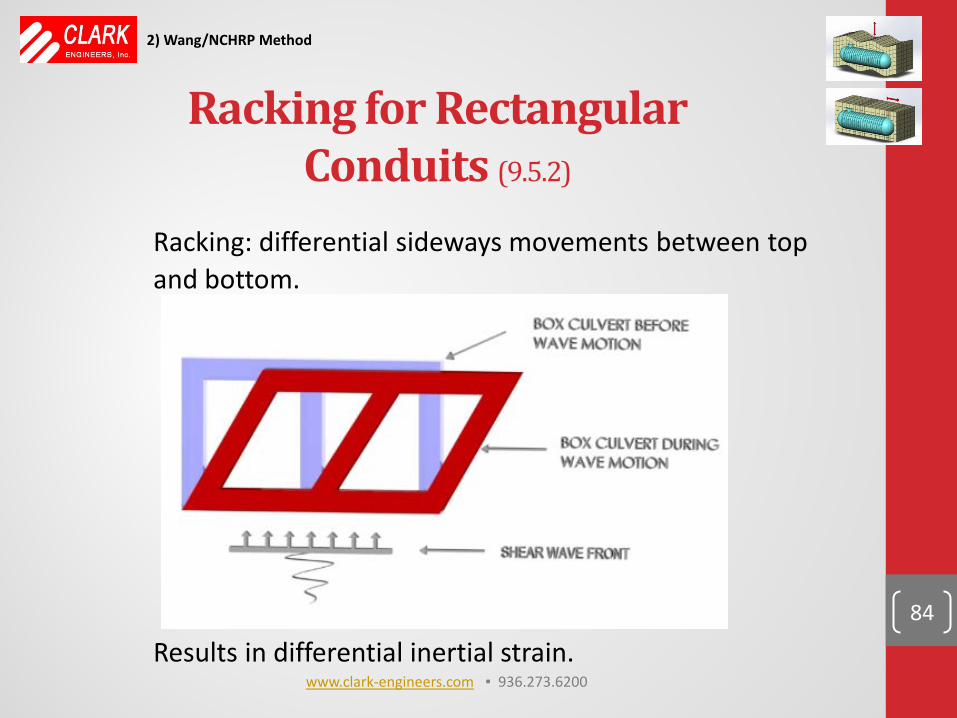
Racking for Rectangular

Conduits (9.5.2)

Racking: differential sideways movements between top and bottom.

Results in differential inertial strain.

84






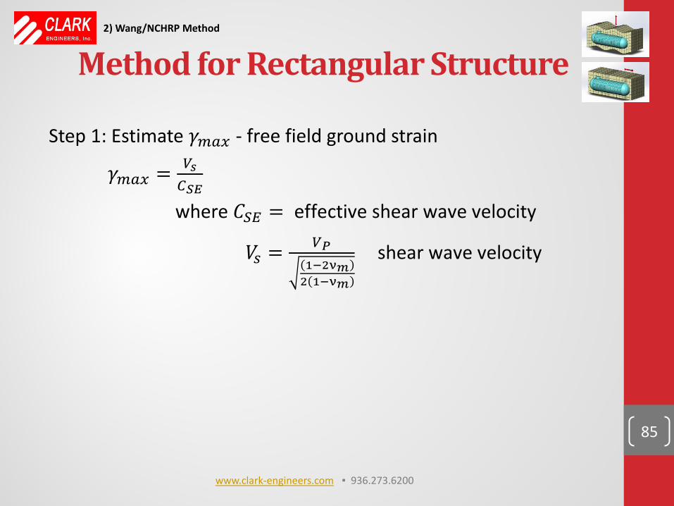
Method for Rectangular Structure Step 1: Estimate 𝛾𝑐𝑎𝑚 - free field ground strain

𝛾𝑐𝑎𝑚 = 𝑉𝑠𝐶𝑆𝑆

where 𝐶𝑆𝐸 = effective shear wave velocity

𝑉𝑠 = 𝑉𝑃1−2ν𝑐2 1−ν𝑐

shear wave velocity

85






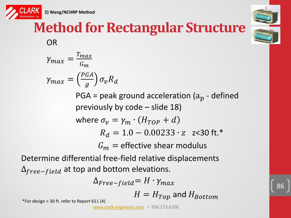
Method for Rectangular Structure OR

𝛾𝑐𝑎𝑚 = 𝑇𝑐𝑎𝑚𝐺𝑐

𝛾𝑐𝑎𝑚 = 𝑃𝐺𝐴𝑔

𝜎𝑣𝑅𝑑

PGA = peak ground acceleration (ap - defined previously by code – slide 18) where 𝜎𝑣 = 𝛾𝑐 ∙ 𝐻𝑇𝑇𝑃 + 𝑑 𝑅𝑑 = 1.0 − 0.00233 ∙ 𝑧 z<30 ft.* 𝐺𝑐 = effective shear modulus Determine differential free-field relative displacements ∆𝑓𝑟𝑒𝑒−𝑓𝑛𝑒𝑛𝑑 at top and bottom elevations.

∆𝐹𝑟𝑒𝑒−𝑓𝑛𝑒𝑛𝑑= 𝐻 ∙ 𝛾𝑐𝑎𝑚 𝐻 = 𝐻𝑇𝑜𝑝 and 𝐻𝐵𝑜𝑓𝑓𝑜𝑐

86


*For design > 30 ft. refer to Report 611 (4) www.clark-engineers.com ▪ 936.273.6200




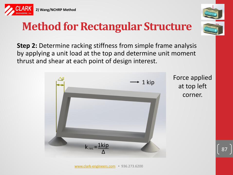
Method for Rectangular Structure Step 2: Determine racking stiffness from simple frame analysis by applying a unit load at the top and determine unit moment thrust and shear at each point of design interest.

87


Force applied at top left

corner.





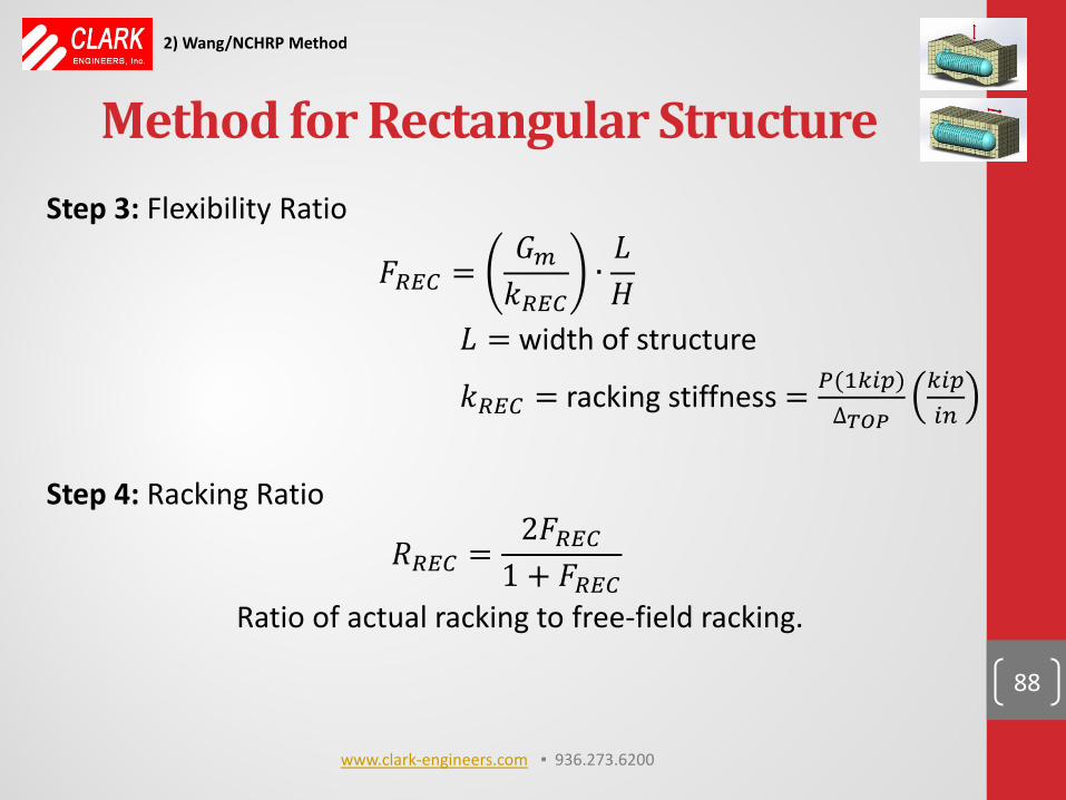
Method for Rectangular Structure Step 3: Flexibility Ratio

𝐴𝑅𝐸𝐶 =𝐺𝑐𝑘𝑅𝐸𝐶

∙𝐿𝐻

𝐿 = width of structure

𝑘𝑅𝐸𝐶 = racking stiffness = 𝑃(1𝑇𝑛𝑝)∆𝑇𝑇𝑃

𝑇𝑛𝑝𝑛𝑛

Step 4: Racking Ratio

𝑅𝑅𝐸𝐶 =2𝐴𝑅𝐸𝐶

1 + 𝐴𝑅𝐸𝐶

Ratio of actual racking to free-field racking.

88






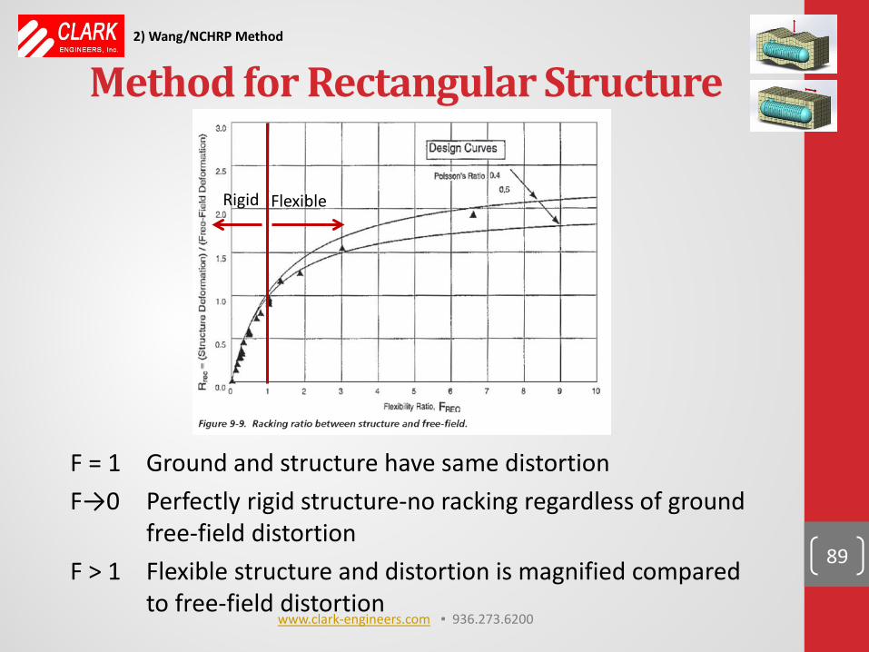
Method for Rectangular Structure

F = 1 Ground and structure have same distortion F→0 Perfectly rigid structure-no racking regardless of ground free-field distortion F > 1 Flexible structure and distortion is magnified compared to free-field distortion

89


Rigid Flexible





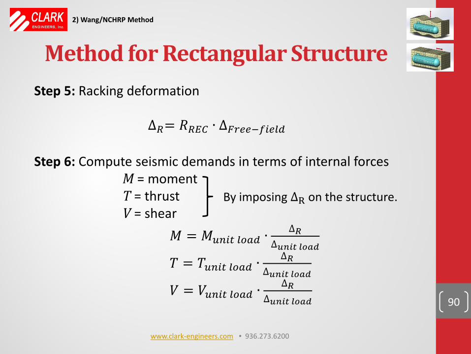
Method for Rectangular Structure Step 5: Racking deformation

∆𝑅= 𝑅𝑅𝐸𝐶 ∙ ∆𝐹𝑟𝑒𝑒−𝑓𝑛𝑒𝑛𝑑 Step 6: Compute seismic demands in terms of internal forces M = moment T = thrust V = shear 𝑀 = 𝑀𝑢𝑛𝑛𝑓 𝑛𝑜𝑎𝑑 ∙

∆𝑅∆𝑢𝑖𝑖𝑙 𝑙𝑐𝑎𝑙

𝑇 = 𝑇𝑢𝑛𝑛𝑓 𝑛𝑜𝑎𝑑 ∙∆𝑅

∆𝑢𝑖𝑖𝑙 𝑙𝑐𝑎𝑙

𝑉 = 𝑉𝑢𝑛𝑛𝑓 𝑛𝑜𝑎𝑑 ∙∆𝑅

∆𝑢𝑖𝑖𝑙 𝑙𝑐𝑎𝑙

90

By imposing ∆R on the structure.






Seismic effects must be added to other load cases to obtain total stress normal load effects Note that Wang/NCHRP method does not discuss sloshing. This must be included in the analysis.

91






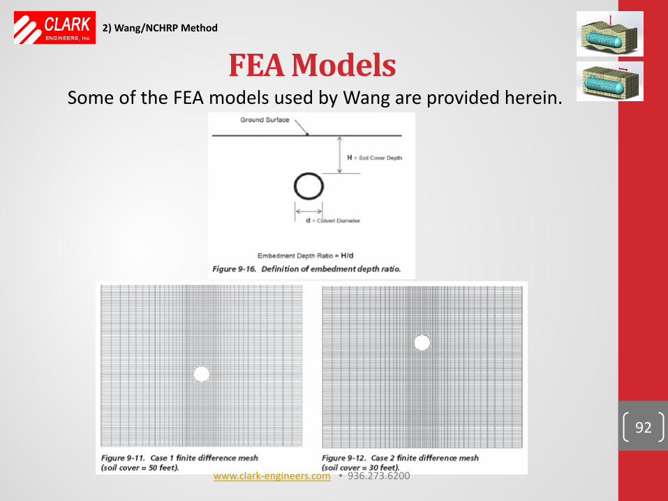
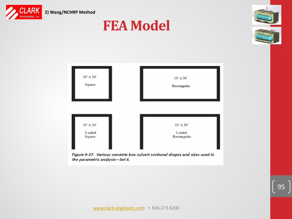
FEA Models

92


Some of the FEA models used by Wang are provided herein.





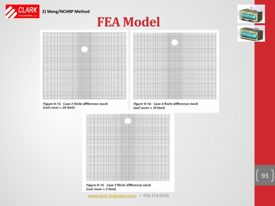
FEA Model

93






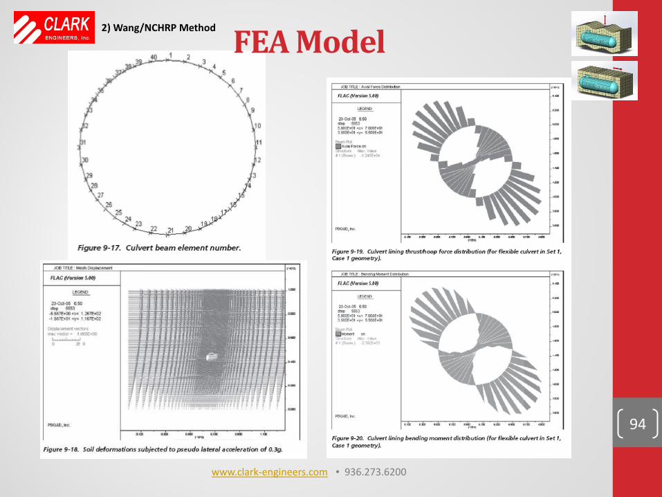
FEA Model

94






FEA Model

95






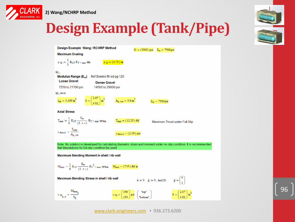
Design Example (Tank/Pipe)

96






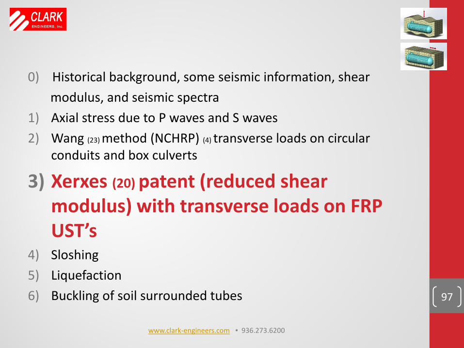
0) Historical background, some seismic information, shear modulus, and seismic spectra 1) Axial stress due to P waves and S waves 2) Wang (23) method (NCHRP) (4) transverse loads on circular

conduits and box culverts

3) Xerxes (20) patent (reduced shear modulus) with transverse loads on FRP UST’s


97





Xerxes Method

Granted Patent Patent No. US 6,397,168 B1 Date of Patent May 28, 2002 Seismic Evaluation Method for Underground Structures. A brief summary of some pertinent points follow.

98

3) Xerxes Method





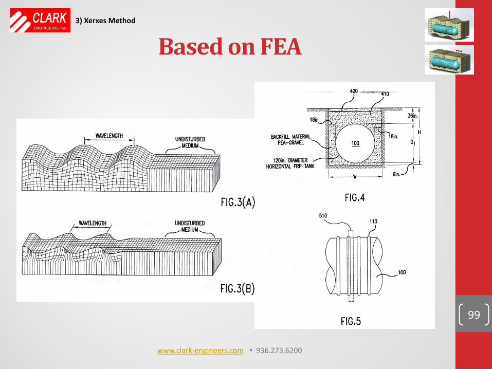
Based on FEA

99

3) Xerxes Method





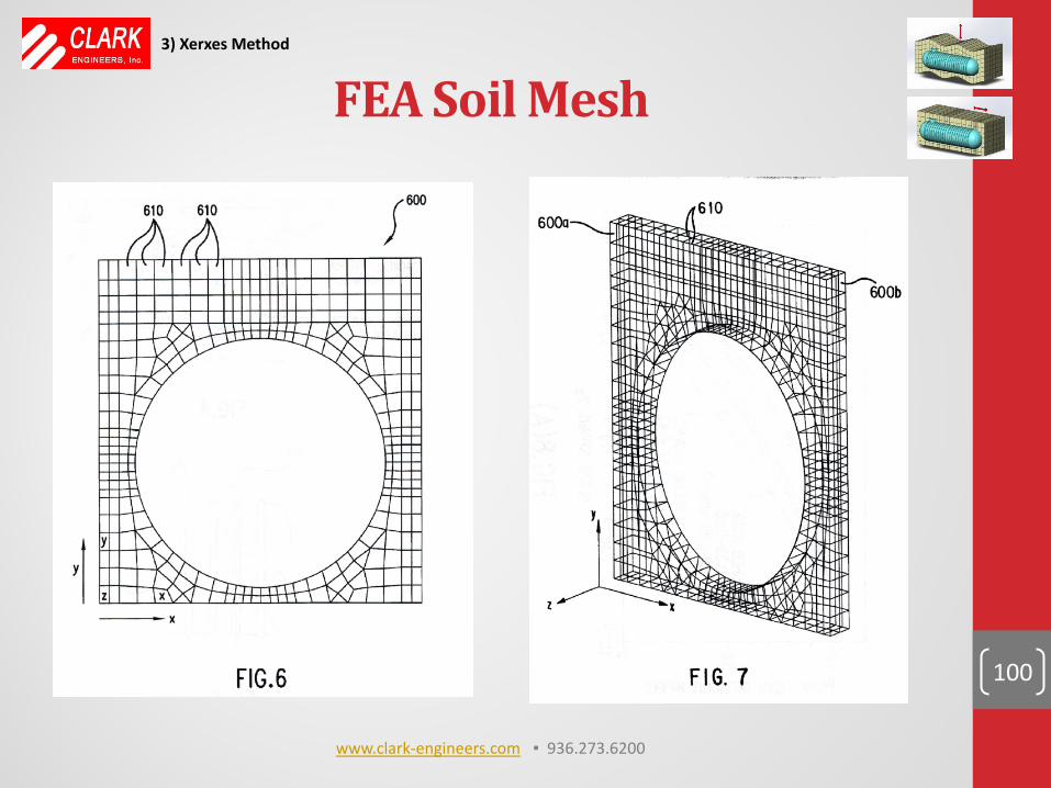
FEA Soil Mesh

100

3) Xerxes Method





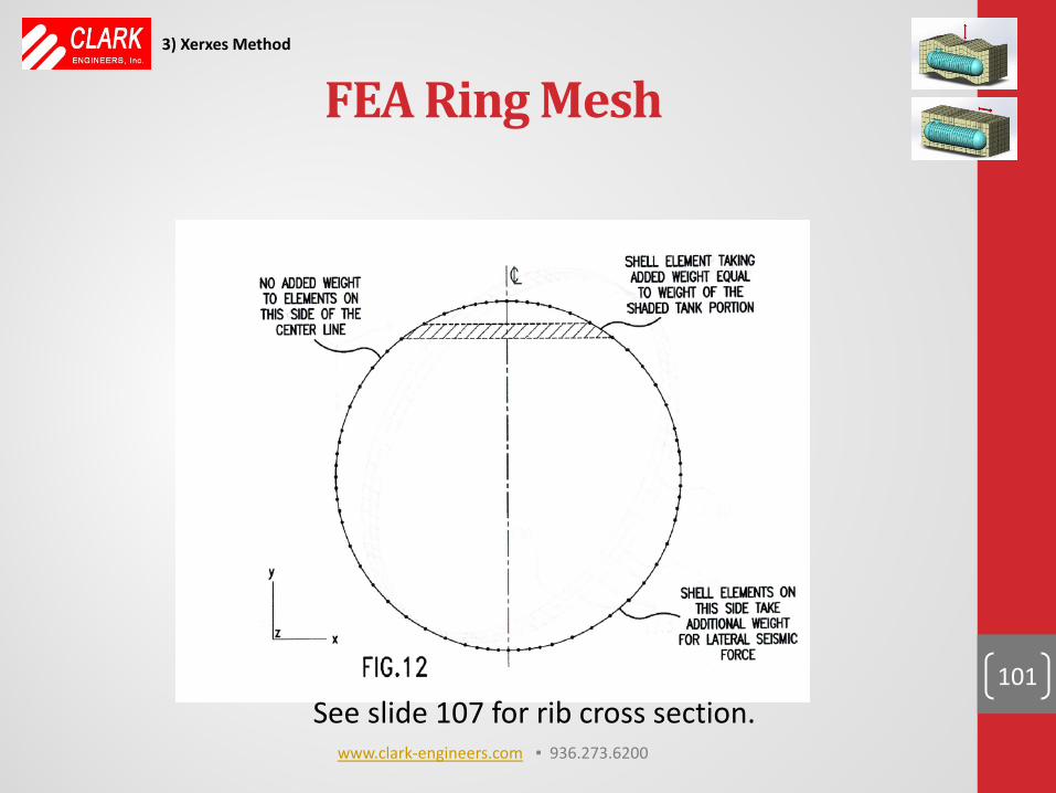
FEA Ring Mesh

101

3) Xerxes Method


See slide 107 for rib cross section.




Xerxes Method

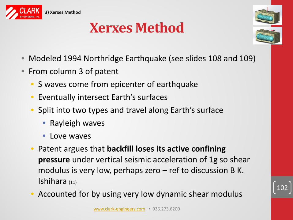
• Modeled 1994 Northridge Earthquake (see slides 108 and 109) • From column 3 of patent

• S waves come from epicenter of earthquake • Eventually intersect Earth’s surfaces • Split into two types and travel along Earth’s surface

• Rayleigh waves • Love waves

• Patent argues that backfill loses its active confining pressure under vertical seismic acceleration of 1g so shear modulus is very low, perhaps zero – ref to discussion B K. Ishihara (11)

• Accounted for by using very low dynamic shear modulus 102

3) Xerxes Method





Xerxes Method

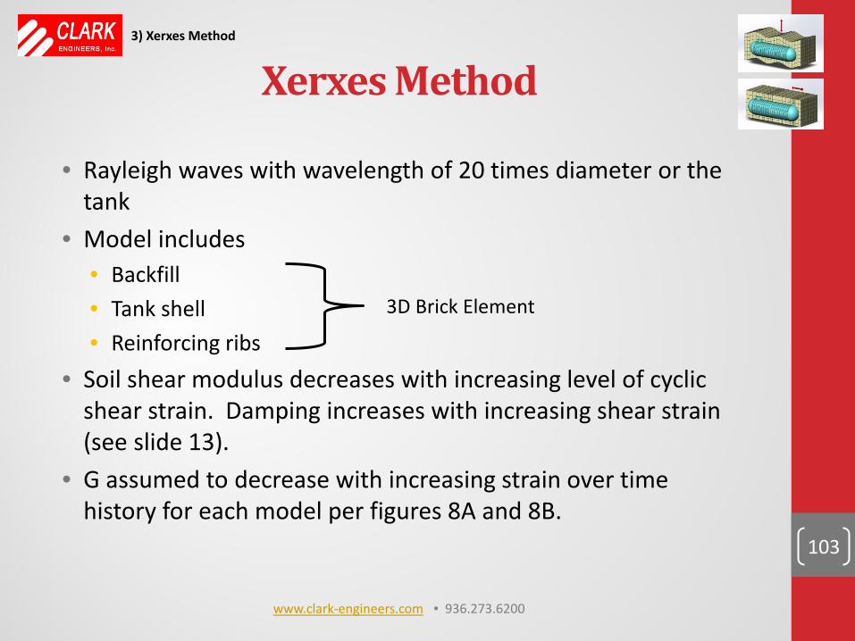
• Rayleigh waves with wavelength of 20 times diameter or the tank

• Model includes • Backfill • Tank shell • Reinforcing ribs

• Soil shear modulus decreases with increasing level of cyclic shear strain. Damping increases with increasing shear strain (see slide 13).

• G assumed to decrease with increasing strain over time history for each model per figures 8A and 8B.

103

3D Brick Element

3) Xerxes Method





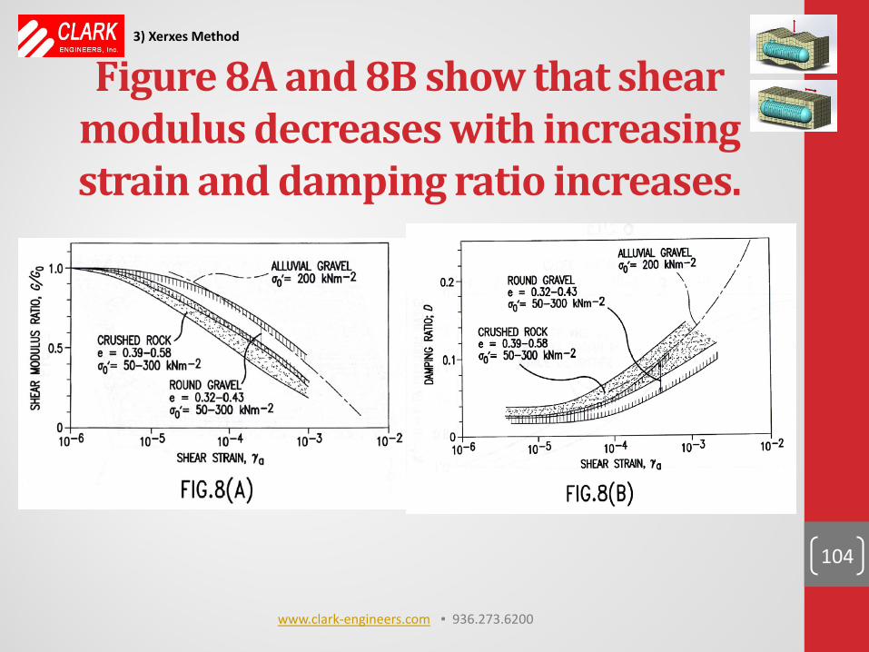
Figure 8A and 8B show that shear modulus decreases with increasing strain and damping ratio increases.

104

3) Xerxes Method





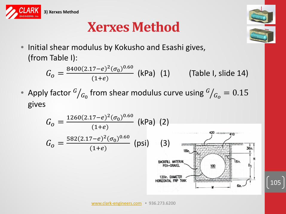
Xerxes Method • Initial shear modulus by Kokusho and Esashi gives,

(from Table I):

𝐺𝑜 = 8400 2.17−𝑒 2 𝜎0 0.60

(1+𝑒) (kPa) (1) (Table I, slide 14)

• Apply factor 𝐺 𝐺0� from shear modulus curve using 𝐺 𝐺𝑐� = 0.15 gives

𝐺𝑜 = 1260 2.17−𝑒 2 𝜎0 0.60

(1+𝑒) (kPa) (2)

𝐺𝑜 = 582 2.17−𝑒 2 𝜎0 0.60

(1+𝑒) (psi) (3)

105

3) Xerxes Method





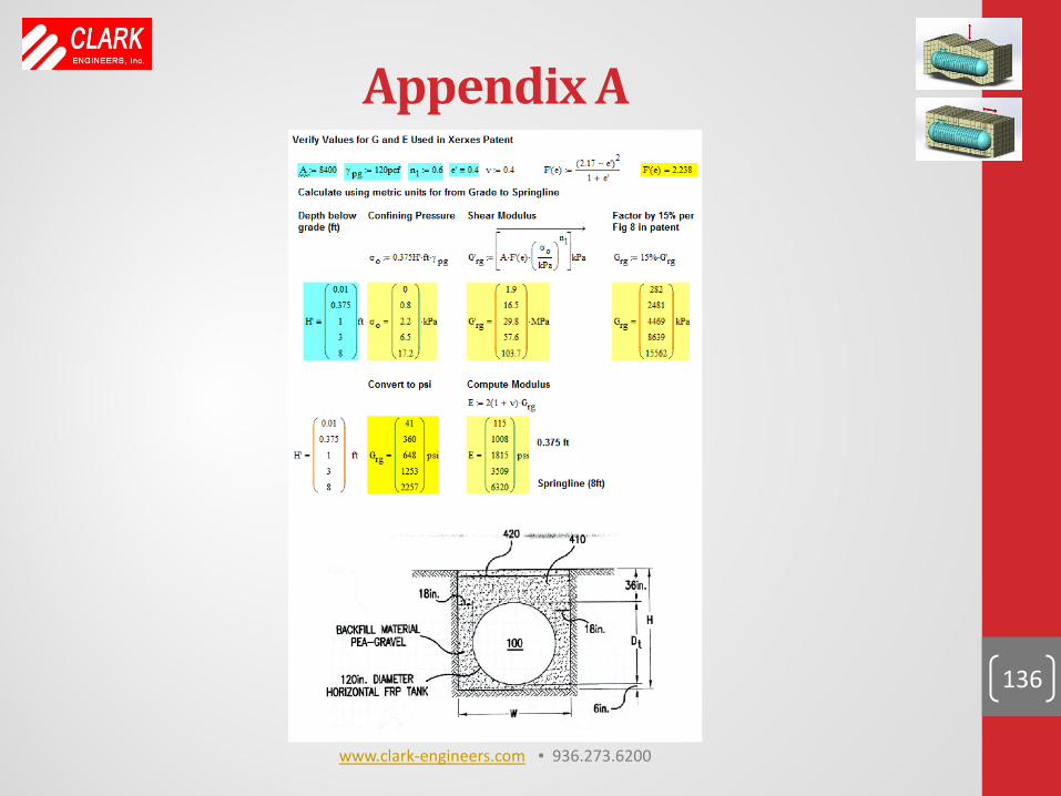
Xerxes Method • Confining pressure is taken as 3 8⁄ 𝛾𝐻 • Void ratio assumed to be 𝑒 = 0.4 and 𝛾𝑠𝑜𝑛𝑛 = 120𝑝𝑐𝑙 • Results in shear modulus varied from top to bottom of 360 psi

to 2257 psi (constant over bottom half)* • Young’s modulus varied similarly from 1008 psi to 6320 psi.* • Tank properties are 𝐸 = 900,000 𝑝𝛾𝑑, 𝜈 = 0.3, 𝛾𝐹𝑅𝑃 = 0.061 𝑝𝑐𝑑 Metric Evaluation *These values confirmed by independent check see Appendix A, slide 136. 106

3) Xerxes Method





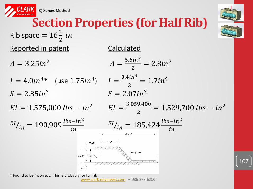
Rib space = 16 12

𝑑𝑖

Reported in patent Calculated

𝐴 = 3.25𝑑𝑖2 𝐴 = 5.6𝑛𝑛2

2= 2.8𝑑𝑖2

𝐼 = 4.0𝑑𝑖4* (use 1.75𝑑𝑖4) 𝐼 = 3.4𝑛𝑛4

2= 1.7𝑑𝑖4

𝑆 = 2.35𝑑𝑖3 𝑆 = 2.07𝑑𝑖3

𝐸𝐼 = 1,575,000 𝑙𝑙𝛾 − 𝑑𝑖2 𝐸𝐼 = 3,059,4002

= 1,529,700 𝑙𝑙𝛾 − 𝑑𝑖2

𝐸𝐸𝑛𝑛⁄ = 190,909 𝑛𝑐𝑠−𝑛𝑛2

𝑛𝑛 𝐸𝐸

𝑛𝑛⁄ = 185,424 𝑛𝑐𝑠−𝑛𝑛2

𝑛𝑛

* Found to be incorrect. This is probably for full rib.

Section Properties (for Half Rib)

107

3) Xerxes Method





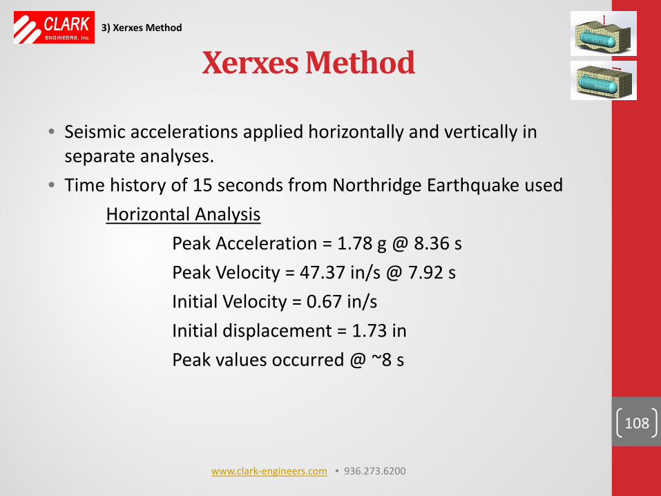
Xerxes Method

• Seismic accelerations applied horizontally and vertically in separate analyses.

• Time history of 15 seconds from Northridge Earthquake used Horizontal Analysis Peak Acceleration = 1.78 g @ 8.36 s Peak Velocity = 47.37 in/s @ 7.92 s Initial Velocity = 0.67 in/s Initial displacement = 1.73 in Peak values occurred @ ~8 s

108

3) Xerxes Method





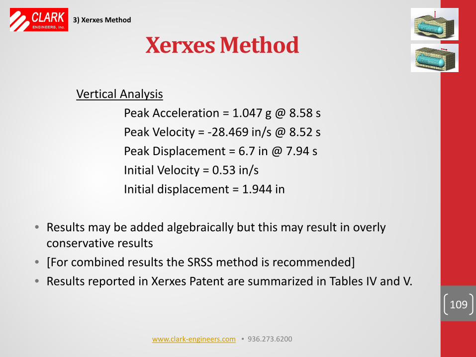
Xerxes Method

Vertical Analysis Peak Acceleration = 1.047 g @ 8.58 s Peak Velocity = -28.469 in/s @ 8.52 s Peak Displacement = 6.7 in @ 7.94 s Initial Velocity = 0.53 in/s Initial displacement = 1.944 in • Results may be added algebraically but this may result in overly

conservative results • [For combined results the SRSS method is recommended] • Results reported in Xerxes Patent are summarized in Tables IV and V.

109

3) Xerxes Method





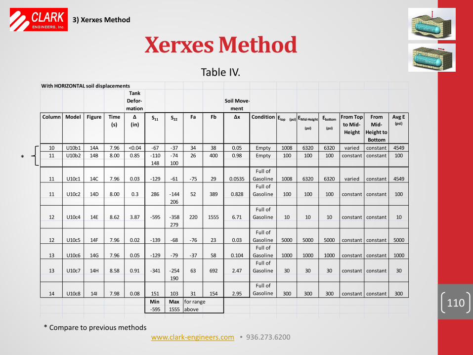
Xerxes Method

110

Tank Defor-mation

Soil Move-ment

Column Model Figure Time (s)

∆ (in)

S11 S22 Fa Fb ∆x Condition Etop (psi) EMid-Height

(psi)

Ebottom

(psi)

From Top to Mid-Height

From Mid-

Height to Bottom

Avg E (psi)

10 U10b1 14A 7.96 <0.04 -67 -37 34 38 0.05 Empty 1008 6320 6320 varied constant 454911 U10b2 14B 8.00 0.85 -110 -74 26 400 0.98 Empty 100 100 100 constant constant 100

148 100

11 U10c1 14C 7.96 0.03 -129 -61 -75 29 0.0535Full of

Gasoline 1008 6320 6320 varied constant 4549

11 U10c2 14D 8.00 0.3 286 -144 52 389 0.828Full of

Gasoline 100 100 100 constant constant 100206

12 U10c4 14E 8.62 3.87 -595 -358 220 1555 6.71Full of


12 U10c5 14F 7.96 0.02 -139 -68 -76 23 0.03Full of


13 U10c6 14G 7.96 0.05 -129 -79 -37 58 0.104Full of


13 U10c7 14H 8.58 0.91 -341 -254 63 692 2.47Full of


14 U10c8 14I 7.98 0.08 151 103 31 154 2.95Full of

Gasoline 300 300 300 constant constant 300Min Max for range-595 1555 above

With HORIZONTAL soil displacements

Table IV.

3) Xerxes Method

*

* Compare to previous methods www.clark-engineers.com ▪ 936.273.6200




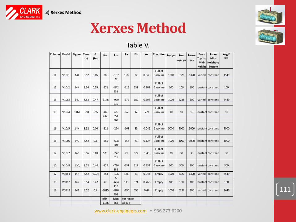
Xerxes Method

111

Table V.

Column Model Figure Time (s)

∆ (in)

S11 S22 Fa Fb ∆x Condition Etop (psi) EMid-

Height (psi)

Ebottom

(psi)

From Top to

Mid-Height

From Mid-

Height to Bottom

Avg E (psi)

14 V10c1 14J 8.52 0.05 -286 -167 158 32 0.046Full of


15 V10c2 14K 8.54 0.55 -971 -842 -116 531 0.804Full of


15 V10c3 14L 8.52 0.47 -1146 -990 -179 680 0.504Full of


15 V10c4 14M 8.58 0.95 -82 226 -62 868 2.9Full of

Gasoline 10 10 10 constant constant 10432 351

368

16 V10c5 14N 8.52 0.04 -311 -224 -161 35 0.046Full of


16 V10c6 14O 8.52 0.1 -585 -508 -158 83 0.127Full of


17 V10c7 14P 8.56 0.69 573 -272 71 622 1.43Full of


17 V10c8 14Q 8.52 0.46 -829 -726 -131 212 0.333Full of


17 V10b1 14R 8.52 <0.04 -253 -196 126 23 0.044 Empty 1008 6320 6320 varied constant 454927

18 V10b2 14S 8.54 0.47 -776 -694 113 371 0.768 Empty 100 100 100 constant constant 100410

18 V10b3 14T 8.52 0.4 -1015 -870 -190 655 0.44 Empty 1008 6238 100 varied constant 2449492

Min Max for range-1146 868 above

3) Xerxes Method





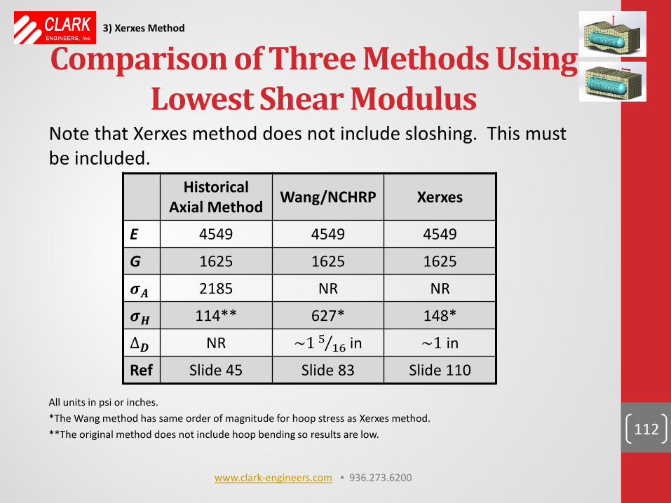
Comparison of Three Methods Using Lowest Shear Modulus

112

3) Xerxes Method

Note that Xerxes method does not include sloshing. This must be included. All units in psi or inches. *The Wang method has same order of magnitude for hoop stress as Xerxes method. **The original method does not include hoop bending so results are low.

Historical Axial Method Wang/NCHRP Xerxes

E 4549 4549 4549

G 1625 1625 1625

𝝈𝑨 2185 NR NR

𝝈𝑯 114** 627* 148*

∆𝑫 NR ~1 516⁄ in ~1 in

Ref Slide 45 Slide 83 Slide 110






conduits and box culverts 3) Xerxes (20) patent (reduced shear modulus) with transverse

loads on FRP UST’s


113





Sloshing • Convective (sloshing) component computed according to

ASCE 7-10, Section 15.7.6.1 page 152. Sloshing mass is computed per ACI 350.3-06, Eqn 9-16, page 48.

• Ref ASCE 7-10, Section 15.7.6.1.1 “Distribution of Hydrodynamic and Intertia Forces”, page 153 (1)

“…the method given in ACI 350.3 is permitted to be used to determine the vertical and horizontal distribution of hydrodynamics and Inertia forces on the walls of circular and rectangular tanks.” • “Analysis of Pressurized Horizontal Vessels Under Seismic Excitation”, by Carluccio, Fabbrocino, Salzano and

Manfredi (7), states that, for circular horizontal tanks with (fluid depth)/(tank radius) between 0.5 and 1.6,

“approximate values for hydrodynamic pressures…can be obtained from solutions for the rectangular of equal dimension…”

114

4) Sloshing





Sloshing

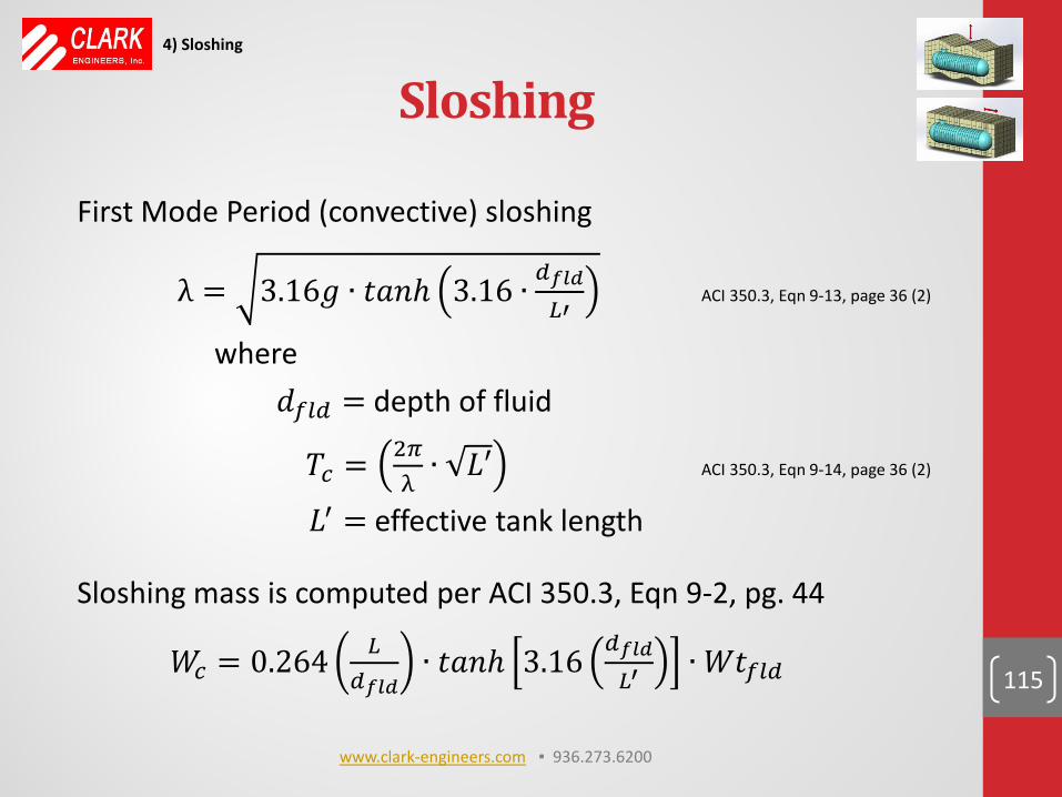
First Mode Period (convective) sloshing

λ = 3.16𝑔 ∙ 𝑡𝑎𝑖𝑡 3.16 ∙ 𝑑𝑓𝑙𝑙𝐷′

ACI 350.3, Eqn 9-13, page 36 (2)

where 𝑑𝑓𝑛𝑑 = depth of fluid

𝑇𝑐 = 2𝜋λ∙ 𝐿𝐹 ACI 350.3, Eqn 9-14, page 36 (2)

𝐿′ = effective tank length

Sloshing mass is computed per ACI 350.3, Eqn 9-2, pg. 44

𝑊𝑐 = 0.264 𝐷𝑑𝑓𝑙𝑙

∙ 𝑡𝑎𝑖𝑡 3.16 𝑑𝑓𝑙𝑙𝐷′

∙ 𝑊𝑡𝑓𝑛𝑑

115

4) Sloshing





Sloshing

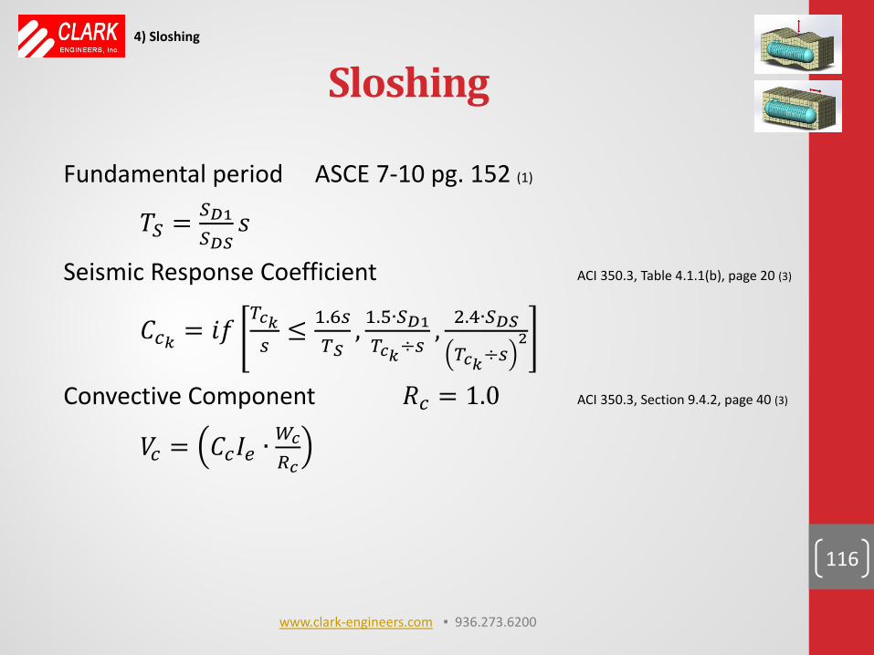
Fundamental period ASCE 7-10 pg. 152 (1)

𝑇𝑆 = 𝑆𝐷1𝑆𝐷𝑆

𝛾

Seismic Response Coefficient ACI 350.3, Table 4.1.1(b), page 20 (3)

𝐶𝑐𝑇 = 𝑑𝑙𝑇𝑠𝑇𝑠≤ 1.6𝑠

𝑇𝑆, 1.5∙𝑆𝐷1𝑇𝑠𝑇÷𝑠

, 2.4∙𝑆𝐷𝑆

𝑇𝑠𝑇÷𝑠2

Convective Component 𝑅𝑐 = 1.0 ACI 350.3, Section 9.4.2, page 40 (3)

𝑉𝑐 = 𝐶𝑐𝐼𝑒 ∙𝑊𝑠𝑅𝑠

116

4) Sloshing





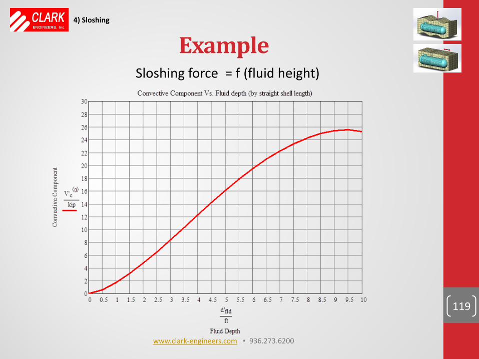
Method for Sloshing Calculations

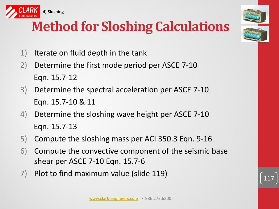
1) Iterate on fluid depth in the tank 2) Determine the first mode period per ASCE 7-10 Eqn. 15.7-12 3) Determine the spectral acceleration per ASCE 7-10 Eqn. 15.7-10 & 11 4) Determine the sloshing wave height per ASCE 7-10 Eqn. 15.7-13 5) Compute the sloshing mass per ACI 350.3 Eqn. 9-16 6) Compute the convective component of the seismic base

shear per ASCE 7-10 Eqn. 15.7-6 7) Plot to find maximum value (slide 119)

117

4) Sloshing





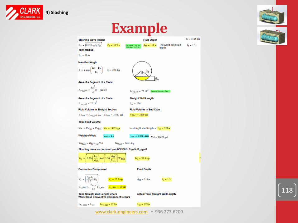
Example

118

4) Sloshing





Example

119

4) Sloshing

Sloshing force = f (fluid height)







loads on FRP UST’s 4) Sloshing

5) Liquefaction 6) Buckling of soil surrounded tubes

120





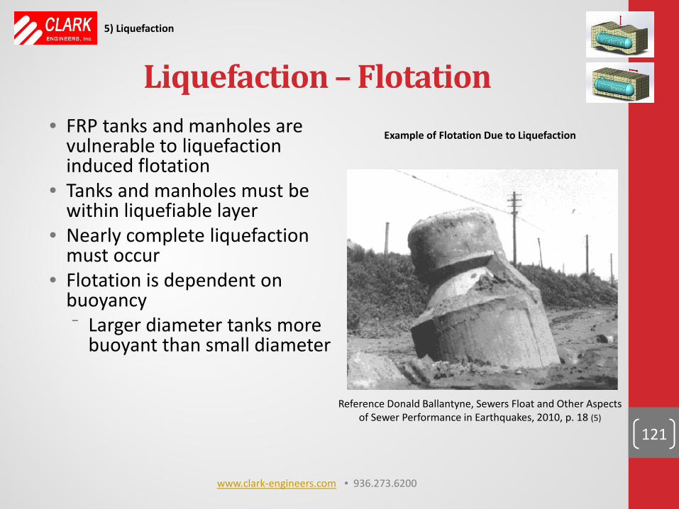
Liquefaction – Flotation • FRP tanks and manholes are

vulnerable to liquefaction induced flotation

• Tanks and manholes must be within liquefiable layer

• Nearly complete liquefaction must occur

• Flotation is dependent on buoyancy ⁻ Larger diameter tanks more

buoyant than small diameter

121

5) Liquefaction

Reference Donald Ballantyne, Sewers Float and Other Aspects of Sewer Performance in Earthquakes, 2010, p. 18 (5)

Example of Flotation Due to Liquefaction





Liquefaction Reference Lambe and Whitman, Soil Mechanics p. 445 (13)

• Liquefaction susceptibility is greatest in fine uniform sand or silt

• Fine sands precise size range from 0.06mm to 0.2mm • Uniformity coefficient

𝑈𝑐 = 𝐷60𝐷10

> 2 Fine sand

𝐷60 is particle diameter at which 60% of weight is finer than 𝐷10 where 𝐷10 is 10% of weight is finer. ibid p. 32

122

5) Liquefaction





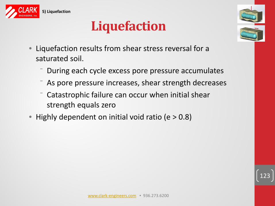
Liquefaction • Liquefaction results from shear stress reversal for a

saturated soil. ⁻ During each cycle excess pore pressure accumulates ⁻ As pore pressure increases, shear strength decreases ⁻ Catastrophic failure can occur when initial shear

strength equals zero • Highly dependent on initial void ratio (e > 0.8)

123

5) Liquefaction





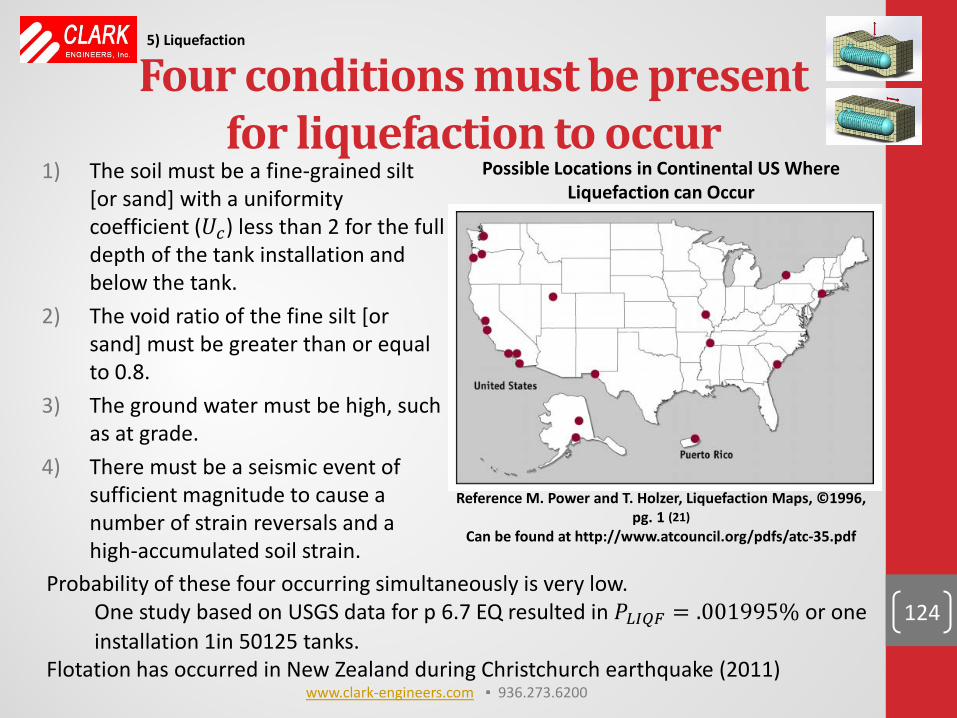
Probability of these four occurring simultaneously is very low. One study based on USGS data for p 6.7 EQ resulted in 𝑃𝐷𝐸𝐸𝐹 = .001995% or one installation 1in 50125 tanks.

Flotation has occurred in New Zealand during Christchurch earthquake (2011)

Four conditions must be present for liquefaction to occur

1) The soil must be a fine-grained silt [or sand] with a uniformity coefficient (𝑈𝑐) less than 2 for the full depth of the tank installation and below the tank.

2) The void ratio of the fine silt [or sand] must be greater than or equal to 0.8.

3) The ground water must be high, such as at grade.

4) There must be a seismic event of sufficient magnitude to cause a number of strain reversals and a high-accumulated soil strain.

124

Reference M. Power and T. Holzer, Liquefaction Maps, ©1996, pg. 1 (21)

Can be found at http://www.atcouncil.org/pdfs/atc-35.pdf

Possible Locations in Continental US Where Liquefaction can Occur

5) Liquefaction





Mitigation of Potential for Liquefaction

• Avoid areas with possible liquefaction if at all possible • If must install in location with fine sand with potential for

liquefactions ⁻ Consider soil improvement ⁻ Ballast tanks to be neutral if soil liquefies ⁻ Install stone columns ⁻ Use compaction grouting ⁻ Directionally drill below layer for pressure lines and siphons ⁻ Install anchors below susceptible layers - helical piles ⁻ Install fins on pipe to activate more backfill – or use deadman

anchors for UST’s ⁻ Design backfill to release pressure ⁻ Design so that repairs may be easily made if possible

125

5) Liquefaction






conduits and box culverts 3) Xerxes (20) patent (reduced shear modulus) with transverse

loads on FRP UST’s 4) Sloshing 5) Liquefaction

6) Buckling of soil surrounded tubes

126





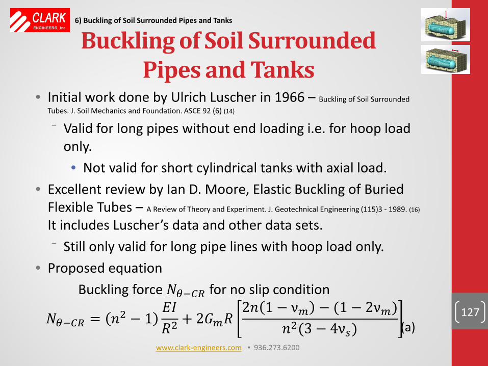
Buckling of Soil Surrounded Pipes and Tanks

• Initial work done by Ulrich Luscher in 1966 – Buckling of Soil Surrounded Tubes. J. Soil Mechanics and Foundation. ASCE 92 (6) (14)

⁻ Valid for long pipes without end loading i.e. for hoop load only. • Not valid for short cylindrical tanks with axial load.

• Excellent review by Ian D. Moore, Elastic Buckling of Buried Flexible Tubes – A Review of Theory and Experiment. J. Geotechnical Engineering (115)3 - 1989. (16)

It includes Luscher’s data and other data sets. ⁻ Still only valid for long pipe lines with hoop load only.

• Proposed equation Buckling force 𝑁𝜃−𝐶𝑅 for no slip condition

𝑁𝜃−𝐶𝑅 = 𝑖2 − 1𝐸𝐼𝑅2 + 2𝐺𝑐𝑅

2𝑖 1 − ν𝑐 − (1 − 2ν𝑐)𝑖2(3 − 4ν𝑠) 127

(a)

6) Buckling of Soil Surrounded Pipes and Tanks





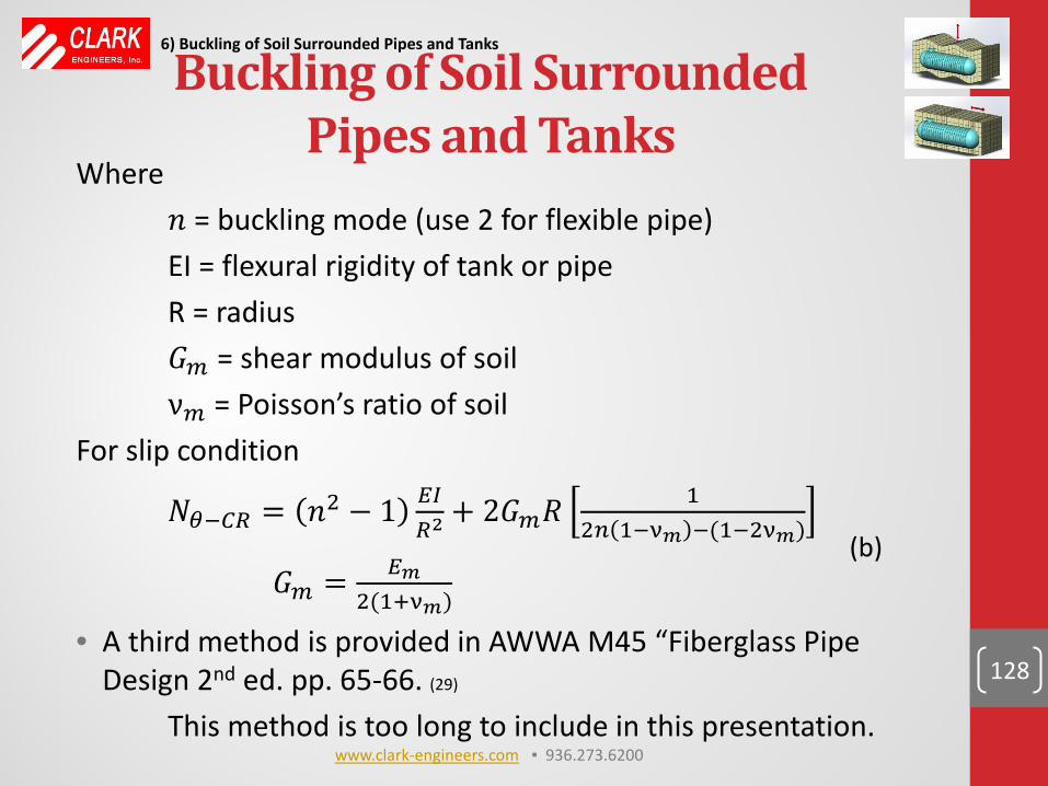
Where 𝑖 = buckling mode (use 2 for flexible pipe) EI = flexural rigidity of tank or pipe R = radius 𝐺𝑐 = shear modulus of soil ν𝑐 = Poisson’s ratio of soil For slip condition

𝑁𝜃−𝐶𝑅 = 𝑖2 − 1 𝐸𝐸𝑅2

+ 2𝐺𝑐𝑅1

2𝑛 1−ν𝑐 −(1−2ν𝑐)

𝐺𝑐 = 𝐸𝑐2(1+ν𝑐)

• A third method is provided in AWWA M45 “Fiberglass Pipe Design 2nd ed. pp. 65-66. (29)

This method is too long to include in this presentation.

128


(b)






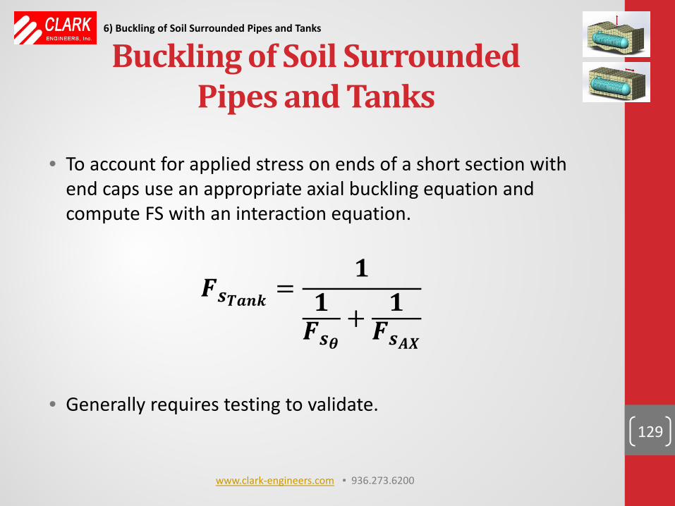
• To account for applied stress on ends of a short section with

end caps use an appropriate axial buckling equation and compute FS with an interaction equation.

𝑭𝒔𝑻𝒂𝑻𝑻 =𝟏

𝟏𝑭𝒔𝜽

+ 𝟏𝑭𝒔𝑨𝑨

• Generally requires testing to validate.

129







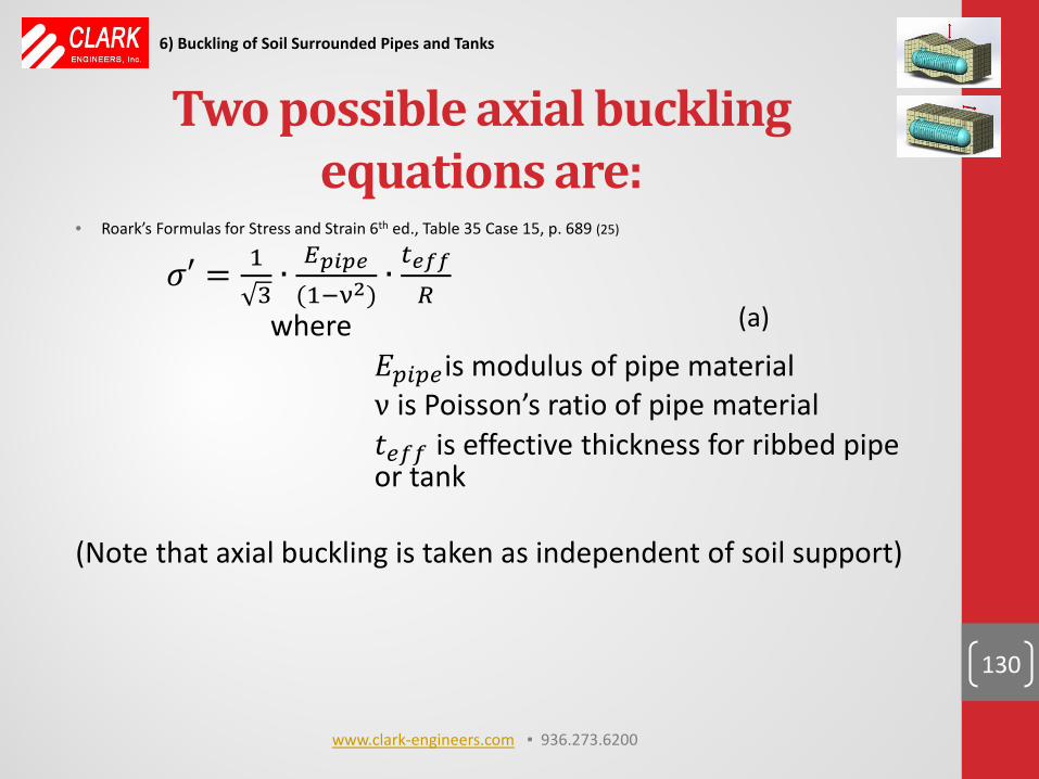
Two possible axial buckling equations are:

• Roark’s Formulas for Stress and Strain 6th ed., Table 35 Case 15, p. 689 (25)

𝜎𝐹 = 13∙ 𝐸𝑝𝑖𝑝𝑠

(1−ν2)∙ 𝑓𝑠𝑓𝑓

𝑅

where 𝐸𝑝𝑛𝑝𝑒 is modulus of pipe material ν is Poisson’s ratio of pipe material 𝑡𝑒𝑓𝑓 is effective thickness for ribbed pipe or tank (Note that axial buckling is taken as independent of soil support)

130

(a)






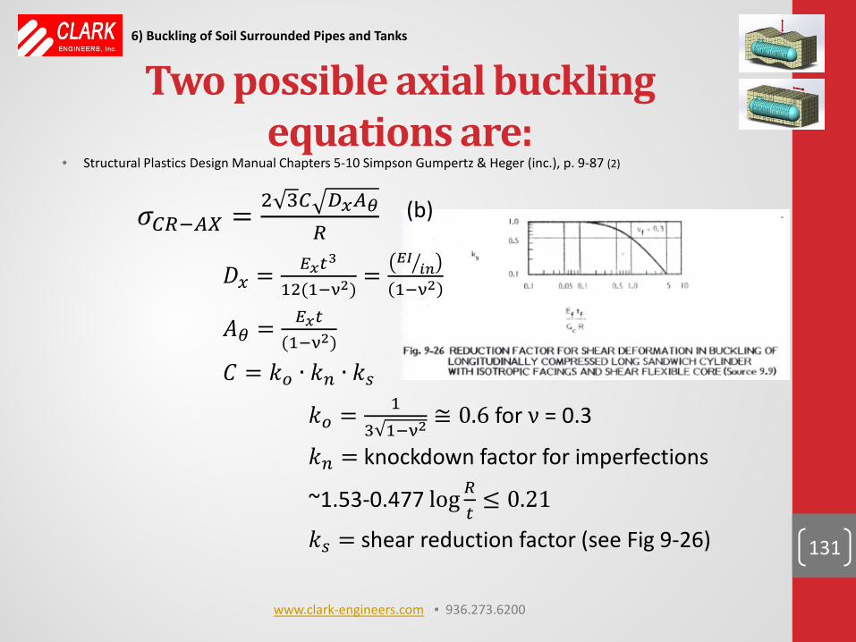
• Structural Plastics Design Manual Chapters 5-10 Simpson Gumpertz & Heger (inc.), p. 9-87 (2)

𝜎𝐶𝑅−𝐴𝐴 = 2 3𝐶 𝐷𝑚𝐴𝜃𝑅

𝐷𝑚 = 𝐸𝑚𝑓3

12(1−ν2)=

𝑆𝐸𝑖𝑖�

1−ν2

𝐴𝜃 = 𝐸𝑚𝑓(1−ν2)

𝐶 = 𝑘𝑜 ∙ 𝑘𝑛 ∙ 𝑘𝑠

𝑘𝑜 = 13 1−ν2

≅ 0.6 for ν = 0.3

𝑘𝑛 = knockdown factor for imperfections

~1.53-0.477 log 𝑅𝑓≤ 0.21

𝑘𝑠 = shear reduction factor (see Fig 9-26) 131

(b)


Two possible axial buckling equations are:





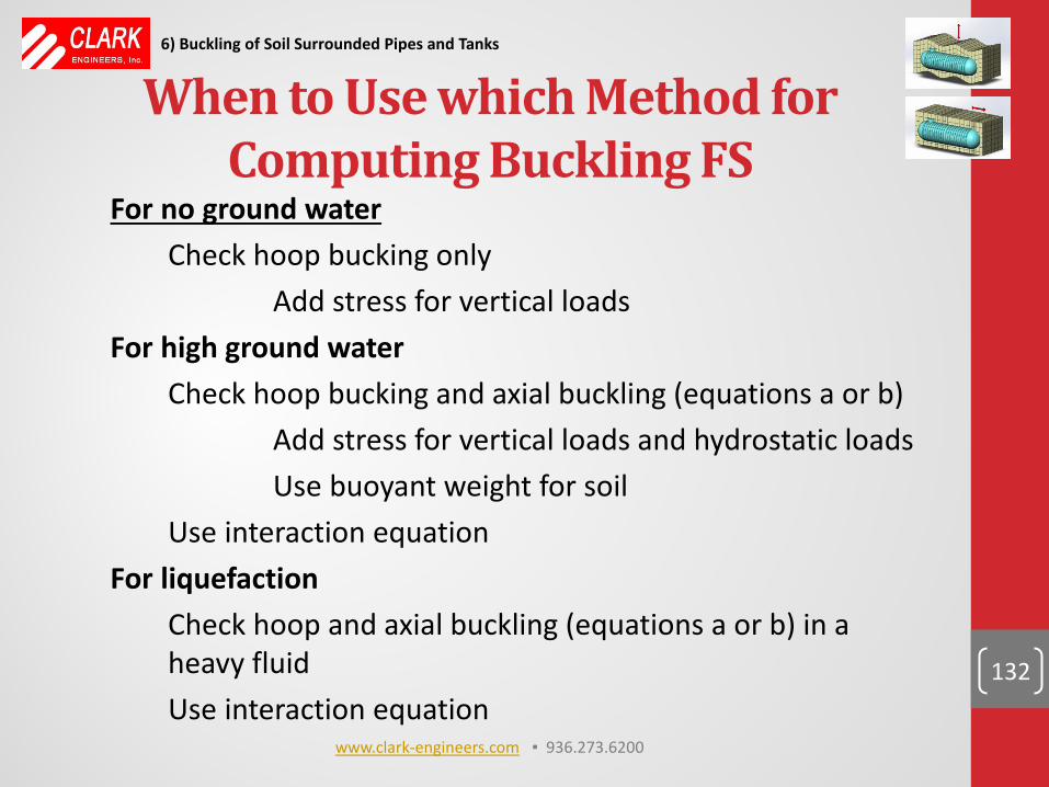
When to Use which Method for Computing Buckling FS

For no ground water Check hoop bucking only Add stress for vertical loads For high ground water Check hoop bucking and axial buckling (equations a or b) Add stress for vertical loads and hydrostatic loads Use buoyant weight for soil Use interaction equation For liquefaction Check hoop and axial buckling (equations a or b) in a heavy fluid Use interaction equation

132






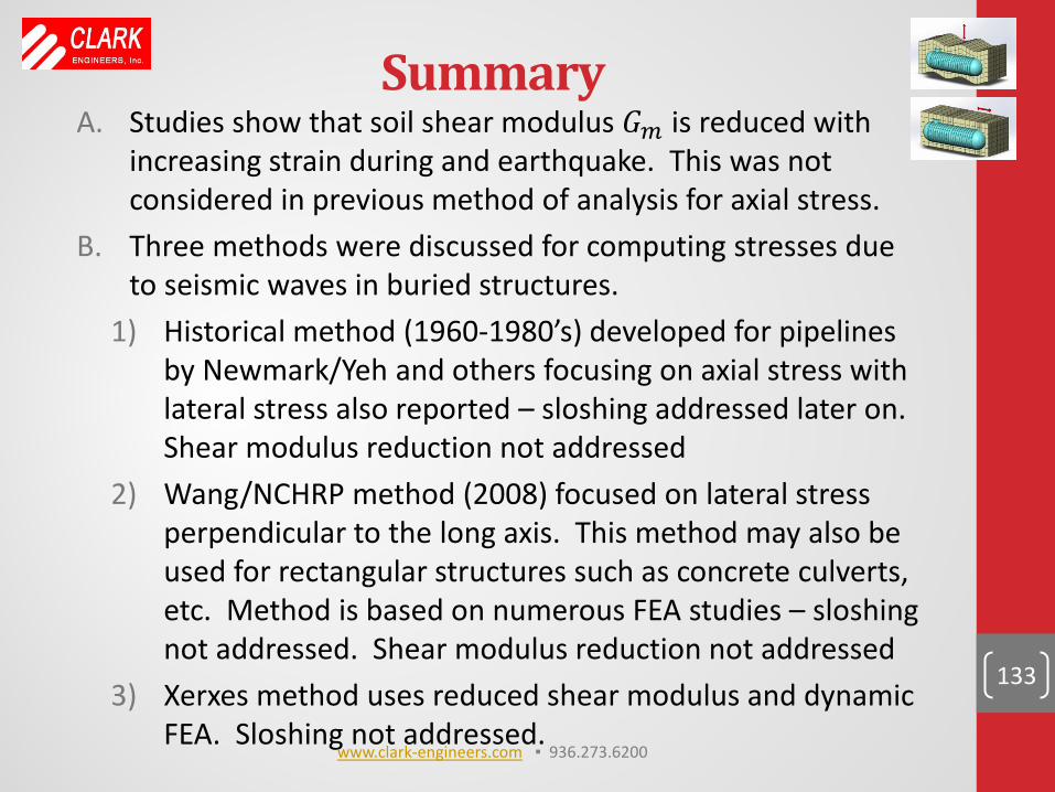
Summary A. Studies show that soil shear modulus 𝐺𝑐 is reduced with

increasing strain during and earthquake. This was not considered in previous method of analysis for axial stress.

B. Three methods were discussed for computing stresses due to seismic waves in buried structures.

1) Historical method (1960-1980’s) developed for pipelines by Newmark/Yeh and others focusing on axial stress with lateral stress also reported – sloshing addressed later on. Shear modulus reduction not addressed

2) Wang/NCHRP method (2008) focused on lateral stress perpendicular to the long axis. This method may also be used for rectangular structures such as concrete culverts, etc. Method is based on numerous FEA studies – sloshing not addressed. Shear modulus reduction not addressed

3) Xerxes method uses reduced shear modulus and dynamic FEA. Sloshing not addressed.

133





Summary

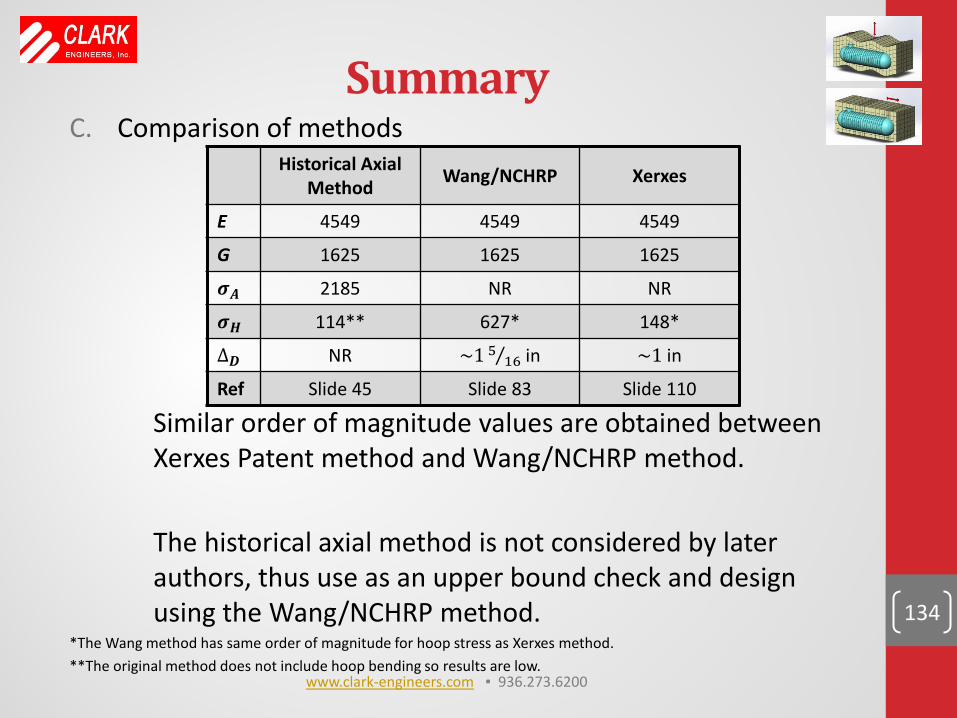
C. Comparison of methods Similar order of magnitude values are obtained between Xerxes Patent method and Wang/NCHRP method. The historical axial method is not considered by later authors, thus use as an upper bound check and design using the Wang/NCHRP method. *The Wang method has same order of magnitude for hoop stress as Xerxes method. **The original method does not include hoop bending so results are low.

134


Historical Axial Method Wang/NCHRP Xerxes

E 4549 4549 4549

G 1625 1625 1625

𝝈𝑨 2185 NR NR

𝝈𝑯 114** 627* 148*

∆𝑫 NR ~1 516⁄ in ~1 in

Ref Slide 45 Slide 83 Slide 110




Summary

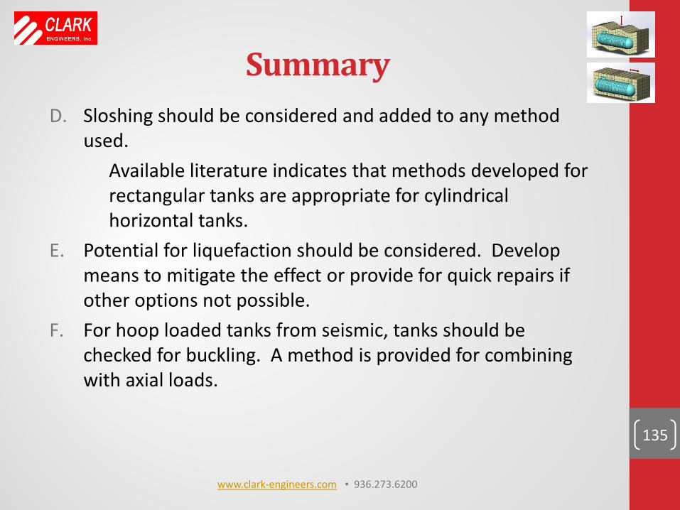
D. Sloshing should be considered and added to any method used.

Available literature indicates that methods developed for rectangular tanks are appropriate for cylindrical horizontal tanks. E. Potential for liquefaction should be considered. Develop

means to mitigate the effect or provide for quick repairs if other options not possible.

F. For hoop loaded tanks from seismic, tanks should be checked for buckling. A method is provided for combining with axial loads.

135





Appendix A

136





1. ASCE 7-10: Minimum Design Loads for Buildings and Other Structures, May 12, 2010, American Society of Civil Engineers.

2. Structural Plastics Design Manual : Phases 2 and 3, 1978, Simpson Gumpertz & Heger Inc., Chap. 5-10.. 3. ACI Committee 350, 2006, Seismic Design of Liquid-Containing Concrete Structures and Commentary: ACI

350.3-06, American Concrete Institute. 4. Anderson, D. et al, Chapter 9, 2008, NCHRP Report 611: Seismic Analysis and Design of Retaining Walls, Buried

Structures, Slopes, and Embankments, Transportation Research Board. 5. Ballantyne, D., September 1, 2010, Sewers Float and Other Aspects of Sewer Performance in Earthquakes, MMI

Engineering. 6. Bowles, J., 1996, Foundation Analysis and Design, 5th Ed., p. 123, The McGraw-Hill Companies, Inc. 7. Carluccio, A. et al, October 1, 2008, Analysis of Pressurized Horizontal Vessels Under Seismic Excitation, World

Conference of Earthquake Engineering. 8. Fahimifar, A. & Vakilzadeh, A., May 2009, Numerical and Analytical Solutions for Ovaling Deformation in

Circular Tunnels Under Seismic Loading, International Journal of Recent Trends in Engineering. 9. Freeman, S., March 2007, Response Spectra as a Useful Design and Analysis Tool for Practicing Structural

Engineers, ISET Journal of Earthquake Technology. 10. Iqbal, M. & Goodling, E., December 1975, Seismic Design of Buried Piping, Second ASCE Specialty Conference

on Structural Design of Nuclear Plant Facilities. 11. Ishihara, K., September 26, 1996, Soil Behavior in Earthquake Geotechnics, Oxford University Press. 12. Karamanos, S., July 2004, Sloshing Effects on Seismic Design of Horizontal-Cylindrical and Spherical Vessels, The

American Society of Mechanical Engineers. 13. Lambe, W. & Whitman, R., January 1, 1969, Soil Mechanics (Series in Soil Engineering), John Wiley and Sons. 14. Luscher, U., Nov/Dec 1966, Buckling of Soil-Surrounded Tubes, ASCE Journal of the Soil Mechanics and

Foundations Division. 15. Moehle, J. (ed.), April 1995, Earthquake Spectra: The Professional Journal of the Earthquake Engineering

Research Institute: Supplement C to Vo.11, Northridge Earthquake of January 17, 1994 Reconnaissance report-Vol 1, Earthquake Engineering Research Institute.

References

137





References

138

16. Moore, I., March 1989, Elastic Buckling of Buried Flexible Tubes—A Review of Theory and Experiment, Journal of Geotechnical Engineering.

17. Newmark, N., September 1971, Earthquake Response Analysis of Reactor Structures, First International Conference on Structural Mechanics in Reactor Technology.

18. Newmark, N. and Rosenblueth, E., January 1971, Fundamentals of Earthquake Engineering, Prentice-Hall 19. Papaspyrou, S. et al, May 5, 2004, Sloshing Effects in Half-Full Horizontal Cylindrical Vessels Under Longitudinal

Excitation, The American Society of Mechanical Engineers. 20. Plecnik, J. et al, May 28, 2002, Seismic Evaluation Method for Underground Structures, US Patent 6397168 B1,

US Patent Office. 21. Power, M. and Holzer, T., 1996, Liquefaction Maps, Applied Technology Council. 22. Shah, H. and Chuh, S., July 1974, Structural Analysis of Underground Structural Elements, ASCE Journal of the

Power Division. 23. Wang, J., June 1, 2003, Seismic Design of Tunnels: a Simple State-of-the-Art Design Approach, Parsons

Brinckerhoff Inc. 24. Yeh, C., October 1964, Seismic Analysis of Slender Buried Beams, Bulletin of the Seismological Society of

America. 25. Young, W., January 1989, Roark’s Formulas for Stress and Strain, 6th ed., McGraw-Hill. 26. Braille, L., February 26, 2010, “Seismic Waves Demonstrations and Animations,” Purdue University from

http://web.ics.purdue.edu/~braile/edumod/waves/WaveDemo.htm. 27. 2015, “US Seismic Design Maps,” USGS from http://earthquake.usgs.gov/hazards/designmaps/usdesign.php 28. N.d., “ASCE 7-10, Figure 22-1,” USGS from

http://earthquake.usgs.gov/hazards/designmaps/downloads/pdfs/2010_ASCE-7_Figure_22-1.pdf 29. Fiberglass Pipe Design - Manual of Water Supply Practices M45, 2nd ed., 2005, American Water Works

Association.






Documents

Seismic Design for Buried Flexible · PDF fileSeismic Design for Buried Flexible Structures 1 ... various methods used for seismic design of ... conduit/tank. • Stress in buried