Embed Size (px)
Citation preview
Selesaikan Persamaan Diferensial Berikut:1. y ''- 5y ' + 6y = 02. y(4)+2y(3)+ 3y '' + 2y ' + y = 03. y '' + 6y ' - 7y = 0; y(0) = 0; y '(0) = 4
In[1]:= DSolve[y''[x] - 5 y'[x] + 6 y[x] ⩵ 0, y, x]
Out[1]= y → Function{x}, ⅇ2 x C[1] + ⅇ3 x C[2]
In[2]:= DSolve[y''[x]-5y'[x]+6y[x]=0]
Input:
y′′(x) - 5 y′(x) + 6 y(x) 0
ODE names:
Autonomous equation:
y′′(x) -6 y(x) + 5 y′(x)Sturm-Liouville equation:
ⅆ
ⅆxⅇ-5 x y′(x) + 6 ⅇ-5 x y(x) 0
Sturm-Liouville equation »
ODE classification:
second-order linear ordinary differential equation
Alternate forms:
y′′(x) 5 y′(x) - 6 y(x)
y′′(x) + 6 y(x) 5 y′(x)
Differential equation solutions: Approximate form
Solve as a homogeneous linear equation | ▾
Hide steps
y(x) c1 ⅇ2 x + c2 ⅇ
3 x
Possible intermediate steps:
Solve ⅆ2y(x)
ⅆx2 - 5 ⅆy(x)
ⅆx+ 6 y(x) 0 :
Assume a solution will be proportional to
ⅇλ x for some
constant λ .
Substitute y(x)
λ x into the
ⅇλ x into the
differential equation:
ⅆ2
ⅆx2ⅇλ x - 5
ⅆ
ⅆxⅇλ x + 6 ⅇλ x 0
Substitute ⅆ2
ⅆx2 ⅇλ x
λ2 ⅇλ x
andⅆ
ⅆxⅇλ x
λ ⅇλ x :
λ2 ⅇλ x - 5 λ ⅇλ x + 6 ⅇλ x 0
Factor out ⅇλ x
:
λ2 - 5 λ + 6 ⅇλ x 0
Since ⅇλ x ≠ 0 for
any finite λ
, the zeros must come from the polynomial:λ2 - 5 λ + 6 0
Factor:(λ - 3) (λ - 2) 0
Solve for λ :λ 2 or λ 3
The root λ
2 gives
y1(x)
c1 ⅇ2 x as a
solution, where
c1 is an
arbitrary constant.
2 contoh_materi_wolfram.nb
The root λ
3 gives
y2(x)
c2 ⅇ3 x as a
solution, where
c2 is an
arbitrary constant.The general solution is the sum of the above solutions:
Answer:
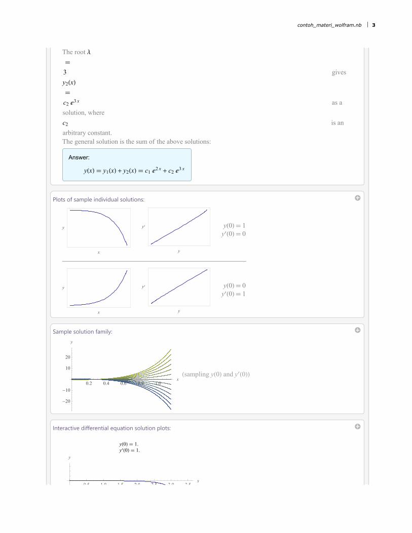
y(x) y1(x) + y2(x) c1 ⅇ2 x + c2 ⅇ
3 x
Plots of sample individual solutions:
x
y
y
y′ y(0) 1y′(0) 0
x
y
y
y′ y(0) 0y′(0) 1
Sample solution family:
0.2 0.4 0.6 0.8 1.0x
-20
-10
10
20
y
(sampling y(0) and y′(0))
Interactive differential equation solution plots:
0.5 1.0 1.5 2.0 2.5 3.0 3.5x
y
y(0) 1.y′(0) 1.
contoh_materi_wolfram.nb 3
0.5 1.0 1.5 2.0 2.5 3.0 3.5
000
000
000
y(x)
Initial conditions:
y(0)
y′(0)
More controls
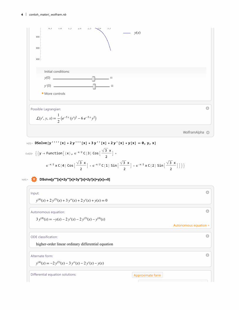
Possible Lagrangian:
ℒ(y′, y, x)1
2ⅇ-5 x (y′)2 - 6 ⅇ-5 x y2
In[3]:= DSolve[y''''[x] + 2 y'''[x] + 3 y''[x] + 2 y'[x] + y[x] ⩵ 0, y, x]
Out[3]= y → Function{x}, ⅇ-x/2 C[3] Cos3 x
2 +
ⅇ-x/2 x C[4] Cos3 x
2 + ⅇ-x/2 C[1] Sin
3 x
2 + ⅇ-x/2 x C[2] Sin
3 x
2
In[4]:= DSolve[y''''[x]+2y'''[x]+3y''[x]+2y'[x]+y[x]⩵0]
Input:
y(4)(x) + 2 y(3)(x) + 3 y′′(x) + 2 y′(x) + y(x) 0
Autonomous equation:
3 y(4)(x) -y(x) - 2 y′(x) - 2 y(3)(x) - y(4)(x)
Autonomous equation »
ODE classification:
higher-order linear ordinary differential equation
Alternate form:
y(4)(x) -2 y(3)(x) - 3 y′′(x) - 2 y′(x) - y(x)
Differential equation solutions: Approximate form
Solve homogeneous linear equation |
4 contoh_materi_wolfram.nb
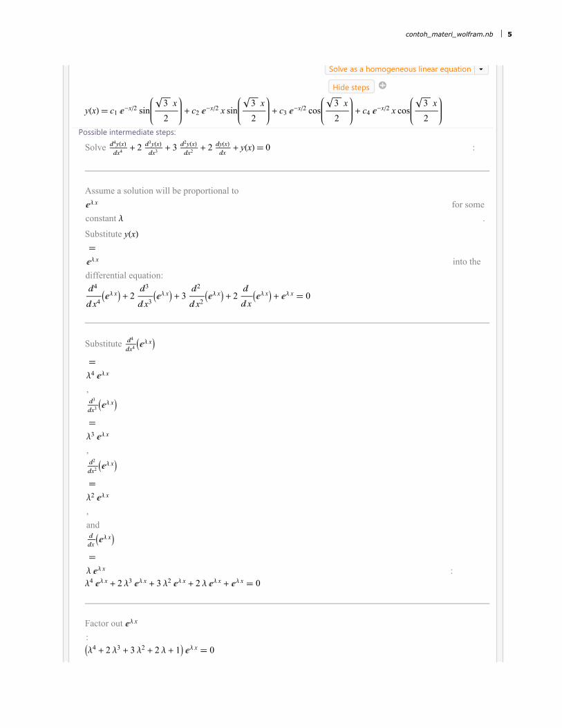
Solve as a homogeneous linear equation | ▾
Hide steps
y(x) c1 ⅇ-x/2 sin
3 x
2+ c2 ⅇ
-x/2 x sin3 x
2+ c3 ⅇ
-x/2 cos3 x
2+ c4 ⅇ
-x/2 x cos3 x
2
Possible intermediate steps:
Solve ⅆ4y(x)
ⅆx4 + 2 ⅆ3y(x)
ⅆx3 + 3 ⅆ2y(x)
ⅆx2 + 2 ⅆy(x)
ⅆx+ y(x) 0 :
Assume a solution will be proportional to
ⅇλ x for some
constant λ .
Substitute y(x)
ⅇλ x into the
differential equation:
ⅆ4
ⅆx4ⅇλ x + 2
ⅆ3
ⅆx3ⅇλ x + 3
ⅆ2
ⅆx2ⅇλ x + 2
ⅆ
ⅆxⅇλ x + ⅇλ x 0
Substitute ⅆ4
ⅆx4 ⅇλ x
λ4 ⅇλ x
,ⅆ3
ⅆx3 ⅇλ x
λ3 ⅇλ x
,ⅆ2
ⅆx2 ⅇλ x
λ2 ⅇλ x
,
andⅆ
ⅆxⅇλ x
λ ⅇλ x :λ4 ⅇλ x + 2 λ3 ⅇλ x + 3 λ2 ⅇλ x + 2 λ ⅇλ x + ⅇλ x 0
Factor out ⅇλ x
:
λ4 + 2 λ3 + 3 λ2 + 2 λ + 1 ⅇλ x 0
contoh_materi_wolfram.nb 5
Since ⅇλ x ≠ 0 for
any finite λ
, the zeros must come from the polynomial:λ4 + 2 λ3 + 3 λ2 + 2 λ + 1 0
Factor:
λ2 + λ + 12 0
Solve for λ :
λ -1
2+ⅈ 3
2or λ -
1
2+ⅈ 3
2or λ -
1
2-ⅈ 3
2or λ -
1
2-ⅈ 3
2
The roots λ
-12
±
ⅈ 32
both
have muliplicity
2 and give
y1(x) c1 ⅇ-1/2+ⅈ 3 2 x
,
y2(x) c2 ⅇ-1/2-ⅈ 3 2 x
,
y3(x) c3 ⅇ-1/2+ⅈ 3 2 x
x
,
y4(x) c4 ⅇ-1/2-ⅈ 3 2 x
x as
solutions, where
c1
,
c2
,
c3
,
and
c4 are
arbitrary constants.The general solution is the of the above solutions
6 contoh_materi_wolfram.nb
The general solution is the sum of the above solutions:
y(x) y1(x) + y2(x) + y3(x) + y4(x)
c1 ⅇ-1/2+ⅈ 3 2 x
+ c2 ⅇ-1/2-ⅈ 3 2 x
+ c3 ⅇ-1/2+ⅈ 3 2 x
x + c4 ⅇ-1/2-ⅈ 3 2 x
x
Apply Euler's identity
ⅇα+ⅈ β ⅇα cos(β) + ⅈ ⅇα sin(β) :
y(x) c1 ⅇ-x/2 cos3 x
2+ ⅈ ⅇ-x/2 sin
3 x
2+ c2 ⅇ-x/2 cos
3 x
2- ⅈ ⅇ-x/2 sin
3 x
2+
c3 x ⅇ-x/2 cos3 x
2+ ⅈ ⅇ-x/2 sin
3 x
2+ c4 x ⅇ-x/2 cos
3 x
2- ⅈ ⅇ-x/2 sin
3 x
2
Regroup terms:
y(x) (c1 + c2) ⅇ-x/2 cos
3 x
2+ (c3 + c4) ⅇ
-x/2 x cos3 x
2+
ⅈ (c1 - c2) ⅇ-x/2 sin
3 x
2+ ⅈ (c3 - c4) ⅇ
-x/2 x sin3 x
2
Redefine c1 + c2
as c1 ,
ⅈ (c1 - c2) as
c2 ,
c3 + c4 as
c3 , and
ⅈ (c3 - c4) as
c4 , since
these are arbitrary constants:
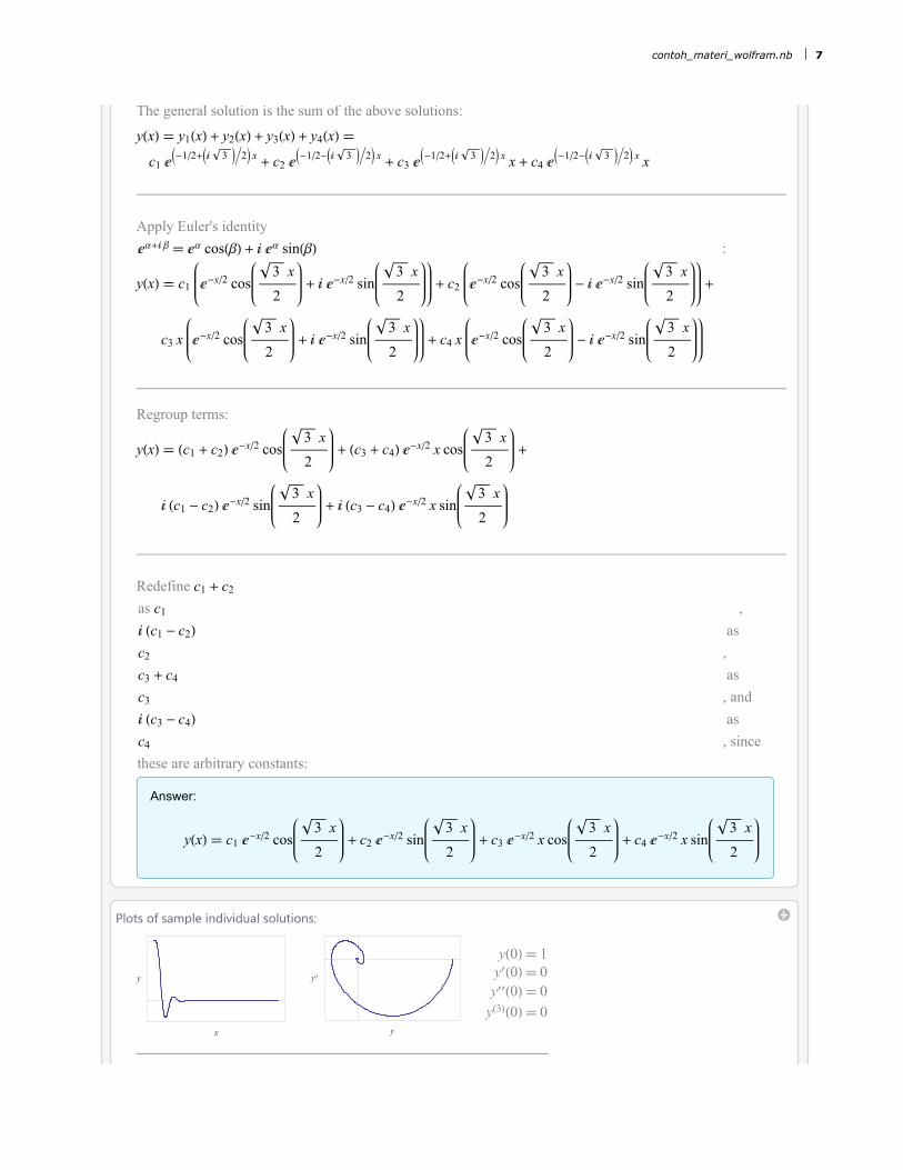
Answer:
y(x) c1 ⅇ-x/2 cos
3 x
2+ c2 ⅇ
-x/2 sin3 x
2+ c3 ⅇ
-x/2 x cos3 x
2+ c4 ⅇ
-x/2 x sin3 x
2
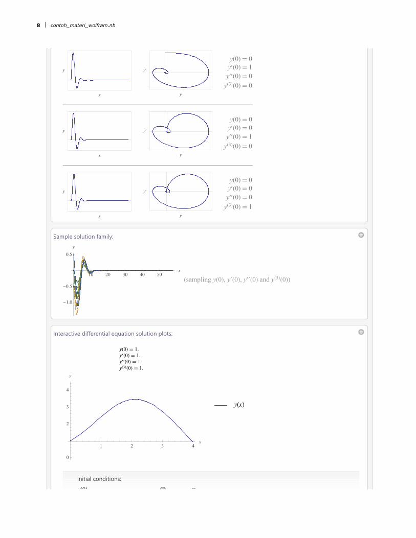
Plots of sample individual solutions:
x
y
y
y′
y(0) 1y′(0) 0y′′(0) 0
y(3)(0) 0
contoh_materi_wolfram.nb 7
x
y
y
y′
y(0) 0y′(0) 1y′′(0) 0
y(3)(0) 0
x
y
y
y′
y(0) 0y′(0) 0y′′(0) 1
y(3)(0) 0
x
y
y
y′
y(0) 0y′(0) 0y′′(0) 0
y(3)(0) 1
Sample solution family:
10 20 30 40 50x
-1.0
-0.5
0.5
y
(sampling y(0), y′(0), y′′(0) and y(3)(0))
Interactive differential equation solution plots:
1 2 3 4x
0
2
3
4
y
y(0) 1.y′(0) 1.y′′(0) 1.y(3)(0) 1.
y(x)
Initial conditions:
y(0)
8 contoh_materi_wolfram.nb
y(0)
y′(0)
y′′(0)
y(3)(0)
More controls
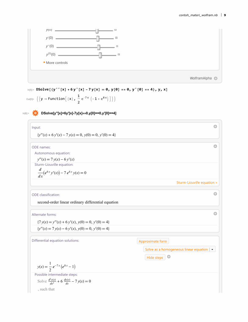
In[5]:= DSolve[{y''[x] + 6 y'[x] - 7 y[x] ⩵ 0, y[0] == 0, y'[0] == 4}, y, x]
Out[5]= y → Function{x},1
2ⅇ-7 x -1 + ⅇ8 x
In[6]:= DSolve[y''[x]+6y'[x]-7y[x]⩵0,y[0]==0,y'[0]==4]
Input:
{y′′(x) + 6 y′(x) - 7 y(x) 0, y(0) 0, y′(0) 4}
ODE names:
Autonomous equation:
y′′(x) 7 y(x) - 6 y′(x)Sturm-Liouville equation:
ⅆ
ⅆxⅇ6 x y′(x) - 7 ⅇ6 x y(x) 0
Sturm-Liouville equation »
ODE classification:
second-order linear ordinary differential equation
Alternate forms:
{7 y(x) y′′(x) + 6 y′(x), y(0) 0, y′(0) 4}
{y′′(x) 7 y(x) - 6 y′(x), y(0) 0, y′(0) 4}
Differential equation solutions: Approximate form
Solve as a homogeneous linear equation | ▾
Hide steps
y(x)1
2ⅇ-7 x ⅇ8 x - 1
Possible intermediate steps:
Solve ⅆ2y(x)
ⅆx2 + 6 ⅆy(x)
ⅆx- 7 y(x) 0
, such that
contoh_materi_wolfram.nb 9
y(0) 0
and
y′(0) 4 :
Assume a solution will be proportional to
ⅇλ x for some
constant λ .
Substitute y(x)
ⅇλ x into the
differential equation:
ⅆ2
ⅆx2ⅇλ x + 6
ⅆ
ⅆxⅇλ x - 7 ⅇλ x 0
Substitute ⅆ2
ⅆx2 ⅇλ x
λ2 ⅇλ x
andⅆ
ⅆxⅇλ x
λ ⅇλ x :
λ2 ⅇλ x + 6 λ ⅇλ x - 7 ⅇλ x 0
Factor out ⅇλ x
:
λ2 + 6 λ - 7 ⅇλ x 0
Since ⅇλ x ≠ 0 for
any finite λ
, the zeros must come from the polynomial:λ2 + 6 λ - 7 0
Factor:(λ - 1) (λ + 7) 0
Solve for λ :λ -7 or λ 1
10 contoh_materi_wolfram.nb
The root λ
-7 gives
y1(x)
c1 ⅇ-7 x as a
solution, where
c1 is an
arbitrary constant.
The root λ
1 gives
y2(x)
c2 ⅇx as a
solution, where
c2 is an
arbitrary constant.The general solution is the sum of the above solutions:
y(x) y1(x) + y2(x) c1 ⅇ-7 x + c2 ⅇ
x
Solve for the unknown constants using the initial conditions:
Compute ⅆy(x)
ⅆx:
ⅆy(x)
ⅆx
ⅆ
ⅆxc1 ⅇ
-7 x + c2 ⅇx
-7 c1 ⅇ-7 x + c2 ⅇ
x
Substitute y(0) 0
into y(x)
ⅇ-7 x c1 + ⅇx c2 :c1 + c2 0
Substitute y′(0) 4
into ⅆy(x)
ⅆx
-7 ⅇ-7 x c1 + ⅇx c2 :-7 c1 + c2 4
Solve the system:
contoh_materi_wolfram.nb 11
Solve the system:
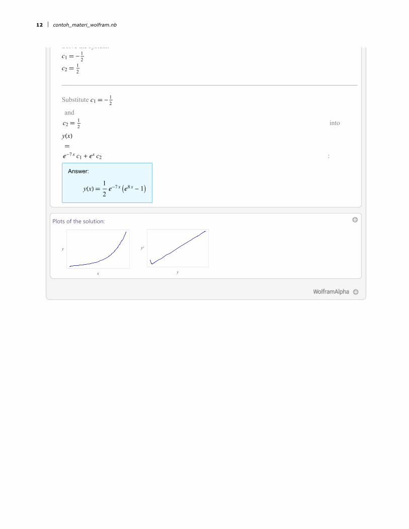
c1 -12
c2 12
Substitute c1 -12
and
c2 12
into
y(x)
ⅇ-7 x c1 + ⅇx c2 :
Answer:
y(x)1
2ⅇ-7 x ⅇ8 x - 1
Plots of the solution:
x
y
y
y′
12 contoh_materi_wolfram.nb

![· Selesaikan persamaan kuadratik berikut. x2+2x ... [5 markah] 2x2 -15= Solve the following simultaneous linear equations by using the substitution method. Selesaikan persamaan](https://img.pdfslide.tips/doc/110x75/5e235f7904efd13f22228c5d/selesaikan-persamaan-kuadratik-berikut-x22x-5-markah-2x2-15-solve-the.jpg)


![· Selesaikan persamaan kuadratik di bawah dengan menggunakan kaedah pemfaktoran. 2x x —A [5 marks] [5 markah] Solve the quadratic equation below using factorization method. Selesaikan](https://img.pdfslide.tips/doc/110x75/5e32c109038c123f03475ef8/selesaikan-persamaan-kuadratik-di-bawah-dengan-menggunakan-kaedah-pemfaktoran-2x.jpg)