Embed Size (px)
Citation preview
sensors
Article
Self-Organizing Traffic Flow Prediction withan Optimized Deep Belief Network for Internetof Vehicles
Shidrokh Goudarzi 1 , Mohd Nazri Kama 1 , Mohammad Hossein Anisi 2,*,Seyed Ahmad Soleymani 3 and Faiyaz Doctor 2
1 Advanced Informatics School, Universiti Teknologi Malaysia Kuala Lumpur (UTM), Jalan Semarak,Kuala Lumpur 54100, Malaysia; [email protected] (S.G.); [email protected] (M.N.K.)
2 School of Computer Science and Electronic Engineering, University of Essex, Colchester CO4 3SQ, UK;[email protected]
3 Faculty of Computing, Universiti Teknologi Malaysia Kuala Lumpur (UTM), Skudai, Johor 81310, Malaysia;[email protected]
* Correspondence: [email protected]
Received: 18 August 2018; Accepted: 10 October 2018; Published: 15 October 2018�����������������
Abstract: To assist in the broadcasting of time-critical traffic information in an Internet of Vehicles(IoV) and vehicular sensor networks (VSN), fast network connectivity is needed. Accurate trafficinformation prediction can improve traffic congestion and operation efficiency, which helps toreduce commute times, noise and carbon emissions. In this study, we present a novel approachfor predicting the traffic flow volume by using traffic data in self-organizing vehicular networks.The proposed method is based on using a probabilistic generative neural network techniques calleddeep belief network (DBN) that includes multiple layers of restricted Boltzmann machine (RBM)auto-encoders. Time series data generated from the roadside units (RSUs) for five highway links areused by a three layer DBN to extract and learn key input features for constructing a model to predicttraffic flow. Back-propagation is utilized as a general learning algorithm for fine-tuning the weightparameters among the visible and hidden layers of RBMs. During the training process the fireflyalgorithm (FFA) is applied for optimizing the DBN topology and learning rate parameter. MonteCarlo simulations are used to assess the accuracy of the prediction model. The results show that theproposed model achieves superior performance accuracy for predicting traffic flow in comparisonwith other approaches applied in the literature. The proposed approach can help to solve the problemof traffic congestion, and provide guidance and advice for road users and traffic regulators.
Keywords: deep belief network; historical time traffic flows; restricted Boltzmann machine;optimization; traffic flow prediction
1. Introduction
In an IoV and VSN, vehicles act as senders, receivers and routers to broadcast data to a network ortransportation agency as part of an integrated Intelligent Transportation System (ITS) [1]. The collecteddata can be used for traffic flow prediction to ensure safe, free-flow of traffic in metropolitan areas.The application of sensor networks as a roadside communication infrastructure is regularly used invarious current intelligent transportation and smart highway systems. The roadside units (RSUs) offera secure infrastructure along the road which are responsible for broadcasting periodic safety messagesto road users. Typically, RSUs are located every 300 m to 1 km and transmit data at the interval ofevery 300 ms. Therefore, placing RSUs along a long stretch of highway to offer ubiquitous connectivityis not economically viable. Hence, vehicles should be able to use other vehicles to transmit and receive
Sensors 2018, 18, 3459; doi:10.3390/s18103459 www.mdpi.com/journal/sensors
Sensors 2018, 18, 3459 2 of 18
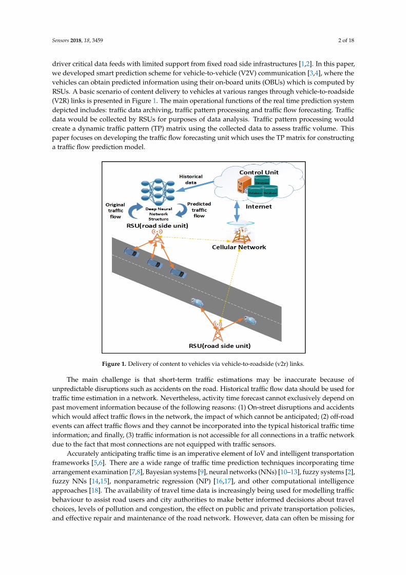
driver critical data feeds with limited support from fixed road side infrastructures [1,2]. In this paper,we developed smart prediction scheme for vehicle-to-vehicle (V2V) communication [3,4], where thevehicles can obtain predicted information using their on-board units (OBUs) which is computed byRSUs. A basic scenario of content delivery to vehicles at various ranges through vehicle-to-roadside(V2R) links is presented in Figure 1. The main operational functions of the real time prediction systemdepicted includes: traffic data archiving, traffic pattern processing and traffic flow forecasting. Trafficdata would be collected by RSUs for purposes of data analysis. Traffic pattern processing wouldcreate a dynamic traffic pattern (TP) matrix using the collected data to assess traffic volume. Thispaper focuses on developing the traffic flow forecasting unit which uses the TP matrix for constructinga traffic flow prediction model.
2 of 18
vehicles to transmit and receive driver critical data feeds with limited support from fixed road side
infrastructures [1,2]. In this paper, we developed smart prediction scheme for vehicle‐to‐vehicle
(V2V) communication [3,4], where the vehicles can obtain predicted information using their on‐board
units (OBUs) which is computed by RSUs. A basic scenario of content delivery to vehicles at various
ranges through vehicle‐to‐roadside (V2R) links is presented in Figure 1. The main operational
functions of the real time prediction system depicted includes: traffic data archiving, traffic pattern
processing and traffic flow forecasting. Traffic data would be collected by RSUs for purposes of data
analysis. Traffic pattern processing would create a dynamic traffic pattern (TP) matrix using the
collected data to assess traffic volume. This paper focuses on developing the traffic flow forecasting
unit which uses the TP matrix for constructing a traffic flow prediction model.
Figure 1. Delivery of content to vehicles via vehicle‐to‐roadside (v2r) links.
The main challenge is that short‐term traffic estimations may be inaccurate because of
unpredictable disruptions such as accidents on the road. Historical traffic flow data should be used
for traffic time estimation in a network. Nevertheless, activity time forecast cannot exclusively
depend on past movement information because of the following reasons: (1) On‐street disruptions
and accidents which would affect traffic flows in the network, the impact of which cannot be
anticipated; (2) off‐road events can affect traffic flows and they cannot be incorporated into the typical
historical traffic time information; and finally, (3) traffic information is not accessible for all connections
in a traffic network due to the fact that most connections are not equipped with traffic sensors.
Accurately anticipating traffic time is an imperative element of IoV and intelligent transportation
frameworks [5,6]. There are a wide range of traffic time prediction techniques incorporating time
arrangement examination [7,8], Bayesian systems [9], neural networks (NNs) [10–13], fuzzy systems
[2], fuzzy NNs [14,15], nonparametric regression (NP) [16,17], and other computational intelligence
approaches [18]. The availability of travel time data is increasingly being used for modelling traffic
behaviour to assist road users and city authorities to make better informed decisions about travel
choices, levels of pollution and congestion, the effect on public and private transportation policies,
and effective repair and maintenance of the road network. However, data can often be missing for
specific timeframes due to noise in the reading or corrupted data [19–22]. Various machine learning,
probabilistic and statistical modelling approaches have attempted to solve the problem of missing
Figure 1. Delivery of content to vehicles via vehicle-to-roadside (v2r) links.
The main challenge is that short-term traffic estimations may be inaccurate because ofunpredictable disruptions such as accidents on the road. Historical traffic flow data should be used fortraffic time estimation in a network. Nevertheless, activity time forecast cannot exclusively depend onpast movement information because of the following reasons: (1) On-street disruptions and accidentswhich would affect traffic flows in the network, the impact of which cannot be anticipated; (2) off-roadevents can affect traffic flows and they cannot be incorporated into the typical historical traffic timeinformation; and finally, (3) traffic information is not accessible for all connections in a traffic networkdue to the fact that most connections are not equipped with traffic sensors.
Accurately anticipating traffic time is an imperative element of IoV and intelligent transportationframeworks [5,6]. There are a wide range of traffic time prediction techniques incorporating timearrangement examination [7,8], Bayesian systems [9], neural networks (NNs) [10–13], fuzzy systems [2],fuzzy NNs [14,15], nonparametric regression (NP) [16,17], and other computational intelligenceapproaches [18]. The availability of travel time data is increasingly being used for modelling trafficbehaviour to assist road users and city authorities to make better informed decisions about travelchoices, levels of pollution and congestion, the effect on public and private transportation policies,and effective repair and maintenance of the road network. However, data can often be missing for
Sensors 2018, 18, 3459 3 of 18
specific timeframes due to noise in the reading or corrupted data [19–22]. Various machine learning,probabilistic and statistical modelling approaches have attempted to solve the problem of missingdata in traffic forecasting [23–29]. A study by van Lint et al. [30] showed a travel time forecastingmodel based on a neural system for handling missing traffic information while in Sun et al. [31] trafficstreams estimation based on using a Bayesian model was presented where missing historical trafficinformation was estimated by utilizing a Gaussian blend display to visually verify the traffic dataforecast. Various specialists have shown that hybrid methods have better results in terms of accuracyand precision compared with individual techniques [32]. Hybrid methods based on fuzzy logic can bepotential alternatives to enhance precision in traffic flow prediction as described in [33] while in [34]a novel method based on neural networks is utilized in traffic time estimation.
Artificial neural networks (ANNs) have been widely used for time series prediction problems sincetheir inception in the 1980s. In classical neural networks, training algorithms akin to back- propagationonly try to model the dependence of the output from the input. Restricted Boltzmann Machines(RBMs), instead, are networks of stochastic neurons that can be trained in a greedy fashion. Deepbelief networks are obtained by stacking RBMs on one another so that the input to one layer is givenby the hidden units of the adjacent layer, as if they were data, and adding a last discriminative layer.The RBM, might even yield better results than traditional neural networks with higher accuracy. Ina RBN, the hidden units are independent given the visible states. So, they can quickly get an unbiasedsample from the posterior distribution when given a data-vector. This is a big advantage overdirect belief nets. The multi-layer perceptron (MLP) and radial basis function networks (RBFN) arewell-known approaches. Often gradient descent methods are used for training these approaches andback propagation (BP) is used as the learning algorithm [27].
However, there are some limitations of using conventionally shallow ANNs for real worldproblems such as traffic flow prediction in highways based on VANET-cellular systems. The first issueis related to the design of the ANN topology. It is found that the larger the size of the hidden layer themore prone the model is to overfitting the training data. The second problem is related to deciding theinitial value of the ANN weights. BP is a supervised learning method which uses samples of inputand output data to modify weights of connections between units (neurons) across the network layers.The appropriate selection of initial weights can increase the speed with which the model is able toconverge. Both these problems are amplified when the input parameter space is very large as in thecase of traffic flow prediction. Hence there is a need to be able to transform the input parameters intoa reduced and manageable feature space with which to construct the prediction model. Equally thereis a need to determine the optimal number of hidden neurons for training the model. Finally, the thirdproblem is determining a suitable learning rate during the models training phase. Here there is a needto incorporate an automated way of selecting the most appropriate learning rates as the model isbeing trained. To solve these problems, we proposed a novel traffic flow prediction model based onDBNs comprised of multiple stacked restricted Boltzmann machine (RBM) auto-encoders. RBMs arenetworks of stochastic units with undirected interactions between pairs of visible and hidden unitswhich can be used to learn a probability distribution over its set of inputs. By stacking multiple RBMsonto one another DBNs are trained using greedy layer-wise learning which aims to train each layerof a DBN in a sequential and unsupervised way, feeding lower layer results to the upper layers tocapture a representational hierarchy of relationships within the training data [10–13]. Each trainedlayer represents feature encoders which can be helpful in the discrimination of the target output space.This unsupervised training process can provide an optimal start for supervised training as well asextract and learn a reduced set of features representing the input parameters. Supervised learning isthen performed using backpropagation for fine-tuning the weight parameters among the visible andhidden layers of RBMs for training the traffic flow prediction model. The firefly Algorithm (FFA) isfurther applied for selecting the optimal number of connected units (neurons) and learning rate duringtraining of the proposed model which has been termed DRBM-FFA. In brief, the main contribution ofthis study can be listed as follows:
Sensors 2018, 18, 3459 4 of 18
• We define a dynamic traffic pattern matrix to assess traffic volume data;• We propose a 3-layer DBN composed of two RBMs to determine the salient features from time series
traffic volume data for constructing a traffic flow prediction model on VANET-cellular systems.• We utilize FFA algorithm to optimize and select the sizes of the learning rates in neural
networks and;• We perform simulations and explain how to use historical traffic data for traffic volume prediction.
The reminder of this paper is organized as follows: Section 2 shows the initial Traffic Pattern (TP)matrix to assess traffic time data at five highway links. A dynamic (TP) matrix predictor based ona DBN of RBMs is presented in Section 3. The (FFA) algorithm for selecting the best number of unitsand for selecting the rates of learning of deep belief nets is explained in Section 4. We demonstrate ourpredictions and results in Section 5 and the conclusions in Section 6.
2. Assessing Traffic Pattern Matrix
This section focuses on the effective procedure to predict traffic pattern in vehicularcommunications for utilization in real-time applications, such as dynamic traffic management. RSUscan collect speed and flow data and the information gathered can be delivered to a control unit thatautomatically estimates volume of traffic [35].
The pattern of traffic can be characterized as a matrix on a temporal and spatial scale. The spatialscale incorporates the entire area of the street for which specific trip times can be anticipated.The temporal scale incorporates adequate time spans to characterize the impact of traffic on travel time.Traffic volume is specified as the number of vehicles that cross a section of road per unit time withina selected period. Volume of traffic can influence travel time together with speed of vehicles which isutilized as a marker for congestion. We assigned the weights at given times and locations to createthe TP matrix based on congestion level to optimize travel times. The principal task here is to derivea historical days’ database by using the assumption that traffic patterns are repetitive during a tighttime period, for example, traffic time for 10 a.m. traffic can be viewed from 9 a.m. to 11 a.m. Thissearch window can locate comparative traffic patterns rapidly. There are traffic examples of differentdays which are recorded in the database inside a time span of ±x minutes for time estimation. Ourscenario links to V2R communications and measures vehicles moving at speeds of 100 km/h (~27 m/s)crossing each of the RSU with a coverage range of 200 m (radius). This relates to the high contactduration of 200 × 2/27 ≈ 15 s.
In our simulation, we assumed that the road section consists of k links and each link showsa section of road. Each section should be equipped with one RSU, the amount of days in historicaldatabase is denoted by i = 1, 2, 3, . . . ni, j = 0, 5, 10, . . . , nj representing information in a five minutesresolution, and t which is the prediction time on prediction day p. The start time of the traffic patternon historical days denoted by ts. v(i, t− j, p) designates velocity on prediction day p at link k at timet− j. Similarity, h = 1, 2, 3, . . . , nh shows the number of days in historical database and ts shows thebeginning time of the traffic pattern on historical days then v(i, ts − j, h) shows on historical day h atlink k at time ts − j. Travel time on a road is mainly affected by the congestion present on the road. Thiscongestion may occur due to bottlenecks. Weights are applied to account for the congestion produceddue to the type of bottlenecks, whenever and wherever it occurs. We set the weights according to therapid speed of each section. These weights have to be higher for the sections with lower rapid speedswhich represented bottlenecks. The following practical formula is utilized in Equation (1):
w(i, j) =1
[v(i, t− j, p)]C(1)
where, C is a constant. The search is executed in ±x minutes of estimation time t on historical daysso t + x ≥ ts ≥ t− x. The basic purpose of the pattern matching process is to find the most similarhistorical pattern(s). Hence, the primary task is to generate some historical days’ database. One way of
Sensors 2018, 18, 3459 5 of 18
searching these patterns is to discover the entire historical database for the most similar pattern, butthis makes the search process computationally intensive. Hence, the sum of the squared differencebetween the prediction time traffic pattern and the historical traffic patterns is used as a criterion forfinding similarities between the traffic patterns. The historical traffic pattern having minimum sum ofsquared difference, is regarded as the most similar pattern. The objective function formula for formingthe traffic patterns can be determined by Equation (2):
∆2 (p, t, h, ts) =ni
∑i=0
nj
∑j=0
w(i, j).L(i)
L
[1
v(i, t− j, p)− 1
v(i, ts − j, h)
]2(2)
where the traffic weight in cell (i, j) is shown by w(i, j), length of section i is presented by L(i) and thestretch length of the road is shown by L and ∆2 (p, t, h, ts) denotes the squared difference among thecurrent and historical pattern. After assigning the TP matrix, standard deviation, the coefficient ofdetermination R2, the mean square error and linear regression line parameters should be determined.The TP matrix fixes the trip’s numbers with zones in each short period of time. Each TP matrix isallocated to each transportation option. Each link shows streets and highways and nodes which can beconnected by links. The Table 1 shows values for the highway links.
Table 1. Values for highway links.
Criteria Data Value
Highway free flow template Raw data Data on 5 mn-spaced intervalsspeed 120 km/h 10 km/5 mn interval
Average link length 2 km 5 links traversed/5 mn intervalHighway Congested template Raw data Data on 5 mn-spaced intervals
Average speed 72 km/h 6 km/5 mn intervalAverage link length 2 km 3 links traversed/5 mn interval
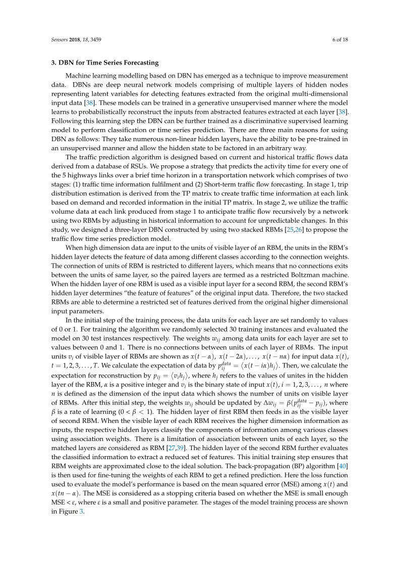
A commercial software called PTV Visum [36] is used to simulate a traffic road network.The software is used for multimodal transportation planning with an integrated network modelfor private and public transport. The TP matrix is used as inputs to the PTV Visum simulation, andthe outputs are the predicted traffic volume. The TP matrix is assigned according to the availabletraffic volumes. The input information from the PTV Visum [37] offers a guideline for the traffic flowcompletion model. Traffic information are collected each minute for five of the links. Figure 2 depictsa screenshot of the simulation showing connections 1–5 that are the highway links.
5 of 18
minimum sum of squared difference, is regarded as the most similar pattern. The objective function
formula for forming the traffic patterns can be determined by Equation (2):
∆ 𝑝, 𝑡, ℎ, 𝑡 𝑤 𝑖, 𝑗 .𝐿 𝑖
𝐿
1𝑣 𝑖, 𝑡 𝑗, 𝑝
1𝑣 𝑖, 𝑡 𝑗, ℎ
(2)
where the traffic weight in cell (i, j) is shown by 𝑤 𝑖, 𝑗 , length of section i is presented by 𝐿 𝑖) and the stretch length of the road is shown by L and ∆ 𝑝, 𝑡, ℎ, 𝑡 denotes the squared difference among
the current and historical pattern. After assigning the TP matrix, standard deviation, the coefficient
of determination 𝑅 , the mean square error and linear regression line parameters should be
determined. The TP matrix fixes the trip’s numbers with zones in each short period of time. Each TP
matrix is allocated to each transportation option. Each link shows streets and highways and nodes
which can be connected by links. The Table 1 shows values for the highway links.
Table 1. Values for highway links.
Criteria Data Value
Highway free flow template Raw data Data on 5 mn‐spaced intervals
speed 120 km/h 10 km/5 mn interval
Average link length 2 km 5 links traversed/5 mn interval
Highway Congested template Raw data Data on 5 mn‐spaced intervals
Average speed 72 km/h 6 km/5 mn interval
Average link length 2 km 3 links traversed/5 mn interval
A commercial software called PTV Visum [36] is used to simulate a traffic road network. The
software is used for multimodal transportation planning with an integrated network model for
private and public transport. The TP matrix is used as inputs to the PTV Visum simulation, and the
outputs are the predicted traffic volume. The TP matrix is assigned according to the available traffic
volumes. The input information from the PTV Visum [37] offers a guideline for the traffic flow
completion model. Traffic information are collected each minute for five of the links. Figure 2 depicts
a screenshot of the simulation showing connections 1–5 that are the highway links.
Figure 2. Case study traffic network with five highways links. The numbers 1 to 5 illustrate 5 highways
links.
3. DBN for Time Series Forecasting
Machine learning modelling based on DBN has emerged as a technique to improve measurement
data. DBNs are deep neural network models comprising of multiple layers of hidden nodes
Figure 2. Case study traffic network with five highways links. The numbers 1 to 5 illustrate5 highways links.
Sensors 2018, 18, 3459 6 of 18
3. DBN for Time Series Forecasting
Machine learning modelling based on DBN has emerged as a technique to improve measurementdata. DBNs are deep neural network models comprising of multiple layers of hidden nodesrepresenting latent variables for detecting features extracted from the original multi-dimensionalinput data [38]. These models can be trained in a generative unsupervised manner where the modellearns to probabilistically reconstruct the inputs from abstracted features extracted at each layer [38].Following this learning step the DBN can be further trained as a discriminative supervised learningmodel to perform classification or time series prediction. There are three main reasons for usingDBN as follows: They take numerous non-linear hidden layers, have the ability to be pre-trained inan unsupervised manner and allow the hidden state to be factored in an arbitrary way.
The traffic prediction algorithm is designed based on current and historical traffic flows dataderived from a database of RSUs. We propose a strategy that predicts the activity time for every one ofthe 5 highways links over a brief time horizon in a transportation network which comprises of twostages: (1) traffic time information fulfilment and (2) Short-term traffic flow forecasting. In stage 1, tripdistribution estimation is derived from the TP matrix to create traffic time information at each linkbased on demand and recorded information in the initial TP matrix. In stage 2, we utilize the trafficvolume data at each link produced from stage 1 to anticipate traffic flow recursively by a networkusing two RBMs by adjusting in historical information to account for unpredictable changes. In thisstudy, we designed a three-layer DBN constructed by using two stacked RBMs [25,26] to propose thetraffic flow time series prediction model.
When high dimension data are input to the units of visible layer of an RBM, the units in the RBM’shidden layer detects the feature of data among different classes according to the connection weights.The connection of units of RBM is restricted to different layers, which means that no connections exitsbetween the units of same layer, so the paired layers are termed as a restricted Boltzman machine.When the hidden layer of one RBM is used as a visible input layer for a second RBM, the second RBM’shidden layer determines “the feature of features” of the original input data. Therefore, the two stackedRBMs are able to determine a restricted set of features derived from the original higher dimensionalinput parameters.
In the initial step of the training process, the data units for each layer are set randomly to valuesof 0 or 1. For training the algorithm we randomly selected 30 training instances and evaluated themodel on 30 test instances respectively. The weights wij among data units for each layer are set tovalues between 0 and 1. There is no connections between units of each layer of RBMs. The inputunits vi of visible layer of RBMs are shown as x(t− α), x(t− 2α), . . . , x(t− nα) for input data x(t),t = 1, 2, 3, . . . , T. We calculate the expectation of data by pdata
ij =⟨
x(t− iα)hj⟩. Then, we calculate the
expectation for reconstruction by pij =⟨vihj
⟩, where hj refers to the values of unites in the hidden
layer of the RBM, α is a positive integer and vi is the binary state of input x(t), i = 1, 2, 3, . . . , n wheren is defined as the dimension of the input data which shows the number of units on visible layerof RBMs. After this initial step, the weights wij should be updated by ∆wij = β(pdata
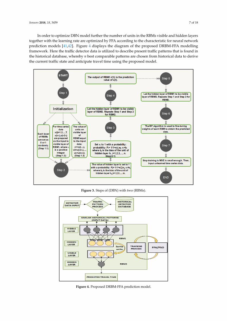
ij − pij), whereβ is a rate of learning (0 < β < 1). The hidden layer of first RBM then feeds in as the visible layerof second RBM. When the visible layer of each RBM receives the higher dimension information asinputs, the respective hidden layers classify the components of information among various classesusing association weights. There is a limitation of association between units of each layer, so thematched layers are considered as RBM [27,39]. The hidden layer of the second RBM further evaluatesthe classified information to extract a reduced set of features. This initial training step ensures thatRBM weights are approximated close to the ideal solution. The back-propagation (BP) algorithm [40]is then used for fine-tuning the weights of each RBM to get a refined prediction. Here the loss functionused to evaluate the model’s performance is based on the mean squared error (MSE) among x(t) andx(tn− α). The MSE is considered as a stopping criteria based on whether the MSE is small enoughMSE < ε, where ε is a small and positive parameter. The stages of the model training process are shownin Figure 3.
Sensors 2018, 18, 3459 7 of 18
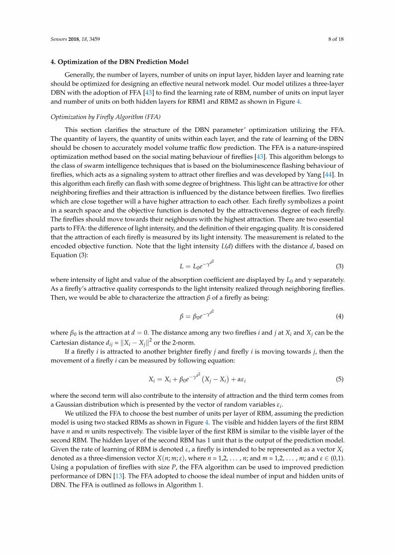
In order to optimize DBN model further the number of units in the RBMs visible and hidden layerstogether with the learning rate are optimized by FFA according to the characteristic for neural networkprediction models [41,42]. Figure 4 displays the diagram of the proposed DRBM-FFA modellingframework. Here the traffic detector data is utilized to describe present traffic patterns that is found inthe historical database, whereby n best comparable patterns are chosen from historical data to derivethe current traffic state and anticipate travel time using the proposed model.
7 of 18
is found in the historical database, whereby n best comparable patterns are chosen from historical
data to derive the current traffic state and anticipate travel time using the proposed model.
Figure 3. Steps of (DBN) with two (RBMs).
Figure 4. Proposed DRBM‐FFA prediction model.
Figure 3. Steps of (DBN) with two (RBMs).
7 of 18
is found in the historical database, whereby n best comparable patterns are chosen from historical
data to derive the current traffic state and anticipate travel time using the proposed model.
Figure 3. Steps of (DBN) with two (RBMs).
Figure 4. Proposed DRBM‐FFA prediction model.
Figure 4. Proposed DRBM-FFA prediction model.
Sensors 2018, 18, 3459 8 of 18
4. Optimization of the DBN Prediction Model
Generally, the number of layers, number of units on input layer, hidden layer and learning rateshould be optimized for designing an effective neural network model. Our model utilizes a three-layerDBN with the adoption of FFA [43] to find the learning rate of RBM, number of units on input layerand number of units on both hidden layers for RBM1 and RBM2 as shown in Figure 4.
Optimization by Firefly Algorithm (FFA)
This section clarifies the structure of the DBN parameter’ optimization utilizing the FFA.The quantity of layers, the quantity of units within each layer, and the rate of learning of the DBNshould be chosen to accurately model volume traffic flow prediction. The FFA is a nature-inspiredoptimization method based on the social mating behaviour of fireflies [43]. This algorithm belongs tothe class of swarm intelligence techniques that is based on the bioluminescence flashing behaviour offireflies, which acts as a signaling system to attract other fireflies and was developed by Yang [44]. Inthis algorithm each firefly can flash with some degree of brightness. This light can be attractive for otherneighboring fireflies and their attraction is influenced by the distance between fireflies. Two fireflieswhich are close together will a have higher attraction to each other. Each firefly symbolizes a pointin a search space and the objective function is denoted by the attractiveness degree of each firefly.The fireflies should move towards their neighbours with the highest attraction. There are two essentialparts to FFA: the difference of light intensity, and the definition of their engaging quality. It is consideredthat the attraction of each firefly is measured by its light intensity. The measurement is related to theencoded objective function. Note that the light intensity L(d) differs with the distance d, based onEquation (3):
L = L0e−γd2(3)
where intensity of light and value of the absorption coefficient are displayed by L0 and γ separately.As a firefly’s attractive quality corresponds to the light intensity realized through neighboring fireflies.Then, we would be able to characterize the attraction β of a firefly as being:
β = β0e−γd2(4)
where β0 is the attraction at d = 0. The distance among any two fireflies i and j at Xi and Xj can be theCartesian distance dij = ‖Xi − Xj‖2 or the 2-norm.
If a firefly i is attracted to another brighter firefly j and firefly i is moving towards j, then themovement of a firefly i can be measured by following equation:
Xi = Xi + β0e−γd2 (Xj − Xi
)+ αεi (5)
where the second term will also contribute to the intensity of attraction and the third term comes froma Gaussian distribution which is presented by the vector of random variables εi.
We utilized the FFA to choose the best number of units per layer of RBM, assuming the predictionmodel is using two stacked RBMs as shown in Figure 4. The visible and hidden layers of the first RBMhave n and m units respectively. The visible layer of the first RBM is similar to the visible layer of thesecond RBM. The hidden layer of the second RBM has 1 unit that is the output of the prediction model.Given the rate of learning of RBM is denoted ε, a firefly is intended to be represented as a vector Xidenoted as a three-dimension vector X(n; m; ε), where n = 1,2, . . . , n; and m = 1,2, . . . , m; and ε ∈ (0,1).Using a population of fireflies with size P, the FFA algorithm can be used to improved predictionperformance of DBN [13]. The FFA adopted to choose the ideal number of input and hidden units ofDBN. The FFA is outlined as follows in Algorithm 1.
Sensors 2018, 18, 3459 9 of 18
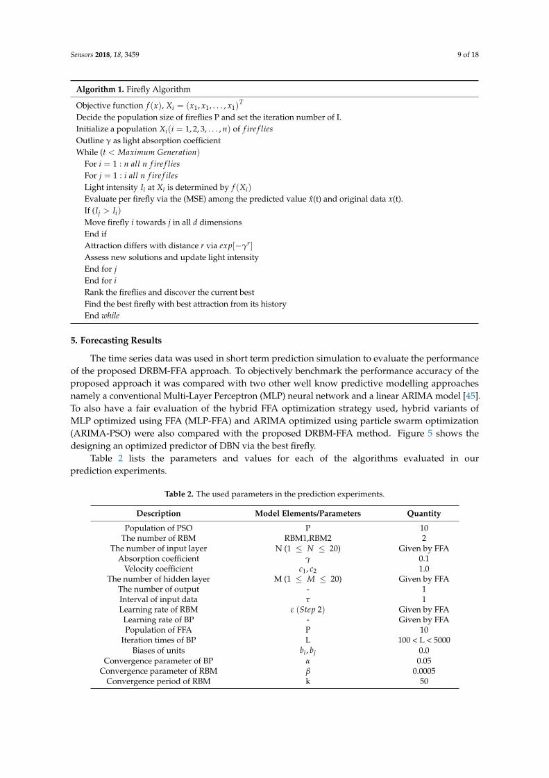
Algorithm 1. Firefly Algorithm
Objective function f (x), Xi = (x1, x1, . . . , x1)T
Decide the population size of fireflies P and set the iteration number of I.Initialize a population Xi(i = 1, 2, 3, . . . , n) of f ire f liesOutline γ as light absorption coefficientWhile (t < Maximum Generation)
For i = 1 : n all n f ire f liesFor j = 1 : i all n f ire f ilesLight intensity Ii at Xi is determined by f (Xi)
Evaluate per firefly via the (MSE) among the predicted value x(t) and original data x(t).If (Ij > Ii)
Move firefly i towards j in all d dimensionsEnd ifAttraction differs with distance r via exp[−γr]
Assess new solutions and update light intensityEnd for jEnd for iRank the fireflies and discover the current bestFind the best firefly with best attraction from its historyEnd while
5. Forecasting Results
The time series data was used in short term prediction simulation to evaluate the performanceof the proposed DRBM-FFA approach. To objectively benchmark the performance accuracy of theproposed approach it was compared with two other well know predictive modelling approachesnamely a conventional Multi-Layer Perceptron (MLP) neural network and a linear ARIMA model [45].To also have a fair evaluation of the hybrid FFA optimization strategy used, hybrid variants ofMLP optimized using FFA (MLP-FFA) and ARIMA optimized using particle swarm optimization(ARIMA-PSO) were also compared with the proposed DRBM-FFA method. Figure 5 shows thedesigning an optimized predictor of DBN via the best firefly.
Table 2 lists the parameters and values for each of the algorithms evaluated in ourprediction experiments.
Table 2. The used parameters in the prediction experiments.
Description Model Elements/Parameters Quantity
Population of PSO P 10The number of RBM RBM1,RBM2 2
The number of input layer N (1 ≤ N ≤ 20) Given by FFAAbsorption coefficient γ 0.1
Velocity coefficient c1, c2 1.0The number of hidden layer M (1 ≤ M ≤ 20) Given by FFA
The number of output - 1Interval of input data τ 1Learning rate of RBM ε (Step 2) Given by FFA
Learning rate of BP - Given by FFAPopulation of FFA P 10
Iteration times of BP L 100 < L < 5000Biases of units bi, bj 0.0
Convergence parameter of BP α 0.05Convergence parameter of RBM β 0.0005
Convergence period of RBM k 50
Sensors 2018, 18, 3459 10 of 18
Short-term prediction accuracy of the DRBM-FFA model compared against the ARIMA, MLP-FFAand ARIMA-PSO are shown in Figure 6. Each algorithm is used to predict traffic flows in all five linksin the traffic network where traffic data is utilized to predict traffic flow for the whole transportationnetwork. The short-term prediction precision of the DRBM-FFA is compared against each of the othermodels and the results are shown in Figures 7–10.
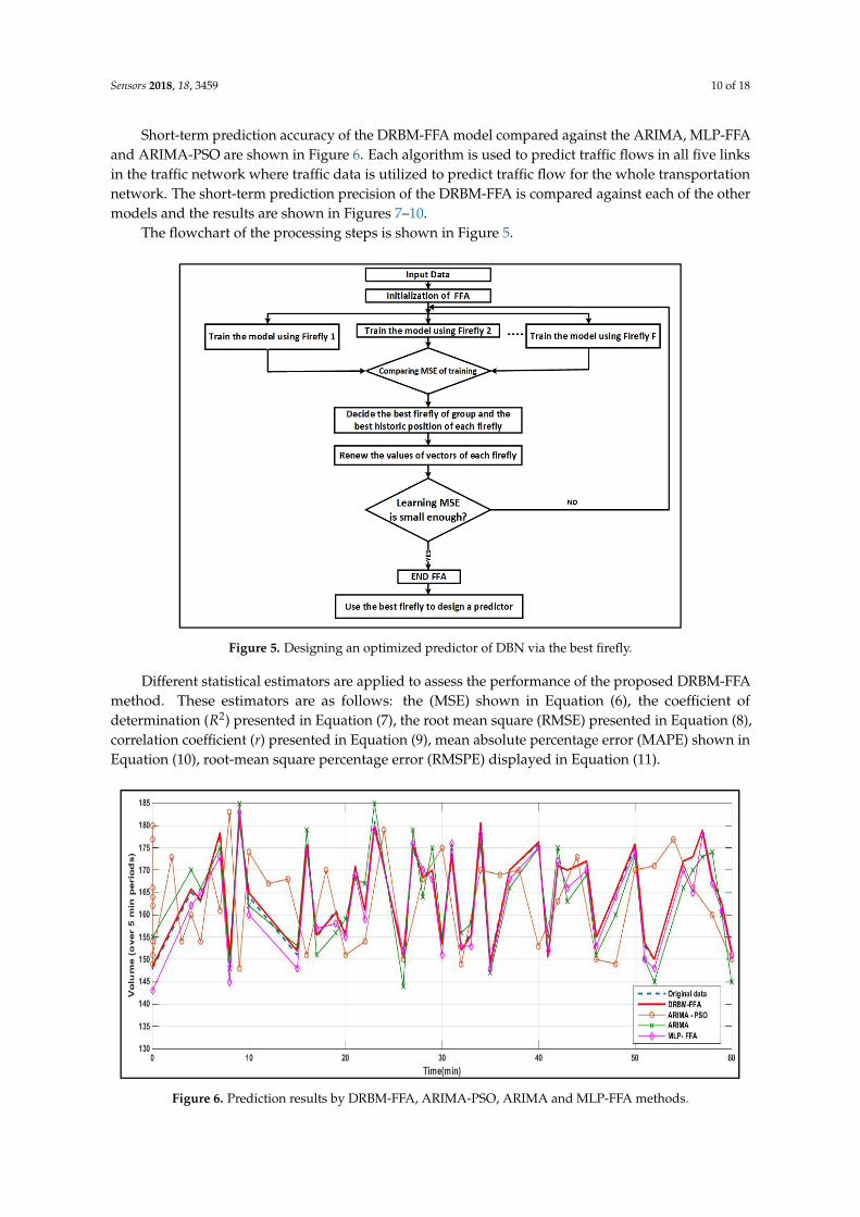
The flowchart of the processing steps is shown in Figure 5.
10 of 18
Short‐term prediction accuracy of the DRBM‐FFA model compared against the ARIMA, MLP‐
FFA and ARIMA‐PSO are shown in Figure 6. Each algorithm is used to predict traffic flows in all five
links in the traffic network where traffic data is utilized to predict traffic flow for the whole
transportation network. The short‐term prediction precision of the DRBM‐FFA is compared against
each of the other models and the results are shown in Figures 7–10.
The flowchart of the processing steps is shown in Figure 5.
Figure 5. Designing an optimized predictor of DBN via the best firefly.
Different statistical estimators are applied to assess the performance of the proposed DRBM‐
FFA method. These estimators are as follows: the (MSE) shown in Equation (6), the coefficient of
determination (𝑅 ) presented in Equation (7), the root mean square (RMSE) presented in Equation
(8), correlation coefficient (r) presented in Equation (9), mean absolute percentage error (MAPE)
shown in Equation (10), root‐mean square percentage error (RMSPE) displayed in Equation (11).
Figure 6. Prediction results by DRBM‐FFA, ARIMA‐PSO, ARIMA and MLP‐FFA methods.
Figure 5. Designing an optimized predictor of DBN via the best firefly.
Different statistical estimators are applied to assess the performance of the proposed DRBM-FFAmethod. These estimators are as follows: the (MSE) shown in Equation (6), the coefficient ofdetermination (R2) presented in Equation (7), the root mean square (RMSE) presented in Equation (8),correlation coefficient (r) presented in Equation (9), mean absolute percentage error (MAPE) shown inEquation (10), root-mean square percentage error (RMSPE) displayed in Equation (11).
10 of 18
Short‐term prediction accuracy of the DRBM‐FFA model compared against the ARIMA, MLP‐
FFA and ARIMA‐PSO are shown in Figure 6. Each algorithm is used to predict traffic flows in all five
links in the traffic network where traffic data is utilized to predict traffic flow for the whole
transportation network. The short‐term prediction precision of the DRBM‐FFA is compared against
each of the other models and the results are shown in Figures 7–10.
The flowchart of the processing steps is shown in Figure 5.
Figure 5. Designing an optimized predictor of DBN via the best firefly.
Different statistical estimators are applied to assess the performance of the proposed DRBM‐
FFA method. These estimators are as follows: the (MSE) shown in Equation (6), the coefficient of
determination (𝑅 ) presented in Equation (7), the root mean square (RMSE) presented in Equation
(8), correlation coefficient (r) presented in Equation (9), mean absolute percentage error (MAPE)
shown in Equation (10), root‐mean square percentage error (RMSPE) displayed in Equation (11).
Figure 6. Prediction results by DRBM‐FFA, ARIMA‐PSO, ARIMA and MLP‐FFA methods. Figure 6. Prediction results by DRBM-FFA, ARIMA-PSO, ARIMA and MLP-FFA methods.
Sensors 2018, 18, 3459 11 of 18
MSE =1r
r
∑i=1
(Dpi − Dai
)2 (6)
R2 = 1−∑r
i=1(
Dpi − Dai)2
∑ri=1(
Dpi − Dav)2 (7)
RMSE =
√1r
n
∑i=1
(Dpi − Dai
)2 (8)
r =∑n
i=1(
Dpi − Dpi).(
Dai − Dai)√
∑ni=1(
Dpi − Dpi). ∑n
i=1(
Dpi − Dpi) (9)
MAPE =1r
n
∑i=1
∣∣∣∣Dpi − Dai
Dai
∣∣∣∣× 100 (10)
RMSPE =
√√√√ 1n
n
∑l=1
[Dpl − Dl
Dl
]2
(11)
where n is the quantity of data, Dpi is the predicted value; Dav is the average of the actual values; Dai isthe actual value; Dpl is the predicted traffic flow; Dl shows the measured traffic flow for link l; Dpi andDai are the mean value of Dpi and Dai, respectively. The coefficient of determination, R2 represents thelinear regression line among the predicted values of the neural network model. The essential output, isapplied as a measure of performance. Expressed differently, R2 is the square of the correlation betweenthe response values and the predicted response values. The closer R2 is to 1, the better the modelcan fit the actual data [46]. This measurement controls the degree of success the fit has in stating thechange of the data. It can be indicated as the square of the multiple correlation coefficients, and thecoefficient of multiple determinations. The smaller amount of MAPE has a superior performancemodel, and conversely, in the case of r. The detail prediction errors (MSEs) for the original data areshown in Table 3.
Table 3. The detail prediction errors (MSEs).
Structure and Evaluation MLP-FFA ARIMA ARIMA-PSO DRBM-FFA
Learning rates 0.85 0.64 0.73 0.98Iterations 336 350 298 200
Learning MSE 109.21 122.4 108.9 98.70Short-term prediction MSE 234.38 280.50 126.11 109.38
Table 3 shows that the DRBM was able to outperform in comparison to the other approaches basedon obtaining the lowest learning MSE and short-term prediction MSE based on the time series resultsshown in Figures 7–10. The MLP with FFA obtained the next lowest learning MSE and short-termprediction MSE followed by the ARIMA. The Monte Carlo method was used to acquire a moreobjective evaluation of the performance of each approach that is based on sampling testing data basedon sub-blocks to evaluate the forecasting efficiency of the algorithm.
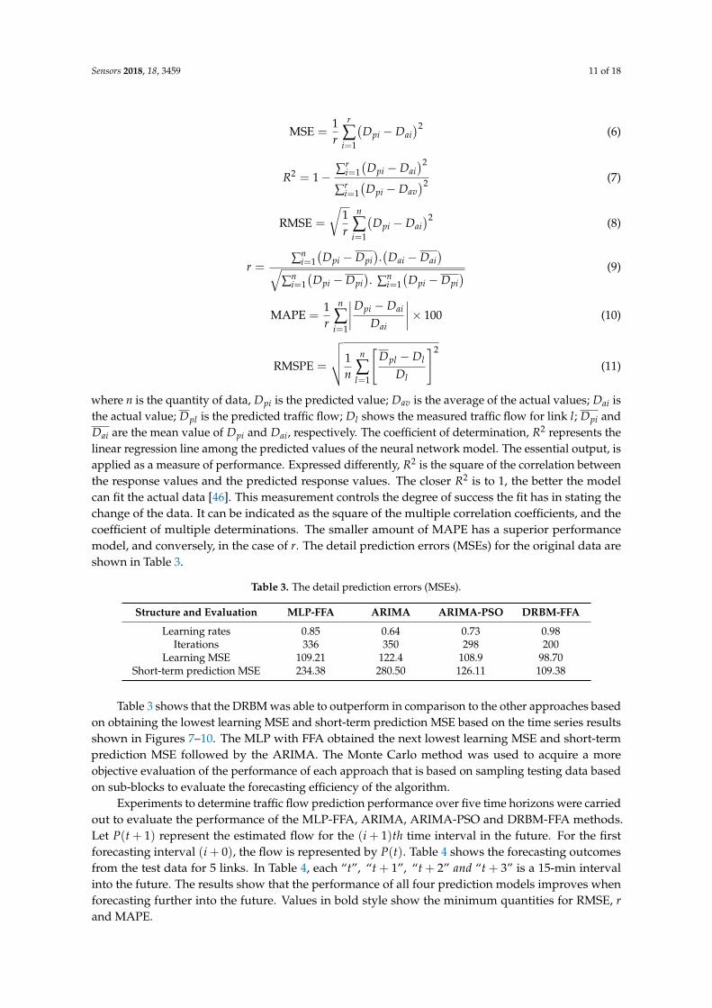
Experiments to determine traffic flow prediction performance over five time horizons were carriedout to evaluate the performance of the MLP-FFA, ARIMA, ARIMA-PSO and DRBM-FFA methods.Let P(t + 1) represent the estimated flow for the (i + 1)th time interval in the future. For the firstforecasting interval (i + 0), the flow is represented by P(t). Table 4 shows the forecasting outcomesfrom the test data for 5 links. In Table 4, each “t”, “t + 1”, “t + 2” and “t + 3” is a 15-min intervalinto the future. The results show that the performance of all four prediction models improves whenforecasting further into the future. Values in bold style show the minimum quantities for RMSE, rand MAPE.
Sensors 2018, 18, 3459 12 of 18
Table 4 shows that all error measurement for DRBM-FFA are less than those for the otheralgorithms for all 15-min prediction intervals. As shown in Table 4, DRBM-FFA outperformedMLP-FFA, ARIMA, and ARIMA-PSO forecasters for all three time intervals. As anticipated, the PSOimproved prediction accuracy of the ARIMA model.
Figure 7 further illustrates the prediction results of selected links every 5 min for DRBM-FFA forthe next 30 min which was determined using root-mean square percentage Error (RMSPE). Figure 7demonstrates the RMSPE for the selected links.
Table 4. Traffic flow prediction results.
Predictor Time Interval r RMSE MAPE
MLP-FFA
t 3.2 6.8 12.07%t + 1 3.5 7.2 13.95%t + 2 3.6 7.8 14.89%t + 3 3.9 7.9 15.32%
ARIMA
t 4.4 9.1 13.56%t + 1 4.6 9.7 15.37%t + 2 6.8 14.2 18.93%t + 3 8.5 15.7 23.24%
ARIMA-PSO
t 3.3 6.8 9.39%t + 1 3.4 6.9 9.89%t + 2 3.7 7.2 10.48%t + 3 3.9 7.8 11.57%
DRBM-FFA
t 2.9 6.1 8.75%t + 1 3.1 6.4 9.63%t + 2 3.4 6.9 10.31%t + 3 3.5 7.1 11.12%
12 of 18
when forecasting further into the future. Values in bold style show the minimum quantities for RMSE,
r and MAPE.
Table 4 shows that all error measurement for DRBM‐FFA are less than those for the other
algorithms for all 15‐min prediction intervals. As shown in Table 4, DRBM‐FFA outperformed MLP‐
FFA, ARIMA, and ARIMA‐PSO forecasters for all three time intervals. As anticipated, the PSO
improved prediction accuracy of the ARIMA model.
Figure 7 further illustrates the prediction results of selected links every 5 min for DRBM‐FFA for
the next 30 min which was determined using root‐mean square percentage Error (RMSPE). Figure 7
demonstrates the RMSPE for the selected links.
Table 4. Traffic flow prediction results.
Predictor Time Interval r RMSE MAPE
MLP‐FFA
t 3.2 6.8 12.07%
t + 1 3.5 7.2 13.95%
t + 2 3.6 7.8 14.89%
t + 3 3.9 7.9 15.32%
ARIMA
t 4.4 9.1 13.56%
t + 1 4.6 9.7 15.37%
t + 2 6.8 14.2 18.93%
t + 3 8.5 15.7 23.24%
ARIMA‐PSO
t 3.3 6.8 9.39%
t + 1 3.4 6.9 9.89%
t + 2 3.7 7.2 10.48%
t + 3 3.9 7.8 11.57%
DRBM‐FFA
t 2.9 6.1 8.75%
t + 1 3.1 6.4 9.63%
t + 2 3.4 6.9 10.31%
t + 3 3.5 7.1 11.12%
Figure 7. RMSPE for the targeted links.
In addition to the given experiments, Monte Carlo [47] method is applied to assess the sensitivity
and accuracy of each predictive algorithm due to the stochastic variation of traffic data. Firstly, in
each experiment, the ratio of traffic flow for links is calculated. Secondly, 50% of the ratio of traffic
flow for links are designated randomly. Thirdly, selected data is increased by a Gaussian random
variable 𝑟. Fourthly, the new ratio of traffic flow for each link are served to the predictive method,
and the results are recorded. The final stage is where, the four previous stages should be repeated
5 10 15 20 25 30
RMS %(10 am) 1.05 4.22 5.36 5.39 6.25 7.34
RMS %(2pm) 1.98 4.36 5.17 8.22 9.43 9.45
RMS %(9pm) 0.92 2.16 5.49 6.29 7.14 8.23
RMS PE
TIME
RMS %(10 am) RMS %(2pm) RMS %(9pm)
Figure 7. RMSPE for the targeted links.
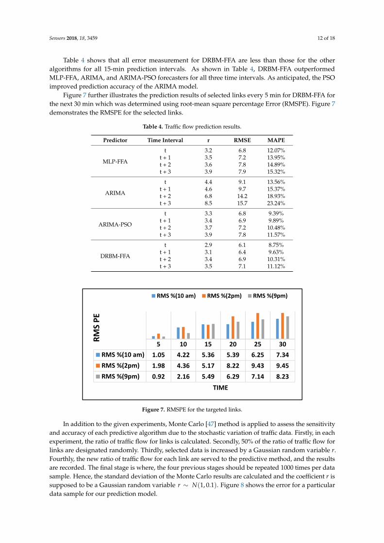
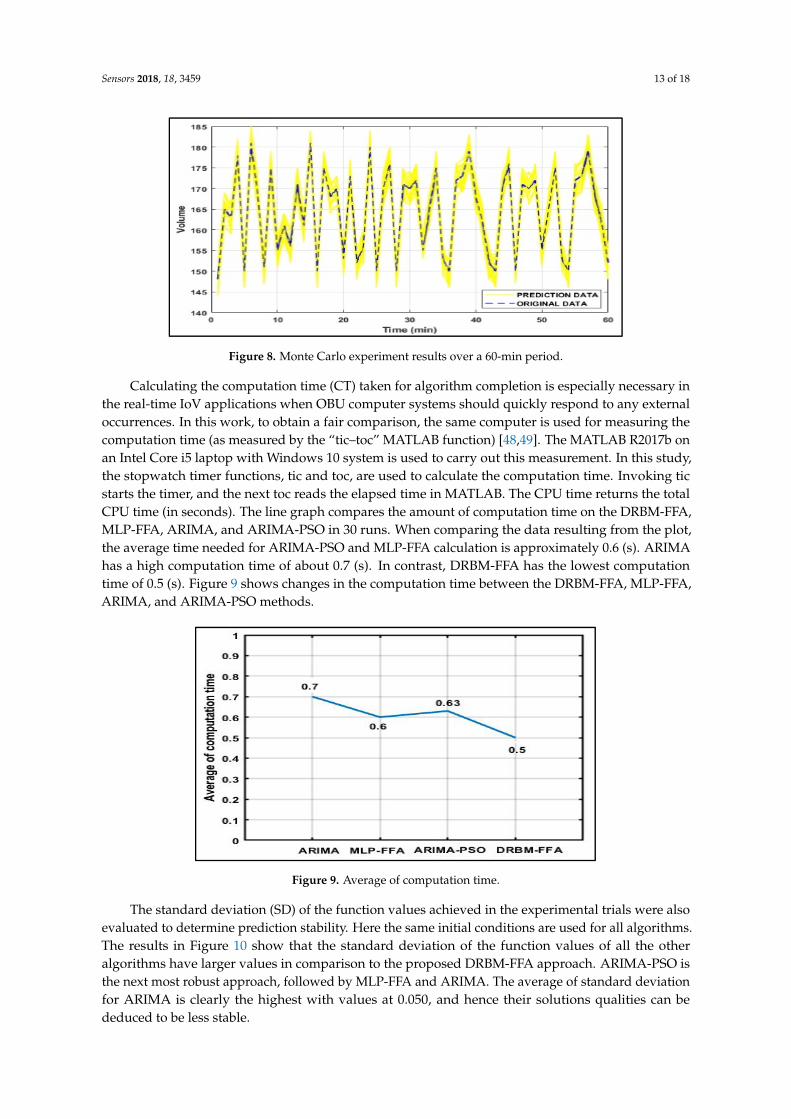
In addition to the given experiments, Monte Carlo [47] method is applied to assess the sensitivityand accuracy of each predictive algorithm due to the stochastic variation of traffic data. Firstly, in eachexperiment, the ratio of traffic flow for links is calculated. Secondly, 50% of the ratio of traffic flow forlinks are designated randomly. Thirdly, selected data is increased by a Gaussian random variable r.Fourthly, the new ratio of traffic flow for each link are served to the predictive method, and the resultsare recorded. The final stage is where, the four previous stages should be repeated 1000 times per datasample. Hence, the standard deviation of the Monte Carlo results are calculated and the coefficient r issupposed to be a Gaussian random variable r ∼ N(1, 0.1). Figure 8 shows the error for a particulardata sample for our prediction model.
Sensors 2018, 18, 3459 13 of 18
13 of 18
1000 times per data sample. Hence, the standard deviation of the Monte Carlo results are calculated
and the coefficient 𝑟 is supposed to be a Gaussian random variable 𝑟~ 𝑁 1,0.1 . Figure 8 shows
the error for a particular data sample for our prediction model.
Figure 8. Monte Carlo experiment results over a 60‐min period.
Calculating the computation time (CT) taken for algorithm completion is especially necessary in
the real‐time IoV applications when OBU computer systems should quickly respond to any external
occurrences. In this work, to obtain a fair comparison, the same computer is used for measuring the
computation time (as measured by the “tic–toc” MATLAB function) [48,49]. The MATLAB R2017b
on an Intel Core i5 laptop with Windows 10 system is used to carry out this measurement. In this
study, the stopwatch timer functions, tic and toc, are used to calculate the computation time. Invoking
tic starts the timer, and the next toc reads the elapsed time in MATLAB. The CPU time returns the
total CPU time (in seconds). The line graph compares the amount of computation time on the DRBM‐
FFA, MLP‐FFA, ARIMA, and ARIMA‐PSO in 30 runs. When comparing the data resulting from the
plot, the average time needed for ARIMA‐PSO and MLP‐FFA calculation is approximately 0.6 (s).
ARIMA has a high computation time of about 0.7 (s). In contrast, DRBM‐FFA has the lowest
computation time of 0.5 (s). Figure 9 shows changes in the computation time between the DRBM‐
FFA, MLP‐FFA, ARIMA, and ARIMA‐PSO methods.
Figure 9. Average of computation time.
The standard deviation (SD) of the function values achieved in the experimental trials were also
evaluated to determine prediction stability. Here the same initial conditions are used for all
algorithms. The results in Figure 10 show that the standard deviation of the function values of all the
other algorithms have larger values in comparison to the proposed DRBM‐FFA approach. ARIMA‐
PSO is the next most robust approach, followed by MLP‐FFA and ARIMA. The average of standard
Figure 8. Monte Carlo experiment results over a 60-min period.
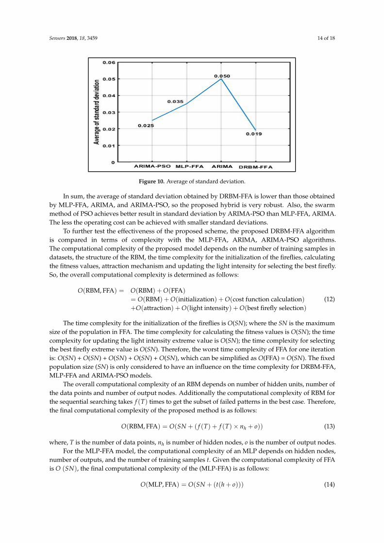
Calculating the computation time (CT) taken for algorithm completion is especially necessary inthe real-time IoV applications when OBU computer systems should quickly respond to any externaloccurrences. In this work, to obtain a fair comparison, the same computer is used for measuring thecomputation time (as measured by the “tic–toc” MATLAB function) [48,49]. The MATLAB R2017b onan Intel Core i5 laptop with Windows 10 system is used to carry out this measurement. In this study,the stopwatch timer functions, tic and toc, are used to calculate the computation time. Invoking ticstarts the timer, and the next toc reads the elapsed time in MATLAB. The CPU time returns the totalCPU time (in seconds). The line graph compares the amount of computation time on the DRBM-FFA,MLP-FFA, ARIMA, and ARIMA-PSO in 30 runs. When comparing the data resulting from the plot,the average time needed for ARIMA-PSO and MLP-FFA calculation is approximately 0.6 (s). ARIMAhas a high computation time of about 0.7 (s). In contrast, DRBM-FFA has the lowest computationtime of 0.5 (s). Figure 9 shows changes in the computation time between the DRBM-FFA, MLP-FFA,ARIMA, and ARIMA-PSO methods.
13 of 18
1000 times per data sample. Hence, the standard deviation of the Monte Carlo results are calculated
and the coefficient 𝑟 is supposed to be a Gaussian random variable 𝑟~ 𝑁 1,0.1 . Figure 8 shows
the error for a particular data sample for our prediction model.
Figure 8. Monte Carlo experiment results over a 60‐min period.
Calculating the computation time (CT) taken for algorithm completion is especially necessary in
the real‐time IoV applications when OBU computer systems should quickly respond to any external
occurrences. In this work, to obtain a fair comparison, the same computer is used for measuring the
computation time (as measured by the “tic–toc” MATLAB function) [48,49]. The MATLAB R2017b
on an Intel Core i5 laptop with Windows 10 system is used to carry out this measurement. In this
study, the stopwatch timer functions, tic and toc, are used to calculate the computation time. Invoking
tic starts the timer, and the next toc reads the elapsed time in MATLAB. The CPU time returns the
total CPU time (in seconds). The line graph compares the amount of computation time on the DRBM‐
FFA, MLP‐FFA, ARIMA, and ARIMA‐PSO in 30 runs. When comparing the data resulting from the
plot, the average time needed for ARIMA‐PSO and MLP‐FFA calculation is approximately 0.6 (s).
ARIMA has a high computation time of about 0.7 (s). In contrast, DRBM‐FFA has the lowest
computation time of 0.5 (s). Figure 9 shows changes in the computation time between the DRBM‐
FFA, MLP‐FFA, ARIMA, and ARIMA‐PSO methods.
Figure 9. Average of computation time.
The standard deviation (SD) of the function values achieved in the experimental trials were also
evaluated to determine prediction stability. Here the same initial conditions are used for all
algorithms. The results in Figure 10 show that the standard deviation of the function values of all the
other algorithms have larger values in comparison to the proposed DRBM‐FFA approach. ARIMA‐
PSO is the next most robust approach, followed by MLP‐FFA and ARIMA. The average of standard
Figure 9. Average of computation time.
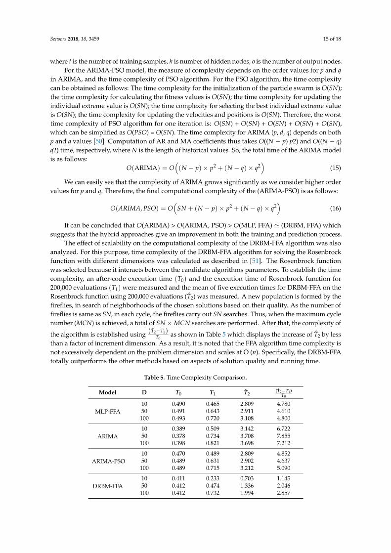
The standard deviation (SD) of the function values achieved in the experimental trials were alsoevaluated to determine prediction stability. Here the same initial conditions are used for all algorithms.The results in Figure 10 show that the standard deviation of the function values of all the otheralgorithms have larger values in comparison to the proposed DRBM-FFA approach. ARIMA-PSO isthe next most robust approach, followed by MLP-FFA and ARIMA. The average of standard deviationfor ARIMA is clearly the highest with values at 0.050, and hence their solutions qualities can bededuced to be less stable.
Sensors 2018, 18, 3459 14 of 18
14 of 18
deviation for ARIMA is clearly the highest with values at 0.050, and hence their solutions qualities
can be deduced to be less stable.
Figure 10. Average of standard deviation.
In sum, the average of standard deviation obtained by DRBM‐FFA is lower than those obtained
by MLP‐FFA, ARIMA, and ARIMA‐PSO, so the proposed hybrid is very robust. Also, the swarm
method of PSO achieves better result in standard deviation by ARIMA‐PSO than MLP‐FFA, ARIMA.
The less the operating cost can be achieved with smaller standard deviations.
To further test the effectiveness of the proposed scheme, the proposed DRBM‐FFA algorithm is
compared in terms of complexity with the MLP‐FFA, ARIMA, ARIMA‐PSO algorithms. The
computational complexity of the proposed model depends on the number of training samples in
datasets, the structure of the RBM, the time complexity for the initialization of the fireflies, calculating
the fitness values, attraction mechanism and updating the light intensity for selecting the best firefly.
So, the overall computational complexity is determined as follows:
𝑂 RBM, FFA 𝑂 RBM 𝑂 FFA𝑂 RBM 𝑂 initialization 𝑂 cost function calculation𝑂 attraction 𝑂 light intensity 𝑂 best firefly selection
(12)
The time complexity for the initialization of the fireflies is O(SN); where the SN is the maximum
size of the population in FFA. The time complexity for calculating the fitness values is O(SN); the
time complexity for updating the light intensity extreme value is O(SN); the time complexity for
selecting the best firefly extreme value is O(SN). Therefore, the worst time complexity of FFA for one
iteration is: O(SN) + O(SN) + O(SN) + O(SN) + O(SN), which can be simplified as O(FFA) = O(SN). The
fixed population size (SN) is only considered to have an influence on the time complexity for DRBM‐
FFA, MLP‐FFA and ARIMA‐PSO models.
The overall computational complexity of an RBM depends on number of hidden units, number
of the data points and number of output nodes. Additionally the computational complexity of RBM
for the sequential searching takes 𝑓 𝑇 times to get the subset of failed patterns in the best case.
Therefore, the final computational complexity of the proposed method is as follows:
𝑂 RBM, FFA 𝑂 𝑆𝑁 𝑓 𝑇 𝑓 𝑇 𝑛 𝑜 (13)
where, T is the number of data points, 𝑛 is number of hidden nodes, o is the number of output nodes.
For the MLP‐FFA model, the computational complexity of an MLP depends on hidden nodes,
number of outputs, and the number of training samples 𝑡. Given the computational complexity of
FFA is 𝑂 𝑆𝑁 , the final computational complexity of the (MLP‐FFA) is as follows:
𝑂 MLP, FFA 𝑂 𝑆𝑁 𝑡 ℎ 𝑜 (14)
Figure 10. Average of standard deviation.
In sum, the average of standard deviation obtained by DRBM-FFA is lower than those obtainedby MLP-FFA, ARIMA, and ARIMA-PSO, so the proposed hybrid is very robust. Also, the swarmmethod of PSO achieves better result in standard deviation by ARIMA-PSO than MLP-FFA, ARIMA.The less the operating cost can be achieved with smaller standard deviations.
To further test the effectiveness of the proposed scheme, the proposed DRBM-FFA algorithmis compared in terms of complexity with the MLP-FFA, ARIMA, ARIMA-PSO algorithms.The computational complexity of the proposed model depends on the number of training samples indatasets, the structure of the RBM, the time complexity for the initialization of the fireflies, calculatingthe fitness values, attraction mechanism and updating the light intensity for selecting the best firefly.So, the overall computational complexity is determined as follows:
O(RBM, FFA) = O(RBM) + O(FFA)
= O(RBM) + O(initialization) + O(cost function calculation)+O(attraction) + O(light intensity) + O(best firefly selection)
(12)
The time complexity for the initialization of the fireflies is O(SN); where the SN is the maximumsize of the population in FFA. The time complexity for calculating the fitness values is O(SN); the timecomplexity for updating the light intensity extreme value is O(SN); the time complexity for selectingthe best firefly extreme value is O(SN). Therefore, the worst time complexity of FFA for one iterationis: O(SN) + O(SN) + O(SN) + O(SN) + O(SN), which can be simplified as O(FFA) = O(SN). The fixedpopulation size (SN) is only considered to have an influence on the time complexity for DRBM-FFA,MLP-FFA and ARIMA-PSO models.
The overall computational complexity of an RBM depends on number of hidden units, number ofthe data points and number of output nodes. Additionally the computational complexity of RBM forthe sequential searching takes f (T) times to get the subset of failed patterns in the best case. Therefore,the final computational complexity of the proposed method is as follows:
O(RBM, FFA) = O(SN + ( f (T) + f (T)× nh + o)) (13)
where, T is the number of data points, nh is number of hidden nodes, o is the number of output nodes.For the MLP-FFA model, the computational complexity of an MLP depends on hidden nodes,
number of outputs, and the number of training samples t. Given the computational complexity of FFAis O (SN), the final computational complexity of the (MLP-FFA) is as follows:
O(MLP, FFA) = O(SN + (t(h + o))) (14)
Sensors 2018, 18, 3459 15 of 18
where t is the number of training samples, h is number of hidden nodes, o is the number of output nodes.For the ARIMA-PSO model, the measure of complexity depends on the order values for p and q
in ARIMA, and the time complexity of PSO algorithm. For the PSO algorithm, the time complexitycan be obtained as follows: The time complexity for the initialization of the particle swarm is O(SN);the time complexity for calculating the fitness values is O(SN); the time complexity for updating theindividual extreme value is O(SN); the time complexity for selecting the best individual extreme valueis O(SN); the time complexity for updating the velocities and positions is O(SN). Therefore, the worsttime complexity of PSO algorithm for one iteration is: O(SN) + O(SN) + O(SN) + O(SN) + O(SN),which can be simplified as O(PSO) = O(SN). The time complexity for ARIMA (p, d, q) depends on bothp and q values [50]. Computation of AR and MA coefficients thus takes O((N − p) p2) and O((N − q)q2) time, respectively, where N is the length of historical values. So, the total time of the ARIMA modelis as follows:
O(ARIMA) = O((N − p)× p2 + (N − q)× q2
)(15)
We can easily see that the complexity of ARIMA grows significantly as we consider higher ordervalues for p and q. Therefore, the final computational complexity of the (ARIMA-PSO) is as follows:
O(ARIMA, PSO) = O(
SN + (N − p)× p2 + (N − q)× q2)
(16)
It can be concluded that O(ARIMA) > O(ARIMA, PSO) > O(MLP, FFA) ' (DRBM, FFA) whichsuggests that the hybrid approaches give an improvement in both the training and prediction process.
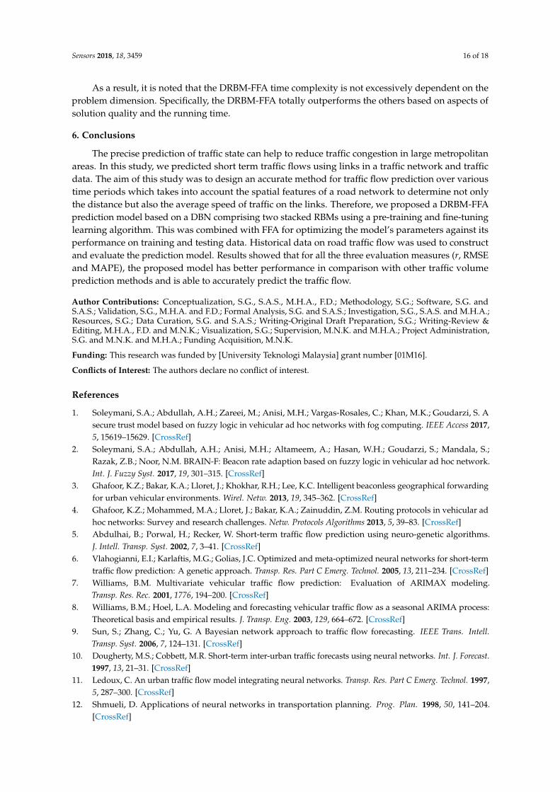
The effect of scalability on the computational complexity of the DRBM-FFA algorithm was alsoanalyzed. For this purpose, time complexity of the DRBM-FFA algorithm for solving the Rosenbrockfunction with different dimensions was calculated as described in [51]. The Rosenbrock functionwas selected because it interacts between the candidate algorithms parameters. To establish the timecomplexity, an after-code execution time (T0) and the execution time of Rosenbrock function for200,000 evaluations (T1) were measured and the mean of five execution times for DRBM-FFA on theRosenbrock function using 200,000 evaluations (T2) was measured. A new population is formed by thefireflies, in search of neighborhoods of the chosen solutions based on their quality. As the number offireflies is same as SN, in each cycle, the fireflies carry out SN searches. Thus, when the maximum cyclenumber (MCN) is achieved, a total of SN×MCN searches are performed. After that, the complexity of
the algorithm is established using (T2−T1)T0
as shown in Table 5 which displays the increase of T2 by lessthan a factor of increment dimension. As a result, it is noted that the FFA algorithm time complexity isnot excessively dependent on the problem dimension and scales at O (n). Specifically, the DRBM-FFAtotally outperforms the other methods based on aspects of solution quality and running time.
Table 5. Time Complexity Comparison.
Model D T0 T1 T2(T2−T1)
T0
MLP-FFA10 0.490 0.465 2.809 4.78050 0.491 0.643 2.911 4.610
100 0.493 0.720 3.108 4.800
ARIMA10 0.389 0.509 3.142 6.72250 0.378 0.734 3.708 7.855
100 0.398 0.821 3.698 7.212
ARIMA-PSO10 0.470 0.489 2.809 4.85250 0.489 0.631 2.902 4.637
100 0.489 0.715 3.212 5.090
DRBM-FFA10 0.411 0.233 0.703 1.14550 0.412 0.474 1.336 2.046
100 0.412 0.732 1.994 2.857
Sensors 2018, 18, 3459 16 of 18
As a result, it is noted that the DRBM-FFA time complexity is not excessively dependent on theproblem dimension. Specifically, the DRBM-FFA totally outperforms the others based on aspects ofsolution quality and the running time.
6. Conclusions
The precise prediction of traffic state can help to reduce traffic congestion in large metropolitanareas. In this study, we predicted short term traffic flows using links in a traffic network and trafficdata. The aim of this study was to design an accurate method for traffic flow prediction over varioustime periods which takes into account the spatial features of a road network to determine not onlythe distance but also the average speed of traffic on the links. Therefore, we proposed a DRBM-FFAprediction model based on a DBN comprising two stacked RBMs using a pre-training and fine-tuninglearning algorithm. This was combined with FFA for optimizing the model’s parameters against itsperformance on training and testing data. Historical data on road traffic flow was used to constructand evaluate the prediction model. Results showed that for all the three evaluation measures (r, RMSEand MAPE), the proposed model has better performance in comparison with other traffic volumeprediction methods and is able to accurately predict the traffic flow.
Author Contributions: Conceptualization, S.G., S.A.S., M.H.A., F.D.; Methodology, S.G.; Software, S.G. andS.A.S.; Validation, S.G., M.H.A. and F.D.; Formal Analysis, S.G. and S.A.S.; Investigation, S.G., S.A.S. and M.H.A.;Resources, S.G.; Data Curation, S.G. and S.A.S.; Writing-Original Draft Preparation, S.G.; Writing-Review &Editing, M.H.A., F.D. and M.N.K.; Visualization, S.G.; Supervision, M.N.K. and M.H.A.; Project Administration,S.G. and M.N.K. and M.H.A.; Funding Acquisition, M.N.K.
Funding: This research was funded by [University Teknologi Malaysia] grant number [01M16].
Conflicts of Interest: The authors declare no conflict of interest.
References
1. Soleymani, S.A.; Abdullah, A.H.; Zareei, M.; Anisi, M.H.; Vargas-Rosales, C.; Khan, M.K.; Goudarzi, S. Asecure trust model based on fuzzy logic in vehicular ad hoc networks with fog computing. IEEE Access 2017,5, 15619–15629. [CrossRef]
2. Soleymani, S.A.; Abdullah, A.H.; Anisi, M.H.; Altameem, A.; Hasan, W.H.; Goudarzi, S.; Mandala, S.;Razak, Z.B.; Noor, N.M. BRAIN-F: Beacon rate adaption based on fuzzy logic in vehicular ad hoc network.Int. J. Fuzzy Syst. 2017, 19, 301–315. [CrossRef]
3. Ghafoor, K.Z.; Bakar, K.A.; Lloret, J.; Khokhar, R.H.; Lee, K.C. Intelligent beaconless geographical forwardingfor urban vehicular environments. Wirel. Netw. 2013, 19, 345–362. [CrossRef]
4. Ghafoor, K.Z.; Mohammed, M.A.; Lloret, J.; Bakar, K.A.; Zainuddin, Z.M. Routing protocols in vehicular adhoc networks: Survey and research challenges. Netw. Protocols Algorithms 2013, 5, 39–83. [CrossRef]
5. Abdulhai, B.; Porwal, H.; Recker, W. Short-term traffic flow prediction using neuro-genetic algorithms.J. Intell. Transp. Syst. 2002, 7, 3–41. [CrossRef]
6. Vlahogianni, E.I.; Karlaftis, M.G.; Golias, J.C. Optimized and meta-optimized neural networks for short-termtraffic flow prediction: A genetic approach. Transp. Res. Part C Emerg. Technol. 2005, 13, 211–234. [CrossRef]
7. Williams, B.M. Multivariate vehicular traffic flow prediction: Evaluation of ARIMAX modeling.Transp. Res. Rec. 2001, 1776, 194–200. [CrossRef]
8. Williams, B.M.; Hoel, L.A. Modeling and forecasting vehicular traffic flow as a seasonal ARIMA process:Theoretical basis and empirical results. J. Transp. Eng. 2003, 129, 664–672. [CrossRef]
9. Sun, S.; Zhang, C.; Yu, G. A Bayesian network approach to traffic flow forecasting. IEEE Trans. Intell.Transp. Syst. 2006, 7, 124–131. [CrossRef]
10. Dougherty, M.S.; Cobbett, M.R. Short-term inter-urban traffic forecasts using neural networks. Int. J. Forecast.1997, 13, 21–31. [CrossRef]
11. Ledoux, C. An urban traffic flow model integrating neural networks. Transp. Res. Part C Emerg. Technol. 1997,5, 287–300. [CrossRef]
12. Shmueli, D. Applications of neural networks in transportation planning. Prog. Plan. 1998, 50, 141–204.[CrossRef]
Sensors 2018, 18, 3459 17 of 18
13. Dia, H. An object-oriented neural network approach to short-term traffic forecasting. Eur. J. Oper. Res. 2001,131, 253–261. [CrossRef]
14. Yin, H.B.; Wong, S.C.; Xu, J.M.; Wong, C.K. Urban traffic flow prediction using a fuzzy-neural approach.Transp. Res. Part C Emerg. Technol. 2002, 10, 85–98. [CrossRef]
15. Lan, L.W.; Huang, Y.C. A rolling-trained fuzzy neural network approach for freeway incident detection.Transportmetrica 2006, 2, 11–29. [CrossRef]
16. El Faouzi, N.-E. Nonparametric traffic flow prediction using kernel estimator. In Proceedings of the 13thInternational Symposium on Transportation and Traffic Theory, Lyon, France, 24–26 July 1996; pp. 41–54.
17. Smith, B.L.; Williams, B.M.; Oswald, R.K. Comparison of parametric and nonparametric models for trafficflow forecasting. Transp. Res. Part C Emerg. Technol. 2002, 10, 303–321. [CrossRef]
18. Huisken, G. Soft-computing techniques applied to short-term traffic flow forecasting. Syst. Anal. Model. Simul.2003, 43, 165–173. [CrossRef]
19. Qu, L.; Li, L.; Zhang, Y.; Hu, J. PPCA based missing data imputation for traffic flow volume: A systematicalapproach. IEEE Trans. Intell. Transp. Syst. 2009, 10, 512–522.
20. Chen, C.; Wang, Y.; Li, L.; Hu, J.; Zhang, Z. The retrieval of intra-day trend and its influence on trafficprediction. Transp. Res. Part C Emerg. Technol. 2012, 22, 103–118. [CrossRef]
21. Smith, B.; Scherer, W.; Conklin, J. Exploring imputation techniques for missing data in transportationmanagement systems. Transp. Res. Rec. 2003, 1836, 132–142. [CrossRef]
22. Kalhor, S.; Anisi, M.; Haghighat, A.T. A new position-based routing protocol for reducing the numberof exchanged route request messages in Mobile Ad-hoc Networks. In Proceedings of the IEEE SecondInternational Conference on Systems and Networks Communications (ICSNC 2007), Cap Esterel, France,25–31 August 2017; p. 13.
23. Sun, S.; Huang, R.; Gao, Y. Network-scale traffic modeling and forecasting with graphical lasso and neuralnetworks. J. Transp. Eng. 2012, 138, 1358–1367. [CrossRef]
24. RAND. Moving Los Angeles: Short-Term Transportation Policy Options for Improving Transportation; RANDCorporation: Santa Monica, CA, USA, 2008.
25. Traffic Choices Study: Summary Report; Federal Highway Administration: Seattle, WA, USA, 2008.26. Mamuneas, T.P.; Nadri, M.I. Contribution of Highway Capital to Industry and National Productivity Growth;
Transportation Research Board: Washington, DC, USA, 1996.27. Ackley, D.H.; Hinton, G.E.; Sejnowski, T.J. A learning algorithm for Boltzmann machines. Cogn. Sci. 1985, 9,
147–169. [CrossRef]28. Hinton, G.E.; Sejnowski, T.J. Learning and relearning in Boltzmann machines. In Paralle l Distributed
Processing: Explorations in the Microstructure of Cognition; Rumel Hart, D.E., McClell, J.L., Eds.; MIT Press:Cambridge, MA, USA, 1986; Volume 1.
29. Hinton, G.E.; Osindero, S.; The, Y.W. A faster learning algorithm for deep belief nets. Neural Comput. 2006, 1,1527–1544. [CrossRef] [PubMed]
30. van Lint, J.W.C.; Hoogendoorn, S.P.; van Zuylen, H.J. Accurate freeway travel time prediction with state-spaceneural networks under missing data. Transp. Res. Part C Emerg. Technol. 2005, 13, 347–369. [CrossRef]
31. Sun, S.; Zhang, C.; Yu, G.; Lu, N.; Xiao, F. Bayesian network methods for traffic flow forecasting withincomplete data. In European Conference on Machine Learning; Springer: Berlin/Heidelberg, Germany, 2004;pp. 419–428.
32. Lawerence, M.J.; Edmundson, R.H.; O’Connor, M.J. The accuracy of combining judgmental and statisticalforecasts. Manag. Sci. 1986, 32, 1521–1532. [CrossRef]
33. Gao, Y.; Er, M.J. NARMAX time series model prediction: Feedforward and recurrent fuzzy neural networkapproaches. Fuzzy Sets Syst. 2005, 150, 331–350. [CrossRef]
34. Zheng, W.; Lee, D.; Shi, Q. Short-term freeway traffic flow prediction: Bayesian combined neural networkapproach. J. Transp. Eng. 2006, 132, 114–121. [CrossRef]
35. Sun, L.; Wu, Y.; Xu, J.; Xu, Y. An RSU-assisted localization method in non-GPS highway traffic withdead reckoning and V2R communications. In Proceedings of the IEEE 2012 2nd International Conferenceon Consumer Electronics, Communications and Networks (CECNet), Yichang, China, 21–23 April 2012;pp. 149–152.
36. Box, G.E.; Jenkins, G.M.; Reinsel, G.C.; Ljung, G.M. Time Series Analysis: Forecasting and Control; John Wiley &Sons: New York, NY, USA, 2015.
Sensors 2018, 18, 3459 18 of 18
37. PTV Group. Available online: http://vision-traffic.ptvgroup.com/en-us/products/ptv-visum/ (accessedon 17 February 2018).
38. LeCun, Y.; Bengio, Y.; Hinton, G. Deep learning. Nature 2015, 521, 436. [CrossRef] [PubMed]39. Hinton, G.E.; Salakhutdinov, R.R. Reducing the dimensionality of data with neural networks. Science 2006,
313, 504–507. [CrossRef] [PubMed]40. Rumelhart, D.E.; Hinton, G.E.; Williams, R.J. Learning representation by back-propagating errors. Nature
1986, 323, 533–536. [CrossRef]41. Zhang, G.P. Time series forecasting using a hybrid ARIMA and neural network model. Neurocomputing 2003,
50, 159–175. [CrossRef]42. Gardner, E.; McKenzie, E. Seasonal exponential smoothing with damped trends. Manag. Sci. 1989, 35,
372–376. [CrossRef]43. Łukasik, S.; Zak, S. Firefly algorithm for continuous constrained optimization tasks. In Computational
Collective Intelligence Semantic Web, Social Networks and Multiagent Systems; Springer: Berlin/Heidelberg,Germany, 2009; pp. 97–106.
44. Yang, X.S. Nature-Inspired Metaheuristic Algorithms; Luniver Press: Beckington, UK, 2010.45. Box, G.E.P.; Jenkins, G. Time Series Analysis, Forecasting and Control; Cambridge University Press: Cambridge,
UK, 1976.46. Goudarzi, S.; Hassan, W.H.; Anisi, M.H.; Soleymani, S.A.; Shabanzadeh, P. A Novel Model on Curve
Fitting and Particle Swarm Optimization for Vertical Handover in Heterogeneous Wireless Networks.Math. Probl. Eng. 2015. [CrossRef]
47. Reuven, Y.R. Simulation and the Monte Carlo Method; John Wiley & Sons, Inc.: Hoboken, NJ, USA, 1981; 304p.48. Tok, D.S.; Shi, Y.; Tian, Y.; Yu, D.L. Factorized f-step radial basis function model for model predictive control.
Neurocomputing 2017, 239, 102–112.49. Lucon, P.A.; Donovan, R.P. An artificial neural network approach to multiphase continua constitutive
modeling. Compos. Part B Eng. 2007, 38, 817–823. [CrossRef]50. Gavirangaswamy, V.B.; Gupta, G.; Gupta, A.; Agrawal, R. Assessment of ARIMA-based prediction techniques
for road-traffic volume. In Proceedings of the Fifth International Conference on Management of EmergentDigital EcoSystems, Luxembourg, 28–31 October 2013; pp. 246–251.
51. Chai-Ead, N.; Aungkulanon, P.; Luangpaiboon, P. Bees and firefly algorithms for noisy non-linearoptimisation problems. In Proceedings of the International Multi Conference of Engineering and ComputerScientists, Hong Kong, China, 16–18 March 2011; Volume 2.
© 2018 by the authors. Licensee MDPI, Basel, Switzerland. This article is an open accessarticle distributed under the terms and conditions of the Creative Commons Attribution(CC BY) license (http://creativecommons.org/licenses/by/4.0/).