Selman Akbulut- Cappell–Shaneson’s 4–dimensional s–cobordism

8/3/2019 Selman Akbulut- Cappell–Shaneson’s 4–dimensional s–cobordism

http://slidepdf.com/reader/full/selman-akbulut-cappellshanesons-4dimensional-scobordism 1/70

ISSN 1364-0380 (on line) 1465-3060 (printed) 425

Geometry & T opology GGGGGGG

G G G GGGG

G

T T T T T T

T T T T T

T T T T

Volume 6 (2002) 425–494

Published: 23 October 2002

Cappell–Shaneson’s 4–dimensional s–cobordism

Selman Akbulut

Department of Mathematics

Michigan State University

MI, 48824, USA

Email: [email protected]

Abstract

In 1987 S Cappell and J Shaneson constructed an s–cobordism H from the

quaternionic 3–manifold Q to itself, and asked whether H or any of its coversare trivial product cobordism? In this paper we study H , and in particularshow that its 8–fold cover is the product cobordism from S 3 to itself. Wereduce the triviality of H to a question about the 3–twist spun trefoil knot inS 4 , and also relate this to a question about a Fintushel–Stern knot surgery.

AMS Classification numbers Primary: 57R55, 57R65

Secondary: 57R17, 57M50

Keywords s–cobordism, quaternionic space

Proposed: Robion Kirby Received: 4 September 2002

Seconded: Ronald Stern, Yasha Eliashberg Accepted: 2 October 2002

c Geometry & T opology P ublications



426 Selman Akbulut

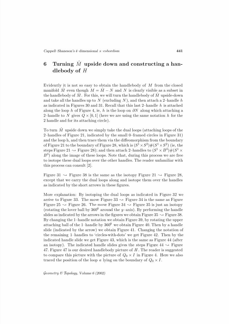
0 Introduction

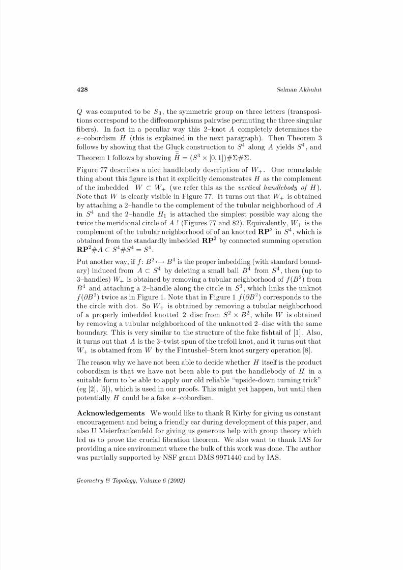
Let Q3 = S 3/Q8 be the quaternionic 3–manifold, obtained as the quotient of the 3–sphere by the free action of the quaternionic group Q8 of order eight,which can be presented by Q8 = i,j,k | i2 = j2 = k2 = −1, ij = k,jk =i,ki = j. Also Q is the 2–fold branched covering space of S 3 branched overthe three Hopf circles; combining this with the Hopf map S 3 → S 2 one seesthat Q is a Seifert Fibered space with three singular fibers. Q is also the 3–foldbranched covering space of S 3 branched over the trefoil knot. Q can also beidentified with the boundaries of the 4–manifolds of Figure 1 (one can easily

check that the above three definitions are equivalent to this one by drawingframed link pictures). The second manifold W of Figure 1, consisting of a 1–and 2–handle pair, is a Stein surface by [9]. It is easily seen that W is a diskbundle over RP2 obtained as the tubular neighborhood of an imbedded RP2

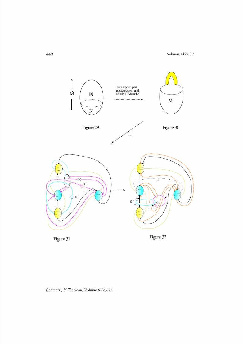
in S 4 . The complement of this imbedding is also a copy of W , decomposingS 4 = W ⌣∂ W .

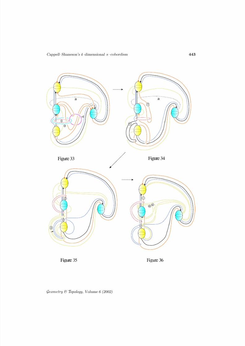
Figure 1

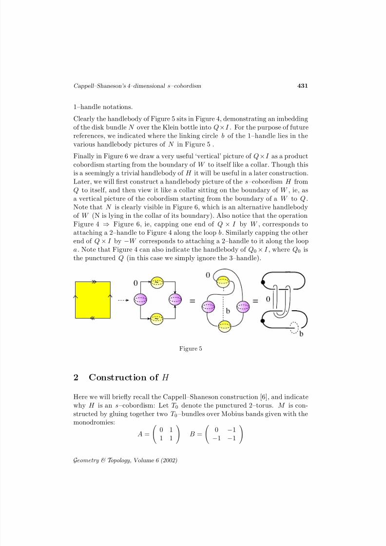
In [6], [7] Cappell and Shaneson constructed an s–cobordism H from Q toitself as follows: Q is the union of an I –bundle over a Klein bottle K and thesolid torus S 1 × D2 , glued along their boundaries. Let N be the D2–bundleover K obtained as the open tubular neighborhood of K ⊂ Q × {1/2} in theinterior of Q × [0, 1]. Then they constructed a certain punctured torus bundleM over K, with ∂M = ∂N , and replaced N with M :

H = M ⌣ (Q × [0, 1] − interior N )

They asked whether H or any of its covers are trivial product cobordisms? Ev-idently the 2–fold cover of H is an s–cobordism H from the lens space L(4, 1)

to itself, and the further 4–fold cyclic coverH of H gives an s–cobordism

from S 3 to itself. For the past 15 years the hope was that this universal coverH might be a non-standard s–cobordism, inducing a fake smooth structure onS 4 . In this paper among other things we will prove that this is not the case bydemonstrating the following smooth identification:

Geometry & T opology , Volume 6 (2002)



Cappell–Shaneson’s 4–dimensional s–cobordism 427

Theorem 1H = S 3 × [0, 1]

We will first describe a handlebody picture of H (Figure 47). Let Q± be thetwo boundary components of H each of which is homemorphic to Q:

∂H = Q− ∪ Q+

We can cap either ends of H with W , by taking the union with W alongQ± ≈ ∂W :

W ± = H ⌣Q± W

There is more than one way of capping H since Q has nontrivial self diffeo-morphisms, but it turns out from the construction that there is a ‘natural’ wayof capping. The reason for bringing the rational ball W into the picture whilestudying Q is that philosophically the relation of W is to Q is similar to therelation of B4 to S 3 . Unable to prove that H itself is a product cobordism, weprove the next best thing:

Theorem 2 W − = W

Unfortunately we are not able to find a similar proof for W + . This is becausethe handlebody picture of H is highly non-symmetric (with respect to its twoends) which prevents us adapting the above theorem to W + . Even though,there is a way of capping H with W + which gives back the standard W , itdoes not correspond to our ‘natural’ way of capping (see the last paragraph of Section 1).

The story for W + evolves in a completely different way: Let W and W + denotethe 2–fold covers of W and W + respectively (note that π1(W ) = Z2 and W is the Euler class −4 disk bundle over S 2 ). We will manege to prove W + isstandard, by first showing that it splits as W #Σ, where Σ a certain homotopy4–sphere, and then by proving Σ is in fact diffeomorphic to S 4 .

Theorem 3

W + =

W

It turns out that the homotopy sphere Σ is obtained from S 4 by the Gluck construction along a certain remarkable 2–knot A ⊂ S 4 (ie, there is an imbed-ding F : S 2 ֒ → S 4 with F (S 2) = A). Furthermore A is the fibered knot inS 4 with fiber consisting of the punctured quaternionic 3–manifold Q0 , withmonodromy φ: Q0 → Q0 coming from the restriction of the order 3 diffemor-phism of Q, which cyclically permutes the three singular fibers of Q (as SeifertFibered space). Recall that, in [15] the Mapping Class group π0(Diff Q) of




428 Selman Akbulut

Q was computed to be S 3 , the symmetric group on three letters (transposi-tions correspond to the diffeomorphisms pairwise permuting the three singularfibers). In fact in a peculiar way this 2–knot A completely determines thes–cobordism H (this is explained in the next paragraph). Then Theorem 3follows by showing that the Gluck construction to S 4 along A yields S 4 , and

Theorem 1 follows by showingH = (S 3 × [0, 1])#Σ#Σ.

Figure 77 describes a nice handlebody description of W + . One remarkablething about this figure is that it explicitly demonstrates H as the complementof the imbedded W ⊂ W + (we refer this as the vertical handlebody of H ).

Note that W is clearly visible in Figure 77. It turns out that W + is obtainedby attaching a 2–handle to the complement of the tubular neighborhood of Ain S 4 and the 2–handle H 1 is attached the simplest possible way along thetwice the meridional circle of A ! (Figures 77 and 82). Equivalently, W + is thecomplement of the tubular neighborhood of of an knotted RP2 in S 4 , which isobtained from the standardly imbedded RP2 by connected summing operationRP2#A ⊂ S 4#S 4 = S 4 .

Put another way, if f : B2 ֒ → B4 is the proper imbedding (with standard bound-ary) induced from A ⊂ S 4 by deleting a small ball B4 from S 4 , then (up to3–handles) W + is obtained by removing a tubular neighborhood of f (B2) fromB4 and attaching a 2–handle along the circle in S 3 , which links the unknot

f (∂B2

) twice as in Figure 1. Note that in Figure 1 f (∂B2

) corresponds to thethe circle with dot. So W + is obtained by removing a tubular neighborhoodof a properly imbedded knotted 2–disc from S 2 × B2 , while W is obtainedby removing a tubular neighborhood of the unknotted 2–disc with the sameboundary. This is very similar to the structure of the fake fishtail of [1]. Also,it turns out that A is the 3–twist spun of the trefoil knot, and it turns out thatW + is obtained from W by the Fintushel–Stern knot surgery operation [8].

The reason why we have not been able to decide whether H itself is the productcobordism is that we have not been able to put the handlebody of H in asuitable form to be able to apply our old reliable “upside-down turning trick”(eg [2], [5]), which is used in our proofs. This might yet happen, but until then

potentially H could be a fake s–cobordism.

Acknowledgements We would like to thank R Kirby for giving us constantencouragement and being a friendly ear during development of this paper, andalso U Meierfrankenfeld for giving us generous help with group theory whichled us to prove the crucial fibration theorem. We also want to thank IAS forproviding a nice environment where the bulk of this work was done. The authorwas partially supported by NSF grant DMS 9971440 and by IAS.





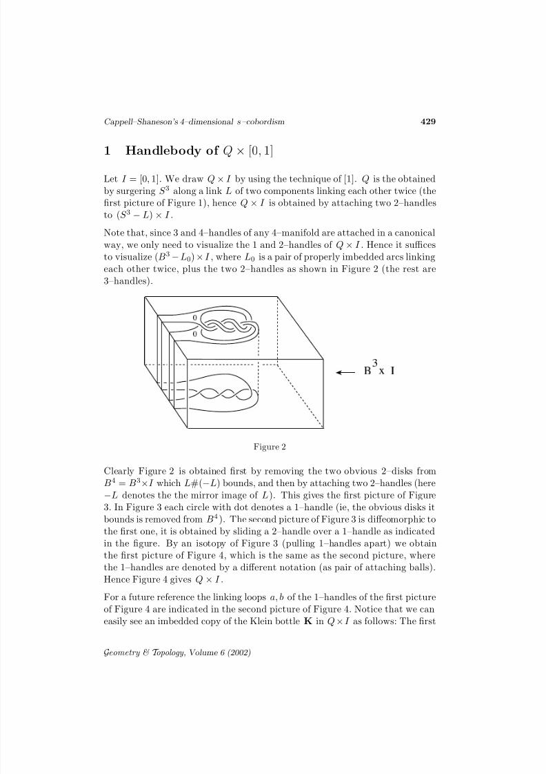
1 Handlebody of Q × [0, 1]

Let I = [0, 1]. We draw Q × I by using the technique of [1]. Q is the obtainedby surgering S 3 along a link L of two components linking each other twice (thefirst picture of Figure 1), hence Q × I is obtained by attaching two 2–handlesto (S 3 − L) × I .

Note that, since 3 and 4–handles of any 4–manifold are attached in a canonicalway, we only need to visualize the 1 and 2–handles of Q × I . Hence it sufficesto visualize (B3 − L0) × I , where L0 is a pair of properly imbedded arcs linking

each other twice, plus the two 2–handles as shown in Figure 2 (the rest are3–handles).

Figure 2

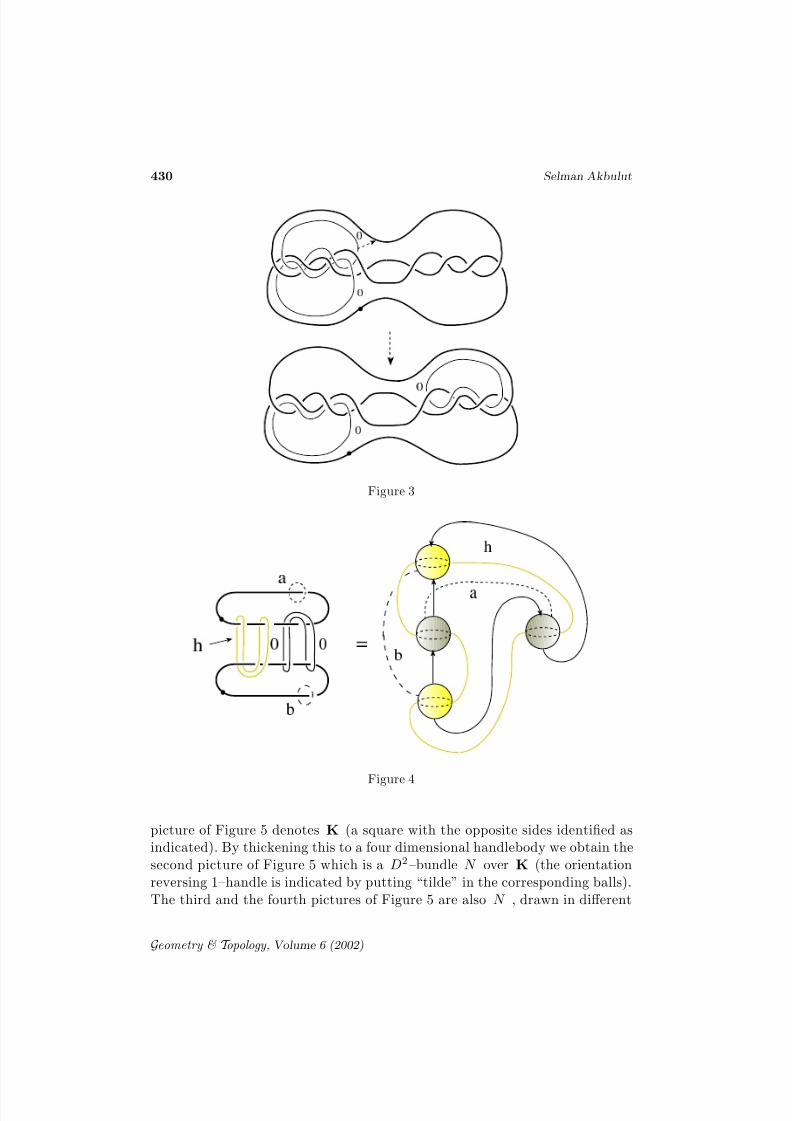
Clearly Figure 2 is obtained first by removing the two obvious 2–disks fromB4 = B3×I which L#(−L) bounds, and then by attaching two 2–handles (here−L denotes the the mirror image of L). This gives the first picture of Figure3. In Figure 3 each circle with dot denotes a 1–handle (ie, the obvious disks itbounds is removed from B4 ). The second picture of Figure 3 is diffeomorphic tothe first one, it is obtained by sliding a 2–handle over a 1–handle as indicated

in the figure. By an isotopy of Figure 3 (pulling 1–handles apart) we obtainthe first picture of Figure 4, which is the same as the second picture, wherethe 1–handles are denoted by a different notation (as pair of attaching balls).Hence Figure 4 gives Q × I .

For a future reference the linking loops a, b of the 1–handles of the first pictureof Figure 4 are indicated in the second picture of Figure 4. Notice that we caneasily see an imbedded copy of the Klein bottle K in Q ×I as follows: The first




430 Selman Akbulut

Figure 3

Figure 4

picture of Figure 5 denotes K (a square with the opposite sides identified asindicated). By thickening this to a four dimensional handlebody we obtain thesecond picture of Figure 5 which is a D2–bundle N over K (the orientationreversing 1–handle is indicated by putting “tilde” in the corresponding balls).The third and the fourth pictures of Figure 5 are also N , drawn in different






432 Selman Akbulut

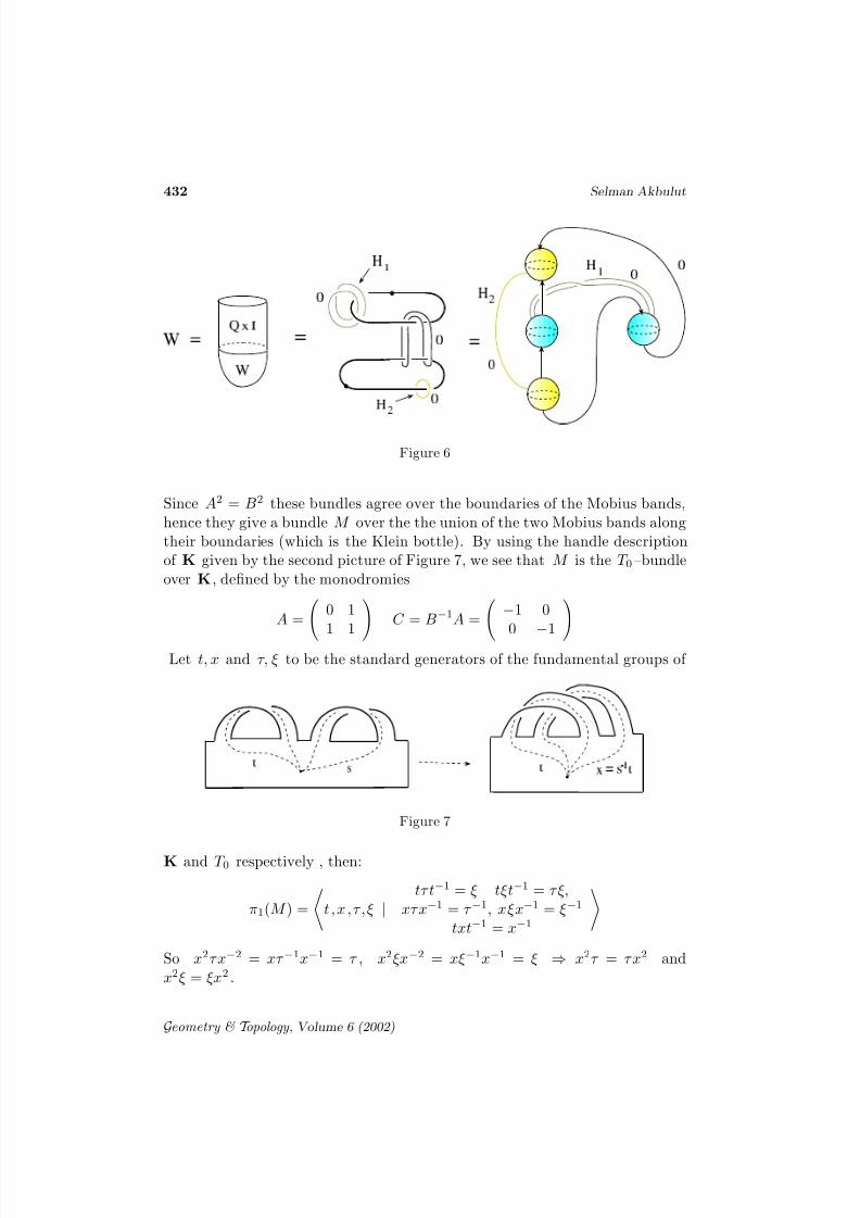
Figure 6

Since A2 = B2 these bundles agree over the boundaries of the Mobius bands,hence they give a bundle M over the the union of the two Mobius bands alongtheir boundaries (which is the Klein bottle). By using the handle descriptionof K given by the second picture of Figure 7, we see that M is the T 0–bundleover K, defined by the monodromies

A =

0 11 1

C = B−1A =

−1 00 −1

Let t, x and τ, ξ to be the standard generators of the fundamental groups of

Figure 7

K and T 0 respectively , then:

π1(M ) =

t,x,τ,ξ |

tτ t−1 = ξ tξt−1 = τ ξ,xτ x−1 = τ −1, xξx−1 = ξ−1

txt−1 = x−1

So x2τ x−2 = xτ −1x−1 = τ , x2ξx−2 = xξ−1x−1 = ξ ⇒ x2τ = τ x2 andx2ξ = ξx2 .





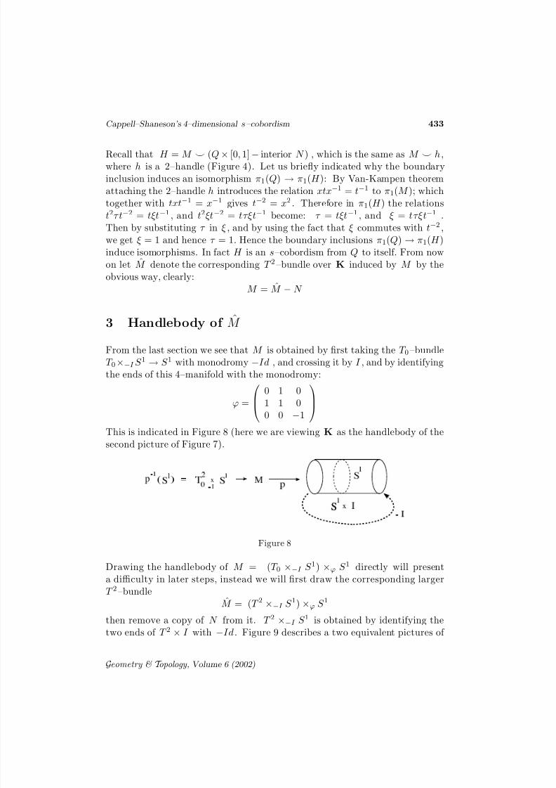
Recall that H = M ⌣ (Q × [0, 1] − interior N ) , which is the same as M ⌣ h,where h is a 2–handle (Figure 4). Let us briefly indicated why the boundaryinclusion induces an isomorphism π1(Q) → π1(H ): By Van-Kampen theoremattaching the 2–handle h introduces the relation xtx−1 = t−1 to π1(M ); whichtogether with txt−1 = x−1 gives t−2 = x2 . Therefore in π1(H ) the relationst2τ t−2 = tξt−1 , and t2ξt−2 = tτξt−1 become: τ = tξt−1 , and ξ = tτξt−1 .Then by substituting τ in ξ , and by using the fact that ξ commutes with t−2 ,we get ξ = 1 and hence τ = 1. Hence the boundary inclusions π1(Q) → π1(H )induce isomorphisms. In fact H is an s–cobordism from Q to itself. From nowon let M̂ denote the corresponding T 2–bundle over K induced by M by the

obvious way, clearly:M = M̂ − N

3 Handlebody of M̂

From the last section we see that M is obtained by first taking the T 0–bundleT 0×−I S 1 → S 1 with monodromy −Id , and crossing it by I , and by identifyingthe ends of this 4–manifold with the monodromy:

ϕ =

0 1 01 1 0

0 0 −1

This is indicated in Figure 8 (here we are viewing K as the handlebody of thesecond picture of Figure 7).

Figure 8

Drawing the handlebody of M = (T 0 ×−I S 1) ×ϕ S 1 directly will presenta difficulty in later steps, instead we will first draw the corresponding largerT 2–bundle

M̂ = (T 2 ×−I S 1) ×ϕ S 1

then remove a copy of N from it. T 2 ×−I S 1 is obtained by identifying thetwo ends of T 2 × I with −Id. Figure 9 describes a two equivalent pictures of




434 Selman Akbulut

the Heegaard handlebody of T 2 ×−I S 1 . The pair of ‘tilde’ disks describe atwisted 1–handle (due to −Id identification (x, y) → (−x, −y)). If need be,after rotating the attaching map of the the twisted 1–handle we can turn it toa regular 1–handle as indicated by the second picture of Figure 9.

Figure 9

Now we will draw M̂ = (T 2 ×−I S 1) ×ϕS 1 by using the technique introduced in[4]: We first thicken the handlebody T 2 ×−I S 1 of Figure 9 to the 4–manifoldT 2 ×−I S 1 × I (the first picture of Figure 10). Then isotop ϕ: T 2 ×−I S 1 →T 2 ×−I S 1 so that it takes 1–handles to 1–handles, with an isotopy, eg,

ϕt = −t 1 − t 01 − t 1 0

0 0 −1

Then attach an extra 1–handle and the 2–handles as indicated in second pic-ture of Figure 10 (one of the attaching balls of the new 1–handle is not visiblein the picture since it is placed at the point of infinity). The extra 2–handlesare induced from the identification of the 1–handles of the two boundary com-ponents of T 2 ×−I S 1 × I via ϕ. So, the second picture of Figure 10 gives thehandlebody of M̂ .

We want to emphasize that the new 1–handle identifies the 3–ball at the center

of Figure 10 with the 3–ball at the infinity by the following diffeomorphism asindicated in Figure 11:

(x,y ,z) → (x, −y, −z)

Figure 12 describes how part of this isotopy ϕt acts on T 2 (where T 2 is repre-sented by a disk with opposite sides identified). This is exactly the reason whywe started with T 2 ×−I S 1 instead of T 20 ×−I S 1 (this isotopy takes place in T 2

not in T 20 !).





Figure 10

Figure 11

Figure 12

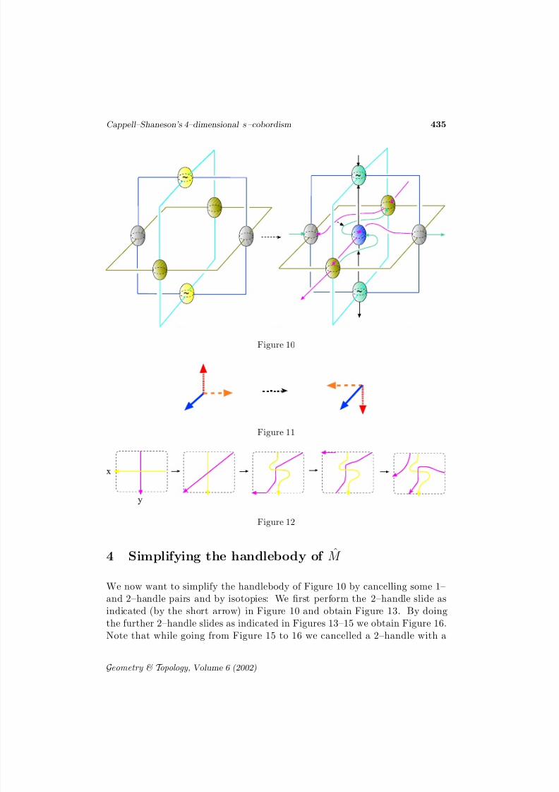
4 Simplifying the handlebody of M̂

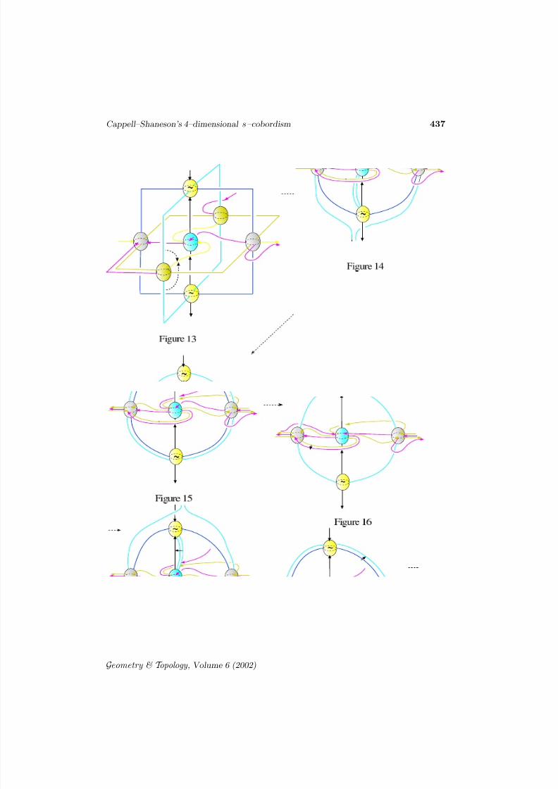
We now want to simplify the handlebody of Figure 10 by cancelling some 1–and 2–handle pairs and by isotopies: We first perform the 2–handle slide asindicated (by the short arrow) in Figure 10 and obtain Figure 13. By doingthe further 2–handle slides as indicated in Figures 13–15 we obtain Figure 16.Note that while going from Figure 15 to 16 we cancelled a 2–handle with a




436 Selman Akbulut

3–handle (ie, we erased a zero framed unknotted circle from the picture).

Figure 17 is the same as Figure 16 except that the twisted 1–handle (two ballswith ‘tilde’ on it) is drawn in the standard way. By an isotopy we go fromFigure 17 to Figure 18. Figure 19 is the same as Figure 18 except that wedrew one of the 1–handles in a different 1–handle notation (circle with a dotnotation).

Note that in our figures, if the framing of a framed knot is the obvious “black-board framing” we don’t bother to indicate it, but if the framing deviates from

the obvious black-board framing we indicate the deviation from to the black-board framing by putting a number in a circle on the knot ( −1’s in the case of Figure 19).

Figure 20 is obtained from Figure 19 by simply leaving out one of the 2 handles.This is because the framed knot corresponding to this 2–handle is the unknotwith 0–framing !, hence it is cancelled by a 3–handle (this knot is in fact the‘horizontal’ framed knot of Figure 10).

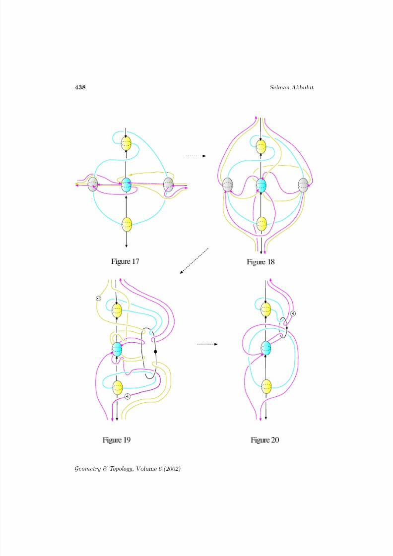
Figure 21 is the desired handlebody of M̂ , it is the same as the Figure 20,except that one of the attaching balls of a 1–handle which had been placed at

the point of infinity is isotoped into R

3

.

5 Checking that the boundary of M̂ is correct

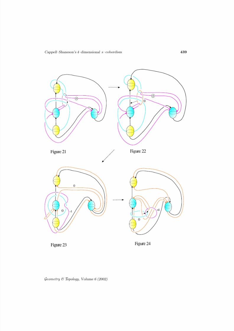
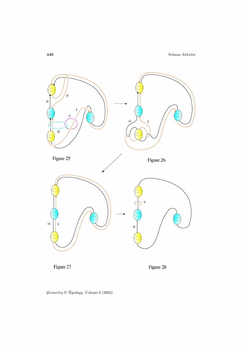
Now we need to check that the boundary of the closed manifold M̂ (minusthe three and four handles) is correct. That is, the boundary of Figure 21 isthe connected sum of copies of S 1 × S 2 ; so that after cancelling them with 3–handles we get S 3 , which is then capped by a 4– handle. This process is doneby changing the interior of M̂ so that boundary becomes visible: By changinga 1–handle to a 2–handle in Figure 21 (ie, turning a ‘dotted circle’ to a zeroframed circle) we obtain Figure 22. Then by doing the indicated handle slidesand isotopies we arrive to Figures 23, 24 and 25. Then by operation of turninga 2–handle to a 1–handle by a surgery (ie, turning a zero framed circle to a‘dotted circle’) and cancelling the resulting 1– and 2–handle pair we get Figure26. By isotopies we obtain the Figure 28, which after surgering the obvious2–handle becomes S 1 × B3 # S 1 × B3 with the desired boundary.








438 Selman Akbulut








440 Selman Akbulut






442 Selman Akbulut








444 Selman Akbulut








446 Selman Akbulut











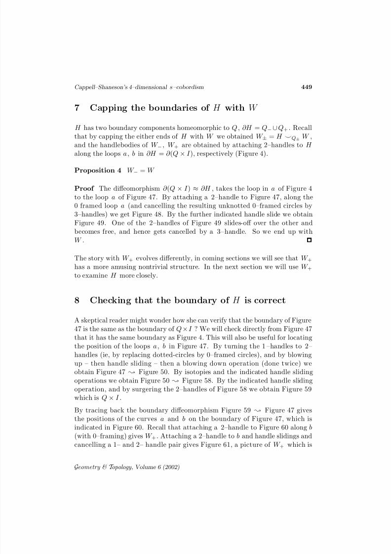
7 Capping the boundaries of H with W

H has two boundary components homeomorphic to Q, ∂H = Q−∪ Q+ . Recallthat by capping the either ends of H with W we obtained W ± = H ⌣Q± W ,and the handlebodies of W − , W + are obtained by attaching 2–handles to H along the loops a, b in ∂H = ∂ (Q × I ), respectively (Figure 4).

Proposition 4 W − = W

Proof The diffeomorphism ∂ (Q × I ) ≈ ∂H , takes the loop in a of Figure 4to the loop a of Figure 47. By attaching a 2–handle to Figure 47, along the0 framed loop a (and cancelling the resulting unknotted 0–framed circles by3–handles) we get Figure 48. By the further indicated handle slide we obtainFigure 49. One of the 2–handles of Figure 49 slides-off over the other andbecomes free, and hence gets cancelled by a 3–handle. So we end up withW .

The story with W + evolves differently, in coming sections we will see that W +has a more amusing nontrivial structure. In the next section we will use W +to examine H more closely.

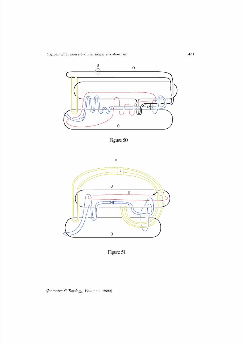
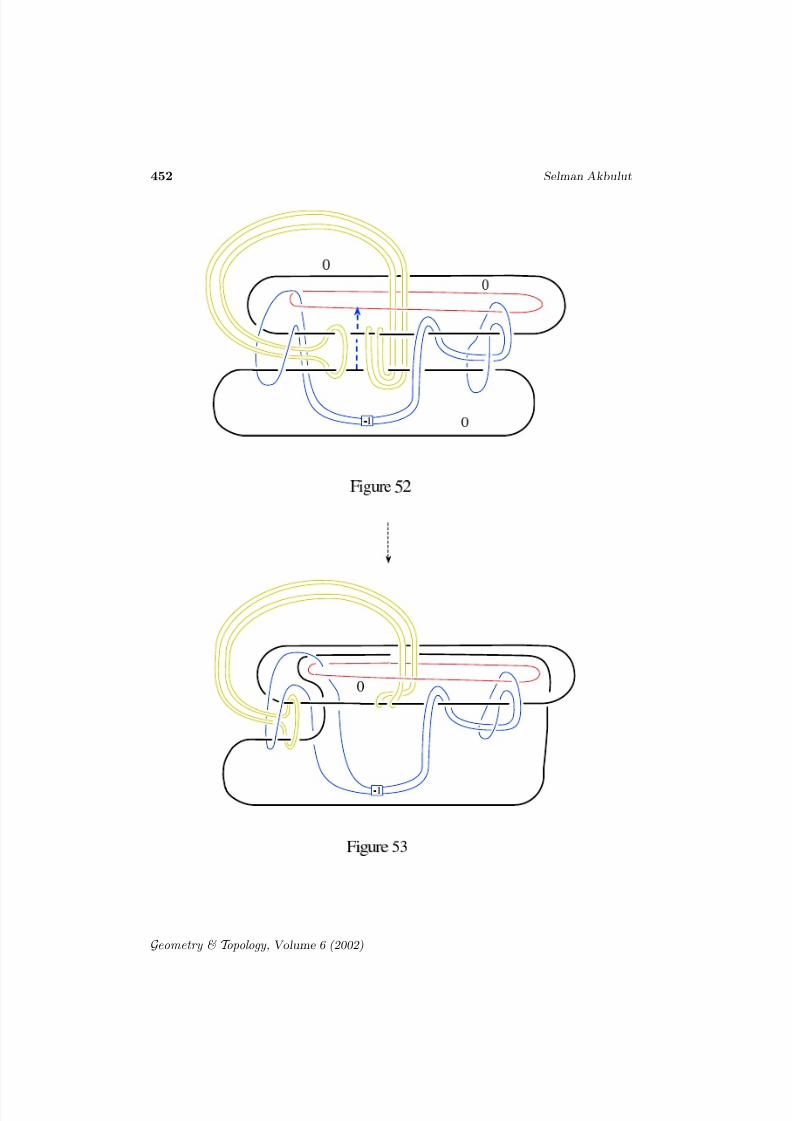
8 Checking that the boundary of H is correct

A skeptical reader might wonder how she can verify that the boundary of Figure47 is the same as the boundary of Q×I ? We will check directly from Figure 47that it has the same boundary as Figure 4. This will also be useful for locatingthe position of the loops a, b in Figure 47. By turning the 1 –handles to 2–handles (ie, by replacing dotted-circles by 0–framed circles), and by blowingup – then handle sliding – then a blowing down operation (done twice) weobtain Figure 47 ; Figure 50. By isotopies and the indicated handle slidingoperations we obtain Figure 50 ; Figure 58. By the indicated handle sliding

operation, and by surgering the 2–handles of Figure 58 we obtain Figure 59which is Q × I .

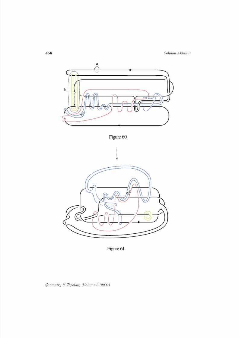
By tracing back the boundary diffeomorphism Figure 59 ; Figure 47 givesthe positions of the curves a and b on the boundary of Figure 47, which isindicated in Figure 60. Recall that attaching a 2–handle to Figure 60 along b(with 0–framing) gives W + . Attaching a 2–handle to b and handle slidings andcancelling a 1– and 2– handle pair gives Figure 61, a picture of W + which is




450 Selman Akbulut

seemingly different than W . Figure 61 should be considered a “vertical picture”of H built over the handlebody of W (notice W is visible in this picture). Inthe next section we will construct a surprisingly simpler “vertical” handlebodypicture of H .

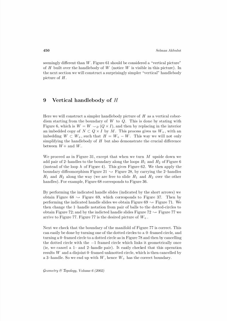
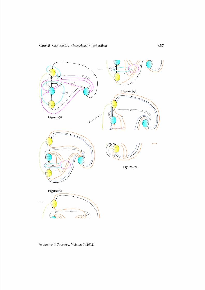
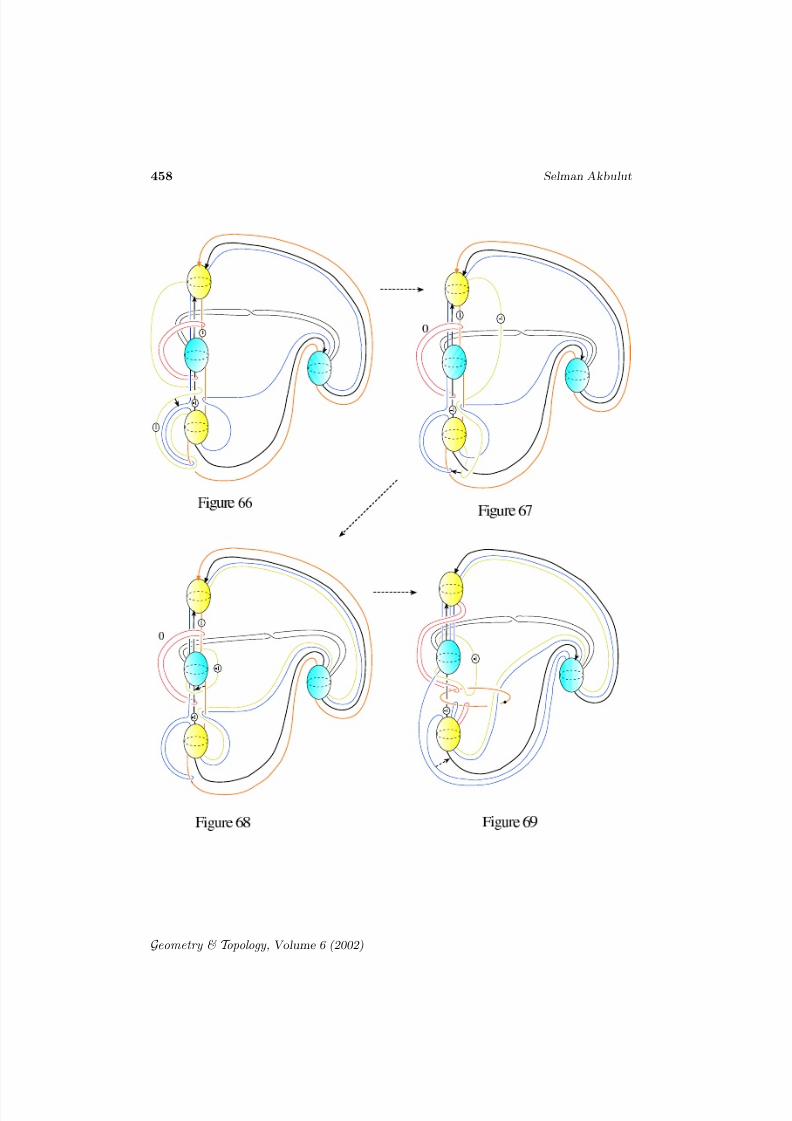
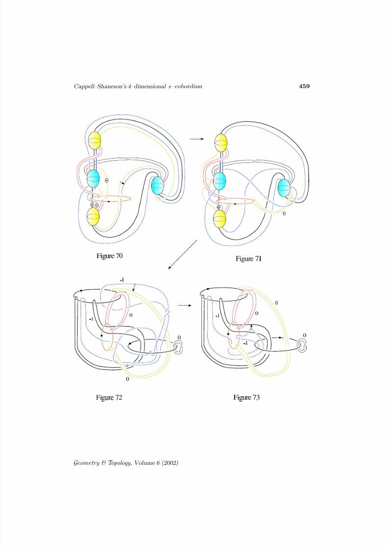
9 Vertical handlebody of H

Here we will construct a simpler handlebody picture of H as a vertical cobor-dism starting from the boundary of W to Q. This is done by stating withFigure 6, which is W = W ⌣∂ (Q × I ), and then by replacing in the interioran imbedded copy of N ⊂ Q × I by M . This process gives us W + , with animbedding W ⊂ W + , such that H = W + − W . This way we will not onlysimplifying the handlebody of H but also demonstrate the crucial differencebetween W + and W −

We proceed as in Figure 31, except that when we turn M upside down weadd pair of 2–handles to the boundary along the loops H 1 and H 2 of Figure 6

(instead of the loop h of Figure 4). This gives Figure 62. We then apply theboundary diffeomorphism Figure 21 ; Figure 28, by carrying the 2–handlesH 1 and H 2 along the way (we are free to slide H 1 and H 2 over the otherhandles). For example, Figure 68 corresponds to Figure 36.

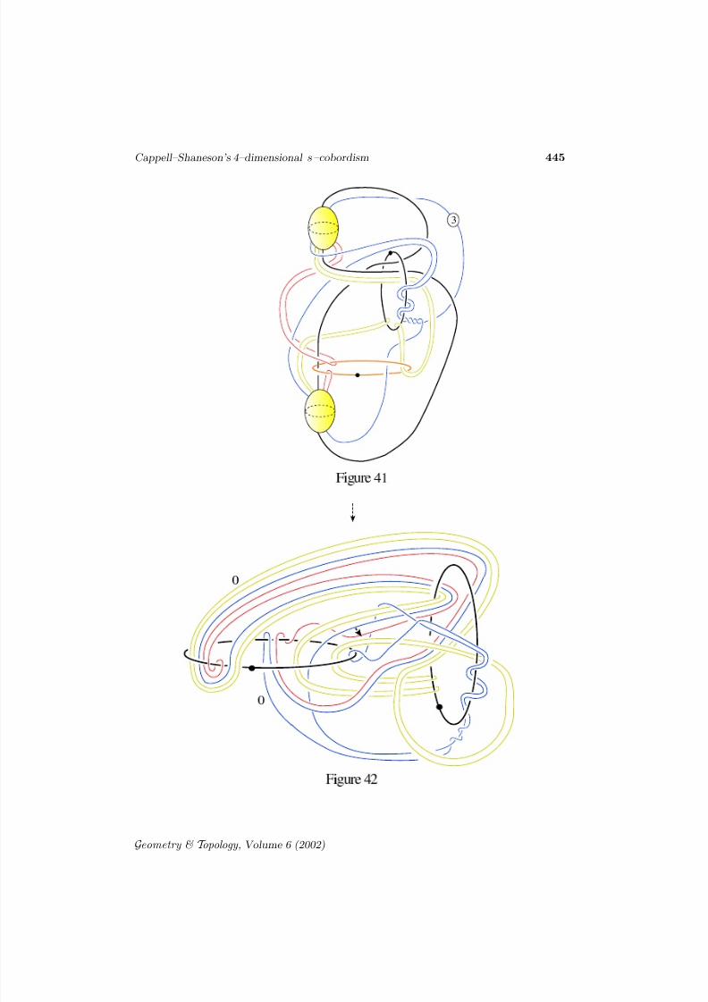
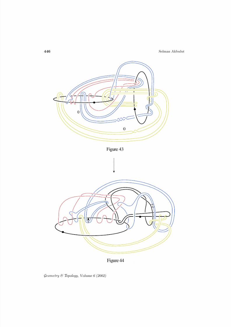
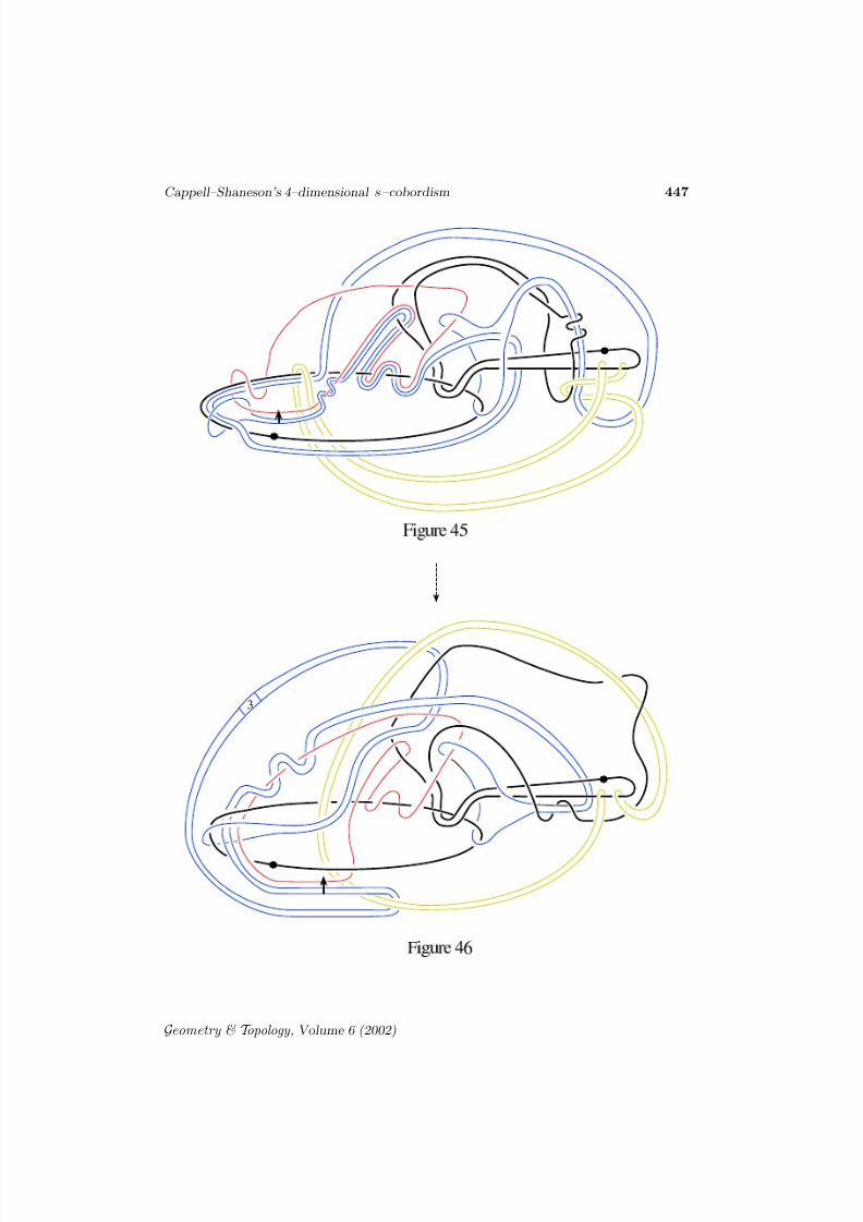
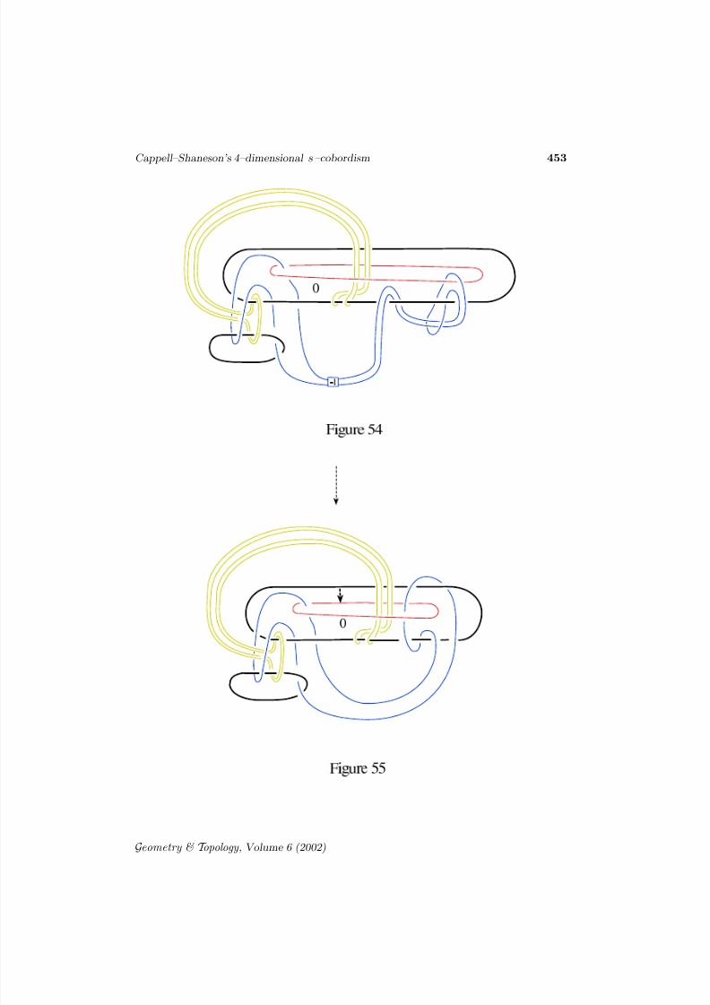
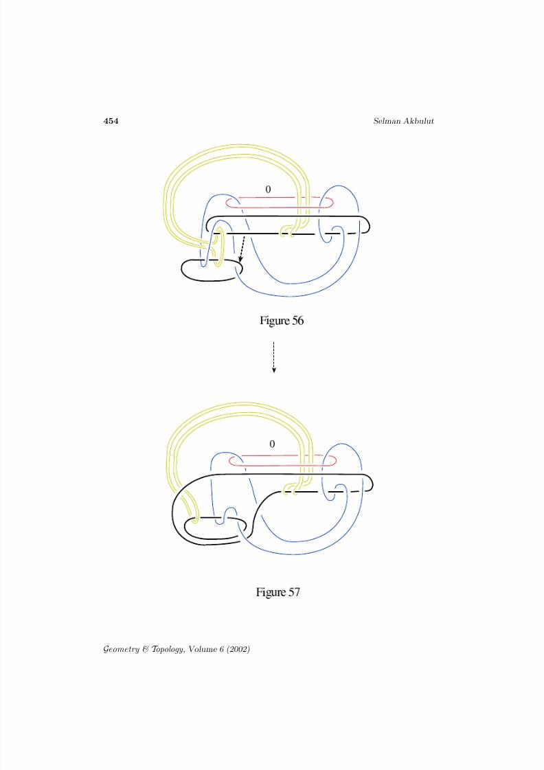
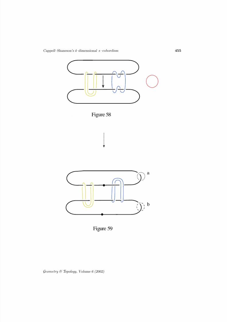
By performing the indicated handle slides (indicated by the short arrows) weobtain Figure 68 ; Figure 69, which corresponds to Figure 37. Then byperforming the indicated handle slides we obtain Figure 69 ; Figure 71. Wethen change the 1–handle notation from pair of balls to the dotted-circles toobtain Figure 72; and by the indicted handle slides Figure 72 ; Figure 77 wearrive to Figure 77. Figure 77 is the desired picture of W + .

Next we check that the boundary of the manifold of Figure 77 is correct. Thiscan easily be done by turning one of the dotted circles to a 0–framed circle, andturning a 0–framed circle to a dotted circle as in Figure 78 and then by cancellingthe dotted circle with the −1 framed circle which links it geometrically once(ie, we cancel a 1– and 2–handle pair). It easily checked that this operationresults W and a disjoint 0–framed unknotted circle, which is then cancelled bya 3–handle. So we end up with W , hence W + has the correct boundary.








452 Selman Akbulut








454 Selman Akbulut








456 Selman Akbulut














460 Selman Akbulut





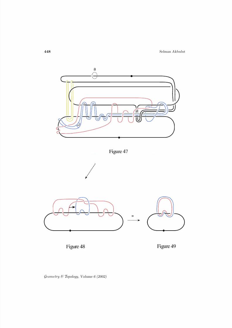
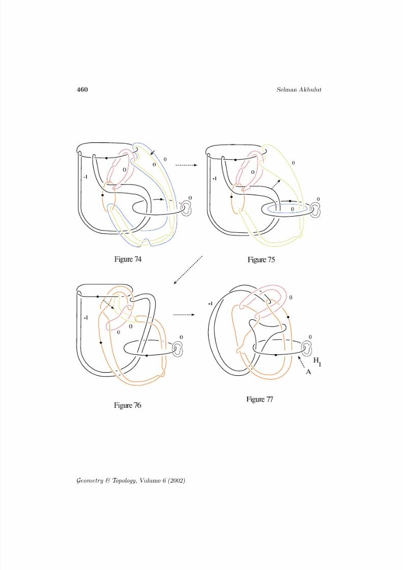
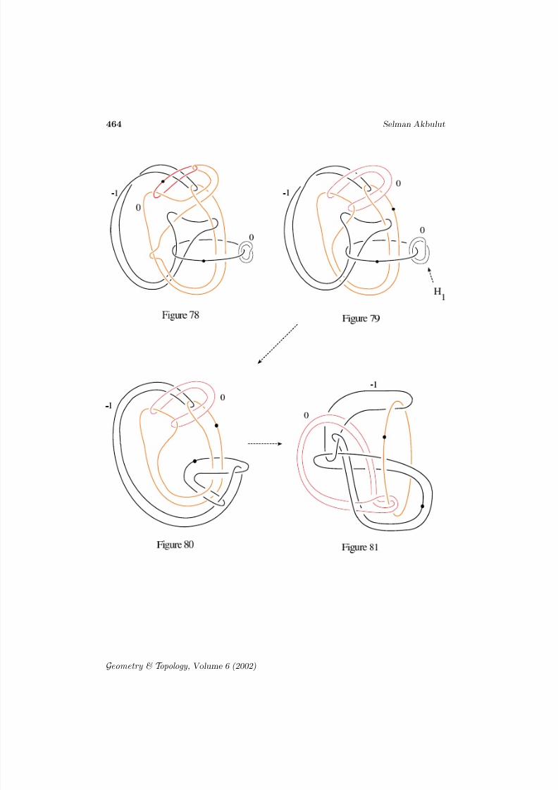
10 A knot is born

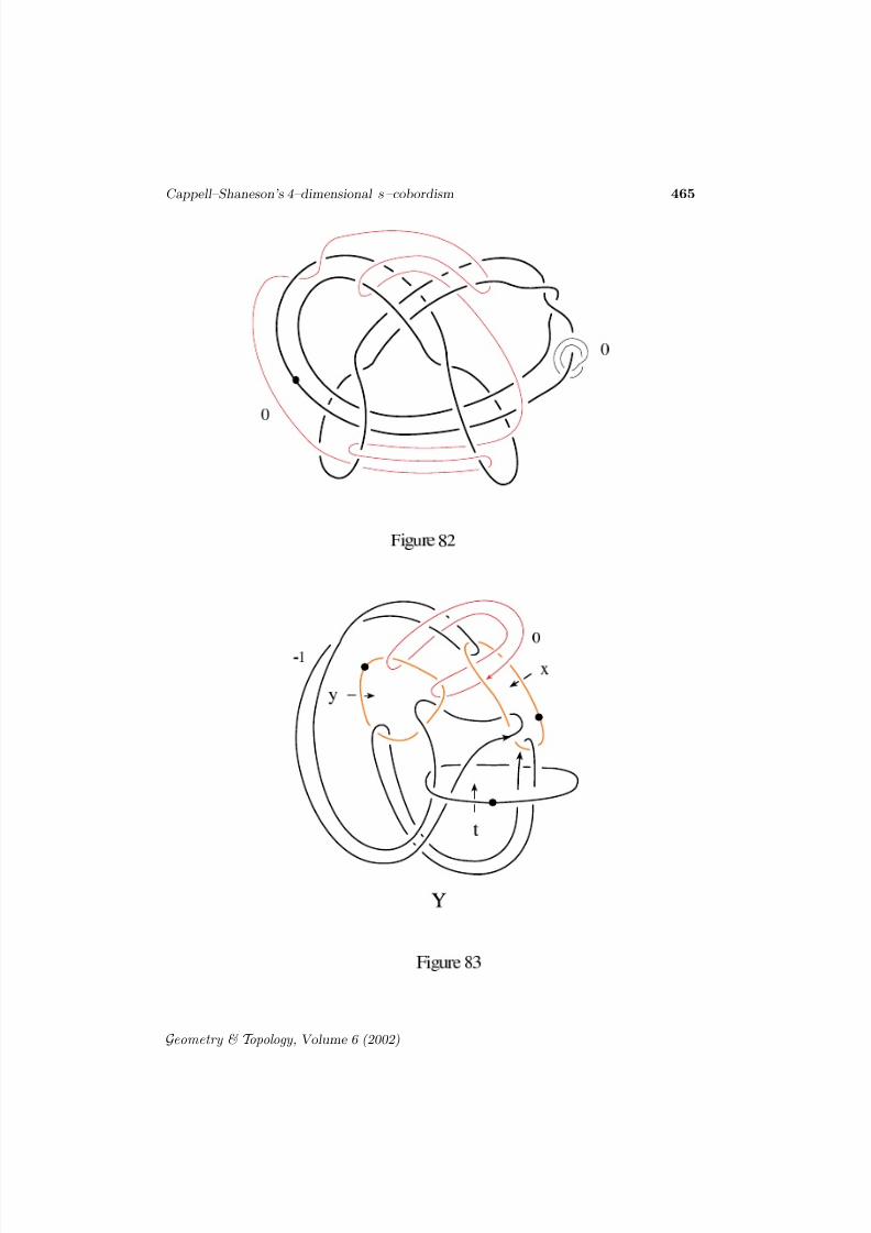
By twisting the strands going through the middle 1–handle, and then by slidingH 1 over this 1–handle we see that Figure 77 is diffeomorphic to the Figure79 (similar to the move at the bottom of the page 504 of [2]). Figure 79demonstrates the complement of the imbedding f : B2 ֒ → B4 with the standardboundary, given by the “dotted circle” A (the 1–handle). This follows fromthe discussion on the last paragraph of the last section. Because there bychanging the interior of Figure 77 we checked that as a loop A is the unknoton the boundary of the handlebody X consisting of all the handles of Figure77 except the 1–handle corresponding to A and the last 2–handle H 1 . Thesame argument works for Figure 79. In addition in this case, the handlebodyconsisting of all the handles of the Figure 79 except the 1-handle correspondingto A and the the 2-handle H 1 , is B4 . So W + is obtained from B4 by carvingout of the imbedded disk bounded by the unknot A (i.e creating a 1–handle A)and then by attaching the 2–handle H 1 . Hence by capping with a standardpair (B4, B2) we can think of f as a part of an imbedding F : S 2 ֒ → S 4 . Letus call A = F (S 2).

We can draw a more concrete picture of the knot A as follows: During the nextfew steps, in order not to clog up the picture, we won’t draw the last 2–handle

H 1 . By an isotopy and cancelling 1– and 2 –handle pair we get a diffeomorphismfrom Figure 79, to Figures 80, 81 and finally to Figure 82. In Figure 82 the‘dotted’ ribbon knot is really the unknot in the presence of a cancelling 2 and3–handle pair (ie, the unknotted circle with 0–framing plus the 3–handle whichis not seen in the figure). So this ribbon disk with the boundary the unknot inS 3 , demonstrates a good visual picture of the imbedding f : B2 ֒ → B4 .

10.1 A useful fundamental group calculation

We will compute the fundamental group of the 2–knot complement S 4 − A, ie,we will compute the group G := π1(Y ), where Y is the handlebody consisting of

all the handles of Figure 79 except the 2–handle H 1 . Though this calculation isnot necessary for the rest of the paper, it is useful to demonstrate why W +− W gives an s–cobordism. By using the generators drawn in Figure 83 we get thefollowing relations for G:

(1) x−1yt−1x−1t = 1(2) x−1yxy = 1(3) txt−1y−1 = 1




462 Selman Akbulut

From (1) and (2) we get t−1x−1t = xy , then by using (3) =⇒ t3 = (tx)3 . Calla = tx so t3 = a3 . By solving y in (3) and plugging into (2) and substitutingx = t−1a we get ata = tat−2a3 = tat−2t3 = tat. Hence we get the presentation:

G = t, a|t3 = a3,ata = tat

Notice that attaching the 2–handle H 1 to Y (ie, forming W +) introducesthe extra relation t4 = 1 to G, which then implies t = x, demonstrating ans–cobordism from the boundary of W to the boundary to W + . The followingimportant observation of Meierfrankenfeld has motivated us to prove the crucialfibration structure for A in the next section.

Lemma 5 [14] G contains normal subgroups Q8 and Z giving the exact

sequences :1 → Q8 → G → Z → 1

1 → Z → G → SL(2, Z3) → 1

Proof Call u := ta−1 = y−1 and v := a−1t = x−1 . First notice thatthe group u, v generated by u and v is a normal subgroup. For example,since u = ta−1 = a−1t−1at = a−1v−1t = a−1v−1av =⇒ a−1va = uv−1 ∈u, v. Also since v = a−1t = a−1ua =⇒ a−1ua = v ∈ u, v. Nowwe claim that u, v = Q8 . This follows from a3 = t3 ∈ Center(G) =⇒u = a−3ua3 = a−1(vu−1)a = vu−1v−1 =⇒ uvu = v . So vu−1 = a−1va =

a−1(uvu)a = (a−1ua)(a−1va)(a−1ua) = v(vu−1)v , implying vuv = u. Sou, v = u, v | uvu = v,vuv = u, which is a presentation of Q8 .

For the second exact sequence take Z = t3 and then observe that G/t3 =SL(2, Z3) (for example, by using the symbolic manipulation program GAPone can check that G/t3 has order 24, then use the group theory fact thatSL(2, Z3) is the only group of order 24 generated by two elements of order3)

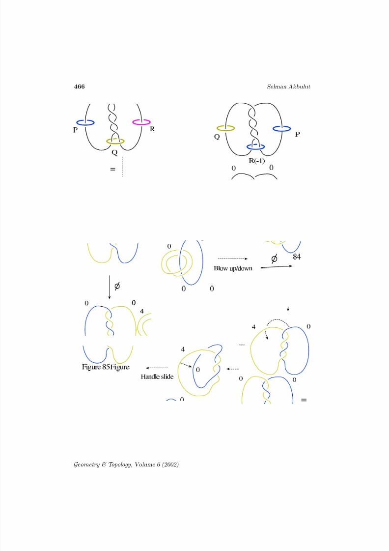
10.2 Fiber structure of the knot A

Consider the order three self diffeomorphism φ: Q → Q of Figure 84. Asdescribed by the the pictures of Figure 85, this diffeomorphism is obtained bythe compositions of blowing up, a handle slide, blowing down, and anotherhandle slide operations. φ permutes the circles P,Q,R as indicated in Figure84, while twisting the tubular neighborhood of R by −1 times. Note that Qcan be obtained by doing −1 surgeries to three right-handed Hopf circles, thenφ is the map induced from the map S 3 → S 3 which permutes the three Hopf circles. Let Q0 denote the punctured Q, then:





Proposition 6 The knot A ⊂ S 4 is a fibered knot with fiber Q0 and mon-

odromy φ.

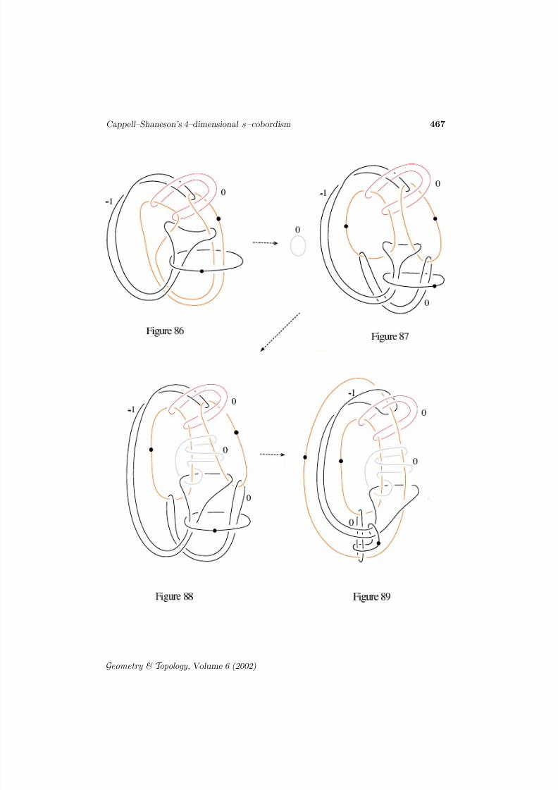
Proof We start with Figure 86 which is the knot complement Y . By introduc-ing a zero framed unknotted circle (ie, by introducing a cancelling pair of 2–and3–handles) we arrive to the Figure 87. Now something amazing happens!: Thisnew zero framed unknotted circle isotopes to the complicated looking circle of Figure 88, as indicated in the figure. The curious reader can check this byapplying the boundary diffeomorphism Figure 77 ⇒ Figure 78 to Figure 88

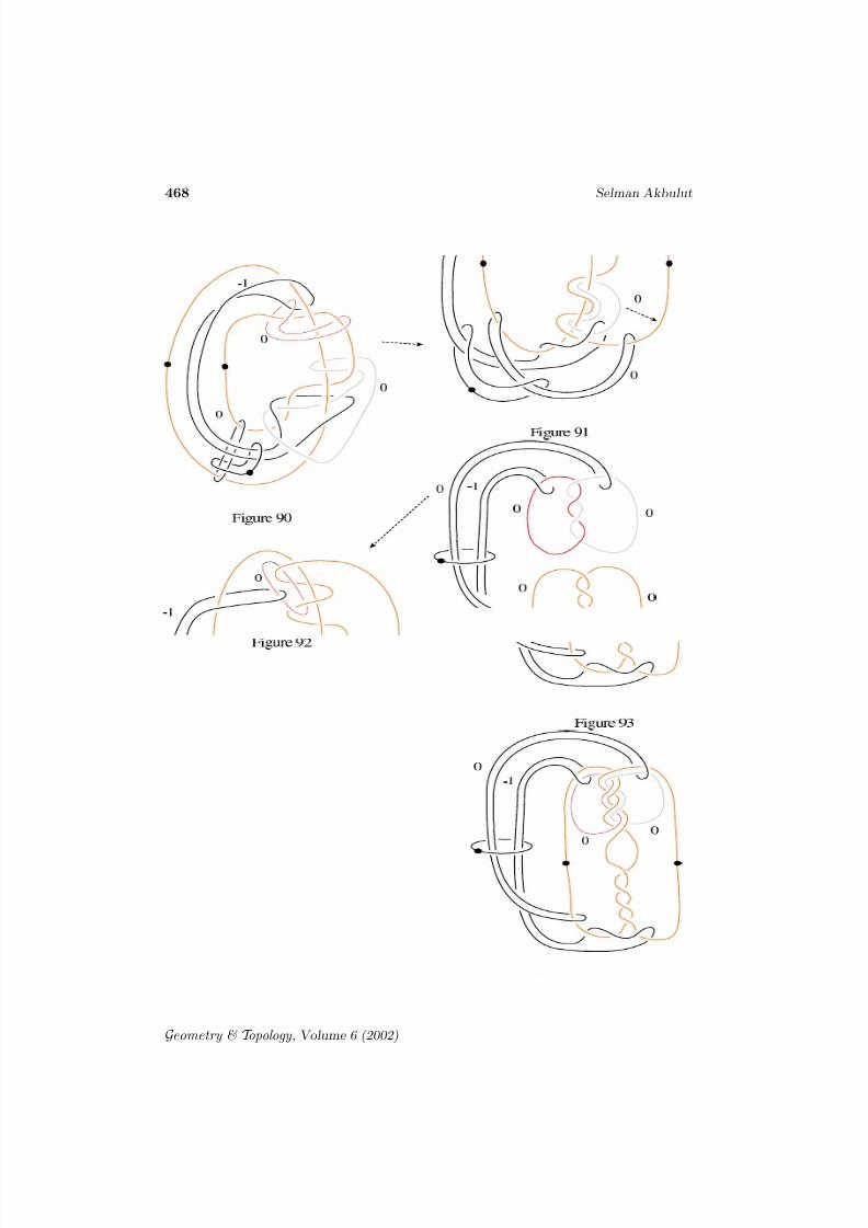
(replacing dotted circle with a zero framed circle) and tracing this new loopalong the way back to the trivial loop!. By isotopies and the indicated handleslides, from Figure 88 we arrive to Figure 92.

Now in Figure 92 we can clearly see an imbedded copy of Q × [0, 1] (recallFigures 3 and 4). We claim that, in fact the other handles of this figure has therole of identifying the two ends of Q × [0, 1] by the monodromy φ. To see this,recall from [4] how to draw the handlebody of picture of :

Q0 × [0, 1]/(x, 0) ∼ (φ(x), 1)

For this, we attach a 1–handle to Q0 × [0, 1] connecting the top to the bottom,

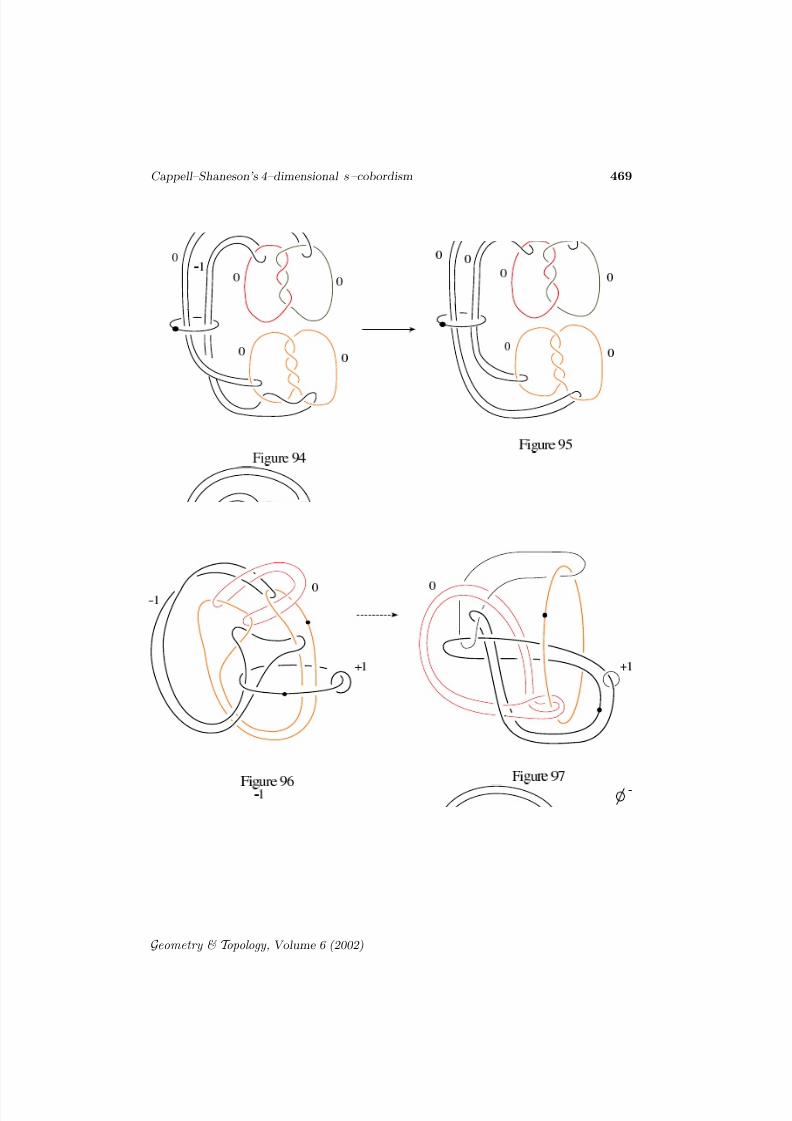
and attach 2–handles along the loops γ # φ(γ ) where γ are the core circlesof the 1–handles of Q × 0 and φ(γ ) are their images in Q × 1 under the mapφ (the connected sum is taken along the 1–handle). By inspecting where the2–handles are attached on the boundary of Q0 × [0, 1] (Figure 93), we see thatin fact the two ends are identified exactly by the diffeomorphism φ. Note that,by changing the monodromy of Figure 94 by φ−1 we obtain Figure 95, whichis the identity monodromy identification Q × S 1 .

11 The Gluck Construction

Recall that performing the Gluck construction to S 4 along an imbedded 2–sphere S 2 ֒ → S 4 means that we first thicken the imbedding S 2 × B2 ֒ → S 4 andthen form:

Σ = (S 4 − S 2 × B2) ⌣ψ S 2 × B2

where ψ: S 2×S 1 → S 2×S 1 is the diffeomorphism given by ψ(x, y) = (ρ(y)x, y),and ρ: S 1 → SO(3) is the generator of π1(SO(3)) = Z2 .




464 Selman Akbulut








466 Selman Akbulut








468 Selman Akbulut








470 Selman Akbulut

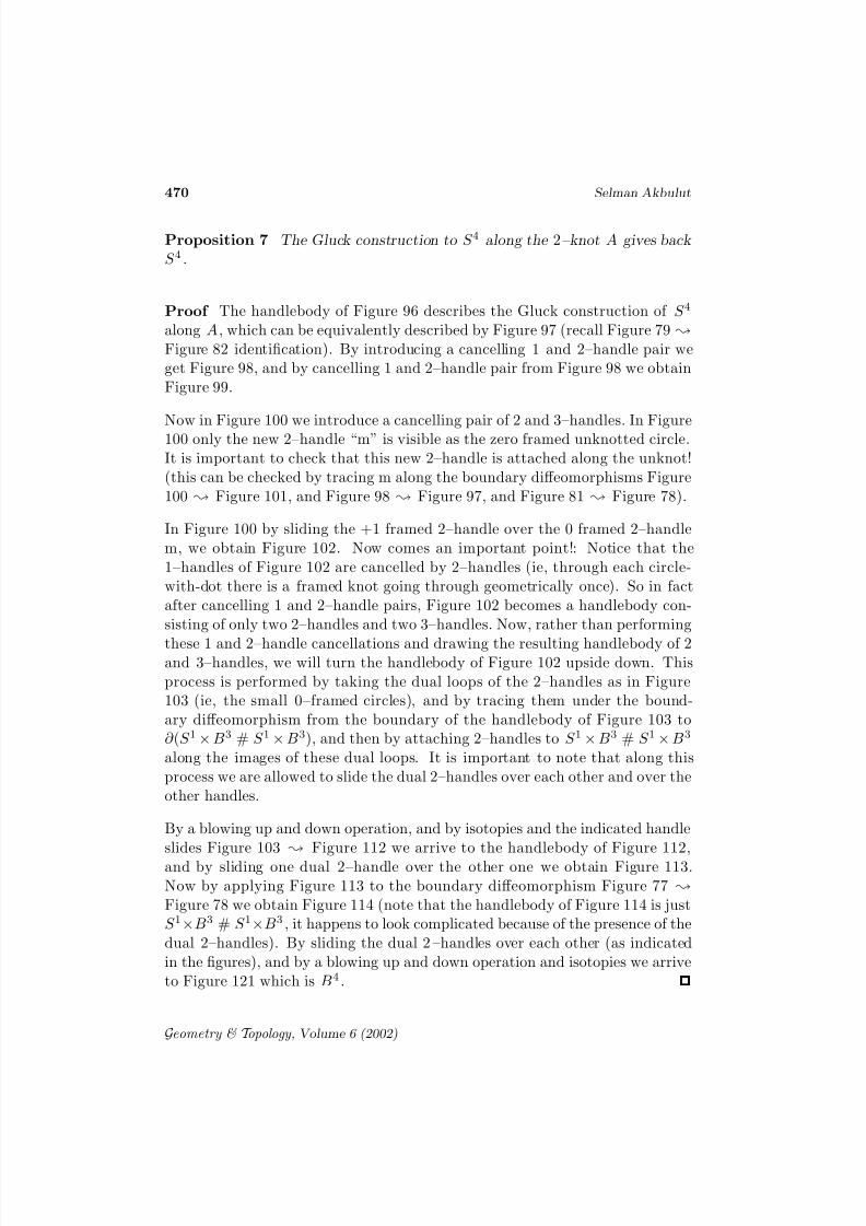
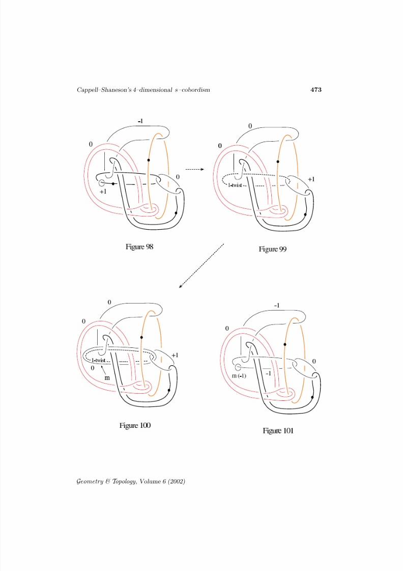
Proposition 7 The Gluck construction to S 4 along the 2–knot A gives back

S 4 .

Proof The handlebody of Figure 96 describes the Gluck construction of S 4

along A, which can be equivalently described by Figure 97 (recall Figure 79 ;

Figure 82 identification). By introducing a cancelling 1 and 2–handle pair weget Figure 98, and by cancelling 1 and 2–handle pair from Figure 98 we obtainFigure 99.

Now in Figure 100 we introduce a cancelling pair of 2 and 3–handles. In Figure100 only the new 2–handle “m” is visible as the zero framed unknotted circle.It is important to check that this new 2–handle is attached along the unknot!(this can be checked by tracing m along the boundary diffeomorphisms Figure100 ; Figure 101, and Figure 98 ; Figure 97, and Figure 81 ; Figure 78).

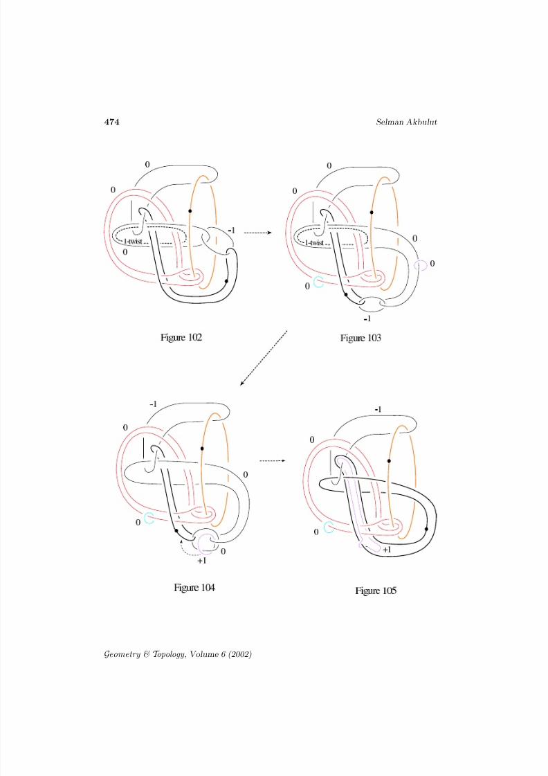
In Figure 100 by sliding the +1 framed 2–handle over the 0 framed 2–handlem, we obtain Figure 102. Now comes an important point!: Notice that the1–handles of Figure 102 are cancelled by 2–handles (ie, through each circle-with-dot there is a framed knot going through geometrically once). So in factafter cancelling 1 and 2–handle pairs, Figure 102 becomes a handlebody con-sisting of only two 2–handles and two 3–handles. Now, rather than performing

these 1 and 2–handle cancellations and drawing the resulting handlebody of 2and 3–handles, we will turn the handlebody of Figure 102 upside down. Thisprocess is performed by taking the dual loops of the 2–handles as in Figure103 (ie, the small 0–framed circles), and by tracing them under the bound-ary diffeomorphism from the boundary of the handlebody of Figure 103 to∂ (S 1 × B3 # S 1 × B3), and then by attaching 2–handles to S 1 × B3 # S 1 × B3

along the images of these dual loops. It is important to note that along thisprocess we are allowed to slide the dual 2–handles over each other and over theother handles.

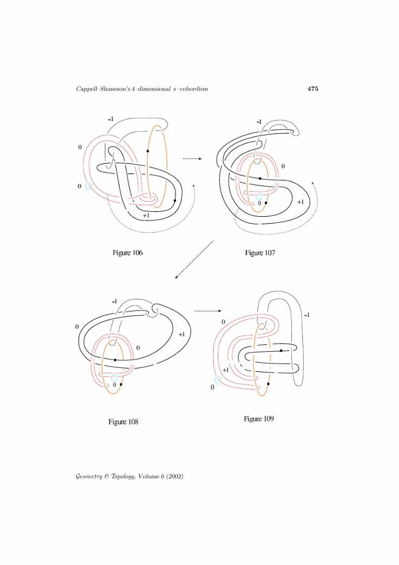
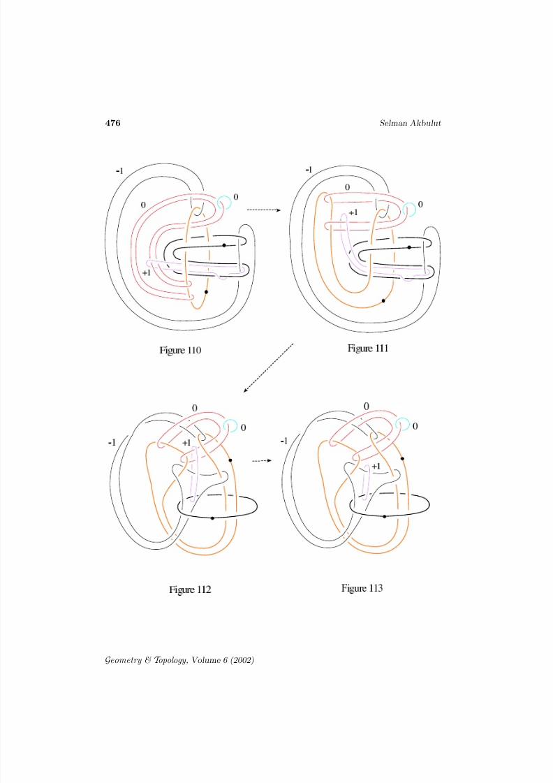
By a blowing up and down operation, and by isotopies and the indicated handleslides Figure 103 ; Figure 112 we arrive to the handlebody of Figure 112,and by sliding one dual 2–handle over the other one we obtain Figure 113.Now by applying Figure 113 to the boundary diffeomorphism Figure 77 ;

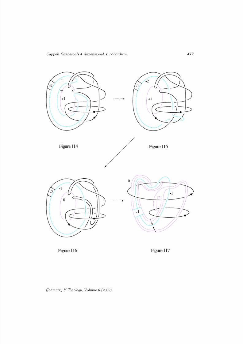
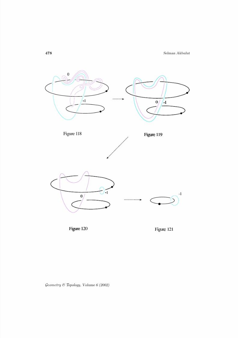
Figure 78 we obtain Figure 114 (note that the handlebody of Figure 114 is justS 1×B3 # S 1×B3 , it happens to look complicated because of the presence of thedual 2–handles). By sliding the dual 2 –handles over each other (as indicatedin the figures), and by a blowing up and down operation and isotopies we arriveto Figure 121 which is B4 .





Remark 8 Note that there is an interesting similarities between this proof and the steps Figure 19 ; Figure 29 of [5], which was crucial in showing thatthe 2–fold covering space of the Cappell–Shaneson’s fake RP4 is S 4 , [10].

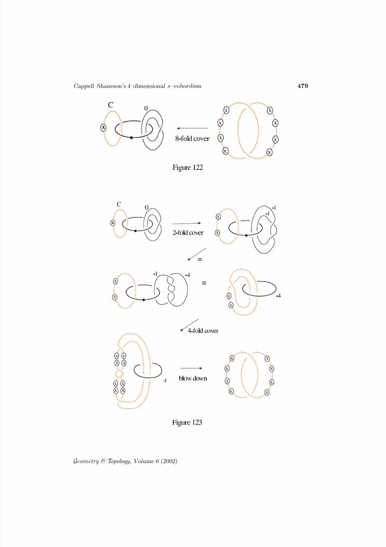
Corollary 9H = S 3 × [0, 1]

Proof ShowingH = S 3 × [0, 1] is equivalent to showing that the 4–manifold

obtained by capping the boundaries of

H with 4–balls is diffeomorphic to S 4 .Observe that under the 8–fold covering map π: S 3 → Q the loop C of Figure

122 lifts to a pair of linked Hopf circles in S 3

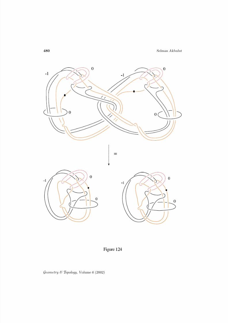
, each of it covering C four times(this is explained in Figure 123). By replacing C in ∂ (W ) by the whole standsof 1– and 2–handles going through that middle 1–handle as in Figure 79 (allthe handles other than H 1 ), and by lifting those 1 and 2–handles to S 3 weobtain the 8–fold covering of H , with ends capped off by 4–balls. Since themonodromy φ has order 3, each strand has the monodromy φ4 = φ. So we needto perform the Gluck construction as in Figure 124, which after handle slidesbecomes Σ#Σ = S 4 (because we have previously shown that Σ = S 4). Notethat the bottom two handlebodies of Figure 124 are nothing but S 4 Gluckedalong A, along with a cancelling pair of 2 and 3–handles (as usual in this pairthe 2–handle is attached to the unknot on the boundary, ie, the horizontal

zero-framed circle, and the 3–handle is not drawn).

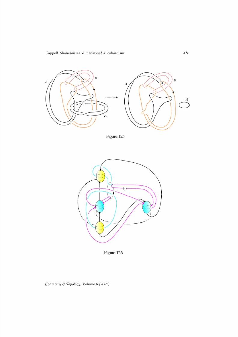
Corollary 10 W + = W

Proof By inspecting the 2–fold covering map in Figure 123, and by observingthat φ2 = φ−1 we get the handlebody of W + in Figure 125. As before, sincethe −4 framed handle is attached along the trivial loop on the boundary weget W + = W #Σ, where Σ is the S 4 Glucked along A (recall the previousCorollary), hence we have W + = W = Euler class − 4 disk bundle over S 2

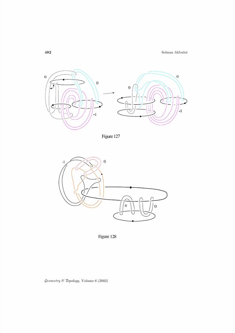
Remark 11 An amusing fact: It is not hard to check that the 2–knot comple-ment Y is obtained by the 0-logarithmic transformation operation performedalong an imbedded Klein bottle K in M̂ − S 1 × B3 (which is M̂ minus a 3–handle) ie, in Figure 21. This is done by first changing the 1–handle notationof Figure 21 (by using the arcs in Figure 126) to circle-with-dot notation, thenby simply exchanging a dot with the zero framing as indicated by the first pic-ture of Figure 127. The result is the second picture of Figure 127 which is Y .This operation is nothing other than removing the tubular neighborhood N of K from M̂ − S 1 × B3 and putting it back by a diffeomporphism which is the




472 Selman Akbulut

obvious involution on the boundary. It is also easy to check that by performingyet another 0–logarithmic transformation operation to Y along an imbeddedK gives S 1 × B3 (this is Figure 77 ⇒ Figure 78). So the operations

S 1 × B3 ⇒ Y ⇒ M̂ − S 1 × B3

are nothing but 0–logarithmic transforms along K. Note that all of the 4–manifolds S 1 × B3 , Y and M are bundles over S 1 ,with fibers B3 , Q0 , andT 0 ×−I S 1 respectively.

Remark 12 Recall [12] that a knot Σn−2 ⊂ S n is said to admit a strong Zm–action if there is a diffeomorphism h: S n → S n with

(i) hm = 1

(ii) h(x) = x for every x ∈ Σn−2

(iii) x, h(x), h2(x),..,hm−1(x) are all distinct for every x ∈ S n − Σn−2

By the proof of the Smith conjecture when n = 3 the only knot that admits astrong Zm action is the unknot. For n = 4 in [11] Giffen found knots that admitstrong Zm actions when m is odd. Our knot A ⊂ S 4 provides an example of knot which admits a strong Zm action for m = 0 mod 3 . This follows fromProposition 7, and from the fact that A is a fibered knot with an order 3monodromy.

Remark 13 Recall the vertical picture of H in Figure 77, appearing as W + −W . We can place H vertically on top of Q × I (Figure 4) by identifying Q+

with Q × 1Z := H ⌣Q+ (Q × I )

Resulting handlebody of Z is Figure 128. As a smooth manifold Z is nothingother than a copy of H . So Figure 128 provides an alternative handlebodypicture of H (the other one being Figure 47).

Remark 14 Let X 4 be a smooth 4–manifold, and C ⊂ X 4 be any loop withthe property that [C ] ∈ π1(X ) is a torsion element of order ±1 mod 3, andU ≈ S 1 × B3 be the open tubular neghborhood of C . We can form:

X̂ := (X − U ) ⌣∂ Y

Recall that π1(Y ) = t, a|t3 = a3,ata = tat, so by Van-Kampen theorem weget π1(X̂ ) = π1(X ), in fact X̂ is homotopy equivalent to X . In particularby applying this process to X = M 3 × I , where M 3 is a 3–manifold whosefundamental group contains a torsion element of order ±1 mod 3, we canconstruct many examples of potentially nontrivial s–cobordisms X̂ from M toitself.








474 Selman Akbulut








476 Selman Akbulut








478 Selman Akbulut








480 Selman Akbulut








482 Selman Akbulut





12 More on A

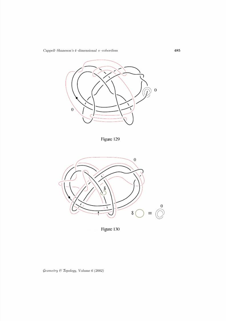
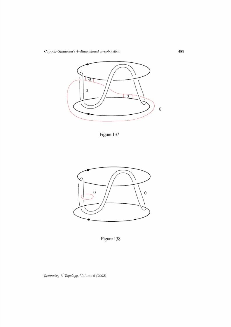
In this section we will give even a simpler and more concrete description of the 2–knot A. As a corollary we will show that W + is obtained from W byperforming the Fintushel–Stern knot surgery operation by using the trefoil knotK ([8]). It is easy to check that Figure 129, which describes A (recall Figure82), is isotopic to Figure 130. To reduce the clutter, starting with Figure 130we will denote the small 0–framed circle, which links A twice, by a single thickcircle δ .

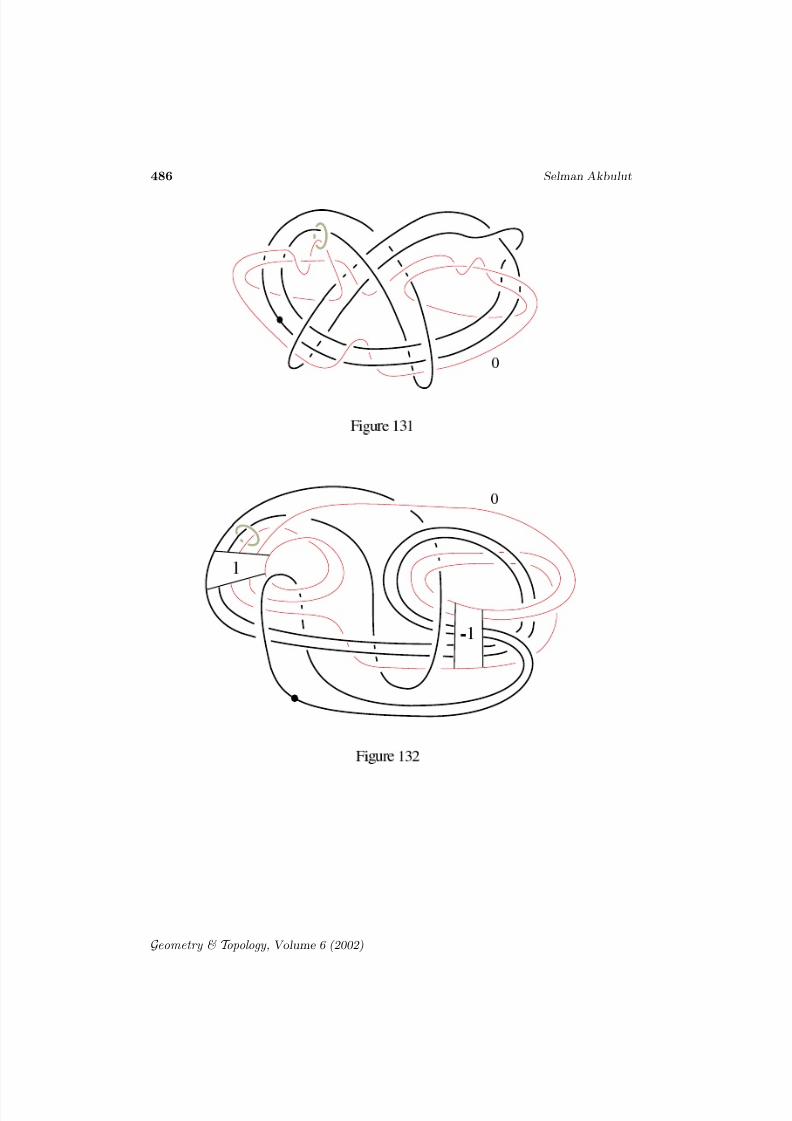
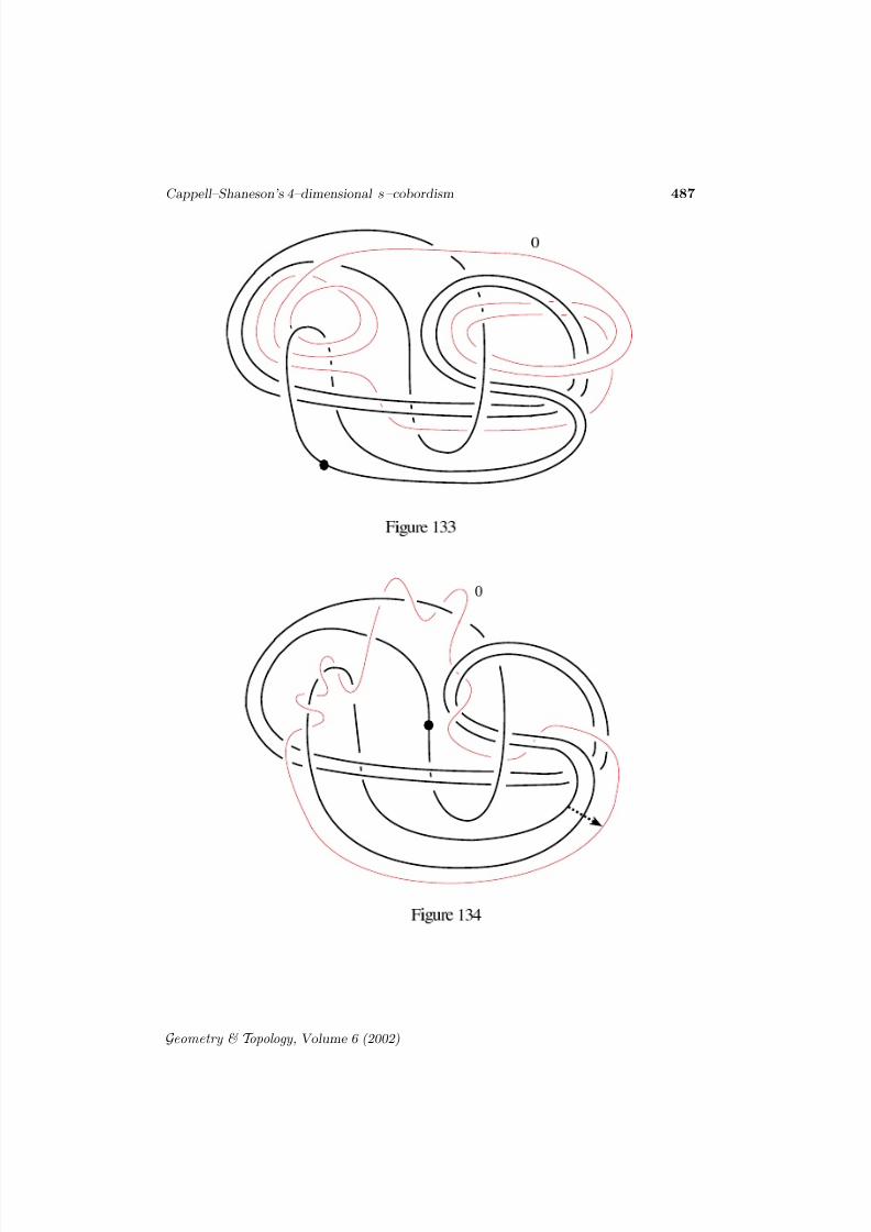
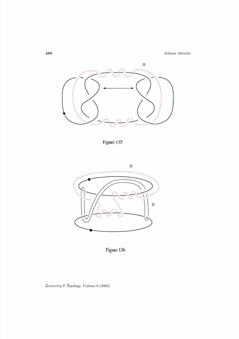
By performing the indicated handle slide to the handlebody of Figure 130 wearrive to Figure 131, which can be drawn as Figure 132. By introducing acancelling pair of 1 and 2–handles to the handlebody of Figure 132, then slidingthem over other handles, and again cancelling that handle pair we get Figure133 (this move is self explanatory from the figures). Then by an isotopy we getFigure 134, by the indicated handle slide we arrive to Figure 135. By drawingthe “slice 1–handle” (see [2]) as a 1–handle and a pair of 2–handles we getthe diffeomorphism Figure 135 ; Figure 136, and a further handle slide givesFigure 137, which is an alternative picture of the 2–knot complement A. Thereader can check that the boundary of Figure 137 is standard by the boundarydiffeomorphism Figure 137 ; Figure 138, which consists of a blowing-up +

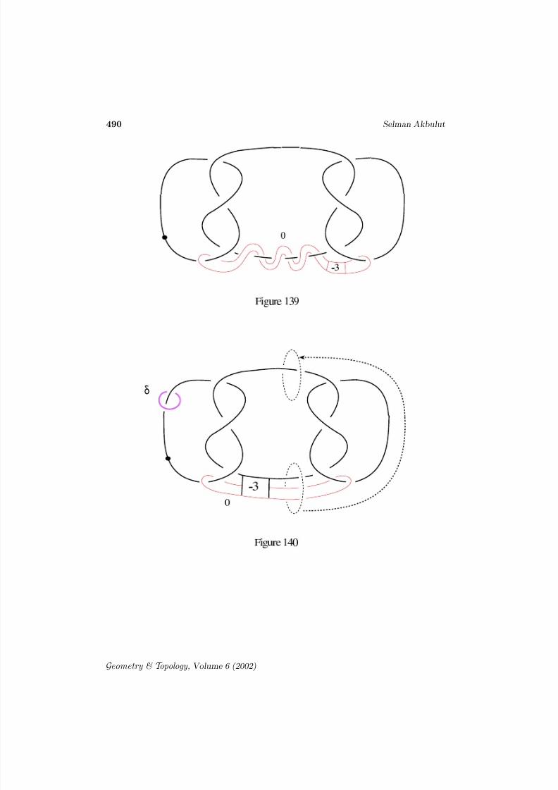
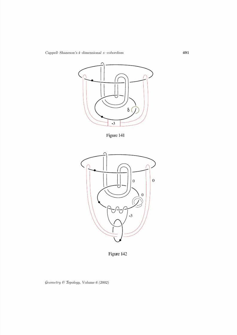
handle sliding + blowing-down operations (done three times).A close inspection reveals that the handlebody of the 2–knot complement A inFigure 135 is the same as Figure 139. Figure 139 gives another convenient wayof checking that the boundary of this handlebody is standard (eg, remove thedot from the slice 1–handle and perform blowing up and sliding and blowingdown operations, three times, as indicated by the dotted lines of Figure 140).Now we can also trace the loop δ into Figure 140, so Figure 140 becomeshandlebody of W + . By drawing the slice 1–handle as a 1–handle and a pair of 2–handles we get a diffeomorphism Figure 140 ; Figure 141. Clearly Figure142 is diffeomorphic to Figure 141. Now by introducing a cancelling pair of 2and 3–handles we obtain the diffeomorphism Figure 142 ; Figure 143 (it is

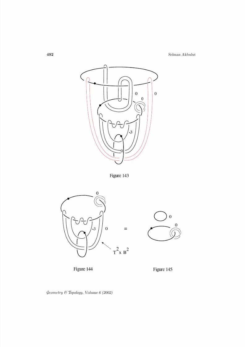
easy to check that the new 2–handle of Figure 143 is attached along the unknoton the boundary).

Now, let us recall the Fintushel–Stern knot surgery operation [8]: Let X bea smooth 4–manifold containing an imbedded torus T 2 with trivial normalbundle, and K ⊂ S 3 be a knot. The operation X ; XK of replacing a tubularneighborhood of T 2 in X by (S 3−K )×S 1 is the so called Fintushel–Stern knotsurgery operation. In [1] and [3] an algorithm of describing the handlebody of




484 Selman Akbulut

X K in terms of the handlebody of X is given. From this algorithm we seethat Figure 144 ; Figure 143 is exactly the operation W ; W K where K isthe trefoil knot. And also it is easy to check that Figure 144 ; Figure 145describes a diffemorphism to W . Hence we have proved:

Proposition 15 W + is obtained from W by the Fintushel–Stern knot surgery

operation along an imbedded torus by using the trefoil knot K

Remark 16 Note that we in fact proved that the knot complement S 4 − Ais obtained by from S 1 × B3 by the Fintushel–Stern knot surgery operation

along an imbedded torus by using the trefoil knot K. Unfortunately this torusis homologically trivial; if it wasn’t, from [8], we could have concluded that W +(hence H ) is exotic.

Remark 17 Now it is evident from From Figure 139 that A is the 3–twistspun of the trefoil knot ([16]). This explains why A is the fibered knot withfibers Q (which is the 3–fold branched cover of the trefoil knot). After thispaper was written, we were pointed out that in [13] it had proven that theGluck construction to a twist-spun knot gives back S 4 . So in hind-sight wecould have delayed the Proposition 7 until this point and deduce its proof from[13], but this would have altered the natural evolution of the paper. Our hands-

on proof of Proposition 7 should be seen as a part a general technique whichhad been previously utilized in [2], [5].

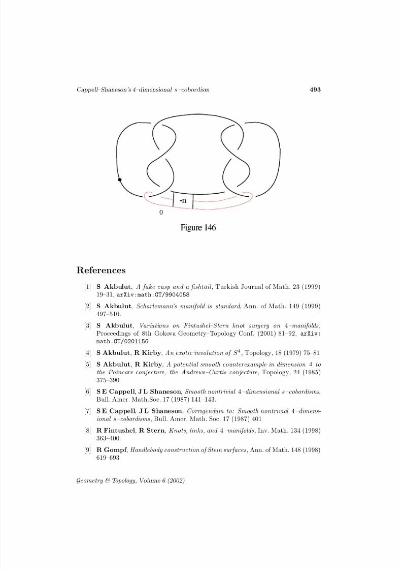
Finally, note that if An is the n–twist spun of the trefoil knot (Figure 146),then one can check that its fundamental group generalizes the presentation of A:

Gn = t, a |a = t−natn,ata = tat = t, a |tn = an,ata = tat








486 Selman Akbulut








488 Selman Akbulut








490 Selman Akbulut








492 Selman Akbulut





References

[1] S Akbulut, A fake cusp and a fishtail , Turkish Journal of Math. 23 (1999)19–31, arXiv:math.GT/9904058

[2] S Akbulut, Scharlemann’s manifold is standard , Ann. of Math. 149 (1999)497–510.

[3] S Akbulut, Variations on Fintushel–Stern knot surgery on 4–manifolds,Proceedings of 8th Gokova Geometry–Topology Conf. (2001) 81–92, arXiv: math.GT/0201156

[4] S Akbulut, R Kirby, An exotic involution of S 4 , Topology, 18 (1979) 75–81

[5] S Akbulut, R Kirby, A potential smooth counterexample in dimension 4 tothe Poincare conjecture, the Andrews–Curtis conjecture, Topology, 24 (1985)375–390

[6] S E Cappell, J L Shaneson, Smooth nontrivial 4–dimensional s–cobordisms,

Bull. Amer. Math.Soc. 17 (1987) 141–143.

[7] S E Cappell, J L Shaneson, Corrigendum to: Smooth nontrivial 4–dimens-ional s–cobordisms, Bull. Amer. Math. Soc. 17 (1987) 401

[8] R Fintushel, R Stern, Knots, links, and 4–manifolds, Inv. Math. 134 (1998)363–400.

[9] R Gompf , Handlebody construction of Stein surfaces, Ann. of Math. 148 (1998)619–693




494 Selman Akbulut

[10] R Gompf , Killing the Akbulut–Kirby 4–sphere, with relevance to the Andrews– Curtis and Schoenflies problems, Topology, 30 (1991) 97–115

[11] C H Giffen, The Generalized Smith Conjecture, Amer. J. Math. 88 (1966) 187–198

[12] C M Gordon, On the Higher-Dimensional Smith Conjecture, Proc. LondonMath. Soc. 29 (1974) 98–110

[13] C M Gordon, Knots in the 4–sphere, Comm. Math. Helv. 51 (1976) 585–596

[14] U Meierfrankenfeld, (Private communications)

[15] T Price, Homeomorphisms of quaternion space and projective planes in four space, J. Austral. Math. Soc. 23 (1977) 112–128

[16] E C Zeeman, Twisting spun knots, Trans. Amer. Math. Soc. 115 (1965) 471–495

Documents

Selman Akbulut- Cappell–Shaneson’s 4–dimensional s–cobordism