Shi Etal Om12

8/12/2019 Shi Etal Om12

http://slidepdf.com/reader/full/shi-etal-om12 1/16

A high-order adaptive time-stepping TVD solver for Boussinesq modeling

of breaking waves and coastal inundation

Fengyan Shi a,⇑, James T. Kirby a, Jeffrey C. Harris b, Joseph D. Geiman a, Stephan T. Grilli b

a Center for Applied Coastal Research, University of Delaware, Newark, DE 19716, USAb Department of Ocean Engineering, University of Rhode Island, Narragansett, RI 02882, USA

a r t i c l e i n f o

Article history:

Received 29 July 2011

Received in revised form 5 December 2011

Accepted 9 December 2011

Available online 17 December 2011

Keywords:

Boussinesq wave model

TVD Riemann solver

Breaking wave

Coastal inundation

a b s t r a c t

We present a high-order adaptive time-stepping TVD solver for the fully nonlinear Boussinesq model of

Chen (2006), extended to include moving reference level as in Kennedy et al. (2001). The equations are

reorganized in order to facilitate high-order Runge–Kutta time-stepping and a TVD type scheme with a

Riemann solver. Wave breaking is modeled by locally switching to the nonlinear shallow water equations

when the Froude number exceeds a certain threshold. The moving shoreline boundary condition is imple-

mented using the wetting–drying algorithm with the adjusted wave speed of the Riemann solver. The

code is parallelized using the Message Passing Interface (MPI) with non-blocking communication. Model

validations show good performance in modeling wave shoaling, breaking, wave runup and wave-

averaged nearshore circulation.

2011 Elsevier Ltd. All rights reserved.

1. Introduction

Boussinesq wave models have become a useful tool for model-

ing surface wave transformation from deep water to the swash

zone, as well as wave-induced circulation inside the surfzone.

Improvements in the range of model applicability have been

obtained with respect to classical restrictions to both weak disper-

sion and weak nonlinearity. Madsen et al. (1991) and Nwogu

(1993) demonstrated that the order of approximation in reproduc-

ing frequency dispersion effects could be increased using either

judicious choices for the form (or reference point) for Taylor series

expansions for the vertical structure of dependent variables, or

operators effecting a rearrangement of dispersive terms in al-

ready-developed model equations. These approaches, combined

with use either of progressively higher order truncated series

expansions (Gobbi et al., 2000; Agnon et al., 1999) or multiple level

representations (Lynett and Liu, 2004), have effectively eliminatedthe restriction of this class of model to relatively shallow water,

allowing for their application to the entire shoaling zone or deeper.

At the same time, the use of so-called ‘‘fully-nonlinear’’ formula-

tions (e.g., Wei et al. (1995) and many others) effectively elimi-

nates the restriction to weak nonlinearity by removing the wave

height to water depth ratio as a scaling or expansion parameter

in the development of approximate governing equations. This ap-

proach has improved model applicability in the surf and swash

zones particularly, where surface fluctuations are of the order of

mean water depth at least and which can represent the total verti-

cal extent of the water column in swash conditions. Representa-

tions of dissipative wave-breaking events, which do not naturally

arise as weak discontinuous solutions in the dispersive Boussinesq

formulation, have been developed usually following an eddy vis-

cosity formulation due to Zelt (1991), and have been shown to

be highly effective in describing surf zone wave height decay.

The resulting class of models has been shown to be highly effective

in modeling wave-averaged surf zone flows over both simple (Chen

et al., 2003; Feddersen et al., 2011) and complex (Geiman et al.,

2011) bathymetries. Kim et al. (2009) have further extended the

formulation to incorporate a consistent representation of boundary

layer turbulence effects on vertical flow structure.

Existing approaches to development of numerical implementa-

tions for Boussinesq models include a wide range of finite differ-

ence, finite volume, or finite element formulations. In this paper,

we describe the development of a new numerical approach forthe FUNWAVE model (Kirby et al., 1998), which has been widely

used as a public domain open-source code since it’s initial develop-

ment. FUNWAVE was originally developed using an unstaggered fi-

nite difference formulation for spatial derivatives together with an

iterated 4th order Adams–Bashforth–Moulton (ABM) scheme for

time stepping (Wei and Kirby, 1995), applied to the fully nonlinear

model equations of Wei et al. (1995). In this scheme, spatial differ-

encing is handled using a mixed-order approach, employing

fourth-order accurate centered differences for first derivatives

and second-order accurate differences for third derivatives. This

choice was made in order to move leading order truncation errors

to one order higher than the O(l2) dispersive terms (where l is

1463-5003/$ - see front matter 2011 Elsevier Ltd. All rights reserved.doi:10.1016/j.ocemod.2011.12.004

⇑ Corresponding author. Tel.: +1 302 831 2449.

E-mail address: [email protected] (F. Shi).

Ocean Modelling 43-44 (2012) 36–51

Contents lists available at SciVerse ScienceDirect

Ocean Modelling

j o u r n a l h o m e p a g e : w w w . e l s e v i e r . c o m / l o c a t e / o c e m o d

http://dx.doi.org/10.1016/j.ocemod.2011.12.004

mailto:[email protected]


http://www.sciencedirect.com/science/journal/14635003

http://www.elsevier.com/locate/ocemod

http://www.elsevier.com/locate/ocemod

http://www.sciencedirect.com/science/journal/14635003


mailto:[email protected]


8/12/2019 Shi Etal Om12


ratio of a characteristic water depth to a horizontal length, a

dimensionless parameter characterizing frequency dispersion),

while maintaining the tridiagonal structure of spatial derivatives

within time-derivative terms. This scheme is straightforward to

develop and has been widely utilized in other Boussinesq models.

Kennedy et al. (2000) and Chen et al. (2000) describe further as-

pects of the model system aimed at generalizing it for use in mod-

eling surf zone flows. Breaking is handled using a generalization to

two horizontal dimensions of the eddy viscosity model of Zelt

(1991). Similar approaches have been used by other Boussinesq

model developers, such as Nwogu and Demirbilek (2001), who

used a more sophisticated eddy viscosity model in which the eddy

viscosity is expressed in terms of turbulent kinetic energy and a

length scale. The presence of a moving shoreline in the swash zone

is handled using a ‘‘slot’’ or porous-beach method, in which the en-

tire domain remains wetted using a network of slots at grid reso-

lution which are narrow but which extend down to a depth

lower than the minimum expected excursion of the modelled free

surface. These generalizations form the basis for the existing public

domain version of the code (Kirby et al., 1998). Subsequently, sev-

eral extensions have been made in research versions of the code.

Kennedy et al. (2001) improved nonlinear performance of the mod-

el by utilizing an adaptive reference level for vertical series expan-

sions, which is allowed to move up and down with local surface

fluctuations. Chen et al. (2003) extended the model to include

longshore periodic boundary conditions and described it’s applica-

tion to modeling longshore currents on relatively straight coast-

lines. Shi et al. (2001) generalized the model coordinate system

to non-orthogonal curvilinear coordinates. Finally, Chen et al.

(2003), Chen (2006) provided revised model equations which cor-

rect deficiencies in the representation of higher order advection

terms, leading to a set of model equations which, in the absence

of dissipation effects, conserve depth-integrated potential vorticity

to O(l2), consistent with the level of approximation in the model

equations.

The need for a new formulationfor FUNWAVE arose from recog-

nition of several crucial problems with the existing code. First, theoriginal model proved to be noisy. or at least weakly unstable to

high wavenumbers near the grid Nyquist limit. In addition, both

the implementation of the eddy viscosity model for surf zone wave

breaking and the interaction of runup with beach slots proved to

be additional sources of noise in model calculations. In the original

unstaggered grid finite difference scheme, these effects led to the

need for periodic application of dissipative filters, with the fre-

quency of filtering increased in areas with active breaking. The

overall grid-based noise generation was found to stem fromseveral

sources. First, Kennedy et al. (2001, personal communications),

during development of a High Performance Fortran (HPF) version

of the code on an early linux cluster, discovered that the noise

was partially due to implementation of boundary conditions and

could be alleviated to an extent. At the same time, the curvilinearmodel developed by Shi et al. (2001) was implemented using a

staggered grid for spatial differencing, and the resulting code was

found to be less susceptible to the general grid noise problem.

A comparison of noise levels in the original FUNWAVE, the stag-

gered grid scheme of Shi et al., and the corrected boundary condi-

tion formulation of Kennedy may be found in Zhen (2004).

Additional sources of noise related either to the eddy viscosity

formulation or interaction between the flow and beach ‘‘slots’’ re-

main less well analyzed or understood. In addition, the perfor-

mance of the slots themselves has been called into question in

several cases involving inundation over complex bathymetry. Slots

which are too wide relative to the model grid spacing may admit

too much fluid before filling during runup, and cause both a reduc-

tion in amplitude and a phase lag in modeled runup events. At theother extreme, slots which are too narrow tend to induce a great

deal of numerical noise, leading to the need for intermittent or

even fairly frequent filtering of swash zone solutions. Poor model

performance in comparison to data for the case of Lynett et al.

(2010), described below in Section 4.3, was the determining factor

in the decision to pursue a new model formulation.

A number of recently development Boussinesq-type wave mod-

els have used a hybrid method combining the finite-volume and fi-

nite-difference TVD (Total Variation Diminishing)-type schemes

(Toro, 2009), and have shown robust performance of the shock-

capturing method in simulating breaking waves and coastal inun-

dation (Tonelli and Petti, 2009, 2010; Roeber et al., 2010; Shiach

and Mingham, 2009; Erduran et al., 2005, and others). The use of

the hybrid method, in which the underlying components of the

nonlinear shallow water equations (which form the basis of the

Boussinesq model equations) are handled using the TVD finite vol-

ume method while dispersive terms are implemented using con-

ventional finite differencing, provides a robust framework for

modeling of surf zone flows. In particular, wave breaking may be

handled entirely by the treatment of weak solutions in the

shock-capturing TVD scheme, making the implementation of an

explicit formulation for breaking wave dissipation unnecessary.

In addition, shoreline movement may be handled quite naturally

as part of the Reiman solver underlying the finite volume scheme.

In this paper, we describe the development of a hybrid finite

volume-finite difference scheme for the fully nonlinear Boussinesq

model equations of Chen (2006), extended to incorporate a moving

reference level as in Kennedy et al. (2001). The use of a moving ref-

erence elevation is more consistent with a time-varying represen-

tation of elevation at a moving shoreline in modeling of a swash

zone dynamics and coastal inundation. A conservative form of

the equations is derived. Dispersive terms are reorganized with

the aim of constructing a tridiagonal structure of spatial deriva-

tives within time-derivative terms. The surface elevation gradient

term are also rearranged to obtain a numerically well-balanced

form, which is suitable for any numerical order. In contrast to pre-

vious high-order temporal schemes, which usually require uniform

time-stepping, we use adaptive time stepping based on a third-order Runge–Kutta method. Spatial derivatives are discretized

using a combination of finite-volume and finite-difference meth-

ods. A high-order MUSCL (Monotone Upstream-centered Schemes

for Conservation Laws) reconstruction technique, which is accurate

up to the fourth-order, is used in the Riemann solver. The wave

breaking scheme follows the approach of Tonelli and Petti

(2009), who used the ability of the nonlinear shallow water equa-

tions (NLSWE) with a TVD solver to simulate moving hydraulic

jumps. Wave breaking is modeled by switching from Boussinesq

to NSWE at cells where the Froude number exceeds a certain

threshold. A wetting–drying scheme is used to model a moving

shoreline.

The paper is organized as follows. Section 2 shows derivations

of the conservative form of theoretical equations with a well-balanced pressure gradient term. The numerical implementation,

including the hybrid numerical schemes, wetting–drying algo-

rithm, boundary conditions and code parallelization, are described

in Section 3. Section 4 illustrates four model’s applications to prob-

lems of wave breaking, wave runup and wave-averaged nearshore

circulations. Conclusions are made in Section 5.

2. Fully-nonlinear Boussinesq equations

In this section, we describe the development of a set of Bous-

sinesq equations which are accurate to O(l2) in dispersive effects.

Here, l is a parameter characterizing the ratio of water depth to

wave length, and is assumed to be small in classical Boussinesqtheory. We retain dimensional forms below but will refer to the

F. Shi et al. / Ocean Modelling 43-44 (2012) 36–51 37

8/12/2019 Shi Etal Om12


apparent O(l2) ordering of terms resulting from deviations from

hydrostatic behavior in order to identify these effects as needed.

The model equations used here follow from the work of Chen

(2006). In this and earlier works starting with Nwogu (1993), the

horizontal velocity is written as

u ¼ ua þu2ð z Þ ð1ÞHere, u

a denotes the velocity at a reference elevation z = z

a, and

u2ð z Þ ¼ ð z a z Þr A þ 1

2 z 2a z 2 rB ð2Þ

represents the depth-dependent correction at O(l2), with A and B

given by

A ¼ r ðhuaÞB ¼ r ua ð3ÞThe derivation follows Chen (2006) except for the additional effect

of letting the reference elevation z a vary in time according to

z a ¼ fh þ bg ð4Þwhere h is local still water depth, g is local surface displacement

and f and b are constants, as in Kennedy et al. (2001). This addition

does not alter the details of the derivation, which are omitted

below.

2.1. Governing equations

The equations of Chen (2006) extended to incorporate a possi-

ble moving reference elevation follow. The depth-integrated vol-

ume conservation equation is given by

gt þ r M ¼ 0 ð5Þwhere

M ¼ H fua þ u2g ð6Þis the horizontal volume flux. H = h + g is the total local water depth

and u2 is the depth averaged O(l

2

) contribution to the horizontalvelocity field, given by

u2 ¼ 1

H

Z gh

u2ð z Þdz

¼ z 2a2 1

6ðh

2 hgþ g2Þ

rB þ z a þ 1

2ðh gÞ

r A ð7Þ

The depth-averaged horizontal momentum equation can be written

as

ua;t þ ðua rÞua þ g rgþ V 1 þ V 2 þ V 3 þR ¼ 0 ð8Þwhere g is the gravitational acceleration and R represents diffusive

and dissipative terms including bottom friction and subgrid lateral

turbulent mixing. V 1 and V 2 are terms representing the dispersive

Boussinesq terms given by

V 1 ¼ z 2a2 rB þ z ar A

t

r g2

2 Bt þg At

ð9Þ

V 2 ¼ r ð z a gÞðua rÞ A þ 1

2ð z 2a g2Þðua rÞB þ 1

2½ A þ gB2

ð10Þ

The form of (9) allows for the reference level z a to be treated as a

time-varying elevation, as suggested in Kennedy et al. (2001). If this

extension is neglected, the terms reduce to the form given originally

by Wei et al. (1995). The expression (10) for V 2 was also given by

Wei et al. (1995), and is not altered by the choice of a fixed or mov-

ing reference elevation.

The term V 3 in (8) represents the O(l2) contribution to the

expression for x u = xi z

u (with i z

the unit vector in the z direction) and may be written as

V 3 ¼ x0i z u2 þx2i

z ua ð11Þwhere

x0 ¼ ðr uaÞ i z ¼ v a; x ua; y ð12Þx2 ¼ ðr u2Þ i z ¼ z a; xð A y þ z aB yÞ z a; yð A x þ z aB xÞ ð13Þ

Following Nwogu (1993), z a is usually chosen in order to opti-

mize the apparent dispersion relation of the linearized model rel-ative to the full linear dispersion in some sense. In particular, the

choice a = ( z a/h)2/2 + z a/h = 2/5 recovers a Padé approximant

form of the dispersion relation, while the choice a = 0.39, corre-

sponding to the choice z a = 0.53h, minimizes the maximum error

in wave phase speed occurring over the range 06 kh6 p. Kennedy

et al. (2001) showed that allowing z a to move up and down with

the passage of the wave field allowed a greater degree of flexibility

in optimizing nonlinear behavior of the resulting model equations.

In the examples chosen here, where a great deal of our focus is on

the behavior of the model from the break point landward, we

adopt Kennedy et al.’s ‘‘datum invariant’’ form

z a ¼ h þ bH ¼ ðb 1Þh þ bg ¼ fh þ ð1 þ fÞg ð14Þ

with f = 0.53 as in Nwogu (1993) and b = 1 + f = 0.47. This corre-sponds in essence to a r coordinate approach, which places the ref-

erence elevation at a level 53% of the total local depth below the

local water surface. This also serves to keep the model reference

elevation within the actual water column over the entire wetted ex-

tent of the model domain.

2.2. Treatment of the surface gradient term

The hybrid numerical scheme requires a conservative form of

continuity equation and momentum equations, thus requiring a

modification of the leading order pressure term in the momentum

equation. A numerical imbalance problem occurs when the surface

gradient term is conventionally split into an artificial flux gradient

and a source term that includes the effect of the bed slope for anon-uniform bed. To eliminate errors introduced by the traditional

depth gradient method (DGM), a so-called surface gradient method

(SGM) proposed by Zhou et al. (2001) was adopted in the TVD

based-Boussinesq models in the recent literatures. Zhou et al. dis-

cussed an example of SGM in 1-D and verified that the slope-

source term may be canceled out by part of the numerical flux

term associated with water depth, if the bottom elevation at the

cell center is constructed using the average of bottom elevations

at two cell interfaces. Zhou et al. also showed a 2D application,

but without explicitly describing 2D numerical schemes. Although

this scheme can be extended into 2D following the same procedure

as in 1D, it was found that the 2D extension may not be trivial in

terms of the bottom construction for a 2D arbitrary bathymetry.

Kim et al. (2008) pointed out that the water depth in the slope-source term should be written in a discretized form rather than

the value obtained using the bottom construction, implying that

their revised SGM is valid for general 2D applications.

For the higher-order schemes, such as the fourth-order MUSCL-

TVD scheme (Yamamoto and Daiguji, 1993; Yamamoto et al., 1998)

used in the recent Boussinesq applications, the original SGM and

the revised SGM may not be effective in removing the artificial

source. This problem was recently noticed by some authors, such

as Roeber et al. (2010), who kept a first-order scheme (second-

order for normal conditions) for the numerical flux term and the

slope-source term in order to ensure a well-balanced solution,

without adding noise for a rapidly varying bathymetry. The

imbalance problem can be solved by a reformulation of this term

in terms of deviations from an unforced but separately specifiedequilibrium state (see general derivations in Rogers et al., 2003

38 F. Shi et al. / Ocean Modelling 43-44 (2012) 36–51

http://-/?-

http://-/?-

8/12/2019 Shi Etal Om12


and recent application in Liang and Marche, 2009). Using this tech-

nique, the surface gradient term may be split as

gH rg ¼ r 1

2 g ðg2 þ 2hgÞ

g grh ð15Þ

which is well-balanced for any numerical order for an unforced, still

water condition.

2.3. Conservative form of fully nonlinear Boussinesq equations

For Chen’s (2006) equations or the minor extension considered

here, H ua can be used as a conserved variable in the construction

of a conservative form of Boussinesq equations, but this results in a

source term in the mass conservation equation, such as in Shiach

and Mingham (2009) and Roeber et al. (2010). An alternative

approach is to use M as a conserved variable in terms of the phys-

ical meaning of mass conservation. In this study, we used M,

instead of H ua, in the following derivations of the conservative

form of the fully nonlinear Boussinesq equations.

Using M from (6) together with the vector identity

r ðuvÞ ¼ ru v þ ðr v Þu ð16Þallows (8) to be rearranged as

Mt þ r MM

H

þ gH rg ¼ H u2;t þua ru2 þ u2 rua

V 1 V 2 V 3 R g ð17Þ

Following Wei et al. (1995), we separate the time derivative dis-

persion terms in V 1 according to

V 1 ¼ V 01;t þ V 001 ð18Þ

where

V 01 ¼

z 2a

2 rB

þ z a

r A

r g2

2

B

þg A ð

19

Þand

V 001 ¼ r gt ð A þ gBÞ½ ð20ÞUsing (15), (19) and (20), the momentum equation can be

rewritten as

Mt þ r MM

H

þ r 1

2 g ðg2 þ 2hgÞ

¼ H u2;t þua ru2 þ u2 rua V 01;t V 001 V 2 V 3 R n o

þ g grh

ð21Þ

A difficulty usually arises in applying the adaptive time-stepping scheme to the time derivative dispersive terms u2;t and

V 01;t , which was usually calculated using values stored in several

time levels in the previous Boussinesq codes such as in Wei et al.

(1995) and Shi et al. (2001). To prevent this, the equation can be

re-arranged by merging the time derivatives on the right hand side

into the time derivative term on the left hand side, giving

V t þ r MM

H

þ r 1

2 g ðg2 þ 2hgÞ

¼ gt ð V 01 u2Þ þ H ua u2 þ u2 rua V 001 V 2 V 3 R

þ g grh ð22Þ

where

V ¼ H ðua þ V 01Þ ð23Þ

In (22) gt can be calculated explicitly using (5) as in Roeber et al.

(2010). Eqs. (5) and (21) are the governing equations solved in this

study. As V is obtained, the velocity ua can be found by solving a

system of equation with tridiagonal matrix formed by (22), in

which all cross-derivatives are moved to the right-hand side of

the equation.

3. Numerical schemes

3.1. Compact form of governing equations

We define

ua ¼ ðu;v Þu2 ¼ ðU 4; V 4ÞM ¼ ðP ;Q Þ ¼ H u þ U 4; v þ V 4½ V 01 ¼ ðU 01;V 01Þ V 001 ¼ ðU 001;V 001Þ V 2 ¼ ðU 2;V 2Þ V ¼ ðU ; V Þ ¼ H ðu þ U 01Þ; ðv þ V 01Þ The generalized conservative form of Boussinesq equations can be

written as

@ W

@ t þ r HðWÞ ¼ S ð24Þ

where W and H(W) are the vector of conserved variables and the

flux vector function, respectively, and are given by

W ¼g

U

V

0B@

1CA; H ¼

P iþ Q j

P 2

H þ 1

2 g ðg2 þ 2ghÞ

h ii þ PQ

H j

PQ H iþ Q 2

H þ 1

2 g ðg2 þ 2ghÞ

h i j

0BBB@

1CCCA ð25Þ

S ¼0

g g @ h@ x þ w x þ HR x

g g @ h@ y

þ w y þ HR y

0B@ 1CA ð26Þ

where

w x ¼ gt ðU 01 U 4Þþ H uU 4; x þv U 4; y þ U 4u x þ V 4u y U 001 U 2 U 3

ð27Þ

w y ¼ gt ðV 01 V 4Þþ H uV 4; x þv V 4; y þ U 4v x þ V 4v y U 001 V 2 V 3

ð28ÞThe expanded forms of ðU 01; V 01Þ; ðU 001; V 001Þ; ðU 2; V 2Þ; ðU 3; V 3Þ and

(U 4, V 4) can be found in Appendix A. For the term R , the bottom

stress is approximated using a quadratic friction equation. For mod-eling wave-generated nearshore currents such as rip current and

alongshore current (Chen et al., 1999, 2003), a Smagorinsky

(1963)-like subgrid turbulent mixing algorithm is implemented.

The eddy viscosity associated with the subgrid mixing is deter-

mined by breaking-induced current field. The detailed formulations

can be found in Chen et al. (1999). The Smagorinsky subgrid mixing

is used in the model application to predicting wave-averaged near-

shore circulation described in Section 4.4.

3.2. Spatial discretization

A combined finite-volume and finite-difference method was ap-

plied to the spatial discretization. Following Toro (2009), two basic

steps are needed to achieve the spatial scheme. The first step isto use a reconstruction technique to compute values at the cell


8/12/2019 Shi Etal Om12


interfaces. The second step is to use a local Riemann solver to get

numerical fluxes at the cell interfaces.

For the flux terms and the first-order derivative terms, a high-

order MUSCL-TVD scheme is implemented in the present model.

The high-order MUSCL-TVD scheme can be written in a compact

form including different orders of accuracy from the second-to

the fourth-order, according to Erduran et al. (2005) who modified

Yamamoto et al.’s (1998) fourth-order approach. In x

-direction,

for example, the combined form of the interface construction can

be written as follows:

/Liþ1=2 ¼ /i þ

1

4 ð1 j1Þvðr ÞD

/i1=2 þ ð1 þ j1Þvð1=r ÞD/iþ1=2

h ið29Þ

/Ri1=2 ¼ /i

1

4 ð1 þ j1Þvðr ÞD

/i1=2 þ ð1 j1Þvð1=r ÞD/iþ1=2

h ið30Þ

where /Liþ1=2 is the constructed value at the left-hand side of the

interface i þ 12

and /Ri1=2 is the value at the right-hand side of the

interface i 12. The values of D⁄/ are evaluated as follows:

D/iþ1=2 ¼ D/iþ1=2 j2D

3 /iþ1=2=6

D/iþ1=2 ¼

/iþ1

/i

D3 /iþ1=2 ¼ D /iþ3=2 2D/iþ1=2 þD/i1=2

D/i1=2 ¼ minmodðD/i1=2;D/iþ1=2;D/iþ3=2ÞD/iþ1=2 ¼ minmodðD/iþ1=2;D/iþ3=2;D/i1=2ÞD/iþ3=2 ¼ minmodðD/iþ3=2;D/i1=2;D/iþ1=2Þ

ð31Þ

In (31), minmod represents the Minmod limiter and is given by

minmodð j; k; lÞ ¼ signð jÞ maxf0; min½j jj; 2 signð jÞk; 2 signð jÞlg:ð32Þ

j1 and j2 in (29) and (30) are control parameters for orders of the

scheme in the compact form. The complete form with (j1,j2) = (1/

3,1) is the fourth-order scheme given by Yamamoto et al. (1998).(j1,j2) = (1/3,0) yields a third-order scheme, while the second-

order scheme can be retrieved using (j1,j2) = (1,0).

v(r ) in (29) and (30) is the limiter function. The original scheme

introduced by Yamamoto et al. (1998) uses the Minmod limiter as

used in (31). Erduran et al. (2005) found that the use of the van-

Leer limiter for the third-order scheme gives more accurate results.

Their finding was confirmed by using the present model in the

benchmark tests for wave runup conducted by Tehranirad et al.

(2011). The van-Leer limiter can be expressed as

vðr Þ ¼ r þ jr j1 þ r

ð33Þ

where

r ¼ D/iþ1=2

D/i1=2

ð34Þ

The numerical fluxes are computed using a HLL approximate

Riemann solver

HðWL;WRÞ ¼HðWLÞ if sL P 0

HðWL;WRÞ if sL < 0 < sR

HðWRÞ if sR 6 0

8><>: ð35Þ

where

HðWL;WRÞ ¼ sRHðWLÞ sLHðWRÞ þ sLsRðWR W

LÞsR

sL

ð36Þ

The wave speeds of the Riemann solver are given by

sL ¼ minð V L n ffiffiffiffiffiffiffiffiffiffiffiffiffiffiffiffiffiffiffiffi

g ðh þ gÞLq

; us ffiffiffiffiffiffius

p Þ; ð37Þ

sR ¼ maxð V R nþ ffiffiffiffiffiffiffiffiffiffiffiffiffiffiffiffiffiffiffiffi

g ðh þ gÞRq

; us þ ffiffiffiffiffiffius

p Þ; ð38Þin which us and us are estimated as

us ¼ 1

2ð V L þ V RÞ nþ

ffiffiffiffiffiffiffiffiffiffiffiffiffiffiffiffiffiffiffiffi g ðgþ hÞL

q

ffiffiffiffiffiffiffiffiffiffiffiffiffiffiffiffiffiffiffiffi g ðgþ hÞR

q ð39Þ

ffiffiffiffiffiffius

p

¼

ffiffiffiffiffiffiffiffiffiffiffiffiffiffiffiffiffiffiffiffi g ðgþ hÞL

q þ

ffiffiffiffiffiffiffiffiffiffiffiffiffiffiffiffiffiffiffiffi g ðgþ hÞR

q 2

þ

ð V L V RÞ n4

ð40

Þand n is the normalized side vector for a cell face.

Higher derivative terms in w x and w y were discretized using a

central difference scheme at the cell centroids, as in Wei et al.

(1995). No discretization of dispersion terms at the cell interfaces

is needed due to using M as a flux variable. The Surface Gradient

Method (Zhou et al., 2001) was used to eliminate unphysical oscil-

lations. Because the pressure gradient term is re-organized as in

Section 2.2, there is no imbalance issue for the high-order MUSCL

scheme.

3.3. Time stepping

The third-order Strong Stability-Preserving (SSP) Runge–Kutta

scheme for nonlinear spatial discretization (Gottlieb et al., 2001)was adopted for time stepping. The scheme is given by

Wð1Þ ¼ W

n þ Dt ðr HðWnÞ þ Sð1ÞÞW

ð2Þ ¼ 3

4W

n þ 1

4 W

ð1Þ þDt r HðWð1ÞÞ þ Sð2Þ h i

ð41Þ

Wnþ1 ¼ 1

3W

n þ 2

3 W

ð2Þ þDt r HðWð2ÞÞ þ Snþ1 h i

in which Wn denotes W at time level n. W(1) andW(2) are values at

intermediate stages in the Runge–Kutta integration. As W is

obtained at each intermediate step, the velocity (u,v ) can be solved

by a system of tridiagonal matrix equations formed by (22). S needs

to be updated using (u,v ,g) at the corresponding time step and an

iteration is needed to achieve convergence.

An adaptive time step is chosen, following the Courant–Friedrichs–Lewy (CFL) criterion:

0 10 20 30 40 500

5

10

15

20

25

30

35

40

45

50

number of processors

s p e e d u p

model

ideal

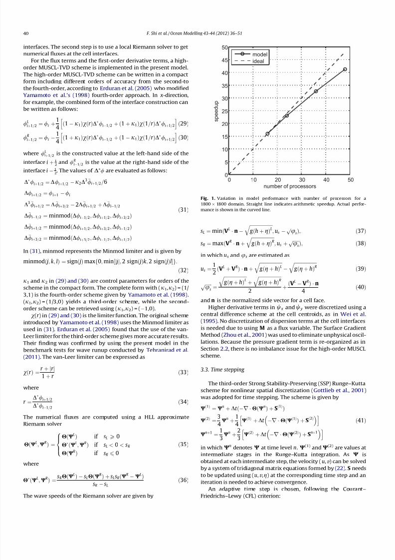
Fig. 1. Variation in model performance with number of processors for a

1800 1800 domain. Straight line indicates arithmetic speedup. Actual perfor-

mance is shown in the curved line.


8/12/2019 Shi Etal Om12


Dt ¼ C min min D x

jui; jj þ ffiffiffiffiffiffiffiffiffiffiffiffiffiffiffiffiffiffiffiffiffiffiffiffi

g ðhi; j þgi; jÞq ;min

D y

jv i; jj þ ffiffiffiffiffiffiffiffiffiffiffiffiffiffiffiffiffiffiffiffiffiffiffiffi

g ðhi; j þgi; jÞq

0B@

1CA

ð42

Þwhere C is the Courant number. C = 0.5 was used in the following

examples.

3.4. Wave breaking and wetting–drying schemes for shallow water

The wave breaking scheme follows the approach of Tonelli and

Petti (2009), who successfully used the ability of NSWE with a TVD

scheme to model moving hydraulic jumps. Thus, the fully nonlin-

ear Boussinesq equations are switched to NSWE at cells where

the Froude number exceeds a certain threshold. Following Tonelli

and Petti, the ratio of surface elevation to water depth is chosen

as the criterion to switch from Boussinesq to NSWE. That means

that all dispersive terms, V 01 in (23) and / x and / y in (26) are zero

at grid points where the wave is breaking. The threshold value wasset to 0.8 in all model tests in Section 4 according to model valida-

tions against experimental data, which is also consistent with

Tonelli and Petti (2009).

The wetting–drying scheme for modeling a moving boundary is

straightforward. The normal flux n M at the cell interface of a dry

cell is set to zero. A mirror boundary condition is applied to the

fourth-order MUSCL-TVD scheme and discretization of dispersive

terms in w x, w y at dry cells. It may be noted that the wave speeds

of the Riemann solver (37) and (38) for a dry cell are modified as

sL ¼ V L n ffiffiffiffiffiffiffiffiffiffiffiffiffiffiffiffiffiffiffiffi

g ðh þ gÞLq

;

sR ¼ V L nþ 2 ffiffiffiffiffiffiffiffiffiffiffiffiffiffiffiffiffiffiffiffi g ðh þ gÞL

q ðright dry cellÞ ð43Þand

sL ¼ V R n ffiffiffiffiffiffiffiffiffiffiffiffiffiffiffiffiffiffiffiffi

g ðh þ gÞRq

;

sR ¼ V R nþ 2

ffiffiffiffiffiffiffiffiffiffiffiffiffiffiffiffiffiffiffiffi g ðh þ gÞR

q ðleft dry cellÞ ð44Þ

3.5. Boundary conditions and wavemaker

We implemented various boundary conditions including wall

boundary condition, absorbing boundary condition following Kirby

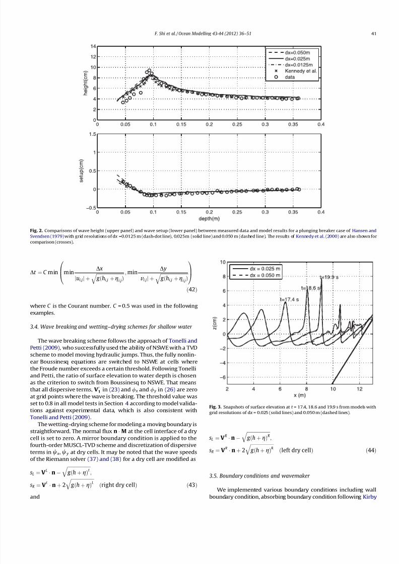
Fig. 2. Comparisons of wave height (upper panel) and wave setup (lower panel) between measured data and model results for a plunging breaker case of Hansen and

Svendsen (1979) with grid resolutions of d x =0.0125 m (dash-dot line), 0.025m (solid line) and 0.050 m (dashed line). The results of Kennedy et al. (2000) are also shown for

comparison (crosses).

Fig. 3. Snapshots of surface elevation at t = 17.4, 18.6 and 19.9 s from models with

grid resolutions of d x = 0.025 (solid lines) and 0.050 m (dashed lines).


8/12/2019 Shi Etal Om12


et al. (1998) and periodic boundary condition following Chen et al.

(2003).

Wavemakers implemented in this study include Wei et al.’s

(1999) internal wavemakers for regular waves and irregular waves.

For the irregular wavemaker, an extension was made to incorpo-

rate alongshore periodicity into wave generation, in order to elim-

inate a boundary effect on wave simulations. The technique exactlyfollows the strategy in Chen et al. (2003), who adjusted the distri-

bution of wave directions in each frequency bin to obtain along-

shore periodicity. This approach is effective in modeling of

breaking wave-induced nearshore circulation such as alongshore

currents and rip currents.

3.6. Parallelization

In parallelizing the computational model, we used a domain

decomposition technique to subdivide the problem into multiple

regions and assign each subdomain to a separate processor core.

Each subdomain region contains an overlapping area of ghost cells

three-row deep, as required by the fourth order MUSCL-TVDscheme. The Message Passing Interface (MPI) with non-blocking

communication is used to exchange data in the overlapping region

between neighboring processors. Velocity components are ob-

tained from Eq. (22) by solving tridiagonal matrices using the par-

allel pipelining tridiagonal solver described in Naik et al. (1993).

To investigate performance of the parallel program, numerical

simulations of an idealized case are tested with different numbers

of processors on the Linux cluster Chimera located at University of

Delaware. The test case is set up in a numerical grid of 1800 1800cells. Fig. 1 shows the model speedup versus number of processors.

It can be seen that performance scales nearly proportional to the

number of processors, with some delay caused by inefficiencies

in parallelization, such as inter-processor communication time.

Chimera nodes consist of 48 cores, so the present simulations on

48 or less cores do not test inter-node communication perfor-

mance on the system.

4. Model tests

The model has been validated extensively using laboratory

experiments for wave shoaling and breaking, as described in the

FUNWAVE manual by Kirby et al. (1998), and a suite of benchmark

tests for wave runup. The interested reader is referred to Shi et al.

(2011) and Tehranirad et al. (2011). In this paper, we will present

four test cases, with a focus on examining the shock-capturing

scheme for modeling wave breaking, the wetting–drying algorithm

for wave runup, and the model capability in predicting wave-in-

duced nearshore circulation. The fourth-order scheme of Yamam-

oto et al. (1998) is used in all the test cases. The effect of using

adaptive time stepping is demonstrated in the wave runup case.

4.1. Breaking waves on a beach

Hansen and Svendsen (1979) carried out laboratory experi-

ments of wave shoaling and breaking on a beach. Waves were

generated on a flat bottom a 0.36 m depth, and the beach slopewas 1:34.26. The experiments included several cases including

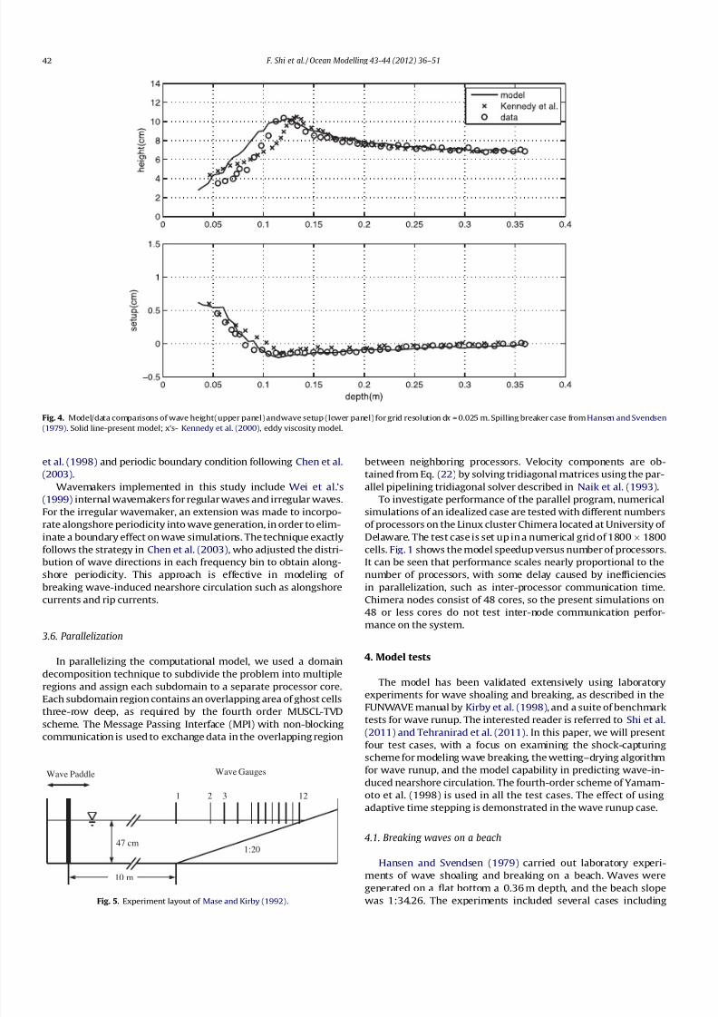
Fig. 4. Model/data comparisons of wave height(upper panel) andwave setup (lower panel) for grid resolution d x = 0.025 m. Spilling breaker case from Hansen and Svendsen

(1979). Solid line-present model; x’s- Kennedy et al. (2000), eddy viscosity model.

47 cm

10 m

Wave Paddle Wave Gauges

1 2 3 12

1:20

Fig. 5. Experiment layout of Mase and Kirby (1992).


8/12/2019 Shi Etal Om12


20 22 24 26 28 30 32 34 36 38 40

0

20

40

60

80

100

Time (sec)

S u r f a c e e l e v a t i o n ( c m )

h=35.0cm

h=30.0cm

h=25.0cm

h=20.0cm

h=17.5cm

h=15.0cm

h=12.5cm

h=10.0cm

h= 7.5cm

h= 5.0cm

h= 2.5cm

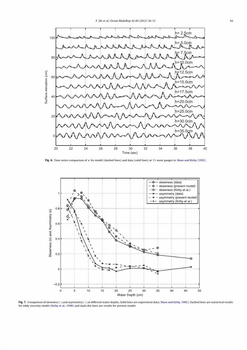
Fig. 6. Time series comparison of g for model (dashed lines) and data (solid lines) at 11 wave gauges in Mase and Kirby (1992).

Fig. 7. Comparison of skewness () and asymmetry () at different water depths. Solid lines are experiment data ( Mase and Kirby, 1992). Dashed lines are numerical results

for eddy viscosity model (Kirby et al., 1998) and dash-dot lines are results for present model.


8/12/2019 Shi Etal Om12


plunging breakers, plunging-spilling breakers and spilling break-

ers. In this paper, we simulate two typical cases: a plunging break-

er and a spilling breaker, respectively. The wave height and wave

period are 4.3 cm and 3.33 s, respectively, for the plunging case,

and 6.7 cm and 1.67 s for the spilling case.

Although the shock-capturing breaking algorithm used in Bous-

sinesq wave models has been examined by previous researchers

(e.g., Tonelli and Petti, 2009; Shiach and Mingham, 2009 and oth-

ers), there is a concern about its sensitivity to grid spacing. Erduran

et al.(2005) discussed numerical diffusivity caused by several types

of limiters in a TVD scheme. In this study, we intended to examine

the grid spacing effect on prediction of breaking wave height. We

adopted three grid sizes, d x = 0.05 m, 0.025m and 0.0125 m,

respectively, for each cases. Fig. 2 shows comparisons of wave

height and wave setup between measured data and numerical re-

sults from model runs with different grid sizes. Results from the

previous version of FUNWAVE with the same breaking parameters

asin Kennedy et al. (2000) arealso plotted in the figure for compar-

ison. The wave breaking location of wave setup/setdown predicted

by the three runs are in agreement with the data, however, the pre-

dicted maximum wave heights are slightly different. Results from

d x = 0.025 m and 0.0125 m grids are very close, indicatinga conver-

gence with grid refinement. All three models underpredict the peak

wave height at breaking and overpredict wave height inside of the

surfzone. This prediction trend was also found in Kennedy et al.

(2000) as shown in the figure. 10% and 9.2% underpredictions of

peak wave height can be found in the tests with dx = 0.025 m and

0.0125 m, respectively, while Kennedy et al. (2000) underpredicted

the peak wave height by 10% with d x = 0.02 m. The present model

with a coarser grid (d x = 0.05 m) underpredicted the peak wave

height by 17%. Numerical errors for wave height prediction over

all measurement locations were estimated using the relative root-

mean-square-error (RMSE) normalized by the measured maximum

wave height. The relative RMSEs for d x = 0.050, 0.025 and 0.0125 m

are 8.2%, 6.8% and 6.0%, respectively. For predictions of wave setup/

set down, the relative RMSE was normalized by the range of setup/

setdown. They are10.8%, 9.6% and 9.0%, respectively,for d x = 0.050,

0.025 and 0.0125 m.

To find the cause of the large underprediction of peak wave

height in the coarser grid model, in Fig. 3, we show snapshots of

surface elevation from model results with d x

= 0.025m and

0.050 m at different times. The model with the finer grid resolution

switched from the Boussinesq equations to NSWE around t = 19.9s

(the model with the coarser grid switched slightly later) at the

point where the ratio of surface elevation to water depth reached

the threshold value of 0.8. Then, a wave is damped at the sharp

front and generates trailing high frequency oscillations. The com-

parison of wave profiles at an early time (i.e. t = 18.6 s) shows that

the coarser grid model underpredicts wave height before the Bous-

sinesq-NSWE switching, indicating that the underprediction is not

caused by the shock-capturing scheme, but by the numerical dissi-

pation resulting from the coarse grid resolution.

It should be mentioned that there is a discontinuity at the point

switching between the Boussinesq equations and NSWE, as

pointed by one of reviewers. The discontinuity is expected to be

small as kh is small in shallow water. In the present case, for exam-

ple, a switch occurs at kh = 0.38, where the ratio of dispersive wave

phase speed to non-dispersive phase speed ð ffiffiffiffiffiffi gh

p Þ is 0.98.

For the spilling breaker case, the models with three different

grid sizes basically predicted slightly different wave peaks as in

the plunging wave case. Fig. 4 shows results from d x = 0.25m, with

comparisons to measured data and Kennedy et al.’s (2000) results.

The relative RMSEs for wave height prediction are 8.5% from the

present model and 7.4% from Kennedy et al. (2000). The relative

RMSE’s for wave setup/set down prediction are 8.5% and 13.0%,

respectively, from the present model and Kennedy et al.

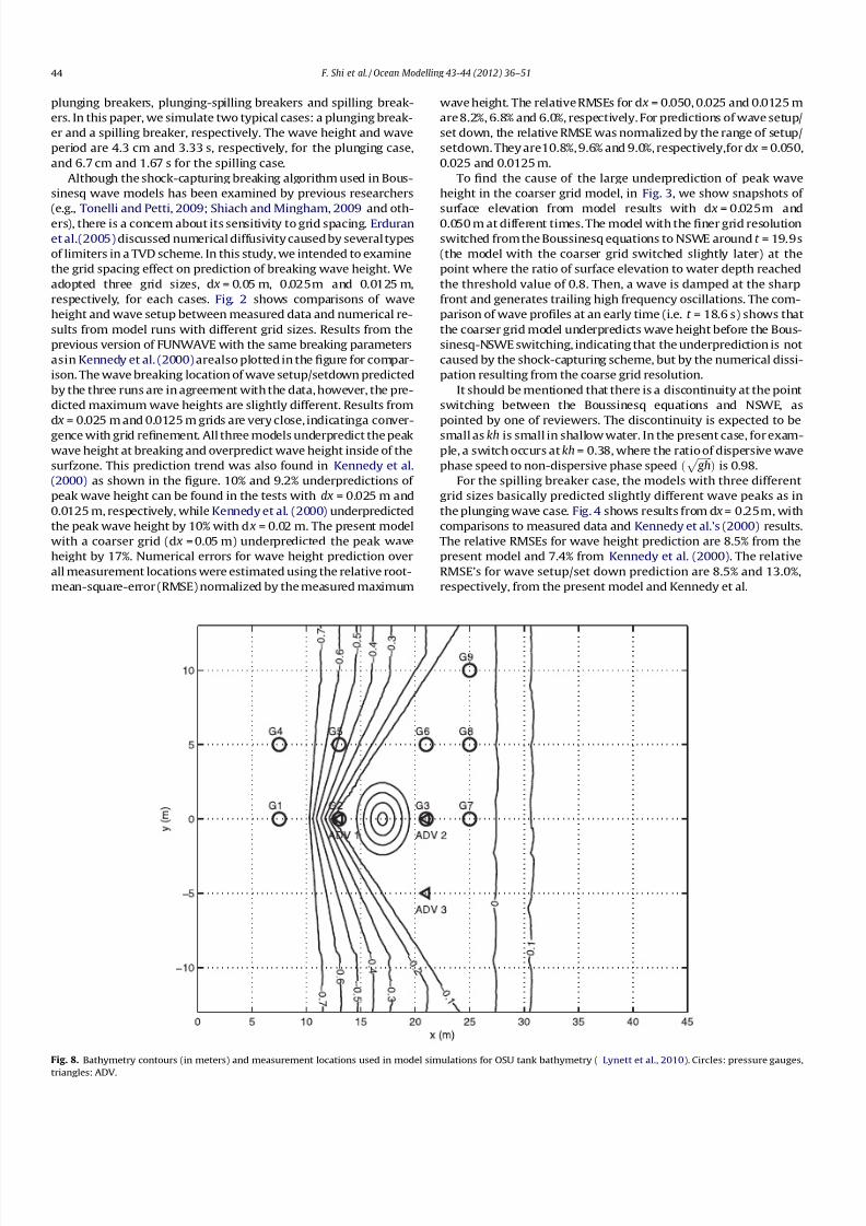
Fig. 8. Bathymetry contours (in meters) and measurement locations used in model simulations for OSU tank bathymetry ( Lynett et al., 2010). Circles: pressure gauges,

triangles: ADV.


8/12/2019 Shi Etal Om12


4.2. Irregular wave shoaling and breaking on a slope

To study irregular-wave properties during shoaling and break-

ing, Mase and Kirby (1992) conducted a laboratory experiment

for random wave propagation over a planar beach. The experimen-

tal layout is shown in Fig. 5, where a constant depth of 0.47 m on

the offshore side connects to a constant slope of 1:20 on the right.

Two sets of random waves with peak frequencies of 0.6 Hz (run 1)

and 1.0 Hz (run 2) were generated by the wavemaker on the off-

shore side. The target incident spectrum was a Pierson–Moskowitz

spectrum. Wave gauges collected time series of surface elevation at

depths h = 47, 35, 30, 25, 20, 17.5, 15, 12.5, 10, 7.5, 5, and 2.5 cm.

The present case has been previously studied using an eddy vis-

cosity model for breaking waves by Kennedy et al. (2000). The

present model was set up following Kennedy et al. (2000), whoused an internal wavemaker located at the toe of the slope, where

surface elevation is measured by gauge 1. The internal wavemaker

signal was constructed following Wei et al. (1999), using low and

high-frequency cutoffs of 0.2 Hz and 10.0 Hz. The simulation time

is the same as the time length of data collection. The computa-

tional domain extends from x = 0 m to 20 m, with a grid size of

0.04 m. The toe of the slope starts at x = 10 m. A sponge layer is

specified at the offshore side boundary, to absorb reflected waves,

but no sponge layer is needed on the onshore boundary, which dif-

fers from Kirby et al. (1998) who used the slot method combined

with a sponge layer at the end of the domain.

We present the model results for run 2 and compare them with

the experimental data measured at the other 11 gauges shown in

Fig. 5. Fig. 6 shows model results (dashed lines) and measured data

(solid lines) from t =20s to t = 40 s at those gauges. Both model

and data show that most waves start breaking at a h = 15 cmdepth.

Except for small discrepancies in wave phases, the model repro-

duces the measured waveform quite well. The standard deviation

of the predicted surface elevation are calculated at all 11 gaugesand compared to the data. The relative computational errors are

between 0.4 7.5%. The relative RMSE of standard deviation calcu-

lated over the 11 gauges is 5.4%.

Third moment statistics of surface elevation provide a good

evaluation of model skill in reproducing wave crest shape. Normal-

ized wave skewness and asymmetry were calculated for both mea-

sured and modeled time series of surface elevation according to

the following formulations,

skew ¼ hg3ihg2i3=2

asym ¼ hH ðgÞ3i

hg2

i3=2

ð45Þ

where H denotes the Hilbert transform, hi is the time-averaging

operator, and the mean has been removed from the time series of

surface elevation.

Fig. 7 shows the skewness and asymmetry predicted by the

present model, the original FUNWAVE (Kirby et al., 1998) and

experiment data. We see, the both models predicted skewness

and asymmetry reasonably well, with a slight overprediction of

wave skewness inside the surf zone. The relative RMSE for skew-

ness prediction, which is normalized by the measured maximum

value, is 6.6% from the present model and 7.1% for Kirby et al.

The relative RMSEs for asymmetry prediction are 12.1% and 7.4%

from the present model and Kirby et al., respectively.

It is worth mentioning that Kirby et al. (1998) employed fre-

quent use of numerical filtering, especially after wave breaking,so that the model run was stable over the entire data time series.

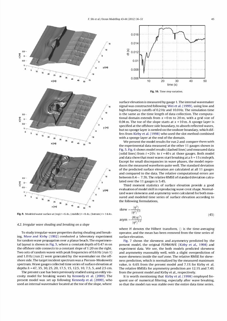
Fig. 9. Modeled water surface at (top) t = 6.4s, (middle) t = 8.4s, (bottom) t = 14.4s.

10 20 30 40 500.006

0.008

0.01

0.012

0.014

0.016

time (s)

d t ( s )

Fig. 10. Time step variation.


8/12/2019 Shi Etal Om12


The present model did not encounter any stability problem and

utilizes no filtering.

4.3. Solitary wave runup on a shelf with a conical island

To examine the wetting–drying method used in the present

model versus the slot method used in Kennedy et al. (2000), Chen

et al. (2000), we performed a simulation of the solitary wave runup

measured recently in a large wave basin at Oregon State Univer-

sity’s O.H. Hinsdale Wave Research Laboratory (Lynett et al.,

2010). The basin is 48.8 m long, 26.5 m wide, and 2.1 m deep. A

complex bathymetry consisting of a 1:30 slope planar beach con-nected to a triangle shaped shelf and a conical island on the shelf

was used and is shown in Fig. 8. Solitary waves were generated

on the left side by a piston-type wavemaker. Surface elevation

and velocity were collected at many locations by wave gauges

and ADV’s in alongshore and cross-shore arrays. Fig. 8 shows wave

gauges (circles) and ADV’s (triangles) used for model/data compar-

isons in the present study. Gauge 1–9 were located at ( x, y) =

(7.5,0.0) m, (13.0,0.0) m, (21.0, 0.0) m, (7.5,5.0) m, (13.0,5.0) m,

(21.0,5.0) m, (25.0,0.0) m, (25.0,5.0) m and (25.0,10.0) m, respec-

tively. ADV 1–3 were located at (13.0,0.0) m, (21.0,0.0) m and

(21.0,5.0) m, respectively.

The modeled bathymetry was constructed by combining the

measured data of the shelf and the analytical equation of the cone,

which was used for the design of the island in the experiment. Thecomputational domain was modified by extending the domain

from x = 0.0 m to 5.0 m with a constant water depth of 0.78 m

in order to use a solitary wave solution as an initial condition.

The width of the computational domain in the y direction is the

same as OSU’s basin. Grid spacing used in the model is 0.1 m in

both directions. A solitary wave solution based on Nwogu’s ex-

tended Boussinesq equations (Wei, 1997) was used with centroid

located at x = 5.0 m at time t = 0 s. The wave height is 0.39 m, as

used in the laboratory experiment.

Fig. 9 shows results of computed water surfaces at t = 6.4 s, 8.4 s

and 14.4 s, respectively. The wave front becomes very steep as the

wave climbs on the shelf, which was well captured by the model.

The wave scattering pattern is clearly seen in the bottom panelof Fig. 9. Wave breaking on the shelf was observed in the labora-

tory experiment and was also seen in the model. Fig. 10 shows

the variation in time stepping during the simulation. The time step

dropped to a minimum, at around t = 6.5 s, as the wave collided

with the island (top panel of Fig. 9). The local Froude number

reached a maximum at t = 6.5 s, reducing the value of the time step

based on (42).

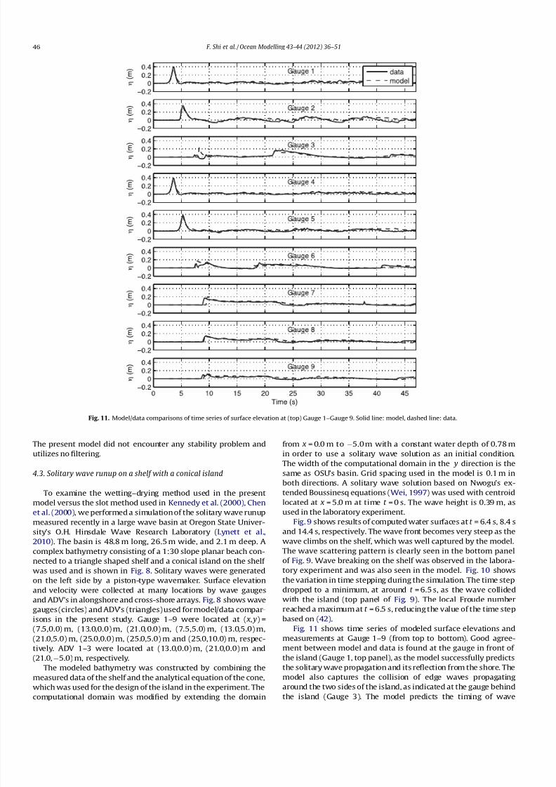
Fig. 11 shows time series of modeled surface elevations and

measurements at Gauge 1–9 (from top to bottom). Good agree-

ment between model and data is found at the gauge in front of

the island (Gauge 1, top panel), as the model successfully predicts

the solitary wave propagation and its reflection from the shore. The

model also captures the collision of edge waves propagating

around the two sides of the island, as indicated at the gauge behindthe island (Gauge 3). The model predicts the timing of wave

Fig. 11. Model/data comparisons of time series of surface elevation at (top) Gauge 1–Gauge 9. Solid line: model, dashed line: data.


8/12/2019 Shi Etal Om12


collision well but over-predicts the peak of wave runup. The mod-

el/data comparisons at Gauges 5, 6, 8, and 9, which are located at

the north-side shelf, indicates that the model predicts wave refrac-tion and breaking on the shelf reasonably well. The averaged RMSE

normalized by the maximum measured wave amplitude is 7.5%

with the maximum RMSE of 11.2% at Gauge 2 and the minimum

RMSE of 3.7% at Gauge 1.

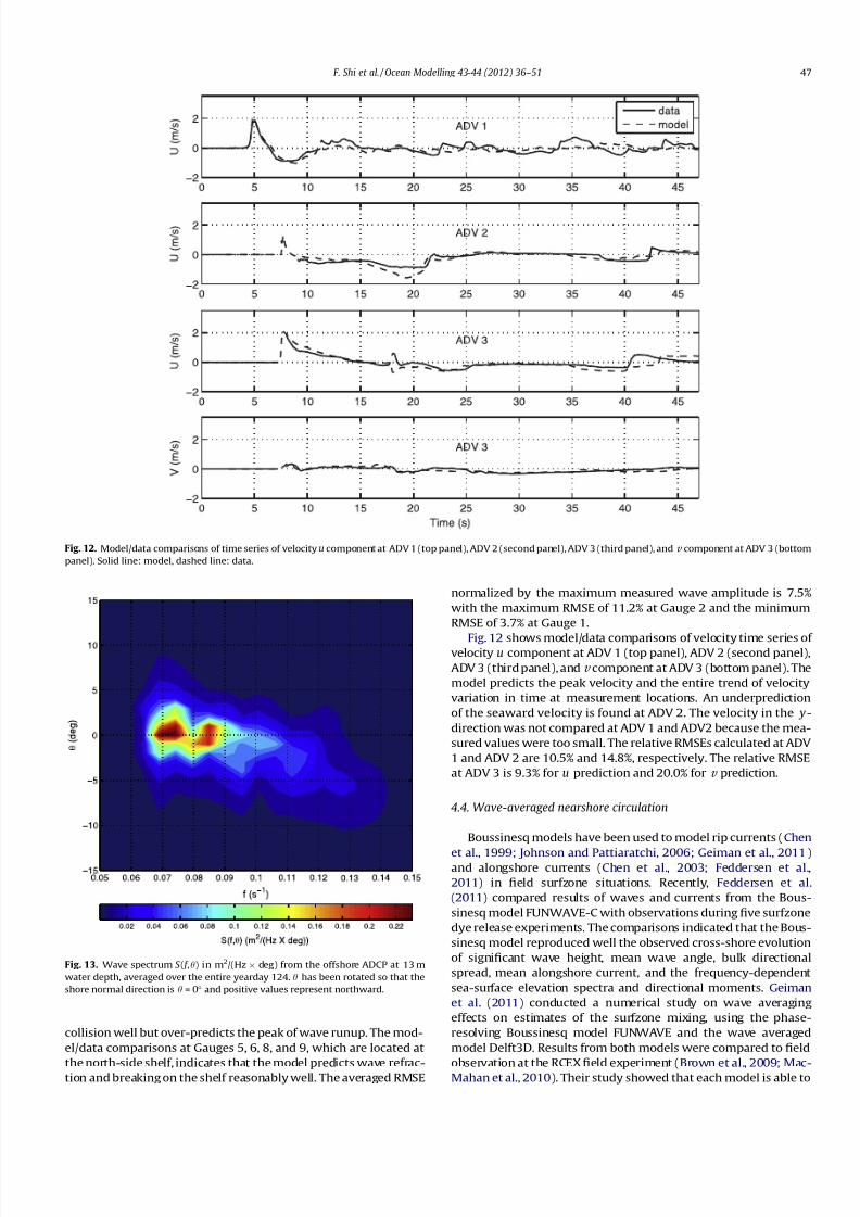
Fig. 12 shows model/data comparisons of velocity time series of velocity u component at ADV 1 (top panel), ADV 2 (second panel),

ADV 3 (third panel), and v component at ADV 3 (bottom panel). The

model predicts the peak velocity and the entire trend of velocity

variation in time at measurement locations. An underprediction

of the seaward velocity is found at ADV 2. The velocity in the y-

direction was not compared at ADV 1 and ADV2 because the mea-

sured values were too small. The relative RMSEs calculated at ADV

1 and ADV 2 are 10.5% and 14.8%, respectively. The relative RMSE

at ADV 3 is 9.3% for u prediction and 20.0% for v prediction.

4.4. Wave-averaged nearshore circulation

Boussinesq models have been used to model rip currents (Chen

et al., 1999; Johnson and Pattiaratchi, 2006; Geiman et al., 2011)and alongshore currents (Chen et al., 2003; Feddersen et al.,

2011) in field surfzone situations. Recently, Feddersen et al.

(2011) compared results of waves and currents from the Bous-

sinesq model FUNWAVE-C with observations during five surfzone

dye release experiments. The comparisons indicated that the Bous-

sinesq model reproduced well the observed cross-shore evolution

of significant wave height, mean wave angle, bulk directional

spread, mean alongshore current, and the frequency-dependent

sea-surface elevation spectra and directional moments. Geiman

et al. (2011) conducted a numerical study on wave averaging

effects on estimates of the surfzone mixing, using the phase-

resolving Boussinesq model FUNWAVE and the wave averaged

model Delft3D. Results from both models were compared to field

observation at the RCEX field experiment (Brown et al., 2009; Mac-Mahan et al., 2010). Their study showed that each model is able to

Fig. 12. Model/data comparisons of time series of velocity u component at ADV 1 (top panel), ADV 2 (second panel), ADV 3 (third panel), and v component at ADV 3 (bottom

panel). Solid line: model, dashed line: data.

Fig. 13. Wave spectrum S ( f ,h) in m2/(Hz deg) from the offshore ADCP at 13 m

water depth, averaged over the entire yearday 124. h has been rotated so that the

shore normal direction is h = 0 and positive values represent northward.


8/12/2019 Shi Etal Om12


reproduce 1-h time-averaged mean Eulerian velocities consistent

with field measurements at stationary current meters. However,

the spatial distribution of wave height inside the surfzone was

different between the two models, due to the different mecha-

nisms for wave breaking.

To check the breaking scheme used in the present model and its

consequences regarding wave-induced currents, we set up the

present model in the same way as in Geiman et al. (2011), except

that no sponge layer was applied for the present model at the

shoreline position. The model used a grid size of d x = d y = 1 m

and a north–south periodic boundary condition in a computational

domain of 732 m 684 m. An internal wavemaker for directional

irregular wave generation was located at 540 m away from the

shoreline. The directional spectra observed at 13 m water depth

during the instrument deployment was divided into 23 31 bins

as shown in Fig. 13. The calculated RMS wave height H rms = 0.65 m

and period T mo = 10.5s.

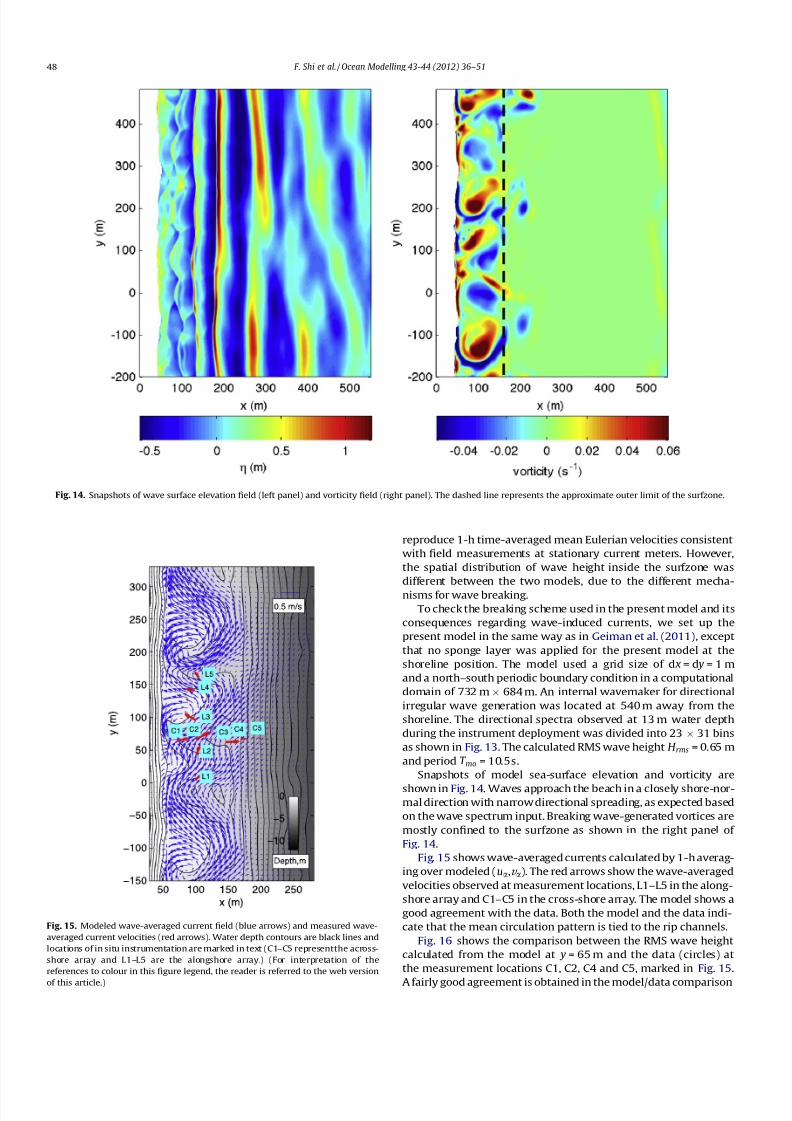
Snapshots of model sea-surface elevation and vorticity are

shown in Fig. 14. Waves approach the beach in a closely shore-nor-mal direction with narrow directional spreading, as expected based

on the wave spectrum input. Breaking wave-generated vortices are

mostly confined to the surfzone as shown in the right panel of

Fig. 14.

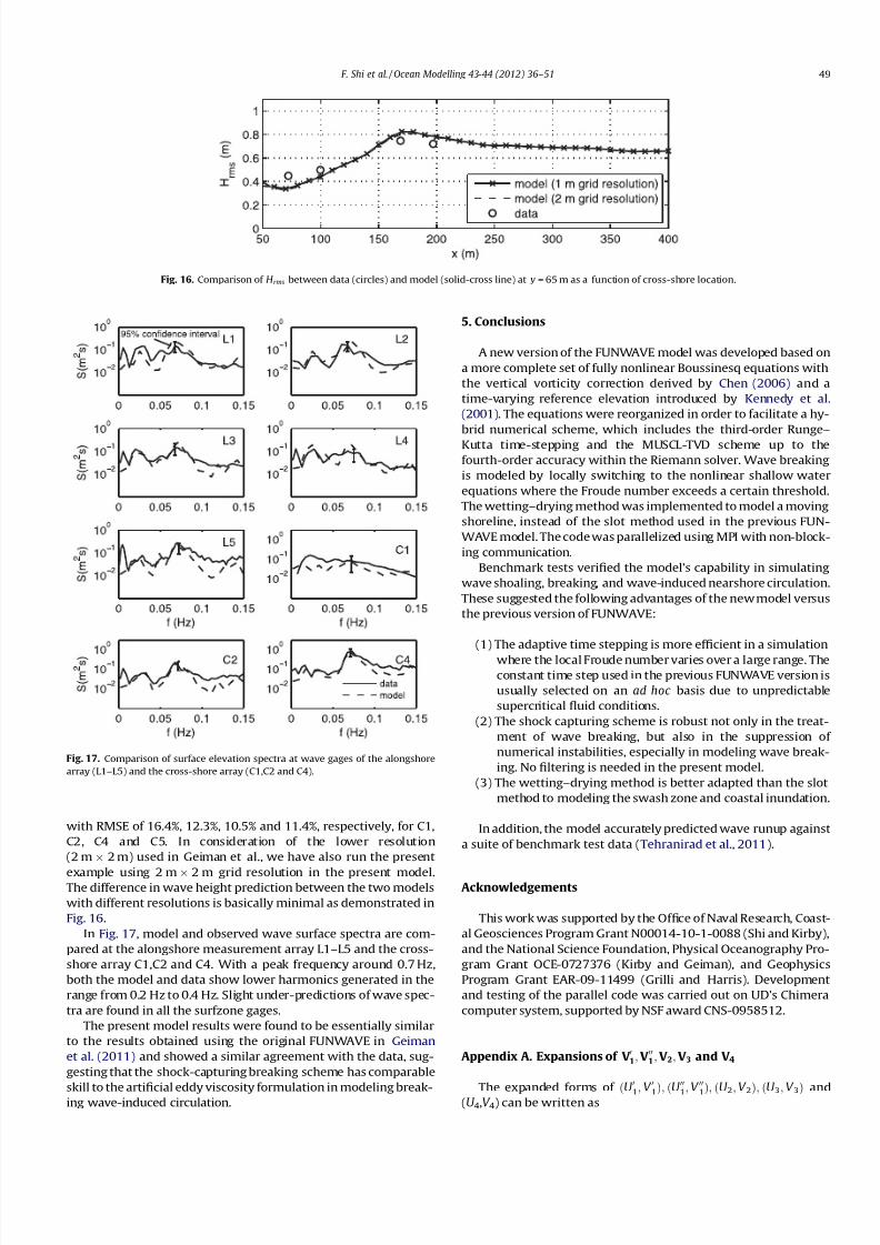
Fig. 15 shows wave-averaged currents calculated by 1-h averag-

ing over modeled (ua,v a). The red arrows show the wave-averaged

velocities observed at measurement locations, L1–L5 in the along-

shore array and C1–C5 in the cross-shore array. The model shows a

good agreement with the data. Both the model and the data indi-

cate that the mean circulation pattern is tied to the rip channels.

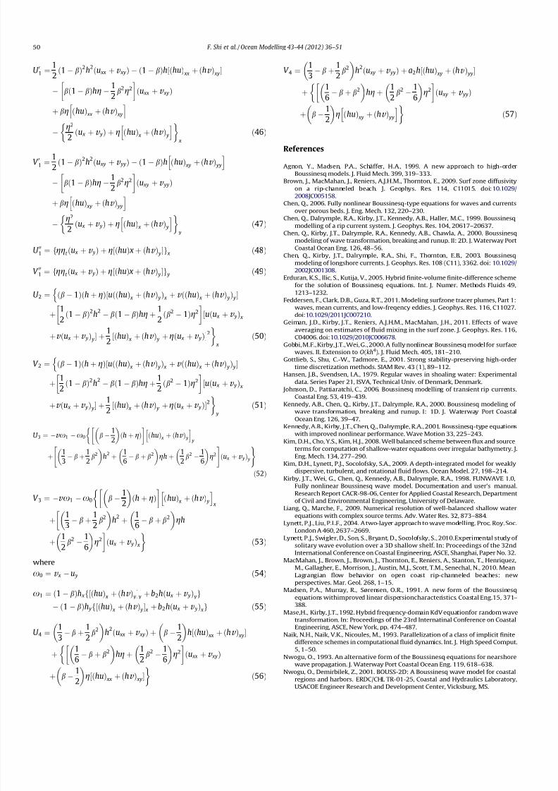
Fig. 16 shows the comparison between the RMS wave height

calculated from the model at y = 65 m and the data (circles) at

the measurement locations C1, C2, C4 and C5, marked in Fig. 15.

A fairly good agreement is obtained in the model/data comparison

Fig. 14. Snapshots of wave surface elevation field (left panel) and vorticity field (right panel). The dashed line represents the approximate outer limit of the surfzone.

Fig. 15. Modeled wave-averaged current field (blue arrows) and measured wave-

averaged current velocities (red arrows). Water depth contours are black lines and

locations of in situ instrumentation are marked in text (C1–C5 representthe across-

shore array and L1–L5 are the alongshore array.) (For interpretation of the

references to colour in this figure legend, the reader is referred to the web version

of this article.)


8/12/2019 Shi Etal Om12


with RMSE of 16.4%, 12.3%, 10.5% and 11.4%, respectively, for C1,

C2, C4 and C5. In consideration of the lower resolution

(2 m 2 m) used in Geiman et al., we have also run the present

example using 2 m 2 m grid resolution in the present model.The difference in wave height prediction between the two models

with different resolutions is basically minimal as demonstrated in

Fig. 16.

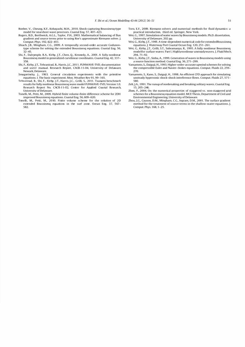
In Fig. 17, model and observed wave surface spectra are com-

pared at the alongshore measurement array L1–L5 and the cross-

shore array C1,C2 and C4. With a peak frequency around 0.7 Hz,

both the model and data show lower harmonics generated in the

range from 0.2 Hz to 0.4 Hz. Slight under-predictions of wave spec-

tra are found in all the surfzone gages.

The present model results were found to be essentially similar

to the results obtained using the original FUNWAVE in Geiman

et al. (2011) and showed a similar agreement with the data, sug-

gesting that the shock-capturing breaking scheme has comparable

skill to the artificial eddy viscosity formulation in modeling break-ing wave-induced circulation.

5. Conclusions

A new version of the FUNWAVE model was developed based on

a more complete set of fully nonlinear Boussinesq equations with

the vertical vorticity correction derived by Chen (2006) and a

time-varying reference elevation introduced by Kennedy et al.

(2001). The equations were reorganized in order to facilitate a hy-

brid numerical scheme, which includes the third-order Runge–

Kutta time-stepping and the MUSCL-TVD scheme up to the

fourth-order accuracy within the Riemann solver. Wave breaking

is modeled by locally switching to the nonlinear shallow water

equations where the Froude number exceeds a certain threshold.

The wetting–drying method was implemented to model a moving

shoreline, instead of the slot method used in the previous FUN-

WAVE model. The code was parallelized using MPI with non-block-

ing communication.

Benchmark tests verified the model’s capability in simulating

wave shoaling, breaking, and wave-induced nearshore circulation.

These suggested the following advantages of the new model versus

the previous version of FUNWAVE:

(1) The adaptive time stepping is more efficient in a simulation

where the local Froude number varies over a large range. The

constant time step used in the previous FUNWAVE version is

usually selected on an ad hoc basis due to unpredictable

supercritical fluid conditions.

(2) The shock capturing scheme is robust not only in the treat-

ment of wave breaking, but also in the suppression of

numerical instabilities, especially in modeling wave break-

ing. No filtering is needed in the present model.

(3) The wetting–drying method is better adapted than the slot

method to modeling the swash zone and coastal inundation.

In addition, the model accurately predicted wave runup against

a suite of benchmark test data (Tehranirad et al., 2011).

Acknowledgements

This work was supported by the Office of Naval Research, Coast-

al Geosciences Program Grant N00014-10-1-0088 (Shi and Kirby),

and the National Science Foundation, Physical Oceanography Pro-

gram Grant OCE-0727376 (Kirby and Geiman), and Geophysics

Program Grant EAR-09-11499 (Grilli and Harris). Development

and testing of the parallel code was carried out on UD’s Chimera

computer system, supported by NSF award CNS-0958512.

Appendix A. Expansions of V 01; V 001; V 2; V 3 and V 4

The expanded forms of ðU 0

1; V 0

1Þ; ðU 00

1; V 00

1Þ; ðU 2; V 2Þ; ðU 3; V 3Þ and(U 4,V 4) can be written as

Fig. 16. Comparison of H rms between data (circles) and model (solid-cross line) at y = 65 m as a function of cross-shore location.

Fig. 17. Comparison of surface elevation spectra at wave gages of the alongshore

array (L1–L5) and the cross-shore array (C1,C2 and C4).


8/12/2019 Shi Etal Om12


U 01 ¼ 1

2ð1 bÞ2

h2ðu xx þv xyÞ ð1 bÞh½ðhuÞ xx þ ðhv Þ xy

bð1 bÞhg 1

2b

2g2

ðu xx þv xyÞ

þ bg ðhuÞ xx þ ðhv Þ xy

h i

g2

2 ðu x

þv y

Þ þg ð

huÞ x

þ ðhv

Þ yh i

x ð46

Þ

V 01 ¼ 1

2ð1 bÞ2

h2ðu xy þv yyÞ ð1 bÞh ðhuÞ xy þ ðhv Þ yy

h i bð1 bÞhg 1

2b2g2

ðu xy þv yyÞ

þ bg ðhuÞ xy þ ðhv Þ yy

h i g2

2 ðu x þv yÞ þ g ðhuÞ x þ ðhv Þ y

h i y

ð47Þ

U 001 ¼ fggt ðu x þv yÞ þ g½ðhuÞ x þ ðhv Þ yg x ð48Þ

V 001 ¼ f

ggt ð

u x

þv y

Þ þg½ð

huÞ x þ ð

hv

Þ yg y ð49

ÞU 2 ¼ ðb 1Þðh þ gÞ½uððhuÞ x þ ðhv Þ yÞ x þv ððhuÞ x þ ðhv Þ yÞ y

nþ 1

2ð1 bÞ2

h2 bð1 bÞhgþ 1

2ðb2 1Þg2

½uðu x þv yÞ x

þv ðu x þv yÞ y þ1

2½ðhuÞ x þ ðhv Þ y þgðu x þv yÞ2

x

ð50Þ

V 2 ¼ ðb 1Þðh þ gÞ½uððhuÞ x þ ðhv Þ yÞ x þv ððhuÞ x þ ðhv Þ yÞ ynþ 1

2ð1 bÞ2

h2 bð1 bÞhgþ 1

2ðb2 1Þg2

½uðu x þv yÞ x

þv ðu x þv yÞ y þ1

2½ðhuÞ x þ ðhv Þ y þgðu x þv yÞ2

y

ð51Þ

U 3 ¼ v x1 x0 b 1

2

ðh þ gÞ

ðhuÞ x þ ðhv Þ y

h i y

þ"

1

3 b þ 1

2b2

h

2 þ 1

6 b þ b2

gh þ 1

2b2 1

6

g2

#ðu x þv yÞ y

)

ð52Þ

V 3 ¼ v x1 x0 b 1

2

ðh þ gÞ

ðhuÞ x þ ðhv Þ y

h i x

þ 1

3 bþ 1

2b2

h

2 þ 1

6 b þ b2

gh

þ 1

2b

2 1

6 g2

ðu x þv yÞ x ð53Þ

where

x0 ¼ v x u y ð54Þ

x1 ¼ ð1 bÞh xf½ðhuÞ x þ ðhv Þ y y þ b2hðu x þv yÞ yg ð1 bÞh yf½ðhuÞ x þ ðhv Þ y x þ b2hðu x þv yÞ xg ð55Þ

U 4 ¼ 1

3 b þ 1

2b

2

h

2ðu xx þv xyÞ þ b 1

2

h½ðhuÞ xx þ ðhv Þ xy

þ 1

6 b þ b2

hgþ 1

2b2 1

6

g2

ðu xx þv xyÞ

þ b 1

2

g½ðhuÞ xx þ ðhv Þ xy

ð56Þ

V 4 ¼ 1

3 b þ 1

2b2

h

2ðu xy þv yyÞ þ a2h½ðhuÞ xy þ ðhv Þ yy

þ 1

6 b þ b2

hgþ 1

2b2 1

6

g2

ðu xy þv yyÞ

þ b 1

2

g ðhuÞ xy þ ðhv Þ yy

h i ð57Þ

References

Agnon, Y., Madsen, P.A., Schäffer, H.A., 1999. A new approach to high-order

Boussinesq models. J. Fluid Mech. 399, 319–333.

Brown, J., MacMahan, J., Reniers, A.J.H.M., Thornton, E., 2009. Surf zone diffusivity

on a rip-channeled beach. J. Geophys. Res. 114, C11015. doi:10.1029/

2008JC005158.

Chen, Q., 2006. Fully nonlinear Boussinesq-type equations for waves and currents

over porous beds. J. Eng. Mech. 132, 220–230.

Chen, Q., Dalrymple, R.A., Kirby, J.T., Kennedy, A.B., Haller, M.C., 1999. Boussinesq

modelling of a rip current system. J. Geophys. Res. 104, 20617–20637.

Chen, Q., Kirby, J.T., Dalrymple, R.A., Kennedy, A.B., Chawla, A., 2000. Boussinesq

modeling of wave transformation, breaking and runup. II: 2D. J. Waterway Port

Coastal Ocean Eng. 126, 48–56.

Chen, Q., Kirby, J.T., Dalrymple, R.A., Shi, F., Thornton, E.B., 2003. Boussinesq

modeling of longshore currents. J. Geophys. Res. 108 (C11), 3362. doi:10.1029/

2002JC001308.

Erduran, K.S., Ilic, S., Kutija, V., 2005. Hybrid finite-volume finite-difference schemefor the solution of Boussinesq equations. Int. J. Numer. Methods Fluids 49,

1213–1232.

Feddersen, F., Clark, D.B., Guza, R.T., 2011. Modeling surfzone tracer plumes, Part 1:

waves, mean currents, and low-freqency eddies. J. Geophys. Res. 116, C11027.

doi:10.1029/2011JC007210.

Geiman, J.D., Kirby, J.T., Reniers, A.J.H.M., MacMahan, J.H., 2011. Effects of wave

averaging on estimates of fluid mixing in the surf zone. J. Geophys. Res. 116,

C04006. doi:10.1029/2010JC006678.

Gobbi, M.F., Kirby, J.T., Wei, G., 2000. A fully nonlinear Boussinesq model for surface

waves. II. Extension to O(kh4). J. Fluid Mech. 405, 181–210.

Gottlieb, S., Shu, C.-W., Tadmore, E., 2001. Strong stability-preserving high-order

time discretization methods. SIAM Rev. 43 (1), 89–112.

Hansen, J.B., Svendsen, I.A., 1979. Regular waves in shoaling water: Experimental

data. Series Paper 21, ISVA, Technical Univ. of Denmark, Denmark.

Johnson, D., Pattiaratchi, C., 2006. Boussinesq modelling of transient rip currents.

Coastal Eng. 53, 419–439.

Kennedy, A.B., Chen, Q., Kirby, J.T., Dalrymple, R.A., 2000. Boussinesq modeling of

wave transformation, breaking and runup. I: 1D. J. Waterway Port Coastal

Ocean Eng. 126, 39–47.

Kennedy, A.B., Kirby, J.T., Chen, Q., Dalrymple, R.A., 2001. Boussinesq-type equations

with improved nonlinear performance. Wave Motion 33, 225–243.

Kim, D.H., Cho, Y.S., Kim, H.J., 2008. Well balanced scheme between flux and source

terms for computation of shallow-water equations over irregular bathymetry. J.

Eng. Mech. 134, 277–290.

Kim, D.H., Lynett, P.J., Socolofsky, S.A., 2009. A depth-integrated model for weakly

dispersive, turbulent, and rotational fluid flows. Ocean Model. 27, 198–214.

Kirby, J.T., Wei, G., Chen, Q., Kennedy, A.B., Dalrymple, R.A., 1998. FUNWAVE 1.0,

Fully nonlinear Boussinesq wave model. Documentation and user’s manual.

Research Report CACR-98-06, Center for Applied Coastal Research, Department

of Civil and Environmental Engineering, University of Delaware.

Liang, Q., Marche, F., 2009. Numerical resolution of well-balanced shallow water

equations with complex source terms. Adv. Water Res. 32, 873–884.

Lynett, P.J., Liu, P.L.F., 2004. A two-layer approach to wave modelling. Proc. Roy. Soc.

London A 460, 2637–2669.

Lynett, P.J., Swigler, D., Son, S., Bryant, D., Socolofsky, S., 2010.Experimental study of

solitary wave evolution over a 3D shallow shelf. In: Proceedings of the 32nd

International Conference on Coastal Engineering, ASCE, Shanghai, Paper No. 32.MacMahan, J., Brown, J., Brown, J., Thornton, E., Reniers, A., Stanton, T., Henriquez,

M., Gallagher, E., Morrison, J., Austin, M.J., Scott, T.M., Senechal, N., 2010. Mean

Lagrangian flow behavior on open coast rip-channeled beaches: new

perspectives. Mar. Geol. 268, 1–15.

Madsen, P.A., Murray, R., Sørensen, O.R., 1991. A new form of the Boussinesq

equations withimproved linear dispersioncharacteristics. Coastal Eng.15, 371–

388.

Mase,H., Kirby, J.T., 1992. Hybrid frequency-domain KdV equationfor random wave

transformation. In: Proceedings of the 23rd Internatinal Conference on Coastal

Engineering, ASCE, New York, pp. 474–487.

Naik, N.H., Naik, V.K., Nicoules, M., 1993. Parallelization of a class of implicit finite

difference schemes in computational fluid dynamics. Int. J. High Speed Comput.

5, 1–50.

Nwogu, O., 1993. An alternative form of the Boussinesq equations for nearshore

wave propagation. J. Waterway Port Coastal Ocean Eng. 119, 618–638.

Nwogu, O., Demirbilek, Z., 2001. BOUSS-2D: A Boussinesq wave model for coastal

regions and harbors. ERDC/CHL TR-01-25, Coastal and Hydraulics Laboratory,

USACOE Engineer Research and Development Center, Vicksburg, MS.


http://dx.doi.org/10.1029/2008JC005158

http://dx.doi.org/10.1029/2008JC005158

http://dx.doi.org/10.1029/2002JC001308

http://dx.doi.org/10.1029/2002JC001308

http://dx.doi.org/10.1029/2011JC007210

http://dx.doi.org/10.1029/2010JC006678

http://dx.doi.org/10.1029/2010JC006678

http://dx.doi.org/10.1029/2011JC007210

http://dx.doi.org/10.1029/2002JC001308

http://dx.doi.org/10.1029/2002JC001308

http://dx.doi.org/10.1029/2008JC005158

http://dx.doi.org/10.1029/2008JC005158

8/12/2019 Shi Etal Om12


Roeber, V., Cheung, K.F., Kobayashi, M.H., 2010. Shock-capturing Boussinesq-type

model for nearshore wave processes. Coastal Eng. 57, 407–423.

Rogers, B.D., Borthwick, A.G.L., Taylor, P.H., 2003. Mathematical balancing of flux

gradient and source terms prior to using Roe’s approximate Riemann solver. J.

Comput. Phys. 192, 422–451.

Shiach, J.B., Mingham, C.G., 2009. A temporally second-order accurate Godunov-

type scheme for solving the extended Boussinesq equations. Coastal Eng. 56,

32–45.

Shi, F., Dalrymple, R.A., Kirby, J.T., Chen, Q., Kennedy, A., 2001. A fully nonlinear

Boussinesq model in generalized curvilinear coordinates. Coastal Eng. 42, 337–

358.Shi, F., Kirby, J.T., Tehranirad, B., Harris, J.C., 2011. FUNWAVE-TVD, documentation

and users’ manual. Research Report, CACR-11-04, University of Delaware,

Newark, Delaware.

Smagorinsky, J., 1963. General circulation experiments with the primitive

equations. I. The basic experiment. Mon. Weather Rev 91, 99–165.

Tehranirad, B., Shi, F., Kirby, J.T., Harris, J.C., Grilli, S., 2011. Tsunami benchmark

results for fully nonlinear Boussinesq wave model FUNWAVE-TVD, Version 1.0.

Research Report No. CACR-11-02, Center for Applied Coastal Research,

University of Delaware.

Tonelli, M., Petti, M., 2009. Hybrid finite volume-finite difference scheme for 2DH

improved Boussinesq equations. Coastal Eng. 56, 609–620.

Tonelli, M., Petti, M., 2010. Finite volume scheme for the solution of 2D

extended Boussinesq equations in the surf zone. Ocean Eng. 37, 567–

582.

Toro, E.F., 2009. Riemann solvers and numerical methods for fluid dynamics: a

practical introduction, third ed. Springer, New York.

Wei, G., 1997. Simulation of water waves by Boussinesq models. Ph.D. dissertation,

University of Delaware, 202 pp.

Wei, G., Kirby, J.T., 1995. A time-dependent numerical code for extendedBoussinesq

equations. J. Waterway Port Coastal Ocean Eng. 120, 251–261.

Wei, G., Kirby, J.T., Grilli, S.T., Subramanya, R., 1995. A fully nonlinear Boussinesq

modelfor surface waves: Part I. Highlynonlinear unsteadywaves. J. Fluid Mech.

294, 71–92.

Wei, G., Kirby, J.T., Sinha, A., 1999. Generation of waves in Boussinesq models using

a source function method. Coastal Eng. 36, 271–299.Yamamoto, S., Daiguji, H., 1993. Higher-order-accurate upwind schemes for solving

the compressible Euler and Navier–Stokes equations. Comput. Fluids 22, 259–

270.

Yamamoto, S., Kano, S., Daiguji, H., 1998. An efficient CFD approach for simulating

unsteady hypersonic shock-shock interference flows. Comput. Fluids 27, 571–

580.

Zelt, J.A., 1991. The runup of nonbreaking and breaking solitary waves. Coastal Eng.

15, 205–246.

Zhen, F., 2004. On the numerical properties of staggered vs. non-staggered grid

schemes for a Boussinesq equation model. MCE Thesis, Department of Civil and

Environmental Engineering, University of Delaware.

Zhou, J.G., Causon, D.M., Mingham, C.G., Ingram, D.M., 2001. The surface gradient

method for the treatment of source terms in the shallow-water equations. J.

Comput. Phys. 168, 1–25.


Documents

Shi Etal Om12