ANOMALOUS DIFFUSION IN TRADING MODELS

SIDIQ BIN MOHAMAD KHIDZIR

FACULTY OF SCIENCE

UNIVERSITY OF MALAYA

KUALA LUMPUR

2010

ANOMALAOUS DIFFUSION IN TRADING MODELS

SIDIQ BIN MOHAMAD KHIDZIR

DISSERTATION SUBMITTED IN FULFILMENT

 OF THE REQUIREMENTS 

FOR THE DEGREE OF MASTER OF SCIENCE

FACULTY OF SCIENCE

UNIVERSITY OF MALAYA

KUALA LUMPUR 

2010

UNIVERSITI MALAYA

ORIGINAL LITERARY WORK DECLARATION

Name of Candidate: Sidiq bin Mohamad Khidzir (IC/Passport No : 830216­71­5009)

Registration/Matric No: SGR070011

Name of Degree: Master of Science (Msc)

Title of Project Paper/ Research Report/ Dissertation/ Thesis (“this Work”):“Anomalous Diffusion in a Trading Model”

Field of Study: Physics

I do solemnly and sincerely declare that:(1) I am the sole author/writer of this Work;(2) This Work is original;(3) Any use of any work in which copyright exists was done by way of fair dealing and for

permitted purposes and any excerpt or extract from, or reference to or reproduction of anycopyright work has been disclosed expressly and sufficiently and the title of the Work andits authorship has been acknowledged in this Work;

(4) I do not have any actual knowledge nor do I ought reasonably to know that the making ofthis work constitutes an infringement of any copyright work.

(5) I hereby assign all and every rights in the copyright to this Work to the University ofMalaya (“UM”), who henceforth shall be owner of the copyright in this Work and that anyreproduction or use in any form or by any means whatsoever is prohibited without thewritten consent of UM having been first had and obtained;

(6) I am fully aware that if in the course of making this Work I have infringed any copyrightwhether intentionally or otherwise, I may be subject to legal action or any other action asmay be determined by UM.

Candidate’s Signature Date

Subscribed and solemnly declared before,

Witness’s Signature DateName:Designation:

i

ABSTRACT

Econophysics is an interdisciplinary research field applying the mathematical methods of

statistical physics to economics and finance. It emphasizes quantitative analysis of large

amounts of economic and financial data as oppose to the more philosophical approach of

political economics. A popular topic studied in econophysics is the distribution of wealth.

Many models have been proposed to explain the trading dynamics [12,13] leading to the

distribution  of  wealth  universally  observed   in  many  countries.  A more   recent   topic   in

econophysics is the movement of money studied by Brockmann in [19,20]. In this work, we

are interested in studying the relation between the distribution of wealth and anomalous

diffusion using a trading model. We plan to do this by studying the diffusion of money in

correspondence to a particular trading model. In particular, our objective is to observe if the

distribution of money displacement lengths and waiting times exhibit scale free behavior

for a particular trading model. We conclude from the observations we made that a trading

model   with   a   resultant   mixed   distributions   of   wealth   with   a   scale   free   tail   exhibits

anomalous diffusion. A trading model with a resultant mixed distributions of wealth with

an  exponential   tail   exhibits   subdiffusion.  A  trading  model  with  a   resultant  exponential

distribution of wealth does not exhibit anomalous diffusion.

ii

ABSTRAK

Ekonofizik   adalah  bidang  penyelidikan   interdisipliner   yang  menerapkan  kaedah­kaedah

matematik  dalam  fizik   statistik   untuk  ekonomi  dan  kewangan.   Ia  menekankan  analisis

kuantitatif data ekonomi dan kewangan berbanding pendekatan yang lebih falsafah seperti

politik   ekonomi.   Topik   popular   yang   dipelajari   dalam   ekonofizik   adalah   pengagihan

kekayaan.   Banyak   model   telah   dicadangkan   untuk   menjelaskan   dinamika   perdagangan

[12,13] seperti yang dilihat dalam taburan pengagihan kekayaan banyak negara. Topik yang

lebih baru dalam ekonofizik adalah pergerakan wang yang diselidiki oleh Brockmann di

[19,20].   Dalam   tesis   ini,   kita   tertarik   untuk   mempelajari   hubungan   antara   pengagihan

kekayaan  dan   anomali   difusi   menggunakan  model   perniagaan.   Kami  merancang  untuk

melakukan  hal   ini  dengan  mempelajari  difusi  wang  dalam korespondensi  untuk  model

perniagaan   tertentu.   Secara   khusus,   tujuan   kami   adalah   untuk   mengamati   jika   edaran

perpindahan   wang   dan   masa   tunggu   menunjukkan   perilaku   bebas   skala   untuk   model

perniagaan tertentu. Kita simpulkan daripada pemerhatian kami bahawa model perniagaan

dengan ekor taburan pengagihan kekayaan bebas skala mengalami anomali difusi. Sebuah

model   perniagaan   dengan   ekor   taburan   pengagihan   kekayaan   eksponen   mengalami

“subdiffusion”.  Model  perniagaan dengan  taburan pengagihan  kekayaan eksponen  tidak

menunjukkan anomali difusi.

iii

ACKNOWLEDGEMENT

With the completion of this thesis, my knowledge of the inner workings of nature

has grown by leaps and bounds. It is with this knowledge that I am subserviently humbled

by   the   greatness   of   Allah   s.w.t   who   holds   within   all   knowledge.   This   journey   to

enlightenment was greatly enriched by Prof Dr Wan Ahmad Tajuddin Wan Abdullah whom

eventually introduced the concept of ergodicity breaking to me when I initially wanted to

simply pursue mathematical finance. This act has caused a major phase shift in the way I

see the world. I have also been immensely helped by Prof Madya Dr Sithi Muniandy who

has taken time to discuss the nuances of my project with me and has allowed me to sit

through his excellent Complex Systems class. I have also been greatly helped by my fellow

computational physics researchers Ephrance Abu Ujum and Hadieh Monajemi who have

been   my   sounding   board   for   ideas   throughout   my   project.   I   am   also   indebted   to   all

academic   and   non­academic   staff   of   the   university   who   have   at   many   times   lifted

potentially heavy burdens off my shoulder and also the administration of the university

itself who have charitably provided me with a scholarship and a tutorship throughout my

project. Last but certainly not least I am deeply and eternally greatful to both my parents

and my sister who have raised me to be the man I am today and to my dearly departed

brother who will always be my eternal companion.  

iv

CONTENTS

ORIGINAL LITERARY WORK DECLARATION i

ABSTRACT ii

ABSTRAK iii

ACKNOWLEDGEMENT iv

CONTENTS v

LIST OF TABLES AND FIGURES ix

Chapter 1 : INTRODUCTION 1

1.1 Background 1

1.2 Problem statement and objective 3

1.3 Scope 3

Chapter 2 : A REVIEW OF THE DISTRIBUTION OF WEALTH, ANOMALOUS

DIFFUSION AND ITS APPLICATION IN THE MOVEMENT OF MONEY

2.1 Wealth and income distributions in empirical data  6

2.2 Statistical Mechanics of Income and Wealth Distributions 11

2.2.1. Boltzmann­Gibbs distribution of wealth 11

2.2.2. Mixed distribution : Boltzmann­Gibbs and Power law distribution of 

wealth  15

2.2.3.Mixed distribution : Lognormal and Power law distribution of wealth 18

v

2.3 Diffusion 21

2.3.1. Normal Diffusion 21

2.3.2. Phenomenology of Anomalous Diffusion  25

2.3.3. Continuous Time Random Walks 27

2.3.4. Subdiffusion 29

2.3.5. Superdiffusion 33

2.3.6. Anomalous diffusion in the movement of money 34

Chapter 3 : DESCRIPTION OF TRADING MODELS, THEIR MODIFICATIONS TO

ANALYZE THE DIFFUSION OF MONEY AND POWER LAW ANALYSIS

METHODS

3.1 Introduction 43

3.2 Trading models and their modifications 45

3.2.1. Modified Chakrabarti trading model 45

3.2.2. Modified Yakovenko trading model 51

3.2.3. Kinetic Economy trading model 52

3.2.4. Modified Kinetic Economy trading model 54

3.3 Statistical Analysis of Monte Carlo Data 56

3.4 Calculating mean squared displacement 57

3.5 Power Law Analysis 58

vi

Chapter 4 : STUDY ON THE RELATION BETWEEN DISTRIBUTIONS OF

WEALTH AND DIFFUSION OF MONEY IN VARIOUS TRADING MODELS

4.1 Chakrabarti trading model with random saving propensity 63

4.1.1. Wealth distribution 63

4.1.2. Probability distribution function of displacement 68

4.1.3. Probability distribution function of waiting time 73

4.1.4. Mean square displacement of Chakrabarti trading model 76

4.2 Yakovenko's Trading Model 77

4.2.1. Wealth distribution 77

4.2.2. Probability distribution function of displacement length and mean squared

displacement 78

4.2.3. Probability distribution function of waiting time 80

4.3 Chakrabarti's trading model with fixed saving propensity 81

4.3.1. Probability distribution function of displacement 82

4.3.2. Probability distribution function of waiting time 84

4.3.3. Mean square displacement 86

4.4 Kinetic Economy trading model 87

4.4.1. Wealth distribution 87

vii

4.4.2.  Probability distribution function of displacement and mean squared 

displacement 92

4.4.3.Probability distribution function of waiting time 95

Chapter 5 : CONCLUSION 98

REFERENCES 101

APPENDIX A : MODIFIED CHAKRABARTI TRADING MODEL

APPENDIX B : MODIFIED YAKOVENKO TRADING MODEL

APPENDIX C : MODIFIED KINETIC ECONOMIES TRADING MODEL

APPENDIX D : P­VALUE ANALYSIS

viii

LIST OF TABLES AND FIGURES

Figure 2.1 Cumulative distribution of income for the UK between 1994­1998.   7

Figure 2.2 Cumulative distribution of income for the USA for 1997. 9

Figure2.3 Cumulative distribution of income for the USA for 1983­2001.  10

Figure 2.4 Boltzmann­Gibbs distribution of money.  14

Figure 2.5 PDF of wealth for the Chakraborti model with fixed saving 

propensities.   16

Figure 2.6 PDF of wealth for the Chakraborti model with randomly distributed 

saving propensities. 17

Figure 2.7  Anomalous diffusion obtained from a random walk simulation 

with a  Gaussian pdf . 21

Figure 2.8 Anomalous diffusion obtained from a random walk simulation with 

non­Gaussian pdf 26

Figure 2.9 Movement of money throughout the United States. 35

Figure 2.10 Jump length pdf of money for the USA. 36

Figure 2.11 Waiting time pdf of money for different population sizes . 37

Table 1 Spatio­temporal scaling processes generated from suitable waiting 

time and jump length exponents. 40

Figure 3.1 Path money flows from one agent to another. 46

ix

Figure 4.1 Cumulative distribution function (cdf) of wealth for the on 

lattice Chakrabarti trading model 64

Figure 4.2 Kolmogorov­Smirnov test of the cdf of wealth for the  Charabarti 

Trading Model 65

Figure 4.3 cdf of wealth for the Chakrabarti trading model 66

Figure 4.4  K­S test of the cdf of wealth for the Modified Charabarti Trading 

Model 67

Figure 4.5  Surface plot of the distribution of displacement 69

Figure 4.6  pdfs of displacement after 4000 million iterations for different 

iterations 70

Figure 4.7  pdf of displacement between 0 and 10 units of displacement  70

Figure 4.8  pdf of displacement between 200 and 631 units of displacement  71

Figure 4.9  Hypothesized and empirical cdf of displacements 72

Figure 4.10  pdf of waiting time after 4000 million iterations 73

Figure 4.11 pdf of waiting time between 10000 and 100000 iterations 74

Figure 4.12  Hypothesized and empirical cdf of waiting times 75

Figure 4.13 Mean squared displacement for the Chakrabarti trading model 76

Figure 4.14 Comparison of the wealth distributions from the original and 

modified Yakovenko trading model 77

x

Figure 4.15 Distribution of displacement after 5 million iterations on a 

linear scale 79

Figure 4.16 Distribution of displacement after 5 million iterations on 

log scaling 79

Figure 4.17 Variance  of distribution of displacement over 5 million 

iterations (normalized by dividing with total number of monies) 80

Figure 4.18 PDF of waiting time after 5 million iterations and the fitting of 

the tail to an exponential distribution 81

Figure 4.19 PDFs of displacement after 4000 million iterations 82

Figure 4.20 PDF of displacement between 200 and 631 units of displacement  83

Figure 4.21 Hypothesized and empirical CDF of jump length 83

Figure 4.22 pdf of waiting time after 4000 million iterations 84

Figure 4.23 pdf of waiting time between 10000 and 40000 iterations 85

Figure 4.24  Hypothesized and empirical cdf of waiting times 86

Figure 4.25 Mean squared displacement for the Chakrabarti trading model 87

Figure 4.26 Cumulative distribution function of wealth for the Kinetic 

Economies trading model for 10 units of money with varied units 

of goods 88

Figure 4.27 Cumulative distribution function of wealth for the Kinetic

xi

 Economiestrading model for 100 units of money with varied units 

of goods 88

Figure 4.28 Cumulative distribution function of wealth for the Kinetic 

Economies trading model for 1000 units of money with varied units 

of goods 88

Figure 4.29 Cumulative distribution function of wealth for the Kinetic 

Economies trading model for a ratio of 10, 100 and 1000 units of 

goods and money without trading without nearest neighbors 90

Figure 4.30 Cumulative distribution function of wealth for the Kinetic 

Economies trading model for a ratio of 10, 100 and 1000 units of 

goods and money without trading with nearest neighbors 90

Figure 4.31 Tail of the cdf of wealth fitted to an exponential distribution for

 10 and 100 units of goods and money 91

Figure 4.32 Tail of the cdf of wealth fitted to a inverse linear distribution for

 1000 and 1000 units of goods and money 92

Figure 4.33 pdfs of displacement after 100 million iterations 93

Figure 4.34  Log­log plots of pdfs of displacement after 100 million iterations 93

Figure 4.35 Mean squared displacement for the Kinetic Economies trading 

model 94

xii

Figure 4.36 pdf of waiting time after 4000 million iterations 95

Figure 4.37 pdf of waiting time between 10000 and 100000 iterations 96

Figure 4.38  Hypothesized and empirical cdf of waiting times 96

xiii

CHAPTER 1 : INTRODUCTION

1.1            Background   

Econophysics   is   an   interdisciplinary   research   field   applying   the   mathematical

methods of statistical physics to economics and finance. It was introduced by analogy with

similar terms such as geophysics and biophysics which describe applications of physics to

different   fields.  The  term was  firstly   introduced by  H Eugene Stanley  in  1995   at   the

Conference of Dynamic Systems in Kolkata in part to legitimize why doctorates in physics

are allowed to work on economic problems [1]. Here, the author argued that the behavior of

humans might conform to analogs of the scaling laws used to describe systems composed

of large numbers of inanimate objects. 

Econophysics emphasizes quantitative analysis of large amounts of economic and

financial  data   as  oppose   to   the  more  philosophical   approach of  political   economics.   It

distances itself from the traditional representative­agent approach which eschews economic

heterogeneity and is pushed to a stable economic equilibrium by an 'invisible hand' [2].

This traditional approach in studying the economy causes discrepancies between theory and

empirical data [47]. Econophysics  is thus closer to econometrics and quantitative finance

but with more emphasis on actual phenomena. It adopts more statistical physics concepts

such as scaling,  universality,  disordered systems and self­organized systems to describe

observations.  Besides  these  tools,  econophysics  is  also  strongly  tied  to   the agent  based

1

modeling approach. With this approach, interacting agents throughout the system will result

in   the   emergence  of   universal   laws  which  are   independent  of  microscopic  details   and

dependent just on a few macroscopic factors [3]. 

The application of physics concepts to economics has a deep history. The origins of

statistical  physics  has  close   ties  with  statistics  which  was  mainly  applied   in  economic

studies. James Clerk Maxwell, in developing the kinetic theory of gases was influenced by

social statistics [4].  Ludwig Boltzmann once stated that “molecules are like individuals”

and to “consider to apply this method to the statistics of living beings, society, sociology

and so forth..” [5]. With these influences, 19th century economists such as Vilfredo Pareto

[6] who were originally trained in the hard sciences transferred mathematical tools such as

Newtonian mechanics and classical thermodynamics to economics. In modern times, the

advent  of  studies   in  nonlinearity  and chaos renewed  interest  of  scientists   in  economics

where questions of predictability in financial time series were asked. This brought upon a

large employment of scientists with familiarity in time series and statistical analysis   to

Wall Street [7]. 

Besides the statistical physics approach to economics, which is the thrust of this

current   work,   there   are   also   significant   overlaps   with   the   complex   adaptive   systems

approach which is related to the Santa Fe Institute [8] and the Agent­Based Computational

Economics approach [9]. In terms of other physics tools, there has been use of gauge theory

2

in stock pricing [10] and also quantum field theory in studying in interest rates  [11]. We

however are not discussing these approaches in this current work.

1.2            Problem statement and objective   

A popular topic studied in econophysics is the distribution of wealth. Many models

have been proposed to explain the trading dynamics [12,13] leading to the distribution of

wealth universally observed in many countries. A more recent topic in econophysics is the

movement of money studied by Brockmann in [19,20]. In this work, we are interested in

studying the relation between the distribution of wealth and anomalous diffusion using a

trading model. We plan to do this by studying the diffusion of money in correspondence to

a particular trading model. In particular, our objective is to observe if the distribution of

money displacement lengths and waiting times exhibit scale free behavior for a particular

trading model.

1.3            Scope    

We firstly describe the distribution of wealth. We state its universal characteristics

by citing empirical distributions of wealth of the US , the UK [12] and other countries. We

then discuss the statistical mechanics behind the distribution of wealth citing three different

theories   [13­15].   We   then   proceed   to   discuss   anomalous   diffusion.   We   firstly   discuss

3

normal  diffusion  and derive   the diffusion  equation   [16].  We  then   introduce  anomalous

diffusion   in   particular   superdiffusion   and   subdiffusion   and  we   reproduce   its   analytical

results based on [16,17]. With this background of anomalous diffusion, we proceed to study

the diffusion of money in the Chakrabarti trading model [13], the Yakovenko trading model

[15] and the Kinetic Economies trading model [18]. We then introduce the theory behind

the analysis  methods  discussed   from [19,20]   to  determine   the   type  of  diffusion   in   the

trading models. This constitutes the literature review portion of the work.

In our methodology, we elaborated on the algorithm of the three models mentioned

before and our modifications on their algorithms that allows us to calculate the diffusion of

money.   Since   we   will   be   analyzing   power   laws   [21],   our   analysis   simply   concerns

obtaining   scaling exponents from the power law distributions. We elaborate on how we

performed this analysis on the pdf of wealth on the trading models, the pdf of displacement

lengths of money and the pdf of waiting times of money. 

We then present the pdf of wealth for all  the three models and we compare this

original result with our modifications on the trading model algorithm. This is to be sure that

our modifications still allow the emergence of the wealth distribution similar to that of the

original trading model. We then present the results of the pdf of displacement length of

money and waiting time of money for all three models. We further confirmed those results

by presenting the plots of mean­squared displacement over time for each of the trading

4

models.  Finally,   for  each  of   the  models,  we compare   the   resultant  exponents  with   the

analytical results as given by [20]. 

Finally we present a summary of our results and we discuss further efforts that we

will do to expand this work.

5

CHAPTER 2 : A REVIEW OF THE DISTRIBUTION OF WEALTH,

ANOMALOUS DIFFUSION AND ITS APPLICATION IN THE

MOVEMENT OF MONEY 

The boom in research in econophysics started around 1995 with the advent of huge

computerized databases giving minute by minute transactions on financial markets.  The

goal at this early stage was to find universal observations from the data. The initial interest

was to study stock market data, exchange rates, interest rates and wealth and income data. 

2.1            Wealth and income distributions in empirical data      

The distribution of wealth and income has been a long studied area in economics

[6]. Empirical data of wealth, which is defined as the net value of assets (financial holdings

and tangible items) however is not attainable in many countries as it is seldom reported by

individuals to the government. Most of the time, income is taken as a proxy for wealth.

However in Britain, assets of the deceased must be reported for inheritance tax. With this

data, the Inland Revenue plotted the income distribution of the whole United Kingdom [2].

An   analysis   was   performed   in  [12]  on   this   income   distribution   where   a   cumulative

6

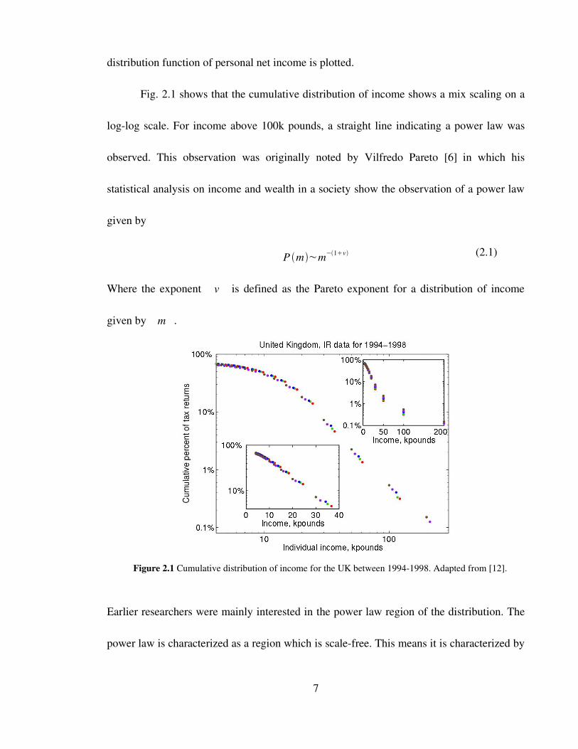
distribution function of personal net income is plotted.

   Fig. 2.1 shows that the cumulative distribution of income shows a mix scaling on a

log­log scale. For income above 100k pounds, a straight line indicating a power law was

observed.  This   observation  was   originally   noted   by   Vilfredo   Pareto  [6]  in   which   his

statistical analysis on income and wealth in a society show the observation of a power law

given by

P m~m−1v (2.1)

Where the exponent   v   is defined as the Pareto exponent for a distribution of income

given by  m . 

Earlier researchers were mainly interested in the power law region of the distribution. The

power law is characterized as a region which is scale­free. This means it is characterized by

7

Figure 2.1 Cumulative distribution of income for the UK between 1994­1998. Adapted from [12]. 

the same functions on log­log plots. These plots however are nonintegrable as they have

infinite variance. However, thanks to efforts by Levy [23] in probability theory, Mandelbrot

[24]  who found applications  of  power   laws   in   financial  data  and  Stanley  who applied

scaling analysis to phase transitions in [25],  power laws have seen greater application in

real world phenomena. 

In [26]  the authors  modeled  the lower income region, which is the income below

100k dollars by an approximation of the Gamma distribution specifically

P m=Cm− exp [−m /T ] (2.2)

where T=1/1 and   C=11/ 1 .   is   related   to   the   saving

propensity by

       =3/1− (2.3)

The   saving   propensity   will   be   elaborated   in   Section   2.2.2   on   the   description   of

Chakrabarti's  Trading Model. It was Dragulescu et. al in  [12], Souma et. al in  [27]  and

Chakraborti et. al in [13] who performed the fitting to the exponential distribution for the

lower   income   region.  It   was   mentioned   in   [12]   that   the   exponentially   fitted   part   is

dominated by the distribution of money but not significantly affected by invested assets.

The  upper   tail   however   shows   a   distribution  of  money  dominated  by   invested   assets.

Though   there   was   a   report   of   mixed   distribution   in   this   analysis,   a   mixed   income

distribution was reported in [28] where the lower income region was fitted to a lognormal

8

distribution. Besides the observation here, a lognormal distribution was fitted originally in

[14]. 

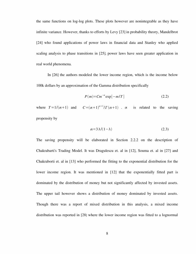
Besides  work  done  on   inheritance   tax  data   from  the  UK,  an  analysis  was  also

performed on income, as given by tax returns of the United States in 1997 [12]. As seen in

Figure 2.2, there was a similar mixed scaling distribution as the data from the UK. It was

proposed that a two class structure exists in income distributions where the higher end of

the tail usually accounts for less than 10% of the population. It can also be observed that the

exponential portion of this data, in regards to the lower income group collapses in a similar

fashion to the UK data. This observation proves to be robust as seen by Yakovenko in [29]

where a plot of income distribution over many years for the USA and after normalizing to

the   so   called   'wealth   temperature',   an   exponential   distribution   appears   in   each   income

9

Figure 2.2 Cumulative distribution of income for the USA for 1997. Adapted from [12]. 

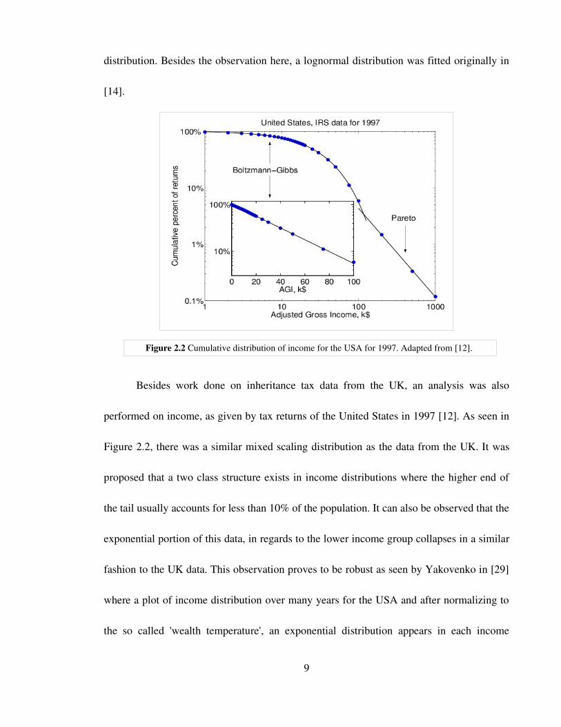
distribution in the time interval. This shows that the lower class income distribution has

stable  properties   similar   to   a   system being   in   thermal  equilibrium.  The higher   income

groups however seem to have more fluctuation with observations of fatter and thinner tails

with the former occurring during boom periods. This is shown in Figure 2.3 below.

Besides data from the UK and USA showing a mixed distribution of income and

wealth, work has been done on Japanese personal income data based on detailed records

obtained from the Japanese National Tax Administration. The findings in [30] show that a

power law is observed at the high income tail and its mean value fluctuates around 2.  Kim

and Yoon [31] have analyzed income distributions for current, labor and property markets

and   they   have   found   that   their   result   is   inconsistent  with   the  power   law  observation.

Clementi  and  Gallegatti   [32]  have   found  that   the  personal   income distribution   in   Italy

10

Figure 2.3 Cumulative distribution of income for the USA for 1983­2001. Adapted from [29]. 

follows a power law in the high income range which considers a percent of the population

and the lower­middle income range has a lognormal distribution which accounts for 99

percent of the population. They have also performed a time dependent analysis similar to

that done by Yakovenko and have found that change in the power law distribution for the

high income range is related to economic growth.  

2.2            Statistical Mechanics of Income and Wealth Distributions   

It  has been noted since Pareto and later Mandelbrot [24]  that  the distribution of

income for   the higher   income group can be  fitted  to  a  power   law.  The distribution  of

income   for   the   lower   income   group   however   has   been   fitted   as   either   a   lognormal

distribution by Simon [14] and later by Montroll and Shlesinger [35] or as a Boltzmann­

Gibbs distribution by Souma [27], Chakrabarti [13] and Yakovenko [15] . Here we attempt

to  discuss   the   phenomenology  behind   these   distributions   and   its   relation   to   economic

systems.    

2.2.1           Boltzmann­Gibbs distribution of wealth   

Physicists   attempting   to   model   economic   behavior   adopt   the   analogy   of   large

systems of interacting particles as seen in the kinetic theory of gases. This methodology is

similar to agent­based simulation. The chief goal of agent­based simulation is to explain

11

economic   results   that  are  not  accounted   for   in   traditional  models.   It  does   this  by  pre­

supposing rules of behavior  applied  to  agents and verifying whether   these micro­based

rules can explain macroscopic regularities   in   the form of complex social  patterns  from

interactions   with   multiple   agents   [49].     These   macroscopic   regularities   of   course   are

difficult to explain using conventional behavioral theories and empirical observations.  

Econophysicists   hypothesized   that   the   regular   patterns   observed   in   income   and

wealth distribution   are due to a natural law for the statistical properties of many body

systems interacting as an economy analogous to gases and liquids. Thus the description of

an economy as a thermodynamic system allows the identification of the income distribution

with the distribution of energies of particles in a gas. 

The Boltzmann­Gibbs distribution states that the probability of finding a physical

system in a state with energy  is given as

P =c e−/T (2.4)

where c is the normalizing constant and T is the scaled temperature. The derivation of this

distribution   assumes   the   statistical   character   of   the   system  (central   limit   theorem)  and

conservation   of   energy.   Consider   N   particles   with   the   total   energy   E.   Assuming   the

particles are distributed by ascending energy levels, the number of permutations of particles

between different energy levels is given by

         W=N !

N 1!N 2!N 3!...(2.5)

12

The logarithm of the multiplicity, W is defined as the entropy, S. For large numbers the

entropy per particle is written as

       SN=−∑

k

N k

Nln N k

N =−∑k

Pk ln Pk(2.6)

Using   the   method   of   Lagrange   Multipliers,   the   distribution   of   particles   with   highest

multiplicity is given by the Boltzmann­Gibbs distribution.

  Due   to   the  general  derivation  behind   the  Boltzmann­Gibbs  distribution,   it  was

proposed that phenomena distributed according to it will be seen in other statistical systems

besides gases. In [15], the argument was that a many body interacting system such as the

economy can be described by the Boltzmann­Gibbs distribution by choosing the conserved

quantity as money. The interaction process (trade) is described by the relation

m ' i=mi−m m ' j=m jm   (2.7)

where agents i and j complete a transaction with the total amount of money before and after

the transaction conserved. This disallows the manufacturing of money by an agent.   This

entire process is similar to the transfer of energy between colliding molecules during the

gas phase. An agent based model based on the relations given above was performed. 

The   authors   discovered   that   with   any   arbitrarily   set   of   rules   determining   m the

resultant distribution of wealth can be fitted to a Boltzmann­Gibbs distribution as shown in

Figure 2.4 below. 

13

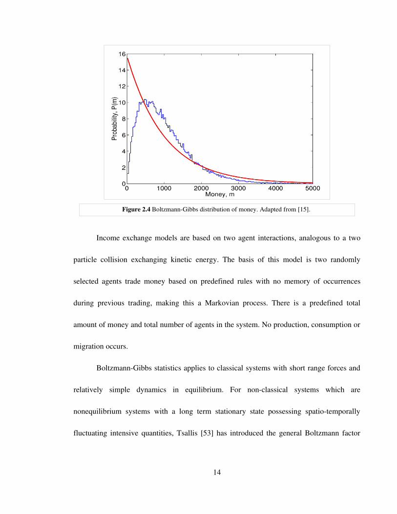
Income exchange models are based on two agent interactions, analogous to a two

particle   collision  exchanging  kinetic   energy.  The  basis  of   this  model   is   two   randomly

selected agents  trade money based on predefined rules with no memory of occurrences

during  previous   trading,  making   this  a  Markovian  process.  There   is  a  predefined   total

amount of money and total number of agents in the system. No production, consumption or

migration occurs. 

Boltzmann­Gibbs statistics applies to classical systems with short range forces and

relatively   simple   dynamics   in   equilibrium.   For   non­classical   systems   which   are

nonequilibrium   systems  with   a   long   term   stationary   state   possessing   spatio­temporally

fluctuating intensive quantities, Tsallis [53] has introduced the general Boltzmann factor

14

Figure 2.4 Boltzmann­Gibbs distribution of money. Adapted from [15]. 

given by

      B=∫0

∞

exp −E f d ={1

1q−1O E}−1/q−1

(2.8)

which is dependent on the entropic index q in which q=1 leads to the ordinary Boltzmann

factor.   The   use   of   the   generalized   Boltzmann   factor   has   found   many   applications   in

complex systems research but we will not apply it in this study.

2.2.2           Mixed distribution : Boltzmann­Gibbs and Power law distribution of wealth   

The resultant wealth distribution depicted previously is unable to account for the

occurrence  of   a  power   law.  A model  designed  by  Chakrabarti   et   al.   in   [13]   allows   a

distribution of wealth  with a mixed distribution as observed in empirical data. The model

is similar to the assumptions made by Yakovenko et al in [15] particularly conservation of

money during a trade. 

Every agent is initialized with a randomly or arbitrarily set amount of money. In a

trade, a pair of agents exchange their money based on the predefined rules. The important

property   of   this   interaction   however   is   that   the   total   amount   of   money   in   a   trade   is

conserved and there is no negative money after a trade. In specific terms,

    mit m j t =mi t1m j t1 (2.9)

where  m t  is the money of agents i  or  j  at time  t . 

15

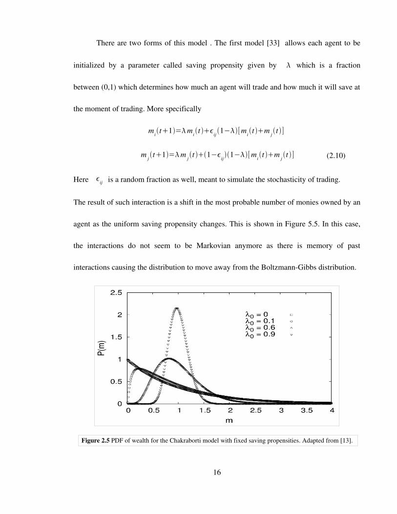
There are two forms of this model  . The first model [33]   allows each agent to be

initialized   by   a   parameter   called   saving   propensity   given   by   which   is   a   fraction

between (0,1) which determines how much an agent will trade and how much it will save at

the moment of trading. More specifically

mit1=mi t ij 1−[mi t m j t ]

         m j t1=m j t 1−ij1−[mit m j t ] (2.10)

Here  ij is a random fraction as well, meant to simulate the stochasticity of trading. 

The result of such interaction is a shift in the most probable number of monies owned by an

agent as the uniform saving propensity changes. This is shown in Figure 5.5. In this case,

the   interactions   do   not   seem   to   be   Markovian   anymore   as   there   is   memory   of   past

interactions causing the distribution to move away from the Boltzmann­Gibbs distribution.

16

Figure 2.5 PDF of wealth for the Chakraborti model with fixed saving propensities. Adapted from [13]. 

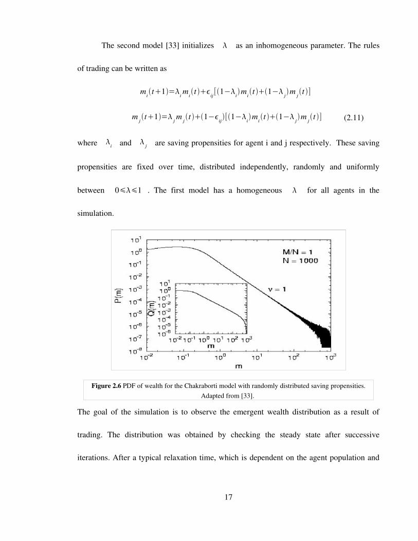
The second model [33] initializes   as an inhomogeneous parameter. The rules

of trading can be written as 

     mit1=i mit ij [1−imi t 1− jm j t ]

m j t1= j m j t 1−ij[1−imi t 1− jm j t ] (2.11)

where  i  and  j  are saving propensities for agent i and j respectively.  These saving

propensities   are   fixed   over   time,   distributed   independently,   randomly   and   uniformly

between   01 .   The   first   model   has   a   homogeneous     for   all   agents   in   the

simulation.

The goal of the simulation is to observe the emergent wealth distribution as a result of

trading.   The   distribution   was   obtained   by   checking   the   steady   state   after   successive

iterations. After a typical relaxation time, which is dependent on the agent population and

17

Figure 2.6 PDF of wealth for the Chakraborti model with randomly distributed saving propensities. Adapted from [33]. 

the distribution of    , a stationary distribution was observed. We show the stationary

distribution in Figure 2.6 above.

A power  law decay  in  the high  income range is  observed.  The exponent of  the

power  law  is   found  to   fit  v=1.  The method of  analysis   to  obtain   the  exponent  was  to

perform a least­squares regression on a log­log plot of distribution of wealth. We ran the

same model using the same parameters as mentioned by the author and performed a power

law analysis as described in the next chapter. 

2.2.3           Mixed distribution : Lognormal and Power law distribution of wealth   

  In   [34]  it   was   claimed   that   the   distribution   of   income   follows   a   lognormal

distribution but transitions into a power law in the last few percentiles. This claim is made

by plotting annual US income distribution for the year 1935­36 on log­normal graph paper.

They found the income is distributed on a straight line, indicating a lognormal distribution,

for the first 98­99 percent of the sample and followed by an inverse power law for the rest.

A model [35,36] was subsequently developed to explain the existence of the mixed

distribution   of   income.   The   basis   of   the   model   is   also   analogous   from   colliding   gas

molecules transferring energy. Interestingly, they hinted on a different rate of obtaining

money similar to that of the saving propensity citing “..training, motivation, risk­taking,

inheritance, luck, intimidation, skill,  etc” as constraints to people. Assuming the income

18

distribution   is   log­normal,   the   probability   that   annual   income   is   between   x   and

xdx  is given by

    p x dx= 1221/2

exp −log xx

2

/22dx / x (2.12)

where  x /x denotes income between the interval whose mean income is given by  x .

This formulation is chosen because a transfer of money   dx   has different meaning to

persons of different levels of income. It is assumed however that transactions are equivalent

if they involved the same fraction of income of the participants.  This means that mean

income shifts as the level goes higher but relative to the mean, the distribution in a given

interval is invariant. 

Pareto­Levy tails can be derived from the log­normal distributions by accounting for

the process of amplification. Let   g x /x be defined as the basic distribution. Given a

probability  which determines the range of the initial distribution g, the next amplified

class is also denoted by   g  but   x   is denoted by   N x .   The basic distribution can

thus be written instead of  g x /x dx /x  as  g x /N x dx /N x . For continuing levels of

amplification, the distribution can be written as

         G y=1−[g y

Ng y /N

2

N 2g y /N 2] (2.13)

where   y=x /x . 1−   is   introduced   to   ensure   the   proper   normalization   of   G(y).

Replacing  y  by  y /N , we can obtain

19

        G y=

NG y /N 1−gy (2.14)

We now obtain the asymptotics for the distribution. If  0 there is no amplifier

class and G(y) goes to g(y). If    y   is large g y0   as seen in the distributions of

incomes. Here the asymptotic form of  G y  is given by

      G y=

NG y /N (2.15)

Writing   G y=Ay−1− ,   we   obtain   =log 1// log N   which   relates   the   Pareto

exponent to the fractal dimension.

Trading models which are based on randomly choosing agents to lose or gain wealth

at arbitrarily set rates can be depicted as a clustering system. These systems have a self­

similar   geometry.   In   clustering   systems,   small   clusters   are   observed   more   frequently

compared   to   larger   size   clusters.   Thus   poorer   and   middle   class   agents   have   a   higher

frequency in the data as oppose to higher income agents which are more scarce. 

The lognormal and Boltzmann­Gibbs distribution could be easily mistaken for one

another as they both decay exponentially. However, the Boltzmann­Gibbs distribution is

found to decay slower compared to the lognormal distribution. The generating mechanisms

are also different in which the Boltzmann­Gibbs distribution is the distribution of energy

for a closed system of interacting particles with no memory and the lognormal distribution

is the distribution of multiplicative growth processes. 

20

2.3            Diffusion   

Diffusion   is   defined   as  a   net   transport   of   molecules   from   a   region   of   higher

concentration to one of lower concentration by random molecular motion. In this work, we

will  consider  two types of diffusion,  normal and anomalous.  We will  use these  two to

characterize the movement of money in the trading models. 

2.3.1           Normal Diffusion   

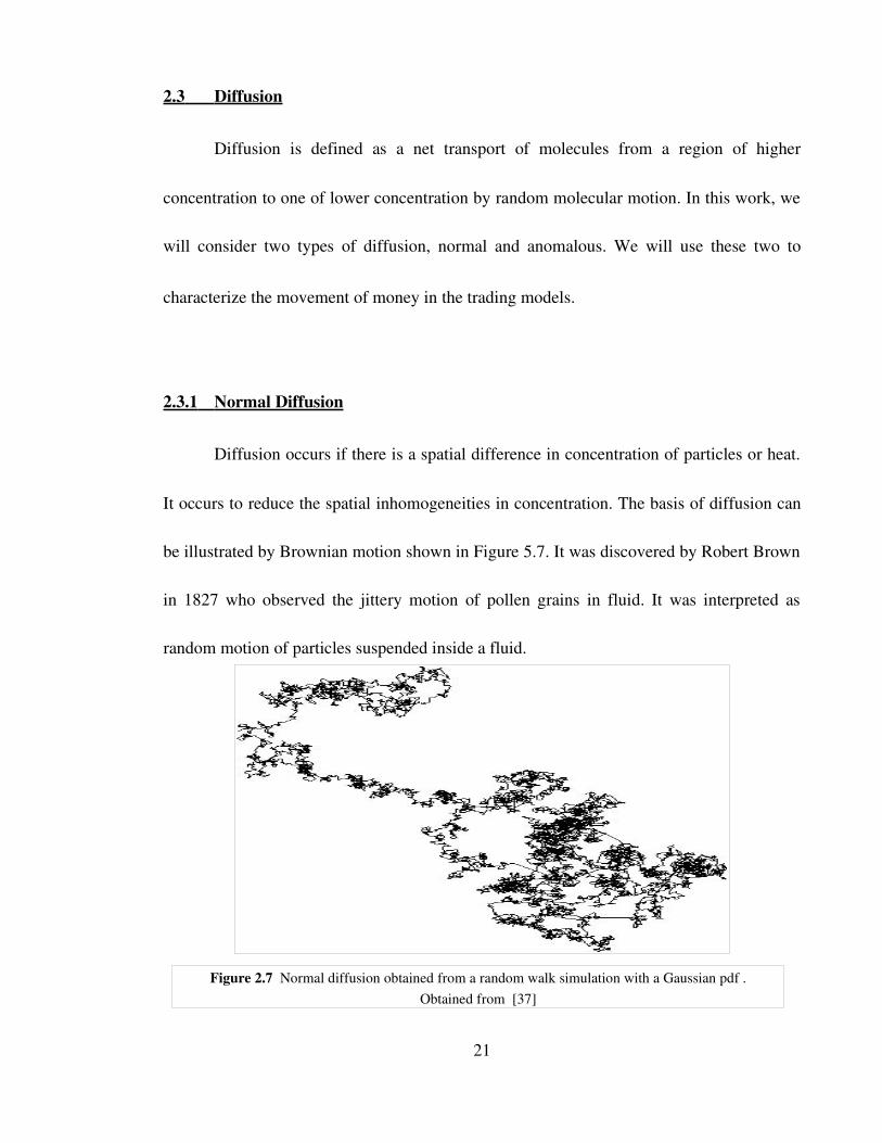
Diffusion occurs if there is a spatial difference in concentration of particles or heat.

It occurs to reduce the spatial inhomogeneities in concentration. The basis of diffusion can

be illustrated by Brownian motion shown in Figure 5.7. It was discovered by Robert Brown

in 1827 who observed the jittery motion of pollen grains in fluid. It  was interpreted as

random motion of particles suspended inside a fluid. 

 

21

Figure 2.7  Normal diffusion obtained from a random walk simulation with a Gaussian pdf .Obtained from  [37]

We have obtained the formalisms below from [16]. Consider the position  r   in

1,2 or 3­D space.  Assuming the position changes in random steps   r   and the time

t  between the two subsequent steps is constant, the position  r n  of a particle after n

steps is given by

r n=rnrn−1r

n−2...r1r0 (2.16)

and   t n=n t .   r n   and   r i   are   random variables.  We  thus  draw these  random

values from the probability density function (pdf)   p r . It yields the probability for

the particle to make a certain step   r i . We assume the steps are independent of each

other. This assumption is similar to that of the Boltzmann­Gibbs distribution as mentioned

previously. Under this assumption and the conservation of energy, we propose that physical

systems whose energy level are distributed according to the Boltzmann­Gibbs distribution

undergo normal diffusion.

To find the mean squared displacement , we find the value of  ⟨r2⟩  from (2.16) to

obtain

⟨r n2 ⟩= ∑

j=1, k= j

n

⟨r j2⟩ ∑

j=1, k≠ j

n

⟨r jr k ⟩ (2.17)

If we assume the mean value for the pdf is at zero, we can rewrite the first and the second

terms on the right hand side as the variance and covariance respectively.

22

  ⟨r n2⟩= ∑

j=1, k= j

n

r , j2 ∑

j=1, k≠ j

n

cov r j ,r k (2.18)

Since we assume the steps the particles take are independent of each other, the covariance is

zero.  Thus we can rewrite (2.18) as

                ⟨r n2⟩= ∑

j=1, k= j

n

r , j2 (2.19)

This is the basis of modeling the Brownian random walk. For this work we will employ the

diffusion equation used in Fickian diffusion explained below.

We assume particle diffusion occurs along the z­dimension in 3­D space between

two   areas   on   the  x­y  plane  perpendicular   to   the   flow.  For   particle   conservation,   time

variation of the density  n z , t  inside a volume  x y z  equals the inflow, minus

the outflow of particles. If  J z , t  is the particle flux,

            ∂ n z , t

∂ t x y z=J z x y−J z z x y

 =−∂ J∂ z

x y z      (2.20)

This leads to the diffusion equation

      ∂n z , t

∂ t=−∂ J∂ z

(2.21)

Physically, particle flux means

J z , t =n z , t v z , t (2.22)

23

Fick's  law states  that  the flux of particles crossing a certain area is  proportional  to  the

density gradient along the axis perpendicular to the area,

     J z=−D ∂n z , t ∂ z

(2.23)

where D is the diffusion coefficient. Thus, we can rewrite (2.21) as

    ∂ n z , t

∂ t=

∂

∂ zD ∂ n z , t

∂ z(2.24)

assuming the diffusion coefficient is constant

    ∂ n z , t

∂ t=D ∂2 n z , t

∂ z2 (2.25)

The solution to this equation is given by the error function, given by

    n z , t =N 0

4Dte−

z2

4 Dt (2.26)

where  N 0  is the total number of particles inside the volume. 

If we were to find the mean squared displacement given by,

⟨ z2t ⟩=∫ z2 n z , t dz

   = ∫ z2 N 0

4Dte−

z2

4 Dt dz (2.27)

Applying the Gaussian integral to solve the integration, we finally obtain

⟨ z2t ⟩=2 Dt (2.28)

Thus we have shown that the mean squared displacement of the random walk has a linear

24

relation with relaxation time. This is characteristic of systems in or close to equilibrium

(ergodic). This result was first reported by Einstein who added that the trajectories of a

Brownian particle can be regarded as memory­less and nondifferentiable so that its motion

is not ballistic.

2.3.2           Phenomenology of Anomalous Diffusion    

Normal   diffusion   is   characterized   by   particle   trajectories   in   fluids   close   to

equilibrium being irregular but still homogeneous. Anomalous diffusion however occurs in

fluids far from equilibrium (non­ergodic) where there exists different types of orbits [38].

This is due to the existence of trajectories 'trapped' for long times in small spatial areas and

long flights of particles, where particles are carried in one step over large distances. 

Processes deviating from the classical Gaussian diffusion occur in a multitude of

systems. These systems can be characterized as disordered systems which can be modeled

by fractal geometry [39]. These anomalous features are seen over the entire data set but

they  can develop after  an  initial  sampling  period or   they may be   transient,   fluctuating

between   an   anomalous   transport   to   a   normal   transport   process   [17].   The   fundamental

signature   of   an   anomalous   transport   process   is   the   deviation   of   the   mean   squared

displacement

⟨r 2⟩=⟨r−⟨r ⟩2⟩~t (2.29)

25

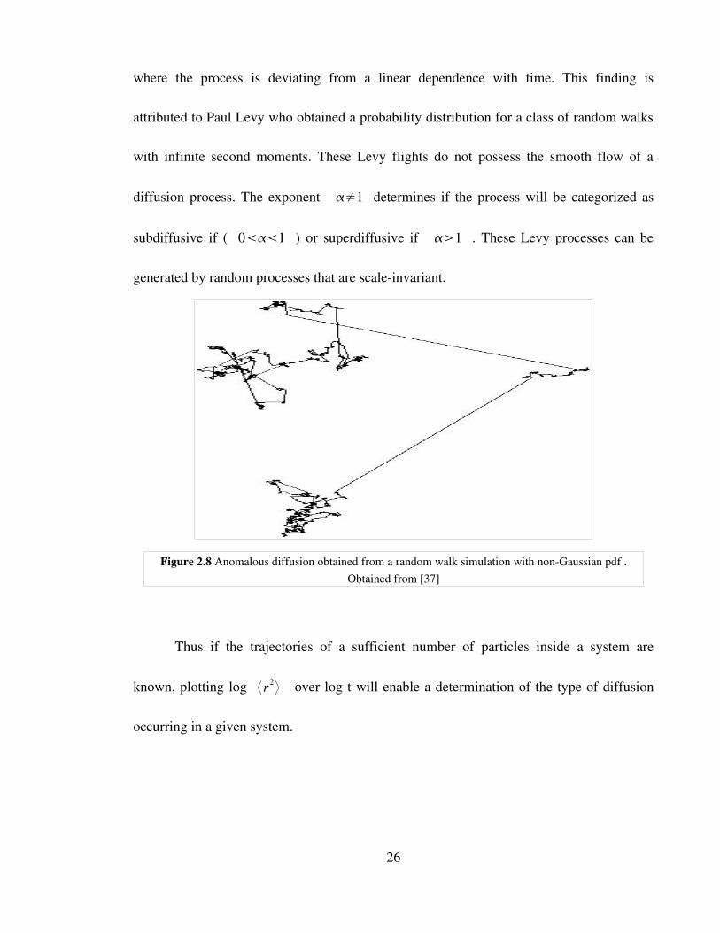
where   the   process   is   deviating   from   a   linear   dependence   with   time.   This   finding   is

attributed to Paul Levy who obtained a probability distribution for a class of random walks

with infinite second moments. These Levy flights do not possess the smooth flow of a

diffusion process. The exponent   ≠1 determines if the process will be categorized as

subdiffusive if ( 01 ) or superdiffusive if   1 . These Levy processes can be

generated by random processes that are scale­invariant. 

Thus   if   the   trajectories   of   a   sufficient   number  of   particles   inside   a   system are

known, plotting log ⟨r2⟩  over log t will enable a determination of the type of diffusion

occurring in a given system.

26

Figure 2.8 Anomalous diffusion obtained from a random walk simulation with non­Gaussian pdf .Obtained from [37]

2.3.3           Continuous Time Random Walks   

Continuous   time random walks  (CTRW) are random walks  whose  time  interval

between successive steps are random intervals. It is a non­Markovian model in which the

knowledge of the diffusing quantity and the time where the last step took place is required

to predict the evolution of the walk. Its statistics are dependent on the failure of the central

limit theorem. This is due to the fact that the CTRW is governed by a wide waiting time

distribution and a wide jump length distribution, in particular, these distributions have an

infinite   second   moment   or   there   exists   long   range   correlations.   The   jump   length   and

waiting time distribution are drawn from the probability distribution function   x , t .

The formalisms for the CTRW as given below is adapted from [16,17].

The jump length probability distribution function is defined by

     x =∫0

∞

dtx , t (2.30)

while the waiting time probability distribution function is defined by

   w t =∫−∞

∞

dxx , t (2.31)

Thus, if  x  and  w t  are independent random variables we can then define  

    x , t =w t x (2.32)

If they are dependent random variables we can define the probability distribution function

based on either choosing to bound the displacement or time random variable. If we allow a

27

jump   length   to   occur   only   over   a   certain   period   of   time,   we   define   the   probability

distribution function as

x , t =p x∣t w t (2.33)

If we allow the random walker to only travel a certain maximum distance, we define the

probability density function (pdf) as

x , t =p x∣t w t  (2.34)

We thus relate superdiffusion to the CTRW process where the characteristic waiting

time given by (2.30) is finite and the jump length variance given by

    2=∫−∞

∞

dxx x2 (2.35)

which   is   diverging.   We   also   relate   subdiffusion   to   the   CTRW   process   of   diverging

characteristic waiting time and  the jump length variance being finite.

The CTRW process is described by

x , t =∫−∞

∞

dx '∫0

∞

dt ' x ' , t ' x−x ' , t−t ' x t (2.36)

It describes the probability distribution function of jumping to x at time t currently in  x '

at   t ' .   x and   t   are   the   initial   position   and   time   respectively.   Thus   the

probability of being in  x  at time  t '  after traveling for t  is given by

W x , t =∫0

t

dt x , t ' t−t ' (2.37)

The probability of not jumping after arriving at x is given by

28

    W x , t =1−∫0

t

dt ' w t ' (2.38)

Montroll and Weiss [40]  have shown that the Fourier­Laplace transform of the pdf

p x , t can be obtained as follows. In Fourier­Laplace space, we rewrite (2.36) as

           k , s=k ' , s ' k w s1 (2.39)

assuming independence of jump length and waiting time. Similarly, we can rewrite (2.37)

as 

W k , s=k , s ' s−s ' (2.40)

and (2.38) as 

s=1− w ss

(2.41)

Solving for  W k , s  we obtain

      W k , s=W 0k

1− s1− s/s  (2.42)

W 0k  denotes the Fourier transform of the initial condition  W 0 x .

2.3.4           Subdiffusion   

As   mentioned   above,   subdiffusion   occurs   when   the   characteristic   waiting   time

diverges but the jump length variance is finite. Subdiffusion has been seen in the studies of

membranes  and electrochemical  systems.  A recent  work being  [54].   In   these  cases   the

29

diffusion of ions through membranes or electrochemical systems will be constrained due to

their  clustered  structure.  We adapt   the   formalisms  of   subdiffusion   from [17].  We  thus

define a long­tailed waiting time pdf given by

         w t ~A/ t 1 (2.43)

whose Laplace space asymptotics is given by

w s~1−s (2.44)

The waiting time distribution is thus the pdf of transition by a single displacement exactly

at given time prior to it. With relation (2.44) and the jump length pdf of a finite jump length

variance given by

k ~1−2 k2 (2.45)

we obtain from (2.42)

   W k , s=W 0k /s

1K s−k2 (2.46)

We can now derive the fractional diffusion equation. 

We start by rewriting (2.46) as 

         W k , ssK k2=W 0k s−1  (2.47)

Rearranging it to 

   sW k , s−W 0k s−1=−W k , sK k2  (2.48)

A Fourier transform of a spatial derivative is given by

30

F d n

dznfz=∫

−∞

∞

[d n

dznf ze−2 i kz]dz=2 ik n F { f z}   (2.49)

Choosing n=2 for the finite jump length similar to the Gaussian case, we can write (2.48) as

             sW k , s−W 0k s−1=K

∂2

∂ x2W x , t    (2.50)

We now define the Caputo derivative which is a derivative of fractional order

      Dt

0 t = 1n−

∫0

t

1

t−t ' 1−n

d n

dt nt ' dt '               (2.51)

The Laplace transform of the Caputo derivative is given by

        L { Dt

0 t }= 1n−

∫0

t

L { 1t−t ' 1−n

}L { d n

dtnt ' }dt '

      =  s−2[s2t ' −s0]  

      =  st ' −s−10 (2.52)

Thus we can rewrite (2.50) using the relation (2.52) as

Dt

0 W x , t =K∂2

∂ x2W x , t (2.53)

Using the symmetry property of the Caputo fractional derivative

  W x , t = Dt−

0 K ∂2

∂ x2W x , t (2.54)

An application of the differential operator  ∂/∂ t  gives 

∂W x , t ∂ t

= Dt1−

0 K∂2

∂ x2W x , t (2.55)

31

where

             Dt

0 W x , t = 1

∂∂ t∫0

t

dt ' W x , t ' t−t ' 1−

(2.56)

To calculate the mean squared displacement we start by finding

   ⟨ x2⟩=limk0

−d 2

dk2W k ,u (2.57)

Taking  W k ,u  from (2.46) we obtain

⟨ x2⟩=u−1 d2

dk2W 0k −2 KW 0k u

−1 (2.58)

Performing the inverse Fourier­Laplace transform, we obtain

⟨ x2t ⟩=2K

1t (2.59)

To show analytically the reason behind the large waiting times, we redefine  (2.50)

           Dt

0 W x , t − Dt

0 W 0x =K∂2

∂ x2W x , t (2.60)

From the definition of the Caputo derivative, the second term on the left hand side is easily

integrable to solve the above equation as

Dt

0 W x , t − t−

1W 0x =K

∂2

∂ x2W x , t (2.61)

The rate of decay of the initial value is an inverse power law as can be seen in the second

term of the left hand side and not exponential as in the standard diffusion situation. 

32

2.3.5           Superdiffusion   

We adapt   the   formalisms  of   superdiffusion   from  [17].  For   the  case  of   a   finite

characteristic  waiting   time  and  diverging   jump  length  variance,   the  pdf  describing   the

random walk is modeled by a Poissonian waiting time and a Levy distribution for the jump

length, given by

        k =exp −∣k∣ (2.62)

whose asymptotics is defined by

            k ~1−∣k∣ (2.63)

Due   to   time   being   finite,   this   process   is   of   a   Markovian   nature.   Levy   processes   are

stochastic processes obeying a generalized central limit theorem. They are stable processes

where the sum of two independent Levy processes is itself a Levy process.

We can obtain the Fourier­Laplace  transform of   W x , t   for Levy flights  by

using (2.63) and the Poissonian waiting time given by

w s=1−s (2.64)

onto (2.46) to obtain

     W k , s= 1sK∣k∣

(2.65)

where   K=

.  Using the same method as above, we can then obtain the fractional

diffusion equation for Levy flights 

33

  ∂W∂ t

=K Dx

−∞W x , t (2.66)

Levy  flights  have  been documented  to  describe motion  of   fluorescent  probes   in   living

polymers, tracer particles in rotating flows [38] and cooled atoms in laser fields [48].

We can also find the characteristic function of the Levy distribution used to generate

the Levy flight. We do so by performing a Fourier transform to obtain

W k , t =exp −K ∣k∣ (2.67)

As can be observed from (2.65) the long jumps are due to the asymptotic property of

the jump length pdf. These long jumps are seen in the figure coupled with clusters which

also contain long jumps but on different length scales. Thus the jump length distribution is

the origin of the scaling nature of the Levy flight. 

It can be shown that the power law asyptotics can be described [17] as

    W x , t ~ K t∣x∣1 (2.68)

Due to this property, the mean squared displacement diverges as  ⟨ x2⟩∞ .

2.3.6           Anomalous diffusion in the movement of money   

The objective behind [19,20] is to infer the statistics of human travel by analyzing

the   circulation   of   bank   notes   in   the   United   States.   Specifically,   finding   a   probability

distribution   function  of   finding  a  displacement  of   length   r   in   time   t   given  by

34

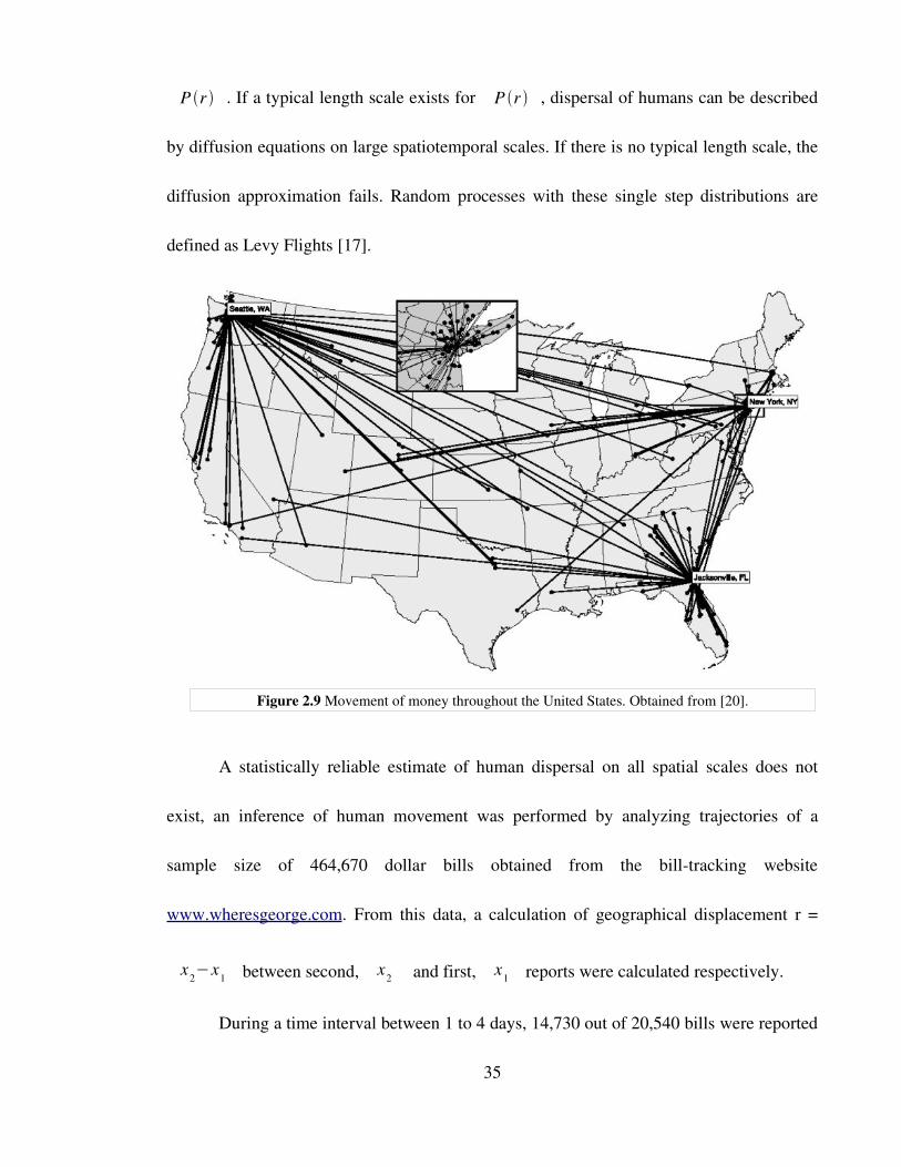
P r . If a typical length scale exists for  P r , dispersal of humans can be described

by diffusion equations on large spatiotemporal scales. If there is no typical length scale, the

diffusion approximation fails.  Random processes with these single step distributions are

defined as Levy Flights [17]. 

A statistically reliable estimate of human dispersal on all  spatial scales does not

exist,   an   inference  of   human  movement  was  performed  by   analyzing   trajectories   of   a

sample   size   of   464,670   dollar   bills   obtained   from   the   bill­tracking   website

www.wheresgeorge.com. From this data, a calculation of geographical displacement r =

x2−x1  between second,  x2   and first,  x1  reports were calculated respectively.

During a time interval between 1 to 4 days, 14,730 out of 20,540 bills were reported

35

Figure 2.9 Movement of money throughout the United States. Obtained from [20].

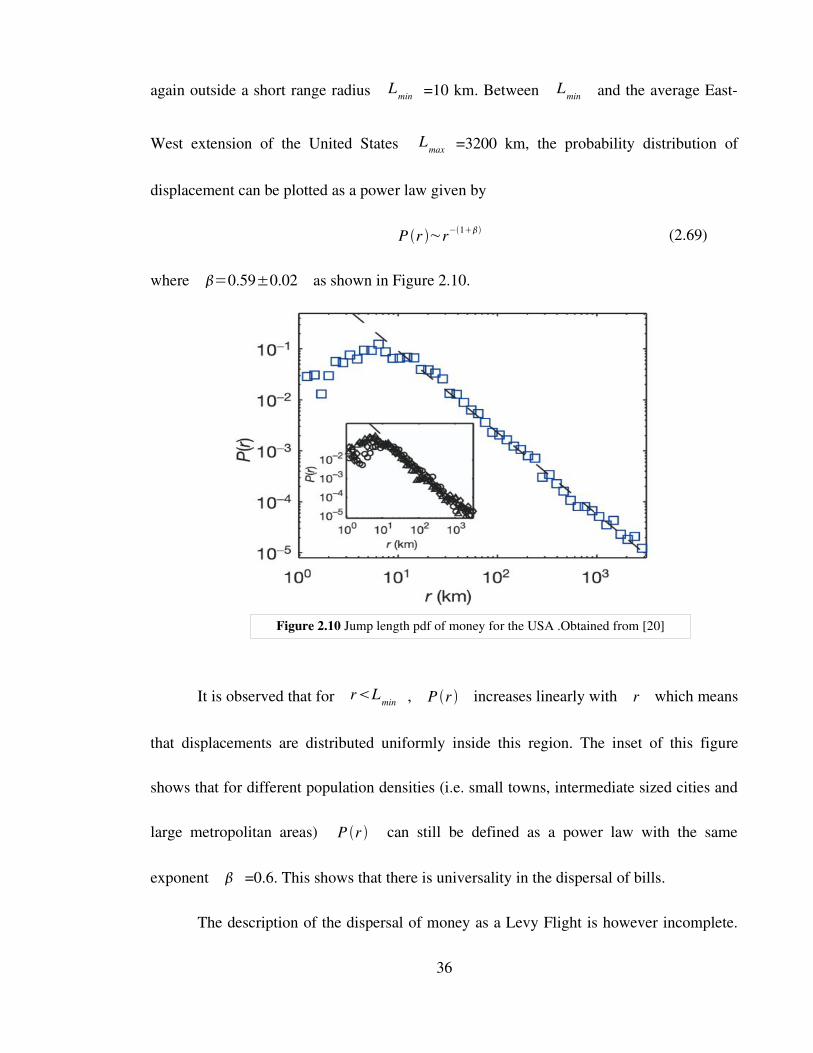
again outside a short range radius  Lmin =10 km. Between  Lmin  and the average East­

West   extension  of   the  United  States   Lmax =3200  km,   the  probability   distribution  of

displacement can be plotted as a power law given by

P r ~r−1 (2.69)

where  =0.59±0.02  as shown in Figure 2.10.

It is observed that for  rLmin ,  P r  increases linearly with  r  which means

that  displacements  are distributed uniformly  inside  this   region.  The  inset  of   this   figure

shows that for different population densities (i.e. small towns, intermediate sized cities and

large  metropolitan  areas)   P r   can   still   be   defined  as   a   power   law with   the   same

exponent  =0.6. This shows that there is universality in the dispersal of bills.

The description of the dispersal of money as a Levy Flight is however incomplete.

36

Figure 2.10 Jump length pdf of money for the USA .Obtained from [20]

This is because bills dispersing due to Levy Flights would have equilibrated after 2 to 3

months. The data shows however that after an average of one year, only 23.6% of bills have

travelled further than 800km while 57.3% have travelled between 50 to 800 km. This is

significantly less ground travelled compared to  Lmax .

Two explanations have been proposed by the authors. First, spatial inhomogeneities

in the form of surroundings, where city life allows localization of bill transfer due to many

economic players in an area as oppose to a suburban surroundings will cause a slowing

down of   the  dispersal   of   bills.   Secondly,   a   scale   free  observation  of   times   t   between

successive displacements leads to subdiffusion [20]. 

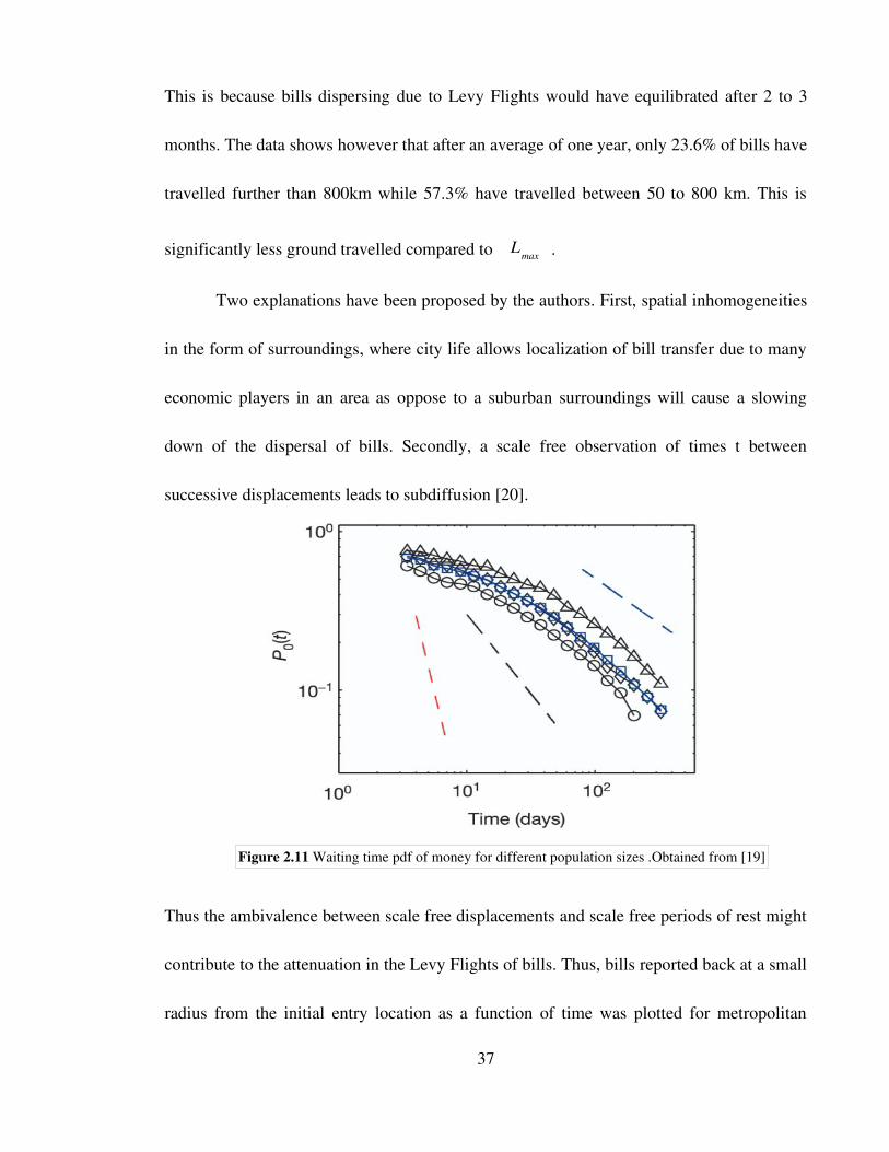
Thus the ambivalence between scale free displacements and scale free periods of rest might

contribute to the attenuation in the Levy Flights of bills. Thus, bills reported back at a small

radius from the initial entry location as a function of time was plotted for metropolitan

37

Figure 2.11 Waiting time pdf of money for different population sizes .Obtained from [19]

cities, intermediate city sizes and small towns. The same asymptotic behavior was observed

again as shown in Figure 2.11 above.

The probability distribution of waiting times can be defined as

P t =At−1 (2.70)

where  =0.60±0.03 . It was reported by the authors that the theoretical exponent 

if  =0.60  where   is the power law exponent from the jump length distribution in

(2.68)   should be   =3.33. Since the measured decay of waiting times is considerably

slower, it was concluded that long waiting times play a significant role in the dispersal of

bills.

Thus,   the   authors   have  performed   an   analysis   of   the  distribution  of  money  by

modeling the process as a CTRW. This is due to the apparent interplay between the scale

free   displacements   and   waiting   times   observed.   As   mentioned   previously,   the   CTRW

consists of a succession random displacements   xn   and random waiting time  t n

drawn from the probability distributions   p x   and   t   respectively. After N

iterations, the position of the walker is given by 

     X N=∑n

N

xn (2.71)

the time of the walker is given by

      T N=∑n

N

tn (2.72)

38

The   object   of   interest   is   the   functional   relationship   of   position   and   time.   If

p x and  t posses existing moments, the central limit theorem implies

X N~N 1 /2 (2.73)

and     T N~N   (2.74)

after   long   times.  Thus   the   scaling   relationship  between  displacement   and   time  can  be

defined using the above equations heuristically as

X t ~t1 /2 (2.75)

However if the spatial increments and waiting time posses an algebraic tail, we define the

pdf of displacement as

p x ~ 1∣ x∣2 where  02 (2.76)

and the pdf of waiting time as

t ~ 1∣ t∣1 where  01 (2.77)

The   second   moment   for   these   distributions   are   divergent.   Thus   the   scaling   for   the

successive displacements and successive time steps scale as

  X N~N 1/ (2.78)

and     T N~N 1/ (2.79)

respectively. Thus it is heuristically seen that the position and time variable scale according

to the exponents   and  . Specifically,

39

  X t ~t/  (2.80)

In this simple way we can observe that long waiting times, signified by the exponent  ,

will allow latency to occur in the displacements as it increases the traveling time.

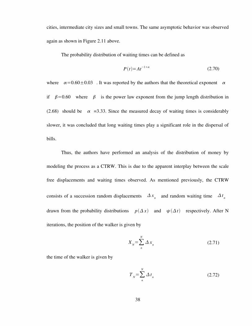
Thus, by choosing suitable  waiting time and jump length exponents in a specific

range,   any  process  with   spatio­temporal   scaling   can  be  generated.  We mention   a   few

examples in Table 1.

Exponents Process

2 Superdiffusive

2 Subdiffusive

=1,02 Levy Flights

01,=2 Fractional Brownian Motion

=1 ,=2 Brownian Motion

In  order   to   further  understand  the properties  of  ambivalent  process,  we have  to

compute the pdf of   W x , t   for   X t . We have obtained the formalisms described

below from [19,20]. The pdf  W x , t can be expressed in terms of the spatial distribution

p x and the temporal distribution  t . As shown in (2.42) the Fourier­Laplace

transform of  W x , t  is 

    W k , s=W 0k

1− s1− s/s (2.81)

40

Table 1 Spatio­temporal scaling processes generated from suitable waiting time and jump length exponents

An inverse Fourier­Laplace transform of this equation is given by

     W x , t = 123

∫ds∫dk est−ikx W k , s (2.82)

Opting for both  p x  and  t  to exhibit algebraic tails as shown in (2.76) and

(2.77) we can write the asymptotics of the expansion of the Laplace transform for the pdf of

jump length as

pk =1−D∣k∣ (2.83)

and the pdf of waiting time as

  s=1−D s (2.84)

Inserting this into (2.80), we obtain

W k , s= u−1

1D ,∣k∣

/u  (2.85)

where  D ,=D/D  is the generalized diffusion constant.

The inverse Laplace transform of (2.81) was obtained as

W x , t = 12∫dk e−ikx

∑n=0

∞

−D ,∣k∣

tn

1 n

        =  W x , t = 12∫dk e−ikx E−D

,∣k∣ t  (2.86)

where   Ez=∑n=0

∞ zn

1 n  is the Mittag­Leffler function. E−D

,∣k∣ t   is the

41

characteristic function of the process. It is a function of  kt/ . Thus, the probability was

expressed as

W x , t =t−2/ L ,x / t

/ (2.87)

where  L ,z =

12

∫dk E−∣k∣−ikz   is the universal scaling function. The spatio­

temporal scaling  X t ~t/  can be extracted from this relation.

42

CHAPTER 3 : DESCRIPTION OF TRADING MODELS, THEIR

MODIFICATIONS TO ANALYZE THE DIFFUSION OF MONEY AND

POWER LAW ANALYSIS METHODS 

3.1            Introduction   

As   has   been   elaborated   in   the   earlier   chapter,   anomalous   diffusion   has   been

observed   in   the   diffusion   of   money   across   the   United   States.   This   observation   has

motivated us to study the diffusion of money in trading models. This was because of the

observation by Brockmann as shown before, that the spatial inhomogeneities existing in a

real   economy  in   the   form of  geographical   location  and  socioeconomic   factors   such  as

population density between geographic locations (please refer to Figure 2.10), will result in

the observation of Levy flights in money displacement as well as long waiting times of

money in a location (please refer to Figure 2.11). A trading model is a suitable candidate

for these observations to occur as its well defined trading rules will result in both a trapping

of money with  specific agents as well as a more vibrant moving money with other agents.

If anomalous diffusion is observed, this means the system is non­ergodic and explains why

the Boltzmann­Gibbs distribution is not obtained even in conservative systems.

The Chakrabarti trading model as discussed in section 2.2.2, is a suitable candidate

to study anomalous diffusion in a trading model as the occurrence of   long waiting times

will naturally happen due to the existence of agents who have large saving propensities.

43

These agents will hold on to monies for longer periods of times due to its propensity to save

more and trade less. Before any analysis can be done, we have to perform a modification on

the Chakrabarti trading model to allow it to trade only with its neighbors and not randomly

with any other agent. This gives spatial coordinates to agents. This is so that we can have a

solidly defined statement of length so that we can measure the displacement of money in

order to determine if  it is distributed according to a scale free distribution. 

Thus in order to achieve our goal, we have to firstly determine in a very simplistic

way if the trading model is undergoing anomalous diffusion. As mentioned in the earlier

chapter, a commonly used method by experimentalists to determine the type of diffusion is

to determine the relation between the log mean squared displacement and the log relaxation

time. If we do obtain a log mean squared displacement which changes non linearly with log

relaxation, the diffusion is anomalous.

We  then  have   to  determine   the  waiting   times  of  money between  trades   among

agents and consequently plot the pdf of waiting times. Similarly, we have to determine the

jump lengths made by the monies in arbitrarily fixed time intervals and plot the pdf of jump

lengths. If we can observe long tails in these plots, we can conclude from the asymptotics

of the waiting time pdf and jump length pdf discussed in  the previous chapter  that  the

waiting times and the jump lengths do not correspond to the normal diffusion case. We thus

obtain the scaling exponents from the waiting time and jump length pdf's in the long tail

44

regions. With these scaling exponents, we can finally determine if money is undergoing

anomalous diffusion using the treatment given by Brockmann.

3.2            Trading models and their modifications   

We elaborate on the modifications required to calculate the diffusion of money in

the Chakrabarti trading model, the Yakovenko trading model (described in section 2.2.1

and 2.2.2 respectively) and the Kinetic Economies trading model [18]. We refer the reader

to the appendices where we have included the computer simulation code for the trading

models to further illuminate the modifications.

3.2.1           Modified Chakrabarti trading model   

As mentioned above, the Chakrabarti  trading model has to be modified to allow

proper calculations of jump lengths and waiting times. Only then can we attempt to perform

diffusion analysis. We now discuss the modifications performed on the Chakrabarti trading

model. We have included the code for this simulation in Appendix A and will highlight the

portions of code related to the discussion.

As mentioned in  the previous chapter,   the Chakrabarti   trading model obtains  its

heterogeneity   from   the   distributed   saving   propensity   among   its   agents   and   with   this

property,   what   is   obtained   is   a   wealth   distribution   similar   to   that   seen   in   data.   The

45

attractiveness   of   the   model   lies   in   its   simplicity   as   many   variables   are   randomly

determined. Particularly in the case of randomly choosing a trading partner and randomly

dividing the profit between two agents. As the paradigm for our study is oriented towards

the money in the trading model, we have to clearly define a path the money will flow to and

also a proper mechanism to track the money's position and time at each location throughout

the trading process.

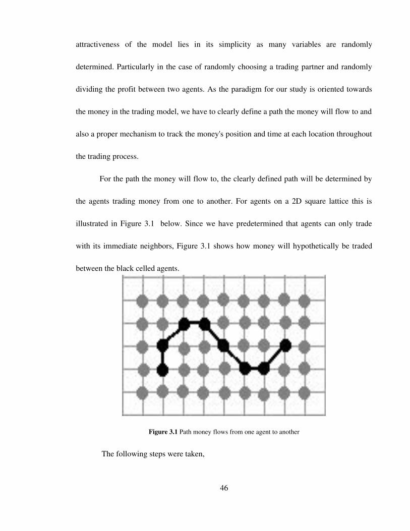
For the path the money will flow to, the clearly defined path will be determined by

the agents trading money from one to another. For agents on a 2D square lattice this is

illustrated in Figure 3.1   below.  Since we have predetermined that agents can only trade

with its immediate neighbors, Figure 3.1 shows how money will hypothetically be traded

between the black celled agents.

Figure 3.1 Path money flows from one agent to another

 The following steps were taken,

46

1. We  firstly  define  a   suitable   lattice  of   agents.  Since  our  goal   is   to  determine   if   the

displacement is scale free, our lattice must be at least 3 orders of magnitude in length.

The lattice size is simply our definition of the area populated by the agents. We have

thus chosen a lattice of 1700 by 10 agents. 

2. Once we have determined the lattice, we have to randomly choose an agent to perform a

trade.  This   agent   can   only   trade  with   its   nearest   neighbor.   The   definition  of   these

neighbors are dependent on where the agent is located. There are three locations which

determine who are the neighbors of an agent. These locations are the edges, the

corners of the main lattices. The code simulating this is presented in page 5 and 6 of

Appendix A.

After  two agents are chosen,   they will  perform a trade with each other.  For  the

original   Chakrabarti   trading   model,   the   trading   process   was   more   straightforward.   A

random fraction determined by an agents' saving propensity will deduct a fraction of money

from the original amount owned by that agent. The deducted fraction will then be tallied

with the other partner's deducted fraction and another random fraction will divide this tally

and add it to each agents current amount of money respectively.

Since we want to study the diffusion of money, we have to know its location and

time during each trade. In programming terms, this is accomplished by saving into an array

a money's  owners.  Thus as  the trading process goes on and money changes hands,   the

47

previous owners of a money will be noted and since we have defined the agents position as

the spatial variable we have knowledge of  the money's trajectory. Similarly after a trade,

the current iteration time will be saved into a array. Thus we currently have knowledge of

time between one trade and another which allows us to calculate the waiting time between

trades.

 The following steps were taken

1. We firstly   initialize a   fixed amount  of  money owned by each agent.  This  money  is

labeled numerically so that we can track the money's position and time. We initialize

each agent with 10 units of money. Thus the first agent is initialized with monies labeled

0 to 9, the second agent with monies 10 to 19 and so on. We will thus initialize 170000

monies in this simulation. The code simulating this is presented in page 2 of Appendix

A.

2. A count will firstly be performed on both agents to determine how much money each

agent has. We then define how much money is used to trade by each agent as the trading

volume.  This   is  accomplished by using the saving propensity  similar   to   the original

trading model. In [13] it was mentioned that a random or arbitrarily distributed saving

propensity produces a robust distribution of wealth. It is thus not dependent on choice of

initial parameters. The code simulating this is presented in page 7 of Appendix A.

3. We then draw a collection of random numbers which is limited by complement of the

48

saving propensity, which is the amount to be traded. Each of these random numbers are

distinct of each other.

4. Since the total number of random numbers drawn are determined by the total amount of

money owned, the random numbers not allocated for trading will be allocated for saving.

Each of these are also random numbers distinct of each other. The purpose of drawing

these random numbers is to introduce stochasticity in the choosing of monies for trading.

5. The chosen random numbers will determine which monies will be traded. They will be

used to call the monies originally initialized. These steps are presented in pages 8 to 9 of

Appendix A.

6. At the same time, an update of the time a trade occurred is performed. 

7. Finally the money labels owned by the agents are cleared and the new money labels as a

result of trading are reinitialized to each agent. The code simulating this is presented in

page 10 of Appendix A.

Now that  we have stated  the modifications  we have made  to   track  the money's

position   and   time   throughout   the   trading   process,   we   can   subsequently   determine   the

displacements of each money in the system after a given period of time and also the waiting

times   between   trades.   We   choose   to   run   the   simulation   over   4   billion   iterations   and

calculate the displacements over a 40 million iteration interval.  We assume that after 4

billion iterations we obtain stable observations of displacement length and waiting time and

49

they converge to stable distributions. To calculate the displacements, we have to know after

a certain period of time where the money currently is and what was it's original position.

We then make use of the determination of distance by applying the Pythagoras theorem.

 The following steps were taken,

1. We firstly determine the horizontal coordinate by simply multiplying the money labels

by 0.1 and apply the floor() function because each agent was originally initialized with

10  units   of   money.  For   example   if   an   agent   owns   the   money   labeled   211,   it   was

originally initialized to agent 21. 

2. The vertical coordinate is determined by how many deductions from the money label the

length of a row in the lattice of agents till it is less than the length. The code simulating

this is presented in page 11 of Appendix A.

The data that we obtain of the displacements has to be sorted into bins in order to

plot   a   distribution   of   displacement.   This   is   done   by   simply   conducting   a   census   of

frequency of a displacement over the entire displacement data. We then perform a measure

of mean square displacement over time which will be elaborated in the sections below.

After the simulation is completed, our next step is to obtain data that will allow us to plot

the waiting time distribution. This is done by simply finding the time difference between

successive jumps of money from one agent to another. This data will then be sorted into

bins in order to plot a distribution of waiting time. This is done by simply conducting a

50

census of frequency of a waiting time over the entire waiting time data. These steps are

presented in page 12 of Appendix A. 

3.2.2           Modified Yakovenko trading model   

We   would   now   attempt   to   confirm   that   the   underlying   structure   behind   the

Chakrabarti   trading   model,   in   particular   the   distributed   saving   propensities   plays   an

important   role   behind   the   anomalous  diffusion  of  money.  We  aim   to   achieve  this   by

performing   an   analysis   of   diffusion   of   money   in   the   Yakovenko   trading   model.   As

mentioned in the previous chapter, the resultant wealth distribution from the Yakovenko

trading   model   is   an   exponential   distribution   and   its   dynamics   is   unit   increments   and

decrements of money between two respective agents chosen randomly throughout the entire

simulation. As the dynamics and resultant wealth distribution differ from the Chakrabarti

trading model, a diffusion analysis which shows non­anomalous diffusion will show that

not all trading dynamics will result in anomalous diffusion. 

Similar   to   the   Chakrabarti   trading   model,   we   performed   modifications   on   the

Yakovenko trading model to allow proper calculations of spatial and temporal analysis of

money diffusion.  These  modifications  are  in  a  similar  method as  described above.  We

however elaborate on some distinctions below. 

The first distinction is the method of choosing random numbers used to call  the

51

initialized monies. Since we opt to trade one unit of money during a trade, we randomly

choose one money from both agents. The rest of the monies will be saved by the agents.

The code simulating this is presented in page 1 of Appendix B. The second distinction is

the dynamics. A winner and a loser will be chosen among the two agents. The winner will

gain a unit of money while the loser loses it. Both agents will then update the number of

monies it owns. This is show in page 2 of Appendix B. Calculation of   the pdf of jump

lengths, waiting times and mean squared displacement is similar to that of the previous

model. We also initialize 170000 units of money to 17000 agents over a 1700 by 10 lattice

of agents over a 6 million iterations simulation which is the amount of simulations before

equilibration   based   on   the   rules   we   have   initialized.   We   assume   that   after   6   million

iterations we obtain stable observations of displacement length and waiting time and they

converge to stable distributions.

3.2.3           Kinetic Economy trading model   

We   would   like   to   investigate   if   other   trading   models   would   also   allow   an

observation  of   anomalous  diffusion   in   its  movement   of  money.  We  adopt   the  Kinetic

Economy trading model which was designed by Wan Abdullah [18]. In this model, an array

of agents are initialized with an arbitrary number of money, goods and price of said goods.

Two agents are randomly chosen to trade where the agent with the higher priced goods

52

buys all that he can from the lower priced agent. The buying agent then changes the price of

his goods to the selling agents price. If the lower priced agent finds he has no more goods,

he buys all that he can from the higher priced agent. The selling agent then changes the

price of his goods to  the buying agents price.  This  trading model   is different from the

Chakrabarti trading model as it introduces goods and price fluctuations into the simulation.

Thus,  trading agents will   trade goods whose price will  be randomly initialized but will

fluctuate based on predefined rules which also means that the wealth is not conserved. This

will   allow an  analysis  of   the  movement  of  money   in   a  more   realistic   environment   in

comparison to the Chakrabarti trading model which is simply trading money. Nevertheless

spatial inhomogeneity that made the Chakrabarti trading model an attractive model to study

also exists in this trading model in the form of high prices causing a trapping of the goods

with an agent or agents unable to trade due to insufficient funds.

The model is simulated as follows :

1. Initialize money, goods and the price of a good to each agent.

2. Randomly choose two agents.

3. The agent with the higher price of goods buys all that he can of goods from the agent

with the lower price.

4. If the agent with the lower price has no more goods, he in turn will buy all that he can

from the agent with the higher price. He will then change his price to that of the agent

53

with the higher price.

5. If the agent with the lower price ends the trade still with goods, the agent with the higher

price will simply switch his price to the lower price.

6. For agents with the same price of goods, we randomly determine who will be the buying

agents and who will be the selling agents.

3.2.4           Modified Kinetic Economy trading model   

Similar to the Chakrabarti trading model, the Kinetic Economy trading model was

latticized to allow an analysis of anomalous diffusion. For this analysis, we will concentrate

on the spatial and temporal tracking of money instead of the other parameters. 

The modified trading model is simulated as below :

1. In   terms   of   choice   of   trading   partners,   agents   are   allowed   to   trade   only   with   its

neighbors. 

2. After randomly choosing two neighbors, a count of the amount of money and goods of

the two agents is performed. The count of money is similar to page 2 and 3 of Appendix

A. The count of goods is presented in the first part of page 1 Appendix C.

3. It will then be determined which agent will be the agent who sells and who buys from

the price's of goods. 

4. A count of how many goods will be bought from the seller based on the amount of

54

money owned by the buyer and the availability of goods from the seller is performed.

These are presented as the second part in page 1 Appendix C.

As  before,   the  monies   are   labeled  numerically   to   allow a   spatial   and   temporal

tracking. Thus, monies will be chosen randomly to be traded for the purchase of goods and

money moved from one agent to another will be tracked of it's new owner and time of trade

thus obtaining spatial and temporal data. This is carried out as follows:

1. The first  step  is   to determine which of  the buyers monies are going  to  be used for

purchasing goods. These monies are chosen randomly and are unique from one another.

The process that allows this to occur is the same as explained above.

2. Then these monies will be stacked to the sellers monies, while the buyer is initialized

with goods from the seller. Thus the buyers and sellers have a new amount of money and

goods respectively from the trade. These are presented in page 2 of Appendix C.

3. After a trade, if the seller has no more goods, he will then proceed to buy back all the

goods from the buyer. At this point, a choice of monies will be performed similar to that

mentioned above. If this occurs, the price of the seller will be changed to that of the

buyer.

4. If the above does not occur, the price of the buyer will be changed to that of the seller.

These are presented in page 3 of Appendix C.

55

Finally a calculation of the jump length and the waiting time will be performed as

described above. 

3.3            Statistical Analysis of Monte Carlo Data   

The Monte Carlo method is one of the main approaches to computer simulations in

statistical physics. Its goal is to provide a probabilistic description of a phenomena using

randomly   generated   numbers   as   the   analogy.  Errors   from   these   descriptions   can   be

estimated  and are   systematically   improvable  by  using  more   sample  configurations  and

larger systems.

We refer to the section on statistical errors in page 30 of [50] in this portion of our

work. If a quantity X is distributed by a Gaussian distribution with mean value  ⟨X ⟩  and

width  , n statistically independent observations of  X i has a mean given by

X=1n∑i=1

n

X i

with  a   standard  error  given  by   /n .   In  order   to   calculate   the  variance,   2 ,  we

consider the deviations  X i=X i−X  where

X 2=1n∑i=1

n

X i2= X 2− X 2

This gives the variance as   2=⟨X 2⟩−⟨X ⟩2 . The expectation value of this quantity is

56

given by   ⟨ X 2⟩=21−1/n .  Using this relation and the standard error relation,  we

obtain

error= X 2 /n−1=∑i=1

n X i2

n n−1

which is used for simple sampling Monte Carlo methods and applied to calculate errors in

this work. Importance sampling Monte Carlo methods which requires the consideration of

time correlations is not considered in the calculation of errors for this work.

3.4            Calculating mean squared displacement   

To determine if a diffusive process is undergoing normal or anomalous diffusion, a

method frequently used by experimentalists [38] is the mean squared displacement. The

determination is done by plotting the log of mean squared displacements versus time given

by 

⟨ x2⟩=t            (3.1)

and obtaining the slope of the plot if it is a straight line. As mentioned in (2.28) if we obtain

=1 , the diffusion is normal. Anomalous diffusion occurs for   1   and   1

named superdiffusive and subdiffusive respectively. 

To  perform  a  measurement   of   the  mean   squared  displacement  we   added   some

instructions   to   the code written  to calculate   the pdf  of  displacement.  After  the binning

57

process for the displacement is complete and we have obtained a pdf of displacement,  we

calculate the mean of the displacement using the formula

⟨ x ⟩=∑i=0

1000

x i P x i (3.2)

Thus we simply multiply each unit of displacement with the probability of obtaining it. The

next step is to calculate the mean squared displacement or the variance. 

      ⟨ x2⟩=1

106 ∑i=0

1000

x i−⟨ x ⟩2 (3.3)

This   is  calculated by subtracting each unit  of displacement  with  the mean,  squaring it,

summing the whole data set and normalizing it with the population size.

3.5            Power Law Analysis    

Measurable quantities usually have a typical scale, such as the heights of human

beings or I.Q's . There are however quantities which do not have a typical scale such as

city sizes [41], earthquakes [42] or wealth. The distributions of these quantities seem to be

right­skewed where there exist uncharacteristic and rarely occurring measurements.  These

distributions  are candidates   that   follow a power   law.  The pure  power   law distribution,

known as the zeta distribution or discrete Pareto distribution is expressed as

        p k =k−/ (3.4)

where k is the measured positive value,   is the power law exponent and   is the

58

Riemann­zeta function given by

           =∑k=1

∞

k− (3.5)

Other names associated with the power law is the Zipf's law [43], named after George Zipf

who claimed the shortest and most efficient words occurred more frequently.

As mentioned above,  distributions that are right skewed are good candidates for

power law distributions.  The most  common method to  present  these distributions  is  by

fitting it onto a log scale. This method however allows a noisy tail in the distribution due to

lack of samples in this region. One method proposed by [44] is to bin data in logarithmic

instead of linear sizes with each bin normalized to the size of its respective bin. Another

method to present these distributions is be plotting the cumulative distribution function.

This is basically a distribution which is stacked from the largest value to the second largest

value and so on till the end of the distribution, giving a cumulative probability distribution

of 1 at the end of the plot. The benefit of cumulative distributions are that there is less noise

at the end of the tail with outlier data not needing to be removed from this region. Fitting a

power law by using methods such as least squares regression on a log­log scale is biased

and inaccurate [46]. A quantitative measure of goodness of fit is needed to assess how well

data approximates to a power law distribution.  This enables identification of interesting

phenomena   that   cause   the   distribution   to   deviate   to   a   power   law.   In   some   cases   the

underlying process may not be generating power law distributed data but sampling error

59

will lead to an impersonification of the distribution. 

Consider the continuous power law distribution [45]

         p x =−1xmin

xxmin

−

  (3.6)

where   is the scaling parameter and  xmin  is the minimum value in a dataset of an

observed power­law region. Say we have a data set with n observations  x i≥xmin  that can

seemingly be fitted to a power law, we want to know the   that will generate that power

law. We thus introduce the likelihood given as

                 px∣=∏i=1

n −1xmin

x i

xmin−

(3.7)

which gives the probability that the data were drawn from the model. The scaling exponent

which gives the highest probability, effectively maximizing the function is the most likely

to generate the data set. Taking the logarithm of the likelihood we obtain

                           L=ln p x∣a=n ln −1−n ln xmin−∑i=1

n

ln x i / xmin (3.8)

Setting  ∂ L /∂=0 and solving for   we obtain the maximum likelihood estimate

=1n [∑i=1

n

ln x i / xmin]−1

(3.9)

We calculate the statistical error of the estimation as given in Section 3.3. We referred to

the description given in [51] to calculate the statistical error. 

60

There has to be an assessment of the goodness of fit of the parameter estimate of the

scaling exponent. This is because even data sampled from an exponential or log­normal

distribution can be fitted to a power law model. We thus define the Kolmogorov­Smirnov

test based on the following statistic, taken from [45]

D= maxx≥xmin

∣S x −P x ∣ (3.10)

where  S x  is the hypothesized cumulative distribution function and  P x  is the

empirical cumulative distribution function. We thus have to perform the  calculation above

returning a value that if suitably small is a possible fit for a power law. 

We thus introduce the p­value which calculates the probability that the data was

drawn from the hypothesized distribution based on the goodness of fit [21]. There is no

known formula for calculating the p­value but a Monte Carlo numerical calculation can be

performed. We include the code that calculates the p­value in Appendix D. The procedure

is to firstly generate a large number of synthetic data sets drawn from the hypothesized

power­law distribution.  This   is   done  by   randomly   choosing     an  arbitrarily  determined

number of data's from the hypothesized power law distribution data. The code simulating

this is presented in page 2 of Appendix D. The number of data sets that are obtained are

typically 100 units less than the sample. After this, we apply the bubble sort to ensure the

distribution is distributed ascendingly. The code simulating this is presented in page 2 of

Appendix D. Then we fit each data set to its own hypothesized power law distribution by

61

using the maximum likelihood estimation as elaborated above. The code simulating this is

presented   in   page   3   of   Appendix   D.   We   then   proceed   to   evaluate   the   probability

distribution   functions   based   on   the   estimated   exponent   and   subsequently   calculate   its

cumulative   distribution   functions.   The   code   simulating   this   is   presented   in   page   3   of

Appendix D. We finally calculate the Kolmogorov­Smirnov statistic. This is accomplished

by calculating the difference between the hypothetical and empirical data sets and sorting

the difference ascendingly. The top most value of each data set is the statistic. The code

simulating this is presented in page 4 of Appendix D. We then count the number of times

the statistic is larger than the statistic of the observed data. We then calculate the fraction of

this number over the total of number of synthetic data sets to finally obtain the p­value. If

this value is close to 1, the original data set may be drawn from a power­law. In [45] where

much  of   this   section   is   referred   to,   the   authors   have   chosen   to   rule   out   a   power­law

hypothesis if   p≤0.10 . The p­value becomes a more reliable test statistic if there is a

large data set because the  Kolmogorov­Smirnov statistic becomes smaller.

62

CHAPTER 4 : STUDY ON THE RELATION BETWEEN

DISTRIBUTIONS OF WEALTH AND DIFFUSION OF MONEY IN

VARIOUS TRADING MODELS 

In this chapter, we present the results of our analysis for the Chakrabarti trading

model   with   fixed   and   randomly   distributed   saving   propensity,   the   Yakovenko   trading

model and the Kinetic Economies trading model. For each trading model, we firstly present

its resultant distribution of wealth and perform a comparison with the nearest neighbors

trading modification of the trading model. We then obtain the pdf of displacement length of

money, p(r) and pdf of waiting time of money, p(t). We finally obtain the mean squared

displacement of money over time.

4.1            Chakrabarti trading model with random saving propensity   

4.1.1           Wealth distribution   

In Fig. 4.1 we obtain the cumulative distribution of agents over a spectrum of wealth

for the off lattice models. There is also the occurrence of the Boltzmann­Gibbs distribution

and long tail similar to that seen in empirical data as well as in the original Chakrabarti and

Chatterjee results [13]. We will use the wealth data in the long tail region to calculate the

power­law exponent  using  the maximum likelihood estimation,  given by (3.9),  and  the

63

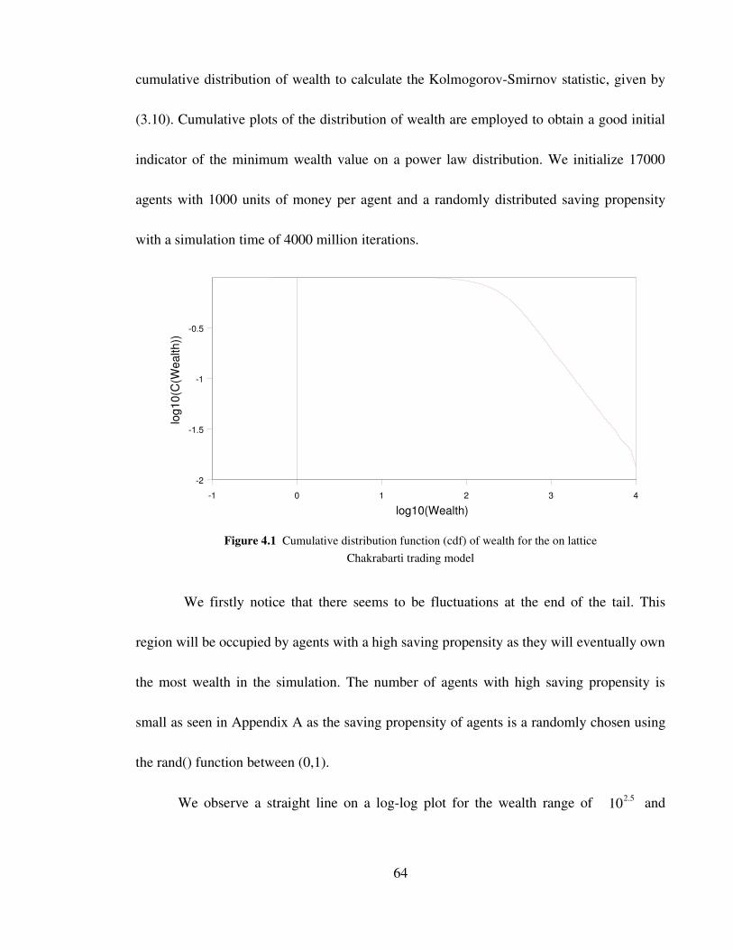
cumulative distribution of wealth to calculate the Kolmogorov­Smirnov statistic, given by

(3.10). Cumulative plots of the distribution of wealth are employed to obtain a good initial

indicator of the minimum wealth value on a power law distribution. We initialize 17000

agents with 1000 units of money per agent and a randomly distributed saving propensity

with a simulation time of 4000 million iterations.

  We firstly notice that there seems to be fluctuations at the end of the tail.  This

region will be occupied by agents with a high saving propensity as they will eventually own

the most wealth in the simulation. The number of agents with high saving propensity is

small as seen in Appendix A as the saving propensity of agents is a randomly chosen using

the rand() function between (0,1). 

We observe a straight line on a log­log plot for the wealth range of   102.5 and

64

Figure 4.1  Cumulative distribution function (cdf) of wealth for the on lattice Chakrabarti trading model

­1 0 1 2 3 4­2

­1.5

­1

­0.5

log10(Wealth)

log1

0(C(

Wea

lth))

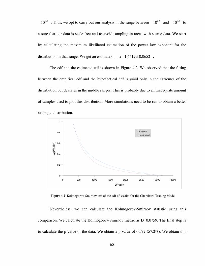
103.8 . Thus, we opt to carry out our analysis in the range between  102.5 and  103.5 to

assure that our data is scale free and to avoid sampling in areas with scarce data. We start

by  calculating   the  maximum  likelihood  estimation  of   the  power   law exponent   for   the

distribution in that range. We get an estimate of  =1.6419±0.0652 .

The cdf and the estimated cdf is shown in Figure 4.2. We observed that the fitting

between the empirical cdf and the hypothetical cdf is good only in the extremes of the

distribution but deviates in the middle ranges. This is probably due to an inadequate amount

of samples used to plot this distribution. More simulations need to be run to obtain a better

averaged distribution.

Nevertheless,   we   can   calculate   the   Kolmogorov­Smirnov   statistic   using   this

comparison. We calculate the Kolmogorov­Smirnov metric as D=0.0759. The final step is

to calculate the p­value of the data. We obtain a p­value of 0.572 (57.2%). We obtain this

65

Figure 4.2  Kolmogorov­Smirnov test of the cdf of wealth for the Charabarti Trading Model

0 500 1000 1500 2000 2500 3000 35000

0.2

0.4

0.6

0.8

1

EmpiricalHypothetical

Wealth

C(W

ealth

)

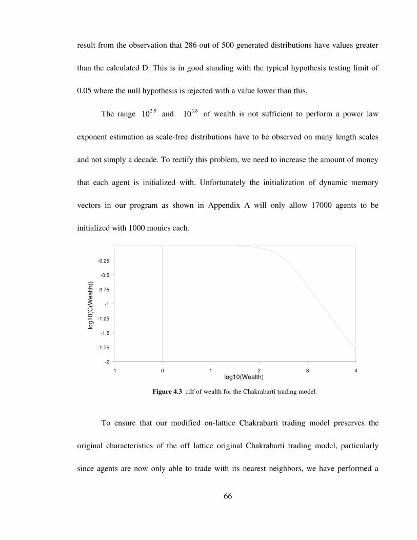
result from the observation that 286 out of 500 generated distributions have values greater

than the calculated D. This is in good standing with the typical hypothesis testing limit of

0.05 where the null hypothesis is rejected with a value lower than this.

The range 102.5 and   103.8 of wealth  is not sufficient to perform a power law

exponent estimation as scale­free distributions have to be observed on many length scales

and not simply a decade. To rectify this problem, we need to increase the amount of money

that  each  agent   is   initialized  with.  Unfortunately   the   initialization  of  dynamic  memory

vectors   in  our  program as   shown  in  Appendix  A will  only  allow 17000 agents   to  be

initialized with 1000 monies each.  

To   ensure   that  our  modified  on­lattice  Chakrabarti   trading  model   preserves   the

original characteristics of  the off  lattice original Chakrabarti   trading model,  particularly

since agents are now only able to trade with its nearest neighbors, we have performed a

66

­1 0 1 2 3 4­2

­1.75

­1.5

­1.25

­1

­0.75

­0.5

­0.25

log10(Wealth)

log1

0(C(

Wea

lth))

Figure 4.3  cdf of wealth for the Chakrabarti trading model

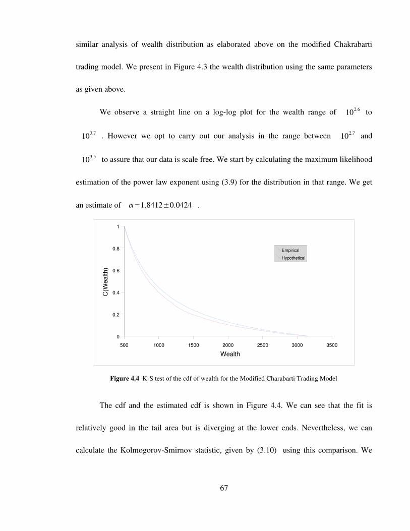
similar  analysis  of wealth distribution as elaborated above on the modified Chakrabarti

trading model. We present in Figure 4.3 the wealth distribution using the same parameters

as given above.     

We observe  a   straight   line  on  a   log­log plot   for   the wealth   range of   102.6 to

103.7 .  However  we  opt   to   carry  out   our   analysis   in   the   range  between   102.7 and

103.5 to assure that our data is scale free. We start by calculating the maximum likelihood

estimation of the power law exponent using (3.9) for the distribution in that range. We get

an estimate of  =1.8412±0.0424 .

The cdf and the estimated cdf is shown in Figure 4.4. We can see that the fit is

relatively good in the tail area but is diverging at the lower ends. Nevertheless, we can

calculate the Kolmogorov­Smirnov statistic, given by (3.10)   using this comparison. We

67

500 1000 1500 2000 2500 3000 35000

0.2

0.4

0.6

0.8

1

EmpiricalHypothetical

Wealth

C(W

ealth

)

Figure 4.4  K­S test of the cdf of wealth for the Modified Charabarti Trading Model

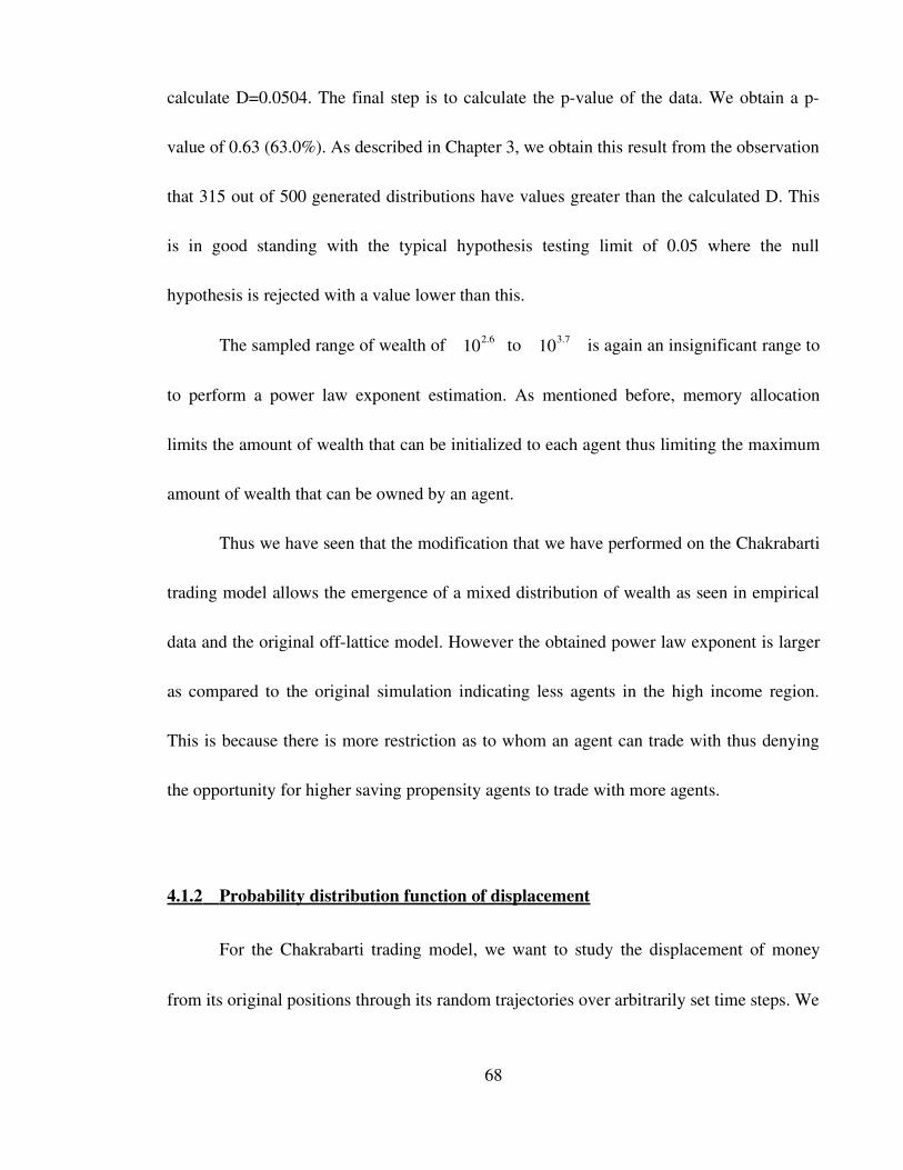
calculate D=0.0504. The final step is to calculate the p­value of the data. We obtain a p­

value of 0.63 (63.0%). As described in Chapter 3, we obtain this result from the observation

that 315 out of 500 generated distributions have values greater than the calculated D. This

is   in   good   standing   with   the   typical   hypothesis   testing   limit   of   0.05   where   the   null

hypothesis is rejected with a value lower than this. 

The sampled range of wealth of  102.6 to  103.7  is again an insignificant range to

to perform a power   law exponent  estimation.  As mentioned before,  memory allocation

limits the amount of wealth that can be initialized to each agent thus limiting the maximum

amount of wealth that can be owned by an agent. 

Thus we have seen that the modification that we have performed on the Chakrabarti

trading model allows the emergence of a mixed distribution of wealth as seen in empirical

data and the original off­lattice model. However the obtained power law exponent is larger

as compared to the original simulation indicating less agents in the high income region.

This is because there is more restriction as to whom an agent can trade with thus denying

the opportunity for higher saving propensity agents to trade with more agents.

4.1.2           Probability distribution function of displacement   

For the Chakrabarti trading model, we want to study  the displacement of money

from its original positions through its random trajectories over arbitrarily set time steps. We

68

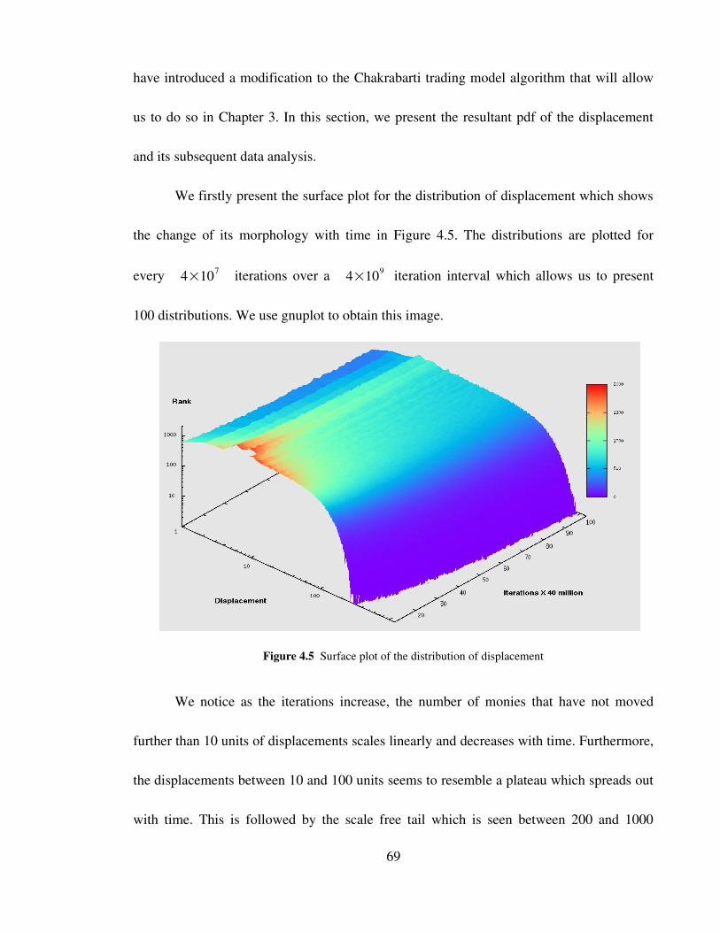
have introduced a modification to the Chakrabarti trading model algorithm that will allow

us to do so in Chapter 3. In this section, we present the resultant pdf of the displacement

and its subsequent data analysis.

We firstly present the surface plot for the distribution of displacement which shows

the change of  its  morphology with time in Figure 4.5. The distributions are plotted for

every   4×107   iterations over a   4×109 iteration interval which allows us to present

100 distributions. We use gnuplot to obtain this image. 

We notice as the iterations increase, the number of monies that have not moved

further than 10 units of displacements scales linearly and decreases with time. Furthermore,

the displacements between 10 and 100 units seems to resemble a plateau which spreads out

with time. This  is followed by the scale free tail  which is seen between 200 and 1000

69

Figure 4.5  Surface plot of the distribution of displacement

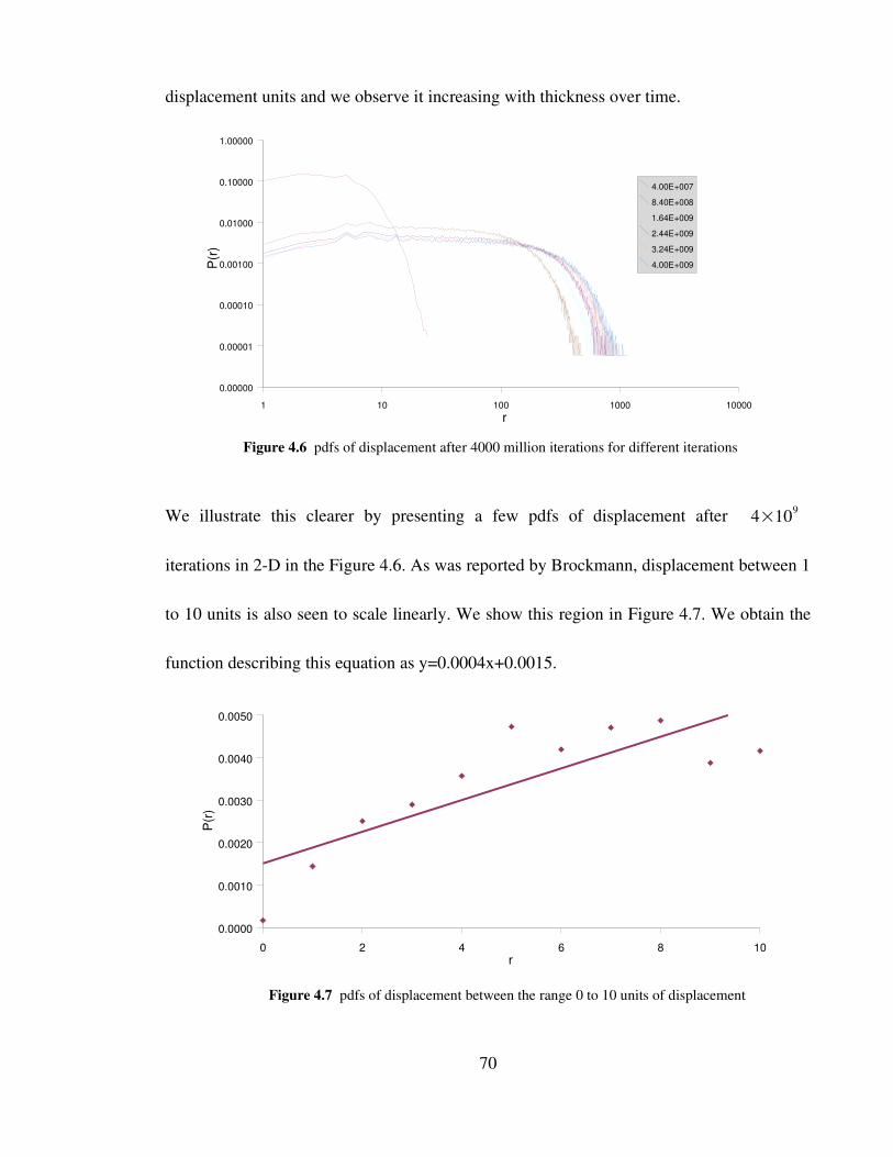
displacement units and we observe it increasing with thickness over time. 

We   illustrate   this   clearer   by   presenting   a   few   pdfs   of   displacement   after   4×109

iterations in 2­D in the Figure 4.6. As was reported by Brockmann, displacement between 1

to 10 units is also seen to scale linearly. We show this region in Figure 4.7. We obtain the

function describing this equation as y=0.0004x+0.0015.

70

Figure 4.6  pdfs of displacement after 4000 million iterations for different iterations

0 2 4 6 8 100.0000

0.0010

0.0020

0.0030

0.0040

0.0050

r

P(r)

Figure 4.7  pdfs of displacement between the range 0 to 10 units of displacement

1 10 100 1000 100000.00000

0.00001

0.00010

0.00100

0.01000

0.10000

1.00000

4.00E+0078.40E+0081.64E+0092.44E+0093.24E+0094.00E+009

r

P(r)

This means there is an exponential growth in displacement during this range. Brockmann

however did not report of a plateau as seen in displacements between 10 to 200 units. We

propose that these displacements are due to monies being in the vicinity of agents with a

high saving propensity. Thus, these agents will hold onto monies for longer periods of time.

We propose that this observation was not seen by Brockmann because displacements that

were reported in wheresgeorge.com are of significant distance.

Now that we have observed the change of the pdf of displacement with time, we

want to perform a power law analysis to allow us to obtain the scaling exponent    as

mentioned in Chapter 2. We firstly present the region of the pdf of displacement which we

propose has scale free behavior in the Figure 4.8.

We opt to sample 465 data points between 200 and 631 units of displacement as the scale

71

Figure 4.8  pdf of displacement between 200 and 631 units of displacement 

2.3 2.4 2.5 2.6 2.7 2.8 2.9­4.5

­4

­3.5

­3

log10(r)

log1

0(P(

r))

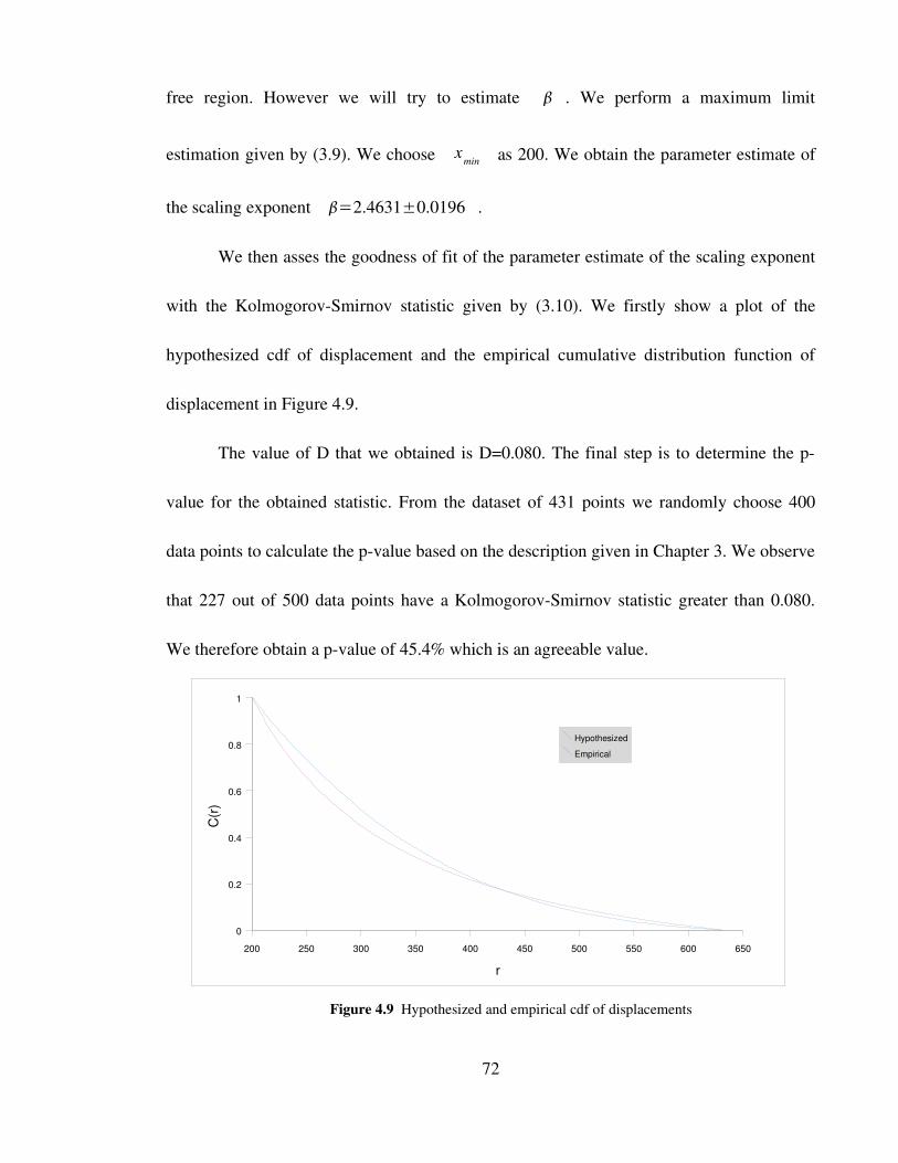
free   region.   However   we   will   try   to   estimate   .   We   perform   a   maximum   limit

estimation given by (3.9). We choose  xmin  as 200. We obtain the parameter estimate of

the scaling exponent  =2.4631±0.0196 . 

We then asses the goodness of fit of the parameter estimate of the scaling exponent

with   the  Kolmogorov­Smirnov  statistic  given  by   (3.10).  We firstly   show a  plot  of   the

hypothesized cdf  of  displacement  and  the  empirical  cumulative distribution  function of

displacement in Figure 4.9. 

The value of D that we obtained is D=0.080. The final step is to determine the p­

value for the obtained statistic. From the dataset of 431 points we randomly choose 400

data points to calculate the p­value based on the description given in Chapter 3. We observe

that 227 out of 500 data points have a Kolmogorov­Smirnov statistic greater than 0.080.

We therefore obtain a p­value of 45.4% which is an agreeable value.   

72

Figure 4.9  Hypothesized and empirical cdf of displacements

200 250 300 350 400 450 500 550 600 6500

0.2

0.4

0.6

0.8

1

HypothesizedEmpirical

r

C(r)

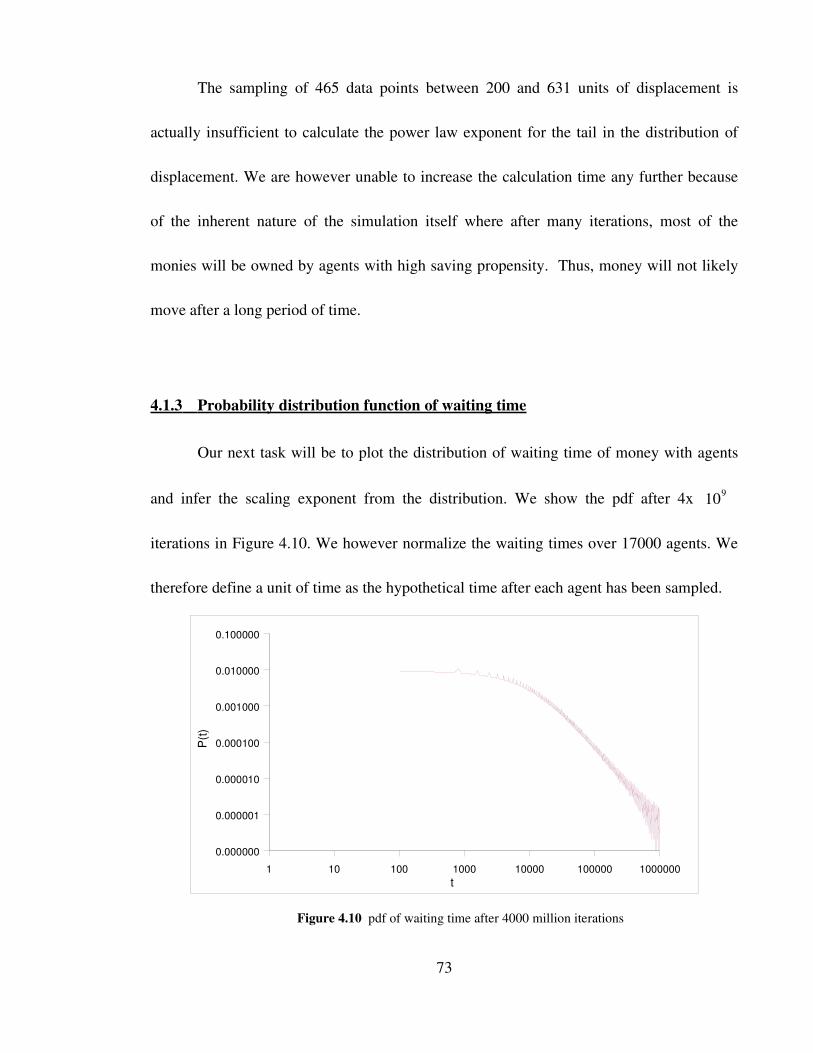
The sampling of  465 data  points  between 200 and 631 units  of  displacement   is

actually insufficient to calculate the power law exponent for the tail in the distribution of

displacement. We are however unable to increase the calculation time any further because

of  the  inherent  nature  of  the simulation  itself  where after  many  iterations,  most  of   the

monies will be owned by agents with high saving propensity.  Thus, money will not likely

move after a long period of time.

4.1.3           Probability distribution function of waiting time   

Our next task will be to plot the distribution of waiting time of money with agents

and  infer   the  scaling  exponent   from  the  distribution.  We show  the  pdf  after  4x 109

iterations in Figure 4.10. We however normalize the waiting times over 17000 agents. We

therefore define a unit of time as the hypothetical time after each agent has been sampled.

73

Figure 4.10  pdf of waiting time after 4000 million iterations

1 10 100 1000 10000 100000 10000000.000000

0.000001

0.000010

0.000100

0.001000

0.010000

0.100000

t

P(t)

We firstly observe the existence of ripples on the distribution. This is actually due to the

statistical  nature of  the random number generation which have a  tendency to bias  their

choice of  numbers.   If  we were   to   repeat   the  experiment  with  a   fairer   random number

generator, the Mersenne Twister random number generator for example [52] the ripples

will  be   less  obvious.  We observe   that  half   the  portion  of  observations  occurred  under

104  iterations. There are however cases where monies have to wait longer than  104

iterations and we hypothesize scale free behavior occurring in this region between  104

and  106  iterations. 

Our next  step  is   to  perform a power  law analysis  on  the scale   free region.  We

present   the   region   in  Figure  4.11.  The   first   step   is   to  perform a  maximum  likelihood

estimation of the scaling exponent (3.9) .    We choose   xmin   as 4 in this case and the

sample size is 900 data points. We obtain the parameter estimate of the scaling exponent as

74

Figure 4.11  pdf of waiting time between 10000 and 100000 iterations 

3.8 4 4.2 4.4 4.6 4.8 5­4.5

­4

­3.5

­3

­2.5

log10(t)

log1

0(P(

t))

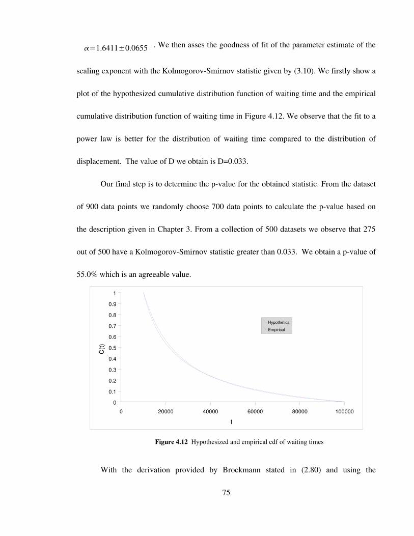
=1.6411±0.0655 . We then asses the goodness of fit of the parameter estimate of the

scaling exponent with the Kolmogorov­Smirnov statistic given by (3.10). We firstly show a

plot of the hypothesized cumulative distribution function of waiting time and the empirical

cumulative distribution function of waiting time in Figure 4.12. We observe that the fit to a

power law is better for the distribution of waiting time compared to  the distribution of

displacement.  The value of D we obtain is D=0.033.

Our final step is to determine the p­value for the obtained statistic. From the dataset

of 900 data points we randomly choose 700 data points to calculate the p­value based on

the description given in Chapter 3. From a collection of 500 datasets we observe that 275

out of 500 have a Kolmogorov­Smirnov statistic greater than 0.033.  We obtain a p­value of

55.0% which is an agreeable value.

  With   the   derivation   provided   by   Brockmann   stated   in   (2.80)   and   using   the

75

Figure 4.12  Hypothesized and empirical cdf of waiting times

0 20000 40000 60000 80000 1000000

0.1

0.2

0.3

0.4

0.5

0.6

0.7

0.8

0.9

1

HypotheticalEmpirical

t

C(t)

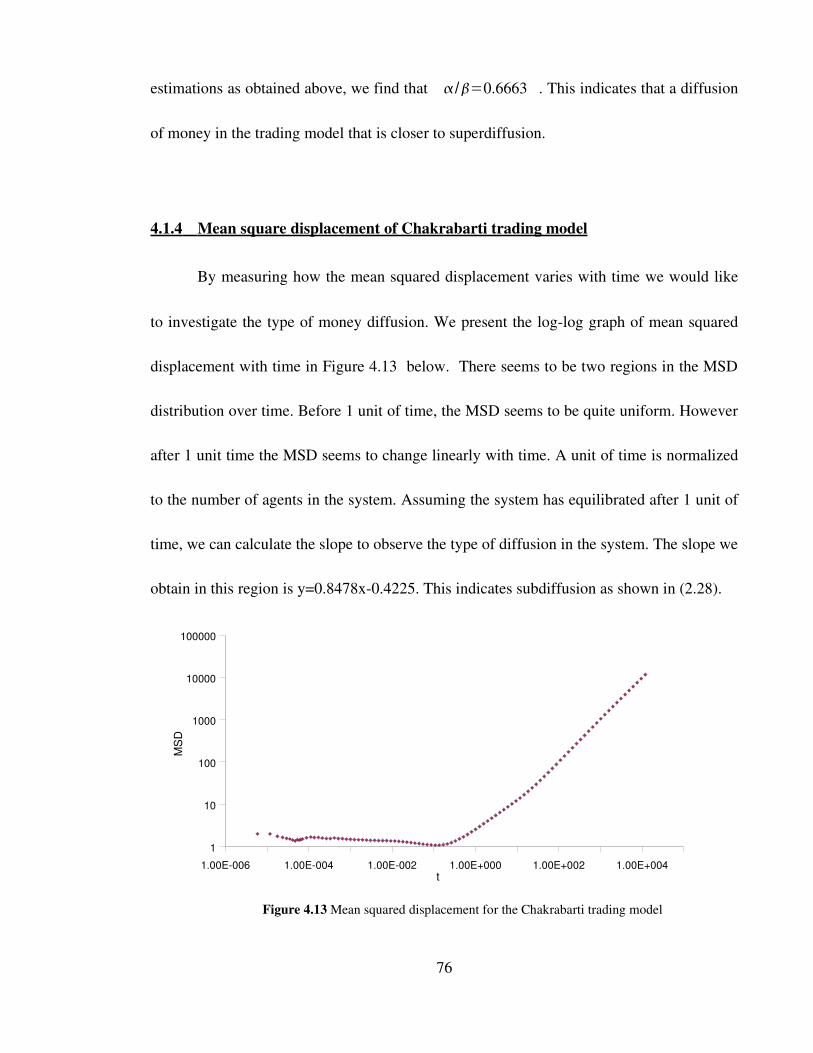
estimations as obtained above, we find that  /=0.6663 . This indicates that a diffusion

of money in the trading model that is closer to superdiffusion.

4.1.4           Mean square displacement of Chakrabarti trading model   

By measuring how the mean squared displacement varies with time we would like

to investigate the type of money diffusion. We present the log­log graph of mean squared

displacement with time in Figure 4.13  below.  There seems to be two regions in the MSD

distribution over time. Before 1 unit of time, the MSD seems to be quite uniform. However

after 1 unit time the MSD seems to change linearly with time. A unit of time is normalized

to the number of agents in the system. Assuming the system has equilibrated after 1 unit of

time, we can calculate the slope to observe the type of diffusion in the system. The slope we

obtain in this region is y=0.8478x­0.4225. This indicates subdiffusion as shown in (2.28).  

76

Figure 4.13 Mean squared displacement for the Chakrabarti trading model

1.00E­006 1.00E­004 1.00E­002 1.00E+000 1.00E+002 1.00E+0041

10

100

1000

10000

100000

t

MSD

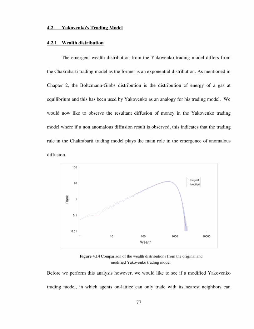
4.2            Yakovenko's Trading Model   

4.2.1           Wealth distribution   

The emergent wealth distribution from the Yakovenko trading model differs from

the Chakrabarti trading model as the former is an exponential distribution. As mentioned in

Chapter   2,  the  Boltzmann­Gibbs   distribution   is   the   distribution   of   energy   of   a   gas   at

equilibrium and this has been used by Yakovenko as an analogy for his trading model.  We

would now like   to  observe  the  resultant  diffusion  of  money  in   the Yakovenko  trading

model where if a non anomalous diffusion result is observed, this indicates that the trading

rule in the Chakrabarti trading model plays the main role in the emergence of anomalous

diffusion. 

Before we perform this analysis however, we would like to see if a modified Yakovenko

trading model,   in which agents on­lattice can only trade with its  nearest  neighbors can

77

1 10 100 1000 100000.01

0.1

1

10

100

OriginalModified

Wealth

Rank

Figure 4.14 Comparison of the wealth distributions from the original and modified Yakovenko trading model 

reproduce   the   Boltzmann­Gibbs   wealth   distribution   similar   to   the   original   Yakovenko

trading model. We initialize 17000 agents with a randomly set amount of money between

(1­1000) per agent over 100 million iterations. We present the distributions of wealth in

Figure 4.14.  We observe on a log­log plot the two distributions only differ slightly in the

lower income region where the distribution is a bit fatter for the lower income region. This

means that the rate of equilibration is slower in the modified trading model. However we

are still  able  to observe a similar wealth distribution as  the original model.  We do not

present the cumulative distribution of wealth in this study because we are unable to see a

clear difference between the original and modified distributions of wealth. 

4.2.2           Probability  distribution   function  of  displacement   length  and  mean   squared   

displacement

We would now like to perform an analysis of anomalous diffusion for the modified

Yakovenko's trading model to compare with Chakrabarti's trading model. We initialized

17000 agents with 10 units of money and the simulation program is ran over 5 million

iterations. We are unable to run the simulation over a longer period of time than this and we

propose the reason below. We firstly obtain the data for jump lengths and present it  in

Figure 4.15 and 4.16. 

78

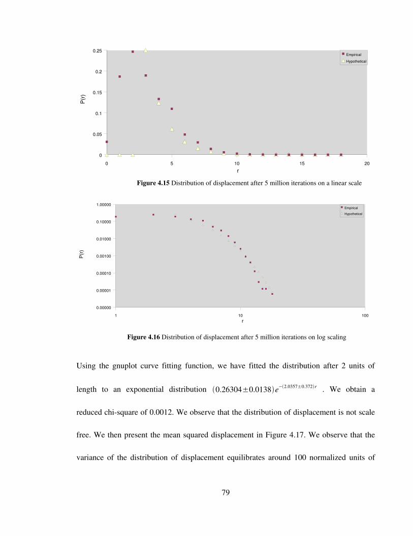
Using the gnuplot curve fitting function, we have fitted the distribution after 2 units of

length   to   an   exponential   distribution 0.26304±0.0138e−2.0357±0.372r .   We   obtain   a

reduced chi­square of 0.0012. We observe that the distribution of displacement is not scale

free. We then present the mean squared displacement in Figure 4.17. We observe that the

variance of the distribution of displacement equilibrates around 100 normalized units of

79

Figure 4.16 Distribution of displacement after 5 million iterations on log scaling

Figure 4.15 Distribution of displacement after 5 million iterations on a linear scale

0 5 10 15 200

0.05

0.1

0.15

0.2

0.25EmpiricalHypothetical

r

P(r)

1 10 100

0.00000

0.00001

0.00010

0.00100

0.01000

0.10000

1.00000EmpiricalHypothetical

r

P(r)

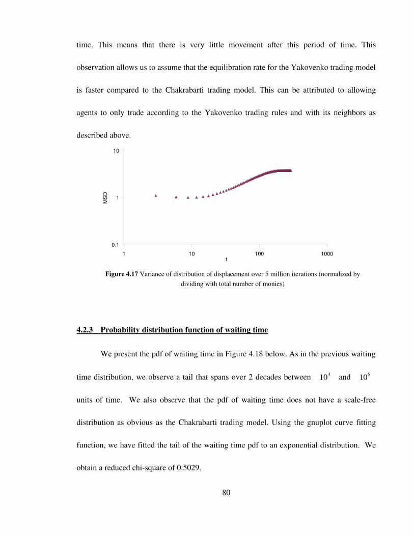
time.   This   means   that   there   is   very   little   movement   after   this   period   of   time.   This

observation allows us to assume that the equilibration rate for the Yakovenko trading model

is faster compared to  the Chakrabarti  trading model. This can be attributed to allowing

agents to only trade according to the Yakovenko trading rules and with its neighbors as

described above. 

4.2.3           Probability distribution function of waiting time   

We present the pdf of waiting time in Figure 4.18 below. As in the previous waiting

time distribution, we observe a tail that spans over 2 decades between  104  and  106

units of time.   We also observe that the pdf of waiting time does not have a scale­free

distribution as obvious as the Chakrabarti trading model. Using the gnuplot curve fitting

function, we have fitted the tail of the waiting time pdf to an exponential distribution.  We

obtain a reduced chi­square of 0.5029.

80

Figure 4.17 Variance of distribution of displacement over 5 million iterations (normalized bydividing with total number of monies)

1 10 100 10000.1

1

10

t

MSD

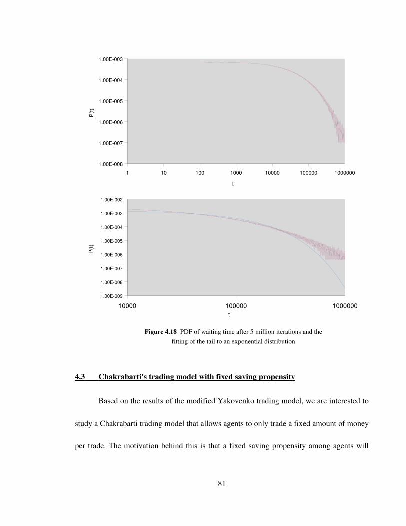
4.3            Chakrabarti's trading model with fixed saving propensity   

Based on the results of the modified Yakovenko trading model, we are interested to

study a Chakrabarti trading model that allows agents to only trade a fixed amount of money

per trade. The motivation behind this is that a fixed saving propensity among agents will

81

Figure 4.18  PDF of waiting time after 5 million iterations and thefitting of the tail to an exponential distribution

10000 100000 10000001.00E­009

1.00E­008

1.00E­007

1.00E­006

1.00E­005

1.00E­004

1.00E­003

1.00E­002

t

P(t)

1 10 100 1000 10000 100000 10000001.00E­008

1.00E­007

1.00E­006

1.00E­005

1.00E­004

1.00E­003

t

P(t)

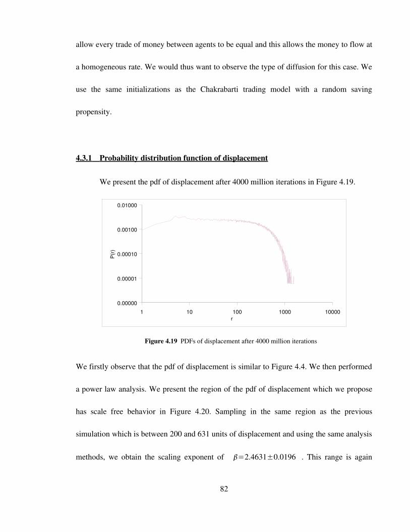
allow every trade of money between agents to be equal and this allows the money to flow at

a homogeneous rate. We would thus want to observe the type of diffusion for this case. We

use   the   same   initializations   as   the   Chakrabarti   trading   model   with   a   random   saving

propensity.

4.3.1           Probability distribution function of displacement   

We present the pdf of displacement after 4000 million iterations in Figure 4.19. 

We firstly observe that the pdf of displacement is similar to Figure 4.4. We then performed

a power law analysis. We present the region of the pdf of displacement which we propose

has   scale   free  behavior   in   Figure  4.20.  Sampling   in   the   same   region   as   the  previous

simulation which is between 200 and 631 units of displacement and using the same analysis

methods,  we obtain the scaling exponent of   =2.4631±0.0196 . This range is  again

82

1 10 100 1000 100000.00000

0.00001

0.00010

0.00100

0.01000

r

P(r)

Figure 4.19  PDFs of displacement after 4000 million iterations

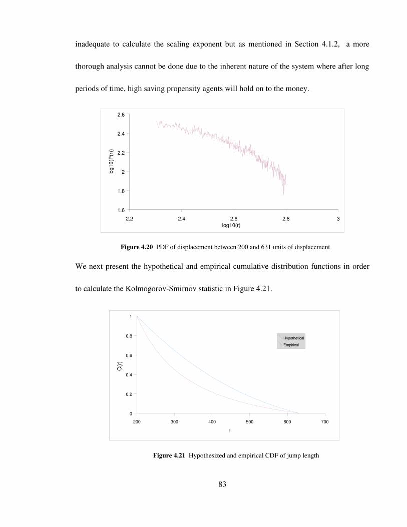
inadequate to calculate the scaling exponent but as mentioned in Section 4.1.2,   a more

thorough analysis cannot be done due to the inherent nature of the system where after long

periods of time, high saving propensity agents will hold on to the money.

We next present the hypothetical and empirical cumulative distribution functions in order

to calculate the Kolmogorov­Smirnov statistic in Figure 4.21. 

83

200 300 400 500 600 7000

0.2

0.4

0.6

0.8

1

HypotheticalEmpirical

r

C(r)

2.2 2.4 2.6 2.8 31.6

1.8

2

2.2

2.4

2.6

log10(r)

log1

0(P(

r))

Figure 4.20  PDF of displacement between 200 and 631 units of displacement 

Figure 4.21  Hypothesized and empirical CDF of jump length

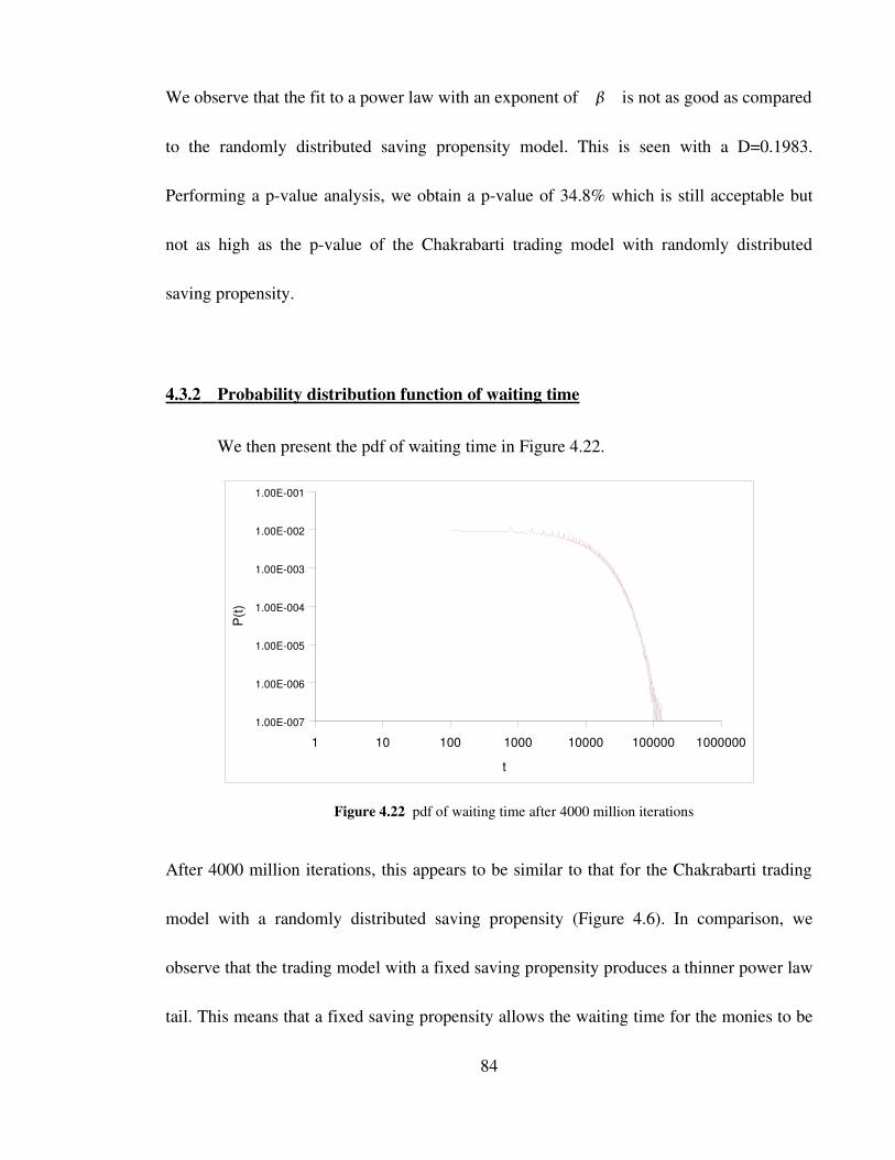
We observe that the fit to a power law with an exponent of   is not as good as compared

to   the   randomly   distributed   saving   propensity   model.   This   is   seen   with   a   D=0.1983.

Performing a p­value analysis, we obtain a p­value of 34.8% which is still acceptable but

not  as  high  as  the p­value of   the Chakrabarti   trading model  with randomly distributed

saving propensity. 

4.3.2           Probability distribution function of waiting time   

We then present the pdf of waiting time in Figure 4.22. 

After 4000 million iterations, this appears to be similar to that for the Chakrabarti trading

model  with   a   randomly  distributed   saving  propensity   (Figure  4.6).   In   comparison,  we

observe that the trading model with a fixed saving propensity produces a thinner power law

tail. This means that a fixed saving propensity allows the waiting time for the monies to be

84

1 10 100 1000 10000 100000 10000001.00E­007

1.00E­006

1.00E­005

1.00E­004

1.00E­003

1.00E­002

1.00E­001

t

P(t)

Figure 4.22  pdf of waiting time after 4000 million iterations

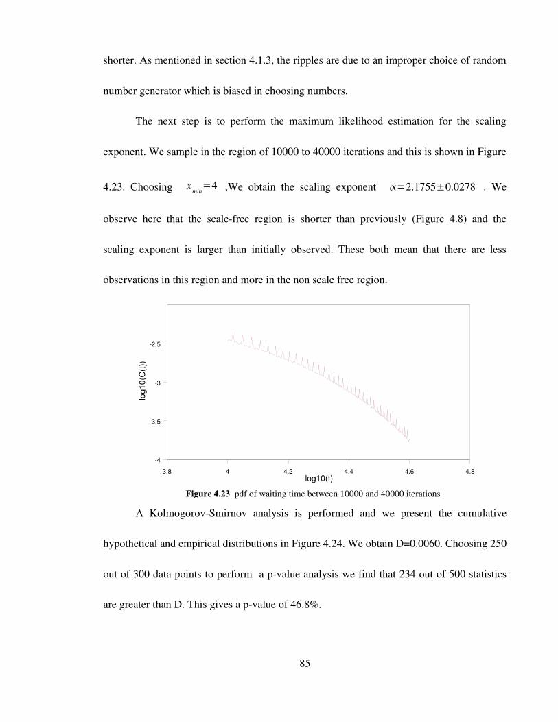
shorter. As mentioned in section 4.1.3, the ripples are due to an improper choice of random

number generator which is biased in choosing numbers. 

The next   step  is   to  perform  the maximum likelihood estimation   for   the scaling

exponent. We sample in the region of 10000 to 40000 iterations and this is shown in Figure

4.23.  Choosing   xmin=4 ,We obtain   the   scaling   exponent   =2.1755±0.0278 .  We

observe  here   that   the   scale­free   region   is   shorter   than  previously   (Figure  4.8)   and   the

scaling  exponent   is   larger   than   initially  observed.  These  both  mean  that   there  are   less

observations in this region and more in the non scale free region. 

A   Kolmogorov­Smirnov   analysis   is   performed   and   we   present   the   cumulative

hypothetical and empirical distributions in Figure 4.24. We obtain D=0.0060. Choosing 250

out of 300 data points to perform  a p­value analysis we find that 234 out of 500 statistics

are greater than D. This gives a p­value of 46.8%.  

85

Figure 4.23  pdf of waiting time between 10000 and 40000 iterations 

3.8 4 4.2 4.4 4.6 4.8­4

­3.5

­3

­2.5

log10(t)

log1

0(C(

t))

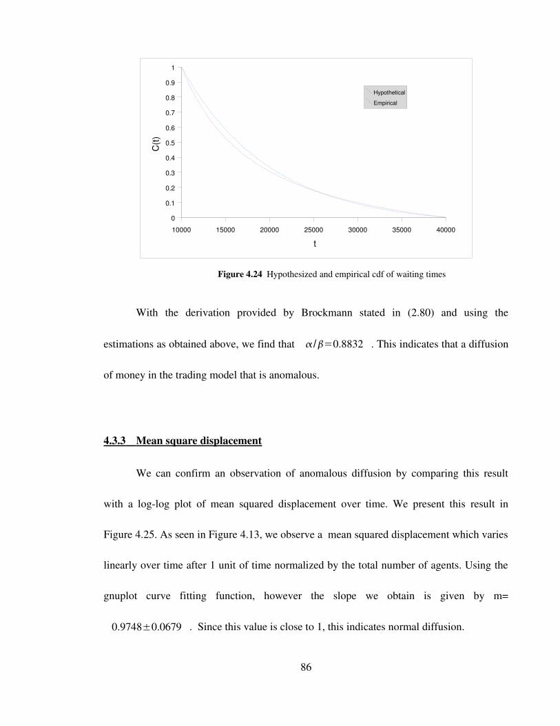
With   the   derivation   provided   by   Brockmann   stated   in   (2.80)   and   using   the

estimations as obtained above, we find that  /=0.8832 . This indicates that a diffusion

of money in the trading model that is anomalous.

4.3.3           Mean square displacement   

We can confirm an observation of anomalous diffusion by comparing this result

with a  log­log plot  of mean squared displacement  over   time.  We present   this   result   in

Figure 4.25. As seen in Figure 4.13, we observe a  mean squared displacement which varies

linearly over time after 1 unit of time normalized by the total number of agents. Using the

gnuplot   curve   fitting   function,  however   the   slope   we   obtain   is   given   by   m=

0.9748±0.0679 .  Since this value is close to 1, this indicates normal diffusion.

86

Figure 4.24  Hypothesized and empirical cdf of waiting times

10000 15000 20000 25000 30000 35000 400000

0.1

0.2

0.3

0.4

0.5

0.6

0.7

0.8

0.9

1

HypotheticalEmpirical

t

C(t)

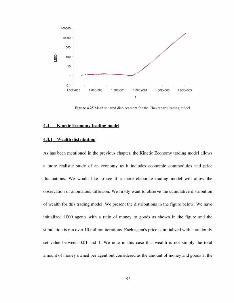
4.4            Kinetic Economy trading model   

4.4.1           Wealth distribution   

As has been mentioned in the previous chapter, the Kinetic Economy trading model allows

a  more   realistic   study  of   an   economy as   it   includes   economic   commodities   and  price

fluctuations.   We   would   like   to   see   if   a   more   elaborate   trading   model   will   allow   the

observation of anomalous diffusion. We firstly want to observe the cumulative distribution

of wealth for this trading model. We present the distributions in the figure below. We have

initialized 1000 agents with a  ratio of money  to  goods as shown in the figure and  the

simulation is ran over 10 million iterations. Each agent's price is initialized with a randomly

set  value between 0.01 and 1.  We note  in   this  case that wealth  is  not simply the total

amount of money owned per agent but considered as the amount of money and goods at the

87

Figure 4.25 Mean squared displacement for the Chakrabarti trading model

1.00E­005 1.00E­003 1.00E­001 1.00E+001 1.00E+003 1.00E+0050.1

1

10

100

1000

10000

100000

t

MSD

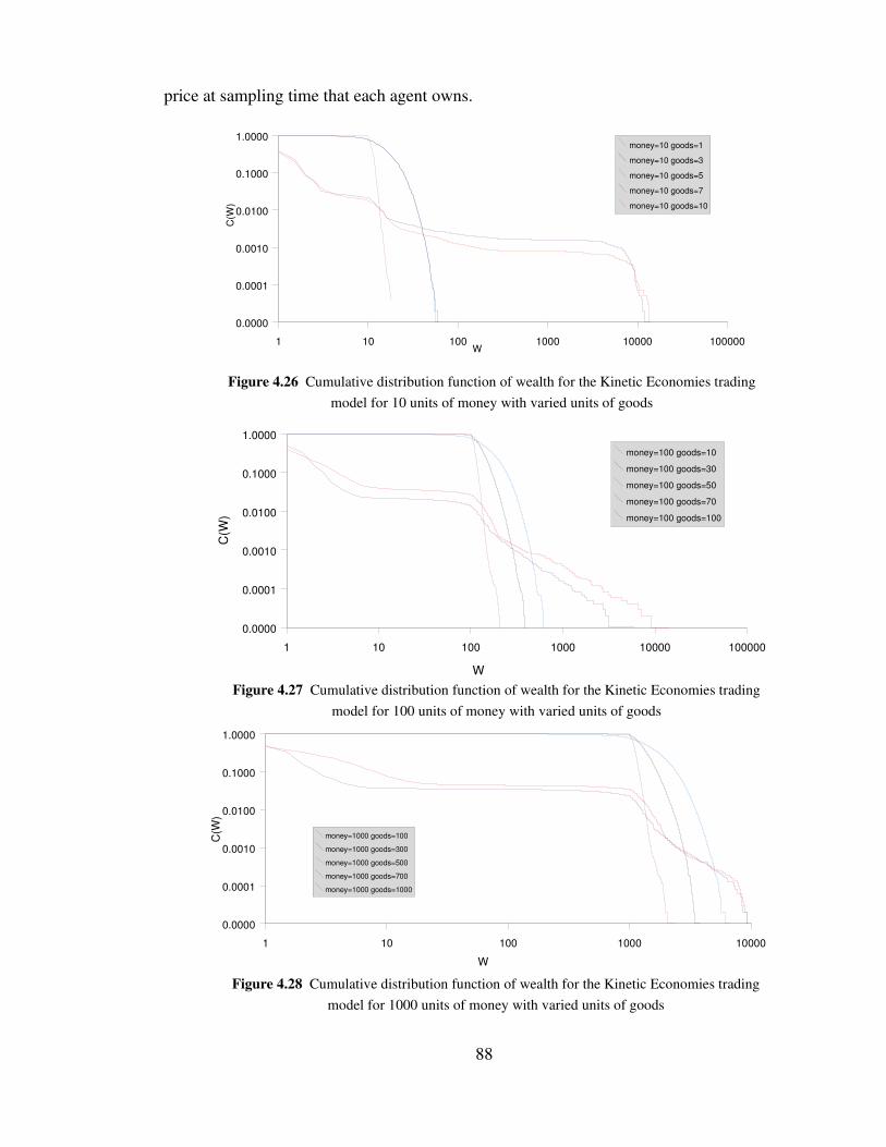
price at sampling time that each agent owns.  

88

1 10 100 1000 10000 1000000.0000

0.0001

0.0010

0.0100

0.1000

1.0000money=100 goods=10money=100 goods=30money=100 goods=50money=100 goods=70money=100 goods=100

W

C(W

)

1 10 100 1000 100000.0000

0.0001

0.0010

0.0100

0.1000

1.0000

money=1000 goods=100money=1000 goods=300money=1000 goods=500money=1000 goods=700money=1000 goods=1000

W

C(W

)

Figure 4.26  Cumulative distribution function of wealth for the Kinetic Economies trading model for 10 units of money with varied units of goods

Figure 4.27  Cumulative distribution function of wealth for the Kinetic Economies trading model for 100 units of money with varied units of goods

Figure 4.28  Cumulative distribution function of wealth for the Kinetic Economies trading model for 1000 units of money with varied units of goods

1 10 100 1000 10000 1000000.0000

0.0001

0.0010

0.0100

0.1000

1.0000money=10 goods=1money=10 goods=3money=10 goods=5money=10 goods=7money=10 goods=10

W

C(W

)

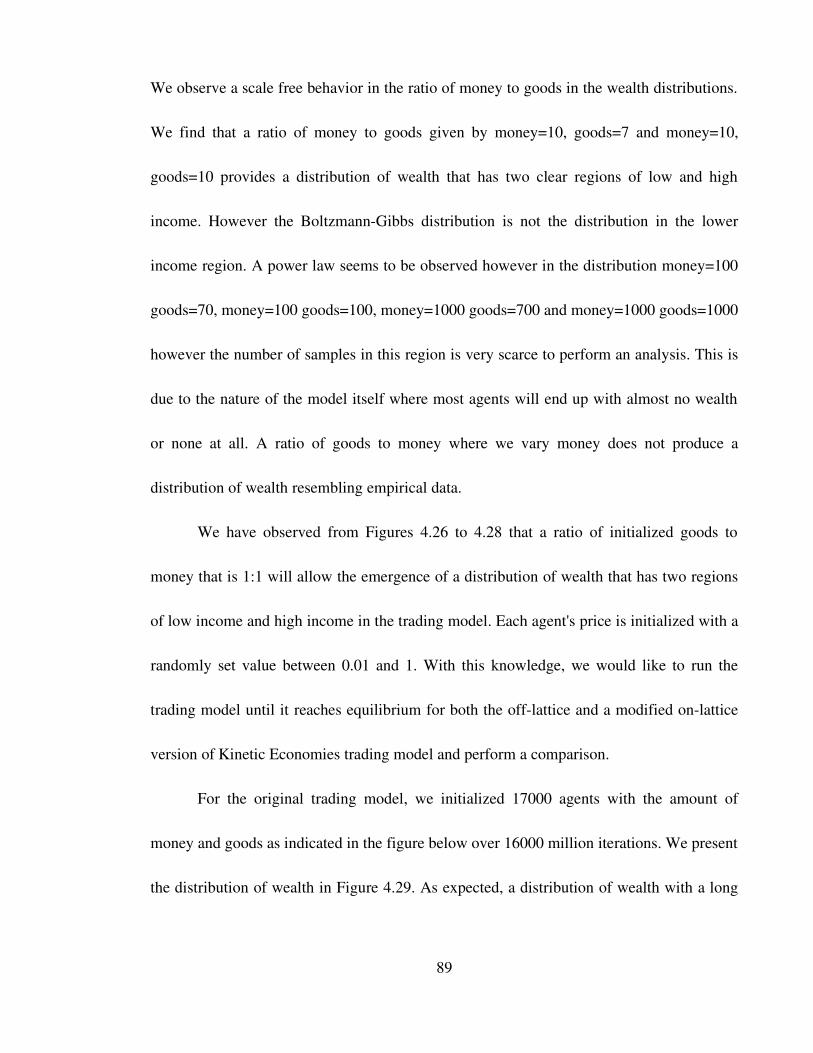
We observe a scale free behavior in the ratio of money to goods in the wealth distributions.

We find  that  a ratio  of money to goods given by money=10, goods=7 and money=10,

goods=10 provides a distribution of wealth   that  has  two clear regions of  low and high

income.  However   the Boltzmann­Gibbs distribution   is  not   the distribution   in   the   lower

income region. A power law seems to be observed however in the distribution money=100

goods=70, money=100 goods=100, money=1000 goods=700 and money=1000 goods=1000

however the number of samples in this region is very scarce to perform an analysis. This is

due to the nature of the model itself where most agents will end up with almost no wealth

or  none at  all.  A  ratio  of  goods  to  money where  we vary  money does  not  produce  a

distribution of wealth resembling empirical data.

We have observed from Figures 4.26 to 4.28 that a ratio  of  initialized goods to

money that is 1:1 will allow the emergence of a distribution of wealth that has two regions

of low income and high income in the trading model. Each agent's price is initialized with a

randomly set value between 0.01 and 1. With this knowledge, we would like to run the

trading model until it reaches equilibrium for both the off­lattice and a modified on­lattice

version of Kinetic Economies trading model and perform a comparison. 

For   the original   trading model,  we  initialized  17000 agents  with  the  amount  of

money and goods as indicated in the figure below over 16000 million iterations. We present

the distribution of wealth in Figure 4.29. As expected, a distribution of wealth with a long

89

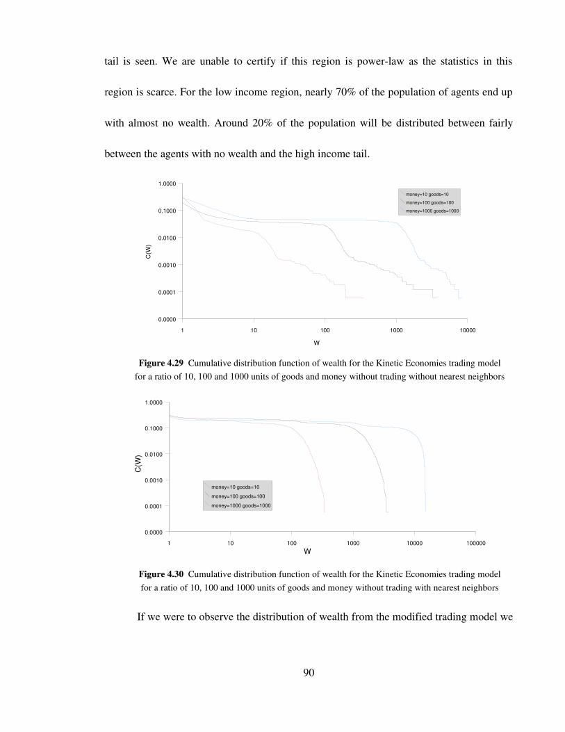
tail  is seen. We are unable to certify if this region is power­law as the statistics in this

region is scarce. For the low income region, nearly 70% of the population of agents end up

with almost no wealth. Around 20% of the population will be distributed between fairly

between the agents with no wealth and the high income tail. 

If we were to observe the distribution of wealth from the modified trading model we

90

1 10 100 1000 10000

0.0000

0.0001

0.0010

0.0100

0.1000

1.0000money=10 goods=10money=100 goods=100money=1000 goods=1000

W

C(W

)

1 10 100 1000 10000 100000

0.0000

0.0001

0.0010

0.0100

0.1000

1.0000

money=10 goods=10money=100 goods=100money=1000 goods=1000

W

C(W

)

Figure 4.29  Cumulative distribution function of wealth for the Kinetic Economies trading model for a ratio of 10, 100 and 1000 units of goods and money without trading without nearest neighbors

Figure 4.30  Cumulative distribution function of wealth for the Kinetic Economies trading model for a ratio of 10, 100 and 1000 units of goods and money without trading with nearest neighbors

find   that   after  16000  million   iterations,   the  distribution  of  wealth  does  not   equilibrate

similarly to the original trading model. This is presented in Figure 4.30. We observe that

the high income region is not scale free and it is better fitted by an exponential distribution.

We show the fittings in the Figure 4.31. 

91

Figure 4.31  Tail of the cdf of wealth fitted to an exponential distribution for 10 and 100 units of goods and money

100 1000 10000

0.0000

0.0001

0.0010

0.0100

money=100 goods=100

Empiricalexponent power law 

W

C(W

)

10 100 10000.0001

0.0010

0.0100money=10 goods=10

empirical exponent power law 

w

C(w)

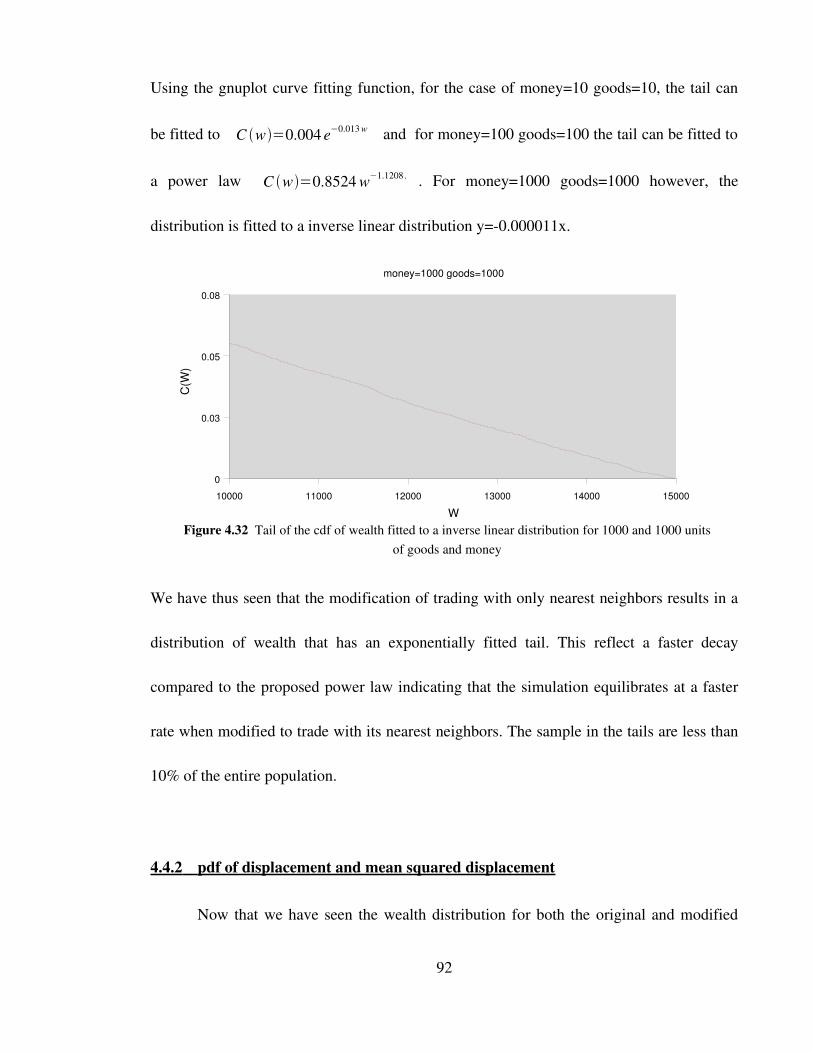
Using the gnuplot curve fitting function, for the case of money=10 goods=10, the tail can

be fitted to  C w=0.004 e−0.013 w  and  for money=100 goods=100 the tail can be fitted to

a   power   law   C w=0.8524 w−1.1208 . .   For   money=1000   goods=1000   however,   the

distribution is fitted to a inverse linear distribution y=­0.000011x. 

We have thus seen that the modification of trading with only nearest neighbors results in a

distribution   of   wealth   that   has   an   exponentially   fitted   tail.   This   reflect   a   faster   decay

compared to the proposed power law indicating that the simulation equilibrates at a faster

rate when modified to trade with its nearest neighbors. The sample in the tails are less than

10% of the entire population. 

4.4.2           pdf of displacement and mean squared displacement   

Now that we have seen the wealth distribution for both the original and modified

92

10000 11000 12000 13000 14000 150000

0.03

0.05

0.08

money=1000 goods=1000

W

C(W

)

Figure 4.32  Tail of the cdf of wealth fitted to a inverse linear distribution for 1000 and 1000 units of goods and money

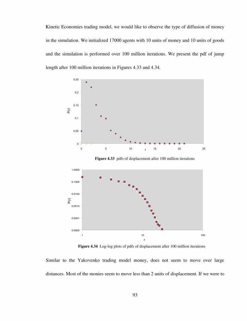
Kinetic Economies trading model, we would like to observe the type of diffusion of money

in the simulation. We initialized 17000 agents with 10 units of money and 10 units of goods

and the simulation is performed over 100 million iterations. We present the pdf of jump

length after 100 million iterations in Figures 4.33 and 4.34.

Similar   to   the   Yakovenko   trading   model   money,   does   not   seem   to   move   over   large

distances. Most of the monies seem to move less than 2 units of displacement. If we were to

93

Figure 4.33  pdfs of displacement after 100 million iterations

Figure 4.34  Log­log plots of pdfs of displacement after 100 million iterations

0 5 10 15 20 250

0.05

0.1

0.15

0.2

0.25

r

P(r)

1 10 1000.0000

0.0001

0.0010

0.0100

0.1000

1.0000

r

P(r)

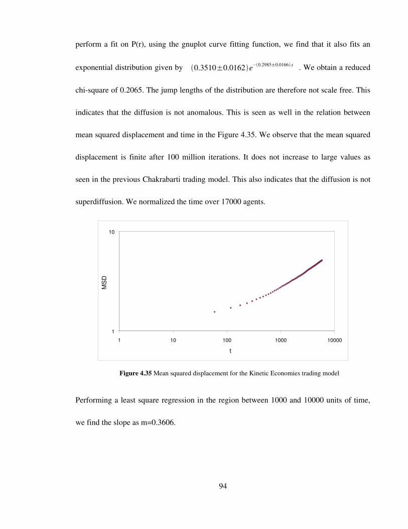
perform a fit on P(r), using the gnuplot curve fitting function, we find that it also fits an

exponential distribution given by  0.3510±0.0162e−0.2985±0.0166 x . We obtain a reduced

chi­square of 0.2065. The jump lengths of the distribution are therefore not scale free. This

indicates that the diffusion is not anomalous. This is seen as well in the relation between

mean squared displacement and time in the Figure 4.35. We observe that the mean squared

displacement is finite after 100 million iterations. It does not increase to large values as

seen in the previous Chakrabarti trading model. This also indicates that the diffusion is not

superdiffusion. We normalized the time over 17000 agents.

Performing a least square regression in the region between 1000 and 10000 units of time,

we find the slope as m=0.3606.

94

1 10 100 1000 100001

10

t

MSD

Figure 4.35 Mean squared displacement for the Kinetic Economies trading model

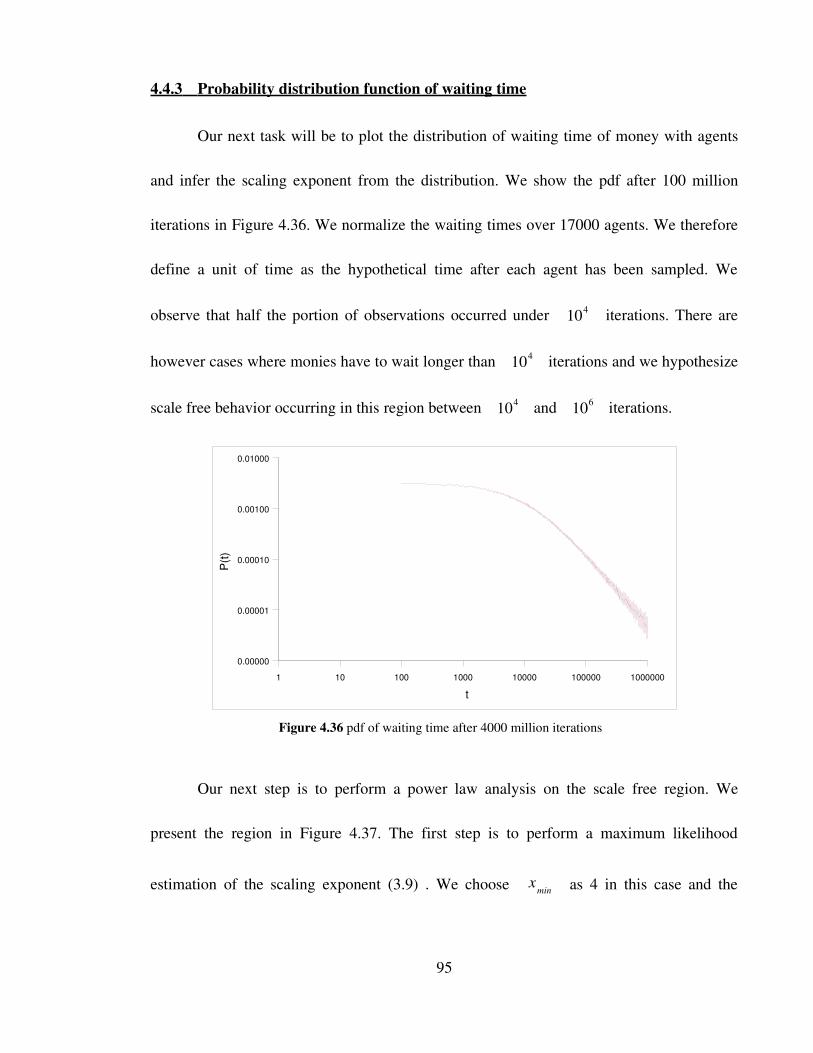
4.4.3           Probability distribution function of waiting time   

Our next task will be to plot the distribution of waiting time of money with agents

and infer the scaling exponent from the distribution. We show the pdf after 100 million

iterations in Figure 4.36. We normalize the waiting times over 17000 agents. We therefore

define  a  unit  of   time as   the hypothetical   time after  each  agent  has  been  sampled.  We

observe that half the portion of observations occurred under   104   iterations. There are

however cases where monies have to wait longer than  104  iterations and we hypothesize

scale free behavior occurring in this region between  104  and  106  iterations. 

Our next  step  is   to  perform a power  law analysis  on  the scale   free region.  We

present   the   region   in  Figure  4.37.  The   first   step   is   to  perform a  maximum  likelihood

estimation of  the scaling exponent  (3.9)  .  We choose   xmin   as  4  in  this  case and the

95

1 10 100 1000 10000 100000 10000000.00000

0.00001

0.00010

0.00100

0.01000

t

P(t)

Figure 4.36 pdf of waiting time after 4000 million iterations

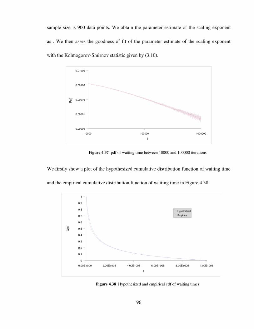
sample size is 900 data points. We obtain the parameter estimate of the scaling exponent

as . We then asses the goodness of fit of the parameter estimate of the scaling exponent

with the Kolmogorov­Smirnov statistic given by (3.10).

We firstly show a plot of the hypothesized cumulative distribution function of waiting time

and the empirical cumulative distribution function of waiting time in Figure 4.38. 

96

10000 100000 1000000

0.00000

0.00001

0.00010

0.00100

0.01000

t

P(t)

Figure 4.37  pdf of waiting time between 10000 and 100000 iterations 

Figure 4.38  Hypothesized and empirical cdf of waiting times

0.00E+000 2.00E+005 4.00E+005 6.00E+005 8.00E+005 1.00E+0060

0.1

0.2

0.3

0.4

0.5

0.6

0.7

0.8

0.9

1

HypotheticalEmpirical

t

C(t)

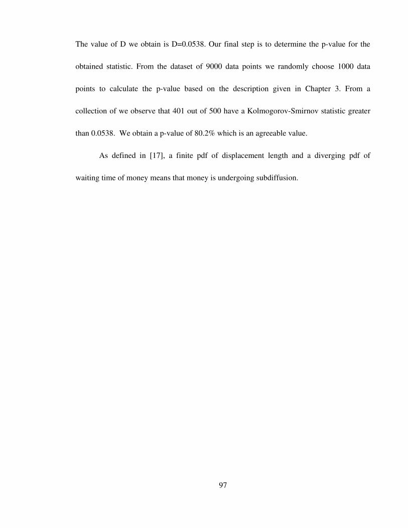
The value of D we obtain is D=0.0538. Our final step is to determine the p­value for the

obtained statistic.  From the dataset of 9000 data points  we randomly choose 1000 data

points   to   calculate   the   p­value   based   on   the   description   given   in   Chapter   3.   From   a

collection of we observe that 401 out of 500 have a Kolmogorov­Smirnov statistic greater

than 0.0538.  We obtain a p­value of 80.2% which is an agreeable value.

As  defined   in   [17],   a   finite  pdf  of  displacement   length  and  a  diverging  pdf  of

waiting time of money means that money is undergoing subdiffusion.

97

CHAPTER 5 : CONCLUSION

The cdf of wealth in the Chakrabarti trading model with a random saving propensity

is   seen   to   be   a   mixed   distribution   of   a   Boltzmann­Gibbs   distribution   and   power   law

distribution in   the low and high  income regions respectively as shown in [13].  This   is

observed   in   our  modification   to   this   trading  model   as  well.  The  cdf  of  wealth   in   the

Yakovenko trading model is observed as an exponential distribution as shown in [15]. This

is observed in our modification to this trading model as well.  The cdf of wealth in the

Kinetic Economies trading model is observed as a mixed distribution where we propose the

tail as scale free. Our modification to the trading model however allows an emergent tail

which is shown to be an exponential distribution but the entire distribution is also mixed.

The diffusion of money in  the Chakrabarti   trading model  with a random saving

propensity has been shown to exhibit  anomalous diffusion.  This  is  seen in a scale free

distribution of the tail of the displacement length pdf and waiting time pdf and a mean

squared displacement relation which is linearly dependent with time with a slope which is

less than 1. The determination of the power law exponent for the displacement length pdf

however has to be improved by learning new ways to increase memory allocation for a

vector. This is so that more money can be initialized per agent and thus more money can be

traded, moved and tracked over the course of the simulation. The solution probably lies in

the realm of high performance computing. Ripples seem to exist in the waiting time pdf and

98

it is probably attributed to the standard C++ random number generator which is known to

bias to certain numbers. We will further the Monte Carlo calculations using the well known

Mersenne   Twister   [52]   random   number   generator.   The   diffusion   of   money   in   the

Yakovenko  trading  model  has  been  shown  to  not  exhibit  anomalous  diffusion.  This   is

because the displacement length pdf decays exponentially. The waiting time pdf has a long

tail but it is not scale free and scales as an exponential. The mean squared displacement

relation with time is also finite. The analysis of the diffusion of money in the Chakrabarti

trading  model  with  a   fixed   saving  propensity   shows   that   is  not  obvious   if   anomalous

diffusion exhibited. A scale free distribution of the tail of the displacement length pdf and

waiting time pdf is seen. However, the analysis of the tails however show that it is less

likely to be scale free compared to the first experiment. The mean squared displacement

relation however is seen to vary linearly with time with a slope which is almost 1 indicating

normal   diffusion.   As   mentioned   above,   we   hope   to   overcome   the   memory   allocation

problem to ensure that an improved analysis of the power­law exponents can be made. The

diffusion of money in  the Kinetic Economies trading model has been shown to exhibit

subdiffusion.   This   is   because   the   displacement   length   pdf   decays   exponentially.   The

waiting time pdf however has a scale free tail. The mean squared displacement relation with

time is finite.

As has been defined in Chapter 2,  inserting into (2.85)  the empirical value of the

99

power law exponent   and   for the waiting time and jump length pdf's respectively

will allow us to perform a fitting of the ambivalence of the empirical waiting time and jump

length distributions and the analytical solution. This however could not be done as we did

not have the software needed to perform the fitting. We suggest the use of the software

Mathematica to perform the fitting in the future.

We can thus conclude from the observations we made that a trading model with a

resultant mixed distributions of wealth with a scale free tail exhibits anomalous diffusion. A

trading   model   with   a   resultant   mixed   distributions   of   wealth   with   an   exponential   tail

exhibits subdiffusion. A trading model with a resultant exponential distribution of wealth

does not exhibit anomalous diffusion.  

100

REFERENCES

1. H.E Stanley, et. al., 1996, “Anomalous fluctuations in the dynamics of complex systems :

from DNA and physiology to econophysics,” Physica A 224, 302­321.

2. Smith A.  An inquiry into the nature and causes of the wealth of nations.  London: W.

Stahan & T. Cadell, 1776.

3. D.   Rickles.  Econophysics   for   philosophers.  Studies   in   History   and   Philosophy   of

Modern Physics, 38(4):948–978, 2007.

4. Gillispie, C. C., 1963, Intellectual factors in the background analysis by probabilities,

Scientific Change (Heinemann, London), pp 431­453.

5. Ball,  P.,   June  2004.  Critical  Mass:  How One Thing  Leads   to  Another,  1st  Edition.

Farrar, Straus and Giroux.

6. V. Pareto, Cours d'economie politique, Lausanne and Paris,1897

7. Derman E. (2004): My Life as a Quant: Reflections on Physics and Finance. Wiley.

8. Anderson, P.W., January 1989. The Economy As an Evolving Complex System (Santa Fe

Institute Studies in the Sciences of Complexity Proceedings). Addison Wesley

Publishing Company.

9. Tesfatsion, L., 2001. Introduction. Comput. Econ. 18(1), 1-8.

10.Ilinski, K., October 1997. Physics of finance. http://arxiv.org/abs/hep-th/9710148.

11.Baaquie, B.E., November 2004. Quantum Finance: Path Integrals and Hamiltonians for

101

Options and Interest Rates. Cambridge University Press.

12.A.A. Dragulescu and V.M. Yakovenko, Exponential and power law probability

distributions of wealth and income in the United Kingdom and the United States,

Physica A 229 213-221.

13.A.  Chakraborti   and  B.K.  Chakrabarti,  Statistical  mechanics   of  money:  How  saving

propensity effects its distribution. Eur. Phys. J. B 17 (2000) 167.

14.H.  A.  Simon,  On a  class  of   skew   income distribution   functions.  Biometrika  42:3/4

(1955), 425­440.

15.A.A. Dragulescu and V.M. Yakovenko, Statistical mechanics of money, The European

Physical Journal B 17 723­729.

16.Vlahos, L., Isliker, H., Kominis, Y., Hizanidis, K., May 2008. Normal and anomalous

diffusion:   A   tutorial.  'Order   and   and  Chaos',   10th  volume,   T.   Bountis   (ed.),   Patras

University Press (2008)

17.R. Metzler and  J. Klafter, The random walks guide to anomalous diffusion: a fractional

dynamics approach. Phys. Rep. 339, 1­77 (2000).

18.W.A.T.  Wan Abdullah,  Teori  kinetik  untuk ekonomi,  Dept  of  Physics,  University  of

Malaya preprint JFUM/2002/001.

19.D. Brockmann, L. Hufnagel and T. Geisel,  The scaling laws of human travel. Nature

439,462­465 (2006) .

102

20.D.   Brockmann,  Anomalous   diffusion   and   the   structure   of   human   transportation

networks. Eur. Phys. J. Special Topics 157,173­189 (2008).

21.M.E.J.  Newman,  Power  Laws,  Pareto  Distributions  and Zipf's  Laws,  Contemporary

Physics 46, 323­351 (2005).

22.Her Majesty Revenue and Customs (2003) Distribution of Personal Wealth. 

23. P. Levy, Calcul des probabilités, Gauthier­Villars, Paris (1925).

24. Mandelbrot,   B.B.   (1982).  The   Fractal   Geometry   of   Nature.   W.H.   Freeman   and

Company.

25. H.   E.   Stanley,  Introduction   to   Phase   Transitions   and   Critical   Phenomena  (Oxford

University Press, Oxford and New York 1971)

26.M. Patriaca, K. Kaski and A. Chakraborti,  Statistical model with a standard Gamma

distribution, Phys. Rev. E 70, 016104 (2004).

27.M Nirei and W Souma, A two factor model of income distribution dynamics, Review of

Income and Wealth (2007), papers.ssrn.com.

28. E.W. Montroll and M.F. Shlesinger, On 1/f noise and other distributions with long tails.

Proc. Natl. Acad. Sci. USA, 79 (1982) 3380.

29.A.C. Silva, V.M. Yakovenko,  Temporal evolution of the 'thermal' and 'superthermal'

income classes in the USA during 1983­2001. Europhys. Lett. 69 304­310.

30.H.   Aoyama   et.   al,  Pareto's   law   for   income   of   individuals   and   debt   of   bankrupt

103

companies. Fractals 8 (2000) 293.

31. Kim K, Yoon SM (2004), Power Law Distribution in Korean Household Incomes.  E­

print: http://arxiv.org/abs/cond­mat/0403161.

32.F. Clementi, M. Gallegati, Power law tails in the Italian personal income distribution.

Physica A 350 (2005) 427–438.

33.A. Chatterjee, B.K. Chakrabarti, S.S. Manna, Pareto Law in a Kinetic Model of Market

with Random Saving Propensity, Physica A 335 (2004) 155.

34.B.   Mandelbrot,  The   Pareto­Levy   law   and   the   distribution   of   income.  International

Economic Review 1 (1960) 79.

35.E.W. Montroll and M.F. Shlesinger, Maximum Entropy Formalism, Fractals, Scaling

Phenomena, and 1/f noise : A tail of tails, Journal of Statistical Physics, Vol. 32. No.2,

1983.

36.D.G. Champernowne, A Model of Income Distribution, The Economic Journal, Vol. 63

No. 250 (Jun., 1953), pp. 318­351.

37.http://chaos.utexas.edu/research/annulus/m22l.gif 

38.T.H. Solomon, E.R. Weeks and H.L. Swinney, Observation of anomalous diffusion and

Levy Flights in a two­dimensional rotating flow, Phys. Rev. Lett. 71, 3975 (1993).

39.Bunde, A., Havlin,  S.,  1995.  Fractals  and disordered systems.  Springer­Verlag New

York, Inc., Secaucus, NJ, USA.

104

40.E. Montroll and G. H. Weiss, Random Walks on Lattices .II. J. Math. Phys. 6, 167 1965.

41. X. Gabaix  (August 1999).  Zipf's Law for Cities: An Explanation. Quarterly Journal of

Economics 114 (3): 739–67

42.A.Sornette, D. Sornette,  Self­organized criticality and earthquakes.  Europhys. Lett., 9

(3), pp 197­202 (1989).

43.G.K.   Zipf,  Human   Behavior   and   the   Principle   of   Least   Effort.   Addison­Wesley,

Reading, MA (1949).

44.M. L. Goldstein, S.A Morris and G. G. Yen,  Problems with fitting to the Power­law

Distribution. Eur. Phys. J. B 41 2 (2004).

45.A.  Clauset,  C.R.  Shalizi  and  M.E.J.  Newman,  Power­law distributions   in  empirical

data, arxiv:0706.1062v1.

46.M. Mitzenmacher, A Brief History of Generative Models for Power Law and Lognormal

Distributions, Internet Mathematics Vol. 1, No. 2: 226­251.

47.Ormerod, P. (1994) The Death of Economics. Faber, London.

48.Bardou, F., J.-P. Bouchaud, A. Aspect, and C. Cohen-Tannoudji. 2002. Levy Statistics

and Laser Cooling: How Rare Events Bring Atoms to Rest. Cambridge: Cambridge

University Press.

49.Billari, FC, Prskawetz, A.(2003). Agent­Based Computational Demography: Using

Simulation to Improve Our Understanding of Demographic Behaviour. Physica Verlag.

105

50.Landau, D.; Binder, K. A Guide to Monte Carlo Simulations in Statistical Physics;

Cambridge University Press: New York, 2000.

51.http://www.weibull.com/AccelTestWeb/mle_maximum_likelihood_parameter_estimatio

n.htm

52.Matsumoto, M., T. Nishimura. 1998. Mersenne twister: A 623-dimensionally

equidistributed uniform pseudorandom number generator. ACM Trans. Modeling Comput.

Simulation 8(1) 3–30.

53.C Tsallis, 1988.Possible generalization of Boltzmann­Gibbs statistics J. Stat. Phys. 52,

479.

54.Kostolowicz et al (2009), Subdiffusion in a membrane and in electrochemical systems,

Physica Scripta 014020.

106

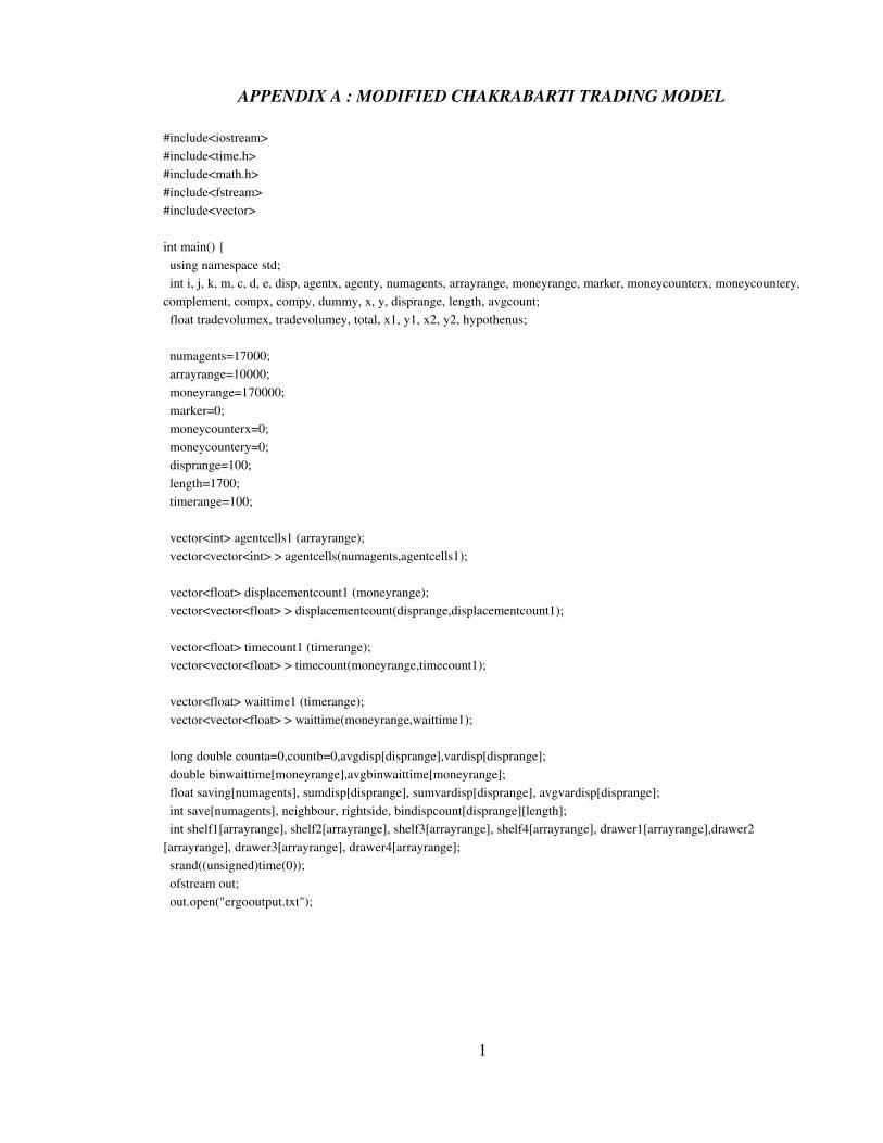
APPENDIX A : MODIFIED CHAKRABARTI TRADING MODEL

#include<iostream> #include<time.h> #include<math.h> #include<fstream> #include<vector> 

int main() {   using namespace std;   int i, j, k, m, c, d, e, disp, agentx, agenty, numagents, arrayrange, moneyrange, marker, moneycounterx, moneycountery,complement, compx, compy, dummy, x, y, disprange, length, avgcount;   float tradevolumex, tradevolumey, total, x1, y1, x2, y2, hypothenus; 

  numagents=17000;   arrayrange=10000;   moneyrange=170000;   marker=0;   moneycounterx=0;   moneycountery=0;   disprange=100;   length=1700;   timerange=100;

  vector<int> agentcells1 (arrayrange);   vector<vector<int> > agentcells(numagents,agentcells1); 

  vector<float> displacementcount1 (moneyrange);   vector<vector<float> > displacementcount(disprange,displacementcount1);

  vector<float> timecount1 (timerange);   vector<vector<float> > timecount(moneyrange,timecount1); 

  vector<float> waittime1 (timerange);   vector<vector<float> > waittime(moneyrange,waittime1); 

  long double counta=0,countb=0,avgdisp[disprange],vardisp[disprange];   double binwaittime[moneyrange],avgbinwaittime[moneyrange];  float saving[numagents], sumdisp[disprange], sumvardisp[disprange], avgvardisp[disprange];   int save[numagents], neighbour, rightside, bindispcount[disprange][length];  int shelf1[arrayrange], shelf2[arrayrange], shelf3[arrayrange], shelf4[arrayrange], drawer1[arrayrange],drawer2[arrayrange], drawer3[arrayrange], drawer4[arrayrange];   srand((unsigned)time(0));   ofstream out;   out.open("ergooutput.txt"); 

1

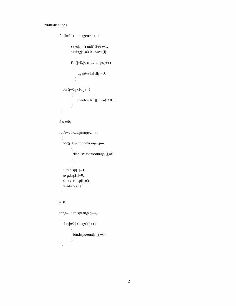
//Initializations 

  for(i=0;i<numagents;i++)       {        save[i]=(rand()%99)+1;        saving[i]=0.01*save[i];              for(j=0;j<arrayrange;j++) 

   {       agentcells[i][j]=0;    } 

      for(j=0;j<10;j++) {

        agentcells[i][j]=j+(i*10); } 

    } 

  disp=0;     for(i=0;i<disprange;i++)     {       for(j=0;j<moneyrange;j++) 

{   displacementcount[i][j]=0; } 

      sumdisp[i]=0;       avgdisp[i]=0;       sumvardisp[i]=0;       vardisp[i]=0;     } 

   e=0; 

  for(i=0;i<disprange;i++)     {       for(j=0;j<length;j++) 

{   bindispcount[i][j]=0; } 

    } 

2

//Trade 

      for(k=0;k<4000;k++) {   for(m=0;m<1000001;m++) 

{       //Initialize shelves and drawers before trading 

      i=0;       while(1) 

{ if(((shelf1[i]!=0)&&(shelf1[i+1]!=0))||((shelf1[i]!=0)&&(shelf1[i+1]

==0))||((shelf1[i]==0)&&(shelf1[i+1]!=0))) {shelf1[i]=0;} else{break;}  i++; } 

            i=0;       while(1) 

{ if(((shelf2[i]!=0)&&(shelf2[i+1]!=0))||((shelf2[i]!=0)&&(shelf2[i+1]

==0))||((shelf2[i]==0)&&(shelf2[i+1]!=0))) {shelf2[i]=0;}   else{break;}   i++; } 

            i=0;       while(1) 

{ if(((shelf3[i]!=0)&&(shelf3[i+1]!=0))||((shelf3[i]!=0)&&(shelf3[i+1]

==0))||((shelf3[i]==0)&&(shelf3[i+1]!=0))) {shelf3[i]=0;}   else{break;}   i++; }

       i=0;       while(1) 

{ if(((shelf4[i]!=0)&&(shelf4[i+1]!=0))||((shelf4[i]!=0)&&(shelf4[i+1]

==0))||((shelf4[i]==0)&&(shelf4[i+1]!=0)))   {shelf4[i]=0;}   else{break;}   i++; 

3

} 

       i=0;       while(1) 

{ if(((drawer1[i]!=0)&&(drawer1[i+1]!=0))||((drawer1[i]!=0)&&(drawer1

[i+1]==0))||((drawer1[i]==0)&&(drawer1[i+1]!=0)))  {drawer1[i]=0;}   else{break;}   i++; } 

            i=0;       while(1) 

{ if(((drawer2[i]!=0)&&(drawer2[i+1]!=0))||((drawer2[i]!=0)&&(drawer2

[i+1]==0))||((drawer2[i]==0)&&(drawer2[i+1]!=0)))   {drawer2[i]=0;}   else{break;}   i++; } 

            i=0;       while(1) 

{ if(((drawer3[i]!=0)&&(drawer3[i+1]!=0))||((drawer3[i]!=0)&&(drawer3

[i+1]==0))||((drawer3[i]==0)&&(drawer3[i+1]!=0))) {drawer3[i]=0;}   else{break;}   i++; } 

            i=0;       while(1) 

{ if(((drawer4[i]!=0)&&(drawer4[i+1]!=0))||((drawer4[i]!=0)&&(drawer4

[i+1]==0))||((drawer4[i]==0)&&(drawer4[i+1]!=0))) {drawer4[i]=0;}   else{break;}   i++; } 

4

//Choose two  neighbouring agents 

      while(1) {   while(1)     {       agentx=rand()%numagents;       rightside=agentx­(length­1);       

 //edges        if(agentx==0) {   neighbour=rand()%3;   if(neighbour==0){agenty=agentx+1;}   else if(neighbour==1){agenty=agentx+length;}   else if(neighbour==2){agenty=agentx+(length+1);}   break; } 

      else if(agentx==(length­1)) {   neighbour=rand()%3;   if(neighbour==0){agenty=agentx­1;}   else if(neighbour==1){agenty=agentx+(length­1);}   else if(neighbour==2){agenty=agentx+length;}   break; } 

      else if(agentx==(numagents­length)) {   neighbour=rand()%3;   if(neighbour==0){agenty=agentx­length;}   else if(neighbour==1){agenty=agentx­(length­1);}   else if(neighbour==2){agenty=agentx+1;}   break; } 

      else if(agentx==(numagents­1)) {   neighbour=rand()%3;   if(neighbour==0){agenty=agentx­(length+1);}   else if(neighbour==1){agenty=agentx­length;}   else if(neighbour==2){agenty=agentx­1;}   break; } 

      //corners  else if((agentx<length)&&(agentx!=0)&&(agentx!=(length­1))) { 

  neighbour=rand()%5;   if(neighbour==0){agenty=agentx­1;}   else if(neighbour==1){agenty=agentx+1;}   else if(neighbour==2){agenty=agentx+(length­1);}   else if(neighbour==3){agenty=agentx+length;}   else if(neighbour==4){agenty=agentx+(length+1);}   break; } 

5

else if((agentx>(numagents­length­1))&&(agentx!=(numagents­length))&&(agentx!=(numagents­1))) {   neighbour=rand()%5;   if(neighbour==0){agenty=agentx­(length+1);}   else if(neighbour==1){agenty=agentx­length;}   else if(neighbour==2){agenty=agentx­(length­1);}   else if(neighbour==3){agenty=agentx­1;}   else if(neighbour==4){agenty=agentx+1;}   break; } 

else if((agentx%length==0)&&(agentx!=0)&&(agentx!=(numagents­length))) {   neighbour=rand()%5;   if(neighbour==0){agenty=agentx­length;}   else if(neighbour==1){agenty=agentx­(length­1);}   else if(neighbour==2){agenty=agentx+1;}   else if(neighbour==3){agenty=agentx+length;}   else if(neighbour==4){agenty=agentx+(length+1);}   break; } 

else if((rightside%length==0)&&(agentx!=(length­1))&&(agentx!=(numagents­1))) {   neighbour=rand()%5;   if(neighbour==0){agenty=agentx­(length+1);}   else if(neighbour==1){agenty=agentx­length;}   else if(neighbour==2){agenty=agentx­1;}   else if(neighbour==3){agenty=agentx+(length­1);}   else if(neighbour==4){agenty=agentx+length;}   break; } 

//not edges or corners  else {   neighbour=rand()%8;   if(neighbour==0){agenty=agentx­(length+1);}   else if(neighbour==1){agenty=agentx­length;}   else if(neighbour==2){agenty=agentx­(length­1);}   else if(neighbour==3){agenty=agentx­1;}   else if(neighbour==4){agenty=agentx+1;}   else if(neighbour==5){agenty=agentx+(length­1);}   else if(neighbour==6){agenty=agentx+length;}   else if(neighbour==7){agenty=agentx+(length+1);}   break; } 

    }     

6

//Count how much money agentx and agenty have respectively   

moneycounterx=0; moneycountery=0; 

   i=0; 

                 while(1) { if(((agentcells[agentx][i]!=0)&&(agentcells[agentx][i+1]!=0))||((agentcells[agentx][i]!=0)

&&(agentcells[agentx][i+1]==0))||((agentcells[agentx][i]==0)&&(agentcells[agentx][i+1]!=0))){moneycounterx++;} 

else{break;} i++; } 

i=0; while(1) { if(((agentcells[agenty][i]!=0)&&(agentcells[agenty][i+1]!=0))||((agentcells[agenty][i]!=0)

&&(agentcells[agenty][i+1]==0))||((agentcells[agenty][i]==0)&&(agentcells[agenty][i+1]!=0))){moneycountery++;} 

else{break;} i++; } 

  if((moneycounterx!=0)&&(moneycountery!=0)){break;} }          

//How much to trade?       

if((1­saving[agentx])*moneycounterx­floor((1­saving[agentx])*moneycounterx)>=0.50) {tradevolumex=ceil((1­saving[agentx])*moneycounterx);} 

else if((1­saving[agentx])*moneycounterx­floor((1­saving[agentx])*moneycounterx)<0.50) {tradevolumex=floor((1­saving[agentx])*moneycounterx);}       

if((1­saving[agenty])*moneycountery­floor((1­saving[agenty])*moneycountery)>=0.50) {tradevolumey=ceil((1­saving[agenty])*moneycountery);} 

else if((1­saving[agenty])*moneycountery­floor((1­saving[agenty])*moneycountery)<0.50) {tradevolumey=floor((1­saving[agenty])*moneycountery);}   

7

//Choose a random collection of numbers based on the counted monies and place into shelves for trading             x=moneycounterx;             shelf1[0]=rand()%moneycounterx;             for(i=1;i<tradevolumex;i++) 

{   dummy=rand()%moneycounterx;   for(j=0;j<i;j++)     {       if(shelf1[j]==dummy) 

{   dummy=rand()%moneycounterx;   j=­1; } 

    }   shelf1[i]=dummy; } 

            y=moneycountery;         shelf2[0]=rand()%moneycountery;         for(i=1;i<tradevolumey;i++) 

{   dummy=rand()%moneycountery;   for(j=0;j<i;j++)     {       if(shelf2[j]==dummy) 

{   dummy=rand()%moneycountery;   j=­1; }     

    }   shelf2[i]=dummy; } 

      

8

//Choose a random collection of numbers not in the trading shelves to place in the saving shelves             complement=0;        for(i=0;i<moneycounterx;i++) 

{   for(j=0;j<tradevolumex;j++) {if(i==shelf1[j]) {marker++;}}   if(marker==0)     {       shelf3[complement]=i;       complement++;     }   marker=0; } 

      compx=complement;             complement=0;        for(i=0;i<moneycountery;i++) 

{   for(j=0;j<tradevolumey;j++) {if(i==shelf2[j]) {marker++;}}   if(marker==0)     {       shelf4[complement]=i;       complement++;     }   marker=0; } 

      compy=complement;              

//Assign randomized numbers stored in shelves to drawers containing the label of money              

for(i=0;i<tradevolumex;i++) {drawer1[i]=agentcells[agentx][shelf1[i]];timecount[drawer1[i]][timer[drawer1[i]]]=1000000*k+m; timer[drawer1[i]]+=1;}       

for(i=0;i<tradevolumey;i++) {drawer2[i]=agentcells[agenty][shelf2[i]];

       timecount[drawer2[i]][timer[drawer2[i]]]=1000000*k+m; timer[drawer2[i]]+=1;}       

for(i=0;i<compx;i++) {drawer3[i]=agentcells[agentx][shelf3[i]];}       

for(i=0;i<compy;i++) {drawer4[i]=agentcells[agenty][shelf4[i]];}       

9

//Temporarily clear agentcells to place new collections inside       i=0; while(1) { if(((agentcells[agentx][i]!=0)&&(agentcells[agentx][i+1]!=0))||((agentcells[agentx][i]!=0)

&&(agentcells[agentx][i+1]==0))||((agentcells[agentx][i]==0)&&(agentcells[agentx][i+1]!=0))) {agentcells[agentx][i]=0;} else{break;} i++; }        i=0;  while(1) { if(((agentcells[agenty][i]!=0)&&(agentcells[agenty][i+1]!=0))||((agentcells[agenty][i]!=0)

&&(agentcells[agenty][i+1]==0))||((agentcells[agenty][i]==0)&&(agentcells[agenty][i+1]!=0))) {agentcells[agenty][i]=0;} else{break;}  i++; }       

//Place back money's into agents via the drawers                   for(i=0;i<compx;i++) 

{agentcells[agentx][i]=drawer3[i];}             j=i;              for(i=0;i<tradevolumey;i++) 

{  agentcells[agentx][j]=drawer2[i];   j++;} 

                    for(i=0;i<compy;i++) 

{agentcells[agenty][i]=drawer4[i];}          j=i;              for(i=0;i<tradevolumex;i++) 

{   agentcells[agenty][j]=drawer1[i];   j++;} 

            

10

if((k%40==0)&&(m==1000000)) {   for(i=0;i<numagents;i++)     {       for(j=0;j<arrayrange;j++) 

{ //current position   x2=i;    

  if(x2>(length­1)) {       while(x2>=length) 

{   x2=x2­length;   y2++; } 

    }   else {       x2=i;       y2=0;     }   

  if(((agentcells[i][j]!=0)&&(agentcells[i][j]!=0))||((agentcells[i][j]!=0)&&(agentcells[i][j]==0))||((agentcells[i][j]==0)&&(agentcells[i][j]!=0))) 

{ //original position x1=floor(agentcells[i][j]*0.1); 

if(x1>(length­1)) { while(x1>=length) 

{ x1=x1­length; y1++; } 

}   else { 

x1=floor(agentcells[i][j]*0.1); y1=0; } 

      hypothenus=(x2­x1)*(x2­x1)+(y2­y1)*(y2­y1); displacementcount[e][agentcells[i][j]]=sqrt(hypothenus); 

  x1=0; y1=0; } 

   x2=0; y2=0; 

      }                  }  

11

  for(i=0;i<length;i++)  { for(j=0;j<moneyrange;j++) 

{ if((displacementcount[e][j]>=i)&&(displacementcount[e][j]<(i+1))) 

{ bindispcount[e][i]+=1; } } 

}

for(i=0;i<moneyrange;i++) { avgdisp[e]+=displacementcount[e][i]; if(displacementcount[e][i]!=0) 

{ avgcount++;} } 

avgdisp[e]=avgdisp[e]/avgcount; 

 avgcount=0;   

for(i=0;i<moneyrange;i++) { 

             vardisp[e]+=(displacementcount[e][i]­avgdisp[e])*(displacementcount[e][i]­avgdisp[e]); }   

  vardisp[e]=vardisp[e]/moneyrange;              e++; } 

    } } 

for(i=0;i<moneyrange;i++)     {       waittime[i][0]=timecount[i][0];     }     for(i=0;i<moneyrange;i++)     {       for(j=1;j<timerange;j++) 

{   if(timecount[i][j]>timecount[i][j­1])     {       waittime[i][j]=timecount[i][j]­timecount[i][j­1];     } } 

    } 

12

  for(k=0;k<10000;k++)     {       for(i=0;i<moneyrange;i++) 

{   for(j=0;j<timerange;j++)     {       if((waittime[i][j]>=(k*100))&&(waittime[i][j]<((k+1)*100))) 

{   binwaittime[k]+=1; } 

    } } 

    }           

  for(i=0;i<disprange;i++)     {       for(j=0;j<length;j++) 

{   out<<" "<<j<<"\t "<<i<<"\t "<<bindispcount[i][j]<<"\n"; } 

      out<<"\n";     } 

   for(i=0;i<10000;i++)      {                   out<<" "<<i*100<<"\t "<<binwaittime[i]<<"\n";      }

  for(i=0;i<disprange;i++)     {       out<<" "<<i*40000000<<"\t "<<vardisp[i]<<"\n";     }

  } 

13

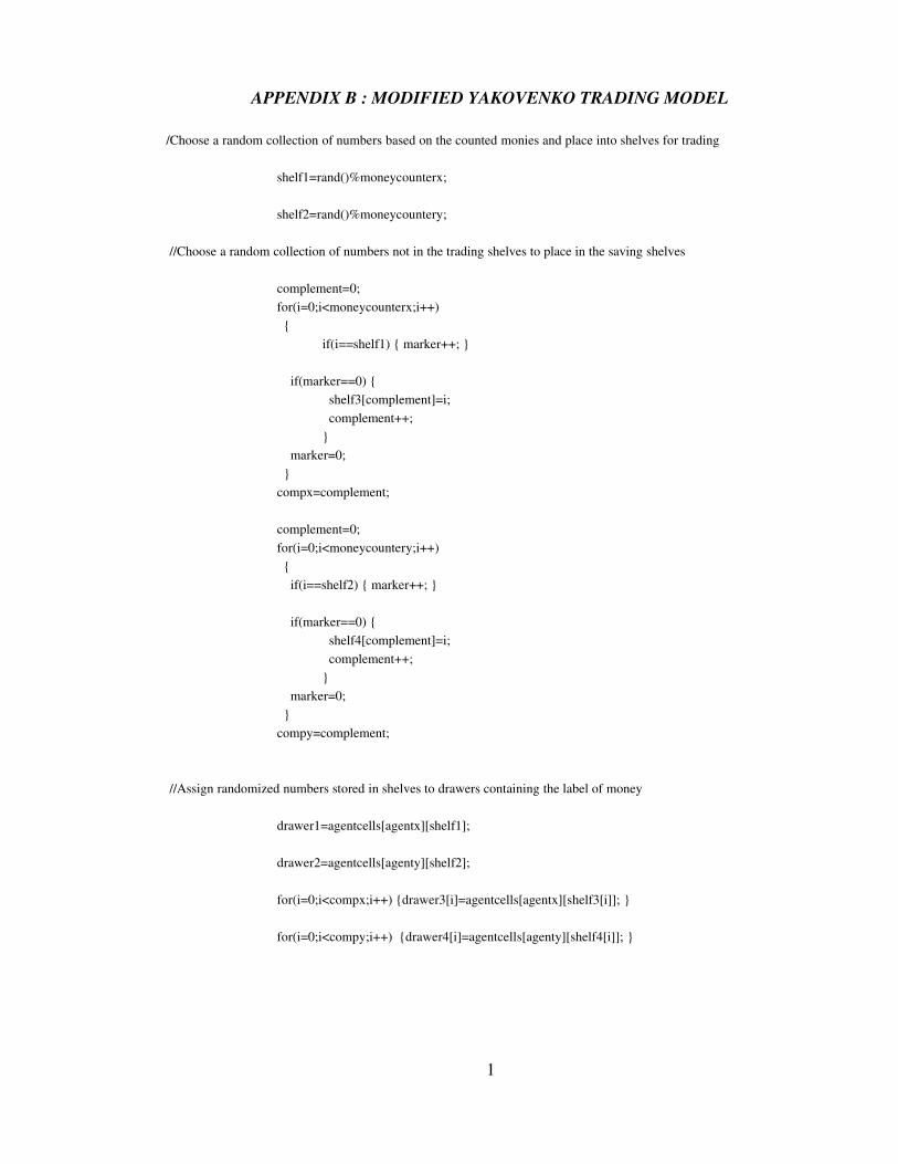
APPENDIX B : MODIFIED YAKOVENKO TRADING MODEL

/Choose a random collection of numbers based on the counted monies and place into shelves for trading 

  shelf1=rand()%moneycounterx;     shelf2=rand()%moneycountery; 

 //Choose a random collection of numbers not in the trading shelves to place in the saving shelves     complement=0;   for(i=0;i<moneycounterx;i++)     { 

if(i==shelf1) { marker++; }           if(marker==0) { 

  shelf3[complement]=i;   complement++; } 

      marker=0;     }   compx=complement;     complement=0;   for(i=0;i<moneycountery;i++)     {       if(i==shelf2) { marker++; }           if(marker==0) { 

  shelf4[complement]=i;   complement++; } 

      marker=0;     }   compy=complement;     

 //Assign randomized numbers stored in shelves to drawers containing the label of money     drawer1=agentcells[agentx][shelf1];     drawer2=agentcells[agenty][shelf2];        for(i=0;i<compx;i++) {drawer3[i]=agentcells[agentx][shelf3[i]]; }     for(i=0;i<compy;i++)  {drawer4[i]=agentcells[agenty][shelf4[i]]; } 

1

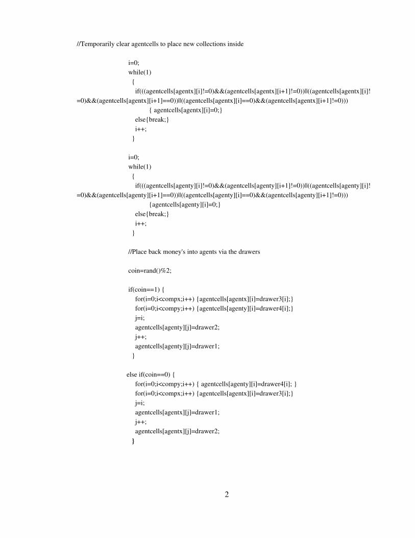
//Temporarily clear agentcells to place new collections inside    i=0;   while(1)     {       if(((agentcells[agentx][i]!=0)&&(agentcells[agentx][i+1]!=0))||((agentcells[agentx][i]!

=0)&&(agentcells[agentx][i+1]==0))||((agentcells[agentx][i]==0)&&(agentcells[agentx][i+1]!=0))) { agentcells[agentx][i]=0;} 

      else{break;}       i++;     } 

  i=0;   while(1)     {       if(((agentcells[agenty][i]!=0)&&(agentcells[agenty][i+1]!=0))||((agentcells[agenty][i]!

=0)&&(agentcells[agenty][i+1]==0))||((agentcells[agenty][i]==0)&&(agentcells[agenty][i+1]!=0))) {agentcells[agenty][i]=0;} 

      else{break;}       i++;     }     //Place back money's into agents via the drawers 

  coin=rand()%2; 

  if(coin==1) {       for(i=0;i<compx;i++) {agentcells[agentx][i]=drawer3[i];}       for(i=0;i<compy;i++) {agentcells[agenty][i]=drawer4[i];}              j=i;            agentcells[agenty][j]=drawer2;       j++;         agentcells[agenty][j]=drawer1;     }   else if(coin==0) {       for(i=0;i<compy;i++) { agentcells[agenty][i]=drawer4[i]; }       for(i=0;i<compx;i++) {agentcells[agentx][i]=drawer3[i];}       j=i;       agentcells[agentx][j]=drawer1;       j++;       agentcells[agentx][j]=drawer2;      } 

2

APPENDIX C : MODIFIED KINETIC ECONOMIES TRADING MODEL    if(price[agentx]>price[agenty) {       buyagent=agentx;       buymoneycounter=moneycounterx;       sellagent=agenty;       sellmoneycounter=moneycountery;} 

    if(price[agenty]>price[agentx]) {       buyagent=agenty;       buymoneycounter=moneycountery;       sellagent=agentx;       sellmoneycounter=moneycounterx;}     if(price[agentx]==price[agenty]) {       coin=rand()%2;       if(coin==1) { 

  buyagent=agentx;   buymoneycounter=moneycounterx;   sellagent=agenty;   sellmoneycounter=moneycountery;} 

      else if(coin==0) {   buyagent=agenty;   buymoneycounter=moneycountery;   sellagent=agentx;   sellmoneycounter=moneycounterx;} 

    }

  numgoods=0;      while(1) {       pricegoods=price[sellagent]*numgoods;       if((pricegoods>buymoneycounter)||(numgoods==goods[sellagent])) { 

  if(pricegoods>buymoneycounter) {       pricegoods=price[sellagent]*(numgoods­1);       numgoods­­;}   break; } 

      numgoods++;}     if(pricegoods­floor(pricegoods)>=0.50) {tradevolume=ceil(pricegoods);}   else if(pricegoods­floor(pricegoods)<0.50) {tradevolume=floor(pricegoods);}  

 

1

 shelf1[0]=rand()%buymoneycounter;   for(i=1;i<tradevolume;i++) {       dummy=rand()%buymoneycounter;       for(j=0;j<i;j++) { 

  if(shelf1[j]==dummy) {       dummy=rand()%buymoneycounter;       j=­1;} } 

      shelf1[i]=dummy;}        complement=0;      for(i=0;i<buymoneycounter;i++) {       for(j=0;j<tradevolume;j++) {if(i==shelf1[j]) {marker++;}}       if(marker==0) { 

  shelf3[complement]=i;   complement++;} 

      marker=0;}   compx=complement;        for(i=0;i<tradevolume;i++) {drawer1[i]=agentcells[buyagent][shelf1[i]];}     for(i=0;i<compx;i++) {drawer3[i]=agentcells[buyagent][shelf3[i]];}        for(i=0;i<arrayrange;i++) {agentcells[buyagent][i]=0;}           for(i=0;i<compx;i++) {agentcells[buyagent][i]=drawer3[i];}     d=0;    for(i=sellmoneycounter;i<(sellmoneycounter+tradevolume);i++) {       agentcells[sellagent][i]=drawer1[d];       d++; }

  pricegoods=0;      goods[buyagent]=goods[buyagent]+numgoods;   goods[sellagent]=goods[sellagent]­numgoods; 

2

  if(goods[sellagent]<=0) {        numgoods=0;   while(1) {       pricegoods=price[buyagent]*numgoods;       if((pricegoods>sellmoneycounter)||(numgoods==goods[buyagent])) { 

  if(pricegoods>sellmoneycounter) {       pricegoods=price[buyagent]*(numgoods­1);       numgoods­­;}   break;} 

      numgoods++; }      if(pricegoods­floor(pricegoods)>=0.50) {tradevolume=ceil(pricegoods);} 

else if(pricegoods­floor(pricegoods)<0.50) {tradevolume=floor(pricegoods);}     shelf2[0]=rand()%sellmoneycounter;    for(i=1;i<tradevolume;i++) {       dummy=rand()%sellmoneycounter;       for(j=0;j<i;j++) { 

  if(shelf2[j]==dummy) {       dummy=rand()%sellmoneycounter;       j=­1;}     } 

      shelf2[i]=dummy;}   

  complement=0;      for(i=0;i<sellmoneycounter;i++) {       for(j=0;j<tradevolume;j++) { if(i==shelf2[j]) { marker++;}}       if(marker==0) { 

  shelf4[complement]=i;   complement++;} 

      marker=0; }   compy=complement; 

        for(i=0;i<tradevolume;i++){drawer2[i]=agentcells[sellagent][shelf2[i]];}     for(i=0;i<compy;i++) {drawer4[i]=agentcells[sellagent][shelf4[i]];} 

   for(i=0;i<arrayrange;i++) {agentcells[sellagent][i]=0;}     for(i=0;i<compy;i++) {agentcells[sellagent][i]=drawer4[i];}     d=0;   for(i=buymoneycounter;i<(buymoneycounter+tradevolume);i++){       agentcells[buyagent][i]=drawer2[d];       d++; }     goods[buyagent]=goods[buyagent]­numgoods;   goods[sellagent]=goods[sellagent]+numgoods;    price[sellagent]=price[buyagent]; }   

    }   else {price[buyagent]=price[sellagent];}

3

APPENDIX D : P­VALUE ANALYSIS

#include<iostream>#include<fstream>#include<time.h>#include<math.h>

int main(){  using namespace std;

  int inputs=432, obse=500, vals=300, youtubeismylife, i, j, k;  float values[inputs][2], randvalue0[obse][vals], randvalue1[obse][vals], dummy0, dummy1, total=0, alpha[obse],sedated,  Sx[obse][vals], Px[obse][vals], Cpx[obse][vals], sumPx[obse], sumSx[obse], diff[obse][vals]; 

  srand((unsigned) time(0));  ofstream out;  out.open("pvalue.txt");  ifstream in;  in.open("matzoball.txt");

  //Initialize arrays

  for(i=0;i<inputs;i++)    {      for(j=0;j<2;j++)

{  values[i][j]=0;}

    }

  for(i=0;i<obse;i++)    {      for(j=0;j<vals;j++)

{  randvalue0[i][j]=0;  randvalue1[i][j]=0;  Sx[i][j]=0;  Px[i][j]=0;  CPx[i][j]=0;}

      sumPx[i]=0;      sumSx[i]=0;    }

1

//data input

  for(i=0;i<inputs;i++)    {      in>>values[i][0];      in>>values[i][1];    }

  //randomly choose data to place in arrays    for(i=0;i<obse;i++)    {      for(j=0;j<vals;j++)

{  youtubeismylife=rand()%inputs;  randvalue0[i][j]=values[youtubeismylife][0];  randvalue1[i][j]=values[youtubeismylife][1];  sumSx[i]+=randvalue1[i][j];}

    }

  //sort data in arrays

  for(i=0;i<obse;i++)    {      for(k=0;k<5000;k++)

{  for(j=0;j<vals;j++)    {      if(randvalue0[i][j+1]<randvalue0[i][j])

{  dummy0=randvalue0[i][j];  dummy1=randvalue0[i][j+1];  randvalue0[i][j]=dummy1;  randvalue0[i][j+1]=dummy0;  dummy0=randvalue1[i][j];  dummy1=randvalue1[i][j+1];  randvalue1[i][j]=dummy1;  randvalue1[i][j+1]=dummy0;}

    }}

    }

2

 //find exponent with MLE

  for(i=0;i<obse;i++)    {      for(j=0;j<vals;j++){total+=log(randvalue0[i][j]/randvalue0[i][1]);}      alpha[i]=1+(vals/total);      total=0;    }

  //roundup exponent to two decimal places

  for(i=0;i<obse;i++)    {      sedated=alpha[i]­floor(alpha[i]);      sedated=sedated*100;      if((sedated­floor(sedated))>=0.5){sedated=floor(sedated)+1;}      else if((sedated­floor(sedated))<0.5){sedated=floor(sedated);}      alpha[i]=floor(alpha[i])+sedated*0.01;    }

  //P(x) and C(x)

  for(i=0;i<obse;i++)    {      for(j=0;j<vals;j++)

{  Px[i][j]=pow(randvalue0[i][j],­1*alpha[i]);  sumPx[i]+=Px[i][j];}

    }

  for(i=0;i<obse;i++)    {      Sx[i][0]=1;      CPx[i][0]=1;    }    for(i=0;i<obse;i++)    {      for(j=1;j<vals;j++)

{  Sx[i][j]=(Sx[i][j­1]­randvalue1[i][j]/sumSx[i]);  CPx[i][j]=(CPx[i][j­1]­Px[i][j]/sumPx[i]);}

    }

3

  //difference between the two

  for(i=0;i<obse;i++)    {      for(j=0;j<vals;j++)

{  diff[i][j]=fabs(Sx[i][j]­CPx[i][j]);}

    }     for(i=0;i<obse;i++)    {      for(k=0;k<5000;k++)

{  for(j=0;j<vals;j++)    {      if(diff[i][j+1]>diff[i][j])

{  dummy0=diff[i][j];  dummy1=diff[i][j+1];  diff[i][j]=dummy1;  diff[i][j+1]=dummy0;}

    }}

    }

    for(i=0;i<obse;i++)      {

out<<" "<<diff[i][0]<<"\n";      }}

4