Signal and Noise in fMRI

fMRI Graduate Course

October 15, 2003

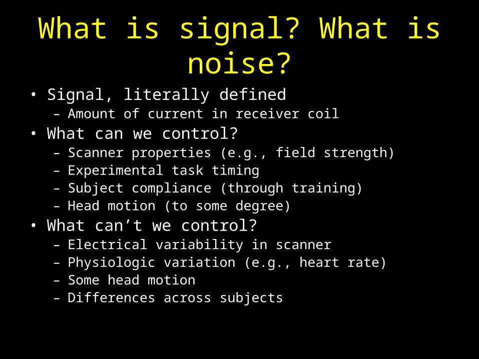
What is signal? What is noise?

• Signal, literally defined– Amount of current in receiver coil

• What can we control?– Scanner properties (e.g., field strength)– Experimental task timing– Subject compliance (through training)– Head motion (to some degree)

• What can’t we control?– Electrical variability in scanner– Physiologic variation (e.g., heart rate)– Some head motion– Differences across subjects

I. Introduction to SNR

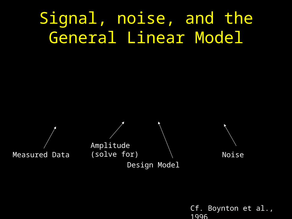
Signal, noise, and the General Linear Model

MYMeasured Data

Amplitude (solve for)

Design Model

Noise

Cf. Boynton et al., 1996

Signal-Noise-Ratio (SNR)

Task-Related Variability

Non-task-related Variability

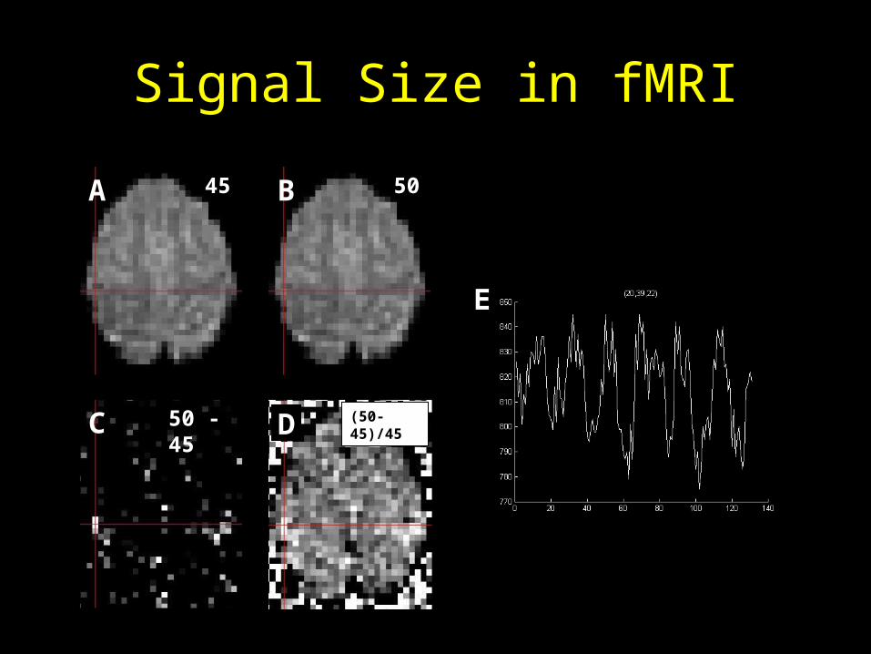
Signal Size in fMRI

45 50

50 - 45

A B

C

E

(50-45)/45D

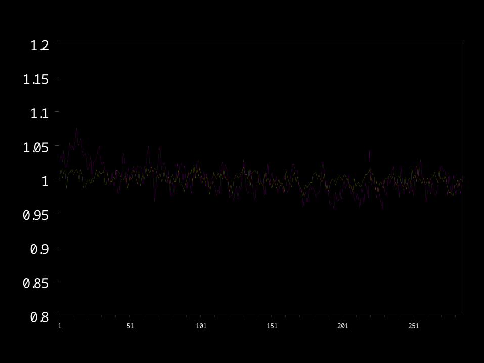
0.8

0.85

0.9

0.95

1

1.05

1.1

1.15

1.2

1 51 101 151 201 251

0.8

0.85

0.9

0.95

1

1.05

1.1

1.15

1.2

1 51 101 151 201 251

Differences in SNR

Voxel 3

Voxel 2

Voxel 1

690 730 770

790 830 870

770 810 850

t = 16

t = 8 t = 5

A

B C

Effects of SNR: Simulation Data

• Hemodynamic response– Unit amplitude– Flat prestimulus baseline

• Gaussian Noise– Temporally uncorrelated (white)– Noise assumed to be constant over epoch

• SNR varied across simulations– Max: 2.0, Min: 0.125

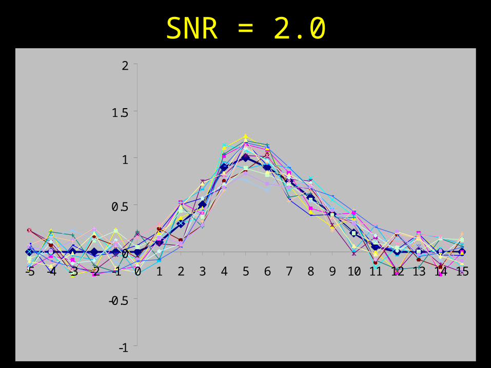
SNR = 2.0

-1

-0.5

0

0.5

1

1.5

2

-5 -4 -3 -2 -1 0 1 2 3 4 5 6 7 8 9 10 11 12 13 14 15

SNR = 1.0

-1

-0.5

0

0.5

1

1.5

2

-5 -4 -3 -2 -1 0 1 2 3 4 5 6 7 8 9 10 11 12 13 14 15

SNR = 0.5

-1

-0.5

0

0.5

1

1.5

2

-5 -4 -3 -2 -1 0 1 2 3 4 5 6 7 8 9 10 11 12 13 14 15

SNR = 0.25

-3

-2

-1

0

1

2

3

4

-5 -4 -3 -2 -1 0 1 2 3 4 5 6 7 8 9 10 11 12 13 14 15

SNR = 0.125

-5

-4

-3

-2

-1

0

1

2

3

4

5

6

-5 -4 -3 -2 -1 0 1 2 3 4 5 6 7 8 9 10 11 12 13 14 15

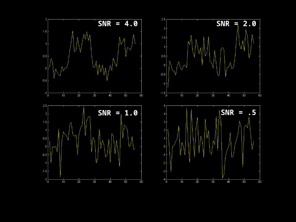
SNR = 4.0 SNR = 2.0

SNR = 1.0 SNR = .5

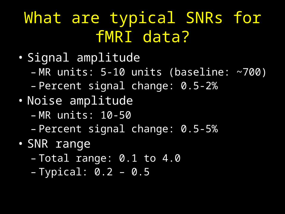
What are typical SNRs for fMRI data?

• Signal amplitude– MR units: 5-10 units (baseline: ~700)– Percent signal change: 0.5-2%

• Noise amplitude– MR units: 10-50– Percent signal change: 0.5-5%

• SNR range– Total range: 0.1 to 4.0 – Typical: 0.2 – 0.5

Effects of Field Strength on SNR

Turner et al., 1993

Theoretical Effects of Field Strength

• SNR = signal / noise• SNR increases linearly with field strength

– Signal increases with square of field strength– Noise increases linearly with field strength– A 4.0T scanner should have 2.7x SNR of 1.5T

scanner

• T1 and T2* both change with field strength– T1 increases, reducing signal recovery– T2* decreases, increasing BOLD contrast

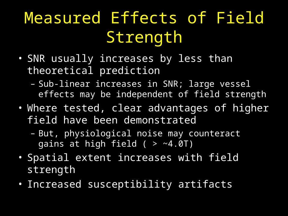
Measured Effects of Field Strength

• SNR usually increases by less than theoretical prediction– Sub-linear increases in SNR; large vessel effects may

be independent of field strength

• Where tested, clear advantages of higher field have been demonstrated– But, physiological noise may counteract gains at high

field ( > ~4.0T)

• Spatial extent increases with field strength• Increased susceptibility artifacts

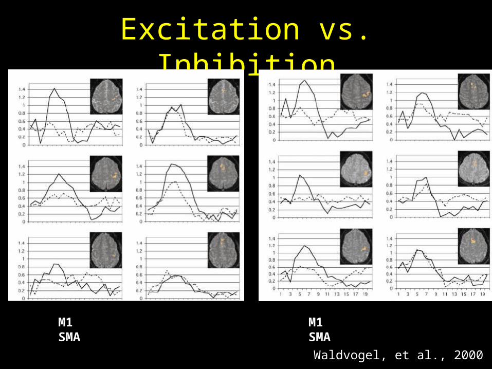
Excitation vs. Inhibition

M1 SMA M1 SMA

Waldvogel, et al., 2000

II. Properties of Noise in fMRI

Can we assume Gaussian noise?

Types of Noise

• Thermal noise– Responsible for variation in background– Eddy currents, scanner heating

• Power fluctuations– Typically caused by scanner problems

• Variation in subject cognition– Timing of processes

• Head motion effects• Physiological changes• Differences across brain regions

– Functional differences– Large vessel effects

• Artifact-induced problems

Why is noise assumed to be Gaussian?

• Central limit theorem

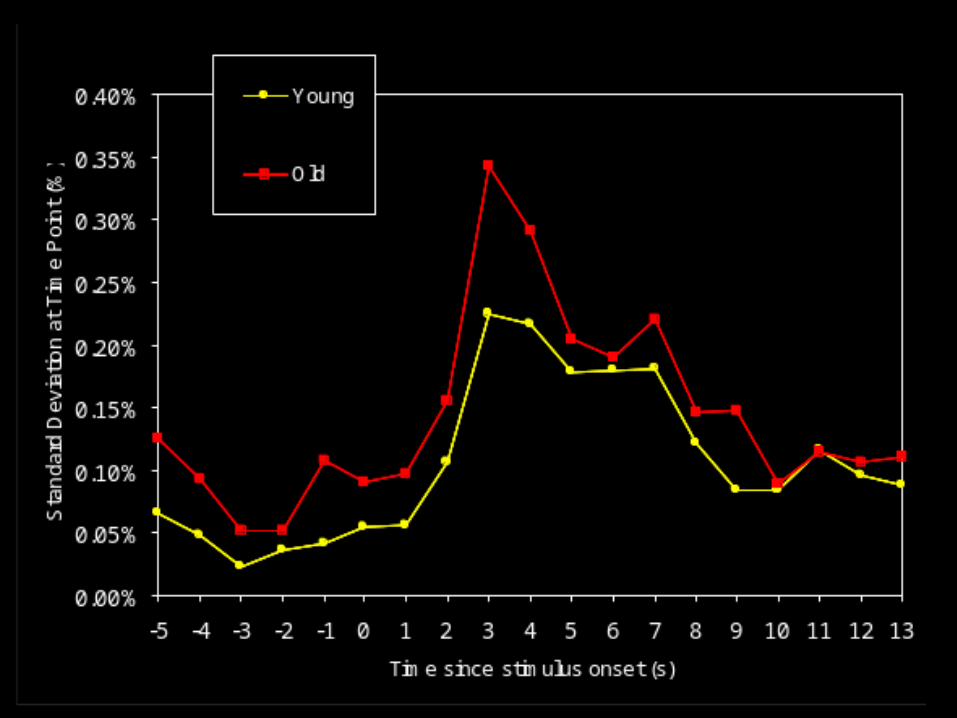
Is noise constant through time?

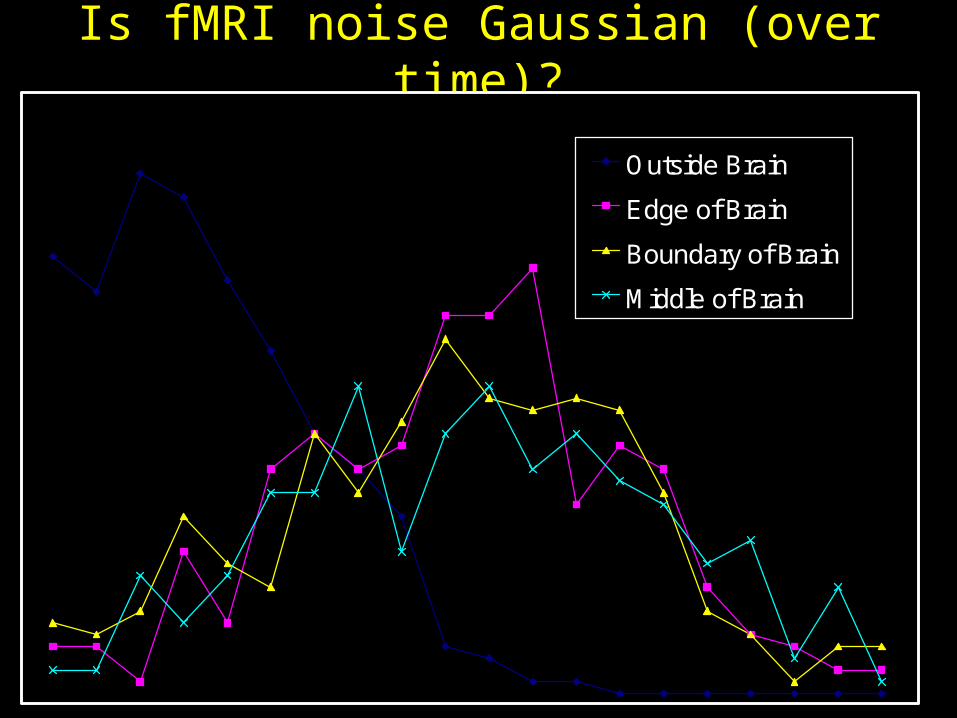
Is fMRI noise Gaussian (over time)?

Outside Brain

Edge of Brain

Boundary of Brain

Middle of Brain

Is Signal Gaussian (over voxels)?

Variability

Variability in Subject Behavior: Issues

• Cognitive processes are not static– May take time to engage– Often variable across trials– Subjects’ attention/arousal wax and wane

• Subjects adopt different strategies– Feedback- or sequence-based– Problem-solving methods

• Subjects engage in non-task cognition– Non-task periods do not have the absence of thinking

What can we do about these problems?

Response Time Variability

A B

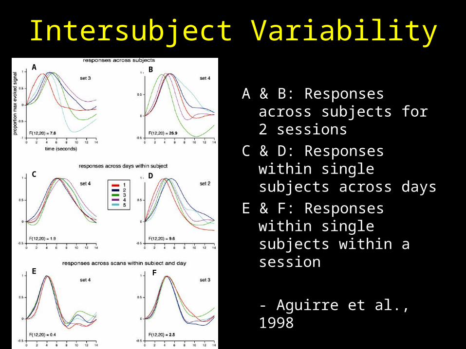
Intersubject Variability

A & B: Responses across subjects for 2 sessions

C & D: Responses within single subjects across days

E & F: Responses within single subjects within a session

- Aguirre et al., 1998

BA

C D

E F

Variability Across Subjects

D’Esposito et al., 1999

Young Adults

Elderly Adults

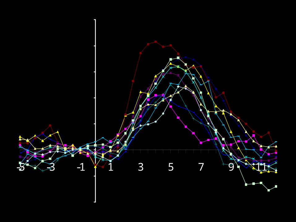
-5 -3 -1 1 3 5 7 9 11

-5 -3 -1 1 3 5 7 9 11

Effects of Intersubject Variability

Parrish et al., 2000

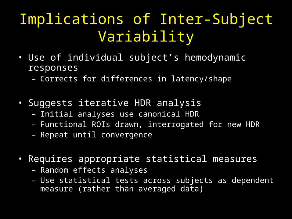
Implications of Inter-Subject Variability

• Use of individual subject’s hemodynamic responses– Corrects for differences in latency/shape

• Suggests iterative HDR analysis– Initial analyses use canonical HDR– Functional ROIs drawn, interrogated for new HDR– Repeat until convergence

• Requires appropriate statistical measures– Random effects analyses – Use statistical tests across subjects as dependent measure

(rather than averaged data)

Spatial Variability?

A B

McGonigle et al., 2000

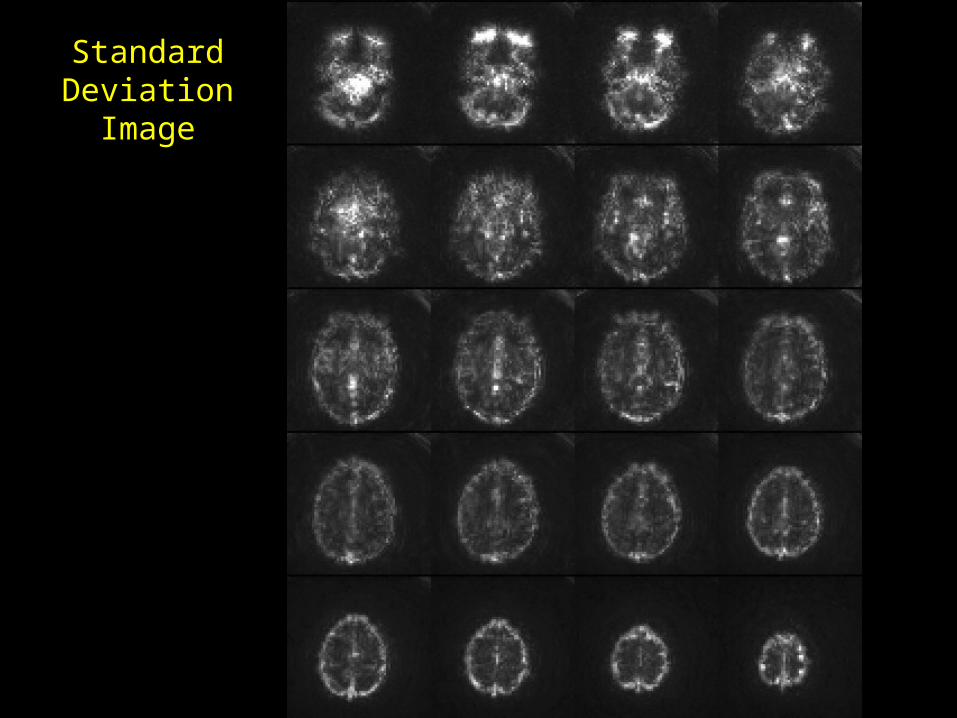
Standard Deviation Image

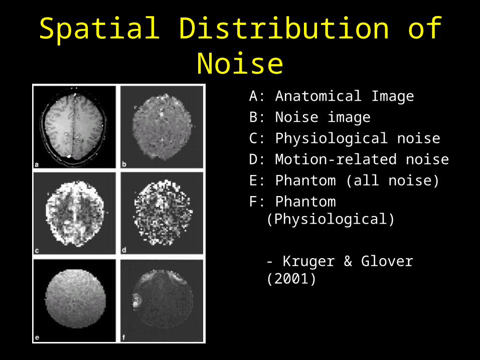
Spatial Distribution of Noise

A: Anatomical Image

B: Noise image

C: Physiological noise

D: Motion-related noise

E: Phantom (all noise)

F: Phantom (Physiological)

- Kruger & Glover (2001)

960

970

980

990

1000

1010

1020

1030

1040

1050

1 51 101 151 201 251

Low Frequency Noise

650

660

670

680

690

700

710

720

730

740

750

1 51 101 151 201

High Frequency Noise

-2

-1.5

-1

-0.5

0

0.5

1

1.5

2

III. Methods for Improving SNR

Fundamental Rule of SNR

For Gaussian noise, experimental power increases with the square root of the

number of observations

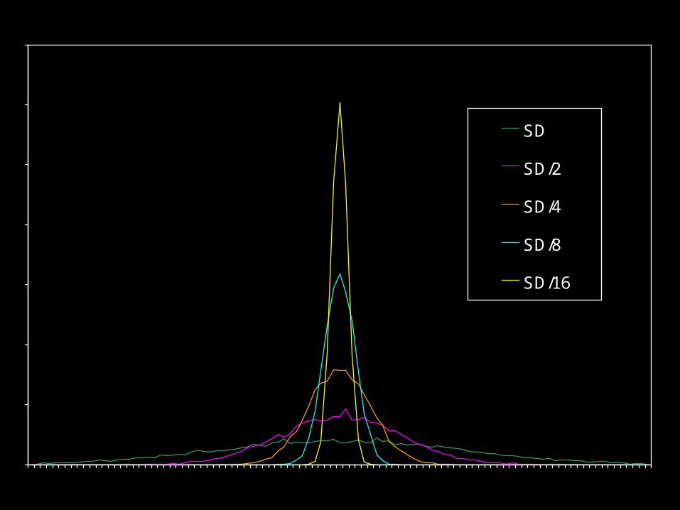
SD

SD/2

SD/4

SD/8

SD/16

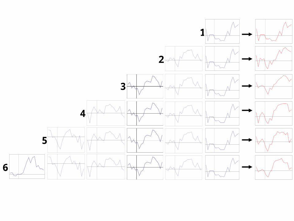
Trial Averaging

• Static signal, variable noise– Assumes that the MR data recorded on each trial are

composed of a signal + (random) noise

• Effects of averaging– Signal is present on every trial, so it remains constant

through averaging– Noise randomly varies across trials, so it decreases

with averaging– Thus, SNR increases with averaging

-0.4

-0.2

0

0.2

0.4

0.6

0.8

1

1.2

1.4

-5 -4 -3 -2 -1 0 1 2 3 4 5 6 7 8 9 10 11 12 13 14 15

Example of Trial Averaging-1.5

-1

-0.5

0

0.5

1

1.5

-5 -4 -3 -2 -1 0 1 2 3 4 5 6 7 8 9 10 11 12 13 14 15

-1

-0.5

0

0.5

1

1.5

2

2.5

-5 -4 -3 -2 -1 0 1 2 3 4 5 6 7 8 9 10 11 12 13 14 15

-1.5

-1

-0.5

0

0.5

1

1.5

-5 -4 -3 -2 -1 0 1 2 3 4 5 6 7 8 9 10 11 12 13 14 15

-1.5

-1

-0.5

0

0.5

1

1.5

2

-5 -4 -3 -2 -1 0 1 2 3 4 5 6 7 8 9 10 11 12 13 14 15

Average of 16 trials with SNR = 0.6

1

2

3

4

5

6

Increasing Power increases Spatial Extent

Subject 1 Subject 2Trials Averaged

4

16

36

64

100

144

500 ms

16-20 s

500 ms

…

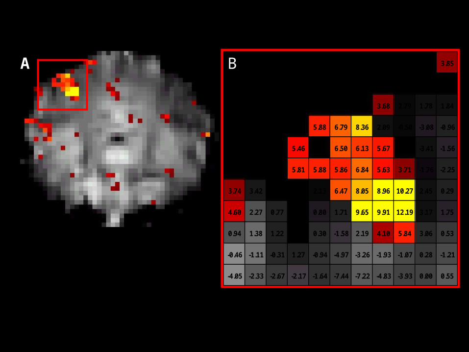
0.00 0.00 0.00 0.00 0.00 0.00 0.00 0.00 0.00 0.00 3.85

0.00 0.00 0.00 0.00 0.00 0.00 0.00 0.00 0.00 2.44 2.41

0.00 0.00 0.00 0.00 0.00 0.00 3.36 3.68 2.79 1.78 1.84

0.00 0.00 0.00 0.00 5.88 6.79 8.36 2.09 -0.50 -3.08 -0.96

0.00 0.00 3.20 5.46 2.00 6.50 6.13 5.67 -0.06 -3.41 -1.56

2.66 2.42 0.01 5.81 5.88 5.86 6.84 5.63 3.71 -1.76 -2.25

3.74 3.42 1.43 0.68 2.13 6.47 8.05 8.96 10.27 2.45 0.29

4.60 2.27 0.77 1.41 0.80 1.71 9.65 9.91 12.19 3.17 1.75

0.94 1.38 1.22 2.96 0.30 -1.58 2.19 4.10 5.84 3.06 0.53

-0.46 -1.11 -0.31 1.27 -0.94 -4.97 -3.26 -1.93 -1.07 0.28 -1.21

-4.05 -2.33 -2.67 -2.17 -1.64 -7.44 -7.22 -4.83 -3.93 0.00 0.55

A B

0

10

20

30

40

50

60

70

80

90

100

0 25 50 75 100 125 150 175 200

Peak latency of reference HDR

4 sec 5 sec 6 sec 4 sec 5 sec 6 sec

Vmax 89 96 72 25 80 98

Correlation of data with prediction

0.997 0.995 0.993 0.960 0.994 0.998

Subject1 Subject 2

Number of Trials Averaged

Num

ber

of S

igni

fica

nt V

oxel

s Subject 1

Subject 2

VN = Vmax[1 - e(-0.016 * N)]

Effects of Signal-Noise Ratio on extent of activation: Empirical Data

Active Voxel Simulation

Signal + Noise (SNR = 1.0)

Noise1000 Voxels, 100 Active

-2

-1.5

-1

-0.5

0

0.5

1

1.5

2

1 3 5 7 9

11

13

15

17

19

-2

-1.5

-1

-0.5

0

0.5

1

1.5

2

1 3 5 7 9

11

13

15

17

19

-2

-1.5

-1

-0.5

0

0.5

1

1.5

2

1 3 5 7 9

11

13

15

17

19

-2

-1.5

-1

-0.5

0

0.5

1

1.5

2

1 3 5 7 9

11

13

15

17

19

• Signal waveform taken from observed data.

• Signal amplitude distribution: Gamma (observed).

• Assumed Gaussian white noise.

Effects of Signal-Noise Ratio on extent of activation:

Simulation Data

0

20

40

60

80

100

120

0 50 100 150 200

SNR = 0.10

SNR = 0.15

SNR = 0.25

SNR = 1.00

SNR = 0.52 (Young)

SNR = 0.35 (Old)

Number of Trials Averaged

Num

ber

of A

ctiv

ated

Vox

els

Old (66 trials) Young (70 trials) Ratio (Y/O)Observed 26 53 2.0Predicted 57% 97% 1.7

Explicit and Implicit Signal Averaging

r =.42; t(129) = 5.3; p < .0001

r =.82; t(10) = 4.3; p < .001

A

B

Caveats

• Signal averaging is based on assumptions– Data = signal + temporally invariant noise– Noise is uncorrelated over time

• If assumptions are violated, then averaging ignores potentially valuable information– Amount of noise varies over time– Some noise is temporally correlated (physiology)

• Nevertheless, averaging provides robust, reliable method for determining brain activity

Accurate Temporal Sampling

Visual HDR sampled with a 1-sec TR

0.13%

0.01%-0.02%

-0.08%

-0.04%

-0.18%

-0.12%

-0.18%

0.29%

0.53%

0.71%

0.60%

0.44%

0.34%

0.24%

0.16%

0.02%

-0.04%-0.07%

-0.20%

-0.10%

0.00%

0.10%

0.20%

0.30%

0.40%

0.50%

0.60%

0.70%

0.80%

-5 -4 -3 -2 -1 0 1 2 3 4 5 6 7 8 9 10 11 12 13

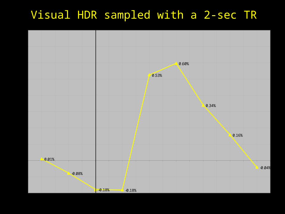
Visual HDR sampled with a 2-sec TR

0.01%

-0.08%

-0.18% -0.18%

0.53%

0.60%

0.34%

0.16%

-0.04%

-0.20%

-0.10%

0.00%

0.10%

0.20%

0.30%

0.40%

0.50%

0.60%

0.70%

0.80%

-5 -4 -3 -2 -1 0 1 2 3 4 5 6 7 8 9 10 11 12 13

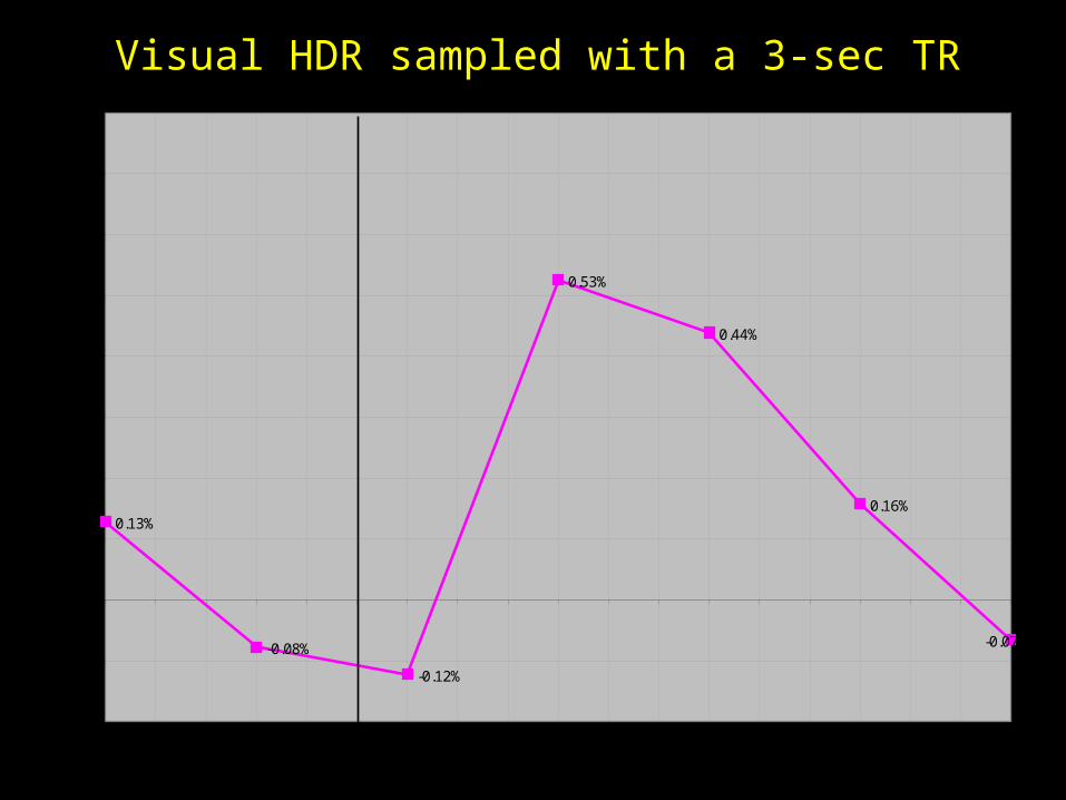
Visual HDR sampled with a 3-sec TR

0.13%

-0.08%

-0.12%

0.53%

0.44%

0.16%

-0.07%

-0.20%

-0.10%

0.00%

0.10%

0.20%

0.30%

0.40%

0.50%

0.60%

0.70%

0.80%

-5 -4 -3 -2 -1 0 1 2 3 4 5 6 7 8 9 10 11 12 13

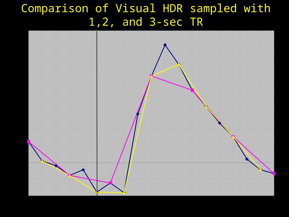
Comparison of Visual HDR sampled with 1,2, and 3-sec TR

-0.20%

-0.10%

0.00%

0.10%

0.20%

0.30%

0.40%

0.50%

0.60%

0.70%

0.80%

-5 -4 -3 -2 -1 0 1 2 3 4 5 6 7 8 9 10 11 12 13

Visual HDRs with 10% diff sampled with a 1-sec TR

-0.20%

-0.10%

0.00%

0.10%

0.20%

0.30%

0.40%

0.50%

0.60%

0.70%

0.80%

-5 -4 -3 -2 -1 0 1 2 3 4 5 6 7 8 9 10 11 12 13

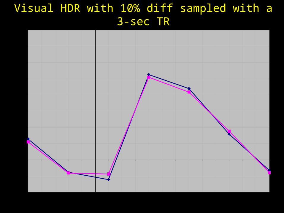
Visual HDR with 10% diff sampled with a 3-sec TR

-0.20%

-0.10%

0.00%

0.10%

0.20%

0.30%

0.40%

0.50%

0.60%

0.70%

0.80%

-5 -4 -3 -2 -1 0 1 2 3 4 5 6 7 8 9 10 11 12 13

Accurate Spatial Sampling

Partial Volume Effects

Partial Volume Effects

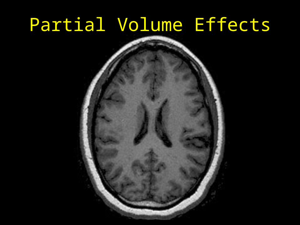
Partial Volume Effects

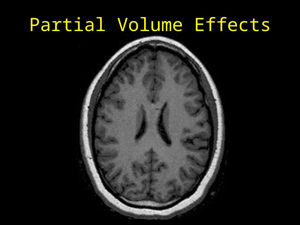
Partial Volume Effects

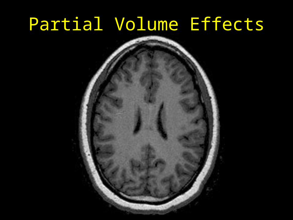
Partial Volume Effects

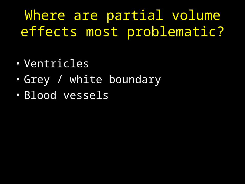
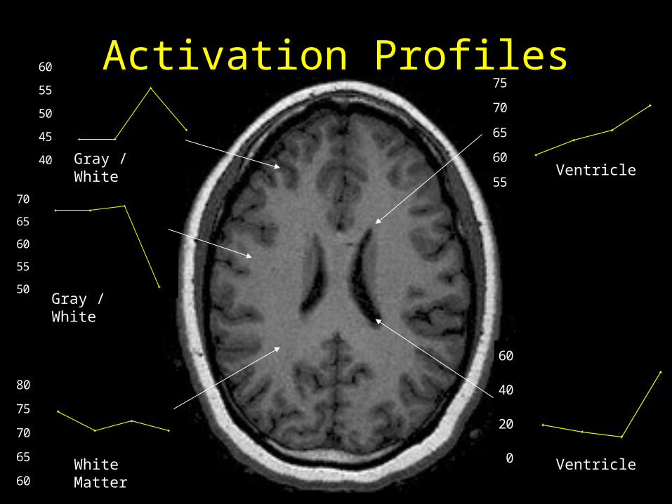
Where are partial volume effects most problematic?

• Ventricles

• Grey / white boundary

• Blood vessels

55

60

65

70

75

0

20

40

60

60

65

70

75

80

50

55

60

65

70

40

45

50

55

60 Activation Profiles

White Matter

Gray / White

Gray / WhiteVentricle

Ventricle

Temporal Filtering

Filtering Approaches

• Identify unwanted frequency variation– Drift (low-frequency)– Physiology (high-frequency)– Task overlap (high-frequency)

• Reduce power around those frequencies through application of filters

• Potential problem: removal of frequencies composing response of interest

Power Spectra

A B