Embed Size (px)
Citation preview
Antennas
© Amanogawa, 2006 – Digital Maestro Series 64
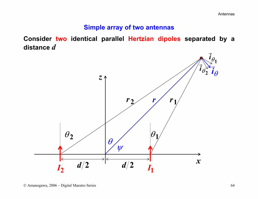
Simple array of two antennas
Consider two identical parallel Hertzian dipoles separated by a distance d
I1I2
z
x
1θ2θ θ
r1r 2 r
d 2 d 2
iθ
i1θ
i2θ
ψ
Antennas
© Amanogawa, 2006 – Digital Maestro Series 65
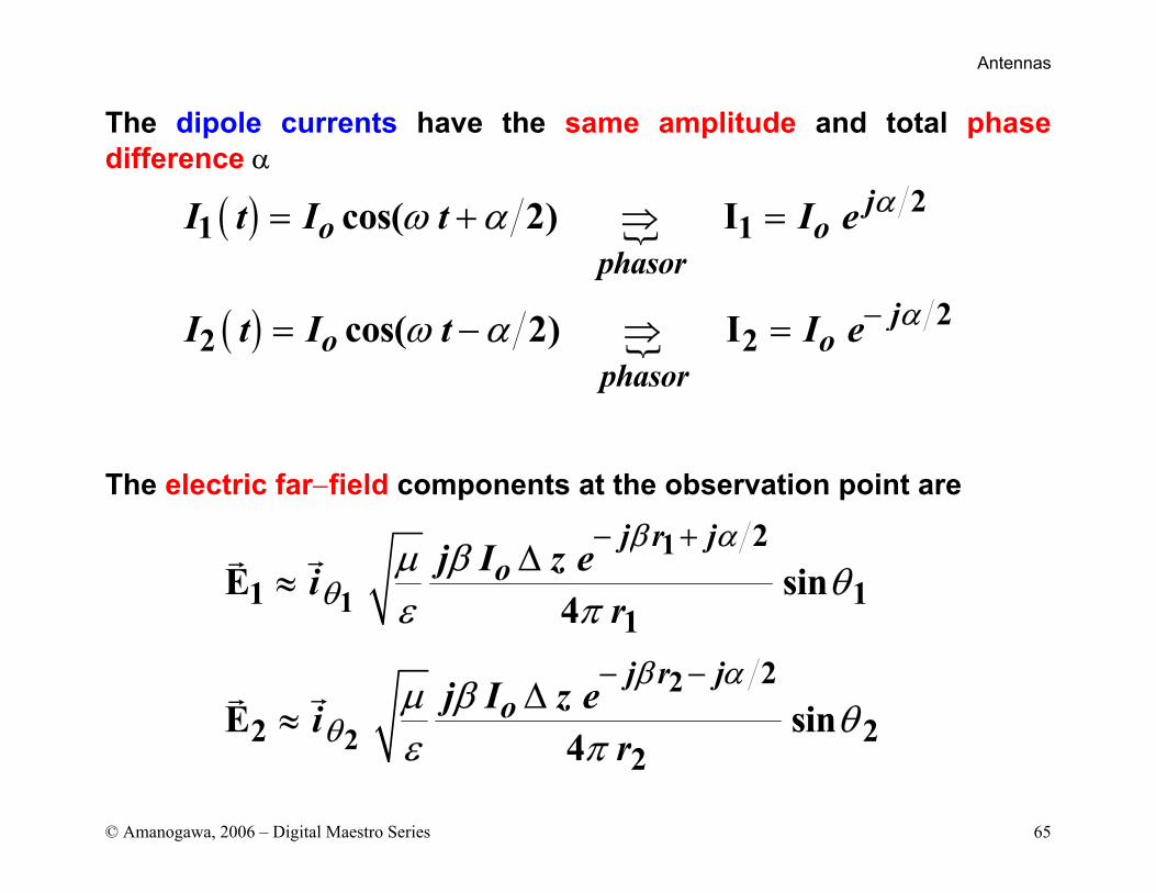
The dipole currents have the same amplitude and total phase difference α
The electric far−field components at the observation point are
( )
( )
21 1
22 2
cos( 2) I
cos( 2) I
jo o
phasorj
o ophasor
I t I t I e
I t I t I e
α
α
ω α
ω α −
= + ⇒ =
= − ⇒ =
j r jo
j r jo
j I z eir
j I z eir
1
1
2
2
2
1 11
2
2 22
E sin4
E sin4
β α
θ
β α
θ
µ β θε π
µ β θε π
− +
− −
∆≈
∆≈
Antennas
© Amanogawa, 2006 – Digital Maestro Series 66
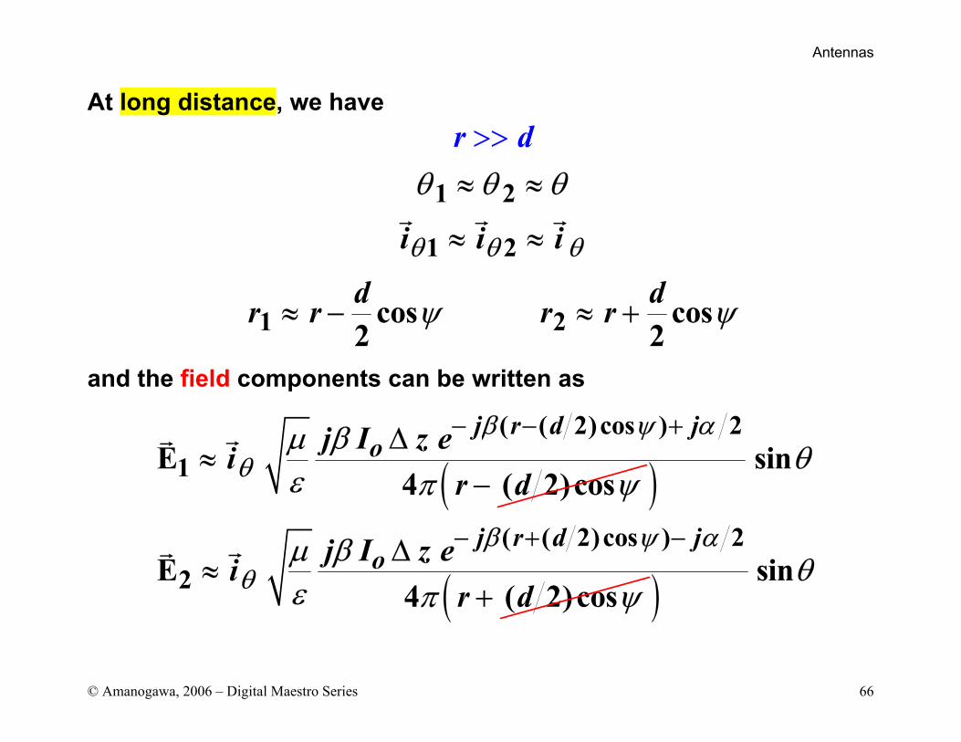
At long distance, we have
and the field components can be written as
1 2
1 2
1 2cos cos2 2
i i i
d dr r
d
r
r
r
θ θ θ
θ θ θ
ψ ψ
≈ ≈
≈ ≈
≈ − ≈ +
>>
j r d joj I z ei
r d
( ( 2)cos ) 21E
4 ( 2)cos
β ψ αθ
µ βε π ψ
− − +∆≈
−( )j r d j
oj I z eir d
( ( 2)cos ) 22
sin
E4 ( 2)cos
β ψ αθ
θ
µ βε π ψ
− + −∆≈
+( ) sinθ
Antennas
© Amanogawa, 2006 – Digital Maestro Series 67
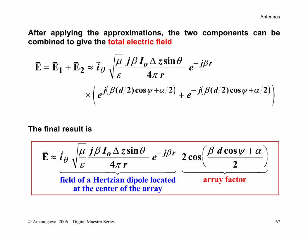
After applying the approximations, the two components can be combined to give the total electric field
The final result is
( ) ( )( )j ro
j d j d
j I zi er
e e
1 2
( 2)cos 2 ( 2)cos 2
sinE E E4
βθ
β ψ α β ψ α
µ β θε π
−
+ − +
∆= + ≈
× +
j roj I z di er
field of a Hertzian dipole locatedat the center of the arra
array y
factor
sin cosE 2 cos4 2
βθ
µ β θ β ψ αε π
−∆ + ≈
Antennas
© Amanogawa, 2006 – Digital Maestro Series 68
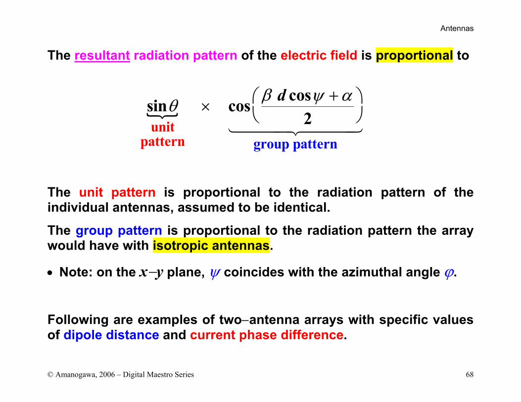
The resultant radiation pattern of the electric field is proportional to
The unit pattern is proportional to the radiation pattern of the individual antennas, assumed to be identical.
The group pattern is proportional to the radiation pattern the array would have with isotropic antennas.
• Note: on the x−y plane, ψ coincides with the azimuthal angle ϕ.
Following are examples of two−antenna arrays with specific values of dipole distance and current phase difference.
d
group patterunit
patt rn ne
cossin cos2
β ψ αθ + ×
Antennas
© Amanogawa, 2006 – Digital Maestro Series 69
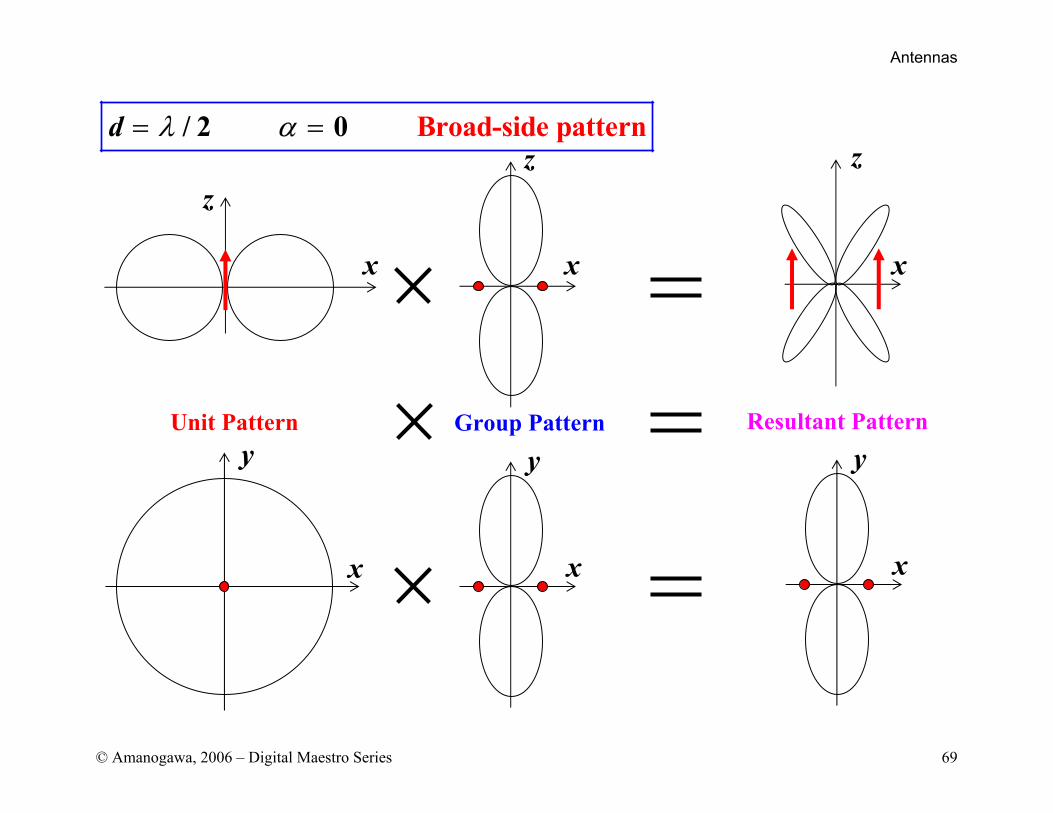
Broad-side / p2 e0 att rnd λ α= =
z
x x
z
x
y
x
yUnit Pattern Group Pattern
x
yResultant Pattern
x
z
Antennas
© Amanogawa, 2006 – Digital Maestro Series 70
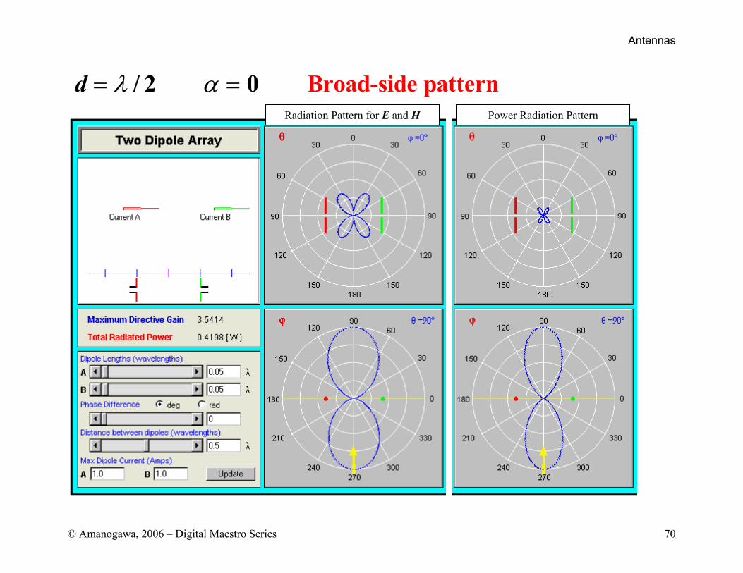
d Broad-side p/ rn0 t2 at eλ α= =Radiation Pattern for E and H Power Radiation Pattern
Antennas
© Amanogawa, 2006 – Digital Maestro Series 71
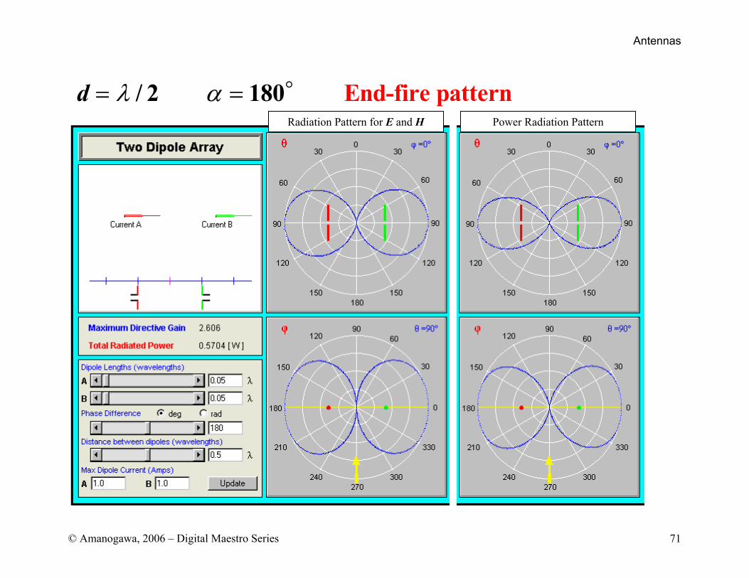
d End-fir/ 2 1 e pattern80λ α= =Radiation Pattern for E and H Power Radiation Pattern
Antennas
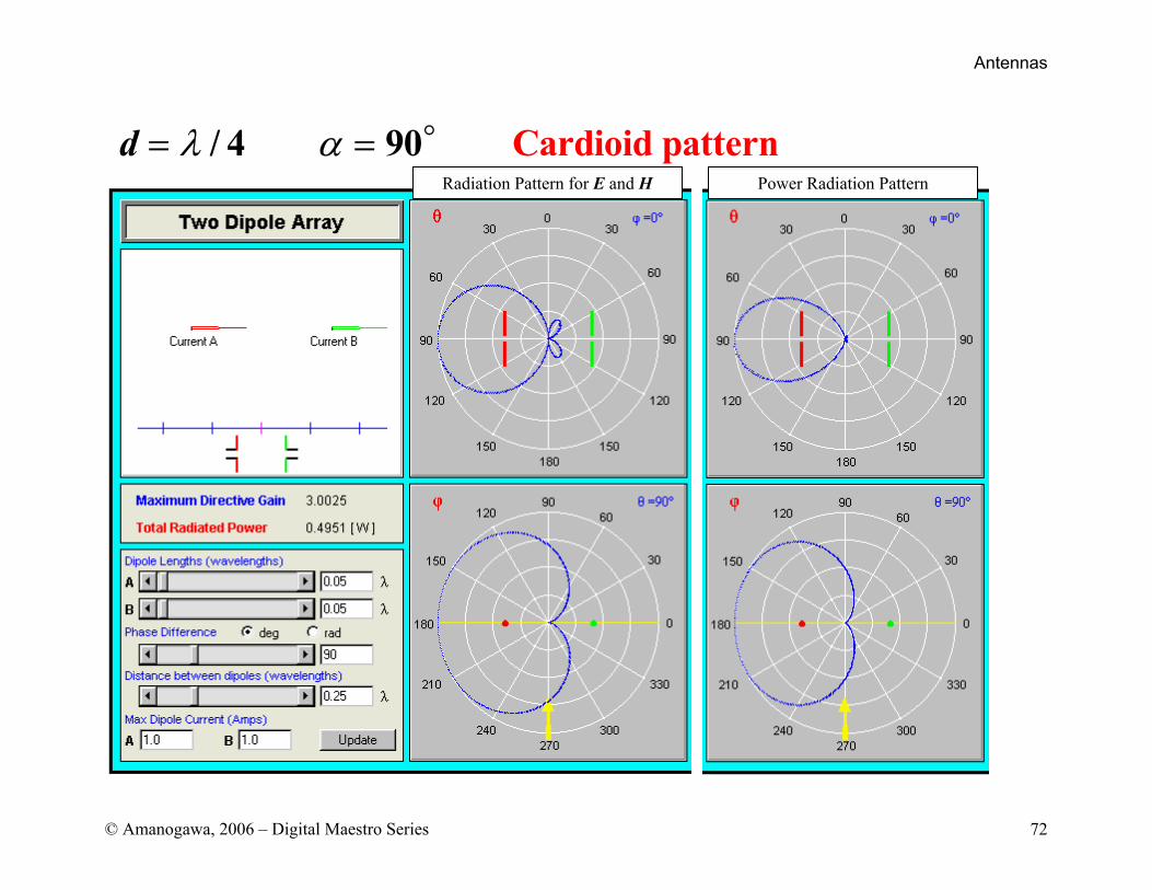
© Amanogawa, 2006 – Digital Maestro Series 72
d Cardioid/ 4 90 patternλ α= =Radiation Pattern for E and H Power Radiation Pattern
Antennas
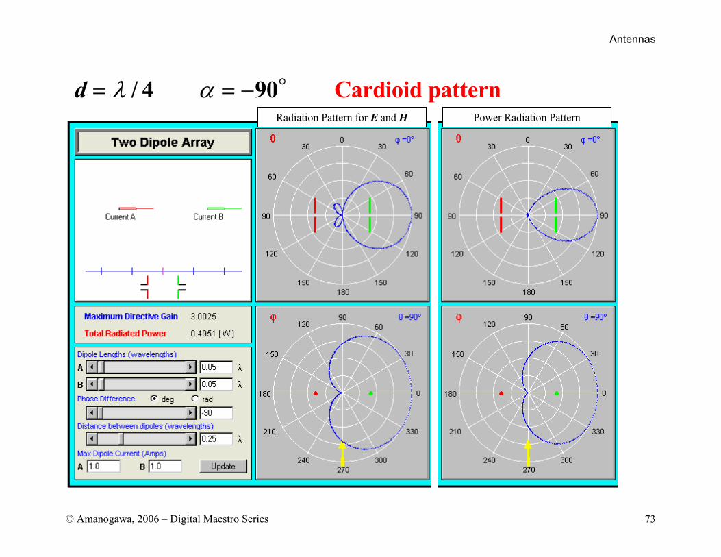
© Amanogawa, 2006 – Digital Maestro Series 73
d Cardioid patter4 9 n/ 0λ α= = −Radiation Pattern for E and H Power Radiation Pattern
Antennas
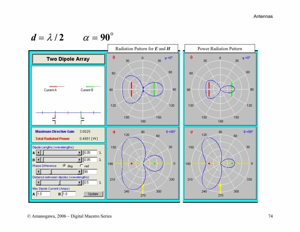
© Amanogawa, 2006 – Digital Maestro Series 74
d / 2 90λ α= =Radiation Pattern for E and H Power Radiation Pattern
Antennas
© Amanogawa, 2006 – Digital Maestro Series 75
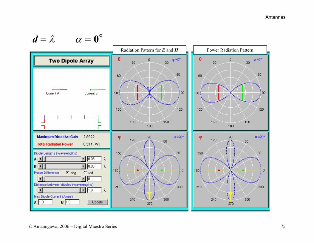
d 0λ α= =Radiation Pattern for E and H Power Radiation Pattern
Antennas
© Amanogawa, 2006 – Digital Maestro Series 76
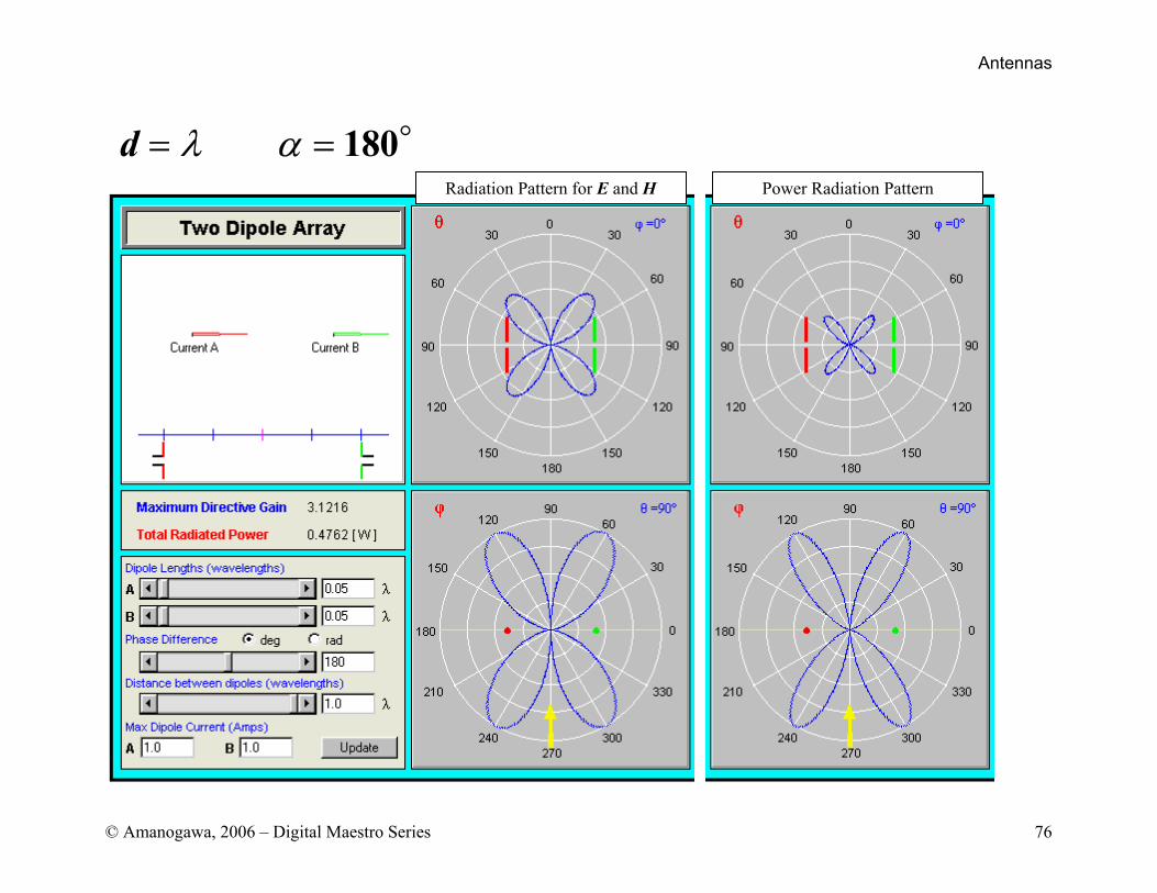
d 180λ α= =Radiation Pattern for E and H Power Radiation Pattern
Antennas
© Amanogawa, 2006 – Digital Maestro Series 77
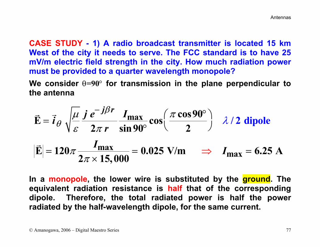
CASE STUDY - 1) A radio broadcast transmitter is located 15 km West of the city it needs to serve. The FCC standard is to have 25 mV/m electric field strength in the city. How much radiation power must be provided to a quarter wavelength monopole? We consider θ=90° for transmission in the plane perpendicular to the antenna
In a monopole, the lower wire is substituted by the ground. The equivalent radiation resistance is half that of the corresponding dipole. Therefore, the total radiated power is half the power radiated by the half-wavelength dipole, for the same current.
max
maxmax
/ 2 dipolecos90E cos2 sin90 2
E 120 0.025 V/m 6.25 A2 15, 000
j rj e Iir
I I
βθ λµ π
ε π
ππ
− ° = °
= =×
⇒=
Antennas
© Amanogawa, 2006 – Digital Maestro Series 78
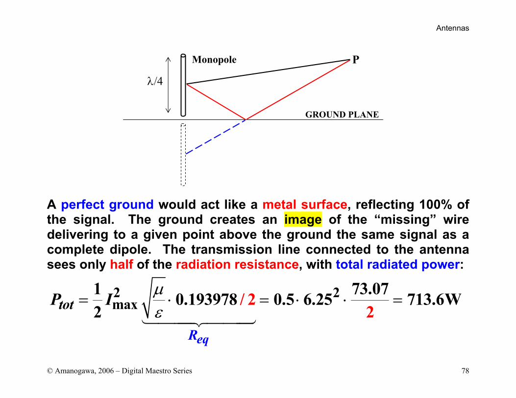
A perfect ground would act like a metal surface, reflecting 100% of the signal. The ground creates an image of the “missing” wire delivering to a given point above the ground the same signal as a complete dipole. The transmission line connected to the antenna sees only half of the radiation resistance, with total radiated power:
2 2max
1 73.070.193978 0.5 6.25 713.622
W2
/
eqR
totP I µε
= ⋅ = ⋅ ⋅ =
P
GROUND PLANE
Monopole
λ/4
Antennas
© Amanogawa, 2006 – Digital Maestro Series 79
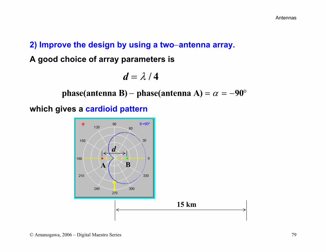
2) Improve the design by using a two−antenna array.
A good choice of array parameters is
which gives a cardioid pattern
dphase(antenna B) phase(antenna A) 90
/ 4 α
λ− = = − °
=
15 km
BA
d
Antennas
© Amanogawa, 2006 – Digital Maestro Series 80
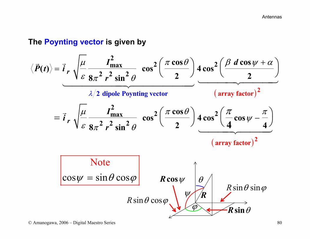
The Poynting vector is given by
( )
( )
r
r
I dP t i
r
Ii
r
2
2
2 dipole Poynting vecto array factor
array fa
22 2max
2 2 2
22 2max
ct
2
r
r
o
2 2
cos cos( ) cos 4 cos
2 28 sin
coscos 4 cos cos
2 48 sin 4
λ
µ π θ β ψ α
ε π θ
µ π θ πψ
ε π θ
π
+=
−
=
θ
ϕψ R
sinR θsin cosR θ ϕ
cosR ψ
Nocos sin cos
teψ θ ϕ=
sin sinR θ ϕ
Antennas
© Amanogawa, 2006 – Digital Maestro Series 81
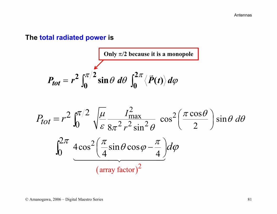
The total radiated power is
2 220 0
sin ( )totP r d P t dπ πθ θ ϕ= ∫ ∫
Only π/2 because it is a monopole
( )2
22max
2 2 2
array facto
2
r
2 cos2 cos sin0 28 sin2
4cos0 4sin cos
4
I dtotr
P r
d
π µ π θ θ θε π θ
π ππ θ ϕ ϕ
−
= ∫
∫
Antennas
© Amanogawa, 2006 – Digital Maestro Series 82
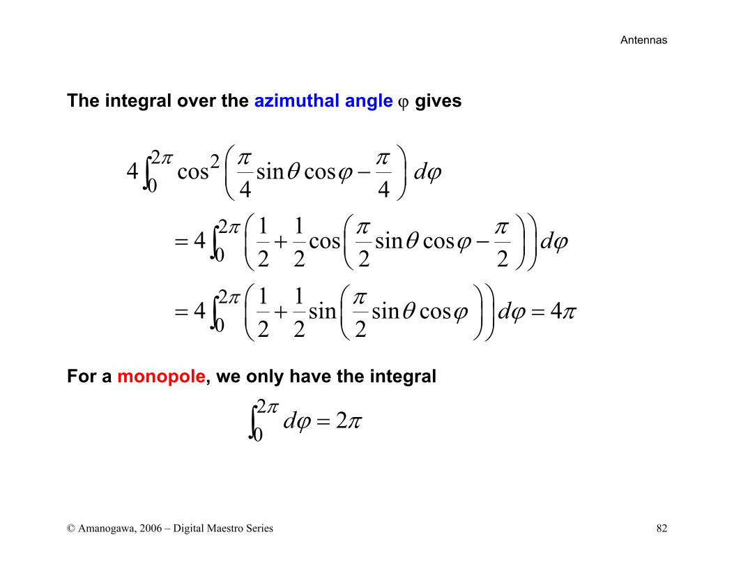
The integral over the azimuthal angle ϕ gives
For a monopole, we only have the integral
2 20
20
20
4 cos sin cos4 4
1 14 cos sin cos2 2 2 21 14 sin sin cos 42 2 2
d
d
d
π
π
π
π πθ ϕ ϕ
π πθ ϕ ϕ
π θ ϕ ϕ π
− = + − = + =
∫
∫
∫
20 2dπ ϕ π=∫
Antennas
© Amanogawa, 2006 – Digital Maestro Series 83
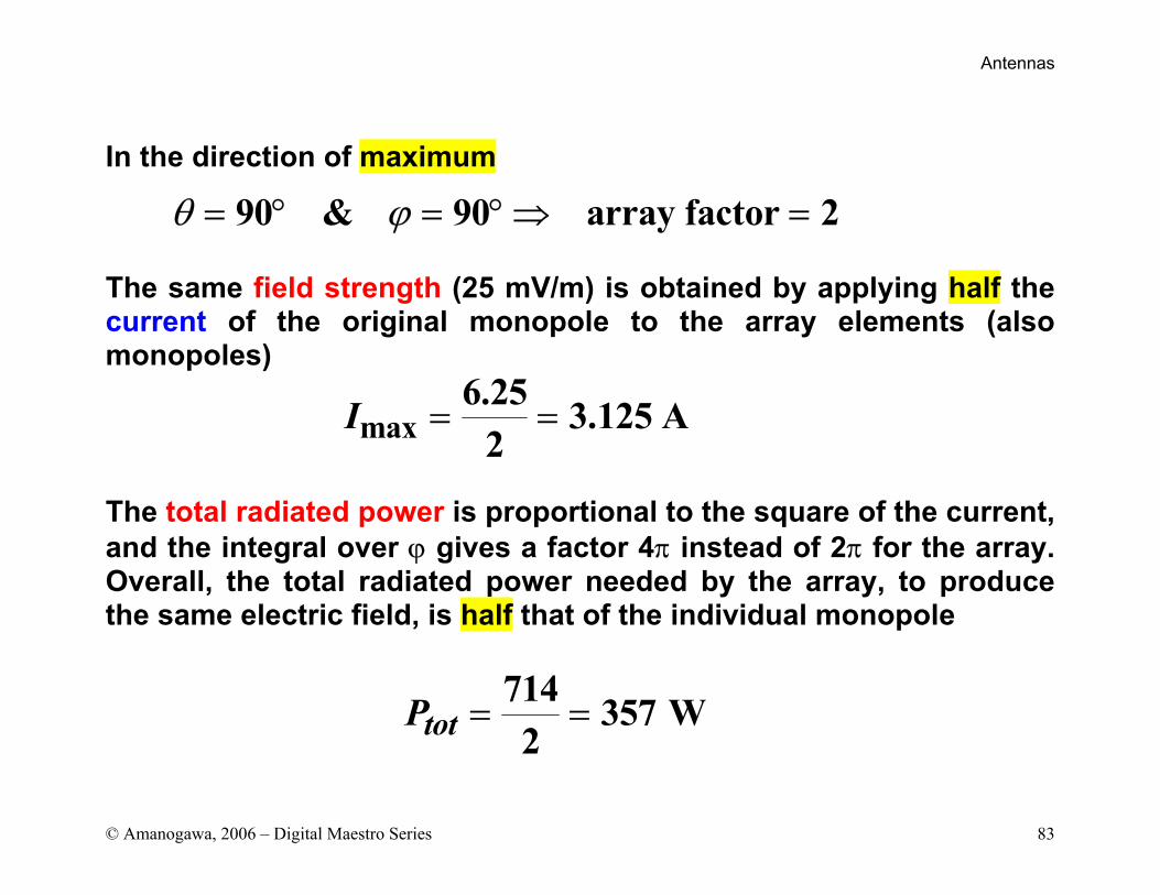
In the direction of maximum
The same field strength (25 mV/m) is obtained by applying half the current of the original monopole to the array elements (also monopoles)
The total radiated power is proportional to the square of the current, and the integral over ϕ gives a factor 4π instead of 2π for the array. Overall, the total radiated power needed by the array, to produce the same electric field, is half that of the individual monopole
90 & 90 array factor 2θ ϕ= ° = °⇒ =
max6.25 3.125 A
2I = =
714 357 W2totP = =
Antennas
© Amanogawa, 2006 – Digital Maestro Series 84
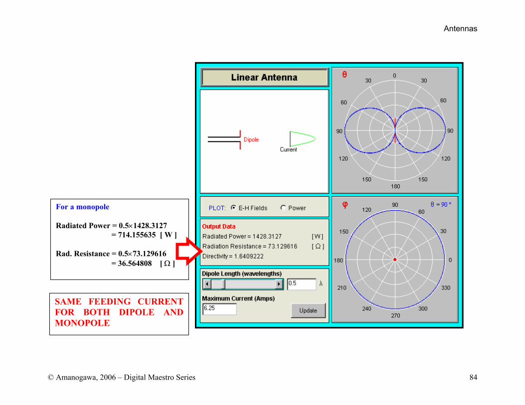
For a monopole Radiated Power = 0.5×1428.3127 = 714.155635 [ W ] Rad. Resistance = 0.5×73.129616 = 36.564808 [ Ω ]
SAME FEEDING CURRENT FOR BOTH DIPOLE AND MONOPOLE
Antennas
© Amanogawa, 2006 – Digital Maestro Series 85
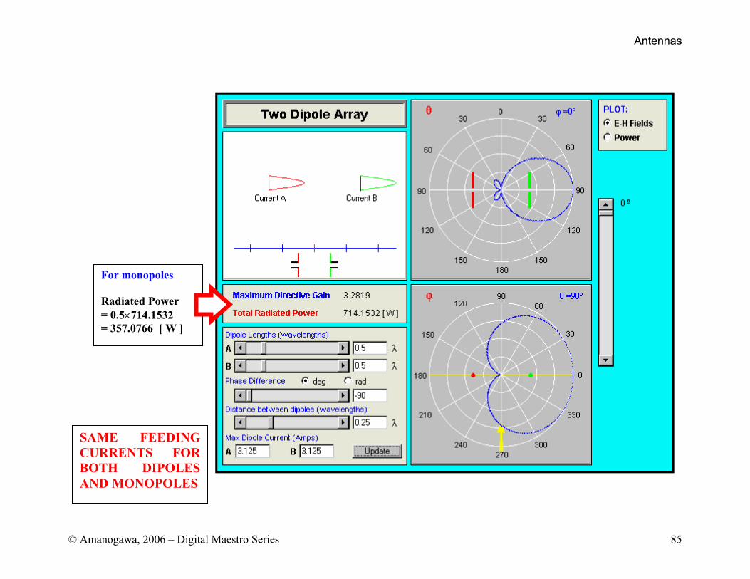
For monopoles Radiated Power = 0.5×714.1532 = 357.0766 [ W ]
SAME FEEDING CURRENTS FOR BOTH DIPOLES AND MONOPOLES
Antennas
© Amanogawa, 2006 – Digital Maestro Series 86
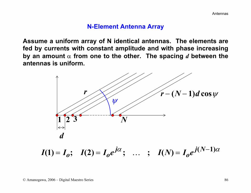
N-Element Antenna Array
Assume a uniform array of N identical antennas. The elements are fed by currents with constant amplitude and with phase increasing by an amount α from one to the other. The spacing d between the antennas is uniform.
r ( 1) cosr N d ψ− −
d
ψ
1 2 3 N
( 1)(1) ; (2) ; ; ( )j j No o oI I I I e I N I eα α−= = =…
Antennas
© Amanogawa, 2006 – Digital Maestro Series 87
The electric field at the observation point (r,ψ) is of the form
j r j r d jo o
j r N d j Noj r j d
o
j N d
jN dj r
o j d
r E e E e e
E e e
E e e
e
eE ee
( cos )
( ( 1) cos ) ( 1)
( cos )
( 1)( cos )
( cos )
( cos )
E( , )
1
11
β β ψ α
β ψ α
β β ψ α
β ψ α
β ψ αβ
β ψ α
ψ − − −
− − − −
− +
− +
+−
+
= + +
+
= + ++
−=
−
…
…
…
We have used( cos )1
( cos )( cos )
0
1 1
jN dNjn d
j dn
eee
β ψ αβ ψ α
β ψ α
+−+
+=
−=
−∑
Antennas
© Amanogawa, 2006 – Digital Maestro Series 88
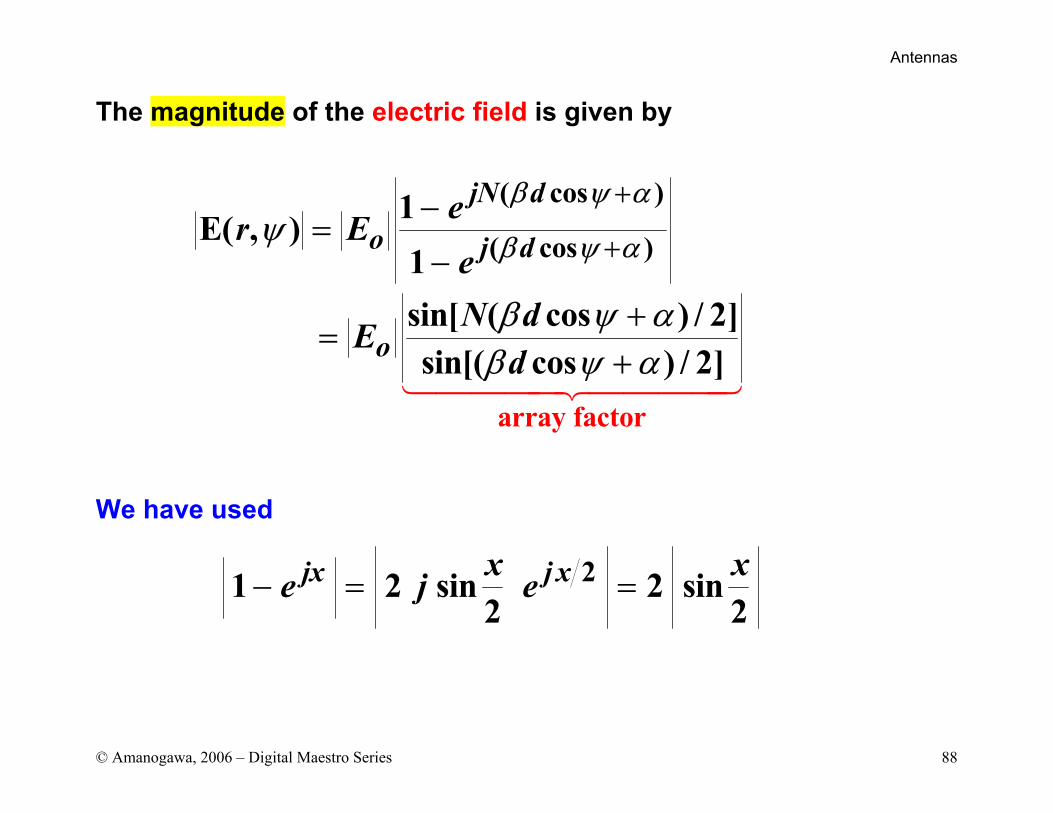
The magnitude of the electric field is given by We have used
ar
( cos )
( cos
ray facto
)
r
1E( , )1sin[ ( cos ) / 2]sin[( cos ) / 2]
jN do j d
o
er EeN dE
d
β ψ α
β ψ αψ
β ψ αβ ψ α
+
+−
=−
+=
+
21 2 sin 2 sin2 2
jx j xx xe j e− = =
Antennas
© Amanogawa, 2006 – Digital Maestro Series 89
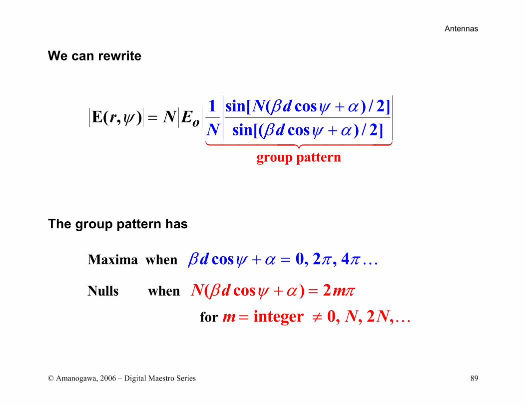
We can rewrite The group pattern has
group pattern
1 sin[ ( cos ) / 2]sin[( cos
E( ,) / 2]
) oN d
N dr N E β ψψ α
β ψ α+
=+
Maxima when
Nulls when
for
( cos ) 2
cos
integer
0,
0,
2
, 2 ,
, 4
NN
d
d mm N
β ψ α
ψ
π π
β α π+ == ≠
+ = …
…
Antennas
© Amanogawa, 2006 – Digital Maestro Series 90
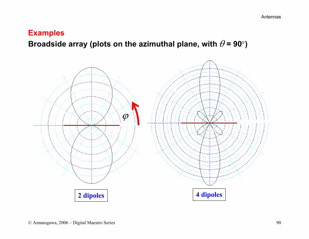
Examples Broadside array (plots on the azimuthal plane, with θ = 90°)
2 dipoles 4 dipoles
ϕ
Antennas
© Amanogawa, 2006 – Digital Maestro Series 91
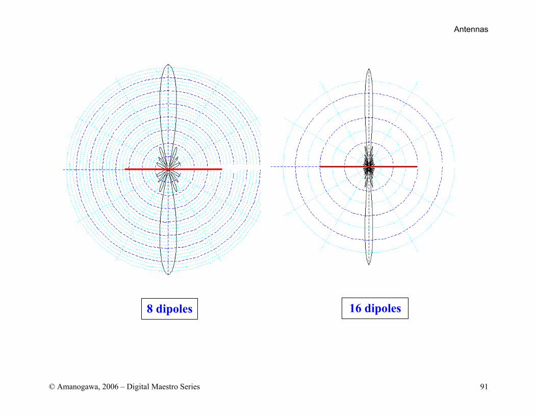
8 dipoles 16 dipoles
Antennas
© Amanogawa, 2006 – Digital Maestro Series 92
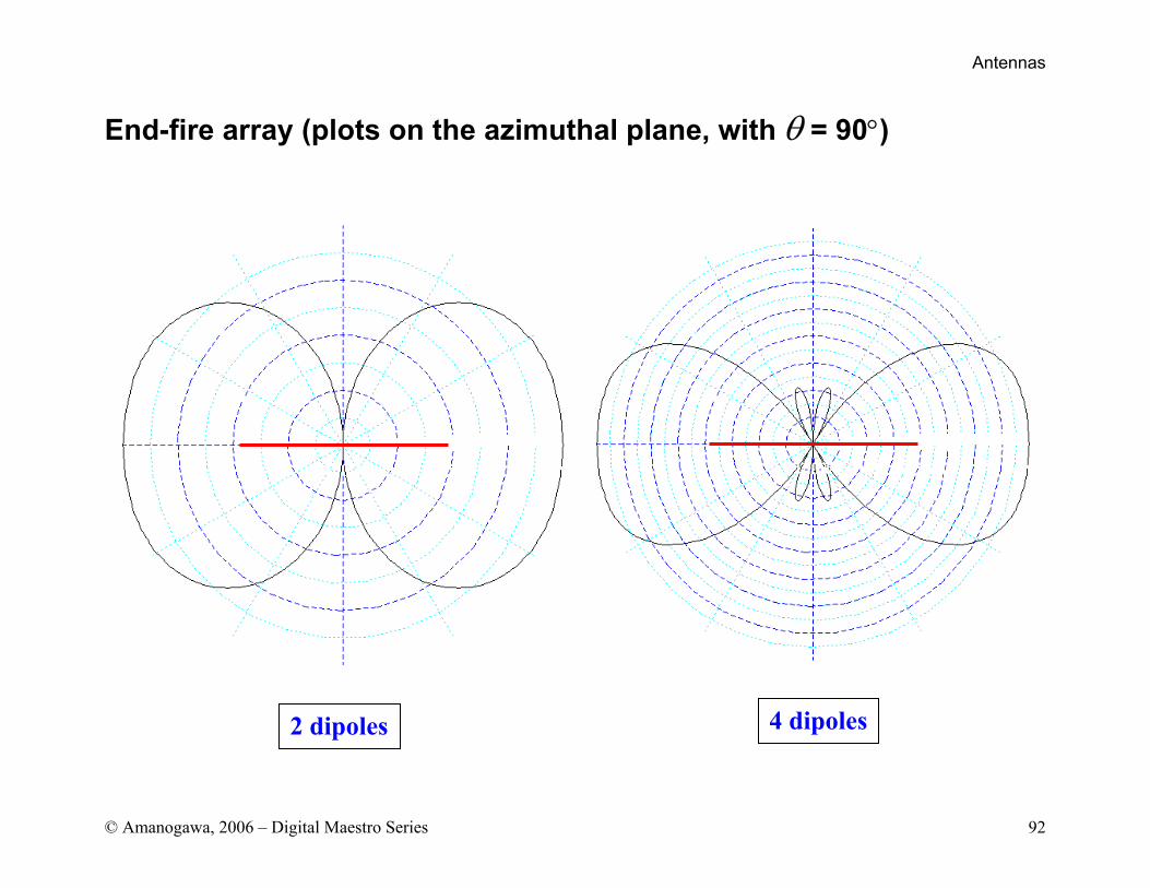
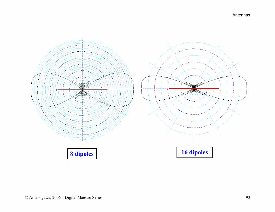
End-fire array (plots on the azimuthal plane, with θ = 90°)
2 dipoles 4 dipoles
Antennas
© Amanogawa, 2006 – Digital Maestro Series 93
8 dipoles 16 dipoles
Antennas
© Amanogawa, 2006 – Digital Maestro Series 94
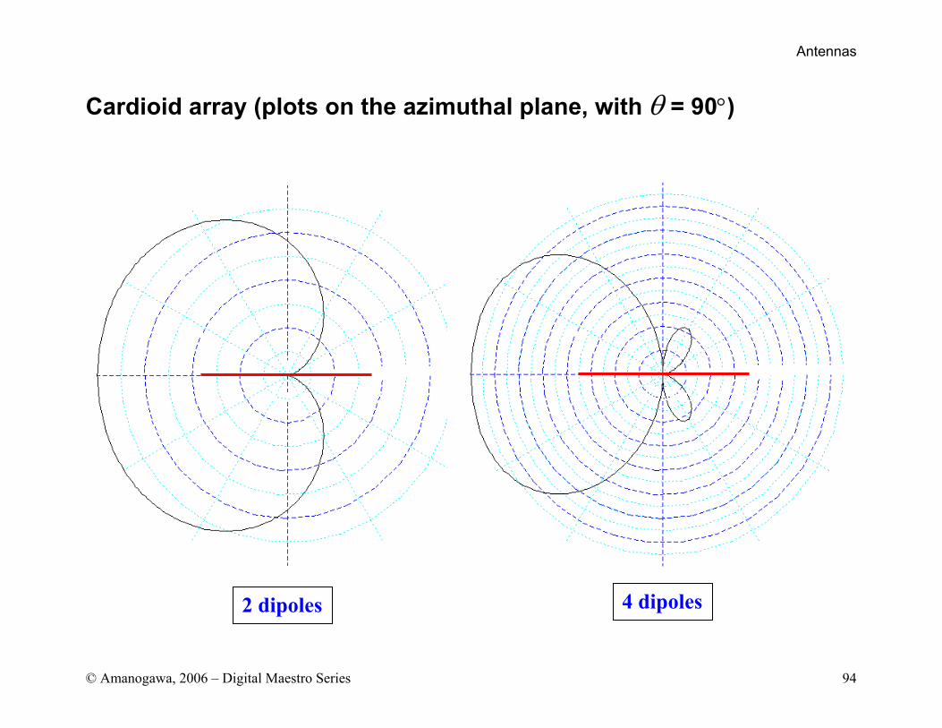
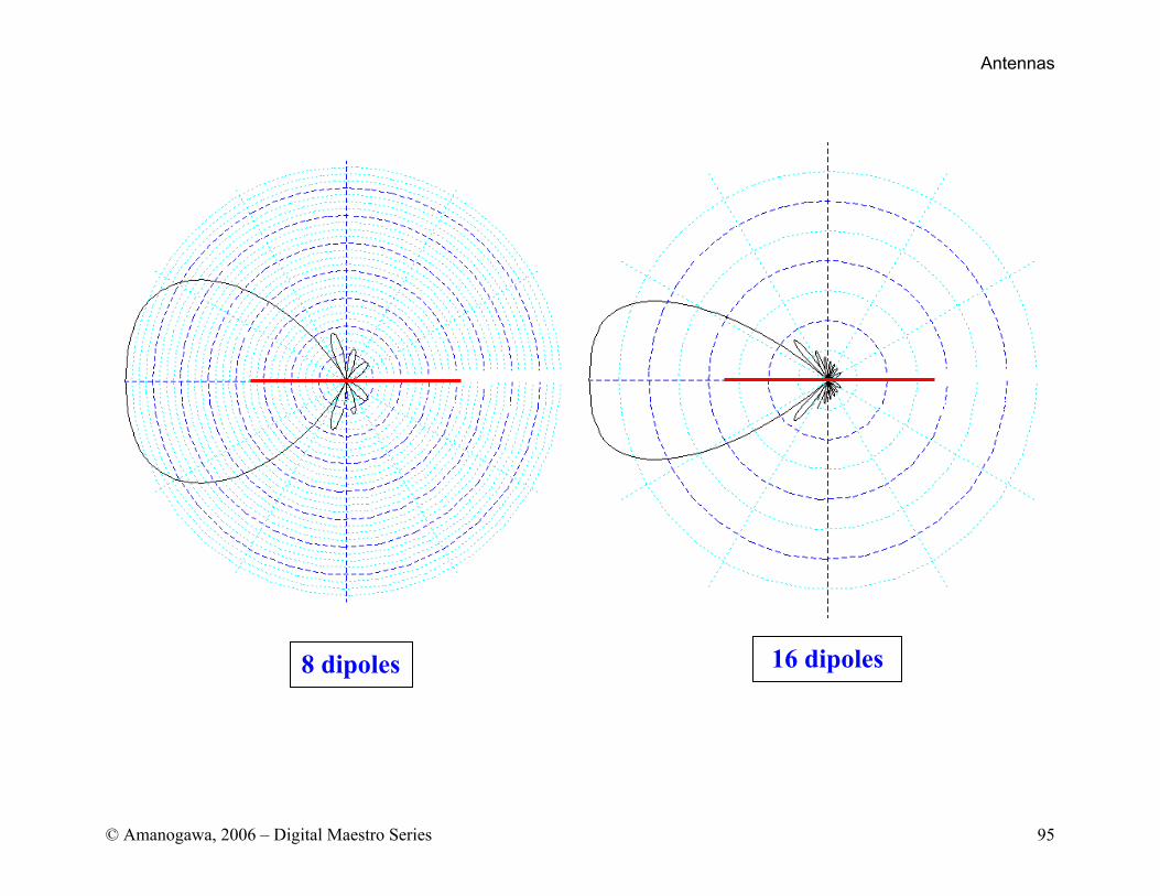
Cardioid array (plots on the azimuthal plane, with θ = 90°)
2 dipoles 4 dipoles
Antennas
© Amanogawa, 2006 – Digital Maestro Series 95
8 dipoles 16 dipoles


![Fibronectin Fibronectin exists as a dimer, consisting of two nearly identical polypeptide chains linked by a pair of C-terminal disulfide bonds. [3] Each](https://img.pdfslide.tips/doc/110x75/56649d4e5503460f94a2e7cf/fibronectin-fibronectin-exists-as-a-dimer-consisting-of-two-nearly-identical.jpg)