Atmos. Chem. Phys., 7, 2259–2270, 2007www.atmos-chem-phys.net/7/2259/2007/© Author(s) 2007. This work is licensedunder a Creative Commons License.

AtmosphericChemistry

and Physics

Simulation of solar radiation during a total eclipse: a challenge forradiative transfer

C. Emde and B. Mayer

Institut für Physik der Atmosphäre, Deutsches Zentrum für Luft- und Raumfahrt (DLR), Oberpfaffenhofen, 82234 Wessling,Germany

Received: 13 December 2006 – Published in Atmos. Chem. Phys. Discuss.: 15 January 2007Revised: 27 March 2007 – Accepted: 20 April 2007 – Published: 4 May 2007

Abstract. A solar eclipse is a rare but spectacular naturalphenomenon and furthermore it is a challenge for radiativetransfer modelling. Whereas a simple one-dimensional ra-diative transfer model with reduced solar irradiance at thetop of the atmosphere can be used to calculate the brightnessduring partial eclipses a much more sophisticated model isrequired to calculate the brightness (i.e. the diffuse radiation)during the total eclipse. The reason is that radiation reachinga detector in the shadow gets there exclusively by horizontaltransport of photons in a spherical shell atmosphere, whichrequires a three-dimensional radiative transfer model. In thisstudy the first fully three-dimensional simulations for a so-lar eclipse are presented exemplified by the solar eclipse at29 March 2006. Using a backward Monte Carlo model wecalculated the diffuse radiation in the umbra and simulatedthe changing colours of the sky. Radiance and irradiance aredecreased by 3 to 4 orders of magnitude, depending on wave-length. We found that aerosol has a comparatively small im-pact on the radiation in the umbra. We also estimated thecontribution of the solar corona to the radiation under theumbra and found that it is negligible compared to the diffusesolar radiation in the wavelength region from 310 to 500 nm.

1 Introduction

The astronomical background of a solar eclipse is well un-derstood and the geometry of the problem is known with veryhigh accuracy, e.g. time and location of the Moon’s shadowon the Earth as well as its diameter and shape (Espenak andAnderson, 2004). Under cloudless sky conditions one canobserve a number of phenomena, for instance the changingcolour of the sky, the corona of the sun or the planets andstars which become visible against the darkening sky. Solar

Correspondence to:C. Emde(claudia.emde@dlr.de)

eclipses are primarily of astronomical interest, for instanceto take measurements of the corona of the sun (Koutchmy,1994). On the other hand, a solar eclipse is an excellentmeans to test radiative transfer models, in particular three-dimensional (3-D) radiative transfer codes. There is a spe-cific need to test those against experimental data which is achallenging task: For that purpose, well-characterised three-dimensional situations are required; the most prominent onesare inhomogeneous clouds. While the measurement corre-sponding to the model output (radiation at the ground or inthe atmosphere) is a straightforward task, the full character-isation of the input parameters (the cloud properties) withhigh enough accuracy to actually constrain the model resultis close to impossible. A solar eclipse solves this problemto some degree: It is a complex three-dimensional problem,ideally suited to test the accuracy of the code: Radiationreaching a detector under the shadow gets there exclusivelyby horizontal (three-dimensional) transport of photons in aspherical shell atmosphere. The model input (distribution ofthe incoming solar radiation at top-of-atmosphere) is knownwith high accuracy. As it turns out, the situation for a solareclipse is reversed compared to the broken cloud case: Whilethe input conditions are easily available, measuring the out-put (radiation under the shadow) is actually a challenging ex-perimental problem which requires careful planning.

Several radiation measurements during total eclipses havebeen carried out, mainly in the 1960s and 1970s (Sharp et al.,1971; Silverman and Mullen, 1975). Recent spectral mea-surements were evaluated only for partial eclipses or in thepre-umbra (Fabian et al., 2001; Aplin and Harrison, 2003).Shaw(1978) developed a greatly simplified radiative trans-fer model wherein sunlight diffuses into the umbra only byfirst- and second-order scattering processes. According toShaw this model can calculate the diffuse radiance in theumbra within an uncertainty of a factor of two.Koepke et al.(2001) used a one-dimensional (1-D) radiative transfer modelfor simulations in the pre-umbra. Both models account for

Published by Copernicus GmbH on behalf of the European Geosciences Union.

2260 C. Emde and B. Mayer: Solar radiation during a total eclipse

surface

TOA

Fig. 1. Typical photon paths in backward tracing. The left panel il-lustrates the calculation of solar zenith radiance and the right panelthe calculation of diffuse solar irradiance. Solid lines are actualphoton trajectories and dashed lines are the contributions to the ra-diance/irradiance according to the local estimate technique, see text.

solar limb darkening. As mentioned above, a 3-D multiplescattering model is required to model the solar radiation in-side the umbral shadow accurately. Monte Carlo methodscan be used for such applications (e.g.,Marshak and Davis,2005). For this particular problem, forward Monte Carlo cal-culations are very time consuming because only a small frac-tion of the photons started outside the shadow reach a sensorplaced in the centre of the umbral shadow, which results inlarge uncertainties or very long computation times. Hence,backward Monte Carlo calculations are appropriate where allphotons are started at the sensor position and followed back-wards towards the top of the atmosphere. As our sensitivitystudies prove, a spherical model atmosphere is required be-cause light entering the atmosphere more than 1000 km awaymay impact the radiance or irradiance in the centre of the um-bral shadow.

Here we describe the radiative transfer code, in particularthe specialities required for the eclipse simulation: backwardMonte Carlo calculations and spherical geometry. We thenpresent quantitative spectral radiance and irradiance calcula-tions for an example location: the Greek island Kastelorizo(36.150◦ N, 29.596◦ E) which was close to the centre of theumbra, see alsoBlumthaler et al.(2006). The results andmethodology presented here give an overview of the radi-ance and irradiance levels to be expected during a total solareclipse and may serve as a benchmark for planning radia-tion observations during future solar eclipses, e.g. to focuson the wavelength regions where the radiation is well abovethe detection limit of the instrument, or to optimise integra-tion time.

The following section describes the methodology used tocalculate the diffuse radiation in the umbra. In Sect. 3 weshow the results of our calculations and in Sect. 4 we sum-marise our conclusions.

2 Methodology

In this section we first describe the radiative transfer modelused for this study. With the backward Monte Carlo codewe calculate the contribution of each location at top-of-atmosphere to the radiance/irradiance at the centre of the um-bra. Then, the incoming (extraterrestrial) irradiance distribu-tion at top-of-atmosphere is derived under eclipse conditions.The product of both (contribution function and extraterres-trial irradiance distribution) gives the radiance/irradiance be-low the umbra.

2.1 Monte Carlo model

The radiative transfer model MYSTIC (Monte Carlo code forthe phYSically correct Tracing of photons In Cloudy atmo-spheres) (Mayer, 1999, 2000) is used for this study. MYSTICis operated as one of several radiative transfer solvers of thelibRadtran radiative transfer package byMayer and Kylling(2005). Originally MYSTIC has been developed as a for-ward tracing method for the calculation of irradiances andradiances in 3-D plane-parallel atmospheres. For this study,the model has been extended to allow backward Monte Carlocalculations in spherical geometry. These extensions wererequired for accurate simulations in the centre of the um-bra. In the following we describe only those model prop-erties which are afterwards required to interpret the resultsof this paper. For general questions about the Monte Carlotechnique and in particular about libRadtran and MYSTICthe reader is referred to the literature (Mayer, 1999, 2000;Mayer and Kylling, 2005; Marshak and Davis, 2005; Caha-lan et al., 2005).

2.1.1 Backward Monte Carlo method

Figure 1 illustrates some typical photon paths through theatmosphere. In a backward simulation, photons are startedat the location of the sensor and traced through the atmo-sphere where they may be scattered or absorbed, until theyleave to space at top-of-atmosphere (TOA) or are absorbedat the surface. The reciprocity principle allows to treat scat-tering and absorption processes in the same way in forwardand backward calculations (Marshak and Davis, 2005; Chan-drasekhar, 1950). At each scattering, a new direction is ran-domly sampled from the scattering phase function at eachparticular location. Absorption is considered by reducingthe photon weight according to Lambert-Beer’s law alongthe photon trajectory. The solid lines in Fig.1 show typi-cal photon paths. For radiance calculations (left) all photonsare started into the viewing direction which is the zenith inthis example. One can easily imagine that only few photonsleave TOA into the direction of the sun. Rather than sam-pling only these few photons in a very narrow solid anglecone, a much more efficient approach is used: In the “localestimate” technique (Marshak and Davis, 2005) we calculate

Atmos. Chem. Phys., 7, 2259–2270, 2007 www.atmos-chem-phys.net/7/2259/2007/

C. Emde and B. Mayer: Solar radiation during a total eclipse 2261

������������������������������������������������������������������������������������������������

������������������������������������������������������������������������������������������������

2

TOAboundary

1

3

sample grid

surface

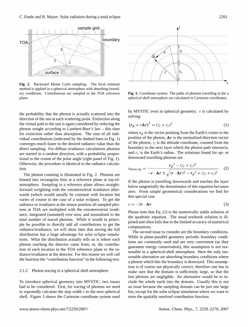
Fig. 2. Backward Monte Carlo sampling. The local estimatemethod is applied in a spherical atmosphere with absorbing bound-ary conditions. Contributions are sampled in the TOA referenceplane.

the probability that the photon is actually scattered into thedirection of the sun at each scattering point. Extinction alongthe virtual path to the sun is again considered by reducing thephoton weight according to Lambert-Beer’s law – this timefor extinction rather than absorption. The sum of all indi-vidual contributions (indicated by the dashed lines in Fig.1)converges much faster to the desired radiance value than thedirect sampling. For diffuse irradiance calculations photonsare started in a random direction, with a probability propor-tional to the cosine of the polar angle (right panel of Fig.1).Otherwise, the procedure is identical to the radiance calcula-tion.

The photon counting is illustrated in Fig.2. Photons arebinned into rectangular bins at a reference plane at top-of-atmosphere. Sampling in a reference plane allows straight-forward weighting with the extraterrestrial irradiance after-wards (which would usually be constant with location butvaries of course in the case of a solar eclipse). To get theradiance or irradiance at the sensor position all sampled pho-tons at TOA are multiplied with the extraterrestrial irradi-ance, integrated (summed) over area, and normalised to thetotal number of traced photons. While it would in princi-ple be possible to directly add all contributions to get theradiance/irradiance, we will show later that storing the fulldistribution has a large advantage for solar eclipse simula-tions. What the distribution actually tells us is where eachphoton reaching the detector came from, or, the contribu-tion of each location in the TOA reference plane to the ra-diance/irradiance at the detector. For this reason we will callthe function the “contribution function” in the following text.

2.1.2 Photon tracing in a spherical shell atmosphere

To introduce spherical geometry into MYSTIC, two issueshad to be considered. First, for tracing of photons we needto repeatedly calculate the step widths to the next sphericalshell. Figure3 shows the Cartesian coordinate system used

z

x

s∆

lz

r

r

er

Fig. 3. Coordinate system. The paths of photons travelling in the aspherical shell atmosphere are calculated in Cartesian coordinates.

by MYSTIC even in spherical geometry.s is calculated bysolving(rp + s1r

)2= (zl + re)

2 (1)

whererp is the vector pointing from the Earth’s centre to theposition of the photon,1r is the normalised direction vectorof the photon,zl is the altitude coordinate, counted from theboundary to the next layer which the photon path intersects,andre is the Earth’s radius. The solutions found for up- ordownward travelling photons are

sdown/up =rp

2− (zl + re)

2

−r · 1r ±

√(r · 1r)2 − rp

2 + (zl + re)2. (2)

If the photon is travelling downwards and touches the layerbelow tangentially the denominator of this equation becomeszero. From simple geometrical considerations we find forthis special case

s = −2r · 1r. (3)

Please note that Eq. (2) is the numerically stable solution ofthe quadratic equation. The usual textbook solution is ill-posed and often fails due to the limited accuracy of numericalcomputations.

The second issue to consider are the boundary conditions.While in plane-parallel geometry periodic boundary condi-tions are commonly used and are very convenient (as theyguarantee energy conservation), this assumption is not rea-sonable in a spherical-shell atmosphere. Here the only rea-sonable alternative are absorbing boundary conditions wherea photon which hits the boundary is destroyed. This assump-tion is of course not physically correct; therefore one has tomake sure that the domain is sufficiently large, so that thelost photons are negligible. An alternative would be to in-clude the whole earth into the domain. Usually this is notan issue because the sampling domain can be just one largebin, except for the solar eclipse simulation where we want tostore the spatially resolved contribution function.

www.atmos-chem-phys.net/7/2259/2007/ Atmos. Chem. Phys., 7, 2259–2270, 2007

2262 C. Emde and B. Mayer: Solar radiation during a total eclipse

0

0.005

0.01

0.015

0.02

0.025

0.03

0.035

70 75 80 85 90 95

L λ/E

0λ

MYSTICSDISORT

4.0

2.0

0.0

-2.0

-4.0

70 75 80 85 90 95

(M-S

)/M

[%]

Θ0 [ o ]

Fig. 4. Comparison between spherical MYSTIC and SDISORT.Zenith radiance at 342 nm as a function of solar zenith angle. (Top)Radiance normalised by the extraterrestrial irradiance; (bottom) rel-ative deviation between MYSTIC and SDISORT in percent.

2.1.3 Model validation

The newly developed backward Monte Carlo model was val-idated by comparison with the well-tested MYSTIC forwardmodel in three-dimensional geometry. The models agreedperfectly within the Monte Carlo noise of much less than1% for all cases tested. The forward MYSTIC model wasvalidated extensively within the Intercomparison of 3-D Ra-diation Codes (I3RC) (Cahalan et al., 2005). The sphericalMonte Carlo model was compared to the pseudo-sphericalmodel SDISORT byDahlback and Stamnes(1991).

A typical result is shown in Fig.4. Here, zenith radiancesare calculated atλ=342 nm. The surface albedo was 0.06,typical for ocean. No aerosol was included in the calcula-tion. Up to a solar zenith angle of 80◦ the difference betweenthe models is below 1% and up to 90◦ it is within 5%. Suchdifferences may be expected because SDISORT is a pseudo-spherical code which does not work accurately for very lowsun. For solar zenith angles above 90◦, e.g. for twilight cal-culations, the uncertainty of SDISORT increases.

2.1.4 Example for the contribution function at TOA

In the following we show the TOA contribution functionsampled by the spherical backward Monte Carlo code out-lined in the previous sections. As described above, this func-tion describes where the photons which arrive at the detectorcame from. As an example, we show the contribution func-tion at TOA for a wavelength of 340 nm. For this simulationwe used a domain size of 1000×1000 km2. The mid-latitudesummer atmosphere byAnderson et al.(1986) was used forthe pressure, temperature, and trace gas profiles. The atmo-sphere was cloudless and aerosol-free. A solar zenith angle

Table 1. Parameters describing the total eclipse at 29 March 2006;from Espenak and Anderson(2004).

t [s] UTC latitude longitude

–300 10:50 34◦40.8′ N 28◦33.7′ E0 10:55 36◦13.3′ N 30◦33.5′ E

300 11:00 36◦46.7′ N 32◦34.6′ E

t [s] ρ θ0 [◦] φ0 [

◦]

–300 1.0499 32.6 18.50 1.0494 35.0 23.3

300 1.0489 37.6 27.8

t [s] Major axis [km] Minor axis [km]

–300 196.2 165.50 200.0 164.1

300 204.7 162.5

θ0 of 35.0◦ was assumed and the solar azimuth angleφ0 was23.3◦ (South-West, or lower-left in the image), correspond-ing to the conditions during the eclipse of 29 March 2006,10:55 UTC, at Kastelorizo (see Table1).

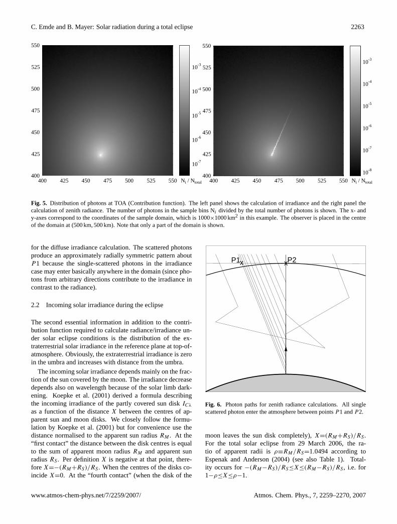
Figure5 shows the contribution function sampled at TOA.The right panel shows a zenith radiance calculation. Themost striking feature – a bright line along the direction ofthe solar azimuth – is easily understood: A large part ofthe radiance in a cloudless atmosphere at 340 nm stems fromsingle-scattered photons. At 340 nm the vertically integratedoptical thicknessτ of the assumed Rayleigh atmosphereis 0.713. According to Lambert-Beer’s law a fraction of1− exp(−τ/ cosθ0)=0.58 of the incoming photons is scat-tered along their direct path to the surface and the chance forbeing scattered a second time is comparatively small.

Figure 6 illustrates that photons arriving at the detectorafter only one scattering event enter the atmosphere alonga straight line between pointsP1 andP2. P1 is the spotwhere a photon directly arrives at the detector without scat-tering (which for zenith radiance is of course a limiting casethat does not actually occur).P1 is close to the bright spotin Fig.5 which indicates the maximum contribution – relatedto a scattering close to the surface.P2 is the other extremewhere a photon is scattered at top-of-atmosphere to reach thedetector. This is a highly unlikely event (due to the exponen-tially decreasing Rayleigh scattering coefficient with height)for which reason the visible line in the contribution functionthins out and probably never reachesP2. The “halo” aroundthe single-scattering line is caused by multiple scattering. Asexpected, the contribution function drops quickly as we moveaway from the single-scattering line. Please note that a loga-rithmic grey-scale was chosen for this plot because otherwisethe contribution of the multiply scattered photons would bebarely visible. The left panel shows the contribution function

Atmos. Chem. Phys., 7, 2259–2270, 2007 www.atmos-chem-phys.net/7/2259/2007/

C. Emde and B. Mayer: Solar radiation during a total eclipse 2263

400 425 450 475 500 525 550400

425

450

475

500

525

550

10-7

10-6

10-5

10-4

10-3

Ni / Ntotal 400 425 450 475 500 525 550400

425

450

475

500

525

550

10-8

10-7

10-6

10-5

10-4

10-3

Ni / Ntotal

Fig. 5. Distribution of photons at TOA (Contribution function). The left panel shows the calculation of irradiance and the right panel thecalculation of zenith radiance. The number of photons in the sample bins Ni divided by the total number of photons is shown. The x- andy-axes correspond to the coordinates of the sample domain, which is 1000×1000 km2 in this example. The observer is placed in the centreof the domain at (500 km, 500 km). Note that only a part of the domain is shown.

for the diffuse irradiance calculation. The scattered photonsproduce an approximately radially symmetric pattern aboutP1 because the single-scattered photons in the irradiancecase may enter basically anywhere in the domain (since pho-tons from arbitrary directions contribute to the irradiance incontrast to the radiance).

2.2 Incoming solar irradiance during the eclipse

The second essential information in addition to the contri-bution function required to calculate radiance/irradiance un-der solar eclipse conditions is the distribution of the ex-traterrestrial solar irradiance in the reference plane at top-of-atmosphere. Obviously, the extraterrestrial irradiance is zeroin the umbra and increases with distance from the umbra.

The incoming solar irradiance depends mainly on the frac-tion of the sun covered by the moon. The irradiance decreasedepends also on wavelength because of the solar limb dark-ening. Koepke et al.(2001) derived a formula describingthe incoming irradiance of the partly covered sun diskICλ

as a function of the distanceX between the centres of ap-parent sun and moon disks. We closely follow the formu-lation by Koepke et al.(2001) but for convenience use thedistance normalised to the apparent sun radiusRM . At the“first contact” the distance between the disk centres is equalto the sum of apparent moon radiusRM and apparent sunradiusRS . Per definitionX is negative at that point, there-fore X=−(RM+RS)/RS . When the centres of the disks co-incide X=0. At the “fourth contact” (when the disk of the

xx P2P1

Fig. 6. Photon paths for zenith radiance calculations. All singlescattered photon enter the atmosphere between pointsP1 andP2.

moon leaves the sun disk completely),X=(RM+RS)/RS .For the total solar eclipse from 29 March 2006, the ra-tio of apparent radii isρ≡RM/RS=1.0494 according toEspenak and Anderson(2004) (see also Table1). Total-ity occurs for−(RM−RS)/RS≤X≤(RM−RS)/RS , i.e. for1−ρ≤X≤ρ−1.

www.atmos-chem-phys.net/7/2259/2007/ Atmos. Chem. Phys., 7, 2259–2270, 2007

2264 C. Emde and B. Mayer: Solar radiation during a total eclipse

0

0.2

0.4

0.6

0.8

1

0 0.5 1 1.5 2 2.5

EC

λ/E

0λ

X

300 nm400 nm500 nm600 nm

0

0.01

0.02

0.03

0.04

0.05

0.05 0.1 0.15 0.2

4000 3000 2000 1000 500 100

r [km]

Fig. 7. Incoming solar irradiance during an eclipse. The irradianceis plotted as a function of distance between the centres of the ap-parent sun and moon disks; the lower axis gives the correspondingdistance from the centre of the umbra in km. The irradiance is nor-malised to its non-eclipse value.

Figure 7 shows the solar irradiance for different wave-lengths as a function ofX for the solar eclipse from 29March 2006, calculated according toKoepke et al.(2001).As expected it is zero forX<0.0494 (=ρ−1). Only the partfor positiveX is shown because the irradiance is symmetricaboutX=0. The small figure shows that the wavelength de-pendence due to solar limb darkening is important for smallX. For radiation calculations inside the umbral shadow thismight be important because these are the photons enteringthe atmosphere closest to the point of interest, below the um-bra.

As a final step we need to project the irradiance distri-bution from Fig.7 onto the model reference plane at TOA.For that purpose, we first need to convert from relative dis-tanceX to absolute distance in the reference plane. Accord-ing to Espenak and Anderson(2004)(see Table1) the widthof the minor axis of the umbral shadow at 10:55 UTC is164.1 km corresponding toX=2·(ρ−1). With ρ=1.0494 wefind thatX=1 corresponds to 1661 km which allows us tolinearly translate betweenX and distances in the referenceplane (please note that the data ofEspenak and Anderson(2004) refer to the surface of the Earth; our reference planeis TOA instead but the 120 km difference may be safely ne-glected compared to the distance between Earth and Moonfor this application). We used this relationship to providethe second axis in Fig.7 which shows the distance in km togive an idea over which distances from the centre of the um-bra the incoming solar irradiance is actually disturbed by theMoon’s shadow. Finally, we project the thus-derived distri-bution onto the TOA reference plane and obtain the incoming

solar irradiance as a function of the coordinatesx andy de-scribing any point the reference plane. In the following wecall

w(x, y) =ECλ(x, y)

E0λ

(4)

the solar eclipse weighting function.Multiplication of the contribution function (see Fig.5)

with w(x, y) gives the actual contribution of each locationin the TOA reference plane to the radiance/irradiance at thecentre of the umbra. The left panel of Fig.8 shows the re-sult for the irradiance, the right panel the respective radiancedata. First, we note that the absolute values are several ordersof magnitude smaller than in Fig.5. This is due to the factthat the main contributions to the radiance/irradiance at theground (single and other low orders of scattering) are sup-pressed by the Moon’s shadow. Second, in contrast to Fig.5the weighted distributions are plotted on a linear scale whichshows that the decrease towards the border of the domain ismuch slower and that even photons entering the atmospheremore than 300 km away from the sensor might contribute sig-nificantly to the result. We find that the rapid decrease in thecontribution function away from the umbra is partly compen-sated by the increase of the incoming solar irradiance. Andthird, the contribution to radiance and irradiance look rathersimilar in contrast to the eclipse-free conditions in Fig.5.To obtain absolute values of the radiance and irradiance wesimply integrate the data from Fig.8 over the domain andmultiply with the extraterrestrial irradianceE0λ.

2.3 Domain size

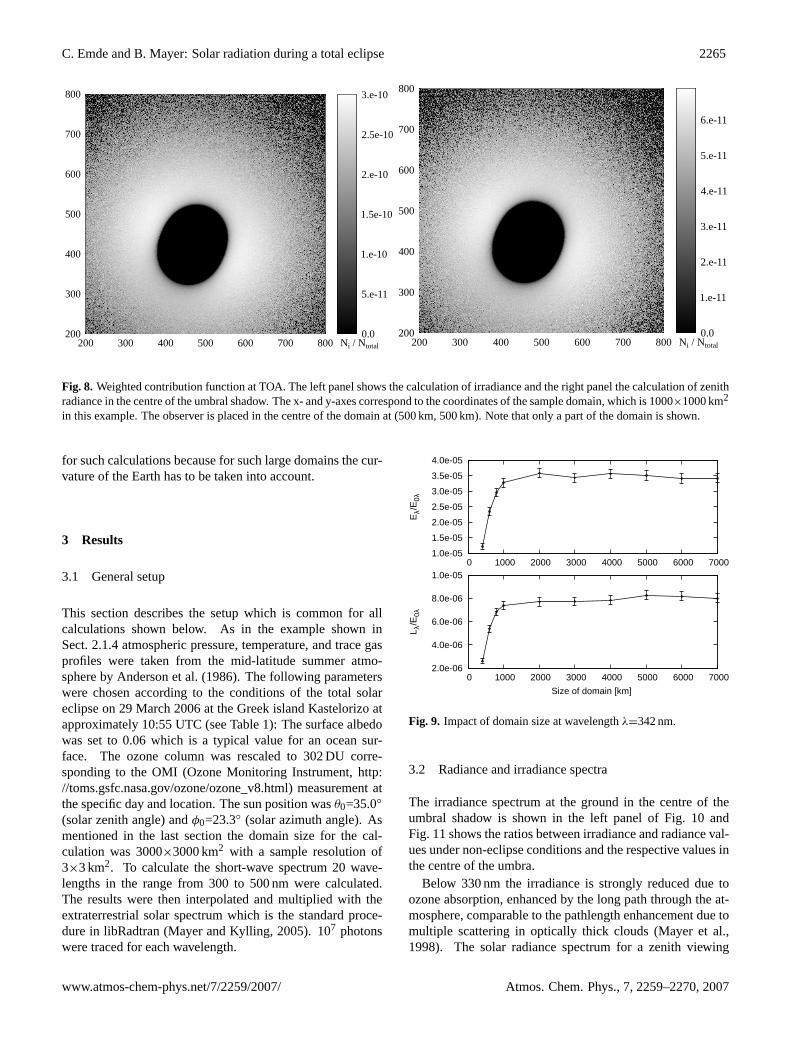
The choice of the domain size is directly related to the ques-tion how far the photons travel through the atmosphere. Fornormal (non-eclipse) conditions and high sun angles smalldomain sizes are sufficient because most of the measuredphotons have entered the atmosphere close to the point wherethe direct beam to the receiver hits TOA. They reach the sen-sor directly or after only a few scattering events in the tropo-sphere as seen in Fig.5. However, in our application the solareclipse weighting function (4) masks those photons and givespreference to photons which enter the domain far away fromthe receiver. The incoming solar irradiance increases rapidlywith the distancer from the centre of the umbra. In additionthe annular area betweenr andr+1r increases linearly withdistance. In order to find an appropriate domain size, calcu-lations for sizes up to 7000×7000 km2 were performed forλ=342 nm. The results are shown in Fig.9. The error barsare 2 standard deviations of the result to quantify the MonteCarlo noise. For domains smaller than 1000×1000 km2 oneobviously gets wrong results for radiances and irradiancesbecause too many photons are absorbed at the boundary ofthe domain. We decided to use a domain size of 3000×3000km2 for the solar eclipse simulations to be on the safe side. Inconsequence a spherical radiative transfer model is required

Atmos. Chem. Phys., 7, 2259–2270, 2007 www.atmos-chem-phys.net/7/2259/2007/

C. Emde and B. Mayer: Solar radiation during a total eclipse 2265

200 300 400 500 600 700 800200

300

400

500

600

700

800

0.0

5.e-11

1.e-10

1.5e-10

2.e-10

2.5e-10

3.e-10

Ni / Ntotal 200 300 400 500 600 700 800200

300

400

500

600

700

800

0.0

1.e-11

2.e-11

3.e-11

4.e-11

5.e-11

6.e-11

Ni / Ntotal

Fig. 8. Weighted contribution function at TOA. The left panel shows the calculation of irradiance and the right panel the calculation of zenithradiance in the centre of the umbral shadow. The x- and y-axes correspond to the coordinates of the sample domain, which is 1000×1000 km2

in this example. The observer is placed in the centre of the domain at (500 km, 500 km). Note that only a part of the domain is shown.

for such calculations because for such large domains the cur-vature of the Earth has to be taken into account.

3 Results

3.1 General setup

This section describes the setup which is common for allcalculations shown below. As in the example shown inSect.2.1.4atmospheric pressure, temperature, and trace gasprofiles were taken from the mid-latitude summer atmo-sphere byAnderson et al.(1986). The following parameterswere chosen according to the conditions of the total solareclipse on 29 March 2006 at the Greek island Kastelorizo atapproximately 10:55 UTC (see Table1): The surface albedowas set to 0.06 which is a typical value for an ocean sur-face. The ozone column was rescaled to 302 DU corre-sponding to the OMI (Ozone Monitoring Instrument,http://toms.gsfc.nasa.gov/ozone/ozone_v8.html) measurement atthe specific day and location. The sun position wasθ0=35.0◦

(solar zenith angle) andφ0=23.3◦ (solar azimuth angle). Asmentioned in the last section the domain size for the cal-culation was 3000×3000 km2 with a sample resolution of3×3 km2. To calculate the short-wave spectrum 20 wave-lengths in the range from 300 to 500 nm were calculated.The results were then interpolated and multiplied with theextraterrestrial solar spectrum which is the standard proce-dure in libRadtran (Mayer and Kylling, 2005). 107 photonswere traced for each wavelength.

1.0e-05

1.5e-05

2.0e-05

2.5e-05

3.0e-05

3.5e-05

4.0e-05

0 1000 2000 3000 4000 5000 6000 7000

Eλ/

E0λ

2.0e-06

4.0e-06

6.0e-06

8.0e-06

1.0e-05

0 1000 2000 3000 4000 5000 6000 7000

L λ/E

0λ

Size of domain [km]

Fig. 9. Impact of domain size at wavelengthλ=342 nm.

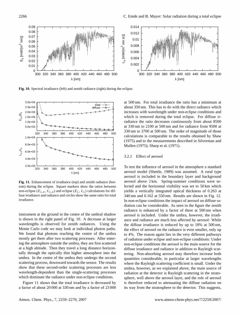
3.2 Radiance and irradiance spectra

The irradiance spectrum at the ground in the centre of theumbral shadow is shown in the left panel of Fig.10 andFig.11shows the ratios between irradiance and radiance val-ues under non-eclipse conditions and the respective values inthe centre of the umbra.

Below 330 nm the irradiance is strongly reduced due toozone absorption, enhanced by the long path through the at-mosphere, comparable to the pathlength enhancement due tomultiple scattering in optically thick clouds (Mayer et al.,1998). The solar radiance spectrum for a zenith viewing

www.atmos-chem-phys.net/7/2259/2007/ Atmos. Chem. Phys., 7, 2259–2270, 2007

2266 C. Emde and B. Mayer: Solar radiation during a total eclipse

0 0.01 0.02

0.03 0.04 0.05 0.06

0.07 0.08 0.09

300 320 340 360 380 400 420 440 460 480 500

Eλ

[mW

/(m

2 nm

)]

λ [nm]

0

0.002

0.004

0.006

0.008

0.01

0.012

0.014

300 320 340 360 380 400 420 440 460 480 500

L λ [m

W/(

m2 n

m s

r)]

λ [nm]

Fig. 10. Spectral irradiance (left) and zenith radiance (right) during the eclipse.

5.0e+03

1.0e+04

1.5e+04

2.0e+04

2.5e+04

3.0e+04

320 340 360 380 400 420 440 460 480 500

Eλ,

n/E

λ

totaldiffuse

2.0e+03

4.0e+03

6.0e+03

8.0e+03

1.0e+04

320 340 360 380 400 420 440 460 480 500

L λ,n

/Lλ

λ [nm]

Fig. 11. Enhancement of irradiance (top) and zenith radiance (bot-tom) during the eclipse. Square markers show the ratios betweennon-eclipse (Eλ,n, Lλ,n) and eclipse (Eλ, Lλ) calculations for dif-fuse irradiance and radiance and circles show the same ratio for totalirradiance.

instrument at the ground in the centre of the umbral shadowis shown in the right panel of Fig.10. A decrease at largerwavelengths is observed for zenith radiances. Using theMonte Carlo code we may look at individual photon paths.We found that photons reaching the centre of the umbramostly get there after two scattering processes: After enter-ing the atmosphere outside the umbra, they are first scatteredat a high altitude. Then they travel a long distance horizon-tally through the optically thin higher atmosphere into theumbra. In the centre of the umbra they undergo the secondscattering process, downward towards the sensor. The resultsshow that these second-order scattering processes are lesswavelength-dependent than the single-scattering processeswhich dominate the radiance under non-eclipse conditions.

Figure11 shows that the total irradiance is decreased bya factor of about 20 000 at 330 nm and by a factor of 23 000

at 500 nm. For total irradiance the ratio has a minimum atabout 350 nm. This has to do with the direct radiance whichincreases with wavelength under non-eclipse conditions andwhich is removed during the total eclipse. For diffuse ir-radiance the ratio decreases continuously from about 8500at 330 nm to 2100 at 500 nm and for radiance from 9500 at330 nm to 3700 at 500 nm. The order of magnitude of thosecalculations is comparable to the results obtained byShaw(1975) and to the measurements described inSilverman andMullen (1975); Sharp et al.(1971).

3.2.1 Effect of aerosol

To test the influence of aerosol in the atmosphere a standardaerosol model (Shettle, 1989) was assumed. A rural typeaerosol is included in the boundary layer and backgroundaerosol above 2 km. Spring-summer conditions were se-lected and the horizontal visibility was set to 50 km whichyields a vertically integrated optical thickness of 0.263 at340 nm and 0.162 at 550 nm. Results are shown in Fig.12.In non-eclipse conditions the impact of aerosol on diffuse ra-diation can be considerable. As seen in the figure the zenithradiance is enhanced by a factor of three at 500 nm whenaerosol is included. Under the umbra, however, the irradi-ance and radiance are much less affected by aerosol: Whilethe diffuse irradiance is reduced by up to 18% at 500 nm,the effect of aerosol on the radiance is even smaller, only upto 4%. The reason again lies in the very different pathwaysof radiation under eclipse and non-eclipse conditions: Undernon-eclipse conditions the aerosol is the main source for thediffuse irradiance and radiance in addition to Rayleigh scat-tering. Non-absorbing aerosol may therefore increase bothquantities considerable, in particular at larger wavelengthswhere the Rayleigh scattering coefficient is small. Under theumbra, however, as we explained above, the main source ofradiation at the detector is Rayleigh scattering in the strato-sphere, well above the aerosol layer, and the role of aerosolis therefore reduced to attenuating the diffuse radiation onits way from the stratosphere to the detector. This suggests,

Atmos. Chem. Phys., 7, 2259–2270, 2007 www.atmos-chem-phys.net/7/2259/2007/

C. Emde and B. Mayer: Solar radiation during a total eclipse 2267

-0.2 0

0.2 0.4 0.6 0.8

1 1.2 1.4 1.6

300 350 400 450 500

(Eλ,

a-E

λ)/E

λ

-0.5

0

0.5

1

1.5

2

300 350 400 450 500

(Lλ,

a-L λ

)/L λ

λ [nm]

eclipsenon-eclipse

Fig. 12. Impact of aerosol. Relative difference between diffuse irra-diance (top) and zenith radiance (bottom) with aerosol (Eλ,a ,Lλ,a)and without aerosol. The solid line is for the solar eclipse and thedashed line is for non-eclipse conditions.

however, that volcanic aerosol in the stratosphere could havea large impact on the radiance and irradiance under the um-bra.

3.2.2 Time series

The radiation at any given time may be simulated from asingle backward Monte Carlo calculation if the distributionof photons leaving TOA has been stored. This distribution,weighted by the distribution of incoming solar irradiance forthe actual location of the shadow at a given time provides theradiance or irradiance at the sensor for this particular time.Table1 shows data fromEspenak and Anderson(2004) in-cluding the exact position of the centre of the umbra every5 min. Please note, however, that this method may only beapplied for short time intervals because solar zenith and az-imuth angles (θ0 andφ0) change with time, resulting in a dif-ferent photon distribution at TOA and in a different shape ofthe shadow. Furthermore the ratio between apparent sun andmoon disksρ varies with time, see Table1. This means thatfor larger time scales the weighting function requires moremodifications than just a displacement and the contributionfunctions needs to be recalculated. Figure13shows the timedependence of irradiance and radiance from 400 s before to400 s after totality for three different wavelengths. For thissimulation, the parametersθ0, φ0 andρ are assumed to beconstant, using their value at 0 s. Aerosol is included in thiscalculation. The horizontal lines are the non-eclipse valuesfor diffuse irradiance and zenith radiance. Irradiance and ra-diance look similar for 342 and 500 nm – both wavelengths

1e-04

0.001

0.01

0.1

1

10

100

1000

-400 -300 -200 -100 0 100 200 300 400

Eλ

[mW

/m2 n

m]

311 nm342 nm500 nm

1e-05

1e-04

0.001

0.01

0.1

1

10

100

-400 -300 -200 -100 0 100 200 300 400

L λ [m

W/m

2 nm

sr]

t [s]

Fig. 13. Simulated time series.t=0 s denotes the time when thecentres of apparent moon and sun disk coincide.

with only little atmospheric absorption. In the zone of to-tality (–80 s<t<80 s) there is only a small decrease towardsthe centre of the shadow,t=0 s. For 311 nm radiance andirradiance are much smaller due to the strong ozone absorp-tion and the values decrease strongly towardst=0 s. Thisshows that for absorbing wavelengths the distance from theobserver to the border of the umbra is very important forthe result while for non-absorbing wavelengths light levelsare relatively homogeneous under the umbra (please note thelogarithmic scale of the plot, however). The curves are non-symmetric about t=0. This is explained by the photon dis-tribution shown in Fig.5. The moon shadow travels roughlyfrom from South-West to North-East; this implies that theline betweenP1 andP2 (from where most of the photons re-ceiving the detector under non-eclipse conditions originated,see Fig.6) is covered by the elliptical moon shadow after theeclipse but not before the eclipse.

3.2.3 Three-dimensional radiative transfer effects near theborder of the umbra

Radiation under the umbra can obviously only be calcu-lated with a three-dimensional radiative transfer model whichconsiders horizontal photon transport. Here we investigatehow horizontal photon transport affects radiance and irra-diance outside but close to the umbra; or in other words,we test the validity of one-dimensional approaches like theone byKoepke et al.(2001). For that purpose we comparedour 3-D simulations with a 1-D approximation, scaling thenon-eclipse Monte Carlo result with the weighting functionEq. (4) exactly as inKoepke et al.(2001). Both calculations,1-D and 3-D, were performed assuming a constant sun posi-tion which has no impact on the conclusions.

www.atmos-chem-phys.net/7/2259/2007/ Atmos. Chem. Phys., 7, 2259–2270, 2007

2268 C. Emde and B. Mayer: Solar radiation during a total eclipse

-20

0

20

40

60

80

100

-140 -120

(Eλ,

3D-E

λ,1D

)/E

λ,3D

[%]

-20

-15

-10

-5

0

5

10

15

20

-400 -200-2

-1.5

-1

-0.5

0

0.5

1

-4000 -2000

120 140 200 400 2000 4000

-20

0

20

40

60

80

100

-140 -120

(Lλ,

3D-L

λ,1D

)/L λ

,3D

[%]

t[s]

-20

-15

-10

-5

0

5

10

15

20

-400 -200

t[s]

-2

-1.5

-1

-0.5

0

0.5

1

-4000 -2000

t [s]

120 140

t [s]

200 400

t [s]

2000 4000

t [s]

311 nm342 nm500 nm

Fig. 14. Comparison between 1-D and 3-D calculations. Relative differences obtained shortly before and after totality.t=0 s denotes thetime when the centres of apparent moon and sun disk coincide.

The relative differences between the 1-D and the 3-D cal-culations are shown in Fig.14 as a function of time, wheret=0 denotes the time when the centres of moon and sun disccoincide. The upper panels show the irradiance and the lowerpanels the radiance calculations.t is negative before andpositive after the eclipse. The left panels show the relativedifference from 110 to 150 s where±113.5 s corresponds tothe times of second and third contacts, respectively. The rel-ative difference is 100% for−113.5 s<t<113.5 s, becausethe 1-D calculation gives 0 in the umbra. The difference de-creases rather quickly, but att=±150 s it is still larger than10% for irradiances at 342 nm and 500 nm. The irradianceis larger in the 3-D calculation, because the weighting func-tion for the extraterrestrial irradiance increases strongly withdistance from the umbra; hence there is a significant net hor-izontal photon transport towards the umbra. The relative dif-ference for zenith radiance decreases faster and for 311 nmthe 3-D calculation becomes clearly smaller compared to the1-D calculation (almost 20% att =130s). This is due tothe asymmetry about t=0 (cp. Fig.13), which has been ex-plained in the previous section. The middle panels showthe differences for±(150 s≤t≤500 s). Here the differencebetween 3-D and 1-D decreases from about 15% to about1%. In the range±(500 s≤t≤4800 s) the difference van-ishes slowly. For the case under consideration this impliesthat about 10 min “away from totality” the 1-D model can besafely used because the related uncertainty drops below 1%.This might be different for large solar zenith angles, though.

3.2.4 Influence of the corona

The corona of the sun is clearly visible in photographs takenduring total eclipses. Here we study the contribution of the

corona to the radiance and irradiance at the ground. Thiscontribution might be important because the corona is theonly source of light reaching the detector directly.

A formula describing the contribution of the corona tothe incoming solar irradiance was derived empirically byNovember and Koutchmy(1996):

Ic(R)

I0= 10−6

(3.670

R18+

1.939

R7.8+

0.0551

R2.5

)(5)

whereIc is the radiance of the corona,I0 is the radiance com-ing from the centre of the solar disk, andR is the distancefrom the centre.R is normalised to the radius of the sunRS , henceR>1. To estimate the maximal corona effect thisformula has been integrated numerically fromR=1 toR=2,where the corona radiance is already decreased by two or-ders of magnitude. Since the radiance decreases more thanexponentially with distance and the measurements used toderive Eq. (5) were performed only up toR=1.7, it is appro-priate to integrate up toR=2. The result of the integrationis I tot

c ≈1.7 · 10−7I0. In order to estimate additional radiationfrom the corona, this value is added to the weighting functionEq. (4). Since the corona is always visible all photons at TOAget an additional weight corresponding to the contribution ofthe corona. The relative difference between calculations withand without corona are shown in Fig.15. For wavelengthslarger than 330 nm the difference is less than 0.1%. Onlyfor short wavelengths close to 300 nm, where the non-coronaradiation is almost completely absorbed along the long hori-zontal path through the atmosphere, the corona has a signifi-cant effect. But the radiance or irradiance at this wavelengthis still too small to be detected with common instrumentsanyway.

Atmos. Chem. Phys., 7, 2259–2270, 2007 www.atmos-chem-phys.net/7/2259/2007/

C. Emde and B. Mayer: Solar radiation during a total eclipse 2269

0.01

0.1

1

10

100

300 350 400 450 500

∆Eλ/

Eλ

[%]

0.01

0.1

1

10

100

300 350 400 450 500

∆Lλ/

L λ [%

]

λ [nm]

Fig. 15. Additional radiation by corona. Relative difference be-tween simulations with and without corona radiation.

3.2.5 Colours of the sky

It is well known from observations that during a solar eclipsethe sky looks similar to a sunset all around the horizon.To simulate the sky color we calculated radiance distri-butions for the complete visible wavelength region 380 to780 nm and converted them to RGB values followingWalker(2003). A photograph taken by Marthinusen (available athttp://www.spaceweather.com/eclipses/29mar06) and the re-sult of the simulation are shown in Fig.16. The obvious sim-ilarity between photograph and simulation indicates nicelythat the three-dimensional spherical backward Monte Carlomodel developed for this study reproduces the wavelengthdependency of the sky radiance successfully.

4 Conclusions

Our simulations have shown that the backward MonteCarlo method is well suited for solar eclipse simulations,especially to model irradiances and radiances in the umbralshadow or close to it. The obtained results are of the sameorder of magnitude as estimated by using a greatly simplifiedmodel, which takes into account only first and second orderscattering processes (Shaw, 1978). Our results are muchmore accurate because we take into account multiple scat-tering. In most previous solar eclipse modelling studies onlyradiation in the pre-umbra was calculated. We showed that1-D approximations used in previous studies give accurateresults at some distance of the umbra but become moreinaccurate close to the border of the umbra before theycompletely fail below the umbra. The impact of aerosolis smaller in the umbra of an eclipse compared to normalnon-eclipse conditions. We could clarify that the radiationemerging from the corona does not affect the radiation

Fig. 16. Reality vs. simulation. The photograph was taken byMarthinusen at 29 March 2006. The simulated Colours of the skyare inserted in the right part of the image.

reaching the umbra significantly. The modelled irradianceand radiance spectra show that radiation measurements inthe umbra are very challenging because the total irradianceis decreased by about a factor of 17 000 at 340 nm and evenmore above 340 nm. The diffuse irradiance or radiance arereduced by a factor of about 5000. Because of the strongozone absorption in the UV-B, almost no radiation reachesthe centre of the umbra in this wavelength region. We hopethat these results are helpful for planning future radiationexperiments and offer to provide calculations for futureeclipses, to help optimising the observations.

Edited by: C. Zerefos

References

Anderson, G., Clough, S., Kneizys, F., Chetwynd, J., and Shet-tle, E.: AFGL Atmospheric Constituent Profiles (0–120 km),Tech. Rep. AFGL-TR-86-0110, AFGL (OPI), Hanscom AFB,MA 01736, 1986.

Aplin, K. L. and Harrison, R. G.: Meteorological effects of theeclipse of 11 August 1999 in cloudy and clear conditions, Proc.R. Soc. Lond. A, 459, 353–371, 2003.

www.atmos-chem-phys.net/7/2259/2007/ Atmos. Chem. Phys., 7, 2259–2270, 2007

2270 C. Emde and B. Mayer: Solar radiation during a total eclipse

Blumthaler, M., Bais, A., Webb, A., Kazadzis, S., Kift, R.,Kouremeti, N., Schallhart, B., and Kazantzidis, A.: Variations ofsolar radiation at the Earth’s surface during the total solar eclipseof 29 March 2006, in: SPIE Proceedings, Stockholm, 2006.

Cahalan, R., Oreopoulos, L., Marshak, A., Evans, K., Davis, A.,Pincus, R., Yetzer, K., Mayer, B., Davies, R., Ackerman, T.,H.W., B., Clothiaux, E., Ellingson, R., Garay, M., Kassianov,E., Kinne, S., Macke, A., O’Hirok, W., Partain, P., Prigarin, S.,Rublev, A., Stephens, G., Szczap, F., Takara, E., Varnai, T., Wen,G., and Zhuraleva, T.: The International Intercomparison of 3DRadiation Codes (I3RC): Bringing together the most advancedradiative transfer tools for cloudy atmospheres, Bull. Am. Mete-orol. Soc., 86, 1275–1293, 2005.

Chandrasekhar, S.: Radiative transfer, Oxford Univ. Press, 1950.Dahlback, A. and Stamnes, K.: A new spherical model for com-

puting the radiation field available for photolysis and heating attwilight, Planet. Space Sci., 39, 671–683, 1991.

Espenak, F. and Anderson, J.: Total solar eclipse of 2006 March 29,Tech. rep., Goddard Space Flight Centre, 2004.

Fabian, P., Winterhalter, M., Rappenglück, B., Reitmayer, H., Stohl,A., Koepke, P., Schlager, H., Berresheim, H., Foken, T., Wichura,B., Häberle, K.-H., Matyssek, R., and Kartschall, T.: TheBAYSOFI Campain- Measurements carried out during the totalsolar eclipse of August 11, 1999, Meteorologische Zeitschrift,10, 165–170, 2001.

Koepke, P., Reuder, J., and Schween, J.: Spectral variation of the so-lar radiation during an eclipse, Meteorologische Zeitschrift, 10,179–186, 2001.

Koutchmy, S.: Coronal physics from eclipse observations, Adv.Space Res., 14, 29–39, 1994.

Marshak, A. and Davis, A. (Eds.): 3D radiative transfer in cloudyatmospheres, Springer, Berlin, Heidelberg, New York, 2005.

Mayer, B.: I3RC phase 1 results from the MYSTIC MonteCarlo model, in: Intercomparison of three-dimensional radiationcodes: Abstracts of the first and second international workshops,pp. 49–54, University of Arizona Press, iSBN 0-9709609-0-5,1999.

Mayer, B.: I3RC phase 2 results from the MYSTIC MonteCarlo model, in: Intercomparison of three-dimensional radiationcodes: Abstracts of the first and second international workshops,pp. 107–108, University of Arizona Press, iSBN 0-9709609-0-5,2000.

Mayer, B. and Kylling, A.: Technical Note: The libRadtran soft-ware package for radiative transfer calculations: Description andexamples of use, Atmos. Chem. Phys., 5, 1855–1877, 2005,http://www.atmos-chem-phys.net/5/1855/2005/.

Mayer, B., Kylling, A., Madronich, S., and Seckmeyer, G.: En-hanced absorption of UV radiation due to multiple scatteringin clouds: experimental evidence and theoretical explanation, J.Geophys. Res., 103, 31 241–31 254, 1998.

November, L. J. and Koutchmy, S.: White-light coronal darkthreads and density fine structure, Astrophys. J., 466, 512–528,1996.

Sharp, W. E., Silverman, S. M., and Lloyd, J. W. F.: Summary ofsky brightness measurements during eclipses of the sun, Appl.Opt., 10, 1207–1210, 1971.

Shaw, G. E.: Sky brightness and polarization during the 1973African eclipse, Appl. Opt., 14, 388–394, 1975.

Shaw, G. E.: Sky radiance during a total solar eclipse: a theoreticalmodel, Appl. Opt., 17, 272–278, 1978.

Shettle, E.: Models of aerosols, clouds and precipitation for atmo-spheric propagation studies, in: Atmospheric propagation in theuv, visible, ir and mm-region and related system aspects, no. 454in AGARD Conference Proceedings, 1989.

Silverman, S. M. and Mullen, E. G.: Sky brightness during eclipses:a review, Appl. Opt., 14, 2838–2843, 1975.

Walker, J.: Colour Rendering of Spectra,http://www.fourmilab.ch/documents/specrend, 2003.

Atmos. Chem. Phys., 7, 2259–2270, 2007 www.atmos-chem-phys.net/7/2259/2007/